ERIM REPORT SERIES RESEARCH IN MANAGEMENT

ERIM Report Series reference number ERS-2000-03-MKT

Publication status / version draft / version February 2000

Number of pages 16

Email address first author Dfok@few.eur.nl

Address Erasmus Research Institute of Management (ERIM)

Rotterdam School of Management / Faculteit Bedrijfskunde

Erasmus Universiteit Rotterdam

PoBox 1738

3000 DR Rotterdam, The Netherlands

Phone: # 31-(0) 10-408 1182

Fax: # 31-(0) 10-408 9020

Email: info@erim.eur.nl

Internet: www.erim.eur.nl

Bibliographic data and classifications of all the ERIM reports are also available on the ERIM website:www.erim.eur.nl

FORECASTING MARKET SHARES FROM

MODELS FOR SALES

Dennis Fok, Philip Hans Franses

ERASMUS RESEARCH INSTITUTE OF MANAGEMENT

REPORT SERIESRESEARCH IN MANAGEMENT

BIBLIOGRAPHIC DATA AND CLASSIFICATIONS

Abstract Dividing forecasts of brand sales by a forecast of category sales, when they are generated frombrand specific sales-response models, renders biased forecasts of the brands’ market shares.In this paper we therefore propose an easy-to-apply simulation-based method which results inunbiased forecasts of the market shares. An illustration for five tuna fish brands emphasizes thepractical relevance of the advocated method.5001-6182 BusinessLibrary of Congress

Classification(LCC)

5410-5417.5 Marketing

M Business Administration and Business EconomicsM 31C 44

MarketingStatistical Decision Theory

Journal of EconomicLiterature(JEL)

M 31 Marketing85 A Business General280 G255 A

Managing the marketing functionDecision theory (general)

European Business SchoolsLibrary Group(EBSLG)

280 K Marketing science (quantitative analysis)Gemeenschappelijke Onderwerpsontsluiting (GOO)

85.00 Bedrijfskunde, Organisatiekunde: algemeenClassification GOO85.4085.03

MarketingMethoden en technieken, operations research

Bedrijfskunde / BedrijfseconomieMarketing / Besliskunde

Keywords GOO

Marktaandeel, ForecastingFree keywords Sales Models, Market Shares, ForecastingOther information

Forecasting Market Shares from Models for Sales

Dennis Fok�

Erasmus Research Institute of Management

Erasmus University Rotterdam

Philip Hans Franses

Econometric Institute and

Department of Marketing and Organization

Erasmus University Rotterdam

Abstract

Dividing forecasts of brand sales by a forecast of category sales, when they

are generated from brand speci�c sales-response models, renders biased forecasts

of the brands' market shares. In this paper we therefore propose an easy-to-apply

simulation-based method which results in unbiased forecasts of the market shares.

An illustration for �ve tuna �sh brands emphasizes the practical relevance of the

advocated method.

Key words: Sales models, Market Shares, Forecasting

�Address for correspondence: D. Fok, Erasmus University Rotterdam, Faculty of Economics, H16-12,

P.O. Box 1738, NL-3000 DR Rotterdam, The Netherlands, e-mail: dfok@few.eur.nl. A computer

program, which was used for all calculations in this paper, can be obtained from the corresponding

author.

1

1 Introduction

The comparison of various market share models in Brodie and Kluyver (1987) aroused

substantial interest in the academic community for the topic of forecasting marketing

performance measures. The subsequent discussion in several International Journal of

Forecasting papers (several of these appeared in special issues in 1987 and 1994) concerned

issues as model speci�cation, parameter estimation, and the selection of functional forms.

Another issue dealt with the question if it is sensible anyway to consider models for market

shares instead of for sales, see for example Wittink (1987). Indeed, with the advent of

the SCAN*PRO model, put forward in Wittink et al. (1988), there are by now many

marketing forecasters who use this model for forecasting sales.

Of course, a natural and practically relevant question concerns the interaction between

models for sales and the potential need of forecasts of market shares. Interestingly, an

extensive literature search (covering articles in various marketing and forecasting jour-

nals) does not reveal any discussion of this matter. This may suggest that the question

is not of interest. On the other hand, it may suggest that managers simply divide fore-

casts of brand sales by forecasts of category sales and take this as a forecast of market

shares. Unfortunately, this approach is rather problematic, as the elements of this ratio

are obviously not independent because the category sales include the brand sales. More

precise, the thus generated forecasts of market shares are biased. Closer inspection of this

problem reveals that analytical solutions are quite diÆcult, and hence one as to resort to

simulation-based methods. In this paper we put forward such a method.

The outline of our paper is as follows. In Section 2, we discuss two methods for forecast-

ing market shares given models for sales. The �rst method is the aforementioned division

of forecasts (which we will call the naive method) and the second and more appropriate

method relies on simulation techniques. In Section 3, we illustrate the practical relevance

of the simulation-based method for an example concerning �ve brands. In Section 4, we

conclude with some remarks.

2

2 Forecasting market shares

Suppose that there are I brands in a certain product category, and suppose the availability

of weekly scanner data on sales and various explanatory variables. One possible form of

a sales model assumes a multiplicative speci�cation to relate explanatory variables such

as promotion and prices to current sales, although other forms are of course also possible.

The sales of brand i, i = 1; : : : ; I at time t, t = 1; : : : ; T can then be modeled as

Si;t = exp(�i + "i;t)

IYj=1

KYk=1

exp(xk;j;t)�k;j;i; (1)

where "t � ("1;t; : : : ; "I;t)0 � N(0;�) and where xk;j;t denotes the k-th explanatory variable

(for example, price or advertising) for brand j at time t and �k;j;i is the corresponding

coeÆcient for brand i. The normality assumption for the error terms is not strictly

necessary, although with this assumption we have that least-squares estimates are the

maximum likelihood estimates. The parameter �i is a brand-speci�c constant. The error

process (or innovation process) "i;t is usually assumed to be only correlated across brands

and not over time, that is, "i;t is assumed independent of "j;t�1; j = 1; : : : ; I. Finally, by

using the exponential transformation, one ensures that sales forecasts are always positive.

To capture lagged structures in (1), one can include lagged sales in the speci�cation.

The most general autoregressive structure follows from the inclusion of lagged sales of

all brands. In that case, when a P -th order autoregressive structure is used, the model

becomes

Si;t = exp(�i + "i;t)

IYj=1

KYk=1

exp(xk;j;t)�k;j;i

IYj=1

PYp=1

S�p;j;i

j;t�p : (2)

Of course, this model can contain too many parameters, and one may wish to reduce that

number by applying the usual variable selection techniques, once the parameters have

been estimated. To estimate the parameters, the model usually is linearized by taking

natural logarithms of the sales. The resulting equations form an I-dimensional vector

autoregressive model with explanatory variables, to be abbreviated as VARX(P ). The

set of reduced-form equations becomes

logSi;t = �i +

IXj=1

KXk=1

�k;j;ixk;j;t +

IXj=1

PXp=1

�p;j;i logSj;t�p + "i;t; (3)

3

with i = 1; : : : ; I. As the error terms may be correlated across brands, the parameters in

these reduced-form equations should be estimated using Generalized Least Squares [GLS].

Even though one constructs models for the sales of I brands, it may be that forecasts

of market shares are needed, also as these are sometimes easier to interpret than sales.

For example, seasonal in uences have less e�ect on market shares than on sales. The

question we address in this paper is how one should generate such forecasts based on the

models for brand speci�c sales.

2.1 A naive method

The market share of brand i at time t, denoted by Mi;t, is de�ned as

Mi;t =Si;tPI

j=1 Sj;t

: (4)

Forecasts of the market shares at time t + 1 based on information on all explanatory

variables up to time t + 1, denoted by Xt+1, and information on realization of the sales

up to period t, denoted by St, should be equal to the expectation of the market shares

given the total amount of information available, denoted by E[Mi;t+1jXt+1;St], that is,

E[Mi;t+1jXt+1;St] = E

"Si;t+1PI

j=1 Sj;t+1

jXt+1;St

#: (5)

It is important now to note that in general the right-hand side of (5) is not equal to,

E[Si;t+1jXt+1;St]PI

j=1 E[Sj;t+1jXt+1;St]: (6)

This expression can be called a naive expectation. Hence, it is therefore not possible to

obtain market shares forecasts directly from sales forecasts. A further complication is that

is also not trivial to obtain a forecast of Si;t+1, as the sales model is de�ned in logs, and

as it is well known that exp(E[logX]) 6= E[X]. Therefore, forecasts of log sales cannot

simply be transformed to sales forecasts using the exponential function. The forecast

based on (6), where sales are forecasted by applying the exponential function to log sales

forecasts, will be called a naive forecast.

For this naive method it is possible to obtain approximate (asymptotic) con�dence

4

intervals by using the, what is called, delta method. This method uses

Var

Si;t+hPI

j=1 Sj;t+h

!= Var(fi(S1;t+h; : : : ; SI;t+h))

=

�@fi

@ logSt+h

�0

Var(logS1;t+h; : : : ; logSI;t+h)

�@fi

@ logSt+h

�;

(7)

where Var(logS1;t+h; : : : ; logSI;t+h) can simply be obtained from (3). For h = 1 this

variance matrix is simply �. For h > 1 the uncertainty in the lagged sales should also be

included in the variance matrix for logSt+h, see for example L�utkepohl (1993). A possi-

ble drawback of these con�dence intervals is that they are always symmetric, and more

importantly, that the intervals are not necessarily con�ned to the [0,1] interval.

2.2 A simulation-based method

Unbiased forecasts of the I market shares should be based on the expected value of the

market shares, that is,

E[Mi;t+1jXt+1;St] =Z +1

0

: : :

Z +1

0

si;t+1PI

j=1 sj;t+1f(s1;t+1; : : : ; sI;t+1jXt+1;St)ds1;t+1; : : : ; dsI;t+1; (8)

where f(s1;t+1; : : : ; sI;t+1jXt+1;St) is the probability density function of the sales con-

ditional on the available information, and si;t+1 denotes a realization of the stochastic

Si;t+1. By the model de�nition in (3) the distribution of St+1, given Xt+1 and St, is log

normal, although of course other functional forms can be considered. Hence, in our case,

(exp(S1;t+1); : : : ; exp(S1;t+I))0 � N(Zt+1;�), where Zt = (Z1;t; : : : ; ZI;t) is the determin-

istic part of the model, that is,

Zi;t = �i +

IXj=1

KXk=1

�k;j;ixk;j;t +

IXj=1

PXp=1

�p;j;i logSj;t�p (9)

The I-dimensional integral in (8) is diÆcult to evaluate analytically. We therefore

choose to compute the expectations using simulation techniques. In short, using the

estimated probability distribution of the sales we generate synthetic (arti�cial) realizations

of the sales. Based on each set of these realizations of all brands, the market shares can

be calculated. The average over a (preferably large) number of replications gives the

expected value in (8).

5

To be more precise, for one-step ahead forecasting, the sales can be simulated using

"(l)t+1 = ("

(l)1;t+1; : : : ; "

(l)I;t+1)

0 from N(0; �̂)

S(l)i;t+1 = exp(�̂i + "

(l)i;t+1)

IYj=1

KYk=1

exp(xk;j;t+1)�̂k;j;i

IYj=1

PYp=1

S�̂p;j;i

j;t+1�p ;(10)

where the index l denotes the simulation iteration. For every draw of "(l)t+1, we calculate the

corresponding realization of the sales, S(l)i;t+1, using the above equation. With a simulated

realization of the sales, we can calculate the corresponding realization of the market shares

using

M(l)i;t+1 =

S(l)i;t+1PI

j=1 S(l)j;t+1

: (11)

Every vector (M(l)1;t+1; : : : ;M

(l)I;t+1)

0 that is generated using this simulation method amounts

to a draw from the joint distribution of the market shares. The expected market shares

can therefore be estimated by averaging over all simulated market shares, that is,

E[Mi;t+1jXt+1;St] =1

L

LXl=1

M(l)i;t+1; (12)

Forecasting h > 1 steps ahead is slightly more diÆcult as the values of the lagged sales

are no longer known. Hence, for these lagged sales we should use the appropriate simulated

values. For example, 2-step ahead forecasts can be calculated by averaging over simulated

values M(l)i;t+2, based on drawings �

(l)t+2 from N(0; �̂) and on drawings S

(l)i;t+1, which are

already used for the 1-step ahead forecasts. Notice that the 2-step ahead forecasts do not

need more simulations than the one-step ahead forecasts.

Finally, in case h > P , that is, all lagged market shares are unknown, the h-step fore-

casts are computed as E[Mi;t+hjXt+h;St] =1L

PL

l=1M(l)i;t+h, where the relevant components

are obtained from

M(l)

i;t+h =S(l)i;t+hPI

j=1 S(l)

j;t+h

S(l)

i;t+h = exp(�̂i + "(l)

i;t+h)

IYj=1

KYk=1

exp(xk;j;t+h)�̂k;j;i

IYj=1

PYp=1

S(l)

�̂p;j;i

j;t+h�p

"(l)

t+h = ("(l)

1;t+h; : : : ; "(l)

I;t+h)0 from N(0; �̂)

: (13)

6

When h � P , some of the lagged sales are observed, and in that case one can use the

observed values instead of the simulated values.

An important by-product of our simulation-based method is that it is now also easy

to calculate con�dence bounds for the forecasted market shares. Actually, the entire

distribution of the market shares can be estimated based on the simulated values. For

example, the lower bound of a 75% con�dence interval is that value for which it holds

that 12.5% of the simulated market shares are smaller. In general, although of course the

lower bound and the upper bound lie within the [0,1] interval.

3 Illustration

The two forecasting methods discussed in the previous sections will be illustrated using

a multiple-equation model for the sales of 5 brands of tuna �sh. The data are analyzed

in Hill and Cartwright (1994) for di�erent reasons, and the relevant observations can be

downloaded from the Journal of Business and Economic Statistics data archives. The

data involve 52 weekly observations on 5 canned tuna �sh brands, concerning sales and

actually paid prices, amongst other variables. As our interest does not necessarily lie in

the most adequate model for these variables, we con�ne our analysis to correlating sales

with prices.

To keep the model relatively simple, we choose the own price, own price lagged and

one-period lagged sales as the explanatory variables. Hence, in the model speci�cation in

(1) we have that I = 5, K = 2, P = 1 and �k;j;i = 0 when i 6= j, and therefore in what

follows we will ignore the subscript j in �k;j;i. In sum, our VARX(1) model for brand i is

Si;t = exp(�i+"i;t) exp(Pi;t)�1;i exp(Pi;t�1)

�2;iS�i

i;t�1

("1;t; : : : ; "I;t)0� N(0;�)

: (14)

Diagnostic checks on the model speci�cation concerning residual autocorrelation and the

approximate normality of the errors do not suggest serious misspeci�cation.

The parameters in this model are estimated by GLS using the �rst 42 observations of

the available data set. The last 10 observations are used to examine the out-of-sample

forecasting accuracy. In Table 1 we report the estimated parameter values for this model.

Most of the coeÆcients appear to be signi�cant and have the expected sign. Notice that

the expected value of �2;i is minus �1;i, as in that case the price di�erences can be seen

7

to have a negative e�ect. Only for brand 5, the current price coeÆcient is positive, but

there it is seen to be insigni�cant.

As our empirical model contains current prices, we need to generate out-of-sample

forecasts for the prices in order to generate out-of-sample sales forecasts. One option is to

use random walk forecasts, that is, future prices are forecasted to be equal to the current

prices. The information set Xt+h then only contains the prices up to period t. A second

option, which we will also consider, is to use a simple vector autoregression [VAR] model

to forecast prices.

We measure prediction accuracy by the root mean squared error [RMSE]. To be more

precise, for h steps ahead forecasts for the periods t + 1 to T for brand i, the relevant

RMSE is calculated as

RMSE =

rPT

l=t+1

�Mi;l �

cMi;l

�2T � t

; (15)

where cMi;l denotes the forecast of the market share of brand i in period l based on

information up to period l � h.

In Table 2 we give the RMSE's (and the sum over the �ve brands), when we use random

walk forecasts for the prices. We consider 1 week to 5 weeks ahead forecasting for all

brands using both the naive method and the simulation method. The forecasts are made

for period 43 up to period 52. The simulation forecasts are based on 10,000 replications.

Clearly, for all forecast horizons and all brands the simulation method performs slightly

better. Interestingly, the di�erences in forecasting accuracy between the naive and the

simulation-based method seem to increase with an increasing forecast horizon. This may

be due to the fact that the simulation method uses the entire distribution of unknown

lagged sales, whereas the naive method only uses the forecasted value.

As discussed in Section 2.2, con�dence bounds can also be calculated for the simulation

method. In fact, the entire distribution can be computed. In Figure 1 we present the 1-

step ahead forecasts, the 75% con�dence bounds and the realizations. It can be seen that

not all realizations are within the con�dence regions. This may suggest that the model

is not adequately speci�ed. Another possibility is that the regions are too small because

no uncertainty about the forecasted prices is included. When a more elaborate model is

used, like for example a (vector) autoregressive model for the prices, the uncertainty in

price forecasts can also be included into the forecasting method.

8

In Table 3 we present the estimated parameters in a VAR(1) model for the prices. This

model can now be used to forecast sales. There are two advantages of using this model.

First, the forecasts will be more accurate as in general better price forecasts lead to better

market share forecasts. And, as mentioned, a second advantage is that the uncertainty

in the price forecasts can be included into the forecasts and con�dence intervals for the

market shares.

In Table 4 we present the RMSE's for both the naive and the simulation forecasts up to

5 steps ahead, where we use the VAR(1) model for the prices. It should be noted here that

the naive forecasts are thus only based on the forecasted prices, whereas our simulation-

based forecasts use the entire (estimated) distribution of the prices. Again it clear that

the simulation method performs best. For all forecasting horizons the simulation method

has the smallest Sum Root Mean Squared Error. Notice that the errors are smaller than

those corresponding with random walk price forecasts. Hence, the VAR(1) model for

prices indeed adds some information to the market share forecasts.

The simulation-based method facilitates the inclusion of uncertainty in the price fore-

casts when computing the con�dence bounds of the market shares. In the speci�c example

considered, it would not be diÆcult to also include uncertainty about prices in the con�-

dence bounds for the naive method as the prices are included linearly in (3). The forecast

error in logSi;t+h is then a linear combination of the error in the log sales model and

the error in the price model, which are both normally distributed. The combined fore-

cast error is therefore also normally distributed and the delta method in (7) still applies.

However, it would become more diÆcult when the price, or another explanatory vari-

able, is included in (3) using a non-linear speci�cation. The forecast error would then

no longer be a combination of normally distributed errors. In short, when one wishes to

consider more complicated functional forms linking sales with explanatory variables, the

simulation-based method becomes even more relevant.

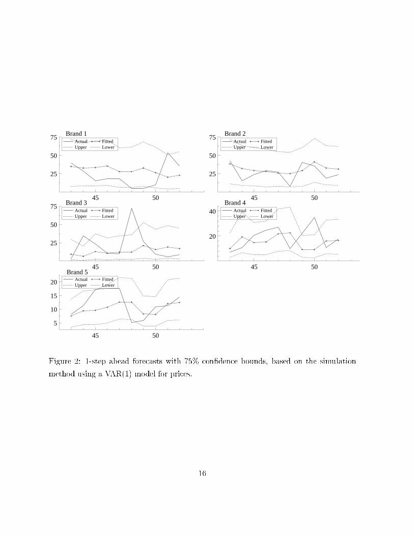
Figure 2 gives the con�dence bounds for 1-step ahead forecasting calculated using the

simulation method. It is clear that the con�dence bounds are much wider than the bounds

given in Figure 1, where the uncertainty in prices is not taken into account. Notice the

asymmetry of the con�dence bounds for brand 3, that is, the forecasted value does not

lie in the middle of the upper and the lower bound.

9

4 Conclusion

In this paper we proposed a simulation-based method to generate forecasts for market

shares in case one considers econometric models to correlate sales with explanatory vari-

ables. The method has various advantages over a naive method. The �rst is that it yields

unbiased forecasts. The second is that it allows the con�dence region of the forecasts to

be asymmetric. Finally, the method is particularly useful if forecasts of explanatory vari-

ables are to be included, as the method takes their full forecast distribution into account.

Our illustration showed some improvement of the new method over a naive method.

References

Brodie, R. J. and C. A. D. Kluyver (1987), A Comparison of the Short Term Forecasting

Accuracy of Econometric and Naive Extrapolation Models of Market Share, Interna-

tional Journal of Forecasting , 3, 423{437.

Hill, R. C. and P. Cartwright (1994), The Statistical Properties of the Equity Estimator,

Journal of Business & Economic Statistics, 12, 141{147.

L�utkepohl, H. (1993), Introduction to Multiple Time Series Analysis, 2nd edn., Springer-

Verlag, Berlin.

Wittink, D. R. (1987), Causal Market Share Models in Marketing: Neither Forecasting

Nor Understanding, International Journal of Forecasting , 3, 445{448.

Wittink, D. R., M. Addona, W. Hawkes, and J. Porter (1988), SCAN*PRO: The Esti-

mation, Validation and Use of Promotional E�ects Based on Scanner Data, working

paper, AC Nielsen, Schaumburg, Illinois, USA.

10

Table 1: Estimated parameter values in an empirical sales

model for 5 canned tuna �sh brands. Standard errors are

given in parentheses. The estimates are based on the �rst

42 observations

S1;t S2;t S3;t S4;t S5;t

Intercept 5.298 9.549 5.904 7.616 5.030

(1.214) (1.805) (1.941) (1.484) (2.367)

exp(Pt) -8.643 -4.497 -10.737 -8.434 3.093

(0.712) (0.444) (0.866) (0.809) (8.195)

exp(Pt�1) 7.328 0.742 7.511 6.083 0.040

(0.939) (0.797) (1.440) (1.073) (8.539)

St�1 0.496 0.264 0.572 0.290 0.134

(0.091) (0.138) (0.118) (0.107) (0.129)

�̂ =

0BBBBBBB@

0:207 �0:024 �0:023 0:036 0:028

�0:024 0:142 �0:023 0:026 0:010

�0:023 �0:023 0:147 0:030 �0:006

0:036 0:026 0:030 0:090 0:005

0:028 0:010 �0:006 0:005 0:011

1CCCCCCCA

11

Table 2: (Sum) Root Mean Squared Error for di�erent forecast horizons over 10 forecasts

for the naive method and the simulation-based [SB] method

1-step 2-step 3-step 4-step 5-step

Naive SB Naive SB Naive SB Naive SB Naive SB

Brand 1 17.55 17.38 20.45 20.07 18.53 18.12 15.51 15.24 15.91 15.81

Brand 2 18.05 17.65 22.15 21.22 17.21 16.15 15.29 14.16 21.06 19.66

Brand 3 26.37 26.14 30.09 29.52 24.01 23.24 21.32 20.64 25.07 24.80

Brand 4 9.58 9.53 11.98 11.66 12.40 11.97 11.60 11.18 9.88 9.66

Brand 5 4.77 4.75 6.83 6.67 7.57 7.29 7.02 6.66 5.61 5.33

Sum 76.33 75.45 91.51 89.14 79.72 76.79 70.74 67.89 77.54 75.26

12

Table 3: Estimated parameter values of a �ve-variate VAR(1)

model for prices

Intercept P1;t�1 P2;t�1 P3;t�1 P4;t�1 P5;t�1

P1;t 0.046 0.484 0.180 0.360 -0.344 0.257

(1.684) (0.126) (0.104) (0.167) (0.213) (2.814)

P2;t -1.237 0.125 0.212 0.426 0.036 2.394

(2.639) (0.198) (0.162) (0.262) (0.333) (4.409)

P3;t -0.511 0.018 -0.020 0.408 0.253 1.386

(1.511) (0.113) (0.093) (0.150) (0.191) (2.525)

P4;t 2.318 0.186 0.039 -0.107 0.376 -3.386

(1.127) (0.084) (0.069) (0.112) (0.142) (1.883)

P5;t 0.022 -0.001 0.001 -0.006 0.001 0.969

(0.037) (0.003) (0.002) (0.004) (0.005) (0.061)

13

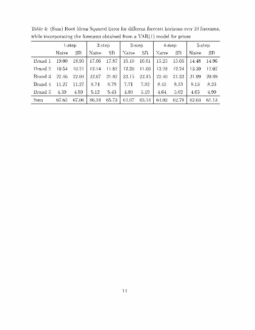
Table 4: (Sum) Root Mean Squared Error for di�erent forecast horizons over 10 forecasts,

while incorporating the forecasts obtained from a VAR(1) model for prices

1-step 2-step 3-step 4-step 5-step

Naive SB Naive SB Naive SB Naive SB Naive SB

Brand 1 19.00 18.95 17.66 17.87 16.10 16.61 15.25 15.66 14.48 14.96

Brand 2 10.54 10.21 12.14 11.82 12.30 11.66 13.28 12.24 13.39 12.07

Brand 3 22.46 22.04 22.67 21.82 23.15 22.15 22.40 21.33 21.99 20.89

Brand 4 11.27 11.27 8.74 8.79 7.71 7.92 8.45 8.53 8.13 8.23

Brand 5 4.39 4.59 5.12 5.43 4.80 5.19 4.64 5.02 4.63 4.99

Sum 67.65 67.06 66.34 65.73 64.07 63.54 64.02 62.78 62.63 61.13

14

45 50

20

40

Brand 1Actual FittedUpper Lower

45 50

25

50

75 Brand 2Actual FittedUpper Lower

45 50

25

50

75Brand 3

Actual FittedUpper Lower

45 50

10

20

30

40 Brand 4Actual FittedUpper Lower

45 50

10

15

20

Brand 5Actual FittedUpper Lower

Figure 1: 1-step ahead forecasts with 75% con�dence bounds, based on the simulation

method.

15

45 50

25

50

75Brand 1

Actual FittedUpper Lower

45 50

25

50

75Brand 2

Actual FittedUpper Lower

45 50

25

50

75Brand 3

Actual FittedUpper Lower

45 50

20

40Brand 4

Actual FittedUpper Lower

45 50

5

10

15

20

Brand 5Actual FittedUpper Lower

Figure 2: 1-step ahead forecasts with 75% con�dence bounds, based on the simulation

method using a VAR(1) model for prices.

16

ERASMUS RESEARCH INSTITUTE OF MANAGEMENT

REPORT SERIESRESEARCH IN MANAGEMENT

Other Publications in the Report Series Research∗ in Management

Impact of the Employee Communication and Perceived External Prestige on Organizational Identification,Ale Smidts, Cees B.M. van Riel & Ad Th.H. PruynERS-2000-01-MKT

Critical Complexities, from marginal paradigms to learning networks, Slawomir MagalaERS-2000-02-ORG

∗ ERIM Research Programs:

LIS Business Processes, Logistics and Information SystemsORG Managing Relationships for PerformanceMKT Decision Making in Marketing ManagementF&A Financial Decision Making and AccountingSTR Strategic Renewal and the Dynamics of Firms, Networks and Industries