S3D User’s Guide 1 Installation of Eclipse

The tool to be used in this User’s Guide is Papyrus, an Eclipse open source Model-Based Engineering tool. Then, the first step is to install Eclipse. The version we are using is Eclipse Neon available from:

https://www.eclipse.org/neon/

The execution of the downloaded file starts an installation wizard opening a window with all the available Eclipse Integrated Development Environments. Among them, select the Eclipse Modeling Tools (EMT):

Figure 1 EMF IDE selection.

Page 2 of 38

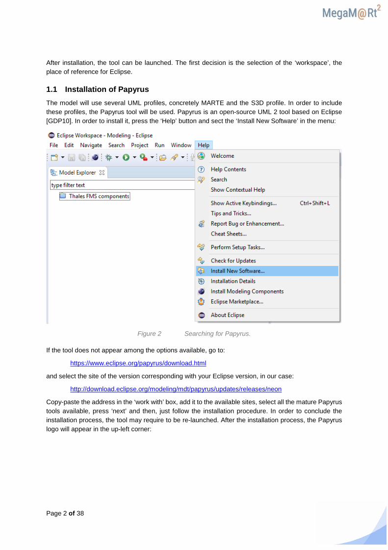
After installation, the tool can be launched. The first decision is the selection of the ‘workspace’, the place of reference for Eclipse.

1.1 Installation of Papyrus The model will use several UML profiles, concretely MARTE and the S3D profile. In order to include these profiles, the Papyrus tool will be used. Papyrus is an open-source UML 2 tool based on Eclipse [GDP10]. In order to install it, press the ‘Help’ button and sect the ‘Install New Software’ in the menu:

Figure 2 Searching for Papyrus.

If the tool does not appear among the options available, go to:

https://www.eclipse.org/papyrus/download.html

and select the site of the version corresponding with your Eclipse version, in our case:

http://download.eclipse.org/modeling/mdt/papyrus/updates/releases/neon

Copy-paste the address in the ‘work with’ box, add it to the available sites, select all the mature Papyrus tools available, press ‘next’ and then, just follow the installation procedure. In order to conclude the installation process, the tool may require to be re-launched. After the installation process, the Papyrus logo will appear in the up-left corner:

Page 3 of 38

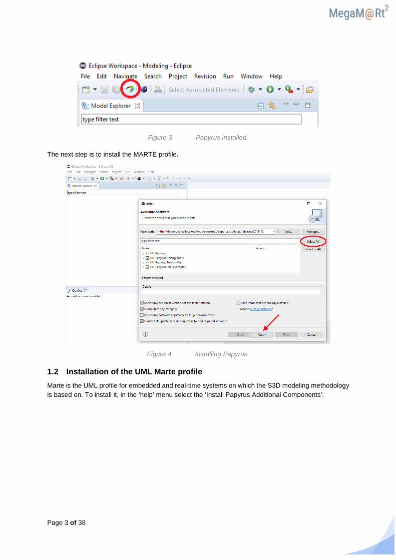
Figure 3 Papyrus installed.

The next step is to install the MARTE profile.

Figure 4 Installing Papyrus.

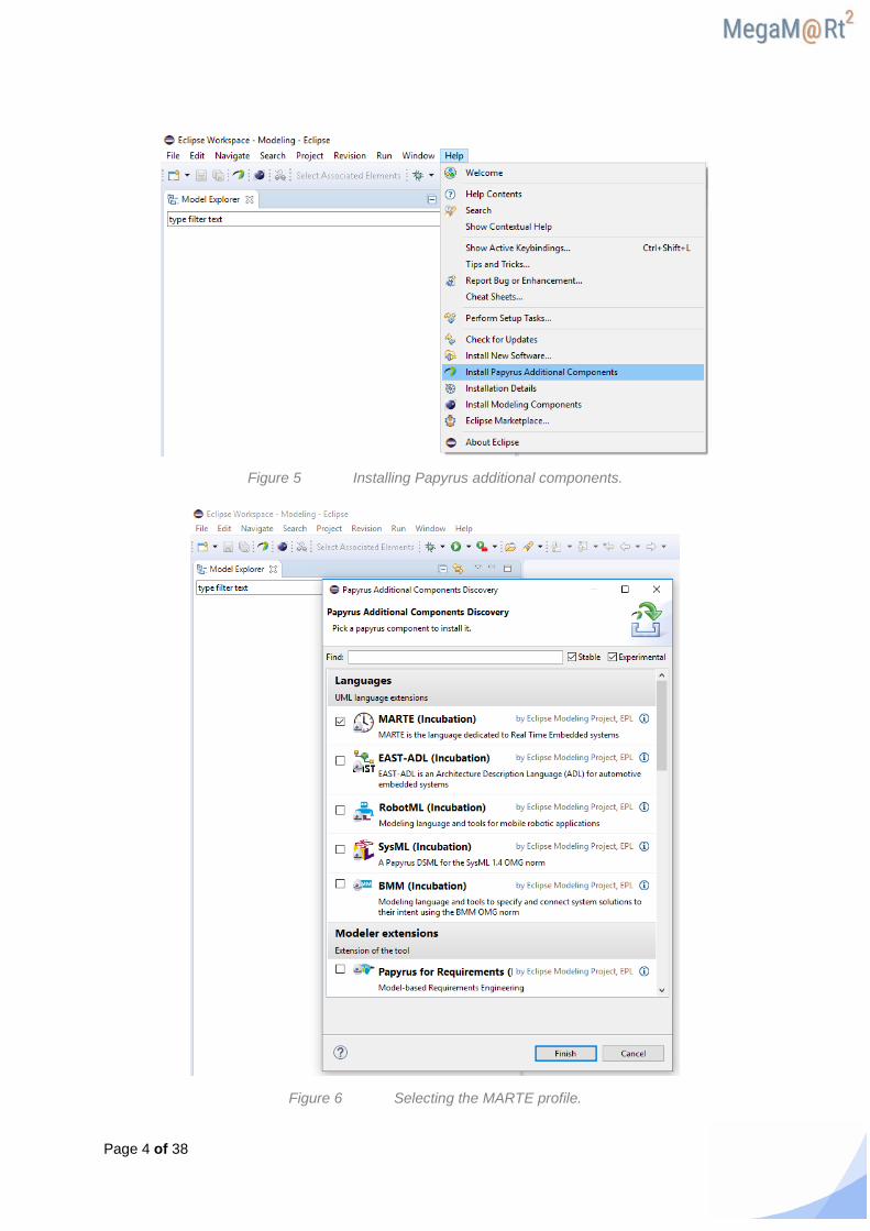
1.2 Installation of the UML Marte profile Marte is the UML profile for embedded and real-time systems on which the S3D modeling methodology is based on. To install it, in the ‘help’ menu select the ‘Install Papyrus Additional Components’:

Page 4 of 38

Figure 5 Installing Papyrus additional components.

Figure 6 Selecting the MARTE profile.

Page 5 of 38

and then, select the MARTE profile as shown in Figure 6. The next step is to install the S3D profile which includes some facilities required by the S3D methodology not covered by the MARTE standard.

1.3 Installation of the S3D profile. As the S3D profile is not officially registered, it is necessary to get it from:

s3d.unican.es

select the ‘Install New Software’ option from the ‘help’ menu, as shown in Figure 2. Now, instead of looking for on-line repositories, just ‘add’ for the file downloaded from the University of Cantabria as shown in Figure 7. Then, proceed as in Figure 4.

1.4 Installation of the C++ IDE. It may be also recommendable to install the IDE for the programming language to be used, in our case, C/C++. In this way, both system engineering based on S3D and code development in C++ can be done in the same environment just by changing the perspective. To do so, once the tool is open, press ‘help’ and then, open the ‘Eclipse Marketplace’, as shown in Figure 8.

Figure 7 Selecting a local profile.

Page 6 of 38

Figure 8 Installing the C/C++ IDE.

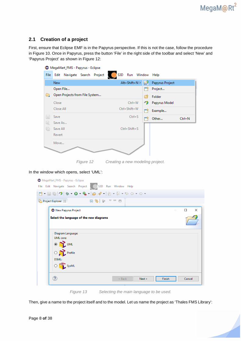
In the new window, select the ‘Programming Language’ category and then search for the C/C++ IDE, as shown in Figure 9. Once found, if you are not registered in the ‘Eclipse Marketplace’, you cannot drag&drop the install button but you can download the installer and follow the instructions. After installation, the IDE will have the EMF and the C/C++ perspectives available, as shown in Figure 11. It is possible to change from one to the other making use of the buttons on the up-right corner of the IDE.

Now we are ready to start developing our system model.

Figure 9 Searching the C/C++ IDE.

Page 7 of 38

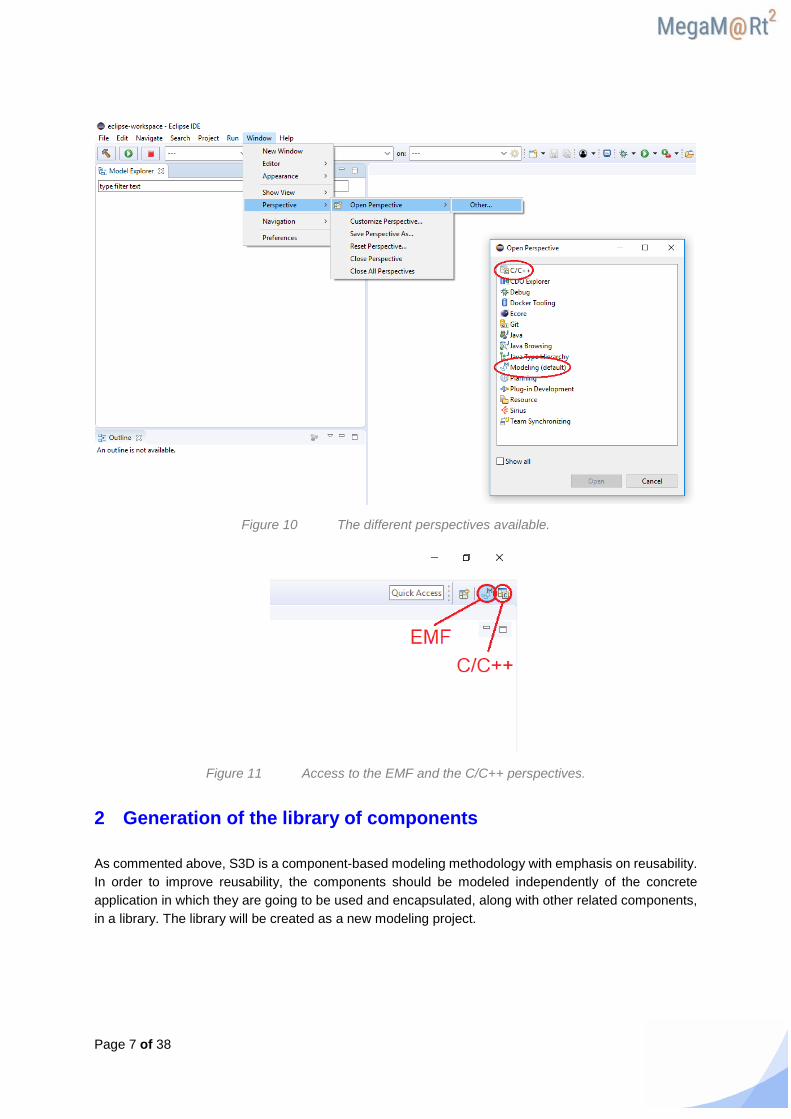
Figure 10 The different perspectives available.

Figure 11 Access to the EMF and the C/C++ perspectives.

2 Generation of the library of components

As commented above, S3D is a component-based modeling methodology with emphasis on reusability. In order to improve reusability, the components should be modeled independently of the concrete application in which they are going to be used and encapsulated, along with other related components, in a library. The library will be created as a new modeling project.

Page 8 of 38

2.1 Creation of a project First, ensure that Eclipse EMF is in the Papyrus perspective. If this is not the case, follow the procedure in Figure 10. Once in Papyrus, press the button ‘File’ in the right side of the toolbar and select ‘New’ and ‘Papyrus Project’ as shown in Figure 12:

Figure 12 Creating a new modeling project.

In the window which opens, select ‘UML’:

Figure 13 Selecting the main language to be used.

Then, give a name to the project itself and to the model. Let us name the project as ‘Thales FMS Library’:

Page 9 of 38

Figure 14 Naming the Project and the Model.

and the model as ‘Thales FMS Components’:

Figure 15 Naming the model root.

Page 10 of 38

Now, we are ready to start.

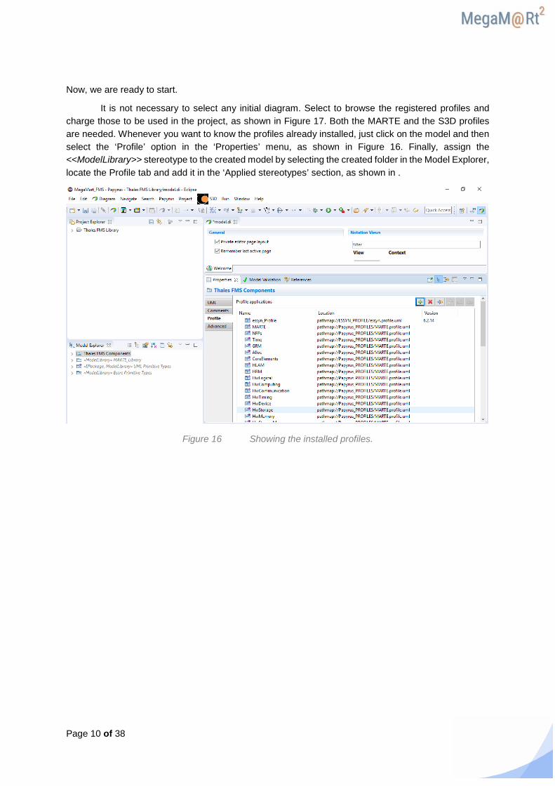
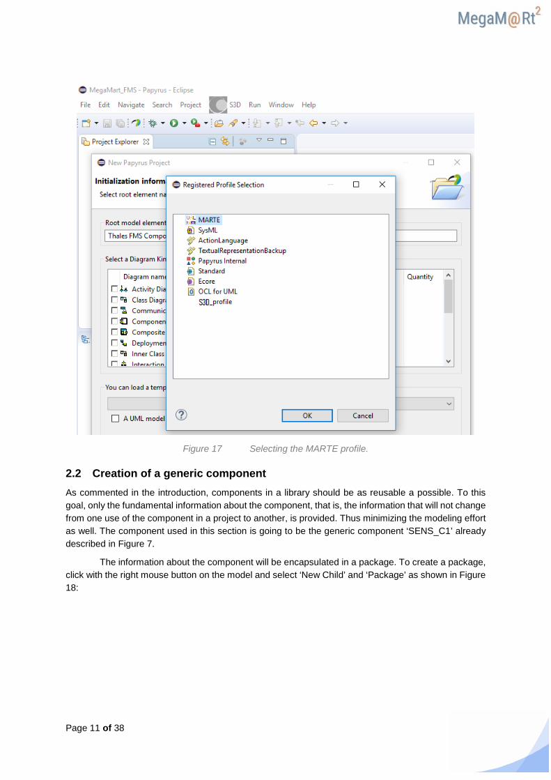
It is not necessary to select any initial diagram. Select to browse the registered profiles and charge those to be used in the project, as shown in Figure 17. Both the MARTE and the S3D profiles are needed. Whenever you want to know the profiles already installed, just click on the model and then select the ‘Profile’ option in the ‘Properties’ menu, as shown in Figure 16. Finally, assign the <<ModelLibrary>> stereotype to the created model by selecting the created folder in the Model Explorer, locate the Profile tab and add it in the ‘Applied stereotypes’ section, as shown in .

Figure 16 Showing the installed profiles.

Page 11 of 38

Figure 17 Selecting the MARTE profile.

2.2 Creation of a generic component As commented in the introduction, components in a library should be as reusable a possible. To this goal, only the fundamental information about the component, that is, the information that will not change from one use of the component in a project to another, is provided. Thus minimizing the modeling effort as well. The component used in this section is going to be the generic component ‘SENS_C1’ already described in Figure 7.

The information about the component will be encapsulated in a package. To create a package, click with the right mouse button on the model and select ‘New Child’ and ‘Package’ as shown in Figure 18:

Page 12 of 38

Figure 18 Generating a Package.

Let’s give the name ‘SENS_C1’. This package will integrate all the relevant information about the component. The first being its characteristics as a functional component, either as an active, real-time unit creating its own thread(s) or a passive, protected unit proving services to other components. The former is stereotyped as ‘RtUnit’. The latter as ‘PpUnit’. In both cases, click with the right mouse-button on the component package and select ‘New Child’ and ‘Component’ as shown in Figure 19:

Page 13 of 38

Figure 19 Creating a Component.

Figure 20 UML properties of a component.

Page 14 of 38

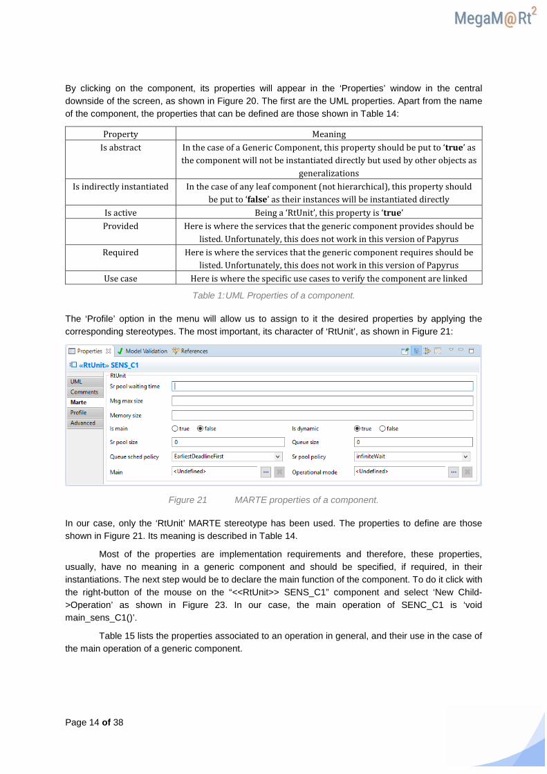
By clicking on the component, its properties will appear in the ‘Properties’ window in the central downside of the screen, as shown in Figure 20. The first are the UML properties. Apart from the name of the component, the properties that can be defined are those shown in Table 14:

Property Meaning Is abstract In the case of a Generic Component, this property should be put to ‘true’ as

the component will not be instantiated directly but used by other objects as generalizations

Is indirectly instantiated In the case of any leaf component (not hierarchical), this property should be put to ‘false’ as their instances will be instantiated directly

Is active Being a ‘RtUnit’, this property is ‘true’ Provided Here is where the services that the generic component provides should be

listed. Unfortunately, this does not work in this version of Papyrus Required Here is where the services that the generic component requires should be

listed. Unfortunately, this does not work in this version of Papyrus Use case Here is where the specific use cases to verify the component are linked

Table 1: UML Properties of a component.

The ‘Profile’ option in the menu will allow us to assign to it the desired properties by applying the corresponding stereotypes. The most important, its character of ‘RtUnit’, as shown in Figure 21:

Figure 21 MARTE properties of a component.

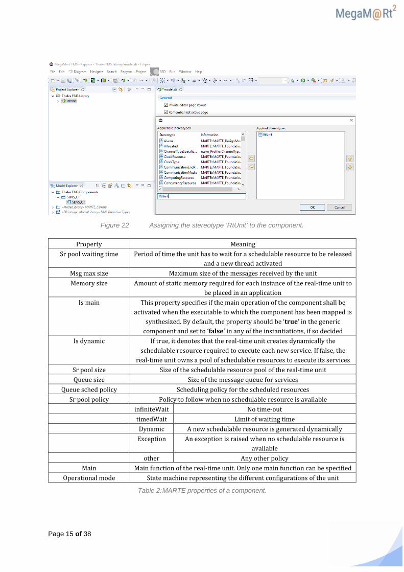
In our case, only the ‘RtUnit’ MARTE stereotype has been used. The properties to define are those shown in Figure 21. Its meaning is described in Table 14.

Most of the properties are implementation requirements and therefore, these properties, usually, have no meaning in a generic component and should be specified, if required, in their instantiations. The next step would be to declare the main function of the component. To do it click with the right-button of the mouse on the “<<RtUnit>> SENS_C1” component and select ‘New Child->Operation’ as shown in Figure 23. In our case, the main operation of SENC_C1 is ‘void main_sens_C1()’.

Table 15 lists the properties associated to an operation in general, and their use in the case of the main operation of a generic component.

Page 15 of 38

Figure 22 Assigning the stereotype ‘RtUnit’ to the component.

Property Meaning Sr pool waiting time Period of time the unit has to wait for a schedulable resource to be released

and a new thread activated Msg max size Maximum size of the messages received by the unit Memory size Amount of static memory required for each instance of the real-time unit to

be placed in an application Is main This property specifies if the main operation of the component shall be

activated when the executable to which the component has been mapped is synthesized. By default, the property should be ‘true’ in the generic

component and set to ‘false’ in any of the instantiations, if so decided Is dynamic If true, it denotes that the real-time unit creates dynamically the

schedulable resource required to execute each new service. If false, the real-time unit owns a pool of schedulable resources to execute its services

Sr pool size Size of the schedulable resource pool of the real-time unit Queue size Size of the message queue for services

Queue sched policy Scheduling policy for the scheduled resources Sr pool policy Policy to follow when no schedulable resource is available

infiniteWait No time-out timedWait Limit of waiting time Dynamic A new schedulable resource is generated dynamically Exception An exception is raised when no schedulable resource is

available other Any other policy

Main Main function of the real-time unit. Only one main function can be specified Operational mode State machine representing the different configurations of the unit

Table 2: MARTE properties of a component.

Page 16 of 38

2.2.1 Component data types and interfaces

The next step is the definition of the data types used in the model of the component. Usually the data types with which the component communicates with its environment.

Figure 23 Declaring an operation.

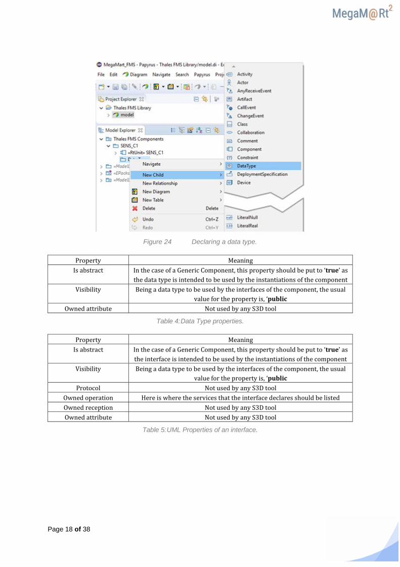
Data types will be included in a new package. Then, select ‘New Child’ and ‘Package’ as it was shown in Figure 18, but now clicking with the right mouse-button on the component package. Let’s call it ‘Data Types’. The data types are included in the package by clicking with the right mouse-button on the package and selecting ‘New Child Data Type’ as shown in Figure 24. Then, the following windows appear where the properties of the data type can be specified (see Table 17:).

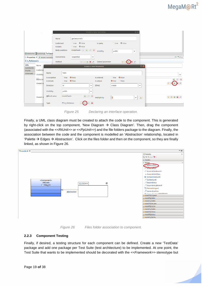
Once the data types are specified, it is possible to declare the interfaces with which the component will interact with its surrounding environment. The procedure is similar as above, but here interfaces are differentiated between provided and required. Therefore, interfaces should be organized inside the ‘Interfaces’ package in two additional packages, ‘prov’ and ‘req’, depending whether they are provided or required by the component. Once these packages have been created, include the interfaces in the relevant folder by selecting ‘New Child Interface’. In this case, the properties to be fixed are

Page 17 of 38

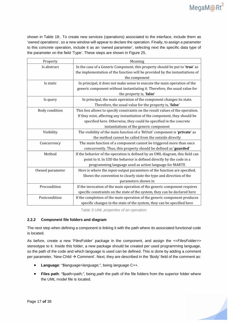
shown in Table 18:. To create new services (operations) associated to the interface, include them as ‘owned operations’, so a new window will appear to declare the operation. Finally, to assign a parameter to this concrete operation, include it as an ‘owned parameter’, selecting next the specific data type of the parameter on the field ‘Type’. These steps are shown in Figure 25.

Property Meaning Is abstract In the case of a Generic Component, this property should be put to ‘true’ as

the implementation of the function will be provided by the instantiations of the component

Is static In principal, it does not make sense to execute the main operation of the generic component without instantiating it. Therefore, the usual value for

the property is, ‘false’ Is query In principal, the main operation of the component changes its state.

Therefore, the usual value for the property is, ‘false’ Body condition This box allows to specify constraints on the result values of the operation.

If they exist, affecting any instantiation of the component, they should be specified here. Otherwise, they could be specified in the concrete

instantiations of the generic component Visibility The visibility of the main function of a ‘RtUnit’ component is ‘private’ as

the method cannot be called from the outside directly Concurrency The main function of a component cannot be triggered more than once

concurrently. Thus, this property should be defined as ‘guarded’ Method If the behavior of the operation is defined by an UML diagram, this field can

point to it. In S3D the behavior is defined directly by the code in a programming language used as action language for MARTE

Owned parameter Here is where the input-output parameters of the function are specified. Shows the convention to clearly state the type and direction of the

parameters shown in Precondition If the invocation of the main operation of the generic component requires

specific constraints on the state of the system, they can be declared here Postcondition If the completion of the main operation of the generic component produces

specific changes in the state of the system, they can be specified here

Table 3: UML properties of an operation.

2.2.2 Component file folders and diagram

The next step when defining a component is linking it with the path where its associated functional code is located.

As before, create a new ‘FilesFolder’ package in the component, and assign the <<FilesFolder>> stereotype to it. Inside this folder, a new package should be created per used programming language, so the path of the code and which language is used can be defined. This is done by adding a comment per parameter, ‘New Child Comment’. Next, they are described in the ‘Body’ field of the comment as:

• Language: “$language=language;”, being language C++.

• Files path: “$path=path;”, being path the path of the file folders from the superior folder where the UML model file is located.

Page 18 of 38

Figure 24 Declaring a data type.

Property Meaning Is abstract In the case of a Generic Component, this property should be put to ‘true’ as

the data type is intended to be used by the instantiations of the component Visibility Being a data type to be used by the interfaces of the component, the usual

value for the property is, ‘public Owned attribute Not used by any S3D tool

Table 4: Data Type properties.

Property Meaning Is abstract In the case of a Generic Component, this property should be put to ‘true’ as

the interface is intended to be used by the instantiations of the component Visibility Being a data type to be used by the interfaces of the component, the usual

value for the property is, ‘public Protocol Not used by any S3D tool

Owned operation Here is where the services that the interface declares should be listed Owned reception Not used by any S3D tool Owned attribute Not used by any S3D tool

Table 5: UML Properties of an interface.

Page 19 of 38

Figure 25 Declaring an interface operation.

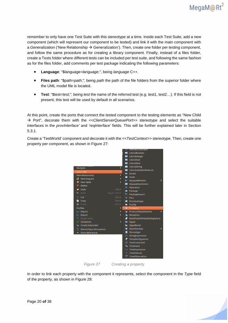
Finally, a UML class diagram must be created to attach the code to the component. This is generated by right-click on the top component, ‘New Diagram Class Diagram’. Then, drag the component (associated with the <<RtUnit>> or <<PpUnit>>) and the file folders package to the diagram. Finally, the association between the code and the component is modelled an ‘Abstraction’ relationship, located in ‘Palette Edges Abstraction’. Click on the files folder and then on the component, so they are finally linked, as shown in Figure 26.

Figure 26 Files folder association to component.

2.2.3 Component Testing

Finally, if desired, a testing structure for each component can be defined. Create a new ‘TestData’ package and add one package per Test Suite (test architecture) to be implemented. At one point, the Test Suite that wants to be implemented should be decorated with the <<Framework>> stereotype but

Page 20 of 38

remember to only have one Test Suite with this stereotype at a time. Inside each Test Suite, add a new component (which will represent our component to be tested) and link it with the main component with a Generalization (‘New Relationship Generalization’). Then, create one folder per testing component, and follow the same procedure as for creating a library component. Finally, instead of a files folder, create a Tests folder where different tests can be included per test suite, and following the same fashion as for the files folder, add comments per test package indicating the following parameters:

• Language: “$language=language;”, being language C++.

• Files path: “$path=path;”, being path the path of the file folders from the superior folder where the UML model file is located.

• Test: “$test=test;”, being test the name of the referred test (e.g. test1, test2…). If this field is not present, this test will be used by default in all scenarios.

At this point, create the ports that connect the tested component to the testing elements as “New Child Port”, decorate them with the <<ClientServerQueuePort>> stereotype and select the suitable interfaces in the provInterface’ and ‘reqInterface’ fields. This will be further explained later in Section 5.3.1.

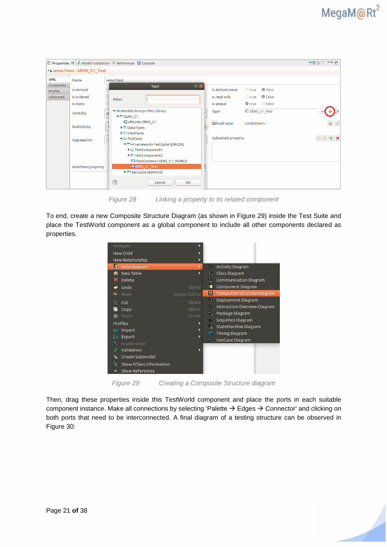
Create a ‘TestWorld’ component and decorate it with the <<TestContext>> stereotype. Then, create one property per component, as shown in Figure 27:

Figure 27 Creating a property

In order to link each property with the component it represents, select the component in the Type field of the property, as shown in Figure 28:

Page 21 of 38

Figure 28 Linking a property to its related component

To end, create a new Composite Structure Diagram (as shown in Figure 29) inside the Test Suite and place the TestWorld component as a global component to include all other components declared as properties.

Figure 29 Creating a Composite Structure diagram

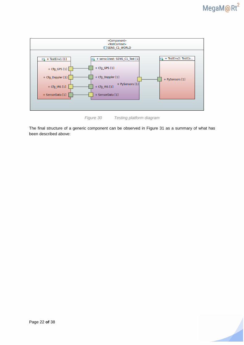
Then, drag these properties inside this TestWorld component and place the ports in each suitable component instance. Make all connections by selecting ‘Palette Edges Connector’ and clicking on both ports that need to be interconnected. A final diagram of a testing structure can be observed in Figure 30:

Page 22 of 38

Figure 30 Testing platform diagram

The final structure of a generic component can be observed in Figure 31 as a summary of what has been described above:

Page 23 of 38

Figure 31 Generic component structure.

Page 24 of 38

3 System modelling

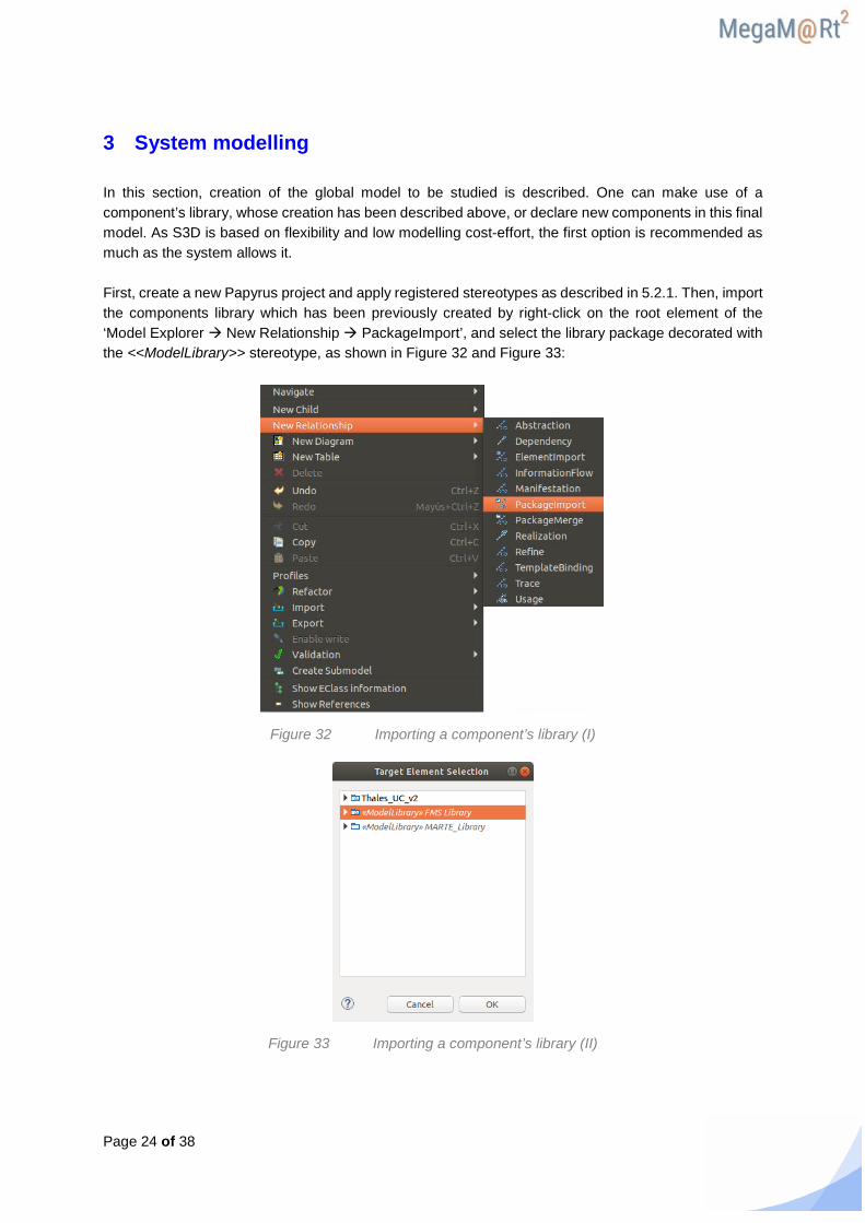
In this section, creation of the global model to be studied is described. One can make use of a component’s library, whose creation has been described above, or declare new components in this final model. As S3D is based on flexibility and low modelling cost-effort, the first option is recommended as much as the system allows it. First, create a new Papyrus project and apply registered stereotypes as described in 5.2.1. Then, import the components library which has been previously created by right-click on the root element of the ‘Model Explorer New Relationship PackageImport’, and select the library package decorated with the <<ModelLibrary>> stereotype, as shown in Figure 32 and Figure 33:

Figure 32 Importing a component’s library (I)

Figure 33 Importing a component’s library (II)

Page 25 of 38

3.1 Creation of the System Views

3.1.1 Application View

Create the Application package in the main model as ‘New child Package’ (Figure 18) and assign the <<ApplicationView>> stereotype. Then, create a new System component as ‘New child Component’, and decorate it with the <<System>> stereotype from eSSYN profile. This component will represent the whole system. Additionally, create another package to include all the system components, which we are going to call ‘SystemComponents’, as represented in Figure 34:

Figure 34 Creation of the Application view

Here, depending on whether components are imported from a component’s library or not, two possible scenarios may appear:

• If the component is imported from the component’s library, instantiate it as ‘New Child Component’, and decorate it with the relevant <<RtUnit>>, <<PpUnit>> or <<Subsystem>> stereotype, depending on the component.

At this point, relate it with the base component using a Generalization (‘New Relationship Generalization’), and select the appropriate component from the library (Figure 35).

Page 26 of 38

Figure 35 Generalization of a library component into the system

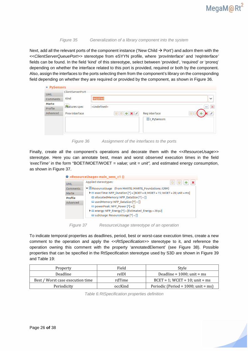
Next, add all the relevant ports of the component instance (‘New Child Port’) and adorn them with the <<ClientServerQueuePort>> stereotype from eSYYN profile, where ‘provInterface’ and ‘reqInterface’ fields can be found. In the field ‘kind’ of this stereotype, select between ‘provided’, ‘required’ or ‘proreq’ depending on whether the interface related to this port is provided, required or both by the component. Also, assign the interfaces to the ports selecting them from the component’s library on the corresponding field depending on whether they are required or provided by the component, as shown in Figure 36.

Figure 36 Assignment of the interfaces to the ports

Finally, create all the component’s operations and decorate them with the <<ResourceUsage>> stereotype. Here you can annotate best, mean and worst observed execution times in the field ‘execTime’ in the form “BOET/MOET/WOET = value; unit = unit”, and estimated energy consumption, as shown in Figure 37.

Figure 37 ResourceUsage stereotype of an operation

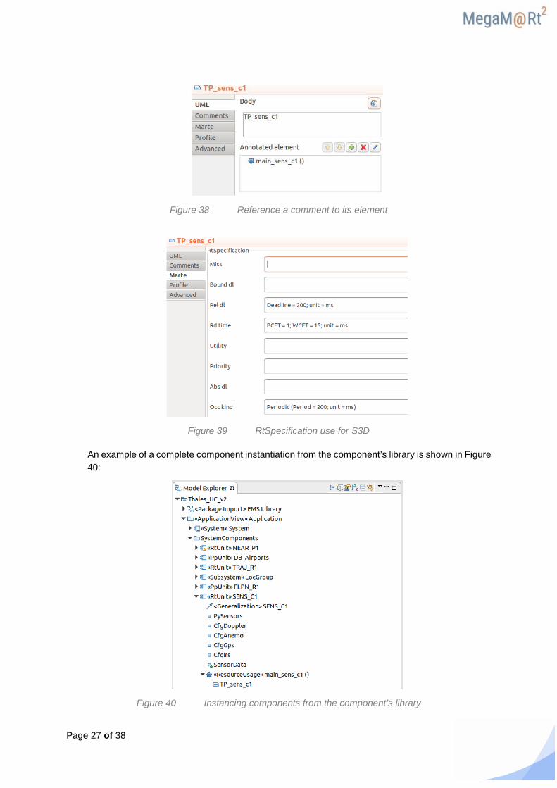
To indicate temporal properties as deadlines, period, best or worst-case execution times, create a new comment to the operation and apply the <<RtSpecification>> stereotype to it, and reference the operation owning this comment with the property ‘annotatedElement’ (see Figure 38). Possible properties that can be specified in the RtSpecification stereotype used by S3D are shown in Figure 39 and Table 19:

Property Field Style Deadline relDl Deadline = 1000; unit = ms

Best / Worst case execution time rdTime BCET = 1; WCET = 10; unit = ms Periodicity occKind Periodic (Period = 1000; unit = ms)

Table 6: RtSpecification properties definition

Page 27 of 38

Figure 38 Reference a comment to its element

Figure 39 RtSpecification use for S3D

An example of a complete component instantiation from the component’s library is shown in Figure 40:

Figure 40 Instancing components from the component’s library

Page 28 of 38

• If the component is directly created on the model, follow the same procedure as described in 5.2.2, creating a package for that component inside the SystemComponents package.

If your components make use of some common code (configuration files, data types, interfaces…), it is needed that these files are reflected in the model. To do so, create a new Common Resources package inside the system components package and decorate it with the <<FilesFolder>> stereotype. Then, follow the procedure described above in “Component file folders and diagram” to indicate the path where these files are located.

Next, within the System general element, components and ports should be rendered. Instantiate the components as Properties (‘New Child Property’). Then, specify the name of the component and indicate which component is this property related to on the ‘Type’ field of the property and selecting it from the previously created ‘SystemComponents’ package, as shown in Figure 28:

At this point, create the ports that connect the global System component to the environment as “New Child Port”, decorate them with the <<ClientServerQueuePort>> stereotype and select the suitable interfaces in the provInterface’ and ‘reqInterface’ fields, as described above (see Figure 36).

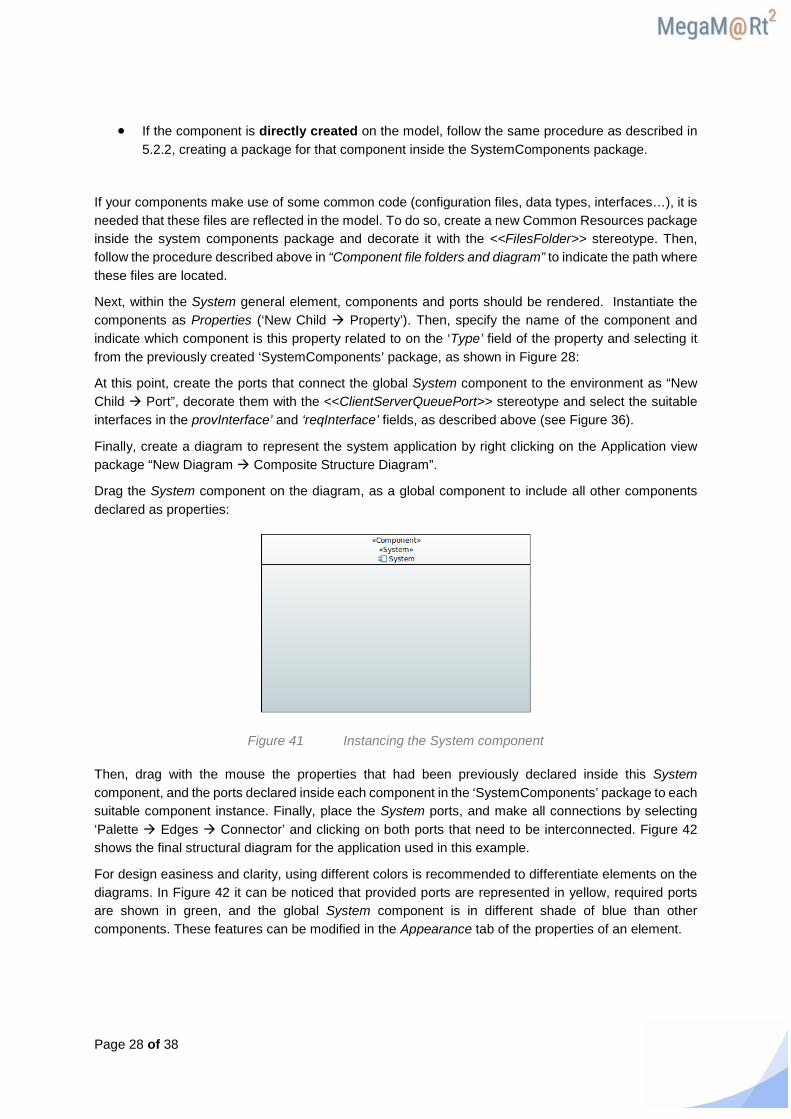
Finally, create a diagram to represent the system application by right clicking on the Application view package “New Diagram Composite Structure Diagram”.

Drag the System component on the diagram, as a global component to include all other components declared as properties:

Figure 41 Instancing the System component

Then, drag with the mouse the properties that had been previously declared inside this System component, and the ports declared inside each component in the ‘SystemComponents’ package to each suitable component instance. Finally, place the System ports, and make all connections by selecting ‘Palette Edges Connector’ and clicking on both ports that need to be interconnected. Figure 42 shows the final structural diagram for the application used in this example.

For design easiness and clarity, using different colors is recommended to differentiate elements on the diagrams. In Figure 42 it can be noticed that provided ports are represented in yellow, required ports are shown in green, and the global System component is in different shade of blue than other components. These features can be modified in the Appearance tab of the properties of an element.

Page 29 of 38

Figure 42 Complete system application diagram

3.1.2 Verification View

Create the Verification package in the main model as ‘New child Package’ and assign the <<VerificationView>> stereotype. If you want to test different environments on your System, you can create a package to include all these environments and assign the stereotype to the one you want to test. Remember that there can only be one package with the stereotype assigned at a time, so if you are switching between different verification views, remember to delete the stereotype from the previous view.

Then, create a new World component as ‘New child Component’, and decorate it with the <<TestContext>> stereotype from eSSYN profile. This component will represent the ‘world’ where our System component is placed, together with the environment components.

Next, create another package to include all the environment components, which we are going to call ‘EnvComponents’. Within this package, create one package per environment component following the same procedure as in 5.2.2, with two exceptions:

• Each component should also be decorated with the <<TestComponent>> stereotype from eSSYN profile, apart from the corresponding <<RtUnit>> or <<PpUnit>> stereotypes (see Figure 44).

• Each component can have different functional codes, each one related to a test. In the FilesFolder package, create one folder per test, and indicate with comments the language, path and test reference, in the same fashion as described above in Component Testing (see ).

Additionally, create a Common Resources package as described in the Application view if your environment components make use of shared code. In the World package, proceed as described in the Application view, instantiating the components as Properties and creating a new “Composite Structure Diagram”. A global diagram with the system and the environment components can be seen in Figure 43:

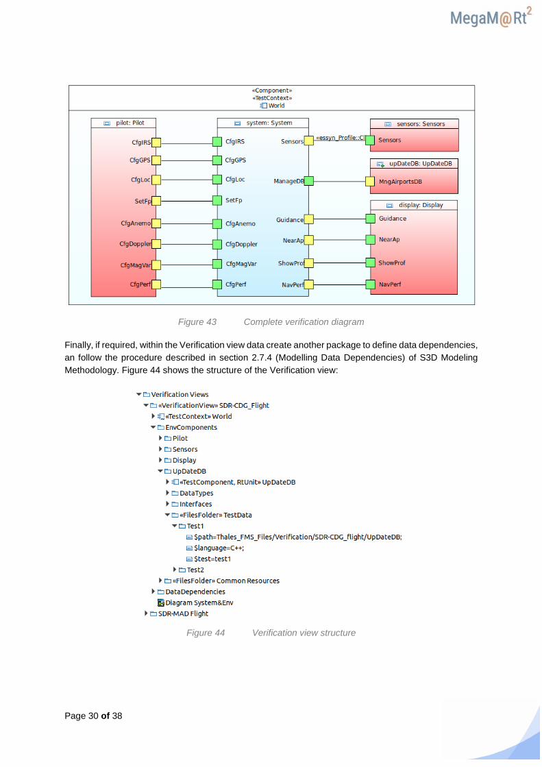
Page 30 of 38

Figure 43 Complete verification diagram

Finally, if required, within the Verification view data create another package to define data dependencies, an follow the procedure described in section 2.7.4 (Modelling Data Dependencies) of S3D Modeling Methodology. Figure 44 shows the structure of the Verification view:

Figure 44 Verification view structure

Page 31 of 38

3.1.3 Memory Spaces View

Create the Memory Spaces package in the main model and apply the <<MemorySpaceView>> stereotype.

Then, create the memory partitions needed in your application as “New Child Component”, and decorate them with the <<MemoryPartition>> stereotype. You will notice that the symbol of the component changes. A structure of the memory space view can be observed in :

Figure 45 Memory spaces view structure

3.1.4 SW Platform View

As before, create a SW Platform package and adorn it with the <<SWPlatformView>> stereotype. Proceeding on the same way as in the memory spaces view, create one component per software used in your application and assign the <<OS>> stereotype, indicating that it is an operative system.

Figure 46 Software platform view structure

3.1.5 HW Resources View

Create the HW resources view and decorate it with the <<HWResourcesView>> stereotype. Now, depending on the system you are designing, different scenarios may appear:

Page 32 of 38

• If you are designing a network system, create one component per network node and adorn them with the <<ComputingResource>> stereotype. Then, create another component to represent the system (use the <<System>> stereotype, and instance the different nodes by creating one property per element and selecting the component it represents using the Type field (Figure 28).

• If the system is centralized (one single computing resource), create one component to represent the whole system and apply the <<ComputingResource>> and <<System>> stereotypes.

In our example we have two nodes (an airplane and a database) that communicate via a wireless link. Thus, we must declare the system and both nodes in the HW resources view:

Figure 47 HW resources view creation

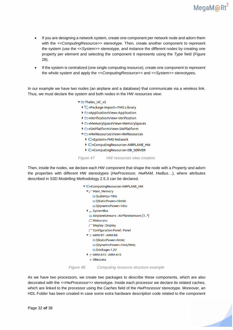
Then, inside the nodes, we declare each HW component that shape the node with a Property and adorn the properties with different HW stereotypes (HwProcessor, HwRAM, HwBus…), where attributes described in S3D Modelling Methodology 2.5.3 can be declared.

Figure 48 Computing resource structure example

As we have two processors, we create two packages to describe these components, which are also decorated with the <<HwProcessor>> stereotype. Inside each processor we declare its related caches, which are linked to the processor using the Caches field of the HwProcessor stereotype. Moreover, an HDL Folder has been created in case some extra hardware description code related to the component

Page 33 of 38

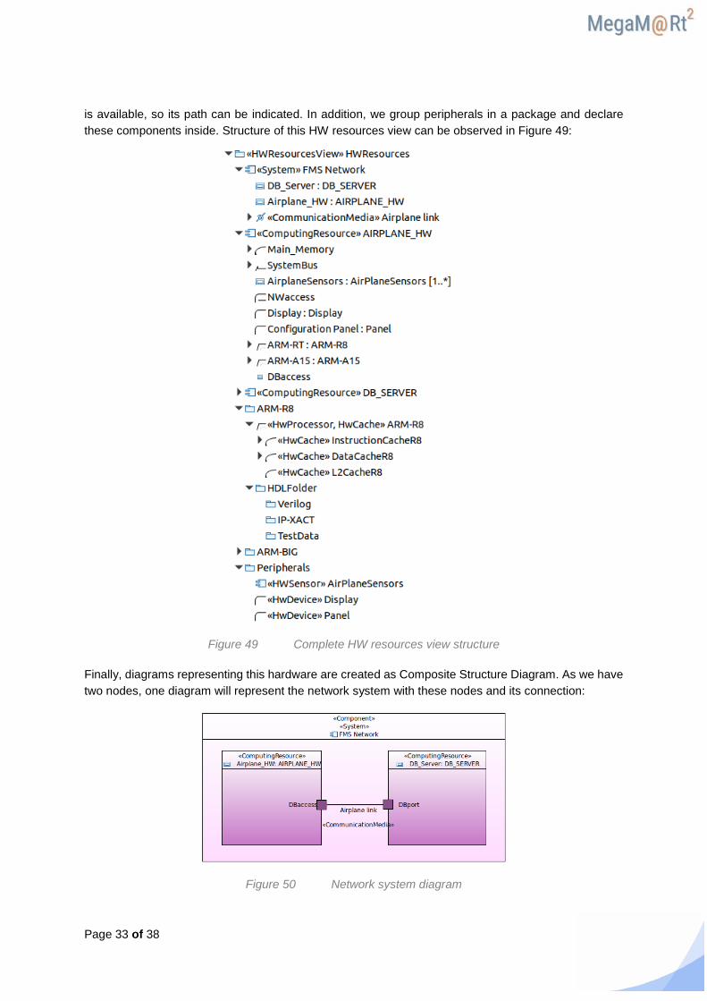
is available, so its path can be indicated. In addition, we group peripherals in a package and declare these components inside. Structure of this HW resources view can be observed in Figure 49:

Figure 49 Complete HW resources view structure

Finally, diagrams representing this hardware are created as Composite Structure Diagram. As we have two nodes, one diagram will represent the network system with these nodes and its connection:

Figure 50 Network system diagram

Page 34 of 38

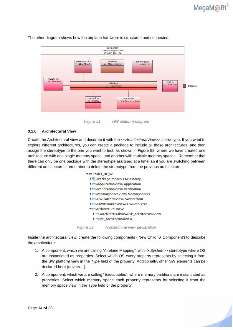
The other diagram shows how the airplane hardware is structured and connected:

Figure 51 HW platform diagram

3.1.6 Architectural View

Create the Architectural view and decorate it with the <<ArchitecturalView>> stereotype. If you want to explore different architectures, you can create a package to include all these architectures, and then assign the stereotype to the one you want to test, as shown in Figure 52, where we have created one architecture with one single memory space, and another with multiple memory spaces . Remember that there can only be one package with the stereotype assigned at a time, so if you are switching between different architectures, remember to delete the stereotype from the previous architecture.

Figure 52 Architectural view declaration

Inside the architectural view, create the following components (‘New Child Component’) to describe the architecture:

1. A component, which we are calling “Airplane Mapping”, with <<System>> stereotype where OS are instantiated as properties. Select which OS every property represents by selecting it from the SW platform view in the Type field of the property. Additionally, other SW elements can be declared here (drivers…).

2. A component, which we are calling “Executables”, where memory partitions are instantiated as properties. Select which memory space each property represents by selecting it from the memory space view in the Type field of the property.

Page 35 of 38

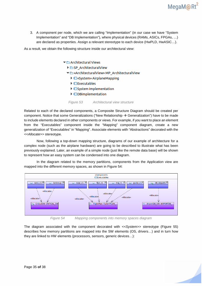
3. A component per node, which we are calling “Implementation” (in our case we have “System Implementation” and “DB Implementation”), where physical devices (RAMs, ASICs, FPGAs, …) are declared as properties. Assign a relevant stereotype to each device (HwPLD, HwASIC…).

As a result, we obtain the following structure inside our architectural view:

Figure 53 Architectural view structure

Related to each of the declared components, a Composite Structure Diagram should be created per component. Notice that some Generalizations (“New Relationship Generalization”) have to be made to include elements declared in other components or views. For example, if you want to place an element from the “Executables” component inside the “Mapping” component diagram, create a new generalization of “Executables” in “Mapping”. Associate elements with “Abstractions” decorated with the <<Allocate>> stereotype.

Now, following a top-down mapping structure, diagrams of our example of architecture for a complex node (such as the airplane hardware) are going to be described to illustrate what has been previously explained. Later, an example of a simple node (just like the remote data base) will be shown to represent how an easy system can be condensed into one diagram.

In the diagram related to the memory partitions, components from the Application view are mapped into the different memory spaces, as shown in Figure 54:

Figure 54 Mapping components into memory spaces diagram

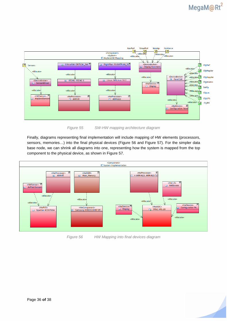
The diagram associated with the component decorated with <<System>> stereotype (Figure 55) describes how memory partitions are mapped into the SW elements (OS, drivers…) and in turn how they are linked to HW elements (processors, sensors, generic devices…):

Page 36 of 38

Figure 55 SW-HW mapping architecture diagram

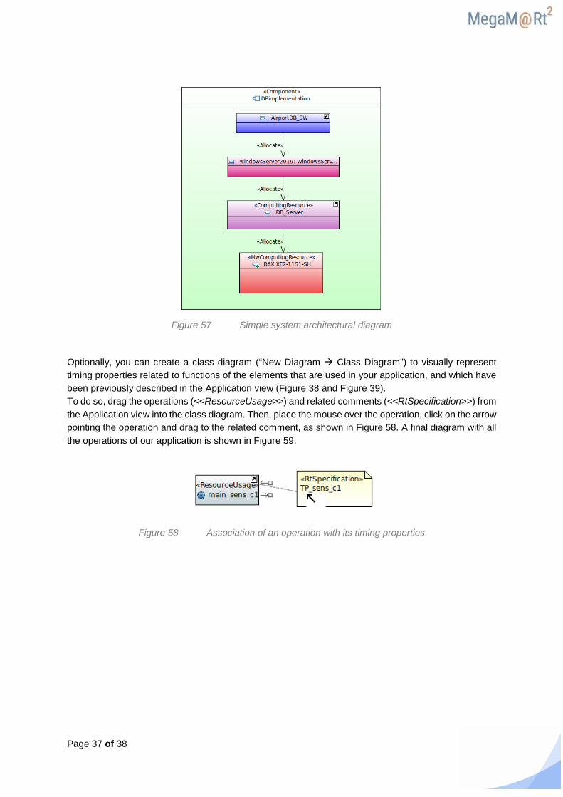
Finally, diagrams representing final implementation will include mapping of HW elements (processors, sensors, memories…) into the final physical devices (Figure 56 and Figure 57). For the simpler data base node, we can shrink all diagrams into one, representing how the system is mapped from the top component to the physical device, as shown in Figure 57.

Figure 56 HW Mapping into final devices diagram

Page 37 of 38

Figure 57 Simple system architectural diagram

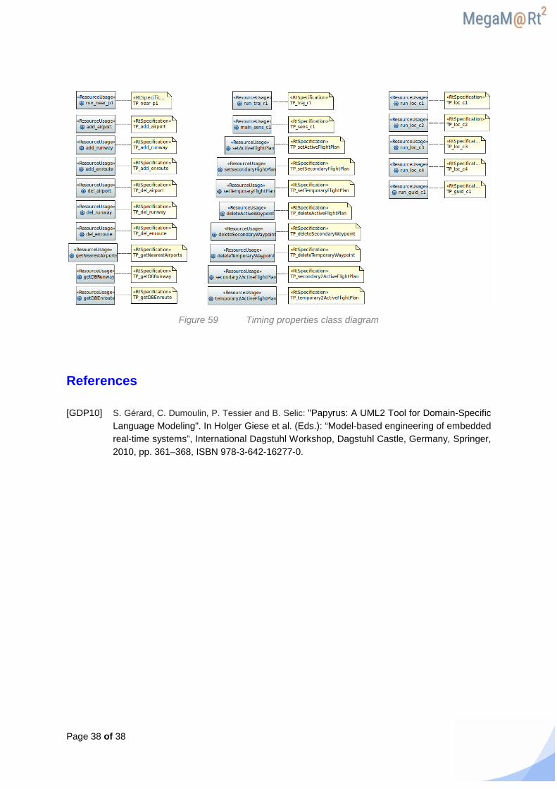
Optionally, you can create a class diagram (“New Diagram Class Diagram”) to visually represent timing properties related to functions of the elements that are used in your application, and which have been previously described in the Application view (Figure 38 and Figure 39). To do so, drag the operations (<<ResourceUsage>>) and related comments (<<RtSpecification>>) from the Application view into the class diagram. Then, place the mouse over the operation, click on the arrow pointing the operation and drag to the related comment, as shown in Figure 58. A final diagram with all the operations of our application is shown in Figure 59.

Figure 58 Association of an operation with its timing properties

Page 38 of 38

Figure 59 Timing properties class diagram

References

[GDP10] S. Gérard, C. Dumoulin, P. Tessier and B. Selic: "Papyrus: A UML2 Tool for Domain-Specific Language Modeling". In Holger Giese et al. (Eds.): “Model-based engineering of embedded real-time systems”, International Dagstuhl Workshop, Dagstuhl Castle, Germany, Springer, 2010, pp. 361–368, ISBN 978-3-642-16277-0.