Robustness of Rasch Fit Statistics in Dichotomous and Rating ...

University of Northern ColoradoScholarship & Creative Works @ Digital UNC

Dissertations Student Research

12-2018

Robustness of Rasch Fit Statistics in Dichotomousand Rating Scale DataSamantha Estrada Aguilera

Follow this and additional works at: https://digscholarship.unco.edu/dissertations

This Text is brought to you for free and open access by the Student Research at Scholarship & Creative Works @ Digital UNC. It has been accepted forinclusion in Dissertations by an authorized administrator of Scholarship & Creative Works @ Digital UNC. For more information, please [email protected].

Recommended CitationEstrada Aguilera, Samantha, "Robustness of Rasch Fit Statistics in Dichotomous and Rating Scale Data" (2018). Dissertations. 536.https://digscholarship.unco.edu/dissertations/536

https://digscholarship.unco.edu?utm_source=digscholarship.unco.edu%2Fdissertations%2F536&utm_medium=PDF&utm_campaign=PDFCoverPages

https://digscholarship.unco.edu/dissertations?utm_source=digscholarship.unco.edu%2Fdissertations%2F536&utm_medium=PDF&utm_campaign=PDFCoverPages

https://digscholarship.unco.edu/students?utm_source=digscholarship.unco.edu%2Fdissertations%2F536&utm_medium=PDF&utm_campaign=PDFCoverPages

https://digscholarship.unco.edu/dissertations?utm_source=digscholarship.unco.edu%2Fdissertations%2F536&utm_medium=PDF&utm_campaign=PDFCoverPages

https://digscholarship.unco.edu/dissertations/536?utm_source=digscholarship.unco.edu%2Fdissertations%2F536&utm_medium=PDF&utm_campaign=PDFCoverPages

mailto:[email protected]

UNIVERSITY OF NORTHERN COLORADO

Greeley, Colorado

The Graduate School

ROBUSTNESS OF RASCH FIT STATISTICS IN

DICHOTOMOUS AND RATING

SCALE DATA

A Dissertation Submitted in Partial Fulfilment

of the Requirement for the Degree of

Doctor of Philosophy

Samantha Estrada Aguilera

College of Education and Behavioral Sciences

Department of Applied Statistics and Research Methods

December 2018

This Dissertation by: Samantha Estrada Aguilera

Entitled: Robustness of Rasch Fit Statistics in Dichotomous and Rating Scale Data.

has been approved as meeting the requirement for the Degree of Doctoral of Philosophy

in College of Education and Behavioral Sciences in Department of Applied Statistics and

Research Methods

Accepted by the Doctoral Committee

______________________________________________________

Susan R. Hutchinson, Ph.D., Research Advisor

_______________________________________________________

Trent Lalonde, Ph.D., Committee Member

_______________________________________________________

Steven Pulos, Ph.D., Committee Member

_______________________________________________________

Heng-Yu Ku, Ph.D., Faculty Representative

Date of Dissertation Defense _________________________________________

Accepted by the Graduate School

_________________________________________________________

Linda L. Black, Ed.D.

Associate Provost and Dean

Graduate School and International Admissions

Research and Sponsored Projects

iii

ABSTRACT

Estrada Aguilera, Samantha. Robustness of Rasch Fit Statistics in Dichotomous and

Rating Scale Data. Published Doctor of Philosophy dissertation, University of

Northern Colorado, 2018.

To understand the role of fit statistics in Rasch measurement, it is necessary to

comprehend why fit is important in measurement. The answer to this question is simple:

applied researchers can only benefit from the desirable properties of the Rasch model

when the data fit the model; however, the currently available fit statistics are flawed. A

problem with fit statistics which are based on residuals is that they are based on unknown

distributional properties (Masters & Wright, 1997; Ostini & Nering, 2006). Rost and von

Davier (1994) developed the Q-Index. The Q-Index makes use of the statistical properties

of the Rasch model, namely, parameter separability and conditional inference. Ostini and

Nering, as early as 2006, called attention to the fact that little research has been

performed on the Q-Index and thus there is little knowledge regarding the fit statistic’s

robustness. To assess the Q-Index robustness, its performance was compared, in the

present study, to the currently popular fit statistics known as Infit, Oufit, and standardized

Infit and Oufit (ZSTDs) under varying conditions of test length, sample size, item

difficulty (normal and uniform), and Rasch model (dichotomous and rating scale). The

simulation consisted of 128 conditions that varied in sample size, test length, item

difficulty distribution, and dimensionality. A series of factorial ANOVAs were conducted

to examine the effect of sample size, test length, item difficulty distribution, and

iv

dimensionality on the fit statistics of interest. The results showed the Q-Index had a large

effect size for dimensionality and for the dichotomous model a medium effect size for

test length. Factorial ANOVAs for Infit, ZSTD Infit, Outfit, and ZSTD Infit resulted in

trivial effect sizes for all the variables of interest. Parameter recovery was also examined,

these findings suggest that the correlation between true and estimated parameters were

high (r > .930) for both the dichotomous Rasch and the rating scale Rasch model

indicating good pameter recovery despite the manipulation of test length, sample size,

item difficulty distribution and dimensionality. Future research may explore the Q-Index

under different measurement disturbances such as local independence or the robustness

of the person Q-Index. Overall more research is needed regarding the robustness of the

Q-Index.

v

TABLE OF CONTENTS

CHAPTER I. INTRODUCTION ........................................................................................ 1

Measurement Disturbances .......................................................................................... 4

Item Fit in the Rasch Model ........................................................................................ 4

Statement of the Problem ............................................................................................ 6

Purpose of the Study .................................................................................................... 7

Research Questions...................................................................................................... 8

Limitations ................................................................................................................. 10

Chapter Summary ...................................................................................................... 10

CHAPTER II. REVIEW OF LITERATURE ................................................................... 12

Overview of Rasch Analysis ..................................................................................... 12

Rasch Models for Ordered Polytomous Items ........................................................... 18

Item Fit in Rasch Analysis......................................................................................... 27

Person Fit in Rasch Analysis ..................................................................................... 28

Properties of an Effective Fit Statistic ....................................................................... 28

Classification of Fit Statistics in ................................................................................ 30

Rasch Analysis .......................................................................................................... 30

Rating Scale Fit Research .......................................................................................... 54

The Q-Index ............................................................................................................... 57

Chapter Summary ...................................................................................................... 62

CHAPTER III. METHODS .............................................................................................. 65

Design Factors ........................................................................................................... 66

Data Generation ......................................................................................................... 67

Number of Replications ............................................................................................. 72

Rasch Analysis .......................................................................................................... 72

Parameter Recovery ................................................................................................... 77

Simulation Procedure ................................................................................................ 79

Pilot Study ................................................................................................................. 81

Data Analysis ............................................................................................................. 85

Chapter Summary ...................................................................................................... 86

vi

CHAPTER IV. RESULTS ................................................................................................ 88

Data Conditions for the Dichotomous Rasch Model ................................................. 88

Q-Index for Dichotomous Rasch Model ................................................................... 91

Infit for the Dichotomous Rasch Model .................................................................... 95

Outfit for the Dichotomous Rasch Model ................................................................. 96

Standarized Infit for the Dichotomous Rasch Model ................................................ 97

Standarized Outfit for the Dichotomous Rasch Model ............................................. 98

Type I and II Errors for the Item Fit Statistics for Dichotomous Rasch Model ...... 100

Parameter Recovery of Dichotomous Rasch Model ................................................ 107

Supplementary Analysis .......................................................................................... 120

Rating Scale Model ................................................................................................. 123

Q-Index for the Rasch Rating Scale Model ............................................................. 125

Infit for the Rasch Rating Scale Model ................................................................... 128

Outfit for the Rasch Rating Scale Model................................................................. 130

Standarized Infit and Standarized Outfit for the Rasch Rating Scale Model .......... 131

Type I and II Errors for the Item Fit Statistics for Rasch Rating Scale Model ....... 133

Parameter Recovery of Rasch Rating Scale Model ................................................. 138

Supplementary Analysis .......................................................................................... 152

Chapter Summary .................................................................................................... 154

CHAPTER V. DISCUSSION ......................................................................................... 160

Performance of Fit Statistics.................................................................................... 160

Dichotomous Rasch Model ..................................................................................... 161

Rating Scale Rasch Model ....................................................................................... 163

General Discussion .................................................................................................. 165

Limitations ............................................................................................................... 168

Recommendations for Future Research ................................................................... 169

Implications for Practice .......................................................................................... 171

Conclusions ............................................................................................................. 172

REFERENCES ............................................................................................................... 174

APPENDIX A. R CODES FOR SIMULATION ........................................................... 187

APPENDIX B. DESCRIPTIVE INFORMATION FOR SIMULATION STUDY........ 200

APPENDIX C. DESCRIPTIVE INFORMATION FOR ITEM FIT STATISTICS ...... 232

APPENDIX D. SUPPLEMENTARY ANALYSIS ........................................................ 280

vii

TABLE OF TABLES

2.1 Summary of literature review findings for Infit, Outfit, ZSTD Infit and

ZSTD Outfit……………………………………………………………

63

3.1 The 4 x 4 x 2 x 2 Factorial Design for Rasch Dichotomous Scale

Model………………………………………………………………………. 71

3.2 The 4 x 4 x 2 x 2 Factorial Design for Rasch Rating Scale

Model…………………………………………………………………..…... 72

3.3 Dichotomous Rasch Model, Q-Index Calculation………………………… 75

3.4 Rasch Rating Scale Model, Q-Index Calculation………………………….. 75

3.5 Fit Indices and Recommended Critical Values……………………………. 78

4.1 Factorial ANOVA of Q-Index on Test Length, Sample Size, Difficulty

Distribution, and Dimensionality………………………………………….. 92

4.2 Descriptive Statistics across Conditions for the Unidimensional and

Multidimensional Dichotomous Rasch Models……………………..…….. 93

4.3 Factorial ANOVA of Infit on Test Length, Sample Size, Difficulty

Distribution, and Dimensionality…………………………………………. 96

4.4 Factorial ANOVA of Outfit on Test Length, Sample Size, Difficulty


4.5 Factorial ANOVA of ZSTD Infit on Test Length, Sample Size, Difficulty


4.6 Factorial ANOVA of ZSTD Outfit on Test Length, Sample Size,

Difficulty Distribution, and Dimensionality………………………………. 100

4.7 Recommended Cutoff Values for Each Item Fit Statistic ………………… 101

4.8 Type I and II Error Rates for the Rasch Dichotomous Model……………. 103

4.9 Parameter Recovery Recommended Cutoffs……………………………... 107

4.10 Maximum, Minimum, Mean, and Standard Deviation of the Bias in the

Absolute Value under the Dichotomous Rasch Model…………………... 109

viii

4.11 Maximum, Minimum, Mean, and Standard Deviation of the RSME under

the Dichotomous Rasch Model………………….………………………..

114

4.12 Relative Bias of the Dichotomous Rasch Model ………………………… 116

4.13 Relative Bias of the Dichotomous Rasch Model after Wright and Douglas

(1977) Correction………………………………………………………….

117

4.14 Factorial ANOVA of Relative Bias on Test Length, Sample Size,

Difficulty Distribution, and Dimensionality……………………………….

118

4.15 Bivariate Correlations between the True and Estimated Parameters……… 119

4.16 Q-Index values for I = 10 for the Two Factor (Multidimensional)

Condition under the Uniform Difficulty Distribution……………………..

121

4.17 Factorial ANOVA of Q-Index on Test Length, Sample Size, Difficulty

Distribution, and Dimensionality………………………………………….

126

4.18 Descriptive Statistics for the Unidimensional and Multidimensional Rasch

Rating Scale Models…………………………….…………………………

127

4.19 Factorial ANOVA of Infit on Test Length, Sample Size, Difficulty


4.20 Factorial ANOVA of Outfit on Test Length, Sample Size, Difficulty

Distribution, and Dimensionality…………………………………………..

130

4.21 Factorial ANOVA of ZSTD Infit on Test Length, Sample Size, Difficulty

Distribution, and Dimensionality………………………………………….

132

4.22 Factorial ANOVA of ZSTD Outfit on Test Length, Sample Size,

Difficulty Distribution, and Dimensionality………………………………

133

4.23 Type I and II Error Rates for the Rasch Rating Scale Model …..………… 137

4.24 Maximum, Mean, and Standard Deviation of the Bias in the Absolute

Value under the Rating Rasch Model after Wright and Douglas (1977)

correction………………..…………………………………………………

141

4.25 Maximum, Minimum, Mean, and Standard Deviation of the Corrected

Bias in the Absolute Value under the Rating Scale Rasch Model ……….. 142

4.26 Relative Bias for the Rasch Rating Scale Model before Wright and

Douglas (1977) Correction………………………………………………..

146

ix

4.27 Relative Bias of the Rasch Rating Scale Model after Wright and Douglas

(1977) Correction………….……………………………………………... 147

4.28 Factorial ANOVA of (Corrected) Relative Bias on Test Length, Sample

Size, Difficulty Distribution, and Dimensionality………………………...

148

4.29 Maximum, Minimum, Mean, and Standard Deviation of the RSME under

the Rating Scale Rasch Model……………………………………………

149

4.30 Bivariate Correlation between the True and Estimated Parameters for All

Conditions………………………………………………………………...

151

4.31 Q-Index values for I = 10 for the Two Factor (Multidimensional)

Condition under the Uniform Difficulty

Distribution………………………………………..………………………

153

4.32 Summary for Dichotomous Rasch Model and Rating Scale Rasch Model.. 156

4.33 Summary Table for the Rating Scale Rasch Model……………………….. 159

x

TABLE OF FIGURES

2.1 Description of thresholds ..................................................................................... 22

4.1 Item difficulty distribution vs. test length for the dichotomous Rasch model

under the Q-Index ................................................................................................ 94

4.2 Dimensionality vs. Test Length for Q-Index under the Rasch Dichotomous

Model. ................................................................................................................. 94

4.3 Relationship between the bias and the generating item parameter under the

dichotomous Rasch model. ............................................................................... 110

4.4 Relationship between the corrected bias and the generated item difficulty for the

dichotomous Rasch model. ............................................................................... 112

4.5 Relationship between RMSE of item difficulty estimates and the generated

difficulty. ........................................................................................................... 115

4.6 Type I error rate for the unidimensional dichotomous Rasch model and Type II

error for the multidimensional. ......................................................................... 104

4.7 Type II error rate for all item fit statistics for the dichotomous multidimensional

Rasch model ...................................................................................................... 106

4.8 Standard deviation trends for all item fit statistics............................................ 125

4.9 Average Q-Index by dimensionality by test length. ......................................... 128

4.10 Corrected bias vs. difficulty for rating scale Model. ........................................ 143

4.11 RMSE for Rasch rating scale for the extreme conditions. ................................ 150

1

CHAPTER I

INTRODUCTION

Mathematical models are beneficial in any field of human inquiry (Ostini &

Nering, 2006). In their simplest form, mathematical models help to quantify, or measure,

a phenomenon of interest. However, difficulty with inflexible mathematical models in the

social sciences led to the development of more appropriate measurement models (Ostini

& Nering, 2006). Psychologists, educational researchers, health sciences researchers as

well as marketing analysts utilize measurement in different contexts whether the

measurement is in the form of a survey, a test, or an attitude inventory. In the words of

Allen and Yen (2001): “Measurement is the assigning of numbers to individuals in a

systematic way as a means of representing the properties of individuals” (p. 2).

Measurement theory is necessary because the traits researchers try to measure are often

unobservable or latent.

Classical test theory (CTT) was developed to address the problems of

mathematical models of measurement in the human sciences (Ostini & Nering, 2006).

CTT was based on the work of Charles Spearman and derived from concepts from the

physical sciences (Ostini & Nering, 2006). A key concept CTT borrowed from the

physical sciences is the idea of error in measurement. Traditionally, researchers made use

of CTT in order to analyze the measurement properties of scores obtained from

2

instruments, such as achievement tests. Unfortunately, CTT has three major limitations.

First, item statistics are sample dependent. Second, respondents’ observed and true scores

are test-dependent. Third, CTT is test oriented rather than item oriented; meaning CTT

cannot predict someone’s ability given performance on a particular item. The limitations,

as well as the difficulties of testing the assumptions of CTT, led to the development of

different measurement models (Ostini & Nering, 2006).

Item response theory (IRT) is an alternative to CTT with roots in applied

psychology (Ostini & Nering, 2006). Item-based test theory has its roots in mathematical

models as well as the work in psychology with gifted children by Jean Binet, Theodore

Simon, and Lewis Terman in the 1910s (Baker & Kim, 2004). The mathematical

foundation of IRT is a function that specifies the probability of an examinee’s response to

an item in a certain manner given the trait level that item is measuring. In other words,

IRT describes, in probabilistic terms, an examinee with a high level of a certain trait who

is likely to provide a response in a distinctive response category, which is different from

that of a person with a low standing on the same trait. Frederic M. Lord and his

subsequent work with Melvin R. Novick, entitled “Statistical theories of mental test

scores” in 1968, is credited with the popularization of the IRT model (Ostini & Nering,

2006). Further, the work by Danish mathematician Georg Rasch in the 1960s played an

equally influential role by developing separately a distinct class of IRT models which

showed “a number of highly desirable features” (Ostini & Nering, 2006, p. 2). This

model is known as the Rasch model.

Rasch analysis is used in educational and psychological testing as well as the

measurement of health status and evaluation measures, among other applications

http://doi.apa.org/psycinfo/1968-35040-000

http://doi.apa.org/psycinfo/1968-35040-000

3

(Christensen, 2013). The Rasch model incorporates a method for ordering examinees

according to their ability as well as ordering items according to their difficulty. An

important Rasch principle is that interval-level measurement can be derived when the

level of some attribute increases concurrently with increases in person ability and item

difficulty (Bond & Fox, 2015). Furthermore, Rasch practitioners and scholars state that in

objective measurement the measurement estimate stays constant, with permissible error,

“across the persons measured, across different brands of instruments, and across

instrument users” (Institute for Objective Measurement, Inc., 2000, para 2). The degree

to which the psychometric properties are obtained from responses to a survey or a test

relies on this objective measurement.

In measurement, the concept of fit helps researchers identify divergences in the

data. These divergences force researchers to pause, reflect, and consider what the data

mean and what the fit indices are indicating. If there is in fact a divergence, the researcher

is left to question whether the model or the data are at fault (Andrich, 1988). In the

situation when a discrepancy between the data and the model exists, it is very likely that

there is an issue with either the data or the data collection (Andrich, 1988). The simplest

solution could be modifying the data collection process or rewording items rather than

changing the model. It is important to investigate whether the data fit the Rasch model, or

any model for that matter. If the data do not fit the model in question, it is not possible to

benefit from the properties of the Rasch model and the use of this model is pointless (R.

M. Smith & Suh, 2003).

4

Measurement Disturbances

Measurement disturbances are conditions that interfere with the measurement of

an underlying latent construct. These latent constructs can be, for example, self-efficacy,

anxiety, ability, or attitude (R. M. Smith, 1991). Latent, or unobserved variables are of

interest in fields like psychology, marketing, and education. Unfortunately, there exists a

variety of measurement disturbances and the manner in which they manifest in the data

varies as well. Guessing, sloppiness, data entry and clerical errors, item bias, test anxiety,

boredom, distractions, and cheating are a few examples of measurement disturbances.

The influence of these factors on the probability of a correct response makes it difficult

for researchers to understand and correctly measure a person’s ability (R. M. Smith &

Plackner, 2009). The effectiveness of a fit statistic can depend on its ability to detect

measurement disturbances (Karabatsos, 2000). Minimizing the impact of measurement

disturbances on the estimates of item difficulty and person ability is vital to objective

measurement (R. M. Smith & Plackner, 2009). For this reason, there is no single fit

statistic that will perfectly detect every one of these disturbances (R. M. Smith &

Plackner, 2009; A. B Smith, Rush, Fallowfield, Velikova, & Sharpe, 2008).

Item Fit in the Rasch Model

Fit has been studied since the introduction of the Rasch model (Gustafsson, 1980;

Rasch, 1980). Rasch (1980) suggested a variety of methods to assess the fit of data. These

methods were graphical and statistical in nature. For Rasch analysis, scholars created

statistical tests of goodness-of-fit with the purpose of understanding fit (Wright &

Linacre, 1994). In practice, misfit is usually determined by mean square fit statistics,

5

which are useful in identifying misfitting items or persons (Linacre, 1995); however, the

currently available fit statistics are flawed.

A problem with many of the current fit measures, which are based on residuals, is

that they are founded on unknown distributional properties (Masters & Wright, 1997;

Ostini & Nering, 2006). When distributional properties are unknown, it is difficult for

researchers and statisticians to justify the critical values for the fit statistic. This in turn,

causes several different ad hoc cutoffs, or critical values, to be proposed by scholars

(Smith et al., 2008; Wright & Linacre, 1994). Many Rasch analysis programs make use

of these residual fit indices, named Infit and Outfit (Bond & Fox, 2015; Wright &

Panchapakesan, 1969). Infit and Outfit statistics can also be presented in a standardized

form such as the t distribution (Bond & Fox, 2015). In the United States and Australia,

the residual-based fit statistics proposed by Wright and Panchapakesan (1969) are quite

popular due to Rasch software such as Winsteps, ConQuest, and RUMM (Linacre, 2006;

Smith et al., 2008; R. M. Smith & Plackner, 2009).

The Q-Index

Rost and von Davier (1994) developed the item Q or Q-Index, which is a response

function method to assess fit in Rasch modeling. The authors stated that the Q-Index is

not based on the differences between observed and expected scores as Infit and Outfit.

For the calculation of the Q-Index the item parameter is conditioned out of the item-fit

index. The Q-Index takes advantage of the Rasch model property of parameter

separability. The Q-Index is constructed on the likelihood of observed response patterns;

however, the fit statistic uses conditional likelihoods. For example, the likelihood of an

item pattern is conditioned on the item score though an estimate of the item parameter is

6

needed for statistical inference purposes. Rost and von Davier claimed that this process

makes the Q-Index “parameter free” with respect to the item parameter (p. 174).

Additionally, the authors believed this quality makes the Q-Index superior to the

currently available methods of assessing fit. Furthermore, Rost and von Davier stated

that the Q-Index takes into consideration the assumptions of both dichotomous and

polytomous Rasch models and for this reason it can be utilized with any unidimensional

dichotomous or polytomous model.

Statement of the Problem

The currently available fit statistics for the Rasch model are flawed. Karabatsos

(2000) stated “although the residual-based fit statistics have been of practical use for

more than 30 years, in many respects they remain unsatisfactory” (p. 159). Karabatsos

also argued that there has been little research regarding the distributional properties of

residual-based fit statistics with rating scales possibly due to the complexity of the rating

scale model. Similarly, Smith (1996) stated that the performance of mean square statistics

for dichotomous data has been researched for more than 30 years; however, the

interpretation and study of fit statistics for polytomous items is considered a recent

development. It is worth noting that Smith’s paper is almost 20 years old to date, yet the

research for polytomous items and fit continues to be lacking with only work by A. B.

Smith et al. (2008), Wang and Chen (2005), and Seol (2016) focusing on the issue.

According to Wu and Adams (2013), practitioners have repeatedly requested guidelines

for the use of residual fit statistics. Likewise, questions on guidelines are a frequent topic

in the popular Rasch listserv (Wu & Adams, 2013). Though this dissertation focused on a

handful of fit statistics, there is a large number of available item fit statistics available in

7

different Rasch software; however, there is a lack of studies comparing the power of item

fit statistics in a systematic and comprehensive manner which results in uncertainty on

which fit statistics are the most efficient and/or powerful (Christensen, Kreiner, &

Mesbah, 2013). Furthermore, Ostini and Nering (2006) considered the response function

method utilized by the Q-Index to show promise; however, little research has been

conducted to date. Particularly Ostini and Nering argued that the key disadvantage of the

Q-Index is the lack of research assessing whether or not it works as intended.

Purpose of the Study

The purpose of fit statistics is to screen misfitting items or persons. If fit statistics

are incorrect, a misfitting item or person may not be located correctly, or they may be

incorrectly identified as misfitting. More importantly, the properties and benefit of using

a certain model, in this case the Rasch model, will hold if and only if the data fit the

model. The Q-Index index has desirable characteristics, which could provide a solution to

applied researchers concerned with the limitations of current fit indices. However, little

research has been performed regarding the robustness of the Q-Index (Ostini & Nering,

2006). Due to the lack of research regarding the Q-Index in addition to the limitations of

residual fit indices, and in order to respond to Ostini and Nering’s (2006) call for research

on the topic, in this dissertation I studied robustness of the Q-Index under varying

conditions of sample size, test length, item difficulty distribution along with the

introduction of the measurement disturbance of multidimensionality. In this study, I

compared the performance of the Q-Index in contrast with residual fit indices, including

Infit and Outfit and standardized Infit and Outfit, which are available in the popular

Rasch software Winsteps (Linacre, 2006). The results of this study provide applied

8

researchers with evidence regarding the robustness of the Q-Index in contrast with the

currently available measures of fit (Linacre, 2006; von Davier, 2001).

The purpose of the current study was to examine how varying conditions of (a)

sample size, (b) test lengths, (c) item difficulty distribution, and (d) measurement

disturbance (in the form of multidimensionality) affect the fit estimates and their standard

errors and Type I error rate. The independent variables were chosen based on previous fit

statistics literature for the Rasch model. For example, sample sizes of N = 30, 100, 150,

and 250 for the Rasch dichotomous model and N = 50, 100, 150, and 250 for the Rasch

rating scale model were chosen based on Linacre’s (1994a) recommendations. Following

the guidelines of Wright and Douglas (1975) and Linacre (1994a) the test lengths of N =

10, 20, and 30 were selected.

Additionally, following the convention for simulation research on the Rasch

model the item difficulty distributions of interest were normally distributed and

uniformly distributed. Due to its popularity, the Rasch software Winsteps is commonly

used for applied research and simulation research (E. V. Smith Jr., 2002; R. M. Smith &

Suh, 2003; Wang & Chen, 2005; Wolfe & McGill, 2011); thus, it was the choice of

Rasch software for this dissertation. Additionally, there exists very little research on the

rating scale model (Seol, 2016; A. B. Smith et al., 2008; Wang & Chen, 2005); thus,

adding this model as a condition was appropriate.

Research Questions

The research questions are as follows:

Q1 For the Rasch dichotomous model, do fit indexes (mean square Infit, mean

square Outfit, Standardized Infit, Standardized Outfit, and Q-index) differ

under varying conditions of sample size, in correctly identifying item

misfit?

9



under varying conditions of test length, in correctly identifying item

misfit?



under varying conditions of dimensionality, in correctly identifying item

misfit?



under varying conditions of item difficulty distribution, in correctly

identifying item misfit?

Q5 What degree of the accuracy of parameter recovery does the Rasch

dichotomous model provide under various simulation conditions when the

accuracy is assessed by correlation, root mean square error, and bias

estimates?

Q6 For the Rasch rating scale model, do fit indexes (mean square Infit, mean



misfit?




misfit?




misfit?





Q10 What degree of the accuracy of parameter recovery does the Rasch rating

scale model provide under various simulation conditions when the


estimates?

10

Limitations

As with all simulation studies, there is the inherent limitation of external validity

due to the “artificial” conditions of the study, making it more difficult to generalize to

“real life” data. Moreover, no simulation study can take into account all possible data

conditions that might influence the results. An additional limitation of this dissertation is

the availability of the Q-Index to applied researchers. When this dissertation was written,

the Rasch software Winmira was the only available software where the Q-Index was

available (von Davier, 2001). In fact, Winmira seems to be moderately popular in Europe

but is less well-known elsewhere. For this reason, the Q-Index may not be readily

available to applied researchers in the United States; however, further research on the Q-

Index such as this dissertation provides, may encourage the implementation of the Q-

Index and the standardized Q-Index into more popular software such as Winsteps or even

R packages such as eRm and mIRT.

Chapter Summary

Rasch modeling is a popular psychometric tool in the educational, social science,

and health sciences. Research on fit is important because if data do not fit the Rasch

model, then interpretations based on the model can be incorrect. The currently available

fit statistics based on residuals are flawed and more research needs to be performed to

determine their distributional properties. This study will provide applied researchers

information on the robustness of the Q-Index as well as a comparison with the currently

available fit statistics such as Infit, Outfit, standardized Infit, and standardized Outfit.

In Chapter I, I introduced the rationale, in addition to the need for the study. I also

briefly described the goals for this study. In Chapter II, I describe the Rasch model in

11

more detail in addition to the Rasch rating scale model and the assumptions for both

models. Briefly, I describe the approaches to fit in Rasch analysis, but focus heavily on

the residual fit statistics which are more popular among Rasch users. Finally, I describe

Rost and von Davier’s (1994) Q-Index. In Chapter II, I also summarize the relevant

literature pertaining to the item fit statistics of interest. Next, in Chapter III, I outline how

the research was accomplished. This chapter includes a description of the manipulated

variables based on the literature reviewed in Chapter II, in addition to a description on

how the simulation was performed and in which software each piece was conducted. In

Chapter IV, I present the results of the study, and finally in Chapter V, I discuss the

results with recommendations for applied researchers.

12

CHAPTER II

REVIEW OF LITERATURE

This review of literature provides relevant background to support the need,

purpose, choice of variables, and research questions for the present study. Chapter II

begins by presenting information on the Rasch model, specifically the dichotomous and

polytomous models, in addition to the assumptions for each model. Different types of fit

approaches are summarized. Moreover, past research on fit analysis in the Rasch

dichotomous model is discussed to understand the current use of rule of thumb critical

values commonly utilized in today’s applied research. Empirical and simulation research

reviewing the use of these critical values is discussed for both the Rasch dichotomous and

polytomous models. Alternatives to the use of rules of thumb critical values are

discussed.

Overview of Rasch Analysis

Cognitive abilities, which are often called “latent traits,” cannot be measured

directly. For this reason, tests, inventories, and surveys are designed to measure these

traits. In the same manner, different techniques of assessing the psychometric properties

of scores obtained from these tests have been developed. One such method is the Rasch

model which was named after Georg Rasch (Rasch, 1980) who developed it in the 1950s

(Christensen et al., 2013). The use of Rasch analysis has increased in the past decades.

Rasch analysis is commonly used in educational and psychological testing. The method is

13

also popular in the measurement of health status and evaluation outcomes (Christensen,

2013). Rasch (1980) initially developed the model for dichotomous data. Since then,

different Rasch measurement models have been developed, including the rating scale

model (Wright & Masters, 1982), partial credit (Masters, 1982), and many facets

(Linacre, 1994b) models. The Rasch model describes responses to a certain number of

items for a given number of examinees assuming these responses are stochastically

independent (Christensen et al., 2013).

In Rasch analysis, two conditions are part of the model: (a) the trait possessed by

the person and (b) the difficulty necessary to provide a certain level of response. The

following function represents the probability of success for an examinee’s response on a

dichotomous item:

𝑃(𝑋𝑣𝑖 = 1 | Θ𝑣 = 𝜃𝑣) = 𝑒(𝜃𝑣−𝛽𝑖)

1+𝑒(𝜃𝑣−𝛽𝑖) (2.1)

Equation 2.1 is the original formulation of the model according to Rasch (1980).

Where 𝑋𝑣𝑖 is a random variable indicating success or failure. 𝑋 = 1 indicates success, for

example, a correct response, while 𝑋 = 0 indicates failure or an incorrect response on the

item. The subscript 𝜈 represents the person while the subscript 𝑖 represents the item. The

probability of a correct response increases as the ability parameter increase toward

infinity. For example, in an educational testing setting the higher the ability of the student

and the easier the item, the greater the probability of a correct response. Likewise, in a

health science example, the person parameter could represent the level of depression, or

pain, while the item parameters would represent the risk of experiencing certain

symptoms related to the trait. Consider a dichotomous item constructed to measure

depression: “Do you have difficulty sleeping in the last two weeks?”. Or, “did your

14

appetite decreased in the last two weeks?”. According to the Rasch model, the level of

depression measured by these items is measured by the person parameter. The Θ𝑣

represents an unobservable, or latent, trait and 𝜃 is the person parameter which denotes

the examinee’s location on the latent trait scale. The 𝛽 represents the item difficulty or

item location parameter on the same latent trait scale, and is an item parameter. Both 𝜃

and 𝛽 are on a logit scale (Christensen et al., 2013). Equation 2.1 is a function of the

difference between the examinee’s ability and the item difficulty (Wu & Adams, 2013).

Consequently, as an examinee’s ability exceeds the difficulty of a given item, the

probability of a correct response increases. From Equation 2.1 it follows that:

𝑃(𝑋𝑣𝑖 = 0 | Θ𝑣 = 𝜃𝑣) = 1 − 𝑃(𝑋 = 1) = 1

1+𝑒(𝜃𝑣−𝛽𝑖) (2.2)

In Equation 2.2 responses are coded as 1 for a correct response and 0 for an

incorrect response. The logit function of the probability of a positive response is:

𝑙𝑜𝑔𝑖𝑡(𝑃[𝑋𝑣𝑖 = 1| Θ𝑣 = 𝜃𝑣]) = 𝜃𝑣 − 𝛽𝑖 (2.3)

For this reason, both 𝜃𝑣 and 𝛽𝑖 are said to be measured on a logit scale (Christensen et al.,

2013). Logit is also known as log-odds. Linacre and Wright (1989) defined logit as “the

distance along the line of the variable that increases the odds of observing the event

specified in the measurement model by a factor of 2.718.., the value of ‘e’” (para. 7). The

Rasch measurements are expressed in logits, but may be re-scaled to suit conventional

scaling such as 0 to 100 while retaining the properties of the measurement of persons and

items on the same scale. For example, in a setting such as educational testing the person

parameter would represent the ability of a student while the item parameter would

represent the easiness or difficulty of the item. In the health sciences, the person

parameter could represent the level of a patient’s depression while the item parameter

15

could represent the gravity of the symptoms related to depression (Christensen et al.,

2013). The scale on which 𝛽 is measured is often claimed to be an interval scale

(Christensen et al., 2013).

The probabilities in the Rasch model representing a difference between person

and item parameters as well as the symmetry of the item and person parameters results in

the item and persons being measured on the same scale. In a situation where the ability is

the same as the difficulty, the probability of success would equal .50. This value also

represents an item’s threshold, which is defined as the point on the ability/difficulty

continuum at which ability and difficulty are the same and where the probability of

success would equal .50 (Christensen et al., 2013).

Georg Rasch derived the Rasch model with the purpose of modeling test behavior

at the item level and for analyzing dichotomous data (1980). In Rasch modeling, the use

of sufficient statistics when calculating item and person parameters eliminates the

interdependency between them. The logistic function of the Rasch model provides an

equal interval, linear scale on which the measurement of items and persons can be

estimated separately. This is referred to as “specific objectivity” by Rasch (1980).

Assumptions of Rasch Analysis

The following properties must be met for the Rasch model to be appropriate.

Monotonicity. Monotonicity refers to the probability of a positive response to an

item which increases along with the increment in ability. In other words, the higher the

ability of an examinee the higher the probability that the examinee will positively, or

correctly, respond to the item.

16

Unidimensionality. Unidimensionality refers to having a single construct or

latent trait that accounts for the performance on items (E. V. Smith Jr., 2002). E. V.

Smith Jr. (2002) discussed that unidimensionality does not necessarily mean that the

items measure a single psychological concept, rather a variety of psychological processes

that function together. If the unidimensionality principle is not met, it is not appropriate

to compute a total score from the measure and use it to compare items or people (Boone,

Staver, & Yale, 2014). Embretson and Reise (2013) warned that “failing to estimate a

dimension that is important in the items will lead to local dependency” (p. 189). E. V.

Smith Jr. further discussed the importance of unidimensionality. First, for a test or survey

with the purpose of assessing a specific construct it is important that different levels of

abilities do not influence the assessment. Second, when the researcher’s purpose is to

order individuals on a given construct it is important that the assessment is

unidimensional. Otherwise it becomes difficult to determine whether two persons with

the same score are similar on the construct of interest.

Local independence. The Rasch model is capable of ordering people according

to their ability as well as ordering items according to their difficulty (Bond & Fox, 2015).

Local independence means that the examinee’s response to an item is not related to (or in

other words is independent of), the response on a different item when the examinee’s

ability is controlled and the correlation of the residuals should be zero (Embretson &

Reise, 2013). The item reponses should only be correlated by the latent trait under study.

Embretson and Reise (2013) explained that “if local independence is violated, then the

response pattern probabilities will be inappropriately reproduced in standard IRT models”

17

(p. 188). In practice, the assumption of local independence is violated if the item

responses are linked in some way. For example, in an introduction to statistics exam if an

item or the response to the item provides a clue that helps the students answer a different

question on the exam, this would result in violation of local independence.

Additionally, the following properties are characteristic of the Rasch dichotomous

and polytomous modes.

Sufficiency. The Rasch model has several sufficiency properties which are given

due to the model’s being part of the exponential family (Christensen et al., 2013). The

most important sufficiency property is that the total score is a sufficient statistic for 𝜃.

This property is not shared with any other IRT model though the property of sufficiency

is common in the field of statistics.

Invariance of parameters. To understand the concept of invariance of

parameters it is important to first understand the definition of sample invariant items.

Sample invariant items are defined as those items which have differences that do not

depend on the person’s ability used to compare the items. In other words, the item

difficulty estimates should be essentially the same regardless of the sample of examinees

(assuming this sample is representative of the population with the trait of interest). For

example, an examinee’s predicted ability should be the same, provided a reasonable

measurement error, for any representative sample of items which are designed to measure

the trait of interest (Christensen et al., 2013; Embretson & Reise, 2013). In the Rasch

model, the item difficulty represents the “easiness” of the item. The invariance of an item

is indicated when the item difficulty estimates are not statistically significantly different

when estimated from separate random samples taken from appropriate populations

18

Rasch Models for Ordered Polytomous Items

Polytomous data refer to items which have more than two responses and are

“inherently ordered” (De Ayala, 2013, p. 162). In this context, ordered means that there is

an order to the responses indicating either more (or less) of the trait being measured.

Polytomous item response models were developed because polytomous items exist

particularly in the field of applied psychological measurement (Ostini & Nering, 2006).

In fact, polytomous items can be found everywhere in the education, health sciences, or

psychological research fields (Ostini & Nering, 2010). Ostini and Nering (2010) declared

that polytomous items “offer a much richer testing experience for the examinee while

also providing more psychometric information about the construct being measured” (p.

3). Polytomous items are also known as rating scale items and/or Likert scales. If the

response categories work as intended, then the information provided by a polytomously-

scored item is more than that from a dichotomously-scored item. Polytomous items, like

dichotomous items, are scored categorically. The difference is that polytomous items

have more than two ordered categories. In practice, researchers go beyond the

dichotomous possibilities of “yes” or “no” and “agree” or “disagree,” especially, in

surveys in fields such as education or the psychological sciences, where the response

options often include four or more ordered responses. For example, an examinee is asked

to indicate his or her level of agreement on a Likert scale such that 1=Strongly Disagree,

2 = Disagree, 3 = Uncertain, 4 = Agree, and 5 = Strongly Agree. Another example is an

examinee’s being asked to rate his level of self-efficacy regarding a certain task (0 = No

confidence at all to 6 = Complete confidence). In both examples, response options

represent polytomous scales. In addition to estimating person parameters and difficulty

19

estimates, the polytomous item response model also provides a set of rating scale

categories, which are the same for all items (Bond & Fox, 2015). Boundaries or

thresholds separate these ordered categories.

Rating Scale Model

One type of Rasch polytomous model is the rating scale model (RSM). The RSM

is an extension of the Rasch model for dichotomous responses developed by Georg

Rasch. The RSM receives its name because of the individual item responses that

represent the rating scales that constitute a response given by examinees (Andersen,

1997).

The RSM is a type of polytomous Rasch model (Bond & Fox, 2015). The

assumptions of the polytomous Rasch model are: (a) the latent trait 𝜃 is a scalar; thus, the

latent trait is unidimensional, (b) the examinees are independent, and (c) the items are

locally independent. In other words, the items are conditionally independent given the

latent trait. Andersen (1973) defined the RSM as shown in Equation 2.4:

𝑃(𝑋𝑣𝑖 = 𝑥 | Θ = 𝜃𝑣) = 𝑒(𝜃𝑣𝑥+ 𝜓𝑖𝑥)

∑ 𝑒(𝜃𝑣ℎ+ 𝜓𝑖ℎ)𝑚𝑖ℎ=0

(2.4)

Where 𝜃𝑣𝑥 is the person parameter and 𝜓𝑖𝑥 is the ith threshold location parameter of item

x. If the responses by examinees are denoted as 𝑋𝑣𝑖 the possible responses are coded as

𝑋𝑣𝑖 = 0, 1, 2, … ,𝑚𝑖 where the number of response categories for any given item i is 𝑚𝑖 +

1. Higher ratings should indicate higher levels on the latent trait of interest (Engelhard,

2013). The scoring of ordered categories, with ordered integers such that 0,1…m, implies

that the distance between these categories is in equal intervals. For example, the distance

between 1 and 2 is the same distance as between 2 and 3 (Engelhard, 2013). This is an

assumption that may or may not be justified for any given dataset.

20

In contrast with assessing proficiency on a task or subject, in practice, the purpose

of an instrument may focus on assessing an individual’s attitude toward a particular topic,

or perhaps personality based on traits such as anxiety or confidence. This type of

instrument utilizes a Likert or Likert-type scale. This Likert-type scale may contain an

even or an odd number of response categories (ranging from three to five to seven or

even nine). Linacre (2000) defined the RSM as a model in which all the items, or a group

of items, have the same rating scale structure. This is the case in attitude surveys or

inventories where the response choices are the same for several items. For example, a

self-efficacy scale may ask examinees to rate their confidence from 1 = No Confidence at

all to 6 = Complete confidence. An attitude scale may ask examinees to rate their

agreement on a 4-point Likert-type scale from 1 = Strongly Disagree, 2 = Disagree, 3 =

Agree, 4 = Strongly Agree. This system avoids mental exhaustion from the examinee’s

having to “figure out” the rating scale for different items in the same survey. Wright

(1999) wrote, “it is impractical and mentally overwhelming to present a different rating

scale structure for each item” (para. 4).

The RSM has an additional feature over the dichotomous Rasch model. The RSM

also gives information on the number of rating scale thresholds which are shared by all

the items in the instrument (Bond & Fox, 2015). Bond and Fox (2015) defined a

threshold as “the level at which the likelihood of being observed in a given response

category (below the threshold) is exceeded by the likelihood of being observed in the

next higher category (above the threshold)” (p. 116). In an instrument with dichotomous

item scores, the examinee’s responses are considered either a success or a failure.

Likewise, in a rating scale the examinee is thought of as failing to agree or failing to

21

endorse a certain category. In the same way, success is defined as an examinee’s

endorsement or agreement with a certain category.

The RSM obtains responses from a series of ordered categories, which are

separated by ordered thresholds. The RSM does not assume what the size of the step

would be to move from one category to another, though the threshold pattern is the same

for all items. An examinee may find it difficult to endorse “6 = Complete Confidence” on

a self-efficacy scale but choose to select a “5 = Very Confident.” Or perhaps an examinee

would have small increases in anxiety going from threshold 1 to 2 but greater increases in

anxiety going from threshold 3 to 4. However, the RSM can detect the threshold structure

of the Likert or Likert-type scale instrument, and with this information the RSM can

estimate “a single set of response category threshold values” which would apply to all the

items in the scale (Bond & Fox, 2015, p. 116).

For example, in a survey of statistics self-efficacy the examinee is asked to rate

his or her confidence to “Identify the scale of measurement for a variable.” The response

categories range from “0 = Total Lack of Confidence” to “4 = Complete Confidence.”

See Figure 1. Assume the item has a difficulty 𝛽 of value 0. When an examinee of ability

𝜃 answers this item, the probability of selecting the “Total Lack of Confidence” category

or the “Not Confident” category depends on whether the person is located above or below

the threshold 𝜏1. If 𝜃 < 𝜏1 then the person responds, “Total Lack of Confidence.” This

hypothetical situation assumes that there are no external factors influencing the examinee,

such as social desirability, for example. This is the same process that occurs at the

thresholds 𝜏2 or 𝜏3. Thus, the responder “passes through” one or more thresholds to select

his or her answer. The number of thresholds of the item is represented by 𝑥𝑗, where j

22

equals the number of response categories minus one. In the case where 𝑥𝑗 = 0 the

examinee did not pass through any thresholds. Likewise, if the examinee has passed

through all thresholds 𝑥𝑗 = 𝑚 (See Figure 2.1).

Total lack of

confidence a

Not Confident Confident Complete

Confidence

𝜏1 𝜏2 𝜏2

Figure 2.1. Description of thresholds

Measurement Disturbances

A measurement disturbance is a condition that interferes with the measurement of

an underlying latent construct (R. M. Smith, 1991). Measurement disturbances refer to a

wide variety of problems, for example, guessing, data entry errors, cheating, test anxiety,

boredom, external distractions, and sloppiness among others (R. M. Smith & Plackner,

2009). These are beyond the person’s ability and the item’s difficulty. In Rasch analysis

only two conditions are part of the model: person ability and item difficulty. Any other

condition that has an impact on measurement is considered noise and thus a measurement

disturbance. Therefore, minimizing the influence of measurement disturbances on

estimation of either item or person parameters is necessary to have objective

measurement.

Historically, Edward Thorndike was the first to enumerate causes for the

disruption of the measurement process (R. M. Smith & Plackner, 2009). R. M. Smith and

Plackner (2009) classified the disturbances into three categories: (a) disturbances that are

the result of a person’s characteristics and independent of the item, (b) disturbances that

23

are a result of an interaction between the person’s characteristics and a property of the

item, and (c) disturbances that are due to a property of the item and independent of the

person’s characteristic. This classification allows researchers to detect the source of the

measurement disturbance and determine which techniques are necessary to detect the

disturbance.

Disturbances due to person characteristics. These disturbances result from

persons’ characteristics and are independent of the item. These types of disturbances are

also the easiest to understand. For example, the response pattern for a student who is

easily distracted will be influenced by external sources such as noise outside the

classroom, extreme temperature in a classroom, and/or noise by other students in the

classroom. Measurement disturbances that fall into this category are test anxiety,

excessive cautiousness, copying, sickness, fatigue, boredom, external distractions, and

guessing, among others.

Disturbances due to interaction. These measurement disturbances result from

the interaction between the examinees’ characteristics and item properties. Although the

characteristics of the examinees and the property of the items are present at every item,

this type of measurement disturbance does not present itself unless the property of the

item interacts with the examinee’s characteristic(s). The following are examples of this

type of measurement disturbance: guessing, sloppiness/excessive carelessness, item

content/person interaction, item type/person interaction, and item bias/person interaction.

Item content/person interaction occurs when the subject matter being tested has been

under-learned or over-learned and results in an under or overestimation of the examinee’s

ability. Item type/person interaction occurs when the type of items in the test being used

24

is “differentially familiar or unfamiliar to a person” (R. M. Smith & Plackner, 2009, pp.

427-428). R. M. Smith and Plackner (2009) argued that the extent to which guessing can

be found in the data depends on the interaction between the person’s tendency to guess

and the tendency of the item to “evoke guessing” (p. 427). Finally, item bias/person

occurs when an item or subset of items favors a particular gender, age group, educational

background, ethnicity, or cognitive style. This may cause for the over or underestimation

of an examinee’s ability.

Disturbances due to item properties. These measurement disturbances are due

to item properties and are independent of the person’s characteristic. R. M. Smith and

Plackner (2009) contended that examples for this type of measurement disturbance are

difficult to find. However, the authors explained that this type of measurement

disturbance could occur via a typographical error on the exam though examinees with

high ability are usually able to overcome this issue. A different reason could be a data

entry error where an incorrect value is entered instead of an accurate one.

R. M. Smith and Plackner (2009) categorized the process of detecting

measurement disturbances into three different categories. The first category is an

examination of the entire response matrix. This examination relies on the analysis of the

item and person parameters. A second approach to investigate the fit of the responses to

individual items is known as item fit. This analysis can primarily focus on the observed

responses; however, the analysis may be more useful when it is based on characteristics

of the examinees, such as gender, age, first language, ethnicity, or cognitive style if the

researcher suspects that a demographic characteristic may be the cause of the

measurement disturbance. This information can be used to create different groups in

25

order to test the invariance property of the item difficulty parameters. The third approach

to detecting measurement disturbances is the examination of the fit of responses for

individual persons. This is known as person fit analysis. This type of analysis can focus

on the response data; however, it may be useful to identify groups of items by inspecting

the items. Nevertheless, there exist measurement disturbances that cannot be easily

identified in either items or examinees (R. M. Smith & Plackner, 2009).

In summary, measurement disturbances hinder the appropriate measurement of an

underlying trait. Within the Rasch model, only two conditions should determine the

outcome of the interaction between a person and the item. These conditions are the

person’s ability and the item difficulty (Schumacker, Mount, Dallas, & Marcoulides,

2005; Smith, 1991). Any other condition, outside the person’s ability and the item

difficulty, can be considered a measurement disturbance.

Multidimensionality. In the 1600s, the thermometer measured both temperature

and atmospheric pressure, which made that type of thermometer multidimensional. When

scientists were able to separate the two constructs it was considered a major scientific

advantage. Social scientists utilize the same approach with latent variables and

unidimensional constructs (Linacre, 2009).

Multidimensionality is a measurement disturbance at the item level in addition to

a property of the Rasch model. Item multidimensionality occurs when an item, or a subset

of items, does not measure the same attributes as the rest of the items in the test

(Karabatsos, 2000). Stout (1987) listed three reasons why unidimensionality, or absence

of multidimensionality, is important to the assessment of responses. First, for any tests

with the purpose of measuring any given ability it is important for the researchers, as well

http://www.refworks.com/refworks2/default.aspx?r=references%7CMainLayout::init

http://www.refworks.com/refworks2/default.aspx?r=references%7CMainLayout::init

26

as the consumers of the results, to know that the measure of the ability is not

“contaminated by varying levels of one or more other abilities displayed by examinees

taking the test” (p. 589). Second, it is important that a test that is designed to measure a

specific construct is in fact measuring a single construct. The scores of a test are more

meaningful when there is only one range for that specific construct. Additionally,

identifying the same construct on the same scale allows for the fair comparison of two

different persons. Stout claimed that in the event where two items are measuring two

different constructs they should be considered as two different tests. Moreover, item bias

for two different groups occurs when there is a discrepancy between the latent ability and

the performance on the item (Mellenbergh, 1989). Violation of the unidimensionality

assumption can cause item bias in addition to bias in the ability parameter estimation (E.

V. Smith Jr., 2002; Setzer, 2008; Yu, Popp, DiGangi, & Jannasch-Pennell, 2007)

The assumption of unidimensionality is at the heart of the Rasch model and other

IRT models. Reckase (1979) studied the applicability of a unidimensional model such as

the Rasch model to multidimensional tests. The author generated a two dimensional

dataset, one dimension with a dominant latent trait and another dimension with multiple

latent traits. The study findings showed that the Rasch model tended to be robust to minor

degrees of multidimensionality given the good parameter recovery for both the ability

and item parameter. Within the IRT framework Drasgow and Parsons (1983) studied

multidimensionality in unidimensional IRT models. The authors simulated the

multidimensional data from a hierarchical factor model. In Drasgow and Parsons’ study,

the authors manipulated the inter-correlations between the factors from strictly

unidimensional (an inter-correlation of 1.0) to multidimensional (an inter-correlation of

27

0). The authors found that the item and ability parameters were affected by

multidimensionality when the inter-correlations between the factors were .39 or lower.

R. M. Smith (1996) stated that Rasch fit statistics have been found to be sensitive to

multidimensionality in situations when a latent trait for each dimension has an

approximately equal number of test items and the inter-correlation between the latent

traits are low.

Item Fit in Rasch Analysis

Christensen et al. (2013) believed that the parsimonious Rasch model is “too

simple” for the model to fit real life data (p. 83). For this reason, it is important that

applied researchers provide “strong empirical evidence” that the Rasch model is

appropriate for the data (p. 83). In the past, there has been and there continues to be a

discussion on the issue of which is the most efficient and appropriate fit statistic, or

combination of fit statistics to use, as well as interpretation of these fit statistics (Masters

& Wright, 1997; Smith et al., 2008).

However, the use of fit statistics in the Rasch model does have difficulties. For

example, Christensen et al. (2013) discussed the technical issues that interfered with the

use of fit statistics in Rasch modeling. First, the authors acknowledged that most of the fit

statistics available in Rasch modeling are based on “unquestionable knowledge” of Rasch

measurement, meaning these statistics are theoretically rather than empirically derived (p.

100). However, the authors also stated that the application of these methods is often

limited and lack of knowledge of statistical inference may hinder the application of these

methods. The authors advised Rasch users to utilize conditional inference, which

guarantees that the results would be consistent and unbiased with large sample sizes.

28

Person Fit in Rasch Analysis

The concept of fit in Rasch modeling describes how well data adhere to the

model. Rasch model users often focus on person fit (DeMars, 2010); however, Rasch’s

(1980) original work does not contain a fit statistic for person fit.Yet, Rasch’s work does

contain a variety of graphical methods that can be used to assess fit, including person fit.

In fact, the development of person fit statistics in Rasch analysis parallels that of the

development of item fit statistics (R. M. Smith & Plackner, 2009). Person fit statistics are

also calculated based on residuals obtained from subtracting the probability (of obtaining

a correct item) matrix minus the score matrix. However, a main difference between item

and person fit is that there are usually more people taking a test or a survey than there are

items on the test or survey. Similar to item fit there exist total fit statistics, which are both

unweighted and weighted, between fit statistics, which are also weighted and unweighted,

and within-groups fit statistics. It is important to note, that most Rasch software does not

contain a person fit statistic, which can be an important instrument in detecting

measurement disturbances in data (R. M. Smith & Plackner, 2009).

Properties of an Effective Fit Statistic

Karabatsos (2000) described two properties that make a fit statistic effective: (a)

the null distribution should be invariant across different types of examinations, and (b)

the fit statistic should be sensitive enough to detect a variety of measurement

disturbances. The null distribution for a Rasch fit statistic represents the probability

distribution when the null hypothesis is true, meaning the data fit the Rasch model. Such

a null distribution contains all the possible values of the fit statistic stored in a 𝑁𝑥𝐿

matrix (where 𝑁 is the number of examinees in the data set and 𝐿 is the number of items

29

on the test). This matrix is generated by the Rasch model, and therefore it fits the model

(Karabatsos, 2000). In order to identify misfit in the Rasch model, the Type I error rate is

often set to .05 in a one-tailed test; thus, the 95% percentile of the null distribution

defines the minimum critical value to classify an item or person as misfitting. Karabatsos

stated that the degree to which a fit statistic consistently detects misfit, in various forms

of measurement disturbances, depends on the fit statistics’ “stability, or invariance, of its

null distribution across different test conditions” (p. 158). In other words, the null

distribution of a fit statistic should not vary as a function of the person or item

distributions, the number of items, or the number of examinees. In a case where the null

distribution does vary as a function of arbitrary properties then the critical value used for

detecting fit (or misfit) needs to change on a case by case basis. For practitioners, a case

by case fit statistic would be impractical and time consuming and could lead to over or

under detection of misfit. In contrast, practitioners utilizing a fit statistic with a “stable

null distribution” would be able to compare the fit between examinees with different

abilities, as well as between items with different difficulty. Such fit statistics would allow

for different examinees using the same metric (Karabatsos, p. 158, 2000).

Provided with a stable null distribution, and hence a stable critical value, for a fit

statistic then it is possible to quantify the rate at which a fit statistic correctly identifies

measurement disturbances. For example, it is possible to simulate a NR x L data matrix

where the data fit the Rasch model (where 𝑁𝑅 represents the number of examinees who

fit the Rasch model and 𝐿 is the number of items on the test); additionally, a simulated

NAx L matrix with aberrant responses can be created (where 𝑁𝐴 represents the number of

examinees with aberrant responses). These aberrant responses can be thought of as

30

responses provided by “cheaters.” These two matrices can be merged into a single data

set.

Classification of Fit Statistics in

Rasch Analysis

There exist different classifications for fit statistics in Rasch modeling. For

example, Christensen et al. (2013) separated the item fit statistics into two categories. The

first type of fit statistic takes the fundamental assumptions of the Rasch model for

granted, and attempts to assess the degree to which “the separate items appear to have

conditional response probabilities that do no depart from the Rasch model probabilities”

(p. 83). The second type of fit statistic addresses the assumption of no differential item

functioning (DIF). DIF is a property of an item which shows to what extent that item may

be measuring different abilities for members of specific subgroups; for example, an item

that measures different abilities for native and non-native English speakers. However,

each item is evaluated one at a time, under the assumption that the rest of the items do not

violate the assumptions of the Rasch model. A number of fit statistics provide

information on specific violations to the model, such as violation of unidimensionality or

violation of local independence between items (Wu & Adams, 2013).

Rost and von Davier (1994) divided measures of item fit into three categories:

1. Likelihood approach where standardized Z values are based on item

patterns or item responses’ likelihood function.

2. Chi-square statistics which compare observed and expected response

frequencies in groups of examinees which are defined a priori.

3. Fit statistics that are based on the averaged deviations of observed and

expected item responses, also known as score residuals.

31

Likelihood Approach

The first category Rost and von Davier (1994) identified was the likelihood

approach. Levine and Rubin (1979) proposed the likelihood approach for testing the fit of

multiple choice tests. For item fit, the likelihood depends strongly on the difficulty of the

items. In the case of person fit, the likelihood depends strongly on the ability level. The

likelihood-based approach to assess item fit, like the chi-square approach, requires the

estimation of both item and person parameters. Additionally, the likelihood-based

approach is appropriate to use with any IRT model, in addition to the Rasch model. The

likelihood 𝐿𝑖 of a dichotomous item for a person 𝑣 is defined in Equation 2.5 as:

𝐿𝑖 = ∏ 𝑝𝑣𝑖𝑥𝑣𝑖(1 − 𝑝𝑣𝑖)

1−𝑥𝑣𝑖𝑁𝑣=1 , (2.5)

Where 𝑥𝑣𝑖 is the dichotomous [0,1] response of the examinee 𝑣 to the item 𝑖. The 𝑝𝑣𝑖

represents the response probability of examinee 𝑣 to the item 𝑖. 𝐿𝑖 depends strongly on

either the difficulty of the item or the ability level (in the case of person fit). Drasgow,

Levine, and Williams (1985) introduced a polytomous likelihood model. This model is a

standardization of the likelihood which takes advantage of the fact that maximum-

likelihood estimators are normally distributed. The fit statistic is based on Z values

defined in Equation 2.6:

𝑍𝑣𝑖 = log (𝐿𝑖−𝐸𝑣𝑖)

(𝑉𝑣𝑖)1/2

, (2.6)

Where 𝐿𝑖 is the likelihood of a dichotomous item pattern for a person, 𝐸𝑣𝑖is the expected

value of the model and 𝑉𝑣𝑖 represents the variance under normal model assumptions. For

item fit, this fit statistic can be added over examinees for individual items. For person fit,

the fit statistic can be accumulated over items for a single examinee. These sums are

considered asymptotically normally distributed. Using data from the verbal portion of the

32

Scholastic Assessment Test (SAT) to illustrate the likelihood approach, where the item

responses were scored as correct, incorrect, omitted, or not-reached, Drasgow et al.

(1985) showed that their standardized fit index had higher rates of misfit detection than

the index developed for the dichotomous model.

As an alternative to residual fit indices, which are discussed in a later section,

where the distributional properties are unknown, Andersen (1973) suggested the use of

the likelihood ratio chi-square test.

The Chi-Square and Residual Approach

The first chi-square fit statistic for Rasch analysis was proposed by Wright and

Panchapakesan (1969). However, this type of fit statistic is not restricted to Rasch or IRT

(Rost & von Davier, 1994). This item fit statistic is based on person raw score groups

which in turn focus on the difference between the observed and expected score for a

group of people which has the same raw score on a test. Additionally, the primary

difficulty with chi-square tests based on a multinomial distribution is that these kinds of

tests require a very large sample size of examinees in addition to more than a dozen items

with at least three or four categories (Ostini & Nering, 2006). If these conditions are not

met, the expected frequencies of the response patterns are small and there is a poor

approximation to the chi-square distribution of the test statistic.

In the chi-square approach, persons are grouped using their test scores or

estimates of their ability level 𝛽. The chi-square statistic for item 𝑖 is defined in Equation

2.7:

𝜒𝑖2 = ∑

𝑛𝑗(𝑜𝑖𝑗−𝑒𝑖𝑗)2

𝑒𝑖𝑗(1−𝑒𝑖𝑗)

𝐽𝑗=1 (2.7)

33

Where 𝑜𝑖𝑗 and 𝑒𝑖𝑗 are the observed and expected proportions of correct responses,

respectively, to item 𝑖 in group 𝑗. The calculation of 𝜒𝑖2 requires estimates of the 𝛽 (the

ability parameters) or a mean estimate for all examinees in a group. Additionally, the

item parameter estimates are required to calculate the expected proportion of correct

responses for each group.

There exist plenty of research regarding the chi-square approach in fit analysis.

Bock (1972) developed the log likelihood 𝐺2 for dichotomous and polytomous items to

assess fit for IRT models. The log likelihood 𝐺2 utilizes the natural log of the differences

between expected and observed proportions to estimate global fit (DeMars, 2010). 𝐺2 is

available in the IRT software BILOG, MULTILOG, and PARSCALE. Yen’s (1981)

index is called 𝑄1 and it assumes an approximately chi-square distribution. In Yen’s

paper, 𝑄1is examined for the 1PL (one parameter logistic model), and other IRT models,

stating that 𝑄1 was suitable for the 1PL (p. 249). Yen’s original article focused on

dichotomous data and the appropriate use of 𝑄1 for the 1PL and other IRT models;

however, the 𝑄1can be calculated for polytomous items (DeMars, 2010). Similar to Yen’s

𝑄1 the 𝐺2 is expected to follow a chi-square distribution. However, in conditions with

large sample sizes and short tests these indices have inflated Type I errors (Orlando &

Thissen, 2000). The chi-square indices that are used to summarize information regarding

fit can be classified into Pearson 𝜒2 and log likelihood 𝜒2 (DeMars, 2010). The log

likelihood 𝜒2 is often symbolized as 𝐺2 to avoid confusion with Pearson 𝜒2 (DeMars,

2010). Bock (1972) and Yen (1981) developed Pearson 𝜒2 indices whereas Orlando and

Thissen (2000) developed modified 𝜒2 and 𝐺2 statistics, which are labeled 𝑆 − 𝜒2 and

𝑆 − 𝐺2. These fit statistics were developed for dichotomous data. In a simulation study,

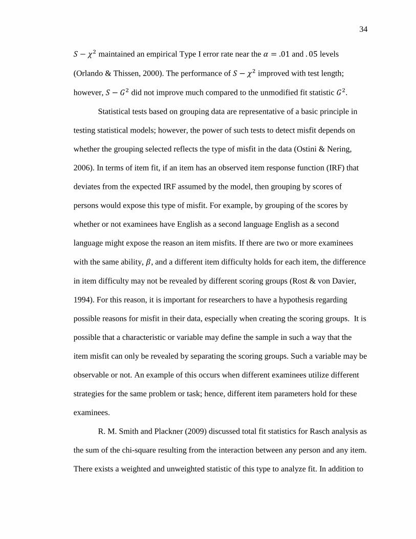
34

𝑆 − 𝜒2 maintained an empirical Type I error rate near the 𝛼 = .01 and . 05 levels

(Orlando & Thissen, 2000). The performance of 𝑆 − 𝜒2 improved with test length;

however, 𝑆 − 𝐺2 did not improve much compared to the unmodified fit statistic 𝐺2.

Statistical tests based on grouping data are representative of a basic principle in

testing statistical models; however, the power of such tests to detect misfit depends on

whether the grouping selected reflects the type of misfit in the data (Ostini & Nering,

2006). In terms of item fit, if an item has an observed item response function (IRF) that

deviates from the expected IRF assumed by the model, then grouping by scores of

persons would expose this type of misfit. For example, by grouping of the scores by

whether or not examinees have English as a second language English as a second

language might expose the reason an item misfits. If there are two or more examinees

with the same ability, 𝛽, and a different item difficulty holds for each item, the difference

in item difficulty may not be revealed by different scoring groups (Rost & von Davier,

1994). For this reason, it is important for researchers to have a hypothesis regarding

possible reasons for misfit in their data, especially when creating the scoring groups. It is

possible that a characteristic or variable may define the sample in such a way that the

item misfit can only be revealed by separating the scoring groups. Such a variable may be

observable or not. An example of this occurs when different examinees utilize different

strategies for the same problem or task; hence, different item parameters hold for these

examinees.

R. M. Smith and Plackner (2009) discussed total fit statistics for Rasch analysis as

the sum of the chi-square resulting from the interaction between any person and any item.

There exists a weighted and unweighted statistic of this type to analyze fit. In addition to

35

this type of fit statistic, the authors discussed the between groups statistics, which are also

available in weighted and unweighted versions. The between-groups fit statistic is based

on a characteristic of the persons, which is used to create separate and meaningful groups.

The characteristic used to create these groups can be ability; however, it can also be other

type of characteristics such as gender, ethnicity, or native -language among other

characteristics. The between-groups fit statistic is useful in detecting differences at the

item level for groups of persons, which were based on the characteristics previously

mentioned. This type of fit statistic is the basis for detecting differential item functioning

(DIF) items. A situation where an item works differently for subgroups is described as a

measurement disturbance in the psychometric literature (R. M. Smith & Plackner, 2009).

The between-groups fit statistic is better for detecting item bias than the separate

calibrations utilizing a multiple t-test method approach (which is regarded as a less

efficient method; R. M. Smith & Plackner, 2009).

R. M. Smith and Hedges (1982), using a simulation, compared the likelihood ratio

chi-square with the Pearson chi-square for fitting the Rasch model. The results of their

study indicated that both the likelihood ratio and the Pearson chi-squares were highly

correlated with the data designed to fit the Rasch model, as well as with data that

simulated measurement disturbances. Gustafsson (1980) and Andersen (1973) suggested

the likelihood ratio chi-square test should be used as an alternative to Wright and

Panchapakesan’s (1969) between-groups fit statistic due to the unknown distributional

properties of the Pearson chi-square. The study by R. M. Smith and Hedges showed that

in simulated data the distributions of the Pearson chi-square and the likelihood ratio chi-

square were almost identical.

36

Additionally, there exist within-group fit statistics. This type of statistic is often

utilized with the between-groups fit statistics and is calculated similarly to the between-

groups fit statistics. The difference is that the within-groups fit statistic is summed over

the persons included in specific subgroups (as opposed to summing over all the persons

responding to an item). The within-group statistic can be weighted or unweighted.

Furthermore, the benefit of the within-group fit statistic is that it is able to detect aberrant

response patterns within subgroups which could be difficult to identify in a complete

sample (R. M. Smith & Plackner, 2009). In general, a disadvantage of the chi-square

approach for testing item fit is that it is not easy to generalize to the polytomous IRT

models. The reason for this disadvantage is that the chi-square approach is frequency

based and thus has additional assumptions that must be met to handle disordered

categories.

Residual Approach

In statistics, residuals are defined as the difference between observed and

expected values under a specific hypothesis. Rost and von Davier (1994) referred to the

approach as the “score residual approach” (p. 174) which was developed within the

Rasch measurement framework. Christensen et al. (2013) separated residuals within the

Rasch framework into two categories: individual response residuals and group residuals.

The score residual approach also requires that item and person parameters are estimated.

In this approach, item fit is evaluated through the deviation of observed and expected

item responses (Ostini & Nering, 2006).

The standardized residuals can be formed by summing squared residuals for

persons or items (Rost & von Davier, 1994). These mean squared residuals can be

37

transformed into t statistics which are approximately normally distributed. Masters and

Wright (1982) generalized this approach to polytomous ordinal responses.

In Rasch modeling, the raw residuals or response residuals are as follows in

Equation 2.8.

𝑅𝑣𝑖 = 𝑋𝑣𝑖 − 𝐸𝑣𝑖 , (2.8)

Where 𝑋𝑣𝑖 represents the score for person 𝑣 and item 𝑖, and 𝐸𝑣𝑖 = E(𝑋𝑣𝑖) represents the

expected value of the residuals. However, in practice 𝐸𝑣𝑖 is often repleaced by 𝐸𝑣�� the

estimates of the expected item scores given that both the item and person parameters are

unknown (Christensen et al., 2013).

Additionally, the standardized residuals are

𝑍𝑣𝑖 = 𝑅𝑣𝑖

√𝑉𝐴𝑅(𝑋𝑣𝑖− 𝐸𝑣𝑖), (2.9)

Thus, the squared residuals are

𝑍𝑣𝑖2 =

𝑅𝑣𝑖

𝑉𝐴𝑅(𝑋𝑣𝑖) , (2.10)

The fit index called Outfit is based on the sum of squared standardized residuals.

For 𝑛 examinees each standardized residual is squared. For every item the examinee

answered the squared residuals are added and the average is taken by dividing by the

number of items. Thus, Outfit is also called Mean Squared Outfit and is computed as

shown in Equation 2.11 (Bond & Fox, 2015).

𝑂𝑢𝑡𝑓𝑖𝑡𝑖 = 1

𝑛∑ 𝑍𝑣𝑖

2𝑛𝑣=1 , (2.11)

Research experience with Outfit has indicated that Outfit is particularly sensitive

to outliers, in particular, with tests that have a broad range of item difficulties and person

abilities (R. M. Smith & Plackner, 2009). For this reason, the weighted version of the fit

38

statistic was developed, called Infit, which is an “information weighted sum” (Bond &

Fox, 2015, p. 269). Infit is referred to as the weighted mean square and is calculated as

shown in Equation 2.12, where each squared standardized residual is divided by the sum

of the variances.

𝐼𝑛𝑓𝑖𝑡 =∑ 𝑅𝑣𝑖

2𝑛𝑣=1

∑ 𝑉𝐴𝑅(𝑋𝑣𝑖)𝑛𝑣=1

, (2.12)

The range of Infit and Outfit consists of non-negative real numbers. Under the

Rasch model Infit or Outfit have an expected value of 1.0 and range from 0 to infinity

(Christensen et al., 2013; Wright & Linacre, 1994). For this reason, values of Infit or

Outfit which are close to zero or higher than one indicate lack of item fit. Mean squares

which are greater than 1.0 indicate underfit to the Rasch model; on the other hand, mean

square values less than 1.0 indicate overfit or redundancy to the Rasch model (Wright &

Linacre, 1994; Linacre, 2002). Underfit would signal the Rasch model does not

adequately capture the underlying structure of the data.

Multiple proposed corrections to the residual fit statistics have been developed;

however, the fact that the residual fit statistics require such corrections indicate they are

flawed from the start (Karabatsos, 2000; Wright & Linacre, 1994). Christensen et al.,

(2013) indicated that it is difficult to know “exactly when these statistics are too small or

too large to be acceptable is, however, a difficult question and the established practice

surrounding these fit statistics is infested with a number of misunderstandings and

misconceptions” (p. 86). Wright and Linacre (1994) recommended a cutoff of 0.6 to 1.4

logits for Infit and Outfit for the rating scale model; however, A. B. Smith et al. (2008)

stated that most methodological studies utilize a range of 0.7 to 1.3 logits. In contrast,

Linacre (2002) suggested a range of .5 to 1.5 as “productive for measurement” indicating

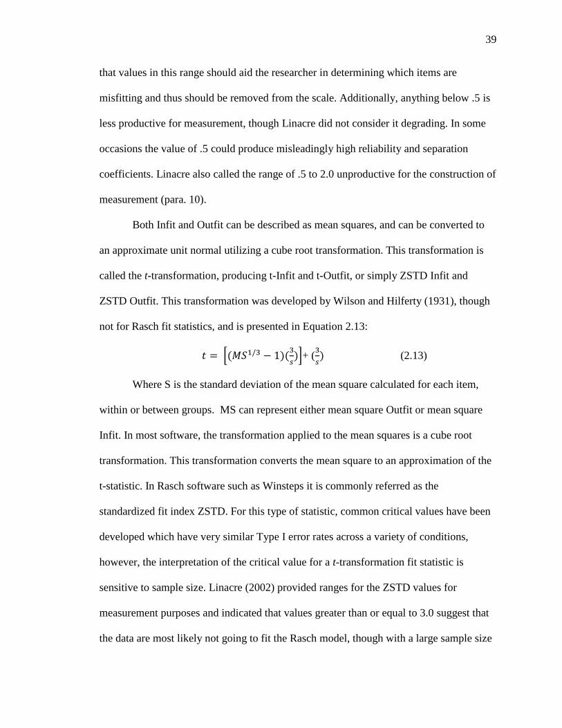
39

that values in this range should aid the researcher in determining which items are

misfitting and thus should be removed from the scale. Additionally, anything below .5 is

less productive for measurement, though Linacre did not consider it degrading. In some

occasions the value of .5 could produce misleadingly high reliability and separation

coefficients. Linacre also called the range of .5 to 2.0 unproductive for the construction of

measurement (para. 10).

Both Infit and Outfit can be described as mean squares, and can be converted to

an approximate unit normal utilizing a cube root transformation. This transformation is

called the t-transformation, producing t-Infit and t-Outfit, or simply ZSTD Infit and

ZSTD Outfit. This transformation was developed by Wilson and Hilferty (1931), though

not for Rasch fit statistics, and is presented in Equation 2.13:

𝑡 = [(𝑀𝑆1/3 − 1)(3

𝑠)]+ (

3

𝑠) (2.13)

Where S is the standard deviation of the mean square calculated for each item,

within or between groups. MS can represent either mean square Outfit or mean square

Infit. In most software, the transformation applied to the mean squares is a cube root

transformation. This transformation converts the mean square to an approximation of the

t-statistic. In Rasch software such as Winsteps it is commonly referred as the

standardized fit index ZSTD. For this type of statistic, common critical values have been

developed which have very similar Type I error rates across a variety of conditions,

however, the interpretation of the critical value for a t-transformation fit statistic is

sensitive to sample size. Linacre (2002) provided ranges for the ZSTD values for

measurement purposes and indicated that values greater than or equal to 3.0 suggest that

the data are most likely not going to fit the Rasch model, though with a large sample size

40

“substantive misfit may be small” (para. 11). R. M. Smith, Schumacker and Bush (1998)

showed that, with varying sample sizes, the standardized fit indices have more consistent

distributional properties than mean square statistics. For this reason, the authors

considered that the standardized fit indices were a better choice than mean square

statistics when it comes to assessing fit to the measurement model.

Problems with Residual-Based

Fit Indices

Many researchers have raised questions regarding the distribution of Infit and

Outfit. Though Infit and Outfit can be thought of as a chi-square statistic for each degree

of freedom there is a different critical value (which can be found in any chi-square

distribution table). The transformation of the chi-square into a mean square divides the

chi-square by its degrees of freedom. However, the chi-square distribution is not

symmetrical about the mean; thus, a fit rule such that mean square < .7 and mean square

> 1.3 has a different Type I error rate for the upper and lower tails (R. M. Smith &

Plackner, 2009; Wu & Adams, 2013). Wu and Adams (2013) and Christensen et al.

(2013) expanded on this issue. First, the method assumes that the distribution of Outfit is

a chi-square, which makes an implicit assumption that 𝒁𝒗𝒊 is also normally distributed.

However, the standardized residuals, 𝒁𝒗𝒊, are a discrete random variable which in the

dichotomous Rasch model, can only take on the values of [0,1]. Second, the sample size

of 𝒁𝒗𝒊 is N = 1 since 𝒁𝒗𝒊 is calculated for each person-item interaction and then is

averaged over persons to assess item fit (and over item to asses person fit; George, 1979).

Consequently, it follows that the test of fit based on 𝒁𝒗𝒊 will be conservative; therefore,

the risk of Type II error is greater. Christensen et al. showed mathematically that the

result of the test of fit for an item would depend significantly on the targeting of the items

41

to the population. Creating well targeted items for examinees with probabilities of correct

responses close to .5 (for the dichotomous Rasch model) would result in items which will

most likely fit the Rasch model. If the items are mistargeted to examinees shown by low

probability of correct responses, then the items would most likely misfit the Rasch model.

A second problem that Christensen et al. (2013) identified is as follows: the

expected value under the Rasch model is denoted by, 𝐸𝑣𝑖 , where person is denoted by 𝑣

and item is denoted by 𝑖. The estimates of expected item scores ��𝑣𝑖 are based on

parameter estimates rather than known parameters. Traditionally, in analyses such as

linear regression ��𝑣𝑖 can replace 𝐸𝑣𝑖. In practice, and utilizing an analysis such as linear

regression, the replacement is not an issue due to the use of consistent estimates of

unknown parameters, because in this situation, the bias and standard errors converge

when the sample size becomes larger. This does not occur with the Rasch model. The

problem is that ��𝑣𝑖 depends on two different types of parameters: item parameters and

person parameters. Consistent estimates may be available for one, but not for both types

of parameters. Christensen et al. maintained that item parameters may be assumed to be

consistent “except for the so-called joint estimates that are known to be inconsistent” (p.

88). In the same manner, person parameter estimates can be considered consistent if the

number of items is large. Although Christensen et al. argued that this is rarely the case, at

least in the health sciences where the number of items often ranges from five to 25. In

addition, Wu and Adams (2013) argued that when ��𝑣𝑖 replaces 𝐸𝑣𝑖 it assumes Outfit

follows a chi-square distribution; however, this only occurs if Outfit is estimated using

best asymptotically normal (BAN) estimators. This would not occur when the

unconditional maximum likelihood (UCON) estimation method is used to estimate the

42

Rasch parameters. Christensen et al. detailed that the bias of the person parameter

depends on the choice of estimating procedure, for example, maximum likelihood (ML),

weighted maximum likelihood (WML), joint maximum likelihood (JML), or Bayesian.

Karabatsos (2000) outlined six problems with commonly used Rasch residual fit

statistics. The first issue is that the standardized residual, 𝑍𝑣𝑖, is nonlinear. Thus, all

Rasch fit statistics are nonlinear. The true distance between two numbers can only be

measured when both numbers are on an interval or ratio scale. However, 𝑍𝑣𝑖 utilizes the

subtraction of nonlinear ordinal scores: 𝑅𝑣𝑖 = 𝑋𝑣𝑖 − 𝐸𝑣𝑖. When two 𝑍𝑣𝑖 functions are

plotted against the logit difference, 𝜃𝜈 − 𝛽𝑖, the observed responses, 𝑋𝑣𝑖, differ for each

𝑍𝑣𝑖 . One function utilizes 𝑋𝑣𝑖 = 1 and the other 𝑋𝑣𝑖 = 0 as a constant. In the case of the

𝑋𝑣𝑖 = 0 function the logit changes from 𝜃𝜈 − 𝛽𝑖 = 0 to 𝜃𝜈 − 𝛽𝑖 = 2 which results in

𝑍𝑣𝑖 = 1.7; however, the change from 𝜃𝜈 − 𝛽𝑖 = 2 to 𝜃𝜈 − 𝛽𝑖 = 4 results in 𝑍𝑣𝑖 = 4.7

which is almost three times larger. Karabatsos concluded, “it appears that, within the

residual framework, only nonlinear judgements can be made about fit to linear

measurement models” (p. 159).

For Rasch modeling to be effective the local independence assumption must be

met. Unidimensionality is met if there is local independence, but local independence is

not the only requirement for unidimensionality (Wright, 1996). Wright (1996) suggested

an approach to identifying subsets of constructs in the Rasch model is principal

components analysis of the residuals 𝑍𝑣𝑖 which requires several steps to check for local

independence in the data. He argued that the successful implementation of the Rasch

model depends on this check. Additionally, Linacre (1998) believed that principal

components of the Rasch residuals is an effective way of identifying multidimensionality.

43

On this topic, Karabatsos (2000) argued that the usefulness of the procedure is limited by

the assumption that 𝑍𝑣𝑖 are measured on an interval scale; however, according to

Karabatsos 𝑍𝑣𝑖 is an ordinal z-score. Finally, Karabatsos argued that even transforming

𝑍𝑣𝑖 would not help because the transformation results in an “even sharper non-linear

function” (p. 160). Karabatsos suggested a different transformation named Model

Deviance Residual and argued that the factor analysis of these residuals would be more

useful. Finally, Karabatsos concluded that the detection of misfit is basically categorizing

and the linearity of 𝑍𝑣𝑖 should not matter if the null distribution is known and stable.

The second problem Karabatsos (2000) outlined in his paper relates to the

responses used for both parameter estimation and fit analysis. In Rasch analysis the

observed response, 𝑋𝑣𝑖, is utilized to estimate both the item and person parameters. The

expected value of the raw residuals, 𝐸𝑣𝑖, is a direct function of these estimated

parameters. This dependency may cause the 𝑍𝑣𝑖 to decrease which results in an under-

detection of misfit. Karabatsos stated that there has been no attempt to research this issue;

however, the author also speculated that it may be difficult to do so in the framework of

residual fit analysis.

The third problem outlined by Karabatsos focuses on a “chain-like dependence”

among the residual fit statistics (Karabatsos, 2000, p. 161). The t distribution of residuals

depends on the mean square distribution, which depends on the standardized residuals,

𝑍𝑣𝑖, distribution. The stability of both the Infit and Outfit distributions depends on the

stability of the 𝑅𝑣𝑖, the response residuals, distribution. The stability of the ZSTD Outfit

null distribution and the ZSTD Infit null distribution depends on the stability of both

Outfit and Infit. The dependency among these distributions causes multiple problems. For

44

example, in the case where a fit statistic does not meet the distributional assumptions for

any given test, other statistics will depend on the information and will also fail to meet

their distributional assumptions (Karabatsos, 2000). Once one distributional assumption

is not met, it follows that the rest of the fit statistics and other statistics of interest will

also fail to meet the assumptions. This can cause both the under- or over-detection of

misfit in Rasch analysis.

The fifth issue outlined by Karabatsos (2000) is that the null distributions of the

standardized residuals, 𝑍𝑣𝑖, Infit, and Outfit vary as a function of arbitrary factors.

Utilizing dichotomous data of a 10 and 20 item test in a simulation, along with sample

sizes ranging from N = 30 to N = 2,000, with the ability, 𝜃, distributed as 𝑁(0,1) and

difficulty, 𝛽, distributed as 𝑈(-1, 1), Karabatsos discussed how changing one of the

sample size test conditions would cause the null distribution to vary. The author noted,

that for a longer test, utilizing the same conditions the null distribution holds. However,

for the 10-item test, the standard deviation of the standardized residuals, 𝑍𝑣𝑖 , decreased as

the sample size decreased. Additionally, as the difficulty range of the items increased the

standard deviation of the standardized residuals, 𝑍𝑣𝑖 , decreased. Similarly, zero is

considered the center of the item scale; however, when the mean of the ability, 𝜃,

distribution increasingly deviates from zero the standard deviation of the standardized

residuals, 𝑍𝑣𝑖 , decreases. Karabatsos noted that this result is expected given that the

standard deviation of the standardized residuals, 𝑍𝑣𝑖 , decreases as a function of the

decreasing sample size.

In addition to these findings, Karabatsos (2000) discussed “lucky” guessing and

item bias as well as the artificial conditions set by simulation conditions. The term

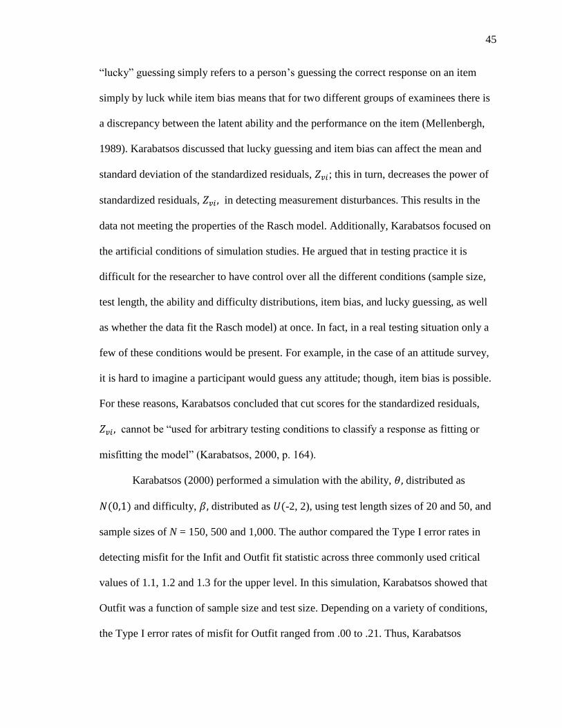
45

“lucky” guessing simply refers to a person’s guessing the correct response on an item

simply by luck while item bias means that for two different groups of examinees there is

a discrepancy between the latent ability and the performance on the item (Mellenbergh,

1989). Karabatsos discussed that lucky guessing and item bias can affect the mean and

standard deviation of the standardized residuals, 𝑍𝑣𝑖; this in turn, decreases the power of

standardized residuals, 𝑍𝑣𝑖 , in detecting measurement disturbances. This results in the

data not meeting the properties of the Rasch model. Additionally, Karabatsos focused on

the artificial conditions of simulation studies. He argued that in testing practice it is

difficult for the researcher to have control over all the different conditions (sample size,

test length, the ability and difficulty distributions, item bias, and lucky guessing, as well

as whether the data fit the Rasch model) at once. In fact, in a real testing situation only a

few of these conditions would be present. For example, in the case of an attitude survey,

it is hard to imagine a participant would guess any attitude; though, item bias is possible.

For these reasons, Karabatsos concluded that cut scores for the standardized residuals,

𝑍𝑣𝑖 , cannot be “used for arbitrary testing conditions to classify a response as fitting or

misfitting the model” (Karabatsos, 2000, p. 164).

Karabatsos (2000) performed a simulation with the ability, 𝜃, distributed as

𝑁(0,1) and difficulty, 𝛽, distributed as 𝑈(-2, 2), using test length sizes of 20 and 50, and

sample sizes of N = 150, 500 and 1,000. The author compared the Type I error rates in

detecting misfit for the Infit and Outfit fit statistic across three commonly used critical

values of 1.1, 1.2 and 1.3 for the upper level. In this simulation, Karabatsos showed that

Outfit was a function of sample size and test size. Depending on a variety of conditions,

the Type I error rates of misfit for Outfit ranged from .00 to .21. Thus, Karabatsos

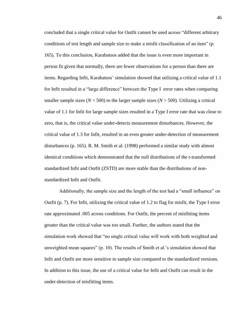
46

concluded that a single critical value for Outfit cannot be used across “different arbitrary

conditions of test length and sample size to make a misfit classification of an item” (p.

165). To this conclusion, Karabatsos added that the issue is even more important in

person fit given that normally, there are fewer observations for a person than there are

items. Regarding Infit, Karabatsos’ simulation showed that utilizing a critical value of 1.1

for Infit resulted in a “large difference” between the Type I error rates when comparing

smaller sample sizes (N < 500) to the larger sample sizes (N > 500). Utilizing a critical

value of 1.1 for Infit for large sample sizes resulted in a Type I error rate that was close to

zero, that is, the critical value under-detects measurement disturbances. However, the

critical value of 1.3 for Infit, resulted in an even greater under-detection of measurement

disturbances (p. 165). R. M. Smith et al. (1998) performed a similar study with almost

identical conditions which demonstrated that the null distributions of the t-transformed

standardized Infit and Outfit (ZSTD) are more stable than the distributions of non-

standardized Infit and Outfit.

Additionally, the sample size and the length of the test had a “small influence” on

Outfit (p. 7). For Infit, utilizing the critical value of 1.2 to flag for misfit, the Type I error

rate approximated .005 across conditions. For Outfit, the percent of misfitting items

greater than the critical value was too small. Further, the authors stated that the

simulation work showed that “no single critical value will work with both weighted and

unweighted mean squares” (p. 10). The results of Smith et al.’s simulation showed that

Infit and Outfit are more sensitive to sample size compared to the standardized versions.

In addition to this issue, the use of a critical value for Infit and Outfit can result in the

under-detection of misfitting items.

47

Karabatsos (2000) demonstrated that the distribution of item difficulties affects

the null distributions of Infit and Outfit fit statistics. In a mathematical demonstration,

Karabatsos varied the distribution of item difficulties while holding the ability of the

examinees constant across six different exams. Each successive exam was more difficult

than the previous. Although the examinees in this hypothetical situation only answered

one response incorrectly the fit statistics differed systematically across the six different

tests. Outfit failed to detect the unexpected response in the tests; furthermore, in four out

of six tests Outfit indicated that the responses fit the Rasch model. Karabatsos concluded

that the response residuals and Outfit increased as a function of the test difficulty.

Additionally, Infit also displayed test dependency, meaning these statistics are tied to a

specific form of the test. Despite the unexpected incorrect response, Infit found that the

responses fit the Rasch model in tests 2 to 5 while flagging the misfit response for tests 1

and 6. Karabatsos argued that a similar demonstration was possible when the distribution

of person abilities varies while holding the item difficulty distribution constant. Finally,

Karabatsos concluded, “it is difficult to directly compare mean-square fit between

individuals with differing ability, and mean-square fit between items differing in

difficulty, with the same ‘metric’” (p. 167). Karabatsos’s results suggest that a minimum

critical value of Infit and Outfit should be used across different distributions of item

difficulty and person ability; however, the author did not provide this cutoff value.

Karabatsos (2000) focused on the “illogic” of the ZSTD Infit and the ZSTD

Outfit. Authors such as R. M. Smith et al. (1998) believed that the null distributions of

the ZSTD Infit and the ZSTD Outfit were more stable than those of Infit and Outfit.

48

However, work by R. M. Smith (1991) showed that the null distributions of the ZSTD

Infit and the ZSTD outfit can vary as a function for test length, the person ability

distribution, and the item difficulty distribution. In addition to the simulation study in his

paper, Karabatsos (2000) utilized data from a cognitive ability test named the Knox Cube

Test (KCT). The KCT analysis consisted of a sample size of N=34 and 11 items. Within

this data set all items fit the Rasch model and the item fit range was -1.5 ≤ standardized

Outfit and standardized Infit ≤ 1.5. However, Karabatsos duplicated the dataset several

times to increase the sample size resulting in 10 different data sets each with twice as

many subjects as the prior data set. The sample size increased while holding constant the

response patterns and distribution of persons’ ability and difficulty the range for the

standardized Infit increased from -1.5 ≤ ZSTD Infit ≤ 1.5 to -.9.9 ≤ ZSTD Infit ≤ 9.9.

However, Wu and Adams (2013) believed that by duplicating the data,

Karabatsos introduced interdependencies between the cases, which resulted in violating

the independence assumption utilized for deriving parameter estimators and fit statistics.

In order to test their hypothesis regarding problems introduced by duplication of cases,

Wu and Adams decided to create two datasets, (a) the first data set was constructed by

duplicating 50 cases 20 times resulting in 1,000 cases and 40 items which fit the Rasch

model, and (b) the second data set was created by simulating 1,000 independent cases

with 40 items which fit the Rasch model. The results for the duplicated dataset showed

that the fit of the standardized t statistics ranged from -10 to 10 and did not fit the Rasch

model. In contrast, the second dataset had t statistics that ranged from -2 to 2.

Additionally, Wu and Adams selected three random samples from the Programme for

International Student Assessment (PISA) with N = 300, 2,500, and the total sample size N

49

= 21,259. The authors found that as the sample size increased the t statistics flagged more

items with misfit. The authors stated, “This does not mean that t statistics provide

erroneous results. On the contrary, fit t statistics tells us the truth that the items are really

misfitting the model when the sample size is large enough to detect (true) misfit” (p.

347). Wu and Adams argued that Karabatsos’ statement that the t statistics diverge as the

samples are duplicated actually demonstrates that when the sample size is large enough

true misfit can be identified.

Karabatsos’ (2000) sixth and final criticism of residual fit analysis is more

general. The Rasch model is a type of numerical conjoint measurement. Conjoint

measurement offers methods to analyze composition rules, which are rules or theories

that describe the relationship among a variety of measurable variables, but utilize only

ordinal information (Krantz & Tversky, 1971). For this type of measurement, residual-

based fit tests often fail to locate “crucial data-model discrepancies” (Karabatsos, 2000,

p. 170). Residual fit tests often find perfect or excellent fit even in the presence of

conjoint measurement violations which results in the under-detection of misfit.

R. M. Smith and Suh (2003) studied the degree to which the Infit and Outfit item

fit statistics could detect violations of the invariance property in Rasch. The researchers

used the software Winsteps to calibrate items and utilized data from a multiple-choice

mathematics competency exam. Additionally, the authors followed the cutoffs

recommended by Wright and Linacre (1994) and concluded that Infit and Outfit were

insensitive to the lack of invariance in the item parameters. Finally, the authors urged

researchers to not rely solely on mean square Infit and Outfit, and stated that using mean

50

square statistics may cause researchers to skip a significant number of misfitting items.

This may impact how researchers view the unidimensionality of the measure.

R. M. Smith and Plackner (2009) conducted a simulation to show the need for the

use of the family of fit statistics, which they considered to include Infit, Outfit, the

between and within fit statistics, and the standardized t-transformations (ZSTD). The

purpose of their study was to test the power of these statistics in detecting fit to detect

both random and systematic measurement disturbances. They defined random

measurement disturbance as guessing when the answer is unknown, while they defined

systematic measurement disturbance as differential item functioning (DIF), meaning the

items work differently for different subgroups. The results of R. M. Smith and Plackner’s

simulation showed that the total item fit statistics, both weighted and unweighted, are

insensitive to bias, specifically DIF, in the data. Regarding the between-items fit statistic,

the statistic was able to detect 36% of the misfitting items, which had a small bias. This

indicates that if bias detection is a priority when assessing fit, then the bias must be large

in order for the statistic to detect the bias. As the bias increased so did the statistic’s

ability to detect misfit. The authors concluded that “the bias would have to be extremely

large before it could be detected by either of the total fit statistics” (p. 433). More

importantly, the authors stated that a combination of fit statistics was necessary to detect

a variety of common measurement disturbances. Additionally, the authors established

that random types of measurement disturbances are better detected by total fit statistics

while systematic types of measurement disturbances are better detected by between fit

statistics.

51

Khan (2014) discussed global fit in the Rasch model and studied parameter

recovery and stability and model fit across a variety of sample sizes and test lengths. The

data were calibrated in the R package Itm. The conditions for Khan’s research included

four test lengths (10, 20, 30, and 50) and two sample sizes (N = 50 and N = 80). These

samples were subsamples from a dataset of 88 male examinees who responded to a non-

verbal cognitive ability test. Khan focused on model fit, rather than item fit. In the Itm

package, model fit is calculated by utilizing Pearson’s chi-square statistic. The author

concluded that it is possible to fit the Rasch model to small sample sizes and short tests,

such as those utilized in this study; however, this may result in unstable item parameters

and poor item parameter recovery.

Most research discussed so far discourages the use of the cutoffs suggested by

Wright and Linacre (1994); however, work by Wu and Adams (2013), Wolfe (2008) and

Wolfe and McGill (2011) provide alternatives to common cutoff values. Wu and Adams

suggested a new approach to find finding critical values or cutoffs for identifying misfit

in the data. The authors conducted empirical and simulation research to establish the

properties of the residual-based fit statistics. Wu and Adams’ research focused on the

dichotomous Rasch model. The authors derived a formula for the variance of the

unweighted fit mean square statistic (Outfit). In this formula, the asymptotic variance

derived by the authors depends only on the sample size, N, i.e., the variance is denoted by

2

𝑁. Wu and Adams identified two advantages to utilizing this asymptotic formula for the

variance: (a) the formula makes it clear that the variance of Outfit is inversely

proportional to the sample size, (b) the simplicity of the formula. Wu and Adams argued

that instead running “lengthy simulations to establish the null distribution” of the residual

52

fit statistics for multiple real life scenarios the mean square can be assumed to have a

“scaled” chi-square distribution and the variance approximately equal to 2

𝑁 (p. 343). The

authors suggested utilizing Equation 2.14 to calculate a range for the critical values to

obtain acceptable fit as opposed to utilizing conventional critical values:

1 ± 2√2

𝑁, (2.14)

Wu and Adams (2013) created a small-scale simulation with data that fit the

Rasch model based on 20 items and a sample size of N = 100. For this condition, the

authors found that the mean square values generally fell between .7 and 1.3. However,

when the same 20 items were used, but the sample size was increased to N = 800 the

values ranged from .9 to 1.1. The authors suggested that the most important takeaway

from their paper is that, since the variance of the mean square statistic depends on the

sample size, then it is illogical to suggest cutoff values for the mean square statistics that

do not take into consideration the sample size. It is important to note that a variation of

this formula is discussed in the simulation study conducted by R. M. Smith et al. (1998)

which in turn states the formula was first suggested via Wright’s personal communication

with the authors.

As Karabatsos (2000) discussed, an issue with Infit and Outfit is that the

distributions of these fit statistics are unknown which makes it difficult to determine the

critical values necessary to identify misfit. Besides Wu and Adams’ (2013) asymptotic

formula for the variance there exist bootstrap procedures for identifying critical values for

fit statistics such as Infit and Outfit (Seol, 2016; Wolfe, 2008; Wolfe & McGill, 2011).

Bootstrap procedures are easy to implement and are readily available. In fact, Wolfe

53

(2008) developed a SAS macro (Statistical Analysis System) named Rasch bootstrap fit

(RBF). Wolfe and McGill (2011) explained that bootstrapping works by constructing “an

empirical estimate of the unknown sampling distribution by generating a probability

distribution of the statistic across a large number of resamplings of an original sample via

sampling with replacement” (p. 7). Then, the discrete and empirically estimated

distribution originated by bootstrapping is considered the population from which a

number of resamples of size N are drawn. In the case of fit statistics, a fit statistic is

computed for each sample drawn and the distribution of these statistics plays the role of

the “empirical estimate” of the sampling distribution for the fit statistic (p. 7).

Wolfe and McGill (2011) focused on the dichotomous Rasch model and

manipulated the test length (20, 40, 80, 160) and the sample size (N = 100, 200, 500,

1,000). The authors also varied the offset distributions, that is, difference in means for the

simulated item and person distributions. Person ability was distributed 𝑁(0,1) while item

difficulty was distributed 𝑁(𝜇, 1) where 𝜇 varied depending on the level of the offset

distribution. For every item, the item slope could take three different values and the lower

asymptote could take two different conditions. This condition determined the nature of

misfit for the item. Data were calibrated using the Winsteps Rasch software. In Wolfe

and McGill’s study, the Type I error rate was defined as the proportion of items which

were incorrectly identified as misfitting while Type II error was defined as the proportion

of items which were not flagged as misfitting but should have been. The results of their

research showed that the Type II error rate was lower for the critical values developed

utilizing the bootstrapping method compared to the rule of thumb critical values set by

Wright and Linacre (1994) which were generally wider in comparison. As with research

54

by Wang and Chen (2005), Karabatsos (2000), and R. M. Smith (1988) among others, the

validity of the rule of thumb critical values in Wolfe and McGill’s study varied as a

function of sample size and test length.

Rating Scale Fit Research

In this section, research focused solely on the rating scale model (RSM), as

opposed to the dichotomous Rasch model, is discussed. Research that focuses on the

RSM is scarce. Thus, in this section work by E. V. Smith Jr. (2002), Wang and Chen

(2005), A. B. Smith et al. (2008), and Seol (2016) is reviewed.

E. V. Smith Jr. (2002) conducted a simulation of rating scale data comparing

principal components analysis (PCA) and fit statistics focusing on the unidimensionality

of the data. The conditions for E.V. Smith Jr.’s simulation was sample size of N = 500,

test length of 30, and a 5-point rating scale. In addition to two levels of ability, E.V.

Smith Jr. also varied the degree of common variance between two components to assess

multidimensionality. The Rasch software Winsteps was utilized to analyze the data. E.V.

Smith Jr. focused on the standardized Infit and Outfit (ZSTD Infit, and ZSTD Outfit)

rather than the mean square fit statistics. In order to interpret the ZSTD Infit and ZSTD

Outfit, E.V. Smith Jr. compared them to the critical value of ±2. The presence of

multidimensionality was determined by the percentage of items with fit values greater

than ±2. The results of the study showed that fit statistics, namely the standardized Infit

and Outfit, were as effective as PCA in detecting multidimensional items.

Research by Wang and Chen (2005) focused on the item parameter recovery and

the standard error of fit estimates under varying conditions of sample size and test length.

Parameter recovery refers to a computer program’s ability to “recover the generating

55

parameters accurately” (p. 377). In order to study parameter recovery, data sets with

known parameters must be created; however, the data can be calibrated under different

conditions of sample size, test length, IRT model, or software. The parameters from the

calibration are compared to the known parameters. Parameter recovery refers to when

the calibrated parameters are similar to the known parameters. If there exists a

statistically significant difference then the estimation is said to be biased. In their

research, Wang and Chen manipulated three independent variables: (a) the type of model

(Rasch dichotomous model and rating scale model), (b) sample size which ranged from

100 to 2,000, and (c) the test length 10, 20, 40, and 60 for the Rasch RSM model and 5,

10, and 20 items for the rating scale model. The rating scale model utilized a five-point

scale. For the Rasch model the item difficulty was 𝑁(0,1); however, for the rating scale

model the “overall difficulties” or the location of the difficulty parameters were -1.0, -

0.5, 0, 0.5, and 1.0. The person abilities had a distribution of 𝑁(0,1). The researchers

utilized the programming language FORTRAN 90 to generate the data and Winsteps to

analyze, or calibrate, the data.

The fit statistics of interest for Wang and Chen were Outfit and Infit, along with

the t-transformed statistics (ZSTD). Test length did not affect the standard deviations of

Infit and Outfit; however, the standard deviations of Infit and Outfit became smaller for

larger sample sizes. In their results, Wang and Chen found that as the item difficulties

became extreme the standard deviations of the fit statistics became smaller, particularly

for Infit ZSTD. For this reason, the authors believed it is “safe” to utilize the common

critical values of ±2 to identify misfitting items only for moderate difficulties (p 387). In

the case of extreme difficulties, these common critical values may be too conservative,

56

which would cause poorly fitting items to be flagged as fitting. Additionally, for smaller

sample sizes in the study (N = 200) Outfit was as large as 2.54 which would cause the

common critical values to flag as misfitting many items the authors considered to be

“good” items. The authors remarked that the common critical value for the mean square

fit statistics are not appropriate. In fact, they suggested that the critical values should be

adjusted according to the sample sizes, consistent with the recommendation shared by

Wu and Adams (2013).

Seol’s (2016) work focused on evaluating a bootstrap method to examine the

critical range of misfit for the rating scale model. Seol focused on bootstrapped

confidence intervals (CIs) utilizing simulated data with the following conditions:

polytomous data on a 5-point scale, five different test lengths (10, 20, 40, 60, 80), and

five different sample sizes (N = 200, 400, 600, 800, 1,000). Additionally, the person

ability and item difficulty were generated with a distribution of 𝑁(0,1), and the difficulty

of the threshold from one category to another was generated with a uniform distribution

𝑈(−2,2). The data were simulated utilizing the software WinGen3 and the calibration

was performed using the Rasch bootstrap fit (RBF) macro by Wolfe (2008). The results

of Seol’s study showed that the critical values developed via the RBF differ from those

suggested by Wright and Linacre (1994) and commonly used by researchers. One of the

findings from Seol’s study partially aligns with findings by Wang and Chen (2005) that

Infit and Outfit varied over different sample sizes. In Seol’s study, as the sample size

became larger the 95% CI for Infit and Outfit became narrower as would be expected.

The author concluded that for the RBF method, it would be inappropriate to utilize the

same critical values for both persons and items; rather, sample size and/or test length

57

should be considered when deriving these critical values. Further, the bootstrap CI

method can be used as an alternative to Infit and Outfit particularly when the distributions

of these fit indices are not well known and depend on the sample size.

Infit and Outfit are the most commonly used fit statistics in health research which

explains the research on a “real” life data set conducted by A. B. Smith et al. (2008). The

work by Smith et al. focused on the impact of sample size on four commonly used fit

statistics. These four fit statistics of interest were Infit and Outfit and the t

transformations of these (ZSTD). The authors utilized data from the Hospital Anxiety &

Depression Scale (HADS) and the Patient Health Questionnaire (PHQ-9). The HADS

consists of seven items on a 4-point scale while the PHQ-9 is a nine item survey on a 4-

point scale. Eight sample sizes were of interest: N = 25, 50, 100, 200, 400, 800, 1,600,

and 3,200. Smith et al. drew 10 samples with replacement for each sample size for the

two instruments. For the HADS there were 1,120 cases and for the PHQ-9 there was a

total of 720 cases used in the study. For the calibration of the items the authors used

Winsteps. Results indicated that while Infit and Outfit remained consistent across sample

sizes, the ZSTD Infit and ZSTD Outfit became increasingly negative beyond N = 200.

The results of Smith et al.’s (2008) study showed that t statistics were very sensitive to

sample size which corroborates results by Wang and Chen (2005) and later Wu and

Adams (2013), though these latter two studies utilized dichotomous data. In contrast, Infit

and Outfit remained relatively stable for rating scale data.

The Q-Index

Tarnai and Rost (1990; as cited by Rost & von Davier, 1994) originally developed

a Person-Q index for the purpose of identifying misfitting persons in the Rasch model.

58

Rost and von Davier (1994) subsequently developed the Q-Index in similar fashion as the

Person-Q. There exist no methodological studies regarding the Q-Index compared to

current item fit statistics in the Rasch model. However, researchers have utilized the Q-

Index in a variety of applied studies, including using the Q-Index in addition to Infit and

Outfit in their studies regarding superitems (items where participants must fill in the

blanks in a text; Eckes, 2011); as a standalone fit statistic for studying motor competence

in early childhood (Utesch et al., 2016); fitting the mixed Rasch model to a reading

comprehension test in order to identify types of readers (Baghaei & Carstensen, 2013);

and assessing the psychometric properties of a sleeping deprivation measure (Janssen,

Phillipson, O'Connor, & Johns, 2017). Yet, Ostini and Nering, as late as 2006, called

attention to the fact that little research has been performed on the Q-Index and thus there

is little knowledge regarding the fit statistic’s robustness.

The Q-Index makes use of the statistical properties of the Rasch model, namely,

parameter separability and conditional inference. Parameter separability refers to the

form in which the parameters in the Rasch model occur linearly and without interactions

(See Equation 2.3). The likelihood equations in which the relation between the person

ability and data are contained are separate from an equation which contains the data and

item difficulty parameters. This occurs due to the algebraic separation of parameters

specified within the Rasch model. This in turn, allows “derivation of conditional

estimation equations” for either item difficulty or person ability (Wright & Stone, 1999,

p. 27). In other words, the equations used to estimate item difficulties do not involve the

person abilities’ parameters and vice versa (Wright & Stone, 1999).

59

The Q-Index does not require estimation of the item parameters for any given

item but it is conditioned on the score distribution of said item (Rost & von Davier,

1994). In other words, the fit of an item, 𝑖, is evaluated with regard to the conditional

probability of its observed response vector. Rost and von Davier’s Q-Index is currently

available in the Rasch software Winmira (von Davier, 2001). The Q-Index can be utilized

with any unidimensional Rasch model, for example, the Rasch dichotomous model, the

rating scale model (Wright & Masters, 1982), the equidistance model (Andrich, 1982),

the partial credit model (Masters, 1982), continuous rating scale model (Müller, 1987),

or the dispersion model (Rost, 1988).

When testing the significance of the fit of an item, the item parameters are

estimated first and then utilized to derive the sampling distribution for the item parameter

(Rost & von Davier, 1994). Unlike the chi-square fit statistics, the Q-Index is not based

on the differences between observed and expected response scores. For this reason, the

Q-Index does not suffer from problems caused by the discrete nature of the response

scores (Rost & von Davier, 1994). Furthermore, the Q-Index is based on the likelihood of

observed response patterns and utilizes the likelihood of an item pattern conditioning on

the score of the item. This results in an item fit index that is essentially free of the item

parameter.

Additionally, the Q-Index utilizes the concept behind a Guttman pattern. The

Guttman pattern was named after sociologist Louis Guttman and is sometimes called the

dominance model (Van Schuur, 2011). The dominance model is also known as

cumulative scale analysis, implicational scale analysis, and Guttman scaling. Guttman

scaling is a type of unidimensional measurement. Louis Guttman’s purpose for this type

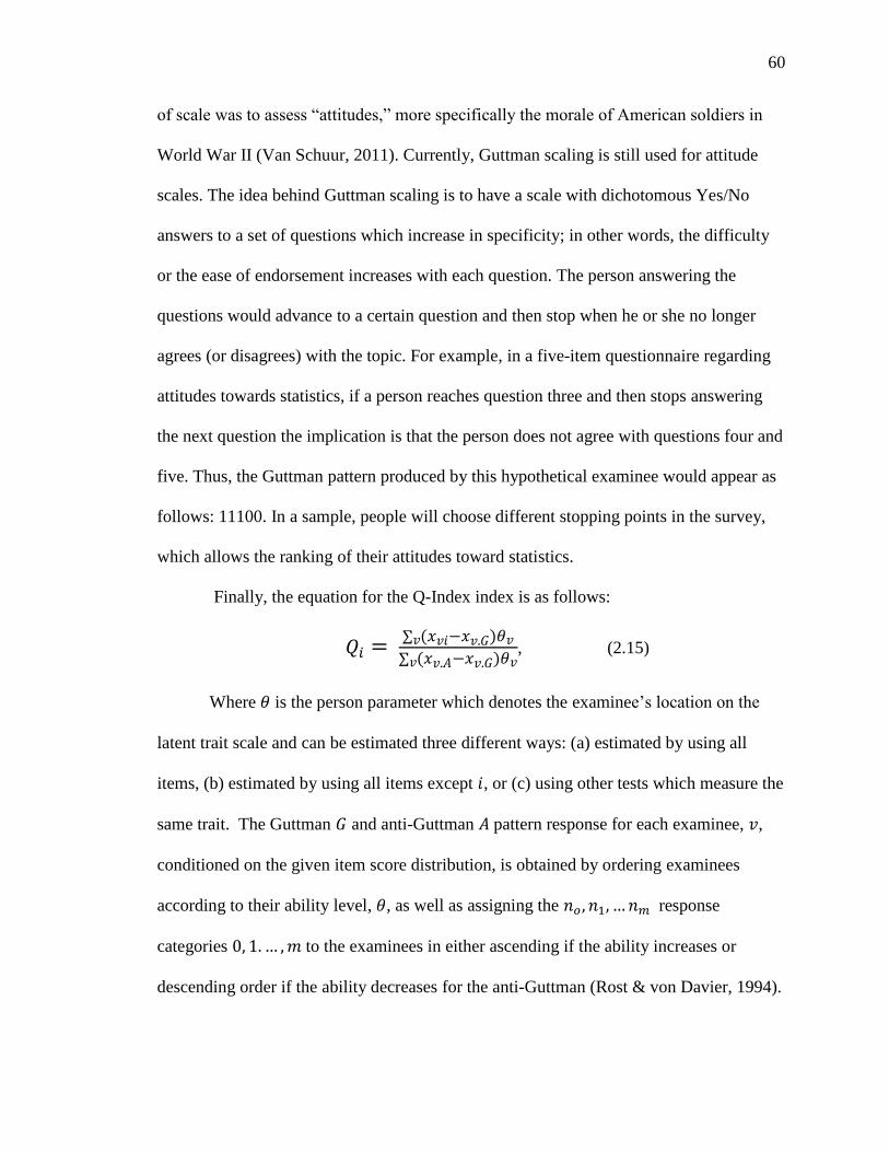
60

of scale was to assess “attitudes,” more specifically the morale of American soldiers in

World War II (Van Schuur, 2011). Currently, Guttman scaling is still used for attitude

scales. The idea behind Guttman scaling is to have a scale with dichotomous Yes/No

answers to a set of questions which increase in specificity; in other words, the difficulty

or the ease of endorsement increases with each question. The person answering the

questions would advance to a certain question and then stop when he or she no longer

agrees (or disagrees) with the topic. For example, in a five-item questionnaire regarding

attitudes towards statistics, if a person reaches question three and then stops answering

the next question the implication is that the person does not agree with questions four and

five. Thus, the Guttman pattern produced by this hypothetical examinee would appear as

follows: 11100. In a sample, people will choose different stopping points in the survey,

which allows the ranking of their attitudes toward statistics.

Finally, the equation for the Q-Index index is as follows:

𝑄𝑖 = ∑ (𝑥𝑣𝑖−𝑥𝑣.𝐺)𝑣 𝜃𝑣

∑ (𝑥𝑣.𝐴−𝑥𝑣.𝐺)𝑣 𝜃𝑣, (2.15)

Where 𝜃 is the person parameter which denotes the examinee’s location on the

latent trait scale and can be estimated three different ways: (a) estimated by using all

items, (b) estimated by using all items except 𝑖, or (c) using other tests which measure the

same trait. The Guttman 𝐺 and anti-Guttman 𝐴 pattern response for each examinee, 𝑣,

conditioned on the given item score distribution, is obtained by ordering examinees

according to their ability level, 𝜃, as well as assigning the 𝑛𝑜 , 𝑛1, … 𝑛𝑚 response

categories 0, 1. … ,𝑚 to the examinees in either ascending if the ability increases or

descending order if the ability decreases for the anti-Guttman (Rost & von Davier, 1994).

61

The Q-Index is available in the Rasch software Winmira and the Continuous

Rating Scale Model program (CRSM; version 1.3; von Davier, 2001; Müller, 1999).

However, the Winmira software has not been updated since 2001, and the CRSM

program is only available upon request from the author (Müller, 1999). The Q-Index is

standardized, and ranges from 0 to 1 with a midpoint of .5. A value of 0 indicates perfect

fit while a value of 1 indicates the item is misfitting (Rost & von Davier, 1994). The

midpoint of .5 indicates the independence of the item and the latent trait, or as Rost and

von Davier (1994) called it, random response behavior which indicates that the person is

answering the items at random. Rost and von Davier stated that Q-Index is “derived for

the ordinal Rasch model” unlike most of the current fit statistics which were developed

for the dichotomous Rasch model (p. 174).

The Q-Index has desirable properties that can make the index superior to the

popular residual fit statistics such as Infit, Outfit, and their standardized versions. The

index was developed for the ordinal Rasch model, unlike the residual fit statistics. For

this reason, I anticipate the performance of the Q-Index to be superior to that of Infit,

Outfit, and the standardized forms when identifying misfit for the rating scale model.

Further, residual fit statistics make use of a number of potential cutoff values causing

confusion among applied researchers who utilize them. The Q-Index may provide a more

clear-cut solution to identifying misfit for applied researchers.

62

Chapter Summary

This chapter focused on the currently available fit statistics for Rasch analysis.

Table 2.1 below summarizes the different findings regarding Infit, Outfit and ZSTD Infit

and ZSTD Outfit reviewed in this chapter. The major approaches to assessing fit in IRT

and Rasch models, including likelihood, chi-square, and the residual approach, were

evaluated in terms of their strengths and weaknesses. Most of the research on fit statistics

in the Rasch analysis is based on the residual fit statistics. Namely, Infit and Outfit are

two of the most popular fit statistics, and most of the methodological research where

there are comparisons of fit statistics includes these fit statistics and their standardized

form (R. M. Smith et al., 1998; A. B. Smith et al., 2008; R. M. Smith & Suh, 2003; Wang

& Chen, 2005). Additionally, researchers suggest the cutoff values for Infit and Outfit

should be reevaluated according to sample size (Wang & Chen, 2005; Wu & Adams,

2013). More importantly, there is very little research regarding fit statistics as a whole

utilizing rating scale data (Seol, 2016; A. B. Smith et al., 2008; Wang & Chen, 2005);

however, a quick search online would show that currently Rasch analysis is popularly

utilized for such data for a variety of topics including mindfulness awareness, coping,

independent living and rehabilitation, and sleepiness, among others (Goh, Marais, &

Ireland, 2017; Janssen, et al., 2017; López-Pina et al., 2016; Pretz et al., 2016).

Additionally, while the Q-Index takes advantage of Rasch properties such as parameter

separability, currently, there is no research regarding the robustness of the fit statistic.

63

Table 2.1

Summary of literature review findings for Infit, Outfit, ZSTD Infit and ZSTD Outfit

Author(s) Findings

Wright and Linacre (1994) Suggest cutoff for Infit and Outfit

Karabatsos (2000) - The stability of the ZSTD Outfit null distribution and

the ZSTD Infit null distribution depends on the

stability of both Outfit and Infit.

The null distributions of the standardized residuals, 𝑍𝑣𝑖,

Infit, and Outfit vary as a function of arbitrary factors.

- Infit and Outfit distributions are unknown which

makes it difficult to determine the critical values

necessary to identify misfit.

- The distribution of item difficulties affects the null

distributions of Infit and Outfit fit statistics

Smith and Suh (2003) - Studied the degree to which the Infit and Outfit item

fit statistics could detect violations of the invariance

property in Rasch.

- Support the 2.00 cutoff for ZSTD Infit and ZSTD

Outfit.

- Concluded that Infit and Outfit were insensitive to the

lack of invariance in the item parameters

Wang and Chen (2005)

Smith et al. (2008)

Wu and Adams (2013)

Suggested that critical values should be adjusted

according to the sample sizes.

Smith et al. (2008) Suggested a different cutoff from Wright and Linacre

(1994) for polytomous data

R. M. Smith and Plackner

(2009)

The results of the simulation showed that the total item

fit statistics, both weighted and unweighted, are

insensitive to bias, specifically DIF, in the data.

Khan (2014) Found that it was possible to fit the Rasch model to

small sample sizes and short tests, such as those

utilized in this study; however, this may result in

unstable item parameter recovery

64

Table 2.1 Continued

Summary of literature review findings for Infit, Outfit, ZSTD Infit and ZSTD Outfit

Author(s) Findings

Rost and von Davier (1994)

Wu and Adams (2013)

Wolfe (2008); Wolfe and

McGill (2011)

Seol (2016)

Developed alternated methods to Infit, Outfit and

ZSTD Infit and ZSTD Outfit

65

CHAPTER III

METHODS

The design, data generation, variables, procedures, and analysis for this

dissertation study are described within this chapter including a detailed description of the

Monte Carlo simulation procedures and Rasch analysis. A Monte Carlo simulation was

used to answer the research questions posed in Chapter I. Recall the purpose of this

proposed study is to examine performance of item fit analysis for the Rasch model. In

this study, the following Rasch model-based fit indices are examined: Q-index, mean

square Infit, mean square Outfit, and standardized Infit and Outfit in terms of their

sensitivity to various data conditions (sample size, number of items, and difficulty

distribution) and one specific type of measurement disturbance: namely

multidimensionality. To reiterate from Chapter I, the following research questions were

used to guide the proposed study.




misfit?




misfit?



66


misfit?








estimates?




misfit?




misfit?




misfit?








estimates?

Design Factors

A 4 𝑥 4 𝑥 2 𝑥 2 𝑥 2 = 128 design was based on four different sample sizes (N =

50, 100, 150, 250), four test lengths (10, 20, 30, and 50 items), and two different Rasch

models (dichotomous and rating scale). In addition to these conditions, a measurement

disturbance in the form of multidimensionality was studied (unidimensional model and

67

multidimensional model). As well, two item difficulty distributions (normal and uniform)

were examined.

Data Generation

Simulated datasets were generated for this study using Monte Carlo simulation

procedures. When using Monte Carlo methods, multiple replications generate an

empirical sampling distribution (Paxton, Curran, Bollen, Kirby, & Chen, 2001), which

allows researchers to assess the average random sampling error. The dichotomous data

for the proposed study was generated using R (version 3.4.3) and the eRm package within

R (Mair & Hatzinger, 2007). Specifically, the functions sim.rasch and sim.xdim were

used for the data generation phase. The first function is used to generate dichotomous

unidimensional data and the second function generates two-factor dichotomous data.

The unidimensional rating scale data were generated by an R function which can

be found in Appendix A and the multidimensional rating scale data were generated using

an R script which also can be found in Appendix A. The multidimensional model for both

dichotomous and rating scale models had two factors. Specifications on the covariance

matrix were similar to those in Setzer’s work (2008).

Sample Size

The sample sizes were set to N = 50, 100, 150, and 250 for the dichotomous data.

These sample sizes are commonly used in the handful of Rasch simulation studies

reviewed in Chapter II (Karabatsos, 2000; Wang & Chen, 2005; Wolfe & McGill, 2011;

Wu & Adams, 2013). Additionally, Linacre (1994b) suggested that for a high stakes

situation a sample size of N = 250 in combination with a test length of 20 would be

necessary to yield stable estimates with a 99% confidence. Linacre suggested that for a

68

95% confidence interval with stable values within ± 1 logit, a minimum sample size of N

= 30 is necessary for dichotomous data.

The following sample size recommendations apply to the Rasch rating scale

model. Green and Frantom (2002) recommended a sample size of at least 100 and a

minimum of at least 20 items for obtaining stable indices when using Rasch rating scale

model analysis. A minimum of N = 50 is needed for polytomous data to obtain a 95%

confidence interval with stable values within ± 1 logit. As well, a sample of N = 150 can

yield stable values with 99% confidence though Linacre (1994a) did not specify for what

type of Rasch model this is true. Consequently, the sample sizes were N = 50, 100, 150,

and 250 based on Linacre’s (1994a) recommendations for polytomous models.

Test Length

The test lengths for this study were I = 10, 20, 30, and 50 items. Wright and

Douglas (1975) stated that as “test length increases above 30 items, virtually no

reasonable testing situation risks a measurement bias large enough to notice” (p. 38).

Further, the authors suggested that “only” when using a test length of 10 items may a

researcher see measurement bias large enough that the item calibration is unstable.

Through personal communication Linacre (October 25, 2017) suggested that 30 items

should be enough provided there are at least 30 persons in the sample.

Item Difficulty

For this study, the item difficulty distributions were manipulated. The person

ability parameters were distributed 𝑁(0,1). Additionally, the item difficulty parameters

were manipulated and distributed 𝑁(0,1) and 𝑈(−2,2) in the same manner as research

by R. M. Smith et al. (1998), Karabatsos (2000), and Seol (2016). Linacre (personal

69

communication, October 25, 2017) explained that regarding this choice, “usually we

think of the items measuring ability as equivalent to a tape measure height. The marks on

a tape measure are uniformly distributed - so a uniform distribution.” In the case where

the items are anticipated to support a pass or fail decision, then item difficulties should be

normally distributed around the pass-fail point. It is important to note that both 𝑁(0,1)

and 𝑈(−2,2) can be considered artificial for applied researchers; however, these

distributions align with the majority of the simulation research

Dimensionality

Finally, dimensionality was manipulated in this study with two levels:

unidimensional and multidimensional. Multidimensionality introduces a measurement

disturbance to the simulation which was intended to help assess the sensitivity of the fit

statistics. The functions utilized are available in eRm within the R software, namely the

sim.rasch and sim.xdim functions. The function sim.xdim requires arguments for the

variance-covariance matrix which determines the relationship between the two

dimensions for the multidimensional condition. The following variance-covariance

matrix based on the work by Setzer (2008) and Suarez-Falcon and Glas (2003) were

used:

𝑆𝑖𝑔𝑚𝑎 = [1 0.5

0.5 1], (3.1)

To summarize, the conditions representing four different sample sizes, three

different levels of test length, two levels of item difficulty distribution, and two levels of

dimensionality were crossed. Table 3.1 represents the design for the Rasch dichotomous

model, for the Rasch rating scale model see Table 3.2. The four digit numbers (e.g., 1111,

1112, etc.) indicate the level of each factor.

70

Table 3.1

The 4 x 4 x 2 x 2 Factorial Design for Rasch Dichotomous Scale Model

Sample Size

Test 1 2 3 4

Length Factor Level Combination

1=10 1= Normal 1=Unidimensional 1111 1112 1113 1114

1=10 2=Uniform 2=Multidimensional 1221 1222 1223 1224

1=10 1= Normal 2=Multidimensional 1121 1122 1123 1124

1=10 2=Uniform 1=Unidimensional 1211 1212 1213 1214













Note. Sample sizes: (1) N=30, (2) N=100, (3) N=150, (4) N=250; Test lengths (1) I =10,

(2) I =20, I =30, I =50; Item difficulty distribution (1) Normal, (2) Uniform;

Dimensionality (1) Unidimensional, (2) Multidimensional.

Similarly, to the Rasch dichotomous model, the ability was distributed 𝑁(0,1)

and the item difficulties were manipulated based on two different distributions: 𝑁(0,1)

and 𝑈(−2,2). In addition, the thresholds were distributed 𝑈(−2, 2) following the work

by Seol (2016). Additionally, both Wang and Chen (2005) and Seol (2016) utilized a 5-

point Likert scale; thus, considering the lack of research for the Rasch rating scale model,

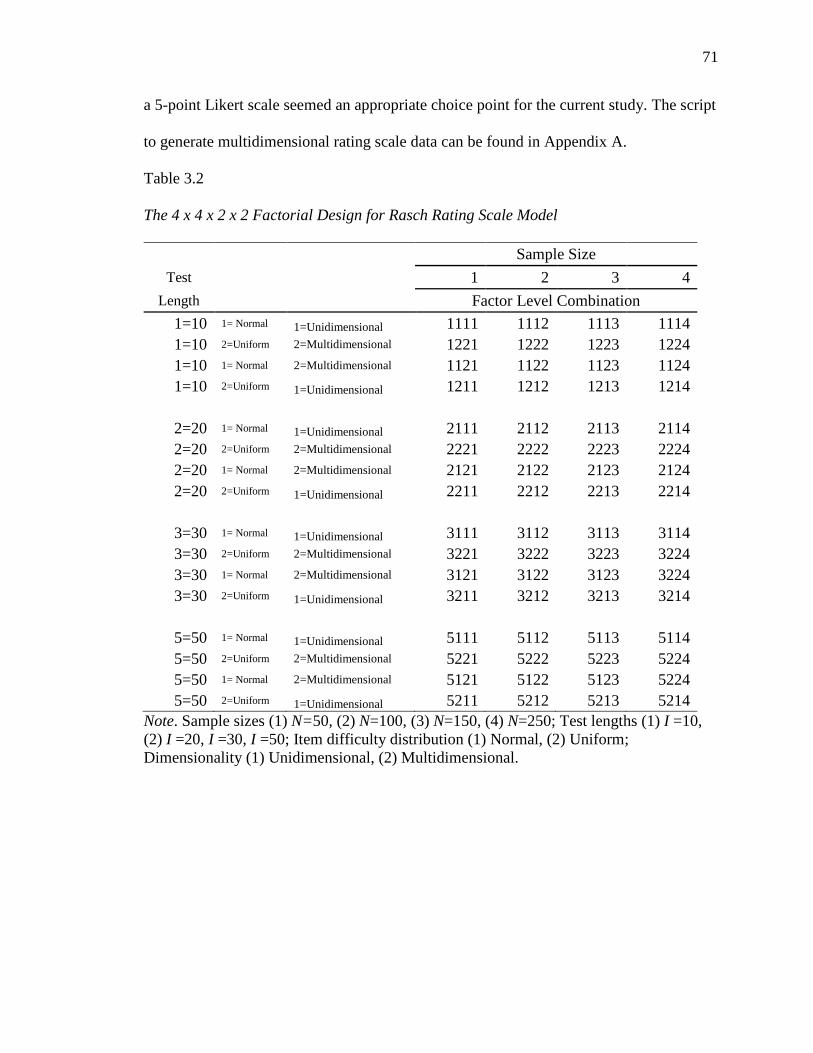
71

a 5-point Likert scale seemed an appropriate choice point for the current study. The script

to generate multidimensional rating scale data can be found in Appendix A.

Table 3.2

The 4 x 4 x 2 x 2 Factorial Design for Rasch Rating Scale Model

Sample Size

Test 1 2 3 4

Length Factor Level Combination

















Note. Sample sizes (1) N=50, (2) N=100, (3) N=150, (4) N=250; Test lengths (1) I =10,

(2) I =20, I =30, I =50; Item difficulty distribution (1) Normal, (2) Uniform;

Dimensionality (1) Unidimensional, (2) Multidimensional.

72

Number of Replications

Consistent with other simulation studies investigating item fit in the Rasch model

(Seol, 2016; R. M. Smith et al., 1998; Wang & Chen, 2005) the current study used 1,000

replications per design condition. The nominal level of α = .05 was used for this study.

Rasch Analysis

Rasch analysis was performed in Winsteps (version 3.91.0; Linacre, 2006)

Winsteps was developed by Linacre (2006) and is a popular software package among

Rasch users. Winsteps utilizes the Joint Maximum Likelihood (JML) estimation method,

which allows estimation of the item and person parameters to occur simultaneously. The

item level fit statistics used in Winsteps are based on the chi-square fit statistics proposed

by Wright and Panchapakesan (1969). The standardized fit statistics, also known as t-

transformations (ZSTD), are also available in Winsteps. The RWinsteps package in the R

software facilitates communication between R and the Rasch modeling software

Winsteps. This package will also facilitated the retrieval of information produced from

the Rasch analysis, such as mean square Infit, mean square Outfit, and standardized Infit

and Outfit from Winsteps (Albano & Babcock, 2015). During this process, the ability

estimates generated by Winsteps were also retrieved in order to utilize them for the

calculation of the Q-Index.

I programmed the Q-Index in R. The function to calculate the Q-Index followed

the description of Equation 2.15 in Chapter II based on Rost and von Davier’s (1994)

work. The R code to calculate this function can be found in Appendix B. To verify the

calculation of the Q-Index was correct, the person abilities were retrieved from Winmira

and imported into R to be used in the calculation of the Q-Index. Table 3.3 represents the

73

comparison of the Q-Index item fit statistics produced by Winmira, the Q-Index item fit

statistic produced by R utilizing the person abilities from Winmira, and the results of the

R function using the person abilities produced by Winsteps. It is important to note that

Winmira utilizes the conditional maximum likelihood estimator (CML) while Winsteps

utilizes joint maximum likelihood (JML) to estimate the item difficulty and person ability

parameters. In Table 3.3, it can be seen that the Q-Index item fit statistics from Winmira

and R (utilizing the person abilities available in Winmira) are identical. In the third

column, the Q-Index item fit statistics are calculated utilizing the person abilities from

Winsteps which utilizes JML estimation which are not too different from those estimated

from Winmira. In Table 3.4, a similar comparison is made for the Rasch rating scale

model, where the estimation of the Q-Index item fit statistic by the three different

approaches appears to differ even less.

74

Table 3.3

Dichotomous Rasch Model, Q-Index Calculation

Q-Index

Item Winmira

R (Winmira person

abilities)

R (Winsteps person

abilities)

1 0.1847 0.1847 0.1776

2 0.2299 0.2299 0.2213

3 0.1462 0.1462 0.1410

4 0.2217 0.2217 0.2146

5 0.3773 0.3773 0.3668

6 0.1563 0.1563 0.1518

7 0.1357 0.1357 0.1322

8 0.1850 0.1850 0.1814

9 0.2227 0.2227 0.2191

10 0.2020 0.2020 0.2012

11 0.1383 0.1383 0.1369

12 0.1843 0.1843 0.1828

13 0.1334 0.1334 0.1351

14 0.2511 0.2511 0.2550

15 0.2486 0.2486 0.2530

Table 3.4

Rasch Rating Scale Model, Q-Index Calculation

Q-Index

Item

Winmira

R (Winmira person

abilities)

R(Winsteps person

abilities)

1 0.1751 0.1751 0.1756

2 0.1138 0.1137 0.1137

3 0.1257 0.1257 0.1260

4 0.1236 0.1235 0.1236

5 0.0848 0.0847 0.0848

6 0.1034 0.1033 0.1035

7 0.1205 0.1204 0.1204

8 0.1216 0.1215 0.1215

9 0.1146 0.1146 0.1144

10 0.0985 0.0984 0.0982

Note: The range of the Q-Index is [0,1]

75

Empirical Type I Error

One of the outcomes that was analyzed is the empirical Type I error rates across

conditions for all five item fit indices. The Type I error rate was computed as the

proportion of correctly fitting items that were falsely rejected based on the item fit

statistics recommended cutoffs. For this purpose a series of “if else” statements were

written in the R program to implement the criterion for misfit for mean square Infit, mean

square Outfit, standardized Infit, standardized Outfit, and the Q-Index. Equation 3.2

illustrates how the Type I error rate was calculated.

𝑇𝑦𝑝𝑒 𝐼 𝑒𝑟𝑟𝑜𝑟 = 𝑝𝑟𝑜𝑝𝑜𝑟𝑡𝑖𝑜𝑛 𝑜𝑓 𝑖𝑡𝑒𝑚𝑠 𝑖𝑛𝑐𝑜𝑟𝑟𝑒𝑐𝑡𝑙𝑦 𝑓𝑙𝑎𝑔𝑔𝑒𝑑 𝑎𝑠 𝑚𝑖𝑠𝑓𝑖𝑡𝑡𝑖𝑛𝑔

𝑁𝑢𝑚𝑏𝑒𝑟 𝑜𝑓 𝑅𝑒𝑝𝑙𝑖𝑐𝑎𝑡𝑖𝑜𝑛𝑠 (3.2)

Mean Square Infit and Outfit

First, I estimated the mean square Infit and Outfit item fit indices for the Rasch

dichotomous model and the rating scale model when all assumptions of the Rasch model

were met. The criteria utilized for the Infit and Outfit fit indices were those suggested by

Wright and Linacre (1994). In their paper, Wright and Linacre suggested that for a (non-

high stakes) multiple choice questionnaire, which would produce dichotomous (correct

versus incorrect) data, the criterion range would be 0.7 to 1.3 for both Infit and Outfit,

which indicates item misfit Additionally, Wright and Linacre suggested the criterion

range of 0.6 to 1.4 for rating scale survey data. The proportion of misfit was recorded at

each replication of the simulation, for example, recording a 1 indicating item misfit if the

estimated item fit statistic fell outside the recommended range by Wright and Linacre and

0 if the estimated item fit statistic fell within the range. In addition to proportions of

76

misfitting items, descriptive statistics such as means, minimum, maximum and standard

deviation of the estimates were examined.

Standardized Infit and Standardized Outfit

The criterion range used in the current study for evaluating the standardized Infit

and Outfit was ±2 (R. M. Smith et al., 1998; R. M. Smith & Suh, 2003; Wang & Chen,

2005). Similar to Infit and Outfit, the proportion of misfit was recorded at every

replication of the simulation. A new dichotomous variable was created, as follows, if an

estimated item fit statistic fell outside the range of ±2 a value of 1 indicated misfit while

0 indicated the estimated fit statistic was within the criterion range of good fit.

The Q-Index

In addition to the outcome variables described above, I studied the criterion for

the Q-Index specified by Rost and von Davier (1994). Recall the Q-Index ranges from 0

to 1 with a midpoint of .5. A value of 0 indicates perfect fit while a value of 1 indicates

misfit. Currently, there is no specified critical value for the Q-Index, though Rost and von

Davier (2001) claimed that .5 indicates random response behavior. For this study, .5 was

the critical value to assess misfit at the item level. A value equal to or greater than .5

indicates misfit while below .5 indicates good fit. Table 3.5 indicates the item fit

statistics of interest along with the possible range of the fit statistics and the

recommended cutoff values from the literature.

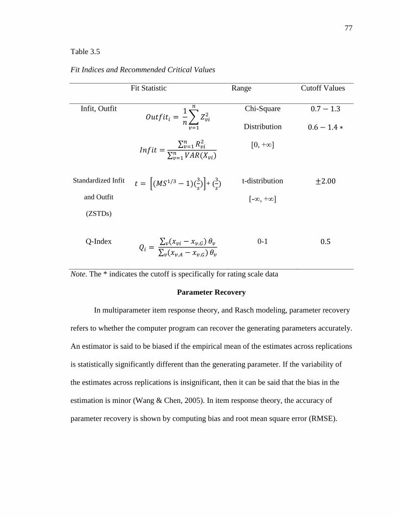
77

Table 3.5

Fit Indices and Recommended Critical Values

Fit Statistic Range Cutoff Values

Infit, Outfit 𝑂𝑢𝑡𝑓𝑖𝑡𝑖 =

1

𝑛∑ 𝑍𝑣𝑖

2

𝑛

𝑣=1

𝐼𝑛𝑓𝑖𝑡 =∑ 𝑅𝑣𝑖

2𝑛𝑣=1

∑ 𝑉𝐴𝑅(𝑋𝑣𝑖)𝑛𝑣=1

Chi-Square

Distribution

[0, +∞]

0.7 − 1.3

0.6 − 1.4 ∗

Standardized Infit

and Outfit

(ZSTDs)

𝑡 = [(𝑀𝑆1/3 − 1)(3

𝑠)]+ (

3

𝑠) t-distribution

[-∞, +∞]

±2.00

Q-Index 𝑄𝑖 =

∑ (𝑥𝑣𝑖 − 𝑥𝑣.𝐺)𝑣 𝜃𝑣

∑ (𝑥𝑣.𝐴 − 𝑥𝑣.𝐺)𝑣 𝜃𝑣

0-1 0.5

Note. The * indicates the cutoff is specifically for rating scale data

Parameter Recovery

In multiparameter item response theory, and Rasch modeling, parameter recovery

refers to whether the computer program can recover the generating parameters accurately.

An estimator is said to be biased if the empirical mean of the estimates across replications

is statistically significantly different than the generating parameter. If the variability of

the estimates across replications is insignificant, then it can be said that the bias in the

estimation is minor (Wang & Chen, 2005). In item response theory, the accuracy of

parameter recovery is shown by computing bias and root mean square error (RMSE).

78

Bias

To assess the estimation bias, the difference between the mean across 1,000

replications and the value generated by the software was used (Wang & Chen, 2005). See

Equation 3.3.

𝐵𝑖𝑎𝑠(𝛽) = (∑��𝑘 −𝛽

1000

1000𝑘=1 ), (3.3)

In Equation 3.3, 𝛽 represents the generating, or population item difficulty value and ��𝑘

denotes the estimate for the kth replication which is generated by Winsteps. In general,

the longer the test the smaller the bias should be (Wang & Chen, 2005). In addition to

this calculation, relative bias can be calculated using the following equation:

𝑅𝑒𝑙𝑎𝑡𝑖𝑣𝑒 𝐵𝑖𝑎𝑠 =𝐵𝑖𝑎𝑠(𝛽)

𝛽∗ 100% (3.4)

Where the numerator of the equation is obtained by Equation 3.3 and the denominatior is

the “true” population item difficulty. The root mean square error has the advantage of

being in the same metric as the item parameter and it is calculated as Equation 3.5 shows:

𝑅𝑆𝑀𝐸 = √(��𝑘−𝛽)2

1000, (3.5)

The sampling variance of the estimates across the 1,000 replications utilizes Equation 3.6

𝑆𝑉(��) = ∑(��𝑘− ��𝑘

)2

10001000𝑘=1 , (3.6)

Where ��𝑘 represents the mean of the estimates over 1,000 replications and ��𝑘 denotes the

estimate for the kth replication over the total number of replications (Wang & Chen,

2005).

79

Simulation Procedure

First, I describe the statistical and measurement software to complete the Monte

Carlo simulation. Next, I describe how this software was used in the process of the

simulation procedure.

Extended Rasch Modeling (eRm)

The extended Rasch modeling (eRm) package is available in the open source

software R. The eRm package can fit the Rasch model such as the rating scale model and

partial credit model. The package also provides a simulation module for various types of

binary data matrices. This package was used for data generation of the dichotomous

Rasch model and its multidimensional condition.

Winsteps

The Rasch modeling software Winsteps was developed by Linacre (2006). The fit

indices available in Winsteps are mean square Infit, mean square Oufit, standardized

Infight, and Ouftit. Additionally, the ability estimates, which were used for estimating the

Q-Index, were obtained from Winsteps.

Winmira

The Winmira Rasch software developed by von Davier (2001) was utilized to

compute the beginning stages of building the Monte Carlo simulation for this dissertation

with the purpose of verifying the accuracy of the Q-Index.

RWinsteps

RWinsteps is a package available in the statistical software R. The RWinsteps

package facilitates communication between R and the Rasch modeling software Winsteps

(Albano & Babcock, 2015).

80

Steps in Simulation

Finally, the simulation process was as follows:

Step 1. Generate Rasch dichotomous or rating scale data via the R software. The

Rasch dichotomous data were generated utilizing the R package eRm

while the rating scale data were generated with an R function available in

Appendix A. These data may be unidimensional or multidimensional

depending on the condition. The files were saved in a text (.txt) form and

were labeled with the condition and file number. To generate

multidimentional dichotomous data the function sim.xdim from eRm was

used within R in order to create a two-factor dataset that violates the

unidimensionality assumption of the Rasch model. The covariance matrix

given to the sim.xdim was that of Equation 3.1.

Step 2. Utilize the RWinsteps package to retrieve the mean square Infit, mean

square Outfit, standardized Infit, and standardized Outfit fit indices along

with the person ability measures which were used in the calculation of the

Q-Index.

In this step, files labeled ifile (which stands for item file and

contains item information) and pfile (for person file and contains person

information) were saved in a text (.txt) form. For example, for the sample

size condition of N=100, this step resulted in 100 ifiles and 100 pfiles.

Among the contents of the ifile were the item difficulty parameter 𝛽, mean

square Infit, mean square Outfit, ZSTD Infit, and ZSTD Outfit. The pfile

contains the person information including the person ability parameter 𝜃.

81

Step 3. Next, the data generated in Step 1 were read into the R software, along

with the information in the pfile and ifile.

Step 4. From the pfile, the person abilities were stripped and used in the

calculation of the Q-Index utilizing an R function I coded myself which

was previously discussed in this chapter. From the ifile, Infit, Outfit,

ZSTD Infit and ZSTD Outfit were retrieved.

Step 5. Within R, the calculated Q-Index was merged with Infit, Outfit, ZSTD

Infit, and ZSTD Outfit by item and replication number.

Step 6. The output file contained all fit statistics for all replications along with an

identifier of whether misfit was detected based on the previously

mentioned cutoffs (0=No item misfit, 1=Item is misfitting).

Step 7. All conditions were merged into a single dataset in SPSS in order to

perform further analyses.

Pilot Study

A pilot simulation study was conducted to test the quality of the data generation

process and estimate computing time. When utilizing simulated data, it is always a

concern that the data generated are indeed following the desired specifications. For this

reason, prior to running the actual simulation, validation of the data in the form of a pilot

study was performed.

First, a unidimensional Rasch dichotomous model with an item difficulty of

𝑁(0,1), sample size of N = 100, and a test length of I = 10 was examined. To generate the

data the function sim.rasch was utilized from the eRm package. To assess for

unidimensionality a confirmatory factor analysis (CFA) with robust maximum likelihood

82

estimation using tetrachloric correlations was also conducted in the R package lavaan,

assuming a congeneric measurement model with one factor. Five different replications

were chosen randomly to assess their unidimensionality, namely replications 38, 11, 15,

5, and 100. Global model fit was evaluated for the above-mentioned replications using

multiple numeric indices including comparative fit index (CFI; Bentler, 1990), Tucker-

Lewis index (TLI; Tucker & Lewis, 1973), root mean squared error of approximation

(RMSEA; Steiger & Lind, 1980), and standardized root mean squared residual (SRMR;

Bentler, 1995). For the majority of the replications except for dataset 15 and 200, the

values of TLI ≥ .95. The majority of the datasets also had a CFI ≥ .95 except for dataset

15. The RMSEA ≤ .06 for all datasets examined and SRMR ≤ .08 (Hu & Bentler, 1999),

which indicated adequate model fit. Tables B1-1 to B1-4 in Appendix B show the results

of these CFAs.

Additionally, Appendix B contains descriptive information for Rasch fit statistics

of interest: Q-Index, Infit, Outfit, ZSTD Infit, and ZSTD Outfit from the dichotomous

model with an item difficulty of 𝑁(0,1). For the Q-Index the majority of the 10 items

ranged from .01 to .46 indicating good item fit according to Rost and von Davier’s (1994)

criterion, which was anticipated in this condition. Table B2 in Appendix B shows the

descriptive information for all fit statistics of interest: Q-Index, Infit, Outfit, ZSTD Infit,

and ZSTD Outfit with a test length of I=10. Tables B4- B7 show test lengths I=20 and

I=30 along with all sample sizes while Tables B8-B26 show each item fit statistic

individually by test length. Table B12 shows the descriptive statistics for Infit, Outfit, and

ZSTDs. The means for Infit and Outfit were exactly, or close to 1.00. For the ZSTDs

mean values were above or below zero. Finally, to assess if the item difficulties were

83

normally distributed, under the condition where item difficulties were generated to be

normally distributed, QQ Plots were graphed in R. For the files under examination the

item difficulties looked roughly normally distributed.

Second, a multidimensional condition with 100 persons and 10 items was

examined with an item difficulty of 𝑁(0,1) for the Rasch dichotomous model. To

generate multidimensional dichotomous data the function sim.xdim from eRm was used

in order to create a two-factor dataset that violates the unidimensionality assumption of

the Rasch model. The variance-covariance matrix given to the sim.xdim was the same as

the one specified by Setzer (2008) and seen in Equation 3.1. Moreover, for the pilot

study where the test length was I = 10, for example, the weights of the items, which

indicate to what factor the items will belong, were based on a 10 x 2 matrix with the

purpose of having items 1-3 pertain to a different factor than items 4-10. See Equation

3.9. A similar pattern was used for conditions where the test length was I = 20 and I = 30.

𝐼𝑡𝑒𝑚 𝑊𝑒𝑖𝑔ℎ𝑡𝑠 =

[

1 0.11 0.11 0.1

0.1 10.1 10.1 10.1 10.1 10.1 10.1 1 ]

(3.9)

To assess the multidimensionality of the replications a CFA was conducted in R

lavaan. A two-factor model fit was evaluated for the above-mentioned replications using

the same indices as with the Rasch dichotomous unidimensional model. The datasets or

replications selected to examine the multidimensionality were 86, 8, 25, 61 and 1. Table

B1-2 in Appendix B shows the results of these CFAs. The values of TLI ≥ .95 except for

84

replications 8 and 61. Similarly CFI ≥ .95 except for replications 8 and 61, RMSEA ≤

.06, though for replication 61 the RMSEA was .607, and SRMR ≤ .08 except for

replication 61. However, it is important to consider the pilot study generated replications

of N = 100 persons as opposed to the recommended sample sizes of N = 200 (DiStefano

& Morgan, 2014).

The Q-Index information for this model (N=100 and I=10) for the dichotomus

Rasch model can be found in Table B11. The maximum exceeded the critical value for

Items 1-3 (Q=.55; Q=.62; Q=.51) which is a good sign the data were generated as

specified since Items 1-3 were expected to show misfit. However, Item 9 also showed a

high Q-Index value (.54) which could be flagged as misfitting according to Rost and von

Davier’s (1994) specifications. Additionally, the mean for the Q-Index across replications

ranged from 0.18-0.27. For Infit across replications, once again examining the maximum

for Items 1-3 (1.43, 1.63, 1.52, respectively) it is clear they are all above the

recommended cutoff of 1.4 suggesting poor fit. This pattern is present in Outfit as well.

Additionally, for the ZSTD Infit, Item 1-3 have maximum values across replications that

exceed the recommended cutoff of ±2, which also correctly suggest these three items are

misfitting.

Third, descriptive information for the fit statistics for the Rasch rating scale model

for the unidimensional condition can be found in Table B3 for N = 100 and I = 10. Once

again, a CFA was conducted for the N = 100 and I = 10 condition, based on five

replications selected at random, and the results can be found in B1-3. These replications

were 10, 19, 38, 44, and 47. Adequate model fit was shown by these replications

individually by examining different fit indices: TLI ≥ .95, CFI ≥ .95, SRMR ≤ .08, and

85

RMSEA ≤ .06 excluding replications 19 and 44. Furthermore, descriptive information

can be found in Appendix B. Tables B2- B7 list the mean and standard deviation along

with minimum and maximum for all the fit statistics of interest: Q-Index, Infit, Outfit,

ZSTD Infit, and ZSTD Outfit across the 100 replications of the pilot study. All the means

for Infit and Outfit were close to unity (one) for the unidimensional Rasch rating scale

model.

Fourth, descriptive information for the item fit statistics for a multidimensional,

two factor Rasch rating scale model can be found in Table B1-4 for I = 50 and N = 250.

Once the data were generated the datasets were visually examined to confirm the data

were generated appropriately with a 5-point Likert scale. The data quality examined was

to assess if the data in fact had two factors to violate the unidimensional assumption of

the Rasch model. Five different replications were chosen randomly, which were 19, 52,

56, 70, and 98. Once the replications were selected global fit was evaluated utilizing the

same numeric indices as above, which were the comparative fit index (CFI; Bentler,

1990), Tucker-Lewis index (TLI; Tucker & Lewis, 1973), root mean squared error of

approximation (RMSEA; Steiger & Lind, 1980), and standardized root mean squared

residual (SRMR; Bentler, 1995). The TLI and CFI ≥ .95 for all datasets, with the

replication 98 being the lowest in CFI = .962. Further, RMSEA ≤ .06 for all datasets

examined and SRMR ≤ .08 (Hu & Bentler, 1999), which indicated adequate model fit.

Data Analysis

IBM SPSS v23 was used to analyze the data. Descriptive and inferential statistics

were utilized to study the effects of the independent variables: test length, sample size,

and difficulty distribution. In order to achieve this, the data needed to be transformed into

86

a “wide” format in SPSS. However, the two models of interest, the dichotomous and

rating scale, were studied separately. That is, an analysis was performed for each model.

For inferential analyses, factorial ANOVAs were performed utilizing the item fit statistics

as dependent variables and test length, sample size, dimensionality, and difficulty

distribution as independent variables. Interactions between the independent variables

were also examined. In terms of parameter recovery, the bias calculated with Equation

3.3 was used to calculate the root mean square error and the relative bias..

In factorial ANOVAs, eta-squared (𝜂2) is commonly useddue to the overlapping

variance from the interaction effects requires an adjustment to eta squared known as

partial eta-square 𝜂𝑝2 (Tabachnick & Fidell, 2007). Partial 𝜂2 is calculated as follows:

𝜂𝑝2 =

𝑆𝑆𝑒𝑓𝑓𝑒𝑐𝑡

𝑆𝑆𝑒𝑓𝑓𝑒𝑐𝑡+ 𝑆𝑆𝑒𝑟𝑟𝑜𝑟, (3.10)

The range of 𝜂𝑝2 is from 0 to 1 (Tabachnick & Fidell, 2007). Cohen (1988)

deemed 𝜂𝑝2 ≥ .0099 a small effect, 𝜂𝑝

2 ≥ .0588 a medium effect, and 𝜂𝑝2 ≥.1379 a large

effect. Where there were statistically significant interactions, tests of simple effects and

interaction plots were conducted as a follow-up.

Chapter Summary

In summary, the simulation described in this chapter was programmed to calculate

the Q-Index in addition to examining its performance and the performance of other

popular item fit statistics such as Infit, Outfit, ZSTD Outfit, and ZSTD Infit. In this

chapter the operational definitions of the dependent and independent variables were

described and the variables selected due to their relevance to the literature and applied

studies. Moreover, I described the different software utilized for the simulation in

addition to the sequence of steps to complete the simulation. The Q-Index was

87

specifically programmed for this simulation and a comparison of the Q-Index

programmed in R to the one produced by the Rasch specialized software Winmira was

described in order to demonstrate the results from my program were equivalent to those

of Winmira. The data conditions were assessed for the specific conditions to verify the

programs were generating data with the correct specifications. For example,

dimensionality of the data was assessed utilizing a confirmatory factor analysis in order

to determine correct data generation for the multidimensional conditions. The distribution

of the item difficulties was also assessed in order to verify that normal and uniform item

difficulties were generated.

88

CHAPTER IV

RESULTS

This chapter presents the results of the analyses proposed in Chapter III. The

organization of the results presentation follows the order of the item fit statistics, which

were the Q-Index, Infit, Outfit, ZSTD Infit, and ZSTD Outfit. Next, analysis of parameter

recovery for the item difficulty parameter is presented.

Data Conditions for the Dichotomous

Rasch Model

Recall that the research questions are divided by Rasch model (dichotomous vs.

rating scale); thus, the results for the dichotomous model are discussed first and the rating

scale results afterwards. The effects of the main factors of interest were investigated by

five factorial ANOVAs and the examination of effect sizes per model. The analyses were

performed in IBM SPSS version 24, using the General Linear Model (GLM) procedure.

Sample size (N = 50, 100, 150, and 250), test length (I = 10, 20, 30, and 50), difficulty

distribution (Uniform vs. Normal), and dimensionality (one factor vs. two factors) were

between-subject factors. The dependent variables were the fit statistics themselves: the Q-

Index, Infit, Outfit, ZSTD Infit, and ZSTD Outfit. Once the ANOVA procedure was

completed in SPSS, the calculation of partial eta-squared (𝜂𝑝2) was conducted separately

in an Excel spreadsheet. The order of the factorial ANOVAs was as follows: Q-Index,

89

Infit, Outfit, ZSTD Infit, and ZSTD Outfit. Research questions one to five concern the

dichotomous Rasch model

Research Questions for the

Dichotomous Rasch Model

The research questions for the Rasch dichotomous model are as follows:




misfit?




misfit?




misfit?








estimates?

Descriptive information for the dichotomous data can be found in Appendix C

Tables C1 to C9 shows the descriptive information such as the minimum, maximum,

mean and standard deviation for the five item fit indices across all test lengths. Values for

the item fit statistics appeared reasonable, though ZSTD Infit had very low and high

values across all conditions of test length ranging from -4.00 to 6.00. Additionally, Figure

4.1 and 4.2 below illustrate the standard deviation of the item fit statistics across sample

90

sizes. Figure 4.1 illustrates both Infit and ZSTD Infit with ZSTD Infit standard deviation

growing larger as the sample size increases, while Infit remains constant. This pattern can

be seen again for ZSTD Outfit and Outfit, though Outfit shows a clearer trend for values

closer to zero than Infit did. Finally, the standard deviation of the Q-Index grows smaller

as the sample size increases.

Figure 4.1. Standard deviation across sample sizes for Infit, ZSTD Infit, and Outfit,

ZSTD Outfit.

91

Figure 4.2. Standard deviation across sample sizes for the Q-Index

Q-Index for Dichotomous Rasch Model

A factorial ANOVA was conducted utilizing test length, sample size, difficulty

distribution, and dimensionality as independent variables and the Q-Index as the

dependent variable. Table 4.1 displays the main effects and two-way interaction effects of

the four factors on the Q-Index for the dichotomous Rasch model. All main effects were

statistically significant at 𝛼 =.01; however, due to the large number of simulated

observations the effect size, partial eta squared 𝜂𝑝2, was examined. As previously

mentioned in Chapter III, 𝜂𝑝2 ranges from 0 to 1 (Tabachnick & Fidell, 2007).

Additionally, Cohen (1988) deemed 𝜂𝑝2 ≥ .0099 a small effect, 𝜂𝑝

2 ≥ .0588 a medium

effect, and 𝜂𝑝2 ≥.1379 a large effect.

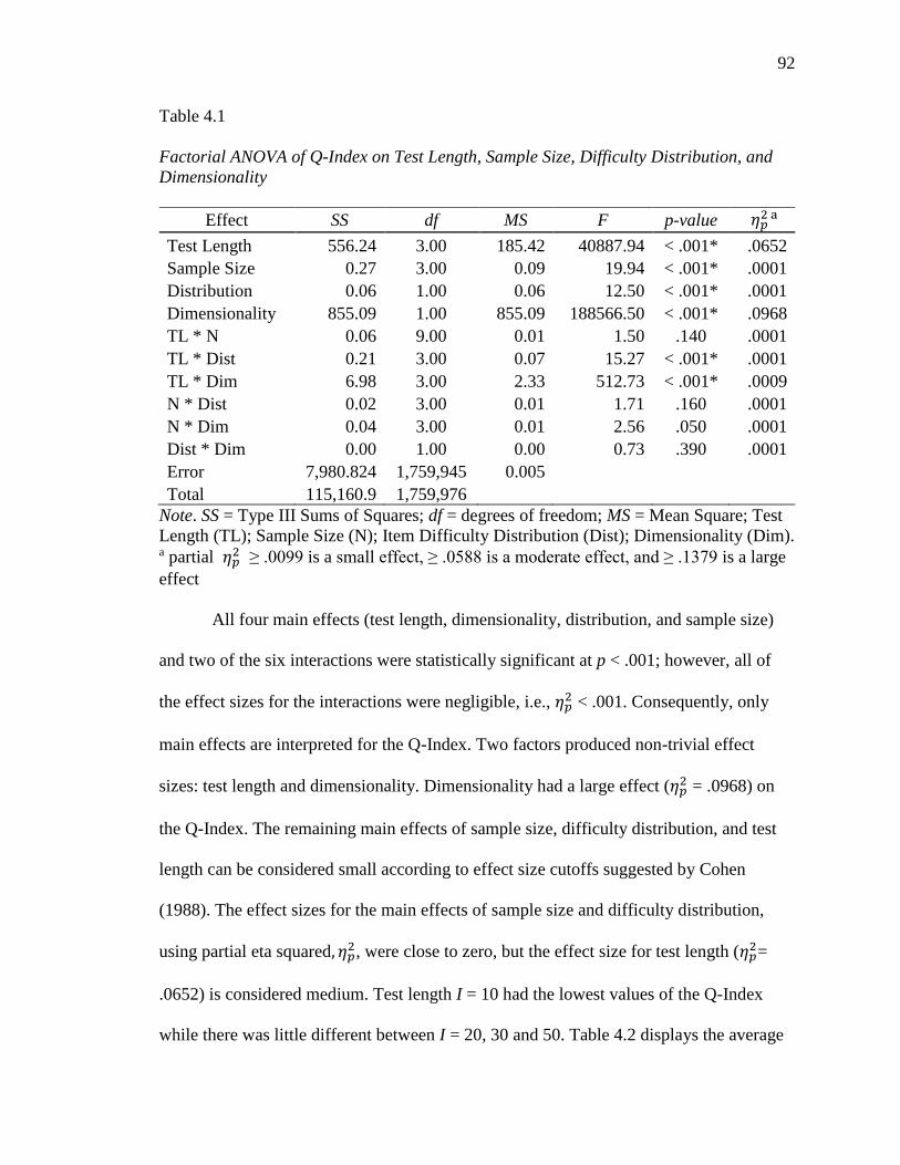
92

Table 4.1

Factorial ANOVA of Q-Index on Test Length, Sample Size, Difficulty Distribution, and

Dimensionality

Effect SS df MS F p-value 𝜂𝑝2 a

Test Length 556.24 3.00 185.42 40887.94 < .001* .0652

Sample Size 0.27 3.00 0.09 19.94 < .001* .0001

Distribution 0.06 1.00 0.06 12.50 < .001* .0001

Dimensionality 855.09 1.00 855.09 188566.50 < .001* .0968

TL * N 0.06 9.00 0.01 1.50 .140 .0001

TL * Dist 0.21 3.00 0.07 15.27 < .001* .0001

TL * Dim 6.98 3.00 2.33 512.73 < .001* .0009

N * Dist 0.02 3.00 0.01 1.71 .160 .0001

N * Dim 0.04 3.00 0.01 2.56 .050 .0001

Dist * Dim 0.00 1.00 0.00 0.73 .390 .0001

Error 7,980.824 1,759,945 0.005

Total 115,160.9 1,759,976

Note. SS = Type III Sums of Squares; df = degrees of freedom; MS = Mean Square; Test

Length (TL); Sample Size (N); Item Difficulty Distribution (Dist); Dimensionality (Dim). a partial 𝜂𝑝

2 ≥ .0099 is a small effect, ≥ .0588 is a moderate effect, and ≥ .1379 is a large

effect

All four main effects (test length, dimensionality, distribution, and sample size)

and two of the six interactions were statistically significant at p < .001; however, all of

the effect sizes for the interactions were negligible, i.e., 𝜂𝑝2 < .001. Consequently, only

main effects are interpreted for the Q-Index. Two factors produced non-trivial effect

sizes: test length and dimensionality. Dimensionality had a large effect (𝜂𝑝2 = .0968) on

the Q-Index. The remaining main effects of sample size, difficulty distribution, and test

length can be considered small according to effect size cutoffs suggested by Cohen

(1988). The effect sizes for the main effects of sample size and difficulty distribution,

using partial eta squared, 𝜂𝑝2, were close to zero, but the effect size for test length (𝜂𝑝

2=

.0652) is considered medium. Test length I = 10 had the lowest values of the Q-Index

while there was little different between I = 20, 30 and 50. Table 4.2 displays the average

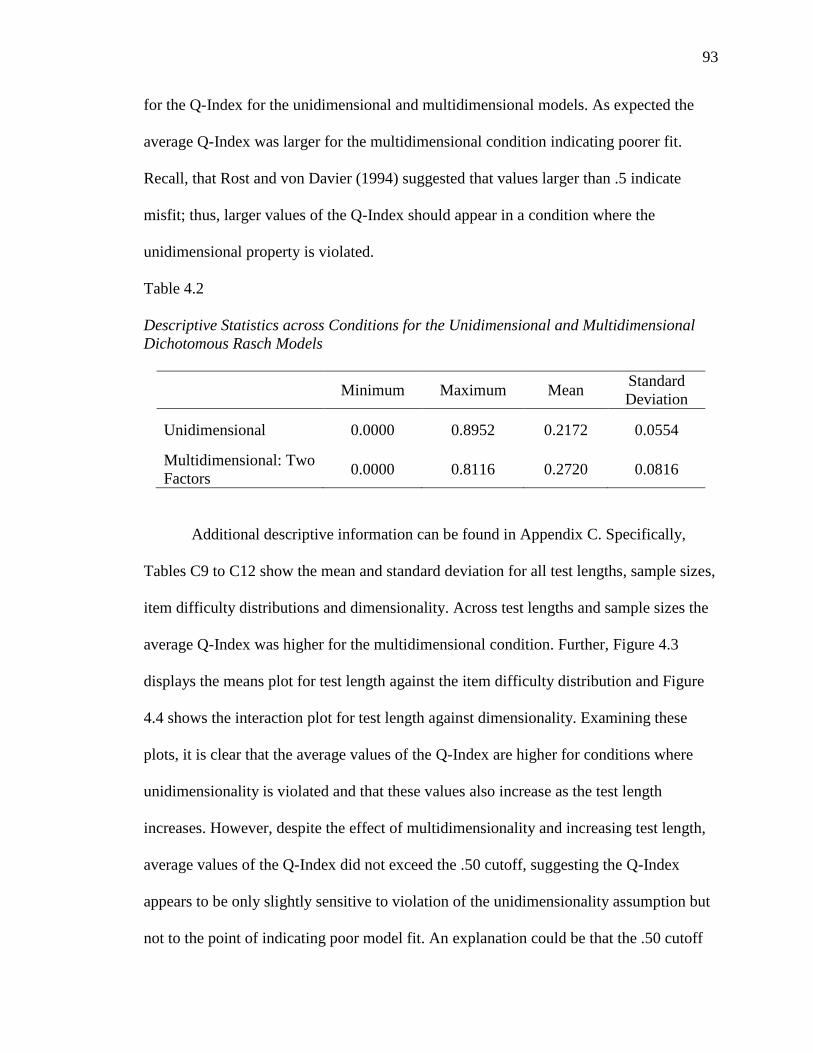
93

for the Q-Index for the unidimensional and multidimensional models. As expected the

average Q-Index was larger for the multidimensional condition indicating poorer fit.

Recall, that Rost and von Davier (1994) suggested that values larger than .5 indicate

misfit; thus, larger values of the Q-Index should appear in a condition where the

unidimensional property is violated.

Table 4.2

Descriptive Statistics across Conditions for the Unidimensional and Multidimensional

Dichotomous Rasch Models

Minimum Maximum Mean Standard

Deviation

Unidimensional 0.0000 0.8952 0.2172 0.0554

Multidimensional: Two

Factors 0.0000 0.8116 0.2720 0.0816

Additional descriptive information can be found in Appendix C. Specifically,

Tables C9 to C12 show the mean and standard deviation for all test lengths, sample sizes,

item difficulty distributions and dimensionality. Across test lengths and sample sizes the

average Q-Index was higher for the multidimensional condition. Further, Figure 4.3

displays the means plot for test length against the item difficulty distribution and Figure

4.4 shows the interaction plot for test length against dimensionality. Examining these

plots, it is clear that the average values of the Q-Index are higher for conditions where

unidimensionality is violated and that these values also increase as the test length

increases. However, despite the effect of multidimensionality and increasing test length,

average values of the Q-Index did not exceed the .50 cutoff, suggesting the Q-Index

appears to be only slightly sensitive to violation of the unidimensionality assumption but

not to the point of indicating poor model fit. An explanation could be that the .50 cutoff

94

suggested by Rost and von Davier (1994) is too liberal. A second explanation could be

that the degree of multidimensionality created for this study was not severe enough to

produce higher values of the Q-Index. A third explanation could be that the Rasch model

is robust to the violation of the assumption of multidimensionality (Anderson, Kahn, &

Tindal, 2017; Drasgow & Parsons, 1983; Harrison, 1986; Reckase, 1979; R. M. Smith,

1996).

Figure 4.3. Item difficulty distribution vs. test length for the dichotomous Rasch model

under the Q-Index

Figure 4.4. Dimensionality vs. test length for thee Rasch dichotomous model under the

Q-Index.

95

Infit for the Dichotomous Rasch Model

The second item fit statistic examined was Infit based on the same independent

variables of test length, sample size, item difficulty distribution, and dimensionality. In

the case of Infit, two of the interaction effects were statistically significant: test length by

dimensionality and test length by distribution; however, the effect sizes were not of

substance, i.e., 𝜂𝑝2 < .0001. Regarding the main effects, test length and sample size were

statistically significant (𝑝 < .001) with 𝜂𝑝2 values that did not even reach a small effect

(𝜂𝑝2 = .0001). Consequently, it appears that for the dichotomous model, Infit is not

impacted by test length, sample size, dimensionality, or difficulty distribution. Table 4.3

displays the results of this factorial ANOVA. Means and standard deviations for Infit can

be found in Appendix C, specifically Tables C13 to C16. In general, there was no great

difference in the averages between the unidimensional and multidimensional model, or

the two different item difficulty distributions. Also, the average value for Infit across test

length and sample sizes remained stable.

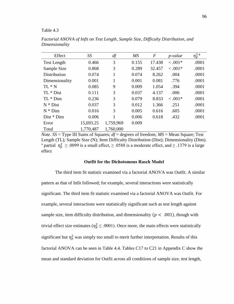
96

Table 4.3

Factorial ANOVA of Infit on Test Length, Sample Size, Difficulty Distribution, and

Dimensionality


Test Length 0.466 3 0.155 17.438 < .001* .0001

Sample Size 0.868 3 0.289 32.457 < .001* .0001

Distribution 0.074 1 0.074 8.262 .004 .0001

Dimensionality 0.001 1 0.001 0.081 .776 .0001

TL * N 0.085 9 0.009 1.054 .394 .0001

TL * Dist 0.111 3 0.037 4.137 .006 .0001

TL * Dim 0.236 3 0.079 8.833 < .001* .0001

N * Dist 0.037 3 0.012 1.366 .251 .0001

N * Dim 0.016 3 0.005 0.616 .605 .0001

Dist * Dim 0.006 1 0.006 0.618 .432 .0001

Error 15,693.25 1,759,969 0.009

Total 1,770,487 1,760,000




effect

Outfit for the Dichotomous Rasch Model

The third item fit statistic examined via a factorial ANOVA was Outfit. A similar

pattern as that of Infit followed; for example, several interactions were statistically

significant. The third item fit statistic examined via a factorial ANOVA was Outfit. For

example, several interactions were statistically significant such as test length against

sample size, item difficulty distribution, and dimensionality (𝑝 < .001), though with

trivial effect size estimates (𝜂𝑝2 ≤ .0001). Once more, the main effects were statistically

significant but 𝜂𝑝2 was simply too small to merit further interpretation. Results of this

factorial ANOVA can be seen in Table 4.4. Tables C17 to C21 in Appendix C show the

mean and standard deviation for Outfit across all conditions of sample size, test length,

97

item difficulty distribution, and dimensionality. Across test lengths and sample size

conditions the average value of Outfit was close to one.

Table 4.4

Factorial ANOVA of Outfit on Test Length, Sample Size, Difficulty Distribution, and

Dimensionality


Test Length 7.082 3 2.361 63.571 < .001* .0001

Sample Size 1.097 3 0.366 9.849 < .001* .0001

Distribution 7.246 1 7.246 195.125 < .001* .0001

Dimensionality 1.269 1 1.269 34.158 < .001* .0001

TL * N 1.972 9 0.219 5.901 < .001* .0001

TL * Dist 7.843 3 2.614 70.394 < .001* .0001

TL * Dim 2.28 3 0.76 20.468 < .001* .0001

N * Dist 0.408 3 0.136 3.658 .012 .0001

N * Dim 0.236 3 0.079 2.121 .095 .0001

Dist * Dim 3.495 1 3.495 94.108 < .001* .0001

Error 65,359.95 1,759,969 0.037

Total 18,29033 1,760,000




effect

Standarized Infit for the

Dichotomous Rasch

Model

The next item fit statistic that was examined using factorial ANOVA was the

standardized Infit (ZSTD Infit). A similar pattern as with mean square Infit and Outfit

occurred. Interactions such as test length against sample size, item difficulty distribution,

and dimensionality, in addition to the interaction between sample size and

dimensionality, and item difficulty distribution by dimensionality were statistically

significant just as the main effects were (𝑝 < .001). However, 𝜂𝑝2 resulted in effect sizes

98

that cannot even be considered small, 𝜂𝑝2 ≤ .0001. Table 4.5 shows the results of this

factorial ANOVA. As with the previous item fit statistics, descriptive information can be

found in Appendix C, specifically Tables C21 to C24. The average value for ZSTD Infit

was close to zero, as anticipated particularly in the unidimensional condition across test

lengths and sample sizes. While the average value of ZSTD Infit for the multidimensional

model was close to zero, the standard deviation was higher than that of the

unidimensional model across sample sizes and test lengths

Table 4.5

Factorial ANOVA of ZSTD Infit on Test Length, Sample Size, Difficulty Distribution, and

Dimensionality




effect

Standarized Outfit for the

Dichotomous Rasch

Model

The analysis continued with the last item fit statistic, utilizing the standardized

Outfit (ZSTD Outfit) as the dependent variable in a factorial ANOVA with test length,


Test Length 227.14 3 75.71 74.05 < .001* .0001

Sample Size 250.26 3 83.42 81.59 < .001* .0001

Distribution 120.04 1 120.04 117.42 < .001* .0001

Dimensionality 232.76 1 232.76 227.68 < .001* .0001

TL * N 152.30 9 16.92 16.55 < .001* .0001

TL * Dist 168.26 3 56.08 54.86 < .001* .0001

TL * Dim 162.74 3 54.24 53.06 < .001* .0001

N * Dist 9.49 3 3.16 3.09 .026 .0001

N * Dim 115.57 3 38.52 37.68 < .001* .0001

Dist * Dim 49.94 1 49.94 48.85 < .001* .0001

Error 1,799,276 1,759,969 1.022

Total 1,801,226 1,760,000

99

sample size, item difficulty distribution, and dimensionality as independent variables.

Table 4.6 shows the results of this factorial ANOVA. Moreover, ZSTD Outfit followed

the same pattern as Infit, Outfit, and ZSTD Infit. Four of the six interactions were

statistically significant as were the main effects of test length and sample size, item

difficulty distribution, and dimensionality, yet none of these yielded a medium or even a

small effect as 𝜂𝑝2 ranged from .0000 to .0001. This scenario repeated itself for the main

effects of test length, sample size, and dimensionality which were all statistically

significant (𝑝 < .001); however, 𝜂𝑝2 did not reach a small effect size. Descriptive

information regarding the ZSTD Outfit can be found in Appendix C, the mean and

standard deviation are presented in Tables C25 to C29. These descriptive statistics

showed a similar pattern to ZSTD Infit where the average value was close to zero across

test lengths, sample size, item difficulty distribution, and dimensionality. However, the

standard deviation for the multidimensional condition had a larger standard deviation

compared the unidimensional conditions.

100

Table 4.6

Factorial ANOVA of ZSTD Outfit on Test Length, Sample Size, Difficulty Distribution,

and Dimensionality


Test Length 215.604 3 71.868 64.772 < .001* .0001

Sample Size 162.984 3 54.328 48.964 < .001* .0001

Distribution 2.506 1 2.506 2.258 .133 .0001

Dimensionality 170.172 1 170.172 153.369 < .001* .0001

TL * N 57.173 9 6.353 5.725 < .001* .0001

TL * Dist 74.096 3 24.699 22.26 < .001* .0001

TL * Dim 192.743 3 64.248 57.904 < .001* .0001

N * Dist 5.525 3 1.842 1.66 .173 .0001

N * Dim 60.238 3 20.079 18.097 < .001* .0001

Dist * Dim 1.36 1 1.36 1.226 .268 .0001

Error 1,952,793 1,759,969 1.11

Total 1,954,005 1,760,000




effect

Type I and II Errors for the Item Fit

Statistics for Dichotomous

Rasch Model

Misfit decisions for the items were coded “0” if no misfit was detected by the

guidelines specified in Chapter III, and “1” if the fit statistic was outside the boundaries

of the specified cutoffs for items not expected to misfit. These codes were averaged

within each cell and across items to determine the Type I error rate. Similarly, the

number of items which were not flagged as misfitting compared to the number expected

to be flagged as misfitting was calculated to identify Type II error. For example, for I =

10 the first three items are placed on one factor and are expected to be the misfitting

items, while the rest of the items are placed in the second factor. Table 4.7 below shows

101

the recommended cutoff values which were used in the simulation to flag for misfitting

items for each item’s fit statistic.

Table 4.7

Recommended Cutoff Values for Each Item Fit Statistics of Interest

Item Fit Statistic

Recommended Cutoff

Infit, Outfit (Dichotomous Rasch Model) 0.7-1.3

Infit, Outfit (Rating Scale Model)

0.6-1.4

Standardized Infit and Outfit (ZSTDs) 2.00

Q-Index 0.5

The critical values produced by the recommended cutoffs from Chapter III were

used to compute Type I and II error rates which are shown in Table 4.8. A Type I error

rate higher than 𝛼 = .05 and a Type II error rate larger than 𝛽 = .20 would be of

concern. Table 4.8 shows how the Type I error for the Q-Index was low, ranging from

.0001 to .0018 across all sample sizes and test lengths. Infit and ZSTD Infit also had low

Type I error rates whereas Outfit exceeded the typical error 𝛼 = .05 being as high as

.1395 for the most extreme condition of for N = 50 and I = 10. Examining Figure 4.8 it is

clear that Outfit tends to have higher Type I error particularly for test lengths (I = 10, 20,

30) with the highest Type I error occurring at the smallest sample size of N = 50. More

importantly, Type I error rates were noticeably lower when the test length was long I =

50. Figure 4.8 presents the Type I error for the cell conditions which meet all the Rasch

model requirements, specifically unidimensionality. In the same figure the Type II error

rate for the cell conditions where unidimensionality was violated is presented.

102

Additionally, the Q-Index has lower Type I error rates compared to the rest of the fit

statistics across test lengths and sample sizes when the unidimensionality assumption of

the Rasch model was met. For the item fit statistic Outfit the Type I error rate seems to be

large particularly when the test length was small, I = 10 and I = 20, though for the rest of

the item fit statistics the Type I error rate appears negligible.

103

Table 4.8

Type I and II Error Rates for the Rasch Dichotomous Model

Dimensionality: One Factor

Type I Error

Dimensionality: Two Factor

Type II Error

Q INFIT ZSTD Infit OUTFIT

ZSTD

Outfit

Q INFIT ZSTD Infit OUTFIT

ZSTD

Outfit

Test Length

Sample

Size

10 50 .0003 .0068 .0199 .1395 .0290 .2972 .0015 .0287 .0744 .0625

100 .0001 .0002 .0189 .0631 .0280 .3001 .2999 .2445 .2466 .2334

150 .0001 .0001 .0203 .0385 .0300 .3003 .3003 .2251 .2655 .2152

250 .0001 .0001 .0180 .0161 .0287 .3002 .3002 .1762 .2818 .1670

20 50 .0016 .0046 .0187 .1258 .0262 .2848 .2972 .2662 .2163 .2628

100 .0001 .0001 .0192 .0327 .0277 .2976 .3000 .2470 .2578 .2427

150 .0001 .0001 .0166 .0162 .0294 .2993 .3001 .2252 .2731 .2211

250 .0012 .0026 .0212 .0874 .0268 .3002 .3003 .1654 .2765 .1529

30 50 .0001 .0001 .0206 .0330 .0279 .2765 .2978 .2576 .2437 .2555

100 .0001 .0001 .0205 .0175 .0287 .2939 .2999 .2295 .2740 .2275

150 .0001 .0001 .0207 .0062 .0278 .2983 .3001 .1989 .2837 .1987

250 .0018 .0018 .0208 .0780 .0254 .2997 .3001 .1366 .2919 .1347

50 50 .0001 .0001 .0200 .0310 .0266 .2715 .2988 .2594 .2578 .2571

100 .0001 .0001 .0200 .0310 .0266 .2923 .3000 .2294 .2841 .2293

150 .0001 .0001 .0205 .0155 .0271 .2971 .3000 .1953 .2913 .1963

250 .0001 .0001 .0210 .0064 .0284 .2997 .3001 .1324 .2959 .1348

103

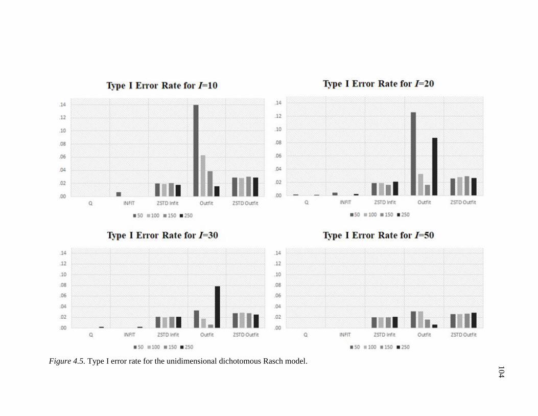
104

Figure 4.5. Type I error rate for the unidimensional dichotomous Rasch model.

104

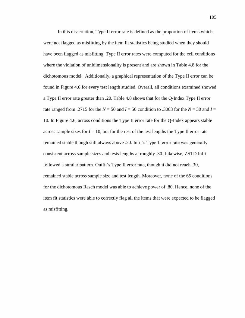
105

In this dissertation, Type II error rate is defined as the proportion of items which

were not flagged as misfitting by the item fit statistics being studied when they should

have been flagged as misfitting. Type II error rates were computed for the cell conditions

where the violation of unidimensionality is present and are shown in Table 4.8 for the

dichotomous model. Additionally, a graphical representation of the Type II error can be

found in Figure 4.6 for every test length studied. Overall, all conditions examined showed

a Type II error rate greater than .20. Table 4.8 shows that for the Q-Index Type II error

rate ranged from .2715 for the N = 50 and I = 50 condition to .3003 for the N = 30 and I =

10. In Figure 4.6, across conditions the Type II error rate for the Q-Index appears stable

across sample sizes for I = 10, but for the rest of the test lengths the Type II error rate

remained stable though still always above .20. Infit’s Type II error rate was generally

consistent across sample sizes and tests lengths at roughly .30. Likewise, ZSTD Infit

followed a similar pattern. Outfit’s Type II error rate, though it did not reach .30,

remained stable across sample size and test length. Moreover, none of the 65 conditions

for the dichotomous Rasch model was able to achieve power of .80. Hence, none of the

item fit statistics were able to correctly flag all the items that were expected to be flagged

as misfitting.

106

Figure 4.6. Type II error rate for all item fit statistics for the dichotomous multidimensional Rasch model

106

107

Parameter Recovery of Dichotomous Rasch Model

Recall that four test lengths, four sample sizes, two difficulty distributions, and

two levels of dimensionality were utilized for a total of 128 conditions. Bias and root

mean square error (RMSE) were used to assess the lack of recovery, in terms of error, of

the item parameters in this study.

Recommended cutoffs utilized in assessing parameter recover are shown in Table

4.9.

Table 4.9

Parameter Recovery Recommended Cutoffs

Assessment Recommended Cutoffs

Bias .05 (Zhang, 2015).

Relative Bias .05 (Hoogland & Boomsma, 1998;

Zhang, 2015)

Root Mean Square Error (RMSE) .3 (Choi & Swartz, 2009).

Bias of Item Difficulty Estimates for the


Bias of the item difficulty estimates was examined to assess parameter recovery.

Raw bias with a magnitude greater than .05 was considered practically significant

(Zhang, 2015). Table 4.10 displays the minimum, maximum, mean, and standard

deviation for bias. The largest magnitudes of bias, in the absolute value, were .0357 and

.0355 for the N = 50 and I = 30 and the N = 50 and I = 20 conditions, respectively. All of

these fell below the absolute bias cutoff of .05 and therefore would not be considered of

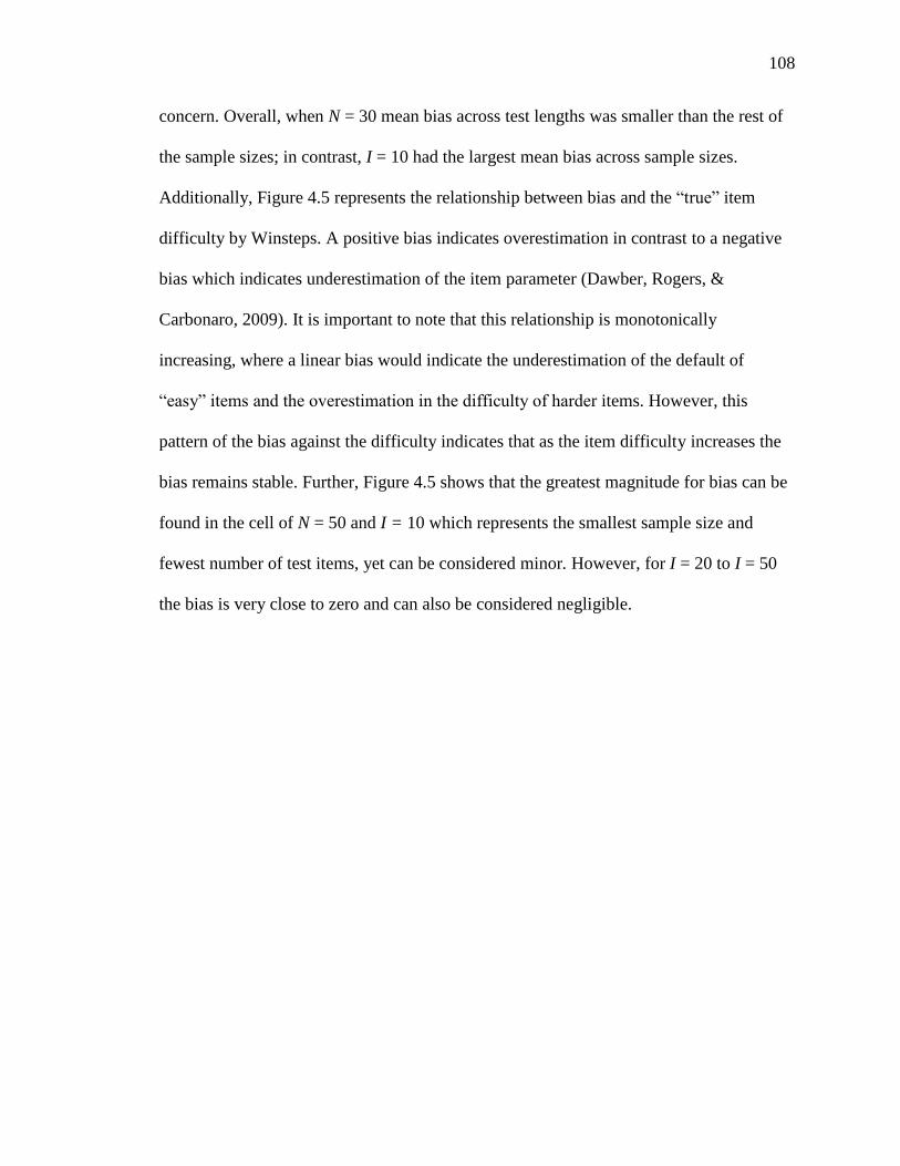
108

concern. Overall, when N = 30 mean bias across test lengths was smaller than the rest of

the sample sizes; in contrast, I = 10 had the largest mean bias across sample sizes.

Additionally, Figure 4.5 represents the relationship between bias and the “true” item

difficulty by Winsteps. A positive bias indicates overestimation in contrast to a negative

bias which indicates underestimation of the item parameter (Dawber, Rogers, &

Carbonaro, 2009). It is important to note that this relationship is monotonically

increasing, where a linear bias would indicate the underestimation of the default of

“easy” items and the overestimation in the difficulty of harder items. However, this

pattern of the bias against the difficulty indicates that as the item difficulty increases the

bias remains stable. Further, Figure 4.5 shows that the greatest magnitude for bias can be

found in the cell of N = 50 and I = 10 which represents the smallest sample size and

fewest number of test items, yet can be considered minor. However, for I = 20 to I = 50

the bias is very close to zero and can also be considered negligible.

109

Table 4.10

Maximum, Minimum, Mean, and Standard Deviation of the Bias in the Absolute Value

under the Dichotomous Rasch Model

Item/Persons Minimum Maximum Mean Standard

Deviation

10/50 0.0308 0.0246 0.0034 0.0039

10/100 0.0161 0.0116 0.0034 0.0028

10/150 0.0154 0.0113 0.0034 0.0023

10/250 0.0121 0.0081 0.0034 0.0019

20/50 0.0378 0.0355 0.0015 0.0039

20/100 0.0186 0.0155 0.0015 0.0027

20/150 0.0145 0.0124 0.0015 0.0023

20/250 0.0075 0.0104 0.0019 0.0018

30/50 0.0257 0.0357 0.0008 0.0035

30/100 0.0155 0.0144 0.0008 0.0025

30/150 0.0129 0.0108 0.0008 0.0021

30/250 0.0086 0.0076 0.0008 0.0016

50/50 0.0296 0.0330 0.0020 0.0036

50/100 0.0194 0.0139 0.0025 0.0026

50/150 0.0181 0.0113 0.0020 0.0022

50/250 0.0123 0.0089 0.0020 0.0018

110

Figure 4.7. Relationship between the bias and the generating item parameter under the dichotomous Rasch model.

110

111

Corrected bias. As referenced in Chapter II, Winsteps utilizes a Joint Maximum

Likelihood (JML) method to estimate ability. The JML method is known to result in item

parameter estimates which are biased. For this reason, Wright and Douglas (1977)

developed a correction factor:

(𝐿−1)

𝐿 Equation 4.1

Where L represents the test length. This correction procedure was implemented in SPSS

after the parameter estimation was complete. Figure 4.6 in which the extreme conditions

of sample size and test length are illustrated shows that the correction is minimal

supporting the claim that the original bias was not large. However, when examining

Figures 4.5 and 4.6 the small variability for I = 10 has diminished indicating the

correction was effective. Yet, this correction might be more useful in a situation where

bias is larger.

112

Figure 4.8. Relationship between the corrected bias and the generated item difficulty for the dichotomous Rasch model.

112

113

Roor Mean Square Error of

Item Difficulty Estimates

To complement the information provided by estimates of bias, the root mean

square error (RMSE) was calculated given that authors have suggested “bias is not a

sound measure of error in measurement” (Khan, 2014, p. 54). By examining both bias

and RMSE both accuracy and variability of the item estimates. RMSE ranges from 0 to 1

with values closer to zero or lower to .3 indicating that the parameter estimate is more

accurate (Choi & Swartz, 2009). Table 4.11 displays the minimum, maximum, mean, and

standard deviation of the RMSE of the item difficulty estimates for the Rasch

dichotomous model under all conditions of test length and sample size. The average

RMSE was well below .3 for all conditions. The average RMSE value was well below

the .3 recommended cutoff for all conditions. However, sample size N = 100 displayed

the highest values for RMSE ranging from .33 to .38 for all test lengths, barely surpassing

the recommended cutoff. As expected, the most extreme condition of N = 50 and I = 10

showed the highest RMSE of .38. Additionally, the magnitude of the RMSE for

individual items was plotted against the generating item difficulty shown in Figure 4.7. In

this side by side plot, it is clear that while the relationship appears constant for (I = 20,

30, 50) there is more variability when I = 10.

114

Table 4.11

Maximum, Minimum, Mean, and Standard Deviation of the RSME under the



Deviation

10/50 0.0001 0.3800 0.0300 0.0200

10/100 0.0001 0.3100 0.0400 0.0300

10/150 0.0001 0.1600 0.0400 0.0200

10/250 0.0001 0.1500 0.0400 0.0200

20/50 0.0001 0.1200 0.0300 0.0200

20/100 0.0001 0.3800 0.0300 0.0300

20/150 0.0001 0.1900 0.0300 0.0200

20/250 0.0001 0.1400 0.0200 0.0200

30/50 0.0001 0.1000 0.0200 0.0100

30/100 0.0001 0.3600 0.0300 0.0200

30/150 0.0001 0.1500 0.0200 0.0200

30/250 0.0001 0.1300 0.0200 0.0100

50/50 0.0001 0.0900 0.0100 0.0100

50/100 0.0001 0.3300 0.0300 0.0300

50/150 0.0001 0.1900 0.0300 0.0200

50/250 0.0001 0.1200 0.0200 0.0200

115

Figure 4.9. Relationship between RMSE of item difficulty estimates and the generated difficulty.

115

116

Relative Bias for Dichotomous

Rasch Model

Bias provides information on the magnitude of difference between the estimated

parameter and the known, or true, parameter. Values of zero for relative bias indicate that

the estimation of the generated parameter is unbiased. The sign in the values of relative

bias indicate under- or over-estimation (Choi, 2010). Table 4.12 displays the relative bias

before the Wright and Douglas correction (1977). Next, Table 4.13 displays the relative

bias for the dichotomous model by test length and sample size after the correction.

Practical significance and acceptable relative bias is established at a magnitude of .05

(Hoogland & Boomsma, 1998; Zhang, 2015).

Table 4.12

Relative Bias of the Dichotomous Rasch Model


Deviation

10/50 -0.0900 0.1400 0.0012 0.0144

10/100 0.0000 0.0943 0.0126 0.0123

10/150 -0.0400 0.1000 0.0010 0.0119

10/250 -0.0400 0.0800 0.0010 0.0112

20/50

-15.8800 13.5000 -0.0259 0.6817

20/100 -9.8500 9.4300 -0.0261 0.4861

20/150 -10.1100 6.4200 -0.0219 0.4022

20/250 -7.6200 5.6300 -0.0097 0.2296

30/50

-1.3700 1.4600 -0.0004 0.0568

30/100 -1.0700 0.9100 -0.0002 0.0399

30/150 -0.8500 0.7100 -0.0003 0.0320

30/250 -0.7100 0.6600 -0.0003 0.0261

50/50

-5.5900 3.0300 -0.0130 0.1667

50/100 -4.8200 1.6800 -0.0192 0.1765

50/150 -3.7000 1.2600 -0.0131 0.1330

50/250 -3.2000 0.9100 -0.0131 0.1253

117

Table 4.13

Relative Bias of the Dichotomous Rasch Model after Wright and Douglas (1977)

Correction


Deviation

10/50 -1.0100 1.0300 -0.0010 0.0500

10/100 0.0000 0.0940 0.0130 0.0120

10/150 0.0000 0.0100 0.0000 0.0010

10/250 0.0000 0.0100 0.0000 0.0010

20/50 -1.5100 1.2800 -0.0030 0.0650

20/100 -0.9400 0.9000 -0.0030 0.0460

20/150 -0.9600 0.6100 -0.0020 0.0380

20/250 -0.7200 0.5300 -0.0010 0.0220

30/50 -0.1300 0.1400 0.0000 0.0050

30/100 -0.1000 0.0900 0.0000 0.0040

30/150 -0.0800 0.0700 0.0000 0.0030

30/250 -0.0700 0.0600 0.0000 0.0030

50/50 -0.5100 0.2800 -0.0010 0.0160

50/100 -0.3900 0.2100 -0.0010 0.0140

50/150 -0.3300 0.1300 -0.0010 0.0130

50/250 -0.3200 0.0400 -0.0010 0.0120

Examining the relative bias post correction, it is clear the majority of the

conditions are exceeding the recommended cutoff of .05. The conditions I = 10 and N =

150 and 250 which did not exceed the .05 cutoff in any direction indicating good

parameter recovery. Further, the I = 10 and N =50, and I = 20 and N = 50 have the largest

maximum and minimum values for the relative bias. Table 4.14 shows the results of an

ANOVA with the relative bias, after the correction, as a dependent variable and test

length, sample size, distribution, and dimensionality as independent variables. It is clear

that a number of these values suggested that while statistical significance existed for the

118

interactions of test length and sample size, item difficulty distribution, dimensionality,

sample size and item difficulty distribution, item difficulty distribution and

dimensionality in addition to the main effects of test length, sample size, and item

difficulty distribution the effect sizes were trivial ranging from 𝜂𝑝2 = .0001 to .0010.

Table 4.14

Factorial ANOVA of Relative Bias on Test Length, Sample Size, Difficulty Distribution,

and Dimensionality.


Test Length 1.037 3 0.346 743.712 < .001* .0010

Sample Size 0.019 3 0.006 13.567 < .001* .0001

Distribution 0.532 1 0.532 1145.145 < .001* .0010

Dimensionality 0.002 1 0.002 4.86 .027 .0001

TL * N 0.134 9 0.015 32.066 < .001* .0001

TL * Dist 1.119 3 0.373 801.942 < .001* .0010

TL * Dim 0.035 3 0.012 25.385 < .001* .0001

N * Dist 0.052 3 0.017 37.353 < .001* .0001

N * Dim 0.000 3 0.000 0.230 .876 .0001

Dist * Dim 0.027 1 0.027 57.294 < .001* .0001




effect

Appendix C.2 contains detailed relative bias information separated by item

difficulty distribution and dimensionality. Table C2.1 to C2.2 show the relative bias, after

the implementation of the Wright and Douglas (1977) correction, for the uniform and

normal item difficulty distribution, the four different test lengths and sample sizes, and

levels of dimensionality. Table C2.1 shows the corrected relative bias for the uniform

item difficulty distribution. In this table it is clear that the relative bias is well below the

.05 recommended cutoff; however, I = 20 for all sample sizes has extreme minimal

values. Table C2.2 shows the corrected relative bias for the normal item difficulty

119

distribution where all values are below the recommended cutoff and there is no sign of

extreme minimum or maximum values.

Correlation between True and Estimated

Item Parameters

Finally, a correlation between the true and estimated parameters was performed to

assess the measure of accuracy and parameter recovery. This correlation was very high r

= .950 . In general, the correlations by condition were all high (r > .940) as can be seen

in Table 4.15 once again indicating good parameter recovery.

Table 4.15

Bivariate Correlations between the True and Estimated Parameters

Item/Persons Uniform Item Difficulty Distribution Random Item Difficulty Distribution

Unidimensional Multidimensional:

Two Factor Unidimensional

Multidimensional:

Two Factor

10/50 .957 .952 .939 .931

10/100 .978 .977 .968 .965

10/150 .985 .984 .978 .976

10/250 .991 .990 .987 .985

20/50 .961 .958 .951 .947

20/100 .981 .979 .975 .974

20/150 .987 .986 .983 .982

20/250 .992 .989 .990 .989

30/50 .955 .952 .924 .918

30/100 .977 .975 .961 .958

30/150 .985 .984 .972 0.97

30/250 .991 .990 .983 .982

50/50 .946 .942 .944 .941

50/100 .972 .970 .973 .969

50/150 .982 .979 .981 .979

50/250 .989 .988 .988 .987

120

Supplementary Analysis

Because the items were aggregated when performing the factorial ANOVAs

analyses it is possible that the aggregation of the items masked the findings for individual

items. Exploring item by item descriptive information was important in order to assess if

the items that were intended to misfit were actually placed in the first factor for the

condition where violation of unidimensionality exists. For example, for the I = 10

condition, Items 1-3 were specified to belong to one factor, while Items 4-10 were

specified to belong to a second factor. Table 4.14 shows the I = 10 multidimensional

condition with uniform item difficulty distribution. The bolded items indicate values that

are above the .5 recommended cutoff by Rost and von Davier (1994). In this table for the

N = 50 condition, Items 1-3 are clearly misfitting if the focus is on the maximum values.

In addition to this, the mean values are higher for Items 1-3 than they are for Itesm 4-7.

However, examining the maximum values Item 6, 7 and 9 would be flagged as misfitting,

however this finging is masked when focusing on the mean across all items. Similar

descriptive information can be found for Infit, Outfit and ZSTD Infit and ZSTD Outfit in

Appendix D in Tables D1 to D8.

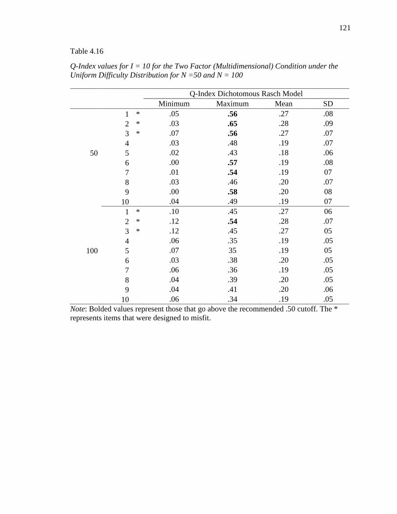
121

Table 4.16

Q-Index values for I = 10 for the Two Factor (Multidimensional) Condition under the

Uniform Difficulty Distribution for N =50 and N = 100

Q-Index Dichotomous Rasch Model

Minimum Maximum Mean SD

1 * .05 .56 .27 .08

2 * .03 .65 .28 .09

3 * .07 .56 .27 .07

4 .03 .48 .19 .07

50 5 .02 .43 .18 .06

6 .00 .57 .19 .08

7 .01 .54 .19 07

8 .03 .46 .20 .07

9 .00 .58 .20 08

10 .04 .49 .19 07

1 * .10 .45 .27 06

2 * .12 .54 .28 .07

3 * .12 .45 .27 05

4 .06 .35 .19 .05

100 5 .07 35 .19 05

6 .03 .38 .20 .05

7 .06 .36 .19 .05

8 .04 .39 .20 .05

9 .04 .41 .20 .06

10 .06 .34 .19 .05

Note: Bolded values represent those that go above the recommended .50 cutoff. The *

represents items that were designed to misfit.

122

Table 4.16 Continued



Q-Index Dichotomous Rasch Model

Minimum Maximum Mean SD

1 * .13 .43 .27 .05

2 * .14 .45 .28 .05

3 * .14 .39 .27 .04

4 .07 .36 .19 .04

150 5 .07 .35 .19 .04

6 .08 .37 .19 .05

7 .07 .37 .19 .04

8 .07 .37 .19 .04

9 .05 .35 .20 .05

10 .08 32 .19 .04

1 * .16 .39 .27 .04

2 * .15 .40 .28 .04

3 * .18 .38 .27 .03

4 .11 .28 .19 .03

250 5 .10 .30 .19 .03

6 .08 .33 .19 .03

7 .11 32 .20 .03

8 .11 .32 .19 .03

9 .09 .35 .20 .04

10 .11 .31 .19 .03



123

Rating Scale Model

Recall that the research questions of this dissertation are divided by the type of

Rasch model. In this section, the results for the rating scale model are presented. There

were four test lengths, three sample sizes, two distributions, and two factor dimensions

leading to 65 conditions. Five factorial ANOVAs were also performed for the Rasch

rating scale model. In similar fashion as with the Rasch dichotomous model, the order of

the factorial ANOVAs is presented by fit index as follows: Q-Index, Infit, Outfit, ZSTD

Infit and ZSTD Outfit.

Research Questions for the

Rasch Rating Scale Model

The research questions for the rating scale Rasch model are:




misfit?




misfit?




misfit?








estimates?

124

First before any analysis was performed, along with the descriptive information

for the dichotomous Rasch model, the descriptive statistics for the Rasch rating scale

model can be found in Appendix C. Tables C5 to C8 show the minimum, maximum,

mean, and standard deviation for all the item fit statistics under the Rasch rating scale

model. It is noteworthy, that for the I = 10 condition, ZSTD Infit and ZSTD Outfit had

averages close to zero, but still had extreme minimum and maximum values. The average

value for Infit and Outfit was close to one across test lengths. Also, the average value of

the Q-Index ranged from .11 to .13. In Figure 4.10 shows the standard deviation of Infit

and ZSTD Infit across the four different sample sizes, and the standard deviation across

sample size for Outfit and ZSTD Outfit while Figure 4.11 shows the standard deviation

across sample size for the Q-Index. Evidently, the standard deviation increases as the

sample size increases for the ZSTD Infit and ZSTD Outfit. This finding is consistent with

A. B. Smith et al. (2008).

125

Figure 4.10. Standard deviation across sample size for Infit, ZSTD Infit and Outfit,

ZSTD Outfit

Figure 4.11. Standard deviation trends for all item fit statistics.

Q-Index for the Rasch Rating Scale Model

A factorial ANOVA was conducted that utilized the Q-Index as a dependent

variable and test length, sample size, item difficulty distribution, and dimensionality as

the independent variables. The results of this analysis are shown in Table 4.17. While

126

interaction effects were statistically significant, the effect sizes were not substantial and

𝜂𝑝2 ranged from .0001 to .0030. Consequently, only main effects are interpreted here.

There was statistical significance for all main effects, yet only dimensionality yielded at

least a medium effect size (F(1, 1,759,969) = 1179.64, p < .001, 𝜂𝑝2 = .1006). Due to the

dimensionality factor only having two conditions a post hoc multiple comparison test was

not possible. However, Figure 4.12 displays the average Q-Index values by test length for

the two dimensionality conditions: unidimensional and multidimensional with two

factors. In this figure, it is easy to see the difference between the average Q-Index for the

unidimensional and multidimensional conditions with the unidimensional condition

yielding higher values for the Q-Index.

Table 4.17

Factorial ANOVA of Q-Index on Test Length, Sample Size, Difficulty Distribution, and

Dimensionality

Effect SS df MS F p-value 𝜂𝑝2

Test Length 24.68 3 8.23 1372.71 < .001* .0023

Sample Size 0.51 3 0.17 28.40 < .001* .0001

Distribution 0.52 1 0.52 86.64 < .001* .0001

Dimensionality 1179.64 1 1179.64 196,877.11 < .001* .1006

TL * N 0.04 9 0.00 0.70 .710 .0001

TL * Dist 3.20 3 1.07 178.07 < .001* .0003

TL * Dim 31.32 3 10.44 1742.36 < .001* .0030

N * Dist 0.01 3 0.00 0.54 .650 .0001

N * Dim 0.17 3 0.06 9.58 < .001* .0001

Dist * Dim 0.13 1 0.13 22.02 < .001* .0001

Error 10,545.26 1,759,969 0.01

Total 42,080.7 1,760,000




effect

127

Recall, that Rost and von Davier (1994) suggested that 0 indicate perfect fit, .5

indicates random response behavior, and 1 indicates misfit for the Q-Index. In theory,

larger values of Q-Index should be found in the multidimensional condition. Surprisingly,

the unidimensional condition displayed a larger mean for the Q-Index = .162 compared to

the mean of the multidimensional two factor model: Q-Index = .097. Yet, descriptive

information for the Q-Index shows that the maximum value for the unidimensional Rasch

model (.451) was lower than the maximum value for the multidimensional (or two-factor

model) where the maximum Q-Index was .709. In addition, the standard deviation for the

multidimensional two-factor model was the larger of the two models, SD = .105. In

Appendix C2, Table C29 to C32 show the mean and standard deviation for the Q-Index

by sample size, test length, dimensionality, and item difficulty distribution. Across test

lengths, the average value of the Q-Index was lower for the multidimensional conditions

than for the unidimensional condition. Below, Table 4.18 shows the descriptive statistics

for the unidimensional and two factor conditions.

Table 4.18

Descriptive Statistics for the Unidimensional and Multidimensional Rasch Rating Scale

Models


Deviation

Unidimensional 0.014 0.462 0.162 0.033

Multidimensional: Two

Factors

0.000 0.709 0.097 0.105

128

Figure 4.12. Average Q-Index by Dimensionality by Test Length.

Infit for the Rasch Rating Scale Model

In similar fashion as the Q-Index, Infit was utilized as a dependent variable in a

factorial ANOVA. The effect size 𝜂𝑝2 ranged from .0009 to .0044. Interaction effects for

test length by item difficulty distribution in addition to test length by dimensionality and

item difficulty distribution by dimensionality were statistically significant (𝑝 < .001),

but based on the negligible effect sizes, they were not examined further. However, though

dimensionality had the largest effect size of this analysis in comparison to the rest of the

design variables (F(1,1759969) = 2741.69, p < .001, 𝜂𝑝2 = . 0044) it was not large enough to

be considered a small effect size.

129

Table 4.19

Factorial ANOVA of Infit on Test Length, Sample Size, Difficulty Distribution, and

Dimensionality


Test Length 593.65 3 197.88 565.83 < .001* .0010

Sample Size 1.46 3 0.48 1.39 .241 .0001

Distribution 56.19 1 56.19 160.67 < .001* .0001

Dimensionality 2741.69 1 2741.69 7839.68 < .001* .0044

TL * N 0.15 9 0.01 0.048 1.000 .0001

TL * Dist 546.15 3 182.05 520.56 < .001* .0009

TL * Dim 573.92 3 191.30 547.03 < .001* .0009

N * Dist 0.01 3 0.00 0.01 .997 .0001

N * Dim 0.50 3 0.16 0.47 .698 .0001

Dist * Dim 24.48 1 24.48 70.02 < .001* .0001

Error 615,497 1,759,969 0.35

Total 2,551,421 1,760,000




effect

The descriptive information for Infit can be found in Appendix C. Tables C33 to

C37, show that the average value for Infit for the unidimensional condition across test

length and sample size was close to one, and the average values for Infit was only slightly

higher for the multidimensional condition. The closeness of these values indicates that

Infit did not distinguish between the unidimensional and multidimensional conditions

across sample size, test length, and item difficulty distribution which is corroborated by

the results of the ANOVA.

130

Outfit for the Rasch Rating Scale Model

The next item fit statistic studied was Outfit. The interaction effects of test length

and item difficulty distribution, as well as test length and dimensionality again

approached a small effect When exploring the main effects, statistically significant

findings werepresent for test length, item difficulty distribution, and dimensionality (F (3,

1,759,969) = 2333.47, p < .001, 𝜂𝑝2 = .0024; F (1, 1,759,969) = 1263.76, p < .001, 𝜂𝑝

2 = .0013

and F(1, 1,759,969) = 1450.11, p < .001, 𝜂𝑝2 = .0015). Consistent with findings on Infit, the

effect sizes for these main effects did not reach the cutoff for a small effect size. Results

can be seen in Table 4.20.

Table 4.20

Factorial ANOVA of Outfit on Test Length, Sample Size, Difficulty Distribution, and

Dimensionality.


Test Length 2333.47 3 777.82 1406.63 < .001* .0024

Sample Size 0.13 3 0.04 0.07 .972 .0001

Distribution 1263.76 1 1263.76 2285.41 < .001* .0013

Dimensionality 1450.11 1 1450.11 2622.42 < .001* .0015

TL * N 1.04 9 0.11 0.21 .993 .0001

TL * Dist 3074.92 3 1024.97 1853.58 < .001* .0031

TL * Dim 2365.95 3 788.65 1426.21 < .001* .0024

N * Dist 0.17 3 0.06 0.10 .955 .0001

N * Dim 0.41 3 0.14 0.25 .860 .0001

Dist * Dim 797.20 1 797.20 1441.67 < .001* .0008

Error 973,207.4 1,759,969 0.553

Total 28,07,673 1,760,000




effect

131

The mean and standard deviations for Outfit can be found in Appendix B2. In

Tables C37 to C41 can be seen that the average value for Outfit is close to one and the

standard deviation tends to be larger for the multidimensional conditions across sample

size, test length, and item difficulty distribution.

Standarized Infit and Standarized

Outfit for the Rasch Rating

Scale Model

Finally, the standardized forms of Infit and Outfit were used as dependent

variables in two separate factorial ANOVAs. ZSTD Infit and ZSTD Outfit showed

statistical significance for all interactions and main effects (p < . 001). Dimensionality in

both ZSTD Infit and ZSTD Outfit had a small effect. Dimensionality almost approached

a small effect size 𝜂𝑝2 = .0042. Similarly, ZSTD Outfit dimensionality displayed a small

effect size 𝜂𝑝2 = .0070 that suggested an effect close to zero. The results for these

factorial ANOVAs can be found in Tables 4.21 and 4.22.

132

Table 4.21

Factorial ANOVA of ZSTD Infit on Test Length, Sample Size, Difficulty Distribution, and

Dimensionality


Test Length 10719.1 3 3573.03 309.50 < .001* .0005

Sample Size 15923.23 3 5307.74 459.76 < .001* .0008

Distribution 8000.09 1 8000.09 692.98 < .001* .0004

Dimensionality 85184.12 1 85184.12 7378.84 < .001* .0042

TL * N 1589.84 9 176.65 15.30 < .001* .0001

TL * Dist 24939.19 3 8313.06 720.09 < .001* .0012

TL * Dim 10334.32 3 3444.77 298.39 < .001* .0005

N * Dist 1442.89 3 480.96 41.66 < .001* .0001

N * Dim 13413.44 3 4471.14 387.30 < .001* .0007

Dist * Dim 14146.5 1 14146.5 1225.40 < .001* .0007

Error 20,317,732 1,759,969 11.54

Total 20,692,987 1,760,000




effect

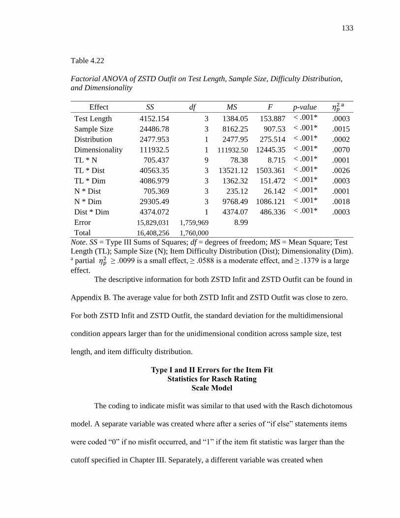
133

Table 4.22

Factorial ANOVA of ZSTD Outfit on Test Length, Sample Size, Difficulty Distribution,

and Dimensionality


Test Length 4152.154 3 1384.05 153.887 < .001* .0003

Sample Size 24486.78 3 8162.25 907.53 < .001* .0015

Distribution 2477.953 1 2477.95 275.514 < .001* .0002

Dimensionality 111932.5 1 111932.50 12445.35 < .001* .0070

TL * N 705.437 9 78.38 8.715 < .001* .0001

TL * Dist 40563.35 3 13521.12 1503.361 < .001* .0026

TL * Dim 4086.979 3 1362.32 151.472 < .001* .0003

N * Dist 705.369 3 235.12 26.142 < .001* .0001

N * Dim 29305.49 3 9768.49 1086.121 < .001* .0018

Dist * Dim 4374.072 1 4374.07 486.336 < .001* .0003

Error 15,829,031 1,759,969 8.99

Total 16,408,256 1,760,000




effect.

The descriptive information for both ZSTD Infit and ZSTD Outfit can be found in

Appendix B. The average value for both ZSTD Infit and ZSTD Outfit was close to zero.

For both ZSTD Infit and ZSTD Outfit, the standard deviation for the multidimensional

condition appears larger than for the unidimensional condition across sample size, test

length, and item difficulty distribution.

Type I and II Errors for the Item Fit

Statistics for Rasch Rating

Scale Model

The coding to indicate misfit was similar to that used with the Rasch dichotomous

model. A separate variable was created where after a series of “if else” statements items

were coded “0” if no misfit occurred, and “1” if the item fit statistic was larger than the

cutoff specified in Chapter III. Separately, a different variable was created when

134

generating the data for the items which were expected to misfit were also coded as “1.”

Items which falsely identified as misffiting were averaged within each cell in order to

determine the Type I error. The Type II error was calculated by counting the number of

items which were not flagged as misfitting and compared to the number of items which

were expected to misfit.

The trend of the Type I error rates remained constant across test lengths, though

the error rates appeared slightly higher for test lengths of I = 30 and I = 50 for ZSTD Infit

across sample sizes. Additionally, the Type I error rate for Outfit decreased as the sample

size increased. This negative trend appears for all test lengths. More importantly, the Q-

Index had the lowest Type I error rate across all sample sizes. The graphical

representation of the Type I error rates can be seen in Figure 4.16 in addition to this

visual information Table 4.23 shows the rates for Type I error.

The Type II error rates are displayed in Table 4.23. Type II error rates were the

highest for Outfit, specifically for the test lengths I = 20 and I = 30. Surprisingly, for both

ZSTD Outfit and ZSTD Infit the Type II error increased with the sample size.

Interestingly, the Type II error for the Q-Index remained constant across sample sizes and

across test lenghts. Yet, none of the 65 conditions achieved a power of .80, in other

words, Type II error was extremely high, which can indicate that none of the item fit

statistics were able to correctly identify the items which should have been flagged as

misfitting.

135

Figure 4.13. Type I Error rate for the Rasch rating scale model.

135

136

Figure 4.14. Type II Error rate for the Rasch rating scale model

136

137

Table 4.23

Type I and II Error Rates for the Rasch Rating Scale Model

Dimensionality: One Factor

Type I Error

Dimensionality: Two Factor

Type II Error

Q INFIT

ZSTD

Infit OUTFIT

ZSTD

Outfit Q INFIT

ZSTD

Infit OUTFIT

ZSTD

Outfit

Test

Length

Sample

Size

10 50 .0001 .0249 .0319 .0289 .0306

.3000 .3542 .2696 .5678 .2943

100 .0001 .0020 0312 .0038 .0305

.3000 .3458 .4185 .5622 .5199

150 .0001 .0001 .0315 .0013 .0310

.3000 .3436 .5151 .5651 .5880

250 .0001 .0001 .0343 .0003 .0337

.3000 .3370 .5767 .5690 .6053

20 50 .0001 .0296 .0364 .0335 .0346

.2961 .4289 .4074 .6742 .3530

100 .0001 .0027 .0380 .0047 .0348

.2992 .4294 .4981 .6914 .5606

150 .0001 .0002 .0373 .0010 .0363

.2999 .4327 .5257 .6963 .6375

250 .0001 .0001 .0362 .0001 .0345

.3000 .4311 .5565 .6988 .6975

30 50 .0001 .0310 .0410 .0328 .0402

.2989 .4646 .4451 .6869 .3614

100 .0001 .0027 .0394 .0036 0381

.2998 .4627 .5089 .6957 .6120

150 .0001 .0003 .0407 .0005 .0405

.3000 .4621 .5264 .6970 .6793

250 .0001 .0001 .0402 .0001 .0391

.3000 .4657 .5437 .6983 .6990

50 50 .0001 .0326 .0418 .0343 .0401

.3000 .3962 .3146 .6475 .0607

100 .0001 .0029 .0413 .0039 .0402

.3001 .4063 .5058 .6535 .5647

150 .0001 .0005 .0408 .0008 .0396

.3000 .4083 .5626 .6529 .6727

250 .0001 .0001 .0420 .0001 .0403

.3000 .4137 .6103 .6509 .6980

137

138

Parameter Recovery of Rasch

Rating Scale Model

Parameter recovery was assessed for the Rasch rating scale model in similar

fashion as with the dichotomous Rasch model. The rationale for examining parameter

recovery is to assess to what extent the known item difficulty parameters which are

calibrated under different conditions of sample size, test length, item difficulty

distribution, and dimensionality differed from the estimated item difficulty parameters. If

the difference between the calibrated and original parameter is negligible then it can be

said that the parameter has been “recovered.” Once again bias and root mean square

error (RMSE) were used to assess the lack of recovery, in terms of error, of the item

parameters in this study.

Bias of Item Difficulty Estimates for the

Rasch Rating Scale Model

The magnitude of the bias was plotted against the overall difficulties for the

extreme conditions of sample size for all levels of test length (a) N =50, I = 10 and N =

250, I = 10, (b) N =50, I = 20 and N = 250, I = 20 (c) N =50, I = 30 and N = 250, I = 30

(d) N =50, I = 50 and N = 250, I = 50 which can be seen in Figure 4.13. The rest of the

conditions can be inferred because the patterns are similar to those in Figure 4.13.

Additionally, Table 4.24 shows the maximum, mean, and standard deviation for

bias in the rating scale model. In examining Table 4.24 it can be seen the mean bias is

negligible for all test lengths. The largest magnitude of the bias was 0.0328 for the test

length I = 20. Even in the most extreme condition of small sample size and short test

length (N = 50 and I = 10) one can see the mean bias estimates are very close to zero in

139

Figure 4.13. In contrast, bias was more clearly visible in this condition for the

dichotomous Rasch model.

140

Figure 4.15.Bias vs item difficulty for extreme conditions for the Rasch rating scale model.

140

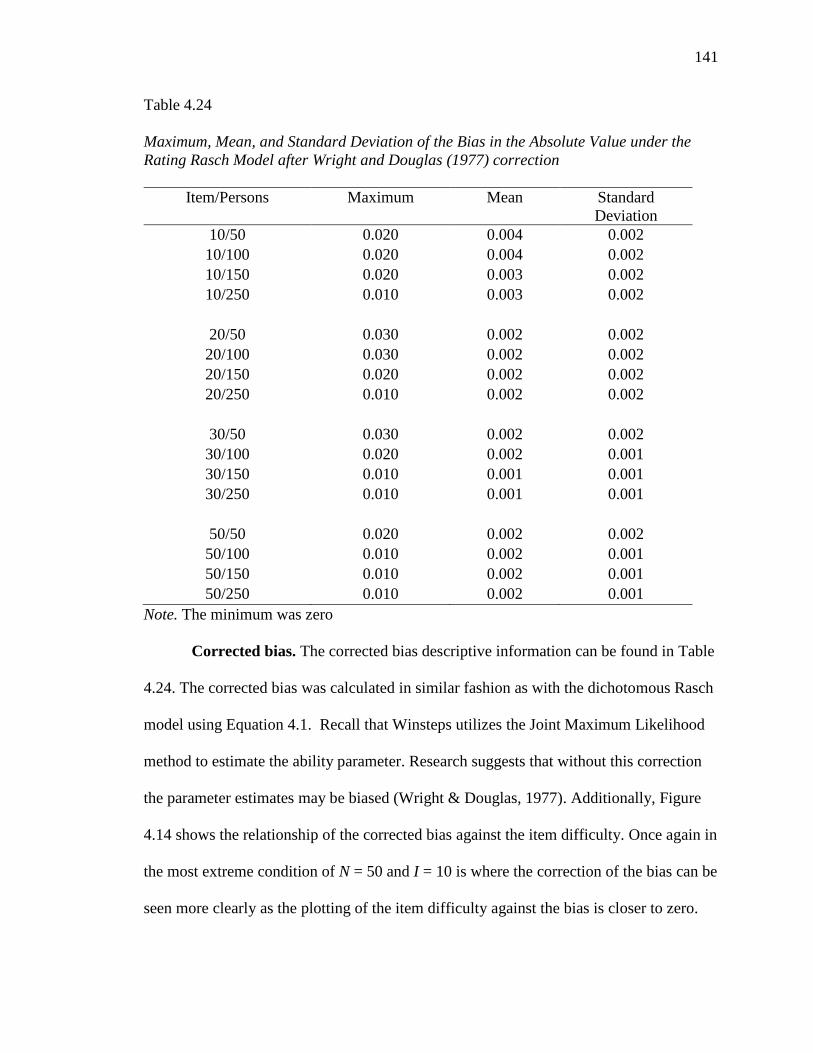
141

Table 4.24

Maximum, Mean, and Standard Deviation of the Bias in the Absolute Value under the

Rating Rasch Model after Wright and Douglas (1977) correction

Item/Persons Maximum Mean Standard

Deviation

10/50 0.020 0.004 0.002

10/100 0.020 0.004 0.002

10/150 0.020 0.003 0.002

10/250 0.010 0.003 0.002

20/50 0.030 0.002 0.002

20/100 0.030 0.002 0.002

20/150 0.020 0.002 0.002

20/250 0.010 0.002 0.002

30/50 0.030 0.002 0.002

30/100 0.020 0.002 0.001

30/150 0.010 0.001 0.001

30/250 0.010 0.001 0.001

50/50 0.020 0.002 0.002

50/100 0.010 0.002 0.001

50/150 0.010 0.002 0.001

50/250 0.010 0.002 0.001

Note. The minimum was zero

Corrected bias. The corrected bias descriptive information can be found in Table

4.24. The corrected bias was calculated in similar fashion as with the dichotomous Rasch

model using Equation 4.1. Recall that Winsteps utilizes the Joint Maximum Likelihood

method to estimate the ability parameter. Research suggests that without this correction

the parameter estimates may be biased (Wright & Douglas, 1977). Additionally, Figure

4.14 shows the relationship of the corrected bias against the item difficulty. Once again in

the most extreme condition of N = 50 and I = 10 is where the correction of the bias can be

seen more clearly as the plotting of the item difficulty against the bias is closer to zero.

142

However, unlike with the dichotomous Rasch the bias correction was not as obvious for

the rest of the conditions given that the initial bias was already very close to zero.

Table 4.25

Maximum, Minimum, Mean, and Standard Deviation of the Corrected Bias in the

Absolute Value under the Rating Scale Rasch Model

Item/Persons Maximum Mean Standard

Deviation

10/50 0.020 0.003 0.002

10/100 0.010 0.003 0.002

10/150 0.010 0.003 0.002

10/250 0.010 0.003 0.002

20/50 0.030 0.002 0.002

20/100 0.020 0.002 0.002

20/150 0.020 0.002 0.002

20/250 0.010 0.002 0.002

30/50 0.030 0.002 0.002

30/100 0.020 0.001 0.001

30/150 0.010 0.001 0.001

30/250 0.010 0.001 0.001

50/50 0.020 0.002 0.002

50/100 0.010 0.002 0.001

50/150 0.010 0.002 0.001

50/250 0.010 0.002 0.001

Note. The minimum was zero.

143

Figure 4.16. Corrected bias vs. item difficulty for Rasch rating scale model.

143

144

Relative Bias for Rasch

Rating Scale Model

Recall that relative bias provides information as to the proportional difference

between the estimated and the true parameter. For relative bias, values of zero indicate

that the parameter is unbiased. Further, the sign of the value provides information

regarding whether the parameter has been over or under estimated. Table 4.23 displays

the values for relative bias by test length and sample size averaged across items;

however, these values were calculated after performing the correction factor

recommended by Wright and Douglas (1977). As with the dichotomous Rasch model,

practical and acceptable significance was set at a magnitude of .05 (Hoogland &

Boomsma, 1998; Zhang, 2015). Though the average value for relative bias was well

below the recommended cutoff of .05 the maximum and minimum values of relative bias

indicate there exist values that are well above this cutoff particularly for the I = 20

condition. The I = 20 condition was also the most problematic condition for the

dichotomous model in terms of relative bias, meaning it yielded large negative values for

the conditions indicating the parameter was being underestimated. Minimal values for the

I = 50 condition showed potential outliers, though the average value of relative bias for

the different test lengths across the I = 50 condition was below .05.

Detailed information about the relative bias by dimensionality and item difficulty

distribution can be found in Appendix C2. From Table C2.3 it is clear that the large

values of relative bias are in the uniform item difficulty distribution where I = 20 for all

sample sizes. Though the average value of the relative bias is below or slightly above the

.05 cutoff the I = 20 condition under a uniform item difficulty distribution has extreme

minimal values which indicate that the parameter was being underestimated for this

145

condition. A further examination was warranted. For this reason, C2.5 details the relative

bias by item, in this further exploration it is clear that Item 9 is an outlier quite possibly

due to the “true” item difficulty distribution utilized when generating the data. Table C2.4

shows the relative bias for all conditions when the item difficulty distribution is randomly

distributed. The relative bias after correction can be found in Table 4.27. Here it is clear

that some of the bias has been removed (Table 4.26 shows the relative bias before the

correction). Yet, there exist many conditions where the relative bias exceeds the

recommended cutoff of .05. For example, when I = 30 across test lengths under the

normal item difficulty distribution, the average value was below .05 but many of the

minimum and maximum values exceeded the cutoff. In contrast, under the uniform item

difficulty distribution on average the corrected relative bias value was below .05, except

for I = 20 and N = 50; however, many of the minimum and maximum values exceeded

the recommended cutoff.

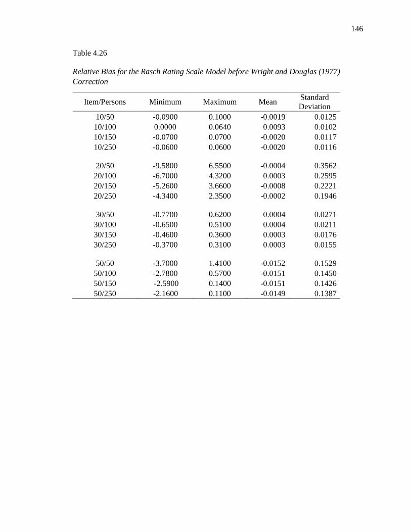
146

Table 4.26

Relative Bias for the Rasch Rating Scale Model before Wright and Douglas (1977)

Correction


Deviation

10/50 -0.0900 0.1000 -0.0019 0.0125

10/100 0.0000 0.0640 0.0093 0.0102

10/150 -0.0700 0.0700 -0.0020 0.0117

10/250 -0.0600 0.0600 -0.0020 0.0116

20/50 -9.5800 6.5500 -0.0004 0.3562

20/100 -6.7000 4.3200 0.0003 0.2595

20/150 -5.2600 3.6600 -0.0008 0.2221

20/250 -4.3400 2.3500 -0.0002 0.1946

30/50 -0.7700 0.6200 0.0004 0.0271

30/100 -0.6500 0.5100 0.0004 0.0211

30/150 -0.4600 0.3600 0.0003 0.0176

30/250 -0.3700 0.3100 0.0003 0.0155

50/50 -3.7000 1.4100 -0.0152 0.1529

50/100 -2.7800 0.5700 -0.0151 0.1450

50/150 -2.5900 0.1400 -0.0151 0.1426

50/250 -2.1600 0.1100 -0.0149 0.1387

147

Table 4.27

Relative Bias of the Rasch Rating Scale Model after Wright and Douglas (1977)

Correction


Deviation

10/50 -0.0800 0.0900 -0.0017 0.0112

10/100 0.0000 0.0640 0.0093 0.0102

10/150 -0.0600 0.0600 -0.0018 0.0105

10/250 -0.0500 0.0500 -0.0018 0.0104

20/50 -9.1000 6.2200 -0.0004 0.3384

20/100 -6.3600 4.1000 0.0003 0.2465

20/150 -4.9900 3.4800 -0.0007 0.2110

20/250 -4.1200 2.2300 -0.0002 0.1849

30/50 -0.7500 0.6000 0.0004 0.0262

30/100 -0.6300 0.4900 0.0003 0.0204

30/150 -0.4500 0.3500 0.0003 0.0170

30/250 -0.3600 0.3000 0.0003 0.0150

50/50 -3.6300 1.3800 -0.0149 0.1499

50/100 -2.7200 0.5600 -0.0148 0.1421

50/150 -2.5400 0.1300 -0.0148 0.1398

50/250 -2.1200 0.1100 -0.0146 0.1359

Moreover, a factorial ANOVA was conducted utilizing relative bias (after

correction) as the dependent variable and test length, sample size, item difficulty

distribution, and dimensionality as independent variables. The results of this ANOVA are

found in Table 4.28, and suggested that the interaction between test length and

dimensionality was statistically significant (𝑝 < .001) and the effect size was the highest

among all the effect sizes in this analysis, yet it would still be considered a small effect

148

(𝜂𝑝2 = .0040). Examining the main effects, test length showed statistical significance

𝑝 < .001) but the effect size was also trivial (𝜂𝑝2 = .0030).

Table 4.28

Factorial ANOVA of (Corrected) Relative Bias on Test Length, Sample Size, Difficulty

Distribution, and Dimensionality


Test Length 92.972 3 30.991 1501.459 < .001* .0030

Sample Size 0.014 3 0.005 0.234 .873 .0001

Distribution 16.792 1 16.792 813.542 < .001* .0001

Dimensionality 25.954 1 25.954 1257.423 < .001* .0010

TL * N 0.04 9 0.004 0.216 .992 .0001

TL * Dist 83.967 3 27.989 1356.04 < .001* .0020

TL * Dim 158.055 3 52.685 2552.522 < .001* .0040

N * Dist 0.019 3 0.006 0.300 .826 .0001

N * Dim 0.035 3 0.012 0.560 .641 .0001

Dist * Dim 13.916 1 13.916 674.226 < .001* .0001




effect

149

Roor Mean Square Error of

Item Difficulty Estimates

Recall that a smaller value of RMSE indicates more accuracy of the item

difficulty parameter. As summarized in Table 4.29 and illustrated in Figure 4.15 the

average RMSE was small, ranging from .0362 to .0126 across conditions. However, a

closer examination reveals that the largest values for RMSE appeared in the condition

with shortest test length (I = 10) across all sample sizes, while the smallest RMSE values

appear in the longer test length (I = 30) condition for sample sizes (N = 100, 150, and

250). Indicating that the RMSE becomes smaller as the test length increases as

anticipated.

Table 4.29

Maximum, Minimum, Mean, and Standard Deviation of the RSME under the Rating Scale

Rasch Model


Deviation

10/50 0.0001 0.2350 0.0362 0.0227

10/100 0.0001 0.1510 0.0349 0.0201

10/150 0.0001 0.1540 0.0343 0.0194

10/250 0.0001 0.1360 0.0340 0.0186

20/50 0.0001 0.3284 0.0223 0.0218

20/100 0.0001 0.2621 0.0194 0.0184

20/150 0.0001 0.1911 0.0183 0.0169

20/250 0.0001 0.1481 0.0175 0.0159

30/50 0.0001 0.2618 0.0181 0.0165

30/100 0.0001 0.1778 0.0149 0.0130

30/150 0.0001 0.1168 0.0136 0.0117

30/250 0.0001 0.0888 0.0126 0.0107

50/50 0.0001 0.2156 0.0239 0.0164

50/100 0.0001 0.1216 0.0216 0.0138

50/150 0.0001 0.1011 0.0207 0.0128

50/250 0.0001 0.0669 0.0201 0.0120

150

Figure 4.17. RMSE for Rasch Rating Scale for the extreme conditions.

150

151

Correlation between True and Estimated

Item Parameters

One final assessment of parameter recovery was performed via a Pearson

bivariate correlation which yielded a high correlation between the true parameter and the

estimated item difficulty parameter generated by Winsteps. The correlation for all

conditions between the true and estimated parameter was r = .967. Additionally, the

correlations by condition were high, i.e., r .918, for all conditions as shown in Table

4.30.

Table 4.30

Bivariate Correlation between the True and Estimated Parameters for All Conditions

Uniform Item Difficulty Distribution Random Item Difficulty Distribution

Item /Persons Unidimensional Multidimensional:

Two Factor Unidimensional

Multidimensional:

Two Factor

10/50 .939 .968 .979 .968

10/100 .968 .965 .990 .977

10/150 .978 .976 .993 .982

10/250 .987 .985 .996 .984

20/50 .951 .947 .985 .966

20/100 .975 .974 .993 .976

20/150 .983 .982 .995 .980

20/250 .990 .989 .997 .983

30/50 .924 .918 .976 .970

30/100 .961 .958 .987 .982

30/150 .972 .970 .992 .986

30/250 .983 .982 .995 .988

50/50 .944 .941 .983 .971

50/100 .973 .969 .992 .982

50/150 .981 .979 .994 .987

50/250 .988 .987 .997 .989

152

Supplementary Analysis

It is possible that the aggregation of the items masked the findings for individual

items. In addition to this, it was important to know, beyond the confirmatory factor

analyses performed on the pilot data. For example, for the I = 10 condition, Items 1-3

were specified to belong to one factor, while Items 4-10 were specified to belong to a

second factor. If the fit indices perform correctly, we would expect to see poorer fit for

the three items specified on the secondary factor than we would for the other seven items

specified to measure the dominant, primary factors. Table 4.31 shows Q-Index values for

the I = 10 condition, with a uniform item difficulty distribution, and under the violation

of unidimensionality. It is important to note that the suggested cutoff of .5 from Rost and

von Davier (1994) is not reached for this condition. However, it is clear that Items 1-3

have higher Q-Index values. For example for N = 50, the mean values are .22 and .23

while for Items 4-10 the Q-Index values range from .05 to .03 which is considerably

lower than those of Items 1-3, suggesting the Q-Index was able to distinguish between

those items on the secondary factor that should fit more poorly and those items on the

larger, primary factor that should fit the data well. This pattern is similar across all

sample sizes for the Q-Index and can be found for the rest of the item fit statistics though

the pattern becomes less clear for ZSTD Infit and ZSTD Outfit which can be due to the

recommended cutoffs. This information can be found in Appendix D in Tables D1 to D8.

153

Table 4.31



Q-Index Rating Scale Model Minimum Maximum Mean SD 1 * .10 .40 .23 .05 2 * .09 .40 .22 .05 3 * .09 .40 .22 .05 4 .00 .18 .05 .02

50 5 .00 .06 .03 .01 6 .01 .07 .03 .01 7 .01 .07 .03 .01 8 .01 .09 .04 .01 9 .01 .07 .03 .01 10 .00 .07 .03 .01 1 * .14 .35 .23 .03 2 * .13 .33 .22 .03 3 * .13 .34 .22 .03 4 .01 .12 .06 .02

100 5 .02 .05 .03 .01 6 .02 .06 .03 .01 7 .02 .06 .03 .01 8 .02 .07 .04 .01 9 .02 .06 .04 .01 10 .02 .05 .03 .01



154

Table 4.31 Continued



Q-Index Rating Scale Model Minimum Maximum Mean SD 1 * .15 .32 .23 .03 2 * .13 .32 .22 .03 3 * .13 .32 .22 .03 4 .02 .11 .06 .01

150 5 .02 .05 .03 .00 6 .02 .05 .03 .01 7 .02 .06 .04 .01 8 .02 .06 .04 .01 9 .02 .06 .04 .01 10 .02 .05 .03 .00 1 * .16 .32 .23 .02 2 * .15 .29 .22 .02 3 * .15 .29 .21 .02 4 .03 .10 .06 .01

250 5 .02 .05 .03 .00 6 .02 .05 .03 .00 7 .02 .05 .04 .00 8 .03 .06 .04 .01 9 .02 .06 .04 .00 10 .02 .05 .03 .00



Chapter Summary

Descriptive and inferential analyses were used to answer the research questions of

interest. To understand the differences among the five item fit statistics a series of

factorial ANOVAs was performed. Parameter recovery was also studied in order to

determine if the item difficulty parameters had been estimated correctly. Table 4.32

summarizes the results for the dichotomous Rasch model.

155

Conclusions Regarding the


Sample size. ANOVAs were conducted to answer research questions 1 through 4.

For the Rasch dichotomous model, the item fit statistics (Q-Index, Infit, ZSTD Infit,

Outfit, ZSTD Outfit) did not vary under the different conditions of sample size (N = 50,

100, 150, and 250). Though tests of sample size were statistically significant, the

statistical significance could be an artifact of the large number of data sets generated for

the simulation. In addition, partial eta squared, used as an estimate of effect size, did not

reach the cutoff to be deemed a small effect for any of the item fit statistics studied under

varying conditions of sample size.

Test length. For the Rasch dichotomous model, the item fit statistics (Q-Index,

Infit, ZSTD Infit, Outfit, ZSTD Outfit) did not vary under the different conditions of test

length (I = 10, 20, 30, and 50). While statistical significance was present (p < .001) the

effect sizes for all the item fit indices were trivial (𝜂𝑝2 ranged from .0001 to .0652).

However, for the Q-Index the second highest effect size was for test length at 𝜂𝑝2 = .0652.

Dimensionality. When differences in fit based on dimensionality (unidimensional

versus multidimensional) were examined, the factorial ANOVAs showed that the Q-

Index was the only item fit statistic to detect the departure from unidimensionality (𝜂𝑝2 =

.0968). (𝜂𝑝2 = .0968) from the conditions where the data were purposely generated to have

two dimensions. The traditional item fit statistics (Infit, ZSTD Infit, Outfit, and ZSTD

Outfit), while showing statistical significance, exhibited only a trivial effect (𝜂𝑝2 = .0001)

when comparing unidimensional and multidimensional conditions.

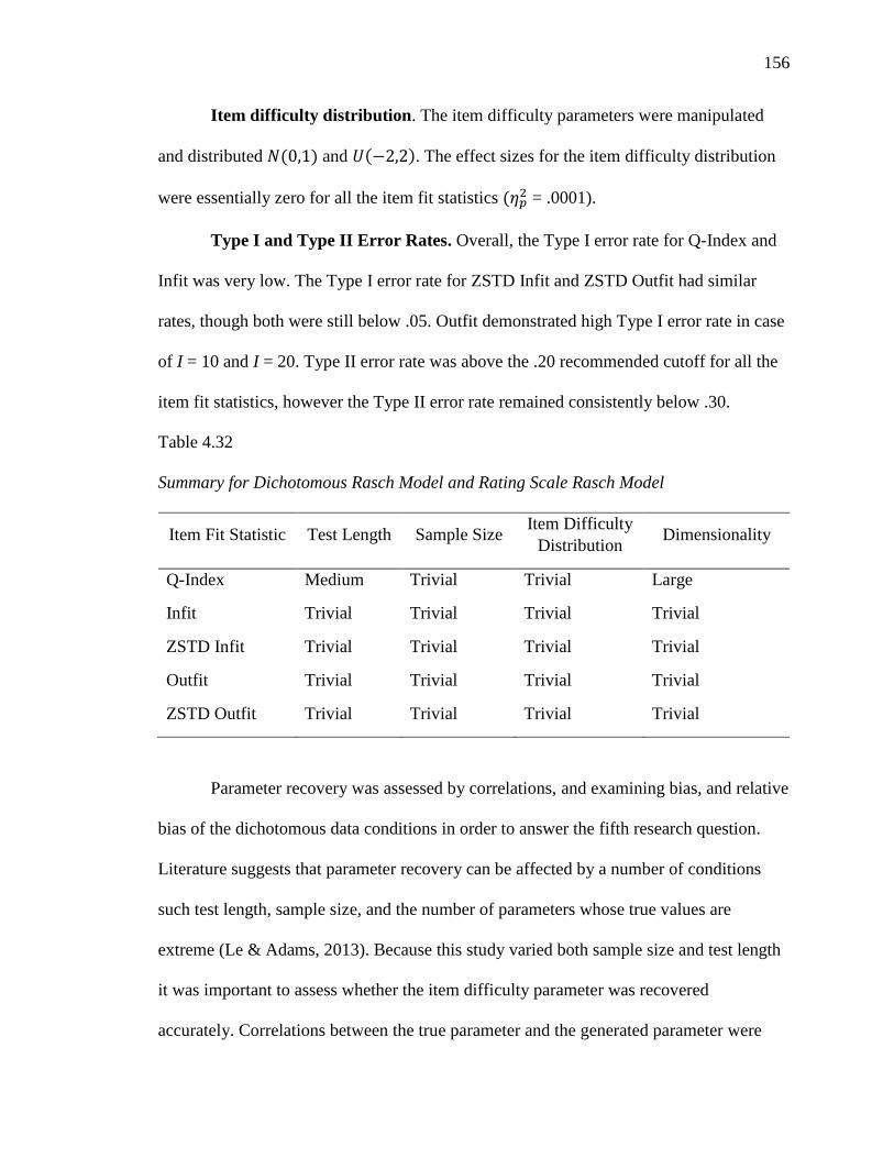
156

Item difficulty distribution. The item difficulty parameters were manipulated

and distributed 𝑁(0,1) and 𝑈(−2,2). The effect sizes for the item difficulty distribution

were essentially zero for all the item fit statistics (𝜂𝑝2 = .0001).

Type I and Type II Error Rates. Overall, the Type I error rate for Q-Index and

Infit was very low. The Type I error rate for ZSTD Infit and ZSTD Outfit had similar

rates, though both were still below .05. Outfit demonstrated high Type I error rate in case

of I = 10 and I = 20. Type II error rate was above the .20 recommended cutoff for all the

item fit statistics, however the Type II error rate remained consistently below .30.

Table 4.32

Summary for Dichotomous Rasch Model and Rating Scale Rasch Model

Item Fit Statistic Test Length Sample Size Item Difficulty

Distribution Dimensionality

Q-Index Medium Trivial Trivial Large

Infit Trivial Trivial Trivial Trivial

ZSTD Infit Trivial Trivial Trivial Trivial

Outfit Trivial Trivial Trivial Trivial

ZSTD Outfit Trivial Trivial Trivial Trivial

Parameter recovery was assessed by correlations, and examining bias, and relative

bias of the dichotomous data conditions in order to answer the fifth research question.

Literature suggests that parameter recovery can be affected by a number of conditions

such test length, sample size, and the number of parameters whose true values are

extreme (Le & Adams, 2013). Because this study varied both sample size and test length

it was important to assess whether the item difficulty parameter was recovered

accurately. Correlations between the true parameter and the generated parameter were

157

high for all conditions. Overall the correlation was 𝑟 = .950 and was high across all

conditions (r > .940). Further, bias was negligible across conditions; however, the

correction factor developed by Wright and Douglas (1977) was still applied to the

dichotomous data. The correction factor only reduced the already negligible bias. Next,

relative bias was examined, it was in this exploration that the condition of I = 20, with

uniform item difficulty distribution showed extreme values of relative bias, larger than

the recommended cutoff of .05. However, the average value of relative bias for this

condition was still well below .05. Overall, parameter recovery was accurate for all

conditions despite the manipulation of test lengths, sample size, item difficulty

distribution, and dimensionality. This indicates that the Rasch model is robust enough to

endure such manipulation of data.

Conclusions Regarding the Rasch

Rating Scale Model

A summary of the results for the Rasch Rating Scale Model follows. Table 4.33

summarizes the findings.

Sample size. A series of factorial ANOVAs was conducted for the Rasch rating

scale model. Across the item fit statistics, the effect sizes were trivial with the values of

partial eta square ranging from .0001 to .0015.

Test length. For the Q-Index the second highest effect size was for the main

effect of test length, however, the effect size was not large enough to be considered a

small effect size (𝜂𝑝2 = .0023). The values of partial eta square 𝜂𝑝

2 for test length across

all the item fit statistics ranged from .0003 to .0030.

Dimensionality. Similarly, to the dichotomous Rasch model, dimensionality was

the only main effect that had a non-trivial effect size for the Q-Index. It is important to

158

note that the effect size for the interaction of test length and dimensionality for the Q-

Index was one of the highest in the analysis but failed to reach the cutoff for a small

effect size 𝜂𝑝2 = 0030. The dimensionality main effect was one of the largest effect sizes

for Infit, but not large enough to be labeled a small effect size. ZSTD Outfit also showed

an effect size that failed to reach the cutoff for small effect (𝜂𝑝2 = . 0070).

Item difficulty distribution. Across the all item fit statistics, the item difficulty

distribution showed statistical significance; however, following the same pattern as the

sample size and test length main effects the values of partial eta squared were trivial. The

values of partial eta square ranged from .0001 to .0013.

Type I and Type II Error. The Type I error rate for the Rasch rating scale for

the Q-Index was low, as it was for Infit. However, for both ZSTD Infit and ZSTD Outfit

the Type I error rate was close to .30 though still under the .05 cutoff. Outfit, had a high

Type I error particularly for N = 50 across all test lengths though not surpassing the .05

cutoff. Finally, the Type II error rate for the rating scale was unfortunaly very high, in all

cases exceeding the .20 recommended cutoff, though the Q-Index and Infit had the lowest

Type II error rates.

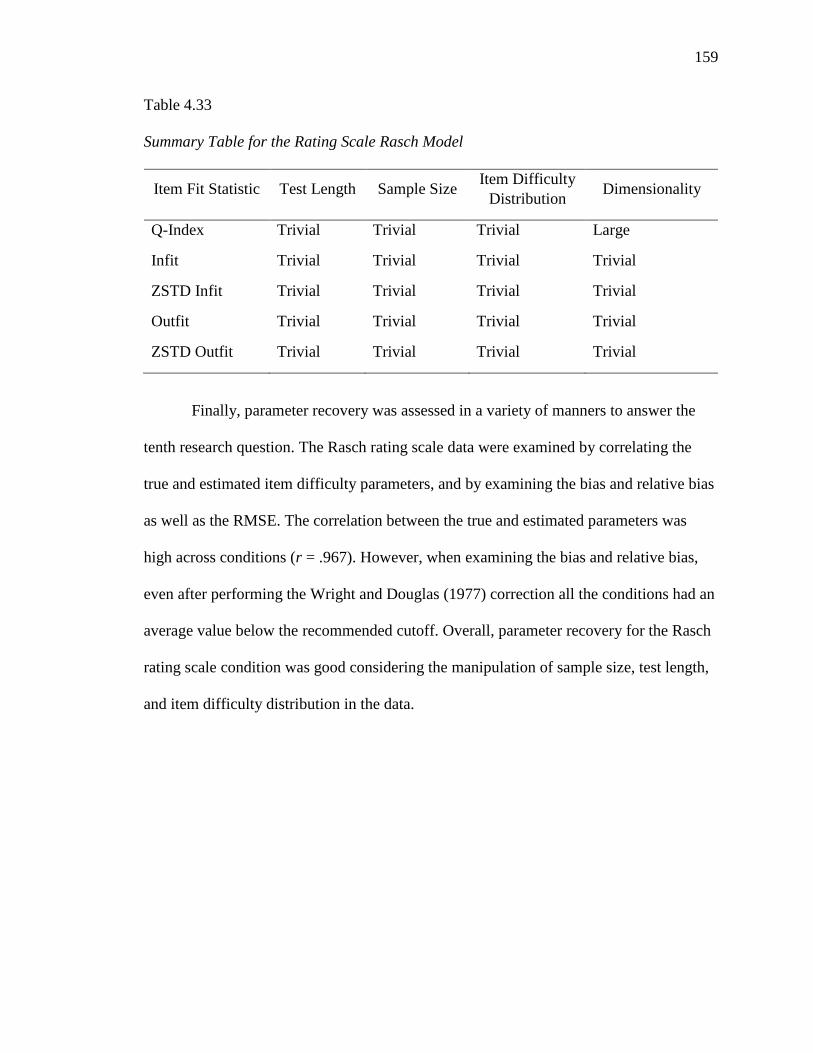
159

Table 4.33

Summary Table for the Rating Scale Rasch Model

Item Fit Statistic Test Length Sample Size Item Difficulty

Distribution Dimensionality

Q-Index Trivial Trivial Trivial Large

Infit Trivial Trivial Trivial Trivial

ZSTD Infit Trivial Trivial Trivial Trivial

Outfit Trivial Trivial Trivial Trivial

ZSTD Outfit Trivial Trivial Trivial Trivial

Finally, parameter recovery was assessed in a variety of manners to answer the

tenth research question. The Rasch rating scale data were examined by correlating the

true and estimated item difficulty parameters, and by examining the bias and relative bias

as well as the RMSE. The correlation between the true and estimated parameters was

high across conditions (r = .967). However, when examining the bias and relative bias,

even after performing the Wright and Douglas (1977) correction all the conditions had an

average value below the recommended cutoff. Overall, parameter recovery for the Rasch

rating scale condition was good considering the manipulation of sample size, test length,

and item difficulty distribution in the data.

160

CHAPTER V

DISCUSSION

This dissertation study focused on the differences among the item fit statistics for

the dichotomous Rasch model and the Rasch rating scale model under varying conditions

of sample size, test length, dimensionality, and item difficulty distribution. This chapter

summarizes and discusses the findings in the context of the existing literature on the topic

of Rasch fit indices. First, the performance of the item fit statistics is discussed, followed

by the findings regarding parameter recovery. The importance of the findings follows the

results discussion. Finally, implications for applied researchers, the limitations of the

study, and recommendations for future research are discussed.

Performance of Fit Statistics

Ostini and Nering (2006) called attention to the fact that little to no research has

been performed utilizing the Q-Index regarding this as the key disadvantage of the fit

statistic. Largely, the results of this dissertation provide information regarding the Q-

Index which was previously non-existent. The results of this study provide applied

researchers with evidence regarding the robustness of the Q-Index in both dichotomous

and rating scale data and in contrast with the currently available measures of fit in

popular software such as Winsteps and Winmira (Linacre, 2006; von Davier, 2001).

161


Among the manipulated variables of interest (sample size, test length,

dimensionality, and item difficulty distribution) for the dichotomous Rasch model, the

only variable with a large effect on the Q-Index was dimensionality. As anticipated the

condition where unidimensionality was violated reported a higher mean value of Q-

Index. Additionally, test length had a medium effect on the Q-Index. However, for the

rest of the item fit statistics none of the interactions or main effects yielded a non-trivial

effect. Similarly, for the Rasch rating scale model, the only main effect which showed at

least a medium effect was dimensionality. Once again, all the interactions and main

effects for the rest of the item fit indices were small to trivial. This was a surprising

finding considering the literature suggests that the Infit and Outfit behave as a function of

sample size (Wang & Chen, 2005; Wu & Adams, 2013).

Next the Type I and II error rates were examined. The Type I error rate was

defined as falsely rejecting an item as not fitting the Rasch model. In terms of Type I

error rates, the Q-Index for the dichotomous Rasch model showed rates well below 𝛼 =

.05 as did Infit, ZSTD Infit, and ZSTD Outfit consistent with Karabatsos work (2000);

however, Outfit displayed Type I error rates which were slightly higher than 𝛼 = .05,

except when test length had 50 items. For the rating scale Rasch model, the Type I error

rates for the Q-Index were low but were higher for ZSTD Infit and ZSTD Outfit across

all test lengths though these rates did not exceed 𝛼 = .05.

162

Summary of Parameter Recovery

Findings for the Dichotomous

Rasch Model

In terms of parameter recovery in this study the analysis indicated that there was

good recovery. In other words, the “true” parameters were estimated accurately by the

Winsteps software even when considering the data were generated with a variety of

conditions such as four different test lengths and sample sizes, two item difficulty

distributions, and two dimensionalities. There was a slight bias for the extreme condition

of short test length (I =10) and small sample size (N = 50) for the dichotomous Rasch

model; however, after correcting the bias with the method suggested by Wright and

Douglas (1977) this bias disappeared. A very important, and surprising, finding was the

good parameter recovery for such small sample sizes as those used in this study. This was

an unexpected finding considering Khan’s (2014) studied also focused on small sample

sizes and test lengths and resulted in poor parameter recovery. However, my study used

the Rasch software Winsteps for parameter estimation; in contrast, Khan’s study utilized

the R package Itm. Khan found that while it was possible to utilize small samples for

Rasch model fit the parameter recovery was not stable. More importantly, in this

dissertation study parameter recovery was accurate after utilizing the Wright and Douglas

(1977) correction (which Khan’s study did not utilize given that Itm uses Maximum

Likelihood Estimation rather than Joint Maximum Likelihood). Another important detail

in the differences in the studies is that Khan did not provide the cutoffs utilized for

determining out of range bias and RMSE values.

163

Rating Scale Rasch Model

Similar to the dichotomous Rasch model, a series of factorial ANOVAs for the

Rasch rating scale model was conducted. Consistent with the results of the Q-Index for

the dichotomous model an effect existed for the Q-index for dimensionality. In one of the

most unexpected results, the mean value for the Q-Index for the unidimensional condition

was higher. Moreover, for the remaining item fit statistics Infit, Outfit, ZSTD Infit, and

ZSTD Outfit the effect sizes were often small and, in many times, trivial. This may

indicate that Infit, Outfit, ZSTD Infit, and ZSTD Outfit are robust to violations of

unidimensionality (Reckase, 1979) given that parameter recovery was also high in the

current study across all conditions where unidimensionality was violated. When

examining the Type I error rates for the Rasch rating scale model, a positive finding was

discovering that the Q-Index had a Type I error rate well below 𝛼 = .05. The

standardized forms of Infit and Outfit had higher error rates than the non-standardized

versions similar to what A. B. Smith et al. (2008) found in their study.

One of the most unexpected results was in the analysis of the rating scale model

data where the average values of the Q-Index were higher (suggesting greater misfit)

under unidimensionality than under the multidimensional condition. In contrast, one

would anticipate high values of the Q-Index in a condition where the property of

unidimensionality is violated. Initially, I considered this could be a mistake in the code,

or in the coding of the data. However, the values of the Q-Index struggled to reach the .5

cutoff criteria. This can be seen in Appendix C2 in Tables C2.20 to C2.28. These tables

present findings for the I = 10 multidimensional condition for the rating scale model with

uniform item difficulty distribution. For the Q-Index, the .5 cutoff is not reached. This

164

finding may indicate that the .5 cutoff suggested by Rost and von Davier (1994) may

need optimization, particularly for the rating scale model. Another indication that the

code worked as anticipated is the high values of the correlations between the true and

estimated parameters indicating good parameter recovery.

Summary of Parameter Recovery

Findings for Rating Scale

Rasch Model

For the rating scale Rasch model the bias was negligible even before the

correction factor. Overall, the results of the simulation had a mean bias of zero indicating

that the item difficulty parameters were unbiased. Further, the high correlations between

the “true” item difficulty parameter and the estimated item difficulty parameter for the

rating scale Rasch model (𝑟 = .967) provides evidence of the calibration accuracy.

Based on further analysis, correlations between the “true” and estimated item difficulty

parameters for each of the 128 conditions in this dissertation also yielded high

correlations. Regarding RMSE, increasing the test length did not always help reduce that

mean value of the RMSE

When examining bias and relative bias, first a correction factor as suggested by

Wright and Douglas (1977) was calculated. After the correction factor was applied,

examining the table values along with plots of bias against the item difficulty distribution

it was easy to see how bias was minimal. However, a very different story was told by the

relative bias values. Large values of relative bias for the I = 20 condition for both the

dichotomous and rating scale Rasch models, as well as extremely low values relative bias

indicated that the item difficulty parameters were being underestimated. Supplementary

analysis by item for the I = 20 conditions indicated that many of the outliers of this

165

conditions came from Item 9 when the item difficulty distribution was normal and under

the multidimensional condition. The item difficulty distribution of Item 9 utilized in the

simulation was extremely small -.0007. Item by item information can be found in

Appendix C in Tables C2.15 and C2.16.

Wang and Chen’s (2005) parameter recovery study is one of the few papers

available utilizing rating scale data. In their study, the authors estimated the difficulty in

Winsteps which utilizes Joint Maximum Likelihood (JML) and successfully corrected the

biased estimates with the Wright and Douglas (1977) function available in Winsteps. The

biased estimation for the item difficulty distribution in this dissertation study was

corrected after the item parameters were estimated but the correction was performed in

SPSS. Similarly, to the Wang and Chen’s study, the biased estimation for the item

difficulty for the rating scale model was removed using the Wright and Douglas

correction.

General Discussion

Rost and von Davier (1994) claimed that the Q-Index was designed specifically

for rating scale data. For the conditions where the data met all the properties of the Rasch

model the Q-Index showed a low Type I error rate. However, while the factorial ANOVA

detected an effect for dimensionality, that is, the difference between the unidimensional

and multidimensional conditions, the direction of the average Q-Index was puzzling

when considering results aggregated across all items where fit appeared to be worse for

the unidimensional than for the multidimensional data. When examining results from the

supplementary, item-level analyses, however, performance of the Q-Index appears to be

more consistent with expectations. At the item-level, Q-Index values were noticeably

166

higher for items on the smaller, secondary factor than on the larger, dominant factor

which suggests the Q-Index was able to distinguish items that should versus should not fit

the Rasch model. In contrast, when data were dichotomous the Q-Index was less

successful in distinguishing items on the dominant versus secondary factors. The

sensitivity of the Q-Index was generally masked in the original results based on

aggregating fit values across all items.

It should be noted that the multidimensional conditions for the dichotomous and

rating scale Rasch models were generated utilizing two different R codes which can be

found in Appendix A3 and Appendix A4, respectively. Initially, I suspected that when

analyzing the data, the Rasch rating scale model was detecting the differences in how the

program to generate the data was coded. However, the supplementary analysis resported

in Chapter IV (see Appendix D in Tables D1 to D8) shows that for the most part the fit

statistics detected the items which were meant to misfit. This is clearer for the Q-Index

than with the rest of the item fit indices (this makes sense given that the Q-Index was the

most sensitive to the violation of dimensionality based on the ANOVA results). However,

the pattern is also clear for Infit and Outfit. For both Rasch models, with two factors and

uniform item difficulty distribution the I = 10 condition had Q-Index values which were

higher for the three items which were meant to misfit; unfortunately, for the rating scale

model though the Q-Index values were higher for the intentionally misfitting items the

value of the Q-Index did not reach .5.

A second puzzling result occurred in the rating scale Rasch model, and again for

the Type II error rates under the multidimensional condition. Overall, the Type II error

rates were higher compared to those in the Rasch dichotomous model contradicting Rost

167

and von Davier’s (1994) claims that the Q-Index might work better for the rating scale

Rasch model. Recall that Setzer (2008) and Suarez-Falcon and Glas (2003) recommended

that the correlation between factors should be set to .5; however, no guidelines were

provided on how the items should be weighted or separated into the factors. When

selecting the number of items, the argument was that an instrument that is expected to be

unidimensional should probably not have 50% of the items belong to one factor and 50%

of the items belong to a different factor. Due to this reasoning in the current study when

the number of items was 10, three items were set up to belong to one factor while the rest

were generated to correlate with a second factor. The multidimensional data were

evaluated to check if the two factor dimensions were generated correctly by utilizing a

confirmatory factor analysis and the item grouping was checked manually. Another

possible explanation is provided by the work of Drasgow and Parsons (1983), who

concluded that when the correlation between factors was less than r = .39, item response

theory analyses were not sensitive to multidimensionality. Perhaps, setting the correlation

between the two factors at .5 was too high to find an effect.

In summary, the Q-Index in the dichotomous Rasch model showed a large effect

for dimensionality and a medium effect for test length. For the rest of the conditions

(item distribution difficulty, sample size) the effect sizes were trivial. Further, the other

fit statistics yielded trivial effect sizes as well. It is important to note that the analysis was

performed by aggregating fit indices across all items, which may have led to the

attenuation of the effect sizes. Similarly, in the Rasch rating scale model for the Q-Index

only dimensionality showed a large effect size, while the rest of the conditions had trivial

effect sizes. The other item fit statistics had trivial effect sizes for all conditions studied.

168

Again, this could be due to the aggregation of the fit indices across all items for the

factorial ANOVA analysis. In the supplementary analysis performed, which can be found

in Chapter IV for the Q-Index and Appendix D for all item fit statistics and Rasch models

it is possible to observe the patterns where one can spot minimum and maximum values

which exceed the recommended cutoffs, but when examining the mean value for the

same item the recommended cutoff is not reached.

Most of the Rasch model literature focuses on the difficulty of having different

cutoffs for the item fit statistics Infit, Outfit, ZSTD Infit and ZSTD Outfit. For this

analysis, the criterion provided by Wright and Linacre (1994) for Infit and Outfit, and

Smith and Suh (2003) for ZSTD Infit and ZSTD Outfit was used. However, work by Wu

and Adams (2013) suggests that the cutoffs need to be calculated for the researcher’s

specific sample size utilizing the equation in Chapter II. It is possible that the Type I and

Type II errors may change if the cutoffs are determined by utilizing the guidelines of Wu

and Adams (2013) which utilize a different procedure that is more specific to the

researcher’s sample size. Similarly, A. B. Smith et al. (2008) suggest different cutoffs for

rating scale than those suggested by Wright and Linacre (1994); perhaps the change in

cutoffs may change the extreme values for the Type II error for the rating scale model.

Limitations

As with any study, this one is limited by the specific conditions manipulated and

studied in the simulation. Simulation studies have inherent limitations of applicability in

real life settings given the data conditions. In addition, the sampling design can be

artificial such as the degree of multidimensionality utilized in this dissertation. For this

reason, the findings of this study may not generalize to all Rasch applications. For

169

example, the current study explored the Q-Index and other item fit statistics in the context

of violation of unidimensionality. In addition to violation of the unidimensionality

assumption, there exist many different factors which can affect how the item fit statistics

behave under the Rasch model such as violations of local independence and presence of

socially desirable responding.

Recommendations for Future Research

The focus of this dissertation was on the Q-Index specifically with item fit; thus,

future research can focus on person fit. The person Q-Index can be found in the pairwise

R package or my existing code can be easily modified to assess person rather than item

fit. The analysis for both the dichotomous Rasch and the rating scale Rasch model

showed an effect for the violation of dimensionality. The degree of multidimensionality

simulated in the current study was chosen based on Setzer’s (2008) recommendations.

Studying the degrees of multidimensionality to understand to what extent it can affect

item calibration would be helpful to applied researchers. Further, the most popular item

fit statistics are currently Infit, Outfit, ZSTD Infit, and ZSTD Outfit (Linacre, 2006; A. B.

Smith et al., 2008; R. M. Smith & Plackner, 2009); however, other item fit statistics such

as the Logit Residual Index could be compared to the Q-Index (Mount & Schumacker,

1998). Additionally, this study focused on two Rasch models, the dichotomous model

and the rating scale model. There exist a variety of Rasch models such as the partial

credit model (Masters & Wright, 1997), many facets model among others in which the

robustness of the Q-Index can be studied (Linacre, 1994b). Likewise, the Rasch model

has three core properties: local independence, unidimensionality, and monotonicity. In

this study, my focus was only on the violation of unidimensionality, but the study of the

170

robustness of the Q-Index to violations of local independence and monotonicity can be

another path for future research. There are also several other measurement disturbances

that can be studied with the dichotomous Rasch model such as guessing, which has been

studied in conjunction with item fit indices, but not the Q-Index (Schumacker, et al.,

2005). In regard to the rating scale Rasch model, while guessing may not be a viable

option (respondents on an attitude measure or survey, may not be inclined to “guess” the

answer), respondents may provide socially desirable responses. Thus, a different path to

study the properties of the Q-Index and the popular item fit statistics might be to study

social desirability as a measurement disturbance.

Another avenue for future research could be optimizing the criteria for identifying

item misfit. Rost and von Davier (1994) recommended a cutoff of .5 to identify misfit in

a dataset based on the Q-Index. However, it would be interesting to investigate what

would happen to the rates of misfit and Type I and Type II error rates with cutoffs above

and below the recommended .5 mark. For example, lowering the cutoff below .5 might

optimize the Type II error rate, particularly for the rating scale model. Finally, future

research could focus on studying the standardized form of the Q-Index. It could be that

the combination of both the Q-Index and the standardized form of this index may be

more helpful in identifying misfit as well as measurement disturbances than the Q-Index

alone. However, the implementation of the standardized form of the Q-Index may require

expertise in mathematical statistics.

A combination of item fit statistics may also be of interest for future research. In

fields such as Structural Equation Modeling, researchers often utilize the combination of

two or more fit indices to guide their research (Hu & Bentler, 1999). In this dissertation

171

study, Infit and the Q-Index had very similar low Type I error rates, as was found by

Karabatsos (2000) for Infit. The Q-Index and Infit had similar Type II error rates. Future

research may focus on what possible combinations of item fit statistics for Rasch analysis

can better inform applied researchers.

Finally, item fit provides evidence of accuracy of the measurement model in the

variable of interest to the researcher; however, targeting can provide evidence of

precision. For example, if the range of the latent trait is different to that of the persons

then the item and person parameters can be said to lack precision and have large standard

errors, in other words, they are mistargeted (Salzberger, 2003). A. B. Smith et al. (2008)

studied Infit, Outfit, ZSTD Infit, and ZSTD Outfit in addition to targeting for the rating

scale model though focusing on real data. Future research may focus on replicating Smith

et al.’s (2008) work with simulated data in addition to examining the Q-Index targeting’s

precision.

Implications for Practice

In the light of the current findings of this study and considering the limitations of

the study, the following recommendations may be useful for applied researchers utilizing

the item fit indices from this study. The Q-Index was capable of identifying measurement

disturbances in the form of unidimensionality violation more so than item fit statistics

such as Infit, Outfit, ZSTD Infit, and ZSTD Outfit. Thus, a recommendation for applied

researchers would be to utilize the Q-Index when they suspect items on their instrument

are not unidimensional given that the Q-Index may be more likely to “pick up” this

measurement disturbance. Further, when examining parameter recovery, Winsteps

showed accuracy in recovering the item difficulty parameters for both the dichotomous

172

and rating scale Rasch models. These findings are consistent with those by Wang and

Chen (2005) which should help applied researchers feel comfortable utilizing Winsteps

for their Rasch analysis research. This is good news for Rasch users, indicating that the

model is robust to violations of unidimensionality (Anderson, Kahn, & Tindal, 2017;

Harrison, 1986). These findings coincide with Reckase’s (1979) study where the Rasch

model tended to be robust to minor degrees of multidimensionality given the good

parameter recovery for both the ability and item parameter. Furthermore, applied

researchers should practice testing the unidimensionality of the Rasch model. In fact, E.

V. Smith Jr. (2002) study provides strategies on how to utilize item fit indices as a tool

for detecting multidimensionality particularly in combination with a principal component

analysis (PCA) of residuals.

One of the advantages of the Rasch model is that practitioners can utilize the

model for small sample sizes. For example, Linacre (1994a) suggested that a sample size

of N = 50 can be used for the Rasch model. In this dissertation, I focused on extremely

small sample sizes (N = 50, 100, 150, 250) for simulation standards, and test lengths (I =

10, 20, 30, 50) and yet parameter recovery was still acceptable. These findings contradict

those of Khan (2014) though his study and this dissertation share similar test lengths.

Thus, applied researchers may find the available literature is inconclusive regarding the

adequate test length and sample size in the context of Rasch modeling despite the

emphasis on the requirement of a specific sample size.

Conclusions

The aims of this dissertation were to study the robustness of the Q-Index when the

property of unidimensionality was violated, and to examine how the performance of the

173

Q-Index compared to the more popular item fit statistics for the dichotomous and rating

scale Rasch models. While a number of studies have focused on the properties of the

Infit, ZSTD Infit, Outfit, and ZSTD this study was the first to examine the properties of

the Q-Index in comparison with those item fit statistics (Karabatsos, 2000; Seol, 2016; A.

B. Smith et al., 2008; R. M. Smith & Plackner, 2009; Wang & Chen, 2005). The most

striking finding was that of the Q-Index outperforming the rest of the item fit statistics in

correctly identifying misfit when unidimensionality was violated in both the dichotomous

and rating scale models. In any type of test, or survey analysis involving the Rasch

model the focus is placed on the measurement of individual respondents’ abilities and

item difficulties. The degree to which these properties are obtained depends in large part

on the degree in which the data fit the Rasch model. For this reason, it is important to

utilize item fit statistics that accurately and reliably detect the measurement disturbances

that could interfere with the appropriate measurement of persons and items.

174

REFERENCES

Albano, A., & Babcock, B. (2015). Package rwinsteps. Retrieved from ftp://cran.r-

project.org/pub/R/web/packages/Rwinsteps/Rwinsteps.pdf

Allen, M. J., & Yen, W. M. (2001). Introduction to measurement theory. Waveland

Press. Long Grove: IL: Waveland Press.

Andersen, E. B. (1973). A goodness of fit test for the Rasch model. Psychometrika,

38(1), 123-140.

Andersen, E. B. (1997). The rating scale model. In van der Linden, W. J., & R. K.

Hambleton (Eds.), Handbook of modern item response theory (pp. 67-84). New

York: Springer.

Anderson, D., Kahn, J. D., & Tindal, G. (2017). Exploring the robustness of a

unidimensional item response theory model with empirically multidimensional

data. Applied Measurement in Education, 30(3), 163-177. doi:

https://doi.org/10.1080/08957347.2017.1316277

Andrich, D. (1982). An extension of the Rasch model for ratings providing both location

and dispersion parameters. Psychometrika, 47(1), 105-113.

Andrich, D. (1988). Rasch models for measurement. Newbury Park, CA: Sage

Publications.

Baghaei, P., & Carstensen, C. H. (2013). Fitting the mixed Rasch model to a reading

comprehension test: Identifying reader types. Practical Assessment, Research &

Evaluation, 18(5), 1-13.

https://doi.org/10.1080/08957347.2017.1316277

175

Baker, F. B., & Kim, S. (2004). Item response theory: Parameter estimation techniques.

New York, NY: CRC Press.

Bentler, P. M. (1990). Comparative fit indexes in structural models. Psychological

Bulletin, 107(2), 238. Retrieved from

https://escholarship.org/content/qt6cn677bx/qt6cn677bx.pdf

Bentler, P. M. (1995). EQS structural equations program manual Multivariate Software.

Bock, R. D. (1972). Estimating item parameters and latent ability when responses are

scored in two or more nominal categories. Psychometrika, 37(1), 29-51.

Bond, T., & Fox, C. M. (2015). Applying the Rasch model: Fundamental measurement in

the human sciences. 711 Third Avenue New York, NY 10017: Routledge.

Boone, W. J., Staver, J. R., & Yale, M. S. (2014). Rasch analysis in the human sciences.

New York, NY: Springer Science and Business Media.

Choi, H. J. (2010). A model that combines diagnostic classification assessment with

mixture item response theory models Doctoral dissertation. University of Georgia,

Athens. Retrieved from https://getd.libs.uga.edu/pdfs/choi_hye-

jeong_201005_phd.pdf

Choi, S. W., & Swartz, R. J. (2009). Comparison of CAT item selection criteria for

polytomous items. Applied Psychological Measurement, 33(6), 419-440. doi:

10.1177/0146621608327801

Christensen, K. B. (2013). Conditional maximum likelihood estimation in polytomous

Rasch models using SAS. ISRN Computational Mathematics.

https://dx.doi.org/10.1177%2F0146621608327801

176

Christensen, K. B., Kreiner, S., & Mesbah, M. (2013). Rasch models in health. Wiley

Online Library.

Cohen, J. C. (1988). Statistical power analysis for the behavioral sciences (2nd ed.).

Malwah, NJ: Lawrence Erlbaum Associfates, Inc.

Dawber, T., Rogers, W. T., & Carbonaro, M. (2009). Robustness of Lord's formulas for

item difficulty and discrimination conversions between classical and item response

theory models. Alberta Journal of Educational Research, 55(4), 512-533.

De Ayala, R. J. (2013). The theory and practice of item response theory. 72 Spring Street,

New York, NY: The Guilford Press.

DeMars, C. (2010). Item response theory. New York: Oxford University Press.

DiStefano, C., & Morgan, G. B. (2014). A comparison of diagonal weighted least squares

robust estimation techniques for ordinal data. Structural Equation Modeling: A

Multidisciplinary Journal, 21(3), 425-

438. https://doi.org/10.1080/10705511.2014.915373

Drasgow, F., Levine, M. V., & Williams, E. A. (1985). Appropriateness measurement

with polychotomous item response models and standardized indices. British Journal

of Mathematical and Statistical Psychology, 38(1), 67-86.

Drasgow, F., & Parsons, C. K. (1983). Application of unidimensional item response

theory models to multidimensional data. Applied Psychological Measurement, 7(2),

189-199. Retrieved from

https://conservancy.umn.edu/bitstream/handle/11299/101643/v07n2p189.pdf?sequen

ce=1

177

Eckes, T. (2011). Item banking for C-tests: A polytomous Rasch modeling approach.

Psychological Test and Assessment Modeling, 53(4), 414-439.

Embretson, S. E., & Reise, S. P. (2013). Item response theory. Mahwah, NJ: Psychology

Press.

Engelhard, G. (2013). Invariant measurement: Using Rasch models in the social,

behavioral, and health sciences. 711 Third Avenue, New York, NY: Routledge.

George, A. A. (1979). Theoretical and practical consequences of the use of standardized

residuals as Rasch model fit statistics. Retrieved from

http://files.eric.ed.gov/fulltext/ED191915.pdf

Goh, H. E., Marais, I., & Ireland, M. J. (2017). A Rasch model analysis of the mindful

attention awareness scale. Assessment, 24(3), 387-398.

Green, K. E., & Frantom, C. G. (2002). Survey development and validation with the

Rasch model. Paper presented at the International Conference on Questionnaire

Development, Evaluation, and Testing, Charleston, SC, Charleston, SC.

Gustafsson, J. (1980). Testing and obtaining fit of data to the Rasch model. British

Journal of Mathematical and Statistical Psychology, 33(2), 205-233.

Harrison, D. A. (1986). Robustness of IRT parameter estimation to violations of the

unidimensionality assumption. Journal of Educational Statistics, 11(2), 91-115.

Retrieved from

http://journals.sagepub.com/doi/pdf/10.3102/10769986011002091?casa_token=Uoo

xirS4Wk4AAAAA:HuEU5OH7CRsw2mVSfhYUQngULugx8lMS3nk_Yu4dHTDs

qbiVS-jzSzfQ9HvBhZpZ_snD9e6XUL-WbA

178

Hoogland, J. J., & Boomsma, A. (1998). Robustness studies in covariance structure

modeling: An overview and a meta-analysis. Sociological Methods &

Research, 26(3), 329-367.

Hu, L., & Bentler, P. M. (1999). Cutoff criteria for fit indexes in covariance structure

analysis: Conventional criteria versus new alternatives. Structural Equation

Modeling: A Multidisciplinary Journal, 6(1), 1-55.

Institute for Objective Measurement, Inc. (2000). Definition of objective measurement.

Retrived from https://www.rasch.org/define.htm

Janssen, K. C., Phillipson, S., O'Connor, J., & Johns, M. W. (2017). Validation of the

Epworth sleepiness scale for children and adolescents using Rasch analysis. Sleep

Medicine, 33, 30-35.

Karabatsos, G. (2000). A critique of Rasch residual fit statistics. Journal of Applied

Measurement, 1(2), 152-176.

Khan, M. I. (2014). Recovery and stability of item parameter and model fit across

varying sample sizes and test lengths in Rasch analysis with small sample. Social

Science International, 30(1), 43. Retrieved from

https://unco.idm.oclc.org/login?url=https://search.proquest.com/docview/154269376

5?accountid=12832

Krantz, D. H., & Tversky, A. (1971). Conjoint-measurement analysis of composition

rules in psychology. Psychological Review, 78(2), 151-169. Retrieved from

http://psycnet.apa.org/fulltext/1971-22010-001.pdf

Le, L. T., & Adams, R. J. (2013) Accuracy of Rasch model item parameter estimation

(2013). Evaluate Rasch item parameter recovery in MML and JML estimations by

http://psycnet.apa.org/fulltext/1971-22010-001.pdf

179

ACER ConQuest Software. Retrieved from the Australian Council for Education

Research ACEReSearch: http://research.acer.edu.au/ar_misc/13

Levine, M. V., & Rubin, D. B. (1979). Measuring the appropriateness of multiple-choice

test scores. Journal of Educational and Behavioral Statistics, 4(4), 269-290.

Retrieved from http://journals.sagepub.com/doi/pdf/10.3102/10769986004004269

Linacre, J. M. (1994a). Sample size and item calibration [or person measure] stability.

Rasch Measurement Transactions, 7(4), 328. Retrieved from

https://www.Rasch.org/rmt/rmt74m.htm

Linacre, J. M. (1994b). Constructing measurement with a many-facet Rasch model. In M.

Wilson (Ed.), Objectiveve measurement: Theory in practice. vol. II. (pp. 129-144).

Norwood, NJ: Ablex Publishing Co.

Linacre, J. M. (1995). The effect of misfit on measurement. Paper presented at the

Annual Meeting of the International Objective Measurement Workshop, Berkeley,

CA. Retrieved from http://files.eric.ed.gov/fulltext/ED390941.pdf

Linacre, J. M. (1998). Detecting multidimensionality: Which residual data-type works

best? Journal of Outcome Measurement, 2(3), 266-283.

Linacre, J. M. (2000). Comparing and choosing between "partial credit models" (PCM)

and "rating scale models" (RSM). Rasch Measurement Transactions, 16(2), 768.

Retrieved from https://www.Rasch.org/rmt/rmt143k.htm

Linacre, J. M. (2002). What do infit and outfit, mean-square and standardized mean?

Rasch Measurement Transactions, 2(16), 878. Retrieved from

https://www.Rasch.org/rmt/rmt162f.htm

180

Linacre, J. M. (2006). A User’s Guide to Winsteps/Ministep: Rasch-Model Computer

Program. Beaverton, OR: Winsteps.com

Linacre, J. M. (2009). Unidimensional models in a multidimensional world. Rasch

Measurement Transactions, 23(2), 1209-1217. Retrieved from

https://www.Rasch.org/rmt/rmt232d.htm

Linacre, J. M., & Wright, B. D. (1989). The “length” of a logit. Rasch Measurement

Transactions, 3(2), 54-55. Retrieved from https://www.Rasch.org/rmt/rmt32b.htm

López-Pina, J., Meseguer-Henarejos, A., Gascón-Cánovas, J., Navarro-Villalba, D.,

Sinclair, V. G., & Wallston, K. A. (2016). Measurement properties of the brief

resilient coping scale in patients with systemic lupus erythematosus using Rasch

analysis. Health and Quality of Life Outcomes, 14(1), 128-136.

Mair, P., & Hatzinger, R. (2007). Extended Rasch modeling: The eRm package for the

application of IRT models in R. Journal of Statistical Software, 20(9), 1-20.

Masters, G. N. (1982). A Rasch model for partial credit scoring. Psychometrika, 47(2),

149-174.

Masters, G. N., & Wright, B. D. (1997). The partial credit model. In W. J. Linden, & R.

K. Hambleton (Eds.), Handbook of modern item response theory (pp. 101-121). New

York: Springer.

Mellenbergh, G. J. (1989). Item bias and item response theory. International Journal of

Educational Research, 13(2), 127-143. https://doi.org/10.1016/0883-

0355(89)90002-5

181

Mount, R. E., & Schumacker, R. E. (1998). Identifying measurement disturbance effects

using Rasch item fit statistics and the Logit Residual Index. Journal of Outcome

Measurement, 1(4), 338-350.

Müller, H. (1999). Probabilistische testmodelle für diskrete und kontinuierliche

ratingskalen: Einführung in die item-response-theorie für abgestufte und

kontinuierliche items [probabilistic test models for discrete and continuous rating

scales: An introduction to item response theory for graded and continuous items].

Bern: Huber.

Müller, H. (1987). A Rasch model for continuous ratings. Psychometrika, 52(2), 165-181.

Orlando, M., & Thissen, D. (2000). Likelihood-based item-fit indices for dichotomous

item response theory models. Applied Psychological Measurement, 24(1), 50-64.

Ostini, R., & Nering, M. L. (2006). Polytomous item response theory models. Thoudsand

Oaks CA: Sage Publications Inc.

Ostini, R., & Nering, M. L. (2010). New perspectives and applications. In M. L. Nering,

& R. Ostini (Eds.), Handbook of polytomous item response theory models (pp. 3-20).

New York, NY: Taylor and Francis Group.

Paxton, P., Curran, P. J., Bollen, K. A., Kirby, J., & Chen, F. (2001). Monte carlo

experiments: Design and implementation. Structural Equation Modeling, 8(2), 287-

312.

Pretz, C. R., Kean, J., Heinemann, A. W., Kozlowski, A. J., Bode, R. K., & Gebhardt, E.

(2016). A multidimensional Rasch analysis of the functional independence measure

based on the national institute on disability, independent living, and rehabilitation

182

research traumatic brain injury model systems national database. Journal of

Neurotrauma, 33(14), 1358-1362.

Rasch, G. (1980). Probabilistic models for some intelligence and attainment tests.

Chicago, IL: University of Chicago Press.

Reckase, M. D. (1979). Unifactor latent trait models applied to multifactor tests: Results

and implications. Journal of Educational Statistics, 4(3), 207-230. Retrieved from

http://www.jstor.org/stable/pdf/1164671.pdf

Rost, J. (1988). Measuring attitudes with a threshold model drawing on a traditional

scaling concept. Applied Psychological Measurement, 12(4), 397-409.

Rost, J., & von Davier, M. (1994). A conditional item-fit index for Rasch models.

Applied Psychological Measurement, 18(2), 171-182.

https://doi.org/10.1177/014662169401800206

Salzberger, T. (2003). Item Information: When Gaps Can Be Bridged. Rasch

Measurement Transactions, 17:1, 910-911. Retrieved from

https://www.rasch.org/rmt/rmt171h.htm

Schumacker, R. E., Mount, R. E., Dallas, I., & Marcoulides, G. A. (2005). Detecting

measurement disturbance effects: The graphical display of item characteristics.

Paper presented at the American Educational Research Association, Montreal,

Canada. Retrieved from http://Raschsig.org/Schumacker_AERA_2005.pdf

Seol, H. (2016). Using the bootstrap method to evaluate the critical range of misfit for

polytomous Rasch fit statistics. Psychological Reports, 118(3), 937-956. doi

10.1177/0033294116649434.

183

Setzer, J. C. (2008). Parameter recovery of the explanatory multidimensional Rasch

model (Doctoral Dissertation).

Smith, A. B., Rush, R., Fallowfield, L. J., Velikova, G., & Sharpe, M. (2008). Rasch fit

statistics and sample size considerations for polytomous data. BMC Medical

Research Methodology, 8(1), 1. 10.1186/1471-2288-8-33 Retrieved from

http://bmcmedresmethodol.biomedcentral.com/articles/10.1186/1471-2288-8-33

Smith, E. V., Jr. (2002). Detecting and evaluating the impact of multidimensionality

using item fit statistics and principal component analysis of residuals. Journal of

Applied Measurement, 3(2), 205-231.

Smith, R. M. (1988). The distributional properties of Rasch standardized residuals.

Educational and Psychological Measurement, 48(3), 657-667.

Smith, R. M. (1991). The distributional properties of Rasch item fit statistics.


Smith, R. M. (1996). Polytomous mean-square fit statistics. Rasch Measurement

Transactions, 10(3), 516-517.

Smith, R. M., & Hedges, L. (1982). Comparison of likelihood ratio χ2 and pearsonian χ2

tests of fit in the Rasch model. Education Research and Perspectives, 9, 1-44.

Retrieved from http://www.Rasch.org/erp4.htm

Smith, R. M., & Plackner, C. (2009). The family approach to assessing fit in Rasch

measurement. Journal of Applied Measurement, 10(4), 424-437.

Smith, R. M., Schumacker, R. E., & Bush, M. J. (1998). Using item mean squares to

evaluate fit to the Rasch model. Journal of Outcome Measurement, 2(1), 66-78.

184

Smith, R. M., & Suh, K. K. (2003). Rasch fit statistics as a test of the invariance of item

parameter estimates. Journal of Applied Measurement, 4(2), 153-163.

Steiger, J. H., & Lind, J. C. (May, 1980). Statistically based tests for the number of

common factors. Paper presented at the Annual Meeting of the Psychometric Society,

Iowa City, IA.

Stout, W. (1987). A nonparametric approach for assessing latent trait unidimensionality.

Psychometrika, 52(4), 589-617.

Suarez-Falcon, J. C., & Glas, C. A. (2003). A comparison of item-fit statistics for the

three-parameter logistic model. Applied Psychological Measurement, 27(2), 87-106.

Tabachnick, B. G., & Fidell, L. S. (2007). Using multivariate statistics. Boston, MA:

Allyn & Bacon/Pearson Education.

Tucker, L. R., & Lewis, C. (1973). A reliability coefficient for maximum likelihood

factor analysis. Psychometrika, 38(1), 1-10. doi: 10.1007/BF02291170

Utesch, T., Bardid, F., Huyben, F., Strauss, B., Tietjens, M., De Martelaer, K., . . . Lenoir,

M. (2016). Using Rasch modeling to investigate the construct of motor competence

in early childhood. Psychology of Sport and Exercise, 24, 179-187.

Van Schuur, W. H. (2011). Ordinal item response theory: Mokken scale analysis. Sage.

von Davier, M. (2001). WINMIRA: A program system for analyses with the Rasch

model, with the latent class analysis and with the mixed Rasch model. Kiel: IPN,

Wang, W., & Chen, C. (2005). Item parameter recovery, standard error estimates, and fit

statistics of the Winsteps program for the family of Rasch models. Educational and

Psychological Measurement, 65(3), 376-404.

185

Wilson, E. B., & Hilferty, M. M. (1931). The distribution of chi-square. Proceedings of

the National Academy of Sciences of the United States of America, 17(12), 684-688.

Wolfe, W. W., & McGill, M. T. (2011). Comparison of asymptotic and bootstrap item fit

indices in identifying misfit to the Rasch model. Iowa City, IA: Research Services,

Assessment and Information, Pearson. Retrieved from

http://images.pearsonassessments.com/images/PDF/NCME-Asymptotic-Bootstrap-

Indices.pdf

Wolfe, W. W. (2008). Computer program exchange RBF. sas (Rasch bootstrap fit): A

SAS macro for estimating critical values for Rasch model fit statistics. Applied


Wright, B. D. (1996). Local dependency, correlations and principal components. Rasch

Measurement Transactions, 10(3), 509-511. Retrieved from

https://www.Rasch.org/rmt/rmt103b.htm

Wright, B. D. (1999). Model selection: Rating scale or partial credit. Rasch Measurement

Transactions, 12(3), 641-642.

Wright, B. D., & Douglas, G. A. (1975). Best test design and self-tailored testing. Paper

presented at the MESA Memorandum no. 19, Department of Education, University of

Chicago. Retrieved from https://www.Rasch.org/memo 19.pdf

Wright, B. D., & Douglas, G. A. (1977). Best procedures for sample-free item

analysis. Applied Psychological Measurement, 1(2), 281-295.

Wright, B. D., & Linacre, J. M. (1994). Reasonable mean-square fit values. Rasch

Measurement Transactions, 8(3), 370. Retrieved from

http://www.Rasch.org/rmt/rmt83b.htm

186

Wright, B. D., & Masters, G. N. (1982). Rating scale analysis. Chicago, IL: MESA Press.

Wright, B. D., & Panchapakesan, N. (1969). A procedure for sample-free item analysis.


Wright, B. D., & Stone, M. H. (1999). Measurement essentials (2nd ed.). Wilmington,

DE: Wide Range.

Wu, M., & Adams, R. J. (2013). Properties of Rasch residual fit statistics. Journal of

Applied Measurement, 14(4), 339-355.

Yen, W. M. (1981). Using simulation results to choose a latent trait model. Applied


Yu, C. H., Popp, S. O., DiGangi, S., & Jannasch-Pennell, A. (2007). Assessing

unidimensionality: A comparison of Rasch modeling, parallel analysis, and

TETRAD. Practical Assessment, Research & Evaluation, 12(14), 1-18.

Zhang, C. (2015). Longitudinal measurement non-invariance on growth parameters

recovery and classification accuracy in growth mixture modeling (Order No.

10075451). Available from ProQuest Dissertations & Theses Global. (1779976314).

Retrieved from

https://unco.idm.oclc.org/login?url=https://search.proquest.com/docview/177997631

4?accountid=12832

187

APPENDIX A

R CODES FOR SIMULATION

188

A.1 SIMULATION CODE FOR UNIDIMENSIONAL RATING SCALE DATA ######################################################################### IRsim <- function(n_persons = NULL, n_questions = NULL, data_type = NULL, thresholds = NULL, Sigma, weightmat) { n = n_persons # Number of persons q = n_questions # Number of question person <- seq(from = -2, to = 2, length.out = n) # Person ability range item <- seq(from = -2, to = 2, length.out = q) # Item difficulty range data <- matrix(nrow = n, ncol = q) # Simulated data frame # Dichotomous data############## if(data_type == "dich") { for(i in 1:q) { for(j in 1:n) { data[j,i] <- rbinom(1, 1, prob = (exp(1) ^ (person[j] - item[i])) / (1 + exp(1) ^ (person[j] - item[i]))) } } }#endif # Polytonomous data############## if(data_type == "poly") { thresholds <- thresholds thresh_var <- 1 item_thresh <- sapply(item, function(x) x + thresh_var * seq(from = -2, to = 2, length.out = thresholds)) for(i in 1:n) { for(j in 1:q) { den <- vector() temp_prob <- vector() for(z in 1:thresholds) { den[z] <- exp(1) ^ sum(person[i] - item_thresh[1:z, j]) } den <- 1 + sum(den) for(z in 1:thresholds) { temp_prob[z] <- (exp(1) ^ sum(person[i] - item_thresh[1:z, j])) / den } temp_prob <- append(1 - sum(temp_prob), temp_prob)

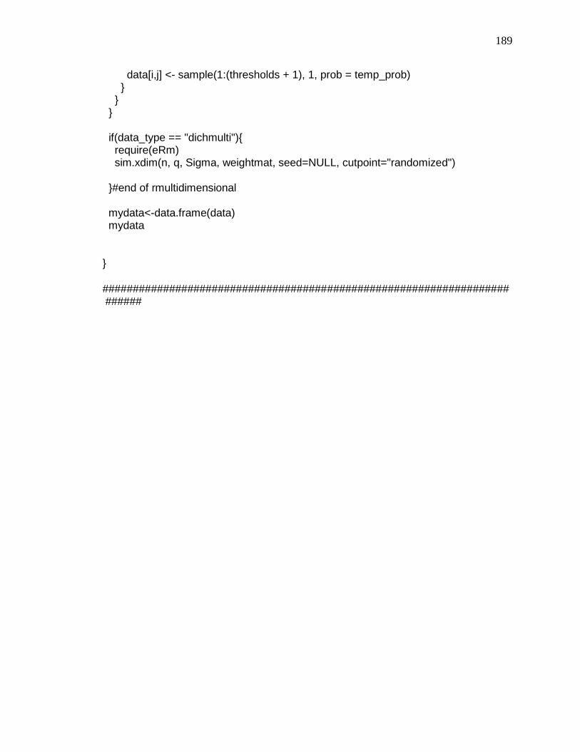
189

data[i,j] <- sample(1:(thresholds + 1), 1, prob = temp_prob) } } } if(data_type == "dichmulti"){ require(eRm) sim.xdim(n, q, Sigma, weightmat, seed=NULL, cutpoint="randomized") }#end of rmultidimensional mydata<-data.frame(data) mydata } #########################################################################

190

A.2 SIMULATION CODE FOR CALCULATING Q-INDEX ######################################################################### items<- 10 samplesizec<-1 # 1 - n=100 testlengthc<-1 # 1 - n=10 #pattern="data" files2<- list.files(pattern="data") for (i in 1:length(files2)) { # Winsteps file with person information, this is needed to get person ability wp<-data.frame(read.table(paste0("pfile_",i,"_.txt"),header=TRUE, sep=",", skip=1)) # Winsteps file with item information. this is needed to get infit, outfit, zinfit and zoutfit wi<-data.frame(read.table(paste0("ifile_",i,"_.txt"),header=TRUE, sep=",", skip=1)) # original data to be used to calculate Q wdat <- data.frame(read.table(paste0("data_",i,"_.txt"), colClasses="character", header=FALSE, sep="")) dat <- do.call(rbind.data.frame, strsplit(wdat$V1, "")); colnames(dat) <- paste0("item", seq(1,ncol(dat))) wsf <- wi[,c("ENTRY", "IN.MSQ", "IN.ZSTD", "OUT.MSQ", "OUT.ZSTD")] #get betas from wp file betas <- as.vector(wp[,"MEASURE"]) #merge data with person ability mergedat<-cbind(dat,betas) #orders data set by ability dat2=dat[order(betas, na.last = NA),] indx <- sapply(dat2, is.factor) dat2[indx] <- lapply(dat2[indx], function(x) as.numeric(as.character(x))) #orders betas from smallest to largest betas=betas[order(betas, na.last = NA)]

191

#Guttman pattern G=data.frame(apply(dat2,2,function(x) x[order(x, na.last = NA)])) AG=data.frame(apply(dat2,2,function(x) x[order(x, na.last = NA, decreasing = TRUE)])) Q=apply((dat2-G)*betas,2,sum)/apply((AG-G)*betas,2,sum) #merge Q with Winsteps fit stats: infit, outfit, zinfit, zOutfit fdata<-data.frame(cbind(Q,wsf)) attach(fdata) misfitIN.MSQ<-ifelse(IN.MSQ<= .6 & IN.MSQ>=1.4,1,0) propmisfit1 <- as.numeric(misfitIN.MSQ==1) misfitIN.ZSTD<-ifelse(IN.ZSTD>= 2 & IN.ZSTD<=-2,1,0) propmisfit2 <- as.numeric((misfitIN.ZSTD==1)) mOUT.MSQ<-ifelse(OUT.MSQ<= .6 & OUT.MSQ>=1.4,1,0) propmisfit3 <- as.numeric(mOUT.MSQ==1) mOUT.ZSTD<-ifelse(OUT.ZSTD<= .6 & OUT.ZSTD>=1.4,1,0) propmisfit4 <- as.numeric(mOUT.ZSTD==1) mQ<-ifelse(Q>= .5,1,0) propmisfit5 <- as.numeric(mQ==1) result <- matrix(0,nrow=length(items),ncol=13) result<-cbind(fdata, propmisfit1, propmisfit2, propmisfit3, propmisfit4, propmisfit5, samplesizec, testlengthc, i) colnames(result)<- c("Q", "ENTRY", "IN.MSQ", "IN.STD", "OUT.MSQ", "OUT.ZSTD", "IN.MSQ Misfit", "IN.ZSTD MISFIT", "OUT.MSQ MISFIT", "OUT.ZTSD MISFIT", "Q MISFIT", "Sample Size", "Test Length", "Iteration") write.table(result, sep = ",", file="result2.csv", append=TRUE, col.names =FALSE, row.names = FALSE) } #########################################################################

193

A.3 RWinsteps CODE #########################################################################

library(RWinsteps)

setwd("C:/Desktop/RSM/")

#the rWinsteps package Winsteps fucntion doesn;t work so I have to run this one

"Winsteps2" after i load the library RWinsteps

Winsteps2=function (cmd, cmdfile = "cmdfile", outfile = "outfile", ifile = "ifile",

pfile = "pfile", newdir = getwd(), run = TRUE, windir = "Winsteps")

{

olddir <- getwd()

setwd(newdir)

if (run) {

if (!missing(cmd))

write.wcmd(cmd, filename = cmdfile)

systemcommand <- paste(windir, "BATCH=YES", cmdfile,

outfile, paste("PFILE=", pfile, sep = ""), paste("IFILE=",

ifile, sep = ""))

gc(FALSE)

time1 <- proc.time()

outval <- system(systemcommand)

time2 <- proc.time()

if (outval != 0)

stop("Winsteps not run - error sending command file")

else cat("\nCommand file sent to Winsteps\n\n")

}

out <- as.Winsteps(cmd = read.wcmd(cmdfile), ifile = read.ifile(ifile,header=TRUE),

pfile = read.pfile(pfile,header=TRUE), daterun = date(), comptime = time2

-

time1)

if (cmdfile == "cmdfile")

unlink("cmd")

if (pfile == "pfile")

unlink("pfile")

if (ifile == "ifile")

unlink("ifile")

if (outfile == "outfile")

unlink(outfile)

setwd(olddir)

return(out)

}

write.ifile=function(ifile,filename, title){

194

write.table(paste(c(";ITEM ",title,

date()),collapse=""),filename,row.names=FALSE,col.names=FALSE, quote=FALSE)

write.csv(ifile,"temp.csv",row.names=FALSE)

file.append(filename,"temp.csv")

}

#############################

#############################

#############################

#the working directory needs to be set for this to work properly

files <- list.files()

i=1

for(i in 1:length(files))

{

data <- read.table(paste0("dataP",i,".txt", sep=""), sep=",", header=TRUE)

Winstepsdat <- data.frame(data)

num_col<-ncol(Winstepsdat)

num_row<-nrow(Winstepsdat)

colnames(Winstepsdat) <- paste("i", 1:num_col, sep="")

Winstepsdat$name<- paste ("p", 1:num_row, sep="")

#must change ni and labels for 1:n??

cmd <- wcmd(title = "R2Winsteps Example", data=paste0("data[",i,"].txt"),item1 = 1, ni

=num_col , name1 = 16, namelen = 5,labels =

paste('i',

1:num_col, sep = ""), hlines = "Y")

write.wdat(Winstepsdat, cmd)

write.wcmd(cmd, paste0("CMFILE[",i,"].cmd") )

Winsteps2(cmd, outfile=paste0("outfile[",i,"].txt"), pfile=paste0("pfile[",i,"].txt"),

ifile=paste0("ifile[",i,"].txt"), windir="C:/Winsteps/Winsteps.exe")

} #end for

#########################################################################

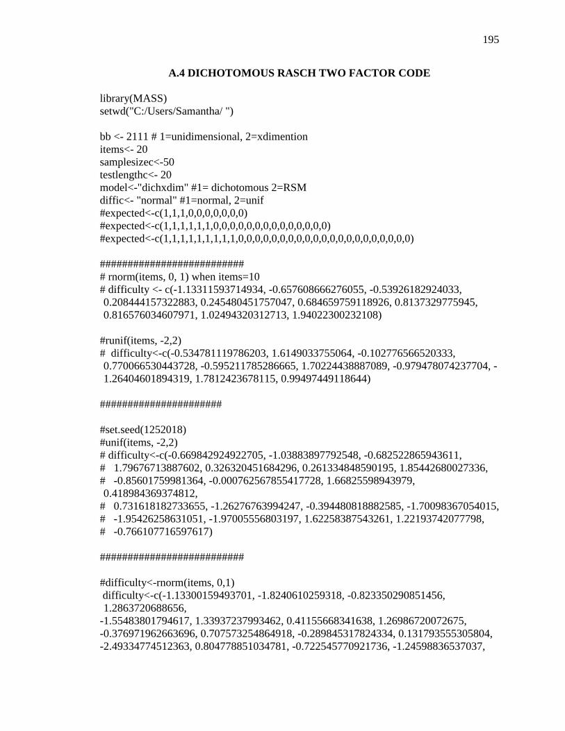
195

A.4 DICHOTOMOUS RASCH TWO FACTOR CODE

library(MASS)

setwd("C:/Users/Samantha/ ")

bb <- 2111 # 1=unidimensional, 2=xdimention

items<- 20

samplesizec<-50

testlengthc<- 20

model<-"dichxdim" #1= dichotomous 2=RSM

diffic<- "normal" #1=normal, 2=unif

#expected<-c(1,1,1,0,0,0,0,0,0,0)

#expected<-c(1,1,1,1,1,1,0,0,0,0,0,0,0,0,0,0,0,0,0,0)

#expected<-c(1,1,1,1,1,1,1,1,1,0,0,0,0,0,0,0,0,0,0,0,0,0,0,0,0,0,0,0,0,0)

##########################

# rnorm(items, 0, 1) when items=10

# difficulty <- c(-1.13311593714934, -0.657608666276055, -0.53926182924033,

0.208444157322883, 0.245480451757047, 0.684659759118926, 0.8137329775945,

0.816576034607971, 1.02494320312713, 1.94022300232108)

#runif(items, -2,2)

# difficulty<-c(-0.534781119786203, 1.6149033755064, -0.102776566520333,

0.770066530443728, -0.595211785286665, 1.70224438887089, -0.979478074237704, -

1.26404601894319, 1.7812423678115, 0.99497449118644)

######################

#set.seed(1252018)

#unif(items, -2,2)

# difficulty<-c(-0.669842924922705, -1.03883897792548, -0.682522865943611,

# 1.79676713887602, 0.326320451684296, 0.261334848590195, 1.85442680027336,

# -0.85601759981364, -0.000762567855417728, 1.66825598943979,

0.418984369374812,

# 0.731618182733655, -1.26276763994247, -0.394480818882585, -1.70098367054015,

# -1.95426258631051, -1.97005556803197, 1.62258387543261, 1.22193742077798,

# -0.766107716597617)

##########################

#difficulty<-rnorm(items, 0,1)

difficulty<-c(-1.13300159493701, -1.8240610259318, -0.823350290851456,

1.2863720688656,

-1.55483801794617, 1.33937237993462, 0.41155668341638, 1.26986720072675,

-0.376971962663696, 0.707573254864918, -0.289845317824334, 0.131793555305804,

-2.49334774512363, 0.804778851034781, -0.722545770921736, -1.24598836537037,

196

-0.199914739572402, 0.433193838716933, -0.758316689325216, 0.445077709786044

)

########################################################################

#30

#rnorm

# difficulty<-c(-0.657608666276055, 1.94022300232108, 0.816576034607971, -

1.13311593714934,

# 0.245480451757047, 0.208444157322883, -0.53926182924033, 1.02494320312713,

# 0.8137329775945, 0.684659759118926, -0.147512576717701, 1.78796572032606,

# -0.786254282076577, -0.637086095709209, -0.178950761811562, -

0.366454770330795,

# 0.00747579236173547, -0.905863155360567, -0.759943568274668,

# 0.243486779016325, -0.790274964498422, -1.1865837977366, -0.529887122046855,

# 0.460418072938017, 0.420184634457039, -0.291864820646343, 0.98651189489772,

# 0.191064232442524, 0.122874313228401, -0.0314796351296583)

# difficulty<-c(-0.97842076048255, -0.257414720021188, 1.89529479295015,

1.50441632419825,

# 1.17165851499885, -1.56361967884004, -1.48566885571927, -1.08487837202847,

# 0.387831119820476, 1.12009734660387, 0.330235633067787, -0.92962718103081,

# -0.82058759778738, -0.493985760957003, 1.38922001235187, 1.36962558608502,

# 1.16840412467718, 0.962263827212155, 1.01288269460201, 1.32349698618054,

# -0.23454509768635, 0.514117700047791, 1.85243690386415, 1.05278060771525,

# -1.13656293042004, -1.38761967886239, -0.95186245534569, -0.122846701182425,

# -0.284047249704599, -1.52429531887174)

#############

dim(weightmat)

length(expected)

dichrasch.sim (reps=100,samplesize = samplesizec, items = testlengthc, data_type =

"dichxdim", thresholds = NULL, Sigma, weightmat)

sim.xxdim<-function (persons, items, Sigma, weightmat, seed = NULL, cutpoint =

"randomized")

{

if (missing(Sigma)) {

ndim <- ncol(persons)

}

else {

ndim <- nrow(Sigma)

}

if (length(persons) == 1) {

if (!is.null(seed))

set.seed(seed)

197

faehig <- mvrnorm(persons, mu = rep(0, nrow(Sigma)),

Sigma = Sigma)

}

else {

faehig <- persons

}

if (length(items) == 1) {

if (!is.null(seed))

set.seed(seed)

#################################################

#################################################

#################################################

schwierig <- difficulty#rnorm(items,0,1)#runif(items, -2,2)#

}

else {

schwierig <- items

}

n.persons <- nrow(faehig)

n.items <- length(schwierig)

if (missing(weightmat)) {

weightmat <- matrix(0, ncol = ndim, nrow = n.items)

if (!is.null(seed))

set.seed(seed)

indvec <- sample(1:ndim, n.items, replace = TRUE)

for (i in 1:n.items) weightmat[i, indvec[i]] <- 1

}

Wp <- apply(weightmat, 1, function(wi) {

Xw <- t(wi) %*% t(faehig)

})

psolve <- matrix(0, n.persons, n.items)

for (j in 1:n.items) for (i in 1:n.persons) psolve[i, j] <- exp(Wp[i,

j] - schwierig[j])/(1 + exp(Wp[i, j] -

schwierig[j]))

if (cutpoint == "randomized") {

if (!is.null(seed))

set.seed(seed)

R <- (matrix(runif(n.items * n.persons), n.persons, n.items) <

psolve) * 1

}

else {

R <- (cutpoint < psolve) * 1

}

return(R)

}

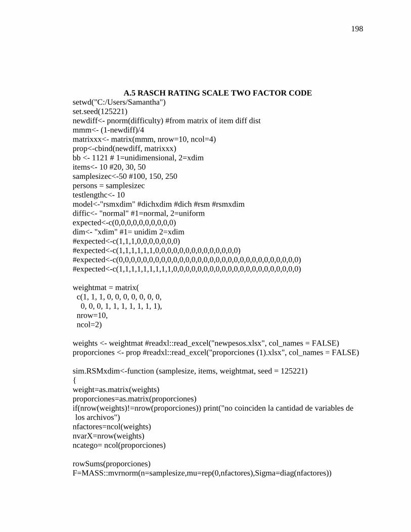
198

A.5 RASCH RATING SCALE TWO FACTOR CODE

setwd("C:/Users/Samantha")

set.seed(125221)

newdiff<- pnorm(difficulty) #from matrix of item diff dist

mmm<- (1-newdiff)/4

matrixxx<- matrix(mmm, nrow=10, ncol=4)

prop<-cbind(newdiff, matrixxx)

bb <- 1121 # 1=unidimensional, 2=xdim

items<- 10 #20, 30, 50

samplesizec<-50 #100, 150, 250

persons = samplesizec

testlengthc<- 10

model<-"rsmxdim" #dichxdim #dich #rsm #rsmxdim

diffic<- "normal" #1=normal, 2=uniform

expected<-c(0,0,0,0,0,0,0,0,0,0)

dim<- "xdim" #1= unidim 2=xdim

#expected<-c(1,1,1,0,0,0,0,0,0,0)

#expected<-c(1,1,1,1,1,1,0,0,0,0,0,0,0,0,0,0,0,0,0,0)

#expected<-c(0,0,0,0,0,0,0,0,0,0,0,0,0,0,0,0,0,0,0,0,0,0,0,0,0,0,0,0,0,0)

#expected<-c(1,1,1,1,1,1,1,1,1,0,0,0,0,0,0,0,0,0,0,0,0,0,0,0,0,0,0,0,0,0)

weightmat = matrix(

c(1, 1, 1, 0, 0, 0, 0, 0, 0, 0,

0, 0, 0, 1, 1, 1, 1, 1, 1, 1),

nrow=10,

ncol=2)

weights <- weightmat #readxl::read_excel("newpesos.xlsx", col_names = FALSE)

proporciones <- prop #readxl::read_excel("proporciones (1).xlsx", col_names = FALSE)

sim.RSMxdim<-function (samplesize, items, weightmat, seed = 125221)

{

weight=as.matrix(weights)

proporciones=as.matrix(proporciones)

if(nrow(weights)!=nrow(proporciones)) print("no coinciden la cantidad de variables de

los archivos")

nfactores=ncol(weights)

nvarX=nrow(weights)

ncatego= ncol(proporciones)

rowSums(proporciones)

F=MASS::mvrnorm(n=samplesize,mu=rep(0,nfactores),Sigma=diag(nfactores))

199

X=F%*%t(weights)

X=scale(X)

apply(X,2,mean)

round(var(X),2)

#GGally::ggpairs(as.data.frame(X))

categorica=matrix(1,nrow=samplesize,ncol=nvarX)

acumulado=t(apply(proporciones,1,cumsum))

thresh=t(apply(acumulado[,-nvarX],1,qnorm))

#View(thresh)

for (i in 1:(ncatego-1))

{

categorica=categorica + (X>rep(1,samplesize)%*%t(thresh[,i]))

}

categoricac=as.data.frame(apply(categorica,2,as.factor))

categoricac

} #end function

200

APPENDIX B

DESCRIPTIVE INFORMATION FOR SIMULATION STUDY

201

B.1 PILOT STUDY DESCRIPTIVE INFORMATION

FOR ITEM FIT STATISTICS

Table B1-1

Global Fit for Unidimensional Condition

Dataset 38 Dataset 11 Dataset 15 Dataset 5 Dataset 100

CFI 1.000 1.000 0.864 0.964 0.918

TLI 1.000 1.153 0.825 0.954 0.895

RMSEA 0.000 0.000 0.065 0.025 0.036

SRMR 0.078 0.061 0.076 0.047 0.048

Table B1-2

Global Fit for Rasch Dichotomous Multidimensional Model


CFI 0.973 0.883 0.788 0.703 0.962

TLI 0.965 0.845 0.720 0.607 0.950

RMSEA 0.055 0.051 0.048 0.069 0.021

SRMR 0.050 0.070 0.073 0.083 0.046

Table B1-3

Global Fit for Rasch Rating Scale Model Condition


CFI 1.000 0.964 1.000 0.952 1.000

TLI 1.151 0.953 1.001 0.938 1.151

RMSEA 0.000 0.063 0.000 0.074 0.000

SRMR 0.054 0.052 0.042 0.053 0.054

Table B1-4

Global Fit for Rasch Rating Scale Two Factor Condition


CFI 0.990 0.980 0.985 0.990 0.962

TLI 0.990 0.980 0.984 0.990 0.960

RMSEA 0.013 0.019 0.017 0.014 0.024

SRMR 0.037 0.038 0.037 0.036 0.042

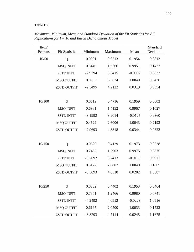
202

Table B2

Maximum, Minimum, Mean and Standard Deviation of the Fit Statistics for All

Replications for I = 10 and Rasch Dichotomous Model

Item/

Persons Fit Statistic Minimum Maximum Mean

Standard

Deviation

10/50 Q 0.0001 0.6213 0.1954 0.0813

MSQ INFIT 0.5449 1.6266 0.9951 0.1422

ZSTD INFIT -2.9794 3.3415 -0.0092 0.8832

MSQ OUTFIT 0.0905 6.5624 1.0049 0.3436

ZSTD OUTFIT -2.5495 4.2122 0.0319 0.9354

10/100 Q 0.0512 0.4716 0.1959 0.0602

MSQ INFIT 0.6981 1.4152 0.9967 0.1027

ZSTD INFIT -3.1992 3.9014 -0.0125 0.9360

MSQ OUTFIT 0.4629 2.6006 1.0043 0.2193

ZSTD OUTFIT -2.9693 4.3318 0.0344 0.9822

10/150 Q 0.0620 0.4129 0.1973 0.0538

MSQ INFIT 0.7482 1.2903 0.9975 0.0875

ZSTD INFIT -3.7692 3.7413 -0.0155 0.9971

MSQ OUTFIT 0.5172 2.0802 1.0049 0.1865

ZSTD OUTFIT -3.3693 4.8518 0.0282 1.0687

10/250 Q 0.0882 0.4402 0.1953 0.0464

MSQ INFIT 0.7851 1.2466 0.9980 0.0741

ZSTD INFIT -4.2492 4.0912 -0.0223 1.0916

MSQ OUTFIT 0.6197 2.0500 1.0033 0.1523

ZSTD OUTFIT -3.8293 4.7114 0.0245 1.1675

203

Table B3


Replications for I = 10 and Rasch Rating Scale Model

Items/Persons Item Fit

Statistic Minimum Maximum Mean

Standard

Deviation

10/50 Q 0.0453 0.3544 0.1441 0.0428

MSQ INFIT 0.4847 1.6487 0.9880 0.1784

ZSTD INFIT -3.3195 2.8816 -0.0513 0.9208

MSQ OUTFIT 0.4975 2.2662 0.9918 0.1908

ZSTD OUTFIT -3.2195 3.6422 -0.0346 0.9262

10/100 Q 0.0637 0.2703 0.1452 0.0300

MSQ INFIT 0.6364 1.6429 0.9893 0.1306

ZSTD INFIT -3.0394 4.0516 -0.0734 0.9545

MSQ OUTFIT 0.6298 1.6596 0.9919 0.1342

ZSTD OUTFIT -2.9494 4.0116 -0.0541 0.9393

10/150 Q 0.0776 0.2531 0.1465 0.0244

MSQ INFIT 0.6594 1.3762 0.9904 0.1040

ZSTD INFIT -3.4993 2.9614 -0.0805 0.9334

MSQ OUTFIT 0.6600 1.3636 0.9917 0.1063

ZSTD OUTFIT -3.5093 2.7714 -0.0685 0.9270

10/250 Q 0.0909 0.2159 0.1459 0.0185

MSQ INFIT 0.7184 1.2648 0.9904 0.0813

ZSTD INFIT -3.5693 2.8513 -0.1069 0.9387

MSQ OUTFIT 0.7212 1.2808 0.9912 0.0830

ZSTD OUTFIT -3.5293 2.9813 -0.0956 0.9275

204

Table B4


Replications for I = 20 and Rasch Dichotomous Model

Items/Persons Item Fit

Statistic


Deviation

10/50 Q 0.0001 0.8761 0.2315 0.0912

MSQ INFIT 0.5331 1.5934 0.9970 0.1307

ZSTD INFIT -3.5893 3.4014 0.0001 0.8562

MSQ OUTFIT 0.1468 6.2319 0.9988 0.3041

ZSTD OUTFIT -2.9894 5.6226 0.0162 0.8932

10/100 Q 0.0619 0.5490 0.2337 0.0712

MSQ INFIT 0.7275 1.3736 0.9989 0.0970

ZSTD INFIT -4.0693 3.9013 -0.0118 0.9157

MSQ OUTFIT 0.3261 6.3576 0.9982 0.2155

ZSTD OUTFIT -3.8993 5.7629 -0.0085 0.9651

10/150 Q 0.0702 0.5180 0.2331 0.0626

MSQ INFIT 0.7569 1.3676 0.999115 0.0825

ZSTD INFIT -3.8692 3.9213 -0.02181 0.9603

MSQ OUTFIT 0.4031 3.8914 1.001475 0.1804

ZSTD OUTFIT -3.2692 5.3217 -0.01214 1.0224

10/250 Q 0.1085 0.4903 0.2335 0.0559

MSQ INFIT 0.8063 1.2981 0.9990 0.0714

ZSTD INFIT -3.7092 4.5012 -0.0383 1.0834

MSQ OUTFIT 0.5279 2.1292 1.0029 0.1476

ZSTD OUTFIT -3.3592 4.8613 -0.0185 1.1400

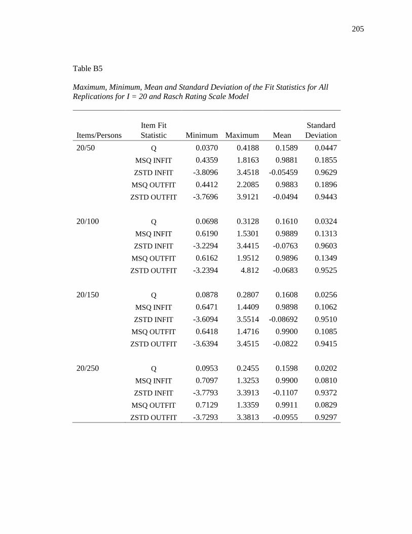
205

Table B5



Items/Persons

Item Fit


Standard

Deviation

20/50 Q 0.0370 0.4188 0.1589 0.0447

MSQ INFIT 0.4359 1.8163 0.9881 0.1855

ZSTD INFIT -3.8096 3.4518 -0.05459 0.9629

MSQ OUTFIT 0.4412 2.2085 0.9883 0.1896

ZSTD OUTFIT -3.7696 3.9121 -0.0494 0.9443

20/100 Q 0.0698 0.3128 0.1610 0.0324

MSQ INFIT 0.6190 1.5301 0.9889 0.1313

ZSTD INFIT -3.2294 3.4415 -0.0763 0.9603

MSQ OUTFIT 0.6162 1.9512 0.9896 0.1349

ZSTD OUTFIT -3.2394 4.812 -0.0683 0.9525

20/150 Q 0.0878 0.2807 0.1608 0.0256

MSQ INFIT 0.6471 1.4409 0.9898 0.1062

ZSTD INFIT -3.6094 3.5514 -0.08692 0.9510

MSQ OUTFIT 0.6418 1.4716 0.9900 0.1085

ZSTD OUTFIT -3.6394 3.4515 -0.0822 0.9415

20/250 Q 0.0953 0.2455 0.1598 0.0202

MSQ INFIT 0.7097 1.3253 0.9900 0.0810

ZSTD INFIT -3.7793 3.3913 -0.1107 0.9372

MSQ OUTFIT 0.7129 1.3359 0.9911 0.0829

ZSTD OUTFIT -3.7293 3.3813 -0.0955 0.9297

206

Table B6

Maximum, Minimum, Mean and Standard Deviation of the Fit Statistics or All

Replications for I = 30 and Rasch Dichotomous

Items/Persons

Minimum Maximum Mean

Standard

Deviation

30/50 Q 0.0001 1.0001 0.2444 0.0932

MSQ INFIT 0.6182 1.6374 0.9977 0.1268

ZSTD INFIT -3.5193 4.1615 -0.0100 0.9063

MSQ OUTFIT 0.2279 7.7997 1.0035 0.2766

ZSTD OUTFIT -3.2694 5.0626 0.0096 0.9382

30/100 Q 0.0554 0.6073 0.2479 0.0728

MSQ INFIT 0.7025 1.4350 0.9989 0.0918

ZSTD INFIT -4.0893 4.2413 -0.0194 0.9566

MSQ OUTFIT 0.4763 3.3678 1.0032 0.1813

ZSTD OUTFIT -3.2993 6.0334 -0.0018 1.0090

30/150 Q 0.0729 0.5688 0.2467 0.0653

MSQ INFIT 0.7523 1.3412 0.9992 0.0809

ZSTD INFIT -3.9592 5.1113 -0.0249 1.0372

MSQ OUTFIT 0.4724 2.4439 1.0016 0.1481

ZSTD OUTFIT -3.6592 5.2924 -0.0118 1.0667

30/250 Q 0.1103 0.5022 0.2470 0.0593

MSQ INFIT 0.8032 1.2719 0.9994 0.0707

ZSTD INFIT -4.5392 5.3512 -0.0344 1.1891

MSQ OUTFIT 0.5768 2.1369 1.0005 0.1256

ZSTD OUTFIT -4.4892 5.1514 -0.0316 1.2132

207

Table B7



Items/Persons Fit


Standard

Deviation

30/50 Q 0.0505 0.4398 0.1619 0.0447

INFIT 0.4752 1.7798 0.9899 0.1881

ZSTD INFIT -3.4095 3.3618 -0.0489 0.9818

OUTFIT 0.4656 2.2039 0.9910 0.1905

ZSTD OUTFIT -3.3295 4.5322 -0.0418 0.9736

30/100 Q 0.0507 0.3045 0.1620 0.0313

INFIT 0.5503 1.4986 0.9910 0.1320

ZSTD INFIT -3.9694 3.2315 -0.0631 0.9767

OUTFIT 0.5639 1.5749 0.9911 0.1336

ZSTD OUTFIT -3.8594 3.4516 -0.0611 0.9718

30/150 Q 0.0858 0.2734 0.1627 0.0248

INFIT 0.6521 1.4354 0.9910 0.1059

ZSTD INFIT -3.5493 3.3914 -0.0773 0.9577

OUTFIT 0.6547 1.6152 0.9913 0.1071

ZSTD OUTFIT -3.5793 4.2616 -0.0728 0.9529

30/250 Q 0.1045 0.2474 0.1643 0.0198

INFIT 0.7441 1.3481 0.9912 0.0837

ZSTD INFIT -3.2993 3.6213 -0.1001 0.9771

OUTFIT 0.7445 1.3321 0.9920 0.0848

ZSTD OUTFIT -3.2993 3.4713 -0.0894 0.9762

208

Table B8

Descriptive Statistics for Infit and Infit ZSTD the Unidimensional Rasch Dichotomous

Model for N = 100 Replications for I=10

Infit Minimum Maximum Mean Standard

Deviation

1 0.64 1.55 1.00 0.10

2 0.62 1.47 1.00 0.10

3 0.70 1.34 0.99 0.10

4 0.64 1.35 0.99 0.10

5 0.66 1.38 0.99 0.10

6 0.65 1.32 0.99 0.10

7 0.68 1.30 1.00 0.09

8 0.68 1.57 1.01 0.10

9 0.63 1.52 1.00 0.11

10 0.66 1.41 1.00 0.11

ZSTD Infit Minimum Maximum Mean Standard

Deviation

1 -3.13 3.12 0.05 0.85

2 -2.63 2.35 0.05 0.77

3 -3.17 2.60 -0.10 0.98

4 -3.44 2.83 -0.10 0.95

5 -2.70 2.87 -0.06 0.95

6 -2.83 2.17 -0.05 0.78

7 -2.40 2.62 0.00 0.80

8 -2.38 2.74 0.08 0.80

9 -2.55 2.32 -0.02 0.74

10 -2.50 2.17 0.02 0.73

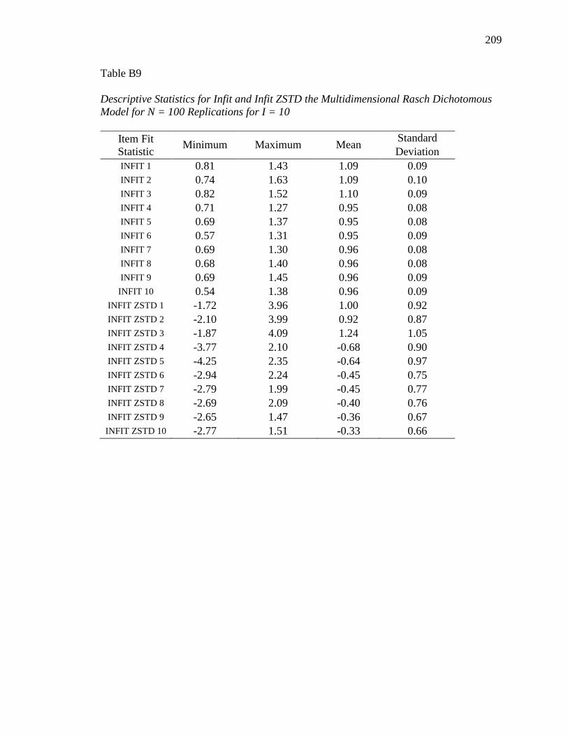
209

Table B9

Descriptive Statistics for Infit and Infit ZSTD the Multidimensional Rasch Dichotomous

Model for N = 100 Replications for I = 10

Item Fit


Standard

Deviation

INFIT 1 0.81 1.43 1.09 0.09

INFIT 2 0.74 1.63 1.09 0.10

INFIT 3 0.82 1.52 1.10 0.09

INFIT 4 0.71 1.27 0.95 0.08

INFIT 5 0.69 1.37 0.95 0.08

INFIT 6 0.57 1.31 0.95 0.09

INFIT 7 0.69 1.30 0.96 0.08

INFIT 8 0.68 1.40 0.96 0.08

INFIT 9 0.69 1.45 0.96 0.09

INFIT 10 0.54 1.38 0.96 0.09

INFIT ZSTD 1 -1.72 3.96 1.00 0.92

INFIT ZSTD 2 -2.10 3.99 0.92 0.87

INFIT ZSTD 3 -1.87 4.09 1.24 1.05

INFIT ZSTD 4 -3.77 2.10 -0.68 0.90

INFIT ZSTD 5 -4.25 2.35 -0.64 0.97

INFIT ZSTD 6 -2.94 2.24 -0.45 0.75

INFIT ZSTD 7 -2.79 1.99 -0.45 0.77

INFIT ZSTD 8 -2.69 2.09 -0.40 0.76

INFIT ZSTD 9 -2.65 1.47 -0.36 0.67

INFIT ZSTD 10 -2.77 1.51 -0.33 0.66

210

Table B10

Descriptive Statistics for the Q-Index the Unidimensional Rasch Dichotomous Model for

N = 100 Replications for I = 10


Deviation

1 0.0327 0.3595 0.1720 0.0443

2 0.0369 0.3850 0.1763 0.0471

3 0.0467 0.3496 0.1681 0.0437

4 0.0306 0.3512 0.1702 0.0446

5 0.0503 0.3886 0.1710 0.0446

6 0.0234 0.3992 0.1740 0.0492

7 0.0419 0.3366 0.1716 0.0427

8 0.0522 0.4029 0.1756 0.0449

9 0.0177 0.3917 0.1770 0.0506

10 0.0238 0.4691 0.1797 0.0537

Table B11.

Descriptive Statistics for the Q-Index the Multidimensional Rasch Dichotomous Model

for N=100 Replications for I = 10.

Q-Index Minimum Maximum Mean Standard

Deviation

1 0.0970 0.5550 0.2727 0.0587

2 0.0685 0.6213 0.2804 0.0650

3 0.0842 0.5102 0.2729 0.0579

4 0.0580 0.4166 0.1883 0.0469

5 0.0447 0.4150 0.1895 0.0495

6 0.0001 0.4112 0.1925 0.0553

7 0.0331 0.3922 0.1951 0.0480

8 0.0216 0.4719 0.1943 0.0526

9 0.0001 0.5454 0.1987 0.0587

10 0.0191 0.4530 0.2003 0.0568

211

Table B12

Descriptive Statistics for Infit the Unidimensional Rasch Dichotomous Model for N =

100 Replications for I = 20


Deviation

1 0.6800 1.4200 1.0000 0.1000

2 0.6900 1.4500 1.0000 0.0900

3 0.6800 1.4000 1.0000 0.0900

4 0.6500 1.4700 0.9900 0.1000

5 0.6700 1.4000 1.0000 0.1000

6 0.5300 1.3900 1.0000 0.1000

7 0.7000 1.4300 1.0000 0.0900

8 0.6700 1.3400 0.9900 0.0900

9 0.6900 1.4100 0.9900 0.0900

10 0.7200 1.3600 1.0000 0.0900

11 0.5400 1.3900 1.0000 0.1000

12 0.6800 1.3900 1.0000 0.0900

13 0.5400 1.5200 1.0000 0.1000

14 0.6900 1.3300 1.0000 0.1000

15 0.6300 1.3800 0.9900 0.0900

16 0.6900 1.5900 1.0000 0.0900

17 0.6100 1.3800 1.0000 0.0900

18 0.6700 1.3800 1.0000 0.0900

19 0.6800 1.3700 1.0000 0.0900

20 0.6900 1.4500 1.0000 0.0900

212

Table B13.

Descriptive Statistics for ZSTD Infit the Unidimensional Rasch Dichotomous Model or N

= 100 Replications for I = 20

ZSTD Infit Minimum Maximum Mean

Standard

Deviation

1 -2.4900 2.6500 0.0400 0.7700

2 -2.7700 2.8000 -0.0100 0.7200

3 -2.5000 2.8400 0.0000 0.7600

4 -2.4800 2.8700 -0.0300 0.7500

5 -2.8700 3.3900 0.0100 0.8100

6 -3.0000 2.7200 0.0300 0.7600

7 -2.5300 2.7700 0.0000 0.8100

8 -2.3900 2.3400 -0.0200 0.7100

9 -2.5800 2.9300 -0.0600 0.8800

10 -2.4800 3.1700 0.0400 0.7200

11 -2.9200 2.5800 0.0200 0.8400

12 -2.8900 2.9000 -0.0500 0.8900

13 -2.4100 2.4700 0.0000 0.7600

14 -2.8200 3.1000 0.0100 0.8000

15 -3.4200 2.3300 -0.0400 0.7800

16 -2.6700 2.3000 0.0100 0.7600

17 -3.1800 3.9100 -0.0100 0.9200

18 -2.2600 2.7000 0.0100 0.7900

19 -2.4700 2.2100 0.0400 0.7000

20 -3.1800 2.8600 -0.0500 0.8900

213

Table B14.

Descriptive Statistics for Outfit the Unidimensional Rasch Dichotomous Model for N =


Outfit Minimum Maximum Mean

Standard

Deviation

1 0.3500 2.5500 1.0100 0.2200

2 0.3800 3.0200 1.0000 0.2500

3 0.4500 2.8400 1.0000 0.2400

4 0.2400 6.2300 0.9900 0.2800

5 0.3800 2.5000 1.0000 0.2200

6 0.4500 3.2300 1.0000 0.2400

7 0.4000 3.7600 1.0100 0.2400

8 0.3700 2.8900 0.9900 0.2600

9 0.5500 2.3500 0.9900 0.1700

10 0.3700 3.9000 1.0200 0.3000

11 0.3400 3.2500 1.0000 0.2300

12 0.5600 2.4100 1.0000 0.1800

13 0.1500 6.3600 1.0000 0.3500

14 0.4300 2.3900 1.0100 0.2100

15 0.3900 2.0700 0.9900 0.2000

16 0.3700 2.5700 1.0000 0.2200

17 0.2900 3.2900 1.0000 0.2200

18 0.2300 4.5000 1.0000 0.2500

19 0.3200 2.7200 1.0100 0.2500

20 0.5400 2.6500 0.9900 0.1700

214

Table B15.

Descriptive Statistics for ZSTD Outfit the Unidimensional Rasch Dichotomous Model for


ZSTD Outfit Minimum Maximum Mean

Standard

Deviation

1 -2.1600 4.1700 0.0700 0.8500

2 -2.1500 3.8900 0.0300 0.8400

3 -2.0900 3.5300 0.0300 0.8300

4 -2.2300 4.8200 0.0100 0.8100

5 -2.5000 3.3100 0.0200 0.8500

6 -2.8000 3.7500 0.0300 0.8000

7 -2.1000 4.3500 0.0400 0.8500

8 -2.0700 5.7600 0.0000 0.8700

9 -2.2100 4.2800 -0.0700 0.8500

10 -2.4100 4.7400 0.0700 0.8300

11 -2.7000 5.3000 0.0200 0.8900

12 -2.4400 4.0900 -0.0200 0.8900

13 -2.0000 4.2700 0.0100 0.8700

14 -2.2800 3.4800 0.0500 0.8500

15 -2.3700 3.1800 -0.0100 0.8200

16 -2.2200 3.6700 0.0200 0.8300

17 -2.5800 4.1500 0.0300 0.9500

18 -2.2800 3.9500 0.0300 0.8500

19 -2.0100 3.3100 0.0700 0.8300

20 -2.7100 3.9200 -0.0500 0.8700

215

Table B16.

Descriptive Statistics for the Infit the Multidimensional Rasch Dichotomous Model for N


Infit Minimum Maximum Mean

Standard

Deviation

1 0.8400 1.4500 1.1000 0.0800

2 0.8200 1.3600 1.0900 0.0800

3 0.8200 1.3900 1.1100 0.0800

4 0.8200 1.4000 1.1000 0.0800

5 0.8200 1.4700 1.1000 0.0800

6 0.8200 1.4100 1.1100 0.0800

7 0.8200 1.3500 0.9600 0.0700

8 0.8200 1.2500 0.9500 0.0700

9 0.8200 1.3000 0.9500 0.0700

10 0.8200 1.1600 0.9600 0.0700

11 0.8200 1.2400 0.9500 0.0700

12 0.8200 1.2400 0.9600 0.0700

13 0.8200 1.2000 0.9600 0.0700

14 0.8200 1.2400 0.9500 0.0700

15 0.8200 1.2600 0.9500 0.0700

16 0.8200 1.1600 0.9600 0.0700

17 0.8200 1.2700 0.9500 0.0700

18 0.8200 1.2800 0.9600 0.0700

19 0.8200 1.2400 0.9500 0.0700

20 0.8200 1.2200 0.9500 0.0700

216

Table B17.

Descriptive Statistics for ZSTD Infit the Multidimensional Rasch Dichotomous Model for


ZSTD Infit Minimum Maximum Mean

Standard

Deviation

1 0.8200 3.8800 1.1700 0.8300

2 0.8200 3.5500 0.8000 0.6800

3 0.8200 3.9200 1.3000 0.9000

4 0.8200 3.4100 0.8000 0.6200

5 0.8200 4.3000 1.1000 0.9100

6 0.8200 4.5000 1.2700 0.8900

7 0.8200 2.4200 -0.4100 0.7700

8 0.8200 1.5500 -0.4900 0.7100

9 0.8200 2.2200 -0.8000 0.9500

10 0.8200 1.4200 -0.4000 0.6700

11 0.8200 2.3900 -0.6500 0.9200

12 0.8200 1.7600 -0.6000 0.8600

13 0.8200 1.5600 -0.2600 0.5200

14 0.8200 1.8200 -0.6000 0.8800

15 0.8200 1.9400 -0.4500 0.6800

16 0.8200 1.1400 -0.2600 0.5200

17 0.8200 2.2000 -0.4400 0.7800

18 0.8200 1.7500 -0.4100 0.7500

19 0.8200 1.9600 -0.5200 0.7400

20 0.8200 1.7200 -0.6200 0.8300

217

Table B18.

Descriptive Statistics for Outfit the Multidimensional Rasch Dichotomous Model for N =

100 Replications for I = 20.

Outfit Minimum Maximum Mean Standard

Deviation

1 0.7600 1.9000 1.1700 0.1600

2 0.5700 3.2000 1.1900 0.2400

3 0.6400 1.7300 1.1600 0.1500

4 0.6700 2.8700 1.2000 0.2200

5 0.5800 3.2000 1.1700 0.2100

6 0.5700 2.0300 1.1800 0.1700

7 0.6000 2.4400 0.9200 0.1500

8 0.4000 1.8800 0.9200 0.1200

9 0.6800 1.7400 0.9300 0.0900

10 0.5700 1.6300 0.9200 0.1200

11 0.6200 1.4500 0.9400 0.1000

12 0.6600 1.3900 0.9300 0.1000

13 0.3000 2.2000 0.9100 0.2300

14 0.6300 1.5900 0.9400 0.1100

15 0.5500 1.6300 0.9200 0.1300

16 0.4300 2.0000 0.9200 0.1700

17 0.4800 1.5000 0.9100 0.1300

18 0.5900 1.5800 0.9300 0.1300

19 0.6300 1.5400 0.9300 0.1300

20 0.6400 1.5400 0.9300 0.1000

218

Table B19

Descriptive Statistics for Outfit ZSTD the Multidimensional Rasch Dichotomous Model

for N = 100 Replications for I = 20

ZSTD Outfit Minimum Maximum Mean Standard

Deviation

1 -1.2400 3.8200 1.1300 0.9000

2 -1.7100 4.5000 0.9100 0.8600

3 -1.6200 4.7100 1.2100 0.9700

4 -1.1300 5.1200 0.9200 0.8300

5 -1.2300 4.9400 1.1100 0.9700

6 -1.2600 5.3200 1.2600 0.9800

7 -3.0100 4.3000 -0.4800 0.8400

8 -2.5600 1.9900 -0.5100 0.7300

9 -3.2700 2.7700 -0.7500 0.8900

10 -2.6100 2.3000 -0.4400 0.7300

11 -3.9000 2.7300 -0.5900 0.8900

12 -3.0200 2.2200 -0.5900 0.8400

13 -2.1000 2.6900 -0.3400 0.7200

14 -3.0600 2.8000 -0.5400 0.8800

15 -2.5900 3.1100 -0.4600 0.7500

16 -2.3400 3.8100 -0.3300 0.7100

17 -2.9400 2.7500 -0.5000 0.8000

18 -2.7400 3.6000 -0.4400 0.8400

19 -2.8300 3.1600 -0.4800 0.8400

20 -2.5700 3.4400 -0.5900 0.8500

219

Table B20




Deviation

1 0.0292 0.4227 0.2086 0.0528

2 0.0307 0.4927 0.2084 0.0537

3 0.0437 0.4491 0.2074 0.0525

4 0.0170 0.4997 0.2046 0.0542

5 0.0367 0.4212 0.2070 0.0549

6 0.0335 0.4683 0.2115 0.0591

7 0.0320 0.5305 0.2069 0.0534

8 0.0457 0.4432 0.2049 0.0546

9 0.0561 0.4804 0.2009 0.0482

10 0.0391 0.5076 0.2128 0.0579

11 0.0060 0.4884 0.2065 0.0538

12 0.0485 0.4367 0.2031 0.0484

13 0.0001 0.5100 0.2119 0.0651

14 0.0534 0.4422 0.2073 0.0518

15 0.0423 0.4708 0.2037 0.0516

16 0.0516 0.5374 0.2075 0.0528

17 0.0293 0.4790 0.2047 0.0508

18 0.0428 0.4367 0.2055 0.0527

19 0.0373 0.4320 0.2107 0.0550

20 0.0498 0.4129 0.2019 0.0472

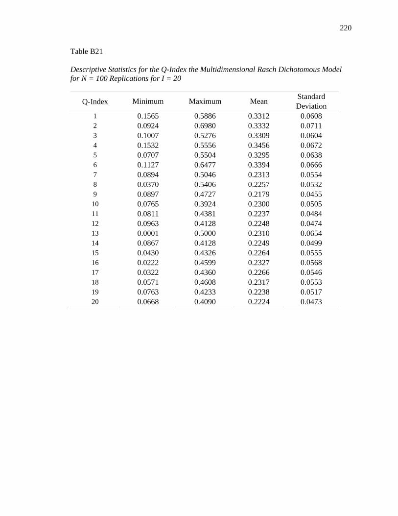
220

Table B21




Deviation

1 0.1565 0.5886 0.3312 0.0608

2 0.0924 0.6980 0.3332 0.0711

3 0.1007 0.5276 0.3309 0.0604

4 0.1532 0.5556 0.3456 0.0672

5 0.0707 0.5504 0.3295 0.0638

6 0.1127 0.6477 0.3394 0.0666

7 0.0894 0.5046 0.2313 0.0554

8 0.0370 0.5406 0.2257 0.0532

9 0.0897 0.4727 0.2179 0.0455

10 0.0765 0.3924 0.2300 0.0505

11 0.0811 0.4381 0.2237 0.0484

12 0.0963 0.4128 0.2248 0.0474

13 0.0001 0.5000 0.2310 0.0654

14 0.0867 0.4128 0.2249 0.0499

15 0.0430 0.4326 0.2264 0.0555

16 0.0222 0.4599 0.2327 0.0568

17 0.0322 0.4360 0.2266 0.0546

18 0.0571 0.4608 0.2317 0.0553

19 0.0763 0.4233 0.2238 0.0517

20 0.0668 0.4090 0.2224 0.0473

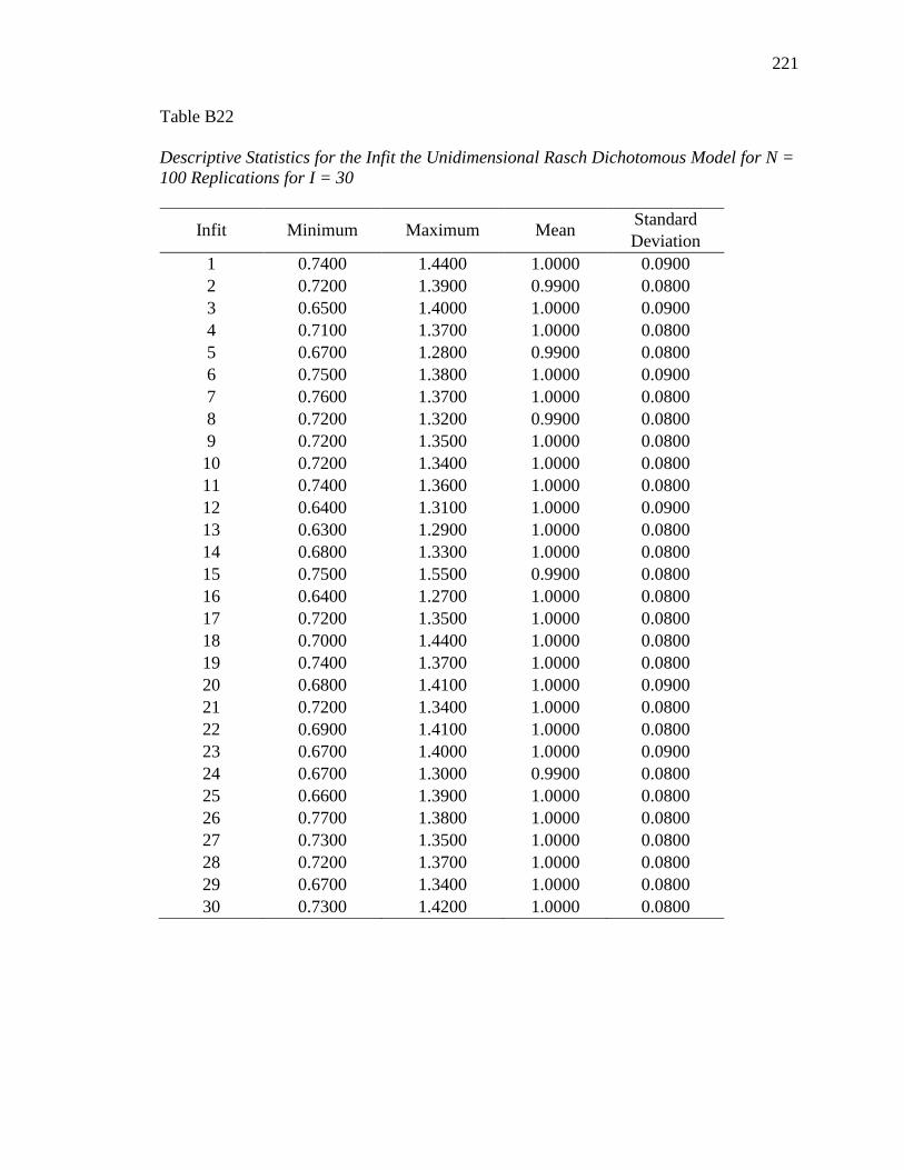
221

Table B22

Descriptive Statistics for the Infit the Unidimensional Rasch Dichotomous Model for N =



Deviation

1 0.7400 1.4400 1.0000 0.0900

2 0.7200 1.3900 0.9900 0.0800

3 0.6500 1.4000 1.0000 0.0900

4 0.7100 1.3700 1.0000 0.0800

5 0.6700 1.2800 0.9900 0.0800

6 0.7500 1.3800 1.0000 0.0900

7 0.7600 1.3700 1.0000 0.0800

8 0.7200 1.3200 0.9900 0.0800

9 0.7200 1.3500 1.0000 0.0800

10 0.7200 1.3400 1.0000 0.0800

11 0.7400 1.3600 1.0000 0.0800

12 0.6400 1.3100 1.0000 0.0900

13 0.6300 1.2900 1.0000 0.0800

14 0.6800 1.3300 1.0000 0.0800

15 0.7500 1.5500 0.9900 0.0800

16 0.6400 1.2700 1.0000 0.0800

17 0.7200 1.3500 1.0000 0.0800

18 0.7000 1.4400 1.0000 0.0800

19 0.7400 1.3700 1.0000 0.0800

20 0.6800 1.4100 1.0000 0.0900

21 0.7200 1.3400 1.0000 0.0800

22 0.6900 1.4100 1.0000 0.0800

23 0.6700 1.4000 1.0000 0.0900

24 0.6700 1.3000 0.9900 0.0800

25 0.6600 1.3900 1.0000 0.0800

26 0.7700 1.3800 1.0000 0.0800

27 0.7300 1.3500 1.0000 0.0800

28 0.7200 1.3700 1.0000 0.0800

29 0.6700 1.3400 1.0000 0.0800

30 0.7300 1.4200 1.0000 0.0800

222

Table B23

Descriptive Statistics for the Infit the Multidimensional Rasch Dichotomous Model for N



Deviation

1 0.7600 1.4700 1.1100 0.0800

2 0.8500 1.5100 1.0900 0.0800

3 0.8500 1.4300 1.1000 0.0800

4 0.7900 1.4500 1.1100 0.0800

5 0.7800 1.5000 1.1100 0.0800

6 0.7300 1.4100 1.1000 0.0700

7 0.8500 1.4000 1.1100 0.0800

8 0.8500 1.3900 1.1000 0.0700

9 0.8900 1.4200 1.1100 0.0800

10 0.7100 1.2700 0.9500 0.0700

11 0.6600 1.2100 0.9500 0.0700

12 0.6900 1.3100 0.9600 0.0700

13 0.7200 1.2400 0.9600 0.0700

14 0.7200 1.2100 0.9500 0.0600

15 0.7100 1.2200 0.9500 0.0700

16 0.6800 1.2300 0.9600 0.0700

17 0.6400 1.2300 0.9500 0.0700

18 0.7000 1.2500 0.9500 0.0700

19 0.7100 1.1700 0.9500 0.0700

20 0.7500 1.3200 0.9600 0.0700

21 0.7300 1.2600 0.9500 0.0600

22 0.7000 1.2400 0.9500 0.0700

23 0.6700 1.2400 0.9500 0.0700

24 0.6700 1.2800 0.9600 0.0700

25 0.7000 1.2700 0.9500 0.0600

26 0.7200 1.1900 0.9500 0.0600

27 0.7600 1.2800 0.9500 0.0700

28 0.7000 1.2700 0.9500 0.0700

29 0.6500 1.2600 0.9500 0.0700

30 0.7000 1.2800 0.9500 0.0700

223

Table B24

Descriptive Statistics for the ZSTD Infit the Unidimensional Rasch Dichotomous Model



Deviation

1 -2.4800 3.1600 0.0400 0.8800

2 -2.3300 3.1100 -0.0300 0.7500

3 -2.7600 2.3500 0.0100 0.7500

4 -2.1100 1.9500 -0.0200 0.6900

5 -3.1400 2.2400 -0.0600 0.8600

6 -3.0900 3.1700 -0.0100 0.8700

7 -2.4400 2.5800 0.0100 0.8200

8 -2.9800 2.3300 -0.0300 0.7600

9 -2.7400 2.5300 -0.0200 0.8700

10 -2.4900 2.2200 -0.0200 0.8100

11 -2.3500 3.0800 -0.0100 0.9700

12 -1.8500 1.9300 0.0300 0.6500

13 -3.0800 3.2100 0.0500 0.8600

14 -2.6100 2.7200 0.0100 0.9200

15 -3.0300 3.8400 -0.0400 0.8600

16 -2.9500 2.7300 0.0300 0.8400

17 -2.9200 2.9100 0.0400 0.8600

18 -2.2900 2.3800 0.0100 0.7800

19 -2.8100 2.8300 0.0500 0.8400

20 -3.2700 2.9000 0.0100 0.9300

21 -2.7300 2.6800 0.0200 0.9200

22 -3.0500 2.7900 -0.0200 0.8100

23 -2.7700 2.7600 -0.0200 0.8200

24 -2.5700 2.6700 -0.0500 0.8400

25 -3.0000 2.9200 -0.0100 0.8900

26 -2.5400 2.7400 0.0000 0.8500

27 -2.5500 2.5000 0.0500 0.7900

28 -2.7500 2.9200 0.0000 0.9900

29 -3.1800 3.4100 -0.0600 1.0000

30 -2.7700 2.9600 0.0100 0.8500

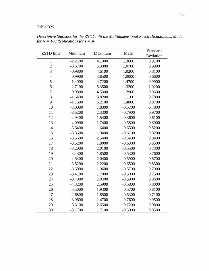
224

Table B25

Descriptive Statistics for the ZSTD Infit the Multidimensional Rasch Dichotomous Model



Deviation

1 -2.2100 4.1300 1.3600 0.9100

2 -0.6700 5.3300 1.0700 0.9900

3 -0.9800 4.6100 1.0200 0.8100

4 -0.9900 3.8500 1.0000 0.6600

5 -1.4000 4.7200 1.4700 0.9900

6 -2.7100 5.3500 1.3200 1.0200

7 -0.9800 4.5300 1.2900 0.9600

8 -1.6400 3.8200 1.1100 0.7800

9 -1.1600 5.2100 1.4800 0.9700

10 -3.0000 1.8300 -0.5700 0.7800

11 -3.5200 2.3300 -0.7900 0.9700

12 -2.9400 1.5400 -0.3600 0.6100

13 -4.0900 1.7400 -0.5800 0.8000

14 -3.5400 1.6400 -0.6500 0.8200

15 -3.3600 1.9400 -0.6100 0.8200

16 -3.5600 2.5400 -0.5400 0.8400

17 -3.5200 1.8000 -0.6300 0.8500

18 -3.2000 2.0100 -0.5500 0.7300

19 -3.4300 1.8500 -0.5300 0.7600

20 -4.5400 2.0400 -0.5900 0.8700

21 -3.5200 2.2200 -0.6500 0.8300

22 -3.6900 1.9600 -0.5700 0.7900

23 -3.4100 1.7000 -0.5000 0.7500

24 -3.4000 2.0400 -0.5900 0.8600

25 -4.3200 2.5900 -0.5800 0.8000

26 -3.5000 1.9300 -0.5700 0.8100

27 -2.6800 1.8500 -0.5300 0.7100

28 -3.9600 2.4700 -0.7600 0.9500

29 -3.3100 2.6500 -0.7200 0.9800

30 -3.1700 1.7100 -0.5900 0.8500

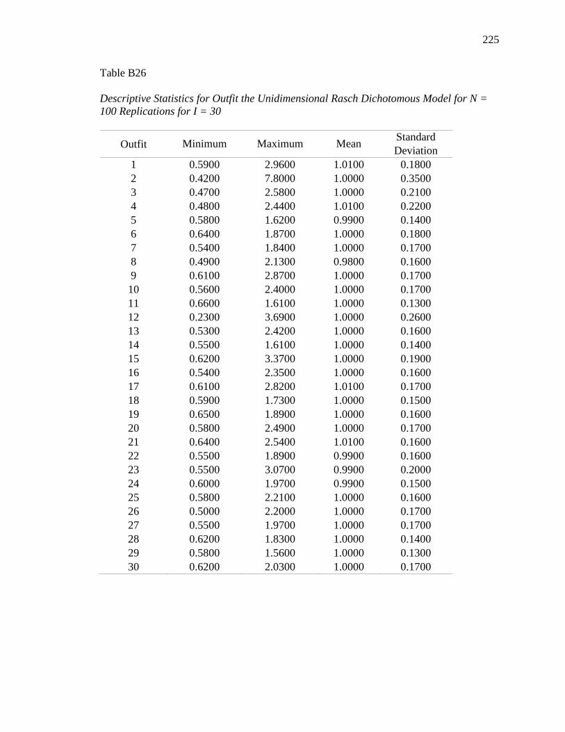
225

Table B26

Descriptive Statistics for Outfit the Unidimensional Rasch Dichotomous Model for N =



Deviation

1 0.5900 2.9600 1.0100 0.1800

2 0.4200 7.8000 1.0000 0.3500

3 0.4700 2.5800 1.0000 0.2100

4 0.4800 2.4400 1.0100 0.2200

5 0.5800 1.6200 0.9900 0.1400

6 0.6400 1.8700 1.0000 0.1800

7 0.5400 1.8400 1.0000 0.1700

8 0.4900 2.1300 0.9800 0.1600

9 0.6100 2.8700 1.0000 0.1700

10 0.5600 2.4000 1.0000 0.1700

11 0.6600 1.6100 1.0000 0.1300

12 0.2300 3.6900 1.0000 0.2600

13 0.5300 2.4200 1.0000 0.1600

14 0.5500 1.6100 1.0000 0.1400

15 0.6200 3.3700 1.0000 0.1900

16 0.5400 2.3500 1.0000 0.1600

17 0.6100 2.8200 1.0100 0.1700

18 0.5900 1.7300 1.0000 0.1500

19 0.6500 1.8900 1.0000 0.1600

20 0.5800 2.4900 1.0000 0.1700

21 0.6400 2.5400 1.0100 0.1600

22 0.5500 1.8900 0.9900 0.1600

23 0.5500 3.0700 0.9900 0.2000

24 0.6000 1.9700 0.9900 0.1500

25 0.5800 2.2100 1.0000 0.1600

26 0.5000 2.2000 1.0000 0.1700

27 0.5500 1.9700 1.0000 0.1700

28 0.6200 1.8300 1.0000 0.1400

29 0.5800 1.5600 1.0000 0.1300

30 0.6200 2.0300 1.0000 0.1700

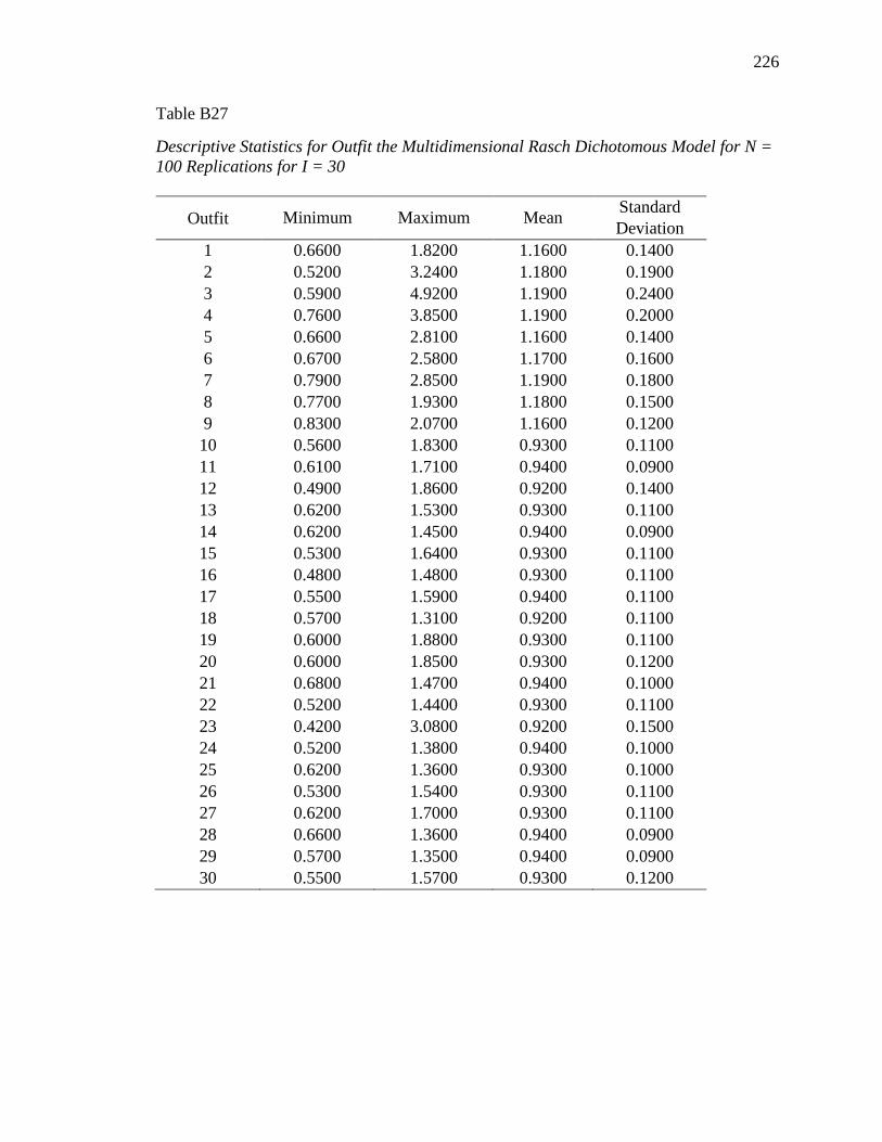
226

Table B27

Descriptive Statistics for Outfit the Multidimensional Rasch Dichotomous Model for N =



Deviation

1 0.6600 1.8200 1.1600 0.1400

2 0.5200 3.2400 1.1800 0.1900

3 0.5900 4.9200 1.1900 0.2400

4 0.7600 3.8500 1.1900 0.2000

5 0.6600 2.8100 1.1600 0.1400

6 0.6700 2.5800 1.1700 0.1600

7 0.7900 2.8500 1.1900 0.1800

8 0.7700 1.9300 1.1800 0.1500

9 0.8300 2.0700 1.1600 0.1200

10 0.5600 1.8300 0.9300 0.1100

11 0.6100 1.7100 0.9400 0.0900

12 0.4900 1.8600 0.9200 0.1400

13 0.6200 1.5300 0.9300 0.1100

14 0.6200 1.4500 0.9400 0.0900

15 0.5300 1.6400 0.9300 0.1100

16 0.4800 1.4800 0.9300 0.1100

17 0.5500 1.5900 0.9400 0.1100

18 0.5700 1.3100 0.9200 0.1100

19 0.6000 1.8800 0.9300 0.1100

20 0.6000 1.8500 0.9300 0.1200

21 0.6800 1.4700 0.9400 0.1000

22 0.5200 1.4400 0.9300 0.1100

23 0.4200 3.0800 0.9200 0.1500

24 0.5200 1.3800 0.9400 0.1000

25 0.6200 1.3600 0.9300 0.1000

26 0.5300 1.5400 0.9300 0.1100

27 0.6200 1.7000 0.9300 0.1100

28 0.6600 1.3600 0.9400 0.0900

29 0.5700 1.3500 0.9400 0.0900

30 0.5500 1.5700 0.9300 0.1200

227

Table B28

Descriptive Statistics for the ZSTD Outfit the Unidimensional Rasch Dichotomous Model



Deviation

1 -2.0200 4.7100 0.0600 0.9200

2 -2.4400 3.9400 -0.0200 0.8600

3 -2.7800 3.7100 0.0100 0.8600

4 -1.8300 4.8800 0.0400 0.8900

5 -2.5200 2.7300 -0.0700 0.8400

6 -2.4700 2.9300 0.0200 0.9400

7 -2.2500 3.1700 0.0300 0.8800

8 -2.1700 3.4700 -0.0700 0.8100

9 -2.3800 4.3600 -0.0300 0.8900

10 -2.1500 4.0600 0.0100 0.8800

11 -2.1400 3.8700 0.0100 0.9800

12 -1.8700 3.6800 0.0200 0.7800

13 -2.3800 5.2900 0.0500 0.9000

14 -2.4400 3.2600 -0.0100 0.8900

15 -2.6100 6.0300 -0.0200 0.9300

16 -2.5500 3.2400 0.0300 0.8700

17 -2.6300 4.8700 0.0500 0.9200

18 -2.0200 3.2600 0.0000 0.7900

19 -2.2900 3.7600 0.0500 0.8600

20 -2.4800 4.0500 0.0300 0.9400

21 -2.5200 3.4700 0.0400 0.9600

22 -2.4200 3.0900 -0.0200 0.8400

23 -2.0800 3.7400 -0.0100 0.8800

24 -2.2800 3.8200 -0.0500 0.8900

25 -2.4500 4.1400 0.0000 0.9200

26 -2.5400 3.6100 0.0300 0.9200

27 -2.4500 2.9700 0.0200 0.8500

28 -2.6100 3.3900 0.0000 0.9600

29 -2.5200 3.5900 -0.0200 0.9900

30 -2.4900 3.9300 0.0200 0.9100

228

Table B29

Descriptive Statistics for ZSTD Outfit the Multidimensional Rasch Dichotomous Model



Deviation

1 -2.1000 4.3600 1.2800 0.9600

2 -1.1000 5.1100 1.1900 0.9700

3 -1.2500 5.0800 1.1300 0.9000

4 -1.2100 4.1500 1.0900 0.7900

5 -1.2900 5.3700 1.3900 1.0100

6 -2.6100 5.1500 1.3400 1.0000

7 -0.9400 4.9300 1.3200 0.9400

8 -1.4400 3.7500 1.2100 0.8900

9 -1.2500 4.5300 1.4000 0.9700

10 -2.7900 2.6500 -0.5500 0.8300

11 -3.2700 4.5500 -0.7400 0.9500

12 -2.7700 2.9200 -0.4700 0.7100

13 -3.3000 2.2200 -0.5800 0.8300

14 -3.0800 2.2700 -0.6100 0.8400

15 -3.0600 2.5400 -0.6000 0.8600

16 -3.3700 2.7600 -0.5500 0.8700

17 -3.0100 2.9200 -0.5900 0.8800

18 -3.1200 2.6500 -0.5600 0.7700

19 -3.1400 2.1600 -0.5200 0.8000

20 -4.4900 3.2900 -0.5900 0.8800

21 -3.0600 2.4200 -0.5900 0.8500

22 -2.9800 2.7200 -0.5900 0.8100

23 -3.1900 2.8500 -0.5500 0.7800

24 -3.4700 2.3500 -0.5700 0.8500

25 -4.1600 2.7500 -0.5700 0.8100

26 -2.7400 3.7700 -0.5600 0.8300

27 -2.7400 2.1000 -0.5500 0.7800

28 -3.6600 2.0600 -0.7000 0.9100

29 -3.1400 2.7500 -0.6700 0.9500

30 -2.8800 3.3200 -0.5700 0.8800

229

Table B30




Deviation

1 0.0800 0.4200 0.2201 0.0489

2 0.0600 1.0001 0.2216 0.0629

3 0.0600 0.4600 0.2227 0.0518

4 0.0800 0.4500 0.2200 0.0502

5 0.0600 0.3700 0.2144 0.0448

6 0.0900 0.4100 0.2205 0.0495

7 0.0800 0.4500 0.2199 0.0501

8 0.0500 0.4100 0.2164 0.0476

9 0.0600 0.4600 0.2161 0.0460

10 0.0700 0.3600 0.2163 0.0443

11 0.0900 0.4100 0.2149 0.0434

12 0.0001 0.4800 0.2252 0.0570

13 0.0400 0.4300 0.2192 0.0487

14 0.0700 0.4000 0.2171 0.0457

15 0.0900 0.5300 0.2160 0.0483

16 0.0400 0.3800 0.2193 0.0467

17 0.0800 0.3800 0.2197 0.0446

18 0.0800 0.4100 0.2183 0.0463

19 0.0800 0.4300 0.2189 0.0464

20 0.0500 0.4200 0.2190 0.0512

21 0.0700 0.4300 0.2179 0.0477

22 0.0500 0.4400 0.2174 0.0488

23 0.0500 0.4200 0.2193 0.0506

24 0.0700 0.4000 0.2151 0.0460

25 0.0500 0.4300 0.2177 0.0464

26 0.0800 0.4100 0.2184 0.0473

27 0.0300 0.4200 0.2216 0.0485

28 0.0700 0.4600 0.2158 0.0456

29 0.0600 0.3800 0.2138 0.0444

30 0.0800 0.4100 0.2201 0.0473

230

Table B31




Deviation

1 0.0800 0.7500 0.3579 0.0659

2 0.0700 0.6400 0.3573 0.0642

3 0.1400 0.8100 0.3636 0.0692

4 0.1500 0.6500 0.3686 0.0671

5 0.1100 0.6100 0.3587 0.0622

6 0.1000 0.5900 0.3570 0.0615

7 0.1800 0.6200 0.3632 0.0641

8 0.1400 0.6300 0.3565 0.0632

9 0.1700 0.6100 0.3567 0.0591

10 0.0600 0.4600 0.2373 0.0548

11 0.0400 0.4600 0.2333 0.0506

12 0.0400 0.5900 0.2428 0.0601

13 0.0700 0.4500 0.2395 0.0539

14 0.0800 0.4400 0.2375 0.0481

15 0.0500 0.4400 0.2367 0.0526

16 0.0300 0.5500 0.2413 0.0549

17 0.0300 0.4600 0.2386 0.0520

18 0.0500 0.4700 0.2374 0.0535

19 0.0700 0.4700 0.2398 0.0545

20 0.0800 0.5000 0.2392 0.0540

21 0.1000 0.4600 0.2385 0.0490

22 0.0600 0.4800 0.2378 0.0556

23 0.0500 0.5600 0.2417 0.0601

24 0.0200 0.5100 0.2389 0.0541

25 0.0600 0.5000 0.2376 0.0491

26 0.0600 0.4400 0.2384 0.0509

27 0.0900 0.4600 0.2368 0.0522

28 0.0600 0.4400 0.2343 0.0509

29 0.0500 0.5000 0.2367 0.0542

30 0.0600 0.4500 0.2393 0.0549

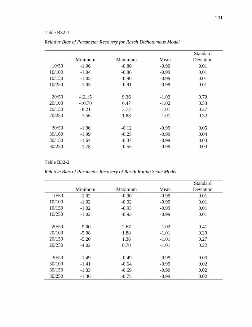
231

Table B32-1

Relative Bias of Parameter Recovery for Rasch Dichotomous Model


Standard

Deviation

10/50 -1.06 -0.86 -0.99 0.01

10/100 -1.04 -0.86 -0.99 0.01

10/150 -1.05 -0.90 -0.99 0.01

10/250 -1.03 -0.91 -0.99 0.01

20/50 -12.15 9.36 -1.02 0.70

20/100 -10.70 6.47 -1.02 0.53

20/150 -8.21 3.72 -1.01 0.37

20/250 -7.56 1.88 -1.01 0.32

30/50 -1.90 -0.12 -0.99 0.05

30/100 -1.99 -0.25 -0.99 0.04

30/150 -1.64 -0.37 -0.99 0.03

30/250 -1.78 -0.55 -0.99 0.03

Table B32-2

Relative Bias of Parameter Recovery of Rasch Rating Scale Model


Standard

Deviation

10/50 -1.02 -0.90 -0.99 0.01

10/100 -1.02 -0.92 -0.99 0.01

10/150 -1.02 -0.93 -0.99 0.01

10/250 -1.02 -0.93 -0.99 0.01

20/50 -9.00 2.67 -1.02 0.41

20/100 -5.98 1.88 -1.01 0.29

20/150 -5.20 1.36 -1.01 0.27

20/250 -4.02 0.70 -1.01 0.22

30/50 -1.49 -0.49 -0.99 0.03

30/100 -1.41 -0.64 -0.99 0.02

30/150 -1.33 -0.69 -0.99 0.02

30/250 -1.36 -0.75 -0.99 0.02

232

APPENDIX C

DESCRIPTIVE INFORMATION FOR

ITEM FIT STATISTICS

233

Table C1

Descriptive Information for All Item Fit Statistics under the Rasch Dichotomous Model

for I = 10

Item/

Persons

Item Fit


Standard

Deviation

10/50 Q-Index 0.0000 0.6464 0.1952 0.0793 Infit 0.4740 1.6549 0.9952 0.1397 ZSTD Infit -3.0000 5.0000 -0.0066 0.8775 Outfit 0.0718 6.3915 1.0040 0.3291 ZSTD Outfit -3.0600 4.9400 0.0346 0.9247

10/100 Q-Index 0.0275 0.5360 0.1959 0.0601

Infit 0.6227 1.4346 0.9970 0.1025 ZSTD Infit -4.0000 5.0000 -0.0128 0.9333 Outfit 0.3691 3.6941 1.0049 0.2247 ZSTD Outfit -3.3300 5.3500 0.0314 0.9962

10/150 Q-Index 0.0417 0.4712 0.1959 0.0525


10/250 Q-Index 0.0738 0.4031 0.1965 0.0460


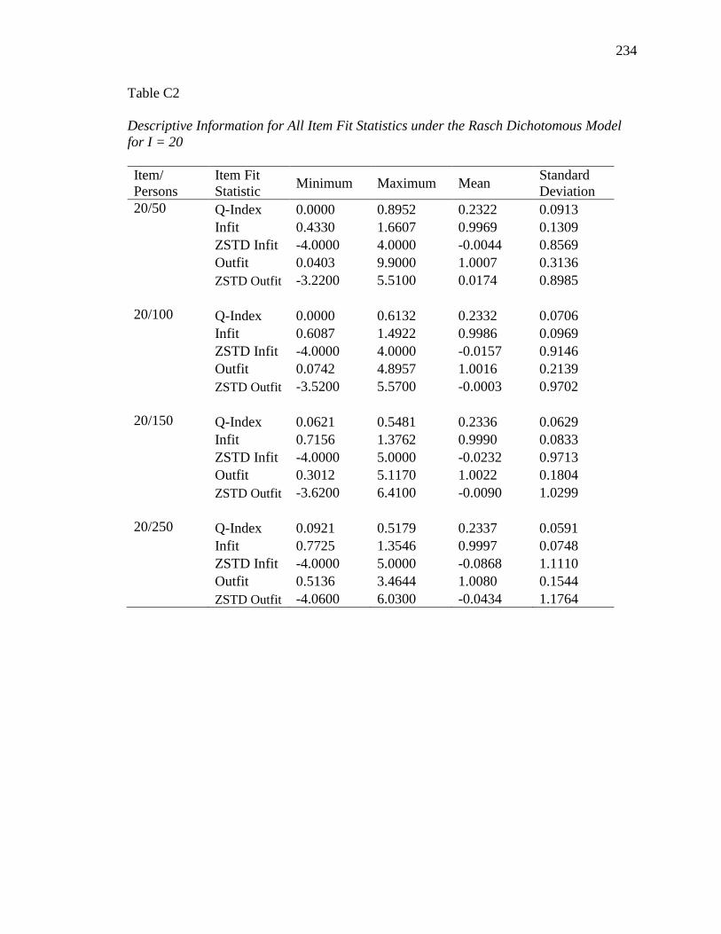
234

Table C2


for I = 20

Item/

Persons

Item Fit


Standard

Deviation


20/100 Q-Index 0.0000 0.6132 0.2332 0.0706

Infit 0.6087 1.4922 0.9986 0.0969 ZSTD Infit -4.0000 4.0000 -0.0157 0.9146 Outfit 0.0742 4.8957 1.0016 0.2139 ZSTD Outfit -3.5200 5.5700 -0.0003 0.9702

20/150 Q-Index 0.0621 0.5481 0.2336 0.0629


20/250 Q-Index 0.0921 0.5179 0.2337 0.0591


235

Table C3


for I = 30

Item/

Persons

Item Fit


Standard

Deviation


30/100 Q-Index 0.0298 0.6315 0.2467 0.0732


30/150 Q-Index 0.0779 0.6158 0.2465 0.0655


30/250 Q-Index 0.0892 0.5297 0.2466 0.0592


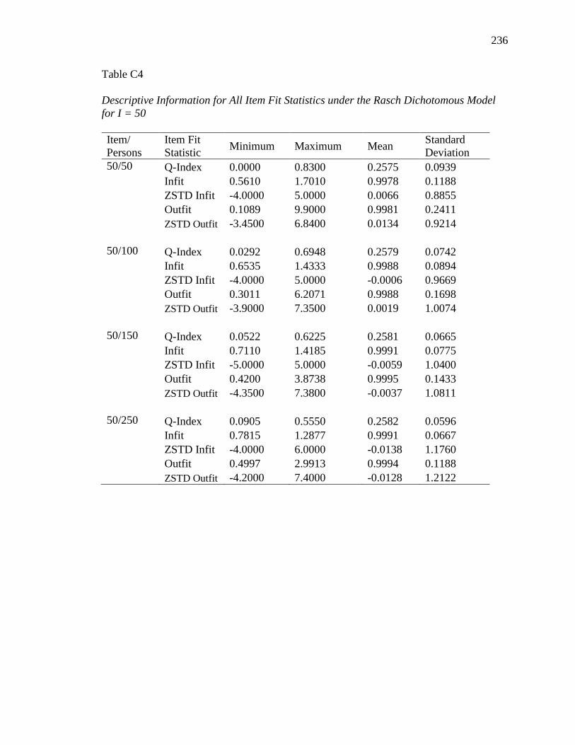
236

Table C4


for I = 50

Item/

Persons

Item Fit


Standard

Deviation

50/50 Q-Index 0.0000 0.8300 0.2575 0.0939 Infit 0.5610 1.7010 0.9978 0.1188 ZSTD Infit -4.0000 5.0000 0.0066 0.8855 Outfit 0.1089 9.9000 0.9981 0.2411 ZSTD Outfit -3.4500 6.8400 0.0134 0.9214

50/100 Q-Index 0.0292 0.6948 0.2579 0.0742


50/150 Q-Index 0.0522 0.6225 0.2581 0.0665


50/250 Q-Index 0.0905 0.5550 0.2582 0.0596


237

Table C5

Descriptive Information for All Item Fit Statistics under the Rasch Rating Scale Model

for I = 10

Item/

Persons

Item Fit


Standard

Deviation

10/50 Q-Index 0.0000 0.4546 0.1171 0.0746

Infit 0.2044 3.4426 0.9904 0.4548

ZSTD Infit -5.0000 6.0000 -0.2230 2.0870

Outfit 0.0774 4.3535 0.9988 0.6034

ZSTD Outfit -4.0000 7.0000 -0.1320 2.0200

10/100 Q-Index 0.0012 0.3513 0.1184 0.0691

Infit 0.3132 2.5617 0.9910 0.4410

ZSTD Infit -7.0000 8.0000 -0.3340 2.8540

Outfit 0.1571 3.5637 0.9992 0.5884

ZSTD Outfit -6.0000 9.0000 -0.2220 2.7750

10/150 Q-Index 0.0043 0.3233 0.1189 0.0678

Infit 0.3390 2.4835 0.9917 0.4372

ZSTD Infit -8.0000 9.0000 -0.4160 3.4620

Outfit 0.1959 3.3858 1.0008 0.5870

ZSTD Outfit -7.0000 10.0000 -0.2850 3.3780

10/250 Q-Index 0.0077 0.3152 0.1192 0.0661

Infit 0.3660 2.4185 0.9918 0.4331

ZSTD Infit -10.0000 10.0000 -0.5590 4.3830

Outfit 0.2048 3.0461 1.0001 0.5816

ZSTD Outfit -8.0000 10.0000 -0.3880 4.3020

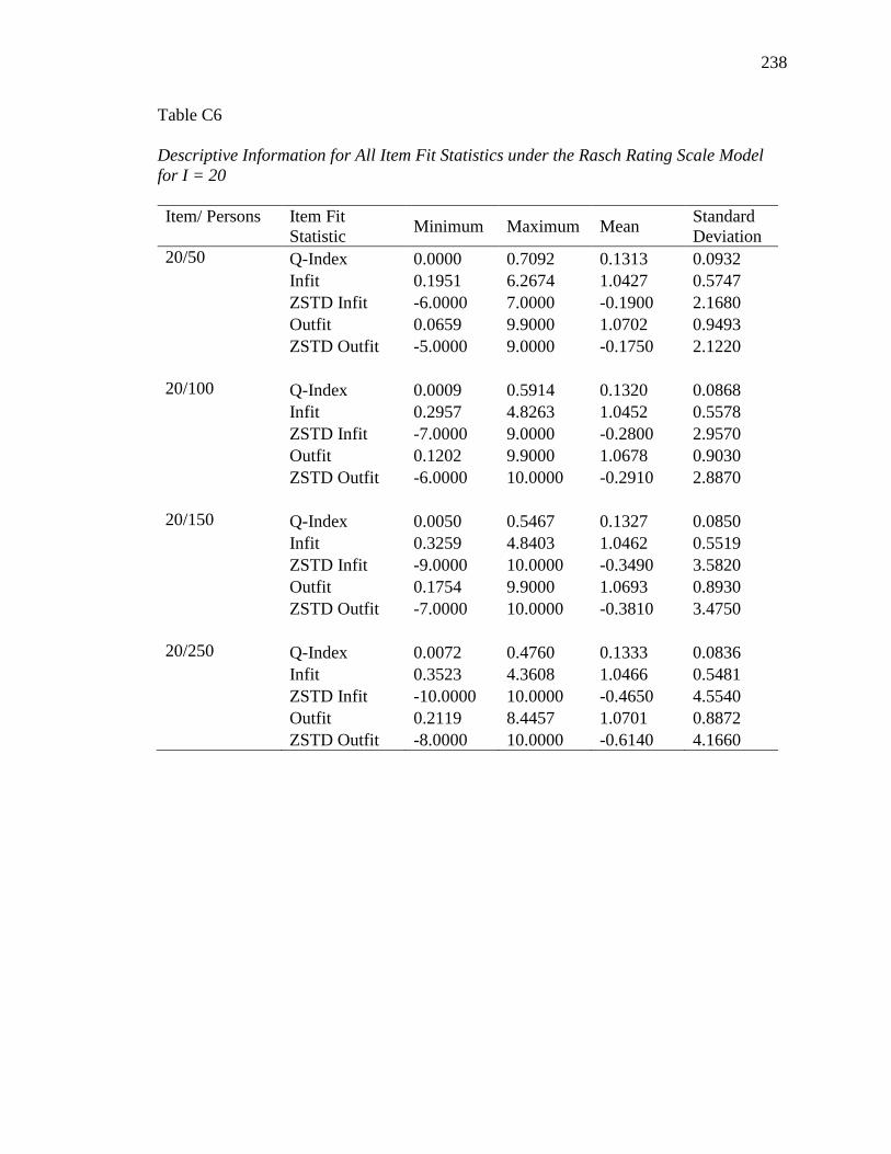
238

Table C6


for I = 20

Item/ Persons Item Fit


Standard

Deviation

20/50 Q-Index 0.0000 0.7092 0.1313 0.0932

Infit 0.1951 6.2674 1.0427 0.5747

ZSTD Infit -6.0000 7.0000 -0.1900 2.1680

Outfit 0.0659 9.9000 1.0702 0.9493

ZSTD Outfit -5.0000 9.0000 -0.1750 2.1220

20/100 Q-Index 0.0009 0.5914 0.1320 0.0868

Infit 0.2957 4.8263 1.0452 0.5578

ZSTD Infit -7.0000 9.0000 -0.2800 2.9570

Outfit 0.1202 9.9000 1.0678 0.9030

ZSTD Outfit -6.0000 10.0000 -0.2910 2.8870

20/150 Q-Index 0.0050 0.5467 0.1327 0.0850

Infit 0.3259 4.8403 1.0462 0.5519

ZSTD Infit -9.0000 10.0000 -0.3490 3.5820

Outfit 0.1754 9.9000 1.0693 0.8930

ZSTD Outfit -7.0000 10.0000 -0.3810 3.4750

20/250 Q-Index 0.0072 0.4760 0.1333 0.0836

Infit 0.3523 4.3608 1.0466 0.5481

ZSTD Infit -10.0000 10.0000 -0.4650 4.5540

Outfit 0.2119 8.4457 1.0701 0.8872

ZSTD Outfit -8.0000 10.0000 -0.6140 4.1660

239

Table C7


for I = 30

Item/

Persons

Item Fit


Standard

Deviation

30/50 Q-Index 0.0000 0.6574 0.1310 0.0945

Infit 0.2171 7.0319 1.0582 0.6619

ZSTD Infit -6.0000 7.0000 -0.2340 2.3630

Outfit 0.0466 9.9000 1.0503 0.8310

ZSTD Outfit -5.0000 9.0000 -0.2330 2.0750

30/100 Q-Index 0.0009 0.5887 0.1318 0.0884

Infit 0.2598 5.4302 1.0603 0.6482

ZSTD Infit -7.0000 9.0000 -0.3420 3.2410

Outfit 0.1553 9.2924 1.0481 0.7989

ZSTD Outfit -5.0000 10.0000 -0.3710 2.8240

30/150 Q-Index 0.0017 0.4785 0.1318 0.0861

Infit 0.3015 4.7867 1.0611 0.6427

ZSTD Infit -8.0000 10.0000 -0.4230 3.9290

Outfit 0.1742 8.6836 1.0477 0.7882

ZSTD Outfit -6.0000 10.0000 -0.4710 3.4200

30/250 Q-Index 0.0051 0.4634 0.1322 0.0849

Infit 0.3226 4.5689 1.0616 0.6389

ZSTD Infit -10.0000 10.0000 -0.6400 4.8290

Outfit 0.2081 5.7990 1.0477 0.7817

ZSTD Outfit -8.0000 10.0000 -0.6700 4.2640

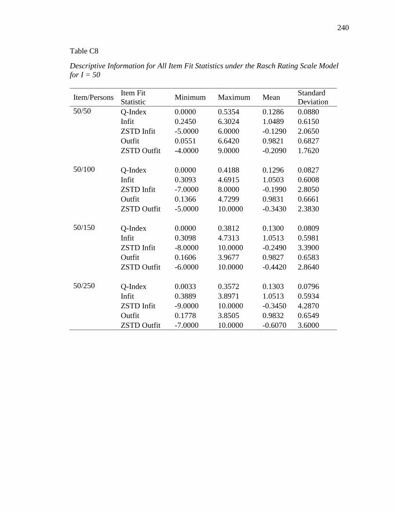
240

Table C8


for I = 50

Item/Persons Item Fit


Standard

Deviation

50/50 Q-Index 0.0000 0.5354 0.1286 0.0880

Infit 0.2450 6.3024 1.0489 0.6150

ZSTD Infit -5.0000 6.0000 -0.1290 2.0650

Outfit 0.0551 6.6420 0.9821 0.6827

ZSTD Outfit -4.0000 9.0000 -0.2090 1.7620

50/100 Q-Index 0.0000 0.4188 0.1296 0.0827

Infit 0.3093 4.6915 1.0503 0.6008

ZSTD Infit -7.0000 8.0000 -0.1990 2.8050

Outfit 0.1366 4.7299 0.9831 0.6661

ZSTD Outfit -5.0000 10.0000 -0.3430 2.3830

50/150 Q-Index 0.0000 0.3812 0.1300 0.0809

Infit 0.3098 4.7313 1.0513 0.5981

ZSTD Infit -8.0000 10.0000 -0.2490 3.3900

Outfit 0.1606 3.9677 0.9827 0.6583

ZSTD Outfit -6.0000 10.0000 -0.4420 2.8640

50/250 Q-Index 0.0033 0.3572 0.1303 0.0796

Infit 0.3889 3.8971 1.0513 0.5934

ZSTD Infit -9.0000 10.0000 -0.3450 4.2870

Outfit 0.1778 3.8505 0.9832 0.6549

ZSTD Outfit -7.0000 10.0000 -0.6070 3.6000

241

Table C9

Mean and Standard Deviation of Q-Index for the Rasch Dichotomous Model when I = 10

Unidimensional Multidimensional

Mean

Standard

Deviation Mean

Standard

Deviation

50 Normal 0.1741 0.0662 0.2180 0.0833 Uniform 0.1724 0.0682 0.2163 0.0853

100 Normal 0.1734 0.0453 0.2181 0.0636 Uniform 0.1743 0.0469 0.2176 0.0651

150 Normal 0.1742 0.0369 0.2179 0.0547 Uniform 0.1746 0.0390 0.2170 0.0574

250 Normal 0.1750 0.0286 0.2193 0.0483 Uniform 0.1747 0.0298 0.2171 0.0505

Table C10



Mean Standard

Deviation Mean

Standard

Deviation

50 Normal 0.2063 0.0750 0.2586 0.1003 Uniform 0.2057 0.0763 0.2582 0.0954

100 Normal 0.2067 0.0517 0.2581 0.0806 Uniform 0.2073 0.0532 0.2607 0.0720

150 Normal 0.2065 0.0418 0.2602 0.0732 Uniform 0.2078 0.0432 0.2599 0.0636

250 Normal 0.2073 0.0326 0.2593 0.0671 Uniform 0.2082 0.0336 0.2600 0.0675

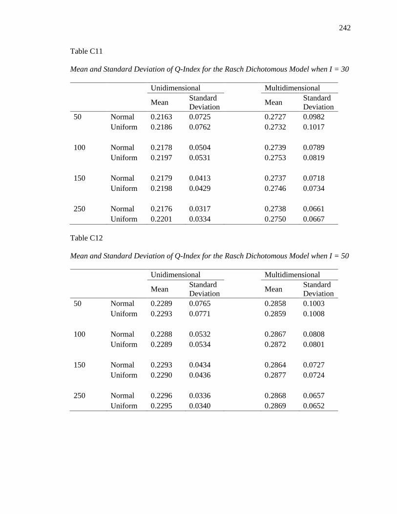
242

Table C11



Mean Standard

Deviation Mean

Standard

Deviation

50 Normal 0.2163 0.0725 0.2727 0.0982 Uniform 0.2186 0.0762 0.2732 0.1017

100 Normal 0.2178 0.0504 0.2739 0.0789 Uniform 0.2197 0.0531 0.2753 0.0819

150 Normal 0.2179 0.0413 0.2737 0.0718 Uniform 0.2198 0.0429 0.2746 0.0734

250 Normal 0.2176 0.0317 0.2738 0.0661 Uniform 0.2201 0.0334 0.2750 0.0667

Table C12



Mean Standard

Deviation Mean

Standard

Deviation

50 Normal 0.2289 0.0765 0.2858 0.1003 Uniform 0.2293 0.0771 0.2859 0.1008

100 Normal 0.2288 0.0532 0.2867 0.0808 Uniform 0.2289 0.0534 0.2872 0.0801

150 Normal 0.2293 0.0434 0.2864 0.0727 Uniform 0.2290 0.0436 0.2877 0.0724

250 Normal 0.2296 0.0336 0.2868 0.0657 Uniform 0.2295 0.0340 0.2869 0.0652

243

Table C13

Mean and Standard Deviation of Infit for the Rasch Dichotomous Model when I = 10


Mean Standard

Deviation Mean

Standard

Deviation

50 Normal 0.9971 0.1405 0.9935 0.1346 Uniform 0.9947 0.1448 0.9954 0.1386

100 Normal 0.9986 0.0983 0.9946 0.1046 Uniform 0.9972 0.0996 0.9974 0.1072

150 Normal 0.9995 0.0800 0.9953 0.0910 Uniform 0.9977 0.0833 0.9982 0.0958

250 Normal 0.9996 0.0614 0.9957 0.0812 Uniform 0.9980 0.0633 0.9982 0.0854

Table C14



Mean Standard

Deviation Mean

Standard

Deviation

50 Normal 0.9966 0.1327 0.9987 0.1314 Uniform 0.9957 0.1360 0.9964 0.1232

100 Normal 0.9987 0.0915 1.0000 0.1067 Uniform 0.9980 0.0941 0.9977 0.0945

150 Normal 0.9989 0.0748 1.0004 0.0956 Uniform 0.9986 0.0764 0.9981 0.0847

250 Normal 0.9992 0.0573 1.0006 0.0884 Uniform 0.9987 0.0589 1.0004 0.0884

244

Table C15



Mean Standard

Deviation Mean

Standard

Deviation

50 Normal 0.9979 0.1254 0.9988 0.1241 Uniform 0.9963 0.1276 0.9976 0.1226

100 Normal 0.9992 0.0872 0.9996 0.0998 Uniform 0.9979 0.0887 0.9988 0.0993

150 Normal 0.9994 0.0710 0.9997 0.0915 Uniform 0.9986 0.0721 0.9993 0.0896

250 Normal 0.9996 0.0548 0.9997 0.0845 Uniform 0.9988 0.0558 0.9992 0.0816

Table C16



Mean Standard

Deviation Mean

Standard

Deviation

50 Normal 0.9979 0.1223 0.9981 0.1148 Uniform 0.9975 0.1221 0.9975 0.1160

100 Normal 0.9990 0.0850 0.9989 0.0936 Uniform 0.9989 0.0856 0.9986 0.0930

150 Normal 0.9992 0.0693 0.9991 0.0850 Uniform 0.9991 0.0698 0.9988 0.0845

250 Normal 0.9990 0.0535 0.9990 0.0775 Uniform 0.9992 0.0539 0.9989 0.0771

245

Table C17

Mean and Standard Deviation of Outfit for the Rasch Dichotomous Model when I = 10


Mean Standard

Deviation Mean

Standard

Deviation

50 Normal 1.0003 0.3193 1.0185 0.2966 Uniform 1.0063 0.3967 0.9908 0.2925

100 Normal 1.0023 0.2117 1.0201 0.2223 Uniform 1.0075 0.2532 0.9896 0.2075

150 Normal 1.0013 0.1680 1.0184 0.1882 Uniform 1.0076 0.2079 0.9898 0.1820

250 Normal 1.0019 0.1295 1.0184 0.1639 Uniform 1.0074 0.1584 0.9917 0.1535

Table C18



Mean

Standard

Deviation Mean

Standard

Deviation

50 Normal 1.0000 0.3371 1.0134 0.2721

Uniform 1.0014 0.3739 0.9882 0.2560

100 Normal 0.9996 0.2166 1.0146 0.2095

Uniform 1.0022 0.2426 0.9899 0.1820

150 Normal 1.0007 0.1793 1.0136 0.1828

Uniform 1.0040 0.1986 0.9905 0.1578

250 Normal 1.0026 0.1381 1.0130 0.1636

Uniform 1.0031 0.1495 1.0133 0.1644

246

Table C19



Mean Standard

Deviation Mean

Standard

Deviation

50 Normal 1.0004 0.2628 1.0042 0.2066 Uniform 0.9950 0.2910 1.0034 0.2407

100 Normal 1.0005 0.1729 1.0048 0.1588 Uniform 1.0009 0.2099 1.0054 0.1835

150 Normal 1.0000 0.1398 1.0042 0.1421 Uniform 0.9998 0.1636 1.0051 0.1625

250 Normal 0.9995 0.1070 1.0045 0.1286 Uniform 0.9992 0.1254 1.0046 0.1436

Table C20



Mean Standard

Deviation Mean

Standard

Deviation

50 Normal 0.9974 0.2669 0.9976 0.2005 Uniform 0.9980 0.2794 0.9993 0.2073

100 Normal 0.9989 0.1797 0.9983 0.1529 Uniform 0.9987 0.1876 0.9995 0.1565

150 Normal 0.9999 0.1472 0.9986 0.1364 Uniform 1.0000 0.1505 0.9995 0.1387

250 Normal 0.9999 0.1140 0.9990 0.1228 Uniform 0.9997 0.1155 0.9996 0.1242

247

Table C21

Mean and Standard Deviation of ZSTD Infit for the Rasch Dichotomous Model when I =

10


Mean Standard

Deviation Mean

Standard

Deviation

50 Normal -0.0045 0.8649 -0.0280 0.9427 Uniform -0.0110 0.8138 0.0172 0.8832

100 Normal -0.0078 0.8643 -0.0530 1.0520 Uniform -0.0144 0.8004 0.0239 0.9936

150 Normal -0.0064 0.8693 -0.0606 1.1280 Uniform -0.0194 0.8204 0.0284 1.0900

250 Normal -0.0139 0.8621 -0.0852 1.3130 Uniform -0.0283 0.8145 0.0298 1.2760

Table C22


20


Mean Standard

Deviation Mean

Standard

Deviation

50 Normal 0.0014 0.8313 -0.0515 0.9247 Uniform 0.0009 0.8043 0.0316 0.8608

100 Normal -0.0002 0.8279 -0.0896 1.0460 Uniform -0.0061 0.7964 0.0330 0.9616

150 Normal -0.0031 0.8279 -0.1150 1.1420 Uniform -0.0092 0.7980 0.0348 1.0650

250 Normal -0.0115 0.8225 -0.1610 1.3430 Uniform -0.0151 0.7947 -0.1600 1.3440

248

Table C23


30


Mean Standard

Deviation Mean

Standard

Deviation

50 Normal 0.0004 0.8825 -0.0250 1.0230 Uniform 0.0037 0.7930 -0.0111 0.8723

100 Normal -0.0015 0.8857 -0.0443 1.1770 Uniform -0.0025 0.7881 -0.0300 1.0070

150 Normal -0.0029 0.8886 -0.0587 1.3230 Uniform -0.0037 0.7860 -0.0395 1.1110

250 Normal -0.0042 0.8864 -0.0847 1.5790 Uniform -0.0092 0.7885 -0.0609 1.3100

Table C24


50


Mean Standard

Deviation Mean

Standard

Deviation

50 Normal 0.0076 0.8413 0.0101 0.9493 Uniform 0.0079 0.8209 0.0007 0.9240

100 Normal 0.0035 0.8356 0.0023 1.1140 Uniform 0.0049 0.8204 -0.0130 1.0620

150 Normal -0.0010 0.8403 -0.0016 1.2430 Uniform 0.0003 0.8225 -0.0212 1.1830

250 Normal -0.0069 0.8406 -0.0216 1.4400 Uniform -0.0052 0.8236 -0.0338 1.3940

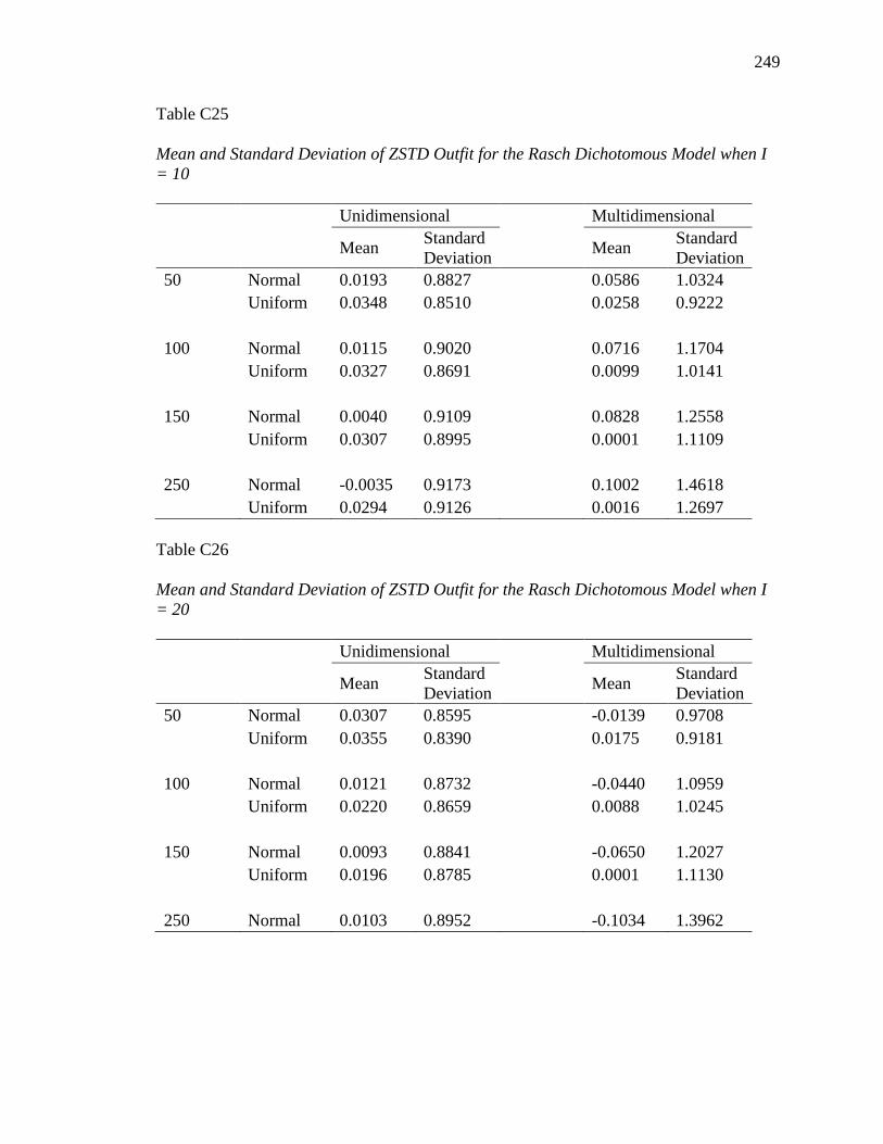
249

Table C25

Mean and Standard Deviation of ZSTD Outfit for the Rasch Dichotomous Model when I

= 10


Mean Standard

Deviation Mean

Standard

Deviation

50 Normal 0.0193 0.8827 0.0586 1.0324 Uniform 0.0348 0.8510 0.0258 0.9222

100 Normal 0.0115 0.9020 0.0716 1.1704 Uniform 0.0327 0.8691 0.0099 1.0141

150 Normal 0.0040 0.9109 0.0828 1.2558 Uniform 0.0307 0.8995 0.0001 1.1109

250 Normal -0.0035 0.9173 0.1002 1.4618 Uniform 0.0294 0.9126 0.0016 1.2697

Table C26


= 20


Mean Standard

Deviation Mean

Standard

Deviation

50 Normal 0.0307 0.8595 -0.0139 0.9708 Uniform 0.0355 0.8390 0.0175 0.9181

100 Normal 0.0121 0.8732 -0.0440 1.0959 Uniform 0.0220 0.8659 0.0088 1.0245

150 Normal 0.0093 0.8841 -0.0650 1.2027 Uniform 0.0196 0.8785 0.0001 1.1130

250 Normal 0.0103 0.8952 -0.1034 1.3962

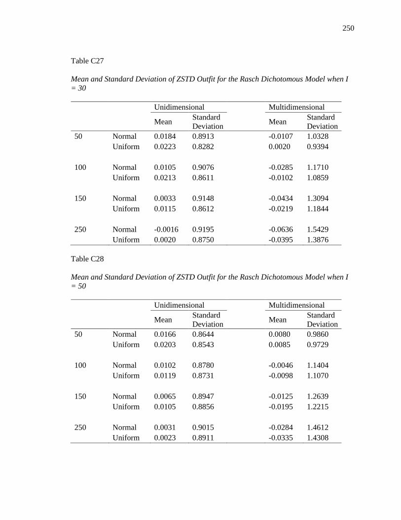
250

Table C27


= 30


Mean Standard

Deviation Mean

Standard

Deviation

50 Normal 0.0184 0.8913 -0.0107 1.0328 Uniform 0.0223 0.8282 0.0020 0.9394

100 Normal 0.0105 0.9076 -0.0285 1.1710 Uniform 0.0213 0.8611 -0.0102 1.0859

150 Normal 0.0033 0.9148 -0.0434 1.3094 Uniform 0.0115 0.8612 -0.0219 1.1844

250 Normal -0.0016 0.9195 -0.0636 1.5429 Uniform 0.0020 0.8750 -0.0395 1.3876

Table C28


= 50


Mean Standard

Deviation Mean

Standard

Deviation

50 Normal 0.0166 0.8644 0.0080 0.9860 Uniform 0.0203 0.8543 0.0085 0.9729

100 Normal 0.0102 0.8780 -0.0046 1.1404 Uniform 0.0119 0.8731 -0.0098 1.1070

150 Normal 0.0065 0.8947 -0.0125 1.2639 Uniform 0.0105 0.8856 -0.0195 1.2215

250 Normal 0.0031 0.9015 -0.0284 1.4612 Uniform 0.0023 0.8911 -0.0335 1.4308

251

Table C29

Mean and Standard Deviation of the Q-Index for the Rasch Rating Scale Model When I =

10


Mean Standard

Deviation Mean

Standard

Deviation

10/50 Normal .1444 .0418 .0885 .0883

Uniform .1436 .0416 .0920 .0901

10/100 Normal .1452 .0291 .0891 .0835

Uniform .1463 .0291 .0929 .0861

10/150 Normal .1458 .0235 .0901 .0833

Uniform .1461 .0241 .0936 .0859

10/250 Normal .1462 .0187 .0904 .0820

Uniform .1471 .0189 .0929 .0838

Table C30


20


Mean Standard

Deviation Mean

Standard

Deviation

50 Normal .1562 .0443 .1086 .1393 Uniform .1603 .0455 .1003 .0914

100 Normal .1590 .0315 .1084 .1330 Uniform .1595 .0314 .1012 .0865

150 Normal .1594 .0258 .1088 .1313 Uniform .1610 .0259 .1016 .0852

250 Normal .1602 .0202 .1092 .1304 Uniform .1611 .0204 .1025 .0843

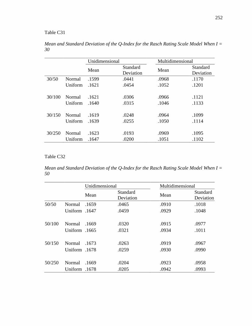
252

Table C31


30


Mean Standard

Deviation Mean

Standard

Deviation

30/50 Normal .1599 .0441 .0968 .1170 Uniform .1621 .0454 .1052 .1201

30/100 Normal .1621 .0306 .0966 .1121 Uniform .1640 .0315 .1046 .1133

30/150 Normal .1619 .0248 .0964 .1099 Uniform .1639 .0255 .1050 .1114

30/250 Normal .1623 .0193 .0969 .1095 Uniform .1647 .0200 .1051 .1102

Table C32


50


Mean Standard

Deviation Mean

Standard

Deviation

50/50 Normal .1659 .0465 .0910 .1018 Uniform .1647 .0459 .0929 .1048

50/100 Normal .1669 .0320 .0915 .0977 Uniform .1665 .0321 .0934 .1011

50/150 Normal .1673 .0263 .0919 .0967 Uniform .1678 .0259 .0930 .0990

50/250 Normal .1669 .0204 .0923 .0958 Uniform .1678 .0205 .0942 .0993

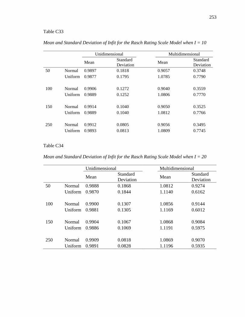
253

Table C33

Mean and Standard Deviation of Infit for the Rasch Rating Scale Model when I = 10


Mean Standard

Deviation Mean

Standard

Deviation

50 Normal 0.9897 0.1818 0.9057 0.3748 Uniform 0.9877 0.1795 1.0785 0.7790

100 Normal 0.9906 0.1272 0.9040 0.3559 Uniform 0.9889 0.1252 1.0806 0.7770

150 Normal 0.9914 0.1040 0.9050 0.3525 Uniform 0.9889 0.1040 1.0812 0.7766

250 Normal 0.9912 0.0805 0.9056 0.3495 Uniform 0.9893 0.0813 1.0809 0.7745

Table C34



Mean

Standard

Deviation Mean

Standard

Deviation

50 Normal 0.9888 0.1868 1.0812 0.9274

Uniform 0.9870 0.1844 1.1140 0.6162

100 Normal 0.9900 0.1307 1.0856 0.9144

Uniform 0.9881 0.1305 1.1169 0.6012

150 Normal 0.9904 0.1067 1.0868 0.9084

Uniform 0.9886 0.1069 1.1191 0.5975

250 Normal 0.9909 0.0818 1.0869 0.9070

Uniform 0.9891 0.0828 1.1196 0.5935

254

Table C35



Mean Standard

Deviation Mean

Standard

Deviation

50 Normal 0.9912 0.1867 1.1384 0.9819 Uniform 0.9883 0.1870 1.1150 0.8365

100 Normal 0.9919 0.1319 1.1427 0.9767 Uniform 0.9893 0.1314 1.1173 0.8201

150 Normal 0.9923 0.1075 1.1439 0.9733 Uniform 0.9897 0.1077 1.1187 0.8135

250 Normal 0.9926 0.0834 1.1446 0.9722 Uniform 0.9901 0.0828 1.1192 0.8085

Table C36



Mean Standard

Deviation Mean

Standard

Deviation

50 Normal 0.9905 0.1888 1.1422 0.8674 Uniform 0.9899 0.1881 1.0730 0.8206

100 Normal 0.9911 0.1324 1.1446 0.8575 Uniform 0.9907 0.1330 1.0748 0.8108

150 Normal 0.9913 0.1082 1.1454 0.8548 Uniform 0.9912 0.1079 1.0772 0.8125

250 Normal 0.9916 0.0837 1.1451 0.8504 Uniform 0.9916 0.0840 1.0768 0.8090

255

Table C37

Mean and Standard Deviation of Outfit for the Rasch Rating Scale Model when I = 10


Mean Standard

Deviation Mean

Standard

Deviation

50 Normal 0.9914 0.1875 1.0360 0.9105 Uniform 0.9888 0.1848 0.9787 0.7457

100 Normal 0.9919 0.1295 1.0346 0.8922 Uniform 0.9899 0.1297 0.9799 0.7439

150 Normal 0.9920 0.1064 1.0391 0.8953 Uniform 0.9918 0.1090 0.9803 0.7425

250 Normal 0.9924 0.0830 1.0372 0.8888 Uniform 0.9917 0.0846 0.9788 0.7396

Table C38



Mean Standard

Deviation Mean

Standard

Deviation

50 Normal 0.9901 0.1923 1.3721 1.7055 Uniform 0.9893 0.1908 0.9291 0.7063

100 Normal 0.9910 0.1339 1.3633 1.6194 Uniform 0.9897 0.1340 0.9272 0.6958

150 Normal 0.9915 0.1097 1.3658 1.6003 Uniform 0.9902 0.1104 0.9296 0.6964

250 Normal 0.9915 0.0836 1.3694 1.5912 Uniform 0.9905 0.0848 0.9289 0.6931

256

Table C39



Mean Standard

Deviation Mean

Standard

Deviation

50 Normal 0.9919 0.1882 1.1164 1.1667 Uniform 0.9895 0.1901 1.1034 1.1468

100 Normal 0.9926 0.1325 1.1097 1.1344 Uniform 0.9899 0.1330 1.1002 1.1037

150 Normal 0.9925 0.1080 1.1060 1.1210 Uniform 0.9907 0.1090 1.1014 1.0919

250 Normal 0.9927 0.0837 1.1066 1.1175 Uniform 0.9910 0.0839 1.1007 1.0811

Table C40



Mean Standard

Deviation Mean

Standard

Deviation

50 Normal 0.9912 0.1908 0.9719 0.9246 Uniform 0.9910 0.1906 0.9742 0.9678

100 Normal 0.9912 0.1335 0.9736 0.9111 Uniform 0.9909 0.1344 0.9767 0.9533

150 Normal 0.9917 0.1093 0.9735 0.9077 Uniform 0.9915 0.1087 0.9743 0.9410

250 Normal 0.9920 0.0845 0.9728 0.9026 Uniform 0.9918 0.0847 0.9763 0.9414

257

Table C41

Mean and Standard Deviation of ZSTD Infit for the Rasch Rating Scale Model when I =

10


Mean Standard

Deviation Mean

Standard

Deviation

50 Normal -0.0459 0.9461 -0.2600 1.6190 Uniform -0.0534 0.9266 -0.5320 3.5900

100 Normal -0.0624 0.9332 -0.4080 2.1760 Uniform -0.0726 0.9129 -0.7930 5.0780

150 Normal -0.0715 0.9335 -0.5120 2.6430 Uniform -0.0932 0.9268 -0.9860 6.2180

250 Normal -0.0973 0.9330 -0.6760 3.3890 Uniform -0.1190 0.9373 -1.3400 7.9100

Table C42


20


Mean Standard

Deviation Mean

Standard

Deviation

50 Normal -0.0526 0.9678 -0.6650 3.1570 Uniform -0.0601 0.9527 0.0163 2.5860

100 Normal -0.0687 0.9586 -0.9680 4.4220 Uniform -0.0810 0.9516 -0.0019 3.6020

150 Normal -0.0822 0.9579 -1.2000 5.3900 Uniform -0.0972 0.9558 -0.0164 4.4110

250 Normal -0.1020 0.9468 -1.6000 6.8850 Uniform -0.1220 0.9555 -0.0336 5.6590

258

Table C43


30


Mean Standard

Deviation Mean

Standard

Deviation

50 Normal -0.0424 0.9804 -0.6090 3.5550 Uniform -0.0560 0.9719 -0.2290 2.7540

100 Normal -0.0568 0.9793 -0.8830 4.9890 Uniform -0.0743 0.9661 -0.3530 3.8470

150 Normal -0.0671 0.9775 -1.0900 6.0920 Uniform -0.0894 0.9701 -0.4440 4.6970

250 Normal -0.0845 0.9797 -1.7000 7.4130 Uniform -0.1110 0.9626 -0.6680 5.8950

Table C44


50


Mean Standard

Deviation Mean

Standard

Deviation

50 Normal -0.0464 0.9866 -0.2200 3.0170 Uniform -0.0492 0.9808 -0.2000 2.4490

100 Normal -0.0624 0.9786 -0.3440 4.2230 Uniform -0.0650 0.9792 -0.3240 3.4140

150 Normal -0.0756 0.9795 -0.4340 5.1600 Uniform -0.0760 0.9745 -0.4100 4.1610

250 Normal -0.0954 0.9773 -0.6220 6.5590 Uniform -0.0959 0.9780 -0.5690 5.3230

259

Table C45

Mean and Standard Deviation of ZSTD Outfit for the Rasch Rating Scale Model when I =

10


Mean Standard

Deviation Mean

Standard

Deviation

50 Normal -0.0364 0.9395 0.2660 2.5150 Uniform -0.0432 0.9052 -0.7160 2.7900

100 Normal -0.0526 0.9223 0.3000 3.5380 Uniform -0.0620 0.9030 -1.0700 3.9450

150 Normal -0.0673 0.9303 0.3380 4.3670 Uniform -0.0668 0.9280 -1.3400 4.8200

250 Normal -0.0835 0.9336 0.3800 5.6070 Uniform -0.0896 0.9348 -1.7600 6.1810

Table C46


20


Mean Standard

Deviation Mean

Standard

Deviation

50 Normal -0.0437 0.9567 -0.2090 3.3320 Uniform -0.0468 0.9436 -0.4010 2.2400

100 Normal -0.0604 0.9518 -0.3870 4.6480 Uniform -0.0671 0.9384 -0.6480 3.1170

150 Normal -0.0731 0.9526 -0.5460 5.6000 Uniform -0.0814 0.9502 -0.8240 3.8370

250 Normal -0.0930 0.9393 -1.1600 6.4970 Uniform -0.1040 0.9456 -1.1000 4.9360

260

Table C47


30


Mean Standard

Deviation Mean

Standard

Deviation

50 Normal -0.0377 0.9735 -0.5950 2.6750 Uniform -0.0475 0.9600 -0.2510 2.8260

100 Normal -0.0515 0.9751 -0.9340 3.7190 Uniform -0.0678 0.9548 -0.4330 3.9610

150 Normal -0.0645 0.9740 -1.1800 4.5260 Uniform -0.0788 0.9611 -0.5600 4.8570

250 Normal -0.0834 0.9751 -1.6600 5.6430 Uniform -0.0998 0.9560 -0.8390 6.1120

Table C48


50


Mean Standard

Deviation Mean

Standard

Deviation

50 Normal -0.0412 0.9761 -0.5260 2.2290 Uniform -0.0413 0.9711 -0.2280 2.3220

100 Normal -0.0600 0.9705 -0.8310 3.1100 Uniform -0.0609 0.9693 -0.4190 3.2810

150 Normal -0.0710 0.9729 -1.0600 3.8040 Uniform -0.0722 0.9650 -0.5620 3.9730

250 Normal -0.0897 0.9711 -1.4300 4.8230 Uniform -0.0915 0.9690 -0.8130 5.0440

261

C.2 RELATIVE BIAS FOR DICHOTOMOUS MODEL

Table C2.1

Relative Bias after Wright and Douglas (1977) Correction by Condition for Rasch Dichotomous Model for Uniform Item Difficulty

Distribution



Deviation Minimum Maximum Mean

Standard

Deviation

10/50 -0.0100 0.0100 0.0005 0.0015 -0.0100 0.0100 0.0004 0.0014

10/100 0.0000 0.0100 0.0005 0.0013 0.0000 0.0100 0.0004 0.0012

10/150 0.0000 0.0100 0.0005 0.0012 0.0000 0.0100 0.0004 0.0012

10/250 0.0000 0.0100 0.0005 0.0012 0.0000 0.0100 0.0004 0.0011

20/50 -1.5100 1.2800 -0.0050 0.0968 -1.2800 1.1200 -0.0049 0.0858

20/100 -0.9400 0.8600 -0.0054 0.0674 -0.9400 0.9000 -0.0045 0.0629

20/150 -0.9600 0.6100 -0.0045 0.0559 -0.9200 0.5000 -0.0039 0.0519

20/250 -0.7200 0.5300 -0.0037 0.0435 0.0000 0.0000 0.0000 0.0006

30/50 -0.0100 0.0100 0.0001 0.0008 -0.0100 0.0100 0.0000 0.0007

30/100 0.0000 0.0100 0.0001 0.0006 0.0000 0.0100 0.0000 0.0006

30/150 0.0000 0.0100 0.0001 0.0005 0.0000 0.0100 0.0000 0.0005

30/250 0.0000 0.0000 0.0001 0.0004 0.0000 0.0000 0.0000 0.0004

50/50 -0.5100 0.2800 -0.0023 0.0228 -0.4600 0.2500 -0.0022 0.0215

50/100 -0.3900 0.2100 -0.0026 0.0205 -0.3600 0.1800 -0.0023 0.0186

50/150 -0.3300 0.0900 -0.0025 0.0190 -0.3200 0.1300 -0.0024 0.0180

50/250 -0.3200 0.0400 -0.0024 0.0176 -0.3300 0.1900 -0.0022 0.0189

261

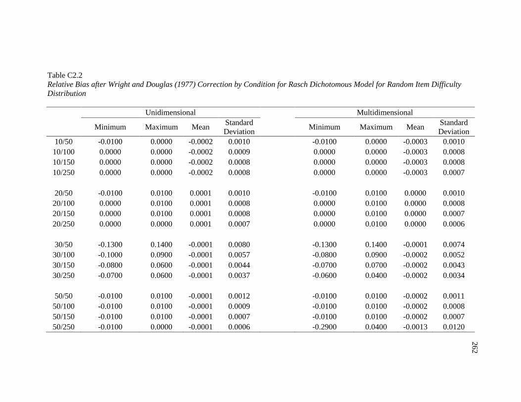
262

Table C2.2

Relative Bias after Wright and Douglas (1977) Correction by Condition for Rasch Dichotomous Model for Random Item Difficulty

Distribution




Standard

Deviation

10/50 -0.0100 0.0000 -0.0002 0.0010 -0.0100 0.0000 -0.0003 0.0010

10/100 0.0000 0.0000 -0.0002 0.0009 0.0000 0.0000 -0.0003 0.0008

10/150 0.0000 0.0000 -0.0002 0.0008 0.0000 0.0000 -0.0003 0.0008

10/250 0.0000 0.0000 -0.0002 0.0008 0.0000 0.0000 -0.0003 0.0007

20/50 -0.0100 0.0100 0.0001 0.0010 -0.0100 0.0100 0.0000 0.0010

20/100 0.0000 0.0100 0.0001 0.0008 0.0000 0.0100 0.0000 0.0008

20/150 0.0000 0.0100 0.0001 0.0008 0.0000 0.0100 0.0000 0.0007

20/250 0.0000 0.0000 0.0001 0.0007 0.0000 0.0100 0.0000 0.0006

30/50 -0.1300 0.1400 -0.0001 0.0080 -0.1300 0.1400 -0.0001 0.0074

30/100 -0.1000 0.0900 -0.0001 0.0057 -0.0800 0.0900 -0.0002 0.0052

30/150 -0.0800 0.0600 -0.0001 0.0044 -0.0700 0.0700 -0.0002 0.0043

30/250 -0.0700 0.0600 -0.0001 0.0037 -0.0600 0.0400 -0.0002 0.0034

50/50 -0.0100 0.0100 -0.0001 0.0012 -0.0100 0.0100 -0.0002 0.0011

50/100 -0.0100 0.0100 -0.0001 0.0009 -0.0100 0.0100 -0.0002 0.0008

50/150 -0.0100 0.0100 -0.0001 0.0007 -0.0100 0.0100 -0.0002 0.0007

50/250 -0.0100 0.0000 -0.0001 0.0006 -0.2900 0.0400 -0.0013 0.0120

254

262

263

Table C2.3

Relative Bias after Wright and Douglas (1977) by Condition for Rasch Rating Scale Model for Uniform Item Difficulty Distribution

Unidimensional Multidimensional: Two Factors



Standard

Deviation

10 /50 -0.0200 0.0900 0.0050 0.0120 -0.0800 0.0300 -0.0093 0.0129

10/100 -0.0100 0.0800 0.0048 0.0112 -0.0600 0.0200 -0.0093 0.0125

10/150 -0.0100 0.0600 0.0048 0.0108 -0.0600 0.0200 -0.0094 0.0125

10/250 -0.0100 0.0500 0.0048 0.0108 -0.0500 0.0200 -0.0094 0.0124

20/50 -9.1000 6.0900 -0.0506 0.5847 -2.2500 6.2200 0.0456 0.3341

20/100 -6.3600 4.1000 -0.0466 0.4075 -1.3800 3.6000 0.0447 0.2699

20/150 -4.9900 2.7300 -0.0460 0.3479 -1.5000 3.4800 0.0401 0.2309

20/250 -4.1200 1.9800 -0.0454 0.2963 -0.6300 2.2300 0.0417 0.2124

30/50 -0.0300 0.0500 0.0010 0.0048 -0.0100 0.0500 0.0026 0.0048

30/100 -0.0200 0.0400 0.0009 0.0039 -0.0100 0.0400 0.0025 0.0042

30/150 -0.0200 0.0400 0.0009 0.0036 -0.0100 0.0300 0.0024 0.0039

30/250 -0.0100 0.0300 0.0009 0.0033 -0.0100 0.0300 0.0024 0.0038

50/50 -3.6300 1.3800 -0.0242 0.1857 -3.6300 0.1700 -0.0333 0.2333

50/100 -2.6100 0.5600 -0.0243 0.1724 -2.7200 0.1400 -0.0327 0.2238

50/150 -2.3500 0.1200 -0.0243 0.1678 -2.5400 0.1300 -0.0327 0.2216

50/250 -1.9700 0.1100 -0.0241 0.1623 -2.1200 0.1100 -0.0321 0.2161

263

264

Table C2.4

Relative Bias after Wright and Douglas (1977) by Condition for Rasch Rating Scale Model for Random Item Difficulty Distribution




Standard

Deviation

10/50 -0.0400 0.0200 -0.0023 0.0081 -0.0200 0.0100 -0.0002 0.0045

10/100 -0.0300 0.0200 -0.0023 0.0075 -0.0200 0.0100 -0.0002 0.0041

10/150 -0.0300 0.0100 -0.0024 0.0074 -0.0200 0.0100 -0.0003 0.0038

10/250 -0.0300 0.0100 -0.0024 0.0072 -0.0100 0.0100 -0.0003 0.0037

20/50 -0.0400 0.0600 0.0008 0.0074 -0.0300 0.0400 0.0026 0.0043

20/100 -0.0300 0.0500 0.0007 0.0066 -0.0200 0.0200 0.0025 0.0037

20/150 -0.0300 0.0500 0.0006 0.0064 -0.0200 0.0200 0.0024 0.0034

20/250 -0.0200 0.0400 0.0006 0.0062 -0.0100 0.0200 0.0024 0.0032

30/50 -0.7500 0.6000 -0.0010 0.0448 -0.5300 0.1600 -0.0011 0.0260

30/100 -0.6300 0.4900 -0.0009 0.0331 -0.3200 0.0900 -0.0012 0.0228

30/150 -0.4500 0.3500 -0.0010 0.0260 -0.3100 0.0800 -0.0011 0.0211

30/250 -0.3600 0.3000 -0.0008 0.0214 -0.2200 0.0500 -0.0012 0.0203

50/50 -0.0900 0.0600 -0.0010 0.0071 -0.0700 0.1100 -0.0010 0.0105

50/100 -0.0600 0.0400 -0.0011 0.0054 -0.0600 0.0800 -0.0011 0.0100

50/150 -0.0500 0.0300 -0.0011 0.0048 -0.0500 0.0700 -0.0011 0.0096

50/250 -0.0400 0.0200 -0.0011 0.0043 -0.0400 0.0600 -0.0012 0.0094

264

265

Table C2.5

Relative Bias after Wright and Douglas (1977) correction by Item for I = 20 for Dichotomous Rasch Model with Uniform Item

Difficulty Distribution and Unidimensionality.


Standard


Standard

Deviation

Item N = 50 N = 100

1 0.0000 0.0000 0.0000 0.0005 0.0000 0.0000 0.0000 0.0003

2 0.0000 0.0000 0.0000 0.0003 0.0000 0.0000 0.0000 0.0002

3 0.0000 0.0000 0.0000 0.0005 0.0000 0.0000 0.0000 0.0003

4 0.0000 0.0000 0.0001 0.0002 0.0000 0.0000 0.0001 0.0002

5 0.0000 0.0000 0.0003 0.0010 0.0000 0.0000 0.0003 0.0007

6 0.0000 0.0000 0.0003 0.0012 0.0000 0.0000 0.0003 0.0009

7 0.0000 0.0000 0.0001 0.0002 0.0000 0.0000 0.0001 0.0002

8 0.0000 0.0000 0.0000 0.0004 0.0000 0.0000 0.0000 0.0003

9 -1.5100 1.2800 -0.1025 0.4216 -0.9400 0.8600 -0.1103 0.2817

10 0.0000 0.0000 0.0001 0.0002 0.0000 0.0000 0.0001 0.0002

11 0.0000 0.0000 0.0002 0.0008 0.0000 0.0000 0.0002 0.0005

12 0.0000 0.0000 0.0002 0.0004 0.0000 0.0000 0.0002 0.0003

13 0.0000 0.0000 0.0000 0.0003 0.0000 0.0000 0.0000 0.0002

14 0.0000 0.0000 -0.0002 0.0008 0.0000 0.0000 -0.0001 0.0006

15 0.0000 0.0000 0.0000 0.0002 0.0000 0.0000 0.0000 0.0002

16 0.0000 0.0000 0.0001 0.0002 0.0000 0.0000 0.0000 0.0002

17 0.0000 0.0000 0.0001 0.0002 0.0000 0.0000 0.0000 0.0001

18 0.0000 0.0000 0.0001 0.0002 0.0000 0.0000 0.0001 0.0002

19 0.0000 0.0000 0.0001 0.0003 0.0000 0.0000 0.0001 0.0002

20 0.0000 0.0000 0.0000 0.0004 0.0000 0.0000 0.0000 0.0003

265

266

Table C2.6


Difficulty Distribution and Unidimensionality.



Standard

Deviation

Item N = 150 N = 250

1 0.0000 0.0000 0.0000 0.0003 0.0000 0.0000 0.0000 0.0002

2 0.0000 0.0000 0.0000 0.0002 0.0000 0.0000 0.0000 0.0001

3 0.0000 0.0000 -0.0001 0.0003 0.0000 0.0000 -0.0001 0.0002

4 0.0000 0.0000 0.0001 0.0001 0.0000 0.0000 0.0001 0.0001

5 0.0000 0.0000 0.0003 0.0005 0.0000 0.0000 0.0003 0.0004

6 0.0000 0.0000 0.0003 0.0007 0.0000 0.0000 0.0003 0.0005

7 0.0000 0.0000 0.0001 0.0001 0.0000 0.0000 0.0001 0.0001

8 0.0000 0.0000 0.0000 0.0002 0.0000 0.0000 0.0000 0.0002

9 -0.9600 0.6100 -0.0916 0.2337 -0.7200 0.5300 -0.0762 0.1797

10 0.0000 0.0000 0.0001 0.0001 0.0000 0.0000 0.0001 0.0001

11 0.0000 0.0000 0.0002 0.0005 0.0000 0.0000 0.0002 0.0003

12 0.0000 0.0000 0.0002 0.0003 0.0000 0.0000 0.0002 0.0002

13 0.0000 0.0000 0.0000 0.0002 0.0000 0.0000 0.0000 0.0001

14 0.0000 0.0000 -0.0001 0.0005 0.0000 0.0000 -0.0001 0.0004

15 0.0000 0.0000 0.0000 0.0001 0.0000 0.0000 0.0000 0.0001

16 0.0000 0.0000 0.0000 0.0001 0.0000 0.0000 0.0000 0.0001

17 0.0000 0.0000 0.0000 0.0001 0.0000 0.0000 0.0000 0.0001

18 0.0000 0.0000 0.0001 0.0001 0.0000 0.0000 0.0001 0.0001

19 0.0000 0.0000 0.0001 0.0002 0.0000 0.0000 0.0001 0.0001

20 0.0000 0.0000 0.0000 0.0002 0.0000 0.0000 0.0000 0.0002

266

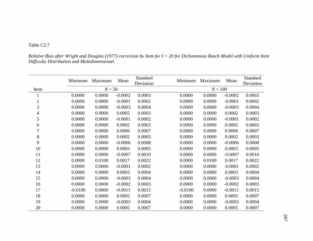
267

Table C2.7


Difficulty Distribution and Multidimensional.



Standard

Deviation

Item N = 50 N = 100

1 0.0000 0.0000 -0.0002 0.0003 0.0000 0.0000 -0.0002 0.0003

2 0.0000 0.0000 -0.0001 0.0002 0.0000 0.0000 -0.0001 0.0002

3 0.0000 0.0000 -0.0003 0.0004 0.0000 0.0000 -0.0003 0.0004

4 0.0000 0.0000 0.0002 0.0003 0.0000 0.0000 0.0002 0.0003

5 0.0000 0.0000 -0.0001 0.0002 0.0000 0.0000 -0.0001 0.0002

6 0.0000 0.0000 0.0002 0.0003 0.0000 0.0000 0.0002 0.0003

7 0.0000 0.0000 0.0006 0.0007 0.0000 0.0000 0.0006 0.0007

8 0.0000 0.0000 0.0002 0.0003 0.0000 0.0000 0.0002 0.0003

9 0.0000 0.0000 -0.0006 0.0008 0.0000 0.0000 -0.0006 0.0008

10 0.0000 0.0000 0.0003 0.0005 0.0000 0.0000 0.0003 0.0005

11 0.0000 0.0000 -0.0007 0.0010 0.0000 0.0000 -0.0007 0.0010

12 0.0000 0.0100 0.0017 0.0022 0.0000 0.0100 0.0017 0.0022

13 0.0000 0.0000 -0.0001 0.0002 0.0000 0.0000 -0.0001 0.0002

14 0.0000 0.0000 0.0003 0.0004 0.0000 0.0000 0.0003 0.0004

15 0.0000 0.0000 -0.0003 0.0004 0.0000 0.0000 -0.0003 0.0004

16 0.0000 0.0000 -0.0002 0.0003 0.0000 0.0000 -0.0002 0.0003

17 -0.0100 0.0000 -0.0011 0.0015 -0.0100 0.0000 -0.0011 0.0015

18 0.0000 0.0000 0.0005 0.0007 0.0000 0.0000 0.0005 0.0007

19 0.0000 0.0000 -0.0003 0.0004 0.0000 0.0000 -0.0003 0.0004

20 0.0000 0.0000 0.0005 0.0007 0.0000 0.0000 0.0005 0.0007

267

268

Table C2.8





Standard

Deviation

Item N = 150 N = 250

1 0.0000 0.0000 -0.0002 0.0002 0.0000 0.0000 -0.0002 0.0001

2 0.0000 0.0000 -0.0001 0.0001 0.0000 0.0000 -0.0001 0.0001

3 0.0000 0.0000 -0.0003 0.0002 0.0000 0.0000 -0.0003 0.0002

4 0.0000 0.0000 0.0002 0.0002 0.0000 0.0000 0.0001 0.0001

5 0.0000 0.0000 -0.0002 0.0001 0.0000 0.0000 -0.0002 0.0001

6 0.0000 0.0000 0.0001 0.0002 0.0000 0.0000 0.0001 0.0001

7 0.0000 0.0000 0.0005 0.0004 0.0000 0.0000 0.0005 0.0003

8 0.0000 0.0000 0.0002 0.0001 0.0000 0.0000 0.0002 0.0001

9 0.0000 0.0000 -0.0006 0.0005 0.0000 0.0000 -0.0006 0.0004

10 0.0000 0.0000 0.0003 0.0002 0.0000 0.0000 0.0003 0.0002

11 0.0000 0.0000 -0.0008 0.0006 0.0000 0.0000 -0.0008 0.0005

12 0.0000 0.0100 0.0016 0.0013 0.0000 0.0100 0.0016 0.0010

13 0.0000 0.0000 -0.0001 0.0001 0.0000 0.0000 -0.0001 0.0001

14 0.0000 0.0000 0.0003 0.0002 0.0000 0.0000 0.0002 0.0002

15 0.0000 0.0000 -0.0003 0.0003 0.0000 0.0000 -0.0003 0.0002

16 0.0000 0.0000 -0.0002 0.0001 0.0000 0.0000 -0.0002 0.0001

17 0.0000 0.0000 -0.0011 0.0009 0.0000 0.0000 -0.0011 0.0006

18 0.0000 0.0000 0.0005 0.0004 0.0000 0.0000 0.0005 0.0003

19 0.0000 0.0000 -0.0003 0.0002 0.0000 0.0000 -0.0003 0.0002

20 0.0000 0.0000 0.0005 0.0004 0.0000 0.0000 0.0005 0.0003

268

269

Table C2.9

Relative Bias after Wright and Douglas (1977) correction by Item for I = 20 for Dichotomous Rasch Model with Random Normal Item




Standard

Deviation

Item N = 50 N = 100

1 0.0000 0.0000 -0.0001 0.0005 0.0000 0.0000 -0.0001 0.0003

2 0.0000 0.0000 -0.0001 0.0003 0.0000 0.0000 -0.0001 0.0002

3 0.0000 0.0000 -0.0001 0.0005 0.0000 0.0000 -0.0001 0.0004

4 0.0000 0.0000 0.0000 0.0002 0.0000 0.0000 0.0000 0.0002

5 0.0000 0.0000 0.0002 0.0010 0.0000 0.0000 0.0002 0.0007

6 0.0000 0.0000 0.0002 0.0012 0.0000 0.0000 0.0002 0.0009

7 0.0000 0.0000 0.0000 0.0002 0.0000 0.0000 0.0000 0.0001

8 0.0000 0.0000 -0.0001 0.0004 0.0000 0.0000 -0.0001 0.0003

9 -1.2800 1.1200 -0.0986 0.3716 -0.9400 0.9000 -0.0908 0.2671

10 0.0000 0.0000 0.0000 0.0002 0.0000 0.0000 0.0000 0.0002

11 0.0000 0.0000 0.0002 0.0007 0.0000 0.0000 0.0001 0.0005

12 0.0000 0.0000 0.0001 0.0004 0.0000 0.0000 0.0001 0.0003

13 0.0000 0.0000 -0.0001 0.0003 0.0000 0.0000 -0.0001 0.0002

14 0.0000 0.0000 -0.0002 0.0007 0.0000 0.0000 -0.0002 0.0005

15 0.0000 0.0000 -0.0001 0.0002 0.0000 0.0000 0.0000 0.0002

16 0.0000 0.0000 0.0000 0.0002 0.0000 0.0000 0.0000 0.0001

17 0.0000 0.0000 0.0000 0.0002 0.0000 0.0000 0.0000 0.0001

18 0.0000 0.0000 0.0001 0.0002 0.0000 0.0000 0.0000 0.0002

19 0.0000 0.0000 0.0000 0.0003 0.0000 0.0000 0.0000 0.0002

20 0.0000 0.0000 -0.0001 0.0004 0.0000 0.0000 -0.0001 0.0003

269

270

Table C2.10





Standard

Deviation

Item N = 150 N = 250

1 0.0000 0.0000 -0.0001 0.0003 0.0000 0.0000 -0.0002 0.0001

2 0.0000 0.0000 -0.0001 0.0002 0.0000 0.0000 -0.0001 0.0001

3 0.0000 0.0000 -0.0001 0.0003 0.0000 0.0000 -0.0003 0.0002

4 0.0000 0.0000 0.0000 0.0001 0.0000 0.0000 0.0001 0.0001

5 0.0000 0.0000 0.0002 0.0005 0.0000 0.0000 -0.0002 0.0001

6 0.0000 0.0000 0.0003 0.0007 0.0000 0.0000 0.0002 0.0001

7 0.0000 0.0000 0.0000 0.0001 0.0000 0.0000 0.0005 0.0003

8 0.0000 0.0000 -0.0001 0.0002 0.0000 0.0000 0.0002 0.0001

9 -0.9200 0.5000 -0.0775 0.2194 0.0000 0.0000 -0.0006 0.0003

10 0.0000 0.0000 0.0000 0.0001 0.0000 0.0000 0.0003 0.0002

11 0.0000 0.0000 0.0001 0.0004 0.0000 0.0000 -0.0008 0.0005

12 0.0000 0.0000 0.0001 0.0002 0.0000 0.0000 0.0016 0.0010

13 0.0000 0.0000 -0.0001 0.0002 0.0000 0.0000 -0.0001 0.0001

14 0.0000 0.0000 -0.0002 0.0004 0.0000 0.0000 0.0002 0.0002

15 0.0000 0.0000 -0.0001 0.0001 0.0000 0.0000 -0.0003 0.0002

16 0.0000 0.0000 0.0000 0.0001 0.0000 0.0000 -0.0002 0.0001

17 0.0000 0.0000 0.0000 0.0001 0.0000 0.0000 -0.0011 0.0006

18 0.0000 0.0000 0.0000 0.0001 0.0000 0.0000 0.0005 0.0003

19 0.0000 0.0000 0.0000 0.0002 0.0000 0.0000 -0.0003 0.0002

20 0.0000 0.0000 -0.0001 0.0002 0.0000 0.0000 0.0005 0.0003

270

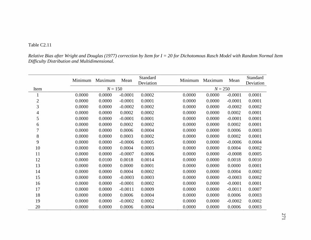
271

Table C2.11




Standard


Standard

Deviation

Item N = 150 N = 250

1 0.0000 0.0000 -0.0001 0.0002 0.0000 0.0000 -0.0001 0.0001

2 0.0000 0.0000 -0.0001 0.0001 0.0000 0.0000 -0.0001 0.0001

3 0.0000 0.0000 -0.0002 0.0002 0.0000 0.0000 -0.0002 0.0002

4 0.0000 0.0000 0.0002 0.0002 0.0000 0.0000 0.0002 0.0001

5 0.0000 0.0000 -0.0001 0.0001 0.0000 0.0000 -0.0001 0.0001

6 0.0000 0.0000 0.0002 0.0002 0.0000 0.0000 0.0002 0.0001

7 0.0000 0.0000 0.0006 0.0004 0.0000 0.0000 0.0006 0.0003

8 0.0000 0.0000 0.0003 0.0002 0.0000 0.0000 0.0002 0.0001

9 0.0000 0.0000 -0.0006 0.0005 0.0000 0.0000 -0.0006 0.0004

10 0.0000 0.0000 0.0004 0.0003 0.0000 0.0000 0.0004 0.0002

11 0.0000 0.0000 -0.0007 0.0006 0.0000 0.0000 -0.0008 0.0005

12 0.0000 0.0100 0.0018 0.0014 0.0000 0.0000 0.0018 0.0010

13 0.0000 0.0000 0.0000 0.0001 0.0000 0.0000 0.0000 0.0001

14 0.0000 0.0000 0.0004 0.0002 0.0000 0.0000 0.0004 0.0002

15 0.0000 0.0000 -0.0003 0.0003 0.0000 0.0000 -0.0003 0.0002

16 0.0000 0.0000 -0.0001 0.0002 0.0000 0.0000 -0.0001 0.0001

17 0.0000 0.0000 -0.0011 0.0009 0.0000 0.0000 -0.0011 0.0007

18 0.0000 0.0000 0.0006 0.0004 0.0000 0.0000 0.0006 0.0003

19 0.0000 0.0000 -0.0002 0.0002 0.0000 0.0000 -0.0002 0.0002

20 0.0000 0.0000 0.0006 0.0004 0.0000 0.0000 0.0006 0.0003

271

272

Table C2.12

Relative Bias after Wright and Douglas (1977) correction by Item for I = 20 for Rasch Rating Scale Model with Uniform Item




Standard

Deviation

Item N = 50 N = 100

1 -0.0100 0.0100 -0.0003 0.0026 -0.0100 0.0100 -0.0005 0.0018

2 -0.0100 0.0100 -0.0001 0.0018 0.0000 0.0000 -0.0001 0.0012

3 -0.0100 0.0100 -0.0004 0.0026 -0.0100 0.0100 -0.0005 0.0019

4 0.0000 0.0100 0.0010 0.0012 0.0000 0.0000 0.0009 0.0008

5 -0.0100 0.0300 0.0030 0.0054 -0.0100 0.0200 0.0026 0.0038

6 -0.0200 0.0300 0.0030 0.0068 -0.0100 0.0200 0.0031 0.0047

7 0.0000 0.0100 0.0011 0.0012 0.0000 0.0000 0.0009 0.0008

8 -0.0100 0.0100 -0.0002 0.0022 -0.0100 0.0100 -0.0004 0.0015

9 -9.1000 6.0900 -1.0259 2.4167 -6.3600 4.1000 -0.9425 1.5745

10 0.0000 0.0000 0.0010 0.0012 0.0000 0.0000 0.0009 0.0009

11 -0.0100 0.0100 0.0023 0.0040 -0.0100 0.0100 0.0022 0.0031

12 -0.0100 0.0100 0.0016 0.0025 0.0000 0.0100 0.0015 0.0017

13 0.0000 0.0000 0.0001 0.0015 0.0000 0.0000 0.0000 0.0010

14 -0.0200 0.0100 -0.0011 0.0044 -0.0100 0.0100 -0.0011 0.0031

15 0.0000 0.0000 0.0002 0.0012 0.0000 0.0000 0.0001 0.0008

16 0.0000 0.0000 0.0003 0.0011 0.0000 0.0000 0.0001 0.0008

17 0.0000 0.0000 0.0002 0.0011 0.0000 0.0000 0.0001 0.0008

18 0.0000 0.0000 0.0010 0.0012 0.0000 0.0000 0.0009 0.0009

19 0.0000 0.0100 0.0013 0.0016 0.0000 0.0000 0.0011 0.0011

20 -0.0100 0.0100 -0.0003 0.0024 -0.0100 0.0100 -0.0004 0.0017

272

273

Table C2.13

Relative Bias after Wright and Douglas (1977) correction by Item for I = 20 for

Rasch Rating Scale Model with Uniform Item Difficulty Distribution and Multidimensional.



Standard

Deviation

Item N = 150 N = 250

1 -0.0100 0.0100 -0.0005 0.0016 0.0000 0.0000 -0.0005 0.0012

2 0.0000 0.0000 -0.0002 0.0010 0.0000 0.0000 -0.0002 0.0008

3 -0.0100 0.0000 -0.0005 0.0015 0.0000 0.0000 -0.0006 0.0011

4 0.0000 0.0000 0.0009 0.0007 0.0000 0.0000 0.0009 0.0005

5 -0.0100 0.0100 0.0027 0.0031 -0.0100 0.0100 0.0027 0.0024

6 -0.0100 0.0100 0.0033 0.0039 -0.0100 0.0100 0.0030 0.0030

7 0.0000 0.0000 0.0009 0.0007 0.0000 0.0000 0.0008 0.0005

8 0.0000 0.0000 -0.0004 0.0012 0.0000 0.0000 -0.0003 0.0009

9 -4.9900 2.7300 -0.9316 1.2634 -4.1200 1.9800 -0.9187 0.9765

10 0.0000 0.0000 0.0009 0.0007 0.0000 0.0000 0.0009 0.0005

11 0.0000 0.0100 0.0022 0.0024 0.0000 0.0100 0.0022 0.0018

12 0.0000 0.0100 0.0014 0.0014 0.0000 0.0000 0.0014 0.0011

13 0.0000 0.0000 0.0000 0.0009 0.0000 0.0000 -0.0001 0.0007

14 -0.0100 0.0100 -0.0012 0.0025 -0.0100 0.0000 -0.0013 0.0019

15 0.0000 0.0000 0.0001 0.0007 0.0000 0.0000 0.0001 0.0006

16 0.0000 0.0000 0.0001 0.0006 0.0000 0.0000 0.0001 0.0005

17 0.0000 0.0000 0.0001 0.0006 0.0000 0.0000 0.0001 0.0005

18 0.0000 0.0000 0.0009 0.0007 0.0000 0.0000 0.0009 0.0006

19 0.0000 0.0000 0.0010 0.0009 0.0000 0.0000 0.0010 0.0007

20 0.0000 0.0000 -0.0004 0.0013 0.0000 0.0000 -0.0004 0.0010

273

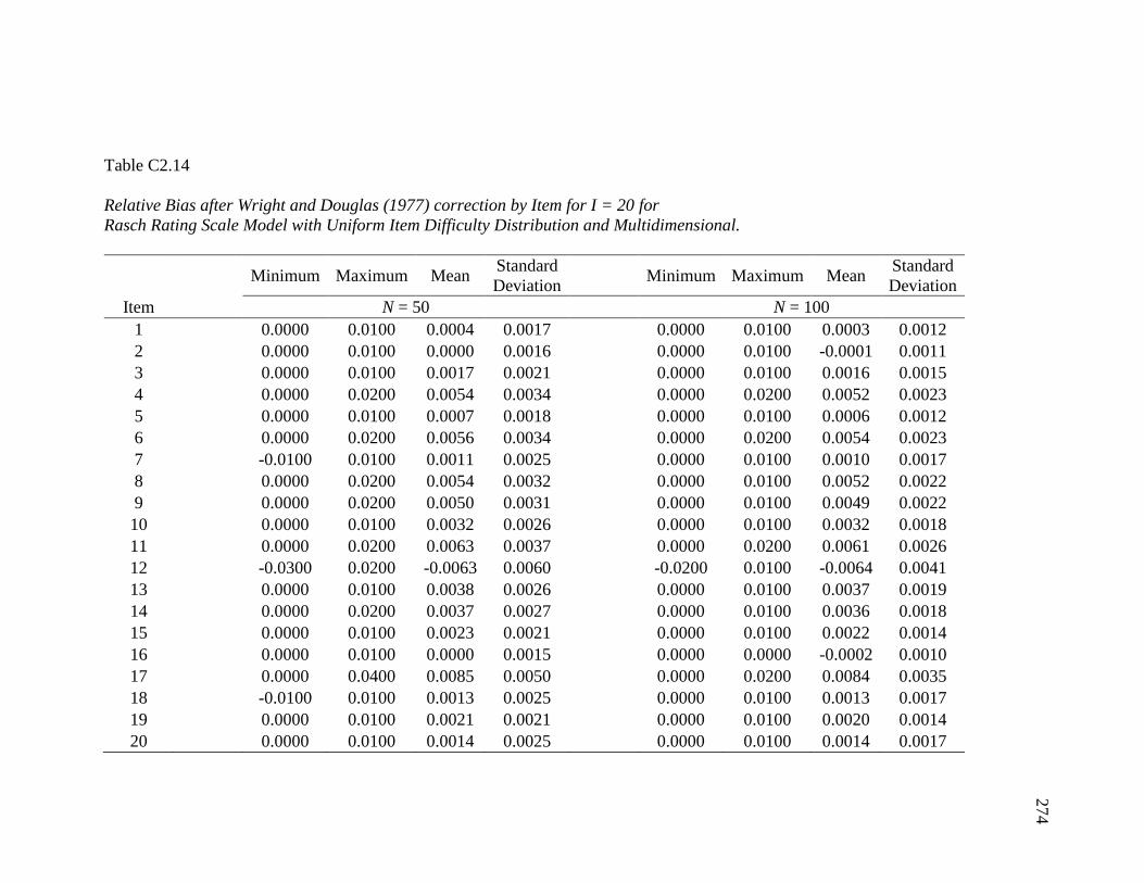
274

Table C2.14

Relative Bias after Wright and Douglas (1977) correction by Item for I = 20 for

Rasch Rating Scale Model with Uniform Item Difficulty Distribution and Multidimensional.



Standard

Deviation

Item N = 50 N = 100

1 0.0000 0.0100 0.0004 0.0017 0.0000 0.0100 0.0003 0.0012

2 0.0000 0.0100 0.0000 0.0016 0.0000 0.0100 -0.0001 0.0011

3 0.0000 0.0100 0.0017 0.0021 0.0000 0.0100 0.0016 0.0015

4 0.0000 0.0200 0.0054 0.0034 0.0000 0.0200 0.0052 0.0023

5 0.0000 0.0100 0.0007 0.0018 0.0000 0.0100 0.0006 0.0012

6 0.0000 0.0200 0.0056 0.0034 0.0000 0.0200 0.0054 0.0023

7 -0.0100 0.0100 0.0011 0.0025 0.0000 0.0100 0.0010 0.0017

8 0.0000 0.0200 0.0054 0.0032 0.0000 0.0100 0.0052 0.0022

9 0.0000 0.0200 0.0050 0.0031 0.0000 0.0100 0.0049 0.0022

10 0.0000 0.0100 0.0032 0.0026 0.0000 0.0100 0.0032 0.0018

11 0.0000 0.0200 0.0063 0.0037 0.0000 0.0200 0.0061 0.0026

12 -0.0300 0.0200 -0.0063 0.0060 -0.0200 0.0100 -0.0064 0.0041

13 0.0000 0.0100 0.0038 0.0026 0.0000 0.0100 0.0037 0.0019

14 0.0000 0.0200 0.0037 0.0027 0.0000 0.0100 0.0036 0.0018

15 0.0000 0.0100 0.0023 0.0021 0.0000 0.0100 0.0022 0.0014

16 0.0000 0.0100 0.0000 0.0015 0.0000 0.0000 -0.0002 0.0010

17 0.0000 0.0400 0.0085 0.0050 0.0000 0.0200 0.0084 0.0035

18 -0.0100 0.0100 0.0013 0.0025 0.0000 0.0100 0.0013 0.0017

19 0.0000 0.0100 0.0021 0.0021 0.0000 0.0100 0.0020 0.0014

20 0.0000 0.0100 0.0014 0.0025 0.0000 0.0100 0.0014 0.0017

274

275

Table C2.15

Relative Bias after Wright and Douglas (1977) correction by Item for I = 20 for Rasch Rating Scale Model with Uniform Item




Standard

Deviation

Item N =150 N = 250

1 0.0000 0.0100 0.0003 0.0012 0.0000 0.0000 0.0002 0.0009

2 0.0000 0.0100 -0.0001 0.0011 0.0000 0.0000 -0.0001 0.0009

3 0.0000 0.0100 0.0016 0.0015 0.0000 0.0100 0.0016 0.0011

4 0.0000 0.0200 0.0052 0.0023 0.0000 0.0100 0.0050 0.0018

5 0.0000 0.0100 0.0006 0.0012 0.0000 0.0000 0.0005 0.0010

6 0.0000 0.0200 0.0054 0.0023 0.0000 0.0100 0.0052 0.0018

7 0.0000 0.0100 0.0010 0.0017 0.0000 0.0100 0.0011 0.0014

8 0.0000 0.0100 0.0052 0.0022 0.0000 0.0100 0.0050 0.0017

9 0.0000 0.0100 0.0049 0.0022 0.0000 0.0100 0.0048 0.0017

10 0.0000 0.0100 0.0032 0.0018 0.0000 0.0100 0.0031 0.0014

11 0.0000 0.0200 0.0061 0.0026 0.0000 0.0200 0.0060 0.0021

12 -0.0200 0.0100 -0.0064 0.0041 -0.0200 0.0100 -0.0060 0.0032

13 0.0000 0.0100 0.0037 0.0019 0.0000 0.0100 0.0036 0.0015

14 0.0000 0.0100 0.0036 0.0018 0.0000 0.0100 0.0036 0.0015

15 0.0000 0.0100 0.0022 0.0014 0.0000 0.0100 0.0021 0.0012

16 0.0000 0.0000 -0.0002 0.0010 0.0000 0.0000 -0.0002 0.0008

17 0.0000 0.0200 0.0084 0.0035 0.0000 0.0200 0.0082 0.0029

18 0.0000 0.0100 0.0013 0.0017 0.0000 0.0100 0.0013 0.0014

19 0.0000 0.0100 0.0020 0.0014 0.0000 0.0100 0.0019 0.0011

20 0.0000 0.0100 0.0014 0.0017 0.0000 0.0100 0.0014 0.0014

275

276

Table C2.16

Relative Bias after Wright and Douglas (1977) correction by Item for I = 20 for Rasch Rating Scale Model with Random Normal Item




Standard

Deviation

Item N = 50 N = 100

1 0.0000 0.0100 0.0003 0.0018 0.0000 0.0000 0.0002 0.0013

2 0.0000 0.0000 -0.0010 0.0014 0.0000 0.0000 -0.0011 0.0010

3 0.0000 0.0100 0.0002 0.0018 0.0000 0.0000 0.0001 0.0013

4 -0.0200 0.0400 0.0071 0.0082 -0.0100 0.0200 0.0069 0.0059

5 -0.0100 0.0100 -0.0001 0.0033 -0.0100 0.0100 -0.0003 0.0023

6 -0.0100 0.0100 -0.0007 0.0039 -0.0100 0.0100 -0.0010 0.0026

7 0.0000 0.0200 0.0038 0.0028 0.0000 0.0100 0.0036 0.0019

8 0.0000 0.0100 -0.0004 0.0017 0.0000 0.0000 -0.0005 0.0011

9 -2.2500 6.2200 0.8930 1.2156 -1.3800 3.6000 0.8768 0.8535

10 0.0000 0.0200 0.0035 0.0026 0.0000 0.0100 0.0033 0.0018

11 -0.0100 0.0100 0.0003 0.0026 0.0000 0.0100 0.0003 0.0020

12 0.0000 0.0100 0.0018 0.0023 0.0000 0.0100 0.0018 0.0016

13 0.0000 0.0000 -0.0016 0.0013 0.0000 0.0000 -0.0017 0.0009

14 -0.0100 0.0100 0.0016 0.0028 0.0000 0.0100 0.0016 0.0020

15 0.0000 0.0000 -0.0017 0.0013 0.0000 0.0000 -0.0018 0.0009

16 0.0000 0.0100 -0.0010 0.0015 0.0000 0.0000 -0.0011 0.0010

17 0.0000 0.0100 0.0007 0.0021 0.0000 0.0100 0.0006 0.0015

18 0.0000 0.0200 0.0029 0.0024 0.0000 0.0100 0.0028 0.0017

19 0.0000 0.0200 0.0037 0.0027 0.0000 0.0100 0.0035 0.0018

20 0.0000 0.0100 0.0000 0.0018 0.0000 0.0000 -0.0002 0.0012

276

277

Table C2.17





Standard

Deviation

Item N = 150 N = 250

1 0.0000 0.0000 0.0001 0.0010 0.0000 0.0000 0.0000 0.0008

2 0.0000 0.0000 -0.0011 0.0007 0.0000 0.0000 -0.0012 0.0006

3 0.0000 0.0000 0.0000 0.0010 0.0000 0.0000 0.0000 0.0008

4 -0.0100 0.0200 0.0064 0.0046 0.0000 0.0200 0.0063 0.0037

5 -0.0100 0.0100 -0.0003 0.0020 0.0000 0.0100 -0.0004 0.0016

6 -0.0100 0.0100 -0.0010 0.0023 -0.0100 0.0100 -0.0010 0.0018

7 0.0000 0.0100 0.0034 0.0015 0.0000 0.0100 0.0034 0.0011

8 0.0000 0.0000 -0.0006 0.0009 0.0000 0.0000 -0.0006 0.0007

9 -1.5000 3.4800 0.7866 0.6927 -0.6300 2.2300 0.8199 0.5144

10 0.0000 0.0100 0.0032 0.0014 0.0000 0.0100 0.0031 0.0011

11 0.0000 0.0100 0.0003 0.0016 0.0000 0.0000 0.0002 0.0012

12 0.0000 0.0100 0.0017 0.0013 0.0000 0.0000 0.0016 0.0010

13 0.0000 0.0000 -0.0018 0.0007 0.0000 0.0000 -0.0018 0.0005

14 0.0000 0.0100 0.0014 0.0016 0.0000 0.0100 0.0014 0.0012

15 0.0000 0.0000 -0.0018 0.0007 0.0000 0.0000 -0.0019 0.0005

16 0.0000 0.0000 -0.0012 0.0008 0.0000 0.0000 -0.0012 0.0006

17 0.0000 0.0100 0.0005 0.0012 0.0000 0.0000 0.0005 0.0009

18 0.0000 0.0100 0.0027 0.0013 0.0000 0.0100 0.0026 0.0010

19 0.0000 0.0100 0.0033 0.0015 0.0000 0.0100 0.0033 0.0011

20 0.0000 0.0000 0.0010 0.0000 0.0000 -0.0003 0.0007

277

278

Table C2.18


Difficulty Distribution and Unidimensional.



Standard

Deviation

Item N = 50 N = 100

1 -0.0100 0.0000 -0.0014 0.0017 0.0000 0.0000 -0.0015 0.0011

2 0.0000 0.0000 -0.0006 0.0011 0.0000 0.0000 -0.0007 0.0008

3 -0.0100 0.0100 -0.0022 0.0022 -0.0100 0.0000 -0.0023 0.0015

4 0.0000 0.0100 0.0025 0.0016 0.0000 0.0100 0.0023 0.0010

5 0.0000 0.0100 -0.0008 0.0013 0.0000 0.0000 -0.0010 0.0009

6 0.0000 0.0100 0.0023 0.0015 0.0000 0.0100 0.0023 0.0010

7 -0.0100 0.0200 0.0065 0.0043 0.0000 0.0200 0.0059 0.0029

8 0.0000 0.0100 0.0025 0.0016 0.0000 0.0100 0.0023 0.0011

9 -0.0200 0.0100 -0.0056 0.0047 -0.0200 0.0000 -0.0055 0.0032

10 0.0000 0.0100 0.0040 0.0026 0.0000 0.0100 0.0037 0.0018

11 -0.0300 0.0100 -0.0071 0.0061 -0.0200 0.0100 -0.0075 0.0042

12 -0.0200 0.0600 0.0185 0.0132 -0.0100 0.0500 0.0179 0.0090

13 0.0000 0.0000 -0.0003 0.0010 0.0000 0.0000 -0.0005 0.0007

14 0.0000 0.0100 0.0036 0.0022 0.0000 0.0100 0.0033 0.0016

15 -0.0100 0.0100 -0.0026 0.0024 -0.0100 0.0000 -0.0027 0.0017

16 -0.0100 0.0000 -0.0012 0.0015 0.0000 0.0000 -0.0014 0.0011

17 -0.0400 0.0200 -0.0109 0.0085 -0.0300 0.0100 -0.0109 0.0060

18 -0.0100 0.0200 0.0061 0.0039 0.0000 0.0200 0.0060 0.0029

19 -0.0100 0.0100 -0.0025 0.0023 -0.0100 0.0000 -0.0025 0.0016

20 -0.0100 0.0200 0.0056 0.0040 0.0000 0.0100 -0.0015 0.0029

278

279

Table C2.19


Difficulty Distribution and Unidimensional.



Standard

Deviation

Item N = 150 N = 250

1 0.0000 0.0000 -0.0015 0.0009 0.0000 0.0000 -0.0015 0.0007

2 0.0000 0.0000 -0.0007 0.0007 0.0000 0.0000 -0.0008 0.0005

3 -0.0100 0.0000 -0.0023 0.0012 -0.0100 0.0000 -0.0023 0.0010

4 0.0000 0.0100 0.0023 0.0009 0.0000 0.0000 0.0023 0.0007

5 0.0000 0.0000 -0.0010 0.0007 0.0000 0.0000 -0.0010 0.0006

6 0.0000 0.0100 0.0022 0.0009 0.0000 0.0000 0.0022 0.0007

7 0.0000 0.0100 0.0059 0.0024 0.0000 0.0100 0.0061 0.0019

8 0.0000 0.0000 0.0023 0.0009 0.0000 0.0000 0.0023 0.0007

9 -0.0100 0.0000 -0.0056 0.0027 -0.0100 0.0000 -0.0056 0.0020

10 0.0000 0.0100 0.0037 0.0014 0.0000 0.0100 0.0037 0.0011

11 -0.0200 0.0000 -0.0075 0.0034 -0.0100 0.0000 -0.0073 0.0026

12 -0.0100 0.0500 0.0177 0.0077 0.0000 0.0400 0.0181 0.0059

13 0.0000 0.0000 -0.0005 0.0006 0.0000 0.0000 -0.0004 0.0004

14 0.0000 0.0100 0.0033 0.0013 0.0000 0.0100 0.0033 0.0010

15 -0.0100 0.0000 -0.0027 0.0014 -0.0100 0.0000 -0.0027 0.0010

16 0.0000 0.0000 -0.0014 0.0008 0.0000 0.0000 -0.0014 0.0006

17 -0.0300 0.0000 -0.0110 0.0049 -0.0200 0.0000 -0.0109 0.0038

18 0.0000 0.0100 0.0059 0.0023 0.0000 0.0100 0.0057 0.0018

19 -0.0100 0.0000 -0.0025 0.0013 -0.0100 0.0000 -0.0025 0.0011

20 0.0000 0.0100 0.0057 0.0022 0.0000 0.0100 0.0056 0.0017

279

280

APPENDIX D

SUPPLEMENTARY ANALYSIS

281

Table D1

Infit values for the rating scale and dichotomous Rasch models for I = 10 for the two

factor (multidimensional) condition under the uniform difficulty distribution for N = 50

and N =100

Infit RSM Infit Dichotomous Minimum Maximum Mean SD Minimum Maximum Mean SD

1 * 1.69 2.45 2.08 0.12 -2.49 2.45 -0.28 0.77 2 * 1.74 2.57 2.21 0.10 0.73 1.61 1.11 0.14 3 * 1.75 2.58 2.24 0.12 -2.00 4.00 0.77 0.95 4 0.65 3.44 1.41 0.32 0.57 2.75 1.17 0.26

50 5 0.36 0.73 0.52 0.05 -2.10 4.72 0.75 0.99 6 0.34 0.63 0.48 0.05 0.73 1.46 1.08 0.14 7 0.32 0.58 0.45 0.04 -1.00 2.00 0.42 0.61 8 0.23 0.65 0.44 0.06 0.39 3.39 1.15 0.39 9 0.31 0.59 0.44 0.04 -1.50 3.48 0.43 0.80 10 0.35 0.69 0.53 0.05 0.75 1.54 1.11 0.12 1 * 1.81 2.34 2.08 0.08 -2.00 4.00 0.84 0.95 2 * 1.97 2.43 2.21 0.07 0.65 2.85 1.15 0.22 3 * 1.98 2.56 2.24 0.09 -1.92 3.96 0.78 0.99 4 0.85 2.41 1.43 0.22 0.62 1.42 0.95 0.11

100 5 0.42 0.63 0.52 0.03 -3.00 2.00 -0.34 0.80 6 0.36 0.59 0.47 0.03 0.45 1.89 0.93 0.19 7 0.36 0.54 0.44 0.03 -2.60 2.58 -0.30 0.81 8 0.31 0.58 0.44 0.04 0.61 1.34 0.94 0.11 9 0.33 0.57 0.44 0.03 -3.00 3.00 -0.41 0.84 10 0.43 0.64 0.53 0.04 0.43 1.88 0.91 0.17

Note: Bolded values represent those that go above the recommended cutoff. The *


282

Table D2

Infit values for the rating scale and dichotomous Rasch models for I = 10 for the two


and N =250

Infit RSM Infit Dichotomous

Minimum Maximum Mean SD Minimum Maximum Mean SD

1 * 1.85 2.36 2.08 0.07 -2.48 3.62 -0.37 0.80

2 * 2.01 2.41 2.21 0.06 0.58 1.33 0.95 0.12

3 * 2.04 2.48 2.25 0.07 -2.00 2.00 -0.18 0.59

4 1.03 2.21 1.44 0.17 0.11 2.96 0.90 0.32

150 5 0.44 0.63 0.52 0.03 -1.91 2.95 -0.19 0.72

6 0.38 0.55 0.47 0.03 0.61 1.38 0.95 0.12

7 0.37 0.53 0.44 0.02 -3.00 2.00 -0.28 0.78

8 0.35 0.54 0.44 0.03 0.45 2.23 0.93 0.23

9 0.34 0.51 0.44 0.03 -2.43 3.17 -0.23 0.80

10 0.44 0.63 0.53 0.03 0.64 1.34 0.96 0.12

1 * 1.92 2.24 2.08 0.05 -3.00 2.00 -0.19 0.69

2 * 2.09 2.40 2.21 0.04 0.47 3.32 0.93 0.27

3 * 2.02 2.42 2.25 0.05 -2.16 3.81 -0.19 0.73

4 1.04 1.88 1.43 0.13 0.62 1.43 0.95 0.12

250 5 0.43 0.62 0.52 0.02 -2.00 2.00 -0.14 0.55

6 0.42 0.53 0.47 0.02 0.26 4.17 0.91 0.36

7 0.39 0.52 0.44 0.02 -1.79 3.07 -0.14 0.72

8 0.37 0.53 0.44 0.02 0.65 1.31 0.95 0.11

9 0.38 0.52 0.44 0.02 -3.00 2.00 -0.31 0.73

10 0.44 0.62 0.53 0.02 0.44 2.03 0.92 0.21



283

Table D3

Outfit values for the rating scale and dichotomous Rasch models for I = 10 for the two


and N =100

Outfit RSM Outfit Dichotomous


1 * 1.52 2.68 2.11 0.16 0.83 1.41 1.11 0.09 2 * 1.60 2.48 2.08 0.13 -2.00 4.00 1.11 0.93 3 * 1.59 2.60 2.10 0.15 0.71 1.87 1.16 0.16 4 0.35 1.32 0.75 0.15 -1.82 4.16 1.01 0.93

50 5 0.35 0.67 0.48 0.04 0.80 1.42 1.09 0.09 6 0.34 0.62 0.45 0.04 -2.00 3.00 0.58 0.60 7 0.32 0.54 0.42 0.04 0.64 2.82 1.16 0.27 8 0.30 0.74 0.47 0.08 -1.15 3.59 0.59 0.82 9 0.31 0.58 0.42 0.04 0.82 1.43 1.11 0.09 10 0.35 0.65 0.49 0.04 -2.00 5.00 1.21 0.99 1 * 1.79 2.54 2.11 0.12 0.79 1.68 1.15 0.15 2 * 1.73 2.44 2.09 0.10 -1.82 4.51 1.09 1.01 3 * 1.81 2.58 2.11 0.11 0.71 1.22 0.95 0.08 4 0.45 1.11 0.76 0.10 -3.00 2.00 -0.50 0.81

100 5 0.40 0.58 0.48 0.03 0.58 1.47 0.93 0.14 6 0.35 0.55 0.45 0.03 -2.87 2.16 -0.43 0.86 7 0.35 0.51 0.42 0.03 0.70 1.20 0.95 0.08 8 0.33 0.64 0.47 0.05 -3.00 2.00 -0.54 0.85 9 0.34 0.53 0.42 0.03 0.59 1.62 0.92 0.12 10 0.41 0.59 0.49 0.03 -2.60 2.52 -0.50 0.81



284

Table D4

Outfit values for the rating scale and dichotomous Rasch models for I = 10 for the two


and N = 250

Outfit RSM Outfit Dichotomous


1 * 1.81 2.48 2.12 0.09 0.65 1.23 0.96 0.08 2 * 1.84 2.35 2.08 0.08 -2.00 1.00 -0.22 0.52 3 * 1.87 2.34 2.10 0.09 0.40 2.00 0.91 0.21 4 0.53 1.04 0.77 0.08 -2.07 3.26 -0.26 0.70

150 5 0.42 0.57 0.48 0.02 0.75 1.35 0.96 0.08 6 0.35 0.51 0.44 0.02 -3.00 3.00 -0.39 0.75 7 0.36 0.49 0.42 0.02 0.58 1.74 0.93 0.15 8 0.35 0.63 0.47 0.04 -2.38 3.10 -0.36 0.77 9 0.34 0.49 0.42 0.02 0.70 1.29 0.96 0.08 10 0.42 0.57 0.49 0.02 -3.00 2.00 -0.29 0.67 1 * 1.88 2.36 2.12 0.07 0.53 1.89 0.93 0.17 2 * 1.90 2.30 2.08 0.06 -2.01 2.51 -0.29 0.74 3 * 1.91 2.37 2.10 0.07 0.68 1.25 0.96 0.08 4 0.57 1.03 0.76 0.06 -2.00 2.00 -0.24 0.54

250 5 0.42 0.55 0.48 0.02 0.37 2.14 0.90 0.22 6 0.40 0.50 0.45 0.02 -2.19 2.43 -0.30 0.71 7 0.37 0.48 0.42 0.02 0.73 1.22 0.95 0.08 8 0.38 0.58 0.47 0.03 -3.00 2.00 -0.48 0.76 9 0.37 0.50 0.42 0.02 0.56 1.49 0.92 0.14 10 0.43 0.55 0.49 0.02 -2.75 2.24 -0.45 0.79



285

Table D5

ZSTD Infit values for the rating scale and dichotomous Rasch models for I = 10 for the

two factor (multidimensional) condition under the uniform difficulty distribution for N =

50 and N =100

ZSTD Infit RSM ZSTD Infit Dichotomous Minimum Maximum Mean SD Minimum Maximum Mean SD

1 * 3.00 6.00 4.32 0.39 0.88 1.39 1.10 0.08 2 * 3.00 5.00 4.56 0.31 -2.00 4.00 1.32 0.96 3 * 3.00 5.00 4.57 0.35 0.80 1.63 1.15 0.13 4 -1.00 4.00 1.27 0.83 -1.75 4.47 1.22 0.98

50 5 -4.00 -1.00 -2.99 0.42 0.86 1.34 1.09 0.08 6 -5.00 -2.00 -3.35 0.41 -1.00 3.00 0.74 0.60 7 -5.00 -2.00 -3.58 0.42 0.76 2.66 1.17 0.22 8 -5.00 -2.00 -3.60 0.56 -1.43 4.32 0.73 0.82 9 -5.00 -2.00 -3.62 0.44 0.90 1.33 1.10 0.07 10 -5.00 -2.00 -2.92 0.44 -2.00 4.00 1.47 0.97 1 * 5.00 7.00 6.08 0.39 0.81 1.57 1.14 0.12 2 * 5.00 7.00 6.43 0.31 -1.54 4.25 1.32 1.01 3 * 5.00 8.00 6.45 0.34 0.73 1.15 0.95 0.06 4 -0.50 4.00 1.85 0.79 -3.00 2.00 -0.65 0.83

100 5 -6.00 -3.00 -4.25 0.40 0.60 1.32 0.92 0.11 6 -6.00 -3.00 -4.80 0.40 -3.22 2.35 -0.59 0.85 7 -6.00 -4.00 -5.15 0.40 0.75 1.18 0.95 0.07 8 -7.00 -3.00 -5.17 0.56 -4.00 2.00 -0.62 0.88 9 -7.00 -4.00 -5.20 0.41 0.64 1.43 0.93 0.10 10 -5.00 -3.00 -4.17 0.42 -3.12 2.71 -0.56 0.86



286

Table D6

ZSTD Infit values for the rating scale and dichotomous Rasch models for I = 10 for the

two factor (multidimensional) condition under the uniform difficulty distribution for N

=150 and N = 250

ZSTD Infit RSM ZSTD Infit Dichotomous


1 * 6.00 9.00 7.43 0.39 0.75 1.24 0.96 0.07 2 * 7.00 9.00 7.84 0.32 -2.00 1.00 -0.32 0.55 3 * 7.00 9.00 7.90 0.34 0.49 1.89 0.90 0.17 4 0.30 5.00 2.30 0.78 -2.22 2.32 -0.40 0.72

150 5 -6.00 -3.00 -5.20 0.42 0.76 1.21 0.96 0.07 6 -7.00 -5.00 -5.94 0.41 -3.00 2.00 -0.48 0.78 7 -7.00 -5.00 -6.34 0.40 0.65 1.95 0.93 0.13 8 -8.00 -5.00 -6.35 0.55 -2.76 3.88 -0.45 0.84 9 -8.00 -5.00 -6.41 0.43 0.72 1.22 0.96 0.07 10 -6.00 -4.00 -5.08 0.42 -3.00 2.00 -0.34 0.66 1 * 8.00 10.00 9.52 0.33 0.56 1.75 0.93 0.14 2 * 9.00 10.00 9.85 0.12 -2.87 3.20 -0.37 0.75 3 * 9.00 10.00 9.86 0.12 0.71 1.17 0.96 0.07 4 0.30 6.00 2.90 0.76 -2.00 1.00 -0.29 0.53

250 5 -9.00 -5.00 -6.74 0.43 0.51 1.96 0.90 0.18 6 -9.00 -6.00 -7.61 0.42 -2.47 2.77 -0.36 0.72 7 -9.00 -7.00 -8.15 0.40 0.76 1.21 0.95 0.06 8 -10.00 -6.00 -8.20 0.54 -3.00 2.00 -0.55 0.72 9 -9.00 -7.00 -8.25 0.43 0.65 1.36 0.92 0.11 10 -9.00 -5.00 -6.60 0.44 -2.69 1.81 -0.54 0.76



287

Table D7

ZSTD Outfit values for the rating scale and dichotomous Rasch models for I = 10 for the


=50 and N = 100

ZSTD Outfit RSM ZSTD Outfit Dichotomous


1 * 2.00 5.00 3.58 0.45 0.93 1.28 1.11 0.06

2 * 2.00 5.00 3.28 0.43 -1.00 5.00 1.78 0.94

3 * 2.00 5.00 3.23 0.46 0.84 1.56 1.16 0.10

4 -2.00 0.90 -0.47 0.39 -1.45 4.88 1.60 1.00

50 5 -4.00 -1.00 -2.61 0.30 0.89 1.26 1.09 0.06

6 -4.00 -2.00 -2.87 0.29 -1.00 3.00 0.96 0.60

7 -4.00 -2.00 -3.03 0.31 0.79 1.85 1.17 0.16

8 -4.00 -0.90 -2.68 0.57 -1.26 3.59 0.94 0.80

9 -4.00 -2.00 -3.03 0.34 0.94 1.30 1.10 0.06

10 -4.00 -2.00 -2.56 0.31 -1.00 5.00 1.89 1.00

1 * 4.00 6.00 5.02 0.47 0.87 1.45 1.14 0.09

2 * 3.00 6.00 4.62 0.45 -1.64 4.78 1.71 1.04

3 * 3.00 6.00 4.54 0.46 0.82 1.11 0.95 0.05

4 -2.00 0.50 -0.74 0.37 -3.00 2.00 -0.85 0.82

100 5 -5.00 -3.00 -3.74 0.28 0.67 1.22 0.92 0.08

6 -5.00 -3.00 -4.13 0.29 -2.94 2.15 -0.76 0.85

7 -5.00 -3.00 -4.36 0.30 0.76 1.12 0.95 0.05

8 -6.00 -2.00 -3.89 0.60 -4.00 2.00 -0.83 0.85

9 -6.00 -3.00 -4.36 0.32 0.68 1.24 0.93 0.08

10 -5.00 -3.00 -3.68 0.29 -4.09 2.46 -0.75 0.86



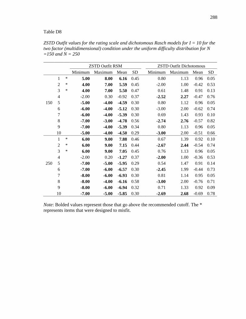
288

Table D8

ZSTD Outfit values for the rating scale and dichotomous Rasch models for I = 10 for the


=150 and N = 250

ZSTD Outfit RSM ZSTD Outfit Dichotomous


1 * 5.00 8.00 6.16 0.45 0.80 1.13 0.96 0.05

2 * 4.00 7.00 5.59 0.45 -2.00 1.00 -0.42 0.53

3 * 4.00 7.00 5.50 0.47 0.61 1.48 0.91 0.13

4 -2.00 0.30 -0.92 0.37 -2.52 2.27 -0.47 0.76

150 5 -5.00 -4.00 -4.59 0.30 0.80 1.12 0.96 0.05

6 -6.00 -4.00 -5.12 0.30 -3.00 2.00 -0.62 0.74

7 -6.00 -4.00 -5.39 0.30 0.69 1.43 0.93 0.10

8 -7.00 -3.00 -4.78 0.56 -2.74 2.76 -0.57 0.82

9 -7.00 -4.00 -5.39 0.34 0.80 1.13 0.96 0.05

10 -5.00 -4.00 -4.50 0.29 -3.00 2.00 -0.51 0.66

1 * 6.00 9.00 7.88 0.46 0.67 1.39 0.92 0.10

2 * 6.00 9.00 7.15 0.44 -2.67 2.44 -0.54 0.74

3 * 6.00 9.00 7.05 0.45 0.76 1.13 0.96 0.05

4 -2.00 0.20 -1.27 0.37 -2.00 1.00 -0.36 0.53

250 5 -7.00 -5.00 -5.95 0.29 0.54 1.47 0.91 0.14

6 -7.00 -6.00 -6.57 0.30 -2.45 1.99 -0.44 0.73

7 -8.00 -6.00 -6.93 0.30 0.81 1.14 0.95 0.05

8 -8.00 -4.00 -6.16 0.58 -3.00 2.00 -0.76 0.71

9 -8.00 -6.00 -6.94 0.32 0.71 1.33 0.92 0.09

10 -7.00 -5.00 -5.85 0.30 -2.69 2.68 -0.69 0.78



Robustness of Rasch Fit Statistics in Dichotomous and Rating ...

Documents

Transcript of Robustness of Rasch Fit Statistics in Dichotomous and Rating ...