INTERNET DELAY STATISTICS: DETERMINATION AND MEASUREMENT

OF SOCIAL CONNECTEDNESS USING A DICHOTOMOUS HURST

PARAMETER

by

MARK L. DEVIRGILIO

A THESIS

Submitted in partial fulfillment of the requirements

for the Master of Science in Engineering

in

The Department of Electrical and Computer Engineering

to

The School of Graduate Studies

of

The University of Alabama in Huntsville

HUNTSVILLE, ALABAMA

2010

ii

iii

THESIS APPROVAL PAGE

Submitted by Mark DeVirgilio in partial fulfillment of the requirements for the degree of

Master of Science in Engineering and accepted on behalf of the Faculty of the School of

Graduate Studies by the thesis committee.

We, the undersigned members of the Graduate Faculty of The University of Alabama in

Huntsville, certify that we have advised and supervised the candidate on the work

described in this thesis. We further certify that we have reviewed the thesis manuscript

and approve it in partial fulfillment of the requirements for the degree of Master of

Science in Engineering.

iv

ABSTRACT

The School of Graduate Studies

The University of Alabama in Huntsville

Degree: Master of Science in Engineering

College/Dept.: Engineering/Electrical and Computer Engineering

Name of Candidate: Mark L. DeVirgilio

Title: Internet delay statistics: Determination and measurement of social connectedness

using a dichotomous Hurst parameter

As Internet delay times become more important to the social status of recreational

Internet users, the ability to differentiate among sites and users using statistical measures

beyond average packet delays may be of commercial value. One such statistical measure

is the Hurst parameter of a long-range dependent process. A Hurst parameter can be used

as a measure of a communication system’s burstiness or peculiarity. The notion of

measuring a dichotomous Hurst parameter from segmented day and night delay data is

introduced in order to capture changes in Internet delay statistics caused by human

activity, site performance, and the autonomous systems of the Internet. This thesis

documents the development and implementation of an analytical tool that can measure

dichotomous Hurst parameters. Confirmations of dichotomous Hurst parameters were

obtained at the 95% confidence level for several popular Internet sites from around the

world. The theoretical basis and subsequent usefulness of a dichotomous Hurst parameter

are also discussed in this thesis.

v

ACKNOWLEDGMENTS

I would like to thank Dr. Pan for his patient guidance and willingness to teach an

old dog new tricks. He was able to steer my interests in Internet radar and analogous

delay statistics toward the development of a useful measurement tool and the examination

of long-range dependent statistical processes. I would also like to thank Dr. Wu for

listening to my narrow view of mathematics and suggesting the value of a dichotomous

Hurst parameter. In addition, I would like to thank Dr. Joiner for providing a meticulous

and independent assessment to ensure my research did not founder on technical issues or

mathematical hurdles.

vi

TABLE OF CONTENTS

Page

LIST OF FIGURES .......................................................................................................... vii

LIST OF ABBREVIATIONS AND ACRONYMS .......................................................... ix

LIST OF SYMBOLS ...........................................................................................................x

Chapter

1. INTRODUCTION ........................................................................................................ 1

2. BACKGROUND, PRACTICE, AND THEORY ......................................................... 4

3. DEVELOPMENT AND CALIBRATION OF HURST PARAMETER

MEASUREMENT TOOL ......................................................................................... 14

4. EXPERIMENT, RESULTS, AND DISCUSSION ..................................................... 21

5. CONCLUSION AND APPLICATION ...................................................................... 42

APPENDIX A: Code for FARIMA (0,d,0) Generation .................................................... 46

APPENDIX B: Code for Hurst Parameter Measurements ............................................... 48

REFERENCES ................................................................................................................. 50

vii

LIST OF FIGURES

Figure Page

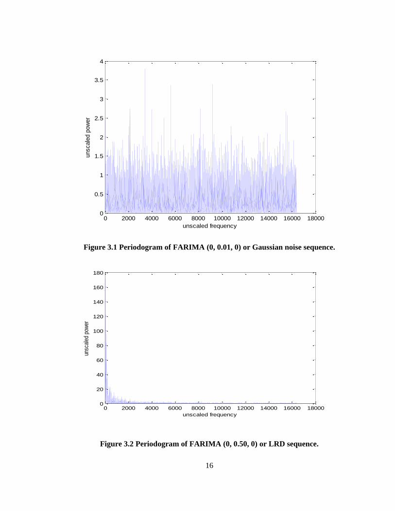
3.1 Periodogram of FARIMA (0, 0.01, 0) or Gaussian noise sequence. ........................ 16

3.2 Periodogram of FARIMA (0, 0.50, 0) or LRD sequence. ........................................ 16

3.3 Log-log periodogram using half the spectral components. ....................................... 18

3.4 Log-log periodogram using only low frequency components. ................................. 19

3.5 Mean and standard deviations of the measuring tool outputs. .................................. 20

4.1 Successful data collection sites. ................................................................................ 22

4.2 Typical Linux shell scrip. ......................................................................................... 22

4.3 Apple raw data and final column format. ................................................................. 24

4.4 Tata Motors delays sampled during Central time day. ............................................. 25

4.5 Baidu delays sampled during Central time day. ....................................................... 27

4.6 Baidu delays sampled during Central time night. ..................................................... 27

4.7 Baidu delay difference from median......................................................................... 28

4.8 Baidu delay difference periodogram. ........................................................................ 29

4.9 Baidu night Central time regression line. ................................................................. 30

4.10 Baidu day Central time regression line. .................................................................. 31

4.11 Hurst parameter measurement summary. ............................................................... 32

viii

4.12 Hurst parameter change direction. .......................................................................... 35

4.13 Apple Hurst parameters at different Central time starting points. .......................... 36

4.14 Google Hurst parameters at different Central time starting points. ........................ 37

4.15 Tata Motors Hurst parameters at different Central time starting points. ................ 38

4.16 Baidu data clipped at three sigma above median delay. ......................................... 39

4.17 Baidu using half of the available spectral components. .......................................... 40

ix

LIST OF ABBREVIATIONS AND ACRONYMS

ACF autocorrelation function

ARIMA autoregressive integrated moving average

AS autonomous systems

FARIMA (p,d,q) fractional autoregressive integrated moving average

where (p=autoregressive, d=differencing, q=moving average)

ICMP Internet Control Message Protocol

IID independent and identically distributed

IP Internet protocol

LRD long-range dependent

NIST National Institute of Science and Technology

PING Packet InterNet Groper

RFC Request for comments

R/S rescaled adjusted range

RTO retransmission timeout

SS self-similar

std standard deviation

TCP Transmission Control Protocol

URL Uniform resource locator

var variance

x

LIST OF SYMBOLS

linear regression constant term

linear regression slope term

d fractional differencing exponent

H Hurst parameter

frequency steps

autocorrelation function (ACF)

variance

1

CHAPTER 1

INTRODUCTION

While the birth of the Internet was a highlight of the 20th century, the

21st century is celebrating the growth of the Internet in connecting and enriching the lives

of millions. Social applications such as Facebook, YouTube, and World of Warcraft

(WoW) are enabling social connectedness and asserting claims for more bandwidth and

less packet delays from Internet servers and the backbone of autonomous systems (AS).

Few nascent Internet researchers in the 1980s would have predicted the scope of online

social networks, but marketing claims such as WoW's advertisement of "8 million players

in the World’s leading massively multiplayer role playing game" suggest that a

significant portion of the Internet's capability is dedicated to social interactions [1]. New

social classes are being determined by Internet delays. For example, when a Ventrilo

Voice over IP chat is attempted by new user or "newbie" and produces a time-distorted

drawl, this weak connectedness is sufficient to place the newbie on the bottom of his or

her online social order. Soon newbies learn that connecting during certain hours can

reduce Internet delays and thus help with their online social ascendency. A good research

question to pursue is as follows: What are the deeper statistics behind changing Internet

packet delays when examined from a socially relevant time scale measured in minutes

and days?

2

Previous researchers have left this time scale relatively unexplored. One reason is

because the famous Bellcore network delay data from the early 1990s had a sampling

time scale in the milliseconds. Leland et al. [2] used these sampling times to produce

about a day’s worth of data for different Ethernet links as limited by the extant logging

equipment. The resulting time series data were sufficient to demonstrate in a visual sense

the self-similarity (SS) of network delays. In addition, the resulting time series were short

enough to limit suspected variations in the first and second moments, which would have

spoiled the mathematics behind the related phenomenon of long-range dependence

(LRD). In the engineering realm, a time series is said to have the properties of long-range

dependence if the shape of its autocorrelation function exhibits a slow decay. A Hurst

parameter can be used to describe this decay, and the parameter can theoretically vary

between 0.5 and 1.0. The lower value suggests no LRD, while the higher value suggests

interactions are taking place. In the online social interaction realm, higher Hurst numbers

may indicate a busier or more bursty connection to an Internet accessible site or server.

Despite their sampling time choices, these researchers still noticed that variations

in network delay times threatened their arguments for LRD, when ten-second and above

sampling times were used. Thus, current research on Internet delays covering periods

from minutes to days is sparse, as weak sense stationary (WSS) assumptions necessary

for cleaner LRD mathematics may be violated by diurnal fluctuations. In contrast to delay

time research, current research on a related phenomenon of Internet traffic congestion

and its commensurate LRD properties is vibrant. WSS assumptions are readily met by the

commonly used millisecond time sampling intervals. Unfortunately, millisecond time

scales are of lower importance to social connectedness.

3

Two motivational elements for this study are the sparse research on suspected

diurnal variations in delay time statistics and the dramatic changes in the Internet since

Leland et al. conducted their study almost two decades ago. A search of the literature

found that in 2005, Iranian researchers identified diurnal and weekly delay time patterns

while analyzing Internet data taken among interconnected computers within their country

[3]. However, Internet delay data taken in 2009 by the author of this thesis failed to show

simple diurnal variations in mean delay times when communicating with local and

international Internet sites and servers. In addition, this author suspects that diurnal

variations may be artifacts of regional computer networks that rely on a limited set of

Internet router domains or autonomous systems (AS). The lack of recently observed

diurnal variations and the possibility of detecting social interaction effects provided

additional motivation to search deeper into the statistical properties of Internet delay data.

This thesis is arranged into five chapters. Chapter 2 presents the background on

the phenomena of long-range dependence and its associated statistical properties.

Chapter 3 presents the development and calibration of a dichotomous Hurst parameter

measurement tool. Chapter 4 presents the details of the data collection and measurement

tool outputs. The measurement results are in a tabular form, and a busy reader may want

to examine this section first. Chapter 5 presents a conclusion and suggests additional uses

for a novel statistic on Internet delays.

4

CHAPTER 2

BACKGROUND, PRACTICE, AND THEORY

Few discussions on the physical phenomena of long-range dependence (LRD)

would be complete without mentioning the work of Hurst on describing the historical

flood patterns of the Nile Basin. He discovered that flooding patterns could not be

adequately characterized by Markovian processes, which are usually associated with

independent and identically distributed (IID) random variables [4]. Yet, the distribution

of flood levels appeared to have a Gaussian shape. While Hurst did not find a 7-year

Joseph effect pattern of cyclic variations, he did find patterns within patterns, in which

longer periods of higher or lower flooding were interspersed by shorter periods of lower

or higher flooding respectively [5]. These repeated underlying patterns found in higher-

level patterns was a sign of self-similarity. Hurst suggested that physical phenomena such

as sunspots, changing evaporation rates, or river silting created a memory effect in the

flood patterns [4]. This effect was apparent across different historical time scales.

The eponymous Hurst parameter, which in the context of this thesis can vary

around 0.5 to 1.0, will be used to describe certain LRD processes. A Hurst parameter of

0.5 describes a statistical process whose elements are independent and can be derived

from a Gaussian distribution. Brownian motion or a Wiener process can be described by

a Hurst parameter of 0.5, and this process is Markovian. Hurst observed that the periods

5

of Nile Basin floods had a Hurst parameter well above 0.5, which strongly suggested

long-range dependence. Rhythmic flooding could have affected the Hurst parameter, as

the flooding frequencies would have distorted the characteristic decaying exponential

shape of the spectral density. This spectral density shape idea is important, and this thesis

will use the logarithmic slope of a periodogram to estimate the Hurst parameter.

A decade after Hurst published his work suggesting that a LRD pattern described

Nile flooding events, Mandelbrot refined a related idea of self-similar (SS) patterns when

he examined clusters of errors in communication traffic. One standard approach of the era

was to model communication errors as a memoryless process based on a geometric

distribution. Mandelbrot’s contribution to electrical engineering was the introduction of a

property called conditional stationarity, which implies that future probabilities are

dependent on events or conditions that have already occurred. In his words, Mandelbrot

[6] believed that “this conditional concept may be the key to the necessary task of

describing the structure of many empirical intermittent phenomena.” It was not until the

early 1980s that researchers began collecting Internet delay statistics and started to notice

burst-like or memory effects.

Mills, in 1983, wrote a comprehensive Request for Comments 889 (RFC) on

Internet delay measurements. He used a tool called Packet InterNet Groper (PING) that

could send Internet Control Message Protocol (ICMP) packets to probe Internet

Transmission Control Protocol (TCP) transmission delays. The reader should note that

TCP packets are sent on a connection basis, while ICMP packets sent on a connectionless

basis. Mills [7] discounted this technical difference and found that “The incidence of

6

long-delay bursts, or glitches, varied widely during the experiments. ... Glitches did not

seem to correlate well with increases in baseline delay, which occurs as the result of

traffic surges.” The author of this thesis will use TCP packet delays to avoid potential

sources of errors arising from the use of connectionless ICMP packets. Despite the

protocol issue, Mills’ work was taken as early evidence of LRD phenomena in Internet

packet delays, and it was not until the early 1990s that researchers quantitatively

associated LRD and SS phenomena with Internet delay statistics

In 1994, Leland et al. [2] analyzed Bellcore network data and used a Hurst

parameter to characterize the self-similarity of the observed patterns. Their primary

mathematical assumption was to treat the time sequence of delay data, X(k), as

covariance stationary or what is known as wide-sense stationary (WSS). This allowed

them to approximate the autocorrelation function (ACF) , by

, (2.1)

where

k = 0,1,2, ...

H = Hurst parameter and limited such that

L(t) = slowly varying time function.

Next, these researchers created a new process

from the first time series by

averaging elements of X(k) in blocks of size m and by ensuring that these blocks were

7

non-overlapping and sequential. Thus,

is the average of the first 50 elements from

X(k) and

is the average of the third set of 50 elements from X(k). The use of the

variable m for the new process’ block size and not an exponent is a source of confusion,

so one needs to be cautious. The new sequence is “second order self-similar” because of

the WSS condition placed on the original time series.

(2.2)

, (2.3)

where

variance of rescaled time series

k = 0,1,2, ...

m = 0,1,2, ... .

In addition, Leland et al. suggested that if the WSS condition was not rigorously

met, then the sequence could still be “asymptotically self-similar”:

. (2.4)

In practical terms, if a time series cannot be proven to be WSS, then a researcher can

make an assumption that it is so in the limit and must collect as much data as possible to

satisfy the limit concerns. The notion of favoring very long block sizes or the frequency

domain equivalent of using the lower frequency spectral components will be addressed in

8

this thesis. From Equation 2.2, one can see that the log of the m-block sized variances

plotted against the log of various m-values can yield an estimate for the Hurst parameter.

More striking to these researchers was the realization that time plots of the new

sequences showed the features of self-similarity over timescales of 0.01, 0.1, 1.0, 10.0,

and 100.0 seconds and had common features of delay burst patterns. The Bellcore

network traffic data thus showed the features of Mandelbrot’s self-similarity, and these

researchers associated LRD characteristics to most of the data. Likewise, this thesis

assumes that Internet delay data has SS and LRD properties that can be teased out by

using simple manipulations of the data.

Leland et al. used a more sophisticated technique to calculate Hurst parameters.

According to these researchers [2], “The absence of any limit law results for the statistics

corresponding to the R/S analysis or the variance plot make them inadequate for a more

refined data analysis.” The issue facing them was the slow convergence of the

covariances after many or infinitely many steps. Such convergence concerns and

associated proofs of central limit theorems are beyond the scope of this thesis. In

addition, Pacheco, Roman, and Vargas [8] reported in 2008 that rescaled adjusted range

(R/S) techniques required 60,000 data points in order to converge at Hurst parameters

above 0.73. A quick calculation showed that delay data sampled every ten seconds for a

week and then split into day and night segments would fall short by 30,000 points. Thus,

it was decided not to use R/S methods or the slopes found in the variance versus block

size plots to measure Hurst parameters.

9

Without being able to describe mathematically the first and second moment

functions of real Internet delay data, one has to examine reports of non-stationary data. If

such data were common, then measurements of Hurst parameters would not be fruitful.

Although not published in a refereed journal, Mukherjee's [9] 1992 work is frequently

cited as being one of the first to recognize diurnal variations in Internet delay times.

Diurnal variations would imply that Internet delay times are not stationary in their first

moment, which violates a condition for LRD or SS behaviors. Therefore, all delay data

should be inspected for significant diurnal variations around their means. Judging from

Mukherjee’s report, a 5% variation in the mean would be significant. Internet delay data

exceeding such a variation limit could not be used because of the complexities in

developing a suitable Hurst parameter measurement tool for non-WSS data. Luckily, no

significant variations in the mean or median delay times were found in the data from

11 Internet sites.

Finding a bounding function for the delay data as shown in (2.1) would make

the mathematics more tractable and would aid in a more direct calculation of a Hurst

parameter. Maejima [10] discussed the mathematics behind the weak convergence of

infinite sequences with growing variances. However, the possibility of guessing a

bounding function for the underlying stochastic process was remote, as specific Internet

delay mechanisms were not investigated as part of this thesis. Thus, an empirical

approach was needed to measure Hurst parameters, even at the expense of losing some

statistical information. Understanding the relation between the autocorrelation function

and the spectral power density according to the Wiener-Khinchin-Einstein theorem

10

suggested that a frequency domain technique could yield statistically valid Hurst

parameters.

A frequency domain approach to measuring Hurst parameters was chosen, and

this approach uses periodograms or power spectral density plots. These plots can be

readily created using a discrete Fourier transform of the time series data. Engineering

analysis tools such as MATLAB have built in periodogram routines. Indeed, Moulines

and Soulier [11] in an article titled “Semiparametric spectral estimation for fractional

processes” summarized the extant methods for measuring Hurst parameters from

periodograms. Some of these methods were quite involved, as their goal was to support

each step of a particular method by mathematically rigorous arguments. However, one of

the salient points for most of their methods was that the lower frequency components of

the power spectral density plot were more important than the higher frequency

components in characterizing self-similarity or long-range dependence.

The infinite m-block size issue was alluded to earlier in this chapter. This issue is

notionally matched to collecting data for long time intervals, which allows for the

capturing of low frequency components. Cappe et al. [12] discussed the equivalence of

using low frequency components and the aggregation of longer and longer time blocks in

the R/S method. They also discussed the nuances of limiting the bandwidth. One positive

effect was to reduce the bias in the Hurst parameter estimate, and one negative effect was

to increase the variance by limiting the number of samples. Their recommendation that a

“careful choice of the bandwidth should ideally mitigate these two effects” was not

quantified. A trial and error method was thus indicated, with a preference given to the

11

lower frequency components. By discounting higher frequency components, the complete

statistical nature of the times series is sacrificed. Yet, the selected lower frequencies

allow for measurements of Hurst parameters, which are of primary interest to this thesis.

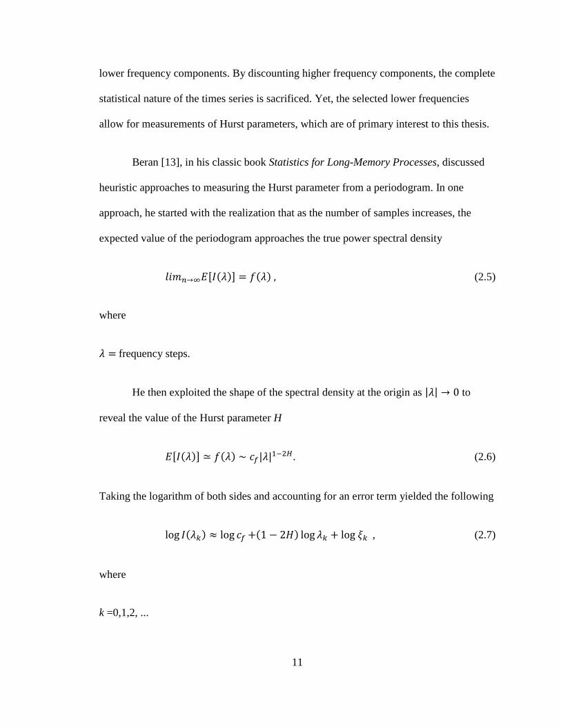
Beran [13], in his classic book Statistics for Long-Memory Processes, discussed

heuristic approaches to measuring the Hurst parameter from a periodogram. In one

approach, he started with the realization that as the number of samples increases, the

expected value of the periodogram approaches the true power spectral density

(2.5)

where

frequency steps.

He then exploited the shape of the spectral density at the origin as to

reveal the value of the Hurst parameter H

. (2.6)

Taking the logarithm of both sides and accounting for an error term yielded the following

, (2.7)

where

k =0,1,2, ...

12

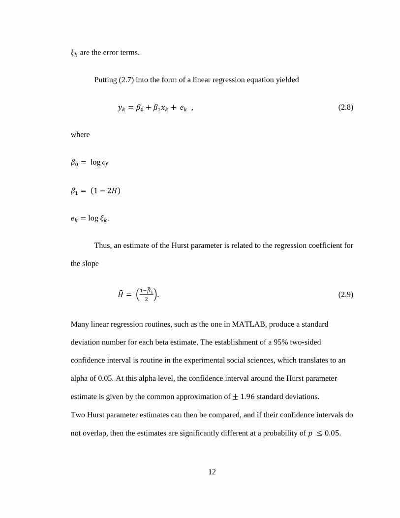
are the error terms.

Putting (2.7) into the form of a linear regression equation yielded

, (2.8)

where

.

Thus, an estimate of the Hurst parameter is related to the regression coefficient for

the slope

. (2.9)

Many linear regression routines, such as the one in MATLAB, produce a standard

deviation number for each beta estimate. The establishment of a 95% two-sided

confidence interval is routine in the experimental social sciences, which translates to an

alpha of 0.05. At this alpha level, the confidence interval around the Hurst parameter

estimate is given by the common approximation of standard deviations.

Two Hurst parameter estimates can then be compared, and if their confidence intervals do

not overlap, then the estimates are significantly different at a probability of

13

Beran did not provide advice on k or the number of low frequency components to

measure. Chapter 3 answers this question by first creating calibration sequences to test

the statistical nature of a Hurst parameter estimation tool and then by tuning the tool with

actual data.

14

CHAPTER 3

DEVELOPMENT AND CALIBRATION OF HURST PARAMETER

MEASUREMENT TOOL

The first task was the generation of time series data that reflected Hurst

parameters in the range from about 0.5 to 1.0. The pioneering work of Granger and

Joyeux [14] in the early 1980s on the fractional differencing of the autoregressive part of

a time series generator now allows for the easy production of calibration sequences.

These researchers introduced the idea of using fractional differencing of an

autoregressive integrated moving average (ARIMA) model to simulate long-memory

time series. They adjusted a differencing parameter in the model to produce a time series

that would mimic the spectral density of a long-memory time series. Granger was focused

on modifying and applying time series models to problems in the field of economics, and

he subsequently applied his work to distant areas such as the environment. His Nobel

Prize suggested that his work was applicable to diverse fields such as engineering.

One such modified ARIMA model is called a Fractional Autoregressive

Integrated Moving Average (FARIMA) model with parameters (p, d, q). Parameters p

and q represent the powers of the autoregressive and moving average functions. For this

thesis, p and q are set to 0, which implies that the FARIMA generator will create a time

series determined by the fractional differencing variable d and defined by

15

, (3.1)

whereby is a sampled Gaussian random process and d is the fractional differencing

exponent [13]. This exponent is related directly to the Hurst parameter by

There are several ways to use a supplied d to create fractional differencing, and

the chosen method uses 100 integrations of a gamma function to create the effect. The

generator was implemented in MATLAB code that is shown in Appendix A, and a

reference to the algorithm’s source is in the code [15]. The generator outputs are better

viewed in the frequency domain, as it is hard to distinguish between FARIMA time series

generated with different Hurst parameters. The periodogram of the generator output for H

= 0.51 or d = 0.01 is close to fractional Brownian motion and is shown in Figure 3.1.

Please note that the generator cannot take H = 0.50 as an input because of a discontinuity

at this point. The periodogram for H = 1.0 or d = 0.5 is that of a strong LRD process and

is shown in Figure 3.2. The expected exponential decay of the spectral envelope is

apparent.

The development of MATLAB code for the Hurst parameter measurement tool

was a straightforward task, because the periodogram and linear regression routines are

built-in functions and MATLAB handles large data arrays in a natural fashion. Raw time

series data containing over 70,000 points were expected. This number comes about from

sampling Internet delays every 10 seconds for over a week. The code is in Appendix B.

However, two practical modifications recursively learned from running the tool against

trial data need to be discussed.

16

Figure 3.1 Periodogram of FARIMA (0, 0.01, 0) or Gaussian noise sequence.

Figure 3.2 Periodogram of FARIMA (0, 0.50, 0) or LRD sequence.

0 2000 4000 6000 8000 10000 12000 14000 16000 180000

0.5

1

1.5

2

2.5

3

3.5

4

unscaled frequency

unscale

d p

ow

er

0 2000 4000 6000 8000 10000 12000 14000 16000 180000

20

40

60

80

100

120

140

160

180

unscaled frequency

unsc

aled

pow

er

17

The first modification involved differencing the time sequence data from the

median instead of the mean to even out the distribution skew and to center it around zero

delay. This modification had minimal effect when processing the FARIMA generated

sequences because the mean and median of the symmetrical underlying normal

distribution are theoretically the same. For example, the same 60,000 element FARIMA

(0, H=0.75, 0) sequence produced a mean of 0.0436 seconds and a Hurst parameter of

0.7200 with a 95% confidence interval from 0.7037 to 0.7362. Using a median of

0.0393 seconds, the measurement tool produced a Hurst parameter of 0.7498 with a

95% confidence interval from 0.7356 to 0.7634. The change is slight, but noticeable.

Differencing from the median ensured that most results from preliminary real-world data

fell within the desired Hurst parameter boundaries of 0.5 to 1.0. A rationale for this

decision was that real data is more symmetrical around the median when compared to the

mean because of the distorting effects of long-delay outliers. Internet delays cannot be

shorter than the propagation delay and processing time of around 10 to 200 milliseconds,

but can extend outwards to many seconds.

The second modification of the measurement tool involved selecting the low

frequency or local components of the periodogram that will support the regression

estimate of the slope. The effects of this modification could not be verified with the

FARIMA generated calibration sequences because of an idiosyncrasy of the generation

method. Global use of the entire periodogram is inherently more accurate when analyzing

FARIMA generated sequences. This result has been reported in the literature, and the

performance over using low frequency components is further accentuated when the Hurst

parameter approaches 1.0 [16]. Figure 3.3 shows the performance of the measuring tool

18

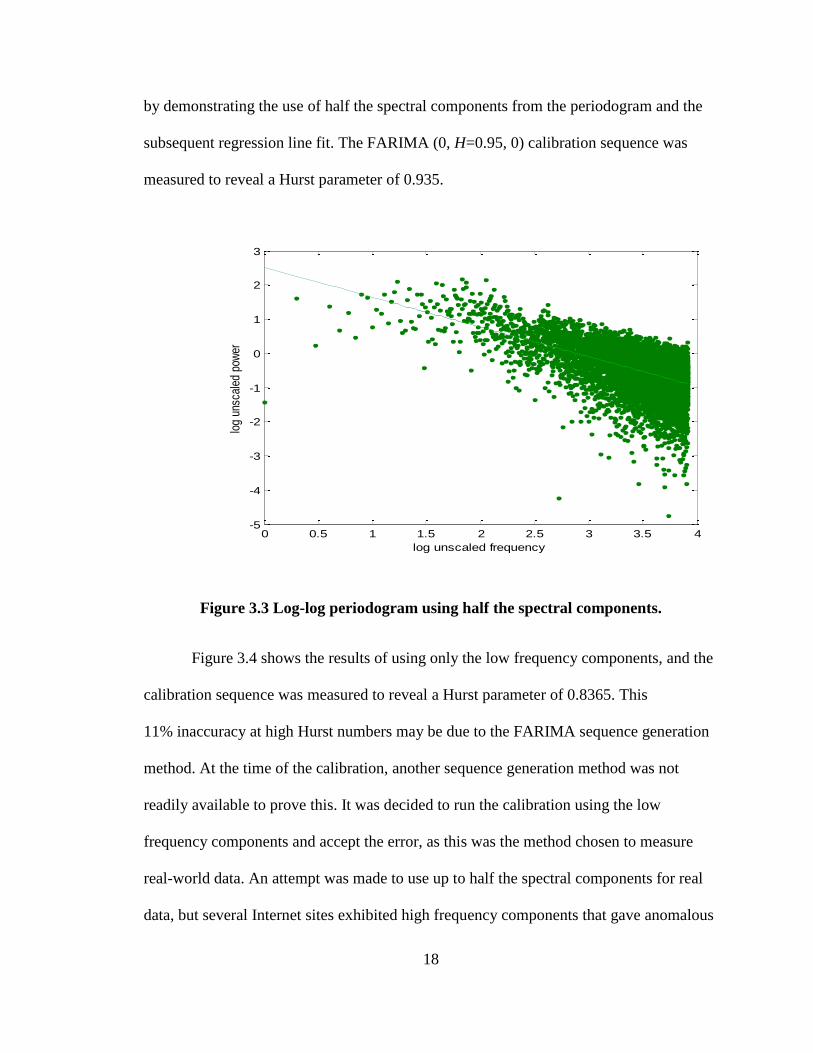
by demonstrating the use of half the spectral components from the periodogram and the

subsequent regression line fit. The FARIMA (0, H=0.95, 0) calibration sequence was

measured to reveal a Hurst parameter of 0.935.

Figure 3.3 Log-log periodogram using half the spectral components.

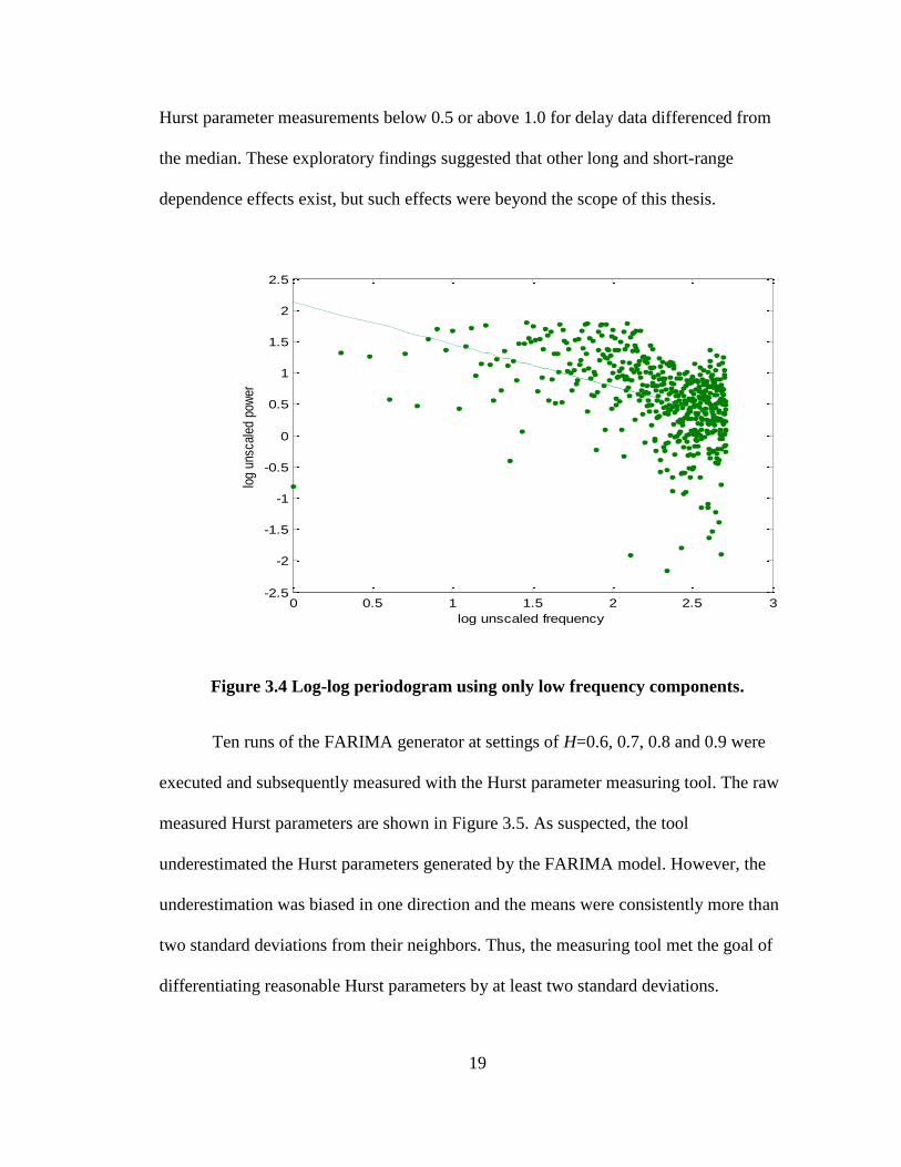
Figure 3.4 shows the results of using only the low frequency components, and the

calibration sequence was measured to reveal a Hurst parameter of 0.8365. This

11% inaccuracy at high Hurst numbers may be due to the FARIMA sequence generation

method. At the time of the calibration, another sequence generation method was not

readily available to prove this. It was decided to run the calibration using the low

frequency components and accept the error, as this was the method chosen to measure

real-world data. An attempt was made to use up to half the spectral components for real

data, but several Internet sites exhibited high frequency components that gave anomalous

0 0.5 1 1.5 2 2.5 3 3.5 4-5

-4

-3

-2

-1

0

1

2

3

log unscaled frequency

log

unsc

aled

pow

er

19

Hurst parameter measurements below 0.5 or above 1.0 for delay data differenced from

the median. These exploratory findings suggested that other long and short-range

dependence effects exist, but such effects were beyond the scope of this thesis.

Figure 3.4 Log-log periodogram using only low frequency components.

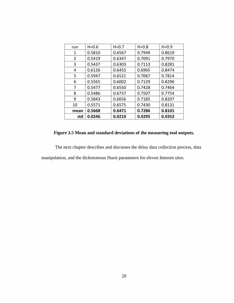
Ten runs of the FARIMA generator at settings of H=0.6, 0.7, 0.8 and 0.9 were

executed and subsequently measured with the Hurst parameter measuring tool. The raw

measured Hurst parameters are shown in Figure 3.5. As suspected, the tool

underestimated the Hurst parameters generated by the FARIMA model. However, the

underestimation was biased in one direction and the means were consistently more than

two standard deviations from their neighbors. Thus, the measuring tool met the goal of

differentiating reasonable Hurst parameters by at least two standard deviations.

0 0.5 1 1.5 2 2.5 3-2.5

-2

-1.5

-1

-0.5

0

0.5

1

1.5

2

2.5

log unscaled frequency

log

unsc

aled

pow

er

20

run H=0.6 H=0.7 H=0.8 H=0.9

1 0.5810 0.6567 0.7949 0.8619

2 0.5419 0.6347 0.7091 0.7970

3 0.5437 0.6303 0.7113 0.8281

4 0.6126 0.6455 0.6965 0.8474

5 0.5947 0.6521 0.7067 0.7814

6 0.5565 0.6002 0.7129 0.8296

7 0.5477 0.6550 0.7428 0.7464

8 0.5486 0.6737 0.7507 0.7754

9 0.5843 0.6656 0.7185 0.8207

10 0.5571 0.6575 0.7430 0.8131

mean 0.5668 0.6471 0.7286 0.8101

std 0.0246 0.0210 0.0295 0.0352

Figure 3.5 Mean and standard deviations of the measuring tool outputs.

The next chapter describes and discusses the delay data collection process, data

manipulation, and the dichotomous Hurst parameters for eleven Internet sites.

21

CHAPTER 4

EXPERIMENT, RESULTS, AND DISCUSSION

The selection of destination Internet sites from which to collect delay data from

was an idiosyncratic process, and the process relied on the familiarity of candidate sites

with this author. The only guiding rule was that the sponsors of these sites have a

worldwide distribution. Data collection from over twenty sites was attempted, and each

attempt was done in isolation to prevent overload or queuing bias of the Blackhawk

Linux server. The server IP address was 146.229.162.184, and it was located at the

University of Alabama in Huntsville. Collection periods averaged two weeks, and eleven

sites were successfully sampled. A success was indicated when at least a week’s worth of

uninterrupted data was collected. Ten or so failures were attributed to maintenance on the

Blackhawk server, power outages, remote site problems, or Internet router issues. The

common names, IP addresses, and collection dates are listed in Figure 4.1. The Google

site required the use of its URL, as it rotated through several IP addresses. Thus, the last

octet is marked with an asterisk. The Japanese traceroute server went offline, so the last

consistently responding server in the path was used. Its IP address is listed in the

comment field.

22

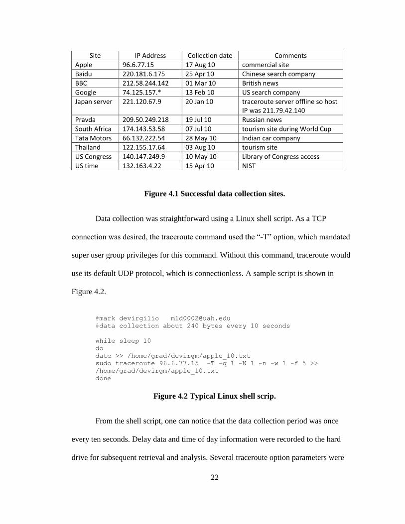
Figure 4.1 Successful data collection sites.

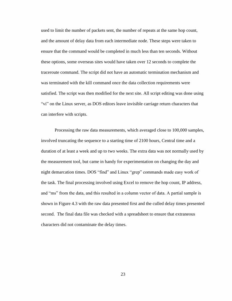
Data collection was straightforward using a Linux shell script. As a TCP

connection was desired, the traceroute command used the “-T” option, which mandated

super user group privileges for this command. Without this command, traceroute would

use its default UDP protocol, which is connectionless. A sample script is shown in

Figure 4.2.

#mark devirgilio mld0002@uah.edu

#data collection about 240 bytes every 10 seconds

while sleep 10

do

date >> /home/grad/devirgm/apple_10.txt

sudo traceroute 96.6.77.15 -T -q 1 -N 1 -n -w 1 -f 5 >>

/home/grad/devirgm/apple_10.txt

done

Figure 4.2 Typical Linux shell scrip.

From the shell script, one can notice that the data collection period was once

every ten seconds. Delay data and time of day information were recorded to the hard

drive for subsequent retrieval and analysis. Several traceroute option parameters were

Site IP Address Collection date Comments

Apple 96.6.77.15 17 Aug 10 commercial site

Baidu 220.181.6.175 25 Apr 10 Chinese search company

BBC 212.58.244.142 01 Mar 10 British news

Google 74.125.157.* 13 Feb 10 US search company

Japan server 221.120.67.9 20 Jan 10 traceroute server offline so host IP was 211.79.42.140

Pravda 209.50.249.218 19 Jul 10 Russian news

South Africa 174.143.53.58 07 Jul 10 tourism site during World Cup

Tata Motors 66.132.222.54 28 May 10 Indian car company

Thailand 122.155.17.64 03 Aug 10 tourism site

US Congress 140.147.249.9 10 May 10 Library of Congress access

US time 132.163.4.22 15 Apr 10 NIST

23

used to limit the number of packets sent, the number of repeats at the same hop count,

and the amount of delay data from each intermediate node. These steps were taken to

ensure that the command would be completed in much less than ten seconds. Without

these options, some overseas sites would have taken over 12 seconds to complete the

traceroute command. The script did not have an automatic termination mechanism and

was terminated with the kill command once the data collection requirements were

satisfied. The script was then modified for the next site. All script editing was done using

“vi” on the Linux server, as DOS editors leave invisible carriage return characters that

can interfere with scripts.

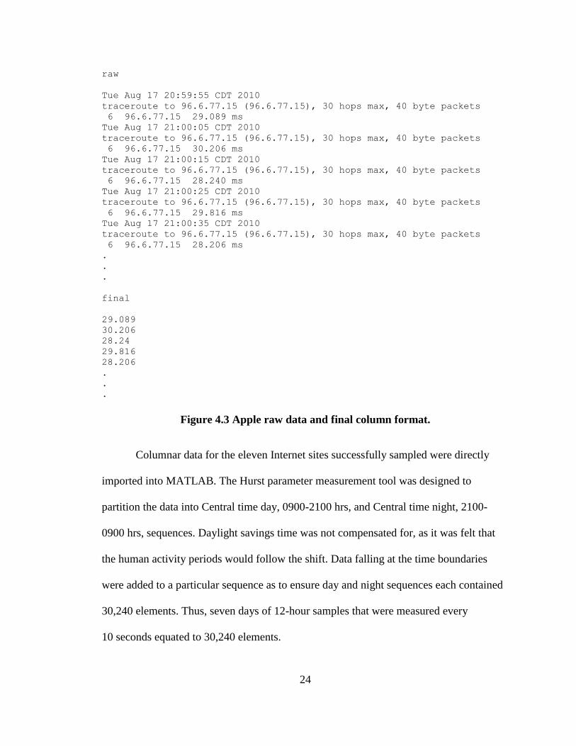
Processing the raw data measurements, which averaged close to 100,000 samples,

involved truncating the sequence to a starting time of 2100 hours, Central time and a

duration of at least a week and up to two weeks. The extra data was not normally used by

the measurement tool, but came in handy for experimentation on changing the day and

night demarcation times. DOS “find” and Linux “grep” commands made easy work of

the task. The final processing involved using Excel to remove the hop count, IP address,

and “ms” from the data, and this resulted in a column vector of data. A partial sample is

shown in Figure 4.3 with the raw data presented first and the culled delay times presented

second. The final data file was checked with a spreadsheet to ensure that extraneous

characters did not contaminate the delay times.

24

raw

Tue Aug 17 20:59:55 CDT 2010

traceroute to 96.6.77.15 (96.6.77.15), 30 hops max, 40 byte packets

6 96.6.77.15 29.089 ms

Tue Aug 17 21:00:05 CDT 2010

traceroute to 96.6.77.15 (96.6.77.15), 30 hops max, 40 byte packets

6 96.6.77.15 30.206 ms

Tue Aug 17 21:00:15 CDT 2010

traceroute to 96.6.77.15 (96.6.77.15), 30 hops max, 40 byte packets

6 96.6.77.15 28.240 ms

Tue Aug 17 21:00:25 CDT 2010

traceroute to 96.6.77.15 (96.6.77.15), 30 hops max, 40 byte packets

6 96.6.77.15 29.816 ms

Tue Aug 17 21:00:35 CDT 2010

traceroute to 96.6.77.15 (96.6.77.15), 30 hops max, 40 byte packets

6 96.6.77.15 28.206 ms

.

.

.

final

29.089

30.206

28.24

29.816

28.206

.

.

.

Figure 4.3 Apple raw data and final column format.

Columnar data for the eleven Internet sites successfully sampled were directly

imported into MATLAB. The Hurst parameter measurement tool was designed to

partition the data into Central time day, 0900-2100 hrs, and Central time night, 2100-

0900 hrs, sequences. Daylight savings time was not compensated for, as it was felt that

the human activity periods would follow the shift. Data falling at the time boundaries

were added to a particular sequence as to ensure day and night sequences each contained

30,240 elements. Thus, seven days of 12-hour samples that were measured every

10 seconds equated to 30,240 elements.

25

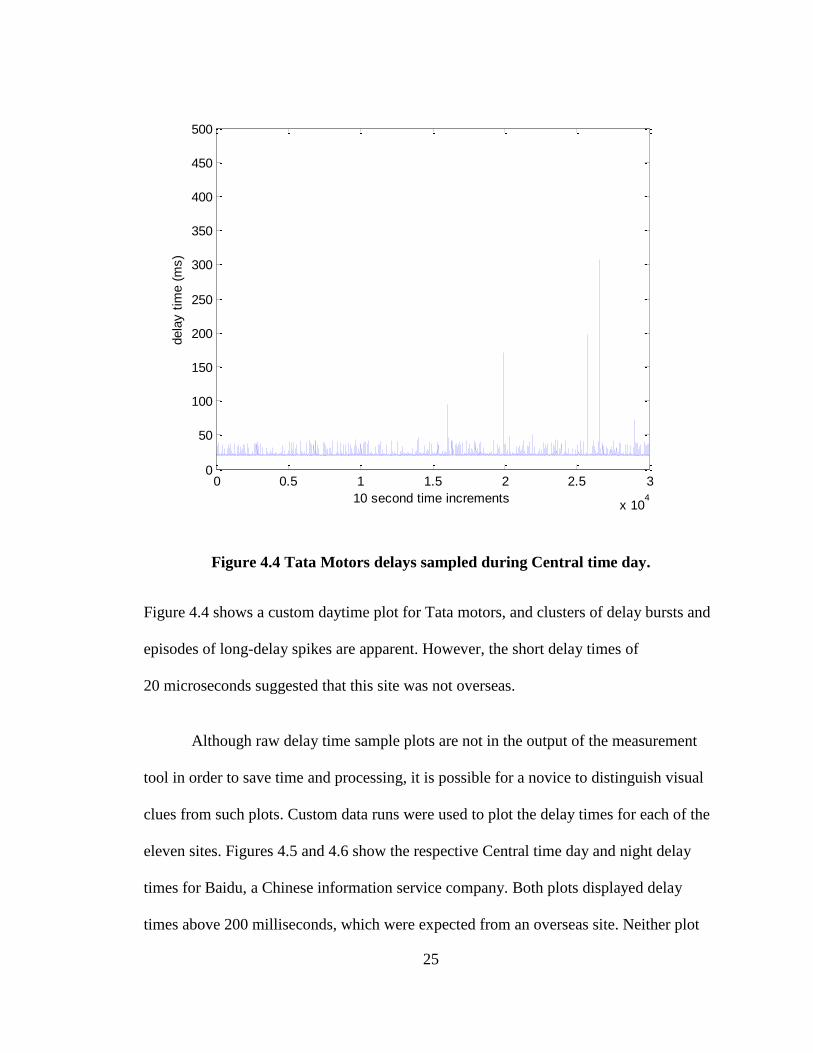
Figure 4.4 Tata Motors delays sampled during Central time day.

Figure 4.4 shows a custom daytime plot for Tata motors, and clusters of delay bursts and

episodes of long-delay spikes are apparent. However, the short delay times of

20 microseconds suggested that this site was not overseas.

Although raw delay time sample plots are not in the output of the measurement

tool in order to save time and processing, it is possible for a novice to distinguish visual

clues from such plots. Custom data runs were used to plot the delay times for each of the

eleven sites. Figures 4.5 and 4.6 show the respective Central time day and night delay

times for Baidu, a Chinese information service company. Both plots displayed delay

times above 200 milliseconds, which were expected from an overseas site. Neither plot

0 0.5 1 1.5 2 2.5 3

x 104

0

50

100

150

200

250

300

350

400

450

500

10 second time increments

dela

y t

ime (

ms)

26

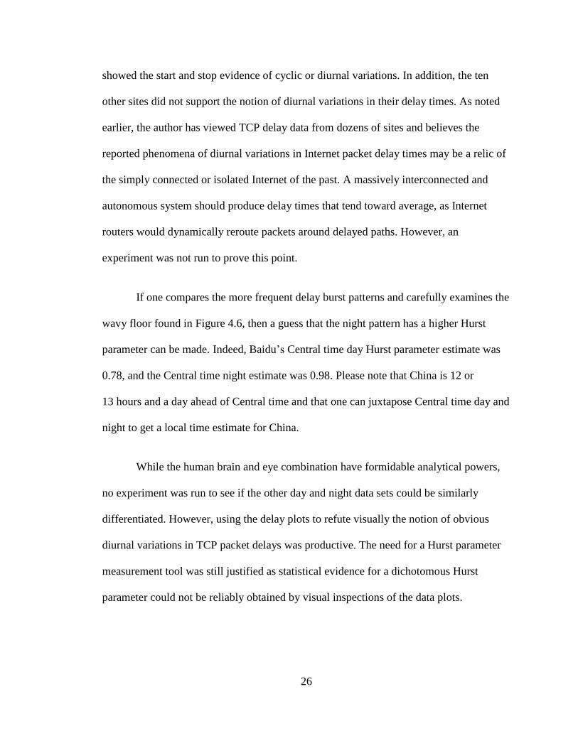
showed the start and stop evidence of cyclic or diurnal variations. In addition, the ten

other sites did not support the notion of diurnal variations in their delay times. As noted

earlier, the author has viewed TCP delay data from dozens of sites and believes the

reported phenomena of diurnal variations in Internet packet delay times may be a relic of

the simply connected or isolated Internet of the past. A massively interconnected and

autonomous system should produce delay times that tend toward average, as Internet

routers would dynamically reroute packets around delayed paths. However, an

experiment was not run to prove this point.

If one compares the more frequent delay burst patterns and carefully examines the

wavy floor found in Figure 4.6, then a guess that the night pattern has a higher Hurst

parameter can be made. Indeed, Baidu’s Central time day Hurst parameter estimate was

0.78, and the Central time night estimate was 0.98. Please note that China is 12 or

13 hours and a day ahead of Central time and that one can juxtapose Central time day and

night to get a local time estimate for China.

While the human brain and eye combination have formidable analytical powers,

no experiment was run to see if the other day and night data sets could be similarly

differentiated. However, using the delay plots to refute visually the notion of obvious

diurnal variations in TCP packet delays was productive. The need for a Hurst parameter

measurement tool was still justified as statistical evidence for a dichotomous Hurst

parameter could not be reliably obtained by visual inspections of the data plots.

27

Figure 4.5 Baidu delays sampled during Central time day.

Figure 4.6 Baidu delays sampled during Central time night.

0 0.5 1 1.5 2 2.5 3

x 104

0

500

1000

1500

10 second time increments

dela

y tim

e (m

s)

0 0.5 1 1.5 2 2.5 3

x 104

0

500

1000

1500

10 second time increments

dela

y tim

e (m

s)

28

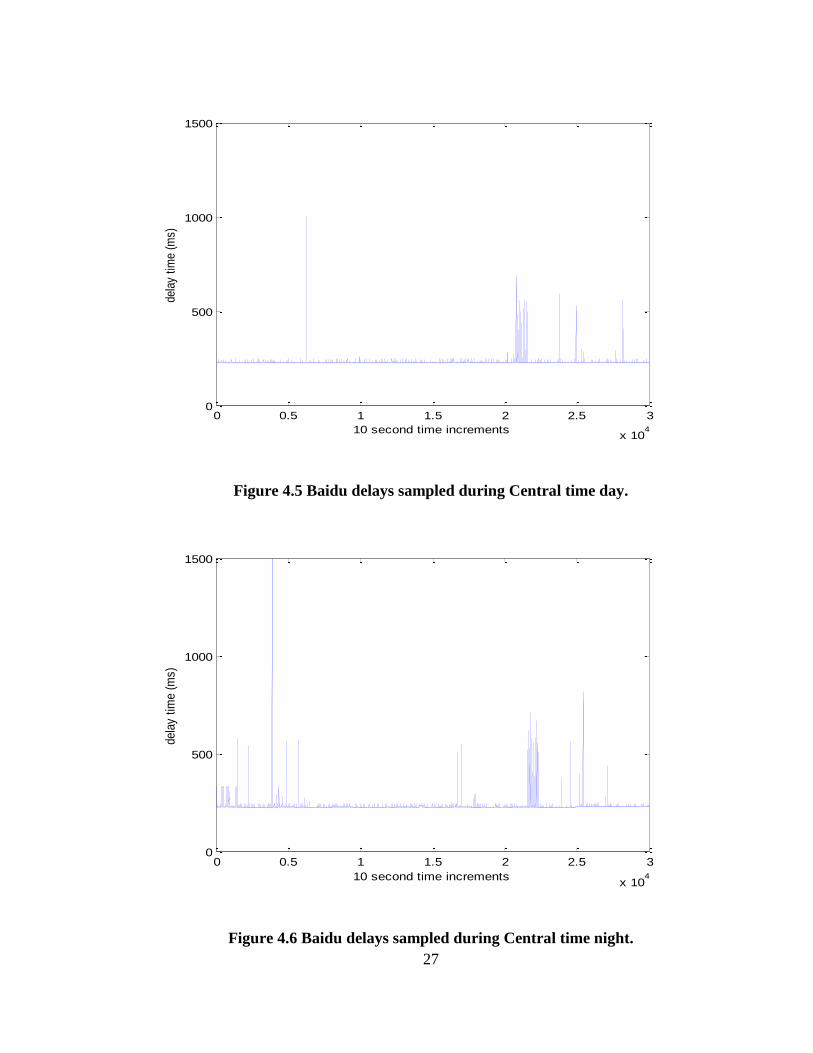
The three graphic outputs of the Hurst parameter measurement tool are plots of

the delay time differences from the median value, a periodogram of these differences, and

a least squares regression plot of the log-log periodogram. They are shown in Figures 4.7,

4.8, and 4.9, respectively. The mean and median of the time series as well as the Hurst

parameter estimate and 95% confidence interval are numerically presented in the

MATLAB execution window. The confidence interval was calculated from the standard

deviation of the slope estimate and using 1.96 standard deviations away as the lower and

upper bounds. Processing day and night data segments from a single data set required

two iterations of the tool, with the time period being selected by a hardcoded parameter.

Figure 4.7 Baidu delay difference from median.

0 0.5 1 1.5 2 2.5 3 3.5

x 104

-200

0

200

400

600

800

1000

1200

1400

10 second time increments

dela

y d

iffe

rence (

ms)

29

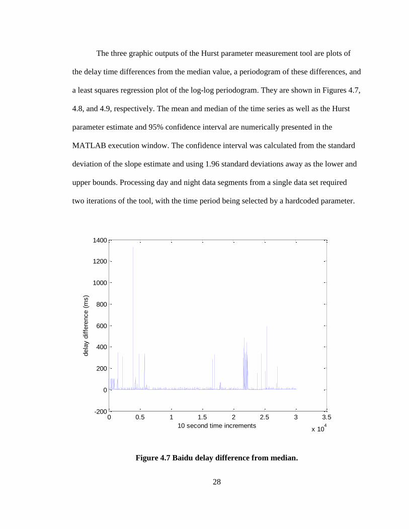
The second graphical output from the measurement tool is a periodogram or

power spectral density of the delay differences from the median. Notice that the entire

day or night data set is used to construct the graph. Figure 4.8 shows a periodogram for

the Baidu data as referenced to 2100-0900 hours, Central time. As only the decay shape

of the spectrum near the origin is used by the measurement tool for the Hurst parameter

calculation, the information in the higher frequency components is discarded. A cursory

look at this high frequency information from several sites revealed interesting

periodicities, which suggested the presence of discrete events in the time domain. In

theory, this information could be used to categorize the short-range dependence of the

time series and may be of future value. This topic will be discussed in the conclusion.

Figure 4.8 Baidu delay difference periodogram.

0 2000 4000 6000 8000 10000 12000 14000 16000 18000-3

-2

-1

0

1

2

3

4

5

unscaled frequency

unscale

d p

ow

er

30

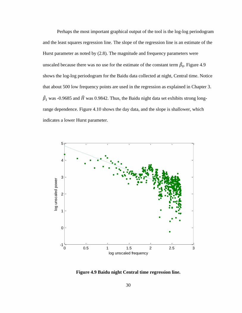
Perhaps the most important graphical output of the tool is the log-log periodogram

and the least squares regression line. The slope of the regression line is an estimate of the

Hurst parameter as noted by (2.8). The magnitude and frequency parameters were

unscaled because there was no use for the estimate of the constant term Figure 4.9

shows the log-log periodogram for the Baidu data collected at night, Central time. Notice

that about 500 low frequency points are used in the regression as explained in Chapter 3.

was -0.9685 and was 0.9842. Thus, the Baidu night data set exhibits strong long-

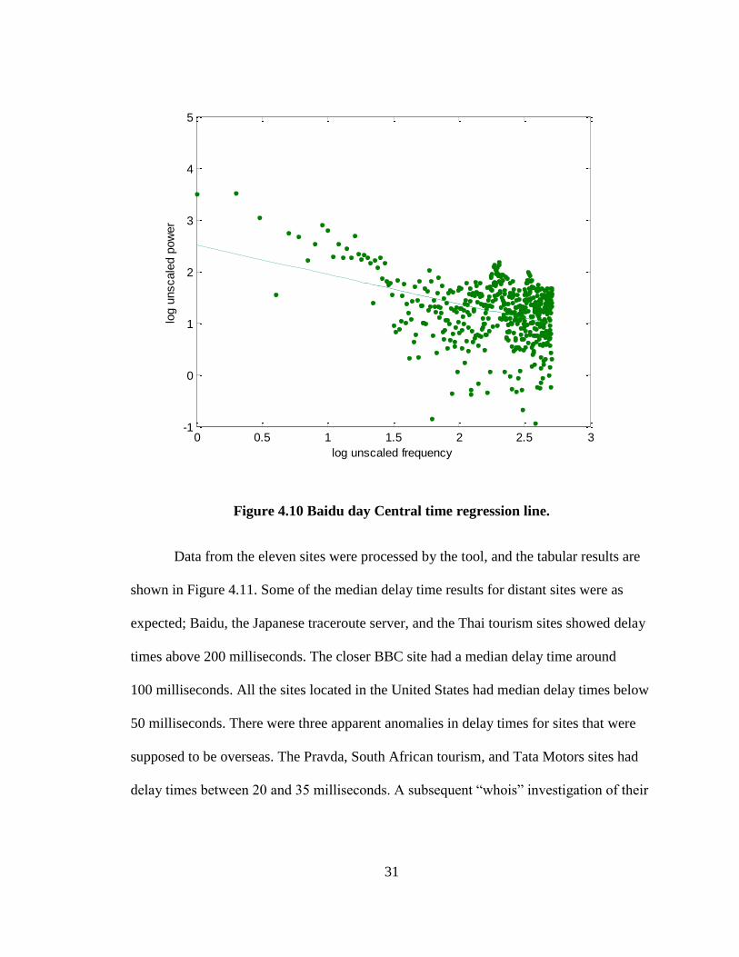
range dependence. Figure 4.10 shows the day data, and the slope is shallower, which

indicates a lower Hurst parameter.

Figure 4.9 Baidu night Central time regression line.

0 0.5 1 1.5 2 2.5 3-1

0

1

2

3

4

5

log unscaled frequency

log u

nscale

d p

ow

er

31

Figure 4.10 Baidu day Central time regression line.

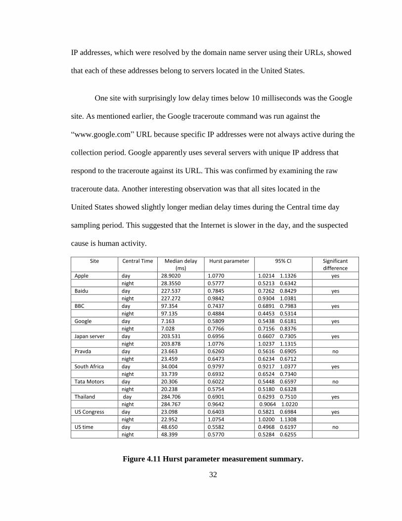
Data from the eleven sites were processed by the tool, and the tabular results are

shown in Figure 4.11. Some of the median delay time results for distant sites were as

expected; Baidu, the Japanese traceroute server, and the Thai tourism sites showed delay

times above 200 milliseconds. The closer BBC site had a median delay time around

100 milliseconds. All the sites located in the United States had median delay times below

50 milliseconds. There were three apparent anomalies in delay times for sites that were

supposed to be overseas. The Pravda, South African tourism, and Tata Motors sites had

delay times between 20 and 35 milliseconds. A subsequent “whois” investigation of their

0 0.5 1 1.5 2 2.5 3-1

0

1

2

3

4

5

log unscaled frequency

log u

nscale

d p

ow

er

32

IP addresses, which were resolved by the domain name server using their URLs, showed

that each of these addresses belong to servers located in the United States.

One site with surprisingly low delay times below 10 milliseconds was the Google

site. As mentioned earlier, the Google traceroute command was run against the

“www.google.com” URL because specific IP addresses were not always active during the

collection period. Google apparently uses several servers with unique IP address that

respond to the traceroute against its URL. This was confirmed by examining the raw

traceroute data. Another interesting observation was that all sites located in the

United States showed slightly longer median delay times during the Central time day

sampling period. This suggested that the Internet is slower in the day, and the suspected

cause is human activity.

Site Central Time Median delay (ms)

Hurst parameter 95% CI Significant difference

Apple day 28.9020 1.0770 1.0214 1.1326 yes

night 28.3550 0.5777 0.5213 0.6342

Baidu day 227.537 0.7845 0.7262 0.8429 yes

night 227.272 0.9842 0.9304 1.0381

BBC day 97.354 0.7437 0.6891 0.7983 yes

night 97.135 0.4884 0.4453 0.5314

Google day 7.163 0.5809 0.5438 0.6181 yes

night 7.028 0.7766 0.7156 0.8376

Japan server day 203.531 0.6956 0.6607 0.7305 yes

night 203.878 1.0776 1.0237 1.1315

Pravda day 23.663 0.6260 0.5616 0.6905 no

night 23.459 0.6473 0.6234 0.6712

South Africa day 34.004 0.9797 0.9217 1.0377 yes

night 33.739 0.6932 0.6524 0.7340

Tata Motors day 20.306 0.6022 0.5448 0.6597 no

night 20.238 0.5754 0.5180 0.6328

Thailand day 284.706 0.6901 0.6293 0.7510 yes

night 284.767 0.9642 0.9064 1.0220

US Congress day 23.098 0.6403 0.5821 0.6984 yes

night 22.952 1.0754 1.0200 1.1308

US time day 48.650 0.5582 0.4968 0.6197 no

night 48.399 0.5770 0.5284 0.6255

Figure 4.11 Hurst parameter measurement summary.

33

The main feature of the summary table in Figure 4.11 is the confirmation of

dichotomous Hurst parameters for eight of the eleven sites tested. As a side note, some

sites exhibited Hurst parameters above 1.0 and these could be the results of statistical

fluctuations in the real world data or biases from the measurement tool’s tuning

parameters. Three sites did not exhibit dichotomous Hurst parameters during their one-

week observation periods, and they will be discussed first.

Based on the overlap of their 95% confidence intervals, the Pravda, Tata Motors,

and US timeserver sites did not have significantly different day and night Hurst

parameters. All three did have Hurst parameters that tended toward the low side of the

scale and ranged from 0.56 to 0.65. This range suggested weak long-range dependence,

and the dependence did not change significantly between day and night. One possible

explanation is that these sites have low popularities, which isolated them from social use

fluctuations. In addition, their median delays were higher in the day, and these delays

were also common to the other four sites in the United States that showed dichotomous

Hurst parameters. Thus, the measured Hurst parameters of all tested sites in the United

States may be indicative of social activity and sever loadings and not the common

daytime slowdown of the autonomous systems connecting these sites. More research is

needed to confirm the idea that unpopular sites have lower Hurst parameters.

All four overseas sites exhibited dichotomous Hurst parameters. Two of these

sites, a Japanese internal server and a Thai tourism site, were presumed to be low on the

social interest order. The Baidu and BBC sites presumably have much greater traffic due

to their popularities, and thus, social interest may not be the only cause of the observed

34

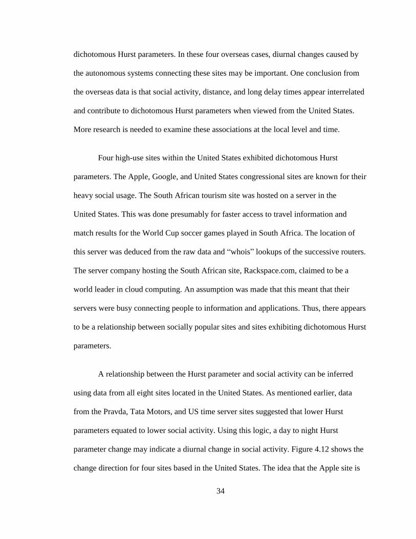
dichotomous Hurst parameters. In these four overseas cases, diurnal changes caused by

the autonomous systems connecting these sites may be important. One conclusion from

the overseas data is that social activity, distance, and long delay times appear interrelated

and contribute to dichotomous Hurst parameters when viewed from the United States.

More research is needed to examine these associations at the local level and time.

Four high-use sites within the United States exhibited dichotomous Hurst

parameters. The Apple, Google, and United States congressional sites are known for their

heavy social usage. The South African tourism site was hosted on a server in the

United States. This was done presumably for faster access to travel information and

match results for the World Cup soccer games played in South Africa. The location of

this server was deduced from the raw data and “whois” lookups of the successive routers.

The server company hosting the South African site, Rackspace.com, claimed to be a

world leader in cloud computing. An assumption was made that this meant that their

servers were busy connecting people to information and applications. Thus, there appears

to be a relationship between socially popular sites and sites exhibiting dichotomous Hurst

parameters.

A relationship between the Hurst parameter and social activity can be inferred

using data from all eight sites located in the United States. As mentioned earlier, data

from the Pravda, Tata Motors, and US time server sites suggested that lower Hurst

parameters equated to lower social activity. Using this logic, a day to night Hurst

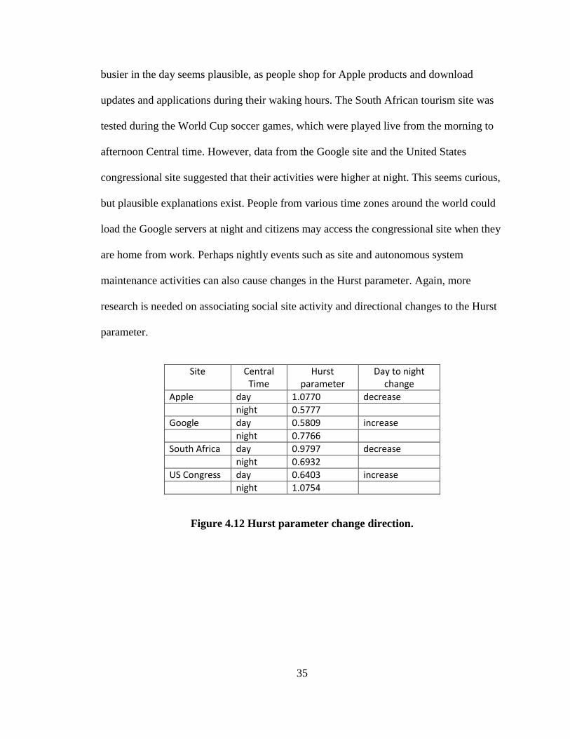
parameter change may indicate a diurnal change in social activity. Figure 4.12 shows the

change direction for four sites based in the United States. The idea that the Apple site is

35

busier in the day seems plausible, as people shop for Apple products and download

updates and applications during their waking hours. The South African tourism site was

tested during the World Cup soccer games, which were played live from the morning to

afternoon Central time. However, data from the Google site and the United States

congressional site suggested that their activities were higher at night. This seems curious,

but plausible explanations exist. People from various time zones around the world could

load the Google servers at night and citizens may access the congressional site when they

are home from work. Perhaps nightly events such as site and autonomous system

maintenance activities can also cause changes in the Hurst parameter. Again, more

research is needed on associating social site activity and directional changes to the Hurst

parameter.

Site Central Time

Hurst parameter

Day to night change

Apple day 1.0770 decrease

night 0.5777

Google day 0.5809 increase

night 0.7766

South Africa day 0.9797 decrease

night 0.6932

US Congress day 0.6403 increase

night 1.0754

Figure 4.12 Hurst parameter change direction.

36

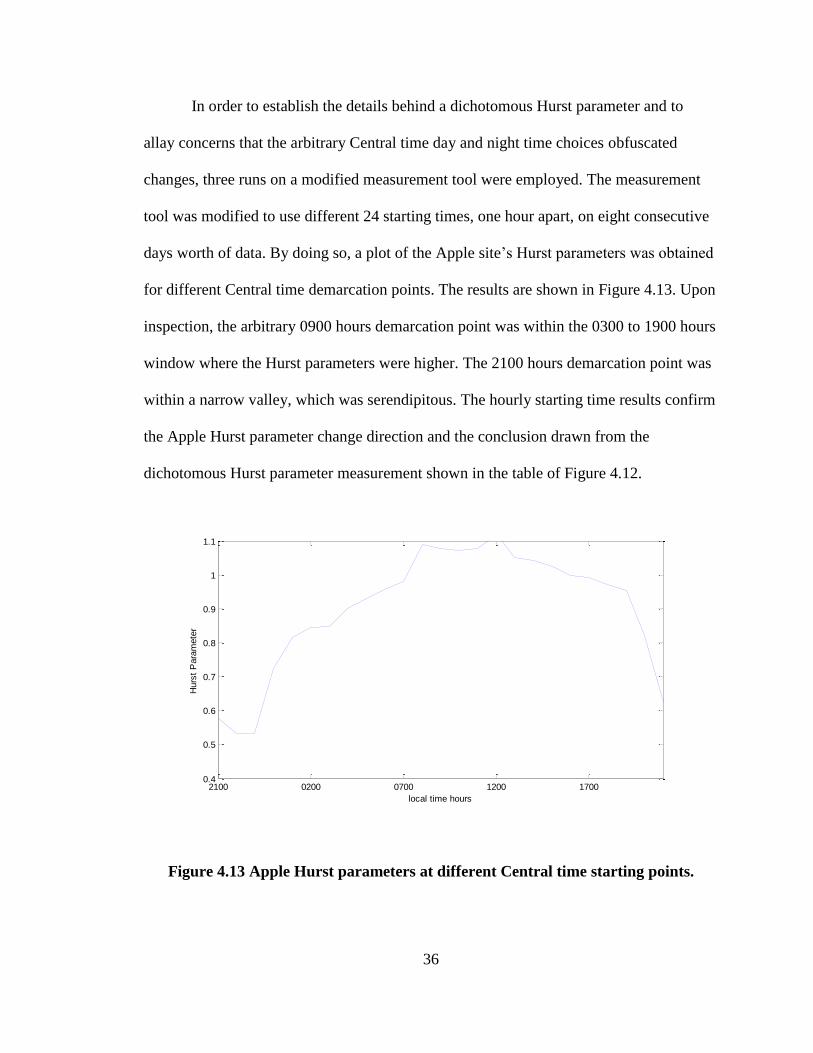
In order to establish the details behind a dichotomous Hurst parameter and to

allay concerns that the arbitrary Central time day and night time choices obfuscated

changes, three runs on a modified measurement tool were employed. The measurement

tool was modified to use different 24 starting times, one hour apart, on eight consecutive

days worth of data. By doing so, a plot of the Apple site’s Hurst parameters was obtained

for different Central time demarcation points. The results are shown in Figure 4.13. Upon

inspection, the arbitrary 0900 hours demarcation point was within the 0300 to 1900 hours

window where the Hurst parameters were higher. The 2100 hours demarcation point was

within a narrow valley, which was serendipitous. The hourly starting time results confirm

the Apple Hurst parameter change direction and the conclusion drawn from the

dichotomous Hurst parameter measurement shown in the table of Figure 4.12.

Figure 4.13 Apple Hurst parameters at different Central time starting points.

2100 0200 0700 1200 17000.4

0.5

0.6

0.7

0.8

0.9

1

1.1

local time hours

Hurs

t P

ara

mete

r

37

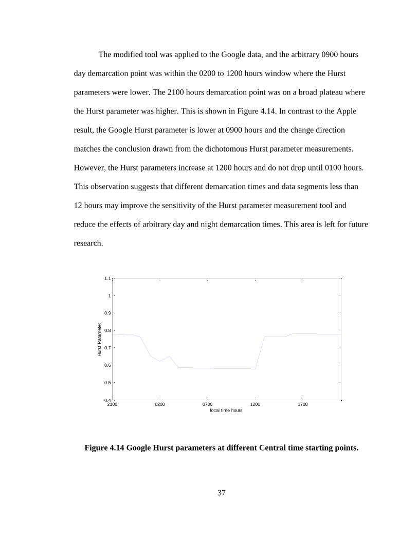
The modified tool was applied to the Google data, and the arbitrary 0900 hours

day demarcation point was within the 0200 to 1200 hours window where the Hurst

parameters were lower. The 2100 hours demarcation point was on a broad plateau where

the Hurst parameter was higher. This is shown in Figure 4.14. In contrast to the Apple

result, the Google Hurst parameter is lower at 0900 hours and the change direction

matches the conclusion drawn from the dichotomous Hurst parameter measurements.

However, the Hurst parameters increase at 1200 hours and do not drop until 0100 hours.

This observation suggests that different demarcation times and data segments less than

12 hours may improve the sensitivity of the Hurst parameter measurement tool and

reduce the effects of arbitrary day and night demarcation times. This area is left for future

research.

Figure 4.14 Google Hurst parameters at different Central time starting points.

2100 0200 0700 1200 17000.4

0.5

0.6

0.7

0.8

0.9

1

1.1

local time hours

Hurs

t P

ara

mete

r

38

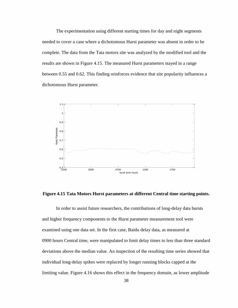
The experimentation using different starting times for day and night segments

needed to cover a case where a dichotomous Hurst parameter was absent in order to be

complete. The data from the Tata motors site was analyzed by the modified tool and the

results are shown in Figure 4.15. The measured Hurst parameters stayed in a range

between 0.55 and 0.62. This finding reinforces evidence that site popularity influences a

dichotomous Hurst parameter.

Figure 4.15 Tata Motors Hurst parameters at different Central time starting points.

In order to assist future researchers, the contributions of long-delay data bursts

and higher frequency components to the Hurst parameter measurement tool were

examined using one data set. In the first case, Baidu delay data, as measured at

0900 hours Central time, were manipulated to limit delay times to less than three standard

deviations above the median value. An inspection of the resulting time series showed that

individual long-delay spikes were replaced by longer running blocks capped at the

limiting value. Figure 4.16 shows this effect in the frequency domain, as lower amplitude

2100 0200 0700 1200 17000.4

0.5

0.6

0.7

0.8

0.9

1

1.1

local time hours

Hurs

t P

ara

mete

r

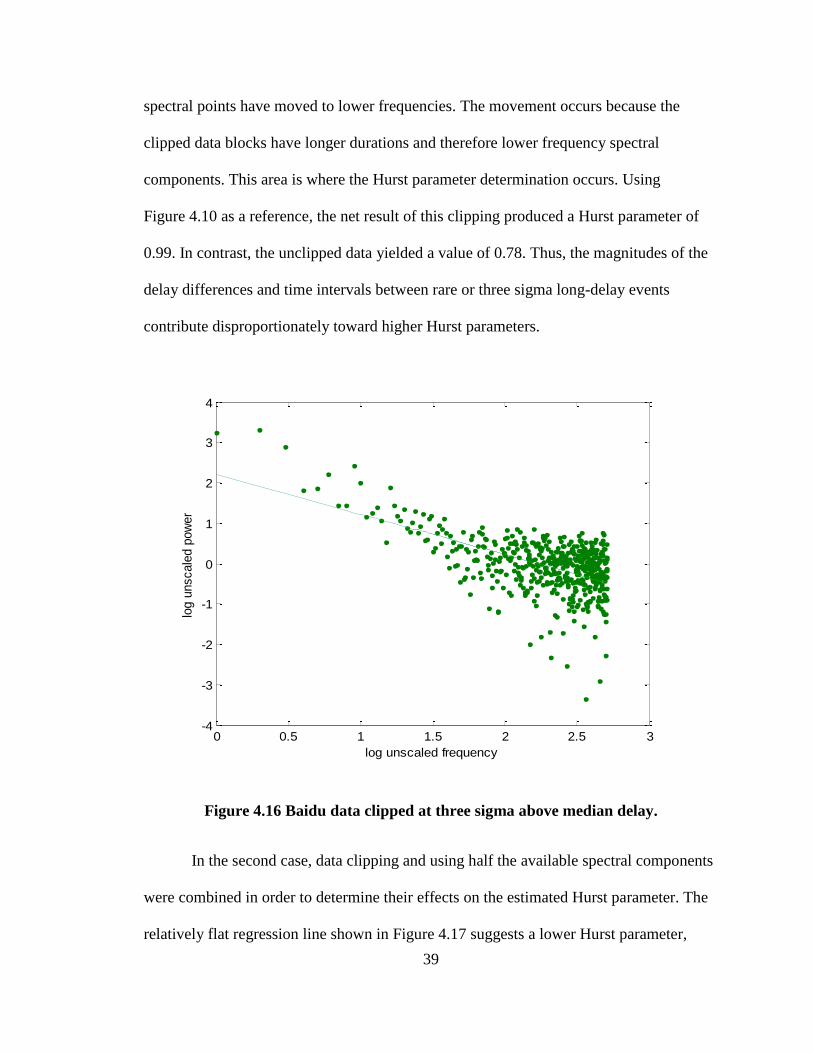
39

spectral points have moved to lower frequencies. The movement occurs because the

clipped data blocks have longer durations and therefore lower frequency spectral

components. This area is where the Hurst parameter determination occurs. Using

Figure 4.10 as a reference, the net result of this clipping produced a Hurst parameter of

0.99. In contrast, the unclipped data yielded a value of 0.78. Thus, the magnitudes of the

delay differences and time intervals between rare or three sigma long-delay events

contribute disproportionately toward higher Hurst parameters.

Figure 4.16 Baidu data clipped at three sigma above median delay.

In the second case, data clipping and using half the available spectral components

were combined in order to determine their effects on the estimated Hurst parameter. The

relatively flat regression line shown in Figure 4.17 suggests a lower Hurst parameter,

0 0.5 1 1.5 2 2.5 3-4

-3

-2

-1

0

1

2

3

4

log unscaled frequency

log u

nscale

d p

ow

er

40

which was estimated at 0.53. This estimate is reasonable as the preponderance of higher

frequency spectral components were flat and noise like. In the time domain, this noise

translates to low cross correlation values between measurements taken from every

10 seconds to every 320 seconds.

Figure 4.17 Baidu using half of the available spectral components.

The sloping data elements in Figure 4.17 demonstrate that higher Hurst

parameters are favored when the measurement tool uses lower frequency components. In

the time domain, these lower frequency components translate to high cross correlation

values among measurements taken at intervals above 320 seconds or about 5 minutes.

Speculating on casual mechanisms beyond human activity and the autonomous systems

0 0.5 1 1.5 2 2.5 3 3.5 4-4

-3

-2

-1

0

1

2

3

4

log unscaled frequency

log u

nscale

d p

ow

er

41

of the Internet to explain these interacting data points at lower frequencies was not

attempted. Yet, the development of a two-slope Hurst parameter measurement tool to

handle all the data points may be warranted, as distinct steeper and flatter regions suggest

underlying longer and shorter-range dependent processes.

Chapter 5 recapitulates the findings, discusses confidence in the results, and

suggests applications for a dichotomous Hurst parameter. It will suggest that social

activities are one factor behind dichotomous Hurst parameters.

42

CHAPTER 5

CONCLUSION AND APPLICATION

Eight of the eleven Internet sites tested exhibited significantly different

dichotomous Hurst parameters at the 95% confidence level. None of the eleven Internet

sites exhibited rhythmic diurnal changes in packet delay times as reported by earlier

researchers. Chapter 3 detailed the development and calibration of a Hurst parameter

measurement tool, which used a log-log periodogram approach. The experiment showed

that FARIMA sequences could not accurately calibrate the tool because of the truncated

periodogram employed. However, testing using FARIMA sequences showed that the tool

could precisely resolve Hurst parameters 0.1 units apart and at the 95% confidence level.

Both recursive work from using the tool on preliminary data and evidence from the

literature suggested that favoring lower frequency components would produce Hurst

parameters in the desired 0.5 to 1.0 range. Using the tool on real data proved this idea

correct for 11 cases, but tuning may be required for more varied data sets.

The findings of dichotomous Hurst parameters fill a gap left by Borella and

Brewster [17]. In 1998, they measured Hurst parameters that varied “dramatically

between consecutive 5-15 minute periods.” Thus, they did not speculate on how a Hurst

parameter could change between day and night. One should note that their time period

was at the lower margin of the data used by the Hurst parameter measurement tool. The

43

lower 1/32 of the spectral components employed by the tool corresponded to sampling

times above 320 seconds or about 5 minutes. At time scales above 5 minutes, all eleven

Internet sites had measurable Hurst parameters. This finding suggests that LRD behaviors

of Internet delays are prevalent at time intervals of up to a week. Future research is

needed expand this interval to weeks or months.

Three overseas sites and five popular sites in the United States had dichotomous

Hurst parameters that changed according to day and night collection periods based on

Central time. These findings suggested that there is merit in segmenting delay time data

into periods relevant to diurnal human activity. However, not all the Hurst parameters

changed in a unidirectional fashion, as Central time day Hurst parameters went up for

some sites and went down for other sites. It was expected that busier sites would have

higher Hurst parameters in the day. The Apple site corroborated this supposition while

the Google site did not. However, further experimentation suggested that a fixed and

arbitrary 12 hour day or night period may not be optimal for finding Hurst parameters.

Optimal periods could be based on local server times and user patterns.

Manipulation of the measurement tool showed that three sigma delay outliers and

lower frequency components of the periodograms produced dramatic effects on the

estimated Hurst parameters. Optimum tuning for the measurement tool included

differencing the delay values from the median delay in order to better balance the shape

of the distribution. Tuning also included using frequencies from the lower 1/32 of the

periodogram for the least squares regression estimate of the slope.

44

One practical use of a Hurst parameter to characterize Internet round trip delays

was discussed by Hagiwara et al. in 2001 [18]. These researchers used a simulation to

prove that higher Hurst parameters could lead to higher packet losses, and they suggested

a compensation method to adjust retransmission timeout (RTO) algorithms according to

the prevailing Hurst parameter. An issue that influenced their method was the required

calculation of real time Hurst parameters using limited data and computational power.

Their solution was to use an R/S approximation, in which the running ratio of

two variances from different time scales produced dynamic Hurst parameter estimates.

These researchers did not attempt to test their solution with real data. The findings in this

thesis suggest that Hurst parameters can be calculated before hand, and RTO corrections

for several days in advance can be based on dichotomous Hurst parameters.

Internet packet delays and traffic are related phenomena, and accurately modeling

traffic is an ongoing technical challenge. Fares and Woodward [19] stated in 2009, “The

ability to predict traffic congestion is one of the fundamental requirements of modern

network design.” These researchers created a predictive model to find nodes suspected of

causing traffic congestion. However, they used simulated LRD data to test their model.

Real-world node data is available as the traceroute command used in this thesis can

produce data for each node in the path to the test site. By doing so, Hurst parameters for

each node can be calculated, and diurnal node behaviors can be recorded. If a node

exhibits a dichotomous Hurst parameter, then a predictor of node behavior is available for

traffic modeling or traffic control.

45

A primary purpose for examining dichotomous Hurst parameters was to find

statistical measures beyond average delay times and associated variances that could be

used to characterize or fingerprint Internet sites. As was discussed earlier, median delay

times cluster together depending on geographic regions and cannot be used alone to

differentiate some sites. For example, the United States congressional site and the Pravda

site had Central time night delays of 23.5 and 23.0 milliseconds, respectively. However,

their respective Hurst parameter estimates were 0.69 and above 1.0 and were significantly

different at the 95% confidence level. A database of Hurst parameters kept by each user

and updated daily could be used to profile his or her favorite sites.

A software application that enhances a user’s social connectedness could first use

a Hurst parameter to differentiate sites and then could suggest better times to visit these

sites. Although consistently low delay times are paramount for “twitch” games played on

the Internet, the social feel of a site may also be determined by the burstiness of its TCP

connection. The Hurst parameter is a good measure of this burstiness. Thus, an

application could learn about a user’s site preferences and delay tolerances and then

could create an itinerary of optimal times to access each site. According to the data

collected in this thesis, it may be better to visit the Apple and the Google sites during

different periods for optimal connectedness. Future research is required to generalize this

finding and extend it to sites from around the world. In addition, future research on the

two-stage nature and possible longer and shorter-range dependence of delay times may

add another type of fingerprint that a software application can use.

46

APPENDICES

47

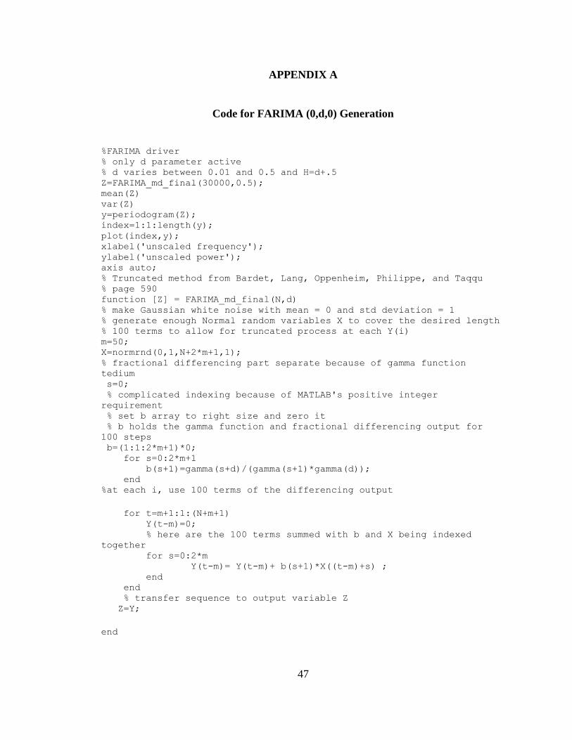
APPENDIX A

Code for FARIMA (0,d,0) Generation

%FARIMA driver % only d parameter active % d varies between 0.01 and 0.5 and H=d+.5 Z=FARIMA_md_final(30000,0.5); mean(Z) var(Z) y=periodogram(Z); index=1:1:length(y); plot(index,y); xlabel('unscaled frequency'); ylabel('unscaled power'); axis auto; % Truncated method from Bardet, Lang, Oppenheim, Philippe, and Taqqu % page 590 function [Z] = FARIMA_md_final(N,d) % make Gaussian white noise with mean = 0 and std deviation = 1 % generate enough Normal random variables X to cover the desired length % 100 terms to allow for truncated process at each Y(i) m=50; X=normrnd(0,1,N+2*m+1,1); % fractional differencing part separate because of gamma function

tedium s=0; % complicated indexing because of MATLAB's positive integer

requirement % set b array to right size and zero it % b holds the gamma function and fractional differencing output for

100 steps b=(1:1:2*m+1)*0; for s=0:2*m+1 b(s+1)=gamma(s+d)/(gamma(s+1)*gamma(d)); end %at each i, use 100 terms of the differencing output

for t=m+1:1:(N+m+1) Y(t-m)=0; % here are the 100 terms summed with b and X being indexed

together for s=0:2*m Y(t-m)= Y(t-m)+ b(s+1)*X((t-m)+s) ; end end % transfer sequence to output variable Z Z=Y;

end

48

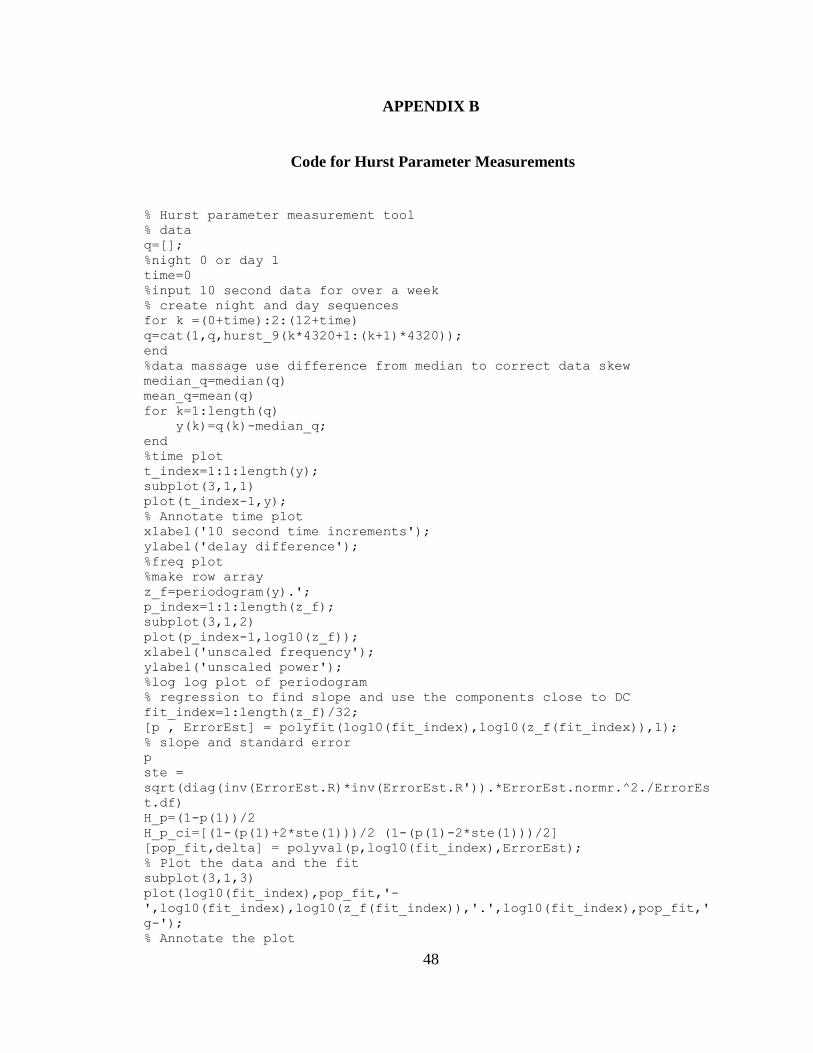
APPENDIX B

Code for Hurst Parameter Measurements

% Hurst parameter measurement tool % data q=[]; %night 0 or day 1 time=0 %input 10 second data for over a week % create night and day sequences for k =(0+time):2:(12+time) q=cat(1,q,hurst_9(k*4320+1:(k+1)*4320)); end %data massage use difference from median to correct data skew median_q=median(q) mean_q=mean(q) for k=1:length(q) y(k)=q(k)-median_q; end %time plot t_index=1:1:length(y); subplot(3,1,1) plot(t_index-1,y); % Annotate time plot xlabel('10 second time increments'); ylabel('delay difference'); %freq plot %make row array z_f=periodogram(y).'; p_index=1:1:length(z_f); subplot(3,1,2) plot(p_index-1,log10(z_f)); xlabel('unscaled frequency'); ylabel('unscaled power'); %log log plot of periodogram % regression to find slope and use the components close to DC fit_index=1:length(z_f)/32; [p , ErrorEst] = polyfit(log10(fit_index),log10(z_f(fit_index)),1); % slope and standard error p ste =

sqrt(diag(inv(ErrorEst.R)*inv(ErrorEst.R')).*ErrorEst.normr.^2./ErrorEs

t.df) H_p=(1-p(1))/2 H_p_ci=[(1-(p(1)+2*ste(1)))/2 (1-(p(1)-2*ste(1)))/2] [pop_fit,delta] = polyval(p,log10(fit_index),ErrorEst); % Plot the data and the fit subplot(3,1,3) plot(log10(fit_index),pop_fit,'-

',log10(fit_index),log10(z_f(fit_index)),'.',log10(fit_index),pop_fit,'

g-'); % Annotate the plot

49

xlabel('log unscaled frequency'); ylabel('log unscaled power');

50

REFERENCES

[1] World of Warcraft. (2010). Original Game: 10 day free trial. Available:

<http://www.worldofwarcraft.com/burningcrusade/trial/>.

[2] W. E. Leland, M. S. Taqqu, W. Willinger, and D. V. Wilson, “On the self-similar

nature of Ethernet traffic (extended version),” IEEE/ACM Trans. on Networking, vol.

2, no. 1, pp. 1-15, Feb. 1994.

[3] E. Kamrani and M. Mehraban, “Modeling internet delay dynamics using system

identification,” IEEE Int. Conf. on Industrial Technology, Mumbai, India, December

15-17, 2006, pp. 430-438.

[4] H. E. Hurst, The Nile. London: Whitefriars Press, 1952.

[5] H. E. Hurst, “Long-term storage capacity of reservoirs,” Trans. Am. Soc. Civil Eng.,

vol. 116, pp. 770–799, 1951.

[6] B. Mandelbrot, “Self-similar error clusters in communication systems and the concept

of conditional stationarity,” IEEE Trans. Commun. Technol., vol. 13, pp. 71-90,

1965.

[7] D. L. Mills, (1983). Internet delay experiments (RFC 889). Available:

<http://www.ietf.org/rfc/rfc889.txt>.

[8] J. C. Ramirez Pacheco, D. Torres Roman, and L. Estrada Vargas, “R/S statistic:

Accuracy and implementations,” 18th International Conference on Electronics,

Communications, and Computers, Puebla, Mexico, March 3-5, 2008, pp. 17-22.

[9] A. Mukherjee, “On the dynamics and significance of low frequency components of

Internet load,” Dept. Comp. and Info. Sci., University of Pennsylvania, Philadelphia,

PA, Rep. MS-CIS-92-83/DSL-12, Dec. 1992.

[10] M. Maejima, “Limit Theorems for Infinite Variance Sequences,” In Theory and

Applications of Long-range Dependence, P. Doukhan, G. Oppenheim, and M. S.

Taqqu, Eds. Boston, MA: Birkhäuser, 2003, pp. 157-164.

[11] E. Moulines and P. Soulier, “Semiparametric spectral estimation for fractional

processes,” In Theory and Applications of Long-range Dependence, P. Doukhan, G.

Oppenheim, and M. S. Taqqu, Eds. Boston, MA: Birkhäuser, 2003, pp. 251-301.

[12] O. Cappe, E. Moulines, J. C. Pesquet, and X. Yang, “Long-range dependence and

heavy-tail traffic modeling for teletraffic data,” IEEE Signal Processing Magazine,

vol. 19, pp. 14-27, May 2002.

51

[13] J. Beran, Statistics for long-memory process. New York, NY: Chapman and Hall,

1998.

[14] C. W. J. Granger and R. Joyeux, “An introduction to long-memory time series

models and fractional differencing,” Journal of Time Series Analysis, vol. 1, pp. 15-

29, 1980.

[15] J-M. Bardet, G. Lang, G. Oppenheim, A. Philippe, and M. S. Taqqu, “Generators of

long-range dependent processes: A survey,” In Theory and Applications of Long-

range Dependence, P. Doukhan, G. Oppenheim, and M. S. Taqqu, Eds. Boston, MA:

Birkhäuser, 2003, pp. 579-623.

[16] J-M. Bardet, G. Lang, G. Oppenheim, A. Philippe, S. Stoev, and M. S. Taqqu,

“Semi-parametric estimation of the long range dependence parameter,” In Theory

and Applications of Long-range Dependence, P. Doukhan, G. Oppenheim, and M. S.

Taqqu, Eds. Boston, MA: Birkhäuser, 2003, pp. 557-577.

[17] H. S. Borella and G. B. Brewster, “Measurement and analysis of long-range

dependent behavior of Internet packet delay,” INFOCON ’98, 17th Joint Annual

Conference of the IEEE Computers and Communications Societies, San Francisco,

CA, Mar. 29 - Apr. 2, 1998, vol. 2, pp. 497-504.

[18] T. Hagiwara, H. Majima, T. Matsuda, and M. Yamamoto, “Impact of round trip

delay self-similarity on TCP performance,” Proceedings of the Tenth International

Conference on Computer Communications and Networks, Scottsdale, AZ, Oct. 15-

17, 2001, pp. 166-171.

[19] R. H. Fares and M. E. Woodward, “The use of long range dependence for network

congestion prediction,” 1st International Conference on Evolving Internet, Cannes

and La Bocca, France, August 23-29, 2009, pp. 119-124.