Robust Runtime Optimization andSkew-Resistant Execution of Analytical

SPARQL Queries on Pig

Spyros Kotoulas12⇤, Jacopo Urbani2⇤, Peter Boncz32, and Peter Mika4

1 IBM Research, Ireland Spyros.Kotoulas@ie.ibm.com

2 Vrije Universiteit Amsterdam, The Netherlands jacopo@cs.vu.nl

3 CWI Amsterdam, The Netherlands boncz@cwi.nl

4 Yahoo! Research Barcelona, Spain pmika@yahoo-inc.com

⇤ these authors have contributed equally to this work

Abstract. We describe a system that incrementally translates SPARQLqueries to Pig Latin and executes them on a Hadoop cluster. This systemis designed to work e�ciently on complex queries with many self-joinsover huge datasets, avoiding job failures even in the case of joins withunexpected high-value skew. To be robust against cost estimation er-rors, our system interleaves query optimization with query execution,determining the next steps to take based on data samples and statisticsgathered during the previous step. Furthermore, we have developed anovel skew-resistant join algorithm that replicates tuples correspondingto popular keys. We evaluate the e↵ectiveness of our approach both on asynthetic benchmark known to generate complex queries (BSBM-BI) aswell as on a Yahoo! case of data analysis using RDF data crawled fromthe web. Our results indicate that our system is indeed capable of pro-cessing huge datasets without pre-computed statistics while exhibitinggood load-balancing properties.

1 Introduction

The amount of Linked Open Data (LOD) is strongly growing, both in the formof an ever expanding collection of RDF datasets available on the Web, as wellsemantic annotations increasingly appearing in HTML pages, in the form ofRDFa, microformats, or microdata such as schema.org.

Search engines like Yahoo! crawl and process this data in order to providemore e�cient search. Applications built on or enriched with LOD typically em-ploy a warehousing approach, where data from multiple sources is brought to-gether, and interlinked (e.g. as in [11]).

Due to the large volume and, often, dirty nature of the data, such Extrac-tion, Transformation and Loading (ETL) processes can easily be translated into“killer” SPARQL queries that overwhelm the current state-of-the-art in RDFdatabase systems. Such problems typically come down to formulating joins thatproduce huge results, or to RDF database systems that calculate the wrong joinorder such that the intermediate results get too large to be processed. In this

paper, we describe a system that scalably executes SPARQL queries using thePig Latin language [16] and we demonstrate its usage on a synthetic benchmarkand on crawled Web data. We evaluate our method using both a standard clusterand the large MapReduce infrastructure provided by Yahoo!.

In the context of this work, we are considering some key issues:

Schema-less. A SPARQL query optimizer typically lacks all schema knowledgethat a relational system has available, making this task more challenging. Ina relational system, schema knowledge can be exploited by keeping statistics,such as table cardinalities and histograms that capture the value and frequencydistributions of relational columns. RDF database systems, on the other hand,cannot assume any schema and store all RDF triples in a table with Subject,Property, Object columns (S,P,O). Both relational column projections as well asforeign key joins map in the SPARQL equivalent into self-join patterns. There-fore, if a query is expressed in both SQL and SPARQL, on the physical algebralevel, the plan generated from SPARQL will typically have many more self-joinsthan the relational plan has joins. Because of the high complexity of join orderoptimization as a function of the number of joins, SPARQL query optimizationis more challenging than SQL query optimization.

MapReduce and Skew. Linked Open Data ETL tasks which involve cleaning,interlinking and inferencing have a high computational cost, which motivatesour choice for a MapReduce approach. In a MapReduce-based system, data isrepresented in files and that can come from recent Web crawls. Hence, we havean initial situation without statistics and without any B-trees, let alone multipleB-trees. One particular problem in raw Web data is the high skew in join keysin RDF data. Certain subjects and properties are often re-used (most notoriousare RDF Schema properties) which lead to joins where certain key-values willbe very frequent. These keys do not only lead to large intermediate results, butcan also cause one machine to get overloaded in a join job and hence run out ofmemory (and automatic job restarts provided by Hadoop will fail again). This isindeed more general than joins: in the sort phase of MapReduce, large amountsof data might need to be sorted on disk, severely degrading performance.

SPARQL on Pig. The Pig Latin language provides operators to scan datafiles on a Hadoop cluster that form tuple streams, and further select, aggregate,join and sort such streams, both using ready-to-go Pig relational operators aswell as using user-defined functions (UDFs). Each MapReduce job materializesthe intermediate results in files that are replicated in the distributed filesystem.Such materialization and replication make the system robust, such that the jobsof failing machines can be restarted on other machines without causing a queryfailure. However, from the query processing point of view, this materializationis a source of ine�ciency. The Pig framework attempts to improve this situationby compiling Pig queries into a minimal amount of Hadoop jobs, e↵ectivelycombining more operators in a single MapReduce operation. An e�cient queryoptimization strategy must be aware of it and each query processing step shouldminimize the number of Hadoop jobs.

Our work addresses these challenges and proposes an e�cient translation ofsome crucial operators into Pig Latin, namely joins, making them robust enoughto deal with the issues typical of large data collections.

Contributions. We can summarize the contributions of this work as follows. (i)We have created a system that can compute complex SPARQL queries on hugeRDF datasets. (ii) We present a runtime query optimization framework that isoptimized for Pig in that it aims at reducing the number of MapReduce jobs,therefore reducing query latency. (iii) We describe a skew-resistant join methodthat can be used when the runtime query optimization discovers the risk fora skewed join distribution that may lead to structural machine overlap in theMapReduce cluster. (iv) We evaluate the system on a standard cluster and aYahoo! Hadoop cluster of over 3500 machines using synthetic benchmark data,as well as real Web crawl data.

Outline. The rest of the paper is structured as follows. In Section 2 we presentour approach and describe some of its crucial parts. In Section 3 we evaluateour approach on both synthetic and real-world data. In Section 4 we report onrelated work. Finally, in Section 5, we draw conclusions and discuss future work.

2 SPARQL with Pig: overview

In this section, we present a set of techniques to allow e�cient querying over dataon Web-scale, using MapReduce. We have chosen to translate the SPARQL 1.1algebra to Pig Latin instead of making a direct translation to a physical algebrain order to readily exploit optimizations in the Pig engine. While this work isthe first attempt to encode full SPARQL 1.1 in Pig, a complete description ofsuch process is elaborate and goes beyond the scope of this paper.

The remaining of this section is organized as follows: in Sections 2.1 and 2.2,we present a method for runtime query optimization and query cost calculationsuitable for a batch processing environment like MapReduce. Finally, in subsec-tion 2.3, we present a skew detection method and a specialized join predicatesuitable for parallel joins under heavy skew, frequent on Linked Data corpora.

2.1 Runtime query optimization

We adapt the ROX query optimization algorithm [1, 10] to SPARQL and MapRe-duce. ROX interleaves query execution with join sampling, in order to improveresult set estimates. Our specific context di↵ers to that of ROX in that:– SPARQL queries generate a large number of joins, which often have a multi-

star shape [5].– The overhead of starting MapReduce jobs in order to perform sampling is

significant. The start-up latency for any MapReduce job lies within tens ofseconds and minutes.

– Given the highly parallel nature of the environment, executing several queriesat the same time has little impact on the execution time of each query.

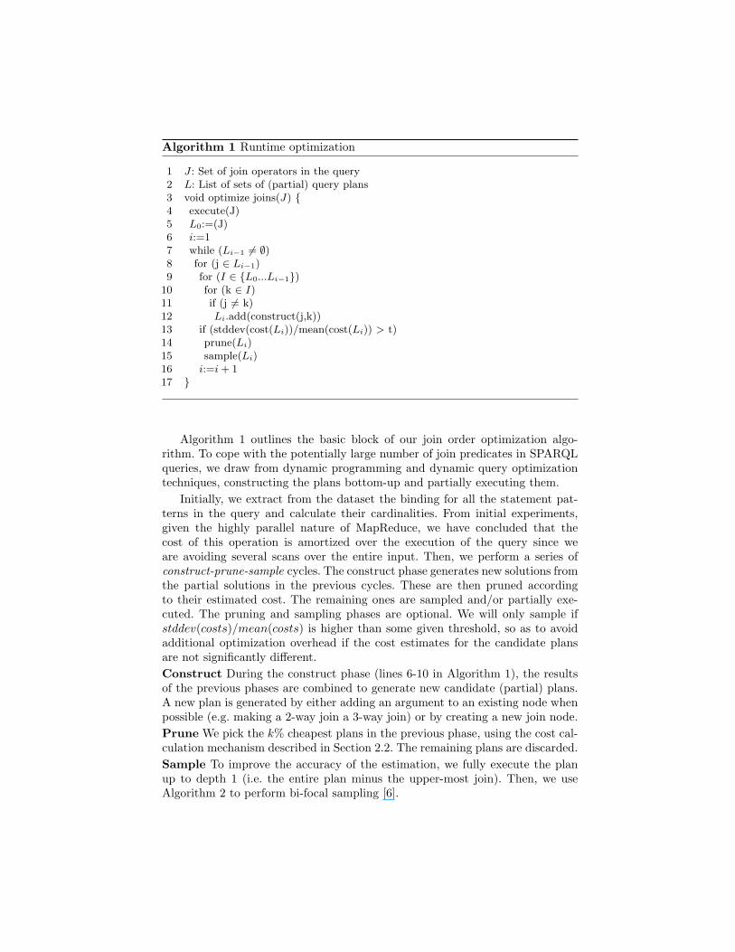
Algorithm 1 Runtime optimization

1 J : Set of join operators in the query2 L: List of sets of (partial) query plans3 void optimize joins(J) {4 execute(J)5 L0:=(J)6 i:=17 while (Li�1 6= ;)8 for (j 2 Li�1)9 for (I 2 {L0...Li�1})

10 for (k 2 I)11 if (j 6= k)12 Li.add(construct(j,k))13 if (stddev(cost(Li))/mean(cost(Li)) > t)14 prune(Li)15 sample(Li)16 i:=i + 117 }

Algorithm 1 outlines the basic block of our join order optimization algo-rithm. To cope with the potentially large number of join predicates in SPARQLqueries, we draw from dynamic programming and dynamic query optimizationtechniques, constructing the plans bottom-up and partially executing them.

Initially, we extract from the dataset the binding for all the statement pat-terns in the query and calculate their cardinalities. From initial experiments,given the highly parallel nature of MapReduce, we have concluded that thecost of this operation is amortized over the execution of the query since weare avoiding several scans over the entire input. Then, we perform a series ofconstruct-prune-sample cycles. The construct phase generates new solutions fromthe partial solutions in the previous cycles. These are then pruned accordingto their estimated cost. The remaining ones are sampled and/or partially exe-cuted. The pruning and sampling phases are optional. We will only sample ifstddev(costs)/mean(costs) is higher than some given threshold, so as to avoidadditional optimization overhead if the cost estimates for the candidate plansare not significantly di↵erent.Construct During the construct phase (lines 6-10 in Algorithm 1), the resultsof the previous phases are combined to generate new candidate (partial) plans.A new plan is generated by either adding an argument to an existing node whenpossible (e.g. making a 2-way join a 3-way join) or by creating a new join node.Prune We pick the k% cheapest plans in the previous phase, using the cost cal-culation mechanism described in Section 2.2. The remaining plans are discarded.Sample To improve the accuracy of the estimation, we fully execute the planup to depth 1 (i.e. the entire plan minus the upper-most join). Then, we useAlgorithm 2 to perform bi-focal sampling [6].

Algorithm 2 Bi-focal sampling in Pig

1 DEFINE bifocal sampling(L, R, s, t)2 RETURNS FC {3 LS = SAMPLE L s;4 RS = SAMPLE R s;5 LSG = GROUP LS BY S;6 RSG = GROUP RS BY S;7 LSC = FOREACH LSG GENERATE flatten(group), COUNT(LSG) as c;8 RSC = FOREACH RSG GENERATE flatten(group), COUNT(RSG) as c;9 LSC = FOREACH LSC GENERATE group::S as S ,c as c;

10 RSC = FOREACH RSC GENERATE group::S as S ,c as c;11 SPLIT LSC INTO LSCP IF c>=t, LSCNP IF c<t;12 SPLIT RSC INTO RSCP IF c>=t, RSCNP IF c<t;13 // Dense14 DJ = JOIN LSCP BY S, RSCP BY S using ’replicated’;15 DJ = FOREACH RA GENERATE LSCP::c as c1, RSCP::c as c2;16 // Left sparse17 RA = JOIN RSC BY S, LSCNP BY S;18 RA = FOREACH RA GENERATE LSCNP::c as c1, RSC::c as c2;19 // Right sparse20 LA = JOIN LSC BY S, RSCNP BY S;21 LA = FOREACH LA GENERATE LSC::c as c1, RSCNP::c as c2;22 // Union results23 AC = UNION ONSCHEMA DA, RA, LA;24 $FC = FOREACH AC GENERATE c1⇤c2 as c;}

There is a number of salient features in our join optimization algorithm:– There is a degree of speculation, since we are sampling only after constructing

and pruning the plans. We do not select plans based on their calculated costusing sampling, but we are selecting plans based on the cost of their ‘sub-plans’ and the operator that will be applied.

– Nevertheless, our algorithm will not get ‘trapped’ into an expensive join,since we only fully execute a join after we have sampled it in a previouscycle.

– Since we are evaluating multiple partial solutions at the same time, it isessential to re-use existing results for our cost estimations and to avoid un-necessary computation. Since the execution of Pig scripts and our run-timeoptimization algorithm often materialize intermediate results anyway, thelatter are re-used whenever possible.

2.2 Pig-aware cost estimation

Using a MapReduce-based infrastructure gives rise to new challenges in costestimation. First, queries are executed in batch and there is significant overheadin starting new batches. Second, within batches, there is no opportunity for

sideways information passing [14], due to constraints in the programming model.Third, when executing queries on thousands of cores, load-balancing becomesvery important, often outweighing the cost for calculating intermediate results.Fourth, random access to data is either not available or very slow since thereare no data indexes. On the other hand, reading large portions of the input isrelatively cheap, since it is an embarrassingly parallel operation.

In this context, we have developed a model based on the cost of the following:Writing a tuple (w); Reading a tuple (r); The cost of a join per tuple. In Hadoop,a join can be performed either during the reduce phase (jr), essentially a com-bination of a hash-join between machines and a merge-join on each machine, orduring the map phase (jm), by loading one side in the memory of all nodes, es-sentially a hash-join. Obviously, the latter is much faster than the former, sinceit does not require repartitioning of the data on one side or sorting, exhibitsgood load-balancing properties, and requires that the input is read and writtenonly once; The depth of the join tree(d), when considering only the reduce-phasejoins. This is roughly proportional to the number of MapReduce jobs requiredto execute the plan. Considering the significant overhead of executing a job, weconsider this separately from reading and writing tuples.

The final cost for a query plan is calculated as the weighted sum of the above,with indicatory weights being 3 for w, 1 for r, 10 for jr, 1 for jm and a valueproportional to the size of the input for d.

2.3 Dealing with Skew

The significant skew in the term distribution of RDF data has been recognized asa major barrier to e�cient parallelization [12]. In this section, we are presentinga method to detect skew and a method for load-balanced joins in Pig.Detecting skew To detect skew (and estimate result set size), we are presentingan implementation of bi-focal sampling [6] for Pig and report the pseudocode inAlgorithm 2. Similar to join optimization, one of the main goals is to minimizethe number of jobs. L, R, s and t refer to the left side of the join, the right sideof the join, the sampling rate and the number of tuples that the memory canhold respectively. Initially, we sample the input (lines 3-4), group by the joinkeys (lines 6-7) and count the number of occurrences of each key (lines 7-10).We split each side of the join by key popularity using a fixed threshold, whichis dependent on the amount or memory available to each processing node (lines11-12). We then perform a join between tuples with popular keys (lines 14-15)and a join for each side for tuples with non-popular keys and the entire input(lines 17-21).

This algorithm generates seven MapReduce jobs out of which two are Map-only jobs that can be executed in parallel and four are jobs with Reduce phasesthat happen concurrently in pairs. In fact, it is possible to implement our algo-rithm in two jobs, programming directly on Hadoop instead of using Pig primi-tives.Determining join implementation In Pig, it is up to the developer to choosethe join implementation. In our system, we choose according to the following:

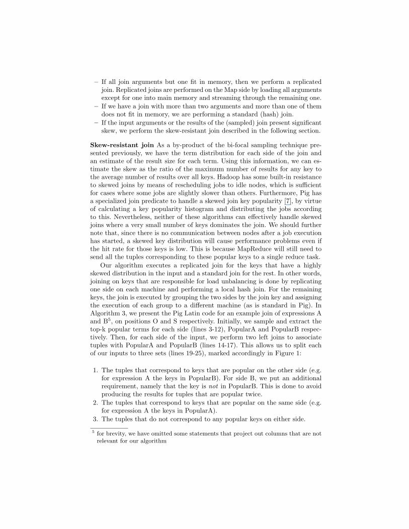
– If all join arguments but one fit in memory, then we perform a replicatedjoin. Replicated joins are performed on the Map side by loading all argumentsexcept for one into main memory and streaming through the remaining one.

– If we have a join with more than two arguments and more than one of themdoes not fit in memory, we are performing a standard (hash) join.

– If the input arguments or the results of the (sampled) join present significantskew, we perform the skew-resistant join described in the following section.

Skew-resistant join As a by-product of the bi-focal sampling technique pre-sented previously, we have the term distribution for each side of the join andan estimate of the result size for each term. Using this information, we can es-timate the skew as the ratio of the maximum number of results for any key tothe average number of results over all keys. Hadoop has some built-in resistanceto skewed joins by means of rescheduling jobs to idle nodes, which is su�cientfor cases where some jobs are slightly slower than others. Furthermore, Pig hasa specialized join predicate to handle a skewed join key popularity [7], by virtueof calculating a key popularity histogram and distributing the jobs accordingto this. Nevertheless, neither of these algorithms can e↵ectively handle skewedjoins where a very small number of keys dominates the join. We should furthernote that, since there is no communication between nodes after a job executionhas started, a skewed key distribution will cause performance problems even ifthe hit rate for those keys is low. This is because MapReduce will still need tosend all the tuples corresponding to these popular keys to a single reduce task.

Our algorithm executes a replicated join for the keys that have a highlyskewed distribution in the input and a standard join for the rest. In other words,joining on keys that are responsible for load unbalancing is done by replicatingone side on each machine and performing a local hash join. For the remainingkeys, the join is executed by grouping the two sides by the join key and assigningthe execution of each group to a di↵erent machine (as is standard in Pig). InAlgorithm 3, we present the Pig Latin code for an example join of expressions Aand B5, on positions O and S respectively. Initially, we sample and extract thetop-k popular terms for each side (lines 3-12), PopularA and PopularB respec-tively. Then, for each side of the input, we perform two left joins to associatetuples with PopularA and PopularB (lines 14-17). This allows us to split eachof our inputs to three sets (lines 19-25), marked accordingly in Figure 1:

1. The tuples that correspond to keys that are popular on the other side (e.g.for expression A the keys in PopularB). For side B, we put an additionalrequirement, namely that the key is not in PopularB. This is done to avoidproducing the results for tuples that are popular twice.

2. The tuples that correspond to keys that are popular on the same side (e.g.for expression A the keys in PopularA).

3. The tuples that do not correspond to any popular keys on either side.

5 for brevity, we have omitted some statements that project out columns that are notrelevant for our algorithm

Not popular

Popularin A

Popularin B

A

Popularin A and B

Not popular

Popularin B

Popularin A

Popularin A and B

B

11

2 2

33

Fig. 1: Schematic representation of the joins to implement the skew-resistant join

We use the above to perform replicated joins for the tuples corresponding topopular terms and standard joins for the tuples that are not. The tuples in Acorresponding to popular keys in A (APopInA) are joined with the tuples inB that correspond to popular keys in A using a replicated join (line 28). Thesituation is symmetric for B (line 29). The tuples that do not correspond topopular keys from either side are processed using a standard join (line 31). Theoutput of the algorithm is the union of the results of the three joins.

We should note that our algorithm will fail if APopInB and BPopInA are notsmall enough to be replicated to all nodes. But this can only be true if there aresome keys that are popular in both sets. Joins with such keys would anyway leadto an explosion in the result set (since the result size of each of these popularkeys is the product of their appearances in each side).

3 Evaluation

We present an evaluation of the techniques presented in this paper using syn-thetic and real data, and compare our approach to a commercial RDF store.

We have used two di↵erent Hadoop clusters in our evaluation: a modest clus-ter, part of the DAS-4 distributed supercomputer, and a large cluster installed atYahoo!. The former was used to perform experiments in isolation and consists of32 dual-core nodes, with 4GB of RAM and dual HDDs in RAID-0. The Yahoo!Hadoop cluster we have used in our experiment consists of over 3500 nodes, eachwith two quad-core CPUs, 16 GB RAM and 900GB of local space. This clusteris used in a utility computing fashion and thus we do not have exclusive access,meaning that we can not exploit the full capacity of the cluster and our runtimesat any point might be (negatively) influenced by the jobs of other users. We thusonly report actual, but not best possible performance.

In order to compare our approach with existing solutions, we deployed Vir-tuoso v7 [4], a top-performing RDF store, on an extremely high-end server: a4-socket 2.4GHz Xeon 5870 server (40 cores) with 1TB of main memory and 16magnetic disks in RAID5, running Red Hat Enterprise Linux 6.0.

We chose two datasets for the evaluation. Firstly, the Berlin SPARQL bench-mark [3], Business Intelligence use-case v3.1 (BSBM-BI). This benchmark con-sists of 8 analytical query patterns from the e-commerce domain. The choice for

Algorithm 3 Skew-resistant join

1 DEFINE skew resistant join(A, B, k)2 RETURNS result {3 SA = SAMPLE A 0.01; //Sample first side4 GA = GROUP SA BY O;5 GA2 = FOREACH GA GENERATE COUNT STAR(SA), group;6 OrderedA = ORDER GA2 BY $0 DESC;7 PopularA = LIMIT OrderedA k;8 SB = SAMPLE B 0.01; //Sample second side9 GB = GROUP SB BY S;

10 GB2 = FOREACH GB GENERATE COUNT STAR(SB), group;11 OrderedB = ORDER GB2 BY $0 DESC;12 PopularB = LIMIT OrderedB k;1314 PA = JOIN A BY O LEFT, PopularA BY O USING ’replicated’;15 PPA= JOIN PA BY O LEFT, PopularB BY S USING’replicated’;16 PB = JOIN B BY S LEFT, PopularB BY S USING ’replicated’;17 PPB= JOIN PB BY S LEFT, PopularA BY S USING ’replicated’;1819 SPLIT PPA INTO APopInA IF PopularA::O is not null,20 APopInB IF PopularB::S is not null, ANonPop IF21 PopularA::0 is not null and PopularB::S is not null;2223 SPLIT PPB INTO BPopInB IF PopularB::S is not null, BPopInA24 IF PopularA::O is not null and PopularB::S is null, BNonPop25 IF PopularA::0 in not null and PopularB::S is not null;2627 // Perform replicated joins for popular keys28 JA= JOIN BPopInB BY S, APopInB BY O USING ’replicated’;29 JB= JOIN APopInA BY S, BPopInA BY S USING ’replicated’;30 // Standard join for non�popular keys31 JP = JOIN ANonPop BY O, BNonPop BY S;3233 $result = UNION ONSCHEMA JA, JB, JP; }

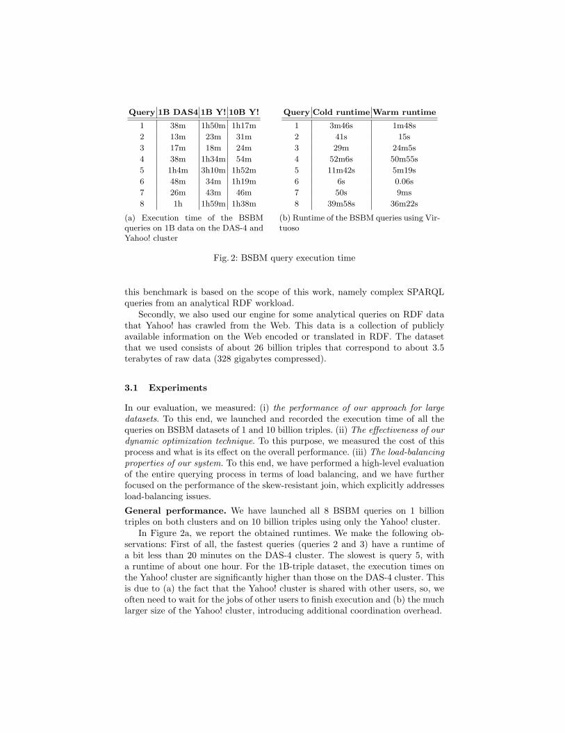
Query 1B DAS4 1B Y! 10B Y!

1 38m 1h50m 1h17m

2 13m 23m 31m

3 17m 18m 24m

4 38m 1h34m 54m

5 1h4m 3h10m 1h52m

6 48m 34m 1h19m

7 26m 43m 46m

8 1h 1h59m 1h38m

(a) Execution time of the BSBMqueries on 1B data on the DAS-4 andYahoo! cluster

Query Cold runtime Warm runtime

1 3m46s 1m48s

2 41s 15s

3 29m 24m5s

4 52m6s 50m55s

5 11m42s 5m19s

6 6s 0.06s

7 50s 9ms

8 39m58s 36m22s

(b) Runtime of the BSBM queries using Vir-tuoso

Fig. 2: BSBM query execution time

this benchmark is based on the scope of this work, namely complex SPARQLqueries from an analytical RDF workload.

Secondly, we also used our engine for some analytical queries on RDF datathat Yahoo! has crawled from the Web. This data is a collection of publiclyavailable information on the Web encoded or translated in RDF. The datasetthat we used consists of about 26 billion triples that correspond to about 3.5terabytes of raw data (328 gigabytes compressed).

3.1 Experiments

In our evaluation, we measured: (i) the performance of our approach for largedatasets. To this end, we launched and recorded the execution time of all thequeries on BSBM datasets of 1 and 10 billion triples. (ii) The e↵ectiveness of ourdynamic optimization technique. To this purpose, we measured the cost of thisprocess and what is its e↵ect on the overall performance. (iii) The load-balancingproperties of our system. To this end, we have performed a high-level evaluationof the entire querying process in terms of load balancing, and we have furtherfocused on the performance of the skew-resistant join, which explicitly addressesload-balancing issues.General performance. We have launched all 8 BSBM queries on 1 billiontriples on both clusters and on 10 billion triples using only the Yahoo! cluster.

In Figure 2a, we report the obtained runtimes. We make the following ob-servations: First of all, the fastest queries (queries 2 and 3) have a runtime ofa bit less than 20 minutes on the DAS-4 cluster. The slowest is query 5, witha runtime of about one hour. For the 1B-triple dataset, the execution times onthe Yahoo! cluster are significantly higher than those on the DAS-4 cluster. Thisis due to (a) the fact that the Yahoo! cluster is shared with other users, so, weoften need to wait for the jobs of other users to finish execution and (b) the muchlarger size of the Yahoo! cluster, introducing additional coordination overhead.

Listing 1.1: Exploratory SPARQL queriesSELECT (count(?s) as ?f) (min(?s) as ?ex) ?ct ?di ?mx ?mi{

{SELECT ?s (count(?s) as ?ct) (count(distinct ?p) as ?di) (max(?p) as ?mx)(min(?p) as ?mi) {?s ?p ?o.} GROUP BY ?s}

GROUP BY ?ct ?di ?mx ?mi ORDER BY desc(?f) LIMIT 10000}

SELECT ?p (COUNT(?s) AS ?c) {?s ?p ?o.} GROUP BY ?p ORDER BY ?c

SELECT ?C (COUNT(?s) AS ?n ) {?s a ?C.} GROUP BY ?C ORDER BY ?n

We also note that the runtime does not proportionally increase with thedata size on the Yahoo! cluster: the runtimes for the one and ten billion-tripledatasets are comparable. Such behavior is explained by the fact that a propor-tional amount of resources is allocated to the size of the input and the (sig-nificant) overhead to start MapReduce jobs does not increase. Our approach,combined with the large infrastructure at Yahoo! allows us to scale to muchlarger inputs while keeping the runtime fairly constant.

To verify the performance in a real-world scenario and on messy data, wehave launched three non-selective SPARQL queries, reported in Listing 1.1, overan RDF web crawl of Yahoo!. The first query is used for identifying ”charac-teristic sets” [13]: frequently co-occurring properties with a subject. The secondidentifies all the properties used in the dataset and sorts them according to theirfrequency. The third identifies the classes with the most instances. These queriesare typical of an exploratory ETL workload on messy data, aimed at creating abasic understanding of the structure and properties of a web-crawled dataset.

From the computation point of view, the first two queries have non-boundproperties and the last one has a very non-selective property (rdf:type) . There-fore they will touch the entire dataset, including problematic properties thatcause skew problems. The runtime of these three queries was respectively 1 hourand 21 minutes, 29 minutes and 25 minutes. The first query required 6 MapRe-duce jobs to be computed. The second and third each required 3 jobs.

It is interesting to compare the performance for BSBM against a standardRDF store (Virtuoso), even if the approaches are radically di↵erent. We loaded10 billion BSBM triples on the platform described previously. This process took61 hours (about 2.5 days) and was performed in collaboration with the Virtuosodevelopment team to ensure that the configuration was optimal.

We executed the 8 BSBM queries used in this evaluation and we report theresults in Figure 2b. For some queries, Virtuoso is many orders of magnitudefaster than our approach (namely, for the simpler queries like queries 1,2, 6 and7). For the more expensive queries, the di↵erence is less pronounced. However,this performance comes at the price of a loading time of 61 hours, necessary tocreate the database indexes. To load the data and run all the queries on Virtu-oso, the total runtime amounts to 63 hours, while in our MapReduce approach,it amounts to 8 hours and 40 minutes. Although we can not generalize this con-

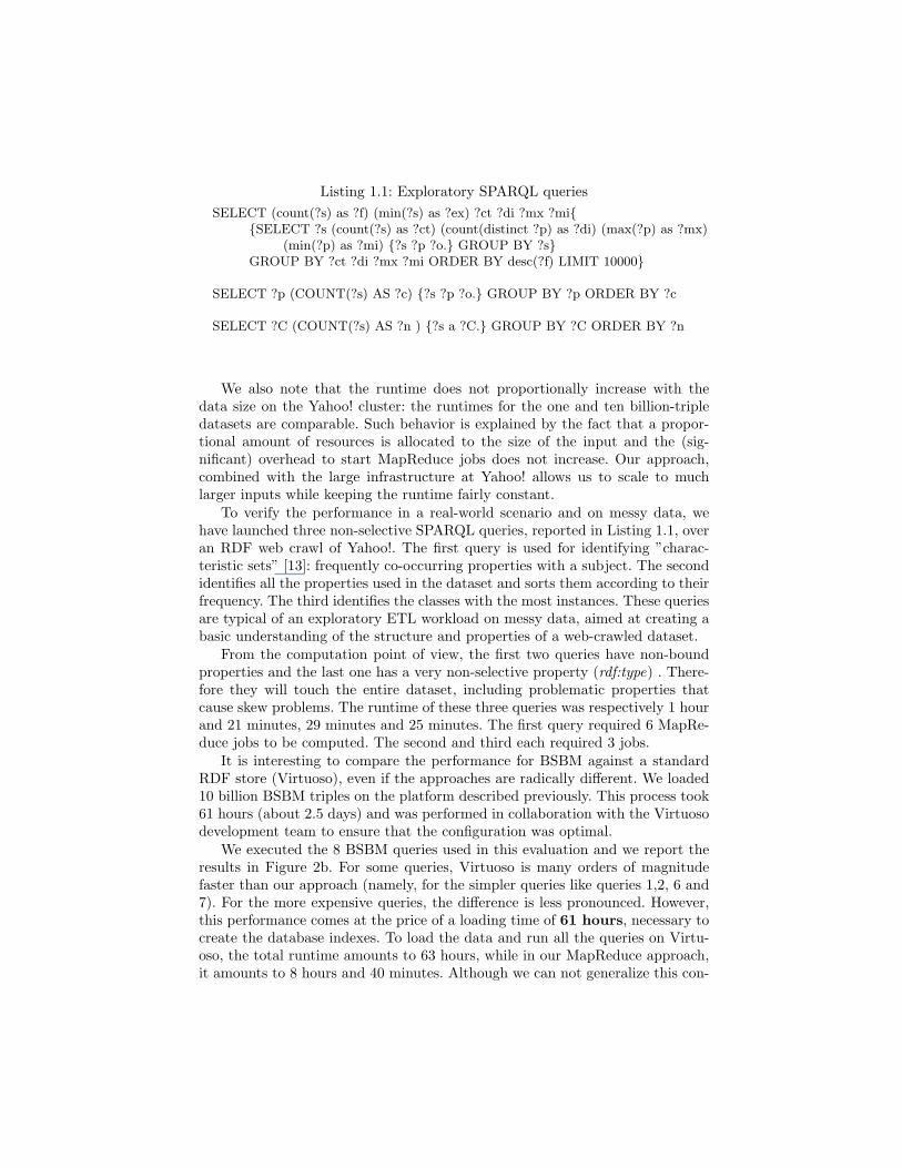
Query Cost input Cost dyn. Final query

extraction optimizer execution

1 5m58s 12m12s 19m43s

2 4m22s n.a. 9m5s

3 5m46s n.a. 11m58s

4 6m22s 14m41s 16m55s

5 7m37s 34m3s 23m21s

6 8m12s 14m25s 25m10s

7 5m17s 6m17s 14m3s

8 8m7s 25m14s 27m2s

Table 1: Breakdown of query runtimes on 1B BSBM data

1"

1.5"

2"

2.5"

3"

3.5"

4"

4.5"

5"

1" 2" 3" 4" 5" 6" 7" 8"

max$ru

n(me/avg$run(

me$

Query$

Map"jobs"

Reduce"jobs"

Skew%resistant,Join Standard,join Skewed,Pig,join7.444407 7444407 7.435536 7435536 14712562 14.7125627.171898 7171898 7.44526 7445260 15222484 15.2224846.846509 6846509 7.71953 7719530 15480332 15.4803328.031175 8031175 6.781385 6781385 14579335 14.5793358.338536 8338536 6.677068 6677068 15064830 15.064837.718776 7718776 8.33958 8339580 15276993 15.2769936.988908 6988908 9.658339 9658339 14605823 14.6058236.987234 6987234 7.719273 7719273 15448438 15.4484387.166306 7166306 6.989345 6989345 15904262 15.9042627.434722 7434722 6.780244 6780244 16028453 16.0284536.772644 6772644 9.379523 9379523 15436619 15.4366196.610677 6610677 9.170394 9170394 15667872 15.6678726.611979 6611979 7.172604 7172604 15001336 15.0013367.034329 7034329 7.174411 7174411 15178646 15.1786466.840467 6840467 6.988282 6988282 15921476 15.9214769.378686 9378686 6.671456 6671456 15537895 15.5378958.03298 8032980 6.840754 6840754 15661794 15.661794

7.718393 7718393 6.853333 6853333 15069536 15.0695367.037779 7037779 8.032342 8032342 15553211 15.5532118.639919 8639919 6.611304 6611304 15081025 15.0810258.912407 8912407 6.612637 6612637 14829761 14.8297618.321148 8321148 7.92703 7927030 15708465 15.7084656.775556 6775556 9.69276 9692760 16503101 16.5031016.668647 6668647 7.541059 7541059 15830437 15.8304377.533555 7533555 9.543576 9543576 15471421 15.4714219.744701 9744701 9.372974 9372974 16146658 16.1466589.372421 9372421 6.691908 6691908 15919851 15.9198518.624926 8624926 8.634754 8634754 16158957 16.1589579.665113 9665113 8.742813 8742813 16278956 16.2789569.169475 9169475 9.591875 9591875 16268376 16.2683769.168914 9168914 9.014395 9014395 16426524 16.4265249.535133 9535133 9.240234 9240234 16924815 16.9248156.670845 6670845 9.597329 9597329 17012159 17.0121596.635968 6635968 9.733461 9733461 17161229 17.1612296.703297 6703297 7.533915 7533915 16974466 16.9744667.540321 7540321 7.282981 7282981 16785313 16.7853138.43968 8439680 9.456818 9456818 16547096 16.547096

8.448404 8448404 12.697658 12697658 16767928 16.7679287.276617 7276617 10.27742 10277420 17718004 17.7180049.697108 9697108 8.330576 8330576 17527739 17.5277398.908008 8908008 9.624898 9624898 17242460 17.242469.546406 9546406 10.895828 10895828 17566904 17.5669046.630042 6630042 10.345621 10345621 17645580 17.645586.691389 6691389 8.137103 8137103 17825013 17.8250137.265595 7265595 10.302287 10302287 17380274 17.380274

0,

20,

40,

60,

80,

100,

120,

140,

#Records,,(millions),

Reduce,tasks,

Skew1resistant,Join,

Standard,join,

Skewed,Pig,join,

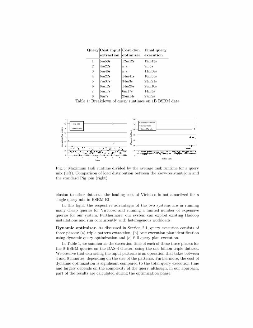
Fig. 3: Maximum task runtime divided by the average task runtime for a querymix (left). Comparison of load distribution between the skew-resistant join andthe standard Pig join (right).

clusion to other datasets, the loading cost of Virtuoso is not amortized for asingle query mix in BSBM-BI.

In this light, the respective advantages of the two systems are in runningmany cheap queries for Virtuoso and running a limited number of expensivequeries for our system. Furthermore, our system can exploit existing Hadoopinstallations and run concurrently with heterogenous workloads.

Dynamic optimizer. As discussed in Section 2.1, query execution consists ofthree phases: (a) triple pattern extraction, (b) best execution plan identificationusing dynamic query optimization and (c) full query plan execution.

In Table 1, we summarize the execution time of each of these three phases forthe 8 BSBM queries on the DAS-4 cluster, using the one billion triple dataset.We observe that extracting the input patterns is an operation that takes between4 and 8 minutes, depending on the size of the patterns. Furthermore, the cost ofdynamic optimization is significant compared to the total query execution timeand largely depends on the complexity of the query, although, in our approach,part of the results are calculated during the optimization phase.

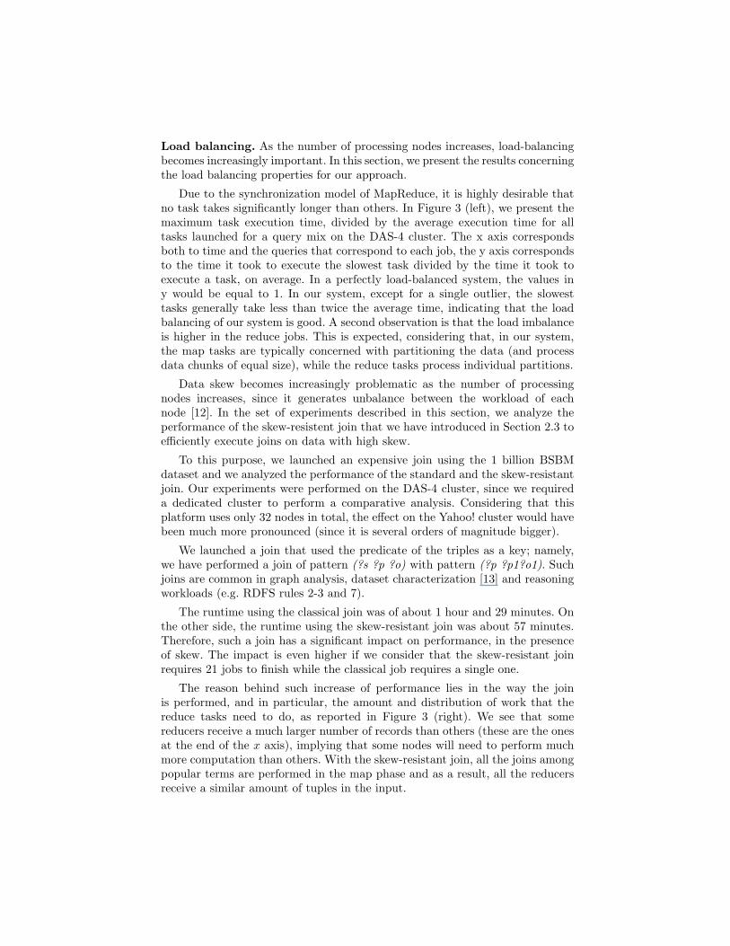
Load balancing. As the number of processing nodes increases, load-balancingbecomes increasingly important. In this section, we present the results concerningthe load balancing properties for our approach.

Due to the synchronization model of MapReduce, it is highly desirable thatno task takes significantly longer than others. In Figure 3 (left), we present themaximum task execution time, divided by the average execution time for alltasks launched for a query mix on the DAS-4 cluster. The x axis correspondsboth to time and the queries that correspond to each job, the y axis correspondsto the time it took to execute the slowest task divided by the time it took toexecute a task, on average. In a perfectly load-balanced system, the values iny would be equal to 1. In our system, except for a single outlier, the slowesttasks generally take less than twice the average time, indicating that the loadbalancing of our system is good. A second observation is that the load imbalanceis higher in the reduce jobs. This is expected, considering that, in our system,the map tasks are typically concerned with partitioning the data (and processdata chunks of equal size), while the reduce tasks process individual partitions.

Data skew becomes increasingly problematic as the number of processingnodes increases, since it generates unbalance between the workload of eachnode [12]. In the set of experiments described in this section, we analyze theperformance of the skew-resistent join that we have introduced in Section 2.3 toe�ciently execute joins on data with high skew.

To this purpose, we launched an expensive join using the 1 billion BSBMdataset and we analyzed the performance of the standard and the skew-resistantjoin. Our experiments were performed on the DAS-4 cluster, since we requireda dedicated cluster to perform a comparative analysis. Considering that thisplatform uses only 32 nodes in total, the e↵ect on the Yahoo! cluster would havebeen much more pronounced (since it is several orders of magnitude bigger).

We launched a join that used the predicate of the triples as a key; namely,we have performed a join of pattern (?s ?p ?o) with pattern (?p ?p1?o1). Suchjoins are common in graph analysis, dataset characterization [13] and reasoningworkloads (e.g. RDFS rules 2-3 and 7).

The runtime using the classical join was of about 1 hour and 29 minutes. Onthe other side, the runtime using the skew-resistant join was about 57 minutes.Therefore, such a join has a significant impact on performance, in the presenceof skew. The impact is even higher if we consider that the skew-resistant joinrequires 21 jobs to finish while the classical job requires a single one.

The reason behind such increase of performance lies in the way the joinis performed, and in particular, the amount and distribution of work that thereduce tasks need to do, as reported in Figure 3 (right). We see that somereducers receive a much larger number of records than others (these are the onesat the end of the x axis), implying that some nodes will need to perform muchmore computation than others. With the skew-resistant join, all the joins amongpopular terms are performed in the map phase and as a result, all the reducersreceive a similar amount of tuples in the input.

We also report reduce task statistics for the the skew-resistant join imple-mentation in Pig, which calculates a histogram for join keys to better distributethem across the join tasks. Although the size of the cluster is small enough toensure an even load-balance, we note that the standard Pig skewed join sendsalmost double the number of records to each reduce task. This is attributed tofact that our approach shifts much of the load for joining to the Map phase.

4 Related Work

We have compared our approach with previous results from three related ar-eas: (i) MapReduce query processing (ii) adaptive and sampling-based queryoptimization and (iii) cluster-aware SPARQL systems.

In the relational context, similar e↵orts towards SQL query processing overa MapReduce cluster are e.g. Hive [21] and HadoopDB [2]. Both projects do notprovide query optimization when data is raw and unprocessed. Data import is anecessary first step in HadoopDB and may be costly. In Hive, query optimizationbased on statistics is only available if the data has been analyzed as a prior step.

On-the-fly query optimization in Manimal [9] analyzes MapReduce jobs on-the-fly and tries to enhance them by inserting compression code and sometimeseven on-the-fly indexing and index lookup steps.

Situations where there is absence of data statistics in the relational contextof query optimization has led to work on sampling and run-time methods. Ourwork reuses the bi-Focal sampling algorithm [6] which came out of the work inthe relational community to use sampling for query result size estimation. Inthis work, we have adapted the bi-focal algorithm using the Pig language.

The rigid structure of MapReduce and high latencies in starting new jobs ledus to adjust the dynamic re-optimization strategies to these constraints. Otherinteresting run-time approaches are sideways-information passing [14] in largeRDF joins. These are not easily adaptable to the constraints of MapReduce.

With the ever growing sizes of RDF data available, scalability has been aprimary concern and major RDF systems such as Virtuoso [4], 4store [18], andBigData [20] have evolved to parallel database architectures targeting clusterhardware. RDF systems typically employ heavy indexing, going as far as creatingreplicated storage in all six permutations of triple order [15, 22], which makesdata import a heavy process. Such choice puts them in a disadvantage whenthe scenario involves processing huge amounts of raw data. As an alternativeto the parallel database approach, there are several other projects that processSPARQL queries over MapReduce. PIGSparQL [19] performs a direct mappingof SPARQL to Pig without focusing on optimization. RAPID+ [17] providesa limited form of on-the-fly optimization where look-ahead processing tries tocombine multiple subsequent join steps. The adaptiveness of this approach ishowever limited compared to our sampling based run-time query optimization.

5 Conclusions

In this paper, we have presented an engine for the processing of complex analyticSPARQL 1.1 queries, based on Apache Pig. In particular, we have developed:(i) a translation from SPARQL 1.1 to Pig Latin, (ii) a method for runtimejoin optimization based on a cost model suitable for MapReduce-based systems,(iii) a method for result set estimation and join key skew detection, and (iv) amethod for skew-resistant joins written in Pig. We have evaluated our approachon a standard and a very large Hadoop cluster used at Yahoo! using syntheticbenchmark data and real-world data crawled from the Web.

In our evaluation, we established that our approach can answer complexanalytical queries over very large synthetic data (10 Billion triples from BSBM)and over the largest real-world messy dataset in the literature (26 Billion triples).We compared our performance against a state-of-the-art RDF store on a large-memory server, even though the two approaches bear significant di↵erences.While our approach is not competitive in terms of query response time, oursystem has the advantage that it does not require a-priori loading of the data,and thus has far better loading plus querying performance. Furthermore, oursystem runs on a shared architecture of thousands of machines, significantlyeasing deployment and potentially scaling to even larger volumes of data. Weverified that the load in our system is well-balanced and our skew-resistant joinsignificantly outperforms the standard join of Pig for skewed key distributionsin the input.

In this work, for the first time, it has been shown that MapReduce is suitedfor very large-scale analytical processing of RDF graphs and it is, in fact, bettersuited than a traditional RDF store in a setting where a relatively small numberof queries will be posted on a very large dataset.

We see future work in optimizing our architecture to further reduce overhead.This could be achieved by turning to an approach that adaptively indexes partof the input or performs part of the computation outside of Pig so as to reducethe number of jobs. Similarly, parts of the skew-resistant join can be alreadycalculated during Bi-focal sampling (e.g. sampling and extracting the popularterms for the input relations).

Although in this paper we have presented our algorithm to handle skewedjoins in the context of Pig, we expect that the result is transferrable to a generalparallel data-processing framework.

Summarizing, in this paper, we have presented a technique with which tech-nologies like MapReduce and Pig can be employed for large-scale SPARQLquerying. The presented results are promising and set the lead for a new viablealternative to traditional RDF stores for executing expensive analytical querieson large volumes of RDF data.

Acknowledgements. Spyros Kotoulas and Jacopo Urbani were partially sup-ported by EU project LarKC (FP7-215535) and the Yahoo! Faculty ResearchEngagement Program. Peter Boncz was partially supported by EU project LOD2(FP7-257943).

References

1. R. Abdel Kader, P. Boncz, S. Manegold, and M. van Keulen. ROX: run-timeoptimization of XQueries. SIGMOD, 2009.

2. A. Abouzeid, K. Bajda-Pawlikowski, D. Abadi, A. Rasin, and A. Silberschatz.HadoopDB: An Architectural Hybrid of MapReduce and DBMS Technologies forAnalytical Workloads. PVLDB, 2(1):922–933, 2009.

3. C. Bizer and A. Schultz. The Berlin SPARQL Benchmark. International Journalon Semantic Web and Information Systems (IJSWIS), 5(2):1–24, 2009.

4. O. Erling. Virtuoso, a Hybrid RDBMS/Graph Column Store. DEBULL, 35(1):3–8,2012.

5. M. Gallego, J. Fernandez, M. Martınez-Prieto, and P. Fuente. An empirical studyof real-world SPARQL queries. In USEWOD2011 at WWW 2011.

6. S. Ganguly, P. Gibbons, Y. Matias, and A. Silberschatz. Bifocal sampling forskew-resistant join size estimation. SIGMOD Record, 25(2):271–281, 1996.

7. A. Gates, O. Natkovich, S. Chopra, P. Kamath, S. Narayanamurthy, C. Olston,B. Reed, S. Srinivasan, and U. Srivastava. Building a high-level dataflow systemon top of Map-Reduce: the Pig experience. PVLDB, 2(2):1414–1425, 2009.

8. M. Ivanova, M. Kersten, N. Nes, and R. Goncalves. An architecture for recyclingintermediates in a column-store. TODS, 35(4):24, 2010.

9. E. Jahani, M. Cafarella, and C. Re. Automatic Optimization for MapReducePrograms. PVLDB, 4(6):385–396, 2011.

10. R. Kader, M. van Keulen, P. Boncz, and S. Manegold. Run-time Optimizationfor Pipelined Systems. Proceedings of the IV Alberto Mendelzon Workshop onFoundations of Data Management, 2010.

11. G. Kobilarov, T. Scott, Y. Raimond, S. Oliver, C. Sizemore, M. Smethurst,C. Bizer, and R. Lee. Media meets semantic web — how the BBC uses DBpe-dia and linked data to make connections. ESWC 2009.

12. S. Kotoulas, E. Oren, F. van Harmelen, and F. van Harmelen. Mind the data skew:distributed inferencing by speeddating in elastic regions. WWW, 2010.

13. T. Neumann and G. Moerkotte. Characteristic sets: Accurate cardinality estima-tion for RDF queries with multiple joins. ICDE, 2011.

14. T. Neumann and G. Weikum. Scalable join processing on very large RDF graphs.SIGMOD, 2009.

15. T. Neumann and G. Weikum. The RDF-3X engine for scalable management ofRDF data. The VLDB Journal, 19(1):91–113, 2010.

16. C. Olston, B. Reed, U. Srivastava, R. Kumar, and A. Tomkins. Pig latin: a not-so-foreign language for data processing. SIGMOD, 2008.

17. P. Ravindra, V. Deshpande, and K. Anyanwu. Towards scalable RDF graph an-alytics on MapReduce. In Proceedings of the 2010 Workshop on Massive DataAnalytics on the Cloud, page 5. ACM, 2010.

18. M. Salvadores, G. Correndo, S. Harris, N. Gibbins, and N. Shadbolt. The designand implementation of minimal RDFS backward reasoning in 4store. The SemanicWeb: Research and Applications, pages 139–153, 2011.

19. A. Schatzle and G. Lausen. PigSPARQL: mapping SPARQL to Pig Latin. SWIM:the 3th International Workshop on Semantic Web Information Management, 2011.

20. L. SYSTAP. Bigdata R�.21. A. Thusoo, J. Sarma, N. Jain, Z. Shao, P. Chakka, N. Zhang, S. Anthony, H. Liu,

and R. Murthy. Hive: a petabyte scale data warehouse using Hadoop. ICDE, 2010.22. C. Weiss, P. Karras, and A. Bernstein. Hexastore: sextuple indexing for semantic

web data management. PVLDB, 1(1):1008–1019, 2008.