Riparian Shading Study - Brown's Creek Watershed District
174
September 5, 2018 Prepared by: Olivia Sparrow (EOR and University of Minnesota) For the Brown’s Creek Watershed District Saint Anthony Falls Laboratory Project Report #585 Riparian Shading Study
-
Upload
khangminh22 -
Category
Documents
-
view
2 -
download
0
Transcript of Riparian Shading Study - Brown's Creek Watershed District

September 5, 2018
Prepared by: Olivia Sparrow (EOR and University of Minnesota)
For the Brown’s Creek Watershed District
Saint Anthony Falls Laboratory Project Report #585
Riparian Shading Study

Cover Images
Brown’s Creek south of Millbrook Circle
Funding for this project was provided by the Clean Water Land and Legacy Amendment Fund through an Accelerated
Implementation Grant and by the Brown’s Creek Watershed District.

E O R : w a t e r | e c o l o g y | c o m m u n i t y P a g e | i
TABLE OF CONTENTS
LIST OF TABLES ................................................................................................................................................... V
ACKNOWLEDGEMENTS ...................................................................................................................................... V
GLOSSARY ......................................................................................................................................................... VI
ACRONYMS ....................................................................................................................................................... IX
EXECUTIVE SUMMARY ....................................................................................................................................... X
1. INTRODUCTION ........................................................................................................................................... 1
2. BACKGROUND ............................................................................................................................................. 2
3. STUDY AREA CHARACTERIZATION ............................................................................................................... 13
3.1. Climate ....................................................................................................................................................... 13 3.2. Watershed, Water Resources, and Hydrology ........................................................................................... 14 3.3. Ecological Classification ............................................................................................................................. 18 3.4. Topography and Geology ........................................................................................................................... 20 3.5. Soils ............................................................................................................................................................ 27 3.6. Plant Communities ..................................................................................................................................... 29
3.6.1. Historic Vegetation ...................................................................................................................... 29 3.6.2. Existing Vegetation ...................................................................................................................... 29
3.7. Floodplain, Upland, and Wetland Wildlife ................................................................................................. 33 3.8. Aquatic Biota.............................................................................................................................................. 33
4. LITERATURE REVIEW SUMMARIES .............................................................................................................. 36
5. RIPARIAN SHADE ANALYSIS ........................................................................................................................ 37
5.1. Existing Conditions ..................................................................................................................................... 37 5.1.1. Method ........................................................................................................................................ 37 5.1.2. Results ......................................................................................................................................... 44 5.1.3. Discussion .................................................................................................................................... 57
5.2. Sensitivity Analysis ..................................................................................................................................... 59 5.2.1. Method ........................................................................................................................................ 60 5.2.2. Results ......................................................................................................................................... 61 5.2.3. Discussion .................................................................................................................................... 65
5.3. Future Conditions ...................................................................................................................................... 67 5.3.1. Method ........................................................................................................................................ 68 5.3.2. Results ......................................................................................................................................... 71 5.3.3. Discussion .................................................................................................................................... 77
6. STREAM TEMPERATURE MODEL ................................................................................................................. 79
6.1. Existing Conditions ..................................................................................................................................... 79 6.2. Future Conditions ...................................................................................................................................... 85 6.3. Discussion .................................................................................................................................................. 90
7. RECOMMENDATIONS ................................................................................................................................. 94
8. LITERATURE CITED .................................................................................................................................... 100
APPENDIX A. LITERATURE REVIEW ON ESTIMATING RIPARIAN SHADE .................................................... 109

E O R : w a t e r | e c o l o g y | c o m m u n i t y P a g e | i i
A.1. Introduction ............................................................................................................................................. 109 A.2. Background .............................................................................................................................................. 112
A.2.1. Terminology: Canopy Cover, Canopy Closure, and Shade ......................................................... 113 A.3. Direct and Indirect Measurements .......................................................................................................... 115
A.3.1. Air and Space-Borne Methods ................................................................................................... 115 A.3.2. Ground-Based Methods ............................................................................................................ 117 A.3.3. Ancillary Data ............................................................................................................................ 123
A.4. Modeling (Theoretical Relationships) ...................................................................................................... 124 A.5. Outlook for Further Areas of Research .................................................................................................... 125 A.6. Conclusions .............................................................................................................................................. 126
APPENDIX B. TRADE-OFFS OF GRASSY AND WOODY RIPARIAN VEGETATION .......................................... 128
B.1. Aquatic Fauna .......................................................................................................................................... 131 B.2. Erosion, Sediment, and Channel Morphology ......................................................................................... 133
B.2.1. Channel Morphology ................................................................................................................. 133 B.2.2. Erosion Control in Riparian Buffer Zones .................................................................................. 137 B.2.3. Filtering Sediment from Runoff ................................................................................................. 137
B.3. Microclimate ............................................................................................................................................ 138 B.4. Groundwater and Baseflow ..................................................................................................................... 138 B.5. Organic Carbon and Primary Production ................................................................................................. 141 B.6. Phosphorus .............................................................................................................................................. 141 B.7. Climate Change Adaptation ..................................................................................................................... 141 B.8. Maintenance ............................................................................................................................................ 143 B.9. Landowner Willingness ............................................................................................................................ 143 B.10. Conclusions and Management Implications ............................................................................................ 144
APPENDIX C. COLLECTED DATA AND ANALYSIS RESULTS ........................................................................ 146
APPENDIX D. SUITABLE PLANTS.............................................................................................................. 154
APPENDIX E. RIPARIAN SHADE MONITORING PLAN ............................................................................... 155
E.1. Parameters .............................................................................................................................................. 155 E.2. Method .................................................................................................................................................... 156
E.2.1. Equipment List ........................................................................................................................... 158 E.2.2. Data Form .................................................................................................................................. 159
E.3. Reporting Results and Recommending Corrective Actions ..................................................................... 160 E.4. Implementation ....................................................................................................................................... 160

E O R : w a t e r | e c o l o g y | c o m m u n i t y P a g e | i i i
LIST OF FIGURES
Figure 1. Location Map of Brown's Creek and Impairments ......................................................................................... 4 Figure 2. Heat Load Duration Curve 2000-2007 WOMP Station (Emmons & Olivier Resources, 2010) ........................ 5 Figure 3. Daily Average Flow and Temperature During Days When the Daily Average Temperature Exceeded 18ºC at
the WOMP Site (Emmons & Olivier Resources, 2012) ................................................................................. 6 Figure 4. Stream Geomorphology and Thermal Buffer Improvements (1 of 2) (Emmons & Olivier Resources, 2012) . 8 Figure 5. Stream Geomorphology and Thermal Buffer Improvements (2 of 2) (Emmons & Olivier Resources, 2012) . 9 Figure 6. Existing Riparian Shade in Fall 2011 Estimated Using LiDAR and Calibrated to Observed Stream
Temperatures (Herb & Correll, 2016) ......................................................................................................... 11 Figure 7. Summary of Monthly Air Temperature and Precipitation in 2012 and 2014 (Herb & Correll, 2016) ........... 13 Figure 8. Flow Duration Curve (2000-2007) at WOMP Station ................................................................................... 14 Figure 9. Landlocked Basins of Brown's Creek Watershed (Emmons & Olivier Resources, 2017) .............................. 16 Figure 10. Water Resources in Study Area .................................................................................................................. 17 Figure 11. BCWD Management Classifications of Wetlands in Study Area ................................................................. 18 Figure 12. Ecoregion of Study Area ............................................................................................................................. 19 Figure 13. Bedrock Geology of Study Area .................................................................................................................. 21 Figure 14. Surficial Geology of Study Area .................................................................................................................. 22 Figure 15. Typical Cross Section of the Brown’s Creek Headwaters Region (Emmons & Olivier Resources, 2017) .... 23 Figure 16. Typical Cross Section of the Brown's Creek Middle Reach (Emmons & Olivier Resources, 2017) ............. 24 Figure 17. Typical Cross Section of the Brown’s Creek Gorge (Emmons & Olivier Resources, 2017) .......................... 25 Figure 18. Soils of Study Area ...................................................................................................................................... 28 Figure 19. Pre-Settlement Vegetation near Study Area .............................................................................................. 31 Figure 20. Existing Native and Natural Plant Communities ......................................................................................... 32 Figure 21. Adult Brown Trout Caught in Oak Glen Golf Course on Sept. 13, 2016 (Photo Credit: MN DNR) .............. 34 Figure 22. YOY Brown Trout Caught in Brown's Creek Gorge on Sept. 30, 2016 (Photo Credit: Mike Majeski, EOR) . 34 Figure 23. Length-Frequency Distribution of Brown Trout Captured in Brown's Creek Gorge (Lallaman, 2017) ....... 35 Figure 24. Illustrative guide showing cross-sectional configuration, composition and delineative criteria of major
stream types (Rosgen, 1994) ..................................................................................................................... 38 Figure 25. Evolutionary stages of channel adjustment (Rosgen, 1994) ....................................................................... 38 Figure 26. Location of Representative and Sampled Reaches ..................................................................................... 39 Figure 27. Setup for Center Photograph ...................................................................................................................... 40 Figure 28. Example Transect with Photograph Locations............................................................................................ 40 Figure 29. Example of Hemispherical Photographs (Reach 3, Transect 7) .................................................................. 40 Figure 30. Steps of Hemispherical Photographs Analysis ............................................................................................ 43 Figure 31. Stage-Shade Curves at Forested and Grassy Transects .............................................................................. 47 Figure 32. Transect Shade Estimated with WinSCANOPY on Average and at Positions .............................................. 48 Figure 33. Correlation Coefficients of Independent and Dependent Variables .......................................................... 49 Figure 34. Independent Variables vs. Average Transect Shade ................................................................................... 50 Figure 35. Variation in Transect Shade (WinSCANOPY) Based on Woody Riparian Vegetation Composition ............ 51 Figure 36. Transect Shade Estimated using WinSCANOPY in Comparison to Shade Estimated from LiDAR ............... 52 Figure 37. Transect Shade Estimated using WinSCANOPY in Comparison to Shade Calibrated in Brown’s Creek
Thermal Study ............................................................................................................................................ 53 Figure 38. Average Transect Shade Estimated using LiDAR and WinSCANOPY (Omitting Reach 7) ............................ 54 Figure 39. Average Reach Shade Estimated Using LiDAR and WinSCANOPY (Omitting Reach 7) ............................... 54 Figure 40. Profile of Existing Conditions Riparian Shade along Brown's Creek ........................................................... 54 Figure 41. Updated Riparian Shade Analysis using WinSCANOPY (Shade Conditions in Year 2011) ........................... 55 Figure 42. Growing Season Shade Estimated in WinSCANOPY using Hemispherical Photographs from Mid-Summer
and Late Summer ....................................................................................................................................... 56 Figure 43. Flow Duration Curve at Highway 15 and at McKusick (Oak Glen) from April to October 2017.................. 57 Figure 44. Base Scenario of Sensitivity Analysis .......................................................................................................... 61 Figure 45. Sensitivity Analysis of Modeled Shade to Stream Azimuth ........................................................................ 62

E O R : w a t e r | e c o l o g y | c o m m u n i t y P a g e | i v
Figure 46. Sensitivity Analysis of Modeled Shade to Stream Width (0° Azimuth) ....................................................... 62 Figure 47. Sensitivity Analysis of Modeled Shade to Stream Width (90° Azimuth) ..................................................... 62 Figure 48. Sensitivity Analysis of Modeled Shade to Vegetation Height ..................................................................... 63 Figure 49. Sensitivity Analysis of Modeled Shade to Vegetation Crown (Diameter) ................................................... 63 Figure 50. Sensitivity Analysis of Modeled Shade to Vegetation Density ................................................................... 63 Figure 51. Sensitivity Analysis of Modeled Shade to Vegetation Offset ...................................................................... 64 Figure 52. Sensitivity Analysis of Modeled Shade to Azimuth under Optimized Grassy Conditions ........................... 64 Figure 53. Sensitivity Analysis of Modeled Shade to Azimuth under Offset Woody Conditions ................................. 64 Figure 54. Sensitivity Analysis of Modeled Shade to Azimuth With Optimized Grassy and Woody Vegetation ......... 65 Figure 55. Summary of Simulated Total Daily Shade from Variables Modified in Sensitivity Analysis ........................ 66 Figure 56. Concept Shade Restoration Plan for Segment 13 ....................................................................................... 72 Figure 57. Concept Shade Restoration Plan for Segment 12 ....................................................................................... 73 Figure 58. Concept Shade Restoration Plan for Segment 11 ....................................................................................... 74 Figure 59. Concept Shade Restoration Plan for Segment 10B ..................................................................................... 75 Figure 60. Targeted Shade Restoration Scenario IV .................................................................................................... 76 Figure 61. Estimated Shade Over Time as Vegetation Establishes in Oak Glen Golf Course Restoration ................... 77 Figure 62. Shade Inputs to Existing Conditions CE-QUAL-W2 Models in Thermal and Riparian Shading Studies ....... 79 Figure 63. Simulated and Observed Daily Average Stream Temperature in 2012 at the McKusick (Oak Glen),
Stonebridge, and WOMP Monitoring Stations ........................................................................................... 81 Figure 64. Simulated and Observed Daily Maximum Stream Temperature in 2012 at the McKusick (Oak Glen),
Stonebridge, and WOMP Monitoring Stations ........................................................................................... 82 Figure 65. Simulated and Observed Daily Average Stream Temperature in 2014 at the McKusick (Oak Glen),
Stonebridge, and WOMP Monitoring Stations ........................................................................................... 83 Figure 66. Simulated and Observed Daily Maximum Stream Temperature in 2012 at the McKusick (Oak Glen),
Stonebridge, and WOMP Monitoring Stations ........................................................................................... 84 Figure 67. Comparison of Existing Riparian Shading with the Shade Restoration Scenarios ...................................... 85 Figure 68. Monthly Mean Water Temperatures in June, July, and August under Existing and Shade Restoration
Conditions in 2012 and 2014 ...................................................................................................................... 86 Figure 69. Daily Maximum Water Temperatures at Monitoring Stations under Existing Conditions and Shade
Restoration Scenario IV .............................................................................................................................. 87 Figure 70. Total Hours Exceeding Threat Temperature ............................................................................................... 88 Figure 71. Total Days with at Least 1 Hour Exceeding Threat Temperature ............................................................... 89 Figure 72. Heat Load Duration Curve 2000-2007 WOMP Station (Emmons & Olivier Resources, 2010) .................... 99 Figure 73. Major Heat Flux Processes in a Stream (Interpretation of Moore et al., 2005) ....................................... 109 Figure 74. Detailed Diagram of Causal Pathways to Changing Water Temperature and Impaired Biota (Sappington &
Norton, 2010) ........................................................................................................................................... 111 Figure 75. Canopy Cover (a) and Canopy Closure (b) Measured Across a Stream .................................................... 114 Figure 76. Midday Shading of Streams with North-South (a) and East-West (b) Orientations in Northern Hemisphere
.................................................................................................................................................................. 115 Figure 77. Clinometer Used to Estimate Topographic (30°) and Vegetative Cover (55°) Angles (Dent et al., 2000) 118 Figure 78. Modified Densiometer (Dent et al., 2000) ................................................................................................ 118 Figure 79. Solar Pathfinder (SolarPathinder, 2016) ................................................................................................... 120 Figure 80. Hemispherical Photo with Sun Path ......................................................................................................... 121 Figure 81. Existing Riparian Vegetation Types in Study Area: (1) Woody, (2) Shrubby, (3) Grassy, (4) Manicured .. 129 Figure 82. Early Stages in the Natural Development of a Fertile Lowland Wisconsin Trout Stream from Overgrazed
(a) to Very Productive (D) (White & Brynildson, 1967) ............................................................................ 135 Figure 83. Late Stages in the Natural Development of a Fertile Lowland Wisconsin Trout Stream from Very Productive
(E-F) to Overforested (G&H) (White & Brynildson, 1967) ........................................................................ 136 Figure 84. Locations for Riparian Shade Monitoring Program .................................................................................. 155 Figure 85. Example Transect with Photograph Locations.......................................................................................... 157 Figure 86. Example of Hemispherical Photograph .................................................................................................... 157 Figure 87. Setup for Center Photo ............................................................................................................................. 157

E O R : w a t e r | e c o l o g y | c o m m u n i t y P a g e | v
LIST OF TABLES
Table 1. BCWD Projects and Programs Timeline (Emmons & Olivier Resources, 2017) ................................................ 2 Table 2. Water Temperature Criteria for Brown Trout (Emmons & Olivier Resources, 2010; Mccullough, 1999) ....... 5 Table 3. LiDAR Survey Specifications for Washington County (Block F) (Minnesota Department of Natural Resources,
2017) ........................................................................................................................................................... 12 Table 4. Soils Located within 200 Feet of Stream in Study Area ................................................................................. 27 Table 5. Preliminary Identification of Representative Reaches in the Study Area ...................................................... 37 Table 6. Transects Selected for Stage-Shade and Validation Monitoring .................................................................... 42 Table 7. WinSCANOPY Settings .................................................................................................................................... 43 Table 8. Evaluation of User Error in WinSCANOPY Analysis ........................................................................................ 56 Table 9. Range of Physical Characteristics at Grassy Study Area Transects ................................................................ 60 Table 10. Physical Characteristics Before and After Shade Restoration ...................................................................... 70 Table 11. Physical Characteristics of Oak Glen Golf Course Before and After Stream Restoration ............................ 70 Table 12. Summary of Existing and Future Shade at Target Shade Restoration Segments ......................................... 71 Table 13. Estimated Costs of Targeted Shade and Stream Restoration ...................................................................... 71 Table 14. RMSE of 2012 and 2014 Existing Conditions Simulations ............................................................................ 80 Table 15. Change in Simulated Monthly Mean Stream Temperature between McKusick and WOMP ...................... 85 Table 16. Thermal Improvement Implementation Plan (Updated from the BCWD WMP’s Brown's Creek Management
Plan) ............................................................................................................................................................ 95 Table 17. Ground-Based Methods for Indirectly Measuring Cover, Closure and Shade ........................................... 119 Table 18. Comparative Benefits of Woody and Grassy Riparian Vegetation for Small Coldwater Streams .............. 130 Table 19. Attributes of Aquatic Ecosystems Affected by Temperature (Sappington & Norton, 2010) ..................... 132 Table 20. Minimum Buffer Width Based on Topography and Sensitivity of Resource (Emmons & Olivier Resources,
2001, 2007a) ............................................................................................................................................. 138 Table 21. Transect Locations and Channel Characteristics ........................................................................................ 146 Table 22. Vegetation Characteristics at Transects ..................................................................................................... 148 Table 23. Plant Identification Key .............................................................................................................................. 151 Table 24. Photo Analysis Results at Transects ........................................................................................................... 152 Table 25. Plants Suitable for Planting in Brown's Creek Riparian Corridor ............................................................... 154
ACKNOWLEDGEMENTS
Primary Author
Olivia Sparrow, University of Minnesota and Emmons & Olivier Resources, Inc. (EOR)
Academic Advisors
William Herb, Saint Anthony Falls Laboratory, University of Minnesota
Bruce Wilson, Department of Bioproducts and Biosystems Engineering, University of Minnesota
John Gulliver, Department of Civil, Environmental, and Geo-Engineering, University of Minnesota
Brown’s Creek Watershed District Staff
Karen Kill, District Administrator Camilla Correll, EOR Kevin Biehn, EOR Kristine Maurer, EOR
Mike Majeski, EOR Mike Talbot, EOR Jared Fabian, EOR Joe Pallardy, EOR
Funding for this project was provided by the Clean Water Land and Legacy Amendment and the
Brown’s Creek Watershed District.

E O R : w a t e r | e c o l o g y | c o m m u n i t y P a g e | v i
GLOSSARY
Term Definition Aspect Slope orientation relative to north, south, east, and west. Atmospheric Transmissivity
The ratio of global solar radiation at the ground to extraterrestrial solar radiation. This value indicates the amount of solar radiation that is scattered by dust particles or water vapor as it travels through the atmosphere. The value is typically between 0.4 and 0.9.
Azimuth (Stream Azimuth)
The direction that the stream is flowing relative to due north measured by orienting a compass downstream with the direction of the meander. In some applications, azimuth is measured relative to due south +/- 90° where a north or south-flowing stream would have an azimuth of 0° and a southeast/northwest flowing stream would have an azimuth of -45°.
Bankfull Width The width of the channel at the average annual high water mark. Baseflow The part of stream discharge sourced from groundwater seeping into the
stream. Climate Change A long‐term change in climate patterns such as temperature and rainfall.
Changes in climate have a large impact on water quality, lake and wetland water levels, and stream and river flows.
Critical Temperature
The water temperature at which direct mortality of aquatic biota (i.e. fish and macroinvertebrates) is expected.
Diffuse Radiation The solar radiation reaching the Earth's surface after the direct solar beam is scattered by molecules or particulates in the atmosphere. Typically expressed in irradiance units (W/m2).
Direct Radiation The solar radiation that reaches the Earth’s surface without being absorbed, scattered, or reflected in the atmosphere. Typically expressed in irradiance units (W/m2).
Dissolved Oxygen The level of free, non‐compound oxygen present in water or other liquids. It is an important parameter in assessing water quality because of its influence on the organisms living within a body of water.
Extraterrestrial Radiation
The intensity (power) of solar radiation at the top of the Earth’s atmosphere. Typically expressed in irradiance units (W/m2).
Geomorphology
The study of the processes responsible for the shape and form, or morphology, of watercourses. It describes the processes whereby sediment (e.g. silt, sand, gravel) and water are transported from the headwaters of a watershed to its mouth.
Global Radiation See Total Radiation. Gradient The slope of the stream channel. Height Above River The difference in elevation of the top of vegetation and the water surface. Hyporheic Zone A region beneath and alongside a stream bed where there is mixing of
shallow groundwater and surface water. Impaired Biota A biotic impairment means that a water body is not supporting the aquatic
organisms that it should. The challenge is in determining the stressors (i.e. conditions affecting the biota). The EPA has defined a protocol for identifying stressors and analyzing the Total Maximum Daily Load (TMDL) for each primary stressor.

E O R : w a t e r | e c o l o g y | c o m m u n i t y P a g e | v i i
Impaired Waters Streams or lakes that do not meet their designated uses because of excess pollutants or other identified stressors.
Impervious A hard surface that either prevents or retards the entry of water into the soil and causes water to run off the surface in greater quantities and at an increased rate of flow than pervious surfaces prior to development.
Indirect Radiation See Diffuse Radiation. Landlocked Basin A basin or localized depression that does not have a natural outlet at or
below the water elevation of the 10-day precipitation event with a 100-year return frequency.
Latent Heat Loss A type of energy released or absorbed in the atmosphere which is related to changes in phase between liquids, gases, and solids. Such phase transitions include vaporization (evaporation), condensation, fusion (melting), freezing, sublimation, and vapor deposition.
Macroinvertebrates Organisms without backbones which are visible to the eye without the aid of a microscope. Aquatic macroinvertebrates live on, under, and around rocks and sediment on the bottoms of lakes, rivers, and streams.
Photosynthetically Active Radiation
The spectral range of solar radiation from 400 to 700 nanometers that photosynthetic organisms are able to use in the process of photosynthesis.
Pyranometer A pyranometer is a sensor used to measure solar radiation flux density (W/m2) reaching a flat surface from the hemisphere above within a wavelength range of 0.3 μm to 3 μm.
Regression Analysis
A set of statistical modeling processes for estimating the relationships between variables.
Riparian Situated on the banks of a water body. River Left The left-hand side of the river or stream as it would appear to an observer
who is facing downstream. River Right The right-hand side of the river or stream as it would appear to an
observer who is facing downstream. Rosgen Classification
A classification system for rivers based on channel slope, width to depth ratio, bed material, entrenchment ratio, and sinuosity (Rosgen, 1994).
Senescence The process of aging in plants due to stress or age. For perennial plants, periods of organ and plant cell senescence lead to plant dormancy such as winter in cold climates. While senescence includes all parts of a plant, it’s commonly observed during self-induced organ senescence, such as autumn senescence (shedding) of deciduous leaves from trees, shrubs, or grassy species.
Sensible Heat Loss A type of energy released or absorbed in the atmosphere which is related to changes in temperature of a gas or object but with no change in phase.
Shade One minus the ratio of total solar radiation under and over the canopy. Shade is measured or calculated on an instantaneous, daily, or seasonal basis. Shade varies based on the structure of overhead vegetation, adjacent topography, and position of the sun. Temporal variation in shade is due to the varying position of the sun, the variable intensity of incoming solar radiation, and plant growth /senescence.
Sinuosity The ratio of channel length to valley length. Solar Constant The amount of extraterrestrial shortwave radiation received on a surface
perpendicular to solar rays above the earth atmosphere.

E O R : w a t e r | e c o l o g y | c o m m u n i t y P a g e | v i i i
Solar Radiation The radiant energy emitted by the sun which includes wavelengths between 300 to 3000 nm. Approximately half of the radiation is in the visible short-wave part of the electromagnetic spectrum. The other half is mostly in the near-infrared part, with some in the ultraviolet part of the spectrum. Typically expressed in irradiance units (W/m2).
Substrate The percent of channel bed composed of each size class of material (i.e. bedrock, bolder, cobble, gravel, sand or fines).
Thalweg Depth The deepest part of the channel measured relative to the water’s surface. Threat Temperature
The water temperature at which aquatic biota experience increased physiological stress, reduced growth, and egg mortality.
Total Hemisphere Gap Fraction
The ratio of the number of pixels in the photograph classified as sky and the total number of pixels in the photograph as calculated in the software WinSCANOPY. The total hemisphere gap fraction does not account for the projection of the lens onto the plane of the photograph, and so it does not reflect the real canopy above the lens.
Total Hemisphere Openness
The ratio of open sky in a hemispherical photograph relative to the total hemisphere area above the lens as calculated in the software WinSCANOPY. This is sometimes referred to as percent open sky. In comparison to the gap fraction, openness accounts for the projection of the area above the lens onto a flat plane (i.e. the image).
Total Radiation
The sum of the diffuse and direct solar radiation reaching a surface. Typically expressed in irradiance units (W/m2).
Total Site Factor The ratio of average daily direct and indirect solar radiation under and over the canopy over the simulation period as calculated in the software WinSCANOPY by analyzing hemispherical photographs.
Transect A straight line or narrow section through an object or natural feature and along which observations are made or measurements taken.
Water Table The underground surface beneath which earth materials such as soil or rock are saturated with water.
Wetted Width The width of the wetted surface of a stream measured perpendicular to the direction of flow and subtracting mid-channel point bars and islands that are above the bankfull depth.
Zenith The point in the sky directly above an observer. Solar radiation is most powerful when the sun is at this location (i.e. at midday).

E O R : w a t e r | e c o l o g y | c o m m u n i t y P a g e | i x
ACRONYMS
BCWD Brown’s Creek Watershed District
BMP Best management practice
cm centimeter
DBH Diameter at breast height
DEM Digital elevation model
dm decimeter
DSM Digital surface model
EBLF Eastern Broadleaf Forest
ECS Ecological Classification System
EOR Emmons & Olivier Resources, Inc.
fasl feet above sea level
FVA Function and Value Assessment
GIS Geographic Information System
GPS Global positioning system
HAR Height above river
HSG Hydrologic Soil Group
IBI Indices of biotic integrity
LiDAR Light Detection and Ranging
masl meters above sea level
MINUHET MINnesota Urban Heat Export Tool
MNDNR Minnesota Department of Natural Resources
MNEIM Minnesota and Northeast Iowa Morainal
NPC Native Plant Communities
NRCS Natural Resources Conservation Service
PAR Photosynthetically active radiation
PLS Public Land Survey
RMSE Root Mean Square Error
SBPM St. Paul-Baldwin Plains and Moraines
SGCN Species of Greatest Conservation Need
SNTEMP Stream Network and Stream Segment Temperature Models Software
SSTEMP Stream Segment Temperature Model
THPP Trout Habitat Preservation Project
TMDL Total Maximum Daily Load
TSMP Trout stream mitigation project
TSS Total suspended solids
USACOE United States Army Corps of Engineers
USDA United States Department of Agriculture
USGS United States Geological Survey
WCD Washington Conservation District
WIDNR Wisconsin Department of Natural Resources
WMP Watershed Management Plan
WOMP Watershed Outlet Monitoring Program

E O R : w a t e r | e c o l o g y | c o m m u n i t y P a g e | x
EXECUTIVE SUMMARY
Brown’s Creek is a designated trout stream located in Washington County, Minnesota. High stream
temperature is one of the primary stressors contributing to the creek’s impairment for biota due to
lack of coldwater assemblage. The Brown’s Creek Watershed District (BCWD) has studied and
implemented policies, programs, and projects to lower the stream temperature (See Section 2). The
BCWD’s Total Maximum Daily Load (TMDL) Implementation Plan (2012) identified increasing shade
provided by riparian vegetation as one of the main strategies for lowering stream temperatures to
levels that can support biotic health. Since then, the BCWD has collected monitoring data and
developed the hydrologic, hydraulic, and thermal watershed model needed to design targeted shade
restoration projects.
The purpose of this Riparian Shading Study was to develop a targeted riparian shade restoration plan
within the three unforested miles of Brown’s Creek located between Manning Avenue/County Road
15 and County Road 55/Stonebridge Trail in order to reduce monthly mean baseflow stream
temperatures by 0.5 to 1°C. The study also mitigated potential detrimental impacts of increased
shade, such as erosion of stream banks, and identified guidelines for shade restoration design.
Brown’s Creek winds through low-lying wetlands and woodlands with hydric soils. Groundwater
discharges to the creek at multiple locations and recharges from the creek in others. Historically, the
creek supported brook trout and the riparian buffer was primarily oak barrens vegetation. More
recently, a stocked brown trout population has struggled to establish. Section 3 describes the study
area characteristics pertinent to riparian and stream temperature management decisions.
The first of two literature reviews in this study identified hemispherical photography as the best-
suited method for comparing shade provided by grassy and woody riparian vegetation along small
streams (See Section 4). Direct measurements of shade using arrays of light sensors are useful in
validating hemispherical photography results. Physical characteristics of the stream and vegetation
are useful in diagnosing differences in observed shade. Canopy cover, closure, and stream
temperature are not acceptable surrogate measurements for shade.
The second literature review compared the functions of riparian buffers composed of grassy and
woody species. Controlling sediment and phosphorus, increasing dissolved oxygen, supporting
aquatic fauna, and maintaining groundwater inputs are all functions of riparian buffers that
contribute to achieving the BCWD’s watershed management objectives. The review considers how
modifying vegetation may alter these functions. Forested buffers are considered a best practice for
protecting coldwater streams, however afforestation of the meadows along Brown’s Creek may
result in negative changes to channel morphology, exacerbating turbidity levels that are already
elevated and causing a loss of trout habitat. Streams with forested buffers are typically wide and
shallow whereas streams with grassy buffers are narrow and deep with overhanging banks. The
latter is optimal for supporting trout, although opening the canopy to incoming solar radiation too
much could radically warm the stream. The practical implication of these trade-offs is that both
grassy and woody riparian vegetation are beneficial to small coldwater streams. Riparian
management strategies should support a mosaic of grassy and woody vegetation by thinning densely
forested buffers and planting trees or shrubs in meadows along the stream. This approach will

E O R : w a t e r | e c o l o g y | c o m m u n i t y P a g e | x i
simultaneously improve stream shade and bank stability, working towards a common overarching
goal of supporting the health of coldwater biota.
Shade provided by grassy and woody riparian vegetation on Brown’s Creek was assessed using
hemispherical photos of the canopy overhanging the creek (See Section 5). Shade was estimated
using the program WinSCANOPY by simulating the solar path across each monitoring location
relative to the detailed canopy structure from the hemispherical photos. The results of the
hemispherical photograph analysis were extrapolated to the entire main branch of Brown’s Creek
using a correlation with relative shade estimated by LiDAR analysis. The direct use of LiDAR data
would have underestimated existing shade and over-estimated the potential stream temperature
benefits of shade restoration. Solitary trees in grassy meadows along the creek were found to
increase shade above 80%. Shade at locations with no riparian trees ranged from 10% to 61% with
an average of 34%. Shade varied from 8% to 97% and was 61% on average across the study area.
The segment of the Oak Glen Golf Course that was restored in 2012 was found to have an average
shade of 46% which is a significant increase from 10% shade pre-restoration.
The physical characteristics of Brown’s Creek and its riparian vegetation were analyzed further to
understand how shade restoration projects could be optimized for both stream temperature and
bank stability objectives. Tree plantings will be most effective on the south bank of east-west oriented
segments and can be set back approximately 10 m from the edge of the stream to prevent detrimental
impacts to bank stability while still providing shade benefits. In a narrow stream such as Brown’s
Creek, optimizing grassy vegetation improvements will greatly increase shade without introducing
woody vegetation. Grassy improvements should focus on establishing cover on banks and using
species with maximized height and canopy to hang over the stream. The results indicate that
optimized grassy vegetation can achieve more than 75% shade where the stream orientation is
between 315° to 45° or between 135° to 225° relative to due north.
A targeted shade restoration plan for the BCWD was developed based on the riparian shade analysis.
Four stream segments (Segments 10b, 11, 12, and 13) were identified as high priorities for shade
restoration. Segments are located between County Road 15/Manning Avenue and the south side of
the Millbrook Development. These were amongst the segments identified for in-stream thermal
improvements in the District’s TMDL Implementation Plan and Watershed Management Plan (WMP).
Concept plans were developed for the four segments to illustrate the proposed grassy vegetation
enhancements and tree plantings in addition to stream meander restoration, where applicable (See
Figure 49 to Figure 52). These projects are expected to increase the average shade from 76% to 84%
between County Road 15/Manning Avenue and the St. Croix River. Shade is expected to increase by
2% to 4% within 5 to 10 years of planting when grassy vegetation is mature. Shade will continue to
increase, albeit at a slower pace, for 50 to 150 years as the woody vegetation matures. The estimated
cost of each project ranges from $92,000 to $498,000, including administrative, engineering,
construction/implementation, 2-year maintenance, and a 20% contingency. The total cost of
implementing the four projects is estimated to be $928,152. This will be an important long term
investment that will also help the stream adapt to climate change as air temperatures continue to
rise.
The cumulative benefit of shade restoration throughout the study area may be a tipping point for
supporting brown trout and coldwater biota at critical periods in Brown’s Creek. The stream
E O R : w a t e r | e c o l o g y | c o m m u n i t y P a g e | x i i
temperature benefits of shade restoration were assessed using the District’s CE-QUAL-W2 stream
temperature model under various wet/dry precipitation and cool/warm air temperature conditions
(See Section 6). The modeling indicates that shade restoration will decrease monthly mean stream
temperatures in the summer by 0.16 to 0.52°C. This will provide much needed refuge for brown trout
at the bottom of the gorge in warm and dry summers. When the summers are cool and wet, brown
trout will be supported by cooler stream temperatures up through the middle reach of Brown’s
Creek. Daily maximum stream temperatures will still occasionally exceed the threat and critical
thresholds for brown trout and the duration of exceedances will continue to be challenging for
coldwater biota in July under warm/dry climate conditions. Shade restoration alone will not fully
address high stream temperatures in Brown’s Creek although they will shift stream temperature
trends below the threat and critical thresholds under some circumstances. The BCWD will need to
continue implementing other stream cooling measures identified in the District’s TMDL
Implementation Plan and WMP, such as baseflow augmentation, pond disconnection, and beaver
management. These other strategies will be more effective when shade is restored along the creek.
The recommendations of the Riparian Shading Study are described in Section 7. The
recommendations include an implementation plan for the four high priority shade restoration
projects in addition to the remaining in-stream morphological and riparian buffer projects identified
in the District’s TMDL Implementation Plan and WMP. Additional shade restoration activities and
programs are recommended through invasive plant management, guidance on best practices for
increased shade, and management plans for plant communities. Continued use of the hemispherical
photography equipment, modeling tools, and approaches applied in this study is recommended as
part of the District’s annual monitoring program to assess the long term success of shade restoration
efforts as detailed in Appendix E. Shade maintenance should include annual enhancements to small
riparian areas that have stunted grassy vegetation, emergent vegetation, exposed banks, or new
sediment accumulation.
Shade is yet another benefit of buffers that should be considered when restoring and managing
riparian vegetation along small coldwater streams. The mosaic approach to riparian vegetation
management presented in this study is different from current guidance in Minnesota developed with
a focus on rural setting sand non-thermal pollutants. The applicability of this study to other
watersheds should be tested using similar methods. The District will continue monitoring riparian
shade along Brown’s Creek as recommendations are implemented and will continue learning from
this unique case study in restoring an urbanizing coldwater trout stream.

E O R : w a t e r | e c o l o g y | c o m m u n i t y P a g e | 1
1. INTRODUCTION
Brown’s Creek is a designated trout stream located in Washington County, Minnesota. It flows
through the communities of May Township, Stillwater Township, the City of Grant and the City of
Stillwater before discharging to the St. Croix River. High stream temperature is one of the key
stressors contributing to the creek’s impairments for biota and lack of coldwater assemblage. The
Brown’s Creek Watershed District (BCWD) has identified increasing shade provided by riparian
vegetation as one of the main strategies for controlling stream temperatures to levels that can
support biotic health. However, the BCWD has also observed that dense canopy cover can have
detrimental impacts on other water quality parameters, such as streambank erosion exacerbating
already elevated turbidity levels.
The purpose of this Riparian Shading Study was to develop a targeted riparian shade restoration
implementation plan within the three unforested miles of Brown’s Creek to reduce monthly mean
baseflow stream temperatures by 0.5 to 1°C. Development of this plan should mitigate potential
detrimental impacts of increasing shade in the riparian corridor and should identify best practices
for designing shade restoration plans.
This report is a record of the study’s methodology, findings, and recommendations organized as
follows:
Background: The history of managing stream temperature and biotic health of Brown’s
Creek.
Study Area Characterization: A summary of the soils, hydrology, channel, and other
characteristics of the study area relevant to riparian management decisions.
Literature Reviews: A review of literature on the analysis of riparian shading, its impacts on
stream temperature and biotic health, and what additional research is needed to guide
riparian management decisions. An additional review conducted to identify the trade-offs of
grassy or woody riparian vegetation for coldwater streams.
Riparian Shade Analysis: An updated shade analysis using hemispherical photographs and
a sensitivity analysis of shade to physical channel and vegetation characteristics. Concept
plans and estimated benefits of targeted shade restoration.
Stream Temperature Model: An updated stream temperature model for Brown’s Creek
with revised riparian shade in the existing conditions scenario and analysis of shade
restoration scenarios.
Recommendations: Shade restoration implementation plan, monitoring, and next steps for
controlling temperature in Brown’s Creek, including estimated costs.
The scope of the study did not include assessing the contributions of groundwater inputs to Brown’s
Creek as a means to lower stream temperature.

E O R : w a t e r | e c o l o g y | c o m m u n i t y P a g e | 2
2. BACKGROUND
Brown’s Creek is one of the few remaining designated coldwater trout streams in the Twin Cities
Metropolitan Area. From Highway 15 to the St. Croix River, Brown’s Creek is classified as a Class 2A
stream. Class 2A waters are protected to permit the propagation and maintenance of a healthy
community of cold water sport or commercial fish and associated aquatic life, and their habitats (MN
Rule 7050.0222, Subp. 2). Since its establishment in 1997, the BCWD has taken a proactive approach
to restoring and protecting the ecological integrity of Brown’s Creek as illustrated in Table 1. This
section provides background on stream temperature mitigation in Brown’s Creek in relation to
supporting the health of the stream’s ecosystem, of which the trout fishery is a major indicator.
Table 1. BCWD Projects and Programs Timeline (Emmons & Olivier Resources, 2017)
The BCWD recognized that as a Class 2A stream, Brown’s Creek was particularly sensitive to upland
development activities and so developed the first watershed-wide hydrologic and hydraulic model
in 1998 to better understand the water budget in Brown’s Creek and the impacts of land development
throughout the watershed. The District used this understanding to define its first Rules and
Regulations in 1999 which included volume control standards to maintain surface water-
groundwater interactions after land developments increase impervious surfaces in the watershed.

E O R : w a t e r | e c o l o g y | c o m m u n i t y P a g e | 3
These rules were developed to mimic the natural hydrology of the system and required a Permit
Applicant to match a pre-development runoff volume under post-development conditions. In 2007,
the District revised its Rules to require a Permit Applicant to match a pre-settlement runoff volume
under post-development conditions. In the same year as defining the BCWD’s first Rules and
Regulations (1999) the Minnesota Department of Natural Resources (MNDNR) realigned the
segment of the Brown’s Creek in the Oak Glen Golf Course upstream of McKusick Road that previously
ran through McKusick wetland in order to improve fisheries habitat and reduce thermal pollution
(Emmons & Olivier Resources, 2017). The District balanced the need for flood control and protecting
the trout fishery from extreme stream temperatures by constructing the Trout Habitat Preservation
Project (THPP) and Kismet Basin in the headwaters of the watershed in 2001. In 2002, the City of
Stillwater constructed a diversion structure for the trout stream mitigation project (TSMP) to direct
flows from the Long Lake drainage area into the McKusick Lake to avoid, minimize, and mitigate the
environmental impacts of developing the Annexation Area. By diverting storm events up to a 2.6-inch
rainfall event into McKusick Lake, instead of discharging to Brown’s Creek, the diversion significantly
reduced the heat load contributed to the creek from the Long Lake (Emmons & Olivier Resources,
2012).. The City constructed a small weep orifice at the bottom of the diversion structure in 2002 to
maintain cold baseflow contributions to Brown’s Creek, however assessment of the performance of
this orifice and feasibility of retrofitting the structure found that the soils are not conducive to
maintaining baseflow contribution to the creek. In the first decade of its existence, the BCWD also
collected valuable monitoring data in understanding and diagnosing the health of the creek.
Brown’s Creek is split into three reaches: the headwaters upstream of Highway 96 near County Road
15/Manning Avenue, the middle reach between Highway 96 and County Road 55/Stonebridge Trail,
and the gorge reach downstream of County Road 55/Stonebridge Trail to the St. Croix River. All three
reaches are impaired for aquatic recreation and aquatic life due to low levels of dissolved oxygen,
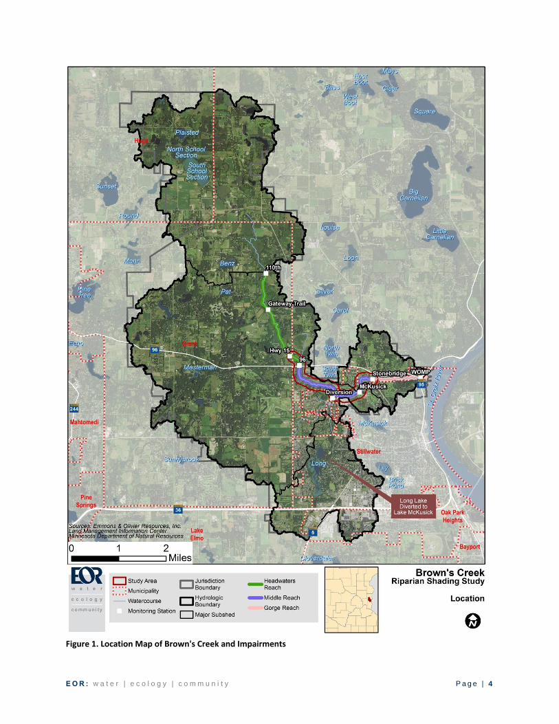
lack of coldwater fish assemblage, and high levels of E. coli bacteria (Figure 1). Upstream of County
Road 15/Manning Avenue, the headwaters reach is also impaired due to a low score of the Minnesota
Macroinvertebrate Index of Biological Integrity (M-IBI). These impairments were listed on the
federal 303(d) list between 2002 and 2008.
The District began a Total Maximum Daily Load (TMDL) Impaired Biota study in 2007 to diagnose
the main factors causing the aquatic life impairment. Naturally occurring wetland conditions were
identified as the main stressor to aquatic life in the headwaters reach upstream of County Road
15/Manning Avenue. Downstream of County Road 15/Manning Avenue and in the middle and gorge
reaches, the study found that high stream temperature was a primary stressor contributing to the
low indices of biotic integrity (IBI) in Brown’s Creek, in addition to excess total suspended solids
(TSS) and high concentrations of copper. Further monitoring and investigation of possible TSS
sources since the TMDL Impaired Biota study has not identified concentrated TSS loads in the upper
and middle reaches of Brown’s Creek. Due to uncertainties related to the reliability of the copper
monitoring data, copper loading allocations were not developed.
E O R : w a t e r | e c o l o g y | c o m m u n i t y P a g e | 4
Figure 1. Location Map of Brown's Creek and Impairments

E O R : w a t e r | e c o l o g y | c o m m u n i t y P a g e | 5
In the absence of a numeric temperature standard for streams across Minnesota, the BCWD
developed water temperature goals to protect the long-term survival of cold water species in Brown’s
Creek. The analysis of stream temperature’s impact on biota in Brown’s Creek focused on the brown
trout threat temperature of 18.3°C or 65°F, which is defined as the point of physiological stress,
reduced growth, and egg mortality (Table 2). The failure of trout to establish a breeding population
taken together with the absence of cold water fish and invertebrate species were evidence that the
high stream temperatures had sustained effects on biota. The temperature in
Brown’s Creek exceeded the threat temperature at both Highway 15 and McKusick Road based on
15-minute interval stream temperature data collected from 2000 to 2008. The study also reviewed
the frequency of high temperatures, duration of high temperatures, and rate of change in
temperature, all to which brown trout are sensitive. A period of 48 hours when the threat
temperature is exceeded is generally considered significantly stressful and 72 hours as extremely
stressful (Emmons & Olivier Resources, 2010).
Table 2. Water Temperature Criteria for Brown Trout (Emmons & Olivier Resources, 2010; Mccullough, 1999)
Criteria Temperature
Impact of Exceedance on Brown Trout (°C) (°F)
Threat 18.3 65 physiological stress, reduced growth, and egg mortality
Critical 23.9 75 direct mortality
As part of the Impaired Biota TMDL study, the TMDL and heat load allocations for Brown’s Creek
were developed with the threat temperature of 18.3°C as the water quality goal to provide a margin
of safety as opposed to the critical temperature of 23.9°C, at which direct mortality can be expected.
An energy budget was developed to assess the heat load capacity of Brown’s Creek under specific
flow ranges at the WOMP station, as illustrated in the heat load duration curve (Figure 2). The
energy budget indicated that a 6%
reduction in thermal loading (i.e.
energy input) was needed across the
entire contributing drainage area to
Brown’s Creek1 to sufficiently lower
stream temperatures and mitigate
exceedances of the threat
temperature. The required load
reduction was based on the
difference between the allowed heat
input and the average heat input
observed during the 198 days when
the threat temperature was exceeded
from 2003 to 2009 (EOR, 2010).
Figure 2. Heat Load Duration Curve 2000-2007 WOMP Station (Emmons & Olivier Resources, 2010)
1 The contributing drainage area to Brown’s Creek is everything east of Manning Avenue minus the drainage area to the Diversion Structure and some smaller landlocked areas identified near County Road 5 (Emmons & Olivier Resources, 2012).

E O R : w a t e r | e c o l o g y | c o m m u n i t y P a g e | 6
After understanding the stressors and load capacity of the creek, the BCWD then developed a TMDL
Implementation Plan in 2012 to define the mitigation strategies needed to meet the goals of the TSS
and stream temperature TMDLs. The plan was focused on addressing the impairment for aquatic life
due to lack of coldwater fish assemblage and due to high turbidity from Highway 15 (Manning
Avenue) to the St. Croix River (river ID 07030005-520). During the development of the plan, further
analysis of stream temperature and weather data was conducted to assess the potential impacts of
the Long Lake Diversion Structure installed in 2002. The analysis concluded that lower flows and
lower water temperatures after 2002 were due to multiple factors, including construction of the
diversion, lower precipitation, and lower air temperature relative to 2001 and 2002. Additional
analysis is needed to quantify the relative impacts of these factors on groundwater contribution to
Brown’s Creek as well as appropriations. All subsequent data analysis only looked at the years after
2002 when the diversion structure was installed.
Figure 3. Daily Average Flow and Temperature During Days When the Daily Average Temperature Exceeded 18ºC at the WOMP Site (Emmons & Olivier Resources, 2012)
Each point represents one day.
The importance of baseflow thermal conditions was reviewed in the TMDL Implementation Plan in
comparison to thermal loads during storm events. From 2003 to 2009, approximately 80% of the
exceedances of the threat temperature (18.3°C) occurred during baseflow conditions due to factors
such as lack of riparian shading, changes in stream geomorphology, decreases in baseflow, and
changes in climate. Approximately 20% of the exceedances occurred during stormflow conditions
due to the thermal load from direct stormwater runoff or from ponds.
-
10
20
30
40
50
60
70
80
90
19
99
20
00
20
01
20
02
20
03
20
04
20
05
20
06
20
07
20
08
20
09
Flo
w (
cfs
)
15
16
17
18
19
20
21
22
23
24
25
Te
mp
era
ture
(°C
elc
ius)
Flow During Exceedances Water Temperature (deg. C) During Exceedances
THPP construction Diversion Installed

E O R : w a t e r | e c o l o g y | c o m m u n i t y P a g e | 7
The TMDL Implementation Plan identified strategies to address baseflow condition exceedances,
including increased shading through vegetative buffers, in-stream morphological improvements, and
increasing the groundwater contribution to the stream (i.e. re-establishing groundwater connections
lost as a result of the Diversion Structure and/or evaluating the impacts that groundwater
appropriations for irrigation of golf courses have on the stream). The Plan prioritized opportunities
for in-stream cooling improvements through stream geomorphology and thermal buffer
improvements as shown in Figure 4 and Figure 5, including 2.5 miles of high priority buffer
improvements. The costs and estimated benefits of the stream geomorphology and thermal buffer
improvements are detailed in the Implementation Plan Table. In addition, the Plan identified non-
structural BMPs that would reduce thermal load to Brown’s Creek, including minimizing impervious
areas, disconnecting impervious surfaces, and achieving additional volume control through
rainwater harvesting. Stormflow implementation activities were also identified but are not relevant
to this study (Emmons & Olivier Resources, 2012).
The highest priority stream restoration project identified in the TMDL Implementation Plan was the
lower stream segment through the Oak Glen Golf Course where turf grass was mowed to the edge of
the stream. The potential stream temperature benefits were assessed using a simplified thermal
model developed using the Stream Segment Temperature Model (SSTEMP) which works on an
individual stream segment basis and uses steady-state hydrology and meteorology in addition to
defined stream geometry and shading inputs. The SSTEMP model results indicated that the stream
and buffer restoration would reduce would reduce the predicted daily mean temperature by 2.8°C
(5°F) and the maximum daily temperature by 3.3°C (6°F). Instead of modeling all of the planned
improvements, the BCWD decided to collect additional climatological data to improve certainty of
future modeling efforts and committed to monitoring the stream temperature benefits of the Oak
Glen Golf Course restoration in comparison to the predictions from the model (Emmons & Olivier
Resources, 2012).
Through the TMDL Implementation Plan, the BCWD also committed to taking an adaptive
management decision making approach to implementing the Plan given uncertainties in quantifying
the improvements associated with thermal load reduction projects. This meant that the District was
committed to continuing monitoring activities to measure the stream temperature and biotic health
response to implementation activities while also reducing the uncertainty and identifying if
additional implementation activities are needed (Emmons & Olivier Resources, 2012).
Since finalizing the TMDL Implementation Plan, the BCWD has constructed or participated in the
construction of multiple stormwater retrofits to mitigate stormflow heat loads to Brown’s Creek. In
addition, the District restored the lower segment of Brown’s Creek through the Oak Glen Golf Course
in 2012 to lower baseflow stream temperatures. The District has also reviewed all proposed
development activities to ensure compliance with the District’s Rules and Regulations, which include
requirements for Better Site Design (e.g. reduce impervious cover and disconnect impervious
surfaces) and providing volume control for the 2-year, 24-hour event. The district has also enhanced
the monitoring program to include a weather station, baseflow surveys, macroinvertebrate surveys,
and additional groundwater monitoring in addition to the stream temperature and flow monitoring
called for in the TMDL Implementation Plan. The BCWD assessed the period of monitoring data
collected from 2009 to 2012 to evaluate trends in water quality,

E O R : w a t e r | e c o l o g y | c o m m u n i t y P a g e | 8
Figure 4. Stream Geomorphology and Thermal Buffer Improvements (1 of 2) (Emmons & Olivier Resources, 2012)

E O R : w a t e r | e c o l o g y | c o m m u n i t y P a g e | 9
Figure 5. Stream Geomorphology and Thermal Buffer Improvements (2 of 2) (Emmons & Olivier Resources, 2012)
E O R : w a t e r | e c o l o g y | c o m m u n i t y P a g e | 1 0
including stream temperature. The assessment identified a warming trend in stream temperature
over the study period that was largely attributed to decreasing groundwater levels and higher than
normal air temperatures (Emmons & Olivier Resources, 2016). The District’s monitoring program is
continuing to develop a record by which the effectiveness of structural and non-structural BMPs can
be evaluated relative to the TMDL goals for stream temperature. A long-term data record is needed
to capture variability in climate in order to specifically assess the response of stream temperature
and biotic health to BMPs implemented in the watershed.
In order to address limitations to stream temperature modeling identified in the TMDL
Implementation Plan, the BCWD installed its own weather station 2011. The meteorological data
collected at the station, in addition to other data collected as part of the District’s full monitoring
program, provided the input and calibration data necessary to develop a more detailed stream
temperature model for estimating the benefits of potential thermal BMPs.
From 2014 to 2016, the BCWD developed a stream temperature model to assess the impact of stream
temperature mitigation options, including increased riparian shading, increased stream baseflow,
and disconnection of stormwater ponds. The model was developed in CEQUAL-W2 to simulate
stream temperature at an hourly time step in Brown’s Creek from Highway 15 (Manning Avenue) to
the St. Croix River for a continuous period (April to October) in 2012 and 2014. The calibration to
observed stream temperature, stream flow, and groundwater levels using lateral inputs (i.e.
groundwater distribution, rate, and temperature) and the wind sheltering coefficient was able to
reproduce observed stream temperatures within 1.0 to 1.3°C. Two future riparian shade scenarios
were assessed by increasing shade to new minimum thresholds of 50% and 75%. The model results
indicated that increasing riparian shade will provide the greatest stream temperature reduction in
comparison to the other mitigation options, although some uncertainties remain regarding the other
mitigation options. Even further, increasing shade would enhance the benefit of other mitigation
strategies. In other words, increasing riparian shading may lower in-stream temperatures to the
point where the benefits of stormwater pond retrofits is more noticeable. The expected benefit of
increasing riparian shade to a minimum threshold of 75% was a reduction in monthly mean stream
temperature on the order of 0.5 to 1°C over the entire modeled section of the creek (Herb & Correll,
2016).
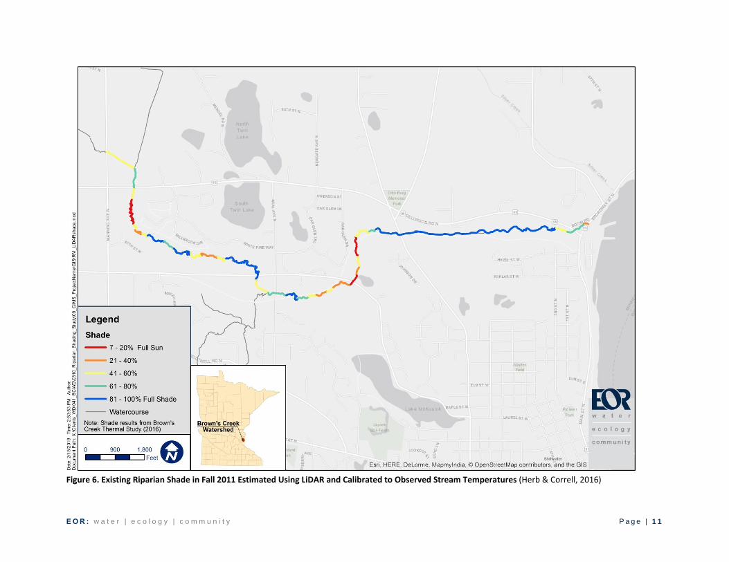
The Brown’s Creek Thermal Study also made recommendations for targeting shade improvements.
Understanding the amount of shade provided by riparian vegetation is crucial in determining stream
temperature and is an important parameter specified in stream temperature models. Although the
development of the Brown’s Creek stream temperature model utilized several tools and methods to
assess the percentage of the creek shaded by tree canopy, one of the limitations in model
development was in the riparian shading analysis. The analysis was based on a geospatial analysis
using Light Detection and Ranging (LiDAR) data, which is collected through remote sensing method
of examining the surface of the Earth. The State’s LiDAR data (Table 3) was the best available data
for riparian analysis at the time, but generally LiDAR does not work well for characterizing shading
at smaller scales, such as tall grass shading a narrow stream channel, and so the analysis focused on
tree canopy coverage. The percent shade estimated using ArcMap solar radiation analysis tool to
analyze LiDAR data is illustrated in Figure 6.
E O R : w a t e r | e c o l o g y | c o m m u n i t y P a g e | 1 1
Figure 6. Existing Riparian Shade in Fall 2011 Estimated Using LiDAR and Calibrated to Observed Stream Temperatures (Herb & Correll, 2016)

E O R : w a t e r | e c o l o g y | c o m m u n i t y P a g e | 1 2
Table 3. LiDAR Survey Specifications for Washington County (Block F) (Minnesota Department of Natural Resources, 2017)
Flight date November 14, 2011
Sensor Leica sensor ALS50-II MPiA with IPAS inertial measuring unit and a dual frequency airborne GPS receiver
Scan angle (cutoff) 40°
Average flying height 2012 m (6,600 feet) above mean terrain
Pulse rate frequency 99.5 kHz
Swath overlap 10%
Returns collected First, second, third, last
Point density 1.5 points/m2
Area used in study 26 km2
The Brown’s Creek Thermal Study recommended that additional analysis should be conducted to
better determine local shading conditions in the understory and areas with predominantly grass or
shrub vegetation. The increase in riparian shading required to lower stream temperatures by 1°C
would be a substantial effort along 2.5 miles of the stream. The Brown’s Creek Thermal Study
recommended targeting which reaches are most suitable for riparian shade restoration based on
factors such as channel width and orientation. Additional consideration is also needed for what type
of vegetation could be supported by the soils found along Brown’s Creek (Herb & Correll, 2016).
The Fourth Generation Watershed Management Plan (WMP) for Brown’s Creek outlines the steps the
BCWD will take from 2017 to 2026 to meet a set of 15 issue categories (Emmons & Olivier Resources,
2017). While many of the issues, goals and implementation items are related to riparian vegetation,
stream temperature, and biotic health, the primary goal related to this Riparian Shading Study is the
following:
Goal #3: Stream Management ‐ Improve the water quality and ecological integrity of Brown’s
Creek and its tributaries.
Sub-Issue: Water Quality, Aquatic Habitat, and Fisheries Protection
Policy: The BCWD is committed to the improvement of the water quality and
ecological integrity of Brown’s Creek and its tributaries, including maintaining a
viable cold‐water fishery
Sub-Goal D: Achieve and maintain in‐stream water temperatures of 18.3°C (65°F) or
lower in the trout stream portion of Brown’s Creek
Implementation Item #3: Implement thermal improvements listed in Table
61 of the WMP, which includes increasing shade from riparian vegetation
along 2.5 miles of the creek as called for in the Brown’s Creek Thermal Study
and the TMDL Implementation Plan.
The Riparian Shading Study was undertaken to address the recommendations of the Brown’s Creek
Thermal Study such that thermal buffer improvements to increase shading could be targeted and
implemented within the 2017-2026 planning cycle by the BCWD.

E O R : w a t e r | e c o l o g y | c o m m u n i t y P a g e | 1 3
3. STUDY AREA CHARACTERIZATION
This section summarizes the characteristics of natural resources in the study area that are pertinent
to riparian vegetation and stream temperature management decisions. The characteristics of the
study area also provide context for our review of literature on the comparative benefits of riparian
vegetation types (Appendix B) by focusing on studies with similar characteristics. Characteristics
were based on previous studies and monitoring data collected by the BCWD and other agencies.
Appendix A of the BCWD 2017-2026 WMP outlines a comprehensive inventory of the natural
resources in the watershed and available data. The District’s Impaired Biota TMDL study and TMDL
Implementation Plan are also useful sources for additional information on the characteristics of the
study area.
3.1. Climate
The climate of the Brown’s Creek watershed is consistent with the climate for the Seven County
Metropolitan Area. The summers are fairly short with an average temperature of about 70 degrees
F. Snowfall covers much of the ground from late fall to early spring. The average winter temperature
is about 18°F. The average annual temperature is 46.3°F and the average annual precipitation is 33.6
inches (Emmons & Olivier Resources, 2007b).
The BCWD operates a weather station (45.063857, -92.855826) installed on July 22, 2011 to monitor
multiple parameters, including air temperature, humidity, wind speed, wind direction, precipitation,
and solar radiation. Air temperature and precipitation observed at the station in 2012 and 2014 are
illustrated in Figure 7. These two years are simulated in the District’s stream temperature model in
the Brown’s Creek Thermal Study and this Riparian Shading Study to assess a warm-dry year (2012)
and a cool-wet year (2014).
Figure 7. Summary of Monthly Air Temperature and Precipitation in 2012 and 2014 (Herb & Correll, 2016)
A trend analysis of local climate data indicates that the Brown’s Creek watershed is experiencing
changes in precipitation and temperature which presents challenges to watershed management
decision-making. The trends in climate being seen in the BCWD include: annual average air
temperature is increasing, air temperature in winter months in particular is increasing, annual
rainfall depths are increasing an average of 0.16 inches per year and there is an increasing trend in
the mean rainfall depth during wet periods (Emmons & Olivier Resources, 2017). Amongst multiple
statewide trends, droughts are expected to become more common as the increases in rainfall cannot
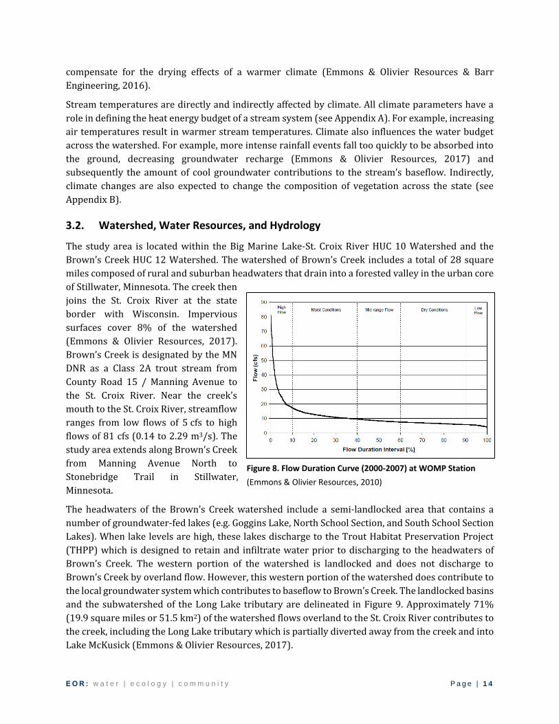
E O R : w a t e r | e c o l o g y | c o m m u n i t y P a g e | 1 4
compensate for the drying effects of a warmer climate (Emmons & Olivier Resources & Barr
Engineering, 2016).
Stream temperatures are directly and indirectly affected by climate. All climate parameters have a
role in defining the heat energy budget of a stream system (see Appendix A). For example, increasing
air temperatures result in warmer stream temperatures. Climate also influences the water budget
across the watershed. For example, more intense rainfall events fall too quickly to be absorbed into
the ground, decreasing groundwater recharge (Emmons & Olivier Resources, 2017) and
subsequently the amount of cool groundwater contributions to the stream’s baseflow. Indirectly,
climate changes are also expected to change the composition of vegetation across the state (see
Appendix B).
3.2. Watershed, Water Resources, and Hydrology
The study area is located within the Big Marine Lake-St. Croix River HUC 10 Watershed and the
Brown’s Creek HUC 12 Watershed. The watershed of Brown’s Creek includes a total of 28 square
miles composed of rural and suburban headwaters that drain into a forested valley in the urban core
of Stillwater, Minnesota. The creek then
joins the St. Croix River at the state
border with Wisconsin. Impervious
surfaces cover 8% of the watershed
(Emmons & Olivier Resources, 2017).
Brown’s Creek is designated by the MN
DNR as a Class 2A trout stream from
County Road 15 / Manning Avenue to
the St. Croix River. Near the creek’s
mouth to the St. Croix River, streamflow
ranges from low flows of 5 cfs to high
flows of 81 cfs (0.14 to 2.29 m3/s). The
study area extends along Brown’s Creek
from Manning Avenue North to
Stonebridge Trail in Stillwater,
Minnesota.
The headwaters of the Brown’s Creek watershed include a semi-landlocked area that contains a
number of groundwater-fed lakes (e.g. Goggins Lake, North School Section, and South School Section
Lakes). When lake levels are high, these lakes discharge to the Trout Habitat Preservation Project
(THPP) which is designed to retain and infiltrate water prior to discharging to the headwaters of
Brown’s Creek. The western portion of the watershed is landlocked and does not discharge to
Brown’s Creek by overland flow. However, this western portion of the watershed does contribute to
the local groundwater system which contributes to baseflow to Brown’s Creek. The landlocked basins
and the subwatershed of the Long Lake tributary are delineated in Figure 9. Approximately 71%
(19.9 square miles or 51.5 km2) of the watershed flows overland to the St. Croix River contributes to
the creek, including the Long Lake tributary which is partially diverted away from the creek and into
Lake McKusick (Emmons & Olivier Resources, 2017).
Figure 8. Flow Duration Curve (2000-2007) at WOMP Station
(Emmons & Olivier Resources, 2010)

E O R : w a t e r | e c o l o g y | c o m m u n i t y P a g e | 1 5
The shape of the Brown’s Creek channel influences the quality of habitat for fish and
macroinvertebrates. Within the study area, Brown’s Creek is classified under the Rosgen
Classification System (Rosgen, 1994) as C3, C4, C4c, E4, and E4/5. Channel substrate in the study area
includes sand, cobble, and fine to coarse gravels in addition to the organic soils common to the
wetland areas along the creek. Bankfull width varies from 2 to 5 m. The longitudinal slope of the
creek is flat (less than 1%) and sinuosity ranges from 1 to 1.3 (Emmons & Olivier Resources, 2008).
Several segments within the study area have been identified as priorities for stream restoration to
provide healthy, diverse, and sinuous aquatic habitat for coldwater biota, including the segment east
of Manning Avenue North that was likely straightened for agricultural purposes and several points
south of the Millbrook development where sedimentation is straightening the channel. Sites with
severe bank erosion are also identified on an ongoing basis to protect properties and mitigate
sediment loads to the creek. Channel restoration projects are also opportunities for riparian
vegetation improvements.
Multiple wetlands are located within or adjacent to the creek in the study area and include seasonally
flooded basins, hardwood wetlands, shallow marsh, shrub wetland, and shallow open water
communities (Figure 10). The District conducted a Function and Value Assessment (FVA) of all
wetlands in terms of the functions they serve on the landscape and the value they provide based on
an inventory of all wetlands in the watershed greater than 1 acre in size in 1998 and updated in 2005.
The management classifications resulting from the FVA for wetlands in the study area are shown in
Figure 11.
Many of the water resources in the study area are either wholly or partially groundwater dependent.
The shallow groundwater table actively contributes to the Creek’s baseflows to varying degrees
throughout the year and along the length of the stream as explained in the Brown’s Creek Thermal
Study:
“The downstream section, from the WOMP station to Stonebridge, represents a higher slope
reach with relatively high rates of baseflow input with a low temperature (9 °C). The middle
section, extending from Stonebridge to McKusick/Neal, represents a low slope reach with no
baseflow input (based on the 2014 baseflow surveys). However, piezometer measurements
in 2015 by EOR staff suggest that the middle reach was a losing reach in early summer and a
gaining reach later in the year. The upper reach extends from McKusick/Neal to Manning
Avenue, and is low slope with variable temperature baseflow inputs, based on the 2014
piezometer measurements.” (p. 4)
Water appropriations in the Brown’s Creek watershed are primarily from groundwater. The largest
groundwater appropriations in the Brown’s Creek watershed come from municipal water supply
wells and golf course irrigation wells. Groundwater appropriations affect groundwater levels below
groundwater dependent natural resources. In 2014 a BCWD Groundwater Appropriations Study
found that large pumping wells were lowering groundwater levels in bedrock aquifers below
Brown’s Creek by more than two feet. Further studies are required to determine the connection
between the creek and the bedrock aquifers and the effect of the pumping on groundwater dependent
natural resources (Emmons & Olivier Resources, 2017). Appendix A of the District’s 2017-2026 WMP
provides a detailed overview of the groundwater resources underlying the watershed.

E O R : w a t e r | e c o l o g y | c o m m u n i t y P a g e | 1 6
Figure 9. Landlocked Basins of Brown's Creek Watershed (Emmons & Olivier Resources, 2017)

E O R : w a t e r | e c o l o g y | c o m m u n i t y P a g e | 1 7
Figure 10. Water Resources in Study Area
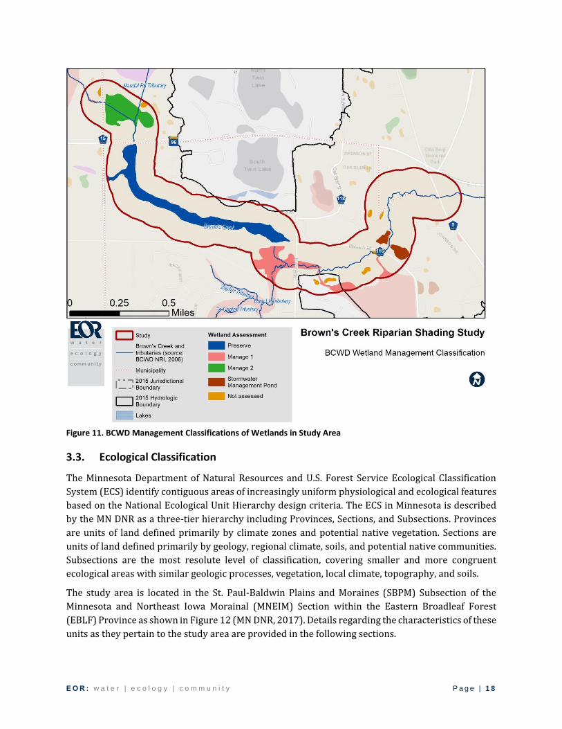
E O R : w a t e r | e c o l o g y | c o m m u n i t y P a g e | 1 8
Figure 11. BCWD Management Classifications of Wetlands in Study Area
3.3. Ecological Classification
The Minnesota Department of Natural Resources and U.S. Forest Service Ecological Classification
System (ECS) identify contiguous areas of increasingly uniform physiological and ecological features
based on the National Ecological Unit Hierarchy design criteria. The ECS in Minnesota is described
by the MN DNR as a three-tier hierarchy including Provinces, Sections, and Subsections. Provinces
are units of land defined primarily by climate zones and potential native vegetation. Sections are
units of land defined primarily by geology, regional climate, soils, and potential native communities.
Subsections are the most resolute level of classification, covering smaller and more congruent
ecological areas with similar geologic processes, vegetation, local climate, topography, and soils.
The study area is located in the St. Paul-Baldwin Plains and Moraines (SBPM) Subsection of the
Minnesota and Northeast Iowa Morainal (MNEIM) Section within the Eastern Broadleaf Forest
(EBLF) Province as shown in Figure 12 (MN DNR, 2017). Details regarding the characteristics of these
units as they pertain to the study area are provided in the following sections.

E O R : w a t e r | e c o l o g y | c o m m u n i t y P a g e | 1 9
Figure 12. Ecoregion of Study Area
E O R : w a t e r | e c o l o g y | c o m m u n i t y P a g e | 2 0
3.4. Topography and Geology
Topography and aspect are important factors in the development and formation of soil, soil erosion
potential, and the type and stability of vegetation for a given location. Topography within the study
area includes gently rolling hills and low-lying wetland areas. Elevation in the study area ranges from
826.1 to 940.3 fasl (251.8 to 286.6 masl). Slope in the study area ranges from 0 to 170 percent, where
the very steep slopes are on roadside embankments and valley banks.
The District’s 2017-2026 WMP characterized and categorized three distinct landforms along Brown’s
Creek, as follows and as illustrated in the typical cross sections on the next pages:
Headwaters Region of Brown’s Creek includes the northern portion of the watershed from
Highway 96 to the Goggins-School Section Chain-of-Lakes (Figure 15). The study area
includes the lower headwaters region from Highway 15/Manning Avenue to Highway 96.
Brown’s Creek Middle Reach includes the central portion of the Brown’s Creek south of
Highway 96 to County Road 55 (Figure 16) and is entirely within the study area.
Brown’s Creek Gorge includes the Brown’s Creek corridor downstream of County Road 5 to
the St. Croix River (Figure 17). The gorge is downstream of the study area but is included in
the District’s stream temperature model.
The bedrock geology formations below the study area, from youngest to oldest, include the Prairie
du Chien Group dolostone, the Jordan Sandstone, and the St. Lawrence Sandstone (Figure 13).
Brown's Creek Middle Reach is less influenced by the bedrock than is the Brown's Creek Gorge.
Bedrock valleys exist where ancient streams eroded the bedrock, but those valleys have since been
buried by thick glacial sediments. In the study area, Brown's Creek runs across the buried bedrock
valleys rather than parallel to them.
The surficial geology is dominated by moraines and outwash related to the Superior Lobe glaciation
(Cromwell Formation)(Figure 14). Later alluvial deposits of sand and gravel are found along the
creek bed. Lacustrine clay deposits, likely from a pro-glacial lake, are found in the area near Brown's
Creek Park. The glacial deposits are eroded away where the middle section of Brown's Creek enters
the lower gorge.
Many springs and seeps have been identified within the study area along the creek (Figure 14) as
part of the MN Geological Survey Karst Features Database, a compilation of historical documentation,
field surveys by DNR staff, and approved citizen submittals up to date as of February 16, 2018. In the
middle section of Brown's Creek the seeps emanate from glacial deposits close to the creek bed. This
contrasts with the gorge area where the springs and seeps often emanate from the bedrock away
from and at higher elevation than the creek bed. Springs and seeps are more common in the coarser
sand and gravel deposits than in the lacustrine clay deposits near Brown's Creek Park. In a 2015
study, comparison of water levels in Brown's Creek and groundwater levels from in-stream
piezometers showed that the middle section of Brown's Creek can be gaining or losing groundwater
during different times of the non-winter months (Emmons & Olivier Resources, 2015).

E O R : w a t e r | e c o l o g y | c o m m u n i t y P a g e | 2 1
Figure 13. Bedrock Geology of Study Area

E O R : w a t e r | e c o l o g y | c o m m u n i t y P a g e | 2 2
Figure 14. Surficial Geology of Study Area

E O R : w a t e r | e c o l o g y | c o m m u n i t y P a g e | 2 3
Figure 15. Typical Cross Section of the Brown’s Creek Headwaters Region (Emmons & Olivier Resources, 2017)

E O R : w a t e r | e c o l o g y | c o m m u n i t y P a g e | 2 4
Figure 16. Typical Cross Section of the Brown's Creek Middle Reach (Emmons & Olivier Resources, 2017)

E O R : w a t e r | e c o l o g y | c o m m u n i t y P a g e | 2 5
Figure 17. Typical Cross Section of the Brown’s Creek Gorge (Emmons & Olivier Resources, 2017)

E O R : w a t e r | e c o l o g y | c o m m u n i t y P a g e | 2 6
This page was intentionally left blank.

E O R : w a t e r | e c o l o g y | c o m m u n i t y P a g e | 2 7
The topography and geology in these regions of the creek’s riparian corridor were the basis for the
hydrologic cycle of the watershed and the resulting unique flora and fauna in each region. For
example, the level and gently rolling topography in the headwaters region and middle reach formed
the many lakes and wetlands that provide significant recharge to the groundwater table which, in
turn, supports cool flows in Brown’s Creek. Topography also relates to stream temperature in that it
defines the local time of sunset and sunrise and can significantly shade the stream throughout each
day, depending on the height of the valleys.
3.5. Soils
Soil formation is the result of the interaction of parent material, climate, organisms, topographic
position or slope, and time. Collectively, these factors help determine the dominant plant and animal
communities, which in turn influences future soil development. Soils within the SBPM Subsection are
typically characterized as Alfisols and Molisols, with parent material classified as clay loams, sandy
loams, loamy sands, and sands. Twenty soil units are identified by the USDA/NRCS Web Soil Survey
to occur within 200 feet of the creek in the study area including silt loam, sandy loam, muck, and rock
outcrop. Seelyeville muck (540) and Rifle muck (541) soils units are comprised of all hydric soil
groups and characterized as very poorly drained soils (Table 4 and Figure 18). In addition, Markey
muck (543), Aburndale silt loam, baronet silt loams are considered predominately hydric. The
aforementioned soils units are primarily located directly adjacent to or below the creek in the study
area. Remaining soils within 200 feet of the creek were classified as not hydric or predominately not
hydric. The hydric classifications of the soils indicate which plant species will be best-suited for
plantings in the study area (i.e. only certain trees succeed in wet and hydric soils).
Table 4. Soils Located within 200 Feet of Stream in Study Area
ID Soil Unit Name Dominant Drainage Class
HSG % Hydric
Soil %
Distribution
49 Antigo silt loam, 0 to 2 percent slopes Well drained B 0 4
49B Antigo silt loam, 2 to 6 percent slopes Well drained B 0 18
49C Antigo silt loam, 6 to 15 percent slopes Well drained B 0 9
49D Antigo silt loam, 15 to 35 percent slopes Well drained B 0 1
189 Auburndale silt loam, 0 to 2 percent slopes Poorly drained B/D 95 11
456 Barronett silt loam Poorly drained C/D 92 1
1847 Barronett silt loam, sandy substratum Poorly drained B/D 90 2
120 Brill silt loam Moderately well drained C 5 0.8
155C Chetek sandy loam, 6 to 12 percent slopes Somewhat excessively
drained A 0
1
452 Comstock silt loam Somewhat poorly drained B/D 4 0.5
449 Crystal Lake silt loam, 1 to 3 percent slopes Moderately well drained C 3 0.1
264 Freeon silt loam, 2 to 6 percent slopes Moderately well drained C/D 3 1
266 Freer silt loam Somewhat poorly drained C/D 5 0.02
177B Gotham loamy sand, 1 to 6 percent slopes Excessively drained A 0 0.2
342D Kingsley sandy loam, 12 to 18 percent slopes Well drained C 0 2
454C Mahtomedi loamy sand, 6 to 12 percent slopes Excessively drained A 0 8
454D Mahtomedi loamy sand, 12 to 25 percent slopes Excessively drained A 0 7
1820F Mahtomedi variant-Rock outcrop complex, 25 to 60 percent slopes
Excessively drained A 0 2
543 Markey muck Very poorly drained A/D 95 0.5
507 Poskin silt loam Somewhat poorly drained B/D 3 1
153B Santiago silt loam, 2 to 6 percent slopes Well drained B 0 5
153C Santiago silt loam, 6 to 15 percent slopes Well drained B 0 9
540 Seelyeville muck Very poorly drained A/D 100 15

E O R : w a t e r | e c o l o g y | c o m m u n i t y P a g e | 2 8
Figure 18. Soils of Study Area

E O R : w a t e r | e c o l o g y | c o m m u n i t y P a g e | 2 9
3.6. Plant Communities
3.6.1. Historic Vegetation
Oak and aspen savannas were dominant pre-settlement plant communities of the SBPM Subsection,
especially on moraine ridges and along streams. Tallgrass prairie and maple-basswood forest were
also found within the Subsection, found primarily in rolling plains and along steep ravines,
respectively. Marschner’s map of the Original Vegetation of Minnesota (1974) and later adaptation
of Marschner’s Map (Wendt and Coffin 1988) provide a unique overview of the vegetation that
existed prior to European settlement across the state. The maps are based on the Public Land Survey
(PLS) of 1847-1907; the latter generalizes the vegetation types identified in the former. Restrictions
of map accuracy, due to limitations of the PLS methodology, inhibit the level of resolution the maps
provide; therefore, adjacent historic land cover and bearing tree2 data were also examined to identify
historic vegetation communities that likely existed within the study area and along the Study reach.
The mapping data indicate that the study area was historically comprised of oak openings and
barrens (Figure 19). Wet prairie, big woods-hardwoods (e.g. oak maple, basswood, and hickory),
conifer bogs and swamps, prairie, and lakes are also indicated in the surrounding area and may have
also historically occurred within the study area. Bearing tree data within the study area include black
oak, white oak, and bur oak. Other tree species identified in surrounding areas included tamarack,
spruce, aspen, and birch.
Historical disturbance associated with grasslands and savannas such as oak barrens likely included
fire, high wind events, periodic flooding, and grazing by large mammals. These disturbances
sustained the oak barrens landscape, preventing woody vegetation from establishing into a later-
succession, dense forest.
3.6.2. Existing Vegetation
The typical vegetation within the headwaters region and middle reach of Brown’s Creek illustrated
in Figure 15 and Figure 16 include shrub carr wetlands, sedge meadow, oak woodlands, and
floodplain forests. As such, riparian vegetation within the study area varies from forested to grassy
vegetation, in addition to one segment north of Highway 96 with riprap, mowed turf grass, and
ornamental vegetation bordering the stream.
There are no MNDNR Native Plant Communities (NPC) mapped within the study area. However,
several NPCs are mapped in adjacent areas. Native communities in the surrounding vicinity include
Northern Very Wet Ash Swamp, Northern Wet Meadow/Carr, Southern Rich Conifer Swamp,
Southern Dry-Mesic Oak Forest, Southern Dry Prairie, and Southern Mesic Maple-Basswood Forest
2 As part of the PLS, surveyors notched, blazed and scribed bearing trees to facilitate the relocation of the corners of rectangular survey grids should the wooden corner post or corner stone be lost or moved. Bearing trees were also required where surveyors had to meander around impassable areas, such as lakes. Surveyors recorded the species, diameter distance to corner, and azimuth (i.e. bearing from the corner) of each bearing tree. Surveyors also recorded witness and line trees that were found along the line or near the corner but were not required to record as much information as for the bearing trees. The Natural Heritage Information System Bearing Tree Database contains computerized records only of the bearing trees at standard section and quarter-section survey corners (Almendinger, 1996).

E O R : w a t e r | e c o l o g y | c o m m u n i t y P a g e | 3 0
(Figure 20). The BCWD has also mapped natural communities such as the Maple-Basswood Forest
that extends into the eastern extent of the study area (Figure 20). The Maple-Basswood Forest
connects to a similar NPC identified by the DNR with a ‘C’ condition ranking which means that the
community has “fair ecological integrity” which means they show strong evidence of human-caused
degradation, but retain some characteristic species and have some potential for recovery with
protection and management (Minnesota Biological Survey, 2018).
Exotic and invasive species are present and ever increasing within the Brown’s Creek watershed.
They affect the quality of our natural resources in many ways by degrading wildlife habitat and water
quality, and can negatively affect the quality of our native plant communities. The BCWD is managing
invasive terrestrial plant species, such as reed canary grass and buckthorn, to restore healthy plant
communities in the watershed and along the creek. Heavy growth of curly leaf pondweed was found
in the creek at Highway 15 and above McKusick Road which could hinder trout suitability by slowing
water, warming water temperature, and increasing fine sediment deposition over spawning gravel
(Washington Conservation District, 2016). Several of the woodlands in the headwaters region are in
good condition and do not display the heavy levels of buckthorn that frequently characterize oak
communities within the region. In general, the woodland communities tend to be in better condition
in the areas adjacent to the wetlands and to show more evidence of disturbance away from the
wetlands (Emmons & Olivier Resources, 2017). A complete list of invasive plant species found in the
watershed is provided in Appendix A of the District’s WMP.

E O R : w a t e r | e c o l o g y | c o m m u n i t y P a g e | 3 1
Figure 19. Pre-Settlement Vegetation near Study Area

E O R : w a t e r | e c o l o g y | c o m m u n i t y P a g e | 3 2
Figure 20. Existing Native and Natural Plant Communities

E O R : w a t e r | e c o l o g y | c o m m u n i t y P a g e | 3 3
3.7. Floodplain, Upland, and Wetland Wildlife
The SBPM Subsection is home to 149 Species of Greatest Conservation Need (SGCN), including 74
state or federally endangered, threatened, or of special concern. The study area falls within a
township identified as having 51-100 SGCN records and SGCN richness of 31-50. Habitat loss and
degradation, invasive species and completion, and pollution are identified as the greatest problems
for SGCN in the Subsection. Prairie, oak savanna, grassland, and stream habitats, among others, are
all considered key habitats within the Subregion. MN DNR recommended stream habitat actions
include:
a) Maintain good water quality, hydrology, geomorphology, and connectivity in priority
stream reaches
b) Maintain and enhance riparian areas along priority stream reaches
c) Provide technical assistance and protection opportunities to interested individuals and
organizations
The BCWD inventoried unique species in the headwater region and middle reach of Brown’s Creek
in 2015. The natural communities along the creek provide significant habitat and form a wildlife
corridor through the watershed. The unique species identified in the two regions are illustrated in
Figure 15 and Figure 16.
The mosaic of wetlands, forest, and grassland communities support a variety of animals. In particular,
there are records of the Blanding’s turtle (a state-listed threatened species), Red-shouldered hawk
(a state-listed species of special concern), and Hooded warbler (classified as a “Rare Regular” species
by the Minnesota Ornithologists Union) in the headwaters region. In addition, large wetlands in the
headwaters region support healthy populations of painted and snapping turtles in addition to several
species of frogs and toads. Due to the quality and size of the wetland communities, the potential for
additional rare species is high (Emmons & Olivier Resources, 2017).
The wetland and shrub-carr communities in the middle reach of Brown’s Creek provide important
breeding and foraging habitats for many resident and migratory species of birds, such as Ring-necked
duck, Mallard, Broad-winged hawk, Killdeer, Pileated woodpecker, Chimney swift, Alder flycatcher,
Great-crested flycatcher, and Barn swallow. In addition, common herpetile species such as Common
garter snakes, Green frogs, Western chorus frogs, and Northern leopard frogs are most likely to be
prevalent within this somewhat developed reach of Brown’s Creek (Emmons & Olivier Resources,
2017).
3.8. Aquatic Biota
Ultimately, the purpose behind strategies to decrease stream temperatures is to support healthy
coldwater fish assemblage in Brown’s Creek. Brown trout have been stocked yearly since 1958 in
Brown’s Creek. The DNR typically stocks between 800 and 1,000 yearlings, but sometimes stocks
several size classes. Historically, fish surveys did not report many trout, sometimes fewer than 20
individuals, and the trout were primarily young-of-year (YOY) which indicated possible natural

E O R : w a t e r | e c o l o g y | c o m m u n i t y P a g e | 3 4
reproduction in Brown’s Creek. Still, long-term fish survey data indicated that brown trout were not
establishing well in Brown’s Creek. From 1998-2004, stream habitat improvement projects in
conjunction with lower water temperatures lead to higher trout populations in the creek. However,
fish surveys conducted from 2004 to 2007 showed a decline trout population. Natural reproduction
was confirmed sporadically (1966, 1976, 1989, and 1998-2001) but not consistently enough to
maintain a sustainable population. Native brook trout, another coldwater fish species historically
found in Brown’s Creek, were not found in the 2000, 2005, and 2008 MNDNR surveys (Emmons &
Olivier Resources, 2012).
Recent surveys at different locations along Brown’s Creek have provided useful data to better
understand the health and stability of the brown trout community in Brown’s Creek. On September
13, 2016, a fish survey conducted by the Minnesota DNR in the Oak Glen Golf Course between the
crossings of Brown’s Creek State Trail and the second cart path found eight adult trout that had
survived since the previous stocking in 2014 (Figure 21). Although their findings did not indicate
natural reproduction had occurred, it seemed imminent since the large females captured were of the
size and age that could reproduce. On September 30, 2016, EOR captured a young-of-year brown
trout while conducting a macroinvertebrate survey in the gorge downstream of the Oak Glen Golf
Course (Figure 22). This was an indication that natural reproduction of brown trout had occurred
since the previous year’s stocking.
Figure 21. Adult Brown Trout Caught in Oak Glen Golf Course on Sept. 13, 2016 (Photo Credit: MN DNR)
Figure 22. YOY Brown Trout Caught in Brown's Creek Gorge on Sept. 30, 2016 (Photo Credit: Mike Majeski, EOR)
More recently in 2017, a complete fish community survey was conducted in the lower, middle, and
headwater reaches of Brown’s Creek. The middle reach of Brown’s Creek was surveyed north and
south of the Highway 96 crossing east of Highway 15. The survey results indicated that the middle
reach of Brown’s Creek contained an IBI score of zero or “Very Poor” due to the lack of detectable
presence of coldwater species such as rainbow darters and brown trout. The fish community found
in the middle reach was more consistent with a cool or warmwater system than a coldwater system.
Survey samples were also conducted in June between the Stonebridge Trail and Highway 95
crossings in the lower (gorge) reach of Brown’s Creek. A total of 140 brown trout were collected in
the gorge, of which nearly half were considered young-of-year, indicating good natural reproduction
occurred in 2016. The frequencies of observed fish lengths are summarized in Figure 23. The size of
the young-of-year brown trout captured in June as part of this study indicated that the fish were not
part of the 100 brown trout stocked by a Stillwater High School in May of 2017. Four rainbow darters

E O R : w a t e r | e c o l o g y | c o m m u n i t y P a g e | 3 5
were also captured in the lower reach. Overall, the fish community survey resulted in an IBI score of
30 or “Fair” ranking for the lower reach indicating that the stream has experienced moderate
degradation of biotic integrity. The four rainbow darters indicate a significant increase relative to
previous surveys but still indicate a critically small and restricted population (Lallaman, 2017).
Figure 23. Length-Frequency Distribution of Brown Trout Captured in Brown's Creek Gorge (Lallaman, 2017)
Coldwater fish populations are supported by environmental conditions and the macroinvertebrate
community which can also be assessed for indications of biotic health. As such, the BCWD has also
conducted macroinvertebrate surveys from 2015 to 2017 in the lower, middle, and upper reaches of
Brown’s Creek. Over the three years of monitoring, all three reaches were found to contain similar
taxa that were consistent with the previous years’ surveys. All sites contained taxa with both high
and low pollution tolerance levels, indicating some level of urbanization impacts, but also ample
oxygen levels and good habitat. These results indicate good water quality and stable conditions in
Brown’s Creek over the last 3 years (Rufer, 2017).
The Minnesota Pollution Control Agency (MPCA) will conduct a watershed assessment in 2020, with
the Intensive Watershed Monitoring program beginning in 2019, to re-evaluate the status of biotic
health in Brown’s Creek using all monitoring data collected as part of the Brown’s Creek Impaired
Biota TMDL study and recent biological surveys. Brown’s Creek will be removed from the impaired
waters list when the IBI score meets the threshold for southern coldwater streams (ranking of 45 +/-
13) and when instream TSS meets the state’s numeric standard for class 2A coldwater streams
(10 mg/L) (Emmons & Olivier Resources, 2012).
In addition to aquatic biota, beavers are also common in the middle reach of Brown’s Creek. They are
active in the stream, building dams which cause ponding into the floodplain that can also result in
tree mortality under the sustained inundation.

E O R : w a t e r | e c o l o g y | c o m m u n i t y P a g e | 3 6
4. LITERATURE REVIEW SUMMARIES
The purpose of the riparian shade review in Appendix A was to identify the best-suited methods for
comparing shade provided by grassy and woody riparian vegetation. There are few studies in North-
Central America which have quantitatively assessed grassy riparian shade and none using rigorous
field measurements. The review found that hemispherical photography is the best-suited method for
comparing shade provided along small streams by grassy vegetation to woody vegetation. In
addition, direct measurements of shade using arrays of pyranometers or other light sensors are
useful in validating indirect measurements of shade from hemispherical photography. Canopy cover
and closure are not acceptable surrogate measurements for shade because they do not vary based on
the position of the sun in the sky. In addition to shade, ancillary data on the physical characteristics
of the stream and vegetation should be collected in order to diagnose differences in shade at multiple
monitoring locations and assess which variables can be used to predict shade.
The second literature review in Appendix B was conducted to seek out the most recent information
regarding the comparative benefits of grassy and woody riparian buffers with respect to their
environmental functions. These environmental functions included sediment control, phosphorus
control, increasing dissolved oxygen, supporting aquatic fauna, and maintaining groundwater inputs
to the creek. All of these functions are relevant to the watershed management objectives and
priorities of the BCWD. The review was conducted to support the well-informed riparian
management decisions primarily focused on stream temperature management from this study with
a full view of the potential trade-offs with other watershed management objectives. Overall, the most
relevant trade-offs of establishing forested streams was the resulting changes that occur in the
channel morphology and resulting loss of trout habitat. Streams with woody riparian vegetation
typically are wide and flat, whereas streams with grassy buffers are deep and narrow along with
overhanging banks. The latter is considered to be more optimal for supporting trout and other
wildlife, although there must be a balance with regards to opening the canopy to the extent that
incoming solar radiation radically increases stream temperature. Multiple other factors are
considered in Appendix B. The practical implications for these trade-offs is that both grassy and
woody riparian vegetation provide necessary benefits to coldwater stream systems and riparian
management strategies should use a balanced, mosaic approach to a variety of vegetation types. This
means that multiple benefits could arise from thinning out over-forested buffers while others could
arise from sporadic tree plantings in open meadows. The specific take-away for the riparian shading
study is that a widespread tree-planting approach to increase shade would likely result in several
detrimental impacts such as increased erosion of the streambanks. The Riparian Shading Study
should assess and propose measures to increase shade while mitigating the potential detrimental
impacts of changes to the riparian buffers.

E O R : w a t e r | e c o l o g y | c o m m u n i t y P a g e | 3 7
5. RIPARIAN SHADE ANALYSIS
Existing riparian shade in the study area was analyzed using hemispherical photographs to address
the limitations of LiDAR identified in the Brown’s Creek Thermal Study. Further steps were taken to
understand where plantings would be most effective and to define a targeted shade restoration
scenario.
5.1. Existing Conditions
5.1.1. Method
Data Collection
The study area was limited to Brown’s Creek between the Stonebridge Trail and Highway 15 /
Manning Avenue. Reaches within the study area were selected for monitoring based on their unique
vegetation composition, estimated shade, and channel geometry. The representative reaches
included three un-shaded areas identified by Herb and Correll (2016) as having less than 20% shade.
In addition, a reference reach with established woodlands was selected to represent the maximum
attainable shade and the recently restored location in lower Oak Glen Golf Course was selected to
represent improved conditions 5-years post construction. The geometry of these reaches was
assessed using the Rosgen Classification system in the Brown’s Creek Stream Classification Study
(2007), which identified unique E4, E5, C3, and C4 classifications within the study area. The criteria
for these classifications and the stages of channel adjustment are illustrated in Figure 24 and Figure
25. The characteristics of the representative reaches are listed in Table 5 and the locations are
illustrated in Figure 26. The selection of representative reaches based on these characteristics
facilitated comparisons of shade provided by different vegetation and at locations with different
channel geometry.
Table 5. Preliminary Identification of Representative Reaches in the Study Area
Representative Reach ID
Rosgen Classification
Estimated Shade
Vegetation Reach Length
(m)
1 E5 41-60% Shrub Carr 291
2 C3 61-80% Woodland & Lawn 159
3 E4/5 0-20% Sedge Meadow 396
4 C4 61-100% Woodland 222
5 C4 21-40% Woodland & Sedge Meadow 197
6 E4 21-40% Woodland 194
7 C4c 0-60% Mixed 395
Total: 1,855
A portion of each representative reach was monitored to assess the riparian shade. The necessary
sample reach length was estimated by multiplying the average wetted width of the stream by 40
(Dent et al., 2000). For this study, the average wetted width of Brown’s Creek was approximately 3
m and the resulting sample reach length was 120 m. The distance between transects was calculated
by dividing the sample reach by ten (Dent et al., 2000), resulting in 11 evenly spaced transects (12 m
apart) to be monitored in each sample reach. A total of 77 transects (i.e. points along the creek) were
monitored to evaluate riparian shade in the representative reaches. The above sampling scheme

E O R : w a t e r | e c o l o g y | c o m m u n i t y P a g e | 3 8
enabled analysis of individual representative reaches, comparison of one reach to another, and
analysis of multiple reaches at a watershed scale.
Figure 24. Illustrative guide showing cross-sectional configuration, composition and delineative criteria of major stream types (Rosgen, 1994) 3
Figure 25. Evolutionary stages of channel adjustment (Rosgen, 1994)
3 ENTRH = Entrenchment Ratio = Flood prone width / Bankfull width SIN = Sinuosity = Channel length / Valley length W/D = Width to Depth Ratio

E O R : w a t e r | e c o l o g y | c o m m u n i t y P a g e | 3 9
Figure 26. Location of Representative and Sampled Reaches

E O R : w a t e r | e c o l o g y | c o m m u n i t y P a g e | 4 0
Hemispherical (fisheye) photographs were collected at each transect in the study area between July
and September of 2017 using a Sony Alpha 6000 (ILCE-6000) camera with a fisheye lens mounted
by a self-leveling apparatus developed by Regent Instruments, Inc. attached to the ballhead of a Benro
TAD28AIB2 Adventure Aluminum Tripod and with the lens facing skyward (Figure 27). The tripod
was adjusted to lower the camera as close as possible to the stream surface without risking water
damage to the equipment. A tape measure was used to set up and collect three photos across each
transect at the center, left, and right4 (Figure 28). Transect locations were recorded using a
GeoExplorer 6000 handheld global positioning system (GPS) and, where accuracy was low, marked
using flagging tape.
Figure 27. Setup for Center Photograph
Figure 28. Example Transect with Photograph Locations
Figure 29. Example of Hemispherical Photographs (Reach 3, Transect 7)
The photos were collected during baseflow conditions in the creek because this flow condition has
been demonstrated to be a critical time of temperature stress for aquatic organisms in Brown’s Creek
4 The left and right sides of the transects were identified when looking downstream.
Photo #1
Center Photo #2
Left
w = wetted width
1/6 w
1/2 w
5/6 w
Photo #3
Right
Left Middle Right

E O R : w a t e r | e c o l o g y | c o m m u n i t y P a g e | 4 1
and it is the condition when stream shade is most essential to control stream temperature. Of the 77
transects, two were visited twice to test for variability in shade caused by vegetation growth and
senescence later in the season (Reach 3 Transect 6 and Reach 4 Transect 5). The remaining 75
transects were visited once during the monitoring period.
The physical characteristics of each transect were also collected to account for factors that may
influence shade, including vegetation and channel characteristics. Where feasible, past studies and
datasets were referenced to supplement field data from this study. Only the herbaceous vegetation
immediately adjacent to the water’s edge were characterized, in addition to woody vegetation that
could be seen while standing in the creek at the transect. The physical characteristic assessment
included the following:
Channel characteristics:
Wetted width: The width of the wetted surface, subtracting mid-channel point bars and
islands that are above the bankfull depth, measured using tape.
Thalweg depth: The deepest part of the channel measured with a surveyor’s rod.
Stream azimuth: The direction that the stream is flowing relative to due north. Measured by
orienting a compass downstream with the direction of the meander.
Classification of valley type, valley width and constraint ratio 5: Rosgen Stream Classification.
Bankfull width 3: Width of the channel at the average annual high water mark.
Gradient 3: Slope of the channel.
Sinuosity 3: Ratio of the channel length to the valley length.
Substrate 3: The percent of channel bed composed of each size class of material (i.e. bedrock,
bolder, cobble, gravel, sand or fines).
Riparian vegetation characteristics:
Dominant overstory species: The species of woody (tree or shrub) which dominates the stand
(i.e. the tallest, and/or greatest in number).
Dominant herbaceous species: The most common herbaceous species.
Species composition: Other species.
Height of vegetation above river: Maximum height of herbaceous vegetation measured in field,
mode height of herbaceous vegetation measured in field, and maximum height of vegetation
above the water surface estimated using 2011 LiDAR.
Buffer width: Width of uninterrupted native vegetation averaged over the representative
reaches.
Activities within the riparian area: Document other factors influencing composition of plant
species, such as beavers, grazing, mechanical disturbance, harvesting, development, fire,
restoration, or recreational activities.
One of the steps in the riparian shade analysis was extrapolate the findings at each of the 77 transects
to estimate shade in the rest of the study are that was not monitored. Two additional locations were
monitored in the study area that were separate from the 77 transects in the sample reaches. The field
5 Channel characteristic were determined using past studies, surveys, and other monitoring work by BCWD.

E O R : w a t e r | e c o l o g y | c o m m u n i t y P a g e | 4 2
data at these two locations were needed to validate the predictive model for shade in un-monitored
parts of the study area. These two locations are referred to as Reach 2 Transect 0 and Reach 6
Transect 0.
Several additional days at the end of the monitoring period were spent collecting data at four
transects selected to represent the range of vegetation types and stream orientations in the study
area (Table 6). The same procedure for collecting photographs as outlined above was used except
that five photos were taken at each position (center, left, right) across the transect instead of one.
The camera was set at varying heights above the water surface for each of the five photos. The process
was repeated with a pyranometer to measure solar radiation below the canopy at five stages at the
three positions across each transects. These photos were collected to evaluate the variability in shade
due to camera lens height above the water surface under controlled vegetation type and stream
orientation. The solar radiation measurements were collected to validate the results of the
hemispherical photograph analysis.
Table 6. Transects Selected for Stage-Shade and Validation Monitoring
Vegetation Stream Orientation
East South
Grassy Reach 3 - Transect 9 Reach 3 - Transect 6
Woody Reach 4 - Transect 5 Reach 2 - Transect 0
In total, 297 photos were collected across the study area in addition to characterizing the channel
dimensions and vegetation at 79 transects.
Data Analysis
The hemispherical photographs were analyzed using the software WinSCANOPY (Regent
Instruments, Inc.) in multiple steps illustrated in Figure 30. First, the position of magnetic north in
each photo was identified using the red LED northfinder from the equipment. Second, the colors in
the photo were grouped based on a user-defined legend. Third, the groupings were then used to
classify which areas of the photo were canopy and which were sky. An intermediate, fourth, step was
sometimes taken to edit the legend or add masks to the image where the sunblock apparatus had
been used in the field. The fifth and final step to the photo analysis was to simulate the sunpath at
each time step over the course of the defined analysis period.
The analysis settings used for all photos are summarized in Table 7. These settings defined how the
position of the sun and solar radiation were calculated. The program specifications for the camera,
lens, and hemisphere were provided by Regent Instruments, Inc., the developers of WinSCANOPY
and supplier of the camera, lens, and mount equipment. Color classes and masks were defined for
each photograph and are saved in the project files.
The main output from WinSCANOPY used in this study is the total site factor, which is the ratio of
average daily direct and indirect solar radiation under and over the canopy during the simulation
period (i.e. the growing season). Average shade throughout the growing season was then calculated
as 1 minus the total site factor. Average transect shade was calculated as the average of the center,
left and right shade results. Average reach shade was calculated as the average of all transect shade
levels in each reach.
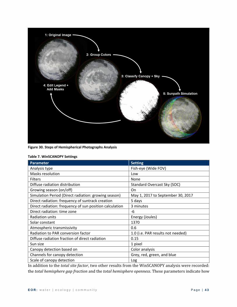
E O R : w a t e r | e c o l o g y | c o m m u n i t y P a g e | 4 3
Figure 30. Steps of Hemispherical Photographs Analysis
Table 7. WinSCANOPY Settings
Parameter Setting
Analysis type Fish-eye (Wide FOV)
Masks resolution Low
Filters None
Diffuse radiation distribution Standard Overcast Sky (SOC)
Growing season (on/off) On
Simulation Period (Direct radiation: growing season) May 1, 2017 to September 30, 2017
Direct radiation: frequency of suntrack creation 5 days
Direct radiation: frequency of sun position calculation 3 minutes
Direct radiation: time zone -6
Radiation units Energy (Joules)
Solar constant 1370
Atmospheric transmissivity 0.6
Radiation to PAR conversion factor 1.0 (i.e. PAR results not needed)
Diffuse radiation fraction of direct radiation 0.15
Sun size 1 pixel
Canopy detection based on Color analysis
Channels for canopy detection Grey, red, green, and blue
Scale of canopy detection Log
In addition to the total site factor, two other results from the WinSCANOPY analysis were recorded:
the total hemisphere gap fraction and the total hemisphere openness. These parameters indicate how

E O R : w a t e r | e c o l o g y | c o m m u n i t y P a g e | 4 4
much of the sky above the stream is blocked by vegetation and topography using different
approaches. The total hemisphere gap fraction is the ratio of the number of pixels in the photograph
classified as sky to the total number of pixels in the photograph. As such, the total hemisphere gap
fraction does not account for the projection of the lens onto the plane of the photograph, and so it
does not reflect the real canopy above the lens. In comparison, total hemisphere openness accounts
for the hemispherical projection of the open sky regions projected onto the photograph. Both
parameters are independent from the position of the sun. These results were recorded from the
WinSCANOPY analysis because they relate to canopy cover and closure, which are commonly used
when discussing shade although they cannot be used as a surrogate for shade (See Appendix A). Total
hemisphere gap fraction is similar to 1 minus canopy cover. Total hemisphere openness is similar to
1 minus canopy closure. WinSCANOPY provides many other results that were not utilized in this
study, such as leaf area index.
Shade-stage curves were developed for the four transects where photos were taken at five different
heights above the stream surface. It is assumed that baseflow conditions were consistent during the
period of these photos (September 10 to 13, 2017). A factor was developed using these curves to
correct shade to a consistent elevation immediately above the stream surface. Corrections for other
variables, such as herbaceous vegetation growth, were not implemented but will be assessed further
in the main author’s thesis.
The last piece of the shading data analysis effort was to examine methods for extrapolating the
shading results from the monitored reaches to unmonitored reaches in order to create an updated
version of the existing shading conditions initially developed in the Brown’s Creek Thermal Study.
First, a regression analysis was conducted to assess the correlation of the transect characteristics
(e.g. stream azimuth, vegetation height, etc.) with the resulting average transect shade. Second, the
WinSCANOPY analysis results were extrapolated to other areas of the creek, relying on the original
results of the ArcMap solar radiation analysis of LiDAR data conducted in the Brown’s Creek Thermal
Study (hereafter referred to as “LiDAR analysis” and “LiDAR-based shade”, familiarity with the study
area and best judgement informed by the WinSCANOPY results.
5.1.2. Results
The full record of data collected in this study is provided in Appendix C which is organized by the
channel characteristics, vegetation characteristics, and results of the photo WinSCANOPY analysis.
Over 130 plant species were identified adjacent to the stream in the study area as detailed in Table
22 of Appendix C, including native, invasive, exotic, and ornamental species. Eleven invasive or exotic
species were identified at the study area transects, including Amur maple, common burdock, birds-
foot trefoil, common buckthorn, Canada thistle, glossy buckthorn, garlic mustard, honeysuckle
(Lonicera spp.), purple loosestrife, reed canary grass, and watercress. At least one of these
invasive/exotic species were identified at each transect. The most common invasive species
identified were reed canary grass (152), glossy buckthorn (58), Canada thistle (17), and common
buckthorn (15). Plants were only identified if they could be seen while standing in the creek at each
transect.
The stage-shade curves in Figure 31 indicate that shade did not change significantly with lens height
in forested reaches, but it was a significant factor in grassy reaches where shade typically increased

E O R : w a t e r | e c o l o g y | c o m m u n i t y P a g e | 4 5
as the camera was lowered towards the stream. These curves were used to develop a correction
factor for any photos collected in transects with grassy to mixed riparian vegetation. The correction
factor was the most significant for reaches with north-south orientation, and resulted in, for example,
an incremental increase in shade of 20% where the lens was 0.4 m above the water surface. On
average, the correction factor resulted in 7% more shade in grassy reaches.
The final shade results from the WinSCANOPY analysis, including the correction for lens height above
the stream, are illustrated in Figure 32 for every transect in the study area. These results illustrate
that the shade at each position across a transect typically varies more in grassy reaches than in
forested reaches. As such, photos need to be collected at multiple positions across the transect
instead of taking a single photo from the middle of the stream in order to estimate shade across the
entire transect. Average transect shade (i.e. the purple line in Figure 32) ranged from 8% to 97% in
each sampled reach with a mean value of 61%.
A regression analysis of the correlation between multiple independent variables (i.e. the channel and
vegetation characteristics) and average shade identified many potential correlations (Figure 33 and
Figure 34). Regression analysis is a set of statistical modeling processes for estimating the
relationships between variables. Two of the most highly correlated variables with transect shade
(shade.avg) were the type of vegetation (veg.code.avg) and shade estimated using LiDAR in the
Brown’s Creek Thermal Study (shade.lidar.leafoff.dsm). The regression analysis was unsuccessful in
developing a reliable predictive model for shade using the physical characteristics of each transect.
The range of average transect shade at locations with various levels of woody vegetation is illustrated
in Figure 35 and demonstrates the lack of certainty in predicting shade simply using the type of
vegetation.
Another regression analysis was more successful in developing a predictive model to correct the
results of the LiDAR analysis with the WinSCANOPY-based shade. LiDAR-based shade is compared to
WinSCANOPY-based shade spatially (Figure 36), averaged by transect (Figure 38), and averaged by
reach (Figure 39). As part of the Brown’s Creek Thermal Study, the LiDAR-based shade were revised
to calibrate the stream temperature model. The calibrated shade is illustrated in comparison to the
WinSCANOPY results in Figure 37. The lognormal relationship between LiDAR and WinSCANOPY-
based average transect shade (Figure 38) resulted in an R2 value of 0.54. Looking at the results on an
average reach basis (Figure 39) was more successful with an R2 value of 0.76. Both of the regression
models used a lognormal relationship such that the predicted shade was not less than zero percent
or greater than 100% given the range of inputs to the model (i.e. the original LiDAR-based shade from
the Brown’s Creek Thermal Study). In addition, the shade results for Reach 7 were not included in
the regression analysis since the LiDAR data was collected before the 2012 restoration of Oak Glenn
Golf Course and the hemispherical photographs used in the WinSCANOPY analysis were collected
after the restoration project.
The existing conditions riparian shade analysis conducted in the Brown’s Creek Thermal Study was
updated using the WinSCANOPY results applied across the sampled and representative reaches
monitored in this Riparian Shading Study. The WinSCANOPY results were aggregated on a 40 m
segment basis throughout the monitored reaches. This processing was necessary since the stream
temperature model simulates the creek in 40 m segments. In areas that were not monitored in this
study, the pre-calibration existing shade estimated using LiDAR in the Brown’s Creek Thermal Study

E O R : w a t e r | e c o l o g y | c o m m u n i t y P a g e | 4 6
was adjusted using the lognormal regression formula shown in Figure 39. Lastly, the areas in the Oak
Glen Golf Course that were mowed to the water’s edge prior to the 2012 stream restoration project
were set to 10% shade such that the existing conditions analysis would represent pre-restoration
conditions in 2012. The original and final corrected shade along the profile of Brown’s Creek is shown
in Figure 40.
In comparison to the mowed grass conditions in 2011/2012 in the Oak Glen Golf Course, the
hemispherical photo analysis results for representative Reach 7 indicate that current shading is
approximately 46% in the golf course. This is the estimated total shade over an entire growing season
(May to October) and is averaged over the length of the stream from McKusick Road at the golf course
to the Brown’s Creek Trail crossing near Stone Bridge Trail.
Hemispherical photograph analysis is the best-suited method for indirectly estimating shade and is
less intensive than directly measuring solar radiation at multiple sites over a growing season (See
Appendix A). The uncertainties in hemispherical photo analysis were identified and mitigated where
possible, as follows:
The horizontal level of the camera can affect the view angle used when capturing the image.
This was mitigated for by using an auto-balancing mount for the camera and adjusting the
position using small weights to center the bubble level.
Shade is unevenly distributed across the width of the stream. This was assessed through the
sampling design which included multiple photos across the stream width.
Depending on the wind conditions, the motion of vegetation introduces more potential
variability in the shade results. A multi-shutter release was used for several sampled reaches
which could be used to assess the impact of this factor on the WinSCANOPY results in the
future, however such analysis was not included in this study.
Randomness and variability of shade at monitoring locations and other locations in the study
area was accounted for in the sample design.
The method used in simulating solar pathway and incoming solar radiation in WinSCANOPY
has several known limitations such as underestimating the radiation reflected through the
canopy by leaves. This was mitigated for by directly measuring solar radiation at four
transects in order to validate the WinSCANOPY results. Further review and processing of the
solar radiation measurements will be conducted as part of the main author’s thesis.

E O R : w a t e r | e c o l o g y | c o m m u n i t y P a g e | 4 7
Figure 31. Stage-Shade Curves at Forested and Grassy Transects
Woody South: Reach 2, Transect 0 Woody East: Reach 4, Transect 5
Grassy South: Reach 3, Transect 6 Grassy East: Reach 3, Transect 9

E O R : w a t e r | e c o l o g y | c o m m u n i t y P a g e | 4 8
Figure 32. Transect Shade Estimated with WinSCANOPY on Average and at Positions
left
middle
right
average

E O R : w a t e r | e c o l o g y | c o m m u n i t y P a g e | 4 9
Figure 33. Correlation Coefficients of Independent and Dependent Variables
Correlation Coefficient Legend
─1

E O R : w a t e r | e c o l o g y | c o m m u n i t y P a g e | 5 0
Figure 34. Independent Variables vs. Average Transect Shade
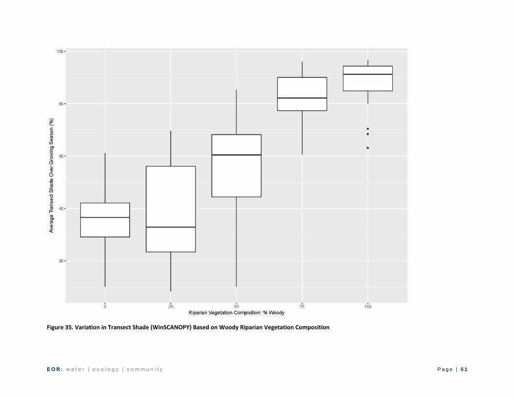
E O R : w a t e r | e c o l o g y | c o m m u n i t y P a g e | 5 1
Figure 35. Variation in Transect Shade (WinSCANOPY) Based on Woody Riparian Vegetation Composition

E O R : w a t e r | e c o l o g y | c o m m u n i t y P a g e | 5 2
Figure 36. Transect Shade Estimated using WinSCANOPY in Comparison to Shade Estimated from LiDAR

E O R : w a t e r | e c o l o g y | c o m m u n i t y P a g e | 5 3
Figure 37. Transect Shade Estimated using WinSCANOPY in Comparison to Shade Calibrated in Brown’s Creek Thermal Study
Calibrated for Thermal Study (2017)

E O R : w a t e r | e c o l o g y | c o m m u n i t y P a g e | 5 4
Figure 38. Average Transect Shade Estimated using LiDAR and WinSCANOPY (Omitting Reach 7)
Figure 39. Average Reach Shade Estimated Using LiDAR and WinSCANOPY (Omitting Reach 7)
Figure 40. Profile of Existing Conditions Riparian Shade along Brown's Creek

E O R : w a t e r | e c o l o g y | c o m m u n i t y P a g e | 5 5
Figure 41. Updated Riparian Shade Analysis using WinSCANOPY (Shade Conditions in Year 2011)

E O R : w a t e r | e c o l o g y | c o m m u n i t y P a g e | 5 6
The canopy structure changes over the growing season. The implication of this variable with
respect to the timing of photograph collection was tested by collecting repeated photos at
three transects at different times during the monitoring period. The resulting shade
estimated using mid-summer (July/August) and late summer (September) photos indicated
that some locations have more variable shade from senescence late in the summer than
others which have consistent shade (Figure 42). However, there was an insufficient number
of re-sampled locations to determine a trend and adjust other results accordingly.
Figure 42. Growing Season Shade Estimated in WinSCANOPY using Hemispherical Photographs from Mid-Summer and Late Summer
Categorization of canopy and sky areas in photographs is affected by resolution of photos and
by user-defined color classification. This was mitigated by using a camera with high
resolution photos and by repeating the analysis of several photos by a second person. User
error in WinSCANOPY appears to be minor based on the repeated analysis conducted for two
of the study area transects. On average for each transect, the difference in shade estimated
by two different users ranged from -0.3% to -0.2% (Table 8).
Table 8. Evaluation of User Error in WinSCANOPY Analysis
Reach and Transect Difference in Shade
Left Middle Right Average
Reach 4, Transect 5 -1% -1% 0.3% -0.3%
Reach 1, Transect 5 1% -2% 1% -0.2%
Variable depth of flow and height of lens above water surface were accounted for by
monitoring only during baseflow conditions and assessing the sensitivity of shade to lens
height above the water surface. The first transects were monitored in July when flows were
in the mid-range flow regime but otherwise activities were limited to dry conditions or low
flows (Figure 43).

E O R : w a t e r | e c o l o g y | c o m m u n i t y P a g e | 5 7
Figure 43. Flow Duration Curve at Highway 15 and at McKusick (Oak Glen) from April to October 2017
5.1.3. Discussion
Comparing shade estimated using ArcMap solar radiation analysis of LiDAR data in the Brown’s
Creek Thermal Study and to the results of analyzing the hemispherical images indicates that the
analysis of LiDAR data frequently underestimated shade. This is likely due to the limitations of the
LiDAR data itself, as it was collected in November 2011 after leaf-off and has limited accuracy in
identifying small herbaceous vegetation. Correcting the LiDAR-based estimates using the
WinSCANOPY results worked well in areas with mixed forested vegetation, perhaps due to the dense
coniferous vegetation even after leaf off. However, the corrections did not work well in areas with
predominantly deciduous canopy such as the dense willow woodland upstream of McKusick Road
North in Oak Glen Golf Course. As of 2011 when the LiDAR was flown, the canopy should have been
established since the willows were planted in 1999 during a MNDNR stream restoration project. As
such, these results indicate that LiDAR flown after leaf off requires varying corrections based on
species composition in woodlands. Overall, the updated existing shade (Figure 41) indicates that
Brown’s Creek is more shaded than estimated in the Brown’s Creek Thermal Study.
Analysis of the hemispherical photographs collected in Reach 7 (the segment of the Oak Glen Golf
Course Restored in 2012) indicates that as of 2017, vegetation had established to the point of
providing 38% shade across the sampled reach, with the shade at individual transects ranging from
8 to 80%. The un-calibrated shade estimated using 2011 LiDAR data in the Brown’s Creek Thermal
Study at the same location was an average of 14% and ranged from 6 to 24%. The correction formula
for LiDAR cannot be applied to Reach 7 because the input data (LiDAR and hemispherical
photographs) were taken under different vegetation conditions. However, the results indicate that
the segments of the restoration with young trees have not yet established to provide the expected
shade restoration. The herbaceous vegetation is providing approximately 20% shade in this reach.

E O R : w a t e r | e c o l o g y | c o m m u n i t y P a g e | 5 8
Continued monitoring of shade at these same locations in Reach 7 will provide the data needed to
assess the lag time between plantings to reaching target shade levels.
Riparian shade analyses are commonly conducted to develop inputs for stream temperature models.
In the case of this and other studies, those stream temperature models use the same shade value for
a segment of the stream and over the course of the entire model period, sometimes up to an entire
growing season. While these total growing season shade levels averaged across the length of the
stream are useful for stream temperature models, they mask the factors influencing the variability in
shade. The existing conditions riparian analysis in this study provides useful insight into some of
those factors by using hemispherical photography. The WinSCANOPY results in Figure 32 illustrate
how much riparian shade can vary across the stream width and along the length of the stream. In
addition, the stage-shade curves illustrated that shade estimated with hemispherical photographs in
grassy reaches varies significantly based on the height of the camera lens above the stream surface.
The WinSCANOPY results shown are total shade over the growing season which is calculated on a
sub-daily time step basis to consider the variability in the position of the sunpath and the intensity
of sunlight over the growing season. The remaining factor potentially resulting in further temporal
variation in shade is vegetation growth. It was assumed in this study that collecting the hemispherical
photographs in July, August, and early September captured typical vegetation conditions when shade
is critical to stream temperature control. This assumption could not be comprehensively assessed
within this study due to the limited occurrences of baseflow conditions and the time required to
complete each sampled reach. As such, monitoring each transect monthly was not feasible given the
time constraints.
The stage-storage curves were also useful in identifying the significant shade (close to 70%) that can
be provided by overhanging herbaceous vegetation on the north bank of an east-west oriented
stream (see the bottom right panel of Figure 31). In comparison, similar vegetation on a north-south
oriented stream (see the bottom left panel) provides consistently low shade of 30 to 40%. While these
results may be specific to the two transect monitored, the results reinforce the findings from other
studies in grassy streams: that shade is more challenging to attain in north-south oriented reaches
than east-west. Even further, there would seem to be much more potential to add shade on the south
bank in the east-west stream through plantings.
The updated shade analysis also refines our understanding of the length of unshaded areas along the
creek (less than 55% shade) which was previously estimated to be 3 km (1.9 miles) but with the
refined shade analysis, there is only 1.3 km (0.8 miles) unshaded. Increasing the threshold of what is
considered "low" shading in the mitigation scenarios would target additional areas up to a total of
3.7 km (2.3 miles) if anything less than 85% shade was considered for implementation activities.
Developing a predictive model for shade using the physical characteristics of each transect proved
difficult in this study. Part of the challenge is the vast number of spatiotemporal variables influencing
shade, including channel characteristics (e.g. width, depth, azimuth, and slope), upland topography,
and vegetation structure (e.g. height, width, distance from stream, species, and location relative to
transect). Assessing the influence of these variables in nature also makes it challenging to control for
variability and discern the sensitivity of shade to modifications in individual parameters, although
monitoring a single system helped to control the range of some variables to be within the range of a
small stream. The challenges faced in the regression analysis indicate that larger sample size is

E O R : w a t e r | e c o l o g y | c o m m u n i t y P a g e | 5 9
needed within representative reaches to develop a regression model based on physical parameters.
However, such a predictive model is not required when trying to assess existing shade conditions
because hemispherical photographs themselves provide the data needed to assess existing shade
levels and validate LiDAR-based estimates. Although the hemispherical photography equipment and
analysis software was expensive, gathering the field-based physical data for a hypothetical predictive
model would also require considerable cost in labor. Beyond assessing existing shade, a predictive
model would be helpful in assessing the canopy structure required to attain target shade levels in the
future, or optimize plantings where they will provide the greatest increase in shade. These topics are
addressed in the next section on assessing future shade conditions.
In hindsight, the monitoring program for this study could have been strengthened by consistently
collecting the following data:
Width of overhanging bank
Height of bank adjacent to stream
Density of vegetation (i.e. high, medium, low or on a scale of 1 to 0)
Mode vegetation height
LiDAR data collected in the summer with a sub-1 m resolution
Additional representative reaches with mixed or shrubby vegetation
5.2. Sensitivity Analysis
Gaining insight into the shade provided by understory in comparison to tree canopy is essential for
this study to guide future riparian management decisions, such as long term investment in expanding
the riparian tree canopy or quickly enhancing riparian shrubs and grasses. After the existing
conditions riparian shading analysis (Section 5.1) and trade-offs assessment (Appendix B), three
critical questions remained to be addressed in order to develop a targeted plan for riparian shade
restoration in Brown’s Creek:
1. Under what conditions can herbaceous riparian vegetation sufficiently shade Brown’s Creek?
2. How far can woody vegetation be planted away from the stream while sufficiently increasing
shade for Brown’s Creek? A horizontal separation of tree plantings from the creek will help
sustain the integrity of terrestrial resources (e.g. sedge meadows), improve the survival rate
of tree plantings where they can be located in non-hydric soils, and provide stream shade
while maintaining herbaceous cover on the streambank in order to prevent streambank
erosion.
3. Under which physical conditions will plantings be most effective (i.e. provide the greatest
increase in shade)?
The above questions were assessed using a sensitivity analysis of the range of physical structure of
Brown’s Creek and its riparian vegetation found in the study area.
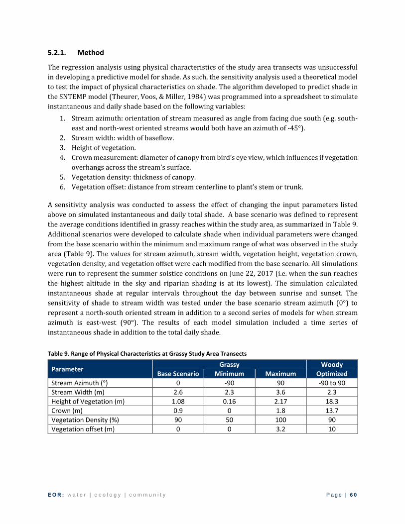
E O R : w a t e r | e c o l o g y | c o m m u n i t y P a g e | 6 0
5.2.1. Method
The regression analysis using physical characteristics of the study area transects was unsuccessful
in developing a predictive model for shade. As such, the sensitivity analysis used a theoretical model
to test the impact of physical characteristics on shade. The algorithm developed to predict shade in
the SNTEMP model (Theurer, Voos, & Miller, 1984) was programmed into a spreadsheet to simulate
instantaneous and daily shade based on the following variables:
1. Stream azimuth: orientation of stream measured as angle from facing due south (e.g. south-
east and north-west oriented streams would both have an azimuth of -45°).
2. Stream width: width of baseflow.
3. Height of vegetation.
4. Crown measurement: diameter of canopy from bird’s eye view, which influences if vegetation
overhangs across the stream’s surface.
5. Vegetation density: thickness of canopy.
6. Vegetation offset: distance from stream centerline to plant’s stem or trunk.
A sensitivity analysis was conducted to assess the effect of changing the input parameters listed
above on simulated instantaneous and daily total shade. A base scenario was defined to represent
the average conditions identified in grassy reaches within the study area, as summarized in Table 9.
Additional scenarios were developed to calculate shade when individual parameters were changed
from the base scenario within the minimum and maximum range of what was observed in the study
area (Table 9). The values for stream azimuth, stream width, vegetation height, vegetation crown,
vegetation density, and vegetation offset were each modified from the base scenario. All simulations
were run to represent the summer solstice conditions on June 22, 2017 (i.e. when the sun reaches
the highest altitude in the sky and riparian shading is at its lowest). The simulation calculated
instantaneous shade at regular intervals throughout the day between sunrise and sunset. The
sensitivity of shade to stream width was tested under the base scenario stream azimuth (0°) to
represent a north-south oriented stream in addition to a second series of models for when stream
azimuth is east-west (90°). The results of each model simulation included a time series of
instantaneous shade in addition to the total daily shade.
Table 9. Range of Physical Characteristics at Grassy Study Area Transects
Parameter Grassy Woody
Base Scenario Minimum Maximum Optimized
Stream Azimuth (°) 0 -90 90 -90 to 90
Stream Width (m) 2.6 2.3 3.6 2.3
Height of Vegetation (m) 1.08 0.16 2.17 18.3
Crown (m) 0.9 0 1.8 13.7
Vegetation Density (%) 90 50 100 90
Vegetation offset (m) 0 0 3.2 10

E O R : w a t e r | e c o l o g y | c o m m u n i t y P a g e | 6 1
Three additional scenarios were developed after the sensitivity analysis to represent the following
inputs under the full range of stream azimuth:
1. Parameters for grassy vegetation that maximizes shade.
2. Parameters for woody vegetation (mature black willow) offset from the stream centerline
(Table 9).
3. Combination of the above two scenarios with tree offset optimized to provide shade while
not being located immediately adjacent to stream.
The sensitivity analysis was limited in that it did not consider the following:
topographic shade (which determines the local time of sunrise and sunset).
multi-day or full season simulation.
plant growth.
variability of incident radiation based on time of day.
Validation to measured radiation or other shade prediction methods (e.g. WinSCANOPY).
5.2.2. Results
The results of the sensitivity analyses are illustrated by the time series plots on the following pages.
Each plot shows the instantaneous shade simulated throughout the day on June 22, 2017 and the
total daily shade is labeled below the legend. The results of the base scenario are illustrated in Figure
44. The results of modifying individual parameters from the base scenario within the range observed
in the study area are illustrated in Figure 45 to Figure 51. The sensitivity of shade to stream azimuth
under optimal grassy conditions is shown in Figure 52. The time series shown in Figure 53 illustrate
the instantaneous shade provided by trees offset from the stream. Lastly, Figure 54 illustrates shade
provided by optimal grassy conditions in addition to trees offset from the stream.
Figure 44. Base Scenario of Sensitivity Analysis

E O R : w a t e r | e c o l o g y | c o m m u n i t y P a g e | 6 2
Figure 45. Sensitivity Analysis of Modeled Shade to Stream Azimuth
Figure 46. Sensitivity Analysis of Modeled Shade to Stream Width (0° Azimuth)
Figure 47. Sensitivity Analysis of Modeled Shade to Stream Width (90° Azimuth)

E O R : w a t e r | e c o l o g y | c o m m u n i t y P a g e | 6 3
Figure 48. Sensitivity Analysis of Modeled Shade to Vegetation Height
Figure 49. Sensitivity Analysis of Modeled Shade to Vegetation Crown (Diameter)
Figure 50. Sensitivity Analysis of Modeled Shade to Vegetation Density

E O R : w a t e r | e c o l o g y | c o m m u n i t y P a g e | 6 4
Figure 51. Sensitivity Analysis of Modeled Shade to Vegetation Offset
Figure 52. Sensitivity Analysis of Modeled Shade to Azimuth under Optimized Grassy Conditions
Figure 53. Sensitivity Analysis of Modeled Shade to Azimuth under Offset Woody Conditions
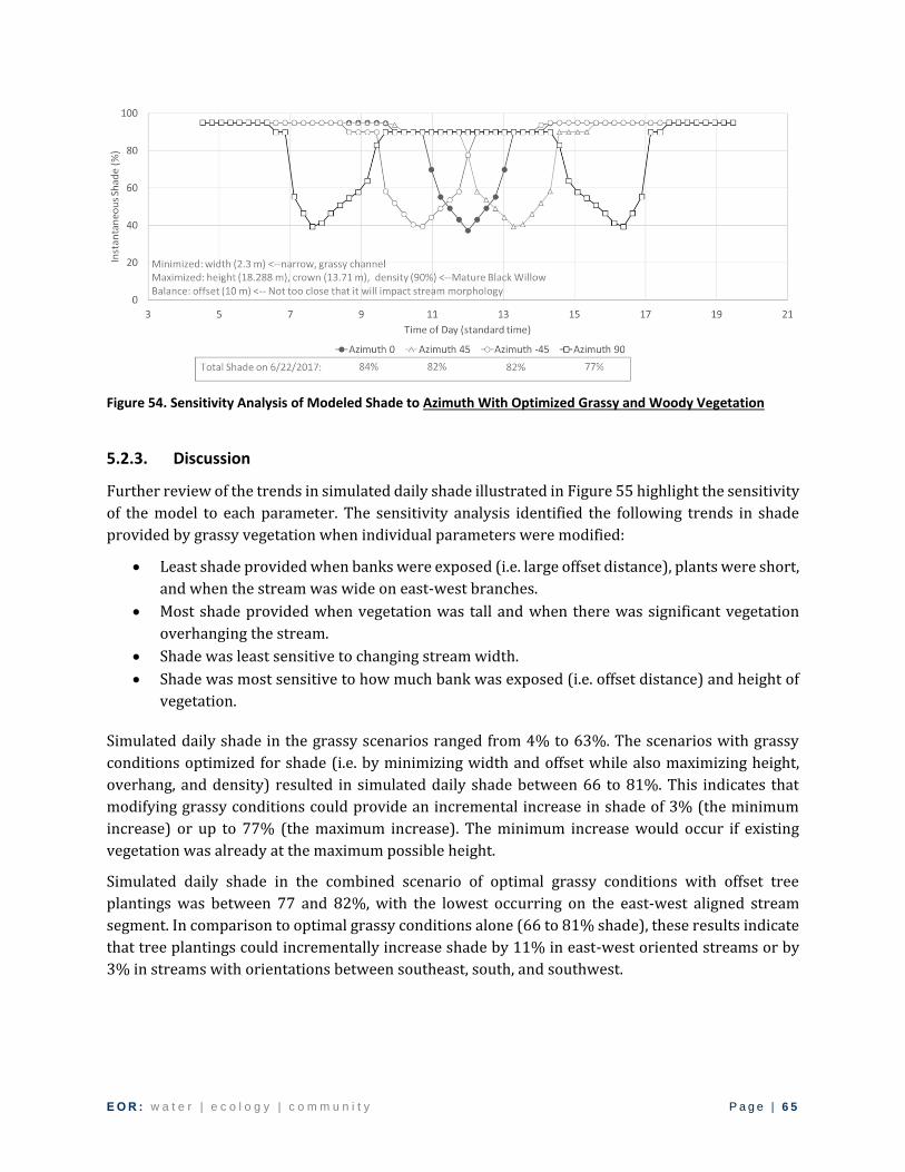
E O R : w a t e r | e c o l o g y | c o m m u n i t y P a g e | 6 5
Figure 54. Sensitivity Analysis of Modeled Shade to Azimuth With Optimized Grassy and Woody Vegetation
5.2.3. Discussion
Further review of the trends in simulated daily shade illustrated in Figure 55 highlight the sensitivity
of the model to each parameter. The sensitivity analysis identified the following trends in shade
provided by grassy vegetation when individual parameters were modified:
Least shade provided when banks were exposed (i.e. large offset distance), plants were short,
and when the stream was wide on east-west branches.
Most shade provided when vegetation was tall and when there was significant vegetation
overhanging the stream.
Shade was least sensitive to changing stream width.
Shade was most sensitive to how much bank was exposed (i.e. offset distance) and height of
vegetation.
Simulated daily shade in the grassy scenarios ranged from 4% to 63%. The scenarios with grassy
conditions optimized for shade (i.e. by minimizing width and offset while also maximizing height,
overhang, and density) resulted in simulated daily shade between 66 to 81%. This indicates that
modifying grassy conditions could provide an incremental increase in shade of 3% (the minimum
increase) or up to 77% (the maximum increase). The minimum increase would occur if existing
vegetation was already at the maximum possible height.
Simulated daily shade in the combined scenario of optimal grassy conditions with offset tree
plantings was between 77 and 82%, with the lowest occurring on the east-west aligned stream
segment. In comparison to optimal grassy conditions alone (66 to 81% shade), these results indicate
that tree plantings could incrementally increase shade by 11% in east-west oriented streams or by
3% in streams with orientations between southeast, south, and southwest.

E O R : w a t e r | e c o l o g y | c o m m u n i t y P a g e | 6 6
Figure 55. Summary of Simulated Total Daily Shade from Variables Modified in Sensitivity Analysis

E O R : w a t e r | e c o l o g y | c o m m u n i t y P a g e | 6 7
These results address the original questions behind the sensitivity analysis, as follows:
1. Under what conditions can herbaceous riparian vegetation sufficiently shade Brown’s Creek?
The greatest grassy shade is provided in Brown’s Creek when the following conditions occur in
the channel and riparian zone:
Stream width is minimized to 2.3 m
Vegetation is established on the streambank and there is no exposed bank
Vegetation height is maximized to 2.17 m
Vegetation overhang is maximized to 0.6 m
Vegetation density is maximized to 95%
The optimal conditions are within the range observed in the study area. Simulating these
conditions resulted in total shade on the summer solstice of 81% in a north-south oriented
stream, 79% in a southeast or southwest oriented stream, and 66% in an east-west oriented
stream. Conditions for shade throughout the study area could be optimized by managing riparian
vegetation, such as introducing tall herbaceous species, or by restoring the channel morphology,
such as the narrowing of the creek that occurred through the Oak Glen Golf Course after the 2012
restoration project. Even further, the above simulations did not include topographic shade and
so could be enhanced on sites with overhanging stream banks and adjacent valleys or other
topographic features.
With a target for shade between 75 to 85% in Brown’s Creek, these results indicate that optimal
grassy vegetation can meet the District’s shade target where the stream orientation is between
320° to 45° or between 135° to 225° as measured using a compass relative to due north.
2. How far can woody vegetation be planted away from the stream while sufficiently increasing shade
for Brown’s Creek?
The sensitivity analysis indicates that woody vegetation can be planted approximately 10 m away
from the stream and increase the shade sufficiently to meet the District’s shade target.
3. Under which physical conditions will plantings be most effective (i.e. provide the greatest increase
in shade) for Brown’s Creek?
Tree plantings would be most effective and provide the greatest increase in shade when located
on the south bank of an east-west oriented segment. This trend compliments the trend in grassy
shade, where the least shade is provided in east-west branches.
5.3. Future Conditions
This section describes the concept plans developed for riparian shad improvements in the unshaded
areas of the creek. These concept plans were then used to estimate the future shade along the study
area with these improvements as well as estimating the time to maturity of shade.

E O R : w a t e r | e c o l o g y | c o m m u n i t y P a g e | 6 8
5.3.1. Method
High Priority Segments for Shade Restoration
Areas requiring shade restoration were first prioritized where the existing conditions riparian shade
analysis (Figure 41) indicated less than 80% shade is currently provided. Segment 5 is located
downstream of McKusick Road through Oak Glen Golf Course was also identified as having shade
below the 80% threshold but has already been restored and so was not included in the shade
restoration plan. The priority areas include the following creek segments6:
Segment 13, downstream of Manning Ave/Highway 15
Segment 12, upstream of Highway 96
Segment 11, downstream of Highway 96
Segment 10 (upper and middle section), south of Millbrook Development
Segment 8, upstream of Neal Avenue
Segment 6 (lower section), upstream of McKusick Road at Oak Glen Golf Course
Segment 4 (upper section), downstream of Brown’s Creek State Trail and Golf Course
Further review of the above short-list helped differentiate levels of priority. Upper Segment 10,
Segment 8, lower Segment 6, and upper Segment 4 are relatively short segments featuring relatively
well established under and overstory canopies. As such, optimizing the vegetation and channel form
for shade in these areas is lower priority than in the long and open segments, such as Segment 13.
Focusing on high priority implementation of Segments such as Segment 13 and postponing low
priority shade improvements also provides more time in which to monitor Segments 10, 8, and 4
with the WinSCANOPY equipment. These sites were not monitored directly as part of the Riparian
Shading Study, however pre-restoration measurements are needed to estimate the stream
temperature benefits and develop the concept plans for such improvements. This monitoring effort
is included in the recommendations of the study and in Appendix E. The benefits of thinning dense
tree canopies, such as those that are overcome with terrestrial invasive species, were not assessed
and/or identified in this Study.
The remaining high priority segments for shade restoration are the following locations:
Segment 13, downstream of Manning Ave/Highway 15
Segment 12, upstream of Highway 96
Segment 11, downstream of Highway 96
Segment 10 (middle section), south of Millbrook Development
These four high priority areas have clear opportunities for improving riparian vegetation to increase
shade. Segments 13 and 12 were also identified in the TMDL implementation plan as being high or
medium priority for morphology improvements, respectively. Segment 12 has no vegetated buffer
on the east bank in some locations and so was also identified as a high priority for buffer width
improvements.
6 Segment numbering is consistent with the TMDL Implementation Plan and as illustrated in Figure 15 and Figure 17.

E O R : w a t e r | e c o l o g y | c o m m u n i t y P a g e | 6 9
Targeted Shade Restoration Plan
Concept plans were developed for the four high priority shade restoration segments to illustrate the
extents of herbaceous planting/enhancement areas and tree planting locations following the best
practices identified in the sensitivity analysis. Where applicable, restoration of the stream meander
was also illustrated in the plans.
The soils and hydrology information for these restoration segments were reviewed to assess what
types of riparian vegetation could be established and supported by future restoration efforts. The
assessment considered pre-settlement vegetation (i.e. oak barrens described in Section 3.6) and
considered what current conditions may limit the ability to re-establish certain types of vegetation.
For example, certain tree species may have low survival rates in urban wetlands with hydric soils,
active hydrology, and subject to pollutants from urban runoff. In addition, existing plant communities
surrounding these segments were considered so that plantings for shade restoration would enhance
or maintain the quality of the overall plant community. After reviewing these considerations, a
preliminary list of grassy to woody plant species was developed (Appendix D) as a reference for
designers of shade restoration plans in Brown’s Creek. These species are typically suitable for
planting in the riparian corridor of Brown’s Creek and offer optimized characteristics for shade, such
as rapid growth and maximized height. Selection of species for particular locations in each
restoration project should be conducted during detailed design in consultation with a landscape
architect and ecologist.
Predicted Shade under Restored Conditions
The predictive shade model used in the sensitivity analysis (Section 5.2) was applied again to
estimate the increase in shade offered by enhancing herbaceous riparian buffers and targeting tree
plantings shown in the concept plans. Typical canopy structure characteristics of the black willow
species was used to represent future canopy structure of the restoration projects at maturity. Black
willows were selected for this analysis because their fast growth rate relative to other tree species
that could thrive in the riparian zones along Brown’s Creek. In addition, black willow trees tend to
have a broad crown, with branches extending out away from the main trunk, which makes them well-
suited to the application of establishing shade along the creek through tree plantings set back from
the water’s edge. Other tree species suitable to the riparian conditions along Brown’s Creek, such as
the others listed in Appendix D, may be selected during the design of shade restoration projects to
improve the survival rate of tree plantings, especially in areas with known beaver activity. The
existing and future characteristics of each segment used in the predicted shade analysis are
summarized in Table 10. A correction factor was calculated by comparing the existing conditions
results of the predictive model in comparison to the WinSCANOPY results and this factor was applied
to the future results.
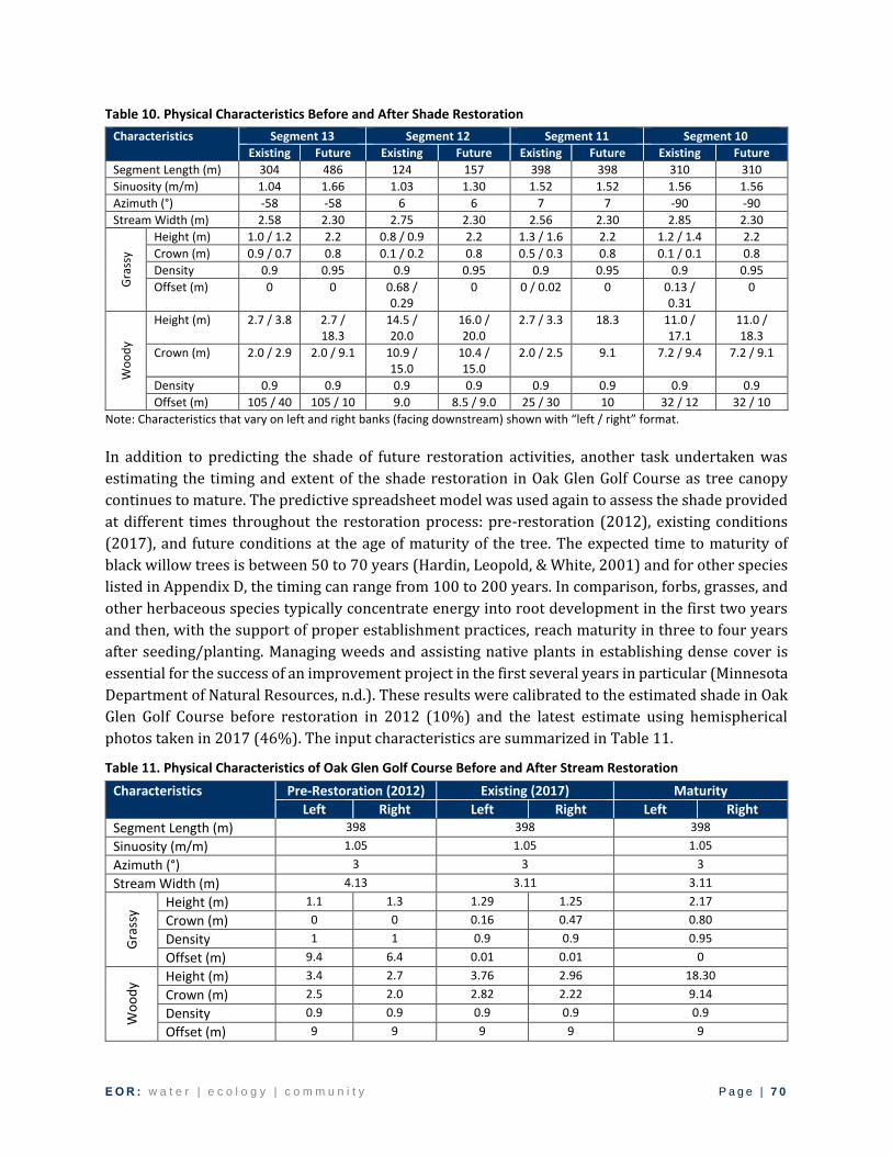
E O R : w a t e r | e c o l o g y | c o m m u n i t y P a g e | 7 0
Table 10. Physical Characteristics Before and After Shade Restoration
Characteristics Segment 13 Segment 12 Segment 11 Segment 10
Existing Future Existing Future Existing Future Existing Future
Segment Length (m) 304 486 124 157 398 398 310 310
Sinuosity (m/m) 1.04 1.66 1.03 1.30 1.52 1.52 1.56 1.56
Azimuth (°) -58 -58 6 6 7 7 -90 -90
Stream Width (m) 2.58 2.30 2.75 2.30 2.56 2.30 2.85 2.30
Gra
ssy
Height (m) 1.0 / 1.2 2.2 0.8 / 0.9 2.2 1.3 / 1.6 2.2 1.2 / 1.4 2.2
Crown (m) 0.9 / 0.7 0.8 0.1 / 0.2 0.8 0.5 / 0.3 0.8 0.1 / 0.1 0.8
Density 0.9 0.95 0.9 0.95 0.9 0.95 0.9 0.95
Offset (m) 0 0 0.68 / 0.29
0 0 / 0.02 0 0.13 / 0.31
0
Wo
od
y
Height (m) 2.7 / 3.8 2.7 / 18.3
14.5 / 20.0
16.0 / 20.0
2.7 / 3.3 18.3 11.0 / 17.1
11.0 / 18.3
Crown (m) 2.0 / 2.9 2.0 / 9.1 10.9 / 15.0
10.4 / 15.0
2.0 / 2.5 9.1 7.2 / 9.4 7.2 / 9.1
Density 0.9 0.9 0.9 0.9 0.9 0.9 0.9 0.9
Offset (m) 105 / 40 105 / 10 9.0 8.5 / 9.0 25 / 30 10 32 / 12 32 / 10
Note: Characteristics that vary on left and right banks (facing downstream) shown with “left / right” format.
In addition to predicting the shade of future restoration activities, another task undertaken was
estimating the timing and extent of the shade restoration in Oak Glen Golf Course as tree canopy
continues to mature. The predictive spreadsheet model was used again to assess the shade provided
at different times throughout the restoration process: pre-restoration (2012), existing conditions
(2017), and future conditions at the age of maturity of the tree. The expected time to maturity of
black willow trees is between 50 to 70 years (Hardin, Leopold, & White, 2001) and for other species
listed in Appendix D, the timing can range from 100 to 200 years. In comparison, forbs, grasses, and
other herbaceous species typically concentrate energy into root development in the first two years
and then, with the support of proper establishment practices, reach maturity in three to four years
after seeding/planting. Managing weeds and assisting native plants in establishing dense cover is
essential for the success of an improvement project in the first several years in particular (Minnesota
Department of Natural Resources, n.d.). These results were calibrated to the estimated shade in Oak
Glen Golf Course before restoration in 2012 (10%) and the latest estimate using hemispherical
photos taken in 2017 (46%). The input characteristics are summarized in Table 11.
Table 11. Physical Characteristics of Oak Glen Golf Course Before and After Stream Restoration
Characteristics Pre-Restoration (2012) Existing (2017) Maturity
Left Right Left Right Left Right
Segment Length (m) 398 398 398
Sinuosity (m/m) 1.05 1.05 1.05
Azimuth (°) 3 3 3
Stream Width (m) 4.13 3.11 3.11
Gra
ssy
Height (m) 1.1 1.3 1.29 1.25 2.17
Crown (m) 0 0 0.16 0.47 0.80
Density 1 1 0.9 0.9 0.95
Offset (m) 9.4 6.4 0.01 0.01 0
Wo
od
y
Height (m) 3.4 2.7 3.76 2.96 18.30
Crown (m) 2.5 2.0 2.82 2.22 9.14
Density 0.9 0.9 0.9 0.9 0.9
Offset (m) 9 9 9 9 9

E O R : w a t e r | e c o l o g y | c o m m u n i t y P a g e | 7 1
5.3.2. Results
Concept plans for the targeted shade restoration in Brown’s Creek are illustrated in Figure 56 to
Figure 59. Each concept plan includes a description of the segment and recommended
implementation activities. In addition, each concept plan includes a summary of site characteristics,
benefits of shade restorations, and costs. The expected future shade from the improvements is
summarized in Table 12 and illustrated in Figure 60. The temperature benefits were estimated using
the District’s stream temperature model and are the results of implementing all shade restoration
projects shown in the concept plan (Future Scenario IV of the model). See Section 6.2 for additional
detail on the stream temperature modeling.
Table 12. Summary of Existing and Future Shade at Target Shade Restoration Segments
Segment Average Growing Season Shade
Existing (2011) Future
Segment 13 44% 82%
Segment 12 75% 83%
Segment 11 49% 80%
Segment 10B 56% 84%
Segment 5 (lower Oak Glen Golf Course) 6% 79%
All Segments (Manning Ave to St. Croix River) 76% 84%
The cost of each implementation project is detailed in Table 13. These costs include the enhancement
of herbaceous vegetation, planting trees, and restoring the stream morphology where warranted. In
addition, the cost of administration and engineering, in addition to a 20% contingency, is included.
Property acquisitions or easement costs are not included in the estimates.
Table 13. Estimated Costs of Targeted Shade and Stream Restoration
Segments
Construction/Implementation
Admin. & Engineering
20% Contingency
Total Native
Herbaceous Community
Enhancement
Native Tree
Planting
Stream Restoration
13 $55,500 $3,330 $208,000 $95,000 $83,039 $498,235
12 $18,500 $185 $57,200 $55,000 $29,212 $175,274
11 $49,950 $3,885 $- $12,000 $15,320 $91,922
10B $33,300 $3,700 $36,000 $48,000 $27,120 $162,720
Total $157,250 $11,100 $301,200 $210,000 $154,692 $928,152 1) The following materials & labor are included in the unit NATIVE TREE PLANTING cost: tree (~1" caliper potted
stock), herbivore protection, weed barrier, 2-year warranty & associated 2-year maintenance
2) The following materials & labor are included in the unit NATIVE HERBACEOUS PLANT COMMUNITY
ENHANCEMENT cost: seed bed and/or invasive treatment preparation; seed, seeding, mulch, select planting (10%
of area at 24" on center spacing) of live plants, 2-year establishment maintenance
3) The following materials & labor are included in the unit STREAM RESTORATION cost: all materials, equipment and
labor necessary to execute the probable project including 2-year establishment maintenance
4) Cost do not include property acquisitions or easement costs

E O R : w a t e r | e c o l o g y | c o m m u n i t y P a g e | 7 2
Figure 56. Concept Shade Restoration Plan for Segment 13

E O R : w a t e r | e c o l o g y | c o m m u n i t y P a g e | 7 3
Figure 57. Concept Shade Restoration Plan for Segment 12

E O R : w a t e r | e c o l o g y | c o m m u n i t y P a g e | 7 4
Figure 58. Concept Shade Restoration Plan for Segment 11
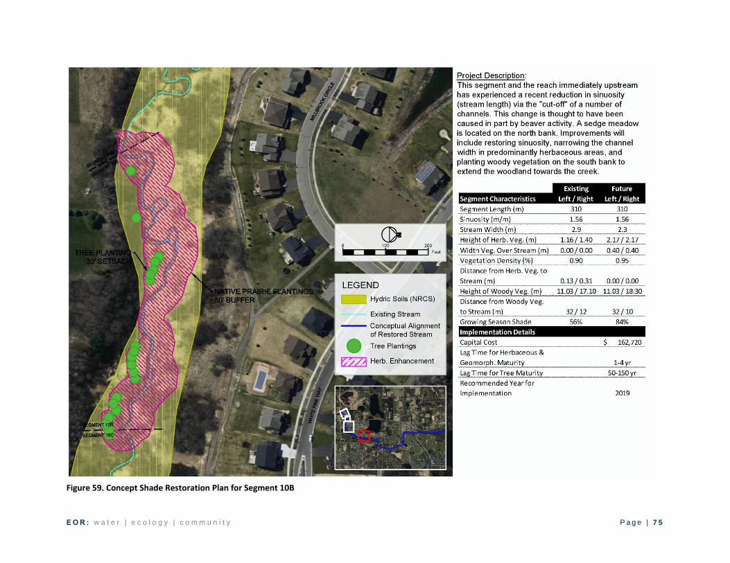
E O R : w a t e r | e c o l o g y | c o m m u n i t y P a g e | 7 5
Figure 59. Concept Shade Restoration Plan for Segment 10B

E O R : w a t e r | e c o l o g y | c o m m u n i t y P a g e | 7 6
Figure 60. Targeted Shade Restoration Scenario IV

E O R : w a t e r | e c o l o g y | c o m m u n i t y P a g e | 7 7
The estimated shade provided by vegetation over time in Oak Glen Golf Course is illustrated by the
blue line in Figure 61 using the typical characteristics of a black willow tree under the future scenario
60 years after the restoration. This indicates that 75% shade may be achieved approximately 42
years after the planting. In comparison, other trees listed in Appendix D grow more slowly and so
would not reach 75% shade for approximately 80 years, as shown by the orange line. The pivot point
in both curves is based on the WinSCANOPY analysis in Reach 7 showing 46% shade in 2017. The
steepness of the curve before this pivot indicates that early on after a stream restoration projects,
there will be a rapid increase in shade in the first 5 years due to channel narrowing, herbaceous
vegetation establishment, and the small canopy of the young tree.
Figure 61. Estimated Shade Over Time as Vegetation Establishes in Oak Glen Golf Course Restoration
5.3.3. Discussion
Targeting shade restoration at four high priority segments of Brown’s Creek in addition to previous
restoration efforts in the Oak Glen Golf Course is expected to increase the average shade between
Manning Avenue to the St. Croix from 76% to 84%, which is an 8% increase in shade overall. Based
on the growth rate of vegetation expected to be used in these restoration efforts, approximately 2 to
4% of the shade increase is expected to be provided by mature grassy vegetation and young woody
vegetation within 5 to 10 years of planting. The remaining 4 to 6% shade increase overall will be
provided once the woody vegetation reaches maturity, which varies based on species between 50 to
150 years.
In terms of reducing heat load to the stream, the shade restoration efforts overall would provide an
8% increase in shade over the growing season, which can also be looked at as an 8% reduction in
heat load from solar radiation to Brown’s Creek. The total heat load to the creek includes many other
heat sources, such as stormwater. The District’s Impaired Biota TMDL study identified the need for a
6% reduction in heat load to the creek to lower stream temperatures below the threat temperature
for brown trout (18.3°C). The stream temperature model developed by the District since the TMDL
study was updated to assess the potential stream temperature benefits in Section 6.
The estimated costs for the targeted shade restoration improvements are $928,152 in total capital
costs, including two years of inspection and maintenance of vegetation. These improvements are
included in the Higher Priority Implementation Plan and Thermal Improvement Activities in the

E O R : w a t e r | e c o l o g y | c o m m u n i t y P a g e | 7 8
District’s 2017-2026 WMP, in addition to other stream restoration needs. Reordering the timing of
these thermal improvement implementation activities based on priorities for shade restoration is
warranted in light of the lag-time in realizing the shade benefits, even for grassy vegetation. Section
7 includes recommendations for a new order of implementing the thermal improvements, pending
the willingness of the property owners of the land surrounding Segments 13 and 12.
Further detailed design of each shade restoration improvement will be necessary, especially on
Segments 13 and 12 where the recommended improvements include a restored stream meander and
where the design needs to be informed by land owner preferences. Public outreach will also be useful
for the residents adjacent to Segments 10 and 11 in the Millbrook development. In addition, detailed
planting plans will be informed by ecological site assessments in order to maintain or enhance the
vegetative communities adjacent to these segments. Cost-savings may be realized by reducing the
size of vegetation (i.e. shrubs and grasses instead of trees), although the placement of these species
relative to the stream will need to be optimized for shade enhancement without detrimental impacts
to streambank erosion. The benefits realized by the restoration efforts may also be accelerated where
shrubs and grasses may be used to establish shade faster than tree canopy.
The sensitivity analysis in Section 5.2 and the timing of shade restoration estimated above indicates
that optimizing grassy buffers can provide significant and relatively rapid increase in shade. As such,
grassy riparian buffers on Brown’s Creek should be both maintained and restored to maximize height
of vegetation and minimize exposed banks, which are the two parameters to which shade is most
sensitive. The concept plans for shade restoration address how this approach can be applied to
complete segments. In addition, this approach should be considered during maintenance and
ongoing activities, such as:
Removal of invasive woody species should be accompanied with herbaceous plantings to
enhance understory cover, height, and minimize exposed banks.
District and consulting field staff should watch for and record the locations of areas in the
creek that have stunted grassy vegetation, emergent vegetation, or exposed banks. The
district should allocate annual funding for maintenance of these small sites, including erosion
control blanket, planting plugs, and seeding during appropriate times of year (e.g. late spring
or summer when there are stable flows) to enhance grassy vegetation and shade.
This Riparian Shading Study has provided much insight into shade conditions in Brown’s Creek and
has familiarized the District with useful tools in assessing shade in the field and estimating the timing
and extent of future shade. The District has the opportunity to continue advancing the knowledge
around riparian management in small, urbanizing, coldwater prairie streams as they look to
implement the improvements by monitoring the timing and extent of shade before and after these
improvements using the hemispherical photography analysis method. Additional data over time will
also help improve the predictive shade model as well as provide insights into how shade varies over
a single season. Such monitoring will help the district continue to evaluate progress towards shade
restoration and ultimately restoration of aquatic health in Brown’s Creek. In addition, continued
monitoring will provide insights applicable to other stream systems and buffer restoration efforts
across Minnesota and North-Central America. The recommended monitoring plan for the District’s
shade improvements is detailed in Appendix E.

E O R : w a t e r | e c o l o g y | c o m m u n i t y P a g e | 7 9
6. STREAM TEMPERATURE MODEL
The stream temperature model was assembled based on the United States Army Corps of Engineers
(USACE) model, CEQUAL-W2 by William Herb (Saint Anthony Falls Laboratory, University of
Minnesota) as part of the Brown’s Creek Thermal Study in 2016. CEQUAL-W2 is a two-dimensional
(2-D) model for flow, temperature and nutrient transport which can be applied to lakes, rivers, and
reservoirs. For modeling a well-mixed stream such as Brown’s Creek, the 2-D capability of the model
over the stream wise distance and depth is not needed, but this feature may be useful in the future
for modeling in-stream ponds due to beaver dams. The CEQUAL package simulates flow and
temperature with high resolution in time, such as hourly time steps. An alternative stream
temperature modeling package developed at the United States Geological Service (USGS), SNTEMP,
was considered during the Brown’s Creek Thermal Study, however, SNTEMP is not well suited for
modeling the propagation of heated stormwater pulses through a small stream because it is limited
to daily time steps. Development of the Brown’s Creek model described further in the Brown’s Creek
Thermal Study. The following section describes the updates made to the model as part of this study
and the new results of shade restoration scenarios.
6.1. Existing Conditions
The existing conditions scenario of the stream temperature model was updated with the refined
riparian shade analysis results of this study. In addition, the detailed channel characteristics
monitored during the study were used to update the width of the channel in the model. The updates
to the model increased the average shade across all segments from 61% to 76% (Figure 62) and
widened the stream from a constant width of 1.6 m to the average observed width of 3.4 m. A few of
the modeled segments near Stonebridge Trail became hydrodynamically unstable with the increased
width and so it was limited to 2.5 m in these segments so that the model could run successfully. All
other model inputs were the same as was modeled in the Brown’s Creek Thermal Study.
Figure 62. Shade Inputs to Existing Conditions CE-QUAL-W2 Models in Thermal and Riparian Shading Studies
100% Shade means no solar radiation will reach the water surface.

E O R : w a t e r | e c o l o g y | c o m m u n i t y P a g e | 8 0
The model was run for the same simulation periods in 2012 and 2014 (April through October) as the
Brown’s Creek Thermal Study. The increased shade resulted in cooler water temperatures in the
updated simulation. This modification was partially offset by the widening of the stream, which
increased the water surface area subject to solar radiation and decreased the depth of the stream.
The model was re-calibrated to observed temperatures at the three monitoring stations (WOMP,
Stonebridge, and McKusick/Oak Glen) using groundwater temperature as the calibration parameter.
Adjustments to the wind sheltering coefficient were also tested but the model was less sensitive to
this parameter and so the input was left at a constant coefficient of 0.3. In order to calibrate the model
of 2012 (the warm and dry year), groundwater temperatures in the upper branches of the model
(Manning Avenue to Stonebridge Trail) were increased by 3.8°C on average and the lower branch
(Stonebridge Trail to the St. Croix River) was increased from a constant temperature of 9°C to 10°C.
Calibration of the model to observations in 2014 (the cool and wet year) was performed by increasing
the constant groundwater temperature in the lower branch from 9°C to 12°C.
The observed and simulated stream temperatures under existing conditions in 2012 are shown in
Figure 63 and Figure 64 for daily average and maximum temperatures, respectively. Similar
comparisons are provided for 2014 in Figure 65 and Figure 66. Overall, temperature simulations
were somewhat better in 2014, the wetter and cooler year. The root-mean-square error (RMSE) is a
measure of the typical error in simulated temperature values versus observed temperatures, and is
calculated as follows on a daily basis:
𝑅𝑀𝑆𝐸 = √∑ (𝑇𝑠𝑖 − 𝑇𝑜𝑖)2𝑛
𝑖
𝑛
where Tsi and Toi are the simulated and observed temperature at the ith day, respectively, and n is
the total number of days. The RMSE for the daily mean and maximum temperatures at each
monitoring location are summarized in Table 14 for both the full simulation period (April to October)
and the typically warm months of the year (July and August). Overall, the RMSE was better (smaller)
during the months of July and August than when looking at the full simulation period. The RMSE
values also indicate that the simulated stream temperature had a better fit with observed daily mean
temperatures than with daily maximum temperatures. In addition, the RMSE was typically lower in
the 2014 simulation than in 2012. Looking at the months of July and August, the RMSE for mean
temperatures was between 1.4 and 2.0°C in 2012 at each of the monitoring locations and in 2014 was
between 0.5 to 0.6°C. This level of calibration is consistent with the level of calibration achieved in
the Brown’s Creek Thermal Study which focused on the WOMP monitoring station.
Table 14. RMSE of 2012 and 2014 Existing Conditions Simulations
Year Period
RMSE (°C)
WOMP Stonebridge McKusick
Mean Max Mean Max Mean Max
2012 April to October 1.4 1.4 2.0 2.0 1.7 1.7
July and August 1.2 1.2 1.2 1.8 1.1 1.8
2014 April to October 0.9 2.2 0.9 1.1 0.8 1.3
July and August 0.6 1.4 0.5 0.8 0.5 1.1

E O R : w a t e r | e c o l o g y | c o m m u n i t y P a g e | 8 1
Figure 63. Simulated and Observed Daily Average Stream Temperature in 2012 at the McKusick (Oak Glen), Stonebridge, and WOMP Monitoring Stations

E O R : w a t e r | e c o l o g y | c o m m u n i t y P a g e | 8 2
Similar to the results in the Brown’s Creek Thermal Study, the maximum daily temperatures shown
in Figure 64 and Figure 66 suggest that the model is over-predicting maximum temperatures on some
wet days, particularly in 2014. This could be due to the assumptions made in the routing of
stormwater (directly vs. indirectly connected), limitations in the MINUHET simulations of runoff
temperature and flow rates from impervious areas, or in the CEQUAL model itself (heat routing
during highly transient storm flow).
Figure 64. Simulated and Observed Daily Maximum Stream Temperature in 2012 at the McKusick (Oak Glen), Stonebridge, and WOMP Monitoring Stations
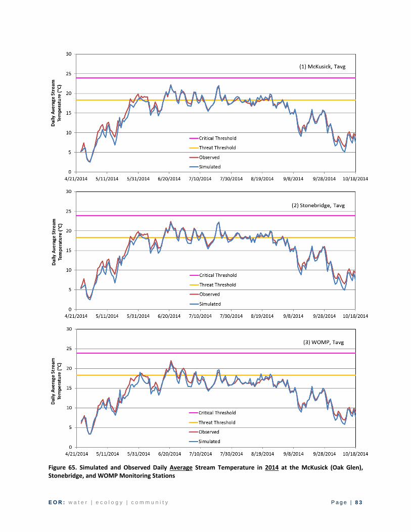
E O R : w a t e r | e c o l o g y | c o m m u n i t y P a g e | 8 3
Figure 65. Simulated and Observed Daily Average Stream Temperature in 2014 at the McKusick (Oak Glen), Stonebridge, and WOMP Monitoring Stations
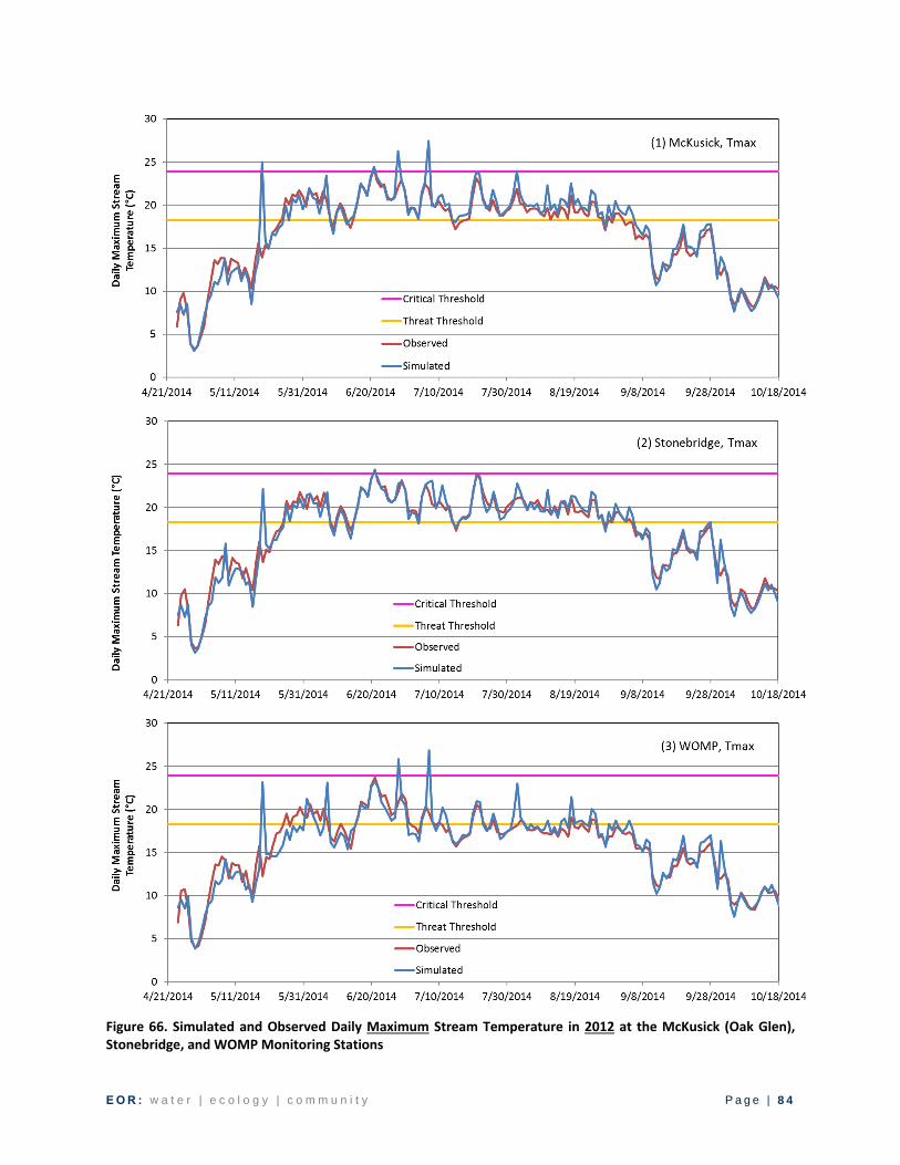
E O R : w a t e r | e c o l o g y | c o m m u n i t y P a g e | 8 4
Figure 66. Simulated and Observed Daily Maximum Stream Temperature in 2012 at the McKusick (Oak Glen), Stonebridge, and WOMP Monitoring Stations

E O R : w a t e r | e c o l o g y | c o m m u n i t y P a g e | 8 5
6.2. Future Conditions
Four future conditions scenarios (listed below) were developed to estimate the stream temperature
reductions resulting from increasing shade to varying degrees. The first two scenarios were updates
to the shade restoration scenarios assessed in the Brown’s Creek Thermal Study. The stream
temperature benefits estimated in this study are different because they are in comparison to the new
existing conditions scenario. The shade levels defined in the shade restoration scenarios are shown
in comparison to those of the existing conditions scenario in Figure 67.
1. Shade Restoration I: Minimum shade of 50%
2. Shade v II: Minimum shade of 75%
3. Shade Restoration III: Minimum shade of 85%
4. Shade Restoration IV: Targeted shade restoration plan (Figure 60)
Figure 67. Comparison of Existing Riparian Shading with the Shade Restoration Scenarios
Over the entire length of the modeled stream, the results indicate that monthly mean stream
temperatures between June and August will decrease on the order of 0.16 to 0.52°C under the
targeted shade restoration scenario. The simulated temperature changes under future scenarios are
summarized in Table 15 and are illustrated in Figure 68 and Figure 69 on monthly and daily bases,
respectively.
Table 15. Change in Simulated Monthly Mean Stream Temperature between McKusick and WOMP
Month Year Change in Monthly Mean Temperature (°C)
Scenario I: 50% Minimum
Scenario II: 75% Minimum
Scenario III: 85% Minimum
Scenario IV: Targeted
June 2012 -0.11 -0.41 -0.63 -0.42
2014 -0.04 -0.15 -0.23 -0.16
July 2012 -0.12 -0.42 -0.65 -0.44
2014 -0.07 -0.24 -0.37 -0.26
August 2012 -0.14 -0.50 -0.78 -0.52
2014 -0.05 -0.20 -0.31 -0.21

E O R : w a t e r | e c o l o g y | c o m m u n i t y P a g e | 8 6
2012: Warm & Dry 2014: Cool & Wet Ju
ne
July
Au
gust
Figure 68. Monthly Mean Water Temperatures in June, July, and August under Existing and Shade Restoration Conditions in 2012 and 2014
Note: The critical threshold temperature for Brown Trout (i.e. when mortality is expected) is 23.9°C.

E O R : w a t e r | e c o l o g y | c o m m u n i t y P a g e | 8 7
2012: Warm & Dry 2014: Cool & Wet M
cKu
sick
(O
ak G
len
)
Sto
ne
bri
dge
WO
MP
Figure 69. Daily Maximum Water Temperatures at Monitoring Stations under Existing Conditions and Shade Restoration Scenario IV
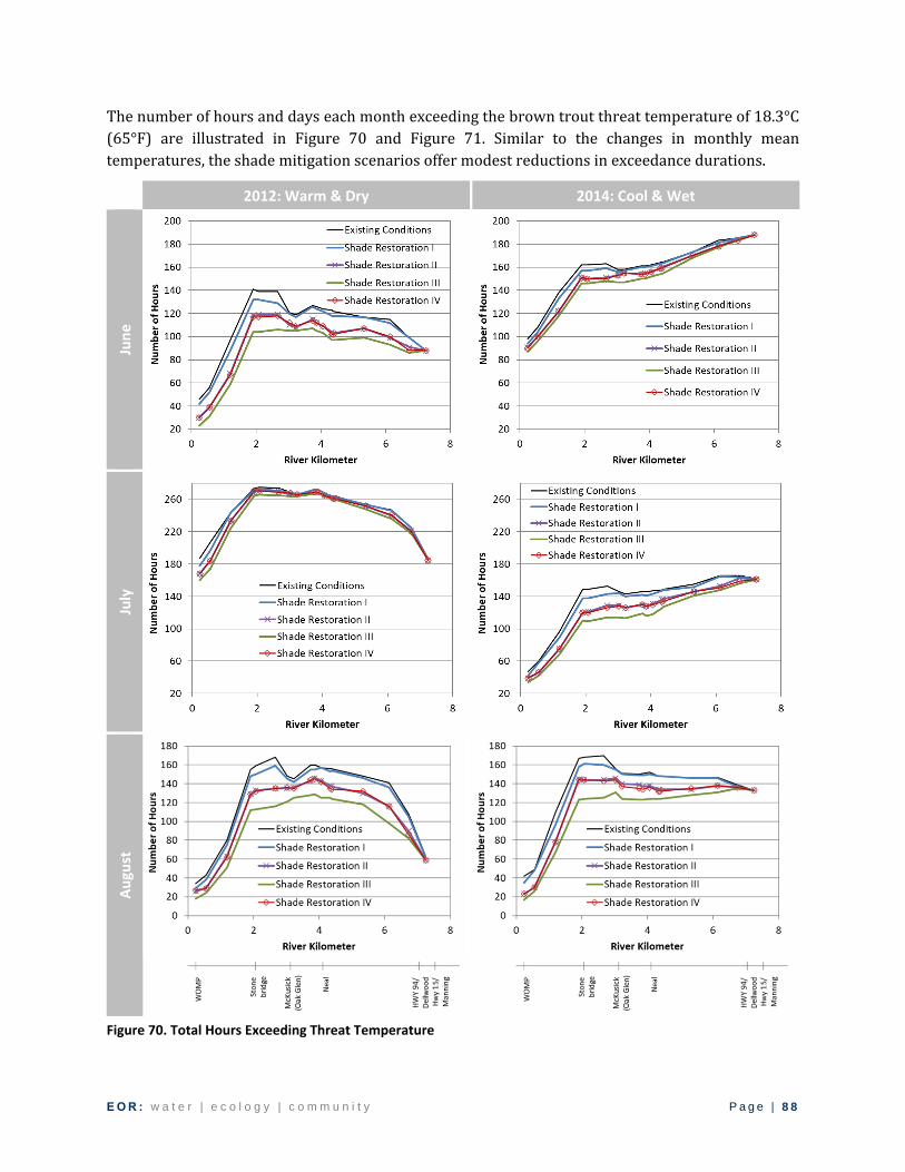
E O R : w a t e r | e c o l o g y | c o m m u n i t y P a g e | 8 8
The number of hours and days each month exceeding the brown trout threat temperature of 18.3°C
(65°F) are illustrated in Figure 70 and Figure 71. Similar to the changes in monthly mean
temperatures, the shade mitigation scenarios offer modest reductions in exceedance durations.
2012: Warm & Dry 2014: Cool & Wet
Jun
e
July
Au
gust
Figure 70. Total Hours Exceeding Threat Temperature

E O R : w a t e r | e c o l o g y | c o m m u n i t y P a g e | 8 9
2012: Warm & Dry 2014: Cool & Wet Ju
ne
July
Au
gust
Figure 71. Total Days with at Least 1 Hour Exceeding Threat Temperature
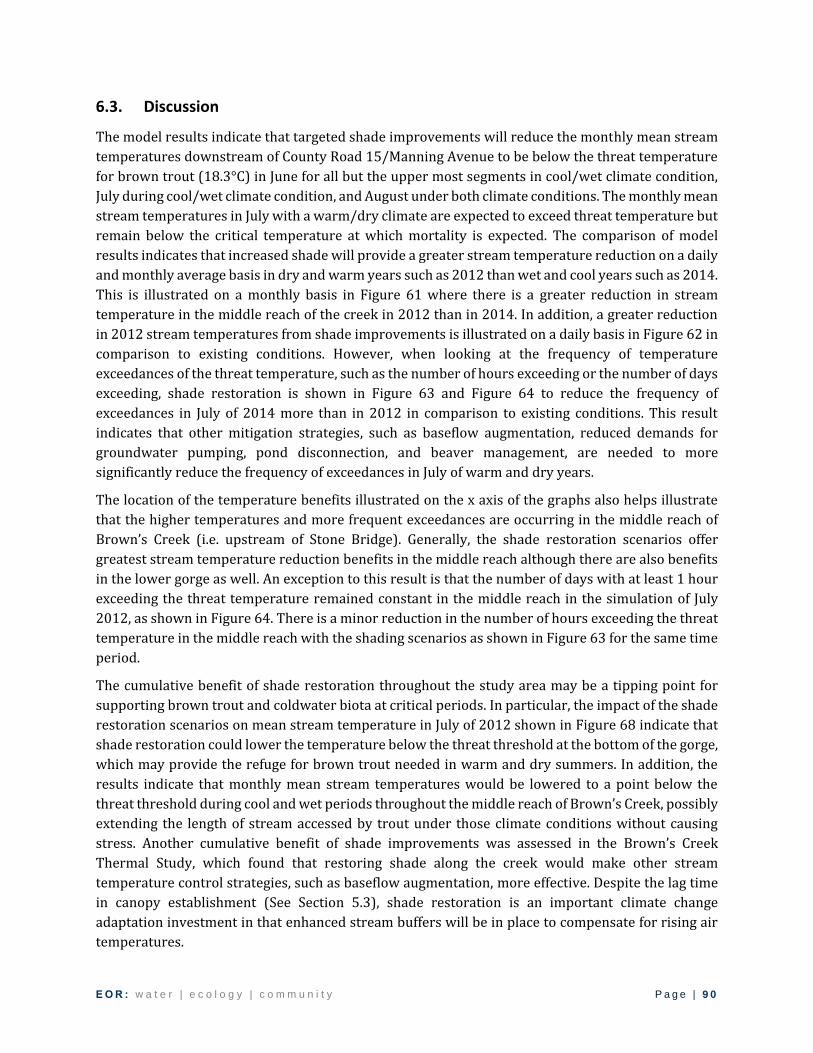
E O R : w a t e r | e c o l o g y | c o m m u n i t y P a g e | 9 0
6.3. Discussion
The model results indicate that targeted shade improvements will reduce the monthly mean stream
temperatures downstream of County Road 15/Manning Avenue to be below the threat temperature
for brown trout (18.3°C) in June for all but the upper most segments in cool/wet climate condition,
July during cool/wet climate condition, and August under both climate conditions. The monthly mean
stream temperatures in July with a warm/dry climate are expected to exceed threat temperature but
remain below the critical temperature at which mortality is expected. The comparison of model
results indicates that increased shade will provide a greater stream temperature reduction on a daily
and monthly average basis in dry and warm years such as 2012 than wet and cool years such as 2014.
This is illustrated on a monthly basis in Figure 61 where there is a greater reduction in stream
temperature in the middle reach of the creek in 2012 than in 2014. In addition, a greater reduction
in 2012 stream temperatures from shade improvements is illustrated on a daily basis in Figure 62 in
comparison to existing conditions. However, when looking at the frequency of temperature
exceedances of the threat temperature, such as the number of hours exceeding or the number of days
exceeding, shade restoration is shown in Figure 63 and Figure 64 to reduce the frequency of
exceedances in July of 2014 more than in 2012 in comparison to existing conditions. This result
indicates that other mitigation strategies, such as baseflow augmentation, reduced demands for
groundwater pumping, pond disconnection, and beaver management, are needed to more
significantly reduce the frequency of exceedances in July of warm and dry years.
The location of the temperature benefits illustrated on the x axis of the graphs also helps illustrate
that the higher temperatures and more frequent exceedances are occurring in the middle reach of
Brown’s Creek (i.e. upstream of Stone Bridge). Generally, the shade restoration scenarios offer
greatest stream temperature reduction benefits in the middle reach although there are also benefits
in the lower gorge as well. An exception to this result is that the number of days with at least 1 hour
exceeding the threat temperature remained constant in the middle reach in the simulation of July
2012, as shown in Figure 64. There is a minor reduction in the number of hours exceeding the threat
temperature in the middle reach with the shading scenarios as shown in Figure 63 for the same time
period.
The cumulative benefit of shade restoration throughout the study area may be a tipping point for
supporting brown trout and coldwater biota at critical periods. In particular, the impact of the shade
restoration scenarios on mean stream temperature in July of 2012 shown in Figure 68 indicate that
shade restoration could lower the temperature below the threat threshold at the bottom of the gorge,
which may provide the refuge for brown trout needed in warm and dry summers. In addition, the
results indicate that monthly mean stream temperatures would be lowered to a point below the
threat threshold during cool and wet periods throughout the middle reach of Brown’s Creek, possibly
extending the length of stream accessed by trout under those climate conditions without causing
stress. Another cumulative benefit of shade improvements was assessed in the Brown’s Creek
Thermal Study, which found that restoring shade along the creek would make other stream
temperature control strategies, such as baseflow augmentation, more effective. Despite the lag time
in canopy establishment (See Section 5.3), shade restoration is an important climate change
adaptation investment in that enhanced stream buffers will be in place to compensate for rising air
temperatures.

E O R : w a t e r | e c o l o g y | c o m m u n i t y P a g e | 9 1
The Brown’s Creek Thermal Study estimated the stream temperature reduction benefits of shade
restoration to be on the order of 0.5 to 1.1°C for monthly mean temperature. However, the updated
scenarios in this study indicate that targeted shade restoration (Scenario IV) will provide benefits on
the order of 0.16 to 0.52°C. This difference in benefits is primarily due to the limitations of LiDAR
data analysis in estimating the existing shade. As detailed in Section 5, the riparian shade analysis in
this study used more detailed field-based data (hemispherical photography) which found existing
shade to be greater than what was estimated using LiDAR data, which was the best available data at
the time of the Brown’s Creek Thermal Study. By underestimating existing shade, the LiDAR data
analysis indicated that there were more unshaded areas along Brown’s Creek than identified in this
study while also indicating that increasing shade would offer a greater benefit in comparison to
existing conditions than found in this study if the same benchmark is used to classify a segment as
being “unshaded”. The difference in the extent and potential benefits of shade restoration is
illustrated when looking at Scenarios I and II. The Brown’s Creek Thermal Study assessed shade
restoration scenarios similar to Scenarios I and II in this study, which raise shade to a minimum of
50% and 75% across the entire model extents. In this Riparian Shading Study, a third level of
restoration was added in Scenario III up to a minimum of 85%. In the Brown’s Creek Thermal Study,
Scenario II resulted in a 20% increase in shade across the modeled reach whereas the similar
scenario in this study resulted in an 8% increase in shade. The new Scenario III in this study offers a
12% increase in shade across the model reach while the targeted Scenario IV offers an 8% increase.
By acquiring hemispherical photography equipment and analysis software, the District has a better
understanding of how much shade is currently provided along the creek and the potential benefit of
increasing shade. Since the benefits are lower than previously estimated, these results also indicate
the need to look at other mitigation methods to lower stream temperature.
In terms of reducing heat load to the stream, the shade restoration efforts overall would provide an
8% increase in shade over the growing season, which can also be looked at as an 8% reduction in
heat load to Brown’s Creek. The District’s Impaired Biota TMDL study identified the need for a 6%
reduction in heat load to the creek to lower stream temperatures below the threat temperature for
brown trout (18.3°C). The TMDL allocation was developed with monitoring data at the WOMP station
that included a few years of record before the Long Lake Diversion Structure was constructed. The
TMDL implementation plan identified the need for further monitoring post-diversion to update the
heat load duration curve analysis and refine our understanding of when temperature exceedances
occur. Overall, the BCWD’s modeling analyses since the TMDL Implementation Plan have indicated
that baseflow exceedances are more common than stormflow exceedances (Herb & Correll, 2016). In
addition, the creation of the TMDL allocations based at the WOMP station may underestimate the
heat load reduction necessary for temperature control upstream of the Brown’s Creek Gorge, where
temperature is more sensitive primarily due to lower topographic shade. As such, it is expected that
more than a 6% reduction in heat load is necessary to meet the threat temperature threshold in the
Middle Reach of Brown’s Creek. Additional mitigation efforts beyond increasing riparian shade will
need to focus on other contributions to high baseflow stream temperatures such as enhancing
groundwater contributions and removing beaver dams. Further assessments of the potential cooling
benefits offered by beaver management are needed to better understand the extent of potential
benefits and the tradeoffs involved, such as flooding, heating in a reservoir, enhanced recharge
throughout the floodplain, and overall ecosystem health.

E O R : w a t e r | e c o l o g y | c o m m u n i t y P a g e | 9 2
The results of the stream temperature model scenarios are also interesting to consider in relation to
the District’s ongoing biotic monitoring (See Section 3.8) in the Oak Glen Golf Course in particular.
The simulated stream temperatures exceed the threat and critical threshold temperatures under
existing and shade restoration scenarios in the golf course. However, finding evidence of natural
reproduction of brown trout after the restoration but before the tree canopy has fully established
shade suggests that restoration of the in-stream habitat structure (i.e. refugia) and overhanging
herbaceous vegetation can significantly improve the conditions supporting trout on a short time
frame. The 2012 restoration is also located between very well shaded areas of the creek and the fish
survey results may indicate that the restoration provided sufficient short-term improvements to
encourage fish passage between the well-shaded segments. Considering these assertions reinforces
the benefits of restoring in-stream habitat and quickly enhancing herbaceous vegetation beyond
what is indicated by the stream temperature model. As such, the thermal improvement projects
identified in the TMDL Implementation Plan and the District’s WMP beyond the four shade
restoration projects prioritized in this study are still expected to offer significant benefits to aquatic
life in Brown’s Creek. For example, Segment 8 is identified for morphological improvements in the
WMP and is situated between well-shaded segments, which is similar to the Oak Glen Golf Course.
Although Segment 8 was not identified as a high priority for shade restoration in this study, it was
estimated to have existing shade between 65 to 75% which could be improved by herbaceous and
woody vegetation enhancements as part of the morphological restoration.
The Brown’s Creek Thermal Study also assessed the potential cooling capabilities of other mitigation
strategies, such as baseflow augmentation and pond retrofits. The results indicated that increasing
riparian shade could enhance the benefits of these mitigation methods. In addition to providing
shading recommendations at specific locations in the study area, this Riparian Shading Study also
provides best practices in targeting shade enhancements which could be applied to enhancing
shading along surface drainage tributaries to Brown’s Creek and around ponds. More recently,
annual monitoring by the Washington Conservation District has found that warm water from
McKusick Wetland may be a significant heat load to Brown’s Creek. Further investigation of this and
other reservoirs may aid in addressing stream temperature issues in the creek.
Another take-away from the data analysis and application in the stream temperature model update
is that field data is needed to validate and refine shade estimated using LiDAR. In the Brown’s Creek
Thermal Study, shade was estimated using LiDAR and then was uniformly scaled to calibrate the
model to observed stream temperatures. The field-validation process in this Riparian Shading Study
developed a log-normal formula to correct shade estimated using LiDAR, which is a non-uniform
process. This process removed shade as a calibration parameter in this study and, as a result, other
parameters were tested to calibrate the model. The calibration required an increase in groundwater
temperature relative to what was modeled in the Brown’s Creek Thermal Study. The need for
increasing groundwater temperatures to calibrate the existing conditions scenario indicates that:
temperature of groundwater discharge to the stream was warmer on average than what
was indicated by the field measurements in 2012 and 2014,
groundwater contributions to the stream continues to play a critical role in determining
stream temperatures, and

E O R : w a t e r | e c o l o g y | c o m m u n i t y P a g e | 9 3
there may be other sources of heat loads during dry and warm years that were not
simulated in the model, such as beaver dams.
The Brown’s Creek Thermal Study also identified the need for further analysis of the impact of beaver
dams along Brown’s Creek. The questions around beaver dam impacts still stand after the Riparian
Shading Study per the above discussion. The model uses an average stream width for the modeled
extents of the creek and therefore does not include local channel features such as wide bends and
beaver ponds. While local stream widening over short distances is not expected to significantly
change stream temperature, beaver ponds can have a significant affect both on flow and temperature
downstream of the pond, and would make a worthwhile addition to the model in the future. Such
future studies would need to focus on specific dam locations and install monitoring equipment to
assess relevant variables (e.g. groundwater level, groundwater temperature, stream level, stream
temperature, etc.). A beaver dam analysis would not be able to rely on the District’s stream
temperature model scenarios of 2012 and 2014 since such beaver dam monitoring was not in place
during those years. Overall, further assessments of the potential cooling benefits offered by beaver
management are needed to better understand the extent of potential benefits and the tradeoffs
involved, such as flooding, heating in a reservoir, enhanced recharge throughout the floodplain, and
overall ecosystem health. Beaver activity has broad impacts and benefits to urban areas and riparian
ecosystems beyond stream temperature that need to be considered as well.
Stepping back from stream temperature analyses, it is also important to recognize the other benefits
offered by enhancing the plant communities in riparian buffers along Brown’s Creek. As discussed in
Appendix B, riparian buffers provide many benefits such as capturing pollutants in urban and rural
runoff before they reach the creek. Riparian buffers also provide habitat for terrestrial wildlife, such
as pollinators, and are a critical corridor in which terrestrial invasive species need to be controlled
to sustain healthy biodiversity. Riparian buffers also provide climate change mitigation benefits
unique to urbanizing areas by mitigating heat island effect and sequestering carbon and filtering air
pollutants. The District’s continued investment in protecting and restoring riparian buffers will yield
stream temperature benefits in addition to many others along the riparian corridor.

E O R : w a t e r | e c o l o g y | c o m m u n i t y P a g e | 9 4
7. RECOMMENDATIONS
Shade Restoration Projects
The recommendations of this study related to riparian shade include implementing the four targeted
shade restoration projects, incorporating shade restoration best practices into the District’s other
activities, and monitoring progress towards shade targets.
Improvements to these and other segments for thermal benefits were included in the TMDL
Implementation Plan and BCWD WMP (Brown’s Creek Management Plan) with preliminary cost
estimates. The concept plans for the targeted shade restoration projects in Segments 10B, 11, 12, and
13 are provided in Figure 56 to Figure 59. These plans and the detailed cost estimates were used to
develop a recommended Thermal Improvement Implementation Plan for stream and shade
restoration projects. The implementation plan schedule and costs are detailed in Table 16.
Implementing the targeted shade restoration projects as early as possible is recommended due to
the lag time in establishing full shade benefits for these high-priority locations. As such, the four
shade restoration projects are recommended for implementation before other thermal improvement
activities. No projects are recommended for implementation in 2017 and 2018 to provide sufficient
time for gathering funding for the first high-priority shade implementation project in 2019 following
this study. The other three shade restoration projects are recommended for implementation in 2020,
2021, and 2022. Segments 12 and 13 are recommended to be implemented last of the four targeted
shade restoration projects because it is expected that additional time is needed to attain funding and
gain landowner support than the other two projects. The remaining thermal improvements planned
in the WMP and TMDL Implementation Plan are included in the recommended schedule between
2023 to 2026.
Thermal improvement projects are a high priority in the 10 year period of the District’s WMP and the
TMDL Implementation Plan. The WMP included estimated implementation costs for improvements
to morphology, vegetation composition, and buffer width as assessed in the TMDL Implementation
Plan in 2012. The implementation costs for the high priority shade restoration projects in Segments
10B, 11, 12, and 13 were updated to include the engineering design, administration, two years of
maintenance, and contingency.
Remaining funds from the Riparian Shading Study are recommended for use in engaging
stakeholders of the high priority shade restoration projects and beginning the design of the first
improvement project in Segment 11. Additional funding opportunities are expected to become
available in 2018 to further assist in accelerating the implementation of these projects.

E O R : w a t e r | e c o l o g y | c o m m u n i t y P a g e | 9 5
Table 16. Thermal Improvement Implementation Plan (Updated from the BCWD WMP’s Brown's Creek Management Plan)
Thermal Improvement Implementation Activities ** Segment
ID* Estimated
Cost 2017 2018 2019 2020 2021 2022 2023 2024 2025 2026
1,306 feet on City of Stillwater /Millbrook Development 11 $91,922 √
450 feet on Brown’s Creek Cove/Millbrook Development 9 $10,000 √
325 ft upstream of county Road 5 *** 3 $3,000 √
3,200 feet adjacent to Millbrook Develop./Holland Property 10B $162,720 √
1,800 feet on Oak Glen LLC and State of MNDNR 6 $15,000 √
653 feet on Schubert properties 4 $15,000 √
653 feet on City of Stillwater Property (Brown’s Creek Park) 8 $94,000 √
131 ft upstream of Wolf Marine *** 1 $3,000 √
392 ft upstream of Wolf Marine *** 2 $5,750 √
Approximately 1,000 feet on Grogan property 14 $13,000 √
950 feet upstream of Hwy 96 12 $175,274 √
1,045 ft on Costa Lorraine M Properties 13 $498,235 √
Total costs for activities to improve reaches of the creek categorized as having degraded stream channel geomorphology by addressing: lack of buffer, stream width, over-hanging banks, and profile and alignment
$1,086,901 -- -- $91,922 $162,720 $498,235 $175,274 $94,000 $13,000 $30,000 $21,750
* This refers to the proposed thermal improvement projects found in the TMDL Implementation Plan. * * Implementation activities identified in Brown’s Creek TMDL Implementation Plan (2012), Brown’s Creek Thermal Study (2016) and the BCWD WMP (2017). Changes in cost
estimates reflect inclusion of design, 2-year maintenance, permitting, and additional investigation costs.
*** Plantings done in last 5 years have not been evaluated for mortality/success in establishing. Additional tree and herbaceous enhancements may still be required for shade
benefits.
√ Recommended Schedule for Implementation

E O R : w a t e r | e c o l o g y | c o m m u n i t y P a g e | 9 6
Shade Restoration Activities and Programs
Beyond the specific projects, it is also recommended that shade restoration be incorporated into
other District activities and programs as follows:
1. Invasive Plant Management:
Include herbaceous plantings to enhance understory cover, increase herbaceous canopy
height, and minimize exposed banks following the removal of invasive woody and grassy
species within 5 m of the stream bank.
2. Guidance on Best Practices for Increased Shade:
The District should develop guidance on best practices for increasing shade while limiting the
potential detrimental erosion impacts of dense tree canopy cover.
3. Management Plans for Plant Communities:
Develop management plans for plant communities adjacent to Brown’s Creek to enhance and
protect the biodiversity and values of these unique communities. Management goals should
focus on improved native vegetation communities, increased riparian shading through
strategic vegetation design, and increased habitat diversity. The sedge meadow south of the
Highway 96 crossing of Brown’s Creek (adjacent to Segment 11 in this study) and the Maple
Basswood Forest along the lower gorge reach of Brown’s Creek are examples of plant
communities for which Management Plans would be prepared. Management plans for the
Brown’s Creek riparian corridor should include:
a. Mapping of desired plant communities and outcomes,
b. Identification of seeding mixes and planting choices for specific areas,
c. Discussion of treatment and management options for invasive species and pests,
d. Outline of timeline and timing of management activities,
e. Breakdown of management activity costs,
f. Suggestions for evaluation methodology,
g. Identification of potential funding sources, and
h. Valuable management references.
Much of the Brown’s Creek riparian corridor and immediate watershed is comprised of
private land owners. In order to facilitate behavioral changes and improve vegetation
conditions, community assessment and engagement will be essential in the long term success
of these management plans. Possible community assessment tools include a landowner
survey and interviews with individual landowners to help identify what motivates behaviors
and what they value about the creek. Further steps could involve hands on activities designed
to educate corridor landowners about why riparian vegetation management is important,
how riparian vegetation can be designed in a variety of ways to merge with their personal
aesthetics, and what funding sources are available to them. In addition, actions could include
the creation of a native shoreline team consisting of landowners, in which members are
empowered with information and tools to help neighbors facilitate native vegetation
establishment and management. Forums, workshops, and other forms of public engagement
could also be initiated.

E O R : w a t e r | e c o l o g y | c o m m u n i t y P a g e | 9 7
Shade Monitoring and Maintenance
Continued use of the hemispherical photography equipment, modeling tools, and approaches applied
in this study is recommended as part of the District’s annual monitoring program to achieve the
following components to a long term successful shade restoration effort:
Assess shade before restoration using hemispherical photographs where projects go beyond
the representative reaches of this study.
Assess shade after restoration using hemispherical photographs collected at the same
locations as the pre-restoration monitoring. Continued monitoring of shade at the same
transects in Reach 7 as in this study will provide the data needed to assess the lag time
between plantings to reaching target shade levels.
A detailed plan for monitoring shade in Brown’s Creek watershed to meet the above objectives is
outlined in Appendix E. The cost estimates for the shade restoration projects include two years of
monitoring and maintenance of the herbaceous and tree plantings. Beyond that and monitoring for
mortality of tree plantings, this study and the monitoring recommendations in Appendix E do not
include any further guidance on evaluating the success of enhancing the plant communities adjacent
to the stream segments. It is assumed that such guidance and recommendations would be included
in Management Plans specific to each plant community.
In addition to monitoring shade at project locations, there is also the opportunity to identify and
restore shade at small sites. During other field work activities, staff should identify riparian areas
that have stunted grassy vegetation, emergent vegetation, exposed banks, or new sediment
accumulation. The district should allocate $2,600 in annual funding for maintenance of these small
sites, including erosion control blanket, planting plugs, and seeding during appropriate times of year
(e.g. late spring or summer when there are stable flows) to enhance grassy vegetation and shade.
This annual cost is estimated assuming small sites will total 5,000 square feet of improvements.
Disturbances such as grazing or burning will be needed to maintain riparian vegetation composition
and prevent succession to over-forested state.
Reducing Stream Temperatures and Restoring Aquatic Life
The stream temperature modeling scenarios indicate that the targeted shade restoration will reduce
monthly mean stream temperatures by 0.16 to 0.52°C but will have minimal impact on reducing the
number of hours and days exceeding the threat temperature in July during dry and warm years. This
result indicates that additional mitigation strategies are still necessary to support coldwater biota in
the middle and gorge reaches of Brown’s Creek. Other stream temperature control strategies include
baseflow augmentation, stormflow management, and mitigating beaver dam impacts. Baseflow is
sustained in Brown’s Creek by groundwater contributions which could be enhanced by reducing
groundwater withdrawals and increasing infiltration in the groundwatershed. Depending on the
practice, the latter could also help reduce warm stormflows to the creek. Infiltration might also be
enhanced by disconnecting anthropogenic drainage pathways, such as the ditched wetland north of
Segment 13 or retrofitting the ponds in Oak Glen Golf Course which are directly connected to Brown’s
Creek. The Brown’s Creek Thermal Study found that such retrofits would become more effective once
shade is restored along the creek. Beaver ponds can have a significant affect both on flow and
E O R : w a t e r | e c o l o g y | c o m m u n i t y P a g e | 9 8
temperature downstream of the pond, and would make a worthwhile addition to the model in the
future. The need to further assess these strategies and continue implementation is also underscored
by the fact that the creek’s temperature will need to be protected from the impacts of climate change
both directly on water temperature and indirectly through modifications to the water balance.
Further assessment of the potential cooling benefits offered by beaver management is needed along
with the potential tradeoffs involved, such as flooding, heating in a reservoir, enhanced recharge
throughout the floodplain, and the ecosystem health benefits of beaver activity.
The monitoring needs identified in the Brown’s Creek Thermal Study will provide the data needed to
address the above opportunities for investigation and stream temperature reduction:
“A broad array of monitoring data were used in this the project to calibrate and verify the
stream temperature model. Monitoring efforts should be continued in the future, to further
characterize baseflow sources and to enable trend analysis in stream flow and temperature.
1) In-stream flow and temperature monitoring should be continued at existing sites (WOMP,
Stonebridge, Highway 15/Manning) to build a long-term record and enable trend analysis of
flow rates and water temperatures.
2) Additional temperature monitoring at sites of interest, e.g. wetland and stormwater inputs
and beaver ponds. Wherever possible, temperature monitoring should be combined with
flow monitoring, to enable better estimates of thermal impact.
3) Groundwater and baseflow continues to be a data need for Brown’s Creek. The existing
gaging sites can provide long term records for trend analysis of baseflow, but the seasonal
and spatial variability of baseflow inputs is still not well characterized. Pairing piezometer
measurements with a means to measure the corresponding flow source rates would be an
effective method to characterize baseflow sources.
4) The BCWD climate station provided valuable information on local precipitation, air
temperature, and solar radiation in the watershed. Continued operation of this station in the
future will be helpful both for any additional modeling work, and for trend analysis of flow
and temperature.” (p. 30)
Stream temperature and flow monitoring conducted by the Washington Conservation District (WCD)
in addition to aquatic biota monitoring conducted by the District and MPCA provide the data needed
to assess the combined effectiveness of stream temperature mitigation implementation activities on
restoring aquatic life in Brown’s Creek. In the WCD’s annual monitoring report, it is recommended
that the stream temperature and flow data be analyzed to identify under what flow conditions the
threshold temperatures are exceeded each year. This could be conducted by annually updating the
heat load duration curves previously developed for the TMDL study (Figure 72) to assess trends in
the timing and frequency of exceeding the threshold temperatures for fish stress and mortality at the
three long term WCD monitoring locations: the Manning, Stonebridge, and WOMP stations. Section
3.E of the District’s Impaired Biota TMDL study details the method used for developing the heat load
duration curve.

E O R : w a t e r | e c o l o g y | c o m m u n i t y P a g e | 9 9
Figure 72. Heat Load Duration Curve 2000-2007 WOMP Station (Emmons & Olivier Resources, 2010)
As the District continues to collaborate with stakeholders on projects and programs to assist in
establishing a self-sustaining brown trout population, it is also recommended that a coordinated
approach be implemented to marking stocked and surveyed fish. This will assist all stakeholders in
evaluating the success of implementation activities and the need for ongoing stocking moving
forward.
Broader Implications
The water quality benefits of riparian vegetation recently led to state-wide legislation requiring
riparian buffers across Minnesota. Minnesota’s buffer law requires buffer restoration along
90,000 miles of public waters and ditches within the next two years. State agencies and local soil and
water conservation districts are developing and distributing guidance to farmers to aid in successful
compliance, although the enforcement of the new legislation is understandably contentious in
agricultural areas. Shade provided by herbaceous vegetation and the resulting benefits to reducing
the temperature of small streams and tributaries is yet another reason to protect and enhance
riparian buffers across the state. State buffer guidance should consider the results and
recommendations of this study to betted reflect these benefits.
In addition, the District should reach out to other watershed management organizations of coldwater
systems to share the results of this study and share the equipment and software acquired for this
study. Doing so will help answer similar questions in other watersheds and will assist in assessing
how transferrable the findings of the studies are in different settings.
In conducting this applied research study and continuing to monitor shade following the
implementation of projects, the District is also in a position to advance the dialogue by publishing
and presenting their findings in journals and at regional conferences, especially those focused on the
management of coldwater fisheries and other surface water-groundwater dependent natural
resources.

E O R : w a t e r | e c o l o g y | c o m m u n i t y P a g e | 1 0 0
8. LITERATURE CITED
Allen, A., & Chapman, D. (2001). Impacts of afforestation on groundwater resources and quality. Hydrogeology Journal, 9(4), 390–400. https://doi.org/10.1007/s100400100148
Almendinger, J. C. (1996). Minnesota’s Bearing Tree Database. St. Paul, MN.
Annear, R. L., Berger, C. J., & Wells, S. A. (2001). CE-QUAL-W2 Version 3.1 Shading Algorithm. Portland, Oregon.
Archibold, O. W., & Ripley, E. A. (2004). Assessment of seasonal change in a young aspen (Populus tremuloides Michx.) canopy using digital imagery. Applied Geography, 24(1), 77–95. https://doi.org/10.1016/j.apgeog.2003.11.001
Armstrong, A., & Stedman, R. C. (2012). Landowner willingness to implement riparian buffers in a transitioning watershed. Landscape and Urban Planning, 105(3), 211–220. https://doi.org/10.1016/j.landurbplan.2011.12.011
Barilotti, A., Sepic, F., Abramo, E., Crosilla, F., & Growing, R. (2007). Improving the morphological analysis for tree extraction: a dynamic approach to lidar data. Geographical, 26–31.
Bechtold, W. A., Mielke, M. E., & Zarnoch, S. J. (2002). Comparison of Field Methods and Models to Estimate Mean Crown Diameter. Northern Journal of Applied Forestry, 19(4), 177–182.
Beschta, R. L., & Platts, W. S. (1986). Morphological Features of Small Streams: Significance and Function. JAWRA Journal of the American Water Resources Association, 22(3), 369–379. https://doi.org/10.1111/j.1752-1688.1986.tb01891.x
Blann, K., Frost Nerbonne, J., & Vondracek, B. (2002). Relationship of Riparian Buffer Type to Water Temperature in the Driftless Area Ecoregion of Minnesota. North American Journal of Fisheries Management, 22(2), 441–451. https://doi.org/10.1577/1548-8675(2002)022<0441:RORBTT>2.0.CO;2
Bode, C. A., Limm, M. P., Power, M. E., & Finlay, J. C. (2014). Subcanopy Solar Radiation model: Predicting solar radiation across a heavily vegetated landscape using LiDAR and GIS solar radiation models. Remote Sensing of Environment, 154, 387–397. https://doi.org/10.1016/j.rse.2014.01.028
Boegh, E. V. A., Olsen, M., Conallin, J., & Holmes, E. (2009). Modelling the spatial variations of stream temperature and its impacts on habitat suitability in small lowland streams. Ecohydrology of Surface and Groundwater Dependent Systems: Concepts, Methods and Recent Developments. IAHS Publ. 328, 34–41.
Bonnor, G. (1967). Estimation of ground canopy density from ground measurements. Journal of Forestry, 544–547.
Boulton, A. J., Findlay, S., Marmonier, P., Stanley, E. H., & Valett, H. M. (1998a). the Functional Significance of the Hyporheic Zone in Streams and Rivers. New York, 59–81. https://doi.org/10.1146/annurev.ecolsys.29.1.59
Boulton, A. J., Findlay, S., Marmonier, P., Stanley, E. H., & Valett, H. M. (1998b). The Functional Significance of the Hyporheic Zone in Streams and Rivers. New York, 59–81.

E O R : w a t e r | e c o l o g y | c o m m u n i t y P a g e | 1 0 1
https://doi.org/10.1146/annurev.ecolsys.29.1.59
Bour, H., El Merabet, Y., Ruichek, Y., Messoussi, R., & Benmiloud, I. (2017). An Efficient Sky Detection Algorithm From Fisheye Image Based on region classification and segment analysis. Transactions on Machine Learning and Artificial Intelligence, 5(4). https://doi.org/10.14738/tmlai.54.3335
Bren, L. J. (1998). The geometry of a constant buffer-loading design method for humid watersheds. Forest Ecology and Management, 110(1–3), 113–125. https://doi.org/10.1016/S0378-1127(98)00275-8
Brown, A. E., Zhang, L., McMahon, T. A., Western, A. W., & Vertessy, R. A. (2005). A review of paired catchment studies for determining changes in water yield resulting from alterations in vegetation. Journal of Hydrology, 310(1–4), 28–61. https://doi.org/10.1016/j.jhydrol.2004.12.010
Burkart, M. R., James, D. E., & Tomer, M. D. (2004). Hydrologic and terrain variables to aid strategic location of riparian buffers. Journal of Soil and Water Conservation, 59(5), 216–223.
Carbonneau, P. E., & Piégay, H. (2012). Fluvial Remote Sensing for Science and Management. Fluvial Remote Sensing for Science and Management. Chichester, West Sussex, UK: John Wiley & Sons. https://doi.org/10.1002/9781119940791
Chen, Y. D., Carsel, R. F., McCutcheon, S. C., & Nutter, W. L. (1998). Stream temperature simulation of forested riparian areas: I. Watershed-scale model development. Journal of Environmental Engineering, 124(4), 304–315.
Chirhart, J. (2014). Development of a Fish-Based Index of Biological Integrity for Minnesota’s Rivers and Streams. Saint Paul, MN.
Constantz, J. (1998). Interaction between stream temperature, streamflow, and groundwater exchanges in alpine streams. Water Resources Research, 34(7), 1609. https://doi.org/10.1029/98WR00998
Constantz, J. (2010). Heat as a tracer to determine streambed water exchanges. Water Resources Research, 46(4), 1–20. https://doi.org/10.1029/2008WR006996
Coroi, M., Skeffington, M. S., Giller, P., Gormally, M., & O’Donovan, G. (2007). Using GIS in the Mapping and Analysis of Landscape and Vegetation Patterns Along Streams in Southern Ireland. Biology & Environment: Proceedings of the Royal Irish Academy, 106(3), 287–300. Retrieved from http://www.jstor.org/stable/20728601%5Cnfile:///Users/biogis5/Box Sync/Papers Library/Files/03/03AB074C-2088-4279-8E96-9F5D4F96A9A9.pdf%5Cnpapers3://publication/doi/10.3318/BIOE.2006.106.3.287
Cramer, M. L. (2012). Stream Habitat Restoration Guidelines. Olympia, Washington.
Daubenmire, R. F. (1959). A canopy-cover method of vegetation analysis. Northwest Science, 33, 43–46.
Davies-Colley, R. J. (1997). Stream channels are narrower in pasture than in forest. New Zealand Journal of Marine and Freshwater Research, 31(5), 599–608. https://doi.org/10.1080/00288330.1997.9516792

E O R : w a t e r | e c o l o g y | c o m m u n i t y P a g e | 1 0 2
Davies-Colley, R. J., & Payne, G. W. (1998). Measuring Stream Shade. Journal of the North American Benthological Society, 17(2), 250–260. https://doi.org/10.2307/1467966
Davies-Colley, R. J., & Rutherford, J. C. (2005). Some approaches for measuring and modelling riparian shade. Ecological Engineering, 24(5 SPEC. ISS.), 525–530. https://doi.org/10.1016/j.ecoleng.2004.01.006
Deas, M. L., & Lowney, C. L. (2000). Water Temperature Modeling Review. California Water Modeling Forum.
Dent, L., Mulvey, M., Ades, D., Thom, B., Clinton, J., Godwin, D., … Pettit, G. (2000). Stream Shade and Canopy Cover Monitoring Methods. Water Quality Monitoring Technical Guidebook.
DeWalle, D. R. (2008). Guidelines for riparian vegetative shade restoration based upon a theoretical shaded-stream model. Journal of the American Water Resources Association, 44(6), 1373–1387. https://doi.org/10.1111/j.1752-1688.2008.00230.x
DeWalle, D. R. (2010). Modeling stream shade: Riparian buffer height and density as important as buffer width. Journal of the American Water Resources Association, 46(2), 323–333. https://doi.org/10.1111/j.1752-1688.2010.00423.x
Emmons & Olivier Resources. (2001). Benefits of wetland buffers: a study of functions, values and size.
Emmons & Olivier Resources. (2007a). Statement of Need and Reasonableness.
Emmons & Olivier Resources. (2007b). Third Generation Watershed Management Plan. Retrieved from https://www.pca.state.mn.us/sites/default/files/tmdl-brownscreek-map.pdf
Emmons & Olivier Resources. (2008). Brown’s Creek Stream Classification.
Emmons & Olivier Resources. (2010). Brown’s Creek Impaired Biota TMDL.
Emmons & Olivier Resources. (2012). Brown’s Creek TMDL Implementation Plan.
Emmons & Olivier Resources. (2015). In-Stream Piezometer Study Results.
Emmons & Olivier Resources. (2016). Brown’s Creek Watershed District 2015 Trend Analysis.
Emmons & Olivier Resources. (2017). Brown’s Creek Watershed District 2017-2026 Watershed Management Plan.
Emmons & Olivier Resources, & Barr Engineering. (2016). Watershed Management Plan 2011-2021. Minneapolis, MN. Retrieved from http://www.metrovancouver.org/services/water/WaterPublications/2002_Watershed_Management_Plan.pdf
Fausch, K., Torgersen, C., Baxter, C., & Li, H. W. (2002). Landscapes to riverscapes: Bridging the gap between research and conservation of stream fishes. BioScience, 52(6), 483–498. https://doi.org/http://dx.doi.org/10.1043/0006-3568(2002)052(0483:LTRBTG)2.0.CO;2
Federal Water Pollution Control Act. (1972). 33 United States Congress. Retrieved from https://www3.epa.gov/npdes/pubs/cwatxt.txt
Galatowitsch, S., Frelich, L., & Phillips-Mao, L. (2009). Regional climate change adaptation strategies

E O R : w a t e r | e c o l o g y | c o m m u n i t y P a g e | 1 0 3
for biodiversity conservation in a midcontinental region of North America. Biological Conservation, 142(10), 2012–2022. https://doi.org/10.1016/j.biocon.2009.03.030
Garner, G., Malcolm, I. A., Sadler, J. P., Millar, C. P., & Hannah, D. M. (2015). Inter-annual variability in the effects of riparian woodland on micro-climate, energy exchanges and water temperature of an upland Scottish stream. Hydrological Processes, 29(6), 1080–1095. https://doi.org/10.1002/hyp.10223
Gartner, W. C., Love, L. L., & Erkkila, D. (2002). Economic Impact and Social Benefits Study of Coldwater Angling in Minnesota. St. Paul, MN.
Glatthorn, J., & Beckschäfer, P. (2014). Standardizing the protocol for hemispherical photographs: Accuracy assessment of binarization algorithms. PLoS ONE, 9(11), 1–19. https://doi.org/10.1371/journal.pone.0111924
Greenberg, J. A., Hestir, E. L., Riano, D., Scheer, G. J., & Ustin, S. L. (2012). Using Lidar Data Analysis To Estimate Changes in Insolation Under. Journal of the American Water Resources Association, 95616(5), 1–10.
Hannah, D. M., Malcom, I. A., Soulsby, C., & Youngson, A. F. (2008). A comparison of forest and moorland stream microclimate, heat exchanges and thermal dynamics. Hydrological Processes, 22, 919–940. https://doi.org/10.1002/hyp.7003
Hardin, J. W., Leopold, D. J., & White, F. M. (2001). Textbook of Dendrology (9th ed.). Boston, MA: McGraw-Hill.
Herb, W., & Correll, C. (2016). Brown’s Creek Thermal Study.
Herunter, H. E., Macdonald, J. S., & MacIsaac, E. A. (2003). Influence of logging road right-of-way size on small stream water temperature and sediment infiltration in the interior of B.C. In E. MacIsaac (Ed.), Forestry Impacts on Fish Habitat in the Northern Interior of British Columbia: A Compendium of Research from the Stuart- Takla Fish-Forestry Interaction Study (Canadian T, pp. 129–143). Vancouver, British Columbia: Fisheries and Oceans Canada.
Hession, W. C., Pizzuto, J. E., Johnson, T. E., & Horwitz, R. J. (2003). Influence of bank vegetation on channel morphology in rural and urban watersheds. Geology, 31(2), 147–150. https://doi.org/10.1130/0091-7613(2003)031<0147:IOBVOC>2.0.CO;2
Hewlett, J. D., & Fortson, J. C. (1982). Stream Temperature Under an Inadequate Buffer Strip in the Southeast Piedmont. JAWRA Journal of the American Water Resources Association, 18(6), 983–988. https://doi.org/10.1111/j.1752-1688.1982.tb00105.x
Hollaus, M., Wagner, W., Eberhöfer, C., & Karel, W. (2006). Accuracy of large-scale canopy heights derived from LiDAR data under operational constraints in a complex alpine environment. ISPRS Journal of Photogrammetry and Remote Sensing, 60(5), 323–338. https://doi.org/10.1016/j.isprsjprs.2006.05.002
Hornbeck, J. W., Martin, C. W., & Eagar, C. (1997). Summary of water yield experiments at Hubbard Brook Experimental Forest, New Hampshire. Canadian Journal of Forest Research, 27(12), 2043–2052. https://doi.org/10.1139/x97-173
Hunt, R. L. (1979). Removal of woody streambank vegetation to improve trout habitat. Technical Bulletin 115. Madison, WI.

E O R : w a t e r | e c o l o g y | c o m m u n i t y P a g e | 1 0 4
Jackson, C. R., Leigh, D. S., Scarbrough, S. L., & Chamblee, J. F. (2015). Herbaceous Versus Forested Riparian Vegetation: Narrow and Simple Versus Wide, Woody and Diverse Stream Habitat. River Research and Applications, 31(7), 847–857. https://doi.org/10.1002/rra.2783
Jarčuška, B., Kucbel, S., & Jaloviar, P. (2010). Comparison of output results from two programmes for hemispherical image analysis: Gap light analyser and winscanopy. Journal of Forest Science, 56(4), 147–153.
Jennings, S. B., Brown, N. D., & Sheil, D. (1999). Assessing forest canopies and understorey illumination: canopy closure, canopy cover and other measures. Forestry, 72(1), 59–74. https://doi.org/10.1093/forestry/72.1.59
Johansen, K., Phinn, S., Dixon, I., Douglas, M., & Lowry, J. (2007). Comparison of image and rapid field assessments of riparian zone condition in Australian tropical savannas. Forest Ecology and Management, 240(1–3), 42–60. https://doi.org/10.1016/j.foreco.2006.12.015
Jones, R., Travers, C., Rodgers, C., Lazar, B., English, E., Lipton, J., … Martinich, J. (2013). Climate change impacts on freshwater recreational fishing in the United States. Mitigation and Adaptation Strategies for Global Change, 18(6), 731–758. https://doi.org/10.1007/s11027-012-9385-3
Julian, J. P., Stanley, E. H., & Doyle, M. W. (2008). Basin-scale consequences of agricultural land use on benthic light availability and primary production along a sixth-order temperate river. Ecosystems, 11(7), 1091–1105. https://doi.org/10.1007/s10021-008-9181-9
Kelley, C. E., & Krueger, W. C. (2005). Canopy cover and shade determinations in Riparian zones. Journal of the American Water Resources Association, 41(1), 37–46. https://doi.org/10.1111/j.1752-1688.2005.tb03715.x
Korhonen, L., Korhonen, K. T., Rautiainen, M., & Stenberg, P. (2006). Estimation of forest canopy cover: A comparison of field measurement techniques. Silva Fennica, 40(4), 577–588. https://doi.org/citeulike-article-id:7886289
Lallaman, J. (2017). Fish Community Survey of Brown Creek Washington County, MN.
Lantz, R. L. (1971). Guidelines for Stream Protection in Logging Operations. Portland, Oregon: Oregon State Game Commission. Retrieved from http://archive.org/details/guidelinesforstr14lant
Levia, D. F., Carlyle-Moses, D., & Tanaka, T. (2011). Forest Hydrology and Biogeochemistry: Synthesis of Past Research and Future Directions. Ecological Studies. Springer. https://doi.org/10.1007/978-94-007-1363-5
Li, G., Jackson, C. R., & Kraseski, K. A. (2012). Modeled riparian stream shading: Agreement with field measurements and sensitivity to riparian conditions. Journal of Hydrology, 428–429, 142–151. https://doi.org/10.1016/j.jhydrol.2012.01.032
Link, T. E., Marks, D., & Hardy, J. P. (2004). A deterministic method to characterize canopy radiative transfer properties. Hydrological Processes, 18(18), 3583–3594. https://doi.org/10.1002/hyp.5793
Lisein, J., Pierrot-Deseilligny, M., Bonnet, S., & Lejeune, P. (2013). A photogrammetric workflow for the creation of a forest canopy height model from small unmanned aerial system imagery. Forests, 4(4), 922–944. https://doi.org/10.3390/f4040922

E O R : w a t e r | e c o l o g y | c o m m u n i t y P a g e | 1 0 5
Lyons, J., Stewart, J. S., & Mitro, M. (2010). Predicted effects of climate warming on the distribution of 50 stream fishes in Wisconsin, U.S.A. Journal of Fish Biology, 77(8), 1867–1898. https://doi.org/10.1111/j.1095-8649.2010.02763.x
Lyons, J., Thimble, S. W., & Paine, L. K. (2000). Grass Versus Trees: Managing Riparian Areas to Benefit Streams of Central North America. Journal of the American Water Resources Association, 36(4), 919–930. https://doi.org/10.1111/j.1752-1688.2000.tb04317.x
Lyons, J., Thimble, S. W., & Paine, L. K. (2000). Grass Versus Trees: Managing Riparian Areas to Benefit Streams of Central North America. Journal of the American Water Resources Association, 36(4), 919–930. https://doi.org/10.1111/j.1752-1688.2000.tb04317.x
Lyons, J., Weigel, B. M., Paine, L. K., & Undersander, D. J. (2000). Influence of Intensive Rotational Grazing on Bank Erosion, Fish Habitat Quality, and Fish Communities in Southwestern Wisconsin Trout Streams. Journal of Soil and Water Conservation, 55(3), 271–276.
Marshall, D. W., Fayram, A. H., Panuska, J. C., Baumann, J., & Hennessy, J. (2008). Positive effects of agricultural land use changes on coldwater fish communities in southwest Wisconsin streams. North American Journal of Fisheries Management, 28(3), 944–953. https://doi.org/10.1577/m06-139.1
McBride, M., Hession, W. C., & Rizzo, D. M. (2008). Riparian reforestation and channel change: A case study of two small tributaries to Sleepers River, northeastern Vermont, USA. Geomorphology, 102(3–4), 445–459. https://doi.org/10.1016/j.geomorph.2008.05.008
McBride, M., Hession, W. C., Rizzo, D. M., & Thompson, D. M. (2007). The influence of riparian vegetation on near-bank turbulence: A flume experiment. Earth Surface Processes and Landforms, 32(13), 2019–2037. https://doi.org/10.1002/esp.1513
Mccullough, D. A. (1999). A Review and Synthesis of Effects of Alterations to the Water Temperature Regime on Freshwater Life Stages of Salmonids, with Special Reference to Chinook Salmon. Seattle, WA.
Mellina, E., Moore, R. D., Hinch, S. G., Macdonald, S., Pearson, G., Macdonald, J. S., & Pearson, G. (2002). Stream temperature responses to clearcut logging in British Columbia: the moderating influences of groundwater and headwater lakes. Canadian Journal of Fisheries and Aquatic Sciences, 59(12), 1886–1900. https://doi.org/10.1139/f02-158
Mertes, L. A. K. (2002). Remote sensing of riverine landscapes. Freshwater Biology, 47(4), 799–816. https://doi.org/10.1046/j.1365-2427.2002.00909.x
Minnesota Biological Survey. (2018). Prairie Extremely Rich Fen – Condition Ranking Guidelines.
Minnesota Department of Natural Resources. (n.d.). Managing , Restoring and Re-establishing Prairie and Savanna Communities, 13.
Minnesota Department of Natural Resources. (2017). LiDAR Elevation, Twin Cities Metro Region, Minnesota, 2011. Retrieved March 6, 2018, from ftp://ftp.gisdata.mn.gov/pub/gdrs/data/pub/us_mn_state_mngeo/elev_lidar_metro2011/metadata/metadata.html
Minshall, G. W., Robinson, C. T., & Lawrence, D. E. (1997). Postfire responses of lotic ecosystems in Yellowstone National Park, U.S.A. Canadian Journal of Fisheries and Aquatic Sciences, 54(1),

E O R : w a t e r | e c o l o g y | c o m m u n i t y P a g e | 1 0 6
2509–2525. https://doi.org/10.1139/cjfas-54-11-2509
Mitro, M., Lyons, J., & Sharma, S. (2010). Coldwater Fish and Fisheries Working Group Report, (December).
MN DNR. (2017). St. Paul-Baldwin Plains and Moraines Subsection. Retrieved January 19, 2018, from http://www.dnr.state.mn.us/ecs/222Md/index.html
Moore, R. D., Spittlehouse, D. L., & Story, A. (2005). Riparian microclimate and stream temperature response to forest harvesting: A review. Journal Of The American Water Resources Association, 7(4), 813–834. https://doi.org/10.1111/j.1752-1688.2005.tb04465.x
Murgatroyd, A. L., & Ternan, J. L. (1983). The impact of afforestation on stream bank erosion and channel form. Earth Surface Processes and Landforms, 8(4), 357–369. https://doi.org/10.1002/esp.3290080408
Nerbonne, B. A., & Vondracek, B. (2001). Effects of local land use on physical habitat, benthic macroinvertebrates, and fish in the Whitewater River, Minnesota, USA. Environmental Management, 28(1), 87–99. https://doi.org/10.1007/s002670010209
Paletto, A., & Tosi, V. (2009). Forest canopy cover and canopy closure: Comparison of assessment techniques. European Journal of Forest Research, 128(3), 265–272. https://doi.org/10.1007/s10342-009-0262-x
Peterson, A. M. (1993). Effects of Electric Transmission Rights-of-Way on Trout in Forested Headwater Streams in New York. North American Journal of Fisheries Management, 13(3), 581–585. https://doi.org/10.1577/1548-8675(1993)013<0581:EOETRO>2.3.CO;2
Quigley, T. M. (1981). Estimating contribution of overstory vegetation to stream surface shade. Wildl. Soc. Bull, 9(1), 22–27. https://doi.org/10.2307/3782013?ref=no-x-route:594a415628b4c1ca799355b8cc331820
Read, J. S. (2016). An integrated assessment of lake and stream thermal habitat under climate change. Middleton, WI. Retrieved from https://www.sciencebase.gov/catalog/item/5a53d604e4b01e7be2308760
Regent Instruments Inc. (2015). Winscanopy Canopy Structure and Solar Radiation. Retrieved April 12, 2017, from http://regent.qc.ca/assets/winscanopy_about.html
Rich, P. M., Wood, J., Vieglais, D. A., Burek, K., & Webb, N. (1999). Hemiview User Manual. Retrieved from ftp://ftp.dynamax.com/manuals/HemiView_Manual.pdf
Ringold, P. L., Van Sickle, J., Rasar, K., & Schacher, J. (2003). Use of hemispheric imagery for estimating stream solar exposure. Journal of the American Water Resources Association, 39, 1373–1384. https://doi.org/10.1111/j.1752-1688.2003.tb04424.x
Rosgen, D. L. (1994). A classification of natural rivers. Catena, 22(3), 169–199. https://doi.org/10.1016/0341-8162(94)90001-9
Rufer, M. (2017). Brown’s Creek Macroinvertebrate Study.
Rutherford, J. C., Davies-Colley, R. J., Quinn, J. M., Stroud, M. J., & Cooper, A. B. (1997). Stream Shade: Towards a Restoration Strategy. NIWA Client Report: DOC303. Hamilton, New Zealand.

E O R : w a t e r | e c o l o g y | c o m m u n i t y P a g e | 1 0 7
Sappington, K., & Norton, S. B. (2010). Causal Analysis Diagnostic Decision Information System Volume 2: Sources, Stressors & Responses: Temperature. Retrieved February 17, 2017, from https://www3.epa.gov/caddis/ssr_temp_int.html
SolarPathinder. (2016). Instruction manual for the SolarPathfinder Unit. Linden, TN. Retrieved from https://www.solarpathfinder.com/pdf/pathfinder-manual.pdf
Sovell, L. A., Vondracek, B., Frost, J. A., & Mumford, K. G. (2000). Impacts of rotational grazing and riparian buffers on physicochemical and biological characteristics of Southeastern Minnesota, USA, streams. Environmental Management, 26(6), 629–641. https://doi.org/10.1007/s002670010121
Stott, T. (1997). A comparison of stream bank erosion processes on forested and moorland streams in the Balquhidder Catchments, central Scotland. Earth Surface Processes and Landforms, 22(4), 383–399. https://doi.org/10.1002/(SICI)1096-9837(199704)22:4<383::AID-ESP695>3.0.CO;2-4
Sweeney, B. W. (1992). Streamside forests and the physical, chemical, and trophic characteristics of Piedmont streams in eastern North America. Water Science and Technology, 25(11), 2653–2673.
Sweeney, B. W. (1993). Effects of streamside vegetation on macroinvertebrate communities of White Clay Creek in eastern North-America. Proceedings of the Academy of Natural Sciences of Philadelphia, 144, 291–340.
Sweeney, B. W., Bott, T. L., Jackson, J. K., Kaplan, L. a, Newbold, J. D., Standley, L. J., … Horwitz, R. J. (2004). Riparian deforestation, stream narrowing, and loss of stream ecosystem services. Proceedings of the National Academy of Sciences of the United States of America, 101(39), 14132–14137. https://doi.org/10.1073/pnas.0405895101
Sweeney, B. W., & Newbold, J. D. (2014). Streamside forest buffer width needed to protect stream water quality, habitat, and organisms: A literature review. Journal of the American Water Resources Association, 50(3), 560–584. https://doi.org/10.1111/jawr.12203
Theurer, F. D., Voos, K. A., & Miller, W. J. (1984). Instream water temperature model.
Trimble, S. W. (1993). The distributed sediment budget model and watershed management in the Paleozoic Plateau of the upper midwestern United States, 14(3), 285–303.
Trimble, S. W. (1997). Stream channel erosion and change resulting from riparian forests. Geology, 25(5), 467–469. https://doi.org/10.1130/0091-7613(1997)025<0467:SCEACR>2.3.CO;2
U.S. Environmental Protection Agency. (2017). National Summary of State Information. Retrieved May 7, 2017, from https://ofmpub.epa.gov/waters10/attains_nation_cy.control
Wang, L., Lyons, J., & Kanehl, P. (2003). Impacts of Urban Land Cover on Trout Streams in Wisconsin and Minnesota. Transactions of the American Fisheries Society, 132(5), 825–839. https://doi.org/10.1577/T02-099
Wang, L., Lyons, J., Kanehl, P., & Gatti, R. (1997). Influence of watershed land use on habitat quality and biotic integrity in Wisconsin streams. Fisheries, 22(6), 7–12. https://doi.org/10.1577/1548-8446(1997)022<0006
Washington Conservation District. (2016). 2016 Water Monitoring Report.

E O R : w a t e r | e c o l o g y | c o m m u n i t y P a g e | 1 0 8
Weatherley, N. S., & Ormerod, S. J. (1990). Forests and the temperature of upland streams in Wales: a modelling exploration of the biological effects. Freshwater Biology, 24(1), 109–122. https://doi.org/10.1111/j.1365-2427.1990.tb00312.x
Wehrly, K. E., Brenden, T. O., & Wang, L. (2009). A Comparison of Statistical Approaches for Predicting Stream Temperatures Across Heterogeneous Landscapes. JAWRA Journal of the American Water Resources Association, 45(4), 986–997. https://doi.org/10.1111/j.1752-1688.2009.00341.x
White, R. J., & Brynildson, O. M. (1967). Guidelines for Management of Trout Stream Habitat in Wisconsin. Madison, WI.
Zimmerman, R. C., Goodlett, J. C., & Comer, G. H. (1967). The Influence of Vegetation on Channel Form of Small Streams. In Symposium on River Morphology, Publication No. 75. International Association of Hydrological Sciences (pp. 255–275). Bern, Switzerland: International Association of Hydrological Sciences. Retrieved from http://www.telcom.uvm.edu/~pbierman/classes/gradsem/2005/papers/zimm1967.pdf

E O R : w a t e r | e c o l o g y | c o m m u n i t y P a g e | 1 0 9
APPENDIX A. LITERATURE REVIEW ON ESTIMATING RIPARIAN SHADE
The objective of this section is to review the literature on shade provided by grassy and woody
riparian vegetation to small streams of the North-Central United States. The best-suited instruments,
measures, and methods for further study on this topic are identified in addition to areas for further
research.
A.1. Introduction
Fish and macroinvertebrates found in coldwater streams support regionally significant recreational
uses and economic benefits. In Minnesota alone, coldwater angling provides an estimated annual
economic value of $148.7 million in direct sales, $90.35 million in income, and 3,300 jobs (Gartner,
Love, & Erkkila, 2002). However, rising water temperatures in coldwater streams currently threaten
the health and survival of coldwater biota. Almost 60% of the coldwater streams assessed for water
quality impairments across the U.S. are currently impaired, which means they are too polluted to
naturally support coldwater fisheries. The seventh most common cause of stream impairments
across the country is water temperature (U.S. Environmental Protection Agency, 2017). Beyond the
current threats and impairments, 62% of suitable habitat for coldwater fisheries is ultimately
projected to decline across the country by 2100 at the current rate of climate change. Lost coldwater
fisheries will be replaced by less valuable warm water and rough fisheries at an estimated cost of
$380 million to $1.5 billion in recreational fishing damages (Jones et al., 2013). Restoring and
sustaining naturally reproducing coldwater fisheries is of economic significance regionally and
nationally.
High water temperatures cause physiological stress, reduced growth, reduced reproductive success,
and increased mortality of coldwater biota. Stream temperature is influenced by the heat fluxes
depicted in Figure 73, such as incoming solar radiation, outgoing longwave radiation, evaporative
and conductive heat transfers, streambed conduction, and the temperature of flows entering the
stream.
Figure 73. Major Heat Flux Processes in a Stream (Interpretation of Moore et al., 2005) Note: Does not illustrate the friction generated by rapidly moving water over steep slopes (Moore, Spittlehouse, & Story, 2005)

E O R : w a t e r | e c o l o g y | c o m m u n i t y P a g e | 1 1 0
The first law of thermodynamics (conservation of energy) states that energy cannot be created nor
destroyed, only converted from one form to another (Equation 8-1). Applying the first law to stream
temperature defines an equation for net heat flux (Equation 8-2).
Change in heat storage = net heat flux = heat energy in – heat energy out Equation 8-1
𝑞𝑛𝑒𝑡 = 𝑞𝑠𝑤 + 𝑞𝑎𝑡𝑚 + 𝑞𝑏 + 𝑞𝑙 + 𝑞ℎ + 𝑞𝑔 + 𝑞𝑢𝑠 + 𝑞𝑑𝑠 + 𝑞𝑡𝑟𝑖𝑏 + 𝑞𝑟𝑢𝑛 + 𝑞ℎ𝑦𝑝 +
𝑞𝑔𝑤 Equation 8-2
where qsw is short-wave (solar) radiation, qatm is downwelling long-wave (atmospheric) radiation, qb
is upwelling long-wave (water surface) radiation, ql is latent heat flux, qh is sensible heat flux, qg is
conduction between the water and the bed, qus is the volume and temperature of incoming flows
upstream of the system boundary, qds is the volume and temperature of flows leaving the system, qtrib
and qrun are the respective volume and temperature of flows entering the stream from tributaries and
surface runoff, qhyp is the hyporheic exchange, and qgw is the volume and temperature of groundwater
flowing into the stream (Deas & Lowney, 2000). The water temperature rises when the net heat flux
(qnet) is positive.
Specific heat sources and human activities influencing heat fluxes into and out of coldwater streams
are illustrated in Figure 74. The branches of the flowchart illustrate the causal pathways from heat
sources and human activities that affect water temperature and, ultimately, impair biotic health.
Many of the causal changes occur as land is developed, harvested, or farmed. This is consistent with
the observed decline in ecosystem health and biodiversity of coldwater streams due to the effects of
urbanization and intensive agriculture (Wang, Lyons, & Kanehl, 2003; Wang, Lyons, Kanehl, & Gatti,
1997). Altering land cover in a watershed influences both the water and energy balance of the system
and, as a result, can increase stream temperatures directly and indirectly. For example, warm
discharge from industrial sites directly increases stream temperature whereas bank erosion
indirectly increases stream temperature by increasing the surface area exposed to solar radiation.
Impervious surfaces introduced to the landscape through urbanization reduce infiltration, reduce
groundwater discharge to streams, increase runoff, and increase temperature of runoff. Intensive
agriculture includes active farming or intensive grazing of stream corridors which typically results
in removal of the vegetative canopy shading the stream.
Climate change is also altering the overarching meteorological conditions that affect stream
temperature. Climate change impacts include modified air temperature, humidity, cloud cover,
precipitation quantity and intensity, vegetation composition and cover, growing season, and
groundwater temperatures. At a much smaller scale, microclimates can also develop above a stream
where meteorological parameters such as wind velocity are different from those above the riparian
vegetation canopy (Hewlett & Fortson, 1982; Weatherley & Ormerod, 1990).

E O R : w a t e r | e c o l o g y | c o m m u n i t y P a g e | 1 1 1
Figure 74. Detailed Diagram of Causal Pathways to Changing Water Temperature and Impaired Biota (Sappington & Norton, 2010)

E O R : w a t e r | e c o l o g y | c o m m u n i t y P a g e | 1 1 2
Strategies to limit thermal pollution of streams can be categorized as rainfall event controls and
baseflow controls. Event controls lower the temperature of stormwater runoff from warm,
impervious surfaces before discharging to the stream. Baseflow controls lower the temperature of
the stream during baseflow conditions which occur between rainfall events and are a critical period
of temperature stress for aquatic organisms (Herb & Correll, 2016). Stream baseflow temperature
can only be controlled by channel morphology, groundwater contributions, and riparian vegetation.
Channel morphology, such as overhanging banks, can shade the outer edges of the stream. Deep
channels and pools provide refugia for fish and macroinvertebrates on warm summer days.
Groundwater inputs (Mellina et al., 2002) and hyporheic exchange (Constantz, 1998, 2010) provide
cool inputs into the stream, the greatest of which occur in small headwater streams (Bren, 1998;
Burkart, James, & Tomer, 2004). Riparian vegetation limits the amount of radiation reaching the
stream surface by intercepting incoming solar and atmospheric radiation by either absorbing or
reflecting the incoming radiation. This mechanism is more simply referred to hereafter as shade.
Riparian vegetation also influences the microclimate immediately above the stream, such as air
temperature, humidity, and wind speed, which can also affect heat fluxes such as evaporation,
conduction, and long wave emission rates (Davies-Colley & Payne, 1998; Rutherford, Davies-Colley,
Quinn, Stroud, & Cooper, 1997). Since solar radiation is a dominant contributor to warming streams,
shade is one of the most important mechanisms for reducing thermal pollution (Dent et al., 2000).
The purpose of this review is to identify the best-suited methods for comparing shade provided by
grassy and woody riparian vegetation. We hypothesize that (1) shade is dependent upon the plant
morphology of riparian buffers but can be amplified or dampened by other site characteristics and
(2) grassy vegetation provides less shade than woody vegetation. This review focused on small
streams in North-Central America but studies from other regions were referenced where applicable.
The methods identified in this review will be applied in the BCWD Riparian Shading Study.
The focus of this review on riparian shade is not intended to diminish the importance of other stream
temperature controls, such as groundwater inflows, or the significance of other benefits provided by
riparian buffers. Instead, the focus is intended to justify the needs and methods for future quantified
analysis of shade variation based on vegetation type. Such studies will define the limits of riparian
shade management such that other stream temperature control strategies will be pursued where
shade alone is insufficient to meet target stream temperatures.
The review begins with background on studies of riparian shade impacts on stream temperature and
biotic health, in addition to outlining common terminology found in the literature. The review is then
organized into sections reviewing the methods for measuring and modeling shade, followed by the
future outlook for areas of further research. The best-suited methods for assessing both grassy and
woody riparian shading are identified in addition to ancillary diagnostic data needed to explain
variation in measured shade.
A.2. Background
Multiple sources testify to the benefits of forested buffers on stream temperature while also warning
that deforestation causes stream temperature increases of 2 to 5°C (Herunter, Macdonald, &
MacIsaac, 2003; Minshall, Robinson, & Lawrence, 1997). A diverging area in the literature is that
there are compelling indications that grassy vegetation improves the health of coldwater streams in

E O R : w a t e r | e c o l o g y | c o m m u n i t y P a g e | 1 1 3
comparison to woody vegetation, although the mechanisms remain unclear (Hunt, 1979; Marshall,
Fayram, Panuska, Baumann, & Hennessy, 2008).
The shade provided by grassy buffers is typically estimated or described in qualitative terms in the
literature. For example, multiple studies qualitatively noted that grassy buffers provided less shade
than forested buffers (Hunt, 1979; John Lyons, Thimble, & Paine, 2000; B. W. Sweeney, 1993). No
research in the Upper Midwest has rigorously measured shade in streams with grassy vegetation,
although some have estimated shade using models. Grassy riparian shade was estimated as an input
to multiple models developed to simulate stream temperature but field measurements were not
collected to calibrate and validate the estimated parameterization (Blann, Frost Nerbonne, &
Vondracek, 2002; Boegh, Olsen, Conallin, & Holmes, 2009; DeWalle, 2010). Beyond the geographic
area of this review, one study in Oregon measured canopy cover along a stream with riparian grasses,
sedges, forbs, and sparse willow trees. These meadow sites were found to have cover between 9 and
35% (Kelley & Krueger, 2005).
Other site factors influence how much shade is provided by the same vegetative canopy. For example,
Kelley and Krueger (2005) also found that streams with east-west orientation had greater shade than
north-south oriented streams. The difference was likely due to the declination of the sun and the
position of the vegetation. Stream azimuth is one of multiple site characteristics beyond vegetation
type that may dictate stream shade. Throughout the review, studies are identified that that assessed
the impacts of spatially and temporally variable physical characteristics, however these findings are
typically limited to sites with woody vegetation. Overall, the quantifiable difference in shade due to
plant morphology may be amplified or dampened by other characteristics but the extent of this
influence on shade in grassy streams is unclear based on current literature.
A.2.1. Terminology: Canopy Cover, Canopy Closure, and Shade
Understanding the differences between canopy cover, canopy closure, and shade are essential when
considering the literature regarding shade provided by different types of riparian vegetation.
Canopy cover and closure were included in this review because they are sometimes used as a
surrogate or predictor of shade. There is inconsistency in use of the term canopy cover in the
literature of forest management and ecological research. This review utilizes the forestry definition
of canopy cover as the percent of forest area occupied by the vertical projection of tree crowns
(Bonnor, 1967). An example of assessing canopy cover above a stream is illustrated in Figure 75(a).
In comparison, ecological research uses the same term canopy cover to refer to the relative amount
of sky hemisphere obscured above a given point, but this is more accurately referred to as canopy
closure (Jennings, Brown, & Sheil, 1999). Canopy closure is the projection of a hemisphere onto a
plane (Daubenmire, 1959) and is expressed as a percentage of non-visible sky within a certain zenith
angle (Korhonen, Korhonen, Rautiainen, & Stenberg, 2006). An example of assessing canopy closure
above a stream is illustrated in Figure 75(b). In the example shown, the full zenith angle of 180° is
being assessed. Although the example is shown from a cross-sectional perspective, canopy closure
may be assessed in all directions to look at the full hemisphere. In the illustrated examples, canopy
closure is approximately 67% whereas canopy cover is approximately 70%. The difference between
measurements varies based on the streamside vegetation and the zenith angle used in the canopy
closure measurement. In addition, closure may or may not include topography in addition to

E O R : w a t e r | e c o l o g y | c o m m u n i t y P a g e | 1 1 4
vegetative canopy closure. Another parameter referenced in the literature is openness, which is
simply one minus canopy closure. The terms canopy cover and closure are used distinctly hereafter
to clearly describe the methods and findings of past studies.
Figure 75. Canopy Cover (a) and Canopy Closure (b) Measured Across a Stream
Of these two somewhat analogous parameters, canopy closure is more common in ecologically
oriented research because it is a measure of canopy architecture that can better assist in estimating
the amount of solar radiation intercepted by the canopy than canopy cover. In comparison, canopy
cover only indicates how much radiation would reach the ground when the sun is directly above a
point on the ground. Both canopy cover and closure vary throughout the growing season due to
changes in plant height and leaf area. Neither parameter has diurnal variation since they are
independent from the position of the sun and the intensity of solar radiation.
In comparison, stream shade is the percentage of solar energy that is obscured or reflected by
vegetation or topography above a stream (Dent et al., 2000). Unlike canopy cover and closure, stream
shade varies throughout each day and season due to the position of the sun and intensity of solar
radiation. The orientation of a stream modifies the effectiveness of streamside vegetation in blocking
incoming solar radiation. For example, two trees on the east and west banks of a north-south channel
(Figure 76(a)) will provide limited shade due to the angle of the sun. In comparison, the same
vegetation on the south bank of an east-west channel would provide full shade while the north bank
vegetation would provide minimal shade benefit (Figure 76(b)). Grassy vegetation in both instances
would provide less shade unless the ratio of vegetation height to channel width was high enough for
grasses to provide similar shade levels.

E O R : w a t e r | e c o l o g y | c o m m u n i t y P a g e | 1 1 5
Figure 76. Midday Shading of Streams with North-South (a) and East-West (b) Orientations in Northern Hemisphere
A.3. Direct and Indirect Measurements
Indirect and direct measurements of shade are common in the literature, in addition to references to
the two other parameters previously described (canopy cover and closure). The instruments and
methods for directly and indirectly measuring canopy cover, canopy closure, and shade by air/space
and ground are reviewed in this section. Their applicability for comparing shade provided by grassy
and woody riparian vegetation is also assessed. This review did not include canopy growth models,
such as the crown diameter regression (Bechtold, Mielke, & Zarnoch, 2002) or the somewhat related
variables of leaf area index and biomass.
A.3.1. Air and Space-Borne Methods
Remote sensing was first linked to the fields of stream ecology and fluvial geomorphology in 2002
when technology improvements enabled identification of riverine systems at a hectametric or
kilometric scale (Fausch, Torgersen, Baxter, & Li, 2002; Mertes, 2002). Since then, the resolution of
data collected through this method has continued improving at a rapid pace. This section provides a
brief introduction to remote sensing from satellite and aircraft and outlines the applicability and
limitations of such methods in assessing canopy cover, canopy closure, and shade.
Remote sensing equipment includes both the platform (e.g. satellite, aircraft, or drone) and the
sensor which collects the data. Data in the USA is typically collected from conventional or unmanned
aircraft, not satellites, due to government regulations limiting satellite imagery resolution to 50 cm
(Carbonneau & Piégay, 2012). The sensors are used to collect optical imagery, light detection and
ranging (LiDAR) data which shows elevation, and other data, such as infrared.
The following four properties describe the resolution of a remote sensing data acquisition system:

E O R : w a t e r | e c o l o g y | c o m m u n i t y P a g e | 1 1 6
Spatial resolution: the ground footprint of a single image pixel or number of data points
collected on a unit area basis, which defines the size of the smallest object which can be
resolved on the ground;
Spectral resolution: the range of radiation wavelengths and the width of individual band,
which defines the ability to identify certain material, such as chlorophyll;
Temporal resolution: the elapsed time between repeated imagery, which defines how well
changes can be detected; and
Radiometric resolution (also referred to as bit depth): the amount of information devoted
to and stored with each pixel, which defines how fine differences in image brightness can be
refined (Carbonneau & Piégay, 2012).
Remote sensing imagery is used for the study and management of riparian vegetation to map
vegetation types, vegetation species, and historical changes, and to measure vegetation
characteristics. For example, remotely sensed data can be used to assess morphological features,
maximum stand age, and height of vegetation. Canopy density, canopy closure and shade can also be
assessed using LiDAR data in combination with Geographic Information System (GIS) analysis
methods. For example, a Light/Laser Penetration Index (LPI) can be determined by analysis of LiDAR
data (Barilotti, Sepic, Abramo, Crosilla, & Growing, 2007) and in turn can be used to estimate
openness (one minus canopy closure) although LPI results in high closure estimates in settings with
low and dense vegetation in comparison to other methods of estimating closure (Bode, Limm, Power,
& Finlay, 2014).
Several GIS analysis tools are available to simulate solar radiation above a canopy and the shadow
cast by vegetation on a ground or river surface. These tools have been developed to assist in light-
sensitive variables, such as plant growth, while they are also used for evaluating potential locations
for solar energy generation. First, a digital surface model (DSM) raster of the canopy is derived from
LiDAR (Greenberg, Hestir, Riano, Scheer, & Ustin, 2012; Hollaus, Wagner, Eberhöfer, & Karel, 2006)
or photogrammetry (Lisein, Pierrot-Deseilligny, Bonnet, & Lejeune, 2013). Second, GIS-based solar
radiation models are run to simulate the solar radiation reaching points or areas of interest, such as
segments along the surface of a stream. Examples of these tools include the ArcMap solar radiation
analysis tool and the GRASS GIS r.sun solar model. Each tool has various settings to modify aspects
of the analysis such as the duration of the simulation or the frequency at which to calculate total solar
radiation. The ArcMap tool conducts this analysis by determining if the stream is shaded for all sun
angles over the course of a day and integrates the total solar radiation reaching each point over the
analysis time period defined by the user. Both the ArcMap and GRASS models have limitations in that
they cannot simulate solar radiation that penetrates through the canopy either by small gaps or by
reflection off the vegetation. This limitation results in close to 100% shade estimates for cases where
vegetation completely overhangs across the stream surface. This limitation was successfully
accounted for using LPI in a study of a 17 m wide creek with both woody and grassy riparian
vegetation through development and application of the Subcanopy Solar Radiation (SSR) model
(Bode et al., 2014). While such tools can be applied at a regional or watershed scale using remotely
sensed datasets, multiple studies recommended extensive empirical data to assess broad spatial
variations (Julian, Stanley, & Doyle, 2008). LiDAR and other GIS datasets can also be useful in
estimating the physical parameters of topography and riparian vegetation adjacent to the stream in

E O R : w a t e r | e c o l o g y | c o m m u n i t y P a g e | 1 1 7
order to upscale or extrapolate estimated shade at specific points using ground-based methods
(Section A.3.3).
The spatial resolution of LiDAR data and the timing of data collection are other limitations to using
GIS-based solar radiation models for shade estimates. Spatial resolution is an important
consideration, especially for small reaches and vegetation structure where field measurements may
be more appropriate (Coroi, Skeffington, Giller, Gormally, & O’Donovan, 2007). An object must be
eight times larger than the pixel size to be detected by half of the pixels (i.e. 50% accuracy) or 16
times larger for 80% accuracy. When trying to capture vegetation, this means the resolution of
imagery needs to be less than 1 m for large trees or less than 10 cm for shrubs, and even smaller for
grasses (Carbonneau & Piégay, 2012). Users may begin to face computational power limitations
when beginning to use high resolution LiDAR datasets. Publically available LiDAR in Minnesota is
often collected after leaf-fall and so shade estimated using such LiDAR is typically underestimated
(Herb & Correll, 2016). The cost of collecting LiDAR in the summer and with the detail necessary for
assessing shade from grassy vegetation was estimated in 2017 to be approximately $13,500 for the
study area of the BCWD Riparian Shading Study. Field and remote measurements of riparian
characteristics (e.g. percent canopy cover, organic litter, canopy continuity, tree clearing, bank
stability, and flood damage) were compared and found field measurements to be more cost effective
at small scale between 1 to 200 km while remote image analysis was superior at large scale from 200
to 2000 km (Johansen, Phinn, Dixon, Douglas, & Lowry, 2007).
Overall, the benefits of remote sensing and GIS science advancements to riparian management
include the capability of repeated, synoptic data collection and the measurement of numerous
biophysical parameters. However, the objective and scale of the application must be considered to
determine if field measurements are more cost-effective than remote sensing methods. Remote
sensing technology could be used for other helpful information, such as mapping the location of
specific types of vegetation; however, such analysis is not pursued further in this study. The
applicability of remotely sensed data for assessing stream shade is expected to continue to change as
the technology for collecting, processing, and analyzing the data continues to quickly improve and
become more cost-effective.
A.3.2. Ground-Based Methods
There are indirect and direct ground-based methods for measuring shade. The only way to directly
measure shade is to measure solar radiation above and below the canopy for the same monitoring
period. Multiple instruments are available for indirectly estimating canopy cover, canopy closure,
and shade from the ground, including the densiometer, the clinometer, the solar pathfinder, and
hemispherical photography (Table 17). This section reviews indirect and direct methods organized
by each type of equipment. Visual estimation was not included because of its low accuracy.
Clinometer
A clinometer is commonly used by foresters to estimate the height of trees or the grade of a slope. As
illustrated in Figure 77, a clinometer can also be used to measure the angle from the horizon (dashed
line) to the open sky above topographic formations or riparian vegetation. From these
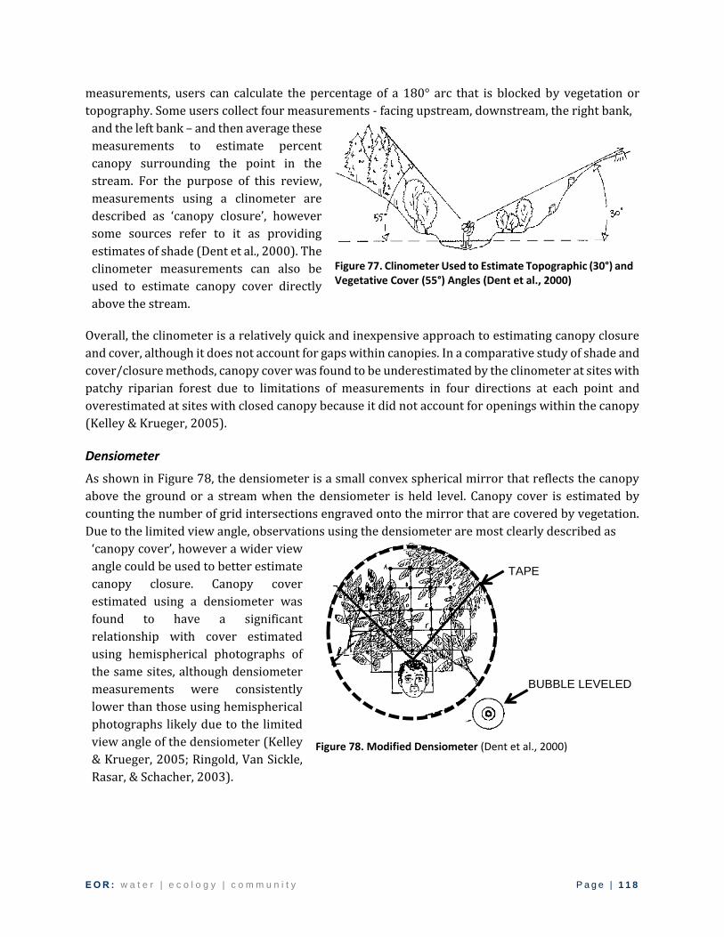
E O R : w a t e r | e c o l o g y | c o m m u n i t y P a g e | 1 1 8
measurements, users can calculate the percentage of a 180° arc that is blocked by vegetation or
topography. Some users collect four measurements - facing upstream, downstream, the right bank,
and the left bank – and then average these
measurements to estimate percent
canopy surrounding the point in the
stream. For the purpose of this review,
measurements using a clinometer are
described as ‘canopy closure’, however
some sources refer to it as providing
estimates of shade (Dent et al., 2000). The
clinometer measurements can also be
used to estimate canopy cover directly
above the stream.
Figure 77. Clinometer Used to Estimate Topographic (30°) and Vegetative Cover (55°) Angles (Dent et al., 2000)
Overall, the clinometer is a relatively quick and inexpensive approach to estimating canopy closure
and cover, although it does not account for gaps within canopies. In a comparative study of shade and
cover/closure methods, canopy cover was found to be underestimated by the clinometer at sites with
patchy riparian forest due to limitations of measurements in four directions at each point and
overestimated at sites with closed canopy because it did not account for openings within the canopy
(Kelley & Krueger, 2005).
Densiometer
As shown in Figure 78, the densiometer is a small convex spherical mirror that reflects the canopy
above the ground or a stream when the densiometer is held level. Canopy cover is estimated by
counting the number of grid intersections engraved onto the mirror that are covered by vegetation.
Due to the limited view angle, observations using the densiometer are most clearly described as
‘canopy cover’, however a wider view
angle could be used to better estimate
canopy closure. Canopy cover
estimated using a densiometer was
found to have a significant
relationship with cover estimated
using hemispherical photographs of
the same sites, although densiometer
measurements were consistently
lower than those using hemispherical
photographs likely due to the limited
view angle of the densiometer (Kelley
& Krueger, 2005; Ringold, Van Sickle,
Rasar, & Schacher, 2003).
Figure 78. Modified Densiometer (Dent et al., 2000)
TAPE
BUBBLE LEVELED

E O R : w a t e r | e c o l o g y | c o m m u n i t y P a g e | 1 1 9
Table 17. Ground-Based Methods for Indirectly Measuring Cover, Closure and Shade
Method
Can
op
y C
ove
r
Can
op
y C
losu
re
Stre
am S
had
e
Type of Veg. Cover Estimated
Sample Size 1
Accuracy Difficulty Speed of measurement
Durability Data Processing
Special Operating Conditions
Equipment Cost
Visual estimate 3
☒ ☐ ☐ F Large Low Simple Quick High Low None. $0
Clinometer 1, 2
☒ ☒ ☐ F Medium Unknown Simple Quick High Low
Internal moisture can obscure reading & foul moving parts if dropped in stream. 2
$200
Densiometer 1, 2, 3
☒ ☒ ☐ F Large Quite
accurate Simple Quick High Low
Difficult to keep hand-held device level. 2
$100
Solar pathfinder 2
☐ ☐ ☒ F, M Unknown Unknown Simple Quite Quick Medium High
Prone to user error. Operating equipment in center of rapidly stream can be challenging. 2
$300
Hemispherical photography
1.2, 3 ☒ ☒ ☒ F, M, G Small High Simple Quite Slow Delicate High
Different lighting conditions can cause problems. 2 Cloudy conditions provide best contrast.
$5000 to $9500
Notes: F = Forest, M = Mixed, G = Grass 1 (Kelley & Krueger, 2005) 2 (Dent et al., 2000) 3 (Paletto & Tosi, 2009), including GRS and spherical densiometers Protocols for indirect methods are available from other sources such as the Oregon Water Quality Monitoring Technical Guidebook (Dent et al., 2000).

E O R : w a t e r | e c o l o g y | c o m m u n i t y P a g e | 1 2 0
Canopy cover or closure measurements using the densiometer or clinometer are sometimes used as
a surrogate or index of shade using relationships between the two measurements; however, the
variability (R2 = 0.62 to 0.72) may be unacceptable in some studies and is likely due to vegetation and
channel characteristics (Dent et al., 2000). One study used all three methods: a clinometer,
densiometer, and hemispherical photographs at the same locations to estimate canopy cover, in
addition to shade estimated using the hemispherical photographs. The study compared the canopy
cover to shade at the same locations. The results indicated that shade is more likely to be proportional
to cover at sites with east-west orientated streams because the sun is directly over the stream when
energy inputs are low at the beginning and end of the day. Shade is less likely to be proportional to
cover at sites with north-south orientation because the least shade will be provided when the sun is
directly overhead in the middle of the day (when energy inputs are highest). In the northern
hemisphere, this means that vegetation on the south bank of east-west oriented reaches provides
more shade than the north bank, and north-south oriented reaches are more constantly exposed to
radiation through the southern facing opening of the riparian canopy. Research requiring an
understanding of shade, and not cover or closure, should employ methods suited to directly or
indirectly measuring shade (Kelley & Krueger, 2005). As such, indirect estimates of shade based on
cover or closure measured using a clinometer or densiometer are inappropriate for assessing grassy
and forested shade.
Solar Pathfinder
Shade can be interpreted from a single,
instantaneous field photograph collected
using the Solar Pathfinder. The Solar
Pathfinder is an apparatus that was
developed for application in urban
settings to evaluate tree shade in
potential sites for solar panels. To use
the pathfinder, the apparatus is set up on
a rooftop or other point of interest using
the tripod illustrated in Figure 79. A
solar pathway chart is located on the
hemisphere at the top of the apparatus.
Users are meant to take a photograph of
the solar pathway chart at the top of the
apparatus to record the reading (i.e.
shadow cast by surrounding vegetation
or buildings) at each site. This method is
less precise than hemispherical
photographs (Dent et al., 2000).
Figure 79. Solar Pathfinder (SolarPathinder, 2016)

E O R : w a t e r | e c o l o g y | c o m m u n i t y P a g e | 1 2 1
Hemispherical Photography
Overall, hemispherical photography provides the most reliable estimates of shade for the full range
of canopy structure and the imagery collects the maximum amount of information, although it is more
expensive and fragile than the other instruments (Davies-Colley & Payne, 1998). Hemispherical
photographs can be used to estimate canopy cover using a 30° viewing angle in addition to canopy
closure using a viewing angle greater than 60° (Paletto & Tosi, 2009). The
quality of hemispherical images relies on the
resolution of the image captured by the camera (i.e. the
number of pixels) and calibration of the fisheye lens to
the camera. In addition, the software used to assess
canopy structure from the photographs may affect the
results, which is discussed later in this section. One
study also reviewed the sample size required to attain
reliable measurements. In the open meadow site, the
hemispherical photo method was the only practical
method since it required the smallest sample size. This
was because the hemispherical photograph method
provided the most repeatable and accurate
measurements of all instruments (Kelley & Krueger,
2005).
Figure 80. Hemispherical Photo with Sun Path
Hemispherical photographs are processed using software such as WinSCANOPY, HemiView, and Gap
Light Analyzer (GLA) to simulate solar radiation above and below the canopy, and estimate shade
provided by topography and riparian vegetation (Jarčuška, Kucbel, & Jaloviar, 2010; Regent
Instruments Inc., 2015; Rich, Wood, Vieglais, Burek, & Webb, 1999). GLA is a freeware option and use
of it requires additional software, such as Sidelook, to pre-process hemispherical photographs to
differentiate between canopy and sky. The other options, such as WinSCANOPY and HemiView, are
sold in packages with the necessary equipment to collect hemispherical photographs and include
technical support for use of the software. From a review of the available information on the three
options, WinSCANOPY was found to be best-suited for use in assessing both grassy and forested
vegetation because of the higher resolution camera, the provision of a calibrated fisheye lens, and
advanced features in the software beyond HemiView, such as multiple methods of assessing the same
parameters. Jarčuška, Kucbel, and Jaloviar (2010) found that use of GLA and Sidelook provided
different results than WinSCANOPY, indicating that consistent hardware and software are required
for repeatable results. As such, results from past studies using hemispherical photograph analysis
may not be comparable to future analyses if different hemispherical photography hardware,
software, and settings of each are used. Even when using the same equipment and software there are
modifications which may significantly impact the results, such as the exposure settings when
collecting the photograph, the procedure for classifying sky and canopy regions in the photograph,
and the analysis settings in the software. The analysis is particularly sensitive to overexposed
photographs (Glatthorn & Beckschäfer, 2014). The temporal variability in riparian shade estimated
using GLA has been reduced by confining analyses to summer and baseflow conditions (Julian et al.,
2008). Hemispherical photographs have also been used to assess the sensitivity of shade to the

E O R : w a t e r | e c o l o g y | c o m m u n i t y P a g e | 1 2 2
orientation of a stream by rotating the images to different azimuths in GLA (Julian et al., 2008). Recent
advancements in the application of machine learning will likely assist in streamlining the
classification of sky and canopy regions of imagery (Bour, El Merabet, Ruichek, Messoussi, &
Benmiloud, 2017), which would be particularly helpful in processing a large number of photographs.
One of the remaining limitations to estimating shade by analyzing hemispherical photographs is that
radiation reflected off of leaves through the canopy to the stream surface is not represented in the
analysis (Regent Instruments Inc., 2015).
Hemispherical photography is preferred over the solar pathfinder due to the difference in precision.
Although the hemispherical photograph method is more expensive because of initial equipment and
software costs, it does afford a proportionately higher degree of accuracy and repeatability. This
reduces the need for replicating measurements to enhance precision. In addition, the hemispherical
photograph method is applicable for comparing the influence of grasses, shrubs, and trees on light
penetration (Dent et al., 2000). Overall, hemispherical photography was the best suited technique for
assessing the structure of plant canopies and estimation of solar radiation (Paletto & Tosi, 2009), the
latter of which is reviewed further in the next section.
Pyranometer or Other Light Sensor
The only way to directly measure shade is to measure solar radiation using individual sensors or
arrays of sensors above and below the canopy for the same monitoring period. Total or global solar
radiation can be measured using a solar radiometer, such as the pyranometer and pyrheliometer.
Other sensors quantify radiation as heat or as photosynthetically active radiation (PAR). Alternative
sensors, such as light meters, were not reviewed in detail due to their limited spectral range. With
any sensor, radiation varies spatially and temporally due to the position of the sun, atmospheric
conditions, topography, and vegetation structure. Measurements below the canopy also have a high
level of variability at the microsite scale. The uncertainties can be accounted for by increasing the
number of sensors in an array or aggregating results over time (Link, Marks, & Hardy, 2004). While
arrays of solar and thermal radiometers have been successfully deployed to measure radiation
reaching the ground below a tree canopy (Link et al., 2004), no studies were found which deployed
an array on a stream surface.
Using sensors to directly measure shade at the stream surface over a long period of time may pose
practical and financial challenges. For example, potential damage to the sensors would need to be
mitigated by the method of installation and/or uninstallation / reinstallation to avoid damage during
storms. Depending on the scale of the study, installing multiple sensor arrays at points of interest
along the stream may be cost-prohibitive. In addition, the sensitivity of the sensor to spatially
variable cloud cover or other atmospheric conditions would necessitate collection of the “above
canopy” measurements close and simultaneous to the “below canopy” measurements. Due to these
limitations, direct measurements of solar radiation may be better suited to parameterizing and
validating the results of solar radiation models, in addition to assessing how shade changes
seasonally and spatially due to establishment of tree foliage (Archibold & Ripley, 2004).
With any of the ground-based methods of assessing shade, there is also the remaining question of
how scalable the results are beyond the monitoring locations or beyond the study area/watershed.
Results of indirect and direct measurements of solar radiation and shade at a given point along a river

E O R : w a t e r | e c o l o g y | c o m m u n i t y P a g e | 1 2 3
with a mix of forested and unforested riparian buffers have been upscaled or extrapolated to the
entire watershed using a raster of the river with information regarding adjacent vegetation, river
width, channel orientation, and canopy cover calculated using land cover rasters and empirical
relationships between physical characteristics and shade (Julian et al., 2008).
A.3.3. Ancillary Data
Riparian vegetation and channel characteristics are important to monitor in stream shade analyses
because they can assist in diagnosing the reasons for variability in stream shade and, in doing so, can
assist in predicting shade in un-monitored areas. As noted throughout the review, site characteristics
such as stream azimuth can amplify or dampen the shade provided by vegetation. Other ancillary
data should be collected in order to consider these factors when analyzing the results of directly or
indirectly measured shade. This additional data is also important in that it will help researchers
compare the results in different study areas. A review of methods for measuring each parameter is
beyond the scope of this review but is specified by the OWEB Watershed Assessment Manual (Dent
et al., 2000). The following vegetation and channel characteristics may account for variability in
stream shade:
Buffer width: Distance from stream’s edge to the outer edge of riparian vegetation. Buffer height: Estimate average height of riparian stand each side of the stream. Dominant overstory species: Document the dominant tree species of tree in the stand. Dominant shrub species: Document the most common and shade-influencing shrub. Species composition: Document the percentage of conifer, hardwood, mixed tree, shrub, and
grassland. Diameter distributions and basal area: Measure diameter of trees within a given survey plot
at 4.5 feet above the ground. Use the diameters to calculate basal area. Stand health: when measuring diameter, document tree health (dead, diseased, or dying). Activities within the riparian area: Document factors influencing plant species such as
beavers, grazing, mechanical disturbance, fire, restoration, or recreational activities. Classification of valley type, valley width and constraint ratio: Such as Rosgen Classification. Bankfull width: Width of the channel at the average annual high water mark. Gradient: Slope of the channel. Sinuosity: Ratio of the valley slope to the channel slope. Wetted width: Using a tape measure the width of the wetted surface, subtracting mid-channel
point bars and islands that are above the bankfull depth. Thalweg depth: Measure the deepest part of the channel with surveyor’s rod or tape. Substrate: Estimate the percent of channel bed composed of each size class of material Stream azimuth: Measured with a compass by orienting yourself downstream and with the
direction of the valley (not a meander). Topographic shade angle: Using a clinometer measure the angle to the highest topographic
source of shade (ridge top, terrace) orienting yourself in four directions (upstream, left, right and downstream).
It is assumed that other factors at a study location scale, such as climate and watershed
characteristics, would also be included in the background of the study.

E O R : w a t e r | e c o l o g y | c o m m u n i t y P a g e | 1 2 4
A.4. Modeling (Theoretical Relationships)
In the midst of the development and advancement of stream temperature models since the 1980s,
multiple algorithms have also been developed to estimate shade based on physical characteristics.
This section provides some background on these algorithms but the reader is directed to original
source material for detailed methodologies.
There is some overlap between this and previous sections in the simulation of solar radiation. Some
of the indirect methods of measuring shade include simulation of solar radiation, such as in the GIS
tools used to assess LiDAR-derived canopy surfaces and the software used to process hemispherical
photographs. The algorithms described below both simulate the position of the sun, the intensity of
solar radiation, and the shadow cast by topography and riparian vegetation.
One of the first algorithms to assess shade across a stream surface (Quigley, 1981) was applied and
modified for the Stream Network Temperature (SNTEMP) model. The SNTEMP model represented
shade across the stream surface as a function of characteristics defined on both the left and right
banks of the stream, including topographic shade (which determines the local time of sunrise and
sunset), height of vegetation, crown measurement, vegetation offset, and vegetation density (Theurer
et al., 1984).
Another program named SHADE was later developed to dynamically calculate riparian shade at a
watershed scale using (at that point) novel remotely sensed data and GIS technologies (Chen, Carsel,
McCutcheon, & Nutter, 1998). The model was built to be used in stream temperature models in the
Hydrologic Simulation Program-FORTRAN (HSPF). The SHADE algorithm was also adapted with
some modifications into the stream temperature model CE-QUAL-W2 (Annear, Berger, & Wells,
2001).
Both of the above efforts to model shade across the stream surface used the density of the canopy to
represent the transmission of direct solar radiation through vegetation to the stream surface.
Another method was later developed to estimate the radiation extinction coefficient using a path-
length form of Beer’s law instead of the vegetation density input (DeWalle, 2010). DeWalle (2010)
applied this updated model in assessing the impact of changing buffer characteristics on shade in
multiple scenarios. The results indicated that vegetation on the south bank of east-west streams
provided 70% of total daily shade (i.e. south bank vegetation provides more shade than vegetation
on the north bank). In addition, the results indicated that for small streams up to 6 m wide, only the
first 12 m of buffer width is needed to provide shade for stream temperature control as long as the
vegetation is tall (~30 m) and has a dense leaf area index (~6). Vegetation beyond a 12 m buffer
width provides minimal benefits in terms of stream shade (DeWalle, 2010). The results suggested
that shade could be optimized by maintaining a buffer height to stream width ratio of at least 5,
although the model was limited in in that it ignored the effects of overhanging vegetation. DeWalle
(2010) also provided the following generalized equation for estimating an optimum buffer width for
an east-west stream:
𝑏𝑢𝑓𝑓𝑒𝑟 𝑤𝑖𝑑𝑡ℎ 𝑓𝑜𝑟 𝐸 − 𝑊 𝑠𝑡𝑟𝑒𝑎𝑚 = 𝑏𝑢𝑓𝑓𝑒𝑟 ℎ𝑒𝑖𝑔ℎ𝑡
tan(𝑚𝑎𝑥. 𝑠𝑜𝑙𝑎𝑟 𝑎𝑙𝑡𝑖𝑡𝑢𝑑𝑒)−
𝑠𝑡𝑟𝑒𝑎𝑚 𝑤𝑖𝑑𝑡ℎ
2

E O R : w a t e r | e c o l o g y | c o m m u n i t y P a g e | 1 2 5
The works of DeWalle (2010), Chen et al. (1998), and Davies-Colley and Rutherford (2005) were later
modified to create SHADE2 (Li, Jackson, & Kraseski, 2012). Li et al. (2012) also conducted a sensitivity
analysis to assess the effects of varying vegetation buffer characteristics on stream shade. Both
sensitivity analyses by Li et al. (2012) and DeWalle (2010) are helpful in developing guidelines for
improved buffer design. In addition, the complexity of shade response to multiple physical
characteristics of the stream and vegetation helps illustrate why understanding these dynamics from
field observations seems so challenging.
All of the above models calculate instantaneous shade at defined time intervals throughout a single
day, which is then integrated to calculate total daily shade. The shade input used in many stream
temperature models is average shade over multiple days. However, no studies were found that
assessed the extent to which shade varies throughout the growing season either through model
analysis or field measurements. Representing heterogeneous vegetation at a single location (i.e. a
mixture of grassy and woody vegetation) seems to be a limitation of most models. SHADE appears to
be the only model that can assess heterogeneous vegetation characteristics along the length of the
stream, whereas all other models require average or idealized (i.e. straight channel) characteristics.
Actual shade along a meandering stream was found to be bounded by modeled shade for an idealized
straight channel and a circular pool (Davies-Colley & Rutherford, 2005). None of the model
algorithms have represented the effect of riparian vegetation on diffuse solar and long-wave
radiation. The effect of riparian vegetation on diffuse radiation has previously been identified as
small and negligible (DeWalle, 2008). An overall gap in the literature for modeling stream shade is a
lack of analysis in very small streams (~1 to 3 m wide) and grassy buffer vegetation. In addition, none
of the models consider vegetation growth as a factor causing temporal variability in shade.
A.5. Outlook for Further Areas of Research
Much of the literature provides detailed analysis of the benefits of forested buffers in terms of stream
temperature and other stream management objectives. In contrast, two of the reviewed studies
found coldwater fish habitat improved in sites with grassy riparian vegetation in comparison to sites
with woody vegetation. However, the reasons behind this correlation are unclear. Grassy canopy is
clearly less extensive than woody canopy coverage but the extent to which other site characteristics
amplify or dampen the effectiveness of each canopy in shading a stream shade is unclear, especially
for grassy riparian buffers.
The literature does not present a clear understanding of how much shade is provided by grassy
vegetation – especially for small streams – whereas multiple studies have reported on canopy cover,
closure, and shade in woody areas. Since shade is a key mechanism by which riparian vegetation
controls stream temperature, this gap severely limits a quantified approach to planning and
implementing riparian management for the purpose of protecting coldwater streams and fisheries.
Further research into the relationship between canopy cover, canopy closure, and shade should
instead focus on standardizing best practices in directly measuring shade or interpreting shade from
hemispherical photographs. In addition, clear terminology for instantaneous, total daily and average
seasonal shade should be applied in future studies to assist transfer of findings to other research and
application. Using consistent approaches in the field will also assist in understanding the influence of
physical stream and vegetation characteristics on shade. Another helpful area for future research is

E O R : w a t e r | e c o l o g y | c o m m u n i t y P a g e | 1 2 6
assessing the temporal variability of shade in terms of the position of the sun and growth of
vegetation. This would assist other researchers in collecting field observations within a timeframe
that can reasonably be used as representing typical vegetation conditions during peak thermal stress.
Heterogeneous stream channel and vegetation characteristics result in significant variability in
stream shade observed in the field, making it challenging for designers and decision makers to have
clear take-aways for best practices in optimizing buffers for stream temperature control. Stream
shade models are especially useful in understanding the effect of each characteristic on stream shade.
However, multiple improvements to stream shade models could improve their usefulness even
further, such as the following capabilities:
Variable canopy structure at multiple setbacks from a single point in the stream
Vegetation growth over the period of analysis
Provide the typical range of vegetation parameters for common riparian species
Aggregate results for an entire stream segment
Output instantaneous, daily, monthly, and seasonal shade results
Graphical and accessible user interface for designers and decision makers
Effect of riparian vegetation on diffuse solar and long wave radiation
Understanding the amount of shade provided by grassy and woody riparian vegetation in the Upper
Midwest would better inform stream temperature model parameters, stream restoration design, and
riparian management decisions. Quantitative comparison of the two will also assess if shade is a
mechanism correlating grassy buffers with IBI improvements. Comparing the two vegetation types
does not imply that one may be better in all cases. Instead, the comparison informs an understanding
of where forested and grassy buffers are best suited to meet watershed management objectives, such
as stream temperature control.
Future studies assessing the physical characteristics of monitoring sites in addition to estimating
shade will address the current gap of understanding how much shade is provided by grassy
vegetation in comparison to woody buffers and will expand our understanding of what other factors
affect stream shade. Understanding stream shade in this way is critical to managing and protecting
coldwater ecosystems. Such studies will enable the development of energy budgets for coldwater
stream TMDLs and will inform a targeted approach to riparian management to restore stream shade
where it is needed most. Even further, understanding the limits of restoring stream shade necessary
for identifying when and where other stream temperature mitigation measures, such as augmenting
groundwater contributions to a stream, are needed to support viable coldwater fisheries.
A.6. Conclusions
Hemispherical photography is the best-suited method for comparing shade provided along small
streams by grassy vegetation to woody vegetation in future studies. Direct measurements of shade
using arrays of pyranometers or other light sensors are useful in validating indirect measurements
of shade from hemispherical photography. Canopy cover and closure are not acceptable surrogate
measurements for shade because they do not vary based on the position of the sun in the sky. Canopy
cover only assesses how much of the sky is blocked by canopy directly above a point, whereas canopy
closure assesses how much of the sky is blocked in the hemisphere above the same point.

E O R : w a t e r | e c o l o g y | c o m m u n i t y P a g e | 1 2 7
In addition to shade, ancillary data are needed to assess which stream and vegetation characteristics
impact shade the most. The following site characteristics should be monitored to diagnose why shade
varies between monitoring points and assess which variables can be used to predict shade:
Channel Characteristics: Riparian Vegetation:
Classification of valley type, valley width and constraint ratio
Bankfull width Gradient Sinuosity Wetted width Thalweg depth Substrate Stream azimuth Topographic shade angle
Buffer width Buffer height Dominant overstory species Dominant shrub species Species composition Diameter distributions and basal area Stand health Canopy cover Activities within the riparian area

E O R : w a t e r | e c o l o g y | c o m m u n i t y P a g e | 1 2 8
APPENDIX B. TRADE-OFFS OF GRASSY AND WOODY RIPARIAN VEGETATION
The nationwide encouragement of forested buffers was originally intended as a best management
practice to mitigate the effects of logging near stream systems, such as impacts on hydrology, water
quality, and biodiversity (“Federal Water Pollution Control Act,” 1972; Lantz, 1971). Application of
this practice of restoring a state (i.e. forested land cover) rather than a function (e.g. biotic health in
streams) in prairie streams of the North-Central America has unclear justification. The body of
literature was reviewed to seek out the most recent information regarding the comparative benefits
of grassy and woody riparian buffers with respect to their environmental functions such as sediment
control, phosphorus control, increasing dissolved oxygen, supporting aquatic fauna, and maintaining
groundwater inputs to the creek. All of these functions are relevant to the watershed management
objectives and priorities of the BCWD. This review was used to develop well-informed riparian
management decisions primarily focused on stream temperature management, but with a full view
of the potential trade-offs with other watershed management objectives.
The purpose of this review was to summarize the relevant literature on the comparative benefits of
grassy and woody riparian vegetation types found in the study area. Four distinct types of existing
riparian vegetation are found in the study area and are referred to hereafter as woody, shrubby,
grassy, and manicured (Figure 81). The literature generally refers to shrubby vegetation as a subtype
of woody vegetation. Throughout the study area, there is variation in age, buffer width, and
combinations of these vegetation types although manicured conditions are rare. There was only one
location with manicured conditions in the study area where riprap and ornamental plants are
maintained along the stream’s edge and buffered upland by mowed turf grass. The literature review
did not cover the benefits or impacts of such conditions because they are generally understood to be
contrary to the watershed management objectives of the BCWD.
Woody and grassy vegetation have a range of possible definitions in the literature. Few studies
provide detailed information on specific vegetation characteristics. For example, forestry
management studies typically compare forested to unforested or deforested conditions when
assessing the impacts of clear cut harvesting. Such studies do not discern if the deforested conditions
are bare-earth or herbaceous cover. This review uses the following definitions of Lyons, Thimble, and
Paine (2000):
“Woody vegetation includes both shrubs and trees, but they must occur at a density that
provides at least 75 percent canopy closure at a height of more than 2 m for the riparian zone
to be considered wooded. Based on this definition, wooded riparian zones will shade most of
the stream bank and channel during summer months. Grassy vegetation encompasses grass,
forb, and herbaceous species that do not exceed 2 m in height. Grassy vegetation must cover
more than 75 percent of the ground in dense growths with no more than a few widely
scattered trees or shrubs present for the riparian zone to be considered grassy.” (p. 920)
Grassy riparian zones consist of unmanaged (i.e., prairie, meadow) vegetation while manicured
riparian zones consist of managed landscapes (i.e., lawn, pasture, riprap).

E O R : w a t e r | e c o l o g y | c o m m u n i t y P a g e | 1 2 9
Figure 81. Existing Riparian Vegetation Types in Study Area: (1) Woody, (2) Shrubby, (3) Grassy, (4) Manicured
The comparative benefits of grassy and woody riparian vegetation are summarized in Table 18. The
left column in Table 18 outlines the environmental, social, and financial benefits of riparian
vegetation. The benefits are described as objectives to more clearly indicate the type of change that
would address the stressors in Brown’s Creek and priorities in the BCWD. In addition, some of the
benefits can be influenced by multiple mechanisms introduced by riparian vegetation (e.g. filtering
surface runoff while also improving water quality by nutrient uptake) and these mechanisms are
defined as well. This list of benefits is not intended to be a comprehensive list of all benefits of riparian
vegetation to stream ecosystems but instead outlines the factors most relevant to the BCWD. Each
vegetation type is classified as providing no, some, or full benefits to small coldwater streams as
indicated by the symbols in the right columns.
Some benefits of riparian buffers were not reviewed due to time constraints, lack of literature, or lack
of relevancy to the study area. For topics not covered herein, readers are directed to Lyons et al.
(2000) which provides a comprehensive review of the comparative environmental benefits of grassy
and woody riparian vegetation along small streams in North-Central America, including bank
stability, channel morphology, erosion, terrestrial runoff, subsurface inputs, hydrology, organic
matter, primary production, macroinvertebrates, cover, water temperature, and fish.
(1) (2)
(3) (4)

E O R : w a t e r | e c o l o g y | c o m m u n i t y P a g e | 1 3 0
Table 18. Comparative Benefits of Woody and Grassy Riparian Vegetation for Small Coldwater Streams
○ no benefits are provided under any condition
◔ ◑ ◕ partial benefits are provided (to varying extents of 25, 50, and 75%), sometimes under different conditions
● full benefits are provided under all conditions
n/a – unclear differentiation of benefits in literature
Beyond the environmental benefits of buffers are social and financial benefits, although few were
included in this review. The social benefits of riparian buffers include the following, although it is
unclear if grassy or woody vegetation provide greater benefits:
Aesthetic benefits, which are typically evaluated with surveys of people using or living
adjacent to the stream.
Recreational benefits, such as supporting fishing, swimming, canoeing, walking, picnicking,
and bird watching in or near the riparian buffer. Such benefits can partially be assessed by
the number of people using the recreational opportunities, or benefitting from the riparian
buffer.
Quality of life is an overarching, cumulative improvement from the many benefits of riparian
buffers impacting community and land owners, such as aesthetics, property values, and tax
revenues.
Noise mitigation.
Crime and safety on trails adjacent to riparian buffer.
Educational opportunities (e.g. Home Owner Association volunteers).
Benefit Woody Grassy
Support aquatic fauna (fish and macroinvertebrates) ◔ ◕
Reduce suspended sediment in the stream by:
(1) Stabilizing stream bank (channel morphology) ◔ ◕ (2) Stabilizing upland areas ◑ ◑ (3) Filtering sediment from runoff before it reaches stream ● ●
Improve microclimate conditions as a means to reduce stream temperature ◔ ●
Raise or maintain groundwater levels in order to increase or sustain groundwater contributions to the stream.
○ ○
Improve carbon cycling and dissolved oxygen levels. ◑ ◑
Reduce phosphorus in the stream by:
(1) Controlling TSS (see above) ◔ ◕
(2) Filtering dissolved phosphorus from runoff ◑ ●
(3) Nutrient uptake in hyporheic zone ◔ ●
Adapt to climate change n/a n/a
Maintain vegetated buffer (i.e. maintenance requirements) ◑ ◑
Landowner willingness n/a n/a

E O R : w a t e r | e c o l o g y | c o m m u n i t y P a g e | 1 3 1
The following financial costs and benefits of riparian buffers are more appropriate to assess when
reviewing specific restoration opportunities while others (e.g. DNR fish stocking) are beyond the
scope of this study:
Capital cost.
Operations and maintenance costs.
Monitoring of performance.
Longevity of infrastructure.
Land acquisition, landowner compensation, and landowner negotiations, which could include
considering conflicts with adjacent land use, such as golf courses.
DNR fish stocking.
Avoiding regulatory fines, such as TMDL related fines through the St. Croix phosphorus
TMDL.
Avoided dredging cost in Wolf Marina, although the source of sediments has not been
assessed and confirmed.
Property value.
Funding sources.
Income from hunting and harvesting.
B.1. Aquatic Fauna
Aquatic fauna in coldwater stream systems are supported by the physical structures of their habitat
and by water quality, both of which are influenced by riparian vegetation.
Coldwater fish require several key habitat features to feed, hide, and spawn. First, salmonids need
clean gravel large enough so that it is not moved by high flows and small enough for spawning females
to excavate their nests. Second, fish require a variety of feeding and hiding areas, including deep pools
and riffles for adults in addition to shallow and slow flowing areas for juveniles. Third, they need
cover to protect themselves from predation near the feeding and spawning areas, such as roots,
overhanging banks, overhanging vegetation, debris accumulation, and pore spaces within the
streambed. Fourth, juveniles require low velocity refugia in side channels and off-channel features in
the floodplain during high flows in the main channel (Cramer, 2012).
As outlined in the next section regarding the impact of riparian vegetation on channel morphology,
it seems that grassy vegetation may be better suited to providing the physical habitat ideal for
coldwater fish although some woody debris would provide good diversity in the habitat structure.
Large woody debris provides excellent cover for fish (J Lyons, Thimble, & Paine, 2000), however the
excessive erosion, sedimentation, and flattening of the channel cross section typically observed in
forested channels would neglect the substrate, diverse depths, and overhanging banks that are ideal
for salmonid habitat. Shrubs are not a good alternative for fish habitat since they do not provide much
woody debris, do not have much root mass, and provide minimal cover (J Lyons, Thimble, et al.,
2000). In comparison, the overhanging and undercut banks found in grassy reaches are very
supportive of salmonids. The potential for emergent vegetation to become established in shallow
areas of streams in order to provide cover and stabilizing functions was not assessed in this literature
review.

E O R : w a t e r | e c o l o g y | c o m m u n i t y P a g e | 1 3 2
In addition to habitat structure, fish are also supported by water quality. Certain temperatures, pH,
oxygen, and turbidity levels are necessary to support the biological integrity of a stream system,
including macroinvertebrates and in turn higher trophic levels (i.e. economically important fish). As
such, understanding the processes changing these parameters is essential to protecting fish habitat.
The processes include water cycling, sediment transport, nutrient cycling, and environmental
thermodynamics. There are multiple ways in which these processes interact. For example, the
amount of water entering a stream from groundwater and tributaries via the water cycle influences
the stream temperature via environmental thermodynamics. In turn, stream temperature affects the
physical, chemical, and biological components of aquatic systems (Table 19) with impacts beyond
the biotic health of fish. For example, water temperature affects rates of nutrient cycling and the
solubility of oxygen, both of which are tied to other water quality issues such as algal blooms.
Ultimately, stream temperatures must be maintained within a specified range to support the health
of macroinvertebrates and fish. For example, brown trout (Salmo trutta) begin to experience
increased physiological stress, reduced growth, and egg mortality when water temperature exceeds
18.3°C. Direct mortality is expected at the critical stream temperature of 23.9°C (Mccullough, 1999).
Table 19. Attributes of Aquatic Ecosystems Affected by Temperature (Sappington & Norton, 2010)
Category Attributes
Physical Water density, thermal stratification, solubility of oxygen & other chemicals
Chemical Rates of nutrient cycling, contaminant transformation rates
Biological Organism survival, growth, reproduction, development, behavior, habitat preference, competition
Overall, multiple sources testify to the benefits of forested buffers on stream temperature and warn
that deforestation causes stream temperature increases of 2 to 5°C (Herunter et al., 2003; Minshall
et al., 1997). Measured canopy cover in streams with forested buffers varies from 50 to 88% (Kelley
& Krueger, 2005). There is agreement in literature that forested buffers provide more shade than
grassy buffers, although the latter has typically been assessed by qualitative analysis. Sweeney and
Newbold (2014) identified a range of forested buffer widths needed to protect stream temperatures
in different settings. Their findings illustrated that multiple factors influence the relationship of
stream temperature and vegetation beyond plant morphology, such as channel width, length of
exposed channel, topography, azimuth, latitude, and longitude. Forested buffers also provide other
benefits, such as sediment control, to varying extents based on buffer width (Bernard W. Sweeney &
Newbold, 2014). There is divergence in the literature regarding the relation of these other benefits
to stream temperature and biotic health.
There are compelling indications that grassy vegetation improves the health of coldwater streams in
comparison to woody vegetation, although the mechanisms remain unclear. Experiments conducted
by the Wisconsin Department of Natural Resources found increased trout biomass in reaches where
woody streambank vegetation had been removed in strip cuts. Stream temperature and solar
radiation reaching the stream also increased at these sites but these impacts seemed to be overcome
by other factors in order to improve biotic health. For example, trout habitat was correlated with
mean summer stream flow which increased at these sites (Hunt, 1979). More recently, another study
found that grassy vegetation and management practices improved the fish community structure (i.e.

E O R : w a t e r | e c o l o g y | c o m m u n i t y P a g e | 1 3 3
IBI7 scores) in coldwater streams in rural southwestern Wisconsin in comparison to sites with
forested buffers. The improved IBI scores were found in areas with intensive implementation of
conservation practices since the 1970s, such as planting riparian grass cover, as well as in areas
where the wooded canopy was degraded (Marshall et al., 2008). Possible causality or mechanisms
behind the correlation of grassy buffers with improved IBI were not assessed in the same study, but
other studies have identified the benefits of grassy buffers in comparison to forested buffers.
In addition to coldwater fish, riparian vegetation also effects aquatic macroinvertebrates. For
example, the contribution of woody debris into the stream supports shredders such as stoneflies and
caddisflies. In comparison, grassy vegetation support more collectors and grazers than in woody
reaches. Overall, grassy vegetation supports more invertebrates per unit area than woody vegetation
(J Lyons, Thimble, et al., 2000), although justification for this difference remains unclear.
B.2. Erosion, Sediment, and Channel Morphology
Suspended sediment is one of the stressors influencing the biotic impairments in Brown’s Creek.
Sediment in the stream is relevant to sustaining the health of coldwater streams because coldwater
fish cannot reproduce where fine sediment has settled onto the streambed, sediment suspended in
the water column impairs gill function, and suspended sediment can also raise water temperatures.
Erosion and sedimentation of a stream also changes the channel’s shape and pathway, which can
degrade or enhance aquatic habitat for coldwater biota. This section summarizes the relation of
riparian vegetation on sediment based on its ability to (1) change the shape of the channel, (2)
stabilize upland riparian buffers, and (3) filter sediment from runoff before it reaches the stream.
B.2.1. Channel Morphology
The literature consistently identifies the effects of grassy and woody vegetation on the channel shape.
Numerous studies found that channels are significantly wider when they have forested buffers in
comparison to narrow channels with grassy buffers (Davies-Colley, 1997; Hession, Pizzuto, Johnson,
& Horwitz, 2003; Jackson, Leigh, Scarbrough, & Chamblee, 2015; McBride, Hession, & Rizzo, 2008; B.
W. Sweeney, 1992; B W Sweeney et al., 2004; Trimble, 1997; Zimmerman, Goodlett, & Comer, 1967).
Channel widening may be due to weak bank armoring when understory vegetation is suppressed by
tree canopy (Blann et al., 2002; Davies-Colley, 1997; Stott, 1997), woody debris destabilizes/scours
the channel (J Lyons, Thimble, et al., 2000), and there are highly turbulent flows over forested buffers
(McBride, Hession, Rizzo, & Thompson, 2007). Urbanized watersheds tend to have wider channels
than undeveloped watersheds, however channel widening due to forested buffers is independent of
urbanization (Hession et al., 2003). A narrow forested buffer (~1 to 3 m wide) was also found to
widen the channel, although to a lesser extent than very wide forested buffers (Jackson et al., 2015).
7 Indices of biotic integrity (IBI) are frameworks for evaluating the health of biota in cold and warm water stream systems. IBI frameworks and protocols are defined by the U.S. EPA and state agencies, with specific metrics for cold and warmwater systems as well as for fish and macroinvertebrates (Chirhart, 2014). Poor IBI scores indicate that natural systems are polluted or degraded to the point where fish and macroinvertebrates are no longer supported. As such, results of IBI analyses are indicators of overall stream health. However, once a stream is identified as being impaired, additional study and assessment is needed to identify the biological, physical, or chemical reasons for degradation.

E O R : w a t e r | e c o l o g y | c o m m u n i t y P a g e | 1 3 4
In addition to changing the width to depth ratio, riparian vegetation has been found to change the
profile of the stream. Down cutting (i.e. downward erosion through the streambed) has been
observed in rivers where wooded buffers have replaced historically prairie or savanna landscapes in
the bluffland tributaries to the Mississippi River (Nerbonne & Vondracek, 2001; Sovell, Vondracek,
Frost, & Mumford, 2000; Trimble, 1993, 1997). Woody streams tend to have fewer pools, more
sediment, and more variation in dimensions and water velocity than grassy streams (J Lyons,
Thimble, et al., 2000). One study diverged from this trend in analyzing the diversity of habitat in
wadeable streams in Tennessee using the Shannon-Wiener method and found that grassy streams
had less diverse habitat than forested streams, including higher proportions of run and glide habitat
(Jackson et al., 2015). Streams with forested buffers have also been found to have steeper
longitudinal slope than streams with grassy buffers (Jackson et al., 2015) while another study found
no difference in channel slope based on riparian vegetation (Hession et al., 2003).
In comparison to woody vegetation, successional buffers (grasses and forbs) allow for dense
vegetative cover, less bank erosion, stable banks, and narrower, deeper channels than woodland
buffers (Beschta & Platts, 1986; Murgatroyd & Ternan, 1983; Nerbonne & Vondracek, 2001;
Peterson, 1993; Sovell et al., 2000; Zimmerman et al., 1967). For example, intensive rotational grazing
and grassy buffers led to less fine substrate in the stream channel as compared to continuous grazing
of woody buffers in southwestern Wisconsin trout streams (J Lyons, Weigel, Paine, & Undersander,
2000). Another study of a stream in Wisconsin estimated that grassy reaches could trap and store
approximately 2,100 to 8,800 m3 of sediment per stream kilometer more than forested reaches
(Trimble, 1997). Stream narrowing may be related to grassy vegetation having very dense fine root
mass in top 30 cm of the streambank which helps to accumulate sediments in the inside bend over
time (Jackson et al., 2015).
One diverging area of research is whether the impacts of forested buffers on channel erosion and
geometry are a benefit or detriment to stream temperature and biotic health. Sweeney et al. (2004)
refer to wider channels as being beneficial to the ecosystem because the larger streambed offers a
larger ecosystem per unit length, which is supported by earlier research on improved
macroinvertebrate health in forested stream settings (B. W. Sweeney, 1993). However, channel
widening both increases the surface area subject to solar radiation and results in a shallow stream
which minimizes the chance for cool refugia for biota. The deep and narrow shape identified in grassy
stream systems reduces the stream surface exposed to radiation and provides cool refugia for biota
at the bottom of the channel due to vertical stratification of stream temperature. The natural
succession of the channel form and riparian vegetation in Wisconsin streams is illustrated in Figure
82 and Figure 83. The recommended management strategy for supporting trout and other wildlife is
to implement controls that maintain stages D, E, and F (White & Brynildson, 1967).

E O R : w a t e r | e c o l o g y | c o m m u n i t y P a g e | 1 3 5
Figure 82. Early Stages in the Natural Development of a Fertile Lowland Wisconsin Trout Stream from Overgrazed (a) to Very Productive (D) (White & Brynildson, 1967)
Continued on next page

E O R : w a t e r | e c o l o g y | c o m m u n i t y P a g e | 1 3 6
Figure 83. Late Stages in the Natural Development of a Fertile Lowland Wisconsin Trout Stream from Very Productive (E-F) to Overforested (G&H) (White & Brynildson, 1967)

E O R : w a t e r | e c o l o g y | c o m m u n i t y P a g e | 1 3 7
Blann et al. (2002) developed stream temperature models of small coldwater streams (6 to 8 m wide)
in southeastern Minnesota and found that mean and maximum stream temperatures were more
sensitive to the width to depth ratio than percent shading. The daily mean temperatures increased
by 0.3 to 0.48°C when the width to depth ratio increased from 15 to 30. In contrast, daily mean
temperatures fluctuated by 0.18 to 0.28°C when the width to depth ratio was held constant. Narrow
streams with grassy and woody buffers had nearly identical efficacy of mediating temperatures. For
example, a narrow segment with a grassy buffer (36% shade) mediated temperature as well as a
similar segment with a woody buffer (68% shade). These findings indicated that shading became
more important to control stream temperature as the width to depth ratio increased (i.e. shading was
needed more when the stream widened). In addition, grassy riparian vegetation on stream segments
with a width less than 2.5 m were able to provide 50% shade, which was similar to the shade
provided by woody vegetation (Blann et al., 2002). These findings clarify that the amount of shade
provided by grassy and forested vegetation may be sufficient for channels that have stabilized in the
width to depth ratio typical of that riparian vegetation. Further research on the correlation of riparian
vegetation and health of aquatic fauna are reviewed in Section B.1.
The width to depth ratio of a channel is relevant to coldwater biotic health due to its implications for
stratification of water temperatures through the water column, the impact of suspended sediment
on fish gill function, the fate of sediment along the stream changing suitable substrate for fish habitat.
Other factors, such as changes to flow regime and sediment load in a watercourse, also have a
significant impact on channel morphology but are not within the scope of this review.
B.2.2. Erosion Control in Riparian Buffer Zones
Upland of the immediate channel banks, woody vegetation is better than grassy vegetation at
stabilizing high banks (i.e. greater than 1 m above the water surface) and very steep slopes (i.e.
greater than 1:1 or 100% slopes). Bank stability can be further enhanced by mechanical stabilization
methods, such as installation of large rip-rap at the toe of the slope. Grassy vegetation may be more
appropriate woody vegetation to stabilize areas with low banks and flat slopes (J Lyons, Thimble, et
al., 2000).
B.2.3. Filtering Sediment from Runoff
Filtering sediment from runoff before it reaches a stream is critical to prevent impacts on water
quality in the receiving water body. Filtering out sediment is also necessary to protect groundwater
dependent natural resources, such as Brown’s Creek, and adjacent groundwater dependent wetlands
because fine sediments captured by riparian vegetation can clog soils in the riparian buffer and
reduce the amount of groundwater recharge occurring in the buffer zone (Boulton, Findlay,
Marmonier, Stanley, & Valett, 1998b).
The effectiveness of riparian buffers in treating pollutants in runoff varies based on buffer width
(Bernard W. Sweeney & Newbold, 2014). The recommended buffer width to achieve a specific
function, such as sediment removal, was previously reviewed for the BCWD in the Statement of Need
and Reasonableness (SONAR) as a basis for the District’s rules for development activity. The SONAR

E O R : w a t e r | e c o l o g y | c o m m u n i t y P a g e | 1 3 8
identifies the recommended buffer widths in Table 20 for sediment control based on the slope of the
ground and sensitivity of the receiving water body.
Table 20. Minimum Buffer Width Based on Topography and Sensitivity of Resource (Emmons & Olivier Resources, 2001, 2007a)
Special Feature Recommended Minimum Width (feet)
Shallow slopes (<5%) or low quality wetland 50
Steep slopes (5‐15%) and/or sensitive wetland 100
Slopes over 15% Consider buffer width additions
Areas with woody vegetation have slightly better infiltration capabilities than grassy areas, although
in the end the sediment trapping capabilities for runoff are roughly similar. Site specific conditions
dictate the efficiency of woody and grassy filter strips (John Lyons et al., 2000).
B.3. Microclimate
Microclimate is a combination of multiple parameters, such as the wind speed, relative humidity, and
air temperature, immediately above the stream surface. Shifts in microclimate due to variation in
riparian vegetation can significantly change the energy budget of a stream and ultimately influence
stream temperature. For example, latent heat in grassy reaches was found to be 60 to 87% less than
forested reaches (Garner, Malcolm, Sadler, Millar, & Hannah, 2015). A detailed energy-balance study
of a grassy and forested reaches of a pristine, sub-arctic stream found that over two years of detailed
climate monitoring, both latent heat and sensible heat were sinks (losses) for stream temperature
during the summer in both forested and grassy reaches, however the average magnitude of both
sinks was greater in the grassy reach. Latent heat (evaporation) was an energy loss in both reaches
and was greater in grassy than forested conditions likely due to lower humidity and higher wind
speed above the water surface where it was bounded by grassy vegetation. Sensible heat was also an
energy loss in the summer for both reaches and was greater for grassy than forested likely due to
higher wind speed causing more turbulence in the air above the water surface (Hannah, Malcom,
Soulsby, & Youngson, 2008). Overall, the literature indicates that the microclimate above grassy
streams has a greater potential to cool the temperature of the stream in the summer than it does in
woody streams. However, the applicability of these findings to Brown’s Creek is unclear since the
studies were conducted in a sub-arctic climate.
B.4. Groundwater and Baseflow
Significance
Brown’s Creek is a groundwater dependent natural resource and the creek’s baseflow is sustained
by groundwater discharging into the stream. We are interested in understanding how changing
riparian vegetation could change groundwater levels near the stream and ultimately change
baseflow. Maintaining or increasing baseflow is one method of cooling stream temperatures and is
considered beneficial to trout habitat.
Other factors impacting groundwater and baseflow include land development and groundwater
pumping. Groundwater recharge in urbanizing areas is largely impacted by the construction of
impervious surfaces, which disconnect surface water-groundwater interactions. The BCWD has

E O R : w a t e r | e c o l o g y | c o m m u n i t y P a g e | 1 3 9
implemented retrofit projects and rules for development activity to reverse and prevent such
disconnection. Pumping reduces the amount of groundwater available in the water balance to
recharge the creek and can ultimately reduce baseflows as well. The Brown’s Creek Thermal Study
(2016) assessed the potential stream temperature improvements from lowering groundwater
demands.
Review
The literature assessing the impact of vegetation on groundwater levels and baseflow are framed as
the impacts of establishing woody vegetation (afforestation), removing woody vegetation
(deforestation or harvest), allowing woody vegetation to re-establish after harvest (regeneration)
and conversion of one dominant woody species to another.
Afforestation results in multiple changes to the water budget that reduce groundwater recharge and
ultimately lead to lowering of the local water table. As trees establish, the changes to the water budget
include increased interception, increased evapotranspiration, and increased water-holding capacity
in the unsaturated zone of the soil profile. A review of studies in Ireland and Northern Europe found
that afforestation increases the fraction of rainfall that is intercepted by the canopy and then
evaporates before it reaches the ground. Coniferous forests tend to intercept and evaporate more
rainfall than deciduous forests due to the higher roughness coefficient of coniferous foliage. In
addition, trees have a greater demand for groundwater than grasses which results in greater
transpiration. Highly organic forest litter has a high capacity for holding water. A higher potential
infiltration rate through soils in forested areas than in grassy areas is counteracted by the greater
demand for water by the trees and by capillary action. Capillary action moves groundwater higher
into the unsaturated zone of the soil profile to address the soil moisture deficit in soils below forests.
The soil moisture deficit below forests is typically greater than below grasses. All of these
modifications to the water budget decrease the amount of rainfall that recharges groundwater in
forested areas which generally results in reduced surface runoff, erosion, streamflow, and
groundwater recharge near the stream during flood events (Allen & Chapman, 2001). Another review
of studies in small streams of North-Central America identified the same trend that wooded
floodplains have lower local water tables than grassy floodplains due to the higher water demand of
woody vegetation. As such, forested riparian buffers are more likely to reduce baseflow than grassy
buffers of a stream (J Lyons, Thimble, et al., 2000).
Paired watershed studies monitor at least two watersheds – a control and a treatment watershed –
over two periods (calibration and treatment) to assess the impacts of the treatment(s) on the water
balance and biogeochemical processes. The calibration period accounts for differences between the
watersheds, although they should be selected for similar size, geology, climate, and other factors.
Seasonal climate variations over the entire study are accounted for by monitoring the control
watershed. In forestry studies, experimental forests typical undergo various stages of forestry (i.e.
harvest/deforestation, afforestation, regrowth, and forest conversion) with various treatments (i.e.
grazing or herbicide application to prevent regrowth) and are compared to an undisturbed control
watershed. These studies often refer to volume of water discharged to the downstream water body
as water yield. A synthesis of these experimental forest studies supports the previously discussed
trends in that forest harvesting (i.e. deforestation) decreases interception, decreases
evapotranspiration, increases groundwater recharge, and raises the groundwater table. The

E O R : w a t e r | e c o l o g y | c o m m u n i t y P a g e | 1 4 0
resulting impact on groundwater discharge to the receiving surface water body depends on the
distance of the harvest to the waterbody and the geology. In general, if the groundwater discharges
to the surface water body faster than groundwater recharges, then the harvest will not impact water
yield or streamflow. Overall, forest harvesting typically increases groundwater fluxes to surface
water bodies, including an increase in dry-season baseflow. These trends are subject to local
variation in climate, vegetation, soils, and geology. In addition, harvesting is only expected to have a
demonstrable effect on water yield if more than 20% of a watershed is harvested. In addition, soil
compaction during harvesting can reduce infiltration to the point where baseflows do not increase
after harvesting. While the general hydrologic response to harvesting is clear, specific predictions of
impacts at a site cannot be made precisely unless the site has been intensively studied (Levia, Carlyle-
Moses, & Tanaka, 2011).
Groundwater levels and streamflows respond within days to forest harvest (deforestation) while
they take years to respond to afforestation. The latter is likely due to the time needed to reach
equilibrium in the water cycle with the new water use by the trees (Brown, Zhang, McMahon,
Western, & Vertessy, 2005). The immediate impact of clearcutting a forest on the flow regime in the
receiving watercourse was tested in the Hubbard Brook Experimental Forest. The results indicated
that more days throughout the year had a baseflow at the clear-felled site than the forested site,
where the watercourse appears to become intermittent during the growing season. This experiment
and another strip-cutting experiment were monitored for over twenty years, at which point a the
number of days with baseflow receded as the trees regenerated (Hornbeck, Martin, & Eagar, 1997).
The above cited reviews acknowledged that their findings generalize the impacts of forestry on
groundwater recharge and discharge in relation to streamflow. The ability to develop a clear, direct
linkage from literature for broad application is limited by the lack of long term field experiments
extending from pre-forestry, harvest, regrowth, and repeated harvest. Allen and Chapman (2001)
noted that site specific trends can only be assessed with a detailed understanding of the
interrelationships between variables such as “land cover, rainfall, infiltration, evapotranspiration,
the spatial distribution of water-table and piezometric altitudes, and the anisotropic nature of the
surface water/groundwater circulation system” (p.394). Two-dimensional modeling is
recommended to understand the hyporheic zone at specific locations in a watershed (Boulton,
Findlay, Marmonier, Stanley, & Valett, 1998a). Modeling of small stream systems in southeastern
Minnesota suggested that woody buffers increased lateral groundwater flow and decreased stream
temperatures in comparison to grazed and grassy buffers (Blann et al., 2002).
Take-Aways
Although the broad-scale trend that forest harvest increases groundwater levels and baseflow is
consistent in the literature, it remains unclear how applicable this trend would be to riparian
vegetation management in Brown’s Creek due to its unique characteristics and the small scale of
riparian management activities relative to the size of the watershed. The literature suggests that
changing less than 20% of the vegetation in a watershed will not have a significant impact on
groundwater levels and baseflow. As the District considers riparian management alternatives, the
impacts on the local groundwater table should not be a concern if only small changes are made to the
vegetation composition. It is recommended that any sites with large-scale changes be monitored
before and after the activities take place to assess impacts on groundwater levels and baseflow.

E O R : w a t e r | e c o l o g y | c o m m u n i t y P a g e | 1 4 1
Additional modeling, such as a 2D groundwater-surface water model, may provide further insight
into how vegetation could impact baseflow in Brown’s Creek.
B.5. Organic Carbon and Primary Production
Carbon contributions to streams from plant debris are necessary to support aquatic microorganisms
and macroinvertebrates and the sources of the material largely dictate the type of assemblages.
Woody riparian buffers contribute more woody debris to streams than grassy riparian buffers
(Jackson et al., 2015) and typically support shredders and detrivores. However, as noted in Section
B.1, grassy buffers support more invertebrates (typically collectors and grazers) per unit area than
woody vegetation (J Lyons, Thimble, et al., 2000).
The light transmitted through the riparian canopy to the water surface is the primary energy source
for aquatic ecosystems. Woody riparian buffers can become too dense and provide so much shade
that it becomes the limiting factor for photosynthesis and primary production in the stream
ecosystem (J Lyons, Thimble, et al., 2000). Too much primary production can occur in systems with
high nutrient loads and can have detrimental impacts on stream ecosystems, such as eutrophication
and depletion of dissolved oxygen.
B.6. Phosphorus
Phosphorus control is relevant to the BCWD because Brown’s Creek is a tributary to the Lake St. Croix
which has a TMDL for phosphorus. Soils and duff layer qualities are important in determining efficacy
of forested buffers in treating surface runoff. In general, forested buffers are very good at infiltrating,
slowing down and modifying runoff. Woodlands are better at assimilating nitrogen except when
nitrogen-fixing shrubs are present. Grassy buffers are also effective at infiltrating runoff and trapping
sediment at a rate similar to woodlands. Grassy buffers are generally more effective at assimilating
phosphorus than woodland buffers (J Lyons, Thimble, et al., 2000).
B.7. Climate Change Adaptation
While climate change mitigation benefits will help reduce greenhouse gas emissions, climate change
adaptation is also necessary to estimate and plan for climate change impacts that can no longer be
avoided. In a coldwater stream such as Brown’s Creek, climate change is expected to change
precipitations patterns which may impact flow regime in the creek, air temperatures, stream
temperature, and the health of vegetative communities. Adaptation strategies can be further
categorized as those that resist the impacts of climate change, those that facilitate changes, and those
that encourage resilience to change.
The USGS and Wisconsin DNR have conducted multiple studies on the projected impacts of climate
change on streams and lakes across the upper Midwestern United States. Most recently, they found
that streams have a more variable warming rate than lakes which indicates that environmental
factors such as hydrology and land-use may be more influential in enabling or mitigating the impacts
of climate change on stream systems than lakes (Read, 2016). Models of 50 fish species were
developed for 393 sites across Wisconsin, 69 of which included brown trout, in order to assess the
impacts of climate change on each species. The total length of stream supporting brown trout was

E O R : w a t e r | e c o l o g y | c o m m u n i t y P a g e | 1 4 2
projected to decrease under the limited, moderate, and major warming scenarios by 7.9, 33.1, and
88.2%, respectively (J. Lyons, Stewart, & Mitro, 2010). Multiple simplifications limit the detail of such
models and interrelationships in assessing the stream ecosystems. For example, the impact of rising
air temperatures on stream temperatures is expected to vary based on factors such as groundwater,
streamflow, and riparian vegetation characteristics (Wehrly, Brenden, & Wang, 2009). Adaptation
strategies outlined in the Coldwater Fish and Fisheries Working Group Report prepared by the
Wisconsin Initiative on Climate Change Impacts include a combination of watershed management,
riparian management, water management, and stream restoration strategies. They also recommend
using stream temperature models to evaluate if the loss of coldwater fisheries is inevitable. As it
relates to this review, their recommendations regarding riparian management are to consider the
trade-offs and locally conducted research on grassy and woody alternatives so that:
“Management of appropriate riparian vegetation can be used to promote stream bank and
channel stability, to reduce erosion and siltation in streams, to protect streams from damage
attributable to high flow events, and to provide shading during summer to maintain the lower
temperatures of groundwater input over longer lengths of coldwater streams.” (Mitro, Lyons,
& Sharma, 2010)
Climate change is also expected to impact terrestrial vegetation and natural habitats. Biodiversity is
already threatened by the non-climate stressors of habitat fragmentation, habitat loss, invasive
species, and pollution. While climate change effects could be resisted by intensively managing those
non-climate stressors, facilitation and resilience strategies should also be considered during scenario
planning for ecological assessments conducted as part of projects such as designing a stream
restoration with riparian plantings. Regions with current climates analogous to the projected future
of Minnesota in 50 years have been estimated as those located approximately 500 km SSW. The most
significant ecosystem impacts anticipated for oak savannas include:
“Increased tree mortality from drought, pests, and disturbances;
Influx of exotic submersed aquatics in lakes;
Shorter hydroperiods in wetlands, and
Expansion of weedy grassland species” (Galatowitsch, Frelich, & Phillips-Mao, 2009).
The key adaptation strategies in this setting are to:
“Manage forests for reduced water stress;
Use fire to reduce dominance by weedy grassland species; and
Monitor changes in community composition to detect species’ declines” (Galatowitsch et al.,
2009).
Overall, this review of climate change adaptation strategies broadly indicates that the BCWD is
implementing appropriate strategies to mitigate the impacts of climate change on Brown’s Creek
however there are additional strategies the District could implement to assist vegetation in adapting
to climate change. Projections indicate that there may be increased tree mortality from drought,
pests, and disturbances, meaning that particular attention to assisting tree species in the watershed
is needed to maintain canopy cover and shade. Additional studies and more rigorous literature

E O R : w a t e r | e c o l o g y | c o m m u n i t y P a g e | 1 4 3
review would help assess the specific range of impacts climate change may have to the water and
energy balance of the creek, in addition to the potential subsequent impacts on vegetation.
B.8. Maintenance
When left undisturbed, riparian vegetation will follow a typical pathway of succession from grassy to
woody vegetation. As such, disturbances such as grazing or burning would be necessary to maintain
a grassy buffer with dominant herbaceous vegetation (J Lyons, Thimble, et al., 2000). In comparison,
maintenance of forested buffers in the BCWD is also proving to be a challenge with need for bank
stabilization projects and management of invasive species such as buckthorn, honeysuckle, and
oriental bittersweet. An important consideration for any seeding or planting to enhance vegetative
communities is considering the growth and survival rates of both grassy and woody vegetation in
order to mitigate such losses where possible through increased number of plantings or procedures
to follow in the early years of establishing the new plant communities.
B.9. Landowner Willingness
Improvements to riparian vegetation along some segments of Brown’s Creek will depend on the
willingness of landowners to partner with the BCWD on implementation activities. One study from
the Chesapeake Bay area surveyed both urban and agricultural landowners (both residential) in
urbanizing watersheds. The study participants were 80% male, 73% college educated, and of an
average age of 62. The study findings include the following:
Owners of large rural properties rank themselves more knowledgeable on buffers compared
to owners of small rural properties.
Urban residents had less exposure to buffer information compared to rural residents.
Urban residents also rank their stream reaches as having higher water quality compared to
rankings by rural residents.
Urban residents are 94% less likely than rural residents to be willing to implement buffers.
Outcome expectations associated with riparian buffer implementation were also a positive
predictor (p = 0.032), meaning that as respondents more strongly believed that a buffer next
to their stream would make various improvements, they were more willing to implement a
buffer.
A greater proportion of neighborhood friendships increased implementation willingness (p
= 0.044). Land use type, parcel size, and stream length were not associated with increased
buffer implementation willingness
Gaining support of urban residents for buffer implementation may require modifying buffer
implementation – i.e. more types, sizes, shapes to fit the urban aesthetic and also focus more
on increased appearances and decreased maintenance efforts.
This will likely require education and outreach on what urban buffers are, what types of
programs they may qualify for, and information focused on expectations and tangible
outcomes (e.g. better drinking water, nature for kids to play) with a particular emphasis on
local examples.

E O R : w a t e r | e c o l o g y | c o m m u n i t y P a g e | 1 4 4
Peer pressure also appears to be a real thing where neighborhoods are tight knit. Residents
follow the lead of their neighbors with respect to both existing norms and the potential for
change. Residents are more likely to implement buffer if a close friend does it.
Landowner expectation seems to be the one identified mechanism to change attitudes toward
buffers.
Transitioning landscapes may not have definitive norms for lawn behavior and as such there
may be areas more easily swayed to implement buffers. (Armstrong & Stedman, 2012)
These findings indicate that landowner outreach, education, and neighborhood-wide action
strategies may assist in gaining the support of landowners in implanting buffer improvements.
Specifically understanding the aesthetic preferences of landowners in the study area with respect to
riparian buffers would require surveys and outreach.
B.10. Conclusions and Management Implications
Riparian vegetation is relevant to multiple components of stream ecosystems. Overall, the most
relevant trade-offs related to establishing forested buffers on Brown’s Creek are the potential
detrimental impacts on channel morphology and trout habitat, in addition to several benefits of
having some woody vegetation near the stream. The practical implications for these trade-offs is that
both grassy and woody riparian vegetation provide benefits to coldwater stream systems and
riparian management strategies should use a balanced, mosaic approach with a variety of vegetation
types. This means that multiple benefits could arise from thinning out over-forested buffers while
others could result from targeted tree plantings in open meadows. For this Riparian Shading Study,
a widespread tree-planting approach to increase shade would likely result in several detrimental
impacts such as increased erosion of the streambanks. The Riparian Shading Study should assess and
propose measures to increase shade while mitigating the potential detrimental impacts of changes
to the riparian buffers. In addition, the following take-aways are particularly relevant to this study:
Minor changes to riparian vegetation are not expected to impact local groundwater table
levels.
Additional strategies may be needed to assist vegetation in adapting to climate change,
particularly trees.
Additional analysis of climate change impacts on the water and energy balances of Brown’s
Creek would assist in making decisions related to climate change adaptation.
Additional maintenance activity, such as grazing or burning, may be needed to maintain a mix
of grassy and woody riparian vegetation and prevent over-forestation.
Riparian buffers provide many other benefits that were not covered in this review. Riparian buffers
provide habitat for terrestrial wildlife, such as pollinators, and are a critical corridor in which
terrestrial invasive species need to be controlled to sustain healthy biodiversity. Riparian buffers also
provide climate change mitigation benefits unique to urbanizing areas by mitigating heat island effect
and sequestering carbon and filtering air pollutants. One area that warrants further literature review
and study are the trade-offs for each vegetation type related to beaver habitat and activity in an
urbanizing watershed. These potential trade-offs are particularly relevant since beaver activity can
directly raise stream temperature in reservoirs behind dams and/or could decrease downstream as

E O R : w a t e r | e c o l o g y | c o m m u n i t y P a g e | 1 4 5
a result of enhanced groundwater recharge below the reservoirs. Beaver activity also has broader
impacts and benefits to urban areas and riparian ecosystems beyond stream temperature that need
to be considered together.
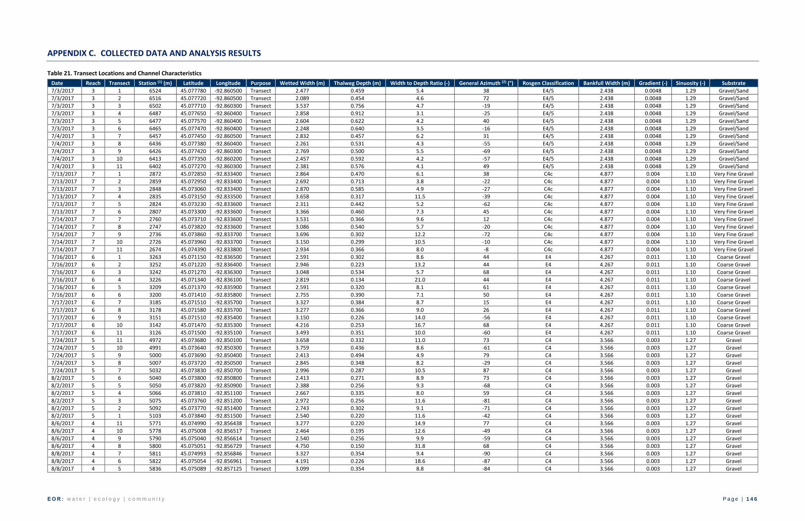
E O R : w a t e r | e c o l o g y | c o m m u n i t y P a g e | 1 4 6
APPENDIX C. COLLECTED DATA AND ANALYSIS RESULTS
Table 21. Transect Locations and Channel Characteristics
Date Reach Transect Station (1) (m) Latitude Longitude Purpose Wetted Width (m) Thalweg Depth (m) Width to Depth Ratio (-) General Azimuth (2) (°) Rosgen Classification Bankfull Width (m) Gradient (-) Sinuosity (-) Substrate
7/3/2017 3 1 6524 45.077780 -92.860500 Transect 2.477 0.459 5.4 38 E4/5 2.438 0.0048 1.29 Gravel/Sand
7/3/2017 3 2 6516 45.077720 -92.860500 Transect 2.089 0.454 4.6 72 E4/5 2.438 0.0048 1.29 Gravel/Sand
7/3/2017 3 3 6502 45.077710 -92.860300 Transect 3.537 0.756 4.7 -19 E4/5 2.438 0.0048 1.29 Gravel/Sand
7/3/2017 3 4 6487 45.077650 -92.860400 Transect 2.858 0.912 3.1 -25 E4/5 2.438 0.0048 1.29 Gravel/Sand
7/3/2017 3 5 6477 45.077570 -92.860400 Transect 2.604 0.622 4.2 40 E4/5 2.438 0.0048 1.29 Gravel/Sand
7/3/2017 3 6 6465 45.077470 -92.860400 Transect 2.248 0.640 3.5 -16 E4/5 2.438 0.0048 1.29 Gravel/Sand
7/4/2017 3 7 6457 45.077450 -92.860500 Transect 2.832 0.457 6.2 31 E4/5 2.438 0.0048 1.29 Gravel/Sand
7/4/2017 3 8 6436 45.077380 -92.860400 Transect 2.261 0.531 4.3 -55 E4/5 2.438 0.0048 1.29 Gravel/Sand
7/4/2017 3 9 6426 45.077420 -92.860300 Transect 2.769 0.500 5.5 -69 E4/5 2.438 0.0048 1.29 Gravel/Sand
7/4/2017 3 10 6413 45.077350 -92.860200 Transect 2.457 0.592 4.2 -57 E4/5 2.438 0.0048 1.29 Gravel/Sand
7/4/2017 3 11 6402 45.077270 -92.860300 Transect 2.381 0.576 4.1 49 E4/5 2.438 0.0048 1.29 Gravel/Sand
7/13/2017 7 1 2872 45.072850 -92.833400 Transect 2.864 0.470 6.1 38 C4c 4.877 0.004 1.10 Very Fine Gravel
7/13/2017 7 2 2859 45.072950 -92.833400 Transect 2.692 0.713 3.8 -22 C4c 4.877 0.004 1.10 Very Fine Gravel
7/13/2017 7 3 2848 45.073060 -92.833400 Transect 2.870 0.585 4.9 -27 C4c 4.877 0.004 1.10 Very Fine Gravel
7/13/2017 7 4 2835 45.073150 -92.833500 Transect 3.658 0.317 11.5 -39 C4c 4.877 0.004 1.10 Very Fine Gravel
7/13/2017 7 5 2824 45.073230 -92.833600 Transect 2.311 0.442 5.2 -62 C4c 4.877 0.004 1.10 Very Fine Gravel
7/13/2017 7 6 2807 45.073300 -92.833600 Transect 3.366 0.460 7.3 45 C4c 4.877 0.004 1.10 Very Fine Gravel
7/14/2017 7 7 2760 45.073710 -92.833600 Transect 3.531 0.366 9.6 12 C4c 4.877 0.004 1.10 Very Fine Gravel
7/14/2017 7 8 2747 45.073820 -92.833600 Transect 3.086 0.540 5.7 -20 C4c 4.877 0.004 1.10 Very Fine Gravel
7/14/2017 7 9 2736 45.073860 -92.833700 Transect 3.696 0.302 12.2 -72 C4c 4.877 0.004 1.10 Very Fine Gravel
7/14/2017 7 10 2726 45.073960 -92.833700 Transect 3.150 0.299 10.5 -10 C4c 4.877 0.004 1.10 Very Fine Gravel
7/14/2017 7 11 2674 45.074390 -92.833800 Transect 2.934 0.366 8.0 -8 C4c 4.877 0.004 1.10 Very Fine Gravel
7/16/2017 6 1 3263 45.071150 -92.836500 Transect 2.591 0.302 8.6 44 E4 4.267 0.011 1.10 Coarse Gravel
7/16/2017 6 2 3252 45.071220 -92.836400 Transect 2.946 0.223 13.2 44 E4 4.267 0.011 1.10 Coarse Gravel
7/16/2017 6 3 3242 45.071270 -92.836300 Transect 3.048 0.534 5.7 68 E4 4.267 0.011 1.10 Coarse Gravel
7/16/2017 6 4 3226 45.071340 -92.836100 Transect 2.819 0.134 21.0 44 E4 4.267 0.011 1.10 Coarse Gravel
7/16/2017 6 5 3209 45.071370 -92.835900 Transect 2.591 0.320 8.1 61 E4 4.267 0.011 1.10 Coarse Gravel
7/16/2017 6 6 3200 45.071410 -92.835800 Transect 2.755 0.390 7.1 50 E4 4.267 0.011 1.10 Coarse Gravel
7/17/2017 6 7 3185 45.071510 -92.835700 Transect 3.327 0.384 8.7 15 E4 4.267 0.011 1.10 Coarse Gravel
7/17/2017 6 8 3178 45.071580 -92.835700 Transect 3.277 0.366 9.0 26 E4 4.267 0.011 1.10 Coarse Gravel
7/17/2017 6 9 3151 45.071510 -92.835400 Transect 3.150 0.226 14.0 -56 E4 4.267 0.011 1.10 Coarse Gravel
7/17/2017 6 10 3142 45.071470 -92.835300 Transect 4.216 0.253 16.7 68 E4 4.267 0.011 1.10 Coarse Gravel
7/17/2017 6 11 3126 45.071500 -92.835100 Transect 3.493 0.351 10.0 -60 E4 4.267 0.011 1.10 Coarse Gravel
7/24/2017 5 11 4972 45.073680 -92.850100 Transect 3.658 0.332 11.0 73 C4 3.566 0.003 1.27 Gravel
7/24/2017 5 10 4991 45.073640 -92.850300 Transect 3.759 0.436 8.6 -61 C4 3.566 0.003 1.27 Gravel
7/24/2017 5 9 5000 45.073690 -92.850400 Transect 2.413 0.494 4.9 79 C4 3.566 0.003 1.27 Gravel
7/24/2017 5 8 5007 45.073720 -92.850500 Transect 2.845 0.348 8.2 -29 C4 3.566 0.003 1.27 Gravel
7/24/2017 5 7 5032 45.073830 -92.850700 Transect 2.996 0.287 10.5 87 C4 3.566 0.003 1.27 Gravel
8/2/2017 5 6 5040 45.073800 -92.850800 Transect 2.413 0.271 8.9 73 C4 3.566 0.003 1.27 Gravel
8/2/2017 5 5 5050 45.073820 -92.850900 Transect 2.388 0.256 9.3 -68 C4 3.566 0.003 1.27 Gravel
8/2/2017 5 4 5066 45.073810 -92.851100 Transect 2.667 0.335 8.0 59 C4 3.566 0.003 1.27 Gravel
8/2/2017 5 3 5075 45.073760 -92.851200 Transect 2.972 0.256 11.6 -81 C4 3.566 0.003 1.27 Gravel
8/2/2017 5 2 5092 45.073770 -92.851400 Transect 2.743 0.302 9.1 -71 C4 3.566 0.003 1.27 Gravel
8/2/2017 5 1 5103 45.073840 -92.851500 Transect 2.540 0.220 11.6 -42 C4 3.566 0.003 1.27 Gravel
8/6/2017 4 11 5771 45.074990 -92.856438 Transect 3.277 0.220 14.9 77 C4 3.566 0.003 1.27 Gravel
8/6/2017 4 10 5778 45.075008 -92.856517 Transect 2.464 0.195 12.6 -49 C4 3.566 0.003 1.27 Gravel
8/6/2017 4 9 5790 45.075040 -92.856614 Transect 2.540 0.256 9.9 -59 C4 3.566 0.003 1.27 Gravel
8/6/2017 4 8 5800 45.075051 -92.856729 Transect 4.750 0.150 31.8 68 C4 3.566 0.003 1.27 Gravel
8/8/2017 4 7 5811 45.074993 -92.856846 Transect 3.327 0.354 9.4 -90 C4 3.566 0.003 1.27 Gravel
8/8/2017 4 6 5822 45.075054 -92.856961 Transect 4.191 0.226 18.6 -87 C4 3.566 0.003 1.27 Gravel
8/8/2017 4 5 5836 45.075089 -92.857125 Transect 3.099 0.354 8.8 -84 C4 3.566 0.003 1.27 Gravel

E O R : w a t e r | e c o l o g y | c o m m u n i t y P a g e | 1 4 7
Date Reach Transect Station (1) (m) Latitude Longitude Purpose Wetted Width (m) Thalweg Depth (m) Width to Depth Ratio (-) General Azimuth (2) (°) Rosgen Classification Bankfull Width (m) Gradient (-) Sinuosity (-) Substrate
8/8/2017 4 4 5845 45.075022 -92.857223 Transect 5.207 0.271 19.2 67 C4 3.566 0.003 1.27 Gravel
8/8/2017 4 3 5856 45.074998 -92.857361 Transect 4.293 0.131 32.7 -74 C4 3.566 0.003 1.27 Gravel
8/8/2017 4 2 5871 45.075065 -92.857540 Transect 3.785 0.256 14.8 -65 C4 3.566 0.003 1.27 Gravel
8/8/2017 4 1 5886 45.075144 -92.857680 Transect 3.785 0.198 19.1 -30 C4 3.566 0.003 1.27 Gravel
8/13/2017 1 1 7246 45.082376 -92.862881 Transect 2.845 0.531 5.4 -39 E5 2.286 0.0001 1.01 Sand
8/13/2017 1 2 7233 45.082340 -92.862726 Transect 2.464 0.363 6.8 -64 E5 2.286 0.0001 1.01 Sand
8/13/2017 1 3 7221 45.082285 -92.862588 Transect 2.667 0.271 9.8 -65 E5 2.286 0.0001 1.01 Sand
8/13/2017 1 4 7209 45.082225 -92.862459 Transect 2.591 0.366 7.1 -55 E5 2.286 0.0001 1.01 Sand
8/19/2017 1 5 7197 45.082178 -92.862322 Transect 2.235 0.579 3.9 -53 E5 2.286 0.0001 1.01 Sand
8/19/2017 1 6 7184 45.082114 -92.862191 Transect 3.073 0.521 5.9 -55 E5 2.286 0.0001 1.01 Sand
8/19/2017 1 7 7172 45.082053 -92.862067 Transect 2.184 0.610 3.6 -43 E5 2.286 0.0001 1.01 Sand
8/19/2017 1 8 7160 45.081977 -92.861960 Transect 3.048 0.476 6.4 -43 E5 2.286 0.0001 1.01 Sand
8/19/2017 1 9 7148 45.081925 -92.861822 Transect 2.388 0.439 5.4 -51 E5 2.286 0.0001 1.01 Sand
8/19/2017 1 10 7135 45.081862 -92.861691 Transect 2.362 0.637 3.7 -59 E5 2.286 0.0001 1.01 Sand
8/19/2017 1 11 7122 45.081808 -92.861554 Transect 2.540 0.518 4.9 -67 E5 2.286 0.0001 1.01 Sand
8/29/2017 2 11 6807 45.079736 -92.860022 Transect 2.515 0.195 12.9 -5 C3 4.267 0.004 1.02 Cobble
8/29/2017 2 10 6817 45.079817 -92.860055 Transect 2.515 0.174 14.5 -16 C3 4.267 0.004 1.02 Cobble
8/29/2017 2 9 6831 45.079949 -92.860068 Transect 3.251 0.159 20.5 -13 C3 4.267 0.004 1.02 Cobble
8/29/2017 2 8 6843 45.080042 -92.860084 Transect 2.464 0.241 10.2 -13 C3 4.267 0.004 1.02 Cobble
8/29/2017 2 7 6853 45.080133 -92.860065 Transect 2.591 0.335 7.7 31 C3 4.267 0.004 1.02 Cobble
8/30/2017 2 6 6869 45.080261 -92.859964 Transect 2.286 0.302 7.6 27 C3 4.267 0.004 1.02 Cobble
8/30/2017 2 5 6882 45.080371 -92.859906 Transect 2.286 0.302 7.6 45 C3 4.267 0.004 1.02 Cobble
8/30/2017 2 4 6891 45.080441 -92.859848 Transect 2.489 0.342 7.3 26 C3 4.267 0.004 1.02 Cobble
8/30/2017 2 3 6905 45.080565 -92.859834 Transect 2.743 0.229 12.0 -7 C3 4.267 0.004 1.02 Cobble
8/30/2017 2 2 6915 45.080657 -92.859834 Transect 2.388 0.287 8.3 11 C3 4.267 0.004 1.02 Cobble
8/30/2017 2 1 6933 45.080810 -92.859870 Transect 4.470 0.250 17.9 -7 C3 4.267 0.004 1.02 Cobble
9/10/2017 3 0 6684 45.078759 -92.860235 Test 2.159 0.211 10.3 0 E4/5 2.438 0.0048 1.29 Gravel/Sand
9/10/2017 3 6 6465 45.077473 -92.860448 Stage 1.981 0.546 3.6 -19 E4/5 2.438 0.0048 1.29 Gravel/Sand
9/10/2017 3 6 6465 45.077473 -92.860448 Stage 1.981 0.546 3.6 -19 E4/5 2.438 0.0048 1.29 Gravel/Sand
9/10/2017 3 6 6465 45.077473 -92.860448 Stage 1.981 0.546 3.6 -19 E4/5 2.438 0.0048 1.29 Gravel/Sand
9/10/2017 3 6 6465 45.077473 -92.860448 Stage 1.981 0.546 3.6 -19 E4/5 2.438 0.0048 1.29 Gravel/Sand
9/10/2017 3 6 6465 45.077473 -92.860448 Stage 1.981 0.546 3.6 -19 E4/5 2.438 0.0048 1.29 Gravel/Sand
9/11/2017 3 9 6426 45.077420 -92.860300 Stage 2.845 0.652 4.4 -67 E4/5 2.438 0.0048 1.29 Gravel/Sand
9/11/2017 3 9 6426 45.077420 -92.860300 Stage 2.845 0.652 4.4 -67 E4/5 2.438 0.0048 1.29 Gravel/Sand
9/11/2017 3 9 6426 45.077420 -92.860300 Stage 2.845 0.652 4.4 -67 E4/5 2.438 0.0048 1.29 Gravel/Sand
9/11/2017 3 9 6426 45.077420 -92.860300 Stage 2.845 0.652 4.4 -67 E4/5 2.438 0.0048 1.29 Gravel/Sand
9/11/2017 3 9 6426 45.077420 -92.860300 Stage 2.845 0.652 4.4 -67 E4/5 2.438 0.0048 1.29 Gravel/Sand
9/12/2017 2 0 6953 45.080987 -92.859853 Stage 3.048 0.211 14.5 1 C3 4.267 0.004 1.02 Cobble
9/12/2017 2 0 6953 45.080987 -92.859853 Stage 3.048 0.211 14.5 1 C3 4.267 0.004 1.02 Cobble
9/12/2017 2 0 6953 45.080987 -92.859853 Stage 3.048 0.211 14.5 1 C3 4.267 0.004 1.02 Cobble
9/12/2017 2 0 6953 45.080987 -92.859853 Stage 3.048 0.211 14.5 1 C3 4.267 0.004 1.02 Cobble
9/12/2017 2 0 6953 45.080987 -92.859853 Stage 3.048 0.211 14.5 1 C3 4.267 0.004 1.02 Cobble
9/13/2017 4 5 5836 45.075091 -92.857132 Stage 2.946 0.339 8.7 -89 C4 3.566 0.003 1.27 Gravel
9/13/2017 4 5 5836 45.075091 -92.857132 Stage 2.946 0.339 8.7 -89 C4 3.566 0.003 1.27 Gravel
9/13/2017 4 5 5836 45.075091 -92.857132 Stage 2.946 0.339 8.7 -89 C4 3.566 0.003 1.27 Gravel
9/13/2017 4 5 5836 45.075091 -92.857132 Stage 2.946 0.339 8.7 -89 C4 3.566 0.003 1.27 Gravel
9/13/2017 4 5 5836 45.075091 -92.857132 Stage 2.946 0.339 8.7 -89 C4 3.566 0.003 1.27 Gravel
9/14/2017 6 0 3281 45.071036 -92.836660 Test 2.667 0.500 5.3 37 E4 4.267 0.011 1.10 Coarse Gravel (1) Creek distance from the St. Croix based on stationing used in the Brown’s Creek Thermal Study. (2) General azimuth measured relative to due south.

E O R : w a t e r | e c o l o g y | c o m m u n i t y P a g e | 1 4 8
Table 22. Vegetation Characteristics at Transects
Date Reach Transect
Vegetation Type (1)
Wetted Edge (2) (m)
Height of Herb. Veg. (m) Max. Height of Woody Vegetation (3)
(m)
Reach Buffer Width (4) (m)
Dominant Overstory Species Dominant Understory
Species Additional Species
Max. Mode
L R L R L R L R L R L R L R L R L R
7/3/2017 3 1 M M -0.241 -0.241 1.775 1.714 NA NA 8.704 13.570 44.501 189.352 BW BW ELD RC JW,SN JW,SN
7/3/2017 3 2 M G -0.457 -0.121 1.989 1.867 NA NA 8.704 12.754 44.501 189.352 BW NONE RC RC ELD SN,JW
7/3/2017 3 3 G G 0.000 -0.051 1.928 1.958 NA NA 1.424 1.272 44.501 189.352 NONE NONE RC RC SN,JW SN
7/3/2017 3 4 G M -0.152 -0.089 1.653 2.171 NA NA 1.216 1.366 44.501 189.352 NONE MXB RC RC SN SN,JW
7/3/2017 3 5 G G -0.381 -0.165 1.958 1.501 NA NA 1.111 1.148 44.501 189.352 NONE NONE SN RC SN,JW SN
7/3/2017 3 6 G G -0.229 -0.442 1.989 1.592 NA NA 1.189 1.041 44.501 189.352 NONE NONE RC RC SN,JW NONE
7/4/2017 3 7 M G 0.000 -0.165 3.086 1.958 NA NA 1.161 1.840 44.501 189.352 NONE NONE SA RC SN JW,SN
7/4/2017 3 8 G G -0.432 0.191 1.958 1.684 NA NA 1.161 1.753 44.501 189.352 NONE NONE RC RC JW,SN,HT SN,JW
7/4/2017 3 9 G G -0.279 0.000 1.867 2.019 NA NA 1.261 1.146 44.501 189.352 NONE NONE RC RC SN,MF SN,JW,WP
7/4/2017 3 10 M G -0.051 -0.216 2.080 1.684 NA NA 4.131 1.146 44.501 189.352 MXB NONE SA NONE RC,SN,JW,BJ RC,SN,JW,BT
7/4/2017 3 11 M G -0.432 -0.146 1.470 1.806 NA NA 1.329 1.382 44.501 189.352 MXB MXC RC RC HT,JW,FM,WSW JW
7/13/2017 7 1 M M -0.229 -0.857 2.050 NA NA NA 3.926 4.044 9.164 8.172 RM,SWO SWO GDW,SN,RC LS,GDW JW JW,RC,WP,BE,GC
7/13/2017 7 2 M M 0.000 0.000 NA 2.202 NA NA 6.194 3.151 9.164 8.172 RM SWO GDW GDW PG,BC,BFT,BS,
CA,FB,BFT,GO,HP BN,RC,WP,SN
7/13/2017 7 3 M M -0.229 -0.203 1.562 1.989 1.257 1.257 4.209 2.721 9.164 8.172 RM,BB,T SWO,CH,RP JW LS SWMIL,RC,SW,WP,HT RC,JW,SGO,BN,SN,GC,HT
7/13/2017 7 4 M G 0.000 0.000 1.897 1.409 1.348 1.196 2.566 2.421 9.164 8.172 CH,GDW NONE RC JW JW,SN,CD,MH,LS,RM,C,WP,FB LS,JW,SN,RC,NC,FB,BGB,
CD,WG,DF,GLGO,MB
7/13/2017 7 5 G G -0.127 -0.038 1.867 1.958 1.257 1.257 2.145 2.391 9.164 8.172 NONE NONE RC NA JW,HT,S,BN,SGO,WH,WHBB,
BT,BS,GLGO,PS,ALT RC,FM,JW,MB,FB,GO
7/13/2017 7 6 G G 0.000 -0.038 1.989 1.928 1.257 1.257 2.277 2.336 9.164 8.172 NONE NONE SOR NBF RC,SN,JW,GC,BN,CMIL,
SWTL,SWW,FB JW,RC,SWMIL,HT,WP,LS,CGO,
FB,BGB,MB,ALT,PS,GLGO
7/14/2017 7 7 M M -0.127 -0.025 1.836 1.928 1.227 1.318 2.388 2.346 9.164 8.172 SWO,RM SWO,RM RC RC JW,SN,NBF,FB,GLGO,
PS,BLA,WG,BGB JW,GI,SWMIL,YR,CD,
WG,WC,BGB
7/14/2017 7 8 M M 0.000 -0.457 2.050 1.867 1.348 1.196 2.171 2.766 9.164 8.172 SWO SWO JW NBF NBF,RC,GO,GM,WHBB,
SOR,BGB,WG,GWD WB,S,JW,RDW,BGB,
SGO,PS,CT
7/14/2017 7 9 M G 0.000 0.140 1.592 1.775 1.196 1.018 2.427 2.469 9.164 8.172 SWO NONE LS NA JW,NBF,RC,GLGO,FB,BT,GO,PS JW,RC,SWMIL,SOR,GC,SM,BGB,
BS,WHBB,MB,GO,WG,GLGO
7/14/2017 7 10 G G -0.152 -0.051 2.019 1.638 1.196 1.288 2.180 2.856 9.164 8.172 NONE NONE SOR NA JW,RC,LS,MB,GO,SPR JW,RC,SWMIL,PB,AWH,WHBB,
GO,WH,WG,BE,PS,BGB
7/14/2017 7 11 M M 0.152 -0.940 2.080 2.080 1.562 1.440 10.856 5.005 9.164 8.172 HL KC RC RC CR,JW,BTD,ALT,BLA SN,CR
7/16/2017 6 1 F F -0.076 0.457 NA NA NA NA 4.448 4.758 16.891 6.902 SW,MM,AM BE,SW,RDW RC RC JW,CA,NEA,DW JW,B,SN
7/16/2017 6 2 F F 0.000 0.000 NA NA NA NA 4.448 5.433 16.891 6.902 SW WBC,SW NA RC B,JW,RC,FB,GC,GLGO,YR,
GO,S,DW,GM,MM SN,B,T,DW
7/16/2017 6 3 F F 0.000 0.292 NA NA NA NA 5.614 6.293 16.891 6.902 SW,BE SW,SA,BE RC JW,BN JW,SN,B,DW,GB,R RC,SN,AG
7/16/2017 6 4 F F 0.406 0.318 NA NA NA NA 6.788 5.957 16.891 6.902 BE,GB,DW BE GI GI DW,JW,RC,BC JW,GA
7/16/2017 6 5 F F 0.686 0.229 NA NA NA NA 6.452 6.276 16.891 6.902 BE SA,BE JW JW SW,RC,GI GI,SNR,GO,SF
7/16/2017 6 6 F F 0.229 0.203 NA NA NA NA 8.953 6.276 16.891 6.902 BE,DW BE DW SW JW,RC,MM JW,SW,WN,MM
7/17/2017 6 7 F F 0.254 0.254 NA NA NA NA 7.287 5.766 16.891 6.902 BE,SA,DW SA,AM,DW JW B RC,GI,B,GO BE,GA,DF,GI,S,GO,SF,SW
7/17/2017 6 8 F F 0.000 0.356 NA NA NA NA 5.818 5.026 16.891 6.902 SA,RDW SA,RDW RC SA JW,SN,SW,WP,S,GO,SM RC,JW,GI
7/17/2017 6 9 F F 0.000 0.127 NA NA NA NA 5.072 7.013 16.891 6.902 RDW,BE SIM RR NA JW,B,RC,VP,R SW,JW,DW,BN, GI,CGO,B,MM
7/17/2017 6 10 F F -0.356 0.732 NA NA NA NA 3.513 4.815 16.891 6.902 RM,BE,AM,SM BE BE,DW BE,R JW,RC,GI,SN,B,RDW,YR,GO,R BN,GI,DW,RR
7/17/2017 6 11 F F 0.737 0.000 NA NA NA NA 4.368 3.852 16.891 6.902 DW DW RDW JW SW,BE,JW,RC,SN,WP,FB RC,SW,BE,RM,GO,RDW,SN
7/24/2017 5 11 M F 0.102 0.495 1.623 NA 1.623 NA 5.565 4.513 60.564 62.346 SA SA FB SF RC,SN,JW,WP,BC,GO JW,R,GO
7/24/2017 5 10 M F 0.000 0.000 1.245 NA 1.245 NA 4.428 5.372 60.564 62.346 BE SA,DW RC JW JW,WP,SN RC,SN,LF
7/24/2017 5 9 M M 0.127 -0.305 1.653 1.653 1.196 1.288 5.919 2.302 60.564 62.346 AM,SA SA,DW,BE RC SN,JW JW,WP,SN RC,SF,LF,WP,AM, ALT,MB,YR,FB,W
7/24/2017 5 8 F F -0.254 0.305 NA NA NA NA 7.003 3.937 60.564 62.346 SA,BE AM,BE RC JW JW,SN,SF SN,G
7/24/2017 5 7 M F 0.000 0.229 1.524 NA 1.524 NA 6.211 4.123 60.564 62.346 SA,BE SA,AM JW JW,BC LS,RC,CA,FM,ALT, WN,GSW,GC,LF
RC,SN,WN,ARR,PG,MH,DW
8/2/2017 5 6 M M 0.787 0.254 0.175 1.775 0.256 1.440 4.311 4.833 60.564 62.346 SA,GB,BE SA SWTL RC SPR,LS,BLA,WP,NBF,PF,L SW,WP,LS,SPR,JW,PS,FB

E O R : w a t e r | e c o l o g y | c o m m u n i t y P a g e | 1 4 9
Date Reach Transect Vegetation
Type (1) Wetted Edge (2)
(m)
Height of Herb. Veg. (m) Max. Height of Woody Vegetation (3)
(m)
Reach Buffer Width (4) (m)
Dominant Overstory Species Dominant Understory
Species Additional Species
Max. Mode
L R L R L R L R L R L R L R L R L R
8/2/2017 5 5 G G 0.000 0.965 1.989 2.171 1.379 1.318 3.773 5.128 60.564 62.346 SA,GB,BE SA,MXB RC RC JW,SW,BGB,FB,SOR,BON JW,LS,FB,SOR
8/2/2017 5 4 G G 0.406 -0.152 1.958 1.806 1.562 1.501 4.827 6.713 60.564 62.346 SA,BE SA,MXB RC RC JW,FM,FB,WP,BC,SWMIL,CT,BON CT,SN,JW,BLA
8/2/2017 5 3 M F -0.051 0.330 1.440 1.440 0.561 NA 4.641 9.064 60.564 62.346 SA,MXB SA,MXB RC JW PS,FB,WG,SOR,SW,BON DW,RC
8/2/2017 5 2 G M -0.102 0.457 2.476 1.867 1.288 1.440 4.641 8.004 60.564 62.346 BE,MXB SA,DW,MXB RC JW JW,BLA,BON,SN RC,YR,GO,CT
8/2/2017 5 1 G M -0.102 0.406 2.019 2.110 1.440 1.440 4.435 6.383 60.564 62.346 BE,MXB SA,DW,BE,MXB RC RC LS,PS,SN,AG,BON, BLA,WP,JW,CT,FB
JW,WP,CT,FB,SN,WG,AG
8/6/2017 4 11 F F 0.889 0.000 1.592 NA 1.440 NA 5.150 5.786 59.165 51.416 SA CB JW CB SN,BT,BW,RC,SSFN SA,JW,SSFN
8/6/2017 4 10 F F 0.102 1.295 1.501 0.896 1.227 0.195 5.150 5.745 59.165 51.416 SA SA JW SWTL BE,SN,SSFN,GC,RC,R,HT GO,RC,SN,JW,HT,SSFN
8/6/2017 4 9 M F -0.610 0.610 1.928 0.988 1.745 0.622 2.129 4.800 59.165 51.416 BE SA RC JW LF,WP,SN,HP,GO,CGO SSFN,RC,BTD,SWD
8/6/2017 4 8 M M 0.203 0.000 1.501 1.531 1.018 1.318 8.235 5.620 59.165 51.416 SA,BE,GB SA RC JW JW,BTD,SWTL,GO,FB,PS,SSFN,CT,
BLA,NSW,GSW,JP,WCUC,NWP BN,SSFN,SN,SF,BE,ENS
8/8/2017 4 7 M F -0.610 0.914 1.867 1.168 1.348 1.168 8.235 16.333 59.165 51.416 SA,MXB SA,CB RC JW JW,CT,JP,SN,WCUC SSFN,WPI,RP,SWTL
8/8/2017 4 6 M F -0.076 0.356 2.019 1.318 1.227 1.318 6.188 11.833 59.165 51.416 GDW SA,BE GDW JW SW,RC,FM,CT,WCUC,SW,
JW,SSFN,JP,SN,MM,CE S,GO,RC,SSFN,GC
8/8/2017 4 5 F F 0.000 0.432 0.774 1.018 0.470 0.409 8.983 15.663 59.165 51.416 CB,SA SA,CB,BE NA JW SSFN,BTD,JW,CA, CB,RR,SF,CJ,SNR
BTD,GC,SSFN,SF,LF
8/8/2017 4 4 F F 0.000 0.000 0.835 0.835 0.348 0.165 7.390 17.586 59.165 51.416 SA,CB,HS CB,SA CB LF JW,LF,RR,CB JW,SSFN
8/8/2017 4 3 F F 0.000 1.219 0.927 NA 0.500 NA 6.459 19.686 59.165 51.416 CB,SA SA,HS,CB,MXB PG LF RR,CB,SSFN,JW,LF,S JW,SSFN,MM
8/8/2017 4 2 F F 0.406 0.711 1.018 NA 0.592 NA 12.667 16.135 59.165 51.416 SA CB,SA,BE BTD LF HP,HS,RC,SSFN,JW,
BN,CB,LF,GC,C SSFN,BC,HS
8/8/2017 4 1 M F 0.000 0.254 1.836 1.501 1.196 1.501 13.231 14.613 59.165 51.416 SA,BE BE,GB SSFN JW JW,RR,LF,WP,JP,RC,LPFO SSFN,CT,RC,SW,HS
8/13/2017 1 1 G G -0.279 -0.356 1.745 1.379 1.196 0.988 5.681 6.680 134.498 121.968 CE NONE RC RC JP,SN,WP,JW,LS,BN JW,SN,SSFN,SN, WP,WCUC,WSW
8/13/2017 1 2 G G -0.457 -0.203 1.806 2.019 1.111 1.196 5.287 5.821 134.498 121.968 NONE DW RC BT ALT,SN JW,SSFN,SN,RC,GO,BT
8/13/2017 1 3 G G -0.102 -0.533 1.928 1.928 1.196 1.288 1.582 1.780 134.498 121.968 NONE NONE RC RC JW,SN,BT,LS,SSFN JW,SN,WP,BC,DW,AM,SSFN,BT
8/13/2017 1 4 G G -0.254 -0.076 1.318 1.562 0.988 1.257 1.573 1.682 134.498 121.968 NONE NONE RC RC SSFN,FB,WP,SN,ALT,GO,GWD JW,SN,SSFN,BT
8/19/2017 1 5 G G -0.406 -0.610 1.897 1.928 0.866 1.257 1.631 1.933 134.498 121.968 NONE PBI RC RC FM,FB,BT,JW,GO,SW WP,JW,SSFN,BT
8/19/2017 1 6 G G -0.330 0.000 1.714 2.171 0.774 1.111 1.590 4.366 134.498 121.968 NONE PBI,SA RC JW FM,SN,SSFN RC,SSFN,FM,SN,GO
8/19/2017 1 7 G M -0.610 -0.559 1.003 1.562 1.003 1.111 1.564 5.330 134.498 121.968 NONE SA,GB RC RC JW,BT,SN,SSFN JW,SSFN,BT
8/19/2017 1 8 M M -0.914 0.000 1.592 1.745 1.018 1.196 3.559 5.330 134.498 121.968 SA SA,GB FM FM RC,JW,ALT,BT SSFN,FB,WP,GO,BT
8/19/2017 1 9 M M -0.203 -0.762 1.653 1.379 0.957 1.111 3.559 3.276 134.498 121.968 SA,GB SA RC RC FM,JW,SSFN,GO,ALT,NSW FB,WP,JW
8/19/2017 1 10 G M -0.813 -0.610 1.684 1.958 1.018 1.196 1.957 3.483 134.498 121.968 NONE SA RC RC JW,BT FB,JW
8/19/2017 1 11 G G -0.406 -0.203 1.806 1.989 1.196 1.227 1.638 2.436 134.498 121.968 NONE SA RC RC FM,JW,WP,BT FB,JW,SF
8/29/2017 2 11 M M -0.203 -0.635 1.714 1.501 1.227 0.957 10.597 15.588 4.084 60.459 WW,WPI,
GB,HS PCW,SA,GB,PO RC WSW FM,WP RC,LS
8/29/2017 2 10 M M -0.279 -0.076 1.867 1.470 1.018 1.470 15.674 19.262 4.084 60.459 WW,WPI,
GB,HS PCW,SA,GB,PO NA RC BN,RC,LS,JW,SN,SSFN,CMIL CT,BN,JP,WSW
8/29/2017 2 9 F F 0.254 0.127 0.439 0.348 0.439 0.348 15.946 12.961 4.084 60.459 SA,GB,BE,WW GB,BE,BCH SSFN GB RR,GB MM
8/29/2017 2 8 M F 3.175 0.279 0.744 0.165 0.744 0.165 13.183 20.424 4.084 60.459 SP,SIM,WS, GB,RB,BE
GB,HS TG GB NONE NONE
8/29/2017 2 7 M F 1.905 0.000 0.531 0.439 0.531 0.439 13.183 20.424 4.084 60.459 SP,WS,GB,
RB,BE GB,SA,MM TG RR NONE NONE
8/30/2017 2 6 M M 0.152 -0.406 1.018 2.202 0.866 1.348 7.260 18.258 4.084 60.459 RP,SP,AB,RB,WW GB,WW H BN TG,RC,SSFN,JW,BT,PLWH BE,RC,WP,HP,SSFN,
ALT,GB,LF
8/30/2017 2 5 M M 0.000 0.000 1.928 2.050 0.927 1.379 12.920 1.996 4.084 60.459 RB,T,SIM,WW WW,WPI SSFN NA RC,JP,WG,WP,TG,AM, BON,BE,SWMIL, SCF
RC,JW,ALT,BES,SSFN,DW, BT,PS,HP,FM,LS,GB
8/30/2017 2 4 M M 0.076 0.000 0.912 1.867 1.196 1.196 19.515 1.907 4.084 60.459 WW,SM,SIM WW,WPI BT H CA,SSFN,BN,LS,TG,
GI,BL,PLWH,MH JW,SN,RC,BT,RR,
SSFN,AM,PA
8/30/2017 2 3 M M 0.889 0.000 0.287 1.531 0.287 1.018 14.452 2.446 4.084 60.459 RP,SM,SIM WW,WPI,PCW,B
E TG SSFN NONE
RC,BES,SN,WP, CA,JW,WHBB
8/30/2017 2 2 M M 1.245 0.102 0.256 2.202 0.256 1.257 18.045 12.393 4.084 60.459 DW,WW,RP,
SM,SIM DW,BE,WPI, SIM,PO,SPI
TG H NONE GB,PA,DW,BL,JW, SSFN,RC,BT,S,JP
8/30/2017 2 1 F F 0.000 1.111 1.168 1.168 0.470 0.470 17.624 16.528 4.084 60.459 BE,SIM GB,BE,SIM SSFN SSFN BT,SF,CA,MM,GB JW,SA

E O R : w a t e r | e c o l o g y | c o m m u n i t y P a g e | 1 5 0
Date Reach Transect Vegetation
Type (1) Wetted Edge (2)
(m)
Height of Herb. Veg. (m) Max. Height of Woody Vegetation (3)
(m)
Reach Buffer Width (4) (m)
Dominant Overstory Species Dominant Understory
Species Additional Species
Max. Mode
L R L R L R L R L R L R L R L R L R
9/10/2017 3 0 G G -0.076 0.000 2.476 1.836 1.318 1.531 1.256 1.465 44.501 189.352 NONE QA,SA,DW NA RC SN,RC,SSFN,BT,JW,CT,BON,WCUC AM,JW,YR,SN
9/10/2017 3 6 G G -0.254 -0.229 2.324 2.324 1.227 1.018 1.161 1.113 44.501 189.352 NONE SA RC RC SN,JW SF,JW,HT,WCUC,SN
9/10/2017 3 6 G G -0.254 -0.229 2.324 2.324 1.227 1.018 1.161 1.113 44.501 189.352 NONE SA RC RC SN,JW SF,JW,HT,WCUC,SN
9/10/2017 3 6 G G -0.254 -0.229 2.324 2.324 1.227 1.018 1.161 1.113 44.501 189.352 NONE SA RC RC SN,JW SF,JW,HT,WCUC,SN
9/10/2017 3 6 G G -0.254 -0.229 2.324 2.324 1.227 1.018 1.161 1.113 44.501 189.352 NONE SA RC RC SN,JW SF,JW,HT,WCUC,SN
9/10/2017 3 6 G G -0.254 -0.229 2.324 2.324 1.227 1.018 1.161 1.113 44.501 189.352 NONE SA RC RC SN,JW SF,JW,HT,WCUC,SN
9/11/2017 3 9 G G -0.508 0.000 2.324 2.324 1.257 2.171 1.261 1.146 44.501 189.352 NONE NONE RC JW SN,WCUC,JW,CT RC,WP,SN,BT
9/11/2017 3 9 G G -0.508 0.000 2.324 2.324 1.257 2.171 1.261 1.146 44.501 189.352 NONE NONE RC JW SN,WCUC,JW,CT RC,WP,SN,BT
9/11/2017 3 9 G G -0.508 0.000 2.324 2.324 1.257 2.171 1.261 1.146 44.501 189.352 NONE NONE RC JW SN,WCUC,JW,CT RC,WP,SN,BT
9/11/2017 3 9 G G -0.508 0.000 2.324 2.324 1.257 2.171 1.261 1.146 44.501 189.352 NONE NONE RC JW SN,WCUC,JW,CT RC,WP,SN,BT
9/11/2017 3 9 G G -0.508 0.000 2.324 2.324 1.257 2.171 1.261 1.146 44.501 189.352 NONE NONE RC JW SN,WCUC,JW,CT RC,WP,SN,BT
9/12/2017 2 0 F F 0.483 1.806 1.245 1.018 1.245 1.018 15.538 7.871 4.084 60.459 GB,SA,BE,RP SA,GB GB JW CA,JW,SSFN,BT,LS,HP,SF,NBM SSFN,RC,BT,NBM
9/12/2017 2 0 F F 0.483 1.806 1.245 1.018 1.245 1.018 15.538 7.871 4.084 60.459 GB,SA,BE,RP SA,GB GB JW CA,JW,SSFN,BT,LS,HP,SF,NBM SSFN,RC,BT,NBM
9/12/2017 2 0 F F 0.483 1.806 1.245 1.018 1.245 1.018 15.538 7.871 4.084 60.459 GB,SA,BE,RP SA,GB GB JW CA,JW,SSFN,BT,LS,HP,SF,NBM SSFN,RC,BT,NBM
9/12/2017 2 0 F F 0.483 1.806 1.245 1.018 1.245 1.018 15.538 7.871 4.084 60.459 GB,SA,BE,RP SA,GB GB JW CA,JW,SSFN,BT,LS,HP,SF,NBM SSFN,RC,BT,NBM
9/12/2017 2 0 F F 0.483 1.806 1.245 1.018 1.245 1.018 15.538 7.871 4.084 60.459 GB,SA,BE,RP SA,GB GB JW CA,JW,SSFN,BT,LS,HP,SF,NBM SSFN,RC,BT,NBM
9/13/2017 4 5 F F 0.000 0.483 0.835 1.018 0.561 0.439 8.983 15.663 59.165 51.416 GB,SA SA,GB,BE SSFN SSFN BT,CA,LS,GB,RR,GO,RC,SNR,W JW,SF,LF,BN
9/13/2017 4 5 F F 0.000 0.483 0.835 1.018 0.561 0.439 8.983 15.663 59.165 51.416 GB,SA SA,GB,BE SSFN SSFN BT,CA,LS,GB,RR,GO,RC,SNR,W JW,SF,LF,BN
9/13/2017 4 5 F F 0.000 0.483 0.835 1.018 0.561 0.439 8.983 15.663 59.165 51.416 GB,SA SA,GB,BE SSFN SSFN BT,CA,LS,GB,RR,GO,RC,SNR,W JW,SF,LF,BN
9/13/2017 4 5 F F 0.000 0.483 0.835 1.018 0.561 0.439 8.983 15.663 59.165 51.416 GB,SA SA,GB,BE SSFN SSFN BT,CA,LS,GB,RR,GO,RC,SNR,W JW,SF,LF,BN
9/13/2017 4 5 F F 0.000 0.483 0.835 1.018 0.561 0.439 8.983 15.663 59.165 51.416 GB,SA SA,GB,BE SSFN SSFN BT,CA,LS,GB,RR,GO,RC,SNR,W JW,SF,LF,BN
9/14/2017 6 0 F F 0.381 0.254 1.470 1.714 1.196 0.866 6.827 6.990 16.891 6.902 BE,DW BE,SA JW JW RC,GC,SSFN,C,B,GI RC,SSFN,GI,B (1) G = grassy, F = forest, M = mixed (2) Wetted edge is the distance from the water’s edge to riparian vegetation. A positive number means there was an exposed (un-vegetated) bank. A negative wetted edge was tracked to indicate there was very dense vegetation and streambank hanging above the water surface. (3) Maximum height of woody vegetation assessed using 2011 LiDAR data within 10 m of transect. (4) Average buffer width for representative reaches estimated using aerial imagery. Mowed grass or pavement was not considered a buffer. Herb. = herbaceous Position of observation denoted by: L = left, R = right when looking downstream All heights of vegetation measured relative to the water surface. NA = data not available or not collected
GB Invasive or exotic species identified

E O R : w a t e r | e c o l o g y | c o m m u n i t y P a g e | 1 5 1
Table 23. Plant Identification Key
Acronym Common Name Scientific Name Acronym Common Name Scientific Name Acronym Common Name Scientific Name
AB American basswood Tilia americana GDW Gray dogwood Cornus racemosa RB River birch Betula nigra
AG American germander Teucrium canadense GI Ground ivy ** Glechoma hederacea RC Reed canary grass * Phalaris arundinacea
ALT Arrow-leaved tearthumb Persicaria sagittata GLGO Grass-leaved goldenrod Euthamia graminifolia RDW Red-osier dogwood Cornus sericea
AM Amur maple * Acer ginnala GM Garlic mustard * Alliaria petiolata RM Red maple Acer rubrum
ARR American red raspberry Rubus idaeus GO Goldenrod Solidago spp. RP Red pine Pinus resinosa
AWH American water horehound Lycopus americanus GSW Great St. John's-wort Hypericum pyramidatum RR Red raspberry Rubus idaeus
B Common burdock * Arctium minus GWD Great water dock Rumex britannica S Sedge Carex spp.
BB Buttonbush Cephalantus occidentalis H Hosta ** Funkia spp. SA Speckled alder Alnus incana
BC Blue cohosh Caulophyllum thalictroides HL Imperial honey locust Gleditsia triacanthos 'Impcole' SCF Straw-colored flatsedge Cyperus strigosus
BCH Black cherry Prunus serotina HP America hog peanut Amphicarpaea bracteata SF Sensitive fern Onoclea sensibilis
BE Boxelder Acer negundo HS Honeysuckle * Lonicera spp. SGO Showy goldenrod Solidago speciosa
BES Black-eyed Susan Rudbeckia hirta HT Horsetail Equisetum spp. SIM Silver maple Acer saccharinum
BFT Birds-foot trefoil * Lotus corniculatus JP Spotted joe-pyeweed Eutrochium maculatum SM Sugar maple Acer saccharum
BGB Dark green bulrush Scirpus atrovirens JW Jewelweed, Spotted touch-me-not Impatiens capensis SN Stinging nettle Urtica dioica
BJ Colorado bluejoint grass Calamagrostis canadensis KC Kentucky coffeetree Gymnocladus occidentalis SNR White snakeroot Ageratina altissima
BL Blue lobelia Lobelia siphilitica L Loosestrife * Lythrum spp. SOR Soft rush Juncus effusus
BLA Broad-leaf arrowhead Sagittaria latifolia LF Lady fern Athyrium Filix-femina SP Spruce Picea
BN Bittersweet nightshade ** Bidens connata LPFO Lesser purple fringed orchid U Platanthera psycodes SPI Scotch pine ** Pinus sylvestris
BON Common boneset Eupatorium perfoliatum LS Lake sedge Carex lacustris SPR Spikerush Eleocharis spp.
BS Bebb's sedge Carex bebbii MB Marsh bellflower Campanula aparinoides SSFN Small-spike false nettle Boehmeria cylindrica
BT Purple-stem beggarticks Bidens connata MF Monkey flower Mimulus spp. SW Sandbar willow Salix interior
BTD Devil's beggarticks Bidens frondosa MH Meadow horsetail Equisetum pratense SWD Smartweed Persicaria spp.
BW Black willow Salix nigra MM Mountain maple Acer spicatum SWMIL Marsh/swamp milkweed Asclepias incarnata
C Clover Trifolium spp. MXB Mixed broadleaf trees n/a SWO Swamp white oak Quercus bicolor
CA Canada anemone Anemone canadensis MXC Mixed coniferous trees n/a SWTL Thyme-leaf speedwell ** Veronica serpyllifolia
CB Common buckthorn * Rhamnus cathartica NA Not applicable (no dominant species) SWW Water speedwell Veronica catenata
CD Curly dock ** Rumex crispus NBF Northern blue flag Iris versicolor T Tamarack Larix laricina
CE Cut leaf elderberry Sambucus nigra laciniata NBM Nodding bur-marigold Bidens cernua TG Kentucky bluegrass ** Poa pratensis
CGO Canada goldenrod Solidago canadensis NC Narrowleaf cattail ** Typha angustifolia VP Veiny pea Lathyrus venosus
CH Cock-spur hawthorn Crataegus crus-galli NEA New England aster Symphyotrichum novae-angliae W Watercress * Nasturtium officinale
CJ Creeping jenny ** Lysimachia nummularia NONE no vegetation WB Wild bergamot Monarda fistulosa
CR Common reed Phragmites spp. NSW Nodding smartweed Persicaria lapathifolia WBC Wild black currant Ribes americanum
CMIL Common milkweed Asclepias syriaca NWP Northern water plantain Alisma triviale WC White clover ** Trifolium repens
CT Canada thistle * Cirsium arvense PA Panicled aster Symphyotrichum lanceolatum WCUC Wild cucumber Echinocystis lobata
DF Daisy fleabane Erigeron strigosus PB Pennsylvania buttercup Ranunculus pensylvanicus WG Woolgrass Scirpus cyperinus
DW Dogwood Cornus spp. PBI Paper birch Betula papyrifera WH Water hemlock Cicuta maculata
ELD Elderberry Sambucus spp. PCW Plains cottonwood Populus deltoides WHBB Bulblet-bearing water hemlock Cicuta bulbifera
ENS Enchanter's nightshade Circaea lutetiana PF Purple monkey flower, Allegheny monkey flower Mimulus ringens WN Canadian wood nettle Laportea canadensis
FB Fowl bluegrass Poa palustris PG Prickly gooseberry Ribes cynosbati WP Wild pea, Marsh vetchling Lathyrus palustris
FM Fowl manna grass Glyceria striata PLWH Purple-leaved willow-herb Epilobium coloratum WPI White pine Pinus strobus
G Grass (unidentified) n/a PO Pin oak Quercus palustri WS White spruce Picea glauca
GA Green ash Fraxinus pennsylvanica PS Porcupine sedge Carex hystericina WSW Water smartweed Persicaria amphibia
GB Glossy buckthorn * Frangula alnus QA Quaking aspen Populus tremuloides WW Weeping willow ** Salix babylonica
GC Giant chickweed ** Myosoton aquaticum R Raspberry Rubus spp. YR Yellow rocket Barbarea spp. * Exotic/Invasive Species ** Non-Native Species U Unique Species

E O R : w a t e r | e c o l o g y | c o m m u n i t y P a g e | 1 5 2
Table 24. Photo Analysis Results at Transects
Date Reach Transect Time of Photo Lens Height (m) Gap Fraction Openness
Growing Season Shade (WinSCANOPY) Growing Season
Shade (LiDAR) Variable Lens Height Constant Lens Height
C L R C L R C L R Avg C L R Avg C L R Avg C L R Avg
7/3/2017 3 1 10:52 10:57 11:04 0.476 0.318 0.337 0.35 0.12 0.21 0.23 0.50 0.12 0.19 0.27 0.88 0.95 0.74 0.85 0.88 0.95 0.74 0.85 0.11
7/3/2017 3 2 12:12 12:17 12:31 0.286 0.432 0.349 0.45 0.28 0.28 0.34 0.33 0.22 0.21 0.26 0.13 0.45 0.76 0.45 0.20 0.45 0.76 0.47 0.11
7/3/2017 3 3 13:15 13:23 13:28 0.298 0.298 0.298 0.73 0.48 0.66 0.62 0.55 0.35 0.50 0.47 0.13 0.36 0.08 0.19 0.20 0.36 0.13 0.23 0.11
7/3/2017 3 4 14:05 14:30 14:21 0.343 0.368 0.343 0.72 0.63 0.59 0.65 0.55 0.49 0.45 0.50 0.10 0.18 0.38 0.22 0.17 0.18 0.63 0.33 0.11
7/3/2017 3 5 15:49 15:54 15:58 0.343 0.311 0.419 0.66 0.42 0.45 0.51 0.49 0.32 0.35 0.38 0.21 0.64 0.42 0.42 0.35 0.64 0.84 0.61 0.11
7/3/2017 3 6 16:39 16:48 16:45 0.292 0.305 0.337 0.67 0.41 0.46 0.51 0.50 0.30 0.35 0.38 0.19 0.51 0.39 0.36 0.28 0.51 0.64 0.48 0.11
7/4/2017 3 7 11:22 11:25 11:33 0.222 0.337 0.241 0.55 0.30 0.40 0.42 0.44 0.28 0.30 0.34 0.62 0.77 0.48 0.63 0.62 0.77 0.65 0.68 0.11
7/4/2017 3 8 12:06 12:08 12:21 0.324 0.248 0.248 0.79 0.58 0.59 0.65 0.61 0.44 0.46 0.50 0.07 0.16 0.45 0.23 0.12 0.16 0.61 0.30 0.06
7/4/2017 3 9 12:52 13:05 13:09 0.267 0.248 0.267 0.73 0.20 0.68 0.54 0.56 0.17 0.52 0.42 0.06 0.69 0.23 0.33 0.09 0.69 0.33 0.37 0.06
7/4/2017 3 10 13:53 14:01 13:57 0.216 0.362 0.298 0.70 0.43 0.52 0.55 0.52 0.34 0.39 0.41 0.16 0.37 0.48 0.34 0.20 0.37 0.74 0.44 0.06
7/4/2017 3 11 14:27 14:32 14:35 0.216 0.222 0.248 0.78 0.42 0.66 0.62 0.59 0.33 0.50 0.47 0.09 0.58 0.18 0.28 0.11 0.58 0.25 0.32 0.06
7/13/2017 7 1 12:40 12:47 12:52 0.286 0.457 0.292 0.51 0.32 0.13 0.32 0.35 0.23 0.09 0.23 0.32 0.42 0.91 0.55 0.48 0.42 0.91 0.60 0.24
7/13/2017 7 2 14:32 14:37 14:43 0.273 0.254 0.394 0.32 0.13 0.08 0.17 0.25 0.11 0.06 0.14 0.67 0.81 0.92 0.80 0.67 0.81 0.92 0.80 0.24
7/13/2017 7 3 15:41 15:44 15:48 0.267 0.343 0.178 0.71 0.40 0.42 0.51 0.55 0.33 0.32 0.40 0.19 0.59 0.31 0.36 0.27 0.59 0.37 0.41 0.24
7/13/2017 7 4 16:24 16:26 16:29 0.337 0.406 0.387 0.86 0.76 0.75 0.79 0.71 0.62 0.59 0.64 0.04 0.19 0.12 0.12 0.06 0.19 0.23 0.16 0.24
7/13/2017 7 5 17:29 17:32 17:38 0.267 0.330 0.318 0.83 0.60 0.75 0.73 0.67 0.49 0.61 0.59 0.03 0.38 0.07 0.16 0.05 0.38 0.11 0.18 0.24
7/13/2017 7 6 18:20 18:22 18:25 0.260 0.387 0.279 0.84 0.75 0.36 0.65 0.67 0.62 0.30 0.53 0.03 0.11 0.77 0.31 0.04 0.11 0.77 0.31 0.06
7/14/2017 7 7 11:51 11:56 11:59 0.292 0.368 0.425 0.83 0.69 0.73 0.75 0.67 0.56 0.58 0.60 0.12 0.19 0.16 0.16 0.18 0.19 0.32 0.23 0.06
7/14/2017 7 8 12:20 12:25 12:31 0.318 0.368 0.203 0.80 0.67 0.23 0.57 0.64 0.53 0.21 0.46 0.09 0.35 0.70 0.38 0.14 0.35 0.70 0.40 0.06
7/14/2017 7 9 13:27 13:30 13:33 0.381 0.387 0.368 0.87 0.79 0.77 0.81 0.71 0.64 0.62 0.66 0.02 0.07 0.08 0.06 0.04 0.07 0.14 0.08 0.06
7/14/2017 7 10 14:38 14:40 14:45 0.368 0.400 0.362 0.87 0.66 0.66 0.73 0.72 0.55 0.54 0.60 0.04 0.40 0.24 0.23 0.07 0.40 0.41 0.29 0.06
7/14/2017 7 11 15:25 15:29 15:35 0.260 0.324 0.241 0.49 0.35 0.31 0.38 0.38 0.29 0.23 0.30 0.60 0.67 0.79 0.68 0.60 0.67 0.79 0.68 0.08
7/16/2017 6 1 11:16 11:18 11:23 0.368 0.533 0.438 0.08 0.12 0.03 0.07 0.05 0.08 0.02 0.05 0.93 0.79 0.99 0.90 0.93 0.79 0.99 0.90 0.23
7/16/2017 6 2 11:58 12:08 12:19 0.425 0.514 0.546 0.17 0.10 0.07 0.11 0.11 0.07 0.04 0.07 0.75 0.85 0.97 0.86 0.75 0.85 0.97 0.86 0.23
7/16/2017 6 3 13:09 13:13 13:16 0.298 0.540 0.387 0.11 0.08 0.12 0.10 0.08 0.06 0.08 0.07 0.79 0.84 0.82 0.82 0.79 0.84 0.82 0.82 0.23
7/16/2017 6 4 13:59 14:03 14:09 0.540 0.546 0.591 0.04 0.03 0.03 0.03 0.03 0.03 0.03 0.03 0.96 0.96 0.97 0.97 0.96 0.96 0.97 0.97 0.23
7/16/2017 6 5 15:02 15:06 15:10 0.311 0.483 0.616 0.04 0.05 0.03 0.04 0.03 0.04 0.02 0.03 0.97 0.95 0.98 0.96 0.97 0.95 0.98 0.96 0.28
7/16/2017 6 6 16:13 16:18 16:22 0.286 0.451 0.400 0.06 0.06 0.06 0.06 0.05 0.05 0.05 0.05 0.95 0.96 0.94 0.95 0.95 0.96 0.94 0.95 0.28
7/17/2017 6 7 10:21 10:25 10:29 0.356 0.438 0.502 0.09 0.09 0.10 0.09 0.06 0.06 0.07 0.06 0.91 0.90 0.92 0.91 0.91 0.90 0.92 0.91 0.28
7/17/2017 6 8 11:04 11:16 11:23 0.349 0.400 0.502 0.27 0.16 0.24 0.23 0.18 0.11 0.16 0.15 0.58 0.72 0.81 0.70 0.58 0.72 0.81 0.70 0.28
7/17/2017 6 9 12:23 12:27 12:31 0.476 0.578 0.502 0.06 0.05 0.08 0.06 0.05 0.04 0.07 0.05 0.95 0.87 0.89 0.90 0.95 0.87 0.89 0.90 0.28
7/17/2017 6 10 13:04 13:08 13:12 0.413 0.438 0.489 0.16 0.12 0.14 0.14 0.11 0.09 0.09 0.10 0.93 0.89 0.94 0.92 0.93 0.89 0.94 0.92 0.28
7/17/2017 6 11 13:48 13:53 14:04 0.425 0.476 0.489 0.48 0.28 0.30 0.35 0.33 0.19 0.21 0.24 0.29 0.50 0.80 0.53 0.59 0.50 0.80 0.63 0.28
7/24/2017 5 11 9:57 10:02 10:05 0.292 0.311 0.419 0.24 0.32 0.11 0.23 0.17 0.21 0.09 0.16 0.81 0.70 0.94 0.82 0.81 0.70 0.94 0.82 0.20
7/24/2017 5 10 11:26 11:36 11:40 0.286 0.273 0.298 0.38 0.41 0.24 0.35 0.26 0.28 0.16 0.23 0.60 0.42 0.91 0.64 0.60 0.42 0.91 0.64 0.20
7/24/2017 5 9 12:10 12:14 12:19 0.286 0.546 0.235 0.61 0.64 0.53 0.59 0.43 0.46 0.36 0.42 0.14 0.20 0.35 0.23 0.21 0.20 0.47 0.29 0.20
7/24/2017 5 8 13:46 14:00 14:05 0.381 0.318 0.540 0.14 0.11 0.20 0.15 0.11 0.10 0.16 0.12 0.72 0.79 0.54 0.68 0.72 0.79 0.54 0.68 0.20
7/24/2017 5 7 15:15 14:55 15:18 0.406 0.565 0.400 0.02 0.12 0.02 0.06 0.02 0.09 0.02 0.04 0.98 0.92 0.98 0.96 0.98 0.92 0.98 0.96 0.20
8/2/2017 5 6 11:34 11:43 11:46 0.318 0.514 0.470 0.77 0.78 0.77 0.77 0.60 0.61 0.59 0.60 0.05 0.04 0.08 0.06 0.08 0.04 0.18 0.10 0.15
8/2/2017 5 5 12:40 12:44 12:49 0.318 0.533 0.445 0.73 0.51 0.82 0.69 0.57 0.39 0.66 0.54 0.04 0.16 0.04 0.08 0.07 0.16 0.08 0.10 0.15
8/2/2017 5 4 13:05 13:15 13:20 0.286 0.375 0.464 0.74 0.70 0.50 0.64 0.56 0.53 0.39 0.49 0.06 0.06 0.52 0.22 0.09 0.06 0.52 0.23 0.15
8/2/2017 5 3 14:03 14:06 14:10 0.394 0.533 0.483 0.44 0.51 0.40 0.45 0.36 0.39 0.33 0.36 0.62 0.42 0.78 0.61 0.62 0.42 0.78 0.61 0.15
8/2/2017 5 2 14:45 15:04 15:07 0.318 0.438 0.470 0.60 0.61 0.54 0.58 0.47 0.47 0.44 0.46 0.50 0.42 0.75 0.56 0.79 0.42 0.75 0.66 0.15
8/2/2017 5 1 15:27 15:44 15:47 0.406 0.438 0.514 0.77 0.67 0.77 0.74 0.60 0.51 0.60 0.57 0.05 0.12 0.09 0.08 0.09 0.12 0.22 0.14 0.15
8/6/2017 4 11 10:38 10:44 10:49 0.483 0.489 0.445 0.08 0.11 0.05 0.08 0.06 0.09 0.05 0.07 0.96 0.92 0.95 0.94 0.96 0.92 0.95 0.94 0.45
8/6/2017 4 10 11:29 11:33 11:35 0.419 0.489 0.476 0.12 0.10 0.13 0.12 0.08 0.07 0.09 0.08 0.79 0.79 0.82 0.80 0.79 0.79 0.82 0.80 0.45
8/6/2017 4 9 12:02 12:06 12:10 0.445 0.413 0.495 0.10 0.02 0.11 0.08 0.07 0.01 0.08 0.05 0.93 0.94 0.96 0.94 0.93 0.94 0.96 0.94 0.45
8/6/2017 4 8 12:53 13:02 13:07 0.533 0.483 0.495 0.19 0.24 0.13 0.19 0.14 0.19 0.09 0.14 0.81 0.75 0.89 0.82 0.81 0.75 0.89 0.82 0.45
8/8/2017 4 7 9:38 9:45 9:49 0.337 0.381 0.445 0.23 0.15 0.08 0.15 0.17 0.10 0.06 0.11 0.86 0.89 0.97 0.90 0.86 0.89 0.97 0.90 0.45
8/8/2017 4 6 10:44 10:50 10:57 0.521 0.597 0.546 0.45 0.09 0.28 0.28 0.34 0.07 0.22 0.21 0.78 0.77 0.92 0.82 0.78 0.77 0.92 0.82 0.45
8/8/2017 4 5 12:06 12:11 12:14 0.406 0.394 0.540 0.06 0.05 0.07 0.06 0.05 0.05 0.05 0.05 0.89 0.91 0.94 0.91 0.89 0.91 0.94 0.91 0.45
8/8/2017 4 4 12:47 12:57 13:05 0.413 0.578 0.514 0.04 0.03 0.03 0.03 0.03 0.02 0.02 0.02 0.95 0.98 0.96 0.96 0.95 0.98 0.96 0.96 0.57

E O R : w a t e r | e c o l o g y | c o m m u n i t y P a g e | 1 5 3
Date Reach Transect Time of Photo Lens Height (m) Gap Fraction Openness
Growing Season Shade (WinSCANOPY) Growing Season
Shade (LiDAR) Variable Lens Height Constant Lens Height
C L R C L R C L R Avg C L R Avg C L R Avg C L R Avg
8/8/2017 4 3 14:18 14:24 14:28 0.546 0.559 0.578 0.04 0.06 0.05 0.05 0.03 0.05 0.03 0.04 0.95 0.90 0.96 0.94 0.95 0.90 0.96 0.94 0.57
8/8/2017 4 2 14:42 14:45 14:47 0.433 0.546 0.502 0.09 0.09 0.08 0.09 0.06 0.06 0.05 0.06 0.94 0.89 0.93 0.92 0.94 0.89 0.93 0.92 0.57
8/8/2017 4 1 15:21 15:26 15:29 0.425 0.495 0.559 0.22 0.16 0.22 0.20 0.16 0.11 0.17 0.14 0.88 0.90 0.88 0.89 0.88 0.90 0.88 0.89 0.57
8/13/2017 1 1 10:14 10:20 10:25 0.222 0.279 0.216 0.81 0.50 0.42 0.57 0.66 0.40 0.34 0.47 0.07 0.44 0.44 0.32 0.09 0.44 0.56 0.37 0.07
8/13/2017 1 2 10:58 11:04 11:09 0.324 0.324 0.394 0.76 0.37 0.49 0.54 0.62 0.30 0.45 0.46 0.05 0.52 0.51 0.36 0.08 0.52 0.51 0.37 0.07
8/13/2017 1 3 11:53 11:58 12:01 0.362 0.356 0.394 0.51 0.51 0.60 0.54 0.66 0.40 0.48 0.51 0.08 0.45 0.36 0.30 0.14 0.45 0.67 0.42 0.07
8/13/2017 1 4 12:42 12:47 12:51 0.375 0.591 0.305 0.85 0.83 0.50 0.73 0.70 0.69 0.40 0.60 0.03 0.04 0.50 0.19 0.05 0.04 0.77 0.29 0.07
8/19/2017 1 5 10:07 10:13 10:16 0.298 0.254 0.241 0.74 0.42 0.38 0.51 0.59 0.33 0.32 0.42 0.15 0.42 0.80 0.45 0.22 0.42 0.80 0.48 0.07
8/19/2017 1 6 10:50 10:56 11:02 0.337 0.521 0.248 0.87 0.57 0.23 0.56 0.72 0.48 0.22 0.47 0.02 0.22 0.93 0.39 0.03 0.22 0.93 0.39 0.07
8/19/2017 1 7 11:42 11:48 11:57 0.267 0.279 0.178 0.74 0.41 0.53 0.56 0.58 0.30 0.43 0.44 0.09 0.25 0.46 0.27 0.13 0.25 0.55 0.31 0.07
8/19/2017 1 8 12:27 12:31 12:35 0.273 0.394 0.375 0.75 0.23 0.61 0.53 0.59 0.18 0.50 0.42 0.12 0.61 0.44 0.39 0.18 0.61 0.79 0.53 0.07
8/19/2017 1 9 13:06 13:10 13:14 0.260 0.229 0.286 0.69 0.49 0.22 0.47 0.54 0.37 0.17 0.36 0.20 0.32 0.84 0.45 0.28 0.32 0.84 0.48 0.05
8/19/2017 1 10 13:59 14:09 14:14 0.197 0.178 0.248 0.65 0.16 0.23 0.35 0.50 0.13 0.18 0.27 0.37 0.78 0.86 0.67 0.45 0.78 0.86 0.70 0.05
8/19/2017 1 11 14:36 14:42 14:49 0.311 0.260 0.241 0.74 0.33 0.55 0.54 0.59 0.27 0.46 0.44 0.11 0.59 0.52 0.41 0.18 0.59 0.52 0.43 0.05
8/29/2017 2 11 12:42 12:48 12:54 0.533 0.540 0.521 0.51 0.27 0.27 0.35 0.38 0.20 0.20 0.26 0.19 0.55 0.61 0.45 0.49 0.55 0.61 0.55 0.28
8/29/2017 2 10 13:34 13:39 13:42 0.546 0.616 0.584 0.29 0.31 0.25 0.29 0.23 0.24 0.19 0.22 0.59 0.60 0.64 0.61 0.59 0.60 0.64 0.61 0.28
8/29/2017 2 9 14:22 14:26 14:30 0.565 0.603 0.603 0.05 0.05 0.06 0.05 0.05 0.04 0.06 0.05 0.97 0.97 0.97 0.97 0.97 0.97 0.97 0.97 0.28
8/29/2017 2 8 15:23 15:28 15:31 0.489 0.711 0.654 0.12 0.22 0.04 0.13 0.12 0.18 0.04 0.11 0.86 0.67 0.94 0.82 0.86 0.67 0.94 0.82 0.28
8/29/2017 2 7 16:08 16:13 16:16 0.368 0.438 0.584 0.11 0.24 0.09 0.15 0.09 0.17 0.09 0.11 0.78 0.62 0.88 0.76 0.78 0.62 0.88 0.76 0.45
8/30/2017 2 6 9:29 9:37 9:43 0.483 0.591 0.489 0.31 0.36 0.10 0.26 0.23 0.27 0.08 0.19 0.32 0.30 0.78 0.47 0.73 0.30 0.78 0.60 0.45
8/30/2017 2 5 10:24 10:32 10:37 0.419 0.419 0.514 0.46 0.36 0.29 0.37 0.32 0.26 0.21 0.26 0.47 0.78 0.59 0.61 0.93 0.78 0.59 0.77 0.45
8/30/2017 2 4 11:22 11:26 11:30 0.387 0.432 0.413 0.44 0.43 0.27 0.38 0.33 0.32 0.21 0.29 0.55 0.58 0.72 0.61 0.55 0.58 0.72 0.61 0.45
8/30/2017 2 3 11:58 12:00 12:03 0.483 0.483 0.457 0.39 0.37 0.25 0.34 0.29 0.28 0.19 0.25 0.42 0.45 0.63 0.50 0.96 0.45 0.63 0.68 0.45
8/30/2017 2 2 12:32 12:39 12:45 0.438 0.552 0.514 0.33 0.28 0.28 0.30 0.24 0.20 0.20 0.21 0.58 0.65 0.65 0.63 0.58 0.65 0.65 0.63 0.45
8/30/2017 2 1 12:57 1:04 1:09 0.521 0.489 0.521 0.11 0.10 0.10 0.10 0.09 0.08 0.09 0.09 0.88 0.89 0.90 0.89 0.88 0.89 0.90 0.89 0.45
9/10/2017 3 0 11:13 11:19 11:23 0.438 0.400 0.495 0.81 0.70 0.40 0.64 0.64 0.55 0.31 0.50 0.09 0.22 0.38 0.23 0.19 0.22 0.89 0.43 0.03
9/10/2017 3 6 13:05 13:46 14:27 0.718 0.184 0.724 0.87 0.47 0.81 0.72 0.72 0.36 0.65 0.58 0.03 0.30 0.08 0.13 0.10 0.30 0.31 0.23 0.11
9/10/2017 3 6 13:09 13:53 14:35 0.578 0.292 0.584 0.84 0.55 0.76 0.72 0.68 0.42 0.60 0.57 0.04 0.29 0.16 0.16 0.12 0.29 0.45 0.29 0.11
9/10/2017 3 6 13:17 14:00 14:42 0.445 0.445 0.445 0.80 0.60 0.70 0.70 0.64 0.47 0.54 0.55 0.07 0.28 0.25 0.20 0.16 0.28 0.53 0.32 0.11
9/10/2017 3 6 13:28 14:11 14:51 0.318 0.565 0.305 0.77 0.64 0.62 0.67 0.60 0.50 0.47 0.52 0.10 0.23 0.28 0.20 0.16 0.23 0.44 0.28 0.11
9/10/2017 3 6 13:35 14:17 14:59 0.171 0.705 0.159 0.72 0.74 0.55 0.67 0.55 0.59 0.41 0.52 0.12 0.12 0.42 0.22 0.14 0.12 0.47 0.25 0.11
9/11/2017 3 9 10:07 10:49 11:22 0.711 0.178 0.711 0.85 0.25 0.77 0.62 0.69 0.21 0.63 0.51 0.03 0.67 0.09 0.27 0.11 0.67 0.34 0.38 0.06
9/11/2017 3 9 10:10 10:55 11:29 0.578 0.311 0.578 0.83 0.25 0.76 0.61 0.66 0.21 0.61 0.49 0.04 0.68 0.11 0.28 0.12 0.68 0.30 0.37 0.06
9/11/2017 3 9 10:16 11:01 11:32 0.445 0.445 0.451 0.80 0.26 0.73 0.60 0.63 0.21 0.57 0.47 0.06 0.72 0.17 0.32 0.12 0.72 0.37 0.40 0.06
9/11/2017 3 9 10:22 11:07 11:37 0.311 0.559 0.337 0.76 0.35 0.70 0.60 0.59 0.27 0.54 0.47 0.07 0.69 0.21 0.32 0.11 0.69 0.34 0.38 0.06
9/11/2017 3 9 10:39 11:16 11:49 0.184 0.711 0.171 0.74 0.37 0.65 0.59 0.56 0.30 0.50 0.45 0.08 0.45 0.28 0.27 0.10 0.45 0.33 0.29 0.06
9/12/2017 2 0 17:24 17:05 17:41 0.311 0.718 0.254 0.08 0.09 0.09 0.09 0.05 0.06 0.07 0.06 0.93 0.93 0.85 0.90 0.93 0.93 0.85 0.90 0.32
9/12/2017 2 0 17:28 17:10 17:45 0.400 0.565 0.330 0.08 0.09 0.09 0.09 0.06 0.07 0.07 0.06 0.92 0.92 0.85 0.90 0.92 0.92 0.85 0.90 0.32
9/12/2017 2 0 17:31 17:12 17:47 0.489 0.470 0.438 0.08 0.09 0.09 0.09 0.06 0.07 0.07 0.06 0.92 0.92 0.85 0.90 0.92 0.92 0.85 0.90 0.32
9/12/2017 2 0 17:35 17:16 17:51 0.603 0.330 0.718 0.09 0.09 0.09 0.09 0.06 0.06 0.07 0.06 0.92 0.92 0.87 0.90 0.92 0.92 0.87 0.90 0.32
9/12/2017 2 0 17:36 17:19 17:53 0.711 0.419 0.572 0.09 0.09 0.09 0.09 0.06 0.07 0.07 0.06 0.92 0.92 0.86 0.90 0.92 0.92 0.86 0.90 0.32
9/13/2017 4 5 12:59 12:34 13:24 0.711 0.318 0.413 0.07 0.06 0.07 0.07 0.05 0.06 0.05 0.06 0.86 0.87 0.94 0.89 0.86 0.87 0.94 0.89 0.45
9/13/2017 4 5 13:01 12:36 13:29 0.572 0.445 0.489 0.07 0.06 0.08 0.07 0.05 0.06 0.06 0.06 0.86 0.88 0.93 0.89 0.86 0.88 0.93 0.89 0.45
9/13/2017 4 5 13:08 12:45 13:31 0.445 0.222 0.565 0.08 0.06 0.08 0.08 0.06 0.06 0.06 0.06 0.85 0.87 0.92 0.88 0.85 0.87 0.92 0.88 0.45
9/13/2017 4 5 13:14 12:50 13:35 0.248 0.578 0.711 0.08 0.06 0.09 0.07 0.06 0.06 0.06 0.06 0.85 0.90 0.91 0.89 0.85 0.90 0.91 0.89 0.45
9/13/2017 4 5 13:18 12:54 13:37 0.324 0.711 0.635 0.07 0.05 0.08 0.07 0.06 0.05 0.06 0.05 0.88 0.93 0.91 0.91 0.88 0.93 0.91 0.91 0.45
9/14/2017 6 0 8:48 8:51 8:56 0.406 0.451 0.400 0.14 0.15 0.13 0.14 0.11 0.11 0.10 0.11 0.91 0.88 0.95 0.91 0.91 0.88 0.95 0.91 0.23
Position of photograph or observation denoted by: C = center, L = left, R = right (looking downstream)

E O R : w a t e r | e c o l o g y | c o m m u n i t y P a g e | 1 5 4
APPENDIX D. SUITABLE PLANTS
The following list of plant species is provided as a reference for designers of shade restoration plans
in the Brown’s Creek watershed. The list is not all-inclusive, but characterizes species optimal for
shading in Brown’s Creek. These species are endemic to Washington County and suited to the hydric
soils common in the Brown’s Creek stream corridor. These species are common in riparian habitats
such as streambanks, wetlands, floodplains, and meadows. In addition, species selection is based on
shade benefit in terms of their height, canopy width, and growth rate. Ecological and design
professionals should be consulted to determine a specific planting/seeding plan for each particular
site.
Table 25. Plants Suitable for Planting in Brown's Creek Riparian Corridor
TREE
Common Name Scientific Name Wetland Status Mature Height / Form
Silver Maple Acer saccharinum FACW 30-32m / large canopy
River birch Betula nigra FACW 20m / slender to round crown
Tamarack Larix laricina FACW 20m / tapered crown
Bur Oak Quercus macrocarpa FAC 30m / broad crown
Peachleaf Willow Salix amygdaloides FACW 10-15m
Black Willow Salix nigra OBL 15-25m / broad crown
SHRUB
Common Name Scientific Name Wetland Status Mature Height
Speckled alder Alnus incana FACW 3-7.5m
Buttonbush Cephalanthus occidentalis OBL 1.25-4.5m
Silky dogwood Cornus amomum FACW 1.75-3.5m
Red-osier dogwood Cornus sericea FACW 1-2.5m
Swamp Rose Rosa palustris OBL 1.5-2.5m
Slender Willow Salix petiolaris OBL 2-3.5m
Nannyberry Viburnum lentago FAC 3-7.5m
GRASS
Common Name Scientific Name Wetland Status Mature Height
Big Bluestem Andropogon gerardii FAC 60-210cm
Rattlesnake Manna Grass Glyceria canadensis OBL 60-150cm
American managrass Glyceria grandis OBL 90-150cm
Prairie cord grass Spartina pectinata FACW 90-240cm
FORB
Common Name Scientific Name Wetland Status Mature Height
Turtlehead Chelone glabra OBL 60-120cm
Common boneset Eupatorium perfoliatum OBL 60-120cm
Spotted Joe-pye Weed Eutrochium maculatum OBL 60-300cm
Sawtooth sunflower Helianthus grosseserratus FACW 60-300cm
Cup Plant Silphium perfoliatum FACW 90-240cm
Blue vervain Verbena hastata FACW 30-180cm
Ironweed Vernonia fasciculate FACW 90-180cm

E O R : w a t e r | e c o l o g y | c o m m u n i t y P a g e | 1 5 5
APPENDIX E. RIPARIAN SHADE MONITORING PLAN
The objective of this monitoring plan is to assess how shade along Brown’s Creek changes after the
implementation of shade restoration projects. This plan does not include a method for assessing the
progress of enhancing the quality of plant communities overlapped by the shade restoration projects.
The high priority locations of shade restoration projects recommended in the Riparian Shading Study
and previously implemented projects are shown in Figure 84. Segments 4, 6, and 8 are also included
in this monitoring plan as the next priorities for monitoring and implementation. Additional locations
may be added as small sites needing restoration are identified and/or invasive riparian vegetation
management activities are performed along with shade restoration plantings.
Figure 84. Locations for Riparian Shade Monitoring Program
E.1. Parameters
The key parameter to be assessed in this monitoring plan is the change in shade provided to the water
surface of Brown’s Creek due to the implementation of shade restoration projects. Additional
parameters include the physical characteristics of the channel and riparian vegetation needed as
diagnostic data for assessing the shade results and progress towards shade targets.

E O R : w a t e r | e c o l o g y | c o m m u n i t y P a g e | 1 5 6
E.2. Method
The following outlines the method for collecting field data and assessing shade in Brown’s Creek:
After identifying a reach or small site that will undergo shade restoration or other changes to
channel or vegetation characteristics, identify multiple transects (points along the length of
the reach) spaced approximately 10 m apart with a total of at least 11 transects per reach.
The sample reach and transect locations are already defined for the shade restoration
projects prioritized in the Riparian Shading Study.
Collect hemispherical photographs at each transect under baseflow conditions in June, July,
or August. Take three photos at each transect from the center, left, and right (Figure 85)
measured using a tape measure secured in place with pins (Figure 87). Identify the left and
right sides of the transect when looking downstream. The fisheye lens of the camera must
face skywards to capture the riparian canopy overhanging the stream (Figure 86). Adjust the
tripod to lower the camera as close as possible to the water surface while keeping the camera
dry. At the center photo location, collect a handheld global positioning system (GPS) point
beside the camera and at the elevation of the lens. An equipment list is provided in Section
E.2.1. Fill in the data form provided in Section E.2.2 for each day of field work, including
additional characteristic assessment data. Access each transect from upstream or
downstream of the sampled reach to avoid trampling the riparian vegetation.
Pre-Restoration Frequency: Monitor location once before the shade restoration project or
improvement is implemented. Note that this step is not necessary for the stream segments
monitored in the Riparian Shading Study.
Post-Restoration Frequency: Starting immediately after shade restoration/improvement
activities, monitor every two years for a total of eight post-implementation visits. Note that
for the Oak Glen Golf Course 2012 restoration site, the first of eight monitoring activities was
conducted as part of the Riparian Shading Study.
Enter all observations into the overall data collection spreadsheet on EOR’s server8. Save
copies of the completed field data forms here as well as retaining the original hard copies of
the forms. Save and rename all photos with a reach, transect, and position (e.g.
“R01T05M.jpg” for Reach 1, Transect 5, Middle Position).
Analyze each photo in the software WinSCANOPY using the same parameter settings as the
Riparian Shading Study. Save the analyzed photos and associated WinSCANOPY files in a
separate folder in the BCWD Library on EOR’s server6. Record the WinSCANOPY results for
each photo in a spreadsheet containing all monitoring results, including: total site factor, total
hemisphere gap fraction, and total hemisphere openness.
In the results spreadsheet, calculate the shade estimated by WinSCANOPY in each photo as 1
minus the total site factor. Calculate the average shade at each transect (i.e. the average of
shade at the left, middle, and right positions) and the average across the sampled reach.
Analysis of the collected data and WinSCANOPY analysis results is detailed in the next section.
8 X:\Clients_WD\041_BCWD\LIBRARY\Monitoring_data\Shade

E O R : w a t e r | e c o l o g y | c o m m u n i t y P a g e | 1 5 7
Figure 85. Example Transect with Photograph Locations
Figure 86. Example of Hemispherical Photograph
Figure 87. Setup for Center Photo
Photo #3
Right
Photo #1
Center
Photo #2
Left
w = wetted width
1/6 w
1/2 w
5/6 w

E O R : w a t e r | e c o l o g y | c o m m u n i t y P a g e | 1 5 8
E.2.1. Equipment List
All equipment is available through the BCWD’s engineering consultant, Emmons & Olivier Resources.
Long Tape Measure
Pins
Short Tape Measure
Surveyor’s Rod
Compass
GPS Handheld
Tripod
Camera, O-Mount, and Remote
Clipboard
Pen
Data Forms (Section E.2.2)
O-Mount Camera

E O R : w a t e r | e c o l o g y | c o m m u n i t y P a g e | 1 5 9
E.2.2. Data Form
Date Wind: Constant Motion (CM) or Still (S)
Page of Light: Overcast (O), Partly Cloudy (PC), Cloudy (C), Sunny (S)
Surveyor(s) Photo Location: Left (L), Middle (M), Right (R) (looking downstream)
Reach #
Transect # (1)
Stream Azimuth(2) (°)
Wetted Width (m)
Thalweg Depth (m)
Width of Exposed Bank (m)
Width of Overhanging Bank (m)
Height of Bank Adjacent to Stream (m)
Mode Height of Herbaceous Vegetation (m)
Width of Overhanging Herbaceous Vegetation (m)
Density of Vegetation (3)
Dominant Under &
Overstory Species(5)
Distance to Nearest Tree(4) (m)
Photo Location (L, M, R)
GPS Point Location(6) (L, M, R)
Time of Photo
Lens Height above Stream (m)
L L L L L L L L L L L L
R R R R R R R R R R R R
M M M M
L L L L L L L L L L L L
R R R R R R R R R R R R
M M M M
L L L L L L L L L L L L
R R R R R R R R R R R R
M M M M
(1) Begin numbering transects at upstream end of sampled reach. (2) Measure the direction that the stream is flowing at the transect relative to due north. (3) On a scale of 0 to 1 where 0 represents low density of vegetation (e.g. mowed turfgrass) and 1 represents high density vegetation (e.g. no sunlight penetrating through canopy). (4) Measured if tree is within 15 m of stream. (5) Visible from stream (6) Collect a GPS point at one of the three photographs collected across each transect. All heights measured relative to water surface. At each transect, note activities within the riparian area influencing plant establishment, such as beavers, grazing, mechanical disturbance, development, etc. Review the tree planting plan and confirm the number of trees that have survived.

E O R : w a t e r | e c o l o g y | c o m m u n i t y P a g e | 1 6 0
E.3. Reporting Results and Recommending Corrective Actions
Updates on the shade trends will be included in the Washington Conservation District’s annual
monitoring reports. The results should include trends in average shade at each transect and averaged
across the sampled reaches over time. From the shade trend analysis and additional field data, the
reporting should discuss potential corrective actions, if necessary, and update the estimated lag time
(e.g. Figure 61) until target shade will be achieved. Continued monitoring of shade at the same
transect locations over time will provide the data needed to assess the lag time from the time of
planting to reaching target shade levels. The characteristic assessment data will also provide the
necessary information to diagnose issues with shade establishment by tracking changes in
morphology and plant establishment. Corrective actions may include planting new trees due to
mortality or loss from beaver activity, beaver management, and additional herbaceous plantings to
enhance near-stream canopy structure. Particular attention is needed to the height of herbaceous
vegetation, exposed streambank, and success of tree establishment as shade is very sensitive to these
characteristics. The recommended timing and cost of corrective actions should also be presented in
these reports.
Every five years, at the same time as the BCWD’s hydrologic and hydraulic model update, it is also
recommended that the Brown’s Creek Stream Temperature Model in CE-QUAL-W2 be updated using
the observed shade. Pertinent model results include simulated daily maximum and mean stream
temperatures as well as the number of hourly and daily exceedances of the threat temperature.
E.4. Implementation
Washington Conservation District staff will incorporate data collection from this monitoring plan
into their ongoing monitoring activities in the Brown’s Creek watershed. Their team is well suited to
take on this task and can establish the necessary capacity as they bring in and train new staff. BCWD
will procure further assistance where needed from EOR and the Saint Anthony Falls Laboratory to
process the hemispherical photographs and periodically update the stream temperature model.