Fast Shape from Shading

for Phong-Type Surfaces

Oliver Vogel, Michael Breuß, Thomas Leichtweis, and Joachim Weickert

Mathematical Image Analysis Group,Faculty of Mathematics and Computer Science, Building E1.1

Saarland University, 66041 Saarbrucken, Germany.{vogel,breuss,leichtweis,weickert}@mia.uni-saarland.de

Abstract. Shape from Shading (SfS) is one of the oldest problems inimage analysis that is modelled by partial differential equations (PDEs).The goal of SfS is to compute from a single 2-D image a reconstruction ofthe depicted 3-D scene. To this end, the brightness variation in the imageand the knowledge of illumination conditions are used. While the qualityof models has reached maturity, there is still the need for efficient nu-merical methods that enable to compute sophisticated SfS processes forlarge images in reasonable time. In this paper we address this problem.We consider a so-called Fast Marching (FM) scheme,which is one of themost efficient numerical approaches available. However, the FM schemeis not trivial to use for modern non-linear SfS models. We show howthis is done for a recent SfS model incorporating the non-Lambertianreflectance model of Phong. Numerical experiments demonstrate that –without compromising quality – our FM scheme is two orders of magni-tude faster than standard methods.

1 Introduction

Given a single 2-D image, the aim of Shape from Shading (SfS) is to infer the3-D depth of the surface of depicted objects. For this, SfS uses the brightnessvariation in the image together with information on intensity and position ofthe light source. Much progress has been achieved in the last years in modellingSfS. As proper model components have been identified, SfS is now consideredto be a well-posed problem. In recent model extensions, also non-Lambertiansurfaces are taken into account within this well-posed framework. Thus, SfS hasreached a reasonable level of maturity. However, these advances on the modellingside also lead to new challenges for numerical methods in this field. In order toobtain 3-D reconstructions of good quality it is recommended to use modern,highly non-linear SfS models together with large, high-resolution input images.Thus, a proper algorithm must be able to deal with the arising large non-linearproblems in reasonable computing time. In this paper, we show how to use aFast Marching (FM) scheme for this purpose. It turns out that this is not trivialbecause of the involved non-linearities.

Brief history of SfS models. The SfS-problem is a classic problem in com-puter vision. It was introduced in the works of Horn [1]. In particular, his model

assumptions of an orthographic camera and Lambertian surface reflectance be-came a standard for early SfS research, see the review article [2]. However, theauthors of [2] also concluded that orthographic SfS models do not perform wellon synthetic data, and even worse on real-world images.

In recent years, sophisticated models employing a more realistic perspectiveprojection have been developed [3–5]. In [5], it was shown that the perspectivecamera model, together with a point light source at the optical centre of thecamera and a non-linear light attenuation term, leads to the well-posedness ofthe SfS-task. Recently, this class of perspective SfS models has been extendedto cover also non-Lambertian surface reflectance. In [6], the Lambertian diffusereflection has been substituted by the model of Oren and Nayar [7] for thepurpose of facial recognition. Another approach has been introduced in [8], wherethe reflectance model of Phong [9] well-known from computer graphics is used.

The Fast Marching method. The SfS models of interest infer the problemto solve boundary value problems for a class of non-linear hyperbolic partial dif-ferential equations (PDEs) called Hamiton-Jacobi equations. The fast marching(FM) method is an efficient technique for solving such problems. It was intro-duced by Tsitsiklis [10] and further developed by Sethian [11].

Our contribution. We show how to use the FM technique for the highlynonlinear, perspective SfS model given in [8] which especially incorporates lightattenuation and the non-Lambertian reflectance model of Phong.

In particular, we address the following issues. We consider the problem tocompute an initial guess of the depth in surface points with the minimal distanceto the camera. The estimation is non-trivial for highly non-linear models such asthe one we use. For this estimate, a suitable set of corresponding image pointsneeds to be identified in advance. In order to realise the scheme, one also needsto perform in each discretisation point a fixed-point iteration, for which we givea well-working scheme here.

Having solved these problems, we compare the method with other schemes inthe Lambertian case, confirming that our FM scheme is two orders of magnitudefaster without a trade-off in accuracy. Then we apply the FM scheme directlyfor Phong-type non-Lambertian SfS of objects in real-world images taken witha standard digital camera. We show that our FM scheme delivers high-qualityresults in just a few seconds of computing time, while the method from [8] wecompare with takes hours for computing comparable results.

Relation to previous work. It is quite well-known that FM schemes mayoutperform other discretisation methods for the class of problems we are in-terested in, provided it is possible to construct such a scheme. The potentialusefulness of FM schemes has also been noticed by other authors in the field ofSfS. The first one who applied FM to the SfS problem was Sethian [11]. Themodel he considered was the classic orthographic Lambertian model with a sin-gle far light source. Later, Kimmel and Sethian used FM for the same set-up butwith an oblique light source [12]. In [13], Yuen et al. apply FM at a Lambertianmodel incorporating a perspective projection. Let us note that this model isformulated in terms of unknown surface normals – in contrast to the unknown

depth as in [5, 3] – and it does not include a light attenuation term. Tankus etal. perform FM at a perspective Lambertian model also not incorporating lightattenuation [14]. In [15], Prados and Soatto develop a FM approach based onideas from optimal control theory. However, while they claim that their approachholds for perspective SfS with Lambertian reflectance, they only show computa-tional results of their scheme for the classic orthographic model also consideredin [11]. The paper [16] is an extension of the work [13], addressing problems withstrong gradients of the authors’ previous method arising by occluded regions.

As it is of importance in the context of this paper, let us stress that upto now the light attenuation has not been taken consequently into account inFM, and that non-Lambertian reflectance models have not been considered atall within an FM scheme. Note that exactly terms corresponding to these modelassumptions yield strong non-linear contributions.

Paper organisation. After briefly introducing the Phong-type SfS modelin Section 2, we describe in Section 3 in detail its discretisation of the SfS model,making use of the FM method. We then proceed elaborating on the choice ofpoints featuring the initial guess of the 3-D depth in Section 4. Sections 5 and 6are devoted to the experimental evaluation and a conclusion, respectively.

2 The Perspective SfS Model with Phong-type

Reflectance

The SfS model we deal with in this paper is given in [8]. We briefly review herethe developments in that work.

The Phong reflection model. It is adequate to begin the presentation ofthe SfS model with the modeling ansatz given by the brightness equation due toPhong [9]. Assuming thereby the presence of only one light source, it reads as

I = kaIa +1

r2

(

kdId cosφ + ksIs(cos θ)α)

(1)

where I := I(x) is the normalised grey value of the image pixel located at

x = (x1, x2)T

∈ R2, and r = uf is the distance of the surface point from the

light source. In (1), the intensities of ambient, diffuse, and specular componentsof light are denoted by Ia, Id and Is, respectively. In analogous notation, theconstants ka, kd, and ks with ka + kd + ks ≤ 1 denote the ratio of ambient,diffuse, and specular reflection.

Discussing the light reflection contributions, the ambient light models a baseintensity in the depicted scene, i.e., a basic illumination present everywhere.The diffusely reflected light in each direction is proportional to the cosine of theangle φ between surface normal and light source direction. In our scenario, thelatter is identical to the direction of the optical centre. The amount of specularlight also reflected in this direction is proportional to (cos θ)α, where θ is theangle between the ideal (mirror) reflection direction of the incoming light andthe optical centre. The number α is a constant depending on the roughness ofthe material. An ideal mirror reflection can be described via α → ∞. Note also

that the cosine in the specular term is to be set to zero if it yields negativevalues.

The SfS model. Plugging in appropriate expressions, the brightness equa-tion (1) yields a nonlinear Hamilton-Jacobi equation. For details of the derivationsee [8]. One (usual) important model assumption not mentioned up to now is thevisibility of the surface. This means that it is in the front of the optical centre,so that the unknown 3-D depth u is strictly positive. Employing then the changeof variables v := v(x) = ln(u(x)), the resulting model is given by

JM − kdId exp (−2v) −MksIs

Qexp (−2v)

(

2Q2

M2− 1

)α

= 0 , (2)

where J(x) = (I − kaIa)f2/Q, M(x) =√

f2|∇v|2 + (∇v · x)2 + Q2, and Q(x) =

f/

√

|x|2

+ f2. In this description, |.| is the Euclidean vector norm and f is thefocal length relating the optical centre of the camera and the retinal plane.

The terms occuring in (2) can be distinguished by their ordering correspond-ing to their appearance within the brightness equation (1).

Note that ∇v =(

∂∂x1

v, ∂∂x2

v)T

=: (vx1, vx2

)T contains first-order spa-

tial derivatives, and thus the given model is a first-order PDE. It needs to besupplemented by boundary conditions: for details see the section concerned withexperiments. The expressions in (2) are also the basis for our numerical imple-mentation of the FM scheme.

3 Discretisation and Fast Marching Implementation

It is of importance to discretise the occuring spatial derivatives in the correctfashion, as in the case of hyperbolic PDEs like the currently given Hamilton-Jacobi equation it is well-known that simply using central differences leads to ablow-up of numerical solutions. In order to ensure the stability of our algorithmas well as the validity of reasonable theoretical properties, we thus employ anupwind method as in [5, 4, 8].

Spatial Discretisation. We use the following conventions:

– vi,j denotes the approximation of v (ih1, jh2), where

– i and j are the coordinates of the pixel (i, j) in x1- and x2-direction, respec-tively, and

– h1 and h2 are the corresponding mesh widths in our pixel grid.

Then the spatial discretisation of derivatives reads as

vx1(ih1, jh2) ≈ h−1

1 min (0, vi+1,j − vi,j , vi−1,j − vi,j) , (3)

vx2(ih1, jh2) ≈ h−1

2min (0, vi,j+1 − vi,j , vi,j−1 − vi,j) . (4)

Terms like Q, I and exp (−2v) can be evaluated pointwise at (i, j), so that wehave completely defined the spatial discretisation of (2). We refrain from writing

down the complete discrete expression of the scheme, as this is quite cumbersomeand does not give more insight.

Fast Marching. Let us now turn to the FM method. We only sketch herethe idea behind it, as there are many extensive descriptions available in theliterature, see especially [11].

The basic principle behind the FM scheme applied in the SfS setting is toadvance monotonically a front from the foreground of the depicted object tothe background. Thereby, the pixels are distinguished by the labels ’known’,’trial’ and ’far’, respectively, referring thereby via ’known’ and ’trial’ to thecorresponding 3-D depth.

In the beginning, all pixels are labelled as ’far’ with their depth values setto infinity. However, since the FM method propagates information from theforeground to the background, it relies on correct depth values being supplied inthe pixel which is most in the foreground, i.e. the pixel with minimum depth. Inthe case of complex images which consist of multiple segments, for each of thesesegments the correct depth in the point with minimum depth must be supplied.These points are called singular points. These singular points are then markedas ’trial’, which concludes the initialisation of the method.

For FM methods on SfS it is common to just require this data to be pro-vided. Other methods like [5], however, do not require the knowledge of giveninitial depth data. We therefore aim at estimating very precisely the locationsof singular points and obtain a SfS method using the FM scheme that does notrely on any depth information to be provided. The task of estimating this datawill be the subject of the next section.

The ’trial’ candidate with the smallest computed depth is then marked as’known’, taking the computed 3-D depth in this point as the estimate. The pixelsadjacent in terms of the stencil to the new set of known points are updated withrespect to their label, marking them as ’trial’. The described process is thenrepeated until all image pixels are marked ’known’.

Fixed-Point Iteration. Updating the depth at ’trial’ points consists ofsolving the discrete form of (2) for v in this point. In contrast to other SfStechniques using FM, we need to solve a nonlinear equation. This is not trivialin our case, since near the solution, the derivative of (2) is very low, makingstandard solvers like the Newton method diverge in most cases. To avoid this,we employ the Regula Falsi: Starting with two values v1 and v2 such that v1 < v2

and the left-hand side L of (2) is negative in v1 and positive in v2, one chooses

v3 :=L(v2)v2 − L(v1)v1

L(v2) − L(v1), (5)

which is between v1 and v2. If L at v3 is negative, set v1 := v3, otherwise setv2 := v3. Repeating this until v1 and v2 are very close together yields an estimatefor the solution of (2) in this pixel. Note that computing the derivatives involvescomputing a minimum. Depending on v1, v2 and v3, these minima might changewithin the estimation process. Thus, it is necessary to update the values ofv1, v2, v3 during the process.

4 Estimating the Initial Depth

The FM methods for SFS rely on the knowledge of ground truth data at sin-gular points, i.e. at points with locally minimal depth. However, in general thiskind of data is not given. Thus, these depth values need to be estimated. Inthe experimental section, we will show that a good estimate is crucial for thereconstruction quality.

In most other works, this issue is neglected. In [4], the problem is solved byobtaining an initial estimate for the depth using an orthographic SfS method.Their perspective method, however, is not comparable with the one used in thispaper, since they neglect the light attenuation term. By doing this, their solutionis invariant to multiplicative scalings of the depth. This is not true in our case. Toobtain a working method, we either need to know the correct depth at singularpoints or estimate both the singular points and their depth.

In this section, we will introduce ways to estimate the locations of singularpoints and estimate their depths as correctly as possible.

Lambertian Case. For simplicity, we first focus on the Lambertian case,i.e. ka = ks = 0, kd = 1. In this simplified model, the brightness of a pixel isdetermined by two main factors: (i) The angle between surface normal and lightsource direction φ and (ii) the light attenuation because of the distance of thesurface point to the light source. Directly from the model (1) we obtain thesimple equation

I = Id

cosφ

u2f2. (6)

Assuming the surface to be continuously differentiable, the points of minimaldepth are the points where the derivatives of the depth vanish, which means thesurface normal points directly to the viewer. This results in φ = 0, which leadsby use of cos 0 = 1 and re-arranging (6) to

u =

√

Id

1

If2. (7)

Knowing the coordinates of singular points, we can compute the depth. It re-mains to determine the coordinates of singular points. Singular points are lo-cal minima in depth. Since minima in depth mean both less attenuation anda maximum Lambertian reflectance, this suggests that local maxima in imagebrightness are the singular points. At the image boundary, it might happen thatwe have brightness maxima that do not satisfy φ = 0. In this case, there can beerrors. In most cases, this does not affect the reconstruction quality significantly.

Due to sampling and quantisation artifacts, it is possible that this estimatemight be slightly off, both in the location of singular points and in the estimateddepth. This effect is usually rather small.

In conclusion, we propose to search local maxima in the image and estimatetheir depth according to equation (7). Boundary pixels should not be consid-ered, since the estimate might be incorrect due to φ not being zero. The points

obtained in this way should be marked as ’trial’ points for the subsequent FMmethod. In the Phong case which follows we use the same approach.

Phong Case. To obtain a good estimate for singular points in the generalcase, we review the model equation again. Essentially, we have

I = kaIa +kdId cosφ + ksIs (cos θ)

α

u2f2. (8)

At singular points, we have φ = θ = 0, which simplifies equation (8) to

I = kaIa +kdId + ksIs

u2f2. (9)

Now, after shifting the grey values down by the ambient brightness to I − kaIa,we can separate diffuse and specular light and compute the diffuse brightness I ′

by

I ′ =kdId

kdId + ksIs

(I − kaIa) . (10)

Now, we can make use of the equation (7) using I ′ instead of I.

5 Experiments

In this section, we evaluate the presented method on both synthetic and real-world images. We discuss the accuracy and importance of the initial estimatesat singular points. In comparison to other methods in the field, we evaluate theaccuracy and the performance of our method.

Note that for none of the experiments, any a-priori depth information is used.In the cases where we need depth initialisation at singular points, we use theestimation method introduced in Section 4.

Lambertian case. First, we restrict the method to diffuse reflection only.We compare the reconstruction quality and performance with the methods ofPrados et al. [5], Cristiani et al. [17], and Vogel et al. [18], which use all the sameLambertian model, but different schemes. Visually, the reconstructions of thesemethods are almost identical. Their performance, however, is different.

Figure 1 shows the vase surface [2], a classic test surface for SfS algorithms,and a rendered version of this surface using a Lambertian model. The renderingparameters are f = 492, Id = 100000, 128× 128 pixels.

When detecting the local maxima, we notice that around the maxima, wehave more than just one point with the same maximal grey value. This is a resultfrom the quantisation of the image. Since we set the depth estimates of thesepoints to ’trial’, only one of them will be used as an actual depth estimate. Thismight not be the actual position of the singular point, but it is close.

Figure 2 shows the reconstructions of the vase surface using both the pre-sented method and the reference methods. The results are visually very similar.In Figure 2, also a reconstruction can be found where we manually chose a wrongdepth at the singular points, i.e. we multiplied the estimates with a factor 0.9.We can see that this distorts the reconstruction.

Fig. 1. Vase surface and Lambertian rendered image.

Fig. 2. Reconstruction of the vase using a Lambertian model. Left: Reference methods.Middle: Our method. Right: Wrong depth estimate.

Table 1 supports our visual impression. It shows the relative average deptherrors for the reconstructions. With the correct depth estimates, our methodis about as good as the three reference methods. In fact, all reconstructionsare nearly perfect. The quality of the reconstruction using the faulty estimationtechnique is a lot worse. This means the correctness of our initial guess is crucialfor the reconstruction quality.

Phong case. Now we evaluate the method on a synthetic image renderedusing the Phong reflectance model. We compare to the same methods as before,but since the reference methods only consider a Lambertian model, we addition-ally compare to the method of Vogel et al. [8] using the Phong model.

Figure 3 shows a rendered version and the ground truth of the Mozart face [2],a classic test image. This time, we rendered the image using the Phong reflectancemodel. Parameters for the rendering are f = 500, Id = Is = 100000, kd =

Table 1. Results of the Lambertian vase experiment.

Method Depth Error Initialisation Time Computation Time

Prados et al. 0.39% ≈ 0s 36.99s

Cristiani et al. 0.31% ≈ 0s 28.89s

Vogel et al. 0.32% ≈ 0s 2.96s

Our method 0.39% 0.02s 0.39s

Wrong initialisation 8.15% 0.02s 0.39s

Fig. 3. Mozart surface and rendered image using the Phong model.

Fig. 4. Reconstructions of the Mozart surface. Left: Lambertian methods. Middle:Vogel et al. using the Phong model. Right: Our method.

0.7, ks = 0.3, α = 5. Note that the Mozart face is a perfect test image formultiple sectors in an image, of which each has its own singular point.

In Figure 4, we show reconstructions of the Mozart face using our method, themethod of Vogel et al., and the three Lambertian reference methods. The Phongreconstructions are clearly more accurate than the Lambertian ones. Table 2shows the reconstruction errors and computation times of the Mozart experi-ment. We notice that the error of our method is about equal to the one of themethod of Vogel et al., and it the Lambertian methods w.r.t. quality.

Again, our method is up to two orders of magnitude faster than any of theother methods. Another important observation is that the performance gain ismuch larger on the Mozart test image compared to the vase. The reason for thisis the larger size of the Mozart image.

Table 2. Results of the Phong Mozart experiment. Methods marked with (L) use aLambertian model for the reconstruction.

Method Depth Error Initialisation Time Computation Time

Prados et al. (L) 12.58% 0.02s 158.62s

Cristiani et al. (L) 12.17% 0.02s 170.37s

Vogel et al. (L) 12.56% 0.02s 16.33s

Vogel et al. 5.39% 0.02s 68.76s

Our method 5.07% 0.03s 1.85s

Fig. 5. Real input image: Rook, knight, and pawn.

Fig. 6. Reconstructions of chess figures. Left: [8] with Phong. Right: Our method.

This suggests that on high-resolution images, our method might have a clearadvantage over other methods in the field. This is particularly interesting forreal-world images. Many authors apply their methods to relatively small testimages, at most 256 × 256 pixels, usually even much less. We now apply ourmethod to a full-size real-world image with 8 megapixels. On such images, thereference methods take very long to converge.

A Real-World Experiment. Figure 5 shows a photograph of three chessfigures: a rook, a knight, and a pawn. The original image has size 3264 × 2448and has been taken with a digital camera with flash in a darkened room.

For the reconstruction, we used the known square pixel sizes of 1.61µm andthe known focal length of 70.2mm. This gives for pixel size 1 a relative focallength of f = 43478, which we used for the reconstruction. Since scaling Ia, Id andIs only stretches the reconstructed surface by a factor that depends quadraticallyon the scaling factor, their magnitude is not important for the reconstructionprocess. For simplicity, we just chose them all equal to 100000. We manuallyestimated the other parameters to kd = 0.6, ks = 0.4 and α = 10. We neglectedambient light, i.e. we set ka = 0.

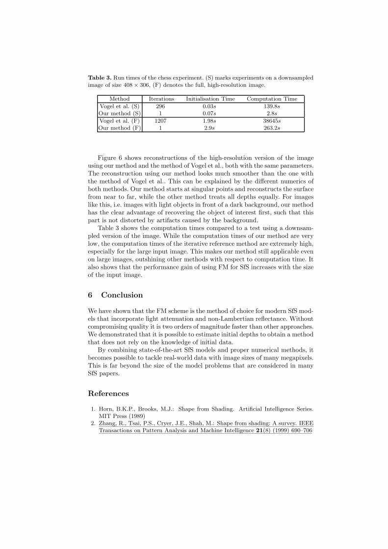
Table 3. Run times of the chess experiment. (S) marks experiments on a downsampledimage of size 408 × 306, (F) denotes the full, high-resolution image.

Method Iterations Initialisation Time Computation Time

Vogel et al. (S) 296 0.03s 139.8s

Our method (S) 1 0.07s 2.8s

Vogel et al. (F) 1207 1.98s 38645s

Our method (F) 1 2.9s 263.2s

Figure 6 shows reconstructions of the high-resolution version of the imageusing our method and the method of Vogel et al., both with the same parameters.The reconstruction using our method looks much smoother than the one withthe method of Vogel et al.. This can be explained by the different numerics ofboth methods. Our method starts at singular points and reconstructs the surfacefrom near to far, while the other method treats all depths equally. For imageslike this, i.e. images with light objects in front of a dark background, our methodhas the clear advantage of recovering the object of interest first, such that thispart is not distorted by artifacts caused by the background.

Table 3 shows the computation times compared to a test using a downsam-pled version of the image. While the computation times of our method are verylow, the computation times of the iterative reference method are extremely high,especially for the large input image. This makes our method still applicable evenon large images, outshining other methods with respect to computation time. Italso shows that the performance gain of using FM for SfS increases with the sizeof the input image.

6 Conclusion

We have shown that the FM scheme is the method of choice for modern SfS mod-els that incorporate light attenuation and non-Lambertian reflectance. Withoutcompromising quality it is two orders of magnitude faster than other approaches.We demonstrated that it is possible to estimate initial depths to obtain a methodthat does not rely on the knowledge of initial data.

By combining state-of-the-art SfS models and proper numerical methods, itbecomes possible to tackle real-world data with image sizes of many megapixels.This is far beyond the size of the model problems that are considered in manySfS papers.

References

1. Horn, B.K.P., Brooks, M.J.: Shape from Shading. Artificial Intelligence Series.MIT Press (1989)

2. Zhang, R., Tsai, P.S., Cryer, J.E., Shah, M.: Shape from shading: A survey. IEEETransactions on Pattern Analysis and Machine Intelligence 21(8) (1999) 690–706

3. Tankus, A., Sochen, N., Yeshurun, Y.: A new perspective [on] shape-from-shading.In: Proc. Ninth International Conference on Computer Vision. Volume 2. IEEEComputer Society Press, Nice, France (October 2003) 862–869

4. Tankus, A., Sochen, N., Yeshurun, Y.: Perspective shape-from-shading by fastmarching. In: Proc. 2004 IEEE Computer Society Conference on Computer Visionand Pattern Recognition. Volume 1. IEEE Computer Society Press, Washington,DC (June-July 2004) 43–49

5. Prados, E., Faugeras, O.: Shape from shading: A well-posed problem? In:Proc. 2005 IEEE Computer Society Conference on Computer Vision and PatternRecognition. Volume 2. IEEE Computer Society Press, San Diego, CA (June 2005)870–877

6. Ahmed, A., Farag, A.: A new formulation for shape from shading for non-Lambertian surfaces. In: Proc. 2006 IEEE Computer Society Conference on Com-puter Vision and Pattern Recognition. Volume 2. IEEE Computer Society Press,New York, NY (June 2006) 17–22

7. Oren, M., Nayar, S.: Generalization of the Lambertian model and implications formachine vision. International Journal of Computer Vision 14(3) (1995) 227–251

8. Vogel, O., Breuß, M., Weickert, J.: Perspective shape from shading with non-Lambertian reflectance. In Rigoll, G., ed.: Pattern Recognition. Volume 5096 ofLecture Notes in Computer Science. Springer, Berlin (June 2008) 517–526

9. Phong, B.T.: Illumination for computer-generated pictures. Communications ofthe ACM 18(6) (1975) 311–317

10. Tsitsiklis, J.N.: Efficient algorithms for globally optimal trajectories. IEEE Trans-actions on Automatic Control 40(9) (September 1995) 1528–1538

11. Sethian, J.A.: Level Set Methods and Fast Marching Methods. Second edn. Cam-bridge University Press, Cambridge, UK (1999)

12. Kimmel, R., Sethian, J.A.: Optimal algorithm for shape from shading and pathplanning. Journal of Mathematical Imaging and Vision 14(3) (2001) 237–244

13. Yuen, S.Y., Tsui, Y.Y., Chow, C.K.: Fast marching method for shape from shad-ing under perspective projection. In: Proceedings of the 2nd IASTED Interna-tional Conference on Visualization, Imaging and Image Processing, Malaga, Spain(September 2002) 584–589

14. Tankus, A., Sochen, N., Yeshurun, Y.: Shape-from-shading under perspective pro-jection. International Journal of Computer Vision 63(1) (June 2005) 21–43

15. Prados, E., Soatto, S.: Fast marching method for generic shape from shading. InParagios, N., Faugeras, O., Chan, T., Schnorr, C., eds.: Variational, Geometric,and Level Set Methods in Computer Vision. Volume 3752 of Lecture Notes inComputer Science. Springer (2005) 320–331

16. Yuen, S.Y., Tsui, Y.Y., Chow, C.K.: A fast marching formulation of perspectiveshape from shading under frontal illumination. Pattern Recognition Letters 28

(2007) 806–82417. Cristiani, E., Falcone, M., Seghini, A.: Some remarks on perspective shape-from-

shading models. In Sgallari, F., Murli, F., Paragios, N., eds.: Scale Space andVariational Methods in Computer Vision. Volume 4485 of Lecture Notes in Com-puter Science. Springer, Berlin (2007) 276–287

18. Vogel, O., Breuß, M., Weickert, J.: A direct numerical approach to perspectiveshape-from-shading. In Lensch, H., Rosenhahn, B., Seidel, H.P., Slusallek, P.,Weickert, J., eds.: Vision, Modeling, and Visualization. AKA, Berlin (November2007) 91–100