Digital Object Identifier (DOI):10.1007/s002850100100

J. Math. Biol. 43,377–396 (2001) Mathematical Biology

Sze-Bi Hsu · Tzy-Wei Hwang · Yang Kuang

Rich dynamics of a ratio-dependent one-preytwo-predators model

Received: 14 November 2000 / Revised version: 18 February 2001 /Published online: 19 September 2001 – c© Springer-Verlag 2001

Abstract. The objective of this paper is to systematically study the qualitative propertiesof a ratio-dependent one-prey two-predator model. We show that the dynamics outcome ofthe interactions are very sensitive to parameter values and initial data. Specifically, we showthe interactions can lead to all the following possible outcomes: 1) competitive exclusion;2) total extinction, i.e., collapse of the whole system; 3) coexistence in the form of positivesteady state; 4) coexistence in the form of oscillatory solutions; and 5) introducing a friendlyand better competitor can save a otherwise doomed prey species. These results reveal farricher dynamics compared to similar prey dependent models. Biological implications ofthese results are discussed.

1. Introduction

Generally, a predator-dependent predator-prey model takes the form{x′ = xg(x/K)− yP (x, y), x(0) > 0,y′ = cyP (x, y)− dy, y(0) > 0.

(1.1)

When P(x, y) = p(x/y), we call model (1.1) (strictly)ratio-dependent. The tra-ditional (or prey-dependent) model takes the form{

x′ = xg(x/K)− yp(x), x(0) > 0,y′ = cyp(x)− dy, y(0) > 0

(1.2)

Mathematically, we may think both the traditional prey-dependent and ratio-de-pendent models as limiting cases (c = 0 for the former and a = 0 for the latter)of the general Beddington-DeAngelis type predator-dependent functional response

S.-B. Hsu: Department of Mathematics, National Tsing Hua University, Hsinchu, Taiwan,R.O.C. Research supported by National Council of Science, Republic of China.

T.-W. Hwang: Department of Mathematics, Kaohsiung Normal University, 802, Kaohsiung,Taiwan, R.O.C. Research supported by National Council of Science, Republic of China.

Y. Kuang: Department of Mathematics, Arizona State University, Tempe, AZ 85287-1804,USA. Correspondence should be directed to this author: kuang@asu.edu. Work is partiallysupported by NSF grant DMS-0077790 and is initiated while visiting the National Centerfor Theoretical Science, Tsing Hua University, Hsinchu, Taiwan R.O.C.

Mathematics Subject Classification (2000) : 34D05, 34D20, 92D25

Key words or phrases: Ratio-dependent predator-prey model – Competitive exclusion –Extinction – Coexistence – Limit cycle

378 S.-B. Hsu et al.

P(x, y) = αx/(a+bx+cy)or the or Hassell-Varley typeP(x, y) = P(x/yγ ), γ ∈[0, 1]. (Beddington(1975), DeAngelis et al.(1975), Hassell and Varley(1969)). Thisview is also plausible biologically (Cosner et al.(1999)).

When p(x) = αx/(m+ x) and g(x/K) = r(1 − x/K), model (1.2) becomesthe following well studied Michaelis-Menten type predator-prey system (see thereferences cited in Kuang and Freedman(1988)).{

x′ = rx(1 − x/K)− αxy/(m+ x), x(0) > 0,y′ = y(−d + f x/(m+ x)), y(0) > 0

(1.3)

where r,K, α,m, f, d are positive constants and x(t), y(t) represent the populationdensity of prey and predator at time t respectively. The prey grows with intrinsicgrowth rate r and carrying capacity K in the absence of predation. The predatorconsumes the prey with functional response of Michaelis-Menten type cxy/(m+x)and contributes to its growth with rate f xy/(m+x). The constant d is the death rateof predator. This model exhibits the well-known “paradox of enrichment” observedby Hairston et al.(1960) and by Rosenzweig(1969) which states that according tomodel (1.3), enriching a predator-prey system (increasing the carrying capacityK)will cause an increase in the equilibrium density of the predator but not in thatof the prey, and will destabilize the positive equilibrium (the positive steady statechanges from stable to unstable as K increases). An equivalent paradox is the socalled “biological control paradox” which was recently brought into discussion byLuck (1990), stating that according to (1.3), we cannot have both a low and stableprey equilibrium density. However, in reality, there are numerous examples of suc-cessful biological control where the prey are maintained at densities less than 2%of their carrying capacities (Arditi and Berryman (1991)). This clearly indicatesthat the paradox of biological control is not intrinsic to predator-prey interactions.Another noteworthy prediction from model (1.3) is that prey and predator speciescan not extinct simultaneously (mutual extinction). This, however, contradicts Ga-use’s classic observation of mutual extinction in the protozoans, Paramecium and itspredator Didinium (Gause(1934), Luckinbill(1973), Abrams and Ginzburg(2000)),and the well cited experimental observation of Huffaker (Huffaker(1958)).

Until very recently, both ecologists and mathematicians chose to ignore therich dynamics provided by the strict ratio-dependent models, especially that on theboundary and close to the origin (the origin is a singular equilibrium, which rendersdirect local stability analysis impossible). Some researchers regard such interest-ing dynamics as “pathological behavior”. However, some empirical and theoreticalevidence (e.g., Akcakaya et al.(1995, Ecology)) suggests that such “pathologicalbehavior” is not only realistic, but the lack of such dynamics in prey-predatormodels actually makes them pathological in a biological sense. Recent efforts (Ku-ang and Beretta(1998), Kuang(1999), Jost et al.(1999)) show that the presupposed“pathological behavior” of solutions are not pathological at all. To see this pointmore clearly, consider the following example of “pathological behavior”. For ra-tio-dependent model, even if there is a positive steady state, both prey and predatorcan still go extinct (Kuang(1999)). The extinction (i.e., the collapse of the system)may occur in two distinct ways. One of the way is both species become extinctregardless of the initial densities, such as the Gause’s classic observation of mutual

Dynamics of a ratio-dependent model 379

extinction in the protozoans, Paramecium and its predator Didinium (Gause(1934),Abrams and Ginzburg(2000)). The other way is both species will die out only ifthe initial prey/predator ratio is too low. In the first case, extinction often occur as aresult of high predator efficiency in catching and/or converting prey biomass). Thesecond way has some subtle and interesting implications. For example, it indicatesthat altering the ratio of prey to predators through over-harvesting of prey species,or over-stocking of predators may lead to the collapse of the whole system and theextinction of both species.

It turns out that, in many aspects, the ratio-dependent models actually providethe richest dynamics, while the prey-dependent ones provide the least in dynam-ical behavior (Kuang and Beretta(1998), Jost et al.(1999), Hsu et al.(2001) andBerezovskaya et al.(2001)). Since the ratio-dependent form use one less parameterthan the Beddington-DeAngelis one, it is thus more appealing for both analyticaland experimental applications (Jost and Arditi(2000)).

During the period of between late eighties and late nineties, there is a muchheated debate on the validity of the ratio-dependent based population models(Ab-rams(1994, 1997), Abrams and Ginzburg(2000)) and there are still some legiti-mately controversial aspects of ratio-dependence (such controversies can be foundin Abrams and Ginzburg(2000)). A specific main controversial aspect is that welldocumented mechanistic justification of the ratio-dependent model (Cosner et al.(1999)) requires high population densities of both prey and predator species whilemost interesting dynamics of ratio-dependent models occurs near the origin. Thisis certainly a valid concern if the area of the population interaction is large (Arditiand Ginzburg (1989), Cosner et al. (1999)), Abrams and Ginzburg (2000)), since insuch case, predators will spend most effort in searching rather than interfering eachother. Hence, the functional response is likely to be much more sensible to preydensity than predator density. However, if the habitat is small and free of refugeesfor prey, then arguably, ratio dependence formulation may remain valid even whendensities are low, since predators can remain effectively interfering each other. Forvery small patch or field, even when the numbers of individuals of prey and preda-tors are low, their densities may remain high. In such case, ratio-dependence can bea valid model mechanism which suggests that mutual extinction is highly possible.This provides a simple and plausible explanation for Gause’s classic observationof mutual and deterministic extinction in the protozoans, Paramecium and its pre-dator Didinium (Abrams and Ginzburg (2000)). Indeed, deterministic extinctionof both species is, while an extreme outcome of the predator-prey interaction inthe field, is becoming ever more frequent and worrisome. The public believes thisresulted from the fragmentation of habitats and the ever shrinking sizes of thesepatches which may diminish or deprive of prey refugees (Fischer (2000)). Ratiodependence, while a special case of the general predator dependence ones (Bedd-ington-DeAngelis or Hassell-Varley type (Cosner et al.(1999)), is currently the onlyone that provides a simple and plausible support to such public view in additionto providing a plausible explanation of the success of biological controls (Ebertet al.(2000)).

The following Michaelis-Menten type ratio-dependent predator-prey systemwas studied extensively (Kuang and Beretta(1998), Jost et al.(1999), Hsu et al.(2001),

380 S.-B. Hsu et al.

Berezovskaya et al.(2001), and the references cited))

{x′ = rx(1 − x/K)− αxy/(my + x), x(0) > 0,y′ = y(−d + f x/(my + x)), y(0) > 0

(1.4)

where r,K, α,m, f, d are positive constants and x(t), y(t) represent the populationdensity of prey and predator at time t respectively. The prey grows with intrinsicgrowth rate r and carrying capacityK in the absence of predation. The predator con-sumes the prey with functional response of Michaelis-Menten type cxy/(my + x)and contributes to its growth with rate f xy/(my + x). The constant d is the deathrate of predator. It is straightforward to generalize the above two species model tothe situation when one prey species shared by two competing predator species. Thisresults in the following three species strict ratio-dependent predator-prey model

x′ = rx(1 − x

K)− c1xy1

a1x + y1 +my2− c2xmy2

a2x + y1 +my2

y′1 = y1(−d1 + e1c1x

a1x + y1 +my2)

y′2 = y2(−d2 + e2c2mx

a2x + y1 +my2).

(1.5)

Here the meanings of r,K are obvious and c1, c2 are searching efficiency constants.m is the relative predation rate of y2 with respect to y1. c1/a1, c2m/a2 describesthe maximum per-capita capturing rate for y1, y2 respectively. e1, e2 are conversionrates and d1, d2 are death rates. This model can also be formally derived from thegeneral multi-species ratio-dependent model construction procedures proposed inArditi and Michalski(1996).

Our analysis on this ratio-dependent one prey-two predators model revealsmany new and interesting dynamics. While competitive exclusion principle stillhold for most parameter values for the competing predators, it is very often that wesee both can go extinct as either the result of the parameter values or the selectionof initial data. In fact, for certain choices of parameters and initial values, even theprey species can go extinct, which in turn cause the extinction of both predators.Still, for some parameter values, coexistence is possible in both the forms of pos-itive steady state and oscillatory solutions. Most surprisingly, we show that whena predator is capable of driving the prey and itself to extinction, the introductionof a predator which is more friendly (to prey) and is a stronger (compared to theexisting one) competitor may save the prey species.

2. The preliminary results

It is convenient to scale the variables. Let x = x/K, y1 = y1, y2 = my2, c1 =c1, c2 = c2, a1 = a1K, a2 = a2K, e1 = e1K, e2 = e2Km. Making these changesand dropping the bars from the resulting equations yields the following system

Dynamics of a ratio-dependent model 381

without K and m.

x′ = rx(1 − x)− c1xy1

a1x + y1 + y2− c2xy2

a2x + y1 + y2= X(x, y1, y2)

y′1 = y1(−d1 + e1c1x

a1x + y1 + y2) = Y1(x, y1, y2)

y′2 = y2(−d2 + e2c2x

a2x + y1 + y2) = Y2(x, y1, y2)

(2.1)

We consider only the biologically meaningful initial condition

x(0) ≥ 0, y1(0) ≥ 0, y2(0) ≥ 0.

Due to the boundedness of the functional responses, we see that

lim(x,y1,y2)→(0,0,0)

X(x, y1, y2) = lim(x,y1,y2)→(0,0,0)

Y1(x, y1, y2)

= lim(x,y1,y2)→(0,0,0)

Y2(x, y1, y2) = 0.

Hence, if we let X(0, 0, 0) = Y1(0, 0, 0) = Y2(0, 0, 0) = 0, then these functionare continuous on R3+ = {(x, y1, y2) : x ≥ 0, y1 ≥ 0, y2 ≥ 0}. Indeed, straightfor-ward computation shows that they are Lipschizian on R3+. Hence solution of (2.1)with nonnegative initial condition exists and is unique. It is also easy to see thatthese solutions exist for all t > 0 and stay nonnegative. In fact, if x(0) > 0, thenx(t) > 0 for all t > 0. Same is true for y1 and y2 components. Hence, the interiorof R3+ is invariant for model (2.1).

Observe thatx′ ≤ rx(1 − x),

which implies thatlimt→∞ sup x(t) ≤ 1.

This implies that for any 0 < ε < 1, we have x(t) < 1 + ε for large t. Let

d = min{d1, d2}.

We have

x′ + y′1/e1 + y′

2/e2 = rx(1 − x)− (d1/e1)y1 − (d2/e2)y2≤ (r + d)x − d(x + y1/e1 + y2/e2).

This leads to

limt→∞ sup(x(t)+ y1(t)/e1 + y2(t)/e2) ≤ (r + d)/d. (2.2)

Hence we have shown that model (2.1) is dissipative. It is also straightforwardto show that the first and second derivatives of x, y1, y2 are all continuous andbounded.

382 S.-B. Hsu et al.

3. Competitive exclusion: extinction of at least one predator

Observe that if e1c1 ≤ a1d1, then for positive solutions,

y′1 = −y1((a1d1 − e1c1)x + d1y1 + d1y2)/(a1x + y1 + y2)) < 0.

Clearly y1(t) is strictly decreasing and hence it must tend to a nonnegative constant,say y10. Since the model is dissipative, we have a positive constant, say M, suchthat for large time, say for t > t0 > 0, a1x + y1 + y2 < M. If y10 �= 0, then thereis a t1 > t0, such that for t > t1, we have y1(t) > y10/2. Hence, for t > t1, wehave

y′1 < −d1y10

2My1

which implies that limt→∞ y1(t) = 0 �= y10.This contradiction shows that we musthave y10 = 0. Similar statement can be made for the y2 species. We summarize theabove argument as the following theorem.

Lemma 3.1. Consider (2.1). If e1c1 ≤ a1d1, then limt→∞ y1(t) = 0. If e2c2 ≤a2d2, then limt→∞ y2(t) = 0.

The next theorem is the result of the application of a comparison argument.

Theorem 3.1. If a2 ≥ a1 and

e1c1

d1− a1 >

e2c2

d2− a2 > 0, (3.1)

in (2.1), then limt→∞ y2(t) = 0.

Proof. We assume that (3.1) holds true. Let z = y1 + y2 and θ > 0 to be deter-mined. We have

θy′

2

y2− y′

1

y1= P(x, z)

(a1x + z)(a2x + z)

where

P(x, z) = θ(a1x + z)((e2c2 − a2d2)x − d2z)−(a2x + z)((e1c1 − a1d1)x−d1z)

= [a1θ(e2c2 − a2d2)− a2(e1c1 − a1d1)]x2 + (d1 − d2θ)z

2

+[θ(e2c2 − a2d2 − a1d2)− (e1c1 − a1d1 − a2d1)]xz

= A(θ)x2 + B(θ)xz+ C(θ)z2. (3.2)

The discriminant of (3.2) is

#(θ) = [θ(e2c2 − a2d2 − a1d2)− (e1c1 − a1d1 − a2d1)]2 − 4[a1θ(e2c2 − a2d2)

−a2(e1c1 − a1d1)](d1 − d2θ)

= θ2(e2c2 − a2d2 − a1d2)2 + (e1c1 − a1d1 − a2d1)

2

−2θ(e2c2 − a2d2 − a1d2)(e1c1 − a1d1 − a2d1)+ 4a1d2(e2c2 − a2d2)θ2

−4θ [a1d1(e2c2 − a2d2)+ a2d2(e1c1 − a1d1)] + 4a2d1(e1c1 − a1d1)

= θ2((e2c2 − a2d2)+ a1d2)2 + ((e1c1 − a1d1)+ a2d1)

2

Dynamics of a ratio-dependent model 383

−2θ [(e2c2 − a2d2)− a1d2)((e1c1 − a1d1)− a2d1)

+2a1d1(e2c2 − a2d2)+ 2a2d2(e1c1 − a1d1)]

= [θ(e2c2 − a2d2 + a1d2)− ((e1c1 − a1d1 + a2d1)]2

−2θ [−2a2d1(e2c2 − a2d2)

−2a1d2(e1c1 − a1d1)+ 2a1d1(e2c2 − a2d2)+ 2a2d2(e1c1 − a1d1)]

= [θ(e2c2 − a2d2 + a1d2)− ((e1c1 − a1d1 + a2d1)]2

+4θ(a1 − a2)d1d2[(e1c1

d1− a1)− (

e2c2

d2− a2)].

We chose

θ = θ∗ = e1c1 − a1d1 + a2d1

e2c2 − a2d2 + a1d2> 0.

Then, from (3.1) and the fact that a2 ≥ a1, we see that

#(θ∗) = 4θ∗(a1 − a2)d1d2[(e1c1

d1− a1)− (

e2c2

d2− a2)] ≤ 0.

Notice that #(θ∗) = 0 if and only if a1 = a2.

We now would like to determine the signs of the coefficients of x2 and z2 in(3.2). For the coefficient of x2, we have

A(θ∗) = a1θ∗(e2c2 − a2d2)− a2(e1c1 − a1d1)

= 1

e2c2 − a2d2 + a1d2[a1(e2c2 − a2d2)(e1c1 − a1d1 + a2d1)

−a2(e2c2 − a2d2 + a1d2)(e1c1 − a1d1)]

= 1

e2c2 − a2d2 + a1d2[(a1 − a2)(e1c1 − a1d1)(e2c2 − a2d2)

−a1a2d1d2[(e1c1

d1− a1)− (

e2c2

d2− a2)] < 0.

For the coefficient of z2, we have

C(θ∗) = d1−d2θ∗ = −d1d2

e2c2 − a2d2 + a1d2[(e1c1

d1−a1)−(e2c2

d2−a2)+a2−a1] < 0.

Therefore P(x, z) ≤ 0. Since #(θ∗) = 0 if and only if a1 = a2, in which case wehave the coefficient of xz

B(θ∗) = θ∗(e2c2 − a2d2 − a1d2)− (e1c1 − a1d1 − a2d1)

= 2

e2c2 − a2d2 + a1d2[a2d1(e2c2 − a2d2)− a1d2(e1c1 − a1d1)]

= 2

e2c2 − a2d2 + a1d2a1d1d2(e2c2/d2 − e1c1/d1) < 0.

Hence, P(x, z) = 0 if and only if one of the following is true:i): #(θ∗) < 0 and hence x = z = 0;ii): #(θ∗) = 0 and hence a1 = a2 and (−A(θ∗))1/2x = −(−C(θ∗))1/2z.

384 S.-B. Hsu et al.

Since x ≥ 0, z ≥ 0,we see that (ii) also leads to x = z = 0. Clearly, z = 0 impliesthat y1 = y2 = 0. In summary, we have shown that

P(x, z) = 0 implies that x = y1 = y2 = 0. (3.3)

Consider now a Liapunov function of the form

V = V (x, y1, y2) = yθ∗

2

y1.

Then

dV/dt = VP (x, z)

(a1x + z)(a2x + z)≤ 0.

dV/dt = 0 if and only if y2 = 0 or P(x, z) = 0. Since P(x, z) = 0 also im-plies that y2 = 0, we thus have dV/dt = 0 if and only if y2 = 0. The standardLiapunov-LaSalle theorem implies that

limt→∞ y2(t) = 0.

This proves the theorem. �Observe that when y′

i = 0, we have

x = y1 + y2

eici/di − ai, i = 1, 2.

Hence, (3.1) simply states that predator 1 has a lower break-even prey density re-quirement than predator 2. In the rest of this paper, we say predator i is a strongerpredator than predator j , if i �= j, and

aj ≥ ai andeici

di− ai >

ej cj

dj− aj > 0. (3.4)

To conclude this section, we point out that in order to have (x, y1, y2)→(x∗, y∗

1 , 0), it is necessary to have

e1c1/d1 − a1 ≥ e2c2/d2 − a2.

This suggests that Theorem 3.1 is reasonably sharp. To see this, suppose(x, y1, y2)→(x∗, y∗

1 , 0). Then

d1 = (e1c1x∗)/(a1x

∗ + y∗1 )

andd2 ≥ (e2c2x

∗)/(a2x∗ + y∗

1 )

Thend1/(e1c1) = x∗/(a1x

∗ + y∗1 )

andd2/(e2c2) ≥ x∗/(a2x

∗ + y∗1 )

Hencee1c1/d1 − a1 = y∗

1/x∗ ≥ e2c2/d2 − a2.

Dynamics of a ratio-dependent model 385

4. System saver

We say a predator is a system destroyer if left alone with a prey population, itdrives both itself and the prey to extinction (forming a collapsing predator-preyinteraction). For example, according to Theorem 2.6 of Kuang and Beretta(1998),if

eici/ai > dici/(ci − r), ci > r, i = 1, 2,

then predator i is a system destroyer. We say a predator is a system saver if itsintroduction to a collapsing predator-prey system can prevent the prey from goingextinct. The main objective of this section is to show that system savers do exist.

Theorem 4.1. If a2 ≤ min{a1, e2} and

e1c1/a1 > d1c1/(c1 − r), c1 > r, (4.1)

e2c2

d2− a2 >

e1c1

d1− a1 > 0, (4.2)

x∗ = 1 − c2

r(1 − a2d2

e2c2) > 0, (4.3)

in (2.1), then the boundary steady state E2 := (x∗, 0, y∗2 ), where y∗

2 = (e2c2/d2 −a2)x

∗, is locally asymptotically stable. Therefore, predator 2 is a system saver.

Proof. Direct computation shows that the variational matrix atE2 isA = (aij )3×3,

where

a11 = x∗(−r + c2a2y∗2#

−2),

a13 = −c2a2(x∗)2#−2,

a21 = a23 = 0,

a22 = −d1 + e1c1x∗#−1 = d1[(e1c1/d1 − a1)x

∗ − y∗2 ]#−1 < 0,

a31 = e2c2(y∗2/#)

2,

a33 = e2c2x∗y∗

2#−2

# = a2x∗ + y∗

2 = e2c2x∗/d2.

Since a21 = a23 = 0, we see that to determine the local asymptotical stability ofE2, it is sufficient to study that of

A22 =[a11 a13a31 a33

]. (4.4)

We have

det(A22) = re2c2(x∗)2y∗

2/#−2 > 0

tr(A22) = −rx∗ + c2x∗y∗

2 (a2 − e2)#−2 < 0.

This together with a22 < 0 imply that E2 is locally asymptotically stable. �It is obvious that the above theorem remains true if we replace the simple con-

dition of a2 ≤ e2 by the sharper but more complicated one of tr(A22) = −rx∗ +

386 S.-B. Hsu et al.

c2x∗y∗

2 (a2 − e2)#−2 < 0. Condition (4.3) simply ensures that prey species can

coexist with predator 2 alone.Figure 1 illustrates an example where predator 1 is a destroyer and Figure 2

shows that for this destroyer, predator 2 is a system saver. Here a1 = a2 = d1 =d2 = 1, c1 = 2.800, c2 = 1.800, e1 = 0.536, e2 = 1. For this set of parameters,solutions are very sensitive to initial population values. If initial value of predator1 is too large, or initial value of prey is too small, total extinction is the outcome.

5. Total extinction

In this section, we consider the possibility of total extinction in model (2.1). Thiscan happen through many ways. For an example, the addition of a system destroy-er which is also a stronger competitor will eliminate the competitor and the preyspecies, leading to total extinction of the system. This is simply the result of ourTheorem 3.1 and Theorem 2.6 of Kuang and Beretta(1998). Explicit conditions interm of model parameters for this to happen can be easily obtained. This forms thefollowing theorem.

Theorem 5.1. If a2 ≥ a1 and

e1c1/a1 > d1c1/(c1 − r), c1 > r, (5.1)

Fig. 1. This figure shows the solution of (2.1) when r = 1, a1 = a2 = d1 = d2 = 1, c1 =2.800, c2 = 1.800, e1 = 0.536, e2 = 1, x(0) = 1, y1(0) = 0.1, y2(0) = 0.The top curve (atthe beginning) depicts prey species and the bottom curve (at the beginning) depicts predator1. Clearly, predator 1 is a destroyer.

Dynamics of a ratio-dependent model 387

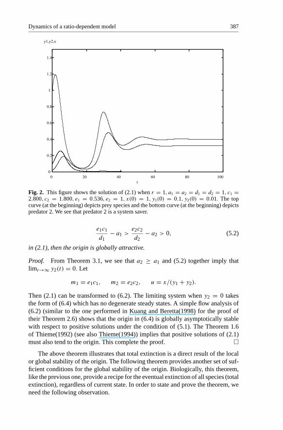
Fig. 2. This figure shows the solution of (2.1) when r = 1, a1 = a2 = d1 = d2 = 1, c1 =2.800, c2 = 1.800, e1 = 0.536, e2 = 1, x(0) = 1, y1(0) = 0.1, y2(0) = 0.01. The topcurve (at the beginning) depicts prey species and the bottom curve (at the beginning) depictspredator 2. We see that predator 2 is a system saver.

e1c1

d1− a1 >

e2c2

d2− a2 > 0, (5.2)

in (2.1), then the origin is globally attractive.

Proof. From Theorem 3.1, we see that a2 ≥ a1 and (5.2) together imply thatlimt→∞ y2(t) = 0. Let

m1 = e1c1, m2 = e2c2, u = x/(y1 + y2).

Then (2.1) can be transformed to (6.2). The limiting system when y2 = 0 takesthe form of (6.4) which has no degenerate steady states. A simple flow analysis of(6.2) (similar to the one performed in Kuang and Beretta(1998) for the proof oftheir Theorem 2.6) shows that the origin in (6.4) is globally asymptotically stablewith respect to positive solutions under the condition of (5.1). The Theorem 1.6of Thieme(1992) (see also Thieme(1994)) implies that positive solutions of (2.1)must also tend to the origin. This complete the proof. �

The above theorem illustrates that total extinction is a direct result of the localor global stability of the origin. The following theorem provides another set of suf-ficient conditions for the global stability of the origin. Biologically, this theorem,like the previous one, provide a recipe for the eventual extinction of all species (totalextinction), regardless of current state. In order to state and prove the theorem, weneed the following observation.

388 S.-B. Hsu et al.

Lemma 5.1. Assume e1c1 > a1d1, and e2c2 > a2d2. Let Sx, Sy1 , Sy2 be the iso-surfaces defined by X(x, y1, y2) = 0, Y1(x, y1, y2) = 0, Y2(x, y1, y2) = 0, re-spectively. If ((Sx ∩ Sy1)∪ (Sx ∩ Sy2))∩R3+ = (0, 0, 0), then all positive solutionsof model (2.1) tend to the origin.

Proof. The condition of ((Sx ∩ Sy1) ∪ (Sx ∩ Sy2)) ∩ R3+ = (0, 0, 0) implies thatin R3+, Sx does not intersect with Sy1 or Sy2 except at the origin. It is easy to seethat Sy1 is the plane defined by d−1

1 (e1c1 − a1d1)x = y1 + y2 and Sy2 is the planedefined by d−1

2 (e2c2 − a2d2)x = y1 + y2. Observe that Sx intersect the x-axis at(0, 0, 0) and (K, 0, 0). If we view the x-axis as a vertical axis and y1- and y2-axesas ground ones, then the condition of ((Sx ∩Sy1)∪ (Sx ∩Sy2))∩R3+ = (0, 0, 0) im-plies that Sx sits above both Sy1 and Sy2 .Hence, if (x1, y1, y2) ∈ Sy1 , (x2, y1, y2) ∈Sy2 , (x3, y1, y2) ∈ Sx, then x3 > max{x1, x2}. Without loss of generality, we mayassume that

d−11 (e1c1 − a1d1) > d

−12 (e2c2 − a2d2).

We see that if (x1, y1, y2) ∈ Sy1 , (x2, y1, y2) ∈ Sy2 then we have x1 < x2. Thesetogether imply that if (x1, y1, y2) ∈ Sy1 , (x2, y1, y2) ∈ Sy2 , (x3, y1, y2) ∈ Sx, thenx3 > x2 > x1. If we divide the interior of R3+ into four separate regions:

R1 = {(x, y1, y2) : x > 0, y1 > 0, y2 > 0, x′ > 0, y′1 > 0, y′

2 > 0}

R2 = {(x, y1, y2) : x > 0, y1 > 0, y2 > 0, x′ ≤ 0, y′1 > 0, y′

2 > 0}

R3 = {(x, y1, y2) : x > 0, y1 > 0, y2 > 0, x′ ≤ 0, y′1 > 0, y′

2 ≤ 0}

R4 = {(x, y1, y2) : x > 0, y1 > 0, y2 > 0, x′ ≤ 0, y′1 ≤ 0, y′

2 ≤ 0}.A simple flow analysis shows that solutions starting in R1 enters R2 in finite time,and then in finite time it enters R3, and then in finite time enters R4. The processof boundary crossing resembles an one way traffic and the sequence is alwaysR1→R2→R3→R4. Once enters R4, it stays there. The monotonicity of all thecomponents of the solution and the fact that R4 contains no steady state ensuresthat the solution tends to the origin.

If d−11 (e1c1 − a1d1) = d−1

1 (e2c2 − a2d2), then Sy1 = Sy2 , in which case, wesee that our proof above can be adapted to deal with it. �

We are now ready to give explicit conditions for model (2.1) to exhibit totalextinction as the result of the global stability of the origin.

Theorem 5.2. Assume that min{c1, c2} > r, and

max{ d1

e1c1 − a1d1,

d2

e2c2 − a2d2} ≤ min{c1 − r

ra1,c2 − r

ra2}. (5.3)

Then the origin is globally attractive for model (2.1).

Dynamics of a ratio-dependent model 389

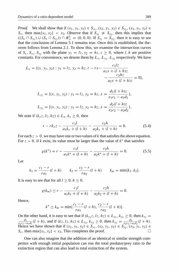
Proof. We shall show that if (x1, y1, y2) ∈ Sy1 , (x2, y1, y2) ∈ Sy2 , (x3, y1, y2) ∈Sx, then max{x1, x2} < x3. Observe that if Sy1 �= Sy2 , then this implies that((Sx ∩ Sy1) ∪ (Sx ∩ Sy2)) ∩ R3+ = (0, 0, 0). If Sy1 = Sy2 , then it is easy to seethat the conclusion of Lemma 5.1 remains true. Once this is established, the the-orem follows from Lemma 2.1. To show this, we examine the intersection curvesof Sx, Sy1 , Sy2 with the plane y1 = lz, y2 = hz, z ≥ 0, where l, h are positiveconstants. For convenience, we denote them byLx,Ly1 , Ly2 respectively. We have

Lx = {(x, y1, y2) : y1 = lz, y2 = hz, r − rx− c1lz

a1x + (l + h)z

− c2hz

a2x + (l + h)z= 0},

Ly1 = {(x, y1, y2) : y1 = lz, y2 = hz, x = d1(l + h)z

e1c1 − a1d1},

Ly2 = {(x, y1, y2) : y1 = lz, y2 = hz, x = d2(l + h)z

e2c2 − a2d2}.

We note if (kxz, lz, hz) ∈ Lx, kx ≥ 0, then

r − rkxz− c1l

a1kx + (l + h)− c2h

a2kx + (l + h)= 0. (5.4)

For each z > 0,we may have one or two values of k that satisfies the above equation.For z > 0, if k exist, its value must be larger than the value of k∗ that satisfies

g(k∗) = r − c1l

a1k∗ + (l + h)− c2h

a2k∗ + (l + h)= 0. (5.5)

Let

k1 = c1 − r

ra1(l + h) k2 = c2 − r

ra2(l + h) km = min{k1, k2}.

It is easy to see that for all l ≥ 0, h ≥ 0,

g(km) ≤ r − c1l

a1k1 + (l + h)− c2h

a2k2 + (l + h)= 0.

Hence,

k∗ ≥ km = min{c1 − r

ra1(l + h),

c2 − r

ra2(l + h)}.

On the other hand, it is easy to see that if (ky1z, lz, hz) ∈ Ly1 , ky1 ≥ 0, then ky1 =d1

e1c1−a1d1(l + h), and if (kz, lz, hz) ∈ Ly2 , ky2 ≥ 0, then ky2 = d2

e2c2−a1d2(l + h).

Hence we have shown that if (x1, y1, y2) ∈ Sy1 , (x2, y1, y2) ∈ Sy2 , (x3, y1, y2) ∈Sx, then max{x1, x2} < x3. This completes the proof. �

One can also imagine that the addition of an identical or similar strength com-petitor with enough initial population can rise the total predator/prey ratio to theextinction region that can also lead to total extinction of the system.

390 S.-B. Hsu et al.

6. Coexistence

It is easy to observe that system (2.1) does not admit an isolated positive steadystate. So, coexistence in the form of asymptotically stable positive steady state isimpossible. System (2.1) admits degenerate positive steady states (steady state thathas zero as one of its eigenvalue) only when

e1c1

d1− a1 = e2c2

d2− a2. (6.1)

One can easily see that degenerate positive steady states are positive solutions of

r(1 − x) = c1xy1

a1x + y1 + y2+ c2xy2

a2x + y1 + y2

d1 = e1c1x

a1x + y1 + y2.

Numerical simulations show (e.g., Figure 3) that under (6.1), positive solutions allquickly tend to one of these degenerate positive steady states that dependent oninitial conditions.

The main objective in this section is to show both analytically and numerical-ly that for some range of parameters, all three species can coexist in the form ofoscillatory solutions. The method is the now standard approach (e.g., Smith and

Fig. 3. This figure shows the solution of (2.1) when r = 1, a1 = a2 = d1 = d2 = 1, c1 =0.700, c2 = 0.800, e1 = 2.143, e2 = 2.250, x(0) = 1, y1(0) = 0.200, y2(0) = 1.500. Thesolution tends to a degenerate steady state.

Dynamics of a ratio-dependent model 391

Waltman (1995), p65) of finding conditions that can lift a nontrivial positive peri-odic solution on the boundary, say x − y1 plane (assume it exists) to the interior ofthe three dimensional positive cone. To facilitate this presentation, we first wouldlike to transform the system (2.1). Let

m1 = e1c1, m2 = e2c2, u = x/(y1 + y2).

Then (2.1) can be transformed to

u′ = −ru2(y1 + y2)+ y1

y1 + y2g1(u)+ y2

y1 + y2g2(u)

y′1 = y1(−d1 + m1u

a1u+ 1)

y′2 = y2(−d2 + m2u

a2u+ 1)

(6.2)

where

gi(u) = u

aiu+ 1(Aiu+Bi), Ai = rai−mi+diai, Bi = r−ci+di i = 1, 2.

(6.3)In the rest of this section, we assume that (3.1) holds and a2 < a1. Let

λi = di/(mi − diai), i = 1, 2.

Recall that Theorem 3.1 shows that if 0 < λ1 < λ2 and a2 ≥ a1, then limt→∞ y2(t)

= 0. Consider for the moment the boundary system{u′ = −ru2y1 + g1(u)

y′1 = y1(−d1 + m1u

a1u+ 1)

(6.4)

Hopf bifurcation Theorem and Theorem 2.9 of Hsu et al. (2000) together implythat if A1 > 0, B1 < 0 and λ1 is near and less than θ1, where θ1 is the point wherethe prey isocline y1 = g1(u)/(ru

2) attains its maximum, then there is a uniquelimit cycle on the boundary (u − y1 plane) /∗ = {(u∗(t), y∗

1 (t)) : 0 ≤ t ≤ T1}.In order to obtain the coexistence of species y1 and y2, it is convenient to selectb2 := m2/d2 as a bifurcation parameter and study the possibility of the bifurcationof limit cycle / = {(u∗(t), y∗

1 (t), 0) : 0 ≤ t ≤ T1} into the positive octant.

Theorem 6.1. In system (6.2), let 0 < λ1 < λ2 and a2 < a1. Then there existsb∗

2, a2 < b∗2 < a2 − a1 +m1/d1 such that for b2 = m2/d2 sufficiently close to b∗

2,

system (6.2) has a periodic orbit inside the positive octant near the u− y1 plane.

Proof. We observe that the condition 0 < λ1 < λ2 is equivalent to

b2 = m2/d2 < a2 − a1 +m1/d1.

/ is a stable (unstable) limit cycle if∫ T1

0

u∗(t)− λ2

a2u∗(t)+ 1dt < 0 (> 0).

392 S.-B. Hsu et al.

Notice that∫ T1

0(m2u

∗(t)a2u∗(t)+ 1

− d2)dt = (m2 − d2a2)

∫ T1

0

u∗(t)− λ2

a2u∗(t)+ 1dt.

Let

µ(b2) = 1

T1

∫ T1

0

b2u∗(t)

a2u∗(t)+ 1dt.

Then, / is stable (unstable) if µ(b2) < 1(µ(b2) > 1). Clearly, µ(b2) is strictlyincreasing in b2 and µ(a2) < 1. In order to show that there exists b∗

2, a2 < b∗2 <

a2 − a1 +m1/d1 such that µ(b∗2) = 1, it suffices to show that for b2 = a2 − a1 +

m1/d1, µ(b2) > 1.Equivalently, whenλ1 = λ2 = λ, we have∫ T1

0u∗(t)−λ2a2u

∗(t)+1dt > 0.Since ∫ T1

0

u∗(t)− λ1

a1u∗(t)+ 1dt = 0,

we have∫ T1

0

u∗(t)− λ2

a2u∗(t)+ 1dt =

∫ T1

0

u∗(t)− λ2

a2u∗(t)+ 1dt − η

∫ T1

0

u∗(t)− λ1

a1u∗(t)+ 1dt

=∫ T1

0(u∗(t)− λ)

[1

a2u∗(t)+ 1− η

a1u∗(t)+ 1

]dt

= (a1 − a2η)

∫ T1

0

(u∗(t)− λ)(u∗(t)− η−1a1−a2η

)

(a1u∗(t)+ 1)(a2u∗(t)+ 1)dt.

Let η = 1+λa11+λa2

. Due to the assumption of a1 > a2, we see that

a1 − a2η = a1 − a2

1 + λa2> 0.

Hence ∫ T1

0

u∗(t)− λ2

a2u∗(t)+ 1dt =

∫ T1

0

(a1 − a2η)(u∗(t)− λ)2

(a1u∗(t)+ 1)(a2u∗(t)+ 1)dt > 0.

That is, µ(b2) > 1. This shows that there exists b∗2, a2 < b∗

2 < a2 − a1 + m1/d1such that µ(b∗

2) = 1. From Theorem 7.1 of Smith and Waltman (1995)(p65), wesee that for b2 close to b∗

2, system (6.2) has a periodic orbit in the positive octantnear the u− y1 plane. �

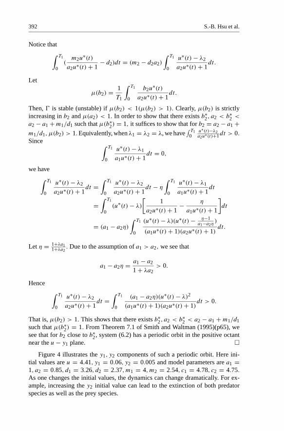
Figure 4 illustrates the y1, y2 components of such a periodic orbit. Here ini-tial values are u = 4.41, y1 = 0.06, y2 = 0.005 and model parameters are a1 =1, a2 = 0.85, d1 = 3.26, d2 = 2.37,m1 = 4,m2 = 2.54, c1 = 4.78, c2 = 4.75.As one changes the initial values, the dynamics can change dramatically. For ex-ample, increasing the y2 initial value can lead to the extinction of both predatorspecies as well as the prey species.

Dynamics of a ratio-dependent model 393

Fig. 4. This figure shows the y1, y2 components of a periodic orbit of system (6.2). Hereinitial values are u = 4.41, y1 = 0.06, y2 = 0.005 and model parameters are r = 1, a1 =1, a2 = 0.85, d1 = 3.26, d2 = 2.37,m1 = 4,m2 = 2.54, c1 = 4.78, c2 = 4.75.

Remark 6.1. If 0 < λ1 < λ2, a1 < a2, then from Theorem 3.1, we see thatlim y2→0 as t→∞. Under these conditions, the proof of Theorem 6.1 also showsthat

∫ T1

0

u∗(t)− λ2

a2u∗(t)+ 1dt =

∫ T1

0

(a1 − a2η)(u∗(t)− λ)2

(a1u∗(t)+ 1)(a2u∗(t)+ 1)dt < 0

since

a1 − a2η = a1 − a2

1 + λa2< 0.

Hence µ(b2) < 1 for all

b2 = m2/d2 < a2 − a1 +m1/d1,

which is equivalent to say that / is stable. This is consistent with Theorem 3.1.

7. Discussion

Our systematical work on system (2.1) reveals that the ratio-dependent model isricher in boundary dynamics (extinction dynamics) compare to the prey-dependent

394 S.-B. Hsu et al.

one

x′ = rx(1 − x)− c1xy1

x + a1− c2xy2

x + a2

y′1 = y1(−d1 + e1c1x

x + a1)

y′2 = y2(−d2 + e2c2x

x + a2).

(7.1)

This prey-dependent model resembles the chemostat model with two competingpredator species (Butler et al.(1983), Smith and Waltman(1995)). It can be shownsimilarly that it produces competitive exclusion and possibly coexistence similarto the ones for (2.1) (Hsu et al.(1978a, b)), but can not generate total extinctionand can not exhibit the system saver phenomenon due to the lack of degeneracy atorigin. In general, the above model has a limiting dynamics of a two-dimensionalpredator-prey model reduced from itself.

Mathematically and biologically (Cosner et al.(1999)), both (2.1) and (7.1) canand should be viewed as limiting cases of the more realistic Beddington-DeAngelisone

x′ = rx(1 − x)− c1xy1

x + a1 + b1(y1 + y2)− c2xy2

x + a2 + b2(y1 + y2)

y′1 = y1(−d1 + e1c1x

x + a1 + b1(y1 + y2))

y′2 = y2(−d2 + e2c2x

x + a2 + b2(y1 + y2)),

(7.2)

Again, due to the lack of degeneracy at the origin in model (7.2) when a1 > 0 anda2 > 0, we observe that it also will not produce the above mentioned extinctiondynamics. Still, we can speculate that such extinction dynamics can be viewed asthe possible approximate scenario of model (7.2) when a1 and a2 are small andother relevant conditions are met, and can ultimately be brought into reality whenstochastic events are taken into account. Due to the competitive exclusion outcome,neither of these models are expected to generate chaotic solutions.

Another striking phenomenon that can often be observed in simulation workof model (2.1) is its highly sensitivity on initial population levels, especially whenthese levels are relatively low. This is also not shared by either (7.1) or (7.2).

A recent finding of Jost and Arditi(2000) shows that prey-dependent and ra-tio-dependent model can fit well with the time series generated by each other.Interestingly, the ratio-dependent time series reportedly were always more reliablyidentified. This together with our analysis of (2.1) in this paper and previous worksuggest that ratio-dependent models are more flexible and versatile.

We would like to point out here that our analysis of model (2.1), while coversmany aspects, is far from complete. Many questions of the dynamics of this mod-el remain untouched. For example, it is unclear at this moment whether or not asystem saver can save both the ailing prey and predator species in an collapsingpredator-prey interaction. Most of our results provide sets of sufficient conditionsfor various dynamical scenarios to occur. It will be interesting both mathematical-ly and biologically to know what kind of necessary conditions for such dynamics

Dynamics of a ratio-dependent model 395

behaviors. For example, assume that we know if scenario A dynamics takes place,then condition set B must be met. Assume further that we can manage to violatecondition set B, then we can avoid scenario A dynamics. In some special cases,such necessary conditions are easy to obtain. A more systematic and completecoverage of such necessary conditions is likely to be a nontrivial task. Naturally,these interesting topics should be pursued in the future. It is also easy to see thatthere is room for the improvement of our various sufficient conditions. In short, weknow model (2.1) is capable of generating rich and new dynamics, but its detailedqualitative and general dynamical picture remains to be seen.

Acknowledgements. The authors would like to thank the referees for their helpful sugges-tions that improved the presentation of this manuscript.

References

Abrams, P.A.: The fallacies of “ratio-dependent” predation, Ecology, 75, 1842–1850 (1994)Abrams, P.A.: Anomalous predictions of ratio-dependent models of predation, OKIOS, 80,

163–171 (1997)Abrams, P.A., Ginzburg, L.R.: The nature of predation: prey dependent, ratio-dependent or

neither? TREE, 15, 337–341 (2000)Akcakaya, H.R., Arditi, R., Ginzburg, L.R.: Ratio-dependent prediction: an abstraction that

works, Ecology, 76, 995–1004 (1995)Arditi, R., Berryman, A.A.: The biological paradox, Trends in Ecology and Evolution 6, 32

(1991)Arditi, R., Michalski, J.: Nonlinear food web models and their response to increased basal

productivity, in Food webs: Integration of Patterns and Dynamics, eds. G. A. Polis andK. O. Winemiller, pp122–133, Chapman and Hall, New York (1996)

Arditi, R., Ginzburg, L.R.: Coupling in predator-prey dynamics: ratio-dependence, J. Theor.Biol., 139, 311–326 (1989)

Beddington, J.R.: Mutual interference between parasites or predators and its effect onsearching efficiency, J. Anim. Ecol., 44, 331–340 (1975)

Beretta, E., Kuang, Y.: Global analyses in some delayed ratio-dependent predator-prey sys-tems, Nonlinear Analysis, T.M.A., 32, 381–408 (1998)

Berezovskaya, F., Karev, G., Arditi, R.: Parametric analysis of the ratio-dependent preda-tor-prey model, J. Math. Biol., to appear (2001)

Berryman, A.A.: The origins and evolution of predator-prey theory, Ecology 73, 1530–1535(1992)

Berryman, A.A., Gutierrez, A.P., Arditi, R.: Credible, realistic and useful predator-preymodels, Ecology, 76, 1980–1985 (1995)

Berryman, A.A., Michalski, J., Gutierrez, A.P., Arditi, R.: Logistic theory of food webdynamics, Ecology, 76, 336–343 (1995a)

Butler, G.J., Hsu, S.B., Waltman, P.: Coexistence of competing predators in a chemostat,J. Math. Biol., 17, 133–151 (1983)

Cosner, C., DeAngelis, D.L., Ault, J.S., Olson, D.B.: Effects of spatial grouping on thefunctional response of predators, Theor. Pop. Biol., 56, 65–75 (1999)

DeAngelis, D.L., Goldstein, R.A., O’Neill, R.V.: A model for trophic interaction, Ecology,56, 881–892 (1975)

Ebert, D., Lipsitch, M., Mangin, K.L.: The effect of parasites on host population density andextinction:experimental epidemiology with Daphnia and six microparasites, AmericanNaturalist, 156, 459–477 (2000)

396 S.-B. Hsu et al.

Fischer, M.: Species loss after habitat fragmentation, TREE, 15, 396 (2000)Gause, G.F.: The struggle for existence, Williams & Wilkins, Baltimore, Maryland, USA

(1934)Ginzburg, L.R., Akcakaya, H.R.: Consequences of ratio-dependent predation for steady state

properties of ecosystems, Ecology, 73, 1536–1543 (1992)Hale, J.: Ordinary Differential Equations, Krieger Publ. Co., Malabar (1980)Hassell, M.P., Varley, C.C.: New inductive population model for insect parasites and its

bearing on biological control, Nature, 223, 1133–1137 (1969)Hsu, S.B., Hwang, T.W., Kuang, Y.: Global analysis of the Michaelis-Menten type ratio-de-

pendent predator-prey system, J. Math. Biol., 42, 489–506 (2001)Huffaker, C.B.: Experimental studies on predation: dispersion factors and predator-prey

oscillations, Hilgardia, 27, 343–383 (1958)Huisman, G., DeBoer, R.J.: A formal derivation of the ‘Beddington’ functional response,

J. Theor. Biol., 185, 389-400 (1997)Hsu, S.B., Hubbell, S.P., Waltman, P.: Competing predators, SIAM J. Appl. Math., 35, 617–

625 (1978a)Hsu, S.B., Hubbell, S.P., Waltman, P.: A contribution to the theory of competing predators,

Ecological Monographs, 48, 337–349 (1978b)Jost, C.: Predator-prey theory: hidden twins in ecology and microbiology, OIKOS 90, 202–

208 (2000)Jost, C., Arditi, R.: Identifying predator-prey process from time-series, Theor. Pop. Biol., 57,

325–337 (2000)Jost, C., Ellner, S.P.: Testing for predator dependence in predator-prey dynamics: a non-

parametric approach, Proc. Roy. Soc. Lond. B., 267, 1611–1620 (2000)Jost, C., Arino, O., Arditi, R.: About deterministic extinction in ratio-dependent predator-

prey models. Bull. Math. Biol., 61, 19–32 (1999)Kuang, Y.: Rich dynamics of Gause-type ratio-dependent predator-prey system, The Fields

Institute Communications 21, 325–337 (1999)Kuang, Y., Beretta, E.: Global qualitative analysis of a ratio-dependent predator-prey system,

J. Math. Biol., 36, 389–406 (1998)Kuang, Y., Freedman, H.I.: Uniqueness of limit cycles in Gause-type predator-prey ststems,

Math. Biosci., 88, 67–84 (1988)Luck, R.F.: Evaluation of natural enemies for biological control: a behavior approach,

Trends in Ecology and Evolution, 5, 196–199 (1990)Luckinbill, L.S.: Coexistence in laboratory populations of Paramecium aurelia and its pre-

dator Didinium nasutum, Ecology, 54, 1320–1327 (1973)Michalski, J., Arditi, R.: Food web structure at equilibrium and far from it: is it the same?,

Proc. R. Soc. Lond. B., 185, 459–474 (1995)Michalski, J., Poggiale, J.-Ch., Arditi, R., Auger, P.M.: Macroscopic dynamic effects of

migrations in patchy predator-prey systems, J. Theor. biol., 259, 217–222 (1997)Rosenzweig, M.L.: Paradox of enrichment: destabilization of exploitation systems in eco-

logical time, Science, 171, 385–387 (1969)Smith, H., Waltman, P.: The Theory of the Chemostat, Cambridge University Press, 1995

(1995)Thieme, H.: Convergence results and a Poincare-Bendixson trichotomy for asymptotically

autonomous differential equations, J. Math. Biol., 30, 755–763 (1992)Thieme, H.: Asymptotically autonomous differential equations in the plane. II. Stricter Po-

incare-Bendixson type results, Differential Integral Equations 7, 1625–1640 (1994)