Optimal Avoidance and Evasion Tactics in Predator-Prey ...

J. theor. Biol. (1984) 106, 189-206

Optimal Avoidance and Evasion Tactics in Predator-Prey Interactions

D. WEIHS? AND P. W. WEBB

School of Natural Resources, University of Michigan, Ann Arbor, Michigan 48109, U.S.A.

(Received 30 September 1982, and in final form 16 August 1983)

A kinematic analysis of optimal avoidance and evasion techniques for prey is presented. The analysis is mainly directed towards piscivorous interactions but can include other aquatic and terrestrial cases. Avoidance is defined as maneuvering for position by prey, before the predator starts a chase, while evasion is an escape response to an attack.

Two separate optimal avoidance methods are found and analyzed- minimizing time within sighting range; and maximizing instantaneous distance. The second method leads to the well-known “fountain effect” of fish school break-up when predators are in the vicinity.

The optimal evasion technique involves escape at a small angle (up to 20”) from the heading directly away from the predator. This is in agreement with observations of escaping minnows.

1. Introduction

Interactions between a predator and its prey are important to determining the predator’s food intake, but are essential to the prey because it seeks to survive. Because these interactions are so significant, their general nature has been widely studied (e.g. Schoener, 1971; Krebs & Davies, 1978; Stroud & Clepper, 1979). However, the kinematic problem of how predators and prey should maneuver to maximize their success has received relatively little treatment. Thus, Howland (1974) proposed an evasion model for prey to escape predators moving at constant, size-dependent speed and turning radius. As Howland (1974) points out, his model is highly simplified. For example, his optimal escape tactic was for prey to enter a safe zone delineated by the predator’s smallest turning radius. In water, turning radii can be so small, and independent of speed (Webb, in press) that such a safe zone has little meaning. Howland also assumed constant radius turns, which are unlikely to occur. Furthermore, only one tactic was considered whereas

t Permanent address and address for correspondence: Department of Aeronautical Engineering Technion, Haifa, Israel.

IRY

0022-5193/84/020189+18 $03.00/O 0 1984 Academic Press Inc. (London) Ltd.

190 D. WEIHS AND P. M. WbBR

real responses vary depending on predator type and kinematics (Nursall. 1974, for example). Webb (1976) modified Howland’s model for the case of a lunging fish at high acceleration rates.

The purpose of the present paper is to evaluate the kinematics of some optimal tactics that consider some further points in predator-prey interac tions. We concentrate on fish-fish interactions, but believe the results to be rather generally applicable to aquatic and terrestrial predator and elusive prey systems. Aerial interactions (insects, birds and bats) are probably more complex as the height and height changes of the participants also influence the energetics of the system; i.e. energy is required to change height, or even to maintain height in air, while for neutrally buoyant fish this effect is non-existent, and very small for non-neutrally buoyant fish.

First, we describe the nature of an interaction to identify decision points pertinent to prey escape, and consequently to focus the analysis. This is similar to, but more general than the interaction schemes usually proposed (e.g. Elliott, McTaggart-Cowan, & Holling, 1977) as the prey’s actions are also considered. We start with a predator, P, searching an unbounded space (no barriers exist). Prey, E, is also moving in that space and eventually P and E come within some threshold interaction distance. (Both P and E are assumed to travel at constant speeds, U and V, respectively, in the analysis.) The interaction begins when one or both of the participants notices and responds to the other(s).

One possibility is that P may be observed first by E, in which case E may decide to take avoidance action to reduce the probability of detection, or to enhance its future chances of escape. Successful search by P often leads to a stalk, in which P begins specific moves directed at E, and an attack when P is close enough. E may decide to take evasive action, choosing kinematics that will tend to maximize the distance separating P and E. For practical purposes, the only difference between observed stalks and attacks will be relative speeds of P and E. E’s response may result in P aborting the attack, or following E in a chase. This description clearly shows distinct options for E of avoidance when a directed attack is possible but has not occurred, and evasion, when E knows it is the target.

A chase may be aborted by P or P may choose to attempt to capture/sub- due E. The latter may also trigger responses by E, influencing the outcome. This “endgame” is likely to occur over small finite distances and at high speeds. Then some variables that are of lesser importance in avoidance and evasion become critical: e.g. P and E cannot be treated as point masses, response latency is of the order of interaction times, etc. In addition, new case-specific and usually poorly known variables are introduced; e.g. prey shape, predator mouth size and suction in water, claws and reach in cats.

OPTIMAL PREDATOR AVOIDANCE 191

etc. Therefore, it is clear that the endgame situation is distinct from other phases and requires analysis of a different type. Thus, the present paper studies the avoidance and evasion stages of the interaction.

2. Analysis

(A) THE AVOIDANCE PROBLEM

We assume that the predator P is moving in a straight line at constant speed U. Prey E is moving at constant speed V. At a defined starting time for the initiation of avoidance behavior, the distance between P and E is D. At this instant, E starts the avoidance maneuver, while P continues its previous motion, as it has not started to follow E.

This situation allows E to modify its trajectory so as to minimize the probability of being caught. This can be done in a number of ways, two of which are examined here. Firstly, to move out of P’s sighting range in minimum time, thus reducing the chances of a chase starting. Experiments on fish larvae (Hunter, 1972) and adult predators (Luecke & O’Brien, 1981; Schmidt & O’Brien, 1982) indicate that prey chasing by teleosts occurs mainly when E is located within a cone of less than 90” half angle, measured from P’s head. Attacks are thus much less likely when the prey is outside of this cone which will therefore be used to delimit the visual range mentioned above. This sighting angle is obviously substantially less than the visual angle of the eyes (Easter, Johns & Baumann, 1977). Secondly, maximize the future distance, so as to improve the chance of escape if P decides to start chasing E at some future time. Here the strategy is not to minimize the probability of a chase developing, but to maximize E’s chance of escape in the event of a chase.

For both cases, we define a Cartesian coordinate system (X, Y) with origin at the predator’s mouth, moving with P (see Fig. 1). If E is at rest, it will be moving at speed -LJ (towards P) in this coordinate system. We look at planar (two-dimensional) trajectories only, for simplicity, as all the salient features of these behaviors will appear in essentially the same form for 3-D motions (except for the aerial interactions mentioned in the Introduction).

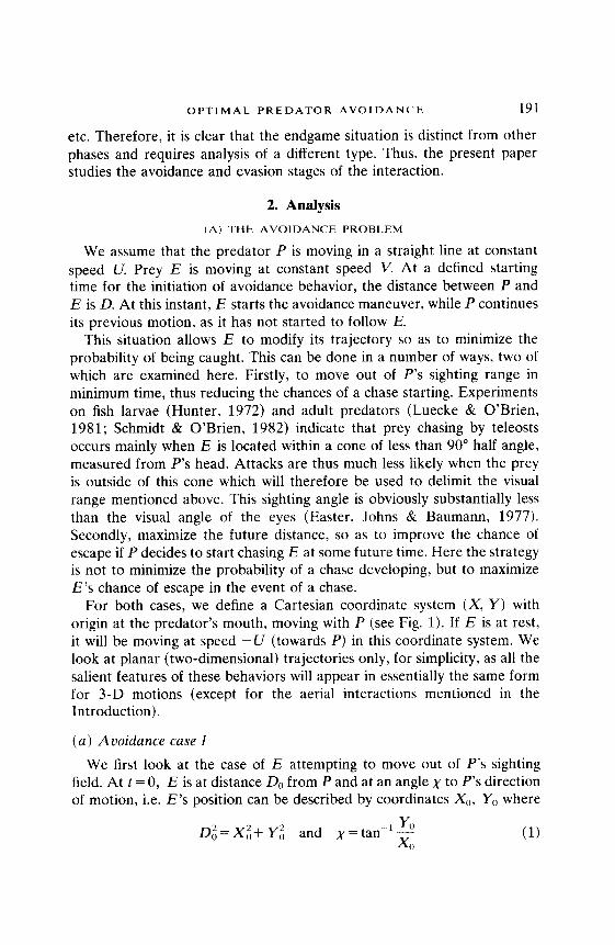
(a) Auoidance case I

We first look at the case of E attempting to move out of P’s sighting field. At f = 0, E is at distance D,, from P and at an angle x to P’s direction of motion, i.e. E’s position can be described by coordinates X0, Y,, where

Dg=Xz+ Yi and x=tan-‘? 0

192 D. WEIHS AND P. M. WEBB

k 0

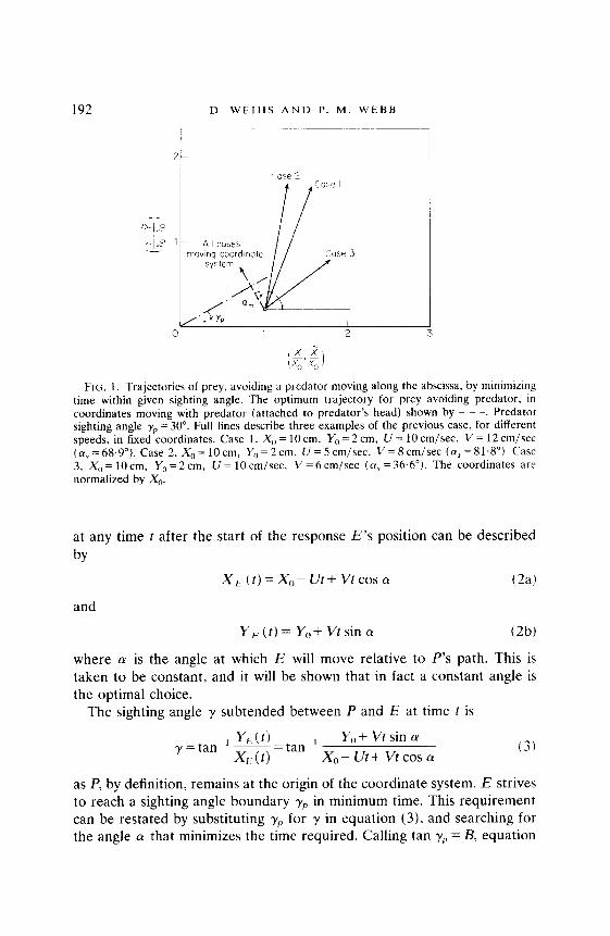
FIG. 1. Trajectories of prey, avoiding a predator moving along the abscissa, by minimizing time within given sighting angle. The optimum trajectory for prey avoiding predator. in coordinates moving with predator (attached to predator’s head) shown by - - -. Predator sighting angle v, = 30”. Full lines describe three examples of the previous case, for different speeds, in fixed coordinates. Case 1, X,, = 10 cm, Y,, = 2 cm. CJ = 10 cm/se& V = 12 cm/set (a, = 68.9”). Case 2, X0 = 10 cm, Y0 = 2 cm. U = 5 cm/set, V = 8 cm/set (a, = 81.8”). Case 3, X,,=lOcm, Y,=2cm. U=lOcm/sec. V = 6 cmjsec ( LY, = 36.6”). The coordinates are normalized by X0.

at any time t after the start of the response E’s position can be described

by

xfi (t)=Xo- ur+ vtcos a (2a)

and

Y,(t)= Y,,+Vfsincw (2b)

where (Y is the angle at which E will move relative to P’s path. This is taken to be constant, and it will be shown that in fact a constant angle is the optimal choice.

The sighting angle y subtended between P and E at time t is

-, YE(f) y=tan xt(t)=tan 1 Y,, + Vt sin ff

x,,- ut+ vt cos a (31

as P, by definition, remains at the origin of the coordinate system. E strives to reach a sighting angle boundary yP in minimum time. This requirement can be restated by substituting y,, for y in equation (3), and searching for the angle (Y that minimizes the time required. Calling tan y,, = B, equation


(3) can be written as

B= Y,+Vtsin(~

X-Ut+Vtcosa forO<B<oo (O<y,<90’) (4)

or

t= BX,- Y,,

V(sina-Bcoscu)+BU (5)

B, X0, YO, V and U are fixed quantities. The minimization of t is therefore achieved by maximizing the term in brackets in equation (5), i.e. sin (Y - B cos (Y + max. This is obtained by differentiation as

or

cosa+Bsina=O

1 tariff,=-g=-cot yP

(6)

(7)

where (Y, is the angle for which time within sighting angle rP is minimized. From equation (7) we see that the optimal avoidance maneuver is for E to move in a straight line normal to the line defining the limits of P’s sighting angle. This angle is, as mentioned above, less than 90”. In the case of anchovy (Engraulis mordax) Hunter (1972) obtained a sighting angle of 7, = 30”. In this case E should move at 60” (Fig. 1) to the predator’s heading.

One should recall that the trajectories defined above are in a system moving with P; T? see E’s path in inertial coordinates (fixed with the environment) X, Y, one has to transform the angles. From equation (7)

Vs

tan(Ym=V x

where V,, V, are the y, x components of E’s velocity, in the moving system. The angle observed in the fixed system cy, will thus be defined by

V tan cf, = v,+c/

as a velocity U is added to the x component. This can be written as

v+u u cot a, = L-cot ff,+

VS Vsinff,’

(9)

(10)

And E’s path is

x=x,+vtcos(Y, (114

y = Yo+ Vt sin cy, (lib)


where CY, is obtained by substituting LY,,, from equation (7) into equation (10). Equations (11) show clearly the added complications involved in using the inertial coordinates, as the escape angle will now depend also on the velocities of both predator and prey, whereas only one parameter, the sighting angle came into the calculation based on the P-fixed system. Examples of trajectories calculated from equations (11) appear in Fig. 1.

As mentioned previously we take the speeds of both predator and prey to be constant during the interaction. This can be generalized to include variable speeds-but the solutions would be much more complicated mathematically. This can be achieved in principle by breaking up the variable speed trajectory into a series of constant speed segments applying the analysis above to each. The accuracy of this technique increases as the number of steps grows. Also, the initiation distance is assumed independent of predator speed. This assumption, while probably not realistic in some cases, influences the present result only indirectly, as no derivatives of the initial distance appear in the analysis. Obviously, the numerical values of the various parameters will be affected, but if the dependence of initiation distance on speed is known for a given predator-prey combination it can easily be applied.

(b) Avoidance case II

Experimental data on search volumes of predatory fish show, however, that prey chasing is possible, though less likely, at angles larger than r,,. Thus E must take this possibility into account also by a second strategy. In addition, situations occur in schools and herds, where an attack is initiated by P, but the specific target among many E is still undefined. These situations involve E attempting to improve its future escape chances by moving in a trajectory that will maximize the future distance at any time. Assuming the predator P still continues moving in its original direction, it is obvious (see Fig. 2) that this means E should move in a line, directly away from P at all times (except for some special cases which will be discussed separately). This can be formalized mathematically as the differential equation

dy Y -- dx-x-x,

(12)

where x, y are inertial coordinates, and X~ the instantaneous predator position. Both x and y, are functions of f, (equations (ll)), however, complicating the solution procedure. The problem defined here is the inverse of the well-known pursuit problem (Davis, 1962), but before solving it, we look at the special cases.


E Prey trapctory

fl J ! Predator tra]ectory

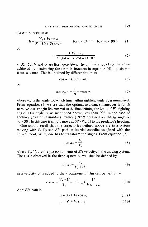
FIG. 2. Schematic description of avoidance trajectory, maximizing the instantaneous distance between prey and predator. Predator P is moving along the positive x axis, and prey E along the curve. Time t, denotes start of the avoidance maneuver, with P at the origin of the coordinates. At time t,, P is directly beneath E.

First, take the case where Y,=O, i.e. P is heading directly towards E. The requirement of staying on the line of sight to the predator means E will escape along the x axis. Mathematically, this is stated as

dy z=o (13)

as Y,, = 0, y = 0 at time zero, dy/dx = 0, and no y component of motion occurs. However, if P is faster, or starts moving faster at some future time, this strategy ends up with E being caught, so that a slower evader has to develop a different escape technique. This is described in detail in the next section.

A similar situation may occur if YO/XO is very small, and P is very fast, so again a behavior of the type described here, while mathematically optimal, may be useless for E in the sense that it gets caught.

Also, when E is to the left of P (see Fig. 2) it is probably energetically wasteful to continue the trajectory predicted by equation (12) and E may stop avoidance at any time.

To solve the general case of avoidance by maximizing the instantaneous distance, we take the predator to move along the y-axis. This helps simplify the solution procedure for the differential equation (12), and does not affect the solution in any real sense. The equation is now, for E’s position E (x, y)

dy Y-YP dy dx- x Or xdx=y-yp.

(14)


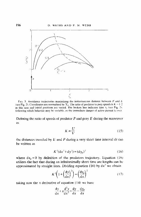
FIG. 3. Avoidance trajectories maximizing the instantaneous distance between P and E (see Fig. 2). Coordinates are normalized by Yo. The ratio of predator to prey speeds is K = 1.1 in this case and initial positions are varied. The broken line indicates time I, (see Fig. 2). following which behavior may be variable. as the immediate danger of active pursuit is OVCT.

Defining the ratio of speeds of predator P and prey E during the maneuver as

+ (1.5)

the distances traveled by E and P during a very short time interval dt can be written as

K ‘(dx’+ dy’) = (dy,)’ (16)

where dx, = 0 by definition of the predators trajectory. Equation (16) utilizes the fact that during an infinitesimally short time arc lengths can be approximated by straight lines. Dividing equation (16) by dx’ we obtain

p( I+(!$) +j= taking now the x derivative of equation (14) we have

dy d=y dy dy, z+X&Y=z-&

(17)

OPTIMAL PREDATOR AVOIDANCE

or

xd2Y= dhJ dx’ dx

substituting dy,,/dx from equation (17) into (18))

*KJpJLx~

this can be solved by defining w = dyldx so that

the solution of equation (20) is obtained by separation

dw dx -z&K-.-- J1+w2 X

and integrating each side, resulting in

197

(18)

(19)

(20)

(21)

sinh-’ (w) = *K 1 nx+lnC,=ln(C,X’“) (22)

where C, is a constant of integration which will be obtained from initial conditions.

where C,, and CI1 are the constants for the two solutions, respectively. y is found by integrating again, as w = dyldx.

c,, xlpK 1 X’+K ~+C~,(forK#l,--1)

“2 1-K 2C,, l+K (24)

CT’,, is a second constant of integration. Only the first solution is written out, as it was found to lead to physically acceptable results. Each of the two solutions of equation (23) leads to a further two solutions when the values of Cr are computed (see below), one of each being an acceptable solution. C,, and C,, are obtained from the conditions at the time of initiation of the evasive maneuver.

x = x0; y= Y” (25a)

x=x,; dy Yo -=- dx X,,’ (2%)


Substituting equation (25b) into equation (23) we obtain

c,,=+(-1*1+&G) and from equations (25a) and (26) we obtain for C,,

c = y Cl, xh-“+ 1 xlith -- 21 (1 2 1-K 2c,, l+K’

(26)

(27)

For the case of K = 1, which was excluded in equation (24) (K = -1 is of no interest) equation (23) is integrated to give

y+nx-L+C 4c, I

1’1

where by applying equations (25). we obtain

C 121= Y(,-+lnX,,+g. I1

(29)

Results of sample calculations appear in Figs 3 and 4, with P moving on the positive y axis (x = 0) for typical values of K, and initial positions. The

X

v,

FIG. 4. As in Fig. 3. Here the trajectories for various speed ratios K. at initial prey position X,, = Y,,/2 are traced.


calculations were normalized by YO, so that the starting points are all Y,, = 1. It should be noted that both equations (24) and (28) actually represent multiple solutions, with the signs being chosen to obtain continuous, positive solutions for y, when calculating for a given x, with Yo, X0 and K as input parameters. It is rather cumbersome to transform the present solution to the time plane, and so comparison with photographic data is difficult. To find instantaneous positions of P at E, at a given time, take P’s speed to be unity (normalize by U). Then P will move one unit along x = 0 (the y axis) in each time unit, while E will be moving l/K units, along the relevant curve. The broken lines in Figs 3 and 4 show the positions of E when P is at the same y (so that the line connecting the centers of mass is horizontal). This line also delimits the area to the right of which behavior is expected to be variable as the immediate danger will have receded, and avoidance can end. The actual comparison with data can either be done with the aid of tracking machines which digitize positions, or by projecting successive photographs on each other, displacing them such that the predator’s head is always at the same spot.

(B) THE EVASION PROBL,EM

Next we look at the optimal escape maneuvers for E once P has started attacking a specific prey. This situation is the basis for a large number of theoretical studies of the differential game type (Isaacs, 1975). Solutions are usually extremely complex and usually multivalued in the general case.

Here we examine only the evasion stage defined in the Introduction; E responds to the directed behavior of P towards E in stalks and attacks. If P chooses to chase E, it is assumed to align its motion with the instantaneous lines joining P and E, as shown by Lanchester & Mark (1975) for a teleostean fish. As we are looking at trajectories, and not trying to calculate forces, the coordinate system suggested in the first section, attached to the predator’s head, with abscissa in the (now instantaneous) direction of motion, is still applicable. By treating the problem in this coordinate system, we gain the advantage of being continually in the starting position of the evasion maneuver. Thus the differential equation of the second avoidance case does not occur.

At time t=O, the distance between the centers of mass of P and E is D =X0. E starts its evasive maneuver at angle (Y. In the present problem the escape angle (Y is taken constant in the moving coordinate system, and we look for the angle which will result in the largest miss-distance, i.e. largest minimum distance. Thus, the problem defined here is a special case of the second general avoidance situation described in the previous section.


The difference here is that E is now certain that P is following but intends to induce an aborted attack by extending the duration of the interaction and its cost to P, compared to avoidance where P was not actively following E. Taking P to move in the x direction in this case and again fixing the coordinate system to its head, the distance at any given time t after the evasive maneuver starts is (see equation (2))

D’=[(X,,-Uf)+Vtcosa]‘+(Vtsin(~)’ (30)

where Y,, = 0 as P is heading in E’s direction, at least initially. We now look for the time at which the distance will be minimal, assuming constant escape angle a. This is found when

dD’ -= 0 at

or

t(min. dist.) = x(,(u-vcosa)

v’-2uvcos a+ U2’

We define the ratio of velocities during the maneuver as

so that equation (32) now takes the form

XC, K -cos CY t - ml”

V I-2Kcosa+K”

(31)

(321

(15)

(33)

It can be shown, that for all positive real K, 1 + K’ 2 2K so that whenever K > cos CY, t,i” is positive. When K is smaller than cos (Y (i.e. predator is moving more slowly than prey) fmin found here is negative, meaning that the distance between P and E is growing for all times after the evasion process starts. These cases will later be examined separately, but it is intuitively clear that a simple escape along the line connecting the centers of mass of P and E, away from P ((Y = 0), is best in this case.

When K = cos LY = 1, the solution has a singularity, i.e. no minimum time exists. This describes a case where P and E are moving in the same direction, at the same speed, and therefore the distance stays constant and no minimum exists.


Returning to the problem of finding the angle a that maximizes the minimum distance, we substitute equation (33) in (30). obtaining

2K cos a-K'-cos'a ' K'-2K coscl+l 3

+sin2aK'-2K cos a-kcos'a (I-2K cos cx +K')' (34)

which after some algebraic manipulations can be reduced to

05,i” = sin’ a

K'-2K coscx-t 1’ (35)

We now find the maximum value of of,,,,, as a function of (Y, with parameter K, by setting

aof min -zz 0 aa

(36)

or, explicitly

2sinacosa(K’-2K cosa+l)-2K sin’s

(K'-2K cos a + l)* = 0. (37)

We have already described the case K = cos cx = 1 which is the only case for which the denominator can take the value 0, so that for all other cases, it suffices to look at the numerator only.

-2Ksin3cu+2sin~cos~(K’-2Kcosa+l)=O. (38)

This is a third order algebraic equation, with three different solutions for cr. The first of these is given by

sin LY =0 or (Y =O. (39)

As discussed above, equation (39) gives a maximum when K < 1, i.e. prey is faster, and a minimum of zero (prey captured) when K > 1. (It also gives a minimum of zero when Q = rr, E moves directly toward P, but this is of no interest here.)

The other solutions are now obtained by dividing equation (38) by sin LY, leaving

-K sin*cr+K’coscr--2K cos*cw+cosa=0

which can be rearranged as a quadratic equation for cos (Y as

Kcos*cu-(K’+l)cosa+K=O

(40)

(41)


the solutions are

K’+l J

K’+l’ +K’+I K’-1 1 cos cY =2K+

--..m.m...-*-=K.- 2K 2K 2K ‘K ~42)

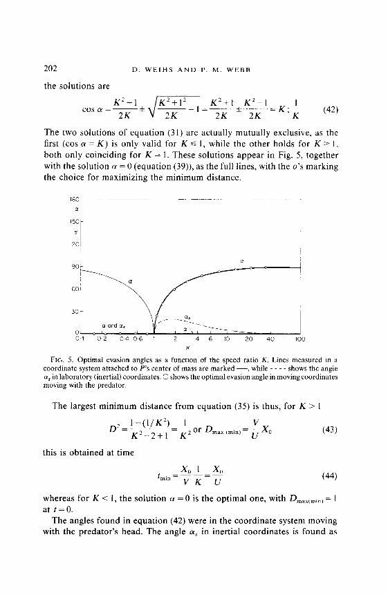
The two solutions of equation (31) are actually mutually exclusive, as the first (cos (Y = K) is only valid for K d 1, while the other holds for K 2 I, both only coinciding for K = 1. These solutions appear in Fig. 5, together with the solution LY = 0 (equation (39)), as the full lines, with the o’s marking the choice for maximizing the minimum distance.

180 1

CI

150 [

‘i IPot

a

0 ; 1” :I -1 01 02 O-4 0 6 1 2 4 6 IO 20 40 100

K

FIG. 5. Optimal evasion angles as a function of the speed ratio K. Lines measured in a coordinate system attached to P’s center of mass are marked -, while - - - - shows the angle (Y, in laboratory (inertial) coordinates. 0 shows the optimal evasion angle in moving coordinates moving with the predator.

The largest minimum distance from equation (35) is thus, for K > 1

D2J-(l/K’)z~or D V

K’-2+1 K2 mdx (min) = -

u X0

this is obtained at time

x0 1 x0 &- -=- VK U

(43)

(44)

whereas for K < 1, the solution (Y = 0 is the optimal one, with Dmax(min) = I at t=O.

The angles found in equation (42) were in the coordinate system moving with the predator’s head. The angle a, in inertial coordinates is found as


in the avoidance case 1 (see equation (10)). This angle (for K > 1) is shown by the broken line in Fig. 5. Thus, the optimum angle for evasion is always less than 21” from the line heading directly away from the predator.

3. Results and Discussion

(A) AVOIDANCE

Our analysis predicts two different optimal avoidance tactics depending on whether the objective of E is to attempt to avoid an interaction (case I), or to anticipate a chase (case II). The predicted optimal avoidance angles are sufficiently different that each should be distinguishable experimentally, or the use of mixed strategies identifiable. However, it seems likely that a particular alternative would be preferable for certain species. We suggest that avoidance case I would be most likely to be found for zooplankters. This is because many of these are capable of very high acceleration rates and speeds and are often more transparent than other aquatic or terrestrial prey. Indeed, the sighting angles for fish used here are based on responses of zooplankton and may reflect relative visibility rather than optical acuity (Easter et a/., 1977). More opaque objects, for example fish, might be sufficiently prominent stimuli in a predator’s peripheral vision that avoidance case I would be excluded.

Therefore, we suggest avoidance case II is likely to be that most frequently encountered in piscivorous interactions. The analysis predicts the fountain effect for escaping prey in groups, as regularly described for aquatic prey (Nursall, 1973; Partridge, 1982). Here the attack is certainly directed, but against a group where initially an individual will not identify itself as the specific target. Then every individual should seek to maximize its future distance from the predator (the avoidance solution) to increase the probability of evasion success should it become the specific target as an attack develops.

(B) EVASION

No experimental observations have been made to explicitly test the predictions for optimal evasion tactics. Data for averaged response parameters are available for fathead minnows attacked by some teleost predators (Webb & Skadsen, 1980; Webb, in press). The predators struck at prey oriented at 80 to 90” to the prey’s axis so that LY,~ was 3 to 18”. Predator speed varied from 50 to 100 cm/set and prey evasion speeds were about half (K = l-2). These results are of the correct order (Fig. 5) but the variability in these averaged data is too high to come to definitive conclusions.


I Cl GENERAL

Prolonging the interaction is the likely strategy for prey species. First, the capabilities of predators are often finite. For example, cheetahs are fast but rapidly exhaust. Lions have only 4 to 10 seconds when their acceleration rates exceed those of typical prey (Elliott ef af., 1977). Thereafter, lion top speeds are lower than their prey. In the aquatic environment. air supply of diving predators must be limiting.

Second, cover of some sort is usually relatively close. This can be illus- trated using aquatic habitats where, for fish prey, some sort of cover is usually within a distance of a few meters. Cover may include either physical refuges on the bottom, among vegetation, reefs, etc., or schools (see Hobson, 1968; Weihs & Webb, 1983; Keenleyside, 1979). At fish maximum speeds, such cover can be reached in about 2-4 set (Wardle, 1975; Weihs & Webb, 1983). Group activity is, of course, a well known refuge for any prey that reduces the probability of capture through dilution and confusion effects (Foster & Treherne, 1982).

Third, an avoidance or evasive response is often sufficient signal to the predator of prey awareness that the predator voluntarily aborts the interaction (Webb, 1982).

Therefore, the optimal tactics predicted by the above analysis provide realistic options for animals by extending the duration of predator-prey interactions.

The analyses in section 2’do not consider response latencies of predator or prey. However, these are relatively easy to include in the following manner. Take the response latency to include reaction and decision times, as well as the time required for angular position changes and acceleration to the escape speed (these latter two are usually simultaneous as acceleration is accompanied by direction changes (Weihs, 1973; Webb, 1978).) Thus, when looking at E’s trajectory, one can transform the real distance-time curve to an equivalent curve, starting at some later time but having E move at constant speed. The time difference 7r thus obtained (displacement time 1 can be equated to the response latency defined above. Mathematically this is written as

I’ vdt= V(t-Tr) (4.5) (I

where u is the real (variable) prey speed and the time t is the total time elapsed for a given maneuver. r, as defined above can now be seen, in the coordinate system moving with the predator, as an additional motion of E in the negative x direction. of UT,. Thus, for example, equation (2a) will


have the form

X,(t)=X,,-uf-uT,+VfCOSa (46)

and equation (5) becomes;

t= B(X, - UT,) - y,, V(sina-Bcosa)+BU

and the analysis following equation (5), as well as the optimal strategies are essentially unchanged.

However, response latencies may influence the shape of avoidance and evasion trajectories in a different way too. These might tend towards polygonal rather than smoothly curved paths if prey requires a finite time to assess the new situation after initiating a maneuver. The length of the sections could be several animal lengths at the escape speeds of terrestrial and aquatic animals and reasonable decision times. Nevertheless, a polygonal path should still approximate the optimal escape curves.

Response latencies will only become critical in the endgame phase when distances between P and E become very small. However, as mentioned before, this is not in the scope of the present paper.

Speeds are also considered constant in our analysis for purposes of analytical simplicity. However, the key parameter in all the situations examined is the ratio of predator and prey speeds, K. As mentioned previously optimal escape trajectories could be calculated where acceleration and hence variable speeds occur in chases by discrete modification of K. Since a change in speed and heading (linear and angular accelerations occur) involve predator and/or prey decisions, an extended chase could be divided into moves about such decision points for which discrete values of K could be applied in sequence. This would result in a numerical scheme for calculating specific trajectories, by substituting instantaneous velocities and numerically integrating to obtain the actual trajectories. This was not attempted in the present paper, as such calculations are specific to each interaction and no conclusions of general interest are to be obtained.

This study was supported by the National Science Foundation under grant number PCM-8006469.

REFERENCES

DAVIS. H. T. (1962). Introduction to Nonlinear Diferenrial and Integral Equations. New York: DCWX.

EASTER. S. %.JOHNS. P. R. & BAUMANN. L. R. (1977). Vision Res. 17,469. ELLIO’~, J. P.. MCTAGGART-COWAN, I. & HOI.I.ING, C. S. (1977). Can. I 2001. 55. 1811.

206 D. WElHS AND P. M. WEBB

FOSTEK, W. A. & TREHEKNE. J. E. (1982). Nature 293, 466. HOBSON, E. S. (1968). U.S. Bureau Fisheries Wildlife Res. Rep. 73, 1-92. HOWLAND, H. C. (1974). J. theor. Biol. 47, 333. HUNTER, J. R. (1972). U.S. Fish. Bull. 70, 821. ISAACS. R. (1975). Differential Games. Huntingdon, New York: Krieger. KEENLEYSIDE. M. H. A. (1979). Diversity and Adaptation in Fish Behavior. New York:

Springer-Verlag. KREBS, J. R. & DAVIES, N. B. (1978). Behavioral Ecology. Sunderland. Massachusetts:

Sinauer. LANCHESTER, B. S. & MARK, R. F. (1975). J. exp. Biol. 63, 627. LUECKE. C. & O‘BRIEN. W. J. ( 1981). Can. J. Fish. Aqua!. Sci. 38, 1264. NURSALL. J. R. (1973). J. Fish. Res. Bd Can. 30, 1161. PARTRIDGE, B. L. (1982). Sci. Am. 246, 90. SCHOENEK, T. W. (1971). Rev. Ecol. Syst. 2, 369. SCHMIDT, D. & O‘BRIEN, W. J. (1982). Can. J. Fish. Aquat. Sci. 39, 475. STROUD, R. H. & CLEPPER, H. (1979). Predator-Prey Systems in Fisheries Management.

Washington, D.C.: Sport Fishing Institute. WARDLE. C. S. (1975). Nature 255, 725. WEBB. P. W. (1976). J. exp. Biol. 65, 157. WEBB. P. W. (1978). J. exp. Biol. 74, 211. WEBB. P. W. (1982). J. camp. Physiol. (in press). WEBB, P. W. (1982). U.S. Fish. Bull. 79, 727. WEBB, P. W. & SKADSEN. J. M. (1980). Can. J. Zool. 58, 1462. WEIHS, D. (1973). Biorheology 10, 343. WEIHS, D. & WEBB, P. W. (1983). In: Fish Biomechanics (Webb, P. W. & Weihs D., eds.)

New York: Praeger.

Optimal Avoidance and Evasion Tactics in Predator-Prey ...

Documents

Transcript of Optimal Avoidance and Evasion Tactics in Predator-Prey ...