Predator-prey dynamics in models of prey dispersal in two-patch environments

Predator-Prey Dynamics in Models of Prey Dispersal in Two-Patch Environments*

YANG KUANG Department of Mathematics, Arizona State University Tempe, Arizona 85287-1804

AND

YASUHIRO TAKEUCHI Department of Applied Mathematics, Faculty of Engineering, Shizuoka Uniuersity Hamamatsu 432, Japan

Received 16 September 1992; revised 9 March 1993

ABSTRACT

Models are presented for a single species that disperses between two patches of a heterogeneous environment with barriers between patches and a predator for which the dispersal between patches does not involve a barrier. Conditions are established for the existence, uniform persistence, and local and global stability of positive steady states. In particular, an example that demonstrates both the stabilizing and destabilizing effects of dispersion is presented. This example indicates that a stable migrating predator-prey system can be made unstable by changing the amount of migration in both directions.

1. INTRODUCTION

Interest has been growing in the study of mathematical models of populations dispersing among patches in a heterogeneous environment [l--5, 8, 9, 11, 13-17, 20, 24, 26-31, and references cited therein]. Many of the existing models deal with a single population dispersing among patches. Some of them deal with competition and predator-prey interactions in patchy environments.

The analysis of these models has been centered around the coexis- tence of populations and the stability (local and global) of equilibria. There are also a few papers that focus on the existence and location of positive steady states when the dispersal rate among patches is relatively

*Dedicated to Paul Waltman on the occasion of his 60th birthday.

MATHEMATICAL BIOSCIENCES 120:77-98 (1994)

OElsevier Science Inc., 1994

77

655 Avenue of the Americas, New York, NY 10010 0025-5564/94/$7.00

78 YANG KUANG AND YASUHIRO TAKEUCHI

small [ll, 131. The single-species dynamics in a patchy environment has been well studied. Recently, by applying cooperative system theory (cf. [2.5]), Takeuchi [28] succeeded in showing that in a system composed of several patches connected by diffusion and occupied by a single species, if the species is able to survive at a globally stable equilibrium point when the patches are isolated, then it continues to do so for any diffusion rate at a different equilibrium (depending on the diffusion rate). In other words, diffusion among patches will not destabilize single-population dynamics. This result greatly generalizes some previously known results [2-4, 13, 141.

Existing results on dynamics of two interacting populations in a patchy environment have largely been restricted to persistence and extinction analyses due to the increased complexity of global analysis. The known results on global stability are usually too general to be of any use in real mathematical or biological applications. Stabilizing and/or destabilizing effects of dispersions remain largely unknown due to difficulties involved in local stability analyses. Nevertheless, it is generally accepted among both mathematicians and biologists that discrete diffusion tends to stabilize ecosystems.

The main objective of this paper is to prove or disprove this well- adopted point of view for some particular classes of models. We will see in Section 4, through an example, that discrete diffusions are capable of both stabilizing and destabilizing a given ecosystem. Specifically, we are able to show that for that example, the dispersion stabilizes the system when the dispersal rate is small and then destabilizes the system when the dispersal rate is further increased. Thus, the assertion that “migration is a stabilizing influence in population interactions” is not true without qualification.

In two recent articles [29, 301, Takeuchi proved that introducing refuge patches in patchy environments tends to stabilize the population interaction, for example, allowing species to coexist. Our study here further confirms such a point of view.

The model we chose to study here is a special case of the one introduced and analyzed in Freedman and Takeuchi [9]. The model deals with a single species that disperses between two patches (instead of the n in [91) in a heterogeneous environment with barriers between patches with a predator for which the dispersal between patches does not involve a barrier.

Systems where there are barriers for dispersal among prey but not among predators are well known in nature. One example is described in [161, where cyclamen mites disperse among strawberry plants with the space between plants as a barrier to their dispersion. There, predators are mainly several species of small wasps, which do not consider the space between plants as barriers.

PREDATOR-PREY DYNAMICS WITH DISPERSAL 79

A second example is given in 1201. The prey are the members of the porcupine caribou herd that dwell in‘the northern Yukon Territory of Canada. Their dispersion carries them across rivers and mountains. These are clearly barriers to their dispersion. One of the predator populationfor this herd is the golden eagle. For these birds, the rivers and mountains do not form barriers.

The paper is organized as follows. In the next section we describe our model in detail. Results on boundedness of solutions, existence of boundary and interior equilibria, and persistence and extinction of predator species are presented. In Section 3, we obtain criteria for local and global stability of positive equilibria via Routh-Hurwitz criteria and Lyapunov functions, respectively. We also consider the special case when one patch is free of predators. In Section 4, we present an example with a Michaelis-Menten type of predator functional response, which demonstrates both the stabilizing and destabilizing effects of dispersion on the population dynamics. In the final discussion section, we try to interpret our mathematical results in terms of their ecological implications and formulate our conclusions. We also point out some future research directions.

2. THE MODEL AND PRELIMINARIES

In this paper, we consider the following predator-prey system in a two-patch environment:

Xi(O) > 0, Y(O) a 0, i = 1,2,

where the dot denotes differentiation with respect to time and g&xi), p&xi), and s(y) are continuously differentiable functions. Here x,(t) represents the prey population in the ith patch, i = 1,2, at time t a 0. We think of patches with a barrier only as far as the prey population is concerned; the predator population has no barriers between patches. Thus y(t) stands for the total predator population for both patches.

g,(x,> is the specific growth rate for the prey population in the absence of predation when it is restricted to the ith patch. Due to limited resources, g,(x,> is generally a decreasing function of xi; it eventually becomes negative since the ith patch can support only a finite population due to limited resources. This is modeled by the following assumption.


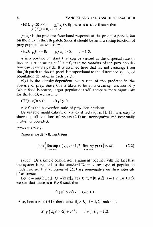
(Hl): g,(O) > 0; g:(xi) < 0; there is a Ki > 0 such that gi(Ki) = 0, i = 1,2.

pi(xi) is the predator functional response of the predator population on the prey in the ith patch. Since it should be an increasing function of prey population, we assume

(H2): p,(O) = 0; pl(xi) > 0, i = 1,2.

E is a positive constant that can be viewed as the dispersal rate or inverse barrier strength. If E = 0, then no member of the prey population can leave its patch. It is assumed here that the net exchange from the jth patch to the ith patch is proportional to the difference xj - xi of population densities in each patch.

s(y) is the density-dependent death rate of the predator in the absence of prey. Since this is likely to be an increasing function of y (when food is scarce, larger populations will compete more vigorously for the food), we assume

(H3): s(O) > 0; s’(y) 2 0.

c, > 0 is the conversion ratio of prey into predator. By suitable modifications of standard techniques [l, 131, it is easy to

show that all solutions of system (2.1) are nonnegative and eventually uniformly bounded.

PROPOSITION 2.1

There is an M > 0, such that

max( limsupxi( t), i = 1,2; limsupy(t)) < M. t-+” t’+”

(2.2)

Proof By a simple comparison argument together with the fact that the system is related to the standard Kolmogorov type of population model, we see that solutions of (2.1) are nonnegative on their intervals of existence.

Let c = max{c,, cJ, Gi = max{xig(xi): xi E [O, Kill, i = 1,2. By (H3), we see that there is a 9 > 0 such that

js( j) > c( G, + G2) + 1.

Also, because of (Hl), there exist fi > Ki, i = 1,2, such that

Pilgi( ~i)l> Gj + c-‘, i#j; i,j=1,2.


We define for a solution (xl(t), x,(t), y(t)> of system (2.1),

B(t)=B(x,,x,,y)-c[x,(t)+x,(t)l+y(t).

Then we have

8(t) =c[il(t)+qt)] +j(t)

G c[~l(t)g,(~lw)+ %W&zW)l - YW(Y(W

Clearly, if one of the three inequalities holds-_(i) x,(t) > P,, (ii> x,(t) > 2z, (iii) y(t) 2 y-then B(t) < - 1. Thus we have

limsupB(t) ,< c(P, + a,)+ j = L. f--)+71

This in turn implies that (2.2) holds for

M= max{c-‘L,L},

proving the proposition. n

The origin E,(O,O,O) is clearly an equilibrium. When E = 0, E, = (K,, K,,O) is also an equilibrium. For E # 0, the following existence and stability result in x,x2 space is known from Takeuchi [28]:

System (2.1) has a unique equilibtium of the form E, = E,(E) = (X1(~), X2( E),O), where XJ E) > 0, i = 1,2. Moreouer, E, is globally aqmp- totically stable with initial values xi(O) > 0, i = 1,2, y(O) = 0.

It is easy to see that E, and E, are the only two boundary equilibria of system (2.1).

We say that system (2.1) is uniformly persistent (see L6.121 for more details) if there exists a 6 > 0, such that if x,(O) > 0, x,(O) > 0, y(O) > 0, then min{liminf, ~ +u x,(t), i = 1,2, lim inf, -f +lo y(t)} > 6, where S is independent of x,(O), x,(O), y(O).

The following extinction-persistence results are special cases of Theorems 5.2 and 5.3 in [9]. However, the proofs given there are not complete; for this reason, we restate and prove them here.

PROPOSITION 2.2 (Freedman and Takeuchi [9])

Define

d = d( e) = -s(O) + cIpI(X1( l ))+ CZP&( El). (2.3)


The following statements are true:

(i) If d < 0, then lim, ~ +co x,(t) = ii, i = 1,2, lim, j += y(t) = 0. (ii) If d > 0, then system (2.1) exhibits uniform persistence.

Proof Part (i) follows from the proof of Theorem 5.2 in [9]. In the following, we give the proof of part (ii>.

Clearly, the nonnegative cone R: in R3 is positively invariant. There are only two compact invariant sets on the boundary of RI, namely E, and E,. Suppose P E intR+. ’ Let CL(P) be the omega limit set of the orbit through P, and denote W+ (E,) the strong stable manifold of E,. We claim that

W+(E,)nR;={( x1,x2,y): x,=x,=o,y>,o}.

In order to prove this, we consider the Jacobian at E,, which takes the form

J(J%) =

g,(O) - E E 0

E g2(0)-• 0 0 0 - 40)

Denote the eigenvalues of J(E,) by A,(E), A,(E), and A, = - s(O). Clearly, one of the eigenvectors of A, is (O,O,l). It is also easy to see that eigenvectors of A, and A, must take the form (a,, a,,O). By an elementary algebraic computation, we see that czl(yz < 0, which implies that J(E,) cannot have eigenvectors in the interior of RI. Note that A,(E) and A,( E) satisfy

A2 - [si(O) + gz(O) -2e]A+ s,(O)g,(O) - &r(O) + g,(O)] =O.

For 0 G E 6 g,(O)g,(O)/[g,(O) + g,(O)], we must have A,( E) > 0, A,( E) > 0 [since when E = 0, A,(O) > 0, A,(O) > 01. And for E > g,(OIg,(O)/[g,(O) + g2(0)], we have A,( E)A~(E) < 0, which always implies that one of A,(E) and AZ(e) is positive. Thus J(E,) has at most two eigenvalues with negative real parts, and they both must be real if they exist. This together with the fact that J(E,) has no positive eigenvectors implies our claim.

The rest of the proof follows that of Theorem 5.3 in [9]. n

Indeed, d(E) determines the sign of the eigenvalue for the eigenvec- tor of E,(E) that does not lie in the xlxz plane. If d(E) > 0, then E,(E) repels neighboring trajectories in the interior of the first quadrant, whereas if d(e) < 0, then E,(E) attracts neighboring trajectories in the interior of the first quadrant.

83 PREDATOR-PREY DYNAMICS WITH DISPERSAL

An immediate consequence of the above propositions is

PROPOSITION 2.3

Zf d( E) > 0, then Jystem (2.1) has a positive equilibtium.

Proo$ This follows from Theorem 6.3 in Hutson and Schmitt [171.

3. STABILITY ANALYSIS

Throughout this section, we assume that d(e) > 0. By Proposition 2.3, we know that system (2.1) has at least one positive equilibrium. In the following we will denote it (them) as E* = (XT, xz, y*).

We consider first the local stability of E”. The Jacobian of the linearized system evaluated at E* takes the form

%1(-G, l > E

J( E*) = E %(X2*1 6)

Cl P;(G)Y* c2PxG)Y*

where

aji = Uii( XT, E) = &( XT) + x:g;( XT) - y*p;( XT) - E, i = 1,2. (3.1)

Since

XT&(x;) -y*p,(x:) + ‘(Xi* - XT) = 0, i#j; i,j=1,2,

we have

a,,( XL*, 6) = - 63 + xi”g’( x’) + y” -y- I

[

PXX”) -@(XT) 3

I i# j.

I

For convenience, we denote

Qi=Q,(x:,y*)=x~g;(xi*)+y* x*- [

PiCxT) P’(4 . 1 (3.2) 1

Then

uii( XT, 6) = Q, - EX;/X), i# j. (3.3)


We note that p,<x~> > 0, cipi(xT)y* > 0, and gi(xT> < 0, i = 1,2. De- note

I, = a,, + az2 - s’( y*)y*,

4 = alla22 - e2 + Y$ [&T)cipl(xi*) - s’(Y*hil?

13 = - EY*[C2P;(m4XT) + CIPxXT)P2(X;)I

+ %c,P;(GP2(G)Y*

+ a,,c,P;(mP,(xT)Y*- s’(Y*)Y*(w22 - E2).

The characteristic equation for the eigenvalues of J(E*) is

By the well-known Routh-Hurwitz criteria [7, pp. 233-2341 we thus have that E* is locally asymptotically stable if and only if I, < 0, I, < 0 and I,Z, < Z,. In particular, we have

PROPOSITION 3.1

Assume that Qi(xT,y*) < 0, i = 1,2. Then E* is locally asymptotically stable if and only if I, I, < I,.

ProoJ Clearly, QJxT, y*) G 0 implies that

aii < - EX~*/X,*, i# j.

This in turn implies that

a11a22 >, l 2.

Now it is straightforward to verify that I, < 0 and Z3 < 0. This com- pletes the proof. n

For example, if pi(x) = (Y~X or aix2, where (Y~ > 0, i = 1,2, then pJxF> G x,*p/(xT>, and thus Qi(xT, y*) G 0.

In the rest of this section, we consider the global stability of E*. For simplicity, we consider only the Lotka-Volterra version of system (2.1):

~,=XI(Y1-klXl-(YIY)+E(Xz-X1), x,(O) > 0,

i2 = x2(~2 - k,x, - ‘Y~Y) + 6(x1- ~21, x2(0) > 0, (3.4)

jJ = y( - s - 6y + CIXl + C2X2)) Y(0) > 0,


where yi,ki, cq,ci, i = 1,2; E and s are positive constants; and 6 2 0. We make use of the standard Lyapunov function

Its derivative along a solution of (3.4) takes the form

li = ; Ui( xi - x’) ( yi - &Xi - aiy + z$) i=l

I

i+j

+ us(y - y*)( - s - 6y + c1x1+ czx*)

=- i: Uiki(Xi-XT)2-(y-y*) i: Ui(Yi(Xi-XT) i=l i=l

i=l

where

T(q,x2) = (71x2 (Xl - x1*12

x,xT

+ ~*2x1 (x2 - Q2

x24

-(~+~)(x,-~~,(x2-~;,.

If we choose

then we have

I;= - ; uiki(xi-x~)2- 6(y-y*)2- Er(X1,X2). i=l

It is easy to show that

86

Thus we have

YANG KUANG AND YASUHIRO TAKEUCHI

ri< - 5 Uik,(Xi -XT)‘- #f-/-q2 (x1 - x*)(x2 - 4) i=l

- qy-yy.

Clearly, if

then for 6 >O and (x,,~~,y)#((x:,xz*,y*), v<O. Therefore E* is globally asymptotically stable.

If S = 0, then

It is easy to see that the only bounded invariant set in z is the equilibrium E*. By the well-known Lyapunov-LaSalle theorem, we again conclude that E* is globally asymptotically stable. Therefore we have proved the following theorem.

THEOREM 3.1

The positive equilibrium E* in (3.4) is globally asymptotically stable if

REMARK 3.1

It should be pointed out here that condition (3.7) is independent of y*. For sufficient conditions depending on y*, we can choose proper values for a,, i = 1,2,3, different from that of (3.6) and make use of the term - Ny - y*)* in l? For the original system (2.0, we can try to use the more general Lyapunov function

For more relevant details on this Lyapunov function, one can refer to Freedman and Takeuchi [lo], where such a Lyapunov function was used.


REMARK 3.2

It is easy to see that if E = 0 or patch 1 and patch 2 are similar in the sense that x7 = xt, (Ye = (Y*, p1 = &, then (3.7) is satisfied, and therefore E* is globally asymptotically stable. This result is relevant to the findings in [18, 191.

In the following, we think of patch 2 as a refuge for prey x in order to avoid predation by predator y. System (3.4) is thus reduced to

& = x1( r, - k,x, - q y) -t 6(X* - X,)) x,(O) > 0, (3.8a)

& = X2( r* - k,x,) + c( xi - X2)) -Q(O) > 0, (3.8b)

)i=y(-s-6y+P,x,), Y(0) > 0. (3.8c)

We adopt the same Lyapunov function as defined by (3.5). We choose

cr* = XT, u2 = x;.

From previous arguments, we obtain

I’<- ~k,x’(x,-x~)z-qX;(X1-X;)(y-y*) i=l

+ fl3 A(% - XT)(Y - Y*) - (738(Y -r*)‘.

Hence if we choose

then 9 G 0. Similar to previous arguments, we can show that E* is globally asymptotically stable. Hence we have

THEOREM 3.2

In Jystem (3.8), if E* exists, then it is globally asymptotically stable.

The above theorem indicates that dispersion among a two-patch environment with the Lotka-Volterra growth dynamics and with one patch predator-free can never destabilize the system. We conjecture that this is true for system (3.4) as well. However, this is not true for the general system (2.1), as we will see in the next section.

4. STABILIZATION AND DESTABILIZATION EFFECTS OF DISPERSION

Theorem 3.1 indicates that in order to maintain the global asymptoti- cal stability of E* in system (3.4), the dispersal rate may have to be small. Note that when E = 0, E* in system (3.4) is globally asymptoti-


tally stable; hence the question of whether dispersion serves as a stabilizing or destabilizing factor, or both, in the case of system (3.4) remains open.

A relevant and more interesting question is: Is it always true that the greater the dispersion rate, the more stable the system becomes?

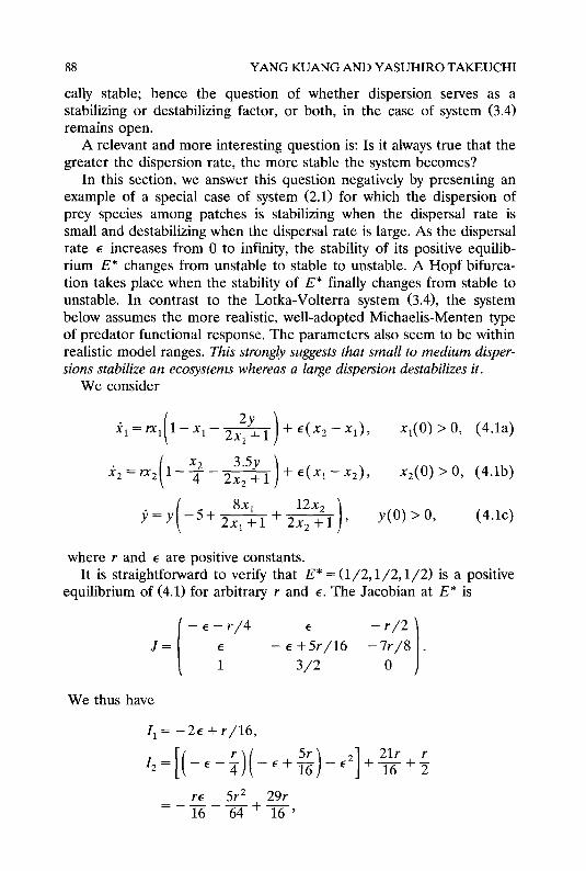
In this section, we answer this question negatively by presenting an example of a special case of system (2.1) for which the dispersion of prey species among patches is stabilizing when the dispersal rate is small and destabilizing when the dispersal rate is large. As the dispersal rate E increases from 0 to infinity, the stability of its positive equilibrium E* changes from unstable to stable to unstable. A Hopf bifurcation takes place when the stability of E* finally changes from stable to unstable. In contrast to the Lotka-Volterra system (3.4), the system below assumes the more realistic, well-adopted Michaelis-Menten type of predator functional response. The parameters also seem to be within realistic model ranges. This strongly suggests that small to medium dispersions stabilize an ecosystems whereas a large dispersion destabilizes it.

We consider

x1(O) > 0, (4.la)

x2(O) > 0, (4.lb)

Y(0) > OF (4.lc)

where r and E are positive constants. It is straightforward to verify that E* = (l/2,1/2,1/2) is a positive

equilibrium of (4.1) for arbitrary r and E. The Jacobian at E* is

We thus have

- E - r/4 E -r/2

E - E +5r/16 - 7r/8 1 312 0

I, = - 2~ + r/16,

1.

.5r2 29r =_--- ;‘6 64 +16’


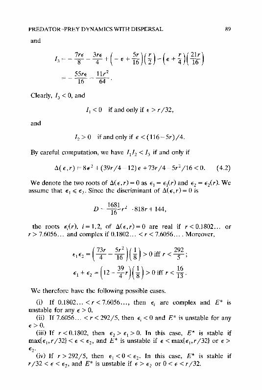
and

17=_~_~+(_~+~)(3)_(e+~)(~)

55re llr’ =__-- 16 64’

Clearly, I3 < 0, and

I, < 0 if and only if E > r/32,

and

I, > 0 if and only if E < (116-5r)/4.

By careful computation, we have I, Z, < 1, if and only if

A(E,r)=8e2+(39r/4-12)E+73r/4-5r2/16<0. (4.2)

We denote the two roots of A(E, r) = 0 as pi = El(r) and Ed = E&j. We assume that E, =G e2. Since the discriminant of A( E, r) = 0 is

D = 1681

TTr

2 - 818r + 144,

the roots q(r), i = 1,2, of A(e,r) = 0 are real if r < 0.1802... or r > 7.6056... and complex if 0.1802.. . < r < 7.6056.. . . Moreover,

We therefore have the following possible cases.

(i> If 0.1802.. . < r < 7.6056.. ., then q are complex and E* is unstable for any E > 0.

(ii) If 7.6056.. . < r < 292/5, then q < 0 and E* is unstable for any E > 0.

(iii) If r < 0.1802, then l 2 > pi > 0. In this case, E* is stable if maxlq, r/32} < E < Ed, and E* is unstable if E < max{Ei,r/32} or E >

E2.

(iv) If r > 292/5, then l 1 < 0 < e2. In this case, E* is stable if r/32 < E < cZ, and E* is unstable if E > Ed or 0 < E < r/32.


However, we note that Ed > r/32 if and only if r < 48/41. This can be seen from the fact that

*(&,r)=Fr>O forr>O,

which implies that either e2 2 e1 2 r/32, or e1 < l 2 < r/32. Therefore, in case (iii), we must have pi > r/32 if E* > r/32. In case (iv), it is impossible for Ed > r/32, and hence E* is always unstable. This shows that E* is always unstable if r > 0.1802.

We thus have proved the following.

THEOREM 4.1

Zn system (4.1), assume that r < 0.1802. The following statements are true

(i) E* is unstable if l < l 1 (ii) E* is locally asymptotically stable if E, < E < e2. (iii) E* is unstable for E > l 2.

For an example, if r = l/13 = 0.076923, then pi and Ed are roots of

32e2 -456 +3791/676 = 0.

We have pi = 0.138 and Ed = 1.268, while r/32 = 0.0024. Therefore in this case E* is locally asymptotically stable if e1 < E < Ed and unstable if E < pi or E > e2.

In fact, we can show the following.

THEOREM 4.2

A Hopf bifurcation takes place around E* when l = l 2, assuming that r < 0.1802. Zn other words, a unique, small-amplitude periodic solution bifurcates ffom the unstable equilibrium as l increases through e2.

Proof The characteristic equation of J at E* is

h3-zIIA2+z2h-z~=0. (4.3)

Let Ai = hi(e) be roots of (4.3). Since Z3 = A,A,A, < 0, we see that when E = l 2 we must have A, = iw, A, = - iw for some w > 0, and A, < 0. Indeed, at E = l 2,

I, = A, + A, + A, = A, and I, = A,A,A, = w2A3.

PREDATOR-PREY DYNAMICS WITH DISPERSAL

Hence

A, = Z,, W=dm.

Denote A’= dA(~)/de. We have

h, = rA/16-55r/16-2h2

3A2 -21,/I+ z, .

Clearly Z2 = 02. Hence

signRe A’IAzi, = signRe 32 w2 - 55r + irw

-26~ - i21, I = -signRe[(2w - i2Z,)(32w2 -55r + irw)].

We thus have

signReh’lA=j, =sign{llOr-2Z,r-641,/Z,}

= sign{ 110r - 2Z,r - 641,).

At E=E~,

llOr-2Z,r-64Z2=l10r-2r -2~*+& ( 1

-64 ( -kt2-&r’+$r

= 8rc + 2

zr2 - 6r. 8

Since

Hence

Z,Z, = Z3 at E = E,, i=1,2,

A(q,r)=O fori=1,2.

O=A(E2,r)-A(E1,r)=8($- e~)+(~r-12)(e2-EI).

Since e1 # l 2, we have S(E* + El)+ (39/4)r - 12 = 0. Therefore,

signRe A’lA\=io = sign 8~~ + Tr -6 [ 1 = sign[8E2 -4( l 2 + Ed)]

=sign[e2--eE1]>O.


Theorem 4.2 now follows from the well-known Hopf bifurcation theorem [7, p. 3441. a

Again, let us consider the previous example when r = l/13. In this case a Hopf bifurcation takes place when E increases through E = 1.268.

Biologically, system (4.1) has the following features:

(1) Both patches have the same intrinsic growth rate for prey X. Patch 2 has a carrying capacity four times that of patch 1; for example, patch 2 is four times bigger.

(2) The predator is more efficient in catching prey in patch 2 (3.5 vs. 2) but has a smaller conversion rate (24/7 vs. 4). This is quite reasonable in the sense that the extra prey caught will be used less efficiently.

(3) It is safe to disperse from one patch to another.

It is interesting to know whether the results in this section are global. Theoretically, this remains unknown. Numerically, it seems to us that they are indeed global. The following figures provide solutions corre- sponding to three values of E, E < pi, e1 < E < E*, and E > cZ, when r = 0.0769 ( = l/13) in system (4.1). In this case, we have pi = 0.138 and l f = 1.268.

In the Figures 1-3, xg = y. These figures are obtained by using the differential equation solver PHASER. The algorithm used is Runge- Kutta. The ranges of xi’s are indicated in the figures.

Figures la, lb, lc illustrate xi versus time, i = 1,2,3, respectively, with initial conditions x,(O) = x,(O) = x,(O) = 0.505 and E = 0.08 < E,. The end time is set as 3000.

Figures 2a, 2b, 2c illustrate xi versus time, i = 1,2,3, respectively, with initial conditions x,(O) = x,(O) = x,(O) = 1 and E = 1, E, < E < E*. The end time is taken as 1000.

Figures 3a, 3b, 3c illustrate xi versus time, i = 1,2,3, respectively, with initial conditions x,(O) = x,(O) = x,(O) = 0.6 and E = 2 > Ed. The time ends at 2000.

5. DISCUSSION

In this paper, we have analyzed a Gause-type predator-prey system with prey dispersal in a two-patch environment. Conditions for persistence and extinction are presented. Results on the existence and local and global stability of the positive steady state are obtained.

In order to have global stability, our criterion requires that the dispersal rate E be bounded above by some related constant. This observation is further supported by the example presented in Section 4. In that example, we have shown that small to medium dispersal rates (E , = 0.136 and l 2 = 1.268 vs. r = l/13) tend to stabilize the system


(a)

1.- I

t

x3

Cc)

FIG. 1. e = 0.08 and T = 3000. x,(O) = 0.505; i = 1,2,3.


t

(a)

r

x3 -

500 t,

600 + -

!l 700 +

1e.s-

600 900 loot

---c--t---- -

FIG. 2. t

Cc)

I = 1 and T = 1000. xi(O) = 1, i = 1,2,3.

1


x1 VS. Tin*: 1. seeeee

00 t

r

x3 m.B-

Cc)

FIG. 3. E = 2 and T = 2000. xi(O) = 0.6, i = 1,2,3.


whereas large and very small dispersal rates (E > l 2 and E < l 1) may destabilize it. This is quite surprising in the sense that most of the existing results tend to show that diffusions are stabilizing forces [l, 2, 14, 22, 27, 28, and references cited therein]. This is indeed true in general for continuous diffusion within the same patch [l, 2, 14, 22, 24, and references cited therein]. On the other hand, this seems reasonable. Since very great dispersion among patches may have the side effect of overreaction to the difference in the densities among different patches, this, of course, can be the cause of destabilization. This suggests that dispersion among patches should be regulated. Neither no dispersion nor unlimited dispersion may serve the interest of stabilizing the given ecosystem!

It is interesting to note that a refuge patch for prey does not destabilize the interaction as supported by our Theorem 3.3. This is in accordance with recent results of Takeuchi [29, 301. This observation may be useful in planning and controlling ecosystems.

Mathematically, our approach in principle can be applied to handle many-patch environments (those with more than two patches). We can also assume that there are barriers to predator dispersal among patches, and the dispersal dynamics may be nonlinear as proposed in [9]-[ll] and [13]. Naturally, these considerations will make our analysis more complicated, and we leave them to future investigations.

Research of Y. Kuang partially supported by National Science Founda- tion grant DMS-9102549.

REFERENCES

L. .I. S. Allen, Persistence and extinction in Lotka-Volterra reaction diffusion equations, Math. Biosci. 65:1-12 (1983). L. .I. S. Allen, Persistence, extinction, and critical patch number for island populations, J. Math. Biol. 24:617-625 (1987). E. Beretta and Y. Takeuchi, Global stability of single-species diffusion Volterra models with continuous time delays, Bull. Math. Biol. 49:431-448 (1987). E. Beretta and Y. Takeuchi, Global asymptotic stability of Lotka-Volterra diffusion models with continuous time delays, SIAM J. Appl. Math. 48:627-651 (1988). E. Beretta, F. Solimano, and Y. Takeuchi, Global stability and periodic orbits for two patch predator-prey diffusion-delay models, Math. Biosci. 85:153-183 (19871. G. J. Butler, H. I. Freedman, and P. Waltman, Uniformly persistent systems, Proc. Am. Math. Sot. 96:425-430. L. Edelstein-Keshet, Mathematical Models in Biology, Random House, New York, 1988.


8 H. I. Freedman, Single species migration in two habitats: persistence and extinction, Math. Model. 8778-780 (1987).

9 H. I. Freedman and Y. Takeuchi, Global stability and predator dynamics in a model of prey dispersal in a patchy environment, Nonlinear Anal., TMA 13:993-1002 (1989).

10 H. I. Freedman and Y. Takeuchi, Predator survival versus extinction as a function of dispersal in a predator-prey model with patchy environment, Appl.

Anal. 31:247-266 (1989). 11 H. 1. Freedman and P. Waltman, Mathematical models of population interac-

tion with dispersal. I. Stability of two habitats with and without a predator, SZAMJ. Appl. Math. 32:631-648 (19771.

12 H. I. Freedman and P. Waltman, Persistence in models of three interacting predator-prey populations, Math. Biosci 68:213-231 (1984).

13 H. I. Freedman, B. Rai, and P. Waltman, Mathematical models of population interactions with dispersal. II. Differential survival in a change of habitat, J. Muth. Anal. Appl. 115:140-154 (1986).

14 A. Hastings, Dynamics of a single species in a spatially varying environment: the stabilizing role of high dispersal rates, J. Math. Biol. 28:181-208 (19851.

15 R. D. Holt, Population dynamics in two patch environments: some anomalous consequences of optional habitat selection, Theor. Pop. Biol. 28:181-208 (1985).

16 C. B. Huffaker and C. E. Kennett, Experimental studies on predation: predation and cyclamen-mite populations on strawberries on California, Hilgurdiu

26:191-222 (1956). 17 V. Hutson and K. Schmitt, Permanence and the dynamics of biological systems,

Math. Biosci. 111:1-71 (1992). 18 Y. Kuang and H. L. Smith, Global stability in infinite delay, Lotka-Volterra type

systems, J. Dij@r. Equations 102X1993). 19 Y. Kuang, R. H. Martin, and H. L. Smith, Global stability for infinite delay,

dispersive Lotka-Volterra systems: weakly interacting populations in nearly identical patches, J. Dynum. Diner. Equations 3:339-360 (1991).

20 N. R. LeBlond, Porcupine Caribou Herd, Canadian Arctic Resources Comm., Ottawa, 1979.

21 S. A. Levin, Dispersion and population interactions, Am. Nut. 1008:207-228 (19741.

22 S. A. Levin, Spatial patterning and the structure of ecological communities, in Some Muthematicul Questions in Biology, Vol. VII, l-35 (D. Ludwig, ed.), Am. Math. Sot., Providence, R.I., 1976.

23 S. A. Levin and L. A. Segal, Hypothesis for origin of planktonic patchiness, Nuture 259:659 (1976).

24 L. A. Segal and S. A. Levin, Application of nonlinear stability theory to the study of the effects of diffusion on predator-prey interactions, Topics in Statistical Mechanics and Biophysics: A Memorial to Julius L. Jackson, 123-152. AIP Conf. Proc., No. 27 (W. D. Lakin, ed.) Amer. Inst. Phys., New York, 1976.

25 H. L. Smith, On the asymptotic behavior of a class of deterministic models of cooperating species, SZAM J. Appl. Math. 46:368-375 (1986).

26 Y. Takeuchi, Global stability in generalized Lotka-Volterra diffusion systems, J. Math. Anal. Appl. 116:209-221 (1986).

27 Y. Takeuchi, Diffusion effect on stability of Lotka-Volterra models, Bull. Math. Biol. 46:585-601 (1986).


28 Y. Takeuchi, Cooperative systems theory and global stability of diffusion models, Accu A&. Math. 14:49-57 (1989).

29 Y. Takeuchi, Diffusion-mediated persistence in two-species competition Lotka- Volterra model, Math. Biosci. 95:65-83 (1989).

30 Y. Takeuchi, Conflict between the need to forage and the need to avoid competition: persistence of two-species model, Math. Biosci. 99:181-194 (1990).

31 R. R. Vance, The effect of dispersal on population stability in one-species, discrete space population growth models, Am. Nut. 123:230-254 (19841.

Predator-prey dynamics in models of prey dispersal in two-patch environments

Documents

Transcript of Predator-prey dynamics in models of prey dispersal in two-patch environments