
HARVESTING A TWO-PATCH PREDATOR-PREY METAPOPULATION
18
Transcript of HARVESTING A TWO-PATCH PREDATOR-PREY METAPOPULATION
NATURAL RESOURCE MODELING
Volume 12, Number 4, Winter 1999
HARVESTING A TWO-PATCH
PREDATOR-PREY METAPOPULATION
ASEP K. SUPRIATNAJurusan Matematika
FMIPA Univesitas PadjadjaranKm 21 Jatinangor-Bandung, Indonesia
Fax: 62-22-4218676
Current address: Dept. of Applied MathematicsUniversity of AdelaideSA 5005, Australia
E-mail: [email protected]
HUGH P. POSSINGHAMDept. of Environmental Science and Management
University of AdelaideRoseworthy SA 5371, Australia
ABSTRACT. A mathematical model for a two-patchpredator-prey metapoplation is developed as a generalizationof single-species metapopulation harvesting theory. We �ndoptimal harvesting strategies using dynamic programming andLagrange multipliers. If predator economic eÆciency is rel-atively high, then we should protect a relative source preysubpopulation in two di�erent ways: directly, with a higherescapement of the relative source prey subpopulation, and in-directly, with a lower escapement of the predator living in thesame patch as the relative source prey subpopulation. Numer-ical examples show that if the growth of the predator is rela-tively low and there is no di�erence between prey and predatorprices, then it may be optimal to harvest the predator to ex-tinction. While, if the predator is more valuable compared tothe prey, then it may be optimal to leave the relative exporterprey subpopulation unharvested. We also discuss how a `neg-ative' harvest might be optimal. A negative harvest might beconsidered a seeding strategy.
KEY WORDS: Fisheries, harvesting strategies, predator-prey metapopulation, seeding strategy.
1. Introduction. This paper studies optimal harvesting strate-
gies for a two-patch predator-prey metapopulation. The dynamics of
the predator-prey metapopulation is de�ned by four coupled di�erence
This paper was presented at the World Conference on Natural Resource Mod-elling, CSIRO Division of Marine Research, Hobart, Australia, December 15 18,1997.
Copyright c 1999 Rocky Mountain Mathematics Consortium
1
2 A.K. SUPRIATNA AND H.P. POSSINGHAM
equations. Optimal harvesting strategies for the metapopulation are
derived using dynamic programming and Lagrange multipliers. The
theory presented here is a generalization of single-species metapopula-
tion harvesting theory developed by Tuck and Possingham [1994].
The optimal strategy for managing a dynamic renewable resource
was not established until Clark [1971, 1973 and 1976], explored opti-
mal harvesting strategies for a single-species population using dynamic
programming. Clark showed that if the growth rate of the resource is
less than the discount rate, then a rational sole owner maximizing the
net economic gain of a resource should exploit the resource to extinc-
tion. Clark's work [1971, 1973 and 1976] has been very in uential in
the development of an economic theory of renewable resource exploita-
tion and has been extended to include various economic and biological
complexities (Reed [1982], Agnew [1982], Gatto et al. [1982], Clark and
Tait [1982], Ludwig and Walters [1982], Chaudhuri [1986 and 1988],
Mesterton-Gibbons [1996], Tuck and Possingham [1994], Ganguly and
Chaudhuri [1995], Supriatna and Possingham [1998]).
Spatial heterogeneity is recognized as a factor that needs to be
taken into account in population modelling in general (Dubois [1975],
Goh [1975], Hilborn [1979], Lefkovitch and Fahrig [1985], Matsumoto
and Seno [1995]), and in �sheries modelling in particular (Beverton
and Holt [1957], Brown and Murray [1992], Frank [1992], Frank and
Leggett [1994], Parma et al. [1998]). In the ocean, population patches
may exist from scales of meters to thousands of kilometers and often
occur in response to physical and biological processes, like advection,
temperature and food quality (Letcher and Rice [1997]). The inclusion
of spatial heterogeneity may change the decisions that should be made
to manage a �shery (Tuck and Possingham [1994], Pelletier and Magal
[1996], Brown and Roughgarden [1997]). With the inclusion of spatial
heterogeneity into Clark's [1976] model, Tuck and Possingham [1994]
found some rules of thumb for optimal economic harvesting of a two-
patch single-species metapopulation system. One of their rules is that
a relative source subpopulation, that is a subpopulation with a greater
per-capita larval production, should be harvested more conservatively
than a relative sink subpopulation. We de�ne the terms `relative source'
and `relative sink' subpopulation more precisely in the next section.
Supriatna and Possingham [1998] showed that, in some circum-
stances, Tuck and Possingham's [1994] single-species harvesting rules
PREDATOR-PREY METAPOPULATION 3
of thumb are preserved in the presence of a predator. Our previous
model (Supriatna and Possingham [1998]) assumed that predation af-
fects the predator survival. In this paper, we modify our previous
model to assume that predation a�ects predator recruitment, that is,
prey consumption primarily increases the predator population through
production and survival of young rather than adult survival. The re-
sults in this paper show that the most signi�cant rule, that we should
harvest a relative source subpopulation more conservatively than a rela-
tive sink subpopulation, is robust, regardless of the biological structure
of the population. We also explore the situation in which the optimal
harvest for one of the populations is negative. While at �rst glance
this appears unlikely, a negative harvest could be implemented in some
cases by seeding a population.
2. The model. Consider a predator-prey metapopulation that
coexists in two di�erent patches, patch 1 and patch 2. The movement
of individuals between the local populations is a result of dispersal by
juveniles. Adults are assumed to be sedentary, and they do not migrate
from one patch to another patch. Let the number of the prey (predator)
in patch i at the beginning of period k be denoted by Nik (Pik) and the
survival rate of adult prey (predator) in patch i be denoted by ai (bi),
respectively. The proportion of juvenile prey and predator from patch
i that successfully migrate to patch j are pij and qij , respectively, see
Figure 1. Let SNik = Nik�HNik(SPik = Pik�HPik) be the escapement
of the prey (predator) in patch i at the end of that period, with HNik
(HPik) the harvest taken from the prey (predator). Furthermore, let
the dynamics of exploited metapopulation of these two species be given
by the equations:
(1) Ni(k+1) = aiSNik + �iSNikSPik + piiFi(SNik) + pjiFj(SNjk);
(2)Pi(k+1) = biSPik + qii(Gi(SPik) + �iSNikSPik)
+ qji(Gj(SPjk) + �jSNjkSPjk);
where the functions Fi(Nik) and Gi(Pik) are the recruit production
functions of the prey and predator in patch i at time period k. We
will assume that the recruit production functions are logistic for the
remainder of this paper, that is, Fi(Nik) = riNik(1 � Nik=Ki) and

4 A.K. SUPRIATNA AND H.P. POSSINGHAM
p
p p
21
2211N N21
p12
P2
q21
P1
q11
q12
q12
q22
β1 N1 P1 2 2 2β N P
Patch 1 Patch 2
q22
q11
q21
FIGURE 1. The relationships between the dynamics of the populations in atwo-patch predator-prey metapopulation. The number of prey and predatorare Ni and Pi, respectively. The prey and predator juvenile migration rates arepij and qij , respectively. The number of predator's o�springs in patch i fromthe conversion of eaten prey is �iNiPi, which is distributed into patch i andj with proportion qii and qij , respectively, while some of them (1� qii � qij),
either die or are lost from the system.
Gi(Pik) = siPik(1� Pik=Li), where ri(si) denotes the intrinsic growth
of the prey (predator) and Ki (Li) denotes the local carrying capacity
of the prey (predator), with �i < 0 and �i > 0.
If �Xi(Xik; Sik) =R Xik
SXik(pX�cXi(�)) d� represents the present value
of net revenue from harvesting subpopulation Xi in period k, where
X = NorP , pX is the price per unit harvested population X, cXi is
the cost to harvest subpopulation Xi (it may depend on location), and
� is a discount factor, then to obtain an optimal harvest from the �shery
we should maximize net present value
(3) PV =
TXk=0
�k2Xi=1
�Ni(Nik; SNik) +
TXk=0
�k2Xi=1
�Pi(Pik; SPik);
subject to equations (1) and (2), with nonnegative escapement less than

PREDATOR-PREY METAPOPULATION 5
or equal to the population size. We will assume � = 1=(1 + Æ) for the
remainder of this paper, where Æ denotes a periodic discount rate, e.g.,
Æ = 10%.
Supriatna and Possingham [1998] used dynamic programming to ob-
tain optimal harvesting strategies for a similar predator-prey metapop-
ulation. They generalized the method in Clark [1976] and Tuck and
Possingham [1994], and they found that in some circumstances harvest-
ing strategies for a single-species metapopulation can be generalized in
the presence of predators. Following Supriatna and Possingham [1998]
we use dynamic programming to obtain optimal harvesting strategies
by maximizing net present value in equation (3) and we �nd implicit
expressions for optimal escapements S�
Ni0and S�
Pi0in the form:
(4)
pN � cNi(S�
Ni0)
�= (ai + �iS
�
Pi0 + piiF0
i (S�
Ni0))(pN � cNi(Ni1))
+ pijF0
i (S�
Ni0)(pN � cNj(Nj1))
+ qii�iS�
Pi0(pP � cPi(Pi1))
+ qij�iS�
Pi0(pP � cPj(Pj1));
(5)
pP � cPi(S�
Pi0)
�= (bi + qii�iS
�
Ni0 + qiiG0
i(S�
Pi0))(pP � cPi(Pi1))
+ qij�iS�
Ni0(pP � cPj(Pj1))
+ qijG0
i(S�
Pi0)(pP � cPj(Pj1))
+ �iS�
Ni0(pN � cNi(Ni1)):
These equations are the general form of the optimal harvesting equation
for a two-patch predator-prey metapopulation. If there is no predator
mortality associated with migration qii+qij = 1, and costs of harvesting
are spatially independent, then these equations are the same as in
Supriatna and Possingham [1998]. If �i = �i = 0, then the optimal
harvesting equation for a single-species metapopulation (Tuck and
Possingham [1994]) is obtained. Furthermore, if there is no migration
between patches, pij = qij = 0 for i 6= j, and F 0(S) = ai +
piiF0
i (SNi0) together with �i = �i = 0, then the equation reduces to
the optimal harvesting equation for a single-species population (Clark
[1976]). Although we can show that the escapements S�
Xi0 found by
solving these implicit equations are independent of the time horizon
6 A.K. SUPRIATNA AND H.P. POSSINGHAM
considered, we do not show it in this paper. Consequently, due to the
time independence, there is a notational change for the remainder of
the paper, that is, we simply use S�
Xito denote optimal escapement
for subpopulation X in patch i. We discuss some properties of these
escapements in the following section.
3. Results and discussion. In this section we discuss some
properties of the optimal escapements de�ned by equations (4) and (5).
We compare the optimal escapements between the two subpopulations.
For the remainder of the paper we assume that market price for the
predator is higher than or equal to the price for the prey, that is,
pP = mpN with m � 1, and prey vulnerability is the same in both
patches, that is, �1 = �2 = �.
To facilitate some comparisons of the properties of our optimal es-
capements, we adopt the following de�nitions from Tuck and Possing-
ham [1994] and Supriatna and Possingham [1998]:
1. Prey subpopulation i is a relative source subpopulation if its per
capita larval production is greater than the per capita larval production
of prey subpopulation j, that is, ri(pii + pij) > rj(pjj + pji). If this is
the case, then prey subpopulation j is a relative sink subpopulation.
2. Prey subpopulation i is a relative exporter subpopulation if it ex-
ports more larvae to prey subpopulation j than it imports (per capita),
that is, r1p12 > r2p21. If this is the case, then prey subpopulation j is
called a relative importer subpopulation.
3. The fraction �i=j�ij is called the biological eÆciency and the
fraction m(qii+qij)�i=j�ij is called the economic eÆciency of predator
subpopulation i.
3.1. Negligible costs analysis. To simplify the analysis, the costs
of harvesting are assumed to be negligible. Using these assumptions,
and substituting all derivatives of the logistic recruitment functions, Fiand Gi, into equations (4) and (5), we can �nd explicit expressions for
the optimal escapements S�
Ni and S�
Pi:
S�
Ni =Aim(qi1 + qi2)(2si=Li) + CiBi
�i
;(6)
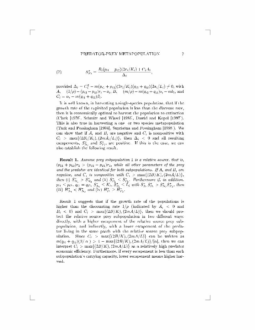
PREDATOR-PREY METAPOPULATION 7
S�
Pi =Bi(pi1 + pi2)(2ri=Ki) + CiAi
�i
;(7)
provided �i = C2i �m(pi1 + pi2)(2ri=Ki)(qi1 + qi2)(2si=Li) 6= 0, with
Ai = (1=�)� (pi1+ pi2)ri� ai, Bi = (m=�)�m(qi1+ qi2)si�mbi, and
Ci = �i +m(qi1 + qi2)�i.
It is well known, in harvesting a single-species population, that if the
growth rate of the exploited population is less than the discount rate,
then it is economically optimal to harvest the population to extinction
(Clark [1976], Schmitt and Wissel [1985], Dawid and Kopel [1997]).
This is also true in harvesting a one- or two-species metapopulation
(Tuck and Possingham [1994], Supriatna and Possingham [1998]). We
can show that if Ai and Bi are negative and Ci is nonpositive with
Ci > maxf(2Bi=Ki); (2mAi=Li)g, then �i < 0 and all resulting
escapements, S�
Niand S�
Pi, are positive. If this is the case, we can
also establish the following result.
Result 1. Assume prey subpopulation 1 is a relative source, that is,
(p11 + p12)r1 > (p22 + p21)r2, while all other parameters of the prey
and the predator are identical for both subpopulations. If Ai and Bi are
negative, and Ci is nonpositive with Ci > maxf(2B=K); (2mA=L)g,
then (i) S�
N1> S�
N2and (ii) S�
P1� S�
P2. Furthermore if, in addition,
pi1 � pi2, qi1 = qi2, S�
Ni� Ki, S
�
Pi� Li with S�
N1S�
P1> S�
N2S�
P2, then
(iii) H�
N1< H�
N2and (iv) H�
P1� H�
P2.
Result 1 suggests that if the growth rate of the populations is
higher than the discounting rate 1=� (indicated by Ai < 0 and
Bi < 0) and Ci > maxf(2B=K); (2mA=L)g, then we should pro-
tect the relative source prey subpopulation in two di�erent ways:
directly, with a higher escapement of the relative source prey sub-
population, and indirectly, with a lower escapement of the preda-
tor living in the same patch with the relative source prey subpop-
ulation. Since Ci > maxf(2B=K); (2mA=L)g can be written as
m(qii + qij)(�=j�j) > 1 + maxf(2B=K); (2mA=L)g=j�j, then we can
interpret Ci > maxf(2B=K); (2mA=L)g as a relatively high predator
economic eÆciency. Furthermore, if every escapement is less than each
subpopulation's carrying capacity, lower escapement means higher har-
vest.
8 A.K. SUPRIATNA AND H.P. POSSINGHAM
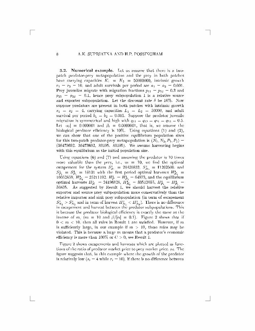
3.2. Numerical example. Let us assume that there is a two-
patch predator-prey metapopulation and the prey in both patches
have carrying capacities K1 = K2 = 50000000, intrinsic growth
r1 = r2 = 10, and adult survivals per period are a1 = a2 = 0:001.
Prey juveniles migrate with migration fractions p11 = p12 = 0:3 and
p21 = p22 = 0:1, hence prey subpopulation 1 is a relative source
and exporter subpopulation. Let the discount rate Æ be 10%. Now
suppose predators are present in both patches with intrinsic growth
s1 = s2 = 4, carrying capacities L1 = L2 = 50000, and adult
survival per period b1 = b2 = 0:001. Suppose the predator juvenile
migration is symmetrical and high with q11 = q12 = q21 = q22 = 0:5.
Let j�ij = 0:000001 and �i = 0:0000001, that is, we assume the
biological predator eÆciency is 10%. Using equations (1) and (2),
we can show that one of the positive equilibrium population sizes
for this two-patch predator-prey metapopulation is ( �N1; �N2; �P1; �P2) =
(36473692; 36473692; 83105; 83105). We assume harvesting begins
with this equilibrium as the initial population size.
Using equations (6) and (7) and assuming the predator is 10 times
more valuable than the prey, i.e., m = 10, we �nd the optimal
escapement for the system S�
N1= 20420833, S�
N2= 11262500, and
S�
P1= S�
P2= 18131 with the �rst period optimal harvests H�
N1=
16052859, H�
N2= 25211192, H�
P1= H�
P2= 64973, and the equilibrium
optimal harvests H�
N1= 24196828, H�
N2= 33512055, H�
P1= H�
P2=
56835. As suggested by Result 1, we should harvest the relative
exporter and source prey subpopulation more conservatively than the
relative importer and sink prey subpopulation (in term of escapement
S�
N1> S�
N2and in term of harvest H�
N1< H�
N2). There is no di�erence
in escapement and harvest between the predator subpopulations. This
is because the predator biological eÆciency is exactly the same as the
inverse of m, (m = 10 and �=j�j = 0:1). Figure 2 shows that if
0 < m < 10, then all rules in Result 1 are satis�ed. However, if m
is suÆciently large, in our example if m > 10, these rules may be
violated. This is because a large m means that a predator's economic
eÆciency is more than 100% or C > 0, see Result 1.
Figure 2 shows escapements and harvests which are plotted as func-
tions of the ratio of predator market price to prey market price, m. The
�gure suggests that, in this example where the growth of the predator
is relatively low (si = 4 while ri = 10), if there is no di�erence between
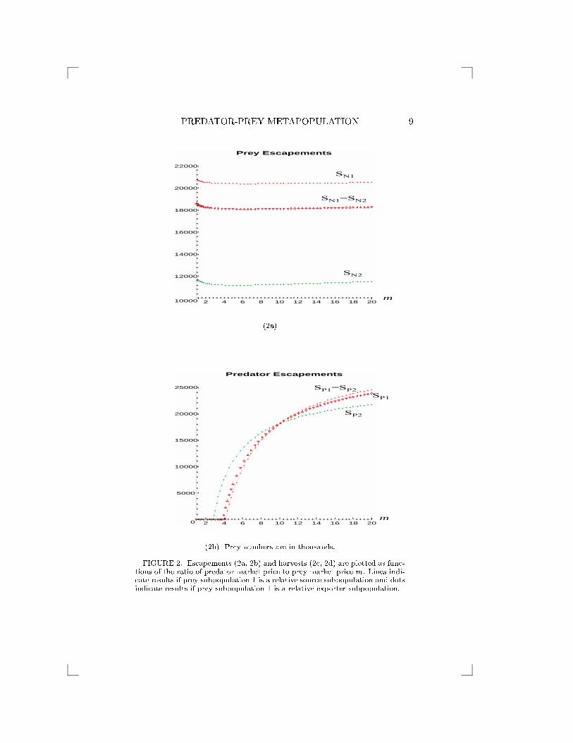
PREDATOR-PREY METAPOPULATION 9
2018161412108642
22000
20000
18000
16000
14000
12000
10000
Prey Escapements
SN1=SN2
SN1
SN2
m
(2a)
2018161412108642
25000
20000
15000
10000
5000
0
Predator Escapements
SP1
SP2
SP1=SP2
m
(2b) Prey numbers are in thousands.
FIGURE 2. Escapements (2a, 2b) and harvests (2c, 2d) are plotted as func-tions of the ratio of predator market price to prey market price m. Lines indi-cate results if prey subpopulation 1 is a relative source subpopulation and dotsindicate results if prey subpopulation 1 is a relative exporter subpopulation.

10 A.K. SUPRIATNA AND H.P. POSSINGHAM
600550500450400
50000
40000
30000
20000
10000
0
Prey Harvests
HN2
HN2
HN1
HN1
m
(2c)
600550500450400
40000
30000
20000
10000
00000
Predator Harvests
HP1HP2
HP1=HP2
m
(2d)
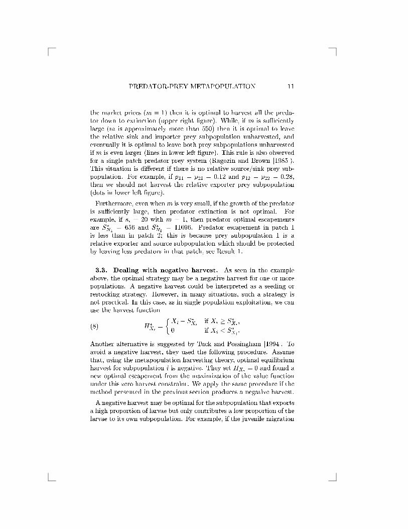
PREDATOR-PREY METAPOPULATION 11
the market prices (m = 1) then it is optimal to harvest all the preda-
tor down to extinction (upper right �gure). While, if m is suÆciently
large (m is approximately more than 550) then it is optimal to leave
the relative sink and importer prey subpopulation unharvested, and
eventually it is optimal to leave both prey subpopulations unharvested
if m is even larger (lines in lower left �gure). This rule is also observed
for a single patch predator-prey system (Ragozin and Brown [1985]).
This situation is di�erent if there is no relative source/sink prey sub-
population. For example, if p11 = p21 = 0:12 and p12 = p22 = 0:28,
then we should not harvest the relative exporter prey subpopulation
(dots in lower left �gure).
Furthermore, even whenm is very small, if the growth of the predator
is suÆciently large, then predator extinction is not optimal. For
example, if si = 20 with m = 1, then predator optimal escapements
are S�
N1= 656 and S�
N2= 11096. Predator escapement in patch 1
is less than in patch 2; this is because prey subpopulation 1 is a
relative exporter and source subpopulation which should be protected
by leaving less predators in that patch, see Result 1.
3.3. Dealing with negative harvest. As seen in the example
above, the optimal strategy may be a negative harvest for one or more
populations. A negative harvest could be interpreted as a seeding or
restocking strategy. However, in many situations, such a strategy is
not practical. In this case, as in single population exploitation, we can
use the harvest function
(8) H�
Xi=
�Xi � S�
Xiif Xi � S�
Xi,
0 if Xi < S�
Xi.
Another alternative is suggested by Tuck and Possingham [1994]. To
avoid a negative harvest, they used the following procedure. Assume
that, using the metapopulation harvesting theory, optimal equilibrium
harvest for subpopulation i is negative. They set HXi= 0 and found a
new optimal escapement from the maximization of the value function
under this zero harvest constraint. We apply the same procedure if the
method presented in the previous section produces a negative harvest.
A negative harvest may be optimal for the subpopulation that exports
a high proportion of larvae but only contributes a low proportion of the
larvae to its own subpopulation. For example, if the juvenile migration

12 A.K. SUPRIATNA AND H.P. POSSINGHAM
parameters for the prey in the previous example are p11 = p21 = 0:2
and p12 = p22 = 0:065 with m = 10, then the optimal equilibrium
harvest for the prey subpopulation 2 is H�
N2 = �1427582, while all
other subpopulations have a positive harvest. This strategy suggests
that we should seed prey into subpopulation 2 and harvest the results
from prey subpopulation 1 and both predator subpopulations. To avoid
a negative harvest for prey subpopulation 2, we set HN2= 0 and, using
the method of Lagrange multipliers, we maximize the present value
in equation (3) with this additional constraint. The new equilibrium
optimal escapements S�
N1; S�
N2; S�
P1, and S�
P2satisfy equations:
(pN � cN1(SN10
))
�= (pN � cN1
(N11))[a1 + p11F0
1(SN10) + �1SP10 ]
+ (pP � cP1(P11))[q11�1SP10 ]
+ (pP � cP2(P21))[q12�1SP10 ]
+ (pN � cN2(SN20
))
�p12F
0
1(SN10)(1� 1=�)
Z
�(9)
+ (pN � cN1(N11))
�p12p21F
0
1(SN10)F 0
2(SN20)
Z
�
+ (pP � cP2(P21))
�p12F
0
1(SN10)q22�2SP20Z
�
+ (pP � cP1(P11))
�p12F
0
1(SN10)q21�2SP20Z
�;
(pP � cP2(SP20))
�= (pP � cP2(P21))[b2 + q22G
0
2(SP20) + q22�2SN20]
+ (pP � cP1(P11))[q21G0
2(SP20) + q21�2SN20]
+ (pN � cN2(SN20
))
��2SN20
(1� 1=�)
Z
�
+ (pN � cN1(N11))
�p21F
0
2(SN20)�2SN20
Z
�(10)
+ (pP � cP2(P21))
��2SN20
q22�2(SP20)
Z
�
+ (pP � cP1(P11))
��2SN20
q21�2(SP20)
Z
�;
PREDATOR-PREY METAPOPULATION 13
-5000000
0
5000000
10000000
15000000
20000000
25000000
30000000
SN1 SN2 HN1 HN2
Seeding Zero Harvest Modified zero harvest
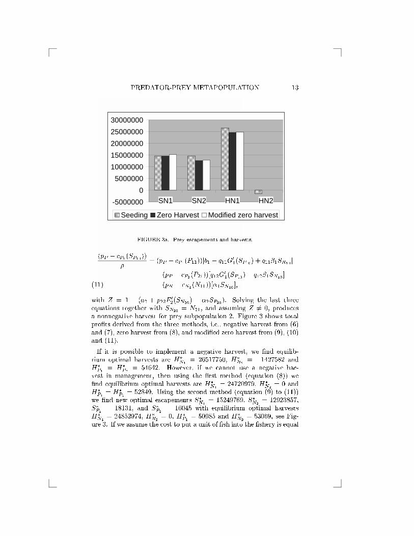
FIGURE 3a. Prey escapements and harvests.
(pP � cP1(SP10))
�= (pP � cP1(P11))[b1 + q11G
0
1(SP10) + q11�1SN10]
+ (pP � cP2(P21))[q12G0
1(SP10) + q12�1SN10]
+ (pN � cN1(N11))[�1SN10
];(11)
with Z = 1 � (a2 + p22F0
2(SN20) + �2SP20). Solving the last three
equations together with SN20= N21, and assuming Z 6= 0, produces
a nonnegative harvest for prey subpopulation 2. Figure 3 shows total
pro�ts derived from the three methods, i.e., negative harvest from (6)
and (7), zero harvest from (8), and modi�ed zero harvest from (9), (10)
and (11).
If it is possible to implement a negative harvest, we �nd equilib-
rium optimal harvests are H�
N1= 26517750, H�
N2= �1427582 and
H�
P1= H�
P2= 54642. However, if we cannot use a negative har-
vest in management, then using the �rst method (equation (8)) we
�nd equilibrium optimal harvests are H�
N1= 24720979, H�
N2= 0 and
H�
P1= H�
P2= 52849. Using the second method (equation (9) to (11))
we �nd new optimal escapements S�
N1= 15249769, S�
N2= 12923857,
S�
P1= 18131, and S�
P2= 16045 with equilibrium optimal harvests
H�
N1= 24852974, H�
N2= 0, H�
P1= 50985 and H�
N2= 53069, see Fig-
ure 3. If we assume the cost to put a unit of �sh into the �shery is equal
14 A.K. SUPRIATNA AND H.P. POSSINGHAM
0
10000
20000
30000
40000
50000
60000
SP1 SP2 HP1 HP2
Seeding Zero Harvest Modified zero harvest
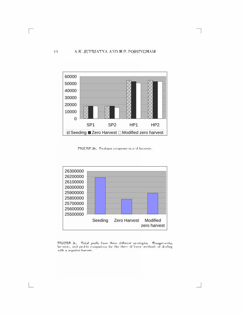
FIGURE 3b. Predator escapements and harvests.
255000002560000025700000258000002590000026000000261000002620000026300000
Seeding Zero Harvest Modifiedzero harvest
FIGURE 3c. Total pro�t from three di�erent strategies. Escapements,harvests, and pro�ts comparison for the three di�erent methods of dealingwith a negative harvest.
PREDATOR-PREY METAPOPULATION 15
to the pro�t per unit �sh from harvesting, then, neglecting all associ-
ated costs, the total revenue from the harvest is, if a negative harvest
is allowable, HN1+HN2
+ 10(HP1 +HP2) = 26183008 currency units.
This revenue is above the revenue if we use zero harvest from either
the �rst or second method, i.e., 25777959 from the �rst method and
25893514 from the second method. This suggests a negative harvest is
optimal.
4. Conclusion. Harvesting strategies for a predator-prey metapop-
ulation are established as a generalization of harvesting strategies for
a single-species metapoplation. Some properties of the escapements
for a single-species metapopulation (Tuck and Possingham [1994]) are
preserved in the presence of the predator, such as the strategies on how
to harvest relative source and sink subpopulations. We found that if
there are no di�erences between the biological parameters of the local
populations, except migration parameters, we should harvest a relative
source prey subpopulation more conservatively than a relative sink sub-
population. This is the same as the rule of thumb derived from work
on the single-species metapopulation (Tuck and Possingham [1994]).
In addition, we should harvest the predator subpopulation living in the
same patch with the relative source prey subpopulation more heavily
than the other predator subpopulation.
In this paper we have discussed how a `negative' harvest might
occur. Under some circumstances our equations show that a negative
harvest is optimal. A negative harvest might be considered a seeding
strategy. In many situations a seeding strategy is impractical, so in
this case an alternative strategy of imposing zero harvest, for the
population which has a negative harvest, is the best that can be
done. If it is possible to implement a negative harvest, numerical
examples show that if the market price of the predator is much greater
than the market price of the prey, then it may be optimal to feed
the predator by seeding the prey populations, especially the exporter
prey subpopulation. Numerical examples show that this strategy could
increase the total net revenue compared to zero prey harvest strategies.
Acknowledgments. We thank two anonymous referees who made
helpful suggestions. We also thank Drew Tyre, Brigitte Tenhumberg,
Shane Richards, Ian Ball and Kristin Munday who read an earlier
16 A.K. SUPRIATNA AND H.P. POSSINGHAM
version of the manuscript and provided many useful suggestions. The
�rst author gratefully acknowledges �nancial support from AusAID in
undertaking this work.
Appendix
Proof of Result 1. Let R = (1=�) � ai, S = m((1=�) � bi), rim =
(pii + pij)ri, sim = m(qii + qij)si.
1. If �SN = (S�
N1� S�
N2)�1�2, then using Equations 6 and 7 we
obtain
�SN =
��
4s2mKL
(r2m � r1m)
��2R
L� C
�
�
2C
L
�C �
2S
K
�sm(r1m � r2m)
= sm
�2
L
�C
�C �
2B
K
��
4smR
KL
��(r2m � r1m):
Clearly, S�
N1> S�
N2, since (2B=K) � C � 0 and �i < 0.
2. We can prove s�P1 � S�
P2similarly, since we have
�Sp = C
�C
�C �
2B
K
��
4smR
KL
�(r2m � r1m):
3. Recall that equilibrium harvests are given by
H�
Ni=
�aS�
Ni+ piirS
�
Ni
�1�
S�
Ni
K
�
+ pjirS�
Nj
�1�
S�
Nj
K
�+ �S�
NiS�
Pi
�� S�
Ni
and
H�
Pi= bS�
Pi+ qii
�sS�
Pi
�1�
S�
Pi
L
�+ �S�
NiS�
Pi
�
+ qji
�sS�
Pj
�1�
S�
Pj
L
�+ �S�
NjS�
Pj
�� S�
Pi:
PREDATOR-PREY METAPOPULATION 17
The di�erence between these two harvests, H�
N1 and H�
N2, is
H�
N1�H�
N2= (a� 1)(S�
N1� S�
N2)
+ r
�(p11 � p12)S
�
N1
�1�
S�
N1
K
�
+ (p21 � p22)S�
N2
�1�
S�
N2
K
��
+ �(S�
N1S�
P1� S�
N2S�
P2)
< 0:
4. Similarly, we can prove H�
P1�H�
P2� 0 if qi1 = qi2.
REFERENCES
T.T. Agnew [1982], Stability and Exploitation in Two-Species Discrete TimePopulation Models with Delay, Ecol. Model. 15, 235 249.
R.J.H. Beverton and S.J. Holt [1957], On the Dynamics of Exploited Fish Popu-lations, Fisheries Investigations Series 2, London Ministry of Agriculture, Fisheriesand Food.
G. Brown and J. Roughgarden [1997], A Metapopulation Model with PrivateProperty and a Common Pool, Ecol. Econ. 22, 65 71.
L.D. Brown and N.D. Murray [1992], Population Genetics, Gene Flow, and StockStructure in Haliotis rubra and Haliotis laevigata, in Abalone of the World: Biology,Fisheries and Culture (S.A. Shepherd, M.J. Tegner and S.A. Guzman del Proo,eds.), Fishing News Books, Oxford, 24 33.
K. Chaudhuri [1986], A Bioeconomic Model of Harvesting a Multispecies Fishery,Ecol. Model. 32, 267 280.
K. Chaudhuri [1988], Dynamic Optimization of Combined Harvesting of a Two-Species Fishery, Ecol. Model. 41, 17 25.
C.W. Clark [1971], Economically Optimal Policies for the Utilization of Biologi-cally Renewable Resources, Math. Biosci. 12, 245 260.
C.W. Clark [1973], Pro�t Maximization and Extinction of Animal Species, J.Polit. Econ. 81, 950 961.
C.W. Clark [1976], Mathematical Bioeconomics: The Optimal Management ofRenewable Resources, First edition, John Wiley, New York.
C.W. Clark and D.E. Tait [1982], Sex-Selective Harvesting of Wildlife Popula-tions, Ecol. Model. 14, 251 260.
H. Dawid and M. Kopel [1997], On the Economically Optimal Exploitation of aRenewable Resource: The Case of a Convex Environment and a Convex ReturnFunction, J. Econ. Theor. 76, 272 297.
D.M. Dubois [1975], A Model of Patchiness for Prey-Predator Plankton Popula-tions, Ecol. Model. 1, 67 80.
18 A.K. SUPRIATNA AND H.P. POSSINGHAM
K.T. Frank [1992], Demographic Consequences of Age-Speci�c Dispersal in Ma-rine Fish Populations, Canad. J. Fish. Aquat. Sci. 49, 2222 2231.
K.T. Frank and W.C. Leggett [1994], Fisheries Ecology in the Context of Ecolog-ical and Evolutionary Theory, Ann. Rev. Ecol. Syst. 25, 401 422.
S. Ganguly and K. Chaudhuri [1995], Regulation of a Single-Species Fishery byTaxation, Ecol. Model. 82, 51 60.
M. Gatto, A. Locatelli, E. Laniado and M. Nuske [1982], Some Problems of E�ortAllocation on Two Non-Interacting Fish Stocks, Ecol. Model. 14, 193 211.
B.S. Goh [1975], Stability Vulnerability and Persistence of Complex Ecosystems,Ecol. Model. 2, 105 116.
R. Hillborn [1979], Some Long Term Dynamic of Predator-Prey Models withDi�usion, Ecol. Model. 6, 23 30.
L. Lefkovitch and L. Fahrig [1985], Spatial Characteristics of Habitat Patches andPopulation Survival, Ecol. Model. 30, 297 308.
H. Letcher and J.A. Rice [1997], Prey Patchiness and Larvae Fish Growth andSurvival Inferences from an Individual-Based Model, Ecol. Model. 95, 29 43.
D. Ludwig and C.J. Walters [1982], Optimal Harvesting with Imprecise ParameterEstimates, Ecol. Model. 14, 273 292.
H. Matsumoto and H. Seno [1995], On Predator-Prey Invasion into a Multi-Patchy Environment of Two Kinds of Patches, Ecol. Model. 79, 131 147.
M. Mesterton-Gibbons [1996], A Technique for Finding Optimal Two-SpeciesHarvesting Policies, Ecol. Model. 92, 235 244.
D. Palletier and P. Magal [1996], Dynamics of a Migratory Population underDi�erent Fishing E�ort Allocation Schemes in Time and Space, Canad. J. Fish.Aquat. Sci. 53, 1186 1199.
A.M. Parma, P. Amarasekare, M. Mangel, J. Moore, W.W. Murdoch, E. Noon-burg, M.A. Pascual, H.P. Possingham, K. Shea, W. Wilcox and D. Yu, [1998],WhatCan Adaptive Management Do for our Fish, Forests, Food, and Biodiversity?, In-tegrative Biol. 1, 16 26.
D.L. Ragozin and G. Brown, Jr. [1985], Harvest Policies and NonmarketValuation in a Predator-Prey System, J. Environ. Econ. Manage. 12, 155 168.
W.J. Reed [1982], Sex-Selective Harvesting of Paci�c Salmon: A TheoreticallyOptimal Solution, Ecol. Model. 14, 261 271.
T. Schmitt and C. Wissel [1985], Interdependence of Ecological Risk and Eco-nomic Pro�t in the Exploitation of Renewable Resources, Ecol. Model. 28,201 215.
A.K. Supriatna and H.P. Possingham [1998], Optimal Harvesting for a Predator-Prey Metapopulation, Bull. Math. Biol. 60, 49 65.
G.N. Tuck and H.P. Possingham [1994], Optimal Harvesting Strategies for aMetapopulation, Bull. Math. Biol. 56, 107 127.