Reliability Engineering and System Safety 107 (2012) 71–81

Contents lists available at ScienceDirect

Reliability Engineering and System Safety

0951-83

doi:10.1

n Corr

Gadjah

E-m

journal homepage: www.elsevier.com/locate/ress

Structure and sensitivity analysis of individual-based predator–prey models

Muhammad Ali Imron a,b,n, Andre Gergs c, Uta Berger b

a Wildlife Ecology and Management, Faculty of Forestry, Gadjah Mada University, Bulaksumur, Yogyakarta, Indonesiab Dresden University of Technology, Faculty of Forest Geo and Hydro-sciences, Piennerstrasse 8, 01737 Tharandt, Germanyc RWTH Aachen University, Institute for Environmental Research, Worringer Weg 1, 52074 Aachen, Germany

a r t i c l e i n f o

Article history:

Received 15 October 2010

Received in revised form

6 April 2011

Accepted 6 July 2011Available online 23 July 2011

Keywords:

Individual-based model

Ecology

Panthera

Notonecta

Conservation

Population dynamics

Screening design sensitivity analysis

20/$ - see front matter & 2011 Elsevier Ltd. A

016/j.ress.2011.07.005

esponding author at: Wildlife Ecology and Man

Mada University, Bulaksumur, Yogyakarta, Indon

ail address: muhammadali.imron@gmail.com

a b s t r a c t

The expensive computational cost of sensitivity analyses has hampered the use of these techniques for

analysing individual-based models in ecology. A relatively cheap computational cost, referred to as the

Morris method, was chosen to assess the relative effects of all parameters on the model’s outputs and to

gain insights into predator–prey systems. Structure and results of the sensitivity analysis of the

Sumatran tiger model – the Panthera Population Persistence (PPP) and the Notonecta foraging model

(NFM) – were compared. Both models are based on a general predation cycle and designed to

understand the mechanisms behind the predator–prey interaction being considered. However, the

models differ significantly in their complexity and the details of the processes involved. In the

sensitivity analysis, parameters that directly contribute to the number of prey items killed were found

to be most influential. These were the growth rate of prey and the hunting radius of tigers in the PPP

model as well as attack rate parameters and encounter distance of backswimmers in the NFM model.

Analysis of distances in both of the models revealed further similarities in the sensitivity of the two

individual-based models. The findings highlight the applicability and importance of sensitivity analyses

in general, and screening design methods in particular, during early development of ecological

individual-based models. Comparison of model structures and sensitivity analyses provides a first step

for the derivation of general rules in the design of predator–prey models for both practical conservation

and conceptual understanding.

& 2011 Elsevier Ltd. All rights reserved.

1. Introduction

Predator–prey interaction is one of the classic ecological issuesthat has been extensively described by mathematical models andincreasingly simulated by means of spatially explicit computermodels. This interaction is frequently described as numericalresponses at the population level and as functional responses atthe individual level. For the latter, the Holling Type II function [1]was found to adequately describe empirical observations in manyspecies [2,3], and is most commonly applied in the mathematicaldescription, but also has been adapted to simulation models.

Current developments in individual-based models (IBMs) inecology have opened new opportunities for testing the suitabilityof theoretical predator–prey interaction concept for the analysisof natural predator–prey systems and for practical conservation[4–6]. IBMs have frequently been used to understand and predictpopulation dynamics that emerge from individual traits. Exam-ples include the prediction of population dynamics arising from

ll rights reserved.

agement, Faculty of Forestry,

esia. Tel.: þ49 17676398833.

(M.A. Imron).

food availability in water flea [7] or the role of individual home-range maintenance behaviour [8] in the assessment of populationpersistence of the Iberian lynx [9], tiger [10], and the Floridapanther [11] for conservation purpose.

One of the fundamental processes in the development of IBMsis the model analysis. This step involves various approaches andtechniques such as the robustness test, statistical analysis, sensi-tivity analysis, etc. [6]. In spite of the large number of studiesemploying IBMs for ecological and evolutionary processes thathave been published in the last two decades [5], very few havebeen concerned with evaluating individual-based models bymeans of sensitivity analyses. In fact, sensitivity analyses mightimprove ecological models by investigating uncertainties in theparameters, helping us to take inference from the results, tounderstand the model itself, and to gain insight into the systemsrepresented by the model [6,12].

IBMs sometimes involve many uncertain parameters duringmodel development. To identify those parameters, which willhave a major influence on the output of a model, the sensitivity ofselected parameters is usually tested using the traditional ‘‘onefactor at a time’’ (OAT) method [13]. For example, Karanth andStith [14] as well as Nilsson [15] tested the effect of prey densityand size on the dynamics of predator population or predation

M.A. Imron et al. / Reliability Engineering and System Safety 107 (2012) 71–8172

behaviour, while MacCarthy et al. [16] studied the effect offecundity and the initial number of birds on the populationviability of the helmeted honeyeater. A comprehensive sensitivityanalysis of all parameters is considered to be a computationalprocess that is not feasible for complex IBMs. Therefore, this kindof analysis is only recommended for relatively simple IBMs [6]. Inaddition, the use of the sensitivity analysis for IBMs has beenneglected due to missing links between the purpose of IBMs andthe inferences taken from the results of sensitivity analysis, aswell as the usefulness of robustness tests for IBMs [6].

Sensitivity analysis methods vary with different techniques,ranging from local to global and from quantitative to qualitativesensitivity analysis. Among these techniques, screening methodshave been recommended to deal with highly complex models[17,12]. In the study presented, the importance of sensitivityanalysis as a crucial part in the early development of anyecological individual-based model is addressed. Two predator–prey models of different complexities were chosen in order toderive ecological implications for the particular predator–preysystems, to deduce possible generalisations for the parameterisa-tion of such models and to test the feasibility of two sensitivityanalysis methods during the process of IBM development.

2. Model description

The main similarities and differences between the twopredator–prey models are described following the ODD (over-view, design concepts, and details) protocol as suggested byGrimm et al. [6]. The first example is the Panthera PopulationPersistence (PPP), a relative complex predator–prey model,describing the population dynamics of Sumatran tigers and theirprey [18]. A more detailed description of the PPP model is given inAppendix A.

Table 1The ranks of the influential parameters in the PPP model after the sensitivity analysis

Parameter name Description

Amat Maturity age

Cm Carrying capacity for Red Muntjac

Cs Carrying capacity for Sambar deer

Gm Growth rate of Red Muntjac

Gs Growth rate of Sambar deer

Hfem Home-range size for female

Hmale Home-range size for male

Htrad Hunting radius of tigers to detect the presence of

Pc Probability of successful hunting

Ppreg Probability to pregnant

Tfer Time duration to switch fertility status

Tfm Time duration to feed Red Muntjac

Tfol Time duration for cubs to follow their mother

Tfs Time duration to feed Sambar deer

Tmate Time duration for mating

mfeed Mean rate of movement distance during feeding

mfer Mean rate of movement distance during fertile

mhunt Mean rate of movement distance during hunting

mmat Mean rate of movement distance during mating

mpar Mean rate of movement distance during parentin

mpreg Mean rate of movement distance during pregnanc

mrand Mean rate of movement distance during random

sfeed Standard deviation of movement distance during

sfer Standard deviation of movement distance during

shunt Standard deviation of movement distance during

smat Standard deviation of movement distance during

spar Standard deviation of movement distance during

spreg Standard deviation of movement distance during

srand Standard deviation of movement distance during

The values and units are based on available studies, and if not indicated, adjusted par

a Ten most influential parameters in the PPP model.

The second model is the less complex Notonecta foragingmodel (NFM), describing the interdependent dynamics of thebackswimmers Notonecta maculata foraging on their zooplanktonprey Daphnia magna. The processes, equations, and parameters ofthe NFM have been published [19,20] and a brief description isalso provided in Appendix B.

2.1. Purpose, state variables and scale

The major purpose of the two individual-based models is tounderstand the potential mechanisms behind the specificpredator–prey interaction. Moreover, the PPP model is designedin order to understand the factors determining the populationpersistence of the Sumatran tiger, using parameterisations ofTesso Nilo national park on Sumatra Island. Based on laboratorystudies, the purpose of the backswimmer model is to assess andquantify the role of predators foraging on the populationdynamics of the backswimmer N. maculata and its zooplanktonprey D. magna.

Within the two models, all individuals of both predator andprey are characterised by a number of state variables at the start ofthe simulation. The population dynamics of the Sumatran tigerand two prey species, Sambar deer and Red Muntjac, are simulatedin the PPP model. The individuals of Sumatran tiger are differ-entiated by sex, age, age classes, hunger-level, starvation level, andthe reproduction-related status for female tigers. Individuals ofSambar deer and Red Muntjac are differ in age classes. Propertiesof N. maculata are instar, encounter distance as well as attack- andsuccess coefficients. D. magna properties are body length and thecorresponding size class. The probability of attack and success aswell as the time spent handling prey depend on the body length ofthe encountered daphnid. Brief descriptions of the parametersused in the PPP and NFM are given in Tables 1 and 2, respectively.

and scoring approach.

Values and units Ranks

825 days [24] 28

2.2 ind/km2 [25] 5a

1.4 ind/km2 [25] 4a

2–3 ind/year [26] 8a

1 ind/year [27] 13

70 km2 [28] 23

116 km2 [28] 14

prey 1000 m2 (adjusted) 6a

50% [29] 2a

50% (adjusted) 21

25 days [30] 17

1–3 days [30,24] 7a

660 days [30] 1a

7 days [30,24] 12

2 days [30,24] 28

400 m/day [10] 9a

1000 m/day [10] 19

movement 1500 m/day [10] 24

3000 m/day [10] 10a

g 1500 m/day [10] 3a

y 2000 m/day [10] 26

movement 2000 m/day [10] 11

feeding 400 m/day [10] 15

fertile 1000 m/day [10] 25

hunting movement 1500 m/day [10] 16

mating 1000 m/day [10] 29

parenting 800 m/day [10] 18

pregnancy 1000 m/day [10] 27

random movement 2000 m/day [10] 20

ameters are used.

Table 2Description, range (minimum and maximum values for five larval instars), units and relative importance of the parameters of NFM, based on m and s.

Parameter name Description Min Max Units m s

Aa Maximum attack rate 5.4 11.2 – 21.6 20.37

Ax0 Prey size most preferentially attacked 0.7 2.06 mm 18.4 22.51

s Prey size 0.6 3.7 mm 12 10.95

Sb Relative range of prey sizes successfully attacked �0.437 0.705 mm2 11.6 15.58

nd Initial number of daphnid prey 1 500 – 7.6 9.84

Ab Relative range of prey sizes preferentially attacked 0.16 0.4 mm2 6.4 13.22

Hb Minimum handling time 1.548 2.22 – 5.6 12.52

de Encounter distance 0.508 2.02 cm 5.2 8.6

Sy0 Relative minimum success rate �48.52 21 – 4.4 4.1

Ay0 Relative minimum attack rate 0.4 3.2 – 3.2 6.1

Sa Maximum success rate 38.3 116.54 – 3.2 4.38

Sx0 Prey size most successfully attacked 1.38 2.3 mm 1.2 1.79

Ha Relative change of handling time with increasing prey size 0.034 0.278 1/mm 0.8 1.8

Capital letters indicate parameters of lognormal functions for calculating attack rates (ar) and success rates (sr) and parameters of the linear function for calculating

handling times (th), functions are given in Appendix B. Small letters indicate ecological parameters.

attacking

success

handling

searching

Yes

Yes

No

No

starvationlevel

to other sub-models

Fig. 1. Conceptual diagram of the two models on the basis of a general predation

cycle. The key predation behaviour in the PPP model and the NFM is driven by the

change in the state of starvation level. The predation behaviour leads to other sub-

models such as mating behaviour for the PPP model.

M.A. Imron et al. / Reliability Engineering and System Safety 107 (2012) 71–81 73

The PPP model is mainly based on the earlier model ofTIGMOD [10] for factor parameterisation. In spite of the attrac-tiveness of the Sumatran tiger and the attention that is drawn tothe conservation, this species lacks of behavioural informationwhich are important for developing IBM. By contrast, backswim-mers are less attractive from a conservation point of view and yetthis species has been comprehensively studied through empiricalstudies and models [21–23]. Hence, the behavioural data of thisspecies is much better than that available for the Sumatran tiger.

2.1.1. Process overview and scheduling

The PPP model and the NFM involve similar key aspects ofpredation behaviour as shown in Fig. 1. The foraging processes aredescribed on the basis of a general predation cycle including fourconditional events (searching, attack, capture success, and hand-ling) as suggested by Gerritsen and Strickler [24], instead of usingclassic functional response curves. Within the predation cycle, thepredator starts searching or waiting for prey. An encounterbetween predator and prey is followed by an attack. In case ofcapture success, the predator starts feeding during a certainhandling time. Rates of attack in the PPP model are determined

by hunger-level, whereas in the NFM these are defined bystochastic probabilities. Both models determine the huntingsuccess through stochastic probabilities.

Despite differences in ecosystems and predator characteristics,both models take the distances between predator and prey intoaccount in a similar manner: an attack might occur whenever aprey item enters the predators hunting range. As an activepredator, tigers actively search for prey and are capable of detect-ing prey populations within a hunting radius. As ‘‘sit and wait’’predators, backswimmers usually attack prey encountered withina perceptive area from perch sites. However, the two modelsslightly differ in the formulation of the hunting radius or theencounter distance. The PPP model computes the distance betweentiger and prey in a spatially explicit manner, whereas in the NFM,distances are empirically included in differential equations.

Besides the similarities in the foraging processes, both of themodels differ in the overall behaviour of how predation affectsthe output of the model. Within the PPP, important behaviour isconsidered for every age classes, except for predation behaviour,which is only simulated in sub-adults and adults; cubs have tofollow the behaviour of the mother. In the NFM model predationis simulated for all of the five instars during larval development.

2.1.2. Design concepts

The ability of individual tigers to detect other individuals (preyfor sub-adults and adults, mates for adults, and mother for cubs)and the environmental conditions lead to changed states inindividuals. Accordingly, changed states in individuals directlylead to different behaviour. Output of the model are the totalnumber and dispersal of tigers, the total number of prey, and theprey killed by tigers within a 5-years time horizon.

Individual backswimmers are able to sense daphnid prey andenvironmental conditions. The probability of attack and successas well as handling time depends on the size of the preyencountered. Except for predation no interactions between indi-viduals are considered and population dynamics do not emergefrom any properties of the individuals in the current state of themodel. The predation behaviour of backswimmers is expressed inempirically derived, differential equations that are formulated assubmodels and include a set of instar-specific parameters. Formodel analysis the prey killed within 3 h was recorded.

2.2. Sensitivity analyses

In order to identify a subset of parameters that significantlyaffect the output of the models, screening design methods wereused, which are known for their low computational effort. As an

M.A. Imron et al. / Reliability Engineering and System Safety 107 (2012) 71–8174

output, these approaches provide qualitative ranks of parameterimportance for the model evaluated [25]. The screening methodused involves a simple ‘‘One Factor At a Time (OAT)’’ technique,which varies one factor per simulation run to observe thevariation in the output.

Morris [17] suggested an OAT technique based on the computa-tion of each input parameter with a number of incremental ratios,called elementary effects, which are averaged to assess the overallimportance of the input. This technique is referred to as the Morrismethod hereafter. The principle of the Morris method is to evaluatewhich parameters may be considered important or negligible, linearand additive or nonlinear and those that may interact with otherparameters [17,26]. For each of the input parameters two sensitiv-ity measures are computed. Parameter m estimates the overallinfluence and parameter s estimates the higher order effects of thegiven parameter, i.e. interactions with other parameters and/or itsnonlinear behaviour. Details described in Morris [17].

The experimental design of the Morris method includesrandomised OAT experiments which were run using the Simula-tion Environment for Uncertainty and Sensitivity Analysis (SIM-LAB) version 2.2 [27]. In the experiments the impact of changingthe value of each factor is evaluated. The number of modelexecutions (n) is calculated from the product of the number oftrajectories (r) and the number of model input factors (k) as:n¼r(kþ1). For each of the model input factors, the Morris methodoperates on selected levels, which correspond to different quan-tiles of the factor distribution. Since computational costs increasewith the number of input factors and the number of levelsselected, a relative low number of levels were chosen in theanalysis of the PPP model, whereas in the NFM the lower numberof input variables allowed for the application of a relative highnumber of levels.

For the analyses, 4 random levels were chosen from 29parameters to generate 150 experimental samples in the PPPmodel. For the backswimmer model, 8 levels were chosen from 13parameters and generating a 70-sample experiment. Because thePPP model has multiple outputs, the most influential factor wasidentified by scoring approach. Therefore, factors were groupedinto subsets, in accordance to their influence on the model output.Most influential factors of multiple outputs were identified by thesum of their Savage scores, for details see Campolongo et al. [26].

Further sensitivity analyses of selected parameters were car-ried out, in order to achieve a more detailed understanding ofpredator–prey systems. Parameter values were gradually changedto test their effect on the output of interest in the models.Significant changes in the model outputs were tested by meansof non-parametric multiple and pairwise statistical tests, i.e.Kruska–Wallis test and Mann–Whitney U test, respectively, usingthe statistical package SPSS 11.5 in order to identify the ranges ofparameter values that were relatively insensitive to changes. Bothmodels were simulated by gradually changing the most impor-tant parameters, following plausible values. Other less influentialparameters were fixed according to existing studies.

3. Results

In the following section, the results of the sensitivity analysesas conducted for the PPP and NFM are shown separately beforecomparing the influence of hunting distances on the output of thetwo models.

3.1. The PPP model

The outputs parameters of the PPP model were sensitive todifferent input parameters. The number of tigers and the prey

killed were sensitive to the time required by tigresses to take careof their cubs (Tfol), the number of dispersed tigers was highlyinfluenced by a change in the hunting radius (Htrad) values, andthe number of prey was sensitive to the growth rate of RedMuntjac (Gm).

Fig. 2 shows the plot of m and s values of every inputparameter affecting the output parameters of the PPP model.The order in the graphs corresponds to the relative importance ofeach parameter to interested outputs. The Tfol is shown at the topof plot m and s values for the number of tigers, but the separationwith other parameters is not as clear as for the number of preykilled. The m and s values for Htrad are displayed as the highestfrom all parameters in the term of numbers of dispersed tigers.However, other parameters do not show a clear separationbetween each others. The Gm in the graph for the number of preyis clearly shown to be separated from other parameters, indicat-ing that this parameter highly influences the output.

Table 1 shows the scores and ranks of all parameters affectingthe overall outputs in the PPP model. The 10 most influentialparameters in the model were selected for further analysis of thepredator–prey interaction. Among those parameters selected,Htrad was introduced in the PPP model after being adapted fromthe TIGMOD model and is the only unknown parameter for tigers.

To test the effect of the most important parameters for eachoutput variables, gradual changes to those parameters wereevaluated against the output. A non-parametric comparison testshowed a significant difference for the number of tigers (Kruskal–Wallis, H¼101.89, po0.01) and the number of prey killed(Kruskal–Wallis, H¼101.99, po0.01) when a change was madefor Tfol from 600–700 days. Dispersed tigers showed a significantdifference (Kruskal–Wallis, H¼71.98, po0.01) when Htrad wasgradually changed from 100 to 2000 m. The total number of preyat the end of simulation also showed a significant difference(Kruskal–Wallis, H¼76.36, po0.01) if Gm was changed from 0 to6 individuals. Fig. 3 shows the boxplot diagram of the effects ofthose three parameters on the output of the PPP model. Thenumber of tigers appeared to be relatively stable at the values ofTfol below 670 days, and suddenly were dropped at values above670 days. A similar pattern can also be seen for the number ofprey killed by tigers. The number of prey killed abruptly changedfor the values above 670 days.

A group comparison analysis using 100–700 m of Htrad showedthat the number of dispersed tiger was significantly different(Krusskal–Wallis, H¼47.43, po0.01) and was not significantlydifferent for the interval between 800 and 2000 m (Krusskal–Wallis, H¼10.44, p40.01).These indicate that the number ofdispersed tigers is shown to be sensitive to the change of a Htrad

up to 700 m, and relatively insensitive for values above that. Thenumber of prey was shown to be sensitive at the values of Gm

between 1 and 3, and relatively insensitive for the values of 0 and1, as well as for 3–5 individuals.

3.2. The NFM

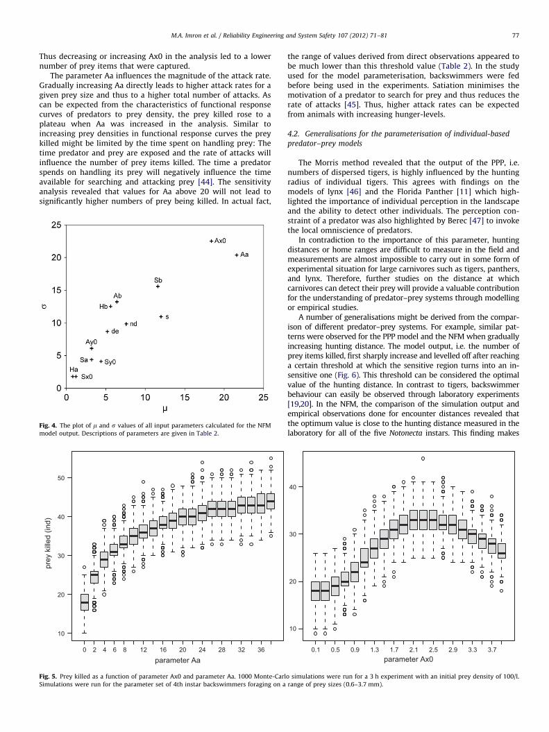
The relative sensitivity of the parameters as calculated for theoutput of the NFM is shown in Fig. 4. Additionally, values of m ands determined for each of the parameters are given in Table 2. Twoparameters, Aa and Ax0, were detected to have relatively strongeffects on the fluctuation in the number of prey killed comparedto other parameters and thus considered to be the most impor-tant parameters for the NFM. Within the model framework, thesetwo parameters are used to calculate the probability of attackinga particular prey item. This attack rate is formulated as alognormal function of the prey size for each of the five Notonecta

instars. The parameter Aa determines the maximum attack rate,whereas Ax0 is the prey size corresponding to the maximum

σ

Tfol

PcTferTmat

Cs

7

8

7

6

6

5

5

4

4

3

3

2

2

1

1

σ

Htrad

Par

feed

Cspreg

20000 4000 6000 8000 10000 12000 14000

1000

2000

3000

4000

5000

6000

5

10

105 15 20 25 30

15

20

σ

Gm

CmCs

TfolPc

1000 2000 3000 4000 5000

500

1000

1500

2000

2500

3000

3500

σ

TfolPc

TfmCm

Htrad

Fig. 2. The plot of m and s values of all input parameters into different output parameters of the PPP model, i.e. the total number of tigers (A), the number of dispersed

tigers (B), the total prey numbers (C), and the total number of prey killed by tigers (D). Descriptions of parameters given in Table 1.

M.A. Imron et al. / Reliability Engineering and System Safety 107 (2012) 71–81 75

attack rate, i.e. the prey size which is most preferentially attacked.Furthermore, a number of parameters were identified as havingan intermediate influence on the prey killed compared to others.These were the predators encounter distance (de), the parametersSb and Ab, which are proportional to the range of prey sizes most(successfully) attacked, the size and number of prey itemsinitially available (s, nd) and the slope of handling time linearregression (Hb).

Similar to the PPP model, both Aa and Ax0 were graduallychanged to test their effect on the prey killed. Fig. 5 shows the boxplot diagram of the prey killed as a function of Ax0 and Aaparameters. The non-parametric comparison tests showed ahighly significant difference of number of prey killed (Kruskal–Wallis, H¼28,540.51, po0.01) when the Aa were graduallychanged over the values from 0 to 39. The number of prey killedwas found to be sensitive between the values of 0 and 20, andrelatively insensitive for the values above 20. The model outputdiffered significantly when gradually increasing the parameterAx0 from 0.1 to 4.0 (Kruskal–Wallis, H¼9319.57, po0.01).However, the number of prey killed by backswimmers did notshow any similar sensitivities above or below certain values ofAx0: The model output was sensitive to the changes in parametervalues from 0.5 to 1.9, and between the values of 2.6 and 4. Thenumbers of prey eaten were shown to be relatively insensitive atvalues of Ax0 between 2.0 and 2.5.

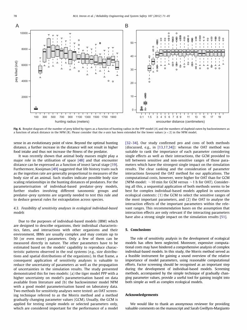
3.3. Comparing sensitivity-related to distances

The sensitivity of the number of prey killed as a function of thechanging parameters of the hunting radius in the PPP model andencounter distance in the NFM were compared. Fig. 6A shows theprey killed by tigers fluctuated below the Htrad values of 400 m andrelatively insensitive to a change of hunting radius above that value(Mann–Whitney U test, U¼5199.50; p¼0.01). Fig. 6B displays a

relatively high sensitivity of prey killed by backswimmers below2.0 cm of encounter distance, and relative insensitivity above thatvalue (Mann–Whitney U test, U¼2,469,448.50; po0.01).

4. Discussion

The sensitivity analysis plays a major role in the developmentof ecological models in general [33] and in population viabilityanalysis, in particular [16]. Sensitivity analyses provide an insightinto the interrelations between input parameters and outputvariables as well as into overall performance of the model, whichis important for drawing conclusions from the data gained bysimulations [33].

4.1. Implications for the predator–prey systems analysed

The sensitivity analyses of the PPP model have provided uswith new insights into modelling processes for tiger–prey rela-tionships. As carnivores, tigers are believed to depend on the preyabundance and size [14,37–39]. Surprisingly, the number of tigersin the PPP model did not mainly depend on the density of the preypopulation as suggested by Karanth and Stith [14] with the preydepletion model. The use of the homogenous spatial distributionbetween individual in the prey depletion concept has conse-quences on the dependency of the functional responses of pre-dators on the prey density as indicated by Cosner et al. [40]. Thismight explain the dependency of the prey depletion model on theinitial density of prey, but not for the PPP.

The number of tiger and prey killed in the PPP model aresensitive to the time required by tigresses to raise the cubs (Tfol).However, the outputs are very sensitive between Tfol of 670 and680 days. The predator dynamics is known to be affected by thetransition of immature predators into mature ones in an age stage

600 610 620 630 640 650 660 670 680 690 700

time duration to follow mother (days)

tiger

s (in

d)

600 610 620 630 640 650 660 670 680 690 700

prey

kill

ed (i

nd)

time duration to follow mother (days)

100 300 500 700 900 1100 1300 1500 1700 1900

hunting radius (meters)

disp

erse

d tig

er (i

nd)

0 1 2 3 4 5

growth rate of red muntjac (ind)

prey

(ind

)

0

10

20

30

40

0

2000

4000

6000

8000

5

0

5

0

5000

10000

15000

Fig. 3. The number of tigers (A) and the number of prey killed (B) as a function of Tfol, the number of dispersed tigers as a function of Htrad (C), and the number of prey as a

function of Gm. Due to expensive computational costs, the repetition for each simulation were carried out for 15 times.

M.A. Imron et al. / Reliability Engineering and System Safety 107 (2012) 71–8176

structured predator population [41]. In the PPP model, it is morelikely the shorter the Tfol, the higher the number of tigers at theend of a simulation. A tigress is soon ready for the nextreproductive periods after raising her cubs or being separatedfrom them [32]. The findings in this presented study disagreewith Takahara’s findings [42] which considered a predatorsindividual needs to be the driver of the number of prey killed.In the PPP model, the predation behaviour of a tigress with cubs issimulated differently to a tigress without cubs, as are sub-adultfemales and males as well as adult males. The hunger-level of atigress with cubs has higher increment than the other groups inevery time step than those groups. Thus, the longer the timeinvested for raising cubs, the more likely that prey will be killedby tigers as shown in the PPP model. The threshold, where theoutputs were sensitive to a small change in the Tfol, agrees withthe finding from Sunquist [32] which showed an observation

study at 660 days was used by adult female tigers to raisetheir cubs.

As revealed by the Morris method, the number of prey killedby backswimmers was highly influenced by the parameters Ax0and Aa, both of which are attack rate parameters in the NFMframework. The parameter Ax0 equals the prey size which ispreferentially attacked by a backswimmer instar. In laboratorystudies it was shown that the prey size mostly eaten increases tosome extent during the growth of the backswimmers [19,43]. Forbackswimmers of a particular size changing the value of Ax0 ledto an intermediate range of stabilised model output. In thesensitivity analysis, lower numbers of prey killed were observedbelow and above this range. The humped shaped pattern of themodel output is in accordance with the prey sizes which areattacked most successfully, whereas capture success was found todecrease in smaller and larger prey for the instar shown [19].

M.A. Imron et al. / Reliability Engineering and System Safety 107 (2012) 71–81 77

Thus decreasing or increasing Ax0 in the analysis led to a lowernumber of prey items that were captured.

The parameter Aa influences the magnitude of the attack rate.Gradually increasing Aa directly leads to higher attack rates for agiven prey size and thus to a higher total number of attacks. Ascan be expected from the characteristics of functional responsecurves of predators to prey density, the prey killed rose to aplateau when Aa was increased in the analysis. Similar toincreasing prey densities in functional response curves the preykilled might be limited by the time spent on handling prey: Thetime predator and prey are exposed and the rate of attacks willinfluence the number of prey items killed. The time a predatorspends on handling its prey will negatively influence the timeavailable for searching and attacking prey [44]. The sensitivityanalysis revealed that values for Aa above 20 will not lead tosignificantly higher numbers of prey being killed. In actual fact,

Fig. 4. The plot of m and s values of all input parameters calculated for the NFM

model output. Descriptions of parameters are given in Table 2.

0 2 4 6 8 12 16 20 24 28 32 36

parameter Aa

prey

kill

ed (i

nd)

10

20

30

40

50

Fig. 5. Prey killed as a function of parameter Ax0 and parameter Aa. 1000 Monte-Carl

Simulations were run for the parameter set of 4th instar backswimmers foraging on a

the range of values derived from direct observations appeared tobe much lower than this threshold value (Table 2). In the studyused for the model parameterisation, backswimmers were fedbefore being used in the experiments. Satiation minimises themotivation of a predator to search for prey and thus reduces therate of attacks [45]. Thus, higher attack rates can be expectedfrom animals with increasing hunger-levels.

4.2. Generalisations for the parameterisation of individual-based

predator–prey models

The Morris method revealed that the output of the PPP, i.e.numbers of dispersed tigers, is highly influenced by the huntingradius of individual tigers. This agrees with findings on themodels of lynx [46] and the Florida Panther [11] which high-lighted the importance of individual perception in the landscapeand the ability to detect other individuals. The perception con-straint of a predator was also highlighted by Berec [47] to invokethe local omniscience of predators.

In contradiction to the importance of this parameter, huntingdistances or home ranges are difficult to measure in the field andmeasurements are almost impossible to carry out in some form ofexperimental situation for large carnivores such as tigers, panthers,and lynx. Therefore, further studies on the distance at whichcarnivores can detect their prey will provide a valuable contributionfor the understanding of predator–prey systems through modellingor empirical studies.

A number of generalisations might be derived from the compar-ison of different predator–prey systems. For example, similar pat-terns were observed for the PPP model and the NFM when graduallyincreasing hunting distance. The model output, i.e. the number ofprey items killed, first sharply increase and levelled off after reachinga certain threshold at which the sensitive region turns into an in-sensitive one (Fig. 6). This threshold can be considered the optimalvalue of the hunting distance. In contrast to tigers, backswimmerbehaviour can easily be observed through laboratory experiments[19,20]. In the NFM, the comparison of the simulation output andempirical observations done for encounter distances revealed thatthe optimum value is close to the hunting distance measured in thelaboratory for all of the five Notonecta instars. This finding makes

0.1 0.5 0.9 1.3 1.7 2.1 2.5 2.9 3.3 3.7parameter Ax0

10

20

30

40

o simulations were run for a 3 h experiment with an initial prey density of 100/l.

range of prey sizes (0.6–3.7 mm).

100 300 500 700 900 1100 1300 1500 1700 1900

hunting radius (meters)

pey

kille

d (in

d)

0.1 1.5 3 4 5 6 7 8 9 11 13 15 17 19

encounter distance (centimeters)

2000

4000

6000

8000

10000

0

10

20

30

40

50

Fig. 6. Boxplot diagram of the number of prey killed by tigers as a function of hunting radius in the PPP model (A) and the numbers of daphnid eaten by backswimmers as

a function of attack distance in the NFM (B). Please consider that the x-axis has been extended for the lower values (xo2) in the NFM model.

M.A. Imron et al. / Reliability Engineering and System Safety 107 (2012) 71–8178

sense in an evolutionary point of view. Beyond the optimal huntingdistance, a further increase in the distance will not result in higherfood intake and thus not increase the fitness of the predator.

It was recently shown that animal body masses might play amajor role in the utilisation of space [48] and that encounterdistance can be expressed as a function of insect larval stage [19].Furthermore, Kooijman [49] suggested that life history traits suchas the ingestion rate are generally proportional to measures of thebody size of an animal. Such studies indicate possible body sizescaling relationships in the hunting distances of predators. For theparameterisation of individual-based predator–prey models,further studies involving different taxonomic groups andpredator–prey systems are urgently needed to test this rule andto deduce general rules for extrapolation across species.

4.3. Feasibility of sensitivity analyses in ecological individual-based

models

Due to the purposes of individual-based models (IBM) whichare designed to describe organisms, their individual characteris-tics, fates, and interactions with other organisms and theirenvironment, IBMs are usually complex and may contain up to50 (or even more) parameters. Only a few of them can bemeasured directly in nature. The other parameters have to beestimated based on the models’ capability to reproduce charac-teristic patterns observed in the real systems (e.g., size distribu-tions and spatial distributions of the organisms). In that frame, aconsequent application of sensitivity analyses is valuable toreduce the uncertainty of parameters as well as the propagationof uncertainties in the simulation results. The study presenteddemonstrated this for two models: (a) the tiger model PPP with ahigher uncertainty on model’s parameterisation based on dataavailable from literature and (b) the backswimmer model NFMwith a good model parameterisation based on laboratory data.Two methods for sensitivity analyses were tested: an OAT screen-ing technique referred to as the Morris method and a methodgradually changing parameter values (GCM). Usually, the GCM isapplied for testing simple models or selected parameters only,which are considered important for the performance of a model

[32–34]. Our study confirmed pro and cons of both methods(discussed, e.g., in [13,17,34]): whereas the OAT method wassuitable to rank the importance of each parameter consideringsingle effects as well as their interactions, the GCM provided totell between sensitive and non-sensitive ranges of those para-meters which have the strongest single impact on the simulationresults. The clear ranking and the consideration of parameterinteractions favoured the OAT method for our applications. Thecomputational costs, however, were higher for OAT than for GCM(NFM-model: �10 min for GCM versus �1 h for OAT). Consider-ing all this, a sequential application of both methods seems to bebest for complex individual-based models applied in uncertainecological contexts: (1) the GCM to select the sensitive ranges ofthe most important parameters, and (2) the OAT to analyse theinteraction effects of the important parameters within the rele-vant ranges. This recommendation bases on the assumption thatinteraction effects are only relevant if the interacting parametershave also a strong single impact on the simulation results [51].

5. Conclusions

The role of sensitivity analysis in the development of ecologicalmodels has often been neglected. Moreover, expensive computa-tional costs may have hindered a comprehensive analysis of complexindividual-based models. In this study, the Morris method served asa feasible instrument for gaining a sound overview of the relativeimportance of model parameters, using reasonable computationalefforts. Factor screening should be recognised as an important stepduring the development of individual-based models. Screeningmethods, accompanied by the simple technique of gradually chan-ging parameter values, provide a useful tool for gaining insight intoboth simple as well as complex ecological models.

Acknowledgements

We would like to thank an anonymous reviewer for providingvaluable comments on the manuscript and Sarah Gwillym-Margianto

M.A. Imron et al. / Reliability Engineering and System Safety 107 (2012) 71–81 79

for her proofreading services. The first author received scholar-ship from DAAD, German Academic Exchange Services.

Appendix A. The PPP model description

A.1. Purpose

The specific purpose of the PPP model is to investigate thepotential mechanisms of tiger population dynamics under differ-ent environmental and management options. The simulated areaof the PPP model is the Tesso Nilo National Park and itssurrounding landscape. The model was implemented in NETLOGOv. 4.1 [50].

A.2. Process overview and scheduling

The overall behaviour of tigers in the PPP model includesageing, movement, hunger and starvation, hunting, feeding,reproduction, mortality and dispersal. The ageing process simplysimulates increasing age in increment of 0.5 days, similar to thetime step of the model. The age of an individual then determinesits different behaviour according to its internal state. Fig. A1shows the behaviour of tigers in different age classes within thePPP model. Movements in the PPP are defined as random move-ment and directed movement.

The PPP model simulates an increase in the hunger-level ofindividuals by 10 for sub-adults and adults, 12.5 for females withcubs and no hunger behaviour for cubs. If an individual reaches itshunger-level of 90, this is the onset of starvation behaviourleading to natural mortality when the starvation level reaches30 after 60 days. Feeding behaviour resets the starvation levelinto zero and reduces the hunger-level by 12.5 per time stepduring feeding. The hunting behaviour of a tiger is driven by itshunger-level. A tiger is able to sense a prey within a certainhunting radius. Hunting success is assumed to be 50% on anyhunting occasion [31], and tigers have a preference for killingSambar deer [51]. If Sambar deer is absent from the model, thenthe tiger will only kill available prey. The PPP model simulates thereproduction of tigers through three processes: fertility schedul-ing, mating, pregnancy and giving birth. A female reaches sexualmaturity at the age of 825 days [32]. In this case fertilityscheduling is initiated. The inter-oestrous interval of a femaletiger is around 25 days during which the female is fertile forabout 5 days. A fertile female will call to an adult male for mating.However, mating will only occur when hunger-levels of indivi-duals are lower than 60 and there is no starvation. Mating lastsfor 2 days [32] and the female will have a 50% chance of becoming

Ageing

Cubs

Sub-adult Adult

Oldfollow-mom

dispersalhungerstarvinghuntingfeeding

FertilityMatingReproductionParenting

die

Fig. A1. The flow-chart diagram of a tiger’s basic behaviour in different age

classes. Grey boxes show behaviour common to different age classes while empty

boxes display behaviours that is particular for specific age class. The dotted box

illustrates the hunting behaviour which is similar to the NFM.

pregnant. The gestation period for a female is 102–103 days[10,28,28]. A pregnant female has a random probability of givingbirth to 1–3 cubs with a ratio of males to females of 1:3. Anewborn tiger will usually adopt all characteristics from itsmother except for its sex class, age, its hunger-level, and itsstarvation level. The age of cubs is set as 0 at the time step ofbirth. The hunger and starvation levels are also set as 0 until thecubs reach sub-adulthood. A female with cubs will not displayany mating behaviour until the cubs reach sub-adult classes.Density dependent birth rates for both Red Muntjac and Sambardeer are simulated.

At the sub-adult level, tigers search for a home range. Thehome range of a male might overlap with that of one or severalfemales but never with the home range of another male. An adultindividual without a home range is removed from the model butis not considered as a dead individual. The PPP model calculatesthis as a dispersed individual.

A.3. Design concept

The dynamics of the tiger population are expected to emergefrom the interaction between tiger individuals, prey, and habitat.The PPP model explicitly simulates four types of interaction. Thefirst is a prey–habitat interaction, which shows the movementand the foraging behaviour of prey in different habitat types. Theprey decides whether to move to the next patch or to staydepending on certain habitat indices. Such indices also determinethe energy gained by the prey while foraging. The second type ofinteraction is a tiger–prey interaction, which represents thebehaviour of a tiger hunting prey. The third type of interactionis tiger–prey habitat, which represents the time taken to consumeprey that has been killed in different land-use types. The fourthtype is a tiger–tiger interaction, which simulates the behaviour ofmating and parental care (between a mother and her cubs).

A tiger prefers to kill large prey. However, when there is nolarge prey in the hunting radius, the tiger will automaticallysearch for small prey. Newborn tigers inherit this preference forlarge prey. Adult tigers are known to compete for resources andmating [32]. When an adult individual cannot establish a homerange, the model considers it as transient and omits it from thelandscape. Tigers are able to detect both prey and a mate, and acub senses the presence of its mother to be followed. Stochasticityis applied to the probability of a tiger to successfully hunt forprey, the probability of becoming pregnant, the number of newcubs and the proportion of male and female cubs. Collectivenessoccurs during mating and parenting behaviour. A male and afemale will remain together over the mating period, and a femalewill stay with its cubs until they reach the sub-adult class.

A.4. Details

Initialisation. An adult male Sumatran tiger requires 116 km2

to maintain a home-range, and 70 km2 for an adult female [30].We set the population to 20 sub-adult tigers with 10 males and 10females. The densities of Red Muntjac and Sambar deer in tropicalforest were set according to the findings of O’Brien et al. [29].Sambar deer has a density range of 0.88–1.42 individuals/ha,whereas Red Muntjac has a range of 3.96–4.44 individuals/ha.The model has 203�149 grid cells, representing the Tesso NiloNational Park and its surrounding land-use. Each grid cell repre-sents 12.7 ha and is specified by habitat quality, corresponding tothe land-use types. We included four main types of prey beha-viour: movement, for aging, reproduction, and mortality. Preymovement is defined by two main factors: direction and distance.The distance refers to data obtained for red deer movement [52],which varies from 0.23–7 km/day. The direction of movement is

M.A. Imron et al. / Reliability Engineering and System Safety 107 (2012) 71–8180

driven by habitat quality indices. The probability of prey move-ment is calculated as follows:

a¼ b1=ðb1þb0Þ

with a being the movement probability to the next patch, b1 beingthe habitat index of the next patch, and b0 being the habitat indexof the current patch (Table 2). If a ao0.5 then the prey will stay inthe current patch, otherwise it will move to the next patch. We didnot differentiate between the distance and direction for Sambardeer and Red Muntjac. Prey will remain in a patch and consume acertain amount of the food resource in that particular patch. Preyreceives different resource values in different land-use types. Atthe same rate of increased hunger-level, the greater the humanintervention, the less the energy that is gained from the patch, andconsequently the more easily the prey becomes hungry. Both RedMuntjac and Sambar deer increase their hunger-level by 10 levelsper time step. Since we do not have any data on the rate ofconsumption of prey species within different habitat types, weused the same rate for all types of habitats.

Red Muntjac starts to reproduce annually from the age of 2–4years with probability of a number of litters consisting of3 individuals. Sambar deer reproduces annually with 1 l fromthe age of 2–6 years. Both prey die when they reach a maximumage (approx. 10 years for Red Muntjac and 17 years for Sambardeer), from acute starving (hunger-level is greater than 200), and/or are killed by tigers. Both Sambar and Red Muntjac havedensity-dependant birth rates. Both will continue to reproduceuntil the population reaches the carrying capacity.

Appendix B. The model description of the NFM

B.1. Purpose

The Notonecta model was designed to predict the functionalresponses of juvenile N. maculata foraging on D. magna. Moreoverit was intended to assess whether the combination of foragingelements selected (encounter distance, attack rate, success rate,and handling time) account for the size selectivity observed inlaboratory studies. The model is implemented in Delphis usingBorland Delphis 2007 for the Win32s Professional Edition.

B.2. States variables and scales

The model is arranged into three hierarchical levels: theecosystem, the population, and the individuals. The ecosystemlevel features the light regime (light/dark) and the volume of thetest vessel at the laboratory scale. The state of the daphnidpopulation is defined as the abundance of D. magna, which isallowed to change due to backswimmer predation only whereasthe N. maculata population is restricted to a single backswimmerin the current state of the model. Individual backswimmers andindividual daphnids are characterised by a set of state variables atthe start of the simulation. Properties of D. magna are theidentification number and size. Backswimmer properties areinstar, encounter distance, handling time as well as attack-and-success coefficients. Attack rate, success rate, and handling timedepend on the size of the prey item encountered.

B.3. Process overview and scheduling

The model proceeds in discrete time steps in seconds. Itfollows a general predation cycle divided into four stages: (1) Aprey item is randomly chosen and the time until an encounter iscalculated. The probability of (2) attack and (3) capture success iscalculated for the prey item selected. In case of capture success

handling time is calculated and the prey item eaten is removedfrom the population (4).

B.4. Design concepts

Population size of Daphnia depends on the foraging of indivi-dual Notonecta. However, population dynamics do not emergefrom any individual properties. An adaptation or fitness seeking isnot explicitly modelled, but is included in the empirical sub-models. Environmental and population level factors sensed byNotonecta are the light regime and the daphnid prey. The interac-tion between individual Notonecta and Daphnia is feeding. Thebody length of Daphnia is stochastically selected from a normaldistribution. Variations in attack rates and success rates of Noto-necta are generated by a normal distribution with the mean of1 and a coefficient of variation resulting in an individual parametermultiplied by the mean rate calculated from submodels. Thedecision whether to attack, or whether the attack is successful, isbased on two random numbers between 0 and 1 selected in everyencounter. In case the calculated rate exceeds the random numberthe attack or the success is rejected. Handling time is calculated forevery daphnid cough, using a normal distribution.

B.5. Details

The initialisation of settings comprises the Notonecta instarand Daphnia sizes, the volume of the environment, prey abun-dances tested, simulation time, and the number of Monte-Carloruns. Sensitivity analyses of single parameters were carried outusing a single backswimmer foraging on 100 prey items, 0.6–3.7 mm in size, in a 1l environment for 3 h, running 1000 Monte-Carlo simulations. No additional input is necessary for the simula-tion. Equations and parameters of submodels described belowwere derived empirically from laboratory experiments. The timeuntil an encounter (te) between predator and prey is calculatedbased on the predators encounter volume and an encounterprobability depending on the prey size (s) and density, i.e. theratio of the prey number (nd) and the volume of the environment(n). The encounter volume is assumed to be a hemisphere wherethe radius equals the backswimmers encounter distance (de).Time until encounter is given by

te¼ ð2:095 de3 vÞ=ðð0:35sþ0:34Þð0:006 nd2þ0:12 ndÞÞ

The attack rate (Ar) was observed to depend on prey size (s)and is calculated by means of a lognormal function where Aa, Ab,Ax0 and Ayo are instar specific parameters:

Ar¼ ðAy0þAa expð�0:5 lnðs Ax0=AbÞÞÞ=100

Here, the success rate (Sr) is calculated in the same mannerusing the parameters Sa, Sb, Sx0, and Sy0. The handling time (th),i.e. the time from the actual attack until the release of daphnid,remains is calculated by means of a linear regression of Daphniasize (s) and log transformed handling time data, using the instarspecific parameters Ha and Hb and a proportionality factort¼1[s]:

th¼ 10Ha sþHbt

References

[1] Hinrichsen RA. Population viability analysis for several populations usingmultivariate state-space models. Ecological Modelling 2009;220:1197–202.

[2] Real L. Kinetics of functional response. American Naturalist 1977;111:289–300.

[3] Jeschke J, Koop M, Tollrian R. Predator functional responses: discriminatingbetween handling and digesting prey. Ecological Monographs 2002;72:95–112.

M.A. Imron et al. / Reliability Engineering and System Safety 107 (2012) 71–81 81

[4] Grimm V. Ten years of individual-based modeling in ecology: what have welearned and what could we learn in the future? Ecological Modeling 1999;115:129–48.

[5] DeAngelis DL, Mooij WM. Individual-based modelling of ecological andevolutionary process. Annual Review of Ecology and Systematics 2005;36:147–68, doi:10.1146/annurev.ecolsys.36.102003.152644.

[6] Grimm V, Berger U, Bastiansen F, Eliassen S, Ginot V, Giske J, et al. A standardprotocol for describing individual-based and agent-based models. EcologicalModelling 2006;198:115–26.

[7] Preuss T, Hammers-Wirtz M, Hommen U, Rubach M, Ratte H. Developmentand validation of an individual-based Daphnia magna population model: theinfluence of crowding on population dynamics. Ecological Modelling 2009;220:310–29.

[8] Wang M, Grimm V. Home range dynamics and population regulation: anindividual-based model of the common shrew sorex araneus. EcologicalModelling 2007;205:397–409.

[9] Kramer-Schadt S, Revilla E, Wiegand T, Breitenmoser U. Fragmented land-scapes, road mortality and patch connectivity: modeling influences on thedispersal of eurasian lynx. Journal of Applied Ecology 2004;41:711–23.

[10] Ahearn SC, Smith JLD, Joshi AR, Ding J. TIGMOD: an individual-based spatiallyexplicit model for simulating tiger/human interaction in multiple use forests.Ecological Modelling 2001;140:81–97.

[11] Cramer PC, Portier KM. Modeling Florida panther movements in response tohuman attributes of the landscape and ecological settings. Ecological Model-ling 2001;140:51–80.

[12] Cariboni J, Gatelli D, Riska R, Satelli A. The role of sensitivity analysis inecological modelling. Ecological Modelling 2007;203:167–82.

[13] Saltelli A, Ratto M, Stefano Tarantola FC. Sensitivity analysis practices:strategies for model-based inference. Reliability Engineering and SystemSafety 2006;91:1109–25.

[14] Karanth UK, Stith BM. Prey depletion as critical determinant of tigerpopulation viability. In: Seindensticker J, Christie S, Jackson P, editors. Ridingthe tiger: tiger conservation in human dominated landscapes. CambridgeUniversity Press; 1999. p. 100–13.

[15] Nilsson PA. Predator behaviour and prey density: evaluating density-depen-dent intraspecific interaction on predator functional responses. AnimalEcology 2001;70:14–9.

[16] MacCarthy MA, Burgman MA, Ferson S. Sensitivity analysis for models ofpopulation viability. Biological Conservation 1995;73:93–100.

[17] Morris MD. Factorial sampling plans for preliminary computational experi-ments. Technometrics 1991;33:161–74.

[18] Imron.MA. An individual-based model approach for the conservation of theSumatran Tiger Panthera tigris sumatrae population in Central Sumatra. PhDthesis, TU Dresden, Germany; 2011. pp. 200.

[19] Gergs A, Ratte HT. Predicting functional response and size selectivity ofjuvenile Notonecta maculata foraging on Daphnia magna. Ecological Modelling2009;220:3331–41.

[20] Gergs A, Hoeltzenbein NI, Ratte HT. Diurnal and nocturnal functionalresponse of juvenile Notonecta maculata considered as a consequence ofshifting predation behaviour. Behavioural Process 2010;85:151–6.

[21] Cook RM, Cockrell BJ. Predator ingestion rate and its bearing on feeding timeand theory of optimal diets. Journal of Animal Ecology 1978;47:529–47.

[22] Giller PS, Mcneill S. Predation strategies, resource partitioning and habitatselection in Notonecta (Hemiptera, Heteroptera). Journal of Animal Ecology1981;50:789–808.

[23] Scott MA, Murdoch WW. Selective predation by the backswimmer, Noto-necta. Limnology and Oceanography 1983;28:352–66.

[24] Gerritsen J, Strickler J. Encounter probabilities and community structure inzooplankton—mathematical model. Journal of Fisheries Research Board ofCanada 1977;34:73–82.

[25] Saltelli A, Tarantola S, Campolongo F, Ratto M. Sensitivity analysis inpractices a guide to assessing scientific models. Sussex England: John Wileyand Sons; 2004.

[26] Campolongo F, Cariboni J, Saltelli A. An effective screening design forsensitivity analysis of large models. Environmental Modelling and Software2007;22:1509–18.

[27] SIMLAB, Simlab version 2.2, free software for uncertainty and sensitivityanalysis, /http://simlab.jrc.ec.europa.euS, 2010. Joint Research Centre of theEuropean Commission. Downloaded in May 2010.

[28] Sunquist M, Karanth KU, Sunquist F. Ecology, behaviour and resilience of thetiger and its conservation needs. In: Seindensticker J, Christie S, Jackson P,editors. Riding the tiger: tiger conservation in human dominated landscapes.Cambridge University Press; 1999. p. 5–18.

[29] O’Brien TG, Kinnaird MF, Wibisono HT. Crouching tigers, hidden prey:Sumatran tiger and prey populations in a tropical forest landscape. AnimalConservation 2003;6:131–9.

[30] Franklin N, Bastoni, Sriyanto, Siswomartono D, Manangsang J, Tilson R. Last ofthe Indonesian tigers: a cause for optimism. In: Seindensticker J, Christie S,Jackson P, editors. Riding the tiger: tiger conservation in human dominatedlandscapes. Cambridge University Press; 1999. p. 130–47.

[31] Sunquist M. What is a tiger? ecology and behavior In: Tilson R, Nyhus PJ,editors. Tigers of the world the science, politics and conservation of Pantheratigris. 2nd ed.. 32 Jamestown Road, London NW1 7BY, UK: Academic Press;2010. p. 16–34.

[32] Sunquist ME. The social organization of tigers (Phantera tigris) in RoyalChitawan National Park, Nepal, Smitsonian contribution to zoology.336 ed.Washington: Smitsonian Institution Press; 1981.

[33] Thornton KW, Lessem AS, Ford DE, Stirgus CA. Improving ecologicalsimulation through sensitivity analysis. Simulation 1979, doi:10.1177/003754977903200503.

[34] Hayes JW, Stark JD, Shearer KA. Development and test of a whole-lifetimeforaging and bioenergetic growth model for drift-feeding brown trout. TheAmerican Fisheries Society 2000;129:315–32.

[37] Miquelle D, Smirnov EN, Merril TW, Myslenkov AE, Quigley HB, HornockerMG, et al. Hierarhical spatial analysis of amur tiger relationships to habitatand prey. In: Christie S, Seindensticker J, Jackson P, editors. Riding the tiger:tiger conservation in human dominated landscapes. Cambridge UniversityPress; 1999. p. 71–99.

[38] Ramakrishnan U, Coss RG, Pelkey NW. Tiger decline caused by reduction oflarge ungulate prey: evidence from a study of leopard diets in southern India.Biological Conservation 1999;89:113–20.

[39] Karanth UK, Nichols JD, Kumar NS, Link WA, Hines JE. Tiger and their prey:predicting carnivore densities from prey abundance. PNAS 2004:4854–8.

[40] Cosner C, DeAngelis DL, Ault JS, Olson DB. Effect of spatial grouping on thefunctional response of predators. Theorical Population Biology 1999;56:65–75.

[41] Wang W, Takeuchi Y, Saito Y, Nakaoka S. Predator system with parental carefor predators. Theorical Biology 2006;241:451–8.

[42] Takahara Y. Individual base model of predator–prey shows predator domi-nant dynamics. BioSystems 2000;57:173–85.

[43] McArdle BH, Lawton JH. Effects of prey size and predator instar on thepredation of daphnia by notonecta. Ecological Entomology 1979;4:267–75.

[44] Holling C. The principles of insect predation. Annual Review of Entomology1961;6:163–82.

[45] Hohberg K, Traunspurger W. Foraging theory and partial consumption in atardigrade-nematode system. Behavioral Ecology 2009;20:884–90.

[46] Pe’er G, Kramer-Schadt S. Incorporating the perceptual range of animals intoconnectivity models. Ecological Model 2008;213:73–85.

[47] Berec L. Mixed encounters, limited persception and optimal foraging. Bulletinof Mathematical Biology 2000;62:849–68, doi:10.1006/bulm.2000.0179.

[48] Jetz W, Carbone C, Fulford J, Brown JH. Scaling of animal space use. Science2004:266–8.

[49] Kooijman S. Dynamic energy and mass budgets in biological systems. GreatBritain: Cambridge University Press; 0-521-78608-8.

[50] Wilensky U. NetLogo.1rc3 edition Evanston, IL., netlogo 4: Center forConnected Learning and Computer-Based Modeling, Northwestern Univer-sity; 1999.

[51] Reddy HS, Srinivasulu C, Rao KT. Prey selection by Indian tiger (Panthera tigristigris) in Nagarjunasagar Srisailam tiger reserve, India. Mammalian Biology2004;69:384–91.

[52] Fryxell JM, Hazell M, Brger L, Dalziel BD, Haydon DT, Morales JM, et al.Multiple movement modes by large herbivores at multiple spatiotemporalscales. PNAS 2008;105:19114–9. /www.pnas.org/cgi/doi/10.1073/pnas.0801737105S.