Effects of Predator and Prey Dispersal on Success or Failure of Biological Control

Bulletin of Mathematical Biology (2009) 71: 2025–2047DOI 10.1007/s11538-009-9438-2

O R I G I NA L A RT I C L E

Effects of Predator and Prey Dispersal on Success or Failureof Biological Control

Sanyi Tanga,∗, Robert A. Chekeb, Yanni Xiaoc

aCollege of Mathematics and Information Science, Shaanxi Normal University, Xi’an710062, People’s Republic of China

bNatural Resources Institute, University of Greenwich at Medway, Central Avenue,Chatham Maritime, Chatham, Kent, ME4 4TB, UK

cDepartment of Applied Mathematics, Xi’an Jiaotong University, Xi’an 710049,People’s Republic of China

Received: 7 November 2008 / Accepted: 12 June 2009 / Published online: 27 June 2009© Society for Mathematical Biology 2009

Abstract Biological control, defined as the reduction of pest populations by natural en-emies, is often a component of integrated pest management strategies. Augmentation ofnatural enemy numbers by planned releases is a common biological control method, thesuccesses and failures of which have been extensively reviewed. The effectiveness of bi-ological control is influenced by how populations of predators and prey (or hosts andparasitoids) disperse in patchy environments. Here, we address the question of whethersuch dispersal leads to beneficial or detrimental pest control outcomes by developing asimple predator-prey model with constant releases of natural enemies in a two-patch en-vironment. Theoretical and numerical results for all possible cases indicate that populationdispersal has significant effects on the persistence of pests. For some ranges of dispersalrates or parameter space, dispersal is beneficial for pest control measures but this is not sofor other ranges when it is detrimental. Therefore, knowledge of pest and natural enemydispersal is crucial for understanding the effectiveness of biological control in a patchyenvironment. Finally, the model is generalised for multi-patch systems.

Keywords Natural enemy · Pest · Biological control · Dispersal

1. Introduction

Biological control, defined as the reduction of pest populations by natural enemies, is onecomponent of integrated pest management strategies. Typically, it involves an active hu-man role, often with augmentation of natural enemies usually by supplemental releases.Biological control has been used against weeds and vertebrate pests such as rabbits as well

∗Corresponding author.E-mail addresses: [email protected]; [email protected] (Sanyi Tang),[email protected] (Robert A. Cheke), [email protected] (Yanni Xiao).

mailto:[email protected]




2026 Tang et al.

as to control invertebrates including nematodes, insects, and arachnids. The controllingagents used have included insect predators and parasitoids, predatory mites, entomopatho-genic nematodes, and vertebrates. The latter have included cane toads against beetles suchas white-grub Phyllophaga spp. and Cane Beetles Dermolepida albohirtum, and ducks tocontrol locusts Locusta migratoria. In addition, microbial agents such as bacteria, viruses,and fungi are also used in biological control programmes. Thus, biological control is animportant subject in applied ecology in theory and practice. Theoretical treatments includethe host-parasitoid models of Nicholson–Bailey (1935) recently expanded by Tang andCheke (2008) and the classic predator-prey models of Lotka (1920) and Volterra (1931).However, neither Nicholson and Bailey nor Lotka and Volterra dealt specifically withdispersal, another important topic in applied ecology (see papers in DeBach and Rosen,1991), although laboratory studies have investigated the effects of manipulating disper-sal on the outcome of predator-prey interactions (Huffaker, 1958; Takafuji, 1976) and theroles of host and parasitoid dispersal have been considered theoretically (Hassell, 1978,2000). Dispersal is also fundamental to the concept of metapopulations (Levins, 1970;Hanski and Gilpin, 1997). Several workers have elaborated on metapopulation modelsaddressing dispersal issues and there have also been publications on dispersal applied tohost-pathogen dynamics (Dwyer and Hails, 2002). Here, we link biological control mod-els with metapopulation concepts to address the question of whether, theoretically, disper-sal by predators and/or their prey promotes or inhibits the success of biological control.

Dispersal of pests and natural enemies has significant effects on pest control, but inpractice, more information is required on the dispersal of both natural enemies and pests toassess the success or failure of biological control operations. Therefore, the quantificationof the movement patterns of pest species is necessary information to underpin theorieson spatial dynamics and pest management. For instance, dispersal is a major aspect ofthe life-history of many insects and is often believed to be a stabilizing force in theirpopulation dynamics (Stein et al., 1994) and dispersal patterns of herbivorous insects inagroecosystems have been associated with pest outbreaks (Kareiva, 1982). On the otherhand, studies on the dispersal of natural enemies have demonstrated the importance ofmovement in the efficiency of inundative releases (Saavedra et al., 1997; McDougall andMills, 1997) and in the establishment of insects introduced for insect pest control (Hopperand Roush, 1993).

The successes and failures of biological control have been extensively reviewed (De-Bach and Rosen, 1991; Collier and Van Steenwyk, 2004; Stiling and Cornelissen, 2005).A number of factors can influence the effectiveness of biological control agents includ-ing agent specificity (generalist or specialist), the type of agent (predator, parasitoid, orpathogen), the timing and number of releases, the method of release, synchrony of thenatural enemy with the host, field conditions, and release rate (DeBach and Rosen, 1991;Van den Driesche and Bellows, 1996; Collier and Van Steenwyk, 2004; Stiling and Cor-nelissen, 2005).

Many research papers have assessed the relative impact of release rates on the ef-fectiveness of augmentative biological control. Augmentative or inundative, biologicalcontrol is the release of large numbers of natural enemies to augment natural enemy pop-ulations or to inundate pest populations with natural enemies. Collier and Van Steenwyk(2004) reviewed articles in which the effectiveness of augmentative biological controlagents as a function of release rates were measured. The effect of release rates on the suc-cessful implementation of augmentative biological control was assessed when parasitoids

Effects of Predator and Prey Dispersal on Success or Failure 2027

and predators were utilized as biological control agents. In addition, the relative impactof release rates was compared with factors such as the method and timing of releases andwhen pesticides were used in conjunction with biological control agents.

The aim of this paper is to investigate how population dispersal affects the persistenceof pests and whether it is beneficial to pest control or not. The difference between successand failure in biological control can be due to exogenous limitations or to endogenousprocesses. We focus on population dispersal to find more general aspects of the inter-actions between natural enemies and pests in a patchy environment that can be used toimprove success and minimize the risks of biological control.

We propose a simple prey-predator model with constant releasing of natural enemiesin a two-patch environment. Theoretical and numerical results for all possible cases indi-cate that population dispersal has significant effects on the persistence of pests. For someranges of dispersal rates or parameter space, population dispersal is beneficial to pestcontrol; for other ranges of dispersal rates, the results imply that population dispersal isdetrimental to pest control. Therefore, knowledge of pest and natural enemy dispersal iscrucial for understanding the effectiveness of biological control in a patchy environment.The methods developed here can be extended to a general model.

2. A simple model with constant releasing of natural enemies

Consider the classical pest and natural enemy interaction model with the addition of aconstant releasing rate of natural enemies, i.e. the following Lotka–Volterra model:

⎧⎪⎪⎨

⎪⎪⎩

dx(t)

dt= ax(t) − bx(t)y(t),

dy(t)

dt= cx(t)y(t) − dy(t) + u,

(1)

where x, y denote the number of pests and natural enemies, respectively. a, b, c, d, and u

are positive constants.The assumptions in the model (1) are: (i) The pest grows unboundedly in a Malthusian

way in the absence of any predation, governed by the ax term in (1). (ii) The effect of thenatural enemy is to reduce the pest’s per capita growth rate by a term proportional to thepest and natural enemy populations; this is the −bxy term. (iii) In the absence of any pestfor sustenance, the natural enemy’s death rate results in exponential decay, the dy termin (1). (iv) The pest’s contribution to the natural enemy’s growth rate is cxy; that is, it isproportional to the available prey as well as to the size of the predator population. (v) Therelease rate of natural enemies is a constant u.

It is easy to see that there are two steady states: E∗ = (0, y∗) = (0, ud), and if u < ad

b

then there is an unique interior equilibrium E∗(x∗, y∗) with x∗ = bac

[ adb

− u], y∗ = ab

.By linearization stability analysis, we see that if u > ad

bthen the equilibrium with pest

eradication (EPE) E∗ is locally stable; if u < adb

then the interior equilibrium E∗ is locallystable. Similarly, we can define the threshold value Ru = ad

bu= a

by∗ , and thus if Ru < 1 thenthe EPE E∗ is stable. Otherwise, it is unstable.

2028 Tang et al.

Furthermore, E∗ is globally stable under the existence condition u < adb

or Ru < 1. Infact, if we choose the following Lyapunov function

V = x∗[

x

x∗− ln

x

x∗

]

+ b

cy∗

[y

y∗− ln

y

y∗

]

(2)

and the following is satisfied

dV

dt= −b(x − x∗)(y − y∗) + b

c(y − y∗)

[

c(x − x∗) + u

y− u

y∗

]

= bu

c(y − y∗)

[1

y− 1

y∗

]

= − bu

cyy∗(y − y∗)2 ≤ 0, (3)

then the interior equilibrium E∗ is globally stable, if it exists. Similarly, if we choose theLyapunov function

V = x + b

cy∗

[y

y∗ − lny

y∗

]

(4)

we can prove the global stability of equilibrium E∗.The simple model (1) implies that we can control the release rate u of natural enemies

such that Ru < 1, i.e. the EPE is globally stable, and the effect of releasing rates on thesuccessful implementation of biological control can be assessed through the thresholdcondition Ru > 1 or Ru < 1.

3. Two-patch model

The main aim of this paper is to investigate how dispersal in a patchy environment influ-ences pest control. So, let us consider the following model which allows the populationsto move within two patches

⎧⎪⎪⎪⎪⎪⎪⎪⎪⎪⎪⎪⎨

⎪⎪⎪⎪⎪⎪⎪⎪⎪⎪⎪⎩

dx1(t)

dt= a1x1(t) − b1x1(t)y1(t) + d21x2(t) − d12x1(t),

dy1(t)

dt= c1x1(t)y1(t) − d1y1(t) + u1 + D21y2(t) − D12y1(t),

dx2(t)

dt= a2x2(t) − b2x2(t)y2(t) − d21x2(t) + d12x1(t),

dy2(t)

dt= c2x2(t)y2(t) − d2y2(t) + u2 − D21y2(t) + D12y1(t),

(5)

where xi (i = 1,2) is the number of pests in patch i, yi is the number of natural enemiesin patch i, d12, d21,D12,D21 are non-negative constants. dij (i, j = 1,2, i �= j) representsthe immigration rate of pests from the ith patch to the j th patch, and Dij (i, j = 1,2,


i �= j) represents the immigration rate of natural enemies from the ith patch to the j thpatch. All other parameters in model (5) are identical to those in model (1).

Rearranging system (5) yields

⎧⎪⎪⎪⎪⎪⎪⎪⎪⎪⎪⎪⎨

⎪⎪⎪⎪⎪⎪⎪⎪⎪⎪⎪⎩

dx1(t)

dt= (a1 − d12)x1(t) − b1x1(t)y1(t) + d21x2(t),

dx2(t)

dt= (a2 − d21)x2(t) − b2x2(t)y2(t) + d12x1(t),

dy1(t)

dt= c1x1(t)y1(t) − (d1 + D12)y1(t) + u1 + D21y2(t),

dy2(t)

dt= c2x2(t)y2(t) − (d2 + D21)y2(t) + u2 + D12y1(t).

(6)

In the following, we will focus on model (6) and investigate its dynamical behaviour andthe biological implications.

3.1. Natural enemy subsystem

Let x1 = 0, x2 = 0 in system (6), and consider the following natural enemy subsystem

⎧⎪⎪⎨

⎪⎪⎩

dy1(t)

dt= −(d1 + D12)y1(t) + u1 + D21y2(t),

dy2(t)

dt= −(d2 + D21)y2(t) + u2 + D12y1(t).

(7)

It is easy to see that the system (6) has an unique positive equilibrium E∗ = (y∗u1

, y∗u2

)

with

y∗u1

= D21u2 + u1D21 + u1d2

d1d2 + d1D21 + D12d2, y∗

u2= d1u2 + D12u2 + D12u1

d1d2 + d1D21 + D12d2.

Its characteristic equation has two negative eigenvalues, which means that E∗ is globallyasymptotically stable due to the model’s linearity.

3.2. The stability and threshold conditions of EPE of model (6)

Based on Section 3.1, it is seen that the two-patch system (6) has an unique EPE Er �=(0,0, y∗

u1, y∗

u2) and its stability can be determined by the eigenvalues of the following

Jacobian matrix:

JEr =

⎛

⎜⎜⎝

(a1 − d12) − b1y∗u1

d21 0 0d12 (a2 − d21) − b2y

∗u2

0 0c1y

∗u1

0 −(d1 + D12) D21

0 c2y∗u2

D12 −(d2 + D21)

⎞

⎟⎟⎠

�=(

A 0B C

)

. (8)

2030 Tang et al.

This is a lower block triangular matrix, and all eigenvalues of C have negative realparts. Therefore, the stability of the equilibrium with pest eradication Er can be deter-mined by the eigenvalues of matrix A, and its characteristic equation is

λ2 − β1λ + β2 = 0 (9)

with

β1 = a1 + a2 − d21 − d12 − b1y∗u1

− b2y∗u2

and

β2 = [a1 − d12 − b1y

∗u1

][a2 − d21 − b2y

∗u2

] − d21d12.

Let s(A) be the maximum real part of the eigenvalues of matrix A and ρ(A) be the spectralradius of matrix A. It is easy to see that

s(A) =β1 +

√

β21 − 4β2

2

= (a1 − d12 − b1y∗u1

) + (a2 − d21 − b2y∗u2

) +√

[(a1 − d12 − b1y∗u1

) − (a2 − d21 − b2y∗u2

)]2 + 4d21d12

2.

(10)

Thus, if we set the threshold value Ru1u2 which determines the stability of the equilib-rium with pest eradication Er , i.e. s(A) < 0 if and only if Ru1u2 < 1. It follows from thedefinition of s(A) that Ru1u2 > 1 if and only if β1 > 0 or

β1 ≤ 0 and β2 < 0; (11)

Ru1u2 < 1 if and only if

β1 ≤ 0 and β2 > 0. (12)

The condition β1 > 0 means that the sum of intrinsic growth rates of pests in twopatches is larger than the total removal rate of pest populations in two patches. Accordingto the definitions of y∗

u1, y∗

u2, we can rearrange β1 as follows:

β1 = b1y∗u1

[a1 − d12

b1y∗u1

− 1

]

+ b2y∗u2

[a2 − d21

b2y∗u2

− 1

]

, (13)

and β2 becomes

β2 = b1b2y∗u1

y∗u2

[a1 − d12

b1y∗u1

− 1

][a2 − d21

b2y∗u2

− 1

]

− d21d12

= b1b2y∗u1

y∗u2

{[a1 − d12

b1y∗u1

− 1

][a2 − d21

b2y∗u2

− 1

]

− d21d12

b1b2y∗u1

y∗u2

}

. (14)


Fig. 1 The effects of population dispersal on the sign of β2, where D12,D21 vary from 0 to 1 and allother parameters are given as follows: a1 = 1, b1 = 0.35, c1 = 0.2, d1 = 0.1, a2 = 1, b2 = 0.35, c2 = 0.2,d2 = 0.1, u2 = 0.5, u1 = 0.5, d12 = 0.2, d21 = 0.2.

In expressions (13) and (14), a1−d12b1y∗

u1can be considered as a threshold value at the

first patch, and a2−d21b2y∗

u2a threshold value at the second patch. Therefore, if a1−d12

b1y∗u1

< 1 anda2−d21b2y∗

u2< 1, then we have β1 < 0 and the sign of β2 depends on the dispersal rates of

the pests and natural enemies, which means that the different dispersal rates may resultin different dynamical behaviour of model (6). The numerical results shown in Fig. 1indicate how the dispersal of natural enemies affects the sign of β2.

In the following, we will show that if s(A) < 0 (i.e. Ru1u2 < 1), then the equilibriumwith pest eradication Er is globally stable. In fact, it follows from the non-negativity ofsolutions of system (6) that we have

⎧⎪⎪⎨

⎪⎪⎩

dy1(t)

dt≥ −(d1 + D12)y1(t) + u1 + D21y2(t),

dy2(t)

dt≥ −(d2 + D21)y2(t) + u2 + D12y1(t),

(15)

which means for sufficiently large t and small ε > 0 that we have

(y1(t), y2(t)

)>

(y∗

u1− ε, y∗

u2− ε

).

2032 Tang et al.

Without loss of generality, we assume that the above inequality holds true for all t ≥ 0.Consequently, we have

⎧⎪⎪⎨

⎪⎪⎩

dx1(t)

dt≤ (a1 − d12)x1(t) − b1x1(t)

(y∗

u1− ε

) + d21x2(t),

dx2(t)

dt≤ (a2 − d21)x2(t) − b2x2(t)

(y∗

u2− ε

) + d12x1(t).

(16)

Then it suffices to show that positive solutions of the following auxiliary system

⎧⎪⎪⎨

⎪⎪⎩

dx1(t)

dt= (a1 − d12)x1(t) − b1x1(t)

(y∗

u1− ε

) + d21x2(t),

dx2(t)

dt= (a2 − d21)x2(t) − b2x2(t)

(y∗

u2− ε

) + d12x1(t)

(17)

tend to zero as t goes to infinity. Let A1 be the matrix defined by

A1 = diag(−b1,−b2).

Since s(A) < 0 and s(A+ εA1) are continuous for small ε, so when ε is small enough westill have s(A+ εA1) < 0. Consequently, the solutions of the model (16) approach zero ast tends to infinity, which implies that the equilibrium with pest eradication Er is globallystable if Ru1u2 < 1 holds true.

The conditions which guarantee the stability of EPE clearly show the effect of popu-lation dispersal on the persistence of the pest. We will address this in more detail in thecoming sections.

3.3. Some special cases

In the absence of population dispersal between two patches, i.e. d21 = d12 = D21 =D12 = 0, the system (5) reduces to two independent subsystems

⎧⎪⎪⎨

⎪⎪⎩

dx1(t)

dt= a1x1(t) − b1x1(t)y1(t),

dy1(t)

dt= c1x1(t)y1(t) − d1y1(t) + u1

(18)

and⎧⎪⎪⎨

⎪⎪⎩

dx2(t)

dt= a2x2(t) − b2x2(t)y2(t),

dy2(t)

dt= c2x2(t)y2(t) − d2y2(t) + u2.

(19)

It follows from Section 2 that the EPEs in each isolated patch are (0, y∗1 ) = (0,

u1d1

) and(0, y∗

2 ) = (0,u2d2

), respectively. Further, if the threshold values Ru1 = a1b1y∗

1< 1 and Ru2 =

a2b2y∗

2< 1, then the EPEs (0, y∗

1 ) and (0, y∗2 ) are globally stable in two isolated patches; if

Ru1 > 1 and Ru2 > 1, then the pest population can be persistent in each isolated patch.


In the following, we will address how population dispersal affects the stability of EPEEr , i.e. the persistence of pests in both patches when dispersal occurs within two patches.

Assume first that the pest population can be persistent in each isolated patch, i.e.,Rui

> 1, i = 1,2. It follows from (10) that we have

2s(A) = (a1 − d12 − b1y

∗u1

) + (a2 − d21 − b2y

∗u2

)

+√

[(a1 − d12 − b1y∗

u1

) − (a2 − d21 − b2y∗

u2

)]2 + 4d21d12. (20)

If d21 = d12, then we have

2s(A) = (a1 − b1y

∗u1

) + (a2 − b2y

∗u2

) − 2d21

+√

[(a1 − b1y∗

u1

) − (a2 − b2y∗

u2

)]2 + 4d221

≥ (a1 − b1y

∗u1

) + (a2 − b2y

∗u2

)

= a1

[

1 − 1

Ru1

d2 + D21 + D21u2/u1

d2 + D21 + D12d2/d1

]

+ a2

[

1 − 1

Ru2

d1 + D12 + D12u1/u2

d1 + D12 + D21d1/d2

]

. (21)

Thus, if the parameters D12,D21, d1, d2, u1, u2 satisfy the balance equation

D21u2

d2= D12u1

d1, (22)

then we have s(A) > 0, i.e. Ru1u2 > 1 holds true. Of course, the balance equation is sat-isfied if D21 = D12, d1 = d2, u1 = u2. Therefore, we can conclude that if the dispersalrates of the pest populations in the two patches are equal (i.e. d12 = d21), and the parame-ters D12,D21, d1, d2, u1, u2 related to natural enemies in two patches satisfy the balanceequation (22), then the dispersal of populations does not affect the persistence of the pestpopulation, i.e. the pest population can also be persistent in both patches when popula-tion dispersal occurs and Rui

> 1, i = 1,2. Thus, during the lifetime of the predator withpersistence of the pest assumed, the values of the fractions on each side of Eq. (22) couldbe equivalent, leading to a balance, even though the dispersal rates, death rates, and ratesof release could differ in each patch. If this holds true, it means that the end result ofdispersal and additions from releases in one patch is the same as in the other patch overthe lifetime of the predator in both patches. We also note that if D21 = D12 = 0 (i.e. thepredator populations cannot disperse between the two patches) and d21 = d12 > 0, it iseasily obtained that s(A) > 0, i.e. Ru1u2 > 1 holds true when Rui

> 1, i = 1,2.Now suppose that the pest has been eradicated in each isolated patch, i.e. Rui

< 1, i =1,2. Similarly, if d12 = d21, then we have

2s(A) = (a1 − b1y

∗u1

) + (a2 − b2y

∗u2

) − 2d21

+√

[(a1 − b1y∗

u1

) − (a2 − b2y∗

u2

)]2 + 4d221

2034 Tang et al.

= (a1 − b1y

∗u1

) + (a2 − b2y

∗u2

)

+ [(a1 − b1y∗u1

) − (a2 − b2y∗u2

)]2

√[(a1 − b1y∗

u1) − (a2 − b2y∗

u2)]2 + 4d2

21 + 2d21

≤ (a1 − b1y

∗u1

) + (a2 − b2y

∗u2

) + ∣∣(a1 − b1y

∗u1

) − (a2 − b2y

∗u2

)∣∣

= 2 max{a1 − b1y

∗u1

, a2 − b2y∗u2

}

= 2 max

{

a1

[

1 − 1

Ru1

d2 + D21 + D21u2/u1

d2 + D21 + D12d2/d1

]

,

a2

[

1 − 1

Ru2

d1 + D12 + D12u1/u2

d1 + D12 + D21d1/d2

]}

. (23)

Therefore, if the balance equation (22) holds true or more specifically if D21 = D12, d1 =d2, u1 = u2, then we have s(A) < 0, i.e. Ru1u2 < 1. It follows that the pest population hasalso been eradicated in both patches when population dispersal occurs. In this case, if thenatural enemy population cannot disperse between the two patches, i.e. D12 = D21, it iseasy to show that s(A) < 0, i.e. Ru1u2 < 1 holds true when Rui

< 1, i = 1,2. Therefore, wealso see that in this special case the dispersal of populations does not affect the persistenceof the pest population in two patches.

Finally, let us consider Ru1 > 1 and Ru2 < 1 (or Ru1 < 1 and Ru2 > 1), and see howthe dispersal affects control of the pest. For this case, we consider the following specialcases.

Assume that d21 = d12 = 0, D12 > 0 and D21 > 0, then we have

2s(A) = (a1 − b1y

∗u1

) + (a2 − b2y

∗u2

) +√

[(a1 − b1y∗

u1

) − (a2 − b2y∗

u2

)]2

= (a1 − b1y

∗u1

) + (a2 − b2y

∗u2

) + ∣∣(a1 − b1y

∗u1

) − (a2 − b2y

∗u2

)∣∣

= 2 max{a1 − b1y

∗u1

, a2 − b2y∗u2

}

= 2 max

{

a1

[

1 − 1

Ru1

d2 + D21 + D21u2/u1

d2 + D21 + D12d2/d1

]

,

a2

[

1 − 1

Ru2

d1 + D12 + D12u1/u2

d1 + D12 + D21d1/d2

]}

. (24)

If

s(A) = a1

[

1 − 1

Ru1

d2 + D21 + D21u2/u1

d2 + D21 + D12d2/d1

]

, (25)

then the sign of s(A) is determined by the sign of

1 − 1

Ru1

d2 + D21 + D21u2/u1

d2 + D21 + D12d2/d1,

from which we can define the threshold value R0 = Ru1d2+D21+D12d2/d1d2+D21+D21u2/u1

. Thus, if R0 > 1,

then the pest population is persistent. Otherwise, it will be eradicated. Therefore, if


Ru1 > 1 and Ru2 < 1, i.e. the predator in the first patch has a higher chance to attackthe prey than those in the second patch. So, the predator populations are more likely tomove from the second patch to the first patch, which clarifies that the dispersal rate D21

should be larger than D12. If so, we can choose D12 as a parameter, and fix all others inR0, then R0 < 1 implies that

Ru1

d2 + D21 + D12d2/d1

d2 + D21 + D21u2/u1< 1, (26)

i.e.

D12 <d1

d2

(d1 + D21)(1 − Ru1) + D21u2/u1

Ru1

. (27)

If

s(A) = a2

[

1 − 1

Ru2

d1 + D12 + D12u1/u2

d1 + D12 + D21d1/d2

]

, (28)

we can also define the threshold value R0 = Ru2d1+D12+D21d1/d2d1+D12+D12u1/u2

and obtain results similarto the above.

Based on the above discussion, we obtain that s(A) < 0 (Ru1u2 < 1) if and only ifR0 < 1 and vice versa. These results imply that we can control the dispersal rates D12

and D21 such that Ru1u2 > 1 or Ru1u2 < 1, which means whether the pest populationwill be eradicated in both patches or not depends on the dispersal rates, even if the pestis persistent in a single isolated patch. The results also clarify that predator populationdispersal reduces pest outbreaks and is beneficial to pest control. Similarly, when Ru1 < 1and Ru2 > 1 we can obtain the same results.

Now assume that D12 = D21 = 0, d12 > 0, d21 > 0, then y∗u1

= y∗1 = u1

d1, y∗

u2= y∗

2 = u2d2

.

If Ru1 = a1b1y∗

1= a1d1

b1u1> 1 and Ru2 = a2

b2y∗2

= a2d2b2u2

< 1, according to the formulae for β1 and

β2 given in (13) and (14), we have

β1 = b1y∗u1

[a1 − d12

b1y∗u1

− 1

]

+ b2y∗u2

[a2 − d21

b2y∗u2

− 1

]

= a1

[

1 − 1

Ru1

]

+ a2

[

1 − 1

Ru2

]

− d12 − d21 (29)

and

β2 = b1b2y∗u1

y∗u2

[a1 − d12

b1y∗u1

− 1

][a2 − d21

b2y∗u2

− 1

]

− d21d12

=[

a1

(

1 − 1

Ru1

)

− d12

][

a2

(

1 − 1

Ru2

)

− d21

]

− d12d21. (30)

Thus, according to the sufficient and necessary conditions which guarantee the s(A) > 0,in this special case we can easily get the threshold conditions such that s(A) > 0(Ru1u2 > 1) or s(A) < 0 (Ru1u2 < 1,or β1 ≤ 0 and β2 > 0) from the formulae for β1

2036 Tang et al.

and β2 given by (29) and (30). In particular, we can obtain the threshold values of dis-persal rates of the pest populations such that they disappear in both patches. Therefore,the results also clarify that pest dispersal reduces their outbreaks and is beneficial to pestcontrol in certain parameter spaces. But we also note that population dispersal may resultin more severe outbreaks of pests. This indicates that population dispersal can also bedetrimental to pest control and this will be addressed in more detail in the coming section.

4. Numerical investigations and biological implications

Knowledge of pest and natural enemy dispersal and population dynamics are crucial forunderstanding and predicting pest outbreaks and for developing pest management andcontrol strategies. In the previous section, we theoretically investigated how populationdispersal affects the persistence of pests. For the simple system (5), the results obtainedin Section 3 imply that we can only obtain the threshold conditions at which the pestmay or may not outbreak for some special cases, and it was not easy to get the thresholdconditions under the complete parameter space. Thus, in the following, we address howthe dispersal of pest and natural enemy populations affects the extinction and persistenceof the pest numerically. In particular, we focus on the following three cases:

Case 1 Ru1 > 1 and Ru2 < 1, i.e. the pest can be persistent in the first isolated patch anddies out in the second isolated patch.

If we fix the parameters as follows:

a1 = 4, b1 = 0.7, c1 = 0.2, d1 = 0.1, a2 = 1,

b2 = 0.3, c2 = 0.2, d2 = 0.1, u2 = 0.5, u1 = 0.5, (31)

d12 = 0.4, d21 = 0.4

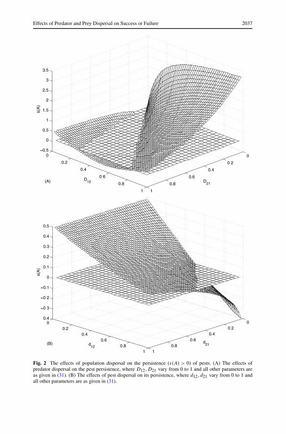
and let D12,D21 vary; it follows that we have Ru1 = 1.1429,Ru2 = 0.6667, which meansthat the pest can be persistent in the first isolated patch and dies out in the second isolatedpatch. Now let D12 and D21 vary from 0 to 1, and we numerically calculate the values ofs(A) as shown in Fig. 2(A). The results shown in Fig. 2(A) clarify the effects of dispersalof natural enemies on the sign of s(A), i.e. the persistence of the pest depends on thedispersal rates of natural enemies.

For this case, in order to reduce the number of pests in the first patch such that s(A) < 0(Ru1u2 < 1, i.e. the pest dies out in both patches), intuitively the dispersal rate D21 shouldbe larger than the dispersal rate D12 because the pest can outbreak or has a larger numberin the first patch, and the results shown in Fig. 2(A) confirm this. But if we further increasethe dispersal rate D21 of natural enemies from the second patch to the first patch andmaintain the dispersal rate D12 relatively small, the results shown in Fig. 2(A) imply thatthe pests can be persistent in both patches. In fact, if D21 � D12, then most of the naturalenemies in the second patch move from this patch to the first patch such that populationsof local natural enemies in the second patch are too low and cannot suppress the pests inthe second patch any more. Consequently, the pests outbreak in both patches.

Similarly, we can fix D12, D21 and study the effects of varying dispersal rates of thepests on their persistence in both patches. For example, if we choose d21, d12 as parame-ters, and fix D21 = D12 = 0.4 and the others are as given in (31). The values of s(A) with


Fig. 2 The effects of population dispersal on the persistence (s(A) > 0) of pests. (A) The effects ofpredator dispersal on the pest persistence, where D12,D21 vary from 0 to 1 and all other parameters areas given in (31). (B) The effects of pest dispersal on its persistence, where d12, d21 vary from 0 to 1 andall other parameters are as given in (31).

2038 Tang et al.

respect to d12 and d21 imply that in this case the pests can only be eradicated if their dis-persal rate from the first patch to the second patch is relatively large and the dispersal rateof pests from the second patch to the first patch is relatively small (Fig. 2(B)).

If Ru1 < 1 and Ru2 > 1, i.e. the pests can be persistent in the second isolated patch anddie out in the first isolated patch, we can obtain results similar to those shown in Case 1.

Case 2 Ru1 > 1 and Ru2 > 1, i.e. the pests can be persistent in each isolated patch.What we want to know in this case is whether we can control the dispersal rates of

the pests and natural enemies such that the EPE is stable (i.e. s(A) < 0 or Ru1u2 < 1). Toaddress this question, we fix parameters as follows:

a1 = 4, b1 = 0.7, c1 = 0.2, d1 = 0.1, a2 = 2,

b2 = 0.35, c2 = 0.2, d2 = 0.1, u1 = 0.5, u2 = 0.5, (32)

d12 = 0.05, d21 = 0.95

and let D12 vary from 0 to 0.8, and D21 vary from 0 to 1. It follows from the formulaefor Ru1 and Ru2 that we have Ru1 = 1.1429,Ru2 = 1.1429, i.e. the pests outbreak in bothisolated patches.

The results shown in Fig. 3(A) clearly indicate that s(A) is negative for some planeparameter ranges of D12 and D21, and this is more likely to happen only when D12 ≈ D21.Note also that if we choose d21 � d12, i.e. the dispersal rate of the pest from the secondpatch to the first patch is significantly larger than its dispersal rate from the second patchto the first patch, then extensive numerical investigations imply that this is one of twoways to eradicate the pests in this case. The other way is to control the dispersal rates d12

and d21 such that d21 d12.From a biological point of view, when the pests are persistent in any single isolated

patch and the aim is to eradicate them by controlling their dispersal rates, we can limittheir dispersal from the first patch to the second patch but allow them to move from thesecond patch to the first patch at high rates, i.e. d21 � d12. At the same time, the naturalenemies can freely move between the two patches with the same dispersal rates. If so,the pests can be quickly eradicated in the second patch. Consequently, the pest may dieout in both patches even if they could have been persistent in each isolated patch. Thisresult clarifies that field boundaries can act as barriers to limit the pest movement, and suchbarriers could change the population dynamics of the pests by influencing their movementbetween fields, and further have an impact on a pest control programme.

Case 3 Ru1 < 1 and Ru2 < 1, i.e. the pests die out in both isolated patches.For this case, can the pests be eradicated no matter how large the dispersal rates are?

Or can the pests be persistent in both patches if they have different dispersal rates in eachpatch? To answer these questions, we fix parameters as follows:

a1 = 2, b1 = 0.5, c1 = 0.2, d1 = 0.1, a2 = 1,

b2 = 0.3, c2 = 0.2, d2 = 0.1, u1 = 0.5, u2 = 0.5, (33)

d12 = 0.4, d21 = 0.4


Fig. 3 The effects of population dispersal on the persistence of pests. (A) The effects of predator dispersalon the pest’s persistence, where D12 varies from 0 to 0.8, D21 varies from 0 to 1, and all other parametersare as given in (32). (B) The effects of pest dispersal on its persistence, where D12,D21 vary from 0 to 1and all other parameters are as given in (33).

2040 Tang et al.

and let D12, D21 vary from 0 to 1. It follows from the formulae of Ru1 and Ru2 that wehave Ru1 = 0.8,Ru2 = 0.6667, i.e. the pests can be eradicated in both isolated patches.

Numerical results shown in Fig. 3(B) imply that s(A) may be positive for some planeparameter ranges of D12 and D21, and the results also imply that this happens only if thedifference between D12 and D21 is quite big, i.e. D12 � D21 or D12 D21. Otherwise,the pests will also die out in both patches if they are extinct in both isolated patches.

It follows from all of the above three cases that whether the pest population is per-sistent or not depends on the dispersal rates of the pest population or the natural enemypopulation. These results imply that reducing or increasing population dispersal couldboth allow the pest species to explode to much higher levels, and so be more difficult toeradicate, or to maintain a low population, and hence be easier to eradicate.

We also note that from a practical point of view, it is interesting to consider the case inwhich one patch is a farmland and the other is a wasteland or an abandoned farmland. As-sume that natural enemies are only released in the farmland (i.e. u2 > 0), that pests in theneighboring wasteland immigrate into the farmland (i.e. d12 > 0) and that the parametervalues are fixed as follows:

a1 = 2, b1 = 0.35, c1 = 0.2, d1 = 0.1, a2 = 2,

b2 = 0.35, c2 = 0.2, d2 = 0.1, u1 = 0.01, u2 = 0.8, (34)

d12 = 0.7, d21 = 0.

This could represent the first patch as wasteland and the second as farmland. Note that wechoose u1 sufficiently small (here u1 = 0.01) rather than u1 = 0 such that the wastelandhas a pest-free equilibrium. Numerical results shown in Fig. 4(A) imply that s(A) is posi-tive for all dispersal rates of natural enemies, and consequently the pest outbreaks in bothpatches if u2 is relatively small. If we hope to control the pest, the releasing rate of naturalenemies in the farmland (i.e. u2) should be large enough. This means that if we furtherincrease the releasing rate u2 such that it reaches a certain threshold value (for exampleu2 = 1.4 here), we may control the pest such that it dies out in both patches, as shown inFig. 4(B). These results indicate that the release of natural enemies may or may not beeffective for this practical case.

5. Further development

In previous sections, we investigated the simplest predator-prey model for pest control byreleases of natural enemies at constant rates. However, all of the methods developed pre-viously can be used to study the following quite general predator-prey model in isolatedpatch i:

⎧⎪⎪⎨

⎪⎪⎩

dxi

dt= fi(xi)xi − gi(xi, yi)yi,

dyi

dt= γigi(xi, yi)yi − diyi + ui,

(35)

where xi and yi are the population abundances of pests and natural enemies, respectively,fi(xi) is the per capita net rate of increase, di represents the per capita death rate of


Fig. 4 The effects of natural enemy dispersal and releasing rate on the persistence of pests, where D12and D21 vary from 0 to 1 and all other parameters are as given in (34). (A) u2 = 0.8. (B) u2 = 1.4.

2042 Tang et al.

the predator population, and γi denotes the conversion efficiency of pests to predator,gi(xi, yi) is the per capita functional response of the predator or the rate of pest attack.For example, we assume that the production of pests (in the absence of natural enemies)follows the usual logistic growth, and the pest-dependent functional response is of theHolling type II form (Holling, 1965), i.e. we have

fi(xi) = ri

(

1 − xi

Ki

)

, gi(xi, yi) = αixi

1 + αiThixi

where αi is the instantaneous search rate, i.e. the average number of encounters withpests per predator per unit of searching time and Thi the handling time, i.e. the time be-tween a pest being encountered and search being resumed. We should emphasize herethat many other growth functions including the Beverton–Holt (Beverton and Holt, 1956;Cooke et al., 1999) and the Gompertz growth (Gompertz, 1925) functions have been pro-posed for the pest population, as have several other pest-dependent functional responsefunctions such as Holling’s types I and III. Different combinations of those functionsresult in different predator-prey systems and different dynamical behaviour.

From a biological point of view, the general assumptions on fi(xi) and gi(xi, yi) areas follows:

(A1) fi ∈ C ′([0,∞),R), fi(0) > 0 and there exists K > 0 such that fi(K) = 0.(A2) gi ∈ C ′([0,∞) × [0,∞),R), gi(0, yi) = 0 and ∂gi

∂xi> 0 for all xi > 0, yi > 0.

Now consider pest and natural enemy populations that disperse among n patches, wehave the following general model:

⎧⎪⎪⎪⎪⎪⎨

⎪⎪⎪⎪⎪⎩

dxi

dt= fi(xi)xi − gi(xi, yi)yi +

n∑

j=1

djixj , 1 ≤ i ≤ n,

dyi

dt= γigi(xi, yi)yi − diyi + ui +

n∑

j=1

Djiyj , 1 ≤ i ≤ n,

(36)

where dii,Dii,1 ≤ i ≤ n, are non-positive constants, dji and Dji (i �= j ) are non-negativeconstants. dii = −∑n

j=1,j �=i dij and Dii = −∑n

j=1,j �=i Dij represent the emigration ratesof pests and natural enemies in the ith patch, respectively; dji and Dji (i �= j ) denotethe immigration rate of pests and natural enemies from the j th patch to the ith patch,respectively. If we further assume that there are no births and deaths of the individualsduring the dispersal process, then we have

n∑

j=1

dji −n∑

j=1

dij = 0,

n∑

j=1

Dji −n∑

j=1

Dij = 0.

For the system (36), the EPE satisfies the following equation

−(di − Dii)yi + ui +n∑

j=1,i �=j

Djiyj = 0, 1 ≤ i ≤ n. (37)


Denote

D =

⎛

⎜⎜⎜⎝

−(d1 − D11) D21 · · · Dn1

D12 −(d2 − D22) · · · Dn2...

......

...

D1n D2n · · · −(dn − Dnn)

⎞

⎟⎟⎟⎠

,

(38)

Y =

⎛

⎜⎜⎜⎝

y1

y2...

yn

⎞

⎟⎟⎟⎠

, U =

⎛

⎜⎜⎜⎝

u1

u2...

un

⎞

⎟⎟⎟⎠

then Eq. (37) becomes

DY + U = 0. (39)

Therefore, if we assume that D is a non-singular matrix, then we have Y ∗ = D−1U .Clearly, D is irreducible and has non-negative off-diagonal elements. Then s(D) is asimple eigenvalue of D with a positive eigenvector. In the following, we always assumethat s(D) < 0, i.e. Y ∗ is globally stable due to the linearity of the subsystem.

Thus, Er = (0,0, . . . ,0, y∗1 , y∗

2 , . . . , y∗n) is an unique EPE of the system (36). The Ja-

cobian matrix of system (36) at point Er can be calculated as follows:

JEr�=

(F − V 0

B D

)

, (40)

where D is given by (38), F = diag(f1(0), f2(0), . . . , fn(0)),

B = diag

(

γ1y∗1

∂g1

∂x1

(0, y∗

1

), γ2y

∗2

∂g2

∂x2

(0, y∗

2

), . . . , γny

∗n

∂gn

∂xn

(0, y∗

n

))

and

V =

⎛

⎜⎜⎜⎜⎝

y∗1

∂g1∂x1

(0, y∗1 ) − d11 −d21 · · · −dn1

−d12 y∗2

∂g2∂x2

(0, y∗2 ) − d22 · · · −dn2

......

......

−d1n −d2n · · · y∗n

∂gn

∂xn(0, y∗

n) − dnn

⎞

⎟⎟⎟⎟⎠

. (41)

It follows that the matrix F is non-negative and V has the Z sign pattern (Van den Driess-che and Watmough, 2002). Let RU = ρ(FV −1), then it follows from the methods givenby Van den Driessche and Watmough (2002) and Wang and Zhao (2004) that we have thefollowing two sufficient and necessary conditions:

RU > 1 iff s(F − V ) > 0, RU < 1 iff s(F − V ) < 0. (42)

In particular, when n = 2 we can easily use the above two sufficient and necessaryconditions to study the stability of EPE and obtain the expected results such as thoseshown in Section 3.

2044 Tang et al.

Another possible way to develop the model is to include more than one control strategyinto it, i.e. other integrated control tactics like chemical and cultural control such as havebeen considered in a general system (Tang and Chen, 2004; Tang and Cheke, 2005; Tanget al., 2005; Van Lenteren, 1995, 2000). We leave this for our future work.

6. Discussion

The aim of this paper was to understand how dispersal in a patchy environment influ-ences the stability properties of pest and natural enemy interaction models. So, we haveproposed simple two-patch model to investigate the effects of a population dispersal be-tween two patches on the persistence of pests. The theoretical results obtained here implythat reducing or increasing dispersal of pests or natural enemies may not only result inmore severe pest outbreaks, but also can be beneficial for pest control. Therefore, knowl-edge about pest dispersal, natural enemy dispersal and population dynamics can be usedto predict pest outbreaks and to develop optimal pest management strategies. We notethat the effects of spatial heterogeneity on the competition model and foodweb modelhave been extensively investigated by Amarasekare and Nisbet (2001) and Amarasekare(2008). Their main results imply that competitive asymmetry (or foodweb complexity)and the dispersal rates have strong effects on local dynamics. Our model formulation,compared with their models, involves a biological control mechanism (i.e. the releasingrates u1, u2). Thus, our models not only can be used to investigate effect of dispersal pat-tern on the persistence or extinction of pests, but also can be used to design the optimalpest control strategies.

The extensive numerical investigations shown in this paper clarify that the dispersalrates of insect pests and natural enemies may dramatically change the dynamical behav-iour, i.e. the persistence of the insect population. Three special cases were considered:Case 1 indicates that if the pest can be persistent in any one of the isolated patches anddies out in the other patch, we can control the dispersal rate of the pest or the dispersalrate of the natural enemy within a certain range such that the pest dies out in both patches.However, the results implied that biological control may be unsuccessful if the dispersalrate of the predator from the isolated patch where the pest dies out to the patch wherethe pest is persistent is too large. Case 2 shows that if the pests can be persistent in bothisolated patches, we still can control the dispersal rates of the pest or the predator suchthat the pest dies out in both patches. However, in order to realize this goal, the differ-ence between dispersal rates of the predator or the pest in the two patches must be quitebig. On the other hand, if the pests dies out in both isolated patches and the differencein dispersal rates of the predator or the pest in both patches is quite large, the pest canoutbreak in both patches. The numerical results obtained in Case 3 clarify this point. Insummary, whether the pest population is persistent or not depends on the dispersal ratesof the pest population or the natural enemy population. These results imply that reducingor increasing population dispersal could both allow the pest species to explode to muchhigher levels, and so be more difficult to eradicate, or to maintain a low population andhence be easier to eradicate.

The numerical investigations also clarify that knowledge about pest dispersal and pop-ulation dynamics can be used to predict pest outbreaks and to develop pest management


strategies. Therefore, dispersal of pest and predator populations is a topic of great con-cern to individuals developing various integrated pest management programmes (VanLenteren, 1995; Van Lenteren and Woets, 1988), and the interplay between environmen-tal heterogeneity and individual movement is an extremely important aspect of ecologicaldynamics.

The results given here indicate that the dispersal of pests and natural enemies couldbe either beneficial or detrimental to pest control, depending on a number of factors suchas the dispersal rates or the status of any single patch (extinction or persistence). Theseresults indicate that knowledge of pest and natural dispersal and the dynamical behaviourof predator-prey systems in patchy environments is crucial for understanding the effec-tiveness of biological control.

From a practical point of view, we also numerically investigate the case in which onepatch is a farmland and the other is a wasteland or an abandoned farmland, and assumethat the natural enemies are released only in farmlands (here u1 u2 in the model). Theresults indicate that the pest may outbreak in both patches if the releasing rate u2 in thefarmland is relatively small or below some threshold value; whilst the pest is controlled ifu2 is greater than the threshold value. So, in order to control the pest the releasing rate ofnatural enemies in farmland must be large enough. Consequently, we can conclude thatthe releasing of natural enemies may or may not be effective.

The results presented here are supported by empirical investigations. In his classic ex-periments involving predatory mites Typhlodromus occidentalis attacking Eotetranynchussexmaculatus prey mites on oranges, Huffaker (1958) experienced extinction of both mitesor co-existence with cycles depending upon how he manipulated the system. In somecases, when the prey went extinct in one habitat patch, they re-established themselvesby migrating to new patches before being attacked again by predators. Similarly, Taka-fuji (1976) investigated dispersal behaviour in a predacious phytoseiid mite Phytoseiuluspersimilis in relation to the density of its prey Tetranychus kanzawai while changing theability of either species to disperse by introducing bridges or barriers between habitatpatches. With all prey patches available to the predator, the prey became extinct but coex-istence was possible using barriers to reduce the dispersal of the predators and allowingmore chances for the prey to disperse. The effects of dispersal on the outcome of predator-prey models has also been investigated by Crowley (1981), Jansen and Sabelis (1992), andPels and Sabelis (1999), amongst others.

However, biological control is only one component of an integrated pest management(IPM) strategy (Greathead, 1992; Hoffmann and Frodsham, 1993; Neuenschwander andHerren, 1988; Parker, 1971). It is known that overuse of a single control tactic is dis-couraged to avoid or delay the development of resistance by the pest to the control tactic,to minimize damage to non-target organisms, and to preserve the quality of the environ-ment. So, in order to control the pest and protect the environment, IPM has been shown byexperiments to be more effective than classical methods (such as biological or chemicalcontrol only). Therefore, in the future, we will take into account IPM strategies and studythe effects of dispersal on pest control in a wider context.

Acknowledgements

We would like to thank the referees for their careful reading of the original manuscriptand many valuable comments and suggestions that greatly improved the presentation of

2046 Tang et al.

this paper. This work is supported by the National Natural Science Foundation of China(NSFC, 10871122 (S.Y. Tang), 10701062 (Y.N. Xiao)), by Program for New CenturyExcellent Talents in University (NCET, Y.N. Xiao) and by SRF for ROCS, SEM.

References

Amarasekare, P., 2008. Spatial dynamics of Foodwebs. Annu. Rev. Ecol. Evol. Syst. 39, 479–500.Amarasekare, P., Nisbet, R.M., 2001. Spatial heterogeneity, source-sink dynamics, and the local coexis-

tence of competing species. Am. Nat. 158, 572–584.Beverton, R.J., Holt, S.J., 1956. The theory of fishing. In: Graham, M. (Ed.), Sea Fisheries; Their Investi-

gation in the United Kingdom, pp. 372–441. Edward Arnold, London.Collier, T., Van Steenwyk, R., 2004. A critical evaluation of augmentative biological control. Biol. Control

31, 245–256.Cooke, K., Van den Driessche, P., Zou, X., 1999. Interaction of maturation delay and nonlinear birth in

population and epidemic models. J. Math. Biol. 39, 332–352.Crowley, P.H., 1981. Dispersal and the stability of predator-prey interactions. Am. Nat. 118, 673–701.DeBach, P., Rosen, D., 1991. Biological Control by Natural Enemies. Cambridge University Press, Cam-

bridge.Dwyer, G., Hails, R., 2002. Manipulating your host: host-pathogen population dynamics, host dispersal

and genetically modified baculoviruses. In: Bullock, J.M., Kenward, R.E., Hails, R. (Eds.), DispersalEcology, pp. 173–193. Blackwell, Oxford.

Gompertz, B., 1925. On the nature of the function expressive of the law of human mortability. Philos.Trans. 115, 513–585.

Greathead, D.J., 1992. Natural enemies of tropical locusts and grasshoppers: their impact and potentialas biological control agents. In: Lomer, C.J., Prior, C. (Eds.), Biological Control of Locusts andGrasshoppers, pp. 105–121. C.A.B. International, Wallingford.

Hanski, I., Gilpin, M.E., 1997. Metapopulation Dynamics: Ecology, Genetics and Evolution. AcademicPress, San Diego.

Hassell, M.P., 1978. The Dynamics of Predator-Prey Systems. Princeton University Press, Princeton.Hassell, M.P., 2000. The Spatial and Temporal Dynamics of Host-Parasitoid Intereactions. Oxford Univer-

sity Press, London.Hoffmann, M.P., Frodsham, A.C., 1993. Natural Enemies of Vegetable Insect Pests. Cooperative Exten-

sion. Cornell University, Ithaca.Holling, C.S., 1965. The functional response of predators to prey density and its role in mimicry and

population regulation. Mem. Entomol. Can. 45, 3–60.Hopper, K.R., Roush, R.T., 1993. Mate finding, dispersal, number released, and the success of biological

control introductions. Ecol. Entomol. 18, 321–331.Huffaker, C.B., 1958. Experimental studies on predation: dispersion factors and predator-prey oscillations.

Hilgardia 27, 343–383.Jansen, V.A.A., Sabelis, M.W., 1992. Prey dispersal and predator persistence. Exp. Appl. Acarol. 14,

215–231.Kareiva, P., 1982. Experimental and mathematical analyses of herbivore movement: quantifying the influ-

ence of plant spacing and quality on foraging discrimination. Ecol. Monogr. 52(3), 261–282.Levins, R., 1970. Extinction. Ann. NY Acad. Sci. 231, 123–138.Lotka, A.J., 1920. Undamped oscillations derived from the law of mass action. J. Am. Chem. Soc. 42,

1595–1599.McDougall, S.L., Mills, N.J., 1997. Dispersal of Trichogramma platnery Nnagarkatti (Hym., Trichogram-

matidae) from point-source releases in an apple orchard in California. J. Appl. Entomol. 121,205–209.

Neuenschwander, P., Herren, H.R., 1988. Biological Control of the Cassava Mealybug, Phenacoccus mani-hoti, by the Exotic Parasitoid Epidinocarsis lopezi in Africa. Philos. Trans. R. Soc. Lond. Ser. B, Biol.Sci. 318, 319–333.

Nicholson, A.J., Bailey, V.A., 1935. The balance of animal populations. Part I. Proc. Zool. Soc. Lond. 3,551–598.

Parker, F.D., 1971. Management of pest populations by manipulating densities of both host and parasitesthrough periodic releases. In: Huffaker, C.B. (Ed.), Biological Control. Plenum, New York.


Pels, B., Sabelis, M.W., 1999. Local dynamics, overexploitation and predator dispersal in an acarinepredator-prey system. Oikos 86, 573–583.

Saavedra, J.L.D., Torres, J.B., Ruiz, M.G., 1997. Dispersal and parasitism of Heliothis virescens eggs byTrichogramma pretiosum (Rriley) in cotton. J. Pest Manag. 43(2), 169–171.

Stein, S.J., Price, W.P., Craig, T.P., Itami, J.K., 1994. Dispersal of a galling sawfly: implications for studiesof insect population dynamics. J. Anim. Ecol. 63, 666–676.

Stiling, P., Cornelissen, T., 2005. What makes a successful biological control agent? A meta-analysis ofbiological control agent performance. Biol. Control 34, 236–246.

Takafuji, A., 1976. The effect of the rate of successful dispersal of a Phytoseiid mite, Phytoseiulus persim-ilis ATHIAS-HENRIOT (Acarina: Phytoseiidae) on the persistence in the interactive system betweenthe predator and its prey. Popul. Ecol. 18, 1438–3896.

Tang, S.Y., Chen, L.S., 2004. Modelling and analysis of integrated pest management strategy. DiscreteContin. Dyn. Syst. B 4, 759–768.

Tang, S.Y., Cheke, R.A., 2005. State-dependent impulsive models of integrated pest management (IPM)strategies and their dynamic consequences. J. Math. Biol. 50, 257–292.

Tang, S.Y., Cheke, R.A., 2008. Models for integrated pest control and their biological implications. Math.Biosci. 215, 115–125.

Tang, S.Y., Xiao, Y.N., Chen, L.S., Cheke, R.A., 2005. Integrated pest management models and theirdynamical behaviour. Bull. Math. Biol. 67, 115–135.

Van den Driesche, R.D., Bellows, T.S., 1996. Biological Control. Chapman & Hall, London.Van den Driessche, P., Watmough, J., 2002. Reproduction numbers and sub-threshold endemic equilibria

for compartmental models of disease transmission. Math. Biosci. 180, 29–48.Van Lenteren, J.C., 1995. Integrated pest management in protected crops. In: Dent, D. (Ed.), Integrated

Pest Management, pp. 311–320. Chapman & Hall, London.Van Lenteren, J.C., 2000. Measures of success in biological control of arthropods by augmentation of

natural enemies. In: Wratten, S., Gurr, G. (Eds.), Measures of Success in Biological Control, pp. 77–89. Kluwer Academic, Dordrecht.

Van Lenteren, J.C., Woets, J., 1988. Biological and integrated pest control in greenhouses. Annu. Rev.Entomol. 33, 239–250.

Volterra, V., 1931. Variations and fluctuations of a number of individuals in animal species living together.In: R.N. Chapman: Animal Ecology. McGraw Hill, New York. Translation.

Wang, W.D., Zhao, X.Q., 2004. An epidemic model in a patchy environment. Math. Biosci. 190, 97–112.

Effects of Predator and Prey Dispersal on Success or Failure of Biological Control

Documents

Transcript of Effects of Predator and Prey Dispersal on Success or Failure of Biological Control