CONTROL OF NONLINEAR DYNAMIC MODELS OF PREDATOR-PREY TYPE

Oecol. Aust., 16(1): 81-98, 2012

Oecologia Australis16(1): 81-98, Março 2012http://dx.doi.org/10.4257/oeco.2012.1601.07

CONTROL OF NONLINEAR DYNAMIC MODELS OF PREDATOR-PREY TYPE

Amit Bhaya1 & Magno Enrique Mendoza Meza2

1 Federal University of Rio de Janeiro, COPPE/NACAD, Department of Electrical Engineering. P.O. Box: 68516 - Rio de Janeiro, RJ. Brazil, ZIP: 21941-972.2 Federal University of ABC (UFABC), Center of Engineering, Modeling and Applied Social Sciences (CECS). Rua Santa Adélia, 166 - Bloco A, Torre 1, Sala 742, Bangu, Santo André, São Paulo, SP, Brazil. ZIP: 09210-170.E-mails: [email protected], [email protected], [email protected]

ABSTRACTIn the ecological context, a large class of population dynamics models can be written as dynamical systems of

one or two variables, i.e., each variable represents a population density of a species. When one or more species is removed from the system (harvested), it is necessary to introduce a control (harvest policy) in order to avoid the extinction of species, due to harvesting. A threshold policy (TP) and a threshold policy with hysteresis (TPH) reviewed and discussed in this paper can be used to avoid the collapse of population densities, governed by predator-prey models. A threshold policy changes the dynamics of a predator-prey dynamical system in such a way that a stable positive equilibrium point is achieved. In other words, coexistence of both species occurs. A threshold policy with hysteresis changes the dynamics so that a limit cycle (bounded oscillation) is achieved, i.e., coexistence of species with a bounded oscillation in population densities occurs. This paper studies the continuous and discrete logistic model for one species and the Lotka-Volterra and Rosenzweig-MacArthur models for two species. The TP and TPH are seen to be versatile and useful in renewable resources management, being simple to design and implement, with some advantages in a situation of overexploitation, as well as in the presence of different types of uncertainties. The design of the policies is carried out by appropriate choice of virtual equilibria in a simple and intuitive manner, and the mathematics used is simple.Keywords: Nonlinear predator-prey models; threshold policy; threshold policy with hysteresis.

RESUMOCONTROLE DE MODELOS DINÂMICOS NÃO LINEARES DO TIPO PREDADOR-PRESA. No

contexto ecológico, uma ampla classe de modelos de dinâmica populacional pode ser escrita como sistemas dinâmicos não lineares em uma ou duas variáveis, i.e., cada variável representa uma densidade populacional de uma espécie. Quando uma ou mais espécies são removidas do sistema (colheita), é necessário introduzir um controle (política de colheita) para evitar a extinção das espécies devido à colheita. Uma política de limiar (TP do inglês) e uma política de limiar com histerese (TPH do inglês) revisadas e discutidas neste artigo podem ser utilizadas para evitar o colapso das densidades populacionais governadas pelos modelos do tipo predador-presa. Uma política de limiar muda a dinâmica de um sistema predador-presa de maneira que um ponto de equilíbrio positivo estável é alcançado. Em outras palavras, permite a coexistência das espécies. Uma política de limiar com histerese muda a dinâmica de maneira que um ciclo limite é alcançado (oscilação limitada), isto é, ocorre a coexistência das espécies com oscilação limitada nas densidades populacionais. Este artigo estuda o modelo logístico contínuo e discreto de uma espécie e os modelos Lotka-Volterra e Rosenzweig-MacArthur de duas espécies. A TP e a TPH parecem ser versáteis e úteis na gestão de recursos renováveis , sendo simples para projetar e implementar, com algumas vantagens em uma situação de sobreexploração (excesso de exploração), bem como na presença de diferentes tipos de incertezas. O projeto das políticas é realizado por uma apropriada escolha dos equilíbrios virtuais de uma maneira simples e intuitiva, e a matemática utilizada é simples.Palavras-chave: Modelos não lineares predador-presa; política de limiar; política de limiar com histerese.

BHAYA, A. & MEZA, M.E.M.

Oecol. Aust., 16(1): 81-98, 2012

82

RESUMENCONTROL DE MODELOS DINAMICOS NO LINEALES DEL TIPO DEPREDADOR-PRESA. En

un contexto ecológico, un gran grupo de modelos de dinámica poblacional pueden ser escritos como sistemas dinámicos no lineales en una o dos variables, i.e., cada variable representa la densidad poblacional de una especie. Cuando una o mas especies son retiradas del sistema (captura), es necesario introducir un control (política de captura) para evitar la extinción de las especies por la captura. La política de umbral (threshold policy TP) y la política de umbral con histéresis (TPH) que son revisadas y discutidas en este artículo, pueden ser usadas para evitar el colapso de las densidades poblacionales gobernadas por los modelos de tipo depredador-presa. La política de umbral, modifica la dinámica de un sistema depredador-presa de tal modo que un punto de equilibrio estable es alcanzado. En otras palabras, permite la coexistencia de las especies. La política de umbral con histéresis modifica la dinámica de manera que un ciclo límite es alcanzado (oscilación limitada), es decir, ocurre la coexistencia de especies con oscilación limitada de las densidades poblacionales. Este artículo estudia el modelo logístico continuo y discreto de una especie y los modelos Lotka-Volterra y Rosenzweig-MacArthur de dos especies. TP y TPH parecen ser versátiles y útiles en la gestión de recursos renovables, siendo simples de diseñar e implementar, con algunas ventajas en casos de sobreexplotación, asi como ante la presencia de diferentes tipos de incertidumbre. El diseño de políticas es llevado a cabo mediante la elección adecuada de equilibrios virtuales de una manera simple e intuitiva y la matemática usada es sencilla.Palabras clave: Modelos depredador-presa no lineales; política de umbral; política de umbral con histéresis.

INTRODUCTION

This paper is a survey of work published over the last few years by the authors. The proposed threshold policy (TP) is based on the application of control Liapunov functions (Sontag 1989), exploring the structure of the predator-prey systems and the backstepping idea (Sepulchre et al. 1997) for the regular form (Utkin 1992), as well as using the concept of real and virtual equilibria (Costa et al. 2000) to derive an on-off or variable structure control.

A large class of predator-prey models can be written as a nonlinear dynamical system (Gurney & Nisbet 1998, Kot 2001) either in discrete or continuous time. In many contexts, it is necessary to introduce control (an exogenous input) into these dynamics. Without loss of generality, we assume that the control corresponds to the removal of a proportion of the prey population in models of one species. In the context of two species dynamics described by the classical predator-prey models, this control action corresponds for example to the removal of the predator species. The introduction of this control into the population dynamics is to avoid the extinction of species, even though overexploitation of species may occur, in addition to other goals such as, for example, economic ones.

Consumer-resource dynamics models include, amongst others, predator-prey, host-parasitoid and herbivore-plant dynamics, which may present a myriad of dynamical behaviors as a result of multiplicity of equilibrium states as well as different initial conditions and parameter values.

Overexploitation is one of the most serious problems in the world fisheries and, to avoid it, different policies are applied (Hjerne & Hansson 2001, Kaitala et al. 2003). The most commonly used policies in the area of harvesting are: (i) the constant escapement policy, which seeks to maintain the stock at a target level by harvesting all fish in excess of the target and by not harvesting if estimated stock size is below the target; (ii) the constant harvest effort policy (Loehle 2006), which removes a desired fraction of the estimated stock each year (the harvest is directly proportional to the estimated stock size); and (iii) the threshold policy (TP), which is intermediate between the well-known constant escapement and constant harvest rate policies (Collie & Spencer 1993, Quinn & Deriso 2000).

Several papers on the control of nonlinear ecological system models under perturbations have been devoted to the study of vulnerability and non-vulnerability of ecosystems subjected to continual, unpredictable, but bounded disturbances due to


Oecol. Aust., 16(1): 81-98, 2012

83

changes in climatic conditions, diseases, migrating species, etc. (Beddington & May 1977, Lee & Leitmann 1983, Steele & Henderson 1984, Vincent et al. 1985). Fradkov & Pogromsky (1998) applied the so-called speed gradient method of adaptive control of oscillations to control the populations of two competitive species. Their method was specific to the Lotka-Volterra model of population dynamics. Emel’yanov et al. (1998) presented a general methodology, referred to as induced internal feedback, for the control of uncertain nonlinear dynamic systems. It is based on on-off control as well as continuous versions of the latter and applied to the Lotka-Volterra system.

Although the continuous logistic model is considered as a drastic simplification of the real-world complexities inherent in predator-prey systems, it can still provide useful insight into the underlying behavior of the system. This type of model has been studied in (Noy-Meir 1975, Clark 1976, 1985, Kot 2001) in the continuous-time case with an emphasis on the productive aspects of renewable-resource management, from the point of view of the optimal control.

The stability properties of predator-prey systems have been studied by graphical techniques, i.e., stability analysis of the predator and prey isoclines in the phase plane, and complemented by mathematical analysis of system behavior (Noy-Meir 1975, Van de Koppel & Rietkerk 2000, Van de Koppel et al. 1996). There are several papers that deal with predator-prey system subject to a harvest (Brauer & Soudack 1978, 1979a, 1979b, 1981, 1982).

Extinction of species is one of the most serious problems facing resource exploitation and, to avoid it, different policies are applied. This paper is concerned with the introduction of exogenous controls, called the threshold policy (TP) and the threshold policy with hysteresis (TPH), into predator-prey models of one and two species.

The stability of predator-prey models in the context of renewable resource exploitation subject to TP and TPH is studied in this paper. TP and TPH are defined and analyzed for different predator-prey models of one and two species. TP and TPH are versatile and useful in the management of renewable resources, being simple to design and implement, and also have advantages in situations of overexploitation.

In the context of grazing management, a TP and a TPH can be used to prevent the collapse of the vegetation-herbivore dynamics system. TP changes the dynamics of vegetation-herbivore system so that a stable positive equilibrium point is reached, and TPH changes the dynamics so that a limit cycle (bounded oscillation) is achieved.

POPULATION DYNAMICS MODELS

A large class of models that describe population dynamics, e.g. predator-prey type, can be written as nonlinear dynamical systems (Gurney & Nisbet 1998, Kot 2001). Specifically, there are

One species models. In this case the predator population density is considered a constant. These models are called one dimensional models (1-D)

(1)

where a state variable denotes the species population density, and describes the species growth function, which is continuous generally, nonnegative and bounded, for example, a logistic function.

Two species models. These models are called bidimensional models or two dimensional

where the state variable x denotes the prey population density and the state variable y denotes the predator population density; the functions 1f and 3f describe the prey and predator growth functions, respectively. The function 2f describes the interaction when the predator finds the prey, and it is called the functional response of the predator to prey density, when )(2 xf depends on x , it is called prey density-dependent, when ),(2 yxf depends on x and y , it is called predator density-dependent, and when ),(2 yxf depends on yx / , it is called ratio-dependent. These equations constitute the simplest representation of the essence of the nonlinear predator-prey interaction (May 1973, Gurney & Nisbet 1998). The form of the system (2)-(3) is known as the regular form in the control literature (Utkin 1992). Grazing systems used and controlled by man could be considered as a

),x(xfx =

y)x(f)x(fx 21 += (2)

(3) y)x(fy 3=


Oecol. Aust., 16(1): 81-98, 2012

84

special case of predator-prey systems. The interaction herbivore-vegetation (predator-prey) is sufficiently similar in its general characteristic to make this theory useful in this case as well (Rietkerk et al. 1997, Van de Koppel & Rietkerk 2000). This interaction is formulated and studied as a predator-prey system subject to a harvest in Meza et al. (2006b).

Host-parasite systems can also be considered as a particular case of the predator-prey interaction (Krivan 1997).

POPULATION DYNAMICS MODELS WITH EXOGENOUS CONTROL

This paper focuses on the introduction of an exogenous control a in population dynamics system models of one or two species, as shown below:

One species models.(4)

(5)

(6)

It is assumed that the control action corresponds to the removal of a proportion of the prey population, in one species models, motivating the introduction of control term u in the model (4). In the context of two species, which constitute the classical origin of predator-prey models, the control action of proportional removal corresponds to the removal of the predator species, i.e., motivating the introduction of the control term 2u in (6). (The control is interpreted as the choice of harvesting policy).

DESIRABLE CHARACTERISTICS OF A CONTROL IN THE ECOLOGICAL CONTEXT

Throughout this paper, the control term corresponds to the removal of a certain species in such a way that extinction of both species does not occur.

Furthermore, the control should have the following characteristics:

Simplicity of implementation: (i) the mathematical expression of the control must be as

simple as possible, (ii) the control must not depend as far as possible on the system parameters, so that the latter do not need to be estimated.

Nonnegative control. This corresponds to the proportional removal of one of the species. In other words, it is assumed that the control corresponds only to removal, i.e. we consider “harvesting” of a certain species.

Minimal monitoring. Refers to the number of population densities that need to be monitored to implement a certain control. In the context of the two species model (5), (6) if only one density is used to design the control, we refer to this as output feedback; if both densities are used, then we call this state feedback.

Promotion of coexistence. Both species must reach sustainable equilibrium levels, in which the populations, in appropriate units, are both positive.

Robustness. The TP and TPH must be robust to parameter uncertainties of the systems, as well as errors and delay in the implementation of policies.

THRESHOLD POLICY (TP)

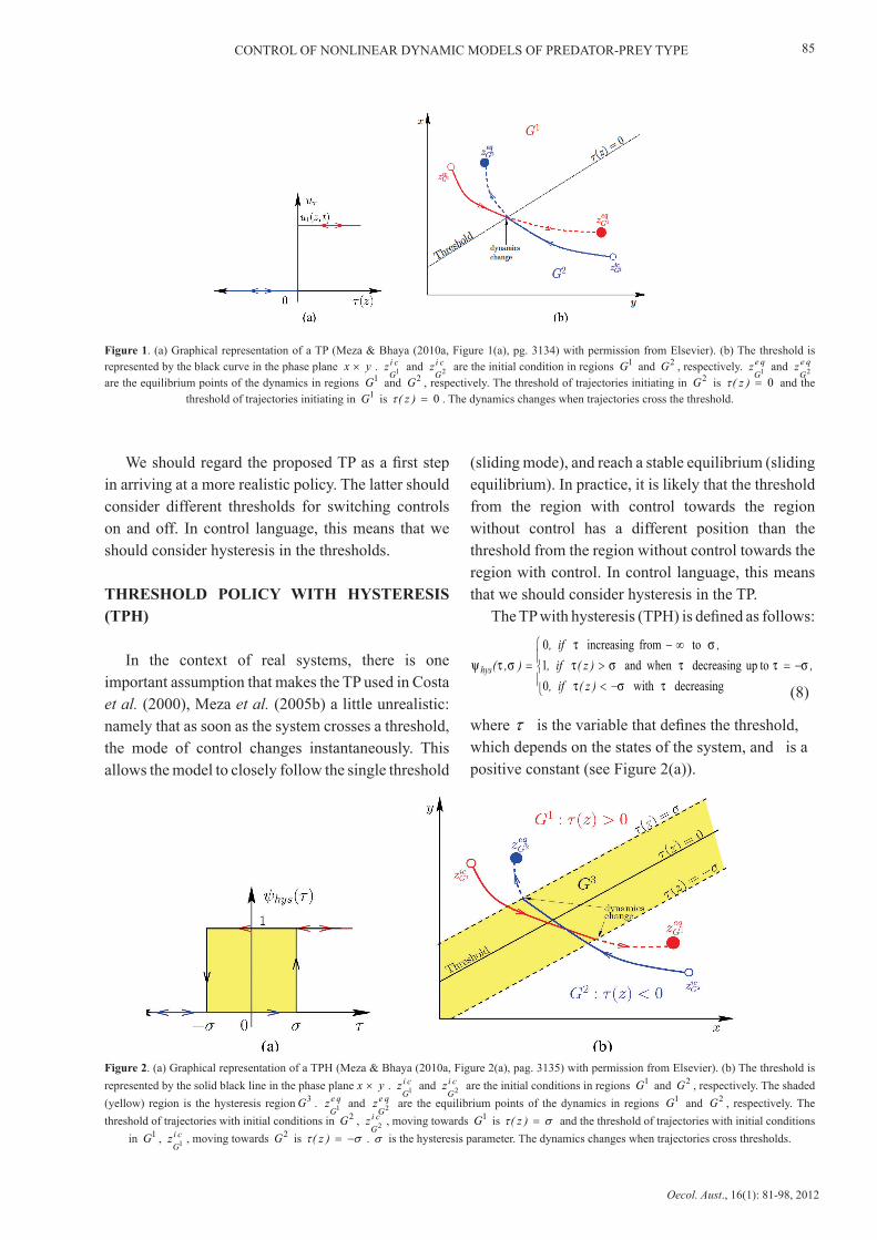
Threshold policies (on-off controls) for dynamical systems are strategies that switch the control inputs from one level to another whenever a certain measured variable crosses a predetermined single threshold (a line or a curve that depends on the state vector).

In the context of fishing management, Collie & Spencer (1993) introduced a so-called threshold policy (TP), which is intermediate between the well known constant escapement and constant harvest rate policies (Quinn & Deriso 2000). A TP is defined as follows: if abundance is below the threshold level, there is no harvest; above the threshold, a constant harvest rate is applied. The TP is also referred to as an on-off control and is a special and simple case of variable structure control in the control literature (Utkin 1978, Filippov 1988, Utkin 1992, Edwards & Spurgeon 1998).

We establish a standard notation for a TP (see Figure 1(a)), denoting it as the function )(τψ defined as follows:

<>

=,if

if)(

0001

ττ

τψ (7)

where τ is the threshold that should be chosen adequately, depending on the problem to be solved.

,u)x(xfx −=

y)x(f)x(fx 21 +=

23 uy)x(fy −=

Two species models.


Oecol. Aust., 16(1): 81-98, 2012

85

Figure 1. (a) Graphical representation of a TP (Meza & Bhaya (2010a, Figure 1(a), pg. 3134) with permission from Elsevier). (b) The threshold is represented by the black curve in the phase plane yx × . ci

Gz

1 and ciG

z 2 are the initial condition in regions 1G and 2G , respectively. qe

Gz

1 and qeG

z 2

are the equilibrium points of the dynamics in regions 1G and 2G , respectively. The threshold of trajectories initiating in 2G is 0=)z(τ and the threshold of trajectories initiating in 1G is 0=)z(τ . The dynamics changes when trajectories cross the threshold.

We should regard the proposed TP as a first step in arriving at a more realistic policy. The latter should consider different thresholds for switching controls on and off. In control language, this means that we should consider hysteresis in the thresholds.

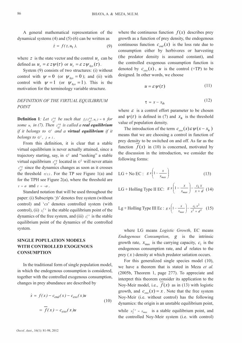
THRESHOLD POLICY WITH HYSTERESIS (TPH)

In the context of real systems, there is one important assumption that makes the TP used in Costa et al. (2000), Meza et al. (2005b) a little unrealistic: namely that as soon as the system crosses a threshold, the mode of control changes instantaneously. This allows the model to closely follow the single threshold

−<−=>

∞−=

decreasingwith0 toupdecreasing whenand1

tofrom increasing0

τστσττστ

στστψ

)z(if,,)z(if,

,if,),(hys

(sliding mode), and reach a stable equilibrium (sliding equilibrium). In practice, it is likely that the threshold from the region with control towards the region without control has a different position than the threshold from the region without control towards the region with control. In control language, this means that we should consider hysteresis in the TP.

The TP with hysteresis (TPH) is defined as follows:

(8)

where τ is the variable that defines the threshold, which depends on the states of the system, and is a positive constant (see Figure 2(a)).

Figure 2. (a) Graphical representation of a TPH (Meza & Bhaya (2010a, Figure 2(a), pag. 3135) with permission from Elsevier). (b) The threshold is represented by the solid black line in the phase plane yx × . ci

Gz

1 and ciG

z 2 are the initial conditions in regions 1G and 2G , respectively. The shaded

(yellow) region is the hysteresis region 3G . qeG

z 1 and qe

Gz

2 are the equilibrium points of the dynamics in regions 1G and 2G , respectively. The threshold of trajectories with initial conditions in 2G , ci

Gz

2 , moving towards 1G is στ =)z( and the threshold of trajectories with initial conditions in 1G , ci

Gz

1 , moving towards 2G is στ −=)z( . σ is the hysteresis parameter. The dynamics changes when trajectories cross thresholds.


Oecol. Aust., 16(1): 81-98, 2012

86

A general mathematical representation of the dynamical systems (4) and (5)-(6) can be written as

),u,z(fz τ= (9)

where z is the state vector and the control τu can be defined as )(τψετ zu = or )(τψετ hyszu = .

System (9) consists of two structures: (i) without control with 0=ψ (or 0=hysψ ); and (ii) with control with 1=ψ (or 1=hysψ ). This is the motivation for the terminology variable structure.

DEFINITION OF THE VIRTUAL EQUILIBRIUM POINT

Definition 1: Let qeGiz be such that 0

1 =)u,z(f iqe

Gi for some iu in (7). Then qe

Giz is called a real equilibrium if it belongs to iG and a virtual equilibrium if it belongs to jG , ij ≠ .

From this definition, it is clear that a stable virtual equilibrium is never actually attained, since a trajectory starting, say, in 1G and “seeking” a stable virtual equilibrium qe

Gz

1 located in 2G will never attain qe

Gz

1 since the dynamics changes as soon as it crosses the threshold )z(τ . For the TP see Figure 1(a) and for the TPH see Figure 2(a), where the threshold are

στ = and στ −= .Standard notation that will be used throughout the

paper: (i) Subscripts ‘fs’ denotes free system (without control) and ‘cs’ denotes controlled system (with control), (ii) sf

iz is the stable equilibrium point of the dynamics of the free system, and (iii) sc

iz is the stable equilibrium point of the dynamics of the controlled system.

SINGLE POPULATION MODELS WITH CONTROLLED EXOGENOUS CONSUMPTION

In the traditional form of single population model, in which the endogenous consumption is considered, together with the controlled exogenous consumption, changes in prey abundance are described by

u)x(c)x(c)x(fx exoend −−=

u)x(c)x(f exo−=

(10)

where the continuous function )(xf describes prey growth as a function of prey density, the endogenous continuous function )(xcend is the loss rate due to consumption either by herbivores or harvesting (the predator density is assumed constant), and the controlled exogenous consumption function is denoted by )(xcexo , u is the control (=TP) to be designed. In other words, we choose

)(τψε=u (11)

thxx −=τ (12)

where ε is a control effort parameter to be chosen and )(τψ is defined in (7) and thx is the threshold value of population density.

The introduction of the term )()( thexo xxxc −ψε means that we are choosing a control in function of prey density to be switched on and off. As far as the function )(xf in (10) is concerned, motivated by the discussion in the introduction, we consider the following forms:

LG + No EC :

−

maxxxxg 1 (13)

LG + Holling Type II EC:

dxxc

xxxg

max +−

− 11 (14)

Lg + Holling Type III Ec :

22

211

dxxc

xxxg

max +−

− (15)

where LG means Logistic Growth, EC means Endogenous Consumption, g is the intrinsic growth rate, maxx is the carrying capacity, 1c is the endogenous consumption rate, and d relates to the prey ( x ) density at which predator satiation occurs.

For this generalized single species model (10), we have a theorem that is stated in Meza et al. (2005b, Theorem 1, page 277). To appreciate and interpret this theorem consider its application to the Noy-Meir model, i.e., )(xf as in (13) with logistic growth, and xxcexo =)( . Note that the free system Noy-Meir (i.e. without control) has the following dynamics: the origin is an unstable equilibrium point,

while maxsf xx =

2 is a stable equilibrium point, and the controlled Noy-Meir system (i.e. with control)


Oecol. Aust., 16(1): 81-98, 2012

87

has the following dynamics: the origin is an unstable equilibrium point, and the point max

sc x)g/(x ε−= 1 2

is an stable equilibrium. Thus, the introduction of a TP is responsible for new dynamic behavior, i.e., convergence to the threshold htx , if sc

ht xx 2 > , which

is called sliding equilibrium (Utkin 1992, Meza et al. 2005b).

It is possible to choose the threshold level htx such that sf

htsc xxx

2

2 << , resulting in an increase in the stabilized vegetation level. With this choice of htx , the points scx

2 and sfx 2 become virtual

equilibria. In fact, it is easy to show that any choice of [ ]sfsc

ht x,xx 2

2 ∈ (yellow interval in Figure 3(a) and

3(b)) leads to the same situation; i.e., the points scx 2

, sfx 2 are virtual equilibria and the globally stable

equilibrium under TP is htx . In this sense, the choice

of the threshold position is guided by studying the nature of the equilibria, i.e., all real equilibria should be unstable and any stable equilibrium should be virtual, so that the only equilibrium that remains is the sliding equilibrium at htx . Robustness of TPs to uncertainties in measurement can be observed in the grazing model. Such an uncertainty can occur either in the measurement of the vegetation x , and is denoted x∆ , or as a small delay t∆ in the switching from one value of the control ψ to another, see Meza & Bhaya (2010a). Essentially, any threshold position that maintains the nature of the equilibria results in stabilization of the populations, and this result in the so called robustness of the controlled system to measurement errors and other uncertainties.

Figure 3. (a) Equilibria with linear consumption curve )x(C with average slope ( g<1ε ). Equilibrium points of the system without control - sfx 2 ,

0 1 =sfx . Equilibrium points of the system with control - scx

2 , 0 1 =scx . (b) Equilibria with linear consumption curve )x(C with large slope (

g>2ε ). Equilibrium points of the system without control maxsf xx =

2 . Equilibrium points of the system with control, 0 2 =scx . The region on

the right of htx is the region with control that has the equilibrium point located in the region without control, and the region on the left of htx is the region without control that has the equilibrium point located in the region with control. All trajectories with initial condition in this region tend

to achieve their respective equilibrium points and so that cross the threshold the dynamics changes.

Figure 4. (a) Time evolution of the population density of the logistic model without control. (b) Time evolution of the population density of the logistic model with proportional control, when g>ε . (c) Time evolution of the population density of the logistic model with TP. Parameter values: 1=g ,

2 1=maxx , 1=ε and 9 =htx .


Oecol. Aust., 16(1): 81-98, 2012

88

Figure 4(a) shows the simulation of the logistic model without control, the system stabilizes at

maxx ; Figure 4(b) shows the simulation of logistic model under proportional control, the system goes to extinction; and Figure 4(c) shows the simulation of the logistic model under a TP, the system stabilizes at threshold thx avoiding the extinction of species.

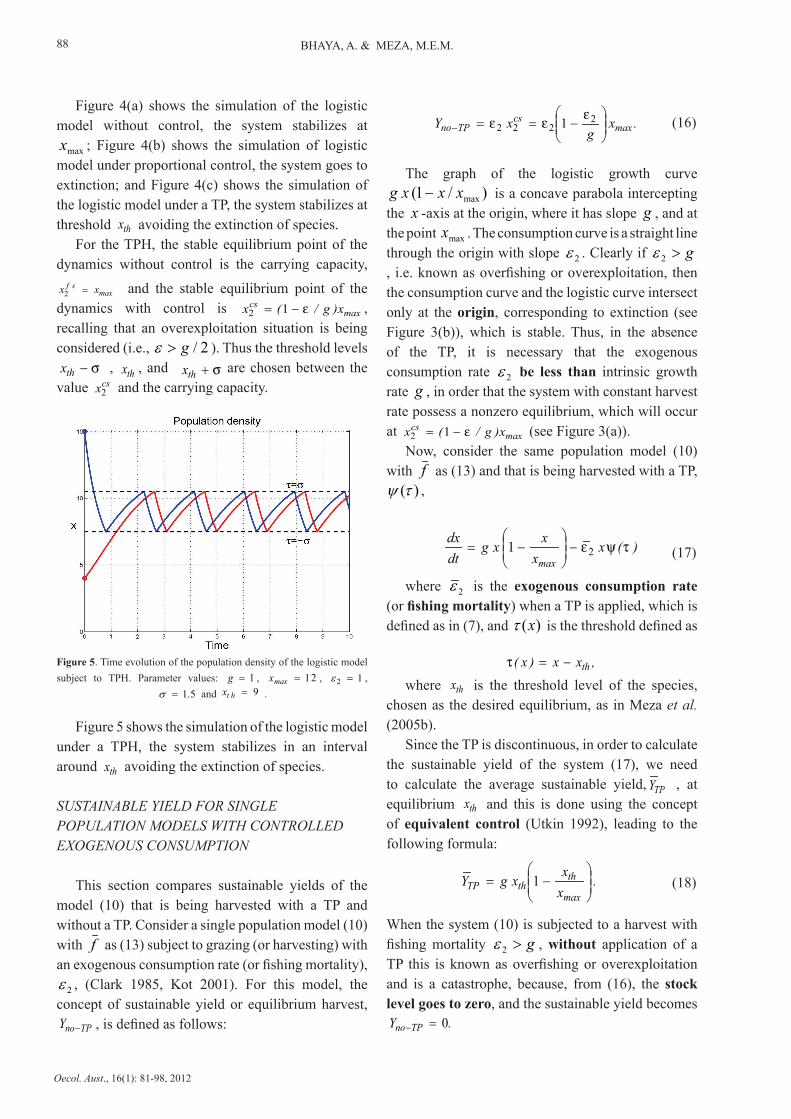
For the TPH, the stable equilibrium point of the dynamics without control is the carrying capacity,

maxsf xx =

2 and the stable equilibrium point of the dynamics with control is

maxcs x)g/(x ε−= 12 ,

recalling that an overexploitation situation is being considered (i.e., 2/g>ε ). Thus the threshold levels σ−thx , thx , and σ+thx are chosen between the value csx2 and the carrying capacity.

Figure 5 shows the simulation of the logistic model under a TPH, the system stabilizes in an interval around thx avoiding the extinction of species.

SUSTAINABLE YIELD FOR SINGLE POPULATION MODELS WITH CONTROLLED EXOGENOUS CONSUMPTION

This section compares sustainable yields of the model (10) that is being harvested with a TP and without a TP. Consider a single population model (10) with f as (13) subject to grazing (or harvesting) with an exogenous consumption rate (or fishing mortality),

2ε , (Clark 1985, Kot 2001). For this model, the concept of sustainable yield or equilibrium harvest, TPnoY − , is defined as follows:

.x

gxY max

csTPno

−==−

2222 1 εεε (16)

The graph of the logistic growth curve )/1( maxxxxg − is a concave parabola intercepting

the x -axis at the origin, where it has slope g , and at the point maxx . The consumption curve is a straight line through the origin with slope 2ε . Clearly if g>2ε, i.e. known as overfishing or overexploitation, then the consumption curve and the logistic curve intersect only at the origin, corresponding to extinction (see Figure 3(b)), which is stable. Thus, in the absence of the TP, it is necessary that the exogenous consumption rate 2ε be less than intrinsic growth rate g , in order that the system with constant harvest rate possess a nonzero equilibrium, which will occur at max

cs x)g/(x ε−= 12 (see Figure 3(a)).Now, consider the same population model (10)

with f as (13) and that is being harvested with a TP, )(τψ ,

)(x

xxxg

dtdx

maxτψε21 −

−=

where 2ε is the exogenous consumption rate (or fishing mortality) when a TP is applied, which is defined as in (7), and )(xτ is the threshold defined as

,xx)x( th−=τ

where thx is the threshold level of the species, chosen as the desired equilibrium, as in Meza et al. (2005b).

Since the TP is discontinuous, in order to calculate the sustainable yield of the system (17), we need to calculate the average sustainable yield, TPY , at equilibrium thx and this is done using the concept of equivalent control (Utkin 1992), leading to the following formula:

(17)

.

xxxgYmax

ththTP

−= 1 (18)

When the system (10) is subjected to a harvest with fishing mortality g>2ε , without application of a TP this is known as overfishing or overexploitation and is a catastrophe, because, from (16), the stock level goes to zero, and the sustainable yield becomes .Y TPno 0=−

Figure 5. Time evolution of the population density of the logistic model subject to TPH. Parameter values: 1=g , 2 1=maxx , 12 =ε ,

51.=σ and 9 =htx .


Oecol. Aust., 16(1): 81-98, 2012

89

This shows the advantage of a TP (10) with f as (13) in an overexploitation situation. Observe, however, that the advantage of a threshold policy is only a relative one in the sense that it allows periods of overexploitation with nonzero average sustainable yield. Of course, the maximum average sustainable yield that results from (18) and which occurs at 2/xx maxth = is the same as that obtained by the application of a continuous constant harvest rate (16). However, the latter must always be below the level of overexploitation g<2ε .

SINGLE POPULATION DISCRETE MODELS SUBJECT TO TP AND TPH

The continuous logistic model is considered since it provides useful insight into the underlying behavior of the system. It has been studied in the continuous-time case with an emphasis on the productive aspects of renewable-resource management. We consider that the continuous logistic model (13) subject to a general control takes the form:

u

xxxgx

max−

−= 1

where the parameter are defined as in equations (13-15), and is the control policy. The logistic model (19) with standard discretization (forward Euler) is as follows

u)k(x)k(x

xgg)k(xmax

−

−+=+ 11

(19)

(20)

with the discretization step size 1=h . It is well known that the discrete logistic model (20) has chaotic solutions (Mickens 1994, Murray 2002). A nonstandard scheme was introduced in (Mickens 1994) to alleviate these problems and leads to difference equations that preserve the desirable qualitative behavior of their continuous counterpart. A logistic discrete time model is obtained according to nonstandard discretization method in Mickens (1994), by making the following replacements: (i) ( ) φ/)()1( kxkxx −+= , (ii) )(kxx → , (iii)

)()1(2 kxkxx +→ ,

(21)

where )(hφφ = is a function of the discretization step size. Another logistic discrete time model is obtained with nonstandard discretization according to Mickens (2003), by making the following replacements:(i) ( ) φ/)k(x)k(xx −+= 1 (ii) )k(x)k(xcxx 122 +−→−= , (iii) )k(x)k(xx 12 +→

(22)

where )(hφφ = . The behavior of the models (21) and (22) (with uncertainties) under TP and TPH has been analysed in Meza & Bhaya (2010a), in which the control policy u could be a TP or a TPH with a delay in the application. The following uncertainties are also introduced: (i) Uncertainty in the intrinsic growth rate ( )ρ2011 .gg += ; (ii) Uncertainty in the carrying capacity ( )ρ201100 .xmax += ; (iii) Uncertainty in the effort policy and overexploitation ( 2/g>ε

( )ρε 20170 .. += ; (iv) Delay in the measurement of the population density, which implies in delay in the application of the control )dk(xx −=∆ ; (v) Uncertainty and delay in the measurement of the population density ( )ρρ 201 .xx += ∆∆ ; and (vi) Uncertainty in the distance to the threshold level thxx −=

∆∆ρρτ are

considered in models (20-22), where 5 101 .r = , 8=d and ρ is an uniformly distributed random number (variable) between 1− and 1, ( )ρ201 .+ means that the respective variable fluctuates around the mean or true value by %0 2± , ∆x with 8=d means that a delay of 8 units is considered in the application of all control policies.

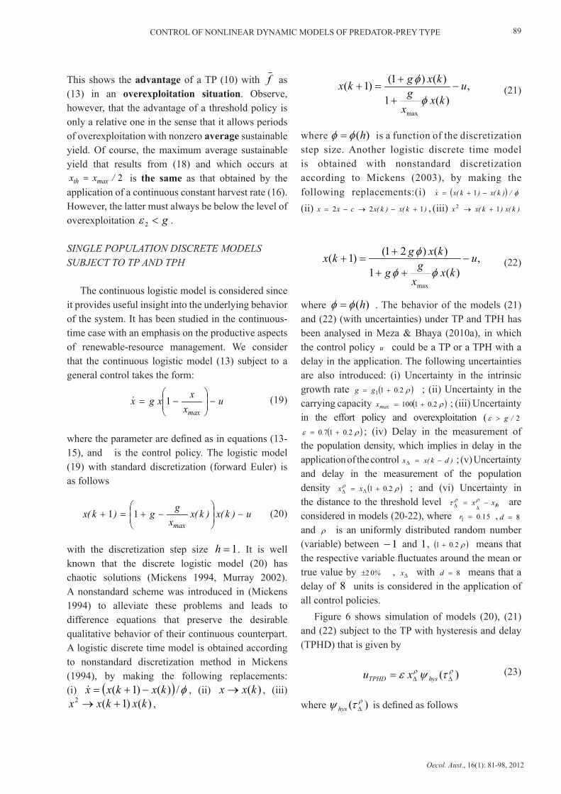
Figure 6 shows simulation of models (20), (21) and (22) subject to the TP with hysteresis and delay (TPHD) that is given by

)( ρρ τψε ∆∆= hysTPHD xu

where )( ρτψ ∆hys is defined as follows

(23)

,)(1

)()21()1(

max

ukx

xgg

kxgkx −++

+=+

φφ

φ

,)(1

)()1()1(

max

ukx

xg

kxgkx −+

+=+

φ

φ


Oecol. Aust., 16(1): 81-98, 2012

90

<+−≥>

>+≤−<=

∆∆∆∆

∆∆∆∆∆

).k()k(andor,if

)k()k(andor,if)(hys ρρρρ

ρρρρρ

ττστστ

ττστσττψ

1 1

1 0

The TPHD avoids the extinction of species even when the systems are subject to uncertainties and

overexploitation, maintaining the population densities in positive values, see Figure 6.

(24)

ONE-PREDATOR ONE-PREY MODELS SUBJECTED TO A TPH

A large class of predator-prey models can be written as the nonlinear dynamical system as defined in (2) and (3). In this section, we study the Rosenzweig-MacArthur and the Lotka-Volterra predator-prey models subject to a TPH.

We consider the introduction of an exogenous control, x

hysu and yhysu , corresponding respectively to

the removal of each species. If the control is applied, the model (2), (3) becomes

xhysuy)x(f)x(fx −+= 21

,uy)x(fy yhys−= 3

where xhysu and y

hysu are the TPH on prey and predator, respectively.

LOTKA-VOLTERRA PREDATOR-PREY MODEL

Costa et al. (2000) proposes a mathematical model for a harvesting schedule of predator-prey systems guided by a management policy called a weighted escapement policy (WEP). This policy determines

the sustainable harvest of prey and predators in a deterministic setting, when both species are subject to constant effort harvesting.

One example of a TP, known as a weighted escapement policy (WEP), in which a threshold is built from a weighted (or linear) combination of prey and predator densities was proposed in Costa et al. (2000). The TP was used to stabilize a Lotka-Volterra system under simultaneous harvesting of the prey and predator. Consider the general system (2)-(3), where xrf 11 = , xaf −=2 , xbrf +−= 23 . The Lotka-Volterra system under simultaneous TP on both species, where the parameter 1r is the growth rate of the prey, 2r is the mortality rate of the predator, a , b represent the interaction coefficients between the species. )()z(uu hys

xhys τψ1= and )()z(uu hys

yhys τψ2=

where xu 11 ε= and yu 22 ε= are the harvesting actions (proportional controls), 1ε and 2ε are the harvesting intensities (control effort parameters), and )(hys τψ is defined as in equation (8); and all parameters are positive. The threshold defined in Costa et al. (2000) has the following form

dSyx −+= 21 αατ

where dS is the weighted sum of species (constant), 1α and 2α are attributed population weights. Note that

(25)

(26)

(27)

Figure 6. Logistic discrete-time models (20), (21), (22) with different parameters 1=h , 07921 .=φ , 28721 . in Figures (a), (b), (c), respectively, using the TPHD control policy (23) with a threshold level 0 8 =htx . Simulations are presented for each choice of discretization for three different random choices of the parameter ρ . In all cases (a), (b), (c), and for 5 4 simulations, for random values of the parameter ρ , extinction was never

observed (Meza & Bhaya (2010a, Figure 6(a), 6(b), 6(c) pg. 3140) with permission from Elsevier).


Oecol. Aust., 16(1): 81-98, 2012

91

use of the threshold (27) requires the measurement of both species densities.

Verification of the conditions of the TPH theorem

A theorem was stated in Meza & Bhaya (2009) for the stability of the Lotka-Volterra model subject to TPH, and it is called TPH theorem. In this section, we verify conditions of the TPH theorem that are needed to prove the stability of the model under the TPH. Figure 7 shows the graphical representation of the TPH in a phase plane.

Note that the free Lotka-Volterra system has the following dynamics: the origin, ( ) ( )00

1

1

1 ,y,xz sfsfsf == is an unstable equilibrium (saddle point), while

( ) ( )a/r,b/ry,xz sfsfsf12

2

2

2 == is a center point, and the

controlled Lotka-Volterra system has the following dynamics: the origin, ( ) ( )00

1

1

1 ,y,xz scscsc == , is an unstable equilibrium (saddle point), and the point

( ) ( )a/)r(,b/)r(y,xz scscsc1122

2

2

2 εε −+== is a center

point. In both cases, the trajectories in the phase portrait are only closed trajectories and not limit cycles.

The switching lines στ = and στ −= must be chosen so that the equilibrium points sfz

2 and scz 2 are

both virtual, as shown in Figure 7, and this verifies the first condition of the TPH theorem. The second condition requires that the vector field be directed to a region, in which the system will stabilize. The third condition requires that the slope of the lines στ = and στ −= be appropriate in order for the second condition to be satisfied. The fourth condition ensures the existence of the stabilization region. For more details about conditions of the TPH theorem, the reader is referred to Meza & Bhaya (2009). Thus, the introduction of a TPH is responsible for new dynamic behavior, i.e., a bounded oscillation between the switching lines is achieved (see Figure 8(c)). In Figures 8(a) and 8(b) when TPH is not applied some trajectories approach extinction (the origin), whereas in Figure 8(c) under TPH, trajectories are bounded away from extinction by the lower switching line.

Figure 8. (a) Phase portrait dynamics of the Lotka-Volterra model without harvesting. (b) Phase portrait dynamics of the Lotka-Volterra system with harvesting (when 5021 .== εε ). (c) Phase portrait dynamics of the the Lotka-Volterra system with TPH. Parameter values: 1=a , 1=b , 11 =r ,

12 =r , 201 .=α 12 =α , 10.=σ , 5021 .== εε and 1=dS (Meza & Bhaya (2009, Fig. 4(a), 4(b), 4(c), pg. 143) with permission from Theory in Biosciences).

ROSENZWEIG-MACARTHUR PREDATOR-PREY MODEL

As mentioned in the introduction, we consider the introduction of an exogenous control corresponding

to the removal of the predator. The model (2), (3) therefore becomes

y)x(f)x(fx 21 += (28)

Figure 7. Graphical representation of the TPH in the phase plane for the Lotka-Volterra model under a TPH. The yellow region is the hysteresis region 3G . The points qe

Gz

2 and qeG

z 1 are the stable equilibria of the

dynamics in region 2G and 1G , respectively, and both are virtual. The points ci

Gz

1 and ciG

z 2 are the initial conditions in region 1G and 2G ,

respectively.


Oecol. Aust., 16(1): 81-98, 2012

92

,uy)x(fy hys−= 3

In this section, it is shown that the TPH is also valid for the control of the classical Rosenzweig-MacArthur predator-prey model that corresponds to the choice )K/x(xrf −= 1 1 , )Ax(/xf += 2 ,

( ))AJ(/J)Ax(/xsf +−+= 3 (Brauer & Soudack 1981, 1982), where r is the intrinsic growth rate of the prey, K is the carrying capacity of the environment, A is the half saturation constant, s conversion efficiency of predator, and J is the minimum prey population for which the predator can survive below the carrying capacity K , KJ < . We choose this model because it can be regarded as one of the simplest nontrivial paradigms proposed after the more classical but biologically unrealistic Lotka-Volterra system. In this case, we consider harvesting of only the predator

)(yu hyshys τψε2= , where 2ε is the harvesting intensity (control effort parameter) and )(hys τψ is defined as in equation (8), and τ is a threshold that has the following form

,yy: th−=τ

where hty is the predator threshold level.

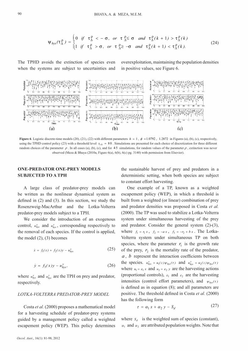
Verification of the conditions of the TPH theorem

The switching lines στ = and στ −= must be chosen so that the equilibrium points sfz

2 and scz

2 are both virtual, as shown in Figure 9. The third condition of the TPH theorem is required solely for the Lotka-Volterra model. Here the remaining conditions are verified, with the aim of

(29)

Figure 9. Design of the TPH for the Rosenzweig-MacArthur system. The horizontal black solid line is the threshold τ . The switching lines 0=− στ and 0=+ στ are dashed.

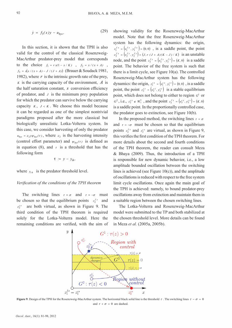
showing validity for the Rosenzweig-MacArthur model. Note that the free Rosenzweig-MacArthur system has the following dynamics: the origin,

( ) ( )00 1

1

1 ,y,xz sfsfsf == , is a saddle point, the point

( ) ( )K/)JK()AJ(r,Jy,xz sfsfsf −+== 2

2

2 is an unstable

node, and the point ( ) ( )0 3

3

3 ,Ky,xz sfsfsf == is a saddle

point. The behavior of the free system is such that there is a limit cycle, see Figure 10(a). The controlled Rosenzweig-MacArthur system has the following dynamics: the origin, ( ) ( )00

1

1

1 ,y,xz scscsc == , is a saddle point, the point ( )scscsc y,xz

2

2

2 = is a stable equilibrium point, which does not belong to either to region 1G or

2G , i.e., 2 2 +ℜ∉scz , and the point ( ) ( )0

3

3

3 ,Ky,xz scscsf == is a saddle point. In the proportionally controlled case, the predator goes to extinction, see Figure 10(b).

In the proposed method, the switching lines στ = and στ −= must be chosen so that the equilibrium points sfz

2 and scz 2 are virtual, as shown in Figure 9,

this verifies the first condition of the TPH theorem. For more details about the second and fourth conditions of the TPH theorem, the reader can consult Meza & Bhaya (2009). Thus, the introduction of a TPH is responsible for new dynamic behavior, i.e., a low amplitude bounded oscillation between the switching lines is achieved (see Figure 10(c)), and the amplitude of oscillations is reduced with respect to the free system limit cycle oscillations. Once again the main goal of the TPH is achieved: namely, to bound predator-prey oscillations away from extinction and maintain them in a suitable region between the chosen switching lines.

The Lotka-Volterra and Rosenzweig-MacArthur model were submitted to the TP and both stabilized at the chosen threshold level. More details can be found in Meza et al. (2005a, 2005b).


Oecol. Aust., 16(1): 81-98, 2012

93

Figure 10. (a) The Rosenzweig-MacArthur model without control. (b) Phase portrait dynamics of the Rosenzweig-MacArthur system with proportional control ( )202 .=ε (Meza et al. (2005b, Fig. 5(a), 5(b), pag. 279) with permission from Elsevier). (c) Phase portrait dynamics of the Rosenzweig-

MacArthur system with threshold policy ( )202 .=ε . Parameter values: 2=r , 0 6=K , 1=s , 0 1=A and 0 2=J .

HERBIVORE-VEGETATION DYNAMICS IN SEMI-ARID GRAZING SYSTEMS

A more realistic model of vegetation-herbivore systems was proposed in Van de Koppel & Rietkerk (2000). These authors investigated the implications of herbivore population dynamics in a vegetation regulated system susceptible to soil degradation. First, they investigated the conditions for which multiple steady states arise as a consequence of soil degradation (Rietkerk et al. 1997, Van de Koppel & Rietkerk 2000). Second, they compared with models with more explicit dynamics of semi-arid soils, where the conditions for multiple stable states arise and are related to the parameters of the ecosystem.

We review the model considered in Van de Koppel & Rietkerk (2000) of a grazing system in semi-arid soil. Consider the dynamical system:

( )( )

−=

−−=

HdebV)t(H

VbHl)V(zh)t(V *

where V is the vegetation density, H is the herbivore density, h is the coefficient relating specific vegetation growth to water availability, l is the loss rate of vegetation tissue due to senescence, b is a coefficient relating per capita consumption to herbivore density, e is the consumption-to-growth conversion coefficient, d represents the natural mortality rate of the herbivore, )V(z* expresses water availability as a function of vegetation standing crop, and

W

*

rVkVzkV

p)V(z++

+=

µ10 where µ is a coefficient

relating the specific uptake rate of water by vegetation to water availability, Wr is the rate of water loss due to evaporation and drainage, p stands for the rainfall

(30)

(also called the rainfall rate, and is determined by the climate), 0Z is the minimum water infiltration in the absence of vegetation and k is a half saturation constant.

HERBIVORE-VEGETATION DYNAMICS IN SEMI-ARID GRAZING SYSTEMS SUBMITTED TO TP

In this section, we propose a modification to the model (30) that describes the effects of the application of an on-off policy, and subsequently analyze this model. The policy dictates whether grazing occurs or not, according to the measured level of the variables involved, which are the vegetation and/or herbivore density. It is assumed that the policy is enacted by an exogenous agent, i.e., human intervention. The proposed on-off policy splits the vegetation-herbivore phase-plane into two regions: one with grazing and other without grazing.

The model of vegetation-herbivore dynamics under the proposed on-off policy is as follows:

( )( )

−=

−−=

,Hd)()t(H

,V)(l)V(zh)t(V *

τψ

τψ

2

1

Where

<>

=,)H,V(ifHb

)H,V(if)(

000

1 ττ

τψ

<≤>

=,)H,V(ifHbe

dk,)H,V(ifk)(

00 11

2 ττ

τψ

)H,V(τ is the threshold and, as mentioned before, creates two structures in system (31): (i) grazing is permitted when 0<τ and (ii) not permitted

(31)

(32)

(33)


Oecol. Aust., 16(1): 81-98, 2012

94

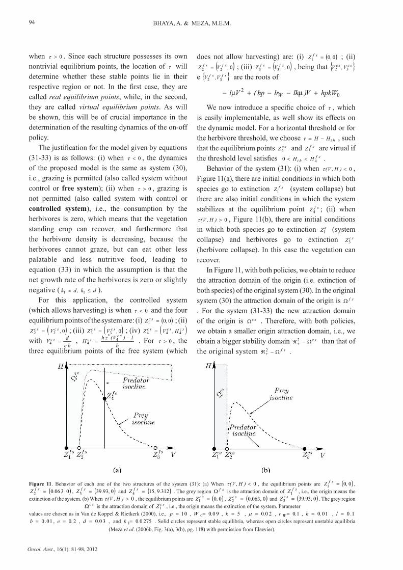
when 0>τ . Since each structure possesses its own nontrivial equilibrium points, the location of τ will determine whether these stable points lie in their respective region or not. In the first case, they are called real equilibrium points, while, in the second, they are called virtual equilibrium points. As will be shown, this will be of crucial importance in the determination of the resulting dynamics of the on-off policy.

The justification for the model given by equations (31-33) is as follows: (i) when 0<τ , the dynamics of the proposed model is the same as system (30), i.e., grazing is permitted (also called system without control or free system); (ii) when 0>τ , grazing is not permitted (also called system with control or controlled system), i.e., the consumption by the herbivores is zero, which means that the vegetation standing crop can recover, and furthermore that the herbivore density is decreasing, because the herbivores cannot graze, but can eat other less palatable and less nutritive food, leading to equation (33) in which the assumption is that the net growth rate of the herbivores is zero or slightly negative ( dk,dk ≤≈ 11 ).

For this application, the controlled system (which allows harvesting) is when 0<τ and the four equilibrium points of the system are: (i) ( )00

1 ,Z sc = ; (ii) ( )0

2

2 ,VZ scsc = ; (iii) ( )0 3

3 ,VZ scsc = ; (iv) ( )scscsc H,VZ

4

4

4 = with

bedV sc =

4 , b

l)V(zhH

sc*sc −=

4

4 . For 0>τ , the

three equilibrium points of the free system (which

does not allow harvesting) are: (i) ( )00 1 ,Z sf = ; (ii)

( )0 2

2 ,VZ sfsf = ; (iii) ( )0

3

3 ,VZ sfsf = , being that scsc V,V 3

2

e sfsf V,V 3

2 are the roots of

002 =−+−−+− WW lkrhpkWV)lklrhp(Vl µµ

We now introduce a specific choice of τ , which is easily implementable, as well show its effects on the dynamic model. For a horizontal threshold or for the herbivore threshold, we choose htHH −=τ , such that the equilibrium points scZ

4 and sfZ 3 are virtual if

the threshold level satisfies sfht HH

4 0 << .Behavior of the system (31): (i) when 0<)H,V(τ ,

Figure 11(a), there are initial conditions in which both species go to extinction sfZ

1 (system collapse) but there are also initial conditions in which the system stabilizes at the equilibrium point sfZ

4 ; (ii) when 0>)H,V(τ , Figure 11(b), there are initial conditions

in which both species go to extinction csZ1 (system collapse) and herbivores go to extinction scZ

3 (herbivore collapse). In this case the vegetation can recover.

In Figure 11, with both policies, we obtain to reduce the attraction domain of the origin (i.e. extinction of both species) of the original system (30). In the original system (30) the attraction domain of the origin is sf Ω . For the system (31-33) the new attraction domain of the origin is sc Ω . Therefore, with both policies, we obtain a smaller origin attraction domain, i.e., we obtain a bigger stability domain sc 2 Ω−ℜ+ than that of the original system sf 2 Ω−ℜ+ .

Figure 11. Behavior of each one of the two structures of the system (31): (a) When 0<)H,V(τ , the equilibrium points are ( )00 1 ,Z sf = ,

( )03, 0.06 2 =sfZ , ( )039.93,

3 =sfZ and ( ) 9.31215, 4 =sfZ . The grey region sf Ω is the attraction domain of sfZ

1 , i.e., the origin means the extinction of the system. (b) When 0>)H,V(τ , the equilibrium points are ( )00

1 ,Z sc = , ( )00.063, 2 =scZ and ( )039.93,

3 =scZ . The grey region sc Ω is the attraction domain of scZ

1 , i.e., the origin means the extinction of the system. Parametervalues are chosen as in Van de Koppel & Rietkerk (2000), i.e., 0 1=p , 9 00 0 .W = , 5=k , 2 00.=µ , 10 .r W= , 1 0 0.h = , 1 0 .l =

1 0 0 .b = , 2 0.e = , 3 00.d = , and 275 00 1 .k = . Solid circles represent stable equilibria, whereas open circles represent unstable equilibria (Meza et al. (2006b, Fig. 3(a), 3(b), pg. 118) with permission from Elsevier).


Oecol. Aust., 16(1): 81-98, 2012

95

CONCLUSION

The proposed threshold policies possess all the desirable characteristics of a control that can be applied in an ecological context, i.e. (i) easy to implement; (ii) the control is carried through the removal of only one species; (iii) only one species needs to be monitored; and (iv) species coexistence is achieved; (v) robustness to measurement and implementation errors is achieved. Moreover, in comparison with several existing methods, both old and new, it seems to be the only one that combines all these desirable characteristics (Meza et al. 2005a).

In all cases the design of the TP and TPH, together with the determination of the threshold followed three basic steps:1. Calculate the equilibrium points of each structure (with control and without control).2. Determine the stable equilibrium points of each structure.3. Choose a threshold level such that the stable equilibrium points of each structure become virtual for TP; switching lines στ = and στ −= are

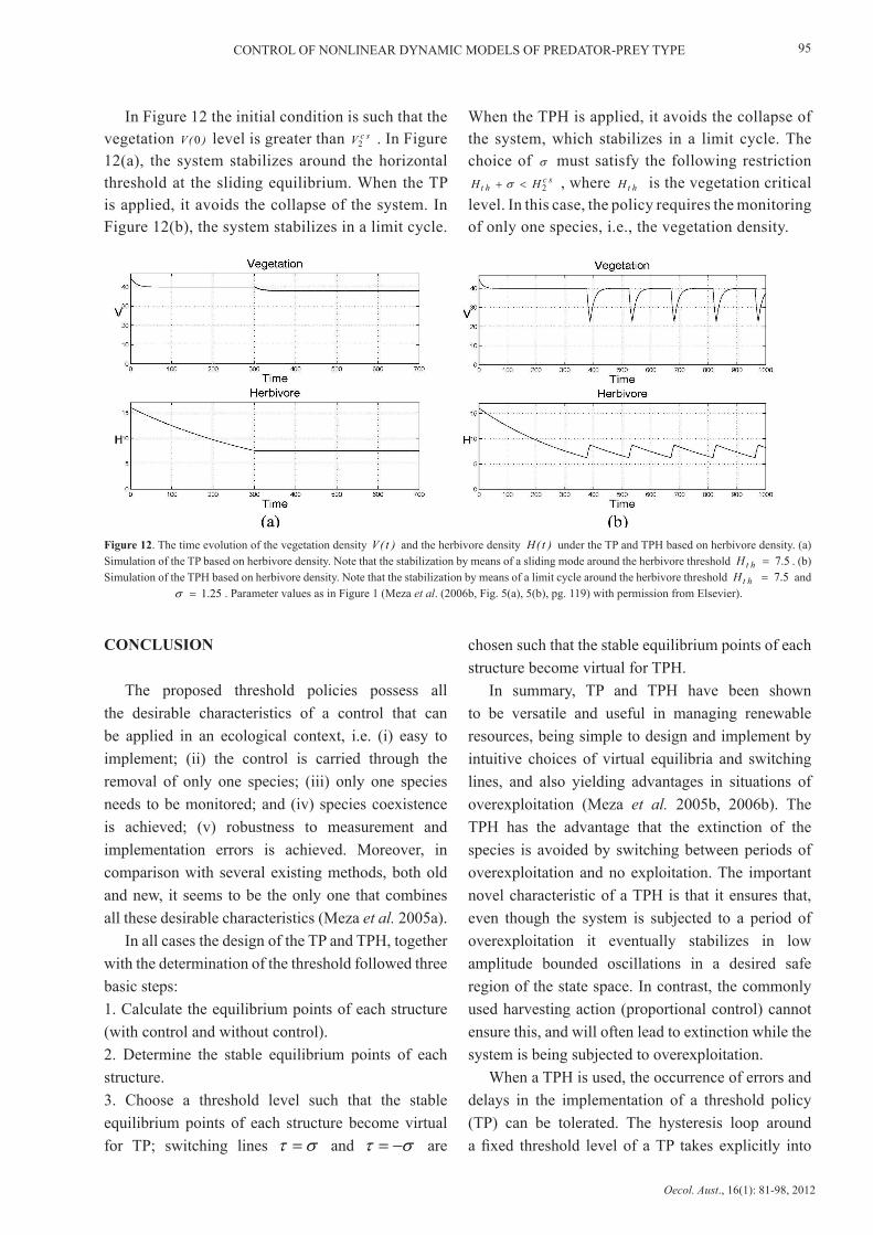
In Figure 12 the initial condition is such that the vegetation )(V 0 level is greater than scV

2 . In Figure 12(a), the system stabilizes around the horizontal threshold at the sliding equilibrium. When the TP is applied, it avoids the collapse of the system. In Figure 12(b), the system stabilizes in a limit cycle.

When the TPH is applied, it avoids the collapse of the system, which stabilizes in a limit cycle. The choice of σ must satisfy the following restriction

scht HH

2 <+ σ , where htH is the vegetation critical level. In this case, the policy requires the monitoring of only one species, i.e., the vegetation density.

Figure 12. The time evolution of the vegetation density )t(V and the herbivore density )t(H under the TP and TPH based on herbivore density. (a) Simulation of the TP based on herbivore density. Note that the stabilization by means of a sliding mode around the herbivore threshold 7.5 =htH . (b) Simulation of the TPH based on herbivore density. Note that the stabilization by means of a limit cycle around the herbivore threshold 7.5 =htH and

1.25=σ . Parameter values as in Figure 1 (Meza et al. (2006b, Fig. 5(a), 5(b), pg. 119) with permission from Elsevier).

chosen such that the stable equilibrium points of each structure become virtual for TPH.

In summary, TP and TPH have been shown to be versatile and useful in managing renewable resources, being simple to design and implement by intuitive choices of virtual equilibria and switching lines, and also yielding advantages in situations of overexploitation (Meza et al. 2005b, 2006b). The TPH has the advantage that the extinction of the species is avoided by switching between periods of overexploitation and no exploitation. The important novel characteristic of a TPH is that it ensures that, even though the system is subjected to a period of overexploitation it eventually stabilizes in low amplitude bounded oscillations in a desired safe region of the state space. In contrast, the commonly used harvesting action (proportional control) cannot ensure this, and will often lead to extinction while the system is being subjected to overexploitation.

When a TPH is used, the occurrence of errors and delays in the implementation of a threshold policy (TP) can be tolerated. The hysteresis loop around a fixed threshold level of a TP takes explicitly into


Oecol. Aust., 16(1): 81-98, 2012

96

REFERENCES

BEDDINGTON, J.R. & MAY, R.M. 1977. Harvesting natural

populations in a randomly fluctuating environment. Science, 197:

463-465, http://dx.doi.org/10.1126/science.197.4302.463

BRAUER, F. & SOUDACK, A.C. 1978. Response of

predator-prey systems to nutrient enrichment and proportional

harvesting. International Journal of Control, 27: 65-86, http://

dx.doi.org/10.1080/00207177808922348

BRAUER, F. & SOUDACK, A.C. 1979a. Stability regions

and transition phenomena for harvested predator-prey

systems. Journal of Mathematical Biology, 7: 319-337,

http://dx.doi.org/10.1007/BF00275152

BRAUER, F. & SOUDACK, A.C. 1979b. Stability regions in

predator-prey systems with constant-rate prey harvesting. Journal of

Mathematical Biology, 8: 55-71, http://dx.doi.org/10.1007/BF00280586

BRAUER, F. & SOUDACK, A.C. 1981. Coexistence properties

of some predator-prey systems under constant rate harvesting

and stocking. Journal of Mathematical Biology, 12: 101-114,

http://dx.doi.org/10.1007/BF00280586

BRAUER, F. & SOUDACK, A.C. 1982. On constant effort

harvesting and stocking in a class of predator-prey systems.

Journal of Mathematical Biology, 95: 247-252.

CLARK, C.W. 1976. Mathematical Bioeconomics: The Optimal

Management of Renewable Resources. John Wiley & Sons, New

York. 368p.

CLARK, C.W. 1985. Bioeconomics Modelling and Fisheries

Management. John Wiley & Sons, New York. 304p.

account such occurrences and stabilizes the dynamics by means of low amplitude bounded oscillations in the region delimited by the hysteresis itself. Finally, from the management standpoint, it is important to stress that the proposed strategy does not interfere directly in the harvesting intensities. As is well known, such interference usually meets several obstacles in its implementation.

Evidently, since there is always error in the estimate of stock size (species abundance), it is crucial to study the effect of these errors and uncertainties on the performance of a given policy, and this is the main objective of the paper (Meza & Bhaya 2010a), which studies the response of three logistic discrete-time models to a sustained perturbation (removal of species through harvesting). The contribution of this paper is to show that a control policy called threshold policy with delay (TPD) and threshold policy with hysteresis and delay (TPHD) can be used in the discrete-time case to deal with the problem of uncertainties in estimation and modeling.

Notable features of the threshold policies proposed in Meza et al. (2006a) are as follows: (i) Despite the fact that the ratio-dependent model displays more complex dynamics (mutual extinction, semi-stable limit cycles etc.) than its density-dependent counterpart, simple threshold or on-off policies involving constant effort removal/no control, suffice to take the system to a globally stable coexistence equilibrium; (ii) The mathematical analysis is quite tractable and standard phase plane methods are effective. (iii) Threshold policies of the type used in this paper can be used in the stabilization of a large class of models used in mathematical ecology, and their practical implementation is, in principle, quite simple, since it only involves estimation of population densities. These issues as well as robustness issues are treated in another paper (Meza & Bhaya 2009).

In Meza & Bhaya (2010b) a special case of the TP was applied to two different virus dynamics models with drug-resistant mutant, using drug therapy with a reverse transcriptase inhibitor. Simulations show that this control is effective, obtaining a smaller systemic cost of treatment than that obtained in Kwon (2007), as well as maintaining the uninfected cells in a small bounded neighborhood of a pre-specified level. The controller is designed by appropriate choice of so called virtual equilibrium points. In an ecological

context, there are also several papers that applied the TP in different models (Costa & Meza 2006a, 2006b, 2006c, 2006d).

In summary, threshold policies have been shown to be versatile and useful in managing renewable resources, being simple to design and implement, and also yielding advantages in situations of overexploitation.

ACKNOWLEDGEMENT: This research was partially financed by the agency CNPq, CAPES (both authors) and FAPERJ (Amit Bhaya) FAPESP (Magno Enrique Mendoza Meza) and represents an updated survey of work published over the last few years by the authors, as cited within the text.


Oecol. Aust., 16(1): 81-98, 2012

97

COLLIE, J.S. & SPENCER, P.D. 1993. Management strategies

for fish populations subject to long term environmental variability

and depensatory predation. Technical Report 93-02, Alaska Sea

Grant College, 629-650, 820p.

COSTA, M.I.S.; KASZKUREWICZ, E.; BHAYA, A. & HSU,

L., 2000. Achieving global convergence to an equilibrium

population in predator-prey systems by the use of

discontinuous harvesting policy. Ecological Modelling, 128:

89-99, http://dx.doi.org/10.1016/S0304-3800(99)00220-3

COSTA, M.I. S. & MEZA, M.E. M. 2006a. Application of a

threshold policy in the management of multispecies fisheries and

predator culling. Mathematical Medicine and Biology-A Journal

of the IMA, 23: 63-75, http://dx.doi.org/10.1093/imammb/dql005

COSTA, M.I.S. & MEZA, M.E.M. 2006b. Coexistence in

a chemostat: application of a threshold policy. Chemical

Engineering Science, 61: 3400-3402, http://dx.doi.org/10.1016/j.

ces.2005.11.033

COSTA, M.I.S. & MEZA, M.E.M. 2006c. Dynamical stabilization

of grazing systems: An interplay among plant-water interaction,

overgrazing and a threshold management policy. Mathematical

Biosciences, 204: 250-259, http://dx.doi.org/10.1016/j.

mbs.2006.05.010

COSTA, M.I.S. & MEZA, M.E.M. 2006d. Harvesting of

dynamically complex consumer-resource systems: Insights from

a threshold management policy. Ecological Complexity, 3: 193-

199, http://dx.doi.org/10.1016/j.ecocom.2006.03.003

EDWARDS, C. & SPURGEON, S.K. 1998. Sliding Mode

Control: Theory and Applications. Vol. 7 of Systems and Control

Book Series. Taylor and Francis, London. 237p.

EMEL’YANOV, S.V.; BUROVOI, I.A. & LEVADA, F.Y. 1998.

Control of Indefinite Nonlinear Dynamics Systems. Vol. 231 of

Lecture Notes in Control and Information Sciences. Springer-

Verlag, Great Britain.

FILIPPOV, A.F. 1988. Differential Equations with Discontinuous

Righthand Sides. Kluwer Academic, Dordrecht. 316p.

FRADKOV, A.L. & POGROMSKY, A.Y. 1998. Introduction to

Control of Oscillations and Chaos. Vol. 35 of Nonlinear Science.

World Scientific, Singapore. 391p.

GURNEY, W.S.C. & NISBET, R.M. 1998. Ecological dynamics.

Oxford University Press, New York, NY. 352p.

HJERNE, O. & HANSSON, S. 2001. Constant catch or

constant harvest rate? The Baltic Sea cod (Gadus morhua L.)

fishery as a modeling example. Fisheries Research, 53: 57-70,

http://dx.doi.org/10.1016/S0165-7836(00)00266-6

KAITALA, V.; JONZÉN, N. & ENBERG, K. 2003. Harvesting

strategies in a fish stock dominated by low-frequency variability:

the Nowegian spring-spawning herring (Clupea harengus).

Marine Resources Economics, 18: 263-274.

KOT, M. 2001. Elements of Mathematical Ecology. Cambridge

University Press, Cambridge. 473p.

KRIVAN, V. 1997. Dynamical consequences of optimal, host

feeding on host- parasitoid population dynamics. Bulletin of

Mathematical Biology, 59: 809-831.

KWON, H.D. 2007. Optimal treatment strategies derived

from a HIV model with drug-resistant mutants. Applied

Mathematics and Computation, 188: 1193-1204, http://

dx.doi.org/10.1016/j.amc.2006.10.071

LEE, C.S. & LEITMANN, G. 1983. On optimal long-term

management of some ecological systems subject to uncertain

disturbances. International Journal of Systems Science, 14: 979-

994, http://dx.doi.org/10.1080/00207728308926509

LOEHLE, C. 2006. Control theory and the management of

ecosystems. Journal of Applied Ecology, 43: 957-966, http://

dx.doi.org/10.1111/j.1365-2664.2006.01208.x

MAY, R. 1973. Stability and Complexity in Model Ecosystems.

Princeton University Press, New Jersey, NJ. 292p.

MEZA, M.E. M. & BHAYA, A. 2009. Realistic threshold

policy with hysteresis to control predator-prey continuous

dynamics. Theory in Biosciences, 128: 139-149, http://

dx.doi.org/10.1007/s12064-009-0062-3

MEZA, M.E.M. & BHAYA, A. 2010a. Control theory and the

management of ecosystems: A threshold policy with hysteresis is

robust. Applied Mathematics and Computation, 216: 3133-3145,

http://dx.doi.org/10.1016/j.amc.2010.04.015

MEZA, M.E.M. & BHAYA, A. 2010b. Virus dynamics models

subjected to a hybrid on-off control. Journal of Biological Systems,

18: 339-356, http://dx.doi.org/10.1142/S0218339010003287

MEZA, M.E.M.; BHAYA, A. & KASZKUREWICZ, E. 2005a.

Controller design techniques for the Lotka-Volterra nonlinear

system. Revista Controle & Automação, 16: 124-135.

MEZA, M.E. M.; BHAYA,A. & KASZKUREWICZ, E. 2006a.

Stabilizing control of ratio-dependent predator-prey models.

Nonlinear Analysis: Real World Applications, 7: 619-633, http://

dx.doi.org/10.1016/j.nonrwa.2005.04.001

MEZA, M.E.M.; BHAYA, A.; KASZKUREWICZ, E. &

COSTA, M.I.S. 2005b. Threshold policies control for

predator-prey systems using a control Liapunov function


Oecol. Aust., 16(1): 81-98, 2012

98

approach. Theoretical Population Biology, 67: 273-284,

http://dx.doi.org/10.1016/j.tpb.2005.01.005

MEZA, M.E.M.; BHAYA, A.; KASZKUREWICZ, E. &

COSTA, M.I.S. 2006b. On-off policy and hysteresis on-off

policy control of the herbivore-vegetation dynamics in a semi-

arid grazing system. Ecological Engineering, 28: 114-123,

http://dx.doi.org/10.1016/j.ecoleng.2006.05.005

MICKENS, R.E., 1994. Nonstandard Finite Difference Models of

Differential Equations. World Scientific, Singapore. 249p.

MICKENS, R.E. 2003. A nonstandard finite-difference scheme

for the Lotka-Volterra system. Applied Numerical Mathematics,

45: 309-314, http://dx.doi.org/10.1016/S0168-9274(02)00223-4

MURRAY, J.D. 2002. Mathematical Biology I. An Introduction.

Third Edition. Springer-Verlag, New York. 574p.

NOY-MEIR, I. 1975. Stability of grazing systems: An

application of predator-prey graphs. Journal of Ecology, 63:

459-481, http://dx.doi.org/10.2307/2258730

QUINN, T.J. & DERISO, R.B. 2000. Quantitative Fish Dynamics.

Biological Resource Management Series. Oxford University

Press, Oxford. 560p.

RIETKERK, M.; VAN DEN BOSCH, F. & VAN DE KOPPEL,

J. 1997. Site-specific properties and irreversible vegetation

changes in semi-arid grazing systems. Oikos, 80: 241-252,

http://dx.doi.org/10.2307/3546592

SEPULCHRE, R.; JANKOVIC, M. & KOKOTOVICC, P. 1997.

Constructive Nonlinear Control. Series on Communications and

Control Engineering (CCES). Springer-Verlag, London. 313p.,

http://dx.doi.org/10.1007/978-1-4471-0967-9

SONTAG, E.D. 1989. A ‘universal’ construction of Artstein’s

theorem on nonlinear stabilization. Systems and Control Letters,

13: 117-123, http://dx.doi.org/10.1016/0167-6911(89)90028-5

STEELE, J.H. & HENDERSON, E.W. 1984. Modeling

long-term in fish stocks. Science, 224: 985-987, http://

dx.doi.org/10.1126/science.224.4652.985

UTKIN, V.I. 1978. Sliding Modes And Their Applications

In Variable Structure Systems. Translation A. Parnakh. Mir

Publishers, Moscow. 257p.

UTKIN, V.I. 1992. Sliding Modes In Control And Optimization.

Springer-Verlag, Berlin. 286p.

VAN DE KOPPEL, J.; HUISMAN, J.; VAN DER WAL, R. &

OLFF, H., 1996. Patterns of herbivory along a productivity

gradient: An empirical and theoretical investigation. Ecology, 77:

736-745, http://dx.doi.org/10.2307/2265498

VAN DE KOPPEL, J. & RIETKERK, M. 2000. Herbivore

regulation and irreversible vegetation change in semi-arid

grazing systems. Oikos, 90: 253-260, http://dx.doi.org/10.1034/

j.1600-0706.2000.900205.x

VINCENT, T.L.; LEE, C.S. & GOH, B.S. 1985. Maintenance

of an equilibrium state in the presence of uncertain inputs.

International Journal of Systems Science, 16: 1335-1344,

http://dx.doi.org/10.1080/00207728508926755

Submetido em 21/07/2010 Aceito em 19/11/2010

CONTROL OF NONLINEAR DYNAMIC MODELS OF PREDATOR-PREY TYPE

Documents

Transcript of CONTROL OF NONLINEAR DYNAMIC MODELS OF PREDATOR-PREY TYPE