Predator interference and stability of predator–prey dynamics

1 23

Journal of Mathematical Biology ISSN 0303-6812 J. Math. Biol.DOI 10.1007/s00285-014-0820-9

Predator interference and stability ofpredator–prey dynamics

Lenka Přibylová & Luděk Berec

1 23

Your article is protected by copyright and

all rights are held exclusively by Springer-

Verlag Berlin Heidelberg. This e-offprint is

for personal use only and shall not be self-

archived in electronic repositories. If you wish

to self-archive your article, please use the

accepted manuscript version for posting on

your own website. You may further deposit

the accepted manuscript version in any

repository, provided it is only made publicly

available 12 months after official publication

or later and provided acknowledgement is

given to the original source of publication

and a link is inserted to the published article

on Springer's website. The link must be

accompanied by the following text: "The final

publication is available at link.springer.com”.

J. Math. Biol.DOI 10.1007/s00285-014-0820-9 Mathematical Biology

Predator interference and stability of predator–preydynamics

Lenka Pribylová · Ludek Berec

Received: 5 September 2013 / Revised: 8 July 2014© Springer-Verlag Berlin Heidelberg 2014

Abstract Predator interference, that is, a decline in the per predator consumption rateas predator density increases, is generally thought to promote predator–prey stabil-ity. Indeed, this has been demonstrated in many theoretical studies on predator–preydynamics. In virtually all of these studies, the stabilization role is demonstrated asa weakening of the paradox of enrichment. With predator interference, stable limitcycles that appear as a result of environmental enrichment occur for higher values ofthe environmental carrying capacity of prey, and even a complete absence of the limitcycles can happen. Here we study predator–prey dynamics using the Rosenzweig–MacArthur-like model in which the Holling type II functional response has beenreplaced by a predator-dependent family which generalizes many of the commonlyused descriptions of predator interference. By means of a bifurcation analysis weshow that sufficiently strong predator interference may bring about another stabilizingmechanism. In particular, hysteresis combined with (dis)appearance of stable limitcycles imply abrupt increases in both the prey and predator densities and enhanced

Electronic supplementary material The online version of this article (doi:10.1007/s00285-014-0820-9)contains supplementary material, which is available to authorized users.

L. Pribylová (B)Section of Applied Mathematics, Department of Mathematics and Statistics, Faculty of Science,Masaryk University, Kotlárská 2, 611 37 Brno, Czech Republice-mail: [email protected]

L. BerecDepartment of Biosystematics and Ecology, Institute of Entomology, Biology Centre ASCR,Branišovská 31, 370 05 Ceské Budejovice, Czech Republic

L. BerecFaculty of Science, Institute of Mathematics and Biomathematics, University of South Bohemia,Branišovská 31, 370 05 Ceské Budejovice, Czech Republic

123

Author's personal copy

http://dx.doi.org/10.1007/s00285-014-0820-9

L. Pribylová, L. Berec

persistence and resilience of the predator–prey system. We encourage refitting the pre-viously collected data on predator consumption rates as well as for conducting furtherpredation experiments to see what functional response from the explored family is themost appropriate.

Keywords Population stability · Functional response · Intraspecific competition ·Predation · Predator–prey model

Mathematics Subject Classification 92B05 · 92D25 · 37G10 · 37G15

1 Introduction

Predator–prey theory is still to a large extent marked by an effort to cope with thelegacy of Lotka and Volterra (Lotka 1920; Volterra 1926; Kot 2001) and the para-dox of enrichment (Rosenzweig 1971; Vos et al. 2004; Boukal et al. 2007). That is,it still largely dangles round the issue of mechanisms stabilizing and destabilizingpredator–prey dynamics, which mostly translates to the issue of functional response(e.g. Murdoch and Oaten 1975; Magnússon 1999; Fryxell et al. 2007; Boukal et al.2008; Berec 2010). A recently suggested family of functional responses and its effecton predator–prey dynamics is the topic of this study.

The most common functional response that occurs in nature appears to be the typeII functional response (Hassell et al. 1976; Begon et al. 1990). In its classical formula-tion, it assumes that predators need some time to handle their prey upon locating it, thatsearching for prey and handling prey are mutually exclusive activities, and that preda-tors do not interfere in their searching and handling activities (Holling 1959). However,there are other plausible mechanisms that lead to the same functional response form,such as a combination of linear predation rate and density-dependent anti-predatorbehaviour of prey (Pavlova et al. 2010). Regardless of the underlying mechanism, theper capita predator consumption rate increases, at a decelerating rate, with increasingprey density (Gascoigne and Lipcius 2004). The type II functional response of preda-tors is also a part of the prototype predator–prey model demonstrating the paradoxof enrichment where stable oscillations bifurcate out of a stable equilibrium once theenvironmental carrying capacity of prey exceeds a critical value (Rosenzweig 1971;Kot 2001).

The assumption of independence of functional response of predator density, dom-inating predator–prey theory, is not always satisfactory (Skalski and Gilliam 2001).Individual predators do not always act independently of conspecifics, effects of twoor more predators do not always sum up, and competition among predators doesnot always occur only through prey depletion. Predator interference, occurring whenthe (per capita) predator consumption rate decreases as predator density increases, isa well-documented and wide-ranging phenomenon. Actually, it is a collective termembracing a number of specific mechanisms. One can think of (i) behavior typicalof territorial animals where individuals “waste time” in direct contests thus decreas-ing time each could otherwise devote to searching for or handling prey (Spradbery1970; Beddington 1975; Ruxton et al. 1992), (ii) predators that steal already subdued

123


Predator interference and stability

prey from one another (Arnqvist et al. 2006), (iii) prey that can escape predation evenif they are already “locked in” by predators (Huisman and DeBoer 1997), (iv) preywhich react to an increasing predator density by changing behavior which makes themmore difficult to locate and/or capture (Ruxton 1995), (v) prey heterogeneous in theirvulnerability to predation (Abrams 1994), or (vi) spatially aggregated predators andprey (Cosner et al. 1999).

Predator interference has already found its way into predator–prey models; despitethe variety of mechanisms, a common pattern that appears to emerge from modelingpredator interference is its stabilizing effect on predator–prey dynamics (Rogers andHassell 1974; Ruxton et al. 1992; Ruxton 1995; Huisman and DeBoer 1997; Krivanand Vrkoc 2004). An intuitive explanation for this is that a decrease in individualconsumption rate with increasing predator density can negatively affect reproduction,growth and/or survival of predators and hence the predator population is controlled byits own density in a form of implicit negative density dependence (Begon et al. 1990). Amore quantitative, model-based view on predator interference as a stabilizing mech-anism largely comes from the Beddington–DeAngelis functional response replac-ing the Holling type II functional response in the Rosenzweig–MacArthur predator–prey model with the logistic growth of prey. Incorporation of the predator-dependentBeddington–DeAngelis functional response causes the predator isocline to changefrom vertical to slanted to the right, which in turn has an effect of delaying occurrenceof the paradox of enrichment—the Hopf bifurcation marking the onset of predator–prey oscillations occurs for higher values of the environmental carrying capacity ofprey (Rosenzweig and MacArthur 1963; Cantrell and Cosner 2001). This stabiliz-ing role of predator interference has even become sort of conventional wisdom inpopulation ecology (Holt 2011).

Berec (2010) introduced a novel family of functional responses dependent on preda-tor density, of which the type II functional response as well as common types of func-tional responses modeling predator interference were special cases. In particular, allof the common types (Hassell–Varley, ratio-dependent, Beddington–DeAngelis) canbe viewed as arising from encounter rates of predators with their prey that decreasewith increasing predator density (Berec 2010). With this novel family, predator inter-ference was shown to stabilize predator–prey dynamics once its strength was not toohigh. For other members of this family which modeled higher predator interferencestrengths three coexistence equilibria co-occurred (Berec 2010). Berec (2010) alsoshowed why this previously unreported multi-equilibrial regime could not occur ifonly the Beddington–DeAngelis functional response was considered.

The study by Berec (2010) considered only the number and character (i.e. stability)of coexistence equilibria. Here we extend this study by looking more thoroughlyat the system dynamics when some of the coexistence equilibria are unstable, andcharacterize system bifurcations that may occur, for an even more general predator-dependent functional response. In particular, we are interested in the occurrence ofmulti-stability regimes, aiming to seek for general conditions on predator-dependentfunctional responses that would produce multiple coexistence equilibria in a predator–prey model.

123



2 Model

We consider the following predator–prey model with a predator-dependent functionalresponse,

d N

dt= r N

(1 − N

K

)− P f (N , P),

d P

dt= eP f (N , P) − m P .

(1)

In this model, N and P are prey and predator densities, respectively, r is the intrinsicper capita growth rate of prey, K is the environmental carrying capacity of prey, mis the per capita predator mortality rate, and e is the efficiency with which consumedprey are transformed into new predators. The prey population grows logistically in theabsence of predators and the predator population dies out exponentially in the absenceof prey. For the predator functional response f (N , P) that links prey and predatordynamics we consider a generalized Holling type II functional response, in which theencounter rate λ of predators with their prey is a smooth and declining function of thepredator density P:

f (N , P) = λ(P)N

1 + hλ(P)N(2)

where λ(0) = λ0 and λ′(P) < 0; h is the predator handling time of one prey. Wethus model predator interference, assuming that the higher is the predator density, thelonger it takes any individual predator to encounter a prey. Combining the genericmodel (1) with the functional response (2), our primary model to be analyzed is

d N

dt= r N

(1 − N

K

)− λ(P)N

1 + hλ(P)NP,

d P

dt= e

λ(P)N

1 + hλ(P)NP − m P .

(3)

As a specific example of the function λ(P) we consider the function

λ(P) = λ0

(b + P)w, (4)

with b > 0, λ0 > 0, and w > 0 (Berec 2010). Notice that the case w = 0 simplifies to aconstant λ(P) = λ0 and f (N , P) becomes the Holling type II functional response; theresulting model (1), the Rosenzweig–MacArthur predator–prey model, is the prototypefor occurrence of the paradox of enrichment (Rosenzweig 1971). For w = 1, we have

f (N , P) = (λ0/b)N

1 + P/b + h(λ0/b)N(5)

which is actually the Beddington–DeAngelis functional response (Beddington 1975;DeAngelis et al. 1975). Hence, varying w in the predator encounter rate (4) doesnot produce a single functional response but rather a family of functional responses,

123



whereas varying b or λ0 would give only one. Moreover, it is easy to show that forany fixed predator density P and any parameters λ0, b and w, the functional response(2) combined with the predator encounter rate (4) is an increasing, concave functionof N . On the other hand, for any fixed prey density N , it is a decreasing function ofP , as expected for a model of predator interference.

The model (1) has invariant isoclines N = 0 and P = 0 that correspond to expo-nential extinction of the predator without prey and logistic dynamics of the prey with-out predator, respectively. Stability properties of two boundary equilibria [0, 0] and[K , 0], related to the logistic dynamics of prey with predator extinction, were studiedin Appendix A of Berec (2010): whereas the extinction equilibrium [0, 0] is always asaddle point, the prey-only equilibrium [K , 0] is locally stable for any K if e < mhand for K < m/[λ(0)(e − mh)] if e > mh; if K > m/[λ(0)(e − mh)] for e > mhthen [K , 0] is a saddle point.

In this paper, we focus on coexistence equilibria of the model (3). Berec (2010)showed that for 0 < w < 1, the model (3) with the predator encounter rate (4) couldhave at most one coexistence equilibrium. For w > 1, however, the non-trivial isoclinesmay intersect in zero, one or three points with positive N and P and we thus may havezero, one or three coexistence equilibria in this case (Berec 2010). In addition, in thecase of three co-occurring coexistence equilibria a saddle point was shown to separateeither two stable coexistence equilibria or one stable coexistence equilibrium and oneunstable coexistence equilibrium; where just one coexistence equilibrium occurred,this could either be stable or unstable (Berec 2010).

In what follows, we look more thoroughly at dynamics of the model (3), and char-acterize bifurcations that may occur. The non-linear phenomena that we are going toobserve include bistability and hysteresis caused by a cusp bifurcation, appearance ofa limit cycle due to a Hopf bifurcation, and disappearance of a stable limit cycle dueto a homoclinic bifurcation. All of these phenomena have important consequences forpredator–prey dynamics.

3 Results

3.1 Cusp bifurcation, hysteresis, and multiple coexistence equilibria

A coexistence equilibrium [N∗, P∗] of the model (3) satisfies

N∗ = KC2

λ(P∗), (6)

P∗ = C1λ(P∗) − C2

λ2(P∗), (7)

where C1 = ere−hm and C2 = m

K (e−hm). Hence, if e − hm ≤ 0 then no coexistence

equilibrium exists. Therefore, we assume e − hm > 0 from here on, and have C1 > 0and C2 > 0. Since we assume λ′(P) < 0 the Eq. (6) implies that as the predatorequilibrium P∗ > 0 increases so does the prey equilibrium N∗ > 0. Moreover, theEq. (7) gives a necessary condition

123



λ(P∗) > C2 (8)

for [N∗, P∗] to be a coexistence equilibrium of the model (3).The Eq. (7) defines an implicit function

F(P∗) := P∗λ2(P∗) − C1(λ(P∗) − C2) = 0 (9)

of the non-zero predator equilibrium P∗ [(having one-to-one correspondence to thenon-zero prey equilibrium N∗ via the Eq. (6)]. In a limit point related to merging anddisappearance of two equilibria on a fold of the equilibrium manifold the value of P∗satisfies F ′(P∗) = 0, which can be equivalently expressed as

λ3(P∗) − C1(2C2 − λ(P∗))λ′(P∗) = 0. (10)

(recall that we assume λ(P) is smooth). In Appendix A.1 we show that this conditionis both necessary and sufficient for vanishing of the Jacobian of the model (3) at acoexistence equilibrium.

Sinceλ′(P∗) < 0, the Eq. (10) also yields that for P∗ to be a limit point we must haveλ(P∗) > 2C2. In particular, λ(0) > 2C2 is a necessary condition for a fold bifurcationto occur. Hence, if λ(P∗) ≤ 2C2 then no coexistence equilibrium of the model (3)with predator interference (i.e.} with λ′(P) < 0) can undergo the fold bifurcation.

For our specific family of functional responses (2)–(4) we are most interested inhow dynamics of the model (3) vary with the strength of predator interference w,i.e. with individual functional responses forming this family. Substituting the predatorencounter rate λ(P) (4) into the condition (10) and denoting

Λ := λ(P∗) = λ0

(b + P∗)w, (11)

we get the following necessary condition for the fold bifurcation to occur:

bΛ2 + C1(1 − w)Λ + C1C2(2w − 1) = 0 . (12)

This implies that we can have one limit point for 0 < w < 12 , no limit point for

12 ≤ w ≤ 1 and up to two limit points for w > 1. At a critical value wc > 1 that satisfies

(1 − wc)2 = 4bC2

C1(2wc − 1) (13)

the two limit points merge at

Λc = C1(wc − 1)

2b. (14)

Note that the critical value wc does not depend on the predator handling time h.Merging of two branches of limit points in a two-parameter space is a cusp bifur-

cation (Kuznetsov 1998; Seydel 2010). Two-parametric bifurcation diagrams displaythis situation as a V-shaped curve with a cusp (Fig. 1a). Around the cusp point, this

123



a

c d

b

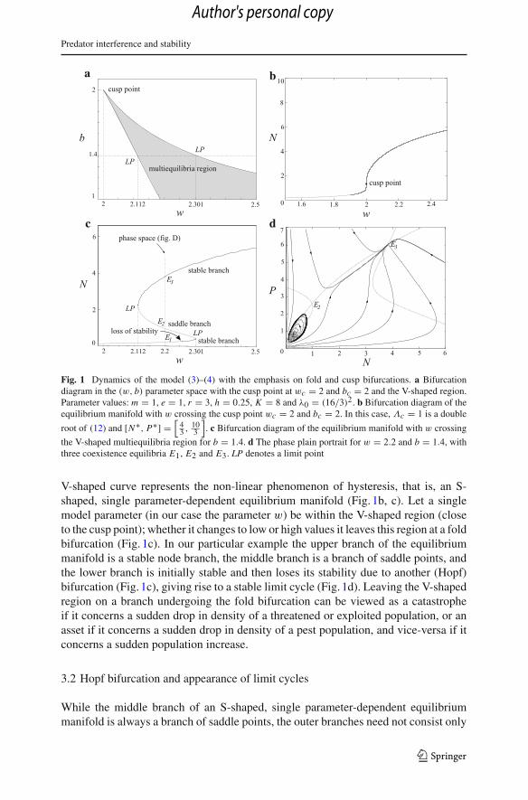
Fig. 1 Dynamics of the model (3)–(4) with the emphasis on fold and cusp bifurcations. a Bifurcationdiagram in the (w, b) parameter space with the cusp point at wc = 2 and bc = 2 and the V-shaped region.Parameter values: m = 1, e = 1, r = 3, h = 0.25, K = 8 and λ0 = (16/3)2. b Bifurcation diagram of theequilibrium manifold with w crossing the cusp point wc = 2 and bc = 2. In this case, Λc = 1 is a double

root of (12) and [N∗, P∗] =[

43 , 10

3

]. c Bifurcation diagram of the equilibrium manifold with w crossing

the V-shaped multiequilibria region for b = 1.4. d The phase plain portrait for w = 2.2 and b = 1.4, withthree coexistence equilibria E1, E2 and E3. LP denotes a limit point

V-shaped curve represents the non-linear phenomenon of hysteresis, that is, an S-shaped, single parameter-dependent equilibrium manifold (Fig. 1b, c). Let a singlemodel parameter (in our case the parameter w) be within the V-shaped region (closeto the cusp point); whether it changes to low or high values it leaves this region at a foldbifurcation (Fig. 1c). In our particular example the upper branch of the equilibriummanifold is a stable node branch, the middle branch is a branch of saddle points, andthe lower branch is initially stable and then loses its stability due to another (Hopf)bifurcation (Fig. 1c), giving rise to a stable limit cycle (Fig. 1d). Leaving the V-shapedregion on a branch undergoing the fold bifurcation can be viewed as a catastropheif it concerns a sudden drop in density of a threatened or exploited population, or anasset if it concerns a sudden drop in density of a pest population, and vice-versa if itconcerns a sudden population increase.

3.2 Hopf bifurcation and appearance of limit cycles

While the middle branch of an S-shaped, single parameter-dependent equilibriummanifold is always a branch of saddle points, the outer branches need not consist only

123



of stable equilibria. Hopf bifurcations can occur on these branches in which case limitcycles do appear.

Stable coexistence equilibria may lose their stability in a Hopf bifurcation (Fig. 3).A necessary condition for the Hopf bifurcation and concomitant appearance of a limitcycle to occur in a coexistence equilibrium [N∗, P∗] is

Λ′ = (e + hm − ΛK h(e − hm))Λ2

e(ΛK (e − hm) − m), (15)

where we defineΛ′ := λ′(P)|P=P∗ (16)

We prove this statement in Appendix A.2, showing that the condition (15) is bothnecessary and sufficient for vanishing of the trace of the Jacobian of the model (3) ata coexistence equilibrium.

Again, we make this result more specific by considering our specific family offunctional responses (2)–(4). Substituting the specific predator encounter rate λ(P)

(4) into the condition (15), we get the third-order polynomial

AΛ3 + BΛ2 + CΛ + D = 0 , (17)

whereA = K 2hb(e − hm)3 > 0,

B = K (e − hm)2(hK er − b(e + hm) − wK e(e − hm)),

C = K e(e − hm)(wm(e − hm) − r(2hm + e)),

D = emr(e + hm) > 0.

(18)

Numerical simulations show that for any w > 0 this polynomial has two dis-tinct positive roots, the larger of which satisfies the necessary condition (8) forexistence of the coexistence equilibrium of the model (3). For general proper-ties of the polynomial (17) see Appendix A.3. As an example, for m = 4,e = 2, r = 1, h = 0.25, and K = 4 the polynomial (17) has the formΛ3 − 5Λ2 − 4Λ + 6 = 0, with two positive roots Λ1

.= 0.811 < C2 = 1 andΛ2

.= 5.527 > C2. Using the formulas (6) and (7), the corresponding coexistenceequilibrium at which the Hopf bifurcation may occur is [N∗, P∗] .= [0.724, 0.296]for Λ = Λ2. For given values of w and b, e.g. w = 0.5 and b = 1, the valueof λ0 can be calculated from the equality λ0 = Λ2(b + P∗)w .= 6.293. Fig-ure 2a shows the parameter w crossing the Hopf bifurcation point wH = 0.5 forthese selected parameters. This example also shows how we can apply our generalresults to predator–prey systems with specific forms of the predator encounter rateλ(P).

We will not study uniqueness and stability of limit cycles here, but numerical sim-ulations show that commonly they are unique and stable. However, sometimes twolimit cycles may coexist (Fig. 2b): the unstable inner cycle comes from a subcriticalHopf bifurcation, while the stable outer cycle arises in a cycle limit point (Fig. 2c).Hence, for an interval of w we have a bistability of an equilibrium and a limit cycle

123



a b

cd

Fig. 2 Dynamics of the model (3)–(4) with the emphasis on Hopf bifurcations. a Bifurcation diagramof the equilibrium manifold with the parameter w crossing the supercritical Hopf bifurcation point (HB)wH = 0.5 for K = 4. b Phase plane portrait with two limit cycles for w = 0.8 and K = 33. c Bifurcationdiagram of the equilibrium manifold with the parameter w undergoing a subcritical Hopf bifurcation forK = 33. d Bifurcation diagram in the (w, K ) parameter space with supercritical and subcritical Hopfbifurcation branches. Common parameter values: m = 4, e = 2, r = 1, h = 0.25, b = 1 and λ0

.= 6.3. LPdenotes a limit point, GH denotes the generalized Hopf point at which the character of the Hopf bifurcationchanges from subcritical to supercritical, or vice versa

that is however of a different character than in the hysteresis case. Still, also here asudden switch in population density may occur. Numerical bifurcations suggest thatthe interval of w for which the two limit cycles coexist is the one with w < 1. Wealready know that no fold bifurcations can occur in this interval.

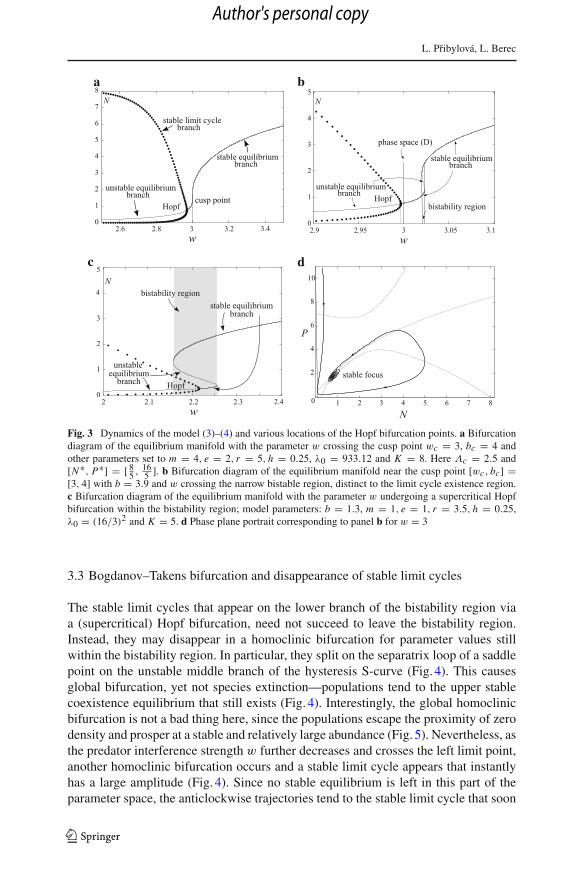
If no fold bifurcation exists or a hysteresis is present yet a (supercritical) Hopfbifurcation occurs below the bistability region (from the perspective of parameter w)then the stable limit cycle amplitude increases with decreasing w and relatively quicklyapproaches separatrices of the extinction saddle point [0, 0] and the prey-only saddlepoint [K , 0] (Fig. 3a, b). Practically this is fatal for one or both populations, sinceboth can be arbitrarily close to zero for some time for sufficiently low values of w.Chance events can then easily make one or both populations extinct. If prey go extinctfirst, both populations eventually vanish. If predators go extinct first, prey may eithervanish, too, or have good luck, recover and attain its environmental carrying capacityK . An analogous situation occurs if a stable coexistence equilibrium on the lowerbranch of a hysteresis-caused bistability region loses stability via a (supercritical)Hopf bifurcation and the emerging stable limit cycle succeeds to leave the bistabilityregion (Fig. 3c).

123



a b

dc

Fig. 3 Dynamics of the model (3)–(4) and various locations of the Hopf bifurcation points. a Bifurcationdiagram of the equilibrium manifold with the parameter w crossing the cusp point wc = 3, bc = 4 andother parameters set to m = 4, e = 2, r = 5, h = 0.25, λ0 = 933.12 and K = 8. Here Λc = 2.5 and[N∗, P∗] = [ 8

5 , 165 ]. b Bifurcation diagram of the equilibrium manifold near the cusp point [wc, bc] =

[3, 4] with b = 3.9 and w crossing the narrow bistable region, distinct to the limit cycle existence region.c Bifurcation diagram of the equilibrium manifold with the parameter w undergoing a supercritical Hopfbifurcation within the bistability region; model parameters: b = 1.3, m = 1, e = 1, r = 3.5, h = 0.25,λ0 = (16/3)2 and K = 5. d Phase plane portrait corresponding to panel b for w = 3

3.3 Bogdanov–Takens bifurcation and disappearance of stable limit cycles

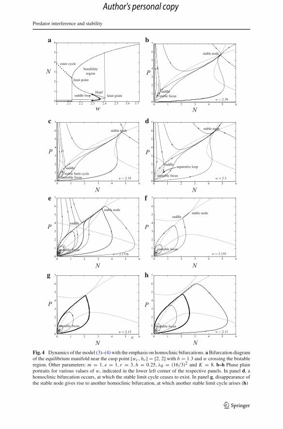
The stable limit cycles that appear on the lower branch of the bistability region viaa (supercritical) Hopf bifurcation, need not succeed to leave the bistability region.Instead, they may disappear in a homoclinic bifurcation for parameter values stillwithin the bistability region. In particular, they split on the separatrix loop of a saddlepoint on the unstable middle branch of the hysteresis S-curve (Fig. 4). This causesglobal bifurcation, yet not species extinction—populations tend to the upper stablecoexistence equilibrium that still exists (Fig. 4). Interestingly, the global homoclinicbifurcation is not a bad thing here, since the populations escape the proximity of zerodensity and prosper at a stable and relatively large abundance (Fig. 5). Nevertheless, asthe predator interference strength w further decreases and crosses the left limit point,another homoclinic bifurcation occurs and a stable limit cycle appears that instantlyhas a large amplitude (Fig. 4). Since no stable equilibrium is left in this part of theparameter space, the anticlockwise trajectories tend to the stable limit cycle that soon

123



a b

dc

e f

hg

Fig. 4 Dynamics of the model (3)–(4) with the emphasis on homoclinic bifurcations. a Bifurcation diagramof the equilibrium manifold near the cusp point [wc, bc] = [2, 2] with b = 1.3 and w crossing the bistableregion. Other parameters: m = 1, e = 1, r = 3, h = 0.25, λ0 = (16/3)2 and K = 8. b–h Phase plainportraits for various values of w, indicated in the lower left corner of the respective panels. In panel d, ahomoclinic bifurcation occurs, at which the stable limit cycle ceases to exist. In panel g, disappearance ofthe stable node gives rise to another homoclinic bifurcation, at which another stable limit cycle arises (h)

123



0 20 40 60 80 1000

1

2

3

4

5

6

Time

Pre

y de

nsity

, N

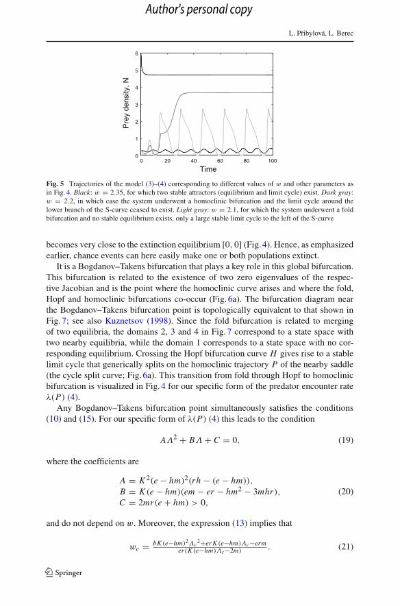
Fig. 5 Trajectories of the model (3)–(4) corresponding to different values of w and other parameters asin Fig. 4. Black: w = 2.35, for which two stable attractors (equilibrium and limit cycle) exist. Dark gray:w = 2.2, in which case the system underwent a homoclinic bifurcation and the limit cycle around thelower branch of the S-curve ceased to exist. Light gray: w = 2.1, for which the system underwent a foldbifurcation and no stable equilibrium exists, only a large stable limit cycle to the left of the S-curve

becomes very close to the extinction equilibrium [0, 0] (Fig. 4). Hence, as emphasizedearlier, chance events can here easily make one or both populations extinct.

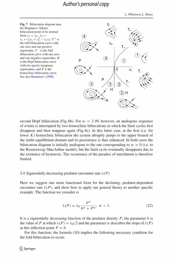
It is a Bogdanov–Takens bifurcation that plays a key role in this global bifurcation.This bifurcation is related to the existence of two zero eigenvalues of the respec-tive Jacobian and is the point where the homoclinic curve arises and where the fold,Hopf and homoclinic bifurcations co-occur (Fig. 6a). The bifurcation diagram nearthe Bogdanov–Takens bifurcation point is topologically equivalent to that shown inFig. 7; see also Kuznetsov (1998). Since the fold bifurcation is related to mergingof two equilibria, the domains 2, 3 and 4 in Fig. 7 correspond to a state space withtwo nearby equilibria, while the domain 1 corresponds to a state space with no cor-responding equilibrium. Crossing the Hopf bifurcation curve H gives rise to a stablelimit cycle that generically splits on the homoclinic trajectory P of the nearby saddle(the cycle split curve; Fig. 6a). This transition from fold through Hopf to homoclinicbifurcation is visualized in Fig. 4 for our specific form of the predator encounter rateλ(P) (4).

Any Bogdanov–Takens bifurcation point simultaneously satisfies the conditions(10) and (15). For our specific form of λ(P) (4) this leads to the condition

AΛ2 + BΛ + C = 0, (19)

where the coefficients are

A = K 2(e − hm)2(rh − (e − hm)),

B = K (e − hm)(em − er − hm2 − 3mhr),

C = 2mr(e + hm) > 0,

(20)

and do not depend on w. Moreover, the expression (13) implies that

wc = bK (e−hm)2Λc2+er K (e−hm)Λc−erm

er(K (e−hm)Λc−2m). (21)

123



a

b c

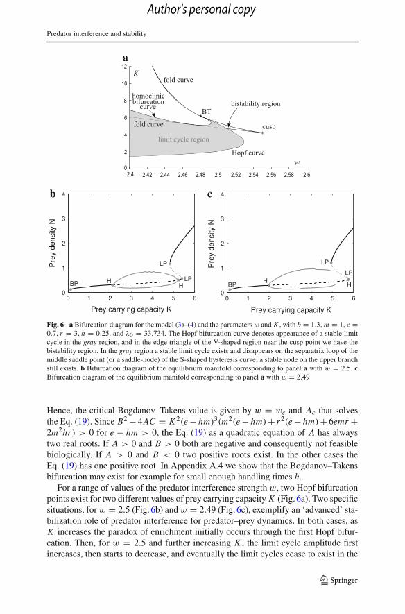
Fig. 6 a Bifurcation diagram for the model (3)–(4) and the parameters w and K , with b = 1.3, m = 1, e =0.7, r = 3, h = 0.25, and λ0 = 33.734. The Hopf bifurcation curve denotes appearance of a stable limitcycle in the gray region, and in the edge triangle of the V-shaped region near the cusp point we have thebistability region. In the gray region a stable limit cycle exists and disappears on the separatrix loop of themiddle saddle point (or a saddle-node) of the S-shaped hysteresis curve; a stable node on the upper branchstill exists. b Bifurcation diagram of the equilibrium manifold corresponding to panel a with w = 2.5. cBifurcation diagram of the equilibrium manifold corresponding to panel a with w = 2.49

Hence, the critical Bogdanov–Takens value is given by w = wc and Λc that solvesthe Eq. (19). Since B2 − 4AC = K 2(e − hm)3(m2(e − hm) + r2(e − hm) + 6emr +2m2hr) > 0 for e − hm > 0, the Eq. (19) as a quadratic equation of Λ has alwaystwo real roots. If A > 0 and B > 0 both are negative and consequently not feasiblebiologically. If A > 0 and B < 0 two positive roots exist. In the other cases theEq. (19) has one positive root. In Appendix A.4 we show that the Bogdanov–Takensbifurcation may exist for example for small enough handling times h.

For a range of values of the predator interference strength w, two Hopf bifurcationpoints exist for two different values of prey carrying capacity K (Fig. 6a). Two specificsituations, for w = 2.5 (Fig. 6b) and w = 2.49 (Fig. 6c), exemplify an ‘advanced’ sta-bilization role of predator interference for predator–prey dynamics. In both cases, asK increases the paradox of enrichment initially occurs through the first Hopf bifur-cation. Then, for w = 2.5 and further increasing K , the limit cycle amplitude firstincreases, then starts to decrease, and eventually the limit cycles cease to exist in the

123



Fig. 7 Bifurcation diagram nearthe Bogdanov–Takensbifurcation point of its normalform y1 = y2, y2 =ε1 + ε2 y1 + y2

1 − y1 y2. T + isthe fold bifurcation curve withone zero and one positiveeigenvalue, T − is the foldbifurcation curve with one zeroand one negative eigenvalue, His the Hopf bifurcation curvewith two purely imaginaryeigenvalues, and P is thehomoclinic bifurcation curve.See also Kuznetsov (1998)

second Hopf bifurcation (Fig. 6b). For w = 2.49, however, an analogous sequenceof events is interrupted by two homoclinic bifurcations at which the limit cycles firstdisappear and then reappear again (Fig. 6c). In this latter case, at the first (i.e. forlower K ) homoclinic bifurcation the system abruptly jumps to the upper branch ofthe multi-equilibrium domain and its persistence is thus enhanced. In both cases thebifurcation diagram is initially analogous to the one corresponding to w = 0 (i.e. tothe Rosenzweig–MacArthur model), but the limit cycle eventually disappears due tothe existence of hysteresis. The occurrence of the paradox of enrichment is thereforelimited.

3.4 Sigmoidally decreasing predator encounter rate λ(P)

Here we suggest one more functional form for the declining, predator-dependentencounter rate λ(P), and show how to apply our general theory to another specificexample. The function we consider is

λ(P) = λ0bw

bw + Pw, w > 1. (22)

It is a sigmoidally decreasing function of the predator density P; the parameter b isthe value of P at which λ(P) = λ0/2 and the parameter w describes the slope of λ(P)

at this inflection point P = b.For this function, the formula (10) implies the following necessary condition for

the fold bifurcation to occur:

123



a b

c d

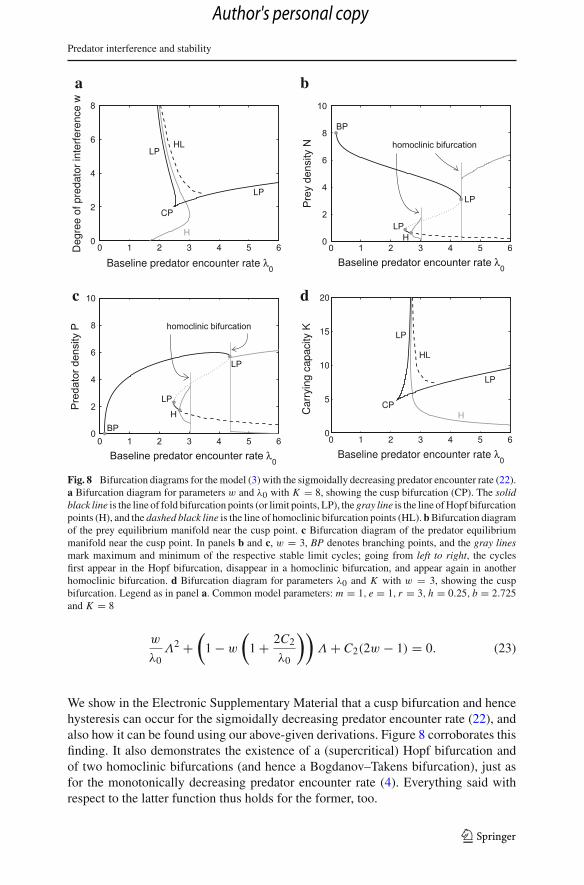
Fig. 8 Bifurcation diagrams for the model (3) with the sigmoidally decreasing predator encounter rate (22).a Bifurcation diagram for parameters w and λ0 with K = 8, showing the cusp bifurcation (CP). The solidblack line is the line of fold bifurcation points (or limit points, LP), the gray line is the line of Hopf bifurcationpoints (H), and the dashed black line is the line of homoclinic bifurcation points (HL). b Bifurcation diagramof the prey equilibrium manifold near the cusp point. c Bifurcation diagram of the predator equilibriummanifold near the cusp point. In panels b and c, w = 3, BP denotes branching points, and the gray linesmark maximum and minimum of the respective stable limit cycles; going from left to right, the cyclesfirst appear in the Hopf bifurcation, disappear in a homoclinic bifurcation, and appear again in anotherhomoclinic bifurcation. d Bifurcation diagram for parameters λ0 and K with w = 3, showing the cuspbifurcation. Legend as in panel a. Common model parameters: m = 1, e = 1, r = 3, h = 0.25, b = 2.725and K = 8

w

λ0Λ2 +

(1 − w

(1 + 2C2

λ0

))Λ + C2(2w − 1) = 0. (23)

We show in the Electronic Supplementary Material that a cusp bifurcation and hencehysteresis can occur for the sigmoidally decreasing predator encounter rate (22), andalso how it can be found using our above-given derivations. Figure 8 corroborates thisfinding. It also demonstrates the existence of a (supercritical) Hopf bifurcation andof two homoclinic bifurcations (and hence a Bogdanov–Takens bifurcation), just asfor the monotonically decreasing predator encounter rate (4). Everything said withrespect to the latter function thus holds for the former, too.

123



4 Discussion

Since the publication of the Lotka-Volterra predator–prey model in 1920’s (Lotka1920; Volterra 1926), the stability of predator–prey interactions has been virtually acontinuous enterprise in the theoretical ecological literature. Today, a fair amount ofstabilizing and destabilizing mechanisms have been identified (Murdoch and Oaten1975; Oaten and Murdoch 1975; Briggs and Hoopes 2004; Gross et al. 2004; Voset al. 2004, and references therein). One of the more commonly studied mecha-nisms has been the intraspecific predator interactions, including predator cannibalism(Kohlmeier and Ebenhöh 1995; Magnússon 1999) and, more often, predator inter-ference (Rogers and Hassell 1974; Ruxton et al. 1992; Ruxton 1995; Huisman andDeBoer 1997). In particular, interference between predators has been found to be amajor stabilizing factor in predator–prey systems (DeAngelis et al. 1975; van Voornet al. 2008). In this paper, we study the effect of a family of functional responsesthat generalizes many classical descriptions of predator interference on predator–preydynamics. Most importantly, we show that changes in predator interference strengthmay give rise to hysteresis and (dis)appearance of stable limit cycles, phenomena thatcan make both species more vulnerable to extinction.

Our major assumption is that the per predator encounter rate of prey λ(P) is adecreasing function of predator density; otherwise, we use the classical Rosenzweig–MacArthur predator–prey model formulation with logistic growth of prey and withpredators limited in their consumption by a non-negligible prey handling time (e.g. Kot2001). The Rosenzweig–MacArthur model of predator–prey dynamics assumes theHolling type II functional response. As a consequence, the predator isocline is vertical,intersects the prey isocline (at most) once, and a supercritical Hopf bifurcation withappearance of stable limit cycles occurs once the predator isocline crosses the vertexof the prey isocline from right to left (Rosenzweig 1971). When the Holling typeII functional response is replaced by the Beddington–DeAngelis one, the predatorisocline stays straight but leans to the right (Beddington 1975; DeAngelis et al. 1975).As a consequence, the paradox of enrichment occurs for larger carrying capacitieswhen compared to the Holling type II functional response, if at all, which has givenrise to the notion that predator interference is a major stabilizing factor of predator–prey dynamics (DeAngelis et al. 1975; van Voorn et al. 2008). Finally, for sufficientlystrong predator interference functional responses from the family we consider cause thepredator isocline to bend to the right, and if sufficiently bent, it may intersect the preyisocline at three points, thus giving rise to hysteresis and fold and cusp bifurcations.Fold and cusp bifurcations have not been observed in the previous two cases. Moreover,stable limit cycles that may appear on the lower branch of the hysteresis curve (dueto the Hopf bifurcation) may break up on its middle branch (due to a homoclinicbifurcation).

We have already emphasized in the introduction that varying the parameter w

representing the strength of predator interference in the predator encounter rate (4)does not actually produce a single functional response but rather a family of func-tional responses. As this parameter varies from low to high values, we observea number of dynamical transitions and may thus characterize predator interfer-ence strengths for which different dynamical regimes emerge. We thus reveal that

123



whereas for low values of w just a single, low-density equilibrium exists whichcan be either stable or unstable, for very high values of w a unique, high-densityequilibrium occurs that is always stable. Perhaps most interestingly, for interme-diate values of w three coexistence equilibria emerge and the system may existin two alternative stable states. These alternative states can either be both sta-ble or the lower one, due to a supercritical Hopf bifurcation, may actually be alimit cycle. In the latter case, if the predator interference strength w decreases,the limit cycle amplitude increases which threatens one or both interacting pop-ulations. Such a potential threat can be mitigated by an occurrence of a homo-clinic bifurcation at an intermediate value of w. This bifurcation causes an inter-ruption of the stable limit cycle and makes the high-density coexistence equilib-rium globally attracting. All that said, most persistent systems of predators andprey with respect to the predator interference strength are likely those with inter-mediate and very high values of w. In any case, all else being equal, functionalresponses with higher values of w have a stronger potential for stabilizing predator–prey dynamics with predator interference. In our opinion, the most important con-tribution of our study is that there is one more aspect of stabilization that thepredator interference brings, and that this aspect is related to the occurrence ofhysteresis.

An interesting question is what would happen if we let the predator interferencestrength w to evolve in the predator by natural selection. Would the eventual evo-lutionary endpoints correspond to low or high persistence regimes of predator–preydynamics, i.e. to low or high values of w? The way predator interference should go toevolutionarily is not a priori clear. Predators could decrease the degree of interferencethrough, e.g. evolution of more effective protection of acquired food and/or moreeffective searching and handling strategies, but they could also invest in better ways ofhow to steal otherwise subdued prey to others. Does even a potential for polymorphismexist within the predator population? We are convinced that for understanding all ofthe facets of predator interference, such an evolutionary study would be more thaninteresting to conduct.

Fold and cusp bifurcations mark abrupt changes in state variables and have beensubjects of an extensive research. Recently, they have been observed also in bothecological models (Lade et al. 2013) and eco-epidemiological models (Hilker et al.2009), but their history in ecology goes at least to the work of Ludwig et al. (1978) onthe spruce budworm population dynamics. Actually, the whole currently very popularissue of regime shifts is based on the concepts of fold and cusp bifurcations (Schefferet al. 2001; Scheffer and Carpenter 2003; Lade et al. 2013). And in all of these works,hysteresis has been shown to have immense practical significance with respect to pop-ulation management and risk of population extinction. In particular, not all instancesof hysteresis have a positive effect on population viability as we demonstrate here.For example, in the eco-epidemiological model of Hilker et al. (2009), bistabilityoccurs between two levels of infection prevalence. When a stable limit cycle appearsthrough a supercritical Hopf bifurcation on the lower branch of the hysteresis curveand then splits on the middle branch through a homoclinic bifurcation, the proportionof infectious individuals all of a sudden increases to much higher values. Similarly richbifurcation structure as revealed in this paper has also been found in a stage-structured

123



population model (Baer et al. 2006) or recently in a predator–prey model with a strongAllee effect in prey (Aguirre et al. 2014).

We give a general protocol for exploring Rosenzweig–MacArthur-like systems inwhich the predator encounter rate λ(P) of the Holling-type-II-like functional responseis a decreasing function of the predator density P (Electronic Supplementary Mate-rial). Our analysis is made for a general λ(P) of this type, which depends on anumber of model parameters. If we claim that a bifurcation occurs for a criticalvalue of the parameter Λ, we can claim that it occurs also for all involved modelparameters, the critical value of which is determined implicitly—and it exists. Weuse the general analysis to find important starting points for the numerical con-tinuation and plotting of bifurcation diagrams in specific cases, such as finding acusp point in Electronic Supplementary Material. For a general λ(P) we just canclaim that if the predator density exceeds such and such value, the fold (cusp, Hopf,Bogdanov–Takens) bifurcation will not occur. So, for any specific λ(P), we knowwhat to look for and where. Then, we need to use standard tools to draw a completepicture.

Another question relevant to our study is whether experiments exist that collateddata on predator functional response and that give some support for relatively strongpredator interference w > 1 in our convex or sigmoidal form of λ(P). This is a diffi-cult question to answer, since many empirical studies on predator functional responsevaried just the predator density, in the effort to distinguish among Holling type I–IIIfunctional responses. And this is also the reason why the Holling type II functionalresponse appears to dominate predator–prey theory (Skalski and Gilliam 2001). How-ever, Skalski and Gilliam (2001) collected data on 19 predator–prey systems andshowed that predator-dependent functional responses they considered (Beddington–DeAngelis, Crowley-Martin, and Hassell–Varley) could provide better descriptionsof predator feeding over a range of predator–prey abundances. In particular, treatingthe Holling type II model as the null hypothesis, comparison with the Beddington–DeAngelis model resulted in rejection of the Holling type II model in favor of theBeddington–DeAngelis model in 18 of the 19 data sets. Still, no single functionalresponse was shown to best describe all of the 19 data sets (Skalski and Gilliam2001). Given that the family of functional responses proposed in Berec (2010) andexplored in this paper is a generalization of both the Beddington–DeAngelis andHassell–Varley models, it would be more than interesting to refit these 19 data setsby our model and see what values of w best describe the data and whether this familydescribes all of the 19 data sets well. In general, when predator interference has beentested as an alternative to the Holling type II model, it has almost exclusively beenmodeled by the Beddington–DeAngelis model. Our family of functional responsesprovides an additional flexibility and moreover has non-standard dynamical implica-tions for both the predator and prey. Further experiments allowing for a straightfor-ward fitting of prey- and predator-dependent functional responses are also more thanwelcome.

Acknowledgments LP acknowledges support from the project CZ.1.07/2.2.00/15.0203 “Univerzitnívýuka matematiky v menícím se svete”. LB acknowledges institutional support RVO:60077344.

123



Appendix A

A.1 Fold bifurcation

Here we show that if a coexistence equilibrium of the model (1) exists then the con-dition (10) is equivalent to the existence of one zero eigenvalue of the Jacobian ofthis model evaluated at this equilibrium. Let us define a function g(N , P) such thatf (N , P) = Ng(N , P) where f (N , P) is the predator functional response (2). Inaddition, let A denote the Jacobian of the model (1) and [N∗, P∗] any coexistenceequilibrium of this model. By direct computation we have

A =(

r − r 2N∗K − P∗g − P∗N∗gN −N∗g − P∗N∗gP

eP∗g + eP∗N∗gN eN∗g + eP∗N∗gP − m

), (24)

where g = g(N∗, P∗), gN = ∂g(N∗, P∗)/∂ N and gP = ∂g(N∗, P∗)/∂ P . Since forthe coexistence equilibrium eN∗g = m, we get

tr A = r − r 2N∗K − P∗g − P∗N∗gN + eP∗N∗gP (25)

anddet A = r

(1 − 2N∗

K

)eP∗N∗gP + m P∗g + m2

eg P∗gN . (26)

Since the functional response (2) implies g(N , P) = λ(P)/[1 + hλ(P)N ], we have

gN = −g2h and gP = λ′ g2

λ2 . (27)

Substituting (27) and (6) into (26), we get

det A = P∗gm(

r(

1 − 2C2Λ

)Λ′Λ2 + e−hm

e

). (28)

Consequently, the condition (10) is equivalent to the condition det A = 0 at a coex-istence equilibrium [N∗, P∗] and is a necessary condition for this equilibrium to bea limit point. Generic change in a single model parameter will change sign of thedeterminant det A. Consequently, the local phase space changes qualitatively.

A.2 Hopf bifurcation

For a Hopf bifurcation to occur at a parameter value in a two-dimensional system, realparts of the complex eigenvalues of the Jacobian evaluated at the respective systemequilibrium have to transversally cross zero (i.e. change sign) when the parametercrosses that value. Denoting by a the bifurcation parameter and by μ(a) ± iω(a)

the respective pair of complex eigenvalues, we require μ(ac) = 0, ω(ac) > 0, andμ′(ac) �= 0 at a bifurcation point a = ac as a necessary conditions for a Hopfbifurcation to occur. we note that

123



μ(a) = tr A(a)

2and ω(a) = det A(a) . (29)

where A(a) denotes the Jacobian evaluated at the system equilibrium correspondingto the parameter a.

Now we will prove that if a coexistence equilibrium of the model (1) exists thenthe condition (15) is necessary and sufficient for vanishing of the trace of the Jacobianof the model (1) at that equilibrium. Denoting g(N , P) = f (N , P)/N then at thecoexistence equilibrium

P∗g = r(

1 − N∗K

). (30)

Consequently, at this equilibrium the trace (25) of the Jacobian of the model (1)simplifies to

tr A = −r N∗K + r

(1 − N∗

K

)N∗g

(h + e Λ′

Λ2

). (31)

Since r > 0 and according to (6) N∗K = C2

Λ> 0 at the coexistence equilibrium, we

havetr A = −r N∗

K

(1 + K

(C2Λ

− 1)

g(

h + e Λ′Λ2

)), (32)

where C2 = mK (e−hm)

. Since the model (1) implies g = rλ/C1, a necessary andsufficient condition for vanishing of the trace of the Jacobian of the model (1) at thecoexistence equilibrium is

1 = K(

1 − mK (e−hm)Λ

) Λ(e − hm)

e

(h + e Λ′

Λ2

)(33)

or

1 = (K (e − hm)Λ − m)(hΛ2 + eΛ′)eΛ2 (34)

which is equivalent to the condition (15).Similar manipulation with the expression (28) and replacement of Λ′ with the

right-hand side of (15) gives the second necessary condition

r(KΛ(e − hm) − 2m)(ΛK h(e − hm) − (e + hm))2

K (e − hm)Λ2e(ΛK (e − hm) − m)+ e − hm

e> 0. (35)

This second condition det A > 0 excludes the neutral saddle case (with two realopposite eigenvalues).

A.3 Hopf bifurcation in the special case of λ(P) satisfying (4)

For the special case of λ(P) satisfying (4), the condition (15) simplifies to (17). Wegive here some properties of the polynomial ϕ(Λ) = AΛ3 + BΛ2 + CΛ + D on theleft-hand side of (17).

For a coexistence equilibrium to exist, we must have e − hm > 0. Consequently,A = K 2hb(e − hm)3 > 0 and D = erm(e + hm) > 0. The cubic polynomial ϕ(Λ)

123



then satisfies ϕ(0) > 0 and limΛ→∞ ϕ(Λ) = ∞. Let wB = hK er−b(e+hm)K e(e−hm)

be the

value of w at which B = 0. Analogously, let wC = r(2hm+e)m(e−hm)

be the value of w atwhich C = 0. Since

wC − wB = (e + hm)(bm + K er)

emK (e − hm)> 0 (36)

at the coexistence equilibrium, B decreases linearly with w and C increases linearlywith w, B or C need to be negative for any w at the coexistence equilibrium. (Theproof is evident: let us suppose that B ≥ 0 and C ≥ 0 concurrently, consequentlyw ≤ wB and w ≥ wC which is the contrary to wB < wC .)

Let Λmin = − B3A +

√B2−3AC

3A denote the local minimum of the cubic poly-nomial ϕ(Λ). Now we will show that this local minimum indeed exists, i.e.} thatthe discriminant d(w) = B2 − 3AC is positive for any w at the coexistence equi-librium. The function d(w) is a quadratic convex function of w with minimum inwmin = bhm+2hK er−2be

2K e(e−hm). From this,

d(wmin) = 3

4(bhm2 + 4mhK er + 4bem + 4e2 Kr)hb(e − hm)4 K 2 > 0. (37)

Consequently Λmin exists and for B < 0 it has to be positive. If B ≥ 0, then C < 0and consequently

√B2 − 3AC > B also gives positivity of Λmin . Simulations show

that ϕ(Λmin) ≤ 0 and hence that the polynomial (17) has a positive root for any w,but we don’t have any analytical proof for ϕ(Λmin) ≤ 0 yet.

A.4 Bogdanov–Takens bifurcation can occur for small handling times h

Let us have the handling time h small enough so that r < e−hmh . This implies A < 0

in (20) and since C > 0, there exists one positive real root Λc of the quadraticequation (19). We will show that this Λc satisfies the condition (8) necessary for thecorresponding P∗ to be a coexistence equilibrium. Let 0 < Λc ≤ C2 = m

K (e−hm).

Consequently,

0 = AΛc + B + CΛc

≥ AC2 + B + CC2

= K er(e − hm) > 0, (38)

which cannot happen and thus the contrary Λc > C2 is true. Consequently, the criticalBogdanov–Takens bifurcation point occurs at the coexistence equilibrium [N∗, P∗]that satisfies P∗ = λ−1(Λc) and N∗ = m

(e−hm)Λc. Generic change of any two of the

parameters λ0, K , e, h, m, and r will change sign of the trace and determinant ofthe Jacobian at the corresponding coexistence equilibrium and violate the existenceof two zero eigenvalues. This change then necessarily causes a saddle separatrix loopsplit near the critical parameters.

123



References

Abrams PA (1994) The fallacies of “ratio-dependent” predation. Ecology 75:1842–1850Aguirre P, Flores JD, González-Olivares E (2014) Bifurcations and global dynamics in a predator–prey

model with a strong allee effect on the prey, and a ratio-dependent functional response. Nonlinear AnalReal World Appl 16:235–249

Arnqvist G, Jones TM, Elgar MA (2006) Sex-role reversed nuptial feeding reduces male kleptoparasitismof females in Zeus bugs (Heteroptera: Veliidae). Biol Lett 2:491–493

Baer SM, Kooi BW, Kuznetsov YA, Thieme HR (2006) Multiparametric bifurcation analysis of a basictwo-stage population model. SIAM J Appl Math 66:1339–1365

Beddington JR (1975) Mutual interference between parasites or predators and its effect on searching effi-ciency. J Animal Ecol 44:331–340

Begon M, Harper JL, Townsend CR (1990) Ecology: individuals, populations and communities, 2nd edn.Blackwell Scientific Publications, Oxford

Berec L (2010) Impacts of foraging facilitation among predators on predator–prey dynamics. Bull MathBiol 72:94–121

Boukal DS, Sabelis MW, Berec L (2007) How predator functional responses and Allee effects in prey affectthe paradox of enrichment and population collapses. Theor Popul Biol 72:136–147

Boukal DS, Berec L, Krivan V (2008) Does sex-selective predation stabilize or destabilize predator–preydynamics? PLoS One 3(7):e2687

Briggs CJ, Hoopes MF (2004) Stabilizing effects in spatial parasitoid–host and predator–prey models: areview. Theor Popul Biol 65:299–315

Cantrell RS, Cosner C (2001) On the dynamics of predator-prey models with the Beddington–DeAngelisfunctional response. J Math Anal Appl 257:206–222

Cosner C, DeAngelis D, Ault JS, Olson DB (1999) Effects of spatial grouping on the functional responseof predators. Theor Popul Biol 56:65–75

DeAngelis DL, Goldstein RA, O’Neill RV (1975) A model for tropic interaction. Ecology 56:881–892Fryxell JM, Mosser A, Sinclair ARE, Packer C (2007) Group formation stabilizes predator–prey dynamics.

Nature 449:1041–1044Gascoigne JC, Lipcius RN (2004) Allee effects driven by predation. J Appl Ecol 41:801–810Gross T, Ebenhöh W, Feudel U (2004) Enrichment and foodchain stability: the impact of different forms

of predator–prey interaction. J Theor Biol 227:349–358Hassell MP, Lawton JH, Beddington JR (1976) The components of arthropod predation. 1. The prey death

rate. J Animal Ecol 45:135–164Hilker FM, Langlais M, Malchow H (2009) The Allee effect and infectious diseases: extinction, multista-

bility, and the (dis-)appearance of oscillations. Am Nat 173:72–88Holling CS (1959) Some characteristics of simple types of predation and parasitism. Can Entomol 91:385–

398Holt RD (2011) Natural enemy–victim interactions: do we have a unified theory yet? In: Scheiner SM,

Willig MR (eds) The theory of ecology. University of Chicago Press, Chicago, pp 125–162Huisman G, DeBoer RJ (1997) A formal derivation of the “Beddington” functional response. J Theor Biol

185:389–400Kohlmeier C, Ebenhöh W (1995) The stabilizing role of cannibalism in a predator–prey system. Bull Math

Biol 57:401–411Kot M (2001) Elements of mathematical ecology. Cambridge University Press, CambridgeKuznetsov YA (1998) Elements of applied bifucation theory, 2nd edn. Applied Mathematical Sciences, vol

112. Springer, BerlinKrivan V, Vrkoc I (2004) Should “handled” prey be considered? Some consequences for functional response,

predator–prey dynamics and optimal foraging theory. J Theor Biol 227:167–174Lade SJ, Tavoni A, Levin SA, Schlüter M (2013) Regime shifts in a social-ecological system. Theor Ecol

6:359–372Lotka AJ (1920) Undamped oscillations derived from the law of mass action. J Am Chem Soc 42:1595–1599Ludwig D, Jones DD, Holling CS (1978) Qualitative analysis of insect outbreak systems: the spruce bud-

worm and forest. J Animal Ecol 47:315–332Magnússon KG (1999) Destabilizing effect of cannibalism on a structured predator–prey system. Math

Biosci 155:61–75

123



Murdoch WW, Oaten A (1975) Predation and population stability. In: Macfayden A (ed) Advances inecological research, vol 9. Academic Press, London, pp 1–131

Oaten A, Murdoch WM (1975) Functional response and stability in predator–prey systems. Am Nat109:289–298

Pavlova V, Berec L, Boukal DS (2010) Caught between two Allee effects: trade-off between reproductionand predation risk. J Theor Biol 264:787–798

Rogers DJ, Hassell MP (1974) General models for insect parasite and predator searching behaviour: inter-ference. J Animal Ecol 43:239–253

Rosenzweig ML (1971) Paradox of enrichment: destabilization of exploitation ecosystems in ecologicaltime. Science 171:385–387

Rosenzweig ML, MacArthur RH (1963) Graphical representation and stability conditions of predator–preyinteractions. Am Nat 97:209–223

Ruxton GD (1995) Short term refuge use and stability of predator–prey models. Theor Popul Biol 47:1–17Ruxton GD, Gurney WSC, Roos AMD (1992) Interference and generation cycles. Theor Popul Biol 42:235–

253Scheffer M, Carpenter SR (2003) Catastrophic regime shifts in ecosystems: linking theory to observation.

Trends Ecol Evol 18:648–656Scheffer M, Carpenter SR, Foley JA, Folke C, Walker B (2001) Catastrophic shifts in ecosystems. Nature

413:591–596Seydel R (2010) Practical bifurcation and stability analysis, 3r edn. Springer, BerlinSkalski GT, Gilliam JF (2001) Functional responses with predator interference: viable alternatives to the

Holling type II model. Ecology 82:3083–3092Spradbery JP (1970) Host finding by Rhyssa persuasoria (L.), an ichneumonid parasite of siricid woodwasps.

Animal Behav 18:103–114Volterra V (1926) Fluctuation in the abundance of a species considered mathematically. Nature 118:558–560van Voorn GAK, Stiefs D, Gross T, Kooi BW, Feudel U, Kooijman SALM (2008) Stabilization due to

predator interference: comparison of different analysis approaches. Math Biosci Eng 5:567–583Vos M, Kooi BW, DeAngelis DL, Mooij WM (2004) Inducible defences and the paradox of enrichment.

Oikos 105:471–480

123


Predator interference and stability of predator–prey dynamics

Documents

Transcript of Predator interference and stability of predator–prey dynamics