
Study on Properties of Rice Husk Ash and Its Use as Cement Replacement Material
Upload
khangminh22Category
view
6download
0
eureca 2014 – Conference Paper
Paper Number: CE01
1
Rice Husk as a Fuel Source in
Direct Carbon Fuel Cells
Chin Choon Ming1*
, Veena A Doshi1, Wong Wai Yin
1
1Taylor’s University Lakeside Campus, Malaysia
Abstract
The increase in global energy demand and rising of the greenhouse gas emission from
Southeast Asia drives developing nations such as Malaysia to use energy that is more
sustainable with lower greenhouse gas emissions. In this research, rice husk is
proposed to be used as a potential fuel source in direct carbon fuel cells. In this study,
rice husk that was obtained from Sekinchan, Malaysia was initially dried for 24 hours
at temperature of 105oC and milled into size of less than 2 mm. Subsequently, it was
pyrolysed in a furnace at three sets of temperatures, which are 400, 500 and 600 oC
with heating rate of 10 oC min
-1. Residence time of 1 hour and 2 hours were
conducted for all samples. The biochars produced were analysed to determine the
physicochemical properties and structural properties. The study revealed that biochar
that has a higher fixed carbon content and surface area, low moisture and ash content
is a favourable fuel for direct carbon fuel cells. From the proximate analysis, it was
shown that biocharproduced at 600 oC and 1 hour has the lowest mass loss at
temperature between 25 and 600 oC. But the lower carbon content produced at 600
oC
and 1 hour, it was shown to contain lower sulphur content that is highly desired as
solid oxide fuel cell fuel source. Pyrolysis treatment has improved the rice husk
surface area from 1.4825 to 254.5275 m2/g. In summary, biochar produced at 600
oC
and 1 hour show the most potential to be used as fuel for solid oxide direct carbon
fuel cell.
Keywords: Biomass, Lignin, Pyrolysis, Biochar, Solid OxideDirect Carbon Fuel Cell.

eureca 2014 – Conference Paper
Paper Number: CE01
2
1. Introduction
Worldwide, energy demand had a drastic growth resulting from the rising
number of industry and population. The 2013 reports on worldwide energy demand
from Energy Information Administration (EIA) of United States have forecasted an
increment of 43.64% within the next 5 years assuming that there are no changes in
energy consumption policies[1].Furthermore, due to the rise of greenhouse gas
emission in Southeast Asia, it is essential for an Asian country such Malaysia to use
energy that is sustainable and able to reduce emission of greenhouse gas.According to
the Five Fuel Policy, biomass has been identified to be one of the potential renewable
energy by Malaysian government as the production of biomass in Malaysia was found
to be 168 million tonnes in year 2014. Agricultural wastes such as oil palm shell, rice
straw, sugarcane bagasse, and rice husk are the main resources of biomass in
Malaysia.
Direct carbon fuel cells (DCFC) has been identified as an efficient electricity
generator that converts chemical energy in solid carbon into electrical energy directly.
The expected electrical efficiency is above 70 % for DCFC,which is double of the
electricity efficiency generated in coal-fired plants. Furthermore, DCFC releases 50 %
less in CO2 emissiondue to CO2 will again be consumed by biomass [2]. In biomass, the
useful carbon content can be measured by the percentage of lignin found within it.
The higher the lignin percentage is, the higher the carbon content [2]. The technology
available to convert biomass into fuel source such as biocharis known to be pyrolysis.
Pyrolysis is a process which decomposes the biomass at high temperature without the
presence of air [3]. The carbon rich solids termed as biochar which is produced from
this process can be fed into the DCFC as the fuel source.
As a one of the producer and exporter of rice, the utilisation of rice crop
residues, rice husk as a fuel source in a DCFC has the potential of reducing the CO2
emission. However, most of the rice husk has been used to fertilise the farm field
which resulted loss of energy to the atmosphere. There are only a few of researches
performed to investigate the potential of carbon fuel derived by biomass as a fuel
source in DCFC [4]. Moreover, the studies of sustainability of biochar derived from
rice husk as a fuel source in DCFC has not been looked into. The performance
(efficiency, stability and power output) of a DCFC is strongly dependent to the
physicochemical properties of the biochar. A high carbon content and less
contaminates of biochar provides more efficient and less failure in the operation of the
DCFC. Crystal structure and surface area are the indication of the electrochemical
reactivity of the biochar.
There is no research that has been performed so far to investigate the
influences of physicohemical properties of biochar derived from rice husk to the
performance in a DCFC. In addition, the development of the desired properties of
biochar that fed into DCFC has not been optimised in terms of pyrolysis conditions
such as temperature and residence time.

eureca 2014 – Conference Paper
Paper Number: CE01
3
1.1 Objectives
1. To analyse the effect of pyrolysis process conditions (temperature and residence
time) on the development of biochar properties produced from rice husk.
2. To study the effects of temperature and process duration on the yield of biochar.
3. To determine the physicochemical characteristic of the biochar produced and
validate it with literature.
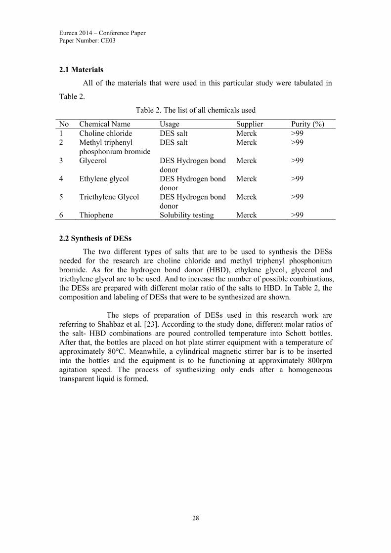
2. Methodology
The rice husks (rice scientific name: oryza sativa) was collected from
Sekinchan, Malaysia. The biochars were prepared for pyrolysis process, after which
they were analysed. A summary of the overall methodology is summarized in the
flowchart in Figure 2-1.
Figure 2-1: Methodology flowchart.
2.1 Sample Preparation
The rice husks were first dried in oven at 105 oC for 24 hours to remove the
moisture content. It was then milled into a size between the ranges of 1 to 2 mm using
a cutting mill with a 2 mm blade. After that, it was sieved with a Retch sieve shaker.
The equipment used is Pulverisette14 variable speed rotor mill located at Monash
University.
2.2 Pyrolysis process parameters
The pyrolysis of rice husk samples were carried out using furnace with
nitrogen gas stream input to ensure oxygen free in the furnace. 20 g of each sample
was placed into furnace and three set of temperatures was performed at 400, 500, and
600 oC with a heating rate of 10
oC min
-1. Residence time 1 hour and 2 hours was
Sample preparation (Drying and milling)
--- Drying at 105 oC for 24 hours and mill into size range between 1 to 2 mm
Pyrolysis process [Objective 2]
--- Process conditions setting: Temperature 400, 500, and 600 oC; Residence time 1 hour and 2 hours
Products (Biochar) [Objective 1]
--- Analyse the effect of pyrolysis process conditions to biochar characteristic
Analysis the characteristic of biochar
--- using TGA, CHNS, BET and FTIR which analyse the physicochemical properties, structural properties and chemisorption characteristic of the biochar
Validation of the results [Objective 3]
--- Validate this research results with the literature

eureca 2014 – Conference Paper
Paper Number: CE01
4
conducted for all samples. Summary of pyrolysis process parameters used in this
research for rice husk is shown in Table 2-1.
Table 2-1: Pyrolysis process parameters.
Materials
Sample
weight
(g)
Sample
size
(mm)
Temperature
(oC)
Heating
rate
(oC/min)
Residence
time
(hours)
Rice Husk
20.0 Range
1.0 - 2.0
400, 500
and 600 10 1 and 2
2.3 Experiment Setup
Pyrolysis was done by using furnace (model: MTI KSL-1100X) (Figure 2-2)
located in process laboratory in Taylor’s University. The furnace is heating by using
coils and it had N2 gas input to provide free oxygen atmospheric conditions. The
temperature limit of the furnace is 700 oC, thus the experiment was ensured to be
conduct at lower than this temperature. Furthermore, the flowrate of N2 gas was
unable to measure due to the unsatisfied range of the flowrate gauge and thus the N2
gas was allowed to flow in an approximate flowrate during the experiment conducted.
Figure 2-2: Furnace (MTI KSL-1100X).
2.3.1 Experimental Procedure
20 g of samples were stuffed into crucible and covered by aluminum foil.
Crucible was then put into furnace and nitrogen gas started introduce in. Regulator
was set into desired temperature (400, 500 and 600 oC) and residence time (1 and 2
hours).Run button was pressed and hold to start the timer and the main switch is then
turned on to start heating. Cool down of the samples were allowed after the process.
The nitrogen input and the electrical power was then turned off.
Nitrogen
flowrateco
nttroller
Nitrogen
inlet
Regulator Main switch

eureca 2014 – Conference Paper
Paper Number: CE01
5
2.4 Biochar characteristic
Analysis such as TGA, BET, FTIR, and CHNSwasperformed to obtain the
characteristic of biochar.
2.4.1 Thermogravimetric Analysis (TGA)
TGA was used to determine the physical properties of fixed carbon, ash,
volatile matter and moisture of biochar. The equipment used was
Thermogravimetricanalyser (Settaram TGA92) located at Monash University,
Malaysia. The procedure was: 0.1 g of the biochar sample was heated to 110 oC with
N2 inert gas, and held for 20 minutes to eliminate moisture content entirely. After that,
increase the temperature from 110 oC to 950
oC, held it for 30 minutes inerting with
N2 gas to remove volatiles matters completely. At the temperature of 950 oC, inert gas
supply will be cut off, and switched to air and held for 20 more minutes, by allowing
combustion of carbon to occur, leaving only the ash. The analysis is carried out at
heating rate of 10 oCmin
-1.
2.4.2 Brunauner-Emmett-Teller (BET)
BET was used to determine the specific surface area and porosity of the
biochar. The equipment used is Micrometrics 3Flex Surface CharacterisationAnalyser
located a LabAlliance, Malaysia. The procedure was: 0.5 g of biochar samples was
degassed at 90 oC for first 60 minutes followed by 300
oC for the next 480
minutes.CO2 was used as adsorption gas and the adsorption was studied at 0 oC under
circulating water bath.
2.4.3 Fourier Transform Infrared Spectroscopy (FTIR)
FTIR was used to obtain the infrared spectrum of adsorption of the biochar.
The chemical bonds and functional groups of the biochar can be determined. The
analysis was done in Monash University using the Thermo Scientific FT-IR. The
graph was plotted into software named OMRIC. The procedure was: 0.1 g of biochar
was put on top of the scope then enclosed it with the clamper above. Run the software
and data was recorded in the wavelength of 525 to 4000 cm-1
.
2.4.4 Elemental Analysis (CHNS)
CHNS was used to determine the carbon, hydrogen and nitrogen contents of
biochar. The equipment used is Ultimate analysis (Euro EA3000 series, Elemental
Analyser). Samples were sent to University of Malaysia Pahang for this analysis. The
procedure was: 0.5 g of biochar sample was combusted in a crucible with the present
of vanadium pentoxide catalyst, and then purified electrolytic copper and copper
oxide in a packed reactor. The gas mixture containing nitrogen, carbon dioxide, water,
and sulphur dioxide flows into the chromatographic column, where separation takes
place. Eluted gases were sent to the thermal conductivity detector (TCD) where
electrical signals processed by the Eager 300 software provide percentages of nitrogen,
carbon, hydrogen, and sulfur contained in the sample.

eureca 2014 – Conference Paper
Paper Number: CE01
6
3. Results and Discussion
3.1 Thermogravimetricanalysis of biochar
Thermogravimetric analysis was carried out forevery sample to observe the
losses of mass (TG) proportional to the thermal effect (DTA) which occurred during
operation of SOFC. The results from this analysis are compared with carbon black
that fed in as fuel source in SOFC. Figure 3-1 shows the curve of TG and DTA for
biochar derived at 400 oC and 1 hour (Sample 1), 500
oC and 1 hour (Sample 2), 600
oC and 1 hour (Sample 3), 400
oC and 2 hours (Sample 4), 500
oC and 2 hours
(Sample 5), and 600 oC and 2 hours (Sample 6) respectively using N2 as shield gas.
Sample 1 Sample 4
Sample 2 Sample 5
Sample 3 Sample 6
Figure 3-1: Curve of TG and DTA for biochar derived at various pyrolysisconditions.
Highest mass loss between the temperature ranges of 25 to 1000 oC was
observed from Sample 1, 26 wt%, followed by Sample 2, 25 wt%, Sample 4, 23 wt%,
Sample 5, 16 wt%, Sample 6, 15 wt% and Sample 3, 13 wt%.Summary of the results
is recorded in Table 3-1.

eureca 2014 – Conference Paper
Paper Number: CE01
7
Table 3-1: Mass loss of the biochar samples on TGA analysis.
Sample Pyrolysis
conditions
Mass loss
(wt %)
1 400oC, 1 Hour 26
2 500 oC, 1 Hour 25
3 600 oC, 1 Hour 13
4 400 oC, 2 Hours 23
5 500 oC, 2 Hours 16
6 600oC, 2 Hours 15
It is determined that the biochar produced does not have a mass loss which
similar to activated carbon (mass loss up to 20 %) between the temperature ranges of
25 to 600 oC which is favourable to use as fuel source in SOFC as there would be a
reduction of the duration and efficiency of the fuel if there is a mass loss below SOFC
operating temperature (700 to 1000 oC)[4].
3.2 Elemental analysis of biochar
According to Salman & associates [5], raw rice husk has a carbon content of
42.78 wt%. Results obtained from this research shows that the carbon content
increases when the pyrolysis temperature increases which it is agree with many other
research. Besides, sulphur content is lower than 1 wt% which is definitely suitable to
become a fuel source of SOFC as the sulphur is a poison to SOFC constituents.The
highest carbon content of 51.99 wt% was recorded for biochar produced at 500 oC and
residence time of 1 hour while the lowest sulphur content of 0.054 wt% was recorded
for biochar produced at 500 oC and residence time of 2 hours. To be potential to
become the SOFC fuel source, high carbon content and low sulphur content was
required. Thus, the biochar that produced at 600 oC and 1 hour have the most potential
among the samples as it has the second high carbon content of 49.17 wt% and
relatively low sulphur content. But it is still lower than carbon black carbon content
(>90 wt %) that usually tested on SOFC. Compared it to raw rice husk, the carbon
content has increased by 6.39 wt%, this is because the vaporisation of major volatile
compound in lignocellulosic biomass starts at temperature 600 oC. Table 3-2 lists the
elemental analysis results for biochar.
Table 3-2: Elemental analysis results.
Sample
No. Pyrolysis conditions
N
(wt %)
C
(wt %)
H
(wt %)
S
(wt %)
1 400oC,10
oC min
-1,1 Hour 1.02 48.56 3.025 0.759
2 500 oC,10
oC min
-1,1 Hour 0.97 51.99 2.341 0.591
3 600 oC,10
oC min
-1,1 Hour 0.83 49.17 2.107 0.295
4 400 oC,10
oC min
-1,2 Hour 0.92 47.89 2.799 0.068
5 500 oC,10
oC min
-1,2 Hour 0.84 48.33 2.153 0.054
6 600oC,10
oC min
-1,2 Hour 0.66 33.91 2.712 0.113
It was found that the fixed carbon will have highest yield when at high
temperature and shorter residence time [6]. However residence time does not make a
huge change in element composition of biochar claimed by Mengie [7]. As observed
from graph (Figure 3-2), the percentage of fixed carbon produced having a direct
proportional relationship to the temperature and an inverse proportional relationship

eureca 2014 – Conference Paper
Paper Number: CE01
8
to the residence time. This is because the fully decomposed of rice husk happened
before residence time of 2 hours.
Figure 3-2: Effect of temperature and residence time to the fixed carbon yieldof
biochar.
3.3 Surface and porosity of biochar
Pyrolysis enhanced rice husk surface area and porosity. It will be further
enhanced when it treated at higher temperature. The results obtained from BET
analysis shows in Table 5-3.Rice husk has a surface area of 1.4825 m2/g and biochar
has a surface area of 254.5275 m2/g, it proven that pyrolysis has improved the surface
area of rice husk by almost 200 times as the biochar produced in temperature 600 oC
and residence time 1 hour. Besides, the pore size also has a greatly improved from
rice husk to biochar. Total area and total volume of the pore were greatly improved as
well.As mentioned in literature, larger surface area and porosity of solid carbon fuel
used in SOFC has a huge effect to its performance. Results shows biochar derived
from rice husk has potential to become fuel source in SOFC as it has high surface area
and a pore size larger than 50 nm.
Table 3-3: BET analysis results.
Sample Surface Area
(m2/g)
Pore Size
(nm)
Total Area
(m2/g)
Total Volume
(cm3/g)
Rice Husk 1.4825 18.7807 0.78 0.00181
Biochar
(600 oC, 1 hour)
254.5275 55.603 5.996 0.10869
3.4 Chemisorptions of biochar
From the infrared spectrum showed in Figure 3-4, it is observed that every
sample has a major peak in the range of wavenumbers from 900 to 1300 cm-1
. The
peak located from this range is subjected to the aliphatic ether C-O and alcohol C-O
stretching. It confirms that the chemical bonds are mainly C-O.Salman[6] stated that
raw rice husk spectrum has a major band of peak at 3500 cm-1
wavenumber and peak
at range of 866 cm-1
to 1044 cm-1
, which the main peak is found to be characteristics
of generic oxygenated hydrocarbon due to the biomass is dominated by cellulosic
fraction. Follow by the peak at range 866 cm-1
to 1044 cm-1
, it is indicated that the
presence aromatic structures. The results that Salman[6] obtained also showed that
38
39
40
41
42
400 500 600
% F
ixed
Ca
rbo
n
Temperature (oC)
Effect of temperature and residence time to the fixed
carbon yield produced by pyrolysis
1 hour
2 hours

eureca 2014 – Conference Paper
Paper Number: CE01
9
pyrolysis eliminated the major peak at 3500 cm-1
and remain the peak on 866 cm-1
to
1044 cm-1
after the rice husk has been pyrolysed. Compared to the result that obtained
in this research, it has similar findings with Salman as the peak was normalised at
1100 cm-1
.
Figure 3-4: FTIR results.
4. Conclusions
In conclusion, biochar produced from pyrolysis of rice husk at 600 oC and 1
hour showsbest potential as carbon fuel for solid oxide fuel cells.This is due to its low
mass loss when subjected to heating up to 600 oC, high carbon content of 49.17 wt%,
low sulphur content (2 wt %) when compared to other biochars produced in this study.
The surface area of biochar produced at this condition was 254.5275 m2/g which is
100 times higher than the untreated rice husk (1.4825 m2/g). For future work, it is
recommended to optimise the pyrolysis process condition in order to produce better
quality of biochar that can be applied to SOFC. In addition, the objectives may
include the testing of the biochar produced in SOFC in order to investigate the cell
performance and power output. The study on pre-and post-treatment techniques can
be included to further improve the development of desired biochar properties such as
higher carbon content in biochar, larger surface area and pore diameter, and higher
degree of disorder of graphite structure.
References
[1] EIA U, I.e.o., Energy Information Administration (EIA), Office of Integrated
Analysis and Forecasting. US Department of Energy, 2013.
[2] Giddey, S.a.S.B., The holy grail of carbon comb. Materials forum, 2010: p. 181-
185.
[3] Janewit Wannapeera, N.W., Suneerat Pipatmanomai, Product yields and
characteristics of rice husk, rice straw and corncob during fast pyrolysis in a
drop-tube/fixed bed reactor. Songklanakarin Journal of Science and Technology,
2008.
[4] Magdalena D., P.T.R.S.M.S.J.J., Biomass Fuels for Direct Carbon Fuel Cell with
Solid Oxide Electrolyte. Int. J. Electrochem. Sci 8, 2013: p. 3229 - 3253.
[5] Salman Raza Naqvi, Y.U., Suzana Yusup, Fast Pyrolysis of Rice Husk in a Drop
Type Pyrolyzer for Bio-oil and Bio-char production. Australian Journal of Basic
and Applied Sciences, 2014.
[6] repository, F.c.d., Chapter 2. Wood carbonisation and the product it yields.
Forestry Department, US, 2012.
[7] Parmila Devi, A.K.S., Effect of Temperature on Biochar Properties during Paper
Mill Sludge Pyrolysis.ChemTech, 2013.

eureca 2014 – Conference Paper
Paper Number: CE02
10
Investigate the Common Factor
in Poisoning Herbs
Eric J Y Tan1, Mohamed Nassir
1*
1Taylor's University Lakeside Campus, Malaysia
Abstract
Herbs had been long used as a medicine to cure many illnesses and diseases. The
Aconitum napellus (Aconite), Actaea spicata (Baneberry), Nicotiana tabacum
(Tobacco), Datura stramonium (Jimson weed), Lonicera xylosteum (Fly honeysuckle),
and Cannabis sativa (Marijuana) were chosen as the research subjects of this project.
These herbs are known to have poisoning effects. Six herbs were chosen and then
categorized into three groups as high, medium and low poisoning level. This research
was to determine if there is a common factor between herbs of same poisoning level
or amongst all herbs. The chemical constituents and the physical properties of each
poisoning herb are investigated to find the common factor between these six
poisoning herbs. The chemical constituents are determined by using journal papers
and other sources available. The physical properties of each poisoning herbs would
also be determined by obtaining details published in journal papers, herb dictionaries,
and observation through reliable pictures from various sources available. It was found
that the common factor among all herbs is alkaloid. Another chemical compound
found only in four of these poisoning herbs was the flavonoids. Regarding the
physical properties, the investigation shows that there is no common factor. This
result suggests that the impact of weather, ecosystem, and topography are the main
factors in deciding the physical properties not the poisoning behavior of the herbs.
The existence of alkaloid suggests to a certain degree of confident that poisoning
effect is related to alkaloids.
Keywords: Poisoning herb, alkaloid, common factor, Aconitum, Cannabis.
eureca 2014 – Conference Paper
Paper Number: CE02
11
1. Introduction
Herbs have long been used as a medicine to cure many illnesses and diseases.
They are, to a certain extent, available all around the world naturally or by growing
them for living. Most herbs nowadays are usually processed first before consumption,
yet, they can also be consumed directly. Even though herbs have chemical
components which are used to cure illnesses and diseases, some herbs also have
poison or toxic effect which can be very lethal to living beings. Among thousands of
herbs, there are some poisoning herbs. The six herbs chosen in this study were chosen
based on classifications in the journals, books, and/or dictionaries and they were
categorized under three categories. The morphology (genus’s origin) and habitant
(diversity) are not included in this study simply because there is no evidence to see
either the morphology or habitant as factors in poisoning. However, we elect to
mention briefly some of these characteristics in the text. The crucial purpose of this
study is to determine any common factor, chemical or physical, that exists amongst
the six chosen herbs, if any. It is away from the common tradition, the medicines are
all considered poisoning in their nature within an accept percentage and, consequently
medicines are poisons under control. The fear which could arise through this research
is that the poisoning level could exceed the limit and become lethal.
Aconitum napellus, commonly known as Aconite, belongs to the family
Ranunculaceae, which consists of about 100 species of the plant genus [1]. It is
commonly found in alpine and subalpine regions [2]. It is usually perennial or
biennial herbs, often with stout leafy stems, bulbs or creeping rhizomes. Its leaves are
mostly cauline, lobed and rarely divided. Its flowers have simple or branched recemes.
Aconitum is an essential component in formulations of Chinese and Japanese
traditional medicine due to its various pharmacological properties such as analgesic,
anti-flammatory, cardio tonic effect, blood pressure elevation, and anesthetics effect
[1]. Despite being a medicine to various illnesses, it is also used as a complete source
of arrow poison in China due to one of its chemical components, diterpene alkaloid
which is highly toxic [1].
Actaea spicata Linn, also known as Baneberry, belongs to the family
Ranunculaceae [3]. According to a survey of ethnopharmacologic records, it reveals
that the plant has been traditionally used in the treatment of inflammation, lumbago,
chorea, rheumatism, scrofula, rheumatic fever, and nervous disorders [3]. It is also
used as laxative, purgative, expectorant, emetic, and stomachic [3].
Cannabis sativa, also known as Marijuana, belongs to the Cannabaceae family
and Cannabis genus [4]. The Cannabis plant have been grown and processed for
many uses. Many of its plant parts are used as medicine for humans and livestock, the
whole seeds and seed oil are consumed by humans, seeds and leaves of the plant are
fed to animals, where else the seeds oil and stalks are burned for fuel [4]. It started
being used in the Central and Northeast Asia region with its current use being spread
all around the world as a recreational drug or as a medicine albeit unauthorized [5].
Datura stramonium L., also known as Jimson weed, belongs to the Solanaceae
family and Datura L. genus [6]. The Datura plant is native to Asia, but it is also
found in the United States, Canada, and the West indies. It is usually widespread in

eureca 2014 – Conference Paper
Paper Number: CE02
12
regions with high abundance in temperate, tropical and subtropical regions [6]. In
Ayurvedic medicine, the Datura plant is described as a useful remedy for various
human ailments such as inflammation, bruises and swellings, ulcers, wounds,
toothache, asthma and bronchitis, rheumatism and gout, fever, and many more [6]. In
addition, the ancient Hindu Physicians regarded it as sedative, tonic, antispasmotic,
antiseptic, intoxicant, narcotic, and also useful in skin disorders and leucoderma [7].
Nicotiana tabacum L., which is commonly known as Tobacco, belongs to the
Solanaceae family [8]. Tobacco is widely cultivated all over the world, especially in
China. The tobacco is widely used in the tobacco industry. On the other hand, the
tobacco seed gives linoleic acid, which can be used in formulation of plastics,
protective coatings, as dispersants, biolubricant, surfactant, and cosmetics [8].
Another component found in tobacco seeds would be the glyceride oil, which is a raw
material used in the coating industry, mainly for preparation of printing inks, dye etc.
[9].
The Lonicera xylosteum, commonly known as Fly honeysuckle, belongs to the
family Caprifoliaceae [10]. It can be found mainly in temperate region of the Northern
Hemisphere, containing about 12 genera and 450 species [10]. Several species of the
Lonicera genus was used for the treatment of respiratory infections, headache, and
acute fever [10]. In addition, it was also used as antioxidant agent, hypotensive,
sedative, and anti-pyretic medicines [10].
2. Methodology
This project focuses mainly in finding the common factor amongst the six
poisoning herbs whether chemicals in their natural or physical in their appearance.
The chemical composition of each herb is obtained through reviewed journal papers
or other available sources. On the other hand, all details and descriptions of the
physical properties of each poisoning herbs such as the appearances of the leaves, the
shape of the stem, and the tree are also obtained through reviewed journal papers and
herb dictionaries.
2.1 The Search for Common Factor in Chemical Composition
According to various reviewed journal papers, the poisoning herbs consist of
many chemical components. Some of these six poisoning herbs has unique chemical
components such that they were named after their genus, such as aconitine [1] in
Aconitum plant and cannabinoids [5] in Cannabis plant. The chemical components
found from reviewed papers are summarized in Table 1, Table 2, and Table 3
according to the toxicity levels of the herbs. They were tabulated in three different
categories comprising high, medium, and low level toxicity.

eureca 2014 – Conference Paper
Paper Number: CE02
13
Table 1. The Characteristics of High Level Poisoning Herbs
Herbs Physical Properties Habitat Chemical
Constituents
Reference
Aconitum
napellus
(Aconite)
Tuberous roots
Spirally arranged
palmate deeply
Palmately lobed
leaves, dentate,
rarely divided.
Alpine and
subalpine
regions,
Northern
hemisphere,
Nepal.
Diterpenoid
alkaloids,
flavanol
glycosides.
[1, 2, 11-13]
Actaea
spicata
(Baneberry)
About 30–70 cm
(12–28 in.) in
height; shiny stem,
angularly curved
from nodes, base
with 3–4 scales
White flowers, with
weak fragrant
Alternate basal
triangular blade
shaped leaves,
darkish green,
usually with 3
leaflets
Native to
Europe; grows
in
temperate
Himalayas from
Hazara
to Bhutan.
Steroids,
alkaloids,
flavonoids,
tannins,
carbohydrat
es, proteins,
pesticides,
arsenic,
heavy
metals,
aflatoxins,
microbes.
[3, 14, 15]

eureca 2014 – Conference Paper
Paper Number: CE02
14
Table 2. The Characteristics of Medium Level Poisoning Herbs
Herbs Physical Properties Habitat Chemical
Constituents
Reference
Nicotiana
tabacum
(Tobacco)
An erect glandular-
pubescent herb.
Leaves large,
oblonglanceolate,
acuminate, the lower
semiamplexicaul and
decurrent.
Flowers rosy or
reddish, pedicelled, 4-
5 cm long, in many-
flowered, usually
panicled racemes.
Native to
tropical
America;
cultivated
mainly in
Andhra
Pradesh,
Maharashtra,
Karnataka,
Uttar
Pradesh,West
Bengal.
pyridine
alkaloid,
organic acids,
glucosides,
tahacinin,
tahacilin,
chlorogenic,
caffeic, oxalic
acids,
terpenic,
carcinogenic
substances.
[14, 16]
Datura
stramonium
(Jimson
weed)
Large and coarse
shrub of about 3 to 4
feet in height
Large, whitish roots
Green or purple,
hairless, cylindrical,
erect and leafy stem,
branching repeatedly
in a forked manner
Flowers are ebracteate,
regular, pentamerous,
and are hypogynous
Dry and spiny fruits;
initially green, but
becomes brown when
matured
Seeds are dull,
irregular, and dark-
colored
The Himalaya
from
Kashmir to
Sikkim up to
2,700 m,
hilly districts
of Central and
South
India.
tropane
alkaloids,
atropine,
scopolamine,
daturic acid,
chlorgenic
acid, ferulic
acid.
[6, 14]

eureca 2014 – Conference Paper
Paper Number: CE02
15
Table 3. The Characteristics of Low Level Poisoning Herbs
Herbs Physical Properties Habitat Chemical
Contituents
Reference
Cannabis
sativa
(Marijuana)
Green or dark
green leaves
Erect stems which
vary from 0.2-2.0
m.
Cultivated all
over the
country.
Commonly
occurs in
waste
grounds,
along road
side, often
becoming
gregarious
along the
irrigation
channels of
gardens.
Cannabinoids,
Cannabidiol,
Tetrahydrocannab
inol, amino acids,
proteins,
enzymes,
hydrocarbons,
simple aldehydes,
simple ketones,
steroids,
alkaloids,
flavanoids,
flavonol
glycosides.
[5, 17]
Lonicera
xylosteum
(European
Fly
honeysuckle)
Has fairly small,
irregular flower. 5
petals, united,
corolla yellowish-
white color
Tapering buds,
brown, hairy.
Round seed,
flattened,
glandular hairy,
deep red, glossy
berry fruit.
Temperate
region of
Northern
Hemisphere,
Pakistan.
Iridoids,
bisiridoids,
alkaloids,
glycosides,
triterpenoids,
saponins,
coumarin
glycosides,
flavone
glycosides.
[10, 18]

eureca 2014 – Conference Paper
Paper Number: CE02
16
2.2 The Search for Common Factors in Physical Properties
Similarly, the physical properties of each poisoning herbs were obtained from
various reviewed papers and herb dictionaries. Pictures relevant to each part of the
herbs are also used to investigate if there is any common factor amongst these
poisoning herbs chosen for study. The physical analysis relies on parts such as the
leaves, the stem and the tree of each herb. All details are tabulated in Table 4, Table 5,
and Table 6.
Table 4. Comparison of leaf characteristic between 6 poisoning herbs
Leaf Common Factor
High
level
poisoning
Aconitum
stem ends with leaves
leaves with 3 parts
sharp at the end
secretion is thick
blue in color
Actaea
3 leaves at the end of
stem
the angle between the
midrib and the veins is
about 30°
elliptical shape leaf
sharp ends around the
leaf
green in color
3 leaves at
the end of
stem
has cavities
Medium
level
poisoning
Nicotiana
many leaves clusters
at 1 branch
green in color
the angle between the
midrib and the veins
is about 80°
Datura
the angle between the
midrib and the veins is
about 30°
elliptical shape leaf
irregular, messy
cavities
1 leaf at each stem
no
similarities
Low
level
poisoning
Cannabis
the angle between the
midrib and the veins
is about 30°
7 leaves at the end of
stem
the point of branching
for veins is the same
the border of leaves is
like saw
symmetrical
Lonicera
twin leaves
dark green in color
regular, no cavities
only 1 midrib with
many veins
elliptical shape leaf
thick hair
curl at the end of leaf
no
similarities

eureca 2014 – Conference Paper
Paper Number: CE02
17
Table 5. Comparison of the stem between 6 poisoning herbs
Stem Common Factor
High
level
poisoning
Aconitum
1.5m tall
divided at the end
big leaves
flowers are clustered
covers the plant like a
helmet
Actaea
2m tall
bad smell
big, triangular
leaves
white, square
shaped flowers
fruits are
clustered
big leaves
Medium
level
poisoning
Nicotiana
1m tall
very big leaves
pink flowers, also has
white flowers but very
rare
Datura
0.5m tall
bad smell
stem divided into
2 at the end
leaves very tall
cavities at the end
long and white
flowers
leaves covered
with spikes
leaves are
similarly big
Low level
poisoning
Cannabis
1.5m tall
leaves are very long
small and yellow
flowers
rich of fibers
Lonicera
2m tall
leaves facing
each other
oval shape leaves
flowers appears
as double at the
end of stem
no similarities

eureca 2014 – Conference Paper
Paper Number: CE02
18
Table 6. Comparison of trees characteristic between 6 poisoning herbs
Tree Common Factor
High
level
poisoning
Aconitum
cone-shape
tall
flowers at the end
of stem
fruitless
Actaea
hemispherical shape
short
flowering plant
fruits at the end of
the stem
flowering plant
Medium
level
poisoning
Nicotiana
flowering plant
leaves very dense
many flowers at
each stem
1 main stem with
many branches
along the stem
Datura
flowering plant
leaves very dense
1 flower at each stem
leaves branches out
only at the end of the
stem
flowering plant
leaves densely
packed
Low level
poisoning
Cannabis
1 tall shoot,
leaves branching
out along stem
flowering plant
Lonicera
very dense
flowering plant
flowering plant
3. Results and Discussion
Having all possible chemical constituents and physical properties, an extensive
cross investigation was carried out to determine the common factors.
3.1 Common Factors in Chemical Composition
The six herbs as mentioned before were classified under three groups as high,
medium, and low poisoning level. Regarding the chemical composition, it is found
that the common chemical composition in all six herbs shown in Table 1, Table 2, and
Table 3 is the alkaloid chemical compound. The alkaloid is an organic compound
which usually contains at least one nitrogen atom in a heterocyclic ring. It is found
that the alkaloid compound in each herb differs a little, yet all belong to same the
same category of alkaloids. Based on the nature of this study, one can suggest that
alkaloid is a common factor. Examining for another common factor, the findings
shows that another chemical compound known as flavonoids is found in the high
poisoning level (Aconitum, Actaea), in the medium level (Datura), and finally in the
low level (Cannabis). Despite the fact that this flavonoids is not found in all six herbs
it is possibly appear in very small undetectable amount or under different name.

eureca 2014 – Conference Paper
Paper Number: CE02
19
Table 7 provides a summary of possible common chemical compound which exists in the six
poisoning herbs under study.
Table 7. Possible common factor in 6 poisoning herbs
Herb Alkaloid Flavanoid
Aconitum ✔ ✔
Actaea ✔ ✔
Datura ✔ ✔
Nicotiana ✔
Cannabis ✔ ✔
Lonicera ✔
Some of the alkaloid compounds that exists in the six herbs under investigation are shown in
Figure 1, Figure 2, Figure 3, and Figure 4. All these alkaloid compounds are believed to be
responsible for the poisoning effect. The pharmaceutical companies are extracting these
alkaloid compounds for their drug manufacturing which strongly suggests that these are
poisons in their nature and the drug companies are trying to utilize these compounds for their
products [1, 2, 6].
Figure 1 Various types of alkaloids found in Aconitum herb [2]
Figure 2 Alkaloid nornicotine found in Nicotiana herb [16]

eureca 2014 – Conference Paper
Paper Number: CE02
20
Figure 3 Various types of alkaloids found in Datura herb [6]
Figure 4 Tetrahydrocannabinol (THC) compound found in Cannabis herb [17]
3.2 Common Factor in Physical Properties
The physical appearance of the herbs was investigated and information was
gathered in Table 4. The physical appearance under investigation are the structure of
the leaves, how the leaves attached to the stem, the color of the leaves, the veins of the
leaves, the structure of the border of the leaves, how dense the leaves are attached to
the stem, the shape of the flower or the fruit of each herb. It is found that there are
some similarities among each group but it is not conclusive amongst all chosen herbs.
The color, seemingly, could be considered as a common factor since the color ranges
from green to yellowish green. The structure of the leaves has shown that the leaves
are mostly curled and not smoothly shaped. It is found that the leaves are attached to
the stem in mainly cluster-like attachment –the case that could be considered as a
common factor. The midrib and the veins show other similarity as they appear almost
in a single structure. According to Table 5, for high and medium level category
poisoning herbs, the leaves are similarly large. However, it is observed that not all six
herbs share this property. The area of the leaves is not a common factor, however it is
well-known that the environment and the climate (cold, dry, hot) has its influence on
the area of the leaves.

eureca 2014 – Conference Paper
Paper Number: CE02
21
The structure of the stem shown in Table 5 does show some similarities
whether amongst all six herbs or between each group. Stems, for instance, are all
having same color. The stems have all rooted in ground to almost similar depth. The
stems are apparently not poisoning in their nature and no evidence was shown that the
stems of these herbs are varied in their length which ranges between 20 cm to about 2
m. Regarding the physical appearance of the stems, Table 4 shows they share one
property which is they are strong and erected almost in same fashion.
Lastly, the structure of the trees was shown in Table 6. It is shown that all six
poisoning herbs listed in Table 6 have flowers. The importance of this observation
comes with a conclusion that all poisoning herbs are a flowering plant. Keep in mind
that not all flowering plants are poisoning in nature. The shape of these flowers vary
amongst the six herbs, however, Table 6 shows some similarities among each group.
The color of the flowers could be considered close enough to be listed as a common
factor. Color, as it is biologically determined, is subjected to other factors such as the
type of the soil, the amount of the sun that hits the stem and so on. The inspection of
the stems could be very valuable if it is examined under microscope, for this, the
study continues to show in more depth if any similarity could be concluded. The
stems are not a part of the poisoning factor, but if it is found that they have been
affected, even to a certain extent, this piece of knowledge will be very valuable.
4. Conclusion
Herbs are very important to our life since they are the source of nutritious
ingredients and the pivot that the pharmaceutical studies are considering. Medicines are
herbals in their chemical structures but, unfortunately, they were chemically synthesized.
In this project, poisoning herbs are the only one considered for good reason which is to
educate people how to deal with these herbs. People, lacking of knowledge, are smoking
tobacco and marijuana without paying attention to the poisoning ingredients in them. The
study shows evidence of some similarities among poisoning herbs despite how strong the
poisoning ingredient is. It is found that a chemical compound such as alkaloids and
flavonoids are common factors among poisoning herbs. Regarding physical properties,
the study have shown some evidence of similarities such as the color of the leaves and
existence of flowers in these herbs. It is similarity or dissimilarity, the study adds some
basic knowledge in a comparative fashion to make sense when it comes to distinguishing
herbs much easier that thought before.
References
[1] S. Gajalakshmi, P. Jeyanthi, S. Vijayalakshmi, and V. Devi Rajeswari,
"Phytochemical Constituent of Aconitum species-A review," International
Journal of Applied Biology and Pharmaceutical Technology, vol. 2, pp. 121-
127, 2011.
[2] S. Sajan L, "Phytochemicals, Traditional Uses and Processing of Aconitum
Species in Nepal," Nepal Journal of Science and Technology, vol. 12, pp. 171-
178, 2011.

eureca 2014 – Conference Paper
Paper Number: CE02
22
[3] M. Reecha, B. Gundeep, and S. Anupam, "Pharmacognostic Standardization
of Actaea spicata," Journal of Pharmaceutical and Biomedical Sciences, vol.
7, 2011.
[4] Monika, N. Kour, and M. Kaur, "Antimicrobial Analysis of Leaves of
Cannabis sativa," Journal of Science, vol. 4, pp. 123-127, 2014.
[5] M. A. ElSohly and D. Slade, "Chemical constituents of marijuana: The
complex mixture of natural cannabinoids," Life Sciences, vol. 78, pp. 539-548,
12/22/ 2005.
[6] B. P. Gaire and L. Subedi, "A review on the pharmacological and
toxicological aspects of Datura stramonium L.," Journal of Integrative
Medicine, vol. 11, 2013.
[7] P. Sharma and R. A. Sharma, "Comparative Antimicrobial Activity and
Phytochemical Analysis of Datura stramonium L. Plant Extracts and Callus In
vitro," European Journal of Medicinal Plants, vol. 3, pp. 281-287, 2013.
[8] M. T. Mohammad and N. A.-r. Tahir, "Evaluation of Chemical Compositions
of Tobacco (Nicotiana tabacum L) Genotypes Seeds," Annual Research &
Review in Biology, vol. 4, pp. 1480-1489, 2014.
[9] M. Zlatanov, M. Angelova, and G. Antova, "Lipid Composition of Tobacco
Seeds," Bulgarian journal of Agricultural Science, vol. 13, pp. 539-544, 2007.
[10] D. Khan, Z. Wang, S. Ahmad, and S. Khan, "New antioxidant and
cholinesterase inhibitory constituents from Lonicera quinquelocularis,"
Journal of Medicinal Plant Research, vol. 8, pp. 313-317, 2014.
[11] L. Portti. (2014, 14 April 2014). Monkshood. Available:
http://www.luontoportti.com/suomi/en/kukkakasvit/monkshood
[12] M. Duffell, "The distribution and native status of Monkshood Aconitum
napellus sl. L. in Shropshire," Dissertation, University of Birmingham, 2009.
[13] V. S. Nidhi Srivastava, Barkha Kamal, A.K. Dobriyal, Vikash Singh Jadon,
"Advancement in Research on Aconitum sp. (Ranunculaceae) under Different
Area: A Review," Biotechnology, 2010.
[14] C. P. Khare, "Indian Medicinal Plants, An Illustrated Dictionary," ed. New
York: Springer, 2007.
[15] L. Portti. (2014, 14 April 2014). Baneberry. Available:
http://www.luontoportti.com/suomi/en/kukkakasvit/baneberry
[16] A. R. Rakesh Roshan Mali, "Phytochemical Properties and Pharmcological
Activities of Nicotiana Tabacum: A Review," Indian Journal of
Pharmaceutical & Biological Research (IJPBR), vol. 1, 2013.
[17] Y. V. Ankit Srivastava, "Microscopical and Chemical Study of Cannabis
sativa," J Forensic Res, vol. 5, 2013.
[18] L. Portti. (2014, 14 April 2014). Fly Honeysuckle. Available:
http://www.luontoportti.com/suomi/en/puut/fly-honeysuckle

Eureca 2014 – Conference Paper
Paper Number: CE03
23
Desulphurization of Fuel Oil Using
Ionic Liquid Analogue
Ho Szu Jie, Kaveh Shahbaz, Rashmi G Walvekar
Taylors’ University Lakeside Campus, Malaysia
Abstract
Sulphur compounds are widely recognized as the most undesirable component to be
existing in refinery processes nowadays. Since thiophene is one of the major sulphur
component present in oil refinery and the presence of this particular impurity always
causes difficulties to the refinery companies, the solubility of thiophene was studied and
analysed in methyl triphenyl phosponium bromide (MTPB) and choline chloride (ChCl)
based deep eutectic solvents at temperatures of 25 ºC, 35 ºC and 45 ºC under
atmospheric pressure. The aim of this study is to research on the behaviour of specific
type DESs towards thiophene, as a base for application of DESs in the field of
desulfurization of fuel oil. Combinations of DESs which were chosen to be studied was
prepared by mixing MTPB or ChCl as base and three different hydrogen bond donor
(glycerol, ethylene glycol, triethylene glycol). After that, High performance liquid
chromatography (HPLC) was used for quantitative analysis of solubility of thiophene in
the each of the DESs synthesized. The experiment resulted that MTPB with ethylene
glycol has the highest solubility of thiophene, with approximately 26.89% wt at
temperature of 45ºC. Whereas, DES with ChCl and glycerol combination had the
lowest solubility of thiophene with approximately 3.9% wt at 25 ºC.
Keywords: Deep Eutectic Solvents, Thiophene, Solubility, Sulphur, Refinery

Eureca 2014 – Conference Paper
Paper Number: CE03
24
1. Introduction
Fuel such as coal, oil and natural gas were formed from organic matter over
millions of years [1, 2]. The fuels were formed by burying the organic matter under
the earth, compressed by layers of sand, sediment and rocks. This process forms fuel
in the underground which is known as fossil fuels after a long period of time. Until
today, fossil fuels are still the primary fuel source for human. Fossil fuels branches
into five main types, coal, natural gas, oil, petroleum and liquefied petroleum gas
(LPG) [3]. Oil is the common name for crude oil and it exists in the form of liquid
hydrocarbon fuels. The crude would be further processed into petroleum and LPG.
Crude oil is a dense, dark fluid containing variety of complex hydrocarbon molecules,
along with organic impurities such as, sulphur, nitrogen polycyclic aromatics and
asphaltenes, heavy metals and metal salts [4].
The more impurities present in the oil, the lower the quality of the crude oil. It
is important to remove the unwanted impurities because just by being present, specific
impurities could affect the whole refinery process and causing a lot of problems in
treatment process.
Suphur is the third most abundant chemical element in petroleum, queuing
behind carbon and hydrogen with concentrations may exceed 10% in some heavy
crudes [4, 5]. This is because sulphur emissions from combustion of fuels have a great
impact in human health and the overall environment. Emission of sulphur compound
into environment is the root of production of SOx, which will cause chain reaction
into acid rain, ozone depletion, and respiratory insufficiency in human [6, 7].
Furthermore, the sulphur element that exists in fuels also reduces the
performance of automotive catalytic converters. As a result, environmental
regulations are now to decrease the level of sulphur in fuel [1, 4, 8, 9]. For example,
the petroleum industry was bounded to produce ultra-low sulphur diesel (ULSD)
which contains a maximum of 15ppm sulphur content by 2010 [7, 9, 10].
The aromatic sulphur compounds, thiophenes, benzothiophenes, and alkylated
derivatives are more difficult to be removed from crude oil [6, 9-12]. The cause of
difficulty of removal is due to the aromaticity and consequent low reactivity of the
alkyl groups adding into the ring compound [10, 11]. The term dibenzothiophenes
resulted from adding another ring to the benzothiophene family and this brings the
compound the most difficult to desulphurized [4, 11].
In industry, the existing desulphurization methods are caustic washing method,
dry gas desulphurization method, hydrodesulphurization and biodesulphurization.

Eureca 2014 – Conference Paper
Paper Number: CE03
25
Table 1. The Existing Desulphurization Methods in Industry [6, 8, 9, 12, 13]
Desulphuri
zation
Technique
Working Mechanism Advantages Disadvantages
Caustic
washing
method
Using caustic
solution to remove
sulphides in crude
oil
Simple process
Low cost
Poor output quality
Lower efficiency
Cannot remove organic
sulphides
Produce too much sulphide
containing wastewater
Dry gas
desulphuriz
ation
method
Two staged gas
stripping process to
remove sulphur
content
Reduced corrosion in
pipeline
Better working
condition
Significantly reduce
H2S
Feed stock water content affects
the efficiency
Sulphate-reducing bacteria can
convert organic sulphides into
inorganic sulphides
Low removal of other sulphur
containing compound
Hydrodesul
phurization
Catalytic
desulphurization
process which
convert organic
sulphur compound
into H2S and H2
Widely used in 1955
Efficient
desulphurization
Complicated procedure
High production cost
High material consumption
Shortened catalyst life
Biodesulph
urization
Converting sulphur
in oil into sulphur
element by
introducing C-S
bond cleavage from
enzyme catalyst
Non- harmful
Quality of output will
not be affected
Low efficiency
Highly specific bacteria
Caustic washing method was the first desulfurization method and it is only
mainly to remove the sulfides from the crude oil using a caustic solution. This process
is very simple and it could be operated at a very low cost. But, this process could not
remove many of the sulfur compounds, produces low quality crudes, has low
desulfurization efficiency and produces a too much sulfide-containing wastewater
[13].
Dry gas desulfurization method has advanced tremendously in after the 1990s,
this process has high desulfurization efficiency with a minimum of 85% sulfur
recovery and desulfurization efficiency of more than 95% [1]. In stage one, the sulfur
compounds are removed from crude oil, then the sulfur compounds are removed via
second stage after allowing the crude to settle and dehydrated [13]. However, some
part of the process have been eliminated due to too high of investment cost [1]. But,
this method has a major disadvantage which is the efficiency of the desulphurization
will change with the water content of the feedstock [13, 14].
Commonly, the removal of sulfur content from oil is attained using
conventional hydrodesulphurization process (HDS). HDS is a sulfur removal
treatment which the sulfur components are hydrogenated into hydrogen sulfides and
Eureca 2014 – Conference Paper
Paper Number: CE03
26
hydrocarbons at high temperature and pressure with the presence of metal catalysts [6,
13]. However, this typical process requires high economic investments and operation
costs [6, 8, 9, 12, 13] and HDS faces difficulties in removing stable and recalcitrant
heterocyclic sulfur components such as dibenzothiophene (DBT) and its alkylated
forms [8, 13]. Furthermore, the increasing ratio of heavy crude oil supply, the sulfur
concentration in oil keeps increasing and this would lead to shortening the lifespan of
catalysts [13]. The example of HDS is according to the following reaction:
Ni + H2S NiS + H2 ΔG (500K) = -42.3 kJ/mol (1)
As biodesulfurization (BDS) serves as an alternative method of desulfurization,
microorganism that specialized in utilizing sulfur-containing compounds could be
used to remove sulfur from fuel by breaking the carbon sulfur bond, thereby releasing
sulfur in a water soluble form [4, 8, 13]. Although the capital cost and BDS is lower
than HDS, this alternative has a very low conversion rate, various parameters needs to
be controlled for enzyme’s optimum working condition and the bacterium are highly
specific [8, 13].
In 1990 when the concept of green chemistry introduced, Ionic Liquids (ILs)
captured a lot of researcher’s attention. ILs is a molten salts group that are generally
consists of bulky an asymmetric organic cations and organic or inorganic anions [6,
15, 16]. ILs are environmentally friendly, non-volatile, easily designable, high
solvating, non-flammable and have high thermal stability, and even have simple
regeneration process [9]. Ionic liquids once aimed to replace the current inefficient
and expensive desulphurization process and also have been considered a potential
solvent to be used in extraction processes [6, 17]. Current literature hugely contrasts
with the advantages if ILs. Most ILs has quite high hazardous toxicity and very poor
biodegradable level [18-20]. In addition, the synthesis of ILs is a complicated,
expensive and non-environmentally friendly process since it requires a large amount
of salts and solvents to allow the anions to exchange completely [14, 17, 21].
To overcome the major disadvantages of ILs, a new generation of solvent,
named Deep Eutectic Solvents has emerged. Deep eutectic solvents (DESs) serve as a
low cost alternative for ILs [14, 15, 17-19]. This is because DESs has shown to have
similar properties with ILs, especially the potential of the solvent to be tuned and
customize according to the particular usage in chemistry [14, 17, 20]. Basically, DESs
can be obtained by simply mixing two safe components which are capable of forming
a eutectic mixture through hydrogen bond interaction [15, 18]. For extraction of water,
thiols and KOH, all of it are still under experimenting level. Through experiments, ILs
such as 1-alkyl-3methylimidazolium tetrafluoroborate, 1-alkyl-3methylimidazoluim
hexafluorophosphate and trimethylamine hydrochloride showed high selectivity,
particularly towards aromatic sulphur and nitrogen compounds [9]. Meanwhile,
another research group have reported that a Lewis basic mixture of quarternary
ammonium salt which glycerol was found to be successful as an extraction medium
for glycerol from biodiesel based on rapeseed and soy beans and concluded the two
classes of DESs that has the most convincing potential in extraction process is
ammonium salt and phosphunium salt based DESs [14].
In this work, the aim is to synthesize DESs with ammonium salt or
phosphunium salt as a base that will be able to remove a specific type of aromatic
sulphur component (thiophene) in fuel oil effectively by liquid-liquid solubility

Eureca 2014 – Conference Paper
Paper Number: CE03
27
experimental procedure under three different temperature and pressure. The solubility
of thiophene in the synthesized DESs will be tested and the work also explores the
behavior of DESs towards solvation of sulphur containing compound so that DESs
could be used in the deep desulphurization field of liquid fuel in the future.
2. Methodology
For solubility testing, it is very important to ensure both of the solute and
solvents has high purity because it may affect the measured solubility. Similarly, the
samples taken from the saturated solution needs to be ensured to contain zero
precipitated solute, which will overestimate the solubility values [22].
Figure 1. Overall Procedures for Research Methodology
According to Fig. 1, the overall procedure for research methodology were
firstly, the DESs were synthesized according to the research work from Shahbaz et al.
[23]. After the synthesizing, solubility testing experiment was carried out using
thiophene as solute and DESs as solvent to measure the solubility limit of thiophene
in DESs. After that, the content of thiophene in DESs was measured using HPLC and
the results were analysed and validated.
When using the Karl Fisher Coulometer to determine the water content of
DESs, it was impossible to avoid any air moisture to dissolve into the DESs. As DESs
were immediately sealed with parafilm, it was impossible to completely remove the
air moisture present inside the Schott bottles. This factor would slightly affect the
accuracy of the water content measurement.
Synthesis of Deep
Eutectic Solvents
Perform solubility testing
experiment using thiophene
and synthesized DESs
Measurement the
concentration of thiophene
in DESs after experiment
using HPLC
Error analysis and results
validation
Eureca 2014 – Conference Paper
Paper Number: CE03
28
2.1 Materials
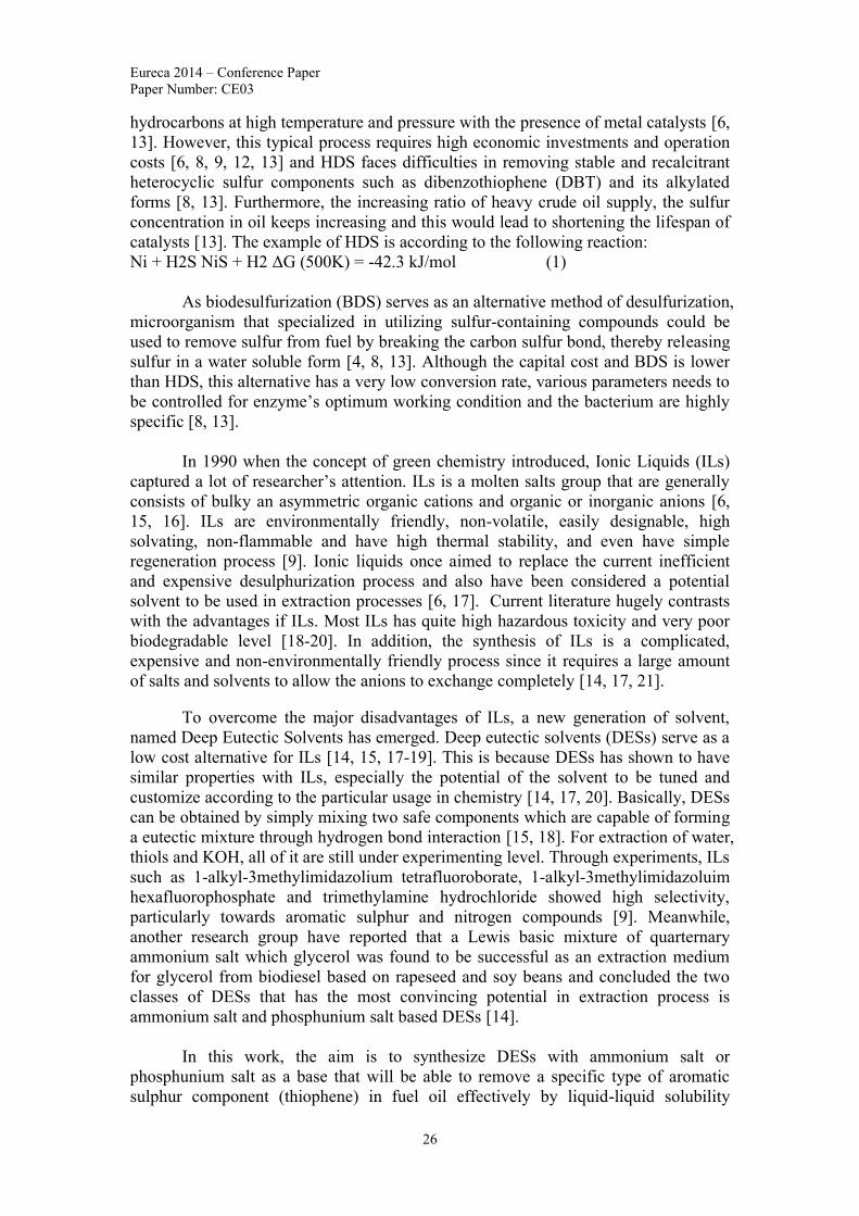
All of the materials that were used in this particular study were tabulated in
Table 2.
Table 2. The list of all chemicals used
No Chemical Name Usage Supplier Purity (%)
1 Choline chloride DES salt Merck >99
2 Methyl triphenyl
phosphonium bromide
DES salt Merck >99
3 Glycerol DES Hydrogen bond
donor
Merck >99
4 Ethylene glycol DES Hydrogen bond
donor
Merck >99
5 Triethylene Glycol DES Hydrogen bond
donor
Merck >99
6 Thiophene Solubility testing Merck >99
2.2 Synthesis of DESs
The two different types of salts that are to be used to synthesis the DESs
needed for the research are choline chloride and methyl triphenyl phosphonium
bromide. As for the hydrogen bond donor (HBD), ethylene glycol, glycerol and
triethylene glycol are to be used. And to increase the number of possible combinations,
the DESs are prepared with different molar ratio of the salts to HBD. In Table 2, the
composition and labeling of DESs that were to be synthesized are shown.
The steps of preparation of DESs used in this research work are
referring to Shahbaz et al. [23]. According to the study done, different molar ratios of
the salt- HBD combinations are poured controlled temperature into Schott bottles.
After that, the bottles are placed on hot plate stirrer equipment with a temperature of
approximately 80°C. Meanwhile, a cylindrical magnetic stirrer bar is to be inserted
into the bottles and the equipment is to be functioning at approximately 800rpm
agitation speed. The process of synthesizing only ends after a homogeneous
transparent liquid is formed.

Eureca 2014 – Conference Paper
Paper Number: CE03
29
Table 3. The Compositions of DES to be synthesized
Salt HBD Molar Ratio
(Salt : HBD) Abbreviations
Choline chloride Ethylene glycol 1:1.75 DES 1
Choline chloride Ethylene glycol 1:2 DES 2
Choline chloride Ethylene glycol 1:2.5 DES 3
Choline chloride Triethylene
glycol 1:3 DES 4
Choline chloride Triethylene
glycol 1:4 DES 5
Choline chloride Triethylene
glycol 1:5 DES 6
Choline chloride Glycerol 1:1.5 DES 7
Choline chloride Glycerol 1:2 DES 8
Choline chloride Glycerol 1:3 DES 9
Methyl triphenyl
phosphonium bromide Ethylene glycol 1:3 DES 10
Methyl triphenyl
phosphonium bromide Ethylene glycol 1:4 DES 11
Methyl triphenyl
phosphonium bromide Ethylene glycol 1:4 DES 12
Methyl triphenyl
phosphonium bromide
Triethylene
glycol 1:3 DES 13
Methyl triphenyl
phosphonium bromide
Triethylene
glycol 1:4 DES 14
Methyl triphenyl
phosphonium bromide
Triethylene
glycol 1:5 DES 15
Methyl triphenyl
phosphonium bromide Glycerol 1:2 DES 16
Methyl triphenyl
phosphonium bromide Glycerol 1:3 DES 17
Methyl triphenyl
phosphonium bromide Glycerol 1:4 DES 18
According to Table 3, by changing the molar ratio and conducting the mixing
at 25°C - 45°C, it could save a lot of budget during scaling up of the reaction. A lot of
energy cost could be saved for mixing of DESs and fuel at room temperature. And by
changing the molar ratio, different types of DESs could be synthesized and enlarged
the area of testing of this work.
2.3 Solubility of Thiophene in DESs
The conventional shake flask method of determining the equilibrium solubility
of any solute in solvents at any given temperature, which is the most accurate method
for solubility determination, was adopted for this work. In this work, 5 mL of
thiophene was added to 5mL of each DESs. The samples were then mixed at 298.15K
with an orbital shaker operating at 200rpm for 1 hour. The above procedure was
repeated for different temperatures (308.15 K and 318.15 K) to determine the highest
value of thiophene solubility in DES. After allowing overnight settling, 100mg of

Eureca 2014 – Conference Paper
Paper Number: CE03
30
DES layer was diluted with 10mL acetonitrile which was the mobile phase for High
Performance Liquid Chromatogram (HPLC). The solutions were then analysed using
HPLC to determine the content of thiophene in DESs.[22].
The HPLC model, specifications and analysis conditions are as below, in
Table 4.
Table 4. The HPLC specifications and analysis conditions
Item(s) Specifications
Column oven: CTO-10AS
Auto injector: SIL-10 AD
System controller: SCL-10A
Detector: SPD-10A
Liquid chromatography: LC-10AD
Degasser: DGU-10AL
Solvent proportioning valve: FCV-10AL
Column: Eclipse plus C18
3.5µm
4.6×100mm
Mobile phase: Acetonitrile
Flow rate: 1 mL/min
Column temperature: 298.18 K
Detector temperature: 308.15 K
Injection volume: 10 µL
3.0 Results and Discussion
The HPLC was calibrated by injecting five different concentrations of thiophene in
acetonitrile solutions, which created a calibration curve for thiophene. Each sample
was analyzed three times to get the accurate results from HPLC analysis.
Figure 2. Standard chromatographs and chromatograms obtained from samples
shows typical thiophene standard chromatographs and (b) represents the typical
chromatograms obtained from samples.

Eureca 2014 – Conference Paper
Paper Number: CE03
31
In Fig. 2, the calibration of HPLC was performed before actually analyse the
content of DESs. The standard chromatographs peak was noted to be tally with the
typical chromatograms obtained from samples. This shows that the content measured
was 99% accurate. The linear correlation coefficient (R2) for curve was found to be
0.99 which represented excellent linearity.
Figure 3. The graph of thiophene solubility against temperature for DES 1, 2
and 3
According to Fig. 3 above, DES 1 has the highest value of thiophene solubility
(8.76%) at 25°C followed by DES 2 (8.71%) and DES 3 (8.67%). All three DESs
solubility increases when temperature increases. This happens due to the increase in
kinetic energy between the particles in the solution that enhances the percentage of
the thiophene molecules to dissolve into the DESs particles. But at 45°C, the
solubility of DES 1 had started to exceed DES 2 which was the leading solubility at
35°C and 45°C.
Figure 4. The graph of thiophene solubility against temperature for DES 4, 5
and 6

Eureca 2014 – Conference Paper
Paper Number: CE03
32
According to Fig. 4 above, DES 4 has the highest value of thiophene solubility
(13.05%) at 25°C followed by DES 5 (11.15%) and DES 6 (10.25%). All three DESs
solubility increases when temperature increases. This happens due to the increase in
kinetic energy between the particles in the solution that enhances the percentage of
the thiophene molecules to dissolve into the DESs particles. At 45°C, the solubility of
DES 4 continued to lead after 5 and 6.
Figure 5. The graph of thiophene solubility against temperature for DES 7, 8
and 9
DES 9 had the lowest thiophene solubility among all 18 DESs under 3
different temperature. Whereas according to Fig. 5, at 25°C DES 7 has the highest
value of thiophene solubility (4.85%) followed by DES 8 (4.26%) and DES 9 (3.91%).
All three DESs solubility increases when temperature increases. This happens due to
the increase in kinetic energy between the particles in the solution that enhances the
percentage of the thiophene molecules to dissolve into the DESs particles.
Among all of the ChCl based DESs, the DES combination that was able to
dissolve the highest number of thiophene was DES 4 (13.05%), ChCl – Ethylene
Glycol with molar ratio 1:1.75 at 45°C. The theoretical reason behind this value was
the 45°C provides the highest kinetic energy to the molecules of DESs in compared to
25°C and 35°C. The increasing movement of molecules of DES, it provides more
space for solute (thiophene) to dissolve. For ChCl – glycerol combination, it provides
the lowest solubility was because glycerol consists of three hydroxyl group, compared
to two hydroxyl group from ethylene glycol and triethylene glycol. The increase in
number of hydroxyl group increases the strength of intermolecular forces. Therefore,
decreases the solubility of thiophene. This showed that DES 1 to 6 would have
stronger solute – solvent attraction than DES 7, 8 and 9.

Eureca 2014 – Conference Paper
Paper Number: CE03
33
Figure 6. The graph of thiophene solubility against temperature for DES 10,
11 and 12
DES 10 had the highest thiophene solubility among all 18 DESs under 3
different temperature. Whereas according to Fig. 6, at 25°C DES 10 had the highest
value of thiophene solubility (23.23%) followed by DES 11 (22.24%) and DES 12
(21.34%). All three DESs solubility increases when temperature increases. This
happens due to the increase in kinetic energy between the particles in the solution that
enhances the percentage of the thiophene molecules to dissolve into the DESs
particles.
Figure 7. The graph of thiophene solubility against temperature for DES 13,
14 and 15
According to Fig. 7 above, DES 13 has the highest value of thiophene
solubility (18.39%) at 25°C followed by DES 14 (17.72%) and DES 15 (16.40%).
Furthermore, a possible theoretical explanation for decrease of solubility in DES 13
and 15 was the result of the dominating chemical bond between the thiophene and the
hydrogen bond donor present in the DESs (triethylene glycol) over that between the
sulfuric compounds and the salt (MTPB). These interactions are perceived to go in
opposite directions to each other due to the presence of Br which serves as the

Eureca 2014 – Conference Paper
Paper Number: CE03
34
hydrogen bond donor in the formation of the DES. As the temperature increased, the
interaction from the side of hydrogen bond donor in the DESs became weakened and
overtaken by the interaction from the side of the salt, which consequently gave rise to
the sudden drop in the measured solubility values [22].
Figure 8. The graph of thiophene solubility against temperature for DES 16,
17 and 18
According to Fig. 8 above, DES 16 has the highest value of thiophene
solubility (9.13%) at 25°C followed by DES 17 (7.40%) and DES 18 (7.14%).
Furthermore, a possible theoretical explanation for decrease of solubility in all three
of these DESs is as the same as DES 13, 14 and 15.
Among all of the MTPB based DESs, the DES with combination that was able
to dissolve the highest number of thiophene was DES 10 (23.23%), MTPB –
triethylene glycol with molar ratio 1:3 at 45°C. The theoretical reason behind this
value was the 45°C provides the highest kinetic energy to the molecules of DESs in
compared to 25°C and 35°C. The increasing movement of molecules of DES, it
provides more space for solute (thiophene) to dissolve. For MTPB – glycerol
combination, it provides the lowest solubility was because glycerol consists of three
hydroxyl group, compared to two hydroxyl group from ethylene glycol and
triethylene glycol. The increase in number of hydroxyl group increases the strength of
intermolecular forces. Therefore, decreases the solubility of thiophene. This showed
that DES 10 to 15 would have stronger solute – solvent attraction than DES 16, 17
and 18.
Overall, MTPB based DESs had higher solubility than ChCl based DESs. This
may due to the sulphide group in thiophene having higher solute – solvent attraction
force with MTPB molecule than ChCl molecules. Meanwhile, ChCl based DESs did
not faced decreasing solubility with increasing temperature, only MTPB based had.
This strongly proved that theoretical chemical bonding regarding presence of Br
atoms as mentioned above was true.
Basically, the range of the experimental testing was small (25°C - 45°C)
because this may be helpful during scaling up. In industrial refinery, operating at

Eureca 2014 – Conference Paper
Paper Number: CE03
35
atmospheric temperature is widely encouraged as this would save millions of money
in industrial refinery zones.
4.0 Conclusion
The solubility of thiophene in MTPB and ChCl based DES with a combination
of different salt to HBD was studied at different temperatures under atmospheric
pressure. It was found that MTPB – ethylene glycol (1:3) had the highest thiophene
solubility with 26.87% wt at 45°C. Whereas ChCl – glycerol (1:3) had the lowest
solubility results with 3.91% wt at 25°C. The results clearly reflected the structure of
DESs heavily affect the sulphuric compound dissolving rate. Actually, the usage
potential of DESs in desulfurization of crude oil is still a fresh topic. The idea of
manipulating the affinity properties in DESs and sulphur content in crude oil is very
doable and logical as DESs has already been used in some extraction process.
References
[1] R. Jamil, L. Ming, I. Jamil, and R. Jamil, "Application and Development
Trend of Flue Gas Desulfurization (FGD) Process: A Review," International
Journal of Innovation and Applied Studies, vol. 4, pp. 286-297, 2013.
[2] I. G. Huges and T. P. A. Hase, Measurements and Their Uncertainties: A
practical guide to modern error analysis. United States: Oxford University
Press Inc., New York, 2010.
[3] S. Laboratories. (2008, 15 May). Basic Refinery Processes.
[4] G. A. Adegunlola, Oloke, J.K., Majolagbe, O. N., Adebayo, E. A.,
Adegundola C. O., Adewoyin A. G and Adegunlola F.O., "Microbial
desulphurization of crude oil using Aspergillus flavus," European Journal of
Experimental Biology, p. 4, 2012.
[5] H. V. Doctor and H. D. Mustafa, "Innovative Refining Technology - Crude
Oil Quality Improvement (COQI)," Real Innovators Group, Chemical
Engineering Division, RIG House, 2007.
[6] A. R. Ferreira, M. G. Freire, J. C. Ribeiro, F. M. Lopes, J. G. Crespo, and J. A.
P. Coutinho, "Ionic liquids for thiols desulfurization: Experimental liquid-
liquid equilibrium and COSMO-RS description," Fuel, vol. 128, pp. 314-329,
2014
[7] Q. A. Acton, Aromatic Polycyclic Hydrocarbons - Advances Research and
Application. Atlanta, Georgia: Scholarly Editions, 2013.
[8] A. A. Nuhu, "Bio-catalytic Desulfurization of Fossil Fuels: a mini review,"
College of Sciences, King Fahd University of Petroleum and Minerals, vol.
12, pp. 9-23, 2013.
[9] A. A. P. Kumar and T. Banerjee, "Thiophene separation with ionic liquids for
desulphurization: A quantum chemical approach," Fluid Phase Equilibria, vol.
278, pp. 1-8, 4/15/ 2009.
[10] F. G. Petzold, "Novel Catalyst for The Removal of Aromatic Sulfur Species
From Refinery Streams," B.S., University of Louisville, 2011.
[11] Q. A. Acton, Sulfones - Advances in Research and Application, 2013 ed.
Atlanta, Georgia: ScholarlyBrief, 2013.

Eureca 2014 – Conference Paper
Paper Number: CE03
36
[12] B. Zhang, Z. Jiang, J. Li, Y. Zhang, F. Lin, Y. Liu, et al., "Catalytic oxidation
of thiophene and its derivatives via dual activation for ultra-deep
desulfurization of fuels," Journal of Catalysis, vol. 287, pp. 5-12, 3// 2012.
[13] L. H. Liu Lin, Qian Jianhua, Xing Jinjuan, "Progress in the Technology for
Desulfurization of Crude Oil," China Petroleum Processing and
Petrochemical Technology, vol. 12, p. 4, 2010.
[14] K. Shahbaz, F. S. Mjalli, M. A. Hashim, and I. M. AlNashef, "Eutectic
solvents for the removal of residual palm oil-based biodiesel catalyst,"
Separation and Purification Technology, vol. 81, pp. 216-222, 2011.
[15] A. Boisset, J. Jacquemin, and M. Anouti, "Physical properties of a new Deep
Eutectic Solvent based on lithium bis[(trifluoromethyl)sulfonyl]imide and N-
methylacetamide as superionic suitable electrolyte for lithium ion batteries and
electric double layer capacitors," Electrochimica Acta, vol. 102, pp. 120-126,
7/15/ 2013.
[16] U. Domańska, E. V. Lukoshko, and M. Królikowski, "Separation of thiophene
from heptane with ionic liquids," The Journal of Chemical Thermodynamics,
vol. 61, pp. 126-131, 6// 2013.
[17] K. Shahbaz, F. S. Mjalli, M. A. Hashim, and I. M. AlNashef, "Using Deep
Eutectic Solvents Based on Methyl Triphenyl Phosphunium Bromide for the
Removal of Glycerol from Palm-Oil-Based Biodiesel," Energy & Fuels, vol.
25, pp. 2671-2678, 2014/04/20
[18] Q. Zhang, K. De Oliveira Vigier, S. Royer, and F. Jerome, "Deep eutectic
solvents: syntheses, properties and applications," Chemical Society Reviews,
vol. 41, pp. 7108-7146, 2012
[19] R. B. Leron, A. Caparanga, and M.-H. Li, "Carbon dioxide solubility in a deep
eutectic solvent based on choline chloride and urea at
T = 303.15–343.15 K and moderate pressures," Journal of
the Taiwan Institute of Chemical Engineers, vol. 44, pp. 879-885, 11// 2013.
[20] L. Bahadori, M. H. Chakrabarti, F. S. Mjalli, I. M. AlNashef, N. S. A. Manan,
and M. A. Hashim, "Physicochemical properties of ammonium-based deep
eutectic solvents and their electrochemical evaluation using organometallic
reference redox systems," Electrochimica Acta, vol. 113, pp. 205-211, 12/15/
2013.
[21] M. H. Chakrabarti, F. S. Mjalli, I. M. AlNashef, M. A. Hashim, M. A.
Hussain, L. Bahadori, et al., "Prospects of applying ionic liquids and deep
eutectic solvents for renewable energy storage by means of redox flow
batteries," Renewable and Sustainable Energy Reviews, vol. 30, pp. 254-270,
2// 2014.
[22] Z. S. Gano, F. S. Mjalli, T. Al-Wahaibi, Y. Al-Wahaibi, and I. M. AlNashef,
"Solubility of Thiophene and Dibenzothiophene in Anhydrous FeCl3- and
ZnCl2-Based Deep Eutectic Solvents," Industrial & Engineering Chemistry
Research, vol. 53, pp. 6815-6823, 2014/04/23 2014.
[23] K. Shahbaz, F. S. Mjalli, M. A. Hashim, and I. M. AlNashef, "Prediction of
deep eutectic solvents densities at different temperatures," Thermochimica
Acta, vol. 515, pp. 67-72, 3/10/ 2011.

eureca 2014 – Conference Paper
Paper Number: CE04
37
Investigation on Used Tea
Leaves-Derived CO₂ Adsorbent
Jagvinder Singh, Rebecca Lim Xiao Yien, Veena Doshi
Energy Research Group, School of Engineering, Taylor’s Lakeside Campus, Malaysia
Abstract
In this study, used tea leaves are used as raw material to produce activated
carbon (AC). Characterization of used tea leaves-derived AC is studied as low-cost
adsorbents to capture carbon dioxide (CO₂) which has been a major contributing
factor in relation to global warming recently. Effects of parameters such as production
method, activating chemical agent and ratio of chemical to tea leaves during chemical
activation to the characterization of AC and its potential to adsorb CO₂ are
investigated. The production methods selected for investigation are chemical
activation and pre-treated chemical activation. Where else, for the activating
chemicals, potassium hydroxide (KOH) and phosphoric acid (H₃PO₄) were chosen.
The mass ratio of activating chemical to used tea leaves of 2:1 and 1:1 are studied.
The characterization of the used tea leaves-derived AC was analysed by using Fourier
Transform Infrared Spectroscopy (FTIR), Thermogravimetric analysis (TGA) and
Brunauer-Emmett-Teller (BET). In order for CO₂ adsorption, it is desired that
properties such as large surface area, considerable amount of micropores and good
surface reactivity are developed during AC production. From the results obtained, the
specific surface area and total pore volume of the ACs produced varied from 336m²/g
to 1044 m²/g and 0.17cm³/g to 0.59cm³/g respectively. The AC with the highest
potential for CO₂ adsorption is the AC produced by chemical activation with H₃PO₄
at ratio of 2:1.
Keywords: Activated carbon, Used Tea Leaves, Adsorption, Carbon dioxide, Biomass.

eureca 2014 – Conference Paper
Paper Number: CE04
38
1. Introduction
In recent decades, air pollution has become a major concern amongst the
community. The increase in volume of human activities such as industrialization and
urbanization has been the major contributing factor to air pollution. One of the
primary air pollutants is carbon dioxide (CO₂). CO₂ is primarily produced from the
combustion of fossil fuels such as coal and petroleum distillates which are widely
used as a source of energy in transportation and electricity generation. In accordance
to the International Agency report (2007) on world energy statistics, coal contributed
at about 29 billion metric tons of CO₂ which made up to 42% of the world CO₂ emissions in 2007 alone [1]. Unfortunately, the utilization of fossil fuels in these areas
is unlikely to reduce in the near future as there is no practical alternative yet. Thus,
preventing CO₂ emissions from these activities is very unlikely at this stage.
Therefore, there is an urgent need to capture and control the emission of CO₂.
There are many available technologies for CO₂ removal. The technology that
is recently receiving much attention is adsorption due to its simple process and low
cost of operations[1]. Adsorption uses adsorbents as a capturing material, and one of
the most widely used adsorbent is activated carbon (AC). AC’s large active surface
area, favorable pore size distribution, surface chemistry and the degree of polarity
makes it very suitable for many environmental applications [2-5]. Charcoal is the
most suitable raw material for AC production due to its rich carbon content.
Unfortunately, the source of charcoal is limited and expensive. Therefore, alternative
carbonaceous sources which are sustainable, easily available and cheap are being
investigated. Numerous studies have been done to investigate the potential of biomass
materials as an alternative raw material for AC production and many have been
proven effective. Coconut husk, palm oil materials, grass cuttings, horse manure,
wood, orange peel, treated sewage, wall nut shell are a few example of effective
biomass derived AC [5-9].
For this research, the potential of used tea leaves as AC on CO₂ adsorption
will be investigated? Tea leaves are chosen because it is largely produced in Malaysia.
Tea leaves are widely used all over the world to produce the world’s second most
consumed beverage, tea. The waste tea leaves are mostly discarded as waste. Only a
small amount of the used tea leaves are used as fertilizers. Therefore, tea leaves
produce a lot of waste. This makes tea leaves a fairly cheap and environmental
friendly carbonaceous source for AC production. Studies have been done previously
to investigate the potential of tea leaves as AC. E.Akar et al. (2013) investigated the
potential of tea leaves as AC for removal of malachite green from aqueous solution
and the results showed that the AC produced can be used as an efficient adsorbent for
the removal of malachite green [3]. Besides that, A. Gundogdu et al. performed an
investigation to study the physicochemical characteristics of activated carbon produce
from tea industry waste. The ACs produced from this study showed good
characteristic of AC [4]. Therefore, it is evident that tea leaves are good raw material
for AC preparation. However, no investigation have been made on used tea leaves
derived AC for CO₂ removal applications. Thus, this study will investigate the
potential of used tea leaves-derived CO₂ adsorbent.
There are many parameters that influence the quality of the produced AC. The
effect of preparation method, activating agent and ratio of activating agent to tea
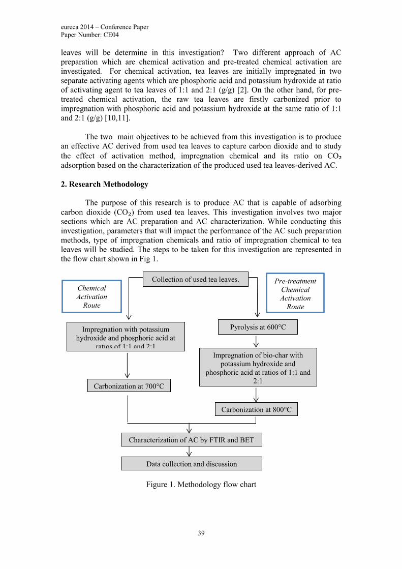
eureca 2014 – Conference Paper
Paper Number: CE04
39
leaves will be determine in this investigation? Two different approach of AC
preparation which are chemical activation and pre-treated chemical activation are
investigated. For chemical activation, tea leaves are initially impregnated in two
separate activating agents which are phosphoric acid and potassium hydroxide at ratio
of activating agent to tea leaves of 1:1 and 2:1 (g/g) [2]. On the other hand, for pre-
treated chemical activation, the raw tea leaves are firstly carbonized prior to
impregnation with phosphoric acid and potassium hydroxide at the same ratio of 1:1
and 2:1 (g/g) [10,11].
The two main objectives to be achieved from this investigation is to produce
an effective AC derived from used tea leaves to capture carbon dioxide and to study
the effect of activation method, impregnation chemical and its ratio on CO₂ adsorption based on the characterization of the produced used tea leaves-derived AC.
2. Research Methodology
The purpose of this research is to produce AC that is capable of adsorbing
carbon dioxide (CO₂) from used tea leaves. This investigation involves two major
sections which are AC preparation and AC characterization. While conducting this
investigation, parameters that will impact the performance of the AC such preparation
methods, type of impregnation chemicals and ratio of impregnation chemical to tea
leaves will be studied. The steps to be taken for this investigation are represented in
the flow chart shown in Fig 1.
Figure 1. Methodology flow chart
Collection of used tea leaves.
Impregnation with potassium
hydroxide and phosphoric acid at
ratios of 1:1 and 2:1
Data collection and discussion
Pyrolysis at 600°C
Pre-treatment
Chemical
Activation
Route
Chemical
Activation
Route
Carbonization at 800°C
Impregnation of bio-char with
potassium hydroxide and
phosphoric acid at ratios of 1:1 and
2:1 Carbonization at 700°C
Characterization of AC by FTIR and BET

eureca 2014 – Conference Paper
Paper Number: CE04
40
2.1 Materials
Used tea leaves are collected from Selvi’s Corner Curry House situated in
Bandar Puteri, Selangor, Malaysia. Potassium hydroxide and phosphoric acid are
purchased from Sigma-Aldrich that has purity greater than 85% and assay of 85%
respectively.
2.2 Collection and storage of used tea leaves.
The leaves are collected batch by batch for an interval of 2-3 days to ensure
that fungus or any microorganism do not grow on the tea leaves while it is being
stored for collection. The tea leaves are first subjected to series of washing with
distilled water to remove impurities such as milk and sugar that may be present in it.
The washed tea leaves are then pre-dried under the sun for about 4-5 hours. The
process is followed by placing the pre-dried tea leaves into an oven at 110°C for about
15 hours to ensure the tea leaves are completely dry. Finally, the tea leaves are filled
in a sealable container and stored in a dry cool place.
2.3 Preparation of AC
Two different methods of AC production will be studied: chemical activation
and pre-treated chemical activation. For chemical activation, the dried tea leaves are
first impregnated in 20%wt phosphoric acid with impregnation chemical to tea leaves
ratios of 1:1 and 2:1 (g/g). The tea leaves are allowed to stand for 24 hours at room
temperature. After that, the mixture is filtered and the impregnated product is dried
for about 15 hours in an oven at 110°C. The product is then carbonized at temperature
of 700°C for 2 hours in a furnace. After being cooled down to room temperature, the
product is neutralized with an alkaline solution until neutral pH of 7 is achieved.
Finally, the product is washed with distilled water to remove any impurities. The
same steps are repeated by replacing phosphoric acid with 50%wt potassium
hydroxide as the impregnation chemical.
For pre-treated chemical activation, the dried tea leaves are first pyrolysed
(carbonized) in a furnace under nitrogen gas flow. The furnace is run at a rate of
10°C/min to the optimal temperature of 600°C. The carbonized substance is then
impregnated with 20wt% phosphoric acid with activating agent to tea leaves ratios of
1:1 and 2:1(g/g). The mixture is allowed to stand for 24 hours at room temperature.
After 24 hours, the excess solution is removed by filter and the impregnated tea leaves
are dried at 110°C for about 15 hours in an oven. The obtained sample is then heated
at 800°C for 2 hours in a furnace. After being cooled down to room temperature, the
product is neutralized by an alkaline solution until pH value of 7 is obtained. Finally,
the product is washed with distilled water and dried at 110°C in an oven for about 15
hours. The same steps are repeated by using 50%wt potassium hydroxide as the
impregnation chemical. Acid solution will be used as a neutralizing chemical.

eureca 2014 – Conference Paper
Paper Number: CE04
41
2.4 Characterization of samples
2.4.1 Proximate analysis
TGA analyzer is used to perform proximate analysis to obtain information on
moisture, ash, fixed carbon and volatile matter content in used tea leaves.
To run TGA, firstly, 0.1g of tea leaves sample is heated to 110°C under
nitrogen gas for 20 minutes to eliminate the moisture content in the sample. Then the
temperature is increased to 950°C and held for 30 minutes under nitrogen flow to
remove volatile matters from the sample. After 30 minutes of heating at 950°C, the
nitrogen gas supply is cut off and switched to air for 20 minutes to allow combustion
of carbon to take place, leaving only ash behind. The heating is done at a rate of
10°C/min.
2.4.2 Ultimate analysis
Elemental analyzer (Euro EA3000 series) is used to perform ultimate analysis
in which carbon, hydrogen, nitrogen and sulfur contents of used tea leaves and pre-
treated used tea leaves can be determined.
Firstly, 0.5 g of sample is combusted in sample of tin and vanadium pentoxide
catalyst, purified by a reactor packed with electrolytic copper and copper oxide.
Gasses such as N₂, CO₂, H₂O and SO₂ enter the chromatographic column for
separation to take place. Eluted gasses are sent to the thermal conductivity (TCD)
where electrical signals processes by the Eager 300 sotfware provide values of
nitrogen, carbon, hydrogen and sulfur content in percentage that is in the sample.
2.4.3 Fourier Transform Infrared Spectroscopy (FTIR) analysis
Fourier Transform Infrared Spectrometer is used to perform FTIR. FTIR is
analysis provides information about functional groups and covalent bonds present in
the sample.
To prepare the sample for FTIR analysis, a small amount of sample and KBr
powder are first added into a mortar at ratio of 1:99 respectively. The mixture is
grinded until homogeneous with a pestel. After that, die is assembled with lower die,
polished face up. A small amount of the mixture is inserted into the cylinder bore (just
enough to cover the surface) and even out with a plunger. Then the second die is
gently inserted, polished face down into the bore, followed by the plunger. The
assembled die with the plunger is then placed into the hydraulic press. The knob of
the hydraulic press is tighten to ensure that the cylinder bore is held in place firmly.
Force is increased to roughly 10 tons under vacuum by pulling the hydraulic pump
handle downwards. The die is left under pressure for 20 seconds. After 20 seconds,
the vacuum is released and die is removed from the press. Dies are dismantled and
formed pellet disk is placed onto disk holder. Finally, the disk holder is mounted in
the spectrometer for analysis.

eureca 2014 – Conference Paper
Paper Number: CE04
42
2.4.4 Brunauer-Emmett-Teller (BET) analysis
Brunauer-Emmett-Teller (BET) analyzer is used to perform this analysis. BET
is run to determine the surface characteristic of the samples such as total surface area
and pore size.
To carry out BET analysis, 0.5 grams of sample is first degassed at 90°C for
60 minutes followed by 300°C for the subsequent 480 minutes. N₂ are used as
adsorption gas and the adsorption is studied at 0°C under circulating water bath.
3. Results and Discussion
3.1 Proximate and Ultimate analysis
The results from the proximate and ultimate analysis show that used tea leaves
have good potential for AC production. High percentage of carbon content which is
necessary to produce good quality AC is available in used tea leaves. Besides that, the
volatile matter in used tea leaves which helps the pore structure formation is relatively
high. Moisture content made up a small percentage of the used tea leaves which is
desired for AC production because the moisture present may combine with char
carbon during pyrolysis to produce gaseous by-products which may result in low yield
of porous carbon [12]. Overall, used tea leaves showed good properties of precursor
to be used for AC production.
Table 1. Proximate analysis of used tea leaves and pre-treated used tea leaves.
No Sample Moisture [%] Volatile
Matter [%]
Fixed Carbon
[%] Ash [%]
1 Used tea leaves 7 70 22 1
2 Pre-treated used
tea leaves 6 17 67 10
Table 2. Ultimate analysis of used tea leaves and pre-treated used tea leaves.
No Sample N[%] C[%] H[%] S[%]
1 Used tea leaves 3.83 46.4 6.809 1.019
2 Pre-treated use tea
leaves 4.07 71.91 2.415 2.303
3.2 BET analysis
In Table 3, it is shown that CAP2 developed the largest surface area at
1044m²/g and PCAP1 developed the lowest total surface area with only 336m²/g.
Besides that, Table 3 also shows that all H₃PO₄ activated AC samples prepared in this
experiment are microporous because more than 70% of the total pore volume of these
samples was contributed by micropore volume. The only sample with low percentage
of micropore volume is CAK1 which is the only KOH activated sample.

eureca 2014 – Conference Paper
Paper Number: CE04
43
Table 3. Textural parameters of the prepared activated carbon.
No Sample Method Activating
Agent
Impregnation
ratio
BET
surface
area
(m²/g)
Micropore
Surface
area (m²/g)
Total
pore
Volume
(cm³/g)
Micropore
Volume
(cm³/g)
1 CAP2 Chemical
Activation H₃PO₄ 2:1 1044 930 0.59 0.451
2 CAK1 Chemical
Activation KOH 1:1 478 357 0.412 0.17
3 CAP1 Chemical
Activation H₃PO₄ 1:1 761 713 0.377 0.27
4 PCAP1
Pre-treated
Chemical
Activation
H₃PO₄ 1:1 336
312 0.166 0.13
3.3 Effect of Parameters
The type of preparation method, activating agent and impregnation ratio seems
to have a significant effect on the properties of the used tea leaves-derived AC as can be
seen in Table 3. The AC produced by chemical activation with H₃PO₄ at ratio of 1:1
(CAP1) had larger BET surface area, micropore surface area, total volume and
micropore volume compared to the chemical activation with KOH at ratio of 1:1 sample
(CAK1). This suggests that H₃PO₄ is more suitable to be used as an activating agent to
prepare used tea leaves-derived AC compared to KOH. For preparation method,
chemical activation method produced used tea leaves-derived AC with significantly
higher quality compared to pre-treated chemical activation method. This can be noticed
when properties of CAP1 is compared with PCAP1. CAP1 which is prepared by
chemical activation was able to developed 760m²/g of surface area while PCAP1 which
was prepared by pre-treated chemical activation only developed 336m²/g of surface area.
This can be justified by to loss of most volatile matter during pre-treatment process at
600°C. As stated in literature, raw material with high volatile matter is desired for AC
production because volatile matter plays an important role in the formation of pores in
AC [12]. The pre-treatment process has eliminated most of the volatile matter from
used tea leaves (decreased from 70%-17%) that has affected the pore formation for pre-
treated method. Lastly, the effect of impregnation ratio of the activating agent to used
tea leaves can be studied by comparison of CAP2 and CAP1. CAP2 which was
prepared by H₃PO₄ at ratio 2:1 produced larger surface area compared to CAP1 which
was prepared by H₃PO₄ at ratio 1:1. This is due to the fact that activating agent reduces
the formation of tars and any other liquids that may cause blocking of the pores and
restrict the formation of porous structure in the AC [6]. Thus, larger ratio of activating
agent produces AC with better adsorption properties.
3.4 CO₂ adsorption
The CO₂ adsorption potential of the used tea leaves-derived AC is determined
based on the characterization of the ACs produced. The main properties that is required
for effective adsorption of CO₂ are high total surface area, high micropore surface area
and high pore volume[4]. All the used tea leaves-derived AC produced in this study

eureca 2014 – Conference Paper
Paper Number: CE04
44
developed high percentage of micropore surface area which made up more than 70% of
the total surface area for each samples. The micropore volumes for almost all the ACs
produced (except CAK1) are relatively high as well, comprising more than 70% of the
total volume. However, not all AC produced exhibit large total surface area. CAK1 and
PCAP1developed total surface area that is too low to be used for CO₂ adsorption as it
will not be efficient. Nevertheless, CAP2 and CAP1 samples developed considerable
amount of total surface area to be used in CO₂ adsorption application. A study done by
W.Hao et al (2013) showed that AC produced by horse manure with total surface area
of 841m²/g of which 742m²/g is made up of micropore surface area and has a
micropore volume of 0.379cm³/g, had a CO₂ adsorption capacity of 1.45mmol/g [2].
This horse manure-derived AC had the highest CO₂ capacity compared to the other AC
produced in this same study. Besides that, A.S Ello et al. produced AC with total
surface area of 1130m²/g and micropore volume of 0.48cm³/g [13]. This particular AC
had a CO₂ adsorption capacity of 3.9mmol/g [13]. Therefore, by comparing the results
from these two studies with the results from this experiment, it is safe to state that used
tea leaves do have potential to produce effective AC to be used in CO₂ adsorption and
the best combination of parameters for AC preparation with used tea leaves are
chemical activation with H₃PO₄ at ratio of 2:1.
4. Conclusion
Used tea leaves-derived activated carbons (ACs) were prepared by chemical
activation and pre-treated chemical activation with H₃PO₄ and KOH as activating
agent at ratio of activating agent to used tea leaves of 1:1 and 2:1. From the results
obtained and comparison with other studies, used tea leaves AC displayed desirable
properties to be used as adsorbent in CO₂ removal applications. For parameters
investigated in this experiment, it was found that the preparation method, activating
agent and ratio of activating agent did influence the characteristic/properties of the
used tea leaves prepared AC. Chemical activation method produced AC with better
properties compared to pre-treated activation method. H₃PO₄ is a better activating
agent compared to KOH for used tea leaves prepared AC. Lastly, larger ratio of
activating agent to used tea leaves produced AC with larger surface area and better
micropore distribution. The best combination of parameters investigated in this study
for used tea leaves-derived AC are chemical activation with H₃PO₄ at ratio of 2:1.
These combination of parameter produced AC with the highest total surface area of
1044m²/g in which 930m²/g is made up of micropore surface area.
5. Reference
[1] K. Ramasubramanian, H. Verweij, and W. S. Winston Ho, “Membrane
processes for carbon capture from coal-fired power plant flue gas: A modeling
and cost study,” J. Memb. Sci., vol. 421–422, pp. 299–310, Dec. 2012.
[2] W. Hao, E. Björkman, M. Lilliestråle, and N. Hedin, “Activated carbons
prepared from hydrothermally carbonized waste biomass used as adsorbents for
CO2,” Appl. Energy, vol. 112, pp. 526–532, Dec. 2013.

eureca 2014 – Conference Paper
Paper Number: CE04
45
[3] E. Akar, A. Altinişik, and Y. Seki, “Using of activated carbon produced from
spent tea leaves for the removal of malachite green from aqueous solution,”
Ecol. Eng., vol. 52, pp. 19–27, Mar. 2013.
[4] A. Gundogdu, C. Duran, H. B. Senturk, M. Soylak, M. Imamoglu, and Y. Onal,
“Physicochemical characteristics of a novel activated carbon produced from tea
industry waste,” J. Anal. Appl. Pyrolysis, vol. 104, pp. 249–259, Nov. 2013.
[5] I. Ozdemir, M. Şahin, R. Orhan, and M. Erdem, “Preparation and
characterization of activated carbon from grape stalk by zinc chloride
activation,” Fuel Process. Technol., vol. 125, pp. 200–206, Sep. 2014.
[6] A. Heidari, H. Younesi, A. Rashidi, and A. Ghoreyshi, “Adsorptive removal of
CO2 on highly microporous activated carbons prepared from Eucalyptus
camaldulensis wood: Effect of chemical activation,” J. Taiwan Inst. Chem.
Eng., vol. 45, no. 2, pp. 579–588, Mar. 2014.
[7] M. a. Lopez-Velazquez, V. Santes, J. Balmaseda, and E. Torres-Garcia,
“Pyrolysis of orange waste: A thermo-kinetic study,” J. Anal. Appl. Pyrolysis,
vol. 99, pp. 170–177, Jan. 2013.
[8] N. Ferrera-Lorenzo, E. Fuente, I. Suárez-Ruiz, and B. Ruiz, “KOH activated
carbon from conventional and microwave heating system of a macroalgae
waste from the Agar–Agar industry,” Fuel Process. Technol., vol. 121, pp. 25–
31, May 2014.
[9] M. C. Ribas, M. a. Adebayo, L. D. T. Prola, E. C. Lima, R. Cataluña, L. a.
Feris, M. J. Puchana-Rosero, F. M. Machado, F. a. Pavan, and T. Calvete,
“Comparison of a homemade cocoa shell activated carbon with commercial
activated carbon for the removal of reactive violet 5 dye from aqueous
solutions,” Chem. Eng. J., vol. 248, pp. 315–326, Jul. 2014.
[10] M. : G. Martinez, M.L: Moiraghi, L :Agnese, “Making and some properties of
activated carbon produced from agricultural industrial residues from
argentina,” J. Argentina Chem. Soc., vol. 91, no. 6 2, pp. 5–10, 2003.
[11] J. Park, I. Hung, Z. Gan, O. J. Rojas, K. H. Lim, and S. Park, “Activated carbon
from biochar: influence of its physicochemical properties on the sorption
characteristics of phenanthrene.,” Bioresour. Technol., vol. 149, pp. 383–9,
Dec. 2013.
[12] S. Deng, H. Wei, T. Chen, B. Wang, J. Huang, and G. Yu, “Superior CO2
adsorption on pine nut shell-derived activated carbons and the effective
micropores at different temperatures,” Chem. Eng. J., vol. 253, pp. 46–54, Oct.
2014.
[13] A. S. Ello, L. K. C. de Souza, A. Trokourey, and M. Jaroniec, “Development of
microporous carbons for CO2 capture by KOH activation of African palm
shells,” J. CO2 Util., vol. 2, pp. 35–38, Sep. 2013.

Eureca 2014 – Conference Paper
Paper Number: CE05
46
Optimising Yield and Production Cost of
Bioactive Compounds using Process
Synthesis and Design Approach
Joanne W.R. Chan1, Chien Hwa Chong
1,*, Nur Farihah Abdul Malek
1, Denny K. S.
Ng2, Chun Hong Khek
1, Adam Figiel
3, Aneta Wojdyło
4
1School of Engineering, Taylor’s University, No 1, Jalan Taylor‘s,47500 Subang Jaya,
Selangor, Malaysia 2 Department of Chemical and Environmental Engineering/Centre of Excellence for
Green Technologies,University of Nottingham Malaysia Campus, Broga Road, 43500
Semenyih, Selangor, Malaysia. 3Institute of Agricultural Engineering, Wroclaw University of Environmental and Life
Sciences,
Chelmonskiego 37/41 Street, Wroclaw 51-630, Poland. 4Department of Fruit and Vegetable Technology, Wroclaw University of
Environmental and Life Sciences, Chelmonskiego 37/41 Street, Wroclaw 51-630,
Poland.
* Email: [email protected]
Abstract
Herbs are well known for medicinal purposes throughout human history. The benefits
of herbs are wide which include healing of different diseases, maintaining and
restoring body balances. Bioactive compounds of herbs are found in herbs which
recognize as the compounds that help in defencing human body by deterring
formation of free radical chain reaction to attack human body’s cells. However,
postharvest processing of herbs using drying and extraction methods influenced the
quality and quantity of the bioactive compounds. This paper presents a systematic
conceptual synthesis and design approach for optimization of bioactive compounds
extraction from herbs. In this work, Pro II 9.1 is used for process simulation and
analysis on the bioactive compound production. To demonstrate the proposed
approach of process optimization, a case study on Strobilanthes Crispus production is
presented. Selection of technologies and parameters in design processes can optimise
the productivity and minimize the operation cost for bioactive compounds production.
The optimized process configurations found in this study is Convective air drying-
supercritical fluid extraction and ultrafiltration. It is able to retain most of the phenolic
acids without overshooting the operating cost. The operating cost of this process is
$US29304.94 kg/annual which is 1.26 times lower than combined microwave vacuum
drying- supercritical fluid extraction- ultrafiltration and product yield of 56494.06
kg/annual which is 5.23 times higher than Convective air drying- conventional solvent
extraction - ultrafiltration .
Keywords: Bioactive compounds, Process synthesis, Strobilanthes Crispus,
Extraction, Drying

Eureca 2014 – Conference Paper
Paper Number: CE05
47
1. Introduction
For centuries, natural herbs are being studied for their medicinal purposes throughout
human history. Natural antioxidants are consider more favourable compare to
synthetic drugs which contain possibility of side effect when consumed long term.
Moreover, modern medicines are more expensive compare to herbal medicine that can
be grown and gathered easily with little or no cost (Conde et al.,2010). Therefore, in
recent years, there is an increase of extracting the bioactive compounds of herbs to
produce medicine. World Health Organization (WHO) estimated that 80% of the
world populations are depended on herbal medicine for their primary health
care(Ranilla et al.,, 2010). Malaysia’s herbs have the potential to produce medicine
which possess high antioxidant activity, anti-AIDS, and anticancer properties (Liza et
al.,2010).
Bioactive compounds are generally produced as secondary metabolites in plants other
than the primary biosynthetic compounds such as amino acids, proteins,
carbohydrates and lipids (Azmir et al., 2013). Various types of bioactive components
can be found in herbs, for example, glycosides (saponins and anthraquinine
glycosides), resins and antioxidant compounds (flavonoids, phenolic acids and
quinones). The natural components that are at interest is the antioxidants specifically
phenolic compounds. Natural antioxidant compounds are much effective than the
synthetic compounds which contain toxicity and carcinogenicity (Ernst 1998) . These
compounds help to defense human bodies by deterring formation of free radicals
chain reaction. Hence, formation of hydroperoxides and attacks of free radicals to
human body’s cells are prevented (Karakaya and Kavas, 1999). Moreover, they are
responsible for preventing degenerative diseases such as aging, cancer, cardiovascular
disease, Alzheimer’s disease and muscular degeneration (Wootton-Beard and Ryan
2011).
The family species of Strobilanthes crispus is Acanthaceae which its common name
is ‘pecah kaca’ in Malaysia and ‘daun picah beling’ in Jakarta. It is used widely for
traditional medicine of antidiabetic, antilytic, diuretic and laxative. It is also proved
scientifically to have antioxidant effects antihyperglysemic, and hypolipidemic
effects (Ismail et al., 2000), anti-AIDS, anticancer activity (Liza et al., 2010) and
exhibit antioxidant activity (Afrizal, 2008). Therefore, Strobilanthes Crispus is
chosen for analysis in this work. The objective of this work is to maximize the
production yield and reducing production cost via different technologies and process
configurations.
The post-harvesting process of medicinal herbs is crucial in the industry as it affects
the quantity and quality of the bioactive components production (Khorshidi et al.,
2009). According to the previous works, the processes that are commonly used to
produce bioactive compound such as antioxidant are drying, extraction and
concentration(Cerón et al., 2014). Note that in order to optimize the bioactive
compound production, systematic process synthesis and design is needed. In this
work, a systematic approach for synthesizing and optimizing the processes in
pharmaceutical industry is presented.
This work is in line with process intensification (PI) as presented in Ponce-Ortega et
al., (Ponce-Ortega et al., 2012). PI is defined as an approach to develop novel
methods in comparing the traditional processes to improve the existing processes

Eureca 2014 – Conference Paper
Paper Number: CE05
48
which leads to a substantial production. Some strategies to achieve PI are reducing
equipment size, minimizing waste generation, energy consumption, increasing
production efficiency, etc. (Lutze et al., 2011). In this work, a systematic approach is
presented for production of bioactive compounds. A case study on extraction of
bioactive compound from Strobilanthes Crispus is presented. Following the proposed
approach, reviewing and selection of technologies and process configurations based
on techno-economic criteria is first performed. Next, the selected technologies and
process is analyzed by process synthesis and simulation . In this work, PRO II 9.1
(Invensys Software, USA) is used as the simulator to analyze the process performance
and interactions of processes and to adapt a fuzzy optimization to identify the
synthesized process configurations where operating cost is minimized and product
yield is maximized.
2. Production of Bioactive Compounds in Pharmaceutical Industry
2.1. Pretreatment Technologies
Drying is the process of reducing water content by means of heat and mass transfer
which helps to preserve the product from decomposition of microbial growth, reduce
weight for transportation and save storage space (Karimi et al., 2012). The
application of drying for pre-treatment of extraction is reported to give a better
productivity of antioxidant reported by Ceron et al.,, 2014 (Cerón et al., 2014). In the
study, drying process is important as the tissue of raw materials will be more brittle
which allows a rapid cell wall breakdown for grinding and homogenization steps in
extraction process. With proper pretreatment process, more bioactive components are
released into the solvents and minimized enzymatic degradation and loss of
antioxidants compounds.
As most of the bioactive compounds are not stable at high temperature and long
drying time, freeze drying (FD) which operate at low temperate and pressure can be
used. However, FD is a time-consuming process and high operation cost as it
consume high amount of energy. On the other hand, air drying (AD) has the lowest
operating cost, but it is unable to preserve much bioactive compounds during the
pretreatment process. Due to the limitations of the conventional drying processes,
advanced technologies such as ultrasonic, microwave, heat pump, vacuum and hybrid
system have also been developed (Chong et al., 2014).
Microwave assisted drying technologies has been reported to have shorter drying time
compare to convective hot air drying. The application of combined vacuum
microwave drying (C/MVD) reduces the drying time as there is rapid removal of
internal moisture due to large vapour pressure difference between the outer and inner
of the targeted substances (Chong et al., 2014). The molecules with permanent dipolar
moment rotate rapidly in the change of electric field that give rise to friction force and
collision of free ions due to the electric field will generate heat. As water molecules
are polar component, it is suitable to use microwave energy for dehydration process.
Compare to the conventional hot air drying it is an improvement of drying technology.
This is because hot air drying has lower drying rate that takes longer time. The
product surface has to be dried first and subsequently mass transfer occurs from inner
of the substance being dried to external surface. However, the dried outer layer is a
poor conductor of heat throughout the drying process. Whereas microwave drying can
penetrate the dry outer layer and heat the substances throughout all high moisture area.

Eureca 2014 – Conference Paper
Paper Number: CE05
49
C/MVD is a technology that combines microwave heating with vacuum drying. This
hybrid system is able to dry thermo sensitive products as the vacuum conditions lower
the liquid vapor and is performed in the absence of oxygen. C/MVD also promotes
efficient water which reduces structural changes by preventing shrinkage and induces
porous tissues (Schulze et al., 2014).
2.2.Extraction Technologies
The extraction process of bioactive components is intricate due to delicate properties
of low boiling point of the components that easily disintegrate when expose to high
temperature. Studies have been conducted throughout the year to preserve and ways
to glean high amount of bioactive constituents from herbs. There are two types of
extraction processes are being applied in industry, which are solvent extraction and
supercritical fluid extraction (SFE). It is noted that extraction of bioactive compound
from medicinal herbs is mainly SFE for higher yield. The common used fluid is
carbon dioxide (CO2). Supercritical CO2 has high diffusivity than other fluids which
enhance mass transfer for higher extraction rate (Chen et al., 2011). The significant
disadvantage of SFE is high capital and operation cost. Therefore, process
optimization is a critical step to improve the process performance. Studies show that
the addition of solvent to SFE process is economically viable. This is because
bioactive compounds such as flavonoids and tannins are polar compound. Hence, co-
solvent (ethanol) is added to increase the polarity of CO2 which eventually increase
the extraction yield. Liza et al. investigated on the extraction performance of
flavonoid bioactive compounds from Strobilanthes Crispus with the use of
supercritical CO2 and ethanol mixture (Liza et al., 2010). The solvation power of
supercritical fluid can be manipulated by changing pressure and temperature to
achieve high selectivity. According to Liza et al., the pressure of SFE is an important
factor that affects the yield of bioactive compound followed by extraction time and
temperature.
On the other hand, solvent extraction is a traditional and state of the art method in
obtaining bioactive compound from herbs. It deals with transporting solute (bioactive
compounds) from one phase (raw materials) into another one (solvent) until it reaches
the final equilibrium distribution. A recent discovery is natural product components
such as sugars, organic acids, amino acid, choline or urea are excellent solvent in
extraction of bioactive compounds which is known as natural deep eutectic solvents
(NaDES). Yuntao Dai (2014) investigated NaDES as a new extraction solvent for
phenolic metabolites form Carthamus tinctorius (Dai et al., 2013). Based on the result,
the characteristic of this solvent is beneficial for extraction compared to deep eutectic
solvent (DES) and ionic liquid (IL) as it have adjustable viscosity, more sustainable
and exist as liquid state even below 0°C. However, this solvent inherits high viscosity
properties which will hinder the extraction efficiency. Few methods were suggested
to increase the yield by mixing water with NaDES, increase the operating temperature
or increase the transport rate by mechanical agitation. The report stated that the yield
of phenolic compounds by using NaDES as solvent is up to 14% higher than water
and ethanol. Therefore, NaDES is chosen to be used in the extraction method as
solvent in this case study rather than the conventional ethanol solvent.

Eureca 2014 – Conference Paper
Paper Number: CE05
50
3. Proposed Systematic Approach
By reviewing all the available technologies in the literature, two most reliable and
efficient processes were selected for further analysis. Fig. 1 shows the processing
steps of production of bioactive compound from herbs. As shown, different
processing pathways compiled and showed in a superstructure. Note that the
processing steps are divided into three stages which are pretreatment, extraction and
concentration. In the first stage, the potential technologies, which taken into
consideration, are convective air drying (CAD) and combined vacuum microwave
drying (C/MVD) system. After the pretreatment process, the bioactive compound is
expected to be extracted via conventional extraction (CE) by using novel solvent
NaDES (sucrose-choline chloride) or supercritical fluid. Once the compounds are
extracted, concentration process is needed to increase the value of the products. The
final stage is concentration by vacuum distillation (VD) or ultrafiltration ( UF)
Once the process configuration is fixed, the process can be further analyzed via
process simulation to estimate the performance and interactions of the system. In
addition, the operatin cost can also be estimated. Note that this proposed systematic
approach able to assist design engineers and decision makers to compare and design
various process alternatives to reach the same objective. For the conventional
extraction, the concentration is done by back extraction (BE) which will be classified
as VD.
Figure. 1. Superstructure for process synthesis design
4. Case Study
To demonstrate the proposed approach, a case study on production of pheolic
compound from Strobilanthes Crispus herb is solved. In this case study, it is expected
to design a process with capacity of 1000 kg/hr of Strobilanthes Crispus herb and
working hours of 8330 per year. The operating conditions for each technology are
shown in Table 1. These data was reviewed and acquired from secondary source from
journals that have investigated comprehensively the optimum conditions of each
technology. To analyze the process performance, production of bioactive compound
was simulated via PRO II 9.1 (Invensys Software, USA). The detail simulation
procedure is discussed in the following section.
Raw
Materials
CAD CE
C/MVD
Tech: j
Final
Products UF
VD
SFE
Tech: l Tech: n
Fp Fi Fm Fk
Pre-treatment Extraction Concentration

Eureca 2014 – Conference Paper
Paper Number: CE05
51
Table 1: Operating conditions for each technology
Technologies Parameter Value Ref.
PRETREATMENT:
Combined
microwave vacuum
drying
Pressure, kPa 4-6 (Wojdyło et al.,
2009)
Microwave power, W 480
Convective air
drying
Air Velocity, m/s 0.8 (Jałoszyński et
al., 2008)
Temperature, °C 50
EXTRACTION:
Supercritical Fluid
extraction
Conventional
Solvent Extraction
Ethanol Concentration, % 60
Temperature, °C 45 (Lenucci et al.,
2010)
Pressure, MPa 30
NaDES Concentration, % 75 (Dai et al., 2013)
Temperature 40
CONCENTRATION:
Ultrafiltration
Membrane
Transmembrane pressure, kPa 240 (Vladisavljević
et al., 2003)
Temperature, °C 25
Vacuum
Distillation
Temperature, °C 45 (Cerón et al.,
2014)
First of all, the input components and desired products need to be defined in the
simulation for conventional and non-conventional components. The input stream of
the solid feedstock is only taken into account of main components of the herbs such as
lignin, cellulose, sugars (glucose), protein (lysine) and the biological molecules are
caffeic acid, ferulic acid, gentisic acid, vanillic acid, syringic acid, p-coumaric acid
and p-hydroxy acid which are found in the tropical herb (Afrizal 2008). Next, the
suitable physicochemical properties for calculations in the simulation are selected. In
this work, NRTL is used to model the thermodynamic properties because NRTL can
use to model phase behavior of vapour-liquid extraction and liquid-liquid extraction.
While Peng-Robinson is applied for the supercritical fluid extraction for calculation of
the solubility of CO2 (Kondo et al., 2002). Next, the unit operations are chosen and
connected with operating condition set accordingly in the simulation environment.
The outputs of the simulator including mass and energy balance can be obtained for
further evaluation of the feasibility of the process.
Fuzzy optimization is used to balance out techno-economic analysis (e.g. production
yield and economic). The results from previous process flow designs are not easily
satisfied as the two objectives contrast with each other whereby high efficiency of
equipment will increase the operating cost. Hence, optimisation comes in place to find
a balance between these parameters. In the optimisation model, the λ represented the
multiple objective functions. The range of λ is between 1 and 0. Hence, λ will be near
to 1 when final product flow rate, Fp comes close to the upper limit and OC reaches
the lower limit. On the other hand, the operating cost (OC) which is the constraint has
the inverse response compare to Fp which is the goal of the study. Therefore, upper
and lower limit has to be predetermined to reach a satisfaction degree for the fuzzy
goals to be maximized (Cerón et al., 2014; Ng et al., 2012; Sánchez and Cardona
2012). The fuzzy optimisation equations are as follow: 𝑶𝑪𝑼− 𝑶𝑪
𝑶𝑪𝑼 − 𝑶𝑪𝑳 ≥ 𝝀 ( 1 )

Eureca 2014 – Conference Paper
Paper Number: CE05
52
𝑭𝒑− 𝑭𝑷𝑳
𝑭𝒑𝑼− 𝑭𝒑
𝑳 ≥ 𝝀 , (𝟎 ≤ 𝝀 ≤ 𝟏) ( 2 )
Where OCU and OCL are the upper and lower limit of operating cost (OC), 𝐹𝑝𝑈and
𝐹𝑝𝐿 is the upper and lower limit of each process flow rate respectively. λ is the
interdependence variable. This generic model is able to be applied into different case
studies (Tay (Tay et al., 2011) et al., 2011). For this study, the optimization models
are used to maximize product flow rate, Fp and minimize operating cost, OC. Mixed
linear integer programming (MILP) is applied for this optimization problem. The
model is solved by using LINGO version 15.0.
𝑭𝒋 ≤ 𝑰𝒋𝑭𝒊 𝒎𝒂𝒙 ; ∑ 𝑰𝒋 = 𝟏𝒛
𝒋=𝟏 ( 3)
𝑭𝒍 ≤ 𝑰𝒍𝑭𝒌 𝒎𝒂𝒙 ; ∑ 𝑰𝒍 = 𝟏𝒛
𝒍=𝟏 ( 4)
𝑭𝒎 ≤ 𝑰𝒏𝑭𝒎 𝒎𝒂𝒙 ; ∑ 𝑰𝒏 = 𝟏𝒛
𝒏=𝟏 ( 5)
Where Ij , Il and In is the binary integer which represent the presence (=1) or absence
(=0) of the technology j/l/n. The maximum number of technology will be restricted by
this eq. 14-16. The maximum flow rate of 𝐹𝑖 𝑚𝑎𝑥 is depended on the raw material input
while 𝐹𝑘 𝑚𝑎𝑥 and 𝐹𝑚
𝑚𝑎𝑥 is depended on the type of technology chosen and yield.
5. Results and Discussion
Table 2 shows the result of final product flow rates generated by process simulator
SCISIM Pro/II v.9.1. Phenolic compounds are able to be obtained from all process
configurations. The solvent is also recovered and recycled back to the extraction
column and so it shows low trace of ethanol or SUCH in the final product. For
example, CAD-SFE-UF contained 15.71 wt% of ethanol which is 13.4 kg/hr and the
input flow rate is 160 kg/hr. 12 times of the solvent is recycles back to minimize the
cost for raw material. For CAD-CSE-BE, only 2.05 wt% of SUCH in the final product.
Besides that, the product flow rate are differ for SFE and CSE. This can be explained
as the back extraction after CE will have input of sodium hydroxide solution that
increase the total amount of product flow rate. Sodium hydroxide is partially retained
in the product but it will not cause harm as the concentration is low. The input
concentration of NaOH is 0.02 M.
Table 3 clearly presents the percentage yield and operating cost for each process
configurations. The descending order of %yield of total phenolic acid from the
Strobilanthes Crispus is C/MVD SFE UF, CAD SFE UF, C/MVD SFE VD, CAD
SFE VD, C/MVD CE VD and the least is CAD CE VD. The yield from C/MVD SFE
UF is the highest which is 10.28% and 10.23% different from C/MVD CSE BE and
CAD CSE BE configurations respectively. When comparing the pretreatment
technologies, C/MVD will have higher yield than CAD. This may due to the
oxidation of phenolic acid whereby air is introduced in the drying process (Cerón
Salazar 2013). CAD is less effective in retaining the phenolic acid because the drying
rate is slower than C/MVD which in turn needed long drying time. The exposure to
the high heat environment will contribute to the degradation of the compounds.
Microwave drying is effective in removing water which has polar attributes. Water
molecules rotates when microwave is introduced that increase the kinetic energy for
internal heating (Chong et al., 2014). Therefore, the result clearly depicts that C/MVD
is effective in removing water and preserving the oxygen and heat sensitive phenolic
compounds.

Eureca 2014 – Conference Paper Paper Number: CE05
53
Table 2 : Mass flow rate of product breakdown in each process configuration
Solvent
SFE
Solvent
CE
Product (kg/hr)
CAD-SFE-UF C/MVD -SFE-UF CAD-SFE-VD C/MVD-SFE-VD CAD-CSE-BE C/MVD-CSE-BE
Mass Flow
Rate (kg/hr) 160 100 85.3 98.78 85 200 845.4 835.26
Mass Fraction, %
Ethanol 0.95
15.7101 15.8877 42.1314 49.9969
CO2 31.0592 31.6656
15.8938
Water 0.5 0.25 0.4606 0.5282 0.5794 0.6066 52.7921 53.1864
Lysine
38.4717 38.4659 40.6418 21.7244 20.1147 20.3029
Caffeic Acid
1.0800 0.9346 1.0854 0.4631
Ferulic Acid
2.3599 2.0420 2.3712 1.0114
Gentisic Acid
1.4716 1.2797 1,4828 0.6380 0.0006 0.0006
Vanillic Acid
1.5001 1.3301 1.5235 0.6760 0.0310 0.0320
Syringic Acid
1.8425 1.6022 1.8560 0.7983 0.0001 0.0002
P-coumaric
Acid 1.6627 1.4832 1.6929 0.7585 0.0968 0.0995
P-hydroxy
Acid 1.1905 1.1311 1.2381 0.6115 0.5319 0.5386
SUCH
0.75
2.0493 2.0749
NAOH
3.2292 3.2684
Cellulose
0.0000 0.0000

Eureca 2014 – Conference Paper
Paper Number: CE05
54
Table 3 :Yield and operating cost of each process configuration
Configurations Yield, % OC,
$US/hr
OC,
$US/yr
CAD SFE VD 23.58 4.436 36953.35
C/MVD SFE VD 23.92 4.444 37017.18
CAD SFE UF 23.89 4.368 36383.24
C/MVD SFE UF 24.41 4.375 36447.07
CAD CSE BE 14.08 1.296 10795.69
C/MVD CSE BE 14.13 1.304 10859.53
Figure 2: Yield and operating cost of each process configuration
From Figure 2, the highest operating cost for phenolic acids production is C/MVD
SFE VD with a total of $US 37017 per annual follow by CAD SFE VD, C/MVD SFE
UF and then CAD SFE UF. The operating cost for conventional solvent extraction is
lower with $US 10860 and $US 10795 for C/MVD CSE BE and CAD CSE BE
respectively. The results from Figure 2 elucidated that technology with supercritical
fluid extractor will have a higher production cost. However, this high end
technologies will retain the most desire product. The cost of SFE is significantly high
compare to CE due to high pressure vessel which needs high electricity and
maintenance cost. On the flip side, this equipment is able to reduce process time
which has economical benefits. For CSE will requires 6 hours of processing while
SFE process only requires 2 hours (Catchpole et al., 2012). Iin economic point of
view, C/MVD result in higher operating cost compare to CAD due to higher amount
of electricity is needed to convert electrical energy to microwave energy. However,
the yield from C/MVD is higher by 2% compare to CAD. Hence, optimisation has to
be done in order to determine the most adequate process configuration.
36,953 37,017 36,383 36,447
10,796 10,860
0
5000
10000
15000
20000
25000
30000
35000
40000
0
5
10
15
20
25
30
CAD SFE VD C/MVD SFE VD CAD SFE UF C/MVD SFE UF CAD CSE BE C/MVD CSE BE
Op
era
tin
g C
ost
, US$
/yr
Yie
ld, %
Process Configurations
Yield OC

Eureca 2014 – Conference Paper
Paper Number: CE05
55
6. Fuzzy Optimization
The process configurations are undergo optimization to obtain phenolic compounds
that maximize production yield and minimize operating cost. The operating hour is set
at 8330 hours per year The fuzzy targets are shown in table 4 with energy cost of
respective technologies.
Table 4 : Fuzzy target for respective configurations
Fuzzy Target C/MVD SFE UF CAD CSE BE CAD SFE UF
λ - - 0.294
Fp (kg/hr) 9.683 5.603 6.782
Fp (kg/annual) 196428 10795.7 56494.06
OC (US$/hr) 4.444 1.296 3.518
OC (US$/annual) 37017 10859.53 29304.94
Energy costj
(US$/annual)
421.29 357.46 214.6
Energy costl
(US$/annual)
17800 115.59 7535.32
Energy costn
(US$/annual)
79.74 649.85 528.08
j: pretreatment technology , l : extraction technology and n: concentration technology
Configuration 1:
The production yield and the total operating cost for configuration 1 are 9.683 kg/hr
(196428 kg/annual) and $US4.444 kg/hr ($US37017 per annual) from 83.3 ton per yr
of Strobilanthes Crispus. This process configuration has the highest production yield
with the high-end technologies of convective vacuum microwave dryer (C/MVD),
supercritical fluid extractor (SFE) and ultrafiltration (UF) for the pretreatment,
extraction and concentration technology respectively. The operating cost is mostly
influence by SFE of 48.8% follow by C/MVD with 1.15% of the total operating cost.
This is due to the high pressure vessel and microwave generation that requires lots of
energy for pumps and electricity.
Configuration 2:
The lower limit of the 6 process configurations is CAD CSE BE which has lower cost
and purity. This process minimize OC as it operates at atmospheric pressure so the
use of pump is lesser. The estimated operating cost is $US 1.296 kg/hr ($US10859.53
kg/annual) and production yield of 1.296 kg/hr (10795.7 kg/annual). The OC is lower
due to the absent of high-end technology of SFE that contribute the most to the energy
cost. It is clearly shows that the total operating cost is mostly affected by the
technology pathway chosen.
Configuration 3:
As shown above, both configurations show a huge contrast for phenolic compounds
yield and operating cost. Configuration 1 will has high yield and OC while
configuration 2 has low values for both parameters. Therefore, optimization is done to
satisfy the objective function of maximizing Fp and minimizing OC. From Eq. 1 and 2,
the fuzzy model is constructed as follow:

Eureca 2014 – Conference Paper
Paper Number: CE05
56
𝟒.𝟒𝟒𝟒 − 𝑶𝑪
𝟒.𝟒𝟒𝟒 – 𝟏.𝟐𝟗𝟔≥ 𝝀 ( 6 )
𝑭𝒑− 𝟓.𝟓𝟖𝟑
𝟗.𝟔𝟖𝟑− 𝟓.𝟓𝟖𝟑≥ 𝝀 , (𝟎 ≤ 𝝀 ≤ 𝟏) in kg/hr ( 7 )
Table 4 shows the results for λ which is the degree of satisfaction for minimizing
operating cost and maximizing production yield where λ is 0.29. The optimized
process configuration is CAD SFE UF with operating cost of $US3.518 kg/hr
($US29304.94 kg/annual ) and product yield of 3.518 kg/hr (56494.06 kg/annual). As
compare to previous configuration, this process generates 3.5 times lesser and 5.23
times higher than configurations 1 and 2 respectively. The operating cost is 1.26 times
lesser and 2.7 times higher than configurations 1 and 2 respectively. This shows that
the high-end technology has a better economic viability. The chosen technologies able
to generate high production yield with less degradation without overshooting the
operating cost.
7. Conclusions
Process simulation is a great tool to obtain mass and energy balance for techno-
economic analysis. Production yield and energy flow rate is acquired for different
process configuration. Fuzzy optimization helps to determine the balance of techno-
economic as both production yield and operating cost are contradicting to each other.
The optimized process configurations have various combinations of conventional and
high-end technologies which is CAD SFE UF. It is able to retain most of the phenolic
acids without overshooting the operating cost. The operating cost of this process is
$US29304.94 kg/annual which is 1.26 times lower than C/MVD SFE UF and product
yield of 56494.06 kg/annual which is 5.23 times higher than CAD SFE UF.
Nomenclature
CAD Convective Air Drying
C/MVD Microwave Vacuum Drying
CSE Conventional Solvent Extraction
SFE Supercritical Fluid Extraction
BE Back Extraction
UF Ultrafiltration
MW Microwave
DES Deep Eutectic Solvent
IL Ionic Liquid
NaDES Natural Deep Eutectic Solvent
𝐹𝑃 Final Product Flow Rate
𝐹𝑃𝐿 Lower Limit of Each Process Flow Rate
𝐹𝑃𝑈 Upper Limit of Each Process
Flow Rate
F Flow Rate
OC Operating Cost
OCU Upper Limit of Operating Cost
OCL Lower Limit of Operating Cost
Y Yield
λ Multiple Objective Functions
j Pre-treatment
k Output from technology j
l Extraction
n Concentration
Acknowledgements
The authors acknowledge financial support by Polish Ministry of Science and Higher
Education through research project N312 031 32/2036 and N N310 146835.

Eureca 2014 – Conference Paper
Paper Number: CE05
57
References
Afrizal.. "Bioactivity and Stability Studies on Strobilanthes Crispus (2008)".
University Science, Malaysia.
Azmir, J., Zaidul, I., Rahman, M., Sharif, K., Mohamed, A., Sahena, F., Jahurul, M.,
Ghafoor, K., Norulaini, N., and Omar, A. (2013). "Techniques for extraction
of bioactive compounds from plant materials: a review." Journal of Food
Engineering, 117(4), 426-436.
Catchpole, O., Tallon, S., Dyer, P., Montanes, F., Moreno, T., Vagi, E., Eltringham,
W., and Billakanti, J. (2012). "Integrated supercritical fluid extraction and
bioprocessing." American Journal of Biochemistry and Biotechnology, 8(4),
263-87.
Cerón, I., Ng, R., El-Halwagi, M., and Cardona, C. (2014). "Process synthesis for
antioxidant polyphenolic compounds production from Matisia cordata
Bonpl.(zapote) pulp." Journal of Food Engineering, 134, 5-15.
Chen, K., Yin, W., Zhang, W., and Pan, J. (2011). "Technical optimization of the
extraction of andrographolide by supercritical CO2." Food and Bioproducts
Processing, 89(2), 92-97.
Chong, C. H., Figiel, A., Law, C. L., and Wojdyło, A. (2014). "Combined drying of
apple cubes by using of heat pump, vacuum-microwave, and intermittent
techniques." Food and Bioprocess Technology, 7(4), 975-989.
Conde, E., Moure, A., Domínguez, H., Parajó, J., and Rizvi, S. (2010). "Extraction of
natural antioxidants from plant foods." Separation, extraction and
concentration processes in the food, beverage and nutraceutical industries,
506-594.
Dai, Y., Witkamp, G.-J., Verpoorte, R., and Choi, Y. H. (2013). "Natural deep
eutectic solvents as a new extraction media for phenolic metabolites in
Carthamus tinctorius L." Analytical chemistry, 85(13), 6272-6278.
Ernst, M. (1998). "Harmless herbs? A review of the recent literature." The American
journal of medicine, 104(2), 170-178.
Ismail, M., Manickam, E., Danial, A. M., Rahmat, A., and Yahaya, A. (2000).
"Chemical composition and antioxidant activity of Strobilanthes crispus leaf
extract." The Journal of nutritional biochemistry, 11(11), 536-542.
Jałoszyński, K., Figiel, A., and Wojdyło, A. (2008). "Drying kinetics and antioxidant
activity of oregano." Acta Agrophysica, 11(1), 81-90.
Karakaya, S., and Kavas, A. (1999). "Antimutagenic activities of some foods."
Journal of the Science of Food and Agriculture, 79(2), 237-242.
Karimi, F., Rafiee, S., Taheri-Garavand, A., and Karimi, M. (2012). "Optimization of
an air drying process for Artemisia absinthium leaves using response surface
and artificial neural network models." Journal of the Taiwan Institute of
Chemical Engineers, 43(1), 29-39.
Khorshidi, J., Mohammadi, R., Fakhr, T., and Nourbakhsh, H. (2009). "Influence of
drying methods, extraction time, and organ type on essential oil content of
rosemary (Rosmarinus officinalis L.)." Natural Science, 7(11), 42-44.
Kondo, M., Goto, M., Kodama, A., and Hirose, T. (2002). "Separation performance of
supercritical carbon dioxide extraction column for the citrus oil processing:
Observation using simulator." Separation science and technology, 37(15),
3391-3406.
Lenucci, M. S., Caccioppola, A., Durante, M., Serrone, L., Leonardo, R., Piro, G., and
Dalessandro, G. (2010). "Optimisation of biological and physical parameters

Eureca 2014 – Conference Paper
Paper Number: CE05
58
for lycopene supercritical CO2 extraction from ordinary and high‐pigment
tomato cultivars." Journal of the Science of Food and Agriculture, 90(10),
1709-1718.
Liza, M. S., Abdul Rahman, R., Mandana, B., Jinap, S., Rahmat, A., Zaidul, I. S. M.,
and Hamid, A. (2010). "Supercritical carbon dioxide extraction of bioactive
flavonoid from Strobilanthes Crispus (Pecah Kaca)." Food and Bioproducts
Processing, 88(2–3), 319-326.
Lutze, P., Gani, R., and Woodley, J. M. (2011). "Phenomena-based process synthesis
and design to achieve process intensification." Computer Aided Chemical
Engineering, 221-225.
Ponce-Ortega, J. M., Al-Thubaiti, M. M., and El-Halwagi, M. M. (2012). "Process
intensification: New understanding and systematic approach." Chemical
Engineering and Processing: Process Intensification, 53, 63-75.
Ranilla, L. G., Kwon, Y.-I., Apostolidis, E., and Shetty, K. (2010). "Phenolic
compounds, antioxidant activity and in vitro ihibitory potential against key
enzymes relevant for hyperglycemia and hypertension of commonly used
medicinal plants, herbs and spices in Latin America." Bioresource Technology,
101(12), 4676-4689.
Sánchez, Ó. J., and Cardona, C. A. (2012). "Conceptual design of cost-effective and
environmentally-friendly configurations for fuel ethanol production from
sugarcane by knowledge-based process synthesis." Bioresource technology,
104, 305-314.
Schulze, B., Hubbermann, E. M., and Schwarz, K. (2014). "Stability of quercetin
derivatives in vacuum impregnated apple slices after drying (microwave
vacuum drying, air drying, freeze drying) and storage." LWT-Food Science
and Technology, 57(1), 426-433.
Tay, D. H., Ng, D. K., Sammons Jr, N. E., and Eden, M. R. (2011). "Fuzzy
optimization approach for the synthesis of a sustainable integrated
biorefinery." Industrial & Engineering Chemistry Research, 50(3), 1652-1665.
Vladisavljević, G., Vukosavljević, P., and Bukvić, B. (2003). "Permeate flux and
fouling resistance in ultrafiltration of depectinized apple juice using ceramic
membranes." Journal of Food Engineering, 60(3), 241-247.
Wootton-Beard, P. C., and Ryan, L. (2011). "Improving public health?: The role of
antioxidant-rich fruit and vegetable beverages." Food Research International,
44(10), 3135-3148.

eureca 2014 – Conference Paper
Paper Number: CE06
59
Antioxidant potential of Malaysian
Medicinal Plant
Kalananthni Pushpanathan1*
, Rajesh Rajasekaran2
1 Taylor’s University, Selangor, Malaysia
2Taylor’s University, Selangor, Malaysia
Abstract
The objective of this research is to study the phytochemical content of Malaysian
medicinal plants (Andrographis paniculata, Morinda Citrifolia and Ficus Deltoidea).
This study involves the investigation on total phenolic content, total flavonoid content
and DPPH scavenging activity using different method of extraction - hot water
extraction and ultrasonic assisted extraction and different solvents – water, 80%
ethanol and 80% methanol. In addition to that, synergistic effect of these plants was
also studied. Effect of freeze drying on plant extracts was studied. From the
experiment, Ficus deltoidea leaves has the highest amount of phenolic content,
flavonoid content and better scavenging activity compared to Andrographis
paniculata and Morinda citrifolia when extracted with ultrasonic method using 80%
methanol. As for synergistic effect, plant combination shows lower phytochemical
content and scavenging activity compared to Ficus deltoidea. From this research, it is
found that freeze drying increases the scavenging activity of plant extracts.
Keywords: Morinda citrifolia, Ficus deltoidea, Andrographis paniculata, antioxidant,
free radicals

eureca 2014 – Conference Paper
Paper Number: CE06
60
1. Introduction
It is expected that more than 366 million of the world population will be
affected by diabetes mellitus by the year 2030[1]. Diabetes mellitus is a disease
caused by hyperglycemia and disruption in fat and protein which results from the
defects in insulin secretion and insulin action [2]. Type 1 diabetes is caused by the
destruction β-cells of the pancreas and abnormalities in carbohydrate, fat and protein
metabolism which shows resistance to insulin [3]. People with type 1 diabetes require
insulin for survival. Type 2 diabetes is the common type of diabetes with 90% of the
total cases caused by the failure of the insulin to act against the glucose level [3].
Without insulin action in human body, the amount of glucose rises and poses more
health threats like retinopathy, nephropathy and neuropathy [1].
Recent study has shown that oxidative stress has been linked with the
development of diabetes mellitus [4]. Oxidative stress does play an important role in
diabetes mellitus. Oxidative stress creates complications at microvascular and
macrovascular level [3]. Oxidative stress contributes to the malfunction of two major
mechanisms involved in maintaining glucose level – insulin resistance and insulin
secretion [3]. Oxidative stress is basically the imbalance between the oxidants and the
antioxidants [2]. When the ability of the oxidants is limited to defend the system from
the oxidants, oxidative stress is exerted on the cells [3]. The damage created by
oxidative stress is permanent [5]. Free radicals are electrically charged molecules
where they have an unpaired electron [6]. Hence, these free radicals seek another
electron to neutralize themselves [6]. After capturing the electron, another free radical
is created in the process triggering a chain reaction producing thousands of free
radicals within seconds [7]. These free radicals need to be deactivated using
antioxidants [5]. If the antioxidants are unable to control the free radicals, these free
radicals would cause damages to proteins, lipids and DNA [8]. This would lead to cell
death or physiological dysfunctions such as diabetes and cancer [3].
Hence, there must be a balance between oxidants and antioxidants [2]. When
antioxidants ability to deactivate the oxidants is limited, the damages to the cells are
extensive [5]. Two mechanisms of antioxidants were identified – chain-breaking
mechanisms and removal of Reactive Oxygen Species initiators [9]. Plant phenolic
compounds have been proven to protect the cells from oxidants [10].Plant phenolic
compound could actually protect against degenerative disease due to oxidative stress
[11]. Plant phenolic compounds have been proven to protect the cells from oxidants
[10]. It has been proven that this phytochemical exists in all the three plants used in
this research [13, 14, 15].
Phenolic compounds are divided into two major groups - flavonoids and non-
flavonoids [16]. Flavonoids are used for anti-allergenic, anti-inflammatory, anti-
bacterial and also anti-hepatotoxic purposes [17]. The flavonoid level in each plant
differs as they are affected by various factors such as species, light and etc. [18]. In
plants, it has been proven that to resist infection or radiation, plants produce more of
flavone or flavonol which are the constituents of flavonoids [17]. This proves that the
level of flavonoids in plants is vital for the resistance of external threats. This increase
in flavonoid level is vital as it is capable of free radical scavenging [17]. This is the
basis of DPPH free radical scavenging. DPPH is used to replicate the free radicals.

eureca 2014 – Conference Paper
Paper Number: CE06
61
Hence any impact on DPPH can be interrelated to oxidative damage caused by free
radicals.
Medicinal plants have been used for years to limit the effects of diabetes
mellitus. In recent years, many studies have been carried out to find a safer cure for
diabetes mellitus. More than 200 bioactive components from plants have been
identified as glucose reducing components [19]. Some of the bioactive components
identified are phenolic, flavonoids, triterpenoids and alkaloids [20, 21, 22]. These
bioactive components play a crucial role as antioxidants. Flavonoids are the largest
group of phenolic compound [16]. These two phytochemicals are often related to cure
of diabetes mellitus [23]. Flavonoid is a major component involved in antidiabetic
activity. This proved by a research carried out on type 2 diabetic rats strongly suggest
that flavonoids is indeed an active component involved in antidiabetic [10]. This is
also further validated by another study done – both in- vitro and in vivo studies shows
that phenolics has positive effects on glucose homeostasis.
The medicinal plants chosen to carry out the experiments are Mengkudu
(Morinda citrifolia), Mas Cotek (Ficus deltoidea) and Hempedu Bumi (Andrographis
paniculata). These plants are chosen based on the following criteria. Firstly, these
plants are listed as plants with potential anti-diabetic activity. [24]. Secondly, these
medicinal plants are part of the priority species for the development programme in
Malaysia [25]. Finally, the availability of the plants in Malaysia is also taken into
account.
Flavonoids are the main chemical component in Andrographis paniculata
which are responsible for the plants' biological activities [24]. Hence the plant
exhibits antioxidant properties. Ficus deltoidea exhibits medicinal properties as they
possess phenolic compounds in them [25]. Flavonoids are also a major component of
Morinda citrifolia [26]. Total phenolic content and total flavonoid content for the
leaves are low compared to the fruits [27].
For extraction of the plants – water, methanol and ethanol are often used. It
was found that methanol extraction is better compared to aqueous extraction and
ethanol extraction as the total phenolic content and the total flavonoid content were
the highest compared to other method of extraction. But DPPH scavenging activity
was higher in aqueous extraction followed by ethanol extraction and methanol
extraction [24]. Total phenolic content and total flavonoid content were higher in
samples extracted by methanol [25]. DPPH scavenging activity was also higher in
methanol extraction compared to aqueous extraction. Binary solvent system is used in
this study as it has been proven to maximize the active compounds in the plants [28].
It has to be understood that even though flavonoids are vital for health,
flavonoids would not be as effective as a component on its own [13]. Flavonoids rely
on different phytochemicals which gives flavonoids the ability to defend the cells
from oxidants [13]. Rutin along with vitamin C and vitamin E when combined
produced better free radical scavenging [14]. Combination of fruits actually yielded
better antioxidant activity compared to just one fruit [29]. One single purified
phytochemical can never replace the health benefits of the combination of natural
phytochemicals which exists in plants [30].

eureca 2014 – Conference Paper
Paper Number: CE06
62
Plant phenolic is heat sensitive hence using freeze drying would be a better choice
compared to oven drying [31]. Freeze drying prevents the growth of microorganisms
[31]. In addition to that, freeze drying slows down lipid oxidation significantly [31].
Freeze drying is the best method to preserve antioxidant activity and nutrient content
of plants as it actually increases the level of phenolic compounds [32]. But it has been
argued that freeze drying might cause reduction in antioxidant activity due to
degradation of certain compounds (phenolics and flavonoids) [31].
The study is carried out to measure the antioxidant activity of Andrographis
paniculata, Ficus deltoidea and Morinda citrifolia individually and synergistically
using the leaves of these plants for total phenolic content and total flavonoid content
measurement and DPPH Free Radical Scavenging. Different solvents (water, 80%
methanol and 80% ethanol) are used to extract the plants in two methods of extraction
– hot water extraction and ultrasonic assisted extraction. The study is also carried out
to study the effect of freeze drying on plant extracts with the highest antioxidant
activity. The bioactive component - rutin is identified through HPLC analysis.
2. Research methodology
2.1 Material and Method
2.1.1 Plant material
Hempedu Bumi (Andrographis paniculata), Noni (Morinda citrifolia) and
Mas Cotek (Ficus deltoidea) were purchased from a plant supplier in Sungai Buloh,
Selangor, Malaysia. The leaves are cleaned and sun-dried for 24 hours before cutting
into small pieces using a clean scissors.
2.1.2 Chemicals
Distilled water, Methanol, Ethanol (96%), Sodium hydroxide, +(-)catechin,
Sodium carbonate, Sodium nitrite, Folic-Ciocalteu reagent, Gallic acid, Aluminium
chloride, 2,2-diphenyl-1-picrylhydrazyl (DPPH)
2.1.3 Apparatus
Water bath, Ultrasonic cleaner, 100 ml and 500ml measuring cylinder,
Whatman No.1 filter paper, Beaker, Aluminium foil, Laboratory bottles.
2.2 Extraction
The conditions were standardised for both the extraction methods. This is done
to study the efficiency of each method with different solvents. Solid to solvent ratio
used is 1:15, the temperature used is 45℃ and the duration for extraction is 40
minutes. Three different solvents are used - distilled water, 80% methanol and 80%
ethanol to extract the plants.

eureca 2014 – Conference Paper
Paper Number: CE06
63
2.2.1 Hot water extraction
The leaves are cut into pieces and placed into conical flasks. The conical flask
is then filled with 15 ml of solvent. The conical flask is then placed in a water bath
(CloudLab Scientific Sdn. Bhd., Model MT-1034, Malaysia) at 45ºC for 45 minutes. The
extracts are then filtered using filter paper (Whatman International Ltd., England) into
beakers. The extraction is done in triplicates for each solvent.
2.2.2 Ultrasonic assisted extraction
The leaves are cut into pieces and placed into laboratory bottles. The conical
flask is then filled with 15 ml of solvent. The laboratory bottles are then placed into
the ultrasonic cleaner (Soluzioni Technologiche Inc., Model Sonica 5300EP S3, Italy) at
45ºC for 45 minutes. The extracts are then filtered into beakers. The extraction is done
in triplicates for each solvent.
Figure 1: Ultrasonic cleaner (Soluzioni Technologiche Inc., Model Sonica 5300EP S3,
Italy) [33]
2.2.3 Preparation of combination of extracts (synergistic energy)
2.5 ml of each plant extract are mixed thoroughly. The plant is extracted using the
solvent which shows the highest phenolic content. The solvent is then centrifuged at
2500 rpm for 10 minutes.
2.3 Phytochemical content
2.3.1 Total phenolic content
It is measured using Folin-Ciocalteu colorimetric [34]. A total of 0.1 ml of
plant extract is added 0.2 ml of Folin-Ciocalteu reagent. The mixture is then added
with 2 ml of distilled water. The mixture is then left to rest at room temperature for 3
minutes. Then, 1 ml of 20% sodium carbonate is added to the mixture. The mixture is
left to be incubated at room temperature for an hour. The absorbance of the mixture
was measured at 765 nm using an UV-Spectrophotometer (Dynamica, Model RB-10).
Blank sample was prepared as explained above except by replacing the plant extract
with distilled water. Determinations of total phenolic content were carried out with

eureca 2014 – Conference Paper
Paper Number: CE06
64
the respect to gallic acid standard curve. Measurements were carried out in triplicates.
The results were expressed in term of milligrams of gallic acid per 100 g dried weight
(mg GAE/100 g DW). The total phenolic content (mg GAE/ 100 g DW) was gauged
using the following the equation:
𝑇𝑜𝑡𝑎𝑙 𝑝ℎ𝑒𝑛𝑜𝑙𝑖𝑐 𝑐𝑜𝑛𝑡𝑒𝑛𝑡 (𝑚𝑔 𝐺𝐴𝐸/100 𝑔 𝐷𝑊) =𝐺𝐴𝐸 ×V
M×100 (1)
GAE: Gallic acid equivalence (mg/ml) attained from the standard curve
V: Total volume of solvent used during the assay (ml)
M: Mass of plants used during the assay (g)
2.3.2 Preparation of Standard Curve for Total Phenolic Content
Gallic acid with different concentrations (0.2, 0.4, 0.6, 0.8 and 1.0 mg/ml) were
prepared. 0.1 ml of the gallic acid solution is added with 0.2 ml of Folin-Ciocalteu
reagent. The mixture is the added with 2 ml of distilled water. Then, 1 ml of 20%
sodium carbonate is added to the mixture. The mixture is left to be incubated at room
temperature for an hour. The absorbance of the mixture was measured at 765 nm
using an UV-Spectrophotometer. Blank sample was preparing the mixture as
explained above except by replacing the plant extract with distilled water. A standard
curve is plotted - y-axis represents the absorbance while x-axis represents the
concentration of the gallic acid. The calibrated equation obtained from the standard
curve is y=2.5899x+0.5302 (R2=0.8704).
2.3.3 Total flavonoid content [35]
Plant extracts (0.25 ml) were mixed with 1.25ml of distilled water and 0.075
ml of 5% (w/v) sodium nitrite solution. The mixture was incubated at room
temperature for 6 minutes and 0.15 ml of 10% (w/v) aluminium chloride was added to
the mixture. 1 M of sodium hydroxide (0.5 ml) was added to the mixture and then
0.275 ml of distilled water was added. The absorbance of the mixture was measured at
510 nm using an UV-Spectrophotometer. Blank sample was prepared as explained
above except by replacing the plant extract with distilled water. Determinations of
total flavonoid content were carried out with the respect to (+)-catechin standard
curve. Measurements were carried out in triplicates. The results were expressed in
term of milligrams of (+)-catechin per 100 g dried weight (mg CE/100 g DW). The
total phenolic content (mg CE/ 100 g DW) was gauged using the following the
equation:
Total flavonoid content (mg CE/100 g DW): CE ×V
M×100
CE: (+)-catechin equivalence (mg/ml) attained from the standard curve
V: Total volume of solvent used during the assay (ml)
M: Mass of plants used during the assay (g)

eureca 2014 – Conference Paper
Paper Number: CE06
65
2.3.4 Preparation of Standard Curve for Total Flavonoid Content
(+)-catechin with different concentrations (0.1, 0.3, 0.5 and 0.7 mg/ml) were
prepared. Plant extracts (0.25 ml) were mixed with 1.25ml of distilled water and
0.075 ml of 5% (w/v) sodium nitrite solution. The mixture was incubated at room
temperature for 6 minutes and 0.15 ml of 10% (w/v) aluminium chloride was added to
the mixture. 1 M of sodium hydroxide (0.5 ml) was added to the mixture and then
0.275 ml of distilled water was added. The absorbance of the mixture was measured at
510 nm using an UV-Spectrophotometer Blank sample was prepared as explained
above except by replacing the plant extract with distilled water. A standard curve is
plotted - y-axis represents the absorbance while x-axis represents the concentration of
the (+)-catechin. The calibrated equation obtained from the standard curve is y =
3.3216x + 7E-05 (R2=0.9821) [36].
2.3.5 DPPH scavenging activity [37]
Plant extracts (0.1 ml) is added with 3.9 ml of ethanolic DPPH (60x10-5
M).
The mixture is then kept in the dark for 30 minutes at room temperature. This is done
to block UV light as UV light would trigger free radicals [37]. This will disrupt the
results of the experiment. The solution is then measured for absorbance using
spectrophotometer at 517 nm. Due to the reaction, the colour of the solution will
change from deep violet to light yellow. Radical scavenging activity is calculated
using the following formula:
%Inhibition = 𝐴𝐵−𝐴𝐴
𝐴𝐵 (3)
𝐴𝐴= Absorption of extract
𝐴𝐵= Absorption of blank sample
This is carried out for all the plant extracts including the combination of the extracts.
Determinations are carried out in triplicates.
2.3.6 HPLC analysis
10 mg of plant extract is dissolved in 10 ml of diluents. Since water, methanol
and ethanol were used – water extracts are dissolved in water, extracts using
methanol are dissolved in methanol and ethanol extract are dissolved in ethanol. The
wavelength used is 280 nm. The mobile phase A will be 1% acetic acid and mobile
phase B will be acetonitrile. Flow rate will be 1ml per minute. This would be carried
out at room temperature [37]. HPLC analysis is carried out to identify the
components in the plants and also to quantify them. This will be done for all the plant
extracts including the combinations of the extracts.
2.3.7 Freeze drying
The plant extract with the highest antioxidant activity will be freeze dried.
After freeze drying, all the phytochemical analysis and the antioxidant activity will be
carried out on the extract. This is carried out to determine the effectiveness of freeze
drying on antioxidants. Freeze drying is carried out over a span of 3 days. The
equipment used is a vacuum freeze dryer. The sample is placed in a sealed container.

eureca 2014 – Conference Paper
Paper Number: CE06
66
The container is then placed in the freeze dryer. The standard temperature used is -
80℃ and the pressure of vacuum is varies between 0.6 mB.
3. Results and Discussion
3.1 Phytochemical Content and Antioxidant Scavenging Activity Analysis
Based on figure 2 and 3, it can be observed that the recovery of phenolics is the
higher in ultrasonic extraction compared to hot water extraction. 80% methanol gives
the highest recovery of phenolics followed by 80% ethanol and water for each plant
species. From this experiment, it was found that Ficus deltoidea has the highest
phenolic content as compared to Andrographis paniculata and Morinda citrifolia.
Figure 2: Total phenolic content for hot water extraction
Figure 3: Total phenolic content for ultrasonic extraction
Based on figure 4 and 5, it can be seen that the recovery of flavonoids are
highest in ultrasonic extraction compared to hot water extraction. 80% methanol gives
the highest recovery of phenolics followed by 80% ethanol and water for each plant
species. For the recovery of flavonoids, it can be established that it is better to extract
the plants using ultrasonic and using methanol as the solvent.
0
50
100
150
200
250
300
350
Morinda Citrifolia Andrographis
Paniculata
Ficus Deltoidea
TP
C (
mg
GA
E /
10
0 g
DW
)
Plants
Total Phenolic Content - Hot water extraction
Water
80% Ethanol
80% Methanol
050
100150200250300350400450
Morinda Citrifolia Andrographis
Paniculata
Ficus Deltoidea
TP
C (
mg
GA
E /
10
0 g
DW
)
Plants
Total Phenolic Content - Ultrasonic extraction
Water
80% Ethanol
80% Methanol
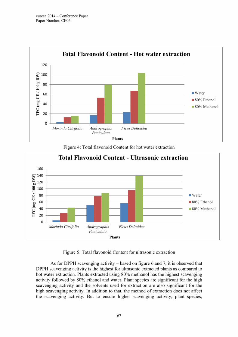
eureca 2014 – Conference Paper
Paper Number: CE06
67
Figure 4: Total flavonoid Content for hot water extraction
Figure 5: Total flavonoid Content for ultrasonic extraction
As for DPPH scavenging activity – based on figure 6 and 7, it is observed that
DPPH scavenging activity is the highest for ultrasonic extracted plants as compared to
hot water extraction. Plants extracted using 80% methanol has the highest scavenging
activity followed by 80% ethanol and water. Plant species are significant for the high
scavenging activity and the solvents used for extraction are also significant for the
high scavenging activity. In addition to that, the method of extraction does not affect
the scavenging activity. But to ensure higher scavenging activity, plant species,
0
20
40
60
80
100
120
Morinda Citrifolia Andrographis
Paniculata
Ficus Deltoidea
TF
C (
mg
CE
/ 1
00
g D
W)
Plants
Total Flavonoid Content - Hot water extraction
Water
80% Ethanol
80% Methanol
0
20
40
60
80
100
120
140
160
Morinda Citrifolia Andrographis
Paniculata
Ficus Deltoidea
TF
C (
mg
CE
/ 1
00
g D
W)
Plants
Total Flavonoid Content - Ultrasonic extraction
Water
80% Ethanol
80% Methanol

eureca 2014 – Conference Paper
Paper Number: CE06
68
solvents and method of extraction used to extract the plants are essential to achieve
high scavenging activity.
Figure 6: DPPH scavenging for hot water extraction
Figure 7: DPPH scavenging for ultrasonic extraction
From all the data measured, it is established that Ficus deltoidea is the best
among the three plant species to be used as a cure or a prevention supplement for
diabetes mellitus. It has the highest phenolic content - 401.15 mg GAE/100 g DW,
flavonoid content - 139.16 mg CE/100 g DW and DPPH scavenging activity - 91.91%
compared to Andrographis paniculata and Morinda citrifolia. Andrographis
paniculata has phenolic content of 154.03 mg GAE/100 g DW, flavonoid content of
0
10
20
30
40
50
60
70
80
90
100
Morinda Citrifolia Andrographis
Paniculata
Ficus Deltoidea
DP
PH
sca
ven
gin
g a
ctiv
ity
(%
)
Plants
DPPH Scavenging Activity -Hot water extraction
Water
80% Ethanol
80% Methanol
0
10
20
30
40
50
60
70
80
90
100
Morinda Citrifolia Andrographis
Paniculata
Ficus Deltoidea
DP
PH
sca
ven
gin
g a
cti
vit
y (
%)
Plants
DPPH Scavenging Activity - Ultrasonic extraction
Water
80% Ethanol
80% Methanol
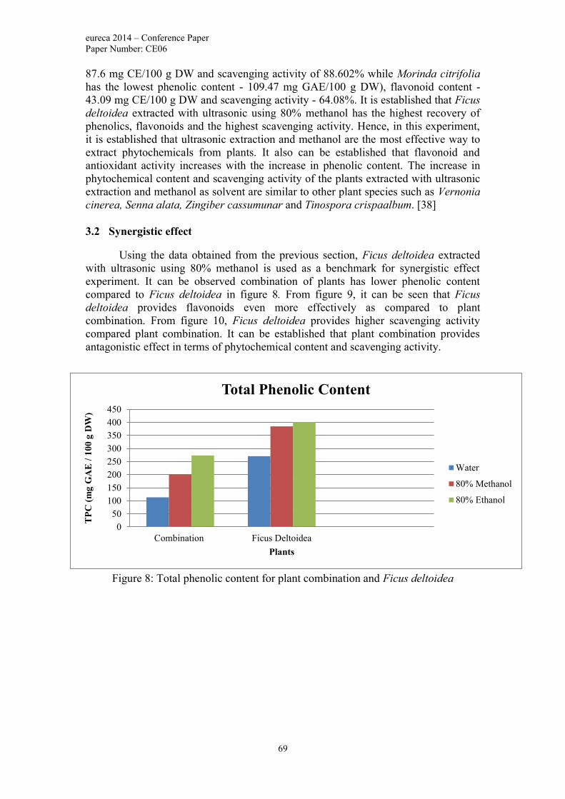
eureca 2014 – Conference Paper
Paper Number: CE06
69
87.6 mg CE/100 g DW and scavenging activity of 88.602% while Morinda citrifolia
has the lowest phenolic content - 109.47 mg GAE/100 g DW), flavonoid content -
43.09 mg CE/100 g DW and scavenging activity - 64.08%. It is established that Ficus
deltoidea extracted with ultrasonic using 80% methanol has the highest recovery of
phenolics, flavonoids and the highest scavenging activity. Hence, in this experiment,
it is established that ultrasonic extraction and methanol are the most effective way to
extract phytochemicals from plants. It also can be established that flavonoid and
antioxidant activity increases with the increase in phenolic content. The increase in
phytochemical content and scavenging activity of the plants extracted with ultrasonic
extraction and methanol as solvent are similar to other plant species such as Vernonia
cinerea, Senna alata, Zingiber cassumunar and Tinospora crispaalbum. [38]
3.2 Synergistic effect
Using the data obtained from the previous section, Ficus deltoidea extracted
with ultrasonic using 80% methanol is used as a benchmark for synergistic effect
experiment. It can be observed combination of plants has lower phenolic content
compared to Ficus deltoidea in figure 8. From figure 9, it can be seen that Ficus
deltoidea provides flavonoids even more effectively as compared to plant
combination. From figure 10, Ficus deltoidea provides higher scavenging activity
compared plant combination. It can be established that plant combination provides
antagonistic effect in terms of phytochemical content and scavenging activity.
Figure 8: Total phenolic content for plant combination and Ficus deltoidea
0
50
100
150
200
250
300
350
400
450
Combination Ficus Deltoidea
TP
C (
mg
GA
E /
10
0 g
DW
)
Plants
Total Phenolic Content
Water
80% Methanol
80% Ethanol

eureca 2014 – Conference Paper
Paper Number: CE06
70
Figure 9: Total flavonoid content for plant combination and Ficus deltoidea
Figure 10: DPPH scavenging for plant combination and Ficus deltoidea
For the solvents used for extraction, 80% methanol has the highest recovery of
phytochemicals and highest scavenging activity. Methanol has a polarity index of 5.1.
Methanol is an amphiphilic compound which consists of single atom of tetraedic
carbon which is connected to 3 hydrogen atoms and –OH group. –Oh group is the
polar group while the hydrogen atoms are the water insoluble hydrocarbon chain. Due
to its structure consisting of polar and non-polar groups, polar and non-polar
molecules can be dissolved in the methanol [40]. This makes methanol a better
solvent in extracting phytochemicals compared to ethanol and water. [41].
As for extraction method, it has to be understood that plant cells are enclosed
in cell wall. This primary cell wall is made up of tough material called cellulose [42].
Cellulose decomposes at 500℃ [43]. This cellulose can withstand high pressure [42].
While the secondary cell wall is made up of highly cross-linked phenolic molecules
[44]. High amount of force is needed to overcome the structure of the cell. Ultrasonic
waves create cavitations which grow in volume until it collapses [45]. This creates a
0
20
40
60
80
100
120
140
160
Combination Ficus Deltoidea
TF
C (
mg
CE
/ 1
00
g D
W)
Plants
Total Flavonoid Content
Water
80% Methanol
80% Ethanol
0
10
20
30
40
50
60
70
80
90
100
Combination Ficus Deltoidea
DP
PH
sca
ven
gin
g a
ctiv
ity
(%
)
Plants
DPPH Scavenging Activity
Water
80% Methanol
80% Ethanol

eureca 2014 – Conference Paper
Paper Number: CE06
71
strong force which is strong enough to rupture the cell wall of the plant cell. This
allows solvent diffusion into the cell thus increasing the contact surface area between
the cell contents and the solvent used for extraction [46].
For the study synergistic effect - combining Andrographis paniculata, Ficus
deltoidea and Morinda citrifolia provides negative synergistic effect. Plant
combination creates interaction between phenolics which is called co-pigmentation
reactions [47]. This creates more complex molecules [48]. With complex molecules
created, it allows polymerization to occur [47]. Significant changes to molecular
structures of the phenolics will affect the antioxidant capacity of the phenolic
compounds [49].It was suggested that hydrogen bonding occurs between the phenolic
compounds. This affects the ability of the hydroxyl group. This directly results in the
reduction of antioxidant activity of the phenolic compounds [50, 51].
3.3 Freeze drying
As Ficus deltoidea extracted using ultrasonic method with 80% methanol has
the highest scavenging activity overall, it is subjected to freeze drying. Based on
figure 8, it can be seen that scavenging activity has increased from 91.91% to 93.62%
after freeze drying. It has been established that freeze drying has a significant effect
on the scavenging activity. It proves that freeze drying can be a suitable preservation
method for plant extracts – preserving the phenolics and flavonoids of the plants.
Figure 11: Scavenging activity before and after freeze drying
3.4 HPLC Analysis
For HPLC analysis, flavonoid focused in this research is rutin. From HPLC
profile of Morinda citrifolia (retention time of 5.135 minutes), peak height of rutin of
54 is low compared to other flavonoids present in the plant extract. This applies to the
other two plant species – Andrographis paniculata and Ficus deltoidea. HPLC profile
of Andrographis paniculata shows no presence of rutin. This could be due to the
degradation of the plant extract. While for Ficus deltoidea, the HPLC profile shows
low traces of rutin in the extract (retention time of 4.921 minutes) with peak height of
91
91.5
92
92.5
93
93.5
94
Before After
DP
PH
sca
ven
gin
g a
ctiv
ity
(%
)
DPPH Scavenging Activity- Freeze Drying
80% Methanol

eureca 2014 – Conference Paper
Paper Number: CE06
72
60 compared to other flavonoids present in the plant extract. Although the amount of
rutin is low, it has a significant positive effect on the glucose homeostasis [59, 60].
Presence of rutin in supplements for diabetes would definitely help stabilise the
glucose level in human body along with other flavonoids. Ficus deltoidea has the
highest amount of rutin compared to the other two plant species.
Figure 10: HPLC profile of Morinda citrifolia
Figure 11: HPLC profile of Andrographis paniculata

eureca 2014 – Conference Paper
Paper Number: CE06
73
Figure 12: HPLC profile of Ficus deltoidea
3.5 Error analysis
Errors are inevitable in an experiment. In order to reduce random errors in the
study, replication is carried out. Extraction of each plant is carried out in triplicates in
order to increase accuracy. The phytochemical content and DPPH scavenging activity
also carried out in triplicates. Average of the value is then measured.
Systematic errors are present throughout the study. Weighing balance used in
the study is extremely sensitive. It has to be calibrated each time before using it. The
weighing balance responds to any vibrations around it making the values fluctuate.
Hence, the weighing balance is used carefully by keeping any source of vibration. In
addition to that, the UV spectrophotometer was used extensively in this study. The
UV spectrophotometer is calibrated using a blank sample. It was calibrated after each
measurement to ensure that the value is accurate. The auto zero option is used for
each measurement to reduce the systematic error. The linearity of standard curves is
affected by systematic error in this study. The equations obtained from standard
curves are not accurate as the value of R2 is not 1.
4. Conclusion
As a conclusion, the objectives of this study are to measure phenolic content,
flavonoid content and DPPH scavenging activity of Andrographis paniculata, Ficus
deltoidea and Morinda citrifolia. The extraction methods – hot water extraction
method and ultrasonic assisted extraction used are different to observe the efficiency
of each method in extracting the phytochemicals from the leaves. Different solvents
are used in this study to extract the leaves – 80% ethanol, 80% methanol and water.
From the study, it is found that the ultrasonic assisted extraction is a better method to
extract compared to hot water extraction. In addition to that, the best solvent to extract
the leaves would be 80% methanol. The best plant to use as a remedy for diabetes
among these three plants would Ficus deltoidea.
The finding from this study would be useful as the comparison is done for
three different plants and two different methods of extractions. The solvents used for
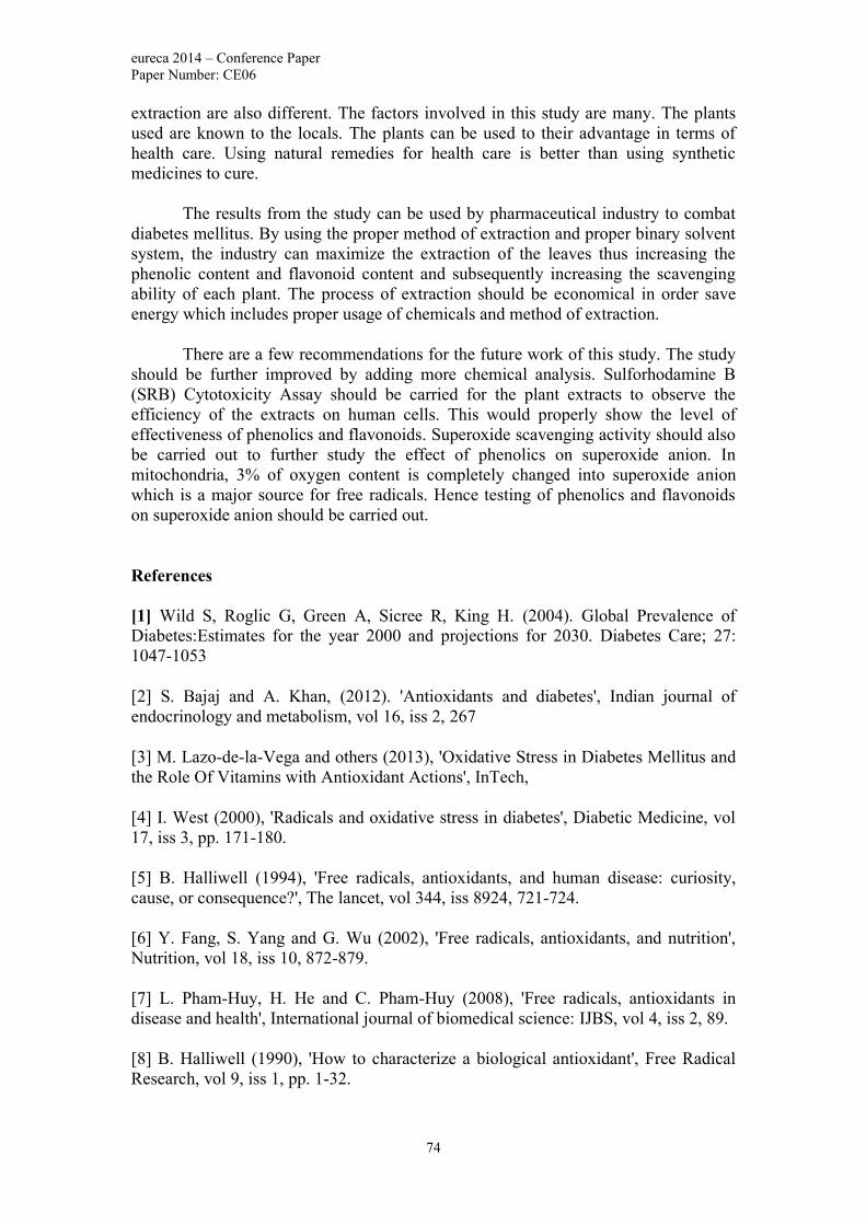
eureca 2014 – Conference Paper
Paper Number: CE06
74
extraction are also different. The factors involved in this study are many. The plants
used are known to the locals. The plants can be used to their advantage in terms of
health care. Using natural remedies for health care is better than using synthetic
medicines to cure.
The results from the study can be used by pharmaceutical industry to combat
diabetes mellitus. By using the proper method of extraction and proper binary solvent
system, the industry can maximize the extraction of the leaves thus increasing the
phenolic content and flavonoid content and subsequently increasing the scavenging
ability of each plant. The process of extraction should be economical in order save
energy which includes proper usage of chemicals and method of extraction.
There are a few recommendations for the future work of this study. The study
should be further improved by adding more chemical analysis. Sulforhodamine B
(SRB) Cytotoxicity Assay should be carried for the plant extracts to observe the
efficiency of the extracts on human cells. This would properly show the level of
effectiveness of phenolics and flavonoids. Superoxide scavenging activity should also
be carried out to further study the effect of phenolics on superoxide anion. In
mitochondria, 3% of oxygen content is completely changed into superoxide anion
which is a major source for free radicals. Hence testing of phenolics and flavonoids
on superoxide anion should be carried out.
References
[1] Wild S, Roglic G, Green A, Sicree R, King H. (2004). Global Prevalence of
Diabetes:Estimates for the year 2000 and projections for 2030. Diabetes Care; 27:
1047-1053
[2] S. Bajaj and A. Khan, (2012). 'Antioxidants and diabetes', Indian journal of
endocrinology and metabolism, vol 16, iss 2, 267
[3] M. Lazo-de-la-Vega and others (2013), 'Oxidative Stress in Diabetes Mellitus and
the Role Of Vitamins with Antioxidant Actions', InTech,
[4] I. West (2000), 'Radicals and oxidative stress in diabetes', Diabetic Medicine, vol
17, iss 3, pp. 171-180.
[5] B. Halliwell (1994), 'Free radicals, antioxidants, and human disease: curiosity,
cause, or consequence?', The lancet, vol 344, iss 8924, 721-724.
[6] Y. Fang, S. Yang and G. Wu (2002), 'Free radicals, antioxidants, and nutrition',
Nutrition, vol 18, iss 10, 872-879.
[7] L. Pham-Huy, H. He and C. Pham-Huy (2008), 'Free radicals, antioxidants in
disease and health', International journal of biomedical science: IJBS, vol 4, iss 2, 89.
[8] B. Halliwell (1990), 'How to characterize a biological antioxidant', Free Radical
Research, vol 9, iss 1, pp. 1-32.
eureca 2014 – Conference Paper
Paper Number: CE06
75
[9] Vaya and M. Aviram (2001), 'Nutritional antioxidants mechanisms of action,
analyses of activities and medical applications', Current Medicinal Chemistry-
Immunology, Endocrine \& Metabolic Agents, vol 1, iss 1,99-117.
[10] F. Chen, H. Xiong, J. Wang, X. Ding, G. Shu and Z. Mei (2013), 'Antidiabetic
effect of total flavonoids from Sanguis draxonis in type 2 diabetic rats', Journal of
ethnopharmacology, vol 149, iss 3,729-736.
[11] J. Kinsella, E. Frankel, B. German and J. Kanner (1993), 'Possible mechanisms
for the protective role of antioxidants in wine and plant foods.', Food technology.
[12] J. de la Fuente and S. Manzanaro (2003), 'Aldose reductase inhibitors from
natural sources', Nat. Prod. Rep., vol 20, iss 2, 243-251.
[13] P. Pietta and P. Mauri (2001), 'Analysis of flavonoids in medicinal plants.',
Methods in enzymology, vol 335,26.
[14] A. Negre-Salvayre, A. Affany, C. Hariton and R. Salvayre (1991), 'Additional
antilipoperoxidant activities of alpha-tocopherol and ascorbic acid on membrane-like
systems are potentiated by rutin', Pharmacology, vol 42, iss 5,262-272.
[15] I. Podmore, H. Griffiths, K. Herbert, N. Mistry, P. Mistry and J. Lunec (1998),
'Vitamin C exhibits pro-oxidant properties', Nature, vol 392, iss 6676, 559--559.
[16] C. Sulaiman and I. Balachandran (2012), 'Total phenolics and total flavonoids in
selected Indian medicinal plants', Indian journal of pharmaceutical sciences, vol 74,
iss 3, 258.
[17] J. B.Harborne and C. A Williams (2000) ,`Advances in flavonoid research since
1992', Phytochemistry, 55,481-504.
[18] G.Duthrie and A. Crozier (2000), `Plant-derived phenolic antioxidants', Current
Opinion in Clinical Nutrition and Metabolic Care, vol 3,447-451.
[19] H. Misbah, A. Aziz and N. Aminudin (2013), 'Antidiabetic and antioxidant
properties of Ficus deltoidea fruit extracts and fractions', BMC complementary and
alternative medicine, vol 13, iss 1,118.
[20] M. Manickam, M. Ramanathan, M. Farboodniay Jahromi, J. Chansouria and A.
Ray (1997), 'Antihyperglycemic activity of phenolics from Pterocarpus marsupium',
Journal of natural products, vol 60, iss 6, 609-610.
[21] S. Panda and A. Kar, 'Apigenin, (2007), (4 ‘, 5, 7-trihydroxyflavone) regulates
hyperglycaemia, thyroid dysfunction and lipid peroxidation in alloxan-induced
diabetic mice', Journal of Pharmacy and Pharmacology, vol 59, iss 11,1543-1548.
[22] B. Dineshkumar, A. Mitra and M. Mahadevappa (2011), 'Antidiabetic and
hypolipidemic effects of mahanimbine (carbazole alkaloid) from murraya koenigii
(rutaceae) leaves', International Journal of Phytomedicine, vol 2, iss 1.

eureca 2014 – Conference Paper
Paper Number: CE06
76
[23] E. Lulekal, E. Kelbessa, T. Bekele and H. Yineger (2008), 'An ethnobotanical
study of medicinal plants in Mana Angetu District, southeastern Ethiopia', Journal of
ethnobiology and Ethnomedicine, vol 4, iss 1, 10.
[24] M. Sharma and S. Joshi (2011), 'Comparison of anti-oxidant activity of
Andrographis paniculata and Tinospora cordifolia leaves', J Curr Chem Pharm Sc, vol
1,1-8.
[25] S. Wahid, T. Mahmud, M. Maziah, A. Yahya, M. Rahim and others, (2010),
'Total phenolics content and antioxidant activity of hot water extracts from dried
Ficus deltoidea leaves', J. Trop. Agric. and Fd. Sc, vol 38, iss 1,115-122.
[26] R. Pal, K. Girhepunje, N. Thirumoorthy and M. Hussain (2011), 'Antioxidant and
free radical scavenging activity of ethanolic extract of Morinda citrifolia', Annals of
Biological Research, vol 2, iss 1,127 – 131.
[27] S. Deshmukh, V. Wadegaonkar, R. Bhagat and P. Wadegaonkar (2011), 'Tissue
specific expression of Anthraquinones, flavonoids and phenolics in leaf, fruit and root
suspension cultures of Indian Mulberry (Morinda citrifola L.)', POJ, vol 4, iss 1,6-13.
[28] G. Spigno and D. De Faveri (2007), 'Antioxidants from grape stalks and marc:
Influence of extraction procedure on yield, purity and antioxidant power of the
extracts', Journal of Food Engineering, vol. 78, no. 3,793-801.
[29] R. Liu (2003), 'Health benefits of fruit and vegetables are from additive and
synergistic combinations of phytochemicals', The American journal of clinical
nutrition, vol 78, iss 3,517-520.
[30] M. Eberhardt, C. Lee and R. Liu (2000), 'Nutrition: Antioxidant activity of fresh
apples', Nature, vol 405, iss 6789, 903-904.
[31] N.Shofian, A. Hamid, A. Osman, N. Saari, F. Anwar, M. Pak Dek and M.
Hairuddin (2011), 'Effect of freeze-drying on the antioxidant compounds and
antioxidant activity of selected tropical fruits', International journal of molecular
sciences, vol 12, iss 7, 4678-4692.
[32] J. Vuthijumnok, A. Molan and J. Heyes, 'Effect of freeze-drying and extraction
solvents on the total phenolic contents, total flavonoids and antioxidant activity of
different Rabbiteye blueberry genotypes grown in New Zealand'.
[33] Medicalexpo.com, 'Medical ultrasonic bath / stainless steel - 90l |Sonica 90L S3 -
SOLTEC',2014.[Online].Available:http://www.medicalexpo.com/prod/soltec/medical
-ultrasonic-baths-stainless-steel-70126-576303.html. [Accessed: 07- Oct- 2014].
[34] C. Chong, C. Law, A. Figiel, A. Wojdyło and M. Oziemblowski. (2013), 'Colour,
phenolic content and antioxidant capacity of some fruits dehydrated by a combination
of different methods', Food chemistry, vol. 141, no. 4,3889-3896.
[35] N. Ozsoy, A. Can, R. Yanardag and N. Akev. (2008), 'Antioxidant activity of
Smilax excels L. leaf extracts', Food Chemistry, vol. 110, no. 3,571-583.

eureca 2014 – Conference Paper
Paper Number: CE06
77
[36] M. Shaperi (2014), 'Comparison of Different Methods for Extraction of Herb',
Undergraduate, Taylor's University.
[37] K. Saha, N. Lajis, D. Israf, A. Hamzah, S. Khozirah, S. Khamis and A. Syahida.
(2004), 'Evaluation of antioxidant and nitric oxide inhibitory activities of selected
Malaysian medicinal plants', Journal of Ethnopharmacology, vol. 92, no. 2, 263-267.
[38] W. Pukumpuang, 'Total phenolic contents, antibacterial and antioxidant activities
of some Thai medicinal plant extracts', J. Med. Plants Res., vol. 6, no. 36, 2012.
[39] S. Vimala, S. Rohana, A. Rashih and M. Juliza. (2012), 'Antioxidant Evaluation
in Malaysian Medicinal Plant: Persicaria minor (Huds.) Leaf', Science Journal of
Medicine and Clinical Trials.
[40] H. Ghaziaskar and N. Homayoun, 'Solubility of Gallic Acid in Methanol, Ethanol,
Water, and Ethyl Acetate', J. Chem. Eng. Data, vol. 53, no. 3, pp. 776-778, 2008.
[41] J. Eloff, 'Which extractant should be used for the screening and isolation of
antimicrobial components from plants?', Journal of Ethnopharmacology, vol. 60, no.
1, pp. 1-8, 1998.
[42] P. Dhonukshe, 'Cell polarity in plants', Communicative & Integrative Biology,
vol. 2, no. 2, pp. 184-190, 2009.
[43] Ccrc.uga.edu, 'Plant Cell Wall Basics', 2014. [Online]. Available:
http://www.ccrc.uga.edu/~mao/intro/ouline.htm. [Accessed: 07- Oct- 2014].
[44] Cellulose MSDS, 1st ed. Houston: ScienceLab, 2013, p. 1.
[45] Hielscher.com, 'Ultrasonic Extraction and Preservation', 2014. [Online].
Available: http://www.hielscher.com/extraction_01.htm. [Accessed: 07- Oct- 2014].
[46] D. Santos, R. Vardanega and M. De Almeida, 'Intensification of bioactive
compounds extraction from medicinal plants using ultrasonic
irradiation', Pharmacognosy Reviews, vol. 8, no. 16, p. 88, 2014.
[47] D. Pingret, A. Fabiano-Tixier and F. Chemat, 'An Improved Ultrasound
Clevenger for Extraction of Essential Oils', Food Anal. Methods, vol. 7, no. 1, pp. 9-
12, 2013.
[48] L. Jakobek, M. Šeruga and P. Krivak, 'The influence of interactions among
phenolic compounds on the antiradical activity of chokeberries ( Aronia
melanocarpa )', Int J Food Sci Nutr, vol. 62, no. 4, pp. 345-352, 2011.
[49] A. Castañeda-Ovando, M. Pacheco-Hernández, M. Páez-Hernández, J.
Rodríguez and C. Galán-Vidal, 'Chemical studies of anthocyanins: A review', Food
Chemistry, vol. 113, no. 4, pp. 859-871, 2009.

eureca 2014 – Conference Paper
Paper Number: CE06
78
[50] M. Pinelo, L. Manzocco, M. Nuñez and M. Nicoli, 'Interaction among Phenols in
Food Fortification: Negative Synergism on Antioxidant Capacity', Journal of
Agricultural and Food Chemistry, vol. 52, no. 5, pp. 1177-1180, 2004.
[51] M. Hidalgo, C. Sánchez-Moreno and S. de Pascual-Teresa, 'Flavonoid–flavonoid
interaction and its effect on their antioxidant activity', Food Chemistry, vol. 121, no. 3,
pp. 691-696, 2010.

eureca 2014 – Conference Paper
Paper Number: CE07
79
Treatment of Palm Oil Refinery
Effluent using Advanced Oxidation Process
Chooi San Lai1, Rajesh Rajasekaran
2*, Veena Doshi
3
1, 2*, 3 School of Engineering, Taylor’s University,
Subang Jaya, Selangor, Malaysia.
Abstract
Palm oil refinery effluent (PORE) is a type of wastewater that produces from palm oil
industries. High demand and constant production of refined palm oil in worldwide
cause the volume of PORE to be continuously increases. PORE has high level of
chemical oxygen demand (COD) and biochemical oxygen demand (BOD) due to the
presence of organic matters. These organic matters are harmful to environment such
as aquatic lives. Hence, it is essential to treat PORE before discharging it back to
environment. In this research, Advanced Oxidation Process is used to treat PORE to
reduce COD and BOD level as well as composition of organic matters. The treatment
method that is chosen is Fenton Process from Advanced Oxidation Process. For the
Fenton process, it uses two chemicals to produce hydroxyl radicals. Then, the
hydroxyl radicals produced that have high oxidizing power will break down the
organic matters presence in PORE. Thus, COD and BOD level of PORE is reduced
and safe to discharge back to environment thus reduce harmfulness to aquatic lives as
well. Besides Fenton process, physical treatment conducted for this research in order
to study the characteristic of organic matters in PORE. Physical treatment has been
conducted by only changing pH and temperature of raw PORE samples without
adding chemicals or Fenton reagent. The experiment samples also tested the COD and
BOD testing. As a result, 0.5M of Fenton reagent obtained highest reduction of
percentage of COD and BOD level which are 63.6% and 61.3% respectively.
Furthermore, COD and BOD level of PORE for pH treatment obtained highest
reduction at pH 7 which COD and BOD level is 37.5% and 34.9% respectively. Apart
from that, temperature treatment of obtained highest reduction at temperature of 80oC
which COD and BOD level of PORE is 25.6% and 23.1% respectively.
Keywords: Palm Oil Refinery Effluent (PORE), Wastewater Treatment, Advanced
Oxidation Process (AOP), Fenton Process, Hydroxyl Radicals.

EURECA 2014 – Conference Paper
Paper Number: CE07
80
1. Introduction
Malaysia is one of the largest palm oil producers in the world and palm oil
refinery effluent is the significant pollutants from the palm oil mill [1]. There were
approximately 60 million tonnes of palm oil refinery effluent (PORE) produced in
year 2010 [2]. High demand of palm oil from worldwide causes the increment of
PORE produced after the process. PORE is produced during the process of refinery of
palm oil. As a result, refined palm oil will be produced and PORE will be treated as
wastewater from the refinery process. PORE contains 95-96% of water, 4-5% of total
solids and 0.6-0.7% of oil [3]. PORE that produced from the refinery process contains
of oil and grease and suspended solids. There are traces of organic matters presence in
PORE. This is due to the chemicals that used during the refinery process. The COD
and BOD level of the suspension is high because of the presence of organic matters.
BOD stands for Biochemical Oxygen Demand and it measures the amount of oxygen
that needed by aerobic organisms in the water to degrade the organic matters whereas
for COD stands for Chemical Oxygen Demand and it measures amount of organic
compounds in the water [4]. BOD is used to measure the amount of oxygen that
required by microorganisms while stabilizing the organic matters that present in
PORE while COD measures oxygen equivalent of organic matters in PORE [4]. High
level of COD and BOD level could harm the aquatic lives. The high BOD and COD
level of PORE could cause death of the aquatic lives and hence ecosystem would be
imbalance. Thus, PORE has to be treated to achieve the standard of DOE before
discharging it to the environment.
There are several ways to treat the PORE such as biological treatment and
physical treatment as well as physical-chemical treatment. These types of treatments
aim to reduce COD and BOD level of PORE before discharging back to environment.
Wastewater treatment is important for the palm oil refinery process as the process is
ongoing for everyday. Hence, many types of treatment are proposed to treat PORE.
Currently, PORE is treated by using conventional method which is biological method.
The conventional treatment method needed microorganism to breakdown the organic
matters that contains in PORE. Since microorganisms are used, an optimum
environment must be created for the microorganism to grow. For instance,
temperature of the wastewater could not be higher than 30oC. Hence, wastewater has
to be cooled down to optimum temperature for microorganisms to grow before
starting the treatment. In addition, pH level of wastewater has to be maintained and
adjusted to the optimum level. It is to provide optimum and suitable environment for
the microorganisms to grow to decompose organic matters that presence in
wastewater. Besides, there will be time delayed on treatment when the
microorganisms are dead.
In this research, a chemical treatment has been chosen to treat PORE which is
Advanced Oxidation Process. There are many types of advanced oxidation process
such as Fenton process, Ozonation process, Hydrogen Peroxide Oxidation process,
Photocatalytic Oxidation process [5]. For this research, Fenton process from
Advanced Oxidation Process has been chosen to treat PORE. Fenton process was
discovered by H.J.H Fenton in year 1894 in and he stated hydrogen peroxide could
decompose by using iron salt to the form of hydroxyl radicals (*OH) to degrade
organic matters [6]. Currently, Fenton reagent is often used in wastewater that are
from several industries such as olive oil production industries and dye industries,
paper production industries, pharmaceutical industries [6,7]. Fenton reagent that used

EURECA 2014 – Conference Paper
Paper Number: CE07
81
in this research consists of iron (II) sulphate and hydrogen peroxide. Fenton reagent
generates OH radicals from hydrogen peroxide that have high oxidative power and it
obtains general organic pollutant abatement [6].
Then, iron (II) sulphate acts as the catalyst of the Fenton process which
catalyses and enhances the production of hydroxyl radicals. The rate of production of
OH radicals directly reflects to the duration of decomposition of organic matters in
wastewater. When the rate of production of hydroxyl radical is high, the duration
needed to decompose organic matters in wastewater would be shorter. Fenton process
that chosen in this research could be used at ambient temperature and pressure, hence
it is easy to conduct the experiments using Fenton reagent. However, PORE must be
maintained at pH 3 because the precipitation of ferric hydroxide will produced when
the Fenton reagent is operating at higher pH whereas iron complex ions will be
produced when it is operating at pH lower than pH 3 [6]. Overall, it is an effective
treatment in decomposing organic matters that are presence in the wastewater.
By applying Fenton Process to treat PORE, organic matters content in PORE
could be reduced before it discharges to the environment. Then, as the composition of
organic matters is reduced, COD and BOD levels of PORE will be reduced as well.
Thus, pollution of the water by PORE is expected to be minimised after treating
PORE with Fenton Reagent. In this research, experiments with different parameters of
Fenton Reagent were conducted in order to obtain optimum concentration of Fenton
Reagent for PORE treatment. Besides, physical treatments such as pH treatment and
temperature treatment also were conducted in order to compare with the results of
Fenton process. Furthermore, COD and BOD testing of samples are conducted to
determine the effectiveness of Fenton Reagent as well as the physical treatments of
PORE.
3. Research Methodology
3.1 Overall Research Design
This research is based on quantitative research. The main objective of this
research is to decompose organic matters in wastewater (PORE). Hence, initial and
final value of BOD and COD level in PORE will be determined. For physical
treatment, pH and temperature of raw PORE are changed in order to observe the
effect of pH and temperature change on raw PORE without adding Fenton reagent.
Whereas for the experiments of chemical treatment were conducting at ambient
temperature and pressure as well as maintained the pH of PORE at pH 3. By changing
the concentration of the Fenton Reagent, an optimum and suitable concentration of
reagent would be obtained to decompose the organic matters in PORE effectively.
3.2 Treatment Methods
3.2.1 Chemical Treatment
Chemical treatment is used to treat PORE in this research. The main chemicals
that use would be iron (II) sulphate and hydrogen peroxide. The preparation of Fenton
reagent was based on the selected ratio. In this project, the selected ratio for both
chemicals was 1:2 which indicates ratio of iron (II) sulphate: hydrogen peroxide
respectively. The calculation of required concentration of Fenton reagent is shown in
Equation (1):
EURECA 2014 – Conference Paper
Paper Number: CE07
82
𝑁𝑜. 𝑜𝑓 𝑚𝑜𝑙𝑒𝑠 = 𝑀𝑎𝑠𝑠 𝑜𝑓 𝑐ℎ𝑒𝑚𝑖𝑐𝑎𝑙
𝑀𝑜𝑙𝑒𝑐𝑢𝑙𝑎𝑟 𝑤𝑒𝑖𝑔ℎ𝑡 𝑜𝑓 𝑐ℎ𝑒𝑚𝑖𝑐𝑎𝑙 (1)
From the Equation 1, number of moles for the Fenton reagent was selected before
calculating the required mass for Fenton reagent. Then, mass of chemical indicates the
total mass of iron (II) sulphate and hydrogen peroxide and it was prepared based on
the selected ratio. Lastly, the molecular weight of chemical indicates total molecular
weight of Fenton reagent which is summation of molecular weight of iron (II)
sulphate and hydrogen peroxide.
After calculating the required mass of iron (II) sulphate and hydrogen
peroxide, Fenton process was then conducted. First, iron (II) sulphate was dissolve in
500ml of PORE sample. Then, pH of sample was adjusted to pH 3 with 0.1M of
sulphuric acid. After that, hydrogen peroxide was added into sample. The mixture was
then left for 30 minutes for the reaction between PORE and Fenton Reagent to be
completed. The experiments were conducted with 0.1M increment from 0.1-0.5M of
Fenton reagent. Then, each parameter was repeated until concurrence results were
obtained.
3.2.2 Physical Treatment
Physical treatment that use in this project was conducted by adjusting the pH
and temperature of PORE. This treatment was conducted with the absence of Fenton
reagent. In this treatment, pH range that use for experiments is from pH 2 to pH 10.
The difference of pH between each sample was 2. In this treatment, 0.01M of
sulphuric acid/sodium hydroxide was added into the raw sample in order to change
the pH of PORE. After final pH of raw PORE, COD and BOD testing were conducted.
Then, another batch of experiments will be conducted by changing
temperature of raw PORE. The range of temperature will be 20-100oC with 20
oC
difference for each sample. The sample of PORE will be heated to reach desired
temperature. After the heating process, samples will be used to conduct COD and
BOD tests as well.
3.3 Sample Testing
3.3.1 COD Testing
In this experiment, COD test was conducted to observe effectiveness of
Fenton Reagent and also physical treatment in decomposing organic matters in PORE.
The procedure of COD testing was referred to section 5220 C. Closed Reflux,
Titrimetric Method for COD from the Standard Methods for the Examination of
Water and Wastewater [8]. There were several reagents needed for this testing which
are standard potassium dichromate digestion solution, sulphuric acid reagent, ferrion
indicator solution, standard ferrous ammonium sulphate titrant (FAS). Thermoreactor
Type ECO 8 instrument was used for COD testing. This COD testing required a blank
sample for reference purposed. Blank sample needed distilled water as the sample of
testing. First step of the test was to wash the culture tube with 20% H2SO4, the aim
was to prevent any contamination of the culture tube [8]. Then, placed 2.5ml of
sample in culture tube and potassium dichromate digestion solution was added. After
that, 3.5ml of sulphuric acid reagent was added. Lastly, the testing tube was closed
and gentle mixing by inverting the tube for several times. For this testing, sample

EURECA 2014 – Conference Paper
Paper Number: CE07
83
heated to 150°C and left to reflux for two hours. Then, Ferroin indicator and FAS
were added to the sample for titration after it cools to room temperature. The
end point of titration was the colour changed of sample from blue-green to reddish
brown [8].
There are some precautions needed to take in account during the testing. Face
shield and glove was worn when handling the samples. The reason was there will be
some gases releases during the heating process of the samples. Besides, the samples
were heated to 150oC which required glove to protect hand when handling.
3.3.2 BOD Testing
For BOD test, it was referred to section 5210 B. 5-Day BOD Test from
Standard Methods for the Examination of Water and Wastewater [8]. The duration of
testing for BOD was five days for each sample. The model of instrument that use for
testing was Eutech Instrument (TN-100). Before conducting the test, the pH of sample
of PORE was determined. Then, it was adjusted to the optimum range of pH 7.0-7.2
and sulphuric acid or sodium hydroxide can be used to adjust the pH of the sample.
Besides, optimum temperature which samples needed adjust to the
temperature of 20 ± 3 °C [8]. After preparing the samples, BOD test was conducted.
The samples were diluted for experimental testing. First, 1ml of diluted sample added
into the bottle and dilution water will be added until the neck of bottle for further
dilution. Next, aluminium foil was used to wrap the solution bottle for incubation
purposed after gentle mixing. In this testing, blank solution which contains deionized
water was used as reference of BOD test. The procedure to prepare blank solutions
was identical as procedure to prepare BOD samples for PORE. Then, value of
Dissolved Oxygen (DO) of sample was measured from day-0 to day-5.
3.4 Data Analysis
For the data analysis, results of experiments as well as sample testing were
collected for further analysis. Each parameter was repeated until concurrence value of
results obtained. One of the main objectives of this project is to determine the
effectiveness of Fenton Reagent in decomposing organic matters. Hence, the data for
initial and final reading of the treated sample such as COD and BOD were recorded.
Then, all the results were tabulated in table forms in order to calculate the efficiency
of Fenton Reagent in decomposing organic matters. Besides, data of experiments for
physical treatment were recorded and tabulated in a graph as well.
4.0 Results and Discussion
4.1 Chemical Treatment
4.1.2 Fenton Process
Fenton Process is a type of Advanced Oxidation Process that utilizes iron (II)
sulphate and hydrogen peroxide to produce free radicals. The free radicals that
produce have high oxidizing power and it is an effective way to decompose organic
compounds due to the unselectively of the free radicals [5]. In this project, Fenton
process with different concentrations was chosen to treat PORE and the effectiveness
of Fenton reagent was determined as well. The effectiveness of Fenton reagent was
determined by the COD and BOD testing.

EURECA 2014 – Conference Paper
Paper Number: CE07
84
COD vs Concentration of Fenton Reagent
Concentration of Fenton Reagent (M)
0.0 0.1 0.2 0.3 0.4 0.5 0.6
CO
D (
mg/L
)
400
500
600
700
800
900
1000
4.1.2 pH of Fenton
There is a condition when conducting Fenton process for PORE which it has
to be adjusted at pH 3. The organic compounds removal efficiency decreases when
the pH level of Fenton process is higher than pH 4.0 and also when pH level is lower
than pH 3 [9]. Then, the outcome of this project research shows that percentage of
removal of organic compounds increases as the concentration of Fenton reagent
increases. This is because at different pH, production of hydroxyl radicals would be
affected as well. The hydroxyl radicals have oxidation potential of 1.8V and 2.7V
when it is at neutral pH and acidic solution respectively [10, 11]. However, when pH
of Fenton reagent is lower than pH 3, hydroxyl radicals will be scavenging by the
hydrogen ions. Hence, it causes the reduction in generation of hydroxyl radicals [12].
In addition, hydrogen peroxide will self-decompose when the pH of solution is higher
than pH 3 [13].
4.1.3 Concentration of Fenton Reagent
In this research, range of concentration of Fenton reagent was set at 0.1M to
0.5M with the difference of 0.1M for each testing. Table 1 shows the results for
Fenton process that conducted to treat PORE and the COD as well as BOD results are
expressed as mean value of the results.
Table 1. Results of PORE after treated with Fenton Reagent
Parameters Raw PORE Concentration of Fenton Reagent (M)
0.1 0.2 0.3 0.4 0.5
pH 5.76 3.00 3.00 3.00 3.00 3.00
COD (mg/L) 1408 960 832 704 640 512
BOD (mg/L) 1359 913 794 680 577 494
Figure 1: Results of COD level of PORE after Fenton Process Treatment with
standard deviation value

EURECA 2014 – Conference Paper
Paper Number: CE07
85
BOD vs Concentration of Fenton Reagent (M)
Concentration of Fenton Reagent (M)
0.0 0.1 0.2 0.3 0.4 0.5 0.6
BO
D (
mg/L
)
400
500
600
700
800
900
1000
Figure 2. Results of BOD level of PORE after Fenton Process Treatment with
standard deviation value
As refer to Table 1, it shows that the COD value and BOD for each sample are
reduced after the Fenton treatment. Form Table 1, 0.5M of Fenton reagent removed
highest amount of organic compounds in PORE. It reduced total of 896 mg/L of COD
and 865 mg/L of BOD level. The reason is because the hydroxyl radicals that
produced in 0.5M Fenton reagent is highest among the samples. Moreover, sample
that used 0.1M of Fenton reagent reduced the least amount of COD and BOD level.
From the data, it shows that sample react with 0.1M of Fenton reagent has only
removed 448 mg/L of COD level and 446 mg/L of BOD level.
Furthermore, Fig. 1 and Fig. 2 show the trend of COD and BOD reduction in
each sample after the treatment. The values of COD and BOD level were included the
respective standard deviation for Fig. 1 and Fig. 2. The standard deviation for COD
and BOD level is 11 mg/L and 10.5 mg/L respectively. The concentration of Fenton
reagent affects the outcome of treatment due to the hydroxyl radicals that produced
during the treatment process. At higher concentration of Fenton reagent, larger
amount of hydroxyl radicals could be produced for decompose the organic
compounds unselectively in PORE [6, 14]. Fenton reagent is effective in
decomposing organic compounds in PORE in which the effectiveness is measured by
obtaining reduction in COD and BOD level. Table 2 shows the percentage of
reduction of COD and BOD level in Fenton process with different concentration.

EURECA 2014 – Conference Paper
Paper Number: CE07
86
Table 2. Percentage of Reduction of COD and BOD level by Fenton Process
Percentage of Reduction (%) Concentration of Fenton Reagent (M)
0.1 0.2 0.3 0.4 0.5 COD (mg/L) 31.8 40.9 50 54.5 63.6 BOD (mg/L) 32.8 33.2 49.9 57.5 61.3
Figure 3. Percentage of Reduction of COD level in PORE
Figure 4. Percentage of Reduction of BOD level in PORE
As refer to Table 2, Fenton reagent that reduced highest amount of COD and
BOD level is 0.5M while 0.1M reduced the least amount of COD and BOD level.
From the data, 0.5M of Fenton reagent reduced 63.6% of COD level and 61.3% of
BOD level whereas 0.1M of Fenton reagent reduced 31.8% of COD level and 32.8%
of BOD level. Hence, the results of Fenton process have only approximately 60% of
COD and 35% of BOD reduction obtained respectively.
During the Fenton process, the reagent that reacted with organic compounds in
PORE would break down the organic compounds into carbon dioxide gas and water.
When the concentration of Fenton reagent is high, more carbon dioxide would be
Reduction of COD vs Concentration of Fenton Reagent
Concentration of Fenton Reagent (M)
0.0 0.1 0.2 0.3 0.4 0.5 0.6
Red
uct
ion o
f C
OD
lev
el (
%)
0
10
20
30
40
50
60
70
(b) Reduction of BOD vs Concentration of Fenton Reagent
Concentration of Fenton Reagent (M)
0.0 0.1 0.2 0.3 0.4 0.5 0.6
Red
uct
ion o
f B
OD
lev
el (
%)
30
35
40
45
50
55
60
65

EURECA 2014 – Conference Paper
Paper Number: CE07
87
produced during the experiment. There were bubbles formed and gas released during
the process due to the decomposition of organic compounds. The organic compounds
will be released carbon dioxide gas, water and salts will be formed after the treatment
[5, 6]. Furthermore, there was a layer of precipitate deposited at the bottom of the
beaker. The layer is iron salt which is a result from the decomposition of organic
compounds. The gas releases and salt formed indicates that COD and BOD level of
PORE reduced. The Fenton process is more effective when concentration is higher as
there were more available hydroxyl radicals that can attack the organic compounds
readily [9]. Hence, COD and BOD level of PORE would be reduced.
4.1.4 Effects of Concentration of Iron (II) Sulphate and Hydrogen Peroxide
There was some deposition of salts after the Fenton process that caused by the
high concentration of Fe2+
to produce Fe3+
(ferrous ions) which are less reactive
towards hydroxyl peroxide. Hence, the effectiveness of Fenton reagent would be
reduced. In addition, when the iron salts formed, it causes additional cost has to spend
in order to get rid of the iron sludge [15]. Thus, concentration of iron is important to
obtain effective Fenton Process. Besides, concentration of hydrogen peroxides is also
a crucial factor for the Fenton process. For instance, hydroxyl radicals that excess will
formed other structure with the organic compounds instead for decompose it [9]. As a
result, more research should be done to obtain better and more effective Fenton
process to decompose organic compounds in PORE.
4.2 Physical Treatment
Besides Fenton process, physical treatment also conducted in order to study
the characteristic of organic compounds in PORE. First, the organic compounds that
contains in PORE are mostly free fatty acids that obtained after the degumming
process from the refinery process of palm oil [16]. There are some saturated and
unsaturated fatty acids contain in PORE. The fatty acid sensitive towards pH and
temperature changes in which the bonds in fatty acid will be broken down and form a
new product.
In this research, pH and temperature treatment were conducted on PORE with
different range. After the treatment, COD and BOD level tests were conducted for the
results of physical treatment. Table 12 and Table 13 show the results of the physical
treatment.
Table 3. COD and BOD Results of pH Treatment
pH COD (mg/L) Percentage of Reduction (%)
BOD (mg/L)
Percentage of Reduction (%)
3.0 576 25 532 23 5.0 672 12.5 641 7.2 5.76 (RAW)
768 - 691 -
7.0 480 37.5 450 34.9 9.0 512 33.3 483 30.1
For the pH treatment, 0.1M of sulphuric acid and sodium hydroxide were used
to adjust the pH of the PORE. In this experiment, there was no Fenton reagent added
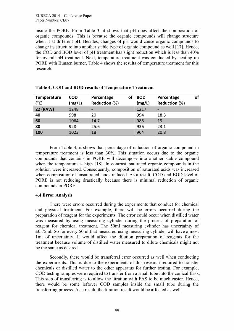
EURECA 2014 – Conference Paper
Paper Number: CE07
88
inside the PORE. From Table 3, it shows that pH does affect the composition of
organic compounds. This is because the organic compounds will change structure
when it at different pH. Besides, changes of pH would cause organic compounds to
change its structure into another stable type of organic compound as well [17]. Hence,
the COD and BOD level of pH treatment has slight reduction which is less than 40%
for overall pH treatment. Next, temperature treatment was conducted by heating up
PORE with Bunsen burner. Table 4 shows the results of temperature treatment for this
research.
Table 4. COD and BOD results of Temperature Treatment
Temperature (oC)
COD (mg/L)
Percentage of Reduction (%)
BOD (mg/L)
Percentage of Reduction (%)
22 (RAW) 1248 - 1217 - 40 998 20 994 18.3 60 1064 14.7 986 19 80 928 25.6 936 23.1 100 1023 18 964 20.8
From Table 4, it shows that percentage of reduction of organic compound in
temperature treatment is less than 30%. This situation occurs due to the organic
compounds that contains in PORE will decompose into another stable compound
when the temperature is high [18]. In contrast, saturated organic compounds in the
solution were increased. Consequently, composition of saturated acids was increased
when composition of unsaturated acids reduced. As a result, COD and BOD level of
PORE is not reducing drastically because there is minimal reduction of organic
compounds in PORE.
4.4 Error Analysis
There were errors occurred during the experiments that conduct for chemical
and physical treatment. For example, there will be errors occurred during the
preparation of reagent for the experiments. The error could occur when distilled water
was measured by using measuring cylinder during the process of preparation of
reagent for chemical treatment. The 50ml measuring cylinder has uncertainty of
±0.75ml. So for every 50ml that measured using measuring cylinder will have almost
1ml of uncertainty. It would affect the dilution preparation of reagents for the
treatment because volume of distilled water measured to dilute chemicals might not
be the same as desired.
Secondly, there would be transferral error occurred as well when conducting
the experiments. This is due to the experiments of this research required to transfer
chemicals or distilled water to the other apparatus for further testing. For example,
COD testing samples were required to transfer from a small tube into the conical flask.
This step of transferring is to allow the titration with FAS to be much easier. Hence,
there would be some leftover COD samples inside the small tube during the
transferring process. As a result, the titration result would be affected as well.

EURECA 2014 – Conference Paper
Paper Number: CE07
89
There is a way to minimise the errors that occurred during the experiments.
The way is to repeat the experiments until the concurrence values are obtained. Then,
all the apparatus and equipment used must be in good conditions such as no crack and
all the label or indications on the apparatus are cleared. Lastly, all the reagents that
used in treatments must be handled with care. It is to avoid contaminations happens to
the reagents that have been prepared for the experiments. The contamination of
reagents affects the final results of testing and hence reliability of final results of
treatments will be reduced. Overall, precautions have to be taken in to account in
order to minimize the errors that occur during the treatment process.
5.0 Conclusions
In a conclusion, the objectives of this research which are to treat PORE with 5
parameters of Fenton reagent to obtain at least 50% of reduction of COD and BOD
level as well as study the characteristics of organic compounds in the PORE were
achieved. The objectives of this research could be achieved due to deep study of
experiments and literature studies as well as methods of analysis have been completed.
It has been concluded that 0.5M of Fenton reagent has the highest efficiency of
reducing COD and BOD level of PORE as it reduced 63.6% and 61.3% of COD and
BOD level respectively. The percentage of reduction of COD and BOD level for
0.5M of Fenton reagent is the highest compared to the other parameters while the
0.1M of Fenton reagent has lowest of percentage of reduction of COD and BOD level.
For 0.1M of Fenton reagent, COD and BOD level that reduced was 31.8% and 32.8%
respectively. Besides, physical treatment that conducted experiments obtained
reduction of COD and BOD level as well. For pH treatment, the highest reduction of
COD and BOD level obtained at pH 7. And the result for percentage of reduction of
COD and BOD level is 37.5% and 34.9% respectively. While for temperature
treatment, the highest reduction of COD and BOD level obtained at temperature of
80oC. Then, the results of reduction of COD and BOD level for the parameter are 25.6%
and 23.1% respectively. The physical treatment reduced lower percentage of COD
and BOD due to the organic compounds in PORE was not decomposed fully. Instead,
some of the organic compounds changed structure to a more stable form in which
from unsaturated fatty acids to saturated acids. Overall, chemical treatment has higher
reduction of COD and BOD level because organic compounds in PORE were
decomposed fully during the Fenton process whereas organic compounds did not
decompose fully during physical treatment process which results in lower reduction in
COD and BOD level.
There is always room for improvement hence some recommendations are
recommended for the future work of this project. First recommendation is the
concentration of Fenton reagent could be fixed at wider range such as from 0.1 to
1.0M. The study about effectiveness of Fenton reagent could be done more
intensively with the help of wide range of Fenton reagent for chemical treatment.
Besides, the limitation of Fenton reagent could be studied as well by using wider
range of concentration. Furthermore, more testing could be done such as HPLC
testing in order to determine the content of PORE before and after the treatment and
effectiveness of Fenton reagent can be further study as well. Apart from that, more
research must be done to study to improve the mechanism of Fenton process on the
PORE in order to scale up the Fenton process for PORE treatment process in

EURECA 2014 – Conference Paper
Paper Number: CE07
90
industries scale. For instance, research on widen the range of pH required for Fenton
process as well as method for reduction of formation of iron sludge during the Fenton
process should be studied in order to optimized the Fenton process.
References
[1] M.M. Bello, M.M. Nourouzi, L. Chuah Abdullah, Thomas S.Y. Choong, Y.S.
Koay and S. Keshani, 2013. POME is Treated for Removal of Color from
Biologically Treated Pomein Fixed Bed Column: Applying Wavelet Neural Network
(WNN). Journal of Hazardous Materials 262 (2013), pp.106-113.
[2] M. Othman, M. Hassan, Y. Shirai, A. Baharuddin, A. Ali and J. Idris, 2014.
Treatment of Effluents from Palm Oil Mill Process to Achieve River Water Quality
for Reuse as Recycled Water in a Zero Emission System, Journal of Cleaner
Production, vol 67, pp. 58--61.
[3] A.R. Khalid and W.A.W. Mustafa, 1992. External Benefits of Environmental
Regulation: Resource Recovery And The Utilisation Of Effluents. Environmentalist
12, pp.277–285.
[4] A.H. Ibrahim, I. Dahlan, M.N. Adlan and A.F. Dasti, 2012. Comparative Study on
Characterization of Malaysian Palm Oil Mill Effluent. Research Journal of Chemical
Sciences, pp.3.
[5] R. Munter, 2001. Advanced Oxidation Processes-Current Status and Prospects.
Proc. Estonian Acad. Sci. Chem., 2001, 50,2. pp.59-80.
[6] A. Babuponnusami and K. Muthukumar, 2013. A Review on Fenton and
Improvements to the Fenton process for Wastewater Treatment. Journal of
Environmental Chemical Engineering 2(2013), pp.557-572.
[7] J.M. Orchando-Pulido, G. Hodaifa, M.D. Victor-Ortega, S. Rodriguez-Vives and
A. Martinez-Ferez, 2013. Reuse of Olive Mill Effluents from Two-Phase Extraction
Process by Integrated Advanced Oxidation and Reverse OsmosisTtreatment. Journal
of Hazardous Materials 263P (2013). pp.158-167.
[8] Franklin L. Burton and H.D. Stensel, 1991. Wastewater Engineering Treatment,
Disposal and Reuse., 3rd Edition. McGraw-Hill International Editions.
[9] X. Cao et al., 2014. 'Treatment of Tetrahydrofuran Wastewater by the Fenton
Process: Response Surface Methodology as an Optimization Tool', Water Science &
Technology, vol 695, pp. 1080-1087.
[10] Buxton, G.V., Greenstock, C.L., Helman, W.P., Ross, A.B., 1988. Critical review
of rate constants for reactions of hydrated electrons, hydrogen atoms, and hydroxyl
radicals (OH , O ) in aqueous solution. J. Phys. Chem. Ref. Data • •y 17, 513–780.
[11]T. El-Morsi, M. Emara, H. Abd El Bary, A. Abd-El-Aziz and K. Friesen,
'Homogeneous degradation of 1,2,9,10-tetrachlorodecane in aqueous solutions using
hydrogen peroxide, iron and UV light', Chemosphere, vol. 47, no. 3, pp. 343-348,
2002.
EURECA 2014 – Conference Paper
Paper Number: CE07
91
[12] Y. Samet, E. Hmani and R. Abdelhedi, 2012. Fenton and Solar Photo-Fenton
Processes for the Removal of Chlorpyrifos Insecticide in Wastewater. (2012). pp.537-
542.
[13] S. Sharma , J.P. Ruparelia and Manish L. Patel. 2011. A General Review on
Advanced Oxidation Processes for Waste Water Treatment. (2011). pp.1-6.
[14]S. Lin and C. Lo, 'Fenton process for treatment of desizing wastewater', Water
Research, vol. 31, no. 8, pp. 2050-2056, 1997.
[15] A.Cesaro et al., 2013. Wastewater Treatment by Combination of Advanced
Oxidation Processes and Conventional Biological Systems. J Bioremed Biodeg.
[16] P. Mfilinge, T. Meziane, Z. Bachok and M. Tsuchiya, 'Total Lipid and Fatty Acid
Classes in Decomposing Mangrove Leaves of Bruguiera gymnorrhiza and Kandelia
candel: Significance with respect to Lipid Input', J Oceanogr, vol. 61, no. 3, pp. 613-
622, 2005.
[17] Wolf, B. A,, Pasquale, S. M., and Turk, J. (1991) Biochemistry 30,6372-6379
SES, (1994). ‘The UV/Oxidation Handbook’. Solarcham environment system,
Markham, Ontario, Canada
[18]R. Pearcy, 'Effect of Growth Temperature on the Fatty Acid Composition of the
Leaf Lipids in Atriplex lentiformis (Torr.) Wats.', PLANT PHYSIOLOGY, vol. 61, no.
4, pp. 484-486, 1978
[19] M. N. Ahamad, M. Saleemullah, H.U Shah, Iqtidar A. Khalil and A.U.R. Saljoqi,
2007. Determination Of Beta Carotene Content In Fresh Vegetables Using High
Performance Liquid Chromatography, Vol. 23, No. 3, Pp. 767-770.
[20] Shahidi F, Naczk M., 2003. Phenolics in food and nutraceuticals. Boca Raton,
Fla, USA: CRC Press.
[21] M. Brebu and C. Vasile, 2010. Thermal Degradation of Lignin—a
review', Cellulose Chemistry & Technology, vol 44, iss 9, p. 353.
[22] T. Katterer, M. Reichstein, O. Andrien and A. Lomander, 1998. Temperature
Dependence of Organic Matter Decomposition: a Critical review usingLliterature
Data Analyzed with Different Models', Biology and fertility of soils, vol 27, iss 3, pp.
258--262.
[23] Mpob.gov.my, 'The Official Portal of Malaysian Palm Oil Board', 2014. [Online].
Available: http://www.mpob.gov.my/palm-info/environment/520-achievements.
[Accessed: 10- Oct- 2014].
[24] 'Organic Matter Content of Wastewater and Manure', Oklahoma Cooperative
Extension Fact Sheets, iss -1760, 2014
[25] M. Padda, , 2006. Phenolic Composition and Antioxidant Activity of
Sweetpotatoes [Ipomoea Batatas (L.) Lam].
[26] A. Toledano Zabaleta, 2014. Lignin Extraction, Purification and
Depolymerization study', Servicio Editorial de la Universidad del Paris Vasco/Euskal
Herriko Unibertsitatearen Argitalpen Zerbitzua.

EURECA 2014 – Conference Paper
Paper Number: CE07
92
[27] Oller, I., Malato, S. & Sanchez–Perez, J. A.2011 Combination of Advanced
Oxidation Processes and Biological Treatments for Wastewater Decontamination–a
review. Science of the Total Environment409 (20), 4141–4166.
[28] A. Bernal-Martinez et al., 2005. Combining Anaerobic Digestion and Ozonation
to Remove PAH from Urban Sludge', Process biochemistry, vol 40, iss 10, pp.
3244—3250.
[29] S. Esplugas, J. Gimenez, S. Contreras, E. Pascual and M. Rodriguez, 2002
'Comparison of Different Advanced Oxidation Processes for Phenol
Degradation', Water research, vol 36, iss 4, pp. 1034--1042.
[30] A. Wang, J. Qu, J. Ru, H. Liu and J. Ge, 2005. Mineralization of an Azo dye
Acid Red 14 by electro-Fenton's reagent using an Activated Carbon Fiber
Cathode, Dyes and Pigments, vol 65, iss 3, pp. 227—233.
[31] A. Heponiemi and U.Lassi, Advanced Oxidation Process in Food Industry
Wasterwater Treatement-A Review. (2012). pp.313-338.
[32] W. H. Glaze et al. The Chemistry of Water Treatment Processes involving Ozone,
Hydrogen Peroxide and UV-radiation. Ozone: Sci. Eng., 1987, 9, 335–352
[33] Liu, S. T., Huang, J., Ye, Y., Zhang, A. B., Pan, L. & Chen, X. G. Microwave
Enhanced Fenton Process for the Removal of Methylene Blue from Aqueous Solution.
Chemical Engineering Journal215–216, pp.586–590.
[34] M. Muruganandham and M. Swaminathan, 2004. Photochemical Oxidation of
Reactive Azo dye with UV-H2O2 process. Dyes and Pigments, vol. 62, no. 3, pp. 269–
275.
[35] P. K. Malick and S. K. SAHA, 2003. Oxidation of Direct Dyes with Hydrogen
Peroxide using Ferrous Ions as a Catalyst. Sep. Purif. Technol., v. 31, n. 3, p. 241-250.

EURECA 2014 – Conference Paper
Paper Number: CE08
93
Characterization and Theoretical
Modelling of DES Based Nano-Fluid
Mohamed Osama1, Rashmi G. Walvekar
1*, Kaveh Shahbaz
1
1Department of Chemical Engineering, Taylor’s University Lakeside Campus,
Malaysia. *Corresponding Author E-mail: [email protected]
Abstract- In this research, the stability of functionalized Graphene (Graphene Oxide)
nano-particles dispersed in, different deep eutectic solvents (by molar ratios) base
liquid composed of ethylene glycol as a hydrogen bond donor and methyl tri-phenyl
phosphonium bromide as a salt, at weight fractions of 0.01%, 0.02% and 0.05% was
studied and evaluated, quantitatively and qualitatively. This was done using zeta
potential analysis to assess the likelihood of settling and optical microscope to
observe the dispersion quality and evaluate the sizes of cluster at different weight
fractions. Along with this, the thermal conductivity data of the nano-fluid samples
measured at temperatures of 25 °C, 30 °C, 40 °C, 50 °C, 60 °C and 70 °C was
analyzed and compared with predictions of theoretical models. It was found generally
that classical models under-predicts the thermal performance of the nano-fluid
samples. Moving-particles model namely Rashmi and Kumar models showed
conflicting prediction performance. While, Rashmi model can predict thermal
conductivity at some temperatures with errors as low as 0.1%, the Kumar model
lowest error is found to be around 10% and the highest error is around 56%. A simple
empirical modification to the Kumar model is presented which improves the
predictions accuracy to that of Rashmi model.
Keywords: Nano-Fluid, DES, Graphene Oxide, Thermal Conductivity, Viscosity.

EURECA 2014 – Conference Paper
Paper Number: CE08
94
1. Introduction
Fluids are used as heat carriers in heat transfer systems in many chemical and
process industries. The increase of efficiency of these heat transfer systems is strongly
related to the thermal conductivity of the heat carrier fluid. It is well known that the
suspension of solid particles in a liquid improves the thermo-physical properties such
as thermal conductivity of the host fluid. The nano-particles suspension is favored due
to their smaller size which overcomes clogging and sedimentation-prone issues
associated with micro-sized particles [1]. Fluids in which nano-particles are dispersed
are known as nano-fluids, a name which was coined by Choi in 1995 [2]. Though, as
time elapses, nano-particles are prone to self-agglomeration due to their high surface
energy. The agglomerates size can be as large as micro-sized particles. These large
agglomerates are prone to sedimentation which lowers the enhancement of thermo-
physical properties [3]. Therefore, the stability of the nano-particles suspension is
very critical in evaluating the thermal performance and efficiency of nano-fluids. The
suspension can be stabilized through the use of additives such as surfactants, chemical
functionalization, homogenization, sonication and many other techniques [3].
However, the use of additives affects the thermo-physical properties of the nano-fluid.
Another route to stabilize the nano-particles suspension is to rely on vibration and
mechanical means. Nevertheless, agglomerates will form again as the time elapses [4].
Therefore, vibrations and mechanical techniques deal with symptoms by breaking
agglomeration rather than addressing the root causes and eliminating them to prevent
the formation of agglomerates.
Traditionally, the nano-fluid preparation has been researched on conventional
heat carriers such as water and synthetic oil. Adding to their low thermal performance,
the stability of nano-suspension in these base fluids is rather limited to the use of
additives. New class of fluids has emerged known as ionic liquid which has thermo-
physical properties far superior to conventional liquids. It is reported that nano-
particles such as graphene and multi-walled carbon nano-tubes can be dispersed in
ionic liquids without the use of surfactants [3]. Unfortunately, many reports have
pointed out the hazardous toxicity of ionic liquids along with their expensive
synthesis [5]. This has led to the emergence of deep eutectic solvents (DES) which are
far more environmentally friendly owing to their biodegradability and non-toxicity.
Along with that, their synthesis is far cheaper and exhibit similar thermo-physical
properties as ionic liquids [5]. This novel class of fluids can be very promising to
resolve issues related to the stability of nano-particles suspension. Along with that, the
graphene nano-particles have very high thermal conductivity. Therefore, the
combination of DES with graphene nano-particles to produce DES based graphene
nano-fluid is very promising. In this research, a DES based nano-fluid is produced
using grapehene oxide as nano-particles. The produced nano-fluid is characterized
qualitative and quantitatively to assess the stability and the dispersion quality.
Furthermore, the thermal conductivity data of the DES based fluid used in this
research is analyzed, evaluated and compared with predictions obtained from
available theoretical models.

EURECA 2014 – Conference Paper
Paper Number: CE08
95
2.0 Experimental Procedure
2.1 Chemical
Ethylene glycol and methyl tri-phenyl phosphonium bromide (MTBP) which
were used in the DES sysnthesis were obatianed from Merck Millipore at a high
purity of > 99%. The DESs were prepared at molar ratios of 3:1, 4:1 and 5:1 of
ethylene glycol to MTBP respectively. The graphene nano-particles were purchased
from the Graphene Supermarket, United States with high purity of 98%. The graphene
nano-powder has an average thickness of 60 nm and a particle size in the range of 3 –
7 microns.
2.2 Analytical and Measuring Instruments
In this research, the Zetasizer Nano device (from Malvern Instruments) was
used to characterize the stability of the samples by means of measuring the zeta
potential. The Swift M10D Series Digital Microscope was used to characterize the
dispersion quality of the graphene oxide nano-particles in DES based nano-fluid. The
used thermal conductivity data was measured at different temperatures using KD 2
Pro.
3.2 DES and Nano-Fluids synthesis
In this research graphene nano-particles were dispersed in DES base fluid.
DES samples with one salt namely methyl triphenyl phosphonium bromide (MTPB)
is to be obtained. MTPB is combined with a hydrogen bond donor (HBD) namely,
ethylene glycol in different molar ratios of salt:HBD to produce different DESs. The
DES base fluids are to be prepared by mixing the salt with the HBDs in the prescribe
molar ratios by a magnetic stirrer at a temperature of 353.15 K and a high rpm until a
homogenous and colorless liquid is observed [8]. The rpm value was increased until
high vortex was observed. The rpm value which creates vortex is inversely
proportional to the size of the magnetic bar.
The GO nano-particles were dispersed at low weigh fraction of graphene
nano-particles. Wang et al [9] stated that at weight fractions up to 0.09%, the
graphene Ion-Nano-fluid will not be stable and will coagulate in a couple of hours. In
their study, the weight fraction of the graphene nano-particles is restricted to the range
of 0.03% - 0.06%. In this study, 0.01%, 0.02% and 0.05% weight fractions are used.
These weight fractions are similar to that used by Wang et al, and this will make the
comparison between the results of the two studies possible and more meaningful. The
suspensions then were homogenized using direct probe sonication for 15 minutes
using (Branson, SLP-T model). This was followed by water-bath sonication at room
temperature for 1 hour using (Elma, ELmasonic-P). (Table 2) shows the composition
of DES, GO weight concentrations and the designation for the samples which are used
in this research.

EURECA 2014 – Conference Paper
Paper Number: CE08
96
Table 1. DES and Nano-Fluid Sample Details
(HBD)
(Salt)
Molar Ratio
(HBD/Salt) DES Sample NF Sample
GO
Wt%
Ethylene
glycol MTPB
3 DES 1
GNF1 0.01
GNF 2 0.02
GNF3 0.05
4 DES 2
GNF 4 0.01
GNf 5 0.02
GNF 6 0.05
5 DES 3
GNF 7 0.01
GNF 8 0.02
GNF 9 0.05
2.4 Thermal Conductivity Measurements
The thermal conductivity was measured using thermal properties analyzer
KD-2 Pro. Calibration was done using standard glycerin to inspect the accuracy of the
probe. A water-bath was used to heat and maintain the nano-fluid samples at different
temperature. Three readings were taken at each temperature for each sample. Average
values were used to represent the thermal conductivity of the DES based nano-fluid.
The readings were taken at temperatures of 25 °C, 30 °C, 40 °C, 50 °C, 60 °C and
70 °C. The measured thermal conductivities were compared with those computed or
predicted using the theoretical models in Table 1. This allows evaluating how well the
existing theoretical models predict the behavior of DES based nano-fluid.
3. Methodology and Data
3.1 Thermal Conductivity Models
Table 1 shows the thermal conductivity models which are used in this research.
The parameters of these models are volume fraction ϕ, thermal conductivity
coefficient k of the nano-particle and the base fluid, l particle length, d particle
diameter, r particle radius and μ fluid viscosity. The terms n, C and T0 are constants.
The models were selected based on the parameters accessibility through experimental
measurements. The subscripts eff, bf, p refer to the effective property of nano-fluid,
base-fluid and nano-particles respectively. The symbol kB represents the Boltzmann
constant The term classification in the right side of the Table 1 shows the basis
mechanism based on which the model was derived. The classical models are derived
based on the assumption of motionless particles [6]. The Rashmi model is derived
from Patel’s model [7]. The model was modified to suit application to nano-tube
shaped particles. Moreover, the liquid is assumed to be spherical in shape.
The ability of the classical models to predict the thermal conductivity of DES
based nano-fluid was examined using the thermal conductivity data obtained at room
temperature. For Rashmi’s and Kumar’s model, the ability for these two models to
predict the behaviour of DES based nano-fluid was examined for all the temperatures

EURECA 2014 – Conference Paper
Paper Number: CE08
97
since both models are temperature and volume fractions dependant. The two models
were attempted to be fitted with the experimental data and the quality of the resulting
plot indicated how well each model predicts the behaviour of DES based nano-fluids.
This was done by the grouping the unknown sub-variables and constants into one
main variable. Accordingly, the Rashmi and Kumar models were simplified to the
form shown in Equations 3.2 and 3.3, respectively.
keff = kf +kp∅ C0
(1−∅)+ C1∅ (T − T0)
keff = kf +∅
(1−∅) T C0
In this paper, the author suggests an empirical modification for the Kumar
model to include a power variable which controls the volume fraction term in the
Kumar model. The inclusion of this variable into Kumar model was found to increase
the predictions accuracy for the thermal behaviour of the particular DES based nano-
fluid that this research is based on. Equation (3.4) shows the modification made to
the Kumar model.
keff = kf + (∅
(1 − ∅))
n
T C0
Table 2. Thermal Conductivity Models
Ref Model Name & Formulation Classification
[6]
Maxwell 𝒌𝒆𝒇𝒇 = [𝒌𝒑 + 𝟐𝒌𝒃𝒇 + 𝟐(𝒌𝒑 − 𝒌𝒃𝒇)𝝓
𝒌𝒑 + 𝟐𝒌𝒃𝒇 − (𝒌𝒑 − 𝒌𝒃𝒇)𝝓] 𝒌𝒃𝒇
Classical
Hamilton and
Crosser
𝒌𝒆𝒇𝒇 = [𝒌𝒑 + (𝒏 − 𝟏)𝒌𝒃𝒇 − (𝒏 − 𝟏)(𝒌𝒃𝒇 − 𝒌𝒑)𝝓
𝒌𝒑 + (𝒏 − 𝟏)𝒌𝒃𝒇 + (𝒌𝒃𝒇 − 𝒌𝒑)𝝓] 𝒌𝒃𝒇
Jeffrey
𝒌𝒆𝒇𝒇 = [𝟏 + 𝟑𝜷𝝓 + 𝝓𝟐 (𝟑𝜷𝟐 +𝟑𝜷𝟑
𝟒+
𝟗𝜷𝟑
𝟏𝟔
𝝌 + 𝟐
𝟐𝝌 + 𝟑
+𝟑𝜷𝟒
𝟐𝟔+ ⋯ )] 𝒌𝒃𝒇
Bruggeman
𝝓 (𝒌𝒑 − 𝒌𝒆𝒇𝒇
𝒌𝒑 + 𝟐𝒌𝒆𝒇𝒇) + (𝟏 − 𝝓) (
𝒌𝒃𝒇 − 𝒌𝒆𝒇𝒇
𝒌𝒃𝒇 + 𝟐𝒌𝒆𝒇𝒇) = 𝟎
[7] Rashmi
𝒌𝒆𝒇𝒇 = 𝒌𝒃𝒇 [𝟏 +𝒌𝒑
𝟐𝝓(𝒓𝒑+𝒍𝒑)
𝒓𝒑𝒍𝒑
𝒌𝒃𝒇 (𝟑(𝟏−𝝓)
𝒓𝒃𝒇)
] +𝑪𝝓(𝑻 − 𝑻𝟎)
𝒓𝒃𝒇𝟐 𝒍𝒃𝒇
𝟐 𝝁𝒃𝒇
𝐥𝐧 (𝒍𝒑
𝒅𝒑)
Carbon
Nano-Tube
[8] Kumar 𝒌𝒆𝒇𝒇 = 𝒌𝒃𝒇 + 𝒄𝟐 𝒌𝒑𝑻
𝝅𝝁𝒅𝒑𝟐
𝝓 𝒓𝒃𝒇
(𝟏 − 𝝓)
Brownian
Motion
(1)
(2)
(3)

EURECA 2014 – Conference Paper
Paper Number: CE08
98
4. Reported Outcomes
4.2 Zeta Potential Analysis
The zeta potential analysis was performed for nano-fluid samples GNF 4,
GNF 5 and GNF 6. The zeta potential values for the aforementioned nano-fluid
samples were found to generally show an average zeta potential value of 25 mv which
indicates a moderate stability [9]. Fig 1 shows a scatter plot for the zeta potential
values for the tested nano-samples.
Figure 1. Zeta Potential Values
It can be seen from Fig 1 that the zeta potential value is highest for GNF 6 and
lowest for GNF 4. The result indicates that at weight fractions of 0.01% and 0.05%,
the stability is higher compared to in-between weight fraction of 0.02%. Moreover,
the zeta potential value for GNF 24 falls in the region of good stability. The zeta
values of GNF 5 and GNF 6 fall in the region of good stability with the zeta value of
GNF 4 being closer to the area of moderate stability and GNF 5 being closer to the
area of some stability with light settling. It is to be noted that these readings have been
taken after a period of about 3 – 4 months. This shows a high stability for DES based
nano-fluids, moreover zeta potential values for fresh samples prepared under the same
conditions are more likely to show higher zeta potential values judging from the
results shown in Fig 1.
4.2 Optical Microscope Results
Fig 2 shows the dispersion for nano-fluid samples GNF 2 as captured using
40X magnification lens. It can be seen that there is generally a good dispersion of the
graphene oxide nano-particles (GONPs) in the DES base fluid. Optical measurements
were taken of the clusters observed in each sample. It is to be noted that since this is a
normal light microscope, the measurements do not give an exact and accurate sizes of

EURECA 2014 – Conference Paper
Paper Number: CE08
99
the cluster in the nano-fluid samples, however it can give an impression or qualitative
assessments of the cluster sizes in each nano-fluid sample. In this paper, the cluster
sizes are measured and represented by the length size as observed and measured using
the optical microscope. In Fig 3, a plot shows the average extent of the cluster size for
each samples based on the cluster length.
Figure 2. Optical Micrograph of GNF 2
Figure 3. Cluster Size as Measured Using 40X Magnification
4.6 Thermal Conductivity Models Analysis
4.6.1 Classical Models
The classical models were found to have the same prediction for the thermal
conductivity of the DES based nano-fluid. The classical models at room temperature
generally under-predicted the actual performance of the DES based nano-fluid
samples except for samples GNF 7 and GNF 9. The prediction errors or deviation of

EURECA 2014 – Conference Paper
Paper Number: CE08
100
the classical models is shown in Table 2. The errors for samples GNF 7 and GNF 9 is
quite low which shows that DES 3 based nano-fluid samples do not generally exhibit
superior enhancements of thermal conductivity at room temperature as when
compared with DES 1 based nano-fluid samples.
Table 2. Classical Model Percentage Errors
Sample Error%
GNF 1 -22
GNF 2 -25
GNF 3 -31
GNF 7 3
GNF 8 19
GNF 9 -2.5
4.6.2 Moving Particles Models
Fig 4 shows the errors of predictions of Kumar model, Rashmi model and the
Kumar modified model for thermal conductivity data at temperature of 50 °C. It can
be seen from Fig 4 that the empirically modified Kumar model has the smallest errors
as when compared with the other two models. Rashmi model has comparable small
deviation as well, but for the pure Kumar model the deviation is relatively large. It is
to be noted that the quality of predicting the thermal performance of DES based nano-
fluid under research depends on the surrounding temperature and the molar ratio of
HBD to salt. Generally, the Rashmi model was found to predict the thermal
conductivity of DES 3 better at temperatures of 30 and 60 °C.
Figure 4. Prediction Accuracy of Brownian-Motion Models At T = 50 °C

EURECA 2014 – Conference Paper
Paper Number: CE08
101
6. Conclusions
The DES based nano-fluid was prepared at different molar ratios of the HBD
and the salt. The zeta potential values and optical micrographs indicate a good
stability and uniform dispersion. The classical models were found to under-predict the
actual performance of the DES based nano-fluid. Generally DES 1 exhibit superior
performance at room temperature meanwhile the enhancement of DES 3 at room
temperature is less significant. The Rashmi and the modified Kumar show better
prediction of the thermal performance of DES based nano-fluid.
References
[1] S. U. S. Choi and J. A. Eastman. (1995). Enhancing thermal conductivity of
fluids with nanoparticles.
[2] S. C. Robert Taylor, Todd Otanicar, Patrick Phelan, Andrey Gunawan, Wei
Lv, Gary Rosengarten, Ravi Prasher and Himanshu Tyagi. (2012). Critical
Review of the Novel Applications and Uses of Nanofluids. Paper presented at
the ASME 2012 Third International Conference on Micro/Nanoscale Heat and
Mass Transfer, Atlanta, Georgia, USA.
[3] F. Wang, L. Han, Z. Zhang, X. Fang, J. Shi, and W. Ma. (2012). Surfactant-
free ionic liquid-based nanofluids with remarkable thermal conductivity
enhancement at very low loading of graphene. Nanoscale Research Letters,
vol. 7, p. 314.
[4] M. M. Kostic. (2006). Critical Issues and Application Potentials in Nanofluids
Research. Paper presented at the ASME Multifunctional Nanocomposites
International Conference, Honolulu, Hawaii, USA.
[5] Q. Zhang, K. De Oliveira Vigier, S. Royer, and F. Jerome. (2012). Deep
eutectic solvents: syntheses, properties and applications,. Chemical Society
Reviews, vol. 41, pp. 7108-7146.
[6] J.-H. Lee, S.-H. Lee, C. Choi, S. Jang, and S. Choi. (2010). A Review of
Thermal Conductivity Data, Mechanisms and Models for Nanofluids.
International Journal of Micro-Nano Scale Transport, vol. 1, pp. 269-322.
[7] W. Rashmi, A. F. Ismail, I. Sopyan, A. T. Jameel, F. Yusof, M. Khalid, et al.
(Dec 2011). Stability and thermal conductivity enhancement of carbon
nanotube nanofluid using gum arabic. Journal of Experimental Nanoscience,
vol. 6, pp. 567-579.
[8] D. H. Kumar, H. E. Patel, V. R. R. Kumar, T. Sundararajan, T. Pradeep, and S.
K. Das, "Model for Heat Conduction in Nanofluids," Physical Review Letters,
vol. 93, p. 144301, 09/27/ 2004.
[9] K. Shahbaz, F. S. Mjalli, M. A. Hashim, and I. M. AlNashef. (June 2011).
Using Deep Eutectic Solvents Based on Methyl Triphenyl Phosphunium
Bromide for the Removal of Glycerol from Palm-Oil-Based Biodiesel. Energy
& Fuels, vol. 25, pp. 2671-2678.

eureca 2014 – Conference Paper
Paper Number: CE09
102
Fractionation of Sugar from Hydrolysis
of Pretreated Cellulose by Ultrafiltration
and Reuse of Enzyme.
Nguyen Huynh Thao Thy1*
, Rajesh Rajasekaran1, Masniroszaime Md Zain
1
1Department of Chemical Engineering, Taylor’s University, Malaysia
Abstract
Bioethanol process using cellulosic materials have been emerging a interesting field
with a high potential of replacing petroleum-based fuel, as a future alternative. This
work emphasized on improvement of enzymatic hydrolysis of alkaline NaOH-
pretreatment cellulose by applying ultrafiltration membrane 10 kDa cutoff in order to
minimise sugar inhibition on enzymes, reuse enzyme in hydrolysis and recover sugar
for subsequent fermentation. An improvement in the methodology of enzymatic
hydrolysis with ultrafiltration was made that the membrane was installed at the end of
tube connecting with a peristaltic pump to continuously remove glucose from
hydrolysis reaction hence sugar was unable to inhibit enzyme activity and enzyme
was retained inside reactor for reusing purpose. The combination of NaOH 1M
alkaline pretreatment, enzymatic hydrolysis of cellulose with the optimum 3%
enzyme dosage, ultrafiltration 10 kDa cutoff was evaluated to obtain the highest
sugar concentration at 266mg/ml after 6 hour hydrolysis. In comparison between
hydrolysis with ultrafiltration and hydrolysis without ultrafiltration, the sugar
concentration in hydrolysis with ultrafiltration was very much higher than that in
hydrolysis without ultrafiltration in all enzyme dosages (1.5%, 3%, 6%). The
hydrolysis with filtration produced time a profile in six hours with continuously
significant increase in sugar concentration. Only a small reduction initially for 1.5%
dosage and no reduction in sugar concentration in 3% and 6% dosage. Hence the
effect of product inhibition in hydrolysis was minimized subsequently. In addition, a
direct relationship between sugar concentration inside hydrolysis reactor, enzyme
dosage and rate of sugar removal was observed during the hydrolysis process. Higher
enzyme dosage in hydrolysis required a higher rate of sugar removal sufficient to
avoid inhibition in hydrolysis reaction.
Keywords: enzymatic hydrolysis of cellulose, product inhibition, ultrafiltration, reuse
of enzyme cellulase, alkaline pretreatment, Cellic Ctec enzymes.

eureca 2014 – Conference Paper
Paper Number: CE09
103
1. Introduction
Technology of cellulose-based ethanol production has been continuously
advanced over the past decades with progressive efforts of making the process more
cost-effective and reachable for large-scale industrial production. Hence, nowadays
bioethanol is considered as a very potential alternate to conventional fossil fuel usage
causing environmental concerns such as green-house effects and global warming.
Feedstock containing cellulose to produce bioethanol comes from two main sources,
i.e., the first generation (sugar, and starch like corn, wheat, soya, and grains) and the
second generation (agricultural crop residues like palm empty fruit bunches, sugar
bagasse and corn stovers). However, it was discussed that the first generation
feedstock causes a dilemma and a debatable issue on food versus fuel due to its
negative impacts on regional water source, biodiversity, soil quality [1, 2, 3, 4, 5]. In
contrast, the second generation feedstock from non-food source is able to avoid such
issues and create a newly environmental-friendly way to reuse cellulosic biomass by
producing a value-added ethanol product.
The production of bioethanol from cellulose consists of sub-processes namely
a) pretreatment of cellulose for more susceptibility as well as increase in enzymatic
accessibility, b) hydrolysis of cellulose to sugar, c) fermentation of sugar to ethanol to
subsequent product purification. Research and development have been on the progress
to manage and optimize these sub-process in order to improve its both technological
and economic feasibilities [6]. Pretreatment of cellulose plays an important role,
which had an impact on hydrolysis later. Without pretreatment, only 20% out of total
cellulose are converted to glucose [17]. This is due to the reason that the recalcitrant
structure of cellulose was disrupted, results in an decrease in degree of
polymorerization. Hence cellulose after pretreatment is more susceptible and
accessible for enzyme to hydrolyze. [18]. Methods of pretreatment are various and
depends on the economic factor, type of feedstock, severity degree and so on. Unlike
acid pretreatment causing a severe corrosion on equipment and generating undesirable
inhibiting byproducts, alkaline pretreatment is safer to use, minimize corrosion and
more preferable in the industry of bioethanol production [15, 16]. In addition,
hydrolysis by using enzymes named cellulases is more preferable in cellulosic
bioethanol process due to its advantages in term of lower energy consumption, limited
formation of inhibiting byproducts in subsequent fermentation, high sugar yield,
operating under mild conditions compare to acid hydrolysis [7, 8]. On the other hand,
two major disadvantages existing as obstacles in enzymatic hydrolysis of cellulose are
accessibility for enzyme to cellulose and sugar inhibition on enzyme activity. These
results in an increase in overall production cost.
To overcome the obstacles in the usage of enzyme cellulases in hydrolysis,
research and development in two strategies have been conducted firstly to decrease
the crystallinity of cellulose with strong solvents hence improve enzyme accessibility
and secondly to reduce product inhibition by the removal of sugar from the hydrolysis
process [6]. This paper will focus on the second strategy of reducing product
inhibition.
The application of membrane separation in hydrolysis to continuously remove
sugar was proven to be very suitable and effective in a number of research papers
especially, the use of ultrafiltration membrane 10 kDa cutoff (1 Da = 1 g/mol) [6, 9,
10, 11]. Enzyme cellulase as protein with large molecular weight from 35 to 65 kDa

eureca 2014 – Conference Paper
Paper Number: CE09
104
will be retained, whereas glucose molecular (150-180 Da) will be penetrated through
membrane barrier [6, 12]. Thus, the high potential of ultrafiltration membrane is
applied for reducing sugar inhibition, the recovery of sugar and reuse of enzymes.
When sugar product is concentrated after hydrolysis and enzyme is reused, cost
saving in subsequent downstream separation and enzyme consumption in hydrolysis
will make the overall bioethanol process more cost-effective.
Experiments studied the combination of ionic liquid pretreatment, hydrolysis
by a synergy of enzymes, plus different membrane filtration configuration (side
membrane reactor, 5kDa or 10 kDa cutoff membranes, nanofiltration, electrolysis)
showed very supportive results about the application of membranes in hydrolysis of
cellulose [11, 15, 16]. 90% conversion of cellulose to glucose with 98% of enzymes
retained were achieved [11]. In addition, testing with a ceramic membrane with higher
mechanical strength under the same condition was showed its feasibility to use in
industrial scale up [15]. Other research targeted at 50% conversion using 10kDa side
membrane reactors managed to reduce inhibition on enzyme and increase conversion
[16]. Hence the suitability and effectiveness of membrane filtration was sufficient
proven to solve limitations in saccharification of cellulose to sugar by reduce product
inhibition, recycle of enzyme and recovery of sugar for subsequent fermentation
process.
However membrane filtration has its own disadvantages due to the occurrence
of concentration polarization, membrane fouling. This resulted in a decrease in
productivity again when a certain permeate flux was exceeded [10]. An explanation to
this phenomena is due to the accumulated cellulose on the surface of membrane
surface, consequently preventing hydrolysis. Plus the simultaneous loss of cellobiose-
an intermediate of sugar into the permeate of membrane as a limiting factor [13].
Moreover, the use of ionic liquid as a pretreatment method is not preferred in
industrial production of bioethanol because the very high cost, and being a cost driver
taking 33% of total production cost [11]. All of these factors makes the application of
ultrafiltration membrane difficult to reach fully commercialization in bioethanol
sector, which still prefers acid or alkaline pretreatment because of its low cost and
high sugar conversion.
Hence the focus of this research is about combination of alkaline pretreatment,
enzymatic hydrolysis with high activity of B-glucosidase and ultrafiltration membrane
10 kDa cutoff to evaluate the performance of hydrolysis and feasibility in applying for
industry.
2. Objectives
This research aimed at studying the feasibility of the combination of alkaline
NaOH pretreatment, hydrolysis of cellulose with high activity in -glucosidases, and
ultrafiltration membrane 10kDa cutoff to reduce the sugar inhibition on enzyme,
recover glucose for subsequent fermentation and reuse enzyme.

eureca 2014 – Conference Paper
Paper Number: CE09
105
3. Methodology
3.1 Materials
Microcrystalline cellulose purchased from R&M Chemical has degree of
polymerization 210-270, able to undergo pH 5.5-7.0. Alkaline was sodium hydroxide
NaOH dissolving in water to make pH 5.0. The enzyme used in hydrolysis of
cellulose was Cellic Ctec from Novozymes, which is a blend of aggressive cellulases,
high level of -glucosidases. Ultrafiltration membrane has molecular weight cutoff of
10 kDa, made of regenerated cellulose.
3.2 Method
3.2.1 Pretreatment
Microcrystalline cellulose (50g) was soaked in aqueous sodium hydroxide
(1M) 8% solid loading at 1000C in a water bath. After 3 hours pretreatment, the liquid
portion was drained out, left the pretreated cellulose preserved with water. For every
subsequent hydrolysis experiment, pretreated cellulose was filtrated by Whatman
filter paper to remove water.
3.2.2 Enzymatic hydrolysis and ultrafiltration
Hydrolysis of pretreated cellulose was tested with different enzyme dosages
(1.5%, 3%, 6% and 30%) with and without ultrafiltration at 450C, pH 5.0 citrate
buffer under magnetic stirrer for 6 hours at 10% solid loading (mass of cellulose
(g)/total volume (ml). Samples were taken from the hydrolysis reactor and at the
permeate for total reducing sugar quantification by dinitrosalicylic acid DNS method
for total reducing sugar. Readings of absorbance for each sample were concordant and
obtained by repetition of twice for each measurement. From the concordant readings
of absorbance, sugar concentrations were converted and considered as preliminary
data for this experiment.
Figure 1: Experimental setup of enzymatic hydrolysis with ultrafiltration

eureca 2014 – Conference Paper
Paper Number: CE09
106
A membrane was attached at the beginning of a tube used to remove sugar
solution by a peristaltic pump and thus enzymes and cellulose were retained inside the
reactor. After the first 2-3 hours, ultrafiltration was started to perform. Fig. 1 showed
the experimental set up of hydrolysis with ultrafiltration.
4. Results and discussion
The experiments were divided into two parts. In part one, hydrolysis of
pretreated microcrystalline was carried out without ultrafiltration at four different
enzyme dosages (1.5%, 3%, 6% and 30%). In part two, the same hydrolysis
experiments were conducted with ultrafiltration membrane 10kDa cutoff. Plus the
pretreated cellulose was contained inside a sieve ball, hanging suspended inside the
hydrolysis reactor.
Figure 2. Time profile of hydrolysis for different enzyme dosages without
ultrafiltration
Glucose liberated from hydrolysis reaction was measured in term of sugar
concentration for every hour inside the reactor. As can be seen in Fig. 2, the sugar
concentration is directly proportional to the enzyme dosage. For higher enzyme
dosage or enzyme loading, there are more cellulases accessing to polymeric chains of
cellulose to release glucose monomers, thus results in higher sugar concentration [8].
However, it is observed that for all four dosages there is the same trend occurring.
After the first two or three hours hydrolysis, sugar concentration started to decrease.
This trend became obvious with significant reduction in sugar released for hydrolysis
with 6% and 30% dosage of enzymes. An explanation for this phenomena is due to
the product inhibition on the enzyme. The presence of released glucose causes
inhibition on cellulases, or reduces the enzymatic activity of cellulases [9, 14].
Therefore the presence of sugar have an effect on the rate of glucose released
and the concentration of sugar dropped after the second hours during hydrolysis (refer
to Fig. 2).

eureca 2014 – Conference Paper
Paper Number: CE09
107
To reduce the inhibition effect of sugar on enzyme cellulases, ultrafiltration
membrane was applied in the second part of the experiment by means of continuously
removing sugar from hydrolysis.
Figure 3. Time profile of 1.5% dosage in hydrolysis with ultrafiltration and 3 ml/min
rate of sugar removal.
For the 1.5% dosage hydrolysis experiment (Fig. 3), which ultrafiltration
started after two hours, the sugar concentration inside the reactor continuously
increased significantly by two folds from 6.7 mg/ml to nearly 13 mg/ml due
to the effective removal of sugar by the membrane, thus minimized the sugar
inhibition on cellulases.
Figure 4. Time profile of 3% dosage in hydrolysis with ultrafiltration and 10-15
ml/min rate of sugar removal.

eureca 2014 – Conference Paper
Paper Number: CE09
108
Figure 5. Time profile of 6% dosage in hydrolysis with ultrafiltration and 30 ml/min
rate of sugar removal.
The following hydrolysis with ultrafiltration at 3% and 6% enzyme dosage
respectively are shown in Fig. 4 and Fig. 5 with increasing rate of sugar removal. No
reduction in sugar concentration occurred throughout 6 hours experiments. A rapid
increase in sugar concentration inside the reactor from nearly 80 mg/ml up to 266
mg/ml for 3% dosage with a flow rate controlled at 10 to 15 ml/min (Fig. 4).
Although hydrolysis with 6% enzyme dosage (Fig.5) showed the same trend with a
moderate increase in sugar released with a higher removal rate to 30 ml/min, sugar
concentration with 6% dosage at 105 mg/ml was actually lower more than half in
comparison to that of 3% dosage hydrolysis at 266 mg/ml after six hours hydrolysis
reactions. It was explained that when a certain permeate flux was reached due to a
small amount of pretreated cellulose accumulated on the retentate side of the
membrane and the loss of cellobiose as intermediate sugar before completely
converting to glucose into permeate of membrane [6, 10]. In addition, another
hypothesis for this phenomena was that the rate of sugar removal was probably not
sufficiently high to avoid sugar inhibition occurring inside the reactor, the amount
of sugar inside the hydrolysis reactor was still high enough to cause inhibition
on enzyme.

eureca 2014 – Conference Paper
Paper Number: CE09
109
Figure 6. Comparison of hydrolysis with and without ultrafiltration (UF) at 1.5%
dosage.
Figure 7. Comparison of hydrolysis with and without UF at 3% dosage.
Figure 8. Comparison of hydrolysis with and without UF at 6% dosage.
From Fig. 6 to Fig. 8, a comparison was made for sugar concentration profile
during 6 hours between ultrafiltration and without ultrafiltration according to each
enzyme dosage at 1.5%, 3% and 6% respectively. Clearly showing in graphs that in

eureca 2014 – Conference Paper
Paper Number: CE09
110
all cases, hydrolysis with ultrafiltration produced more sugar, or showed very much
higher sugar concentration without any reduction compared to that without
ultrafiltration except for the case of 1.5% dosage which a small decrease occurred
during first 2 hours, due to the continuous removal of sugar by the membrane and the
ability to retain cellulases inside the reactor.
Figure 9. Comparison of hydrolysis at dosages of 1.5%, 3% and 6% with UF.
In these research experiments, among three enzyme dosage 1.5%, 3% and 6%
used in hydrolysis with ultrafiltration, the 3% dosage is the optimum enzyme dosage,
which always results in a relatively higher glucose concentration during 6 hours
hydrolysis of pretreated cellulose compared to 1.5% and 6% dosage (Fig. 9).
Therefore, the conditions applied in these experiments (alkaline-pretreated cellulose,
hydrolysis at 450C and pH 5.0, under magnetic stirring, 10% solid loading and
membrane ultrafiltration for sugar removal at flowrate 10-15 ml/min), was able to
handle low enzyme dosage of 3% as the optimum dosage giving the highest sugar
concentration at more than 250 mg/ml compared to 1.5% and 6% at approximate 12
mg/ml and 105 mg/ml respectively after 6 hours.
Comparing the research on enzymatic hydrolysis of cellulose without
application of membrane filtration conducted by Rabelo’s group, the system could
only handle a low solid loading at 3% to give 91% conversion of cellulose to sugar.
An decrease by half in enzyme loading in other words, more enzyme dosage resulted
in moderate drop in glucose produced and cellulose conversion. When 20% solid
loading with same enzyme loading was applied, a significant drop in conversion from
97.9% to 44.4%. This substantial drop was due to the increase in sugar released from
cellulose, but the presence of sugar in the hydrolysis reaction itself was a inhibition
factor to affect enzyme cellulase activity subsequently [15, 16]. Whereas hydrolysis in
this experiment work, was able to handle high solid loading at 10%, with load enzyme
dosage of 3% for producing high concentration of sugar by continuously removing
sugar product from hydrolysis to avoid inhibition on enzymes.
In comparison with the results of Abels’s in 2013 and Lazano’s in 2014, in
which membrane filtration was applied in hydrolysis, the effect of sugar inhibition

eureca 2014 – Conference Paper
Paper Number: CE09
111
was minimized to give constant concentration of sugar at permeate and retentate at
both sides of the membrane to obtain 90% conversion but at quite low solid loading (1%
and 2%) and high enzyme loading (700 U/g for cellulase) with an addition of a
filtration unit after the hydrolysis reactor. Whereas for this research, the ultrafiltration
membrane was directly installed at the end of the tube connected with a peristaltic
pump to fractionate sugar released from hydrolysis.
It is predicted that there is probably a direct relation between sugar
concentration inside hydrolysis reactor, enzyme dosage and rate of removal sugar in
hydrolysis with ultrafiltration membrane. In the experiment of 1.5% dosage, sugar
removal rate 3 ml/min (Fig. 3), the sugar concentration decreased initially and quickly
increased again when filtration started after two hours. Furthermore, with double
enzyme dosage 3% (Fig. 4) and an adjusted flowrate to 10-15 ml/min, an continuous
rise without dropping in sugar concentration and applied for 6% dosage. Thus, there
should be an improvement space to further study the relationship between these three
parameters with the purpose of finding a minimum rate of removing sugar, hence
maximizing glucose released from cellulose or conversion of cellulose to glucose and
minimizing sugar inhibition in hydrolysis of cellulose.
In this research work, there were still some errors and uncertainties during the
experiments. Firstly cellulose loss occurred when primary filtration after pretreatment
using Whattman filter paper. However, the dosage of enzyme as well as the
percentage of solid loading in hydrolysis for each experiment was totally based on the
initial quantity of microcrystalline cellulose before undergoing pretreatment.
Secondly the measurement of sugar concentration after every hour was by using
DNS method in the reaction of sugar and DNS reagent to give a brown to black color
intensity through spectrophotometer. The darker the color, the higher sugar obtained
in hydrolysis. During the sugar measurement step, the method did not give a stable
reading, whereas the reading will drop slightly. Hence double measurements and an
average reading was taken to obtain concordant reading. This can probably give some
softs of inaccuracy in preliminary data obtained. The very high sugar concentration
like in the case of 3% and 6% dosages, resulted back color samples were obtained, a
notice in spectrophotometer showed “out of the range of 540 nm wavelength”. Hence
a dilution of sample with dilution factor of 10 was used in order to take reading. The
dilution by water might result in slight inaccurate compared to original one during the
pipetting of water for the dilution task.
5. Conclusion
This work highlighted the suitability of applying ultrafiltration membrane in
hydrolysis process to remove glucose product continuously, thus minimize the
product inhibition on cellulases. The combination of industry-preferred alkaline 1M
sodium hydroxide pretreated microcrystalline cellulose, hydrolysis using cellulases
Cellic Ctec from Novovymes and ultrafiltration membrane 10 kDa cutoff was
effective to work together in a whole integrity. Based on the result, it was proved that
concentration of sugar in hydrolysis with ultrafiltration was much higher than that in
hydrolysis without filtration with insignificant reduction in sugar produced (1.5%
dosage) and no sugar drop observed for 3% and 6% dosages. In addition, this method
was able to handle low enzyme dosage (3% as optimum) to obtain the highest sugar

eureca 2014 – Conference Paper
Paper Number: CE09
112
concentration plus high solid loading (10%) in hydrolysis. The significant difference
of this research compared to others, was that the direct attachment of ultrafiltration
membrane material at the end of the tube connected with a pump to remove sugar
produced in hydrolysis reactor, this method is potentially a new way of applying
membranes to fractionate sugar in hydrolysis, and considered to be very effective to
reduce product inhibition, increase conversion of cellulose to sugar, able to retain
enzymes for reuse as a way of cost saving. A direct relationship between enzyme
dosage and the rate of removing sugar was found . Higher enzyme dosage, increase
sugar removal rate is necessary to ensure concentration of sugar inside reactor not
sufficiently high to cause product inhibition on enzyme. Hence a further study on this
relationship in order to clarify would be suggested for improvement.
Acknowledgement
I would like to express my deep gratefulness and thanks to two of my
supervisors Dr. Rajesh and Ms. Masni, who have guided me through the research
successfully with a contributive result. A deep thank to the Mr. Douglas as module
coordinator of my final year project subject for providing me all necessary skills to
conduct research, identify research gap and how to contribute to the body of scientific
knowledge through research activity, sharing results for improvements.
References
[1] Agbor, V. B. et al. (2011). Biomass pretreatment: Fundamentals toward
application. Biotechnology Advances, 29, 675-685.
[2] Brown, L. (2006). Exploding U.S. grain demand for automotive fuel threatens
world food security and political stability. Earth Policy Institute.
[3] Groom, M. J., Gray E. M., Townsend, P. A. (2008). Biofuels and biodiversity:
principles for creating better policies for biofuel production. Conserv Biol, 22,
602-9.
[4] Simpson, T. W. et al. (2008). The new gold rush: fueling ethanol production while
protecting water quality. Environ Qual., 2008, 37.
[5] Sun, Y., Cheng, J. (2002). Hydrolysis of lignocellulosic materials for ethanol
production: a review. Bioresour Technol., 83,1-11.
[6] Abels, C. et al. (2013). Membrane-based recovery of glucose from enzymatic
hydrolysis of ionic liquid pretreated cellulose. Bioresource Technology, 149, 58-
64.
[7] VanDyk, J. and Pletschke, B. (2012). A review of lignocellulose bioconversion
using enzymatic hydrolysis and synergistic cooperation between enzymes-factors
affecting enzymes, conversion and synergy. Biotechnology Advance, 30, 1458-
1480.
[8] Joshi, B. et al. (2011). Lignocellulosic ethanol production: current practices and
recent developments. Biotechnology and Molecular Biology Review, 6(8), 172-
182.
[9] Andric, P., Meyer, A. S., Jensen, P. A., Dam-Johansen, K. (2010). Reactor design
for minimizing product inhibition during enzymatic lignocellulose hydrolysis:
significance and mechanism of cellobiose and glucose inhibition on cellulolytic
enzymes. Biotechnology Advances, 28, 308-324.

eureca 2014 – Conference Paper
Paper Number: CE09
113
[10] Belafi-Bako, K., Koutinas, A., Nemestothy, N., Gubicza, L., Webb, C. (2006).
Continuous enzymatic cellulose hydrolysis in a tubular membrane bioreactor.
Enzyme and Microbial Technology, 38, 155-161.
[11] Gan, Q., Allen, S. J., Taylor, G. (2002). Design and operation of an integrated
membrane reactor for enzymatic cellulose hydrolysis. Biochemical Engineering
Journal 12, 223-229.
[12] Al-Zuhair, S., Al-Hosany, M., Zooba, Y., Al-Hammadi, A., Al-Kaabi, S. (2013).
Development of a membrane bioreactor for enzymatic hydrolysis of cellulose.
Renewable Energy, 56, 85-89.
[13] Lozano, P., Bernal, B., Jara, A. G., Belleville, M. P. (2014). Enzymatic
membrane reactor for full saccharification of ionic liquid-pretreated
microcrystalline cellulose. Bioresource Technology, 151 (2014), 159-165.
[14] Bezerra, R. M. F., and Dias, A. A. (2005). Enzymatic kinetics of cellulose
hydrolysis-inhibition by ethanol and cellobiose. Applied Biochemistry and
Biotechnology, 126, 49-59.
[15] Rabelo, C. S., Filho, M. R., Costa C. A. (2013). Lime pretreatment and
fermentation of enzymatically hydrolyzed sugarcane bagasse. Appl Biochem
Biotechnol, 169: 1696-1712.
[16] Fuentes, L. G., Rabelo, S. C., Filho, R. M., Costa, C. A. (2011). Kinetics of lime
pretreatment of sugarcane bagasse to enhance enzymatic hydrolysis. Appl
Biochem Biotechnol, 163: 612-625.
[17] Zhang, Y., and Lynd, L. (2004). Toward an aggregated understanding of
enzymatic hydrolysis of cellulose: noncomplexed cellulose systems. Biotechnol
Bioeng, 88:797-824.
[18] Harmsen, P., Huijgen, W., Lopez, B., Bakker, C. (2010). Literature review of
physical and chemical pretreatment processes for lignocellulosic biomass.
Conserv Biol, 22: 602-9.

eureca 2014 – Conference Paper
Paper Number: CE10
114
Hibiscus Sabdariffa as a Coagulant
for Treating Dye Wastewater
Nor Azhreeha Abdul Hamed1*
, Nurhazwani Ismail2
1*, 2 School of Engineering, Taylor’s University,
Subang Jaya, Selangor, Malaysia
Abstract
Coagulation process has been very important in wastewater treatment industry
including dye wastewater. It has been reported as one of the best pre-treatment in
wastewater treatment because of its low cost and high efficiency in color removal.
Coagulant aid used in this process, helps to neutralize the suspended charged particles
in dye synthetic wastewater. The coagulant aid utilized widely in the industry is the
conventional chemical-based coagulant. The objective of this study is to investigate
the impacts of natural-based coagulant as a coagulant aid in synthetic dye wastewater
treatment using the coagulation process and to compare its performance as an
alternative to the conventional chemical-based coagulant, aluminium sulphate. The
natural-based coagulant used in this study is Hibiscus Sabdariffa and Jatroha Curcas
and the dye used in dye synthetic water is Congo Red dye. It has been found that the
quality of color removal using natural coagulant is comparable to the chemical-based
coagulant. Hence, could be a good substitute for aluminium sulphate. Highest color
removal was recorded at 98.86% for the combination of both the natural coagulant at
50:50 volume ratio at its best working condition of pH 2, coagulant dosage of 50 mg/l
and initial dye concentration of 200 mg/l. Color removal using aluminium sulphate at
pH 10 was found to be at 99.24%.
Keywords: Natural coagulant, Coagulation, Wastewater treatment, Dye.

eureca 2014 – Conference Paper
Paper Number: CE10
115
1. Introduction
Dye wastewater is one of the most produced industrial pollution mainly
contributed by the textile industry and posed as a threat to the environment because of
its aromatic and bio-recalcitrance properties [1]. Treatments recommended for the
removal of dye color is the physico-chemical treatment which has its advantages and
disadvantages. One of the important processes in the wastewater treatment is
coagulation. During coagulation, coagulant neutralizes electrical charges of fine
particles such as color producing organic substances in the water to assemble
microflocs. Microflocs also known as impurities come to rest at the bottom and
separated via water suspension. Microflocs may not be visible to the eye but by
comparing before and after coagulation treatment, water after treatment should have
less color or clearer compared to the untreated water. Generally there are two existing
types of coagulant, which is conventional chemical-based coagulant and natural
organic coagulant. The most utilized chemical-based coagulant is ferric and alum
based. Ferric-based normally utilized in a range of pH from 4 to 11 and consequently
utilized for color removal at high and low pH [2]. Alum-based coagulants that are
widely used, namely, alum chloride (AlCl3), and aluminium sulphate is the most
extensively used coagulant and also has been used in wastewater treatment for many
decades [3]. It is widely used in the industry because of its effectiveness, low cost and
availability. Nevertheless, conventional chemical-based coagulant has been indicated
to be the cause of neurological diseases such as Alzheimer, dementia and other bad
effects on human wellbeing such as irritable bowel, amnesia, seizures, abdominal
cramps, energy loss and learning impairment. Hence, the huge interests on natural
coagulant’s properties as a coagulant to treat wastewater and to further improve and
increase its efficiency. The research will be done to find the suitability of Hibiscus
Sabdariffa, Jatropha Curcas or the combination of both to treat dye wastewater and
enhance its performance in the treatment process and the possibility of its usage as a
substitute for the conventional chemical-based coagulant in the future. Based
on previous research Jatropha Curcas has been reported to be a successful coagulant
and limited studies were found on Hibiscus Sabdariffa efficiency as a natural
coagulant [4].
2. Methodology
2.1 Coagulating Agent Preparations
Jatropha Curcas commonly known as Roselle and Hibiscus Sabdariffa are
both locally grown in Sabah and Negeri Sembilan, Malaysia. Coagulation mechanism
that works with soluble organic pollutants that exists in the wastewater depends upon
the electrostatic attraction of pollutants to the cationic coagulants in the solution. This
clearly shows that coagulation process is dependent on pollutants charged state [3].
Several previous studies showed that organic coagulants commonly are efficient in
the removal of dye and shows the ability to act as a coagulant when used to remove
anionic nature of dyes [5]. The positive charged acid amino in the protein from seeds
is important in neutralizing charges of particles in synthetic dye wastewater [1, 6].
The approximate compositions of seeds are shown in (Table 1). Mature seeds were
washed with tap water and again with distilled water, dried in the oven at 60 ± 2 °C
for 24 hours to remove the moisture. The dried seeds then were pulverized using
Fanda JE-116 blender to powdery form and will be used with distilled water as its

eureca 2014 – Conference Paper
Paper Number: CE10
116
protein extraction agent. 5g of powdered seeds and 100ml of distilled water are
blended together at room temperature for 5 minutes and filtered with muslin cloth.
These solutions are advised to be used on the same day for the best stability.
Syafalni’s research stated the best result in coagulation activity of combined
coagulants is at the ratio of 50:50 due to the increase in any dosage may result in self-
coagulation [7].
Table 1. Proximate composition of Jatropha Curcas and Hibiscus Sabdariffa seed.
% composition
Jatropha Curcas Hibiscus Sabdariffa
Moisture 8.14 ± 0.10 5.00 ± 0.19
Crude fat 20.83 ± 0.55 46.24 ± 0.20
Crude
Protein 27.32 ± 0.39 29.40 ± 3.00
Ash Content 4.47 ± 0.11 4.90 ± 0.40
Carbohydrate 39.24 ± 0.19 16.89 ± 2.00
2.2 Synthetic Dye Wastewater Preparation
Stock solution for synthetic dye wastewater will be prepared by adding congo
red dye (C.I. No. 22120, Direct Red 28) with chemical formula of C32H22N6O6S2Na2
directly into distilled water without further purification. Precisely weighed quantity of
dye will be dissolved with distilled water to make up 250mg/l stock solution. Stock
solutions will be diluted with distilled water for different concentrations of dye
wastewater in jar test and the required pH can be achieved by adding hydrochloric
acid or sodium hydroxide.
2.3 Jar Test
Jar test basically consists of a few beakers filled with dye water solution dosed
with coagulant solution. The mixture then would be stirred at 100 rpm 4 minutes after
the coagulant was dosed and then stirred at 40 rpm for 25 minutes to give time for
flocculation. The samples then stand for half an hour to allow flocs to settle and the
suspended flocs to be observed. The overhead stirrer used in jar test experiment is
R50D Precision Overhead Stirrer from CAT Scientific with an adjustable speed from
50 to 1600 rpm.
2.3.1 Preliminary Experiment
Jar test of all three coagulants, Hibiscus Sabdariffa, Jatropha Curcas and combination
of both extracts at 50:50 volume ratio was done at constant temperature, same pH of 4,
dosage of 50 mg/l and concentration of dye wastewater of 50 mg/l and 200 mg/l.
Coagulant with highest coagulation activity then will be used to determine the suitable
working condition. [8].

eureca 2014 – Conference Paper
Paper Number: CE10
117
Table 2. Working Condition for natural coagulant performance.
Parameters Value
pH
4
Coagulant dosage
50 mg/l
Temperature
20
Rapid mixing speed 110 rpm
Time 4 minutes
Slow mixing speed 50 rpm
Time 25 minutes
2.3.2 Experimental Run
The experiment of the optimization of parameters will be done using each
selected range of parameters; pH (2-7), coagulant dosage (20-70 mg/l) and the effect
on different concentration of dye stock solution (50-300 mg/l). Values for fix
parameters of pH, initial concentration of dye wastewater and coagulant dosage will
be 4, 50 mg/l and 50 mg/l respectively. All the values were predetermined based on
optimum parameters for coagulation activity in previous studies [5]. Optimum
parameters from this jar test then will be used as the parameters in the jar test
experiment to compare selected natural coagulant with aluminium sulphate.
Table 3. Experimental parameters.
Varied parameters pH Coagulant dosage Wastewater
concentration
Fixed parameters temperature temperature temperature
coagulant dosage pH coagulant dosage
wastewater concentration
wastewater concentration
pH
mixing speed and time
mixing speed and time mixing speed and time
2.3.3 Natural Coagulants Performance
Jar test of Jatropha Curcas, Hibiscus Sabdariffa and combination of both at
50:50 volume ratio was done again at the optimized parameters for the best working
condition at constant room temperature, pH of 2, dosage of 50 mg/l and concentration
of dye wastewater of 200 mg/l. Coagulant with highest coagulation activity then will
be used in the performance comparison to chemical-based coagulant jar test
experiment.
2.3.4 Performance Comparison of Natural-based and Chemical-based Coagulant
Jar test of coagulants, selected natural coagulant and chemical based coagulant was
done by using the best working condition. The result shows the natural coagulant

eureca 2014 – Conference Paper
Paper Number: CE10
118
either comparable or incomparable to the conventional chemical-based coagulant
based on the percentage of color removal. Aluminium sulphate, Al2(SO4)3 from
Sigma-Aldrich was the chemical-based coagulant used.
2.4 Coagulation Activity
Samples before coagulation (S0) and after coagulation process (Si) that has
stand for half an hour, was tactfully collected without disrupting settled flocs to
measure the turbidity and light absorption values. The coagulant activities from the
coagulation process were then calculated using the values from the measured
absorbed light using Eq. (1);
Coagulation activity = (S0 –Si )
So x 100 (%) (1)
2.5 Analysis of Data
Physical and chemical properties of the wastewater need to be evaluated
before and after each coagulation treatment for the results of this experiment.
2.5.1 Water Characteristic Test
The removal of colour is determined by turbidity and colour removal (clarity).
Physical properties such as changes of turbidity, colour and sludge produced can be
observed. Turbidity of water is inversely proportional to clarity of water. Turbidity of
water will be measured using Eutech Instruments Turbidimeter TN-100 in
Nephelometric Turbidity Units (NTU) with the range of 0 – 1000 NTU accuracy of
±2% for 0 – 500 NTU and ±3% for 501 – 1000 NTU. Removal of the dye colour from
the wastewater can be evaluated using the HALO RB-10 with the maximum
absorbance wavelength of 549 nm and wavelength accuracy of ±0.5nm. Pictures of
wastewater should be taken before and after coagulation process to easily be
compared and evaluated.
2.5.2 Chemical Analysis
Chemical analysis that will be done in this research is pH measurement and
COD test. The pH values of wastewater will be taken using Hanna Instruments
HI98127B pH meter with the accuracy of ±0.01. COD is a test to measure the oxygen
required to oxidize nearly all compounds that can be chemically oxidized. Unlike
BOD, that only measures the amount of organic compounds that can be oxidized [9].
This can be done with titration method of wastewater with potassium dichromate
(K2Cr2O7) bought from Sigma-Aldrich (product number: 207802). This test can be
done by using K2Cr2O7 in boiling concentrated sulphuric acid at the temperature of
150 °C, in the presence of a silver catalyst (Ag2SO4) to facilitate the oxidation. After
digestion, the remaining unreduced K2Cr2O7 is titrated with ferrous ammonium sulfate
to calculate the amount of K2Cr2O7 consumed. The amount use in the titration is
proportional to the amount of organics that exists in the wastewater.

eureca 2014 – Conference Paper
Paper Number: CE10
119
3. Result Outcomes & Discussion
3.1 Preliminary Experiment
Both seed extracts has been reported to possess the positive electrical charges
amino acids that will be the main component in neutralizing pollutants in dye
wastewater [10, 11]. Dye particles in water exist as colloids and as a result of their
polar molecules, these particles keeps an electrical equilibrium point also known as
the isoelectric point. Coagulation activity depends a lot on the percentage of cationic
protein in seeds as the dye particles are negatively charged.
Figure 1. Coagulation Activity of Different Type of Seed Extracts.
Based on Fig. 1, it is found that concentration of dye at 200 mg/l shows that
the combination of both seed extracts works the best at 40.08% of coagulation activity.
The experiment was repeated at dye concentration of 50 mg/l to further investigate its
effectiveness. It is shown again that the combination works the best at 23.51% of
coagulation activity. From the results, we can conclude that the behavior of both seeds
is similar to each other in coagulation process as the percentage coagulation activity is
close to each other. This was caused by the similar chemical composition and acid
amino content. It also shows that combination of different type of coagulants
could work as efficiently or even better in wastewater treatments using coagulation
process [7].
3.2 Parameter Optimization
Different types of coagulant give different efficiencies of removal and works
at different operating conditions such as pH, dosage, concentration and temperature.
Hence, the combination seed extract’s best working condition as a coagulant was also
done in order to increase its efficiency. Natural coagulants were reported to
perform the best under acidic condition since dye wastewater mainly consists of
negative charge particles. The surface charge of coagulants, solubility of particles and
matter and the stabilization of its suspension can be affected by pH level of dye
wastewater [12].

eureca 2014 – Conference Paper
Paper Number: CE10
120
Figure 2. Effect of pH on Coagulation Activity.
Fig. 2 shows the highest percentage colour removal is at pH 2 with the value
of 92.32%. It is also shown that the removal of colour decreases significantly at pH
value of 3 to 9. This shows that the removal of colour is higher in acidic condition.
Similar results were also reported by some researches [12]. The protein amino acid in
the combination of natural coagulant is positively charged which in result acts as a
cationic polyelectrolyte. Dye wastewater particles exist negatively charged and both
H. Sabdariffa and J. Curcas are attractive to be used as a coagulant. Cationic
polyelectrolytes acts as a coagulant aid in treatment of wastewater [12]. The
decrement of colour removal may also be caused by partial denaturation by the attack
of the hydroxyl group (OH-) [5].
Figure 3. Effect of Coagulation Dosage on Coagulation Activity.
Shown in Fig. 3, increasing amount of dosage up to 50 mg/l leads to the
increments on the colour removal. Removal percentage of dye colour was also shown
to be above 95% at the coagulant dosage range of 30 to 60 mg/l and highest
coagulation activity at dosage of 50 mg/l for 98.96% colour removal. The decreasing
percentage of colour removal may be caused by overdosing of coagulant. This
decrement can be caused by the solid re-suspension. It was reported that at higher
0
20
40
60
80
100
0 2 4 6 8 10
Co
agu
lati
on
act
ivit
y (%
)
pH
pH Effect on Coagulation Activity
Color removal
COD removal
0
20
40
60
80
100
0 20 40 60 80 100
Co
agu
lati
on
act
ivit
y (%
)
Coagulant dosage (mg/l)
Effect of Coagulant Dosage on Coagulation Activity
Colour removal
COD removal
Turbidity removal

eureca 2014 – Conference Paper
Paper Number: CE10
121
coagulant concentration, the coagulant positive charges on the particle surface cause
the particles to re-disperse [8]. At lower dosage or no dosage of coagulant was a result
of the dosage is too low to initiate coagulation process [5]. Similar results of
coagulant overdosing were also reported by other researches [5, 12].
Figure 4. Effect of Initial Dye Concentration on Coagulation Activity.
Fig. 4 shows that the percentage color removal increases with the increments
of initial dye concentration only until the concentration of 200 mg/l. It is also shown
that the coagulation activity is all above 95% except for initial dye concentration of
400 mg/l. It can be deduce that coagulant dosage needs to be increased after the
concentration of 200 mg/l. This can be due to not enough charges in the coagulant to
neutralize all the charged particles [12]. With the coagulant dosage of 50 mg/l, it is
clearly shown that it can remove 98.78% from the synthetic dye wastewater with the
initial concentration of 200 mg/l.
3.3 Natural Coagulant Coagulation Performance
Figure 5. Natural Coagulants Performance.
0
20
40
60
80
100
0 100 200 300 400
Co
agu
lati
on
act
ivit
y (%
)
Initial synthetic dye wastewater concentration (mg/l)
Effect of Initial Dye Concentration on Coagulation Activity
Color removal (%)
COD removal (%)
Turbidity removal (%)
96
96.5
97
97.5
98
98.5
99
99.5
100
Jatropha Curcas Hibiscus Sabdariffa Combination
Co
agu
lati
on
act
ivit
y (%
)
Natural coagulant
Natural Coagulants Performance

eureca 2014 – Conference Paper
Paper Number: CE10
122
Based on result shown in Fig. 5, it is found that all three coagulants work
similarly at the percentage above 95% colour removal. This was caused by the similar
chemical composition and acid amino content in both seeds. The combination of both
seed extracts still the best coagulant in coagulation treatment because of its higher
colour removal percentage at 98.86% compared to Jatropha Curcas and Hibiscus
Sabdariffa individual extracts. It has been reported that combination of different type
of coagulants could work as efficiently or even better in wastewater treatments using
coagulation process [7].
3.4 Performance comparison of natural-based coagulant and chemical-based
coagulant.
Figure 6. Chemical and Natural-based Coagulant Performance.
From Fig. 6, it was found that the natural combination of both seed extracts is
comparable to chemical-based coagulant, aluminium sulphate in terms of percentage
colour and turbidity removal. It was reported in other researches that natural
coagulants can work at par or even better compared to chemical-based coagulants.
Moringa Oleifera was reported to work better than chemical-based coagulant [13].
Similar results were also reported [8, 14].
4. Conclusions
The best working condition for the combination of both seed extracts was
determined to be at the pH value of 2, coagulant dosage of 50 mg/l and works
significantly well for concentration of dye wastewater upto 200 mg/l. It is also
concluded that at higher concentration of dye wastewater more dosage of coagulant
needed in the coagulation process as more cations needed to neutralize the particle
charges in the wastewater. Experimental result shows that at these working conditions,
percentage of colour removal is at 98.86% for the combination of seed extracts.
Meanwhile percentage colour removal of Jatropha Curcas and Hibiscus Sabdariffa
97.36 and 98.5% respectively. Result shows that all three extracts works very well as
a coagulant but combination of both extract at 50:50 volume ratio was used in
performance comparison with chemical-based coagulant, aluminium sulphate because
40.00
50.00
60.00
70.00
80.00
90.00
100.00
Alum sulphate Combination
Co
agu
lati
on
act
ivit
y (%
)
Coagulant
Chemical and Natural-based Coagulant Performance
Colour removal
COD removal
Turbidity removal

eureca 2014 – Conference Paper
Paper Number: CE10
123
of its highest coagulation activity. Test on COD and turbidity analysis was also done
and percentage removal for both is 49.02% and 67.49%. This research also shows that
coagulation process for synthetic dye wastewater using natural-based coagulant is
comparable to the quality of synthetic dye wastewater treated with conventional
chemical-based coagulant. Hence, it can be used as a substitute for aluminium
sulphate as the commercial coagulant in the industry.
References
[1] Zhou, S., Gao, B., Yue, Q., Wang , Y., Li , Q., Dong , H. (2013). Study of
Enteromorpha polysaccharides as a new-style coagulant aid in dye wastewater
treatment. Journal of Carbohydrate Polymers.
[2] Mirjana, G. A., Marina, B. S., Jelena, M. P. (2012). Evaluation of the
efficiency of natural coagulant obtained by ultrafiltration of common bean
seed extract in water turbidity removal. Journal of Ecological Engineering, 49,
48 - 52.
[3] Jeon, J. R., Kim, E. J., Kim , Y. M., Kumarasamy, M., Kim, J. H., & Chang, Y.
(2009) Use of Grape Seed and its Natural Polyphenol Extracts as a Natural
Organic Coagulant for Removal of Cationic Dyes. Chemosphere 77. pp. 1090
-1098.
[4] Abidin, Z. Z., Md. Shamsudin, N. S., Madehi, N., & Sobri, S. (2012)
Optimisation of a Method to Extract the Active Coagulant Agent from
Jatropha Curcas Seeds for Use in Turbidity Removal. Industrial Crops and
Products 41. pp. 319 - 323.
[5] Heredia, J. B., Martin , J. S., Regalado, A. D., Bustos, C. J., (2009). Removal
of Alizarin Violet 3R ( anthraquinonic dye) from aqueous solution by natural
coagulants. Journal of Hazardous Materials, 45 - 49.
[6] Okuda, T., Baes, A. U., Nishijima, W., Okada, M., (2001). Isolation and
characterization of coagulant extracted from Moringa Oleifera seed by salt
solution. Journal of Water Res., 35, 405 - 410.
[7] Syafalni R. A., Abustan I., Ibrahim A. N., (2013). Wastewater treatment using
bentonite, the combinations of bentonite-zeolite, bentonite-alum, and
bentonite-limestone as adsorbent and coagulant. International Journal of
Environmental Sciences, 4(3), 379 – 391.
[8] Chun, Y. Y., (2010). Emerging usage of plant-based coagulants for water and
wastewater treatment. Journal of Process Biochemistry, 1437 - 1444.
[9] Rofe, B. H. (1994) Wastewater Treatment: Evaluation and Implementation:
Proceedings of Water Environment '94. Thomas Telford.

eureca 2014 – Conference Paper
Paper Number: CE10
124
[10] Karaj S. & Mueller J. (2010) Determination of Physical, Mechanical and
Chemical Properties of Seeds and Kernals of Jatropha Curcas. Journal of
Industrial Crops & Products 32(2). pp. 129 – 138.
[11] Tounkara, F., Cissouma A. I., Nikoo M., Yang N., & Xu X. (2013). Physico
Chemical Properties and Antioxidant Activity of Roselle Seed Extracts.
Advance Journal of Food Science & Technology 5(11), pp. 1483 – 1489.
[12] Patel, H., & Vashi, R. T., (2010). Removal of Congo Red dye from its aqueous
solution using natural coagulants. Journal of Saudi Chemical Society, 46 - 49.
[13] Eman, N. A., Suleyman, A. M., Hamzah, M. S., Alam, M. Z., & Salleh, M. M.
(2010) Production of Natural Coagulant from Moringa Oleifera Seed for
Application in Treatment of Low Turbidity Water. Water Resource and
Protection. pp. 259 - 266.
[14] Guibal, E., & Roussy, J. (2007) Coagulation and Flocculation of Dye
Containing Solution Using a Biopolymer (Chitosan). Reaction Function
Polymer 67. pp. 33 - 42.

eureca 2014 – Conference Paper
Paper Number: CE11
125
Removal of Residual Catalyst from Palm
Oil-Based Biodiesel Using New Ionic
Liquids Analogous
Phing Hui Min1, Kaveh Shahbaz
1, Rashmi Walvekar
1
1Taylor’s University, School of Engineering, Chemical Engineering, Kuala Lumpur,
Malaysia
Abstract
Biodiesel is produced through transesterification of triglyceride and methanol in the
presence of alkali catalyst to form glycerol and biodiesel. A number of purification
methods are used to remove undesired products that are retained inside the biodiesel.
The purified biodiesel grade should adhere to the international standard specifications
EN 41214 and ASTM D6751. Residual potassium hydroxide (KOH) catalyst is one of
the impurities in biodiesel that has to be removed after transesterification reaction.
Deep eutectic solvents (DESs) were introduced in order to remove residual KOH
catalyst from palm oil-based biodiesel. All the DESs were formed by one salt and two
hydrogen bond donors (HBDs). In this work, choline chloride (ChCl) was used as the
salt while glycerol and ethylene glycol were used as the hydrogen bond donors. Six
DESs based on choline chloride were synthesized with various compositions of salt
and HBDs to remove the catalyst. All the DESs (DES1, DES2, DES3, DES4, DES6
and DES7) were successful to reduce the KOH content in biodiesel. The results of the
experiment demonstrated the removal efficiency of KOH increase with the increase of
DES:biodiesel molar ratios and the mole fraction of HBD in mixture of DES. DES2
and DES4 in this work had performed their outstanding efficiency in removing KOH
content in palm oil-based biodiesel. All tested DESs were able to decrease KOH
content in biodiesel below the specification limit set by the international standards EN
14214 and ASTM D6751 (5 mg/kg). The optimum DES to biodiesel molar ratio for
each DES was determined. The result shown indicated DES4 was the best solvent for
removal of KOH from biodiesel.
Keywords: Removal, Catalyst, Biodiesel, Transesterification, Deep eutectic solvent.

eureca 2014 – Conference Paper
Paper Number: CE11
126
1. Introduction
It has been expected that the transportation energy use increases from year
2005 to 2035 with an overall percentage of 1.8% per year around the world. The
industrial sector and transportation sector have been classified as the first and second
largest energy consumption sector in global. At the same time, it has been accounted
that the transportation sector could cover up 60% of the oil in the world thus resulting
in substantial growth of oil demand. There are approximately 97.6% of oil is used as
the fossil fuel for transportation sector with traces amount of natural gas. Figure 1
shows the production and consumption of oil around the world between 1965 and
2009 [1].
Figure 1. Total production and consumption of oil between 1965 and 2009.
Biodiesel as a renewable energy has been receiving much attention to
overcome these problems due to its environmental benefits and its sources which
derived from animal fats, plant oils, wastes or renewable sources such as cooked
vegetable oils. It has several advantages over biodiesel to fossil fuel as being
biodegradable, renewable, emit slight amount of carbon dioxide (CO2) with no net
addition to atmospheric CO2 level thus decreases global warming issues. Besides,
biodiesel has high combustion efficiency due to its properties likely the same with
fossil based biodiesel which has high cetane number and flash point. Biodiesel has
low sulfur and aromatic content yet it possesses high energy content [2-4].
Four major methods are used to produce biodiesel, for example direct-use or
blending of oils [5, 6], microemulsion [7], thermal cracking [8, 9] and
transesterification [10]. Figure 2 shows the most common method in biodiesel
production, which is transesterification of triglyceride and alcohol in the presence of
alkali catalyst to form glycerol and fatty acids alkyl esters (FAAE). Triglycerides are
the main components in vegetable oils. Methanol is the common alcohol utilized by
the industries due to low cost and good chemical properties which helps in producing
low viscosity of biodiesel [11]. Potassium hydroxide (KOH) is used as the alkali
catalyst due to its high conversion rate in transesterification reaction [12]. The
viscosity of triglycerides is generally reduced after transesterification reaction; as a
result improve the physical properties of biodiesel [13].

eureca 2014 – Conference Paper
Paper Number: CE11
127
Figure 2. Transesterification reaction.
Transesterification reaction can be categorized into acids, alkalis and enzymes
catalytic transesterification. Enzyme-catalyzed transesterification has its own
advantages. It is able to produce high yield of methyl esters, absence of side reactions
and ease up glycerol recovery to produce high grade of glycerol [14, 15]. Moreover,
enzyme-catalyzed transesterification is applicable for feedstocks with free fatty acid
(FFA) ranging from 0.5% to 80% [16, 17]. Nevertheless, enzyme-catalyzed
transesterification is not commercialized due to high lipase catalyst’s production cost,
longer reaction time as compare to alkali-catalyzed transesterification reaction as well
as limitation of regeneration and reuse of biocatalysts within a long operating time [10,
14]. Acid and alkali catalyzed transesterification are utilized in biodiesel production
typically. The acid-catalyzed transesterification reaction is sensitive to the presence of
water. Canakci and Gerpen et al. [18] revealed that concentration of water at 1 g kg-1
presence in the reaction mixture can affect the yields of ester in the transesterification
of vegetable oil. When the water concentration reaches to the point of 50 g kg-1
,
transesterification reaction is completely inhibited. More disadvantages of
homogeneous acid catalytic transesterification include equipment corrosion, produced
wastes from neutralization process, difficult to recycle, formation of secondary
products, higher reaction temperature, long reaction times, slow reaction rate, weak
catalytic activity and elaborate engineering process [19].
The best biodiesel production is achieved by using homogeneous alkali
catalyst [20]. Sodium hydroxide (NaOH) and potassium hydroxide (KOH) are
common catalysts used in the alkali-catalyzed transesterification [21]. This method
produces high yield of fatty acid methyl esters (FAME) from triglycerides at high
conversion rate within a short reaction time (30-60 min) [1, 14]. Alkali-catalyzed
transesterification can be carried out at ambient pressure and moderate temperature
range of 40-60°C with low catalyst concentration range of 0.5-2.0 wt%. Alkaline
catalytic method is the most efficient and economical catalytic method than other
method. The conversion rate of an alkaline catalyst is approximately 4000 times faster
by comparing it with same amount of acid catalysts use in transesterification reaction
[22, 23].
On the other hand, alkali-catalyzed reaction has its disadvantages as well.
These drawbacks include the high consumption of energy, difficult to have recovery
of glycerol, requirement of treating alkaline wastewater after reaction, interference of

eureca 2014 – Conference Paper
Paper Number: CE11
128
FFA and water during the reaction as well as occurrence of undesirable side reaction
due to low selectivity [14, 15, 24]. Homogeneous base catalytic transesterification
requires post reaction separation of catalyst, by-product and product at the end of the
reaction which increases biodiesel cost. During transesterification process,
saponification will occur if significant amount of FFAs found in the vegetable oils
react with the alkali catalyst. As a result, separation of final product into biodiesel and
glycerol becomes more difficult. Subsequently, wastewaters produce from
purification of biodiesel (water washing) increase [21]. The presence of water content
in vegetable oils also contributes to the happening of saponification. Soap produced
consumes some of the alkali catalyst thus reduced the efficiency of catalyst in the
transesterification reaction. The formation of gels from the soap decreases the yield of
methyl ester (biodiesel) and makes the separation of glycerol more difficult [25].
Impurities contain in produced biodiesel include free glycerol, residual KOH
catalyst, methanol, water and soap. These impurities can decrease the performance of
the car engine. Thus, several stages of purification method for example evaporation of
residual methanol, neutralization reaction and water washing are require to remove
the impurities in biodiesel before commercializing the biodiesel to market.
The presence of residual KOH catalyst in produced biodiesel can cause carbon
residue deposited in fuel injection system. Consequently, these carbon residues could
poison the emission control system. Besides, residual KOH catalyst induces engine
filter blockages therefore reduce the engine performance in general [26]. In addition,
the presence of residual KOH catalyst reduces the quality of biodiesel.
Therefore, biodiesel purification process is an essential. Biodiesel purification
methods can be categorized into three major methods, i.e. water washing, dry washing
and membrane extraction [26, 27]. In general, water washing method uses water as
the medium to dissolve impurities in biodiesel. Washing step is repeated a few times
until clear water phase is observed. Water washing has several disadvantages which
are high production cost, high energy consumption, long production time, production
of polluting liquid effluent, also considerable loss of desired product due to retention
in water phase [28]. On the other hand, dry washing method used ion exchange resin
or magnesium silicate powder as an adsorbent to remove impurities. Unfortunately,
the purified biodiesel grade after dry washing cannot accomplish specification limit
set by the international standard EN 14214. Dry washing method increases the
production cost due to the expenses of added material in purification process. Another
purification method is membrane extraction. Membrane extraction performs a liquid-
liquid extraction to remove impurities. However, cost of material used in membrane
extraction is expensive, also high flow rate of material stream causes fouling effect in
the membrane.
Deep eutectic solvent (DES) is characterized as a mixture of two or more
inexpensive and benign components that associated by hydrogen bond interactions to
form eutectic mixtures [29]. They exit as liquid phase below 100°C due to the large
freezing point depression resulted from strong hydrogen bond [30] In general, DES
can be synthesised from organic halide salts and hydrogen bond donors [2].
Shahbaz et al. explored another application of DES in removing residual
catalyst KOH from palm oil-based biodiesel. His team demonstrated DESs that are

eureca 2014 – Conference Paper
Paper Number: CE11
129
made from ChCl and glycerol are successfully in removing residual KOH and water
content lower than the limit set by the EN 14214 and ASTM D6571 [31]. Besides, the
researcher also discovered that new combination of DESs from ammonium salt:
ethylene glycol at 1:2.03 molar ratio has higher efficiency in eliminating total glycerol
compared to conventional ammonium salt: glycerol. It is projected that the new
ternary DESs composed of ChCl, glycerol and ethylene glycol have the capabilities to
remove both glycerol and residual KOH in produced biodiesel. Also, some ternary
DES exhibits lower freezing point than binary DES of the similar components which
is more advantageous in industrial application [32]. In this project, the new DESs
(ChCl: glycerol: ethylene glycol) are investigated as solvent to remove KOH catalyst
to below the permissible level set by EN 14214 and ASTM D6751 biodiesel
international requirement.
2. Experimental section
2.1. Materials
Palm oil is widely available in Malaysia, also, it is found abundant in South
East Asian countries [33]. Palm oil-based biodiesel possess highest cetane number
among other vegetable oils could provide better ignition quality for diesel engine [14,
34, 35]. For these reasons, palm oil is chose as the raw material in transesterification
reaction to produce biodiesel. RBD palm oil is utilized in this work due to trace
amount of impurities that contain inside the RBD palm oil. RBD palm oil (Yee Lee
Sdn Bhd) was obtained at the local mart.
Chemicals such as methanol and potassium hydroxide pellets with purity of
99.8% and 98.9% respectively were purchased from Merck, Malaysia mainly for
biodiesel production. For synthesis of DES, choline chloride salt (C5H14ClNO) and
glycerol (C3H8O3) and ethylene glycol (C2H6O2) as two hydrogen bond donors (HBDs)
with high purity ( >99%) were purchased from Merck, Malaysia. These three
chemicals are used to synthesize DESs without further purification. Mass fraction of
water in these chemicals is < 10-4
as per the guide from the manufacturer.
2.2. Production of palm oil-based biodiesel
500 g of RBD palm oil was added into a beaker and was heated up by using
water bath (Daniel DNP 9051) to carry out alkali catalyzed transesterification reaction.
Potassium hydroxide as a catalyst (1wt% of palm oil) was mixed with methanol to
form potassium methoxide. The homogeneous potassium methoxide solution was
added into the beaker which operating at a reaction temperature of 333.15 K. Molar
ratio of palm oil to methanol was 1:10 (methanol in excess) was prepared in this
experiment to increase yield of product. The mixture was stirred by an agitator at a
constant speed of 400 rpm. After the mixing for 2 hours, the mixture was cooled to
room temperature and was then poured into a separation funnel. Two layers of liquids
will be formed after overnight settling. The biodiesel phase at the upper layer was
separated from the rich glycerol phase at bottom layer.

eureca 2014 – Conference Paper
Paper Number: CE11
130
2.3. Deep eutectic solvents (DESs) synthesis
In this work, choline chloride (ChCl) was used as the salt while glycerol and
ethylene glycol were selected as the HBD to synthesize seven ternary DESs with
various compositions. 20 g of ChCl was prepared and the mass of HBDs were varied
based on the specified molar ratios in each synthesized DES. The mass of each
chemical was measured precisely by using weighing balance Shimadzu TX423L.
DES mixture was added into screw cap vial and a magnetic stirrer was put into the
vial to homogenize the mixture. The screw cap vial was sealed with parafilm to
prevent moisture from surrounding air contacting with DES in the vial. DES mixture
was heated up to 80 °C on a hot plate stirrer (IKA C-MAG HS 7) and was stirred at
300 rpm for one hour until a homogeneous colourless liquid phase was obtained.
Table 1 shows the molar ratios of salt and HBDs in different DES.
Table 1. Molar ratios of salt and HBDs in each synthesized DES.
Abbreviation Molar ratio
ChCl Glycerol Ethylene glycol
DES1 1 1 1
DES2 1 2 1
DES3 1 1 2
DES4 1 2 2
DES5 2 1 1
DES6 2 2 1
DES7 2 1 2
2.4. Characterization of deep eutectic solvents
2.4.1. Freezing temperature
Mettler Toledo Differential Scanning Calorimeter (DSC 1 STARe System) is
used to measure the freezing points of all the samples of DES. The instrument is first
calibrated against known standards using water and 2-propanol to assure the accuracy
of measurement before carrying out the experiment.
2.4.2. Water content
Karl Fisher titration method is employed to determine the water content of all
the DESs. The instrument is calibrated against the known standard using Hydranal-
water standard 1.00 mg/g to ensure the measurement accuracy of the Karl Fisher
coulometer.
2.5. Extraction of residual KOH catalyst using DESs
Liquid-liquid extraction process is performed in removal of KOH catalyst in
biodiesel phase. Each synthesized DES was added to the biodiesel phase which
separated from glycerol-rich phase at different molar ratios (ranging 0.5, 1.0, 2.0, 2.5
mole DES per 1 mole biodiesel). The samples were agitated at 200 rpm using an
orbital shaker for 1 hour at ambient temperature. After 2 hours of settling, the upper
layer of purified biodiesel is removed from the used DES for KOH content analysis
using inductively coupled plasma-optical emission (ICP-OES).

eureca 2014 – Conference Paper
Paper Number: CE11
131
2.6. KOH content analysis
The residual KOH catalyst in final product (after extraction process) was
measured using the PerkinElmer Optima 7000 DV ICP-OES instrument (PerkinElmer,
Inc., Shelton, CT, USA). ICP-OES instrument is equipped with WinLab 32 utilizing
argon (99.99%) as the carrier gas to measure the content of potassium in biodiesel.
Table 2 shows the ICP-OES analytical condition while doing the sample analysis. The
wavelength is set at 766.486 nm for the analysis of potassium content. The oil
standard for potassium (500 mg/kg) was diluted in xylene solution (Merck, >99%) at
five various concentrations (0.1, 0.25, 0.5, 0.75 and 1 ppm). The oil based in this
work was supplied by Conostan Company. The solutions of different concentrations
were inserted into the ICP-OES to conduct the calibration. Linear correlation
coefficient (R2) was obtained and the result show a good linearity of 0.998. All
purified biodiesel samples were injected into ICP-OES to determine the potassium
content after the determination of potassium peak area. The potassium content in all
biodiesel samples was calculated with reference to calibration.
Table 2. ICP analytical conditions.
Plasma gas flow 15 L/min
Auxiliary gas flow 1.5 L/min
Nebulizer gas flow 0.45 L/min
RF power 1450 W
Pump flow rate 1 mL/min
Read delay 90 s
Processing Peak area
Replicates 3
Torch Quartz for axial view
3. Results and discussions
3.1. Biodiesel synthesis
The palm oil-based biodiesel was synthesized through alkali catalyzed
transesterification of triglycerides with methanol in the presence of alkali catalyst
which is potassium hydroxide (KOH). The produced biodiesel was not purified in the
washing column; it is then analyzed by ICP-OES directly. Table 3 shows the results
of ICP-OES for the analysis of KOH content in produced biodiesel before extraction
using the DESs. 69.978 mg/kg of KOH content was detected in unpurified biodiesel
which has over the limitation set by the international standards EN 14214 and ASTM
D6751 (5 mg/kg).
Table 3. KOH content of unpurified biodiesel.
Attributes KOH content (mg/kg)
Produced biodiesel 69.978
EN 14214 5
ASTM D6751 5

eureca 2014 – Conference Paper
Paper Number: CE11
132
3.2. DESs synthesis
Choline chloride (ChCl) was mixed with two different hydrogen bond donors:
glycerol and ethylene glycol at seven different molar ratios to form seven ChCl based
DESs (DES1 – DES7). The chemicals combination ChCl: glycerol DES was chosen
due to its high removal efficiency of KOH catalyst; on the other hand, ChCl: ethylene
glycol DES can eliminate high amount of glycerol from palm oil-based biodiesel [31,
36]. DES molar ratios were used based on lowest freezing point attained for the
combination of salt to HBD. During the synthesis of DES, salt:HBD mixture had
formed a white viscous gel during the first 20 minutes of mixing process. A clear
liquid phase with some undissolved salt was then formed after another 30 minutes of
mixing. A continuous of mixing process was required until a homogeneous liquid
phase of DES was observed. Colourless liquid was appeared in all the newly
synthesized ternary DESs at the ambient temperature except for DES5. DES5
appeared as a cloudy white liquid phase or a colourless mixture of solid and liquid
based on the temperature of the mixture. The existence of solid sediment at the
bottom of the mixture revealed that the quantity of salt was in excess corresponding to
the HBDs (2:1:1 ChCl:glycerol:ethylene glycol). This condition also expressed that
DES5 does not reach to the eutectic point at that given salt:HBD:HBD molar ratio.
Stronger hydrogen bonding was achieved between salt and hydrogen bond donors by
increased the amount molar ratio of hydrogen bond donors as described in DES2,
DES3, DES4, DES6, and DES7. All DESs had complete dissolution except DES5
thus DES5 was not studied further and was not taken as extraction solvent in this
work.
Table 4 shows the freezing point for all synthesized DESs. It has been reported
that all synthesized DESs have lower freezing points than their constituting
components. The freezing temperatures of synthesized DESs are basically below the
room temperature. This property has in turn indicated the normal behavior of DES. In
addition, it can be observed that hydrogen bond donors had shown its large
contribution in lowering freezing point of DES by strengthens salt: HBD hydrogen
bonding interactions and by decrease its lattice energy. This can be observed where
freezing temperature of DES significantly decreases as the hydrogen bond donors’
molar ratio increase. Besides, water content of all synthesized ChCl based DESs was
studied. As shown in Table 4, the water content of all newly synthesized DESs are
slightly higher than 0.1 wt% except for DES 1 and DES 6 which has water content of
0.0908 wt% and 0.0959 wt% respectively. The average water content of all
synthesized DESs was 0.1 wt% which was consistent with the physical properties of
deep eutectic solvents (1 wt%).
Table 4. Freezing point and water content of all DESs.
DES Freezing temperature (°C) Water content (mg/kg)
1 8.36 908
2 -4.28 1018
3 -18.06 1158
4 -23.75 1303
6 12.25 959
7 22.77 1189

eureca 2014 – Conference Paper
Paper Number: CE11
133
3.3. Removal of KOH residues from biodiesel
Synthesized DESs were added into produced biodiesel at four different molar
ratios of DES to biodiesel (0.5:1, 1:1, 2:1 and 2.5:1) to determine maximum removal
efficiency of residual catalyst in biodiesel. DES: biodiesel were mixed for one hour.
The extraction process was then carried out at room temperature. After two hours of
settling, two layers are formed due to the density difference where the upper phase
was purified biodiesel and bottom phase was spent DES. It was detected that the DES
layer is immiscible with biodiesel phase so it can be wholly separated from the
biodiesel. The purified biodiesel phase was analyzed by using ICP-OES for its KOH
content through measuring the concentration of potassium element in the biodiesel. Calibration for ICP-OES was done before injecting the sample for analyzing. The result had
indicated a perfect linearity as the linear correlation coefficients (R2) has shown a value which
was greater than 0.99.
Figure 3 and Figure 4 demonstrate the results for KOH content in biodiesel
after extraction using all studied DESs. The KOH content in biodiesel before
extraction was 69.98 mg/kg which was incredibly higher than maximum
concentration specified by EN 14214 and ASTM D6751 (5 mg/kg). All studied DESs
were able to reduce KOH content below the standard at low DES: biodiesel molar
ratio (1.0) except for DES1, DES3 and DES7.
In general, the increase of DES: biodiesel molar ratio up to 2.5 shows
excellent KOH extraction for all DESs except for DES1. All DES: biodiesel molar
ratios for DES1 could not meet the EN 14214 and ASTM D6751 standard. Figure 3
has shown all DES:biodiesel molar ratios for DES1 were failed to remove KOH
content in biodiesel. Same condition goes to low DES:biodiesel molar ratios (0.5:1
and 1:1) for DES3. On the other hand, all DES:biodiesel molar ratios of DES2 were
successfully reduce the KOH content in biodiesel below EN 14214 and ASTM D6751
standard test limit. It was also detected that higher molar ratios of DES:biodiesel in
DES3 (2:1 and 2.5:1) had successfully reduced KOH content from biodiesel. The
removal efficiency of KOH using DES1, DES2 and DES3 were above 93.33%. It can
be observed in Figure 3, the optimum KOH removal was attained by DES2 which
removed all KOH content at lowest DES: biodiesel molar ratio of 0.5:1.

eureca 2014 – Conference Paper
Paper Number: CE11
134
Figure 3. KOH removed after extraction by [ChCl:glycerol:ethylene glycol] DES1,
DES2 and DES3.
ICP results for KOH removal by ChCl: glycerol: ethylene glycol DES (DES4,
DES6 and DES7) were shown in Figure 4.2. All DES4:biodiesel molar ratios (0.5:1,
1:1, 2:1 and 2.5:1) were perfectly reduced KOH content in biodiesel below the
standard limitation. Low DES: biodiesel molar ratio (0.5) in DES6 did not provide a
good KOH removal efficiency. However, it is noticeable that removal efficiency of
KOH was improved with the increase of DES: biodiesel molar ratio. Hence, higher
DES: biodiesel molar ratios from DES6 (1:1, 2:1 and 2.5:1) and two higher DES:
biodiesel molar ratios from DES7 (2:1 and 2.5:1) could reduce KOH content below
EN 14214 and ASTM D6751 specifications. The maximum removal efficiency of
KOH content in biodiesel was found at 2.5:1 DES: biodiesel molar ratio in all studied
DES. DES2, DES3, DES4, DES6 and DES7 have a maximum removal efficiency of
95.34%, 95.09%, 98.61%, 96.00% and 97.48%, respectively.
Figure 4. KOH removed after extraction by [ChCl:glycerol:ethylene glycol] DES4,
DES6 and DES7.

eureca 2014 – Conference Paper
Paper Number: CE11
135
Apart from the increase of KOH removal efficiency by the increase of DES to
biodiesel molar ratio, one of the elements which can affect the extraction performance
is the composition molar ratio of DES. When the mole fraction of glycerol in DES
increases from 0.33 to 0.50 (DES1 and DES2 in Figure 4.1), the removal efficiency of
KOH increases. This outcome is reinforced by the research work completed by
Shahbaz et al. [31] in which glycerol-based DESs have larger impact in removal of
residual catalyst. Besides that, increase of the mole fraction of ethylene glycol had
resulted in an incremental improvement of KOH removal in biodiesel. KOH removal
efficiency increases when the mole fraction of ethylene glycol in DES increases from
0.25 to 0.40 (DES 2 and DES 4 in Figure 5). In this research work, the average
removal efficiency of KOH using ternary DES is 92.14 %.
As shown in Figure 5, all DES: biodiesel molar ratio of DES2 and DES4 were
successfully reduced KOH content in biodiesel to the permissible level. DES2 has
molar composition ratio of 1 mole of salt, with 2 moles of glycerol and 1 mole of
ethylene glycol while DES4 has molar composition ratio of 1 mole of salt, with 2
moles of glycerol and 2 mole of ethylene glycol. It is not difficult to discover that
both DESs have similar glycerol molar composition ratio. Because KOH has high
solubility in glycerol, it resulted in increase of DES capability to dissolve more KOH
in DES. Hence DES2 and DES4 can easily remove large amount of residual catalyst
from biodiesel at very low DES: biodiesel molar ratio.
Figure 5. Comparison of removal efficiency of DES2 and DES4.
0.5: 1 up to 2.5:1 DES: biodiesel molar ratios were used in this project. In fact,
the use of higher DES: biodiesel molar ratios (e.g. 3.0 to 10.0) can be used in order to
increase the removal efficiency of KOH catalyst in biodiesel. However, by observing
the exponential trends in Figure 3 and Figure 4, the increment of removal efficiency
of KOH using higher DES: biodiesel molar ratio may be little or no increment at all.
In addition, DES will be present in excess corresponding to biodiesel when more DES
molar ratios are added. According to Figure 3 and Figure 4, all studied DESs were
0
1
2
3
4
5
6
0.0 0.5 1.0 1.5 2.0 2.5 3.0
Co
nce
ntr
atio
n o
f KO
H (
mg
/kg)
DES: Biodiesel molar ratio
DES 2
DES 4
ASTM D6751

eureca 2014 – Conference Paper
Paper Number: CE11
136
successfully to reduce KOH content below the international standard specification
using DES: biodiesel molar ratios of 2.0. Hence, it is not necessary to increase DES:
biodiesel molar ratio since this molar ratio had given good removal efficiency. In
addition, it is not cost effective to increase DES: biodiesel molar ratios to higher
values with little increment of KOH removal efficiency as higher DES: biodiesel
molar ratio will require higher amount of ChCl, glycerol and ethylene glycol when
synthesizing DES. As a result, capital cost of project increases.
Intermolecular attraction took place between solvent (DES) and solute (KOH).
Intermolecular attractions include hydrogen bonding, ion pairing, dipole and Van der
Waals interactions. High removal efficiency of KOH using DES is basically due to
the polarity of ternary DES to form hydrogen bonding between hydrogen bond donors
with chloride anion in ammonium salt. Because of the polarity of DESs and the
presence of hydroxyl group in both DES and KOH as well as the solvation force of
KOH in biodiesel, DESs have high affinity to the attraction of KOH as dipole-dipole
attraction and hydrogen bonding was took place during extraction process [36].
According to the research work done by Atadashi et al. [37], the author had
revealed that the KOH content in biodiesel had been reduced by 96.25% after the
separation process using ultra-filtration membrane technology. The initial content of
KOH in palm oil-based biodiesel before membrane separation was 9.607 mg/kg. After
the separation process, the KOH content was then reduced to 0.36 mg/kg. However,
there was formation of saturated membrane after a few cycles run of biodiesel through
ultra-filtration membrane. Removal efficiency of KOH was decreased along with
repeated membrane separation process. This result had in turn contributed to the use
of DES as extraction solvent where spent DESs did not decreasing much efficiency to
extract KOH catalyst for few cycles of extraction process continuously [31].
DES2, DES3, DES4, DES6 and DES7 were able to reduce KOH content to
below the ASTM and EN standard at the minimum DES usage. Table 5 shows the
optimum molar ratios for all used DESs with the corresponding removal efficiency of
KOH. DESs which have similar optimum DES: biodiesel molar ratio was compared
in terms of KOH removal efficiency. The comparison result had finalized DES4,
DES6 and DES7 as the three best DESs to remove residual catalyst from biodiesel.
The optimum DES in this project was rule by the DES performance which gave high
KOH removal efficiency with the minimum usage of DES. Hence, it can be
concluded that the optimum molar ratio of all studied DESs in removal of KOH
catalyst was undertaken by DES4 at 0.5:1 DES to biodiesel molar ratio as it removed
residual catalyst below the standard specification at the minimum usage of DES.
Table 5. Optimum molar ratios for KOH removal using DESs.
DES Optimum molar ratio (DES:biodiesel) Removal efficiency (%)
1 - -
2 0.5:1 93.33%
3 2.0:1 94.49%
4 0.5:1 93.91%
6 1.0:1 93.38%
7 2.0:1 96.59%

eureca 2014 – Conference Paper
Paper Number: CE11
137
4. Conclusion
In this work, we had presented and examined a new purification method for
the removal of residual KOH catalyst from palm oil-based biodiesel by using
ammonium-based DESs. Seven ChCl-based DESs with different compositions of
HBD were synthesized and were examined as new solvents to remove KOH catalyst.
Synthesized DESs were added into palm oil-based biodiesel at different molar
ratio of DES: biodiesel at room temperature. Shahbaz et al. [31] who employed binary
DES to eliminate residual catalyst reported that ChCl: glycerol and ChCl: ethylene
glycol DESs have certain impact on the removal of residual KOH catalyst. All studied
DESs in this work have an average removal efficiency of 92.14 % where the highest
removal efficiency was achieved at the highest DES: biodiesel molar ratio (2.5) in
each synthesized ternary DES. The experimental KOH removal efficiency obtained
was also higher than ultra-filtration membrane separative technology contributed by
Atadashi et al. [37]. This outcome has supported the advantages of new ternary DESs
as potential extraction solvent to eliminate residual catalyst from palm oil-based
biodiesel.
In addition, all tested DES: biodiesel molar ratio of DES2 and DES4
demonstrated excellent removal of KOH in biodiesel. Both DESs were successfully
reduced the amount of catalyst to permissible level set by EN 14214 and ASTM
D6751 international biodiesel standards. DES: biodiesel molar ratio (2.5: 1 for DES6),
(2.5: 1 for DES7) and (2.5: 1 for DES4) were disclosed as the most effective
extraction solvent which has removal efficiency of 96.00%, 97.48% and 98.61%
respectively. The optimum molar ratio of all studied DESs in removal of KOH
catalyst was undertaken by DES4 at 0.5:1 DES to biodiesel molar ratio as it removed
residual catalyst below the standard specification at the minimum usage of DES.
Acknowledgements
The author would like to express her utmost gratitude to her final year project
supervisor, Dr. Kaveh Shahbaz for exemplary guidance and constant monitoring
throughout the project work. The author would also like to offer her sincere
appreciation to the Centre for Ionic Liquids (UMCiL) from University of Malaya for
their cordial support which helped the author in completing the research work on time.
References
[1] A. E. Atabani, A. S. Silitonga, I. A. Badruddin, T. M. I. Mahlia, H. H.
Masjuki, and S. Mekhilef, "A comprehensive review on biodiesel as an
alternative energy resource and its characteristics," Renewable and
Sustainable Energy Reviews, vol. 16, pp. 2070-2093, 5// 2012.
[2] K. Shahbaz, F. S. Mjalli, M. A. Hashim, and I. M. AlNashef, "Using Deep
Eutectic Solvents Based on Methyl Triphenyl Phosphunium Bromide for the
Removal of Glycerol from Palm-Oil-Based Biodiesel," Energy & Fuels, vol.
25, pp. 2671-2678, 2011/06/16 2011.
[3] F. Ma and M. A. Hanna, "Biodiesel production: a review," Bioresource
Technology, vol. 70, pp. 1-15, 10// 1999.

eureca 2014 – Conference Paper
Paper Number: CE11
138
[4] M. Lapuerta, O. Armas, and J. Rodríguez-Fernández, "Effect of biodiesel fuels
on diesel engine emissions," Progress in Energy and Combustion Science, vol.
34, pp. 198-223, 4// 2008.
[5] C. Adams, J. F. Peters, M. C. Rand, B. J. Schroer, and M. C. Ziemke,
"Investigation of soybean oil as a diesel fuel extender: Endurance tests,"
Journal of the American Oil Chemists’ Society, vol. 60, pp. 1574-1579,
1983/08/01 1983.
[6] C. R. Engler, L. A. Johnson, W. A. Lepori, and C. M. Yarbrough, "Effects of
processing and chemical characteristics of plant oils on performance of an
indirect-injection diesel engine," Journal of the American Oil Chemists’
Society, vol. 60, pp. 1592-1596, 1983/08/01 1983.
[7] A. W. Schwab, M. O. Bagby, and B. Freedman, "Preparation and properties of
diesel fuels from vegetable oils," Fuel, vol. 66, pp. 1372-1378, 10// 1987.
[8] C.-C. Chang and S.-W. Wan, "China's Motor Fuels from Tung Oil," Industrial
& Engineering Chemistry, vol. 39, pp. 1543-1548, 1947/12/01 1947.
[9] P. Tamunaidu and S. Bhatia, "Catalytic cracking of palm oil for the production
of biofuels: Optimization studies," Bioresource Technology, vol. 98, pp. 3593-
3601, 12// 2007.
[10] D. Y. C. Leung, X. Wu, and M. K. H. Leung, "A review on biodiesel
production using catalyzed transesterification," Applied Energy, vol. 87, pp.
1083-1095, 4// 2010.
[11] E. Rashtizadeh, F. Farzaneh, and M. Ghandi, "A comparative study of KOH
loaded on double aluminosilicate layers, microporous and mesoporous
materials as catalyst for biodiesel production via transesterification of soybean
oil," Fuel, vol. 89, pp. 3393-3398, 11// 2010.
[12] E. Santacesaria, G. M. Vicente, M. Di Serio, and R. Tesser, "Main
technologies in biodiesel production: State of the art and future challenges,"
Catalysis Today, vol. 195, pp. 2-13, 11/15/ 2012.
[13] S. J. Clark, L. Wagner, M. D. Schrock, and P. G. Piennaar, "Methyl and ethyl
soybean esters as renewable fuels for diesel engines," Journal of the American
Oil Chemists Society, vol. 61, pp. 1632-1638, 1984/10/01 1984.
[14] H. Fukuda, A. Kondo, and H. Noda, "Biodiesel fuel production by
transesterification of oils," Journal of Bioscience and Bioengineering, vol. 92,
pp. 405-416, // 2001.
[15] H. Noureddini, X. Gao, and R. S. Philkana, "Immobilized Pseudomonas
cepacia lipase for biodiesel fuel production from soybean oil," Bioresource
Technology, vol. 96, pp. 769-777, 5// 2005.
[16] A. Gog, M. Roman, M. Toşa, C. Paizs, and F. D. Irimie, "Biodiesel production
using enzymatic transesterification – Current state and perspectives,"
Renewable Energy, vol. 39, pp. 10-16, 3// 2012.
[17] M. Lee, J. Lee, D. Lee, J. Cho, S. Kim, and C. Park, "Improvement of
enzymatic biodiesel production by controlled substrate feeding using silica gel
in solvent free system," Enzyme and Microbial Technology, vol. 49, pp. 402-
406, 9/10/ 2011.
[18] M. Canakci and J. Van Gerpen, "Biodiesel production via acid catalysis,"
1999.
[19] M. Goff, N. Bauer, S. Lopes, W. Sutterlin, and G. Suppes, "Acid-catalyzed
alcoholysis of soybean oil," Journal of the American Oil Chemists' Society,
vol. 81, pp. 415-420, 2004/04/01 2004.

eureca 2014 – Conference Paper
Paper Number: CE11
139
[20] A. Abbaszaadeh, B. Ghobadian, M. R. Omidkhah, and G. Najafi, "Current
biodiesel production technologies: A comparative review," Energy Conversion
and Management, vol. 63, pp. 138-148, 11// 2012.
[21] L. C. Meher, M. G. Kulkarni, A. K. Dalai, and S. N. Naik, "Transesterification
of karanja (Pongamia pinnata) oil by solid basic catalysts," European Journal
of Lipid Science and Technology, vol. 108, pp. 389-397, 2006.
[22] M. K. Lam, K. T. Lee, and A. R. Mohamed, "Homogeneous, heterogeneous
and enzymatic catalysis for transesterification of high free fatty acid oil (waste
cooking oil) to biodiesel: A review," Biotechnology Advances, vol. 28, pp.
500-518, 7// 2010.
[23] D. Y. C. Leung and Y. Guo, "Transesterification of neat and used frying oil:
Optimization for biodiesel production," Fuel Processing Technology, vol. 87,
pp. 883-890, 10// 2006.
[24] J. Maçaira, A. Santana, F. Recasens, and M. Angeles Larrayoz, "Biodiesel
production using supercritical methanol/carbon dioxide mixtures in a
continuous reactor," Fuel, vol. 90, pp. 2280-2288, 6// 2011.
[25] G. Çaylı and S. Küsefoğlu, "Increased yields in biodiesel production from
used cooking oils by a two step process: Comparison with one step process by
using TGA," Fuel Processing Technology, vol. 89, pp. 118-122, 2// 2008.
[26] M. Berrios and R. L. Skelton, "Comparison of purification methods for
biodiesel," Chemical Engineering Journal, vol. 144, pp. 459-465, 11/1/ 2008.
[27] M. A. Dubé, A. Y. Tremblay, and J. Liu, "Biodiesel production using a
membrane reactor," Bioresource Technology, vol. 98, pp. 639-647, 2// 2007.
[28] M. Canakci and J. Van Gerpen, "Biodiesel production from oils and fats with
high free fatty acids."
[29] C. Yue, D. Fang, L. Liu, and T.-F. Yi, "Synthesis and application of task-
specific ionic liquids used as catalysts and/or solvents in organic unit
reactions," Journal of Molecular Liquids, vol. 163, pp. 99-121, 10/15/ 2011.
[30] A. P. Abbott, D. Boothby, G. Capper, D. L. Davies, and R. K. Rasheed, "Deep
Eutectic Solvents Formed between Choline Chloride and Carboxylic Acids:
Versatile Alternatives to Ionic Liquids," Journal of the American Chemical
Society, vol. 126, pp. 9142-9147, 2004/07/01 2004.
[31] K. Shahbaz, F. S. Mjalli, M. A. Hashim, and I. M. AlNashef, "Eutectic
solvents for the removal of residual palm oil-based biodiesel catalyst,"
Separation and Purification Technology, vol. 81, pp. 216-222, 9/22/ 2011.
[32] Y.-T. Liu, Y.-A. Chen, and Y.-J. Xing, "Synthesis and characterization of
novel ternary deep eutectic solvents," Chinese Chemical Letters, vol. 25, pp.
104-106, 1// 2014.
[33] M. Hayyan, F. S. Mjalli, M. A. Hashim, and I. M. AlNashef, "A novel
technique for separating glycerine from palm oil-based biodiesel using ionic
liquids," Fuel Processing Technology, vol. 91, pp. 116-120, 1// 2010.
[34] M. Mofijur, H. H. Masjuki, M. A. Kalam, A. E. Atabani, M. Shahabuddin, S.
M. Palash, et al., "Effect of biodiesel from various feedstocks on combustion
characteristics, engine durability and materials compatibility: A review,"
Renewable and Sustainable Energy Reviews, vol. 28, pp. 441-455, 12// 2013.
[35] G. Knothe, J. H. Van Gerpen, and J. Krahl, The biodiesel handbook vol. 1:
AOCS press Champaign, IL, 2005.
[36] K. Shahbaz, F. S. Mjalli, M. A. Hashim, and I. M. AlNashef, "Elimination of
All Free Glycerol and Reduction of Total Glycerol from Palm Oil-Based

eureca 2014 – Conference Paper
Paper Number: CE11
140
Biodiesel Using Non-Glycerol Based Deep Eutectic Solvents," Separation
Science and Technology, vol. 48, pp. 1184-1193, 2013/04/01 2013.
[37] I. M. Atadashi, M. K. Aroua, A. R. Abdul Aziz, and N. M. N. Sulaiman,
"Removal of residual palm oil-based biodiesel catalyst using membrane ultra-
filtration technique: An optimization study," Alexandria Engineering Journal,
vol. 53, pp. 705-715, 9// 2014.

eureca 2014 – Conference Paper
Paper Number: CE12
141
An Investigation on the Relationship
between Activated Carbon Micropore and
CO2 Adsorption
Raveena Menon, Rebecca Lim Xiao Yein*, Veena Doshi
1School of Engineering, Taylor’s University, Malaysia
Abstract
Carbon dioxide (CO2) which is emitted in abundance is harmful to the
environment and therefore various methods and techniques have been done to capture
CO2 for a better and cleaner environment. Carbon adsorption is one of the up-coming
methods used in capturing CO2 however this method is not considered to be the most
sustainable approach. There is a need for a cheap adsorbent in the carbon dioxide
adsorption industry. Activated carbon is commonly used as an adsorbent for this
process as it’s porous like structure would be suitable medium for the capturing of
CO2.The significant characteristics of activated carbon would be that it is reusable,
cheap and environmentally friendly. Currently, extensive research has been done in
regards with the characterization of activated carbon, however these researches has
not been done using spent tea leaves obtained from restaurants for CO2 adsorption.
This study focuses on different activating agents, carbonization temperature as well as
different heating rate of the raw material. The initial stage would consist of the
chemical activation of the material using Potassium Hydroxide (KOH) and Potassium
Carbonate (K2CO3) and the second stage would include carbonization of the material
in at 800⁰C, 600⁰C and 500⁰C and a heating rate of 5⁰C/min and 10⁰C/min for 2
hours. The final stage would be the characterization analyses of the material using
Proximate Analysis, Ultimate Analysis, Fourier Transform Infrared
Spectrophotometer (FTIR) and Brunauer- Emmett- Teller (BET) analysis. The FTIR
analysis shows that there is significant difference the strength of the C-H and C=C
bond at 500˚C for KOH at 10⁰C/min compared to the other samples. As for the BET
analysis a higher surface areas of 731m2
/g as well as smaller micropore size of
1.93nm of was found in sample impregnated with K2CO3 at 600° compared to the
500⁰C and 800⁰C.
Keywords: Activated carbon, Spent tea leaves, Micropores, Adsorption, Carbon
dioxide

eureca 2014 – Conference Paper
Paper Number: CE12
142
1. Introduction
The extensive use of fossil fuel as an energy source has caused the formation
of greenhouse gas mainly carbon dioxide has been a contributing factor towards
global warming [1]. In 2005, Malaysia itself emitted approximately 138.04 million
metric tons of carbon dioxide into the environment [2]. The major source of this CO2
emission would be from the combustion of fossil fuel, industrial emission, and
transportation sector and energy usage in residential areas. The effect of high
concentration of this gas has cause global climate changes and decline in human
health [3]. Thus, it is important for us to contain this gas before it leads to further
destruction to our environment. However, it is important for us to remember that
carbon dioxide plays significant role in the growth of plants in our earth mainly for
the photosynthesis process. This gas is much needed to help plants to grow faster,
larger as well as live in drool conditions [4]. So, the main aim would be to control the
emission and not to eliminate it completely.
Currently, in the market there are many techniques and equipment used for the
separation and capture of CO2. Carbon sequestration is one of the most matured and
common method used to control carbon dioxide emission yet this technique is not
considered to be the most sustainable approach. There are many other techniques that
e.g. cryogenics, adsorption technique, absorption technique and membrane separation
that are also used to capture carbon dioxide [1]. However, the adsorption process
outstands other technologies in terms of cost saving, high CO2 adsorption capacity and
high CO2 selectivity [4]. In the adsorption process the emitted gas molecules is
captured by the solid substance, which would cause the gas molecule to either
disappear into the solid substance or either stick at the outer surface of the substance
[5]. Silica gel, zeolites, , activated carbon, ion-exchange resins ,activated alumina,
metal oxides, meso-porous slilicates and other surface-modified porous media are
some examples of conventional solid absorbents. Absorbents like carbon fibers and
their composites as well as metal organic frameworks, in recent years, have been
developed for gas separation [6]. Currently, there are still a wide range of
optimization products available to improve the performance of these materials and a
large range of new sorbent can still be investigated even though there is already a vast
variety of sorbents available for CO2 separation. Besides that, another advantage of
the adsorption process is that this technology enables product recovery and no
chemical pollutants are needed for the capture of CO2, making it a more
environmental friendly [8, 9]. The current commercial activated carbon available in
the market mainly produced from coal is said to be unsustainable and expensive, thus
there is an urgent need to obtain a new substitution for the product [7]. To date many
researches have been conducted in the field of carbon dioxide adsorption using
activated carbon as an adsorbent. Though much research has been done in this area,
there is always room for improvement as well as further exploration in this area. The
most common area that can be exploited would be the base of the raw material used.
In this 21st century the focus on a clean and greener environment can be widely seen.
Thus, the utilization of waste materials as the base of activated carbon is highly
encouraged. The natural activated carbon can be produced from coconut shell, saw
dust, agriculture waste, old tires and many more [10]. The greatest properties of
natural activated carbon that makes it a suitable adsorbent would be its porous
structure, its availability in abundance, its reusability, cost of the raw material and
most importantly environmental friendly [11].

eureca 2014 – Conference Paper
Paper Number: CE12
143
Activated carbon is a carbonaceous material that contains many porous like
surface which is a good adsorbent for the capture of small particles. Due to their
porous structure, it has expansive surface area which has a lot of holes and tunnels
over their surface. This surface allows materials and particles to fill up these holes
with the respective materials. The carbon content is said to be between the ranges of
87% to 97% [11]. However, the surface area, hardness and other properties may vary
according to the type of raw material used [8]. Some of the natural raw material that
can used to develop activated carbon would be coconut shell, industrial waste and
bamboo [10]. The greatest properties of natural activated carbon that makes it as a
suitable adsorbent would be its porous structure, its availability in abundance, its
reusability and most importantly environmental friendly [11]. The selection of raw
material as the base of the activated carbon is very important as different raw
materials can produce varied amount of micropore and mesopores during the thermal
and chemical activation process [12]. The existence of this mesopores structures does
not allow effective adsorption to occurs thus during activation the presences of this
structure will not allow more channels for the creation of micropore structure. In
addition, to the amount of macropores structure, mesopores structure, the percentage
of carbon, cellulosic and lignin components in the materials contributes in the
formation of micropores in the material [13].The conversion of the raw material to
activated carbon requires two main activation processes which are chemical activation
and thermal activation. The chemicals normally used are either an acid or strong base
such as phosphoric acid, potassium hydroxide, zinc chloride and sodium hydroxide
[14]. Phosphoric acid and zinc chloride are activating agents usually used for the
activation of lignocellulosic materials which have not been previously carbonized,
while alkaline metal compounds usually KOH are used for activation of coal
precursors or char. The positive aspect in the chemical activation method in
comparison with the thermal activation would be that in this method the activation of
the raw material is done in room temperature as well as shorter activation time
[15].Besides that, it is stated that chemical activation produces higher surface area in
terms of pores formation and also higher yield of carbon. This is because the chemical
agents used in this process are substances that contain dehydrogenation properties that
prevent formation of tar and reduce the production of other volatile products [14].
Where else for the thermal activation the raw material will be carbonized at high
temperature with the absent of oxygen gas [15, 16]. For complete oxygen free
carbonization, an inert gas normally nitrogen gas will be purged into the furnace.
During this carbonization period only 80 percent of the carbon content will be
attained. Besides that, this thermal activation process also removes most of hydrogen,
the non-carbon elements and oxygen in gaseous form by means of pyrolytic
decomposition causing the formation of organized crystallographic [17, 18]. Both
this activation process are done to increase the surface area and develop porous of the
raw material The effectiveness of the activated carbon to adsorb gasses depends on
the number of carbon elements in the material as well as the pore size [19].
Therefore this research project will be focusing on carbon dioxide adsorption
using spent tea leaves. The reason for the selection of this raw material would be its
availability in abundance, cost effective and its carbonaceous physical properties [9].
In the process of preparing tea beverage, once the essence of the tea leaves has been
extracted, it will then be discarded into the dustbin as waste. Hence, spent tea leaves
are considered to be a contributing factor towards the production of solid waste [11].
Currently, there a many research conducted using waste tea leaves but very limited
study were conducted using the spent tea leaves form hawker stalls and restaurants as
2

eureca 2014 – Conference Paper
Paper Number: CE12
144
most of the leaves used are from the tea factories itself. Besides that, in the project the
effect of carbonization temperature, heating rate and activating agent on activated
carbon characterization will be studied. It is believed that these three parameters
strongly affect the micropore structure of the activated carbon which in directly lead
to the efficiency and the development of the micropores of the activated carbon. Thus
it is important to identify whether the efficiency and structure of an activated carbon
changes with carbonization temperature, carbonization heating rate and the type of
activating agents. The research question for this project is ‘Does the carbonization
temperature, carbonization heating rate and type of activating agent affect the
micropore structures formed on used tea leaves-derived activated carbon ? In addition
the purpose of using two different activating agents, KOH and K2CO3 would be to
study whether a similar effect on micropore structure of the activated carbon can be
obtained from these chemicals. It is also well known that carbon surface area and
micropore volume has adhesive effect on CO2 adsorption rate. The bigger the surface
area and micropore volume, the higher the carbon dioxide adsorption rate [10].
Besides that, when selecting the raw material for the activated carbon it is important
to take pore volume, composition, particle size, chemical structure, mineral content,
pore size distribution and specific surface area into consideration as these properties
has an effect on the volume of mesopores and micropore structur [9]. In this project
another angle that can be focused on would be does the changes in surface area and
micropore structure of an activated carbon have an effect on the CO2 adsorption rate?
For, gas adsorption due to its molecular structure large micropore volume is required
for efficient CO2 adsorption.
2. Research Methodology
The main objective of conducting this study would be to develop an efficient
activated carbon and study its relationship between the adsorption rate and micropore
structure. The parameter that would be manipulated in this project is carbonization
temperature, carbonization heating rate and the type of chemical activating agents.
2.1 Materials
The raw material used for the production of activated carbon is spent tea
leaves. An average of 4 kg spent tea leaves were obtained from each restaurant around
the Subang Jaya area everyday. The spent tea leaves obtained form the restaurant has
a mixture of all types of tea leaves however majority of the tea leaves are fermented
black tea. Besides that, this study will be focusing on the three parameters rather than
the types of the spent tea leaves. The collected sample were washed several times
with distilled water for the removal of impurities and dried in a forced air convection
oven (FAC -50) at 110⁰C for 24 hours. The two chemical activating agents used were
anhydrous Potassium Carbonate (R&M Chemicals) and Potassium Hydroxide (R&M
chemicals). For the neutralization process 1% Hydrochloric Acid (R&M Chemicals)
was used [10, 22, 24, and 25].
2.2 Preparation of Activated Carbon
This section was divided into three main sections which are chemical
activation, thermal activation and neutralization process. For the chemical activation,
Potassium Hydroxide (KOH) and Potassium Carbonate (K2CO3) will be added into

eureca 2014 – Conference Paper
Paper Number: CE12
145
the raw material for the initial activation process. The equation used for preparation of
the material based on the impregnation ratio would be as follows:
Impregnation ratio = Mass of Alkaline
Mass of Raw Material (1)
The selected impregnation ratio for Potassium Carbonate (K2CO3) was 1.5 and
for Potassium Hydroxide (KOH) it was decided that an impregnation ratio of 2.0
would give the most effective results [22, 24]. Thus, 500 gram of K2CO3 is mixed
with 400 ml of distilled water and 333 gram of tea leaves to give a ratio of 1.5 The
similar method will be used to prepare Potassium Hydroxide activation only this time
a ratio of 2.0 was used to prepare the sample. Both the samples were stirred at 200
rpm for 3 hours and left overnight for complete impregnation. Once the chemical
activation is complete all the sample will be placed in the oven again and dried at
110⁰C for 24 hours [22,61].The dried impregnated spent tea leaves was then
transferred into a ceramic crucible, covered with an aluminum foil and inserted into a
high temperature furnace (KSL-1100X) for 120 minutes. The thermal activation is
conducted at constant carbonization period at three different temperatures and heating
flow rate. The selected temperatures would be 500⁰C, 600⁰C and 800⁰C, where else
for the heating rate would be 5⁰C/min, and 10 ⁰C/min. Once the samples have been
carbonized, it will then be left at room temperature to be cooled. Cooled samples will
then need to be neutralized to remove the remaining chemicals on the samples. A pH
meter with a probable calibration error of 5% (Hanna pH Meter HI 110 series) was
used to measure the pH of the sample. Initially 1% of Hydrochloric acid was added
onto the carbonized sample for the removal of organic salt. The samples will be
washed and filtered repeatedly with distilled water until it reaches the required pH of
6.5-7. The washed sample was then placed in the forced air convection oven (FAC -
50) and dried at 110⁰C for 24 hours [10, 11, 24,and 25].
2.3 Structural characterization and Analysis of Activated Carbon
There will be three major analysis conducted on the activated carbon samples .
Those analysis include Proximate and Ultimate analysis, Fourier Transform Infrared
Spectrophotometer (FTIR) and Brunauer- Emmett- Teller (BET)
2.31 Proximate and Ultimate analysis
A Proximate thermogravimetric method on the spent tea leaves to identify the,
major components , carbon content, ash content , volatile matter and moisture level
of the raw material by means of comparing the percentage of weight change with the
temperature for each TG chart (ASTM D7582 standard method). Where as for
Ultimate analysis a CHNS analyzers was used to determine the structural content in
the material
2.32 Fourier Transform Infrared Spectrophotometer (FTIR)
An analysis on the surface functional group of the raw material, impregnated
samples and the final activated carbon was done using Perkin Elmer Fourier
Transform Infrared Spectrophotometer. The first step in conducting this FTIR
analysis would by adding 1:99 ratio of the activated carbon sample with KBr powder.

eureca 2014 – Conference Paper
Paper Number: CE12
146
This mixture was grinded using a pestle and mortar until a perfectly mixed powder is
formed and a small amount of it was placed in a cylindrical bore in between two dies.
The assembled cylindrical bore was then placed into a hydraulic press to pelletize the
mixture. The force was set at 10 tons at a vacuumed pressure state for 20 seconds. The
third step was to remove and dismantle the cylindrical bore from the hydraulic press.
A disc like shaped sample mixture was then removed from in between the dies and
placed onto a disc holder and molded into the FTIR Spectrophotometer. This analysis
would produce a graph comparing the Wave number vs. Transmittance and can be
used for sample with covalent bond. The spectra range recorded would be from
4000cm-1
to 450 cm-1
[22]. Last but not least, before running the analysis it is
important to make sure that the activated carbon samples are dried in the oven for few
hours before the analysis to prevent any moisture build up in the sample. Another
precaution that needs to be taken into consideration would be to ensure that the
polished surface of the die is wiped clean and is free from any dust or finger prints.
2.33 Brunauer- Emmett- Teller (BET)
To calculate the pore size distribution, surface area, micropore and mesopores
structure for each sample a Brunauer- Emmett- Teller (BET) method was used. In this
method the specific area (degassed at 110⁰C for 12 hours) was obtained from the
application of multipoint N2 adsorption isotherm with the BET equation at a pressure
of p/po = 0.5-0.3.As for the pore distribution a cylindrical pore model using Non
Local Density functional Theory (NTDFT) method was used to calculate the total
mesopores and micropore volume. The relative pressure used for the calculation of
total pore volume was 0.95 bars. A fitting error at a range of 0.03 to 0.35% varied
throughout the whole experiment. Estimation on the micropore volume as well as the
micropore surface area was estimated using a t-plot method of the BET model [25].
3.0. Results and Discussion
This section is divided into main four sections .The first section would discuss
the structural analysis of the raw and pretreated material using proximate and ultimate
analysis. The second section would be focusing of the effect of activating agent,
carbonization temperature and carbonization heating rate on the BET analysis. The
third section is about the structural bond of the samples using FTIR analysis. The final
section focuses on the relationship of the activated carbon micropore with the carbon
dioxide adsorption capacity
3.1 Characteristics of Raw Material
3.1.1 Proximate Analysis
The initial moisture in the raw spent material is 7.5% and after carbonization
the percentage of moisture decreased to around 5%. This shows that carbonization of
raw material reduces the moisture level by 2.5%. Only slight amount of moisture was
reduced because the initial raw sample was already dried in an oven at 110°C for 24
hours, during this period most of the water content in the sample would have already
vaporized. For storage purposes a moisture level of less than 3% is much preferred
because the presence of high moisture will result in fungal growth and multiplication
which could cause carbon blockage [48].The higher moisture level in the raw spent

eureca 2014 – Conference Paper
Paper Number: CE12
147
leaves and carbonized sample compared to the recommended value is due to the
longer period taken to send the sample for the proximate analysis thus, a slight
amount of moisture may have entered the sample bottles [27, 30]. From table 3.1 it is
seen that the raw spent tea leaves sample has volatile matter of 70% and after
carbonization the amount reduced to 17.5%. At high temperatures the organic
substances in the material would degrade causing instability in the carbon matrix
which will result in formation of gas and liquid tar as well as high carbon content [10,
30].For the raw tea leave sample the amount of fixed carbon was 22% and after
carbonization it increased to 68%. The fixed carbon content specifies the amount non
volatile in the sample which would be in the form of pure carbon. However, high
fixed carbon gives a more friable texture of the carbon where as high volatile matter
and lower fixed carbon content gives higher carbon strength [30]. Lastly for the ash
content, the raw material has extremely little ash content of 0.5%, on the other hand
the carbonized sample has 10%.The increase in ash content is due to the residual
remain of the inorganic substances in the material. This inorganic material when
exposed to high temperature it would turn to ash as it is unable to convert itself to
carbon molecules. The range of ash content is generally between 2% to 10%. High
ash content can cause catalytic effect and increase hydrophilic structure during
regeneration process [10, 27,30]
Table 3.1: Proximate Analysis of raw sample and carbonized sample.
Moisture
level (%)
Volatile
matter (%)
Fixed
Carbon (%)
Ash Content
(%)
Raw spent tea leaves 7.5 70 22 0.5
Carbonized sample
at 600°C 5 17 68 10
3.1.1 Ultimate Analysis
Ultimate analysis of the raw tea leaves has a reasonable amount of carbon
content of 46.40% and after carbonization the amount of carbon increased to 71.91%.
Higher carbon content in the sample produces better activated carbons quality which
also related to the adsorption capacity of the activated carbon [29] .As for the amount
of hydrogen, the percentage of hydrogen decreases when exposed to high temperature
because hydrogen element has a very low molecular weight of one thus, the hydrogen
content is easily vaporized from the hydrocarbon formation during carbonized. Lastly,
the sulphur content in the raw material is around 1 % and after carbonization it
increases to 2.3%.Low sulphur content is preferred as high sulphur content in the
activated carbon can cause corrosion, clinking and slugging in the equipment [29,33].
Table 3.2 Ultimate Analysis of raw spent tea leaves and carbonized sample
Carbon (%) Hydrogen
(%)
Nitrogen
(%)
Sulphur
(%)
Raw spent tea leaves 46.40 6.809 3.830 1.019
Carbonized tea leaves
at 600°C 71.91 2.415 4.070 2.303

eureca 2014 – Conference Paper
Paper Number: CE12
148
3.2 Structural Characteristics of the Activated Carbon
As shown in table 3.3 the maximum surface area obtained is 732m2/g .which
falls under the minimum range of the typical surface area range of 700m2/g
to1800m2/g. As for the micropore size the smallest diameter of the pores obtained is
1.93nm and the largest is 3.55nm. For effective carbon dioxide adsorption
ultramicropore (<1nm) is much preferred. However, in this project only two samples
has fallen under the micropore category. This could be due to the fact that the
dehydration and elimination reaction was incomplete thus more mesopores structure
was formed. The range on micropore in this project lies between 0.35cm3/g to
0.446cm3/g. [31,34].
Table 3.3: Surface area and porosity of the activated carbon at different parameters
Activating
agent Parameters
Surface Area
(m2/g)
Micropore
Volume (cm3/g)
Micropore
Size (nm)
KOH
800°C at
10°C/min 654.33 0.404 2.47
600°C at
10°C/min 710.99 0.346 1.95
500°C at
10°C/min 608.28 0.478 3.14
600°C at
5°C/min 478.29 0.393 3.28
K2CO3
600°C at
10°C/min 732.82 0.360 1.93
600°C at
5°C/min 501.39 0.446 3.55
3.2.1 Effect of different activating agents on BET analysis
Based on the BET analysis obtained in table 3.3 it is seen that K2CO3 shows
more promising results compare to KOH in terms of surface total surface area ,
micropore area and micropore size. At carbonization temperature of 600°C and
heating rate of 10°C/min, a difference of 4% is obtained for the surface area both the
activating agent and as for the micropore size a difference of 0.02nm was achieved.
The similar relationship was also found at a heating rate of 5°C/min, with a difference
of 5% in surface area and 0.2nm in micropore size. The reason of K2CO3 being a
better chemical activating agent could be that carbonates has better catalytic reactivity
towards the dehydration of spent tea leaves compared to hydroxides [35,36]. In
addition, it can also be said that K2CO3 has better ability to decompose the
lignocellulosic biomass of the tea leaves compared to KOH. Thus , for a more
efficient and environmental friendly activated carbon the use of K2CO3 as an activated
carbon is much encouraged [22,35,36].
3.2.2 Effects of different carbonization temperature on BET analysis
The BET results shows that 600°C givens the highest surface area , highest
micropore volume and the smallest micropore size followed by 800°C and the least is
500°C.This is because at low temperature of 500°C the reaction between the chemical

eureca 2014 – Conference Paper
Paper Number: CE12
149
activating agent and the carbonization heat is taking place slowly hence an improper
pore structure is formed. As temperature from 500°C to 600°C the surface area and
porosity of the activated carbon increases due to high reaction between the chemical
activating agent of KOH and K2CO3 with the thermal activation process which
produces tar from the crosslink framework generated by the chemical activating agent.
However, for 800°C the reason the surface area and porosity of the activated carbon
decreases could be that during combustion and chemical activation large amount of
the volatile matter has been released making the sample more friable. Another reason
for the decrease in surface area at 800°C could be due to high breakdown of
micropore wall at high temperature [10,15,18, 22].
3.2.3 Effects of different carbonization heating rate on BET analysis
As for the heating rate it is seen that 10°C/min is a more suitable carbonization
heat rate as higher surface area, higher micropore volume and smaller micropore size
is obtained. At carbonization temperature of 600°C and heating rate of 10 °C/min the
KOH impregnated samples has a surface area of 710.29m2/g, a micropore area of
679.73m2/g and a micropore size 1.95, whereas when comparing with 5°C/min the
surface area is only 478.29m2/g, micropore area is 327.95cm
2/g and finally micropore
size of 3.28 which is already a mesopores. A similar relation was also found in
samples impregnated with KOH, the higher heating rate of 10°C /min had better
porosity structure compared to 5°C/min. This difference is porosity value is because
at lower heating rate the volatile product removed per unit time is higher compared to
a higher heat rate. At lower heating rate a longer time is taken to the complete
carbonization process, allowing complete removal of the volatile matter in sample
thus, allowing complete breakdown of the micropore wall. This reaction would also
contribute in the reduction of micropore volume, and increase the formation of
mesopores in the sample [23, 37].
3.4 FTIR Analysis
When comparing all the spectra values it is seen that all the samples have
similar stretching vibration of hydroxyl compound from 3500-3200 cm-1
. This
indicates that all the samples have strong links of hydrogen bond. In comparison with
heating rate samples carbonized at 5 ˚C/min have stronger O-H bonds. In addition,
KOH samples has slightly stronger O-H bonds compared to the K2CO3 sample, this
indicates that KOH activating agents has more dehydration properties compared to
K2CO3. The spectrum shown in K2CO3 and KOH at 500˚C at 10 ˚C/min has an
extremely very weak asymmetric C-H stretching compared to all the other samples.
This difference could be due to the existence of high moisture level in the sample. The
reduction in the C-H level also indicates that the particular activation has reduced the
hydrogen value in the samples. Similar wavelengths and peaks is seen at the C=C
bonds at 1623 cm-1
K2CO3 at 600˚C at 10 ˚C/min and 5 ˚C/min. For samples
impregnated in KOH for the C-H asymmetric bending disappears at 10 ˚C/min. lastly,
the formation of C-C stretching bond of K2CO3 for 500˚C at 10 ˚C/min has disappear
form the sample. Thus, based on the peaks and spectrum lines obtained from the FTIR
analysis it is seen that sample carbonized at 500˚C at 10 ˚C/min forms weak carboxyl
bonds [17, 22, 28].

eureca 2014 – Conference Paper
Paper Number: CE12
150
3.5 The performance of carbon dioxide adsorption based on activated carbon
micropore size
For an effective gas adsorption processes the pore size of an adsorbent to
capture the gas has to be maximum 5 times the adsorbents molecular size thus with
CO2 having a molecular size of 0.209nm the pore size of an activated carbon has to
be lesser than 1nm for effective adsorption [17,31]. However too small pore sizes
(<0.26nm) also can prevent carbon dioxide adsorption [31]. In this study the range of
micropore sizes are in between 1.93nm to 3.55nm. Based on theoretical analysis the
carbon dioxide adsorption for the activated carbon samples in this study is considered
to be less effective, however based on similar pore sizes it is seen that a higher range
of micropore size still has the ability to adsorb CO2 [17,31,38,39]. In comparison,
with other studies it is seen at a micropore size of 2.47nm the CO2 adsorption is 2.98
mmol/g whereas for micropore size of 1.95nm CO2 adsorption is 4.10 mmol/g [24]. In
another study, for the micropore size of 3.14nm the CO2 adsorption is 2.25 mmol/g
and for 3.28nm the adsorption is 1.93 mmol/g [38]. Besides that, when comparing
this results with a commercial activated carbon there is a difference of only 2.6
mmol/g with the sample activated at 600°C at 10°C/min with KOH [24]. Thus, this
shows that these activated carbon samples have the abilities to absorb carbon dioxide
even with larger micropore sizes. Further more it is also seen that smaller micropore
sizes gives better CO2 adsorption [17, 31]. The results of the CO2 adsorption is only
limited to certain parameter as most of the adsorption rates given in other journals are
conducted in different temperature and pressure. Thus, only a limited amount of
results can be obtained.
4.0 Conclusion
In this study, a low cost and environmental friendly activated carbon
adsorbent can be developed from spent tea leaves. Based on the proximate and
ultimate analysis obtained it is found that the raw spent tea leaves has a good carbon
content, low ash and moisture content making it a suitable raw material for activated
carbon. Besides that it was also seen that the carbonization process increases the
carbon content and reduces the moisture content in the sample. This proves that the
carbonization process increased the carbon content in the raw material. However, it
was also seen that during carbonization process the % yield decreases with respect to
increasing temperature and decreasing heating rate. As for the effect of activating
agent towards the micropore structure and surface area it was found that K2CO3
produced higher surface area 732m2/g and smaller micropores size of 1.93nm
compared to KOH. In addition for the effect of temperature towards the surface area
and micropore size it was found that the optimum temperature is 600°C as higher
amount of surface area was obtained compared to 800°C and 500°C. As for the
heating rate it was found that samples carbonized at 10C/min have better porous
structure compared to the samples heat at 5°C/min. Hence, it was found that
sample chemically activated by K2CO3 at 600°C at 10°C/min produced the most
porous structure compared to other parameter but still is not the most efficient
activated carbon.

eureca 2014 – Conference Paper
Paper Number: CE12
151
References
1] S. Khalili, A. Ghoreyshi, and M. Jahanshahi.(2013).Carbon dioxide captured by
multi-walled carbon nanotube and activated charcoal: A comparative study.
Chemical Industry Chemical. Engineering, 1(19) .
[2] W.K. Fong, H. Matsumoto, C.S. Ho and Y.F. Lun.(2007).Energy Consumption
and Carbon dioxide Emission Consideration in the Urban Planning Process in
Malaysia.Faculty of Built Environment, University Technology Malaysia,
Malaysia .
[3] C. Res, W. Soon, S. L. Baliunas, A. B. Robinson, and Z. W. Robinson.(1999).
Environmental effects of increased atmospheric carbon dioxide, (13) .
[4] M. S. Shafeeyan, W. M. A. W. Daud, A. Houshmand, and A. Shamiri (2010).A
review on surface modification of activated carbon for carbon dioxide adsorption.
Journal Analysis Application Pyrolysis. 2( 89)no. 2
[5] Suhas, P. Carrot, and Riberiro Carrott.(2006).Lignin from natural adsorbent to
activated carbon : A review,” Science Direct. 1(98)
[6] J.-R. Li, Y. Ma, M. C. McCarthy, J. Sculley, J. Yu, H.-K. Jeong, P. B. Balbuena,
and H.-C. Zhou.(2011).Carbon dioxide capture-related gas adsorption and
separation in metal-organic frameworks,” Coordinate Chemical 15(255)
[7]G. Barbieri, A. Brunetti, F. Scura, and E. Drioli (2009).CO2 Separation by
Membrane Technologies: Applications and Potentialities.The University of
Calabria.
[8]C.-H. Yu. (2012).A Review of CO2 Capture by Absorption and Adsorption,”
Aerosol Air Quality.Response .
[9] V. C. Renge, S. V Khedkar, and S. V Pande (2012). Removal of heavy metals
from waste water using low cost adsorbents : A review.4 (2).
[10] B. Tiryaki, E. Yagmur, A. Banford, and Z. Aktas.(2013).Comparison of activated
carbon produced from natural biomass and equivalent chemical composition,”
Journal Anaysis. Appication. Pyrolysis.1(105)
[11]E. P. Leimkuehler.(2010).Production, Characterization, and Applications of
Activated Carbon. University of Missouri.
[12] P. Alivisators, O. Yaghi, and C. Murray.(2010).Carbon capture: Beyond 2020,”
Gaithersburg.
[13]D. Lozano-Castelló, D. Cazorla-Amorós, and a Linares-Solano(2004). Usefulness
of CO2 adsorption at 273 K for the characterization of porous carbons. Carbon
New York 7(42).

eureca 2014 – Conference Paper
Paper Number: CE12
152
[14] S. Pradhan.(2011). Production and characterization of Activated Carbon
produced from a suitable Industrial sludge.
[15] N. B.Amri.(2008).Preparation of activated carbon from waste tires char
impregnated with potassium hydroxide and carbon dioxide gasification .
University Science Malaysia.
[16] N. B. Jabit.(2012).The production and characterization of activated carbon using
local agricultural.
[17] M. Sevilla and A. B. Fuertes.(2011).Sustainable porous carbons with a superior
performance for CO2 capture,” Energy Environment Science.5(4).
[18] L.-Y. Meng and S.-J. Park.(2012).Investigation of Narrow Pore Size Distribution
on Carbon Dioxide Capture of Nanoporous Carbons,” Bulletin. Korean Chemical.
Society11 (33).
[19] M. M. A. A.- Obaidi.(2011).Catalytic Gasification of Empty Bunch for Tar Free
Hydrogen Rich Has Production. University Putra Malaysia.
[20] E. Akar, A. Altinişik, and Y. Seki.(2013).Using of activated carbon produced
from spent tea leaves for the removal of malachite green from aqueous solution.
Ecologyl. Engineering.,1( 52),
[21] K. L. Wasewar.(2010). Adsorption of Metals onto tea Factory Waste: A review.
1,(3),
[22] I. I. Gurten, M. Ozmak, E. Yagmur, and Z. Aktas.(2012).Preparation and
characterisation of activated carbon from waste tea using K2CO3. Biomass and
Bioenergy,1(37
[23] W. N. W. Salleh and a. F. Ismail.(2012).Effects of carbonization heating rate on
CO2 separation of derived carbon membranes. Seperation Purification.
Technology(88)
[24] A. Heidari, H. Younesi, A. Rashidi, and A. Ghoreyshi.(2014).Adsorptive
removal of CO2 on highly microporous activated carbons prepared from
Eucalyptus camaldulensis wood: Effect of chemical activation.,” Journal.
Taiwan Institute of Chemical Engineering,2(45),
[25] S. Dinesh.(2011).Development and Characterization of Pellet activated carbon
from new Precursor,National Institue of Technology Roukela.
[26] Hireo Toda, I. Toda, and Tomokazu Takahata.(2012). Effect of Flow Channel on
Specific Surface Rea of Steam Activated Carbon Material from Coffee Bean
Wastes .Trans. Gigaku.1(1) vol,
[27] N. Adilla, S. Yusup, and L. Hon, “Kinetic Studies on Carbon Dioxide Capture
using Activated Carbon,” vol. 35, pp. 361–366, 2013.

eureca 2014 – Conference Paper
Paper Number: CE12
153
[28] R. H. Hesas, A. Arami-niya, W. Mohd, A. Wan, and J. N. Sahu (2013).
Preparation and Characterization of Activated Carbon ,1(8).
[29] Billy T H Guan, P. Abdul, and T. Y. H, “Physical preparation of activated carbon
from sugarcane bagasses anf corn husk its physical and chemical,” Int. J. Eng.
Res. scince Technol., vol. 2, no. 3, pp. 1–10, 2013.
[30]Food And Agriculture Oranization of the united Nations, Industrial Charcoal
making. rome: FAO Forestry Department, 1985, pp. 30–40.
[31] A. Boonpoke, S. Chiarakorn, N. Laosiripojana, S. Towprayoon, and A.
Chidthaisong, “Synthesis of Activated Carbon and MCM-41 from Bagasse and
Rice Husk and their Carbon Dioxide Adsorption Capacity,” vol. 2, pp. 77–81,
2011.
[32] J. Pastor-Villegas, J. F. Pastor-Valle, J. M. M. Rodríguez, and M. G. García,
“Study of commercial wood charcoals for the preparation of carbon adsorbents,”
J. Anal. Appl. Pyrolysis, vol. 76, no. 1–2, pp. 103–108, Jun. 2006.
[33]Sgs.com, 'Proximate and Ultimate Analysis', 2014. [Online]. Available:
http://www.sgs.com/Trade/Commodity-Trading/Ore-Coal-Biofuels-Steel-and-
Fertilizers/Coal-Coke-and-Biofuels-Analysis/Proximate-and-Ultimate-
Analysis.aspx. [Accessed: 10- Nov- 2014].
[34] T. Sito and C. Nakaoka, “( 12 ) United States Patent,” Method Prep. Hydrog.
Catal., vol. 2, no. 12, 2005.
[35] X. Jin, Z. Yu, Y. U. Wu, and X. Jin, “Preparation of activated carbon from lignin
obtained by straw puling by KOH and K2CO3 chemical activation,” vol. 46, pp.
79–85, 2012.
[36] Deng H, Li G, Yamg H, Tang J,” Preparation of activated carbons from cotton
stalk by microwave assisted KOH and K2CO3 activation “, chemical
Engineering Journal, Vol.163, NO.3,pp373-381.
[37] K. Kumar, R. K. Saxena, and A. K. Sarkar, “Effect of heating rate on the char
yield and pore structure of chars prepared from viscose rayon cloth,” vol. 8, pp.
149–152, 2000.
[38] L.-C. Chen, “Facile Preparation of Nitrogen-Doped Activated Carbon for Carbon
Dioxide Adsorption,” Aerosol Air Qual. Res., pp. 916–927, 2014.
[39] N. a. Rashidi, S. Yusup, and A. Borhan, “Development of Novel Low-Cost
Activated Carbon for Carbon Dioxide Capture,” Int. J. Chem. Eng. Appl., vol. 5,
no. 2, pp. 90–94, Apr. 2014.

eureca 2014 – Conference Paper
Paper Number: CE13
154
Performance of POME blended Nano-
lubricant
Sharmini Jegachandra1, Rebecca Lim Xiao Yien
1*, Rashmi Walvekar
1
1Department of Chemical Engineering, Taylor’s University Lakeside Campus,
Malaysia.
*Corresponding Email: [email protected]
Abstract
POME derived from palm oil transesterification process possesses quality including
high viscosity and lubricating properties which enables it to form protective boundary
layer to reduce wear properties on metal surfaces. Graphene nanoparticles on the
other hand possess high thermal conductivity and small morphology which enables it
to reduce friction and withstand high pressure. By adding the POME and graphene
into conventional bio-lubricant, it is believed that their combined properties will lead
to a breakthrough in nanolubricant research field. The study aims to produce a stable
nanolubricant blended with optimum proportions of POME and graphene oxide.
Surface modification of graphene was conducted by simplified Hummers method.
The presence of peaks from FTIR spectroscopy at 3409.18 cm-1
and 1627.24 cm-1
indicates the presence of OH and COOH groups and successful oxidation of graphene
nanoparticles. Graphene oxide with 0.01 to 0.03 wt% was blended with POME of 1 to
5wt% in TMP ester base oil to obtain different proportion of nanolubricant. After a
two weeks of visual observation, GO with 0.01wt%+1wt%POME,
0.025wt%+2.5wt%POME and 0.03wt%+2.5wt% POME was selected to be the most
stable nanolubricant. The lubricant sample was then analysed zeta potential to
characterize the stability of particles. The thermal conductivity and viscosity
measurement was also made to study the thermophysical properties. It is observed
that with the increase in graphene concentration, an increase is observed in thermal
conductivity and viscosity of the sample.
Keywords: Nanolubricant, Palm oil methyl esters, graphene oxide.

eureca 2014 – Conference Paper
Paper Number: CE13
155
1. Introduction
In today’s world, high amount of energy output is provided by fossil fuels.
However with increasing demand and decreasing supply, the need to look for
alternative sources increases [1]. Almost all of the daily life process requires fossil
fuel, from generation of electricity up to machine lubricants. Apart from the threat of
insufficient fossil supply, the pollution and hazard created from fossil fuel emission
also leads to strict restriction to be imposed, which ultimately leads to interest in
alternative sources [1]. Lubrication plays major role in environmental pollution. In
fact, a big fraction of lubricants contributes to the ecological damage during or after
its usage.
Lubricant purposes to inhibit progressive wear, reduce friction at the same
time enhance efficiency and durability in engine components [2].Mineral oil based
lubricants have been ruling the market since 20th century. With much cheaper option,
the market has outshined the production of plant based lubricants [3]. However,
mineral oil based lubricant contains high amount of sulphur and phosphate which
adversely affects the environment. With enforcement of environment regulation to
minimize release of heavy metals such as Sulphated Ash, Phosphorus and Sulphur
(SAPS), plant based lubricant is gaining more and more attention [2].
As mentioned, plant based lubricant or commonly termed biolubricant is in
limelight as alternative for mineral oil based lubricant due to better lubricating
performance. Biolubricant derived from vegetable oil offers added advantages over
mineral oils with biodegradability, less emission of carbon dioxide and highly
renewable [4]. Palm oil methyl ester (POME) is a type of methyl ester derived from
palm oil which has good potential to be used as bio-lubricant. POME is prepared by
means of transesterification process where palm oil is reacted with methanol in
presence of catalyst (usually alkali) to form methyl or ethyl esters. POME is suitable
material for it has high oxidative values that increases the lubricity, combustion and
reduces the emission [5]. Apart from that, esters are polar lubricants where they form
physical bonds with surface oxide layer when transferred to metal surfaces [6]. The
suitability of palm oil methyl ester as lubricants have been widely discussed and
proven. The paper on palm oil methyl esters and its emulsion effect on lubricant
performance and engine wear have shown how POME has better resistivity against
wear compared to ordinary diesel [7]. Similarly the research on wear prevention
characteristics of a palm oil based TMP (trimethylolpropane) ester as an engine
lubricant how addition of POME has improved the tribology properties of lubricant to
perform better compared to mineral oils [8].
Trimethylpropane (TMP) as base stock for biolubricant is highly preferred in
the study of alternative lubricant. This is due to its benefits of having low melting
points, which allows it to react at lower temperature and being available at cheaper
price which reduces the cost of the process [9]. Using vegetable oil by itself as
lubricant cannot provide best performance, especially at higher temperatures [10].
eureca 2014 – Conference Paper
Paper Number: CE13
156
Therefore, the use of polyol incorporated with methyl ester was investigated.
Reportedly, the transesterification of polyol and methyl ester would result in polyol
esters that contribute to better performing biolubricants [11].This is proven as
transesterification removes the hydrogen molecules from the beta carbon position of
substrate consequently improving oxidative and thermal stability of the ester [11].
Zulkifli and co-workers [8] have shown how TMP esters improved coefficient friction
and wear preventive properties. Study by Resul and co-workers on properties of
modified jatropha biolubricant by means of transesterification with
trimethylolpropane also showed improved viscosity, wear, pour point and oxidative
stability [9].
New research trend shows that addition of nanoparticles has the tendency to
enhance the property of lubricating oil by creating a protective layer [5].
Nanoparticles mixed with lubrication oil have the ability to decrease the friction
coefficient and increase pressure which improves the anti-wear and anti-friction
properties [12]. The use of nano diamonds and SiO2 in liquid paraffin oil in minute
concentration has reportedly improved anti-wear and antifriction properties [13]. The
exceptional tribology, self-mending and eco-friendly nature of Cu nanoparticles
results in many research published in area of nanolubricant [14]. With the emerging
study on the potential nanoparticle for lubrication purpose, the potential of graphene
for the synthesis of nanolubricant is questioned. Graphene is a thin layer of carbon,
where the carbon atoms are connected in hexagonal honey comb lattice, with one
carbon atom covalently bonded to another three carbon atoms. Graphene sheets are
extremely thin, with one atom thick and flat in shape. For a very thin material,
graphene is very strong with high mechanical strength, thermal stability and charge
mobility [15]. The use of graphene is considered in lubricant preparation is due to the
fact that addition of this nanoparticles eliminates the need to use anti-wear
and extreme pressure additives which are highly toxic and hazardous to the
environment [15].
Nanoparticles despite its excellent tribology properties cannot be used directly
due to its high surface energy. This may result in the particles to agglomerate and
settle down [5]. Therefore, to produce a uniform colloid of nanoparticle infused
lubricant, surface modification of the particles became necessary. Many have reported
that the modified nanoparticles have good dispersion in lubricating oils [15]. Only
when nanoparticles uniformly dispersed in the lubricant, it is able to perform to its
fullest. Luo et al. [12] reported that modified Al2O3 shows excellent dispersion
stability and is difficult to agglomerate in lubricating oil. Li and Zhu [16] also proved
that the modified SiO2 particles in hydrocarbon can disperse stably in lubricating oils.
Extensive research on Cu as nanoparticle results in outstanding anti-wear and friction
reducing properties with its modified surface. Apart from that, test conducted by
Ingole et al.[13] on the dispersion of TiO2 nanoparticles shows that, TiO2 particles
settles and agglomerates faster when no surfactants or dispersion agents is introduced.
However when the dispersion is achieved, high wear and friction resistance is shown.
eureca 2014 – Conference Paper
Paper Number: CE13
157
In this study, a breakthrough is intended to develop potential nanolubricant
with enhanced friction and wear resistance utilizing the properties of POME, TMP
and graphene oxide nanoparticles. The objective of the paper is to produce a well
dispersed, and stable homogeneous lubricant blended with different proportions of
POME and graphene which subsequently improves thermophysical and triblological
properties of blend at the end of this research.
2. Methodology
2.1 Materials
The main component of the experiment includes TMP esters, POME and
graphene. Trimethylolpropane (TMP) used as base stock was obtained from Emery
Oleochemicals. POME was obtained from Sime Darby. Graphene of 98.7% purity
was obtained from Graphene Supermarket, United States. Hydrochloric acid (HCl),
potassium permanganate (KMnO4), phosphoric acid (H3PO4) and hydrogen peroxide
(H2O2) for synthesis of functionalized graphene were obtained from Sigma-Aldrich.
2.2 Preparation of Graphene Oxide
The graphene powders were first functionalized using Simplified Hummer’s
method. A total net mass of 0.8g of graphene was weighed and added into solution
containing strong oxidizing agent namely sulphuric acid and phosphoric acid. The
acids were prepared at a ratio of 4:1 whereby 320ml of sulphuric acid and 80ml of
phosphoric acid were measured. As soon as the graphene was added into the acid, 18g
of potassium permanganate were gradually added into the mixture. The mixture was
left to stir for 3 days. The oxidation process comes to a halt when the addition of
300ml of deionized water and 50ml of hydrogen peroxide. Upon adding hydrogen
peroxide, the brown suspension turns bright yellow. Next with a ratio of 1:10
hydrochloric acid and deionized water were added into the suspension. The
suspension was decanted and centrifuged at 8000rpm to isolate the paste samples
from the remaining solution. The paste collected was then dissolved in deionized
water. The suspension was washed for 5-7 times until its pH value becomes 7. To
ease this step a few drops of sodium hydroxide was added to fasten the neutralization
process. The suspension was further filtered and the paste was collected and kept in a
petri dish. Finally, the collected sample was put into an oven (FAC 350) operating at
60°C±1°C until the sample becomes completely dry.
2.3 Characterisation of Graphene Oxide
The characterisation of graphene oxide particles were recorded using Fourier
Transform Infrared Spectra (FTIR) on a Perkin Elmer Spectrum 100
spectophotometer using Potassium Bromide (KBr) as mulling agent. Sample to KBr

eureca 2014 – Conference Paper
Paper Number: CE13
158
ratio of 1:99 was transferred to mortar and grinded homogeneously with a pestle.
Cylinder bore was assembled with provided die, shiny surface facing upward. A small
amount of ground sample mixture was added just enough to cover the surface of the
die. The plunger was inserted and lightly swivelled to obtain a flat and even surface.
Once even surface was obtained, the second die was inserted into the bore, with shiny
surface facing the sample and followed by plunger. The assembled die was then
placed to the hydraulic press. The die was ensured to be held firmly and tightly in the
hydraulic press. At vacuum condition, force of 10 tons was applied by pulling the
pump handle downwards. The die was left under pressure for 20 seconds. After 20
sec, vacuum was slowly released and die was removed from the press. Sample was
removed from the dismantled die and placed in a disc holder, which was then placed
in the spectrophotometer for analysis.
2.4 Preparation of nanolubricant
Two set of lubricant oil was prepared for the experiment purpose, one set
containing graphene and POME and another without POME. Graphene with
concentration of 0.01, 0.025 and 0.03 wt% was carefully measured in closed weighing
balance. Similarly, POME with concentration of 1, 2.5 and 3 wt% was measured. The
measured values of graphene and POME were added to the TMP ester to make up
total lubricant of 20g. The prepared sample was sonicated in an ultrasonic bath
(Sonica Ultrasonic Cleaner) for 4 hours at 25°C to obtain a well dispersed
nanolubricant sample. The sample was then kept for monitoring of the stability for a
period of a week. At the end of the week, most stable sample from all three different
concentrations will be analysed using Malvern Zeta Potential Analyser from
University of Notthingham, Semenyih.
2.5 Thermophysical Properties of Nanolubricant
2.5.1 Thermal Conductivity
Thermal conductivity measure the ability of the sample to conduct heat. Thermal
conductivity of lubricant samples was measured using the KD2-pro equipment
(Decagon,USA), which is a portable thermal analyser. Before usage, the thermal
portable analyser was first calibrated with provided standard glycerine to ensure
validity and accuracy of the data [11]. The study of thermal conductivity was
conducted with a single needle probe of 6 cm. The thermal conductivity of prepared
nanolubricant was measured for temperature of 25-60°C as specified by Gupta et al.
[8] for this experiment.
3.5.2 Viscosity Measurement
Viscosity being an important parameter for lubrication is also measured in this
experiment. The viscosity of the nanolubricant sample defines its characteristics by
determining the formation of a film between a moving and stationary part [10]. The
samples were tested using the enhanced Brookfield UL Adapter, which consists of

eureca 2014 – Conference Paper
Paper Number: CE13
159
precise cylindrical spindle rotating inside accurately machined tube, attached to the
standard Brookfield DVII+ Pro Viscometer for small sample size (16ml)
measurement. Brookfield Rotary Method ASTM D2893 was used to measure the
dynamic viscosity.
3. Results and Discussion
3.1 Characterisation of Graphene Oxide
Graphene oxide by means of simplified Hummers method was synthesised
using graphene in concentrated acid with strong oxidizing agent. This method was
opted as it appears to be utmost effective and less harmful for graphene oxidation as
well as being the most common method of graphene synthesis [17, 18]. Simplified
Hummers method is productive in making of graphene oxide as the surface of
graphene oxide are highly oxygenated, bearing hydroxyl, epoxide, diol, ketone and
carboxyl functional group which has the ability to modify the van der Waals
interaction significantly and allow solubility in water and organic solvent; in this case
TMP ester [15, 19]. With the presence of additional carbonyl and carboxyl at the
edges and both sides of plane, thin sheet of graphene oxide can be obtained as
described in literature [15, 17].
FTIR is opted to identify the structure and functional group in synthesized
graphene oxide. Based on fig.1, it is clearly observed that functionalization method
opted is successful in oxidizing graphene. As the peaks highlight components in
higher concentration, the peaks at 3409.18 cm-1
and 1630 cm-1
show the adsorption of
hydroxyl (-OH) from water molecules on graphene oxide, which concludes the strong
hydrophilicity of the sample [17]. The presence of peaks at 1627.24 cm-1
and 798.41
cm-1
can be ascribed to the stretching vibration of C=C and C=O of carboxylic acid
and carbonyl groups that exists at the edges of graphene oxide [20]. Finally the peaks
at 1376.67 cm-1
and 1087.46 cm-1
relates to the stretching vibration of C-O of
carboxylic acid and C-OH of alcohol respectively [17].

eureca 2014 – Conference Paper
Paper Number: CE13
160
Fig.1: FTIR spectrum of graphene oxide
3.2 Preparation and Stability of Nanolubricant
The samples were prepared in three different concentrations of 0.01wt%,
0.025wt% and 0.03wt%. The concentration was chosen based on literature that proves
that lower concentration provides good improvement to friction and wear as the
nanoparticles improves the properties of base oil by deposits on rubbing surface [14].
Similarly, concentration of POME were kept between 1 to 5wt% to study the
performance of anti-wear characteristics with 5wt% is expected to provide the best
anti-wear characteristics as reported in literature [11]. Table 1 shows the
nanolubricant sample preparation according to weight percentage. As the work was
done with digital precision unit, the error is taken to be half of the precision unit. In
this case, as the weighing balance smallest precision is 0.001g, the error to be
considered is ±0.0005g.
To ensure the stability of the sample and graphene well dispersed within the
mixture, dispersion using ultrasonic bath was chosen. After dispersing for 4 hours
under room temperature condition, it can be seen that the lubricant are uniformly
dispersed. Fig 2 shows the well dispersed nanolubricant sample for 0.01wt%,
0.025wt% and 0.03 wt% of graphene oxide. Due to the high surface energy of
nanoparticles, graphene oxide has the tendency to agglomerate and settle down.
Hence to ensure the prepared samples are stable and homogeneous, the prepared
solution was monitored visually for duration of two weeks to see if there is phase
separation or agglomeration. When no such occurrences observed, the sample can be
analysed further for stability with Zeta Potential Analyser and Optical Microscopic
Images.

eureca 2014 – Conference Paper
Paper Number: CE13
161
Table 1: Amount of graphene, POME and TMP used for preparation of nanolubricant
Graphene POME TMP
(wt%) (g) (wt%) (g) (g)
0.01
0.002 0 0 19.998
0.002 1 0.2 19.798
0.002 2.5 0.5 19.498
0.002 5 1 18.998
0.025
0.005 0 0 19.995
0.005 1 0.2 19.795
0.005 2.5 0.5 19.495
0.005 5 1 18.995
0.03
0.006 0 0 19.994
0.006 1 0.2 19.794
0.006 2.5 0.5 19.494
0.006 5 1 18.994
TOTAL 0.052 5.1 234.848
Fig 2: Dispersed nanolubricant sample after 5 days.
After a period of two weeks of visual observation, it is noticed that the
samples with 0.01wt%GO+1wt%POME, 0.025wt%GO+2.5wt%POME and
0.03wt%GO+2.5wt%POME has the highest stability compared to other samples
where sedimentation is observed. It is also observed that higher the concentration of
GO, darker the colour of the solution as the solution turns from clear yellow to brown,
which indicates that more graphene oxide particles are dispersed in the solution. As
for the POME addition, it is observed that the samples with POME have higher
0.025 wt% GO 0.01 wt% GO 0.03 wt% GO

eureca 2014 – Conference Paper
Paper Number: CE13
162
stability compared to the one without POME. This is due to the presence of oleic acid
in POME that acts as stabilizer for the graphene and TMP ester for well distributed
and stable nanolubricant.
3.3 Validation of Stability of Nanolubricant
The Zeta Potential absolute value is selected to describe the agglomeration of
nanoparticles. Zeta potential values describe the potential difference between
dispersion medium and the stationary layer of fluid attached to the dispersed particles.
Basically it is a representation of surface charge repulsing between particles to avoid
agglomeration [21]. In zeta potential, the higher the absolute value, the more will the
dispersion resist agglomeration and the longer the duration of stability [22]. In short,
the zeta potential values between 0 mV to ±5 mV shows strong agglomeration of
dispersed particles, ±10 mV to ±30 mV shows incipient instability and values above
±30 mV shows overall good stability [22, 23]. In this research, the zeta potential
values are expected to exceed ±30 mV for highly stable and dispersed nanolubricant.
Figure 3 below shows the zeta potential graph against total counts along with the zeta
potential values. It is clear that the values are above ±30 mV for all three samples
stated earlier which implies that the nanolubricants prepared are highly stable.
However, it is to be noted that the values are not completely accurate. In order to
conduct the zeta potential test, it is vital to have the refractive index, viscosity and
dielectric constant of the dispersed solvent. Although the refractive index and
viscosity was measured, the dielectric constant was assumed from the palm oil
dielectric constant as there was no reported literature on the dielectric constant of
TMP ester. Hence, slight variation in the result is expected.
Figure 3 (a): Zeta Potential of 0.01wt% GO+1wt%POME, -30.2mV, (b) Zeta
Potential of 0.025wt% GO+2.5wt%POME, -251mV, (c) Zeta Potential of 0.03wt%
GO+2.5wt% POME, -41.7mV

eureca 2014 – Conference Paper
Paper Number: CE13
163
3.4 Thermal Conductivity
The thermal conductivity of stable nanolubricant samples were measured at
temperature varying from 25°C to 60°C. Fig 4 below shows the plot of thermal
conductivity of nanolubricant with respect to change in temperature.
Figure 4: Thermal Conductivity vs. Temperature
Based on the result, it can be seen that as the concentration of graphene oxide
increased, the thermal conductivity increased. This is due to the properties of
graphene nanoparticles that are relatively high compared to base oil. From the fig 3
above, it can be observed an increment from 1% at 25°C and 5.3% at temperature of
60°C. This is due to the Brownian motion and outstanding thermal conductivity
properties of nanoparticles [24]. As the temperature increases, nanoparticles gain
high energy which in turn increases the kinetic energy and bombardments of
nanoparticles [11].
Increase in thermal conductivity is highly regarded for lubricants as they allow
hydrodynamic film formation especially under high slip and high load conditions [25]
Also, high thermal conductivity increases the amount of energy transferred from the
lubricant to the contacting material and fluid, whereby decreasing the temperature in
the contact zone and subsequently increase the viscosity and reduce the friction and
wear properties.
3.5 Viscosity
The viscosity of samples was measured according to Brookfield Rotary
Method ASTM D2893. Dynamic viscosity measures the fluid’s resistance to flow
when is subjected to force. The dynamic viscosity of the stable nanolubricant sample
is measured at 40°C which is a standard temperature used to measure efficiency of
lubricant. The measured values are as shown below.
0.13
0.15
0.17
0.19
0.21
0.23
0.25
25 30 35 40 45 50 55 60
The
rmal
Co
nd
uct
ivit
y (W
/m.K
)
Temperature (°C)
0.01
0.01+1P
0.025
0.03
0.03+2.5P

eureca 2014 – Conference Paper
Paper Number: CE13
164
Figure 5: Dynamic Viscosity of Nanolubricant Sample
Based on the observation it can be seen that viscosity increases with the
increase of graphene oxide concentration. Compared to TMP ester base oil, there is an
increment of 32-48% in overall viscosity of lubricant. When spherical or tubular
nanoparticles are introduced to base oil in a low concentration, it is a common
phenomenon to observe a decrease in viscosity. This is due to the structure that
enables the nanoparticle to settle between oil layers that lead to ease movement of
fluid, i.e. lower viscosity. However graphene due to its flat structure has the opposite
impact. The structure allows agglomeration to take place where when concentration is
increased, large particles are created, which prevents the movement of oil layer and
thus resulting in increase of viscosity [26]. Still, is also observed that the
nanolubricant with addition of POME has slightly lower viscosity compared to the
one without POME. This might be due to the presence of double bonds in POME that
reduces the viscosity by 1.7-3.25%.
4. Conclusion
In this work, graphene oxide was successfully modified by oxidation via
Simplified Hummers Method. The presence of functional groups like hydroxyl
(3409.18 cm-1
and 1630 cm-1
), carboxyl (1627.24 cm-1
and 798.41 cm-1
) and carbonyl
further proves the surface modification of graphene oxide. Nanolubricant with
different proportion blend were prepared and monitored for stability. After duration of
two weeks of visual observation, it is seen that the blend of
0.01wt%GO+1wt%POME, 0.025wt%GO+2.5wt%POME and
0.03wt%GO+2.5wt%POME has the highest stability compared to all the samples.
Zeta Potential Analysis for all three samples shows high stability values with values
exceeding ±30mV. The thermal conductivity measured for all blends of graphene with
and without POME blending shows that, the thermal conductiity increases with the
0
10
20
30
40
50
60
70
80
Vis
cosi
ty (
cP)
Nanolubricant
Viscosity

eureca 2014 – Conference Paper
Paper Number: CE13
165
increase of temperature. This is deduced to be the effect of graphene oxide that allows
in energy gain of nanolubricant with respect to temperature that increased the kinetic
energy and bombardness of nanoparticles. Higher viscosity is also observed in the
nanolubricant compared to the base oil shows the impact of graphene oxide in
enhancing viscosity at high temperature which is suitable for tribology blend that
would contribute to the breakthough in nanolubricant field with the usage of
biolubricant as base oil.
References
1. Borugadda, V.B. and V.V. Goud, Thermal, oxidative and low temperature
properties of methyl esters prepared from oils of different fatty acids
composition: A comparative study. Thermochimica Acta, 2014. 577(0): p. 33-
40.
2. Kumar, G.S., et al., Tribological and emission studies on two stroke petrol
engine lubricated with sunflower methyl ester. Tribological and emission
studies on two stroke petrol engine lubricated with sunflower methyl ester,
2012. 71(Aug 2012): p. 562-565.
3. On, D. Biolubricants- Te sector gradually organises itself. 2012. 3.
4. Ghazali, R., M. Yusof, and S. Ahmad, Non-Food Applications of Palm-Based
Products – Market Opportunities and Environmental Benefits. Palm Oil
Developments, 2004. 44: p. 8-14.
5. Zulkifli, N.W.M., et al., Experimental Analysis of Tribological Properties of
Biolubricant with Nanoparticle Additive. Procedia Engineering, 2013. 68(0):
p. 152-157.
6. Fernández Rico, J.E., A. Hernández Battez, and D. Garcıa Cuervo, Wear
prevention characteristics of binary oil mixtures. Wear, 2002. 253(7–8): p.
827-831.
7. Mofijur, M., et al., Palm Oil Methyl Ester and Its Emulsions Effect on
Lubricant Performance and Engine Components Wear. Energy Procedia,
2012. 14(0): p. 1748-1753.
8. Zulkifli, N.W.M., et al., Wear prevention characteristics of a palm oil-based
TMP (trimethylolpropane) ester as an engine lubricant. Energy, 2013. 54(0):
p. 167-173.
9. Gunam Resul, M.F.M., T.I. Mohd. Ghazi, and A. Idris, Kinetic study of
jatropha biolubricant from transesterification of jatropha curcas oil with
trimethylolpropane: Effects of temperature. Industrial Crops and Products,
2012. 38(0): p. 87-92.
10. Mobarak, H.M., et al., The prospects of biolubricants as alternatives in
automotive applications. Renewable and Sustainable Energy Reviews, 2014.
33(0): p. 34-43.

eureca 2014 – Conference Paper
Paper Number: CE13
166
11. Masjuki, H.H. and S.M. Sapuan, Palm oil methyl esters as lubricant additive
in a small diesel engine. Journal of the American Oil Chemists’ Society, 1995.
72(5): p. 609-612.
12. Luo, T., et al., Tribological properties of Al2O3 nanoparticles as lubricating
oil additives. Ceramics International, 2014. 40(5): p. 7143-7149.
13. Ingole, S., et al., Tribological behavior of nano TiO2 as an additive in base
oil. Wear, 2013. 301(1–2): p. 776-785.
14. Alves, S.M., et al., Tribological behavior of vegetable oil-based lubricants
with nanoparticles of oxides in boundary lubrication conditions. Tribology
International, 2013. 65(0): p. 28-36.
15. Kuila, T., et al., Chemical functionalization of graphene and its applications.
Progress in Materials Science, 2012. 57(7): p. 1061-1105.
16. Li, Z. and Y. Zhu, Surface-modification of SiO2 nanoparticles with oleic acid.
Applied Surface Science, 2003. 211(1–4): p. 315-320.
17. LEILA SHAHRIARY, A.A.A., Graphene Oxide Synthesized by using
Modified Hummers Approach. International Journal of Renewable Energy and
Environmental Engineering, 2014. 2(1): p. 58-63.
18. Song, J., X. Wang, and C.-T. Chang, Preparation and Characterization of
Graphene Oxide. Journal of Nanomaterials, 2014. 2014: p. 6.
19. Dreyer, D.R., et al., The chemistry of graphene oxide. Chemical Society
Reviews, 2010. 39(1): p. 228-240.
20. Guo, H.-L., et al., A Green Approach to the Synthesis of Graphene
Nanosheets. ACS Nano, 2009. 3(9): p. 2653-2659.
21. Park, S.D., et al., Pool boiling CHF enhancement by graphene-oxide nanofluid
under nuclear coolant chemical environments. Nuclear Engineering and
Design, 2012. 252(0): p. 184-191.
22. Souza, N.S., et al., Physical properties of nanofluid suspension of
ferromagnetic graphite with high Zeta potential. Physics Letters A, 2012.
376(4): p. 544-546.
23. Dukhin, A.S., P.J. Goetz, and B. Travers, Use of Ultrasound for
Characterizing Dairy Products. Journal of Dairy Science, 2005. 88(4): p.
1320-1334.
24. Wang, F., Han, L., Zhang, Z., Fang, X., Shi, J. & Ma, W. (2012) Surfactant-
free ionic liquid-based nanofluids with remarkable thermal conductivity
enhancement at very low loading of graphene. Nanoscale Research Letters
7(1):1-7.
25. A. Peterson, 'Environmentally Adapted Lubricants – Properties and
Performance', pp. 1-47, 2006.
26. Ettefaghi,E.-o.-l., Thermal and reological properties of oil based nanofluid
from different carbon nanostructures. International Communications in Heat
and Mass Transfer,2013. 48(0): p.178-182.

eureca 2014 – Conference Paper
Paper Number: CE14
167
Wastewater Treatment by Immobilized
Algae in Membrane Bioreactor Siow Y. Ying
1*, Masniroszaime M. Zain
2, Nurhazwani Ismail
3
1School of Engineering, Taylor’s University, Malaysia
*Corresponding author: [email protected]
Abstract
Today, heavy metal contaminations are one of the main environmental concern in the
world. In the near future, the availability of fresh clean water will be limited due to
contamination of water. Metal removal using combinations of biological process and
membrane separation process have become more popular. From the previous studies,
several methods have been developed for the removal of heavy metal ions from
aqueous wastes like biosorption, ion exchange, electroplating, membrane process, etc.
An immobilized algae, Nannochloropsis Oculata was used to remove three heavy
metals, cadmium, lead and arsenic ions by biosorption and membrane separation in
membrane bioreactor (MBR) because of its high metal removal capability and
economically feasible. The capability of Nannochloropsis Oculata in removing heavy
metals were assessed based on different parameters which are the effects for initial
concentration of metal ions, pH solution and contact time of metal ions. The
Langmuir and Freundlich models were studied to identify the relationship between the
amount of the metal ions adsorbed by the algae at a specific time and the equilibrium
concentration of the solution. Two kinetic models, Pseudo first order and Pseudo
second order reaction were used to analyse the rate of sorption of metal ions into the
biomass. Initial studies have shown that removal of the particular three heavy metals
using N. Oculata from aqueous solution in membrane bioreactor shows a potential in
the application of wastewater treatment.
Keywords: membrane bioreactor, heavy metals, Nannochloropsis Oculata, biosorbent,
wastewater
1. Introduction
Water is an important resource, for the growth of social, economic as well as
the entire ecosystem [1]. The rising standard of living, increasing population growth,
industrial or agricultural activities are the main concerns that impacting the
availability of clean water. The wastes that are discharged into the environment from
industries or sanitation system are the main causes in contamination of water supply
and even threaten the health of human being.
The presence of heavy metals in wastewater has become major focus of
environmental pollution. With the rapid development of industries from various
sectors, wastes are uncontrollably discharge into the environment [2]. Mining and
construction industries eventually produce and release large amount of wastes
containing heavy metals into nearby ground water sources. Hence, it can be directed
into drinking water and accumulate in human body once polluted water is being

eureca 2014 – Conference Paper
Paper Number: CE14
168
consumed. Other industries including electroplating, photography, electric appliance
manufacturing, metal surface treating and others [2] are tending to discharge
wastewater containing toxic metal ions. There are few heavy metals that are very
hazardous and most often to human poisoning such as lead, mercury, arsenic and
cadmium whereas other heavy metals like copper, zinc and chromium are required by
body in small amount but toxic in big doses.
Amongst the heavy metals mentioned, cadmium and lead are the leading toxic heavy
metals that have been paid much attention in the field. These heavy metals pose the greatest hazard to
human health or to the environment or may cause corrosion. Exposure to lead may cause liver and
kidney damage or even mental retardation. The major sources of this metal release into the
environment are coal burning, automobile emission, painting, etc [3]. On the other hand, cadmium was
chosen in this study as it is a commonly used metal in industrial processes which is very dangerous. It
may cause kidney damage, bone fracture, infertility and damage to immune system [3]. Arsenic is
another heavy metal which is known to be carcinogen that apparently affecting the central nervous
system, causing skin and lung [3].
2. Methodology
2.1 Materials and Equipments
In this research study, the chemicals used in preparing synthetic wastewater
were cadmium nitrate tetrahydrate, (Cd (NO3)2.4H20, R&M Marketing), lead nitrate,
Pb (NO3)2, R&M Marketing) and sodium hydrogen arsenate heptahydrate ( NaHAsO4.
7H2O, R&M Marketing). Sodium alginate, C6H7O6Na and sodium chloride, NaCl
were purchased from R&M Marketing too. The microalgae, N. Oculata strain and F/2
medium used in the growth of microalgae were purchased from Algaetech
International Sdn. Bhd., Kuala Lumpur, Malaysia. A piece of ultrafiltration membrane
sheet (14650-47-D, Satorius Germany) were used in determining the permeate flux.
Autoclave (WAC-60, Daihan Scientific Co. Ltd., Korea) was used to sterilize
the instruments and solutions whereas the cultivation of algae was carried out using
Laminar Flow Cabinet (AHC-4D1, ESCO Micro (M) Sdn. Bhd.). Atomic Absorption
Spectrophotometer (Z-2000, ChemoPharm, Hong Kong) was used to analyse the final
concentration of the solutions. Besides that, the absorbance of microalgae was
measured using UV Spectrophotometer (Hasa RB10, Malaysia) while centrifuge
(Universal-32R, Hettich, Germany) was used in harvesting the microalgae. Different
concentrations of the solutions were used and shaked in Digital Orbital Shaker
(LM400D, Yihder Technology, Taiwan). Preparation of arsenic solution was carried
out under fume hood with respirator and chemical resistant gloves for safety measures.
2.2 Experimental Procedures
2.2.1 Preparation of biosorbent
F medium is used as a medium for algae growth. The medium was prepared
by adding 3 ml of F medium into 1L of seawater. The solution was then transferred
into the bottle and autoclaved at 121°C for 15 minutes. The apparatus and solutions
used such as measuring cylinder, distilled water and conical flask were also sterilized
in autoclave. The cultivation of microalgae was carried out in Laminar Flow Cabinet
to minimize the assays contamination. Two sets of solutions containing mixture of
20ml of microalgae in 100 ml medium were prepared. The growth of N. Oculata was
carried at room temperature with the light intensity of 1800 lux. The parameter was

eureca 2014 – Conference Paper
Paper Number: CE14
169
being monitored to ensure the growth of algae. UV spectrophotometer was used in
determining the absorbance of microalgae in every five days. Harvesting of
microalgae was carried out after the microalgae reached its optimum growth. It is
filled into the centrifuge bottle to separate the microalgae from the medium by
centrifuge. The harvested microalgae was rinsed and collected. It was then suspended
with 2% of sodium alginate solution to obtain a mixture of algae-alginate solution and
hence it was immobilized. Alginate beads were formed when sodium alginate solution
was titrated into 2% calcium chloride solution. The immobilized microalgae was left
in the solution for it to be harden then rinsed with saline solution and stored in the
refrigerator at 4°C.
2.2.2 Preparation of Metal Ions Solution as Synthetic Wastewater
The synthetic wastewater containing cadmium, lead and arsenic ions will be
prepared in the chemical laboratory. The synthetic wastewater solution was prepared
by mixing and diluting different metal ions solution into 1L of distilled water. Lead
nitrate with 63% weight of lead dissolved in 1L of distilled was used to produce
wastewater containing Pb ions [5]. Cadmium solution was prepared using 0.125g of
cadmium nitrate tetrahydrate dissolved into 1L distilled water while arsenic solution
was using sodium hydrogen arsenate heptahydrate diluted in 1 L of distilled water [6].
Different concentration of lead, arsenic and cadmium ions (100, 175, 200, 225 mg/L)
were prepared for further testing.
2.2.3 Determination of metal ions uptake by microalgae with different parameters
The effects of different parameters on three heavy metals removal by
microalgae were assessed. To determine the effect of initial concentration of the
solution, the concentration of metal ions will be carried out in the solutions that are
ranging from 100-225 mg/l in every 25 mg/l internal at a constant pH. About 1g of
alginate bead was added in each conical flask with different concentration. For the pH
testing, the synthetic solutions were adjusted to the desired pH by adding 0.1M of
hydrochloric acid (HCl) or 0.1M of sodium hydroxide (NaOH) solution. Experiment
was carried out in pH 4,5,6,7,8. Each conical flask containing 100 ml of synthetic
metal ion solution with different pH value was added with 1g of alginate beads. The
time required for the biosorbent to reach the equilibrium was determined by taking
samples at certain intervals with standard volume of solution. Samples were taken
from 10-60 minutes in every 10 minutes interval until reached the equilibrium. 1 g of
alginate beads was added into 100 ml of metal ion solution. For the measurements of
permeate flux, different concentrations of stock solution were prepared. 200ml of
prepared solution was fed into filtration cell with the pressure of 2 bar.
2.2.4 Data Analysis
Before determining the concentration of the stock solution, the absorbance
value of each sample was measured using UV spectrophotometer. Before analysing,
beakers were shaked at 100rpm using Digital Orbital Shaker. The samples with
varying variables were filtered using a filter paper and analysed by Atomic

eureca 2014 – Conference Paper
Paper Number: CE14
170
Absorption Spectrophotometer (AAS). The amount of metal ions adsorbed will be calculated
using the Eq. (1) below:
qo=𝑉
𝑆 (Ci-Cf) (1)
where qo is the sorbate uptake (mg sorbate/g biomass), Ci is the initial
concentration of metal ion (mg/l), Cf is the final concentration of metal ion (mg/l), V
is the volume in aqueous solution (L) and S stands for the amount of the biosorbent
solid (g).
Two simple kinetic models, pseudo first order reaction and pseudo second
order reaction are the most commonly used kinetic models in biosorption process to
analyse the rate of adsorption of metal ions onto the microalgae [7]. The kinetic rate
constant (k2), the R² and qₑ of the model were aimed to have the highest value in
which it indicated a good correlation for the adsorption of metal ions.
Langmuir and Freundlich models are used for modeling of biosorption
equilibrium in the presence of one metal ion with constant pH. The linearized form of
Langmuir isotherm for single metal sorption by algae can be described in the
following equation. 𝐶
𝑞=
1
𝐾 .𝑞𝑚+
1
𝑞𝑚. 𝐶 (2)
Where , q is the amount of metal ions adsorbed per specific amount of
adsorbent (mg/g) and C is equilibrium concentration (mg/L); qm is the amount of
metal ions required (mg/g) and k stands for Langmuir equilibrium constant.
For fitting the model into experimental data, Freundlich definitely provide
better fit for higher equilibrium metal concentration in the solution [8]. Freundlich
model is an empirical model that describes monolayer or multiplayer adsorption of
metal ions on the surface of adsorbent. In fact, this model provides a more realistic
description of the adsorption of metal ions because the sorption is attached to
heterogeneous surface or surfaces that attached to affinity sites. The equation of
Freundlich model in linearized form can be expressed as below.
log 𝑞 = log 𝐾𝑓 +1
𝑛. log 𝐶 (3)
Where Kf is the biosorption equilibrium constant, which indicated the sorption
capacity while n is the Freundlich equilibrium constant indication of biosorption
capacity. The possible errors that could have affected the results were the imperfect
surface of the cuvette cell. Scratches and fingerprint adhering the wall should be
removed to obtain more accurate data. Parallax error could be avoided by taking
readings perpendicular with the eye level.
3. Results and Discussion
3.1. Biosorption Isotherm
From the results shown, it was found that the equilibrium data satisfied both
the Langmuir and Freundlich isotherm models. Freundlich equation seems to fit better
as the values of R2 were found to be 0.9586, 0.9948 and 0.9901 because it has higher
correlation factor. On the other side, the R2 value of Langmuir equation was found to
be 0.9117, 0.9291 and 0.9891for cadmium, lead and arsenic ions. However, the

eureca 2014 – Conference Paper
Paper Number: CE14
171
limitation of Freundlich isotherm is that it failed at higher pressure. The results and
parameters obtained are shown in Tables 1 and 2.
Table 1: Data collection of Langmuir model
Parameters Metal ions
Cadmium Lead Arsenic
qm (mg/g) 4.08 6.41 4.62
K (L/mg) 0.005 0.002 0.005
R2
0.9117 0.9291 0.9891
Table 2: Data collection of Freundlich model
Parameters Metal ions
Cadmium Lead Arsenic
n 0.55 0.73 0.57
Kf 50.22 74.66 45.24
R2
0.9586 0.9948 0.9901
3.2. Kinetic Study
From the graph, the rate constant, k1 and k2, amount of heavy metal adsorbed,
qe and the linear regression correlation coefficient, R2 can be obtained. Pseudo second
order equation seems to fit better as the values of R2 were found to be 0.991, 0.9856
and 0.9963 because the correlation factor is closer to 1. An R2 value of 1 is a perfect
fit. For Pseudo first order equation, the R2 value was found to be 0.9127, 0.8548and
0.8908 for cadmium, lead and arsenic ions.
Table 3: Data collection of Pseudo first order model
Parameters Metal ions
Cadmium Lead Arsenic
k1 (min-1
) 0.089 0.070 0.087
qe (mg/g) 11.76 4.36 7.36
R2
0.9127 0.8548 0.8908
Table 4: Data collection of Pseudo second order model
Parameters Metal ions
Cadmium Lead Arsenic
k2 (min-1
) 0.029 0.041 0.047
qe (mg/g) 2.83 2.67 2.97
R2
0.991 0.9856 0.9963
3.3. Relationship Study on the Effect of Different Parameters
Figure 1 shows the graph of three metals uptake by biosorbent at different
contact time. It is clearly shown arsenic has comparably higher metal uptake compare
to the lead and arsenic ions. It can be explained that algal species are more likely to
absorb metal ions with greater electronegativity and smaller ionic radius [11]. As refer

eureca 2014 – Conference Paper
Paper Number: CE14
172
to the periodic table, arsenic ion has the largest electronegativity followed by lead ion
and lastly cadmium.
Figure 1: Effect of contact time with different metal ions
In the study of effect of the initial concentration of the metal ions in the
synthetic solution, five different concentrations are used to investigate the effect
sorption capacities which are 100, 125, 175,200 and 225 respectively. Initially, metal
sorption increased with increase in initial concentration of metal ion in the solution.
However, it will become saturated after a certain concentration. In contrast with
sorption, the removal of metal decreases as concentration of the solution increases.
The graph of the amount of metal uptake by immobilized N. Oculata against initial
concentration was plotted in Figure 2.
The sorption of the metal ions on immobilized microalgae is highly depending
on the pH of the solution. The sorption of metal ions was determined at the pH
ranging from 4 to 8. The results were tabulated in the following table. The maximum
percentage removal was found at the pH range of 6-7. Very low removals of metal
ions are found at pH below 4. It can be justified that the metal uptake is highly
dependent on the functional groups on the surface of microalgae. At low pH, he
charge on the surface of microalgae is associated with H+ ions, thus it repulses the
positively charged metals ions from binding. As pH increases, high pH value which is
in alkaline phase, the biomass surface has become more negatively charged and
allows the metal cation to bind together [12]. However, there is high repulsion of
electrostatic between cations and surface sites and precipitations of metals tend to
occur at high pH which results in decreasing of metal uptake by N. Oculata.
Figure 2: Effect of initial concentration with different metal ions

eureca 2014 – Conference Paper
Paper Number: CE14
173
Figure 3: Effect of pH with different metal ions
4. Conclusion
There are three main targets to be achieved in this research paper. In order
provide access of clean water as a final outcome, the high percentage removal of
cadmium, lead and arsenic ions are expected by using Nannochloropsis Oculata as
biosorbent in the application of membrane bioreactor. Batch experiments were
conducted to investigate the efficiency of metal ions removal. The optimum contact
time of removing three metal ions are approximately 50 minutes. It was observed that
the contact time work its best to reach the maximum removal is attained after an hour
of contact time. By taking the initial concentration of the range of 100-225 mg/L of
the aqueous solution, the removals of metal ions are the highest at the initial
concentration of 100mg/L. It calculated that removal of 14.9% for cadmium ion, 12.5%
for lead ion and 15.7% for arsenic ion. For the study of pH the optimum pH occur at
the pH range of 6-7. For the equilibrium modeling for sorption study, Freundlich
model fit better for the modeling of biosorption equilibrium in the presence of one
metal that showed multilayer of adsorption. The kinetic study of metal sorption by N.
Oculata followed Pseudo second order reaction best from the experiment results. This
research shows the immobilized microalgae, Nannochloropsis Oculata a potential
biosorbent for the removal of heavy metals in wastewater using MBR.
In future work, various types of heavy metals could be used to analyze the
performance and capability of immobilized N. Oculata in membrane bioreactor. Other
than that, other performance characteristic such as COD removal, nitrogen removal
and total phosphate removal can be used parameters that affect that performance of
immobilized microlage.
References
[1] Mack C, Burgess JE. and Duncan JR. (2004). Membrane bioreactor for metal
recovery from wastewater: A review. Department of Biochemistry, Microbiology and
Biotechnology, Rhodes University, 30(4), 521.
[2] Nilanjana, Das., Vimala, R. and Karthika, P. (2008). Biosorption of heavy metals-
An overview, Indian Journal of Biotechnology, 7,159-169.

eureca 2014 – Conference Paper
Paper Number: CE14
174
[3] Hima, KA. et al. (2007). Biosorption: An eco-friendly alternative for heavy metal
removal, African Journal of Biotechnology, 6(25), 2924-2931.
[4] Cecchi, F. et al. (2003). Membrane bioreactor processes: A must for the
wastewater treatment plants of the lagoon of Venice. Annali di Chimica, 93(4), 381-
388.
[5] Saki P, Mafigholami R and Takdastan A (2013). Removal of cadmium from
industrial wastewater by steel slag. Jundishapur J Health Sci, 5(1), 23-34.
[6] Yee W.S. and Marwan M.S. (2013). Arsenic biological interaction kinetics in
wastewater. Taylor’s University Eureca 2013, 147-148.
[7] Jianlong, Wang. and Can, Chen. (2009). Biosorbents for heavy metals removal
and their future, Biotechnology Advances, 27, 195-226.
[8] Mehta, S. K., Tripathi, B. N., and Gaur, J. P. (2002). Enhanced sorption of Cu2+
and Ni2+ by acid-pretreated Chlorella vulgaris from single and binary metal solutions.
J. Appl. Phycol, 14, 267–273.
[9] Food and Agriculture Organization of the United Nations (2013). Algal
Production, FAO Corporate Document Repository.
[10] iSixSigma (2000). Design of Experiment- A primer. Six Sigma Tools and
Template.
[11] Mehta S.K. and J.P. Gaur (2005). Use of algae for removing heavy metal ions
from wastewater: Progress and prospects, Critical reviews in biotech., 25, 113-152.
[12] Christina M. and Paula M.L.C. (2012). Metal uptake by microalgae: Underlying
mechanism and practical applications, Biotechnol. Prog., 28(2), 300-311.
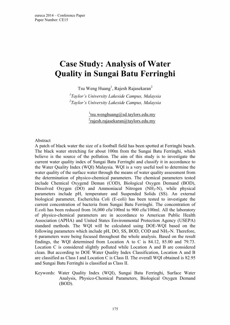
eureca 2014 – Conference Paper
Paper Number: CE15
175
Case Study: Analysis of Water
Quality in Sungai Batu Ferringhi
Tsu Weng Huang1, Rajesh Rajasekaran
2
1Taylor’s University Lakeside Campus, Malaysia
2Taylor’s University Lakeside Campus, Malaysia
Abstract
A patch of black water the size of a football field has been spotted at Ferringhi beach.
The black water stretching for about 100m from the Sungai Batu Ferringhi, which
believe is the source of the pollution. The aim of this study is to investigate the
current water quality index of Sungai Batu Ferringhi and classify it in accordance to
the Water Quality Index (WQI) Malaysia. WQI is a very useful tool to determine the
water quality of the surface water through the means of water quality assessment from
the determination of physico-chemical parameters. The chemical parameters tested
include Chemical Oxygend Deman (COD), Biological Oxygen Demand (BOD),
Dissolved Oxygen (DO) and Ammoniacal Nitrogen (NH3-N), while physical
parameters include pH, temperature and Suspended Solids (SS). An external
biological parameter, Escherichia Coli (E-coli) has been tested to investigate the
current concentration of bacteria from Sungai Batu Ferringhi. The concentration of
E.coli has been reduced from 16,000 cfu/100ml to 900 cfu/100ml. All the laboratory
of physico-chemical parameters are in accordance to American Public Health
Association (APHA) and United States Environmental Protection Agency (USEPA)
standard methods. The WQI will be calculated using DOE-WQI based on the
following parameters which include pH, DO, SS, BOD, COD and NH3-N. Therefore,
6 parameters were being focused throughout the whole analysis. Based on the result
findings, the WQI determined from Location A to C is 84.12, 85.00 and 79.73.
Location C is considered slightly polluted while Location A and B are considered
clean. But according to DOE Water Quality Index Classification, Location A and B
are classified as Class I and Location C is Class II. The overall WQI obtained is 82.95
and Sungai Batu Ferringhi is classified as Class II.
Keywords: Water Quality Index (WQI), Sungai Batu Ferringhi, Surface Water
Analysis, Physico-Chemical Parameters, Biological Oxygen Demand
(BOD).

eureca 2014 – Conference Paper
Paper Number: CE15
176
1. Introduction
The access to clean water is a basic essential requirement or needs of human
life. More than 70 percent of the Earth’s surface is covered by water, 97.5 percent out
of 70 percent is saltwater, leaving only 2.5 percent as fresh water [1]. The remaining
is saline and ocean-based. This means that the competition for a clean, copious supply
of water for drinking, cooking, bathing, and sustaining life intensifies increasing
dramatically every year. In Malaysia, the most tapped raw water sources are rivers [2].
There are total 180 rivers whereby 150 of them are the major river systems while 97
percent of Malaysia’s water supply comes from those rivers and streams [3].
According to the Department of Environmental, in the Environment Quality Report
2009 showed that 46 percent out of the total river in Malaysia is polluted when
compared to the previous years [4]. The accessibility of clean water will be more
challenging if pollution continues to occur. Fresh water is not only vital for protecting
public health, it also play some important roles especially in providing ecosystem
habitats. Therefore, it is important to determine the water quality to determine the
classification of the current river. It is important to have a good water quality for a
healthy river.
The water quality is judged or classified based on evaluating the water quality
index (WQI). Water quality index serves as a mean indication of water quality
assessment through determination of physico-chemical parameters of surface water.
Furthermore, WQI can be used as an indicator of water pollution by providing
feedback on the quality of water to the policy makers and environmentalist. Water
quality index is important to be measured in order to determine health of the river
before consuming or safe to use in other purposes. In order to develop these water
quality indexes, several parameters have to be considered. The parameters are
physical, chemical, biological and radioactive. Each of the parameters has significant
impact on the water quality [5]. The physical parameters include temperature, pH,
turbidity, total dissolved solids and total suspended solids. In terms of chemical, the
parameters involve Dissolved Oxygen (DO), Biochemical Oxygen Demand (BOD),
Chemical Oxygen Demand (COD), nitrates and total phosphate. Fecal coliform such
as Escherichia Coli (E-coli) and groups of microorganism are classified under
biological parameters. Measurements of these indicators can be used to indicate and
determine the classification of the river by comparing with the national water quality
standards of Malaysia from Water Environment Partnership in Asia (WEPA) and
Interim National Water Quality Standards for Malaysia (INWQS). When these
conditions are not met, species population in the water become stress and eventually
dies. Therefore, a good water quality is important for maintaining a healthy river and
ecosystem.
1.1 Study Area
According to New Straits Times, February 2014, a patch of black water the size of
a football field has been spotted at Ferringhi beach [6]. The black water stretching for
about 100m from the Sungai Batu Ferringhi, which believe is the source of the
pollution. A loosen control valve from a nearby sewage treatment plant is the cause of
the black effluence that being released to the river then flow out to the sea. The

eureca 2014 – Conference Paper
Paper Number: CE15
177
possibility of black effluence is the bacteria called Escherichia Coli (E-coli) [6]. Both
faecal coliform and E.coli reading’s in the river were at a staggering 16,000 cfu per
100ml [6].
1.2 Research Scopes
1. What is the current Water Quality Index (WQI) of Sungai Batu Ferringhi?
2. Are the concentration of E.Coli reduces?
1.3 Objectives
Although a massive cleanup was carried out by the Department of Environmental
on February 2014, this research is to analyze the latest characteristics of water quality
at Sungai Batu Ferringhi. The objectives are the following:
1. To investigate the current water quality indexes through several biological
and physio-chemical parameters of Sungai Batu Ferringhi;
2. Classify the Sungai Batu Ferringhi in accordance to the Water Quality
Index (WQI) Malaysia.
2.0 Research Methodology
2.1 Overall Methodology Process Flowchart
Collect Water Samples
Collect Water Samples
Measurements of the six
paprameters:
• In-situ measurements
•Laboratory analysis of collected samples
Measurements of the six
paprameters:
• In-situ measurements
•Laboratory analysis of collected samples
Data used to calculate
individual parameter
quality index or group to calculate
WQI
Data used to calculate
individual parameter
quality index or group to calculate
WQI
Determination of river quality
STATUS under the National
Water Quality Standards for
Malaysia
Determination of river quality
STATUS under the National
Water Quality Standards for
Malaysia
Classification Classification

eureca 2014 – Conference Paper
Paper Number: CE15
178
Figure 1. Procedure for Calculating Water Quality Index (WQI) [7].
2.2 Sampling Surface Waters
The sample is taken 10 cm below the surface away from the edge using
telescopic sampling system or polyethylene dipper (TW-06282-90) at predetermined
locations. The samples were collected form 3 different predetermined locations
including upstream, mid-stream and downstream of Sungai Batu Ferringhi. All the
sample containers were labeled before site collection. The samples were collected by
directly filling the container from the surface body and by decanting the water from a
collection device [8]. During transferring the samples using a collective device, the
device was avoided by from contacting with the sample containers. Preservations
have been done on the site immediately at the time of sample collection. Collected
samples were placed into the icebox with temperature approximately 4 °C during
transportation to lower or retard the metabolism of the organism on the sample. All
the samples were stored in the refrigerator with temperature less than 6 °C with
covered layer to maintain dark condition. The overall laboratory analysis was
completed within 14 days from the date of sample collection.
Figure 2. Sampling Station include Upstream (Top Tight), Midstream (Bottom Left)
and Downstream (Bottom Right)
2.3 In-Situ Measurements
The in-situ parameters include pH, Temperature and Dissolved Oxygen (DO)
were conducted on site. Temperature and pH were measured using portable probe
meter (Microcomputer pH Meter, TI9000) by WalkLAB that provided by the
university laboratory. For DO, a portable Dissolved Oxygen Tester (Extech DO600)
was used at the site.

eureca 2014 – Conference Paper
Paper Number: CE15
179
2.4 Ex-Situ Measurements
Table 1. Standard Methods Used In Chemical Analysis for Liquid Samples [8].
Parameters Analytical Methods
Biological Oxygen Demand (BOD) APHA 5210B: 5-Day BOD Test
Chemical Oxygen Demand (COD) APHA 5220C: Closed Reflux, Titrimetric
Method
Ammonia Nitrogen (NH3 – N) APHA 4500 - NH3C
Dissolved Oxygen (DO) APHA 4500 O-C or Portable Meter
E.coli USEPA 1603
All the sample preparation and preservations conducted were following on the
standard procedures provided by American Public Health Association (APHA) and
United States Environmental Protection Agency (USEPA) Methods
2.5 Laboratory Analysis
The laboratory analysis results were recorded and Water Quality Index (WQI)
equation was applied to determine the water quality index of the samples. Refer to Eq.
(1) below:
WQI = 0.22SIDO + 0.19 SIBOD + 0.161SICOD + 0.15SIAN + 0.16SISS + 0.12SIpH Eq (1)
where;
SIDO = Sublndex DO (% saturation)
SIBOD = Sublndex BOD
SICOD = Sublndex COD
SIAN = Sublndex NH3-N
SISS = Sublndex SS
SipH = Sublndex pH
0 ≤ WQI ≤ 100
Subindex, SI was calculated using the equation as shown on Table 3. Different
parameter has different subindex with different ranges.
Table 2. Best-Fit Equations for the Estimation of Various Subindex Values [9].
Subindex, SI Equation Ranges
Dissolved Oxygen, SIDO = 0
=100
= -0.395 + 0.030 x2 –
0.00020 x3
For x ≤ 8 %
For x ≥ 92 %
For 8 % < x < 92%
Biochemical Oxygen
Demand, SIBOD
= 100.4 – 4.23 x
= 108e-0.055x
– 0.1
For x ≤ 5
For x> 5
Chemical Oxygen
Demand, SICOD
= -1.33x + 99.1 For x ≤ 20

eureca 2014 – Conference Paper
Paper Number: CE15
180
= 103e-0.0157x
– 0.04x For x > 20
Ammoniacal Nitrogen,
SIAN
= 100.5 – 105x
= 94e-0.537x
– 5 abs(x -2)
For x ≤ 0.3
For 0.3 < x < 4
Suspended Solids, SISS = 97.5e-0.00676x
= 0.05x
=71e-0.0016x
- 0.015x
= 0
For x ≤ 100
For 100 < x < 1000
For x ≥1000
pH, SIPH = 17.2 – 17.2x + 5.02x2
= -242 + 95.5x – 6.67 x2
= -181 + 82.4x – 6.05 x2
= 536 – 77.0x + 2.76 x2
For x <5.5
For 5.5 ≤ x < 7
For 7 ≤ x ≤ 8.75
For x ≥ 8.75
The x in Table 2 represents the concentration of each parameter in mg/L except for
pH. After each subindex for each parameter has been calculated, the values will be
substitute into Equation 3 to calculate Water Quality Index, WQI. The classification
of river will be conducted once the value of WQI is confirmed. The classification of
river water is based on Table 3 below.
Table 3. Classification of Water Quality Index [9].
Parameter Unit Class
I II III IV V
Ammoniacal
Nitrogen
mg/l < 0.1 0.1 - 0.3 0.3 - 0.9 0.9 - 2.7 > 2.7
Biological Oxygen
Demand
mg/l < 1 1 - 3 3 - 6 6 - 12 > 12
Chemical Oxygen
Demand
mg/l < 10 10 - 25 25 - 50 50 - 100 > 100
Dissolved Oxygen mg/l > 7 5 - 7 3 - 5 1 - 3 < 1
pH - > 7 6 - 7 5 - 6 < 5 > 5
Total Suspended
Solid
mg/l < 25 25 – 50 50 - 150 150 - 300 > 300
Water Quality
Index (WQI)
- < 92.7 76.5 –
92.7
51.9 –
76.5
31.0 –
51.9
> 31.0
2.5.1 Total Suspended Solids
APHA 2540D: Total Suspended Solids Dried at 103-105 0C is the analysis standard
for determining the total suspended solids in water. In this final year projects, the
analytical procedures from the APHA Standards were followed but not the equipment
set-up. For the experiment set-up, the operating principle remained the same but
different type of apparatus was used as shown in the following figure.

eureca 2014 – Conference Paper
Paper Number: CE15
181
Figure 3: Experimental Set-up for Total Suspended Solids
3.0 Results and Discussion
3.1 Physical Parameters
3.1.1 Total Suspended Solids
Total Suspended Solids (TSS) represents the amount of the particles presence
in the water. It consists of inorganic and organic particles. High concentration of TSS
is one of the many reasons why the water quality deterioration leading to aesthetic
issue [10]. The increase of not only increase the cost of water treatment, it is also
caused some impacts of ecological degradation of aquatic environments. The water
sample from Sungai Batu Ferringhi only contains organic particles based on the
assumption that no any other industrial (Heavy or Light) area is built along the river.
There is an existing of a small-scale Tilapia fish farm being built at the side of
Location A. The concentration of TSS is the highest at Location A (Up-Stream) of the
river with the mean value of 2.49 mg/L. The high mean value of TSS found at
Location A is believed cause from the discharge of water from the fish warm when
the water of the feedstock is being changed. All the water that contains organic
matters is directly discharged into the river. Despite the concentration is at the highest
on Location A, the concentration decreases along the river. Location B has the mean
value of 1.47 mg/L while Location C has the lowest mean value of 1.38 mg/L. The
concentration trend of TSS is decreased from 2.49 to 1.38 mg/L which indicate that
the organic matter is being dissolved along the river by the microorganism. Location
A, B and C are classified as Class I under the Department of Environmental Water
Quality Index Classifications since the concentration of TSS is less than 25 mg/L.
3.1.2 pH
Location A has the value of 7.52, B with the value of 6.97 and lastly Location
C with the value of 6.38. The pH value started to decline from 7.52 to 6.38 as it
reaches Location C. Location A is more approach to alkaline region while B and C are
started to approach to acidic region. In another words, the pH from A to C is declined
from alkaline region to acidic region. This indicates that activity of hydrogen ion
started to increase right after the water flow out from location A. Despite the activity
of hydrogen ion increases, the status of location A and B are close to neutral while the

eureca 2014 – Conference Paper
Paper Number: CE15
182
pH value at Location C is considered slightly acidic. In general, the pH values
recorded at Location A, B and C are almost at neutral level. Based on the DOE Water
Quality Index Classification, Location A is classified as Class I whereas for Location
B and C are classified under Class II. The pH values for all locations are fall within
the acceptable limit of 6 to 8 [11].
Figure 5: Concentration of physical parameters from sampling locations.
3.2 Chemical Parameters
3.2.1 Dissolved Oxygen
The average concentration of DO obtained from Location A to C is 8.97 mg/L,
8.15 mg/L and 8.01 mg/L as shown in Figure 4.4.1. The concentration of DO has been
depleted from 8.97 mg/l to 8.01 mg/L along the river. Location A has the highest
concentration of DO since the concentration of COD and BOD is the lowest. This
confirmed the sentence saying that the concentration of DO is lower due to high
concentration of COD and BOD. This is proven by referring to the concentration of
DO, COD and BOD at Location C. The concentration of COD and BOD at Location
C is the highest but lowest concentration of DO. The low concentration of DO is due
to high COD and BOD concentration which rapidly consumed the oxygen content of
the river during the decomposition of organic matters, suspended solids and etc.
According to DOE Water Quality Index Classification, Location A, B and C are
classified under Class I as the concentration of DO in water is higher than 7 mg/L.
Despite with the high concentration of BOD and COD, the concentration of DO is
classified under Class I.
3.2.2 Biochemical Oxygen Demand
Location A has the value of 5 mg/L, Location B with 8 mg/L and lastly
Location C with the concentration of 10 mg/L. the concentration of BOD at Location
B increased from 5 mg/L to 8 mg/L and eventually reached to 10 mg/L at Location C.
This increasing trend of BOD level in the river is due to the oxygen demand required
for breaking down the organic matters by the microorganism increased. The
microorganism at Location B has to dissolve the organic matters from the discharge
(a) Total Suspended Solids (mg/L) (b) pH

eureca 2014 – Conference Paper
Paper Number: CE15
183
water at Location A as the organic matters flow to B. Therefore, the concentration of
BOD is raised from 5 mg/L to 8 mg/L. For Location C, the burden of microorganism
to dissolve organic matters increased. At the Location C (downstream), the area is
surrounded by residential area, restaurants and a sewage treatment plant is sitting right
beside the downstream thus, the source of pollutions determined. Some of the
discharge from the residential areas or restaurants might escape and flew into the river.
Hence, the oxygen demand of microorganism required to break down the organic
matters at Location C is the highest. As stated by the Department of Environmental
(DOE) Water Quality Index Classifications Malaysia, Location A is classified as
Class III whereas Location B and C are classifies as Class IV. According to Interim
National Water Quality Standards (INWQS) for Malaysia, extensive treatment is
required at Location A where Location B and C can be only used for irrigation
purposes according to INWQS as the concentration falls between 6 to 12 mg/L.
3.2.3 Chemical Oxygen Demand
Location A has the lowest value of 32 mg/L, Location B with the
concentration of 48 mg/L and maximum value of 64 mg/L at Location C. According
to Figure 4.3, the concentration of COD has been increased from Location A to C.
For Location A, 30 mg of oxygen is being consumed per litre of solution. The
concentration above 25 mg/L is classified as Class III according to DOE Water
Quality Index Classification [9]. Both Location A and C are classified as Class III and
Location D is classified as Class IV with the concentration of 64 mg/L. Location C
has the higher concentration of COD value compared to others is due to high
decomposition of organic matters and suspended solids that produced from the
activities nearby. Extensive requirement is needed at Location A and C needed
extensive treatment if the water is used as water supply according to NWQS for
Malaysia while the water at Location C is only for irrigation purposes and not
consumable. Location C has the highest concentration of COD compared to other
locations due to higher decomposition demand of organic and inorganic contaminants
from the surrounding activities as mentioned in section 3.2.2.
3.2.4 Annoniacal Nitrogen
Location A has the value of 0.3 mg/L and Location C with the concentration
of 0.1 mg/L. For Location B, the concentration for NH3-N cannot be detected, as the
value is not more than 0.1 mg/L. 0.3 mg/L of NH3-N was detected at Location A is
believed that caused by the fish farming activity beside the stream. The discharged
water from the farm which contains high concentration of excreta that produced by
the fish and is directly being discharged into the river. Hence, high level of ammonia
was detected at Location A. Excreta contain organic and inorganic substances
including nutrients which pose a potential threat to human health and the environment
[12]. According to DOE Water Quality Index Classification, Location A and C are
classified under Class II and Location B as Class I. Conventional treatment is required
Location A and C.

eureca 2014 – Conference Paper
Paper Number: CE15
184
Figure 6: Concentration of chemical parameters from sampling locations.
3.3 Biological Parameter
3.3.1 Escherichia Coli
The concentration obtained from Location A, B and C are 800 cfu/100ml, 640
cfu/100ml and 920 cfu/100ml. 800 cfu/100ml of E.coli was found a Location A which
believe the source of pollution is from the fish farm located at the side of the stream.
The discharged water from the farm which contains animal fecal materials are directly
being discharged to the river without any treatment. Thus, high colony-forming unit
per 100 ml water of E.coli was found at Location A. At Location B, moderate amount
of E.coli was obtained as the bacteria can remain in streambed sediments for long
(a) Dissolved Oxygen (mg/L) (b) Biological Oxygen Demand (mg/L)
(c) Chemical Oxygen Demand (mg/L) (d) Ammoniacal Nitrogen (mg/L)
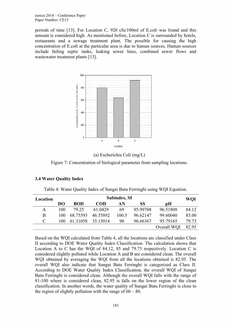
eureca 2014 – Conference Paper
Paper Number: CE15
185
periods of time [13]. For Location C, 920 cfu/100ml of E.coli was found and this
amount is considered high. As mentioned before, Location C is surrounded by hotels,
restaurants and a sewage treatment plant. The possible for causing the high
concentration of E.coli at the particular area is due to human sources. Human sources
include failing septic tanks, leaking sewer lines, combined sewer flows and
wastewater treatment plants [13].
3.4 Water Quality Index
Table 4: Water Quality Index of Sungai Batu Ferringhi using WQI Equation.
Based on the WQI calculated from Table 4, all the locations are classified under Class
II according to DOE Water Quality Index Classification. The calculation shows that
Location A to C has the WQI of 84.12, 85 and 79.73 respectively. Location C is
considered slightly polluted while Location A and B are considered clean. The overall
WQI obtained by averaging the WQI from all the locations obtained is 82.95. The
overall WQI also indicate that Sungai Batu Ferringhi is categorized as Class II.
According to DOE Water Quality Index Classification, the overall WQI of Sungai
Batu Ferringhi is considered clean. Although the overall WQI falls with the range of
81-100 where is considered clean, 82.95 is falls on the lower region of the clean
classification. In another words, the water quality of Sungai Batu Ferringhi is close to
the region of slightly pollution with the range of 60 – 80.
Location Subindex, SI WQI DO BOD COD AN SS pH
A 100 79.25 61.0429 69 95.99708 96.51808 84.12
B 100 68.75593 46.55892 100.5 96.62147 99.60040 85.00
C 100 61.31058 35.15014 90 96.66367 95.79165 79.73
Overall WQI 82.95
(a) Escherichia Coli (mg/L)
Figure 7: Concentration of biological parameter from sampling locations.

eureca 2014 – Conference Paper
Paper Number: CE15
186
4.0 Conclusion As can be seen from the findings, the water quality from Location A to C has
been depleted along the river. This indicated that the level of pollution has been
increased despite that the overall WQI of Sungai Batu Ferringhi is considered clean
according to DOE Water Quality Index Classification based on water quality index.
The overall WQI determined is 82.95 and Sungai Batu Ferringhi is classified as Class
II. In term of biological parameter, the concentration of E.coli has been reduced from
16,000 cfu/100ml to 900 cfu/100ml. Conventional treatment is required for Sungai
Batu Ferringhi and is only suitable for recreational use only for body contact.
References
[1] National Geographic, “Clean Water Crisis, Water Crisis Facts, Water Crisis
Resources - National Geographic”, 2014.
[2] Emeritus Prof. Dato’ Wira Ir. Dr Mohd. Noor Salleh. Zaki “Potable Water
Quality Characteristics”, November, 2011.
[3] Dr K.Kalithasan. “Urban Rivers: A Vital Sources of Drinking Water”, GAB
Foundation, 2013.
[4] Department of Environmental. “Environment Quality Report 2009: River
Water Quality”, Department of Environment Malaysia, 2011.
[5] Ministry of Natural Resources and Environment Malaysia. “Study on The River
Quality Trends and Indexes in Peninsular Malaysia”, 2009.
[6] P.Nambiar and B.Kaur. “Major E.coli Contamination in Batu Ferringhi
Confirmed”. New Straits Times, February, 2014.
[7] Global Environment Centre. “River Water Quality Monitoring and
Classification”, 2014.
[8] C. Decker and K. Simmons. “Surface Water Sampling”. United States
Protection Agency, Science and Ecosystem Support Division,
SESDPROC-201-R3, February 28, 2013.
[9] Department of Environment. “Interim National Water Quality Standards for
Malaysia”, Malaysia, 2008.
[10] G.S. Bilotta, R.E. Brazier. “Understanding the Influence of Suspended Solids
on Water Quality and Aquatic Biota”, Water Research, Volume 42, Issue
12, pp2849-2861, June, 2008.
[11] W.A.Amneera, Nr. Wahidatul Azura Zainon Najib, Siti Rawdhoh Mohd Yusof
and S.Ragunathan. “Water Quality Index of Perlis River, Malaysia”.
International Journal of Civil & Environmental Engineering, vol. 13, pp.1-
2, April. 2014.
[12] World Health Organization. “Wastewater and Excreta: Hazards or Resources”.
Water Sanitation and Health (WSH), 2014.
[13] United States Environmental Protection Agency. “Chapter 2: Bacteria and
Water Quality”. National Water Program, June, 2008.

eureca 2014 – Conference Paper
Paper Number: EE01
187
Electromagnetic Analysis of a Novel Double
Rotor Interior Permanent Magnet Motor
Lam Pin Wen, Aravind CV*, Reynold Hariyadi
Computer Intelligence Applied Research Cluster
Taylor’s University School of Engineering, Malaysia
Abstract
Among various types of electric motor, permanent magnet motor is competent for
high torque applications. Its torque producing point is resultant of air gap flux linkage
between permanent magnet inbuilt in rotor and the stator winding. The reduction in
air gap length improves the flux linkage, however it can only be reduced to a certain
extend due to torque pulsation occurrence that increases cogging torque due to
retention capability of the machine. In this paper, a novel Double Rotor Interior
Permanent Magnet (DRIPM) motor is proposed for improved torque performance.
The key to this proposed structure is by introducing an additional outer rotor to the
conventional Interior Permanent Magnet (IPM) motor structure. Consequently, this
double rotor structure provides higher torque generation through an increase in torque
producing point by utilising the flux linkage at stator yoke, meanwhile allowing the
reduction of air gap length as the attraction of magnetic flux is distributed evenly from
the inner and outer rotor. An electromagnetic analysis on the effect of torque
producing capability to utilize the stator yoke flux is analysed using finite element
method is done. In this research, conventional IPM motor, Double Magnet Permanent
Magnet (DMPM) motor, and the proposed double rotor interior permanent magnet
motor are evaluated for comparison through the motor constant square density and
average torque. The proposed structure provides an improvement of 77% and 6% of
the motor constant square density value than that of the conventional motor and
DMPM motor respectively, while an increase of 51% and 17% of average torque
value compared to the conventional motor and DMPM motor are reported in this
paper.
Keywords: Double rotor, air gap flux linkage, interior permanent magnet motor,
finite element analysis, motor constant square density.

eureca 2014 – Conference Paper
Paper Number: EE01
188
1. Introduction
Over the last years with technology advancement, electric motors being an
important element for electromechanical energy conversion in industry [1, 2]. Electric
motors are then continued to research to improve its torque for lower power
consumption especially for applications like Electric Vehicle (EV) [3, 4]. As a result,
motor with higher torque generation draws lesser current from EV during transient
state of acceleration and braking, allowing EV to travel for a further distance. In
addition, with the recent development of permanent magnet, high air gap flux density
can be obtained with the significant improved residual flux properties, thus permanent
magnet motors have been a popular research topic nowadays to suit the modern
technology needs. Double rotor permanent magnet motors however becoming a
research topic for such applications and is expected to provide higher torque
generation in comparison to the conventional Interior Permanent Magnet (IPM)
motors.
With the structure of double rotor motor to a vehicle, each rotor can operate
individually to perform electronic differential to provide the required torque for each
driving wheel and at different wheel speed [5]. The function of continuous variable
transmission to power split can also be done with double rotor motors so that the
internal combustion engine in hybrid electric vehicle can perform at narrow speed
region to maximize the fuel efficiency [6]. Likewise double rotor motor is used for
wind turbine to split the output power to obtain the optimal efficiency for wind energy
harvesting [7]. In this paper, a novel Double Rotor Interior Permanent Magnet
(DRIPM) motor is proposed for improve torque performance in comparison to the
conventional IPM motor. As air gap flux linkage between the stator and rotor is the
factor for torque production, maximizing the air gap flux linkage in directly improves
the motor torque performance [8, 9]. Thus the main objective is to improve the motor
constant square density through an increase in torque producing capability of the
proposed structure by maximizing the air gap flux linkage around the stator core of an
IPM motor. The mechanical and magnetic evaluation of the proposed DRIPM motor
is compared to the conventional motor for the same sizing and volume.
2. Machine Design
Fig. 1 is the proposed DRIPM motor exploded view with the stator is made up
with double header stator core of 24 poles with coil winding of star connection, while
the stator core is a T and I structure of stator laminations. The inner and outer rotor
are made up with laminated rotor cores of 4 poles with each facing at the mutual axis.
Figure 1. Double Rotor Interior Permanent Magnet Motor (Exploded View).
Stator Core
Coil Windings
Outer Rotor
Inner Rotor CoreOuter Rotor Core
Magnet
Magnet
StatorInner Rotor

eureca 2014 – Conference Paper
Paper Number: EE01
189
Each pole of the inner and outer rotors are inbuilt with permanent magnet of
the same size and properties. The double rotor structure gives an advantage to
overcome the limitation of toque pulsation occurrence in conventional single rotor
motor which constrains the minimum size of air gap length. Table 1 shows the
structural dimensions of DRIPM motor. The theory of increasing the torque
characteristic for motor reluctance through maximizing the flux by double the rotor is
presented in [10]. The design for both conventional and proposed motor are using the
design guidelines presented in [11].
Table 1. DRIPM Motor Design Parameters.
Parameter Unit (𝑚𝑚)
Outer diameter 112
Outer rotor inner diameter 95
Air gap length 0.5
Inner rotor outer diameter 41
Shaft diameter 16
Permanent magnet length 22
Permanent magnet height 2.5
Stack length 65
Turns per pole 70
Rated current 5 𝐴
Outer rotor pole arc 36 𝑑𝑒𝑔
Inner rotor pole arc 90 𝑑𝑒𝑔
Stator inner surface pole arc 11 𝑑𝑒𝑔
Stator outer surface pole arc 11 𝑑𝑒𝑔
3. Motor Operating Principles
Permanent magnet motors operating principles is based on the power effects
of magnetic circuit that tend to minimize the opposing magnetic flux lines of
magnetic circuit [12]. It operates based on the interaction of magnetic field
established by electromagnet of armature winding with that of the permanent magnet
inbuilt at rotor [12]. For a three phase motor, when current injection to the motor in
phase 𝐴, air gap flux linkage between stator and rotor is then generated to produce the
torque. As torque is produced, the rotor starts to rotate to minimize the opposing
magnetic flux lines of the magnetic circuit governed by Fleming’s left hand rule [12].
Meanwhile when the opposing magnetic flux for phase 𝐴 is at minimum, current is
then injected to next phase for continuous rotation of the rotor. Saying so, the torque
produced by a motor depends on the air gap flux linkage as shown in Fig. 2.
Figure 2. Operating Principles of DRIPM Motor.
𝐴
𝐴
ɸ
ɸ

eureca 2014 – Conference Paper
Paper Number: EE01
190
4. Electromagnetic Torque Production Theory
Figure 3. Magnetic Circuit (a) Single Rotor (b) Double Rotor.
Fig. 3 (a) shows the equivalent magnetic circuit of the conventional permanent
magnet motor while Fig. 3 (b) illustrates the circuit of the motor with double rotor.
The selection design of the pole-arc is important since it is significant in influencing
the torque producing capability by the motor. Reducing the air gap length between
stator and rotor increase the magnetic flux linkage [8, 9]. On the contrary the
properties of permanent magnet with strong attraction of flux results in cogging
torque especially when the motor is moving at a lower speed, thus there is a limit to
the air gap length [12, 13]. Eq. (1) shows the basic equation for magneto motive force
(𝐹𝑚 ). The relation of flux linkage (ɸ𝑠 ) of single rotor to air gap reluctance is
presented in Eq. (2) below.
𝐹𝑚 = ɸ𝑠Ʀ𝑎 (1)
ɸ𝑠 ∝1
Ʀ𝑎
(2)
where Ʀ𝑎 is the air gap reluctance [𝐴/𝑊𝑏]. To improvise the torque performance of
the motor, it can be done by either by optimising control circuit or to optimise the
parameters of the motor especially the pole arcs. The motor is then introduced an
outer rotor to overcome the torque pulsation factor which allow to reduce the air gap
length of the motor [14]. The reduced air gap length not only minimizes the
reluctance contact flux linkage area, but the structure through dual air gap also double
the torque producing point. The introduction of the dual air gap increases the magneto
motive force around twice that of the conventional motor is shown in Eq. (3). The
flux linkage (ɸ𝑑) over the double rotor air gap reluctance is expressed as in Eq. (4).
𝐹𝑚 + 𝐹𝑚 = ɸ𝑑 (Ʀ𝑎
2+
Ʀ𝑎
2) (3)
ɸ𝑑 =2𝐹𝑚
Ʀ𝑎
(4)
The improvement in magnetic flux however will increase the torque of the
motor is be proven by Eq. (5) where torque is directly proportional to the square of
magnetic flux.
𝑇 =1
2 𝐿 ɸ𝑑
2 (5)
Ʀ𝑎
2
Ʀ𝑎
2
𝐹𝑚
Ʀ𝑎 ɸ𝑠 ɸ𝑑 𝐹𝑚
𝐹𝑚
(a) (b)

eureca 2014 – Conference Paper
Paper Number: EE01
191
where 𝑇 is torque [𝑁𝑚] and L is the inductance [𝐻]. Given from Eq. (5), when the
flux of a motor increases it also affects in increasing the torque. Thus it shows that the
double rotor motor have better magnetic flux and torque producing capability.
5. Finite Element Analysis Method
Finite Element Analysis (FEA) tool is used to design and analysis of the motor
constant square density as well to find the equivalent nodal force from distributed
load force in stress analysis based on the numerical method [10]. The performance of
a motor is greatly dependent on its geometry, hence studies using magnetic circuit are
difficult. To provide an accurate analysis for the motor design, an electromagnetic
field analysis using finite element method is necessary. The conventional IPM motor,
DMPM motor, and proposed DRIPM motor are designed and simulated using the
same method of FEA. From the simulation, the direction of flux flow, magnetic flux
density, and the torque performance of the motor are evaluated. As shown in Fig. 4 is
the flux density of the proposed motor at different rotational angle position so that to
maximize the air gap flux linkages by observing the flux flow. The motor is position
at rotational angle of 0°, 7.5°, 15°, 22.5°, 30°, 37.5° respectively as shown from Fig. 4
(a) to (f).
Figure 4. Flux Flow for Various Rotational Angle.
The lines around the motor indicate the flux saturation point and are evenly
distributed among each quarter segment, thus allowing the motor to rotate freely at a
slower rotational speed. As shown in Fig. 4 (a), the flux saturated around stator of
45°, 135°, 225° and 315° as the position of permanent magnets. Likewise the
saturated flux is aligned between the permanent magnets and the stator pole for Fig. 4
(b) to (f) due to the attraction of magnetic flux, thus allowing the rotation of the
rotors.
(a) Flux density at 0° (b) Flux density at 7.5° (c) Flux density at 15°
(d) Flux density at 22.5° (e) Flux density at 30° (f) Flux density at 37.5°
Stator
Outer
Rotor
CoilInner
Rotor
Stator
Outer
Rotor
CoilInner
Rotor
Stator
Outer
Rotor
CoilInner
Rotor
Stator
Outer
Rotor
CoilInner
Rotor
Stator
Outer
Rotor
CoilInner
Rotor
Stator
Outer
Rotor
CoilInner
Rotor

eureca 2014 – Conference Paper
Paper Number: EE01
192
6. Results and Discussion
6.1 Evaluation Parameters
For comparison on the level of performance for conventional and proposed
structure, the methods of calculation motor constant square density (𝐺) is used. This
evaluation is very useful as it includes the torque, power, and volume of the machine
designs. The motor constant square density (𝐺) is given as in Eq. (6).
𝐺 =(𝐾𝑚)2
𝑉 (6)
where 𝐾𝑚 is the machine constant in [ 𝑁𝑚/𝐴/𝑊−(1/2) ], 𝑉 is the volume of the
machine [𝑚3]. The machine constant can be further expressed as in Eq. (7).
𝐾𝑚 =𝐾𝑇
√𝑃 (7)
where 𝐾𝑇 is the torque constant [𝑁𝑚/𝐴] and 𝑃 is the input power to the coil winding
[𝑊]. Meanwhile the torque constant is given as in Eq. (8).
𝐾𝑇 =𝑇𝑎𝑣𝑔
𝐼 (8)
where 𝑇𝑎𝑣𝑔 is the fundamental torque [𝑁𝑚] and 𝐼 is the maximum current input to the
machine [𝐴].
6.2 Static Torque Characteristics
Fig. 5 shows the average torque of DRIPM motor produced at no load when
single phase current is injected at different phase angle from 0° to 90° with an interval
of 10° in between. It can be observes that the torque is highest at the 10° where rotor
starts to rotate from the original position with excitation from the single phase current
magnetic flux. However as the rotor becomes unaligned with the exited stator the
torque generated is reduced gradually. At phase angle 0° is considered as happy state
as the air gap flux is not contributed to the torque due to excited stator is aligned with
the position of permanent magnet.

eureca 2014 – Conference Paper
Paper Number: EE01
193
0 10 20 30 40 50 60 70 80 90Phase Angle [Deg.]
0.0
0.5
1.0
1.5
2.0
2.5
3.0
3.5
4.0
4.5
5.0
5.5
Figure 5. Static Torque Characteristics.
6.3 Torque Current Characteristics
As shown in Fig. 6 is the torque-current characteristics of DRIPM motor with
different input current of 2A, 3A, 4A, and 5A respectively to determine the relation
between input current and torque. The torque characteristics at each input current
shows the same behaviour. From the graph, the increase of excitation current
increases torque producing capability of the motor. However there is a rated current
for every motor depending on the thickness of coil winding that can withstand the
amount of heat.
0 10 20 30 40 50 60 70 80 90Phase Angle [Deg.]
0.0
0.5
1.0
1.5
2.0
2.5
3.0
3.5
4.0
4.5
5.0
5.5 2A3A4A5A
Figure 6. Torque-Current Characteristics.
6.4 Three Phase Torque Characteristics
Fig. 7 (a) shows the torque generated when individual phase is excited
sequentially. Each phase current is given an input of 5A but excited with phase angle
difference of 10° intervals. As shown in the graph, phase A is excited at 0° until when
it reaches phase angle of 10°, phase current B is excited, and phase current C at 20°.
The sequential excitation loop is repeated using appropriate control system method,
thus generating complete excitation phase as shown in Fig. 7 (b). With this sequential
excitation method purpose to minimize the torque ripple while maintaining the
average torque. The proposed DRIPM motor provides 51% and 17% more average
torque in comparison to that of the IPM motor and DMPM motor respectively.
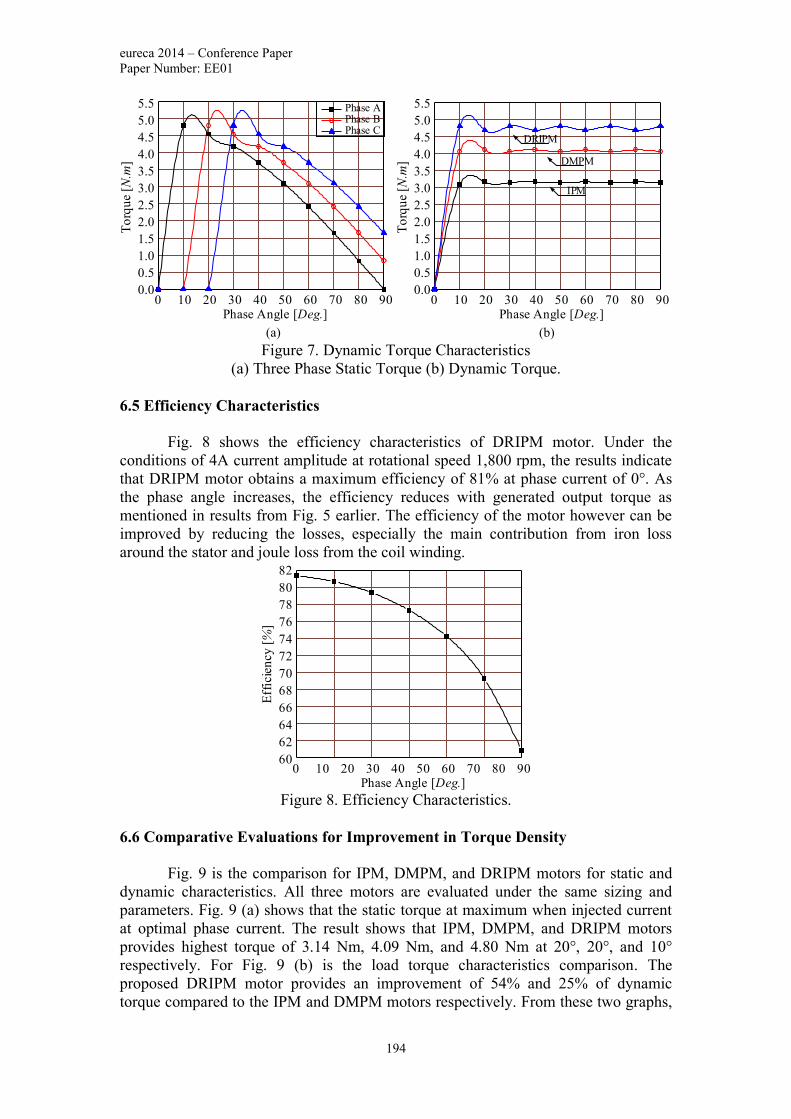
eureca 2014 – Conference Paper
Paper Number: EE01
194
0 10 20 30 40 50 60 70 80 90Phase Angle [Deg.]
0.0
0.5
1.0
1.5
2.0
2.5
3.0
3.5
4.0
4.5
5.0
5.5 Phase A Phase B Phase C
0 10 20 30 40 50 60 70 80 90Phase Angle [Deg.]
0.0
0.5
1.0
1.5
2.0
2.5
3.0
3.5
4.0
4.5
5.0
5.5
DRIPM
DMPM
IPM
Figure 7. Dynamic Torque Characteristics
(a) Three Phase Static Torque (b) Dynamic Torque.
6.5 Efficiency Characteristics
Fig. 8 shows the efficiency characteristics of DRIPM motor. Under the
conditions of 4A current amplitude at rotational speed 1,800 rpm, the results indicate
that DRIPM motor obtains a maximum efficiency of 81% at phase current of 0°. As
the phase angle increases, the efficiency reduces with generated output torque as
mentioned in results from Fig. 5 earlier. The efficiency of the motor however can be
improved by reducing the losses, especially the main contribution from iron loss
around the stator and joule loss from the coil winding.
0 10 20 30 40 50 60 70 80 90Phase Angle [Deg.]
60
62
64
66
68
70
72
74
76
78
80
82
Figure 8. Efficiency Characteristics.
6.6 Comparative Evaluations for Improvement in Torque Density
Fig. 9 is the comparison for IPM, DMPM, and DRIPM motors for static and
dynamic characteristics. All three motors are evaluated under the same sizing and
parameters. Fig. 9 (a) shows that the static torque at maximum when injected current
at optimal phase current. The result shows that IPM, DMPM, and DRIPM motors
provides highest torque of 3.14 Nm, 4.09 Nm, and 4.80 Nm at 20°, 20°, and 10°
respectively. For Fig. 9 (b) is the load torque characteristics comparison. The
proposed DRIPM motor provides an improvement of 54% and 25% of dynamic
torque compared to the IPM and DMPM motors respectively. From these two graphs,
(a) (b)

eureca 2014 – Conference Paper
Paper Number: EE01
195
it is observed that the improved torque of DRIPM motor is not completely due to the
fact of double magnet as DRIPM motor has higher average torque than DMPM motor.
0 10 20 30 40 50 60 70 80 90Phase Angle [Deg.]
IPMDMPMDRIPM
0.0
0.5
1.0
1.5
2.0
2.5
3.0
3.5
4.0
4.5
5.0
5.5
Rotational Speed [rpm]
0.0
0.5
1.0
1.5
2.0
2.5
3.0
3.5
4.0
4.5
5.0
5.5
IPM
DMPM
DRIPM
0 300 600 900 1200 1500 1800
Figure 9. (a) Static Characteristics (b) Dynamic Characteristics.
Table 2 shows the evaluation on IPM motor and DRIPM motor torque
characteristics. It demonstrates the static characteristics value derived from the
different current phase considering the motor constant square density.
Table 2. Comparison of Motor Constant Square Density.
Parameter IPM DMPM DRIPM
𝐼 [𝐴] 5 5 5
𝑉 [𝑚3] 5.99𝑒−4 5.99𝑒−4 5.97𝑒−4
𝑇𝑎𝑣𝑔 [𝑁𝑚] 2.821 3.658 4.267
𝐾𝑡 [𝑁𝑚/𝐴] 0.420 0.543 0.558
𝐾𝑚 [𝑁𝑚/𝐴/𝑊−(1/2)] 0.042 0.054 0.056
𝐺 [𝑁𝑚2/𝐴2/𝑊/𝑚3] 2.944 4.927 5.219
7. Conclusion
Static measurement characteristics of the double rotor interior permanent
magnet motor developed on the basis of increasing the air gap by proposing an outer
rotor. The proposed DRIPM motor provides an improvement of 77% and 6% for
motor constant square density compared to the conventional IPM motor and DMPM
motor respectively. The proposed DRIPM has 51% and 16% increment of average
torque than that of the conventional IPM motor and DMPM motor respectively.
However the drawback of this motor is that it produces high iron and joule loss due to
the design structure of stator and coil winding located in the middle of the motor. For
future work, it is recommend to use higher grade silicon steel with lower core loss
characteristics for the laminated core.
References
[1] Hyun Deog Yoo, Elena Markevich, Gregory Salitra, Daniel Sharon, Doron
Aurbach, “On The Challenge of Developing Advanced Technologies for
(a) (b)

eureca 2014 – Conference Paper
Paper Number: EE01
196
Electrochemical Energy Storage and Conversion”, Materials Today, vol. 17, issue
3, pp. 110-121, Apr. 2014.
[2] Zhu, Z Q, D Howe, “Electrical Machines and Drives for Electric, Hybrid and
Fuel Cell Vehicles”, Proceedings of IEEE, vol. 95, no. 4, pp 746-765, Apr. 2007.
[3] Liu Ping, Liu He-ping, “Application of Z-source Inverter for Permanent-magnet
Synchronous Motor Drive System for Electric Vehicles”, Procedia Engineering,
vol. 15, pp. 309-314, 2011.
[4] Xu Peng, Hou Zhe, Guo Guifang, Xu Gang, Cao Binggang, Liu Zengliang,
“Driving and Control of Torque for Direct-Wheel-Driven Electric Vehicle with
Motors in Serial”, Expert Systems with Applications, vol. 38, issue 1, pp. 80-86,
Jan. 2011.
[5] Kawamura, N Hoshi, T W Kim, T Yokoyama, T Kime, “Analysis of Anti-
Directional-Twin-Rotary Motor Drive Characteristics for Electric Vehicles”,
IEEE Trans. On Industrial Electronics, vol. 44, no. 1, pp. 64-70, Feb. 1997.
[6] Hofman T, Steinbuch, M, Van Druten R, Serrarens AF, “Design of CVT-Based
Hybrid Passenger Cars”, IEEE Transactions on Vehicular Technology, vol.58,
no.2, pp. 572-587, Feb. 2009.
[7] Sun, M Cheng, W Hua, L Xu, “Optimal Design of Double-Layer Permanent
Magnet Dual Mechanical Port Machine for Wind Power Application”, IEEE
Trans. On Magnetics, vol. 45, no. 10, pp. 4613-4616, Oct. 2009.
[8] Lam Pin Wen, Aravind CV, Reynold Hariyadi, “Comparative Evaluation of a
Novel Field Assisted Permanent Magnet Machine with Conventional IPM using
Motor Constant Square Density”, International Conference on Electrical Power
Engineering and Applications (ICEPEA2014), 15-16 Nov. 2014, Langkawi,
Malaysia (Accepted for presentation).
[9] Reynold Hariyadi, Aravind CV, Lam Pin Wen “Comparative Evaluation of a
Novel Field Assisted Permanent Magnet Machine with Conventional IPM using
Motor Constant Square Density”, International Conference on Electrical Power
Engineering and Applications (ICEPEA2014), 15-16 Nov. 2014, Langkawi,
Malaysia (Accepted for presentation).
[10] Aravind CV, Grace I, Rozita T, Rajparthiban R, Rajprasad R, Wong YV,
“Universal Computer Aided Design for Electrical Machines”, 2012 IEEE 8th
International Colloquium on Signal Processing and its Applications (CSPA), pp.
99-104, 23-25, Mar. 2012.
[11] Grace I, Teymourzadeh R, Bright S, Aravind CV, “Optimised Toolbox for the
Design of Rotary Reluctance Motors”, 2011 IEEE Conference on Sustainable
Utilization and Development in Engineering and Technology (STUDENT), pp.1-
6, 20-21, Oct. 2011.
[12] Krishnamurthy, M, Fahimi, B, Edrington, “Comparison of Various Converter
Topologies for Bipolar Switched Reluctance Motor Drives” In Power Electronics
Specialists Converence, PESC’05, pp. 1858-1864, 2005.
[13] Xu Huazhong, Ma Sha, “Research and Simulation of Permanent Magnet
Synchronous Motor based on Coordination Control Technology”, Procedia
Engineering, vol. 16, pp. 157-162, 2011.
[14] Aravind CV, Norhisam M, Aris I “Double Rotor Switched Reluctance Motors:
Fundamentals and Magnetic Circuit Analysis” IEEE Student Conference on
Research and Development, Cyberjaya, Malaysia, 19-20 Dec. 2011.

eureca 2014 – Conference Paper
Paper Number: EE02
197
Improvement in the Performance of the
Double Rotor Switched Reluctance
Machine Using Magnetic Circuit Design
Reynold Hariyadi, Aravind, C.V*, Lam Pin Wen
Computer Intelligence Applied Research Cluster
Taylor’s University, School of Engineering, Malaysia
Abstract The need of magnet-less machine for industrial applications are increasing, and one of
the most common magnet-less machine is switched reluctance machine. Switched
reluctance machine utilises the basic concept of attraction and repulsion principle, and
together with the air-gap reduction an improvement in the production of the torque
generation is separated earlier. The concept of dual air-gap to improve the torque
density of the switched reluctance machine is attempted by researchers in recent
times. The concept of dual air-gap shows a high starting torque density in the machine
which allows an early steady state in the machine performance compared to the
conventional machine. As the drawback, the dual air-gap machine is not able to
produce higher torque average and drags is presence for industrial application.
Therefore, a novel through modification of magnetic circuit of the dual air-gap in
double rotor switched reluctance machine is proposed. In this paper, a comparison in
terms of motor torque constant square density between three machines of
conventional switched reluctance machine (SRM), double rotor switched reluctance
machine (DRSRM), and the proposed dual air-gap machine is presented. The results
shows that there is an improvement in the average torque by 13% compare to the
SRM and 39% compare to the DRSRM. The proposed dual air-gap machine, it is also
showing an improvement in motor constant square density by 37% and 114% of SRM
and DRSRM, respectively.
Keywords: dual air-gap, double rotor, switched reluctance, motor constant square
density, torque generation.
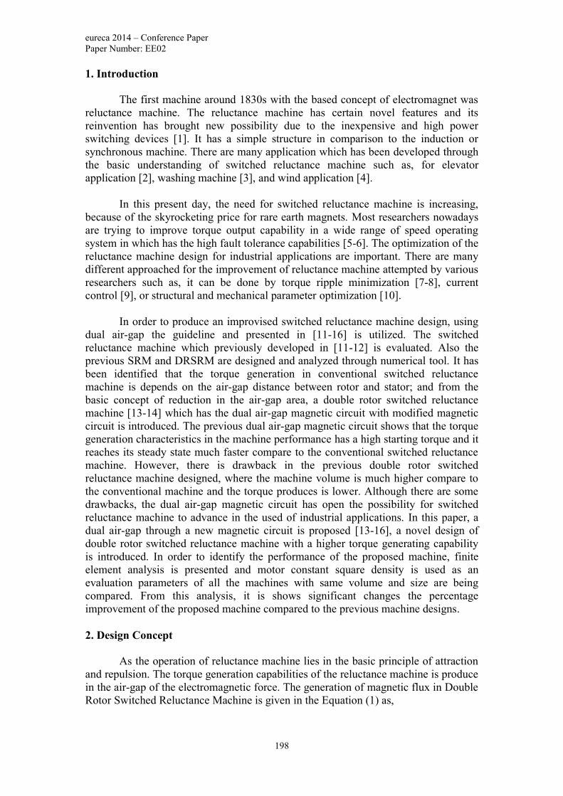
eureca 2014 – Conference Paper
Paper Number: EE02
198
1. Introduction
The first machine around 1830s with the based concept of electromagnet was
reluctance machine. The reluctance machine has certain novel features and its
reinvention has brought new possibility due to the inexpensive and high power
switching devices [1]. It has a simple structure in comparison to the induction or
synchronous machine. There are many application which has been developed through
the basic understanding of switched reluctance machine such as, for elevator
application [2], washing machine [3], and wind application [4].
In this present day, the need for switched reluctance machine is increasing,
because of the skyrocketing price for rare earth magnets. Most researchers nowadays
are trying to improve torque output capability in a wide range of speed operating
system in which has the high fault tolerance capabilities [5-6]. The optimization of the
reluctance machine design for industrial applications are important. There are many
different approached for the improvement of reluctance machine attempted by various
researchers such as, it can be done by torque ripple minimization [7-8], current
control [9], or structural and mechanical parameter optimization [10].
In order to produce an improvised switched reluctance machine design, using
dual air-gap the guideline and presented in [11-16] is utilized. The switched
reluctance machine which previously developed in [11-12] is evaluated. Also the
previous SRM and DRSRM are designed and analyzed through numerical tool. It has
been identified that the torque generation in conventional switched reluctance
machine is depends on the air-gap distance between rotor and stator; and from the
basic concept of reduction in the air-gap area, a double rotor switched reluctance
machine [13-14] which has the dual air-gap magnetic circuit with modified magnetic
circuit is introduced. The previous dual air-gap magnetic circuit shows that the torque
generation characteristics in the machine performance has a high starting torque and it
reaches its steady state much faster compare to the conventional switched reluctance
machine. However, there is drawback in the previous double rotor switched
reluctance machine designed, where the machine volume is much higher compare to
the conventional machine and the torque produces is lower. Although there are some
drawbacks, the dual air-gap magnetic circuit has open the possibility for switched
reluctance machine to advance in the used of industrial applications. In this paper, a
dual air-gap through a new magnetic circuit is proposed [13-16], a novel design of
double rotor switched reluctance machine with a higher torque generating capability
is introduced. In order to identify the performance of the proposed machine, finite
element analysis is presented and motor constant square density is used as an
evaluation parameters of all the machines with same volume and size are being
compared. From this analysis, it is shows significant changes the percentage
improvement of the proposed machine compared to the previous machine designs.
2. Design Concept
As the operation of reluctance machine lies in the basic principle of attraction
and repulsion. The torque generation capabilities of the reluctance machine is produce
in the air-gap of the electromagnetic force. The generation of magnetic flux in Double
Rotor Switched Reluctance Machine is given in the Equation (1) as,
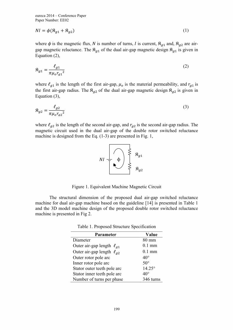
eureca 2014 – Conference Paper
Paper Number: EE02
199
𝑁𝐼 = 𝜙(𝔎𝑔1 + 𝔎𝑔2) (1)
where 𝜙 is the magnetic flux, 𝑁 is number of turns, 𝐼 is current, 𝔎𝑔1 and, 𝔎𝑔2 are air-
gap magnetic reluctance. The 𝔎𝑔1 of the dual air-gap magnetic design 𝔎𝑔1 is given in
Equation (2),
𝔎𝑔1 =ℓ𝑔1
𝜋𝜇𝑜𝑟𝑔12
(2)
where ℓ𝑔1 is the length of the first air-gap, 𝜇𝑜 is the material permeability, and 𝑟𝑔1 is
the first air-gap radius. The 𝔎𝑔2 of the dual air-gap magnetic design 𝔎𝑔2 is given in
Equation (3),
𝔎𝑔2 =ℓ𝑔2
𝜋𝜇𝑜𝑟𝑔22
(3)
where ℓ𝑔2 is the length of the second air-gap, and 𝑟𝑔2 is the second air-gap radius. The
magnetic circuit used in the dual air-gap of the double rotor switched reluctance
machine is designed from the Eq. (1-3) are presented in Fig. 1,
Figure 1. Equivalent Machine Magnetic Circuit
The structural dimension of the proposed dual air-gap switched reluctance
machine for dual air-gap machine based on the guideline [14] is presented in Table 1
and the 3D model machine design of the proposed double rotor switched reluctance
machine is presented in Fig 2.
Table 1. Proposed Structure Specification
Parameter Value
Diameter 80 mm
Outer air-gap length ℓ𝑔1 0.1 mm
Outer air-gap length ℓ𝑔2 0.1 mm
Outer rotor pole arc 40°
Inner rotor pole arc 50°
Stator outer teeth pole arc 14.25°
Stator inner teeth pole arc 40°
Number of turns per phase 346 turns
𝔎𝑔2
𝔎𝑔1 ɸ 𝑁𝐼

eureca 2014 – Conference Paper
Paper Number: EE02
200
Outer Rotor
Coil
Inner Rotor
Shaft
Stator
Figure 2. Proposed Double Rotor Switched Reluctance Machine
3. Finite Element Analysis (FEA)
Finite Element Analysis (FEA) tool is used as an identifier of the torque
density in the machine design. In this machine design experiment the finite element
analysis of the proposed machine uses industrial standard FEA tools based on the
JMAG [15-16] software. The proposed machine magnetic flux characteristics is
presented in Fig. 3,
Outer RotorInner Rotor
ShaftCoil
Stator
Outer RotorInner Rotor
ShaftCoil
Stator
Outer RotorInner Rotor
ShaftCoil
Stator
Outer RotorInner Rotor
ShaftCoil
Stator
Outer RotorInner Rotor
ShaftCoil
Stator
Outer RotorInner Rotor
ShaftCoil
Stator
(ii) Flux at 8.4375 deg (iii) Flux at 19.6875 deg(i) Flux at aligned
(vi) Flux at unaligned(v) Flux at 36.5625 deg(iv) Flux at 19.6875 deg
Figure 3. Proposed Double Rotor Switched Reluctance Machine Circuit
The magnetic flux at different positions between the stator core and double
rotor core are presented. In this condition, when the machine at aligned position, the
magnetic flux produces at its maximum. As the rotor starts to move further away from
the initial position at 0°, the magnetic flux is gradually decrease and at the same time
the torque is starts to generate, and then when the rotors reaches its complete
unaligned position the flux linkage is reached its minimum constant value.

eureca 2014 – Conference Paper
Paper Number: EE02
201
4. Results and Discussion
4.1 Evaluation Parameters
For comparison on the level of performance for conventional and proposed
structure, the methods of calculation Motor Constant Square Density 𝐺 is used. This
evaluation is very useful as it includes the torque, power, and volume of the machine
designs. The Motor Constant Square Density 𝐺 is given as in Equation (4).
𝐺 =(𝐾𝑚)2
𝑉 (4)
where 𝐾𝑚 is the machine constant in [ 𝑁𝑚/𝐴/𝑊−(1/2) ], 𝑉 is the volume of the
machine [𝑚3]. The machine constant can be further expressed as in Equation (5).
𝐾𝑚 =𝐾𝑇
√𝑃 (5)
where 𝐾𝑇 is the torque constant [𝑁𝑚/𝐴] and 𝑃 is the input power to the coil winding
[𝑊]. The torque constant is given as in Equation (6).
𝐾𝑇 =𝑇𝑎𝑣𝑔
𝐼 (6)
where 𝑇𝑎𝑣𝑔 is the fundamental torque [𝑁𝑚] and 𝐼 is the maximum current input to the
machine [𝐴].
4.2 Dynamic Characteristics
Dynamic characteristics are important for studying the state of the machine
under the normal operating condition with load. In the dynamic characteristics
experiment the excitation state is created based on the alternating conditions between
opening and closing switches in accordance with the position of the rotor’s rotation. It
can be predicted that the timing setting of an alternating conditions is able to causes a
major changes in the torque properties. In the analysis results of the dynamic
characteristics experiment in torque waveform is presented in Fig 4., The graph in Fig.
4 shows that the torque waveform of dynamic characteristics is presented when the
voltage application width 𝜃𝑤 is 30 𝑑𝑒𝑔 with the changing voltage application 𝜃𝑠 starts
−5 𝑑𝑒𝑔 , 0 𝑑𝑒𝑔 , and 5 𝑑𝑒𝑔 . The results shows that the changing application at
−5 𝑑𝑒𝑔 in application width of 30 𝑑𝑒𝑔, gives high torque generations compare to
other changing voltage applications. From this experimental results it can be
explained that the best voltage time changes for the circuit controller is 5 degree early
within the 30 degree application ranges.

eureca 2014 – Conference Paper
Paper Number: EE02
202
90 105 120 135 150 165 180
Rotational Angle [Deg.]
θs = -5 deg θs = 0 deg θs = 5 deg
-1.2
0.0
1.2
2.4
3.6
4.8
6.0
7.2
8.4
9.6
10.8
12.0
Figure 4. Torque Characteristics (𝜃𝑤: 30 𝑑𝑒𝑔)
4.3 Drive Characteristics
These type of machines require electronic control drive in order to operate at
the operational condition. In the drive characteristics experiment the physical
phenomena analysis of the magnetic circuit and drive circuit is created, where both is
use to create a torque analysis model. The circuit diagram which designed for this
experiment contains a voltage source and an ON/OFF square wave voltage of three-
phase switching are controlled depending on the timing settings Fig. 5 shows that
whether the iron loss is taken into account or not, it shows no effect on the torque
production because of the iron loss ratio to output is small. Fig. 6 shows the efficiency
of the machine when it moves at different rotational speed, and when the rotation
speed at 1200 𝑟𝑝𝑚 shows that efficiency and the peaks efficiency of the proposed
machine is about 89%.
Rotation Speed [r/min]
0 600 1200 1800 2400
0
1
2
3
4
5Iron loss not accounted for
Iron loss accounted for
Figure 5. Speed Torque Characteristics
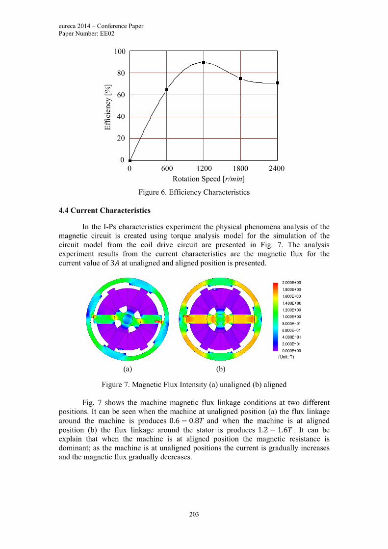
eureca 2014 – Conference Paper
Paper Number: EE02
203
Rotation Speed [r/min]
0 600 1200 1800 24000
20
40
60
80
100
Figure 6. Efficiency Characteristics
4.4 Current Characteristics
In the I-Ps characteristics experiment the physical phenomena analysis of the
magnetic circuit is created using torque analysis model for the simulation of the
circuit model from the coil drive circuit are presented in Fig. 7. The analysis
experiment results from the current characteristics are the magnetic flux for the
current value of 3𝐴 at unaligned and aligned position is presented.
Figure 7. Magnetic Flux Intensity (a) unaligned (b) aligned
Fig. 7 shows the machine magnetic flux linkage conditions at two different
positions. It can be seen when the machine at unaligned position (a) the flux linkage
around the machine is produces 0.6 − 0.8𝑇 and when the machine is at aligned
position (b) the flux linkage around the stator is produces 1.2 − 1.6𝑇 . It can be
explain that when the machine is at aligned position the magnetic resistance is
dominant; as the machine is at unaligned positions the current is gradually increases
and the magnetic flux gradually decreases.
(a) (b)

eureca 2014 – Conference Paper
Paper Number: EE02
204
4.5 Comparative Evaluations
Fig. 8 shows the machine static characteristics of the proposed Improved
Double Rotor Switched Reluctance Machine (IDRSRM). It has higher torque
generation compare to Switched Reluctance Machine (SRM) and Double Rotor
Switched Reluctance Machine (DRSRM).
Rotation Angle [deg]
0 5 10 15 20 25 30 35 40 45-10.0
-7.5
-5.0
-2.5
0.0
2.5
5.0
7.5
10.0
SRM DRSRM IDRSRM
Figure 8. Static Torque Characteristics
Fig. 9, the DRSRM shows that the machine design has the capabilities to reach
steady state faster than the other two machines, moreover it has highest starting torque
compare to the SRM and proposed machine.
Rotation Angle [deg]
0 5 10 15 20 25 30 35 40 45
SRM DRSRM IDRSRM
-1
0
1
2
3
4
5
6
7
Figure 9. Machine Operational Static Characteristics

eureca 2014 – Conference Paper
Paper Number: EE02
205
In Table 2, the comparative evaluation of motor torque constant square density
between the proposed machine, double rotor switched reluctance machine and
conventional switched reluctance machine with the same diameter is presented.
Table 2. Comparison on Figure of Merit
Figure of Merit SRM DRSRM IDRSRM
𝐼 [𝐴] 5 5 5
𝑉 [𝑚3] 2.13𝑒−3 2.20𝑒−3 1.99𝑒−3
𝑇𝑎𝑣𝑔 [𝑁𝑚] 3.85 3.13 4.36
𝐾𝑡 [𝑁𝑚 𝐴⁄ ] 0.77 0.63 0.87
𝐾𝑚 [𝑁𝑚/𝐴/𝑊−(1
2)] 0.077 0.063 0.087
𝐺 [𝑁𝑚2/𝐴2/𝑊/𝑚3] 27.87 17.84 38.20
As it can be seen in Table 2, the average torque of the proposed machine
structure is gradually increase over the conventional switched reluctance machine and
double rotor switched reluctance machine. In addition, the motor torque constant
square density value of the proposed machine showing an increase by twice of the
conventional Switched Reluctance Machine.
5. Conclusion
The proposed machine is developed based on the basic of double salient dual
air-gap structure. The proposed design is structured, simulated, and evaluated using
the standard finite element analysis. The results of the conventional switched
reluctance machine (SRM), double rotor switched reluctance machine (DRSRM), and
novel double rotor switched reluctance machine (IDRSRM) are compared as for
performance evaluation. The initial investigation shows that a percentage
improvement in the motor constant square density by 37% in the comparison of SRM
and 114% in the comparison of DRSRM and the improvement of the proposed
IDRSRM. The average torque which improved by 13% in comparison to the
conventional SRM and 39% compare to the DRSRM, all the machine which were
compared are for the same size and volume of the machine design.
References
[1] R, Krishnan. Switched Reluctance Motor Drives: Modelling, Simulation, Analysis,
Design, and Applications. Wiley-Interscience, State: New York. 2011.
[2] Kumar, T. Dinesh, and A. Nagarajan. "Design of Switched Reluctance Motor for
Elevator Application." Journal of Asian Scientific Research 3.3 (2013): 258-267.
[3] Horst, G. and French, A. Rotor position sensing in a dynamoelectric machine
using coupling between machine coils, patent US 5,701,064. 23 December 1997.
[4] Cardenas, R.; Ray, W.F.; Asher, G.M., "Switched reluctance generators for wind
energy applications," Power Electronics Specialists Conference, 1995. PESC '95
Record, 26th Annual IEEE, vol.1, pp.559,564 vol.1, 18-22 Jun 1995.
[5] R. Krishnan, Switched Reluctance Motor Drives: Modelling Simulation, Analysis,
Design, and Applications. BocaRaton, FL: CRC Press, 2001.

eureca 2014 – Conference Paper
Paper Number: EE02
206
[6] Blaabjerg, F.; Kjaer, P.C.; Rasmussen, P.O.; Cossar, C., "Improved digital
current control methods in switched reluctance motor drives," Power Electronics,
IEEE Transactions on , vol.14, no.3, pp.563,572, May 1999.
[7] Mikail, R.; Husain, I; Sozer, Y.; Islam, M.; Sebastian, T., "Four-quadrant torque
ripple minimization of switched reluctance machine through current profiling
with mitigation of rotor eccentricity problem and sensor errors," Energy
Conversion Congress and Exposition (ECCE), 2012 IEEE, pp.838,842, 15-20
Sept. 2012.
[8] Mikail, R.; Sozer, Y.; Husain, I; Islam, M.; Sebastian, T., "Torque ripple
minimization of switched reluctance machines through current profiling," Energy
Conversion Congress and Exposition (ECCE), 2011 IEEE, vol., no.,
pp.3568,3574, 17-22 Sept. 2011.
[9] Blaabjerg, F.; Kjaer, P.C.; Rasmussen, P.O.; Cossar, C., "Improved digital
current control methods in switched reluctance motor drives," Power Electronics,
IEEE Transactions on , vol.14, no.3, pp.563,572, May 1999.
[10] Matsuo, T.; Lipo, T.A, "Rotor design optimization of synchronous reluctance
machine," Energy Conversion, IEEE Transactions on, vol.9, no.2, pp.359, 365,
Jun 1994.
[11] Grace, I; Teymourzadeh, R.; Bright, S.; Aravind, C.V., "Optimised toolbox for
the design of rotary reluctance motors," Sustainable Utilization and Development
in Engineering and Technology (STUDENT), 2011 IEEE Conference on , pp.1,6,
20-21 Oct. 2011.
[12] Aravind, C.V.; Grace, I; Rozita, T.; Rajparthiban, R.; Rajprasad, R.; Wong, Y.V.,
"Universal computer aided design for electrical machines," Signal Processing
and its Applications (CSPA), 2012 IEEE 8th International Colloquium on, pp.99,
104, 23-25 March 2012.
[13] Aravind, C.V., Norhisam, M., Aris, I., et. al. “Double Rotor Switched Reluctance
Motors: Fundamentals and Magnetic Circuit Analysis.” IEEE Student Conference
on Research and Development, Cyberjaya, Malaysia, 19-20 Dec. 2011.
[14] Aravind CV, Norhisam M, M.H. Marhaban, I. Aris “Analytical Design of Double
Rotor Switched Reluctance Motor using Optimal Pole Arc Values” International
Review in Electrical and Electronics, Vol.7, No.1, pp.no.3314-3324, Feb.2012.
[15] Lam Pin Wen, Aravind CV, Reynold Hariyadi ``Comparative Evaluation of a
Novel Field Assisted Permanent Magnet Machine with Conventional IPM using
Motor Constant Square Density" International Conference on Electrical Power
Engineering and Applications (ICEPEA2014), 15-16 Nov.2014, Langkawi,
Malaysia (Accepted for presentation)
[16] Reynold Hariyadi, Aravind CV, Lam Pin Wen ``Comparative Evaluation of a
Novel Field Assisted Permanent Magnet Machine with Conventional IPM using
Motor Constant Square Density" International Conference on Electrical Power
Engineering and Applications (ICEPEA2014), 15-16 Nov.2014, Langkawi,
Malaysia (Accepted for presentation)

eureca 2014 – Conference Paper
Paper Number: ME01
207
Development of a Design Optimization
Methodology for a Home Appliance
Product Part Design
Andrew Yee Chin Wei1, Mohammad Hosseini Fouladi
1, Yap Kim Haw
2
1Taylor’s University Lakeside, Malaysia
2Panasonic HA Air-Conditioning (M) Sdn. Bhd., Malaysia
Abstract The motivation behind this research study is the idea of optimization which can be very
beneficial as it can help future production in terms of costing, research and development of
better designs to improve older counterparts. The main objectives of this research project are
to utilize the Altair HyperWorks software to perform optimization on a fan motor bracket top
plate to craft a Standard Operating Procedure (SOP), implement optimization technology to
create a SOP for the optimization process of a home appliance product part design and to
perform experimental modal analysis on the product part. Modal analysis and experimental
modal analysis will be performed on the product part design using NX Nastran, Brüel & Kjær
MTC Hammer and Pulse Reflex where the natural frequencies and mode shapes can be
obtained from the software for validation. In accordance with that, the optimization results
obtained will be used to compare the effects of optimization on the dynamic properties of the
model. The equipment used in this research study are mostly industrial based CAE software
comprising of Altair HyperWorks and NX Nastran. At the end of this research project, the
results to be accomplished would be the familiarization of the standard operating procedure to
perform an optimization process using Altair HyperWorks and NX Nastran, the ability to
perform an experimental modal analysis on a product part design, the maximization of the
natural frequency and stiffness of the home appliance product part design and to avoid
resonance in the product part design. By utilizing topography optimization, parametric beads
were inserted into the model part, increasing the stiffness of the design. In addition to that, the
stiffness of the part design is found to have increased after performing an optimization
procedure. Thus, the fan motor bracket top plate is less prone to experience resonance at a
lower frequency.
Keywords: Optimization, Home Appliances, Vibration Attenuation, Modal Analysis.

eureca 2014 – Conference Paper
Paper Number: ME01
208
1. Introduction
1.1 Research Background
In the manufacturing industry today, the reliability of the 3D mechanical
design of a product part is very crucial as it saves an abundance of time and resources
by first performing computational analysis on the 3D model in computer software.
Along the years, engineers have learned to trust Computer-Aided Engineering (CAE)
tools such as Finite Element Analysis (FEA), Computational Fluid Dynamics (CFD)
and motion simulation [1]. However, when transitioning into the manufacturing stage,
material wastage becomes a major factor in company losses. Thus, all the modern
manufacturing enterprises today are determined to develop the best optimized reduced
weight and cost effective products that meet the intended design functionality and
reliability. In addition to that, optimization of a part design can also increase the value
of the product by means of cost reduction through efficient material usage. Besides
that, an optimization process will also help increase the designer’s knowledge of their
product behaviour and improve their design while obeying the data obtained from the
previous analysis. This structural optimization tool helps in reducing production time
as well. In the last few years, structural optimization has emerged as the valuable tool
to develop new design proposals especially in automobile and aircraft industries [2].
Nowadays, computer software such as ANSYS and SolidWorks already have
the optimization module integrated into the software [2]. For an optimization process
to be performed, three criteria are required by the designer which are the design
parameters, constraints of the part design and the objectives of the optimization
process. The design parameter simply means the design variables which the designer
wants to adjust to save material usage during manufacturing. As for the constraint, the
designer or user can define the allowable ranges to be obtained in the simulation result.
The objectives or goals of the product is to determine the optimization output in terms
of reducing material wastage or minimizing model size and others.
The purpose of this project is to produce a standard operating procedure (SOP)
to undergo an optimization process on a simple home appliance part design. In this
case, an internal component of an air-conditioner manufactured by Panasonic HA Air-
Conditioning Malaysia Sdn. Bhd. will be used as the project material. By performing
an optimization on a simple structure, the manufacturing process of the product part
design will take less time as numerical analysis will aid in determining the best design
for manufacturing to obtain the optimal design. Besides that, the main function of an
optimization procedure is to identify the most optimum design for the component
whereby the strength of the part design is the most efficient and can withstand high
force and pressure. The idea of optimization is very beneficial as it can help future
production in terms of costing, research and development of better designs to improve
older counterparts. In the near future, the sustainability of the products manufactured
by Panasonic will be able to surpass other competitor’s products by a wide margin
based on the application of optimization whereby the strength and stiffness of the
product can withstand high workloads and long durations of time. Thus, creating a
SOP for optimization is crucial to challenge new competitors and lead the pack in the
air-conditioning industry.
In addition to that, this project also studies the benefits of an optimization
procedure on a modal analysis of a structure. The purpose of a modal analysis is to
identify the mode shapes produced by a design structure whereby the model reacts to
the various natural frequencies when resonance is achieved. Thus, the stiffness of the

eureca 2014 – Conference Paper
Paper Number: ME01
209
model can be found by using the natural frequency equation which will be explained
more in the literature review section of this report. This is where optimization plays
an important role in determining the most optimum design to attain a stiffer model
structure. From this, the optimized model will only reach resonance at a higher natural
frequency ensuring the longer lifespan of the product part when external forces are
present in the working system.
1.2 Project Scope
In the industry today, there are four types of structural optimization techniques.
The first being size optimization, shape optimization, topography and lastly topology
optimization. The project covers topography optimization as topology optimization
utilizes the density and homogenization method [3]. The assembly of the part design
also hinders the ability to carry out topology optimization as material reduction will
not enable proper installation of the fan motor bracket top plate as well as
manufacturing feasibility. Besides that, the response surface method is also covered in
this project. Thus, the boundary of the project includes the design parameters,
constraints of the part design and objectives of the optimization process. In
accordance to the scope, experimental modal analysis will also be carried out on the
product part design where the purpose of the optimization process is to increase the
stiffness and robustness of the design where validation is required by comparing the
results to the numerical modal analysis. In accordance to that, the range of random
vibration frequencies that the structure is being subjected to is only for filled transport
packages and unit loads. In addition to that, the scope for this project is only limited to
an investigation of an air-conditioning component.
1.3 Project Objectives
For this research project, the objectives are to utilize the ANSYS software to
perform optimization on a simple steel plate to craft a Standard Operating Procedure
(SOP), perform numerical modal analysis to obtain mode shapes of a fan motor
bracket top plate, perform experimental modal analysis to validate numerical modal
analysis results with physical testing and to implement optimization technology to
create SOP for the optimization process of a fan motor bracket top plate to increase
material stiffness using Altair HyperWorks.
2. Research Methodology
2.1 Finite Element Modal Analysis
The research paper also consists of a computational analysis which utilizes the
capabilities of numerical modal analysis to simulate the dynamic properties of the fan
motor bracket top plate in a free-free condition using NX Nastran. Following the
procedure to undergo the analysis, some minor adjustments must be made beforehand
to increase accuracy in the mode shapes obtained. Computer modelling alone cannot
determine the dynamic bahaviour of a structure completely. Therefore, modal analysis
was formulated to determine the dynamic characteristics of a system in forms of
natural frequencies and mode shapes [4]. In the research study, the free-free condition
will be used as the basis of the project where no external forces will be acted on the
product part. In a free-free condition, the dynamic characteristics of the simulation

eureca 2014 – Conference Paper
Paper Number: ME01
210
model is determined by observing the mode shapes of the model. From this, the
nautral frequencies of the model at which mode shapes are formed can be obtained.
However, the failure of determining the most optimum design for a model will
hamper the capabilities of modal analysis. Threfore, a new method must be researched
to fuse optimization and modal analysis together to form a robust design simulation.
The mode shapes and regular frequencies of a structure are its fundamental dynamic
properties. Modal analysis is utilized to differentiate these mode shapes and their
eigenvalues. Thus, the basic structural dynamic information obtained from the modal
analysis gives an accurate identification of the structural properties of the mode
shapes. In addition, modern modal analysis test methods have been created to enhance
testing and reduce information requirement for analysis to give the dynamic
properties of the structure. To carry out a modal analysis procedure through NX
Nastran, the solver normally utilized is the Lanczos algorithm [4]. However, in modal
analysis, there are certain limitations which have yet to be solved by researchers in
today’s generation. For instance, non-linear structures tend to affect the analysis and
introduce problems in the information attainment as well as disrupt the evaluations of
natural frequencies from the mode shapes. As the volume of the model increases, the
properties of the structure also changes which is generally insufficient to perform a
direct model analysis [5]. The range of frequencies must be increased to enable the
software to compute the mode shapes where resonance occurs. Besides that, another
limitation in modal analysis is the inability to specifically analyze the forced response
problems, transient response problems and random response of the model structure. In
accordance to that, the mode shapes produced from the modal analysis might not have
significant differences when the material assignment to the model in the pre-
processing is changed. This problem proceeds as an issue when various materials are
analyzed which makes it more difficult for the designer to evaluate the relationship of
different materials on mode shape attainment.
2.1.1 Geometry and Mesh Checking
Before numerical analysis can be done, the part geometry as shown in Fig. 1.0
must first be checked and cleaned using the NX Nastran modelling tools. The idea
behind this procedure is to remove any holes found in the model part, remove
unnecessary convex and concave fillets, maintaining an overall constant thickness
throughout the model and checking other part features which has no discernable effect
on the results. This procedure is important as structure features can cause low quality
mesh.
Figure 1.0 Geometry of the Fan Motor Bracket Top Plate

eureca 2014 – Conference Paper
Paper Number: ME01
211
Figure 1.1 Midsurface Offset of Part
Figure 1.2 Mesh of the Fan Motor Bracket Top Plate
The idea behind this current step is to allow easier shell meshing whereby the
part is offset to half of its initial thickness where the overall thickness of the structure
is 0.7mm. Shell meshing was utilized in this study instead of volumetric meshing as it
saves computational time due to the lower number of elements used and the quality of
the mesh can be monitored easily [6]. In accordance with that, a low number of
triangular elements and an abundance of quadratic elements where used in the
meshing procedure which indicates a high quality mesh as shown in Fig. 1.2. The
element size set for the meshing was 3.0mm in order to save computational time as
well. Besides that, the material properties are also inserted into the mesh input
whereby the material tested is rolled steel. The properties of steel are shown in Table
1.0 below:-
Table 1.0 Rolled Steel Properties
Mass Density (kg/mm3) Young’s Modulus (kPa) Poisson Ratio
8.75x10⁶ 213x10
6 0.29

eureca 2014 – Conference Paper
Paper Number: ME01
212
2.1.2 Normal Mode Analysis
Figure 1.3 Mode Shape of Model at 285.7 Hz
For the finite element modal analysis of this study, the SOL 103 Real
Eigenvalues is used. The Lanczos method was utilized in this study to extract the real
eigenvalues as it is efficient in extracting eigenvalues and eigenvectors. The square
root of the eigenvalues give the natural frequencies of the model whereas the
eigenvectors give the normal modes of the structure. Fig. 1.3 depicts the mode shape
of the structure at 285.7 Hz where the part experiences resonance. In addition to that,
the range of the natural frequency tested was set to be from 1 Hz to 300 Hz for normal
modes extraction following the ISO 13355:2001 which states that the natural
frequency of the structure being studied is for filled transport package and unit loads
and not subjected to higher random vibrations due to it being an internal component
of an outdoor air-conditioning unit [7].
2.2 Experimental Modal Analysis
In this study, the roving hammer test was carried out on the structure. For this
study, the Multiple Input Multiple Output (MIMO) was used where the multiple
inputs refer to multiple excitation points where a hammer is used to knock the points
and the multiple output points refers to the usage of accelerometers to measure the
dynamic response of the structure. By incorporating multiple hitting points and
accelerometer points, the response of the structure is easier to be monitored and
measured. In the case of a MIMO testing procedure, it is easier to perform the
experiment as some reference points might not be able to measure a mode accurately
where other reference points are able to capture the mode thus obtaining good quality
results [8].
2.2.1 Pre-Test Planning
In Fig. 2.0, it shows the modal assurance criterion (MAC) plot for the test analysis
model (TAM) and the finite element model. The purpose of doing this procedure is to
ensure that the accelerometer points and knocking points selected are well correlated
with the finite element model to ensure the TAM’s effectiveness and reliability. TAM
is important to set-up the geometry for modal testing. It represents the characteristics
of the model but comprising of limited degree of freedoms. By exciting critical degree
of freedom points, it simplifies the test structure and in turn saves time for testing.
The TAM can be produced by manually selecting the points on the structure based on
elements comprising of nodes.

eureca 2014 – Conference Paper
Paper Number: ME01
213
Figure 2.0 Correlation of Numerical Modal Analysis and Test Analysis Model
2.2.2 Experimental Set-Up
For the experimental set-up, the Pulse Reflex software was used to obtain the
structures wireframe to depict the basic shape of the model geometry. In Fig. 2.1, the
points shown are extracted from the test analysis model. Lines are drawn from point
to point to create the shape of the structure. These points consisting of 4 uniaxial
accelerometers and knocking points are then inserted into Brüel & Kjær MTC
Hammer for accelerometer placement and knocking procedures. Then, data is
measured and collected in the form of frequency response function (FRF) graphs
when the structure is excited at the corresponding knocking and accelerometer points
using the roving hammer. These FRF graphs as shown in Fig. 2.2 contain the mode
shapes of the structure at certain natural frequencies. Each peak shows the mode
shapes of the structure [9].
Figure 2.1 Geometry Decimation of Structure

eureca 2014 – Conference Paper
Paper Number: ME01
214
Figure 2.2 Example of an FRF graph
Figure 2.3 Sensor Placement and Hanging Method
Figure 2.4 Insulation of Test Rig
The scope of this research only covers the replication of a free-free boundary
condition where the structure is hanged by using elastic chords to simulate a free
moving body without constraints as seen in Fig. 2.3. By constraining the movement of
the structure, the results obtained from performing the experimental modal analysis
(EMA) will be inaccurate causing undetermined dynamic properties. Besides that, the
accelerometer wires can also act as constraints to the structure. Therefore, the wires
are placed far apart from each other to prevent tangling and interference with one
another during testing.
In addition to that, the test rig utilized is also insulated with foam padding to
reduce any random vibrations from the ground from affecting the results of the EMA.
Thus, the structure will be able to vibrate freely without environmental errors.

eureca 2014 – Conference Paper
Paper Number: ME01
215
2.3 Altair HyperWorks Optimization Process
2.3.1 Optimization Procedure of Numerical Model
In HyperWorks, there are three sub-applications which are used for an
optimization process. These applications are HyperMesh, Optistruct and HyperView.
This section lays out the overall optimization process carried out in Altair
HyperWorks. The Standard Operating Procedure is shown in Fig. 2.5 below:-
Figure 2.5 Flow Chart of Optimization Process in HyperWorks
All the steps in the Figure above are carried out in HyperMesh where
boundary conditions are inserted and design variables are set. For the meshing
procedure, the element size is set as 3mm and the mesh type is set to mixed where
tetrahedron and hexadecimal mesh types are used.
Figure 2.6 Meshing Setting
Meshing Meshing
Insert Material Properties
Insert Model Property
Load Collector
Load Step
Topography Optimization
View Results

eureca 2014 – Conference Paper
Paper Number: ME01
216
The first step of the optimization process is to insert the material properties
into the model part. In HyperMesh, the mass density, young’s modulus and poisson
ratio are only required for the material properties. The input data is similar as stated in
Section 3.1.1.
Figure 2.7 Material Properties Setting
As for the model property, the thickness of the model is input value. For this
model part, the plate thickness is 0.7mm. The PSHELL card image is selected as the
model part inserted into the software is a shell and not a solid. A shell design part has
a lower computational processing time as compared to a solid design part. Thus,
making the optimization process more efficient.
Figure 2.8 Model Property Setting.
As for the load collector, the input data is the range of frequency whereby the
model experiences. For the research paper, the range covered is between 1 Hz and 300
Hz. The number of modes to extract is not set here as the range is already inserted into
the software.

eureca 2014 – Conference Paper
Paper Number: ME01
217
Figure 2.9 Load Collector Setting
In load step, the type of analysis is set as normal modes to obtain the mode
shapes of the design part. This is done to ensure that the software produces the
required data only.
Figure 2.9.1 Load Step Setting.
2.3.2 Topography Optimization
To carry out this procedure, the design space is first selected based on the
limitations of the model part. For the fan motor bracket top plate, only a small area is
allowed to be altered utilizing the optimization technique. The required input data for
a topography optimization are bead width, draw angle and draw height. Selection of
the design space is in the form of node selection. Thus, the start and end location of
bead creation is set by selecting the nodes on the model part. By inserting these
parameters, the software is able to compute the necessary data to produce a new
design. The bead height is set as 7mm, draw angle to be 600 and draw height to be
3.5mm. Then, by running Optistruct, optimal results are obtained which are then
displayed in HyperView.

eureca 2014 – Conference Paper
Paper Number: ME01
218
Figure 2.9.2 Topography Setting
3. Results & Discussion
3.1 Correlation of Experimental Modal Analysis and Experimental Modal
Analysis
(a) (b)
Mode 1
As seen in Fig. 3.0, the mode shapes of the EMA and Finite Element (FE)
modal analysis are almost similar to each other. This shows that the experiment was
conducted smoothly and accurately. This comparison is made to show validation of
EMA with FE modal analysis which applies for real world application. By performing
the test, only 4 mode shapes can be extracted. Thus, assuring that computational
analysis can also be used to produce results similar to that of experimental results. In
addition to that, time can also be saved by performing FEA whereby experimental
procedures and set-up take an absurd amount of time before any results can be
obtained. However, this validation process is important to justify the precision and
accuracy of real testing results in the industry.

eureca 2014 – Conference Paper
Paper Number: ME01
219
(a) (b)
Mode 2
Mode 3
Mode 4
Figure 3.0 The Comparison of the Numerical Modal Analysis Mode Shapes (a) and
Experimental Modal Analysis Mode Shapes (b) for Mode 1, 2, 3 and 4 of the Fan
Motor Bracket Top Plate
Table 2.0 Correlation of Mode-Pairs
FE Modal
Mode
Finite
Element
Modal
Analysis
Frequency
EMA
Mode
Experimental
Modal
Analysis
Frequency
MAC Frequency,
% Error
1 82.7686 1 63.7643 0.943 29.8041
2 161.581 2 165.651 0.750 -2.4572
3 218.087 3 242.862 0.863 -10.2012
4 285.678 4 266.812 0.920 7.07081

eureca 2014 – Conference Paper
Paper Number: ME01
220
The table above shows the error between the work frequency and the reference
frequency. The work frequency shows the mode shapes of the FE modal analysis
while the reference frequency shows the mode shapes produced from the EMA. Major
errors can be seen in the first, third and fourth mode where the percentage error
exceeds 5% as shown in the frequency error data in Table 2.0. These errors arise from
the EMA test. External factors such as ground vibration and irregular knocking force
are the main contributors for such huge errors. Other errors such as the interference of
the accelerometer wires can also lead to inaccurate data collection during knocking.
Thus, to perform an error free EMA test, the structure tested has to be placed in a still
environment without any presence of wind as well as experience zero random
vibrations from the surroundings which can only be replicated in a virtual domain. It
can be said that EMA can never be 100% accurate as errors are always present in
many forms.
Figure 3.1 Correlation of Numerical Modal Analysis and Experimental Modal
Analysis of First Test
Figure 3.2 Correlation of Numerical Modal Analysis and Experimental Modal
Analysis of Second Test.
The MAC plot for the first test as seen in Fig. 3.1, shows bad correlation due
to the input of too many accelerometers which constricted the mobility of the
structure preventing a free-free boundary condition environment. The number of
knocking points set was also found to be a major problem as an abundance of
knocking points can lead to high inaccuracy of results arising from human errors.
Besides that, the geometry decimation of the first structure was unreliable as the

eureca 2014 – Conference Paper
Paper Number: ME01
221
points selected were not connected to the main body of the structure where the
isolated points are moving independently. Thus, for the second test results as seen in
Fig. 3.2, the MAC plot was improved by reducing the number of accelerometers
utilized, reducing the number of knocking points on the structure and fixing the
geometry decimation to allow each point to act dependently on one another to show a
better mode representation of the EMA test. In addition to that, a good MAC plot will
show a diagonal of 1 and an off-diagonal of less than 0.1 [9].
Table 3.0 Correlation Results of Second Test
Reference Modes (Hz)
R1 R2 R3 R4
Work Modes (Hz) 63.764 165.651 242.862 266.812
W1 82.574 0.943 0.036 0.011 0.011
W2 161.201 0.013 0.750 0.025 0.000
W3 217.575 0.024 0.124 0.863 0.000
W4 285.006 0.074 0.083 0.070 0.920
3.2 Optimization Results
Based on the utilization of Altair HyperWorks software, an optimized design
can be obtained which outputs the best feasible design suitable for manufacturing and
assembly in an air-conditioning outdoor unit. However, given the limited design space
of the fan motor bracket top plate, there is only so much that optimization can do to
change the design of the part to increase the stiffness without affecting the assembly
configuration. The mass of the actual part was measured to be 179 grams using an
electronic mass balance.
Figure 3.3 Assembly of Fan Motor Bracket Top Plate in an Outdoor Air-Conditioning
Unit

eureca 2014 – Conference Paper
Paper Number: ME01
222
Figure 3.4 Original Design
Figure 3.5 Optimal Design
As can be seen from the optimization result above, topography optimization
was carried out where parametric bead variables require user input. The criteria
required for the optimization procedure are the bead width, draw angle and draw
height [16].
Table 4.0 Topography Bead Variables
Bead Width Draw Angle Draw Height
7mm 600 3.5mm
Figure 3.6 Parametric Bead Parameters

eureca 2014 – Conference Paper
Paper Number: ME01
223
Table 5.0 Comparison of Stiffness between Original and Optimal Design
Original Design Optimal Design
Mode Frequency,
(Hz)
Generalized Stiffness,
(N/m)
Frequency,
(Hz)
Generalized Stiffness,
(N/m)
1 86.1 2.93E+05 95.7 3.62E+05
2 167 1.10E+06 169 1.13E+06
3 223 1.96E+06 229 2.06E+06
4 286 3.23E+06 295 3.43E+06
As seen from the table above, there is an increase of stiffness for each mode of
the optimal design. The resonating frequency of the modes also increases
proportionally with the stiffness. However, the results could only show a single
optimal design given the constraints of the design space of the model part. The limited
amount of design space is constricted based on the feasibility of manufacturing and
company restrictions. Thus, topography optimization can only be carried out on a
small portion of the plate. Besides that, the original design already contained bead
stiffeners at the sides leaving a small amount of area to change the design of the plate.
Hence, by utilizing the optimization module in Altair HyperWorks, the stiffness of the
part model could be increased which in turn lowers the possibility of the part to
resonate at lower frequencies. By doing so, experiencing vibration during
transportation would not pose as a major issue for consumers anymore. Thus,
topography optimization has proven its value by increasing product robustness.
However, in the Altair HyperWorks software, there is no module to carry out the
Design of Experiments procedure as compared to ANSYS. On the other hand, the
validation of EMA and NMA using correlation tools has ensured that the actual model
part being tested has similar material properties with the numerical model. Therefore,
there is no need for an optimization validation in Altair HyperWorks.
4. Conclusions & Future Work
A complete EMA procedure was successfully performed on a fan motor
bracket top plate with comparison to the prior study using FE modal analysis. The
EMA procedure was performed on a fan motor bracket top plate within a frequency
span of 1 Hz – 300 Hz following the ISO 13355:2001 for a random vibration test. As
it can be seen, the results obtained from the experimental modal analysis shows a
maximum of 30% frequency error when correlated with the numerical modal analysis
data. However, in a real world application, the results of FEA can never be applied to
consumer products as it is the simulation of a perfect world. Thus, errors are always
present in physical testing. The correlation of both EMA and FE modal analysis
shows a decent MAC plot but still lacking of accuracy and precision. The mode
shapes produced from the EMA tests show close resemblance to the FE modal
analysis results where the deformation of the structure is almost identical. The errors
arising from EMA testing can be minimized by reducing the number of
accelerometers used as well as the reduction of knocking points during testing.
Besides that, preparation of a good TAM will also ensure a more accurate EMA test
where accelerometer and knocking points are determined. In the near future, an
optimization procedure will be carried out on the fan motor bracket top plate to

eureca 2014 – Conference Paper
Paper Number: ME01
224
increase the stiffness of the structure to prevent cracking or yielding at lower
frequencies. In other words, increasing the natural frequency of the model part where
resonance occurs. By utilizing the Response Surface Methodology (RSM) and Design
of Experiments (DOE), design parameters of the structure can be varied to determine
the best parameter to increase the lifespan of the home appliance product [10]. On a
side note, Altair HyperWorks will be utilized to perform the optimization procedure
on the structure.
Acknowledgment
In the whole process of this research, the author would like to extend his
gratitude to the General Manager of the Cost Management Department (CMD) in
PAPARADMY1, Mr. Cheng Chee Mun for giving me the approval and opportunity to
utilize the NX Nastran software and Brüel & Kjær equipment available at
PAPARADMY1 and to the Deputy Director of PAPARADMY1, Mr. Low Seng Chok
for the approval and distribution of the fan motor bracket top plate for testing.
References
[1] Dassault Systèmes SolidWorks Corp., “SolidWorks Optimization”, Dassault
Systèmes, Concord, MA, USA, 2008.
[2] W. Saleem, F. Yuqing and W. Yunqiao, “Application of Topology Optimization
and Manufacturing Simulations – A new trend in design of Aircraft components”,
Proceedings of the International MultiConference of Engineers an Computer
Scientists 2008, vol. 2, pp.1-4, March 2008.
[3] A. Olason and D. Tidman, “Methodology for Topology and Shape Optimization in
the Design Process”, Department of Applied Mechanics, Chalmers University of
Technology, Goteborg, Sweden, Master’s Thesis ISSN 1652-8557, November
2010.
[4] J. He and Z. Fu, “What is modal analysis”, in Modal Analysis, 1st Edition, Woburn,
MA: Butterworth-Heinemann, 2001.
[5] Hurty, W. C., and Rubinstein, M. F., “Dynamics of Structures”, Prentice-Hall, Inc.,
Englewood Cliffs, NJ, 1964.
[6] P. Kamalanathan, Mohammad H. Fouladi, and K. H. Yap, Experimental Modal
Analysis (EMA) Study on Multi-Bent Copper Phosphorous Suction Tubes,
Journal of Engineering Science and Technology, 1(1), 96-116, 2013.
[7] ISO 1335, Packaging – Complete, filled transport packages and unit loads –
Vertical random vibration test, 2001.
[8] H. Herlufsen, “Modal analysis using multi-reference and multiple-input multiple-
output techniques”, Application note, Naeurum, Denmark, 2004.

eureca 2014 – Conference Paper
Paper Number: ME01
225
[9] L. D. Zhao, Mohammad H. Fouladi, and K. H. Yap, Model Correlation Procedures
for Air-Conditioning Copper Discharge Tube, Journal of Engineering Science
and Technology, 1(1), 40-58, 2013.
[10] N. Stander, W. Roux and K. Craig, “LS-OPT Optimization and Robust Design
Theory”, Livermore Software Technology Corporation, Detroit, 2004.

eureca 2014 – Conference Paper
Paper Number: ME02
226
Optimization of Temperature and Velocity
on Heat Transfer Enhancement of Non-
Aqueous Alumina Nanofluid
J.S. Chan1*
, A. Ghadimi1, H.S.C. Metselaar
2
1School of Engineering, Taylor’s University, 47500 Subang Jaya, Selangor, Malaysia.
2Department of Mechanical Engineering, Faculty of Engineering, University of
Malaya, 50603 Kuala Lumpur, Malaysia.
Abstract
Nanofluids have been a subject of intensive study since pioneering researchers has
recently acknowledged its distinctive heat transfer properties which offer unprecedented
potential for many future engineering applications. Although numerous researches have
been performed in evaluation of the convective heat transfer enhancement of nanofluids,
interaction between factors were neglected and optimization of factors affecting the
convective heat transfer was never performed. Therefore in this investigation, a
multifactorial design method, Design of Experiments (DOE) which takes into account
of interaction between factors was adapted in evaluating the effects of temperature and
velocity on heat transfer of 1% volume concentration EG-water (mass ratio 60:40)
based alumina nanofluid. Besides, optimization of factors, temperature and velocity on
the heat transfer enhancement was also performed using both experimental and
analytical analysis. The experimental study was executed using a straight circular tube
with a constant heat flux condition under laminar flow regime. The ranges of factors
were determined at a temperature and velocity ranges of 15 °C to 35 °C and of 0.35 m/s
to 0.75 m/s, with Nusselt number and Reynolds number as the corresponding responses.
On the other hand, the analytical study was performed using Design Expert (version 7.0)
on the basis of Central Composite Design (CCD) and Response Surface Methodology
(RSM). Statistical analysis of variance (ANOVA) was also carried out to evaluate the
significance of the obtained models. From experimental study and analytical analysis,
the maximum heat transfer enhancement was recorded at values of 115.5% and 108.8%
for heat transfer coefficient and Nusselt number, respectively. Consecutively, the optimum
operating conditions to achieve the highest Nusselt and Reynolds number in the range
of this study was determined at temperature of 35 °C and velocity of 0.6 m/s.
Keywords: Nanofluids, Forced convection, Heat transfer, Laminar flow, Optimization

eureca 2014 – Conference Paper
Paper Number: ME02
227
1. Introduction
The unprecedented expansion of power consumption due to the exponential
growth of technologies and industries in the recent years has made optimizing
efficiency essential in many engineering design processes. Throughout the years,
engineers and scientists have invested much effort in improving the productivity and
efficiency of various engineering design processes such as the heat transfer process.
Heat transfer process portrays a vital role in various fields of applications such as
micro-electronics, refrigeration, cooling systems of nuclear power plants, biomedical
applications and transportation [1]. However, the performance of heat transfer fluids
such as water, ethylene glycol and mineral oils are often limited by their low thermal
conductivities. Driven by the industrial needs of device miniaturization and process
intensification, numerous methods have been attempted in the past few decades to
improve the heat transfer characteristics of existing heat transfer fluids. One of the
techniques in augmentation of the heat transfer characteristics is by introducing
additives, particularly materials which possess high capabilities of heat transfer.
Initially, pioneering researchers such as Ahuja [2] and Hetsroni et al. [3] have
performed the addition of micro and milli sized particles into existing heat transfer
fluids and observed an improvement in heat transfer. However, these micro and milli
sized particles bring major disadvantages. The suspended particles settles rapidly,
forms a layer due to aggregation and after a certain period of time, rapidly cause a
reduction in heat transfer capacity. Although this challenge can be resolved by
increasing the circulation rate, the infliction of friction and erosion will then augment
exponentially, causing irreversible damages to the heat exchange system. Moreover,
these particles also have the tendency to clog flow channels and cause undesirable
pressure drop in fluids [4]. Hence, further researches were performed to resolve the
mentioned challenges and along with the advances in nanotechnology, the development
of nanofluids was instigated.
Nanofluids are fluid suspensions consisting of the dispersion of nanometer-
sized particles that possess attractive features such as a high surface to volume ratio,
high mobility and lesser particle momentum as compared to micro and milli- fluids.
When nanoparticles are adequately dispersed into a homogenized state, nanofluids
contribute various advantageous characteristics such as a significant increase in heat
transfer and stability, reduced risks of erosion and clogging and a reduction in
pumping power [5]. The pathway of research and innovation in the field of nanofluids
was initiated by Masuda et al. [6], which performed research of thermal conductivity
and viscosity influence of various ultra-fine materials such as titanium dioxide, silicon
dioxide and aluminum oxide in Japan. However, it was not until in 1995, where Choi
[7] from the Argon National Laboratory (ANL) has conducted similar research in
these ultra-fine particles and reported significant enhancement in thermal conductivity
and heat transfer of the colloidal suspension. Choi and his colleagues have hence
officially introduced and coined the term “nanofluids” for these suspensions.
As a consequence, the significant findings reported by Choi have sparkled
interests of numerous researchers in investigating the thermal conductivity and heat
transfer characteristics of various types of nanofluids. In terms of the investigation of
thermal conductivity, researchers such as Xuan and Li [8] have reported a significant
enhancement of 55% with only 5% vol. fraction of copper based nanofluids in

eureca 2014 – Conference Paper
Paper Number: ME02
228
transformer oil. Keblinski et al. [9] on the other hand has also observed an
augmentation in thermal conductivity at a rate of 40% and 150% with a dispersion of
only less than 1% vol. fraction of copper nanoparticles and carbon nanotubes (CNT)
in ethylene glycol and oil respectively. Besides that, other researchers such as Lee et
al. [10], Chandrasekar et al. [11], Das et al. [12], Li and Peterson [13], and Dehkordi
et al. [14] have all reported similar agreement in the enhancement of thermal
conductivity in nanofluids, hence validating the significant effects of nanoparticles in
augmenting thermal conductivity.
On the other hand, in terms of heat transfer enhancement, Wen and Ding [15]
studied the influence of the addition of alumina nanoparticles in deionized water
flowing in a copper tube under laminar flow regime. The results indicated that the
Nusselt number was enhanced up to 47% with 1.6% vol. fraction of nanoparticles. Lai
et al. [16] also performed research on 1% vol. concentration of alumina nanofluids
subjected to a constant wall heat flux at a Reynolds number of less than 270 and has
reported a maximum enhancement of 8% in the Nusselt number. Besides that, Ding et
al. [17] also reported notable convective heat transfer enhancement of multi-walled
carbon nanotubes (MWCNT) with water as base fluid and have highlighted that the
heat transfer enhancement depended on Reynolds number, nanoparticle concentration
and pH. Similar agreement was also reported by Heyhat et al. [18] using water-based
alumina nanofluid as the subject of study. Temperature dependence of convective heat
transfer with alumina nanofluids in turbulent flow region under constant heat flux
were also investigated by Kwon et al. [19] and have reported results of an increase in
convective heat transfer coefficient from 14% to 30% as the temperature increased
from 22 °C to 75 °C.
From these researches, it can be concluded that temperature and velocity are
both significant parameters in influencing the heat transfer of nanofluids. Although
numerous investigations were performed in evaluating the heat transfer performance,
these studies were performed with the concept of “changing one factor at a time”.
This technique is tedious and incapable of reaching the true optimum as interaction is
not taken into account. Therefore in this present investigation, the interaction between
factors and the optimization of heat transfer in terms of Nusselt and Reynolds number
and the interaction between temperature and velocity on the enhancement of
convective heat transfer of non-aqueous alumina nanofluids will be investigated and
performed. The experimental analysis will be performed under a laminar flow regime
inside a straight circular tube and under a constant heat flux boundary condition. On
the other hand, the analytical analysis will be performed using Design of Experiments
(DOE), which incorporates techniques of Central Composite Design (CCD) and
Response Surface Methodology (RSM). By performing optimization, a maximum
performance of heat transfer can be obtained. This is especially important when
nanofluids are adapted in various fields of applications in the future such as heating,
ventilation and air-conditioning (HVAC) systems and pressurized water reactor in
nuclear reactors which are all operating in enormous scales. Therefore, a maximized
performance of heat transfer will be desired in these systems to attain the highest
effectiveness and ultimately resulting in a significant improvement in both cost
efficiency and productivity.
eureca 2014 – Conference Paper
Paper Number: ME02
229
2. Methodology
2.1 Preparation of Nanofluids
The nanoparticles chosen for this study were the commercially available γ-
aluminum oxide (Al2O3) nanoparticles with an average size of 13 nm and a purity of
99.8% purchased from Sigma Aldrich. On the other hand, the base fluid selected was
a mixture of ethylene glycol (EG) and distilled water with a mass ratio of 60:40, as
this mixture is commonly used as the heat transfer fluid for heat exchangers,
automobiles and building heating systems in cold regions (Alaska, Canada, Russia,
etc.). Apart from base fluid and nanoparticles, an anionic surfactant, sodium
dodecylbenzene sulfonate (SDBS) in technical grade was also purchased from Sigma
Aldrich to enhance dispersion.
To prepare a stable and homogenous suspension of alumina nanofluids, the
two-step method was adapted. The two-step method is a more affordable technique
compared to one-step method and comprises of producing nanoparticles first before
dispersing them into a suitable liquid host [20]. To begin, ethylene glycol and water
was initially added with a mass ratio of 60:40 and stirred via a magnetic stirrer for an
approximate period of 10 minutes. Next, SDBS was added into the mixture with an
equal amount of mass used for nanoparticles. Again, the suspension was stirred with a
magnetic stirrer for about 15 minutes to ensure homogeneity. According to Dehkordi
et al. [14], SDBS has shown fair results in dispersing alumina nanoparticles without
influencing the thermal conductivity and viscosity of the suspension. Upon achieving
a homogenous mixture, alumina nanoparticles of 1% vol. concentration was added to
the suspension. The colloidal suspension of inhomogeneous nanofluids was then
ultrasonicated for exactly 90 minutes with an ultrasonic bath by Branson (Model 3210
R-MT) with a 40 kHz ultrasonic frequency and power of 350 W. Ultrasonication has
the ability of enhancing the dispersion of agglomerated nanoparticles, hence
significantly increasing the stability of the suspension. In accordance to Dehkordi [4],
90 minutes of ultrasonication is determined as the optimum ultrasonication time.
Alumina nanofluids prepared were found to be stable over a period of more than one
week without any observable sedimentation.
2.2 Measurement of Thermal Conductivity and Viscosity of Nanofluids
2.2.1 Thermal Conductivity of Nanofluids
Next, the thermal conductivities of alumina nanofluid at a temperature range of
15 °C to 35 °C were measured using a KD2 Pro Thermal Properties Analyzer by
Decagon Devices which measures thermal conductivity based on the transient hot wire
(THW) method. Transient hot wire method is determined as one of the most robust and
reliable techniques for the determination of thermal conductivity in nanofluids and was
utilized by various researchers such as Dehkordi et al., Wen and Ding, Ghadimi, Patel
et al., and Halelfadi et al. [14, 15, 21, 22, 23]. A total of 5 readings of thermal
conductivities at an average of 15-minute interval was recorded for each temperature
measurement and was averaged out to minimize error and ensure data reproducibility.
The uncertainty of the measurements of thermal conductivity was within 5% under the
conditions of this work. In order to regulate the temperature of the suspension, a

eureca 2014 – Conference Paper
Paper Number: ME02
230
refrigerated bath circulator manufactured by WiseCircu with an accuracy of ±0.1 °C
was used. The results obtained are shown in Fig. 1, where it was observed that thermal
conductivity increases almost linearly with the rise of temperature. As the preparation
technique of nanofluid was performed in accordance to the works of Dehkordi [4], the
results were compared with the results of Dehkordi as well as ASHRAE data [24].
Results have shown comparatively lower but good agreement of results with Dehkordi,
with a maximum discrepancy of 3.75% at 30 °C. On the other hand, the experimental
thermal conductivity was found to be relatively higher than ASHRAE data, where the
highest discrepancy was recorded as 2.24% at 20 °C.
Figure 1. Effects of temperature on the thermal conductivity of alumina nanofluids
2.2.2 Viscosity of Nanofluids
The viscosity of alumina nanofluids were also measured at the mentioned
temperature range of 15 °C to 35 °C by using a Vibro Viscometer by A&D Company
(Model SV-10) with an uncertainty of ±3%. The regulation of temperature was also
performed by using the same bath circulator manufactured by WiseCircu. The results
obtained are shown in Fig. 2, where it was observed that the viscosity of alumina
nanofluids decreases with increasing fluid temperature.
Figure 2. Viscosity of alumina nanofluids as a function of temperature
0.3
0.32
0.34
0.36
0.38
0.4
0.42
10 15 20 25 30 35 40
Therm
al C
onductivity (
W/m
.K)
Temperature (°C)
Experimental
Dehkordi
ASHRAE
0
10
20
30
40
10 15 20 25 30 35 40
Vis
cosity
(mP
a.s
)
Temperature (°C)
EG-water basedalumina nanofluid

eureca 2014 – Conference Paper
Paper Number: ME02
231
2.3 Experimental System
The experimental system constructed to measure convective heat transfer
coefficient is shown in Fig. 3. The experimental loop consists of a nanofluid reservoir
tank, a peristaltic pump, a heat transfer section, a data acquisition system, a cooling
system and lastly a DC power supply. The peristaltic pump used for this investigation
was manufactured by Longerpump (Model BT600-2J) with an attachable pump head
(Model YZ1515x) and a rotating diameter of 0.056 m with adjustable rotating speed.
The heat transfer section on the other hand consists of a copper tube of 1.54 m in
length and 3.53 mm in inner diameter. Four K-type thermocouples with a precision of
0.1 °C were mounted on the heating section along the copper tube at axial positions
from T1 to T4 of 78 mm, 443 mm, 689 mm and 1191 mm, respectively from the inlet
in order to measure wall temperature distribution. Two K-type thermocouples (Tin and
Tout) were also installed at the inlet and outlet of the test section to measure bulk
temperature. The heating section was heated with a silicon rubber flexible heater
linked to a DC power supply with a maximum power of 90W manufactured by
Watlow Electrics. In order to obtain a constant heat flux condition, the copper tube
was insulated with a thick thermal isolating layer to minimize heat loss. Lastly, the
inlet temperature of the heating section was manipulated by using a cooling system
consisting of a thermal water bath and a heat exchanger. The range of temperature and
velocity performed in this experiment falls from 15 °C to 35 °C and from 0.35 m/s to
0.75 m/s, respectively due to experimental limitations. The experiment was carried
out according to a set of runs determined by the design matrix generated by Design of
Experiments software and all the data collected for the experiment were logged using
a Graphtec data logger.
Figure 3. Schematic diagram of experimental setup

eureca 2014 – Conference Paper
Paper Number: ME02
232
2.3.1 Calibration of Experimental Setup
Prior to the experiment, calibration was performed in order to evaluate the
accuracy and reliability of the experimental system. The experimental setup was
tested using deionized water as the working fluid and the obtained results were
evaluated with the predictions of the well-known Shah equation under the state of
constant heat flux and laminar flow regime [25]:
𝑁𝑢 {1.953(𝑅𝑒𝑃𝑟
𝐷
𝑥)1/3 (𝑅𝑒𝑃𝑟
𝐷
𝑥 ) ≥ 33.3
4.364 + 0.0722𝑅𝑒𝑃𝑟𝐷
𝑥 (𝑅𝑒𝑃𝑟
𝐷
𝑥 ) < 33.3
(1)
The comparison of the heat transfer coefficient between measured data and Shah
equation is presented in Fig. 4, where the experiment was performed at Re = 1157.
Figure 4. Comparison of heat transfer coefficient between measured data and Shah
equation at Re =1157 using deionized water
From Fig. 4, a reasonably good agreement was observed between measured
data and Shah equation, with a maximum deviation of 16% observed at 𝑥 = 78𝑚𝑚. The reason for this deviation may be due to the difference in tube sizing, as Shah
equation was formulated on the basis of large channel tubes, but the copper tube used
in this experiment is much smaller in comparison [15, 25].
0
5
10
15
20
25
30
0 50 100 150 200 250 300 350
Nu
x/D
Measured Data
Shah Eq.

eureca 2014 – Conference Paper
Paper Number: ME02
233
2.4 Data Processing
Once sufficient data was collected from the experiment, the calculation of heat
transfer coefficient, Nusselt number and Reynolds number were be performed.
Initially, convective heat transfer coefficient was calculated by following the
Newton’s law of cooling equation as:
ℎ =𝑞"
𝑇𝑜𝑢𝑡−𝑇𝑖𝑛 (2)
Parameters involved in calculation of Eq.2 include q”, 𝑇𝑜𝑢𝑡 and 𝑇𝑖𝑛 which
represent heat flux, outlet temperature and inlet temperature, respectively. Heat flux
used throughout the experiment remains constant at a constant supply of power at
67.5W. With the convective heat transfer coefficient obtained, the representative
dimensionless group of heat transfer, the Nusselt number was determined by:
𝑁𝑢 =ℎ𝐷
𝑘 (3)
In this equation, parameters D and k denote the inner diameter of copper tube
and thermal conductivity of alumina nanofluid, respectively. Lastly, Reynolds number
was also calculated by:
𝑅𝑒 =𝜌𝑉𝐷
𝜇 (4)
Parameters 𝜌, V, and 𝜇 in this equation constitutes to the density of alumina
nanofluid, velocity of fluid flow and viscosity of alumina nanofluid, respectively.
Upon obtaining the heat transfer coefficient, Nusselt number and Reynolds number,
optimization using Design of Experiments was then performed.
2.5 Optimization using Design of Experiments
The Design Expert (version 7.0) software was used to perform the statistical
design of experiments and data analysis. In this investigation, a five level two factor
central composite design (CCD) and Response Surface Methodology (RSM) were
utilized to optimize the two operating variables: temperature and velocity. The ranges
of variables were as mentioned earlier at ranges of 15 °C to 35 °C and from 0.35 m/s
to 0.75 m/s. On the other hand, the responses were determined as Nusselt number and
Reynolds number.
Consecutively, analysis of variance (ANOVA) was performed to evaluate the
adequacy of the mathematical models. ANOVA determines which factors or
interactions between factors have a significant effect on the responses by using
Fisher’s statistical tests (F-test). Effects calculated using ANOVA that falls below a
confidence level of 95% was discarded to improve regression model. In contrary,
effects which exceed the confidence level of 95% were considered significant. Once
the model was validated, the relationships between the factors and the corresponding
responses will be graphically illustrated as a 3D response surface plot using RSM in
order to obtain the exact optimum values of parameters.

eureca 2014 – Conference Paper
Paper Number: ME02
234
3. Results and Discussion
3.1 Average Convective Heat Transfer of Alumina Nanofluids
Upon calibration of experimental setup, the experiment was performed to
determine the average convective heat transfer, Nusselt number and Reynolds number
of alumina nanofluids. The results obtained were tabulated in Table 1, where the runs of
the experiment were randomized in order to minimize the error of uncontrollable factors.
Table 1. Experimental results in accordance to the random runs randomized by CCD
Runs Tin
(°C)
Tout
(°C)
Velocity
(m/s)
h
(W/m²K) Nusselt No. Reynolds No.
8 25 33 0.65 493.4 4.72 136.0
3 15 22.9 0.75 499.7 4.89 107.5
13 25 33.6 0.55 459.0 4.39 115.0
11 25 33.8 0.55 448.6 4.29 115.0
1 15 26.6 0.35 340.3 3.33 50.1
6 30 38.3 0.55 475.6 4.50 124.3
5 20 29.4 0.55 419.9 4.06 92.3
12 25 33.7 0.55 453.7 4.34 115.0
4 35 41.5 0.75 607.3 5.67 184.5
7 25 34.2 0.45 429.0 4.10 94.1
9 25 33.7 0.55 453.7 4.34 207.3
2 35 44.7 0.35 406.9 3.80 86.1
10 25 33.7 0.55 453.7 4.34 207.3
From the experimental data tabulated in Table 1, a design matrix was then
generated using CCD with factors of temperature and velocity in both coded and actual
values, and their respective responses of Nusselt and Reynolds number. The design
matrix comprises of 4 factorial points, 4 axial points and 5 replications of center point
as illustrated in Table 2. The objective of the replications of center points (Runs 13, 11,
12, 9 and 10) is to obtain a good estimation of experimental errors.
Table 2. Design matrix generated using CCD of variables temperature and velocity
and respective responses of Nusselt and Reynolds number
Run
Factor A
Temperature (°C)
(Coded Value)
Factor B
Velocity (m/s)
(Coded Value)
Response 1
Nusselt Number
Response 2
Reynolds Number
8 25 (0) 0.65 (+0.5) 4.72 136.0
3 15 (-1) 0.75 (+1) 4.89 107.5
13 25 (0) 0.55 (0) 4.39 115.0
11 25 (0) 0.55 (0) 4.29 115.0
1 15 (-1) 0.35 (-1) 3.33 50.1
6 30 (+0.5) 0.55 (0) 4.50 124.3
5 20 (-0.5) 0.55 (0) 4.06 92.3
12 25 (0) 0.55 (0) 4.34 115.0
4 35 (+1) 0.75 (+1) 2.97 184.5

eureca 2014 – Conference Paper
Paper Number: ME02
235
7 25 (0) 0.45 (-0.5) 4.10 94.1
9 25 (0) 0.55 (0) 4.34 115.0
2 35 (+1) 0.35 (-1) 3.80 86.1
10 25 (0) 0.55 (0) 4.34 115.0
Two quadratic polynomial equations for Nusselt and Reynolds number in
accordance to the design matrix generated by CCD were developed to fit the
experimental data using response surface methodology and are as shown respectively
below in terms of coded factors:
𝑁𝑢𝑠𝑠𝑒𝑙𝑡 𝑁𝑜. = 4.33 + 0.44𝐴 + 0.62𝐵 + 0.077𝐴𝐵 − 0.22𝐴2 + 0.3𝐵2 + 0.24𝐴2𝐵 − 0.13𝐴𝐵2 (5)
𝑅𝑒𝑦𝑛𝑜𝑙𝑑𝑠 𝑁𝑜. = 114 + 28.67𝐴 + 39.28𝐵 + 10.25𝐴𝐵 − 17.06𝐴2 + 9.94𝐵2 (6)
In both the equations, parameters A and B represent temperature and velocity,
respectively. With the equations generated, analysis of variance (ANOVA) was then
performed to determine the significance and to assess the “goodness of fit” for both
the equations. Table 3 illustrates the results and evaluation of ANOVA performed on
both Eq. 5 and Eq. 6.
Table 3. Statistical analysis of variance (ANOVA) for responses of Nusselt number
and Reynolds number
Source p-value, Prob. > F
Nusselt Number Reynolds Number
Model < 0.0001, significant < 0.0001, significant
Factor A: Temperature 0.0002 < 0.0001
Factor B: Velocity < 0.0001 < 0.0001
AB 0.0046 < 0.0001
A² 0.0197 0.0025
B² 0.0054 0.0315
A²B 0.0042 eliminated
AB² 0.0444 eliminated
Lack of fit 0.1654, not significant not significant
R-squared 0.9986 0.9979
Adjusted R-squared 0.9967 0.9964
Predicted R-squared 0.9664 0.9620
Adequate precision 93.681 109.238
Referring to Table 3, it can be observed that both the models of Nusselt and
Reynolds number were significant with p-values of less than 0.0001 (p-value < 0.05 is
the indication of significance of model for 95% confidence intervals). The factors of
temperature and velocity and their interaction effects (AB) were found to be highly
significant for both models, as their p-values were all less than 0.0001. Besides that,
the second-order effects (A² and B²) of both the models were also found significant.
Lastly, the A²B and AB² factors were found significant for Nusselt number and
insignificant for Reynolds number. All the insignificant factors will then be discarded
in order to improve the regression model and optimization results. The lack of fit,

eureca 2014 – Conference Paper
Paper Number: ME02
236
which describes the variation of data around the fitted model, is not significant for
both the responses. This implies that the model is fitted well to all data. On the other
hand, an R-squared value of close to 1 and a reasonable agreement between predicted
R-squared and adjusted R-squared is desirable. For both models, both the criteria were
achieved, indicating a satisfactory adjustment of quadratic model to experimental data.
Lastly, adequate precision of greater than 4 represents adequate model discrimination,
which was achieved by both equations of Nusselt and Reynolds number.
Upon validating both the models, two three dimensional graphs were plotted
based on the mathematical models using Response Surface Methodology (RSM) to
evaluate the effects of temperature and velocity. As seen in the figures, both the Nusselt
and Reynolds number increases when the values of temperature and velocity increase.
The optimum operating conditions for temperature and velocity to operate in order to
deliver the highest values of Nusselt and Reynolds number according to Fig. 5 and Fig.
6 is at 35 °C and at 0.75 m/s. The maximum values of Nusselt and Reynolds number
were predicted at 5.67 and 184.5, respectively. The obtain results have shown
reasonable agreement from researchers such as Ding et al. [17], Heyhat et al. [18] and
Kwon et al. [19] on the effects of temperature and velocity on the Nusselt number.
Figure 5. Response surface plot in the studied range of variables for Nusselt number
Figure 6. Response surface plot in the studied range of variables for Reynolds number

eureca 2014 – Conference Paper
Paper Number: ME02
237
3.2 Convective Heat Transfer Enhancement
In order to evaluate the convective heat transfer enhancement of alumina
nanofluids, the convective heat transfer coefficient and the Nusselt number of base
fluids were firstly determined. The convective heat transfer coefficient and Nusselt
number were compared on the basis of Reynolds number; hence the Reynolds
numbers obtained from Table 1 were adapted. The reason for the comparison being
done under the same Reynolds number instead of velocity is that Reynolds number
takes the viscosity effects of the fluid into account, therefore providing a more
realistic and higher accuracy of results. The repetitions of the center point previously
done were excluded as CCD and RSM methods were not used in evaluating the heat
transfer enhancement. Table 4 below depicts the results obtained from the experiment
performed using base fluids.
Table 4. Experimental results of base fluids based on similar Reynolds numbers
No. Tin
(°C)
Tout
(°C) Reynolds No.
Velocity
(m/s)
h
(W/m²K) Nusselt No.
1 25 37.8 136 0.24 308.4 3.02
2 15 27.9 107.5 0.28 306.0 3.06
3 25 39.1 115 0.20 279.9 2.75
4 15 38.4 50.1 0.13 168.7 1.69
5 30 44.4 124.3 0.19 274.1 2.67
6 20 33.8 92.3 0.21 286.0 2.83
7 35 46.3 184.5 0.24 349.3 3.37
8 25 41.1 94.1 0.16 245.2 2.40
9 35 55.9 86.1 0.11 188.9 1.82
From the results obtained, the heat transfer enhancement of alumina
nanofluids were then determined in terms of percentage in enhancement of convective
heat transfer coefficient and Nusselt number, respectively. The results were illustrated
in Table 5.
Table 5. Heat transfer enhancement of alumina nanofluids at varying temperature and
velocity
No. Tin
(°C)
Reynolds
No.
ℎ𝑛𝑓
(W/m²K)
ℎ𝑏𝑓
(W/m²K)
h
(%) 𝑁𝑢𝑛𝑓 𝑁𝑢𝑏𝑓
Nu
(%)
1 25 136 493.4 308.4 60.0 4.72 3.02 56.3
2 15 107.5 499.7 306.0 63.3 4.89 3.06 59.8
3 25 115 453.7 278.0 62.1 4.34 2.75 57.8
4 15 50.1 340.3 168.7 101.7 3.33 1.69 97.0
5 30 124.3 475.6 274.1 73.5 4.50 2.67 68.5
6 20 92.3 419.9 286.0 46.8 4.06 2.83 43.5
7 35 184.5 607.3 349.3 73.8 5.67 3.37 68.3
8 25 94.1 429.0 245.2 75.0 4.10 2.40 70.8
9 35 86.1 406.9 188.9 115.5 3.80 1.82 108.8

eureca 2014 – Conference Paper
Paper Number: ME02
238
As seen in Table 5, the enhancement of convective heat transfer coefficient
ranges from 46.8% to 115.5%, whereas the enhancement of Nusselt number ranges
from 43.5% to 108.8%. The maximum heat transfer enhancement of alumina
nanofluids were both observed at a temperature and Reynolds number of 35 °C and
86.1, respectively. This enhancement percentage reported is significantly higher as
compared to the results of previous researchers such as Wen and Ding [15], Lai et al.
[16] and Kwon et al. [19] who performed alumina nanofluids at different
temperatures, concentrations and Reynolds numbers. From the results, it can be
concluded that the interaction effects plays a significant role in influencing the heat
transfer characteristics of alumina nanofluid and should not be neglected.
3.3 Optimization on Heat Transfer Enhancement
Upon determining the heat transfer enhancement of alumina nanofluids,
optimization in order to investigate the optimum operating conditions was performed.
Optimization is a process that determines the optimum desirability depending on the
boundary conditions, or “goals” set for each of the factors and responses. In the
present investigation, the goal for temperature was set to “in range”, where it means
that temperature is desirable at any point. On the other hand, the goal for velocity was
set to “minimize”, whereas the goals for Nusselt and Reynolds number were set to
“maximize”. The main reason why velocity was limited to a minimum value is
because as the velocity increases, the pumping power required in pumping nanofluid
will also augment, ultimately increasing the operational cost and thus deemed
undesirable. Upon setting the boundary conditions, the 3D desirability plot and
contour plot were then generated using RSM as seen in Fig. 7 and Fig. 8, respectively.
Figure 7. 3D desirability plot for optimum heat transfer enhancement of alumina nanofluids

eureca 2014 – Conference Paper
Paper Number: ME02
239
Figure 8. Contour plot for optimum heat transfer enhancement of alumina nanofluids
As seen in the figures, the highest desirability was determined at a value of
0.538 at the temperature and velocity of 35 °C and 0.60 m/s, respectively. In order to
evaluate the accuracy of the prediction, the experiment was re-performed with
alumina nanofluids at the mentioned parameters in order to determine the uncertainty.
Table 6 illustrates the predicted desirable points, experimental results and the
uncertainty of the prediction.
Table 6. The evaluation of goals and predicted points for corresponding factors and
responses of alumina nanofluid
Factor /
Response Goal
Lower
Limit
Upper
Limit
Desirable point
predicted
Experimental
Data
Error
(%)
Temperature In range 15 35 35 35 -
Velocity Minimize 0.35 0.75 0.6 0.60 -
Nusselt No. Maximize 3.33 5.67 4.8 4.74 1.27
Reynolds No. Maximize 50.1 184.5 138.6 138.6 -
The results obtained in Table 6 shows that the modeling and optimization
performed in this investigation were able to predict the aforementioned conditions
of nanofluid successfully up to an accuracy of 1.27%. Therefore, it can be
concluded that all the results obtained were deemed adequate and accurate, and the
optimum operating condition in accordance to the desired goals falls at a
temperature and velocity values of 35 °C and 0.6 m/s, respectively.

eureca 2014 – Conference Paper
Paper Number: ME02
240
4. Conclusions
This investigation is concerned with the optimization of temperature and
velocity on the heat transfer enhancement on non-aqueous alumina nanofluid using both
experimental and analytical techniques. In terms of experimental study, the
investigation was performed with nanofluids flowing through a circular copper tube
under a constant heat flux condition and a laminar flow regime. The experiment was
performed according to the design matrix generated using Design Expert (version 7.0)
with varying ranges of temperature from 15 °C to 35 °C and velocity of 0.35 m/s to 0.75
m/s. Nusselt number and Reynolds number were chosen as responses. In terms of
analytical techniques, Central Composite Design (CCD) and Response Surface
Methodology (RSM) were applied. Statistical analysis of variance (ANOVA) was also
performed in order to evaluate the significance of models created.
In conclusion, a stable suspension of 1% alumina nanofluid was prepared and
was observed to be stable for more than a week. Thermal conductivities and viscosities
of alumina nanofluid were measured at different temperatures and have achieved good
agreement of results with Dehkordi. On the other hand, the heat transfer enhancement
of alumina nanofluids was evaluated by using CCD and RSM, where the highest heat
transfer coefficient and Nusselt number was determined at values of 607.3 W/m²K and
5.67, respectively at the temperature and velocity of 35 °C and 0.75 m/s. From ANOVA,
the interaction effects between temperature and velocity was found to be significantly
high in influencing the heat transfer enhancement of alumina nanofluids. The maximum
heat transfer enhancement was recorded at a value of 115.5% for heat transfer
coefficient and 108.8% for Nusselt number, which are both significantly higher than the
results reported by previous researchers, hence further proving the significance of the
interaction effects between temperature and velocity. Optimization was performed to
determine the optimum desired operating conditions, where factors temperature and
velocity were set to “in range” and “minimize”, respectively and the goal of both the
responses of Nusselt and Reynolds number were set to “maximize”. Results have
shown that the optimum operating condition in accordance to the desired goals as
mentioned is at a temperature of 35 °C and a velocity of 0.6 m/s. Lastly, error analysis
was performed and an uncertainty of 1.27% was determined, hence validating the
modeling and optimization performed in this investigation.
Future work beyond this study would be to resolve the instability of nanofluids
after a certain period of time. Although nanofluids are able to maintain stability
throughout the experiments performed, long-term stability remains a challenge for
nanofluids and this is one of the major hurdles that remains nanofluids from widely
commercialized in industries. Therefore in the future, research can be performed to
propose an alternative preparation method which has the ability to exceed the stability
of nanofluids produced using both one and two step methods. Another recommendation
of future would be to perform multifactorial design method and optimization on other
factors influencing heat transfer properties of nanofluids such as concentration, particle
size, etc. As reported in this investigation, the interaction effect between temperature
and velocity on the heat transfer enhancement was significant and the enhancement
results were found to be significantly higher than previous researches. Therefore, using
multifactorial design method and optimization of other factors should also be
considered to evaluate the interaction effects and optimum operating conditions in order
to achieve the highest productivity and cost efficiency in a heat transfer system.

eureca 2014 – Conference Paper
Paper Number: ME02
241
References
[1] Wang, X., Mujumdar, A. (2007). Heat transfer characteristics of nanofluids: a
review. International Journal of Thermal Sciences, 46(1), 1-19.
[2] Ahuja, A. (1975). Augmentation of heat transport in laminar flow of polystyrene
suspensions. Journal of Applied Physics, 46(8), 3408-3416.
[3] Hetsroni, G., Rozenblit, R. (1994). Heat transfer to a liquid – solid mixture in a
flume. International Journal of Multiphase Flow, 20(4), 671-689.
[4] Dehkordi, B. (2011). Study of Thermophysical Properties of Alumina Nanofluids.
Doctoral dissertation, University Malaya, Malaysia.
[5] Das, S., Choi, S., Patel, H. (2006). Heat transfer in nanofluids – a review. Heat
Transfer Engineering, 27(10), 3-19.
[6] Masuda H., Ebata A., Teramae K., N. Hishinuma. (1993). Alteration of thermal
conductivity and viscosity of liquid by dispersing ultra-fine particles – dispersion
of Al2O3, SiO2 and TiO2 ultra-fine particles. Netsu Bussei, 7(4), 227-233.
[7] Choi, S. (1995). Enhancing thermal conductivity of fluids with nanoparticles.
ASME-Publications-Fed, 231, 99-106.
[8] Xuan, Y., Li, Q., Hu, W. (2013). Aggregation structure and thermal conductivity
of nanofluids. AIChE Journal, 49(4), 1038-1043.
[9] Keblinski, P., Eastman, J., Cahill, D. (2005). Nanofluids for thermal transport.
Materials Today, 8(6), 36-44.
[10] Lee, J., Hwang, K., Jang, S., Lee, B., Kim, J., Choi, S., Choi, C. (2008). Effective
viscosities and thermal conductivities of aqueous nanofluids containing low
volume concentrations of Al2O3 nanoparticles. International Journal of Heat and
Mass Transfer, 51(11), 2651-2656.
[11] Chandrasekar, M., Suresh, S., Chandra Bose, A. (2010). Experimental
investigations and theoretical determination of thermal conductivity and viscosity
of Al2O3 water nanofluid. Experimental Thermal and Fluid Science, 34(2), 210-
216.
[12] Das, S., Putra, N., Thiesen, P., Roetzel, W. (2003). Temperature dependence of
thermal conductivity enhancement for nanofluids. Journal of Heat Transfer,
125(4), 567-574.
[13] Li, C., Peterson, G. (2006). Experimental investigation of temperature and
volume fraction variations on the effective thermal conductivity of nanoparticle
suspensions (nanofluids). Journal of Applied Physics, 99(8), 84-93.

eureca 2014 – Conference Paper
Paper Number: ME02
242
[14] LotfizadehDehkordi, B., Kazi, S., Hamdi, M., Ghadimi, A., Sadeghinezhad, E.,
Metselaar, H. (2013). Investigation of viscosity and thermal conductivity of
alumina nanofluids with addition of SDBS. Heat and Mass Transfer, 49(8),
1109-1115.
[15] Wen, D., Ding, Y. (2004). Experimental investigation into convective heat
transfer of nanofluids at the entrance region under laminar flow conditions.
International Journal of Heat and Mass Transfer, 47(24), 5181-5188.
[16] Lai, W., Duculescu, B., Phelan, P., Prasher, R. (2006). Convective heat transfer
with nanofluids in a single 1.02-mm tube. Heat Transfer, 3(6), 337-342.
[17] Ding, Y., Alias, H., Wen, D., Williams, R. (2006). Heat transfer of aqueous
suspensions of carbon nanotubes (CNT nanofluids). International Journal of
Heat and Mass Transfer, 49(1), 240-250.
[18] Heyhat, M., Kowsary, F., Rashidi, A., Momenpour, M., Amrollahi, A. (2013).
Experimental investigation of laminar convective heat transfer and pressure drop
of water-based Al2O3 nanofluids in fully developed flow regime. Experimental
Thermal and Fluid Science, 44, 483-489.
[19] Kwon, Y., Lee, K., Park, M., Koo, K., Lee, J., Doh, Y., Lee, S., Kim, D., Jung,
Y. (2013). Temperature dependence of convective heat transfer with Al2O3
nanofluids in the turbulent flow region. Journal of Nanoscience and
Nanotechnology, 13(12), 7902-7905.
[20] Ghadimi, A., Saidur, R., Metselaar, H. (2011). A review of nanofluid stability
properties and characterization in stationary conditions. International Journal of
Heat and Mass Transfer, 54(17), 4051-4068.
[21] Ghadimi, A. (2013). Stability and thermal conductivity of low concentration
titania nanofluids. Doctoral dissertation, University Malaya, Malaysia.
[22] Patel, H., Das, S., Sundararajan, T., Nair, A., George, B., Pradeep, T. (2003).
Thermal conductivities of naked and monolayer protected metal nanoparticle
based nanofluids: Manifestation of anomalous enhancement and chemical effects.
Applied Physics Letters, 83(14), 2931-2933.
[23] Halelfadi, S., Adham, A., Mohd-Ghazali, N., Mare, T., Estelle, P., Ahmad, R.
(2014). Optimization of thermal performances and pressure drop of rectangular
microchannel heat sink using aqueous carbon nanotubes based nanofluid. Applied
Thermal Engineering, 62(2), 492-499.
[24] Wessel, D. (2001). ASHRAE Fundamentals Handbook 2001 (SI Edition).
American Society of Heating, Refrigerating, and Air-Conditioning Engineers
(ASHRAE).
[25] Shah, R., London, A. (1978). Laminar flow forced convection in ducts – 1st ed.
New York: Academic Press.

eureca 2014 – Conference Paper
Paper Number: ME03
243
Personalized Learning in the Engineering
Curriculum: Web-based Approach
Erfan Pakroo1, Douglas Tong Kum Tien
1*, Mohammad Hosseini Fouladi
1
1School of Engineering, Taylor’s University, Malaysia
Abstract
Field of engineering is one of the toughest field of studies and students often do not
enjoy every subject provided in this course. Each person might have their own unique
learning styles and personality traits. By taking this information about those students
and learning about their personalities and intelligence types, it would be easier to
grasp their interest towards a particular subject; by providing personalized learning to
them. In order to do this, firstly a subject which students would find both
uninteresting and more challenging in the engineering curriculum had to be found to
work with. This subject had to also be of important value in the industry. After going
through different surveys done by Taylor’s University’s School of Engineering
students over this matter, the subject of Mechanical Vibration was chosen to work
with in its 2014 August intake. After much research on different personalized learning
techniques, Howard Gardner’s Theory of Multiple Intelligences which divides
learners into 7 different groups was chosen to be worked with. Mainly for two
reasons; firstly that it covers different type of learners and when the focus is put on
one particular group out of the seven, the results can be more accurate and effective
and secondly because no research of this method has been done on core engineering
subjects in the mechanical engineering curriculum before to the knowledge of the
authors. A keynote to be discussed is that this project focuses on a web-based
approach to personalized learning. This is done to evaluate the results to see if a
positive outcome is achieved and hence if the same model could be applicable for
other learning groups and hence on a bigger scale throughout all engineering schools.
The personalized learning took place for couple of group of learners with positive
feedback which shows this kind of web-approach interaction could be achievable with
students if the needed resources are funded and applied.
Keywords: Personalized Learning, Engineering Curriculum, Education, Learning
Styles, Multiple Intelligences.

eureca 2014 – Conference Paper
Paper Number: ME03
244
1. Introduction
One of the main missions in education as a whole is to educate students in a good
competent manner in which the student themselves take interest in particular subjects.
This holds true in all bases of education and the engineering curriculum is no different
than others. Therefore one of the main focuses in the engineering curriculum must
always remain to be educating competent engineers who would be able to apply their
knowledge truly well in the industry and are also able to adapt to technological
advances. With the advancement of technology in recent years and the youth’s
dependency on them, such as computers and tablets, the question permits that would it
be possible to relate their learning process with use of our current technology in a
web-based approach? Furthermore, how could this learning process be more effective
than the current methods carried out in engineering schools around the world. That is
why this project focuses on personalized learning through a web-based approach. The
question that remains to be answered is, can personalized learning be delivered
effectively through a web-based approach in the engineering curriculum? In order to
answer that question, it is initially crucial for one to clearly have a grasp of what
personalized learning is and what it provides to the students rather than the regular
learning methods currently being carried out.
Not only in the School of Engineering, but every classroom in every course at all
universities and even on school level consists of more than a few inattentive students
who do not find the class or the subjects being taught interesting or compelling. This
leads to them being often bored and wondered in the classroom meaning a struggle
lies ahead for the lecturer of that particular to grab their interest and have their
attention. This does not necessarily has to do with how good or bad the lecturer
presents the class and what subject it is, but more so with all the different personalities
the lecturer has to deal with.
The lecturer could present the material in an organized and articulate fashion, but that
still wouldn’t guarantee the full attention of all students. A scenario like this could
lead to several different outcomes. Of course it is still possible for students to review
the subjects taught before the exams take place and practice on their problem solving
skills. Having said that, these kind of practices are not ones that produce competent
engineers for the industry or educational matters later in their career. Hence even if
the results do not backfire in the exams and students are able to score well in them
with the right techniques, it would not be considered as a successful educating process
as it is only a temporary way to fix things and students have not undergone a learning
process in which they were driven by their own interest towards the subject to have a
complete grasp over the particular subject and completely gain intellectual knowledge
over the said subject. This is where personalized learning can come into action to help
with the process.
One of the main reasons to this problem is that many educators are mostly
professionals with degrees in their own profession and have had limited training in
teaching practices. According to J. Holvikivi [1] engineering educators and those
who teach it to aspiring future engineers are mostly professional engineer and
scientists that have mastered their profession and its demands in the engineering
curriculum but only have a very light training in educational sciences. They are well

eureca 2014 – Conference Paper
Paper Number: ME03
245
aware of their own field of science but not entirely familiar with behavioral sciences
and their didactic methods are often superficial. This is considerably more important
in case of engineering education due to a more challenging multidisciplinary field and
difference in epistemological views of learning sciences. So a challenge lies ahead for
the educators to reach out to their students. A challenge which could be tackled by
implementing a successful plan in shape of personalized learning for students. This
project focuses on different methods of personalized learning processes and different
profiles of learners by conducting different surveys and delivering the right tools for a
better learning environment. It focuses on how to reduce this lack of inter-disciplinary
understanding by learning more about the students which in return would help for an
improved communication that eventually leads to didactic methods in engineering.
Different students have their own unique learning styles and personality, but it is
important to find out what the common learning methods that would be interesting to
the majority and different groups of students are; for the sake of delivery of that
specific module or topic to them according to their learning abilities. Some students
might initially be interested in certain fields of physics or chemistry, but teaching and
learning methods play a big role in their pursuit of maintaining that interest as well as
understanding those certain fields. It is crucial for the right methods to be chosen,
because if not, it might be an initiative to drive these students away from the
particular subject and perhaps the field as a whole. So it is important to firstly learn
about students, their characters and their unique learning styles and deliver the
educational knowledge according to their learning abilities, hence delivering
personalized learning. According to a research paper done by N. Orhun [2] it is
conducted that being aware of different learning styles would provide a better
engineering educational experience for the students as well as helping instructors to
relate and understand their students better. But it remains to be answered in what
ways the instructors could reach out to the students and in what manner they could
deliver their educational knowledge to them.
While different kind of books and indoor classroom activities specific to students’
learning abilities are methods used for personalized learning, a web-based approach in
some fields of study have shown to be a very useful learning method and with the
right implementation, can be considered as the perfect method of delivery for
personalized learning. In recent history, e-Learning has become a very active field of
research with huge investments from around the world in it. [3] E-Learning represents
the web-based delivery of contents which links the learners with the instructors. E-
Learning is not specific to one type of teaching and supports different manners of
learning. Not only that, but sometimes it becomes the only possible method of
learning where there is absence of teacher or the student due to different reasons. In
this case it is mainly important since it can be used for instructors to apply different
personal teaching approaches and students to implement personal studying
approaches.
According to Gilbert and Han [4] a traditional classroom consists of a single
instructor and several learners which is a one-to-many relationship. Instructors may
present the information at hand with their own personal style of learning or instructing
which might not be suitable for every student. So this is where the method of
“learning styles” can be carried out for better results. In Kolb’s famous and old
method of “learning styles” there are different kind of learners. In D. Kolb’s research

eureca 2014 – Conference Paper
Paper Number: ME03
246
for effectiveness of these styles [5] learners are put in 4 different groups of learners;
Accommodators who feel and do. Divergers who learn by feeling and watching.
Convergers whose learning style is by thinking and doing and lastly assimilators
whose style is mostly thinking and watching. Also in a research done by Kuri, [6] it
states that students have a broad range of learning preferences and vary in their
performance in the courses they take which feature different teaching approaches.
Lecturers usually use different methods and techniques to reach out to their students
for this matter. Factors affecting engineering students’ performance in a course are
related to how their learning preferences fit with the teaching styles provided for them.
Learning styles is also affected by the students’ method of studying the learning
materials. Based on this method and its findings, a research was conducted by N.
Caligtary [7] which is directly related to learning style. Based on this research, when
students take on their preferred learning styles, their performance was later on
reflected in their academic studies. This study inspected the relationship of
engineering students’ take on learning styles with their performance. The
experimental group for this study consisted of 285 students whom learning styles
were measured by using learning style assessment tool. Four years later upon
graduation, their performance was compared with their learning styles. The study
showed that most students were assimilators followed by divergers (those who
diverge) and convergers (those who converge) with accommodators being in the last
place. This can be considered a good indication of what kind of learners mostly exist
in an engineering curriculum to be referenced on, with assimilators being in the first
place. The final result of this study did in fact show that the theory of learning style
has the potential for guiding students for better individual performances.
Other studies have been done by M. Alseddiqi and S. Abdulrasool [8] to improve
learning effectiveness in engineering curriculum where method Technical and
Vocational Education (TVE) was taken. The purpose of this experiment was to
examine available approaches of learning in TVE and learning styles preferred by
TVE students. The results showed that teachers did not use to apply enough methods
of teaching and on the other hand TVE students had a wide variance of learning
preferences. The experiment allowed students to learn the subjects in their own
learning choices and relate what they were learning into industry applications by
using diagrams, videos, pictures, animations and virtual simulations. It has to be
mentioned that other researches which stand against personalized learning also has
been done. E. Howe and R. Kekwaletswe [9] raise a point in their research that at
university level where there is a strict class schedule, it is hard to maintain a
personalized learning among students with the limited number of class time they have.
Furthermore it is discussed why a web-based approach is the most suitable solution
for this method.
Based on J. Hung’s research, [10] the instructional value of web-based educations has
been an important area of research in information systems education and we-based
education or e-Learning has been a big part in college education in recent years and is
growing rapidly. M. Martinez Cartas’ study [11]focused on a personalized learning
with various models including e-Learning in field of chemical engineering and subject
of fuel technology which had interesting outcomes which shows not only grades of
students and the passing percentage improved when put in the personalized learning
environment, but it also helped increase the optional activities done by students in the
eureca 2014 – Conference Paper
Paper Number: ME03
247
field since more of them realized which activities they are mostly adapted to, based on
their intellectual skills.
The researches done previously, show that when personalized learning took place in
the classrooms, the instructor tried to mix different learning styles in one class. This
would mean at each stage different students would find it interesting. Same thing
happened in the e-Learning approach as well. This project on the other hand focuses
on a personalized learning which dedicates each class to a specific group through a
web-based approach. It must also be noted that Howard Gardner’s Theory of Multiple
Intelligences [12], a theory which divides student into seven different groups where
each individual characteristic traits are taken into account in a manner that indicates
which of those complement each other in order to best deliver the personalized
learning experiment. Also to add to the effectiveness of the approach, unlike previous
researches this project tends to make the learning experiment more personalized by
having the students of specific learning style with specific characteristic traits
watching a complete different tutorial class to those of another group, rather than
trying to fit it all into one tutorial. Since there can’t be multiple classes for students in
the campus for each group, a web-based approach is the best way to deliver these
courses to these students.
2. Research Methodology
It was initially crucial to completely understand the work ahead and highlight the key
missing areas and gaps as there have been a lot of researches done in this field. After
finding those gaps, it was decided the Howard Gardner’s Theory of Multiple
Intelligences can be considered as one of the best ways to approach a core engineering
subject to personalized learning, something that has not been thoroughly focused on
before. It was quite crucial for this research to find the right subject to be studied.
Depending on the engineering school, the number of subjects provided for a
bachelor’s degree is different, but usually varies around 40 subjects. Among all these
subjects, it was important to find out which subject is best suited for this experiment.
There are a few criteria which was decided to be looked at in order to find this subject.
1. How challenging the students find the subject?
2. Which subjects do the student find more uninteresting and unappealing in the
mechanical engineering curriculum?
3. In what ways is a thorough understanding of the subject important in the
industry?
Looking at these three important factors, a survey was conducted among mechanical
engineering last year students who had took majority of the subjects provided in the
school of engineering to indicate which subjects they find most challenging and less
appealing. This survey was done among 26 students detailed in Table 1.
Table 1. Number of Students Taking the Survey
Total Students Students in Semester 7 Students in Semester 8
23 7 16

eureca 2014 – Conference Paper
Paper Number: ME03
248
The students who already had took the core scientific and other elective subjects
provided in the engineering curriculum, took the survey which in return indicated set
of subjects that could have been worked with based on the 3 factors provided. Having
said that, the 3 mentioned factors are not the sole consideration for choosing this
subject. On top of that, a list of subjects that were to be offered in Taylor’s
University’s School of Engineering’s August 2014 intake had to be reviewed to see if
any of the chosen subjects are found there to be worked with.
Upon finding the suitable subject to find the right experimental group, the next step
was always to differentiate different group of learners and learn about their profiles.
Based on Gardner’s Theory of Multiple Intelligences, seven learner’s profiles abilities
and a short description of them are shown in Table 2. [13]
Table 2. Intelligence Types and their Short Description
Intelligence Type Description
Linguistic comfortable with writing or speaking
Logical -
Mathematical
Solve problems with detecting patterns and scientific reasoning
Musical Appreciate the use of sound and voices in rhythmic patterns
Bodily -
Kinesthetic
requires a learning method that gets the learner involved
physically in the process with manual dexterity and physical
agility and balance
Spatial - Visual Interpretation of things is done through creation of visual
images, pictorial imagination and expressions.
Interpersonal Able to relate to others and understand relationships between
people and their situations
Intrapersonal Have personal cognizance and objectivity and the capability to
understand oneself.
These intelligence types provide pivotal and inescapable indication as to people's
preferred learning styles, as well as their behavioral and working styles, and their
natural strengths. [14] The types of intelligence that a person possesses not only
shows that person’s capabilities, but also the manner or method in which they prefer
to learn and develop their strengths as well as how to develop their weaknesses.
Looking back at Table 2, a questionnaire had to be created to capture students’
dependency on different intelligence types. This was done by asking total of 42
questions, 6 for every intelligence type, about simple everyday life matters which in
return would indicate their intelligence type. Figure 1 shows part of one of the
questionnaires answered by one of the students.
Figure 1. Sample of Handed Questionnaire about Types of Intelligences

eureca 2014 – Conference Paper
Paper Number: ME03
249
As Figure 1 shows, there are different questions dedicated to each intelligent type
without students knowing which type they belong to when rating. The white boxes is
where the students rate their approval or disapproval of the statement from 0 to 5,
with 5 being the highest rate of approval. For example question 6 is showing a
student’s assessment of their capability in linguistic learning style while on the other
hand question 5 and 7 rates their logical and mathematical thinking ability. This in
return shows where each students’ capabilities are and students’ intelligences can be
broken down into different sections and they also can be divided to different groups of
learners with personalized learnings of different kinds being delivered to each group
as well as evaluation one personalized learning with different groups to see its
evaluation. Adding to that, this method can fill the void where the weaknesses of
students are. For example if someone has lower capabilities in mathematical
intelligences and higher bodily intelligence, a mathematical subject can be delivered
to them via physical learnings. But whether or not this method can be achieved via a
web-based approach is to be discussed.
After the survey was completed and feedback was gotten, a graph of multiple
intelligence was designed for each student. This graph takes the total rating of all
intelligences for each students and takes percentage of different intelligence types and
shows how in which intelligence types they mostly are comfortable with. Also
another method was chosen where highest scored intelligence would put the student
into a particular group of learner where in total 7 different groups were designated for
students. It has to be emphasized that with limited sources, knowledge, funds and time,
it would be unrealistic to deliver an effective personalized learning to all seven set of
learners who are part of the classroom. So the focus was always to work with one or
couple of these groups with the available sources through a web-based approach and
evaluate the results to see if a positive outcome is achieved and hence if the same
model could be applicable on a bigger scale throughout all engineering schools.
Adding to that, these methods were tested on other learners to evaluate the results and
see if they could be relatable.
So after getting the results and having different group of learners, an experimental
group was chosen. A group that based on their intelligence type, is getting
personalized learning tutorials through the web, where the effectiveness of the
experiment is evaluated through qualitative surveys. It has to be emphasized that this
experiment is not done for the sake of students improving their grades alone, as that
could be achievable with any kind of extra tutorials. There would be no grade
comparison of before and after, but instead of how the experiment drove the students
toward showing more interest in learning of the said subject and if not, finding out
how could it be more effective based on their intelligence type. Adding to that, the
strict policy of not revealing the students’ grades by Taylor’s University’s School of
Engineering adds its backing for the approach to solely be about grade improvement.
Upon completing all the necessary surveys to learn about students’ profiles, it was
necessary to carry out the project for results. The feedback gotten from students lead
each student to have their own graphics and multiple intelligence breakdown. Adding
to that, students’ names were written on each graph to know where they belong. On
the other hand, a virtual class where interaction with students could be reached was
necessary. Initially a Facebook group where this interaction could be carried out was

eureca 2014 – Conference Paper
Paper Number: ME03
250
chosen but later a MOOC class was also created for better interaction with the
students. Apart from videos released for the highest found intelligence group, the
interaction with the students helped for a better delivery of a personalized learning. In
this virtual class, students would reach out for their problems highlighting where they
have problems in understanding. Then the profile of the student who left the comment
was checked from the feedback gotten back from the class to learn about their
learning profile. The video provided tried to focus on the strengths of that person in
learning and cover up their weaknesses with the right approaches. For example,
Figure 2 shows some of the students’ comments on the virtual class in MOOC. All
names are blanked out for privacy protection of the participants in this project.
Figure 2. Interaction with Students in a Virtual Class
The interaction with students was not via MOOC alone and it continued on email
forum as well as a Facebook group, since not all students were comfortable with using
MOOC.
On the other hand the videos delivered to the students based on their learner’s profile,
were uploaded via YouTube and Vimeo. Figure 3 shows an example of this in MOOC.
Figure 3. Video Tutorial based on Student's Request

eureca 2014 – Conference Paper
Paper Number: ME03
251
Since it would defy the purpose of the project to have a grade comparison before and
after delivery of video lectures as well as boundaries in the way to have access to
these grades due to privacy issues, qualitative surveys had to be carried on later on to
find out if the students found these methods useful. These surveys could evaluate the
effectiveness of the approaches taken and find out what improvements can be done
for a better learning environment based on personalized learning.
3. Results and Discussion
As discussed in the methodology section, students were initially undergone surveys to
find which subject is suitable for the experimental group to be chosen based on a few
factors. Table 1 shows different students who took this survey while Table 3 indicates
the results of this survey where the 23 students rated different subjects in order to find
the more challenging and uninteresting subjects. In this survey rating of 1 was
indication of the least challenging and 5 the most challenging. The ratings were not in
ascending or a descending order and students were allowed to rate each section to
their desire rate of 1-5.
Table 3. Students’ Rating of Engineering Curriculum’s Subjects (1 being the Least
Challenging and 5 the Most Challenging)
Type of Subject Rating
of 1
Rating
of 2
Rating
of 3
Rating
of 4
Rating
of 5
Mean
Rating
Project-Based
Subjects 8 9 5 2 0 2.13
Mathematics 2 7 7 5 2 2.91
Core Scientific
Subjects 0 2 5 7 9 4.00
Computer Based
Subjects 4 6 5 5 3 2.87
Elective non-
scientific Subjects 7 8 6 1 1 2.17
All 23 students who took part in this study rated each field individually based on their
experience with these subjects. The mean rating of each category is found by equation 1.
Mean Rating = (𝑛1 𝑥 𝐶1)+(𝑛2 𝑥 𝐶2)+(𝑛3 𝑥 𝐶3)+(𝑛4 𝑥 𝐶4)+(𝑛5 𝑥 𝐶5)
𝑁 (1)
Where n indicates number of people and C is the coefficient of how much that score
weighs, where C1 = 1, C2 = 2, C3 = 3, C4 = 4, C5 = 5.
N is the total number of people in the experiment which is 23.
Furthermore, the students were asked to write 3 additional subjects for each category
that they rated 4 or 5 which they find the hardest. Taking these subjects into account,
Advanced Thermo-Fluids was found to be one of the top rated subjects in terms of
difficulty, but since it was one of the subjects not provided in Taylor’s University’s
August intake, it was not taken into consideration. Next subjects holding a tie were
Theory of Machines and Mechanical Vibration which the latter was chosen at the end
sine it was both a provided subject in this intake and an important one for industry
related work.

eureca 2014 – Conference Paper
Paper Number: ME03
252
In deciding the learner’s profiles and where they belong and evaluating their multiple
intelligences, the surveys that Figure 1 holds an example of, was handed out. These
surveys were sent online to all students to take part in. The sample returned with the
result was not very big as some of the completed surveys were void due to wrong
assessment and filling the boxes with similar numbers by some students. So a better
approach had to be taken and therefore the survey was retaken later by attending a
Mechanical Vibration class upon consulting with the class’s lecturer. This time a
sample of 30 students were surveyed. The results of the survey can be interpreted in a
few different ways. While taking this survey, students were asked to write out their
name with their privacy being protected, in order to be able to have everyone’s
learning profile. Having said that some students still did not feel comfortable to share
their information. Figure 4 shows some of the results of this process with students’
name being blanked out and the highest intelligence of the student highlighted.
Figure 4. Feedback of Student Surveys on their Multiple Intelligences
While scattering the students in 7 different groups based on their dominant
intelligence type can be a good indication of their learning styles, it might not be the
most accurate way to determine it as there can be other intelligence types which score
close to the dominant ones but don’t get mentioned. For that reason, cumulative and
average score of all intelligence types by these students can be found in Table 4.
Table 4. Scores Indicating Students' Multiple Intelligences
Score Lingui
stic
Logical-
Mathema
tical
Musica
l
Bodily-
Kinestheti
c
Spatial-
Visual
Interperson
al Intrapersonal
Cumulat
ive 522 601 452 539 485 491 576
Average
(out of
30)
17.4 20.0 15.1 18.0 16.2 16.4 19.2
Table 4 shows that the dominant intelligence type among students is the Logical -
Mathematical intelligence type. This kind of result is understandable since more

eureca 2014 – Conference Paper
Paper Number: ME03
253
people of this group are driven towards the engineering curriculum. Following that
are group of Intrapersonal learners. These learners are the ones who understand one's
own interests and goals themselves. Intrapersonal learners tend to shy away from
others. They're in tune with their inner feelings having wisdom and motivation with a
strong will, confidence and opinions. They are independent learners that and can learn
through introspection. Since they are most independent of learners, they need books
and creative materials, as well as privacy and time. [15]
A personalized learning of Logical – Mathematical method can be beneficial to both
groups mentioned. Logical learners because obviously that is what they respond to
and enjoy the most learning about. Logical – Mathematical learners might have it
easier with this subject, especially if the right techniques are shown to them. How this
group works, as the name of the profile suggests, is by detecting patterns and
scientific reasoning; therefore logical thinking. They like to analyze problems and
perform mathematical calculations. They are well aware and understand concepts
based on relationship between cause and effect towards a tangible outcome or result.
The learners of this group are more inclined to perform mental arithmetic calculations
and create processes to measure difficult things. Creating these kind of processes,
analyzing machines and such and assessing value of propositions falls in the category.
[16] This method of learning is especially very well suited for engineers and often
times engineers belong to this group. Having said that, not all engineers fall into this
group and can have other learning styles. Since the subject at hand (Mechanical
Vibration) is very much related to logical and mathematical problems, this profile
became crucial; because most learners belonged to this group, it was easier to work
with. When student’s intelligence is not dominated by this group or they have scored
very low in this segment, the personalized learning delivered must be based on their
other intelligences. But since it is a mathematical and logical module after all, it has to
be connected to this intelligence type at some point for the best outcome.
Second highest group, are intrapersonal learners. Intrapersonal learners are often
individual learners themselves, so a web-based learning where they can put their
focus on the videos and learn about it more individually would help them. Hence the
main personalized learning delivered to the students was done with the logical -
mathematical method.
The next two highest ranked groups of this study group are the linguistic and
kinesthetic learners. Linguistic learners, are comfortable with things being explained,
and interpreted to them via language. This group understands relationship between
communication and meaning. Activities that are better done with this set of learners is
following a set of instructions by reading them. They are good with written piece of
works and commentating on events and communication skills. Approach that has to
take place for teaching of Mechanical Vibration for this group may not have the
easiest correlation, but can be done to perfection based on their other skills while
mixing it with linguistic approaches.
The third favored group as the survey suggests, are kinesthetic learners where its
practices requires a learning method that gets the learner involved physically in the
process with manual dexterity and physical agility and balance. The need for one to
be kinesthetically involved to learn things falls under project based learning in the
engineering curriculum. This of course is very common in engineering school and

eureca 2014 – Conference Paper
Paper Number: ME03
254
practiced commonly. The problem that was faced in this section was connecting the
learning technique of providing Mechanical Vibration tutorials to a web-based project.
So based on these results the provided video tutorials for students were mainly
focused on the logical and mathematical learners. The personalized learning
environment set for students based on their learning abilities is of course one of the
main catalyst to drive them towards studying the subject more ambitiously and
therefore increasing their grades, but having said that, results of how suitable these
personalized learning environments have been for students is done through qualitative
surveys and not grade comparison. This is both because these results are prohibited
information from students as well as not missing the key point of motivating students
towards the subject rather than train them for tests and exams. The provided leaning
assessments and videos through the web to the students were assessed by the students.
As mentioned earlier in the paper, providing all lectures based on all intelligence
types for every individual would be next to impossible due to limited sources,
knowledge, funds and time. So the evaluation of the effectiveness of the method was
done where students gave their opinions on the video lectures provided to them and
comparing their feedback with their intelligence type.
On the other hand, as mentioned in the methodology section, students were
encouraged to enquire about different parts of their subject through the virtual class.
For example, when student #4 enquired about part of their course to be taught to them,
this method was taken. Profile of student #4 as shown in Figure 4 (row #5) was
looked at. As mentioned, a graph of intelligence for each student was made for them
to better understand their intelligence type as well. Figure 5 show the graph for
multiple intelligence of student #4. In this graph the x-axis is indicated by numbers
which are different intelligence types listed by 1) Linguistic, 2) Logical-Mathematical,
3) Musical, 4) Bodily-Kinesthetic, 5) Spatial-Visual, 6) Interpersonal, 7) Intrapersonal,
Figure 5. Bar Graph of Student #4 Intelligence Types
Accordingly, each intelligent type was taken percentage wise compared to other
intelligence scores to draw a line graph to see the scatter among different intelligence
types. Figure 6 indicates one of the examples for student #4.
0
5
10
15
20
25
30
1 2 3 4 5 6 7
Score vs. Inteligence Type

eureca 2014 – Conference Paper
Paper Number: ME03
255
Figure 6. Line Plot of Student #4 Multiple Intelligences
Looking at student #4’s feedback, it can be interpreted that this student’s intelligence
is dominated by linguistic intelligence, followed by intrapersonal and logical thinking.
So the lecture provided to them was through this personalized learning of focusing on
linguistic teaching, but mixing it with logical and mathematical approach at times to
best deliver the lecture.
The process of looking at the feedback results for every students and their data and
graphs was done for every student who enquired about different parts of their subjects
via MOOC, Facebook and e-mail as different students were more comfortable with
different interaction methods.
Upon completing these virtual classes, those students who participated in the
experiment were surveyed to find out the effectiveness of this process. First important
factor was to see if these students felt they were assigned to the right personalized
learning methods. This can be interpreted by two methods were first students were
asked their best learning methods which later on was compared to their preferred
learning methods obtained from the surveys. So the students were asked to identify
their dominant intelligence type based on what they believed to be true. Only 3 of the
students thought they are not well identified by their dominant intelligence type which
is a good indication that majority of the students were put into the groups that they
feel is best suited for them as well groups and the survey results are quite accurate.
Firstly, the survey required about the efficiency of web-based lecture videos to
students to see if it was useful. All students found these videos useful as they had a
source to solve their problems and work on their problem solving skills. Having said
that, evaluation of the personalized learning had yet to be done. Apart from the
personalized learning delivered to students who inquired about it in the virtual class,
the videos uploaded in general took an approach in logical – mathematical style of
teaching since that group dominated the class. Evaluating these results among
students, it is found out that these videos were found useful by all students but not
completely relatable to their personalized intelligence for about half of the students.
This is understandable as only 40% of the students’ intelligence was dominated by
logical – mathematical intelligence. On the other hand when students individually

eureca 2014 – Conference Paper
Paper Number: ME03
256
commented in the virtual classroom or emailed requiring about a specific topic, their
profiles were studied and the lecture was delivered to them based on their score.
When these students were surveyed it was concluded that this kind of learning suited
their style perfectly and they were able to comprehend and have a grasp on the subject
by undergoing this experiment, even if limited topics of the subject was covered.
Linguistic learners who enquired about a certain topic in the subject, were asked if
they found the delivered lecture more suitable for them than the other video which
focused on logical method of teaching. 4 out of 5 of the learners of this group
responded in which 3 responses were positive into thinking the second approach
suited their intelligence better. The last student, student #30, even though put in the
linguistic-dominant intelligence group, found the logical approach more suiting for
them. After coming to this realization, profile of student #30 was looked back at along
with its graphs. Figure 7 shows a bar graph of this student’s results.
Figure 7. Bar Graph of Student #30 Intelligence Types
Looking back at Figure 7, it is visible that even though the dominant intelligence of
this student is indicated by linguistic, his logical – mathematical thinking has scored
only 1 point less than linguistic, so it is not far from reality that this person is more
comfortable with logical methods. This is why it is important in this method of
personalized learning not to focus on the dominant intelligence type and take all
intelligence types into account and deliver a personalized learning based on all those
factors. This is why it is important to have a virtual class where students can talk
about their problems and with focus on their profiles, best personalized learning
methods to be delivered to them.
Of course it would not be realistic to deliver an effective personalized learning to
every single individual based on their profile, but a better method that can be used
other than setting people into 7 different groups by their dominant intelligence type is
to put them into different groups by adding cumulative scores of two different
intelligences. This way a more accurate indication of their intelligence can be looked
at. For example if a person is both good at visual and logical intelligence, a method
where the main focus is on these two intelligence types would be more efficient.
0
5
10
15
20
25
Intelligence Score vs. Intelligence Type

eureca 2014 – Conference Paper
Paper Number: ME03
257
4. Conclusion
To sum it up, personalized learning is a method of learning which has had a lot of
research and focus towards itself. It’s a very old method which has been around for a
very long time now and researches done about it show that whenever students are
undergone an experiment which focuses on their abilities of learning, it often has had
positive results. . This is basically because every person have their own characteristic
features, own way of thinking and own way of learning. So basically in a regular
classroom, the lecturer is having a direct relation with dozens of different minds and
hence different learning abilities and it is impossible to keep it interesting for
everyone. Researches done so far indicate how a classroom which features different
learning styles can be interesting to more people, but this project completely focuses
on a particular intelligence model and deliver it based on those characteristic traits
only, to increase the effectiveness of the learning. Of course it has to be mentioned
that with limited sources, funds and time it would be unrealistic to deliver an effective
personalized learning to all seven set of learners who are part of this classroom. So the
focus was to deliver the class based on the dominant intelligence type of the class
while evaluating different students’ profiles and upon their request in a virtual
classroom, look at their profiles and deliver a personalized learning based on their
profile. Doing this for 2 different intelligence types had a positive reaction since
students found them both interesting and useful. Having said that, focusing on one
intelligence alone was not the key decider in those individual lectures. The focus was
put into all of the student’s capabilities and the lecture was delivered combining their
top scored intelligences if they had close scores to each other.
Delivering lectures based on the dominant group of learners in the classroom mainly
kept one group happy, the group that were identified by that intelligence. This of
course proves that personalized learning is a positive approach. Later on when
linguistic learners went on that kind of learning specific to them, majority of them
were more interested with that approach and found it more suiting, further proving
personalized learning is helpful for majority of the students. Having said that, the
question that how can it be delivered for all different groups in an effective manner is
a more complicated one that needs a bigger work. This kind of tuition cannot be done
with a single educator, certainly not an unqualified one, but there are works in the
future that can be done to tackle this issue. The method where the students can partake
in a virtual class and have an educator deliver the lecture based on their profile might
not be the most efficient way of teaching since there would be lot of different groups
in one class, much more than 7 groups. So a system where students can be
participants in this virtual classroom and be part of the educators can be one of the
ways universities can approach this method in the future. Adding to that a longer
survey which identifies different intelligences that one might possess in order to better
understand their learning styles is encouraged.
References
[1] J. j. h. e. f. Holvikivi, 08/2007, "Learning styles in engineering education: the
quest to improve didactic practices," European Journal of Engineering
Education, vol. 32, pp. 401-408.

eureca 2014 – Conference Paper
Paper Number: ME03
258
[2] N. Orhun, 2012, "The Relationship Between Learning Styles and
Achievement in Calculus Course for Engineering Students," Procedia - Social
and Behavioral Sciences, vol. 47, pp. 638-642.
[3] F. f. u. i. Colace, M. d. u. i. De Santo, and L. l. u. i. Greco, 06/2014, "E-
Learning and Personalized Learning Path: A Proposal Based on the Adaptive
Educational Hypermedia System," International Journal of Emerging
Technologies in Learning, vol. 9, pp. 9-16.
[4] J. E. Gilbert and C. Y. Han, 1999, "Adapting instruction in search of ‘a
significant difference” Journal of Network and Computer Applications, vol. 22,
pp. 149-160.
[5] K.D. Kolb, 1998, "Learning styles and disciplinary differences," A. Chickering,
Ed. the Modern American College, pp. 232–255.
[6] K.N. Kuri, 1998, "Kolb’s learning cycle: an alternative strategy for
engineering," Int. Conf. Eng. Education.
[7] C.N. Cagiltay, 08/2008, "Using learning styles theory in engineering
education," European J. Eng. Education, vol. 33, no. 4, pp. 415–424.
[8] A.M. Alseddiqi, M.R. Mishra & A.S. Abdulrasool, 2010, "Improving
Teaching and Learning Effectiveness in Engineering Education," Int. J.
Learning, vol. 17, no. 9, pp. 11–25.
[9] H.E. Howe & K.R. Kekwaletswe, 03/2012, "Personalized Learning Support
through Web 2.0: A South African Context, " J. Educational Technology, vol.
8, no. 4, pp. 42–51.
[10] H.Y. Hung, 2012, "The Effect of Teaching Methods and Learning Style on
Learning Program Design in Web-based Education Systems," J. Educational
Comput. Research, vol. 47, no. 4, pp. 409–427.
[11] M.M. Martinez Cartas, 06/2012, "Using an improved virtual learning
environment for engineering students," European J. Eng. Education, vol. 37,
no. 3, pp. 229–241.
[12] "Howard Gardner's Theory of Multiple Intelligences, 11/2009, " Journal of
Singing, vol. 66, pp. 193-199.
[13] T. Fang-Mei, 06/2014, "Exploring Multiple Intelligences," Journal of Human
Resources & Adult Learning, vol. 10, pp. 11-21.
[14] F. C. Lunenburg and M. R. Lunenburg, 01/2014, "Applying Multiple
Intelligences in the Classroom: A Fresh Look at Teaching Writing,"
International Journal of Scholarly Academic Intellectual Diversity, vol. 16, pp.
1-14.
[15] F. Tai, 2014, “Exploring Multiple Intelligences”, Journal of Human Resources
& Adult Learning, vol. 10, no. 1, pp. 11,21.
[16] A. A. v. e. Wares, 01/2014, "An application of the theory of multiple
intelligences in mathematics classrooms in the context of origami,"
International Journal of Mathematical Education in Science & Technology,
vol. 44, pp. 122-131.

eureca 2014 – Conference Paper
Paper Number: ME04
259
Effectiveness of Contrast
Therapy on Muscle Recovery
Eu Zi Sheng1*
, Mohamed Nassir1
, and Douglas Tong Kum Tien1
1 School of Engineering, Taylors’ University, Malaysia
Abstract
Human often suffered muscle pain and soreness due to the excessive stress on their
body due to intense training or workout. It is very hard to maintain high level
performance and physical strength of an athlete without the intervention of recovery.
There are many studies show that the result of separate heating or cooling temperature
on muscle recovery. A new idea came up with a combination of successive heating
and cooling which performed in a cycle. To ensuring the appropriate results, a
comprehensive study on the muscle physiology and designes has been carried out to
develop the effective heating-cooling cycle instrument associated with the massage
therapy. The effective timing cycle and its duration for the contrast cycle are still
subjected to uncertainty. Therefore, the aim of this research is to investigate the ideal
time cycle and effectiveness of the contrast therapy. In this project, an experiment is
carried out to investigate the appropriate timing ratio for the contrast cycle and its
effectiveness. A sample of twenty male futsal players has been chosen to participate
in this experiment. Each participant performed the contrast therapy with different
timing cycle of 3-, 5-, and 8-minute hot/cold cycle. The statistical data shows that a
5-minute cycle is the best while the 3- and 8-minute cycle shows very little change.
The result suggests that both cycles are either with not enough time or too much
unnecessary time. The study also shows that most of the participants are willing to
adhere to the new technique departing from their traditional techniques after the
physically practiced the new technique.
Keywords: Human muscle, Nerves system, Heating/Cooling device, Thermoelectric
properties, Massage therapy.

eureca 2014 – Conference Paper
Paper Number: ME04
260
1. Introduction
Muscle fatigue is one of the common problems which suffered by most of
athletes who always involved in high intensity activities. Many athletes train
extremely hard without giving their body time to rest which can lead to overload and
poor performances (Mackinnon and Hooper, 1991). One of the most important
aspects of any exercise and strength training program is the recovery which defined as
‘the return of the muscle to its pre exercise state following exercise’ (Tomlin and
Wenger, 2001). Human muscle tends to breakdown and rebuild after performing
repetitive or high intensity activities. Progressively overload and putting excessive
stress on the muscle without rest could lead to tiny injuries and muscle pain.
Therefore, recovery or proper treatment is absolutely necessary to maintain a high
level performance and reduce the risk of getting injuries.
Currently there are many physical therapies that can be used to accelerate the
recovery from fatigue after intense workout or physical training. Cryotherapy (cold
therapy) is one of the common techniques which used to reduce the muscle swelling
and inflammation. Few researches have pointed out that it might have some value in
recovery system muscle contractile disarrangement that caused the delayed-onset
muscle damage (Bailey et al., 2007; Eston & Peters, 1999; Yanagisawa et al., 2003a).
While thermotherapy, also known as heat therapy is a physical therapy which is using
the application of heat to relief the muscle pain and improve the blood circulation of
the body (Prentice, 1999; Brukner & Khan, 2001; Zuluaga et al., 1995). It can be
perform by using heating pack, hot water, ultrasound, and so on. Sports massage is
another technique which has been used to reduce the muscle spasm and soreness. A
proper massage to the affected area could helps in muscle relaxation and minimizes
the muscle contraction. Acupuncture is among the oldest healing therapy which
originates from China. It is performed by inserting the extremely thin needles to the
specific injured point along the skin. It is commonly used to treat lower back pain,
myofascial pain, headache, tennis elbow, and osteoarthritis of the knee by medical
acupuncturists in US (Diehl et al., 1997).
Recently the alternating heating and cooling (known as contrast therapy) has
the potential to cure the muscle pain and recover from muscle fatigue. Alternating
hot–cold water immersion is one of the alternating heat and cold techniques which
widely used and still used in aiding recovery after intense workout or physical
training. Basically it is a water treatment whereby immersing a limb or the entire body
into ice water and then immediately in warm water for several cycles. Applying cold
temperature could reduce the muscle pain and inflammation of the affected area.
Followed with the warm temperature could help enhancing the blood circulation and
hence improving the regeneration process. However, it causes inconvenient to
transfer a person from cold water to warm water and back to cold water again which
lack of flexibility. Setting up all the necessary equipments for the muscle treatment or
therapy is wasting a lot of time and efforts. It is also very inconvenient to transfer an
athlete who suffers muscle pain in the middle of the training or competition to a clinic
or hospital in order to receive the appropriate muscle treatment. Besides, using lots of
ice or water for each muscle treatment is a waste of money and natural resources.
Water immersion technique covers all body without a distinctive location which may
give mixed signal to the brain about the recovery. Furthermore, the prices for each
treatment or repetitive treatments are very costly and unaffordable by most of the

eureca 2014 – Conference Paper
Paper Number: ME04
261
people. Until now there is no solution yet that can perform the alternating hot and cold
treatment efficiently and effectively. Therefore, the challenge of this research is to
propose a new technique with competitive, or even much better, performance
compared to other traditional physical therapies with better flexibility and portability.
At the same time, the new technique is expected to perform the muscle treatment with
less expenses and better environmental sustainability without wasting any water or
ices.
The new idea of combining the heating and cooling together requires two
important issues: one is to have extensive study on muscle and nervous systems to see
the best reaction, and second to designing a portable heating/cooling cycle instrument
which is capable to perform the contrast therapy consisting of alternating applications
of heat and cold in continuous cycles. The new idea is expected to relieve muscle pain
and improve muscle recovery from fatigue efficiently.
The purpose of this study was to investigate the effectiveness of new contrast
therapy with different hot-cold timing ratios. The research questions are to examine
the effectiveness of this contrast therapy in reducing the muscle pain and soreness.
Secondly is to estimate physically the ideal timing ratio for the contrast cycle. This
study contributes to the literature on contrast therapy and provides evidence that
support the use of contrast therapy as an effective modality for muscle recovery. The
results of this research will also determine the ideal timing ratio for the contrast cycle
and serves as a reference and comparable data for the future development and work.
2. Physiological Effects of Contrast Therapy
Recovery is defined as ‘the return of the muscle to its pre exercise state
following exercise’ (Tomlin and Wenger, 2001). During the recovery stage, oxygen is
used to restore the muscle to its pre-exercise condition. Basically the idea of recovery
is to increase the supply of oxygen into the muscle tissue and remove the lactate and
other metabolite wastes (Barnett, 2006; Draper, Bird, Coleman, & Hodgson, 2006).
According to Stephens and Taylor (1972), muscle converts 80% from fatigue within
90 seconds with the normal blood circulation and no sign of recovery without the
existing of blood flow. Tomlin and Wenger (2001) claimed that the fast recovery
period occurred when there is a rapid drop in rate of oxygen consumption and heart
rate.
Thermotherapy makes a significant impact on muscle recovery by causing
vasodilatation (widening of small blood vessels) and vasoconstriction (narrowing the
blood vessels). Applying cooling temperature to the acute injuries could limit the
amount of swelling by preventing less blood flowing into the cooling muscle region.
Enwemeka et al., (2002) has explained that the decrease in tissue temperature would
cause vasocontrcition on the sympathetic fibres by stimulating the cutaneous receptors
which decrease the swelling and inflammation thus lower the risk of the injury.
According to Cochrane (2004), the production of lactate is the sign of
exercising and the intensity and duration affects the amount of production. The
increase of blood lactate level and H+ affecting the muscle contractile performance
and hence develop muscle fatigue. In the studies of Banfi et al., (2007) found that the
contrast and cold water immersions could increase the creatine kinase washout and

eureca 2014 – Conference Paper
Paper Number: ME04
262
blood lactate removal of rugby players. A study by Monedero and Donne (2000) has
proved that active recovery was the best in lactate removal compare with passive
recovery, massage, and combined recovery (active recovery and massage). However,
several studies show that there is no significant impact on the accumulation of the
muscle lactate. According to McArdle et al., (2001), this complex process still
depends on the local blood flow, chemical buffering, movement of lactate from
muscle to blood, lactate conversion in liver, muscle and heart.
Cochrane (2004) proposed that applying cooling temperature could flush away
the lactic acid level in the blood as the accumulation of the lactic acid is believed to
be the primary cause of muscle fatigue. Wilcock et al., (2006) has suggested that cold
immersion could reduce the cell necrosis as well as reduce the metabolism and nerve
conduction velocity which results in lowering the risk of secondary damage. The
recent study from Ascensão (2011) has shown that the cryotherapy has positive
impact on reducing some biochemical functional and repairing the damaged muscle
after a one-off soccer match.
Heat has an opposite effect which could help in muscle relaxation and enhance
blood circulation at the same time. Thermotherapy has shown increasing tissue
temperature could increase the blood flow circulation and muscle elasticity which
causing local vasodilation and hence increase the metabolite production and reduce
muscle spasm (Prentice, 1999; Brukner and Khan, 2001; Zuluaga et al., 1995).
Habash et al., (2006) proved that a hot pack can improve the blood circulation in the
muscle. Improving the blood circulation increases the rate of oxygen supply to the
muscle for muscle recovery. However, applying heat to the swelling part would cause
inflammation. Applying heat after the swelling gone could improve blood circulation
and helps in muscle relaxation (Massett et al., 1998).
Currently, the effectiveness of the contrast therapy and its physiological
effects is still subjected to debate among researchers and medical members. Few
studies has shown that the combination of alternating hot and cold constitute a
thermal modality which has positive impact on the regeneration and alleviation of
muscle pain and soreness (Masuda et al., 2005; Breger et al., 2009; Shih et al., 2012).
The common practiced ratio for warm to cold water for injury treatment ranges
between 3:1 or 4:1 with the hot temperature ranging from 37°C to 43°C and 12°C to
15°C for cold (Bell and Horton, 1987; Myrer et al., 1994; Brukner and Khan, 2001;
Halvorson, 1990). Some studies also shows different time ratios for the heat and cold
cycles, e.g., 1:1, 2:1, 3:1, 4:1, and 5:5 warm to cold ratio (Vaile et al., 2007; Coffey et
al., 2004; Fiscus et al., 2005; Hamlin, 2007). Higgins and Kaminski (1998) suggested
that the duration of the treatment is recommended to repeat twice daily for 20-30 min.
Lehmann et al., (1974) suggested that for physiologic effects to take place the muscle
must reach at least 40°C.
Studies from Masuda et al., (2005) have shown that the repeated thermal
therapy was able to improve from fatigue, pain, sleep disturbance, and low-grade
fever. According to the studies of Breger et al., (2009), 100 therapists were chosen
and 70% of the respondents use the contrast hot-cold water immersion technique also
known as contrast baths as a treatment intervention with different timing, duration,
and temperature. The remaining 30% respondents do not use contrast baths and 69%
of this group explained they do not use contrast baths as there was no evidence to
eureca 2014 – Conference Paper
Paper Number: ME04
263
support the use of the contrast baths (Breger et al., 2009). Shih et al., (2012) also
claimed that contrast baths with repeated alternation of heat (38-40˚C) and cold water
(10-18˚C) immersions was able to increase blood flow to the injured point by a type
of “pumping” action without causing any accumulation of additional edema. Shih et
al., (2012) further explained that the increase in blood flow could be primarily
attributed to the fluctuations of blood flow velocity which transferring more nutrition
and oxygen for the soft tissue to repair during the alternating heating and cooling
cycles.
However, Hing et al., (2008) in their review have shown that the evidence
regarding the efficiency of the contrast baths for physical recovery is still insufficient.
There are also some disadvantages for using the contrast baths as a treatment for
muscle recovery. One of the disadvantages is the flexibility of the contrast baths. It is
not easy to control and switch during the intervals between hot and cold as it might
affects the outcome of the result. The contrast bath is using the water immersion
technique which covers all body without a distinctive location which may give mixed
signal to the brain about the recovery. Furthermore, setting up the equipment for the
contrast baths takes a lot of effort and time. Therefore, a controllable heating/cooling
cycle device will be fabricated to overcome the problems above.
In this study, the controllable heating/cooling cycle device is able to perform
the switching between the hot and cold intervals easily. Besides, the timing ratio
cycles and the duration are adjustable in this device which improves the flexibility of
the treatment. The device will only cover the distinctive injured location of the patient
which improves the accuracy of the signal sent to brain for recovery. However, more
research is required to investigate and prove the effectiveness of the contrast hot-cold
therapy. An experiment will be carried out to investigate and clarify the effectiveness
of the contrast therapy in human muscle recovery.
3. Research Methodology
An experiment is carried out to investigate the effectiveness of the contrast
therapy with different timing ratio and duration for the treatment. In this project, a
controllable heating/cooling cycle device is fabricated that serves as the heating and
cooling protocol for the contrast therapy. The heating-cooling cycle device is
designed in such a way that is capable to provide heating and cooling cycle with
different output temperature range and time interval per cycle. With the aids of this
device, the desired range of temperature and the time interval per cycle for the
contrast therapy can be adjusted accordingly.
3.1 Questionnaire
A questionnaire is prepared to assess the outcome of the study. The
questionnaire consists of three parts: part one has yes/no questions about general
information; part two is multiple choice style questions that serve to evaluate the
conditions of the patients before the treatment; and thirdly, part three consists of three
methods of treatment to evaluate the effectiveness of the each method. The
questionnaire then provides all possible elements that are needed to statistically
analyze the outcome of this experiment.

eureca 2014 – Conference Paper
Paper Number: ME04
264
3.2 Subjects
Twenty-male futsal players (aged 18-24 years) who suffered of calf muscle
pain were randomly chosen to participate in the study. Each subject was given the
contrast therapy for 3 different sessions. In the first session at 3 minutes, 5 minutes
and 8 minutes for each cooling or heating cycle. A questionnaire was constructed and
given to the subjects to record the effects of the contrast therapy after each treatment.
The experiment was conducted in the laboratory of the Taylor’s University and lasted
for a few days.
3.3 Theoretical Framework
Figure 1 and 2 show the soft and hardware flowchart, respectively. For the
software flowchart (Figure 1) shows the programming language for the Arduino UNO.
Then, a suitable programme is designed and tested by running the simulation.
Troubleshooting is required to produce an appropriate programme code to carry out
the function.
Figure 1: Software flowchart
Figure 2: Hardware flowchart
For the hardware flowchart (Figure 2), the project starts with literature review
and background study on the 4 important components which consists of Arduino
UNO, thermoelectric cooler, rotary encoder, and LCD display. The availability of the
materials has been checked and all the datasheet of every component that needed to
fabricate the project have been gathered. After the design has been outlined, all
required components are purchased.
In this project, Arduino UNO has been used to control the sequencing cycle
for the heating and cooling intervals of the project by providing appropriuate
functioning. The programme is written in such a way that user is capable to input the
desired hot and cold intervals of the contrast therapy. A thermoelectric cooler is
associated with the Arduino UNO to produce heating and cooling cycle for the muscle

eureca 2014 – Conference Paper
Paper Number: ME04
265
treatment. Besides, rotary encoder serves as an input key for the user to regulate the
desired hot and cold intervals while the LCD display will be used to display the time
for each interval.
Having completed all requirements, a prototype was built by assembling and
wiring all components into breadboard. The written programme is downloaded in to
the Arduino UNO and a test for outcome of the prototype is carried out.
Troubleshooting takes care of all errors developing during the testing procedure. The
project becomes ready for use.
3.4 Instrumentation
3.4.1 Arduino Uno
The Arduino Uno (Figure 3) is a microcontroller board based on the
ATmega328. This microcontroller is very easy to program and interface with variety
of devices. It consists of 6 analog inputs and 14 Digital I/O pins which suitable for the
need to interface with LCD display, rotary encoder, and thermoelectric cooler. It
required low input voltage to the device which ranged between 7-12V. It consists of
16 MHz Clock Speed and 32k Flash Memory.
Arduino Uno was selected for its flexibility, portable, low cost, small size, and
light. The device powered by USB interface and requires no power supply.
Figure 3: Arduino Uno
Figure 4: Thermoelectric cooler
3.4.2 Thermoelectric Cooler
A semiconductor device (TEC1-12706) is used for the contrast therapy. The
5x5cm ‘P’ and ‘N’ type semiconductor has cold and hot side. By adjusting the input
current of the power supply, the output temperature could easily change according to
the current input, see Figure 4.
3.4.3 LCD display
A 2x16 LCD display (Figure 5) is used to display adjusting time by make
interface with the Arduino and can be programme.

eureca 2014 – Conference Paper
Paper Number: ME04
266
Figure 5: LCD display
Figure 6: Rotary Encoder
3.4.4 Rotary Encoder
A rotary encoder (Figure 6) chosen for its flexibility is able to produce 4
combinations of 2 bit grey code which are 00, 01, 10, and 11.
Figure 7: Programme code for contrast
therapy
Figure 8: Heating-Cooling Cycle Instrument
3.4.5 Software Integration
Arduino 1.0.6 software (Figure 7) is used to program, using Java language, the
heating-cooling cycle instrument and it is compatible with Windows, Mac OS X, and
Linux. It also allows user to write, compile, and upload the code to the arduino board
to perform desired function.
3.4.6 Overall Design of Heating-Cooling Cycle Instrument
Figure 8 shows the overall design of heating-cooling cycle instrument which
consists of a 6V battery, LCD display, Ardunio UNO, thermo-electric cooler, and
rotary encoder.

eureca 2014 – Conference Paper
Paper Number: ME04
267
3.5 Procedure
Experiment was set up as shown in Figure 9. The thermoelectric cooler was
attached to the calf muscle area of the participant by wrapping it using a special
fabric. The temperature was adjusted between 18˚C (cold) and 40˚C (hot). In the first
session, 3 min cycles time was applied to the calf area of the participant for duration
of 9 min to study the effect of the contrast therapy. The experiment was repeated with
5 min cycles time with duration of 15 min and 8 min cycles time with duration of 24
min for the following second and third sessions. Each participant was given a
questionnaire form to record the effect of the contrast therapy after each treatment. An
error of about ±3% is estimated based on the following parameters that were used in
the experiment: estimating the time, estimating the time for contact, power variation
of the power supply, and the human error. Data was collected, tabulated and
statistically analyzed.
Figure 9: Experiment Setup
3.6 Statistical Analysis
In this study, two types of statistical analysis were performed. First, descriptive
analysis was to compare the number, percentage, standard deviation, and mean of the
data groups. Secondly, one-way analysis of variance (ANOVA) was used to
investigate the significant effect of the timing cycle and the interaction effects. In this
analysis, significance of 5% was considered.
4. Results
Table 1 shows the statistical analysis for the first part of the questionnaire
which is about the general information. The study was conducted on males only.
There are 85% of the participants suffer of lower leg pain while the rest of 10% suffer
of numbness and only 5% suffer of swelling. All participants (100%) were suffering
of muscle pain prior to this study. The data shows that only 10% have used the
contrast while the rest of 90% were never used this technique. Regarding to be
touched by someone during the treatment, 75% answered with yes while only 25%
answered no. The result of this estimation could be change after the treatment which

eureca 2014 – Conference Paper
Paper Number: ME04
268
is conducted on the basis of “no touch” therapy. As this treatment is new procedure,
90% of the patients are willing to try it while only 10% are still with old fashion
technique. Regarding the number of previous visits to the therapist, mostly (80%)
have more than three visits. The participants who were conducted therapy are divided
into three categories: 50% for six months, 35% for a year, and 15% for one month.
The participants who got injured in the last week is 25%; 65% in the last two weeks;
and 10% in the last month.
Table 1. Distribution of Sociodemographic Characteristic of Studied Sample Part 1
Sociodemographic data (N=20) %
Age:
Mean±SD 23.45±1.538
Gender:
Male 20 100
Female 0 0
Sympton
Lower leg pain/sore 17 85
Numbness/weakness 2 10
swelling 1 5
Usually suffer muscle pain/soreness
Yes 20 100
No 0 0
Do you use contrast to reduce muscle soreness and pain
Yes 2 10
No 18 90
Do you like to be touched by someone
Yes 15 75
No 5 25
Do you like an alternative procedure for muscle and soreness
pain
Yes 18 90
No 2 10
How many times you have been visited a physical therapist
Once 1 5
Twice 3 15
Three of More 16 80
When was your last visit to a physical therapist
One Month 3 15
Six Months 10 50
One Year 7 35
How long you have been injured
One week 5 25
Two weeks 13 65
One Month 2 10
Table 2 shows the results of the treatment for three cycles. The 10-point scale is
divided into four categories for the pain that still exists after the treatment as 1 (very

eureca 2014 – Conference Paper
Paper Number: ME04
269
painful); 2 (painful); 3 (less painful); and 4 (very less painful). For the 3-minutes
cycle, the mean of 2.15 suggests that the pain is still under the category of painful.
For the cycle of 5 minutes, patients were recovered better as the mean of 3.00 moves
to the category 3 which is less painful. When it come for the cycle of 8 minutes,
patients felt a little better as the mean moves to 3.10 which is still in same category.
Table 2. Means and Standard Deviations of Pretreatment and Post treatment on Total
Pain Score
Time cycle Mean ± SD F P-value
3 min 2.15±0.366 1.00 >.05
5 min 3.00±0.562 31.67* <.05*
8 min 3.10±0.641 33.32* <.05*
*indicates significance differences.
Table 3 shows the one-way ANOVA statistical analysis. The analysis for the whole
group shows a standard deviation of 16.35 while the standard deviation within the
individual group is 10.90. The analysis also shows that F-value is 19 which is much
higher than the F-critical value of 3.1588.
Table 3. One-Way Analysis of Variance for
Source of Variation SS df MS F P-value F crit
Between Individual
Groups 10.90 2 5.45 19 4.757E-07 3.1588
Within the whole
Groups 16.35 57 0.286842105
Total 27.25 59
5 Discussion
In Table 1, only 10% of the participants have used the contrast therapy while
90% were not exposed to this type. This figure suggests that the new method is
relatively very new which agrees with the most published papers where traditional
therapy is the common one. The new technique used here could even influence the
results to be even less than 10% who were exposed to this type of the therapy. When
the participants were asked about being touched by someone else, 75% of the patients
have no objection to do so. The result suggests the psychological influence of
treatments where usually being touched by other people since in their mind that they
never be exposed to any treatment in which massage was done without a hand on their
body.
In contrast to the previous finding, the statistics shows that 90% of the
participants are willing to try the new technique. The number of participants who are
familiar with the therapy is 80% who, at least, have three visits to the therapists. This
high percentage is encouraging as those participants are familiar with the process and
their judgment about the technique is really valuable and could be relied on. The last
two statistical data show that half of the patients were in the physical therapist place
about six months ago despite the fact that one-quarter of them got injured in the last
week. The two results suggest that most of the patients have lost interest in the
traditional therapy due to its ineffectiveness.

eureca 2014 – Conference Paper
Paper Number: ME04
270
Table 3 shows the one-way ANOVA statistics for the three cycle time
categories of the treatments. The cycle of 5 minutes (total of 15 minutes) is
seemingly is the best cycle and shows the recovery could be classified as very good
category. The data shows that the 8-minute-cycle has almost no effect as expected.
Unfortunately, there is no previous results that might be used for comparison. The
only close result was provided by Stephens and Taylor (1972) as the recovery takes
place after 90 seconds of hot–bath immersion. The standard deviation shown by
ANOVA of 10.90 and 16.35 are encouraging and they are within the acceptable
results. The F-value of 19 is really encouraging as the hypothesis set for this statistics
was not rejected; but was strongly accepted.
The statistical analysis and experiment results were used to answer the
research questions:
1. Is contrast therapy effective in reducing the muscle pain and soreness?
The null hypothesis of this research question suggested that the contrast therapy does
significant impact on muscle recovery. According to table 4-2, the results indicated
that there were statistical significances in improvement from painful category to less
painful category. Table 4-3 also has shown that the F-value is 19 which is much
higher than the F-critical value of 3.1588. This indicates the contrast therapy does
significant impact on muscle recovery. Therefore, the null hypothesis of this research
question is accepted which stated that contrast therapy is effective in reducing the
muscle pain and soreness.
2. What is the ideal timing ratio for the contrast cycle?
The null hypothesis of this research question suggested that at 5 minutes cycle
has the higher effect on muscle recovery. Table 4- 2 shows the results of the treatment
for three cycles. For the 3-minutes cycle, the mean of 2.15 suggests that the pain is
still under the category of painful. For the cycle of 5 minutes, patients were recovered
better as the mean of 3.00 moves to the category 3 which is less painful. When it
come for the cycle of 8 minutes, patients felt a little better as the mean moves to 3.10
which is still in same category. The results proven that the 5 minutes cycle has the
higher effect on muscle recovery. Thus, the null hypothesis of this research question
is accepted.
5.1 Limitations
However, there are several limitations that might affect the accuracy and
reliability of the results which have to be considered. One of the limitations that have
to be considered is the human body reaction as different people having different rate
of metabolism. A person with higher metabolism rate might have a better rate of
digestion and elimination of waste product. Nevertheless, it is impossible to have all
the patients with same metabolism rate.
The participants of this study were mainly those who suffered calf muscle pain
and there was a chance that different size of muscle affects the muscle recovery rate.
Different size of muscle group might have different time of healing. This might have
affected the effectiveness of the contrast therapy.

eureca 2014 – Conference Paper
Paper Number: ME04
271
The time of day that the participant undergoes the contrast therapy might have
affected the accuracy of the results. Participants were conducted in different times of
the day depending on the meeting time for contrast therapy. A person at different
times of the day might have different rate of metabolism and body reaction which
affected the rate of recovery. Thus, the difference in rate of recovery might have
affected the accuracy of the data.
Another possible limitation that might have affected the result is this study
contained small sample size. The results measured and calculated might not reliable to
prove the effectiveness of contrast therapy as it only consists of small sample size.
The actual effect of the contrast therapy might have not shown within the small
sample size. The small group of patients could be increased for more reliable analysis
and better results.
6. Conclusions
Muscle fatigue is one of the common problems which suffered by most of
athletes who always involved in high intensity activities. From the literature review, it
has been discovered that there is lack of study shows that the appropriate timing ratio
and duration that does significant impact on human muscle recovery effectively.
This study is crucial to determine the effectiveness of the contrast therapy with
different hot-cold timing ratio.
This research shows that the new methodology for therapy is encouraging and
more studies are needed in the future to explore the importance of the new therapeutic
technique. This study has shown that the contrast therapy is effective in reducing the
muscle pain and soreness and the results have shown statistically improvement from
painful category to less painful category. The effectiveness of this new contrast
therapy is very clear in the statistical data as the null hypothesis set by the experiment
was strongly accepted. The statistical analysis has shown the depth of dissatisfaction
amongst patients regarding the traditional therapy. The willingness of patients to
adhere to the new technique was not surprising at all. This study also determined the
ideal timing ratio for the contrast therapy and the results have shown that 5 minutes is
the best timing ratio for the muscle treatment. This study contributes to the practice of
physical therapy by providing more evidence to support the use of contrast therapy as
an effective modality for muscle recovery.
6.1 Future Work
There are some areas of improvement and future work that can be done in this
study. Since this research only limited to the individuals with calf muscle pain and
soreness, further studies on the effectiveness of contrast therapy with different muscle
groups would improve the reliability of the results and data. Besides, the small group
of patients could be increased for more reliable analysis and better results as the actual
effect of the contrast therapy might have not shown within the small sample size.
Researchers also can explore more into the different combinations of the timing ratio
and validate with the results of this study to determine the best timing ratio for the
contrast therapy. In addition, more research is required to examine the ideal
temperature, duration, and time ratio for the muscle treatment. In the future work, the

eureca 2014 – Conference Paper
Paper Number: ME04
272
researchers can also consider the effect of contrast therapy on nerves system and the
thickness of the skin to the muscle.
References
Ascensão, A., Leite, M., Rebelo, A.N., Magalhäes, S. & Magalhäes, J. 2011, ‘Effects
of cold water immersion on the recovery of physical performance and muscle damage
following a one-off soccer match’, Journal of Sports Sciences, vol. 29, no. 3, pp. 217-
225.
Bailey, D., Erith, S., Griffin, P., Dowson, A., Brewer, D., Gant, N. & Williams, C.
2007, ‘Influence of cold-water immersion on indices of muscle damage following
prolonged intermittent shuttle running’, Journal of sports sciences, vol. 25, no. 11,
pp.1163-1170.
Banfi, G., Melegati, G. & Valentini, P. 2007, ‘Effects of coldwater immersion of legs
after training session on serum creatine kinase concentrations in rugby players’,
British Journal of Sports Medicine, vol. 41, no. 5, p. 339.
Barnett, A. 2006, ‘Using recovery modalities between training sessions in elite
athletes – Does it help?’, Sports Medicine, vol. 36, no. 9, pp. 781–796.
Bell, A.T. & Horton, P.G. 1987, ‘The uses and abuse of hydrotherapy in athletics: a
review’, Athletic Training, vol. 22, no. 2, pp. 115-119.
Breger S,D., Lazaro, R. & MacDermid, J. 2009, ‘A systematic review of the
effectiveness of contrast baths’, Journal of Hand Therapy, vol. 22, no. 1, pp.57-70.
Brukner, P. & Khan, K. 2001, Clinical Review of Sports Medicine, second ed.,
McGraw-Hill, Roseville, NSW.
Cochrane, D.J. 2004, ‘Alternating hot and cold water immersion for athlete recovery:
a review’, Physical Therapy in Sport 5, pp. 26-32.
Coffey, V., Leveritt, M. & Gill, N. 2004, ‘Effect of recovery modality on 4-hour
repeated treadmill running performance and changes in physiological variables’,
Journal of Science and Medicine in Sport, vol. 7, no. 1, pp.1-10.
Diehl, D., Kaplan, G., Coulter, I., Glik, D. & Hurwitz, E. 1997, ‘Use of acupuncture
by American physicians’, The Journal of Alternative and Complementary Medicine,
vol. 3, no. 2, pp.119-126.
Draper, N., Bird, E.L., Coleman, I. & Hodgson, C. 2006, ‘Effects of active recovery
on lactate concentration heart rate and RPE in climbing’, Journal of Sports Science
and Medicine, vol. 5, no. 1, pp. 97–105.
Enwemeka, C.S., Allen, C., Avila, P., Bina, J., Konrade, J. & Munns, S. 2002, ‘Soft
tissue thermodynamics before, during, and after cold pack therapy’, Medicine and
Science in Sports and Exercise, vol. 34, no. 1, pp. 45-50.
eureca 2014 – Conference Paper
Paper Number: ME04
273
Eston, R. & Peters, D. 1999, ‘Effects of cold water immersion on the symptoms of
exercise-induced muscle damage’, Journal of sports sciences, vol. 17, no. 3, pp.231-
238.
Fiscus, K., Kaminski, T. & Powers, M. 2005, ‘Changes in lower-leg blood flow
during warm-, cold-, and contrast-water therapy’, Archives of physical medicine and
rehabilitation, vol. 86, no. 7, pp.1404-1410.
Habash, W.R., Rajeev, B., Krewski, D. & Hafid, T. A. 2006, ‘An Introduction to
Thermal Therapy’, Thermal Therapy, vol. 1, no. 34, pp. 459-489.
Halvorson, G.A. 1990, ‘Therapeutic heat and cold for athletic injuries’, Physician and
Sportsmedicine, vol. 18, no. 5, pp. 87–92.
Hamlin, M. 2007, ‘The effect of contrast temperature water therapy on repeated sprint
performance’, Journal of Science and Medicine in Sport, vol. 10, no. 6, pp.398-402.
Higgins, D. & Kaminski, T.W. 1998, ‘Contrast therapy does not cause fluctuations in
human gastrocnemius intramuscular temperature’, Journal of Athletic Training, vol.
33, no. 4, pp. 336–340.
Hing, W., White, S., Bouaaphone, A. & Lee, P. 2008, ‘Contrast therapy—a
systematic review’, Physical Therapy in Sport, vol. 9, no. 3, pp. 148-161.
Lehmann, J.F., Warren, C.G. & Scham, S.M. 1974, ‘Therapeutic heat and cold’,
Clinical Orthopaedics, vol. 99, pp. 207–245.
Mackinnon, L.T. & Hooper, S. 1991, ‘Overtraining’, National Sports Research
Program, State of the art review, no. 26, pp. 1-13.
Massett, M.P., Lewis, S.J., Bates, J.N. & Kregel, K.C. 1998, ‘Effect of heating on
vascular reactivity in rat mesenteric arteries’, The Journal of Applied Physiology, vol.
85, no. 2, pp. 701-708.
Masuda, A., Kihara, T., Fukudome, T., Shinsato, T., Minagoe, S. & Tei, C. 2005,
‘The effects of repeated thermal therapy for two patients with chronic fatigue
syndrome’, Journal of psychosomatic research, vol. 58, no. 4, pp.383-387.
Monedero, J. & Donne, B. 2000, ‘Effect of recovery interventions on lactate removal
and subsequent performance’, International journal of sports medicine, vol. 21, no. 8,
pp.593-597.
Myrer, J.W., Draper, D.O. & Durrant, E. 1994, ‘Contrast therapy and intramuscular
temperature in the human leg’, Journal of Athletic Training, vol. 29, no. 4, pp. 318–
322.
Prentice, W.E., 1999, Therapeutic Modalities in Sports Medicine, fourth ed.,
WCB/McGraw-Hill, Boston, USA.
Shih, C., Lee, W., Lee, C., Huang, C. & Wu, Y. 2012, ‘Effect of time ratio of heat to
cold on brachial artery blood velocity during contrast baths’, Physical therapy, vol.
92, no. 3, pp. 448-453.

eureca 2014 – Conference Paper
Paper Number: ME04
274
Stephens, J.A. & Taylor, A. 1972, ‘Fatigue of maintained voluntary muscle
contraction in man’, Journal of Physiology, vol. 220, pp. 1-18.
Tomlin, D.L. & Wenger, H.A. 2001, ‘The relationship between aerobic fitness and
recovery from high intensity intermittent exercise’, Sports Medicine, vol. 31, no. 1,
pp. 1–11.
Vaile J.M., Gill N.D. & Blazevich A.J. 2007, ‘The effect of contrast water therapy on
symptoms of delayed onset muscle soreness’, J Strength Cond Res, vol. 21, no. 3, pp.
697-702.
Wilcock, I. M., Cronin, J. B. & Hing, W. A. 2006, ‘Physiological response to water
immersion: A method for sport recovery?’ Sports Medicine, vol. 36, no. 9 pp. 747–
765.
Yanagisawa, O., Miyanaga, Y., Shiraki, H., Shimojo, H., Mukai, N., Niitsu, M. & Itai,
Y. 2003, ‘The effects of various therapeutic measures on shoulder range of motion
and cross-sectional areas of rotator cuff muscles after baseball pitching’, The Journal
of sports medicine and physical fitness, vol. 43, no. 3, pp.356-366.
Zuluaga, M., Briggs, C., Carlisle, J., McDonald, V., McMeeken, J., Nickson, W.,
Oddy, P., Wilson, D. (Eds.), 1995. Sports Physiotherapy: Applied Science and
Practice, Churchill Livingstone, Melbourne.

eureca 2014 – Conference Paper
Paper Number: ME05
275
Dynamic Modeling of
Solar Thermal Air Conditioning
Gabriel Ngui1*
, Chin Hong Lim1
1School of Engineering, Taylor’s University, Jalan Taylor’s, Subang Jaya, Malaysia
Abstract
Air conditioning has evolved over the years to become a large percentage of global
power consumption especially in developed countries with large infrastructure. With
global warming still on the rise and the population across the globe continuing to rise,
the need for a more sustainable approach to heating, ventilation and air conditioning is
growing. Air conditioning systems require four major components; an expansion
valve, an evaporator, a compressor and a condenser. Of those four mentioned, the
compressor is the component that consumes the most amount of power and is the
focus of many studies and efforts to make more efficient in hopes of improving the
overall efficiency of air conditioners. In this project, solar thermal energy will be used
to heat the coolant through the piping system before it enters the compressor to
slightly increase the pressure going into the compressor. This helps save power from
the compressor power load. To verify the feasibility of this approach, the air
conditioning cycle was subjected to a computational fluid dynamics (CFD) simulation
as well as an experiment. The experimental setup consisted of a copper piping system
and a digital water bath that simulates the heat energy received from the Sun. As for
the CFD analysis, the ANSYS Workbench 15.0 software was used to model the
copper pipe that holds the air conditioning coolant. That model was then used to
calculate the pressure change across the horizontal pipe when positive heat flux is
added to the system. However, the experimental data collected did not reflect the
hypothesis made due to a number of errors in the setup. The CFD simulation results,
on the other hand, did correlate with the hypothesis of coolant pressure increasing
along horizontal pipes with solar thermal energy introduced. The economic feasibility
of such an application still requires more experimental data for verification and any
future endeavors in this research subject would require improved experimental setups
and procedures.
Keywords: Computational fluid dynamics, air conditioning, solar energy, vapor
compression, volume of fluid method.

eureca 2014 – Conference Paper
Paper Number: ME05
276
1. Introduction
1.1 Background
The need for a comfortable workspace is universal and a major part of what
makes an environment comfortable to work in is temperature. Indoor temperature is
one of several factors that lead to a comfortable environment such as humidity, air
cleanliness, workspace layout, lighting and so on. Air conditioning has played a huge
role, especially in hot tropical countries, to allow for a more enjoyable working
experience be it in hospitals, offices, classrooms or courtrooms. That being said, air
conditioning also contributes to a large portion of energy demand all across the world,
more so in developed countries. Heating, ventilation and air conditioning (HVAC)
systems are being improved and optimized more and more as the need for higher
energy efficiency becomes a priority [1]. As the world becomes more developed, air
conditioning will continue to grow in demand as will the global population, giving
rise to a struggle to meet power generation demands whilst mitigating the effects of
global warming [2].
The first documented air conditioning unit was invented by Willis Carrier in
the early 1900’s and has since progressed and evolved into a technology that is
essential to modern day living. Large HVAC units and systems can be seen used in
countless buildings; industrial warehouses, commercial office blocks, and various
residential buildings across the globe. Many of the HVAC units currently in use in
shopping malls, offices and houses are vapor compression refrigeration systems that
circulates a coolant through a cycle of expansion and compression that draws heat
from a source and dissipates heat out of the target area [2].
The growing market for air conditioners has its benefits but does contribute to
the global warming issue through the emission of greenhouse gases, namely
chlorofluorocarbons like Freon-12. On top of that, the amount of power required to
sustain an air conditioned society will continue to grow with the number of air
conditioners being used daily. The amount of raw materials and energy that is needed
to match the energy consumption of HVAC systems will only grow larger. According
to the Saudi Electric Company, SCECO, in the year 2002 the use of air conditioning
in residential areas alone contributed to an estimate of 60% of the total residential
power used [3]. With temperatures in tropical countries rising ever so slightly over
time, demand for air conditioning will only increase.
The experimental analysis will examine the hypothesis of the project that is
the pressure of a fluid, which is coolant in this case, flowing through a horizontal pipe
subjected to heat will increase by a small degree. By running simulation in CFD as
well, the two sets of data can be compared and verified.
If proven successful, this alternative source of energy, however small in scale,
will be a welcome addition to the vast array of alternative energy solutions available
to air conditioning units and systems. Given that the feasibility is found to be low, this
method could still be examined further or installed in small scale applications such as
personal air conditioning units in rooms or vehicles.

eureca 2014 – Conference Paper
Paper Number: ME05
277
1.2 Literature Review
1.2.1 Air conditioning
Air conditioning in essence is the heat transfer through a coolant that draws
heat from a source (indoors) and dissipates that heat to a heat sink (outdoors). This
process is also known as the refrigeration cycle or Carnot cycle. There are two
different types of refrigeration cycles being implemented in air conditioners today;
vapor compression and vapor absorption.
Vapor compression is the most commonly used of the two cycles in air
conditioning and refrigeration systems [4]. In a vapor compression cycle, there are
four major components; the compressor, expansion valve, condenser and evaporator.
A liquid coolant is moved through this system to absorb and release heat in the
targeted areas [5]. By comparing the two different cycles, vapor compression almost
always uses more power than a system running on vapor absorption. This is due to the
fact that vapor compression requires large amounts of power for the compressor unit
and that power load scales with the load of the air conditioning system, whereas a
vapor absorption system requires low amounts of power for the absorbent pump. The
absorbent pump does not require additional power to cope with a higher cooling load
as compared to vapor compression.
Vapor absorption runs on the same principle as that of the vapor compression
cycle with one major difference; the mechanical compressor in vapor compression is
replaced by a thermal compressor or pump [6]. Vapor absorption has an advantage
over vapor compression when it comes to energy usage. For vapor compression cycles,
the energy source must be electrical, no other energy types can be used. Vapor
absorption, however, is able to run on heat energy which can be supplied by excess
heat of another system like a heater, engine or boiler. In the case of cooling loads of a
large scale, vapor compression systems are still much more suitable.
1.2.2 Compressors
The function of a compressor is to increase the pressure of fluid in a specific
volume by compression. To do this, the compressor requires electrical energy to
transform into mechanical energy that presses the fluid into a small volume. In an air
conditioner, the compressor represents the most crucial part of system in terms of
power as majority of the power supplied to the air conditioner is used by the
compressor [7].
Compressors used in air conditioning can be segregated into different types,
one of which is the reciprocating compressor. The reciprocating compressor is
actually the oldest type of compressor, appearing in the 1600’s. Very much like a
piston, a reciprocating compressor draws in low pressure vapor as the piston head
moves downwards. On the upstroke, the intake valve is closed and the vapor is then
compressed. The pressure will reach a value that allows the release valve to open, thus
allowing the compressed fluid to exit the chamber. However, this reciprocating
motion does produce high noise levels in the air conditioner as well as produce heat.
The excess heat energy, as a result, can lead to reduced performance [8].

eureca 2014 – Conference Paper
Paper Number: ME05
278
The scroll compressor is comprised of interleaved scrolls that rotate in relation
to one another, producing pockets of compressed fluid along the scrolls. Invented in
the 1900’s, the scroll compressor has been improved into what it is today [9]. Another
type of compressor is the rotary compressor, which can be further separated into
constant speed compressors and variable speed compressors. As opposed to the
reciprocating compressor, rotary compressors increase in efficiency with increasing
operating frequency [10]. This means that rotary compressors work better at high
loads whereas reciprocating compressors would be less efficient at higher loads.
Rotary compressors that operate at low frequencies, however, is found to be
inefficient and results in fluctuating temperatures. To address this, dual rotary
compressors have been introduced to increase the efficiency at low load operations
while maintaining the high load efficiency [11].
Compressor efficiency largely affects the efficiency of the entire air
conditioning unit. The measure of efficiency for an air conditioner is called the
Coefficient of Performance (COP) and it features the power supplied by the
compressor as a major variable. COP is the ratio between the amount of heat that can
be drawn by the evaporator and the amount of power supplied to the system, which is
the power used by the compressor. However, in theory the COP of an ideal air
conditioner should be measured by the mean temperature of input temperature and
output temperature, assuming there is no heat loss [12].
1.2.3 Computational fluid dynamics
Air conditioning has been researched in several different ways. One of the
methods used in this project is computational fluid dynamics with the ANSYS
simulation software. CFD has been used to investigate specific parts of an air
conditioner [13], the fluid flow in the air conditioner [14, 15] as well as the presence
of leakage in ducts [16], and has grown to become a reliable tool to improve air
conditioning performance and efficiency. The industrial sector has gradually
increased its use of CFD as the previous barrier to utilize the technology; large
amounts of memory and hardware to run simulations and modeling, is now being
slowly eradicated. Development of CFD coding also has improved from a place where
it was deemed too unreliable and not user friendly [17]. As a result, the use of CFD is
much more evident now as a viable research tool.
There are various disadvantages to performing analysis using CFD. Studies
have shown that estimation and approximation of flow around turbulent and inner
regions can be met with errors [14]. Also, there can be limitations in approximation of
the effects of buoyancy as well as humidity in the flow of a fluid [15]. That being said,
CFD still provides very accurate calculations and is deemed appropriate for this
application in this project.
Aside from using CFD as a base to research air conditioning, one can also
conduct experiments on various aspects of an air conditioning unit. Most experiments
can be very complicated and requires a large amount of time and energy to monitor
and execute. Furthermore, the possibility of human error in experimental setup, data
collection, calculation and analysis can dampen the effectiveness and accuracy of the
experiment. However, experimental data is still crucial and almost absolutely
necessary to verify and validate any research approach. For this project, an

eureca 2014 – Conference Paper
Paper Number: ME05
279
experiment will be conducted on the compressor and the coolant flow that is directed
towards the compressor.
1.3 Project Aim
By reducing the amount of power the compressor uses in an air conditioner,
the overall efficiency of the air conditioner can be improved. In this project, solar
energy in the form of heat will provide additional compression for the coolant, hence
reducing the load of the compressor. This is similar to how solar thermal refrigeration
systems utilize thermal energy generated by the sun to heat the refrigerant in the solar
collector array [18]. The aim of this analysis is to investigate the feasibility of this
method using CFD and experimental data.
2. Methodology
2.1 Experimental method
The premise of the experiment is a horizontal pipe that carries the refrigerant
will be subjected to a heated water bath in order to simulate the solar thermal energy
received from the Sun. A closed pipe system was designed to carry the refrigerant
through a water bath and is powered by a simple pump. The material used for the pipe
is selected as copper, firstly because the pipes that carry the refrigerant in most split
air conditioners in the outdoor condenser unit are made of copper.
Figure 1: Experimental setup schematic diagram.
Fig. 1 above shows a simplified diagram of the experiment that was conducted
to show the change in pressure across a uniform, copper pipe when subjected to heat,
which is provided by the water bath.
For the above experiment, a simple water pump was installed to ensure
constant fluid flow throughout the pipe system. The liquid inserted into the system
was ethylene glycol, which is a readily available car air conditioning coolant liquid.
Refrigerant gas was not used due to safety reasons as well as being extremely difficult
Pressure gauges
Coolant flow
Pump
Water bath

eureca 2014 – Conference Paper
Paper Number: ME05
280
to handle. Although using refrigerant gas would provide a more accurate result, the
difficulty and complexity of working with it warranted a different type of coolant to
represent the air conditioner refrigerant.
The piping system was installed using copper elbows and connectors, and
thread seal tape was applied where necessary to ensure the entire pipe system is sealed
and would not leak. The liquid was inserted using a copper T-elbow which had an
opening that could be sealed when needed.
The water bath used was a digital water bath that was available in the
university laboratories. The proper safety measures were considered and personal
protective equipment were used at all times. The piping system would be removed
from the water bath when the water bath is increasing its temperature, as the digital
water bath requires time to calibrate the water in the basin to the exact temperature set.
Therefore, the copper pipes are moved away during this process before being placed
back in for data collection.
The experimental procedure starts with the setup of the equipment. The water
bath is turned on and set to the desired temperature. The experiment was performed at
increasing temperatures of intervals of 5 °C starting with 40 °C. When the
temperature of the water bath reached the temperature set, the pipe system was placed
into the water bath and the water pump was turned on. After allowing the readings of
the pressure gauges to stabilize for a minute or two, the pressure at the start of the
submerged copper pipe and the pressure at the end of the submerged copper pipe was
recorded. The water pump was then turned off and the piping system was then
removed from the water bath and allowed to cool. This procedure was repeated for
increasing temperatures; 45 °C, 50 °C, 55 °C and 60 °C.
2.2 Numerical Method (CFD)
The numerical method, or empirical method, involves the calculation of
algorithms and approximation of values that help determine the necessary variables.
In this project, using only the numerical method would be extremely time consuming
and tedious. However, computational fluid dynamics can provide the solution as the
numerical method provides the basis on how CFD calculates and estimates the change
in properties of the material in question. The quantitative research using CFD will
enable the investigation of the change in thermodynamic properties of the coolant in
the portion of the piping system leading up to the compressor of the air conditioner.
The software utilized for this research was ANSYS Workbench 15.0.
A CFD simulation starts with the creation of a geometry model in either 2
dimensions or 3 dimensions. Once a geometry model is completed, the meshing can
be defined and controlled by the user. The next step after meshing would be to start
setting up the solver by defining the boundary conditions, materials, input and output
parameters, and solver method. Initialization of the solution is done once the model
goes through a final check, after which the calculation can begin.
The CFD simulation is designed as a horizontal, uniform pipe and the
pressure at the inlet and outlet of this area are recorded. The relationship between the
change in pressure across the heated region and the amount of heat energy received by

eureca 2014 – Conference Paper
Paper Number: ME05
281
the coolant across the pipe. The pipe is modeled in the 2-dimensional realm and is 20
cm long and 2 cm high, which represents a diameter of 2cm.
Figure 2: Geometry model of the CFD simulation.
The model seen in the above Fig. 2 shows the sectioned pipe where the middle
portion is representing a heated region, where the upper and lower walls are given a
positive heat flux property similar to the previous CFD simulation. In actuality, the
copper pipe that holds the coolant is much longer than 20 cm. However, the scale was
reduced to allow comparison of the results to the experimental data. The mesh was
then generated with similar settings, with number of divisions mesh control and bias
factor along the y-axis.
Figure 3: Mesh of the geometry model.
The solver in the solution setup is set to pressure-based and steady state, with
absolute velocity formation enabled. The models that were enabled for the simulation
was the k-ε turbulence model with standard wall functions on. The materials in the
model are defined as copper for the pipe walls and difluoromethane (R32) as the
refrigerant. The surface body was given the material properties of difluoromethane,
which was edited with a density setting of compressible liquid.
The boundary conditions of the inlet are set to pressure-inlet with a
gauge pressure of 100 Pa and the boundary conditions of the outlet are set to outlet-
vent. Solar thermal energy is simulated as heat flux along the heated region just as the
previous simulation conditions. The solution monitors are set to display the facet
average along the vertical column before and after the heated region, which are named
pressure_input and pressure_output. The simulations were repeated for increasing
heat flux for the heated region from 0 W/m2 to 400000 W/m
2, with intervals of 50000
W/m2 at a time.
Heated region Inlet Outlet

eureca 2014 – Conference Paper
Paper Number: ME05
282
4. Results & Discussion
4.1 Experimental Results
Table 1: Results from the experimental simulation of uniform copper pipe.
Table 2: Results from the experimental simulation of uniform copper pipe in converted units.
The results shown in the above tables were compiled using pressure gauges with
low decimal count reading spacings which made determining the reading difficult.
This may have contributed to possible errors in the results of the experiment. The
experimental data ends at 60 °C due to the fact that the water pump started to
malfunction due to slight pipe leakage at the connectors on the inlet and outlet of the
pump.
Assuming a refrigerant temperature of 35 °C, dimensions of the pipe of
10 cm length and 2 cm diameter, and a thermal conductivity of copper of 399 W/mK,
the heat flux calculated from a high temperature of 40 °C is approximately 50000
W/m2. Therefore, the simulation procedures are done in intervals of 50000 W/m
2 for
every increasing 5 °C.
4.2 CFD Simulation Results
Table 3: Results from the CFD simulation
Water bath temperature
(°C)
Inlet gauge pressure
(psi)
Outlet gauge pressure
(psi)
40 1.2 1.2
45 1.4 1.4
50 1.6 1.5
55 1.7 1.7
60 1.9 1.8
Water bath temperature
(°C)
Inlet gauge pressure
(kPa)
Outlet gauge pressure
(kPa)
40 8.27 8.27
45 9.65 9.65
50 11.03 10.34
55 11.72 11.72
60 13.10 12.41
Heat Flux (W/m2)
Gauge inlet
pressure (Pa)
Gauge outlet
pressure (Pa) ∆P (Pa)
0 89.34 68.15 21.19
50000 89.73 70.10 19.63
100000 90.29 72.87 17.42
150000 90.52 73.97 16.55
200000 90.66 74.70 15.96
250000 90.76 75.15 15.61
300000 90.82 75.47 15.35
350000 90.86 75.68 15.18
400000 90.89 75.84 15.05

eureca 2014 – Conference Paper
Paper Number: ME05
283
4.3 Discussion
The results obtained from the experiment as shown in Tables 1 and 2 show the
pressure of the coolant increasing with the increasing temperature of the water bath.
However, the change in pressure from inlet to outlet is close to none across all
temperatures. This could be due to the fact that the divisions of the pressure readings
on the pressure gauge are too small and the decimal point accuracy of the true result
cannot be read. The results could have a large amounts of errors due to human error in
reading the results, the accuracy flaws in the experimental setup or measurement
equipment, or the faulty experimental design. Furthermore, when compared to the
results obtained from the CFD simulations at a glance, there seems to be no signs of
any correlation whatsoever as the behavior of the results in both sets of data are
different.
The results from the CFD simulation in Table 3 behave very differently as
compared to the experimental results. Although both the gauge pressures at the inlet
and outlet in both experimental and numerical results show an increasing trend, the
rate at which the pressure increases differs from inlet to outlet. As opposed to the
experimental results that has very close readings between inlet and outlet pressures,
the inlet and outlet pressures in the CFD simulation differs by a substantial amount.
The last column in Table 3 illustrates this by showing the difference in pressure from
inlet to outlet. The difference in pressure decreases with increasing heat flux or solar
thermal energy provided.
The most notable result is the outlet pressure recorded from the CFD
simulations which increased at a higher rate than the inlet pressure. With 400000
W/m2 of heat flux added into the pipe, the outlet pressure drops from 90.89 Pa at the
inlet to 75.84 Pa at the outlet. The drop in pressure decreases as the heat flux was
increased. This implicates that the pressure of the coolant after being exposed to solar
thermal energy is higher than the pressure of the coolant if it was not given energy
from the Sun.
This result validates the hypothesis that the fluid refrigerant pressure is
increased when subjected to solar thermal energy as opposed to not being given that
energy. However, the extent of the increase in pressure is not very high. Taking the
results for zero heat flux and 400000 W/m2, the introduction of the positive heat flux
increases the outlet pressure by 11.3%, with an inlet pressure is 100 Pa. It can be
argued that, as the inlet pressure is increased, the outlet pressure may not increase by
the same percentage.
Given the fact that the CFD simulation results does not have comparable
results with any experimental data, due to the poor quality of the experimental results
in this research, the conclusions that are drawn from these results need to be verified
further. However, in this research, the inability to conduct a comprehensive
experiment to mirror the simulation done in the CFD software has hurt the legitimacy
of the results and data that has been collected.

eureca 2014 – Conference Paper
Paper Number: ME05
284
5. Conclusion
The resulting data that was collected from this research project confirms the
hypothesis that was made; that air conditioning coolant can increase in pressure from
the introduction of solar thermal energy right before it reaches the compressor unit in
the vapor compression cycle. However, the economic feasibility of implementing
such an application has yet to be determined as the results from the experiments and
simulations cannot draw such a conclusion.
Using solar thermal energy to directly heat and increase the pressure of the
coolant flowing through the straight, uniform copper pipes that carry the coolant
throughout the air conditioning cycle remains an option that can be explored. The
decisions made in this research regarding the project scope and experimental
procedures did not enable a comprehensive and conclusive study of the behavior of air
conditioning refrigerant when the pipe system before the compressor is exposed to
direct heat energy from the Sun.
It can be concluded that the hypothesis of the possibility of increasing pressure
of air conditioning coolant with solar thermal energy is backed by CFD simulation
results but requires more experimental results to verify. It is not recommended to
continue the research with the same experimental and numerical methods and
procedures due to the fact that the resulting data that was collected from the research
was not conclusive or accurate enough to draw a meaningful conclusion. Any future
work on this research subject would require more literature review and planning in the
research design to ensure the experiments yield beneficial results.
References
[1] Sarevski, V.N., Sarevski, M.N. (2012). Energy efficiency of the
thermocompression refrigerating and heat pump systems. International Journal
of Refrigeration, 1(35), 1067-1079.
[2] Anand, S., Tyagi, S.K. (2012). Exergy analysis and experimental study of a vapor
compression refrigeration cycle. Journal of Thermal Analysis and Calorimetry,
1(10), 961-971.
[3] Najim, A.U. (2002). Energy efficiency in buildings and its effects on the national
economy (Symposium No.1). Dahran, Saudi Arabia: King Fahd University of
Petroleum and Minerals.
[4] Lee, C.K., Lam, H.N. (2014). Simplified explicit calculation algorithms for
determining the performance of refrigerant coils in vapour-compression systems.
International Journal of Refrigeration, 1(38), 178-188.
[5] Kaklan, N., Young, E.A., Celiktas, A. (2012). Solar thermal air conditioning
technology reducing the footprint of solar thermal air conditioning. Renewable
and Sustainable Energy Reviews, 1(16), 6352-6383.
[6] Sarbu, I., Sebarchievici, C. (2013). Review of solar refrigeration and cooling
systems. Energy and Buildings, 1(67), 286-297.
[7] Aprea, C., Mastrullo, R., Renno, C. (2009). Determination of the compressor
optimal working conditions. Applied Thermal Engineering, 1(29), 1991-1997.
[8] Morriesen, A., Deschamps, C.J. (2012). Experimental investigation of transient
fluid flow and superheating in the suction chamber of a refrigeration
reciprocating compressor. Applied Thermal Engineering, 1(41), 61-70.

eureca 2014 – Conference Paper
Paper Number: ME05
285
[9] Duprez, M., Dumont, E., Frere, M. (2010). Modeling of scroll compressors –
Improvements. International Journal of Refrigeration, 1(33), 721-728.
[10] Park, Y.C. (2010). Transient analysis of a variable speed rotary
compressor. Energy Conversion and Management, 1(51), 277-287.
[11] Hirano, K., Shida, S., Tominaga, T., Kitaichi, S., (2010). Development Of A
High Efficiency Dual Compressor For Air Conditioner. International
Compressor Engineering Conference. Paper 1983.
[12] Venkatarathnam, G. (2009). The coefficient of performance of an ideal air
conditioner. International Journal of Refrigeration, 1(32), 1929-1931.
[13] Li, Q., Piechna, J., Muller, N. (2011). Thermodynamic potential of using a
counter rotating novel axial impeller to compress water vapor as refrigerant.
International Journal of Refrigeration, 1(34), 1286-1295.
[14] Moukalled, F., Verma, S., Darwish, M. (2011). The use of CFD for predicting
and optimizing the performance of air conditioning equipment. International
Journal of Heat and Mass Transfer, 1(54), 549-563.
[15] Al-Nasser, A.M., Al-Saedi, H.A., Ben-Mansour, R., Doughan, A.M. (2005).
Airflow and Heat Transfer Characteristics in a Packaged Air-Conditioning Unit:
Experimental and Parametric-Numerical Study. ASHRAE Transactions: Research.
1(4797), 154-164.
[16] Moujaes, S., Gundavelli, R. (2012). CFD simulation of leak in residential HVAC
ducts. Energy and Buildings, 1(54), 534-539.
[17] Ladeinde, F., Nearon, M.D. (1997). CFD Applications In the HVAC&R Industry.
ASHRAE Journal. 1(1), 44-48.
[18] Ullah, K.R., Saidur, R., Ping, H.W., Akikur, R.K., Shuvo, N.H. (2013). A review
of solar thermal refrigeration and cooling methods. Renewable and Sustainable
Energy Reviews, 1(24), 499-513.

eureca 2014 – Conference Paper
Paper Number: ME06
286
Effect of Aircraft Wing Geometry and
Shape on the Lift at Low Subsonic Speeds
Muhammad Azdi Ikhwan bin Zakaria*1, Abdulkareem Sh. Mahdi Al-Obaidi
1
1Department of Mechanical Engineering, School of Engineering, Taylor’s University,
Malaysia
Abstract
This research aims to develop empirical formulae that will quickly and yet accurately
determine the lift produced by the wing based on a set of design requirements. Thus,
in this particular research, Prandtl Lifting Line Theory is utilized and assisted with
existing experimental data of two dimensional airfoils to develop empirical formulae.
Experiments are conducted using low subsonic wind tunnel to generate experimental
data to study the effect of aircraft wing models on the lift. The data collected are
analyzed using Analysis of Variance to develop empirical formulae. The lift
calculated from developed empirical formulae and known theoretical formulae are
compared with the existing experimental data and analyzed. The final outcome of this
research is the effect of aspect ratio on lift is evidenced to be significant at low
subsonic speeds. However, the effects of taper ratio and wing shapes on lift are
concluded to be extremely small at low subsonic speeds. Meanwhile, the empirical
formula developed in this research is evidenced to be underestimating the lift
generated by the wing. It managed to take into account the effect of aspect ratio on lift
however, only yielded similar value of lift for all wing shapes and taper ratio.
Keywords: Low subsonic speed, Wing geometry, Lift, Airfoil, Aspect ratio

eureca 2014 – Conference Paper
Paper Number: ME06
287
1. Introduction
Nowadays, investigations on the subject of aerodynamics characteristics of wing
surface at low subsonic establishment was majorly due to the overall development of
micro-air vehicles; enhanced via the responsiveness of the research community to
conduct research on the respective subject. Commonly define as the smallest group of
unoccupied air vehicle; micro air vehicle possess numerous latent applications
stretching from terrestrial exploration to civil plus military related missions [1-3]. As
do most aircraft, micro air vehicles also relies on the lift produced by its aerodynamic
surfaces of aircraft wing in order for it to fly.
Eventhough the aerodynamic surfaces of aircraft wing have been specifically
known to produce lift of an aircraft for the past few decades, they have been
manufactured in various shapes and geometries. The objective to this is to allow the
wing to meet a predefined set of design requirements in which, in aviation field,
widely known as technical tactical requirements (TTR) [4].
TTR can be exemplified in a scenario where a missile is necessitated to fly over
1700 kilometres in distance at an altitude of 11 kilometres above sea level with a
speed of Mach 3. These requirements provide significant aerodynamic performances
that the missile must achieved. A missile which is designed under these specifications
may not be able to achieve another set of TTR. For instance, a new set of TTR which
required a missile to fly over 3000 kilometres in distance at an altitude of 9 kilometres
above sea level with a speed of Mach 4 [4]
Performance of an aircraft in accomplishing its function is majorly influenced by
the amount of lift produced by its wing configuration [5]. Every configuration on the
other hand is unique and not universal which indicates that a wing designed for a
Mach 3 speed is never to have same performances at Mach 4 speed due to nature of
supersonic fluid flow [4]. Producing an appropriate configuration of wing is the main
key to ensure an aircraft to successfully carry out its function.
However, designing, manufacturing and testing process of each configurations of
wing are used to be very costly and time consuming. Therefore, there arises a need for
empirical formulae that will directly analyse and provide the lifting force produced by
the wing, to the manufacturer once the shapes and geometries of the wing have been
decided. The empirical formulae will help aircraft designers to arrive at a conclusion
sooner than experimentations on the multiple wings plan form.
Thus, the objectives of this research are to study the effect of aircraft wing geometries
and shapes on the lift at low subsonic speed (Mach speed number less than 0.1) and
also to develop empirical formulae that correlates the effect of aircraft wing shapes
(rectangular, triangular, trapezoidal), geometries (Aspect ratio, taper ratio, span area)
to the lift (lift coefficient).

eureca 2014 – Conference Paper
Paper Number: ME06
288
1.1. Theoretical Framework
The theoretical framework of this research comprises of the general nomenclature
of wings, specification of the wing geometrical characteristics investigated in this
research and the simplification in the analysis of this research.
Firstly, the wing shapes selected as parameters in this research are rectangular,
triangular and trapezoidal. These types of wing shapes were selected based on the
common shapes seen to be utilized for aircraft design. For instances, the application
of rectangular wing can be seen to be utilized by the early aircraft as built by Wright’s
brother’s, while triangular wing can be seen to be utilized by the high speed aircraft
like Concorde and lastly, the trapezoidal wing can be seen to be utilized by the
passenger aircraft such as Boeing 747. The wing shapes tested in this research are
illustrated in Fig. (1).
Figure 1: a) Rectangular wing shape b) Triangular wing shape c) Trapezoidal wing
shape
The specific aerodynamic coefficient of wing investigated in this research is lift force.
Lift force is a net upward force of an aircraft resulted by pressure differences between
upper and bottom surfaces of an aircraft when streams passing through it. The
direction of lift force on an aircraft is illustrated in Fig. (2).
Figure 2: Direction of lift force on aircraft

eureca 2014 – Conference Paper
Paper Number: ME06
289
Lift force generated by a wing relies on several wing geometrical characteristics.
These wing geometrical characteristics are calculated based on several wing principal
parameters. The general nomenclature of wing is provided in Fig. (3).
Figure 3: General Nomenclature of Wing
The wing principal parameters are given as followed [8]:
a. Root chord, 𝐶𝑟
b. Tip chord, 𝐶𝑡
c. Wing Span, b
Meanwhile, the tested wing geometrical characteristics included with their
calculations are given as followed [8]:
a. Wing area, 𝑆 = (𝐶𝑟 + 𝐶𝑡
2) (𝑏)
b. Aspect ratio, 𝐴𝑅 = 𝑏2 𝑆⁄
c. Taper ratio, λ = 𝐶𝑟 𝐶𝑡⁄
Airfoil is a two dimensional section of a wing. The airfoil used in this research is a
flat plate airfoil design. The selection of this type of airfoil was due to the
simplification in analysis when compared with the existing experimental data. The
design of flat plate airfoil used in this research is illustrated in Fig. (4).
Figure 4: Flat plate airfoil [9]

eureca 2014 – Conference Paper
Paper Number: ME06
290
Moreover, few generalizations have been made towards the implementation of the
specific analysis in which the angle of attack was presumed to be zero or small as in
below the stall angle magnitude. Meanwhile, the lift coefficient may figuratively be
articulated in terms of lift force curve slope per radians due to objectifying the
correlation of the effect of such parameters on the generated lift.
2. Methodology
The methods used in this research were semi-empirical method and experimental
method. For the semi empirical method, known theoretical formulation was utilized
and assisted with the existing experimental data in order to develop the empirical
formulae. Meanwhile, for the experimental method, wing models were manufactured
and tested inside the low subsonic wind tunnel in order to validate the empirical
formulae developed.
2.1 Semi Empirical Method
The semi empirical method used in this research was the Prandtl’s Lifting Line
Theory, assisted by the experimental data of Alain and Thomas. Based on Prandtl’s
Lifting Line Theory, Eq. (1) was obtained [9]:
𝐶𝐿𝑎= 𝑎 = 𝑎0 [1 + (
𝑎0 57.3
𝜋 𝐴𝑅) (1 + 𝜏)]⁄ (1)
Where,
𝑎0 = 𝑇𝑤𝑜 𝑑𝑖𝑚𝑒𝑛𝑠𝑖𝑜𝑛𝑎𝑙 𝑙𝑖𝑓𝑡 𝑐𝑢𝑟𝑣𝑒 𝑠𝑙𝑜𝑝𝑒
𝐴𝑅 = 𝐴𝑠𝑝𝑒𝑐𝑡 𝑅𝑎𝑡𝑖𝑜 𝜏 = 𝐺𝑙𝑎𝑢𝑒𝑟𝑡 𝑝𝑎𝑟𝑎𝑚𝑒𝑡𝑒𝑟
Eq. (1) was applied to estimate the theoretical values of lift curve slope of all the
wing models used in this research. Meanwhile, Glauert parameter is the estimation
done by the Prandtl - Glauert transformation that as an aircraft is approaching the
speed of sound, infinite pressures are likely to be experienced by the aircraft. The
value of Glauert parameter, τ in Eq. (1) was taken to be 0.25 based on Alain and
Thomas [9] in order to simplify the analysis.
Next, the value of the two dimensional lift curve slope, 𝑎0 in Eq. (1) was also
adopted from the experimental data of Alain and Thomas [1], in which the value was
determined to be 𝑎0 = 0.0938/𝑑𝑒𝑔 [9]. The value of the two dimensional lift curve
slope mentioned was taken from the average value of the experimental data of two
dimensional flat plate airfoils at Reynolds number ranging from 60000 to 200000.
The value was used instead of the conventional value of 𝑎0 = 0.1/𝑑𝑒𝑔 given by thin
airfoil theory due to the good agreement obtained with the experimental data of Alain
and Thomas [9].
On the other hand, the value of aspect ratio, AR in Eq. (1) was taken based on the
geometry of the wing models manufactured. For this particular research, two aspect
ratios of 0.5 and 1.0 have been tested to attain the research objectives.

eureca 2014 – Conference Paper
Paper Number: ME06
291
2.2 Experimental Method
The experimental method used in this research was widely applied to study the
effect of wing characteristics on lift, in which, testing the wing models inside the wind
tunnel. Based on Sagar [1]., the application of wind tunnel was preferred as the
characteristics of flows within the wind tunnel can be controlled appropriately in
order to achieve the objective of the research.
2.2.1 Experimental Apparatus
For this particular research, the wind tunnel application used is a form of low speed
wind tunnel; specifically of the model TDA_M630/12AA/7/28 whereas fine tuning
can be perform up to an amount of 38.35 m/s from 3.33 m/s range with the
supplementary data of 4145 V/50 Hz, 63 mm in diameter fan and 3 HP [10]. Besides,
the wind tunnel is profiled as an open type wind tunnel proportioned to a contraction
ratio of 3.4:1 as well as installed with a small scale rectangular designed test section
with dimension of 0.885 m long plus 0.303 mx 0.303 m in cross section. Furthermore,
the data acquisition apparatus of the wind tunnel encompasses of a Gamma DAQ F/T
transducer; a sensor that translates real time data into force and moment figures. Next,
the usage of the DAQ power cable is due to forming a link between the sensors
towards the DAQ transducer power supply. Finally, the installation of a NI PCI-6220
series PCI DAQ card onto the connected wind tunnel computer is a prerequisite as for
the sensor to precisely record and display the force and moment figures.
2.2.2 Experimental Models
Wing models used in this research were designed by using three dimensional
computer aided design software, Solidworks. The wing models designed in the
Solidworks software were later fabricated by using the computer numeric control
milling machine which is facilitated in Automated Laboratory of Taylor’s University.
All the wing models were made of a thick aluminium plate. The objective to this was
to enhance the surface finish of the wing models hence, reducing the effect of
boundary layer on lift due to the surface roughness of the models [11]. The number of
wing models manufactured was five, in which comprises of two rectangular wing
models, two trapezoidal wing model and two triangular wing model. The rectangular
wing models have semi aspect ratio of 0.5 and 1.0 respectively. Meanwhile, the
trapezoidal have taper ratio of 0.66 and 0.72 respectively and lastly, the triangular
wing models have a similar aspect ratio and surface area with the rectangular wing
model of aspect ratio of 1.0. The reason to this was to isolate the effect of investigated
parameters from the other potential effect of wing geometrical characteristics on lift
such as sweep angle plus percentage of cambered.
2.2.2 Experimental Setup
Experimental setup discussed in this investigation played a pivotal role in
achieving the research objective as few alterations based on extensive research were
made to the overall setup. The experimental setup used in this research was by
positioning the wing model inside the rectangular test section of the wind tunnel. This
was done by mounting the model on a pushrod and later connecting the pushrod to the
load cell. The experimental setup used in this research is illustrated in Fig. (5)
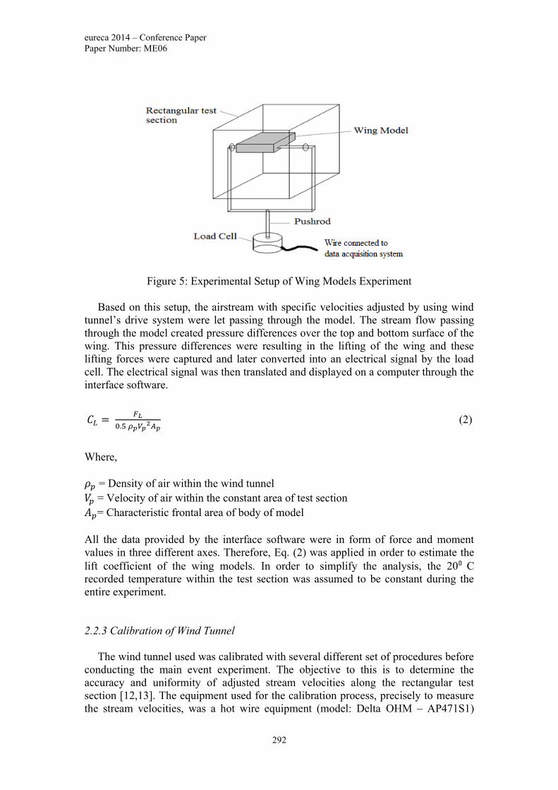
eureca 2014 – Conference Paper
Paper Number: ME06
292
Figure 5: Experimental Setup of Wing Models Experiment
Based on this setup, the airstream with specific velocities adjusted by using wind
tunnel’s drive system were let passing through the model. The stream flow passing
through the model created pressure differences over the top and bottom surface of the
wing. This pressure differences were resulting in the lifting of the wing and these
lifting forces were captured and later converted into an electrical signal by the load
cell. The electrical signal was then translated and displayed on a computer through the
interface software.
𝐶𝐿 = 𝐹𝐿
0.5 𝜌𝑝𝑉𝑝2𝐴𝑝
(2)
Where,
𝜌𝑝 = Density of air within the wind tunnel
𝑉𝑝 = Velocity of air within the constant area of test section
𝐴𝑝= Characteristic frontal area of body of model
All the data provided by the interface software were in form of force and moment
values in three different axes. Therefore, Eq. (2) was applied in order to estimate the
lift coefficient of the wing models. In order to simplify the analysis, the 20° C
recorded temperature within the test section was assumed to be constant during the
entire experiment.
2.2.3 Calibration of Wind Tunnel
The wind tunnel used was calibrated with several different set of procedures before
conducting the main event experiment. The objective to this is to determine the
accuracy and uniformity of adjusted stream velocities along the rectangular test
section [12,13]. The equipment used for the calibration process, precisely to measure
the stream velocities, was a hot wire equipment (model: Delta OHM – AP471S1)

eureca 2014 – Conference Paper
Paper Number: ME06
293
which comprises of a hot wire and an anemometer. Several parameters that were
tested to achieve the purpose of the calibration were the operational frequency of
wind tunnel’s drive system, x – coordinates of rectangular test section and operational
duration of wind tunnel’s drive system. The calibration of wind tunnel setup is
illustrated in Fig. (6).
Figure 6: Experimental Setup for Calibration of Wind Tunnel
The calibration of wind tunnel setup illustrated was used for the entire calibration
purposes experiments however, with different set experimental procedures. For
determining the relationship between the wind tunnel drive system’s frequency and
the stream velocity generated within the test section, the hot wire was fixed to
measure the stream velocities at the center of the test section while the operational
frequency was adjusted to 60 Hz from 0 Hz frequency with the increment of 5 Hz.
Next, for determining the accuracy of stream velocities generated along x – axis of
test section, the operational frequency was fixed to operate at 40 Hz while the hot
wire location was repeatedly changed from one end of the test section to the other end
of the test section with the increment of 10. Then, the similar procedure was adopted
at different operational frequency.
Lastly, for determining the relationship between the operational duration of wind
tunnel’s drive system and the stream velocities generated within the test section, the
operational frequency and the location of hot wire was fixed at 40 Hz and center of
test section respectively. Then, the stream velocities were recorded after 5, 10, 15, 20,
25 and 30 minutes of operational duration.
As a result, for the first calibration of the wind tunnel, It was found out that the
stream velocity produced within the test section exhibits the linear relationship
characteristic with the operational frequency of wind tunnel’s drive system. Hence,
the overall data was represented by the linear equation form, which the setting of
specific operational frequency will be specifically adjusted towards the corresponding
stream velocities inside the test section.
Meanwhile, for the second calibration of wind tunnel, few observations can be
noted. Firstly, the stream velocity within the test section varies with respect to

eureca 2014 – Conference Paper
Paper Number: ME06
294
different position along x – axis and particular operational velocity of the test section.
Secondly, the velocity variations at the preliminary section of the test section were
recorded as positive magnitudes whereas the velocity variations on route to the ending
segment of the test section become negative units. However, the velocity
dissimilarities are exceedingly small and negligible. Thirdly, the velocity variation
gradient along x-axis revealed an almost similar pattern behavior for all operational
velocities. Thus, this concludes of the stream velocity distribution is uniformly
scattered within the wind tunnel’s rectangular test section.
Lastly, for third calibration of wind tunnel, it was found out that the maximum
velocity disparities had occurred after 10 minutes of operating time and the minimum
velocity variation occurring after 25 minutes throughout the wind tunnel operation time
window. Since every interval of the velocity variations is very small and negligible, it
confirms that the velocity variation along the test section is not exclusively dependent
on the time taken for wind tunnel operation. Consequently, the velocity deviation in the
test section does not have substantial variation at diverse duration of operation.
However, in order to eliminate this bias factor, the lift generated by the wing models
will be collected after 10 minutes of operational duration since the velocity distributions
within the test section seems to obtain steady state.
3. Research Outcomes and Discussion
The first set of experiment was conducted by using NACA 0012 airfoil in order to
determine the accuracy of the research methods used. The experimental data obtained
were later validated with the experimental data of Abott [19] as presented in Fig. (7).
Lift Coefficient for NACA 0012 airfoil
Angle of attack, degree
0 2 4 6 8 10 12
Lif
t C
oeff
icie
nt
0.0
0.1
0.2
0.3
0.4
0.5
0.6
Current work
Experimental data Abott
Figure 7: Lift Coefficient for NACA 0012 airfoil at 200000 Reynolds number

eureca 2014 – Conference Paper
Paper Number: ME06
295
Based on Fig. (7), it can be seen that the experimental data obtained had an average
deviation of 12% at 5° angle of attack from the experimental data of Abott [19]. In
addition, the deviations of the data can be seen to be increased to 19% at 10° angle of
attack. The reasoning to this might be due to the sensitivity of the designed test rig
towards the vibration. Even though the load cell was tested to be able to determine
precisely the value of load when the load was placed on top of the test rig in a static
condition, the test rig seems to be vibrating as the wind tunnel was operated.
This assumption was supported with the increasing of data deviation as the
increasing angle of attack. This is because as the angle of attack is increases, the drag
force generated by the wing model will also be increases. Therefore, the large amount
of drag force tend to push the wing model further backward resulting in the inability
of the designed test rig to precisely capture the lift force generated by the wing model.
Another set of experiment was conducted in order to determine the mentioned
behavior. The experiments were performed by using rectangular wing models, both
having flat plate airfoil however, with different aspect ratios which were 0.5 and 1.0.
The experimental data were later validated with the experimental data of Alain and
Thomas [9] as illustrated in Fig. (8).
Lift Coefficient for flat plate airfoils
Angle of attack, degree
0 2 4 6 8 10 12
Lif
t coeff
icie
nt
0.00
0.05
0.10
0.15
0.20
0.25
0.30
Current work
Experimental data Alain & Thomas
Figure 8: Lift Coefficient for various aspect ratios Rectangular wing models at
140000 Reynolds number
Based on Fig. (8), it can be seen that similar behavior of experimental data were
obtained as the previous experimental data. Larger deviations can be seen to occur at
10° angle of attack than at 5° angle of attack. Therefore, this concluded that the
designed test rig was sensitive towards the vibration. As an attempt to reduce the
effect of this factor towards the reliability of the project, the further experiments were
performed by fixing the wing models at 5° angle of attack.
Next set of experiment was performed by all the wing models having a flat plate
airfoil however, with different aspect ratios which were 0.5 and 1.0 respectively. The
aim of this set of experiment was to determine the effect of aspect ratio towards the
lift generated by the wing models.

eureca 2014 – Conference Paper
Paper Number: ME06
296
Based on the Fig. (9), it can be seen that the effect of aspect ratio towards the lift
generated is significant. For instances, the rectangular wing model having an aspect
ratio of 1.0 had generated 0.09 lift coefficient while the rectangular wing model
having an aspect ratio of 0.5 only managed to generate 0.16 lift coefficient. This was
expected as the higher aspect ratio means that the span of the wing is larger hence, the
vortex flow effect that occurred at the wing tip is less exerted by the higher aspect
ratio wing when compared to the lower aspect ratio wing [14]. As evidence, similar
behavior was also predicted by Alain and Thomas [9]. This concluded that the effect
of aspect ratio is significant at low subsonic speeds.
After that, another set of experiment was performed by all the wing models having
a flat plate airfoil and 1.0 aspect ratio. However, unlike in previous set of experiment
which was using rectangular wing models, this set of experiment was performed by
using trapezoidal wing models with different taper ratios of 0.66 and 0.72 respectively.
The aim of this set of experiment was to determine the effect of taper ratio towards
the lift generated by the wing models at low subsonic speeds.
Lift Coefficient for various aspect ratios Rectangular wing models
Types of wing model
0 1 2
Lif
t co
eff
icie
nt
0.00
0.02
0.04
0.06
0.08
0.10
0.12
0.14
0.16
0.18
Rectangular wing model, AR 0.5
Rectangular wing model, AR 1.0
Figure 9: Lift Coefficient for various aspect ratios Rectangular wing models at
140000 Reynolds number
Based on Fig. (10), it can be seen that the more tapered trapezoidal wing had lower
amount of lift generated compared to the less tapered trapezoidal wing. This is
supported by the existing theory where it said that the more tapered wing should have
lesser lift generated due to the less surface area that was chopped off from the wing
[14]. Even so, it can be seen that only small differences in the lift generated between
both trapezoidal wing models and the effect seems to be almost insignificant.
With regards to the small differences data, the behavior observed might be occurred
due to insignificant effect of taper ratio at low subsonic speeds. As evidence, the
tapered wings are usually used for high speed aircraft like Boeing and Concorde
which the speed regimes of the flights are likely to be in higher subsonic or

eureca 2014 – Conference Paper
Paper Number: ME06
297
supersonic speeds. Thus, the effect of taper ratio towards the lift generated at low
subsonic speeds was concluded to be extremely small.
Next, another set of experiment was executed by using three different shapes of
wing models with all having aspect ratio of 1.0; Rectangular, Trapezoidal and
Triangular. The aim of this set of experiment was to determine the effect of wing
shapes towards the lift generated by the wing models.
Lift Coefficient for various taper ratios Trapezoidal wing models
Types of wing model
0 1 2
Lif
t co
effi
cien
t
0.00
0.02
0.04
0.06
0.08
0.10
0.12
0.14
0.16
0.18
Trapezoidal wing model, TR 0.72
Trapezoidal wing model, TR 0.66
Figure 10: Lift Coefficient for various taper ratios Trapezoidal wing models at
140000 Reynolds number
However, problem arises during executing the experiment as the triangular wing
model was designed to have a decreasing thickness along the wing span. This caused
difficulties when trying to drill through the wing model in order to fit in the support
rod within the wing model. Therefore, as a solution, the triangular wing model was
redesigned by having a vertical plate welded at the center, on top of the wing model.
Next, the vertical plate was drilled to enable the support rod to be fitted in, in order to
hold the wing model within the test section. The entire experimental data were
presented in Fig. (11).
Based on Fig. (11), it can be seen that the triangular wing model had significant
deviations from the other shape of wing model. The experimental data seems to
conclude that the triangular wing model had the lowest lift generated. It was indeed
strange as the trapezoidal wing model and the rectangular wing model had almost
insignificant effect due to the different shapes. As the triangular wing model was the
only one to have an addition feature than the others, the experimental data was
suspected to be affected by some errors.
Therefore, as the triangular wing model was seems to be having a vertical fin, a
thorough investigation was performed focusing on the effect of vertical fin on the
distribution of flow passing through it. Based on the existing theories, the vertical fin
is used by most aircrafts nowadays in order to stabilize the aircraft from rotating side
to side. This rotation from side to side is widely called as the yawing moment [20]. In

eureca 2014 – Conference Paper
Paper Number: ME06
298
an attempt to stabilize the aircraft, the vertical fin must be designed straightly aligned
possible on the center of the aircraft body in order to prevent the aircraft from having
a yaw moment.
Lift Coefficient for various shapes of wing models
Types of wing model
0 1 2
Lif
t coeff
icie
nt
0.00
0.02
0.04
0.06
0.08
0.10
0.12
0.14
0.16
0.18
Rectangular wing model
Trapezoidal wing model
Triangular wing model
Figure 11: Lift Coefficient for various shapes of wing models at 140000
Reynolds number
Thus, when rechecking the triangular wing model again, it was found that the
vertical plate was not welded straightly aligned to the center of the wing model
instead, having a slightly off towards the left direction. This might cause the
triangular wing model to be yawed hence, causing the test rig to be vibrated unusually
from the other experiments. As a result, the lift generated by the triangular wing
model was unable to be precisely captured by the load cell. As these errors was
affecting the experimental data of the triangular wing model, this set of experiment
was concluded with the effect of different shapes of wing model is not significant at
low subsonic speeds.
After that, several investigations were done in order to determine the accuracy of
the semi empirical method in estimating the lift generated by the wing models at low
subsonic speeds. For the first investigation, the experimental data for rectangular wing
models with different aspect ratios were compared with the semi-empirical data
obtained in this project. The comparisons of data are presented in Fig. (12).
Based on Fig. (12), it can be seen that the semi empirical method used in this
project managed to estimate the lift generated by the 0.5 aspect ratio rectangular wing
model. However, it can be seen that the semi empirical method used in this project
was underestimating the lift generated by the 1.0 aspect ratio rectangular wing model.
The reasoning to this might be due to the incapability of the semi empirical method to
take into account the vortex induced lift effect. Vortex induced lift effect is the lift
generated due to the flows that are vorticing around the wing. When streams are let
passing through the wing model, at one point, the stream will starting to form a vortex

eureca 2014 – Conference Paper
Paper Number: ME06
299
flow around the wing model. This vortex flow will increases the lift generated by the
wing model. As this factor is not taken into consideration by the semi empirical
method , the semi empirical method used in this project was unable to estimate the lift
generated by the larger aspect ratio wing model. Therefore, it was concluded that the
semi empirical method used in this project was able to estimate the lift generated by
the rectangular wing model however, it tends to underestimate as the increasing of
aspect ratio.
Comparison between experimental data and semi empirical data
for Rectangular wing models
Types of wing model
0 1 2
Lif
t coeff
icie
nt
0.00
0.02
0.04
0.06
0.08
0.10
0.12
0.14
0.16
0.18
Semi empirical data, AR 0.5
Rectangular wing model, AR 0.5
Semi empirical data, AR 1.0
Rectangular wing model, AR 1.0
Figure 12: Comparison between experimental data and semi-empirical data
for Rectangular wing models
For the second and the last investigation, the experimental data for all the wing
models having aspect ratio of 1.0 were compared with the semi empirical data
obtained in this project. The comparison of the data are presented in Fig. (13).
Based on Fig. (13), it can be seen that similar value of lift was estimated by the
semi empirical method used in this project for all the wing models having 1.0 aspect
ratio. The reasoning to this might be due to the incapability of the semi empirical
method applied to take into account the effect of taper ratio and wing shapes towards
the lift generated by the wing models. Based on Fig. (13), it can also be seen that the
semi empirical method used in this project was underestimating the lift generated by
all the wing models except for triangular wing model. The closest estimation by the
semi empirical method for wing models having aspect ratio of 1.0 was the trapezoidal
wing with having taper ratio of 0.72. The deviations between the data was only 0.01.
On the other hand, the furthest estimation of the semi empirical method was occurred
for the triangular wing model which illustrated 0.04 data differences. However, as the
data for the triangular wing model was unreliable due to the several factors discussed
previously, this indicates that the furthest estimation of the semi empirical method
was occurred for the trapezoidal wing model having a taper ratio of 0.66. Again, this
concluded that the semi empirical method applied in this project was unable to take

eureca 2014 – Conference Paper
Paper Number: ME06
300
into account the effect of vortex induced lift, taper ratio and wing shapes when
estimating the lift generated by the wing models at low subsonic speeds.
Comparison between the experimental data and semi empirical data for
all the wing models having 1.0 aspect ratio
Types of wing model
0 1 2
Lif
t coeff
icie
nt
0.00
0.02
0.04
0.06
0.08
0.10
0.12
0.14
0.16
0.18
Semi empirical data, AR 1.0
Rectangular wing model
Trapezoidal wing model, TR 0.72
Trapezoidal wing model, TR 0.66
Triangular wing model
Figure 13: Comparison between the experimental data and semi empirical
data for all the wing models having 1.0 aspect ratio
4. Conclusions
As a result, It was found out that the effect of aspect ratio towards the lift is
significant at low subsonic speeds however, the effect of wing shapes and taper ratio
towards the lift are extremely small. These behavior might be predicted at low
subsonic flow. Also, the empirical formulae developed in this project was found out
to underestimate the lift generated by the wing models. The reasoning to this is due to
the incapability of the empirical formulae developed to take into account the effect of
the vortex induced lift of the wing models. It was also found out that the empirical
formulae developed was unable to take into account the effect of wing shapes and
taper ratio as similar value of lift was yielded for all the wing models with having 1.0
aspect ratio.
As a recommendation for future works, the test rig used in this project can be
redesigned to be mountly rigid to the ground in order to reduce the vibration of the
test rig. This will helps in increasing the accuracy of the experimental data obtained.
This will also allows further investigation on the effect of wing shapes and geometries
on lift at low subsonic speeds at higher angle of attack. Along completing this project,
several interesting areas were determined by the author to be investigated for future
works; the investigation on the aerodynamic performances of micro air vehicle and
the aerodynamic performances of a rotated aircraft due to crash.

eureca 2014 – Conference Paper
Paper Number: ME06
301
Acknowledgment
The authors wish to deliver their appreciation to Taylor’s University School of
Engineering for granted permission to use the wind tunnel facilities in order to
achieve the research objective.
References
[1] Sagar, S. S. (2004). Lift Distributions on Low Aspect Ratio Wings at Low
Reynolds Number. Master’s thesis, Worcester Polytechnic Institute,
Massachusetts, United States.
[2] Thomas, J. M. (1999). Aerodynamic Measurements at Low Reynolds Numbers
for Fixed Wing Micro-Air Vehicles. Paper presented at the RTO AVT/VKI
Special course on Development and Operation of UAVs for Military and Civil
Applications, Von Karman Institute, Sint-Genesius-Rode, Belgium.
[3] Wilson, J. R.. (1998) .Mini Technology for Major Impact. Aerospace America,
Vol. 36, No. 5, pp. 36–42.
[4] Eric T. N. K. (2013). Effect of Wing Configuration on Lift at Supersonic Speeds.
Master’s thesis, Taylor’s University, Subang Jaya, Selangor, Malaysia.
[5] Niculita, C., Bencze, A., Candea, I. (2008). Aircraft Wings: Present and Future.
Bulletin of Transilvania of Brasov. Vol. 1, No. 50, pp. 41-46.
[6] Louis, P. T. (1947). Low Speed Static Stability and Damping-In-Roll
Characteristics of Some Swept and Unswept Low Aspect Ratio Wings (National
Advisory Committee for Aeronautics, Tech. Note. No. 1468). Washington,
United States: Langley Memorial Aeronautical Laboratory.
[7] John, J. H. (1951). Investigation at Low Speed of 45° and 60° Sweptback, Tapered,
Low-Drag Wings Equipped with Various Types of Full-Span, Trailing Edge
(National Advisory Committee for Aeronautics, Tech. Note. No. 2468).
Washington, United States: Georgia Institute of Technology.
[8] Abdulkareem, M. A. O. (1996). Lateral Directional Stability Analysis of a Flying
Body at Supersonic Speeds. Master’s thesis. University of Baghdad, Baghdad,
Iraq.
[9] Alain, P., Thomas, J. M. (2000). Low Reynolds Number Aerodynamics of Low
Aspect Ratio. Journal of Aircraft, Vol. 37, No. 5.
[10] Billy, L. W. K. (2014). Taylor’s Wind Tunnel Manual. Taylor’s University,
Subang Jaya, Selangor, Malaysia.
[11] Huber, A. F. (1985). The Effects of Roughness on an Airfoil at Low Reynolds
Numbers. Master’s thesis. Department of Aerospace and Mechanical Engineering.
University of Notre Dame, Indiana, United States.
[12] Michael, S. S., James, J. G., Andy, P. B., Philippe, G. (1995). Summary of Low
Speed Airfoil Data. Virginia, United States, SoarTech Publications.

eureca 2014 – Conference Paper
Paper Number: ME06
302
[13] Laitone, E. V. (1997). Wind Tunnel Tests of Wings at Reynolds Numbers Below
70000. Experiments in Fluids, Vol. 23, No. 5, pp. 405 -409
[14] Raymer, D. (2014). Aircraft Design: Conceptual Approach. California, United
States, AIIA Education Series.
[15] Brendel, M., Huber, A. F. (1984). An Experimental Investigation of Flow Quality
in an Indraft Subsonic Wind Tunnel Using a Single Hot Wire Anemometer.
University of Notre Dame, Indiana, United States.
[16] Fink, R. (1978). USAF Stability and Control Datcom. California, United States,
McDonnell Douglas Corporation.
[17] Miley, S. J. (1972). An Analysis of the Design of Airfoil Sections for Low
Reynolds Numbers. Doctoral dissertation. Mississippi State University, Starkville.
[18] Anderson, J. D. (2001). Fundamental of Aerodynamics. New York, United States,
McGraw Hill publication.
[19] Abott, I. R. (1959). Theory of Wing Sections. New York, United States, Dover
publication.
[20] Woodfield, A. A. (1969). Measurement of the Yawing Moment and Product of
Inertia of an Aircraft by the Single Point Suspension Method: Theory and Rig
Design (National Advisory Committee for Aeronautics). Washington, United
States: Langley Memorial Aeronautical Laboratory.

eureca 2014 – Conference Paper
Paper Number: ME07
303
Thrust Generation Using Synthetic Jet
Muhammad Hazim bin Anuar*1
, Mushtak Al-Atabi1, Ooi Ferng Lin
1
1School of Engineering, Taylor’s University, Malaysia
Abstract
This study aims to explore new application of synthetic jet that utilizes the generated
thrust for propelling purposes. The feasibility of synthetic jet as the propulsion system
for a small underwater vehicle has already been proven. Nonetheless, there are few to
none study validated its practicality as an airborne propulsion method. Hence, this
study attempts to reveal the possibility of synthetic jet as a novel thruster of micro-air
vehicle by investigating the capability of synthetic jet in term of thrust generation.
Micro-air vehicle (MAV) is classified as aerial vehicle that has size restriction and
deployed for various purposes comprising surveillance watching, military spying and
others. This type of vehicle has developed since few decades ago as there is an on-
going effort to study new techniques for air-vehicle propulsion. A helium-gas blimp
with a volume of 0.5 m3 was referred to estimate roughly the needed thrust by
calculating the drag force. A synthetic jet prototype was developed and tested. Its
capable of producing thrust by pulsatile vortex ring was expected to overcome the
blimp’s drag force. To comply with the objective of this study, the prototype design
replicates the scheme of micro-thruster which has several properties such as small-
size, light-weight and low operating power. The performance of synthetic jet was
assessed using direct thrust measurement. The result was verified with previous
research data. In flight fundamental context, thrust generated by our synthetic jet is
proven to overcome the drag force and the hypothesis is accepted; synthetic jet is a
viable method for airborne propulsion. However, there are several factors (such as
thrust-to-weight ratio, ratio of propeller size to propulsion power, and etc.) must be
considered when dealing with micro-sized flying object and future work must
consider those factors.
Keywords: Synthetic Jet, Thruster, Airborne Propulsion System, Micro-Air Vehicle,
Direct Thrust Measurement.

eureca 2014 – Conference Paper
Paper Number: ME07
304
1. Introduction
The science of flight stated four fundamentals which are lift, weight, thrust, and
drag as shown in Fig.1 [1]. In designing an aircraft, engineers consider those elements
to ensure the airplane travels through the air successfully. In a steady flight, the sums
of all opposing forces are equal and thus complies with the conservation of
momentum principle. Weight and lift force govern the altitude of the plane. To move
the plane forward, the thrust must be greater than the drag [2].
Fluid dynamics define jet as fluid ejection from a duct into relatively large region
through an orifice or nozzle [4]. Meanwhile, synthetic jet is a flow generated by
alternate suction and ejection of the ambient fluid through an orifice with zero net
mass flux. It has distinctive feature which is it enables the transfer of linear
momentum to the flow system. The jet is different from synthetic jet as the net mass
flux is not zero at one end where the fluid is supplied (mass inlet).
The study of thrust generation using synthetic jet has progressed since few
decades ago. Its feasibility in various applications has been proven through a sensible
amount of studies; an effective aerodynamic controller for airplane wing, effective
chemical mixer replacing conventional agitator, viable propulsion method for
underwater autonomous unmanned vehicle, and lastly efficient cooling device for
electronic component [5-8].
Micro-air vehicle is an aerial vehicle flies in low Reynold’s number at velocity up
to 10m/sec [9]. It has numerous potential applications that benefit civilian and
military. Usually, the propulsion system consists of electrical motor and power supply.
The challenge of building this type of vehicle is maintaining the design compactness
with electronic component installation to achieve mass restriction.
Figure 2. Four flight fundamentals [3]
Figure 3. Example of micro-air vehicle with 7.3 cm
wingspan [9]

eureca 2014 – Conference Paper
Paper Number: ME07
305
There is an ongoing effort to study new techniques of micro-air propulsion [10].
To date, there are several methods of synthetic jet actuation, which is driven by
piezoelectric, mechanical, electrostatic, plasma, and acoustic [5]. Each type has been
tested experimentally as well as simulation using computational fluid dynamic
software. However, not even single study had produced a scheme for airborne
propulsion with concrete proof of its practicality when deployed together with air-
vehicle.
This study tends to propose a new application of synthetic jet thruster. It has a
potential to be deployed as thrusters for the flying surveillance camera. This type of
air vehicle moves with slow speed because of low-thrust propulsion system and is
suitable to be used in low wind interference surrounding such as shopping mall,
examination hall and other places that fit to its capability. This idea is inspired by the
immobility of surveillance camera that has a fixed position and limited view.
For that specific use, a synthetic jet prototype was constructed based on crude
approximation of the thrust range needed to move a helium-gas blimp [11]. Helium
gas inside the blimp provides the lifting force to carry payload. Meanwhile, the
calculated drag force of the blimp ranges between 0.05mN to 1.36mN. If the thrust
generated by synthetic jet prototype exceeds the drag force of the blimp, theoretically
this air-vehicle will move forward [1].
A synthetic jet thruster will be placed at the bottom of a blimp parallel to the
vehicle center of buoyancy. The thrust generated from thruster (FSJT) will produce a
reaction force (FR) in the opposite direction. The force supplied from the thruster will
initiate the movement of the blimp and cause it to travel in x-direction. Free body
diagram showed in Fig. 3 provide a clear conception of the system.
The reaction force (FR) generated from synthetic jet thruster will provide a force
to the blimp, FT. According to the Principle of Conservation of Momentum, movement
will be initiated if the total thrust force greater than the total drag as equated in
Equation 1. This blimp will travel at a constant speed when total forces of FT and FD
are equal (Eq. 2).
Thruster
Figure 4. Free body diagram of blimp’s propulsion system

eureca 2014 – Conference Paper
Paper Number: ME07
306
𝛴𝐹𝑇 > 𝛴𝐹𝐷 (1) To initiate blimp movement
𝛴𝐹𝑇 = 𝛴𝐹𝐷 (2) To blimp moves at constant speed
As stated before, this study aims to develop the potential of synthetic jet as a
thrust production device as well as to propose a new application of synthetic jet and
identifies the range of application. Other than that, the objectives include:
i. To identify the range of synthetic jet application as well as to clarify the gap
within the area of study.
ii. To design and build a synthetic jet prototype with optimum geometric
configuration inspired from existing models.
iii. To evaluate and select an appropriate method of measuring thrust specifically
for synthetic jet prototype.
Usually, a synthetic jet model consists of cavity/chamber, diaphragm/membrane
orifice and actuator (shown in Fig. 4) [12-13]. The actuator is used to synthesize jet
flow meanwhile membrane is made up of elastic material which can deflect
correspondingly to the frequency and amplitude of the actuator.
When actuator stimulates movement of the diaphragm in oscillating manner, it
will displace the cavity volume and lead to changes in mass of air inside the cavity.
Mass flow rate flux inside the cavity resulted in pulsatile jet formation. Fig. 5 showed
the formation of synthetic jet flow. (A) Intake stroke. (B) Ejection stroke. (C) Vortex
pinched-off. (D) Successive vortex move away and the process repeats.
Figure 5. Parts of synthetic jet thruster [7]
Figure 6. Synthetic jet formation [13]

eureca 2014 – Conference Paper
Paper Number: ME07
307
2. Methodology
To design a propulsion system of a blimp, it must follow the procedure as shown
in Fig. 6 [11]. Firstly, estimation is made on the total weight of the payload by
considering all possible components that build up the propulsion system. The system
made up of thruster, electronics component and power supply. The total weight of the
system is approximately 450g. Note that, the weights of all components were crudely
estimated except for thruster, which used actual value.
The lifting force of helium gas is 1.02kg/m3 at room temperature and atmospheric
pressure at sea level [11]. From the total estimated payload, the required volume of
the gas is about 0.45m3. Thus, the dimension of the blimp can be determined as well
as the drag. Tayyab [11] proposed a dimension configuration of a 0.5m3
blimp that
has a total surface area of 3.474m2, a length of 2.07m and frontal area of 0.37m
2.
By knowing the dimension of the blimp, drag can be calculated to determine the
thrust need to be generated. Note that, the construction of the blimp is not included in
this research; instead it is just a reference to generate an amount of thrust. The
performance of the thruster can be determined from drag against velocity graph. It
also determines the maximum speed of the blimp can move with the thruster
The synthetic jet prototype geometry was determined by rationing the diameter of
the cavity to diameter of existing model [10]. Using the ratio of 15, our prototype was
scaled down in size to achieve design compactness even though the actuation power is
reduced. It consists of four elementary parts; orifice plate (overall diameter of 5cm
and orifice diameter of 0.3cm), cavity/chamber (diameter of 4.5cm and height of
0.5cm), membrane/diaphragm (rubber) and actuator (speaker). Fig. 7 showed the
prototype 3D drawing and end product.
Figure 7. Propulsion system design procedure

eureca 2014 – Conference Paper
Paper Number: ME07
308
Since this area of study has not specified a standard scheme of thrust measurement
experiment, we have selected the method based on a few factors; resolution,
availability, and reliability. Hence, the performance of the thruster was assessed using
direct thrust measurement in which the thruster was entirely mounted on an electronic
balance [10]. The measurement of thrust was carried out in vertical direction.
However, in real operation, the thruster will be deployed in horizontal direction.
The complexity of the prototype design and the actuation method has lagged this
study. Other factors such as time-constraining research period (twelve weeks) and
limited-budget has caused this research focused more on the construction and testing
the actuation technique that produces a significant deflection to the membrane.
2.1 Synthetic Jet Thrust Calculation
There are several schemes of synthetic jet thrust calculation provided [7,10]. The
fundamental of thrust calculation originates from a slug model (shown in Fig. 8)
which represent stroke ratio denoted as L/D [5,12,13,14]. This non-dimensional
analysis is the ratio of stroke length to the diameter of the ejected fluid. D is the
diameter of the orifice and L can be obtained by integrating the centerline velocity
(𝑈0) of the fluid within the period (T) of one successive ejection. The formula is
stated below:
𝐿 = ∫ 𝑈0(𝑡)𝑑𝑡𝑇
0 (3)
Figure 8. Synthetic jet prototype 3D Drawing using Solidworks (left) and
manufactured prototype (right).
Figure 9. Slug model [7]

eureca 2014 – Conference Paper
Paper Number: ME07
309
The ejected fluid travels away from the orifice at the velocity corresponding to the
membrane actuation speed. It then forms a circle and creating impulse which
determines the vortex strength [7]. The total circulation (Г𝑜) can be calculated using
Equation 4 [10]. Meanwhile, Equation 5 is the formula of synthetic jet thrust (𝑇ℎ)
related to the circulation. This formula contains the density of air (𝜌) , actuation
frequency (𝑓) and effective cross-section area of the jet orifice (𝐴𝑗𝑒).
Г𝑜 =1
2∫ 𝑈𝑜
2𝑇
0𝑑𝑡 (4)
𝑇ℎ = 2𝜌Г𝑜𝑓𝐴𝑗𝑒 (5)
2.2 Direct Thrust Measurement
Thrust measurement using analytic balance is not a new method. It replicates the
practice of force measurement experiment using load cell or force sensor. It has been
practiced by preceding work to directly measure the amount of thrust generated [7,10,
15]. This method uses the relationship between force and mass of Newton’s Second
Law (F=ma). As the acceleration of gravity is considered to be constant at all time,
the force will increase corresponding to mass increment. An analytical balance with
resolution of 0.001g was used to measure the thrust generated by the synthetic jet
prototype.
The setup of the experiment is shown in Fig. 9 whereby the entire synthetic jet
prototype was mounted on the electronics balance. The frequency was controlled by a
function generator. Sine wave was used and the frequency slowly increased. The
results obtained in a unit mass (gram) were recorded and tabulated for analysis. The
measured mass was converted to unit Newton to obtain the thrust force.
The prototype is oriented in y-direction for the thrust measurement purpose as
shown in Fig. 10. However, in real operation, the thruster will be deployed in x-
direction. When the synthetic jet prototype is actuated by the speaker, the membrane
is deflected. This will cause alternate suction and ejection of ambient flow inside the
cavity of the prototype. Then thrust (FSJT) is generated through the orifice. The
reaction force (FR) can be measured by analytic balance in unit gram.
Figure 10. Schematic diagram of experiment set up

eureca 2014 – Conference Paper
Paper Number: ME07
310
3. Results & Discussion
The graphs below show the relationship between actuation frequency and thrust
generated. The graph on the left represents the experimental results (present work)
and on the right is the previous experiment [10].
From Fig. 11 (left), by increasing the actuation frequency using function generator,
the reading of weight increases gradually. The weight increment indicates the
increasing thrust. The pulse generated by synthetic jet produces higher thrust at higher
frequency. This is because the vortex rings produced are close to each other; hence
increase the entrainment effect [5].
Experimental data have a lowest thrust of 0.01mN at 20Hz and highest thrust of
0.31mN at 140 Hz. At 10Hz, no reading was recorded in the analytical balance, means
that the fluid ejected is not able to circulate and produce a pulse. This may come from
Figure 12. Experimental result (left) & experiment by Muller (right)
Figure 11. Synthetic jet prototype orientation in experiment set up
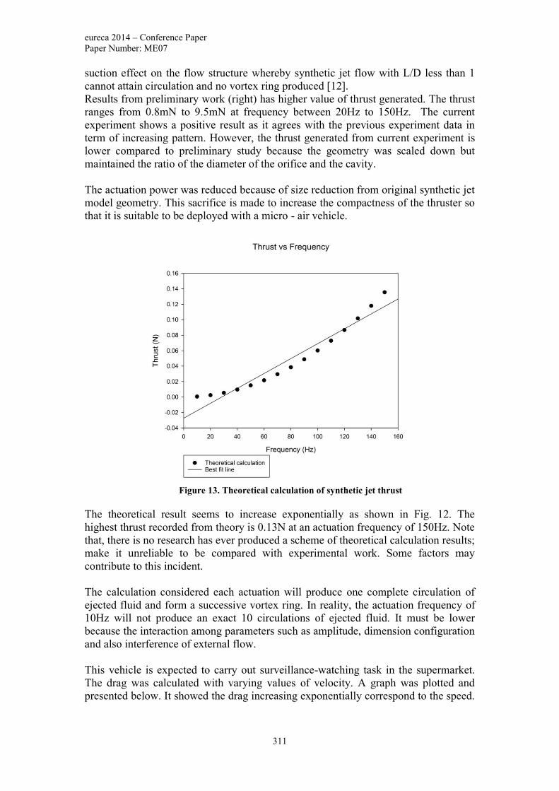
eureca 2014 – Conference Paper
Paper Number: ME07
311
suction effect on the flow structure whereby synthetic jet flow with L/D less than 1
cannot attain circulation and no vortex ring produced [12].
Results from preliminary work (right) has higher value of thrust generated. The thrust
ranges from 0.8mN to 9.5mN at frequency between 20Hz to 150Hz. The current
experiment shows a positive result as it agrees with the previous experiment data in
term of increasing pattern. However, the thrust generated from current experiment is
lower compared to preliminary study because the geometry was scaled down but
maintained the ratio of the diameter of the orifice and the cavity.
The actuation power was reduced because of size reduction from original synthetic jet
model geometry. This sacrifice is made to increase the compactness of the thruster so
that it is suitable to be deployed with a micro - air vehicle.
The theoretical result seems to increase exponentially as shown in Fig. 12. The
highest thrust recorded from theory is 0.13N at an actuation frequency of 150Hz. Note
that, there is no research has ever produced a scheme of theoretical calculation results;
make it unreliable to be compared with experimental work. Some factors may
contribute to this incident.
The calculation considered each actuation will produce one complete circulation of
ejected fluid and form a successive vortex ring. In reality, the actuation frequency of
10Hz will not produce an exact 10 circulations of ejected fluid. It must be lower
because the interaction among parameters such as amplitude, dimension configuration
and also interference of external flow.
This vehicle is expected to carry out surveillance-watching task in the supermarket.
The drag was calculated with varying values of velocity. A graph was plotted and
presented below. It showed the drag increasing exponentially correspond to the speed.
Figure 13. Theoretical calculation of synthetic jet thrust

eureca 2014 – Conference Paper
Paper Number: ME07
312
The maximum thrust generated from synthetic jet prototype was plotted as a
horizontal line to show the limit of propelling capacity.
The graph indicates that the blimp’s velocity must not exceed 0.23m/s because the
thruster cannot overcome the drag force. The total weight of the synthetic jet
prototype is less than 50g. This will benefit the vehicle in term of mass restriction in
which other pertaining component such as extra batteries and more complex
electronics circuit can be fitted into the propulsion system. To make it move faster, a
combination of synthetic jet thrusters would be applicable.
4. Conclusion
The thrust performance of a synthetic jet thruster has been analyzed and it is found
to be a feasible alternative for micro-air vehicle in term of propelling in horizontal
direction. It still needs support from the blimp filled with helium gas to lift up the
entire vehicle plus the synthetic jet thruster. The experimental results showed
maximum thrust production of 0.31mN, which overcome the drag force of the blimp
below 0.23m/s. This vehicle can be improved by constructing a smaller actuator (1/4
of present model) and provide higher actuation power so it can travel faster, and at the
same time reduce the total weight.
Acknowledgement
The authors want to express their gratitude and appreciation to Taylor’s University
School of Engineering for funding this project to enable its successful completion.
Additionally, we would also like to acknowledge Mr. Sunny and Mr. Alif for helping
authors throughout the construction and experimentation of our synthetic jet prototype.
Figure 14. Drag vs velocity graph

eureca 2014 – Conference Paper
Paper Number: ME07
313
Reference
[1] Cook, M. V. (2007). Flight Dynamics Principle. Burlington, MA: Butterworth-
Heinemann.
[2] Datta, S. (2009). Newton’s Third Law of Motion. Physics Education, July-
September 2009, pg. 213.
[3] Grc.nasa.gov, (2014). What is Thrust?. [online] Available at: http://www.
grc.nasa.gov/WWW/k-12/airplane/thrust1.html [Accessed 15 Oct. 2014].
[4] Shames, I.H., 2003. Mechanics of Fluid. 4th edition. New York: McGraw Hill
[5] Glezer, A. & Amitay, M., 2002. Synthetic Jets (Review Paper). Annual Review of
Fluid Mechanics, Volume 34, pp. 503-529.
[6] Lin, O. F., 2013. Final Year Project Thesis: Investigation of Mixing Using
Synthetic Jet, Subang Jaya: Taylor's University School of Engineering.
[7] Thomas, A.P., et al., 2005. Synthetic Jet Propulsion for Small Underwater
Vehicles. Barcelona, IEEE.
[8] Nuventix, Inc., 2007. SynJet: Low-Power "Green" Cooling, Austin, Texas:
Nuventix.
[9] William, R. D., Bernard, B. K., Don, M. B., Daniel, F. K. (1996). Micro Air
Vehicles for Optical Surveillance. The Lincoln Laboratory Journal Volume 9, No. 2
[10] Müller, M.O., Bernal, L.P., Miska, P.K., Washabaugh, P.D., Chou, T.A., Parviz
B.A., Zhang, C., Najafi, K. (2001). Flow Structure and Performance of Axisymmetric
Synthetic Jets. Paper presented at 39th Aerospace Science Meeting & Exhibit, Reno, NV
[11] Tayyab, M., Farooq, U., Ali, Z., Imran, M., Shahzad, F., (2013). Design of a
Blimp Based Unmanned Aerial Vehicle for Surveillance. International Journal of
Engineering and Technology (IJET) Vol 5 No 1.
[12] Thomas, A. P., 2007. Thesis: Exploration Into the Feasibility of Underwater
Synthetic Jet Propulsion. Pasadena: California Institute of Technology.
[13] P. Linden and J. Turner, “The formation of ’optimal’ vortex rings, and the efficiency
of propulsion devices,” Journal of Fluid Mechanics, vol. 427, pp. 61–72, 2001.
[14] Smith, B. L. & Glezer, A., 1998. The Formation and evolution of synthetic jets.
Physical Fluids, Volume 31, pp. 2281-2297.
[15] Krieg, M., Pitty, A., Salehi, M. & Mohseni, K., 2005. Optimal Thrust
Characteristics of a Synthetic Jet Actuator for Application in Low Speed
Maneuvering of Underwater Vehicles. OCEANS MTS/IEEE, Volume 3, pp. 2342-
2347.

eureca 2014 – Conference Paper
Paper Number: ME08
314
Effect of Evaporator Heater Power Input
and Condenser Water Flow Rate on the
Performance of a Refrigerator – Developing
Empirical Models
Ali Naif1*
, Abdulkareem Shafiq Mahdi Al-Obaidi1
1School of Engineering, Taylor’s University, Malaysia
Abstract
Refrigerators are heat pumps that transfer heat from a volume of space as to reduce
the temperature compared to the ambient temperature of its location. Refrigerators are
also the one of the notorious contributors to high monthly electricity bill. This paper
presents first a comparison between theoretical and experimental determination of the
coefficient of performance (COP) of a vapor compression refrigeration cycle.
Secondly, derivation of empirical models based on experimental results that would
allow refrigerator designers to check on the significance of each investigated
parameter on the COP value. There were three models created. Model 1 took both
evaporator heater power input (EHPI) and condenser water flow rate (CWFR) in to
consideration and produced the most accurate at 97.2%. Model 2 and Model 3 just
took into account EHPI and CWFR respectively and produced accuracies of 94.3%
and 3.12% respectively. Therefore, Model 1 was found to be as the best predictor of
COP. The results produced by the final model were within the uncertainty range of -
9.49% and 2.55% compared to the experimental results. This was with in the
acceptable range of ±10%. The overall error could be minimized by including other
important parameter in to the model and also by further limiting the heat transfer to
the surrounding.
Keywords: Coefficient of Performance, Refrigeration, Efficiency, Vapor Compression
Cycle, Empirical model.

eureca 2014 – Conference Paper
Paper Number: ME08
315
1. INTRODUCTION
1.1. Background
Household refrigerators are machines or devices that are normally used for
preserving food by reducing the temperature of its storage compartments. There are a
few types of refrigeration cycles that are suitable to achieve this function. However,
vapor compression refrigeration cycles (VCRC) are the most widely used cycle for
household refrigerators due to its high versatility. On the other hand, refrigerators are
also notorious for their high energy consumption alongside air conditioning systems.
Amongst the many reasons for high energy consumption, around the clock operation
and the complex irreversibility of the individual mechanical and electrical
components are the major two contributing factors. Therefore, optimization of the
performance of a refrigerator has become a necessity.
During the past few decades, ejector-vapor compression cycles (EVCC) has
been probed significantly in efforts to optimize the COP of basic VCRC. Zhu & Jiang
[1] using working fluid R22, Yan et al. [2] using working fluid R134a and Ersoy &
Bilir Sag [3] using various different types of working fluids was able to achieve as
COP improvements as high as 9.1%, 14.5% and 21.0% respectively. Molés et al. [4]
argued that the COP of hybrid cycles operated with low Global Warming Potential
(GWP) refrigerants, such as R1234yf and R1234ze(E), instead of more conventional
ones, such as R134a, improved up to 15% and 20% while the COP of the basic VCC
reduced by 4% to 8%. Still, this study also indicated that replacement of conventional
refrigerants may increase the complexity of the practical system and ultimately the
cost.
In general, although such integrated EVCCs require a similar amount of
operating cost, it contains almost twice the amount of components as a basic VCRC.
This increase in the number of components may require more energy and also would
be subjected to more losses, despite the overall improvement in performance. Thus, it
is believed that the amount of improvement achieved by this hybridization is
relatively low. Moreover, Sarkar [5] indicated that, besides promising improvements
more research was required to make an impact in large scale usage.
Li et al. and Wang et al. [6,7] argued another type of hybridized cycle, which
uses an organic Rankine cycle (ORC) to power up the basic VCC, that improved the
overall COP by 0.47 and 0.6. Both studies agreed that an additional recuperator at the
ORC side of the system would further increase the overall COP. But, once again it
was conclusive that the degree of improvement achieved with severe modification
was unsatisfyingly low. Further modification that may need to rise the COP slightly
more. This would result in further increase in cost of operation and maintenance.
Besides complex physical modification, refrigeration cycles may also be
optimized grounded on mathematical or analytical modeling according to theoretical
or experimental data. Model based optimizations are cheap and ideal methods to
predict the effect of design parameters on the COP of the refrigeration system during
the preliminary design stage. Studies conducted by Domanski et al., Wainaina et al.,
Zhao et al., Wallace et al. and Gonçalves et al. [8-12] provided insightful models that
were related to optimization of the basic VCRC.

eureca 2014 – Conference Paper
Paper Number: ME08
316
Similarly, Jain et al., Yao et al., Waltrich et al., Li & Alleyne, Getu & Bansal
and Navarro-Esbrí et al. [14–19] produced optimization model that may improve the
VCRC. Though, these studied varied off from the simplisity and was deviated to
modified hybrid system and specific operation condition or parameter.
Yusof & Azizuddin [20] performed experimentation and identified how the
differenct parameters of the refrigerators behaved over time. Although, a relationship
between these parameters and the COP were not displayed, the combination the
selective techniques utilized within these studies would provide a platform. These
studies lacked the simple and direct correlation of the COP with other basic operational
parameters.
In order to design a refrigerator system with optimal performance,
predetermining the correlation of individual design parameters to the COP seems
somewhat crucial. Similarly, to understand the significance of the design parameters
in an existing system may also provide time and cost saving assistance. Therefore,
optimization of the simple VCRC could provide priceless and insightful information
which could be used during the preliminary design stage of household refrigerator
systems. With such optimized models, a VCRC refrigeration systems could be design
to have optimal efficiency with low initial cost and almost negligible amount of
testing.
Hence, the aim of this paper is to develop empirical models that correlates the
effects of operational parameters such as the evaporator input and water flow rate
with the coefficient of performance of the refrigerator, and ultimately fabricating a
deign table that could be utilized as a quick, cheap and yet reliably accurate tool
during the preliminary design stage.
1.2. Coefficient of Performance
Overall Coefficient of Performance (COP) is the ratio between the rate of heat,
Qe, absorbed at the evaporator and the net work done, Win, by the compressor as shown
in the Eq. (1) below. It one of the most commonly used measure of performance
efficiency.
𝐶𝑂𝑃𝑅 =𝑄𝑒
𝑊𝑖𝑛=
𝑄𝑒
𝑄𝑐 − 𝑄𝑒=
ℎ1 − ℎ4
ℎ2 − ℎ1 (1)
The performance of refrigerator systems could be improved to perform
exceptionally better by modifying and altering its elements. However, such
modifications and experimentations are usually costly as they may require state of the
art components and research. Carnot cycle or ideal VCRC provide crucial information
about the full potential. But, it would also indisputably overestimate the COP of a real
life refrigeration systems due to the high irreversibility. A comparison between the
fundamental theories of the ideal and actual VCRC would help recognize the losses in
real operations.

eureca 2014 – Conference Paper
Paper Number: ME08
317
2. METHODOLOGY
2.1. Refrigerant Cycle
Vapor compression refrigeration cycles (VCRC) are known to be one of the
most commonly used and versatile refrigeration cycle. VCRC are suitable for almost all
applications in a wide range of cooling capacities from just a few watts to a few
megawatts. As seen in Fig. 1, a basic vapor compression cycle consists of a compressor,
condenser, expansion device, evaporator and a working fluid; a refrigerant.
Figure 1. Simple Vapor Compression Refrigeration Cycle
From state 1 to state 2, the superheated refrigerant undergoes compression
which its temperature and pressure are increased significantly. During this compression
stage, it is necessary that the refrigerant is completely in vapor form because the
presence of liquid may damage the compressor. From state 2 to state 3, the superheated
vapor travels through the condenser where the heat energy with in the refrigerant is
transferred to the surrounding or a sink, across a conductive tubing. Due to this quick
release of heat, the refrigerant liquefies or condenses in to a saturated liquid. However,
the pressure drop from state 2 to state 3 is negligible. Hence, across the expansion valve
from state 3 to state 4, the pressure is dropped drastically. But due to unavoidable heat
absorption, the refrigerant exits the expansion valve in the form of a liquid- vapor
mixture with higher percentage of liquid. The liquid-vapor mixture at state 4 then
absorbs heat from a heat source across conductive tubing to become superheated vapor
at state 1.
2.2. Parameter Selection, Experimental Setup and Assumptions
The experiments for this particular study were conducted using R713
Refrigeration Laboratory Unit by P.A. Hilton Ltd, as seen in Fig. 2. This rig was
specifically designed to study the performance of the refrigeration cycle by solely
controlling the evaporator heater power input (EHPI), ��𝐸𝑉𝐴𝑃, and the condenser water
flow rate (CWFR), ��𝐶𝑂𝑁𝐷. Due to this limitation of the available resources, flexibility
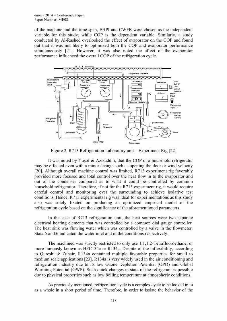
eureca 2014 – Conference Paper
Paper Number: ME08
318
of the machine and the time span, EHPI and CWFR were chosen as the independent
variable for this study, while COP is the dependent variable. Similarly, a study
conducted by Al-Rashed overlooked the effect of evaporator on the COP and found
out that it was not likely to optimized both the COP and evaporator performance
simultaneously [21]. However, it was also noted the effect of the evaporator
performance influenced the overall COP of the refrigeration cycle.
Figure 2. R713 Refrigeration Laboratory unit – Experiment Rig [22]
It was noted by Yusof & Azizuddin, that the COP of a household refrigerator
may be effected even with a minor change such as opening the door or wind velocity
[20]. Although overall machine control was limited, R713 experiment rig favorably
provided more focused and total control over the heat flow in to the evaporator and
out of the condenser compared as to what it could be controlled by common
household refrigerator. Therefore, if not for the R713 experiment rig, it would require
careful control and monitoring over the surrounding to achieve isolative test
conditions. Hence, R713 experimental rig was ideal for experimentations as this study
also was solely fixated on producing an optimized empirical model of the
refrigeration cycle based on the significance of the aforementioned parameters.
In the case of R713 refrigeration unit, the heat sources were two separate
electrical heating elements that was controlled by a common dial gauge controller.
The heat sink was flowing water which was controlled by a valve in the flowmeter.
State 5 and 6 indicated the water inlet and outlet conditions respectively.
The machined was strictly restricted to only use 1,1,1,2-Tetrafluoroethane, or
more famously known as HFC134a or R134a. Despite of the inflexibility, according
to Qureshi & Zubair, R134a contained multiple favorable properties for small to
medium scale applications [23]. R134a is very widely used in the air conditioning and
refrigeration industry due to its low Ozone Depletion Potential (OPD) and Global
Warming Potential (GWP). Such quick changes in state of the refrigerant is possible
due to physical properties such as low boiling temperature at atmospheric conditions.
As previously mentioned, refrigeration cycle is a complex cycle to be looked in to
as a whole in a short period of time. Therefore, in order to isolate the behavior of the

eureca 2014 – Conference Paper
Paper Number: ME08
319
EHPI and the CWFR and, the cycle was simplified and the following assumptions were
made:
Atmospheric temperature, pressure and humidity was set as 27 °C, 100kPa and
75% respectively.
The system runs in steady state.
Kinetic and potential energy as well as friction losses are considered to be
negligible.
Evaporator, Expansion valve, Condenser and Compressor are considered
adiabatic.
The expansion valve process is isenthalpic (constant enthalpy).
The working fluid at the evaporator outlet is completely saturated vapor.
The working fluid at the condenser outlet is completely saturated liquid.
Pressure drop across the evaporator and condenser are negligible.
All heat exchange processes were through Copper tubing or constant thermal
coefficient of the medium.
Experiments were conducted for 20 g/s, 30 g/s, 40 g/s and 50 g/s CWFR, from
the possible minimum to maximum evaporator heater voltage input in increments of
10V. The system automatically sets the EHPI. The minimum and maximum EHPI
value was determined by first observing the lowest evaporator heater voltage input
that resulted the least positive evaporator pressure and the highest evaporator heater
voltage input that cause automatic cut-off of the machine respectively. Each run was
given 5 to 10 minute to stabilize and display a consistent reading for each measure.
2.3. Multiple Linear Regression analysis (MLR)
In this study the data was manipulated using IBM SPSS Statistic 20, a special
software for statistical analysis [24]. As a simple, yet well-established statistical
analysis method, MLR analysis was used to explore the relationship between the
multiple independent and one dependent variables and ultimately producing the
empirical models.
As previously mentioned, independent variable were EHPI and CWFR while
COP was dependent variable for this particular study. The outcome of the study was
to be a mathematical model in the form of a linear equation as shown in Eq. 2, Eq. 3
and Eq. 4 below. Additionally, C1, C2 and C3 would be coefficients for the
mathematical COP models 1 2 and 3.
𝐶𝑂𝑃1 = 𝐶1(��𝐸𝑉𝐴𝑃) + 𝐶2(��𝐶𝑂𝑁𝐷) + 𝐶3 (2)
𝐶𝑂𝑃2 = 𝐶1(��𝐸𝑉𝐴𝑃) + 𝐶3 (3)
𝐶𝑂𝑃3 = 𝐶2(��𝐶𝑂𝑁𝐷) + 𝐶3 (4)

eureca 2014 – Conference Paper
Paper Number: ME08
320
3. RESULTS AND DISCUSSIONS
In order to evaluate the COP, the experimental data was analyzed with respect
to maximum evaporator and condenser pressures. The COP for each run was
calculated using the thermodynamic property tables for the refrigerant R134a.
Complete data was tabulated and the optimized formula for VCRC was produced
through MLR analysis.
3.1. Evaporator Heater Power Input
Evaporator in a refrigeration cycle is the element at which the working fluid is
vaporized by absorbing heat energy. EHPI in this study was the heat source to the
refrigeration cycle. Although the heater power was incremented in Volts, the overall
input for the calculations were in terms rate of heat produced in watts (W).
A linear behavior between the EHPI and the evaporator pressure was observed,
as seen in Fig. 3. It was noted that the average gradient at which the pressure at the
evaporator end increased was by 0.287 kPa/W. This was because, as the EHPI
increased, the refrigerant molecules were subjected to more energy. Therefore, the
molecules undergoes more random and vigorous movements. As a result, the state of
the refrigerant was ideally changed from a mixture to a vapor increasing the fluid
pressure.
Evaporator Heater Power Input, QEVAP (W)
0 200 400 600 800 1000 1200 1400 1600
Evap
ora
tor
Pre
ssure
, P
EV
AP
(kP
a)
0
100
200
300
400
500
600
20 g/s
30 g/s
40 g/s
50 g/s
Regression Line
Figure 3. Effects of Evaporator heater power input on the Evaporator Pressure
On the other hand, the manner at which the data was packed along the, almost
overlapping, best-fit-lines also indicated the effectual ability of the system to adjust its
refrigerant flow rate based on the heat energy transferred in to the refrigerant per unit
time, irrespective of condenser flow rate.

eureca 2014 – Conference Paper
Paper Number: ME08
321
For all CWFR, the COP of the refrigeration cycle increased somewhat linearly
as the EHPI was increased, as seen in Fig 4. It was observed that the gradients of the
regression lines were 0.0015 W-1
, 0.0017 W-1
, 0.0019 W-1
and 0.0021 W-1
for CWFRs,
20g/s, 30g/s, 40g/s and 50g/s respectively. This was due to the increasing difference
in the temperature gradient between the heat source and the refrigerant at the
evaporator end, as the EHPI increased. Moreover, with less relatable data at the most
extreme high and lower EHPI and lower CWFR, the rate of COP increase was poorer.
Evaporator Heater Power Input, QEVAP (W)
0 200 400 600 800 1000 1200 1400 1600
Coeff
icie
nt
of
Per
form
ance
, C
OP
3.0
3.5
4.0
4.5
5.0
5.5
6.0
20 g/s
30 g/s
40 g/s
50 g/s
Regression Line
Figure 4. Effects of Evaporator heater power input on the Coefficient of Performance
Below 500W of EHPI, it was observed that the COP values were randomly
clustered for all CWFR. This was majorly because of the overall low rate of heat
transferred to the refrigerant cycle. Though, as the EHPI passed 500W, the rate of
heat transfer was more significant and distribution, or spreading, of data was observed.
Nevertheless, the overall COP of the refrigerator cycle will partly depend on the
CWFR as well as EHPI.
3.2. Condenser Water Flow Rate
Condenser in a refrigeration cycle is the component at which the compressed
working fluid is turn into a saturated liquid through heat extraction. Hence, CWFR in
this study was the rate at which the mass of the heat sink flow extracting heat energy
across the condenser. Water flow rate was measured in grams per second (g/s).
Similar to the comportment at the evaporator end, the CWFR behaved linearly
with condenser pressure, as observed in Fig. 5. However, unlike the evaporator end,
the gradient at which the pressure changed was negative with increasing CWFR. It
was also noticed that the negative gradient of the slopes increased as the CWFR
increased. Additionally, it was distinguished that the range between the highest and
lowest pressure also reduced with increasing water flow rate. This was because the
rate of heat transfer from the refrigerant to the water rose as the water flow rate

eureca 2014 – Conference Paper
Paper Number: ME08
322
increased. Thus, the refrigerant molecules are subjected to less energy and tends to
behave more stably. This stability converted the superheated refrigerant to a saturated
liquid dropping the pressure across the condenser.
Condenser Water Flow Rate, mCOND
(g/s)
15 20 25 30 35 40 45 50 55
Cond
ense
r P
ress
ure
, P
CO
ND
(kP
a)
800
900
1000
1100
1200
1300
1400
1500
1600
133 W
172 W
216 W
270 W
324.5 W
384 W
444.6 W
532 W
600 W
680 W
765 W
864 W
950 W
1050 W
1155 W
1276 W
1380 W
Regression Line
Figure 5. Effects of Condenser Water Flow Rate on the Condenser Pressure
CWFR also had a positive effect on the COP of the overall system as seen in
Fig. 6. However, the largest range of COP was achieved for 50 g/s due to the greater
heat transfer capability compared to the remaining CWFR fixtures. Likewise, the
smallest range of the COP was obtained for 20 g/s due to lower rate of heat transfer.
Condenser Water Flow Rate, mCOND (g/s)
15 20 25 30 35 40 45 50 55
Co
effi
cien
t o
f P
erfo
rman
ce (
CO
P)
3.0
3.5
4.0
4.5
5.0
5.5
6.0
133 W
172 W
216 W
270W
324.5 W
384 W
444.6 W
532 W
600 W
680 W
765 W
864 W
950 W
1050 W
1155 W
1276 W
1380 W
Regression Line
Figure 6. Effects of Condenser Water Flow Rate on the Coefficient of Performance

eureca 2014 – Conference Paper
Paper Number: ME08
323
Moreover, the gradient of COP was observed to be greater for constant high
EHPI. Yet again, the obtainability of data for low CWFR conditions at the extreme
EHPI was limited. Hence, the gradient of the regression lines when EHPI was 133 W
and 172 W were negative. Besides the low heat transfer rates, fluctuations in
condenser water inlet temperature accumulated to the randomness of data. As a
relatively low amount heat is absorbed by the refrigerant at the evaporator end, the
amount of heat to be expelled into the condenser water was also relatively low.
3.3. Regression Analysis
Based on the experimental results, it was conclusive that an increase in both
EHPI and CWFR had a positive correlations to the COP. Similarly, as the increase in
EHPI positively affected the evaporator pressure and the increase in CWFR negatively
affected the condenser pressure. Therefore, the higher the pressure difference between
the evaporator and the condenser, the higher the COP of the system was believed to be.
The expected outcome of the study was mathematical models in the form of a
linear equations that could predict the COP based on predetermined independent
variable Hence MLR analysis was used. However, numerical regression calculation
generally time consuming if it were to be done manually. Therefore, IBM SPSS
statistics 20 software was utilized to generate the results. Hence, the COP data
obtained was input to the software with respect to the EHPI and CWFR.
According to the descriptive statistical result of the MLR analysis shown in
Table 1, it was found that the mean COP of the system was 4.14 with a standard
deviation of 0.72. Similarly, both EHPI and CWFR had mean values of 661.75W and
36.03 g/s respective while the standard deviations were 370.65 W and 11 g/s
respectively. Therefore, the average COP of this refrigeration unit may vary between
3.42 and 4.86. The average EHPI and the CWFR that would achieve the average COP
were 661.75 W and 36.03 g/s respectively. Moreover, the average evaporator heater
power input may vary between 291.1 W and 1032.4 W, while the condenser water
flow rate may vary between 25.03 g/s and 47.03 g/s.
Table 1 Descriptive Statistics
Variables Mean Standard Deviations
COP 4.14 0.72
QEVAP (W) 661.75 370.65
��𝐂𝐎𝐍𝐃 (g/s) 36.03 11.00
Furthermore, the Table 2 shows the percentage of variability in the dependent
variables that was taken into account by all of the independent variables combined. As
total of three model were generated, Model 1 considered both EHPI and CWFR as
independent variable, while Model 2 and Model 3 only considered EHPI and CWFR
respectively.

eureca 2014 – Conference Paper
Paper Number: ME08
324
Table 2 Model Summary
Models R-square Adjusted R-square
1 0.972 0.971
2 0.943 0.942
3 0.0312 0.0153
R-square, or coefficient of multiple determination in multiple regression, is the
statistical measure of accuracy of the data fitted into regression lines. Therefore, the
closer the value of R-square was to one, the more accurate the data would be. Based on
Table 2, Model 1 produced the highest accuracy with 97.2%. Model 2 was 94.3%
accurate while Model 3 was the least accurate with just 3.12%.
However, as the amount of data are relatively small, the R-square values would
be an over estimation. Thus, the regression software also generated adjusted R-square.
Still, Model 1 produced the highest accuracy with 97.1%. Likewise, Model 2 was 94.2%
accurate while Model 3 was again the least accurate with just 1.5%. The difference in
the R-square and adjusted R-square was small due to the almost negligible effect of the
least significant independent variable, CWFR.
Nevertheless, as the R-square and adjusted R-square values for Model 2 and
Model 3 were compared, it was conclusive that the EHPI contributed more
significantly to the overall COP than CWFR. But, it was also decisive that taking both
dependent variables into consideration produced the most significant model, as in
Model 1.
Moreover, it was necessary to evaluate each of the independent variables in
order to identify which variable in the model contributed most to the COP. Hence, a
set of unstandardized and standardized coefficients based on the beta levels were
produced. The major difference between these two sets of coefficients was that the
standardized coefficients for each of the variable were converted to the same scale.
This was so that a standalone constant was not required, unlike the unstandardized
coefficient as seen in Table 3.
Table 3 Unstandardized and Standardized Beta Coefficients
Unstandardized Coefficients Standardized coefficient
Models B β
1 Constant 2.505 0.000
QEVAP 0.002 0.970
mCOND 0.011 0.169
2 Constant 2.895 0.000
QEVAP 0.002 0.971
3 Constant 3.725 0.000
��𝐂𝐎𝐍𝐃 0.011 0.175
Elimination of zero β level in standardized coefficients would reduce the accuracy
of the model. Therefore, ideally, the unstandardized coefficients would be the more
relevant set of coefficients for the model, provided that both the independent variables

eureca 2014 – Conference Paper
Paper Number: ME08
325
were known. Also, with the findings related to the behavior of R-square and adjusted R-
square for all the models, the most appropriate model was Model 1. Therefore, replacing
the coefficients C1, C2 and C3 in Eq. (2), Model 1 would be presented as:
𝐶𝑂𝑃1 = 0.002(��𝐸𝑉𝐴𝑃) + 0.011(��𝐶𝑂𝑁𝐷) + 2.502 (2.1)
Up on comparison, it was observed that there were uncertainties between the
experimental and the regression model COPs. As seen in Table 4, higher deviations
from the experimental values were resulted in lower CWFR applications compared to
the higher CWFR. The highest deviation was -9.49% when the EHPI was the highest
for the lowest CWFR. In overall system performance, the error ranged from -9.49% to
2.55%. However, the model was also able to achieve results with as accurate as -0.02%
uncertainty. Nevertheless, the result uncertainties were within the expected range of
±10%. The error could be minimized even further by including more effective, yet
varying, parameter such as refrigerant flow rate and also by further limiting the losses.
Table 4 Error Analysis
Evaporator Heater
Power Input
Condenser Water Flow rate
20 g/s 30 g/s 40 g/s 50 g/s
133 - - 0.18 -3.69
172 - 1.55 -1.97 -5.34
216 0.86 0.68 -3.69 -6.75
270 0.63 -0.67 -3.61 -5.58
324.5 0.88 -1.95 -4.87 -5.22
384 -1.14 -1.63 -4.10 -3.85
444.6 0.56 1.39 -1.39 -0.89
532 0.43 1.64 0.92 0.17
600 0.56 2.55 1.85 -1.79
680 -1.66 0.96 0.93 -2.10
765 -3.05 1.10 -0.98 -3.47
864 -5.31 -0.52 -0.02 -2.23
950 -5.62 0.35 -0.33 -3.06
1050 -7.89 -2.50 -2.06 -1.96
1155 -9.49 -3.21 -2.83 -0.97
1276 - -6.60 -3.56 0.77
1380 - -9.26 -3.81 0.11
Also, according to Table 4, it was noticed that the majority of the uncertainties
lied at the negative side. This may have been due to the high heat loss to the
surrounding during the operation.
4. Conclusion
In conclusion, it was found that both the EHPI and CWFR had a positive
effect on the COP of the overall system. Among the three mathematical models
created, Model 1, taking both EHPI and CWFR in to consideration, produced the
highest accuracy in data distribution about the MLR line with 97.2%. Likewise, Model
2, considering just EHPI, was 94.3% accurate while Model 3, considering just CWFR,

eureca 2014 – Conference Paper
Paper Number: ME08
326
was again the least accurate with just 3.12%. Therefore, upon choosing Model 1 as the
best predictor of COP, unstandardized coefficients were assigned to the variables.
Hence, the final COP predictor model was 𝐶𝑂𝑃1 = 0.002(��𝐸𝑉𝐴𝑃) + 0.011(��𝐶𝑂𝑁𝐷) +2.502 . The results produced by the final model had minimum and maximum
uncertainty of -9.49% and 2.55% respectively. The overall uncertainty could be
minimized by incorporating other significant parameter such as refrigerant flow rate
and also by further limiting the heat losses to the surrounding.
References
[1] Y. Zhu and P. Jiang, (2012), “Hybrid vapor compression refrigeration system
with an integrated ejector cooling cycle,” Int. J. Refrig., vol. 35, no. 1, pp. 68–78.
[2] J. Yan, W. Cai, L. Zhao, Y. Li, and C. Lin, (2013), “Performance evaluation of a
combined ejector-vapor compression cycle,” Renew. Energy, vol. 55, pp. 331–337.
[3] H. K. Ersoy and N. Bilir Sag, (2014), “Preliminary experimental results on the
R134a refrigeration system using a two-phase ejector as an expander,” Int. J.
Refrig., vol. 43, pp. 97–110.
[4] F. Molés, J. Navarro-Esbrí, B. Peris, A. Mota-Babiloni, and Á. Barragán-
Cervera, (2014), “Theoretical energy performance evaluation of different single
stage vapour compression refrigeration configurations using R1234yf and
R1234ze(E) as working fluids,” Int. J. Refrig., vol. 44, pp. 141–150.
[5] J. Sarkar, (2012), “Ejector enhanced vapor compression refrigeration and heat
pump systems—A review,” Renew. Sustain. Energy Rev., vol. 16, no. 9, pp.
6647–6659.
[6] H. Li, X. Bu, L. Wang, Z. Long, and Y. Lian, (2013), “Hydrocarbon working
fluids for a Rankine cycle powered vapor compression refrigeration system
using low-grade thermal energy,” Energy Build., vol. 65, pp. 167–172.
[7] H. Wang, R. Peterson, and T. Herron, (2011), “Design study of configurations
on system COP for a combined ORC (organic Rankine cycle) and VCC (vapor
compression cycle),” Energy, vol. 36, no. 8, pp. 4809–4820.
[8] P. a. Domanski, J. Steven Brown, J. Heo, J. Wojtusiak, and M. O. McLinden,
(2014), “A thermodynamic analysis of refrigerants: Performance limits of the
vapor compression cycle,” Int. J. Refrig., vol. 38, pp. 71–79.
[9] P. Wainaina, M. Njue, and W. Ogola, (2013), “Numerical model to optimize
the refrigerant charge for maximum refrigeration capacity,” Therm. Sci., vol.
17, no. 4, pp. 989–995.
[10] L. Zhao, W. Cai, X. Ding, and W. Chang, (2013), “Model-based optimization
for vapor compression refrigeration cycle,” Energy, vol. 55, pp. 392–402.
[11] M. Wallace, B. Das, P. Mhaskar, J. House, and T. Salsbury, (2012), “Offset-
free model predictive control of a vapor compression cycle,” J. Process
Control, vol. 22, no. 7, pp. 1374–1386.
[12] J. M. Gonçalves, C. Melo, and C. J. L. Hermes, (2009), “A semi-empirical
model for steady-state simulation of household refrigerators,” Appl. Therm.
Eng., vol. 29, no. 8–9, pp. 1622–1630.

eureca 2014 – Conference Paper
Paper Number: ME08
327
[13] V. Jain, S. S. Kachhwaha, and G. Sachdeva, (2013), “Thermodynamic
performance analysis of a vapor compression–absorption cascaded
refrigeration system,” Energy Convers. Manag., vol. 75, pp. 685–700.
[14] Y. Yao, M. Huang, and J. Chen, (2013), “State-space model for dynamic
behavior of vapor compression liquid chiller,” Int. J. Refrig., vol. 36, no. 8, pp.
2128–2147.
[15] P. J. Waltrich, J. R. Barbosa, and C. J. L. Hermes, (2011), “COP-based
optimization of accelerated flow evaporators for household refrigeration
applications,” Appl. Therm. Eng., vol. 31, no. 1, pp. 129–135.
[16] B. Li and A. G. Alleyne, (2010), “A dynamic model of a vapor compression
cycle with shut-down and start-up operations,” Int. J. Refrig., vol. 33, no. 3, pp.
538–552.
[17] H. M. Getu and P. K. Bansal, (2007), “Modeling and performance analyses of
evaporators in frozen-food supermarket display cabinets at low temperatures,”
Int. J. Refrig., vol. 30, no. 7, pp. 1227–1243.
[18] J. Navarro-Esbrí, V. Berbegall, G. Verdu, R. Cabello, and R. Llopis, (2007),
“A low data requirement model of a variable-speed vapour compression
refrigeration system based on neural networks,” Int. J. Refrig., vol. 30, no. 8,
pp. 1452–1459.
[19] L. Zhao, W.-J. Cai, X. Ding, and W. Chang, (2013), “Decentralized
optimization for vapor compression refrigeration cycle,” Appl. Therm. Eng.,
vol. 51, no. 1–2, pp. 753–763.
[20] T. M. Yusof and A. Azizuddin, (2010), “Performance Analysis Of A Domestic
Refrigerator,” vol. 9501, no. May, pp. 582–591.
[21] A. a. a. a. Al-Rashed, (2011), “Effect of evaporator temperature on vapor
compression refrigeration system,” Alexandria Eng. J., vol. 50, no. 4, pp. 283–290.
[22] P.A. Hilton Ltd. (1998), Schematic Diagram of R713 Refrigeration Laboratory
Unit. Experimental Operating and Maintenance Manual, Stockbridge,
Hampshire. 1.
[23] B. A. Qureshi and S. M. Zubair, (2011), “Performance degradation of a vapor
compression refrigeration system under fouled conditions,” Int. J. Refrig., vol.
34, no. 4, pp. 1016–1027.
[24] IBM Corp., (2011), “IBM SPSS Statistics for Windows, Version 20.0.” IBM
Corp, Armonk, NY.

eureca 2014 – Conference Paper
Paper Number: ME09
328
An Engineering Approach to
Reduce Noise Level in a Public Area
Neeraj Annand Raj1*
, Mohammad Hosseini Fouladi1
1Taylor’s University Lakeside, Malaysia
Abstract This paper covers the research currently being performed to expand the field of
restaurant acoustics with the case in focus being a restaurant named Temptations in
Taylor’s University Malaysia. Research on this topic was initiated by another student
in 2013 and the goal of this project is to expand on what has been done, to analyse the
restaurant in an alternative manner than the previous research and to implement a
strategy to mitigate the noise and reduce it to a level which is more acceptable.
Initially, a thorough and comprehensive research on the project background has been
performed which encompassed a literature review which covered the basics of sound
as this is not an area which is familiar to the project team nor is it in the scope of
learning in the Mechanical Engineering Degree Programme at Taylor’s University. A
numerical study using the Acoustics Extension in ANSYS 15.0 Workbench,
represents the next phase of the project. Singular and multiple excitations were
represented in the software to study how the sound is behaving and to determine if the
model can be used credibly to perform the analysis. The validation and verification
was done by comparing the results from the numerical analysis with that of the
experimental one whereby the absorption coefficient as well as the theoretical and
actual reverberation times of the restaurant were calculated. From the results, it can be
seen that the numerical model is credible and the behaviour of the sound correlates
with that of the literature review and the experimental analysis. It is also verified that
there is significant basis for this research to be carried out as the target location does
require sound attenuation based on the reverberation times calculated and the manner
in which the sound propagates in the target location from analysing the numerical
results. It was initially intended that the research team should formulate and propose a
cost effective, efficient and ideal strategy to attenuate the noise level in the restaurant
based on research done on potential solutions. However due to significant time
constraints, largely due to issues in using a new application of the software for which
there are extremely limited materials on and which was unavailable for half the
duration of the research, a solution was not able to be completed.
Keywords: Restaurant Acoustics – Numerical – Experimental – Noise – Attenuation

eureca 2014 – Conference Paper
Paper Number: ME09
329
1.0 Introduction
1.1 Research Background
The importance of sound in our lives is something that cannot be overstated. From the
simple act of communicating with one another, to experiencing the audible feast that
is music, our sense of hearing has an intrinsic role in our lives and it gives us a whole
new dimension of experience. However, there is an aspect of sound which brings
much distress and chagrin to us and that is the phenomenon called noise. Noise can be
either good or bad, depending on circumstances, but in general, noise is defined as an
undesirable or disagreeable sound [1]. We encounter noise in many forms, from
construction works, the sound of traffic, impacts of objects being dropped, even a
loud conversation can be classified as noise as it is something that is undesirable.
Sometimes, the presence of noise cannot be avoided and for a long time, this is how
the problem was faced, with tolerance. However, with the advancements in science
and technology we are now able to combat noise, provided we have a substantial
understanding of it.
Acoustics is an area of science that has a wide assortment of applications which all
revolve around the study, understanding, measurement, manipulation and control of
sound. Architectural acoustics represents ‘the study of the generation, propagation and
transmission of sound in rooms, dwellings and other buildings’ [2]. Architectural
acoustics come into play in building design to ensure that its inhabitants are able to fully
maximise, utilise and appreciate its functionality. Take for instance, a restaurant which
serves to provide a place for diners to enjoy a meal in. To be able to fully appreciate the
functionality of a restaurant, the diners must feel that the ambience of the restaurant is
welcoming, comfortable and hospitable. However, one of the most significant issues
that most diners will attest to, as confirmed by a study done by ZAGAT in 2013 across
the United States of America is that noise levels in restaurants are too high thus
disrupting conversations and providing an unsatisfactory atmosphere. Noise in
restaurants usually arise from the sound of the occupants conversing with one another
and sounds from the kitchen both coupled with the lack of sufficient noise treatment.
Architectural acoustics may have been implemented since the age of the Roman
Empire, with their amphitheatres designed in such a way so as to provide exceptional
clarity and fluency required, but restaurant design in terms of acoustics is a relatively
new field of study as suggested by the minimal amount of literature available which
directly relates to it and one which can be delved into and developed exponentially.
This project aims to expand the field of restaurant acoustics with the case in focus
being a restaurant named Temptations in Taylor’s University Lakeside Campus,
Malaysia. Research on this topic was initiated by another student in 2013 and the goal
of this project is to expand on what has been done and to implement a strategy to
mitigate the noise and reduce it to a level which is more acceptable.
1.2 Objectives
This project will be spread out over the course of two semesters as part of two
correlated modules in the Engineering Degree which are Final Year Project 1 & 2. For
the first module, the scope of the works will be the ‘conceive and design’ aspects
whilst the final semester will focus on the ‘implement and operate’ areas. The
objective of this study is summarized as follows:

eureca 2014 – Conference Paper
Paper Number: ME09
330
i. To utilize numerical software analysis to aid in the experimental evaluation
and examination of the acoustics at the target location, Temptations
Restaurant at Taylor’s University
ii. To formulate and propose an efficient, cost effective and ideal strategy to
attenuate the noise level in the restaurant
1.3 Scope
The scope that this project aims to cover focuses on two main areas of study which are
the experimental and numerical fields of research. To supplement the research being
carried out, a thorough and comprehensive study of architectural acoustics and sound
will first be performed, so as to enhance the integrity of the work being performed.
The thesis which was produced by Mohd Afiq (2013) [3] was used as a main
reference and the literature review found in this document is done to fill in the gaps
which were not covered by him. Definitions and explanations of the fundamental
elements of acoustics such as wavelength, frequency, pitch, etc. will not be provided
here and instead, can be referred to that document. The focus of the literature review
of this research will be to breach the gaps that were not covered by Mohd Afiq and to
delve further into Architectural Acoustics.
Numerical analysis of the target location will be performed utilizing an Acoustics
Extension under ANSYS 15.0 Workbench which incorporates creating a basic three-
dimensional model of the target location and analysing it using the software and will
be covered in further detail in the Research Methodology Section. A numerical
analysis has been chosen as the basis and the first step over an analytical and
experimental one due to the fact that it is much easier to perform the optimisation
using a software in which the components, items, layout, etc. of the restaurant can be
altered much more easily and readily. The numerical study will be supported by
experimental works which will be covered by the data acquisition process whereby
the restaurant will be studied and data from it such as noise levels, reverberation
time, sound absorption and distribution, etc. amongst others will be collected in order
to identify the source of the problem. A combination of a numerical and experimental
study will allow for a validation and verification of the results obtained and
comparisons to be identified and drawn, all of which will aid in ascertaining a final
solution to solve the issue at hand as well as enhancing the credibility and quality of
the research being performed [2].
1.4 Research Question
1. How can an engineering approach be utilised to study the behaviour of the
acoustics in the Temptations Restaurant in Taylor’s University in a manner
that is different than what has already been done before
2. How can the noise level of the Temptations Restaurant In Taylor’s University
be reduced to a more acceptable level.
1.5 Contribution to Body of Knowledge
There is a significant lack of literature available for the field of restaurant acoustics as
compared to other architectural structures such as amphitheatres, concert halls, and
eureca 2014 – Conference Paper
Paper Number: ME09
331
places of worship which are the predominant locations for sound treatment. There has
however been a significant increase in the interest devoted to this sound attenuation
for restaurants, but usually without the appropriate scientific approach [9]. The
methods that have been used are usually done based on a general approach taken to all
restaurants without the specialisation or individual aspects of each location taken into
account or even by implementing techniques from other architectural facets [11]. This
research was done in hopes to contribute to this gap in the field of architectural
acoustics whereby by expanding the research that has been done so far and by
providing an alternative way of analysing the sound in the target location than that has
already been carried out. With that, it is hoped to formulate a procedure or template to
be used for analysing sound in restaurants from an engineering approach.
2.0 Research Methodology
This project comes under the field of quantitative study, which is divided into two
methods of analysis i.e. numerical and experimental. The numerical and experimental
analysis will yield results which will be compared and evaluated, from which a
solution will be derived based on the evaluation coupled with the knowledge garnered
from the research phase.
2.1 Numerical Analysis
For the numerical analysis, the software of being used is ANSYS Workbench 15.0
with the addition of the ACT Acoustics Extension. ANSYS is a widely renowned and
powerful simulation software that has been long favoured by the engineering
community in applications for computer-aided engineering and design due to its
versatility, robustness and ease of use.
In the realm of acoustics, there are three different types of analysis that can be
performed which are the modal and harmonic analyses which are in the frequency
purview as well as the transient analysis which is in the time domain. For the analysis
of a room, the harmonic response analysis was chosen for various reasons. As seen in
other works of research, the harmonic response method is favoured over the transient
and modal analyses when the application is based for noise propagating in a room
[10]. A harmonic analysis is selected when the response of a linear structure to loads
which are varying in a sinusoidal (harmonic) manner are acting on it. For the case at
hand, the sinusoidal loads represent the noise generated by the diners and the response
of the linear structure is taken as the air in the restaurant and the walls of the
restaurant itself. A harmonic analysis was also chosen based on the post-processing
and the output quantities available that are required to determine the behaviour of the
sound propagating in the restaurant. For this case, it is necessary to obtain the acoustic
pressure, sound pressure level, the near field parameters as well as the acoustic time-
frequency plot. The software also allows for a visual representation of how a single or
even multiple sources of excitation interfere with one another, reflect of the walls and
propagate throughout the restaurant
Initially for the first phase of this project, the first step was to perform a complete and
thorough study and understanding of the software so that when the actual analysis was
being performed, it could be carried out in an efficient manner. The preliminary steps
include the building of the model of the restaurant in the Design Modeller. A basic

eureca 2014 – Conference Paper
Paper Number: ME09
332
cuboid shaped room was modelled in the Design Modeller with dimensions akin to
that of a simplified version of the Taylor’s Temptations Restaurant just for
familiarisation purposes.
Figure 12 Initial Model
This was followed by the simulation of a more intricate and realistic version of the
restaurant. The next stage is the input of the material data in the Engineering Data
library which will form the materials used to construct the room. The materials were
taken as a close approximation from a visual inspection of the restaurant as well as a
review of the most commonly used building materials in the construction industry and
materials which are common to the region [7]. The estimates and assumptions made
for the numerical analysis were done with as much care and integrity so as to simulate
the acoustic behaviour of the sound acting in the Taylor’s Temptations Restaurant as
accurately as possible. The model is shown below in the Mechanical application with
the walls at the fore representing the front of the restaurant made out of glass. The
materials for each wall and their corresponding dimensions which were obtained from
the measurements taken, as well as the Young’s Modulus and the Poisson’s Ratios
(which require a manual input) are as follows [11]:
Table 7 Wall Dimensions and Properties
Location Material Dimensions (m) Young’s
Modulus
(GPa)
Poisson’s
Ratio
Thickness
(m)
Front Wall
1
Glass 13.67 x 2.45 70 0.23 0.16
Front Wall
2
Glass 21.42 x 2.45
Front Wall
3
Glass 12.08 x 2.45
Front Wall
4
Glass 18.82 x 2.45
Rear Wall 5 Brick &
Cement
7.97 x 2.45 30 0.18
Rear Wall 6 Brick &
Cement
3.36 x 2.45
Rear Wall 7 Brick &
Cement
16.46 x 2.45
Ceiling Gypsum
Plasterboard
- 1.7 - 2.5 0.2 - 0.3
0.05
Floor Ceramic Tile 41.78 0.14 0.16
Inside Air - 0.00011 - -

eureca 2014 – Conference Paper
Paper Number: ME09
333
For simplification, as with the first model, the restaurant is taken to be made out of 4
parts which are the ceiling, the floor, the front walls made out of glass and the rear
walls made out of bricks and cement.
Figure 13 Updated Model
This is followed by the application of the meshing, boundary conditions, fixed
supports of the model. For the mesh, there are several different methods and attributes
that can be changed and altered before the analysis is performed. The element size can
either be left as default or be user defined. The patch conforming method can either be
left as independent or set as tetrahedron. As for the relevance centre, it is either set as
fine, medium or coarse. These factors will all lead to differences in the nodes and
corresponding elements. The result of all this is the accuracy at which the model can
be analysed. A finer mesh will lead to a more accurate rendering and analysis of the
model [16]. However, this accuracy comes at a cost, which is a slower processing
time but it is a necessity in order to enhance the credibility of the work being done.
For this particular model, the element size was taken to be as 0.1m, the patch
conforming method to be independent and the relevance centre to be fine. These input
properties are selected based on standard practices for models of this type as well as
through experience in using this software [17].
Figure 14 Meshing

eureca 2014 – Conference Paper
Paper Number: ME09
334
The next step is the determination of the boundary conditions for the analysis settings.
Firstly, the minimum and maximum of the frequency range is set at 125 and 4000 Hz
respectively as this is usually the frequency range of concern when analysing
restaurants and the optimum speech frequencies [1]. Next, the declaration of the
computational domain (entire geometry of the model) as an ‘acoustic body’ is
performed. The mass density and speed of sound in the medium (taken as the values
for air) of concern are then keyed in. This is a coupled analysis whereby the study is
being done on the interaction of the air in the room with the walls surrounding it as
the propagation of sound occurs. Another boundary condition whereby an acoustic
pressure of ‘0’ magnitude is applied to the outward faces to ensure that all the sound
is contained within the structure to maximise the impact of the sound propagation in
the venue which mimics a worst-case scenario of having no sound escape the venue
[16]. The Fluid Structure Interface (FSI) whereby the acoustic planes that come into
contact with the structural members are also determined and registered into the
software. These represent the action of the pressure transfer from the medium to the
structure. Next, the fixed supports for the restaurant are selected. Due to the nature of
the restaurant’s construction, the fixed supports are selected to be the ceiling, the floor,
and all of the back walls leaving all the front walls free as they are made of glass and
are not connected to any other structures along their surface.
Figure 15 Boundary Conditions
Lastly, the acoustic excitations are defined. There are several types of excitations to
choose from but based on research in this field and the application with ANSYS as
well as the focus of the source of the noise which from the experimental analysis is
confirmed as the patrons of the restaurant, an acoustic incident monopole wave source
is selected [16]. A monopole wave is selected as its symmetry will lead to a
production of harmonic spherical waves irrespective of the medium of propagation
and various sources tend to exhibit behaviour similar to it [17]. The omnidirectional
propagation of the monopole wave is very appropriate for simulating the noise being
generated by diners in the restaurant. The wave is selected to be radiating from the
centre of the room with a phase angle of 90º, and amplitude of 0.025 Pa which is
obtained by converting a noise level rating of 62.2 dbA to Pascal’s. The value of the
noise level is obtained from measurements taken from the restaurant of the average
noise level of the patrons which was found to be 62.2dbA.
An analysis with multiple sources of excitation is then performed with the additional
waves being generated at the centre of each of walls of the restaurant. The reasoning

eureca 2014 – Conference Paper
Paper Number: ME09
335
behind the location of the sources of excitation is to have a more uniform and even
distribution so as to simulate and to view how much of an effect the geometry of the
restaurant has in contributing to the way that the sound waves are travelling in it. This
will lend to an appropriate way to select the best possible solution for the location of
the sound absorbers. The waves are all selected to have the same properties such as
amplitude and phase angle as they are assumed to be of the similar sources which is
conversation from the diners. The waves are placed at a height from the floor to
simulate the mouth level of a diner who would be seating which is approximately 1.2
meters from the ground.
It was hoped that even more sources of excitations could be simulated in the software
but due to time constraints which occurred due to problems with the software itself,
this was not able to be completed. All the analysis will thus be done by analysing the
single and multiple wave sources.
2.2 Experimental Analysis
Measurements will be taken from the restaurant using instruments such as a
measuring tape to obtain the dimensions of the restaurant needed as well as a Sound
Level Meter (type 2 ANSI SI.4) to obtain the decibel level in the restaurant over the
span of several days. This will give an average reading and allow to account for the
expected variances such as crowd volume. All the required apparatus will be provided
by Taylor’s University. Besides that, the source of the noise in the room will be
identified from visual inspection. The source is divided into two potential causes
which are airborne and structure borne and the elements which contribute to these
sources will be identified. From the results obtained through the measurements, the
necessary calculations to obtain the actual values for the reverberation times and the
absorption coefficient will be done. The following equations will be utilised in the
numerical analysis of the restaurant.
The experimental phase involving the calculations and analysis of data will be
followed by a numerical analysis done side-by-side once the necessary values have
been obtained from the measurements. This is so that the understanding of the actual
behaviour of the sound and noise in the room will be enhanced. The results of the
numerical and experimental studies which will yield the actual and theoretical values
should correlate and proving this will greatly enhance the credibility of the research
1) 2.21 Measurements
Before any analysis could be performed, be it numerical or experimental, the first step
taken was to obtain the dimensions of the restaurant. This was done with a measuring
tape and was preferred over obtaining the measurements from the Facilities
Management Office because over time, there have been amendments and
modifications to the restaurant. Although it was significantly time consuming, this
allowed for a more precise and current outlook of the target location. The
measurement of the restaurant was done in meters and then transferred to a computer
to be used in the numerical analysis. The measurements taken were combined and
then modelled as 4 entities namely the ceiling, the floor, the rear walls and the front
walls.

eureca 2014 – Conference Paper
Paper Number: ME09
336
Figure 16 Dimensions of the ceiling
Figure 17 Dimensions of the roof
Figure 18 Dimensions of the rear walls
Figure 19 Dimensions of the front walls

eureca 2014 – Conference Paper
Paper Number: ME09
337
2) 2.2.2 Sound Level Meter
A Type 2 ANSI SI.4 sound level meter was used in this study to obtain the decibel
level in the venue during the experimental analysis. It is a general purpose sound level
meter which is more suited for field use as opposed to the more precise and accurate
Type 1 meter which is more appropriate for studying building acoustics but was not
chosen due to its lack of availability. The tolerance for the Type 2 meter is ± 1.0 dB,
just 0.3 shy of the Type 1 variant. The sound level meter chosen does conform to the
standards set by both the International Electro technical Commission (IEC 60651) as
well as the American National Standards Institute (ANSI SI.4) for the measurement of
sound in buildings [2].
The sound level meter was set with the following functions as per the type of analysis
being performed. An A-Weighting was used as the type of frequencies being detected
are for general sound level measurements in the band that is detectable by the human
ear which is 500 to 8000 Hz. A slow response was chosen as opposed to a fast one as
it allows for a 1 second time constant interchange whereas the alternative is of 125
milliseconds. The appropriate decibel range as well as slower fluctuations will allow
for the readings to be obtained in an easier manner.
In order to calculate the reverberation time of the restaurant, two different approaches
were taken to obtain both the actual and theoretical values.
3) 2.2.3 Potential Noise Sources
Based on a study on architectural acoustics and a visual inspection of the target venue,
the sources of noise in the restaurant were divided by their method of generation and
propagation be it by an airborne route or through the structure itself. Table 8 displays
the findings
Table 8 Potential Sources of Noise
Airborne Noise Structure-borne Noise
Air-Conditioning (13 units)
Fans (4 units)
Kitchen (noise from staff)
Patrons
Impact Noise (cutlery, footsteps, trolleys,
miscellaneous)
4) 2.2.4 Noise Level
It was an objective of this research to identify which of the potential noise sources is
the largest contributor towards the inadequate noise level of the restaurant. In order to
do so, the sound level meter was used to obtain readings of the decibel levels for each
of the potential noise sources identified above. The impact noise was not selected as it
is not a constant and occurs much more infrequently compared to the airborne noise
and it is not as much of a contributor towards to problem at hand as compared to the
airborne noise sources, concurring with literature review on this matter [12]. The
readings were taken in a manner of which the source being measured was isolated
from other potential sources. As for example, the noise from the fan and air-

eureca 2014 – Conference Paper
Paper Number: ME09
338
conditioning systems were taken when the restaurant was empty and the noise from
the patrons and the kitchen was taken when the restaurant was in full service which
was identified as the peak operating time during lunch hour. The measurements were
taken repeatedly over the duration of five days, the plot of which can be seen in the
Figure 20. It can be seen that the noise originating from the fans and air conditioning
system are generally very constant. The noise from the kitchen and patrons does
change but the variance is minimal, approximately 3 and 4 decibels respectively.
Figure 20 Noise Level from various sources over the course of 5 days
To obtain the actual reverberation time of the room, the Impulsive Noise method was
chosen whereby a sound with a large amplitude is utilised to excite all the frequencies
in a room [12]. It was conducted in a manner whereby the restaurant was vacated of
all occupants (bar the people to conduct the testing) and all forms of noise such as
from the air-conditioning, kitchen equipment, fans and ambient music played in the
restaurant were eliminated so as to obtain a clearer recording. The furnishings such as
the tables, chairs and decorative elements were kept in place as they contribute to the
reflection of the sound and also they remain constant whereas the number of patrons
varies. An impulsive noise, in this case a balloon was popped in the dead centre of the
restaurant and the resultant noise generated was recorded in the audio sampling
software Audacity 2.0.6. From there, the waveform recorded is normalized to a level
of 60dB as the impulse generated by the balloon is only approximately 20dB. The
resultant time of propagation of the sound wave to die down is taken as the
reverberation time which coincides with the definition of reverberation time or RT60.
The procedure of normalising or extrapolating results is in accordance with BS EN
ISO 3328 as it can be difficult to generate an impulse of 60 dB and the results
obtained are labelled as RT60 (T20) [14]. The experiment was performed a total of
three times to obtain an average value.
Figure 21 Sound waveform of balloon burst
54
56
58
60
62
64
66
0 1 2 3 4 5 6
Sou
nd
Pre
ssu
re (
dB
A)
Day
Air conditioning Fans Kitchen Patrons

eureca 2014 – Conference Paper
Paper Number: ME09
339
Figure 22 Extrapolated waveform to 60 dBA
The reverberation time obtained by performing the Impulsive Noise method is taken
as the actual reverberation time and will be then compared with the theoretical
reverberation time obtained using the following formula.
Sabine Formula to calculate reverberation time assuming reverberation decay is
continuous [14]
𝑡 =0.16×𝑉
𝐴 (1)
Where
t = reverberation time (s)
V = volume of the room (m3)
A = total absorption of the room surfaces (m2 sabins)
A = Σ (surface area x absorption coefficient)
Whereby sabins is defined as unit sound absorption. It is a product based measure
which is particularly suitable for products discontinuity in space and is calculated by
Number of Sabins per unit = total exposed surface area to sound × absorption coefficient of that material (2)
𝐴 = 𝑆1𝛼1 + 𝑆2𝛼2+. . 𝑆𝑛𝛼𝑛 = ΣSi𝛼𝑖 (3)
Where
A = total absorption of the room surfaces (m2 sabins)
Sn = area of the actual surface (m2)
α = absorption coefficient of the actual surface
𝐴𝑏𝑠𝑜𝑟𝑝𝑡𝑖𝑜𝑛 𝑐𝑜𝑒𝑓𝑓𝑖𝑐𝑖𝑒𝑛𝑡, 𝛼 = 𝐴𝑏𝑠𝑜𝑟𝑏𝑒𝑑 𝑠𝑜𝑢𝑛𝑑 𝑒𝑛𝑒𝑟𝑔𝑦
𝐼𝑛𝑐𝑖𝑑𝑒𝑛𝑡 𝑠𝑜𝑢𝑛𝑑 𝑒𝑛𝑒𝑟𝑔𝑦 (4)

eureca 2014 – Conference Paper
Paper Number: ME09
340
3.0 Results and Discussion
Based on the data obtained from measuring the noise levels from the various sources
over the span of five consecutive days, the average for each of the noise sources is
then calculated and the results are shown in the Table 9. From it, we can see that the
main source and largest contributor of the noise is originating from the patrons
conversing in the restaurant. Therefore, assumptions for the source of excitation for
the numerical analysis of the restaurant will be modelled based on the speech of the
diners.
Table 9 Average decibel level of the potential noise sources
Source of noise Decibel (dbA)
Air conditioning 56.8
Fans 55.8
Kitchen 59.4
Patrons 62.2
5) 3.1 Theoretical Reverberation Time
In order to obtain the theoretical reverberation time, the Sabine formula detailed
previously is utilised. This approach is selected as opposed to the Norris-Eyring and
Millington-Sette methods due to the fact that it is the standard practice for live rooms
with a relatively low absorption coefficient [12]. The Norris-Eyring method states that
there will be a sporadic decay of the sound with the influx of lesser reflections
whereas the Millington-Sette formula is a much more tedious and complex formula
and is used only when there are various absorption coefficients of the materials [11].
The Sabine equation is used in a case where the sound will decay in a continuous and
smooth fashion, leading the sound to behave in a manner which is considered to be
‘live’ and not ‘dead’ as can be seen in the target location [6]. For the Sabine equation,
the first step is to calculate the surface area and volume of the target location. This is
done so by obtaining the values from the modelled restaurant in ANSYS. This
represents a much more accurate and precise manner to obtain the values as the model
of the restaurant in the software was done with the actual dimensions of the restaurant.
This opposes what was done by Mohd. Afiq where the approach taken was to simplify
the geometry of the restaurant and perform the calculations manually. The table below
depicts the volume of the entire restaurant as well as the resultant surface areas which
have been split into 4 components, namely the front walls made out of glass, the rear
walls made out of bricks and cement, the ceiling made from gypsum plasterboard and
the floor made from ceramic tiles.
Table 10 Measurements of the walls for the restaurant
Location Material Area (m2) Volume (m
3)
Front Wall 1-4 Glass 308.843 927.116
Rear Wall 5-7 Bricks & Cement 139.953
Ceiling Gypsum
Plasterboard
946.622
Floor Ceramic Tile 956.953

eureca 2014 – Conference Paper
Paper Number: ME09
341
A tabulation of the absorption coefficients (α) for the respective building materials are
shown below at the various frequency ranges that are of concern for this analysis [12]
Table 11 Absorption coefficient for the building materials used
Material 125 Hz 250 Hz 500 Hz 1000 Hz 2000 Hz 4000 Hz
Glass 0.18 0.06 0.04 0.03 0.02 0.02
Bricks &
Cement
0.01 0.01 0.02 0.02 0.02 0.03
Gypsum
Plasterboard
0.15 0.11 0.04 0.04 0.07 0.08
Ceramic
Tile
0.01 0.01 0.01 0.01 0.02 0.02
The surface areas are then multiplied with their respective absorption coefficients for
the various frequency ranges to obtain the absorption in metric Sabin, and are then
used to obtain the resultant reverberation time as depicted in the table below.
Table 12 Absorption and reverberation time at the various frequencies
Frequency
(Hz)
125 Hz 250 Hz 500 Hz 1000 Hz 2000 Hz 4000 Hz
Absorption of
the room, A
(m2 metric
Sabin)
208.556 133.624 62.583 59.495 94.371 105.237
Reverberation
time, t (s)
0.71 1.11 2.37 2.49 1.57 1.41
From the results garnered, it can be seen that the reverberation time is particularly low
when the frequency range is also low, at values of 125and 250 Hz. For optimum
speech frequencies of 500 and 1000 Hz, the reverberation time is at the peak [5]. The
calculations performed do however have the limitations of ignoring the furnishings of
the restaurant.
6) 3.2 Actual Reverberation Time
These values are then to be compared with the actual reverberation time obtained by
performing the Impulsive Noise method reverberation time test. The normalized and
extrapolated graphs of the sound wave generated from the balloon burst are shown
below. From there, the average of the three reverberation times is obtained to be 1.86
seconds.
From the two sets of experimental results, it can be seen that the reverberation time
calculated for the Temptations Restaurant is well above the acceptable and even
recommended value for a restaurant which is found to be 1.0 to 1.5 seconds [13].
Therefore the task to find a solution to this issue and the purpose of this research is
justified.

eureca 2014 – Conference Paper
Paper Number: ME09
342
Figure 23 Normalized and extrapolated waveforms of the balloon tests
Table 13 Reverberation times from balloon tests
Test Reverberation Time (s)
1 1.90
2 1.97
3 1.70
3.3 Numerical Analysis
7) 3.3.1 Single Source
Figure 14 shows the acoustic sound pressure level with the monopole wave as the
source of excitation propagates through the restaurant. The maximum value of the
SPL is found at the epicentre of the source and the minimum is found at the furthest
possible point from the centre of the source which is the expected wave behaviour.
However, the maximum value of 57.953 does not tally with the input of the excitation
source which is 62.2 dbA (converted to 0.025 Pa) which is due to damping and
dispersion of the wave.
Table 14 Results from Numerical Analysis for single source of excitation
Results Minimum Maximum
Acoustic Sound Pressure
Level (dbA)
33.492 57.953
Acoustic Pressure (Pa) -0.00350 0.00358

eureca 2014 – Conference Paper
Paper Number: ME09
343
Figure 24 Acoustic Sound Pressure Level for single source of excitation
Figure 25 Acoustic Pressure for single source of excitation
The propagation of the acoustic pressure is depicted in the figure above. The acoustic
pressure for this particular analysis is the degree of freedom for the acoustic problem
resolution and thus it can be seen that there is a decrease in the degree of freedom
where there are regions of high pressure. It shows that the pressure is scattered around
the room with the concentration being at the centre where the excitation is placed. The
maximum value of 0.00358 tallies with the literature on this subject as after dispersion,
there is bound to be a drop in the pressure of the source [10]. However, the negative
value for the minimum acoustic pressure attained is not one that can be justified and
that is taken to be as an error for the reasons stated above in the discussion of the
acoustic pressure. From the analysis of the propagation wave in terms of the acoustic
sound pressure level and the acoustic pressure, it can be seen that even with a singular
source, the sound is dispersing throughout the entire restaurant with large areas of
significant levels of sound pressure level and acoustic pressure.
8) 3.3.2 Multiple Source
Table 15 Results from Numerical Analysis for multiple source of excitation
Results Minimum Maximum

eureca 2014 – Conference Paper
Paper Number: ME09
344
Acoustic Sound Pressure
Level (dbA)
3.4121 60.921
Acoustic Pressure (Pa) -0.023307 0.021699
Figure 26 Acoustic Sound Pressure Level for multiple sources of excitation
The figure above shows the acoustic sound pressure level with multiple monopole
waves as the sources of excitation propagating through the restaurant. As with the
single source of excitation, the maximum value of the SPL is found at the epicentre of
the source and the minimum is found at the furthest possible point from the centre of
the source which is the expected wave behaviour. The maximum value of the sound
pressure level has risen now to 60.921 dbA.
Figure 27 Acoustic Pressure for multiple sources of excitation
For the acoustic pressure there is also an increase to 0.0216 Pa as compared to the
single source of excitation. There is a decrease in the degree of freedom towards the
centre of the restaurant as well as where the sources of excitations are placed.
All of the figures shown above depict the maximum values of the sound pressure level
and the acoustic pressure which occur between 1.5 to 2 seconds after the excitation
begins. This tallies with the experimental analysis performed to obtain the
reverberation time, thus showing the critical values are occurring during that period of
reverberation of the sound wave. This also validates that the model is accurate in
simulating how sound normally propagates in a room and thus provides verification of

eureca 2014 – Conference Paper
Paper Number: ME09
345
the numerical simulation [16]. If we compare the propagation of the single wave and
multiple wave excitation, we can see the difference of how multiple sources of
excitation interact with one another and cause interference. The resultant interference
of the multiple wave sources leads to higher values for the acoustic pressure and
acoustic sound pressure level, as can be seen by the coloration of the figures whereby
there are increased tones or yellow, orange and red for the excitation by multiple
sources.
Figure 28 Entire propagation of acoustic Sound Pressure Level for multiple
sources of excitation
By looking at the entire propagation for the excitation with multiple sources, the
interference of the waves after the excitation begins and as the wave disperses it can
be seen clearly whereby around the sources of excitation, there are regions of high
acoustic sound pressure levels throughout the duration of propagation of the wave [7].
This lends to add credibility to the numerical analysis being performed as the wave
behaviour that is depicted tallies with the theory on the matter.
4.0 Conclusion and Future Work
To review the success of this project, one must not only look at the tangible progress
that has been made in terms of results and data, but instead, the progress of the project
is reviewed in terms of the knowledge that has been gained and the resultant work
performed based on that knowledge, all given the sheer difficulty of the task at hand.
It was known from the start that this is a field that the researcher had no significant
technical background in as sound and noise is not covered at all in the in the scope of
learning in the Mechanical Engineering Degree Programme at Taylor’s University.
However, the sheer difficulty in undertaking a research topic for which one has no
foundation in was clearly underestimated, along with the duration it would take to
perform seemingly unassuming tasks such as a study of the basics of sound or
familiarisation with the software being used in the numerical analysis. This, along
with an overestimation of the allotted time led to delays in the predicted progress for
the project. It was assumed that the numerical study could have already been started
by the end of the first semester, however due to the fact that the ANSYS Acoustics
Extension was not available in the university until the second semester and given the
fact that it is a very new component of the software and thus, there are very limited
materials on it, significant delays were experienced. The research team had to perform
most of the analysis by trial and error as opposed to following a standard procedure or
template for which to use the software to perform analysis in a room, let alone a
restaurant. The numerical study that was performed only contained a maximum of

eureca 2014 – Conference Paper
Paper Number: ME09
346
seven sources of excitation whereas in an ideal scenario, each table or even each
patron of the restaurant would be modelled as in individual source of excitation. The
numerical study that was performed was validated by the experimental results
obtained which showed a high reverberation time for the restaurant. The method of
obtaining the reverberation time was a significant advancement on the method
performed by the previous researcher as the restaurant dimensions were not simplified
and instead were done so much more precisely. Given more time and with a greater
understanding of the software, it is a certainty that more significant progress could
have been made to perform a more extensive and complete numerical analysis and
thus, possibly leading to a solution to the noise attenuation problem.
In terms of the literature review for this research, one must really look at the thesis
produced by Mohd Afiq (2013) [4] as this research is based on the work that he has
done. The basics of sound and noise were covered thoroughly by him and therefore
were not to be included in this text but instead, taken as research material on a
personal level to allow for an understanding in this field to be built. The objective
here was to expand the effort that has been done by him and use his work as a
foundation. The focus was on covering the areas not touched on in that text as well as
a study on potential solutions for noise attenuation in restaurants from current journals.
It should be noted, that based on the research performed in this project that restaurant
acoustics is an area of study for which there is inadequate material available from
journal papers which explains their limited appearance as reference material in this
text.
It can be readily concluded that the work being performed for this project over the
duration of this project has been successful, despite the delays and progression made.
It can be affirmed that the necessary building blocks and foundation has been laid for
a successful continuation of this project which will hopefully yield an optimal
solution to the noise attenuation problem for the Taylor’s Temptations Restaurant.
In terms of future work, recommendations on how to alleviate the shortcomings and
limitations from the effort that has been done can be made regarding better time
management and less focus and emphasis on research from journal papers. Besides
this, it is also recommended that more emphasis be placed on the experimental side of
the project, as well as ensuring that the necessary tools such as the software upgrade is
readily available from an earlier stage.
References
[1] Anonymous, 1984, Measuring Sound, Brüel & Kjær, viewed on 24th March
2014
[2] Ginn KB, 1978, Architectural Acoustics, Brüel & Kjær, viewed on 3rd April
2014, ISBN 87 87355 24 8
[3] Mohd Afiq, July 2013, Noise Reduction at Taylor's Temptation Restaurant,
Bachelor of Engineering (hons) Thesis, Scool of Engineering Taylor's
University Malaysia

eureca 2014 – Conference Paper
Paper Number: ME09
347
[4] Anonymous, undated, Reverberation Time, Brüel & Kjær, viewed on 19th April
2014 at <http://www.bksv.com/Library/Dictionary?key=R&st=R>
[5] Long M (2005). Architectural Acoustics. Burlington, MA, USA: Academic
Press. 66-102, ISBN: 9780080527550
[6] Kuttruff H (2000). Room Acoustics. 4th ed. Florence, KY, USA : CRC Press .
102-115. ISBN 9780203186237 [7] M. David Egan (2007). Architectural Acoustics. 3rd ed. USA: McGraw Hill
Higher Education. 320-340.
[8] F. Setaki, M. Tenpierik, M. Turrin, A.v. Timmeren. (2014). Acoustic absorbers
by additive manufacturing. Building and Environment. 72 (1), pg 188-189.
[9] W. J. Cavanaugh, G.G. Tocci, J. A. Wilkes (2010). Architectural Acoustics. 2nd
ed. New Jersey: Jown Wiley & Sons Inc. pg 47-50.
[10] W. J. Cavanaugh, G.G. Tocci, J. A. Wilkes (2010). Architectural Acoustics. 2nd
ed. New Jersey: Jown Wiley & Sons Inc. pg 24-26.
[11] K.W. Harvey (2009). Fundamental Building Materials. USA: Universal-
Publishers. ISBN 978-1-59942-951-9
[12] G. Davis, R. Jones (1989). The Sound Reinforcement Handbook. USA: Yamaha
Corporation of America. pg 65, ISBN 0-88188-900-8
[13] M.S. Khan, C. Cai, K.C. Hung, Acoustic Field and Active Structural Acoustic
Control Modelling in Ansys, Institute of High Performance Computing
Singapore
[14] T. Betlehem, T. Abhayapala (2004), Spherical Harmonic Analysis of
Equalization in a Reverberant Room, National ICT Australia, Department of
Telecommunications Engineering RSISE, Australian National University

eureca 2014 – Conference Paper
Paper Number: ME10
348
Development of an Integrated Approach to
Tube Assembly FE Model Correlation
Z.X. Pang1*
, M. Hosseini Fouladi1, K.H. Yap
2
1School of Engineering, Taylor’s University, Malaysia,
2CMD/CAE, Panasonic Appliances Air-Conditioning R & D (M) Sdn.
Bhd.(PAPARADMY 1), Malaysia
Abstract
Resonance occurs during transportation of an outdoor air-conditioning unit. Structural
failure due to vibration was found on the copper tube assembly located within the
interior of an air-conditioning unit. Modal study is required to prevent copper tube
failures due to vibration during transportation and shipping. Finite element (FE)
modal analysis has been implemented to replace the traditional design cycle, which is
costly and time consuming. However, the reliability of FEA results greatly
corresponds to the accuracy of FE model and also the boundary conditions. Hence,
modal validation is needed to validate the accuracy of FE model with experimental
data. The purpose of this research is to identify an integrated approach to validate the
FE model of copper tube assembly. Finite element modal analysis of copper tube
assembly is conducted using NX Nastran software. Pre-processing which includes
meshing of copper tube and boundary condition setting were also implemented in the
FE model of copper tube assembly. The modal result is obtained using the Lanczos
mode extraction method. Test-analysis model (TAM) is created to represent the actual
test structure. Impact hammer test is conducted based on TAM and measured
frequency response function (FRF) is transferred to Bruel and Kjael PULSE REFLEX
software for modal parameter extraction. Extracted natural frequency and mode shape
is compared with the FE model through modal correlation. Results show good
agreement between the mode shape of FE model and mode shape based on
experiment. On the other hand, natural frequency predicted by FE model is slightly
lower compare to experiment. The maximum percentage differences is about 5%
between natural frequency of FE model and experiment. This difference in natural
frequency is within the allowable range. Hence, validated FE model of copper tube
assembly was ready for design optimization and the calculated dynamic properties of
the copper tube assembly were representative of the actual structure.
Keywords: Modal study, finite element modal analysis, Impact hammer test, Model
correlation.

eureca 2014 – Conference Paper
Paper Number: ME10
349
1. Introduction
In Panasonic Appliances Air Conditioning R&D Malaysia, there are exists
risks of copper tube failures due to transportation and shipping. Copper tube is an
important part in the outdoor air-conditioning unit to complete the refrigerant circuit
through connection with other components. Failure of copper tube may cause leakage
of refrigerant to the environment. The possible reason for this issue may arise from
the exposure of vibrations during transportation. Resonance happens when the
vibration frequency of the system coincides with the natural frequency of the copper
tube assembly [1]. With the occurrence of resonance, a structure will tend to vibrate at
its maximum amplitude, undergo high deformation which ultimately cause
catastrophic structural failure. To avoid resonance, the researcher has employed
mitigation techniques such as the traditional design cycle and the modern Finite
Element Analysis (FEA) to determine the dynamic properties of the structure.
Traditional design cycle is one of the common utilized traditional problem-solving
methods [1]. However, this design cycle requires not only an immense amount of cost,
but also requires a long period of time in order to reach a satisfactory level. Hence,
FEA was introduced as an alternative solution to improve the traditional design cycle.
Various finite element modal studies were conducted in civil infrastructure health
monitoring fields [2, 3]. For an example, Wei et al. [4] have created a FE model for
cable-stayed bridge using ANSYS modeling and simulation software to study the
dynamic properties of the structure. On the other hand, Salam et al. [5] have studied
the prospects of using FE modal analysis to help with bridge examinations in order to
identify locations of critical high stress zone and validates the results with
experimental data obtained from waveform analysis. With the advancement of finite
element modal analysis, a rather detailed study of natural frequency and mode shape
on a complex structure can be obtained easily and therefore able to minimize the costs
and resources spent on traditional design cycle. However, the reliability of FEA
results greatly relates to the accuracy of an FE model and also the boundary
conditions set [6]. Hence, the validation of an FE model with experimental data is a
crucial step in order for an accurate FE model to be produced.
For automobile and aerospace industries, modal analysis practices using FE
method have been conducted since the past decades [7, 8]. The dynamic study of the
structure have become a common practice for companies in these industries before
taking any action to optimize the design of the structure. However, in terms of the air-
conditioning industry, this practice is considered as a new research development in
the field of vibration. The pioneer researchers who started modal study in the air-
conditioning industry are Yusuhiro et al. [9] who made use of modal study to develop
a set of manual for air-conditioning piping design. Later on, Ling et al. [10] invented
an alternative to predict vibration response of air-conditioning unit through digital
simulation technique. The use of modal analysis on air-conditioning units began after
Chuan et al. [11] introduced a boundary condition used to test pipe lining systems of
air-conditioning units during operation. Up to date, Lim et al. [12] have developed a
methodology to correlate FE models with experiments through model correlation. As
compared to the automobile industry, the development of modal analysis in air-
conditioning industry is still observed to be gradually increasing.

eureca 2014 – Conference Paper
Paper Number: ME10
350
Research and development of modal analysis in air-conditioning units so far
focus only on single component studies. Lack of modal study is conducted based on
assembly structure. Hence, the main objective of this research is to develop an
integrated approach to validate the FE model of copper tube assembly with less than
10% error compare to experiment data. Validated FE model of copper tube assembly
can be used for design optimization to avoid structural failure due to vibration.
2. Methodology
2.1 Finite Element Modal Analysis
2.1.1 Meshing
An outdoor air-conditioning unit’s multi-bent deoxidized copper tube
assembly is used for this research. Fig 1 shows the 3D model of the copper assembly
tube and its location in the outdoor air-conditioning unit. The dimension of copper
tube assembly suggests the length and width of the tube is large compared to the
thickness of the tube. Hence, a 2D element (shell element) of copper tube is created
rather than a 3D element [13]. Research has been conducted to compare the accuracy
of 2D and 3D element to predict the natural frequency of multi-bent copper
phosphorus tube [12]. Results show that 2D element yield better prediction of natural
frequency compares with 3D element. This result was supported by Allemang et al
[14] claim that 3D element yield higher natural frequency due to poor bending
behavior compare to 2D element.
Before conducting FE modal analysis, the 2D shell element of the copper tube
assembly is meshed with CQUAD 4 (quadrilateral) element of 1 mm size. Each node
of the CQUAD 4 element consists of 6 DOFs. A total number of 37731 CQUAD
4element is created. The selection meshing element type and meshing size were
proven as the optimum condition by Lim et al in the research about multi-bent
deoxidized copper phosphorus tube [12]. The material assigned to the FE model of
copper tube assembly is C10100 copper material available in material library of NX
Nastran. The young’s modulus for C10100 is 114 GPa.
Figure 1. FE model of outdoor air-conditioning unit and magnified view of copper
tube assembly understudy in PAPARAMY 1.

eureca 2014 – Conference Paper
Paper Number: ME10
351
2.1.2 Copper Tube Assembly
In air-conditioning industry, copper tube is jointed together through brazing
technique. Brazing is different from the welding process as it does not involve melting
of base material [15]. Heat is applied to the copper tube at a temperature of 690 °C -
790 °C to melt the filler material. The filler material use in PAPARADMY 1 is
phosphor copper alloy. Melted filler metal will fill up the gap between copper tube for
the entire length and circumference. The melted filler material allows to solidify once
the gap is completely filled with filler material. Once two copper tubes are connected,
it is assumed that the assembly region will have no relative motion. In NX Nastran,
this condition can be modelled using surface to surface gluing method to link the two
copper tubes together. This method creates a gluing effect as the association between
two surfaces to prevent any relative motion between two connected surfaces of
different mesh sizes [16]. This method allows accurate displacement and load transfer,
resulting an accurate strain and stress condition at the interface. Fig 2 shows the FE
model of copper tube assembly using surface to surface gluing method.
Figure 2. FE model of copper tube assembly using surface-surface gluing method.
2.1.3 Constraint
The interested frequency range for this study is between 3 HZ to 300 Hz. This
interested frequency range is compliant with ISO 13355 Packinging—Complete,
filled transport packages and unit loads [17]. For finite element modal analysis, free
boundary condition is approximate, meaning the structure the structure is freely
suspended in space without any attachments to ground [18]. Hence, no external force
and fixed boundary condition were applied. Also, it was assumed that copper tube
assembly is linear throughout the experiment. Thus, the properties of copper tube
assembly do not change with time [19].
2.2 Experimental Modal Analysis (EMA)
Modal analysis is the study of the natural frequency and mode shape of a
designed structure which is subject to vibration. Knowing these dynamic properties of

eureca 2014 – Conference Paper
Paper Number: ME10
352
the structure help preventing catastrophic failure of the structure due to resonance.
Impact hammer test is one of the most common use experiments to perform modal
analysis of structure. The procedure of EMA requires; pre-test planning, impact
hammer test and parameter estimation.
2.2.1 Pre-Test Planning
Pre-test planning is the first and foremost prerequisite for the experimental
modal analysis. Pre-test planning is conducted to reduce the DOF of FE model to a
suitable set of DOF which can be used for the experiment. The reduced DOF model is
known as the test-analysis model (TAM) which is used to represent the actual model
of copper tube assembly in the experiment. Pre-test planning mainly include the
selection of sensor location and excitation location. The selections of sensor and
excitation points are vital as it strongly affects the results of the model correlation.
Pre-test planning of copper tube assembly is performed using NX Nastran software
with a total of 24 measurement points were selected to capture all desire mode within
interested frequency range. Fig 3 shows the TAM for copper tube assembly together
with the corresponding measurement node number. The numbers appear in Fig 3
indicate the node number for the measurement point use for the experiment.
Figure 3. Test-analysis model for copper tube assembly.
2.2.2 Impact hammer test
Impact hammer test is one of the commonly used methods for modal analysis
of structures [13]. Bruel and Kjaer instrumentation series, namely; miniature impact
hammer type 8204, 0.65 milligram uniaxial accelerometer type 4517 and FFT
analyzer with 12 channel input module type 3053-B-120 was utilized in this
experiment. Fig 4 (b) shows Bruel and Kjaer FFT analyzer use in this experiement.
Bruel and Kjaer MTC Hammer was used as the measurement software and all
accelerometers is calibrated with Bruel and Kjaer calibration exciter type 4294 at 1
kHz before attached to the copper tube assembly. The calibration error for the
accelerometer is within the range of 3%. A free boundary conditions are hardly
modeled in actual tests. Hence, elastic cord is used to approximate free-free boundary

eureca 2014 – Conference Paper
Paper Number: ME10
353
condition of copper tube assembly. Other configurations, including the sampling
frequency of 1023 Hz over a frequency span of 400 Hz, frequency resolution of 1 Hz,
linear averaging and transient weighting is applied for analyses.
Fig 4 (a) shows the setup of the experiment for copper tube assembly with 10
uniaxial accelerometer attached to the structure. The copper tube assembly is excited
with impact hammer over 5 times to obtain an average response for every single
measurement point. The experiment considers the 10 sensors and 24 measurement
points were included and the response of the structure is measured by the uniaxial
accelerometer attached to the structure. The responses measured by the accelerometer
are then processed by Fast Fourier Transform (FFT) analyzer to convert the data into
the frequency response function (FRF). The FRF of copper tube assembly displays the
information about the natural frequency and mode shape of the structure. The
measured FRF of copper tube assembly is transferred to Bruel and Kjaer PULSE
REFLEX software to extract the dynamic properties of the structure through the
parameter estimation process.
(a) (b)
Figure 4. Experimental setup of copper tube assembly (a) and Bruel and Kjaer FFT
analyzer (b).
2.2.3 Model Correlation
Modal Assurance Criteria (MAC) is a validation process to compare the
natural frequency and mode shape obtained through experiment and FE model. The
degree of similarities and dissimilarities of the mode shape between experiment and
FE model can be evaluated based on MAC plot value of 0 to 1. An ideal example of a
correlation outcome will have a diagonal element of more than 0.9 and an off-

eureca 2014 – Conference Paper
Paper Number: ME10
354
diagonal element of 0.1 or less. For a mode shape obtained from experiment (ψEXP)
and mode shape from FEA (ψFEA), the MAC value can be obtained using Eq. (1) [14].
𝑀𝐴𝐶 =|𝜓𝐸𝑋𝑃𝜓𝐹𝐸𝐴|
(𝜓𝐸𝑋𝑃𝑇 𝜓𝐹𝐸𝐴)(𝜓𝐹𝐸𝐴
𝑇 𝜓𝐹𝐸𝐴) (1)
3. Results and observation
3.1 Finite Element Modal Analysis
Finite element modal analysis is conducted using NX Nastran SEMODES 103
solution. The natural frequency and mode shape of the copper tube assembly is
extracted using Lanczos method. Within the frequency range of 3 Hz to 300 Hz, a
total of 7 natural frequencies and its respective mode shapes were predicted. Fig 5
shows the mode shape of the copper tube assembly for mode 1, 4 and 6. As shown in
Fig 5 (a), (b), (c), mode 1, 4 and 6 are bending modes at different natural frequencies.
The natural frequency of each corresponding mode is shown in Table 1.
(a) (b) (c)
Figure 5. Mode shape of copper tube assembly for mode 1 (a), 4 (b) and 6 (c).
3.2 Experimental Modal Analysis (EMA)
Impact hammer test was conducted on copper tube assembly. 10 uniaxial
sensors were utilized and a total of 24 measurement points, including sensor point
were excited using impact hammer. Impact hammer is used to excite each
measurement point with an average of 4 hit per measurement point Hence, Fig 6
shows an example of FRF output obtained from one of the measurement points. The
peak of the FRF indicates the natural frequency of the copper tube assembly. On the
other hand, the mode shape of the structure can be obtained from phase relation
between the frequency response at different measurement point and the amplitude of
FRF. This FRF is transferred to Bruel and Kjaer PULSE REFLEX software to extract

eureca 2014 – Conference Paper
Paper Number: ME10
355
the value for natural frequency and corresponding mode shape of the copper tube
assembly.
Figure 6. Frequency response function (FRF) of copper tube assembly.
3.3 Comparison between FE Model and Experiment
Accuracy of FE model requires validation with experimental data. Accuracy
of FE model were asses through natural frequency obtained from both FE result and
experimental modal analysis. Table 1 compares the natural frequency of the copper
tube assembly obtained from the FEM with natural frequency extracted from the
experimental modal analysis.
Table 1. Comparison between natural frequency of FE model and experiment.
Mode
Natural frequency
Freq. % Difference
FEA EMA
1 48.44 50.28 -3.65
2 62.43 65.86 -5.21
3 88.63 92.30 -3.97
4 129.56 133.68 -3.08
5 189.15 193.62 -2.31
6 207.36 214.18 -3.19
7 281.55 294.65 -4.45
Model correlation is performed to compare the mode shape predicted by FEM
with actual mode shape extracted from the experiment. The coordinate system of the
TAM was aligned with the FE model of copper tube assembly. The comparison
between FE modal model and experimental mode shape can be evaluated based on the
MAC plot show in Table 2. Fig 7 shows the graphical comparison between the mode
shape of FEM with experiment for mode 1.

eureca 2014 – Conference Paper
Paper Number: ME10
356
(a) (b)
Figure 7. Mode shape comparison between mode 1 of FE model (a) and experiment
(b).
Table 2. MAC plot of FE model against experiment.
EMA 1 EMA 2 EMA 3 EMA 4 EMA 5 EMA 6 EMA 7
FEA 1 0.94 0.00 0.00 0.01 0.00 0.02 0.01
FEA 2 0.18 0.85 0.08 0.05 0.01 0.00 0.02
FEA 3 0.00 0.09 0.95 0.01 0.00 0.04 0.06
FEA 4 0.01 0.03 0.01 0.91 0.00 0.02 0.01
FEA 5 0.00 0.02 0.00 0.05 0.96 0.02 0.00
FEA 6 0.01 0.01 0.05 0.01 0.00 0.87 0.01
FEA 7 0.00 0.01 0.02 0.00 0.00 0.02 0.96
4. Discussion
As shown in MAC plot, the diagonal of the plot show fairly acceptable MAC
value of more than 0.8. The results indicate that all FEM mode shapes within the
interested frequency range is well correlated with relations to the EMA outcome
under the accuracy of more than 80%. Hence, it is justified that the configuration
applied to FE model allow accurate prediction on the mode shape of the structure with
an accuracy of more than 80% compared to experiment. As for the off-diagonal
values, overall MAC plot shows value of less than 1. This indicates individual mode
can be distinguished clearly without any similarity with other individual mode.
However, the slightly high MAC value of 1.78 was found between FEM mode 2 and
experiment mode 1 showing a difference in 20%. A good correlation of FEM with
EMA should have an off-diagonal MAC value of less than 0.1. The results of the poor

eureca 2014 – Conference Paper
Paper Number: ME10
357
correlation between FEM mode 2 and experiment mode 1 can be due insufficient of
sensor use to distinguish FEM mode 2 and experiment mode 1.
Although mode shape shows a positive outcome between FE model and
experiment, natural frequency predicted by FE model is slightly lower compare to the
actual natural frequency of copper tube. The largest difference in natural frequency
was found in mode 2, relatively a difference of 5%. The discrepancy may possibly be
due to two factors where; the density of FE model is slightly higher as compared to
actual copper tube and the increasing stiffness due to brazing which affect the natural
frequency of copper tube. Since the relationship between natural frequency and mass
of the structure is inversely proportional, thus increase in density result in lower
natural frequency. However, this difference is still within the acceptable range [20].
A good modal correlation does not come with ease. Several trail experiment
have been conducted before obtaining good correlation plot shows in Table 2.
Parameter including, measuring point used to experiment, sufficient of measured
degree of freedom, number of accelerometer and hanging position may affect the
precision of the experimental result and thus affect the mac plot [21]. In order to deal
with this issue, MAC plot of FE model against initial TAM model need to be assessed
before conducting the experiment. This mac plot allows theoretical prediction of the
correlation between FE models with TAM model represent the actual copper tube
assembly. Experiment can only be conducted when this theoretical prediction
suggests good correlation between FE model and TAM.
5. Conclusions
Modal study is essentially important to avoid risk of copper tube failures due
to transportation and shipping. FE modal analysis is conducted using NX Nastran sol
103 software to identify the dynamic properties of the copper tube assembly. An
experimental modal analysis is conducted to validate the result of FE model. Model
correlation is conducted to identify the similarity and dissimilarity of the mode shape
for FE model and experiment. The correlation result shows good correlation between
FE model and experiment. The similarity of mode shape between FE model and
experiment is more than 80%. The off-diagonal in mac plot shows value of less than
0.1 indicating that the individual mode were clearly differentiated from each other.
The natural frequency of both FE model and experiment were also compared
to identify the percentage difference. Results show that natural frequency predicted
from FE model was slightly lower as compare with experiment. The largest difference
in natural frequency was found in mode 2, relatively a difference of 5%. The
discrepancy may possibly be due to two factors where; the density of FE model is
slightly higher as compared to actual copper tube and the increasing stiffness due to
brazing which affect the natural frequency of copper tube. However, this discrepancy
is still within the desired level. Hence, this validated FE model with the mentioned
configuration could be used in design optimization with great confidence that the
calculated dynamic properties of the copper tube assembly were representative of the
actual structure.

eureca 2014 – Conference Paper
Paper Number: ME10
358
Acknowledgment
This project was carried out with full support of equipment from Panasonic
appliances Air-Conditioning R & D (M) Sdn. Bhd. (PAPARADMY 1), Malaysia.
Special thanks are extended to PAPARADMY 1 Deputy Director Mr. Low Seng
Chok for the approval and procurement of Copper assembly tubes for testing. Also,
the author would like to acknowledge Mr. Cheng Chee Mun, General Manager of the
Cost Management Department (CMD) for authorising the use of B&K test equipment
and Siemens PLM Software.
References
[1] Rao, S. S., Yap, F. F. (2011). Mechanical vibrations. Singapore: Prentice Hall.
[2] Brownjohn, J., Xia, P., Hao, H. and Xia, Y. (2001). Civil structure condition
assessment by FE model updating: methodology and case studies. Finite
Elements in Analysis and Design, 37(10), 761-775.
[3] Nishio, M., Marin, J. and Fujino, Y. (2012). Uncertainty quantification of the
finite element model of existing bridge for dynamic analysis. Journal of Civil
Structural Health Monitoring, 2, 163-173.
[4] Wei, L., Cheng, H. and Li, J. (2012). Modal analysis of a cable-stayed bridge.
Procedia engineering, 31, 481-486.
[5] Rahmatalla, S., Hudson, K., Liu, Y. and Eun, H. (2014). Finite element modal
analysis and vibration-waveforms in health inspection of old bridges. Finite
elements in analysis and design, 78, 40-46.
[6] Banwell, G., Mohr, S., Rothberg, S. and Roberts, J. (2012). Using experimental
modal analysis to validate a finite element model of a tennis racket. Procedia
Engineering, 34, 688-693.
[7] Juang, J. N. (1994). Applied system identification, Englewood Cliffs, NJ: Prentice-
Hall Inc.
[8] Maia, N.M.M., Silva, J.M.M. (1997).Theoretical and experimental modal
analysis. England: Research Studies Press Ltd.
[9] Yasuhiro, A and Tsutomu, S. (2001). Development of Vibration Analysis for Pipe
Design. Nippon Kikai Gakkai Shibu Teiji Sokai Koenkai Koen Ronbunshu, 76,
10.21-10.22.
[10] Ling, J. (2002). The Digital Simulation Of The Vibration Of Compressor And
Pipe System. International Compressor Engineering Conference, 1567.

eureca 2014 – Conference Paper
Paper Number: ME10
359
[11] Duan, C. and Meng, G. (2007). Determining the boundary conditions by
estimating RDOFs CMS for piping system. Building and environment, 42(7),
2660-2666.
[12] Lim, D.Z., M.Hosseini Fouladi, Yap, K.H. (2013). Developing an Integrated
Approach to FE Model Correlation on Multi-bent Deoxidised Copper
Phosphorus Tubes, Degree thesis, Taylor’s University, Malaysia.
[13] Gokhale, N. (2008). Practical finite element analysis. 1st ed. Pune, Maharashtra:
Finite To Infinite.
[14] Allemang, R.J. (2002). The Modal Assurance Criterion: Twenty Years of Use
and Abuse. Proc. IMAC XX, 14-23.
[15] Groover, M. (2012). Introduction to manufacturing processes. Hoboken, New
Jersey: Wiley.
[16] NX 8 Documentation, Siemens PLM Software Inc., Tx, 2011.
[17] International Organization for Standardization. Packaging - Complete, filled
transport packages and unit loads -Vertical random vibration test, ISO 13355,
2001.
[18] Perinpayanagam, S., Ewins, D. J. (2003). Free-Free, Fixed or Other Test
Boundary Conditions for the Best Modal Test?. Conference & exposition on
structural dynamics. 1-7.
[19] He, J. and Fu, Z. (2001). Modal analysis. 1st ed. Oxford: Butterworth-
Heinemann.
[20] Radeq, M. (2001). Comparison of Modal properties, in Comparison of Vibration
properties, Academic Press, Bucuresti, Romania.
[21] Reza Ashory, M. (1999). High quality modal testing methods. PhD thesis,
Imperial College of Science, Technology and Medicine, London.

eureca 2014 – Conference Paper
Paper Number: ME11
360
Evaluation of maximum temperature of
Rayleigh Plesseet Noltingk Neppiras and
Poritsky (RPNNP) equation
Philip Mah Koon Yue*1, Azadeh Ghadimi
1
1Taylor’s University Lakeside, Malaysia
Abstract
The main objective behind this research is to understand the concept of microbubble
cavitation. Cavitation occurs when ultrasound with a frequency of 20 kHz or more is
directed to the fluid which contains microorganisms. During cavitation, a
phenomenon called acoustic cavitation will occur and this phenomenon refers to the
collapsing of a cavitation bubble. Furthermore, this phenomenon can be modelled
numerically with the help of the Rayleigh-Plesset equation. Further study of the
Rayleigh-Plesset (RP) equation can show that it is a nonlinear ODE model which take
into consideration of the radius of the bubble surrounding the liquid. With the help of
other researchers, Noltingk, Neppiras and Poritsky took into consideration the surface
tension as well as the fluid viscosity during the bubble cavitation and added their
findings into the RP equation thus forming the Rayleigh-Plesset Noltingk, Neppiras
and Poritsky (RPNNP) equation. With the understanding of physics terms such as the
placement of pressure on the inner and outer layer of the bubble, derivatives of the
resonant frequency equation could be obtained and later on model using the
MATLAB R2013a software that is found in Taylor’s University Lakeside computer
labs. The findings of this is that when the RPNNP equation is taking into
consideration and compared with the RP equation. The resonant frequency produced
from the RPNNP equation shows that it is greater than the ones from the RP equation.
This is due to the input of the surface tension and fluid viscosity factors.
Keywords: Rayleigh-Plesset Noltingk, Neppiras and Porisky equation , resonant
frequency, cavitation bubble,

eureca 2014 – Conference Paper
Paper Number: ME11
361
1. Introduction
1.1 Research Background
Microbubbles are normally used in the analytical usage for ultrasound. The
microbubbles are formed through the phenomenon called cavitation. Ultrasonic
treatments have the characteristics of a wave for example a pressure wave which
consists of an ultrasound with a frequency of 20 kHz or more. A normal ultrasound
configuration can hold a frequency of 20 kHz to about 100 kHz. In high powered
ultrasound with lower frequency (20 Hz to 100 kHz) is referred to as ‘power
ultrasound’ is capable of causing cavitation which causes inactivation in
microorganisms (Piyasena, Mohareb, & McKellar, 2003). acoustic cavitation refers to
the collapsing of the a cavitation bubble will cause liquid jet to burst towards the
centre of the bubble that is collapsing (Chandrapala, Oliver, Kentish, & Ashokkumar,
2012). Cavitation refers to the shear stress caued by viscous dissipative eddies which
arises from ultrasound disruption from the shock waves produced from bubbles from
the ultrasound imploding. Shear forces which creates eddies that are larger than the
microorganism are more likely to be moved rather than disrupt whereas eddies which
are smaller than the microorganism are more capable of generating a disruptive shear
stresses. The basics of the mathematical models for cavitation used to analyse the
cavitation phenomenon that occurs during cavitation is tthe Rayleigh-Plesset (RP)
equation. This equation came about when Lord Rayleigh who studies the cavitation of
microbubbles and thus came up with the ODE model which then becomes the
Rayleigh-Plesset equation (Stride & Sa, n.d.). Continuing the study of Rayleigh-
Plesset is the works of Noltingk and Neppiras and Poritsky who in turn modified the
original Rayleigh-Plesset equation to form the Rayleigh-Plesset, Noltingk, Neppiras
and Poritsky (RPNNP) equation which took into consideration the surface tension and
fluid viscosity to the model.
1.2 Project Scope
In the research of bubble cavitation, an important equation is created by Lord
Rayleigh during the 19th
century. The RPNNP equation is a nonlinear ODE models
which takes into account the radius change with regards to the time. In the early
stages development of this equation, surface tension as well as fluid viscosity is not
included in the equation but later on was added into the equation by the contributions
of Noltingk and Neppiras and Poritsky and thus the equation was named to be the
RPNNP equation. The project scope that is set for this research is to obtain the
derivative from the RP equation and its evolution to the RPNNP equation. Another
thing that is taken into consideration is the effects of resonant frequency with regards
to its change in bubble radius.
1.3 Project Objectives
The objectives of this research is to derive the RPNNP equation from its
original equation which it’s the Rayleigh-Plesset (RP) equation. Following that
objective is to determine the derivative of the resonant frequency equation and input
the equation into the MATLAB R2013a software and obtaining the graph of resonant
frequency with respect to initial bubble radius. Lastly is to obtain the maximum

eureca 2014 – Conference Paper
Paper Number: ME11
362
temperature equations from the derivative of the RPNNP equation and evaluation of
these values.
2. Research Methodology
2.1 RP equation
The Rayleigh-Plesset equation is a second order nonlinear ODE to take into
account the radius of the bubbles which moves around in the liquid. The RP equation
shows the bubbles in an incompressible fluid of a constant density ρ (Stride & Sa,
n.d.). In the first stages of derivation, the assumption made that the pressure that is
further apart from the bubble is classified as 𝑝∞ as the fluid pressure that is present in
the fluid. Next is the consideration of the sound fields that are driven in the area
further apart from the fluid making
𝑝∞ = 𝑝𝑜 + 𝑃(𝑡) 1.1
Where in this equation 𝑝𝑜 is a constant.
The ODE model that is prepared by Lord Rayleigh with accordance to the 𝑅(𝑡) radius
is shown below:
��𝑅 +3
2��2 =
𝑝𝐿(𝑡)− 𝑝∞
𝜌 1.2
𝑝𝐿 is the pressure of the liquid that can be found on the surface of the bubble.
When the gas bubble that is considered is spherical in an incompressible liquid, the
fluid velocity of u(r,t) is an inverse square law in accordance to range r being the
assumption of an incompressible fluid which gives the equation
𝑢(𝑟, 𝑡) =𝑅2(𝑡)
𝑟2(𝑡)��(𝑡) 1.3
Where the R(t) is the radius and ��(𝑡) is the bubble wall velocity. As time goes by, the
change in the bubble radius causes work to be done from a pressure that is exerted
from the centre of the bubble if there is no bubble present. During the phase when the
pressure highly exceed the bubble radius, it will equals the liquid pressure which is
further from the bubble from the previous assumption 𝑝∞ = 𝑝𝑜 + 𝑃(𝑡) which includes
the component 𝑃(𝑡) (Stride & Sa, n.d.). The differences that can be seen from the
pressure and the pressure done on the bubble wall 𝑝𝐿 gives a similar kinetic energy to
the liquid and can be balanced and expressed as below:
∫ (𝑝𝐿 − 𝑝∞)4𝜋𝑅2𝑑𝑅 = 2𝜋𝜌0𝑅3𝑅2𝑅
𝑅𝑜 1.4
By differentiating equation 1.2 with respect the R and taking note equation 1.5
𝜕��2
𝜕𝑅=
1
��
𝜕��2
𝜕𝑡= 2�� 1.5

eureca 2014 – Conference Paper
Paper Number: ME11
363
Which gives,
𝑝𝐿(𝑡) − 𝑝∞ = 𝑝𝑜 (𝑅�� +3��2
2) + 𝑂(�� 𝑐⁄ ) 1.6
From equation 1.6, the last hand side is the differences of the work done at the bubble
walk at the outer pressure that is further away from the bubble. The right side is the
energy that is given out when it is separated from the liquid. From equation 1.1, when
this condition applies and substituted into equation 1.6 it gives the Rayleigh-Plesset
equation:
𝑅�� +3��2
2= (𝑝𝐿(𝑡) − 𝑝𝑜 − 𝑃(𝑡)) + 𝑂(�� 𝑐⁄ ) 1.7
Or writing as:
𝑅�� +3��2
2=
𝑝0(𝑅0𝑅
)3𝛾
−𝑝0−𝑃(𝑡)
𝜌 1.8
2.2 RPNNP equation
With the help of Noltingk and Neppiras and Poritsky which included the effects of
fluid viscosity, µ, and also surface tension σ to the original RP equation and is called
the Rayleigh-Plesset Nolthingk and Neppiras and Porisky equation (RPNNP) which is
shown below:
𝑅�� +3��2
2=
1
𝜌((𝑝𝑜 +
2𝜎
𝑅𝑜) (
𝑅𝑜
𝑅)
3𝛾
− 𝑝0 − 𝑃(𝑡) −4𝜇
𝑅�� −
2𝜎
𝑅) 2.0
Equation 2.0 shows that the RPNNP equation includes the surface tension as well as
the fluid viscosity on the right hand side of the equation. The viscosity is a factors that
affects the liquid pressure along the bubble surface whereas the viscous component of
the equation is removed with accordance to the spherical symmetry.
FIGURE 1.1 Forces acting on the bubble surface (1)

eureca 2014 – Conference Paper
Paper Number: ME11
364
By applying the boundary conditions that assumes that the bubble was initially in
equilibrium where �� = 0 and if we assume that the pressure at time 0 = 0
P(0) = 0, the inclusion of the boundary conditions makes up the RPNNP equation:
𝑅�� +3��2
2=
1
𝜌((𝑝𝑜 +
2𝜎
𝑅𝑜) (
𝑅𝑜
𝑅)
3𝛾
− 𝑝0 − 𝑃(𝑡) −4𝜇
𝑅�� −
2𝜎
𝑅)
(Sutherland, 2008)
Linearization of the RP and RPNNP equation is done to obtain the oscillatory
response along the driving frequency 𝜔. The assumption of the applied pressure P(t)
is made to be a low amplitude which causes the radius of the bubble to change to be
𝑅 = 𝑅0(1 + 𝑥(𝑡)) where in this case |𝑥| ≪ 1 and everything is remained in terms of
𝑥 (first order).
Resonant frequency for Rayleigh-Pleseet equation
Following the RP equation from 1.8 when 𝑅 = 𝑅0(1 + 𝑥(𝑡)) is substituted into
equation 1.8 while ignoring any second order terms of 𝑥. It gives:
𝑝0(1
1+𝑥)
3𝛾−𝑝0−𝑃(𝑡)
𝜌= 𝑅0
2�� 2.1
Next all the pressure terms is further simplify using binomial theorem:
𝑝0 (1
1+𝑥)
3𝛾
≈ 𝑝0(1 − 3𝛾𝑥) 2.2
When 2.2 is substituted into 2.1 and dividing both side by 𝑅02 it gives:
�� +3𝛾𝑝0𝑥
𝜌𝑅02 =
−𝑃(𝑡)
𝜌𝑅02 2.3
Equation 2.3 shows that it is a linear oscillator equation with resonant frequency and
can be expressed by the following:
𝜔0 =1
𝑅0√
3𝛾𝑝0
𝜌 2.4
(Wolfrum, 2004)
Equation 2.4 is used to be compared with the RPNNP equation of resonant frequency
as the resonant frequency for the RPNNP equation is shown below:
𝜔02 =
1
𝜌𝑅02 (3𝛾 (𝑝0 +
2𝜎
𝑅) −
2𝜎
𝑅) 2.5
(Wolfrum, 2004)

eureca 2014 – Conference Paper
Paper Number: ME11
365
3. Results & Discussion
Using the parameters that had been set in table 1 or else stated otherwise, the
graph of resonant frequency between the RP equation and RPNNP equation is plotted
using the MATLAB R2013a software. A series of matrix system with loop which
related to the initial bubble size as well as the responding frequency.
Table 1.0: Various values for plotting of resonant frequency (Al-juboori, 2012)
Component Units Description
R0 2:10 with step of 1X10⁻³
Vectors or radius from 2-10mm
P0 101.3 KPa Pressure Pa
D 1.5 X 10⁻⁹
Shell Thickness
R01 R01=R0 Inner radius
R01 R02=R0+d Outer radius
σ 7 Surface tension
γ 1000 Fluid density
γs 1100 Shell density
Figure 3.1 Comparison of resounding frequency 𝜔0 between RP equation and RPNNP
equation as a function of the bubble radius which has been set to be initial.
According to figure 3.1, equation 2.4 is used to model the response above where
equation 2.5 is used as a comparison. The values that are fitted into the equation can
be found in Table 1.0. These parameter were adopted by following the experiments
done by (Sutherland, 2008) where the experiments conducted agrees with the findings.
As it is shown from Figure 3.1, the response frequency from the RPNNP equation is

eureca 2014 – Conference Paper
Paper Number: ME11
366
higher for when t=0 due to the fact of the derivative and adoption of the surface
tension as well as the fluid viscosity. Another reason is that for the RPNNP equation,
it depends more on the 𝑅𝑜. The derivative can be found from Equation 2.1. Another
thing to note is that frequency have a tendency to reaches infinity as it start from 0 for
the bubble radius.
Figure 4.1 Maximum temperature using temperature of bulk solution of 500 K with
respect to time
According to figure 3, with the allocated time frame of 30 seconds a study has been
conducted to find out the maximum temperature of the cavitation of the bubble when
undergoing ultrasound treatment. MATLAB R2013a was used to obtain the graph of
the maximum temperature with regards to the time. There are two different
parameters that has been changed which is the changing of the temperature of the bulk
solution. The temperature of the bulk solution for Figure 3.1 is set to be at 500 K. It is
found that the maximum temperature is
1366 K which correlates to the research done by Ashokkumar where the author
reported that by identifying the parameters for the equation the maximum temperature
has a range of 1000-4600 K. With this result the cavitation process could be done in
the future and a thermostat could be placed in along the liquid to measure the
temperature of the solution. The maximum temperature of the cavitation process
could be determined to ensure that the disruption of the microorganism is best given

eureca 2014 – Conference Paper
Paper Number: ME11
367
the temperature of the solution. This is to ensure that the good bacteria that is needed
by humans would be found in the solution and the bad bacteria is discarded from the
solution.
Ashokkumar reported that the study of sonochemical and sonoluminescence effects of
cavitation by having a research done on the mixture between H2O/D2O and found out
that the cavitation of the bubble releases a temperature and was solely dependent on
the type of parameters use. The final approximate temperature found is falling into the
range of 1000-4600 K. The differences can be noted to be due to the difference
samples that are collected from various regions of the cavitation process or known as
‘hot spot’.
Figure 4.2 Maximum temperature using temperature of bulk solution of 1000 K with
respect to time
According to Figure 3.2 the temperature of the bulk solution is set to be at 1000 K and
it is found that by increasing the temperature. The maximum temperature that is
caused by cavitation is 2733 K. The differences of the maximum temperature during
the cavitation process suggest that the temperature of the bulk solution plays a vital
role and therefore must be checked before running the experiment.
4. Conclusions & Future Work
In conclusion, the cavitation process will cause implosion of the bubble to occur when
exposed to ultrasound waves. When ultrasound is emitted into a liquid medium, the
force of the sonic wave will create eddies, these eddies in turn will create bubbles that
are form from transient cavitation. Transient cavitation will then causes the implosion
of bubble to occur. This is mainly due to the shear that is given out by the ultrasound

eureca 2014 – Conference Paper
Paper Number: ME11
368
wave when it is emitted out towards the liquid medium. A maximum temperature will
be achieved to ensure that the good bacteria that is in the liquid medium will stay
alive whereas the bad bacteria will be disrupted with the help of the ultrasound wave.
The resonant frequency that is obtain using the parameters that is given shows that the
RPNNP equation with the added surface tension as well as the fluid viscosity can
greatly affect the outcome from the resonant frequency. It is also noted that from the
graph the resonant frequency obtained at radius = 0 and has a higher tendency of
reaching infinite. The maximum temperature that is recorded from this project is 1366
and 2733 K respectively. Both these values are a respective of the difference in the
temperature of the bulk solution which are 500 and 1000 K respectively. It is found
that the higher the temperature of the bulk solution the higher the maximum
temperature reaches for bubble cavitation.
For future works, the RPNNP equation could be derive further to determine
the relationship between the effects of temperature and pressure towards the change in
bubble cavitation time. Furthermore, the numerical analysis for the effects of the
heating condition could be done to ensure that the bubble cavitation processes is
accurate and experimental works could be done to test out the thermal damping of the
heating process as the RPNNP equation does not consist of thermal damping.
References
Al-juboori, R. A. (2012). Ultrasound technology as a pre-treatment for biofouling
control in Reverse Osmosis ( RO ) system A dissertation submitted by.
Ashokkumar, M. (2011). The characterization of acoustic cavitation bubbles - an overview.
Ultrasonics Sonochemistry, 18(4), 864–72. doi:10.1016/j.ultsonch.2010.11.016
Awad, T. S., Moharram, H. a., Shaltout, O. E., Asker, D., & Youssef, M. M. (2012).
Applications of ultrasound in analysis, processing and quality control of food: A review.
Food Research International, 48(2), 410–427. doi:10.1016/j.foodres.2012.05.004
Chandrapala, J. et al., 2012. Ultrasonics in food processing – Food quality assurance
and food safety. Trends in Food Science & Technology, 26(2), pp.88–98
Piyasena, P., Mohareb, E., & McKellar, R. C. (2003). Inactivation of microbes using
ultrasound: A review. International Journal of Food Microbiology, 87(3), 207–
216. doi:10.1016/S0168-1605(03)00075-8
Stride, E., & Sa, N. (n.d.). Microbubble ultrasound contrast agents : a review, 217,
429–447.
Sutherland, D. A. (2008). Models of Ultrasound Contrast Agents, (October).
Wolfrum, B. (2004). Cavitation and shock wave effects on biological systems.

eureca 2014 – Conference Paper
Paper Number: ME12
369
Gaphene Oxide Nanofluids
Characterization & Electrical Conductivity
Saktiyaramana Karpayah1*
, Azadeh Ghadimi1, Mohammad Taghi Hajibeigy
1
1Energy Research Group, School of Engineering, Taylor’s Lakeside Campus,
Malaysia
Abstract
Recently GO Nanofluids has become one of the emerging topics discussed in
engineering applications due to its favorable characteristics in thermal and electrical
conductivity. The substance is a combination of nano-size particles of graphene oxide
dispersed in a base fluid, commonly distilled water. Two-step preparation method was
used to prepare the nanofluids in this experiment. Graphene oxide nanoparticles were
created by using simplified Hummer’s method. Oxidized from graphite, the material
is proven to have ability to conduct electricity and heat. To determine the
characteristics of the graphene oxide nanosheets, FTIR and XRD test were carried out
on the sample. The corresponding results showed that the graphite was fully reduced
and oxidized to graphene oxide. In order to monitor the stability of the sample photo
capturing was carried out. It was conclude that with a pH around 7.8 and ultrasonic
time of 70 min produced samples that is stable for at one month. In terms of electrical
conductivity enhancement it is showed that sample with 0.03% volume fraction of
graphene oxide has the highest electcial conductivity with a value of 161.44 μS/cm.
This colloidal suspension is able to conduct electricity is basically due to the
formation of dielectric layer and the surface charge of the nanoparticles. In terms of
electrical conductivity enhancement of the base fluid, sample with volume faction of
0.03% produced an enhancement value of 106%. The samples did not show any
significant enhancement when the temperature is manipulated.
Keywords: Graphene Oxide, Nanofluids, Stability, Electrical Conductivity,
Enhancement.

eureca 2014 – Conference Paper
Paper Number: ME12
370
1. Introduction
The combination of nanoparticle with a known fluid produces a colloidal
suspension called nanofluids. The nanoparticles dispersed can vary from metals to
ceramic particles as well as carbon allotropes and all kinds of metal oxide particle,
whereas the general type of fluid used are cooling liquids which can be water, organic
liquids or even oil and kerosene [1]. This liquid substance have gained considerable
attention in recent years due to its ability to enhance thermal conductivity, heat
transfer, and electrical conductivity of the base fluid creating potentials to be used as a
coolant and electrodes in many advance equipment such as high powered laser, x-ray,
microelectronics and industrial cooling applications. Using nanoparticles not only
enhances the characteristics of the base fluid compared with millimeter dispersed
particles but it also does not cause any sedimentation and clogging in pipes as the size
is extremely small and stable in the base fluid [2].
Nanofluids are widely prepared by two-step preparation method whereby the
nanoparticles and the base fluids are created separately from its precursor and
afterward mixed together. After dispersion, there are high chances that the
nanoparticles will agglomerate and sediment forming a two layered solution due to
high van der Waals interaction [3]. To avoid this, secondary treatments such as
addition of surfactants or surface modification, pH control of the nanofluids and
applying strong forces are common steps taken to make sure a stable and
homogeneous solution is formed. Surfactants are chemical compounds, when added to
nanofluids it helps reduce the surface tension of the base fluid making better
immersion of the particles. Sodium dodecyl sulfate (SDS) and Sodium
dodecylbenzenesulfonate (SDBS) are commonly used surfactants. Surface disruption
is a surfactant free method whereby the particles are made hydrophilic by introducing
functional groups to make it immense in aqueous solution. Another step is by pH
control of the nanofluids, by means of acid treatment the zeta potential value of the
nanofluids is moved away from the isoelectric point and producing a stable and
homogenous suspension. Zeta potential is the measure of electrokinetic potential in
mV of nanoparticle surface charge. The further away the zeta potential value from
IEP the less agglomeration is formed and vice versa [4]. Use of ultrasonic vibration is
to successfully break down the cluster of the particles to produce a homogenous
nanofluids. Producing nanofluids that is able to be stable for a very long period of
time can be extremely useful for potential application, one such nanofluids is the
graphene oxide nanofluids.
Recent breakthrough in nanotechnology is using Graphene Oxide (GO) as a
new type of nanofluids in many application areas, one specific to this research is
using as electrodes to conduct electricity. Graphene is a 2D 𝑠𝑝2 nanostructure
material than can be created from graphite. 2D 𝑠𝑝2 means that the graphene is a two
dimensional, one-atom thick bonded to each other by 𝑠𝑝2 bonding. Graphene proved
to be an ideal electrode material because of their high specific surface area
theoretically calculated to be around 2630 𝑚3 𝑔⁄ and further more due to their
chemical stability and the ability to conduct electricity and heat. It is also noted that
the material have high mechanical strength, hence summing all these properties makes
the material suitable to be used as an electrode [5]. Though having good characteristic
yet the material cannot be stable in water due to its hydrophobic properties and tend to
eureca 2014 – Conference Paper
Paper Number: ME12
371
create a two phase suspension. In the contrary graphene oxide proves to be stable in
water for a long period of time because of its hydrophilic nature due to the presence of
functional group [6].
The oxidation of the graphene can be done by either using Brodie’s method or
Hummer’s method. In Brodie’s method the main process is KCLO3-fuming HNO3
whereas Hummer’s method involves reacting graphite with a mixture of potassium
permanganate (KMnO4) and concentrated sulfuric acid (H2SO4) . However both
oxidation methods introduces hydroxyl, carboxyl and epoxy functional group on the
graphene flakes with a carbon/oxygen atomic ratio ~ 2 [7].
Nanofluids are widely acknowledged for its thermal conductivity properties
with less information published about its ability to conduct electricity. Available
publications regarding electrical conductivity of nanofluids mentioned that the
conductivity of nanofluids are based on the ability of charged particles which are the
ions in the suspension to carry the charges (electrons) towards respective electrodes
when an electric potential is applied, which is similar to the functionality of aqueous
electrolyte solution [8]. Also mentioned in the theory of colloidal and surface
chemistry, particles dispersed in a fluid get charged due to the formation of electrical
double layer (EDL) around the particle surface. EDL are constitutes of the surface
charge of the particles with the ion clouds surrounding it. This formation of EDL
mainly depends on the surface charge, size and volume faction of the particles
disbursed in the fluid. Hence, when an electric potential is applied the particles and
the EDL will move towards oppositely charged electrode whereby the mobility of
particles determines the electrical conductivity of a solution [9].
By producing a stable electrical conductive substance, battery technology can
be extremely improved. Currently lithium ion technology are used as rechargeable
battery in laptops, smart phones and many other electronic devices. In a lithium ion
battery the common material used for the cathode is graphite based material. This is
because the material is able to store ions during charging, and discharges. Graphene
oxide which has high specific surface area makes it able to store more ions, thus
producing a high energy density battery. The performance of battery is also directly
connected with the conductivity of the material used as well [10].
The purpose of this study is to examine the characteristics of graphene oxide
nanofluids and also study the electrical conductivity by varying volume concentration
and temperature of graphene oxide nanofluid. Graphene oxide used in this experiment
was dispersed in distilled water as the base fluid with volume factions from 0.005% to
0.03% and experiments conducted with temperature ranging from 25 to 50℃.
2. Methodology
2.1 Materials
Graphite flakes the precursor was purchased from Sigma Aldrich. The
remaining chemicals; sulfuric acid (H2SO4 , 98% concentration), phosphoric acid
( H3PO4 , 98% concentration), potassium permanganate ( KMnO4 , 99.9% purity)

eureca 2014 – Conference Paper
Paper Number: ME12
372
hydrogen peroxide (H2O2 , 30% concentration) and hydrochloric acid (HCI, 37%
concentration) was purchased from Fisher Scientific.
2.2 Preparation of GO
The preparation of GO was done according to simplified hummer’s method
and the whole process takes roughly about four days to prepare. Initially 360ml of
sulfuric acid (H2SO4), and 40ml of phosphoric acid (H3PO4) was mixed in a beaker
using magnetic stirrer. While stirring 3.0g of graphite flakes was added. After 5min of
stirring, potassium permanganate (KMnO4) was added gradually. Precaution should
be taken when adding potassium permanganate as it can be explosive. The solution is
left to stir for three days [11].
After three days hydrogen peroxide (H2O2) was added to the solution in an ice
bath. Ice is used to cool down the reaction as adding hydrogen peroxide can increase
the temperature. The solution is left to stir for another 10 minutes. At the last stage,
the solution is washed with hydrochloric acid (HCI, 1Mole) for 3 times and finally
washed with distilled water until the pH reaches 6 or 7 in a centrifuge (HITACHI,
CR21GIII temperature control centrifuge). The main observation that needs to be
noted is the colour change of the GO suspension from bright yellow to light brown
and finally dark brown. Moreover the suspension will also change from a less viscous
solution to a more viscous jelly like material [11].
The GO suspension is then dried in an oven (PROTECH, FAC-50, forced air
convection oven) for 24 hours at 50℃ to remove water molecules finally producing
graphene oxide Nano-sheets.
2.3 Preparation of GO nanofluids
The prepared graphene oxide sheets were later dispersed in deionized water
(DI water) to produce the desired GO nanofluids with different volume concentration.
Two-step preparation method was used to prepare the samples. After dispersing the
nanoparticles, the solution is ultrasonicated using a horn ultrasonic (Sonic Vibra cell)
for 70min to produce a stable and homogeneous nanofluid. PH of the samples was
maintained at pH7.
2.4 Analysis Method
FTIR and XRD are done to determine the oxidation level, present functional
group and the interstitial distance of the structure. XRD (x-ray diffraction) data is
taken from EMPYREAN, PANALYTICAL and FTIR spectra (Perkin Elmer-
spectrum 100 model).
To determine the stability of GO nanofluids Photo capturing was also carried
out using a digital camera. The test have been carried out on fresh nanofluid as well as
few days after preparation. The formation of sedimentation and the clarity of the
nanofluid were used to determine the stability of the solution.

eureca 2014 – Conference Paper
Paper Number: ME12
373
2.5 Electrical conductivity
The electrical conductivity is measured by a 4-Cell conductivity electrode
meter (CYBERSCAN CON 11) with inbuilt automatic temperature compensation
(ATC). The instrument reads out both the temperature and the conductivity values
simultaneously when fully immersed in the solution. Instrument calibration was done
with de-ionised (DI) water, 5 repeated measurements were measured to get a
consistent reading [12].
The summation of instrumental error and measurement error gives the total
error in the experimental data. In terms of measurement error the error is caused by
the deviation from the mean value obtained due to environmental factors, the error is
known to be ±1%. In terms of the instrumental error, the electrical conductivity and
temperature measurement gives an error of ±1% and 0.1℃ for the range of 0–1999
S/cm. Therefore the total experimental error produced is less than 2%.
3. Results and Discussion
3.1 FTIR Spectrometer Analysis
Fig 1 shows the FTIR result of GO sheets. By analyzing the graph it can be
concluded that oxygen and water containing functional groups are present in the
lattice. The peaks at around 3500 to 3200 cm-1
are due to hydroxyl functional groups
the H bonded OH stretch. A sharp peak at 1374 cm-1
can be assigned to the C=O
starching known to be the carboxyl functional group and the 1066 cm-1
peak for C-O
stretching vibration from the primary alcohol bond. Moreover the peak at 1619 cm
-1
indicates the retention of the C=C even after the oxidation process. The presence of
functional groups helps the graphene sheets to interact with water molecules and
disperse well [6] [13].
Figure 1 FTIR result of GO
3.2 XRD Pattern
The XRD patterns of the GO is shown in Fig 2. In the XRD pattern of the GO,
only one sharp peak around 2θ = 9.7° can be detected, which corresponding to the

eureca 2014 – Conference Paper
Paper Number: ME12
374
(001) plane of graphene oxide, which indicates the presence of functional groups and
other structural defects.
Fig 3 shows the XRD pattern of the graphite, the pattern has peak at 26
indicating the (002) plane. Moreover small peaks at 42 , 44 , and 54 indicating a
significantly crystalline structure of graphite. By comparing both figures it is evident
that the successful reduction of graphite has produced graphene oxide.
Figure 2: XRD pattern of GO
Figure 3: XRD result of graphite [14]
3.3 GO Stability
Stability of nanofluids is related to its zeta potential value and the distance it
has from the isoelectric point (IEP). Zeta potential measures the degree of repulsion of
similar charged particle dispersed in a solution. It represents the electrostatic value of
the particles dispersed, typically having a high zeta potential value more than 30mV
or less than -30mv causes electrostatic force to be greater than the attraction force
0
10000
20000
30000
40000
50000
60000
0 10 20 30 40 50 60 70 80 90
Inte
nsi
ty (
a.u
)
2ϴ (ᵒ)
GO

eureca 2014 – Conference Paper
Paper Number: ME12
375
between the particles, therefore making the nanofluids stable over a period of time.
Having a zeta potential value close to IEP causes it to have a low electrostatic value as
the IEP point is the point with no net electrical charge hence the attraction force of the
particles will be greater causing it to agglomerate and subsequently sediment [8].
One of the key parameter that affects the zeta potential value is the pH of the
solution. By changing the pH of the solution its electrostatic charge of the surface will
change accordingly. Thus to produce a stable GO nanofluids the pH of the solution
was kept around pH 7 from pH 4 by adding drops of Sodium Hydroxide (NaOH) [15].
Besides manipulating the pH of the solution the ultrsonication time also
determines the best dispersion of the GO nanofluids. Providing a longer ultrsonication
time successfully breaks down the clumps of the GO sheets into fine particles. Table 1
shows the pH value of the samples with the ultrasonic time. Fig 4 – Fig 5 shows the
nanofluids produce with corresponding sonication time and Fig 6 – Fig 7 shows the
stability of the nanofluids over a period of one week.
Table 1 pH value and Ultrasonic time of samples
Sample
number
Initial pH Final pH Ultrasonic time
(min)
Stability
(days)
1 4.6 7.3 67 1
2 4.7 6.9 62 1
11 4.5 7.5 70 1
12 5.2 7.4 71 1
3 4.2 7.0 70 7
4 4.4 7.0 66 7 < x < 14
5 5.5 7.1 62 7 < x < 14
6 4.4 6.9 66 7 < x < 14
8 4.5 7.0 73 7 < x < 14
10 5.6 7.5 70 14
9 4.4 7.4 69 14 < x < 30
7 4.3 7.0 64 30
13 40 7.4 70 > 30
14 4.5 7.8 69 > 30
Figure 4: (left) after dispersion, (right) 15min ultrsonication

eureca 2014 – Conference Paper
Paper Number: ME12
376
Figure 5: (left) 30min ultrsonication, (right) 70min ultrosnication
Figure 6: Samples 1-7 (top) 1day after preparation, (bottom) 1 month after preparation.
Figure 7: Samples 8 – 14 (top) 1 day after preparation,
(bottom) 1 month after preparation
Based on fig 4 it can be noted that after dispersing the nanosheets in the water,
the particles does not homogenize in the liquid as its size is still large. After applying
strong forces the particles begin to disburse evenly out in the liquid. As the ultrasonic
time increases the clump of particles begin to break down n disperse in the liquid as
observed in fig 5.
3.4 Electrical Conductivity of GO Nanofluids
Based on Fig 8, the experimental data indicates that the electrical conductivity
of the nanofluids depends on the volume fraction of nanoparticles, when the volume
faction increases the conductivity also increases. Whereas for change in temperature
there is an increase in electrical conductivity of the suspension but the increase is

eureca 2014 – Conference Paper
Paper Number: ME12
377
insignificant in value. The highest value of electrical conductivity, 161.44μS/cm, was
recorded for a volume fraction of 0.03 at a temperature of 50°C and the lowest
recorded value was 60.94μS/cm at room temperature; T=25 °C with volume fraction
0.005.
Figure 8: Electrical Conductivity of GO nanofluids with different volume
fraction
The percentage increase in electrical conductivity of the base fluid with
different volume faction was calculated using the formula (1), where 𝜎 corresponds to
the electrical conductivity of the nanofluids and σ0 correspond to that of the base fluid
which is 1.35 μS/cm. The values are represented in Fig 9
𝑘 =𝜎−𝜎0
𝜎0 × 100% (1)
Fig 9 shows that the rate of enhancement increases with respect to increase in
the nanoparticle volume fraction. This shows that the conductivity has a clear
dependence on the volume fraction but this variation does not reflect on the
temperature in the range of 25 – 50 ℃ . Even as the temperature increases, the
enhancement seems to have the similar value to those of lower temperature. A 44%
increase in the electrical conductivity was observed for 0.005 volume concentration of
GO nanoparticles in water at temperature, T=25 °C. With rise in concentration, a 106%
increase in the electrical conductivity was measured for volume fraction 0.03 at the
same temperature.
According to the theory of colloidal suspension, electrical conductivity in
nanofluids dependence on the formation of dielectric layer on the particle surface and
the net electric charge of the particles. Formation of EDL is based upon three factors
which are the volume fraction of particles, ionic concentrations in the solution and the
physicochemical properties of the particles. When nanoparticles are dispersed in a
polar liquid there will be a formation of electric charge on the particle surface.
Specific to this experiment, when GO particles are dispersed in the base fluid, electric
0
20
40
60
80
100
120
140
160
180
0 10 20 30 40 50 60
con
du
ctiv
ity
μS/
cm
Temperature c
Electical conductivity
0.03% vol
0.0175% vol
0.01125% vol
0.005% vol
0.02375% vol

eureca 2014 – Conference Paper
Paper Number: ME12
378
charge are formed, this consequently causes ions that are oppositely charged to attract
on to GO particle surfaces, which causes the formation of charged diffuse layer
around the particle, known to be the electrical double layer [1], [8], [9].
Figure 9: Enhancement of electrical conductivity of GO nanofluids
In situations when the amount of ions in solution is low such as distilled
water, there is not sufficient ions to compensate the electric charges of the particle,
therefore the net electric charge density becomes higher on the particle surfaces.
Subsequently the enhancement of the electrical conductivity of the nanofluid is
contributed by the formation of EDl and the net surface charge of the particle.
Moreover, having homogeneously dispersed nanoparticles will large surface area,
leads to an improvement in electrophoretic mobility [9], Which leads to the increases
in electric conductivity of the nanofluid. In conclusion when the particles
volume fraction increases, more conducting pathways is formed, which in turn
increases the overall electrical conductivity of the solution as witnessed in this
experiment [1], [8], [9].
4. Conclusion
Graphene oxide was successfully prepared by simplified hummer’s method. After
homogenizing by ultrasonic probe (sonic vibra cell) and alkaline (NaOH) treatment,
sample number 14 is shown to have good stability with pH 7.8 and ultrasonic time of
70min. GO nanofluids with volume concentration 0f 0.03% and temperature of 50℃
is shown to have the highest conductivity value which is 161.44μS/cm. therefore
having an enhancement value of 106% GO nanofluids has a potential to be used as an
electrode in redox flow batteries,
0
20
40
60
80
100
120
140
0 0.005 0.01 0.015 0.02 0.025 0.03 0.035
Enh
acem
ent
of
elec
tica
l co
nd
uct
ivit
y μ
S/cm
volume fraction %
Electrical Conductivity Enhacement
25
30
35
40
45
50

eureca 2014 – Conference Paper
Paper Number: ME12
379
Reference
[1] K. G. K. Sarojini, S. V Manoj, P. K. Singh, T. Pradeep, and S. K. Das,
“Colloids and Surfaces A : Physicochemical and Engineering Aspects
Electrical conductivity of ceramic and metallic nanofluids,” vol. 417, pp. 39–
46, 2013.
[2] Y. Li, J. Zhou, S. Tung, E. Schneider, and S. Xi, “A review on development of
nanofluid preparation and characterization,” Powder Technol., vol. 196, no. 2,
pp. 89–101, Dec. 2009.
[3] R. Saidur, K. Y. Leong, and H. a. Mohammad, “A review on applications and
challenges of nanofluids,” Renew. Sustain. Energy Rev., vol. 15, no. 3, pp.
1646–1668, Mar. 2011.
[4] S. Mukherjee and S. Paria, “Preparation and Stability of Nanofluids-A
Review,” IOSR J. Mech. Civ. …, vol. 9, no. 2, pp. 63–69, 2013.
[5] G. Kucinskis, G. Bajars, and J. Kleperis, “Graphene in lithium ion battery
cathode materials: A review,” J. Power Sources, vol. 240, pp. 66–79, Oct.
2013.
[6] X. Hu, Y. Yu, J. Zhou, and L. Song, “Effect of Graphite Precursor on
Oxidation Degree, Hydrophilicity and Microstructure of Graphene Oxide,”
Nano, vol. 9, no. 3, p. 1450037, Jan. 2014.
[7] C. Botas, P. Álvarez, P. Blanco, M. Granda, C. Blanco, R. Santamaría, L. J.
Romasanta, R. Verdejo, M. a. López-Manchado, and R. Menéndez, “Graphene
materials with different structures prepared from the same graphite by the
Hummers and Brodie methods,” Carbon N. Y., vol. 65, pp. 156–164, Dec.
2013.
[8] M. Mehrali, E. Sadeghinezhad, S. Tahan Latibari, M. Mehrali, H. Togun, M. N.
M. Zubir, S. N. Kazi, and H. S. C. Metselaar, “Preparation, characterization,
viscosity, and thermal conductivity of nitrogen-doped graphene aqueous
nanofluids,” J. Mater. Sci., vol. 49, no. 20, pp. 7156–7171, Jul. 2014.
[9] S. Ganguly, S. Sikdar, and S. Basu, “Experimental investigation of the
effective electrical conductivity of aluminum oxide nanofluids,” Powder
Technol., vol. 196, no. 3, pp. 326–330, Dec. 2009.
[10] V. S. Channu, R. Bobba, and R. Holze, “Graphite and graphene oxide
electrodes for lithium ion batteries,” Colloids Surfaces A Physicochem. …, vol.
436, pp. 245–251, Sep. 2013.
[11] F. Y. Ban, S. R. Majid, N. M. Huang, and H. N. Lim, “Graphene Oxide and Its
Electrochemical Performance,” vol. 7, pp. 4345–4351, 2012.

eureca 2014 – Conference Paper
Paper Number: ME12
380
[12] T. Gao, K. Huang, X. Qi, H. Li, L. Yang, and J. Zhong, “Free-standing SnO2
nanoparticles@graphene hybrid paper for advanced lithium-ion batteries,”
Ceram. Int., vol. 40, no. 5, pp. 6891–6897, Jun. 2014.
[13] J. Coates and R. A. M. Ed, “Interpretation of Infrared Spectra , A Practical
Approach Interpretation of Infrared Spectra , A Practical Approach,” pp.
10815–10837, 2000.
[14] D. Kang and H. S. Shin, “Control of size and physical properties of graphene
oxide by changing the oxidation temperature,” vol. 13, no. 1, pp. 39–43, 2012.
[15] S. D. Park, S. W. Lee, S. Kang, S. M. Kim, and I. C. Bang, “Pool boiling CHF
enhancement by graphene-oxide nanofluid under nuclear coolant chemical
environments,” Nucl. Eng. Des., vol. 252, pp. 184–191, Nov. 2012.

eureca 2014 – Conference Paper
Paper Number: ME13
381
High AOA Aerodynamics of
NACA0012 Airfoil at Low Subsonic
Speeds – Numerical and experimental
Shahrooz Eftekhari1*
, Abdulkareem Sh. Mahdi Al-Obaidi1
1School of Engineering, Taylor’s University, Malaysia
Abstract
Airfoil can be defined as a wing shaped body, which produces aerodynamic as it
moves through fluids. One of the most applicable airfoil in various industries such as
aviation, military, wind tunnel and turbo machinery is NACA 0012 due to its
symmetrical geometry. This paper investigates the aerodynamic characteristics of
NACA 0012 high angle of attack ranging from 𝟎° to𝟏𝟖𝟎° at low subsonic speed with
Mach number less than 0.1 and Reynolds number less than 𝟓 × 𝟏𝟎𝟓. This was done
through numerical simulation as well as experiments. The numerical results were
obtained by a 2-D simulation using ANSYS FLUENT. A meshing with C-type grid
mesh with 120000 cells was applied in the simulation and the 𝒌 − 𝝎 shear stress
transport (SST) turbulence model was utilized. The numerical simulation was
performed for 𝟎°, 𝟓°, 𝟏𝟎°, 𝟏𝟓° and 𝟐𝟎° angle of attack. The results obtained from the
simulations were validated with a reference data and used to verify the experimental
data and methods. The experiments were conducted utilizing subsonic wind tunnel. A
test rig was designed and implemented to allow the change of the angle of attack
while the wind tunnel operates. The data was obtained using a transducer connected to
the test rig structure. The results obtained were then studied critically to understand
the aerodynamic characteristics changes at different angle of attack. The results of the
study shows that increasing the angle of attack results in lift force increase and hence
increase in lift coefficients. The lift increases until the stall angle it starts to decrease
with further increments in the angle of attack. Also the drag force acting on the airfoil
increases as the angle of attack increase and increment in the drag force results in
change of laminar flow to turbulent flow. As the turbulence get higher the flow starts
to separate from the airfoil surface due to eddies generated by turbulence.
Keywords: Airfoil, NACA 0012, Subsonic, Aerodynamic, Angle of Attack.

eureca 2014 – Conference Paper
Paper Number: ME13
382
1. Introduction
Airfoil can be defined as a wing shaped body, which produces aerodynamic as
it moves through fluids. Airfoils are tested, developed and standardized by the
National Advisory Committee of Aeronautics (NACA) which is nowadays known as
the National Aeronautics and Space Administration (NASA) research group. These
airfoils are assigned as NACA followed by digits according to their specific properties.
NACA0012 is of the well-known NACA airfoils that is vastly applied in researches,
evaluations as well as practical applications due to its symmetrical shape [1]. The
importance of NACA0012 application in various industries such as aviation, military,
wind turbine and turbo-machinery has motivated researchers to critically study the
aerodynamic characteristics NACA0012 at different boundary conditions. The
application of airfoils at post stall angle of attack and low subsonic speed with Mach
number less than 0.12 and Reynolds number less than 5 × 10⁵ is increasing due to the
recent developments in small wind turbines for commercial purposes, vertical axis
wind turbine, aerial vehicles such as unmanned aerial vehicles (UAVs) and micro-air
vehicles (MAVs), and also researches on flying birds/insects aerodynamics.
Development of the applications of airfoils at low Reynolds number is the result of
recent studies conducted by researchers on the aerodynamic characteristics of airfoils
at high angle of attack and low subsonic speeds [2, 3]. Aerodynamic characteristics
such as lift and drag coefficients are complex factors which are calculated utilizing Eq.
(1) and Eq. (2) in which 𝐹𝐿 and 𝐹𝐷 are obtained through experiments.
𝐹𝐿 = 1
2𝑉2𝐴𝜌𝑐𝑙 (1)
𝐹𝐷 = 1
2𝑉2𝐴𝜌𝑐𝑑 (2)
Tousif A. et al. [4] numerically studied the lift and drag coefficient behavior of
NACA0012 at 0° to 50° angle of attack and Mach number varying from 0.1 to 1
utilizing the k-𝜔 shear stress transport (SST) turbulence model. In order to get
accurate results, C-type grid topology meshing with 120000 cells were applied. The
simulation results were validated by comparing the results obtained from simulations
with Abbott and von Doenhoff airfoil experiment data [5] as well as Gregory and
O’Reilly data [6] for the drag coefficient and McCroskey experimental data [7] for
the lift coefficient. The results show that increasing the angle of attack from 10° to
50° results in increment in drag coefficient and decrement in lift coefficient. Also the
study shows that the flow behavior at high angle of attack of 30°, 40° and 50° are
extremely unstable and unpredictable..
Douvi C. et al. [8] studied subsonic flow over NACA0012 and the study was
conducted through a 2-D analysis of a flow having Reynolds number of 3 × 10⁶ and
angle of attack ranging from −12° to 20° to examine the dependence of lift and drag
coefficients on angle of attack. The simulation was conducted using ANSYS
FLUENT and the meshing type was set to C-type grid topology with 80000 cell
number. Turbulence models utilized in the study are 𝑘 − 𝜀 , 𝑘 − 𝜔 shear stress
transport (SST) and Spalart-Allmaras. The results obtained were then validated with
Abbott and Von Doenboff data [5] as well as Bacha et al. data [9]. The 𝑘 − 𝜔 shear
stress transport (SST) was found to be the most accurate turbulence model with least
variation from the experimental data.

eureca 2014 – Conference Paper
Paper Number: ME13
383
An experimental study was performed by Y. Zhou et al. [3] to measure the
mean forces acting on NACA0012 at angle of attack ranging from 0° 𝑡𝑜 90° and low
Reynolds number of 5.3 × 10³and 5.1 × 10⁴. A closed loop water tunnel consisting
airfoil support, torque resisting system and load cell was the apparatus utilized in the
experiment. The force measurements were obtained using a load cell at angle of attack
varying with 5° increment for AOA< 20° and 10° increment for 20° < AOA < 90°.
The results were then validated with Critzos et al. [10] and Devinant et al. [11] test
data for 0° < AOA < 90°. The study shows that stall angle is considerably dependent
on the properties of the fluid. Also, the drag coefficient is linear and relatively small
for AOA < 45°.
Y. Zhang et al. [12] numerically simulated, analyzed and studied the flow field
of NACA0012 at °0 to 180° angle of attack using C-type grid with 360 cells around
the airfoil, H-type grid type with 200 cells around airfoil and O-type grid type with
320 cells around airfoil. The Mach number and Reynolds numbers were set to 1.5 and
0.5 × 10⁶ respectively. In order to select the suitable turbulence model, simulation
was performed for angle of attack ranging from 10° to 70° utilizing Spalart-Allmaras,
standard 𝑘 − 𝜀 and 𝑘 − 𝜔 shear stress transport (SST) turbulence models. The
simulation results were compared with Critzos et al. [10]. Based on the results
comparison and scatter analysis, C-type grid meshing and Spalart-Allmaras
turbulence model was found suitable. The simulation results shown a stall angle of
16° while the stall angle based on experimental results is 14°.
Recent studies on aerodynamic characteristics of NACA0012 at pre-stall and
post stall angle of attack were conducted numerically while they do not provide
experimental data. The simulation results have skepticisms which need to be reduced
by conducting experiments. Comparison and analysis of the numerical and
experimental data reduces the inaccuracy and errors of the results obtained.
The present paper studies the aerodynamic characteristics of NACA0012
airfoil at low subsonic speed with 0.1 Mach number and Reynolds number less than
5 × 10⁵. The angle of attack varies from 0° to180°. NACA0012 was chosen because
of its symmetrical geometry and its vast application in various constructions such as
helicopters, Boeing Flying Fortress and vertical axis wind turbines. The study was
performed utilizing numerical simulations as well as experiments. Experiments were
conducted utilizing the subsonic wind tunnel TDA_M630/12AA/7/28 model. The
flow speed was set at 30 m/s throughout the study. The results of the experiments
were benchmarked with numerical results obtained from 2-D simulations using
ANSYS FLUENT. The simulations were performed for 0° to 20° angle of attack and
the results of the simulation were used to verify the experimental data and hence
experimental method. A C-type grid meshing with 120000 cells was generated to
provide sufficient accuracy [4]. The 𝑘 − 𝜔 shear stress transport (SST) turbulence
which is suitable for low Reynolds number was utilized through the numerical
simulation [13]. For validation of the results, the numerical simulations data were
benchmarked against Douvi C. et al. [8] while experimental data were benchmarked
against Abbott and von Doenhoff [5]. The results were then critically analyzed to
provide a better understanding of behavior of aerodynamic characteristics of
NACA0012 at various angle of attack specifically at post stall angles.

eureca 2014 – Conference Paper
Paper Number: ME13
384
2. Research Methodology
This research methodology for this paper consist of two main sections,
numerical and experimental.
2.1 Numerical
2.1.1. Geometry
In order to conduct the numerical simulation, NACA0012 airfoil geometry
was created in FLUENT design modeler by importing the coordinates of the airfoil.
The coordinates of the NACA0012 airfoil profile were obtained utilizing the NACA
airfoil series ordinates formula that is represent in Eq. (3) [14].
±𝑦𝑡 =𝑡
0.2(0.2969√𝑥 − 0.1260𝑥 − 0.3516𝑥2 + 0.2843𝑥3 − 0.1015𝑥4 (3)
Where x is coordinates along the length of the airfoil, from 0 to c (which stands for
chord, or length), y = coordinates above and below the line extending along the length
of the airfoil, these are either yt for thickness coordinates or yc for camber coordinates,
t is maximum airfoil thickness in tenths of chord (i.e. a 12% thick airfoil would be
0.12), m is maximum camber in tenths of the chord and p is position of the maximum
camber along the chord in tenths of chord.
2.1.2. Meshing
A fine meshing is one of the requirements to production of correct simulation
results with high accuracy. The C-type grid topology is applied through the simulation.
The number of cells and growth of the cells are set and controlled utilizing edge
sizing and assigning bias factors. Since the flow near the airfoil is more complex,
therefore the cells are biased from far field towards the airfoil (Fig. 1) [8]. The
geometry mesh characteristics can be seen in (Table 1).
Table 1. Characteristics of Edge Sizing
Linear Surfaces Edge Sizing
Number of Divisions 150
Behavior Hard
Bias Type ------- --- - -
Bias Factor 400
Curved Surfaces Edge Sizing
Number of Divisions 250
Behavior Hard
Bias Factor No Bias
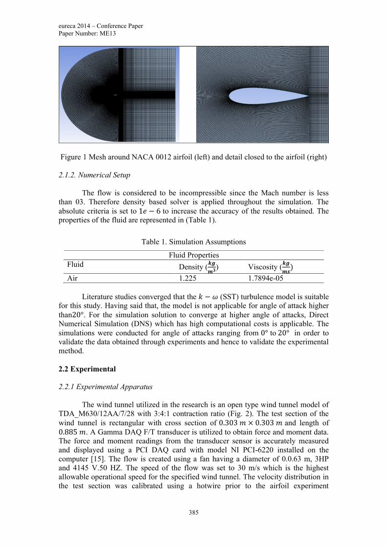
eureca 2014 – Conference Paper
Paper Number: ME13
385
Figure 1 Mesh around NACA 0012 airfoil (left) and detail closed to the airfoil (right)
2.1.2. Numerical Setup
The flow is considered to be incompressible since the Mach number is less
than 03. Therefore density based solver is applied throughout the simulation. The
absolute criteria is set to 1𝑒 − 6 to increase the accuracy of the results obtained. The
properties of the fluid are represented in (Table 1).
Table 1. Simulation Assumptions
Literature studies converged that the 𝑘 − 𝜔 (SST) turbulence model is suitable
for this study. Having said that, the model is not applicable for angle of attack higher
than20°. For the simulation solution to converge at higher angle of attacks, Direct
Numerical Simulation (DNS) which has high computational costs is applicable. The
simulations were conducted for angle of attacks ranging from 0° to 20° in order to
validate the data obtained through experiments and hence to validate the experimental
method.
2.2 Experimental
2.2.1 Experimental Apparatus
The wind tunnel utilized in the research is an open type wind tunnel model of
TDA_M630/12AA/7/28 with 3:4:1 contraction ratio (Fig. 2). The test section of the
wind tunnel is rectangular with cross section of 0.303 𝑚 × 0.303 𝑚 and length of
0.885 𝑚. A Gamma DAQ F/T transducer is utilized to obtain force and moment data.
The force and moment readings from the transducer sensor is accurately measured
and displayed using a PCI DAQ card with model NI PCI-6220 installed on the
computer [15]. The flow is created using a fan having a diameter of 0.0.63 m, 3HP
and 4145 V.50 HZ. The speed of the flow was set to 30 m/s which is the highest
allowable operational speed for the specified wind tunnel. The velocity distribution in
the test section was calibrated using a hotwire prior to the airfoil experiment
Fluid Properties
Fluid Density (𝒌𝒈
𝒎𝟑) Viscosity (𝒌𝒈
𝒎𝒔)
Air 1.225 1.7894e-05

eureca 2014 – Conference Paper
Paper Number: ME13
386
conductions. The experiment operational conditions and corresponding factors were
measured and assumed to be constant (Table 3).
Table 3. Operational Condition
Figure 2. Taylor’s University Subsonic wind tunnel
2.2.1 Experimental Setup
A specific test rig mechanism (Fig. 3) has been designed and implemented. the
test rig consists of four parts:
Push rod
Supporting bars
Connection rod
Worm and wheel gear
Figure 3. Test Rig Mechanism
The worm and wheel gear is utilized as the angle of attack controlling
mechanism for the wind tunnel (Fig. 4). Worm drive gear set consist of two gears,
Fluid Properties
Fluid Speed (𝒎
𝒔) Temperature (℃) Density (
𝒌𝒈
𝒎𝟑) Viscosity (𝒌𝒈
𝒎𝒔)
Air 30 20° 1.225 1.51e-05

eureca 2014 – Conference Paper
Paper Number: ME13
387
worm gear as well as wheel gear. The wheel gear is mounted on the connection rod
which is connected to the airfoil. The wheel gear is not able to rotate the worm gear
due to the wheel gear’s teeth orientation, while the worm gear can rotate the wheel
gear and hence the angle of attack can be adjusted by rotating the worm gear. The test
rig was calibrated using a standard 2N weight to confirm accuracy of force transfer
from airfoil to the load cell through test rig structure.
Figure 4. Rotary Mechanism
2.2.1 Experimental Model
The experiments have been conducted on the NACA 0012 prototype which
have been created utilizing CNC machine. The prototype has a chord length of 0.1 m
and span of 0.09 m. The airfoil has been installed through its aerodynamic center. The
aerodynamic center of the airfoil (Fig. 5) has been be calculated using the Eq. 4:
AC = C
4 (4)
Where AC is the aerodynamic center from the leading edge and C is the chord length
of the airfoil.
Figure 5. Aerodynamic Centre of Airfoil (Left) and Steel NACA 0012 Airfoil (Right)

eureca 2014 – Conference Paper
Paper Number: ME13
388
3. Results and Discussion
3.1 Numerical Results
The results obtained from ANSYS FLUENT consist of lift coefficient (𝐶𝐿) as
well as drag coefficient (𝐶𝐷) . The velocity of the flow has been set to 35 m/s
throughout the simulations. The simulations has been conducted for 0° , 5°, 10° and
15°. Lift and drag coefficients for each angle of attack has been obtained from the
simulation and compared with published data.
Figure 6. CFD 𝐶𝐿 comparison with Published 𝐶𝐿
Figure 7. CFD 𝑪𝑫 Comparison with Published 𝑪𝑫
The stream flow analysis provides a better understanding of the pressure
distribution around the airfoil at different angle of attack (Fig. 8). The flow stream
sticks to the airfoil surface at 0° angle of attack. As the angle of attack increases to 5°
the stream starts to separate from the airfoil’s upper surface, and the separation moves
towards the leading edge of airfoil by increasing the angle of attack. Separation of the
flow from the airfoil results in the formation of eddies starting from where the flow is
0.00E+00
2.00E-01
4.00E-01
6.00E-01
8.00E-01
1.00E+00
1.20E+00
1.40E+00
1.60E+00
0 5 10 15 20
Lift
Co
effi
cien
t
Angle of Attack
Lift Coefficient vs. Angle of Attack
CFD Lift Coefficient
Published Lift Coefficient(Ahmed )
0
0.05
0.1
0.15
0.2
0.25
0.3
0.35
0 5 10 15 20
Dra
g C
oef
fici
ent
Angle of Attack
Drag Coefficient vs. Angle of Attack
CFD Drag Coefficient
Published DragCoefficient (Ahmed )

eureca 2014 – Conference Paper
Paper Number: ME13
389
separated towards the trailing edge of airfoil as the flow tends to stick back to the
airfoil’s surface.
Figure 10. Flow Velocity Stream at 0°, 5°, 10° and 15° Angles of Attack
Formation of eddies causes chaos, therefore the flow loses its laminar
characteristics as since the flow path line is not predictable anymore. Increasing the
angle of attack results in more separated region from the airfoil surface hence more
turbulence (Fig. 11).
Figure 11. Turbulence at 0°, 5°, 10° and 15° Angle of Attack
Flow stream (Fig. 10) shows that the flow stream is symmetry at 0° angle of
attack and the velocity of the upper and lower surface of the airfoil are equal, while

eureca 2014 – Conference Paper
Paper Number: ME13
390
increasing the angle of attack from 0° to 15° results in higher flow velocity on the
upper surface compared to lower surface of the airfoil. Based on Bernoulli’s principle,
air flows at higher speed through regions with lower pressure. Therefore, it can be
said that the pressure at the upper surface of the airfoil is less than the lower surface
airfoil since the upper surface velocity is higher than the velocity at lower surface (Fig.
12).
Figure 12. Pressure Distribution at 𝟎°, 5°, 𝟏𝟎° and 15° Angles of Attack
The pressure difference between the lower and upper body of the airfoil results
in lift force. Increasing the angle of attack from 0° to 15° results in pressure increment
on the lower surface of the airfoil which ultimately results in lift force increment as
the angle of attack increases.
3.2 Experimental Results
The graph (Fig. 13) clearly shows that the lift coefficient almost linearly
increases from 0 to 0.9 as the angle of attack changes from 0° to 16°. While further
increment in the angle of attack up to 20° results in drop in lift. This converges that at
16° is the stall angle and the turbulence of the flow has increased and resulted in a
lower velocity of overt the upper surface and hence higher pressure. Higher pressure
on the upper surface causes the decrement in the lift. However, it can be seen that the
same but less abrupt path of increment in lift coefficient appears with increment of
angle attack from 20° to 42° until it reaches a value of 1.51. It also can be understood
that the lift coefficient becomes negative at angle of attack more than 90 ° and
experiences peak values at the 140° and 165° and shows a symmetrical path of
changes for the lift coefficient. This symmetry in lift coefficient is caused by the
geometry of NACA 0012 where the airfoil has no camber and the flow around the
airfoil is directly affected by the angle of attack.

eureca 2014 – Conference Paper
Paper Number: ME13
391
Figure 13. Lift Coefficient at 0° to 180° Angle of Attack
The drag coefficient at low angle of attack below the stall angle are extremely
small since the flow (Fig. 14). However, it increases exponentially after the stall and
reaches to a maximum value of 2.8 at 90° angle of attack. This great lift coefficient
consists of skin drag as well as turbulent drag. The increment in the skin is due to the
increase in the perpendicular surface contact with the flow stream which resists the
flow stream. While the turbulence drag increases due to the increment in the
separation which creates high turbulence due to the formation of eddies. Further
increment of angle of attack from 90° to 180° results in decrement in drag coefficient
since the flow stream blockage is reduced as well as the flow stream chaos which
results in formation of smaller eddies and lower turbulence. Also, it can be seen that
the drag coefficient at 0° angle of attack is smaller compared to 180° angle of attack.
This can be explained since at 0° angle of attack the flow stream is washed off the
trailing edge which is sharp while at 180° angle of attack the flow is washed off from
the thick leading edge.
Figure 14. Drag Coefficient at 0° to 180° Angle of Attack
Studying relation between the lift and drag coefficient provides an overview of
aerodynamic performance of NACA 0012 (Fig. 15). Drag Coefficient at its lowest for
-1.5
-1
-0.5
0
0.5
1
1.5
2
0 20 40 60 80 100 120 140 160 180 200
Lift
co
effi
cien
t (C
L)
Angle of attack
Lift Coefficient vs. Angle of Attack
Wind Tunnel Experiment Data
0
0.5
1
1.5
2
2.5
3
0 20 40 60 80 100 120 140 160 180 200
Dra
g c
oef
fici
ent
(CL)
Angle of attack (Degrees)
Drag Coefficient vs. Angle of Attack
Wind Tunnel Experiment

eureca 2014 – Conference Paper
Paper Number: ME13
392
0° angle of attack and reaches maximum value at 90 degrees, showing the highest
amount of drag on the airfoil resulting in lowest lift coefficient. For further increase in
the angle of attack, loft coefficient enters its negative characteristic region with
reduction in drag coefficient until it returns to zero at 180°.
Figure 15. Drag Coefficient Relationship with Lift Coefficient
4. Conclusion
Study and investigate the High angles of attack aerodynamics is a challenging and
complicated. In this project an experimental approach is used to determine the effect
of high angle of attack on the aerodynamics of the standard NACA 0012 airfoil at low
subsonic speed of 35 m/s and Reynolds number of 0.2 × 10⁶. The main findings of
this study are concluded as follows:
Increasing the angle of attack results in increment The lift coefficient increases
until it reaches a value of 0.9 at the stall angle of 16° , then it starts to decrease
with further increments in the angle of attack until 20° the lift coefficient
reaches a value of 0.7, However the lift coefficient increases again with
increment of angle of attack to 40°.
The drag force acting on the airfoil increases as the angle of attack increase
and increment in the drag force results in change of laminar flow to turbulent
flow. As the turbulence get higher the flow starts to separate from the airfoil
surface due to eddies generated by turbulence.
Further increment of angle of attack after 90° results in a nearly symmetrical
behaviour of lift and drag coefficients with lift coefficient having negative
value and drag coefficient reducing to 0.
As the comparison of the results with published data converges, the percentage
error of the experiment are to be reduced. The accuracy of the results can be improved
by considering the followings:
Reducing the vibration of the test rig to minimum while the wind tunnel
operates. This has to be reduce the misreading of forces by load cell.
-0.5
0
0.5
1
1.5
2
2.5
3
-1.5 -1 -0.5 0 0.5 1 1.5 2
Lift
Co
effi
ciet
Drag Coefficient
Lift Coefficient vs. Drag Coefficient

eureca 2014 – Conference Paper
Paper Number: ME13
393
Replacement of the wind tunnel’s section wall with a wall which precisely fits
the test section.
Producing the worm and wheel gear with aluminium that is a more rigid
material compared to polypropylene. Also the surface finish of the gears
should be improve and smoothened to allow the gears to rotate smoother.
An automatic rotary mechanism to be added to gears to provide a more
convenient and accurate solution for the change of the angle of attack.
designed to enable the user to change the angle of attack.
References
[1] J. J. Bertin and R. M. Cummings, Aerodynamics for Engineers:
Pearson/Prentice Hall, 2009.
[2] R. P. Justin Petrilli, Ashok Gopalarathnam "A CFD Database for Airfoils and
Wings at Post-Stall Angles of Attack," 31st AIAA Applied Aerodynamics
Conference.
[3] Y. Zhou, M. M. Alam, H. X. Yang, H. Guo, and D. H. Wood, "Fluid forces on
a very low Reynolds number airfoil and their prediction," International
Journal of Heat and Fluid Flow, vol. 32, pp. 329-339, 2// 2011.
[4] M. T. A. Ahmed, S. M. Rafiul Islam, Shabbir Ahmed, Tousif, Computational
Study of Flow around a NACA 0012 Wing Flapped at Different Flap Angles
with Varying Mach Numbers, 2014.
[5] I. H. Abbott and A. E. Von Doenhoff, Theory of Wing Sections, Including a
Summary of Airfoil Data: Dover Publications, 1959.
[6] N. Gregory, C. L. O'Reilly, and H.M.S.O., Low-speed Aerodynamic
Characteristics of NACA 0012 Aerofoil Section, Including the Effects of
Upper-surface Roughness Simulating Hoar Frost: National Physical
Laboratory, 1970.
[7] W. J. McCroskey, A critical assessment of wind tunnel results for the NACA
0012 airfoil [microform] / W.J. McCroskey. Moffett Field, Calif: National
Aeronautics and Space Administration, Ames Research Center, 1987.
[8] T. I. A. a. M. P. D. Douvi C. Eleni, "evaluation of the turbulence models for
the simulation of the flow over a national advisory committee for aeronautics
(NACA) 0012 airfoil " journal of mechanical engieering research vol. 4, pp.
100-111, 2012.
[9] B. Wassim and G. Wahid, "Drag Prediction in Transitional Flow Over Two-
Dimensional Airfoils," in 44th AIAA Aerospace Sciences Meeting and Exhibit,
ed: American Institute of Aeronautics and Astronautics, 2006.
[10] H. H. H. a. R. W. B. Chris C. Critzos, Jr., "AERODYNAMIC
CHARACTERISTICS OF NACA 0012 AIRFOIL SECTION AT ANGLES
OF ATTACK FROM 0° TO 180°," 1955.
[11] P. Devinant, T. Laverne, and J. Hureau, "Experimental study of wind-turbine
airfoil aerodynamics in high turbulence," Journal of Wind Engineering and
Industrial Aerodynamics, vol. 90, pp. 689-707, 6// 2002.
[12] Y. Zhang, Y. Huang, F. Wang, and Z. Tan, "Numerical Simulation of the
Airfoil Flowfields at Angles of Attack from 0° and 180°,"
in Power and Energy Engineering Conference (APPEEC), 2010 Asia-Pacific,
2010, pp. 1-4.

eureca 2014 – Conference Paper
Paper Number: ME13
394
[13] K. Yousefi, S. R. Saleh, and P. Zahedi, "Numerical study of flow separation
control by tangential and perpendicular blowing on the NACA 0012 airfoil,"
International Journal of Engineering, vol. 7, pp. 10-24, 2013.
[14] L. C. L., J. C. W. Brooks, H. A. S., and S. D. W., "Computer Program To
Obtain Ordinates for NACA Airfoils," NASA Langley Technical Report
Server1996.
[15] L. W. K. Billy, "Taylor’s Wind Tunnel Manual.," Taylor’s University, Subang
Jaya, Selangor, Malaysia.

eureca 2014 – Conference Paper
Paper Number: ME14
395
Sintering Study on Commercial
Hydroxyapatite
Thomas Thaddeaus Jacob1*
, Jeffrey Chin1
1 School of Engineering, Taylor's University, Malaysia
Abstract
Hydroxyapatite have been actively researched on for its benefits in the medical field
due to the material possessing a very similar chemical structure to that of bones. Due
to the extensive research it is currently being used to repair small bone defects and
certain dental applications. The current direction the research of hydroxyapatite is
leading is to create a viable substitute for bone transplant. The current setback of
utilising hydroxyapatite as a bone substitute is the weak mechanical properties
possessed by the material. Sintering process have long been proven to increase the
mechanical properties in bioceramics. Single stage sintering process is used to
increase the density and mechanical properties of the hydroxyapatite nanopowder. [1]
The research that is being conducted is the sintering study on commercially available
hydroxyapatite powder manufactured by Merck. The densification behaviour and
mechanical properties were found to be dependent on the thermal history during the
sintering process. To carry out the study, the commercial hydroxyapatite powder was
cold isostatically pressed at 10 MPa and presureless sintered with ramp rate of
10°C/minute at temperature range from 1100 to 1300°C with a holding time of 1hr.
The purpose of this research is to determine the optimal single stage sintering profile
of hydroxyapatite which would result in the best mechanical properties. The main
challenge in conducting this research is determining the optimal single stage sintering
profile that does not compromise the integrity of the sintered hydroxyapatite. Based
on the extensive research it can be concluded that the optimal single stage sintering
profile will produce a sintered commercial hydroxyapatite with higher mechanical
properties.
Keywords: Hydroxyapatite, single stage sintering, mechanical properties

eureca 2014 – Conference Paper
Paper Number: ME14
396
1.0 Introduction
In the past few years there have been a great amount of research on the usage of
biometerials as viable replacements to tissues in medical science. In particular
medical research has been giving a lot of attention in the field of bioceramics as
possible replacement for bone tissue. Based on the extensive research, bioceramics
have been shown to have good biocompatibility with the human body and
significantly reduce the chances of the body rejecting an artificial transplant as
compared to an actual bone transplant. Bioceramics are a much more viable solution
as it has the capability to be mass produced and specifically created to the preferred
specification to the recipient needs and a donor that is a biological match is not
required for a major transplant which is the current main drawback.
Hydroxyapatite (Ca10(PO4)6(OH)2) has of late attracted great prospect as a possible
bioceramic replacement for bone tissue which can be used in a bone transplant.
Hydroxyapatite is at this juncture used for medical applications such as repairing bone
defects, dental surgery, and various others. Hydroxyapatite is also used as a base for
synthetically built biomaterials as it can be constructed into various shapes and is well
known for its high biocompatibility and osteoconductivity. [2]
The medical research community is still showing significant attentions towards
hydroxyapatite due to its similar chemical composition to that of bone tissue. The
current major drawback of hydroxyapatite is its apparent low mechanical properties
within the substance. Research also states how a coating of an apatite layer of
hydroxyapatite around a synthetic material has shown to increase the biocompatibility
of the material with the host body due to the material’s natural promotion towards
protein absorption and cell adhesion. [3] At its current state hydroxyapatite has a low
fracture toughness which would not be viable to create compatible bone transplant
that is able to withstand heavy loads. [4]
The sintering process is technique that utilises heat to heat the desired powder to just
under the materials melting point. This would in turn cause the material to form a
stronger bond with one another. The stronger bonds are caused due to the diffusion of
atoms across the materials boundaries which causes the particles within the material
to fuse thus creating the final product. The sintering process significantly changes the
density of the sintered material, the grain size within the nanoparticles of the material,
and also the size of the final product produced from the process. [5]
Sintering is an essential process in improving the mechanical properties of ceramics.
Sintering involves developing the ceramics microstructure to significantly reduce the
porosity of the material. [6] Obtaining the optimal sintering profile is a key objective
of the study as the sintering profile and mechanism involved would determine the
microstructure and properties of the final product. [7]
The sintering process significantly affects the grain size within the material. Grain
growth within a material during the sintering process is a major part in creating a
product with strong mechanical properties. A final product that possesses a smaller
and denser particle with small grain size nanoparticles is highly desirable. This is due
to the fact that the densification rate of a material is inversely proportional to the grain
size of the final product. [8]

eureca 2014 – Conference Paper
Paper Number: ME14
397
The main purpose of this research is to determine the optimal single stage sintering
profile which results in the highest mechanical properties of hydroxyapatite. The
reasoning behind this research is to further facilitate the research of producing a
viable hydroxyapatite bioceramic for bone transplants.
1.1 Objective
The primary objective of this project can be divided into three main components:
i) To study and understand various aspects of the project by conducting in
depth literature review of journals.
ii) Conduct an experiment to study the effects of various sintering profiles
and the effects on the mechanical properties of hydroxyapatite.
iii) Determine the optimal sintering profile that results in the best mechanical
properties of hydroxyapatite.
The secondary objective of the project is to complete all the modules learning
outcomes in order to achieve the requirements for graduation
2.0 Research Methodology
The main aspect of any experimental research is the research methodology. The
research methodology allows the researcher to clearly and specifically plan and
manage the entire research experimentation requirements in order to achieve the
objective set by the researcher within a specific scope and time frame. The main
objective behind conducting this research is to further support and advance the
research on medical science in order to improve the quality of life of the community
at large.
This experimental research is to study and obtain the optimal single stage sintering
profile of hydroxyapatite which will result in an increase in mechanical properties.
The research methodology of this research can be divided into two major components:
i) Theoretical studies
ii) Practical Experiments
2.1 Theoretical Studies
To conduct any significant research experiment of value an equal proportionate of
time must be used in order to study the current developments and research that have
been recently conducted. The main purpose to conduct literature review and
background study is to understand the significant theories, characteristics and
principles regarding the research experiment. Literature review is also conducted to
ensure that the experiment that is being conducted have not been significantly
researched and would add value to the current development in the related field. For
this research the background studies includes the current development of
hydroxyapatite, the single stage sintering process, and the relationship between
sintering process and increased mechanical strength. The focus of the literature topics
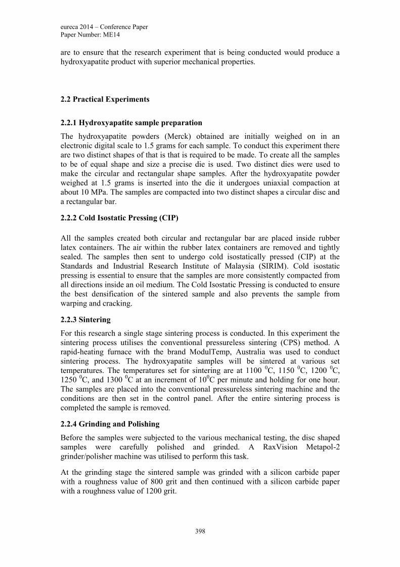
eureca 2014 – Conference Paper
Paper Number: ME14
398
are to ensure that the research experiment that is being conducted would produce a
hydroxyapatite product with superior mechanical properties.
2.2 Practical Experiments
2.2.1 Hydroxyapatite sample preparation
The hydroxyapatite powders (Merck) obtained are initially weighed on in an
electronic digital scale to 1.5 grams for each sample. To conduct this experiment there
are two distinct shapes of that is that is required to be made. To create all the samples
to be of equal shape and size a precise die is used. Two distinct dies were used to
make the circular and rectangular shape samples. After the hydroxyapatite powder
weighed at 1.5 grams is inserted into the die it undergoes uniaxial compaction at
about 10 MPa. The samples are compacted into two distinct shapes a circular disc and
a rectangular bar.
2.2.2 Cold Isostatic Pressing (CIP)
All the samples created both circular and rectangular bar are placed inside rubber
latex containers. The air within the rubber latex containers are removed and tightly
sealed. The samples then sent to undergo cold isostatically pressed (CIP) at the
Standards and Industrial Research Institute of Malaysia (SIRIM). Cold isostatic
pressing is essential to ensure that the samples are more consistently compacted from
all directions inside an oil medium. The Cold Isostatic Pressing is conducted to ensure
the best densification of the sintered sample and also prevents the sample from
warping and cracking.
2.2.3 Sintering
For this research a single stage sintering process is conducted. In this experiment the
sintering process utilises the conventional pressureless sintering (CPS) method. A
rapid-heating furnace with the brand ModulTemp, Australia was used to conduct
sintering process. The hydroxyapatite samples will be sintered at various set
temperatures. The temperatures set for sintering are at 1100 0C, 1150
0C, 1200
0C,
1250 0C, and 1300
0C at an increment of 10
0C per minute and holding for one hour.
The samples are placed into the conventional pressureless sintering machine and the
conditions are then set in the control panel. After the entire sintering process is
completed the sample is removed.
2.2.4 Grinding and Polishing
Before the samples were subjected to the various mechanical testing, the disc shaped
samples were carefully polished and grinded. A RaxVision Metapol-2
grinder/polisher machine was utilised to perform this task.
At the grinding stage the sintered sample was grinded with a silicon carbide paper
with a roughness value of 800 grit and then continued with a silicon carbide paper
with a roughness value of 1200 grit.

eureca 2014 – Conference Paper
Paper Number: ME14
399
At the polishing stage the sample was polished first with a 3 micron polishing cloth
and then with a 1 micron polishing cloth with diamond paste is applied. The polishing
is continuously until a very reflective surface is achieved.
2.2.5 Properties and Structural Analysis
2.2.5.1 X-Ray Diffraction (XRD)
X-Ray Diffraction is used to track the phases and behaviour of the Hydroxyapatite
nanostructures in the experiment. The specimen is place within an X-Ray Diffraction
machine and the structure of the sintered hydroxyapatite along with its characteristics
is determined.
The hydroxyapatite sample that was sintered is placed into the X-Ray Diffraction
machine one at a time. The machine then releases an output graph based on the
composition and structure of the sintered hydroxyapatite. The steps are repeated for
the entire batch of sintered samples.
The concept of X-Ray Diffraction (XRD) is based on Bragg’s law which proves
correlation between the incidence angle a crystal reflects x-ray beams to the periodic
atomic structure of the crystals postulated.
2.2.5.2 Scanning Electron Microscopy (SEM)
Scanning Electron Microscopy (SEM) is used to analyse and observe the morphology
and crystalline structure of the sintered hydroxyapatite. The grain size of the sintered
hydroxyapatite is observed and based on the grain size the morphology, crystalline
structure, and mechanical properties of the sintered sample can be deduced.
The hydroxyapatite sample that was sintered is placed into the Scanning Electron
Microscope one at a time. Before the samples are placed into the Scanning Electron
Microscope they are coated with palladium which acts as a conducting layer to deter
charging from occurring within the microscope. A focused beam of electrons then
scans the sintered sample. An image of the scanned sintered sample is then displayed
with a scale and the picture of the scanned image is then saved. The steps are repeated
for the entire batch of sintered samples.
2.2.5.3 Young’s Modulus
Young’s modulus is the value of the gradient of graph between the stress and strain of
the material. The Young’s modulus is used determine the resistance of the material to
elastic deformation under a load. To obtain the Young’s modulus for this experiment
the sonic resonance technique is utilised to analyse the resonant frequency of the
specimen. The testing instrument (GrindoSonic: MK5 “Industrial”, Belgium) which is
used to determine the resonant frequency of the sintered hydroxyapatite bar by
utilising a transducer to monitor and analyse the vibrational harmonics. The Young’s
modulus is then calculated utilising the formula stated below:

eureca 2014 – Conference Paper
Paper Number: ME14
400
For this research the Young’s Modulus test will be performed to determine the
resistivity of hydroxyapatite to elastic deformation.
2.2.5.4 Bulk Density
Bulk Density test is the mass of particles of a material divided by the total volume
occupied by the material. The bulk density test shows the ability of a material to
function as a support. The water immersion method is used to perform the bulk
density test on the specimen of sintered hydroxyapatite.
First, the entire prepared sample before sintering is weighed in air (W) and the
weights are recorded down. Then, the thickness (t1) and diameter (d1) of each
prepared sample before sintering are recorded down. After the sintering process is
completed the thickness (t2) and diameter (d2) of each sample are recorded down.
Then, the weight of the entire sintered sample in air (Wa) is weighed and recorded
down. Next, the sintered samples are then weighed while immersed in water (Ww) and
recorded down. After, the weight of the sintered sample immersed in water is weighed
in air (Wa+w) and recorded down to determine the porosity of the sample. The bulk
density formula used is as stated below:
𝜌 = 𝑊𝑎
𝑊𝑎 − 𝑊𝑤𝜌𝑤
For this research a bulk density test will be performed to determine the structural
support integrity of the material Hydroxyapatite.
2.2.5.5 Vickers’s Hardness
The Vickers’s Hardness will be determined by using the Vickers’s indentation test.
The Vickers’s indentation test will utilise a microindentation device to create an
indentation with a set load and duration. The indentation left by the test is then
measured using a microscope to determine the diameter of the indentation. The
diameter is then placed into the Vickers’s hardness formula and the Vickers’s
hardness, Hv is determined. The formula for Vickers’s hardness is as stated below:
𝐻𝑣 =1.854 ∗ 𝐹
(𝑑)2
After the sample is prepared it is then placed in a micro indenter machine. The micro
indenter machine is used to apply a load for a set amount of time and the indentation
present on the sample as a result is used to calculate the hardness. The load being
applied to the sintered sample by the micro indenter machine is set at 10N for a
duration of 5 seconds. Once the load application is complete the diameter of the
indentation and the hardness is recorded down. The steps are then repeated twice on

eureca 2014 – Conference Paper
Paper Number: ME14
401
the same sample totalling a number of three indentation per sample. The steps are
then repeated for the rest of the sintered samples.
Through this test the Vickers’s Hardness, 𝐻𝑣 is obtained for the fracture toughness
test.
2.2.5.6 Fracture toughness
Fracture toughness by definition is the strength of a material with a crack to resist
further fracture. It is essentially used to determine the resistance of a material to
fracture when a crack is present. The Niihara (1985) fracture toughness equation is as
shown below:
𝐾𝐼𝐶 = 0.203(𝑐
𝑎)−1.5(𝐻𝑣)(𝑎)0.5
After the sintered sample has undergone the micro indentation test to determine the
hardness, 𝐻𝑣 the samples are then viewed under a digital microscope to observe the
crack that propagate in all four corners of the indentation. A picture is then taken of
each corner of the indentation. Utilising the scale present in the picture a software is
used to measure the length of the crack in micrometres (µm). The lengths are then
placed into the formula and fracture toughness, 𝐾𝐼𝐶 is determined.
For this research the fracture toughness test will be used to determine the fracture
toughness of the material hydroxyapatite. Using the data from this experiment we can
determine if we have found the optimal single stage sintering profile.
3.0 Results and Discussion
3.1 X-Ray Diffraction
Figure 1: X-Ray Diffraction pattern of hydroxyapatite sintered at 1100
oC
Based on Figure1 the X-Ray Diffraction indicates that the sample sintered at 1100oC
peaks are consistent with that of hydroxyapatite which indicates that the sintered

eureca 2014 – Conference Paper
Paper Number: ME14
402
material did not shift into a different material phase. The diffraction patterns show
sharp, clear and high intensity corresponding to hydroxyapatite which proves phase
purity and high crystallinity degree of the sintered sample produced.
Figure 2: X-Ray Diffraction pattern of hydroxyapatite sintered at 1150
oC
Based on Figure 2 the X-Ray Diffraction indicates that the sample sintered at 1150oC
peaks are consistent with that of hydroxyapatite which indicates that the material did
not shift phase into a different material. The diffraction patterns show sharp, clear and
relatively high intensity corresponding to hydroxyapatite which proves phase purity
and good crystallinity degree of the sintered sample produced.
Figure 3: X-Ray Diffraction pattern of hydroxyapatite sintered at 1200
oC
Based on Figure 3 the X-Ray Diffraction indicates that the sample sintered at 1200oC
peaks are consistent with that of hydroxyapatite which indicate that the sintering did

eureca 2014 – Conference Paper
Paper Number: ME14
403
not cause the material to shift phase into a different material. The diffraction patterns
show sharp, clear and very high intensity corresponding to hydroxyapatite which
proves phase purity and very high crystallinity degree of the sintered sample
produced.
Figure 4: X-Ray Diffraction pattern of hydroxyapatite sintered at 1250
oC
Based on Figure 4 the X-Ray Diffraction indicates that the sintered sample peaks are
consistent with that of hydroxyapatite. This proves that the hydroxyapatite sintered at
1250oC did not cause the material to shift phase into a different material. The
diffraction patterns show relatively intensity corresponding to hydroxyapatite which
proves good phase purity and good crystallinity degree of the sintered sample
produced but also indicates minor decomposition of hydroxyapatite as some low
peaks do not correspond with hydroxyapatite.
Figure 5: X-Ray Diffraction pattern of hydroxyapatite sintered at 1300
oC

eureca 2014 – Conference Paper
Paper Number: ME14
404
Based on Figure 5 the X-Ray Diffraction indicates that the sintered sample peaks are
consistent with that of hydroxyapatite. This proves that the hydroxyapatite sintered at
1300oC did not cause the material to shift phase into a different material. The
diffraction patterns show sharp, clear and high intensity corresponding to
hydroxyapatite which proves phase purity and high crystallinity degree of the sintered
sample produced. The diffraction patterns show sharp, clear and relatively high
intensity corresponding to hydroxyapatite which proves phase purity and good
crystallinity degree of the sintered sample produced.
The intensity of the X-Ray Diffraction decreases between the sintered hydroxyapatite
at 1100oC and the sintered hydroxyapatite at 1150
oC. The intensity of the X-Ray
Diffraction then increases when the hydroxyapatite is sintered at 1200oC. The
intensity of the X-Ray Diffraction then continues to decrease between the sintered
hydroxyapatite at 1250oC and the sintered hydroxyapatite at 1300
oC. The X-Ray
Diffraction of the sample sintered at 1300oC is observed to have the lowest intensity
indicating relatively low crystallinity as compared to the rest of the sintered samples.
The clarity and sharpness of the pattern of the sample sintered at 1300oC indicate
phase purity and a very high. The X-Ray Diffraction of the sample sintered at 1200oC
is observed to have the highest intensity indicating phase purity and a very high
crystallinity as compared to the rest of the sintered samples.
3.2 Bulk Density
For this experiment the bulk density is determined by weighing the sintered
hydroxyapatite in different conditions to determine the density of the samples. Water
temperature at the time of the test is at 28oC.
Table 1: Tabulated density of sintered hydroxyapatite samples
Sintered temperature 1100oC 1150
oC 1200
oC 1250
oC 1300
oC
Weight in air, WA (grams) 1.423 1.415 1.419 1.085 1.418
Weight in water, WW (grams) 0.913 0.944 0.960 0.736 0.958
Weight in air after soaked in water, WA+W
(grams) 1.429 1.425 1.422 1.101 1.442
Bulk Density (grams/cc) 2.752 2.933 3.065 2.969 2.920
Based on Table 1 the hydroxyapatite sample sintered at 1100oC has the lowest bulk
density at 2.752 g/cc and the hydroxyapatite sample sintered at 1200oC has the highest
bulk density at 3.065 g/cc. The difference between the weight in air and the weight
after being immersed in water in air is really small for the sample sintered at 1200oC
which indicates that the porosity of the sintered sample is very low thus producing a
sample with a high bulk density.
Based on a research done in a similar field the bulk density of hydroxyapatite sintered
at 1200oC also resulted in a material with low porosity due to the elimination of
residual porosity [10]. The temperature conditions are high enough to significantly
reduce residual porosity of the sample while still being able to prevent the formation
of undesired phases [10].

eureca 2014 – Conference Paper
Paper Number: ME14
405
3.3 Young’s Modulus
For this experiment the Young’s Modulus of each of the sintered hydroxyapatite samples at
different temperatures are determined.
Table 2: Tabulated data of Young’s Modulus of the sintered hydroxyapatite.
Sintered Temperature (oC) Young's Modulus (GPa)
1100 96.1
1150 110.9
1200 108.8
1250 106
1300 103
Based on Table 2 the hydroxyapatite sample sintered at a temperature of 1100oC has
the lowest Young’s Modulus at 96.1GPa and the hydroxyapatite sample sintered at a
temperature of 1150oC has the highest Young’s Modulus at 110.9GPa which indicates
the resistivity of the material to elastic deformation. It can be observed from Figure 6
that the Young’s Modulus increases between the samples sintered at 1100oC and
1150oC, while decreasing steadily between samples sintered at 1150
oC and 1300
oC.
Based on researches conducted on the sintering of ceramics, the average size of the
pores present within the microstructure of the ceramic increases as the sintering
temperature is increased [11]. The Young’s modulus is directly correlated with the
porosity of a material, as the porosity of a sample increases the Young’s modulus
decreases [12].
The hydroxyapatite samples are sintered in a repetitive thermal cycle at a set
increment which can lead to crack nucleation which may result in a loss of strength
[11]. The formation of cracks within the microstructure of the material can result in a
significant influence on the Young’s modulus of the material [13] and [14].The
decrease in Young’s modulus can be attributed to the decomposition of the
hydroxyapatite that prevented the formation of stronger inter-particle bonding within
the ceramic matrix [11].
3.4 Hardness
For this experiment the Vickers’s hardness is performed on each of the sintered
hydroxyapatite samples at different temperatures are determined. Each hydroxyapatite
sintered sample is tested three times in order to obtain an average hardness value. The
test is performed by applying a load of 10N over a period of 5 seconds.
Table 3: Tabulated data of hardness test and mean hardness value.
Sintered Temperature (oC) 1100.00 1150.00 1200.00 1250.00 1300.00
Hardness (Hv) i) 376.00 507.00 549.00 577.00 519.00
ii) 396.00 498.00 548.00 527.00 577.00
iii) 371.00 499.00 575.00 548.00 522.00
Mean Hardness (Hv) 381.00 501.33 557.33 550.67 539.33

eureca 2014 – Conference Paper
Paper Number: ME14
406
Based on Table 3 the hydroxyapatite sample sintered at a temperature of 1100oC has
the lowest Vickers hardness at 381 HV and the hydroxyapatite sample sintered at a
temperature of 1200oC has the highest Vickers hardness at 557.33 HV. The highest
Vickers’s hardness indicates a resistivity towards plastic deformation, penetration,
and bending.
Sintering temperature of the sample is directly correlated to the hardness of the
sample, the higher the sintering temperature the harder the sample produced. This
however does not work infinitely as very high temperature have the tendency to
eliminate the functional group OH in the hydroxyapatite matrix [15]. The elimination
of the fun functional group OH from the hydroxyapatite matrix will lead to the
decomposition of the hydroxyapatite phase that can result in lower mechanical
properties [15].
3.5 Fracture toughness
Based on the Table 4 the hydroxyapatite sample sintered at a temperature of 1100oC
has the highest fracture toughness at 0.93 and the hydroxyapatite sample sintered at a
temperature of 1200oC has the lowest fracture toughness at 0.64. This indicates the
material with the highest fracture toughness has the highest resistance towards the
propagation of cracks present within the material.
Table 4: Tabulated data of fracture toughness.
Sintered Temperature (oC) 1100 1150 1200 1250 1300
Fracture Toughness (MPam^1/2) i) 0.69 0.54 0.57 1.04 0.67
ii) 1.31 0.71 0.54 0.44 0.84
iii) 0.79 0.67 0.46 0.78 0.51
Mean Fracture Toughness
(MPam^1/2) 0.93 0.64 0.52 0.75 0.67
Based on studies done on sintering of ceramics the thermal stress developed during
the cooling phase of the sintering process can cause a variation in the mechanical
properties of the sintered sample [16]. The samples that develop larger grains size
during the cooling stage can create miniscule cracks that can affect the hardness and
fracture toughness of the sintered sample [17]. A higher rate of cooling can result in a
higher stress concentration that would be destructive towards improving the strength
of the material [18]. These factors could have contributed to the fracture toughness
obtained in this experiment.
3.6 Scanning Electron Microscopy
The purpose of this image is to observe the microscopic structure of the sintered
sample and note the grain size and intergranular cracks present within it. Lower
sintering temperature leads to formation of smaller grain size as compared to higher
sintering temperature. The finer grain size of a material corresponds with a higher
resistance to crack propogation and dislocation motion which in turn results in a
higher fracture toughness. [19]

eureca 2014 – Conference Paper
Paper Number: ME14
407
Figure 6: Scanning electron microscopy image of hydroxyapatite sintered at 1100
oC
Figure 6 shows that the grain size of the material are very small and there are many
intergranular cracks present within. This correlates with the results of this experiment
indicating that the sample sintered at 1100oC possesses the highest fracture toughness
in the entire experiment.
Figure 7: Scanning electron microscopy image of hydroxyapatite sintered at 1150
oC
Figure 7 shows the grain size of the material are relatively small and there are many
intergranular cracks present within. This correlates with the results of this experiment
indicating that the sample sintered at 1150oC possesses a relatively high fracture
toughness as compared to the other sintered samples in the experiment.

eureca 2014 – Conference Paper
Paper Number: ME14
408
Figure 8: Scanning electron microscopy image of hydroxyapatite sintered at 1200
oC
Figure 8 shows the grain size of the material are much larger in comparison with the
grain size of the materials sintered at 1100oC and 1150
oC.There are however much
less intergranular cracks present within the sintered sample as a result of a larger grain
size. This correlates with the results of this experiment indicating that the sample
sintered at 1200oC possesses a very low fracture toughness as compared to the other
sintered samples in the experiment.
Figure 9: Scanning electron microscopy image of hydroxyapatite sintered at 1250
oC
Figure 9 show he grain size of the material are larger in comparison with the grain
size of the materials sintered at 1200oC.There are however much less intergranular
cracks present within the sintered sample as a result of a larger grain size. The result
however does not correlate with the results of this experiment indicating that the
sample sintered at 1250oC possesses a relatively high fracture toughness as compared

eureca 2014 – Conference Paper
Paper Number: ME14
409
to the other sintered samples in the experiment. The cause of the irregularity is not
clear but could be attributed to the toughening effect of hydroxyapatite ceramics.
Figure 10: Scanning electron microscopy image of hydroxyapatite sintered at 1300
oC
Figure 10 show the grain size of the material are is the largest in comparison with the
grain size of the materials sintered at 1250oC.There are however very low
intergranular cracks present within the sintered sample as a result of a larger grain
size. The result however does not correlate with the results of this experiment
indicating that the sample sintered at 1300oC possesses a better fracture toughness as
compared to the sample sintered at 1150oC in the experiment. The cause of the
irregularity is not clear but could be attributed to the toughening effect of
hydroxyapatite ceramics.
4.0 Conclusion
This experimental research was conducted to study the sintering of commercial
hydroxyapatite and determine the optimal sintering profile. The results indicate and
initial increase in mechanical properties as the sintering temperature increased from
1100oC to 1200
oC. The results however also indicate a decrease in mechanical
properties at sintering temperatures of 1250oC and 1300
oC. The optimal sintering
profile that results with the best mechanical properties was determined to be the
sample sintered at 1200oC with an increment of 10
oC per minute and holding for one
hour.
The future work in this field would include various different forms of sintering
techniques which would result in different products. It would also include a two-stage
sintering profile to further experiment on the effects of two-stage sintering on
hydroxyapatite.
eureca 2014 – Conference Paper
Paper Number: ME14
410
5.0 References
[1] H. Yang, L. Zhang, X. Guo, X. Zhu and X. Fu, 'Pressureless sintering of silicon
carbide ceramics containing zirconium diboride', Ceramics International, vol. 37,
no. 6, pp. 2031--2035, 2011.
[2] A. Dejaco, V. Komlev, J. Jaroszewicz, W. Swieszkowski and C. Hellmich,
'Micro CT-based multiscale elasticity of double-porous (pre-cracked)
hydroxyapatite granules for regenerative medicine', Journal of biomechanics,
vol. 45, no. 6, pp. 1068--1075, 2012.
[3] D. Trandafir, C. Mirestean, R. Turcu, B. Frentiu, D. Eniu and S. Simon,
'Structural characterization of nanostructured hydroxyapatite--iron oxide
composites', Ceramics International, vol. 40, no. 7, pp. 11071--11078, 2014.
[4] M. Kharaziha and M. Fathi, 'Improvement of mechanical properties and
biocompatibility of forsterite bioceramic addressed to bone tissue engineering
materials', Journal of the mechanical behavior of biomedical materials, vol. 3,
no. 7, pp. 530--537, 2010.
[5] D. Bucevac, A. Radojkovic, M. Miljkovic, B. Babic and B. Matovic, 'Effect of
preparation route on the microstructure and electrical conductivity of co-doped
ceria', Ceramics International, vol. 39, no. 4, pp. 3603--3611, 2013.
[6] X. Wang, X. Deng, H. Bai, H. Zhou, W. Qu, L. Li and I. Chen, 'Two-Step
Sintering of Ceramics with Constant Grain-Size, II: BaTiO3 and Ni--Cu--Zn
Ferrite', Journal of the American Ceramic Society, vol. 89, no. 2, pp. 438--443,
2006.
[7] A. Chinelatto, A. Chinelatto, C. Ojaimi, J. Ferreira and E. Pallone, 'Effect of
sintering curves on the microstructure of alumina--zirconia nanocomposites',
Ceramics International, vol. 40, no. 9, pp. 14669--14676, 2014.
[8] J. Cho, J. Lee, S. Chung, J. Seo and S. Rhee, 'Effect of grain size and density of
spray-pyrolyzed hydroxyapatite particles on the sinterability of hydroxyapatite
disk', Ceramics International, vol. 40, no. 5, pp. 6691--6697, 2014.
[9] N. Rendtorff, S. Grasso, C. Hu, G. Suarez, E. Aglietti and Y. Sakka, 'Zircon–
zirconia (ZrSiO4–ZrO2) dense ceramic composites by spark plasma sintering',
Journal of the European Ceramic Society, vol. 32, no. 4, pp. 787-793, 2011.
[10] A. Cuccu, S. Montinaro, R. Orrù, G. Cao, D. Bellucci, A. Sola and V. Cannillo,
'Consolidation of different hydroxyapatite powders by SPS: Optimization of the
sintering conditions and characterization of the obtained bulk products',
Ceramics International, vol. 41, no. 1, pp. 725-736, 2014.
[11] L. Zhang, K. Gao, A. Elias, Z. Dong and W. Chen, 'Porosity dependence of
elastic modulus of porous Cr3C2 ceramics', Ceramics International, vol. 40, no.
1, pp. 191-198, 2014.
[12] E. Zadeh Hayati, O. Mohammad Moradi and M. Ghassemi Kakroudi,
'Investigation the effect of sintering temperature on Young’s modulus
evaluation and thermal shock behavior of a cordierite–mullite based composite',
Materials & Design, vol. 45, pp. 571-575, 2013.
[13] M. Dimitrijevic, M. Posarac, J. Majstorovic, T. Volkov-Husovic and B. Matovic,
'Behavior of silicon carbide/cordierite composite material after cyclic thermal
shock', Ceramics International, vol. 35, no. 3, pp. 1077-1081, 2009.
[14] S. Martinovic, J. Majstorovic, V. Vidojkovic and T. Volkov-Husovic, 'Influence
of the damage level during quenching on thermal shock behavior of low cement
castable', Science of Sintering, vol. 42, no. 2, pp. 211-219, 2010.
[15] M. Herliansyah, M. Hamdi, A. Ide-Ektessabi, M. Wildan and J. Toque, 'The
influence of sintering temperature on the properties of compacted bovine

eureca 2014 – Conference Paper
Paper Number: ME14
411
hydroxyapatite', Materials Science and Engineering: C, vol. 29, no. 5, pp. 1674-
1680, 2009.
[16] K. Maiti and A. Sil, 'Relationship between fracture toughness characteristics
and morphology of sintered Al2O3 ceramics', Ceramics International, vol. 36,
no. 8, pp. 2337-2344, 2010.
[17] T. Shiota, K. Yasuda and Y. Matsuo, 'Bending Strength Dependence of
Fractoluminescence Intensity in Silica Glass, Single Crystal and Polycrystalline
MgO', Tribology Online, vol. 3, no. 5, pp. 264-267, 2008.
[18] J. Lin, X. Zhang, S. Dong, Y. Yang, W. Han and H. Jin, 'Effects of sintering
velocity on the microstructure and mechanical properties of hot-pressed ZrB2–
SiC–ZrO2f ceramics', Materials & Design, vol. 49, pp. 681-686, 2013.
[19] S. Dasgupta, S. Tarafder, A. Bandyopadhyay and S. Bose, 'Effect of grain size
on mechanical, surface and biological properties of microwave sintered
hydroxyapatite', Materials Science and Engineering: C, vol. 33, no. 5, pp. 2846-
2854, 2013.

eureca 2014 – Conference Paper
Paper Number: ME15
412
Mechanical Simulation and
Review of a Selected Electrical Car
N.T.Saidy1 ,Y. Sabzehmeidani
1, M.T.Hajibeigy
1
1School of Engineering, Taylors University
*Email: [email protected]
Abstract
Cars have always been the major contributor to reduction of earth’s natural resources
as well as being the frontrunner in green house effects, which is one of the main
causes of global warming. Green vehicles have been taken to a new level through
these years by extensive researching and constant improvements. This project focuses
on the mechanical improvement and assembly of an energy efficient electrical car
supported by an electrical hub motor and inside regenerative breaking
implementation. Design and manufacturing of the electrical car have been done based
on engineering facts with precise mathematical formulation and it is validated with
computer simulations to ensure the safety and performance of the vehicle. Chassis and
the knuckles of the electrical car were systematically designed and improved by 63%
using static simulations and the final chassis and knuckle designs were then
manufactured by 3d paper wrapping and CNC machining method respectively. The
aerodynamic performance of the system was handled during the design stage and its
components have been implemented. The contributing factors of the body shell were
experimented and improved in terms of weight to strength ratio.
Key-Words: Chassis, Upright, Aerodynamic, Static simulation, Finite element
analysis

eureca 2014 – Conference Paper
Paper Number: ME15
413
1.0 Introduction
As the time pasts by every year the reduction of petroleum in the world forces
the automotive industry to alternate their source of energy to power vehicles. An
alternative source of energy should be replaced to reduce the dependency to
petroleum energy which is powering up more than 80% of transportation vehicles
nowadays [1]. Statistics shows that 36.4% of energy is used by the transportation
sector in Malaysia and this percentage is rapidly increasing everyday so in order to
face this problem another source of energy should be replaced with petrol in this
sector [2] .One of the best replacements would be Electrical power which is a clean
energy. Higher efficiency, greater acceleration and reduction in carbon footprint are
the benefits of an electric vehicle compared to the conventional internal combustion
engine which this would help the world to save up this valuable source of energy for a
better use.By the time of 2012 the global EV stock exceeded 180000 unites [3]. At that
time companies like Tesla Motors had the lead of EV market with their130MPH speed
and high range cars [4]. With the development of the electrical cars, being sustainable is
not sufficient whereas efficiency should be taken into consideration as well. The most
reasonable method to improve the efficiency is by reducing the weight of the vehicle
while performing in the desirable boundary conditions [4]. In order to reduce the weight
of the vehicle, every component have to be redesigned and mechanically developed
which calls for extensive design and simulation stages.
Mechanical development of an electrical car is the main purpose of this project,
which it focuses on designing and improving the chassis, upright and an aerodynamic
body of an electric vehicle. To prove the capability of the design simulations are carried
out to test design whereas experimental testing has also been done to fully ensure the
generated results from simulation. In the case of chassis and upright weight/strength ratio
is the most important criteria in the design stage and solid works simulations are done to
further reduce the weight of both chassis and upright. Look and aerodynamic of the body
is what that is considered in designing the body shell while SolidWorks flow simulation is
used to test the aerodynamic aspect of the body. Finalized Designs are then manufactured
and fabricated each with their respective chosen material. Chassis was fabricated using
mild steel pipes with a diameter of 21mm.T6 (6061) aluminium alloy was used to
manufacture the upright and it has been manufactured by a CNC machine. In this paper
the design process of chassis, upright and aerodynamic body of an electric is explained
into details and designs are optimized and validated by static simulations under defined
real world conditions. These designs are manufactured using materials selected in the
design stage and the manufactured prototypes are shown in this paper.
2.0 Design
2.1 Chassis
The main purpose of the chassis is to form the overall shape of the car and
protect the passengers from any external invasion. A Space frame is used in this
project as it is much lighter than other types like ladder or cruciform since metal
tubes are used in prototyping them. Lightening the chassis while having a good
response to stresses is the most important criteria of a chassis so in order to reduce the
weight of the chassis there are a number of factors that should be taken into
consideration. Firstly the size of the chassis should be minimized to the smallest size
possible which in order to achieve that the chassis have been designed in a dimension
of 1.75 m length and 0.5 m width which is the size of an average person ; this would

eureca 2014 – Conference Paper
Paper Number: ME15
414
save the unnecessary weight. There are actually different types of static and dynamic
forces acting on the chassis in different situations such as bending , torsion and lateral
loadings which these are forces that have to be considered while designing a chassis
.In order to increase the stiffness of the chassis diagonal braces are used in the design
which is shown Figure1 [5].
The chassis is then designed in Solidworks based on the competition’s criteria
and have been optimized using solid works simulation in the simulation stage. The
finalized design is then constructed using steel pipes.
2.2 Upright
The upright assembly of the car to provide a direct mounting from the
suspension links to the wheels. The challenge of designing the front upright is to be
able to support the electric car under common static and motional conditions [6] .The
car will be subjected to forces unseen by naked eyes no matter it is static or motional
and only the result of these forces can be seen. The design had to be done with
concern safety measure to prevent damages and loss and even death. .Upright is one
of the most critical components of car as it joins the chassis and the suspension unit to
the wheels. There are quite a number of forces acting on the upright in different
situations where lateral forces caused by the cornering of the car and normal force
caused by the weight of the vehicle are the most considerable ones; these forces are
shown in the simulation stage where 2 design solutions were provided for the upright
shown in Figure 2 and 3 to find out whether a thinner steel design is better or a more
complicated aluminium design.
Diagonal members
Figure 15. Chassis designed in Solidworks
Figure2. First design solution for upright Figure3. Second design solution for upright

eureca 2014 – Conference Paper
Paper Number: ME15
415
Comparison have been made in Table 1 based on the criteria needed for the
upright where the second upright design is selected and it weights about 1006.37g.
Upright is then simulated in the simulation stage for testing purposes and to look for
any further improvement. Upright was found to be too strong whereas weigh
reduction took place in the break pad and upright area (Figure 4). Finally the last stage
of simulation is conducted to ensure the performance of the upright.
Attribute weighing
factor
steel
design
Aluminium
design remarks
Mass 3 7 9 1st design:1763g 2nd design:1006g
Cost 0.5 9 6 aluminium is more expensive than steel
Reliability 2 7 8 Based on the simulations the second design
is more reliable
Serviceability 0.5 9 7 steel can be easily welded while aluminium
is not
Performance 2 7 8 the aluminium design is only one piece it has
a better performance
Manufacturability 1.5 8 9 CNC manufacturing is more accurate than
welding
Aesthetics 0.5 8 8
Total 10 5.9 8.3
Figure4.Final upright design
2.3 Aerodynamic Body
In this stage the goal is to have the least amount of drag force and lightest
body possible to directly increase the efficiency of the vehicle .The lowest drag
coefficient and the smallest frontal area are desired in order to have a better
aerodynamic performance since the drag force is directly proportional to the frontal
area (Eq.1).An aerofoil shape has the best aerodynamic performance compared to
Table 1. Upright decision matrix

eureca 2014 – Conference Paper
Paper Number: ME15
416
other shapes where in this case a NACA profile is what that is used as the basis of the
design [7]. NACA 2420 was selected as the backbone of the design and generated
from airfoil generator website since it is the smallest profile that can be fitted in to the
chassis design and a canopy is added to cover the roll bar and act as a door for the
vehicle. The body design is shown in Figure 5 where it shows the final assembly of
the design to the other components.
𝐹𝑑 =1
2 𝜌 𝑣2 𝐶𝑑 𝐴 (1)
where:
𝐹𝑑 = drag force
𝐶𝑑 = drag coefficient
Material selection is then carried out where Cambridge material selector
application is used to compare the selected materials. Carbon fibre, fibre glass and
aluminium were candidate as the materials of the body construction but carbon fibre
was eliminated due to its high cost. Fibreglass and aluminium are compared (Figure
6) where fibreglass is selected because of its low density. There are a few processes
required to manufacture the fibreglass body where in this case fibre glass cloth and
matt are combined to achieve a higher strength and a smoother surface. Furthermore
the ratio of the resin and hardener is also a critical factor for the hardening time of the
body. Table2 is constructed showing all the factors associated in constructing fibre
glass to find the best combination of factors. Layers of fibre glass matt and fibreglass
cloth, resin to hardener ratio, the thickness produced, rated strength and the hardening
time of the model is included in this table (The number in the resin and hardener
section only shows the ratio between resin and the hardener).
Figure 5.Final body design assembled to the chassis

eureca 2014 – Conference Paper
Paper Number: ME15
417
Layer
of
fibre
glass
matt
Layer
of
fibre
glass
cloth
resin
hardener
Produced
thickness
(mm)
Strength
Rated
from 0
to 5
Hardening
time (h)
1 1 2 1 3 2.5 11
2 1 2 1 4.3 3.5 11.3
3 1 2 1 5.8 4.5 12.43
2 1 3 1 4.5 4 18
3.0 SIMULATION
3.1 Upright simulation
In terms of weight distribution which is the portioning of weight within a
vehicle, it can be calculated that the both front wheels together have 59% of weight
distribution whereas the rear wheel yields a 41% [8] .The total weight of the electric
car with load is about 140kg where by considering the safety factor of 4 it can be
calculated as 560k.The possible cases here includes two major parts, which is the
torque acting on the upright while the car is cornering at a required turning radius of
3.5m and when it encounter uneven surface when the cornering is done. When
cornering, the electric car will have centrifugal force of 3275N acting away from the
centre of the turning radius where this force must be opposed by the centripetal force
Table2.Fibre glass and resin-hardener ratio
Figure 6.Material selection chart (young’s modules VS density)

eureca 2014 – Conference Paper
Paper Number: ME15
418
that is created from the lateral friction of the wheel tire sideways (Eq.2). This force
will create a torque of 884 N.m on the upright. Moreover When the car go throught a
bump, the worst case scenario suggests that 2g of force will be acting to the car due to
its weight and the force acting toward the wheel is the normal for which supports the
car[9]. This results into 3241.2N of force and 228N.m of torque acting on the
upright(Eq.3).Static simulations is done on the first and the second optimized model
based on the values from above and the results are shown in Figure 8 and 9.
As it is shown below the deformation occurred in the first model is about 0.006 mm
which is very low whereas the second model shows a deformation of about 0.1 mm.
Fc = m × w2 × r (2)
Where:
m = distributed mass supported by one front wheel, r = required turning radius
Fn = m × g × f (3)
3.2 Chassis Simulation
Frame torsion analysis is done on the chassis shown in figure 10 to study the
torsional rigidity of the chassis Based on the weight distribution results from the
upright simulation section. the weight acting on each front wheel considering a safety
factor of 4 is 165kg where this value is used in the torsional rigidity testing. The
torsional rigidity is calculated using Eq.(4) where the angular displacement is
calculated from Eq.(5)[10]. The distance from the point of application and the centre
of the car is 0.52m and the linear displacement in the Y direction is defined in Figure
10 where the linear displacement on both sides are taken and an average value is
found to achieve a more accurate result.
In addition to that front impact analysis is done where 1800N is acting to the
front plane of the chassis shown in Figure 11. This value is the force acting on the
chassis when stopping the car with a speed of 30 km/h in 2 seconds considering a
safety factor of 2.
Figure 9. Final model simulation Figure 8. Simulation of the first model

eureca 2014 – Conference Paper
Paper Number: ME15
419
𝐾 =𝑇
𝜗 (4)
Where:
K= torsional rigidity (Nm/degree), F=force acting on the arm of the chassis=1650 N
L= distance from the point that the force is applied to the centreline of the car= 0.52m
T= FL = 858Nm
𝜗 = tan−1 (𝑌2+𝑌1)
2𝐿 (5)
Where:
𝜗 = angular displacement
𝑌 = linear diplacement of the right wheel in Y direction
4.0 Result and Discussions
4.1 Chassis
The stress acting on the chassis in the worst situation considering a safety
factor of 4 is 179466144 N/𝑚2 while the yield strength of steel 1010 is 180000000
N/𝑚2. This means that the chassis can withstand the torsion force acting on its arms.
Moreover the torsional rigidity of the chassis was found to be 554.33 Nm/ degree
which is about 33.5kN/ radians, this value is about 50 % more than the stiffness target
Figure 10. Torsional rigidity testing Figure 11. Front impact analysis

eureca 2014 – Conference Paper
Paper Number: ME15
420
for a vehicle which is 15-17 Nm/radians [11].The obtained result from the second
analysis on the chassis shows that the stress acting on the pipes is
109590016N/𝑚2.which is much lower the yield strength of the material used. The
final constructed chassis shown in Figure 12 weighs about 10 kg which is very low in
compare with other prototypes made by steel.
4.2 Upright
The upright design shown in Figure 3 was selected based on Table 1 due to its
better performance, precision in manufacturing and its lower weight which is about
57% lower than the first suggested design. This design was then simulated and found
to be over designed under the defined condition because of its yield strength being
much higher than the stress acting on it and its very small deformation.
The optimized design was introduced as it is explained in design section by
removing the material from the places that are shown as blue colour in Figure 8.
Simulation was also performed on this design shown in figure 9 where it shows a
much higher stress than the first example but it is still way lower than the yield
strength of aluminium 6061. This final design weights about 630 g which is 63%
lighter than its peer and it is manufactured by aluminium using CNC milling machine
shown in Figure 13.
Figure 12. Constructed chassis
Figure 13. Manufactured upright using CNC milling machine

eureca 2014 – Conference Paper
Paper Number: ME15
421
4.3 Aerodynamic body
The design of the aerodynamic body was based on a NACA profile to set a
good backbone for the body design. Material selection was then showed in Figure 6
where fibre glass has a lower density in compare with aluminium which is why
fibreglass is chosen. Table 2 is then constructed to show the strength and the thickness
of the fibre glass dues to its layers and ratios. Using 1 layer of matt and cloth gives a
low thickness fibreglass which is not suitable for this purpose whereas using 3 layers
of matt and 1 layer of cloth can result into 5.8 mm of thickness which is too high, this
is why 2 layers of matt and 1 layer of cloth was selected since it provides a good
strength in compare with the first case and it has a sufficient thickness. 3:1 ratio of
resin provides a longer hardening time which allows you to do the necessary changes
if any issues occurred. It is concluded that the last case where 2 layers of matt is
attached to 1 layer of cloth with resin-hardener ratio of 3:1 is selected. The
constructed model of the body is shown in figure 14.
Figure 14: Final constructed model
5.0 Conclusion
To sum up in order to achieve the highest efficiency possible for an electric
car, weight reduction is crucial. Material reduction without compromising the safety
factors can directly affect the efficiency of the vehicle. In this paper upright and the
chassis are designed based on engineering facts and mathematical formulation.
Eventually these designs are tested and then altered based on the simulation results,
where in this case, both chassis and the upright seem to have sufficient stability under
static and torsional forces. 63% of improvement was achieved in the upright designs
where the preliminary design was developed into a lighter system. Aerodynamic
performance of an electrical car is the second most important characteristic of the
vehicle, which is enhanced by innovative body manufacturing method and precise
eureca 2014 – Conference Paper
Paper Number: ME15
422
experimentation in the material ratio used. The resin and hardener ratio was
experimented in addition to the number of fiber glass matt used where results shows
an about 25% of weight improvement. This paper summarizes all the steps to be
considered and taken in order to design and manufacture an electric vehicle.
References
[1]A. Emadi and F. Berthold, Advanced electric drive vehicles. .
[2]B. Ang, ASEAN energy demand. Singapore: Institute of Southeast Asian Studies,
1986.
[3]C. Anderson and J. Anderson, Electric and hybrid cars. Jefferson, N.C.:
McFarland, 2005.
[4]A. Linde, Electric cars - the future is now!. Dorchester: Veloce Pub., 2010.
[5] R. Pal Singh, 'STRUCTURAL PERFORMANCE ANALYSIS OF FORMULA
SAE CAR. , , (31), 46. doi:2010, No. 31,', Jurnal Mekanikal, vol. 31, no. 31, pp. 46 -
61, 2010.
[6]J. Wong, A, 'Design and Optimization of Upright Assemblies for Formula SAE
Racecar', undergraduate, University of Toronto, 2014.
[7]J. Anderson, Fundamentals of aerodynamics. New York: McGraw-Hill, 2011.
[8]H. Nozaki, 'Effect of the front and rear weight distribution ratio of a Formula car
during maximum-speed cornering on a circuit', International Journal of Automotive
Technology, vol. 9, no. 3, pp. 307-315, 2008.
[9]H. Adams, Chassis engineering. Los Angeles: HP Books, 1993.
[10]Riely. W and George. A, 'Design, Analysis and Testing of a Formula SAE Car
Chassis', in InMotorsports Engineering Conference & Exhibition Indianapolis,
Cornell University, 2002, pp. 12-13.
[11]S. Tebby, 'Methods to Determine Torsion Stiffness in an Automotive Chassis',
CADandA, vol. 8, no., pp. 67-75, 2011.
Copyright © 2022 FDOKUMEN