INTERNATIONAL JOURNAL OF CLIMATOLOGY

Int. J. Climatol. 21: 1–19 (2001)

RETRO-ACTIVE SKILL OF MULTI-TIERED FORECASTS OF SUMMERRAINFALL OVER SOUTHERN AFRICA

WILLEM A. LANDMANa,*, SIMON J. MASONb, PETER D. TYSONa and WARREN J. TENNANTc

a Climatology Research Group, PO Wits, Johannesburg, 2050, South Africab International Research Institute for Climate Prediction, Scripps Institute of Oceanography, Uni6ersity of California San Diego,

Mail Code 0235, La Jolla, CA 92093-0235, USAc South African Weather Bureau, Pri6ate Bag X097, Pretoria, 0001, South Africa

Recei6ed 25 No6ember 1999Re6ised 29 June 2000

Accepted 29 June 2000

ABSTRACT

Sea-surface temperature (SST) variations of the oceans surrounding southern Africa are associated with seasonalrainfall variability, especially during austral summer when the tropical atmospheric circulation is dominant over theregion. Because of instabilities in the linear association between summer rainfall over southern Africa and SSTs of thetropical Indian Ocean, the skilful prediction of seasonal rainfall may best be achieved using physically based models.A two-tiered retro-active forecast procedure for the December–February (DJF) season is employed over a 10-yearperiod starting from 1987/1988. Rainfall forecasts are produced for a number of homogeneous regions over part ofsouthern Africa. Categorized (below-normal, near-normal and above-normal) statistical DJF rainfall predictions aremade for the region to form the baseline skill level that has to be outscored by more elaborate methods involvinggeneral circulation models (GCMs). The GCM used here is the Centre for Ocean–Land–Atmosphere Studies(COLA) T30, with predicted global SST fields as boundary forcing and initial conditions derived from the NationalCentres for Environmental Prediction (NCEP) reanalysis data. Bias-corrected GCM simulations of circulation andmoisture at certain standard pressure levels are downscaled to produce rainfall forecasts at the regional level using theperfect prognosis approach.

In the two-tiered forecasting system, SST predictions for the global oceans are made first. SST anomalies of theequatorial Pacific (NIN0 O3.4) and Indian oceans are predicted skilfully at 1- and 3-month lead-times using a statisticalmodel. These retro-active SST forecasts are accurate for pre-1990 conditions, but predictability seems to haveweakened during the 1990s. Skilful multi-tiered rainfall forecasts are obtained when the amplitudes of large events inthe global oceans (such as El Nino and La Nina episodes) are described adequately by the predicted SST fields. GCMsimulations using persisted August SST anomalies instead of forecast SSTs produce skill levels similar to those of thebaseline for longer lead-times. Given high-skill SST forecasts, the scheme has the potential to provide climateforecasts that outscore the baseline skill level substantially. Copyright © 2001 Royal Meteorological Society.

KEY WORDS: baseline skill; canonical correlation analysis; downscaling; general circulation model; perfect prognosis; seasonalrainfall forecasts; southern Africa

1. INTRODUCTION

Droughts and floods have long been distinctive features of the climate of southern Africa (Tyson, 1986).Variability of the climate has been accentuated by the occurrence of El Nino–Southern Oscillation(ENSO) events, but is by no means dominated by them (Mason and Jury, 1997). Climate variations havean important impact on agriculture, housing, water supply, industry and tourism. With an ever-increasingpopulation that is putting an associated increase in demand on fresh water resources, effective watermanagement has become essential. The need for providing accurate forecasts of rainfall a season ahead,or at least a few months in advance, is becoming more and more necessary in the region. Since

* Correspondence to: South African Weather Bureau, Private Bag X097, Pretoria, 0001, South Africa; e-mail:willem@iri.ldeo.columbia.edu

Copyright © 2001 Royal Meteorological Society

W.A. LANDMAN ET AL.2

understanding the predictability of the atmosphere at seasonal-to-interannual time-scales has improvedconsiderably during the past decade, the provision of such forecasts has become a possibility in general(Carson, 1998) and may prove feasible for southern Africa (Mason and Tyson, 2000). It is this notion thatis explored in this paper.

Variability in sea-surface temperatures (SSTs) has been shown to be related to southern African climatevariability (Nicholson and Entekhabi, 1987; Walker, 1990; Jury and Pathack, 1991; Mason et al., 1994;Mason, 1995; Makarau and Jury, 1997; Mason and Jury, 1997; Rocha and Simmonds, 1997; Reason andLutjeharms, 1998; Reason, 1999) and provides the main source of atmospheric predictability at seasonaltime-scales (Palmer and Anderson, 1994). Inclusion of anomalous SSTs, in the areas surrounding southernAfrica, into seasonal prediction models has enabled predictions of climate variability to be made for theregion (Cane et al., 1994; Hastenrath et al., 1995; Barnston et al., 1996; Mason, 1998; Mattes and Mason,1998; Jury et al., 1999; Landman and Mason, 1999a; Mason and Tyson, 2000). Much effort has gone intoconstructing seasonal forecast algorithms (Wilks, 1995), but most of these prediction algorithms makeextensive use of linear statistics. Many important climate processes demonstrate strong non-linearities andthe forecast skill of statistical models is restricted owing to the exclusion of these processes (Barnston etal., 1994; Carson, 1998). Furthermore, the inherent assumptions of most statistical models, such as thatof Gaussian probability distributions, are frequently invalid. Purely statistical methods of seasonalforecasting, especially those that are linear, are unable to take instabilities within SST–southern Africanrainfall associations into account. However, such changing associations may be simulated by a generalcirculation model (GCM), at least qualitatively (Landman and Mason, 1999b). Further improvements tothe prediction of southern Africa’s summer rainfall on a seasonal scale will be best achieved by usingGCMs.

Physically based dynamical models should outscore statistical models if the ocean-atmosphere systemcontains sufficient inherent predictability (Barnston et al., 1994). Forecast skill using dynamical models ofthe atmosphere can be achieved by first predicting SSTs for regions known to be partly responsible forthe rainfall variability over land. These predicted SST fields are then incorporated in a two-tieredforecasting system to force an atmospheric GCM (Bengtsson et al., 1993; Barnett et al., 1994; Hunt et al.,1994; Graham and Barnett, 1995; Bengtsson et al., 1996; Hunt, 1997; Mason et al., 1999). GCM forecastscan never be perfect because of errors unavoidably present in initial conditions and because of modeldeficiencies (Holton, 1979). The use of parameterization schemes adds to the uncertainty of GCMforecasts of rainfall. Rainfall over southern Africa typically is overestimated by GCMs (Joubert andHewitson, 1997; Mason and Joubert, 1997). Despite these limitations, GCMs have been used to provideskilful seasonal rainfall forecasts for many parts of the globe, but especially in the tropics (Hunt et al.,1994; Hunt, 1997; Shukla, 1998; Stockdale et al., 1998; Mason et al., 1999). It remains to be seen if thereis operational skill for southern Africa, which generally lies outside the tropics, where seasonalpredictability is relatively low because of the greater inherent chaotic instability of the extratropicalatmosphere (Palmer and Anderson, 1994). Tropical atmospheric circulation becomes dominant onlyduring the peak summer rainfall months of December–February (DJF) creating the prospect of higherforecast skill over southern Africa in this season (Mason et al., 1996). The rainfall variability oversouthern Africa at this time of year is related to atmospheric circulation and moisture fields (Taljaard,1986; D’Abreton and Lindesay, 1993; Taljaard, 1994; D’Abreton and Tyson, 1995; Taljaard, 1995;D’Abreton and Tyson, 1996; Mason and Jury, 1997).

In this paper, the skill of statistical and GCM summer rainfall forecast systems for southern Africa iscompared over a 10-year retro-active period from 1987/1988 to 1996/1997. The aim is to assess whethera GCM-based approach to seasonal rainfall estimation can produce rainfall forecasts with skill thatoutscores that of statistical modelling. Only when this is so is operational regional forecasting usingGCMs justified because of the much greater expense involved. The statistical model used here is canonicalcorrelation analysis (CCA), and evolutionary features of SSTs, such as a warming or cooling equatorialPacific Ocean, are used as the only predictors (Landman and Mason, 1999a). The GCM that is used isthe Centre for Ocean–Land–Atmosphere Studies (COLA) T30 18-layer spectral model with a resolutionof roughly 400 km over the study area (Kirtman et al., 1997). The lower boundary conditions of the GCM

Copyright © 2001 Royal Meteorological Society Int. J. Climatol. 21: 1–19 (2001)

MULTI-TIERED RAINFALL FORECASTS 3

are monthly-mean SSTs, predicted using a CCA-based statistical model. The GCM-simulatedcirculation and moisture fields are bias-corrected and downscaled to regional rainfall forecasts (Karl etal., 1990; Cui et al., 1995; von Storch and Navarra, 1995; Rummukainen, 1997). Although GCMsdemonstrate significant skill at global or even continental scale (Mason et al., 1999), they are unableto represent local subgrid-scale features (Joubert and Hewitson, 1997; Mason and Joubert, 1997).Instead, the bias-corrected GCM fields are used as predictors in CCA-based perfect prognosisequations, developed from the relationship between observed circulation and moisture, and summerrainfall over southern Africa. The multi-tiered forecast system presented here is used to define reliableskill estimates over the retro-active forecast period. Retro-active forecasts are compared to the baselineskill level set by the statistical model in order to determine whether operational GCM-based seasonalrainfall forecasting is a realistic option for improved categorized (below-normal, near-normal,above-normal) seasonal rainfall estimation in southern Africa.

2. DATA

2.1. SSTs

SSTs were used as the only predictors in both the CCA seasonal rainfall and SST forecastingmodels. Reconstructed SST fields using empirical orthogonal functions are available for the period1950–1995 (Smith et al., 1996). Optimum interpolation (OI) SST data (Reynolds and Smith, 1994)were obtained from 1996 to date to form a set of 3-month means. During operational predictions,the latest OI data are used to update the SST data set. Both the reconstructed (2° latitude×longitude) and the OI (1° latitude× longitude) sets were reduced to a 6° latitude×4° longitude grid(1078 points) to reduce the large matrices involved in the statistical forecast models. However, largeoceanic features, such as El Nino or La Nina events, are still adequately represented by the coarsergrid.

2.2. Rainfall

DJF rainfall totals for 510 South African stations, 56 stations in Namibia, 7 stations in Lesothoand 25 stations in Botswana were obtained for the period 1950/1951 to 1996/1997. Regional rainfallindices were computed in a manner similar to that of Mason (1998) for nine homogeneous rainfallregions (Landman and Mason, 1999a) defined as: southwestern Cape; south coast; Transkei;KwaZulu–Natal coast; Lowveld; northeastern Highveld; central interior; western interior;northern/western Botswana (Figure 1).

2.3. NCEP reanalysis data

For the initial conditions used to construct an ensemble of GCM forecasts, and for constructingoptimal equations relating rainfall and atmospheric variables such as circulation and moisture, theNational Centers for Environmental Prediction (NCEP) reanalysis data (Kalnay et al., 1996) wereused. For initial conditions, global reanalysis data are available for every 24 h; for circulation andmoisture monthly mean data were used for the window 10°–45°S; 10°W–60°E spanning most ofsouthern Africa and adjacent oceans. The 24 hourly data for the period 1987/1988 to 1996/1997 wereused to obtain the initial conditions. The monthly data for 1950/1951–1996/1997 were used to relatecirculation and moisture at standard pressure levels to rainfall. The data have a 2.5° horizontalresolution.

Copyright © 2001 Royal Meteorological Society Int. J. Climatol. 21: 1–19 (2001)

W.A. LANDMAN ET AL.4

Figure 1. The nine rainfall regions used in this study. Countries shaded grey were not included

3. METHODS

3.1. The statistical seasonal rainfall forecast model

A CCA-based model for forecasting southern African rainfall has been developed for operational useat the South African Weather Bureau. It is described in detail by Landman and Mason (1999a). Oftenused as a forecast technique, CCA (Barnett and Preisendorfer, 1987; Graham et al., 1987a,b; Barnstonand Ropelewski, 1992; Barnston, 1994; Chu and He, 1994; Barnston and Smith, 1996; Shabbar andBarnston, 1996; Landman and Klopper, 1998) was used here to set the baseline statistical model skill levelthat must be exceeded to demonstrate the usefulness of a GCM approach to seasonal rainfall forecasting.The Landman and Mason (1999a) model used in this paper was constructed to relate global-scale SSTs,forming the predictor set, to the regional rainfall indices of DJF that form the predictand set. SSTs wereused as predictors of seasonal rainfall over southern Africa in the CCA model because of the memorythey impart to the climate system (Palmer and Anderson, 1994) and because of their role in ocean–atmosphere interaction in the region (Nicholson and Entekhabi, 1987; Walker, 1990; Jury and Pathack,1991; Mason et al., 1994; Mason, 1995; Mason and Jury, 1997; Rocha and Simmonds, 1997; Reason andLutjeharms, 1998; Reason, 1999).

The model was used to produce regional rainfall forecasts at 1- and 3-months lead-times. A lead-timeof 1-month implies that the forecast/hindcast is for the season beginning 1 month after the end of thepredictor period. The following schematic illustrates the definition of predictor seasons for hindcastingDJF rainfall of 1982 for different lead-times using the CCA model:

1981 1982 1982/1983SON DJF MAM JJA SON [ DJF (3-month lead)

SO NDJ FMA MJJ ASO N [ DJF (1-month lead)

The underlined months indicate the 3-month periods for which observed 3-month SST means werecalculated to produce a forecast of DJF rainfall.

Copyright © 2001 Royal Meteorological Society Int. J. Climatol. 21: 1–19 (2001)

MULTI-TIERED RAINFALL FORECASTS 5

3.2. The SST forecast model

CCA was likewise used to predict near-global (45°N–45°S) SST anomalies. Such an approach has beenshown to work in the prediction of equatorial SSTs in the Pacific Ocean (Barnston and Ropelewski,1992). As with the rainfall forecasting model, the preceding four seasonal (3-month) mean near-globalSSTs were used as predictors. The predictands were the subsequent monthly near-global SSTs. Forrainfall forecasts for the DJF season issued at the beginning of September, SST forecasts for the 7 monthsleading up to March are required. For forecasts made in early November, the SSTs of 5 consecutivemonths are required. The following schematic illustrates the lead-times involved in making forecastsduring early September and early November, respectively, for the 1982/1983 season:

1981 1982 1983SON DJF MAM JJA SO [ S, O, N, D, J, F, M (3-month lead)

SO NDJ FMA MJJ ASO [ N, D, J, F, M (1-month lead)

Although the lead-times refer to the number of months leading up to the target season of DJF, muchlonger leads are involved in predicting the SSTs at the end of the predictand period, i.e. forecasts madein early September for February have a 5-month lead.

In constructing the CCA model, pre-orthogonalization using empirical orthogonal function (EOF)analysis (Barnston, 1994) was performed on the standardized predictor and predictand fields. The numberof EOF modes to be retained in the CCA eigenanalysis was determined to account for about 60% of thevariance of both predictand and predictor fields, following Jolliffe’s (1972) modification of the Guttman–Kaiser criterion (Jackson, 1991). The predictand fields, which are an integration of several 1-month fields,were separated after the prediction to obtain forecasts for each 1-month period contained in the combinedpredictand field. Subsequently the predicted fields were filtered to reduce the noise associated with theCCA forecasts (Press et al., 1992) and were then interpolated to the GCM grid resolution of 3.75°×3.75°.The anomaly fields were smoothed using a grid–spectral–grid conversion at triangular truncation at 15waves. Anomalies over land grid-points were set to zero for this purpose and areas of sea-ice were set to271.4 K. SST anomalies poleward of 45° were decayed exponentially to 0.5 K or less at 2 months.

3.3. The GCM

The COLA GCM was forced by the predicted monthly SSTs from the CCA model detailed above.Initial conditions for the GCM forecasts were derived from the NCEP reanalysis data (Kalnay et al.,1996). Each case of the monthly GCM forecasts consisted of the average of five ensemble membersgenerated using the lagged (24-h) average forecasting technique (Hoffman and Kalnay, 1983). In theabsence of an independent model climatology, GCM mean biases were removed by subtracting the3-month mean forecast errors in the remaining 9 years of the retro-active period. The ideal would be tohave a longer and completely independent GCM model climatology of 20–30 years, but forcomputational reasons it was not practical to build a sufficiently long climatology forced with hindcastSST. Although Atmospheric Model Intercomparison Project (AMIP)-style model climatologies areavailable, because of the relatively weak variances of forecasts compared to observed SSTs, the forecastatmospheric anomalies are likewise likely to be weak. While prognostic fields over the 10-year period cannot, therefore, be considered as truly retro-active, they do not use any information of the target seasonwhen the correction is made for that season. By removing only the GCM bias, it has been assumed thatthe variances of the GCM-simulated fields are correct. Because the target season is excluded whencalculating the GCM’s mean bias, the effect of not using an earlier independent climatology on forecastskill is expected to be minimal. Probably the strongest impact will be to underestimate the skill of theGCM because of the removal of any potentially predictable mean bias of precipitation over theretro-active period.

Copyright © 2001 Royal Meteorological Society Int. J. Climatol. 21: 1–19 (2001)

W.A. LANDMAN ET AL.6

3.4. Downscaling approach

Rather than using model-simulated grid-point rainfall, the perfect prognosis approach (Wilks, 1995) fordownscaling dynamical model quantities was used in this paper. Using CCA (von Storch et al., 1993),observed (NCEP reanalysis) 850, 700, 500 and 200 hPa geopotential heights, 700 hPa relative humidity,850–500 hPa thickness and 500–200 hPa thickness were related to the DJF seasonal indices of the ninehomogeneous rainfall regions shown in Figure 1. These downscaling equations can be used to producerainfall forecasts by applying them to the GCM-simulated atmospheric fields obtained by forcing theGCM with the predicted SSTs at long (3-month) and short (1-month) lead-times. Usually, a perfectprognosis approach makes no attempt to compensate for systematic errors of the dynamical model andassumes that the dynamical model quantities are perfect. Notwithstanding, bias corrections can be, andwere, applied before use in the perfect prognosis equations.

In designing the optimal CCA downscaling model, EOF analysis was performed on the predictor andpredictand sets. The number of modes to be retained in the CCA eigenanalysis problem was determined,as before, using cross-validated forecast skill sensitivity tests. The sensitivity tests were conducted with avarying number of retained predictor and predictand EOF modes to obtain the combination producingthe highest average correlation of the summer rainfall regions. The optimal combination involvedpredictor modes explaining about 90% of the variance and predictand modes explaining about 70% of thevariance. The truncation for the number of CCA modes retained was determined by using theGuttman–Kaiser criterion (Jackson, 1991). For each of the four training periods, two CCA modes wereretained. Table I shows the cross-validation correlations for each of the training periods.

With high cross-validated and statistically significant correlations for the summer rainfall regions, itshould prove possible to achieve good forecast skill, provided that the GCM simulated circulation andmoisture fields are accurate. Due to model deficiencies in both the COLA T30 GCM (Xue and Shukla,1998) and the SST model, perfect prognostic fields are unlikely. Notwithstanding, if there is a SST signalin the climate, a well designed GCM forced with skilful SST forecasts should lead to significantreproducibility of climate anomalies among ensemble members and, hence, predictability (Ward andNavarra, 1997). It is this notion that remains to be tested for southern Africa.

3.5. Estimating forecast skill

There are several methods for determining model output performance (Wilks, 1995). For the statisticalmodels, performance was first estimated over the training period involved in setting up the CCAprediction equations by employing the method of cross-validation (Barnett and Preisendorfer, 1987;Michaelsen, 1987; van den Dool, 1987; Barnston and van den Dool, 1993; Elsner and Schmertmann,1994). For cross-validation, the value that is to be predicted is omitted from the training period. Here,only 1 year was removed from the training period. Cross-validation was employed to:

Table I. Perfect prognosis cross-validation correlations between observed and downscaled regional rainfall for eachof the respective training periods

Region 1951/1952– 1951/1952– 1951/1952– 1951/1952–1992/19931986/1987 1989/1990 1995/1996

Southwestern Cape 0.060.030.070.090.04 −0.02 −0.06 −0.16South coast0.53*Transkei 0.58* 0.61* 0.61*0.49*KwaZulu–Natal coast 0.36* 0.38* 0.36*

0.73*0.77*0.78*0.79*LowveldNortheastern interior 0.68* 0.69* 0.70* 0.66*Central interior 0.81* 0.78* 0.80* 0.80*

0.74* 0.69*0.71*0.72*Western interior0.77*N Namibia/W Botswana 0.79* 0.81* 0.77*

Correlations significant at the 95% level of confidence are marked with an asterisk.

Copyright © 2001 Royal Meteorological Society Int. J. Climatol. 21: 1–19 (2001)

MULTI-TIERED RAINFALL FORECASTS 7

(i) estimate the optimal number of global-scale SST EOF modes and DJF rainfall EOF modes for theCCA rainfall model by maximizing the cross-validated skill;

(ii) estimate the optimal number of combined DJF circulation- and moisture-fields EOF modes and DJFrainfall EOF modes by maximizing the cross-validated skill;

(iii) estimate the skill of grid-point SST predictions;(iv) bias-correct the GCM prognostic fields by removing the mean of the GCM simulations during 9

years of the retro-active period from the simulation of the remaining year.

Cross-validation may indicate biased skill levels (Barnston and van den Dool, 1993). In order to obtainskill levels that are unbiased, model validation should be conducted over a test period that is independentof the training period. This method of model validation is referred to as retro-active forecasting andinvolves the evaluation of predictions compared to observations excluding any information following thetarget year (Wilks, 1995). The retro-active procedure can be illustrated by considering forecasts for DJFduring the 10-year period 1987/1988–1996/1997. The model was first trained with information leading upto and including 1986/1987. Three consecutive years were then predicted using this trained model, andpredictions of DJF rainfall for 1987/1988, 1988/1989 and 1989/1990 were made. The model wassubsequently retrained using data leading up to and including 1989/1990 to predict 1990/1991, 1991/1992and 1992/1993 conditions. This procedure was continued until the 1996/1997 DJF rainfall was predictedusing a model trained with data up to 1995/1996. Thus, statistical-model retro-active DJF rainfallforecasts for the 10-year period starting in 1987/1988 used a training period of 36 years (1951/1952 to1986/1987) for predicting 1987/1988, 1988/1989 and 1989/1990 conditions. Likewise, a training period of39 years (1951/1952–1989/1990) was used for predicting 1990/1991–1992/1993 conditions, a 42-yearperiod (1951/1955–1992/1993) for predicting 1993/1994–1995/1996 and, finally, a 45-year period(1951/1952–1995/1996) for predicting 1996/1997 conditions.

Retro-active forecast validation gives skill levels that are unbiased and gives the best indication of howa model would perform operationally. The retro-active CCA forecasts were variance-adjusted (Ward andFolland, 1991), with the variance defined over the appropriate training periods. The variance-adjustmentensures that near-perpetual forecasts of near-normal rainfall are avoided. Retro-active forecasting wasemployed to establish the performance of the CCA model over the test period in order to obtain thebaseline skill level. It was used also to construct SST forecast fields that constitute the boundary forcingin the GCM during the 10-year testing period. Finally, the performance of the rainfall predictionalgorithms involving the GCM over the retro-active test period was established. The GCM-derivedrainfall forecasts are not strictly retro-active because of the way in which the model biases were removed,but computational constraints precluded a fully retro-active process.

In estimating the skill in predicting the DJF rainfall, each of the observed and predicted fields wasseparated into three equiprobable terciles defining above-normal, near-normal or below-normalconditions. For each homogeneous region of the predictand set, the categorical forecast was comparedwith that of the observed in order to calculate the model skill. Skill levels may be variously defined by thelinear error in probability space (LEPS) scores (Ward and Folland, 1991; Potts et al., 1996), hit scores (thenumber of times a correct category is forecast) (von Storch and Navarra, 1995) and the false alarm ratio(FAR), i.e. the fraction of forecast events that failed to materialize (best possible FAR is zero and worstpossible FAR is one) (Wilks, 1995). Sometimes the false alarm ratio is called the false alarm rate (Wilks,1995; Mason and Graham, 1999).

3.6. Significance testing

In order to see if the hit-scores and LEPS scores are statistically significant, a Monte Carlo test wasperformed (Livezey and Chen, 1983; Wilks, 1995). This was done by randomly creating above-normal,near-normal or below-normal rainfall categories for both a predicted and observed rainfall set, calculatingthe number of hits and the LEPS scores and repeating the procedure 1000 times. For skill determined byhit scores, the 90% confidence level is associated with five hits out of a possible ten, the 95% level with

Copyright © 2001 Royal Meteorological Society Int. J. Climatol. 21: 1–19 (2001)

W.A. LANDMAN ET AL.8

six hits and the 99% level with seven hits. A LEPS score of 35% defines the 90% confidence level, a scoreof 46% the 95% level and a score of 62% the 99% level.

4. RESULTS

4.1. Setting a baseline skill le6el

By quantifying a level of forecast skill, the baseline skill level using the CCA linear statistical model canbe set and, hence, compared to forecasts generated by the GCM. Table II represents a summary of thecategorised (above-normal, near-normal or below-normal) CCA rainfall forecasts made in earlyNovember for the DJF rainfall season for the 10-year period 1987/1988–1996/1997. Rainfall for three ofthe 1-month lead-time retro-active years (1988/1989, 1991/1992 and 1994/1995) is predicted accurately,while poor accuracy is found for 1987/1988 and 1995/1996 (La Nina event). The number of hits is poorerfor the 3-month lead, made in early September, than for the 1-month lead forecasts. Despite theimprovement in skill at the shorter lead-time, forecasts made in September frequently are consistent withthose made in November: forecasts of dry (wet) conditions do not change to wet (dry) with increasinglead-time and years that are predicted skilfully (1988/1989, 1991/1992 and 1992/1993) with a 1-month leadare equally skilfully predicted with a 3-month lead. For both lead-times, there is a strong indication thatthe model has a bias towards forecasting below-normal rainfall conditions. It is possible that this may bethe result of warming of tropical SSTs over recent years (Kawamura, 1994). Notwithstanding the low skilland the bias, the baseline skill level has been set that has to be outscored by the GCM-based forecasts.

4.2. SST forecasts

The CCA model for forecasting of SST anomalies that are used as boundary forcing for the GCM wastested for the equatorial Indian Ocean as well as for the equatorial Pacific Ocean, where useful skill hasbeen demonstrated for similar models (Barnston et al., 1994). Area-averaged indices were calculated forthe Indian Ocean from 3°N to 3°S and 48°E to 104°E and the NIN0 O3.4 region of the Pacific Ocean. Theassessment of predictability was made for the 10-year retro-active period from 1987/1988 to 1996/1997.For comparison, model forecast skill is also compared with the skill that would be obtained usingpersisted SST anomalies as a forecast.

Cross-validated correlations between January predicted and observed Indian Ocean SSTs for 1- and3-month lead-times are 0.73 and 0.69. The January forecast anomalies of the retro-active test period areshown in Figure 2(a,b). Good forecasts were produced for 1988, 1989 and 1994–1997. Only 1990 and1993 were poor. Owing to the importance of the influence of the Indian Ocean SSTs on the climate ofsouthern Africa (Mason and Jury, 1997; Goddard and Graham, 1999), the predictability of this oceanneeds to be further improved. The CCA SST prediction model outperforms persistence forecasting in theIndian Ocean. The correlations between predicted and persisted SST indices are in the vicinity of 0.5 orless (Figure 2(c,d)). Given that the CCA SST prediction model outperforms persistence in the IndianOcean, and that it has been shown that accurate Indian Ocean SST forecasts are essential for the reliablesimulation of climate variability over southern Africa (Goddard and Graham, 1999), model SST forecastsare used as boundary conditions to force the COLA GCM in the multi-tiered scheme being advocated.

For the equatorial Pacific Ocean, 1- and 3-month forecasts give cross-validation correlations betweenpredicted and observed January SSTs of 0.85 and 0.76 for the NIN0 O3.4 region. The January forecastanomalies of the retro-active test period are shown in Figure 2(e,f). The La Nina event of 1989 was wellpredicted, but the strength of the 1992 El Nino event was underestimated by about a half. The subsequentEl Nino event was predicted with improved accuracy, but the predicted anomaly of the 1996 La Ninaevent was very close to zero at 1-month lead, and was positive at a 3-month lead. Poor predictabilityduring the 1990s has been found with other models and may be because of inherent poor predictabilityduring the early part of the decade (Goddard and Graham, 1997; Philander, 1998; Barnston et al., 1999).Since the test period used here is from 1987/1988 to 1996/1997, many of the retro-active predictions are

Copyright © 2001 Royal Meteorological Society Int. J. Climatol. 21: 1–19 (2001)

MULTI-TIERED RAINFALL FORECASTS 9

Copyright © 2001 Royal Meteorological Society Int. J. Climatol. 21: 1–19 (2001)

Tab

leII

.C

ateg

oriz

edC

CA

retr

o-ac

tive

1-m

onth

(lef

tof

/)an

d3-

mon

th(r

ight

of/)

lead

fore

cast

s(l

ower

case

)an

dob

serv

atio

ns(u

pper

case

)fo

rth

eni

nere

gion

s

El

Nin

oE

lN

ino

La

Nin

aH

itsc

ore

LE

PS

Reg

ion

La

Nin

a

1989

/19

94/

1990

/19

93/

1991

/19

92/

1995

/19

88/

1996

/19

87/

1988

1997

1993

1992

1994

1991

1995

1990

1996

1989

a/a

Nb/

bB

a/a

Bb/

bN

b/b

Nn/

bA

a/a

Nn/

aA

a/a

N1(

0)/2

(1)

−20

/−12

a/a

NSo

uthw

este

rnC

ape

b/b

An/

nB

b/b

Ab/

bA

b/b

Nn/

aN

Sout

hco

ast

2(2)

/1(1

)−

65/−

74a/

nN

a/a

Na/

aN

n/b

Nb/

bB

b/b

Bn/

bN

b/b

Nb/

bA

b/b

Nb/

bN

3(1)

/3(1

)−

2/−

14a/

aB

a/a

Ab/

bA

Tra

nske

ib/

bA

b/b

BK

waZ

ulu–

b/b

Bn/

bB

b/n

Bb/

bA

b/b

N4(

1)/4

(2)

21/2

1n/

nA

a/a

Aa/

aN

Nat

alco

ast

b/b

Bb/

bN

n/n

Bb/

nB

b/b

Ab/

bN

n/n

N4(

1)/3

(1)

b/b

N16

/−3

n/n

Nn/

nA

Low

veld

b/b

Ab/

bB

b/b

Nn/

nN

b/n

Bb/

bA

b/b

NN

orth

east

ern

5(2)

/2(1

)9/

−22

b/n

Aa/

nA

n/b

Nin

teri

orb/

bB

b/b

Ba/

nA

b/n

Bb/

bA

b/b

Nn/

bB

5(2)

/3(2

)b/

bA

23/−

2a/

nA

b/b

AC

entr

alin

teri

orb/

bB

b/b

Na/

nA

Wes

tern

inte

rior

b/n

Nb/

bA

b/b

N3(

1)/4

(1)

22/2

8b/

bN

a/a

An/

bB

b/b

Nb/

bA

b/b

Bb/

bN

n/n

Nb/

nB

b/b

Nb/

bN

b/b

N3(

1)/2

(1)

n/n

A−

3/−

25b/

bA

NN

amib

ia/W

Bot

swan

a

8/8

3/3

Hit

s4/

35/

10/

01/

10/

16/

42/

31/

0

Aan

da

refe

rto

abov

e-no

rmal

;N

and

nre

fer

tone

ar-n

orm

al;

Ban

db

refe

rto

belo

w-n

orm

al.

The

hit

scor

eis

the

num

ber

ofco

rrec

tfo

reca

stca

tego

ries

over

the

10ye

ars

for

each

regi

on.

Num

bers

inbr

acke

tsar

eth

enu

mbe

rof

hits

asso

ciat

edw

ith

neit

her

anE

lN

ino

nor

aL

aN

ina

even

t.H

its

refe

rto

the

num

ber

ofco

rrec

tfo

reca

sts

duri

nga

part

icul

arye

ar.

W.A. LANDMAN ET AL.10

Figure 2. Observed (solid line) and retro-active forecasts (dashed line) of the Indian Ocean SST anomalies (°C) for (a) 1-month and(b) 3-month lead-times; correlations between predicted (solid line) and persisted (dashed line) Indian Ocean SSTs for (c) 1-monthlead-times (i.e. using October SSTs) and (d) 3-month lead-times (i.e. using August SSTs); observed (solid line) and forecast (dashedline) SST anomalies for the NIN0 O3.4 domain for (e) 1-month and (f) 3-month lead-times; correlations between predicted (solid line)and persisted (dashed line) NIN0 O3.4 domain SSTs for (g) 1-month lead-times (i.e. using October SSTs) and (h) 3-month lead-times

(i.e. using August SSTs)

Copyright © 2001 Royal Meteorological Society Int. J. Climatol. 21: 1–19 (2001)

MULTI-TIERED RAINFALL FORECASTS 11

Copyright © 2001 Royal Meteorological Society Int. J. Climatol. 21: 1–19 (2001)

Tab

leII

I.C

ateg

oriz

edm

ulti

-tie

red

retr

o-ac

tive

1-m

onth

(lef

tof

/)an

d3-

mon

th(r

ight

of/)

fore

cast

s(l

ower

case

)an

dob

serv

atio

ns(u

pper

case

)fo

rth

eni

nere

gion

s

El

Nin

oE

lN

ino

La

Nin

aH

itsc

ore

Reg

ion

La

Nin

a

1991

/199

219

92/1

993

1993

/199

419

94/1

995

1995

/199

619

96/1

997

1990

/199

119

89/1

990

1988

/198

919

87/1

988

a/a

Na/

aN

n/a

Na/

bB

b/b

Bb/

bN

b/a

Na/

bA

a/a

A4(

3)/3

(2)

Sout

hwes

tern

a/b

NC

ape

a/b

Ab/

bB

b/b

Ab/

aA

a/b

Na/

aN

a/a

N2(

1)/2

(1)

a/a

Na/

aN

a/a

NSo

uth

coas

tT

rans

kei

a/n

Nn/

nB

b/b

Bb/

nA

b/a

Na/

nA

a/a

N3(

1)/3

(2)

n/n

Aa/

aA

a/a

Ba/

nA

n/n

Bb/

bB

b/n

Bb/

aB

a/n

Aa/

nN

Kw

aZul

u–7(

4)/3

(3)

b/b

Aa/

nA

n/n

NN

atal

coas

tn/

nB

n/n

Nn/

nB

n/n

Bn/

nA

n/n

Nn/

nN

n/n

N4(

4)/5

(4)

a/n

Nn/

nA

Low

veld

a/n

An/

nB

n/n

Nn/

nN

n/a

Ba/

nA

n/n

NN

orth

east

ern

7(5)

/4(4

)n/

bA

a/n

An/

nN

inte

rior

n/n

Bn/

nB

n/n

An/

aB

a/n

Aa/

aB

n/n

Na/

nA

4(2)

/2(1

)a/

aA

n/n

AC

entr

alin

teri

orn/

aB

n/n

Nn/

nA

Wes

tern

inte

rior

n/a

Aa/

nA

a/n

N4(

1)/4

(3)

a/a

Na/

aA

a/a

Ba/

nN

n/n

An/

nB

n/n

Nn/

nN

n/n

Bn/

nN

n/n

Na/

aN

6(4)

/5(3

)a/

aA

a/n

AN

Nam

ibia

/WB

otsw

ana

1/1

8/8

Hit

s3/

22/

17/

15/

71/

06/

53/

35/

3

Aan

dre

fer

toab

ove-

norm

al;

Nan

dn

refe

rto

near

-nor

mal

;B

and

bre

fer

tobe

low

-nor

mal

.T

hehi

tsc

ore

isth

enu

mbe

rof

corr

ect

fore

cast

cate

gori

esov

erth

e10

year

sfo

rea

chre

gion

.N

umbe

rsin

brac

kets

are

the

num

ber

ofhi

tsas

soci

ated

wit

hne

ithe

ran

El

Nin

ono

ra

La

Nin

aev

ent.

Hit

sre

fer

toth

enu

mbe

rof

corr

ect

fore

cast

sdu

ring

apa

rtic

ular

year

.

W.A. LANDMAN ET AL.12

likely to suffer from this inherent poor predictability. The correlations between the predicted NIN0 O3.4indices of the 1- and 3-month lead-times and the persisted October and August indices, respectively, areonly slightly lower than those using persistence (Figure 2(g,h)). However, persistence forecasts for theequatorial Pacific Ocean are normally outscored with lead-times exceeding two seasons (Barnston et al.,1994).

4.3. Forecast skill of the multi-tiered scheme

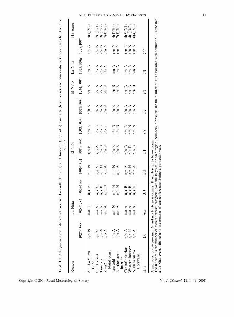
For the 1-month lead multi-tiered forecasts (Table III), the hit scores for the KwaZulu–Natal coast andthe northeastern interior are significant at the 99% level of confidence (hit score of seven), and those ofnorthern Namibia/western Botswana at the 95% level of confidence (hit score of six). Hit scores for thesouthwestern Cape, Lowveld, central interior and western interior outscore chance (hit scores larger thanthree). The skill of the 3-month lead rainfall forecasts is less than that of the 1-month lead forecasts. Thehit scores for the 3-month lead rainfall forecasts (Table III) for the Lowveld and northernNamibia/western Botswana outscore chance and are significant at the 90% level of confidence. For manyof the regions, five or more one-category misses are seen for both lead-times, partly because of the largenumber of near-normal rainfall forecasts issued for some regions, which occur as a result of theunderestimation of the strength of SST anomalies. In general, the multi-tiered approach outperforms thebaseline CCA statistical model, in some cases significantly so (cf. Tables II and III).

Drier than normal conditions frequently prevail over southern Africa during El Nino Pacific warmevents and wetter than normal conditions during La Nina cold events (Ropelewski and Halpert, 1987,1989; Mason and Jury, 1997; Rocha and Simmonds, 1997). The El Nino years of 1991/1992 and1994/1995 were particularly dry and the La Nina years of 1988/1989 and 1995/1996 particularly wet.During the La Nina event of 1988/1989, the downscaling model predicted the widespread above-normalrainfall conditions accurately over both lead-times (Table III). For the La Nina event of 1995/1996, the1-month lead rainfall forecasts were accurate, but near-normal rainfall conditions were predicted for theEl Nino event of 1991/1992 (both lead-times) and for the El Nino event of 1994/1995 (1-month lead).Forecasts of the strength of the 1991/1992 El Nino event are only about half of the observed anomaly,while the rainfall forecasts were for near-normal over the summer rainfall regions. Even with weak SSTanomalies during the 1995/96 La Nina, 1-month lead rainfall forecasts proved accurate. The 3-month leadforecasts for the event predicted near-normal rainfall over the summer rainfall regions. These forecastswere accurate for northern Namibia/western Botswana, but not for the other regions.

The skill scores of GCM-derived forecasts (Table IV) are better than those for the CCA rainfall model.In the latter case, no significant LEPS scores were achieved for any of the regions (Table II). In contrast,

Table IV. Summary of the multi-tiered model skill scores for the nine regions for a1-month (left of /) and a 3-month (right of /) lead-time

Regions A N LEPSB Hitscore

0.7/0.60.0/1.00.7/0.8Southwestern Cape 32/254/30.9/0.8 1.0/1.0 0.7/0.8South coast 2/2 −12/−12

Transkei 0.6/0.8 1.0/0.8 0.7/0.0 3/3 8/8KwaZulu–Natal coast 0.3/1.0 0.5/0.7 0.3/0.5 7/3 60*/1–12

4/104/51.0/1.00.6/0.51.0/1.0Lowveld0.0/1.0 0.4/0.5 1.0/1.0 7/4Northeastern interior 52*/−22

Central interior 0.3/0.7 0.8/0.9 1.0/1.0 4/2 19/−16Western interior 0.5/0.40.7/0.8 16/−104/41.0/1.0

0.3/0.5N Namibia/W Botswana 0.4/0.5 1.0/1.0 6/5 40/22

The false alarm ratios are shown for the different categories (A denotes above-normal, N near-normaland B below-normal).LEPS scores significant at the 95% level of confidence are marked with an asterisk.

Copyright © 2001 Royal Meteorological Society Int. J. Climatol. 21: 1–19 (2001)

MULTI-TIERED RAINFALL FORECASTS 13

Figure 3. (a) LEPS scores for retro-active forecasts for the nine regions (KZC: KwaZulu–Natal coast; NEI: northeastern interior;NWB: northern Namibia/western Botswana; SWC: southwestern Cape; CIN: central interior; WIN: western interior; TRA:Transkei; LOW: Lowveld; SCO: south coast) with a 1-month lead-time; (b) LEPS scores for variance-adjusted retro-active forecastswith a 1-month lead-time. The solid line represents the CCA model scores; the circled line multi-tiered model scores. Horizontal lines

indicate 90, 95 and 99% confidence levels

the GCM-downscaled forecasts gave higher hit scores than the CCA model for all the regions except forthe central interior. The multi-tiered method produced hit scores that outscore chance for seven of thenine regions at 1-month lead-time and for four regions at 3-month lead-time. Even for years that are notassociated with strong equatorial Pacific forcing, the GCM forecasts are associated with high numbers ofhits, for example 1992/1993 and 1996/1997. A few cases can be presented that have FAR values of zero(best possible FAR is zero and worst possible FAR is one), while high FAR values are associated mostlywith below-normal rainfall forecasts.

Comparison of CCA and multi-tiered LEPS scores for a 1-month lead (Figure 3(a)) reveals that themulti-tiered model outperforms its statistical counterpart in all regions except the western and centralinterior and the Lowveld. However, even in these regions, skill levels are only marginally worse than thoseof the CCA model. This is so despite lack of variance-adjustment (Ward and Folland, 1991) in themulti-tiered forecasts. When variance-adjustment is applied to the multi-tiered model, LEPS scoresimprove in most cases, in particular for the central interior and the Lowveld (Figure 3(b)). The forecastskill for both the multi-tiered and CCA techniques are poor for 3-month lead forecasts (Figure 4(a)).None of the LEPS scores are significant at the 90% level of confidence. Applying variance-adjustment tothe 3-month lead-time multi-tiered forecasts (Figure 4(b)) does little to improve skill. For longer leadforecasts, the CCA statistical model continues to outperform the GCM-based approach.

Downscaled categorized forecasts at a 1-month lead-time (left entries) derived from forcing the GCMduring ENSO years with observed rather than predicted SSTs are presented in Table V. Much improvedforecasts are found for the 1991/1992 season when widespread drier than normal conditions are simulatedsuccessfully. Likewise, the favourable rainfall of the 1995/1996 season is accurately predicted. Theforecasts for 1994/1995 are less statisfactory. For a 1-month lead-time, the LEPS scores from observedSSTs are not much better than those obtained from predicted SSTs (Figure 5(a) and Figure 3(a)), but asubstantial improvement in skill for 3-month lead forecasts results from the use of observed SSTs (Figure5(b) and Figure 4(a)).

Copyright © 2001 Royal Meteorological Society Int. J. Climatol. 21: 1–19 (2001)

W.A. LANDMAN ET AL.14

Figure 4. As for Figure 3, but for a 3-month lead-time

Table V. Categorized forecasts (lower case) at a 1-month lead of selected years in theretro-active period, produced from observed DJF SSTs (left of /) and forecasts producedfrom persisted August SST anomalies (right of /) and observations (upper case) for the

nine regions

1991/1992 1994/1995 1995/1996

El Nino El Nino La Nina

Southwestern Cape b/b B a/a N a/b ASouth coast b/b A n/a A a/b NTranskei b/n B n/n N a/b AKwaZulu–Natal coast b/n B n/n B a/b ALowveld b/n B n/b B n/b ANortheastern interior b/n B n/n B n/b ACentral interior b/n B n/b B a/b AWestern interior b/a B n/n N a/b AN Namibia/W Botswana b/n B n/n B n/b N

Hits 8/1 2/5 6/0

A and a refer to above-normal; n and N refer to near-normal; b and B refer to below-normal.Hits refer to the number of correct forecasts during a particular year.

One of the main problems with the multi-tiered approach is that the CCA model used to predict theSST fields underestimates the strength of major ENSO events, particularly in the early stages of anevolving ENSO event. Likewise, the SST anomalies are under-predicted at longer lead-times for the peakof the event. Persisting observed SST anomalies produces amplitudes comparable to the predictedamplitudes. In the foreseeable future, over the longer lead-times, multi-tiered rainfall forecasts frompersisted SST anomalies will, thus, produce forecasts that are at least as skilful as those using predictedanomalies. Multi-tiered forecasts derived from forcing the GCM during ENSO years with Augustpersisted SSTs were satisfactory for the 1994/1995 El Nino, but underestimated the drought of 1991/1992

Copyright © 2001 Royal Meteorological Society Int. J. Climatol. 21: 1–19 (2001)

MULTI-TIERED RAINFALL FORECASTS 15

Figure 5. LEPS scores for retro-active forecasts with (a) 1-month and (b) 3-month lead-times using observed DJF SSTs duringENSO events; (c) LEPS scores of forecasts produced from persisted August SST anomalies during ENSO events. The solid line gives

the CCA model scores; the circled line multi-tiered model scores. Confidence levels and regions are as defined in Figure 3

and the wet conditions of 1995/1996 (right entries of Table V). Persisting observed August global SSTanomalies during these ENSO events produced rainfall forecast skill scores (Figure 5(c)) that arecomparable to those of the 3-month lead forecasts using CCA-derived SST boundary conditions (Figure4(a)). LEPS scores associated with forecasts from observed SSTs during ENSO years outscore those usingpersisted SST anomalies (Figure 5(b,c)).

5. DISCUSSION

Until recently, efforts to model southern African seasonal rainfall have been mainly statistical. Somesuccess has been achieved in this manner. However, given that statistical models do not take into accountthe non-linearities associated with air–sea interactions responsible for interannual rainfall variability oversouthern Africa, and that linear SST and rainfall associations have become unstable during recentdecades, alternative means of forecasting seasonal rainfall has become an urgent necessity. In this paper,an attempt has been made to develop a physically based prediction algorithm for operational applicationto the summer rainfall of southern Africa. To do this, a baseline skill level has been established using a

Copyright © 2001 Royal Meteorological Society Int. J. Climatol. 21: 1–19 (2001)

W.A. LANDMAN ET AL.16

statistical model. The COLA GCM has been used to simulate non-linearities in the climate system and toinvestigate whether it can improve on statistical predictions. In a multi-tiered approach, the SSTs havebeen predicted statistically in a CCA model with lead-times of a few months and used as boundary forcingin the GCM. The GCM-simulated fields have been downscaled to regional level to compare skill levelswith the baseline skill and to test the utility of operational seasonal rainfall forecasts on a regional level.

Evolutionary global SSTs have been used successfully in a CCA model to predict SST anomalies of theequatorial Indian and Pacific (NIN0 O3.4) Oceans. The scheme works well retro-actively for pre-1990conditions, but predictability seems to have weakened during the 1990s. After accurate predictions of the1988/1989 La Nina event, the model underestimated the strength of the subsequent El Nino event of1991/1992 and the La Nina event of 1995/1996. Likewise loss of predictability occurred in the tropicalIndian Ocean after 1989, but appears to have improved from 1994/1995. Forecasts of the tropical IndianOcean anomalies, particularly for the later part of the austral summer rainfall season, are better thanthose predicted with persistence. On this basis the use of the SST forecasts to force the GCM appearsjustified. The NIN0 O3.4. forecast scores are close to those found using persisted SST anomalies as aforecast. Although the retro-active skill levels appear disappointing, in general the 1990s are consideredto have been a period of poor inherent predictability. Thus, the fact that positive skill was indicated forthe period, and that the cross-validated skill levels of the SST model were high, are encouraging results.

Downscaled bias-corrected GCM-produced forecasts in many regions of southern Africa aresignificantly better than the statistical predictions over lead-times of 1 and 3 months. At worst, theGCM-based forecasts are at least comparable with those of the statistical model. Forecasts for a 1-monthlead-time produced higher skill levels than those for 3-months lead-times particularly in the easternregions of the KwaZulu–Natal coast and the northeastern interior. Both multi-tiered and statisticalmodels produce poorer skill levels with longer lead-times.

A number of possibilities have been explored to improve multi-tiered forecast skill. The first was theadjustment of the forecast variance over the retro-active period, which produced somewhat increased skillscores, but only for short lead-times. The longer lead forecast skill remained unaltered and poor rainfallforecasts for three of the four ENSO events occurred because of the inability of the statistical SST forecastmodel to correctly estimate anomalies that form the boundary conditions for the GCM. The SSTamplitudes for the ENSO events were always underestimated. Given improved SST forecasts, rainfallforecast skill should improve significantly. Forcing the GCM with observed rather than predicted SSTs(i.e. perfect SST forecasts) resulted in smaller discrepancies between predicted and observed rainfall forthe ENSO seasons considered. The 3-month lead-time skill using observed SST improved substantially.However, the use of observed conditions is useful only for analysing what actually happened and not forpredicting what might happen in a future situation. When using persisted anomalies for predicting thefuture SST field, the skill did not necessarily improve when forcing the GCM with persisted August (themonth associated with 3-month lead-times) SST anomalies.

6. CONCLUSIONS

The COLA T30 GCM has been used successfully to predict seasonal rainfall over the summer rainfallregion of southern Africa. It has been found that the multi-tiered approach can be applied in anoperational environment, provided that the spatial characteristics and amplitudes of the SST forcing fieldsare described adequately. The multi-tiered scheme is able to produce skill levels that are better thanchance and to outscore the baseline skill level of a linear statistical model. With improved prediction ofSST fields, the multi-tiered scheme has the potential to improve seasonal rainfall forecasts significantly.Until that time, forecasts produced for long lead times with persisted SST anomalies must suffice.Significantly, the potential for GCM seasonal forecasting of rainfall over southern Africa is high. In thepast, statistical modelling offered the best prospects for seasonal climate forecasting; in future, GCMs willundoubtedly provide the best basis for doing so. At present, both methods are needed and are bestblended in a multi-tiered approach to offer pragmatic and cost-effective solutions to a complex problem.

Copyright © 2001 Royal Meteorological Society Int. J. Climatol. 21: 1–19 (2001)

MULTI-TIERED RAINFALL FORECASTS 17

ACKNOWLEDGEMENTS

The rainfall data used were obtained from the South African Weather Bureau and the NationalMeteorological Services of Botswana, Namibia and Lesotho. The utilization of the South AfricanWeather Bureau’s computer resources is acknowledged with gratitude. This paper was funded in part bya grant/cooperative agreement from the National Oceanic and Atmospheric Administration (NOAA). Theviews expressed herein are those of the authors and do not necessarily reflect the views of NOAA or anyof its sub-agencies.

REFERENCES

Barnett TP, Preisendorfer RW. 1987. Origins and levels of monthly and seasonal forecast skill for United States air temperaturedetermined by canonical correlation analysis. Monthly Weather Re6iew 115: 1825–1850.

Barnett TP, Bengtsson L, Arpe K, Flugel M, Graham N, Latif M, Ritchie J, Roeckner E, Schlese U, Schulzweida U, Tyree M. 1994.Forecasting global ENSO-related climate anomalies. Tellus 46A: 381–397.

Barnston AG. 1994. Linear statistical short-term climate predictive skill in the Northern Hemisphere. Journal of Climate 7:1513–1564.

Barnston AG, Ropelewski CF. 1992. Prediction of ENSO using canonical correlation analysis. Journal of Climate 5: 1316–1345.Barnston AG, Smith TM. 1996. Specification and prediction of global surface temperature and precipitation from global SST using

CCA. Journal of Climate 9: 2660–2697.Barnston AG, van den Dool HM. 1993. A degeneracy in cross-validated skill in regression-based forecasts. Journal of Climate 6:

963–977.Barnston AG, van den Dool HM, Zebiak SE, Barnett TP, Ji M, Rodenhuis DR, Cane MA, Leetmaa A, Graham NE, Ropelewski

CR, Kousky VE, O’Lenic EA, Livezey RE. 1994. Long-lead seasonal forecasts—where do we stand? Bulletin of the AmericanMeteorological Society 66: 2097–2114.

Barnston AG, Thiao W, Kumar V. 1996. Long-lead forecasts of seasonal precipitation in Africa using CCA. Weather andForecasting 11: 506–520.

Barnston AG, Glantz MH, He Y. 1999. Predictive skill of statistical and dynamical climate models in SST forecasts during the1997/98 El Nino episode and the 1998 La Nina onset. Bulletin of the American Meteorological Society 80: 217–243.

Bengtsson L, Schlese U, Roeckner E, Latif M, Barnett TP, Graham NE. 1993. A two-tiered approach to long-rang climateforecasting. Science 261: 1026–1029.

Bengtsson L, Arpe K, Roeckner E, Schulzweida U. 1996. Climate predictability experiments with a general circulation model.Climate Dynamics 12: 261–278.

Carson DJ. 1998. Seasonal forecasting. Quarterly Journal of the Royal Meteorological Society 124: 1–26.Cane MA, Eshel G, Buckland RW. 1994. Forecasting Zimbawean maize yield using eastern Pacific sea surface temperatures. Nature

370: 204–206.Chu P-S, He Y. 1994. Long-range prediction of Hawaiin winter rainfall using canonical correlation analysis. International Journal

of Climatology 14: 659–669.Cui M, von Storch H, Zorita E. 1995. Coastal sea level and the large-scale climate state. A downscaling exercise for Japanese

Islands. Tellus 47A: 132–144.D’Abreton PC, Lindesay JA. 1993. Water vapour transport over southern Africa during wet and dry early and summer months.

International Journal of Climatology 13: 151–170.D’Abreton PC, Tyson PD. 1995. Divergent and non-divergent water vapour transport over southern Africa during wet and dry

conditions. Meteorology and Atmospheric Physics 55: 47–59.D’Abreton PC, Tyson PD. 1996. Three dimensional kinematic trajectory modelling of water vapour transport over southern Africa.

Water SA 22: 297–305.Elsner JB, Schmertmann CP. 1994. Assessing forecast skill through cross-validation. Weather and Forecasting 9: 619–624.Goddard L, Graham NE. 1997. El Nino in the 1990s. Journal of Geophysical Research 102: 10423–10436.Goddard LM, Graham NE. 1999. The importance of the Indian Ocean for simulating rainfall anomalies over eastern and southern

Africa. Journal of Geophysical Research 104: 19099–19116.Graham NE, Barnett TP. 1995. ENSO and ENSO-related predictability. Part II: Northern Hemisphere 700-mb height predictions

based on a hybrid coupled ENSO model. Journal of Climate 8: 544–549.Graham NE, Michaelsen J, Barnett TP. 1987a. An investigation of the El Nino–Southern Oscillation cycle with statistical models.

1. Predictor field characteristics. Journal of Geophysical Research 92: 14251–14270.Graham NE, Michaelsen J, Barnett TP. 1987b. An investigation of the El Nino-Southern Oscillation cycle with statistical models.

2. Model results. Journal of Geophysical Research 92: 14271–14289.Hastenrath S, Greischar L, van Heerden J. 1995. Prediction of summer rainfall over South Africa. Journal of Climate 8: 1511–1518.Hoffman RN, Kalnay E. 1983. Lagged average forecasting, an alternative to Monte Carlo forecasting. Tellus 35A: 100–118.Holton JR. 1979. Numerical Prediction. An Introduction to Dynamic Meteorology (2nd edn). Academic Press: San Diego; 173–213.Hunt BG. 1997. Prospects and problems for multi-seasonal predictions: some issues arising from a study of 1992. International

Journal of Climatology 17: 137–154.Hunt BG, Zebiak SE, Cane ME. 1994. Experimental predictions of climate variability for lead times of twelve months. International

Journal of Climatology 14: 507–526.Jackson JE. 1991. A User’s Guide to Principal Components. Wiley: New York.Jolliffe IT. 1972. Discarding variables in principal component analysis. I: Artificial data. Applied Statistics 21: 160–173.

Copyright © 2001 Royal Meteorological Society Int. J. Climatol. 21: 1–19 (2001)

W.A. LANDMAN ET AL.18

Joubert AM, Hewitson BC. 1997. Simulating present and future climates of southern Africa using general circulation models.Progress in Physical Geography 21: 51–78.

Jury MR, Pathack BMR. 1991. A study of climate and weather variability over the tropical southwest Indian Ocean. Meteorologyand Atmospheric Physics 47: 37–48.

Jury MR, Mulenga HM, Mason SJ. 1999. Exploratory long-range models to estimate summer climate variability over southernAfrica. Journal of Climate 12: 1892–1899.

Karl TR, Wang W-C, Schlesinger ME, Knight RW, Portman D. 1990. A method of relating general circulation model simulatedclimate to the observed local climate. Part I: Seasonal statistics. Journal of Climate 3: 1053–1079.

Kalnay E, Kanamitsu M, Kistler R, Collins W, Deaven D, Gandin L, Iredell M, Saha S, White G, Woollen J, Zhu Y, Chelliah M,Ebisuzaki W, Higgins W, Janowiak J, Mo KC, Ropelewski C, Wang J, Leetmaa A, Reynolds R, Jenne R, Joseph D. 1996. TheNCEP/NCAR 40-year reanalysis project. Bulletin of the American Meteorological Society 77: 437–471.

Kawamura R. 1994. A rotated EOF analysis of global sea surface temperature variability with interannual and interdecadal scales.Journal of Physical Oceanography 24: 707–715.

Kirtman BP, Shukla J, Huang B, Zhu Z, Schneider EK. 1997. Multiseasonal predictions with a coupled tropical ocean–globalatmosphere system. Monthly Weather Re6iew 125: 789–808.

Landman WA, Klopper E. 1998. 15-year simulation of the December to March rainfall season of the 1980s and 1990s usingcanonical correlation analysis (CCA). Water SA 24: 281–285.

Landman WA, Mason SJ. 1999a. Operational long-lead prediction of South African rainfall using canonical correlation analysis.International Journal of Climatology 19: 1073–1090.

Landman WA, Mason SJ. 1999b. Change in the association between Indian Ocean sea-surface temperatures and summer rainfallover South Africa and Nambia. International Journal of Climatology 19: 1477–1492.

Livezey RE, Chen WY. 1983. Statistical field significance and its determination by Monte Carlo techniques. Monthly WeatherRe6iew 111: 46–59.

Makarau A, Jury MR. 1997. Predictability of Zimbabwe summer rainfall. International Journal of Climatology 17: 1421–1432.Mason SJ. 1995. Sea-surface temperature–South African rainfall associations, 1910–1989. International Journal of Climatology 15:

119–135.Mason SJ. 1998. Seasonal forecasting of South African rainfall using a non-linear discriminant analysis model. International Journal

of Climatology 18: 147–164.Mason SJ, Graham NE. 1999. Conditional probabilities, relative operating characteristics, and relative operating levels. Weather and

Forecasting 14: 713–725.Mason SJ, Joubert AM. 1997. Simulated changes in extreme rainfall over southern Africa. International Journal of Climatology 17:

291–301.Mason SJ, Jury MR. 1997. Climate variability and change over southern Africa: a reflection on underlying processes. Progress in

Physical Geography 21: 23–50.Mason SJ, Tyson PD. 2000. The occurrence and predictability of drought over southern Africa. In Drought Volume 1: A Global

Assessment, Wilhite DA (ed.). Routledge: New York; 113–134.Mason SJ, Lindesay JA, Tyson PD. 1994. Simulating drought in southern Africa using sea surface temperature variations. Water

SA 20: 15–22.Mason SJ, Joubert AM, Cosijn C, Crimp SJ. 1996. Review of seasonal forecasting techniques and their applicability of southern

Africa. Water SA 22: 203–209.Mason SJ, Goddard L, Graham NE, Yelaeva E, Sun L, Arkin PA. 1999. The IRI seasonal climate prediction system and the

1997/98 El Nino event. Bulletin of the American Meteorological Society 80: 1853–1873.Mattes M, Mason SJ. 1998. Evaluation of a seasonal forecasting procedure for Namibian rainfall. South African Journal of Science

94: 183–185.Michaelsen J. 1987. Cross-validation in statistical climate forecast models. Journal of Climate Applied Meteorology 26: 1589–1600.Nicholson SE, Entekhabi D. 1987. Rainfall variability in equatorial and southern Africa: relationships with sea surface temperatures

along the southwestern coast of Africa. Journal of Climate and Applied Meteorology 26: 561–578.Palmer TN, Anderson DLT. 1994. The prospects of seasonal forecasting—a review paper. Quarterly Journal of the Royal

Meteorological Society 120: 755–793.Philander SG. 1998. Learning from El Nino. Weather 53: 270–274.Potts JM, Folland CK, Jolliffe IT, Sexton D. 1996. Revised ‘LEPS’ scores for assessing climate model simulations and long-range

forecasts. Journal of Climate 9: 34–53.Press WH, Teukolsky SA, Vetterling WT, Flannery BP. 1992. Numerical Recipes in Fortran. The Art of Scientific Computing (2nd

edn). Cambridge University Press: Cambridge; 963 pp.Reason CJC. 1999. Interannual warm and cool events in the subtropical/mid-latitude south Indian Ocean region. Geophysical

Research Letters 26: 215–218.Reason CJC, Lutjeharms JRE. 1998. Variability of the south Indian Ocean and implications for southern African rainfall. South

African Journal of Science 94: 115–123.Reynolds RW, Smith TM. 1994. Improved global sea surface temperature analyses using optimum interpolation. Journal of Climate

7: 929–948.Rocha A, Simmonds I. 1997. Interannual variability of south-eastern African summer rainfall. Part I: relationships with air–sea

interaction processes. International Journal of Climatology 17: 235–266.Ropelewski CF, Halpert MS. 1987. Global and regional scale precipitation patterns associated with the El Nino/Southern

Oscillation. Monthly Weather Re6iew 115: 1606–1626.Ropelewski CF, Halpert MS. 1989. Precipitation patterns associated with the high index of the Southern Oscillation. Journal of

Climate 2: 268–284.Rummukainen M. 1997. Methods for statistical downscaling of GCM simulations. Swedish Meteorological and Hydrological Institute

Report Nr RMK 80. p. 29.

Copyright © 2001 Royal Meteorological Society Int. J. Climatol. 21: 1–19 (2001)

MULTI-TIERED RAINFALL FORECASTS 19

Shabbar A, Barnston AG. 1996. Skill of seasonal climate forecasts in Canada using canonical correlation analysis. Monthly WeatherRe6iew 124: 2370–2385.

Shukla J. 1998. Predictability in the midst of chaos: a scientific basis for climate forecasting. Science 282: 728–731.Smith TM, Reynolds RW, Livezey RE, Stokes DC. 1996. Reconstruction of historical sea surface temperatures using empirical

orthogonal functions. Journal of Climate 9: 1403–1420.Stockdale TN, Anderson DLT, Alves JOS, Balmaseda MA. 1998. Global seasonal rainfall forecasts using a coupled

ocean-atmosphere model. Nature 392: 370–373.Taljaard JJ. 1986. Change of rainfall distribution and circulation patterns over southern Africa in summer. Journal of Climatology

6: 579–592.Taljaard JJ. 1994. Atmospheric circulation systems, synoptic climatology and weather phenomena of South Africa. Part 1: Controls

of the weather and climate of South Africa. South African Weather Bureau Technical Paper No 27: 45.Taljaard JJ. 1995. Atmospheric circulation systems, synoptic climatology and weather phenomena of South Africa. Part 3: The

synoptic climatology of South Africa in January and July. South African Weather Bureau Technical Paper No 29: 64.Tyson PD. 1986. Climate Change and Variability in Southern Africa. Oxford University Press: Cape Town.van den Dool HM. 1987. A bias in skill in forecasts based on analogues and antilogues. Journal of Climate and Applied Meteorology

26: 1278–1281.von Storch H, Navarra AEDS. 1995. Analysis of Climate Variability. Application of Statistical Techniques. Springer–Verlag: Berlin.von Storch H, Zorita E, Cubasch U. 1993. Downscaling of global climate change estimates to regional scales: An application to

Iberian rainfall in wintertime. Journal of Climate 6: 1161–1171.Walker ND. 1990. Links between South African summer rainfall and temperature variability of the Agulhas and Benguela currents

systems. Journal of Geophysical Research 95: 3297–3319.Ward MN, Folland CK. 1991. Prediction of seasonal rainfall in the north Nordeste of Brazil using eigenvectors of sea-surface

temperature. International Journal of Climatology 11: 711–743.Ward MN, Navarra A. 1997. Pattern analysis of SST-forced variability in ensemble GCM simulations: examples over Europe and

the tropical Pacific. Journal of Climate 10: 2210–2220.Wilks DS. 1995. Statistical Methods in the Atmospheric Sciences. Academic Press: San Diego; 467.Xue Y, Shukla J. 1998. Model simulation of the influence of global SST anomalies on Sahel rainfall. Monthly Weather Re6iew 126:

2782–2792.

Copyright © 2001 Royal Meteorological Society Int. J. Climatol. 21: 1–19 (2001)