Response to reviewer 1 (JF Lemieux) - The Cryosphere

Response to reviewer 1 (JF Lemieux) Dear Jean-François, Thank you very much for your helpful comments. We will respond to them below. Review of Presentation and evaluation of the Arctic sea ice forecasting system neXtSIM-F by Williams et al. In this paper the authors present and evaluate a new sea ice forecasting system based on the neXtSIM sea ice model. They have evaluated drift, sea ice thickness and concentration against different datasets and show that the forecasts, in general, show good agreement with the observations. Being also in the business of ice-ocean predictions, I recognize the amount of work that was done by the authors to develop and evaluate this kind of forecasting system. I have, however, two major concerns about the paper. The first one is easy to address. I think the authors need to do a better literature review. We have the impression there are currently only two sea ice forecasting systems (Topaz and GOFS) in the world and that neXtSIM-F is the third one to be proposed. For example, the Danish meteorological institute, the UK Met office, ECMWF, Environment and Climate Change Canada (ECCC) all have operational sea ice forecasting systems. Note also that we (ECCC) have, a few years ago, developed a similar system as neXtSIM-F: a stand alone sea ice model coupled to a slab ocean model (with MLD and SSS initialized from a coupled ice-ocean prediction system and SST from an analysis...). It is not used anymore as it has been replaced by a coupled ice-ocean forecasting system but I think, given the similarities between the two systems, that it should be mentioned. You could then describe what is different (e.g. the ocean heat flux correction you propose...which is interesting by the way.) We agree that our discussion gives the wrong impression of the field, and are quite sorry about this. We have now scaled back our discussion to refer to the papers of Tonani et al (2015), and also the more recent one by Hunke et al (2020, https://link.springer.com/article/10.1007/s40641-020-00162-y) which also gives an idea about trends in the systems. Thanks for the reference about the ECCC stand-alone sea ice forecast RIPS that you sent - we have included it in our introduction as well. The second major concern I have is that neXtSIM-F was evaluated for only half a year. And especially, the evaluation was done during the winter months, that is at a time when there is almost no navigation in the Arctic. I would understand why you would choose this period if your system was designed specifically for the Baltic Sea or the Gulf of St-Lawrence (where there is a lot of navigation during winter). I have the impression that the authors have submitted their paper too early and that it would make more sense to show a complete seasonal cycle of the forecast scores. You mention, anyway, that neXtSIM-F will be operational in November of this year...this is coming soon. This means you will soon have the evaluation for the summer months? Then I really think you should include these.

https://link.springer.com/article/10.1007/s40641-020-00162-y

We agree that this was a major short-coming of the previous version of the paper, and have now completed evaluation for a period of 20 months. neXtSIM-F finally went operational in July 2020, and will be updated in December with the version evaluated in the present paper. This paper will be an important contribution to the field of sea ice forecasting but first the authors need to address these concerns and the minor comments given below. 1 Minor comments 1) p.5 line 19. I guess you use a turning angle for the ocean-ice stress? Please mention it. Yes, it is 25 degrees. Added to paper (section 4.2) 2) p.5 line 22. this is already mentioned above. We have simplified this section and added it to section 4.1, where the slab ocean is introduced. 3) sections 3.6-3.7. What is this the atmospheric forcing you will use once the system becomes operational? I hope it will be the same one used for the evaluation because then it does not make sense. The forcing we will use is the ECMWF forecast described in section 3.6. A line has been added to clarify this. 4) p.8 lines 7-9. You give information that is not needed. We don’t need to know that it was first coded in Matlab. Just say that the version of neXtSIM used for neXtSIM-F is described in Rampal et al. 2016 and Samake et al 2017. OK - we have removed some of the history. 5) p.8 lines 13-14. Mention that the MLD varies spatially and that this spatial field is fixed (I guess) during the 7 days of the forecast. It actually varies with time according to the ocean forecast. We have added a comment to clarify this. 6) section 4.2. Mention how you initialize the sea ice velocity. We added a sentence about this: the ice velocity and also the damage are started from zero. 7) section 4.2. What justifies the values of 0.2 and 0.8 for the initial thin and thick ice? This is a little arbitrary (necessarily so given the difficulty of determining the concentration of thin ice) but the model wasn’t too sensitive to this. 8) p.10 line 19. The first condition (i.e. ct > 0) is not needed, right? Yes you are right - we have removed it. 9) section 5.1. Clearly state how long (time period) is the free run. 10) p. 11, line 6. Typo "the no ice". Fixed. 11) Fig. 3. Explain how you calculate the concentration and uncertainty. Is it the mean over the whole domain? Then it means you have many grid cells with a concentration of zero and many with a concentration close to 1.0. This means the signal you are interested in is kind of buried because most grid cells have a forecast concentration close to the observed one...which is not surprising. We actually average over the union of the ice masks. This still leaves the pack ice, which in our case is usually close to 1, while the observations is usually about 0.9-1. So this signal is less interesting since the observations are also uncertain. The extent is actually the main signal we would like to capture, but we present the comparison of the concentration also.

How do you deal with uncertainties when the concentration is 1 or 0...it cannot be gaussian, right? This is a good question. It turns out that it was quite difficult to estimate uncertainties since we did not know the distribution of the observation errors. Therefore we removed the error shading from most of the plots. For the error plots we kept it as a rough reference level to show when our results were significantly different from the observations. Another interesting thing that came up from the uncertainty analysis was with the drift speed - adding noise to a given set of “true” drift values introduced a bias of 2\sigma^2 to <drift^2> where \sigma^2 is the variance of the drift. Hence one should be a bit careful when comparing drift speeds. 12) p. 13, lines 6-7 and Fig. 6. Is it possible the MEB rheology leads to too much convergence? (e.g. North of the CAA). Yes. It is slightly improved with BBM, but there are still issues with this near the northeast coast of Greenland and the north coast of Svalbard. This has some unfortunate follow-on effects on the summer ice extent in the Greenland Sea especially. 13) p. 13, lines 18-24. Too many numbers given. I don’t think you need to give all these values. We have reduced the number of numbers inline throughout. 14) p. 13, line 27. What do you mean by "eroded"? Please clarify. We mean that by setting a maximum threshold on the uncertainty in the ice drift we had masked the observations in some areas (mainly near the ice edge, coast, and the north pole). We now generally use a higher threshold (10 km/day) so that we can include evaluation in summer, but include a table where we use the lower threshold (1.25 km/day) for 2 winters and show it reduces our errors significantly. However some of the regions with higher errors (eg coast and MIZ) are regions where we have some problems with other variables like thickness and extent so masking them out can help for that reason too. 15) p. 13, line 33. I don’t think the ice is landfast there but it is (very) slowly drifting. Yes, you are right. 16) p. 14, line 1. remove "very respectable"...just give the number and that’s it. Fixed. 17) p. 14, line 10-14. Please clarify this paragraph. It is not clear here what are exactly the experiments (especially the sentence"...without assimilation, with assimilation of concentration and with assimilation of concentration and thickness."). We have now reduced the number of experiments to one free run and one with assimilation of concentration/extent. 18) Fig. 9. I am not surprised persistence is doing so bad here because the beginning of November is a time when there is a lot of ice growth. No wonder the model performs so well. I think it would be good to show another case for example in March. Is it always true that the model beats persistence? Is is always true that assimilation improves the quality of the forecast? Assimilation always improves the forecast concentration and extent compared to the free run (see the new figure 9). However it only beats the persistence in extent in the months Sep-Feb. We now have 4 examples (2 with positive skill (Jan, Sep) and 2 with negative skill (Mar, Jun)). 19) p. 16, lines 13-14: The captions in Fig. 10 and 11 do not match the text here about the dates.

Figs 10 and 11 have now been removed. 20) p. 18, line 1: East Siberian and Chukchi seas...not obvious to me when I look at Figs 10 and 11. These figures and the discussion have now been replaced. 21) Fig. 13 and 14 are not discussed. Are they really needed? They have in fact been replaced. 22) p. 19, lines 11-13: Please rephrase… (This referred to the evaluation against SMOS thin ice thickness.) We decided to remove evaluation against SMOS since errors were dominated by difference in extent. 23) p. 20, line 1. What drifters are we talking about here? Every day at 12:00 we place Lagrangian drifters at the grid points of the OSISAF drift product and advect them for 48h at the ice velocity. The total drift is then compared to the OSISAF drift product. We clarify this in the Data Sources section. 24) p. 25, lines 11-17. I think it could also be the thermodynamic model itself. There is clearly too much ice growth...the model might require some tuning. This should be mentioned. What about the way the thin and thick ice categories are initialized? How does it affect the overestimation of the growth? We have now removed the comparison to SMOS. 25) p. 25, line 19. What do you mean by "fragmentation"? Technically we mean damaging. We have changed this in the paper. 26) p. 25, line 23. I thought neXtSIM is using our grounding scheme for landfast ice? Would it be worth tuning the k1 parameter? We now have the opposite problem of too much fast ice in the Laptev and East Siberian sea. We are currently tuning this parameter, but for this paper we were concentrating on the main parameters of the dynamics (cohesion, Pmax, drag) 27) p. 26, lines 20-22. Is it a result you presented in this paper? Or I just don’t understand the sentence. Please clarify this. Yes it is presented. We clarify the different runs better now (eg free run v forecasts) Congratulations for your work on developing this new sea ice forecasting system. Jean-François Lemieux Thank you.

Anonymous Referee #2 Dear Reviewer 2, Thanks very much for your helpful comments. We will respond to them below.

Interactive comment on “Presentation and

evaluation of the Arctic sea ice forecasting system

neXtSIM-F” by Timothy Williams et al. Dear anonymous reviewer, thank you for your thorough review and helpful comments. We will respond to them below. In this paper the authors introduce a new sea ice forecasting system neXtSIM-F based on the neXtSIM sea ice model and present an evaluation of the model over a single season - winter 2018-19. I feel that this study will be worth publishing in The Cryosphere (although it would likely fit better in GMD than TC). However several changes will be required before this is possible.

General comments 1. It is not made clear enough what the various runs and systems are that are assessed in this study. In particular there is also no mention of the “free run” before it is evaluated in Section 5.1. Section 3 contains information on the observational datasets used in this study but there is no equivalent for the model datasets. This study needs a summary of exactly which runs and systems are being evaluated with perhaps a table. This has now been clarified in a few places (introduction, start of results section, discussion and conclusions). 2. Additionally the names neXtSIM and neXtSIM-F seem to be fairly inter-changeable in the manuscript. I guess the neXtSIM-F forecasting system uses the neXtSIM sea ice model. If so then I think the name of your forecasting system as neXtSIM-F is a bit confusing. This has now been clarified in a few places. 3. The evaluation period is only a few months and does not include the late spring/summer period when many sea ice forecasting systems report their poorest performance. This means that it is hard to put the evaluation here into context with other operational systems. The conclusions of this study would be much strengthened if the authors could perform, and evaluate, a complete annual cycle (or preferably 2).

This is a completely valid criticism and the run is now 20 months. We also have our worst performance in the summer months. 4. In general I find that there are too many figures and stats in the paper, which makes it hard to understand what the take-home message is. We have removed some figures and tables, and replaced some others, and also tried to emphasise the main take-home message more, so hopefully the new figures and tables now help understanding rather than hinder it.

Specific comments 1. In many places the language used in the paper is too informal and colloquial (i.e., in the abstract we have “. . .in our system, we obtain. . .” and on P9 we have “the observed ones”). We have tried to make the language more formal. 2. You need to be careful to distinguish between “sea ice concentration”, which ranges from 0 to 100%, and “sea ice area fraction”, which ranges from 0 to 1 throughout this manuscript. For example in Figure 4 the caption says “concentration” but the scale is +/- 0.5%. This is either a low “concentration” or a high “area fraction”. I assumed the former to start with until I noticed that the text talks about an associated reduction in extent. With changes of +/- 0.5% concentration I wouldn’t expect to see any departure to the 15% contour (extent) so is it actually “area fraction” plotted here? You are correct that it was actually area fraction - we have changed to using concentration with units of % everywhere. 3. I find the abstract to be rather technical and not very abstract. It reads a bit more like a conclusions/summary section. I would encourage the authors to make the abstract more exciting to make the paper more inviting to potential readers. We have removed the numbers from the abstract and tried to make it more inviting. 4. The introduction section (section #1) is rather disjointed. It starts with some motivation for sea ice forecasting (with background on changing climate) but then jumps straight in to say that neXtSIM-F is based on neXtSIM. It doesn’t actually say that neXtSIM(-F) is a sea ice forecasting system! It would be better to include a couple of extra lines to say that this is the case. Perhaps to say something like “Here we introduce a new sea ice forecasting system, neXtSIM-F, that is based upon the neXtSIM model. . .”. Thanks - this is a good sentence that we have used in the introduction. Hopefully introduction is now less disjointed. 5. I find the introduction to operational ocean forecasting systems in Section 2 to be, almost paradoxically, both too detailed and non-existent. I say too detailed because I am left wondering why there is such a thorough introduction provided to the GOFS system when it isn’t really used in this study? Of course, GOFS is only one of many global operational ocean-sea ice forecasting systems and you don’t mention any others apart from TOPAZ and neXtSIM. The Tonani et al. (2015) GODAE paper provides a nice reference describing the world’s operational global forecasting systems. Although several of the systems have doubtlessly moved on since 2015, this reference provides evidence for the breadth of activity in the world. Tonani, M., Balmaseda, M., Bertino, L.,

Blockley, E. W., Brassington, G., Davidson, F., Drillet, Y., Hogan, P., Kuragano, T., Lee, T., Mehra, A., Paranathara, F., Tanajura, C. A. S. and Wang, H.: Status and future of global and regional ocean prediction systems, J. Oper. Oceanogr., 8, sup2, s201-s220, doi:10.1080/1755876X.2015.1049892, 2015. We agree that our discussion gives the wrong impression of the field, and are quite sorry about this. We have now scaled back our discussion to refer to the papers of Tonani et al (2015), and also the more recent one by Hunke et al (2020, https://link.springer.com/article/10.1007/s40641-020-00162-y) which also gives an idea about trends in the systems. 7. The data sources section (#3) does not make it clear which datasets are used for assimilation and which are used for evaluation (and hence which are used for both). At the least it is important to note which datasets are independent from the assimilation. A sentence has been added to the start of each data-source subsection to make it explicit which are used in assimilation and evaluation, and which are used in evaluation only. 8. Related to the above point I find the description of the blended SSMIS+AMSR2 product somewhat confusing. Is this done purely for the evaluation? If not why can’t the DA do this blending by waiting the observations with their respective errors? We now use this only for data assimilation, but it unfortunately became quite inconvenient to use it for evaluation due to missing sections of data in the AMSR2 product particularly. We clarify this in section 2.3. 9. P3, L4: “. . .profiles from Argo floats.”. Why do you only use Argo floats (if that’s true)? Why not CTD/XBT/seals etc.? Here we were only describing what TOPAZ does. However, it also assimilates ice-tethered profiles as well. Other data like the ones you mention are available too late to assimilate in near-real-time. They are used in the TOPAZ reanalysis though (Laurent Bertino, personal communication). 10. I do not understand why a couple of weeks of CFSv2 is used in place or ECMWF. Surely you could get the replacement data from somewhere else (like ECMWF themselves for example)? If not then you should really consider the implications of using CFSv2. Specifically: is this the configuration with unrealistic ice growth caused by the fact that they turned off the stratus cloud formation to improve tropical temperatures and ENSO predictability (as described by Yang et al. 2017 and references therein)?: Yang, Q., M. Wang, J.E. Overland, W. Wang, and T.W. Collow, 2017: Impact of Model Physics on Seasonal Forecasts of Surface Air Temperature in the Arctic. Mon. Wea. Rev., 145, 773–782, https://doi.org/10.1175/MWR-D-16-0272.1 We have now been able to access those missing forecasts and have rerun the free run and the relevant forecasts without needing to plug with CFSv2. This also allows us to delete the section describing CFSv2. 11. I don’t like your “RMSE” for extent as it is exactly the Integrated Ice Edge Error (IIEE) of Goessling et al., (2016). You cite the ensemble extension of the IIEE (the SPS paper of Goessling and Jung, 2018) and say that your RMSE is like a deterministic version of that, which is misleading. It would be better to just cite the 2016 paper instead and call your metric “IIEE” instead of “RMSE”: Goessling, H. F., Tietsche, S., Day, J. J., Hawkins, E., and Jung, T.: Predictability of the Arctic sea ice edge, Geophys. Res. Lett., 43, 1642–1650, https://doi.org/10.1002/2015GL067232, 2016

https://link.springer.com/article/10.1007/s40641-020-00162-y

https://doi.org/10.1175/MWR-D-16-0272.1

Agreed - we have renamed the metric to IIEE to avoid confusion and replaced the reference with your suggested one. 12. In Figure 3 I note that the neXtSIM concentration evolution is very smooth – more so than the low resolution SSMIS data – which I didn’t expect given the resolution of the model. Can you comment on this? Is this caused by the fact that neXtSIM still uses the continuum formulation and so doesn’t resolve small scale features? For this refer to p10 “For all comparisons we average the model fields in time over an appropriate time window (in practice 1, 2 or 7 days), apply some spatial smoothing (being guided by the size of the satellite footprint), and interpolate onto the observation grid.” When comparing to OSISAF SSMIS we average over 1 day and apply some spatial smoothing, as SSMIS is too coarse to resolve the cracks/leads etc. However, we have applied a bit less smoothing this time around (see fig 11). 13. I note with interest that MOSAiC forecasting is mentioned as a motivation for improving sea ice forecasts. There is an international project (SIDFEx) currently coor- dinating operational sea ice drift forecasts specifically to provide guidance to the Po- larstern/MOSAiC. Presently the list of models includes TOPAZ but not neXtSIM. Are there any plans to contribute neXtSIM drift forecasts to SIDFEx? This might be an interesting way to show the skill of neXtSIM in this regard. This would be interesting if it were still possible, and is worth discussing with the leaders of that project. 14. Some of the figures (e.g., Figs 10&11) suggest that the data assimilation is having a rather modest impact on the forecasts compared with many of the operational systems that I have seen in the past. Can you comment as to why that might be? After 2 quite major updates to our sea ice rheology we had to change the assimilation scheme quite a lot. It is now quite conservative in that we mostly leave the model alone, except where the ice mask is incorrect. There is a noticeable improvement in the IIEE for the first days after doing this, although the improvement is diminishing with lead time. 15. On page 20 it is mentioned that the “RMSE for drifters placed on the first day. . .” but this is the 1st time in the manuscript that drifters are mentioned. Can you explain this a bit more please? Every day at 12:00 we place drifters at the grid points of the OSISAF drift product and advect them for 48h at the ice velocity. The total drift is then compared to the OSISAF drift product.

Figures As mentioned above I feel that there are too many figures in this manuscript. In particular in Figs 11 & 12 there are 12 panels and each row looks virtually identical. Apart from telling me that the assimilation is having a rather modest impact, I don’t understand what I’m supposed to do with all this information. Additionally the next similar set of figures, Figs 13-14, don’t even seem to be discussed in the text at all. So are they necessary? We have revised the figures substantially now (eg figs 11-12 and figs 13-14 have been replaced.) Many of the figure captions are too brief and should be improved. I believe that the

Copernicus journal guidelines are that figures should be able to work stand-alone from the text, for which a bit more information is required. We have now checked the captions contain enough information. I find that the x-axis date tick-marks provided on the time-series plots (Figs 3, 5, 7, 12 – less so for Fig 9) are not very useful. With such a short run period it would be better to include more dates. At the very least there minor tick marks should be used to show each day (or 5-days or something). It would also be good to specify this in the figure caption perhaps. We have tried to add enough major and minor tick marks to the time series plots, although the run is a lot longer now. Figure 1 is a bit confusing because I am left wondering whether different time-scales are involved here. Is this a daily schematic or does it depict the whole run? For example the 2 top boxes (initialization) are surely not done each day are they? If not then it should be made clear what is done each day and what isn’t – either in the caption or the figure (or both). Perhaps the initialization boxes could be enclosed in a dotted box or something? These were snapshots, but they have actually been removed to reduce the number of figures. I suggest you should also re-think your use of red-blue colour maps for sea ice concentration. I have seen people use red for less ice (as it’s hotter) and blue for more ice (colder) in the past as well as the other way around. It might be better to avoid the use of a hot<->cold colour-map therefore. We tried out some other colormaps but decided to keep this one for lack of a better alternative.

Technical corrections The 1st instance of “SSMIS” is correct but thereafter it has been changed to “SMMIS”. Fixed Also “first day (4th day)” appears in many places, which is not very consistent P2, L26: CMEMS should be “Copernicus Marine Environment Monitoring Service” Fixed P2, L29: “. . .the version 4.1 of the. . .” – suggest to remove the 1st instance of “the” Here Fixed P2, L30: The reference for CICE v4.1 is Hunke and Lipscomb (2010): Hunke, E. C. and Lipscomb, W. H.: CICE: the Los Alamos sea ice model. Documentation and software users manual, Version 4.1 (LA-CC-06-012), T-3 Fluid Dynamics Group, Los Alamos National Laboratory, Los Alamos, 2010 Thanks - added this P3, L30: “As specified by the validation reports above. . .” should be “As specified by the validation reports cited above. . .” Changed to this. P4, L5: “metrics” should be “metric” Fixed

P4, L6: is extent “above 15%” or “at least 15%”? I thought the latter. In our evaluation script it was >15% - in practice I would expect either to give the same result P4, L13: “. . .can be obtained for 48 hours. . .” sounds like only 48 hours of data. Do you mean this or do you mean the data is available 48-hours behind real-time? In the OSISAF product, the drift is estimated daily from 12:00 on the start date until 48 hours later. In practice this does imply a time lag of at least 48h. “From October to April, however, daily 48-hour ice drift vectors can be obtained at a spatial resolution of 62.5 km.” P5, L5: calculating volume for each model & obs based on thickness like this will involve different areas of ice won’t it? Yes. In the end we decided to remove the SMOS comparison as errors were greatly affected by errors in extent (which we struggled with). P5, L26: “Modelling” is spelt incorrectly as “Modeling” in the NEMO acronym Fixed P5, L31: “. . .if the temperature is below 0C”. Which temperature – surface skin temperature, or near-surface atmosphere temperature (T2M)? Please be more specific. It is T2M: we have added a clarification to the paper. P10, L29: “of these variables” is not adding to this sentence and should be removed Removed P11, L6: “. . .predicts the no ice. . .”. Please remove the “the”. Fixed P11, L11: “averages values” should be “average values” Fixed P11, L19: “underestimation in the Bering Sea”. I presume that you mean the Chukchi Sea here because the Bering Sea is outside your model domain? P13, L33-4: “land-fast“ should be “land-fast ice”? Fixed P13, L35: (as above) I suspect that “Bering Sea” should be “Chukchi Sea” here That is correct, although with the change of simulation length the figures and discussion relating to the free run are quite changed and this sentence has been removed. P14, L9: the title “Evaluation of forecasts with assimilation” is confusing because I doubt that you are actually doing assimilation in your forecasts are you? Perhaps this should be changed to something more like “Forecasts performed from analysed ice conditions”? We are doing a kind of assimilation known as “data insertion” (modifying the initial conditions of the forecast) combined with “nudging” (through the compensating heat flux) P16, L9: Do you mean “significantly” here in the scientific sense of the word? If so include a p-value, if not I suggest changing to “considerably”. Changed to ‘considerably’ P18, Fig 9 caption: “(blue)”, “(orange)”, and “(red)” are provided but not “(green)” This figure has now been removed. P21, Fig 12 caption: “error bars” should be “shading” We have removed references to error bars since we use shading. P26, L7: “limited resources” suggests a deficiency in resource. You should change to “minimal resources” if you wish to suggest that the model is cheap to run. We decided to remove this discussion.

P26, L20-21: “. . .forecasts used saved atmospheric and ocean forecasts as forcing. . .”. What does this mean? This is mainly an issue of forecasts vs hindcast winds which we have clarified in a few places (introduction, start of results section, discussion and conclusions)

Presentation and evaluation of the Arctic sea ice forecasting systemneXtSIM-FTimothy Williams1, Anton Korosov1, Pierre Rampal2,1, and Einar Ólason1

1Nansen Environmental and Remote Sensing Center, Thormøhlensgate 47, 5006 Bergen, Norway and the Bjerknes Center forClimate Research, Bergen, Norway2Université Grenoble Alpes/CNRS/IRD/G-INP, Institut Géophysique de l’Environnement, Grenoble, France

Correspondence: Timothy Williams ([email protected])

Abstract. The neXtSIM-F forecast:::::::::forecasting

:system consists of a stand-alone sea ice model, neXtSIM, forced by the TOPAZ

ocean forecast and the ECMWF atmospheric forecast, combined with daily data assimilation::of

:::sea

:::ice

::::::::::::concentration.

::It

::::uses

::the

:::::novel

::::::Brittle

::::::::::::::::Bingham-Maxwell

::::::(BBM)

:::sea

:::ice

::::::::rheology,

:::::::making

::it

:::the

:::first

:::::::forecast

::::::based

::on

::a

:::::::::continuum

:::::model

::::not

::to

:::use

:::the

::::::::::viscoplastic

::::(VP)

::::::::rheology. It was tested for the northern winter of

::in

:::the

:::::Arctic

:::for

:::the

::::time

::::::period

:::::::::November 2018 –

2019 with different data being assimilated:::June

:::::2020 and was found to perform well

:,:::::::although

:::::there

:::are

:::::some

:::::::::::shortcomings.5

Despite drift not being assimilated in our system, we obtain quite good agreement between observations, comparing well to

more sophisticated coupled ice-ocean forecast systems::the

::::sea

::ice

::::drift

::is:::::good

:::::::::throughout

:::the

:::::year,

:::::being

::::::::relatively

::::::::unbiased,

::::even

:::for

:::::longer

::::lead

:::::times

::::like

:5::::days. The RMSE in drift speed is around 3 km/day

:::::speed

:::and

:::the

::::total

::::::RMSE

:::are

::::also

:::::good

for the first three days, climbing to about 4 km/day for the next day or two; computing the RMSE in the total drift adds about

1 km/day to the error in speed. The drift bias remains close to zero over the whole period from Nov 2018 – Apr 2019.:3::or

:::so10

::::days,

::::::::although

:::they

::::both

::::::::increase

::::::steadily

::::with

::::lead

::::time.

::::The

::::::::thickness

::::::::::distribution

:is::::::::relatively

:::::good,

::::::::although

::::there

:::are

:::::some

::::::regions

:::that

::::::::::experience

::::::::excessive

:::::::::thickening

::::with

:::::::negative

::::::::::implications

:::for

:::the

:::::::::::summer-time

:::sea

:::ice

::::::extent,

::::::::::particularly

::in

:::the

::::::::Greenland

::::Sea.

:

The neXtSIM-F forecast system assimilates OSISAF:::::::::forecasting

::::::system

:::::::::assimilates

::::::::OSI-SAF

:sea ice concentration products

(both SSMI and AMSR2) and SMOS sea ice thickness by modifying the initial conditions daily and adding a compensating15

heat flux to prevent removed ice growing back too quickly. This:::The

::::::::::assimilation

:greatly improved the agreement of these

quantities with observations for the first 3 – 4 days of the forecast::sea

:::ice

:::::extent

:::for

:::the

:::::::forecast

:::::::duration.

1 Introduction

Arctic sea ice has been in great decline in the last number of years (Meier, 2017). Perovich et al. (2018) report that in 2018, the

summer extent was the sixth lowest and the winter extent was the second lowest in the satellite record (1979–2018). Moreover,20

surface air temperatures in the Arctic continued to warm at twice the rate relative to the rest of the globe, and Arctic air

temperatures for the past five years (2014-18) have exceeded all previous records since 1900 (Overland et al., 2018), which

will also contribute to future sea ice decline if it continues.

1

With less sea ice comes an increase in summertime accessibility for shipping. Azzara et al. (2015) considered a range

of different scenarios and projected an increase in the number of vessels operating in the Bering Strait and the U.S. Arctic

of between 100 and 500%. The International Maritime Organization has also recognized that shipping would increase and

adopted an International Code for Ships Operating in Polar Waters (Polar Code)1 on 1 January 2017. This polar code addresses

the increased safety and pollution risks of operating in the Arctic. A recent example of the risks and comcomitant::::::::::concomitant

costs of accidents in the Arctic is the rescue of the fishing vessel Northguider, which ran aground between Spitzbergen and5

Nordaustlandet (Svalbard) after getting into trouble with sea ice. The crew had to be rescued by the Norwegian Coast Guard

icebreaker K.V. Svalbard, who then had to drain 300kL:::300

::kl of diesel from the damaged vessel.2

Thus sea ice forecasting is becoming increasingly important. As well as search and rescue/accident prevention, other appli-

cations are optimized ship (icebreaker) routing based on forecasts (Kaleschke et al., 2016) and support of research activities

– e.g. Schweiger and Zhang (2015) give an example of scheduling of high-resolution SAR images in order to follow the drift10

of some ice-mass balance (IMB) buoys by using the PIOMAS/MIZMAS forecast from the University of Washington. The

planned year-long drift of the Polarstern from September 2019 (part of the MOSAIC project) will also rely:::also

:::::relied

:heavily

on sea ice and weather forecasts.

The sea iceforecast system:::::::::::::::::::Tonani et al. (2015) give

::a

::::good

::::::::overview

:::of

:::the

::::2015

::::::status

::of

::::::::::operational

::::::::::forecasting,

:::::while

:::::::::::::::Hunke et al. (2020,

::::::::Table 1)

::::give

:a:::::::::::::

comprehensive:::list

:::of

:::::::::modelling

:::::::systems

::::that

::::::include

::::sea

:::ice,

:::::most

::of

::::::which

:::are

:::::used15

::in

:::::::national

:::::::::forecasting

::::::::::capacities.

::::They

:::::vary

::in

:::::::::resolution,

::in::::::::::

complexity:::::(with

:::::::regards

::to

:::the

::::::::modelled

:::::::::processes

::::and

:::the

:::::::coupling

:::::::between

:::::these

:::::::::processes)

::::and

::in::::

the::::data


::::::::schemes

:::that

::::are

:::::used.

:::We

::::note

::::::::however

:::that

:::::they

::do

::::not

::::vary

::in

::::their

:::::::::numerical

:::::::::framework

:::::(e.g.

:::::::Eulerian

:::::::::advection

:::::::schemes

::in:::

all::::::::systems)

:::nor

:::in

:::the

::::::::::rheological

:::::::::framework

::::that

:::they

::::use

:::for

::::::sea-ice

:::::(e.g..

::::::::::::::viscous-plastic).

::In

:::this

:::::::review,

:::the

:::::::authors

:::::claim

:::that

:::the

:::::trend

::is:::::::towards

::::::::::::fully-coupled

:::::::systems

:at:::::

high:::::::::resolution.

:::For

::::::::example,

:::the

::::::::ECMWF

:::::::forecast

:::::::coupled

:::ice

:::and

:::::ocean

:::::::models

::to

::::their

:::::::::::atmospheric

:::::model

::in::::::::

between20

::the

::::two

::::::papers

::::(this

::::::system

::::went

::::::::operation

::in:::::June

:::::2018)

::at

:a:::::::::resolution

::of

::::0.1◦.

::::::::::neXtSIM-F

::::uses

:::this

:::::latest

::::::::ECMWF

:::::::product

:::::::::::::::::::::::::::::::::::::::::::::::::::(IFS: integrated forecast system: Owens and Hewson, 2018) to

::::::provide

:::::::forecast

::::::::::atmospheric

:::::::forcing,

:::::along

::::with

:::::ocean

::::::forcing

::::from

:::::::TOPAZ

::::::::::::::::Sakov et al. (2012).

:::::::Another

::::::relevant

::::::::example

::is

:::the

::::::::::replacement

::of

:::::RIPS3

:::::::::::::::::::::(Lemieux et al., 2016a) by

:::::::RIOPS4

:in:::::2016,

::::::having

:::::::NEMO

:::::::coupled

::to

:::the

::::::system,

:::as

::::well

::as

::::::having

:::::other

::::::::processes

::::like

:::::tides

::::::added.

::::Like

::::::::::neXtSIM-F,

:::::RIPS

::::used

::a::::::::::stand-alone

:::sea

:::ice

::::::model25

:::::based

::on

:::the

:::::CICE

:::sea

:::ice

::::::model

:::::which

:::::used

:::::::3DVAR


::of

::::::::OSI-SAF

:::::SSMI

::::and

:::::::AMSR2

::::::::::::concentration,

::as

::::well

:::as

::ice

::::::charts

::::from

:::the

::::::::Canadian

:::Ice

:::::::Service.

::In

:::this

::::::paper,

:::we

::::::::introduce

:a::::

new::::sea

::ice

::::::::::forecasting

:::::::system, neXtSIM-F,

::::::which is based on a stand-alone version of the

sea ice model neXtSIM (Rampal et al., 2016b; ?). The dynamical core of this modelis based on the Maxwell-Elasto-Brittle

(MEB) rheologyas developed for sea ice and originally presented in Dansereau et al. (2016), which showed its capabilities at30

1http://www.imo.org/en/MediaCentre/HotTopics/polar/Pages/default.aspx2https://www.highnorthnews.com/en/svalbard-preparing-extreme-pumping-operation-using-small-boats3::::::Regional

::Ice

:::::::Prediction

::::::Service:

::::::operated

::by

::::ECCC

:::::::::(Environment

:::and

:::::Climate

::::::Change

::::::Canada)

:::from

::::2013

:to::::2016.

4::::::Regional

:::Ice

:::::Ocean

::::::::Prediction

:::::::Service:

::::::operated

:::by

::::::ECCC.

::::See

:https://eccc-msc.github.io/open-data/msc-data/nwp_riops/readme_riops_en/

#technical-documentation.

2

https://www.highnorthnews.com/en/svalbard-preparing-extreme-pumping-operation-using-small-boats

https://eccc-msc.github.io/open-data/msc-data/nwp_riops/readme_riops_en/#technical-documentation

https://eccc-msc.github.io/open-data/msc-data/nwp_riops/readme_riops_en/#technical-documentation

reproducing the main spatial characteristics of sea ice mechanics and deformation : strain localization and scaling (Marsan et al., 2004; Rampal et al., 2008; Stern and Lindsay, 2009).

With the implementation of this rheology in neXtSIM (along with accompanying thermodynamics and general model infrastructure: ?),

MEB was able to be assessed:::::::::::::::::::::::(Rampal et al., 2016a, 2019).

::::::::neXtSIM

::is

:a::::::::::Lagrangian

::::finite

:::::::element

::::::model,

:::and

:::we

:::are

:::::::running

:it::::with

::a:::::::nominal

:::::::triangle

:::side

::::::length

::of

::::::10 km,

::::with

::a:::::::distance

::::from

::::one

::::point

:::of

:a:::::::triangle

::to

:::the

:::::::opposite

:::::edge

:::::being

:::::about

::::::7.5 km.

::::The

:::::name

:::::::::neXtSIM-F

:::::refers

:::to

:::the

:::::entire

::::::::platform,

::::::::including

::::data

::::::::::input/output

::::and

:::::::::::assimilation,

:::::model

:::::::::::initialisation

:::and

:::::::::simulation,

::::::export,

:::::::::::visualisation

:::and

:::::::::evaluation

::of

::::::results

::::(see

::::::Section

:::3).

::::Due

::to

:::the

::::::::relatively

:::::recent

::::::arrival

::of

:::the

:::sea

:::ice5

::::::model,

::::::::::neXtSIM-F

::is:::::::simpler

::::than

::::most

:::::other

:::::::::platforms,

::::both

::in

:::::terms

:::of


:::::::scheme

::::(data

::::::::insertion

::::with

::::::::nudging)

:::and

:::::model

::::::::::components

::::::::::(uncoupled

::to

:::::ocean

::or

:::::::::::atmosphere).

::::(See

:::::::Section

:5:::for

:::::::planned

:::::::::::::improvements.)

::::::::However,

:it::is:::the

::::first


::::::system

:::::based

::on

::a:::::model

::::with

::::::brittle

:::sea

:::ice

:::::::rheology

::::::instead

:::of

::the

:::::::::traditional


:::::(VP)

::::::::rheology.

:It::is

::::also

:::the

::::first

::::::system

:::::being

:::::based

::on

::a:::::::::Lagrangian

:::::::::(adaptive)

:::::::::deforming

::::grid,

::as

::::::::opposed

::to

:::the

::::other

:::::ones

:::::being

:::::based

::on

:::the

:::::::standard

:::::::Eulerian

::::::(fixed)

:::::grids.

:10

:::::::::neXtSIM-F

::::::entered

::::into

:::::::::operations

::as

:::part

::of

:::the

::::::::::Copernicus

::::::Marine

:::and

::::::::::::Environmental

::::::::::Monitoring

:::::::Services

:::::::::(CMEMS)

::on

::7

:::July

:::::2020.

::It

::::was

:::::::equipped

::::with

::::::::neXtSIM

::::v1.0

:::::based

:::on

:::the

:::::::::::::::::::Maxwell-Elasto-Brittle

::::::(MEB)

::::::::rheology

::::::::::::::::::::(Dansereau et al., 2016),

:::::which

:::had

:::::been

:::::shown

:::to

::::::::reproduce

::::::Arctic

:::sea

:::ice

::::drift

:::and

:::::::::::deformation

:::::::::particularly

::::well

::::::::::::::::::::::::Rampal et al. (2016a, 2019).

:::::MEB

:::::::consisted

:::of

::an

::::::elastic

::::::spring

::in

:::::series

::::with

::a:::::::dashpot,

::::::::together

::::with

:::two

:::::main

::::::::::::modifications

::to

:::::::improve

::::::::::localisation

::::and

::to

::::::prevent

::::::::excessive

:::::::::::convergence:

:::the

:::::::damage

::::value

::::was

::::only

::::used

::to

::::::modify

:::the

:::::stress

:::::when

::it

:::::::exceeded

::a::::::::threshold

::of

::::0.95,

::::and15

:a::::kind

::of


:::::stress

::::term

::::was

:::::added

:::::which

::::only

::::::played

:a::::role

:::::when

:::the

::ice

::::was

::::very

::::::::damaged

:::(see

:::::::::Appendix

::::A1).

::::This

:::::::improves

:::the

:::::::::thickness

::::field

::::::::somewhat

:over longer simulations , and it was found that it could also reproduce the observed

temporal deformation scalings, in addition to the spatial ones. In particular, the results show strong multifractality::::(1 –2

::::::years;

::::::::::::::::::Rampal et al. (2019)),

:::but

:::not

::::quite

:::::::enough

::for

::::::longer

::::than

::::that.

::In

:::::::::September

::::2020

:::the

::::core

::of

:::the


:::::::platform

::::was

:::::::replaced

::::with

:a::::new

::::::model:

:::::::neXtSIM

::::v2.0

:::::based

:::on

:a::::::::::preliminary20

::::::version

::of

:::the

:::::novel

:::::::::::::::::::::Brittle-Bingham-Maxwell

::::::(BBM)

:::sea

:::ice

:::::::rheology

::::::::::::::::::::(Ólason et al., in prep.).

:::The

::::new

::::::version

::of

::::::::::neXtSIM-F

:::::enters

:::into

:::::::::operations

::in

:::::::::December

:::::2020.

::::BBM

::::::::consists

::of

:::an

::::::elastic

::::::spring

::in

:::::series

:::::with

::a

:::::::::composite

:::::::element

::::that

:::::::contains

::a:::::::dashpot

::::and

:a::::::::

frictional:::::::

sliding

::::::element

:::in

::::::parallel


::::(For

::a::::::::summary

:::of

:::the

:::::BBM

:::::::::equations,

:::see

:::::::::Appendix

:::::A2.)

:::The

:::::::BBM’s

:::::main

:::::::physical

::::::::::achievement

::::has

::::been

::to

:::::::stabilise

:::the

:::::::::thickness

::for

::::::::::::decadal-scale

::::::::::simulations;

::::::::::::::computationally

::it

::is

:::also

:::::5 – 6

:::::times25

:::::faster,

:::::since

:it::

is::::

able:::

to::be

::::::solved

:::::::::explicitly,

:::::unlike

::::our

::::::version

:::of

:::the

:::::MEB.

::It::::also

::::kept

:::the

::::::::::::improvements

:::in

:::the

:::::::model’s

:::::::::::representation

:::of

:::the

:::::main

::::::spatial

:::and

::::::::temporal

:::::::::::::characteristics

::of

::::::::observed

:::::::::::deformation

:::that

:::::were

::::::gained

:::by

::::::MEB:

:::::strain

:::::::::localization

::::and

::::::scaling

:::::::::::::::::::::::::::::::::::::::::::::::::::::::(Marsan et al., 2004; Rampal et al., 2008; Stern and Lindsay, 2009),

::::::::::::multifractality

::::and

:::::::::::intermittency

::in

::::time

:::::::::::::::::(Rampal et al., 2019), meaning that higher deformations are more localised in space and more intermittent in time than

smaller ones. These properties have strong implications for things like distribution and size of lead openings and how long they30

will stay open, which will in turn have strong impacts on:::::::controls the heat and salt fluxes across the ocean–ice–atmosphere

coupled system. Perhaps more::::More

:pertinently in a forecast context, they also are

::are

::::also highly relevant for navigation.

The paper begins by summarising the current status of sea ice forecasting in the Arctic, and then we assess the dynamical

and thermodynamical behaviour of:::The

:::::paper

::is

::::::::organised

::as

:::::::follows:

:::we

:::::begin

:::by

::::::::::introducing

:::the

:::data

::::and

:::::::methods

::::that

:::we

3

:::use

::::::::::throughout,

:::and

::::then

:::::::evaluate

:the neXtSIM modelin

:’s:::::::general

::::::::::performance

:::for

:a free run over the winter of 2018–2019.35

This is followed by a demonstration of::::from

:::::::::November

::::2018

:::to

::::June

:::::2020

::in

:::::terms

:::of

:::::::::::::::::concentration/extent,

::::::::thickness

::::and

::::drift.

::::This

::::free

:::run

::::uses

:::::::hindcast

::::::forcing

:::::fields.

::::We

:::then

:::::::evaluate

:the neXtSIM-F forecast system

:::::::platform

:for the same winter,

particularly concentrating on the benefits of two different assimilation methods: one assimilating OSISAF and AMSR2 sea

ice concentration , and a second assimilating SMOS ice thickness in regions where sea ice is relatively thin, i.e. lower than

0.5 m::::::period,

:::::when

:::we

::::::::assimilate

::::::::::::concentration

:::but

:::use

:::::::forecast

::::::forcing

:::::fields.5

2 Sea ice forecasting status::::Data

:::::::sources

2.1:::::::

Forecast:::::ocean

:::::::forcing

::::from

:::::::::TOPAZ4

The official European forecast for the Arctic is developed and run by the CMEMS (Copernicus Marine and Environmental

Monitoring Service) ARC-MFC (Arctic Marine Forecasting Centre)5. This uses the TOPAZ system (Simonsen et al., 2018;

Sakov et al., 2012), which uses version 2.2.37 of the Hybrid Coordinate Ocean Model (HYCOM) (Bleck, 2002). In the current10

version (4) of TOPAZ, HYCOM is coupled to a sea ice model derived from the version 4.1 of the Community Ice CodE

(CICE)::::::::::::::::::::::(CICE: Hunke et al., 2010); ice thermodynamics are described in Drange and Simonsen (1996), while the dynamics

are based on the visco-plastic (VP) sea ice rheology (implemented with the elastic-viscous-plastic (EVP) solver of Hunke

and Dukowicz, 1997). The model’s native grid covers the Arctic and North Atlantic Oceans and has a horizontal resolution

of between 11 and 16 km. TOPAZ4 uses the Ensemble Kalman filter method (EnKF; Sakov and Oke, 2008) to assimilate15

remotely sensed sea level anomalies, sea surface temperature, sea ice concentration, sea ice thickness and Lagrangian sea ice

velocities (the latter two in winter only), as well as temperature and salinity profiles from Argo floats:::and

::::::::::ice-tethered

:::::::profilers.

Data assimilation is performed weekly. The most recent validation report (Melsom et al., 2018), reports a bias in drift of about

2 km/day, with an RMSE of about 5–8

::To

:::::force

::::::::neXtSIM,

:::we

:::use

:::the

::::::::following

::::::::variables

::::from

::::::::TOPAZ:

::the

:::::::::::near-surface

:::(30 km/day, and a RMSE in concentration20

of about 0.18–0.20. The ice edge error ranged from about 30–100km (50::m)

:::::ocean

::::::::velocity,

:::the

:::::mixed

:::::layer

:::::depth

::::::(MLD),

::::and

::the

::::sea

::::::surface

::(3 km on average).

::m)

::::::::::temperature

:::and

:::::::salinity

::::(SST

::::and

::::SSS,

:::::::::::respectively).

:::We

::::give

:::::more

::::::details

::of

::::how

::::they

::are

:::::used

::in

::::::Section

:::3.1

::::::below.

The U.S. Naval Research Laboratory runs the Global Ocean Forecast System (Metzger et al., 2017, GOFS 3.1,) which uses

HYCOM 2.2.99 coupled to CICE (Community Ice CodE) on a global grid with 1/12◦ resolution (about 9 km). The assimilation25

package, NCODA (Navy Coupled Ocean Data Assimilation)

2.2:::::::

Forecast:::::::::::atmospheric

::::::forcing

:::::from

::::::::ECMWF

:::For

:::our

:::::::forecast

:::::::::::::demonstration,

:::we

::::use

:::the

:::::latest

:::::::version

::::::(Cycle

:::::45r1)

::of::::

the:::::::::Integrated

:::::::Forecast

:::::::System

:::::from

::::::::ECMWF

::::::::::::::::::::::::::::(IFS: Owens and Hewson, 2018) to

:::::::provide


::::::forcing

:::::fields

::to

::::::::neXtSIM.

::It

::::::consists

::of

:::an


:::::model

:::::::coupled

5Three institutes contribute to the ARC-MFC: the Nansen Environmental and Remote Sensing Center, the Norwegian Meteorological Institute and the

Norwegian Institute for Marine Research.

4

::to

::the

:::::::NEMO

:::3.4

:::::ocean

:::::model

::::::::(Nucleus

::for

::::::::European

:::::::::Modelling

::of

:::the

::::::Ocean), uses the 3DVar method (Parrish and Derber, 1992) to30

assimilate available satellite altimeter observations, satellite and in-situ sea surface temperature as well as in-situ vertical

temperature and salinity profiles from XBTs, Argo floats and moored buoys. Surface information is projected downward

into the water column using Improved Synthetic Ocean Profiles (Helber et al., 2013). In addition, a blend of ice products

are assimilated: concentration from AMSR2 (Advanced Microwave Scanning Radiometer 2: Melsheimer, 2019),::the

::::::LIM2

:::::::::::::::(Louvain-la-neuve

:::Sea

:::Ice

:::::::Model)

:::sea

:::ice

::::::model,

:::the

::::::::ECWAM

:::::::::(ECMWF

::::::WAve

::::::Model)

:::::wave

::::::model,

:and extent from IMS5

(Interactive Multisensor Snow and Ice Mapping System: Helfrich et al., 2007) and MASIE (Multisensor Analyzed Sea Ice Extent: Fetterer et al., 2010).

Metzger et al. (2017) report an RMS drift speed error of about 5–8 km/day in the Arctic. This is similar to TOPAZ, although

different drift products are used for the validation (IABP buoy trajectories, instead of:a::::land

::::::surface

::::::model

:::::::::::(HTESSEL).

:::Its

:::::spatial

:::::::::resolution

::is

::::0.1◦.

:::We

:::use

:::the

:::::10-m

::::wind

:::::::velocity,

:the OSISAF high resolution ice drift)and Melsom et al. (2018) use the vector difference in10

their RMSE definition (which will be higher than the RMS difference between the speeds). GOFS 3.1 also showed an ice edge

error of about 20-50 km (growing with forecast lead time:::2-m

:::air

:::and

::::dew

:::::point

::::::::::temperatures

::::(the

::::latter

::is::::used

::to:::::::::determine

:::the

::::::specific

::::::::humidity

::of

:::air

::for

:::the

:::::latent

::::heat

::::flux

::::::::::calculation),

:::the

:::::mean

:::sea

::::level

::::::::pressure,

:::the

::::long-

::::and

:::::::::short-wave

:::::::::::downwelling

::::::::radiation,

:::and

:::the

::::total

:::::::::::precipitation

::::(this

:::::::becomes

:::::snow

::if

::the

::::2-m

:::air

::::::::::temperature

::is

:::::below

::::0◦C).

3 Data sources15

2.1 Sea ice concentration::::::::products from OSISAF

::::::::OSI-SAF

The Ocean and Sea Ice Satellite Application Facility (OSISAF):::::::OSI-SAF

:provides estimates of sea ice concentration derived

from the Special Sensor Microwave Imager Sounder (SSMIS) radiometer (Tonboe et al., 2016; Tonboe and Lavelle, 2016;

Lavelle et al., 2017) and from AMSR2 (Lavelle et al., 2016a, b; Tonboe and Lavelle, 2015). The SMMIS:::::SSMIS

:algorithm

uses the 19 GHz frequency (vertically polarized, footprint size about 56 km) and the 37 GHz frequency (both vertically and20

horizontally polarized, footprint size about 33 km). The AMSR2 algorithm uses three frequencies: 18.7, 36.5 and 89 GHz

(also in vertical and horizontal polarizations) with footprints from 22 to 5 km). The AMSR2 data are presented on a 10-km

grid, and we chose this product over the higher resolution (3.25 km) ASI product as we found it less noisy near the ice edge.

These products are available daily within 12 hours after acquisition and processing so it is possible to assimilate this data

in operational forecasts.::::::::However,

:::the

:::file

:::for

:::the

:::day

::::::before

:::the

:::::::bulletin

::::date

:::(the

::::day

:::the

::::::model

::is

:::run)

:::::::doesn’t

:::::arrive

:::::early25

::::::enough

::to

::be

::::::::::assimilated

::in

:::our

::::daily

::::run,

:::::which

::is::::::::launched

::at

:::::03:00

:::::::::(European

::::::western

::::::time).

::::::::Therefore,

:::we

:::use

:::the

:::file

:::::from

:::two

::::days

::::::before

:::the

::::::bulletin

:::::date.

As specified in the validation reports above the SMMIS::::cited

:::::above

:::the

::::::SSMIS

:has lower resolution ice concentration but

has the advantage of higher accuracy, while the AMSR2 algorithm has higher resolution but also higher uncertainties. In order

to combine the advantages of these products we generated a blended product that was used both for assimilation and evaluation30

of:::::during

:the forecasts. Blending was performed with a weighted average of the two products (using the errors in the products

5

to calculate the weights):

CB =CLσ

−2L +CHσ

−2H

σ−2H +σ−2L(1)

where C denotes sea ice concentration, σ denotes the concentration uncertainty, index H denotes high resolution (AMSR2)

and L - low resolution (SMMIS::::::SSMIS).

Sea ice extent, used as an evaluation metrics:::::metric of the model, was calculated from the concentration product as a sum

of areas of all pixels within the model domain with concentration above 15%. Sea ice extent uncertainty was calculated as a5

difference between the extents calculated from the sum of concentration and uncertainty and concentration alone.

:::We

:::use

::::both

:::::SSMI

:::and

::::::::AMSR2

:::::::products

:::for


:::by

::the

:::::::::forecasts,

:::but

::::only

:::::SSMI

:::for

::::::::evaluation

:::of

:::the

:::free

:::run

::::and

:::our

::::::::forecasts.

::::This

:::was

:::::::because

:::we

:::::found

:::the

::::::::AMSR2

::::::product

:::::::::somewhat

:::::::::::inconvenient

:::due

::to

:::::::missing

:::::::sections

::of

::::data,

::::::which

::::made

:::our

:::::::::evaluation

:::::::statistics

:::::quite

:::::noisy.

:::::::::(OSI-SAF

:::::SSMI

::is

:::::::therefore

:::not

:::an

::::::::::independent

::::::::validation

::::::dataset

:::for

:::the

:::::::::forecasts.)

10

2.2 Sea ice drift from OSISAF::::::::OSI-SAF

Low resolution::We

::::use

:::this

:::::::product

:::for

:::::::::evaluation

:::of

::::both

:::our

::::free

::::run

:::and

::::our

::::::::forecasts.

:::(It

::is

::::::::therefore

::an

:::::::::::independent

::::::::validation

::::::dataset

:::for

:::our

:::::::::forecasts.)

::To

:::::::produce

:::it,

::::::::::::low-resolution ice drift datasets are computed on a daily basis from aggre-

gated maps of passive microwave (e.g. SSM/I, AMSR-E) or scatterometer (e.g. ASCAT) signals (all channels are used) using

the continuous maximum cross-correlation method (CMCC, Lavergne et al., 2010; Lavergne and Eastwood, 2010; Lavergne, 2010).15

In summer, surface melting and a denser atmosphere preclude the retrieval of meaningful information. From October to April,

however, global:::::::::::::::::::::::::::::::::::::::::::::::::::::::::::::::::(CMCC: Lavergne et al., 2010; Lavergne and Eastwood, 2010; Lavergne, 2010).

:::::Daily

:::::::48-hour ice drift vec-

tors can be obtained for 48 hours at a spatial resolution of 62.5 km. To pick the most trustworthy drift vectors, we apply a

threshold to the drift uncertainty of 1.25:::As

:::part

:::of

:::our

:::::::::evaluation

:::we

:::::::::sometimes

:::::apply

:a::::filter

:::on

:::the

::::::::::uncertainty

:::::given

::in

:::the

::::::product

::to

::::::::::concentrate

:::on

:::the

::::more

::::::precise

:::::::::::observations,

:::::only

:::::::::considering

:::::those

::::::where

:::the

:::::2-day

::::drift

:::::::::uncertainty

::is::::less

::::than20

::::::2.5 km.

::::This

:::::::::completely

::::::::excludes

:::the

:::::::summer

::::::period

::of

::::May

::to

:::::::::September

::::::(RMS


::is:::::about

:::12 km/day. Doing this

still retains:),

:::::since

::::::surface

:::::::melting

:::and

::a::::::denser

:::::::::atmosphere

::::::::preclude

:::the

:::::::retrieval

:::of

::::::precise

::::::::::information.

:::::From

::::::::October

::to

:::::April,

:::we

:::can

::::still

:::::retain

:::::about

:75% of the observation vectors

::::after

:::::using

::::this

::::::::threshold, with the removed ones generally

::::::vectors

::::::::generally

:::::being

:close to the ice edge, coast or the north pole. The error is higher in these region

::::::regions

:as the sub-

images on which the CMCC method is applied must be reduced to limit them to being inside the ice mask (Lavergne and25

Eastwood, 2010). In the case of the north pole, there are fewer observations there, while the vectors in the MIZ have especially

high uncertainties (sometimes up to 6::12 km/day) due to the high velocities in those regions, combined with the relatively long

time interval over which the drift is calculated.

2.3 Thin sea ice thickness from SMOS

This productfrom ESA’s Soil Moisture and Ocean Salinity (SMOS) mission estimates the average thickness of thin ice from30

brightness temperatures retrieved from the low microwave frequency of 1.4 GHz (L-band) a(Kaleschke et al., 2016; Tian-Kunze et al., 2014).

6

It uses an algorithm based on a combined thermodynamic and radiative transfer model which accounts for variations of ice

temperature and ice salinity. These latter two variables are estimated using the following auxiliary data from models:

DOLLARDIF 2-m air temperature and 10-m wind velocity from the Japanese 25-year Reanalysis (JRA-25: Onogi et al., 2007).

DOLLARDIF Sea surface salinity (which cannot be determined from SMOS under ice) is estimated from an 8-year (2002 – 2009)

climatology of results from the MITgcm ice-ocean model (Marshall et al., 1997) run at a resolution of 4km and forced5

by the Era-Interim atmospheric reanalysis.

It also assumes the ice thickness distribution follows the one measured in NASA’s IceBridge airborne campaign (Kurtz et al., 2013).

Although it is distributed on a grid with a resolution of 12.5 km, SMOS has a footprint of about 40 km. It is a daily product

with a delay of only 1 – 2 days so it is possible to assimilate this data in a forecast situation.

Thin ice volume, used for evaluating the forecasts, was calculated by integration of ice thickness (either from observations10

or from the simulated fields) in all pixels with thickness below 0.5 m::In

:::::order

::to

:::::::compare

::::::::neXtSIM

::::drift

::to

::::this

:::::::product,

:::::every

:::day

::at

:::::12:00

:::we

:::::place

:::::::::Lagrangian

:::::::drifters

::at

:::the

:::grid

::::::points

::of

:::the

::::::::OSI-SAF

::::drift

:::::::product

:::and

::::::advect

::::them

:::for

:::48

:::::hours

::at

:::the

::ice

::::::::velocity.

:::The

::::total

::::drift

::is

::::then

::::::::compared

::to:::the

::::::::OSI-SAF

::::drift

:::::::product.

2.3 Sea ice thickness from CS2-SMOS

For:::We

:::use

:::this

:::::::product

:::::::::::::::::::::::::::::(version 2.2: Ricker et al., 2017) for long-term thickness evaluation we use the weekly hybrid CS2-SMOS15

product (version 2.0: Ricker et al., 2017)::::::::evaluation

:::of

:::the

::::free

::::run.

::::This

:::::::product

::is

:a:::::

daily::::::hybrid

:::::::product which combines

thickness estimates from the Cryosat-2 (CS2) altimeter (more reliable for thicker ice (& 0.5m) and from SMOS (:::Soil

::::::::Moisture

:::and

::::::Ocean

:::::::Salinity: better for thin ice). The CS2 altimeter tracks are somewhat sparse so optimal interpolation (OI) is used to

fill the gaps between them and the areas of thin ice. (This is also why the product is weekly and not daily. ):::For

:::this

::::::reason

::::each

:::file

:::::covers

::a

:::::7-day

::::::period. The OI method requires a background field to be created with full coverage, and that is independent20

of the target week so it is created from the CS2 values for the two weeks ahead and behind the target week, and from the SMOS

values for the day before the target week.

The errors from this approach can be particularly high in coastal areas of thick ice (for example north of Greenland and

Canada), which are too thick to be measured by SMOS, but may be only covered by altimeter tracks every 2–3 weeks. For

these gaps in coverage, the product uses the background field.25

From an operational point of view, the need for the background field requires at least two weeks delay before:::::There

::is

::::now

::an

:::::::::operational

:::::::version

::of

::::this

:::::::product,

:::::which

::::only

::::uses

::::CS2

::::data

:::::from

:::one

:::::week

::::::before

:::and

::::after

:::the

:::::target

::::::week.

::A

::::delay

:::of

:::one

:::::week

:::for

::::::::thickness

:::::would

::::::::probably

:::be

:::::::::acceptable

::for

:::::::::::assimilation

::in

:a::::

real::::time

:::::::forecast

::in

:the results for a given target

weekcan be obtained, so it would be difficult to use this product operationally.

2.4 Forecast ocean forcing from TOPAZ430

The TOPAZ ice-ocean forecast was discussed in §3. To force neXtSIM, we use the near-surface (30 m) ocean velocity and

the mixed layer depth (MLD) directly in the model, while the temperature and salinity in the model’s slab ocean are relaxed

7

towards the TOPAZ sea surface (3 m) temperature (SST) and salinity (SSS) (respectively) over a time scale of about a month.

The thickness of the slab ocean is the MLD from TOPAZ.

2.4 Atmospheric forcing from ECMWF

For our forecast demonstration, we use Cycle 45r1 of the Integrated Forecast System from ECMWF (IFS: Owens and Hewson, 2018) to5

force neXtSIM. This is the latest version of the IFS, which came into operation in May 2018. It consists of an atmospheric

model coupled to the NEMO 3.4 ocean model (Nucleus for European Modeling of the Ocean), the LIM2 (Louvain-la-neuve

Sea Ice Model) sea ice model, the ECWAM (ECMWF WAve Model) wave model, and a land surface model (HTESSEL).

We use the 10-m wind velocity, the 2-m air and dew point temperatures (the latter is used to determine the specific humidity

of air for the latent heat flux calculation), the mean sea level pressure, the long- and short-wave downwelling radiation, and the10

total precipitation (this becomes snow if the temperature is below 0◦C).

2.4 Atmospheric reanalysis forcing from CFSv2

Due to problems with our download of the ECMWF forecast , we had to fill a gap in our atmospheric forcing of just

over two weeks, from 15-29 January 2019, with reanalysis forcing. For this we use the Climate Forecast System version 2

(CFSv2, Saha et al., 2014). This is an atmospheric model coupled to the MOM4 ocean model (Modular Ocean Model, Griffies et al., 2004),15

which itself includes a sea-ice component. It also uses the Noah land-atmosphere model Ek et al. (2003), and the 3DVAR

assimilation method (Parrish and Derber, 1992). We use the 10-m wind velocity, the 2-m air and specific humidity of air, the

mean sea level pressure, the long- and short-wave downwelling radiation, the total precipitation and the fraction of this that is

snowfall:::::future.

3 Description of the forecast platform20

As shown in Figure 1 the platform consists of pre-processing steps (including generation of the model mesh and initialization

of the forecast or assimilation of observations), running of the forecast by the neXtSIM model, and post-processing steps

(including forecast evaluation, and visualisation). These steps are explained in details::::detail

:in the section below.

3.1 The neXtSIM model

Example model fields from 26 February 2018 00:00: sea ice concentration; sea ice thickness; sea ice damage; ridged-ice volume25

ratio.

neXtSIM is a stand-alone sea-ice model which can use winds and currents from a variety of atmospheric and oceanic models

(hindcasts or forecasts). This makes it quite flexible and light to run and therefore ideal for a forecasting context. Its dynamical

core is the Maxwell-elasto-brittle (MEB) rheology (Dansereau et al., 2016). Rampal et al. (2016b):::new

::::::::::::::::::::::Brittle-Bingham-Maxwell

::::::(BBM)

:::::::rheology


:::::(Also

::see

:::::::::Appendix

:::A2

::for

::a

::::::::summary.)

:::::::::::::::::::Rampal et al. (2016a) presented results using30

a previous version of neXtSIM including an elasto-brittle (EB) rheology as described in Bouillon and Rampal (2015), showing

8

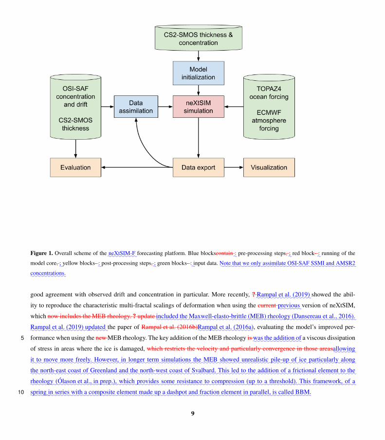
Figure 1. Overall scheme of the:::::::::neXtSIM-F forecasting platform. Blue blockscontain

:: pre-processing steps,

:; red block-

:: running of the

model core, ;:

yellow blocks-:: post-processing steps,

:; green blocks- :

:input data.

:::Note

:::that

:::we

::::only

:::::::assimilate

::::::::OSI-SAF

::::SSMI

:::and

:::::::AMSR2

:::::::::::concentrations.

good agreement with observed drift and concentration in particular. More recently, ?:::::::::::::::::Rampal et al. (2019) showed the abil-

ity to reproduce the characteristic multi-fractal scalings of deformation when using the current:::::::previous version of neXtSIM,

which now includes the MEB rheology. ? update:::::::included

:::the

::::::::::::::::::Maxwell-elasto-brittle

::::::(MEB)

::::::::rheology

::::::::::::::::::::(Dansereau et al., 2016).

:::::::::::::::::::::::Rampal et al. (2019) updated

:the paper of Rampal et al. (2016b)

:::::::::::::::::Rampal et al. (2016a), evaluating the model’s improved per-

formance when using the new MEB rheology. The key addition of the MEB rheology is:::was

:::the

:::::::addition

::of a viscous dissipation5

of stress in areas where the ice is damaged, which restricts the velocity and particularly convergence in those areas:::::::allowing

:it::to:::::

move:::::

more::::::

freely.::::::::However,

:::in

:::::longer

:::::term

::::::::::simulations

:::the

:::::MEB

:::::::showed

:::::::::unrealistic

::::::pile-up

:::of

:::ice


:::::along

::the

:::::::::north-east

:::::coast

::of

:::::::::Greenland

:::and

:::the

:::::::::north-west

:::::coast

::of

:::::::::Svalbard.

::::This

:::led

::to

:::the

:::::::addition

::of

::a::::::::frictional

:::::::element

::to

:::the

:::::::rheology

::::::::::::::::::::(Ólason et al., in prep.),

:::::which

::::::::provides

:::::some

::::::::resistance

:::to

::::::::::compression

::::(up

::to

:a::::::::::

threshold).::::This

::::::::::framework,

::of

::a

:::::spring

:::in

:::::series

::::with

::a

::::::::composite

:::::::element

:::::made

::up

::a:::::::dashpot

:::and

:::::::fraction

::::::element

:::in

:::::::parallel,

:is::::::called

:::::BBM.10

9

The dynamical equations are solved with a finite element method on a Lagrangian (moving) triangular mesh. The code

has evolved from a serial (non-parallelised) Matlab code (used by eg. Rampal et al. (2016b)), to:is

::::::::currently a parallelised C++

code(used by ?, ?,::::used

:::by

::::::::::::::::Rampal et al. (2019), and presented by Samaké et al., 2017). We use this parallelised code

:::::::::::::::::Samaké et al. (2017).

:::::::::Momentum

:::::input

::::::comes

::::from

:::the

:::::wind

::::and

:::::ocean

:::::::stresses

::(a

::::::turning

:::::angle

::of::::

25◦::is

:::::::applied

::to

:::the

:::::ocean

:::::::velocity

:::::from

:::the

:::::ocean

:::::::forcing),

:::the

:::::::Coriolis

:::::force

:::and

:::sea

:::::::surface

:::::slope,

::::and

::::there

::is

::::also

:a:::::basal

:::::stress

::::::applied

::at:::the

:::::::bottom

::of

:::the

:::ice

:::::when5

:it::::::::becomes

::::::::grounded.

::::For

:::this

:::::basal

:::::stress

:::we

::::::follow

:::the

::::::scheme

:::of

:::::::::::::::::::Lemieux et al. (2016b),

:::::using

:::the

:::::::::parameters

::::::::::k1 = 10m,

:::::::::k2 = 15m,

:::::::αb = 20,

::::::::::::::::::u0 = 5× 10−5m s−1.

There is also a thermodynamic component of the code and beneath the ice is a slab ocean with three variables: temperature,

salinity and thickness. The temperature and salinity are modified by the heat and salinity fluxes determined by the thermody-

namical model as ice melts and freezes and as the model interacts with the atmosphere. They are relaxed towards the SST and10

SSS from TOPAZ over a time scale of about one month, while the thickness of the slab ocean is taken directly to be the MLD

of TOPAZ.::::This

:::::varies

:::::::spatially

::::and

::::::evolves

::::with

::::time

:::::::::according

::to

:::the

:::::::forecast

::::from

:::::::TOPAZ.

:The thermodynamical model is

a three-category model (detailed in ?, Appendix A):::::::::::::::::::::::::::::::::::::(detailed in Rampal et al., 2019, Appendix A): open water, newly-formed

ice (treated as one ice layer and one snow layer; Semtner, 1976) and older ice (treated as two ice layers and a snow layer;

Winton, 2000).15

The older ice is characterised in the model by concentration, c, and thickness averaged over the entire cell (effective thickness

or, in other words, volume per unit area), h. The absolute thickness of ice can be computed as the ratio: H = h/c; there is also

an effective snow thickness, s. The young ice has concentration cy , effective and absolute thicknesses, hy and Hy = hy/cy ,

and snow thickness, sy . Hy is constrained so that Hmin ≤Hy ≤Hmax. If Hy <Hmin, cy is reduced to c′y = (Hycy)/Hmin; if

Hy >Hmax, some ice is moved to the older ice category. During this process Hy is reduced to H ′y =Hmax, while cy is also20

reduced to c′y = cy(Hmax−Hmin)/(Hy−Hmin). This concentration reduction is intended to give some lateral decrease in thin

ice volume and not just vertical. The corrected values for hy and sy are h′y = c′yHmax and s′y = c′y(sy/cy); the corresponding

properties for the older ice h, c and s are then increased in a ice-and-snow-volume-conserving manner. The values that we used

for the thresholds on the absolute thin ice thickness are Hmin = 0.05m and Hmax = 0.275m.

The domain we present simulations for is a pan-Arctic one, with a resolution of about 7.5 km. A 7-day forecast for this25

domain can be run on a laptop with 8 cores at 2 GHz in about 3 – 4 hours. Figure 2 shows snapshots of some of the more

interesting variables from neXtSIM. Figure ??a shows the sea ice concentration — note the many thin cracks and leads —

while Figure ??b shows the ice thickness. Figure ??c shows the damage, which is a crucial variable in the MEB rheology.

The effective elastic modulus is lower where it is higher, making it more mobile in those places. Figure ??d shows the volume

fraction of ridged ice, which is higher in places that have been under convergence. This variable is one that could be particularly30

useful for icebreakers wishing to travel into the ice:::runs

::in

:::::about

:::30

::::::minutes

:::::using

:::16

:::::::::processors.

3.2 Initialization of the model fields

Before the model can be run it has to be initialized - the triangular mesh for the destination domain should be generated and

initial values of sea ice concentration and thickness and the slab ocean surface temperature and salinity have to be set. The

10

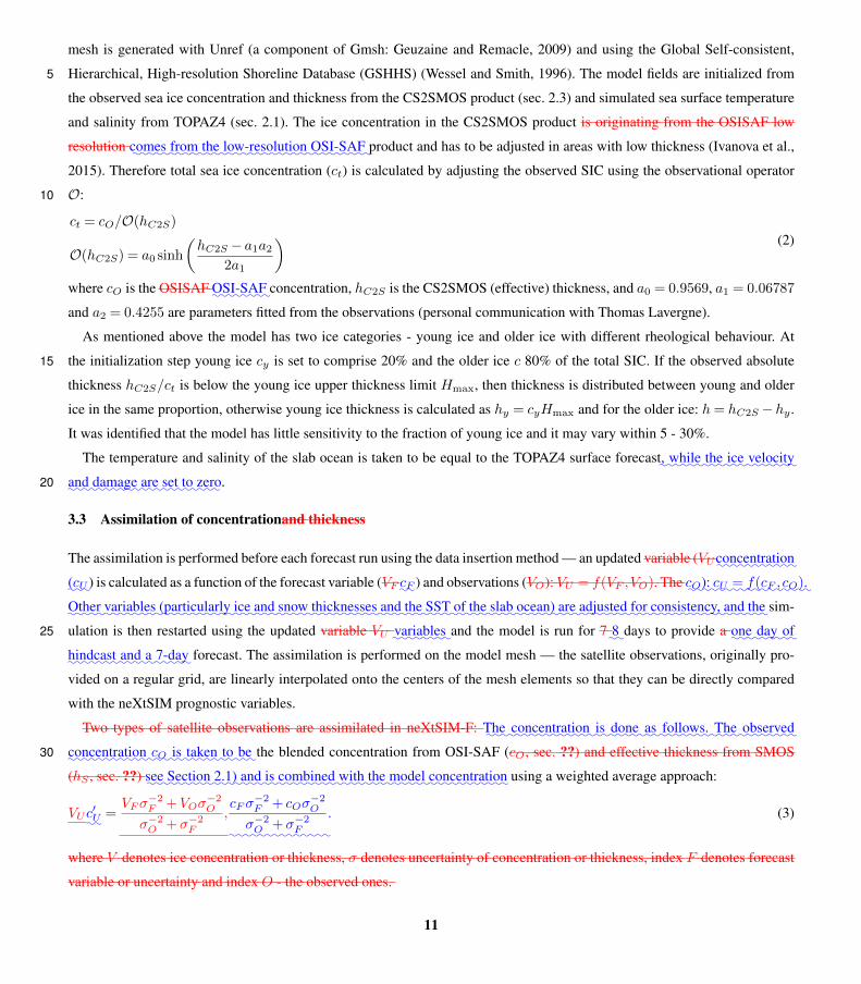
mesh is generated with Unref (a component of Gmsh: Geuzaine and Remacle, 2009) and using the Global Self-consistent,

Hierarchical, High-resolution Shoreline Database (GSHHS) (Wessel and Smith, 1996). The model fields are initialized from5

the observed sea ice concentration and thickness from the CS2SMOS product (sec. 2.3) and simulated sea surface temperature

and salinity from TOPAZ4 (sec. 2.1). The ice concentration in the CS2SMOS product is originating from the OSISAF low

resolution:::::comes

::::from

:::the

::::::::::::low-resolution

::::::::OSI-SAF

:product and has to be adjusted in areas with low thickness (Ivanova et al.,

2015). Therefore total sea ice concentration (ct) is calculated by adjusting the observed SIC using the observational operator

O:10

ct = cO/O(hC2S)

O(hC2S) = a0 sinh

(hC2S − a1a2

2a1

) (2)

where cO is the OSISAF::::::::OSI-SAF concentration, hC2S is the CS2SMOS (effective) thickness, and a0 = 0.9569, a1 = 0.06787

and a2 = 0.4255 are parameters fitted from the observations (personal communication with Thomas Lavergne).

As mentioned above the model has two ice categories - young ice and older ice with different rheological behaviour. At

the initialization step young ice cy is set to comprise 20% and the older ice c 80% of the total SIC. If the observed absolute15

thickness hC2S/ct is below the young ice upper thickness limit Hmax, then thickness is distributed between young and older

ice in the same proportion, otherwise young ice thickness is calculated as hy = cyHmax and for the older ice: h= hC2S −hy .

It was identified that the model has little sensitivity to the fraction of young ice and it may vary within 5 - 30%.

The temperature and salinity of the slab ocean is taken to be equal to the TOPAZ4 surface forecast:,:::::while

:::the

:::ice

:::::::velocity

:::and

:::::::damage

:::are

::set

::to

::::zero.20

3.3 Assimilation of concentrationand thickness

The assimilation is performed before each forecast run using the data insertion method — an updated variable (VU :::::::::::concentration

:::(cU ) is calculated as a function of the forecast variable (VF ::

cF ) and observations (VO): VU = f(VF ,VO). The:::cO):

::::::::::::::cU = f(cF , cO).

:::::Other

:::::::variables

:::::::::::(particularly

::ice

::::and

::::snow

::::::::::thicknesses

:::and

:::the

::::SST

::of

:::the

::::slab

::::::ocean)

::are

::::::::adjusted

::for

::::::::::consistency,

::::and

:::the sim-

ulation is then restarted using the updated variable VU :::::::variables

:and the model is run for 7

:8:

days to provide a:::one

:::day

:::of25

:::::::hindcast

:::and

::a

:::::7-day forecast. The assimilation is performed on the model mesh — the satellite observations, originally pro-

vided on a regular grid, are linearly interpolated onto the centers of the mesh elements so that they can be directly compared

with the neXtSIM prognostic variables.

Two types of satellite observations are assimilated in neXtSIM-F::::The

:::::::::::concentration

::is:::::

done:::as

:::::::follows.

::::The

::::::::observed


:::cO ::

is:::::taken

::to

::be

:the blended concentration from OSI-SAF (cO, sec. ??) and effective thickness from SMOS30

(hS , sec. ??)::see

:::::::Section

:::2.1)

::::and

::is

::::::::combined

::::with

:::the

::::::model

:::::::::::concentration using a weighted average approach:

VUc′U

::=VFσ

−2F +VOσ

−2O

σ−2O +σ−2F,cFσ

−2F + cOσ

−2O

σ−2O +σ−2F.

::::::::::::::

(3)

where V denotes ice concentration or thickness, σ denotes uncertainty of concentration or thickness, index F denotes forecast

variable or uncertainty and index O - the observed ones.

11

The uncertainties of the observed concentration and thickness (σcO and σhO:::(σO) are obtained from the input product and5

uncertainties of the forecast concentration and thickness (σcF , σhF ) are set, respectively to 10% and 0.1 m. The values for

the uncertainties:::::::products,

:::::while

:::the

:::::value

:::for

:::the


:in the forecast variables are chosen


::is

:::set

::to

:::0.3 to

reduce strong discontinuities in the modelled fields.:It::::can

:::also

:::be

::::::thought

::of

::as

::::::::::introducing

:a::::time

:::::scale

::(in

:::::days)

::of

::::::::::1+σ2

O/σ2F

::for

:::::::::relaxation

:::::::towards

:::the

:::::::::::observations

::::that

:::::::depends

:::on

:::the

:::::::relative

::::::::::::uncertainties. Assimilation of both concentration and

thickness is performed in all elements that have valid observations. Even if hO exceeds the theoretically retrievable threshold10

of 0.5 m the value of σhO in such elements is considerably larger than σhF and, thus SMOS observations have almost no impact

on the updated thickness.

::In

:::the

::::pack,

:::the

::::total

::::::(young

::::and

:::old

:::ice)

::::::model


:::cF ::

is:::::::generally

:::::about

::1,

:::::while

:::the

::::::::OSI-SAF


::::can

::be

::::::around

:::0.9.

:::We

:::::found

::::that

:::::using

::c′U::

as:::the

:::::actual

::::::update

:::cU ::::::::

produced:::too

:::::much

::of

:a::::drop

::in


:::::there,

::::::::lowering

:::the

::::::internal

:::::stress

::to

::::near

::::zero

::::and

:::::::allowing

:::too

:::::much

:::::drift.

::::This

::::::quickly

:::led

::to

:::::rapid

:::::build

::up

::of

::::very

:::::thick

:::ice

::in

:::::::unusual

::::::places.15

::::::::Therefore

:::we

:::had

::to::::

take::a::::quite

:::::::::::conservative

::::::::approach

::to

:::our

:::::::::correction

:::and

:::::only

::::::change

:::the

::::::model

::to

:::::make

::::sure

:it::::had

:::the

::::::correct

::ice

:::::mask

::::(this

::is

:a::::kind

:::of


::of

:::::::extent):

cU =

0 c′U < 0.15,

c′U cF < 0.15 and c′U ≥ 0.15,

cF otherwise.:::::::::::::::::::::::::::::::::

(4)

After calculating the updated variables as specified in (3) the fractions and thicknesses of young and older ice are calculated

in the same way as in the initialisation procedure (see sec. 3.2).20

Once all the assimilation steps have been performed the model fields are checked for consistency with each other and cor-

rected if necessary. First, the concentration of young ice is reduced in the elements where the total concentration exceeds 100%.

Second, the surface temperature of the slab ocean is set to the freezing point where new ice was added during assimilation.

The volume of ridged ice, damage and the snow thickness::ice

::::and

::::snow

::::::::::thicknesses are set to zero in the added ice.

:::::Lastly,

:::we

::::need

::to

::::::correct

:::the

::::SST

::of

:::the

::::slab

::::::ocean.

:::::Where

::::new

:::ice

::is

:::::added

::::::during


::it::is

:::set

::to

:::the

:::::::freezing

:::::point,

:::but

::if

:::ice25

:is::::::::removed

::::then

:::the

:::::::situation

::is

::::more

:::::::::::complicated.

:::::Then

:::we

:::::::proceed

::as

::in

:::the

::::::::following

:::::::section.

3.4 Compensating heat flux

One of the side effects of assimilation is that the heat balance in the model is disturbed: reducing the concentration opens more

water and given the temperatures, atmosphere humidity and ocean salinity provided by the forcing, the heat flux out of the

ocean increases and the ice freezes up again very fast. A compensating heat flux is added to the total ocean heat flux in order

to keep the heat balance and prevent refreezing of ice where it was removed by assimilation, thus prolonging the effect of

assimilation. If ct and c′t are respectively the total concentrations before and after assimilation, a compensating heat flux (Qc)5

is calculated if ice was removed — i.e. if ct > 0 and c′t < ct — according to the following formula

Qc =Qo((c′t/ct)

n− 1)

(5)

12

where Qo is the total heat flux from the ocean (sum of flux from the ocean to sea ice and to the atmosphere), and n is a

parameter controlling the strength of correction. The function was chosen so that Qc is zero when the concentration update is

zero, and Qc =−Qo when c′t = 0, i.e. all the ice was removed by assimilation. With n= 1 the reduction of Qc from 0 to −Qo10

is linear and with n > 1 it becomes steeper for values of c′t closer to ct. We use n= 4 for the runs presented here, as this gives

a suitably strong heat flux for a modest reduction in concentration.

4 Results

:::We

:::::begin

::::with

::an

:::::::::evaluation

::of

:a::::free

:::run

::::over

:::the

::::::::20-month

::::::period

::::from

::1

::::Nov

::::2018

::to

:::30

::::June

:::::2020.

::::This

:::::shows

:::the

:::::::general

:::::::strengths

::::and

::::::::::weaknesses

::of

:::the

::::::model.

:::We

::::then

:::::::evaluate

:::the

:::::::::::performance

::of

:::the

:::::::forecast

::::::system

::::over

:::this

::::::period

::to

:::::show

:::the15

:::::::::::improvements

::::::gained

:::by

:::the


::of

::::::::OSI-SAF


4.1 Evaluation of free model run

In this section we demonstrate that the model is generally able to reproduce the overall drift, concentration, and thickness

patterns in observationsof these variables. For all comparisons we average the model fields in time over an appropriate time

window (in practice 1, 2 or 7 days), apply some spatial smoothing (being guided by the size of the satellite footprint), and20

interpolate onto the observation grid. For scalar variables, we define bias as 〈Vmod−Vobs〉 (with 〈·〉 defining the spatial mean

over pixels where both model and observation are defined,::::and

:::::where

:::::either

::::::model

::or


::::have

:::ice.) We also define

RMSE as 〈(Vmod−Vobs)2〉1/2. For the ice velocity we define the bias and RMSE as the mean and RMS values of the difference

in speed respectively — i.e. 〈|umod| − |uobs|〉 and 〈(|umod| − |uobs|)2〉1/2. We also define the vector RMSE (VRMSE), as the

RMS of the vector difference, 〈|umod−uobs|2〉1/2. For the ice extent, we use the terms bias and RMSE a bit loosely: we define5

bias in extent asA10−A01, whereA10 is the total area of pixels where neXtSIM predicts the presence of ice (total concentration

greater than 15 %) but the observation has no ice, while A01 is the total area of pixels where neXtSIM predicts the no ice (total

concentration greater than 15 %) but the observation does have ice; we define RMSE in extent .:::::::::::

Analogously:::to

:::the

::::::RMSE

::for

:::::other

:::::::::quantities,

:::we

:::::define

:::::IIEE

:::::::::::::::::::::::::::::::::::::::::(Integrated Ice Edge Error, Goessling et al., 2016) as A10 +A01. Thus the RMSE

::::IIEE is

always positive, and the bias is positive if neXtSIM is overestimating the total extent and negative if it is underestimating it.10

This definition of the:::For

:::the

:::ice

:::::::velocity

:::we

::::::define

:::the

::::bias

:::and

::::::RMSE

:::as

:::the

:::::mean

::::and

::::RMS

::::::values

:::of

:::the

::::::::difference

:::in

:::::speed

::::::::::respectively

::—

:::i.e.

:::::::::::::::〈|umod| − |uobs|〉::::

and::::::::::::::::::::〈(|umod| − |uobs|)2〉1/2.

:::We

::::also

::::::define

:::the

:::::vector

::::::RMSE

:::::::::(VRMSE),

:::as

:::the

::::RMS

::of

:::the

::::::vector

:::::::::difference,

::::::::::::::::::〈|umod−uobs|2〉1/2.

::::Note

::::that

::::these

::::drift

::::::errors

:::can

::::only

:::be

::::::::calculated

::::::where

::::both

:::::model

::::and

:::::::::observation

::::have

::::ice.

13

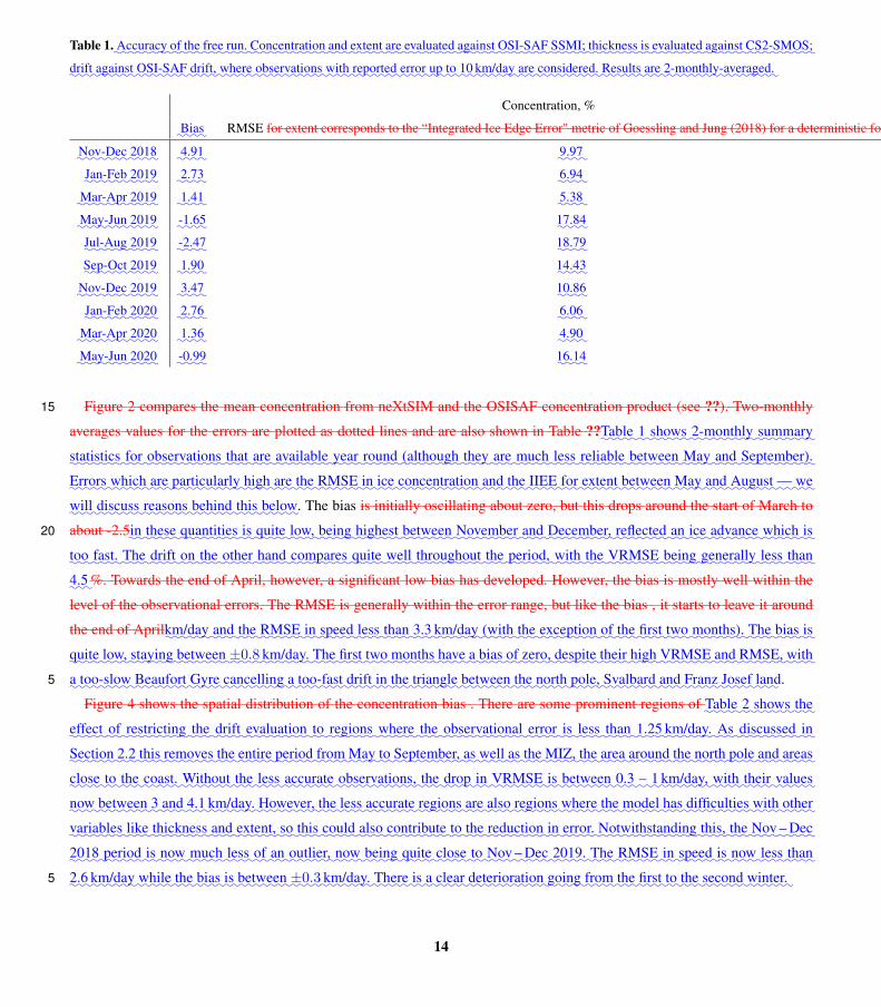
Table 1.:::::::Accuracy

::of

:::the

:::free

:::run.

:::::::::::Concentration

:::and

::::extent

:::are

:::::::evaluated

::::::against

:::::::OSI-SAF

:::::SSMI;

:::::::thickness

::is

:::::::evaluated

:::::against

::::::::::CS2-SMOS;

:::drift

::::::against

:::::::OSI-SAF

::::drift,

:::::where

:::::::::observations

::::with

::::::reported

::::error

:::up

:to::::::::10 km/day

:::are

:::::::::considered.

:::::Results

:::are

::::::::::::::::2-monthly-averaged.

Concentration, % Extent, 106km2 Drift, km/day

::::Bias RMSE for extent corresponds to the “Integrated Ice Edge Error" metric of Goessling and Jung (2018) for a deterministic forecast.

::::Bias

:::::RMSE

: ::::Bias

:::::RMSE

: ::::::VRMSE

:::::::Nov-Dec

::::2018

::::4.91

:::9.97

: ::::0.09

:::0.24

: ::::0.00

:::3.63

: :::5.16

::::::Jan-Feb

::::2019

::::2.73

:::6.94

: ::::0.09

:::0.17

: ::::-0.31

:::2.96

: :::4.00

:::::::Mar-Apr

::::2019

::::1.41

:::5.38

: ::::-0.03

:::0.18

: ::::-0.40

:::2.77

: :::3.65

:::::::May-Jun

::::2019

::::-1.65

::::17.84

::::-0.15

:::0.81

: ::::-0.91

:::3.19

: :::4.19

::::::Jul-Aug

::::2019

::::-2.47

::::18.79

::::-0.06

:::1.05

: ::::0.23

:::3.25

: :::4.75

::::::Sep-Oct

::::2019

::::1.90

::::14.43

::::-0.06

:::0.47

: ::::0.81

:::2.80

: :::4.50

:::::::Nov-Dec

::::2019

::::3.47

::::10.86

::::-0.11

:::0.41

: ::::0.32

:::2.96

: :::4.53

::::::Jan-Feb

::::2020

::::2.76

:::6.06

: ::::0.05

:::0.17

: ::::0.09

:::3.15

: :::4.48

:::::::Mar-Apr

::::2020

::::1.36

:::4.90

: ::::-0.03

:::0.14

: ::::-0.15

:::3.06

: :::4.34

:::::::May-Jun

::::2020

::::-0.99

::::16.14

::::-0.08

:::0.71

: ::::-0.74

:::3.30

: :::4.41

Figure 2 compares the mean concentration from neXtSIM and the OSISAF concentration product (see ??). Two-monthly15

averages values for the errors are plotted as dotted lines and are also shown in Table ??::::Table

::1::::::shows

:::::::::2-monthly

::::::::summary

:::::::statistics

:::for


:::that

:::are

::::::::available

::::year

:::::round

:::::::::(although

::::they

:::are

:::::much

::::less

::::::reliable

::::::::between

::::May

:::and

:::::::::::September).

:::::Errors

:::::which

:::are


::::high

:::are

:::the

::::::RMSE

::in

:::ice


::::and

:::the

::::IIEE

:::for

:::::extent

:::::::between

:::::May

:::and

::::::August

:::—

:::we

:::will

::::::discuss

:::::::reasons

::::::behind

:::this

::::::below. The bias is initially oscillating about zero, but this drops around the start of March to

about -2.5::in

::::these

:::::::::quantities

::is

::::quite

::::low,

:::::being

:::::::highest

:::::::between

:::::::::November

:::and

:::::::::December,

::::::::reflected

::an

:::ice

:::::::advance

::::::which

::is20

:::too

::::fast.

:::The

::::drift

:::on

:::the

:::::other

::::hand

:::::::::compares

::::quite

::::well

::::::::::throughout

:::the

::::::period,

::::with

:::the

::::::::VRMSE

:::::being

::::::::generally

::::less

::::than

:::4.5 %. Towards the end of April, however, a significant low bias has developed. However, the bias is mostly well within the

level of the observational errors. The RMSE is generally within the error range, but like the bias , it starts to leave it around

the end of April::::::km/day

:::and

:::the

::::::RMSE

::in:::::speed

::::less

::::than

:::::::::3.3 km/day

:::::(with

:::the

::::::::exception

:::of

:::the

:::first

::::two

:::::::months).

::::The

::::bias

::is

::::quite

::::low,

::::::staying

:::::::between

:::::::::::±0.8 km/day.

::::The

::::first

:::two

::::::months

:::::have

:a::::bias

::of

::::zero,

::::::despite

:::::their

::::high

:::::::VRMSE

:::and

:::::::RMSE,

::::with

:a:::::::too-slow

::::::::Beaufort

::::Gyre

:::::::::cancelling

:a:::::::too-fast

::::drift

::in

:::the

:::::::triangle

:::::::between

:::the

::::north

:::::pole,

:::::::Svalbard

::::and

:::::Franz

::::Josef

::::land.5

Figure 4 shows the spatial distribution of the concentration bias . There are some prominent regions of:::::Table

:2::::::shows

:::the

:::::effect

::of

:::::::::restricting

:::the

::::drift

:::::::::evaluation

::to:::::::

regions::::::where

:::the

:::::::::::observational

:::::error

::is

::::less

::::than

:::::::::::1.25 km/day.

:::As

::::::::discussed

:::in

::::::Section

:::2.2

:::this

:::::::removes

:::the

:::::entire

::::::period

::::from

::::May

::to::::::::::September,

::as

::::well

::as

:::the

:::::MIZ,

:::the

:::area

::::::around

:::the

:::::north

::::pole

:::and

:::::areas

::::close

::to

:::the

::::::coast.

:::::::Without

:::the

:::less

::::::::accurate

:::::::::::observations,

:::the

::::drop

:::in

:::::::VRMSE

::is

:::::::between

::::0.3

:–:::::::::1 km/day,

::::with

::::their

::::::values

:::now

::::::::between

:3:::and

::::::::::4.1 km/day.

::::::::However,

:::the

::::less

:::::::accurate

::::::regions

:::are

::::also

::::::regions

::::::where

::the

::::::model

:::has

:::::::::difficulties

::::with

:::::other

:::::::variables

::::like

::::::::thickness

:::and

::::::extent,

::so

::::this

:::::could

:::also

:::::::::contribute

::to

:::the

::::::::reduction

::in

:::::error.

::::::::::::::Notwithstanding

::::this,

:::the

:::::::::Nov – Dec

::::2018

::::::period

::is

::::now

:::::much

:::less

:::of

::an

::::::outlier,

::::now

:::::being

:::::quite

:::::close

::to

:::::::::Nov – Dec

:::::2019.

::::The

::::::RMSE

::in

:::::speed

::is

::::now

::::less

::::than

:::::::::2.6 km/day

:::::while

:::the

:::bias

::is:::::::between

::::::::::::±0.3 km/day.

:::::There

::is

:a:::::clear

::::::::::deterioration

:::::going

:::::from

:::the

:::first

::to

:::the

::::::second

::::::winter.

:5

14

Table 2. Accuracy of the free run . Concentration::for

::the

::::::::::2018 – 2019 and extent are evaluated against OSISAF SSMI; thickness

:::::::::2019 – 2020

::::::winters.

::::::::Thickness is evaluated against CS2-SMOS; drift against OSISAF

:::::::OSI-SAF

:drift,

:::::where

::::only

:::::::::observations

::::with

:::::::reported

::::error

:::less

:::than

:::::::::1.25 km/day

:::are

:::::::::considered. Results are averaged over three periods: November – December, January – February and March – April or

just March (CS2-SMOS ice thickness is not available in April):::::::::::::::2-monthly-averaged.

Thickness, m Drift, km/day

Bias RMSE Bias RMSE Bias RMSE Bias RMSE VRMSE

Nov-Dec::::2018 0.14

::::-0.09 5.83

:::0.26

:-0.02

::::-0.13

:0.23

:::2.62 -0.12

:::4.06

::::::Jan-Feb

::::2019 0.26

:::0.09

:-0.06

::::0.36 2.74

::::-0.26 4.05

:::2.22

:::3.27

Jan-Feb::::::

Mar-Apr::::2019 -0.26

::::0.07 4.73

:::0.51

:0.04

::::-0.24 0.16

:::2.21 -0.01

:::3.03

:::::::Nov-Dec

::::2019 0.35

:::0.04

:0.25

:::0.40

:2.52

::::0.19 3.58

:::2.59

:::4.11

Mar-(Apr)::::::Jan-Feb

::::2020 -2.52

::::0.23 6.05

:::0.46

:-0.10

:::0.27 0.21

:::2.41 -0.06

:::3.69

::::::Mar-Apr

::::2020 0.53

:::0.19

:0.39

:::0.56

:2.59

::::0.01 3.49

:::2.39

:::3.64

::::Table

::2::::also

::::::::::summarises

::::the

::::::::::comparison

::of

::::::model

::::::::thickness

::::with

::::the

::::::::::CS2-SMOS

:::::::product.

:::::::RMSE

::is

:::::lower

:::::::(0.26 m)

:::in

:::::::Nov-Dec

:::::2018

:::::since

::::::::thickness

:::was

:::::::::initialised

::::using

:::::::::::CS2-SMOS,

::::and

:::::grows

::to

::::::0.51 m

::::over

:::the

::::first

::::::winter.

:::The

::::::RMSE

::::::grows

::::from

:::::0.4 m

::to

::::::0.56 m

::::over

:::the

::::::second

::::::winter.

:::The

::::bias

::is

::::quite

::::low

::in

:::the

:::first

::::::winter,

:::but

:::::about

:::::0.2 m

:::::from

::::::::Jan – Apr

:::::2020.

::::::Figures

::2

:::and

::3:::::::compare

:::the

:::::mean


::::and

:::::extent

:::::from

::::::::neXtSIM

:::and

:::the

:::::::::OSI-SAF


:::::::product

::::(see

::::2.1).

:::::Since

:::we

::do

::::not

::::have

:::::::enough

::::::::::information

::to

::::::create

::an

:::::error

:::::model

:::for

:::the



:::(for

::::::::example

::it5

:::::cannot

:::be

::::::::Gaussian

:::due

:::to

::its

:::::::::restriction

::to

:::::being

::::::::between

:0::::

and::::::100%)

:::we

:::::could

:::not

::::::::generate

:::::::::confidence

::::::::intervals

:::for

:::the

::::mean


::::but

::::::instead

::::plot

:a::::::shaded

::::area

::::::::::::corresponding

::to:::::::::::::±〈σOSISAF〉1/2:::

for::::::::reference

:::::when

::::::::::considering

:::the

::::bias

:::and

::::::RMSE

::in


:::The

::::::::seasonal

::::cycle

:::for

:::::mean


:::and

:::::extent

::is

::::::::captured

:::::::::reasonably

::::well,

:::but

:::the

::::bias

::is

:::::clearly

:::::::positive

::in

::::::winter

:::and

::::::clearly

::::::::negative

::in

:::::::summer.

:::As

:::::noted

::::from

:::::Table

::1

:::the

::::::RMSE

::in


:::and

:::the

:::::IIEE

:::are

::::very

::::high

:::::::between

::::::::mid-April

::::and

::::::August.

::::The

::::::RMSE

::in


::is::::::::generally

::::::::::comparable

::to

:::the

:::::RMS

::::error

::::level

:::::::outside10

::::these

:::::::periods.

15

Figure 2.:::::::Temporal

:::::::::comparison

::of

:::::model

:::and

:::::::OSI-SAF

:::::SSMI

:::::::::::concentrations.

:::The

::::::shaded

:::area

::in

:::the

::::lower

:::plot

:::::shows

:::the

::::RMS


:of:::

the::::::::::concentration

:::for

:::::::reference

::::when

:::::::::considering

:::the

:::::errors.

:::The

::::bias

:is::::::defined

::as

:::::model

:–::::::::::observation.

Figure 3.:::::::Temporal

:::::::::comparison

::of

:::::extents

:::::from

:::::model

:::and

:::::::OSI-SAF

:::::SSMI

::::::::::::concentrations.

:::The

::::::shaded

:::area

::in:::

the:::::lower

:::plot

:::::shows

:::an

::::::estimate

:::for

::the


::in

::the

::::::extent.

:::The

:::bias

::is

::::::defined

:as:::::

model::–:::::::::observation.

16

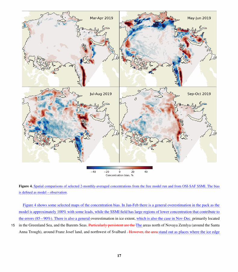
Figure 4.:::::Spatial

::::::::::comparisons

::of

::::::selected

:::::::::::::::2-monthly-averaged

:::::::::::concentrations

::::from

:::the

:::free

:::::model

:::run

::::and

::::from

:::::::OSI-SAF

:::::SSMI.

:::The

::::bias

:is::::::defined

::as

:::::model

:–:::::::::observation.

:::::Figure

::4

:::::shows

:::::some

:::::::selected

::::maps

:::of

:::the


::::bias.

::In

:::::::Jan-Feb

:::::there

:is::a::::::general

::::::::::::overestimation

::in:::the

:::::pack

::as

:::the

:::::model

::is

::::::::::::approximately

:::::100%

::::with

:::::some

:::::leads,

:::::while

::the

::::::SSMI

::::field

:::has

::::large

::::::regions

::of:::::lower


:::that

:::::::::contribute

::to

::the

::::::errors

:::::::::(85 – 90%).

:::::There

::is::::also

:a:::::::general overestimation in ice extent,

:::::which

::is

:::also

:::the

::::case

::in

:::::::::Nov-Dec. primarily located

in the Greenland Sea, and the Barents Seas. Particularly persistent are the:::The areas north of Novaya Zemlya (around the Santa15

Anna Trough), around Franz Josef land, and northwest of Svalbard . However, the area::::stand

:::out

:::as

:::::places

::::::where

:::the

::ice

:::::edge

17

:is:::not

:::::being

:::::::located

::::::::correctly.

::::This

::::::::continues

::::into

::::::::Mar-Apr.

:::The

::::::region

::of

::::::::::::::underestimation

::to

:::the northwest of Svalbard starts

to become underestimated around mid-February.

The map for Nov-Dec shows strong underestimation in the Bering Sea, which was too slow to freeze up in November, and

north of the Novo Sibirski Islands:is

::::::related

::to

:::the

:::::::::::development

::of

:::an

::::arch

:::::::between

:::::there

:::and

:::the

::::::::northeast

:::tip

::of

::::::::::Greenland.20

::::(This

::is::::

also:::::::

related::to

::::::::relatively

:::::large


::in

:::::these

:::::areas,

::::::which

::::::::increases

:::the

::::::::capacity

::of

::::::::::undamaged

:::ice

:::to

::::stay

::::::::::undamaged.)

:::::This

::::::arching

::::also

:::::::reduces

:::the

:::ice

::::::export

:::::::through

:::the

:::::Fram

::::::Strait,

:::the

:::::effect

::of

::::::which

::is

::::seen

:::in

:::the

:::::maps

:::for

::::::::May – Jun

::::and

::::::::Jul – Aug.

:::In

::::::::May – Jun

:::we

::::also

:::see

::::that

:::the

:::ice

::::that

::is

::in

:::the

:::::::::Greenland

::::Sea

::is

::::::::displaced

:::too

:::far

::to

:::the

:::::east,

::::::::producing

::a

::::::double

::::::penalty

:::::effect

::in:::

the:::::::

RMSE::::score. This is strongest from about 3 – 11 Nov. It also returns at the start of

April, although the region extends further in this period than at the start of the winter, following the Siberian coast around to25

the Severny Islands . There are also significant underestimations at the end of the simulation along the coasts of the Beaufort

Sea (particularly Mackenzie Bay), and the Bering and East Siberian Seas. In addition,:::also

:a::::::

result::of the ice off Greenland

is being driven away from the coast too much , leading to a double penalty in the RMSE score at the end of the simulation.

::::::arching

::in

:::this

::::area

:::—

::the

:::ice

::at

:::the

::::::corner

::of

:::::::::Greenland

:is:::too

:::::thick

::to

::be

::::::::exported,

:::and

:::so

:::the

::ice

::::that

::is

:::::::exported

:::has

::::::::detached

::::from

:::the

::::arch

::::away

:::::from

:::the

::::coast

::::and

:::has

::::then

:::::::travelled

:::::::roughly

::::::parallel

::to

:::the

:::::coast

::::::without

:::::being

::::::pushed

:::::back

::::::towards

:::it.

::In30

:::::::Jul – Aug

:::the

::::::thicker

:::ice

:::has

::::::mostly

::::::melted

::::and

::::there

::is

::::less

::of

:a::::::dipole

:::::::situation

:::and

:::::more

::of

::a

:::::::clear-cut

::::::::::::::underestimation.

Temporal comparison of model and OSISAF concentrations. Two-monthly average values of the different errors are plotted

as dotted lines with colours corresponding to the solid lines; these values can be found in Table ??.:::::::Another

:::::::problem

::::area

::is

::::::around

:::the

:::::Novo

::::::Sibirski

:::::::Islands

:::and

:::the

::::::Laptev

::::Sea.

:::::April

::::sees

:::the

::::::model

:::::::opening

::::::slightly

:::too

:::far

::to:::

the::::::

north;::in

::::May

::::and

::::June

::::there

::is

:a::::::strong

:::::::::::::underestimation

::to

:::the

:::::north

::of

:::the

::::::islands

::::and

:::too

:::::much

:::fast

:::ice.

::::The

:::::::::::::underestimation

::is

:::::partly

:::::from

:::too35

:::fast

::::::melting

::::and

:::that

:::the

::::fast

:::ice

:::has

:::not

:::::::detached

::::and

::::::flowed

:::into

::::this

::::area.

:::::There

:is::a::::::similar

:::::::problem

::to

:::the

::::west

::of

::::::::Wrangel

:::::Island

::in

:::the

:::::::Chukchi

::::Sea

::—

:::an

:::::::opening

:::that

::is

:::too

::::large

:::::::::compared

::to

:::the

::::::::::observations

:::and

:::too

:::::much

::::::::land-fast

:::ice

::::close

::to

:::the

:::::coast

:::::which

::::::should

::be

:::::::flowing

:::into

::::this

::::::region.

:::::There

::is

:::also

::a::::large

::::::region

::of


::to

:::the

::::east

::of

::::::::Wrangel

::::::Island,

:::::which

::is

:::::::actually

::an

:::::::artefact

::of

:::the

::::::::boundary

:::::::::conditions

::::that

:::we

:::are

:::::using

::at

::the

:::::open

::::::Bering

:::::Strait

::::::::boundary.

::If

::::there

::is

::::::inflow

::at

:::any

::::open

::::::::::boundaries

::the

:::::value

::of

::::any

::::::tracers

:is:::::taken

::to

:::be

::its

:::::value

::in

:::the5

::::::nearest

::::mesh

::::::::element,

:::and

::in

::::this

::::case

::we

:::are

:::::::getting

:::too

:::::much

::ice

:::::being

::::::::imported

:::::::through

:::the

::::::Bering

:::::Strait,

::::::which

::::leads

::to

::a

:::::::build-up

::at

:::this

::::::::location.

:::The

::::last

:::::things

::to

:::::::mention

:::::about

::::the

::::::::Jul – Aug

::::map

:::are

:::the

:::::strong

:::::::::::::overestimation

::::::around

:::::Franz

:::::Josef

:::::land,

:::and

:::the

::::::dipole

:::::::situation

::in

:::the

:::::::Beaufort

::::sea,

:::::which

::is:::the

:::::result

::of

::a

:::::::too-slow

::::::::Beaufort

:::::Gyre.

::::::::However,

::by

:::::::::Sep – Oct,

:::the

:::::::situation

::::has

::::::::improved

:::::::::::substantially.

:::The

:::::main

:::::::::::disagreement

::is

::in

:::the

:::ice

::::edge

:::::from

:::::::::Severnaya10

::::::Zemlya

:::::round

::to

:::the

::::just

:::past

::::::::Svalbard.

:::::This

:is::::due

::to

::an

:::ice

:::::::advance

::::that

:is:::::::slightly

:::too

::::fast.

Figure 5 shows time series of::::mean


:::and

:::of thickness errors when compared to CS2-SMOS, while Figure 6 also

shows the spatial distribution of the errors. Also refer to Table ?? for the two-monthly averages and the average for March.

Since our run was initialised from this product, the RMSE begins well within the observation error levels, but it grows steadily

over the winter, leaving the shaded area in mid-December::::which

:::::have

::::::already

:::::been

::::::::discussed

::to:::::

some::::::extent

::in

:::the

:::::::context15

::of

:::::Table

::2.

::::The

:::::mean

:::::::observed

::::and

::::::::modelled


::::show

::a::::::steady

:::::::increase

::::after

::::::::::November,

:::but

:::the

::::::::modelled

:::::value

::is

18

Figure 5. Spatial comparisons:::::::::Comparison

:of 2-monthly averaged model and OSISAF concentration

:::::::::CS2-SMOS

::::::::thickness.

:::The

::::::shaded

:::::regions

::::show

:::the

::::RMS


::in

::the

:::::::::CS2-SMOS

::::::product

:::for

::::::::reference.

:::The

:::bias

::is

::::::defined

::as

::::model

::–:::::::::observation.

::::::::increasing

:::::faster

::::than

:::the

::::::::observed

:::one.

::::The

::::::timing

::of

:::::when

::the

::::::::modelled

:::::::increase

:::::starts

::is

::::close

::to:::::when

:::the

::::::::observed

:::::::increase

:::::starts.

:::The

::::::lower

::::plots

::::have

:::the

:::::RMS

:::::::::::uncertainties

::::::plotted

:::for

:::::::::reference,

:::and

:::the

::::::model

::::bias

:is::::::::

generally:::

at:a::::::similar

:::::level

::to

:::this

::::::::::uncertainty.

:::The

::::::RMSE

::is:::::about

:::::twice

:::this


::in

:::the

::::::second

::::::winter. We note here that the error levels in the CS2-

SMOS product are only the interpolation error, and are thus a lower bound as they don’t include uncertainties in the individual20

CS2 and SMOS products. CS2 in particular is sensitive to the ice and snow densities used or the snow thickness which affect

the conversion from freeboard to thickness (Zygmuntowska et al., 2014).

To a large degree, this growth in RMSE is a consequence of misplacement of the ice edge. However there seems to be

systematic underestimation in the central Arctic, and overestimation to the north of Greenland. More local differences are seen

around Banks Islandoff Canada. In at least one case (26 Nov

:::::Figure

::6::::also

:::::shows

:::the

::::::spatial

::::::::::distribution

::of

:::the

::::::errors.

::::::::::Throughout

:::the

:::::winter

:::::there

::is


:::off

:::the

:::::north

:::::coast

::of

:::::::::Greenland

:::::round

::to

:::::Axel

:::::::Heiberg

::::::Island.

::::::Further

::to::::

the::::west

:::::there

:is::

a:::::::thinning

::::(but

:::not

:::an

::::::::opening)

::::from

:::::Axel

:::::::Heiberg

:::::Island

::to

::::Ellef

:::::::Ringnes

::::::Island

:::::which

::::also

:::::seems

::to

::be

::::::related

::to

:::the

::::::::westward

::::drift

:::::along

:::this

:::::coast

:::::being

:::too

::::high.

::::This

:::::::persists

:::::::::throughout

:::the

::::::winter

:::but

:::the

:::::::affected

::::area

:::::::reduces

::::with

:::::time.

::In

::::Oct –3 Dec 2018), this is due to opening to the north and5

east of Banks Island (seen in Sentinel-1 SAR images) , which was captured by the model but which occurred in between

CS2 altimeter passes. Since the ice around there was too thick for SMOS to be reliable, this opening was not present in the

CS2-SMOS product that week. Therefore it is likely that the RMSE at the start of winter is being overestimated due to cases

like this where relatively thick ice in regions of infrequent CS2 coverage is still quite mobile:::Dec

:::::there

::is::a:::::dipole

:::::::pattern

:::::where

:::the

:::ice

::is

:::too

::::thin

::in

:::the

::::::::Beaufort

:::Sea

::::and

:::too

:::::thick

::in

:::the

:::::::triangle

:::::::between

:::the

:::::north

:::::pole,

:::::::Svalbard

::::and

:::::Franz

:::::Josef10

:::::Land.

::::::::However,

::in

::::::::Jan – Apr,

::::this

:::::dipole

:::::::reverses.

The thickness bias begins slightly negative, but increases to a plateau near zero after about 2 months, remaining around there

for the rest of the simulation. While it is encouraging that the mean thickness in the model (roughly total volume in domain

divided by total area) is approximately the same as for the observations,:::::::modelled

::::::::thickness

::is::::

also:::::quite

::::high

:::::::around the

growing underestimation in the central Arctic must be compensating for overestimation elsewhere. We will discuss this further5

in the context of the drift results below, noting that the interpolation error of::::north

::of

::::::::Svalbard,

::in

:::::::contrast

::::with

:::the CS2-SMOS

19

Figure 6.:::::::::Comparisons

::of

::::::::2-monthly

:::::::averaged

:::::model

::::and

:::::::::CS2-SMOS

:::::::thickness.

::::Left

::::hand

:::::::column:

:::bias

:::::maps;

:::::centre

::::::column:

::::::::neXtSIM

:::::::thickness;

::::right

::::hand

::::::column:

:::::::::CS2-SMOS

::::::::thickness.

:::The

::::bias

:is::::::defined

::as

:::::model

:–::::::::::observation.

20

Figure 7. Comparison of model and CS2-SMOS thickness:::::::OSI-SAF

:::drift. The shaded regions show

:::::region

:::::shows

:the RMS uncertainty in

the CS2-SMOS:::::::OSI-SAF

:::drift

:product.

:::The

:::bias

::is

:::::defined

::as:::::model

::–

:::::::::observation.

is also quite high in the central Arctic::::::product,

::::::which

:::has

:::::quite

:::thin

::::ice.

::::This

:::::::build-up

::::::::::contributes

::to

:::the

::::::arching

:::::::::discussed

::in

::::::relation

::to

:::the


:::::errors,

::::::::reducing

:::the

:::ice

:::::export

:::::::through

:::the

:::::Fram

:::::Strait.

::::This

::::::stems

::::from

::::::::damaged

:::ice

:::not

::::::having

::::::enough

::::::::resistance

::to::::::::::::compression.

::In

:::the

:::::BBM

::::::::rheology

::::there

::is

:a:::::::balance

:::::::between

::::::::resisting


:::::::enough

::to

::::stop

:::the

:::::::build-up

::of

:::ice

::at

:::the

:::::coasts

:::and

::::::::resisting

:it:::so

:::::much

:::that

::::drift

:::::::becomes

::::too

::::slow.10

Figure 7 shows the drift bias and RMSE of neXtSIM when compared to the OSISAF:::::::OSI-SAF drift product. The two-monthly

averages are plotted as dotted lines and are also shown in Table ??. The bias::::::shaded

::::area

::::::::::corresponds

::to

::::::::::::〈2σ2

OSI-SAF〉1/2,::::::where

::the

::::::factor

::of

:2::::::

comes:::::from

:::the

:::fact

::::that

::::drift

:::has

::::two

::::::::::components.

::::We

:::also

::::note

::::that

::if

:::one

::::cell

:::has

::::::::::components

:::::::(xi,yi) ::::

with

:::::::::::::::::::::(not-necessarily-Gaussian)

:::::noise

:::::::(εi, δi) :::::

added::to::

it:::::(each

:::::with

::::zero

:::::mean

:::and

::::::::variance

::::σ2i ),

:::the

::::::::::::mean-squared

::::drift

:::in

:::the

:::::::presence

::of

:::::noise,

:15

〈d2〉= 1

N

N∑i=1

〈(xi+ εi)2 +(yi+ δi)

2〉= 1

N

N∑i=1

〈x2i + y2i + ε2i + δ2i 〉=1

N

N∑i=1

(x2i + y2i +2σ2

i

)= 〈d2〉+2〈σ2

OSI-SAF〉:::::::::::::::::::::::::::::::::::::::::::::::::::::::::::::::::::::::::::::::::::::::::::::

(6)

21

Figure 8. Comparisons of 2-monthly averaged model and CS2-SMOS thickness:::::::OSI-SAF

::::drift. Left hand column:

:::The

:::drift

:bias

:::::colour maps

; centre:::(left column:

:)::::show

:::the

:::bias

::in

:::::speed,

::::while

:::the

:::::::directions

::::show

:::the

::::::::difference

::::::between

:::the

:::::model

:::and

::::::::observation

::::::::directions

::::::(arrows

::::::pointing

::up

:::::::indicate

::the

::::::::directions

:::are

::the

::::::same).

:::The

:::::central

::::::column

:::::shows

:::ice

::::::velocity

::::::vectors

::::from

:neXtSIMthickness;

:,::::while

:::the right

hand column : CS2-SMOS thickness:::::shows

:::::::OSI-SAF

::::::vectors.

:::The


:::::colour

::::maps

::::show

:::the

::::::average

:::::::neXtSIM

::::::::::concentration

::::over

::the

::::::analysis

:::::period

::to::::::indicate

:::the

::::::::::approximate

::ice

:::::mask.

:::The

:::bias

::is::::::defined

::as

:::::model


22

:is::::::higher

::::than

:::the

::::::::noise-free

:::::::(“true")

:::::value

::::〈d2〉

:::by

::::::::::2〈σ2

OSI-SAF〉. :It::is::::::::tempting

::to

::::then

:::just

:::::::subtract

::::this

::::::amount

:::::from

:::the

:::::speed

::::when

::::::::::comparing

::::with

:::the

::::::model,

:::but

:::we

:::::::decided

::::that

:::the


:::in

:::the

::::::quoted


:::::could

::be

:::too

:::::::::influential

::::and

:::also

::::that

:::the

::::::model

::::drift

:::has

:::::some

::::::::unknown


:::::::::associated

:::::with

:it:::so

:::we

:::::::persisted

:::::with

::::::directly

::::::::::comparing

:::the

::::drift

::in

:::the

::::::::OSI-SAF

:::::::product

::::with

:::the

:::::model

:::::drift

::in

:::::order

::to

:::::judge

:::::when

:::the

::::::model

::is

:::too

:::fast

::or::::

too::::slow,

::::and

::::::plotted

:::the

:::::error20

::::level

::::::::::::〈2σ2

OSI-SAF〉1/2:::for

:::::::::reference.

::::The

:::::::::difference

::in

:::::speed

::::::(model

::::::speed

:-::::::::observed

::::::speed)

:fluctuates somewhat, but stays

largely within the error limitsof just over ±1.::::The

:::::RMS

::::error

:::for

::::this

:::::::product

::is

::::::::::::approximately

:::1.8 km/day . The RMSE in

speed is very good, averaging about 2.7::::from

:::::::October

::to

:::::May,

:::but

::::::::increases

::to

:::::about

::4 km/day for the whole winter with a

maximum of about::::from

::::May

::to

:::::::::September.

:::::::::However,

:::the

:::::model

::is

::::::starting

::to:::::

show:::::signs

::of

:::::being

:::too

::::slow

::in:::::April

::::and

::::May

:::::2020.

:::The

::::::RMSE

:::in

:::::speed

::::::ranges

:::::::between

:::::about

:::3 – 4.5 km/day

:,:::::which

::is:::::::outside

:::the

::::::::estimated

:::::error

:::for

:::the

::::more

::::::::accurate25

:::::colder

::::::months. The VRMSE (vector RMSE) for the drift is higher than the bias, RMSE and the observation error, since it also

includes errors in direction, but it is still quite low, ranging from about 3-5.5 km/day. It is highest in November-December,

averaging 4.1 km/day, dropping to an average of about 3.6 km/day for January-February, and then to about 3.5:::::RMSE

:::by

:::::about

:::1.5 km/dayfor March-April.

Comparison of model and OSISAF drift. The shaded region shows the RMS uncertainty in the OSISAF drift product.30

:.

Figure 8 shows the general spatial pattern in the errors: drift is too slow in Mackenzie Bay and towards the Alaskan coast

of the Beaufort Sea, and too fast in the MIZ and where the ice is thinner, especially the Laptev Sea. Note the bias maps are

slightly eroded (near the ice edge, coast, and the north pole — see the discussion in §??) compared to the ice mask since we

have not used observations with errors higher than 1.25 km/day. In November::::drift

:::::errors.

::::The

:::::maps

:::for

:::Oct – December, the35

averaged drift map for the OSISAF product shows a reasonably strong Beaufort Gyre but which is centred nearly in line with

the Bering Strait. There is a strong eastward current in the East Siberian Sea and a quite wide trans-polar drift which extends

over to Severnaya Zemlya and the Franz Josef Islands, although it is more connected to the Laptev Sea than the Bering Sea.

These latter two features are mostly captured by the model , but it is not quite capturing the full Beaufort Gyre. This may be

partly due to too much land-fast off Canada. With the exception of around the Beaufort Gyre and the Canadian Archipelago,5

the directional bias is quite low:::Dec

::::2019

:::::show

::::that

::the

:::::::general

:::::::::circulation

::of

:::the

:::::model

::::and

:::the


:::are

:::::::agreeing

:::::well,

::::with

:::the

::::main

::::::feature

:::::being

:::the

:::::gyre

::in

:::the

::::::central

:::::Arctic

:::::::Ocean.

::::::::However,

:::this

:::::gyre

:is:::::::

slightly:::too

::::fast

:::and

:::::there

::is

::::also

:::too

::::much

:::::::::westward

::::drift

:::::along

:::the

::::::::Canadian

::::::::::archipelago.

::::The


::::also

:::::show

:a:::::small

::::gyre

::in

:::the

::::East

:::::::Siberian

:::sea

::::::which

:is::::not

:::::::apparent

::in

:::the

::::::model

:::::drift.

:::The

::::::::strongest

:::::::positive

::::bias

::is

::in

:::the

:::::Kara

::::Sea

:::::::although

:::the

::::::errors

::in

:::the


:::are

::::high

:::::there,

:::::being

::::both

::::close

::to

:::the

:::::coast

:::and

:::the

:::::MIZ.

:::The

::::::model

::is

:::also

::::::::showing

:::::strong

:::::::positive

:::::biases

::in:::the

::::::Laptev

::::and

::::East10

:::::::Siberian

:::seas

::::::where

:::the

:::ice

:is:::::::thinner.

:::On

:::the

:::::other

::::hand,

:::the

::::drift

::in:::the

::::::::Beaufort

:::and

:::::::Chukchi

:::::Seas

:is::::too

::::slow.

In January:::Jan – February, the Beaufort Gyre is more concentrated in the Beaufort Sea, while the transpolar drift is extending

across the entire Arctic from the Bering Sea . There is also an anticyclonic pattern in:::Mar

:::::2020,

::::the

::::::general

::::::pattern

:::in

:::the


::is

:a::::::strong

::::flow

::::from

:::the

::::::Laptev

::::over

::to:::

the:::::::::

Greenland::::Sea,

::::with

::a::::::weaker

:::::::::transpolar

::::drift

::::from

:::the

:::::::Chukchi

::::Sea

::::::joining

:::this

:::::::outflow.

::::The

:::::model

::::also

::::::::produces

:::the

::::flow

::::from

:the Laptev Sea, centered close to Severnaya Zemlya. The model15

is capturing this behaviour quite well, reflecting the drop in VRMSE to a very respectable 3.6 km/day for this period, but it

23

is again missing the coastal part of the Beaufort Gyre. The model direction has much improved from November – December,

with most of the arrows in the bias map pointing up:::but

:::the

::::flow

::::from

:::the

:::::::Chukchi

::::Sea

::is

::::more

:::::::directed

:::::::towards

:::the

::::::::Beaufort

:::Sea

::::than

:::::across

:::to

:::the

::::::::Greenland

::::Sea.

:::::This

::::may

::be

::::::::::contributing

::to:::

the::::::

biases::::seen

::in

:::the

:::::::::thickesses — this probably explains

the drop in VRMSE from the first analysis period.:::too

::::thick

::in

:::the

:::::::Beaufort

::::Sea

:::::while

:::too

:::thin

::in

:::the

::::::region

:::::::between

:::the

::::::Laptev20

:::and

:::::::::Greenland

::::Seas.

::::The

::::drift

::is

::::also

::::::starting

::to

:::::::become

:::too

::::slow

:::::north

::of

:::::::::Greenland

:::and

::::::::Svalbard,

::::and

:::this

::is

::::most

:::::likely

::::due

::to

:::the

:::ice

::::::::build-up

::in

::::those

:::::areas.

:

For the March:In

::::Apr – April period, the drift pattern is more like that of November – December, although there are fewer

valid drift vectors. The VRMSE for this period is now about 3.5 km/day, and::Jun

:::::2020

:::::there

::is

:a:::::::stronger

::::::::Beaufort

::::Gyre

::::and

:a::::::::similarly

:::::strong

::::::::cyclonic

::::gyre

::in

:::the

::::::Laptev

::::Sea.

:::::These

:::::::connect

::to

:::::form

::::quite

::a::::wide

::::::stream

:::::from

:::the

::::::central

::::::Arctic

::to the25

model drift pattern is quite close to that of the OSISAF product (including the full Beaufort Gyre this time). The directional

bias is again relatively low, but is not quite as good as for the January:::::::::Greenland

::::Sea.

:::::While

:::the

::::::model

:::::::captures

:::the

::::gyre

::in

:::the

::::::Laptev

:::Sea,

:::the

::::::::Beaufort

::::Gyre

::is::::less

::::::::::well-defined

::in

::::this

::::::period,

:::::::possibly

:::due

::to:::

the:::ice

:::::being

:::too

:::::thick

::in

:::the

:::::::Beaufort

::::Sea

::at

:::this

::::time.

:::As

::in

:::Jan – February period

::::Mar,

::::Drift

::is

::::also

:::too

::::slow

::to

:::the

:::::north

::of

:::::::::Greenland.

4.2:::::::::Evaluation

::of

::::::::forecasts

::::with

:::::::::::assimilation30

4.3 Evaluation of forecasts with assimilation

The impact of assimilation on the forecasting skills of the model was tested in two experiments. First, we ran a single, 7-day

forecast without assimilation, with assimilation of concentration and:::The

:::::::::::performance

::of

:::the

::::::::::forecasting

::::::system with assim-

ilation of concentration and thickness. Second, the model was run for 6 months with daily assimilation of concentration and

thickness. In this experiment, in:::was

:::::::::evaluated

::::over

:::the

::::same

::::::period

::as

:::the

::::free

:::run

::::was

::in

::::::Section

::::4.1

::::(that

::is

:::the

::20

:::::::months

::::from

:::::::::November

::::2018

:::to

:::the

:::end

::of

:::::June

:::::2020).

::In:

order to reduce computation time, the 7-day forecasts were launched only

every three::::::::::::approximately

::::only

:::::every

:::::seven days with 1-day forecasts being launched in between so that assimilation was still

performed daily.5

The model performance was evaluated against satellite observations of the blended sea ice concentration and sea ice extent

from OSISAF (see sec. ??) and SMOS thickness (see sec. ??:::sea

:::ice

::::::SSMI


::::and

::::drift

:::::from

:::::::::OSI-SAF

::::(see

:::::::Sections

:::2.1

::::and

:::2.2). The bias and RMSE of the forecast sea ice fields werecompared with the

::::::metrics

:::we

:::::used

::in

::::our

:::::::::assessment

:::::were: bias and RMSE of the field averaged over the first day. In the first experiment only errors from a single 7-day

forecast (starting on 7 Nov 2018) were evaluated; in the second one time series of observed and forecast variables were plotted10

and analyzed.

The evaluation shows that even without assimilation the model predictions of ice extentand thickness (orange lines on fig. ??)

are better than the persistence fields (blue lines on fig. ??). Assimilation of concentration only (shown by green lines) reduces

RMSE and bias for both concentration and thickness compared to the run without assimilation. Assimilation of thickness (red

lines) has a smaller impact on the concentration forecast but significantly reduces the RMSE of the thickness. The bias in

the forecast concentration and thickness is greatly reduced by the assimilation and stays closer to zero than the bias in the5

24

Figure 9.:::::::::::::::2-monthly-averaged

::::::forecast

:::::errors

::::::grouped

:::by

:::lead

::::time

::::(lead

:::::times

::are

:::::::indicated

::in:::the

:::::figure

:::::::legends).

:::The

:::free

:::run

:::::errors

:::for

::the

:::::::::::corresponding

::::::periods

:::are

:::::plotted

::as

:::::dotted

::::lines

:::for

:::::::reference

::on

:::the

:::bias

:::and

::::::::::RMSE/IIEE

::::plots.

:::::Upper

::::row:


::::bias,

:::::RMSE

:::and

::::::forecast

::::skill

:::for


::::::grouped

:::by

:::lead

:::::time.

:::::Middle

::::row:


::::bias,

::::IIEE

:::and

::::::forecast

::::skill

:::for

:::::extent

::::::grouped

::by

::::lead

::::time.

:::::Lower

::::row:

::::::::::::::2-monthly-averaged

::::bias,

::::IIEE

:::and

::::::forecast

::::skill

::for

:::::extent

:::::::grouped

::by

:::lead

::::time.

persistence forecast. The errors in::in

::::::::::::concentration;

:::bias

::::and

::::IIEE

::in

::::::extent;

:::::bias,

::::::RMSE

:::and

::::::::VRMSE

::in

::::drift.

::A::::::::::persistence

::::::forecast

::of::::::::::::

concentration:(the forecast are less than errorsin the persistence forecast not only at the day of assimilation (shown

by red arrow) but also for the entire 7-day run::::initial


::::::defined

:::for

::::::::technical

::::::::::convenience

::as:::the

:::::::average

::of

:::the

::::first

::::hour)

::::was

::::used

::as

::a

:::::::::benchmark

:::for


::::and

:::::extent,

::::and

:::::::forecast

::::skill

:::was

:::::::defined

::as:

:

Concentration skill:::::::::::::::

= 1−(

RMSERMSEpersistence

)2

,

::::::::::::::::::::::

(7a)10

Extent skill:::::::::

= 1− IIEEIIEEpersistence

.

::::::::::::::::

(7b)

:::::Thus,

:a::::::model

:::that

::is

:::::::agreeing

::::::::perfectly

::::with

:::the


:::has

::::skill

:::::equal

::to

::1,

:::::while

::it::is

:::::::negative

:::::(with

::no

:::::lower

:::::::bound)

:if:::the

::::::::::persistence

::::error

::is

:::::lower

::::than

:::the

:::::::forecast

::::error.

::::We

::::::decided

::::that

:::::given

:::the

:::::strong

::::::::::dependence

::of

::::drift

:::on

:::::wind,

::its

:::::rapid

::::::::variability

::in

:::::time

:::::would

::::::render

:a::::::::::

persistence:::::::forecast

:::for

::::drift

:a:::::

straw:::::man,

::so

:::for

::::this

:::::::variable

:::we

:::just

:::::::present

:::the

:::::::forecast

:::::errors.

:::We

::::have

::::::rough

::::::::::benchmarks

::::from

:::::some

::::other

:::::::models

:::::::however.

::::::::Although

::::they

:::use

::::::::different

:::::::products

:::for

::::their

:::::::::evaluation

::so

:::we

::::can’t

:::::make

::a

:::::direct

::::::::::comparison,

:::we

::::note

::::that

:::the

::::drift

::::from

:::the

:::::::TOPAZ

:::::::forecast

::::::::generally

:::has

:a::::

bias::in

:::::speed

:::of

:::::about

25

Figure 10. Comparisons::::Maps

:of 2-monthly averaged model

::::::::::daily-averaged

:::::biases

::in:::::::::::concentration

:::::::compared

::to

:::::::OSI-SAF

:::::SSMI

:::for

::::three

:::::::examples

::of

:::::::forecasts,

::::::starting

:::on

:3:::::::

January::::2019

:::::(upper

::::row,

::::::positive

:::::skill) and OSISAF drift

::the

::::other

:::on

:7:::::March

:::::2019

::::::(middle

::::row,

::::::negative

::::skill)

:::and

::6::::::::September

::::2019

:::::(lower

::::row,

:::::::positive). The drift bias colour maps (left column)

::::hand

::::::columns

:show the bias in speed,

:::::::evaluation

:::for

:::the

:::first

:::day

:::of

::::::::simulation

::::(lead

::::time

::-1:

:::::::analysis

::or

:::::::hindcast)

:while the directions

:::right

::::hand

:::::::columns show the difference

between:::::::evaluation

:::for the model and observation directions

:::::eighth

:::day

::of

::::::::simulation

:(arrows pointing up indicate the directions are the

same:::lead

:::time

::7). The central column shows ice velocity vectors from neXtSIM, while the right hand column shows OSISAF vectors. The

concentration colour maps:::::::columns show the average neXtSIM concentration over the analysis period to indicate

:::bias

::in

:the approximate ice

mask::::::::persistence

::::::forecast

::for

::::lead

::::time

:7.::::The

:::bias

::is

:::::defined

::as:::::model

::–

::::::::observation.

26

Figure 11.::::Maps

::of

:::::::::::daily-averaged

:::::biases

::in


::::::::compared

::to

:::::::OSI-SAF

:::::SSMI,

:::and

::::::::modelled

:::and

:::::::observed

:::::::::::concentrations,

:::for

::an

::::::example

::::::forecast

::::::starting

::on

::6

:::June

:::::2019.

:::The

:::::upper

:::row

:::::shows

::the

:::::::::comparison

:::for

::the

:::first

::::day

:of::::::::simulation

:::::while

:::the

::::lower

:::row

:::::shows

:::the

::::::::comparison

:::for

:::the

:::::seventh

::::day

:of:::::::::

simulation.:::The

::::bias

:is::::::defined

::as

:::::model


:::::::2 km/day

::::and

:a::::::::

VRMSE::of

:::::about

:::::::::::5 – 8 km/day

::::::::::::::::::Melsom et al. (2018),

:::::while

:::::::::::::::::::::::Metzger et al. (2017) report

:::an

::::RMS

:::::drift

:::::speed

::::error

::of

:::::about

::::::::::5–8 km/day

::in

:::the

:::::Arctic

:::for

:::the

::::::GOFS

:::3.1

::::::system.

Figures ?? and ?? show the maps of bias in concentration and thickness5

:::::Figure

::9

:::::shows

:::the

:::::::::2-monthly

:::::::averages

:::for

:::the

:::::::different

:::::::metrics

::::::applied

::to

:::the


::::and

:::::extent.

:::We

::::only

::::plot

::::::results

for the first day (4 Nov. 2018) and the second day (5 Nov. 2018) after the assimilation, respectively. Running the model even

without assimilation helps to reduce large negative bias in concentration in the East Siberian and Chukchi seas. Assimilation

of concentration helps to reduce this bias. The impact is evidently pronounced during:::year

::::and

:::two

:::::::months,

:::::since

:::the

:::::error

:::::::statistics

::::from

:::the

:::::2020

:::::results

:::::were

:::::nearly

::::::::identical

::to

:::the

:::::::previous

:::::years.

:::As

::::with

:::the

:::free

::::run,

:the first day in both correcting10

average concentrations in the pack ice (e. g.:::::::::::concentration

:::::from

:::the

:::::::forecast

::is

::::::::generally

::::::higher

::::than

::::::::OSI-SAF

::in

:::the

::::::winter

::::::months.

:::As

:::::::::mentioned

::::::earlier,

:::we

:::::don’t

:::try

::to

:::::::correct

:::this

::as

::::::::reducing

:::the


::in

:::the

::::pack

::::::causes

::::::serious

::::::::problem

::::with

::the

::::drift

::::and

::::::::thickness.

::::The

:::::extent,

::::::which

::is

:::::::adjusted

:::::during

:::::::::::assimilation

:is::::also

:::::lower

::::than

:::the

:::::::observed

::::one

::for

:::the

::::::whole

::::::period,

::by

::::::::differing

:::::::amounts.

::::::Figure

:::10

::::show

:::::some

:::::::example

::::::::forecasts

:::::from

:::::winter

::::and

:::::::autumn,

:::one

::::from

::::::::January,

:::::March

::::and

:::::::::September

::::2019

:::::::::::respectively.

:::The

::::first

::::and

::::third

::::::::examples

:::are

::::::::forecasts

::::with

:::::::positive

::::skill

::in::::::

extent::::::(model

::::does

::::::better

::::than15

::::::::::persistence),

:::::while

:::the

::::::second

:::has

:::::::negative

:::::skill.

::::::::However,

::::they

:::all

::::have

::::::::relatively

:::low

:::::IIEE

:::and

::::::RMSE

::in


::::The

27

Figure 12. Evolution of::::::::::::::2-monthly-averaged

::::bias,

:RMSE (left column) and bias

::::::VRMSE

:::for

:::drift

:::::::grouped

::by

::::lead

:::time

:(right column

:::lead

::::times

:::are

:::::::indicated

:in:::the

:::::figure

::::::legends)

:.:::The

:::lead

:::::times

::::refer

:to:::the

::::start of persistence (blue line), forecast without assimilation

:::each

:::::2-day

:::drift

::::::::evaluation

:::::period

:::e.g.

:::“0"

:::::covers

:::the

:::::period

::::from

:::day

::0 (orange

::::12:00) , forecast with assimilation of SIC only

:to::::

day:2:(red

:::::12:00)and

forecast with assimilation of SIC and SIT. Upper row of plots show:::The

::::free

:::run

:errors in sea ice extent and

::for

:the lower row - in

thin ice thickness::::::::::corresponding

::::::periods

:::are

:::::plotted

::as:::::

dotted::::

lines:::

for:::::::reference. The red arrows show the step at which assimilation was

performed:::bias

::is::::::defined

::as

:::::model


Maps of bias in concentration (upper row) and thin ice thickness (lower row) for 3 different cases: persistence, no assimilation, assimilation

of SIC and SIT. The biases are averaged over 8 Nov 2019 - the first 24 hours after assimilation.

Maps of biases for 9 Nov 2019 - after 48 hours after assimilation (see caption of fig. ?? for details).

::::::January

::::::::example

:::::shows

::::that

::the

:::::rapid

:::::::advance

:in the Kara sea) and adjusting the ice edge position (e.g. in the Fram strait and

Barents sea). Assimilation of thickness improves thin ice fields (e.g. in the Laptev). After 2 days the impact of assimilation

is less pronounced (see Figure ??), however it is obvious that the errors in concentration, thickness and ice edge position are

still smaller than those from the persistence field and the fields from:::Sea

::is

:::::::captured

::::::::relatively

::::well

:::by

:::the

::::::model,

::::and

:::::while

::the

::::::extent

::in

:::the

:::::::::Greenland

:::and

:::::::Barents

::::Seas

::is:::too

:::::high,

:::the

:::ice

::::edge

::is

:::::quite

:::::::variable

:::and

:::the

::::::model

:is::::::

doing:::::better

::::than

:::the

:::::::::persistence

::at

:::this

:::::time.

:::The

::::::March

:::::::example

::::::shows

::an

::::::::example

:::::where

::::there

::is:::::quite

:a::::::::persistent

::::::::negative

:::bias

::to:::the

:::::::::northwest5

::of

:::::::Svalbard

::::and

::in

::the

:::::::Barents

::::Sea.

:::::These

:::::errors

::::::::probably

:::::::originate

::in:::the

:::::ocean

:::::::forcing

:::and

:::::which

:::we

:::are

::::::unable

::to

:::::::::overcome,

::::even

::::with

:::our

::::flux

::::::::::::compensation.

:::The

::::::::::persistence

:::::::forecast

::::does

::::well

::in

:::this

::::::::example

::::since

:::the

:::ice

:::::::::conditions

:::are

:::not

::::::::changing

::::very

:::::much.

::In

:::the

:::::::::September

::::::::example,

:::the

::::bias

::is

::::::similar

::to

:the free run

::but

::it

:::has

::::been

:::::::reduced

:::by

:::the

:::::::::::assimilation.

:::::There

::is

:::still

:a:::::::too-fast

:::ice

:::::::advance

::in

:::the

::::::::European

:::::Arctic

:::but

::it::is

:::::closer

::to

:::the


::::than

:::the

:::::::::persistence

:::::::forecast.

Figure ?? shows time series of mean quantities from the second experiment with assimilation, while Figures ??, ??, and10

?? present maps of bias averaged over the full period. Tables ?? and ?? summarise the average errors from this experiment.

They indicate that concentration, extent, thin ice thickness and drift are consistently well predicted. The 7-day forecasts of

concentration(coloured lines on fig. ??, top) are close to::In

:::the

:::::::summer,

:::we

:::are

::::::::::::systematically

:::::lower

::in::::::::::::

concentration,::::::

partly

:::due

::to

:::::::::differences

:::in

:::the

:::::pack,

:::::which

:::we

:::::don’t

::::::correct

:::for,

::::and

::in

:::the

::::::extent.

:::We

:::are

:::not

::::too

::::::::concerned

:::by

::::::::::differences

::in

:::the

::::pack,

:::as

:::the


:::are

::::still

::::::::::comparable

::to

::::::::::observation

:::::error.

::::::::::Differences

::in

:::the

:::::extent

::::::::however

:::are

::::more

::::::::::concerning.

:::In15

the observations (black line, Figure ??, top) and stay well within the observational uncertainty (grey shaded area, Figure ??)

28

not only during the period of rapid freeze-up (Nov–Dec) but also once ice growth has stabilised (Jan-Mar). The RMSE of

concentration predictions on the first day (4th day) is around 4% (6%) with a slight negative bias of around -0.2 % (-5 %)

(see Table ??). In November – February period the areas with negative bias (up to -20 %) of the concentration forecasts are

predominantly located in the central Arctic. The ice edge in the Barents and Greenland seas is characterised by overestimation20

of ice concentration by 20 – 40 %. In March – April sea ice concentration in the Barents Sea and Fram Strait are strongly

underestimated with average negative bias in concentration of -2 %:::::::summer,

::we

:::::score


:::::badly

:::with

::::this

::::::metric,

::::::largely

:::due

::to

:::the

:::::::::dynamical

::::::::problems

::::also

::::seen

:::in

:::the

:::free

::::run:

:::::::arching

:::::above

:::the

:::::Fram

::::::Strait,

:::and

::::fast

:::ice

::in

:::the

::::::Laptev

::::and

::::East

:::::::Siberian

::::seas

:::that

::is:::too

:::::slow

::to

::::::detach.

::::::Figure

:::11

:::::shows

::a::::::typical

:::::::example

:::::from

::::this

::::time

::::::period.

:::::::Despite

:::the

:::::::::correction

::in

:::::extent

::::::during


:::the

:::ice

:::that

::is

:::::added

::in

:::the

:::::Fram

:::::Strait

::is

::::quite

::::thin

:::and

::it

::::melts

:::::quite

::::::quickly.25

Sea ice extent predictions also closely follow observations: RMSE on the first day (4th day) does not exceed 105 km2

(1.8× 105 km2) with overall a minor negative biasof 2–10×104 km2 (see Table ??). Note the large improvement in extent from

:::::Figure

:::12

:::::shows

:::the

::::bias,

::::::RMSE

::::and

:::::::VRMSE

:::for

:::the

:::::::forecast

::::drift.

::It

:::has

::::::similar

::::::quality

::to

:the free run(also see Table ??).

Thin ice thickness overestimates by the model are consistently higher than observations by 1 – 2 cm on the first day of forecast

and 3 –:,:::::which

::is

::to

:::be

:::::::expected

:::::since

:::we

:::are

:::not

:::::::::modifying

:::::fields

::in

:::the

:::::pack,

::::with

::::::minor


::::that

:::are

:::::::probably

::::just30

:::due

::to


::in::::::extent

::::::::::determining

:::::which


:::are

:::::::included

:::or

:::not.

:::::There

::is::a

:::::small

:::::::negative

:::bias

:::in

:::::speed

::in

:::the

:::::winter

:::::::months,

::::and

:a:::::slight

:::::::positive

::::bias

::in

:::the

::::::::summer.

::::The

:::bias

::is::::

not:::::::showing

:a:::::

large:::::::::variability

::::with

:::::::forecast

::::lead

:::::time,

:::::::although

:::::there

:::are

:::::some

:::::::::exceptions.

:::::With

:::the

::::::::exception

::of

:::the

::::first

::::two

:::::::months,

:::::which

::is:::::::slightly

::::::higher

::::than

:::the

::::::others,

:::the

:::::RMSE

:::::::(RMSE

::in

::::::speed)

::is

::::quite

:::::::::consistent

:::::::::throughout

:::the

:::::whole

:::::::::evaluation

::::::period

::::with

:a::::::steady

:::::::increase

::::with

::::lead

::::time.

::::The

:::::RMSE

:::for

:::the

:::::final

:::day

::is

::::still

::::::mostly

:::less

::::than

:5cm on the 4th day with RMSE growing from 7 to 10 – 14 cm. Area of thin

ice is considerably larger in November – December than in January:::::::km/day.

:::The

::::::::VRMSE,

:::::which

::::::::evaluates

:::the

::::drift

::::::::direction

::as

:::well

:::as

::its

::::::speed,

:::::shows

:a::::::larger

:::::::::dependence

:::on

::::lead

::::time,

:::::::starting

:::::::between

:::4.5 – February.5

Ice drift is predicted with very high accuracy: RMSE for drifters placed on the first day at midday (recall the OSISAF drift

product covers a 2-day period) is between 2.8 and 3.2:5 km/day on average; the VRMSEis slightly higher, ranging from 3.8

:::but

::::::getting

::up

::to

:::::::between

::7 – 4.5

:8 km/day . These values are about 0.5

::by

:::the

::::final

::::day

:::::::::::(occasionally

:::::being

:::::under

::7 km/day higher

than for the free run (see Table ??), which used best estimates (i.e. the first dayof each forecast forcing)for the atmospheric and

ocean forcing; this part of the error is presumably largely due to error:::day

::or

::::over

:::::::::8 km/day).

::::This

::::::::::dependance

:::on

::::lead

::::time

::is10

:::::almost

::::::::certainly

:::due

::to

:::::::::increasing

:::::::::inaccuracy

:in the forecast winds(our forecasts use the full forecast forcing corresponding to

the start day of our forecast). The RMSE and VRMSE do not show significant variations within the studied period from:.

5:::::::::Discussion

::::and

::::::::::conclusions

:::::::::neXtSIM-F

:::::::became


::in

::::July

:::::2020

::as

::::part

::of

:::::::::CMEMS,

:::and

::::this

:::::paper

:::::::presents

:::an

::::::::upgraded

:::::::version

:::that

::::will

:::be

:::::::included

::in

:::::::::December

:::::2020.

::::Here

:::we

::::have

::::::::evaluated

:::the

::::::::neXtSIM

:::::model

:::::itself

::in

:a::::free

:::run

::for

:::the

::::::period

:1:November 2018 to15

March 2019 and almost doesn’t change during the first three days, implying the quality of the forecast drift is reasonably good

29

for the first four days. There is a minor negative bias of -0.2 km/day for Nov-Dec and slight positive bias of 0.05::30

::::June

:::::2020,

::as

::::well

::as

:::the

:::::::::neXtSIM-F

:::::::forecast

::::::::platform

:::::which

:::::::corrects

:::the

:::::initial

:::::::::conditions

::::daily

:::by

::::::::::assimilating

:::sea

:::ice


:::The

::::free

::::run,

:::::which

:::::used

:::::::hindcast

::::::winds,

::::had

::::good

:::::drift,

:::::being

::::::::relatively

::::::::unbiased

:::and

:::::::having

:a::::low

::::::RMSE

::in

:::::speed

:::of

:3 – 0.18

:4 km/dayfor Jan - Apr.20

The RMSE and VRMSE in drifters placed on the fourth day is higher by about 1 – 1.5:.::::The

::::::RMSE

:::was

:::::closer

::to:::2.5 km/day

, but the bias only increases by about 0.1:::::when

:::less

:::::::accurate


::::::::::(uncertainty

:::less

::::than

:::2.5 km /day. (For Nov-Dec, this

actually makes it closer to zero.)

A map of forecast driftbias (see Figure ??) averaged over the entire period and for the first three days of forecast shows that

the model underestimates eastward export of ice north of Greenland by 2 – 3 km/day, underestimates anticyclonic drift in the25

Beaufort Gyre by 1 – 2 km/day, overestimates the Transpolar Drift by:::::2-day

::::drift)

:::::were

::::::filtered

::::out,

:::::::although

:::the


::so

:::::::removed

::::::would

::::also

::be

::::near

:::the

:::::coast

:::and

:::in

:::the

::::MIZ

:::::where

:::we

:::do

::::have

::::::::problems

::::with

::::::::thickness

::::and

:::::extent

:::::::::::respectively.

::::::::::Considering

:::the

::::::::VRMSE,

:::the

:::::::RMSE

::in

:::the

:::::final

:::::::position

::of

:::::each

:::::::::trajectory,

:::::added

:::::about

:1 – 2 km/day and overestimates

westward drift in the Laptev sea by 3 – 5 km/day.

Time series of sea ice concentration, extent, thickness and drift averaged over ice covered waters from OSISAF and SMOS30

observations (black line) and forecasted by neXtSIM (coloured lines). Error-bars indicate the averaged uncertainty in the

observations.

Maps of averaged biases in concentration for the first three days of forecast.

Maps of averaged biases in thin ice thickness for the first three days of forecast.

Map of forecast drift bias (km/day) averaged over Nov 2018 to March 2019 for four first days of forecast.

Accuracy of the scalar variables from the forecasts, with lead time of 1 day and 4 days. Concentration and extent are

evaluated against OSISAF SSMI, thin ice thickness is evaluated against SMOS. The results are averaged over three periods:5

November – December, January – February and March – April. 1 day 4 days 1 day 4 days Nov-Dec -0.19 -0.28 4.02 5.16

Jan-Feb -0.36 -0.55 3.16 4.17 Mar-Apr -1.30 -1.97 4.76 6.12 Nov-Dec -0.03 -0.04 0.09 0.15 Jan-Feb -0.02 -0.02 0.08 0.12

Mar-Apr -0.12 -0.14 0.15 0.18 Nov-Dec 0.00 0.00 0.07 0.10 Jan-Feb 0.02 0.05 0.09 0.14 Mar 0.02 0.05 0.09 0.13

Accuracy of the drift from the forecasts, compared to the OSISAF drift product, with lead times of 1 day and 4 days. The

results are averaged over three periods: November – December, January – February and March – April. 1 day 4 days 1 day 410

days 1 day 4 days Nov-Dec -0.24 -0.05 3.16 4.18 4.50 6.13 Jan-Feb 0.05 0.17 2.79 3.89 3.92 5.32 Mar-Apr 0.08 0.18 2.80 3.77

3.80 5.30

6 Discussion

:::The

::::::model

::::::::thickness

:::was

::::::biased

:::::::slightly

:::too

::::thick

:::in

:::::::general,

:::and

:::::there

:::was

::::also

::a:::::::tendency

:::to

::::have

:a::::::

dipole:::::::::behaviour

::::with

:::one

::or

:::too

:::::areas

:::::being

:::too

:::::thick,

::::and

:::one

::or

::::two

:::::being

:::too

::::thin.

::::The

:::::::location

::of

:::::these

:::::::too-thin

::::::regions

::::::varied

::::over

:::the

::::::winter15

:::(the

::::only

::::time

:::::when

:::the

::::::::::CS2-SMOS


:::::were

::::::::available),

:::but

:::the

::::::::thickness

:::off

:::::::northeast

:::::::::Greenland

::::and

::::north

::::::::Svalbard

30

:::was

:::::::::invariably

:::too

::::high.

:::::This

::::::caused

:::the

::::::::formation

::of

:::an

::::arch

:::::across

:::the

:::::Fram

:::::Strait,

::::::which

::::::limited

:::the

::::::export

::of

:::ice

:::::::through

:::this

::::strait

::in:::the

::::::::summer,

::::::::especially

:::::close

::to

:::the

:::::coast.

For our free run, the model is consistently overestimating the ice extent compared to the OSISAF SSMI concentration and

this dominates the error statistics of both concentration and thickness . There also seems to be a negative bias in the central20

Arctic which could have a number of origins: problems in forcing like the heat fluxes/air temperature; snowfall from forcing;

problems with dynamics:::::When

:::we

::::::::evaluated

:::the


::::and

:::::extent

:::we

:::::found

::::that

:::the

:::sea

:::ice

:::::extent

::in

:::the

:::::::summer

::::was

::::::greatly

:::::::affected

::by

:::the

:::::::arching

:::::::::mentioned

::::::above,

:::in

:::that

:::the

:::::total

:::::extent

::::was

:::too

:::::small

::::and

::::that

:::the

:::ice

::::was

:::also

:::::::::displaced

::::from

:::::where

::it::::::should

::be

:— too much export (discussed further below), or too little convergence, or too little opening (which

would lead to too little new ice formation); problems with the snow cover. However, the total bias is quite close to zero. The25

average drift errors are relatively good overall, with the total RMSE 3.5 – 4.5 km/day (being higher at the start of the winter).

The main bias is in the Beaufort Sea where the model is consistently too slow, and the Laptev Sea where it is too fast. The

drift in the Greenland Sea is consistently too fast, and the transpolar drift is also slightly too fast. This could be related to the

overestimation in extent and also the thickness underestimation in the central Arctic.

Coming to the performance of the forecasts, there are several possible reasons why we observe overestimation of ice30

concentration and thin ice thickness by the model compared to satellite observations. First, the atmospheric forcing used both

for the free run and the forecast may be underestimating air temperatures and, consequently increasing the heat loss from the

ocean and concomitant growth of ice. Second, the passive microwave observations may be underestimating ice concentration

especially in the vicinity of the ice edge where thin ice is dominating. At the same time SMOS observations of sea ice thickness

::::there

::::was

::no

:::ice

:close to the boundary with thick ice thickness can also be quite uncertain and underestimated. Finally, the35

displacement of ice into open waters due to slightly overestimated drift in the model can lead to mismatch of the ice edge

position::::east

::::coast

::of

:::::::::Greenland

::::::(unlike

::in:::the

::::::::::::observations)

:::and

::it

:::::::extended

:::too

:::far

::to

:::the

::::east.

Apart from the:::::There

::::were

::::also

:::less

::::::severe


::in

:::the

::ice

:::::edge

:::::which

::::were

::::::::probably

:::::partly

:::due

::to errors in the forecast

winds, the observed discrepancies in the drift forecasts could be caused by the following. North of Greenland the sea ice may

be simulated as too packed and rigid, which prevents sufficient fragmentation and slows down the drift. In the Beaufort Sea it5

is known that the TOPAZ4 system underestimates the speed of the ocean currents and misplaces the center of the gyre. The

Transpolar Drift could be being overestimated due to positive biases in the atmospheric forcing and overly strong winds, and

the too-thin ice in the central Arctic could also be playing a role. In the Laptev Sea the extent of fast sea ice is underestimated

by neXtSIM. This comes from the fact that in the model polynyas open closer to the shore and therefore sea ice detaches from

the fast ice in:::::ocean

:::::and/or


::::::::forcings,

:::but

:::the

::::other

:::big

:::::issue

:::was

:::the

:::::extent

::of

:the wrong location and drifts offshore10

from there::::::landfast

:::ice

::in

::::May

:::and

::::June

:::in

::the

::::::Laptev

::::and

::::East

:::::::Siberian

::::Seas — if compared to observations from satellite.

:::this

:::was

:::too

::::slow

::to::::::detach

::::and

:::also

::::::::::contributed

::to

::::there

:::::being

:::too

:::::little

::ice

::::::further

:::::away

::::from

:::the

:::::coast

::at

:::this

:::::time.

We also presented and assessed a novel method of nudging: we introduced some compensation for excessive heat flux

due to reduction of concentration in assimilation, whereby the heat flux in the model out of the ocean (this is primarily

to the atmosphere) is reduced according to observations of sea ice concentration . This improves our forecasts of sea ice15

concentration, thickness and extent, reducing errors which occur due to biased atmosphere or ocean forcing. Our experiments

31

with the parameter n in (5) found that linear correction (n= 1) is not sufficient for the improvement due to assimilation to

persist longer than 1:::::Owing

::to

:::the

:::::fairly

:::::::::::conservative

::::::::approach

:::that

:::we

::::had

::to

::::take

::to

:::the


:::the

::::::::forecasts

::::::::generally

:::had

:::the

::::same

:::::::::properties

::as

:::the

::::free

:::run

::::with

::::::regards

::to

::::::::thickness

:::and

:::::drift.

::::The

:::bias

::in

::::drift

:::::::remains

:::::close

::to

::::zero

::for

:::the

::::::whole

:::::8-day

:::::::::simulation,

:::::::although

:::the

::::::RMSE

::in:::::speed

::::and

:::the

:::::::VRMSE

:::::begin

::to

:::::::::deteriorate

::::after

:::::about

::4 – 2 days.20

As written in the description section, running of the model requires relatively limited resources. That allows us to run the

forecast system at high resolution and to cover the entire Arctic region. We use a workstation based on the AMD Ryzen

Threadripper 2990WX CPU, which includes 32 cores being able to run at a base frequency clock speed of about 3.5 GHz.

Our experiments show that running of a 7-day forecast for the entire Arctic ocean at 7.5 km resolution (each mesh triangle is

covering approximately 50 km2) takes approximately 22 min on 8 cores. Run time is proportional to the square of resolution25

(88 min for 3.5 km forecast) and decreases almost linearly with number of cores: 11.5 min for a 7.5-km forecast and 46 min

for a 3.5-km forecast on 16 cores.

:5::::days

:::of

:::::::::simulation

:::(up

:::to

:a::::lead

:::::time

::of

::4)

:::—

::::this

::is

::::::almost

::::::::certainly

:::due

::to::::

less::::::::accurate

:::::winds

::at:::::these

::::lead

::::::times.

:::The

::::::::forecasts

::::also

:::had

::::::greatly

::::::::improved

:::::IIEE

:::::scores

:::::::::compared

::to

:::the

::::free

:::run.

:::::::::However,

:::the

::::more

:::::::serious

::::::::problems

::::with

:::the

::::::summer

::::::extent

::—

::in

:::the

:::::::::Greenland

:::Sea

::::(due

::to::::::::arching)

:::and

::to

:a:::::lesser

::::::degree

:::the

::::::Laptev

:::and

::::East

::::::::Siberian

:::seas

:::::(land

:::fast

::::ice)30

::—

::::were

::::still

::::::present

:::in

:::the

::::::::forecasts. The neXtSIM-F forecast system has been tested for the northern winter of 2018 – 2019

with different data being assimilated and has been found to perform well.

Despite drift not being assimilated in our system, we obtain fairly good agreement with observations, comparing well to

:::::::land-fast

:::ice

:::::could

::::::::possibly

::be

::::::::improved

:::::with

::::::further

::::::tuning

::of

:::the

:::::basal

:::::::::grounding

:::::::scheme,

:::::while

::::the

::::::arching

::::::::problem

::is

::::more

:::::::difficult

::to

:::::solve.

::::::::However,

::::::recent

::::::::::experiments

:::::::indicate

:::that

::::::::changing

:::the

::::role

::of


::in

:the more sophisticated

coupled ice-ocean forecast systems TOPAZ and GOFS. Notwithstanding different time periods and data used to assess the

different forecast systems,:::::::rheology

:::::could

::::give

:::::some

:::::::::::improvements

::::here

:::—

::::note

::::that

:::the

::::::viscous

:::::::::relaxation

::::time

::in

::::(A3)

::::and

:::thus

:::the

::::::entire

::::::::left-hand

::::side

::of

::::(A6)

:::::only

::::::depend

:::on

:::::::damage

:::and

:::not

:::on


::so

:::::larger

:::::::stresses

:::do

:::not

:::::drop

::::very

::::::quickly

::if

:::the

::ice

::is

::::::::::undamaged

:::and

:the forecast sea ice drift by neXtSIM-F gives lower RMSE and VRMSE, and

:::::::::::concentration5

::::drops

:::::(this

:::::makes

:::the

:::::::::right-hand

::::side

::of:::::

(A6)::::drop

::to::::near

::::::zero).

:::::There

::::may

:::be

::::::::additional


::to the bias remains

close to zero over the whole period from Nov 2018 – Apr 2019. The forecasts using saved atmospheric and ocean forecasts as

forcing have good agreement with observations, with only slightly higher errors than the free run for the first four days which

uses best estimates for the ocean and atmospheric forcings.:::::::rheology

:::that

:::::could

:::be

::::made

::to::::help

::::::reduce

:::::::arching

::in

:::this

::::::region.

:

The neXtSIM-F forecast system assimilates OSISAF sea ice concentration and SMOS sea ice thickness by modifying the10

initial conditions daily and adding a compensating heat flux to prevent removed ice growing back too quickly. This greatly

improved the agreement of these quantities with observations for the first 3 – 4 days of the forecast.::::::::::Assimilation

::of

::::::::different

:::data

:::::might

::::also

:::::help:

1.:::Sea

:::ice

:::::::::thickness:

:::we

:::::could

:::use

:::::either

:::the

::::::hybrid

::::::::::CS2-SMOS

:::::::product

:::or

:::the

::::CS2

:::::::::trajectories

::::::::::themselves

::to

:::::limit

:::the

::::build

:::up

::of

:::ice

::on

:::::either

::::side

::of

:::the

:::::Fram

:::::Strait.

::::::::However,

::::this

::::data

::::stops

::in

:::::::::mid-April

::so

:::::::build-up

::::that

::::::occurs

::::later

::::may15

:::still

::be

:::::::enough

::to

:::::cause

:::the

:::::::arching.

32

2.:::Sea

:::ice

:::::::::::deformation:

:::::::::::::::::::::::::::Korosov and Rampal (2017) were

::::able

::to::::::derive

:::sea

:::ice

::::drift

::::from

:::::SAR

::::data

:::::using

:a:::::::::::combination

::of

::::::feature

:::::::tracking

::::and

::::::pattern

::::::::matching.

:::::::::::Deformation

:::can

:::::then

::be

:::::::::calculated

::to

::::::modify

:::the

:::::::damage

:::::::variable

::::and

::::thus

:::::induce

::::::::break-up

::at

:::the

::::right

:::::place.

::::::::::::Unfortunately,

::::this

:::::option

::is

::::also

::::::::::time-limited

::as

::::::surface

:::::melt

:::::makes

:::the

:::ice

::::::::smoother

:::and

:::::stops

:::the

::::::feature

::::::::tracking

::::::::algorithm

::::from

:::::::working

:::as

:::::::::effectively.20

neXtSIM-F will become operational in November as part of the Copernicus Marine Environment Monitoring Services

(CMEMS), and the next steps in the evolution of the system are first to assess the forecast performance for the spring and

summer seasons, and to increase the resolution from about 7.5 km to about 3.5 km. The former task is a challenging one

as passive microwave data becomes less reliable in summer and the SMOS sea ice thickness product is only available from

October to April. Thus the data we have used in this study will either be less reliable or else unavailable outside these months.25

One possible alternative is to use ice charts — e.g.:::::::Another

:::::::::possibility

:::::could

:::be

::to

::::take

:::the

::::::::approach

:::of

::::::::::::::Ying (2019) and

::to

::::::morph

:::the

::::::::modelled

:::ice

:::::mask

:::::onto

:::the

::::::::observed

::::one

::so

:::::that,

:::for

::::::::example,

:::ice

:::in

:::the

:::::::::Greenland

:::sea

::::::could

::be

:::::::moved

:::over

:::::::towards

::::the

:::::coast,

::::::instead

::of

:::::::::removing

::::::thicker

:::ice

::at

:::the

:::ice

:::::edge

:::and

::::::adding

::::::thinner

:::ice

:::::::towards

:::the

::::::coast.

:::::::Possibly

::a

:::::better

:::::source

:::of

:::ice

:::::extent

::::than

:::::::::OSI-SAF


:::::could

::::also

:::be

::::used

::in:::::::::::

conjunction::::with

::::such

::a::::::::morphing

:::::::::approach.

:::For

::::::::example,

:the United States Naval Ice Center6 produces daily, pan-Arctic ice chartsthat could be used for correcting30

the ice extent. Other alternatives for assimilating extent are MASIE and IMS (used by GOFS: see sec. 3) and automatic

:::::::::::::::::::::::::::::::::::::::::::::::::::(Multisensor Analyzed Sea Ice Extent: Fetterer et al., 2010) and

::::IMS

:::::::::::::::::::::::::::::::::::::::::::::::::::::::::::::::(Interactive Multisensor Snow and Ice Mapping System: Helfrich et al., 2007),

::as

::::done

:::by

:::the

:::::GOFS

::::3.1

::::::system

:::for

:::::::example.

:::::::::Automatic

:ice type classification from SAR (synthetic aperture radar):

:is

::::also

:::::::possible

:::now

:e.g. Zakhvatkina et al. (2017) presented an algorithm for processing Radarsat 2 SAR data, while an algorithm for

processing Sentinel 1 SAR data under development at NERSC (Park et al., 2019) will also become operational in November

2019 and be::the

:::::::::algorithm

:::::::::developed

::by

::::::::::::::::::Park et al. (2019) and

:::::::::upgraded

::by

:::::::::::::::::::::Boulze et al. (2020) will

::::::become

::::::::::::operationally

distributed by CMEMS .::in

:::::2021.5

We also plan to test the benefits of assimilation of SAR-derived ice drift (Korosov and Rampal, 2017) on the system. The

proposed approach would be to compute sea ice deformation rates from the observed SAR-derived drift and use this information

to correct the damage field in the model. The expected outcome is to improve the location and timing of lead and ridge

formation, as well as the large-scale drift pattern itself. A framework to produce an ensemble forecast with neXtSIM-F is also

being developed::::::::::::::::::::(Cheng et al., submitted) (as a follow-up of the work of Rabatel et al., 2018), with the ultimate aim of using10

the Ensemble Kalman Filter (EnKF) assimilation method. Work on using EnKF with models running on adaptive meshes (like

neXtSIM) is being developed in parallel at NERSC (Aydogdu et al., 2019).::::This

::::may

::::also

::be

::::::::effective

::at

:::::::::addressing

::::some

:::of

::the

::::::errors

::in

:::the

:::::::forecast.

::::::Finally,

::in

:::::order

::to

:::::::provide

::::more

:::::::::consistent

:::::ocean

::::::inputs

::to

:::the

:::sea

:::ice

:::::model

:::(as

::::well

:::as

::to

::::::provide

:::::more

:::::::realistic

:::::::stresses

:::and

:::::fluxes

:::to

:::the

:::::ocean

:::::::model),

:::::work

::is

:::::::ongoing

::to:::::::

couple::::::::neXtSIM

::::with

:::the

:::::ocean

:::::::models

::::::::HYCOM

::::and

:::::::NEMO,

:::and

:::to15

:::add

::an

:::::::::::atmospheric

::::::::boundary

::::layer

::::::model

::to

:::::::mediate

:::::::between

:::the


::::::model

:::and

:::the

:::ice

::::::and/or

:::::ocean

:::::::models.

:::::Also,

::::::::NeXtSIM

::is

::::::already

:::::::coupled

:::to

:::the

:::::::::::::WAVEWATCH

:3:::::

wave::::::model

:::::::::::::::::(Boutin et al., 2020),

:::so

::::there

::is::::::

scope:::for

:::::::::neXtSIM-F

:::to

::::::include

::::more

:::::::::::components

:::like

:::::wave

:::and

:::::ocean

:::::::models.

:

6https://www.natice.noaa.gov/Main_Products.htm

33

https://www.natice.noaa.gov/Main_Products.htm

Appendix A:::::::::Summary

:::of

:::::::::rheological

:::::::::equations

:::For

:::::::::::completeness

:::we

::::::present

:::the

::::::::::rheological

::::::::equations

:::for

:::the

::::::current


::::::version

:::of

:::::::::neXtSIM-F

::::(see

:::::::::Appendix

::::A1),20

:::and

:::for

:::the

::::::version

::::used

::in

::::this

:::::paper,

:::::which

::::will

:::::::become

:::::::::operational

::in

:::::::::December

::::2020

::::(see

:::::::::Appendix

::::A2).

A1::::::::Modified

::::::::::::::::::::Maxwell-Elasto-Brittle

:::::::(MEB)

:::::::rheology

:::We

::::refer

::::::readers

::to

::::::::::::::::::::Rampal et al. (2019) for

::::most

:::of

:::the

:::::details

:::but

::::give

:::::some

::::::::important


:::::below.

::::The

::::::::::momentum

::::::balance

::is

ρi(h+hy)DuDt

:::::::::::

=∇ · (h(σ+σP))+ τ − ρi(h+hy)(fk×u+ g∇η),::::::::::::::::::::::::::::::::::::::::::

(A1)

:::::where

::::::::u = (u,v)

::is:::the

:::ice

:::::::velocity,

::ρi::

is:::the

::::::density

::of

:::ice,

:::hy::

is:::the

::::mean

::::::young

:::ice

::::::::thickness,

::h

:is:::the

:::::mean

::::::::thickness

::of

:::::older

:::ice,

::σ

::is

:::the

::::::internal

::::::stress,

:::σP ::

is::an

:::::::::additional

:::::plastic

:::::stress

::::that

::is

::::most

::::::active

::::when

::::::::damaged

:::ice

::is

:::::under

:::::::::::convergence,

::τ

::is

::the

::::sum

::of

:::::::stresses

::::::applied

:::by

:::the

::::wind

:::and

::::::ocean

::::::currents

::::and

::by

:::::keels

:::::::::grounding

::on

:::the

:::sea

:::::floor,

:f::is

:::the

:::::::Coriolis

:::::::::parameter,5

:::::::::::::k×u = (v,−u),

::g::is

:::the

::::::::::acceleration

:::due

::to:::::::gravity

:::and

:η::is:::the

:::sea

:::::::surface

::::::height.

:::::There

:is:::an

::::::::evolution

:::::::equation

:::for

:::the

:::::::damage,

:::::which

::is

:::::::::unchanged

::::from

::::::::::::::::::::::::::::::::::::::(Rampal et al., 2019, see equations A8 – A15).

::::The

:::::::::constitutive

::::::::relations

:::are

σ+σ

λ:::::

= EK : ε,::::::::

(A2a)

σP::

=h2e−20(1−c)P∗|∇ ·u|+ δP

1 0 0

0 1 0

0 0 12

ε11

ε22

ε12

,::::::::::::::::::::::::::::::::

(A2b)10

:::::where

::K

::is

:::the

:::::::stiffness

:::::tensor

::::::::::::::::::::::::::::::::::(see equation A4 of Rampal et al., 2019),

:::and

:

λ= λ0(1− d)α−1::::::::::::::

(A3)

:is:::the

:::::::viscous

::::::::relaxation

:::::time,

:::λ0 ::

is::its

::::::(large)

:::::value

:::for

:::::::::undamaged

::::ice,

:d::is::::::::damage,

:::and

:::::α > 1

::is:::an

:::::::exponent

::::::which

:::can

:::be

::::tuned

:::to

::::::control

::::how

:::fast

::λ:::::drops

::::due

::to

:::::::::damaging.

::::Note

:::we

:::::don’t

:::::::consider

::::::young

:::ice

::in

:::the

::::::::::constitutive

:::::::relations

:::::since

::it

::is

:::::::assumed

::to

::be

::::::weak.15

::::Also,

:::P∗::

is:::the

::::::::resistance

:::to


::::and

::δP::

is:a:::::small

:::::::::parameter

::::::needed

:::for

:::::::::numerical

:::::::stability,

:c::is:::the


::of

::::older

:::ice

:::and

:::E

:is:::the

:::::::Young’s

::::::::modulus:

:

E:= e−20(1−c)(1− dE)E0,:::::::::::::::::::

(A4a)

dE:=

d if d≥ 0.95,

0 otherwise,::::::::::::::::

(A4b)

34

:::::where

:::E0::

is:::the

:::::::::undamaged

::::::::Young’s

:::::::modulus

::at

:::::100%


::::and

::dE::

is:a:::::

kind::of

::::::::“effective

::::::::damage".

::::::::Changes

::to

:::the20

::::MEB

::::::::rheology

::as

::::::::presented

::by

::::::::::::::::::::Rampal et al. (2019) are

:::the

:::::extra

::::stress

:::σP::

in:::the

::::::::::momentum

:::::::equation

:::and

:::the

:::use

::of

:::dE ::::::

instead

::of

:::just

::d,

:::::which

::::::helped

::to:::::::improve

::::::::::localisation

::of

:::::::::::deformation.

:

A2::::::::::::::::::::::Brittle-Bingham-Maxwell

:::::::(BBM)

::::::::rheology

::In

:::this

::::::update

::to

:::the

::::::::rheology

:::::::::::::::::::::::::::::::::::::::::::::::::::::(for full details and further validation, see Ólason et al., in prep.),

:::we

:::::could

:::::::simplify

:::::things

::::and

::::make

:::the

::::::model

:::::much

:::::faster

:::::(since

:::we

:::::could

:::use

::an

:::::::explicit

::::::solver)

::by

::::::setting

:::::::σP = 0.

::::Also

:::we

::no

::::::longer

::::::needed

::an

:::::::::“effective

:::::::damage"

:::dE,

::so

::E::is::::::simply

:5

E = e−20(1−c)(1− d)E0.::::::::::::::::::::

(A5)

:::The

::::new

::::::::::constitutive

::::::relation

::is

:

σ+σ

λ

(P +

λd

1− d

)= EK : ε,

::::::::::::::::::::::::::

(A6)

:::::where

P:=

1 for σn ≤ 0 (diverging),

0 for 0< σn < Pmax (elastic),

1− Pmaxσn

for σn > Pmax (ridging),::::::::::::::::::::::::::::::::::

(A7)

:::::where

::::::::::::::::σn = 1

2 (σ11 +σ22)::is

:::the

::::::normal

:::::stress

:::::::(defined

::to

::be

:::::::positive

:::::under

:::::::::convergent

::::::::::conditions),

::::and5

Pmax = P*h2e−20(1−c)

::::::::::::::::::(A8)

:is:::the

::::::::::::concentration-

::::and

:::::::::::::::::thickness-dependent

::::::::threshold

::for

:::::when

:::the

::::::::Bingham

:::::::element

:::::starts

::::::moving

::::(P* :

is::

a:::::::constant

::::::tuning

:::::::::parameter).

:

Author contributions. TW and AK wrote the paper and did the experiments. PR and EO contributed to writing and planning the paper and

experiments. EO was also behind many background developments in the model code.10

Competing interests. No competing interests.

Acknowledgements. We would like to acknowledge support from the Research Council of Norway (RCN) projects neXtWIM #244001 and

Nansen Legacy #276730. The project::::::projects ImpSIM 18CP10 funded by the French Navy (SHOM)

:::and

:::::::::Cryosphere

:::::Virtual

:::::::::Laboratory

35

::::(CVL

::::::::::::::::AO/1-9465/18/I-NS)

:::::funded

:::by

:::the

:::::::European

:::::Space

::::::Agency

:also supported the last phase of this manuscript preparation. We also

benefitted from work done during the project SWARP funded by the European Commission FP7 programme (grant number 607476); from15

the work of::::::::interesting

::::::::discussions

::::with

:Véronique Dansereau on the MEB rheology which greatly improved the simulations presented in

this paper:::and

::::BBM

:::::::rheology; from the work of Abdoulaye Samaké who parallelised the neXtSIM code; and from the contribution of Mika

Malila to the evaluation scripts. Finally, we would like to thank Sylvain Bouillon and Philip Griewank for their original contribution to

building a forecasting system around the neXtSIM sea ice model.

36

References20

Aydogdu, A., Carrassi, A., Guider, C. T., Jones, C. K. R. T., and Rampal, P.: Data assimilation using adaptive, non-conservative, moving

mesh models, Nonlinear Processes in Geophysics Discussions, pp. 1–32, 2019.

Azzara, A. J., Wang, H., Rutherford, D., Hurley, B. J., and Stephenson, S. R.: A 10-year projection of maritime activity in the US Arctic

region, Tech. rep., 2015.

Bleck, R.: An oceanic general circulation model framed in hybrid isopycnic-Cartesian coordinates, Ocean Modelling, 4, 55–88, 2002.25

Bouillon, S. and Rampal, P.: Presentation of the dynamical core of neXtSIM, a new sea ice model, Ocean Modelling, 91, 23–37,

https://doi.org/10.1016/j.ocemod.2015.04.005, 2015.

Boulze, H., Korosov, A., and Brajard, J.: Classification of sea ice types in Sentinel-1 SAR data using convolutional neural networks, Remote

Sensing, 12, 2165, 2020.

Boutin, G., Williams, T., Rampal, P., Olason, E., and Lique, C.: Wave–sea-ice interactions in a brittle rheological framework, The Cryosphere30

Discussions, 2020, 1–39, https://doi.org/10.5194/tc-2020-19, https://tc.copernicus.org/preprints/tc-2020-19/, 2020.

Cheng, S., Aydogdu, A., Rampal, R., Carassi, A., and Bertino, L.: Probabilistic forecasts of sea ice trajectories in the Arctic: impact of

uncertainties in surface wind and ice cohesion, Oceans, submitted.

Dansereau, V., Weiss, J., Saramito, P., and Lattes, P.: A Maxwell elasto-brittle rheology for sea ice modelling, The Cryosphere, 10, 1339–

1359, 2016.35

Drange, H. and Simonsen, K.: Formulation of air-sea fluxes in the ESOP2 version of MICOM, Tech. Rep. 125, Nansen Environmental and

Remote Sensing Center, Thormøhlensgate 47, Bergen 5006, Norway, 1996.

Ek, M., Mitchell, K., Lin, Y., Rogers, E., Grunmann, P., Koren, V., Gayno, G., and Tarpley, J.: Implementation of Noah land surface model

advances in the National Centers for Environmental Prediction operational mesoscale Eta model, J. Geophys. Res, 108, 8851, 2003.

Fetterer, F., Savoie, M., Helfrich, S., and Clemente-Colón, P.: Multisensor Analyzed Sea Ice Extent - Northern Hemisphere (MASIE-NH),

Version 1, https://doi.org/doi.org/10.7265/N5GT5K3K, 2010.

Geuzaine, C. and Remacle, J.-F.: Gmsh: A 3-D finite element mesh generator with built-in pre- and post-processing facilities, International5

Journal for Numerical Methods in Engineering, 79, 1309–1331, https://doi.org/10.1002/nme.2579, https://onlinelibrary.wiley.com/doi/

abs/10.1002/nme.2579, 2009.

Goessling, H. F. and Jung, T.: A probabilistic verification score for contours: Methodology and application to Arctic ice-edge forecasts,

Quarterly Journal of the Royal Meteorological Society, 144, 735–743, https://doi.org/10.1002/qj.3242, https://rmets.onlinelibrary.wiley.

com/doi/abs/10.1002/qj.3242, 2018.10

Goessling, H. F., Tietsche, S., Day, J. J., Hawkins, E., and Jung, T.: Predictability of the Arctic sea ice edge, Geophysical Research Letters,

43, 1642–1650, https://doi.org/10.1002/2015GL067232, https://agupubs.onlinelibrary.wiley.com/doi/abs/10.1002/2015GL067232, 2016.

Griffies, S., Harrison, M., Pacanowski, R., and Rosati, A.: A technical guide to MOM4, Tech. Rep. 5, Geophysical Fluid Dynamics Labora-

tory, NOAA, 2004.

Helber, R. W., Townsend, T. L., Barron, C. N., Dastugue, J. M., and Carnes, M. R.: Validation test report for the improved synthetic ocean15

profile (ISOP) system, part I: Synthetic profile methods and algorithm, Tech. rep., NAVAL RESEARCH LAB STENNIS DETACHMENT

STENNIS SPACE CENTER MS OCEANOGRAPHY DIV, 2013.

Helfrich, S. R., McNamara, D., Ramsay, B. H., Baldwin, T., and Kasheta, T.: Enhancements to, and forthcoming developments in the

Interactive Multisensor Snow and Ice Mapping System (IMS), Hydrological Processes: An International Journal, 21, 1576–1586, 2007.

37

https://doi.org/10.1016/j.ocemod.2015.04.005

https://doi.org/10.5194/tc-2020-19

https://tc.copernicus.org/preprints/tc-2020-19/

https://doi.org/doi.org/10.7265/N5GT5K3K

https://doi.org/10.1002/nme.2579

https://onlinelibrary.wiley.com/doi/abs/10.1002/nme.2579



https://doi.org/10.1002/qj.3242

https://rmets.onlinelibrary.wiley.com/doi/abs/10.1002/qj.3242



https://doi.org/10.1002/2015GL067232

https://agupubs.onlinelibrary.wiley.com/doi/abs/10.1002/2015GL067232

Hunke, E., Allard, R., Blain, P., Blockley, E., Feltham, D., Fichefet, T., Garric, G., Grumbine, R., Lemieux, J.-F., Rasmussen, T., et al.:20

Should Sea-Ice Modeling Tools Designed for Climate Research Be Used for Short-Term Forecasting?, Current Climate Change reports,

pp. 1–16, 2020.

Hunke, E. C. and Dukowicz, J. K.: An Elastic–Viscous–Plastic Model for Sea Ice Dynamics, J. Phys. Oceanogr., 27, 1849–1867, 1997.

Hunke, E. C., Lipscomb, W. H., Turner, A. K., Jeffery, N., and Elliott, S.: CICE: the Los Alamos Sea Ice Model Documentation and Software

User’s Manual Version 4.1 LA-CC-06-012, T-3 Fluid Dynamics Group, Los Alamos National Laboratory, 675, 2010.25

Ivanova, N., Pedersen, L. T., Tonboe, R. T., Kern, S., Heygster, G., Lavergne, T., Sørensen, A., Saldo, R., Dybkjær, G., Brucker, L., and Shokr,

M.: Inter-comparison and evaluation of sea ice algorithms: towards further identification of challenges and optimal approach using passive

microwave observations, The Cryosphere, 9, 1797–1817, https://doi.org/10.5194/tc-9-1797-2015, https://www.the-cryosphere.net/9/1797/

2015/, 2015.

Kaleschke, L., Tian-Kunze, X., Maaß, N., Beitsch, A., Wernecke, A., Miernecki, M., Müller, G., Fock, B. H., Gierisch, A. M., Schlünzen,30

K. H., Pohlmann, T., Dobrynin, M., Hendricks, S., Asseng, J., Gerdes, R., Jochmann, P., Reimer, N., Holfort, J., Melsheimer, C.,

Heygster, G., Spreen, G., Gerland, S., King, J., Skou, N., Søbjærg, S. S., Haas, C., Richter, F., and Casal, T.: SMOS sea ice prod-

uct: Operational application and validation in the Barents Sea marginal ice zone, Remote Sensing of Environment, 180, 264 – 273,

https://doi.org/https://doi.org/10.1016/j.rse.2016.03.009, http://www.sciencedirect.com/science/article/pii/S003442571630102X, special

Issue: ESA’s Soil Moisture and Ocean Salinity Mission - Achievements and Applications, 2016.35

Korosov, A. A. and Rampal, P.: A combination of feature tracking and pattern matching with optimal parametrization for sea ice drift retrieval

from SAR data, Remote Sensing, 9, 258, https://doi.org/10.3390/rs9030258, http://www.mdpi.com/2072-4292/9/3/258, 2017.

Kurtz, N., Farrell, S., Studinger, M., Galin, N., Harbeck, J., Lindsay, R., Onana, V., Panzer, B., and Sonntag, J.: Sea ice thickness, freeboard,

and snow depth products from Operation IceBridge airborne data, The Cryosphere, 7, 1035–1056, 2013.

Lavelle, J., Tonboe, R., Pfeiffer, H., and Howe, E.: Product User Manual for the OSI SAF AMSR-2 Global Sea Ice Concentration, Tech. Rep.

SAF/OSI/CDOP2/DMI/TEC/265, Danish Meteorological Institute, http://osisaf.met.no/docs/osisaf_cdop2_ss2_pum_amsr2-ice-conc_

v1p1.pdf, 2016a.5

Lavelle, J., Tonboe, R., Pfeiffer, H., and Howe, E.: Validation Report for The OSI SAF AMSR-2 Sea Ice Concentration,

Tech. Rep. SAF/OSI/CDOP2/DMI/SCI/RP/259, Danish Meteorological Institute, http://osisaf.met.no/docs/osisaf_cdop2_ss2_valrep_

amsr2-ice-conc_v1p1.pdf, 2016b.

Lavelle, J., Tonboe, R., Jensen, M., and Howe, E.: Product user manual for osi saf global sea ice concentration, Tech. Rep.

SAF/OSI/CDOP2/DMI/SCI/RP/225, Danish Meteorological Institute, 2017.10

Lavergne, T.: Validation and Monitoring of the OSI SAF Low Resolution Sea Ice Drift Product, Tech. Rep.

SAF/OSI/CDOP/Met.no/T&V/RP/131, Norwegian Meteorological Institute, 2010.

Lavergne, T. and Eastwood, S.: Low Resolution Sea Ice Drift Product User’s Manual, Tech. Rep. SAF/OSI/CDOP/met.no/TEC/MA/128,

Norwegian Meteorological Institute, 2010.

Lavergne, T., Eastwood, S., Teffah, Z., Schyberg, H., and Breivik, L.-A.: Sea ice motion from low-resolution satellite sensors: An alternative15

method and its validation in the Arctic, Journal of Geophysical Research: Oceans, 115, 2010.

Lemieux, J.-F., Beaudoin, C., Dupont, F., Roy, F., Smith, G. C., Shlyaeva, A., Buehner, M., Caya, A., Chen, J., Carrieres, T., et al.: The

Regional Ice Prediction System (RIPS): verification of forecast sea ice concentration, Quarterly Journal of the Royal Meteorological

Society, 142, 632–643, 2016a.

38

https://doi.org/10.5194/tc-9-1797-2015

https://www.the-cryosphere.net/9/1797/2015/



https://doi.org/https://doi.org/10.1016/j.rse.2016.03.009

http://www.sciencedirect.com/science/article/pii/S003442571630102X

https://doi.org/10.3390/rs9030258

http://www.mdpi.com/2072-4292/9/3/258

http://osisaf.met.no/docs/osisaf_cdop2_ss2_pum_amsr2-ice-conc_v1p1.pdf



http://osisaf.met.no/docs/osisaf_cdop2_ss2_valrep_amsr2-ice-conc_v1p1.pdf



Lemieux, J.-F., Dupont, F., Blain, P., Roy, F., Smith, G. C., and Flato, G. M.: Improving the simulation of landfast ice by com-20

bining tensile strength and a parameterization for grounded ridges, Journal of Geophysical Research: Oceans, 121, 7354–7368,

https://doi.org/10.1002/2016JC012006, https://agupubs.onlinelibrary.wiley.com/doi/abs/10.1002/2016JC012006, 2016b.

Marsan, D., Stern, H., Lindsay, R. W., and Weiss, J.: Scale dependence and localization of the deformation of Arctic sea ice, Phys. Rev. Lett.,

93, 178 501, 2004.

Marshall, J., Hill, C., Perelman, L., and Adcroft, A.: Hydrostatic, quasi-hydrostatic and non-hydrostatic ocean modeling, J. Geophys. Res.,25

102, 5733–5752, 1997.

Meier, W. N.: Losing Arctic sea ice: Observations of the recent decline and the long-term context, in: Sea Ice, edited by Thomas, D. N.,

chap. 11, pp. 290–303, John Wiley & Sons, 3 edn., 2017.

Melsheimer, C.: ASI Version 5 Sea Ice ConcentrationUser Guide, Tech. rep., University of Bremen, 2019.

Melsom, A., Simonsen, M., Bertino, L., Hackett, B., Waagbø, G. A., and Raj, R.: Quality Information Document For Arctic Ocean Physi-30

cal Analysis and Forecast Product ARCTIC_ANALYSIS_FORECAST_PHYS_002_001_A, Tech. Rep. CMEMS-ARC-QUID-002-001a,

Norwegian Meteorological Institute, 2018.

Metzger, E., Helber, R. W., Hogan, P. J., Posey, P. G., Thoppil, P. G., Townsend, T. L., Wallcraft, A. J., Smedstad, O. M., Franklin, D. S.,

Zamudo-Lopez, L., and Phelps, M. W.: Global Ocean Forecast System 3.1 validation test, Tech. rep., NAVAL RESEARCH LAB STENNIS

DETACHMENT STENNIS SPACE CENTER MS STENNIS SPACE . . . , 2017.35

Ólason, E., Boutin, G., Korosov, A., Rampal, P., and Kimmritz, M.: A new brittle rheology for large-scale sea-ice models, in prep.

Onogi, K., Tsutsui, J., Koide, H., Sakamoto, M., Kobayashi, S., Hatsushika, H., Matsumoto, T., Yamazaki, N., Kamahori, H., Takahashi, K.,

et al.: The JRA-25 reanalysis, Journal of the Meteorological Society of Japan. Ser. II, 85, 369–432, 2007.

Overland, J. E., Hanna, E., Hanssen-Bauer, I., Kim, S.-J., Walsh, J. E., Wang, M., Bhatt, U. S., and Thoman, R. L.: Surface air temperature,

in: Arctic Report Card 2018, NOAA, https://www.arctic.noaa.gov/Report-Card/Report-Card-2018, 2018.

Owens, R. G. and Hewson, T.: ECMWF Forecast User Guide, Tech. rep., ECMWF, Reading, https://doi.org/10.21957/m1cs7h, https://www.

ecmwf.int/node/16559, <p> Replaces previous editions that were available as PDF documents.</p>, 2018.

Park, J.-W., Korosov, A. A., Babiker, M., Won, J.-S., Hansen, M. W., and Kim, H.-C.: Classification of Sea Ice Types in Sentinel-15

SAR images, The Cryosphere Discussions, 2019, 1–23, https://doi.org/10.5194/tc-2019-127, https://www.the-cryosphere-discuss.net/

tc-2019-127/, 2019.

Parrish, D. F. and Derber, J. C.: The National Meteorological Center’s spectral statistical-interpolation analysis system, Monthly Weather

Review, 120, 1747–1763, 1992.

Perovich, D., Meier, W., Tschudi, M., Farrell, S., Hendricks, S., Gerland, S., Haas, C., Krumpen, T., Polashenski, C., Ricker, R., and Webster,10

M.: Sea ice, in: Arctic Report Card 2018, NOAA, https://www.arctic.noaa.gov/Report-Card/Report-Card-2018, 2018.

Rabatel, M., Rampal, P., Carrassi, A., Bertino, L., and Jones, C. K. R. T.: Impact of rheology on probabilistic forecasts of sea ice trajec-

tories: application for search and rescue operations in the Arctic, The Cryosphere, 12, 935–953, https://search.proquest.com/docview/

2014143795?accountid=8579, copyright - Copyright Copernicus GmbH 2018; Last updated - 2018-08-21; SubjectsTermNotLitGenreText

- Arctic region, 2018.15

Rampal, P., Weiss, J., Marsan, D., Lindsay, R., and Stern, H.: Scaling properties of sea ice deformation from buoy dispersion analysis, J.

Geophys. Res., 113, https://doi.org/10.1029/2007JC004143, 2008.

Rampal, P., Bouillon, S., Ólason, E., and Morlighem, M.: neXtSIM: a new Lagrangian sea ice model, The Cryosphere, 10, 1055–1073,

https://doi.org/10.5194/tc-10-1055-2016, 2016a.

39

https://doi.org/10.1002/2016JC012006

https://agupubs.onlinelibrary.wiley.com/doi/abs/10.1002/2016JC012006

https://www.arctic.noaa.gov/Report-Card/Report-Card-2018

https://doi.org/10.21957/m1cs7h

https://www.ecmwf.int/node/16559



https://doi.org/10.5194/tc-2019-127

https://www.the-cryosphere-discuss.net/tc-2019-127/



https://www.arctic.noaa.gov/Report-Card/Report-Card-2018

https://search.proquest.com/docview/2014143795?accountid=8579



https://doi.org/10.1029/2007JC004143

https://doi.org/10.5194/tc-10-1055-2016

Rampal, P., Bouillon, S., Ólason, E., and Morlighem, M.: neXtSIM: a new Lagrangian sea ice model, The Cryosphere, 10, 1055–1073,20

2016b.

Rampal, P., Dansereau, V., Ólason, E., Bouillon, S., Williams, T. D., and Samaké, A.: On the multi-fractal scaling properties of sea ice

deformation, The Cryosphere, pp. 1–45, 2019.

Ricker, R., Hendricks, S., Kaleschke, L., Tian-Kunze, X., King, J., and Haas, C.: A weekly Arctic sea-ice thickness data record from merged

Cryosat-2 and SMOS satellite data, Cryosphere, 11, 1607–1623, https://www.the-cryosphere.net/11/1607/2017/, 2017.25

Saha, S., Moorthi, S., Wu, X., Wang, J., Nadiga, S., Tripp, P., Behringer, D., Hou, Y.-T., Chuang, H.-y., Iredell, M., Ek, M., Meng, J., Yang,

R., Mendez, M. P., van den Dool, H., Zhang, Q., Wang, W., Chen, M., and Becker, E.: The NCEP Climate Forecast System Version 2,

Journal of Climate, 27, 2185–2208, https://doi.org/10.1175/JCLI-D-12-00823.1, https://doi.org/10.1175/JCLI-D-12-00823.1, 2014.

Sakov, P. and Oke, P. R.: A deterministic formulation of the ensemble Kalman filter: an alternative to ensemble square root filters, Tellus A:

Dynamic Meteorology and Oceanography, 60, 361–371, 2008.30

Sakov, P., Counillon, F., Bertino, L., Lisæter, K. A., Oke, P. R., and Korablev, A.: TOPAZ4: an ocean-sea ice data assimilation system for the

North Atlantic and Arctic, Ocean Science, 8, 633–656, 2012.

Samaké, A., Rampal, P., Bouillon, S., and Ólason, E.: Parallel implementation of a Lagrangian-based model on an adaptive mesh in C++: Ap-

plication to sea-ice, J. Comp. Phys., 350, 84–96, https://doi.org/10.1016/j.jcp.2017.08.055, http://www.sciencedirect.com/science/article/

pii/S0021999117306368, 2017.35

Schweiger, A. J. and Zhang, J.: Accuracy of short-term sea ice drift forecasts using a coupled ice-ocean model, Journal of Geophysi-

cal Research: Oceans, 120, 7827–7841, https://doi.org/10.1002/2015JC011273, https://agupubs.onlinelibrary.wiley.com/doi/abs/10.1002/

2015JC011273, 2015.

Semtner, A. J.: A model for the thermodynamic growth of sea ice in numerical investigations of climate, J. Phys. Oceanogr., 6, 379–389,

1976.

Simonsen, M., Hackett, B., Bertino, L., Røed, L. P., Waagbø, G. A., Drivdal, M., and Sutherland, G.: PRODUCT USER MANUAL

For Arctic Ocean Physical and Bio Analysis and Forecasting Products ARCTIC_ANALYSIS_FORECAST_PHYS_002_001_A ARC-5

TIC_ANALYSIS_FORECAST_BIO_002_004 ARCTIC_REANALYSIS_PHYS_002_003 ARCTIC_REANALYSIS_BIO_002_005,

Tech. Rep. CMEMS-ARC-PUM-002-ALL, Norwegian Meteorological Institute, 2018.

Stern, H. and Lindsay, R.: Spatial scaling of Arctic sea ice deformation, Journal of Geophysical Research: Oceans, 114, 2009.

Tian-Kunze, X., Kaleschke, L., Maaß, N., Mäkynen, M., Serra, N., Drusch, M., and Krumpen, T.: SMOS-derived thin sea ice thickness:

Algorithm baseline, product specifications and initial verification, The Cryosphere, 8, 2014.10

Tonani, M., Balmaseda, M., Bertino, L., Blockley, E., Brassington, G., Davidson, F., Drillet, Y., Hogan, P., Kuragano, T., Lee, T., et al.: Status

and future of global and regional ocean prediction systems, Journal of Operational Oceanography, 8, s201–s220, 2015.

Tonboe, R. and Lavelle, J.: The EUMETSAT OSI SAF AMSR-2 Sea Ice Concentration Algorithm Algorithm Theoretical Basis Doc-

ument, Tech. Rep. SAF/OSI/CDOP2/DMI/SCI/MA/248, Danish Meteorological Institute, http://osisaf.met.no/docs/osisaf_cdop2_ss2_

atbd_amsr2-sea-ice-conc_v1p1.pdf, 2015.955

Tonboe, R. and Lavelle, J.: Product user manual for osi saf global sea ice concentration, Tech. Rep. SAF/OSI/CDOP/DMI/SCI/MA/189,

Danish Meteorological Institute, 2016.

Tonboe, R., Lavelle, J., Pfeiffer, R.-H., and Howe, E.: Product user manual for osi saf global sea ice concentration, Tech. Rep.

SAF/OSI/CDOP3/DMI_MET/TEC/MA/204, Danish Meteorological Institute, 2016.

40


https://doi.org/10.1175/JCLI-D-12-00823.1

https://doi.org/10.1175/JCLI-D-12-00823.1

https://doi.org/10.1016/j.jcp.2017.08.055

http://www.sciencedirect.com/science/article/pii/S0021999117306368



https://doi.org/10.1002/2015JC011273




http://osisaf.met.no/docs/osisaf_cdop2_ss2_atbd_amsr2-sea-ice-conc_v1p1.pdf



Wessel, P. and Smith, W. H. F.: A global, self-consistent, hierarchical, high-resolution shoreline database, Journal of Geophysical Research:960

Solid Earth, 101, 8741–8743, https://doi.org/10.1029/96JB00104, https://agupubs.onlinelibrary.wiley.com/doi/abs/10.1029/96JB00104,

1996.

Winton, M.: A Reformulated Three-Layer Sea Ice Model, J. Atmos. Ocean Tech., 17, 525–531, 2000.

Ying, Y.: A multiscale Alignment method for ensemble filtering with displacement errors, Monthly Weather Review, 147, 4553–4565, 2019.

Zakhvatkina, N., Korosov, A., Muckenhuber, S., Sandven, S., and Babiker, M.: Operational algorithm for ice–water classification on965

dual-polarized RADARSAT-2 images, The Cryosphere, 11, 33–46, https://doi.org/10.5194/tc-11-33-2017, https://www.the-cryosphere.

net/11/33/2017/, 2017.

Zygmuntowska, M., Rampal, P., Ivanova, N., and Smedsrud, L. H.: Uncertainties in Arctic sea ice thickness and volume: new estimates and

implications for trends, The Cryosphere, 8, 705–720, 2014.

41

https://doi.org/10.1029/96JB00104

https://agupubs.onlinelibrary.wiley.com/doi/abs/10.1029/96JB00104

https://doi.org/10.5194/tc-11-33-2017




Response to reviewer 1 (JF Lemieux) - The Cryosphere

Documents

Transcript of Response to reviewer 1 (JF Lemieux) - The Cryosphere