
Republic of Turkey
270
Republic of Turkey Ministry of Public Works and Settlement General Directorate of Disaster Affairs Seismic Microzonation for Municipalities Pilot Studies: Adapazari, Gölcük, İhsaniye and Değirmendere February 2004 Prepared by: Financed by:
-
Upload
khangminh22 -
Category
Documents
-
view
0 -
download
0
Transcript of Republic of Turkey

Republic of Turkey
Ministry of Public Works and Settlement
General Directorate of Disaster Affairs
Seismic Microzonation for Municipalities
Pilot Studies: Adapazari, Gölcük, İhsaniye and Değirmendere
February 2004
Prepared by: Financed by:

Seismic Microzonation for Municipalities Rights of Ownership by the General Directorate of Disaster Affairs, Ministry of Public Works and Settlement, Republic of Turkey. The World Institute for Disaster Risk Management, Inc., and the Swiss Agency for Development and Cooperation maintain the right to freely access this document, including the rights for use, reproduction and distribution. This documentation is the result of a collaborative effort, led by the World Institute for Disaster Risk Management, Inc. (DRM) and the General Directorate of Disaster Affairs (GDDA), Ministry of Public Works and Settlement, Republic of Turkey, and financed by the Swiss Agency for Development and Cooperation (SDC) of the Federal Department of Foreign Affairs. The following institutions and individuals contributed to this effort: General Directorate of Disaster Affairs, Ministry of Public Works and Settlement (GDDA); Bogazici University, Kandilli Observatory and Earthquake Research Institute (BU-KOERI), Istanbul; Middle East Technical University (METU), Ankara; Sakarya University (SAU), Adapazari; Swiss Federal Institute of Technology Zurich - Institute for Geotechnical Engineering (ETHZ-IGT); Swiss Federal Institute of Technology Zurich - Institute of Geophysics (ETHZ-IG); Swiss Federal Institute of Technology Lausanne - Institut de Structures (EPFL-IS); Swiss Federal Institute for Snow and Avalanche Research (SLF), Davos; Studer Engineering, Zurich; Virginia Institute of Technology and State University (VT), College of Architecture and Urban Studies; University of Pennsylvania (UP), Wharton School - Risk Management and Decision Processes Center. H. Akman (BU-KOERI), Walter J. Ammann (SLF), Atilla Ansal (BU-KOERI), Sami Arsoy (SAU), Marc Badoux (EPFL-IS), Sadik Bakir (METU), Murat Balamir (METU), Pierre-Yves Bard (University of Grenoble), Jonathan Bray (University of California, Berkeley), Juliane Buchheister (ETHZ-IGT), K. Önder Çetin (METU), Andreas Christen (ETHZ-IG), Barbara Dätwyler (SDC), A. Demir (GDDA), S. Demir (GDDA), Ekrem Demirbas (formerly GDDA, currently General Directorate of Technical Research and Application), M. Demircioğlu
(BU-KOERI), M. E. Durgun (GDDA), Muzaffer Elmas (SAU), Mustafa Erdik (BU-KOERI), Ayfer Erken (Istanbul Technical University, ITU), Donat Fäh (ETHZ-IG), Yasin Fahjan (BU-KOERI), Liam Finn (Kagawa University), Domenico Giardini (ETHZ-IG), Oktay Gökçe (GDDA), Christian Greifenhagen (EPFL-IS), A. Güldemir (GDDA), Ümit Gülerce (ITU), Polat Gülkan (METU), Jürg Hammer (DRM), Walter Hofmann (Brandenberger & Ruosch), İ. Kayakıran (GDDA), Rusen Keles (Ankara University), S. Kök (GDDA), M. Dinçer Köksal (DRM), Oliver Korup (SLF), Frederick Krimgold (DRM, VT), Howard Kunreuther (UP), Aslı Kurtuluş (ITU), Jan Laue (ETHZ-IGT), Pierino Lestuzzi (EPFL-IS), George G. Mader (Spangle Associates), Alberto Marcellini (CNR-IDPA, Milan), Roberto Meli (National University of Mexico), E. Nebioğlu (GDDA), Heinrich Neukomm (Board of the Swiss Federal Institutes of Technology), Akin Önalp (SAU), K. Özener (GDDA), Rocco Panduri (Studer Engineering), Karin Şeşetyan (BU-KOERI), Bilge Siyahi (BU-KOERI), Sarah Springman (ETHZ-IGT), Franz Stössel (SDC), Jost Studer (Studer Engineering), Mustafa Taymaz (GDDA), M. K. Tüfekçi (GDDA), Natasha Udu-gama (DRM), Robert Whitman (MIT, Massachusetts Institute of Technology), S. Yağcı (GDDA), A. Yakut (METU), Susumu Yasuda (Tokyo Denki University), U. Yazgan (METU), T. Yılmaz (METU). The principal authors of “Pilot Studies: Adapazari, Gölcük, İhsaniye and Değirmendere” are: Coordinators: Atilla Ansal and Sarah Springman; Earthquake Hazard: Mustafa Erdik and Domenico Giardini; Microtremor Measurements: Donat Fäh; Geological and Geotechnical Tasks: Akin Önalp, Sarah Springman, Jan Laue, K. Önder Çetin, and Bilge Siyahi; Structural Damage Assessment: Polat Gülkan, Muzaffer Elmas and Pierino Lestuzzi; Data Processing and GIS plotting: Mustafa Taymaz, Ekrem Demirbaş, M. Dinçer Köksal, and Oktay Gökçe. Citation: World Institute for Disaster Risk Management, Inc. and General Directorate of Disaster Affairs, 2004: Seismic Microzonation for Municipalities. Pilot Studies: Adapazari, Gölcük, İhsaniye and Değirmendere. www.DRMonline.net February 2004

Foreword The Kocaeli Earthquake of August 17, 1999 revealed the devastating consequences that earthquakes can have for society and economy. In the aftermath of this earthquake, the General Directorate of Disaster Affairs started initiatives with the objective to mitigate the earthquake risk in Turkey. The General Directorate of Disaster Affairs (GDDA), Ministry of Public Works and Settlement, undertook an endeavor entitled “Microzonation for Earthquake Risk Mitigation” (MERM). The World Institute for Disaster Risk Management, Inc. (DRM) executed the project with financial support from the Swiss Agency for Development and Cooperation (SDC), of the Federal Department of Foreign Affairs, Switzerland. Project design commenced in September 1999. The project was executed between March 2002 and February 2004. This endeavor resulted in the following project documentation, under the generic title of “Seismic Microzonation for Municipalities”: (1) Executive Summary; (2) Manual; and, (3) Reference information, consisting of pilot studies, a state-of-the-art report, and supporting documentation for sustainable implementation. DRM executed the MERM Project with Turkish and international participation: Bogazici University, Kandilli Observatory and Earthquake Research Institute (BU-KOERI), Istanbul; Middle East Technical University (METU), Ankara; Sakarya University (SAU), Adapazari; Swiss Federal Institute of Technology Zurich - Institute for Geotechnical Engineering (ETHZ-IGT); Swiss Federal Institute of Technology Zurich - Institute of Geophysics (ETHZ-IG); Swiss Federal Institute of Technology Lausanne - Institut de Structures (EPFL-IS); Swiss Federal Institute for Snow and Avalanche Research (SLF), Davos; Studer Engineering, Zurich; Virginia Institute of Technology and State University (VT), College of Architecture and Urban Studies; University of Pennsylvania (UP), Wharton School - Risk Management and Decision Processes Center. The present document is entitled “Pilot Studies: Adapazari, Gölcük, İhsaniye and Değirmendere.” It is part of the reference information and shows the application of the guidelines in the manual. The microzonation studies were conducted in two pilot areas: (1) Adapazari, (2) Gölcük, İhsaniye and Değirmedere. The activities can be described in different phases: acquisition and analysis of the geological and geotechnical data, determination of the earthquake hazard, microtremor measurements, evaluation of the liquefaction susceptibility and landslide hazard, mapping and final data evaluation. The damage encountered during the 1999 earthquakes is evaluated for comparison with the seismic microzonation.

Acknowledgements
A project of such dimensions, involving local and governmental authorities as well as several university institutions of worldwide reputation, and consisting of intensely interconnected tasks, can only be accomplished with the volition of all involved parties. Special thanks to:
- The General Directorate of Disaster Affairs (GDDA) and its staff at the DRM MERM project office for their cooperation in the development and implementation of the project.
- The Swiss Agency for Development and Cooperation (SDC) of the Federal Department of Foreign Affairs for funding the project, and its project review team for valuable contributions towards the improvement of project sustainability and implementation.
- The Governors of the provinces of Kocaeli and Sakarya, as well as the authorities of the municipalities involved in the pilot studies for their assistance given to the project team.
- The members of the Technical Advisory Board for their guidance and comments on the project products, making it possible to achieve an international standard that includes state-of-the-art methodologies based on latest research results.
- All members of the project team for the constancy shown in the preparation of the assigned tasks.

Contents Page
Foreword Acknowledgements
1. INTRODUCTION ........................................................................................................1 1.1. SCOPE ............................................................................................................................1 1.2. BACKGROUND ............................................................................................................3 1.3. PILOT STUDY AREAS.................................................................................................6 2. THE GEOLOGY AND GEOTECHNICAL CHARACTERISTICS OF THE
PILOT AREAS .............................................................................................................9 2.1. INTRODUCTION ..........................................................................................................9 2.2. ADAPAZARI AREA .....................................................................................................9
2.2.1 Geology..............................................................................................................9 2.2.2 Soils of Adapazarı............................................................................................10
2.3. IZMIT AREA ...............................................................................................................11 2.3.1 Gölcük and İhsaniye ........................................................................................11 2.3.2 Gölcük..............................................................................................................12 2.3.3 İhsaniye............................................................................................................13 2.3.4 Değirmendere...................................................................................................14
3. ASSESSMENT OF THE SEISMIC HAZARDS IN ADAPAZARI, GÖLCÜK, DEĞİRMENDERE AND İHSANİYE PROVINCES IN NORTHWESTERN TURKEY .....................................................................................................................15
3.1. INTRODUCTION ........................................................................................................15 3.2. TECTONICS ................................................................................................................15 3.3. SEISMICITY ................................................................................................................19 3.4. METHODOLOGY .......................................................................................................21 3.5. RESULTS .....................................................................................................................23 3.6. DISCUSSION...............................................................................................................23 3.7. RESPONSE SPECTRA................................................................................................36 3.8. SPECTRUM COMPATIBLE DESIGN BASIS GROUND MOTION........................36 4. SINGLE-STATION AMBIENT VIBRATION MEASUREMENTS AND
INTERPRETATION FOR THE CITIES OF ADAPAZARI AND GÖLCÜK, TURKEY .....................................................................................................................39
4.1. SUMMARY..................................................................................................................39 4.2. INTRODUCTION ........................................................................................................39 4.3. FIELD CAMPAIGN AND INSTRUMENTATION....................................................40 4.4. COMPUTATION OF H/V RATIOS............................................................................40 4.5. RESULTS FOR THE AREA OF ADAPAZARI .........................................................43
4.5.1 Comparison between synthetic H/V spectral ratios and observations .............50 4.5.2 Comparison between H/V spectral ratios from strong motion recordings and
ambient vibrations............................................................................................53 4.6. RESULTS FOR THE AREA OF GÖLCÜK................................................................54
4.6.1 Comparison between synthetic H/V spectral ratios and observations .............59 4.6.2 Comparison between H/V spectral ratios from strong motion recordings and
ambient vibrations............................................................................................61 5. GEOTECHNICAL SITE CHARACTERIZATION ...............................................63 5.1. INTRODUCTION ........................................................................................................63 5.2. LOCAL SOIL CONDITIONS......................................................................................63
5.2.1 General Remarks..............................................................................................63 5.2.2 Available Data .................................................................................................63 5.2.3 Data consistency and choice of representative boreholes................................71 5.2.4 Interpolation of non-filled grids and hypothetical boreholes...........................80

5.3. SITE CLASSIFICATION.............................................................................................80 5.3.1 Distribution of shear wave velocity for the topmost 30 meters .......................81
5.4. PROCEDURE FOR THE CLASSIFICATION OF HYPOTHETICAL BOREHOLES ACCORDING TO THE TURKISH CODE ................................................................84
5.5. PROCEDURE FOR THE CLASSIFICATION OF HYPOTHETICAL BOREHOLES ACCORDING TO THE NEHRP APPROACH (BSSC 2001)....................................88
6. SITE RESPONSE ANALYSES.................................................................................93 6.1. SHEAR WAVE VELOCITY BETWEEN 30 M AND THE TOP OF THE
BEDROCK ..................................................................................................................93 6.2. INPUT REQUIREMENTS...........................................................................................96
6.2.1 Earthquake input file........................................................................................96 6.2.2 Soil profile .......................................................................................................96 6.2.3 Material parameters .........................................................................................96 6.2.4 Total unit weight ..............................................................................................97 6.2.5 Groundwater level............................................................................................97
6.3. RESULTS OF THE SITE RESPONSE ANALYSIS ...................................................99 7. SEISMIC SOIL LIQUEFACTION ASSESSMENT METHODOLOGIES........102 7.1. INTRODUCTION ......................................................................................................102 7.2. ASSESSMENT OF LIQUEFACTION POTENTIAL ...............................................103
7.2.1 Liquefiable Soils ............................................................................................103 7.3. ASSESSMENT OF TRIGGERING POTENTIAL ....................................................106
7.3.1 Existing SPT-Based Correlations ..................................................................107 7.3.2 Proposed SPT-Based Correlation ..................................................................109 7.3.3 Adjustments for Fines Content ......................................................................114 7.3.4 Magnitude-Correlated Duration Weighting...................................................114 7.3.5 Adjustments for Effective Overburden Stress ...............................................115
7.4. GIS-BASED LIQUEFACTION TRIGGERING ASSESSMENT FOR SAKARYA AND GÖLCÜK CITIES............................................................................................116
8. LANDSLIDE HAZARD...........................................................................................120 8.1. INTRODUCTION ......................................................................................................120 8.2. PROCEDURE OF ANALYSIS AND EVALUATION OF STABILITY .................121 8.3. PARAMETERS FOR CALCULATION....................................................................122
8.3.1 Shear Strength of Slope Material...................................................................122 8.3.2 Maximum Ground Acceleration on the Surface ............................................122 8.3.3 Slope Angle....................................................................................................122
8.4. SLOPE STABILITY COMPUTATION USING KOERISLOPE..............................122 8.4.1 Data Needed for the Slope Stability Study ....................................................123 8.4.2 Output of the Analysis ...................................................................................123
9. BACKGROUND REPORT ON STRUCTURAL DAMAGE; DEVELOPMENT AND IMPLEMENTATION OF A BUILDING DAMAGE SURVEY FOR ADAPAZARI, TURKEY: INTERPRETATION AND SOILS CORRELATION ......................................................................................................125
9.1. EXECUTIVE SUMMARY ........................................................................................125 9.2. COLLAPSE DAMAGE SURVEY IN ADAPAZARI ...............................................127
9.2.1 Introduction....................................................................................................127 9.2.2 Building Morphology ....................................................................................127 9.2.3 Architectural and Structural Features ............................................................129 9.2.4 Column and Wall Indexes..............................................................................132 9.2.5 Conclusions....................................................................................................134
9.3. EARTHQUAKE DAMAGE ASSESSMENT IN TURKEY......................................135 9.3.1 Introduction....................................................................................................135 9.3.2 Post-Earthquake Damage Assessment...........................................................135 9.3.3 Overview........................................................................................................136

9.3.4 Knowledge in EPEDA ...................................................................................137 9.4. SITE-SPECIFIC GEOTECHNICAL CLASSIFICATION AND BUILDING
DAMAGE INTERPRETATION IN ADAPAZARI..................................................139 9.4.1 Introduction....................................................................................................139 9.4.2 Background....................................................................................................139 9.4.3 Effects of Surficial Deposits on Site Response .............................................142 9.4.4 Idealized Soil Profile and Properties .............................................................146 9.4.5 Development of Idealized Response Spectra.................................................146 9.4.6 Overview of Building Stock and Damage Distribution.................................149 9.4.7 Assessment of Local Site Effects on Structural Damage...............................152 9.4.8 Conclusions....................................................................................................154
10. MAPPING BY USING GEOGRAPHIC INFORMATION SYSTEMS (GIS) ...157 10.1. SUMMARY................................................................................................................157 10.2. INTRODUCTION ......................................................................................................157 10.3. DESIGN AND PROCUREMENT .............................................................................157
10.3.1 Office .............................................................................................................157 10.3.2 Hardware........................................................................................................158 10.3.3 Service ...........................................................................................................159 10.3.4 Personnel........................................................................................................159
10.4. TRAINING PROGRAM ............................................................................................159 10.5. RAW DATA ...............................................................................................................159
10.5.1 Process ...........................................................................................................159 10.5.2 Database Design ............................................................................................159 10.5.3 Digitizing .......................................................................................................163 10.5.4 Other Operations............................................................................................163
10.6. COORDINATE SYSTEM..........................................................................................163 10.7. RECOMMENDATIONS AND CONCLUSION .......................................................163 11. INTERPRETATION AND ASSESSMENT...........................................................164 11.1. GENERAL..................................................................................................................164 11.2. SITE CLASSIFICATION...........................................................................................164
11.2.1 Adapazarı Region ..........................................................................................165 11.2.2 Gölcük Region ...............................................................................................165
11.3. SITE AMPLIFICATION............................................................................................165 11.3.1 Adapazarı Region ..........................................................................................166 11.3.2 Gölcük Region ...............................................................................................166 11.3.3 Seismic Microzonation with respect to ground motion .................................166
11.4. LIQUEFACTION SUSCEPTIBILITY.......................................................................167 11.5. LANDSLIDE HAZARD ............................................................................................169 12. REFERENCE............................................................................................................189 APPENDICES…………………………………………………………………………... 196 1. CHAPTER 4..............................................................................................................196 1.1. Appendix 1: Instrument set-up ...................................................................................196 1.2. Appendix 2: Dataset description.................................................................................196 1.3. Appendix 3: SAF Data Format ...................................................................................197 1.4. Appendix 4: Content of the CD-ROM:.......................................................................200 1.5. Microtremor Measurements........................................................................................200
1.5.1 Adapazari region.............................................................................................200 1.5.2 Golcuk region .................................................................................................204
2. CHAPTER 5 AND CHAPTER 6.............................................................................205 2.1. NEHRP RECOMMENDED PROVISIONS FOR SEISMIC REGULATIONS
FOR NEW BUILDINGS AND OTHER STRUCTURES........................................205 2.2. SITE CLASSIFICATIONS ........................................................................................213

2.2.1 In terms of Turkish Earthquake Code.............................................................213 2.2.2 In terms of NEHRP Site Classes.....................................................................219
2.3. SITE RESPONSE ANALYSIS ..................................................................................224 2.3.1 Adazari Region ...............................................................................................224 2.3.2 Golcuk Region ................................................................................................228
3. CHAPTER 8 - KOERISLOPE MANUAL (KOERISLOPE V1.0) 231 3.1. KOERISLOPE DIALOG FORM ...............................................................................231
3.1.1 KoeriSlope Menu Bar Item 231 3.1.2 Data Needed for Slope Stability Study 232 3.1.3 Processing Analysis Status Dialog 233 3.1.4 Output of the Analysis 234
4. CHAPTER 9 -VULNERABILITY CURVES OF TYPICAL RC BUILDINGS.236 4.1. INTRODUCTION ......................................................................................................236 4.2. DEFINITION OF THE TYPICAL RC STRUCTURES ............................................236
4.2.1 Columns alone, type 1 ....................................................................................237 4.2.2 Small walls, type 2..........................................................................................237 4.2.3 Columns and small walls, type 3 ....................................................................237 4.2.4 Column and wall indexes................................................................................238
4.3. METHODOLOGY .....................................................................................................238 4.4. COMPUTATION OF THE VULNERABILITY CURVES ......................................239
4.4.1 Hypotheses......................................................................................................239 4.4.2 Method ............................................................................................................240
4.5. RESULTS ...................................................................................................................241 4.5.1 Computed cases ..............................................................................................241 4.5.2 Results.............................................................................................................241 4.5.3 Discussion.......................................................................................................248
4.6. OUTLOOK .................................................................................................................248 4.7. BIBLIOGRAPHY.......................................................................................................248 5. CHAPTER 9………………………………………………………………………..249 5.1. STRUCTURAL DAMAGE DATA FORM FOR BUILDINGS IN ADAPAZARI...249 5.2 DAMAGE ASSESSMENT FORM……………………………………………….. ..254

TABLE OF FIGURES Figure 1.1. Location of the pilot areas over the Geology Map of the region..................................................... 1 Figure 1.2. Topography around Adapazarı drawn using GTOPO30 and available local maps. Adapazarı is
located on the foot of peninsula-like hills (After Komazawa et al., 2002) .................................................. 8 Figure 1.3. The variation of basin depth in Adapazarı based on the findings of Komazawa et al. (2002) ........ 8 Figure 2.1. Location and general geology of the pilot areas.............................................................................. 9 Figure 2.2. Stratigraphic Column from the Region Studied ............................................................................ 12 Figure 3.1. Location map of the study regions. ............................................................................................... 15 Figure 3.2. Active fault segments in the western section of the North Anatolian Fault Zone, in the Marmara
Sea region (Barka and Kadinsky-Cade, 1988)........................................................................................... 16 Figure 3.3. Active fault map of the region (Şaroğlu et al., 1992) .................................................................... 16 Figure 3.4. Active faults of eastern Marmara region during the last century (Akyüz et al., 2000) ................. 17 Figure 3.5 The recent high-resolution bathymetric map obtained from the survey of the Ifremer RV Le Suroit
vessel that indicates a single, thorough going strike-slip fault system (LePichon et al., 2001). ................ 17 Figure 3.7 Fault segmentation model developed for this study. ...................................................................... 19 Figure 3.8. Historical Earthquakes in the Marmara Sea region (from Ambraseys & Finkel, 1991)............... 19 Figure 3.9. Seismicity of the last century ........................................................................................................ 20 Figure 3.10. The definition of the magnitude probability density for characteristic earthquake model .......... 25 Figure 3.11. An illustrative comparison of recurrence relationships............................................................... 25 Figure 3.12. Sensitivity of the time dependent probabilities for a renewal model with 50 and 5 year exposure
periods (After Abrahamson, 2000) ............................................................................................................ 26 Figure 3.13. PGA contour map at NEHRP B/C boundary site class for 10% probability of exceedance in 50
years (Poissonian model) ........................................................................................................................... 26 Figure 4.1. Microtremor measurements in Adapazarı; S-wave velocity profiles are available from ambient-
vibration array measurements at sites ADU and ADC (Kudo et al., 2002) and YEN, SRF, TEK, ERE, SIC (Yamanaka et al., 2001). BAB, HAS, GEN, SEK and SKR are the strong-motion recording sites. ......... 42
Figure 4.2. Microtremor measurements in Gölcük; S-wave velocity profiles are available from ambient-vibration array measurements at sites GLF and GLH (Kudo et al., 2002). DMD, FOC, LOJ, GYM, GEM and PIR are the strong-motion recording sites........................................................................................... 43
Figure 4.3. Measured fundamental frequencies of resonance in the Adapazarı area (Values in Hz); The zones with similar H/V spectral ratios are given with an index from A to E....................................................... 45
Figure 4.4. Example of an H/V spectral ratio observed in zone A. (Site: ac06_u01)...................................... 46 Figure 4.5. Example of an H/V spectral ratio observed in zone B. (Site: ac07_u05) ...................................... 46 Figure 4.6. Example of an H/V spectral ratio observed in zone C. (Site: ab08_r01) ...................................... 47 Figure 4.7. Example of an H/V spectral ratio observed in zone D. (Site: ay11_c01)...................................... 47 Figure 4.8. Example of an H/V spectral ratio observed in zone E. (Site: ab11_u01) ...................................... 48 Figure 4.9. Map of fundamental frequencies in Adapazarı. Sites at which array measurements have been
performed are given as yellow squares, sites of the strong motion aftershock recordings are given as yellow triangles.......................................................................................................................................... 49
Figure 4.10. Map of the amplitude of the H/V spectral ratio at the fundamental frequency in Adapazarı ...... 50 Figure 4.11. Comparison between H/V ratios of observed noise at observation site ADU (blue line: classical
method; green line: FTAN based) and synthetic H/V spectral ratios (Black curve). The ellipticity of the fundamental-mode Rayleigh wave (red curve) and the first higher mode (magenta curve) are given. The H/V spectral ratios are given at log10 values. ........................................................................................... 52
Figure 4.12. H/V ratios observed at site ADC (blue line: classical method; green line: FTAN based)........... 53 Figure 4.13. Comparison between H/V ratios from ambient vibrations site HAS (blue line: classical method;
green line: FTAN based) and H/V ratios from strong motion recordings (yellow line: classical method, red line: FTAN based) provided by KOERI. ............................................................................................. 54
Figure 4.14. Measured fundamental frequencies of resonance in the Gölcük area (Values in Hz) ................. 55 Figure 4.15. Example of an H/V spectral ratio observed in zone A (Site: gg01_u01) .................................... 56 Figure 4.16. Example of an H/V spectral ratio observed in zone B (Site: gh02_c02_foc).............................. 56 Figure 4.17. Example of an H/V spectral ratio observed in zone C (Site: gg02_r03) ..................................... 57 Figure 4.18. Example of an H/V spectral ratio observed in zone D (Site: gg03_u04) .................................... 57 Figure 4.19. Map of fundamental frequencies in Gölcük. ............................................................................... 58 Figure 4.20. Map of the amplitude of the H/V spectral ratio at the fundamental frequency in Adapazarı. ..... 59 Figure 4.21. Comparison between H/V ratios of observed noise at observation site GLF (blue line: classical
method; green line: FTAN based) and synthetic H/V spectral ratios (Black curve). The ellipticity of the fundamental-mode Rayleigh wave (red curve) and the first higher mode (magenta curve) are given....... 60

Figure 4.22. Comparison between H/V ratios of observed noise at observation site GLH (blue line: classical method; green line: FTAN based) and synthetic H/V spectral ratios (Black curve). The ellipticity of the fundamental-mode Rayleigh wave (red curve) and the first higher mode (magenta curve) are given....... 61
Figure 4.23. Comparison between H/V ratios from ambient vibrations at observation site FOC (blue line: classical method; green line: FTAN based) and H/V ratios from strong motion data (yellow line: classical method, red line: FTAN based) provided by USGS. From the strong motion data six events with peak ground acceleration larger than 15mg were selected for the analysis. ....................................................... 62
Figure 5.1. Summary of a single borehole (http://peer.berkeley.edu/turkey/adapazarı); this borehole has not been used in the further work. Therefore the location is not given............................................................ 65
Figure 5.4. CPTU data for grid Q10 Adapazarı............................................................................................... 68 Figure 5.5. Extracts of the GDDA database for one borehole. This is an example for which more information
was available.............................................................................................................................................. 69 Figure 5.6. Locations of all available boreholes for Adapazarı; Blue points (circles with dots) are data
locations from the GDDA database. Red points are all other data from Sakarya University (triangles are CPT data and squares are borehole data). .................................................................................................. 70
Figure 5.7. Locations of all available boreholes for Gölcük; Blue points (circles with dots) indicate location of sounding from the GDDA data base. Red points show locations of the data received from Sakarya University (squares are borehole data)....................................................................................................... 71
Figure 5.8: Relationship between number of blows from different energy rated penetration tests (while the curve of DPH, DPL and DPL-S are of no account for the current scenario) and density (left) or relative density (right) for narrowly graded sands (DIN 4094). The curve SPT has been used for this study. Note that the chart is only valid for Nk between 3 and 50. ................................................................................. 73
Figure 5.9. Representative borehole for grid Q10 Adapazarı .......................................................................... 75 Figure 5.10. Two different available boreholes for grid P4 Gölcük................................................................ 76 Figure 5.11. Representative borehole selected for grid P4 Gölcük ................................................................. 77 Figure 5.12. Three different boreholes for grid J6 in Gölcük.......................................................................... 78 Figure 5.13. Representative borehole selected for grid J6 in Gölcük .............................................................. 79 Figure 5.14. Area of interpolated boreholes shown in blue in Gölcük. Note that the crossed areas show areas
with no data extrapolation.......................................................................................................................... 80 Figure 5.15. Comparison of different methods adopted to derive the shear wave velocity for the grid Q10 in
Adapazarı................................................................................................................................................... 83 Figure 5.16. Derived and idealized shear wave distribution for grid Q10. The derivation procedure can be
seen in a table format on the left of the figure. All shear wave velocity determination are summarized in single Excel sheets and can be found in the Appendix 2.2 ........................................................................ 83
Figure 5.17. Table for Site classification from Turkish Code (Ministry of public Health, 1997) ................... 86 Figure 5.18. Local Site Classes for Adapazarı ................................................................................................ 87 Figure 5.19 Local Site Class for Gölcük ......................................................................................................... 88 Figure 5.20. Classification of Site classes C-E following the NEHRP approach (BSSC, 2001)..................... 89 Figure 5.21. Classification according to NEHRP for Adapazarı. Note that a classification of potentially
liquefiable zones (class F) has not been done at this stage as a cause of the internal task distribution of this project. ....................................................................................................................................................... 91
Figure 5.22. Classification according to NEHRP for Gölcük. Note that a classification of potentially liquefiable zones (class F) has not been done at this stage as a cause of the internal task distribution of this project. ....................................................................................................................................................... 92
Figure 6.1. Allocation of the Kudo stations ADU and ADC to the grids in the pilot area of Adapazarı (Laue et al. 2003). ................................................................................................................................................... 94
Figure 6.2. Allocation of the Kudo stations GLF and GLH to the grids in the pilot area of Gölcük (Laue et al., 2003).......................................................................................................................................................... 95
Figure 6.3. Peak horizontal Ground Acceleration shown as multiples of g (m/s2) for Adapazarı ................. 100 Figure 6.4. Peak horizontal Ground Accelerations shown as multiples of g (m/s2) for Gölcük. ................... 101 Figure 7.1. Key Elements of Soil Liquefaction Engineering......................................................................... 103 Figure 7.2. Modified Chinese Criteria (after Finn et al., 1994) ..................................................................... 105 Figure 7.3. Liquefaction Susceptibility of Silty and Clayey Sands (after Andrews and Martin, 2000) ........ 105 Figure 7.4 Correlation Between Equivalent Uniform Cyclic Stress Ratio and SPT N1,60-Value for Events of
Magnitude, MW≈7.5 for Varying Fines Contents, with Adjustments at Low Cyclic Stress Ratio as Recommended by NCEER Working Group (Modified from Seed, et al., 1986)..................................... 108
Figure 7.5. Locations of the boreholes used for liquefaction triggering studies in (a) Sakarya and (b) Gölcük.................................................................................................................................................................. 117
Figure 7.6. Liquefaction triggering potential of Sakarya after 17 August, 1999 Kocaeli earthquake, expressed in terms of probability of liquefaction ..................................................................................................... 118

Figure 7.7. Liquefaction triggering potential of Gölcük after 17 August, 1999 Kocaeli earthquake ............ 119 Figure 8.1. A typical section of a slope ......................................................................................................... 120 Figure 8.2. Relationship between slope angle (β), seismic coefficient (A) and minimum stability number (N1)
(Siyahi,1998) ........................................................................................................................................... 121 Figure 8.3. Main Dialog of KoeriSlope Application ..................................................................................... 123 Figure 8.4. Output of the KoeriSlope Application......................................................................................... 124 Figure 9.1. Building Locations ...................................................................................................................... 128 Figure 9.2. Building Locations Differentiated according to Height .............................................................. 128 Figure 9.3. Distribution of Building Height in the Sample ........................................................................... 129 Figure 9.4. Distribution of Soft Stories ......................................................................................................... 130 Figure 9.5. Existence of Torsional Irregularity ............................................................................................. 130 Figure 9.6. Existence of Plan Irregularity...................................................................................................... 131 Figure 9.7. Occurrence of Mezzanine Floors at Ground Level ..................................................................... 131 Figure 9.8. Wall and Column Indexes in y-Direction.................................................................................... 132 Figure 9.9. Wall and Column Indexes in x-Direction.................................................................................... 133 Figure 9.10. Buildings Rated as Adequate .................................................................................................... 133 Figure 9.11. Buildings Rated as Requiring Strengthening ............................................................................ 134 Figure 9.12. Buildings Rated as Requiring to Be Demolished ...................................................................... 134 Figure 9.13. Breakdown according to Usage of the Housing Stock in Turkey ............................................. 135 Figure 9.14. Main Geological Features of Adapazarı Area (after Bakır et al., 2002).................................... 140 Figure 9.15. Variation of Bedrock Depth and Central Municipality Districts in Adapazarı (after Bakır et al.,
2002)........................................................................................................................................................ 141 Figure 9.16. Liquefaction Occurrence Assessment in Adapazarı for the 17 August Earthquake (after Bakır et
al., 2002) .................................................................................................................................................. 142 Figure 9.17. Available Vs versus SPT Correlation Data Extracted from the Geotechnical Database Provided
by GDDA (PEER data is presented in gray squares) ............................................................................... 143 Figure 9.18. Regression Curve (with ±1 standard deviation) Plotted Using Available Vs - SPT Correlation
Data, Extracted from the Geotechnical Database .................................................................................... 144 Figure 9.19. PI Ranges for Data Points in Figure 9.18.................................................................................. 144 Figure 9.20. Estimated Range of Equivalent Vs and Damping Ratio for Soft Surficial Adapazarı Deposits 145 Figure 9.21. Idealized Site Response Model Used to Assess the Effects of Surficial Deposit on Surface
Response.................................................................................................................................................. 146 Figure 9.22. Deep Borehole Logs, Idealized Soil Profile and Variation of Shear Wave Velocity (after Bakır et
al., 2002) .................................................................................................................................................. 147 Figure 9.23. Set of Curves to Construct Site-Specific Spectra for Stiff Sites in Adapazarı .......................... 148 Figure 9.24. Sample Spectra for Soft and Stiff Sites (Outcrop spectrum is the smoothed response spectrum of
Adapazarı record. Soft site spectrum is representative of upper bound envelope for spectral response) 149 Figure 9.26. Building Damage on Stiff Sites along İzmit Street - Borderline between Districts 7 and 9...... 152 Figure 9.27. Building Damage on Soft Sites - District 12 ............................................................................. 153 Figure 10.1. DRM GDDA MERM Geographic Information System and Remote Sensing Project Center,
Ankara Turkey - Office view................................................................................................................... 157 Figure 10.2. DRM DEZA donated A0 size scanner and A0 size plotter + A3 color laser printer................. 158 Figure 10.3. One of the eight workstations donated by DRM DEZA - P4 1.4 GHz, 2 GB Ram Software ... 158 Figure 11.3. Site Classification according to the Turkish Earthquake Code for Adapazarı .......................... 171 Figure 11.4. Site Classification according to NEHRP for Adapazarı ............................................................ 172 Figure 11.5. Site Classification according to equivalent shear wave velocity for Adapazarı ........................ 173 Figure 11.6. Geological units in the Gölcük Region ..................................................................................... 174 Figure 11.7. Variation of elevation in Gölcük............................................................................................... 174 Figure 11.11. Variation of average spectral accelerations calculated by site response analysis in Adapazarı
................................................................................................................................................................. 178 Figure 11.12. Spectral amplification from equivalent shear wave velocity for Adapazarı............................ 179 Figure 11.13. Spectral amplification from microtremor H/V ratios for Adapazarı ....................................... 180 Figure 11.18. Ground shaking zonation map for Adapazarı when overlapping zones are determined for each
grid from average spectral acceleration map obtained from site response analysis and peak spectral amplification map calculated from equivalent shear wave velocity ........................................................ 185
Figure 11.19. Variation of liquefaction susceptibility in Adapazarı.............................................................. 186 Figure 11.20. Variation of landslide hazard in Adapazarı ............................................................................. 187 Figure 1.1. Grid used for the Adapazarı area................................................................................................. 197 Figure 4.1. Sketch of structural type 1 - dimensions in [mm] ....................................................................... 237 Figure 4.2. Sketch of structural type 2 - dimensions in [mm] ...................................................................... 237

Figure 4.3. Sketch of structural type 3 - dimensions in [mm] ....................................................................... 238 Figure 4.4. Top displacement – spectral displacement relationship .............................................................. 239 Figure 4.5. Catching the static nonlinear behavior by means of a pushover analysis.................................... 239 Figure 4.6. Vulnerability curve...................................................................................................................... 239 Figure 4.7. Bilinear approximation of the static nonlinear behavior ............................................................. 240 Figure 4.8. Top displacement – spectral displacement relationship .............................................................. 241 Figure 4.9. Acceleration (left) and displacement (right) spectra based on the Turkish code......................... 241 Figure 4.10. The five damage grades ............................................................................................................ 242 Figure 4.11. Spectral displacement versus normalized top displacement curves for classical RC frame
buildings – high material strengths .......................................................................................................... 243 Figure 4.12. Spectral displacement versus normalized top displacement curves for classical RC frame
buildings – low material strengths ........................................................................................................... 244 Figure 4.13. Spectral displacement versus normalized top displacement curves for RC frame buildings with
small walls – high material strengths....................................................................................................... 245 Figure 4.14. Spectral displacement versus normalized top displacement curves for RC frame buildings with
small walls – low material strengths........................................................................................................ 246 Figure 4.15. Spectral displacement versus normalized top displacement curves for a 5 story RC frame
building with small walls – especially high reinforcement ratio ............................................................. 247 Figure 4.16. Spectral displacement versus normalized top displacement curves for a 3 story RC frame
building with both columns and walls ..................................................................................................... 247
TABLE OF TABLES
Table 3.1. Association of earthquakes between 1500-present with the segmentation proposed for the Northern
Portion of the North Anatolian Fault in the Marmara Region. .................................................................. 20 Table 3.2. Characteristic and renewal model parameters associated with the segments. ................................ 21 Table 4.1. S-wave velocity profiles proposed by Kudo et al. (2002) for two sites in Adapazarı .................... 51 Table 4.2. S-wave velocity profiles proposed by Kudo et al. (2002) for two sites in Gölcük. ........................ 59 Table 7.1. A summary of reviewed and used borelog and SPT blowcount values for liquefaction assessment
analyses.................................................................................................................................................... 117 Table 8.1. Shear strength angle for slope stability calculations in the Adapazarı and Gölcük regions. ........ 122 Table 9.1. Building Damage Statistics in Adapazarı (after Bakır et al., 2002).............................................. 150

Microzonation in Turkey, Reference Information, Pilot Studies, Chapter 1 1 February 2004
1. INTRODUCTION
Atilla Ansal, Department of Earthquake Engineering, Kandilli Observatory and Earthquake Research Institute, Boğaziçi University
1.1. SCOPE The microzonation studies were conducted in two pilot areas (1) Adapazarı, (2) Gölcük, İhsaniye and Değirmedere for the purpose of testing and demonstrating the applicability of the proposed microzonation procedure recommended in the Microzonation Manual. It was decided jointly on July 30, 2001 in a meeting held with General Directorate of Disaster Affairs (GDDA) to select two areas (Adapazarı and Gölcük-İhsaniye-Değirmedere) for the pilot studies. The location and general geology of the pilot areas are shown in Figure 1.1.
Figure 1.1. Location of the pilot areas over the Geology Map of the region
The microzonation studies in the pilot areas were carried out by the participation of researchers from Boğaziçi, Middle East Technical, and Sakarya Universities and Directorate of Disaster Affairs from Turkey, Institute of Geophysics and Institute of Geotechnical Engineering of the Swiss Federal Institute of Technology in Zurich, Structural Engineering Institute of the Swiss Federal Institute of Technology in Lausanne, Studer Engineering from Switzerland, and World Institute of Disaster Risk Management.
The procedure adopted was based on the consensus reached among the researchers involved in the study during the Concept (Ansal et al., 2002a) and Synthesis (Ansal et al., 2003) meetings held at Kandilli Observatory and Earthquake Research Institute of Boğaziçi University, in Istanbul during 13-14 June 2002 and 25-26 January 2003.
The final revisions on the Research Task Group Report (Part 2C - Case Studies dated May 7, 2003) were implemented after the Technical Advisory Board Meeting held in Zurich, Switzerland during June 2 and 3, 2003 in accordance with the Report of Technical Advisory Board (TAB, 2003). These revisions were mainly related to the definition of the

Microzonation in Turkey, Reference Information, Pilot Studies, Chapter 1 2 February 2004
zoning parameters with respect to ground shaking and with the method applied for determining the liquefaction susceptibility. The methodologies followed are explained in detail in Chapter 11.
The related activities concerning the microzonation studies were carried out in seven partly simultaneous and partly consecutive phases. The first phase involved the compilation of the available geological and geotechnical data that was previously obtained for different purposes. A major portion of the available data was supplied by Prof. Önalp of Sakarya University. Limited numbers of additional subsurface explorations were also carried out under the supervision of Prof. Önalp to supplement the available data. The second group of data was supplied by Mr. Demirbaş of General Directorate of Disaster Affairs. These data were forwarded to Institute of Geotechnical Engineering of the Swiss Federal Institute of Technology in Zurich for analysis and evaluation. At the same time, all the available geotechnical data was converted to GIS format at the General Directorate of Disaster Affairs (GDDA) under the supervision of Dr. Köksal of DRM and Mr.Gökçe of GDDA.
The second phase of the study was the evaluation of the earthquake hazard for the microzonation study. In this phase, as previously decided, both pilot areas were divided into approximately 500 x 500 m grids to evaluate earthquake hazard parameters for each grid. The determination of the regional hazard for the pilot areas was one of the important contributions of this study to the state-of-the-practice of microzonation in Turkey. Since the region has experienced a very severe earthquake in the near past, basically two types of assessment were carried out, as explained in detail in Chapter 3 of this report. The first assessment was the estimation of the hazard parameters with respect to the Poisson model for a probability of exceedance of 10% in 50 years. The second assessment was the estimation of the hazard parameters with respect to time dependent probability by a renewal model taking into account the recent earthquakes of 1999. Since the major purpose for the microzonation study is for land use and city planning it was decided to determine the required earthquake hazard parameters based on the Poisson model for a return period of 100 years that corresponds approximately to 40% probability of exceedance in 50 years. This third assessment methodology is adopted as the method to be used for the estimation of the regional hazard parameters for the microzonation studies carried in the pilot areas.
The third phase of the study involved microtremor measurements in the pilot areas and interpretation of the results obtained, as explained in detail in Chapter 4 of this report.
The fourth phase of the study was the evaluation and analysis of the available geotechnical data to determine the necessary parameters for conducting the microzonation with respect to different parameters. Representative soil profiles and site conditions for each grid were determined, as explained in detail in Chapter 5. Site response analysis were conducted for each grid point using the simulated earthquake time histories obtained based on the seismic hazard study, as explained in detail in Chapter 6. However, even though it is recommended to use at least 6 simulated time histories for each grid point in the Microzonation Manual (Part 2B) only one simulated earthquake time history was used in site response analysis due to the time limitations.
The fifth phase involved the evaluation of the liquefaction susceptibility and landslide hazard based on the results obtained in the fourth phase of the study. The procedures adopted and the results obtained are explained in Chapter 7 and Chapter 8, respectively.

Microzonation in Turkey, Reference Information, Pilot Studies, Chapter 1 3 February 2004
The sixth phase was the mapping of the results for the pilot areas taking into consideration the results obtained in the previous phases. A GIS mapping procedure was adopted to evaluate the variation of the calculated parameters in both pilot areas as summarized in Chapter 10.
The last phase involved the final evaluation of all the findings obtained from the studies conducted for specifying the microzonation with respect to site amplification, liquefaction susceptibility and landslide hazard as summarized, in the last chapter (Chapter 11) of this report.
Even though it may be considered not within the scope of a standard microzonation study, since two major earthquakes had taken place in the region, an attempt is also made, as summarized in Chapter 9, to evaluate and assess the damage encountered during these earthquakes for the purpose of comparison with respect to the microzonation that was obtained. The damage data was obtained from different studies conducted in the region after the 1999 earthquakes.
The work done in the different phases are explained in the following chapters of this report. The details concerning the microtremor study and the GIS based program developed for landslide hazard as well as the results obtained from site characterization, site response analysis, and microtremor measurements are given in the Appendix. In addition NEHRP summary pages and a study conducted by P.Lestuzzi on vulnerability of the structures are also given in Appendix.
1.2. BACKGROUND Seismic microzonation requires multi-disciplinary contributions as well as comprehensive understanding of the effects of earthquake generated ground motions on man-made structures. It can be considered as the process for estimating the response of soil layers under earthquake excitations and thus the variation of earthquake ground motion characteristics on the ground surface. The key issue affecting the applicability and thus feasibility of any microzonation study is the suitability and reliability of the parameters selected for zonation.
The main reason behind a microzonation study is to use the obtained variation of the selected parameters for land use and city planning. Therefore it is crucial that the selected microzonation parameters should be meaningful for city planners as well as for public officials and should not lead to controversial arguments among the property owners and city administrators.
The purpose of seismic microzonation is to minimize the damage to the man-made environment. Thus, selection of the zonation parameters should be in accordance with this objective. Different zones could be delineated with respect to selected parameters to provide city planners with some guidelines for specifying population and building density, and, more specifically, building characteristics. All of these analyses have to be considered within a probabilistic framework in order to account for all possibilities that may arise due different earthquake source mechanisms attached with relevant exceedance probabilities (risk) levels that are suitable for the purpose.
Seismic microzonation can be considered as being composed of three main phases. In the first phase, the earthquake source characteristic for the study area needs to be determined more accurately in a probabilistic manner to satisfy the requirements of the civil engineering and urban planning. The second phase is the investigation of the geological and geotechnical site conditions taking into consideration all the relevant factors

Microzonation in Turkey, Reference Information, Pilot Studies, Chapter 1 4 February 2004
(i.e. topographical and basin effects, variations in the soil stratifications, soil nonlinearity, etc.). This information is an essential ingredient for the assessment of site dependent seismic hazard studies. The third phase is the analysis and interpretation of the accumulated data in the first two phases to establish suitable and applicable microzonation parameters that could be utilized for urban planning and thus for earthquake risk mitigation.
The national seismic zoning maps are mostly at small scales such as 1:1,000,000 or less and are mostly based on seismic source zones defined at similar scales. However, seismic microzonation for a town requires 1:5,000 or even 1:1,000 scale studies and needs to be based on seismic hazard studies at similar scales. There appears to be a significant gap between the two zonation approaches in Turkey. The earthquake code utilizes national seismic macrozonation maps in specifying the minimum design requirements. Even though the purpose of earthquake codes are to deliver more site specific related estimation of the induced earthquake forces in accordance with the selected exceedance probability for the structural design, there are incompatibilities regarding the differences among the map scales adopted for estimating the earthquake hazard and the site characterization. Thus one purpose of the seismic microzonation could be to supply input for the structural design by replacing national macrozonation maps. However, the applicability of this approach is questioned by engineers and scientists as well as by public officials in charge of design and construction control, because the reliability and uniformity of these microzonation studies can not be assured. While the country wide macrozonation maps are produced by national experts and go through a careful review process, the same approach can not be followed for the large number of seismic microzonation studies. One possible solution for this scale incompatibility is to increase the scales of seismic zonation maps steadily with the accumulation of geological and seismological data as implemented by USGS in USA (Frankel et al., 2000; Leyendecker et al., 2000).
The general trend in conventional microzonation studies was to simplify the applied methodology by adopting the macrozonation seismic hazard maps as the primary source to estimate the earthquake hazard. In addition, due to the lack of sufficient geological and geotechnical data, a second simplification is to define the site conditions with respect to local geological units. It is important, as pointed out by Wills & Silva (1998) and Willis et al., (2000), to base this classification on accumulated data concerning the characteristics of each geologic unit. However, when conducting a seismic microzonation study at a scale of 1:5000, it is also essential to appreciate the possible variations in each geologic unit. The deviations from the mean values obtained for each geologic unit can exceed the permissible limits to justify its use for assessing the effects of local soil conditions. Wills & Silva (1998) suggested and utilized the average shear wave velocity in the upper 30 m as one parameter to characterize the geologic units while also admitting the importance of other factors such as impedance contrast, 3-dimensional basin and topographical effects, and source effects such as rupture directivity on ground motion characteristics. In the compiled database, they have encountered significant variations in the equivalent shear wave velocities especially in the case of alluvium deposits. These variations were deduced to be mainly due to the age and grain size characteristics, which are not always indicated in the geologic maps. Wills & Silva (1998) suggested using shear wave velocity for classifying site conditions rather than geological units, even though the determination of shear wave velocities requires extensive field investigations.
Even though these two simplifications may appear logical to many engineers and scientists, they are the main source of incorrectness in any microzonation study conducted at a scale of 1:5,000 and thus reduce the reliability and applicability of microzonation.

Microzonation in Turkey, Reference Information, Pilot Studies, Chapter 1 5 February 2004
The increase in the accumulated instrumental and experimental data, as well as the advances in site evaluation and response analyses (Hartzell et al, 1997a), has led to extensive modifications of the microzonation methodology especially during the last decade. It was shown over and over again in the literature (Gazetas et al., 1990; Faccioli, 1991; Ansal et al., 1993; Bard, 1994; Chavez-Garcia et al., 1996; Chin-Hsiung et al., 1998; Gueguen et al., 1998; Kawase, 1998; Athanasopoulus et al., 1999; Hartzell et al., 2001) based on the encountered earthquake damage and strong ground motion records that there are numerous source and site factors (i.e. near field effects, directivity, duration, focusing, topographical and basin effects, soil nonlinearity, etc.) that are neglected in most conventional microzonation studies. However, these are the important parameters in assessing ground motion characteristics. Thus the main deficiency of any conventional microzonation study lies in its simplistic approach.
The response of man-made structures during earthquakes are not only related to structural features but also are controlled by two main factors: earthquake ground motion and local site conditions. Any seismic microzonation study neglecting the probable earthquake ground motion characteristics would be incomplete. In addition, the observed data and accumulated information in recent earthquakes and improved analysis methods available at the present have shown that zonation studies based only on geological formations would lead to limited assessment of the earthquake source and local site effects, thus would not yield accurate and comprehensive information that may be needed for city and urban planning.
One possible reason for this weakness and multiplicity in the seismic microzonation studies is the necessity for interdisciplinary interpretation of the obtained results. However, in most cases, seismic zonation studies, whether they are at macro or micro scale are generally conducted by earth scientists. Unlike seismic macrozonation, seismic microzonation requires an essential input from civil engineering, especially in the field of geotechnical engineering.
The results obtained from microzonation studies need to be treated as time dependent parameters and they have to be updated at regular intervals. And as more data becomes available, the reliability of the microzonation maps and their impact in city and land use planning will increase.
Geological formations, local site classification, equivalent shear wave velocity, peak ground acceleration, spectral amplification and their variation are some of the parameters studied during a seismic microzonation. A consistent approach has to be implemented to assess each parameter with respect to all other parameters. The objective of seismic zonation is to establish a seismic hazard map at a scale of 1:5000 taking into account earthquake source and local site conditions. Thus estimation of the earthquake induced forces and their variation in the investigated area must be the main target in seismic microzonation (Hartzell et al., 1997b). Even though seismic microzonation contains important information for city and urban planning, considering different structures with different functions, site specific studies need to be performed at each site to evaluate the effects of local soil conditions.
The geological and geotechnical site characterization requires detailed studies based on in-situ and laboratory tests, in order to have an accurate database to estimate site response characteristics (Abeki et al., 1995). The reliability of the result of the seismic microzonation study depends directly on how well the site characterization studies were conducted.

Microzonation in Turkey, Reference Information, Pilot Studies, Chapter 1 6 February 2004
The simplest approach is to adopt the seismic macrozonation maps that delineate different seismic regions neglecting all the geological and geotechnical parameters. In this case, the whole city or the whole region would be in the same zone and thus land use and city planning would be identical for all regions and could even be considered as independent of seismic factors. In this case, the earthquake risk mitigation issue is reduced to designing and construction of more earthquake resistant structures in accordance with earthquake codes. The improvements in earthquake risk mitigation can be achieved with the advances in the earthquake codes and with the enhancement in the effectiveness of the design and construction control. However, all the available instrumental and damage data indicates that the earthquake ground motion characteristics could be very variable (Field & Hough, 1997), and in some cases could be stronger than those specified in the existing earthquake codes.
Even though the earthquake ground motion characteristics may be higher than those specified in the earthquake codes, this approach can still be considered as one possible alternative for new construction. However, in most of the highly seismic regions the existing cities have a long history with a large building stock that would not fit into this category. Thus in assessing the vulnerability of these buildings, it appears essential to have a more accurate estimate of the earthquake ground motion characteristics that may take place in the future. Therefore, it is necessary to conduct a comprehensive seismic microzonation for such cities and regions. Considering the legal and financial issues of rehabilitation, the accuracy and the reliability of the microzonation is a crucial parameter. Therefore, it appears necessary to improve the seismic microzonation methodologies to achieve improvements in earthquake risk mitigation policies. This would increase the cost of the seismic microzonation study and may seem to reduce the feasibility of adopting such a methodology. But any improvement in the accuracy and reliability of seismic microzonation would directly affect the rehabilitation costs. The savings that may be accumulated through a more comprehensive microzonation study could justify the increase in the cost of the microzonation study.
The seismic microzonation could be defined as the zonation with respect to ground motion characteristics taking into account source and site conditions (AFPS, 1995; ISSMGE/TC4, 1999). Therefore the major purpose is to estimate the variation of the earthquake ground motion characteristics (Marcellini et al., 1995; Lachet et al., 1996; Fäh et al., 1997; Lungu et al., 2000). But this purpose does not include the estimation of the structural damage distribution. The structural damage during an earthquake may be modeled as a complex function of three interacting factors; source, site and structural characteristics. Since microzonation only involves the first two factors, it may not be possible to model or estimate the structural damage distribution in any region during any earthquake.
1.3. PILOT STUDY AREAS Since no detailed geological investigations were carried out within the scope of the DRM project an attempt is made here to review some of the observations in the literature by various researchers.
According to Rathje et al. (2000) “The Adapazarı basin is a former Plio-Pleistocene lake. The lake sediments are overlain by Pleistocene and early Holocene alluvium transported from the mountains north and south of the basin. This older alluvium is overlain in some areas by recent (mid-to late Holocene) alluvium deposited by the Sakarya River and its tributaries. The City Adapazarı lies essentially on the active flood plains of the Sakarya River, and the river has deposited the soft near-surface sediments underlying

Microzonation in Turkey, Reference Information, Pilot Studies, Chapter 1 7 February 2004
the majority of the city. Additionally, ground water is very shallow in Adapazarı (i.e. less than 2 to 3 meters) due to the proximity of the city to the Sakarya River.”
According to Bray et al., (2000) “The city of Adapazarı is located over Holocene alluvial sediments created by the Sakarya River, which originally flowed westward through Lake Sapanca into the Sea of Marmara but now flows northward through the Adapazarı basin to the Black Sea. As evidence of the active fluvial processes in the Adapazarı basin, a masonry bridge built in a.d.559 on the old alignment of the Sakarya River is now 4 km west of the current river (Ambraseys and Zatopek, 1969). Due to active sedimentation and fluvial action, the subsurface conditions at Adapazarı are such that large variations of soil type and state are to be expected in both the vertical and horizontal directions. The soils reported in typical boring logs include fine sands, silty sands, silty clays, and gravels. The ground water varies seasonably but it is typical at a depth of 1 to 2 meters. As stated previously ……., the surface geology of Adapazarı consists generally of young alluvium but transition into Upper Cretaceous flysch in hills at the southwest part of the city. The Cretaceous bedrock consists primarily of marls, conglomerates, and limestone.”
One of the important studies conducted involved gravity survey in Adapazarı to estimate the bedrock topography by Komazawa et al., (2002). According to the authors “Adapazarı is located in a basin of about 25 x 40 km2. The alluvial plain is very flat. The downtown of Adapazarı is on the northeastern foot of hills. The hills form a row which looks like a peninsula extending eastward into the basin. Sakarya River runs from south to north in the basin, and enters into Black Sea. The main North Anatolia fault of E–W strike forms the southern boundary, and the Duzce fault of NE–SW strike, the southeastern boundary. There are steep mountain ranges of about 1000 m high on the south of the faults. The era of the basement rocks is different between the northern and southern parts: Devonian and Silurian in the northern part and Cretaceous in the southern part. Various rocks such as metamorphic, intrusive and volcanic rocks are observed along the faults. Volcanic ash–soil of Eocene covers these basement rocks. During the 1999 earthquake, surface ruptures with displacement up to 5 m appeared along the North Anatolia fault suggesting at least two narrow depressions of bedrock in the basin. Moreover, it is very noticeable that, dense distribution of linear contours extends in nearly E–W direction along about 40°48´N. The rate of change in gravity is comparable to those along the North Anatolia faults.”
The topography of the region was given by Komazawa et al., (2002) as shown in Figure 1.2. The bedrock topography determined by Komazawa et al., (2002) is used to understand the situation below the Adapazarı pilot area as shown in Figure 1.3.

Microzonation in Turkey, Reference Information, Pilot Studies, Chapter 1 8 February 2004
Figure 1.2. Topography around Adapazarı drawn using GTOPO30 and available local
maps. Adapazarı is located on the foot of peninsula-like hills (After Komazawa et al., 2002)
Figure 1.3. The variation of basin depth in Adapazarı based on the findings of Komazawa
et al. (2002)

Microzonation in Turkey, Reference Information, Pilot Studies, Chapter 2 9 February 2004
2. THE GEOLOGY AND GEOTECHNICAL CHARACTERISTICS OF THE PILOT AREAS
Akın Önalp, Professor of Geotechnical Engineering, Istanbul Kültür University
2.1. INTRODUCTION The main purpose of this Project had been designated as preparing a manual for microzonation studies to be used by the municipalities within the earthquake hazard zones of Turkey. There was no hesitation among the parties concerned at the inception as to which pilot areas to choose, because the region to the east of Marmara Sea offered all possible variations of geology and earthquake conditions for an instructive study such as this Project. The locations were therefore selected to be Adapazarı, İhsaniye, Gölcük, and Değirmendere which had all suffered heavily during the 1999 earthquake and yet possess different geological and geotechnical characteristics owing to their position to the south and the north of the North Anatolian Fault (NAF) as shown in Figure 2.1.
Figure 2.1. Location and general geology of the pilot areas
2.2. ADAPAZARI AREA
2.2.1 Geology The geological studies done in the past have determined that the oldest unit in the region is the Sultaniye metamorphites dating back to Permian-Triassic. This unit consists of volcano-sedimentary and volcano-clastic rocks metamorphosed to schists, quartzites, marble and phyllites. This unit can be observed to the south of the town of Sapanca by the lake.
Akçay metamorphites of the Cretaceous outcrop to the south and southeast of Sapanca.
The Akveren formation of Upper Cretaceous and Lower Eocene, consisting of marl, clayey limestone, mudstone, siltstone, claystone and recifal limestone can be seen on the hills to the west of Adapazarı.

Microzonation in Turkey, Reference Information, Pilot Studies, Chapter 2 10 February 2004
Miocene and Pliocene is represented by the Örencik formation comprising loosely cemented conglomerate, limestone and mudstones.
The Quaternary is the dominant formation in and around Adapazarı which is represented by Holocene and recent sediments, with thicknesses up to several hundred meters.
One widespread speculation is that the Black Sea was formerly connected to the Marmara through the “Strait of Adapazarı-Izmit” when the current Bosporus had not been incised, thus the extreme depth of the basin. It is nevertheless difficult to explain how the basin was filled with sediments up to 1000 m within a short geological time period of seven to ten thousand years.
The groundwater table (GWT) in the region is believed to be closely related to the rivers surrounding the city, thus indicating seasonal fluctuations up to a meter. The average GWT depth in the city is around – 2 m at the present time and construction of the sewage and water supply lines appears to have caused a general drop of about 0.5 m since the earthquake, probably due to the extensive permeable backfill used. The claims that GWT rose markedly shortly before the earthquake are unfounded.
The North Anatolian Fault (NAF) is the dominant geomorphological feature in the area. The NAF runs in an east-west fashion and is known to become active at intervals of approximately a decade. This transform fault generates earthquakes of magnitude 7.2 or higher resulting in widespread damage in Arifiye and Adapazarı city.
2.2.2 Soils of Adapazarı Among the sites chosen, Adapazarı-Arifiye area is the most perplexing and peculiar from the point of view of ground conditions. This city, with a history going back over 1000 years, is located in the vicinity of the River Sakarya. Its name translates as “island market”, indicating a long past of annual flooding and river meandering, which frequently necessitated the use of boats to reach the central market here. Flooding by the river Sakarya was last recorded on the Adapazarı plain in 1963, after which dams constructed upstream have checked the excessive flows of the past. The other stream, Çark, currently flows along the west side of the city, draining the nearby Lake Sapanca northwards. No record of flooding caused by this stream is available, but evidence exists to suggest that it has periodically altered course towards the city center, leaving behind marshes. The altitudes on the axis from Arifiye to the Northern limits of the city of Adapazarı vary between 28 and 32 meters and the area of study can, for most practical purposes, be assumed to be a flat site. The hills to the west of Adapazarı rise up to 250 m.
The upper cretaceous flysch bedrock makes a notch shaped valley along a North-South axis under the city center which has been filled with fluvial and lacustrine sediments for the past 7000 years. The current depth of the basin is estimated to be over 1000 m with the result that earthquakes that hit at intervals of a decade have had devastating effects, possibly due to ground amplification effects. The sediments are soft and loose with the ground water table rising to the surface in spring months in many locations. Carbon dating on fragments of a reed found at a depth of 7.5 m revealed that it could not be older than 700 years. This corresponds to an excessive rate of sedimentation in the Holocene. Overwhelmingly green and occasionally brown non-plastic silts are liquefiable and are found in the top 10 m. The color indicates the genetic property, which are metamorphic rocks along the Geyve Valley through which River Sakarya flows. The brown clays are found below 6 m and are deposits in shallow lakes. Grey clays of high plasticity are sediments likely to be deposits of temporary swamps of the past. A majority of soils in

Microzonation in Turkey, Reference Information, Pilot Studies, Chapter 2 11 February 2004
Arifiye appear to be predominantly clays of high plasticity and organic content, suggesting the presence of large marshes in the past.
A total of about 600 high quality boreholes and soundings have been implemented since the 1999 earthquake by Sakarya University. Most of the boreholes were 15m deep with several selected spots reaching 30 m. Additionally, a pilot borehole of 200 m was drilled in the middle of the city. The information collected from the work during the past three years indicates that the soil conditions in the city can be summarized as follows.
• The soil layering is exceptional: The velocity and the duration of flooding formed layers as thin as a few centimeters and the thickness of most layers rarely exceed a few meters.
• The top 5 m is dominated by silts and their age is between 100 and 1000 years.
• Clays and sands appear as bands, high plasticity clays being sedimented in former marshes or possibly shallow lakes, and the sands and silty sands along former and buried streams.
• Gravel is rarely encountered, and its presence is a clear indication of the former beds of Sakarya and Çark streams.
A total of 3850 samples mostly from the top 15 m depth were classified according to the Turkish Standard TS1500/2000 and 1210 were found to be silts and 1659 clays. All the data available points out to the fact that Adapazarı-Arifiye region is a fine soil zone.
The NAF is approximately 3 km from Arifiye village and 8 km from the center of Adapazarı. Proximity to the fault, however, appeared not to be proportional to building damage.
2.3. IZMIT AREA Izmit area has a unique geological past. The Sea of Marmara has inundated the region during the Triassic and receded in the upper Triassic only to return by the Upper Cretaceous. This marine character of the deposits has persisted until the late Cretaceous. The continental shelves to the North and South of Marmara Sea define a geological and geomorphologic lineation. This linearity is probably a continental meeting region, which joins the abyssal plane that forms the base of the sea and the Paleozoic island arc of Kocaeli peninsula. This connection has subsequently yielded to form the North Anatolian Fault (NAF). The stratigraphy of the region to the North and the South of the NAF is shown in Figure 2.2.
2.3.1 Gölcük and İhsaniye The town of Gölcük and the village of İhsaniye are located on the Armutlu Peninsula which has two basic tectono-stratigraphic units brought together during the Mesozoic. These are the Pamukova and İznik metamorphites. These units are covered by an Upper Cretaceous limestone later overlain by the Bakacak Formation comprising sandstone-siltstone and gravelstone. All these units are covered by land and coastal sediments represented by claystone-sandstone-and limestones of the Kılınç Formation aged Miocene.
The Pliocene (Cenozoic) Aslanbey Formation that is found discordantly over the Kılınç Formation is formed by lightly cemented claystone-sandstone-siltstone and gravelstone. Its thickness has been estimated to be in excess of 700 m.

Microzonation in Turkey, Reference Information, Pilot Studies, Chapter 2 12 February 2004
North flank NAF South flank
Age Formation Properties Age Formation Properties
Quaternary Alluvium Gravel, Sand,
Silt, Clay Quaternary Alluvium
Gravel, Sand,
Silt, Clay
Pliocene Örencik Fm.
Gravelstone, Sandstone,
Mudstone, ClaystonePliocene Arslanbey
Fm.
Conglomerate,
Sandstone, Mudstone, Marl
Upper Miocene Bottom Pliocene
Meşetepe Fm.
Gravelstone, Sandstone, Claystone,
Coal Eocene Sarısu Fm.
Agglomerate,
Tuff, Andezite, Basalt
Lower-Middle
Eocene Çaycuma
Fm. Sandstone, Mudstone,
Marl, Limestone Paleocene İncebel Flysch
Sandstone, Mudstone, Marl,
Conglomerate
Paleocene
Lower Eocene Atbaşı Fm. Marl, Shale,
Sandstone Upper
Cretaceous Bakacak Fm. Olistostromal rocks, Flysch
Upper Cretaceous
Paleocene
Akveren Fm.
Fragmented limestone,Clayey limestone,
Marl
Permo-Triassic
Pamukova Metamorphic
Group
Amphibolite, Metagranite, Shale
Upper Cretaceous
Teksen Fm.
Conglomerate, Sandstone with carbonate levels
Upper Triassic and
earlier
İznik
Metamorphic
Group
Shale, Marble, Meta fragments
Lower Triassic Erikli Fm. Siltstone, Shale, Sandstone
Permo-Triassic Çakraz Fm. Conglomerate, Sandstone, Mudstone
Upper Ordovician
Lower Silurian
Gözdağ Fm.
Sandstone, Shale, Limestone
Lower-Middle Ordovician Aydos Fm.
Quartz, Quartzarenite,
Quartz conglomerate
Lower Ordovician
Kurtköy Fm.
Conglomerate,Arkose
Mudstone
Figure 2.2. Stratigraphic Column from the Region Studied
2.3.2 Gölcük The area studied in Gölcük is about 600 ha and can be typified by two main geological units: The Aslanbey formation representing the Pliocene is observed to the north of the main highway roughly bisecting the town, rising from about 10 to 350 m; and the Quaternary sediments over the Pliocene mainly on the north side of the highway extending into the sea.
The Aslanbey formation is known to contain sandstone-siltstone-claystone, and rarely gravelstone, and can be described as a soft rock although its appearance is of soil

Microzonation in Turkey, Reference Information, Pilot Studies, Chapter 2 13 February 2004
rather than a rock. It is nevertheless considered a reliable stratum for foundations, especially when it is found in the form of sandy-gravely clay. This formation is not permeable and groundwater is not always present, especially on the slopes south of the town.
The quaternary sediments have been supplied by the Selimiye (Kazıklıdere) creek, now reaching the sea on the eastern limit of Gölcük and contain sand-silt and clay. Boreholes on the flat northern part of Gölcük supplied samples which contained organic marine sediments occasionally include shells. The depth of groundwater was measured to be between 2 to 6 m. The thickness of the sediments changes from 15 m along the shore to 1 m in vicinity of the highway. The thickness of the alluvium increases to 50 m towards the east near Kavaklı.
The most important ground feature in and around Gölcük is the presence of the active faults one of which traverses the town along the north coast and another along Atatürk Street within the town center. They have caused widespread damage during the 1999 earthquake. Notably in the military zone where the Turkish Navy was based, evidence of liquefaction is rare and confined to the narrow band along the coast line.
2.3.3 İhsaniye The municipality of İhsaniye is the next center of settlement to the east of Gölcük. The village is about two kilometers inland from the main highway and is characterized by the presence of two streams of Selimiye (Kazıklı) and Asar (Hisar).
The area of study of about 490 ha contains the geological units Iznik metamorphites (Triassic-Lower Cretaceous), Limestone members of the Bakacak formation aged Upper Cretaceous-Mesozoic, Pliocene-Cenozoic aged Aslanbey Formation and the Quaternary alluvium.
The Iznik metamorphites represented by meta-sandstones, meta-siltstones, chert, radiolarite and shales cover a limited area and their thickness has been estimated to be more than 1000 m.
Bakacak Formation consisting mainly of limestones is frequently encountered in the southern limits of the study area. Weathered sections have clayey limestones with a cover of residual soil. The thickness of this formation is around 100 m.
The Aslanbey formation covers significant areas. It consists of loose and lightly cemented sandstones-siltstones-claystones and gravelstones (conglomerates). It often behaves as soil due to past extensive weathering and degradation. Its thickness is in the order of 100 m.
The older geological units of the study area have degraded; they have been eroded and transported by the two streams forming the east and the western limits of the municipality. The alluvium may contain two different compositions, one with boulders and the other with not such coarse material.
Another special feature of Ihsaniye is the presence of deposits of talus, that cover parts of Bakacak and Aslanbey formations and contains the gravels of these rocks (Dmax up to 200 mm), being lightly cemented by carbonates and clay. Their recorded thickness reaches 10 m.
The Kavaklı fault which is 8 kilometers from Gölcük is the main structural defect in İhsaniye and has caused significant damage in 1999.

Microzonation in Turkey, Reference Information, Pilot Studies, Chapter 2 14 February 2004
2.3.4 Değirmendere It is known that the oldest units of the Izmit Bay region are the Yedigoller formation consisting of metasandstones, shales, meta volcanites and metagranotoids of the Paleozoic. These rocks are encountered in the mountains to the south and the southwest of Değimendere. This is overlain by the Pontian aged weakly cemented gravel-sand-claystone-conglomerate series (Örencik Fm.) and the younger deposits including talus and scree.
Limited parts of the town are located on the Paleozoic Yedigöller formation. Pontian aged reddish or yellowish brown land sediments cover the central and the eastern part of the town. Current steep slopes and the Pliocene cover are located over the Pontian aged conglomerates.
Holocene coastal and fluvial sediments cover wide areas on the North part of Değirmendere. The contact between the alluvium and the Pontian is exhibited by the presence of a terrace along the present coast, possibly parallel to the former shoreline, a clear evidence of a tectonic subsidence. Such terraces are commonplace along the coast of Marmara and their presence is an indication of past of earthquake activity. A large alluvial fan has been formed in the Holocene when sea level was much lower and the Değirmendere stream was able to break through the Upper Pleistocene terrace, providing ample sediments to the shore and the sea.
Taluvium is another deposit particular to Değirmendere which was formed along the toe zones of the Paleozoic metamorphite slopes.
The 1999 earthquake has caused several calamities including heavy damage by tsunami-like waves and subsidence of a substantial portion of the shoreline. This subsidence has been attributed to the throw of the fault and submarine slope failure as well as lateral spreading.
The typical geotechnical profile of Değirmendere can be summarized as scree at the toe of the slopes, alluvium of the Quaternary and lightly cemented terrigenous (land) sediments deposited on Paleozoic metamorphics. Ground failure therefore has mainly been observed to be to be limited to the coastal strip. The near surface groundwater table has accordingly also been restricted to the flat areas near the sea.

Microzonation in Turkey, Reference Information, Pilot Studies, Chapter 3 15 February 2004
3. ASSESSMENT OF THE SEISMIC HAZARDS IN ADAPAZARI, GÖLCÜK, DEĞİRMENDERE AND İHSANİYE PROVINCES IN NORTHWESTERN TURKEY
M. Erdik, K. Şeşetyan, M. Demircioğlu, B. Siyahi and H. Akman, Department of Earthquake Engineering, Kandilli Observatory and Earthquake Research Institute, Boğaziçi University
3.1. INTRODUCTION This report presents the essential ingredients of the assessment of the seismic hazard for Adapazarı, Gölcük, Değirmendere and İhsaniye regions conducted in connection with the Earthquake Hazard Task of DRM-MERM Project (Figure 3.1). The study involves a probabilistic estimate of the expected ground motions at the sited locations for the next 50 years. The methodology used in this study is similar to the one used by the U. S. Geological Survey to develop the current seismic hazard maps for the United States. The program utilized in the assessment of the seismic hazard is also the code developed by A. Frankel and used by USGS (Frankel et al., 1996). Necessary tools and examples for the construction of the response spectra and for the simulation of the spectrum compatible design basis ground motion are also presented.
Figure 3.1. Location map of the study regions.
3.2. TECTONICS
The fault segmentation model used in this study is based on a compilation of data from various studies (Barka and Kadinsky-Cade, 1988; Şaroğlu et al., 1992; Akyüz et al., 2000; LePichon et al., 2001; Yaltırak, 2002). Various fault models developed in the mentioned studies are given in Figure 3.2 through Figure 3.6. The fault segmentation model developed for this study is presented in Figure 3.7.

Microzonation in Turkey, Reference Information, Pilot Studies, Chapter 3 16 February 2004
Figure 3.2. Active fault segments in the western section of the North Anatolian Fault Zone,
in the Marmara Sea region (Barka and Kadinsky-Cade, 1988)
Figure 3.3. Active fault map of the region (Şaroğlu et al., 1992)

Microzonation in Turkey, Reference Information, Pilot Studies, Chapter 3 17 February 2004
Figure 3.4. Active faults of eastern Marmara region during the last century (Akyüz et al.,
2000)
Figure 3.5 The recent high-resolution bathymetric map obtained from the survey of the
Ifremer RV Le Suroit vessel that indicates a single, thorough going strike-slip fault system (LePichon et al., 2001).
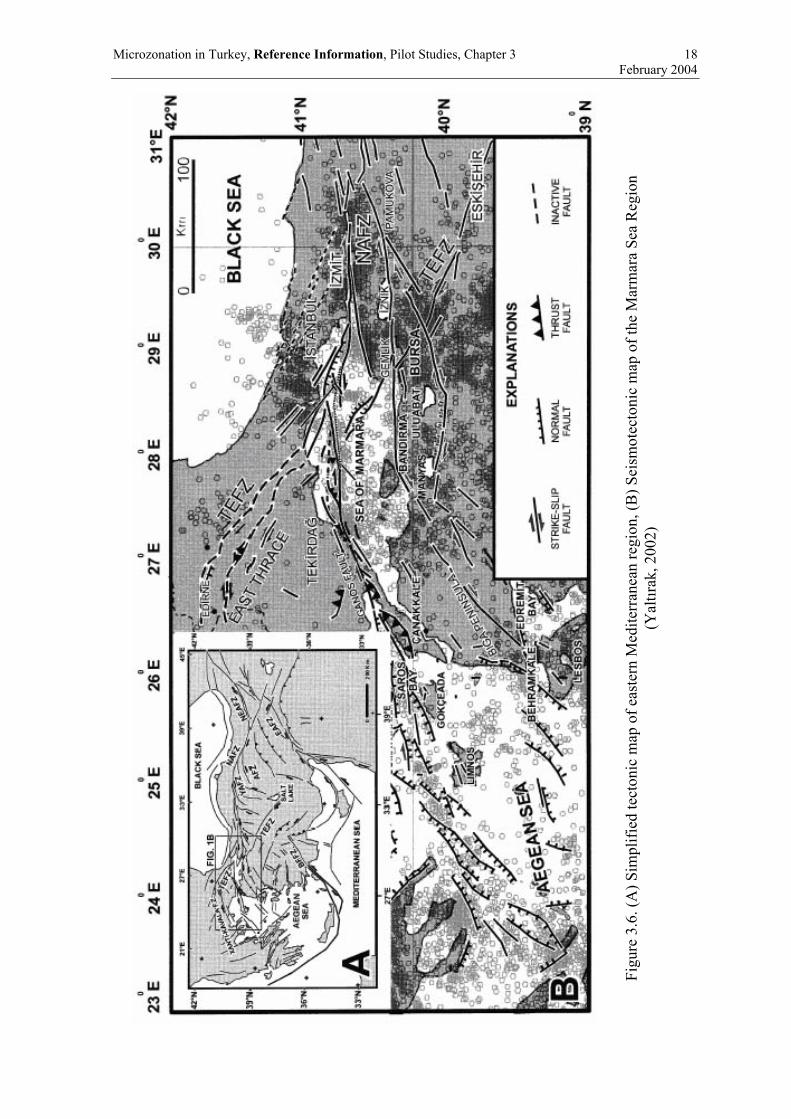
Microzonation in Turkey, Reference Information, Pilot Studies, Chapter 3 18 February 2004
Figu
re 3
.6. (
A) S
impl
ified
tect
onic
map
of e
aste
rn M
edite
rran
ean
regi
on, (
B) S
eism
otec
toni
c m
ap o
f the
Mar
mar
a Se
a R
egio
n (Y
altır
ak, 2
002)

Microzonation in Turkey, Reference Information, Pilot Studies, Chapter 3 19 February 2004
Figure 3.7 Fault segmentation model developed for this study.
3.3. SEISMICITY The historic and instrumental seismicity of the Marmara region has been thoroughly investigated in the report named “Earthquake Risk Assessment in Istanbul Metropolitan Area” prepared by the Earthquake Eng. Dept. of B.U. KOERI (Erdik et al., 2002). The historical seismicity and the seismicity of the 20th century in the Marmara region are illustrated in Figure 3.8 and Figure 3.9 respectively.
Figure 3.8. Historical Earthquakes in the Marmara Sea region
(from Ambraseys & Finkel, 1991)

Microzonation in Turkey, Reference Information, Pilot Studies, Chapter 3 20 February 2004
Figure 3.9. Seismicity of the last century
The association of earthquakes between 1500-present with the segmentation proposed for the Northern Portion of the North Anatolian Fault in the Marmara Region is given in Table 3.1. The historical events, characteristic earthquakes, recurrence intervals and annual probabilities associated with each segment of the model are given in Table 3.2.
Table 3.1. Association of earthquakes between 1500-present with the segmentation proposed for the Northern Portion of the North Anatolian Fault in the Marmara Region.
Earthquake Fault Segment
10.9.1509 (Ms= 7.2) 7, 8
10.5.1556 (Ms=7.2) 9
25.5.1719 (Ms=7.4) 2, 3, 4, 5
2.9.1754 (Ms=6.8) 6
22.5.1766 (Ms=7.1) 7, 8
5.8.1766 (Ms=7.4) 11
10.7.1894 (Ms=7.3) 3, 4, 5
9.8.1912 (Ms= 7.3) 11
17.8.1999 (Ms=7.8) 1, 2, 3, 4

Microzonation in Turkey, Reference Information, Pilot Studies, Chapter 3 21 February 2004
Table 3.2. Characteristic and renewal model parameters associated with the segments. Time dependent Characteristic
Segment Last
Characteristic Earthquake
COV Mean
Recurrence Time
Maximum Magnitude
Time since Last
Eq
50 year prob.
Annual Rate Annual Rate
1 1999 0.5 140 7.2 3 0.0344 0.0007 0.0071 2 1999 0.5 140 7.2 3 0.0344 0.0007 0.0071 3 1999 0.5 140 7.2 3 0.0344 0.0007 0.0071 4 1999 0.5 140 7.2 3 0.0344 0.0007 0.0071 5 1894 0.5 175 7.2 108 0.3734 0.0093 0.0057 6 1754 0.5 210 7.2 248 0.4095 0.0105 0.0048 7 1766 0.5 250 7.2 236 0.3374 0.0082 0.0040 8 1766 0.5 250 7.2 236 0.3374 0.0082 0.0040 9 1556 0.5 200 7.2 446 0.5212 0.0147 0.0050 10 0.5 200 7.2 1000 0.3340 0.0081 0.0050 11 1912 0.5 150 7.5 90 0.4206 0.0109 0.0067 12 1967 0.5 250 7.2 35 0.0203 0.0004 0.0040 13 0.5 600 7.2 1000 0.1771 0.0039 0.0017 14 0.5 600 7.2 1000 0.1771 0.0039 0.0017 15 0.5 1000 7.2 1000 0.0974 0.0020 0.0010 16 1855 0.5 1000 7.2 147 0.0006 0.0000 0.0010 17 1855 0.5 1000 7.2 147 0.0006 0.0000 0.0010 19 1944 0.5 250 7.5 58 0.0597 0.0012 0.0040 21 1999 0.5 250 7.2 3 0.0012 0.0000 0.0040 22 1957 0.5 250 7.2 45 0.0347 0.0007 0.0040 25 0.5 1000 7.2 1000 0.0974 0.0020 0.0010
3.4. METHODOLOGY The earthquake hazards in the region are assumed to be the result of the following contributions, computed in following two steps:
a. Ground motions that would occur as the result from the earthquakes in the magnitude range from 5.0 to 6.9.
b. Ground motions that would result from larger magnitude events in the magnitude range 7.0 and higher.
Part (a) is termed as “background activity”, i.e. the activity not associated with the main tectonic entities. In the computation of part (a), an earthquake catalogue of magnitude 5.0 and higher events are used. These events are not assigned to specific faults (the resolution of the neo-tectonic studies that we have compiled from literature does not allow such an association), but they are assigned to cells of a grid (of size 0.005° x 0.005°), in other words each cell of the grid is assumed to be a potential source for moderately sized events. It is also assumed that a Gutenberg-Richter type recurrence relationship governs the earthquake recurrence in the background.
To compute the seismic activity in each cell first an overall “b” value is calculated for the entire region. Although the maximum likelihood method (Weichert, 1980) yielded a “b” value of 0.8 for the Marmara region, mainly to account for the deficiently reported earthquakes at lower magnitudes, a “b” value of 1.0 is preferred for the analysis. Following that, the “a” value in each source cell is obtained using the earthquake catalogue

Microzonation in Turkey, Reference Information, Pilot Studies, Chapter 3 22 February 2004
considered to be complete since 1900 and 1940 for magnitudes greater than 5.5 and 5.0 respectively. As such, the background activity is assumed to be Poissonian. The girded rates are spatially smoothed with a two-dimensional Gaussian filter with a decay distance of 50 km. This approach is in conformity with what is currently been done by USGS for the assessment of earthquake hazard in California.
Part (b) is related with the seismic energy release along well-defined faults. For this part, a fault segmentation model is developed and it is assumed that energy along these faults is released by characteristic events characterized by magnitude and recurrence time. Two models have been used to determine the seismic activity along these linear source zones: these are a Poisson model using a characteristic earthquake recurrence relationship and a time dependent (renewal) model. The Poisson and the renewal models differ in that in the Poisson model the probability of occurrence of the characteristic event does not change in time, whereas in the renewal model it increases as a function of the time elapsed since the last characteristic event.
The characteristic earthquake recurrence rates are determined by assigning characteristic magnitude and recurrence intervals to each fault segment in the region. The model assumes that seismic energy along the segments ate released by characteristic earthquakes. In this study, the Young and Coppersmith (1985) model is used to determine the magnitude distribution. In this model, the fault generates moderate magnitude earthquake as well as characteristic earthquakes. Figure 3.10 represents the magnitude density function of this model.
Figure 3.11 compares the recurrence relationships that would result from the assumption of “Truncated Exponential (i.e. Gutenberg-Richter) Model” and the “Characteristic Model” based on the Young and Coppersmith (1985) study.
The historical seismicity, the tectonic models and the known slip rates along the faults constitute the main data used in the assignment. The annual rates are then calculated as:
R = 1 / mean recurrence interval (3.1)
The model is Poissonian since the calculated annual probability of occurrence (R) does not change with time.
For the renewal model, the conditional probability for each fault segment is calculated from the mean recurrence interval of the characteristic earthquake determined as explained previously, the elapsed time since the last major earthquake and the exposure period (taken as 50 years). The probabilities are said to be conditional since they change as a function of the time elapsed since the last earthquake. A lognormal distribution with a covariance of 0.5 is assumed to represent the earthquake probability density distribution. The 50 year conditional probabilities thus calculated are converted to effective Poissonian annual probabilities (Pcond) such that (WGCEP, 1995):
Reff = -ln(1 – Pcond) / T (3.2)
The sensitivity of the conditional probabilities to various covariance values for the renewal as well as for the Poisson models for exposure periods of 50 and 5 years is given in Figure 3.12. It can be observed from Figure 3.12 that the probability remains constant for the Poisson model and that as the covariance becomes larger, the conditional probability approaches the Poisson probability.
The total hazard in the region is calculated as the summation of hazards computed in steps (a) and (b).

Microzonation in Turkey, Reference Information, Pilot Studies, Chapter 3 23 February 2004
The ground motion parameters used in the quantification of the earthquake hazard for this study are the peak ground acceleration (PGA) and the spectral accelerations (SA) for natural periods of 0.2 and 1.0 seconds. The ground motions are determined for soft rock (NEHRP B/C boundary) conditions. Boore et al. (1997), Campbell (1997) and Sadigh et al. (1997) have proposed the attenuation relationships used in the assessment of PGA, whereas those of Boore et al. (1997) and Sadigh et al. (1997) have been used for SA. Although the initial choice of these attenuation relationships follow that of USGS studies for California, nevertheless, these Western US–based attenuation relationships have been found to provide good correlation with the attenuation characteristics of ground motion in the Northwestern Anatolia Region (Özbey, 2001; Erdik et al., 2002).
3.5. RESULTS The results of the North-west of Turkey region for 10% probability of exceedance in 50 years for PGA are illustrated in order to give an idea in Figure 3.13.
The results obtained for 10% probability of exceedance in 50 years for PGA and SA at 0.2 sec and 1.0 sec. natural periods at NEHRP B/C boundary site class for the Poissonian and renewal models are presented in Figure 3.14 through Figure 3.19 and Figure 3.20 through Figure 3.25 for (A) Adapazarı and (B) Gölcük, Değirmendere and İhsaniye regions respectively. For display purposes, the hazard maps are overlain with the grids to be used in the quantification (lumping) of the microzonation information in this study, supplied and used by the other teams.
After the last meeting, the result acquired for 40% probability of exceedance in 50 years (about 100 return period) for PGA and SA at 0.2 sec. and 1.0 sec natural periods at NEHRP B/C boundary site class for the Poissonian model and are presented in Figure 3.26 through Figure 3.28 for (A) Adapazarı and in Figure 3.29 through Figure 3.31 for (B) Gölcük, Değirmendere and İhsaniye regions.
3.6. DISCUSSION We would like to put some emphasis on the following points about the hazard assessment results:
Hazard in the region has been assessed for “b” values of both 0.8 (obtained as the result of the maximum likelihood method) and 1.0 (adopted to account for the deficiency in small magnitude events) but the results did not show much difference, since the hazard in the region is essentially controlled by the faults.
Various statistical models have been proposed for the computation of the probability density function, such as Gaussian, log-normal, Weibull, Gamma and Brownian. Among those, the log-normal distribution is the most commonly used in the engineering practice. The Brownian Passage Time (BPT) model is a more recently proposed model and is also assumed to adequately represent the earthquake distribution. The probability density functions of the two models are similar, but the conditional probabilities begin to diverge around the mean recurrence time. However, the BPT distribution yields higher conditional probabilities for large elapsed times since the last earthquake. We have investigated the sensitivity of the annual rates to the model chosen, and to the aperiodicity (alpha, BPT model) and to the coefficient of variation (COV, Lognormal model). The annual rates are highly sensitive to the alpha/COV values, larger values yielding smaller annual rates. The BPT and Lognormal distributions give considerable differences only for large elapsed times since the last characteristic event. A small COV (i.e. 0.3 or less) indicates that the characteristic earthquakes are highly periodic. As the COV grows larger (i.e. 0.7 or higher)

Microzonation in Turkey, Reference Information, Pilot Studies, Chapter 3 24 February 2004
the conditional probabilities approach those of the Poisson probabilities. As such, we have to decide on the appropriate choice of alpha/COV values. Following the California practice, we have used a value of 0.5.
We have experimented with cascade models. It is well known that, even though segments can be mapped separately at the surface, they could combine and be a single structure at depth, or a rupture on one segment could trigger ruptures on others in a cascade model. So two scenarios are envisioned: (1) faults rupture independently, producing characteristic-size earthquakes (the model incorporated in the report reviewed), or (2) fault segments rupture together as a cascade, producing earthquakes of M>7. The Cascade assumption increases the Maximum Magnitude but reduces the rate of occurrence of the more moderate events. Previous rupturing cycles around the Marmara Sea indicate that, on average, one out of three ruptures were multiple segments. The probabilistic results based on cascade models provided about the same earthquake hazard levels obtained from non-cascading models.
Although the comparison between Poissonian and renewal models shows large hazard differences, it does not indicate that the seismic potential in the region (say Adapazarı) is depleted or exhausted. The current “Earthquake Hazard Zoning Map” of Turkey provides an effective PGA of 0.4 g for Adapazarı, which compares favorably with the results obtained from the renewal model.
Finally we would like to note that the methodology adopted causes the concentration of the hazard at some segment junction points such as the junction region of segments S3, S2 and S12 in Figure 3.14 through Figure 3.16. If segment S12 was removed from the model, this “mapping” would disappear.

Microzonation in Turkey, Reference Information, Pilot Studies, Chapter 3 25 February 2004
Figure 3.10. The definition of the magnitude probability density for characteristic
earthquake model
Figure 3.11. An illustrative comparison of recurrence relationships

Microzonation in Turkey, Reference Information, Pilot Studies, Chapter 3 26 February 2004
Figure 3.12. Sensitivity of the time dependent probabilities for a renewal model with 50
and 5 year exposure periods (After Abrahamson, 2000)
Figure 3.13. PGA contour map at NEHRP B/C boundary site class for 10% probability of
exceedance in 50 years (Poissonian model)

Microzonation in Turkey, Reference Information, Pilot Studies, Chapter 3 27 February 2004
Figu
re 3
.14.
PG
A c
onto
ur m
ap a
t NEH
RP
B/C
bou
ndar
y si
te c
lass
fo
r 10%
pro
babi
lity
of e
xcee
danc
e in
50
year
s for
Ada
paza
rı re
gion
(Poi
sson
ian
mod
el)
Figu
re 3
.15.
SA
(T=0
.2se
c) c
onto
ur m
ap a
t NEH
RP
B/C
bou
ndar
y si
te c
lass
for 1
0% p
roba
bilit
y of
exc
eeda
nce
in 5
0 ye
ars f
or
Ada
paza
rı re
gion
(Poi
sson
ian
mod
el)

Microzonation in Turkey, Reference Information, Pilot Studies, Chapter 3 28 February 2004
Figu
re 3
.16.
SA
(T=1
.0se
c) c
onto
ur m
ap a
t NEH
RP
B/C
bou
ndar
y si
te c
lass
for 1
0% p
roba
bilit
y of
exc
eeda
nce
in 5
0 ye
ars f
or
Ada
paza
rı re
gion
(Poi
sson
ian
mod
el)
Figu
re 3
.17.
PG
A c
onto
ur m
ap a
t NEH
RP
B/C
bou
ndar
y si
te c
lass
fo
r 10%
pro
babi
lity
of e
xcee
danc
e in
50
year
s for
Ada
paza
rı re
gion
(Ren
ewal
mod
el)

Microzonation in Turkey, Reference Information, Pilot Studies, Chapter 3 29 February 2004
Figu
re 3
.18.
SA
(T=0
.2se
c) c
onto
ur m
ap a
t NEH
RP
B/C
bou
ndar
y si
te c
lass
for 1
0% p
roba
bilit
y of
exc
eeda
nce
in 5
0 ye
ars f
or
Ada
paza
rı re
gion
(Ren
ewal
mod
el)
Figu
re 3
.19.
SA
(T=1
.0se
c) c
onto
ur m
ap a
t NEH
RP
B/C
bou
ndar
y si
te c
lass
for 1
0% p
roba
bilit
y of
exc
eeda
nce
in 5
0 ye
ars f
or
Ada
paza
rı re
gion
(Ren
ewal
mod
el

Microzonation in Turkey, Reference Information, Pilot Studies, Chapter 3 30 February 2004
Figure 3.20. PGA contour map at NEHRP B/C boundary site class for 10% probability of
exceedance in 50 years for Gölcük region (Poissonian model)
Figure 3.21. SA (T=0.2sec) contour map at NEHRP B/C boundary site class for 10%
probability of exceedance in 50 years for Gölcük region (Poissonian model)

Microzonation in Turkey, Reference Information, Pilot Studies, Chapter 3 31 February 2004
Figure 3.22. SA (T=1.0sec) contour map at NEHRP B/C boundary site class for 10%
probability of exceedance in 50 years for Gölcük region (Poissonian model)
Figure 3.23. PGA contour map at NEHRP B/C boundary site class for 10% probability of
exceedance in 50 years for Gölcük region (Renewal model)

Microzonation in Turkey, Reference Information, Pilot Studies, Chapter 3 32 February 2004
Figure 3.24. SA (T=0.2sec) contour map at NEHRP B/C boundary site class for 10%
probability of exceedance in 50 years for Gölcük region (Renewal model)
Figure 3.25. SA (T=1.0sec) contour map at NEHRP B/C boundary site class for 10%
probability of exceedance in 50 years for Gölcük region (Renewal model)

Microzonation in Turkey, Reference Information, Pilot Studies, Chapter 3 33 February 2004
Figu
re 3
.26.
PG
A c
onto
ur m
ap a
t NEH
RP
B/C
bou
ndar
y si
te c
lass
for
40%
pro
babi
lity
of e
xcee
danc
e in
50
year
s for
Ada
paza
rı re
gion
(P
oiss
onia
nm
odel
)
Figu
re 3
.27.
SA
(T=0
.2 se
c) c
onto
ur m
ap a
t NEH
RP
B/C
bou
ndar
y si
te c
lass
for 4
0% p
roba
bilit
y of
exc
eeda
nce
in 5
0 ye
ars f
or A
dapa
zarı
regi
on(P
oiss
onia
nm
odel
)

Microzonation in Turkey, Reference Information, Pilot Studies, Chapter 3 34 February 2004
Figure 3.28. SA (T=1.0 sec) contour map at NEHRP B/C boundary site class for 40%
probability of exceedance in 50 years for Adapazarı region (Poissonian model).
Figure 3.29. PGA contour map at NEHRP B/C boundary site class for 40% probability of
exceedance in 50 years for Gölcük region (Poissonian model)

Microzonation in Turkey, Reference Information, Pilot Studies, Chapter 3 35 February 2004
Figure 3.30. SA (T=0.2 sec) contour map at NEHRP B/C boundary site class for 40%
probability of exceedance in 50 years for Gölcük region (Poissonian model).
Figure 3.31. SA (T=0.1 sec) contour map at NEHRP B/C boundary site class for 40%
probability of exceedance in 50 years for Gölcük region (Poissonian model).

Microzonation in Turkey, Reference Information, Pilot Studies, Chapter 3 36 February 2004
3.7. RESPONSE SPECTRA The shape of the response spectrum (5% damped) will be taken equal to the so-called “Uniform Hazard Response Spectrum” provided in NEHRP (1997) Provisions. This spectrum is determined on the basis of the site-specific short-period (Sms) and medium-period (Sm1) spectral accelerations as illustrated in Figure 3.32.
Sms = Fa . Ss (3.3)
Sm1 = Fv . S1 (3.4)
Ss and S1 are represented by the SA calculated, respectively, at T=0.2 s and T=1.0 s periods for NEHRP Site Class B/C Boundary and plotted in Figures 3.15, 3.16, 3.18, 3.19, 3.27, 3.28 for Adapazarı region and in Figures 3.21, 3.22, 3.24, 3.25, 3.30, 3.31 for Gölcük region. Fa and Fv are respectively the Short and Medium Period Amplification Factors, originally defined in NEHRP (1997). For the ground motion defined at NEHRP Site Class B/C Boundary, Fa = Fv =1.
Figure 3.32. NEHRP (1997) Uniform Hazard Response Spectrum
3.8. SPECTRUM COMPATIBLE DESIGN BASIS GROUND MOTION
For simulation of time domain ground motion compatible with the response spectra presented, the procedure developed by Deodatis (1996) and coded by Papageorgiou et. al. (2000) will be utilized. The target acceleration spectra compatible time history is a ground motion simulation program generating a synthetic time history of ground acceleration. The time domain simulations are non-stationary with random phase.
Please note that this may not be the perfect methodology since the spectrum on which the simulation is based may not correlate with a physically realizable earthquake and we are fully aware of the issues associated with such an approach. However, other more rigorous approaches (e.g. deterministic simulation of ground motion after de-

Microzonation in Turkey, Reference Information, Pilot Studies, Chapter 3 37 February 2004
aggregation of the probabilistic hazard) are suited more to site-specific studies and are not compatible with the scope and the depth of this investigation.
As an example simulation was done for the centroid of the cell R16 in Adapazarı study area. As a result of the simulation, the acceleration time history, velocity and displacement motions, which depend on acceleration time history, were obtained using the spectral acceleration values at t=0.2 sec and t=1 sec belonging to cell R16. Based on these two parameters, horizontal and vertical components of the simulated time history were obtained as presented in Figure 3.33 and Figure 3.34.
The spectral acceleration values at t=0.2 sec and t=1.0 sec, obtained from the hazard study for 40% probability of exceedance in 50 years, were assigned to the microzonation study cells as Sms and Sm1 respectively and input files for every cell in Adapazarı and Gölcük regions were prepared (Annex 2C.1).

Microzonation in Turkey, Reference Information, Pilot Studies, Chapter 3 38 February 2004
Figu
re 3
.33.
Res
pons
e Sp
ectru
m C
ompa
tible
Ran
dom
H
oriz
onta
l Gro
und
Mot
ion
at C
ell R
16 (F
ree-
field
ou
tcro
p of
NEH
RP
B/C
Bou
ndar
y)
Figu
re 3
.34.
Res
pons
e Sp
ectru
m C
ompa
tible
Ver
tical
G
roun
d M
otio
n at
Cel
l R16
(Fre
e-fie
ld o
utcr
op o
f N
EHR
P B
/C B
ound
ary)

Microzonation in Turkey, Reference Information, Pilot Studies, Chapter 4 39 February 2004
4. SINGLE-STATION AMBIENT VIBRATION MEASUREMENTS AND INTERPRETATION FOR THE CITIES OF ADAPAZARI AND GÖLCÜK, TURKEY
D. Fäh and A. Christen (Swiss Seismological Service, ETH Zürich, Switzerland) with the cooperation of Ü. Gülerce (Istanbul Technical University, Turkey) and C. Greifenhagen (ETH Lausanne, Switzerland).
4.1. SUMMARY Single station ambient vibration measurements have been performed in the two cities Adapazarı and Gölcük in Turkey. These cities suffered heavy damage during the 1999 Kocaeli earthquake. The work presented here is a contribution to the DRM-MERM Project. The main goals of our work are to determine the fundamental frequencies of resonance of the soils within the studied areas, to provide a preliminary interpretation of the subsurface structure and its variation, and to propose a zonation based on the shape of the observed ambient vibration H/V spectral ratios. Published S-wave velocity profiles have been used to compute synthetic H/V spectral ratios, which are then compared to the observation.
4.2. INTRODUCTION The investigation of the local ground condition is an important part of any site-specific hazard assessment. One of the key parameters is the S-wave velocity structure of the unconsolidated sediments and the S-wave contrast between bedrock and sediments. These parameters together with the geometry of the bedrock-sediment interface mainly control the amplification of seismic waves during earthquakes. By knowing the structure, a prediction of amplification effects can be performed with numerical simulation techniques.
The S-wave velocity structure can be obtained through active in-situ measurements such as S-wave seismics, surface-wave measurements with single stations or arrays, and down-hole and cross-hole techniques. Passive methods based on ambient vibrations or microtremors are of special interest. These methods can be applied in urban areas where in general it is not possible to carry out active measurements due to the lack of space for the experimental setup or restrictions on using explosion sources. Array methods were established by Horike (1985) after the pioneering work done by Aki (1957). These methods make use of the dispersive character of surface waves, and allow determining shear-wave velocity profiles from the inversions of dispersion curves. The waves involved in the microtremors are surface waves as well as body waves of P and S-type, and observed wave fields are composed of several different modes that are in general not separated in time. This unknown composition of the wavefield is a major problem in microtremor methods. Array measurements of ambient vibrations have been performed in the target areas by Kudo et al. (2002) and Yamanaka et al. (2001). Their results will be evaluated within our study, and are used for the interpretation of the subsurface structure and its variation.
The fundamental frequency of resonance f0 is a quantity that can be derived from the S-wave velocity structure of the site. Amplification of waves as a function of frequency is therefore directly related to f0. The fundamental frequency can be obtained from a single-station ambient vibration measurement using the H/V method proposed by Nakamura (1989). This method has proven to be the most convenient technique to estimate the fundamental frequency of soft deposits (Lachez and Bard, 1994; Lermo and Chavez-Garcia, 1994) and is applied in this study using an algorithm described in Fäh et al. (2001). If borehole data can be used for calibration, the procedure has the potential to allow estimates

Microzonation in Turkey, Reference Information, Pilot Studies, Chapter 4 40 February 2004
of shear-wave velocity of the unconsolidated sediments. In one-dimensional structures, average H/V spectral ratios can be assumed to measure the ellipticity of the fundamental mode Rayleigh wave. The ellipticity at each frequency is defined as the ratio between the horizontal and vertical displacement eigenfunctions in the P-SV case, at the free surface. Hence the shape of H/V ratios can be used to estimate the shear-wave velocity profile. Yamanaka et al. (1994) and Satoh et al. (2001) applied this idea for deep sedimentary basins, Fäh et al. (2001) and Yamanaka et al. (2001) for shallow sites. Such methods have not been applied in this study, due to the lack of borehole information.
H/V spectral ratios can be considered as the fingerprint of the local structure. By comparing measurements within an area, similar H/V curves are observed on similar local structures. Such comparison therefore allows for a zonation. Each site within one zone is expected to show similar amplification effects during earthquakes. This idea will be applied for the two cities in order to propose a zonation based on the shape of the observed ambient vibration H/V spectral ratios.
4.3. FIELD CAMPAIGN AND INSTRUMENTATION In August 2002 an ambient-vibration measurement campaign was carried out in the area of Adapazarı and Gölcük. The campaign was prepared in Zurich and included a training course for the use of the instruments and analysis software. One of the major difficulties for the planning of the campaign was the lack of geographical maps. This problem could be only partly resolved during the field campaign.
The ambient-vibration measurements were performed with Mars88 recorders and Lennartz 5sec sensors. A standard set-up of the recorders has been used the details of which is given in Appendix 1.1. Three sets of instruments were provided by the Swiss Seismological Service. The equipment was shipped by DEZA. The DRM-MERM project management provided field assistance, and organized accommodation and transportation during the campaign.
During the 20 days of the campaign, 211 measurements were performed inside the Adapazarı area and 31 in Gölcük. Three independent teams performed the measurements. The meaning of the point names is described in Appendix 1.2. An overview of the measuring sites is given in Figures 4.1 and 4.2. During the campaign, the recorded signals were analyzed in order to check their quality. The decision was made for the next day’s measurements based on the latest set of results.
The entire dataset has been analyzed at the Swiss Seismological Service in order to perform a quality control, and to provide a homogeneous dataset and interpretation. Possible flawed parts of the recording and signals caused by near-sensor sources were removed. The dataset is available on CD-ROM; the content of the CD-ROM is described in Appendix 1.4. The data are provided in SAF format. The format is described in Appendix 1.3. The H/V method is shortly described in the following chapter.
4.4. COMPUTATION OF H/V RATIOS
Two methods are applied to compute average H/V ratios. The combination of both then allows for a future inversion of the H/V ratio for the S-wave velocity structure of the site, in case borehole information or seismic measurements may become available.
In the classical polarization analysis in the frequency domain, the polarization is defined as the ratio between the Fourier spectra of the horizontal components and the spectrum of the vertical component. In this study the H/V polarization at a site is computed

Microzonation in Turkey, Reference Information, Pilot Studies, Chapter 4 41 February 2004
as the average from many windows of noise data, each with fixed length. For each window the Fourier spectra are computed and no smoothing is applied to the spectra. The ratio is formed and the polarizations are averaged over all windows using log10 of the single H/V ratios. Finally the average spectral ratio is slightly smoothed. The result for the classical H/V ratio is always shown in blue in the figures.
The SH part of the wavefield contributes to the horizontal component of motion in the measurements. The SH-wave contribution cannot be determined from a single station measurement, because source locations and mechanisms of ambient vibrations are in general unknown. This requires some assumptions concerning the spectral content of SH-waves. A reasonable assumption is that the transverse part of the wave field has a similar spectrum and energy content to the radial part (Fäh et al., 2001). This results in a reduction factor of the square root of 2 for the H/V ratio when considering only P-SV waves. The classical H/V curves in this study are all corrected with this factor.
The second method for H/V ratios tries to reduce the SH-wave influence by identifying P-SV-wavelets from the signal and taking the spectral ratio only from these wavelets. This is done by means of a frequency-time analysis (FTAN) of each of the three components of the ambient vibrations (Fäh et al., 2001). In a frequency-time representation of the vertical signal, the most energetic sections are identified in time for each frequency. We assume that this maximum is related to a single P-SV wavelet.
Because the horizontal component of the wavelet may be phase shifted with respect to the vertical component, it is selected from a time window centered at the arrival time of the maximum energy on the vertical component and with a width of one wave period. The horizontal component is selected as the maximum of the quadratic mean of the spectral values from both components and the H/V ratio is formed for the wavelet with this value. The polarization spectra with this technique are computed for different windows of the noise data and averaged without any smoothing.
In the figures, the result with this FTAN based method is always shown in a green color. The similarity in shape and amplitude of the two H/V curves supports the assumptions made for the SH-wave content for the classical method. We provide an interpretation only for frequencies above 0.2 Hz, because this frequency is the eigenfrequency of the sensor.
The software that has been used to compute H/V spectral ratios (Matlab Routine Analyse13SAF.m) and to visualize the results (Matlab Routine Bild1DRMA.m) are provided on the CD-ROM. The amplitudes of the H/V spectral ratios are always given at log10 scale.

Microzonation in Turkey, Reference Information, Pilot Studies, Chapter 4 42 February 2004
Adapazarı
# #
#
#
#
##
#
###
##
###
##
#
##
##
#
#
#
#
#
#
#
#
#
##
#
#
#
##
# #
##
#
####
#
## #
#
##
##
##
#
#
#
#
#
##
#
#
#
##
#
#
##
#
#
#
#
#
#
##
#
#
#
#
#
##
##
#
#
##
##
##
#
#
##
#
###
###
#
##
#
#
#
#
##
#
#
# #
#
#
#
##
#
#
#
#
#
##
##
#
#
#
##
#
#
##
# #
#
###
#
###
##
#
#
#
#
#
#
#
#
###
##
#
#
#
#
###
#
#
#
#
#
#
#
##
#
###
###
#
#
#
#
#
#
# ##
##
#
#
#
#
#
TEK
SRFBABSEK
SKR
ADUGEN
YEN
HAS
ERESIC
ADC
0 2 4 Kilometer
N
EW
S
Measurement Points
Border Target AreaLakes & RiversStreetsRailroad
#
Figure 4.1. Microtremor measurements in Adapazarı; S-wave velocity profiles are
available from ambient-vibration array measurements at sites ADU and ADC (Kudo et al., 2002) and YEN, SRF, TEK, ERE, SIC (Yamanaka et al., 2001). BAB, HAS, GEN, SEK
and SKR are the strong-motion recording sites.

Microzonation in Turkey, Reference Information, Pilot Studies, Chapter 4 43 February 2004
Gölcük
#
#
#
#
# ##
#
#
#
##
#
#
#
##
#
#
#
#
#
#
#
#
#
#
#
#
#
#
DMD
GLF
GEMGYM
GLH
FOC
LOJ
PIR
N
EW
S
# Measurement Points
0 1 2 Kilometers
Figure 4.2. Microtremor measurements in Gölcük; S-wave velocity profiles are available from ambient-vibration array measurements at sites GLF and GLH (Kudo et al., 2002).
DMD, FOC, LOJ, GYM, GEM and PIR are the strong-motion recording sites.
4.5. RESULTS FOR THE AREA OF ADAPAZARI All ambient vibration records have been analyzed and the fundamental frequency of resonance has been determined for all sites (Figure 4.3). In general, a careful geological investigation of the site is a prerequisite to ensure that the investigated peak in the H/V ratio is related to the fundamental mode Rayleigh wave, and therefore to the fundamental frequency of resonance. In structures with two, or maybe three strong impedance contrasts, we can expect to obtain several peaks related to the fundamental and higher modes Rayleigh waves.
The two-layer case can be observed for the northern part in the Adapazarı area. For this area, array measurements provide S-wave velocity profiles down to bedrock. As we will show later on, numerical simulation of H/V spectral ratios with such profiles show good agreement with measured H/V curves. In the southern part of the Adapazarı area, we have no information about the thickness and layering of the soft sediments. The interpretation given for this area is therefore not unique.
The area of Adapazarı can be divided into several zones with similar shape of the H/V spectral ratios. The zones are shown in Figure 4.3 and examples of H/V spectral ratios for each zone are given in Figure 4.4 to Figure 4.8. The amplitudes are given at log10 scale. The following zones can be distinguished:
A. The fundamental frequency of resonance is between 0.22 and 0.50 Hz, with a second peak at around 0.7-0.8 Hz. For this area, S-wave velocity profiles are available from ambient-vibration array measurements (Kudo et al., 2002; Yamanaka et al., 2001), and the velocity profiles will be discussed further on. The H/V spectral

Microzonation in Turkey, Reference Information, Pilot Studies, Chapter 4 44 February 2004
ratio shown in Figure 4.4 is a typical example of a structure with two layers. The surface sediments are composed of clays and silts, inter-bedded with gravel layers. The thickness of this layer is between 20 and 80 m. The large amplitude of the second peak (0.7-0.8 Hz) is due to the large S-wave velocity contrast between the surface sediments and the deep sediments. The deep sediments have a maximum thickness of about 300 to 400 m.
B. The observed H/V spectral ratios are characterized by one peak at the fundamental frequency of resonance. An example of a measured H/V spectral ratio is given in Figure 4.5. This type of spectrum is observed at the borders of the sedimentary basins. The frequency of the peak is varying from 0.7 Hz to values above 10 Hz, depending of the thickness of the soft sediments. Close to the foot of the hills, the fundamental frequency is high and it is decreasing towards the sedimentary basins. This spatial variation of the structure might be responsible for the excitation of local surface waves during earthquakes. Due to the smooth variation of the fundamental frequency of resonance, we can approximate the structure by a model composed of one-layer of soft sediments over bedrock. An inversion applied to the observed H/V ratios could define the gradient in S-wave velocity of this layer. A prerequisite would be borehole information down to the bedrock layer. The transition between zone B and A is very abrupt, which indicates that the deep sedimentary layer appears at this transition with a rapid increase of the thickness of the deep sediments.
C. Hill area, no clear peak is visible in the H/V spectral ratios. An example of a measured H/V spectral ratio is given in Figure 4.6. This zone can be considered as bedrock. Between the different small hills, small deposits of soft sediments can be identified, with observed fundamental frequency of resonance above 3 Hz. The density of measurements is not sufficient to resolve these small areas.
D. At all stations in this zone, the H/V spectral ratios show a clear peak around 0.4 to 0.5 Hz. An example of a measured H/V spectral ratio is given in Figure 4.7. For some stations an additional peak is seen below 0.2 Hz. For the deep sediments in this zone no geophysical information is available to us, and two possible basin models can be proposed: a deep and a shallow basin with fundamental frequency of resonance below 0.2 Hz or in the 0.4-0.5 Hz range respectively. The deep-basin model would require an interpretation of the observed H/V ratios at low frequencies with a two-dimensional structural model in order to explain the frequency distribution (Steimen et al., 2003). Due to the very clear peak in the H/V ratio, the shallow-basin model is favored. The large amplitudes of the H/V spectral ratio at the fundamental frequency around 0.4 Hz indicate a strong velocity contrast between sediments and bedrock. This can be explained by the presence of a thick layer of lake sediments with very low S-wave velocities. The small variation of the fundamental frequencies indicates a homogeneous layering of the soil deposit, with a maximum thickness of about 150-200 m.
E. The H/V spectral ratios measured in this zone show a double peak with one peak at 0.5 Hz and the other at around 1Hz. These two frequencies correspond to the ones of the neighboring sites to the west in zone D (0.5 Hz) and to the east in zone B (1 Hz). We might expect in zone E a change of the structure, and it may be possible that the layer of very soft lake sediments appear. An interpretation of the H/V spectral ratios with one-dimensional structural models is considered to be not valid anymore.

Microzonation in Turkey, Reference Information, Pilot Studies, Chapter 4 45 February 2004
# #
#
#
#
##
##### #
###
#####
#####
#
###
#
#
####
#
##
# ####
####### ##
####
### ##
##
###
##
###
## ##
##
##
#
##
#
##
##
### #
#
###
#####
### #
######
###
###
#
###
#
# #
#
#
#
##
##
#
#
#
# #
###
##
# #
#
## #
# #####
## ##
##
#
#
#
#
#
##
#
# ##
###
#
#### #
#
#
#
#
##
#
# ##
###
###
##
##
#
## ### #
#
#
##
#
ADC
SICERE
HAS
YENGEN
ADU
SKR
SEK BAB SRF
TEKA
BC
D
CE
+B
0 1 2 3 4 Kilometers
N
EW
S
Border Target AreaRivers
Zone Borders
Fundamental Frequency (Hz)# n/a# 0 - 0.33# 0.33 - 0.66# 0.66 - 1# 1 - 1.33# 1.33 - 1.66# 1.66 - 2# 2 - 2.33# 2.33 - 2.66# 2.66 - 15
Figure 4.3. Measured fundamental frequencies of resonance in the Adapazarı area (Values
in Hz); The zones with similar H/V spectral ratios are given with an index from A to E.

Microzonation in Turkey, Reference Information, Pilot Studies, Chapter 4 46 February 2004
Figure 4.4. Example of an H/V spectral ratio observed in zone A. (Site: ac06_u01)
Figure 4.5. Example of an H/V spectral ratio observed in zone B. (Site: ac07_u05)

Microzonation in Turkey, Reference Information, Pilot Studies, Chapter 4 47 February 2004
Figure 4.6. Example of an H/V spectral ratio observed in zone C. (Site: ab08_r01)
Figure 4.7. Example of an H/V spectral ratio observed in zone D. (Site: ay11_c01)

Microzonation in Turkey, Reference Information, Pilot Studies, Chapter 4 48 February 2004
Figure 4.8. Example of an H/V spectral ratio observed in zone E. (Site: ab11_u01)
The f0 values at each site are finally interpolated linearly and slightly smoothed, resulting in a fundamental frequency map shown in Figure 4.9. The fundamental frequency follows the main geologic features and allows a qualitative description of expected amplification of waves as a function of frequency. At frequencies much below f0 there is no amplification of waves when compared to the hill zone. In our case of a strong impedance contrast between bedrock and sediment, amplification around f0 can be very strong. The amplification at frequencies above f0 depends on the layering of the soils and the incident wave field.

Microzonation in Turkey, Reference Information, Pilot Studies, Chapter 4 49 February 2004
# #
#
$T
#
##
#
###
##
###
$T#
##
#
##
##
#
#
#
#
#
#
#
$T$T#
##
##
# ###
%U
####
#
## #
#
##
##
###
#
##
#
##
#
##
##
#
#
##
#
#
#
#
#
#
#%U
#
%U
#
#
$T
##
##
#
#
####
%U##
#
##
#
####
##
###
#
#
#
#
##
#
#
# #
# #
#
##
#
%U
# #
# #
# # #
#
#
#
##
# #
# # # # %U
###
##
# #
##
# #
#
#
#
# #
# % U
# # # #
#
#
# # # # #
#
#
#
# #
# #
# # #
# # #
###
#
#
#
#
#
## #
##
#
#
#
#
#
#
A
B C
D
C E
B +
1. 3 4 - 1 . 6 6 # 1. 0 1 - 1 . 3 3 # 0. 6 7 - 1 . 0 0 # 0. 3 4 - 0 . 6 6 # 0. 0 0 - 0 . 3 3 # F u n da m e n t a l F r e q u e n cy (Hz)
# Am b i e n t V i b r a t i o n R ecordings% U Arr a y R e c o r d i n g s $ T Str o n g M o t i o n S t a t i o ns
Zo n e B o r d e r s
N
EW S
# 1. 6 7 - 2 . 0 0 # 2. 0 1 - 2 . 3 3 # 2. 3 4 - 2 . 6 6 # 2. 6 7 - 1 5
Figure 4.9. Map of fundamental frequencies in Adapazarı. Sites at which array
measurements have been performed are given as yellow squares, sites of the strong motion aftershock recordings are given as yellow triangles.
The amplitude of the H/V spectral ratio at the fundamental frequency f0 is an indicator for the S-wave velocity contrast between bedrock and sediments, and therefore provides some information on the severity of the resonance effects. The higher the amplitudes the larger is the velocity contrast. The amplitude values of the H/V ratios at each site are interpolated linearly and slightly smoothed, resulting in a map shown in Figure 4.10 at a log10 scale. The amplitude depends on the source-depth distribution and source-distance distribution. Amplitudes of the H/V ratio therefore provide only a qualitative indicator of the possible resonance effects. The largest amplitudes are observed in the zone D, where the layer of very soft sediments causes the large amplitudes of the H/V spectral ratios. The other areas with high amplitude are located in zone B, close to the transition between bedrock and sediments.

Microzonation in Turkey, Reference Information, Pilot Studies, Chapter 4 50 February 2004
# #
#
$T
#
##
#
###
##
###
$T#
##
#
##
##
#
#
#
#
#
#
#
$T$T#
##
##
# ###
%U
####
#
## #
#
##
##
###
#
##
#
##
#
##
##
#
#
##
#
#
#
#
#
#
#%U
#
%U
#
#
$T
##
##
#
#
####
%U##
#
##
#
####
##
#
##
#
#
#
#
##
#
#
# #
# #
#
##
#
%U
# #
#
##
# #
#
#
#
##
# #
# # # # %U
###
##
# #
##
#
#
#
#
#
# #
# % U
# # # #
#
#
# # # # #
#
#
#
# #
# #
# # #
# # #
###
#
#
#
#
#
## #
##
#
#
#
#
#
#
A
B C
D
C E
B +
0.8 1 - 1 . 0 0 # 0.6 1 - 0 . 8 0 # 0.4 1 - 0 . 6 0 # 0.2 1 - 0 . 4 0 # 0.0 0 - 0 . 2 0 # A m p litu d e ( l o g 1 0 v a l u e s)
# Amb i e n t V i b r a t i o n R e cordings% U Arra y R e c o r d i n g s $ T Stro n g M o t i o n S t a t i o n s
Zon e B o r d e r s
N
E W S
Figure 4.10. Map of the amplitude of the H/V spectral ratio at the fundamental frequency
in Adapazarı
The amplitude of the second peak of the H/V spectral ratio provides some information about the velocity contrast between the surface sediments and the deep sediments (in the two-layer over bedrock case). The larger the amplitude of the ratio, the higher is the velocity contrast. An example is the H/V ratio shown in Figure 4.4 with the second peak at 0.7-0.8 Hz. In zone A, we have evidence for this two-layer structure from the array measurements performed by Kudo et al. (2002) and Yamanaka et al. (2001). This interpretation of the second peak is only allowed as long as the f0 of the surface low-velocity layer is considerably larger than the fundamental frequency of the entire soil column.
4.5.1 Comparison between synthetic H/V spectral ratios and observations S-wave velocity profiles are available from ambient-vibration array measurements at sites ADU and ADC (Kudo et al., 2002) and YEN, SRF, TEK, ERE, SIC (Yamanaka et al.,

Microzonation in Turkey, Reference Information, Pilot Studies, Chapter 4 51 February 2004
2001). The models proposed by Kudo are given in Table 4.1. The sites of the arrays could not be exactly reconstructed, and the location error of the site is within a radius of about 50 m. Yamanaka does not provide station coordinates and velocity profiles in tabular form. Our modeling results for these sites are therefore only indicative, and are not shown here.
We have used the proposed structural models in Table 4.1 to compute synthetic H/V spectral ratios, and to compare them to the observed ratios at the sites. The modeling of synthetic H/V ratios requires some assumptions to be made about the distribution of the source positions, and we try to keep the assumptions as general as possible by superposing a multitude of sources over a wide distance range.
Table 4.1. S-wave velocity profiles proposed by Kudo et al. (2002) for two sites in Adapazarı
ADC ADU Vs (m/sec) Thickness (m) Vs (m/sec) Thickness (m) 243 38 441 97 728 242 1500 70 2000 halfspace
166 44 331 88 500 281 878 63 1050 100 1500 halfspace
The numerical technique used is the mode summation method (Panza, 1985; Panza and Suhadolc, 1987) for the P-SV part of the wavefield. The method allows the investigation of signals from well-defined sources and source-receiver distances. For a given structure the P-SV modes are first calculated. From the defined source the energy content of each mode in the Fourier domain is computed, and then summed to derive the actual wavefield. In order to generate synthetic ambient vibration wave fields, multiple sources are considered. Randomly distributed sources are assumed over a certain distance range [x, x+250m] and depth range [0m, 250m]. Twenty distance ranges are treated, namely [250m, 500m], [500m, 750m], ..., [5000m, 5250m] with 100 different random source mechanisms for each range. Finally the average H/V ratio is computed directly in the frequency domain from the 20 times 100 H/V ratios of the single runs with different sources.
The synthetic average H/V spectral ratio for the site ADU is shown in Figure 4.11 as thick black line. The H/V ratio is similar to the observations given in blue and green color. The ellipticity of the fundamental mode Rayleigh wave is shown in red and the first higher mode in magenta. In the modeling, the average H/V ratios are determined by the fundamental mode ellipticity in the frequency band 0.22-0.5 Hz This has been generally observed for structural models with a large velocity contrast between bedrock and sediments for frequencies between the fundamental frequency of resonance f0 of the unconsolidated sediments and the first minimum of the average H/V ratio (Fäh et al., 2001). The shape of H/V ratios in this frequency band depends mostly on the layering of the sediments. The peak of the first higher mode at about 0.6 Hz seems to be present in the observed H/V ratio. The difference in the high frequency range is most probably due to the limited number of layers in the structure used for the modeling and the complexity of the real ambient vibration wavefield.

Microzonation in Turkey, Reference Information, Pilot Studies, Chapter 4 52 February 2004
Figure 4.11. Comparison between H/V ratios of observed noise at observation site ADU (blue line: classical method; green line: FTAN based) and synthetic H/V spectral ratios
(Black curve). The ellipticity of the fundamental-mode Rayleigh wave (red curve) and the first higher mode (magenta curve) are given. The H/V spectral ratios are given at log10
values.
In Kudo et al. (2002), site ADC is classified as a structure with deep sediments. This cannot be confirmed by the measured H/V ratio (Figure 4.12). The fundamental frequency of resonance is around 2.0-2.3 Hz, which is not consistent with the structure ADC given in Table 4.1. Referring to Kudo et al. (2002), site ADC is located in the heavily damaged area of Adapazarı, and a fundamental frequency of about 2 Hz would give a good reason for this damage.

Microzonation in Turkey, Reference Information, Pilot Studies, Chapter 4 53 February 2004
Figure 4.12. H/V ratios observed at site ADC (blue line: classical method; green line:
FTAN based).
For the sites described in Yamanaka et al. (2002) the total thickness of the soft sediments is overestimated leading to a lower fundamental frequency of resonance than measured in Adapazarı. This is due to the fact that only the phase velocity curve of the fundamental mode Rayleigh wave, measured on vertical component recordings, are used to invert for the S-wave velocity profile. This curve is not sufficient to resolve the thickness of the soft sediments. A combined inversion using the phase velocity curves, and the fundamental frequency or ellipticity would resolve this problem. The comparison between the velocity profiles at sites ERE and SIC (Fig. 5 in Yamanaka et al. (2002)) confirms the very rapid increase in the thickness of the soft sediments between zone B and A.
4.5.2 Comparison between H/V spectral ratios from strong motion recordings and ambient vibrations
Acceleration and velocity time histories recorded in Adapazarı and Gölcük area after the main shock were collected and organized in the DRM-MERM project by the Kandilli Observatory and Earthquake Research Institute in Istanbul. The dataset includes motions recorded at 19 stations: 13 in Adapazarı and 6 in Gölcük. All of these stations were temporary stations (except station SKR), which were installed after the Kocaeli Earthquake, and currently uninstalled. Stations were operated by the Earthquake Engineering Department of Bogazici University, Kandilli Observatory and Earthquake Research Institute (KOERI), by the Istanbul Technical University (ITU), by Earthquake Research Department of General Directorate of Disaster Affairs (ERD), by Geological Hazards Team, United States Geological Survey, Golden, Colorado, by Earthquake Hazards Team, United States Geological Survey, Menlo Park, California.

Microzonation in Turkey, Reference Information, Pilot Studies, Chapter 4 54 February 2004
From this dataset, recordings have been selected with a certain level of peak ground motion. The selected recordings have been used to compute average H/V spectral ratios. The entire waveforms (P waves, S waves and coda) were used. Only one example is given here for the recording site HAS in Adapazarı. Four events with peak ground accelerations greater than 50 mg were selected for the analysis. Figure 4.13 provides the comparison between H/V ratios from ambient vibrations and H/V ratios from the earthquake data. In the frequency band between f0 and 1.2 Hz, there is good correspondence between the H/V curves. The variability in the curves obtained from the strong motion recordings is higher due to the limited number of records. Above 1.2 Hz the H/V curves differ considerably, which is due to difference in the composition of the wavefields.
Figure 4.13. Comparison between H/V ratios from ambient vibrations site HAS (blue line: classical method; green line: FTAN based) and H/V ratios from strong motion recordings
(yellow line: classical method, red line: FTAN based) provided by KOERI.
4.6. RESULTS FOR THE AREA OF GÖLCÜK All ambient vibration records have been analyzed and the fundamental frequency of resonance has been determined for all sites (Figure 4.14).

Microzonation in Turkey, Reference Information, Pilot Studies, Chapter 4 55 February 2004
#
#
#
#
# ##
#
#
#
##
#
#
#
#
##
#
#
#
#
#
#
#
#
#
#
#
#
#
DMD
FOC
GLH
GYMGEM
LOJ
PIRA
B
C
D
GLF
0 1 2 Kilometers
N
EW
S
Fundamental Frequency (Hz)# 0 - 0.33
Zone Borders
Figure 4.14. Measured fundamental frequencies of resonance in the Gölcük area (Values in
Hz)
The measured fundamental frequencies of resonance are rather constant (0.2-0.3 Hz) for the sites within the area composed of unconsolidated sediments. Different zones can be distinguished. Examples of H/V spectral ratios for the different zones are shown in Figure 4.15 to Figure 4.18. The amplitudes are given at log10 scale. The change from one zone to the next is very smooth, especially between zones C and D. The borders between the zones are only rough indications.
A. This area shows a particular signal, due to the fact that this area was settled and
flooded during the Kocaeli earthquake, and refilled later on. One can see a peak at 0.35 Hz, quickly followed by a second peak at around 0.7 Hz (Figure 4.15). The large amplitude of the second peak is due to the low S-wave velocity of the refill material. The fundamental frequency of resonance is expected around 0.2 Hz.
B. The measurements in this area show the fundamental frequency at 0.25 Hz, and a second, wide peak with the maximum in at frequencies around 0.7 (in the north-east) and 1.2 Hz (in the south-west) (Figure 4.16). The large amplitude of this second peak indicates a surface layer of soft sediments with low S-wave velocity. This is confirmed by the array measurements at site GLF (see below).
C. The fundamental frequency is around 0.25 Hz (Figure 4.17). The second peak becomes very wide and flat when compared to zone B, with the maximum around 1.5 Hz and a second minimum at about 3.5 Hz. In this zone, the surface layer with soft sediments is disappearing.

Microzonation in Turkey, Reference Information, Pilot Studies, Chapter 4 56 February 2004
D. The fundamental frequency is around 0.25 to 0.3 Hz (Figure 4.18). There is no second peak visible, due to the absence of the soft surface layer. This is confirmed by the array measurements at station GLH (see below).
Figure 4.15. Example of an H/V spectral ratio observed in zone A (Site: gg01_u01)
Figure 4.16. Example of an H/V spectral ratio observed in zone B (Site: gh02_c02_foc)

Microzonation in Turkey, Reference Information, Pilot Studies, Chapter 4 57 February 2004
Figure 4.17. Example of an H/V spectral ratio observed in zone C (Site: gg02_r03)
Figure 4.18. Example of an H/V spectral ratio observed in zone D (Site: gg03_u04)

Microzonation in Turkey, Reference Information, Pilot Studies, Chapter 4 58 February 2004
The decay of the second peak in the H/V spectral ratio shown in Figure 4.16 to Figure 4.18 is an expression of the disappearing of the surface layer with very low S-wave velocity. This is the reason why we cannot draw sharp boundaries between the different zones.
The f0 values at each site are finally interpolated linearly and slightly smoothed, resulting in a fundamental frequency map shown in Figure 4.19, which once again shows the constant values of the fundamental frequency of resonance.
The amplitude of the H/V spectral ratio at the fundamental frequency f0 is shown in Figure 4.20. The amplitudes do not show the large differences like in the Adapazarı area. The largest amplitudes are observed in the zone A and D. One reason for the lower amplitudes in zone B and C could be that the fundamental mode Rayleigh wave is not the dominant mode in the ambient vibration wavefield (see below).
#
#
#
#
# ##
#
#
#
##
#
#
#
##
#
#
#
#
#
#
#
#
#
#
#
#
#
#
A
B
C
D
DMD
PIR
GYMGEM
GLF
FOC
LOJ
GLH
N
EW
S
# 0 - 0.33Fundamental Frequency (Hz)
Zone Borders
Figure 4.19. Map of fundamental frequencies in Gölcük.

Microzonation in Turkey, Reference Information, Pilot Studies, Chapter 4 59 February 2004
#
#
#
#
# ##
#
#
#
##
#
#
#
##
#
#
#
#
#
#
#
#
#
#
#
#
#
#
A
B
C
D
DMD
PIR
GYMGEM
GLF
FOC
LOJ
GLH
N
EW
S
# 0.20 - 0.40Amplitude (log10 values)
0.41 - 0.60#
Zone Borders
Figure 4.20. Map of the amplitude of the H/V spectral ratio at the fundamental frequency
in Adapazarı.
4.6.1 Comparison between synthetic H/V spectral ratios and observations S-wave velocity profiles are available from ambient-vibration array measurements at sites GLF and GLH (Kudo et al., 2002). The models proposed by Kudo are given in Table 4.2. Site GLF is located in zone B where we observe a surface layer of soft sediments. Site GLH is characterized by the absence of this layer. The sites of the arrays could not be exactly reconstructed, and the location error of the site is within a radius of about 50 m. We have used the proposed structural models in Table 4.2 to compute synthetic H/V spectral ratios, and to compare them to the observed ratios at the sites. The modeling is described in Section 4.5.1.
Table 4.2. S-wave velocity profiles proposed by Kudo et al. (2002) for two sites in Gölcük.
GLF GLH Vs (m/sec) Thickness (m) Vs (m/sec) Thickness (m) 150 14 259 70 531 270 950 300 1120 halfspace
303 22 455 60 594 295 950 halfspace
The synthetic average H/V spectral ratio for the site GLF is shown in Figure 4.21 as thick black line, and for site GLH in Figure 4.22. The fundamental frequency is f0 of synthetic H/V spectral ratios are in agreement with the observations given in blue and green color. The ellipticity of the fundamental mode Rayleigh wave is shown in red and

Microzonation in Turkey, Reference Information, Pilot Studies, Chapter 4 60 February 2004
the first higher mode in magenta. For both sites the general shape of the observed H/V ratios can be explained by the numerical modeling.
From the observed H/V curves, we may expect that not only the fundamental mode Rayleigh wave is excited around the fundamental frequency of resonance, but also the first higher mode. For site GLF (Figure 4.21) the first higher mode seems to be dominant around f0. For this frequency band, the modeling does not explain the observations due to the selection of only near-surface sources that excite the ambient vibrations. This selection will excite mostly the fundamental mode Rayleigh waves and not the higher modes.
Figure 4.21. Comparison between H/V ratios of observed noise at observation site GLF (blue line: classical method; green line: FTAN based) and synthetic H/V spectral ratios
(Black curve). The ellipticity of the fundamental-mode Rayleigh wave (red curve) and the first higher mode (magenta curve) are given.

Microzonation in Turkey, Reference Information, Pilot Studies, Chapter 4 61 February 2004
Figure 4.22. Comparison between H/V ratios of observed noise at observation site GLH (blue line: classical method; green line: FTAN based) and synthetic H/V spectral ratios
(Black curve). The ellipticity of the fundamental-mode Rayleigh wave (red curve) and the first higher mode (magenta curve) are given.
4.6.2 Comparison between H/V spectral ratios from strong motion recordings and ambient vibrations
Only one example is given here for the recording site FOC in Gölcük (Figure 4.23). The comparison between H/V ratios obtained from ambient vibrations and strong motion recordings show some agreement below 0.8 Hz. The variability in the curves obtained from the strong motion recordings is very high due to the limited number of records. Above 0.8 Hz, the H/V curves differ considerably, which is due to difference in the composition of the wavefields.

Microzonation in Turkey, Reference Information, Pilot Studies, Chapter 4 62 February 2004
Figure 4.23. Comparison between H/V ratios from ambient vibrations at observation site FOC (blue line: classical method; green line: FTAN based) and H/V ratios from strong motion data (yellow line: classical method, red line: FTAN based) provided by USGS. From the strong motion data six events with peak ground acceleration larger than 15mg
were selected for the analysis.

Microzonation in Turkey, Reference Information, Pilot Studies, Chapter 5 63 February 2004
5. GEOTECHNICAL SITE CHARACTERIZATION
Jan Laue, Juliane Buchheister, Sarah M. Springman, Institute of Geotechnical Engineering (IGT) of the Swiss Federal Institute of Technology (ETH)
5.1. INTRODUCTION The Institute of Geotechnical Engineering (IGT) of the Swiss Federal Institute of Technology (ETH) has been taking part in the Research Task Group. It has conducted the tasks “establishing the local soil conditions” together with “site classification” and “site response analyses”. The tasks have been conducted for the pilot study areas in Adapazarı and Gölcük. The following section deals first with the determination of the local soil condition. The following part covers the task site classification.
5.2. LOCAL SOIL CONDITIONS
5.2.1 General Remarks The aim of the task “Local Site Conditions” is to define hypothetical boreholes, which can be assumed to be located at the center of the grids. A hypothetical borehole should be an idealized borehole, which will be the most representative for the soil conditions in the specific area of interest. In an ideal project, new site investigations might be conducted, almost in the center of each of the grids. In the case of the two pilot areas for this microzonation study, it was not possible to carry out many additional boreholes in areas where there were few or even no information given. The reasons will not be discussed here. The location of the project areas can be seen in other parts of the Report on Pilot studies (e.g. Erdik, 2002).
5.2.2 Available Data For the identification of the local soil conditions, an approach was chosen by taking available existing data into account. Data were available from different sources for the two project areas, with varying degree of information on the site investigations being conducted, reliability and quality of the derived data. This initial situation will be most likely to be the state for every area with existing infrastructure and buildings. Thus this information should be dealt with great care and a plausibility check of the available data is essential prior to carrying out the microzonation procedure. Direct use of this kind of data from such a variety of different sources might lead to an unrealistic scenario, and might not be comparable or even withstand a subsequent confirmation of this approach in terms of the hypothetical boreholes. Nonetheless data from different sources should be taken into account if the quality appears to be acceptable so that it is possible to benefit from an independent view of the soil conditions in overall terms and the reliability of a single site investigation in particular.
Several resources of site investigations were available. Additionally, some site investigations, mainly conducted after the earthquake of 1999, are reported in the literature or are published (e.g. Ansal et al. ed. 2001) or are available on the Internet (e.g. PEER, Figure 5.1). The use of these data in terms of a definition of the representative boreholes, however promising, has not been possible because significant necessary information such as exact coordinates of the location of the site investigations, topographical conditions, depth of groundwater table, information about the site investigation techniques, etc. has not been available. These data have already been interpreted, and only the essence of the results of the original soundings is given in the publications. Thus, they can be used for

Microzonation in Turkey, Reference Information, Pilot Studies, Chapter 5 64 February 2004
comparison and for checking plausibility only but they cannot be used as basic data for the microzonation study.
Mainly two sources of data have been used for the pilot study. The first, and in our view, the most reliable source were data sheets of existing and new boreholes based on drilling work, SPT and CPT data, and some additional laboratory tests summarized by Prof. A. Önalp from Sakarya University. The second source was the GDDA datafiles, which were transformed into a database at the DRM local office by Dr. Köksal. The second source included some of the data available from the first source, but also soundings, which have been used as a base for other publications, and of other origins. The reliability, the density and the quality of the information were, compared with the first source, somewhat variable. Thus the overall quality of this database was difficult to judge and sometimes it would have been easier to conduct new soundings.
The available data from Sakarya University included data sheets of each location (Figure 5.2) giving summarized information of the site investigation conducted including the results of laboratory investigation for some areas. Additionally, the borehole log from the site was available (Figure 5.3), and for some locations, CPT or CPTU data was also included (Figure 5.6).
In total there were 120 sets of data for Adapazarı and 97 sets for Gölcük, which were available from Sakarya University. Additionally 22 (Adapazarı) and 6 (Gölcük) CPT loggings were available, but without further drilling information. Not all of these data sets cover a single 500m * 500m grid point. In some cases, there is more than one borehole available for each grid. Other grids of the original pilot study area were not covered.
306 data sets were available in the database of GDDA in total for Adapazarı, while 66 turned out to be similar sets of boreholes, which already have been received by Sakarya University but with reduced information. 260 sets were included (70 have are reduced versions of the data already been received by Sakarya University) for the Gölcük area. The variation of the information was crucial. For some of the boreholes, a similar amount of data to that given by Sakarya University was available. For other locations, only limited and very simplified information is given. As it is difficult to show the content of the database in this report, Figure 5.2 gives a summary of the data that is included, although originally created by (http://peer.berkeley.edu/turkey/Adapazarı). A simplification of the original site investigation data has already been made before the data was included in the GDDA datafiles. Figure 5.5 shows information in the form it has been stored in the GDDA database.
Initially, 3 different coordinate systems had been used, which complicated any comparisons between the various sets of data. After transferring all coordinates to UTM coordinates, all available boreholes have been plotted for the two areas of the pilot study (Figure 5.6 and 5.7).

Microzonation in Turkey, Reference Information, Pilot Studies, Chapter 5 65 February 2004
Figure 5.1. Summary of a single borehole (http://peer.berkeley.edu/turkey/adapazarı); this borehole has not been used in the further work. Therefore the location is not given.

Microzonation in Turkey, Reference Information, Pilot Studies, Chapter 5 66 February 2004
Figu
re 5
.2. D
ata
Shee
t for
the
grid
Q10
in A
dapa
zarı

Microzonation in Turkey, Reference Information, Pilot Studies, Chapter 5 67 February 2004
Figu
re 5
.3. B
oreh
ole
log
for t
he g
rid Q
10 in
Ada
paza
rı

Microzonation in Turkey, Reference Information, Pilot Studies, Chapter 5 68 February 2004
Figure 5.4. CPTU data for grid Q10 Adapazarı
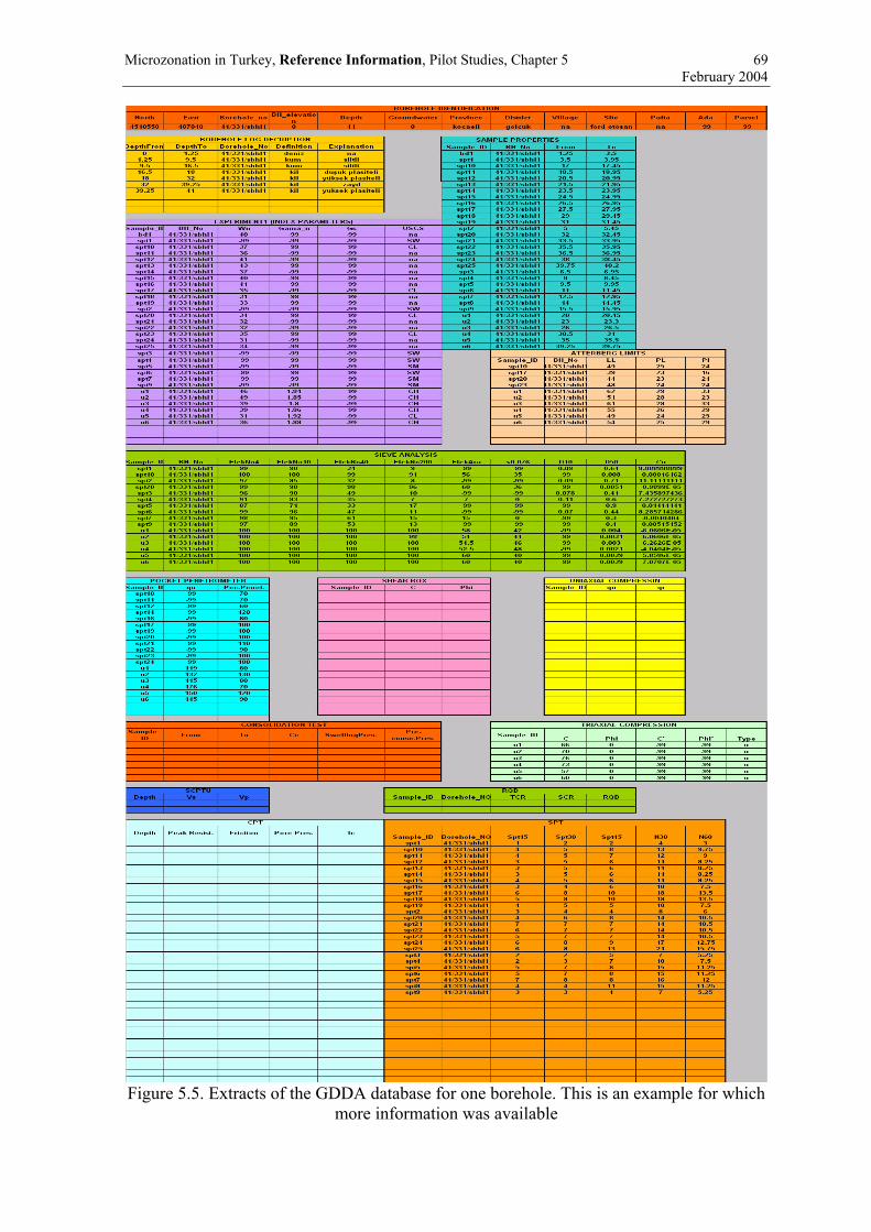
Microzonation in Turkey, Reference Information, Pilot Studies, Chapter 5 69 February 2004
Figure 5.5. Extracts of the GDDA database for one borehole. This is an example for which
more information was available
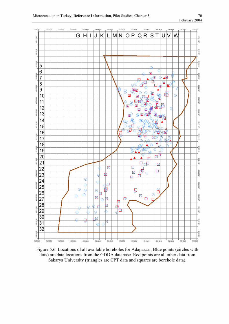
Microzonation in Turkey, Reference Information, Pilot Studies, Chapter 5 70 February 2004
Figure 5.6. Locations of all available boreholes for Adapazarı; Blue points (circles with
dots) are data locations from the GDDA database. Red points are all other data from Sakarya University (triangles are CPT data and squares are borehole data).

Microzonation in Turkey, Reference Information, Pilot Studies, Chapter 5 71 February 2004
Figure 5.7. Locations of all available boreholes for Gölcük; Blue points (circles with dots) indicate location of sounding from the GDDA data base. Red points show locations of the
data received from Sakarya University (squares are borehole data).
5.2.3 Data consistency and choice of representative boreholes All of the available data about the borehole information available for each location has been checked first for consistency. Secondly data from each grid has been compared. Thirdly, a representative borehole has been chosen.
The following bullet points will give an overview of the problems faced with this procedure:
• Case of “double data”. Difficulties occur when a data sheet and original data was available from one borehole, simplifications have already been made and assumption included, which cannot be followed by a third party. Therefore data from this borehole was usually classified as doubtful and a remark has been made in case it has been included for further use.
• Unique numbering system. No unique numbering e.g. Adapazarı Grid Q10, borehole SOZ363 = 54_sau_soz363 in the GDDA database and CPT COZ188 all have the same coordinates, which has not been documented in the available database from the beginning.
• Contradictory information. On some data sheets, a soil was identified as solid (meaning very stiff or hard) but the Atterberg limit test showed a liquid limit that was less than the natural water content. This would indicate that the consistency would be

Microzonation in Turkey, Reference Information, Pilot Studies, Chapter 5 72 February 2004
liquid (e.g. Adapazarı Grid R12). Usually the interpreted consistency of the SPT values was trusted more than a single test result.
• Soil description. The soil description in the borehole logs varies according to the borehole company. For some data sets, borehole data are simplified to one single layer without any other components e.g. Adapazarı Grid K23: “hard clay”. There were additional contradictions with the results of laboratory tests if they were available (Results of tests giving soil mechanical parameter are rare. Sieve analysis results (or at least amount of fines) were more often available for proof checking).
• Often, especially in Adapazarı, the available information showed no predominant component of soil type. These were then identified as a mixture of two soil types e.g. Adapazarı Grid P9: “silt – clay”.
• Difference in details. Borehole information can consist of very thin layers e.g. Adapazarı Grid V19 (layers every 20 cm, 14 layers for 15 m). Sometimes the borehole information has already been summarized to give the main predominant layers e.g. Adapazarı Grid R23 (3 layers for 15 m).
• Nomenclature. There was no consistent description of soils and soil classes according to the e.g. ASCE classification. In some cases, assumptions were necessary for a unified description. Some information on classification has been only available in Turkish. These have been translated as far as possible. Some definition for soil descriptions were still not consistent, so the following interpretation was assumed:
little = slightly
block = cobbles
• In some cases the description of the consistency is missing. The description of the density of coarse soils is usually missing too. As an example Adapazarı Grid U20: “little brown silty CLAY, light brown clayey GRAVEL”. Usually a correlation with the SPT values was made for interpretation of this borehole information.
• Comparability of soundings and borehole log description. SPT values – firmness/ strength of soil as well as consistency were often not consistent. Thus the following SPT N 30 interpretation was assumed for further use:
Fine grained soils
Interpretation of SPT N30 values
N 30 values - interpretation
0-2 very soft 2-8 soft 8-15 stiff 15-30 semi-solid >30 semi-solid to solid
Coarse-grained soils
Density – SPT N30 value diagrams have been adopted according to the German industry standard DIN 4094. An example is given in Figure 5.8 (http://www.grundbau.tu-berlin.de/download/skripte/gb1/kap02.pdf).

Microzonation in Turkey, Reference Information, Pilot Studies, Chapter 5 73 February 2004
Figure 5.8: Relationship between number of blows from different energy rated penetration tests (while the curve of DPH, DPL and DPL-S are of no account for the current scenario)
and density (left) or relative density (right) for narrowly graded sands (DIN 4094). The curve SPT has been used for this study. Note that the chart is only valid for Nk between 3
and 50.
The following decisions have been made in terms of the definition of the representative boreholes:
• The data from borehole logs have been preferred before those available from the data sheet.
• Summarized versions of the borehole log were preferred.
• Unique soil description was preferred e.g. “silty clay” instead of “silt-clay”
• Locations where only CPT data were available were rarely used (only at locations where other information of the soil strata was available).
• Little gravelly sandy clay was usually interpreted as little gravelly and sandy clay and not as little gravelly and little sandy clay e.g. Gölcük Grid I6.
In addition to the influencing factors mentioned above for choice and establishment of the representative boreholes, the topographical conditions (elevation) as well as information on the groundwater situation was needed. For most of the boreholes in Adapazarı, and for some of the boreholes in the Gölcük area, the elevation of the site of the soil investigation was not given. It had to be derived by a more complicated and time-consuming approach using rarely available topographical maps. Information on the groundwater situation was only available for approximately half of the data locations. In addition, seasonal changes could not be taken into account as in most cases (at least for the GDDA database), no time and date of the site investigation was given. The groundwater maps given by the GDDA data base are not included here, since they were submitted late and were only available towards the end of the project, and are also misleading as all
DPH (Dynamic Probing Heavy) DPL (Dynamic Probing Light)- cross section at the tip 10 cm2
DPL-S cross section at tip 5 cm2

Microzonation in Turkey, Reference Information, Pilot Studies, Chapter 5 74 February 2004
available information on the groundwater condition was included independent of the time of the derivation, and are only given in layers of 2.5m thickness.
Taking into account the challenges mentioned above, representative boreholes have been chosen for each grid close to the available existing data. Layer simplification and choice of the representative borehole has been carried out based on engineering judgment. It should not be forgotten that these representative boreholes have been chosen for the microzonation study and not for any other purpose (e.g. replacing site investigation for new buildings).
It has been decided to transmit all representative data in graphical format, which can be transferred into the database. The graphical format allows an easy overview of the data to be used in the next steps of the microzonation project. In addition, a graphical sheet forces further users to be confronted with comments on reliability and the details of the background of data. Also, further users of the hypothetical boreholes are directed to the original borehole numbers and the respective database (GDDA data starts usually with a two digit number, data from Sakarya with a three letter code).
Figure 5.9 shows the representative borehole for the grid Q10, of which the different data sets were already given in the earlier figures. Figure 5.10 – 5.13 show different situations for grid locations in Gölcük.
The soil notation as well as description of the consistency or the density is given in German due to limitations of the program. A translation of all German terms used into English is available at the bottom of each data sheet. A further text block indicates necessary information, which is crucial to be included for each borehole. This information includes the grid number, location of the original borehole chosen to be the representative one, the complete range of boreholes and their distribution within specific grid, and information on the groundwater level. When necessary, comments on reliability of this information are added. The last block indicates the plausibility of the data. It is marked red if there are restrictions in plausibility as well as if there is only one borehole in a grid, which could not be cross – checked with other data.
Figure 5.10 and 5.11 show an example where good correlation could be found among the existing boreholes. Figure 5.12 and 5.13 shows the opposite. Here, three different boreholes could be established within one grid. A river valley could be identified crossing the grid. The slopes on both sides show different topsoil layers. In such cases, the representative borehole has been chosen by means of topographic maps as well as the distribution of soils in the neighboring grids. The main influence is the majority of area represented by the chosen hole in the grid. More than half of the grid is located on the eastern slope for J6 in Gölcük (shown in the Figures 5.12 and 5.13),. The other possibilities are indicated in the text marked in red together with the chosen representative borehole.
Using existing data offers a good opportunity to start a microzonation project without spending too much money on additional data derivation. Nevertheless, this has to be done with great care and knowledge of the local soil conditions. Thus some of the decisions taken by IGT for the two project areas, in terms of the choice of the hypothetical boreholes and their interpretation, might be questionable for local geotechnical engineers, but will be exact enough to fit the purpose of the microzonation study for the project areas and to give examples for future users.

Microzonation in Turkey, Reference Information, Pilot Studies, Chapter 5 75 February 2004
Figure 5.9. Representative borehole for grid Q10 Adapazarı

Microzonation in Turkey, Reference Information, Pilot Studies, Chapter 5 76 February 2004
Figure 5.10. Two different available boreholes for grid P4 Gölcük

Microzonation in Turkey, Reference Information, Pilot Studies, Chapter 5 77 February 2004
Figure 5.11. Representative borehole selected for grid P4 Gölcük

Microzonation in Turkey, Reference Information, Pilot Studies, Chapter 5 78 February 2004
Figure 5.12. Three different boreholes for grid J6 in Gölcük

Microzonation in Turkey, Reference Information, Pilot Studies, Chapter 5 79 February 2004
Figure 5.13. Representative borehole selected for grid J6 in Gölcük

Microzonation in Turkey, Reference Information, Pilot Studies, Chapter 5 80 February 2004
5.2.4 Interpolation of non-filled grids and hypothetical boreholes Based on the available data, additional hypothetical boreholes were identified or interpolated as basis for the other tasks. Interpolation of data to fill empty grid points has been carried out very carefully and was omitted for doubtful cases as well as for cases where extrapolation of borehole data would have been needed. For Adapazarı, the grids G28, H28, H29, H30, I25, I26, I27; I28, I31, I32, J26, K24, K25, K26, K30, K31, L25, L31, M28, N29, O27, P21, P25, P27, Q21, R8, R27, S10, S22, S23, T10, U10, U19, V8 and V12 where interpolated. The interpolated areas for Gölcük are shown in 5.14. In addition to the restricted area, of which no data was available, two grids are shown (Grid G7 and M9) where interpolation has not been carried out due to topographical reasons as well as contradictory data from the neighboring grids. The selected representative boreholes, which will be used as hypothetical data for local soil conditions as well as the detailed input data can be found in the Appendix 2.2.
Figure 5.14. Area of interpolated boreholes shown in blue in Gölcük. Note that the crossed
areas show areas with no data extrapolation.
5.3. SITE CLASSIFICATION
The task site classification is based on the use of the Turkish Code and the NEHRP approach. The boundary information needed for both procedures are the local soil conditions and, in particular the distribution of shear wave velocities in the topmost 30

Microzonation in Turkey, Reference Information, Pilot Studies, Chapter 5 81 February 2004
meters. To conduct this part in a structured manner, firstly the shear wave distribution in the upper layers has been established. The details of how the site classification was carried out will be introduced in the following sections, if they are not already described in more detail in part D of the manual (Ansal 2003). All results of shear wave velocity distributions as well as the classification, can be found in the Appendix 2.2.
5.3.1 Distribution of shear wave velocity for the topmost 30 meters Several procedures can be used to establish the shear wave velocity (Vs) distribution with depth. Aside from measurements in the borehole, which were only available very rarely, several empirical correlations between SPT and CPT data and shear wave velocity can be used. Different approaches are given in Chapter D of the Manual of the MERM project, and the different methods have been studied in comparison. This comparison included mainly correlation with CPT results, measured data from Bakır (2002), linear extrapolation of known data, and SPT correlations. As a result, the correlation of the shear wave velocity with the SPT values seemed to offer the best fit and it has been decided to choose one of these methods. The results of this comparison are not shown and nor are they discussed here in detail due to space restrictions. Figure 5.15 gives an example of the differences in the resulting velocities. The Iyisan method (Iyisan 1996) was used for the pilot study. This relationship is valid for all soil types to estimate shear wave velocity from SPT tests:
Vs = 51.5 N 0.516 (5.1.) The following procedure was established for the estimation of a shear wave velocity
profile for the hypothetical boreholes.
If an SPT profile is available for the hypothetical borehole, then the procedure is as follows:
1. Check if there are borehole measurements for shear wave velocity (Seismic Profile or SCPTU) available
for Adapazarı:
If yes, these test results were used. Usually, the test results were available only for the upper layers so that the deeper layers had to be correlated with the SPT values (see 2.). It has to be noted, that the measured shear wave velocities are smaller than the shear wave velocities determined from the Iyisan method.
for Gölcük:
There are no measured shear wave velocities available for the Gölcük area.
2. Check if an SPT profile is available for the whole depth of the borehole. The SPT profile has been transferred via the Iyisan method to a shear wave velocity profile. As further procedure requires constant shear wave velocity for layer of predefined thickness, a medium value has been chosen for each layer. Idealizations and assumption have to be made for certain situations.
2.1. If the SPT profile is not available for the last layer, it was linearly extrapolated for this last layer up to a depth of 30 meters below surface. In most cases, this extrapolation was constant for fine-grained soils. A slightly increasing shear wave velocity distribution was chosen for coarse-grained material. The soil type of the unknown layer was adopted from the last known layer of the borehole profile.
2.2. If the SPT profile is not available for the top layer (i.e. fill or topsoil layer), an assumption of the shear wave velocity of 100 m/s was made.

Microzonation in Turkey, Reference Information, Pilot Studies, Chapter 5 82 February 2004
2.3. If no SPT results were available only in one intermediate layer, a correlation with the existing measurement data seemed appropriate (comp. 3).
Some additional remarks on the available data from the different data sources are given here:
o The SPT value R was found to be an N70 value rather than an N30 value. This was concluded from the graphical presentation of the SPT values from the data sheets of the borehole company in data sheets from Sakarya University.
o SPT values were extrapolated for 30 cm penetration depth when 50 hits or more were obtained for less than 30 cm penetration. The maximum extrapolated SPT value of N30 = 157 was equal to a shear wave velocity of 700 m/s and this was determined for each case.
o If the SPT value presented in the GDDA database equals 198 it means that no SPT tests were carried out. The value is just a big number since one is needed for the database.
3. No SPT profile exists for the upper 30 m:
for Adapazarı:
If there are no SPT test results available, which is always the case for interpolated boreholes, a correlation between the soil type and the existing vs measurements with depth was used. This correlation works well for the soil types clay, silt and sand. No measurements have been available for gravel so that an assumption has to be made.
for Gölcük:
Shear wave velocities were interpolated between neighboring boreholes if these had been interpolated. No interpolation has been incorporated for the groundwater table.
4. SPT profile exists up to the surface of bedrock in the upper 30 m The shear wave distribution has to be determined for the topmost 30 meters or up to bedrock or competent layer. The value of the shear wave velocity for the competent layer was chosen to be vs = 700 m/s. Therefore shear wave velocities were interpolated to define the depth of the competent layer. This layer is then shown as weathered bedrock = Gravel-Cobbles.
The shear wave velocity reached a value of 700 m/s in the upper 30 m through the linear interpolation process only in few of the boreholes (e.g. Adapazarı Grid G 28, Q18).

Microzonation in Turkey, Reference Information, Pilot Studies, Chapter 5 83 February 2004
Figure 5.15. Comparison of different methods adopted to derive the shear wave velocity
for the grid Q10 in Adapazarı
Figure 5.16. Derived and idealized shear wave distribution for grid Q10. The derivation procedure can be seen in a table format on the left of the figure. All shear wave velocity
determination are summarized in single Excel sheets and can be found in the Appendix 2.2

Microzonation in Turkey, Reference Information, Pilot Studies, Chapter 5 84 February 2004
5.4. PROCEDURE FOR THE CLASSIFICATION OF HYPOTHETICAL BOREHOLES ACCORDING TO THE TURKISH CODE
Site classification according to the Turkish Code is given in detail in the state of the art report (Ansal 2003) as well as being fully documented in the code. A two-step procedure for site classification is established. Figure 5.17 shows the table summarizing the classification. A description of their use can be found in the Turkish Code.
The Turkish Code subdivides the classification in two areas. Initially the soil group A-D has to be determined so that a local site class can be derived. It is clear from Table 12.1 (Figure 5.17) that there are 4 different possibilities for identifying the soil group, which are all equivalent. In terms of comparability of the results of the classification, it has to be decided before the beginning of the classification to follow a certain sequence of decisions. For the pilot study here, it has been decided to focus on SPT – values first and use the shear wave velocities only if there are no SPT values available. The second classification of the Turkish Code “site class” (Table 12.2 in Figure 5.17) correlates the soil group with the expansion of the different layers in the topmost 30 meters.
Some examples will be given under the following bullet points, which might be of use for further applications. In terms of practical use, the check for the soil group should be made from the bottom (& most critical) soil class D to the top A (& least critical). Some special rules for describing the “site class” have to be applied also, which were given here when necessary for the pilot areas.
• Grid N11 from Gölcük is one of the examples where shear wave velocity has been used for site classification.
• There are values given in the tables, which allow the classification in two different groups. This is the case if N30 =16 for silt and clay, N30 =30 for sand and gravel, Vs = 300 m/s for silt and clay, Vs = 400 m/s for sand and gravel (e.g. Gölcük grids O10 or Q6).
• Silt is treated as silty clay.
• In the case of more than one SPT N30 value for one layer, the lowest value is taken to classify the soil group of this layer (on the safe side). e.g. Gölcük Grid E6, M7.
• Fill and top soil cannot be chosen as a classifying layer, even if they would fulfill the requirements. e.g. Gölcük Grid L10.
• The layer that should be the most critical for the classification is usually a soft silt/clay or loose sand/gravel.
• It might be that more than one single layer will be characterized together as a classifying layer. e.g. Gölcük Grid K4.
• Topmost Layer Thickness h1 is the thickness of the “classifying layer” in the first 30 m below surface. In case the classifying type of material (e.g. clay) appears twice, both layers do count for the thickness h1.
• A range of Local Site Classes e.g. from Z1-Z2 is given if the thickness of the “classifying layer” is not clearly defined through the borehole profile. No precise decision has been made.
• A range of Local Site Classes is given if there is already a range specified for the Soil Group (e.g. Gölcük Grid O10). Again, no precise classification has been made.
Microzonation in Turkey, Reference Information, Pilot Studies, Chapter 5 85 February 2004
• In some cases, the last layer of the hypothetical borehole is chosen as the “classifying layer”, so the thickness of the layer is not known and therefore the range indicates this (e.g. Gölcük Grid C5).
• If the “classifying” type of material is found at the top, somewhere in the middle of the borehole profile and in the last layer as well, all layers sum up to the full height of the classifying layer (e.g. Gölcük Grid G9).
• If more than one layer is characterized as the classifying layer, a range in the local site class is given (e.g. Gölcük Grid K4).
• Soil Group A is always classified as Local Site Class Z1 since no term for the topmost layer thickness (h1) is given for this soil group.
• As to the definition of the topmost layer thickness, for this study, the soil group C can never be classified as the local site class Z4 due to the fact that the topmost layer thickness h1 has to be greater than 50 m (h1 > 50 m), whereas the depth of the representative boreholes was always less than 30 meters.

Microzonation in Turkey, Reference Information, Pilot Studies, Chapter 5 86 February 2004
Figure 5.17. Table for Site classification from Turkish Code (Ministry of public Health,
1997)
The Figures 5.18 and 5.19 show the results of the classification according to the Turkish Code. Note that a plot of the local soil groups might be reasonable but it will be misleading as the determination of the local soil group is just an interim step of the classification procedure.

Microzonation in Turkey, Reference Information, Pilot Studies, Chapter 5 87 February 2004
Figure 5.18. Local Site Classes for Adapazarı

Microzonation in Turkey, Reference Information, Pilot Studies, Chapter 5 88 February 2004
Figure 5.19 Local Site Class for Gölcük
5.5. PROCEDURE FOR THE CLASSIFICATION OF HYPOTHETICAL BOREHOLES ACCORDING TO THE NEHRP APPROACH (BSSC 2001)
The relevant four pages of the NEHRP approach are given in the Appendix 2.1, so that the procedure can be followed. It is based on a stepwise approach. Firstly it has to be decided if there is any danger of liquefaction. If so, a grid would be classified as Site Class F. This has not been done here. If any such decision is taken in the liquefaction chapter, the map will be updated accordingly.
A classification into Site Class A and B could not be done for the pilot studies as it has been decided in the project to identify the shear wave velocity for the competent bed rock with Vs = 700 m/s. The average shear wave velocity for Site Class A and B has to rise significantly over 760 m/s to represent hard rock and rock respectively according to NEHRP.
The classification between Site Classes C-E is given in the Figure 5.20. Three possibilities are given for this classification in terms of, Vs , N or chN , us . The definition for the values can be found in the NEHRP approach. The method proposed by NEHRP, which is based directly on the results of the SPT soundings for the top 30 m has not been chosen since measurements were not available for the whole depth and the existing measurements were already included in the available values of the shear wave velocities,

Microzonation in Turkey, Reference Information, Pilot Studies, Chapter 5 89 February 2004
which are based on the Iyisan relationship. The su method was not taken into account because the necessary values are mostly not available.
Figure 5.20. Classification of Site classes C-E following the NEHRP approach (BSSC,
2001)
The basis for the classification for the pilot areas is therefore based on an average shear wave velocity for the first 30-meters of the soil strata. This weighted average of the shear wave velocity Vs for the top 30m is derived using the following formula (formula 4.1.2.3-1 of BSSC 2001):
∑
∑
=
== n
i si
i
n
ii
vd
dVs
1
1 (5.2)
vsi is the shear wave velocity (m/s) of each layer of defined thickness
di is the thickness of any layer between 0 m and 30 m.
As mentioned before only a classification for the site classes C, D and E is presented here. The sequence is given in the following two steps.
1. Check if there is a soft soil layer of more than 3 m thickness present in one of the borehole profiles. If yes, check if it is a soft clay layer and if additional information is available about the plasticity index PI, water contents w and undrained shear strength su. If PI > 20, w > 40% and su < 25 kPa classify as site class E. If no, continue with the categorization from point 2 below. Soft soil layers thinner than 3 m, that might add up in the hypothetical borehole to a layer thickness greater than 3 m, are taken into account as well.
o In most cases the undrained shear strength is not known for the pilot areas. In many grids, two controversial experimental results of the considered clay layer may be found, one that satisfy the above mentioned criteria and one that may not do so, are available (e.g. Adapazarı Grid S18).
o To indicate that a soft clay layer thicker than 3 m is present in the hypothetical borehole (even though the limiting criteria concerning PI, w and su (as mentioned in

Microzonation in Turkey, Reference Information, Pilot Studies, Chapter 5 90 February 2004
the previous paragraph) are not completely fulfilled), a minus is added “– E” to the site class. This is based on the weighted average shear wave velocity.
2. Derivation of the average shear wave velocity (see above) and determination of the site
class. The results of the classification are given in the Figures 5.21 and 5.22.
A table of the classification is included in the Appendix 2.2. For Gölcük, soft layers appear seldom, with the exception of the grids I6, N8 (silt), N9 (silt), P3, P4, P5 (silt), P6 (silt) and Q4, in total these include 8 out of 82 grids. Some of the grids mentioned above have a soft layer thicker than 3 m, some of them have a lower PI and w than necessary for the classification of site class E, and some of them show no additional information for PI and w. Therefore none of these grids were classified as site class E, due to the presence of a soft clay layer.
In the Adapazarı area soft layers (clay and silt) appear in the grids G26, H25, H26, H27, I25, I26, I27, I28 (silt), J24, J25, J26 (silt), J28 (silt), K23, K24, K25, K26, K27 (silt), L24, L25, L26, N8, N11, O10, O11, O13, O14, O15, O17 (silt), O27 (silt), O28 (silt), P9 (silt-clay), P10, P11 (silt-clay), P12, P16, P22, Q9, Q10, Q11, Q12 (soft silt and clay layers alternating), Q13, Q15, Q18 (silt), R8, R9, R11, R12, R13, R14, R16, R17, S7, S9, S10, S11, S12 (silt-clay and silt), S13, S14, S15 (silt), S16 (silt-clay), S17 (silt-clay), S18, S19, S20, T8, T10 (silt), T11 (silt), T12, T13 (silt), T14, T15 (clay and silt), T16, T17, T18, T19, T20, T21, U8, U10 (silt), U11 (silt), U12 (clay and silt), U13, U14, U16, U17, U18, V9, V10, V11, V12 (clay and silt), V18 (clay and clay-silt), W9. Thus almost half of the grids have a soft layer of a varying thickness.
The north of Adapazarı shows a varying distribution in terms of a classification towards site classes, although potential for liquefaction (class F) has not been adjusted here. The southern areas show a more significant area denoted as class E, which lie south of a hill site and another, which is classified as class C and is next to the lake. The classification for Gölcük is less variable showing class C in most cases for Degirmendere and Gölcük, whereas class D more prominent for Ihsaniye.

Microzonation in Turkey, Reference Information, Pilot Studies, Chapter 5 91 February 2004
Figure 5.21. Classification according to NEHRP for Adapazarı. Note that a classification of potentially liquefiable zones (class F) has not been done at this stage as a cause of the
internal task distribution of this project.

Microzonation in Turkey, Reference Information, Pilot Studies, Chapter 5 92 February 2004
Figure 5.22. Classification according to NEHRP for Gölcük. Note that a classification of
potentially liquefiable zones (class F) has not been done at this stage as a cause of the internal task distribution of this project.
Microzonation in Turkey, Reference Information, Pilot Studies, Chapter 6 93 February 2004
6. SITE RESPONSE ANALYSES
Jan Laue, Juliane Buchheister, Sarah M. Springman, Institute for Geotechnical Engineering (IGT) of the Swiss Federal Institute of Technology (ETH), Zurich
The site response analysis determines the main frequencies and amplification that the surface of the ground will experience. There are several ways of achieving this, including simple empirical methods using analogies given in Codes. A more sophisticated method has been chosen for this project, based on a one dimensional analysis, in which an earthquake is introduced to the base rock or a competent layer from where the waves are permitted to travel vertically up through the soil column. This and other similar methods are described in the manual and the state of the art report. The procedure of input and output will be described here in Excel sheets based on the program SHAKE (Schnabel et al. 1972, Idriss & Sun, 1991) to make the analysis easier for inexperienced users (based on version SHAKE91) and will be more suitable, as the newer versions of SHAKE (1999) require a license fee to be paid, which might not be affordable (or necessary) for further use.
Some assumptions have to be made for the analysis. During the work on the pilot area, it has been decided to introduce the earthquake to the top most layers at the height of the competent layer. As described in the chapter on Soil Conditions, only a few of the grids show a competent layer in the topmost 30 meters. Thus, data from the literature had to be taken into account to derive the soil strata up to the competent layer. It was only necessary to represent the soil profile between 30 m and the competent layer with the selected shear wave velocity distribution. Thus the first paragraph will deal with the determination of the shear wave velocities between a depth of 30 m below the surface and the competent layer. The next section summarizes the other input parameters required while the last section gives the results.
6.1. SHEAR WAVE VELOCITY BETWEEN 30 M AND THE TOP OF THE BEDROCK
When no site-specific soundings are available to identify the competent layers, geophysical methods have to be used. Results of array measurements conducted and described by Kudo et al. (2002) were used here. Kudo (comp. Ansal et al. 2003) describes average shear wave velocities over larger areas of soil up to bedrock. Two stations reported for both of the pilot areas are in the area of interest. In Gölcük, the stations GLF and GLH are the stations located in the pilot area, where the stations are ADC and ADU in Adapazarı. The shear wave velocity is given in an average manner for these stations. As the depth at which a value of vs= 700 m/s has been reached is essential a linear increase of vs was assumed in order to derive the depth of the competent layer, so that the shear wave velocity profile with depth could be linearly interpolated between two layers to reach the competent layer. The depths of the surface of the bedrock layer for the 4 relevant stations are given below:
ADU: 281 m
ADC: 126 m
GLH: 171 m
GLF: 193 m
The allocation of the two stations to each grid in the pilot areas has been done based on the results of the microtremor measurements, which are described in the research task group report (Fäh et al. 2003).

Microzonation in Turkey, Reference Information, Pilot Studies, Chapter 6 94 February 2004
The zones determined where relatively constant fundamental frequencies may be found, could be correlated with one of the stations previously described by Kudo et al (2002), so that each grid could be related to one of the stations. Thus a shear wave velocity profile could be established up to the competent layer.
The following figures show the allocation of grid points to the respective stations of the array measurements with respect to the areas defined by Fäh et al. (2003). The Figures 6.1 and 6.2 show the allocation of the different grids to the station given by Kudo.
Figure 6.1. Allocation of the Kudo stations ADU and ADC to the grids in the pilot area of
Adapazarı (Laue et al. 2003).

Microzonation in Turkey, Reference Information, Pilot Studies, Chapter 6 95 February 2004
Figure 6.2. Allocation of the Kudo stations GLF and GLH to the grids in the pilot area of
Gölcük (Laue et al., 2003).

Microzonation in Turkey, Reference Information, Pilot Studies, Chapter 6 96 February 2004
6.2. INPUT REQUIREMENTS
6.2.1 Earthquake input file The earthquake data has been introduced as an outcrop motion. Earthquake data has been received from another task group and reference should be made to the respective chapter (Erdik et al. 2003). A single earthquake for each grid was used for the analysis conducted here. Usually, several different earthquake files should be studied and an average result should be established. The earthquake has been introduced into the calculation in the time domain.
6.2.2 Soil profile The hypothetical borehole was introduced for each grid as the soil profile, including the extension up to competent layer. In case of mixed layers (e.g. sand and silt S+U), the softer layer has been chosen as the representative one.
The following boreholes in Adapazarı had these mixed layers (S=sand, T=clay, U=silt)
Grid number Layer Material parameter G26 S+U U G31 U+S U H32 S+U S P9 T+U T P11 T+U T Q11 T+U T Q16 T+U T R11 T+S T S+T S U+T U S6 T+S T S16 T+U T S17 T+U T S19 T+U T T7 T+U T U9 U+S U U16 T+U T V18 T+U T
6.2.3 Material parameters The shear wave velocity distribution has to be included for each of the materials. In addition, the strain dependency of the material properties has to be allocated to each soil. A brief mention is included in the text, while the respective figures and details can be found in the Annex. The names are given herein (according to the notation given in the SHAKE program series) and their allocation. Several material types have been defined for the Excel sheet calculations.

Microzonation in Turkey, Reference Information, Pilot Studies, Chapter 6 97 February 2004
Mat 1 Top soil:
Chosen strain dependent approach:
G: Vucetic & Dobry with PI=0% D: Vucetic & Dobry with PI=0%
Mat 2 Fill: Chosen strain dependent approach:
G: Seed & Idriss average D: Seed & Idriss average
Mat 3 Silt: Chosen strain dependent approach:
G: Vucetic & Dobry mit PI=15% D: Vucetic & Dobry mit PI=15%
Mat 4 Clay:
Chosen strain dependent approach:
G: Vucetic & Dobry mit PI=30% D: Vucetic & Dobry mit PI=30%
Mat 5 Sand: Chosen strain dependent approach:
G: Seed & Idriss average D: Seed & Idriss average
Mat 6 Gravel:
Chosen strain dependent approach:
G: Seed & Idriss average D: Seed & Idriss average
Mat 7 Kudo unknown material layer:
Chosen strain dependent approach:
G: Seed & Idriss average D: Seed & Idriss average
Mat 8 Bedrock:
Chosen strain dependent approach:
G: Rock Idriss D: Rock Idriss
6.2.4 Total unit weight A total unit weight has to be introduced in the calculation. Due to the lack of availability of representative data, the unit weight had to be estimated. Please note that the density given is the saturated bulk density
Mat 1 Top soil: 18 kN/m3 Mat 2 Fill: 19 kN/m3 Mat 3: Clay 20 kN/m3 Mat 4: Silt 20 kN/m3 Mat 5: Sand 21 kN/m3 Mat 6: Gravel 22 kN/m3 Mat 7: unknown Kudo 21 kN/m3 Mat 8: Bedrock 26 kN/m3
6.2.5 Groundwater level
The groundwater level has to be introduced in the calculations. Again assumptions have to be made according to the different data available.
For both of the Adapazarı and Gölcük areas, data based on the GDDA database and given to public on a map (Köksal, 2003) have been used, even if no differentiation between the date of the derivation has been made. The following tables give the input data for the grids. For Adapazarı, only grids are mentioned where the groundwater table does not lie in the topmost 2.5 meters. The groundwater level is given for all grids for the Gölcük area.

Microzonation in Turkey, Reference Information, Pilot Studies, Chapter 6 98 February 2004
Adapazarı: Grid number Groundwater level
range (m) Grid number Groundwater level
range (m) G26 2.5 – 5 G27 7.5 – 10 G28 12.5 – 15 G29 n.a. G30 n.a. G31 n.a. H25 2.5 – 5 H26 2.5 – 5 H27 7.5 – 10 H28 10 – 12.5 H29 n.a. H30 n.a. H31 n.a. H32 n.a. I27 5 – 7.5 I28 7.5 – 10 I29 10 – 12.5 I30 n.a. I31 12.5 – 15 I32 12.5 – 15 J28 5 – 7.5 J29 7.5 – 10 J30 7.5 – 10 J31 10 – 12.5 J32 10 – 12.5 K28 2.5 – 5 K29 2.5 – 5 K30 5 – 7.5 K31 5 – 7.5 K32 5 – 7.5 L28 2.5 – 5 L29 2.5 – 5 L30 2.5 – 5 L31 2.5 – 5 L32 2.5 – 5 M29 2.5 – 5 M30 2.5 – 5 N18 5 – 7.5 N30 2.5 – 5 O20 7.5 - 10 O21 7.5 – 10 O22 7.5 – 10 O23 2.-5 - 5 P13 2.5 – 5 P14 2.5 – 5 P20 7.5 – 10 P21 7.5 – 10 P22 2.5 – 5 P23 2.5 – 5 Q13 2.5 – 5 Q14 2.5 – 5 Q17 7.5 – 10 Q18 10 – 12.5 Q19 7.5 – 10 Q20 2.5 – 5 Q21 2.5 – 5 R16 7.5 – 10 R17 12.5 – 15 R18 n.a. R19 5 – 7.5 S16 10 – 12.5 S17 n.a. S18 n.a. S19 12.5 – 15 S20 2.5 – 5 S21 2.5 – 5 T15 2.5 – 5 T16 n.a. T17 n.a. T18 n.a. T19 12.5 – 15 T20 5 – 7.5 T21 5 – 7.5 T22 2.5 – 5 U15 2.5 – 5 U16 7.5 – 10 U17 n.a. U18 12.5 – 15 U19 10 – 12.5 U20 5 – 7.5 V18 5 – 7.5 V19 5 – 7.5

Microzonation in Turkey, Reference Information, Pilot Studies, Chapter 6 99 February 2004
Gölcük: Grid number Groundwater level
range (m) Grid number Groundwater level
range (m) D4 0 - 2.5 E4 0 - 2.5 F4 10 - 12.5 G3 5 - 7.5 G4 10 – 12.5 G8 7.5 – 10 G9 5 – 7.5 H3 10 – 12.5 H7 10 – 12.5 H8 7.5 – 10 H9 5 – 7.5 I5 12.5 - 15 I7 12.5 - 15 J4 12.5 - 15 K4 2.5 – 5 K5 7.5 – 10 K11 5 – 7.5 L4 0 – 2.5 L5 7.5 – 10 L10 5 – 7.5 L11 5 – 7.5 M4 2.5 – 5 M5 5 – 7.5 M6 10 – 12.5 M8 10 – 12.5 M10 2.5 – 5 M11 2.5 – 5 N4 2.5 – 5 N5 5 – 7.5 N6 5 – 7.5 N7 5 – 7.5 N8 7.5 - 10 N9 2.5 – 5 N10 5 – 7.5 N11 5 – 7.5 O4 2.5 – 5 O5 2.5 – 5 O6 2.5 – 5 O7 5 – 7.5 O8 5 – 7.5 O9 2.5 – 5 O10 2.5 – 5 P3 0 – 2.5 P4 0 – 2.5 P5 0 – 2.5 P6 2.5 – 5 P7 5 – 7.5 P8 5 – 7.5 Q4 0 – 2.5 Q5 0 – 2.5 Q6 2.5 – 5
6.3. RESULTS OF THE SITE RESPONSE ANALYSIS The following Figures 6.3 and 6.4 show the distribution of Peak horizontal Ground Acceleration (PGA) for both areas of the pilot studies. This map is given here to illustrate that all results used later on for microzonation purposes are based on numbers. The values for each grid show the result for 1 special scenario and have no physical meaning for any other use than building one of the basis for microzonation. The interpreted maps will be included in Chapter 11 of this report. All calculations are available in an electronic version and are added to the Annex. They are summarized in additional tables, which are also included in printed version of the Appendix 2.3.

Microzonation in Turkey, Reference Information, Pilot Studies, Chapter 6 100 February 2004
Figure 6.3. Peak horizontal Ground Acceleration shown as multiples of g (m/s2) for
Adapazarı

Microzonation in Turkey, Reference Information, Pilot Studies, Chapter 6 101 February 2004
Figure 6.4. Peak horizontal Ground Accelerations shown as multiples of g (m/s2) for
Gölcük.
In addition to the Peak Ground Accelerations, the summary tables in the Appendix 2.3 indicate the spectral acceleration and the predominant period resulting from the calculation for the specific input earthquake. Also added into the table are the amplitude of shear strain and the respective depth. The results are not given here, as they are part of chapter 11. The necessity of including the maximum amplitude of shear strain and the related depth will also be discussed in chapter 11.

Microzonation in Turkey, Reference Information, Pilot Studies, Chapter 7 102 February 2004
7. SEISMIC SOIL LIQUEFACTION ASSESSMENT METHODOLOGIES
K. Önder Çetin, Middle East Technical University, Civil Engineering Department, Ankara
7.1. INTRODUCTION Soil liquefaction is a major cause of damage during earthquakes. “Modern” engineering treatment of liquefaction-related issues evolved initially in the wake of the two devastating earthquakes of 1964, the 1964 Niigata and 1964 Great Alaska Earthquakes, in which seismically-induced liquefaction produced spectacular and devastating effects.
Over the nearly four decades that have followed, significant progress has occurred. Initially, this progress was largely confined to improved ability to assess the likelihood of initiation (or “triggering”) of liquefaction in clean, sandy soils. As the years passed, and earthquakes continued to provide lessons and data, researchers and practitioners became increasingly aware of the additional potential problems associated with both silty and gravely soils and the issues of post-liquefaction strength and stress-deformation behavior also began to attract increased attention.
Today, the area of “soil liquefaction engineering” is emerging as a semi-mature field of practice in its own right. This area now involves a number of discernable sub-issues or sub-topics, as illustrated schematically in Figure 7.1, showing that the first step in most engineering treatments of soil liquefaction continues to be (1) assessment of “liquefaction potential”, or the risk of “triggering” (initiation) of liquefaction. There have been major advances here in recent years, and some of these will be discussed.
Once it is determined that occurrence of liquefaction is a potentially serious risk/hazard, the consequences of the potential liquefaction will be assessed. This, now, increasingly involves (2) assessment of available post-liquefaction strength and resulting post-liquefaction overall stability (of a site, and/or of a structure or other built facility, etc.). There has been considerable progress over the past fifteen years in evaluation of post-liquefaction strengths. If post-liquefaction stability is found wanting, then deformation/displacement potential is large, and engineered remediation is typically warranted.
If post-liquefaction overall stability is not unacceptable, then attention is next directed towards (3) assessment of anticipated deformations and displacements. This is a very “soft” area of practice, and much remains to be done here with regard to development and calibration/verification of engineering tools and methods. Similarly, relatively little is known regarding (4) the effects of liquefaction-induced deformations and displacements on the performance of structures and other engineered facilities, and criteria for “acceptable” performance are not well established.
Finally, in cases in which the engineer(s) conclude that satisfactory performance cannot be counted on, (5) engineered mitigation of liquefaction risk is generally warranted. This, too, is a rapidly evolving area, and one rife with potential controversy. Ongoing evolution of new methods for mitigation of liquefaction hazard provides an ever increasing suite of engineering options, but the efficacy and reliability of some of these remain contentious and accurate and reliable engineering analysis of the improved performance provided by many of these mitigation techniques continues to be difficult.
It is not possible, within the confines of this report, to address fully all of these issues (a textbook would be required). Instead, methodologies regarding liquefaction triggering

Microzonation in Turkey, Reference Information, Pilot Studies, Chapter 7 103 February 2004
1. Assessment of the likelihood of “triggering” or initiation of soil liquefaction.
2. Assessment of post-liquefaction strength and overall post-liquefaction stability.
3. Assessment of expected liquefaction-induced deformations and displacements.
4. Assessment of the consequences of these deformations and displacements.
5. Implementation (and evaluation) of engineered mitigation, if necessary.
assessment will be highlighted, and GIS-based applications of these liquefaction triggering methodologies will be demonstrated for the cities of Sakarya and Gölcük after August 17, 1999 Kocaeli Earthquake with Mw = 7.4.
Figure 7.1. Key Elements of Soil Liquefaction Engineering
7.2. ASSESSMENT OF LIQUEFACTION POTENTIAL
7.2.1 Liquefiable Soils The first step in engineering assessment of the potential for “triggering” or initiation of soil liquefaction is the determination of whether or not soils of “potentially liquefiable nature” are present at a site. This, in turn, raises the important question regarding which types of soils are potentially vulnerable to soil liquefaction.
It has long been recognized that relatively “clean” sandy soils, with few fines, are potentially vulnerable to seismically-induced liquefaction. There has, however, been significant controversy and confusion regarding the liquefaction potential of silty soils (and silty/clayey soils), and also of coarser gravely soils and rock fills.
Coarser, gravely soils are the easier of the two to discuss, so we will begin there. The cyclic behavior of coarse gravely soils differs little from that of “sandy” soils, as Nature has little or no respect for the arbitrary criteria established by the standard #4 sieve. Coarse, gravely soils are potentially vulnerable to cyclic pore pressure generation and liquefaction. There are now a number of well-documented field cases of liquefaction of coarse gravely soils (e.g., Evans, 1987; Harder, 1988; Hynes, 1988; Andrus, 1994). These soils do, however, often differ in behavior from their finer, sandy brethren in two ways: (1) they can be much more pervious, and so can often rapidly dissipate cyclically generated pore pressures, and (2) due to the mass of their larger particles, the coarse gravely soils are seldom deposited gently and so do not often occur in the very loose states more often

Microzonation in Turkey, Reference Information, Pilot Studies, Chapter 7 104 February 2004
encountered with finer sandy soils. Sandy soils can be very loose to very dense, while the very loose state is uncommon in gravely deposits and coarser soils.
The apparent drainage advantages of coarse, gravely soils can be defeated if their drainage potential is circumvented by either; (1) their being surrounded and encapsulated by finer, less pervious materials, (2) if drainage is internally impeded by the presence of finer soils in the void spaces between the coarser particles (it should be noted that the D10 particle size, not the mean or D50 size, most closely correlates with the permeability of a broadly graded soil mix), or (3) if the layer or stratum of coarse soil is of large dimension, so that the distance over which drainage must occur (rapidly) during an earthquake is large. In these cases, the coarse soils should be considered to be of potentially liquefiable type, and should be evaluated accordingly.
Questions regarding the potential liquefiability of finer, “cohesive” soils (especially “silts”) are increasingly common at meetings and professional short courses and seminars. Over the past five years, a group of approximately two dozen leading experts has been attempting to achieve consensus regarding a number of issues involved in the assessment of liquefaction potential. This group, referred to hereafter as the NCEER Working Group, have published many of their consensus findings (or at least near-consensus findings) in the NSF-sponsored workshop summary paper (NCEER, 1997), and additional views are coming in a second paper scheduled for publication this year in the ASCE Journal of Geotechnical and Geoenvironmental Engineering (Youd et al., 2001). The NCEER Working Group addressed this issue, and it was agreed that there was a need to reexamine the “Modified Chinese Criteria” (Finn et al., 1994) for defining the types of fine “cohesive” soils potentially vulnerable to liquefaction, but no improved consensus position could be reached, and more study was warranted.
Some of the confusion here is related to the definition of liquefaction. In this paper, the term “liquefaction” will refer to significant loss of strength and stiffness due to cyclic pore pressure generation, in contrast to “sensitivity” or loss of strength due to monotonic shearing and/or remolding. By making these distinctions, we are able to separately discuss “classical” cyclically-induced liquefaction and the closely-related (but different) phenomenon of strain-softening or sensitivity.
Figure 7.2 illustrates the “Modified Chinese Criteria” for defining potentially liquefiable soils. According to these criteria, soils are considered to be of potentially liquefiable type and character if: (1) there are less than 15% “clay” fines (based on the Chinese definition of “clay” sizes as less than 0.005 mm), (2) there is a Liquid Limit of LL ≤ 35%, and (3) there is a current in situ water content greater than or equal to 90% of the Liquid Limit.
Andrews and Martin (2000) have re-evaluated the liquefaction field case histories from the database of Seed et al. (1984, 1985), and have transposed the “Modified Chinese Criteria” to standard conventions (with clay sizes defined as those less than about 0.002 mm). Their findings are largely summarized in Figure 7.3. Andrews and Martin recommend that soils with less than about 10% clay fines (< 0.002 mm) and a Liquid Limit (LL) in the minus #40 sieve fraction of less than 32% be considered potentially liquefiable, that soils with more than about 10% clay fines and LL ≥ 32% are unlikely to be susceptible to classic cyclically-induced liquefaction, and that soils intermediate between these criteria should be sampled and tested to assess whether or not they are potentially liquefiable.

Microzonation in Turkey, Reference Information, Pilot Studies, Chapter 7 105 February 2004
Liquid Limit1 < 32% Liquid Limit ≥ 32%
Clay Content2 <
10%
Susceptible
Further Studies Required
(Considering plastic
non-clay sized grains – such as
Mica)
Clay Content2 ≥
10%
Further Studies Required
(Considering non-plastic clay sized grains – such as mine and quarry
tailings)
Not Susceptible
Notes: 1. Liquid limit determined by Casagrande-type percussion
apparatus. 2. Clay defined as grains finer than 0.002 mm.
Figure 7.2. Modified Chinese Criteria (after Finn et al., 1994)
Figure 7.3. Liquefaction Susceptibility of Silty and Clayey Sands (after Andrews and Martin, 2000)
This is a step forward, as it somewhat simplifies the previous “Modified Chinese” criteria, and transposes it into terms more familiar to Turkish practitioners. We note, however, that there is a common lapse in engineering practice inasmuch as engineers often tend to become distracted by the presence of potentially liquefiable soils, and then often neglect cohesive soils (clays and plastic silts) that are highly “sensitive” and vulnerable to

Microzonation in Turkey, Reference Information, Pilot Studies, Chapter 7 106 February 2004
major loss of strength if sheared or remolded. These types of “sensitive” soils often co-exist with potentially liquefiable soils, and can be similarly dangerous in their own right.
Both experimental research and review of liquefaction field case histories show that for soils with sufficient “fines” (particles finer than 0.074 mm, or passing a #200 sieve) to separate the coarser (larger than 0.074 mm) particles, the characteristics of the fines control the potential for cyclically-induced liquefaction. This separation of the coarser particles typically occurs as the fines content exceeds about 12% to 30%, with the precise fines content required being dependent principally on the overall soil gradation and the character of the fines. Well-graded soils have lesser void ratios than uniformly-graded or gap-graded soils, and so require lesser fines contents to separate the coarser particles. Similarly, clay fines carry higher void ratios than silty particles and so are more rapidly effective at over-filling the void space available between the coarser (larger than 0.074 mm) particles.
In soils wherein the fines content is sufficient as to separate the coarser particles and control behavior, cyclically-induced soil liquefaction appears to occur primarily in soils where these fines are either non-plastic or are low plasticity silts and/or silty clays (PI ≤ 10 to 12%). In fact, low plasticity or non-plastic silts and silty sands can be among the most dangerous of liquefiable soils, as they not only can cyclically liquefy; they also “hold their water” well and dissipate excess pore pressures slowly due to their low permeability.
Soils with more than about 15% fines and with fines of “moderate” plasticity (8% ≤ PI ≤ 15%) fall into an uncertain range. These types of soils are usually amenable to reasonably “undisturbed” (e.g.: thin-walled, or better) sampling, however, and so can be tested in the laboratory. It should be remembered to check for “sensitivity” of these cohesive soils as well as for potential cyclic liquefiability.
The criteria of this section do not fully cover all types of liquefiable soils. As an example, well-studied clayey sand (SC) at a site in the south-eastern U.S. has been clearly shown to be potentially susceptible to cyclic liquefaction, despite a clay content on the order of 15 %, and a Plasticity Index of up to 30% (Riemer et al., 1993). This is a highly unusual material, however, as it is ancient sand that has weathered in place, with the clay largely coating the individual weathered grains, and the overall soil state is unusually “loose”. Exceptions must be anticipated, and judgment will continue to be necessary in evaluating whether or not specific soils are potentially liquefiable.
Two additional conditions necessary for potential liquefiability are: (1) saturation (or at least near-saturation), and (2) “rapid” (largely “undrained”) loading. It should be remembered that phearatic conditions are variable both with seasonal fluctuations and irrigation, and that the rapid cyclic loading induced by seismic excitation represents an ideal loading type.
7.3. ASSESSMENT OF TRIGGERING POTENTIAL Quantitative assessment of the likelihood of “triggering” or initiation of liquefaction is the necessary first step for most projects involving potential seismically-induced liquefaction. There are two general types of approaches available for this: (1) use of laboratory testing of “undisturbed” samples, and (2) use of empirical relationships based on correlation of observed field behavior with various in-situ “index” tests.
The use of laboratory testing is complicated by difficulties associated with sample disturbance during both sampling and reconsolidation. It is also difficult and expensive to perform high-quality cyclic simple shear testing, and cyclic triaxial testing poorly represents the loading conditions of principal interest for most seismic problems. Both sets

Microzonation in Turkey, Reference Information, Pilot Studies, Chapter 7 107 February 2004
of problems can be ameliorated, to some extent, by use of appropriate “frozen” sampling techniques, and subsequent testing in a high quality cyclic simple shear or torsional shear apparatus. The difficulty and cost of these delicate techniques, however, places their use beyond the budget and scope of most engineering studies.
Accordingly, the use of in-situ “index” testing is the dominant approach in common engineering practice. As summarized in the recent state-of-the-art paper (Youd et al., 1997, 2001), four in-situ test methods have now reached a level of sufficient maturity as to represent viable tools for this purpose, and these are (1) the Standard Penetration Test (SPT), (2) the cone penetration test (CPT), (3) measurement of in-situ shear wave velocity (Vs), and (4) the Becker penetration test (BPT). The oldest and still the most widely used of these is the SPT, and this will be the focus of the next section of this report.
7.3.1 Existing SPT-Based Correlations The use of SPT as a tool for evaluation of liquefaction potential first began to evolve in the wake of a pair of devastating earthquakes that occurred in 1964; the 1964 Great Alaskan Earthquake (M = 8+) and the 1964 Niigata Earthquake (M ≈ 7.5), both of which produced significant liquefaction-related damage (e.g.: Kishida, 1966; Koizumi, 1966; Ohsaki, 1966; Seed and Idriss, 1971). Numerous additional researchers have made subsequent progress, and these types of SPT-based methods continue to evolve today.
As discussed by the NCEER Working Group (NCEER, 1997; Youd et al., 2001), one of the most widely accepted and used SPT-based correlations are the “deterministic” relationship proposed by Seed, et al. (1984, 1985). This relationship, with minor modification at low CSR (as recommended by the NCEER Working Group; NCEER, 1997). This familiar relationship is based on comparison between SPT N-values, corrected for both effective overburden stress and energy, equipment and procedural factors affecting SPT testing (to N1,60-values) vs. intensity of cyclic loading, expressed as magnitude-weighted equivalent uniform cyclic stress ratio (CSReq). The relationship between corrected N1,60-values and the intensity of cyclic loading required to trigger liquefaction is also a function of fines content in this relationship, as shown in Figure 7.4.
Although widely used in practice, this relationship is dated, and does not make use of an increasing body of field case history data from seismic events that have occurred since 1984. It is particularly lacking in data from cases wherein peak ground shaking levels were high (CSR > 0.25), an increasingly common design range in regions of high seismicity. This correlation also has no formal probabilistic basis, and so provides no insight regarding either uncertainty or probability of liquefaction.

Microzonation in Turkey, Reference Information, Pilot Studies, Chapter 7 108 February 2004
Figure 7.4 Correlation Between Equivalent Uniform Cyclic Stress Ratio and SPT N1,60-
Value for Events of Magnitude, MW≈7.5 for Varying Fines Contents, with Adjustments at Low Cyclic Stress Ratio as Recommended by NCEER Working Group (Modified from
Seed, et al., 1986)
Efforts at development of similar, but formally probabilistically-based, correlations have been published by a number of researchers, including Liao et al. (1988), Liao and Lum (1998), and more recently Youd and Noble (1997), and Toprak et al. (1999).
The probabilistic relationship proposed by Liao et al. employs a larger number of case history data points than were used by Seed et al. (1984), but this larger number of data points is the result of less severe screening of points for data quality, and so includes some low quality data. This relationship was developed using the maximum likelihood estimation method for probabilistic regression (binary regression of logistic models). The way the likelihood function was formulated did not permit separate treatment of aleatory and epistemic sources of uncertainty, and so overstates the overall variance or uncertainty of the proposed correlation. This can lead to large levels of over-conservatism at low levels of probability of liquefaction. An additional shortcoming was that Liao et al. sought, but failed to find, a significant impact of fines content on the regressed relationship between SPT penetration resistance and liquefaction resistance, and so developed reliable curves only for sandy soils with less than 12% fines.
The relationship proposed by Youd and Noble employs a number of field case history data points from earthquakes which have occurred since the earlier relationships were developed, and excludes the most questionable of the data used by Liao et al. The basic methodology employed, maximum likelihood estimation, is the same, however, and

Microzonation in Turkey, Reference Information, Pilot Studies, Chapter 7 109 February 2004
as a result this correlation continues to overstate the overall uncertainty. The effects of fines content were judgmentally prescribed, a priori, in these relationships, and so were not developed as part of the regression. This correlation is applicable to soils of variable fines contents, and so can be employed for both sandy and silty soils, however, uncertainty (or variance) is high.
The relationship proposed by Toprak et al. also employs an enlarged and updated field case history database, and deletes the most questionable of the data used by Liao et al. As with the studies of Youd et al., the basic regression tool was binary regression, and the resulting overall uncertainty is again very large. Similarly, fines corrections and magnitude correlated duration weighting factors were prescribed a priori, rather than regressed from the field case history data, further decreasing model “fit” (and increasing variance and uncertainty).
Overall, these four prior relationships presented above are all excellent efforts, and are among the best of their types. It is proposed that more can now be achieved, however, using more powerful and flexible probabilistic tools, and taking fullest possible advantage of the currently available field case histories and current knowledge affecting the processing and interpretation of these.
7.3.2 Proposed SPT-Based Correlation This section presents proposed correlations for assessment of the likelihood of initiation (or “triggering”) of soil liquefaction (Cetin, et al., 2000; Seed et al., 2001). These new correlations eliminate several sources of bias intrinsic to previous, similar correlations, and provide greatly reduced overall uncertainty and variance. Indeed, the uncertainty is now sufficiently reduced that the principal uncertainty now resides where it belongs; in the engineer’s ability to assess suitable CSR and representative N1,60 values for design cases.
Key elements in the development of this new correlation were: (1) accumulation of a significantly expanded database of field performance case histories, (2) use of improved knowledge and understanding of factors affecting interpretation of SPT data, (3) incorporation of improved understanding of factors affecting site-specific ground motions (including directivity effects, site-specific response, etc.), (4) use of improved methods for assessment of in-situ cyclic shear stress ratio (CSR), (5) screening of field data case histories on a quality/uncertainty basis, and (6) use of higher-order probabilistic tools (Bayesian Updating). These Bayesian methods (a) allowed for simultaneous use of more descriptive variables than most prior studies, and (b) allowed for appropriate treatment of various contributing sources of aleatory and epistemic uncertainty. The resulting relationships not only provide greatly reduced uncertainty, they also help to resolve a number of corollary issues that have long been difficult and controversial, including: (1) magnitude-correlated duration weighting factors, (2) adjustments for fines content, and (3) corrections for effective overburden stress.
As a starting point, all of the field case histories employed in the correlations were obtained and studied. Additional cases were also obtained, including several proprietary data sets. Eventually, approximately 450 liquefaction (and “non-liquefaction”) field case histories were evaluated in detail. A formal rating system was established for rating these case histories on the basis of data quality and uncertainty, and standards were established for inclusion of field cases in the final data set used to establish the new correlations. In the end, 201 of the field case histories were judged to meet these new and higher standards, and were employed in the final development of the proposed new correlations.
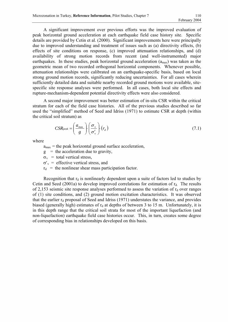
Microzonation in Turkey, Reference Information, Pilot Studies, Chapter 7 110 February 2004
A significant improvement over previous efforts was the improved evaluation of peak horizontal ground acceleration at each earthquake field case history site. Specific details are provided by Cetin et al. (2000). Significant improvements here were principally due to improved understanding and treatment of issues such as (a) directivity effects, (b) effects of site conditions on response, (c) improved attenuation relationships, and (d) availability of strong motion records from recent (and well-instrumented) major earthquakes. In these studies, peak horizontal ground acceleration (amax) was taken as the geometric mean of two recorded orthogonal horizontal components. Whenever possible, attenuation relationships were calibrated on an earthquake-specific basis, based on local strong ground motion records, significantly reducing uncertainties. For all cases wherein sufficiently detailed data and suitable nearby recorded ground motions were available, site-specific site response analyses were performed. In all cases, both local site effects and rupture-mechanism-dependent potential directivity effects were also considered.
A second major improvement was better estimation of in-situ CSR within the critical stratum for each of the field case histories. All of the previous studies described so far used the “simplified” method of Seed and Idriss (1971) to estimate CSR at depth (within the critical soil stratum) as
( )dv
vpeak r
ga
CSR ⋅
′
⋅
=
σσmax (7.1)
where amax = the peak horizontal ground surface acceleration, g = the acceleration due to gravity, σv = total vertical stress, σ′v = effective vertical stress, and rd = the nonlinear shear mass participation factor.
Recognition that rd is nonlinearly dependent upon a suite of factors led to studies by
Cetin and Seed (2001a) to develop improved correlations for estimation of rd. The results of 2,153 seismic site response analyses performed to assess the variation of rd over ranges of (1) site conditions, and (2) ground motion excitation characteristics. It was observed that the earlier rd proposal of Seed and Idriss (1971) understates the variance, and provides biased (generally high) estimates of rd at depths of between 3 to 15 m. Unfortunately, it is in this depth range that the critical soil strata for most of the important liquefaction (and non-liquefaction) earthquake field case histories occur. This, in turn, creates some degree of corresponding bias in relationships developed on this basis.

Microzonation in Turkey, Reference Information, Pilot Studies, Chapter 7 111 February 2004
Cetin and Seed (2001b) propose a new, empirical basis for estimation of rd as a function of; (1) depth, (2) earthquake magnitude, (3) intensity of shaking, and (4) site stiffness (as expressed in Equation 7.2).
It is noted, however, that in-situ CSR (and rd) can “jump” or transition irregularly
within a specific soil profile, especially near sharp transitions between “soft” and “stiff” strata, and that CSR (and rd) are also a function of the interaction between a site and each specific excitation motion. Accordingly, the best means of estimation of in-situ CSR within any given stratum is to calculate CSR directly by means of appropriate site-specific, and event-specific, seismic site response analyses, when this is feasible. As the new correlations were developed using both directly-calculated rd values (from site response analyses) as well as rd values from the statistically unbiased correlation of Equation 7.2, there is no intrinsic a priori bias associated with either approach.
In these new correlations, in-situ cyclic stress ratio (CSR) is taken as the “equivalent uniform CSR” equal to 65% of the single (one-time) peak CSR (from Equation 7.1) as
peakeq CSR)65.0(CSR ⋅= (7.3)
In-situ CSReq was evaluated directly, based on performance of full seismic site response analyses (using SHAKE 90; Idriss and Sun, 1992), for cases where (a) sufficient sub-surface data was available, and (b) where suitable “input” motions could be developed from nearby strong ground motion records. For cases wherein full seismic site response analyses were not performed, CSReq was evaluated using the estimated amax and Equations 7.1 and 7.2. In addition to the best estimates of CSReq, the variance or uncertainty of these estimates (due to all contributing sources of uncertainty) was also assessed (Cetin et al., 2001).
At each case history site, the critical stratum was identified as the stratum most susceptible to triggering of liquefaction. When possible, collected surface boil materials
d < 65 ft:
d
*04,s
*04,s
r
)888.24V0785.0(104.0
*04,swmax
)888.24V0785.0d(104.0
*04,swmax
*04,smaxwd
e201.0258.16
V016.0M999.0a949.2013.231
e201.0258.16
V016.0M999.0a949.2013.231
)V,a,M,d(r ε
+⋅⋅
′
+⋅+−⋅
′
′ σ±
⋅+
⋅+⋅+⋅−−+
⋅+
⋅+⋅+⋅−−+
=
′
′ (7.2a)
d ≥ 65 ft:
d
s
s
r
Vsw
Vsw
swd d
e
VMae
VMa
VaMdr εσ±−⋅−
⋅+
⋅+⋅+⋅−−+
⋅+
⋅+⋅+⋅−−+
=
+⋅⋅
′
+⋅+−⋅
′
′
′
′
)65(0014.0
201.0258.16
016.0999.0949.2013.231
201.0258.16
016.0999.0949.2013.231
),,,(
)888.240785.0(104.0
*04,max
)888.240785.065(104.0
*04,max
*04,max
*04,
*04, (7.2b)
where
0072.0d)d( 850.0rd
⋅=σε [for d < 40 ft], and 0072.040)d( 850.0rd
⋅=σε [for d ≥ 40 ft] (7.2c)

Microzonation in Turkey, Reference Information, Pilot Studies, Chapter 7 112 February 2004
were also considered, but problems associated with mixing and segregation during transport, and recognition that liquefaction of underlying strata can result in transport of overlying soils to the surface through boils, limited the usefulness of some of this data.
The N1,60-values employed were “truncated mean values” within the critical stratum. Measured N-values (from one or more points) within a critical stratum were corrected for overburden, energy, equipment, and procedural effects to N1,60 values, and were then plotted vs. elevation. In many cases, a given soil stratum would be found to contain an identifiable sub-stratum (based on a group of localized low N1,60-values) that was significantly more critical than the rest of the stratum. In such cases, the sub-stratum was taken as the “critical stratum”. Occasional high values, not apparently representative of the general characteristics of the critical stratum, were considered “non-representative” and were deleted in a number of the cases. Similarly, though less often, very low N1,60 values (very much lower than the apparent main body of the stratum, and often associated with locally high fines content) were similarly deleted. The remaining, corrected N1,60 values were then used to evaluate both the mean of N1,60 within the critical stratum, and the variance in N1,60.
For those cases wherein the critical stratum had only one single useful N1,60-value, the coefficient of variation was taken as 20%; a value typical of the larger variances among the cases with multiple N1,60 values within the critical stratum (reflecting the increased uncertainty due to lack of data when only a single value was available).
All N-values were corrected for overburden effects (to the hypothetical value, N1, that “would” have been measured if the effective overburden stress at the depth of the SPT had been 1 atmosphere) [1 atm. ≈ 2,000 lb/ft2 ≈ 1 kg/cm2 ≈ 14.7 lb/in2 ≈ 101 kPa] as
N1 CNN ⋅= (7.4a) where CN is taken (after Liao and Whitman, 1986) as
CN =1
σ’v
___0.5
(7.4b) where σ’v is the actual effective overburden stress at the depth of the SPT in atmospheres.
The resulting N1 values were then further corrected for energy, equipment, and procedural effects to fully standardized N1,60 values as
EBSR160,1 CCCCNN ⋅⋅⋅⋅= (7.5) where CR = correction for “short” rod length,
CS = correction for non-standardized sampler configuration, CB = correction for borehole diameter, and CE = correction for hammer energy efficiency.
The corrections for CR, CS, CB and CE employed correspond largely to those recommended by the NCEER Working Group (NCEER, 1997).
CS was applied in cases wherein a “nonstandard” (though very common) SPT sampler was used in which the sampler had an internal space for sample liner rings, but the rings were not used. This results in an “indented” interior liner annulus of enlarged diameter, and reduces friction between the sample and the interior of the sampler, resulting in reduced overall penetration resistance (Seed et al., 1984 and 1985). The reduction in penetration resistance is on the order of ~10 % in loose soils (N1<10 blows/ft), and ~30 % in very dense soils (N1>30 blows/ft), so CS varied from 1.1 to 1.3 over this range.

Microzonation in Turkey, Reference Information, Pilot Studies, Chapter 7 113 February 2004
Borehole diameter corrections (CB) were as recommended in the NCEER Workshop Proceedings.
Corrections for hammer energy (CE), which were often significant, were largely as recommended by the NCEER Working Group, except in those cases where better hammer/system-specific information was available. Cases where better information was available included cases where either direct energy measurements were made during driving of the SPT sampler, or where the hammer and the raising/dropping system (and the operator, when appropriate) had been reliably calibrated by means of direct driving energy measurements.
Within the Bayesian updating analyses, which were performed using a modified version of the program BUMP (Geyskens et al., 1993), all field case history data were modeled not as “points”, but rather as distributions, with variances in both CSR and N1,60 These regression-type analyses were simultaneously applied to a number of contributing variables, and the resulting proposed correlations are expressed in Equations 7.6 through 7.12.
The “clean sand” (Fines Content ≤ 5%) line of Seed et al. (1984) appears to correspond roughly to PL≈50%. This is not the case, however, as the Seed et al. (1984) line was based on biased values of CSR (as a result of biased rd at shallow depths, as discussed earlier.) The new correlation uses actual event-specific seismic site response analyses for evaluation of in situ CSR in 53 of the back-analyzed case histories, and the new (and statistically unbiased) empirical estimation of rd (as a function of level of shaking, site stiffness, and earthquake magnitude) as presented in Equation 7.2 (Cetin and Seed, 2000) for the remaining 148 case histories. The new (improved) estimates of in-situ CSR tend to be slightly lower, typically of the order of ∼ 5 to 15% lower, at the shallow depths that are critical in most of the case histories. Accordingly, the CSR’s of the new correlation are also, correspondingly, lower by about 5 to 15%, and a fully direct comparison between the new correlation and the earlier recommendations of Seed et al. (1984) cannot be made.
It should be noted that the use of slightly biased (high) values of rd was not problematic in the earlier correlation of Seed et al. (1984), so long as the same biased (rd) basis was employed in forward application of this correlation to field engineering works. It was a slight problem, however, when forward applications involved direct, response-based calculation of in-situ CSR, as often occurs on major analyses of dams, etc.
It was Seed’s intent that the recommended (1984) boundary should represent approximately a 10 to 15% probability of liquefaction, and with allowance for the “shift” in (improved) evaluation of CSR, the 1984 deterministic relationship for clean sands (<5% fines) does correspond to approximately PL ≈ 10 to 30%, except at very high CSR (CSR > 0.3), a range in which data was previously scarce.
Yoshimi et al.(1984) is arguably unconservatively biased at very low densities (low N-values) as these loose samples densified during laboratory thawing and reconsolidation. Their testing provides potentially valuable insight, however, at high N-values where reconsolidation densification was not significant. In this range, the new proposed correlation provides slightly better agreement with the test data than does the earlier relationship proposed by Seed et al. (1984).

Microzonation in Turkey, Reference Information, Pilot Studies, Chapter 7 114 February 2004
7.3.3 Adjustments for Fines Content The new (probabilistic) boundary curve for PL = 20% (again normalized to an effective overburden stress of σ’v = 0.65 atm.) represents a suitable basis for illustration of the new correlation’s regressed correction for the effects of fines content. Both the correlation as well as the mean values (CSR and N1,60) of the field case history data are not corrected for fines (this time the N-value axis is not corrected for fines content effects, so that the (PL=20%) boundary curves are, instead, offset to account for varying fines content.)
In these current studies, based on the overall (regressed) correlation, the energy- and procedure- and overburden-corrected N-values (N1,60) are further corrected for fines content as
N1,60,CS = N1,60 * CFINES (7.6)
where the fines correction was “regressed” as a part of the Bayesian updating analyses. The fines correction is equal to zero for fines contents of FC < 5%, and reaches a maximum (limiting) value for FC > 35%. The maximum fines correction results in an increase of N-values of about +6 blows/ft. (at FC > 35%, and high CSR). This maximum fines correction is somewhat smaller than the earlier maximum correction of +9.5 blows/ft proposed by Seed et al. (1984).
The regressed relationship for CFINES is
( )
⋅+⋅+=
60,1
05.0004.01NFCFCCFINES lim: FC ≥ 5% and FC ≤ 35% (7.7)
where FC = percent fines content (percent by dry weight finer than 0.074 mm), expressed as an integer (e.g. 15% fines is expressed as 15), and N1,60 is in units of blows/30 cm.
7.3.4 Magnitude-Correlated Duration Weighting Both the probabilistic and “deterministic” (based on PL=20%) new correlations are based on the correction of “equivalent uniform cyclic stress ratio” (CSReq) for duration (or number of equivalent cycles) to CSRN, representing the equivalent CSR for a duration typical of an “average” event of MW = 7.5. This was done by means of a magnitude-correlated duration weighting factor (DWFM) as
CSRN = CSReq,M=7.5 = CSReq / DWFM (7.8)
This duration weighting factor has been somewhat controversial, and has been developed by a variety of different approaches (using cyclic laboratory testing and/or field case history data) by a number of investigators. In these current studies, this important and controversial factor could be regressed as a part of the Bayesian Updating analyses. Moreover, the factor (DWFM) could also be investigated for possible dependence on density (correlation with N1,60). As observed, the dependence on density, or N1,60-values, was found to be relatively minor.
The duration weighting factors fall slightly below those recommended by the NCEER Working group, and slightly above (but very close to) recent recommendations of Idriss (2000). Idriss’ recommendations are based on a judgmental combination of interpretation of high-quality cyclic simple shear laboratory test data and empirical assessment of “equivalent” numbers of cycles from recorded strong motion time histories, and are the only other values shown that account for the cross-correlation of rd with magnitude. The close agreement of this very different (and principally laboratory data

Microzonation in Turkey, Reference Information, Pilot Studies, Chapter 7 115 February 2004
based) approach, and the careful (field data based) probabilistic assessments of these current studies, are strongly mutually supportive.
7.3.5 Adjustments for Effective Overburden Stress An additional factor not directly resolved in prior studies based on field case histories is the increased susceptibility of soils to cyclic liquefaction, at the same CSR, with increases in effective overburden stress. This is in addition to the normalization of N-values for overburden effects as per Equation 7.4.
The additional effects of reduction of normalized liquefaction resistance with increased effective initial overburden stress (σ’v) has been demonstrated by means of laboratory testing, and this is a manifestation of “critical state” type of behavior (soils become less dilatant at increased effective stress). The NCEER Working Group (Youd et al., 2001) regarding the correction factor Kσ to be used to correct to the normalized resistance to liquefaction at an initial effective overburden stress of 1 atm. (CSRliq,1atm) as
CSRliq = CSRliq,1atm. Kσ (7.9)
These current studies were not very sensitive to Kσ, as the range of σ’v in the case history data base was largely between σ’v = 600 to 2,600 lb/ft2, but it was possible to “regress” Kσ as part of the Bayesian updating. These are in good agreement with the earlier recommendations, and it is recommended that Kσ can be estimated as
Kσ = ( vσ′ )f-1 (7.10)
where f ≈ 0.6 to 0.8 (as N1,60,cs varies from 1 to 40 blows/ft.) The field case history data of these current studies are not a sufficient basis for extrapolation of Kσ to much higher values of σ’v, and the authors recommend use of σ’v > 2 atm.
The earlier relationships proposed by Seed et al. (1984), Liao et al. (1988, 1998), Youd and Noble (1997), and Toprak (1999) were all stated to be normalized to an effective overburden stress of approximately σ’v = 1 atm (2,000 lb/ft2). The correlation of Seed et al. (1984) was never formally corrected to σ’v = 1 atm., however, as it was noted that the field case histories of the database were “shallow”, and approximately in this range. The database was, however, not centered at σ’v = 1 atm., but rather at lesser overburden (Mean σ’v ≈1,300 lb/ft2or 0.65 atm), and this proves to render this earlier relationship slightly unconservative if taken as normalized to σ’v = 1 atm. (The same is true of all of the previous relationships discussed.) It should be noted, however, that this unconservatism is minimized if the correlations are applied at shallow depths.
For correctness, and to avoid ambiguity, both the earlier relationship of Seed et al. (1984), and the correlations developed in these current studies, need to be formally normalized to σ’v = 1 atm. Accordingly, in these studies, all data are corrected for K σ-effects (by Equations 7.9 and 7.10); not just those data for which σ’v was greater than 1 atm. A recommended limit is Kσ < 1.5 (at very shallow depths.)
The overall correlation can be expressed in parts, as in the previous sections (and Equations 7.6 - 12). It can also be expressed concisely as a single, composite relationship as shown in Equation 7.11.
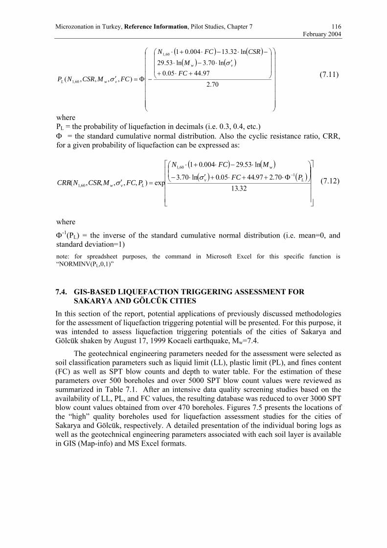
Microzonation in Turkey, Reference Information, Pilot Studies, Chapter 7 116 February 2004
7.4. GIS-BASED LIQUEFACTION TRIGGERING ASSESSMENT FOR SAKARYA AND GÖLCÜK CITIES
In this section of the report, potential applications of previously discussed methodologies for the assessment of liquefaction triggering potential will be presented. For this purpose, it was intended to assess liquefaction triggering potentials of the cities of Sakarya and Gölcük shaken by August 17, 1999 Kocaeli earthquake, Mw=7.4.
The geotechnical engineering parameters needed for the assessment were selected as soil classification parameters such as liquid limit (LL), plastic limit (PL), and fines content (FC) as well as SPT blow counts and depth to water table. For the estimation of these parameters over 500 boreholes and over 5000 SPT blow count values were reviewed as summarized in Table 7.1. After an intensive data quality screening studies based on the availability of LL, PL, and FC values, the resulting database was reduced to over 3000 SPT blow count values obtained from over 470 boreholes. Figures 7.5 presents the locations of the “high” quality boreholes used for liquefaction assessment studies for the cities of Sakarya and Gölcük, respectively. A detailed presentation of the individual boring logs as well as the geotechnical engineering parameters associated with each soil layer is available in GIS (Map-info) and MS Excel formats.
( ) ( )( ) ( )
+⋅+
′⋅−⋅
−⋅−⋅+⋅
−Φ=′70.2
97.4405.0ln70.3ln53.29
ln32.13004.01
),,,,(
60,1
60,1
FCM
CSRFCN
FCMCSRNP
vw
vwL
σ
σ (7.11)
where PL = the probability of liquefaction in decimals (i.e. 0.3, 0.4, etc.) Φ = the standard cumulative normal distribution. Also the cyclic resistance ratio, CRR,for a given probability of liquefaction can be expressed as:
( ) ( )( ) ( )
Φ⋅++⋅+′⋅−
⋅−⋅+⋅
=′−
32.1370.297.4405.0ln70.3
ln53.29004.01
exp),,,,,(1
60,1
60,1Lv
w
Lvw
PFC
MFCN
PFCMCSRNCRRσ
σ (7.12)
where
Φ-1(PL) = the inverse of the standard cumulative normal distribution (i.e. mean=0, andstandard deviation=1) note: for spreadsheet purposes, the command in Microsoft Excel for this specific function is“NORMINV(PL,0,1)”

Microzonation in Turkey, Reference Information, Pilot Studies, Chapter 7 117 February 2004
Table 7.1. A summary of reviewed and used borelog and SPT blowcount values for liquefaction assessment analyses
BORELOG CITY TOTAL # USED # SAKARYA 263 251 GÖLCÜK 306 220 SPT BLOWCOUNTS TOTAL USED SAKARYA 2334 2324 GÖLCÜK 3544 757
(a) (b)
Figure 7.5. Locations of the boreholes used for liquefaction triggering studies in (a) Sakarya and (b) Gölcük.
In addition to the geotechnical engineering parameters mentioned previously, for the estimation of CSR, the variation of peak ground acceleration and/or cyclic shear stresses values at soil sites after August 17, 1999 Kocaeli earthquake, within the cities of Sakarya and Gölcük need to be estimated. For the sake of presenting demonstration applications, peak ground acceleration at soil sites were adopted uniformly as 0.4 g for CSR estimations.
After having compiled geotechnical and earthquake engineering parameters, liquefaction triggering potential for both cities were performed as presented in the Liquefaction Assessment Section of the State of the Art Report. SPT blow counts were corrected for equipment, energy and procedural effects. The energy ratio was assumed to be 45% unless it was reported otherwise. CSR values were estimated based on the assumption of peak ground acceleration at soil sites to be 0.4 g. Rd values were adopted by following the mean curves as also presented in the Liquefaction Assessment Section of the State of the Art Report. The effects of soil structure interaction on the estimation of CSR as well as the liquefaction performance of soils were not incorporated for the sake of simplicity. This simplification is consistent with the potential use of these methodologies

Microzonation in Turkey, Reference Information, Pilot Studies, Chapter 7 118 February 2004
since the main aim of this project is to assess liquefaction risk of undeveloped areas rather than the ones that have developed already contrary to our demonstration cases.
Once CSR, σ′v, FC, N1,60 values for each critical soil layer which were identified by checking the criteria summarized by Andrews and Martin (2000), probability of liquefaction values were estimated as defined in Eq. 7.11. Similarly, factor of safety values corresponding to 20 % probability of liquefaction-CRR contours can also be estimated as defined in Eq. 7.12. Figures 7.6 and 7.7 present maps of liquefaction triggering assessment studies for the cities of Sakarya and Gölcük, respectively. Red zones define the regions where liquefaction triggering probability after August 17, 1999 Kocaeli earthquake is predicted to be greater than 90 %. Similarly, orange and yellow zones define the regions, where liquefaction triggering probabilities after August 17, 1999 Kocaeli earthquake are predicted to be in the range of 70 % - 90 % and 50% to 70 %, respectively. Green, light and deep blue regions, listed in the order of higher to lower risk, are classified as the zones where liquefaction triggering probabilities are estimated to be less than 50 %.
Figure 7.6. Liquefaction triggering potential of Sakarya after 17 August, 1999 Kocaeli earthquake, expressed in terms of probability of liquefaction

Microzonation in Turkey, Reference Information, Pilot Studies, Chapter 7 119 February 2004
Figure 7.7. Liquefaction triggering potential of Gölcük after 17 August, 1999 Kocaeli
earthquake

Microzonation in Turkey, Reference Information, Pilot Studies, Chapter 8 120 February 2004
8. LANDSLIDE HAZARD
Bilge Siyahi and Yasin Fahjan, Department of Earthquake Engineering, Kandilli Observatory and Earthquake Research Institute, Boğaziçi University
8.1. INTRODUCTION Siyahi and Ansal (1993) have proposed a procedure for investigating slope stability for microzonation purpose. This procedure is introduced in the “Manual for Zonation on Seismic Geotechnical Hazards” by TC4, ISSMFE (1999) as a Grade-3 method. Applicability of this procedure was confirmed against an earthquake that occurred in 1967 in the Adapazarı region, Turkey. The stability analysis method is a pseudo-static evaluation of slope stability utilizing a seismic coefficient A to account for the earthquake induced horizontal forces.
Figure 8.1. A typical section of a slope
A linear variation in shear strength τ with depth is assumed and the potential failure surface is taken as a circular arc, as shown in Figure 8.1. The safety factor is calculated as
φγ
φγγ
tantan111
0 NNNaFs === (8.1)
based on the angle of shear strength and stability number N1 representing the configuration of the slope and failure surface. The minimum value of the stability number is determined by carrying out a parametric study in terms of α, β, γ, and n to find out the most critical failure surface as given in Figure 8.2. The variation of minimum N1 can be expressed as a function of β (slope angle) and A (maximum ground acceleration on the surface). It becomes possible at this stage to calculate minimum safety factor Fs, if a φ value can be determined or estimated.
This procedure assumes a circular arc failure and normally consolidated soil. Although all the slopes are not of this type, it can be considered as the most critical condition. Because this procedure is simplified, the failure and parametric study approached is applied. There are generally varieties of slope characteristics in the areas

Microzonation in Turkey, Reference Information, Pilot Studies, Chapter 8 121 February 2004
Topographic Condition
Steepest angle of slope for each 500x500 m grid
Maximum Ground Acceleration on the Surface
Soil Strength of Slope Material
Judgment of Slope Stability for 500x500 m Grid Using Eq. 8.3
and it is difficult to identify slope failure parameters for every slope in detail. Therefore this procedure is applied to be able to make a qualitative evaluation of slope stability.
0
2
4
6
8
10
12
14
0 10 20 30 40 50 60 70 80
Slope angle
N1,
sta
bilit
y nu
mbe
rs
0 g 0,1 g 0,2 g 0,3 g0,4 g 0,5 g 0,6 g 0,7 g
Figure 8.2. Relationship between slope angle (β), seismic coefficient (A) and minimum
stability number (N1) (Siyahi,1998)
8.2. PROCEDURE OF ANALYSIS AND EVALUATION OF STABILITY
The outline of the evaluation method is described below and shown in Figure 8.3. The maximum slope gradient for each 50-m grid, that covers all of the area, is calculated at first. Then the slope stability of each point is judged, using Siyahi and Ansal (1993) procedure taking the maximum ground acceleration value and strength of soil into account.

Microzonation in Turkey, Reference Information, Pilot Studies, Chapter 8 122 February 2004
8.3. PARAMETERS FOR CALCULATION
8.3.1 Shear Strength of Slope Material Shear strength is the most important parameters for applying this procedure. The values of strength adopted are summarized in Table 8.1 for the Adapazarı and Gölcük regions. These are evaluated from data obtained from boreholes in these regions. Since the borehole data covers laboratory and in-situ testing such as SPT, shear box, triaxial and uniaxial tests, for soil and rock deposits in the region, to find the actual values of shear strength, which is represented here such as shear strength angle, φ, or alternatively as the internal friction angle, is rather straightforward in this case.
Table 8.1. Shear strength angle for slope stability calculations in the Adapazarı and Gölcük regions.
Ages of the deposits
Formation Shear strength angle, φ (°)
Description of soil and rock units
Quaternary Alluvium in Adapazarı 25 Sand, gravel, silt, clay Holocene Alluvium in Gölcük 25 Sand, gravel, silt, clay Upper Cretaceous
Akveren (Adapazarı) 35 Conglomerates, sandstone, limestone
Plioecene Aslanbey (Gölcük) 30 Sand, gravel, silt and clay (loosely consolidated fluvial alluvium)
Recent Fill (Gölcük) 15 Gravel and cobble-boulder blocks
8.3.2 Maximum Ground Acceleration on the Surface Within a pseudo-static approach, the effects of an earthquake are represented by constant horizontal and vertical accelerations. Selection of an appropriate pseudo-static coefficient is the most important aspect of a pseudo-static stability analysis. In this procedure, maximum ground acceleration (A) on the surface can be accepted as a pseudo-static coefficient. Maximum ground acceleration on the surface is evaluated based on the one-dimensional ground response analysis as performed by ETHZ.
8.3.3 Slope Angle
The topographical contours are provided in terms of MapInfo tables. The minimum distance among subsequent contours for each cell is computed using the (Ruler) option provided in MapInfo. The relevant steepest slope gradient for each Geo-cell is calculated using the minimum distance and elevations difference in the subsequent contours.
8.4. SLOPE STABILITY COMPUTATION USING KOERISLOPE
KoeriSlope is application developed to estimate slope stability for microzonation purposes. KoeriSlope Version 1.0 in its current form is capable of performing slope stability estimation analysis based on the Siyahi and Ansal (1993) procedure. KoeriSlope is a user-friendly application that operates through Geo-cells systems. Geo-cells (Grids) facilitate the manipulation of data for soil type, slope gradient and earthquake hazards. The application is developed using the MapBasic language and runs efficiently under MapInfo software. The application is integrated with MapInfo and capable to utilizing the powerful features in displaying, querying, manipulating and mapping inventory databases.

Microzonation in Turkey, Reference Information, Pilot Studies, Chapter 8 123 February 2004
KoeriSlope can be launched under MapInfo using the <Run MapBasic Program> feature from the standard menu bar of MapInfo. The main dialog of the application is shown below.
Figure 8.3. Main Dialog of KoeriSlope Application
8.4.1 Data Needed for the Slope Stability Study In order to perform a slope stability analysis, the following input data should be provided for each Geo-cell.
- Maximum expected ground acceleration (seismic coefficient). - Soil friction angle. - Maximum slope gradient.
8.4.2 Output of the Analysis The application computes the N1 stability number, based on the seismic coefficient of acceleration and slope gradient for each Geo-cell. Then slope stability safety factor for each Geo-cell is calculated, as it is described in Eq. (8.1). An output File is provided including all the input information for each Geo-cell in addition to the stability number (N1) and the slope stability factor of safety (FS). A thematic map of the results is also provided as shown in Chapter 11.

Microzonation in Turkey, Reference Information, Pilot Studies, Chapter 8 124 February 2004
Figure 8.4. Output of the KoeriSlope Application

Microzonation in Turkey, Reference Information, Pilot Studies, Chapter 9 125 February 2004
9. BACKGROUND REPORT ON STRUCTURAL DAMAGE; DEVELOPMENT AND IMPLEMENTATION OF A BUILDING DAMAGE SURVEY FOR ADAPAZARI, TURKEY: INTERPRETATION AND SOILS CORRELATION
P. Gülkan, S. Bakır, A. Yakut, T. Yılmaz and U. Yazgan (METU) with Collaboration of M. Elmas (SU) and P. Lestuzzi (EPFL)
9.1. EXECUTIVE SUMMARY Turkey is among countries that have long been affected by natural disasters, in particular earthquakes and floods. The most recent series of devastating earthquakes in 1999 have caused loss of lives of thousands and created an enormous financial burden on the economy, government, industry, insurance sector and public. Rigorous impact of these disasters led the Government of Turkey to initiate a legal revision to explore a natural catastrophe risk management strategy including ways of promoting disaster insurance. For this purpose, various studies financed under loans obtained from the World Bank have been completed. As a result, the Government of Turkey has decided to introduce a compulsory earthquake scheme making it mandatory for residences to take out insurance starting from September 27, 2000. The legal framework of the new scheme has been established by a decree (No. 587) with power of law for Compulsory Earthquake Insurance. A decree is a fast-track legal instrument that must be amended and adopted by parliament within a prescribed time limit. The decree has created the Turkish Catastrophe Insurance Pool (TCIP) for the purpose of relieving the Government of having to provide compensation to earthquake victims. A natural consequence of the creation of TCIP has been a renewed perception to set up a global damage assessment and quantification system for compensation of policy holders. Because of its past experience in such matters, the Disaster Management Research and Implementation Center at Middle East Technical University (DMC/METU) has been contracted by GDDA to train damage assessors. The present contract work described below has been an outgrowth of this experience to ascertain connections between local geological conditions and structural damage distribution patterns.
A parallel activity toward earthquake hazard mitigation was a study funded by the Government of Switzerland and executed through the World Institute for Disaster Risk Management (DRM) to produce a microzonation manual for local governments to follow when making land use decisions with the aim of minimizing seismic risks. The Government of Turkey is represented in this project through the General Directorate of Disaster Affairs because it is through this agency that regulations requiring such studies to be undertaken by municipalities can be issued. Microzonation is not an end to itself but a useful tool that facilitates reaching rational land-use decisions that safeguard public safety from the seismic peril. The region centered around the city of Adapazarı in northwestern Turkey was chosen as the natural site for the case studies because of extensive damages closely linked to improper consideration of local geology in the area. The global research teams are comprised of specialized groups, both international and Turkish, that carries out a coordinated set of activities to produce the Manual of Practice for Microzonation and its supporting documentation.
The World Institute for Disaster Risk Management engaged DMC/METU in order to perform services in respect of “Consultancy Services for Microzonation for Earthquake Risk Mitigation” in accordance with the following conditions:

Microzonation in Turkey, Reference Information, Pilot Studies, Chapter 9 126 February 2004
• Provision of limited data for geotechnical studies in the case study regions (with the bulk of the data coming from other subcontractors in the project)
• Analysis of structural performance of buildings in case study regions
• Analysis of land use management practices at the municipal level
• Preparation of a report including recommendations for strengthening of land use management for earthquake safety
An itemization of the tasks required under this obligation is reproduced below:
• Collection and organization of relevant geological and geotechnical data for the case study areas
• Collection of structural damage data locally through services provided by Sakarya University (SU)
• Preparation of data in transportable GIS format
• Establishing liaison with IS-ENAC EPFL in data identification, definition of data format and review of literature
A great deal can be learned from the pattern of damage experienced in recent or historic earthquakes. Damage patterns correlate well with the distribution of shaking intensity and the relationship of structural conditions with site conditions. Within the corresponding phase of the services DMC/METU was to provide analysis of site conditions to structural performance, drawing from the data collected by SU. Preparation of maps of damage patterns from Adapazarı was an objective. Determination of specific procedures to assess the vulnerability of local construction and description of these practices for inclusion in the Manual were also cited as output from this work. A separate task was subsequently appended to the DMC/METU work package to study the liquefaction vulnerability of the municipal area of Adapazarı and Gölcük, expressing the output in terms of probability numbers.
DMC/METU is also committed to ensuring the sustained implementation of the set of good practices that will be identified in the Manual. To this end, the analytical evaluation of the legal bases for land use management and its regulatory practice will be submitted to DRM under a separate package. Training of municipal personnel and public information on land use management are also parts of this other package.
The present report is intended to answer the question of whether the damage patterns in Adapazarı are indicative of a consistent trend explicable in terms of local site conditions. For this purpose a total of 301 buildings that had collapsed fully were evaluated. This exercise was necessarily a desk study conducted from the design blueprints of the individual buildings. The data collection was done in accordance with the form reproduced in Appendix 5.1, and its interpretation is contained in Section 9.2. None of the buildings in this data set existed at the time of our studies, so there remain a good number of points that must be known if accurate projections for the cause of the damage were to be identified. As a complementary body of data we have also included in Section 9.3 an explanation of the rationale for the damage assessment form used by personnel of GDDA is outlined. The form used in customary practice is given in Appendix 5.2.
Can a correlation be established between structural damage observed in Adapazarı and site conditions? This question is tackled in Section 9.4 on the basis of borehole and laboratory data from soils investigations performed in Adapazarı municipal limits.

Microzonation in Turkey, Reference Information, Pilot Studies, Chapter 9 127 February 2004
9.2. COLLAPSE DAMAGE SURVEY IN ADAPAZARI
9.2.1 Introduction Adapazarı was the scene of spectacular structural damage as well as widespread liquefaction that occurred in the city. The damage survey was conducted during the summer of 2002, nearly three years after the actual event. By that time, extensive repairs had been done in surviving buildings, and many others had been demolished and removed. Homeowners were reluctant to permit another round of examinations to be conducted in their property, so the decision was reached to include those buildings that had collapsed during the earthquake, and had led to loss of human life. When such is the case, the law requires expert witnesses to prepare an affidavit that will establish who the culprits might be. The Department of Civil Engineering, Sakarya University, because of their proximity to the site, had served in this capacity for many buildings on the basis of design blueprints and structural calculations, so the decision was reached to utilize that information source under a new magnifier. The information was extracted through the form reproduced in Appendix 5.1, assuming that the drawings were an accurate replication of the as-built structure. The location coordinates of the buildings were determined by a hand-held GPS device, accurate to about 10 m. This was judged to be an acceptable error.
9.2.2 Building Morphology
The buildings reported by SU were situated in the locations in Figure 9.1. This figure is deliberately superposed on the analog map of the city because even with its poor legibility it allows urban features such as major roads and the Sakarya River banks on the east. The same information is repeated in Figure 9.2 where the districts in the city have been numbered, and the number of stories of these collapsed buildings coded to allow a rapid assessment of the building heights. Building heights are as much a function of the economics of the corresponding usage as it is of zoning laws enacted by the city government. In central urban areas in Turkey there is commonly a mixed form of occupation, where small businesses (small grocery shops, barber shops, lawyers or physicians offices, etc.) are dispersed among the residences under the same roof. The ground story is usually made as free of obstructions to human traffic as possible, and this leads to weak or soft stories at the level where the seismic demand is largest. Figure 9.3 shows that half of the buildings examined in this study were five stories in height. The next largest group is for six story buildings comprising 32 percent of the total, and this is typical for much of recent construction.
The information contained in Figures 9.1-9.3 is useful to establish the overall architectural characteristics of the housing stock in Adapazarı. We believe that extrapolations can safely be made from these figures for reaching general conclusions. There is also reason to believe that most of the buildings in the sample group dated from the post-1975 period, so that their earthquake designs were done according to the provisions of the 1975 edition of that code.
The total number of building in the data set was 301. Interpretation as absolute numbers of normalized graphs in the following will be facilitated when those figures are multiplied with this sum. All buildings were reinforced concrete frames.

Microzonation in Turkey, Reference Information, Pilot Studies, Chapter 9 128 February 2004
Figure 9.1. Building Locations
Figure 9.2. Building Locations Differentiated according to Height

Microzonation in Turkey, Reference Information, Pilot Studies, Chapter 9 129 February 2004
Normalized Distribution of Buildings with Respect to Height
0,040,12
0,50
0,32
0,030,00
0,20
0,40
0,60
0,80
1,00
3 4 5 6 7 Number of Stories
Perc
enta
ge o
f Bui
ldin
gs
Figure 9.3. Distribution of Building Height in the Sample
9.2.3 Architectural and Structural Features The current Turkish earthquake regulations make a clear definition of structural irregularities that lead to added earthquake vulnerability. In general, irregularities in plan are classified as being of type A, with sub-group designated as A1, A2, etc., and irregularities in elevation are described as being of type B. These are each described, and follow universal procedures for quantification. The questions listed under “Irregularities” in the form in Appendix 5.1 have been designed to clarify the prevalence of the distribution of these among the sample of buildings examined by SU.
It is instructive to examine first the distribution of soft stories. A soft story occurs when the lateral rigidity of the horizontal load resisting members at any level is such that the average lateral drift under the design load at that level is more than 50 percent larger than the same quantity calculated for the next story. This property needs a set of calculations to be made. With taller columns and no infill or structural walls, this situation usually is encountered at the ground level in Turkey. In Figure 9.4 we have shown the distribution of this situation in normalized fashion among the buildings in the sample set.
It can be assumed that taller buildings were of more recent dates of construction, and as building height limitations had been eased in recent times owners took advantage of the full height permitted in the zonation decisions. It is quickly seen that while (older) 3-story buildings were evenly distributed with respect to existence of soft stories, taller buildings were about 70 percent that way, and the seven story subset was entirely rated as having the property. In general, the situation for identifying a weak story where the lateral strength at a given story differs by more than 20 percent that at the neighboring story did not arise because designers accounted for that by varying the reinforcement details.

Microzonation in Turkey, Reference Information, Pilot Studies, Chapter 9 130 February 2004
Figure 9.4. Distribution of Soft Stories
Torsional irregularity is defined in the Turkish code as the situation when the average lateral translation under the design forces at a given story differs by more than 20 percent the largest lateral situation at the same story. This usually occurs at the extreme ends of the floor slabs when L-, T- or similar shapes in plan exist. Land ownership patterns sometimes force architects to design such buildings when they wish to take advantage of utilizing the entire buildable footprint area of the land. Figure 9.5 describes the distribution of this property among our sample set.
Figure 9.5. Existence of Torsional Irregularity
Plan irregularity refers to the situation when long projections in plan exist for the building. In addition to the increased likelihood of causing torsional irregularity this situation creates re-entrant corners where stresses are concentrated, and may cause unexpected distress. The data in Figure 9.6 describes this situation. Again taller buildings seem to be more likely to possess this characteristic.
Soft Story Normalized within Corresponding Number of Story
0.50
0.71 0.710.65
1.00
0.50
0.29 0.290.35
0.000.00
0.20
0.40
0.60
0.80
1.00
3 4 5 6 7Number of Stories
Perc
enta
ge o
f Bui
ldin
gs
Soft StoryNo Soft Story
Torsional Irregularity Normalized within Corresponding Number of Story
0.42
0.54
0.77 0.79
1.00
0.58
0.46
0.23 0.21
0.000.00
0.20
0.40
0.60
0.80
1.00
3 4 5 6 7Number of Stories
Perc
enta
ge o
f Bui
ldin
gs
IrregularityNo Irregularity

Microzonation in Turkey, Reference Information, Pilot Studies, Chapter 9 131 February 2004
Plan Irregularity Normalized within Corresponding Number of Story
0,17
0,37 0,35 0,32
0,67
0,83
0,63 0,65 0,68
0,33
0,00
0,20
0,40
0,60
0,80
1,00
3 4 5 6 7Number of Stories
Perc
enta
ge o
f Bui
ldin
gsIrregularityNo Irregularity
Figure 9.6. Existence of Plan Irregularity
From the structural viewpoint, mezzanines can prove to be trouble spots because the lateral strength of short and tall columns are different by large amounts, and the extra inertia effects transmitted to columns at their mid-height are difficult to account for. As Figure 9.7 shows, this situation appears not to have been a widespread practice.
While the post-collapse damage form in Appendix 5.1 has entries for material quality, workmanship and similar features it was not possible to conduct any tests on actual material coupons or cylinders to answer this with clarity. We have relied on the intended material qualities on the calculation sheets which was generally specified as 20 MPa. It is known that the actual strengths may differ by large margins from their intended values. We have also no factual data on whether plain or deformed bars had been used.
Figure 9.7. Occurrence of Mezzanine Floors at Ground Level
Presence of Mezzanine
0 0 5
24912
35
145
71
00
20
40
60
80
100
120
140
160
3 4 5 6 7Number of Stories
Num
ber o
f Bui
ldin
gs
MezzanineNo Mezzanine

Microzonation in Turkey, Reference Information, Pilot Studies, Chapter 9 132 February 2004
9.2.4 Column and Wall Indexes Our experience with the seismic vulnerability of the housing stock in Turkey has taught us that the normalized column and wall areas a given building possesses can serve as a useful index (Shiga et al., 1968; Gülkan & Sözen, 1999). The central idea for expressing vulnerability is expressed as the weight of the structure (which is proportional to its total floor area) divided into the sum of the cross-sectional areas of the columns and walls at the base. This format is attractive because of the ease with which the data can be acquired. Lengthy calculations are not necessary. The outcome is a crisp numerical index that can be matched against a derived yardstick so that a judgment about the vulnerability can be stated. The paper by Shiga et al. is difficult to generalize because it was derived exclusively in relation to a particular group of buildings constructed in accordance with the Japanese practice of the 1960s. Recalibrating their format can best be accomplished by testing its predictive success against observed damage in a collection of buildings with dimensional and material properties based on random choices made during the design and construction stages. This way, the question of whether a rational explanation of the empirical evidence is contained in the theory can be answered with confidence.
Conventional design procedures focus on arriving at proper component dimensions that will accommodate prescribed forces, but a more important issue is to keep structural displacements within prescribed limits. This idea has gained popularity in recent years as the central principle of performance based earthquake design. The concept of limiting ground level drift to prescribed limits was tested against empirical data collected in Erzincan following a major earthquake there in 1992. The article by Gülkan & Sözen (1999) contains the rationalization of the concept of linking column and wall areas to drift, and its comparison with actual data. Basically, the column index is 0.5 times the total cross sectional area of columns at the base plus 1.0 times the area of structural walls divided by the total floor area of the building. Filler wall index is defined as 0.1 times the area of filler walls at the base divided by the total floor area. Because orientation of planar members such as walls is direction dependent, it is possible to express this ratio in the two principal directions of the building. The result of this exercise for the set of buildings in our sample has produced the diagrams in Figures 9.8 and 9.9. We stress that the directions have been defined arbitrarily.
Y-direction
0.000
0.001
0.002
0.003
0.004
0.005
0.000 0.002 0.004 0.006 0.008 0.010
Column + Wall Index
Par
titio
n W
all I
ndex
Figure 9.8. Wall and Column Indexes in y-Direction
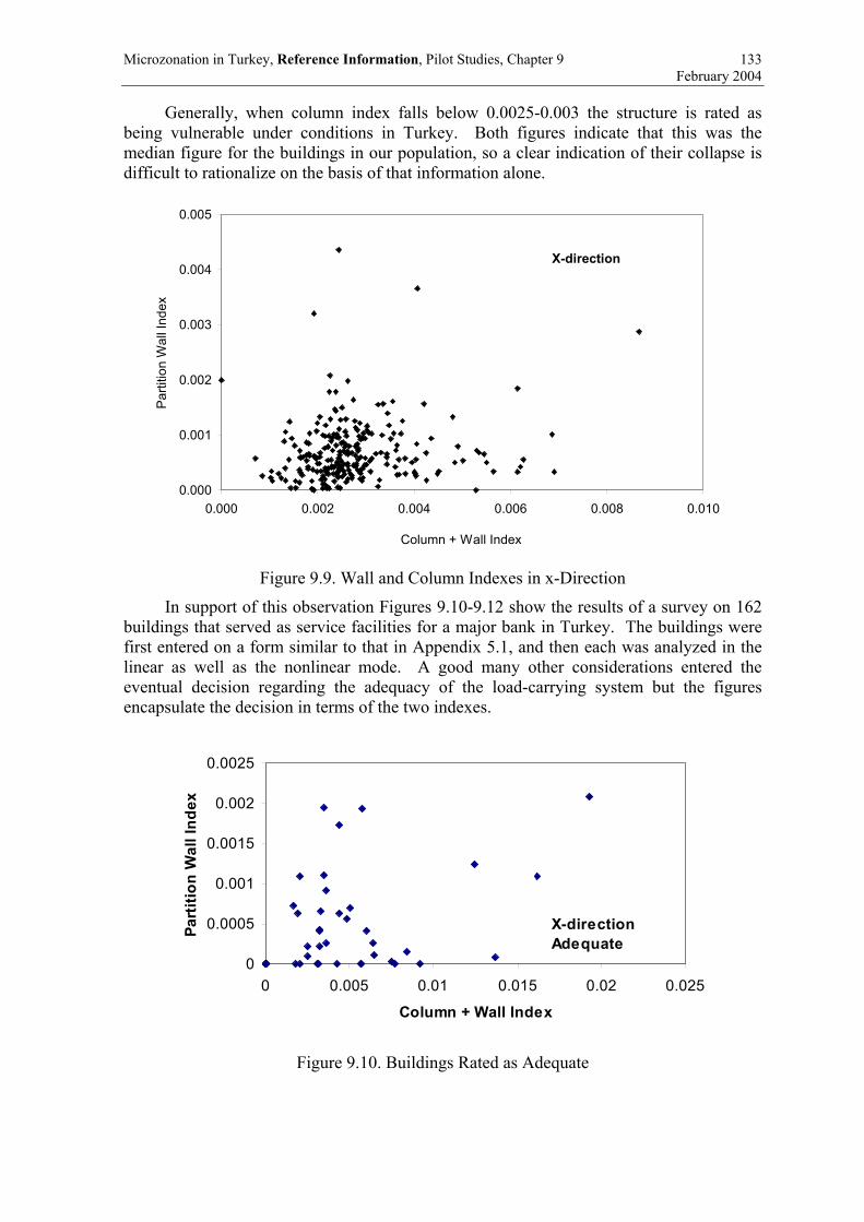
Microzonation in Turkey, Reference Information, Pilot Studies, Chapter 9 133 February 2004
Generally, when column index falls below 0.0025-0.003 the structure is rated as being vulnerable under conditions in Turkey. Both figures indicate that this was the median figure for the buildings in our population, so a clear indication of their collapse is difficult to rationalize on the basis of that information alone.
X-direction
0.000
0.001
0.002
0.003
0.004
0.005
0.000 0.002 0.004 0.006 0.008 0.010
Column + Wall Index
Par
titio
n W
all I
ndex
Figure 9.9. Wall and Column Indexes in x-Direction
In support of this observation Figures 9.10-9.12 show the results of a survey on 162 buildings that served as service facilities for a major bank in Turkey. The buildings were first entered on a form similar to that in Appendix 5.1, and then each was analyzed in the linear as well as the nonlinear mode. A good many other considerations entered the eventual decision regarding the adequacy of the load-carrying system but the figures encapsulate the decision in terms of the two indexes.
0
0.0005
0.001
0.0015
0.002
0.0025
0 0.005 0.01 0.015 0.02 0.025
Column + Wall Index
Part
ition
Wal
l Ind
ex
X-directionAdequate
Figure 9.10. Buildings Rated as Adequate

Microzonation in Turkey, Reference Information, Pilot Studies, Chapter 9 134 February 2004
0
0.0005
0.001
0.0015
0.002
0.0025
0 0.005 0.01 0.015 0.02 0.025
Column + Wall Index
Part
ition
Wal
l Ind
ex
X-directionTo be Strengthened
Figure 9.11. Buildings Rated as Requiring Strengthening
0
0.0005
0.001
0.0015
0.002
0.0025
0 0.005 0.01 0.015 0.02 0.025
Column + Wall Index
Part
ition
Wal
l Ind
ex
X-directionTo be Demolished
Figure 9.12. Buildings Rated as Requiring to Be Demolished
9.2.5 Conclusions
Attempting to piece together a clear post-fact statement for the collapse of the buildings in the data set assembled by SU and analyzed by the DMC/METU team appears to be a challenge. It is known that in Turkey many buildings are built in contravention of their design drawings, and records of these modifications usually do not exist. Buildings on soft and liquefaction-prone sites in Adapazarı were toppled or sunk into their foundations in spectacular ways, but these buildings did not usually suffer structural collapse leading to fatalities. As our building population had been examined for judicial purposes, there is reason to believe that most of them had been instigated by the public prosecutor following human life losses.
We believe that factors not identified in our investigations may have played just as important a role in these collapses. This is borne out by the inconsistency between Figures 9.8-9.9 and 9.10-9.12.

Microzonation in Turkey, Reference Information, Pilot Studies, Chapter 9 135 February 2004
9.3. EARTHQUAKE DAMAGE ASSESSMENT IN TURKEY
9.3.1 Introduction This chapter is intended as a resource for how damage assessment is conducted in
Turkey following earthquakes. Until September 2000, this was the responsibility of the teams assigned to disaster areas by the General Directorate of Disaster Affairs. From that time on, this responsibility was transferred to damage assessors appointed by the Turkish Compulsory Insurance Pool (TCIP) through its operational arm DASK. Because of its immediate relevance we show the distribution of building types of the housing stock in Turkey in Figure 9.13. We note that nearly 7 out of every 8 buildings are fully or partly residential.
It is not yet known how this service will be performed by the teams empowered by TCIP because no major earthquake has occurred, but considerable experience had been accumulated over 40 years at GDDA. In 1994 GDDA had engaged DMC/METU to design a more advanced system of damage assessment to reduce the number of litigations against it by citizens in disagreement with the assessed damage of their property. The remainder of this chapter and Appendix 5.2 are devoted to a description of this new concept and the form that served as its underpinning.
Commercial 6%Education 0.36%
Culture, Health, Social and Sport Oriented 0.25%
İndustrial 1.8%
Institutional 0.42%
Residential and Nonresidential Mixed 12.1%
Religious 0.34%Others 3.72%
No Response 0.049%
Residential 74.9%
Figure 9.13. Breakdown according to Usage of the Housing Stock in Turkey
9.3.2 Post-Earthquake Damage Assessment When a strong earthquake strikes a populated area, a good many buildings may suffer damages of various degrees, occasionally leading to partial or complete collapse in some of them. Building officials and damage inspection teams are then faced with confusing and chaotic circumstances when they must make quick and reliable judgments in assessing the degree of damage, the safety and continued usability of these buildings. This operation is referred to as Emergency Post Earthquake Damage Assessment (or EPEDA). It typically consists of a quick reconnaissance of the buildings in the area to determine whether they can still serve the functions they had been designed for without a substantial reduction in the safety conditions required for human occupancy.

Microzonation in Turkey, Reference Information, Pilot Studies, Chapter 9 136 February 2004
The primary purpose of emergency damage inspection is to protect human lives and to prevent injuries by identifying buildings that have been weakened by the earthquake, and are therefore threatened by subsequent aftershocks. The other important objective of this operation is to avoid unnecessary squandering of resources by singling out habitable and easily repairable buildings. A parallel goal is the quantification of structural damage in a given structure after it has been exposed to a given ground motion so that projections useful for constructing vulnerability curves or insurance loss models. It is conceivable that compensation to insured property owners would be based on the results of this exercise. In fact, the exclusive purpose of damage assessment in Turkey has traditionally been to identify individuals to whom government subsidies would be conferred.
Following an earthquake, the demand for building experts far exceeds their availability. In many instances, inexperienced engineers or poorly trained technicians are assigned to perform this task without being given specific criteria on how to do it. The task of damage assessment is generally done in the following way: the inspection team fills out a form that consists of a series of questions covering general information on the type of structure, its location, and the state of damage of selected components of the building. The questionnaires are tools for the uniform gathering of data. There is no intention to guide the inspector in reasoning about the task he/she faces, nor is there a targeted attempt to assist in the evaluation and decision-making process. The quantitative assessment of the degree of damage in the entire structure is made difficult because it is described in vague or imprecise language, or is beyond their technical capabilities. An all-seeing system for post-earthquake damage assessment is difficult to design for this reason. It can also be the source of endless litigation if not used properly. The work described in this part (Gülkan et al., 1994) was designed initially to upgrade also the form for damage assessment in use in Turkey (Gülkan & Aykut, 1996). Its scope is broad enough to accommodate all forms of engineered construction that might be encountered in Turkey.
The remainder of this chapter is devoted to describing shortly features of the form which is based on visual material contained in the parent document cited in Gülkan et al., (1994). The references to figures or tables in the form given as Appendix 5.2 are in fact to that work. The rating of damage reflected in the form is related strictly to structural damage (Park & Arg, 1985) as expressed through a specific damage model suitable for reinforced concrete components.
We have attached the popularly preferred acronym of EPEDA also to this methodology.
9.3.3 Overview EPEDA is an advisory system for the condition assessment of buildings hit by an earthquake. Its purpose is to assist the assessor during the emergency inspection phase following an earthquake by providing a rational and uniform set of guidelines for this purpose. Based on the inspector’s observations, EPEDA helps in making quick and accurate decisions regarding the severity of the damage and occupancy state of the building. It is not intended to replace the inspector but to guide him through the reasoning process to ensure that the engineer’s approach to the problem is correct. The system provides the background required in particular circumstances, and suggests a second inspection when the damage score is within the transition limits.
The knowledge base upon which the damage state for the entire building is based is the most heavily damaged floor level, which is usually the ground level. When the most heavily damaged floor is too large for the canvassing team to inspect fully, then this

Microzonation in Turkey, Reference Information, Pilot Studies, Chapter 9 137 February 2004
difficulty is bypassed by requiring that only a representative sub-part of that floor should be examined because damage scores are based on ratios rather than on absolute numbers for damaged elements.
The visible part of EPEDA consists of a form (reproduced in Appendix 5.2) that has a number of question for the inspector to answer, and a booklet that serves as a background tool. Some of the questions in the form are answered with the aid of iconized diagrams drawn in detailed form in the booklet, and supported by verbal explanations based on structural theory and empirical data. The questions fall into four major categories:
• Administrative information (ownership, address, casualties, etc.)
• General information (geometric/architectural characteristics, structural features, irregularities, spans, etc.)
• Load-resisting mechanism features (type of framing, wall-frame, or box, type of floor system, whether poured in place or prefabricated, partition wall strengths, type of foundation system, workmanship quality, etc.)
• Attributes of damage and their extent for each type of member for each damage category (permanent drifts, wall crack widths, visible cracks in the horizontal and vertical members, etc.). The form is designed to work also in conjunction with a renewable relational data base.
9.3.4 Knowledge in EPEDA
The methodology embedded in EPEDA is based on the notion of Global Damage State, which is a qualitative measure of the safety of the building under inspection. The score of the Global Damage State directly dictates the decision that should be taken regarding the continued use of the structure. If it is severe, then the building should be immediately evacuated, and eventually demolished. If it is slight, then the building is declared as being safe for continued use, and may be occupied even as aftershocks are occurring. If it is in a state of moderate damage, then the building requires repair, and therefore can be occupied only after retrofit has been done. Any of the outcomes may apply only to the entire building, and not to parts of it. The damage state associated with the building is the result of a consistent reasoning involving three principal elements: evidence derived from the geotechnical state of the local site conditions in the immediate vicinity of the building and its foundations system, the state of the structural system, and additional hazards represented by its deformed configuration. The Global Damage State is determined by calculating the Total Damage Score (TDS), which consists, in the case of reinforced concrete systems, of contributory damage from five different damage sub-scores. The first is called the Damage Exacerbating Score (DES) that reflects the general architectural features of the building. For example, the presence of mezzanine floors or penthouses, plan or elevation irregularities, omission of adequate clearances from adjoining buildings, or having floor levels situated at different levels from them, or spans longer than 7 m, foundations on visibly poor soils, permanent settlements, inferior material or workmanship qualities each brings prescribed DESs. The summed upper limit score for DES is 5.
The System Damage Score (SDS) reflects the structural damage experienced by the framing elements. The inputs to this score are governed by the severity, extent (expressed as element type damage score) and relative importance of the members in question. Ranking of element-level severity falls into the following categories:

Microzonation in Turkey, Reference Information, Pilot Studies, Chapter 9 138 February 2004
Category Multiplier No damage 0 Slight damage 1 Moderate damage 2 Severe damage 4
The inspector is guided in the booklet through elementary theory to facilitate his judgment for a particular damage category. We have determined that even civil engineers must be constantly trained to ensure that their judgments are logical and correct.
Extent reflects how widely spread the damage of all descriptions is in a given type of members, and varies between 0 (none affected) and 1 (all affected to some degree). Relative Element Importance (REI) differentiates between structural members or components serving different functions, particularly in resisting lateral forces. For example, girders are assigned an REI of 1 in reinforced concrete buildings, while columns are assigned 2, and structural walls 6. The Element Damage Score (EDS) is calculated as:
EDS = REI * (# slight damage + 2 # moderate damage + 4 # severe damage) / Total # elements
The booklet contains explanatory discussions of what visual state in a given type of member corresponds to which damage state. We have utilized this form in many earthquake field assignments we have assumed since its development (i.e., Dinar, 1995; Ceyhan-Adana, 1998; Kocaeli, 1999), and found that a total novice can not be expected to use it in an error-free way from the very beginning. The damage descriptions themselves are really no more than expected values with much scatter about that value.
The SDS is then calculated as the sum of the EDSs, normalized with respect to the number of elements contributing to that score in accordance with their relative importance. The remaining three sub-score adding to the TDS are the permanent drift at the most severely distorted floor (PLDS, range 0-10), visible excessive foundation settlement (EFSS, range 0-3), and the visible damage in the stairs and the roof (RSDS, range 0-2). The permanent story displacement, or drift, at the most heavily racked floor (usually the ground level) is accorded a heavy score because it gives an indication of the deformation history of all elements there. The upper limit sum of these three additive sub-scores to TDS plus DES is 20. Inasmuch as the total score for a completely collapsed or very severely damaged building should be 100, 80 percent of SDS is considered in calculating TDS.
When TDS has been calculated, the verbal expressions for the possible damage state are as follows:
0 < TDS < 5 No damage 6 < TDS < 14 Slight damage 15 < TDS < 43 Moderate damage 44 < TDS < 100 Severe damage/collapse
A simple software has been coded to facilitate both the entering of data from inspectors, and calculation of scores for streets, districts, cities or regions. A second examination is recommended when the assessed score is within ±4 points around the transition bounds.

Microzonation in Turkey, Reference Information, Pilot Studies, Chapter 9 139 February 2004
9.4. SITE-SPECIFIC GEOTECHNICAL CLASSIFICATION AND BUILDING DAMAGE INTERPRETATION IN ADAPAZARI
9.4.1 Introduction Development and implementation of a site-specific geotechnical classification methodology (microzonation) for Adapazarı, aiming at estimation of surface response and interpretation of building damage associated with the 17 August 1999 İzmit earthquake are presented. The methodology is essentially a design spectrum approach in which the ground characteristics peculiar to Adapazarı are considered, and applied specifically for the ground surface response calculations based on the recorded motion at Adapazarı during the 17 August earthquake. Implementation was realized over the central municipality districts of the city utilizing the geotechnical data consisting of borehole logs, laboratory test results and in-situ shear wave velocities, provided by the General Directorate of Disaster Affairs (GDDA). Basic intentions considered during the development of the methodology were as follows:
• To include the effects of both, the alluvium thickness over bedrock and surficial soil characteristics, which appear to be the major factors controlling the site response during 17 August earthquake
• The approach could have used the presently available geotechnical data exhaustively and could be continuously improved through integration of new data that might later be available
• The approach would be rational and relatively easy to implement, thus it would constitute a model for future microzonation applications at sites for which a site-specific classification system is deemed necessary
Sites were categorized based on a consideration of the amplification and de-amplification characteristics of soil columns at the borehole locations, depending on depth to bedrock and existence of stiff or soft surficial deposits. Spectral accelerations corresponding to 0.2 s and 0.5 s periods, predicted by the site-specific classification methodology, were plotted over the area of central municipality districts. Building damage interpretation was based on the comparison of spectral acceleration distributions to the distribution of collapsed and heavily damaged buildings on the basis of districts, as well as to the distribution of available collapse cases.
9.4.2 Background
The city of Adapazarı is located at the edge of a sedimentary basin, which is a former lake bed, underlain by the thick sediments of clay (Figure 9.14). A Quaternary alluvium layer, up to a depth of about 15 m and primarily consisting of silt and fine sand deposited by Sakarya River and its tributaries overlay the lake sediments. Bedrock formation descends sharply through the north beneath alluvia and reaches depths in excess of 200 m within the city limits. Variation of the bedrock depth beneath the city is depicted in Figure 9.15. Most of the city is situated over the Quaternary alluvial sediments of the basin, where damage was highly concentrated during the 17 August earthquake.
The relatively shallow surficial deposits have rather low shear wave velocities and partly consist of liquefaction susceptible materials. Due to the pore pressure increase induced by dynamic loading, such materials exhibit further substantial reductions in shear wave velocities accompanied with very high damping capacities during earthquakes. NEHRP (2000) recommends no site-specific evaluations to determine spectral

Microzonation in Turkey, Reference Information, Pilot Studies, Chapter 9 140 February 2004
accelerations for liquefiable soils, in case of structures having fundamental periods of vibration equal to or less than 0.5 second. This is due to the fact that the seismically induced forces are expected to reduce for such structures in case of soil liquefaction occurrence. Nevertheless, an associated reduction in demand cannot be recommended for design purposes, due to a long list of uncertainties involved in the assessment of soil liquefaction.
Figure 9.14. Main Geological Features of Adapazarı Area (after Bakır et al., 2002)
Soil liquefaction related phenomena are known to have had substantial influence on the seismic response and modes of damage of buildings during 17 August earthquake (Bakır et al., 2002). Accordingly, since the main goal of the present work is to ascertain the effects of local ground conditions on the trends of building damage distribution for a post-fact case, the impact of such phenomena has to be incorporated in the evaluation process. In this study, the spectral accelerations are assessed disregarding the impact of soil liquefaction on surface response, as recommended by NEHRP. However, such potential effects are evaluated subsequently, through contrasting the building damage distribution to the distribution of those areas having relatively higher liquefaction potential in the city.

Microzonation in Turkey, Reference Information, Pilot Studies, Chapter 9 141 February 2004
Figure 9.15. Variation of Bedrock Depth and Central Municipality Districts in Adapazarı
(after Bakır et al., 2002)
The extent of the available geotechnical data from Adapazarı precludes the use of rigorous methods requiring detailed specific information (such as fines content throughout the profile) to estimate the liquefaction occurrence. In Figure 9.16, representative field Standard Penetration Test blow count (SPT-N45) data from Adapazarı is compared to the backcalculated forms of liquefaction causing cyclic stress ratio (CSR) curves presented by Seed et al. (1985) for fine contents of 5, 15 and 35%. Back calculations were performed for a magnitude 7.4 earthquake and for 45% energy efficiency. An average PGA of 0.43g is assumed for the nonliquefied soil, based on the 1-dimensional soil response studies. It is observed from Figure 9.16 that a great majority of surface soils classified as silty sand and sand were not dense enough to resist liquefaction during 17 August earthquake. Accordingly, the significance of soil liquefaction on the surface response is characterized here as the percentage of deposits with relatively higher liquefaction susceptibility (sand and silty sand) observed from borehole logs pertaining to the top 10 m of the soil profile. Such an approach, in addition to being relatively easy to implement, provides a useful index to evaluate the impact of soil liquefaction on a relative basis among the sites.

Microzonation in Turkey, Reference Information, Pilot Studies, Chapter 9 142 February 2004
-16
-14
-12
-10
-8
-6
-4
-2
00 10 20 30 40 50 60
Field SPT Blowcount (N45)
Dep
th (m
)
FC=5%
FC=15%
FC=35%
Silty Sand
Sand
Figure 9.16. Liquefaction Occurrence Assessment in Adapazarı for the 17 August
Earthquake (after Bakır et al., 2002)
Besides surficial deposits, the underlying thick medium-stiff clay sediments in Adapazarı have an extensive potential to modify the surface motion response. In NEHRP (2000), sites consisting of soft/medium stiff clays in excess of 120 ft (36 m) thickness are classified as site class F (soils requiring site-specific evaluations). Accordingly, in order to be able to relate the distribution of the observed building damage during 17 August earthquake in Adapazarı to the geotechnical factors, site-specific evaluation is required for a broader area of the city. For this purpose, following two important geotechnical factors are considered:
• Depth to bedrock, which is the fundamental component of the transfer function of motion that propagates from rock to surface through deep alluvial deposits.
• Characteristics of the surficial deposits, which can have a significant potential effect of amplification or de-amplification for specific period ranges.
Deep deposit properties can be assessed based on the results of the work by Bakır et al. (2002), while properties of surficial deposits will be evaluated utilizing the shallow geotechnical investigation database provided by the GDDA.
9.4.3 Effects of Surficial Deposits on Site Response
Database relating the range of recorded small strain shear wave velocities of surficial deposits to the Standard Penetration Test blow counts in Adapazarı, provided by GDDA, is presented in Figure 9.17. Where available, data provided by PEER is also included for comparison purposes. It is to be noted that, due to energy efficiency considerations in SPT-testing, SPT blow count numbers of PEER data are multiplied by 1.33, and no other corrections are utilized due to practical considerations.

Microzonation in Turkey, Reference Information, Pilot Studies, Chapter 9 143 February 2004
0
100
200
300
400
500
600
700
800
0 5 10 15 20 25 30 35 40 45 50
SPT-30cm
Vs(
m/s
)
Figure 9.17. Available Vs versus SPT Correlation Data Extracted from the Geotechnical
Database Provided by GDDA (PEER data is presented in gray squares)
As the next step, a regression analysis utilizing the GDDA data is performed, and the model suggested by Ohta and Goto (1976) for SPT-Vs correlation is applied for the analysis:
Vs = a⋅Nb (9.1) where, Vs (m/s) is the shear wave velocity for small strain excitation and N is the uncorrected SPT blow-count. The parameters a and b are determined by the regression analysis as 5.83 and 1.26, respectively. Plot of the regression curve is presented in Figure 9.18.
It is observed that, for soft surficial deposits, the small strain shear wave velocity is in the range of 85-185 m/s, and significant scatter exists when their values are estimated based on SPT-N blow counts. The plasticity index (PI) ranges of these materials, extracted from the GDDA data, are presented in the form of histograms in Figure 9.19.
In order to develop the correlation curves providing equivalent shear wave velocity and damping ratio relationship, curves relating shear modulus degradation and damping variation to shear strain, provided by Vucetic and Dobry (1991) are utilized for PI=15. The range for such curves, corresponding to the range of low strain shear wave velocities observed in Adapazarı is presented in Figure 9.20. It is important to note that, when an approach based on equivalent linearization is utilized (e.g., SHAKE analyses), representative shear wave velocity and damping ratio values for soils will be represented by such curves, depending on the characteristics of input earthquake utilized in the analyses as well as the engineering properties of underlying deep deposits in the constructed site response models.

Microzonation in Turkey, Reference Information, Pilot Studies, Chapter 9 144 February 2004
0
100
200
300
400
500
600
700
800
0 5 10 15 20 25 30 35 40 45 50
SPT-30cm
Vs(
m/s
)
Figure 9.18. Regression Curve (with ±1 standard deviation) Plotted Using Available Vs -
SPT Correlation Data, Extracted from the Geotechnical Database
0
1
2
3
4
5
6
7
8
9
0-5 5-10 10-15 15-20 20-25 25-30
PI ranges
sam
ple
num
ber
Figure 9.19. PI Ranges for Data Points in Figure 9.18

Microzonation in Turkey, Reference Information, Pilot Studies, Chapter 9 145 February 2004
0.0
50.0
100.0
150.0
200.0
250.0
300.0
0.00 0.05 0.10 0.15 0.20 0.25 0.30damping ratio
Vs(
m/s
) ESTIMATED RANGE FOR SOFT SURFICIAL DEPOSITS, WITHOUT CONSIDERATION OF CYCLIC DEGRADATION
Figure 9.20. Estimated Range of Equivalent Vs and Damping Ratio for Soft Surficial
Adapazarı Deposits
When the effect of surficial deposits on response spectra is investigated, different amplification or de-amplification capacities can be calculated depending on parameters such as shear wave velocity, damping, layer thickness, period of interest (representative of building fundamental periods) and earthquake input motion. In developing a site-specific geotechnical classification, it is of interest to ascertain the site conditions that yield amplification or de-amplification. An overview of such conditions can be attained relatively easily, assuming that the amplification factor for a harmonic incoming wave of period “T” is a reasonable estimate of response-spectrum amplification factor at period “T”.
Based on this assumption, a routine that calculates the locations of specific amplification factors, for a site response model consisting of a damped elastic soil layer on a damped elastic half-space model, depicted in Figure 9.21, is developed utilizing Matlab software. The transfer function is defined as the ratio of the soil surface amplitude to the outcrop amplitude,
(9.2)))/(cos())/(cos(
1)(A)(A
II
I
topStopS VHiVH ′′+′=
ωαωωω
where, VS′ and α′ indicate complex shear wave and impedance ratios, respectively.
Amplification and de-amplification capacities are determined corresponding to specific periods of interest for surficial layer depths of 5.0 and 10.0 m. In calculations, an average large strain shear wave velocity of 250 m/s and 5% damping are assigned for the elastic half-space, while a wide range of shear wave and damping values were utilized for the surficial layer. The results of the proposed approach were validated through comparison to spectral amplifications calculated by PROSHAKE utilizing Adapazarı and El Centro records. As a general trend, it is observed that the amplification ratios are over one (amplification) for the higher shear wave velocities of surficial deposits with the

Microzonation in Turkey, Reference Information, Pilot Studies, Chapter 9 146 February 2004
accompanying low damping ratios, and reduce below one (de-amplification) with reducing shear wave velocities and increasing damping ratio, as would be expected.
Figure 9.21. Idealized Site Response Model Used to Assess the Effects of Surficial Deposit
on Surface Response
9.4.4 Idealized Soil Profile and Properties The idealized soil column developed by Bakır et al. (2002) for Adapazarı is essentially utilized in this study. The model combines the highly consistent stratifications observed in the deep borehole logs and the generally loose silty, sandy character of the surface soils.
Available deep borehole logs, idealized soil profile and corresponding variation of the shear wave velocity of the model is presented in Figure 9.22. Depending on depth to bedrock, the idealized profile was truncated or extended at the base in 1-dimensional site response analyses. The shear wave velocities of surficial deposit and gravel layer intersecting the deep clay deposits were determined employing the empirical equations proposed by Ohta and Goto (1978). The indices used in equations include depth, soil type, geological epoch and Standard Penetration Test blow counts for the surficial deposits. In the analyses, the shear modulus and damping ratio versus shear strain curves presented by Ishibashi and Zhang (1993) are used for all soils. The plasticity indices of 10 and 35 are assigned as average representative values, respectively, for the surface soil and deep clay deposits. Records of aftershocks following 17 August earthquake, captured simultaneously on outcrop and deep alluvium were utilized to calibrate the model through adjustment of shear wave velocities of deep clay profiles dominating the profile. The model was validated to be capable of capturing the site response appropriately in the interval of fundamental vibration period range of the buildings in Adapazarı.
9.4.5 Development of Idealized Response Spectra
Based on the preliminary information obtained from the analytical model studies and using the idealized soil profile, numerous analyses were conducted with the computer program SHAKE for a series of combinations of surficial soil characteristics and alluvium depth. The east-west component of 17 August earthquake Adapazarı record, which was the only available lateral component from that station, was assigned as rock motion in the analyses. The surficial soil thickness was presumed to be 10 m, which is the depth of a considerable portion of the boreholes. The results were compiled to develop an idealized codification of site-specific spectra that can be utilized to assess the spectral accelerations associated with the 17 August earthquake throughout the city. Averaging and regression techniques were utilized in the idealization process.

Microzonation in Turkey, Reference Information, Pilot Studies, Chapter 9 147 February 2004
Figure 9.22. Deep Borehole Logs, Idealized Soil Profile and Variation of Shear Wave
Velocity (after Bakır et al., 2002)
The codification is classified for two main categories of site conditions identified depending on the presence of soft surficial deposits. Such deposits, which impose a significant de-amplification, particularly over the short period range of the response spectra, are identified as follows:
• Sands and silty sands with uncorrected SPT-N45 ≤ 30
• Silt- Clay mixtures with SPT-N45 ≤ 10
Sites having such surficial soil deposits in extent of at least 50% of upper 10 m of borings (i.e., 5 m of total thickness) are referred to here as “soft sites”. Such deposits can develop relatively large damping capacities during strong shaking, and cause significant reductions in seismic demand on common building structures in Adapazarı.
The sites that do not comply with the definitions of “soft site” given above, are referred to here as “stiff site”. Idealized site-specific spectra for such sites, for which the spectral response is essentially dependent on the alluvium thickness, are defined by the following equations:

Microzonation in Turkey, Reference Information, Pilot Studies, Chapter 9 148 February 2004
(g) T
T0.9SA(T) : T T
(g) 90SA(T) : T T T
(g) T0.50.4SA(T) : T T 0
nB
B
BA
AA
=<
.=≤<
Τ+=≤<
(9.3)
where, TA, TB and n are provided in graphical form in Figure 9.23 as a function of depth to bedrock at the site locality. A set of sample spectra generated utilizing the developed codification is shown in Figure 9.24.
0.00
0.05
0.10
0.15
0.20
0.25
0.30
0 50 100 150 200 250
Depth to Rock (m)
Ta (s
ec)
0.00
0.50
1.00
1.50
2.00
2.50
0 50 100 150 200 250
Depth to Rock (m)
n
0.00
1.00
2.00
3.00
4.00
0 50 100 150 200 250
Depth to Rock (m)
Tb (s
ec)
Figure 9.23. Set of Curves to Construct Site-Specific Spectra for Stiff Sites in Adapazarı
For the soft sites, idealized spectrum cannot be reliably developed utilizing equivalent linear site response approach, and true nonlinear analyses are required. On the other hand, a relatively conservative spectrum for such sites can be defined for the period

Microzonation in Turkey, Reference Information, Pilot Studies, Chapter 9 149 February 2004
range up to 0.5 s, regardless of depth to bedrock, as the soft surficial deposit dominates the response. Such a spectrum is representative of site conditions corresponding to the boundary state between soft and stiff site definitions and forms an upper bound envelope spectral response for soft sites. The spectral response is observed to be very sensitive to further reductions in surficial soil stiffness, decreasing drastically at short period range, as surficial deposits get softer. Spectrum representative of soft sites is defined in Figure 9.24.
0.0
0.2
0.4
0.6
0.8
1.0
1.2
1.4
0.0 0.2 0.4 0.6 0.8 1.0 1.2T(sec)
SA
(g)
Adapazarı EWH=60 m & stiff top soilH=150 m & stiff top soilsoft top soil
Figure 9.24. Sample Spectra for Soft and Stiff Sites (Outcrop spectrum is the smoothed
response spectrum of Adapazarı record. Soft site spectrum is representative of upper bound envelope for spectral response)
9.4.6 Overview of Building Stock and Damage Distribution After the earthquake, the Adapazarı Municipality conducted a comprehensive damage assessment survey in the city. Outcome of this survey is provided on the basis of districts within the central municipality area. The total number of buildings investigated in 26 districts covering an area of about 20 km2, was 23,914. The damaged buildings were classified into two damage grades according to the criterion whether the building can be feasibly repaired (light or moderate damage) or has to be demolished and removed (collapse or heavy damage).
Figure 9.2 depicts the area covered during the survey, along with the 26 districts. Corresponding damage statistics are presented in Table 9.1 and the distribution of the ratio of collapsed and heavily damaged buildings to the total number of buildings is plotted in Figure 9.25 on the basis of districts. It can be observed that only few buildings collapsed or experienced heavy damage in the southernmost districts of the city, underlain by stiff and shallow soil deposits. Through north, over the deep alluvium, damage concentration increases significantly in the central districts where the buildings are generally taller compared to the rest of the city.

Microzonation in Turkey, Reference Information, Pilot Studies, Chapter 9 150 February 2004
Table 9.1. Building Damage Statistics in Adapazarı (after Bakır et al., 2002)
District
Collapsed and Heavily Damaged buildings
Moderately and Slightly Damaged Buildings
Undamaged Buildings Total
1-Maltepe 0 (0.0%) 38 (2.4%) 1514 (97.6%) 1552 2-Hızırtepe 7 (0.6%) 40 (3.3%) 1177 (96.2%) 1224 3-Şirinevler 15 (3.7%) 2 (0.5%) 391 (95.8%) 408 4-Güllük 14 (3.3%) 3 (0.7%) 403 (96.0%) 420 5-Mithatpaşa 100 (5.3%) 55 (2.9%) 1735 (91.8%) 1890 6-Yenidoğan 130 (24.6%) 69 (13.0%) 330 (62.4%) 529 7-Pabuççular 185 (28.8%) 51 (7.9%) 407 (63.3%) 643 8-Akıncılar 151 (20.3%) 155 (20.8%) 439 (58.9%) 745 9-Yenicami 83 (25.4%) 36 (11.0%) 208 (63.6%) 327 10-Çukurahmediye 68 (18.6%) 83 (22.7%) 214 (58.6%) 365 11-Semerciler 220 (24.2%) 88 ( 9.7%) 600 (66.1%) 908 12-Tığcılar 60 (11.4%) 150 (28.5%) 317 (60.2%) 527 13-Yenigün 338 (16.5%) 215 (10.5%) 1490 (72.9%) 2043 14-Tepekum 15 (1.7%) 25 (2.8%) 868 (95.6%) 908 15-Şeker 248 (12.5%) 188 (9.5%) 1550 (78.0%) 1986 16-Cumhuriyet 133 (15.4%) 145 (16.8%) 586 (67.8%) 864 17-Orta 114 (13.8%) 84 (10.2%) 626 (76.0%) 824 18-Yahyalar 48 (8.3%) 44 (7.6%) 488 (84.1%) 580 19-Yağcılar 151 (7.1%) 154 (7.2%) 1832 (85.7%) 2137 20-Kurtuluş 60 (10.7%) 44 (7.8%) 457 (81.5%) 561 21-İstiklal 205 (40.8%) 67 (13.3%) 230 (45.8%) 502 22-Karaosman 227 (30.0%) 117 (15.5%) 413 (54.6%) 757 23-Ozanlar 95 (8.6%) 84 (7.6%) 924 (83.8%) 1103 24-Sakarya 86 (8.6%) 63 (6.3%) 849 (85.1%) 998 25-Tekeler 56 (8.0%) 70 (9.9%) 578 (82.1%) 704 26-Tuzla 35 (8.6%) 6 (1.5%) 368 (90.0%) 409 Sum 2844 (11.9%) 2076 (8.7%) 18994 (79.4%) 23914 Heavily damaged central part, which constitutes the business district as well as the bulk of residential and state buildings, has been developed rapidly over the past two decades. A great majority of the buildings constructed in this period are 4-5 story, rarely 6-7 story apartment buildings, typically with high entrance floor. They have reinforced concrete framing system with hollow brick infill walls, almost without an exception. This category of buildings experienced the greatest impact from the earthquake with a considerable portion of which either were totally collapsed or damaged heavily. Some of these buildings were classified as heavily damaged due to foundation displacements beyond tolerable limits, despite minor or no structural damage. Relatively older buildings, mostly 1- or 2-story, are either stone or brick masonry, or traditionally built with timber frame and brick infill. Such buildings, which constitute the majority in the outskirt districts of the city, are relatively fewer in the central section. Collapses in this category of buildings were notably less. With few exceptions, all of the buildings in Adapazarı are built over shallow foundations, while majority of the buildings with 3 or more stories have mat foundations. Evidently, the consistently high ground water level has been the primary controlling parameter over the foundation depth, which ranges between 1-1.5 m throughout the city, irrespective of building characteristics.

Microzonation in Turkey, Reference Information, Pilot Studies, Chapter 9 151 February 2004
Figu
re 9
.25.
Bor
ehol
e Lo
catio
ns a
nd C
ompa
rison
of C
olla
psed
and
Hea
vily
Dam
aged
Bui
ldin
g D
istri
butio
n to
the
Rel
evan
t Soi
l Stif
fnes
s Dat
a in
the
Top
10 m
of t
he B
oreh
ole
Logs
(the
are
a m
arke
d by
the
dotte
d lin
e co
vers
whe
re
foun
datio
n di
spla
cem
ents
of v
ario
us fo
rms a
nd le
vels
wer
e co
mm
only
obs
erve
d)

Microzonation in Turkey, Reference Information, Pilot Studies, Chapter 9 152 February 2004
The fundamental vibration periods of the building types encountered in Adapazarı can be estimated using the empirical expression, T1 ≅ CtHN
3/4 (where HN is the total height of the building and Ct is a coefficient), provided in the 1998 Turkish Seismic Code. The coefficient Ct is specified as 0.05 and 0.07, respectively, for masonry and reinforced concrete frame buildings. Accordingly, the natural period ranges are estimated between 0.1s and 0.3 s for varieties of masonry buildings (1- to 3-story), and between 0.35 s and 0.65 s for reinforced concrete buildings (3- to 7-story).
Two entirely different modes of building damage were observed in the city depending on the stiffness of surficial soils. As a general trend, collapsed or structurally damaged buildings had no or comparatively less foundation displacements (Figure 9.26), while those buildings subjected to various forms of foundation displacements sustained relatively less or no structural damage at all (Figure 9.27). This observation suggests that the sites, which were soft or softened due to soil liquefaction, provided means of natural base isolation that reduced seismically induced forces transmitted to the superstructure during the earthquake. As a result, the number of collapse cases, and hence loss of life, must have been reduced to a certain extent over soft sites.
Figure 9.26. Building Damage on Stiff Sites along İzmit Street - Borderline between
Districts 7 and 9
9.4.7 Assessment of Local Site Effects on Structural Damage Two different sets of damage survey data are utilized here to correlate the local site conditions and the building damage observed in the city. One of these is the survey conducted comprehensively by the Adapazarı Municipality on the basis of districts, also utilized in the previous section to elucidate the general trends in the distribution of damage. The other set is the damage survey data provided by the Civil Engineering Department of Sakarya University (1998) covering part of collapse cases only, but including detailed information regarding building structural and architectural characteristics. The latter set, which has been discussed in detail in Section 9.2 of this document, contains the location coordinates of the buildings as well.

Microzonation in Turkey, Reference Information, Pilot Studies, Chapter 9 153 February 2004
Figure 9.27. Building Damage on Soft Sites - District 12
To overview the potential effects of local sites on the observed structural damage, the distribution of collapsed and heavily damaged buildings is contrasted to the relevant soil stiffness data in the top 10 m of borehole logs in Figure 9.25. The percentage of liquefaction susceptible soils (sand and silty sand) in boreholes are indicated by gray scale circles and soft, non-liquefiable clayey deposits that comply with the soft site definition given in Section 9.4.5 are enclosed in squares.
From Figure 9.25, the heaviest concentrations of damage in the city are observed to be localized on deep alluvial deposits and generally coincide with surface soils that are either stiff or least sensitive to liquefaction (districts 7, 9, 21 and 22). Within the area enclosed by the dashed line in the figure, foundation displacements of various forms and levels were commonly encountered. Within this area, where the sites at borehole locations are generally either highly susceptible to soil liquefaction or already soft, the building damage is relatively reduced, despite the concentration of buildings with higher story numbers with potentially greater vulnerability to the excessive foundation displacements or seismically induced forces. On the other side, the general reduction trend observed in damage concentration through outskirt districts located over the deep alluvial soils can be largely attributed to the decreasing story numbers and thus to the generally reduced building vulnerability.
Utilizing the idealized spectra presented in Section 9.4.5 and depth to bedrock contours shown in Figure 9.2, distribution of spectral accelerations are computed for 0.2 s and 0.5 s periods, respectively representative of the fundamental period ranges of varieties of masonry (1–3 story) and reinforced concrete building (3-7 story) categories encountered in the city. Variations of spectral accelerations, smoothed and grouped by Inverse Distance Weighting algorithm, are contoured in Figure 9.28 for 0.2 s and in Figure 9.29 for 0.5 s. On Figure 9.29, the areas identified as soft sites, as well as the locations of collapsed buildings provided by Sakarya University are superimposed. The soft sites were developed

Microzonation in Turkey, Reference Information, Pilot Studies, Chapter 9 154 February 2004
by the same algorithm, however with a greater resolution and by accepting 150 m as the representative radius for a boring.
As can be observed in Figure 9.28, two spectral acceleration zones were identified corresponding to the 0.2 s period in the city. The distribution is almost uniform with 0.9g in the southern section on relatively shallower deposits of alluvium and 0.8g in northern section where depth of alluvium reaches 200 m. It is to be noted that no buildings represented by the 0.2 s period (the masonry category) were included in the set of collapse cases investigated by Sakarya University. In fact, collapses in this category were markedly rare and more or less uniformly distributed throughout the city. This occurrence can be attributed to the smaller seismically induced forces in this category due to smaller building masses.
Spectral accelerations corresponding to the 0.5 s period, range between 0.6g and 0.9g, increasing through north with increasing alluvium depth, as depicted in Figure 9.29. Nearly all of the collapsed buildings are located within the highest spectral acceleration zone, clearly indicating the influence of alluvium depth on seismically induced force levels imposed over the buildings. Note that, due to the inherently greater building masses in this category, a greater impact in terms of seismically induced forces would result from spectral variations, compared to the category represented by 0.2 s. The other significant observation from Figure 9.29 is that the locations of collapsed buildings rarely coincide with the patches representing soft sites, which is consistent with the post-earthquake observations of significantly reduced levels of structural damage over soft surficial deposits.
9.4.8 Conclusions The rather high degree of non-uniformity observed in the distribution of damage in Adapazarı following the 17 August earthquake clearly indicated the well-known local site effects associated with alluvial basins. These effects, such as motion amplification and low-frequency enhancement, are in general unfavorable to structures with longer periods. However, the remarkable aspect of the post-earthquake scene in the city was the foundation displacements of various forms and levels observed in numerous cases. This phenomenon, which can be largely attributed to the surficial soil characteristics, had a substantial influence on the response and modes of damage of buildings.
The general trends observed in the levels and distribution of damage associated with the 17 August earthquake in Adapazarı are successfully captured through implementation of the idealized spectra developed on the basis of site-specific geotechnical classification. Following are the main conclusions:
Ground response at a specific site in the city is controlled by the two major geotechnical factors: the alluvium thickness, which is highly variable throughout the city, and the presence of soft surficial deposits.
Distribution of spectral accelerations corresponding to 0.2 s period was almost uniform throughout the city, whereas for 0.5 s period the spectral response was relatively varied with the maximum level overlapping the zone where alluvium thickness is greater.
Significant de-amplification of spectral response for the period interval up to 0.5 s is predicted at the sites defined as “soft” according to the idealized site-specific spectra.

Microzonation in Turkey, Reference Information, Pilot Studies, Chapter 9 155 February 2004
Figu
re 9
.28.
Var
iatio
n of
Spe
ctra
l Acc
eler
atio
n fo
r T =
0.2
s

Microzonation in Turkey, Reference Information, Pilot Studies, Chapter 9 156 February 2004
Figu
re 9
.29.
Var
iatio
n of
Spe
ctra
l Acc
eler
atio
n fo
r T =
0.5
s an
d Lo
catio
ns o
f Col
laps
ed B
uild
ings
(dar
k gr
ay p
atch
es m
ark
the
soft
site

Microzonation in Turkey, Reference Information, Pilot Studies, Chapter 10 157 February 2004
10. MAPPING BY USING GEOGRAPHIC INFORMATION SYSTEMS (GIS)
M.D.Köksal (World Institute for Disaster Risk Management - DRM, Virginia, USA), O.Gökçe (General Directorate of Disaster Affairs, GIS and Remote Sensing Project Center - GDDA, Ankara Turkey) with the contribution of M.K.Tüfekçi, K.Özener, S. Demir, A. Demir, S.Kök, S. Yağcı, İ. Kayakıran, E. Nebioğlu, A. Güldemir, M.E.Durgun (General Directorate of Disaster Affairs, GIS and Remote Sensing Project Center - GDDA, Ankara Turkey).
10.1. SUMMARY
All mapping operations for seismic microzonation and land use management purposes for the Project MERM concept were done by using GIS technology. Below is some brief information about the whole process.
10.2. INTRODUCTION A center has been established at General Directorate of Disaster Affairs, Ankara, Turkey for the mapping and GIS activities in the context of MERM. All activities including contracting, design, procurement, data collection, digitizing, transformations to GIS formats, training, exercising, final mapping and interpretations have been completed in one year (2002-2003). DRM were present during all stages at the Center.
10.3. DESIGN AND PROCUREMENT The DRM GDDA contract, establishment of the Center and utility as well as the training program have been designed in nearly three months. The procurement, delivery and finalizing the setup operations lasted more than two months. All other real GIS activities lasted around eight months.
10.3.1 Office GDDA have assigned a wide space at the Department of Disaster Investigations and Building Damage Assessment (Figure 10.1). The Office is a 200 m2 room with and additional small space connected to the office for the server system. The office was later been restored. All furniture is modern and is laid out in suitable format so that the space is comfortable for around 20 people to work. The optimum number is 10 people working with computers only.
Figure 10.1. DRM GDDA MERM Geographic Information System and Remote Sensing Project Center, Ankara Turkey - Office view

Microzonation in Turkey, Reference Information, Pilot Studies, Chapter 10 158 February 2004
10.3.2 Hardware High tech instruments have been donated by DRM - DEZA to GDDA for the GIS Center (Figure 10.2, 10.3). Brief information about this equipment includes:
• A good server system to easily handle the present work and expected to serve in the next 5 years period.
• Eight Workstations - 6 of them are 512 MB Ram, one is 1 GB, one is 2 GB Ram. All are Pentium 4 - 1.4 GHz. Well designed graphic utilities and components are available and all 21'' monitors are very high quality.
One A0 Plotter
One A0 Scanner
One A3 color laser printer
Figure 10.2. DRM DEZA donated A0 size scanner and A0 size plotter + A3 color laser
printer.
Figure 10.3. One of the eight workstations donated by DRM DEZA - P4 1.4 GHz, 2 GB
Ram Software

Microzonation in Turkey, Reference Information, Pilot Studies, Chapter 10 159 February 2004
The latest version of one of the world’s leading GIS software package has been used for Project MERM. For script writing and special processes, additional software packages were provided. Eight GIS Licenses have been procured; one for each workstation.
For the server and workstations an advanced server software system has been used. Special scanning and copying of software packages were useful during the operations.
10.3.3 Service All equipment has up to 3 year under warranty. Unlimited service, maintenance and training for all hardware and software has been made available (when needed) free of charge for one year through agreements.
10.3.4 Personnel A nucleus team of ten GDDA Engineers have been trained during the project period. When necessary, additional basic lecturing has been done for an increment of trained engineers (up to thirty) when needed. The engineers are from different disciplines mainly geology, geodesy and photogrametry, city planning, geophysics and construction engineering.
10.4. TRAINING PROGRAM Training programs have been planned for mainly the research tasks and GIS related activities. Also the sustainable implementation and manual commenting was an important exercise for the engineers. Valuable lecturing by the Project Professors has been organized every week systematically on a topic related to MERM.
10.5. RAW DATA Half of the cartographic data were in paper format at various scales from 1:1000 to smaller scales, belonging to various dates, and the other half was digital. It took almost seven months to optimize and digitize for both pilot areas. More than 100 A0 paper maps were carefully cleaned and then digitized. The already digitized base (topographic) maps needed to be worked on for months because of the non standardized existing methods in the country. Since each part of a district has been digitized by different enterprises through the Municipality, they first had to be put in a same CAD format. After a good layout of CAD formatted base maps had been achieved, these then were transformed to GIS format. Tens of layers were studied carefully and finalized.
The other data group were the scientific data. Since there were a vast quantity of data but in paper format and unfortunately almost all with no coordinates, the work of data entry according to the approved GIS philosophy took plenty of time.
10.5.1 Process Processing of raw data and transformation to GIS formats was based on tasks mentioned below.
10.5.2 Database Design A careful study has been made to design the structure of the GIS process. For this purpose, firstly the relationships between the parameters have been determined (Figure 10.4). Then related forms and tables have been produced for raw data entry. Below are the samples of these studies (Figure 10.5). For beginning the process and using small amount of data, the most simple way to enter this data may be by a regular electronic tabular form such that entering the coordinates x and y and then the data to be mapped in the next column (So

Microzonation in Turkey, Reference Information, Pilot Studies, Chapter 10 160 February 2004
three columns are enough). With this method, each measurement taken in a different location shall be stored in a different row. This is the easiest way of setting up a preliminary database. Simple sorting can be done in this type of format, but for serious query operations and professional work, a well-designed database is recommended.

Microzonation in Turkey, Reference Information, Pilot Studies, Chapter 10 161 February 2004
Figu
re 1
0.4.
Rel
atio
ns a
mon
g pa
ram
eter
s

Microzonation in Turkey, Reference Information, Pilot Studies, Chapter 10 162 February 2004
Figu
re 1
0.5.
Firs
t fra
me
of th
e bo
reho
le d
atab
ase
and
one
page
stru
ctur
al d
amag
e da
taba
se fo
rm d
esig
ned
for M
ERM

Microzonation in Turkey, Reference Information, Pilot Studies, Chapter 10 163 February 2004
10.5.3 Digitizing Almost half of the cartographic data was in paper format and these were digitized for GIS purposes. The time required depended on the extent of the data, it needed a lot of time.
10.5.4 Other Operations
After the database had been designed, already compiled geo-data (in paper format) have been entered in to the database. Prior to this, coordinates have been assigned to all measurement points. Then geo-referencing, optimizations, sorting, filtering, corrections, smoothing, engineering judgment and review operations were carried out. First trial maps were produced and printed, then proper layouts have been designed, data and contours, colors checked, correlations and relations between the properties were reviewed on the map. For colors, red was selected to represent always risky or dangerous areas, whereas blue was adopted for safer areas.
10.6. COORDINATE SYSTEM For MERM, the UTM (Universal Transverse Mercator - European Datum 1950 Central Meridian 30 - a 3 degree Turkish Coordinate System) is used.
10.7. RECOMMENDATIONS AND CONCLUSION For GIS operations, the data to be mapped must be in digital format. The data must have a coordinate system. So every point of measurement or property has an identified place on the map by in terms of unique set of coordinates. The coordinate system and the type of projection must be carefully determined from the beginning. Any data which have no written coordinate must be matched from a known paper map or image and known points should be matched and coordinates must be assigned (geo-referencing). Since vast amount of time have been wasted on coordinate assignment operations for the unknown points, it is highly recommended for future studies that any investigation location or point done at any place must be precisely determined by giving coordinates at that point from the beginning (during investigation) by using proper GPS instruments.
One more recommendation would be that; in order to save time in the future; the number of layers in digital base (topographical) maps must be decreased to four or five at a maximum, by focusing on contours, buildings, roads and rivers.
All scientific data is recommended to be kept in digital electronic format for easy operation with GIS for the future.
Proper training for application of GIS is essential. The design of the GIS system for upcoming centers or offices should be such that the equipment and software packages must be easy to be handled and operated, efficient, fast, good quality, cheap and most important to have excellent maintenance and service as well as training when needed, preferably free of charge. So all agreements, prior to any purchasing of GIS technology, must be well studied. The system should go without any upgrade for at least 3-4 years.
Also it should be remembered that a safe back up system for the data must be established.
As a conclusion, for MERM Project, design of the process took 30% of time, data collection and optimization 60%, and mapping 10%. For already existing utilities, data collection and optimization may go up to 85% and mapping 15%.

Microzonation in Turkey, Reference Information, Pilot Studies, Chapter 11 164 February 2004
11. INTERPRETATION AND ASSESSMENT
Atilla Ansal, Department of Earthquake Engineering, Kandilli Observatory and Earthquake Research Institute, Boğaziçi University
11.1. GENERAL
This chapter was prepared in accordance with the suggestions of the Technical Advisory Board (TAB, 2003) and along the consensus reached among the members of the Research Task Group. The main purpose was to provide case studies in full agreement with the procedures recommended in the Microzonation Manual (Part 2B).
The final stage of the study involved interpretation and assessment of all the available data to finalize the microzonation maps in the selected pilot areas. The pilot areas were divided into squares by a grid system of 500 x 500 meters. This approach is adopted for estimating the effects of site conditions at a scale of 1:5000 by assigning partly hypothetical boreholes at the center of each grid. There were basically two reasons behind this approach (1) to utilize all the available data in each grid in order to have more comprehensive and reliable information about the soil profile; (2) to eliminate the effects of different distances among boreholes or site investigation points during the GIS mapping. The results obtained were mapped using GIS techniques by applying linear interpolation among the grid points, thus enabling a smooth transition of the selected parameters. Soft transition boundaries are preferred to show the variation of the mapped parameters. Better defined clear boundaries were not used and are not recommended due to the accuracy of the study and in addition to allow some flexibility to the city planners and to avoid misinterpretation by the end users that may consider the clear boundaries as accurate estimations of the different zones.
The initial boundaries of the pilot areas were the official boundaries of the cities considered in the in the pilot areas, as shown in Chapter 3. However, for both pilot areas there were no boreholes or in-situ tests mostly in the outer grids, as explained in Chapter 5, thus it was decided to modify the boundaries of the both regions for microzonation study, as will be shown in the maps given in this Chapter. The basic idea was to avoid the need for additional extrapolation that may not be very reliable.
The approach adopted in the assessment of the calculated zonation maps involves the division of the area into three zones as (A, B, and C) as defined in the Microzonation Manual (Part 2B). Since the site characterizations, as well as all the analysis performed, require various approximations as well as some assumptions, it was preferred not to present the numerical values for any parameter. In all cases, the variations of the calculated parameters are considered for each area separately and their frequency distributions were calculated. Thus the zone A shows the most unsuitable 33 percentile, zone B the medium 34 percentile and zone C shows the most favorable 33 percentile.
Thus in making suggestions for the municipalities and city planners who will be utilizing these microzonation maps for establishing the city plans, it is recommended that they should try to avoid A zones as much as possible.
11.2. SITE CLASSIFICATION As explained in detail in Chapter 5, site characterization was conducted based on the boreholes and other related information available for each grid. Each selected soil profile was classified according to the Turkish Earthquake Code and NEHRP site classification, and equivalent shear wave velocities were calculated for each grid point.

Microzonation in Turkey, Reference Information, Pilot Studies, Chapter 11 165 February 2004
11.2.1 Adapazarı Region As explained in detail in the previous sections, the Adapazarı region is mostly located on alluvium deposits, as shown in the geological map in Figure 11.1. The thickness of the alluvial deposit at certain locations is estimated to extend approximately down to 1000 m, as given in Figure 1.3 (Komazawa et al., 2002). The elevation variation in the region is limited (Figure 11.2) and most of the area is flat.
The site conditions with respect to Turkish Earthquake Code and NEHRP site classification for the region are shown in Figures 11.3 and Figure 11.4. The majority of the area is classified as Z3 or Z4 according to the Turkish Earthquake Code and naturally as D or E according to NEHRP, indicating the dominance of loose and soft alluvial deposits in the region.
The variation of equivalent shear wave velocity for the Adapazarı region is shown in Figure 11.5 as described above in terms of three zones (A, B and C). The zone A shows the lower 33 percentile, zone B shows the medium 34 percentile, and zone C shows the upper 33 percentile with respect to equivalent shear wave velocities.
11.2.2 Gölcük Region The geology is slightly more variable in the Gölcük region, as shown in the geological map in Figure 11.6. A large portion of the area is covered by stiffer geological formations and, as shown in the elevation map in Figure 11.7, it is hillier with flat areas located in the north by the Izmit Bay.
The site conditions with respect to the Turkish Earthquake Code and the NEHRP site classification for the region are shown in Figures 11.8 and Figure 11.9. The majority of the area is classified as Z1 or Z2 according to the Turkish Earthquake Code, and naturally as C according to NEHRP, indicating the dominance of stiffer and denser deposits in the region.
The variation of equivalent shear wave velocity for the Gölcük region is given in Figure 11.10 as described above in terms of three zones (A, B, and C). The zone A shows lower 33 percentile, zone B shows the medium 34 percentile, and zone C shows the upper 33 percentile with respect to equivalent shear wave velocities.
11.3. SITE AMPLIFICATION Site response analyses were conducted for both pilot areas using the selected soil profiles and the input time histories obtained for each grid from the regional probabilistic earthquake hazard study. Unfortunately due to the time limitations, only one simulated time histories was used as an outcrop motion and site response analyses were conducted using EERA Excel routines, as explained in detail in Chapter 6.
The basic intention of the site response analysis is to estimate the effect of local site conditions in assessing the site amplification with respect to ground shaking. It would be logical to base this decision on all the available results obtained from site identification based on equivalent shear wave velocity, site response analysis as well as from microtremor measurements conducted in the region. In the case of site response analysis, a suitable parameter is considered to be the average spectral acceleration between 0.5 and 1.5 second periods based on the consensus reached among all parties including TAB (2003). Thus, instead of giving all the parameters obtained by site response analysis, such as peak ground or maximum spectral accelerations, only the variation of the average
Microzonation in Turkey, Reference Information, Pilot Studies, Chapter 11 166 February 2004
spectral accelerations will be mapped in accordance with the relative mapping approach described above in terms of three zones (A, B and C).
The peak spectral amplifications based on equivalent shear wave velocity were calculated using the empirical relationship given by Midorikawa (1987);
Ak=68*Vs-0.6 (11.1)
where Ak is the spectral amplification and Vs is the equivalent shear wave velocity. The peak spectral amplifications calculated based on Eq. (11.1) were evaluated and the variations were also mapped, as in the case of average spectral accelerations obtained by site response analyses.
Even though it is generally accepted that H/V ratios obtained from microtremor records would not lead to very reliable spectral amplification values, they can still be taken into consideration when finalizing the microzonation with respect to site amplification. Therefore, the results obtained from the microtremor study (Chapter 4) were utilized to map the variation of the spectral amplifications only for Adapazarı region, since the number of microtremor measurements was very limited in the Gölcük pilot area. Since the results of the microtremor studies are plotted only for comparison purposes, original measurement locations were used at the mapping stage, neglecting the effects of the spacing between the measurement points.
11.3.1 Adapazarı Region
The results obtained from the site response analyses with respect to average spectral accelerations, and the peak spectral amplifications calculated using equivalent shear wave velocities, are shown in Figure 11.11 and Figure 11.12, respectively. The peak spectral amplifications calculated from H/V ratios obtained from the microtremor study are given in Figure 11.13.
11.3.2 Gölcük Region The results obtained from site response analysis with respect to average spectral accelerations and the peak spectral amplifications calculated using equivalent shear wave velocities are shown in Figure 11.14 and Figure 11.15.
11.3.3 Seismic Microzonation with respect to ground motion
The final mapping with respect to ground shaking can be accomplished by comparing the average spectral accelerations obtained by site response analyses with the peak spectral amplifications calculated using equivalent shear wave velocity. In order to make this comparison, the results obtained from both approaches are shown in a consecutive order for both areas.
As can be seen from these maps, there are similarities and differences. After studying the soil profiles and site classifications, it was observed that at some grid points the site amplifications were relatively high and at some grid points the peak ground accelerations were very low based on the site response analyses. The site response analysis, whether it is conducted by EERA or Shake, would sometimes give unrealistically high spectral amplifications or very low peak ground acceleration values depending on the thickness of the deposit, estimated initial shear moduli, and also on the characteristics of the input acceleration time histories. On the other hand, even though they are more empirical, the spectral amplifications calculated using equivalent shear wave velocities

Microzonation in Turkey, Reference Information, Pilot Studies, Chapter 11 167 February 2004
tend to give more consistent values that appear to be more realistic when compared with the selected soil profiles.
There are basically two possibilities in making the comparison between the average spectral accelerations obtained by site response analysis and peak spectral amplifications obtained from equivalent shear wave velocities.
1. The first option is to use the maps obtained for both parameters and determine the overlapping zones graphically using the GIS program. In the procedure that can be followed in carrying out this assessment, and since both maps were divided in to three zones, it was also essential to have three zones again in the final map. The zone AGS corresponds to overlapping zones of AS and AV or AS and BV or BS and AV. The zone BGS corresponds to overlapping zones of AS and CV or CS and AV or BS and BV. The zone CGS corresponds to overlapping zones of BS and CV or CS and BV or CS and CV obtained from both approaches. Due to the methodology followed for the graphical evaluation, the final map can only be obtained in terms of clear boundaries.
2. The second alternative is to perform this assessment for each grid numerically by adopting the above criteria to determine the three zones and then perform the mapping using the new data. The resulting map obtained from this approach is shown in Figure 11.16.
Since it is easier, faster and less susceptible to errors, and since it has soft boundaries, it was decided to adopt the second alternative to obtain the ground shaking zonation map, as shown in Figure 11.16.
As a last step, the estimated map for the ground shaking is compared with the geology map for Gölcük, as shown in Figure 11.17. It is evident from this map that most part of the alluvium deposit, as expected, is in the zone A of high intensity of ground shaking. However, it is important to observe that certain sections of Aslanbey Formation which was described as “It consists of loose and lightly cemented sandstones-siltstones-claystones and gravelstones (conglomerates). It often behaves as soil due to past extensive weathering and degradation. Its thickness is in the order of 100 m.” (Chapter 2), are also located in zone A. This example demonstrates that zonation with respect to geological formations may not be very accurate due to different factors where in the case of Aslanbey formation it is very likely that the differences in the weathering and degradation requires to define different zones in the same formation for microzonation purposes.
The seismic zonation map with respect to ground shaking was obtained for Adapazarı region based on the second approach as explained above for the Gölcük region, as shown in Figures 11.18. Even though the peak spectral amplifications calculated based on microtremor H/V ratios are not considered very reliable, they seem to agree with the ground shaking zonation map in the case of Adapazarı as shown in Figure 11.13, thus supporting the decision to use the average spectral accelerations and peak spectral amplifications from shear wave velocities as the zonation criteria for the ground shaking microzonation maps.
11.4. LIQUEFACTION SUSCEPTIBILITY The approach adopted to perform microzonation map in terms of the liquefaction susceptibility was based on the method developed by (Youd et al., 2001) and Iwasaki et al. (1982) as recommended in the Manual (Part 2B) and as suggested by TAB (2003). For the purpose of demonstrating the applicability of the proposed approach, the liquefaction susceptibility microzonation map was produced for the Adapazarı region.

Microzonation in Turkey, Reference Information, Pilot Studies, Chapter 11 168 February 2004
A more refined and detailed analysis was presented in Chapter 7 with respect to liquefaction triggering probabilities where all available borehole information was used to assess the liquefaction susceptibility for both case study areas.
In the approach adopted in this chapter, the safety factors were determined for each representative borehole for the Adapazarı region based on the method proposed by Youd et al. (2001). Even though the details of this approach was explained in detail in Ansal et al (2001), it may be appropriate to review the basic steps followed in determining the variation of the safety factors with depth.
Step 1. CSR is calculated from Seed and Idriss (1971) as,
dv
v
v
av rg
aCSR
'65.0
'max
σσ
στ
== (11.2)
where amax= peak horizontal ground surface acceleration g = acceleration of gravity σ v= total vertical overburden stress σ′v = effective vertical overburden stress rd = stress reduction factor.
The average values rd is calculated by the expression (Youd, et al 2001),
)001210.0006205.005729.04177.000.1()001753.004052.04113.000.1(
25.15.0
5.15.0
zzzzzzzrd +−+−
++−= (11.3)
where, z is the depth below ground surface in meters.
Step 2. Corrected N1, 60 values are calculated as,
EBSRN CCCCNCN =60,1 (11.4) where N = measured standard penetration resistance,
CN = factor to normalize N to a common reference effective overburden stress CR = correction for rod length, CS = correction for non-standardized sampler configuration, CB = correction for borehole diameter, CE = correction for hammer energy ratio.
CN was calculated from Kayen et al. (1992), which limits its maximum value to 1.7,
)/'2.1(2.2
avN P
Cσ+
= (11.5)
Taking into consideration the average borehole drilling experience in Turkey, it was
assumed that CE=0.5, CB=1, CS=1.1. CR is corrected as suggested by Youd et al (2001) with respect the depth of the each individual location (CR =0.75 for d<3 m, CR =0.8 for d=3-4m, CR =0.85 for d=4-6m, CR =0.95 for d=6-10m, CR =1 for d=10-30m).
Step 3. Even though the proposed method recommends a further correction to account for the influence of fines content, since there was not sufficient information, this correction was not applied for the present study. However, it is highly recommended that fines correction should be applied in the future microzonation studies. Therefore it is crucial that fines content should be determined for all liquefiable soil layers.
Microzonation in Turkey, Reference Information, Pilot Studies, Chapter 11 169 February 2004
Step 4. The resulting N1,60, is used with modified 5% or less fines content curve of Seed et al. (1985) to evaluate liquefaction resistance CRR using the equation of the curve as given by (Youd et al., 2001);
( ) 2001
451050
135341
260,1
60,1
60,15.7 −
+++
−=
NN
NCRR (11.6)
Step 5. Since the curve given by Eq.(11.6) is valid only for magnitude 7.5 earthquakes magnitude scaling factor MSF need to be applied to adjust to the other magnitudes and the factor of safety may be calculated from,
MSFCSRCRRFS )/( 5.7= (11.7) where MSF would to be chosen from a range of recommended values (Youd et al., 2001). For the Adapazarı case study MSF is taken as 1.
The safety factors were calculated along the whole depth of the borehole for all liquefiable soil layers based on the available SPT-N blow counts using the surface peak ground accelerations calculated from site response analysis, explained in detail in Chapter 6. The liquefaction potential for each borehole was calculated based on the procedure proposed by Iwasaki et al. (1982) using the variation of the safety factors with depth.
Iwasaki et al. (1982) quantified the severity of possible liquefaction at any site by introducing a factor called the liquefaction potential index, PL, defined as
∫= dzzwzFPL )()( (11.8) where z is the below the ground water surface, measured in meters; F(z) is a function of the liquefaction resistance factor, FL, where F(z)=1- FL but if FL>1.0, F(z)=0; and w(z)=10-0.5z. Eq.(6.36) gives values of PL ranging from 0 to 100.
Based on the results reported by Iwasaki et al. (1982) and in accordance with the Microzonation Manual (Part 2B) and TAB (2003), three zones (A, B, and C) were identified with respect to liquefaction potential index. Zone A is the where the liquefaction potential index is PL>15, zone B is the intermediate zone where the liquefaction potential index is 5>PL>15, and zone C is the safest zone where liquefaction potential index is PL<5. The microzonation map for liquefaction susceptibility determined by this approach is shown for Adapazarı region in Figure 11.19.
11.5. LANDSLIDE HAZARD
The zonation with respect to landslide hazard for the Adapazarı and Gölcük regions as explained in detail in Chapter 8 using the KoeriSlope program are given in Figures 11.20 and 11.21. The zonation was in accordance with the Microzonation Manual (Part 2B), where three zones (A, B, and C) were identified with respect to safety factors. Zone A is where the landslide hazard is very likely with a safety factor less than one, zone B is the intermediate zone where the safety factor is between one and two, and zone C is the safest zone, where landslide hazard is unlikely with a safety factor greater than two. As can be observed from the maps given, and as expected, the landslide hazard is negligible for Adapazarı but it needs to be take into account at certain locations in the Gölcük area.

Microzonation in Turkey, Reference Information, Pilot Studies, Chapter 11 170 February 2004
Figu
re 1
1.2.
Var
iatio
n of
ele
vatio
n in
Ada
paza
rı Fi
gure
11.
1. G
eolo
gica
l uni
ts in
the
Ada
paza
rı R
egio
n

Microzonation in Turkey, Reference Information, Pilot Studies, Chapter 11 171 February 2004
Figure 11.3. Site Classification according to the Turkish Earthquake Code for Adapazarı
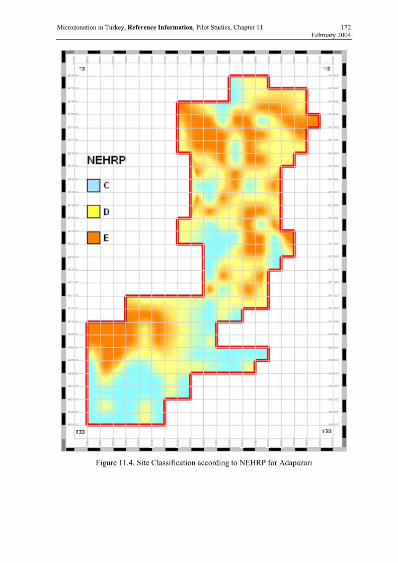
Microzonation in Turkey, Reference Information, Pilot Studies, Chapter 11 172 February 2004
Figure 11.4. Site Classification according to NEHRP for Adapazarı

Microzonation in Turkey, Reference Information, Pilot Studies, Chapter 11 173 February 2004
Figure 11.5. Site Classification according to equivalent shear wave velocity for Adapazarı

Microzonation in Turkey, Reference Information, Pilot Studies, Chapter 11 174 February 2004
Figure 11.6. Geological units in the Gölcük Region
Figure 11.7. Variation of elevation in Gölcük

Microzonation in Turkey, Reference Information, Pilot Studies, Chapter 11 175 February 2004
Figu
re 1
1.8.
Site
Cla
ssifi
catio
n ac
cord
ing
to T
urki
sh E
arth
quak
e C
ode
for G
ölcü
k

Microzonation in Turkey, Reference Information, Pilot Studies, Chapter 11 176 February 2004
Figu
re 1
1.9.
Site
Cla
ssifi
catio
n ac
cord
ing
to N
EHR
P fo
r Göl
cük

Microzonation in Turkey, Reference Information, Pilot Studies, Chapter 11 177 February 2004
Figu
re 1
1.10
. Site
Cla
ssifi
catio
n ac
cord
ing
to e
quiv
alen
t she
ar w
ave
velo
city
for G
ölcü
k

Microzonation in Turkey, Reference Information, Pilot Studies, Chapter 11 178 February 2004
Figure 11.11. Variation of average spectral accelerations calculated by site response
analysis in Adapazarı

Microzonation in Turkey, Reference Information, Pilot Studies, Chapter 11 179 February 2004
Figure 11.12. Spectral amplification from equivalent shear wave velocity for Adapazarı

Microzonation in Turkey, Reference Information, Pilot Studies, Chapter 11 180 February 2004
Figure 11.13. Spectral amplification from microtremor H/V ratios for Adapazarı

Microzonation in Turkey, Reference Information, Pilot Studies, Chapter 11 181 February 2004
Figu
re 1
1.14
. Var
iatio
n of
ave
rage
spec
tral a
ccel
erat
ions
cal
cula
ted
by si
te re
spon
se a
naly
sis i
n G
ölcü
k

Microzonation in Turkey, Reference Information, Pilot Studies, Chapter 11 182 February 2004
Figu
re 1
1.15
. Spe
ctra
l am
plifi
catio
n fr
om e
quiv
alen
t she
ar w
ave
velo
city
for G
ölcü
k

Microzonation in Turkey, Reference Information, Pilot Studies, Chapter 11 183 February 2004
Figu
re 1
1.16
. Gro
und
shak
ing
zona
tion
map
for G
ölcü
k w
hen
over
lapp
ing
zone
s are
det
erm
ined
for e
ach
grid
from
ave
rage
sp
ectra
l acc
eler
atio
n m
ap o
btai
ned
from
site
resp
onse
ana
lysi
s and
pea
k sp
ectra
l am
plifi
catio
n m
ap c
alcu
late
d fr
om e
quiv
alen
t

Microzonation in Turkey, Reference Information, Pilot Studies, Chapter 11 184 February 2004
Figu
re 1
1.17
. Com
paris
on o
f gro
und
shak
ing
map
with
geo
logi
cal f
orm
atio
ns

Microzonation in Turkey, Reference Information, Pilot Studies, Chapter 11 185 February 2004
Figure 11.18. Ground shaking zonation map for Adapazarı when overlapping zones are
determined for each grid from average spectral acceleration map obtained from site response analysis and peak spectral amplification map calculated from equivalent shear
wave velocity

Microzonation in Turkey, Reference Information, Pilot Studies, Chapter 11 186 February 2004
Figure 11.19. Variation of liquefaction susceptibility in Adapazarı

Microzonation in Turkey, Reference Information, Pilot Studies, Chapter 11 187 February 2004
Figure 11.20. Variation of landslide hazard in Adapazarı

Microzonation in Turkey, Reference Information, Pilot Studies, Chapter 11 188 February 2004
Figu
re 1
1.21
. Var
iatio
n of
land
slid
e ha
zard
in G
ölcü
k

Microzonation in Turkey, Reference Information, Pilot Studies - Appendices, Chapter 1 189 February 2004
12. REFERENCE
Abeki, A., Matsuda, I., Enomoto, T., Shigyo, V., Watanabe, K., Tanzawa, Y. & Nakajima, Y. (1995) “A Study of Seismic Microzonation Based on the Dynamic Characteristics of Subsurface Ground Conditions”, Proc. 5th International Conference on Seismic Zonation, Nice, France, (3):2187-2194.
AFPS (1995) “Guidelines for Seismic Microzonation Studies”, French Association for Earthquake Engineering, 18 pp.
Aki, K. (1957) “Space and time spectra of stationary stochastic waves with special reference to micro-tremors”, Bull. Earthquake Res. Inst., Tokyo Univ. 35, 415-457.
Akyuz, H. S., A. Barka, E. Altunel, R. Hartleb, G. Sunal (2000), “Field Observations and Slip Distribution of the November 12, 1999 Duzce Earthquake (M=7.1), Bolu-Turkey”, The 1999 Izmit and Duzce Earthquakes: Preliminary Results, A. Barka, O. Kozacı, S. Akyüz and E. Altunel, Istanbul Tech. Un. Press, Istanbul, pp. 61-70.
Ambraseys, N. N. and C. F. Finkel, (1991), “Long-term seismicity of Istanbul and of the Marmara Sea region”, Terra Nova, 3, pp: 527-539.
Andrews, D. C. A. and Martin, G. R. (2000): “Criteria for Liquefaction of Silty Soils.” 12th World Conference on Earthquake Engineering, Proceedings, Auckland, New Zealand
Andrus, R. D. (1994). "In situ characterization of gravelly soils that liquefied in the 1983 Borah Peak Earthquake." Ph.D. Dissertation, University of Texas at Austin
Ansal, A., Çetin, K.Ö., Demirbaş, E., Elmas, M., Erdik, M., Fäh, D., Giardini, D., Köksal, D., Laue, J., Lestuzzı,P., Önalp, A., Siyahi, B., Sprıngman, S., Studer, J., (2002a) Report of the Meeting On Concepts for Analyses and Interpretation of Results in DRM-MERM Project by Research Task Group, Project Place Web Site
Ansal, A., Erdik, M., Kurtulus, A., Erken, A., Sesetyan, K., Siyahi, B. (2002b) Project MERM Microzonation for Earthquake Risk Mitigation, “Part E. State-of-the Art Report Review of Current Literature on Seismic Microzonation”, Kandilli Observatory and Earthquake Research Institute, Bogaziçi University, Istanbul, Turkey
Ansal, A., Balamir, M., Bakır, S., Buchheister, J., Christen, A., Çetin, K.Ö., Demirbaş, E., Durgun. M., M., Erdik, M., Fäh, D., Giardini, D., Gülkan, P., Hammer, J., Köksal, D., Krimgold, F., Laue, J., Lestuzzi,P., Önalp, A., Siyahi, B., Sprıngman, S., Studer, J., Yasuda, S. (2003) Report of the Synthesis Meeting for the Research and Manual Task Groups in DRM-MERM Project by Research and Manual Task Groups, Project Place Web Site
Ansal,A.M., Şengezer,B.S., İyisan,R. & Gençoğlu,S. (1993) “The Damage Distribution in March 13, 1992 Earthquake and Effects of Geotechnical Factors”, Soil Dynamics and Geotechnical Earthquake Engineering, Ed.P.Seco e Pinto, Balkema, 413-434.
Athanasopoulus, G.A., Pelekis, P.C. & Leonidou, E.A. (1999).”Effects of Surface Topography on Seismic Ground Response in the Egion (Greece) 15 June 1995 Earthquake”, Soil Dynamics and Earthquake Engineering, (18):135-149.
Bakır, B.S., H. Sucuoğlu, and T. Yılmaz (2002). “An Overview of Local Site Effects and the Associated Building Damage in Adapazarı during the 17 August 1999 İzmit Earthquake”, Bulletin of the Seismological Society of America, Vol.92, No.1, pp.509-526.
Bard, P.-Y. (1994) “Effects of Surface Geology on Ground Motion: Recent Results and Remaining Issues”, Proc. 10th ECEE, Vienna, Austria, (1):305-323.
Barka A. A. and K. Kadinsky-Cade, (1988), “Strike-Slip Fault Geometry in Turkey and its influence on earthquake activity”, Tectonics, Vol. 7, No. 3, pp: 663-684.
Barka, A. A., (1992), “The NAFZ”, Annales Tectonicae, Special issue, Supplement to volume VI, pp: 164-195.

Microzonation in Turkey, Reference Information, Pilot Studies - Appendices, Chapter 1 190 February 2004
Boore, D. M., W. B. Joyner, T. E. Fumal (1997), “Equations for Estimating Horizontal Response Spectra and Peak Acceleration from Western North American Earthquakes: A Summary of Recent Work”, Seismological Research Letters, Vol. 68, No. 1, pp. 128-153.
Borcherdt, R.D. (1994) “Estimates of Site Dependent Response Spectra for Design (Methodology and Justification)”, Earthquake Spectra, (10)4:617-653.
Bray, J.D. et al. (2000) “Damage Patterns and Foundation Performance in Adapazarı” Earthquake Spectra, Supplement A to Vol. 16, 1999 Kocaeli, Turkey Earthquake Reconnaissance Report, pp. 163-189
Building Seismic Safety Council (BSSC), 2001, “NEHRP (National Earthquake Hazards Reduction Program) Recommended Provisions for Seismic Regulations for new buildings and other structures”, 2000 Edition, Part1: Provisions (FEMA 368), Chapter 4, BSSC Washington, D.C.
Campbell, K. W. (1997), “Empirical Near-Source Attenuation Relationships for Horizontal and Vertical Components of Peak Ground Acceleration, Peak Ground Velocity, and Pseudo-Absolute Acceleration Response Spectra”, Seismological Research Letters, 68, January/February.
Çetin, K. O. and Seed, R. B. (2001a). "Nonlinear Shear Mass Participation Factor (rd) for Cyclic Shear Stress Ratio Evaluation.", Submitted to the Journal of Geotechnical and Geoenvironmental Engineering.
Çetin, K. O. and Seed, R. B. (2001b). "Nonlinear Shear Mass Participation Factor (Rd) for Cyclic Shear Stress Ratio Evaluation", Research Report No. UCB/GT-2000/08, University of California, Berkeley.
Çetin, K. O., Seed, R. B., Der Kiureghian, A., Tokimatsu, K., Harder, L. F., and Kayen, R. E. (2000). "SPT-Based Probabilistic and Deterministic Assessment of Seismic Soil Liquefaction Initiation Hazard", Research Report No. 2000/05, Pacific Earthquake Engineering Research Center.
Chavez-Garcia, F.J., Cuenca, J. & Sanchez-Sesma, F.J. (1996) “Site Effects in Mexico City Urban Zone. A Complementary Study”, Soil Dynamics and Earthquake Engineering, (15):141-146.
Chin-Hsiung, L., Jeng-Yaw, H. & Tzay-Chyn, S. (1998) “Observed Variation of Earthquake Motion across a Basin-Taipei City”, Earthquake Spectra, (14)1:115-134.
Deodatis, G. (1996), “Non-stationary Stochastic Vector Processes: Seismic Ground Motion Applications”, Probabilistic Engineering Mechanics 11, pp.145-168.
DIN 4094 Beiblatt 1; Baugrund; Erkundung durch Sondierung; Anwendungshilfen, Erklärungen, Ausgabe:1990-12
Erdik et al. (2002), “Earthquake Risk Assessment for the Istanbul Metropolitan Area”, Report prepared by B. U. Kandilli Observatory and Earthquake Research Ins., Dept. of Earthquake Engineering.
Evans, M. D. (1987). "Undrained Cyclic Triaxial Testing of Gravels: The Effect of Membrane Compliance." Ph.D. Thesis, University of California, Berkeley
Faccioli, E. (1991) Seismic Amplification in the Presence of Geological and Topographic Irregularities”, Proc. 2nd International Conference on Recent Advances in Geotechnical Earthquake Engineering, St. Louis, Missouri, State-of-art paper, 1779-1797.
Fäh, D., Christen, A., Gülerce, Ü., Greifenhagen, C., Single-station ambient vibration measurements and interpretation for the cities of Adapazarı and Gölcük, Turkey 16.1.2003 report provided to the DRM-MERM project
Fäh, D., Kind, F. & Giardini, D. (2001) “A theoretical investigation of average H/V ratios”, Geophysical Journal Int., 145, 535-549.

Microzonation in Turkey, Reference Information, Pilot Studies - Appendices, Chapter 1 191 February 2004
Fäh, D., Kind, F. & Giardini, D. (2001) “Inversion of local S-wave velocity structures from average H/V ratios, and their use for the estimation of site-effects”, Journal of Seismology, in press.
Fäh, D., Rüttener, E., Noack, T. & Kruspan, P. (1997) “Microzonation of the City of Basel”, Journal of Seismology, (1):87-102.
Field, E.H. & Hough, S.E. (1997) “The Variability of PSV Response Spectra across a Dense Array Deployed during the Northridge Aftershock Sequence”, Earthquake Spectra, 13(2):243-257.
Finn, W. D. L., Ledbetter, R. H., and Wu, G. (1994) “Liquefaction in Silty Soils: Design and Analysis.” Ground Failures under Seismic Conditions, Geotechnical Special Publication 44, ASCE, New York, pp. 51-76.
Frankel, A., C. Mueller, T. Barnhard, D. Perkins, E. V. Leyendecker, N. Dickman, S. Hanson and M. Hopper (1996), “National Seismic Hazard Maps: Documentation June 1996”, Open File Report 96-532, U. S. Geological Survey, Denver , Colorado.
Frankel, A.D., Mueller, C.S., Barnhard, T.P., Leyendecker, E.V., Wesson, R.L., Harmsen, S.C., Klein, F.W., Perkins, D.M., Dickman, N.C., Hanson, S.L. & Hopper, M.G. (2000) “USGS National Seismic Hazard Maps”, Earthquake Spectra, (16)1:1-15
Gazetas,G., Dakoulas, P. & Papageorgiou, A. (1990) “Local Soil and Source-Mechanism Effects in the 1986 Kalamata (Greece) Earthquake” Earthquake Engineering and Structural Dynamics, (19):431-453
Geyskens, P., Der Kiureghian, A., Monteiro, P. (1993), "Bayesian Updating of Model Parameters", Structural Engineering Mechanics and Materials Report No. UCB/SEMM-93/06, University of California at Berkeley
Gueguen, P., Chatelain, J-L., Guillier, B., Yepes, H. & Egred, J. (1998) “Site Effect and Damage Distribution in Pujili (Ecuador) after the 28 March 1996 Earthquake”, Soil Dynamics and Earthquake Engineering, (17), 329-334.
Gülkan, P., A. Yakut, H. Sucuoğlu, M.S. Yücemen, and E. Çıtıpıtıoğlu, "A Damage Assessment Form for Engineered Buildings in Turkey,” Earthquake Engineering Research Center Report No. 95-01, Middle East Technical University, December, 1994 (in Turkish).
Gülkan, P., and A. Yakut, "An Expert System for Reinforced Concrete Structural Damage Quantification," in Mete A. Sozen Symposium-A Tribute from His Students, Edited by J.K. Wight and M.E. Kreger, ACI Special Publication No. SP-162, 1996, pp.53-71.
Gülkan, P., and M.A. Sozen, “Procedure for Determining Seismic Vulnerability of Building Structures,” ACI Structural Journal, 96, 3, May, 1999, pp. 336-342.
Harder, L. F. (1988). "Use of Penetration Tests to Determine the Cyclic Loading Resistance of Gravelly Soils During Earthquake Shaking." Ph.D. Thesis, University of California, Berkeley.
Hartzell, S., Carver, D. & Williams, R.A. (2001) “Site Response, Shallow Shear-Wave Velocity and Damage in Los Gatos, California, from the 1989 Loma Prieta Earthquake”, BSSA, (91)3:468-478.
Hartzell, S., Cranswick, E, Frankel, A., Carver, D. & Meremonte, M. (1997a) “Variability of Site Response in the Los Angeles Urban Area”, BSSA, (87)6:1377-1400.
Hartzell, S., Harmsen, S., Frankel, A., Carver, D., Cranswick, E. Meremonte, M. & Michael, J. (1997b) “First-Generation Site-Response Maps for the Los Angeles Region Based on Earthquake Ground Motions”, BSSA, (88)2:463-472.
Horike, M. (1985) “Inversion of phase velocity of long-period microtremors to the S-wave-velocity structure down to the basement in urbanized areas”, J. Phys. Earth 33, 59-96.
Hynes, M. E. (1988). "Pore Pressure Generation Characteristics of Gravel under Undrained Loading." Ph.D. Thesis, University of California, Berkeley

Microzonation in Turkey, Reference Information, Pilot Studies - Appendices, Chapter 1 192 February 2004
Idriss, I. M. (2000), "Personal Communication"
Idriss, I. M., Sun, J. I., (1992), "Users Manual for SHAKE91, A Computer Program for Conducting Equivalent Linear Seismic Response Analyses of Horizontally Layered Soil Deposits, Program Modified Based on the Original SHAKE Program Published in December 1972, by Schnabel, Lysmer and Seed, August.
Ishibashi, I. and X. Zhang (1993). Unified Dynamic Shear Moduli and Damping Ratios of Sand and Clay. Soils and Foundations, 33, 182-191
Iwasaki, T., Tokida, K., Tatsuoka, F., Watanabe, S., Yasuda, S., & Sato, H. (1982) “Microzonation of Soil Liquefaction Potential Using Simplified Methods”, Proc. 3rd Int. Conf. On Microzonation, Seattle, 3:1319-1330
Kayen RE, Mitchell JK, Seed RB, Lodge A, Nishio A, Coutinho R. “Evaluation of SPT-, CPT-, and Shear Wave-Based Methods for Liquefaction Potential Assessment Using Loma Prieta Data.” Proceedings of 4th Japan-US Workshop on Earthquake-Resistant Design of Lifeline Facilities and Countermeasures for Soil Liquefaction, 1992; (1):177-204.
Kawase, H. (1998) “The Cause of the Damage Belt in Kobe: ‘The Basin Edge Effect’, Constructive Interference of the Direct S-Wave with the Basin-induced Diffracted/Rayleigh Waves”, Seismological Research Letters, (67):25-34.
Kind, F. (2002) “Development of microzonation methods: application to Basle, Switzerland”, PhD the-sis No.14548, Swiss Federal Institute of Technology, Zurich.
Kishida, H. (1966), "Damage to Reinforced Concrete Buildings in Niigata City with Special Reference to Foundation Engineering", Soils and Foundations, Vol. VII, No. 1.
Koizumi, Y (1966), "Change in Density of Sand Subsoil caused by the Niigata Earthquake", Soils and Foundations, Vol. VIII, No. 2, pp. 38-44.
Komazawa, M., Morikawa, H., Nakamura, K., Akamatsu, J., Nishimura, K., Sawada, S., Erken, A., & Onalp, A.(2002) “Bedrock structure in Adapazarı, Turkey—a possible cause of severe damage by the 1999 Kocaeli earthquake” Soil Dynamics and Earthquake Engineering, (22):829-836
Kudo, K., Kanno, T., Okada, H., Özel, O., Erdik, M., Sasatani, T. Higashi, S, Takahashi, M., Yoshida, K. (2002) “Site-specific issues for strong ground motions during the Kocaeli, Turkey, earthquake of 17 August 1999, as inferred from array observations of microtremors and aftershocks”, Bull. Seism. Soc. Am. 92, 448-465.
Lachet, C. & Bard, P.-Y. (1994) “Numerical and Theoretical Investigations on the Possibilities and Limitations of Nakamura's Technique”, J. Phys. Earth, 42, 377-397.
Lachet, C., Hatzfeld, D., Bard, P.Y., Theodulidis, N., Papaioannou, C. & Savvaidis, A. (1996) “Site Effects and Microzonation in the City of Thessaloniki-Comparison of Different Approaches”, BSSA, (86)6:1692-1703.
Le Pichon, X, A.M.C. Sengör, E. Demirbag, C. Rangin, C. Imren, R. Armijo, N. Görür, N. Çagatay, B. Mercier de Lepinay, B. Meyer, R. Saatçilar and B. Tok ,(2001), “The Active Main Marmara Fault”, Earth and Planetary Science Letters, Vol. 192 (4) pp. 595-616.
Lermo, J. & Chavez-Garcia, J. (1994) “Are Microtremors Useful in Site Response Evaluation?”, Bull. Seism. Soc. Am. 84, 1350-1364.
Leyendecker, E.V., Hunt, R.J., Frankel, A.D. & Rukstales, K.S. (2000) “Development of Maximum Considered Earthquake Ground Motion Maps”, Earthquake Spectra, (16)1:21-40
Liao, S. S. C., Lum, K. Y. (1998), "Statistical Analysis and Application of the Magnitude Scaling Factor in Liquefaction Analysis", Geotechnical Earthquake Engineering and Soil Dynamics III, Vol. 1, 410-421.

Microzonation in Turkey, Reference Information, Pilot Studies - Appendices, Chapter 1 193 February 2004
Liao, S. S. C., Veneziano, D., Whitman, R.V. (1988), "Regression Models for Evaluating Liquefaction Probability", Journal of Geotechnical Engineering, ASCE, Vol. 114, No. 4, pp. 389-409.
Lungu, D., Aldea, A., Cornea, T. & Arion, C. (2000) “Seismic Microzonation of the City of Bucharest”, 6th International Conference on Seismic Zonation, California, USA.
Midorikawa, S. (1987), Prediction of Isoseismal Map in the Kanto Plain due to Hypothetical Earthquake, Journal of Structural Eng. 33B, 43-48.
Ministry of Public Works and Settlement, Government of Republic Turkey 2.9.1997 Official Gazette No. 23098, “Specification for Structures to be Built in Disaster Areas” Part III – Earthquake Disaster Prevention (Chapter 5 through Chapter 13) English Translation, Chapter 12, Kandilli Observatory and Earthquake Research Institute
Marcellini, A., Bard, P.Y., Iannaccone, G., Meneroud, J.P., Mouroux, P., Romeo, R.W., Silvestri, F., Duval, A.M., Martin, C. & Tento, A. (1995b). The Benevento Seismic Risk Project. II- The microzonation”, Proc. 5th International Conference on Seismic Zonation, Nice, France, (1):810-817.
Nakamura, Y. (1989) “A Method for Dynamic Characteristics Estimation of Subsurface using Micro-tremor on the Ground Surface”, QR of RTRI, 30, 25-33.
National Earthquake Hazard Reduction Program (NEHRP) (1997) Recommended Provisions for Seismic Regulations for New Buildings and Other Structures, FEMA 302/303.
NCEER (1997), "Proceedings of the NCEER Workshop on Evaluation of Liquefaction Resistance of Soils", Edited by Youd, T. L., Idriss, I. M., Technical Report No. NCEER-97-0022, December 31, 1997.
NEHRP (1997), Recommended Provisions For Seismic Regulations For New Buildings and Other Structures, FEMA-303, Prepared by the Building Seismic Safety Council for the Federal Emergency Management Agency, Washington, DC.
Ohsaki, Y. (1966), "Niigata Earthquakes, 1964, Building Damage and Soil Conditions", Soils and Foundations, Vol. 6, No. 2, pp. 14-37.
Ohta, Y. and N. Goto (1978). Empirical Shear Wave Velocity Equations in Terms of Characteristic Soil Indexes. Earthq. Engng. Struct.Dynam., 6,167-187.
Ozbey C. (2001), “Empirical Peak Horizontal Acceleration Attenuation Relationship for Northwestern Turkey”, M.Sc. Thesis, KOERI, Bogazici University.
Panza, G.F. & Suhadolc, P. (1987) “Complete strong motion synthetics”, In: Seismic strong motion synthetics, B.A. Bolt (Ed.), Academic Press, Computational Techniques, 4, 153-204.
Panza, G.F. (1985) “Synthetic seismograms: The Rayleigh waves modal summation”, J. Geophysics, 58, 125-145.
Papageorgiou, A., B. Halldorsson and G. Dong (2000), “Target Acceleration Spectra Compatible Time Histories”, University of Buffalo, Dept. of Civil, Structural and Environmental Engrg., NY.
Park, Y.J., and A.H.-S. Ang, “Mechanistic Seismic Damage Model for Reinforced Concrete,” J. Str. Eng., ASCE, 111, 4, April, 1985, pp. 722-739.
Parsons, T., S. Toda, R. S. Stein, A. Barka and J. H. Dieterich, “Heightened odds of large earthquakes near Istanbul: An interaction-based probability calculation”, Science, 288, pp. 661-665, 2000.
Prinz, H., 1997, “Abriss der Ingenieurgeologie mit Grundlagen der Boden- und Felsmechanik, des Erd-, Grund- und Tunnelbaus sowie der Abfalldeponien”, 3. Aufl, Ferdinand Enke Verlag, Stuttgart, Germany

Microzonation in Turkey, Reference Information, Pilot Studies - Appendices, Chapter 1 194 February 2004
Procedure for the Classification of hypothetical borings according to the National Earthquake Hazards Reduction Program (NEHRP)
Rathje, E. et al (2000) “Ground Motions and Site Effects” Earthquake Spectra, Supplement A to Vol. 16, 1999 Kocaeli, Turkey Earthquake Reconnaissance Report, pp. 65-96
Riemer, M. F., Seed, R. B., and Sadek, S. (1993) “The SRS/RFT Soil Evaluation Testing Program.” University of California, Berkeley Geotechnical Report No. UCB/GT-93/01
Sadigh, K., Chang, C.-Y., Egan, J.A., Makdisi, F., Youngs, R.R. (1997) “Attenuation Relationships for Shallow Crustal Earthquakes Based on California Strong Motion Data.” Seismological Research Letters 1997; (68)1: 180-189.
Sakarya University (1998). Geology and Geomorphology of Adapazarı, Report No. 1 (in Turkish).
Saroğlu, F., O. Emre and I. Kuscu (1992), “Active Fault Map of Turkey”, Mineral Res. Explor. Inst. Turkey.
Satoh, T., Kawase, H., Iwata, T. Higaski, S., Sato, T., Irikura, K. & Huang, H. C. (2001) “S-wave velocity structure of Taichung basin, Taiwan estimated from array and single-station records of microtremors”, Bull. Seism. Soc. Am. 91, 1267-1282.
Seed, H. B., Idriss, I. M. (1971), “Simplified Procedure for Evaluating Soil Liquefaction Potential”, Journal of the Soil Mechanics and Foundations Division, ASCE, Vol. 97, No SM9, Proc. Paper 8371, September 1971, pp. 1249-1273.
Seed, H. B., Tokimatsu, K., Harder, L. F., and Chung, R. M. (1985). "Influence of SPT Procedures in soil liquefaction resistance evaluations." Journal of Geotechnical Engineering, ASCE, 111(12), 1425-1445.
Seed, H. B., Tokimatsu, K., Harder, L. F., Chung, R. M. (1984), "The Influence of SPT Procedures in Soil Liquefaction Resistance Evaluations", Earthquake Engineering Research Center Report No. UCB/EERC-84/15, University of California at Berkeley, October, 1984.
Seed, R. B., Cetin, K. O., Der Kiureghian, A., Tokimatsu, K., Harder, L. F. Jr., and Kayen, R. E. (2001) “SPT-Based Probabilistic and Deterministic Assessment of Seismic Soil Liquefaction Potential.” Submitted to the ASCE Journal of Geotechnical and Geoenvironmental Engineering.
Shiga, T., A. Shibata, and T. Takahashi, “Earthquake Damage and Wall Index of Reinforced Concrete Buildings,” Proceedings of the Tohuku District Symposium, Architectural Institute of Japan, No. 12, Dec., 1968, pp. 29-32 (in Japanese).
Steimen, S., Fäh, D., Kind, F., Schmid, C. & D. Giardini (2003) “Identifying 2D resonance in microtremor wave fields”, Bull. Seism. Soc. Am., in press.
Straub, C., H.-G. Kahle, and C. Schindler, (1997), “GPS and Geologic Estimates of the Tectonic Activity in the Marmara Sea region, NW Anatolia”, Journal of Geophysical Research, Vol. 102, No. B12, pp: 27,587-27,601, Dec. 10.
TAB Technical Advisory Board (2003) Report of Technical Advisory Board, Zurich, Switzerland, Project Place Web Site
Technical Committee for Earthquake Geotechnical Engineering, TC4, ISSMGE (1999) “Manual for Zonation on Seismic Geotechnical Hazards”, The Japanese Geotechnical Society.
Toprak, S., Holzer, T. L., Bennett, M. J., Tinsley, J. C. (1999), "CPT- and SPT-based Probabilistic Assessment of Liquefaction Potential, Proceedings of Seventh U.S.-Japan Workshop on Earthquake Resistant Design of Lifeline Facilities and Countermeasures Against Liquefaction.
Toprak, S., Holzer, T. L., Bennett, M. J., Tinsley, J. C. (1999), "CPT- and SPT-based Probabilistic Assessment of Liquefaction Potential, Proceedings of Seventh U.S.-Japan Workshop on Earthquake Resistant Design of Lifeline Facilities and Countermeasures Against Liquefaction.

Microzonation in Turkey, Reference Information, Pilot Studies - Appendices, Chapter 1 195 February 2004
Vucetic, M and R. Dobry (1991). “Effect of soil plasticity on cyclic response”, Journal of Geotechnical Engineering, ASCE, Vol.117, No.1, pp.89-107
Weichert, D. H. (1980), “Estimation of the Earthquake Recurrence Parameters for Unequal Observation Periods for Different Magnitudes”, Bull. Seism. Soc. Am., 70, pp. 1337-1346.
WGCEP94 (1995), “Seismic Hazards in Southern California: Probable Earthquakes, 1994 to 2024”, Bull. Seism. Soc. Am. Vol. 85, pp. 379-439.
Wills, C.J. & Silva, W. (1998) “Shear Wave Velocity Characteristics of Geologic Units in California”, Earthquake Spectra, (14)3:533-566.
Wills, C.J., Peterson, M., Bryant, W.A., Reichle, M., Saucedo, G.J., Tan, S., Taylor, G. & Treiman, J. (2000) “A Site Conditions Map for California based on Geology and Shear Wave Velocity”, BSSA, (90)6B:S187-S208.
Yaltirak, C.(2002), Tectonic evolution of Marmara Sea and its surroundings, Marine Geology, pp.1-37
Yamanaka, H., Kato, M., Hashimoto, M., Gulerce, U., Iyisan, R., Ansal, A. (2002) “Microtremor and earthquake observations in Adapazarı and Duzce, Turkey, for estimation of site amplifications”, Japanese Ministry of Education, Science, Sports and Culture, Grant No.11694134, Proceedings “Assessment of seismic local-site effects at plural test sites, March 2002, 129-145.
Yamanaka, H., Takemura, M., Ishida, H. & Niea, M. (1994) “Characteristics of long-period micro-tremors and their applicability in exploration of deep layers”, Bull. Seism. Soc. Am. 84, 1831-1841.
Yoshimi, Y., Tokimatsu, K., Ohara, J. (1994), "In-situ Liquefaction Resistance of Clean Sands over a Wide Density Range", Geotechnique, Vol. 44, No. 3, pp. 479-494.
Youd, T. L., Idriss, I. M., Andrus, R. D., Arango, I., Castro, G., Christian, J. T., Dobry, R., Finn, W. D. L., Harder, L. F. Jr., Hynes, M. E., Ishihara, K., Koester, J. P., Liao, S. S. C., Marcuson, W. F. III., Martin, G, R., Mitchell, J. K., Moriwaki, Y., Power, M. S., Robertson, P. K., Seed, R. B., and Stokoe, K. H., II. (2001) “Liquefaction Resistance of Soils: Summary Report from the 1996 NCEER and 1998 NCEER/NSF Workshops on Evaluation of Liquefaction Resistance of Soils”, ASCE Journal of Geotechnical and Geoenvironmental Engineering, 127(10):817-833
Youd et al. (2001) Personal Communications
Youd, T. L., Idriss, I. M., Andrus, R. D., Arango, I., Castro, G., Christian, J. T., Dobry, R., Finn, W. D. L., Harder, L. F. Jr., Hynes, M. E., Ishihara, K., Koester, J. P., Liao, S. S. C., Marcuson, W. F. III., Martin, G, R., Mitchell, J. K., Moriwaki, Y., Power, M. S., Robertson, P. K., Seed, R. B., and Stokoe, K. H., II. (1997) Summary Paper, Proc., NCEER Workshop on Evaluation of Liquefaction Resistance of Soils, NCEER-97-0022.
Youd, T. L., Noble, S. K. (1997), "Liquefaction Criteria Based on Statistical and Probabilistic Analyses", Proceedings of the NCEER Workshop on Evaluation of Liquefaction Resistance of Soils, December 31, 1997, pp. 201-205.
Young, R. R. and Coppersmith, K. J. (1985) “Implications of Fault Slip Rates and Earthquake Recurrence Models to Probabilistic Seismic Hazard Estimates.” BSSA 1985; 75: 939-964.

Microzonation in Turkey, Reference Information, Pilot Studies - Appendices, Chapter 1 196 February 2004
APPENDICES
1. CHAPTER 4
1.1. Appendix 1: Instrument set-up Menu Parameter Wert Configuration Sampling 32 ms Configuration Scale_0 2 uV/c Configuration Scale_1 2 uV/c Configuration Scale_2 2 uV/c Configuration Exponent 3 Configuration In channels 3 Configuration Mon channel on Coincidence weight_0 0 Coincidence weight_1 0 Coincidence weight_2 0 Coincidence weight_ext 0 Coincidence coinc_sum 0
1.2. Appendix 2: Dataset description The measurements have a unique identifier for naming the measurement points. The teams are: Team C: Christian Greifenhagen (EPFL), Ali Zeynel Denizlioglu (GDDA), Ismail Kocak (SAU) Team R: Andreas Christen (ETH), Sadullah Yagci (GDDA), Eray Yildrim (SAU) Team U: Ümit Gülerce (ITU), Hatice Erguven (SAU), Coskun Bal (SAU) The point names have a structure corresponding to the following example AC05_R01 A stands for Adapazarı (G would be for Gölcük) C raster field in east-west direction 05 raster field in north-south direction R name of the group that made the measurement 01 this group’s first measurement in this raster field.

Microzonation in Turkey, Reference Information, Pilot Studies - Appendices, Chapter 1 197 February 2004
# #
#
#
#
##
#
###
##
###
####
#
##
##
#
#
#
#
#
#
#
##
#
##
##
# #
##
#
####
#
## #
#
##
##
###
#
##
#
##
#
##
##
#
#
##
#
#
#
#
#
#
##
#
#
#
#
#
##
##
#
#
####
##
#
#
##
#
####
##
#
##
#
#
#
#
##
#
#
# #
#
#
#
##
#
#
#
#
#
##
##
#
#
#
##
#
#
# #
# #
#
###
##
##
##
#
#
#
#
#
#
#
#
###
##
#
#
#
#
###
#
#
#
#
#
#
#
# #
#
###
###
#
#
#
#
#
## #
##
#
#
#
#
#
#
Figure 1.1. Grid used for the Adapazarı area.
The coordinates of the sites are provided in tabular form in the files Adapazarı_Results.xls and Gölcük_Results.xls on the CD-ROM.
1.3. Appendix 3: SAF Data Format
This format has been defined within the European Commission SESAME project (EVG1-CT-200-00026) for the exchange of ambient vibration data.
SESAME ASCII data format (saf) v. 1 (this line must not be modified) # The SESAME ASCII Format can contain an arbitrary number of comment # lines starting with '#' in the header. Parameters are specified on # lines starting without # character, followed by a keyword separated # with a '=' sign from the value of the key. The keyword name can be in # lower or upper case letters, no distinction is made in the # interpretation. # No empty lines are allowed in the header. # The first line indicates the name of the file format,

Microzonation in Turkey, Reference Information, Pilot Studies - Appendices, Chapter 1 198 February 2004
# for automatic format identification tools. # # Two compulsory parameters have to be specified # the sampling rate and the number of points. # # All other parameters are optional, but the response and saturation # information # is highly recommended. # # Data begin after this line : "####--------------------------------" # Data are organized in columns in this order : Vertical, Horizontal_1, # Horizontal_2 # Horizontal_1 generally is N-S, for different orientation parameter # NORTH_ROT can # be set. # Data can be real or integer # # # sampling frequency in Hertz SAMP_FREQ = 125 # number of samples (integer) NDAT = 1200 # date and time of the first sample, read as 5 integers, one real START_TIME=2002 4 26 17 03 12.1233324 # accuracy of the timing, in seconds #very large values indicate manual time setting # GPS ~0.001, DCF ~0.01 TIME_ACCURRACY= 0.001 # Sensor type (accelerometer, seismometer) SENSOR_TYPE = accelerometer # Sensor serial number (character string) SENSOR_ID = Q332 # Sensor name (character string) SENSOR_NAME = Lennartz 5s # Response file code (name of the file in the response directory) RESPFILE = mark1s_098 # Acquisition system (character string) ACQ_SYSTEM = MARS88 # Digitizer serial number (interpreted as character string) DIGITIZER_ID = 345 # saturation value of the digitizer in UNITS SATURATION = 23056 # conversion factor ( V/count) CONV_FACTOR = 1234.5 # transduction factor (Volts/m/s or Volts/m/s^2) TRANS_FACTOR = 12345.6 # Eigen frequency of the sensor SENS_EIGFREQ = 1 # Damping factor of the sensor SENS_DAMPING = 0.7 # Code for the site (exactly 6 characters) STA_CODE= NCE_12 # Station coordinate type, 0= lat/lon, 1= km of local coordinate, # elevation is always in km STA_COORD_TYPE = 0 # coordinates are one real number: 45 30' -> 45.5
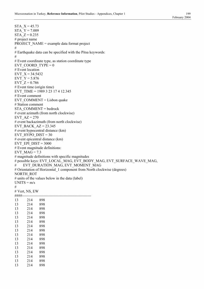
Microzonation in Turkey, Reference Information, Pilot Studies - Appendices, Chapter 1 199 February 2004
STA_X = 45.73 STA_Y = 7.009 STA_Z = 0.235 # project name PROJECT_NAME = example data format project # # Earthquake data can be specified with the Pitsa keywords: # # Event coordinate type, as station coordinate type EVT_COORD_TYPE = 0 # Event location EVT_X = 34.5432 EVT_Y = 5.876 EVT_Z = 0.786 # Event time (origin time) EVT_TIME = 1989 3 23 17 4 12.345 # Event comment EVT_COMMENT = Lisbon quake # Station comment STA_COMMENT = bedrock # event azimuth (from north clockwise) EVT_AZ = 270 # event backazimuth (from north clockwise) EVT_BACK_AZ = 23.345 # event hypocentral distance (km) EVT_HYPO_DIST = 30 # event epicentral distance (km) EVT_EPI_DIST = 3000 # Event magnitude definitions: EVT_MAG = 7.3 # magnitude definitions with specific magnitudes # possible keys: EVT_LOCAL_MAG, EVT_BODY_MAG, EVT_SURFACE_WAVE_MAG, # EVT_DURATION_MAG, EVT_MOMENT_MAG # Orientation of Horizontal_1 component from North clockwise (degrees) NORTH_ROT # units of the values below in the data (label) UNITS = m/s # # Vert, NS, EW ####------------------------------------------------------- 13 214 898 13 214 898 13 214 898 13 214 898 13 214 898 13 214 898 13 214 898 13 214 898 13 214 898 13 214 898 13 214 898 13 214 898 13 214 898 13 214 898 13 214 898 13 214 898

Microzonation in Turkey, Reference Information, Pilot Studies - Appendices, Chapter 1 200 February 2004
13 214 898 13 214 898 13 214 898
1.4. Appendix 4: Content of the CD-ROM: Raw Data of all measurement points in SAF format Report (PDF File) Matlab Routines used for the analysis Excel file containing the coordinates and results (fundamental frequency & amplitude) for all
measurement points in Adapazarı and Gölcük.
1.5. Microtremor Measurements
1.5.1 Adapazari region
Station Measurement Coordinates Date Results
p x y r Latitude Longitude dd mm yy Frequency Amplitude
a a 02 _ c 01 40.8035N 30.3669E 09 08 02 0.42 0.64 a a 02 _ r 01 40.8041N 30.3761E 23 08 02 0.39 0.72 a a 03 _ r 01 40.7955N 30.3805E 26 08 02 0.33 0.72
sek a a 04 _ c 01 _ sek 40.7851N 30.3796E 07 08 02 0.25 0.65 a a 05 _ r 01 40.7777N 30.3795E 12 08 02 0.33 0.57 a a 06 _ r 01 40.7670N 30.3811E 12 08 02 0.50 0.68 a a 06 _ r 02 40.7654N 30.3798E 23 08 02 0.74 0.59 a a 07 _ r 01 40.7558N 30.3828E 10 08 02 2.45 0.79 a a 07 _ r 02 40.7593N 30.3773E 12 08 02 1.14 0.78 a a 07 _ r 03 40.7582N 30.3765E 23 08 02 1.54 0.72 a a 07 _ r 04 40.7571N 30.3761E 23 08 02 3.31 0.63 a a 07 _ r 05 40.7620N 30.3775E 23 08 02 1.09 0.76 a a 07 _ r 06 40.7635N 30.3818E 23 08 02 0.93 0.71 a a 08 _ r 01 40.7518N 30.3815E 08 08 02 n/a n/a a a 08 _ r 02 40.7519N 30.3813E 09 08 02 4.70 0.28 a a 08 _ r 03 40.7544N 30.3828E 09 08 02 n/a n/a
skr a a 09 _ r 01 _ skr 40.7370N 30.3805E 07 08 02 12.20 0.34 a a 09 _ r 02 40.7390N 30.3787E 08 08 02 n/a n/a a a 09 _ r 03 40.7414N 30.3780E 08 08 02 n/a n/a a a 09 _ r 04 40.7442N 30.3781E 08 08 02 4.38 0.22 a a 09 _ r 05 40.7457N 30.3808E 08 08 02 3.25 0.42 a a 10 _ r 01 40.7370N 30.3786E 08 08 02 8.45 0.54 a a 10 _ r 02 40.7347N 30.3806E 27 08 02 5.06 0.73 a a 10 _ r 03 40.7325N 30.3798E 27 08 02 1.02 0.58 a a 10 _ r 04 40.7295N 30.3820E 27 08 02 0.83 0.63 a a 10 _ r 05 40.7339N 30.3810E 27 08 02 2.51 0.60 a a 11 _ r 01 40.7262N 30.3827E 27 08 02 0.54 0.67 a a 13 _ u 01 40.7064N 30.3785E 27 08 02 1.45 0.66 a a 13 _ u 02 40.7007N 30.3755E 27 08 02 1.69 0.63 a a 14 _ u 01 40.6959N 30.3763E 19 08 02 1.57 0.69 a b 02 _ r 01 40.8067N 30.3894E 26 08 02 0.43 0.73 a b 03 _ r 01 40.7941N 30.3893E 12 08 02 0.33 0.68
babali a b 04 _ c 01 _ bab 40.7864N 30.3908E 08 08 02 0.25 0.64 gen a b 04 _ c 02 _ gen 40.7851N 30.3927E 08 08 02 0.27 0.68
a b 04 _ r 01 40.7832N 30.3879E 13 08 02 0.24 0.59

Microzonation in Turkey, Reference Information, Pilot Studies - Appendices, Chapter 1 201 February 2004
a b 05 _ r 01 40.7789N 30.3911E 12 08 02 0.22 0.59 a b 05 _ r 02 40.7761N 30.3871E 14 08 02 0.27 0.57 a b 06 _ r 01 40.7657N 30.3885E 10 08 02 0.45 0.74 a b 06 _ r 02 40.7639N 30.3881E 10 08 02 0.62 0.57 a b 06 _ r 03 40.7713N 30.3889E 10 08 02 0.33 0.66 a b 06 _ r 04 40.7709N 30.3952E 13 08 02 0.30 0.61 a b 06 _ r 05 40.7679N 30.3926E 14 08 02 0.38 0.67 a b 06 _ r 06 40.7690N 30.3853E 23 08 02 0.40 0.71
sic a b 06 _ u 01 _ sic 40.7651N 30.3942E 08 08 02 0.41 0.62 a b 07 _ c 01 40.7556N 30.3935E 10 08 02 1.18 0.44 a b 07 _ c 02 40.7551N 30.3921E 10 08 02 1.11 0.40 a b 07 _ c 03 40.7566N 30.3948E 10 08 02 1.53 0.76 a b 07 _ c 04 40.7562N 30.3943E 12 08 02 2.27 0.66 a b 07 _ r 01 40.7578N 30.3849E 09 08 02 1.55 0.73 a b 07 _ r 02 40.7618N 30.3875E 09 08 02 1.11 0.74 a b 07 _ r 03 40.7595N 30.3863E 10 08 02 1.29 0.74 a b 07 _ r 04 40.7604N 30.3945E 13 08 02 0.91 0.57 a b 07 _ r 05 40.7630N 30.3880E 13 08 02 0.99 0.62 a b 07 _ r 06 40.7560N 30.3895E 14 08 02 1.40 0.40 a b 07 _ r 07 40.7580N 30.3909E 14 08 02 1.52 0.65 a b 07 _ r 08 40.7624N 30.3958E 14 08 02 0.90 0.52 a b 07 _ r 09 40.7601N 30.3924E 23 08 02 1.01 0.74 a b 07 _ r 10 40.7559N 30.3866E 28 08 02 5.06 0.50 a b 07 _ r 11 40.7578N 30.3878E 28 08 02 1.95 0.44 a b 07 _ r 12 40.7568N 30.3871E 28 08 02 1.78 0.73 a b 08 _ c 01 40.7537N 30.3925E 10 08 02 1.13 0.42 a b 08 _ r 01 40.7501N 30.3885E 09 08 02 3.77 0.15 a b 08 _ r 02 40.7474N 30.3952E 16 08 02 7.46 0.57 a b 09 _ c 01 40.7429N 30.3936E 23 08 02 1.31 0.81 a b 09 _ c 02 40.7379N 30.3870E 23 08 02 2.30 0.76 a b 09 _ c 03 40.7386N 30.3882E 23 08 02 2.17 0.69 a b 09 _ c 04 40.7449N 30.3954E 23 08 02 6.91 0.44 a b 09 _ c 05 40.7409N 30.3903E 26 08 02 3.06 0.69 a b 09 _ c 06 40.7437N 30.3909E 27 08 02 4.17 0.58 a b 09 _ c 07 40.7397N 30.3939E 27 08 02 1.15 0.69 a b 09 _ r 01 40.7392N 30.3900E 16 08 02 1.77 0.71 a b 09 _ r 02 40.7449N 30.3929E 16 08 02 1.56 0.85 a b 10 _ r 01 40.7345N 30.3867E 15 08 02 0.93 0.72 a b 10 _ r 02 40.7312N 30.3872E 15 08 02 0.89 0.67 a b 10 _ u 01 40.7297N 30.3926E 27 08 02 0.88 0.68 a b 11 _ r 01 40.7279N 30.3879E 15 08 02 0.63 0.60 a b 11 _ r 02 40.7231N 30.3918E 15 08 02 0.48 0.71 a b 11 _ u 01 40.7183N 30.3864E 27 08 02 0.50 0.70 a b 12 _ r 01 40.7149N 30.3930E 15 08 02 0.46 0.46 a b 13 _ u 01 40.7088N 30.3880E 27 08 02 1.15 0.48 a c 02 _ c 01 40.8012N 30.4043E 09 08 02 0.37 0.75 a c 03 _ c 01 40.7947N 30.4013E 09 08 02 0.31 0.69
tek a c 03 _ u 01 _ tek 40.7951N 30.4011E 08 08 02 0.34 0.63 a c 04 _ r 01 40.7827N 30.4028E 12 08 02 0.30 0.39
srf a c 04 _ u 01 _ srf 40.7915N 30.3968E 08 08 02 0.33 0.58 a c 04 _ u 02 40.7854N 30.4051E 13 08 02 0.28 0.53 a c 05 _ r 01 40.7784N 30.4036E 13 08 02 0.24 0.39
hastane a c 05 _ u 01 _ has 40.7732N 30.3978E 08 08 02 0.25 0.50

Microzonation in Turkey, Reference Information, Pilot Studies - Appendices, Chapter 1 202 February 2004
a c 06 _ c 01 40.7652N 30.4024E 14 08 02 0.37 0.56 a c 06 _ r 01 40.7673N 30.4013E 14 08 02 0.34 0.58 a c 06 _ r 02 40.7657N 30.3990E 28 08 02 0.40 0.64 a c 06 _ u 01 40.7674N 30.4030E 10 08 02 0.30 0.62 a c 07 _ c 01 40.7556N 30.3936E 10 08 02 1.01 0.70 a c 07 _ c 02 40.7621N 30.4005E 13 08 02 0.84 0.55 a c 07 _ c 03 40.7571N 30.4052E 13 08 02 1.40 0.62 a c 07 _ c 04 40.7577N 30.3955E 14 08 02 1.07 0.70 a c 07 _ c 05 40.7549N 30.4030E 14 08 02 1.35 0.52 a c 07 _ c 06 40.7554N 30.4040E 14 08 02 1.96 0.66
ere a c 07 _ u 01 _ ere 40.7615N 30.4060E 08 08 02 0.83 0.58 a c 07 _ u 02 40.7603N 30.4013E 23 08 02 0.91 0.78 a c 07 _ u 03 40.7591N 30.4006E 23 08 02 1.01 0.75 a c 07 _ u 04 40.7553N 30.3995E 23 08 02 2.06 0.64 a c 07 _ u 05 40.7590N 30.4040E 26 08 02 0.99 0.77 a c 07 _ u 06 40.7575N 30.4010E 26 08 02 1.23 0.71 a c 07 _ u 07 40.7599N 30.4069E 26 08 02 0.91 0.70 a c 08 _ c 01 40.7481N 30.4020E 12 08 02 1.77 0.69 a c 08 _ c 02 40.7497N 30.4019E 14 08 02 10.01 0.58 a c 08 _ c 03 40.7489N 30.4020E 15 08 02 2.48 0.80 a c 08 _ c 04 40.7460N 30.4025E 15 08 02 1.58 0.78 a c 08 _ u 01 40.7482N 30.4044E 20 08 02 1.33 0.83 a c 08 _ u 02 40.7498N 30.4039E 20 08 02 6.45 0.33 a c 08 _ u 03 40.7471N 30.4068E 20 08 02 1.03 0.69 a c 09 _ c 01 40.7440N 30.4031E 15 08 02 1.10 0.92 a c 09 _ c 02 40.7415N 30.4035E 16 08 02 1.10 0.75 a c 09 _ c 03 40.7371N 30.4065E 16 08 02 1.03 0.57 a c 09 _ c 04 40.7405N 30.3988E 23 08 02 1.29 0.63 a c 09 _ c 05 40.7447N 30.3993E 23 08 02 2.59 0.81 a c 09 _ r 01 40.7412N 30.3959E 16 08 02 1.38 0.73 a c 10 _ c 01 40.7312N 30.4059E 15 08 02 0.86 0.74 a c 10 _ u 01 40.7322N 30.3963E 19 08 02 0.89 0.71 a c 11 _ u 01 40.7267N 30.4008E 16 08 02 0.94 0.76 a c 12 _ u 01 40.7166N 30.4066E 16 08 02 0.96 0.69 a c 13 _ r 01 40.7078N 30.3970E 15 08 02 1.06 0.64 a c 13 _ u 01 40.7080N 30.4047E 16 08 02 1.05 0.53 a d 02 _ r 01 40.7994N 30.4186E 27 08 02 0.33 0.72 a d 02 _ u 01 40.8061N 30.4102E 12 08 02 0.49 0.69 a d 03 _ u 01 40.7922N 30.4090E 12 08 02 0.31 0.59 a d 04 _ u 01 40.7853N 30.4122E 09 08 02 0.26 0.59 a d 04 _ u 02 40.7877N 30.4113E 13 08 02 0.25 0.71 a d 04 _ u 03 40.7806N 30.4114E 14 08 02 0.31 0.46
yen a d 05 _ u 01 _ yen 40.7765N 30.4110E 09 08 02 0.24 0.60 a d 05 _ u 02 40.7811N 30.4175E 10 08 02 0.31 0.42 a d 05 _ u 03 40.7744N 30.4156E 14 08 02 0.24 0.53 a d 06 _ u 01 40.7628N 30.4148E 09 08 02 1.00 0.50 a d 06 _ u 02 40.7714N 30.4098E 10 08 02 0.26 0.61 a d 06 _ u 03 40.7695N 30.4149E 13 08 02 0.26 0.57 a d 06 _ u 04 40.7630N 30.4166E 23 08 02 0.96 0.57 a d 06 _ u 05 40.7643N 30.4102E 26 08 02 0.36 0.53 a d 06 _ u 06 40.7681N 30.4131E 26 08 02 0.28 0.50 a d 07 _ c 01 40.7582N 30.4123E 12 08 02 1.11 0.65 a d 07 _ c 02 40.7618N 30.4084E 13 08 02 1.12 0.42

Microzonation in Turkey, Reference Information, Pilot Studies - Appendices, Chapter 1 203 February 2004
a d 07 _ u 01 40.7526N 30.4124E 15 08 02 1.72 0.67 a d 07 _ u 02 40.7542N 30.4167E 15 08 02 1.33 0.60 a d 07 _ u 03 40.7610N 30.4185E 15 08 02 0.98 0.51 a d 07 _ u 04 40.7543N 30.4070E 23 08 02 6.14 0.71 a d 07 _ u 05 40.7596N 30.4132E 23 08 02 1.00 0.62 a d 07 _ u 06 40.7607N 30.4167E 26 08 02 0.93 0.51 a d 07 _ u 07 40.7571N 30.4111E 28 08 02 1.43 0.65 a d 07 _ u 08 40.7566N 30.4187E 28 08 02 1.17 0.69
adc a d 08 _ c 01 _ adc 40.7534N 30.4114E 08 08 02 2.28 0.71 a d 08 _ c 02 40.7488N 30.4118E 12 08 02 1.00 0.71 a d 08 _ c 03 40.7509N 30.4075E 26 08 02 4.32 0.91 a d 08 _ c 04 40.7505N 30.4081E 26 08 02 2.93 0.91 a d 08 _ c 05 40.7532N 30.4096E 26 08 02 3.12 0.50 a d 08 _ c 06 40.7504N 30.4124E 26 08 02 1.54 0.59 a d 08 _ c 07 40.7489N 30.4193E 26 08 02 1.50 0.71 a d 08 _ u 01 40.7488N 30.4102E 28 08 02 1.13 0.69 a d 09 _ u 01 40.7436N 30.4098E 20 08 02 1.11 0.83 a d 09 _ u 02 40.7454N 30.4132E 28 08 02 1.20 0.52 a d 10 _ c 01 40.7285N 30.4156E 16 08 02 1.04 0.70 a d 10 _ u 01 40.7353N 30.4186E 19 08 02 1.14 0.65 a d 11 _ c 01 40.7219N 30.4097E 15 08 02 1.07 0.74 a d 12 _ c 01 40.7130N 30.4103E 15 08 02 1.08 0.60 a e 02 _ r 01 40.8034N 30.4280E 26 08 02 0.43 0.73 a e 03 _ r 01 40.7936N 30.4242E 26 08 02 0.31 0.61 a e 03 _ r 02 40.7904N 30.4309E 26 08 02 0.29 0.55 a e 03 _ u 01 40.7945N 30.4266E 12 08 02 0.34 0.61
adu a e 04 _ c 01 _ adu 40.7869N 30.4192E 08 08 02 0.32 0.59 a e 04 _ u 01 40.7848N 30.4268E 10 08 02 0.31 0.50 a e 04 _ u 02 40.7843N 30.4225E 14 08 02 0.35 0.45 a e 05 _ u 01 40.7756N 30.4270E 12 08 02 0.34 0.37 a e 05 _ u 02 40.7743N 30.4207E 13 08 02 0.27 0.47 a e 05 _ u 03 40.7791N 30.4214E 13 08 02 0.29 0.46 a e 06 _ u 01 40.7691N 30.4187E 09 08 02 0.27 0.58 a e 07 _ u 01 40.7581N 30.4240E 14 08 02 0.99 0.71 a e 07 _ u 02 40.7545N 30.4203E 15 08 02 1.17 0.75 a e 08 _ u 01 40.7507N 30.4214E 14 08 02 1.59 0.71 a e 08 _ u 02 40.7516N 30.4196E 15 08 02 1.30 0.72 a e 08 _ u 03 40.7529N 30.4259E 15 08 02 1.16 0.27 a f 02 _ c 01 40.8028N 30.4349E 09 08 02 0.46 0.70 a f 04 _ u 01 40.7884N 30.4369E 12 08 02 0.34 0.41 a f 05 _ u 01 40.7785N 30.4374E 12 08 02 0.37 0.36 a w 10 _ r 01 40.7279N 30.3344E 20 08 02 0.74 0.83 a w 11 _ r 01 40.7209N 30.3349E 19 08 02 0.38 0.98 a w 12 _ r 01 40.7165N 30.3320E 19 08 02 0.36 0.78 a w 12 _ r 02 40.7123N 30.3295E 20 08 02 1.30 0.62 a x 11 _ c 01 40.7232N 30.3384E 28 08 02 0.50 0.73 a x 11 _ r 01 40.7222N 30.3439E 19 08 02 0.40 0.89 a x 11 _ r 02 40.7273N 30.3476E 20 08 02 0.62 0.81 a x 12 _ r 01 40.7147N 30.3415E 19 08 02 0.87 0.48 a x 12 _ r 02 40.7124N 30.3408E 20 08 02 1.34 0.56 a x 12 _ r 03 40.7135N 30.3416E 20 08 02 0.99 0.22 a y 10 _ c 01 40.7318N 30.3547E 19 08 02 1.77 0.59 a y 10 _ c 02 40.7295N 30.3575E 20 08 02 0.91 0.60

Microzonation in Turkey, Reference Information, Pilot Studies - Appendices, Chapter 1 204 February 2004
a y 10 _ c 03 40.7285N 30.3509E 27 08 02 0.61 0.83 a y 11 _ c 01 40.7208N 30.3544E 19 08 02 0.41 0.92 a y 11 _ c 02 40.7255N 30.3546E 20 08 02 0.50 0.80 a y 11 _ c 03 40.7208N 30.3603E 28 08 02 0.42 0.88 a y 12 _ r 01 40.7165N 30.3535E 19 08 02 0.46 0.74 a y 13 _ c 01 40.7051N 30.3592E 20 08 02 n/a n/a a z 10 _ c 01 40.7299N 30.3664E 19 08 02 0.88 0.83 a z 10 _ c 02 40.7326N 30.3622E 20 08 02 2.44 0.50 a z 10 _ c 03 40.7334N 30.3726E 27 08 02 1.36 0.77 a z 10 _ c 04 40.7318N 30.3675E 27 08 02 1.74 0.64 a z 10 _ c 05 40.7303N 30.3618E 27 08 02 0.97 0.66 a z 10 _ c 06 40.7281N 30.3673E 28 08 02 0.70 0.62 a z 10 _ r 01 40.7341N 30.3682E 27 08 02 n/a n/a a z 11 _ c 01 40.7221N 30.3663E 19 08 02 0.42 0.86 a z 12 _ c 01 40.7102N 30.3626E 19 08 02 n/a n/a a z 13 _ u 01 40.7047N 30.3710E 19 08 02 1.37 0.74 a z 14 _ u 01 40.6987N 30.3667E 19 08 02 1.66 0.59
1.5.2 Golcuk region
Station Measurement Coordinates Date Results
p x y r Latitude Longitude dd mm yy Frequency [Hz] Amplitude
DMD G D 01 _ R 01 _ DMD 40.7261N 29.7981E 21 08 02 0.30 0.37 PIR G E 02 _ R 01 _ PIR 40.7226N 29.8201E 21 08 02 0.26 0.50
G E 02 _ R 02 40.7197N 29.8184E 21 08 02 0.25 0.55 G E 02 _ R 03 40.7213N 29.8195E 22 08 02 0.28 0.35 G E 02 _ R 04 40.7188N 29.8183E 22 08 02 0.29 0.36 G F 02 _ R 01 40.7193N 29.8334E 22 08 02 0.31 0.27 G F 02 _ R 02 40.7193N 29.8280E 22 08 02 0.27 0.35 G G 01 _ C 01 40.7247N 29.8400E 22 08 02 0.33 0.55 G G 01 _ U 01 40.7224N 29.8418E 22 08 02 0.33 0.46 G G 02 _ C 01 40.7177N 29.8381E 22 08 02 0.25 0.40 G G 02 _ C 02 40.7154N 29.8368E 22 08 02 0.26 0.40 G G 02 _ C 03 40.7143N 29.8363E 22 08 02 0.27 0.41 G G 02 _ R 01 40.7212N 29.8339E 21 08 02 0.25 0.43 G G 02 _ R 02 40.7177N 29.8335E 21 08 02 0.26 0.51 G G 02 _ R 03 40.7200N 29.8338E 22 08 02 0.24 0.36 G G 02 _ R 04 40.7220N 29.8334E 22 08 02 0.28 0.37
GYM G G 02 _ U 01 _ GYM 40.7206N 29.8399E 21 08 02 0.24 0.56 GEM G G 02 _ U 02 _ GEM 40.7199N 29.8444E 21 08 02 0.26 0.46
G G 02 _ U 03 40.7157N 29.8409E 22 08 02 0.23 0.48 G G 02 _ U 04 40.7182N 29.8409E 22 08 02 0.27 0.25
GLH G G 03 _ U 01 _ GLH 40.7078N 29.8338E 21 08 02 0.27 0.57 G G 03 _ U 02 40.7136N 29.8426E 22 08 02 0.27 0.38 G G 03 _ U 03 40.7112N 29.8451E 22 08 02 0.27 0.38 G G 03 _ U 04 40.7089N 29.8429E 22 08 02 0.27 0.45 G G 03 _ U 05 40.7121N 29.8435E 22 08 02 0.24 0.41
GLF G H 02 _ C 01 _ GLF 40.7216N 29.8482E 21 08 02 0.22 0.50 FOC G H 02 _ C 02 _ FOC 40.7173N 29.8542E 21 08 02 0.24 0.33 LOJ G H 03 _ C 01 _ LOJ 40.7129N 29.8504E 21 08 02 0.25 0.49
G H 03 _ C 02 40.7050N 29.8496E 21 08 02 0.28 0.59 G H 03 _ C 03 40.7102N 29.8501E 22 08 02 0.29 0.36 G H 03 _ C 04 40.7083N 29.8507E 22 08 02 0.28 0.46

Microzonation in Turkey, Reference Information, Pilot Studies - Appendices, Chapter 2 205 February 2004
2. CHAPTER 5 AND CHAPTER 6
2.1. NEHRP RECOMMENDED PROVISIONS FOR SEISMIC REGULATIONS FOR NEW BUILDINGS AND OTHER STRUCTURES

Microzonation in Turkey, Reference Information, Pilot Studies - Appendices, Chapter 2 206 February 2004

Microzonation in Turkey, Reference Information, Pilot Studies - Appendices, Chapter 2 207 February 2004

Microzonation in Turkey, Reference Information, Pilot Studies - Appendices, Chapter 2 208 February 2004

Microzonation in Turkey, Reference Information, Pilot Studies - Appendices, Chapter 2 209 February 2004
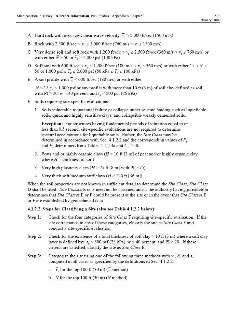
Microzonation in Turkey, Reference Information, Pilot Studies - Appendices, Chapter 2 210 February 2004

Microzonation in Turkey, Reference Information, Pilot Studies - Appendices, Chapter 2 211 February 2004

Microzonation in Turkey, Reference Information, Pilot Studies - Appendices, Chapter 2 212 February 2004

Microzonation in Turkey, Reference Information, Pilot Studies - Appendices, Chapter 2 213 February 2004
2.2. SITE CLASSIFICATIONS
2.2.1 In terms of Turkish Earthquake Code
ADAPAZARI TURKISH CODE GRID X (UTM) Y (UTM) Soil group Local Site Class Remarks G 26 528250 4509250 D Z4 G 27 528250 4508750 B Z1 G 28 528250 4508250 D Z3 interpolated boring G 29 528250 4507750 B Z1 G 30 528250 4507250 B Z1 G 31 528250 4506750 B Z1 H 25 528750 4509750 D Z4 H 26 528750 4509250 D Z4 H 27 528750 4508750 D Z4 H 28 528750 4508250 D Z4 interpolated boring H 29 528750 4507750 D Z3 interpolated boring H 30 528750 4507250 D Z3 interpolated boring H 31 528750 4506750 B-C Z1-Z2 H 32 528750 4506250 B Z1 I 25 529250 4509750 D Z4 interpolated boring I 26 529250 4509250 D Z4 interpolated boring I 27 529250 4508750 D Z4 interpolated boring I 28 529250 4508250 D Z3 interpolated boring I 29 529250 4507750 B Z1-Z2 I 30 529250 4507250 B Z1-Z2 I 31 529250 4506750 D Z3 interpolated boring I 32 529250 4506250 D Z3 interpolated boring J 24 529750 4510250 D Z4 J 25 529750 4509750 D Z4 J 26 529750 4509250 D Z4 interpolated boring J 27 529750 4508750 D Z4 J 28 529750 4508250 D Z3 J 29 529750 4507750 C Z2-Z3 J 30 529750 4507250 B Z1 J 31 529750 4506750 B Z1-Z2 J 32 529750 4506250 C Z3 K 23 530250 4510750 D Z4 K 24 530250 4510250 D Z4 interpolated boring K 25 530250 4509750 D Z4 interpolated boring K 26 530250 4509250 D Z3-Z4 K 27 530250 4508750 D Z4 K 28 530250 4508250 C Z2-Z3 K 29 530250 4507750 D Z3 interpolated boring K 30 530250 4507250 D Z3 interpolated boring K 31 530250 4506750 D Z3-Z4 interpolated boring

Microzonation in Turkey, Reference Information, Pilot Studies - Appendices, Chapter 2 214 February 2004
K 32 530250 4506250 B Z1-Z2 L 23 530750 4510750 C Z2-Z3 L 24 530750 4510250 D Z4 L 25 530750 4509750 D Z4 interpolated boring L 26 530750 4509250 D Z4 L 27 530750 4508750 C Z2 L 28 530750 4508250 D Z3-Z4 L 29 530750 4507750 C Z2 L 30 530750 4507250 C Z2 L 31 530750 4506750 D Z3 interpolated boring L 32 530750 4506250 B Z2 M10 531500 4517300 C Z2-Z3 M 28 531250 4508250 D Z3 interpolated boring M 29 531250 4507750 C Z2 M 30 531250 4507250 D Z4 N 10 531750 4517250 C Z2 N 11 531750 4516750 D Z3 N 17 531750 4513750 D Z3-Z4 N 18 531750 4513250 C Z2-Z3 N 28 531750 4508250 D Z3-Z4 N 29 531750 4507750 D Z3 interpolated boring N 30 531750 4507250 D Z4 O 10 532250 4517250 D Z4 O 11 532250 4516750 D Z3 O 12 532250 4516250 C Z3 O 13 532250 4515750 D Z3 O 14 532250 4515250 D Z3 O 15 532250 4514750 D Z3 O 16 532250 4514250 D Z3-Z4 O 17 532250 4513750 D Z4 O 27 532250 4508750 D Z3 O 28 532250 4508250 D Z3 P 09 532750 4517750 D Z3-Z4 P 10 532250 4517250 D Z3-Z4 P 11 532750 4516750 D Z3 P 12 532750 4516250 D Z4 P 13 532750 4515750 D Z3-Z4 P 14 532750 4515250 D Z3-Z4 P 15 532750 4514750 D Z3 P 16 532750 4514250 D Z4 P 17 532750 4513750 C Z2-Z3 P 20 532750 4512250 C Z2 P 21 532750 4511750 D Z4 interpolated boring P 22 532750 4511250 D Z3-Z4 P 23 532750 4510750 D Z3 P 24 532750 4510250 D Z4

Microzonation in Turkey, Reference Information, Pilot Studies - Appendices, Chapter 2 215 February 2004
P 25 532750 4509750 C Z2 interpolated boring P 26 532750 4509250 D Z3-Z4 P 27 532750 4508750 D Z3 Q 08 533250 4518250 C Z2-Z3 Q 09 533250 4517750 D Z3 Q 10 533250 4517250 D Z3-Z4 Q 11 533250 4516750 D Z3-Z4 Q 12 533250 4516250 D Z3 Q 13 533250 4515750 D Z4 Q 14 533250 4515250 C Z2-Z3 Q 15 533250 4514750 D Z3 Q 16 533250 4514250 C Z2-Z3 Q 17 533250 4513750 C Z2
Q 18 533250 4513250 D Z3 attention: difference between spt N30 values and defined layers
Q 19 533250 4512750 D Z4 Q 20 533250 4512250 D Z4 Q 21 533250 4511750 D Z3 interpolated boring Q 22 533250 4511250 D Z3-Z4 Q 23 533250 4510750 D Z4 Q 24 533250 4510250 D Z4 Q 27 533250 4508750 D Z3 R 07 533750 4518750 A Z1 R 08 533750 4518250 D Z3 interpolated boring R 09 533750 4517750 D Z3-Z4 R 10 533750 4517250 B-C Z1-Z3 R 11 533750 4516750 D Z3 R 12 533750 4516250 D Z3 R 13 533750 4515750 D Z3-Z4 R 14 533750 4515250 D Z3 R 15 533750 4514750 D Z3 R 16 533750 4514250 D Z3 R 17 533750 4513750 D Z3-Z4 R 18 533750 4513250 D Z3 R 19 533750 4512750 B Z2-Z3 R 20 533750 4512250 C Z2 R 21 533750 4511750 D Z3 R 22 533750 4511250 D Z3 R 23 533750 4510750 D Z3 R 24 533750 4510250 D Z4 R 27 533750 4508750 C Z2 interpolated boring R 28 533750 4508250 D Z3 S 06 534250 4519250 C Z2-Z3 S 07 534250 4518750 C Z2 S 08 534250 4518250 C Z2

Microzonation in Turkey, Reference Information, Pilot Studies - Appendices, Chapter 2 216 February 2004
S 09 534250 4517750 D Z3 S 10 534250 4517250 D Z3 interpolated boring S 11 534250 4516750 D Z3 S 12 534250 4516250 D Z3-Z4 S 13 534250 4515750 D Z3 S 14 534250 4515250 D Z3 S 15 534250 4514750 D Z3 S 16 534250 4514250 D Z3 S 17 534250 4513750 D Z3 S 18 534250 4513250 D Z3 S 19 534250 4512750 D Z3 S 20 534250 4512250 D Z3 S 21 534250 4511750 C Z2 S 22 534250 4511250 D Z3-Z4 interpolated boring S 23 534250 4510750 D Z3 interpolated boring S 27 534250 4508250 D Z3 T 07 534750 4518750 D Z3 T 08 534750 4518250 D Z3 T 09 534750 4517750 B Z1-Z2 T 10 534750 4517250 D Z3 interpolated boring T 11 534750 4516750 D Z3 T 12 534750 4516250 D Z3 T 13 534750 4515750 C Z2 T 14 534750 4515250 D Z3 T 15 534750 4514750 D Z3 T 16 534750 4514250 C Z2 T 17 534750 4513750 D Z3 T 18 534750 4513250 D Z3 T 19 534750 4512750 D Z3 T 20 534750 4512250 D Z3 T 21 534750 4511750 D Z3 T 22 534750 4511250 D Z4 T 23 534750 4510750 D Z4 T 26 534750 4508750 D Z3 U 08 535250 4518250 D Z3-Z4 U 09 535250 4517750 D Z3-Z4 U 10 535250 4517250 D Z3-Z3 interpolated boring U 11 535250 4516750 D Z3 U 12 535250 4516250 D Z3 U 13 535250 4515750 D Z3 U 14 535250 4515250 D Z4 U 15 535250 4514750 C Z2 U 16 535250 4514250 D Z3 U 17 535250 4513750 D Z3 U 18 535250 4513250 C Z2 U 19 535250 4512750 D Z3 interpolated boring

Microzonation in Turkey, Reference Information, Pilot Studies - Appendices, Chapter 2 217 February 2004
U 20 535250 4512250 C Z2 V 08 535,750 4,518,250 D Z3-Z4 V 09 535750 4517750 D Z3 V 10 535750 4517250 D Z3 V 11 535750 4516750 D Z3-Z4 V 12 535750 4516250 D Z3-Z4 interpolated boring V 18 535750 4513250 D Z4 V 19 535750 4512750 C Z2-Z3 W 07 536250 4518750 C Z2-Z3 W 08 536250 4518250 C Z2-Z3 W 09 536750 4517750 D Z3 W 10 536250 4517250 D Z3 W 11 536250 4516750 B Z1
GÖLCÜK TURKISH CODE
GRID X (UTM) Y (UTM) Soil group Local Site Class Remarks C5 480750 4509250 B Z1-Z2 D4 481250 4509750 C Z2 D5 481250 4509250 B Z1 D6 481250 4508750 C-B Z1-Z2 E4 481750 4509750 D Z3 E5 481750 4509250 C Z1 E6 481750 4508750 C Z2-Z3 F4 482250 4509750 A Z1 F5 482250 4509250 B Z1-Z2 F6 482250 4508750 A Z1 F7 482250 4508250 D Z3 G3 482750 4510250 A Z1 G4 482750 4509750 C Z2 G5 482750 4509250 C Z2 G6 482750 4508750 C Z2 G8 482750 4507750 C Z2 G9 482750 4507250 C Z2-Z3 H3 483250 4510250 C Z2 H4 483250 4509750 C Z2 interpolated boring H5 483250 4509250 C Z2 H6 483250 4508750 B Z1 H7 483250 4508250 C Z2 H8 483250 4507750 B Z1-Z2 interpolated boring H9 483250 4507250 B Z1 I4 483750 4509750 B Z1 I5 483750 4509250 B Z1 I6 483750 4508750 D Z3-Z4 I7 483750 4508250 C Z2-Z3 interpolated boring I8 483750 4507750 A Z1 I9 483750 4507250 A Z1

Microzonation in Turkey, Reference Information, Pilot Studies - Appendices, Chapter 2 218 February 2004
J4 484250 4509750 B Z1 J5 484250 4509250 C Z2 J6 484250 4508750 A Z1 J7 484250 4508250 B Z1 J8 484250 4507750 A Z1 J9 484250 4507250 B Z1
K11 484750 4506250 D Z3 K4 484750 4509750 C Z2-Z3 K5 484750 4509250 C Z2 K6 484750 4508750 C Z2 K7 484750 4508250 C Z2 K8 484750 4507750 C Z2 K9 484750 4507250 B-C Z1-Z2 interpolated boring L10 485250 4506750 C Z2-Z3 L11 485250 4506250 D Z3 L4 485250 4509750 D Z3 L5 485250 4509250 A Z1 L6 485250 4508750 C Z2 L7 485250 4508250 A Z1 L8 485250 4507750 D Z3 L9 485250 4507250 C Z2 interpolated boring
M10 485750 4506750 D Z3 M11 485750 4506250 C Z2 M4 485750 4509750 C Z2 M5 485750 4509250 C Z2 M6 485750 4508750 C Z2 M7 485750 4508250 B Z2 M8 485750 4507750 C Z2 N10 486250 4506750 C Z2 N11 486250 4506250 C Z2 N4 486250 4509750 C Z2 N5 486250 4509250 B Z1 N6 486250 4508750 C Z2 N7 486250 4508250 B Z1 N8 486250 4507750 D Z3 interpolated boring N9 486250 4507250 D Z3
O1O 486750 4506750 B-C Z1-Z2 O4 486750 4509750 C Z2 O5 486750 4509250 B Z1 O6 486750 4508750 C Z2 O7 486750 4508250 C Z2 O8 486750 4507750 D Z4 O9 486750 4507250 C Z2 P3 487250 4510250 D Z3 P4 487250 4509750 D Z3 P5 487250 4509250 D Z3

Microzonation in Turkey, Reference Information, Pilot Studies - Appendices, Chapter 2 219 February 2004
P6 487250 4508750 C-B Z2 P7 487250 4508250 C Z2-Z3 P8 487250 4507750 C Z2 Q4 487750 4509750 D Z3 Q5 487750 4509250 C Z2 Q6 487750 4508750 B-C Z1-Z3
2.2.2 In terms of NEHRP Site Classes
ADAPAZARI NEHRP
GRID X (UTM) Y (UTM) vS 30 m (m/s) Site class Remarks G 26 528250 4509250 169 E G 27 528250 4508750 343 D G 28 528250 4508250 491 C interpolated boring G 29 528250 4507750 485 C G 30 528250 4507250 390 C G 31 528250 4506750 391 C H 25 528750 4509750 157 E H 26 528750 4509250 150 E H 27 528750 4508750 125 E H 28 528750 4508250 165 E interpolated boring H 29 528750 4507750 360 D interpolated boring H 30 528750 4507250 396 C interpolated boring H 31 528750 4506750 370 D H 32 528750 4506250 512 C I 25 529250 4509750 125 E interpolated boring I 26 529250 4509250 123 E interpolated boring I 27 529250 4508750 156 E interpolated boring I 28 529250 4508250 190 D interpolated boring I 29 529250 4507750 386 C I 30 529250 4507250 376 C I 31 529250 4506750 364 C interpolated boring I 32 529250 4506250 456 C interpolated boring J 24 529750 4510250 209 D-E J 25 529750 4509750 171 E J 26 529750 4509250 145 E interpolated boring J 27 529750 4508750 219 D J 28 529750 4508250 517 C J 29 529750 4507750 420 C J 30 529750 4507250 496 C J 31 529750 4506750 361 C J 32 529750 4506250 374 C K 23 530250 4510750 190 D K 24 530250 4510250 173 E interpolated boring K 25 530250 4509750 317 D interpolated boring K 26 530250 4509250 188 D K 27 530250 4508750 253 D K 28 530250 4508250 455 C K 29 530250 4507750 365 C interpolated boring K 30 530250 4507250 488 C interpolated boring K 31 530250 4506750 210 D interpolated boring K 32 530250 4506250 358 D L 23 530750 4510750 275 D L 24 530750 4510250 449 C-E L 25 530750 4509750 337 D-E interpolated boring L 26 530750 4509250 310 D-E
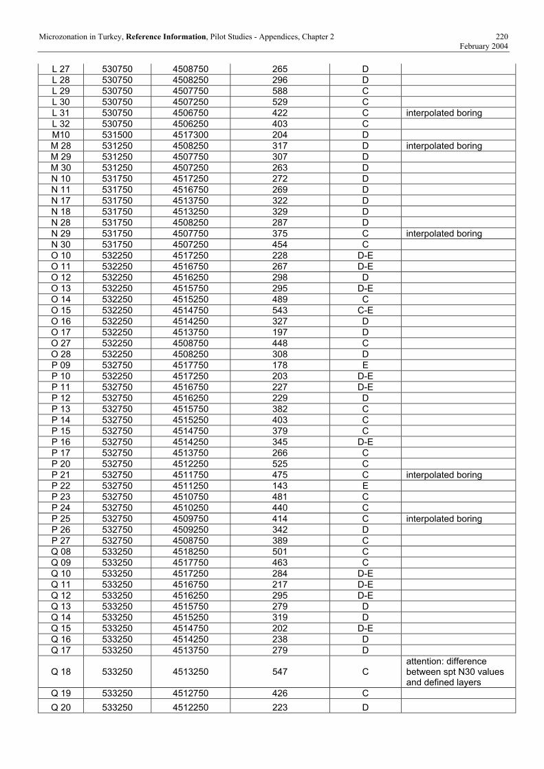
Microzonation in Turkey, Reference Information, Pilot Studies - Appendices, Chapter 2 220 February 2004
L 27 530750 4508750 265 D L 28 530750 4508250 296 D L 29 530750 4507750 588 C L 30 530750 4507250 529 C L 31 530750 4506750 422 C interpolated boring L 32 530750 4506250 403 C M10 531500 4517300 204 D M 28 531250 4508250 317 D interpolated boring M 29 531250 4507750 307 D M 30 531250 4507250 263 D N 10 531750 4517250 272 D N 11 531750 4516750 269 D N 17 531750 4513750 322 D N 18 531750 4513250 329 D N 28 531750 4508250 287 D N 29 531750 4507750 375 C interpolated boring N 30 531750 4507250 454 C O 10 532250 4517250 228 D-E O 11 532250 4516750 267 D-E O 12 532250 4516250 298 D O 13 532250 4515750 295 D-E O 14 532250 4515250 489 C O 15 532250 4514750 543 C-E O 16 532250 4514250 327 D O 17 532250 4513750 197 D O 27 532250 4508750 448 C O 28 532250 4508250 308 D P 09 532750 4517750 178 E P 10 532250 4517250 203 D-E P 11 532750 4516750 227 D-E P 12 532750 4516250 229 D P 13 532750 4515750 382 C P 14 532750 4515250 403 C P 15 532750 4514750 379 C P 16 532750 4514250 345 D-E P 17 532750 4513750 266 C P 20 532750 4512250 525 C P 21 532750 4511750 475 C interpolated boring P 22 532750 4511250 143 E P 23 532750 4510750 481 C P 24 532750 4510250 440 C P 25 532750 4509750 414 C interpolated boring P 26 532750 4509250 342 D P 27 532750 4508750 389 C Q 08 533250 4518250 501 C Q 09 533250 4517750 463 C Q 10 533250 4517250 284 D-E Q 11 533250 4516750 217 D-E Q 12 533250 4516250 295 D-E Q 13 533250 4515750 279 D Q 14 533250 4515250 319 D Q 15 533250 4514750 202 D-E Q 16 533250 4514250 238 D Q 17 533250 4513750 279 D
Q 18 533250 4513250 547 C attention: difference between spt N30 values and defined layers
Q 19 533250 4512750 426 C Q 20 533250 4512250 223 D

Microzonation in Turkey, Reference Information, Pilot Studies - Appendices, Chapter 2 221 February 2004
Q 21 533250 4511750 152 E interpolated boring Q 22 533250 4511250 303 C Q 23 533250 4510750 344 D Q 24 533250 4510250 303 D Q 27 533250 4508750 445 C R 07 533750 4518750 543 C R 08 533750 4518250 353 D interpolated boring R 09 533750 4517750 242 D-E R 10 533750 4517250 280 D R 11 533750 4516750 461 C R 12 533750 4516250 446 C R 13 533750 4515750 152 E R 14 533750 4515250 376 C-E R 15 533750 4514750 257 D R 16 533750 4514250 241 D R 17 533750 4513750 230 D R 18 533750 4513250 685 C R 19 533750 4512750 309 D R 20 533750 4512250 255 D R 21 533750 4511750 321 D R 22 533750 4511250 347 D R 23 533750 4510750 297 D R 24 533750 4510250 367 C R 27 533750 4508750 422 C interpolated boring R 28 533750 4508250 368 C S 06 534250 4519250 262 D S 07 534250 4518750 268 D S 08 534250 4518250 231 D S 09 534250 4517750 446 C-E S 10 534250 4517250 187 D-E interpolated boring S 11 534250 4516750 302 D-E S 12 534250 4516250 217 D-E S 13 534250 4515750 213 D S 14 534250 4515250 432 C S 15 534250 4514750 206 D S 16 534250 4514250 258 D-E S 17 534250 4513750 284 D-E S 18 534250 4513250 307 D-E S 19 534250 4512750 213 D-E S 20 534250 4512250 268 D S 21 534250 4511750 278 D S 22 534250 4511250 161 E interpolated boring S 23 534250 4510750 326 D interpolated boring S 27 534250 4508250 357 D T 07 534750 4518750 205 D T 08 534750 4518250 202 D-E T 09 534750 4517750 540 C T 10 534750 4517250 174 E interpolated boring T 11 534750 4516750 199 D T 12 534750 4516250 285 D-E T 13 534750 4515750 240 D T 14 534750 4515250 328 D T 15 534750 4514750 231 D T 16 534750 4514250 289 D-E T 17 534750 4513750 574 C T 18 534750 4513250 543 C-E T 19 534750 4512750 290 D-E T 20 534750 4512250 252 D T 21 534750 4511750 269 D-E

Microzonation in Turkey, Reference Information, Pilot Studies - Appendices, Chapter 2 222 February 2004
T 22 534750 4511250 323 D T 23 534750 4510750 337 D T 26 534750 4508750 597 C U 08 535250 4518250 159 E U 09 535250 4517750 214 D U 10 535250 4517250 334 D interpolated boring U 11 535250 4516750 263 D U 12 535250 4516250 256 D U 13 535250 4515750 374 D U 14 535250 4515250 154 E U 15 535250 4514750 227 D U 16 535250 4514250 316 D U 17 535250 4513750 295 D-E U 18 535250 4513250 374 C U 19 535250 4512750 407 C interpolated boring U 20 535250 4512250 425 C V 08 535,750 4,518,250 156 E V 09 535750 4517750 281 D-E V 10 535750 4517250 234 D V 11 535750 4516750 211 D V 12 535750 4516250 360 D interpolated boring V 18 535750 4513250 303 D-E V 19 535750 4512750 329 D W 07 536250 4518750 296 D W 08 536250 4518250 296 D W 09 536750 4517750 236 D-E W 10 536250 4517250 158 E W 11 536250 4516750 303 D
GÖLCÜK NEHRP
GRID X (UTM) Y (UTM) vS 30 m (m/s) Site class Remarks C5 480750 4509250 394 C D4 481250 4509750 380 C D5 481250 4509250 462 C D6 481250 4508750 420 C E4 481750 4509750 487 C E5 481750 4509250 355 D E6 481750 4508750 330 D F4 482250 4509750 470 C F5 482250 4509250 363 C F6 482250 4508750 472 C F7 482250 4508250 319 D G3 482750 4510250 493 C G4 482750 4509750 385 C G5 482750 4509250 466 C G6 482750 4508750 457 C G8 482750 4507750 369 C G9 482750 4507250 362 C H3 483250 4510250 328 D H4 483250 4509750 396 C interpolated boring H5 483250 4509250 437 C H6 483250 4508750 394 C H7 483250 4508250 426 C H8 483250 4507750 470 C interpolated boring H9 483250 4507250 414 C I4 483750 4509750 370 C I5 483750 4509250 431 C
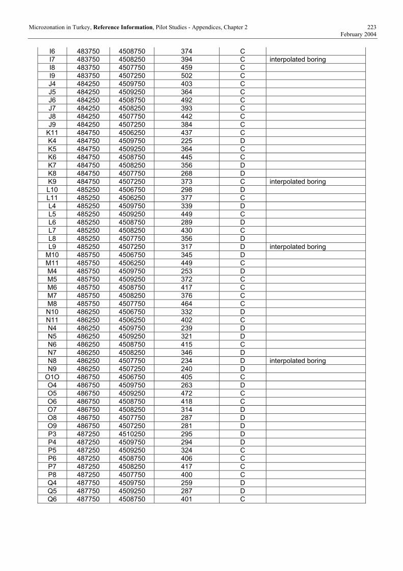
Microzonation in Turkey, Reference Information, Pilot Studies - Appendices, Chapter 2 223 February 2004
I6 483750 4508750 374 C I7 483750 4508250 394 C interpolated boring I8 483750 4507750 459 C I9 483750 4507250 502 C J4 484250 4509750 403 C J5 484250 4509250 364 C J6 484250 4508750 492 C J7 484250 4508250 393 C J8 484250 4507750 442 C J9 484250 4507250 384 C
K11 484750 4506250 437 C K4 484750 4509750 225 D K5 484750 4509250 364 C K6 484750 4508750 445 C K7 484750 4508250 356 D K8 484750 4507750 268 D K9 484750 4507250 373 C interpolated boring L10 485250 4506750 298 D L11 485250 4506250 377 C L4 485250 4509750 339 D L5 485250 4509250 449 C L6 485250 4508750 289 D L7 485250 4508250 430 C L8 485250 4507750 356 D L9 485250 4507250 317 D interpolated boring
M10 485750 4506750 345 D M11 485750 4506250 449 C M4 485750 4509750 253 D M5 485750 4509250 372 C M6 485750 4508750 417 C M7 485750 4508250 376 C M8 485750 4507750 464 C N10 486250 4506750 332 D N11 486250 4506250 402 C N4 486250 4509750 239 D N5 486250 4509250 321 D N6 486250 4508750 415 C N7 486250 4508250 346 D N8 486250 4507750 234 D interpolated boring N9 486250 4507250 240 D
O1O 486750 4506750 405 C O4 486750 4509750 263 D O5 486750 4509250 472 C O6 486750 4508750 418 C O7 486750 4508250 314 D O8 486750 4507750 287 D O9 486750 4507250 281 D P3 487250 4510250 295 D P4 487250 4509750 294 D P5 487250 4509250 324 C P6 487250 4508750 406 C P7 487250 4508250 417 C P8 487250 4507750 400 C Q4 487750 4509750 259 D Q5 487750 4509250 287 D Q6 487750 4508750 401 C

Microzonation in Turkey, Reference Information, Pilot Studies - Appendices, Chapter 2 224 February 2004
2.3. SITE RESPONSE ANALYSIS
2.3.1 Adapazarı Region
GRID X(UTM) Y(UTM) PGA (g)
Pre-dominant
T (s) SA (g)max strain
(%) Depth
(m) remarks G 26 528250 4509250 0.128 0.70 0.50 0.540 41 G 27 528250 4508750 0.370 0.92 1.48 0.031 20 two peaks
G 28 528250 4508250 0.751 0.42 3.21 0.711 7 interpolated, two peaks, max strain in upper 10m
G 29 528250 4507750 0.314 0.92 1.29 0.031 20 two peaks G 30 528250 4507250 0.369 0.72 1.41 0.546 36 two peaks G 31 528250 4506750 0.270 0.92 1.13 0.865 36 H 25 528750 4509750 0.101 0.94 0.38 0.825 42 H 26 528750 4509250 0.189 0.94 0.88 2.041 29 max strain in the upper 30m H 27 528750 4508750 0.106 2.50 0.35 1.678 29 max strain in the upper 30m
H 28 528750 4508250 0.166 0.94 0.81 2.006 29 interpolated, max strain in the upper 30m
H 29 528750 4507750 0.480 0.70 2.04 0.579 9 interpolated, max strain in the upper 10m
H 30 528750 4507250 0.493 0.94 2.92 4.120 5 interpolated, max strain in the upper 5mH 31 528750 4506750 0.267 0.94 1.14 0.832 36 H 32 528750 4506250 0.689 0.20 2.58 0.077 12 max strain in the upper 15m
I 25 529250 4509750 0.321 0.49 1.14 0.568 32 interpolated, Resp Spectra: 2.peak at 0,94/1,14
I 26 529250 4509250 0.134 0.94 0.65 2.917 29 interpolated, max strain in the upper 30m
I 27 529250 4508750 0.172 0.94 0.58 1.130 29 interpolated, max strain in the upper 30m
I 28 529250 4508250 0.160 0.94 0.75 1.919 29 interpolated, max strain in the upper 30m
I 29 529250 4507750 0.384 0.70 1.42 0.550 36 I 30 529250 4507250 0.430 0.94 1.60 0.203 36
I 31 529250 4506750 0.380 0.94 2.01 4.638 8 interpolated, max strain in the upper 10m
I 32 529250 4506250 0.649 0.70 2.57 1.221 8 interpolated, max strain in the upper 10m
J 24 529750 4510250 0.063 2.50 0.28 0.872 42 J 25 529750 4509750 0.074 0.70 0.29 1.274 42 interpolated J 26 529750 4509250 0.410 0.70 1.47 1.022 11 max strain in the upper 15m
J 27 529750 4508750 0.365 0.94 1.80 2.406 9 interpolated, max strain in the upper 10m
J 28 529750 4508250 0.674 0.42 2.73 9.660 3 max strain in the upper 10m J 29 529750 4507750 0.183 0.94 0.60 0.967 32 J 30 529750 4507250 0.167 0.94 0.56 1.014 32
J 31 529750 4506750 0.412 0.94 1.83 0.446 29 interpolated, max strain in the upper 30m
J 32 529750 4506250 0.365 0.94 1.26 0.252 36 K 23 530250 4510750 0.194 0.94 0.06 0.812 29 max strain in the upper 30m
K 24 530250 4510250 0.256 0.94 0.92 0.584 22 interpolated, max strain in the upper 30m

Microzonation in Turkey, Reference Information, Pilot Studies - Appendices, Chapter 2 225 February 2004
K 25 530250 4509750 0.263 0.47 0.96 0.648 32 interpolated
K 26 530250 4509250 0.180 0.92 0.59 0.605 29 interpolated, max strain in the upper 30m
K 27 530250 4508750 0.194 0.94 0.70 0.867 32 K 28 530250 4508250 0.164 0.95 0.57 0.951 32
K 29 530250 4507750 0.409 0.94 2.10 2.369 11 interpolated, max strain in the upper 15m
K 30 530250 4507250 0.217 0.94 0.84 0.951 32 interpolated, great strain also in the upper 10m
K 31 530250 4506750 0.170 0.92 0.64 1.023 29 max strain in the upper 30m K 32 530250 4506250 0.108 2.50 0.38 1.405 36 L 23 530750 4510750 0.321 0.94 1.43 1.156 16 max strain in the upper 20m L 24 530750 4510250 0.357 0.94 1.60 3.514 9 max strain in the upper 10m L 25 530750 4509750 0.397 0.47 1.46 1.164 32 interpolated L 26 530750 4509250 0.082 2.50 0.30 0.625 32 L 27 530750 4508750 0.130 2.50 0.39 1.332 32 L 28 530750 4508250 0.136 2.50 0.38 1.317 36 L 29 530750 4507750 0.650 0.19 2.01 0.104 3 max strain in the upper 10m L 30 530750 4507250 0.808 0.48 3.86 0.702 12 max strain in the upper 15m L 31 530750 4506750 0.539 0.94 2.40 3.130 4 interpolated, max strain in the upper 5mL 32 530750 4506250 0.554 0.48 1.91 0.250 36 M 10 531250 4517250 0.095 0.94 0.27 0.359 32
M 28 531250 4508250 0.106 2.50 0.35 3.600 11 interpolated, max strain in the upper 15m
M 29 531250 4507750 0.238 0.94 1.13 0.519 36 M 30 531250 4507250 0.277 0.92 1.19 0.815 36 N 10 531750 4517250 0.073 0.94 0.21 0.429 32 N 11 531750 4516750 0.367 0.92 0.76 0.330 42 N 17 531750 4513750 0.171 0.94 0.61 0.709 36 N 18 531750 4513250 0.169 0.94 0.59 0.792 32 N 28 531750 4508250 0.401 0.72 1.67 0.516 8 max strain in the upper 10m N 29 531750 4507750 0.275 0.94 1.21 4.472 11 max strain in the upper 15m N 30 531750 4507250 0.541 0.48 2.20 0.570 8 max strain in the upper 10m O 10 532250 4517250 0.088 0.94 0.24 0.412 32 O 11 532250 4516750 0.074 2.50 0.22 0.442 32 Resp Spectra: 2.peak 0.94/ 0.22 O 12 532250 4516250 0.181 0.94 0.71 0.499 37 O 13 532250 4515750 0.065 0.94 0.23 0.440 32 high peaks O 14 532250 4515250 0.067 2.50 0.22 0.447 32 two peaks O 15 532250 4514750 0.067 2.50 0.23 0.466 32 O 16 532250 4514250 0.389 0.70 1.34 0.224 29 max strain in the upper 30m (twice) O 17 532250 4513750 0.227 0.94 0.84 0.372 25 max strain in the upper 30m O 27 532250 4508750 0.356 0.70 1.21 0.465 36 O 28 532250 4508250 0.510 0.24 1.58 0.258 2 max strain in the upper 5m P 09 532750 4517750 0.104 0.70 0.33 0.313 32
P 10 532250 4517250 0.116 0.94 0.36 4.038 9 max strain in the upper 10m, high peaks
P 11 532750 4516750 0.211 0.92 0.75 0.449 32 P 12 532750 4516250 0.162 0.94 0.57 0.351 32

Microzonation in Turkey, Reference Information, Pilot Studies - Appendices, Chapter 2 226 February 2004
P 13 532750 4515750 0.120 0.70 0.38 1.276 32 kein vs+Bohrprofil P 14 532750 4515250 0.070 2.50 0.21 0.432 32 P 15 532750 4514750 0.068 2.50 0.22 0.443 32 P 16 532750 4514250 0.208 0.94 0.89 0.683 36 P 17 532750 4513750 0.270 0.48 1.33 2.707 32 P 20 532750 4512250 0.592 0.20 2.21 0.102 11 max strain in the upper 15m P 21 532750 4511750 0.274 0.94 1.38 1.535 11 max strain in the upper 15m P 22 532750 4511250 0.164 0.94 0.91 1.705 29 max strain in the upper 30m P 23 532750 4510750 0.110 2.50 0.33 1.190 36 P 24 532750 4510250 0.050 2.50 0.15 17.115 42 P 25 532750 4509750 0.197 0.92 0.84 0.255 42 interpolated P 26 532750 4509250 0.125 0.94 0.38 0.594 32 P 27 532750 4508750 0.126 0.94 0.39 0.629 37 interpolated Q 08 533250 4518250 0.064 2.50 0.20 0.406 32 Q 09 533250 4517750 0.168 0.92 0.62 0.450 37 Q 10 533250 4517250 0.124 0.94 0.38 0.728 32 Q 11 533250 4516750 0.094 0.47 0.27 0.406 32 Q 12 533250 4516250 0.310 0.94 1.62 1.227 5 max strain in the upper 5m Q 13 533250 4515750 0.079 0.94 0.23 0.442 32 two peaks Q 14 533250 4515250 0.342 0.92 1.32 0.292 37 Q 15 533250 4514750 0.155 0.94 0.57 0.620 21 max strain in the upper 30m Q 16 533250 4514250 0.458 0.94 1.38 0.391 27 max strain in the upper 30m Q 17 533250 4513750 0.354 0.70 1.36 0.182 29 Q 18 533250 4513250 0.408 0.42 1.81 0.504 7 max strain in the upper 10m Q 19 533250 4512750 0.123 0.93 0.34 1.060 36 Q 20 533250 4512250 0.412 0.94 1.79 0.411 29 max strain in the upper 30m
Q 21 533250 4511750 0.301 0.94 1.11 0.641 19 interpolated, max strain in the upper 20m
Q 22 533250 4511250 0.477 0.94 1.95 0.910 3 max strain in the upper 5m Q 23 533250 4510750 1.270 2.50 0.34 1.170 36 Q 24 533250 4510250 0.061 2.50 0.27 0.659 32 Q 27 533250 4508750 0.267 0.94 1.02 0.735 36 R 07 533750 4518750 0.064 0.94 0.20 0.390 37 two peaks R 08 533750 4518250 0.068 0.94 0.20 0.407 32 interpolated, two peaks R 09 533750 4517750 0.114 0.47 0.33 0.436 32 R 10 533750 4517250 0.119 0.94 0.41 0.443 32 R 11 533750 4516750 0.068 2.50 0.21 0.425 31 R 12 533750 4516250 0.067 2.50 0.21 0.418 32
R 13 533750 4515750 0.130 2.40 0.47 - two constant values for shear strain (0.2; 65535)
R 14 533750 4515250 0.072 0.94 0.21 0.427 33 R 15 533750 4514750 0.077 0.94 0.23 0.458 32 R 16 533750 4514250 0.645 0.70 2.37 0.861 2 max strain in the upper 5m R 17 533750 4513750 0.270 0.94 1.17 0.583 29 max strain in the upper 30m R 18 533750 4513250 0.498 0.24 0.94 0.014 1 high peaks R 19 533750 4512750 0.330 0.72 1.28 0.384 36 R 20 533750 4512250 0.263 0.94 1.03 0.802 25 max strain in the upper 30m

Microzonation in Turkey, Reference Information, Pilot Studies - Appendices, Chapter 2 227 February 2004
R 21 533750 4511750 0.410 0.92 1.77 0.594 26 max strain in the upper 30m R 22 533750 4511250 0.541 0.48 1.69 0.201 36 high peaks R 23 533750 4510750 0.131 0.94 0.35 1.027 36 R 24 533750 4510250 0.545 0.48 1.80 0.213 36 R 27 533750 4508750 0.458 0.94 1.83 0.221 36 interpolated R 28 533750 4508250 0.742 0.17 2.62 0.455 2 max strain in the upper 30m S 06 534250 4519250 0.075 0.94 0.23 0.389 32 S 07 534250 4518750 0.077 0.94 0.23 0.392 32 S 08 534250 4518250 0.073 0.94 0.22 0.148 32 S 09 534250 4517750 0.205 0.92 0.86 0.225 42
S 10 534250 4517250 0.287 0.92 1.33 0.350 24 interpolated, max strain in the upper 30m
S 11 534250 4516750 0.214 0.92 0.91 0.201 42 S 12 534250 4516250 0.154 0.94 0.60 0.511 19 max strain in the upper 20m S 13 534250 4515750 0.196 0.47 0.71 0.438 32 S 14 534250 4515250 0.168 0.94 0.65 0.473 37 S 15 534250 4514750 0.213 0.94 0.63 0.347 32 high peaks S 16 534250 4514250 0.429 0.94 1.95 0.780 22 max strain in the upper 30m S 17 534250 4513750 0.618 0.70 2.09 0.500 16 max strain in the upper 20m S 18 534250 4513250 0.488 0.84 2.20 1.996 7 max strain in the upper 10m S 19 534250 4512750 0.219 0.94 0.91 0.130 19 max strain in the upper 20m S 20 534250 4512250 0.476 0.94 2.16 2.551 4 max strain in the upper 10m S 21 534250 4511750 0.172 0.94 0.70 0.719 32
S 22 534250 4511250 0.227 0.92 0.94 0.927 19 interpolated, max strain in the upper 20m
S 23 534250 4510750 0.125 0.94 0.34 1.055 36 interpolated, Resp Spectra: 2.peak at 02.50/.34
S 27 534250 4508250 0.457 0.94 1.48 0.196 36
T 07 534750 4518750 0.444 0.94 1.50 0.312 24 two high peaks, max strain in the upper 30m
T 08 534750 4518250 0.081 0.41 0.48 0.441 31 high peaks T 09 534750 4517750 0.063 2.50 0.20 0.395 37 Resp Spectra: 2.peak at 0,94/0,19
T 10 534750 4517250 0.193 0.94 0.72 0.789 19 interpolated, max strain in the upper 20m
T 11 534750 4516750 0.264 0.94 1.00 0.614 23 max strain in the upper 30m T 12 534750 4516250 0.195 0.92 0.73 0.492 37 T 13 534750 4515750 0.130 0.94 0.44 0.442 32 T 14 534750 4515250 0.395 0.72 1.93 2.461 4 max strain in the upper 5m T 15 534750 4514750 0.170 0.50 0.42 0.481 32 high peaks T 16 534750 4514250 0.481 0.70 1.86 0.460 9 max strain in the upper 10m T 17 534750 4513750 0.565 0.20 2.42 0.242 3 max strain in the upper 5m T 18 534750 4513250 0.675 0.28 2.46 0.437 3 max strain in the upper 5m T 19 534750 4512750 0.494 0.27 1.76 0.285 3 max strain in the upper 5m T 20 534750 4512250 0.181 0.94 0.72 0.406 32 T 21 534750 4511750 0.195 0.94 0.79 0.660 32 T 22 534750 4511250 0.127 0.94 0.35 1.060 36 T 23 534750 4510750 0.123 0.94 0.33 1.117 36 Resp Spectra: 2.peak at 02.50/.33 T 26 534750 4508750 0.685 0.12 2.04 0.081 2

Microzonation in Turkey, Reference Information, Pilot Studies - Appendices, Chapter 2 228 February 2004
U 08 535250 4518250 0.432 0.94 1.38 - two constant values for shear strain (0.2; 65535)
U 09 535250 4517750 0.085 0.94 0.23 0.402 32 high peaks U 10 535250 4517250 0.131 0.94 0.45 0.455 32 interpolated U 11 535250 4516750 0.145 0.94 0.43 0.466 32 U 12 535250 4516250 0.143 0.94 0.45 0.456 33 U 13 535250 4515750 0.058 2.50 0.22 0.535 32 U 14 535250 4515250 0.282 0.94 1.23 1.859 13 max strain in the upper 15m U 15 535250 4514750 0.086 0.94 0.24 0.432 32 high peaks U 16 535250 4514250 0.352 0.72 1.36 0.329 36 U 17 535250 4513750 0.287 0.94 1.20 0.492 29 max strain in the upper 30m U 18 535250 4513250 0.166 0.94 0.59 0.709 36
U 19 535250 4512750 0.184 0.94 0.76 0.672 36 interpolated, max strain in the upper 10m
U 20 535250 4512250 0.198 2.50 0.52 1.582 32 high peaks V 08 535750 4518250 0.292 0.94 1.06 0.584 19 V 09 535750 4517750 0.075 0.94 0.23 0.405 32 V 10 535750 4517250 0.143 0.94 0.44 0.450 32 V 11 535750 4516750 0.240 0.94 0.91 0.608 23 max strain in the upper 30m
V 12 535750 4516250 0.207 0.94 1.04 0.763 10 interpolated, max strain in the upper 10m
V 18 535750 4513250 0.697 0.94 2.54 1.118 20 max strain in the upper 20m V 19 535750 4512750 0.174 0.94 0.65 0.741 36 W 07 536250 4518750 0.169 0.94 0.66 0.419 37 W 08 536250 4518250 0.174 0.92 0.70 0.451 37 W 09 536750 4517750 0.200 0.94 0.75 0.448 37 W 10 536250 4517250 0.149 0.92 0.56 0.625 29 max strain in the upper 30m W 11 536250 4516750 0.180 0.94 0.69 0.474 37
2.3.2 Golcuk Region
GRID X(UTM) Y(UTM) PGA (g) predominant
T (s) SA (g) max
strain remarks C5 480750 4509250 0.249 0.92 0.87 0.081 interpolated D4 481250 4509750 0.240 0.92 0.83 0.071 D5 481250 4509250 0.280 0.94 0.92 0.081 D6 481250 4508750 0.393 0.24 1.23 0.069 E4 481750 4509750 0.307 0.17 0.92 0.084 double peak E5 481750 4509250 0.324 0.27 1.02 0.078 E6 481750 4508750 0.314 0.70 1.28 0.210 interpolated F4 482250 4509750 0.214 0.94 0.80 0.071 F5 482250 4509250 0.183 0.92 0.72 0.129 interpolated F6 482250 4508750 0.263 0.92 0.90 0.092 interpolated F7 482250 4508250 0.447 0.48 1.38 0.159 max strain in upper 6m G3 482750 4510250 0.329 0.94 1.02 0.072 G4 482750 4509750 0.333 0.36 1.13 0.144 G5 482750 4509250 0.256 0.92 0.90 0.090 G6 482750 4508750 0.343 0.19 1.01 0.097 G8 482750 4507750 0.266 0.94 0.91 0.075 interpolated G9 482750 4507250 0.292 0.27 0.95 0.076 interpolated H3 483250 4510250 0.227 0.92 0.80 0.113 H4 483250 4509750 0.395 0.24 1.20 0.071 interpolated H5 483250 4509250 0.382 0.28 1.09 0.104 some high peaks

Microzonation in Turkey, Reference Information, Pilot Studies - Appendices, Chapter 2 229 February 2004
H6 483250 4508750 0.395 0.27 1.21 0.074 H7 483250 4508250 0.315 0.19 1.03 0.087 H8 483250 4507750 0.278 0.72 0.93 0.170 interpolated H9 483250 4507250 0.275 0.72 0.97 0.149 I4 483750 4509750 0.316 0.92 1.01 0.077 some high peaks I5 483750 4509250 0.198 0.92 0.73 0.121 I6 483750 4508750 0.209 0.94 0.88 2.958 max strain in upper 10m I7 483750 4508250 0.190 0.92 0.74 0.125 interpolated I8 483750 4507750 0.269 0.92 0.92 0.079 I9 483750 4507250 0.256 0.94 0.89 0.079 J4 484250 4509750 0.284 0.92 0.95 0.089 J5 484250 4509250 0.254 0.92 0.84 0.095 J6 484250 4508750 0.214 0.92 0.80 0.106 J7 484250 4508250 0.196 0.94 0.75 0.124 J8 484250 4507750 0.181 0.92 0.72 0.121 J9 484250 4507250 0.275 0.92 0.92 0.090 K4 484750 4509750 0.301 0.94 1.41 0.343 K5 484750 4509250 0.384 0.70 1.35 0.163 K6 484750 4508750 0.339 0.94 1.10 0.071 K7 484750 4508250 0.251 0.70 0.93 0.090 K8 484750 4507750 0.374 0.70 1.36 0.167 K9 484750 4507250 0.392 0.24 1.11 0.066 K11 484750 4506250 0.249 0.92 0.82 0.090 L4 485250 4509750 0.309 0.28 0.93 0.095 L5 485250 4509250 0.253 0.92 0.86 0.113 L6 485250 4508750 0.475 0.70 1.67 0.205 max strain in the upper 10m L7 485250 4508250 0.256 0.92 0.90 0.087 two high peaks L8 485250 4507750 0.334 0.28 1.01 0.084 L9 485250 4507250 0.213 0.94 0.83 0.099 two high peaks L10 485250 4506750 0.335 0.70 1.35 0.419 max strain in the upper 10m L11 485250 4506250 0.363 0.36 1.21 0.108 M4 485750 4509750 0.339 0.94 1.63 0.572 max strain in the upper 30m
M5 485750 4509250 0.603 0.48 1.73 0.150 max strain in the upper 15m, high peaks
M6 485750 4508750 0.392 0.27 1.34 0.075 M7 485750 4508250 0.255 0.70 0.90 0.096 two high peaks M8 485750 4507750 0.244 0.92 0.82 0.105 M10 485750 4506750 0.317 0.70 1.01 0.079 high peaks M11 485750 4506250 0.208 0.92 0.74 0.104 N4 486250 4509750 0.238 0.92 0.91 0.210 two high peaks N5 486250 4509250 0.330 0.70 1.20 0.108 N6 486250 4508750 0.337 0.27 1.04 0.101 N7 486250 4508250 0.337 0.36 1.08 0.089 high peaks N8 486250 4507750 0.232 0.94 0.94 0.580 max strain in the upper 30m N9 486250 4507250 0.359 0.94 1.36 0.966 max strain in the upper 15m N10 486250 4506750 0.417 0.36 1.52 0.185 max strain in the upper 15m
N11 486250 4506250 0.278 0.70 0.98 0.144 two high peaks, max strain in upper 30m
O4 486750 4509750 0.249 0.94 0.87 0.245 max strain in the upper 30m O5 486750 4509250 0.116 0.94 0.53 0.336 O6 486750 4508750 0.271 0.92 0.91 0.090 O7 486750 4508250 0.307 0.92 1.27 0.401 max strain in the upper 30m O8 486750 4507750 0.248 0.94 1.19 0.981 max strain in the upper 20m O9 486750 4507250 0.417 0.36 1.37 0.097
O1O 486750 4506750 0.358 0.70 1.15 0.160 max strain in the upper 30m P3 487250 4510250 0.339 0.93 1.69 3.377 max strain in the upper 10m P4 487250 4509750 0.116 0.94 0.49 0.453 P5 487250 4509250 0.165 0.92 0.58 0.224 P6 487250 4508750 0.281 0.94 0.95 0.307

Microzonation in Turkey, Reference Information, Pilot Studies - Appendices, Chapter 2 230 February 2004
P7 487250 4508250 0.261 0.94 0.87 0.070 P8 487250 4507750 0.306 0.70 1.14 0.234 max strain in the upper 30m
Q4 487750 4509750 0.282 0.70 0.98 0.225 high peaks, max strain in upper 20m
Q5 487750 4509250 0.175 0.92 0.82 1.278 max strain in the upper 30m Q6 487750 4508750 0.277 0.94 0.98 0.170 max strain in the upper 30m

Microzonation in Turkey, Reference Information, Pilot Studies - Appendices, Chapter 3 231 February 2004
3. CHAPTER 8 - KOERISLOPE MANUAL (KOERISLOPE V1.0)
Yasin Fahjan and Bilge Siyahi, Department of Earthquake Engineering, Kandilli Observatory and Earthquake Research Institute, Boğaziçi University
KoeriSlope is application developed to estimate slope stability for microzonation purposes. KoeriSlope Version 1.0 in its current form is capable to perform slope stability estimation analysis based on Siyahi and Ansal (1993) procedure. KoeriSlope is user-friendly application that operates through Geo-cells systems. Geo-cells (Grids) facilitate the manipulation of data for soil type, slope gradient and earthquake hazards. The application is developed using the MapBasic language and runs efficiently under MapInfo software. The application is integrated with MapInfo and capable to utilize the powerful features in displaying, querying, manipulating and mapping inventory databases.
3.1. KOERISLOPE DIALOG FORM KoeriSlope is a MapBasic application with a standard Windows interface. The application can be launched under MapInfo using the <Run MapBasic Program> feature from the standard menu bar of MapInfo. The main dialog of the application is shown below.
The main dialog provides the user different features like the icon which is used to setup the
input data tables’ filenames using the standard Windows Open File Dialog, and icon to open input data files as MapInfo tables. To manipulate the data using MapInfo features, main dialog can be inactivated using the <Hide> icon. To start performing the analysis <Process> icon can be used.
3.1.1 KoeriSlope Menu Bar Item The main function of the menu bar item [KoeriSlope ] is to provide extra features to provides the ability to reactivate the main dialog form using <Show Main Dialog> menu item.

Microzonation in Turkey, Reference Information, Pilot Studies - Appendices, Chapter 3 232 February 2004
3.1.2 Data Needed for Slope Stability Study In order to perform slope stability analysis, the following input data should be provided for each Geo-cell.
- Maximum expected ground acceleration (seismic coefficient). - Soil friction angle. - Maximum slope gradient.
The analysis will be performed for the Geo-cells presented in Grid data table. If Grid data is a mappable table, the <Map> icon in Main dialog will be activated and the analysis results can be mapped. The data should be provided as MapInfo data tables with the specific headers as it is shown below.
Grid Data Input Data
Maximum Expected Ground Acceleration Input Data

Microzonation in Turkey, Reference Information, Pilot Studies - Appendices, Chapter 3 233 February 2004
Soil Friction Angle Input Data
Maximum Slope Gradient Input Data
3.1.3 Processing Analysis Status Dialog Status bar demonstrates the analysis processing status in percentages. The analysis can be halted by using the <Cancel> icon.

Microzonation in Turkey, Reference Information, Pilot Studies - Appendices, Chapter 3 234 February 2004
3.1.4 Output of the Analysis The application computes N1 stability number based on seismic coefficient acceleration and slope gradient for each Geo-cell. Then slope stability safety factor for each Geo-cell is calculated. Output File is provided included all the input information for each Geo-cell in addition to stability number (N1) and the slope stability factor of safety (FS). Thematic map of the results is also provided as it is shown below.
Output Data of KoeriSlope Application

Microzonation in Turkey, Reference Information, Pilot Studies - Appendices, Chapter 3 235 February 2004
Slope Stability Factor of Safety (FS) Thematic Map

Microzonation in Turkey, Reference Information, Pilot Studies - Appendices, Chapter 4 236 February 2004
4. CHAPTER 9 -VULNERABILITY CURVES OF TYPICAL RC BUILDINGS
Pıerıno Lestuzzi, Structural Engineering Institute of the Swiss Federal Institute of Technology, Lausanne.
4.1. INTRODUCTION The present contribution focuses on the vulnerability curve concept, which is a very efficient tool for the prediction of structural damage affecting buildings hit by an earthquake. In contrast to Chapter 9, which deals with post event assessment, the subject discussed here is intended for the preventive assessment of structures. It is of interest to check if the predictions drawn from that procedure actually match the observations made in Adapazari after the earthquake struck on August 17, 1999.
Based on the blueprints of ten typical reinforced concrete buildings, three structural types are defined. The influence of the number of stories and the material strengths are also considered when computing the vulnerability curves.
4.2. DEFINITION OF THE TYPICAL RC STRUCTURES Prof. Elmas at the Sakarya University selected ten RC buildings representative of the structural systems commonly used in Adapazari. For the sake of simplification and in order to assure that the results be usable in other places in Turkey, three typical structural systems were defined based on the ten RC buildings. But before focusing on those types, it is worthwhile to point out general features regarding the structures encountered in Adapazari:
• A great deal of buildings is made of RC frames
• Those frames are similar in both x and y directions
• The slabs always have a depth of 12 cm with 20 cm x 60 cm underbeams but only along the columns (walls) axis.
• The buildings are typically five stories high, with a constant story height of 2.80 m
• Due to trade activities, the story height may reach 4.00 m on the ground floor
• Masonry infills are very widespread in the upper stories but are lacking in the ground story, favoring thus soft story mechanisms
• Irregularities in the plan view are common
• Based on the main features of the ten RC buildings, the three types of typical RC buildings are the following:
• Type 1: RC frames with classical columns (representing four buildings)
• Type 2: RC frames with small walls (representing two buildings)
• Type 3: RC frames with both columns and walls (representing three buildings)
The subsequent material properties were used:
Lower bound Upper bound Cylinder compressive strength of concrete: f’c = 15 MPa 20 MPa Tensile strength of concrete: fct = 4 MPa 4 MPa Yield strength of steel: fy = 235 MPa 500 MPa Ultimate strength of steel: fk = 360 MPa 500 MPa
The geometry and reinforcement properties are given here below.

Microzonation in Turkey, Reference Information, Pilot Studies - Appendices, Chapter 4 237 February 2004
4.2.1 Columns alone, type 1
This case represents classical RC frames.
Cross sections of the columns: 0.6 m x 0.4 m and 0.3 m x 0.7 m Reinforcement: 4∅16 on both long sides
Figure 4.1. Sketch of structural type 1 - dimensions in [mm]
Note that second column is purposefully oriented along its weak axis, modeling thus at best the real structures.
4.2.2 Small walls, type 2 In opposition to the first type, the vertical elements can now be considered as walls even if their length does not exceed 1.0 m. This choice was made based upon reinforcement detailing that clearly showed higher reinforcement ratios at the ends of the elements.
Cross sections of the walls: 1.0 m x 0.25 m Reinforcement:
1 % - 2 % for the whole section with
3 % - 4 % in the edges
0.4 % - 1.3 % in the web
Figure 4.2. Sketch of structural type 2 - dimensions in [mm]
4.2.3 Columns and small walls, type 3 This case actually combines columns and small walls in order to create a frame.

Microzonation in Turkey, Reference Information, Pilot Studies - Appendices, Chapter 4 238 February 2004
Cross sections of the columns: 0.6 m x 0.4 m Cross sections of the walls: 1.5 m x 0.2 m Reinforcement:
0.95 % for the wall section with
3.8 % in the edges
0.5 % in the web
3∅22 on both sides of the columns
Figure 4.3. Sketch of structural type 3 - dimensions in [mm]
It is interesting to notice that none of the above-defined types relates to structural systems that are based on shear walls alone. This is a characteristic that applies to the whole country. In fact, only a single building among the ten selected ones features a 3.8 m long shear wall. It was decided not to consider such a type of structure, as it is not very representative.
4.2.4 Column and wall indexes The column and wall indexes of the typical buildings described above have been computed by means of simplified formulas derived from [GS 99]. The column and wall index varies between 0.009 and 0.024, while the partition wall index features values between 0.002 and 0.006. Those values are rather high compared to the results obtained for the 301 buildings investigated in Chapter 9: Collapse damage survey in Adapazari section. This is not very surprising since the latter sample focuses exclusively on buildings that actually collapsed.
4.3. METHODOLOGY
Vulnerability curves are being used to predict the damage a given structure will undergo. The underlying methodology is thoroughly described in [Lang 02]. The major ideas are recalled here, though.
In general, a vulnerability function is a relationship which defines the expected damage for a building or a class of buildings as a function of the ground motion.
In the present study and because of a lack of information regarding the ground motion, it was chosen to use a plot of the displacement at the top floor ∆top of the examined building (defined by its fundamental frequency), versus the spectral displacement Sd. This curve is solely dependent on the buildings characteristics and can thus easily be plotted with the help of the relation that exists, for the first mode of vibration of a building, between a multiple degree of freedom system and its corresponding equivalent single degree of freedom system. The graphic and algebraic version of the curve are shown in Figure 3.5.

Microzonation in Turkey, Reference Information, Pilot Studies - Appendices, Chapter 4 239 February 2004
( )1fSR dtop ⋅Γ⋅=∆ ∆µ
Top displacement – spectral displacement relationship
Figure 4.4. Top displacement – spectral displacement relationship
Note that for a given ground motion, the curve begins at (Sd(f0) ; ∆y) which corresponds to the elastic state. In the current discussion however, the intensity of the earthquake is not set, it varies as one moves along the x axis.
The damage information is then added on this ∆top - Sd curve by the means of dots which show when a given damage grade is reached, see Figure 3.6. The latter are defined in a way that the degradation of the structure (cracking, creation of plastic hinges), under increased loading, is well caught.
A pushover analysis yields the necessary values of the displacement on the top floor for which a specific event occurs. The nonlinear behavior under lateral loading is thus pointed out.
Figure 4.5. Catching the static nonlinear behavior by means of a pushover analysis
Figure 3.7 shows the “vulnerability” curve that is obtained by combining the two previous figures.
Figure 4.6. Vulnerability curve
For a given building, and without further information regarding the ground motion, the seismic
demand can yet be varied: assuming a design spectrum, one only has to change the PGA used to construct the spectrum to get various values of Sd.
4.4. COMPUTATION OF THE VULNERABILITY CURVES
4.4.1 Hypotheses
All geometric and material features are based, in a simplified way, on the blueprints of the ten buildings. The simplification both facilitates the computation and assures that the obtained vulnerability curves can easily be used to analyze other buildings.

Microzonation in Turkey, Reference Information, Pilot Studies - Appendices, Chapter 4 240 February 2004
Due to the irregularities in the plan layout, it is sensible to limit the computations to a single frame, instead of the whole building, for each structure. That way, complex torsion computations can be avoided.
On top of gravity loads, 30% of the total dead load, set as 12 KPa, was taken into account to compute the masses and axial forces acting upon the vertical elements.
The masonry infills were neglected in the model because they are either isolated from the structure by joints or are subjected to very heavy damage during the strong motion phase.
The damage grades are defined as follows:
• Damage grade 1 (DG1): onset of concrete cracking
• Damage grade 2 (DG2): yielding of the first vertical element
• Damage grade 3 (DG3): all vertical elements on the ground floor have developed a plastic hinge at their base
• Damage grade 4 (DG4): point after which the stiffness tends to zero
• Damage grade 5 (DG5): the top story drift reaches 3 %
4.4.2 Method
As mentioned in the methodology, the vulnerability curve of a given building is obtained by plotting the seismic demand and the capacity of the building to withstand lateral loading in the same graph.
The capacity of the building to withstand lateral loading is usually described by means of a bilinear approximation in the base shear – top displacement (∆top) plane. Such a curve can be obtained with any program that performs nonlinear static analyses. IDARC 4.0 [Valles et al.] was used here. Once the structure is modeled, one only has to choose the shape of the lateral force distribution (usually triangular). The outputs include the base shear – top displacement curve, but also the loading steps for which a given element cracks or yields. This is indeed very useful to define the damage grades.
The bilinear approximation is mainly constructed to compute the fundamental frequency of the multistory building, which corresponds of course to the frequency of the equivalent single degree of freedom system. The capacity reached after the stiffness drops dramatically, defines the plateau value Vb max. The slope of the linear part is given by the point DG2, where the first vertical element yields.
Figure 4.7. Bilinear approximation of the static nonlinear behavior Now, the relation between the displacement on the top floor (∆top) of a multistory building and the
spectral displacement (Sd) of the equivalent single degree of freedom system representing the first mode of vibration, is driven by the modal participation factor Γ and the kind of R – µ∆ rule used to model the nonlinear behavior as shown in Figure 3.9.

Microzonation in Turkey, Reference Information, Pilot Studies - Appendices, Chapter 4 241 February 2004
In the current case, the equal maximum displacement rule was applied for frequencies up to 1.4 Hz. Beyond 2 Hz; the principle of equal energy was applied. Note that the definition of these limits is yet to be subject of the discussion among specialists. Between those two boundaries, an interpolation was used.
Figure 4.8. Top displacement – spectral displacement relationship
4.5. RESULTS
4.5.1 Computed cases A total amount of 16 structures were modeled and their vulnerability curves computed.
3 storeys 5 storeys 7 storeys Type 1 1a3 – 1b3 1a5 – 1b5 1a7 – 1b7 Type 2 2a3 – 2b3 2a5 – 2b5 / 2ah5 – 2bh5 2a7 – 2b7 Type 3 3a2 – 3a4
The letter a respectively b stands for an optimistic respectively pessimistic hypothesis regarding the
material’s strength. The letter h means that the reinforcement ratio is especially high. For type 3, the last figure gives the number of columns that are added to the two walls.
4.5.2 Results Due to a lack of information regarding the ground motion intensity of the earthquakes, only limited conclusions can be drawn so far. It is, however, possible for a preliminary investigation to predict the damage each structure will suffer. The seismic demand was based on the Turkish code [EDP 97]. The design spectra are given in Figure 3.10 for a PGA of 4 m/s2.
Figure 4.9. Acceleration (left) and displacement (right) spectra based on the Turkish code
Figure 3.11 shows, for a specific case, how the damage evolves from damage grade 1 to damage grade 5. The shaded regions represent cracks while the black circles emphasize the plastic hinges.
0
2
4
6
8
10
12
0.1 1 10 100
Frequency [Hz]
Sa [m
/s2]
0
500
1000
1500
2000
2500
3000
3500
4000
0.1 1 10 100
Frequency [Hz]
Sd [m
m]

Microzonation in Turkey, Reference Information, Pilot Studies - Appendices, Chapter 4 242 February 2004
DG 1 DG 2 DG 3
DG 4 DG 5
Figure 4.10. The five damage grades
Each computed structure is described by its capacity and spectral displacement versus normalized (by the building height) top displacement curves. The latter are shown hereafter in Figures 13.12 to 13.17. The squares represent the various damage grades, while the crosses show the stage reached for the following PGA values: 2 m/s2, 4 m/s2 and 6 m/s2.
3 storeys
0.0
0.5
1.0
1.5
2.0
0 50 100 150 200 250 300 350
Sd [mm]
∆ to
p / b
uild
ing
heig
ht [%
]
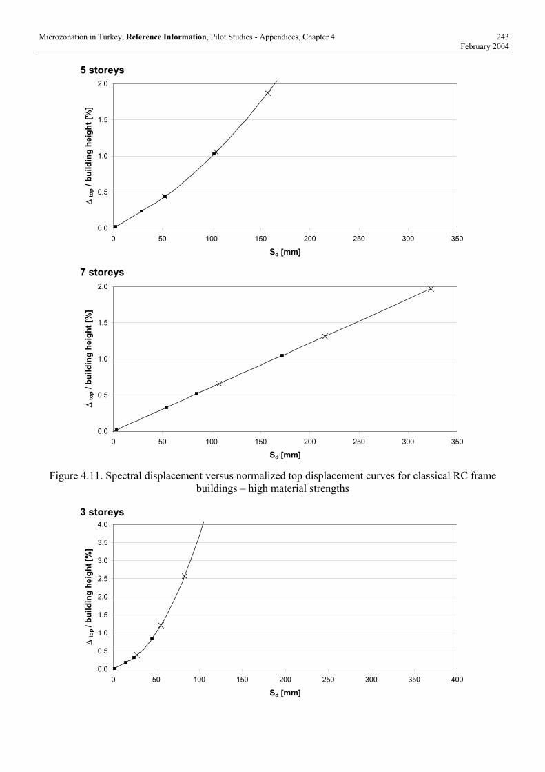
Microzonation in Turkey, Reference Information, Pilot Studies - Appendices, Chapter 4 243 February 2004
5 storeys
0.0
0.5
1.0
1.5
2.0
0 50 100 150 200 250 300 350
Sd [mm]
∆ to
p / b
uild
ing
heig
ht [%
]
7 storeys
0.0
0.5
1.0
1.5
2.0
0 50 100 150 200 250 300 350
Sd [mm]
∆ to
p / b
uild
ing
heig
ht [%
]
Figure 4.11. Spectral displacement versus normalized top displacement curves for classical RC frame
buildings – high material strengths 3 storeys
0.0
0.5
1.0
1.5
2.0
2.5
3.0
3.5
4.0
0 50 100 150 200 250 300 350 400
Sd [mm]
∆ to
p / b
uild
ing
heig
ht [%
]

Microzonation in Turkey, Reference Information, Pilot Studies - Appendices, Chapter 4 244 February 2004
5 storeys
0.0
0.5
1.0
1.5
2.0
2.5
3.0
3.5
4.0
0 50 100 150 200 250 300 350 400
Sd [mm]
∆ to
p / b
uild
ing
heig
ht [%
]
7 storeys
0.0
0.5
1.0
1.5
2.0
2.5
3.0
3.5
4.0
0 50 100 150 200 250 300 350 400
Sd [mm]
∆ to
p / b
uild
ing
heig
ht [%
]
Figure 4.12. Spectral displacement versus normalized top displacement curves for classical RC frame
buildings – low material strengths 3 storeys
0.0
0.5
1.0
1.5
2.0
2.5
3.0
0 50 100 150 200 250 300 350
Sd [mm]
∆ to
p / b
uild
ing
heig
ht [%
]

Microzonation in Turkey, Reference Information, Pilot Studies - Appendices, Chapter 4 245 February 2004
5 storeys
0.0
0.5
1.0
1.5
2.0
2.5
3.0
0 50 100 150 200 250 300 350
Sd [mm]
∆ to
p / b
uild
ing
heig
ht [%
]
7 storeys
0.0
0.5
1.0
1.5
2.0
2.5
3.0
0 50 100 150 200 250 300 350
Sd [mm]
∆ to
p / b
uild
ing
heig
ht [%
]
Figure 4.13. Spectral displacement versus normalized top displacement curves for RC frame buildings
with small walls – high material strengths
3 storeys
0.0
0.5
1.0
1.5
2.0
2.5
3.0
0 50 100 150 200 250 300 350
Sd [mm]
∆ to
p / b
uild
ing
heig
ht [%
]

Microzonation in Turkey, Reference Information, Pilot Studies - Appendices, Chapter 4 246 February 2004
5 storeys
0.0
0.5
1.0
1.5
2.0
2.5
3.0
0 50 100 150 200 250 300 350
Sd [mm]
∆ to
p / b
uild
ing
heig
ht [%
]
7 storeys
0.0
0.5
1.0
1.5
2.0
2.5
3.0
0 50 100 150 200 250 300 350
Sd [mm]
∆ to
p / b
uild
ing
heig
ht [%
]
Figure 4.14. Spectral displacement versus normalized top displacement curves for RC frame buildings
with small walls – low material strengths High material strengths
0.0
0.5
1.0
1.5
2.0
2.5
3.0
0 50 100 150 200
Sd [mm]
∆ to
p / b
uild
ing
heig
ht [%
]

Microzonation in Turkey, Reference Information, Pilot Studies - Appendices, Chapter 4 247 February 2004
Low material strengths
0.0
0.5
1.0
1.5
2.0
2.5
3.0
0 50 100 150 200
Sd [mm]
∆ to
p / b
uild
ing
heig
ht [%
]
Figure 4.15. Spectral displacement versus normalized top displacement curves for a 5 story RC frame
building with small walls – especially high reinforcement ratio 2 walls
0.0
0.5
1.0
1.5
2.0
2.5
3.0
0 50 100 150 200
Sd [mm]
∆ to
p / b
uild
ing
heig
ht [%
]
4 walls
0.0
0.5
1.0
1.5
2.0
2.5
3.0
0 50 100 150 200
Sd [mm]
∆ to
p / b
uild
ing
heig
ht [%
]
Figure 4.16. Spectral displacement versus normalized top displacement curves for a 3 story RC frame
building with both columns and walls

Microzonation in Turkey, Reference Information, Pilot Studies - Appendices, Chapter 4 248 February 2004
By considering the Turkish code for the seismic demand and PGA values of 2 m/s2, 4 m/s2 and 6 m/s2, the following damage grade is reached for the investigated buildings:
Damage grades PGA [m/s2] Structure f0 [Hz] 2 4 6
1a3 2.36 2 2 3 1a5 1.54 3 4 4 1a7 1.05 3 4 4
1b3 2.12 3 4 4 1b5 1.26 3 4 4 1b7 0.96 3 4 4
2a3 2.86 1 2 3 2a5 1.77 2 3 3 2a7 1.13 2 3 3
2b3 2.76 1 3 3 2b5 1.61 3 3 4 2b7 1.0 3 4 4
2ah5 2.18 1 2 3 2bh5 1.61 2 3 4
3a2 1.81 1 2 3 3a4 1.73 1 3 4
4.5.3 Discussion The current investigation clearly shows that
• As expected, compared to columns (type 1), small walls (type 2) delay the degradation.
• The use of good material featuring high values of f’c and fy, enables the wall to withstand a given earthquake with less damage.
• Stocky structures are less exposed to heavy damage than 7 story buildings.
4.6. OUTLOOK
The next step would be the transformation of the x axis of the vulnerability curve from the spectral displacement into the intensity. Such a graph would then enable damage predictions, for a given building, as a function of the seismic demand to be made.
4.7. BIBLIOGRAPHY [EDP 97] Ministry of Public Works and Settlement Government of Republic of Turkey: “Specifications for
Structures to be built in Disaster Areas, part III - Earthquake Disaster Prevention”. Official Gazette No.23390.
[GS 99] Gülkan P., Sozen M. A.: “Procedure for Determining Seismic Vulnerability of Building Structures”. ACI Structural Journal, 96, 3 May, 1999, pp.336-342.
[Lang 02] Lang K.: ”Seismic vulnerability of existing buildings”. Institut für Baustatik und Konstruktion, ETH Zürich, Dissertation No. 14446, 2002.
[Valles et al.] Valles R. E. et al.: “IDARC 2D Version 4.0: A Program for Inelastic Damage Analysis of Buildings”. Technical Report NCEER-96-0010. State University of New York at Buffalo, NY. January 1996.

Microzonation in Turkey, Reference Information, Pilot Studies, Chapter 5 249 February 2004
5. CHAPTER 9
5.1. STRUCTURAL DAMAGE DATA FORM FOR BUILDINGS IN ADAPAZARI

Microzonation in Turkey, Reference Information, Pilot Studies, Chapter 5 250 February 2004

Microzonation in Turkey, Reference Information, Pilot Studies, Chapter 5 251 February 2004

Microzonation in Turkey, Reference Information, Pilot Studies, Chapter 5 252 February 2004

Microzonation in Turkey, Reference Information, Pilot Studies, Chapter 5 253 February 2004

Microzonation in Turkey, Reference Information, Pilot Studies, Chapter 5 254 February 2004
5.2. DAMAGE ASSESSMENT FORM

Microzonation in Turkey, Reference Information, Pilot Studies, Chapter 5 255 February 2004

Microzonation in Turkey, Reference Information, Pilot Studies, Chapter 5 256 February 2004

Microzonation in Turkey, Reference Information, Pilot Studies, Chapter 5 257 February 2004

Microzonation in Turkey, Reference Information, Pilot Studies, Chapter 5 258 February 2004