
Republic of Iraq
130
Republic of Iraq Ministry of Higher Education and Scientific Research Karbala University College of Engineering Department of Civil Engineering Evaluation and Analysis the Effects of Some Parameters on the Operation Efficiency of the Main Water Pipe in Karbala City Using WaterCAD Program A Thesis Submitted to the Department of Civil Engineering University of Kerbela in Partial Fulfillment of the Requirements for the Degree of Master of Science in Civil Engineering (Infrastructure Engineering) By Hussein Ali Hussein (B.Sc. 2005) Supervised by Prof. Dr. Jabbar H. Al-Baidhani Prof. Dr. Musa H. Jassem Al-Shammari November; 2021
-
Upload
khangminh22 -
Category
Documents
-
view
0 -
download
0
Transcript of Republic of Iraq

Republic of Iraq
Ministry of Higher Education
and Scientific Research
Karbala University
College of Engineering
Department of Civil Engineering
Evaluation and Analysis the Effects of Some Parameters on
the Operation Efficiency of the Main Water Pipe in Karbala
City Using WaterCAD Program
A Thesis Submitted to the
Department of Civil Engineering University of Kerbela in Partial
Fulfillment of the Requirements for the Degree of Master of
Science in Civil Engineering (Infrastructure Engineering)
By
Hussein Ali Hussein
(B.Sc. 2005)
Supervised by
Prof. Dr. Jabbar H.
Al-Baidhani
Prof. Dr. Musa H. Jassem
Al-Shammari
November; 2021

سورة يوسف - اآلية )76(


Dedication
To the one who taught me how to stand firmly above the ground... my
respected father
To the wellspring of love, altruism and generosity... my dear mother
To the people closest to myself...my faithful wife
To my soul, the apple of my eyes, and the pulse of my heart... my children
To everyone from whom I received advice and support
I present to you the summary of my scientific efforts.

IV
ACKNOWLEDGMENTS
First of all, I thank God almighty, who granted me the power to
finish this work.
This project would not have been possible without the assistance of
many individuals. I am grateful to those people who volunteered their time
and advice, especially my supervisors, Dr. Jabbar H. Al-Baidahni and Dr.
Musa H. Jassem Al-Shammari, for their guidance, advice, invaluable
remarks, and fruitful discussions throughout the preparation of this thesis.
Without them, the work would not have appeared in this way.
I also wish to express my deep appreciation and gratitude to Dr.
Laith Shakir Rasheed, Dean of the College of Engineering, and Dr. Raid
Rahman AL-Muhana, Head of the Department of Civil Engineering,
Kerbala University, for their help and support throughout the study period.
I am also grateful to the Directorate of Karbala water, especially the
Director of the department Mr. Mohammed Al Nasrrawi, Engineers and
Cadres for their support. Special thanks are also due to Mr. Mohammed
Shmoto, the technical associate of the Karbala Directorate water, Mr.
Moayed Jalwkahn Implementation division officer, Mr. Ahmed Yassin
Head of planning, and to the engineers Mr. Usama, Mr. Safaa branch
administrators in the directorate for their generous help and guidance.
I would also like to express my deepest gratitude to my family for
their support and encouragement. Finally, many thanks to anyone who
helped me and I forgot to mention him.

V
Abstract
The present study will highlight the assessment of the efficiency of
one of the main water pipe Karbala province, it is considered one of the
most important holy province in Iraq and witnesses a large volume of
pilgrims each year. Further, this study was conducted to evaluate the
current main water pipe efficiency to improve its efficiency. A field
reading at different junctions’ locations was taken in the branching and the
main water pipe at different annual seasons, which were in summer,
autumn, winter, and different hours by using an Ultrasonic flowmeter. The
main water pipe is analyzed in two parts. The first part deals with the
analysis of the collected data with the steady flow assumption, and the
second part is simulated and analyzed in the WaterCAD software with the
variation of hourly consumption, which is the unsteady flow assumption.
Based on the results of the first part of the manual analysis, it was
found that there is a clear and a large losses of water at the beginning of
the main water pipe started from junction-1 to junction-5; and then is
accompanied by a clear and large scarcity at the end of the main water pipe.
The total of the losses and scarcity quantities in the main water pipe was
equal to 326.24 𝑚3/ℎ𝑟 and -113.25 𝑚3/ℎ𝑟, respectively. The quantities of
losses are very large compared to the quantities of scarcity, so if the
quantities of losses were controlled, the quantities supplied to the main
water pipe would be enough to fill the presence of scarcities without the
need to increase the quantities supplied based on the steady flow without
any future expansions for junctions. It is noteworthy that controlling the
quantities of losses is very difficult because of the difficulty of detecting
excesses on the network and the absence of water meters in houses to
determine the percentage of losses.

VI
In the second part of the analysis, simulated using WaterCAD
program for six scenarios to analyze and identify the problem of scarcity
according to unsteady flow, and control it to achieve the best solution.
based on simulation of results, it was found that the water needed to
overcome water scarcity was 2400m3/hr. And it cannot be ignored there is
no losses of water in high quantities, especially at the beginning of the main
water pipe, and more specifically in the first five junctions which was
losing quantities of water estimated at 326.24m3/hr. based on manual
calculations, and these losses is because of the use of drinking water for
irrigation of gardens and orchards and a large number of illegal
connections. And this addition to the new capacity of the main water pipe
will take part to increasing the number of junctions according to the needs
Karbala water directorate.

VII
Table of Contents
Dedication……………………………………………………… II
Supervisor Certificate………………………………………... III
ACKNOWLEDGMENTS……………………………………. IV
Abstract………………………………………………………… V
Table of Contents …………………………………………….. VII
List of Figures…………………………………………………... X
List of Tables…………………………………………………. XII
Abbreviations………………………………………………... XIII
Chapter One: Introduction………………………………….2
1.1. Background ........................................................................... 2
1.2. Problem Statement ................................................................ 3
1.3. Study Objectives: .................................................................. 4
1.4. Assumptions .......................................................................... 5
1.5. Outline ................................................................................... 5
Chapter Two: Literature Review ………………………….. 7
2.1. Introduction ........................................................................... 7
2.2. Evaluation and Analysis of water-distribution networks ..... 8
2.3. Summary ............................................................................. 29
2.4. Gap of Knowledge .............................................................. 29
Chapter Three: Theoretical…………………………………. 31
3.1. The Basic Laws for analysis ............................................... 31
3.1.1. Darcy-Weisbach formula ............................................. 33
3.1.2. Hazen-Williams equation ............................................. 36
3.2. Network Analysis Methods ................................................ 40
3.3. Hardy Cross Method ........................................................... 40
3.3.1. Head Balance Method .................................................. 41
3.3.2. Quantity Balance Method ............................................. 42
3.4. Newton-Raphson Method ................................................... 44

VIII
3.5. Computer Models ............................................................... 46
3.5.1. History of computer models. ........................................ 46
3.5.2. Software packages. ....................................................... 47
3.5.3. Development of a system model. ................................. 48
3.6. Water CAD ......................................................................... 48
3.6.1. Junctions ....................................................................... 50
3.6.2. Reservoirs ..................................................................... 50
3.6.3. Pipes ............................................................................. 50
Chapter Four: Field Work…………………………………. 53
4.1. Location .............................................................................. 53
4.2. Al-Sijlah and Al-Feyadh Complexes Project ..................... 55
4.3. The Main Water Pipe .......................................................... 56
4.3.1. Existing Distribution System ....................................... 57
4.3.2. Connections junctions .................................................. 57
4.4. Field Recording Data .......................................................... 58
4.4.1. Recording data in the summer, specifically the month of
August ........................................................................... 60
4.4.2. Recording data in the autumn, specifically the month of
October ......................................................................... 61
4.4.3. Recording data in the winter, specifically the month of
December ...................................................................... 62
Chapter Five: Results and Discussion…………………….. 65
5.1. Analysis of the recorded field data of Main water pipe ..... 65
5.1.1. Consumption type in a mainline pipe ........................... 66
5.2. Building of the hydraulic model using WaterCAD ............ 73
5.3. Proposal Scenarios for the hydraulic Model in WaterCAD
............................................................................................. 78
5.3.1. First scenario ................................................................ 78
5.3.2. Second scenario ............................................................ 81
5.3.3. Third scenario ............................................................... 85

IX
5.3.4. Fourth scenario ............................................................. 88
5.3.5. Fifth scenario ................................................................ 91
5.3.6. Sixth Scenario ............................................................... 94
5.3.7. The summary of scenarios ............................................ 97
Chapter Six: Conclusion and Recommendation………. 100
6.1. Conclusions ....................................................................... 100
6.2. Recommendations ............................................................. 102
6.2.1. Recommendations for operating staff of the main water
pipe ............................................................................. 102
6.2.2. Recommendations for future studies .......................... 104
Reference……………………………………………………… 106
أ ...……………………………………………………………الخالصة

X
List of Figures
Figure 3-1: Closed loop type network. ..................................................... 41
Figure 3-2: Branched-type pipe network. ................................................. 43
Figure 4-1: Geographical location of Karbala relative to Iraq. ................ 53
Figure 4-2: Geographical location of the mainline. .................................. 55
Figure 4-3: Layout plan of the Al-Sijlah and Al-Feada complex project.56
Figure 4-4: The different ultrasonic devices using during record data. ... 58
Figure 4-5: The pressure gauge using for record data. ............................. 59
Figure 4-6: during record data. ................................................................. 63
Figure 5-1: The layout of distribution network in WaterCAD. ................ 74
Figure 5-2: Flex table (pipe table) for identified the characteristics. ....... 75
Figure 5-3: Flex table (junction table) for identified the characteristics. . 76
Figure 5-4: Identify pump characteristics in pump Definitions windows.
............................................................................................... 77
Figure 5-5: Identify pump characteristics in pump Definitions windows.
............................................................................................... 77
Figure 5-6: Calculation summery for simulation at first scenario. ........... 79
Figure 5-7: Head Pressure at junction-p at pump station during 24 hr. ... 80
Figure 5-8: layout of mainline with booster station. ................................ 82
Figure 9: The pump definition for Booster Station. ................................. 83
Figure 5-10: Calculation summery for simulation at second scenario. .... 84
Figure 5-11: Head Pressure at some of junctions during 24 hr. ............... 84
Figure 5-12: The pump definition for 3rd scenario. ................................. 85
Figure 5-13: Calculation summery for simulation at third scenario......... 86
Figure 5-14: Hydraulic Grade line profile for 3rd scenario at 18:00. ..... 87
Figure 5-15: Hydraulic Grade line profile for 3rd scenario at peak time 19:00. ....... 87
Figure 5-16: Hydraulic Grade line profile for 3rd scenario at 20:00. ...... 88
Figure 5-17: Calculation summery for simulation at fourth scenario. ..... 89

XI
Figure 5-18: Hydraulic Grade line profile for 4th scenario at 18:00. ....... 90
Figure 5-19: Hydraulic Grade line profile for 4th scenario at 19:00. ....... 90
Figure 5-20: Hydraulic Grade line profile for 4th scenario at 20:00. ....... 91
Figure 5-21: The pump definition for 5th scenario. ................................. 92
Figure 5-22: Calculation summery for simulation at fifth scenario. ........ 93
Figure 5-23: Hydraulic Grade line profile for 5th scenario at peak time. 94
Figure 5-24: Calculation Summary for Simulation at sixth Scenario ..... 97
Figure 5-25: Hydraulic Grade line profile for 6th scenario at peak
time(19:00)……………………………………………………….…… 97
Figure 5-26: Hydraulic Grade line profile for 6th scenario at peak
time(18:00)……………………………………………..……….……… 98
Figure 5-27: Hydraulic Grade line profile for 6th scenario at peak
time(19:00)……………………………………………...………………98

XII
List of Tables
Table 3-1: Values of Constant in Hazen-Williams Formula. ................... 37
Table 3-2:Values of Hazen-Williams Coefficient for Clean New Pipes of
Different Materials. .................................................................. 38
Table 3-3: Correction Factors for Hazen-Williams Coefficients. ............ 39
Table 4-1: Recording data during morning operation. ............................. 60
Table 4-2: Recording data during afternoon operation. ........................... 60
Table 4-3: Recording data during evening operation. .............................. 60
Table 4-4: Recording data during morning operation. ............................. 61
Table 4-4-5: Recording data during afternoon operation. ........................ 61
Table 4-6: Recording data during evening operation. .............................. 61
Table 4-7: Recording data during morning operation. ............................. 62
Table 4-8: Recording data during afternoon operation. ........................... 62
Table 4-9: Recording data during evening operation. .............................. 62
Table 5-1: Elevation and Demand for branch junctions. .......................... 79
Table 5-2: Elevation and Demand for branch junctions at 4th scenario. .. 88
Table 5-3: Summarizes the advantages and disadvantages of scenarios. . 98

XIII
Abbreviations
Abbreviation Description
SDP Stochastic Dynamic Program
LDRs Linear Decision Rules System
SOP Stochastic Operating Program
NLDR Non Linear Decisions Rules
TPLS Technical Performance Index System
GMC Gandhinagar Municipal Corporation
PROBPB Pipe Burst Possibility
WSR Water System Replacement
PM Pressure Management
PSI Puckorius Scading Index
RSI Ryznar Stability Index
WDS Water Distribution System
WDNs Water Distribution Network System
GA Genetic Algorithm
GIS Geographic Information System
ANN Artificial Neural Network
PDNA Pressure Deficient Network Analysis
ACO Ant Colony Optimization
AHP Analytical Hierchy Processes
DE Differential Evolution
DENET Differential Evolution Network
NRW Non-Revenue Water
AI Aggressiveness Index
HGL Hydraulic Gradient line
WDSs Water Distribution Supply System
CHW Hazen William Coefficient
VR Valve Proportion
CA Condition Assessment
SDGs Sustainable Development Goals System
f Darcy Coefficient Friction
(ASCII) American Standard Coding for Information Interchange

Chapter One
Introduction

Chapter One ……………..………………….…………… Introduction
2
Chapter One: Introduction
1.1. Background
The system of water distribution has been a hydraulic infrastructure,
which contains types of valves, pumps, supplied reservoirs, different
various of tanks, pipes, and among other things. They're all necessary for
delivering water of acceptable quantity at the right pressure. It possible are
Either looped or branched distribution systems. looped systems are favored
over branching systems since they may offer a greater degree of
dependability when coupled with appropriate valving. A pipe break may
also be repaired and isolated in a looping system with little effect on
consumers beyond the local region. Customers downstream from the
breach in a system the branch, on the other hand, will be without water till
the repairs have been finished. A looped design, on the other hand, enables
water to reach the consumer through several paths, boosting system
capacity at any time (Atiquzzaman, 2004). Because of the cost and
significance, the system of water distribution (WDS) is considered
amongst the most important of the water supply system components. Water
distribution network system (WDNs) are designed with the primary goal
of supplying the required amount of water at the essential time with
adequate pressure. Drinking water supplies in several third-world countries
are insufficient to satisfy the demands of consumers.
Along each main water pipe, there are many connections with tiny
ports or pipes, all of which enable flow from or into the main pipe (less
frequently). Main water pipe have a lot of junctions or ports, which are
typically near together but not same the flow at neighboring
junctions(Larock et al., 1999).

Chapter One ……………..………………….…………… Introduction
3
Intermittent water supply systems have been operated and designed
accordingly. Because free flow ports and pressure heads are provided in
the different nodes, discharged at junctions will be relative to the accessible
pressure head at each junction, resulting in a variation in the amount of
water delivered. In the systems of water distribution design, this aspect was
not given much weight. When there is a shortage of water, the problem of
unequal distribution becomes even more serious. Some nodes will receive
more than their fair share, while others will discharge far less than their
proportionate share. One of the design recommendations in design guides
was to guarantee that the variance in pressure head among different nodes
within a distribution zone remained within a specified range, or that the
region was split into smaller zones to fulfill this requirement (Gottipati &
Nanduri, 2014).
1.2. Problem Statement
As a consequence of increasing urbanization and the development of
hundreds of local and large-scale water supply and distribution systems in
the past few decades, many people today have access to clean water and
sufficient sanitation. However, the quality of water utility service is
frequently questioned, and the cost of new systems is frequently
prohibitive. Water supply systems are critical strategic systems that are
physically complex in their design, installation, and operation, posing
significant economic and environmental concerns. They also make a
significant contribution to public health. Despite this, professionals and
engineers frequently underestimate design and operational challenges, and
their direct or indirect impacts, while often considered separately, are
rarely investigated comprehensively (Jalal, 2008).
The present study will focus the assessment of the efficiency of one
of the main water pipes in the Karbala province specifically in the area of

Chapter One ……………..………………….…………… Introduction
4
AL-Feyadh, which belongs to the Al-Kheirat township where the water
complexes are located. The main water pipe has a diameter of 800 mm
ductile from these water complexes, passing through the villages and
countryside’s on the side of the road, and reaching the Najaf road, where it
runs along the Husseiniyat on the road to the province of Karbala.
The line was chosen to conduct the study and increase its operational
efficiency because it is considered the main feeder to Karbala international
airport, which is under construction, and it’s one of the important
infrastructure facilities through one of the junctions branching from it, as
well as the residential complex in Al-Zabilia road towards the Karbala
center. This study contributes to helping the Karbala water directorate to
increase the capability and to get better the hydraulic performance of the
main water pipe.
1.3. Study Objectives:
The main objectives of the present study are:
1. Evaluating the hydraulic performance of the existing main water pipe
that owns a dead-end system and is located in Karbala city in Iraq.
2. Finding the best methods and appropriate solutions to solve this deficit
using an analytical study of the main water pipe.
3. Using Hydraulic analysis software Bentley WaterCAD. under peak
consumption and extended period simulation of 24 hours and its
performance was assessed according to current hydraulic
circumstances.
4. The main hydraulic parameters of main water pipe are the discharge,
required pressure, and other associated factors of them are pipe
diameter, flow velocity, and all those had been studied.

Chapter One ……………..………………….…………… Introduction
5
1.4. Assumptions
1. The main water pipe existing has a dead-end system and the water
moved from the first zone towards the last zone.
2. The main water pipe system operates entirely by a pump station
which is located in a compact unit.
3. The quantity of the flow in main water pipe junctions is unique
because of the difference in level and near of pump station.
4. The quantity of flow is not constant for every junction.
5. Minor losses at the nodes (junctions) are neglected.
1.5. Outline
1. Chapter one describes the overview of main water pipe, objective for
research, the layout of dissertation, and assumptions.
2. Chapter two reviews some of the recent work done on analysis for
water networks and distribution systems.
3. Chapter three describes the theory of water networks and the method
of analysis and program used in assessment.
4. Chapter four survey of main water pipe for case-study.
5. Chapter five presents the results of the analysis and discussion.
6. Chapter six explains the main conclusions and recommendations for
future work.

Chapter Two
Literature Review

Chapter Two ……………..……………..…….…… Literature Review
7
Chapter Two: Literature Review
2.1. Introduction
This chapter aims to provide a systematic and up-to-date review of
achievements concerning of analysis and operation of the water
distribution networks field. It's also discussing problems and key issues in
the context of future research needs in the analysis and operation of water
distribution networks.
Water distribution networks are an essential component of water
delivery systems and one of society's most valuable infrastructure assets.
Simulating hydraulic activity in a looped pipe network is a difficult job that
entails solving a set of nonlinear formulas. The head loss function,
continuity, and energy formulas are all studied at the same time throughout
the solution procedure.
Several techniques for addressing steady-state networks hydraulics
were developed throughout the years. The capacity to model the hydraulic
behavior of major water distribution networks had also significantly
increased in the last two decades, thanks to the development of models and
the availability of low-cost, reliable equipment.
A large number of researchers studied water distribution networks
in various ways. Some of them studied the issue of designing water
distribution networks in general, while others tried to analyze and evaluate
water distribution networks and investigate the problems faced by the
network to find appropriate solutions.

Chapter Two ……………..……………..…….…… Literature Review
8
2.2. Evaluation and Analysis of water-distribution networks
(Alshammari, 2000) Use Hazen-William equation in applied to
calculate the amount of water transported through the pipe at the intake
points and the number of real discharges withdrawn from these points (real
consumption) and from knowing the inhabitants served from these points
and multiplying this number by the per capita consumption rate of water to
know the hypothetical consumption at these points and from comparing the
two quantities was determining the nature of consumption in the network
by calculating of losing based on the mathematical sign, If it is positive
indicating an excess, and if it is negative it indicates the presence of water
scarcity in the network.
(Rajani & Kleiner, 2001) A water supply system's distribution
network has been the most costly component. The degradation of water
mains leads to increased maintenance costs, worse water quality, lower
service quality, water loss, and interruption of street-level activity. Always
water lines repair and renewal must be planned through rehabilitation if
sufficient water supply goals are to be met. Understanding and quantifying
pipe degradation processes is a critical component of the planning process.
In the past 20 years, historical performance data has been used to assess
the structural degradation of water mains. The physical processes that
cause pipe failures typically necessitate data that is both scarce and
expensive to acquire.
(Selvakumar et al., 2002) In the Americas, there is increasing
concern about the requirement to repair, replace, and rehabilitate potable
water distribution and wastewater collecting systems. According to a
recent study performed by the US Environmental Protection Agency,
maintaining and replacing current drinking water infrastructure would cost
$138 billion during the next 20 years. The cost of rehabilitating and

Chapter Two ……………..……………..…….…… Literature Review
9
repairing pipes is expected to reach $77 billion. Epoxy coating, cleaning
and repacking techniques were used for the lining materials.
The CANDA-GA Model was created by (Keedwell & Khu, 2005)
and utilizes a local representative cellular automata, a heuristic-based
method to generate a suitable starting inhabitant for genetic algorithm
starts. Three networks were solved using the CANDA-GA algorithm. The
findings indicate that the suggested technique regularly outperforms the
non-heuristics-based GA method in terms of designing more cost-effective
water distributions networks.
(Al-Zahrani & Syed, 2005) used the minimal cut-set technique to
assess the dependability of a municipal water distribution system. On an
actual water distribution network, a technique for assessing water
distribution system dependability was devised and proven. The technique
consists of two stages: (1) nodal pressures were estimated utilizing the
hydraulic simulation software (EPANET), and (2) nodal and system
reliabilities of the AI-Khobar water distribution system are determined
using the minimal cut-set method. The hydraulic dependability of the core
section of the AI-Khobar water distribution network was found to be 69.73
percent.
(Christodoulou et al., 2006) proposed a framework for managing
urban water distribution systems that combined numerical and analytical
simulation methods with geographical information systems (GIS) for better
dissemination and visualization of important information to management
teams. The state of components in the water distribution system has been
evaluated using numerical simulations and artificial intelligence methods,
forms in the underpinning historical data have been investigated using
artificial neural network (ANN), knowledge is gathered and assessed using
database managing systems and fuzzy logic, and the findings have been

Chapter Two ……………..……………..…….…… Literature Review
10
eventually mapped on GIS for improved visualization. The methodology
and methods created and described in this study have been depending on
data gathered in New York City and then used in Freeport (Long Island,
NY), Limassol, and Larnaca, Cyprus (Cyprus).
(Geem, 2006) utilized a harmony searches optimization method to
identify the best water distribution system design whilst keeping all design
limitations in mind. To discover better design solutions, the harmony
search algorithms replicates a jazz improvising process, in this instance
pipe sizes in a water distribution system. To assess the hydraulic
limitations, the model connects to EPANET, a prominent hydraulic
simulator. The degree of violation is included in the cost function as a
penalty if the design solution vector breaches the hydraulic restrictions.
Under comparable or less favorable circumstances, they applied a model
to five systems of water distribution and produced designs that have been
similar or slightly cost 0.28–10.26percent lower compaed with those
competing for meta-heuristic algorithms like the tabu search, simulated
annealing, and genetic algorithm. The findings indicate, which the
harmony search-based approach is appropriate for designing water
networks.
The pressure-deficient network method (Ang & Jowitt, 2006)
proposed a new technique for solving a water distribution system under
pressure-deficient circumstances (PDNA). The model gradually inserted a
fake reservoir into the network to start nodal flows, with full demanding
loads eventually replacing such reservoirs after it was apparent that the
nodal flow could be met. The PDNA was provided in a format that could
be used to program a computer. The PDNA has been utilized to solve flows
in a basic network, but it should be utilized in conjunction with a

Chapter Two ……………..……………..…….…… Literature Review
11
hydraulically networks solver to solve flows in a looping network; since
the manual calculation is too time-intensive.
(Jamieson et al., 2007) created a model to assess the feasibility and
effectiveness of implementing real-time, near-optimal management for
water-distribution networks. With that in mind, the book's contents cover
the present state of the art as well as some of the challenges that must be
overcome if the aim of near-optimal control is to be realized. Since it would
be difficult to utilize a near-optimal controlling, traditional hydraulic
model simulation for real-time that is theoretically much more efficient,
they used artificial neural networks to replicate the model. The preceding
model was then integrated into a dynamic genetics algorithm that were
developed especially for real-time usage. This method may be used to
generate near-optimal control parameters to satisfy present needs while
minimizing total pump-up prices to the operational horizon.
The Ant Colony Optimization (ACO) methodology was used by
(López-Ibáñez et al., 2008) to find the best pump schedule. They broke
down a pumping timetable into a sequence of numbers, each indicating the
number of hours a pump is active or idle. In comparison to the binary
representation, this decreases the number of possible timetables (search
space). They aimed for the lowest possible electrical cost while still
meeting system limitations. Then used an ant colony Optimization
methodology to solve the optimum pump scheduling instead of utilizing a
penalty function method for constraint violations, and they prioritized the
solutions depending on the significance of the violations. On such a limited
test network and a big real-world network, they have been put to the test.
(Al-Barqawi & Zayed, 2008) developed a robust model to evaluate
the status of water mains and forecast their performance. To create the

Chapter Two ……………..……………..…….…… Literature Review
12
model, the researchers used data gathered from three distinct Canadian
towns. Artificial neural network (ANN) and analytical hierarchy processes
(AHP) have been used to create an integrated model and framework.
Furthermore, a web-based infrastructure management application (CR-
Predictor) based on the combined AHP/ANN model was created to
evaluate water main status. The created tool and models have been verified,
and the findings are reliable (98.51 percent) and that is the median validity
percent. Practitioners and Academics (contractors, consultants, and
municipal engineers) were anticipated to profit from them by prioritizing
rehabilitation and inspection plans for existing water systems.
The following are some of the main advantages of supplying water
for firefighting:
1. Preservation of the economy from the effects of fire
2. Insurance costs for homeowners and businesses in the
neighborhood have been reduced.
3. Human life preservation.
4. Human suffering is reduced. As a result, there seem to be
additional reasons for supplying sufficient fire flows to a
town, in addition to public safety.
Because an appropriate water supply system is a critical component
of a fire protections/suppression system, effectively managing/fighting a
fire emergency requires a thorough study and knowledge of the water
supply system's firefighting capability. Hydrant flow tests may be used to
assess the ability of an existing water distribution system to determine the
available fire flow in a given region. Field assessment of hydrants wherever
they existed, on the other hand, has been deemed excessively expensive,
time-consuming, disruptive, and only approximate. It's also difficult to
physically test each hydrant in the system, therefore computer modeling is

Chapter Two ……………..……………..…….…… Literature Review
13
used to offer a reliable and precise way of forecasting fire flow in a water
supply system.
(Izinyon & Anyata, 2009a) utilized the WaterCAD program to create
a hydraulic system model of the current water distribution network in
Ikpoba Hill, Benin City, Nigeria, which was calibrated for investigations
of steady-state simulation utilizing the system's calibration, operational,
and physical data. The model has been used to analyze an available fire
flow and develop system improvements. The results of the computerized
fire flow analysis for the current network indicate that no node in the
system meets the study's fire flow restrictions. That is, the total available
fire flow for all nodes in the system is 0 l/s, suggesting that the system is
unable to provide the required flow for fire suppression. Nevertheless, the
planned upgraded network, which includes expanded diameters of current
pipes as well as future expansion projections, has available fire rate of
between 40l/s and 29.6l/s at the network's nodes. Hydrant tagging,
numbering, and color-coding may be changed based on the available fire
flow that will improve the fire department's firefighting/suppression
capabilities.
(Tabesh et al., 2009) developed a novel technique for assessing non-
revenue water (NRW) and losses in a systems of water distribution using
the "year water balance" and "minimum night flow" assessments. The
major NRW components, including leakages from reported and
background leakage and un-reported bursts, were assessed using actual or
estimated data, allowing the evaluation of leakage performance indicators.
They have developed a new method that uses a hydraulic simulation
models to assess nodal and pipe leaks. Because leakage is pressure-
dependent, the entire usage is split into two portions, one pressure
dependent and the other independent of local pressures, and the hydraulic

Chapter Two ……………..……………..…….…… Literature Review
14
behavior of the network is investigated. Depending on the suggested
approach, they created a computer coding for evaluating all elements of
water losses. They converted the outcomes to a GIS model for a more
accurate depiction of the findings and system administration. Utilizing the
GIS model's capabilities, they connected the attribute data and map
network and discovered variables influencing network leakage. They also
looked at the consequences of lowering the pressure. A real-life case study
was used to evaluate the concept. The findings revealed that the suggested
model overcomes the limitations of previous methods by more accurately
estimating leaks and other NRW elements in water distribution systems.
The use of algorithms' Differential Evolution (DE) for optimum
rehabilitation and design of existing water distribution systems was the
topic of (Suribabu, 2010). To accomplish a goal of optimization of the
given objective function, the algorithms of Differential Evolution (DE)
uses a notion similar to that of the genetic algorithm. The optimum network
design seems to be a mathematically difficult issue that falls under the NP-
hard category. They used four well-known benchmark networks to
evaluate the effectiveness algorithms of the Differential Evolution (DE).
Within a reasonable number of function evaluations, the DE method
proved to be highly successful in identifying near-optimal or optimum
solutions. In comparison to other algorithms, the algorithms of Differential
Evolution (DE) performed very well.
(Kanakoudis & Tsitsifli, 2010) demonstrates that when the water
tariffs utilized by the water company involve set minimum additional fees
associated with water volumes being charged but not utilized (based on the
most recent meters' measurements), the levels of the Real Shortfalls,
determined thru the established IWA WB, is underestimated by every other
variation, which, while generating revenues (falsely reducing the NRW

Chapter Two ……………..……………..…….…… Literature Review
15
levels), remains unaffected. Because a large part of Real Losses (up to 43
percent in certain cases) generates income, the need to design and execute
any water loss mitigation strategy is reduced. To prevent these erroneous
findings, a change to the IWA WB was suggested that included the entire
economic component. Two Greek cities used the planned modified IWA
WB in their water distribution systems. The findings showed that in
situations in which there are large demand peaks (seasonal), it is preferable
to assess the network across shorter periods. The findings also showed that
throughout periods of high water demand, whenever operational pressure
levels drop, actual losses are lower than during periods of low demand.
(Vasan & Simonovic, 2010) discusses the creation of a DENET
simulation environment for optimum water distribution system design,
which included the use of a differential evolution evolutionary
optimization method connected to the EPANET hydraulic simulation
solver. They developed a model to reduce costs, and they used it to solve
two standard water distribution network optimization issues: The New
York water supplying system and the Hanoi water distribution network.
When compared to previous experiments in the literature, the findings were
encouraging, prompting the researchers to restructure the model with a new
goal of increasing network resilience. The findings of the study showed
that DENET may be used as an alternate tool for designing and managing
water distribution networks that are both cost-effective and dependable.
(Yazdani & Jeffrey, 2011) suggested that water supply systems
could be represented as multi-nodes networks (including hydraulic
connections, storage tanks, and tanks) linked by physical connections
(including pipes), with the network's communication patterns affecting its
durability, efficiency, and reliability in the event of a failure. To establish
relationships between structural features and performance of water

Chapter Two ……………..……………..…….…… Literature Review
16
distribution systems, the researcher used correlation node representations
of water infrastructures and a wide range of advanced and emerging
network theory metrics and metrics to study the building blocks of systems
and identify characteristics such as redundancy and fault tolerance. The
researcher looked at a third-world country's water distribution system and
looked at network expansion methods targeted at ensuring and improving
structural resilience while keeping design and budget limitations in mind.
Water losses will always happen in water distribution systems,
according to (Gomes et al., 2011). Given that the majority of actual losses
happen in distribution pipes and service connections, the researcher's
approach is based on several leakage assessment methodologies from the
literature as well as simulating the water distribution system. This enables
an evaluation of the advantages of pressure control in water distribution
networks, especially in terms of decreasing water output. Furthermore, this
method may be helpful for cost- benefit analysis to assist identify the point
at which decreasing water loss is no longer economically beneficial (the
economic leakage's levels). The implementation of pressure-lowering
valves at the entrance points of the rating regions was assumed in the
hypothetical research articles.
(Ostfeld et al., 2013) The hydraulic simulation of the dynamic pipe
network, according to the investigator, is a study of the municipal water
distribution system to develop an efficient technique of timetabling and
scientific operations. The key to developing an accurate model is to gather
basic data, acquire it, and integrate it into a pipeline modeling process. For
instance, GIS data in an urban piping system generates a computer
simulation of the water delivery system.

Chapter Two ……………..……………..…….…… Literature Review
17
(Mutikanga et al., 2013) Water shortages and financial losses are
plaguing the water sector throughout the globe. Over time, techniques and
procedures have been developed to minimize these losses and improving
the effectiveness of water distribution systems. Current techniques and
methods for assessing, monitoring, and controlling losses in water
distribution systems are discussed in this article. According to the findings
of the study, many water loss control techniques and procedures have been
created and applied. They range from basic management tools like
performance indicators to complex optimization techniques like
evolutionary algorithms. Its applicability to real-world water distribution
systems, on the other hand, is restricted. To bridge the gap between theory
and practice, future research possibilities exist via strong cooperation
between researches institutions and water service providers.
(Bolouri-Yazdeli et al., 2014) Tank operating rules were
mathematical or logical formulae that compute water discharge from a tank
based on flow magnitudes and storage capacity, taking into consideration
system factors. Throughout reality, in each operating period, past system
experiences are utilized to balance tank system parameters. The reservoir
operating rules were created utilizing different optimization methods and
were classified as linear decision rules (LDRs) and constant variables. The
study looked at how real-time operating rules might be applied to a
reservoir system that seeks to meet the entire ultimate demand. With
various magnitudes of flow and reservoir storage, these rules include
Nonlinear Decision Rules (NLDR), LDR, Stochastics Dynamics
Programming (SDP), and Standards Operating Policies (SOP). To organize
the aforementioned principles, the technique of selecting, eliminating, and
multi-attribute decision to represent reality (ELECTER -I ) is employed,

Chapter Two ……………..……………..…….…… Literature Review
18
along with a range of measures, objective functions, and tank performance
objectives (vulnerability, adaptability, and reliability).
(Tricarico et al., 2014) The network topology is used as a continuous
reference for input in most water distribution system redesign methods,
with optimization allowing only duplication/replacements of existing
components. This article presents a novel approach that reports the effect
of current network architecture and performance in terms of its
contribution to the discovery of optimum alternatives that may lead to a
decreased chance of failure to deliver the necessary water, as well as a
lower cost of redesign. The looping frequency and network strength
architecture are studied in particular using a genetic algorithm-based
optimization method that takes into consideration the unpredictable water
requirements at every node. The proposed approach was used in two case
studies that looked at the impact of the structure on total system
dependability and risk.
(Muranho et al., 2014) The Technical Performance Indexes (TPIs)
use to evaluate the operating performance of Water Distribution Systems
(WDNs) is explored in this article, as well as its potential for quickly
identifying issue areas. The article also discusses some of the issues with
existing TPIs and offers new analytic methods to address these issues.
These new analytical techniques (including constraint violation as state
variable slack) have been combined with the pressure-driven simulation
study for demonstration purposes, including assessing operational
performance throughout pipe bursts or firefighting scenarios, and
identifying and accounting for the "supply not satisfied" as a result of those
events.
Chapter Two ……………..……………..…….…… Literature Review
19
(Medeiros et al., 2015) One of the most significant problems that
public managers and system operators confront today is reducing water
loss in water delivery systems. Water loss at high levels has a direct effect
on the system's income and, as a result, on investments and finance.
Moreover, they are liable for causing environmental damage by exploring
and extracting a larger amount of water than is required. To reverse this
condition, various options for water networks partition have been
examined using scenario simulations created with the WaterCAD V8i
water distribution modeling program. The reorganization of the water
distribution system may result in a significant decrease in water loss.
Moreover, the water network's digital model is an essential tool for system
managers to better manage water resources, resulting in both
environmental and economic benefits.
(Dave et al., 2015) The purpose of this research, titled "Analysis of
Continuous Water Distribution System in Gandhinagar City Utilizing
EPANET Software: A Case Study of Sector-8," was to achieve effective
design, development, and analysis of the water distribution system using
EPANET software. The current water distribution system data was
obtained from Town Planning Departments, and Buildings Departments,
Gandhinagar Municipal Corporation (GMC), Road and Gujarat
Government, Gandhinagar, for this study. Three techniques were used to
predict the population of Gandhinagar City over the next thirty years:
Arithmetic Increase Technique, Geometric Increase Technique, and
Incremental Increase Technique. The projected citizenry's water
consumption for the following three decades had also been calculated. The
height of nodes and pipe length was recorded for 285 nodes and an

Chapter Two ……………..……………..…….…… Literature Review
20
equivalent number of pipes using a Google Earth image of Gandhinagar
city. EPANET Software was utilized to analyze pressure, head loss, and
elevation using these data. Pressure and height at different nodes, as well
as pressure losses at different pipes, were the results of this study. The
findings of data analysis in EPANET Software revealed that there is
reduced head loss in Sector-8, Gandhinagar that is critical for maintaining
the constant pressure needed for the continuous water delivery system.
(Choi & Koo, 2015) The pipe burst possibility (ProbPB), the effect
of a burst pipe (ImpPB), and the (WSR) determined as the product of these
two magnitudes were developed for a water distribution system and applied
in a target location for deciding the pipe burst possibility (ProbPB), the
effect of pipe burst (ImpPB), and the WSR determined as the product of
these two magnitudes. When the water supply is cut-off or decreased,
ImpPB was computed separately for the leaking duration period and the
repair work time. To validate this (WSR), pipe replacements have been
carried out using ProbPB, a water provider management indication,
ImpPB, a water consumption management indicator, and the WSR, which
incorporates both of these, by evaluating the WSR reduction impact of
each. As a result, pipe replacements depending on WSR had the greatest
decrease efficiency. The findings showed that the suggested WSR
evaluation model may take into account the perspectives of both the water
supplier and the water user at the same time. Furthermore, the model's cost-
effectiveness has been confirmed.
(Archetti, 2015) In this article, resilience is defined as a networked
infrastructure's capacity to provide service even if certain components fail;
it is dependent on both net-wide measurements of connection and the
function of a single component. The goal of this study was to demonstrate

Chapter Two ……………..……………..…….…… Literature Review
21
how well a set of general methods can be produced using network theory
methods, specifically how the spectral analysis of adjacency and Laplacian
matrices can be used to create a mathematically sound and practical
definition of global connectedness. Second, using a clustering technique in
the subspace covered by the Laplacian matrix's l lowest eigenvectors
allows us to find the network's edges whose failure causes the network to
collapse (vulnerabilities). Even while the majority of the study may be
applied to any networked infrastructure, particular references to Water
Distribution Networks (WDN)will be made. The suggested technique's
operational utility is shown using a standard and three real-world
examples. Nevertheless, depending on an abstract graph context, this work
is only the first step in the creation of tools to assist the investigation of
resilience at global and national levels. The present stage of the study is to
develop graph-based metrics connected with network-wide resilience as
well as techniques to identify vulnerabilities in terms of physical
infrastructure connection. The most important graph theory-based metrics
to assess the overall resilience of a WDN about physical separation since
disruptive occurrences on pipes were found as spectral gap and algebraic
connectivity.
(Vicente et al., 2016) In water distribution systems, pressure
management (PM) is a frequent practice (WDSs). The development of new
scientific and technological techniques for its application has been a
strategic goal in the area for the past decade. However, improvement was
not always reflected in actual activities owing to a lack of systematic
examination of the findings gained in practical situations. This article has
given a thorough examination of the most novel problems connected to PM
to solve this challenge. The suggested approach is depending on a case-

Chapter Two ……………..……………..…….…… Literature Review
22
study comparison of qualitative conceptions that includes 140 published
sources. The findings included a qualitative study of four aspects: (1) the
goals achieved by PM; (2) forms of regulation, including sophisticated
control systems thru electronic controllers; (3) innovative district design
techniques; and (4) the creation of PM-related optimization models.
Because of its technical and practical character, the job of (PM) continues
to develop. The introduction of new technologies, methods, and tactics
necessitates a continuous upgrading of knowledge to keep the scientific
community up to date.
(Mirzabeygi et al., 2016) The propensity of water to corrode and
scale seems to be an etiology of health and economic problems in water
delivery systems. The purpose of this research was to look at the water
stability of the Torbat Heydariye potable water system. This cross-
sectional research used cluster sampling methods, with 90 samples
obtained from 15 clusters using simple random sampling. During the year
2014, all samples were collected from the water distribution network. The
Aggressiveness index (AI), Larson-Skold index (LS), Puckorius scaling
index (PSI), Ryznar Stability index (RSI), and Langelier saturation index
(LSI) were also used to evaluate the water stability (AI). Utilizing a
Geographic Information System, the degree of corrosion in various areas
of Torbat Heydariye was shown. Even though these estimated parameters
were below acceptable limits, the findings showed that high TDS levels
associated with chloride and sulfate anions play a major role in enhancing
water's corrosive propensity.
(Balacco et al., 2017) The use of conventional peak factor formulae
in the water distribution system design might lead to over-dimensioning of

Chapter Two ……………..……………..…….…… Literature Review
23
network pipes, particularly in small towns. This disparity is most likely
attributable to changes in human behavior as a result of improved living
circumstances. Based on these considerations and the access to a large
randomized data sample, a study of water demand for numerous towns in
Puglia was conducted, leading to the establishment of a stochastic
connection between the previous section peak parameter and the number
of people. The use of weekly and monthly peak parameters in the design
of a water distribution system is not required, according to this research,
since contemporary water needs do not seem to be very sensitive to these
fluctuations.
(Seyoum & Tanyimboh, 2017) Water distribution system numerical
simulations have been utilized for a variety of reasons. Planning, design,
monitoring, and control are some instances. Nevertheless, in low-pressure
situations, traditional models that use demand-driven analysis may provide
deceptive findings. Almost all models that use pressure-driven analysis, on
the other hand, do not conduct smooth dynamic and/or water quality
simulations. Tanks, control devices, and pumps for example, are often left
out. The EPANET-PDX simulation model seems to be a pressure-driven
expansion of the EPANET 2 computer simulation that keeps all of
EPANET 2's features, including water quality modeling. It cannot,
however, mimic several chemical compounds at the same time. Water
quality modeling based on a single species is inefficient and rather
inaccurate. The reason for this is because in water distribution networks,
various chemical compounds might coexist. This paper presents EPANET-
PMX (pressure-dependent multi-species extension), a fully integrated
network analysis model that solves these flaws. Both dynamic and steady-

Chapter Two ……………..……………..…….…… Literature Review
24
state simulations are conducted by the model. It may be used in any
network that has a variety of chemical processes and reaction kinetics.
(Shuang et al., 2017) WDNs, or water distribution systems, are a
kind of critical infrastructure network. Components breakdowns in a
(WDN) will cause system failures, resulting in larger-scale responses,
when a catastrophe happens. The purpose of this study is to assess the
development of system reliability and breakdown transmission time for a
WDN suffering cascading failures, as well as to identify key pipes that may
significantly decrease system dependability. The technique takes into
account several variables, including network architecture, water supply and
request balance, demanding multiplier, and pipe breakage isolation. The
study simulates a pipe-based assault with various failure scenarios. To
demonstrate the technique, a WDN case is utilized. The findings indicate
that when a WDN is in limited supply, the lowest capacity becomes the
dominating element in determining the development of system
dependability and failure transmission time. There is a flattened S curve
connection between valve proportion (VR) and system dependability, and
VR has two turning points. It is possible to identify the essential pipelines.
A WDN may enhance system dependability and successfully withstand
cascade failures by using fixed 5percentage valves. The results provide
light on the system's dependability and the time it takes for a cascading
failure to propagate across a WDN. It is helpful in future research focusing
on water utility management and operation.
(Abdelbaki et al., 2017) Mapinfo GIS (8.0) software has been
combined with a hydraulic model (EPANET 2.0) and used in a case study
area, Chetouane, in the north-west of Algeria, for more efficient
management of a water distribution network in a dry region. Water

Chapter Two ……………..……………..…….…… Literature Review
25
shortages, as well as inadequate water management techniques, are
prevalent in the region. The findings revealed that combining GIS and
modeling allows network operators to better evaluate faults, resulting in a
faster reaction time and a better knowledge of the work done on the
network. Managers can diagnose a network, analyze issue solutions, and
forecast future scenarios by combining GIS and modeling as an operational
tool. The latter may help them make educated choices to maintain an
acceptable level of performance for optimum network functioning.
(Agunwamba et al., 2018) In most metropolitan areas, population
growth puts tremendous strain on existing water delivery infrastructure. As
a consequence, total water demand is often not met. Utilizing WaterCAD
and EPANET, this research assessed the performance of the Wadata sub-
zone water distribution network in terms of pressure, velocity, hydraulic
head loss, and nodal demands. Even though there has been no statistically
significant difference between EPANET and WaterCAD findings,
EPANET provided somewhat higher pressure and velocity magnitudes in
approximately 60% of the instances studied. Around 19% (18.52 percent)
of the total nodes number examined had negative pressures, whereas 69
percent (69%) of the nodes having pressures lower than the study' adopted
magnitude. These negative pressures suggest that the distribution network's
head is insufficient to provide water to all areas. Approximately 87.7% of
the flow velocities in the pipes were within the chosen velocity, whereas
around 13% (12.3 percent) of the velocities exceeding the adopted velocity.
These high velocities are partially to blame for the leaks and pipe breaks
that have been recorded in certain parts of the system. The findings of this
research showed that the Wadata sub-water zone's distribution
infrastructure is inefficient under present demand.

Chapter Two ……………..……………..…….…… Literature Review
26
(Mazumder et al., 2018) Water supply systems (WDS) have been
one of the most important types of civil infrastructure. For society's
development and long-term well-being, a dependable and safe water
supply is necessary. As a result, proper maintenance, repair, and
replacement of WDS' enormous physical assets are essential, particularly
in areas where key water infrastructure assets are deteriorating rapidly.
However, owing to a lack of resources, water systems struggle to keep up
with the aging of components in their asset management plans. Utilities
have recently made attempts to modify the conventional condition-based
approach to pipelines asset management that focuses on preserving the
current asset situation, into a service-based approach that explicitly
considers system performance. This article examines the current literature
on different elements of WDS asset management, with an emphasis on
underground pipelines. There includes a review of existing condition
assessment (CA) methods, failure forecasting models, time-dependent
vulnerability modeling techniques, planned maintenance strategies, and
renewal procedures. Various modeling methods for WDS performance
were always discussed, as well as their interaction with other infrastructure
systems. As a result, the paper provides a comprehensive overview of the
different elements that make up a WDS service-based asset management
approach. Various approaches and methods to the different elements are
also compared to assist in the selection of a suitable instrument. An outline
of future investment interdependence and management research
requirements is given.
(Rai & Lingayat, 2019) emphasized the use of the EPANET tool, as
well as the Hardy Cross and Newton-Raphson methods, to effectively

Chapter Two ……………..……………..…….…… Literature Review
27
analyze and distribute a network of pipes. EPANET is computer software
that simulates hydraulic behavior over a long period in a pressurized pipe
network. Hydraulic variables including flow rate and pressure were
subjected to simulation. All connections and flows with their velocities
throughout all pipes have been confirmed to be capable of providing
sufficient water to the research area's network. The residual head at each
node was calculated using the elevation as an input, and the associated flow
characteristics such as nodal request, velocity, and residual head have been
calculated as a result. The results may aid in a better understanding of the
research area's pipeline infrastructure. The researchers found that the
EPANET program saves time and has no limits on the number of nodes,
pipelines, or pumps that may be simulated and evaluated in it, allowing
complicated networks to be solved quickly. The amount of head loss
approaches zero as the number of iterations increases, and balancing flows
at every point are done to validate the acquired results.
(Robert, 2019) The pressure exerted on a water distribution system
due to population increase and aging of the system amounts to the routine
assessment of its functionality. waterCAD and waterGEMS software were
used comparatively in evaluating the serviceability of the water
distribution system of the Federal University of Agriculture Makurdi.
Steady-state analysis was also carried out to determine hydraulic
parameters such as pressure, velocity, head loss, and flow rate. The result
of the statistical analysis revealed that both simulators can be used
interchangeably since there were no statistical differences. The pressure
result indicated low head within the system which resulted in 100 percent
(100%) of the nodes operating below the adopted system pressure of 10
meters. Also, 85 percent (85%) of the system velocity was within the range

Chapter Two ……………..……………..…….…… Literature Review
28
of 0.2 – 3 m/s adopted while 15% of the velocity exceeded the adopted
velocity. The resultant effect of very high velocities in the system
accounted for the pipe burst and leakages detected within the system.
Hence, the system is inefficient and requires strengthening for optimum
performance.
(Yunarni Widiarti et al., 2020) One of the government's initiatives
to help reach the Sustainable Development Goals' goal is to meet people's
drinking water requirements (SDGs). A good distribution system is one of
the most essential factors in meeting drinking water requirements. The goal
of this study is to develop a plan for analyzing the hydraulic model of
potable water distribution. The EPANET 2.0 software was used in the
model. Land elevation, pipe distribution base map, inhabitants, and
discharge were among the data sets used. The findings revealed that the
current design did not meet the requirements for availability, hydraulics
analysis, or calibration. As a result, a redesign is required that meets all
criteria. For the new water distribution system, the findings of the new
design need a two-stage development procedure. According to hydraulic
analysis, more discharge is required to increase pressure and velocity. The
model has been calibrated by comparing simulation results to field data;
the pressure calibration result seemed to be 0.928, and the discharge
calibration result was 0.894. These two findings suggested that the
simulation's outcomes are strongly linked with field circumstances.
Chapter Two ……………..……………..…….…… Literature Review
29
2.3. Summary
Many studies that dealt with designing, analyzing, and evaluating a
water distribution networks using multiple methods and programs such as
EPANET, WaterCAD, and WaterGems. The present study will analyze
and evaluate the characteristics of water distribution network for case-
study in the Holy Karbala province by using a WaterCAD program;
because this program has high efficiency in hydraulic analysis and
simulation. Because it can deal with the GIS program that gives details and
locations of the water distribution system, in addition to the AutoCAD
program from which we can import the network distribution map, in
addition to that the values resulting from the analysis are of high accuracy.
It was noted that in the study (Robert, 2019) the same program was used to
improve the pressures required for the system, but with a different method
for collecting data on flow quantities.
2.4. Gap of Knowledge
First: The field measurements of the water networks were not carried
out in different months of the year for the purpose of knowing the behavior
of the distribution system, its working mechanism, and the amount of real
consumption during one day. Secondly, a portable flowmeter was not used
to measure the real flows in pipes and junctions, but most of the data was
obtained from water meters in houses. Finally, the water quota of
individuals using the distribution system was not addressed and compared
to the actual consumption through withdrawal points.

Chapter Three
Theoretical

Chapter Three …………..……………..…….…………….. Theoretical
31
Chapter Three: Theoretical
3. Background
The network of the main water pipe, distributing pipelines and pure
water stations is an integrated water system. The network can be defined
as the set of pipes for transporting and distributing water according to the
demand areas. These pipes intersect with each other forming knots and thus
form closed or open loops. The water enters the network through some of
these junctions are called the supply junctions, which are often pumping
stations or high tanks, and the water comes out of the network for various
purposes of consumption from several other points known as withdrawal
points. There are several methods of analyzing networks in a routine
manner, such as finding the discharge magnitude in each pipe or the
pressure magnitude in the nodes. Among the main popular techniques of
network analysis were:
1. Hardy Cross Technique.
2. Sections Methods.
3. Newton Raphson Method.
4. Electrical Analog Method.
The Hardy Cross technique is considered one of the most common
techniques in the analysis field due to its ease of application and acceptable
results.
3.1. The Basic Laws for analysis
The basic laws can be summarized in the analysis for water networks
distribution, regardless of the method of analysis used (Swamee & Sharma,
2008), as follows:

Chapter Three …………..……………..…….…………….. Theoretical
32
1. Conservation of Mass: According to the rule of mass conservation,
mass cannot be created or destroyed. In a system, the change, outflows,
and inflows in mass storage all should be balanced. For a certain period,
the mass flow into and out of a controlling volume (via a virtual or
physical barrier) may be represented as:
𝑑𝑀 = 𝜌𝑖 𝑣𝑖 𝐴𝑖 𝑑𝑡 − 𝜌𝑜 𝑣𝑜 𝐴𝑜 𝑑𝑡 ……….…………… 3-1
where
dM = changing the mass of storage in the system (kg),
ρ = densities (kg/m3),
v = speeds (m/s),
A = areas (m2),
dt = time expanded (s).
2. Conservation of Energy: Energy is neither produced nor absent in any
isolated system, according to the Law of Conservation of Energy,
although it may be transformed from one form to another. That is, in
any closed loop, the algebraic total of energy and charges losses is zero.
3. The amount of discharge (Q) depends on the amount of head loss at
the beginning and end of the pipe (head difference), as following
formula:
ℎ𝑓 ∝ 𝑄𝑛, then ℎ𝑓 = 𝑘𝑄𝑛 ……………………………3-2
where
hf = head loss (m),
Q = the discharge (m/s3).
k = variable coefficient depends on different parameters, including
(pipe’s diameter, length, …. etc.)
Several of researchers in the field of network analysis have presented
several methods to determine a magnitude, and among the most commonly
used of these equations were:
1. Darcy-weisbach formula.
2. Hazen-Williams formula.

Chapter Three …………..……………..…….…………….. Theoretical
33
3.1.1. Darcy-Weisbach formula
The Darcy–Weisbach formula is an empirical formula that links the
head losses, or pressure loss, caused by friction over a specified pipe's
length to the average fluid flow velocity for an incompressible fluid. Henry
Darcy and Julius Weisbach are the names of the formula. There is currently
no more precise or generally applicable formula comparison with the
Darcy-Weisbach formula with the Colebrook formula and Moody diagram
(Bhave, 1991).
Figure 3-1:Moody diagram (Bhave, 1991).
Through which the value of the coefficient of friction can be found
through the intersection of the values, where its vertical axis consists of
Relative Pipe Roughness (E/D) and its horizontal axis is Reynolds Number
(Re), which determines the type of flow in pipes.
The Darcy-Weisbach equation has a lengthy history of development,
dating back to the 18th century and continuing until this day. Even though
it is named for two famous nineteenth-century engineers, many others have
contributed to the project. Darcy-Weisbach is a well-known equation that

Chapter Three …………..……………..…….…………….. Theoretical
34
provides linear friction losses in the situation of liquid flow under pressure
in a closed conduit:
ℎ𝑓 = 𝑓𝐿
𝐷
𝑉2
2𝑔 ……………………………. 3-3
Where
𝑓 =4 𝜏𝑜/𝛾
𝑣2/2𝑔 Darcy’s coefficient friction, also can obtaining from
Moody diagram,
g = acceleration due to gravity = 9.81 m/s2,
𝛾 = density of fluid (N/m3)
hf = head loss (m),
L =length of pipe (m),
D =pipe internal diameter (m), and
V=velocity (m/s).
Since basic force equilibrium and dimensional analysis enjoin that
ℎ𝑓 𝛼 𝐿 𝐷−1 𝑉2 𝑔−1, the Darcy-Weisbach equation is considered a logical
formula. However, a complex function of the pipe roughness, pipe
diameter, fluid kinematic viscosity, and flow velocity is the friction factor,
f. The uncertainty in f, which arises from the mechanics of the boundary
layer, hid the correct relationship and led to the development of many
empirical formulas that are irrational, dimensionally inhomogeneous.
A. Laminar Flow
At the beginning of the 1830's the difference between low and high-
velocity flows was clear and at the same time almost independent. The
scientist Jean Poiseuille (1799-1869) and Gotthilf Hagen (1797-1884)
determined low-velocity flow in small pipes. The two scientists did not use
a clear variable for the viscosity, but instead from this they developed
algebric operations with the first and second forces of temperature. One of
the most important results of Poiseuille's and Hagen's research is to obtain

Chapter Three …………..……………..…….…………….. Theoretical
35
accurate results. where the restriction was achieved on small pipes and low
velocity, and the equations they obtained were the first modern and high
accuracy fluid friction equations if they were compared to each other.
Hagen's work was more theoretically sophisticated, while Poiseuille has
more accurate measurements and observations of liquids other than water.
Until 1860, Newton's law of viscosity was not accomplished, and an
analytical derivation of laminar flow was mentioned by the scientist
Osborne Reynolds (1842-1912) the movement from laminar to turbulent
flow and it was found that can be distinguished by the modulus.
𝑅𝑒 =𝑉𝐷
𝜐 ……………………………. 3-4
Since Re in this time referred to as the Reynolds number and have
the scope for laminar flow in pipes is Re less than 2000, while turbulent
flow generally occurs for Re greater than 4000. The ill-defined, ill-behaved
region between those two values is called the critical zone. After the
mechanics and scope on laminar flow was well determined, it was a simple
matter to provide an expression for the Darcy f in the laminar range,
𝑓 =64
𝑅𝑒 ……………………………. 3-5
B. Turbulent Flow
In 1857 the scientist Henry Darcy (1803-1858) presented a new copy
of the Prony equation that relied on experiments with different types of
pipes over a wide velocity range from 0.012 to 0.50 m diameter. J.T.
Fanning (1837-1911) was seemingly the first to effectively join Weisbach's
equation with Darcy's better assessment of the friction factor. Instead of
finding attempting a new mathematical formula for f, he simply published
tables of f magnitudes taken from French, American, English and German
publications, with Darcy being the biggest source. where the designer

Chapter Three …………..……………..…….…………….. Theoretical
36
could search for the value of f from special tables after knowing the
roughness of the pipe material, diameter, and velocity.
For very low values of the relative roughness, Nikuradse’s implicit
equation:
1
√𝑓= 2 × 𝑙𝑜𝑔 (
𝑅𝑒.√𝑓
2.51) ……………………………. 3-6
and Colebrook’s explicit equation:
1
√𝑓= 1.8 × 𝑙𝑜𝑔 (
𝑅𝑒
6.9) ……………………………. 3-7
In the opposite case, the Von Karman relation holds large relative
roughness values.
1
√𝑓= 2 × 𝑙𝑜𝑔 (
3.7𝑒
𝐷⁄)……………………………. 3-8
Colebrook equation, also known as the Colebrook–White equation
is used worldwide covering the whole range of Reynolds numbers and
relative roughness:
1
√𝑓= −2 × 𝑙𝑜𝑔 (
𝑒𝐷⁄
3.7+
2.51
𝑅𝑒.√𝑓) ……………………………. 3-9
3.1.2. Hazen-Williams equation
An empirical formula widely used in water supply engineering for
the flow of water through pipes is due to G.S. Williams and A. Hazen. This
relationship, known as the Hazen-Williams formula (Bhave, 1991), is
𝑉 = 0.849 𝐶𝐻𝑊 𝑅0.63 𝑆0.54 ……………………………. 3-10
where
V = average velocity of flow in m/s,
CHW = Hazen-Williams (HW) coefficient,
R = hydraulic radius in m, and
S = hf/L slope of the energy line.

Chapter Three …………..……………..…….…………….. Theoretical
37
For circular pipes 𝑉 = 4𝑄/𝜋𝐷2, and 𝑅 = 𝐷/4. Substituting these
values and taking 𝑆 = ℎ𝑓/𝐿, equation (3-11) on simplification becomes
ℎ𝑓 =10.68 𝐿 𝑄1.852
𝐶𝐻𝑊1.852 𝐷4.87
……………………………. 3-12
in which L and D are in meters and Q in cubic meters per second. In
practice, the pipe diameter D may also be given in millimeters or
centimeters and the discharge Q in liters per minute, million liters per day
and several other units. Instead of converting the pipe diameter to meters
and pipe discharge to cubic meters per second for the entire network, it
may be advisable to replace 10.68 in equation (3-12) with an appropriate
value. Such values are given in table (3-2).
Table 3-1: Values of Constant in Hazen-Williams Formula (Bhave, 1991). Pipe
diameter,
D, in
Discharge, in
m3/s m3/min m3/h m3/d L/s L/min ML/d
m 10.68 5.438 x 10⁻³ 2.769 x 10⁻⁶ 7.694 x 10⁻⁹ 2.969 x10⁻⁵ 1.512 x 10⁻⁸ 2.768 x 10⁻³
cm 5.869 x 10¹⁰ 2.988 x 10⁷ 1.522 x 10⁴ 42.28 1.631 x10⁵ 83.07 1.521 x 10⁷
mm 4.351 x 10¹⁵ 2.215 x 10¹² 1.128 x 10⁹ 3.134 x 10⁶ 1.209 x10¹⁰ 6.158 x 10⁶ 1.128 x 10¹²
The Hazen-Williams formula is derived for 𝑅 = 0.3 m and 𝑆 =
1/1000. Therefore, the Hazen-Williams coefficient CHW is dependent on
the R and S magnitudes and also the flow conditions. The Hazen-Williams
coefficient magnitudes for common pipe materials as recommended by
Lamont (1981) after examining 372 records are given in table (3-3). These
magnitudes are for a velocity of flow of about 0.9 m/s. These magnitudes
should be corrected as shown in table (3-4) when the velocities are
considerably above or below 0.9 m/s. Lamont emphasizes that the Hazen-
Williams formula is not suitable when the CHW magnitudes are appreciably
below 100.
The Hazen-Williams formula is more suitable for smooth pipes and
therefore for medium to large diameter new pipes. Although it is not quite

Chapter Three …………..……………..…….…………….. Theoretical
38
suitable for old pipes, the formula is used in practice by reducing the CHW
magnitudes.
Table 3-2:Values of Hazen-Williams Coefficient for Clean New Pipes of
Different Materials (Bhave, 1991).
Pipe Material CHW value for pipe diameter in millimeters
75 150 300 600 1200
Uncoated cast iron 121 125 130 132 134
Coated cast iron 129 133 138 140 141
Uncoated steel 142 145 147 150 150
Coated steel 137 142 145 148 148
Wrought iron 137 142 — — —
Galvanized iron 129 133 — — —
Coated spun iron 137 142 145 148 148
Uncoated asbestos
cement 142 145 147 150 —
Coated asbestos
cement 147 149 150 152 —
PVC wavy 142 145 147 150 150
Concrete 69-129 79-133 84-138 90-140 95-141
Pre-stressed
concrete — — 147 150 150
Spun cement-
lined; spun
bitumen-lined,
PVC, brass, lead,
copper
147 149 150 152 153
Newly scraped
mains 109 116 121 125 127
Newly brushed
mains 97 104 108 112 115
Scobey assembled results of more than 1000 determinations made
by himself and others on 147 pipelines ranging in diameters from 25 mm
to 5470 mm and suggested a relationship similar to the Hazen-Williams
formula but with the exponent of S as 0.53. White on the other hand, from
several tests on the glazed and unglazed pipelines, found an average
magnitude of 0.54 for the exponent of S, thereby confirming the exponent
of S in the Hazen-Williams formula.

Chapter Three …………..……………..…….…………….. Theoretical
39
Table 3-3: Correction Factors for Hazen-Williams Coefficients (Bhave, 1991).
CHW Value at
Velocity Below Velocity Above,
0.9 m/s for Each Halving,
Rehalving of Velocity Relative
to 0.9 m/s
Velocity Below Velocity Above,
0.9 m/s for Each Doubling,
Redoubling of Velocity Relative to
0.9 m/s
CHW below 100 add, 5% to CHW value subtract, 5% from CHW value
CHW from 100 to 130 add, 3% to CHW value subtract, 3% from CHW value
CHW from 130 to 140 add, 1% to CHW value subtract, 1% from CHW value
CHW above 140 subtract, 1% from CHW
value
add, 1% to CHW value
The ease of applying this formula has made its use more common
than others, especially in designing water distribution networks and
sprinkler and drip irrigation networks. The ease of applying this formula
because the roughness coefficient magnitude (CHW) takes a fixed
magnitude for all discharges (Q) unlike the coefficient of friction (f) in the
Darcy-Weisbach formula. Conversely, the results of the friction losses
calculations will be less than accurate when using a Darcy-Colebrook-
White formula.
When using the Hazen-Williams formula find that friction losses are
inversely proportional to the magnitude of (CHW), If it takes into account
the change in the roughness characteristics of the tube with time during
use, it is better to choose a low magnitude for this factor during the design
as a safety factor for the future of the network.
The idea of analyzing water distribution networks using any of the
previously mentioned common formulas lies in obtaining the magnitudes
of discharges (Q) and energy losses (of which friction losses (hf) constitute
the largest proportion of them) and this is done for all parts of the network
by fulfilling the basic conditions or laws for energy and mass conservation.
In other words, the analysis of any network is a solution to the non-linear
set of simultaneous formulas, since the relationship of discharge with
energy loss is a non-linear relationship.

Chapter Three …………..……………..…….…………….. Theoretical
40
3.2. Network Analysis Methods
The main methods used in the calculations for analyzing water
networks can be divided as follows:
1. Manual Method: The method of calculations for designing and
analyzing water networks manually is the first method that was
previously available with the aim of achieving the basic laws, whether
by trial and error or by applying the Hardy Cross equation. Due to the
enormous calculations required to be performed in network analysis,
this method was lengthy and tedious, making the designer or analyst
content with approximate results.
2. Computerize Method: These methods have spread after the
development and spread of computers, which sensibly facilitated
manual calculations, and it became possible to analyze entire networks
with less effort than the manual method requires. These computers,
with their large memory and high speed, were helped by using other
analysis methods than the Hardy Cross method, such as the Sections
method and the Newton Raphson method.
3. Electrical Analog Method: This method is based on the similarities
between the flow of electric current in electrical circuits and the flow
of water in networks and pipes, as the current represents the discharge,
the voltage represents the charge (pressure), and the resistance
represents the friction. The technical configuration process to make the
model is complex and very expensive. In addition, the model prepared
for one network cannot be used for another network, and this
determines the use of this method.
3.3. Hardy Cross Method
Professor Hardy-Cross developed the first systematic technique of
network analysis, described as the head equilibrium or 'loop' technique that

Chapter Three …………..……………..…….…………….. Theoretical
41
applies to systems with closed systems of pipes. Presumed pipe flow rates
that satisfy the continuity criterion formula (3-1) are modified loop by loop
till formula (3-2) is met within a modest tolerance in each loop. Presumed
junction head heights are progressively changed until formula (3-1) is
convinced at every junction within a modest tolerance, according to a later
technique developed by Cornish; it may be used in both open-loop and
close- loop networks. This method is considered the easiest available in the
field of water network analysis (Swamee & Sharma, 2008), and it can be
classified into two methods:
3.3.1. Head Balance Method
Closed-loop pipe systems may benefit from his approach. It is likely
more frequently used in comparison with the quantity balancing technique
in this kind of network. Professor Hardy-Cross invented the head balance
technique, which is typically called the Hardy-Cross technique. The major
nines in a system of water distribution are shown in figure (3-2).
The system's outflows have often been believed to happen at nodes
(junctions); these assumptions resulted in regular flows in the pipelines,
simplifying the study.
Figure 3-2: Closed loop type network (Steel, 1979).
The head balancing technique seems to be an iterative process
depending on previously predicted flows in the pipes for a particular pipe

Chapter Three …………..……………..…….…………….. Theoretical
42
system with specified junction outflows. These flows must meet the
continuity requirement at each intersection.
The head balancing criteria states that the mathematical total of the
head losses through any closed - ring system is zero, with the sign
convention of positive clockwise flows (and corresponding head losses).
A single pipe has a head loss as follows:
ℎ𝑓 = 𝑘 𝑄2 ………………………………………….……. 3-13
Once the flow has been assessed with an error ∆𝑄
ℎ𝑓 = 𝑘(𝑄 + ∆𝑄)2 = 𝑘 [𝑄2 + 2 𝑄 ∆𝑄 + (∆𝑄)2] …………… 3-14
Neglecting ∆𝑄2 , assuming ∆𝑄 to be small:
ℎ𝑓 = 𝑘 (𝑄2 + 2 𝑄 ∆𝑄) …………………………..…………. 3-15
Make a closed-loop now. To ensure continuity, ∑ℎ𝑓 = 0 and ∆𝑄
are similar to every pipe.
∑ℎ𝑓 = ∑𝑘𝑄2 + 2∆𝑄 ∑𝑘𝑄 = 0 ………………………..……. 3-16
i.e. ∆𝑄 = −∑𝑘𝑄2
2∑𝑘𝑄= −
∑𝑘𝑄2
2∑𝑘𝑄2
𝑄
………………………………. 3-17
which may be written ∆𝑄 = −∑ℎ
2∑ℎ/𝑄
whereas:
Depending on the expected flow, h = is the head loss in a pipe. Q..
3.3.2. Quantity Balance Method
Figure (3-3) shows a branching pipe system that transports water
from repossessing reservoir A to service reservoirs D, C, and B. F has been
a well straight egress from J.

Chapter Three …………..……………..…….…………….. Theoretical
43
Figure 3-3: Branched-type pipe network (Steel, 1979).
If ZJ is the true elevation of the pressure head at J the head loss along
each pipe can be expressed in terms of the difference between ZJ, and the
pressure head elevation at the other end.
For example: ℎ𝑓𝐴𝐽 = 𝑍𝐴 − 𝑍𝐽.
Expressing the head loss in the form: ℎ𝑓 = 𝑘𝑄2, N such equations
can be written where N is the number of pipes.
i.e.
[ [𝑍𝐴 − 𝑍𝐽]
[𝑍𝐵 − 𝑍𝐽]
⋮ ⋮[𝑍𝐼 − 𝑍𝐽]]
=
[ (𝑆𝐼𝐺𝑁)𝑘𝐴𝐽(|𝑄𝐴𝐽|)
2
(𝑆𝐼𝐺𝑁)𝑘𝐵𝐽(|𝑄𝐵𝐽|)2
⋮
(𝑆𝐼𝐺𝑁)𝑘𝐼𝐽(|𝑄𝐼𝐽|)2]
……..… 3-18
(SIGN) is + or – according to the sign of (ZI - ZJ). Therefore, positive
flows toward the junctions and negative flows opposite to the junction
exist.
KIJ is composed of friction loss and minor loss coefficients.
The continuity equation for flow rates at J is:
∑𝑄𝐼𝐽 − 𝐹 = (𝑄𝐴𝐽 + 𝑄𝐵𝐽 + 𝑄𝐶𝐽 + 𝑄𝐷𝐽) − 𝐹 = 0 ……..… 3-19
Examining formulas (3-18) and (3-19), it is clear that the right
magnitude of ZJ will provide magnitudes of 𝑄𝐼𝐽 derived from formula (3-
and in
general

Chapter Three …………..……………..…….…………….. Theoretical
44
18) that will fulfill formula (3-19). We may get the formula (3-18) by
rearranging the equations.
[𝑄𝐼𝐽] = [(𝑆𝐼𝐺𝑁) (|𝑍𝐼−𝑍𝐽|
𝑘𝐼𝐽)1/2
] …….………………………… 3-20
By establishing an initial estimation of ZJ, computing the pipeline
discharges from formula (3-20), and verifying the continuity requirement
in formula (3-20), the magnitude of ZJ may be determined utilizing an
iterative formula (3-19).
If (∑𝑄𝐼𝐽 − 𝐹) ≠ 0 (with acceptable bounds) a correction, ∆𝑍𝐽 is
made to 𝑍𝐽 and the procedure repeated until equation (3-19) is reasonably
satisfied. A systematic correction for ∆𝑍𝐽 can be developed: expressing the
head loss along a pipe as ℎ𝑓 = 𝑘 𝑄2, for a small error in the estimate 𝑍𝐽,
the correction ∆𝑍𝐽 may be obtained as:
∆𝑍𝐽 =2(∑𝑄𝐼𝐽−𝐹𝐽)
∑𝑄𝐼𝐽
ℎ𝑓𝐼𝐽
………………………………………..…… 3-21
3.4. Newton-Raphson Method
The Newton–Raphson technique, unlike the Hardy Cross technique,
analyzes the whole piping system. For systems of nonlinear formulas, the
Newton–Raphson technique is a strong numerical approach. Assume three
nonlinear formulas exist (Steel, 1979):
𝐹1(𝑄1, 𝑄2, 𝑄3) = 0
𝐹2(𝑄1, 𝑄2, 𝑄3) = 0
𝐹3(𝑄1, 𝑄2, 𝑄3) = 0
] …………………………….……… 3-22
Q1, Q2, and Q3 must all be answered. Decide on a beginning point
(Q1, Q2, Q3). Consider that the solutions of the mathematical formula is
(Q1+∆ Q1, Q2+∆ Q2, Q3+∆ Q3). That is,

Chapter Three …………..……………..…….…………….. Theoretical
45
𝐹1(𝑄1 + ∆𝑄1, 𝑄2 + ∆𝑄2, 𝑄3 + ∆𝑄3) = 0
𝐹2(𝑄1 + ∆𝑄1, 𝑄2 + ∆𝑄2, 𝑄3 + ∆𝑄3) = 0
𝐹3(𝑄1 + ∆𝑄1, 𝑄2 + ∆𝑄2, 𝑄3 + ∆𝑄3) = 0
] ………..…… 3-23
Using Taylor's series to expand the above formulas,
𝐹1 + (𝜕𝐹1
𝜕𝑄1) ∆𝑄1 + 𝐹1 + (
𝜕𝐹1
𝜕𝑄2)∆𝑄2 + 𝐹1 + (
𝜕𝐹1
𝜕𝑄3) ∆𝑄3 = 0
𝐹2 + (𝜕𝐹2
𝜕𝑄1)∆𝑄1 + 𝐹2 + (
𝜕𝐹2
𝜕𝑄2) ∆𝑄2 + 𝐹2 + (
𝜕𝐹2
𝜕𝑄3) ∆𝑄3 = 0
𝐹3 + (𝜕𝐹3
𝜕𝑄1)∆𝑄1 + 𝐹3 + (
𝜕𝐹3
𝜕𝑄2) ∆𝑄2 + 𝐹3 + (
𝜕𝐹3
𝜕𝑄3) ∆𝑄3 = 0]
… 3-24
Arranging the above set of equations in matrix form,
[
𝜕𝐹1/𝜕𝑄1 𝜕𝐹1/𝜕𝑄2 𝜕𝐹1/𝜕𝑄3
𝜕𝐹2/𝜕𝑄1 𝜕𝐹2/𝜕𝑄2 𝜕𝐹2/𝜕𝑄3
𝜕𝐹3/𝜕𝑄1 𝜕𝐹3/𝜕𝑄2 𝜕𝐹3/𝜕𝑄3
] [
∆𝑄1
∆𝑄2
∆𝑄3
] = − [𝐹1
𝐹2
𝐹3
] ……………..… 3-25
Solving Eq. (3-25)
[
∆𝑄1
∆𝑄2
∆𝑄3
] = − [
𝜕𝐹1/𝜕𝑄1 𝜕𝐹1/𝜕𝑄2 𝜕𝐹1/𝜕𝑄3
𝜕𝐹2/𝜕𝑄1 𝜕𝐹2/𝜕𝑄2 𝜕𝐹2/𝜕𝑄3
𝜕𝐹3/𝜕𝑄1 𝜕𝐹3/𝜕𝑄2 𝜕𝐹3/𝜕𝑄3
]
−1
[𝐹1
𝐹2
𝐹3
]……...… 3-26
The discharges seem to be better as a result of knowing the
modifications
[
𝑄1
𝑄2
𝑄3
] = [
𝑄1
𝑄2
𝑄3
] + [
∆𝑄1
∆𝑄2
∆𝑄3
] ………………………….….… 3-27
It could be observed that inverting the matrix repeatedly for a
massive network is time-intensive. As a result, the inverting matrix was
kept and utilized at a minimum of three times to get the adjustments.
In summary, there is no technique for solving such sets of equations
directly, and all pipeline network analysis approaches are iterative. Pipes
network analysis is indeed most suited to digital computer applications like
(EPANET, WaterGEMS, WaterCAD, etc.), although basic networks may

Chapter Three …………..……………..…….…………….. Theoretical
46
be evaluated using a pocket calculator. Also, convergence is considerably
faster with these techniques; nevertheless, because several simultaneous
formulas must be solved, depending on the size of the network, the Hardy-
Cross and Newton-Raphson techniques are only practical for computer
assessment.
3.5. Computer Models
3.5.1. History of computer models.
Before automation, solving network for distributions of flow and
pressure needed laborious and time-consuming manual computations. The
Hardy-Cross numerical technique of analysis for deterministic networks
was used to do these computations. Due to the obvious time and effort
needed to find a solution, only basic pipeline systems with a few loops are
simulated and under restricted circumstances. Electric counterparts were
the first computers used in network modeling, following by huge
mainframe digital computers and smaller microcomputers. A laptop
computer's processing capability now is much better than the first
computing machines, which would take up many floors in an office
building and cost a fraction of the price.
Several early computer models lacked interactive on-screen visuals,
which limited engineers' opportunity to produce and understand model
runs. The user interface seemed basic at best, and it was often an
afterthought. Punch cards or prepared American Standard Coding for
Information Interchange (ASCII) files produced using a text editor were
used to input data. Errors were frequent, and getting a data file to run might
take days, if not weeks, based on the scale and complexity of the system to
be analyzed. A large tabular summary of important network findings was
typically the model output. The findings were time-consuming to interpret,
and usually required hand-drawing pressure contour on system maps.

Chapter Three …………..……………..…….…………….. Theoretical
47
Network modeling had already gained renewed dimensions as a
result of the widespread usage of microcomputers during the last two
decades. Today's engineers use computer models to address a wide range
of hydraulic issues. In the water business, interactive on-screen graphics
are becoming standard for entering and editing network data, as well as
color coding and displaying network maps, characteristics, and analysis
findings. This makes it simpler for the engineer to build, calibrate, and
modify the model, as well as see what's going on in the network in different
scenarios, including noncompliance with system performance
requirements. The engineer may now spend more time thinking about and
assessing system changes rather than scrolling thru pages of computer
printouts, resulting in better operation and design suggestions. The
daunting job of gathering and arranging network data and understanding
huge findings has been considerably eased by the current generation of
computer modeling (Bhadbhade, 2004).
3.5.2. Software packages.
Several of the software packages obtainable offer further capabilities
beyond standard hydraulic modeling, such as water quality assessment
(both reactive species and conservative), network optimization, real-time
simulation, automated network calibration, system head curve generation,
surge (transient) analysis, fire flow modeling, pressure and leakage
management, power cost and energy calculation, travel time determination,
and multi-quality source blending. Some sophisticated models could even
accommodate the full library of hydraulic network components including
reservoirs and multiple inlet/outlet tanks, variable head reservoirs,
cylindrical and variable cross-sectional area tanks, turbines, fixed-and
variable speed pumps, throttle control valves, float valves, flow control
valves, pressure breaker valves, and pressure-regulating valves, pressure-

Chapter Three …………..……………..…….…………….. Theoretical
48
sustaining valves. Computer network models offer a useful tool for
generating educated choices to support various organizational initiatives
and policies because of their predictive capabilities. Modeling was critical
for obtaining a thorough knowledge of system dynamic behavior, as well
as for training operators, maximizing the usage of existing facilities,
lowering operating costs, predicting future facility needs, and resolving
water quality distribution problems (Bhadbhade, 2004).
3.5.3. Development of a system model.
As previously stated, today's computerized instruments for
engineers seem to be impressive and powerful. After choosing the right
software, data must be entered into it to create a computer program of the
water system during the investigation. Physical properties of the system,
including reservoir, topography, lengths and pipe sizes and pump
properties, and also anticipated nodal requests, are all input data.
The mean day flow is distributed across the system is proportional
to land usage, which is how nodal needs are often developed. This is
usually done by determining a demand area for each node, measuring the
area of each various land use within the required zone, expanding the zones
of every various land use in the required zone by its respective standard
day water duty (transformed to L/sec or gal/min), summing the water duties
to every land use within the required zone, and applying the total amount
at the node. The worldwide peaking parameters are then applied to the
water system computer program (Bhadbhade, 2004).
3.6. Water CAD
Water CAD is a useful tool for designing, analyzing, and improving
existing water distribution systems in cities. Water CAD was chosen for
this study because it has a high-quality manual, integration with other

Chapter Three …………..……………..…….…………….. Theoretical
49
external software such as Auto CAD, GIS background support, and
Microsoft Excel, requires less effort and time to build a model than others,
rule-based controls, and ground elevation extraction from shape files and
CAD drawings, and it requires less effort and time to build a model than
others. The Water CAD software also can examine the hydraulics for
various demands at a single node with changing time patterns. Determine
fire flow capabilities for hydrants, model tanks, including those that are not
circular, and model various valve operations using the Hazen-William,
Darcy-Weisbach, or Chezy-Manning equations to account for differing
frictional head losses (Bhadbhade, 2004). The available data and plan of
the distribution network of the water supply system were analyzed to
analyze the distribution network system. Input data collecting, model
creation in Bentley Water Cad, data entry (Elevations, XY coordinates,
base demand, pump data, tank data, and pipe data), model testing, and
hydraulic modeling, as well as problem analysis, are all part of the
modeling process.
The following data was used as input for the distribution system
analysis:
Pipes: Pipe diameters, lengths, material type
Nodes: Elevations and base requirement.
Tanks: the tank's base, minimum and maximum elevations, and
diameter.
Pumps: The pump curve is the most significant characteristic in
pump functioning. Another factor to consider is the pump's
elevation.
The reservoir is a term used to describe a body of water. – elevation.
After all of the parameters are set, the simulation model's outputs are
displayed.

Chapter Three …………..……………..…….…………….. Theoretical
50
Flows through the system at all times.
Flow rates in the pipes.
The tanks' levels.
The curve of the pump.
Water quality and age.
Node pressure head.
Head losses.
3.6.1. Junctions
Junctions are sites in the network where links come together and
water enters or exits (Rossman, 2000). Elevation above some reference
(typically mean sea level), position (X-coordinate, Y-coordinate), and
water demand are the most fundamental input variables for junctions (rate
of withdrawal from the network).
3.6.2. Reservoirs
Reservoirs are nodes in the network that represent an infinite
external water source or sink. The hydraulic head of a reservoir is the most
important input attribute. Because a reservoir is a network's boundary
point, what happens within the network does not effect on its head. As a
result, it doesn't have any computed output attributes.
3.6.3. Pipes
Pipes connect two points in a network to transport water. The flow
is from the end of the higher hydraulic head to the end of the lower
hydraulic head. The start and end nodes, diameter, length, roughness
coefficient, and status were the main hydraulic input parameters for pipes
during the analysis (open or closed). Pipe head loss, velocity, and flow
were among the computed results. The Hazen-Williams equation was used
to calculate friction head losses, with the assumption that viscosity was

Chapter Three …………..……………..…….…………….. Theoretical
51
constant. The following was the Hazen William equation for calculating
friction head losses:
ℎ𝑓 =10.68 𝐿 𝑄1.852
𝐶1.852 𝐷4.87 ………………………..…………… 3-28
Where,
hf = friction of head;
L = the pipe length (m);
Q = discharge (m3/s);
D = diameter (mm) and
C = roughness coefficient, which varies depending on pipe material
and age.

Chapter Four
Field Work

Chapter Four…………..……………..…….…..………….. Field Work
53
Chapter Four: Field Work
This chapter presents the location, layout, characteristics, and
recorded data for the case study that has been studied which was one of the
water main lines in the Karbala province.
4.1. Location
The case study is located in Karbala city, Iraq. Karbala is an Iraqi
city and the center of Karbala province is located in the Middle Euphrates
region. It’s located 105 kilometers south of Baghdad, on the edge of the
desert in the Western Euphrates and the left side of the Al-Hussainiya
district. For more accuracy, the city is located between longitudes of 43˚
15ʹ 0ʺ E - 44˚ 15ʹ 0ʺ E, and latitudes of 32˚ 7ʹ 30ʺ N - 32˚46ʹ 5ʺN the location
of the water pumping project is shown in figure 4-1.
Figure 4-1: Geographical location of Karbala relative to Iraq (Mohammed, 2017).
One of the main objectives of this study is to assessment of the
efficiency and improve the operability of one of the main water pipes in
Karbala city, and Karbala province is an important financial source for the
Iraqi state and for the people who profit through their work from religious
tourism imports, where the main water pipe is linked to three branches

Chapter Four…………..……………..…….…..………….. Field Work
54
belonging to the Karbala Water Directorate, which are the city center and
the two branches of Al-Kheirat and Al-Jadwel Algarby, which are
witnessing a remarkable development infrastructure services.
Many obstacles that faced the field work. Firstly, the difficulty of
excavation extracts the junctions branching from the main line of the water
distribution system, as it requires high coordination with the Karbala Water
Directorate to get formal approvals from its affiliated branches, to be the
main line is administratively followed to three offices, which are the Al-
Kheirat and Al-Jadwel Algarby, sector network water center. Secondly,
they cannot use the equipment outside the water sectors above, and this
needs to be the good stuff of these sectors because they are government
property under the responsibility of these offices. In addition to the
excavation problem, there is another issue that required high accuracy, with
a few available workers and equipment, and because the workers have a
large number of works assigned to them as well as to the issue of the curfew
that accompanied the corona pandemic, therefore delay has happened in
excavation works. Finally, some citizens are working above the connection
sites, and keep them away requires an additional effort. Field works were
performed to obtain data on the junction’s sites branching from the main
line to insert these data into the computer program used in the analysis. The
surveying work was conducted at different times of summer, autumn and
winter and different hours of the day utilizing an Ultrasonic flowmeter to
measure the actual water consumption of the inhabitants, as well as to
measure the operating pressure for those locations and the same periods.

Chapter Four…………..……………..…….…..………….. Field Work
55
4.2. Al-Sijlah and Al-Feyadh Complexes Project
The main water pipe that feeds from the Al-Sijlah and Al-Feyadh
complex project as located in the Al-Kheirat township, where is the
location of the pumping station. The main water pipe is supplied with water
through a pumping station that withdraws water directly from the
Euphrates river. The pumping station is located at the longitude of 44° 17’
13’’ E and latitude of 32° 24’ 33” N as shown in figure 4-2.
Figure 4-2: Geographical location of the main water pipe (Karbala
Water Directorate).
The Sijlah complex project contains an intake to draw water directly
from the Euphrates river. This water is transported to coagulation,
flocculation, and sedimentation processes to remove much of the colloidal

Chapter Four…………..……………..…….…..………….. Field Work
56
materials that cause turbidity, then collected the water in a press-steel tanks
and pumped to the main water pipeline as shown in the layout of the project
plan which is shown in figure 4-3. The project can produce water for
domestic use of approximately 1200 m3/hr.
Figure 4-3: Layout plan of the Al-Sijlah and Al-Feyadh complex project
(Karbala Water Directorate).
The collected water is pumped via two working pumps with design
capacity of each of 600 m3/hr. and two pumps in a break working
alternately, meaning that the amount of water pumped into the main water
pipe from the operational side is 1200 m3/hr.
4.3. The Main Water Pipe
The water is pumped by pumps to the main water pipe. The main
water pipe which has a diameter of 800 mm and of ductile iron-type which
receives water from these water projects, passing through the villages and
countryside on the side of the road, and reaching the Najaf road, where it
runs along the Husseiniyat on the road to the holy city of Karbala. The
water compacts that pump water are located in the area of Al-Kheirat,
specifically in the Al-Sijlha area, as mentioned that previously, and this

Chapter Four…………..……………..…….…..………….. Field Work
57
water conveyance line was established in 2017 and is considered one of the
main conveyance lines in the governorate as the most important linkages
for supplying water to Karbala International Airport site, and it is one of
the important infrastructure projects that contribute to the movement
Visitors, if it is completed, and the ( plans to increase the design capacity
of the main water pipe to include all areas to be fed with water from it.
4.3.1. Existing Distribution System
The main water pipe's working system is known as the "dead ends"
system or "tree branches," because it consists of a main pipe that transports
water and secondary pipes that branching off of it at nodes.
4.3.2. Connections junctions
The junctions are the points where pipes meet. Supplied reservoirs
and storage tanks, for example, are considered junctions because their
(HGL) is defined at the start. There are other types of junction for which
the (HGL) has not yet been determined and for which the pipe network
analysis must be performed. The elevation of all junctions should be
specified above sea level. System maps or drawings can sometimes be used
to determine a junction's elevation (Sileshi, 2011).
The main water pipe has eight branching points in the form of seven
connections, seven of which are 225 mm in diameter of a PVC plastic pipe,
and the last link is 160 mm in diameter according to the data of the Karbala
water directorate as follows:
1. The first link is away from 2000 meters from the pumping station.
2. The second link is away from 7952 meters from the pumping
station.
3. The third link is away from 9402 meters from the pumping station.

Chapter Four…………..……………..…….…..………….. Field Work
58
4. The fourth link is away from 12002 meters from the pumping
station.
5. The fifth link is away from 19252 meters from the pumping station.
6. The sixth link is away from 21452 meters from pumping the
station.
7. The seventh link is away from 27352 meters from the pumping
station.
8. The eighth link at is away from 29652 meters from the pumping
station.
4.4. Field Recording Data
When analyzing any water system, it is critical to understand the
sources supplying water to the system. Without an adequate source, even
the best-designed water systems will fail to deliver the required flow to
water users (Datwyler, 2012).
Figure 4-4: The different ultrasonic devices using during record data.
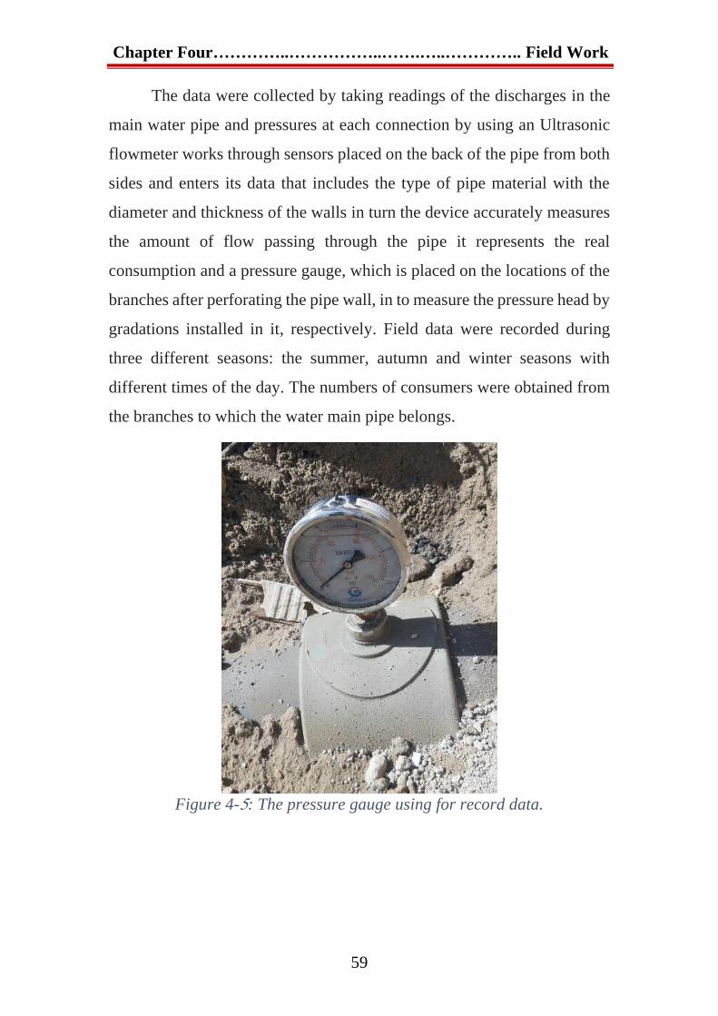
Chapter Four…………..……………..…….…..………….. Field Work
59
The data were collected by taking readings of the discharges in the
main water pipe and pressures at each connection by using an Ultrasonic
flowmeter works through sensors placed on the back of the pipe from both
sides and enters its data that includes the type of pipe material with the
diameter and thickness of the walls in turn the device accurately measures
the amount of flow passing through the pipe it represents the real
consumption and a pressure gauge, which is placed on the locations of the
branches after perforating the pipe wall, in to measure the pressure head by
gradations installed in it, respectively. Field data were recorded during
three different seasons: the summer, autumn and winter seasons with
different times of the day. The numbers of consumers were obtained from
the branches to which the water main pipe belongs.
Figure 4-5: The pressure gauge using for record data.

Chapter Four…………..……………..…….…..………….. Field Work
60
4.4.1. Recording data in the summer, specifically the month of August
Table 4-1: Recording data during morning operation.
location Elevation
(m)
Discharge
(m3/hr)
Pressure
(bar) Inhabitants
At pump station 30.8 942 1
Junction 1 25 212 0.5 5000
Junction 2 28.5 178 0.2 6000
Junction 3 27.5 122 0.1 1000
Junction 4 24.27 153 0.1 6000
Junction 5 25.67 127 0.05 5000
Junction 6 26.94 83 0.05 5000
Junction 7 24.37 36 0.05 3000
Junction 8 25 31 0.05 5000
Table 4-2: Recording data during afternoon operation.
location Elevation
(m)
Discharge
(m3/hr)
Pressure
(bar) Inhabitants
At pump station 30.8 931 1
Junction 1 25 197 0.5 5000
Junction 2 28.5 179 0.2 6000
Junction 3 27.5 108 0.1 1000
Junction 4 24.27 147 0.1 6000
Junction 5 25.67 122 0.05 5000
Junction 6 26.94 79 0.05 5000
Junction 7 24.37 58 0.05 3000
Junction 8 25 41 0.05 5000
Table 4-3: Recording data during evening operation.
location Elevation
(m)
Discharge
(m3/hr)
Pressure
(bar) Inhabitants
At pump station 30.8 940 1
Junction 1 25 202 0.5 5000
Junction 2 28.5 178 0.2 6000
Junction 3 27.5 113 0.1 1000
Junction 4 24.27 152 0.1 6000
Junction 5 25.67 127 0.05 5000
Junction 6 26.94 79 0.05 5000
Junction 7 24.37 53 0.05 3000
Junction 8 25 36 0.05 5000

Chapter Four…………..……………..…….…..………….. Field Work
61
4.4.2. Recording data in the autumn, specifically the month of October
Table 4-4: Recording data during morning operation.
location Elevation
(m)
Discharge
(m3/hr.)
Pressure
(bar) Inhabitants
At pump station 30.8 935 1
Junction 1 25 197 0.5 5000
Junction 2 28.5 181 0.2 6000
Junction 3 27.5 127 0.1 1000
Junction 4 24.27 146 0.1 6000
Junction 5 25.67 122 0.05 5000
Junction 6 26.94 82 0.05 5000
Junction 7 24.37 56 0.05 3000
Junction 8 25 24 0.05 5000
Table 4-4-5: Recording data during afternoon operation.
location Elevation
(m)
Discharge
(m3/hr.)
Pressure
(bar) Inhabitants
At pump station 30.8 947 1
Junction 1 25 195 0.5 5000
Junction 2 28.5 183 0.2 6000
Junction 3 27.5 113 0.1 1000
Junction 4 24.27 142 0.05 6000
Junction 5 25.67 118 0.05 5000
Junction 6 26.94 79 0.05 5000
Junction 7 24.37 78 0.05 3000
Junction 8 25 39 0.05 5000
Table 4-6: Recording data during evening operation.
location Elevation
(m)
Discharge
(m3/hr.)
Pressure
(bar) Inhabitants
At pump station 30.8 933 1
Junction 1 25 193 0.5 5000
Junction 2 28.5 178 0.2 6000
Junction 3 27.5 114 0.1 1000
Junction 4 24.27 143 0.05 6000
Junction 5 25.67 119 0.05 5000
Junction 6 26.94 88 0.05 5000
Junction 7 24.37 69 0.05 3000
Junction 8 25 29 0.05 5000

Chapter Four…………..……………..…….…..………….. Field Work
62
4.4.3. Recording data in the winter, specifically the month of December
Table 4-7: Recording data during morning operation.
location Elevation
(m)
Discharge
(m3/hr.)
Pressure
(bar) Inhabitants
At pump station 30.8 942 1
Junction 1 25 191 0.5 5000
Junction 2 28.5 181 0.1 6000
Junction 3 27.5 127 0.1 1000
Junction 4 24.27 141 0.1 6000
Junction 5 25.67 139 0.05 5000
Junction 6 26.94 84 0.05 5000
Junction 7 24.37 58 0.05 3000
Junction 8 25 21 0.05 5000
Table 4-8: Recording data during afternoon operation.
location Elevation
(m)
Discharge
(m3/hr.)
Pressure
(bar) Inhabitants
At pump station 30.8 935 1
Junction 1 25 181 0.5 5000
Junction 2 28.5 178 0.1 6000
Junction 3 27.5 117 0.1 1000
Junction 4 24.27 137 0.1 6000
Junction 5 25.67 135 0.05 5000
Junction 6 26.94 84 0.05 5000
Junction 7 24.37 72 0.05 3000
Junction 8 25 31 0.05 5000
Table 4-9: Recording data during evening operation.
location Elevation
(m)
Discharge
(m3/hr.)
Pressure
(bar) Inhabitants
At pump station 30.8 942 1
Junction 1 25 184 0.5 5000
Junction 2 28.5 178 0.1 6000
Junction 3 27.5 123 0.1 1000
Junction 4 24.27 139 0.1 6000
Junction 5 25.67 139 0.05 5000
wiping Junction 6 26.94 82 0.05 5000
Junction 7 24.37 59 0.05 3000
Junction 8 25 38 0.05 5000

Chapter Four…………..……………..…….…..………….. Field Work
63
Given the aforementioned data that the areas at the end of the line
do not fully receive a sufficient quantity of water. The field study was
conducted on the operation process and the amount of discharges coming
out of the junctions at the node sites was measured by an ultrasonic
flowmeter and at different times during the summer, autumn and winter
seasons with different times of the day. The data collection will be used for
the hydraulic analysis of the main water pipe using the WaterCAD
program. In the next chapter.
Figure 4-6: during record data.

Chapter Five
Results and
Discussion

Chapter Five …………..…………..…..…….… Results and Discussion
65
Chapter Five: Results and Discussion
This chapter describes the analysis and discussion of the recorded
field data and data generated by the WaterCAD simulation application for
the mainline pipe, then a comparison was made between the simulated
results and the recorded data. The analysis and discussion will be in two
stages: the first stage; is an analysis of the recorded field data alone while,
the second stage: is the analysis of data generated by the WaterCAD
simulation application with field recorded data.
The supply might come from pumps, storage tanks, or reservoirs, or
it could be defined as inflows or outflows at certain points in the network,
and the pressures or head losses thru the system are calculated using the
known flow rates (Izinyon & Anyata, 2009b). The operation performance
was observed under peak consumption and with an extended period
simulation of 24-hours. The performance was evaluated based on existing
hydraulic conditions.
5.1. Analysis of the recorded field data of Main water pipe
The path of the mainline pipe was determined, also branch pipes at
each junction to feed the neighboring areas, and the number of residents in
those areas was estimated based on the site surveys of the water branches
there belong to Karbala water directorate, as indicated in chapter four. In
this part of the analysis, it will be considered that the flow is steady.
The discharge quantities passing through each pipe that branched
from the mainline were measured by the ultrasonic flowmeter. It was
consumed in the areas that passed through the main pipeline branches.
These quantities are compared to the hypothetical consumption quantities
computed from the per capita consumption rate multiplied by the
population of those areas.

Chapter Five …………..…………..…..…….… Results and Discussion
66
5.1.1. Consumption type in a mainline pipe
The consumption data for every customer has been gathered to
assess the water loss in the distribution network. The amount of water used
may be estimated based on the rate of consumption of individuals.
According to the rules of the Ministry of Municipalities and Public Works'
General Directorate of Water, the estimated consumption rate of persons
for water fit for human use per capita is as follows:
1. A person living in the city is 450 liters per day.
2. A person living in the township is 360 liters per day.
3. A person living in villages and rural areas is 250 liters per day.
4. The percentage of lost in networks ranges 20%-45%
The study area in the present study is the township area, so the
consumption rate was determined based on a magnitude 360 liters per
capita per day, the percentage of losses was assumed as 35% of the
consumed quantity, so the total consumption rate with losses was 486 liters
per capita per day. The number of consumers who use each junction was
shown in Table 4-1 in Chapter four to calculate the estimated or
hypothetical discharge for each junction, as following:
𝑨𝒗𝒆𝒓𝒂𝒈𝒆 𝒅𝒐𝒎𝒆𝒔𝒕𝒊𝒄 𝒅𝒆𝒎𝒂𝒏𝒅 = 𝒄𝒐𝒏𝒔𝒖𝒎𝒑𝒕𝒊𝒐𝒏 𝒓𝒂𝒕𝒆 × 𝑷𝒐𝒑𝒖𝒍𝒂𝒕𝒊𝒐𝒏
After finding the amount of the approximate consumption at each
junction, the actual discharge measured by the ultrasonic flow meter is
compared with the estimated approximate discharge, using the same
equation in the study(Alshammari, 2000), and the percentage of scarcity
and loss in each junction is determined as follows:
𝐏𝐞𝐫𝐜𝐞𝐧𝐭 𝐨𝐟 𝒔𝒄𝒂𝒓𝒄𝒊𝒕𝒚 𝐨𝐫 𝐥𝐨𝐬𝐬𝐞𝐬 % =𝐐𝐀−𝐐𝐄
𝐐𝐄× 𝟏𝟎𝟎 % Equation 5-1
where:

Chapter Five …………..…………..…..…….… Results and Discussion
67
QA: Actual consumption discharge measured by the ultrasonic
flowmeter.
QE: Estimation consumption discharge.
The resulting magnitude from the previous equation is a percentage
of scarcity or losses, and the sign of percent magnitude indicates that this
percentage is scarcity or losses in the supplied quantities, as follows:
(+ve) The positive sign indicates that the resulting percentage is a loss in
the supplied quantities.
(-ve) The negative sign indicates that the resulting percentage is a scarcity
in the supplied quantities.
1. Junction-1
From Table 4-1, the number of servants in this Junction is 5000
persons and by multiplying this number by the daily consumption rate,
it can be obtained the estimated approximate consumption in this
junction using the following equation:
𝑨𝒗𝒆𝒓𝒂𝒈𝒆 𝒅𝒐𝒎𝒆𝒔𝒕𝒊𝒄 𝒅𝒆𝒎𝒂𝒏𝒅 = 𝒄𝒐𝒏𝒔𝒖𝒎𝒑𝒕𝒊𝒐𝒏 𝒓𝒂𝒕𝒆 × 𝑷𝒐𝒑𝒖𝒍𝒂𝒕𝒊𝒐𝒏
𝑨𝒗𝒆𝒓𝒂𝒈𝒆 𝒅𝒆𝒎𝒂𝒏𝒅 =𝟒𝟖𝟔𝑳
𝑪.𝒅× 𝟓𝟎𝟎𝟎𝑪 ×
𝟏𝒎𝟑
𝟏𝟎𝟎𝟎𝑳×
𝒅
𝟐𝟒𝒉𝒓= 𝟏𝟎𝟏. 𝟐𝟓 𝒎𝟑/𝒉𝒓
On this basis, the approximate consumption rate in this junction
is 101.25 𝑚3/ℎ𝑟. Using the ultrasonic flowmeter, the discharge
(realistic consumption) passing through this junction measured is 212
𝑚3/ℎ𝑟, so this junction contains a percentage of losses equal to:
𝑷𝒆𝒓𝒄𝒆𝒏𝒕 𝒐𝒇 𝒍𝒐𝒔𝒔𝒆𝒔 % =𝑸𝑨 − 𝑸𝑬
𝑸𝑬× 𝟏𝟎𝟎 %
𝑷𝒆𝒓𝒄𝒆𝒏𝒕 𝒐𝒇 𝒍𝒐𝒔𝒔𝒆𝒔 % =𝟐𝟏𝟐 − 𝟏𝟎𝟏. 𝟐𝟓
𝟏𝟎𝟏. 𝟐𝟓× 𝟏𝟎𝟎 % = 𝟏𝟎𝟗. 𝟒%
It is a very large percent since the daily consumption that is
supposed to contain 35% allowed losses. Meaning that the losses in the
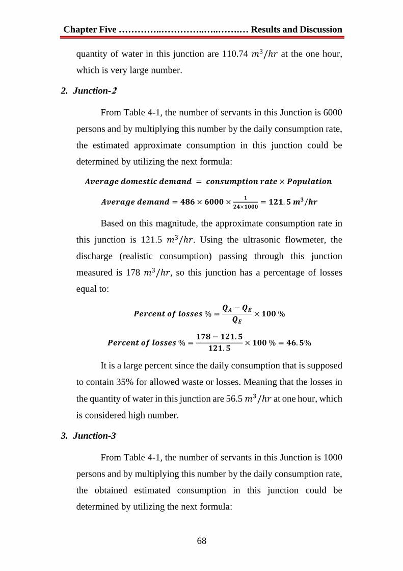
Chapter Five …………..…………..…..…….… Results and Discussion
68
quantity of water in this junction are 110.74 𝑚3/ℎ𝑟 at the one hour,
which is very large number.
2. Junction-2
From Table 4-1, the number of servants in this Junction is 6000
persons and by multiplying this number by the daily consumption rate,
the estimated approximate consumption in this junction could be
determined by utilizing the next formula:
𝑨𝒗𝒆𝒓𝒂𝒈𝒆 𝒅𝒐𝒎𝒆𝒔𝒕𝒊𝒄 𝒅𝒆𝒎𝒂𝒏𝒅 = 𝒄𝒐𝒏𝒔𝒖𝒎𝒑𝒕𝒊𝒐𝒏 𝒓𝒂𝒕𝒆 × 𝑷𝒐𝒑𝒖𝒍𝒂𝒕𝒊𝒐𝒏
𝑨𝒗𝒆𝒓𝒂𝒈𝒆 𝒅𝒆𝒎𝒂𝒏𝒅 = 𝟒𝟖𝟔 × 𝟔𝟎𝟎𝟎 ×𝟏
𝟐𝟒×𝟏𝟎𝟎𝟎= 𝟏𝟐𝟏. 𝟓 𝒎𝟑/𝒉𝒓
Based on this magnitude, the approximate consumption rate in
this junction is 121.5 𝑚3/ℎ𝑟. Using the ultrasonic flowmeter, the
discharge (realistic consumption) passing through this junction
measured is 178 𝑚3/ℎ𝑟, so this junction has a percentage of losses
equal to:
𝑷𝒆𝒓𝒄𝒆𝒏𝒕 𝒐𝒇 𝒍𝒐𝒔𝒔𝒆𝒔 % =𝑸𝑨 − 𝑸𝑬
𝑸𝑬× 𝟏𝟎𝟎 %
𝑷𝒆𝒓𝒄𝒆𝒏𝒕 𝒐𝒇 𝒍𝒐𝒔𝒔𝒆𝒔 % =𝟏𝟕𝟖 − 𝟏𝟐𝟏. 𝟓
𝟏𝟐𝟏. 𝟓× 𝟏𝟎𝟎 % = 𝟒𝟔. 𝟓%
It is a large percent since the daily consumption that is supposed
to contain 35% for allowed waste or losses. Meaning that the losses in
the quantity of water in this junction are 56.5 𝑚3/ℎ𝑟 at one hour, which
is considered high number.
3. Junction-3
From Table 4-1, the number of servants in this Junction is 1000
persons and by multiplying this number by the daily consumption rate,
the obtained estimated consumption in this junction could be
determined by utilizing the next formula:

Chapter Five …………..…………..…..…….… Results and Discussion
69
𝑨𝒗𝒆𝒓𝒂𝒈𝒆 𝒅𝒐𝒎𝒆𝒔𝒕𝒊𝒄 𝒅𝒆𝒎𝒂𝒏𝒅 = 𝒄𝒐𝒏𝒔𝒖𝒎𝒑𝒕𝒊𝒐𝒏 𝒓𝒂𝒕𝒆 × 𝑷𝒐𝒑𝒖𝒍𝒂𝒕𝒊𝒐𝒏
𝑨𝒗𝒆𝒓𝒂𝒈𝒆 𝒅𝒆𝒎𝒂𝒏𝒅 = 𝟒𝟖𝟔 × 𝟏𝟎𝟎𝟎 ×𝟏
𝟐𝟒×𝟏𝟎𝟎𝟎= 𝟐𝟎. 𝟐𝟓 𝒎𝟑/𝒉𝒓
On this basis, the approximate consumption rate in this junction
is 20.25 𝑚3/ℎ𝑟. Using the ultrasonic flowmeter, the discharge
(realistic consumption) passing through this junction measured is 122
𝑚3/ℎ𝑟, so this junction contains a percentage of losses equal to:
𝑷𝒆𝒓𝒄𝒆𝒏𝒕 𝒐𝒇 𝒍𝒐𝒔𝒔𝒆𝒔 % =𝑸𝑨 − 𝑸𝑬
𝑸𝑬× 𝟏𝟎𝟎 %
𝑷𝒆𝒓𝒄𝒆𝒏𝒕 𝒐𝒇 𝒍𝒐𝒔𝒔𝒆𝒔 % =𝟏𝟐𝟐 − 𝟐𝟎. 𝟐𝟓
𝟐𝟎. 𝟐𝟓× 𝟏𝟎𝟎 % = 𝟓𝟎𝟐. 𝟒𝟔%
It is a very large percent since the daily consumption assumes
on allowable 35% of allowed waste or losses. Meaning that the losses
in the quantity of water in this junction are 101.75 𝑚3/ℎ𝑟 at the one
hour, which is very large number.
4. Junction-4
From Table 4-1, the number of servants in this Junction is 6000
persons and by multiplying this number by the daily consumption rate,
it can get the estimated approximate consumption in this junction by
using the following equation:
𝑨𝒗𝒆𝒓𝒂𝒈𝒆 𝒅𝒐𝒎𝒆𝒔𝒕𝒊𝒄 𝒅𝒆𝒎𝒂𝒏𝒅 = 𝒄𝒐𝒏𝒔𝒖𝒎𝒑𝒕𝒊𝒐𝒏 𝒓𝒂𝒕𝒆 × 𝑷𝒐𝒑𝒖𝒍𝒂𝒕𝒊𝒐𝒏
𝑨𝒗𝒆𝒓𝒂𝒈𝒆 𝒅𝒆𝒎𝒂𝒏𝒅 = 𝟒𝟖𝟔 × 𝟔𝟎𝟎𝟎 ×𝟏
𝟐𝟒×𝟏𝟎𝟎𝟎= 𝟏𝟐𝟏. 𝟓 𝒎𝟑/𝒉𝒓
On this basis, the approximate consumption rate in this junction
is 121.5 𝑚3/ℎ𝑟. Using the ultrasonic flowmeter, the discharge
(realistic consumption) passing through this junction measured is 153
𝑚3/ℎ𝑟, so this junction contains a percentage of losses equal to:
𝑷𝒆𝒓𝒄𝒆𝒏𝒕 𝒐𝒇 𝒍𝒐𝒔𝒔𝒆𝒔 % =𝑸𝑨 − 𝑸𝑬
𝑸𝑬× 𝟏𝟎𝟎 %

Chapter Five …………..…………..…..…….… Results and Discussion
70
𝑷𝒆𝒓𝒄𝒆𝒏𝒕 𝒐𝒇 𝒍𝒐𝒔𝒔𝒆𝒔 % =𝟏𝟓𝟑 − 𝟏𝟐𝟏. 𝟓
𝟏𝟐𝟏. 𝟓× 𝟏𝟎𝟎 % = 𝟐𝟓. 𝟗%
It is a very large percent since the daily consumption that is
supposed to contain 35% allowed losses. Meaning that the losses in the
quantity of water in this junction are 31.5 𝑚3/ℎ𝑟 at the one hour,
which is acceptable because it is less than 35%.
5. Junction-5
From Table 4-1, the number of servants in this Junction is 5000
persons and by multiplying this number by the daily consumption rate,
the estimated approximated consumption in this junction is calculated
as follows:
𝑨𝒗𝒆𝒓𝒂𝒈𝒆 𝒅𝒐𝒎𝒆𝒔𝒕𝒊𝒄 𝒅𝒆𝒎𝒂𝒏𝒅 = 𝒄𝒐𝒏𝒔𝒖𝒎𝒑𝒕𝒊𝒐𝒏 𝒓𝒂𝒕𝒆 × 𝑷𝒐𝒑𝒖𝒍𝒂𝒕𝒊𝒐𝒏
𝑨𝒗𝒆𝒓𝒂𝒈𝒆 𝒅𝒆𝒎𝒂𝒏𝒅 = 𝟒𝟖𝟔 × 𝟓𝟎𝟎𝟎 ×𝟏
𝟐𝟒×𝟏𝟎𝟎𝟎= 𝟏𝟎𝟏. 𝟐𝟓 𝒎𝟑/𝒉𝒓
Based on analysis of such value, the approximate consumption
rate in this junction is 101.25 𝑚3/ℎ𝑟. Using the ultrasonic flowmeter,
the discharge (realistic consumption) passing through this junction
measured is 127 𝑚3/ℎ𝑟, so this junction contains a percentage of
losses equal to:
𝑷𝒆𝒓𝒄𝒆𝒏𝒕 𝒐𝒇 𝒍𝒐𝒔𝒔𝒆𝒔 % =𝑸𝑨 − 𝑸𝑬
𝑸𝑬× 𝟏𝟎𝟎 %
𝑷𝒆𝒓𝒄𝒆𝒏𝒕 𝒐𝒇 𝒍𝒐𝒔𝒔𝒆𝒔 % =𝟏𝟐𝟕 − 𝟏𝟎𝟏. 𝟐𝟓
𝟏𝟎𝟏. 𝟐𝟓× 𝟏𝟎𝟎 % = 𝟐𝟓. 𝟒𝟑%
It is considered a high value because it is more than 30% the
daily consumption that is supposed to contain 35% allowed losses.
Meaning that the losses in the quantity of water in this junction are
25.75 𝑚3/ℎ𝑟 at the one hour ,which is large number.

Chapter Five …………..…………..…..…….… Results and Discussion
71
Most of the water losses that go at the first five junctions are to
water the orchards and what is related to agricultural lands, and the
lack of monitoring of users.
6. Junction-6
From Table 4-1, the number of servants in this Junction is 5000
persons and by multiplying this number by the daily consumption rate,
it can get the estimated approximate consumption in this junction by
applying the following equation:
𝑨𝒗𝒆𝒓𝒂𝒈𝒆 𝒅𝒐𝒎𝒆𝒔𝒕𝒊𝒄 𝒅𝒆𝒎𝒂𝒏𝒅 = 𝒄𝒐𝒏𝒔𝒖𝒎𝒑𝒕𝒊𝒐𝒏 𝒓𝒂𝒕𝒆 × 𝑷𝒐𝒑𝒖𝒍𝒂𝒕𝒊𝒐𝒏
𝑨𝒗𝒆𝒓𝒂𝒈𝒆 𝒅𝒆𝒎𝒂𝒏𝒅 = 𝟒𝟖𝟔 × 𝟓𝟎𝟎𝟎 ×𝟏
𝟐𝟒 × 𝟏𝟎𝟎𝟎= 𝟏𝟎𝟏. 𝟐𝟓 𝒎𝟑/𝒉𝒓
On this basis, the approximate consumption rate in this junction
is 101.25 𝑚3/ℎ𝑟. Using the ultrasonic device, the discharge (realistic
consumption) passing through this junction measured is 83 𝑚3/ℎ𝑟, so
this junction contains a percentage of scarcity equal to:
𝑷𝒆𝒓𝒄𝒆𝒏𝒕 𝒐𝒇 𝒔𝒄𝒂𝒓𝒄𝒊𝒕𝒚 % =𝑸𝑨 − 𝑸𝑬
𝑸𝑬× 𝟏𝟎𝟎 %
𝑷𝒆𝒓𝒄𝒆𝒏𝒕 𝒐𝒇 𝒔𝒄𝒂𝒓𝒄𝒊𝒕𝒚 % =𝟖𝟑 − 𝟏𝟎𝟏. 𝟐𝟓
𝟏𝟎𝟏. 𝟐𝟓× 𝟏𝟎𝟎 % = −𝟏𝟖%
It is a reasonable percentage, as it is assumed that the daily
consumption contains 35% of the permissible losses, and this
percentage indicates that the percentage of loss in this junction is less
than 35%, and thus Meaning that the scarcity in the quantity of water
in this junction is -18 𝑚3/ℎ𝑟 at the one hour.
7. Junction-7
From Table 4-1, the number of servants in this Junction is 3000
persons and by multiplying this number by the daily consumption rate,

Chapter Five …………..…………..…..…….… Results and Discussion
72
it is possible to get the estimated approximate consumption in this
junction using the following equation:
𝑨𝒗𝒆𝒓𝒂𝒈𝒆 𝒅𝒐𝒎𝒆𝒔𝒕𝒊𝒄 𝒅𝒆𝒎𝒂𝒏𝒅 = 𝒄𝒐𝒏𝒔𝒖𝒎𝒑𝒕𝒊𝒐𝒏 𝒓𝒂𝒕𝒆 × 𝑷𝒐𝒑𝒖𝒍𝒂𝒕𝒊𝒐𝒏
𝑨𝒗𝒆𝒓𝒂𝒈𝒆 𝒅𝒆𝒎𝒂𝒏𝒅 = 𝟒𝟖𝟔 × 𝟑𝟎𝟎𝟎 ×𝟏
𝟐𝟒 × 𝟏𝟎𝟎𝟎= 𝟔𝟎. 𝟕𝟓 𝒎𝟑/𝒉𝒓
This magnitude of demand indicates that, the approximate
consumption rate in this junction is 60.75 𝑚3/ℎ𝑟. Using the ultrasonic
flowmeter, the discharge (realistic consumption) passing through this
junction measured is 36 𝑚3/ℎ𝑟, so this junction suffers from a clear
and very large scarcity, the percentage of which reaches:
𝑷𝒆𝒓𝒄𝒆𝒏𝒕 𝒐𝒇 𝒔𝒄𝒂𝒓𝒄𝒊𝒕𝒚 % =𝑸𝑨 − 𝑸𝑬
𝑸𝑬× 𝟏𝟎𝟎 %
𝑷𝒆𝒓𝒄𝒆𝒏𝒕 𝒐𝒇 𝒔𝒄𝒂𝒓𝒄𝒊𝒕𝒚 % =𝟑𝟔 − 𝟔𝟎. 𝟕𝟓
𝟔𝟎. 𝟕𝟓× 𝟏𝟎𝟎 % = −𝟒𝟎. 𝟕𝟒%
It is a large percentage, as this junction suffers from a scarcity
in the quantities of water supplied compared to the required demand,
and thus meaning that the scarcity in the quantity of water in this
junction are -24.75 𝑚3/ℎ𝑟 at the one hour, which is considered large.
8. Junction-8
From Table 4-1, the number of servants in this Junction is 5000
persons and by multiplying this number by the daily consumption rate,
the approximated consumption in this junction using the following
equation:
𝑨𝒗𝒆𝒓𝒂𝒈𝒆 𝒅𝒐𝒎𝒆𝒔𝒕𝒊𝒄 𝒅𝒆𝒎𝒂𝒏𝒅 = 𝒄𝒐𝒏𝒔𝒖𝒎𝒑𝒕𝒊𝒐𝒏 𝒓𝒂𝒕𝒆 × 𝑷𝒐𝒑𝒖𝒍𝒂𝒕𝒊𝒐𝒏
𝑨𝒗𝒆𝒓𝒂𝒈𝒆 𝒅𝒆𝒎𝒂𝒏𝒅 = 𝟒𝟖𝟔 × 𝟓𝟎𝟎𝟎 ×𝟏
𝟐𝟒 × 𝟏𝟎𝟎𝟎= 𝟏𝟎𝟏. 𝟐𝟓 𝒎𝟑/𝒉𝒓
On this basis, the approximate consumption rate in this junction
is 101.25 𝑚3/ℎ𝑟. Using the ultrasonic flowmeter, the discharge
(realistic consumption) passing through this junction measured is 31

Chapter Five …………..…………..…..…….… Results and Discussion
73
𝑚3/ℎ𝑟. Therefore, this junction suffers from a clear and large scarcity,
the percentage the scarcity of this junction can be calculated as follows:
𝑷𝒆𝒓𝒄𝒆𝒏𝒕 𝒐𝒇 𝒔𝒄𝒂𝒓𝒄𝒊𝒕𝒚 % =𝑸𝑨 − 𝑸𝑬
𝑸𝑬× 𝟏𝟎𝟎 %
𝑷𝒆𝒓𝒄𝒆𝒏𝒕 𝒐𝒇 𝒔𝒄𝒂𝒓𝒄𝒊𝒕𝒚 % =𝟑𝟏 − 𝟏𝟎𝟏. 𝟐𝟓
𝟏𝟎𝟏. 𝟐𝟓× 𝟏𝟎𝟎 % = −𝟔𝟗. 𝟒%
It is a large percentage, as this junction suffers from a scarcity
in the quantities of water supplied compared to the actual required
demand, and this indicated that the scarcity in the quantity of water in
this junction is -70.25 𝑚3/ℎ𝑟 at the one hour, which is considered large
magnitude.
According to the analysis of aforementioned calculations, it was
found that there is a clear and a large loss of water at the beginning of the
main water pipe started from junction-1 to junction-5 and then is
accompanied by a clear and large scarcity at the end of the main water pipe.
The total of the loss and scarcity quantities in the mainline was equal to
326.24 𝑚3/ℎ𝑟 and -113.25 𝑚3/ℎ𝑟, at the one hour respectively.
The quantities of loss are very large compared to the quantities of
scarcity, so if the quantities of losses were controlled, the quantities
supplied to the mainline would be enough to fill the presence of scarcities
without the need to increase the quantities supplied. It is noteworthy that
controlling the quantities of loss is very difficult because of the difficulty
of detecting excesses on the network and the absence of water meters in
houses to determine the percentage of losses.
5.2. Building of the hydraulic model using WaterCAD
Firstly, it was created a hydraulic model for the distribution network
using the WaterCAD simulation program. It was created by drawing a
network layout, then identifying all the hydraulic properties of the network
parts such as junction elevation, demand, pipes length, pipes diameter,

Chapter Five …………..…………..…..…….… Results and Discussion
74
pipes type, pump characteristics, and hourly rate consumption pattern as
shown in the following figures.
Figure 5-1 shows the interface of the WaterCAD program, in
addition to the main line diagram showing the locations of the junctions
and the resulting offshoots of the main water pipe. After completing the
network diagram, the data for each pipe in the network is entered, including
diameters, lengths and the type of material it is made of to determine
Hazen-William’s modulus existing already in the program according to the
type of pipe through the interface of the (flex-table) window for pipes, as
shown in Figure 5-2
Figure 5-1: The layout of distribution network in WaterCAD.

Chapter Five …………..…………..…..…….… Results and Discussion
75
Figure 5-2: Flex table (pipe table) for identified the characteristics.
Figure 5-3 shows the interface of the (Flex-Table) window it’s in the
program for entering the special information, which includes the elevation
and demand for each junction. In which Figure 5-4 shows the interface for
entering the design characteristics of the pump in terms of discharge, head
pressure, and efficiency where the red line indicates the value of discharge,
while the blue line indicates the value of the pressure head, Program it
automatically draws the pump diagram according to the characteristics
mentioned previously.

Chapter Five …………..…………..…..…….… Results and Discussion
76
Figure 5-3: Flex table (junction table) for identified the characteristics.
Figure 5-5 shows the interface of the special window for drawing
the variance diagram of daily consumption within 24 hours (peak hourly
factor) and determining the peak periods according to the entered values,
where the horizontal axis is the time and the vertical axis is the factor that
multiplies the rate of consumption per hour. It shows that the peak is
concentrated during the morning period at 8 am and at 7 pm.

Chapter Five …………..…………..…..…….… Results and Discussion
77
Figure 5-4: Identify pump characteristics in pump Definitions windows.
Figure 5-5: Identify daily consumption within 24 hours (peak hourly
factor).

Chapter Five …………..…………..…..…….… Results and Discussion
78
Secondly, it was applied a hydraulic model exists to analyze the
fieldwork recorded data compared with simulation results obtained.
Through the fieldwork recording data and the results of the analysis, it was
found that the flowrate quantities of water pumped from the pumping
station are not proportional to the diameter of the main water pipe, and do
not meet the minimum flow velocity in the pipes which is minimum of
0.6m/s as shown in figure 5-2. In addition to the difficulty of reaching water
the end of the line to feed the required areas. Moreover, water cannot reach
the ends in adequate. As the diameter is large and the quantities of water
pumped into it are few, in addition to the losing operations that were at the
beginning, where the design capacity of the line was 1200 𝑚3/ℎ.
5.3. Proposal Scenarios for the hydraulic Model in WaterCAD
The main water pipe will be simulated using WaterCAD for more
than one scenario. It has been proposed to analyze and identify the problem
of scarcity according to unsteady flow, and control it to achieve the best
solution, as follows:
5.3.1. First scenario
In this scenario, the main water pipe is taken as it exists without any
modification of the characteristics of the line in terms of pipe diameters,
elevations, and quantities of water pumped into the mainline, taking into
consideration that the amount of demand for each junction is equal to the
approximate consumption rate as shown in Table 5-1.

Chapter Five …………..…………..…..…….… Results and Discussion
79
Table 5-1: Elevation and Demand for branch junctions.
Junction Label Elevation
(m)
Demand
(m³/h)
Real
demand(m3/hr.)
Percentage
of losses or
scarcity
Junction 1 J-11 25.00 101.25 212 109.4
Junction 2 J-22 28.50 121.50 178 46.5
Junction 3 J-33 27.50 20.25 122 504.46
Junction 4 J-44 24.27 121.5 153 25.9
Junction 5 J-55 25.67 101.25 127 25.43
Junction 6 J-66 26.94 101.25 83 -18
Junction 7 J-77 24.37 60.75 36 -40.74
Junction 8 J-88 25.00 101.25 31 -69.4
Figure 5-6: Calculation summary for simulation at first scenario.
When simulation of the hydraulic model is based on the demand rate
for each junction that is the same as the approximate consumption rate, it

Chapter Five …………..…………..…..…….… Results and Discussion
80
was found that there is a scarcity in the quantities of water supplied during
the morning period for two hours from 8 am to 10 am, and during the
evening period for a four hours from 5 pm to 9 pm, as shown in Figure 5-
6. This scenario simulates the current main water pipe if the losing
quantities are controlled in the first five junctions of the mainline to fill the
scarcity in the last three junctions. As mentioned previously, it is difficult
to control the quantities of loss for the same reasons that were mentioned
previously. This scenario is considered ineffective in solving the problem
of scarcity that exists.
Figure 5-7: Head Pressure at junction-p at pump station during 24 hr.
After the scarcity periods are mentioned in the supplied quantities
and their duration, the head pressures at each junction must be checked
during the 24-hour operating period, because one of the important
requirements in networks is the pressure at each junction. By checking the

Chapter Five …………..…………..…..…….… Results and Discussion
81
profile energy chart during 24 operating hours, it was found that there was
a decrease in pressure during the morning period for two hours from 8 am
to 10 am, besides a decrease in pressure during the evening period for 6
hours from 3 pm to 9 pm, as shown in the figure 5-7 which shows the
energy diagram at the pumping station and for all the junctions from the
main water pipe and based on the demand inputs that were entered into the
program. This indicates a decrease in quantities for 6 hours/day and a
decrease in pressure for 8 hours/day, it is concluding that the drop of
pressure in the program is due to insufficient quantities of provided from
the source. This indicates that this scenario, even if the amount of loss is
controlled, remains ineffective.
5.3.2. Second scenario
In this scenario, the mainline is taken as it exists without any
modification of the characteristics of the line in terms of pipe diameters,
elevations, and quantities of water pumped into the mainline, but adds a
booster station after junction 5 as shown in and figure 5-8, taking into
consideration that the amount of demand for each junction is equal to the
approximate consumption rate as shown in Table 5-1.

Chapter Five …………..…………..…..…….… Results and Discussion
82
Figure 5-8: layout of main water pipe with booster station.
A simulation has been made for the proposed scenario, which is to
add an intermediate pumping station to the same quantity produced at
present, which is, of course, as mentioned, less than the design capacity
under which the pipeline is established. It was found that there was a
problem with operating the mainline with an intermediate lifting station,
which caused an increase in the number of shortage hours during one day
because the quantity received from the pumping station was small and
insufficient, which caused an increase in the hours of scarcity. The scarcity
in the network is in the quantities supplied from Al-Sajelah and Al-Fayada
stations. The work of the booster station is based only on raising the
vertical pressure of each junction after the pump.

Chapter Five …………..…………..…..…….… Results and Discussion
83
Figure 5-9: The pump definition for Booster Station.
Figure 5-10 shows a summary of the simulation calculations for the
proposed scenario, and the hours marked in yellow mean that there is a
problem with the quantities supplied or the pressures during this period.
Figure 5-11 shows the amount of head pressure with time during 24 hours
at some points, such as a point inside the Al-Sijlah and Al-Feyadh station
symbolized by J-P, a point at the fourth junction before the proposed
booster station symbolized by J-4, and a point at the sixth junction after the
proposed booster station symbolized by J-6. This figure shows that from 7
am to 9 pm, the problems begin with pressure and are negative because of
the intermediate pumping station begins by withdrawing additional
quantities of water to treat the junctions after pumping station, and this is
at the expense of the previous ones and leads to a decrease in its quantities,
especially if it is not treated from the source, and this need cannot be filled
with the current supplied quantities, which causes a decrease in pressure
and a scarcity of quantities. Into the quantities supplied must be increased
to solve this problem.

Chapter Five …………..…………..…..…….… Results and Discussion
84
Figure 5-10: Calculation summary for simulation at second scenario.
Figure 5-11: Head Pressure at some junctions during 24 hr.

Chapter Five …………..…………..…..…….… Results and Discussion
85
5.3.3. Third scenario
In this scenario, the main water pipe is taken as it is without any
modification to the characteristics of the line in terms of pipe diameters
and heights, and the production capacity of Al-Sijlah Al-Feyadh station is
added to increase the quantity of supplied water pumped into the main
water pipe to 1800 m3/hr. Taking into consideration that the quantity of
demand for each junction is equal to the approximate rate of consumption
based on the assumption that the field-measured discharge using the
Ultrasonic flowmeter is the Peak hour demand, as shown in Table 5-1.
Figure 5-12: The pump definition for 3rd scenario.
From the summary of the simulation calculations for this scenario
shown in Figure 5-13, it is shown that the supplied quantities are sufficient
to meet the demand needs at each junction, and that the highest discharge
of the required consumption is 1312 m3/hr. at a peak time of 19:00. The
sufficient quantity of water supplied to the mainline does not mean that the
line does not face problems in its operation, so it is necessary to check the
pressures at each junction. Figure 5-15 shows the hydraulic line of the
mainline in the peak period at 19:00, that the pressures for all junctions are
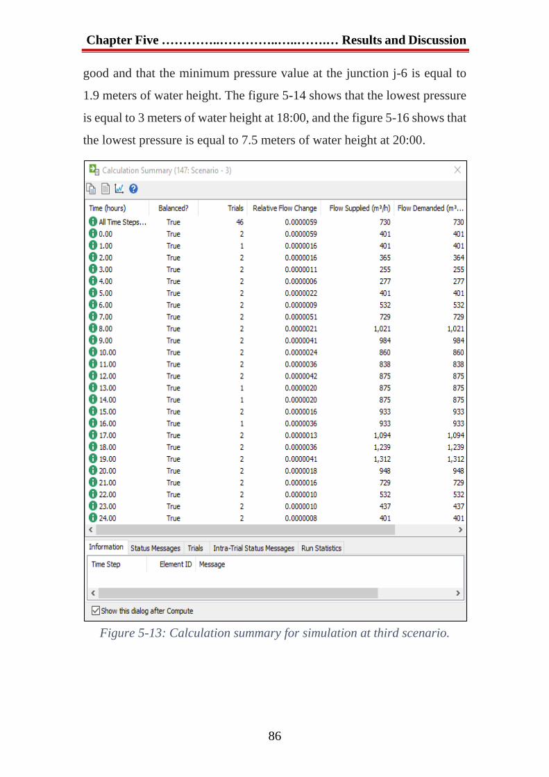
Chapter Five …………..…………..…..…….… Results and Discussion
86
good and that the minimum pressure value at the junction j-6 is equal to
1.9 meters of water height. The figure 5-14 shows that the lowest pressure
is equal to 3 meters of water height at 18:00, and the figure 5-16 shows that
the lowest pressure is equal to 7.5 meters of water height at 20:00.
Figure 5-13: Calculation summary for simulation at third scenario.

Chapter Five …………..…………..…..…….… Results and Discussion
87
Figure 5-14: Hydraulic Grade line profile for 3rd scenario at 18:00.
Figure 5-15: Hydraulic Grade line profile for 3rd scenario at peak time
19:00.
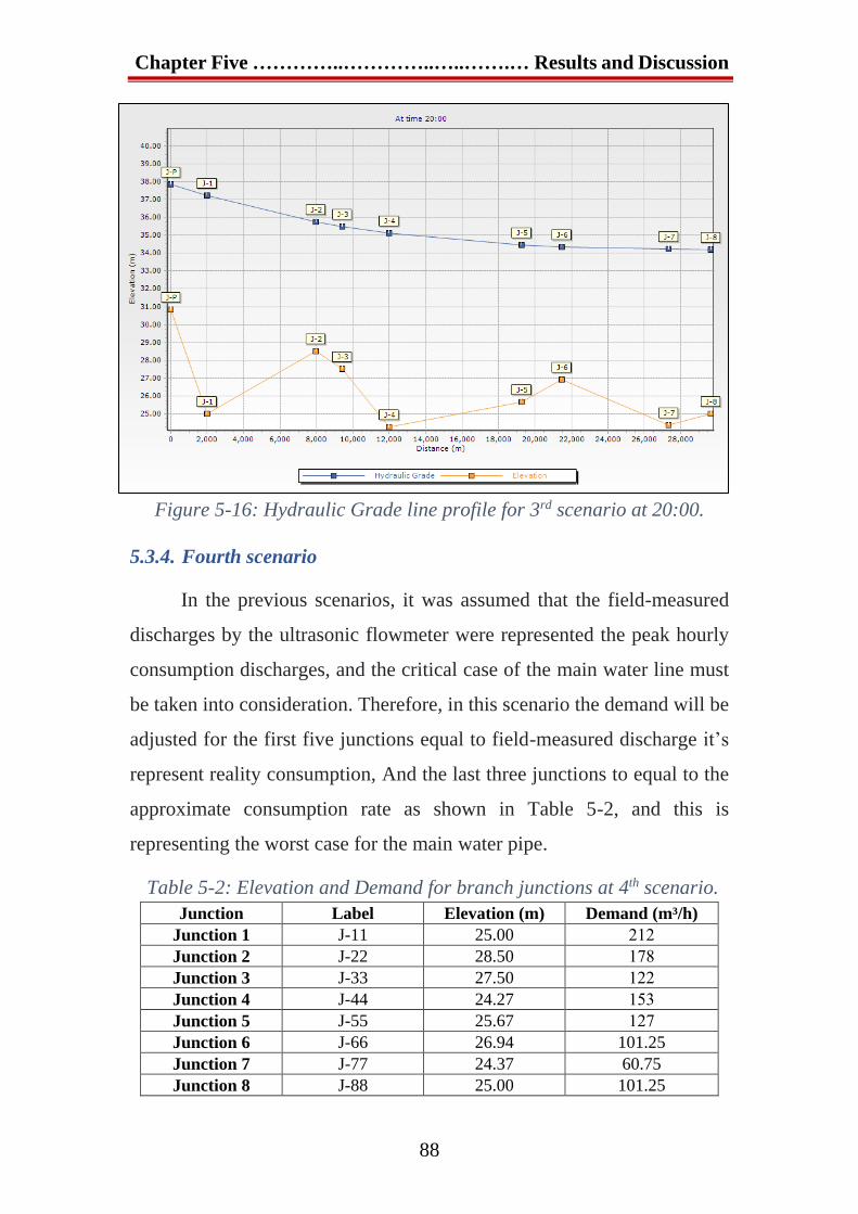
Chapter Five …………..…………..…..…….… Results and Discussion
88
Figure 5-16: Hydraulic Grade line profile for 3rd scenario at 20:00.
5.3.4. Fourth scenario
In the previous scenarios, it was assumed that the field-measured
discharges by the ultrasonic flowmeter were represented the peak hourly
consumption discharges, and the critical case of the main water line must
be taken into consideration. Therefore, in this scenario the demand will be
adjusted for the first five junctions equal to field-measured discharge it’s
represent reality consumption, And the last three junctions to equal to the
approximate consumption rate as shown in Table 5-2, and this is
representing the worst case for the main water pipe.
Table 5-2: Elevation and Demand for branch junctions at 4th scenario.
Junction Label Elevation (m) Demand (m³/h)
Junction 1 J-11 25.00 212
Junction 2 J-22 28.50 178
Junction 3 J-33 27.50 122
Junction 4 J-44 24.27 153
Junction 5 J-55 25.67 127
Junction 6 J-66 26.94 101.25
Junction 7 J-77 24.37 60.75
Junction 8 J-88 25.00 101.25

Chapter Five …………..…………..…..…….… Results and Discussion
89
Figure 5-17: Calculation summary for simulation at fourth scenario.
Figure 5-17 shows a summary of the simulation calculations for the
proposed scenario, and the hours marked in yellow mean that there is a
problem with the quantities supplied or the pressures during this period.
The same figure 5-17 shows that there is a problem with the quantities
supplied to the main water pipe at the peak time at 19:00, and the shortage
in the supplied quantities is approximately 99 m3/hr. This indicates a
shortage for one hour through the analysis based on the supplied quantities
only. In addition to the above, it is necessary to know the amount of
pressure during the peak period to ensure the actual performance of the

Chapter Five …………..…………..…..…….… Results and Discussion
90
main water pipe during operation. Through the hydraulic line of the peak
period shown from Figure 5-18 to Figure 5-20, it is found that 2 hours are
scarce from 6 p.m. to 8 p.m.
Figure 5-18: Hydraulic Grade line profile for 4th scenario at 18:00.
Figure 5-19: Hydraulic Grade line profile for 4th scenario at 19:00.
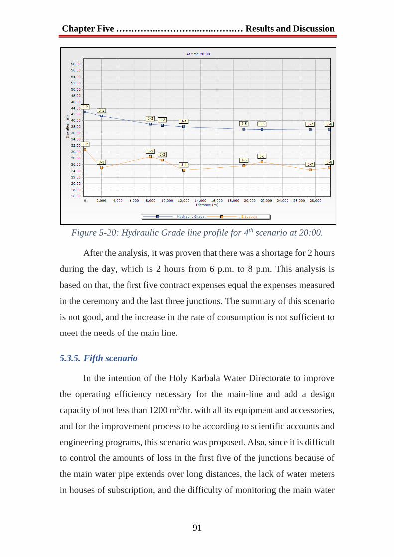
Chapter Five …………..…………..…..…….… Results and Discussion
91
Figure 5-20: Hydraulic Grade line profile for 4th scenario at 20:00.
After the analysis, it was proven that there was a shortage for 2 hours
during the day, which is 2 hours from 6 p.m. to 8 p.m. This analysis is
based on that, the first five contract expenses equal the expenses measured
in the ceremony and the last three junctions. The summary of this scenario
is not good, and the increase in the rate of consumption is not sufficient to
meet the needs of the main line.
5.3.5. Fifth scenario
In the intention of the Holy Karbala Water Directorate to improve
the operating efficiency necessary for the main-line and add a design
capacity of not less than 1200 m3/hr. with all its equipment and accessories,
and for the improvement process to be according to scientific accounts and
engineering programs, this scenario was proposed. Also, since it is difficult
to control the amounts of loss in the first five of the junctions because of
the main water pipe extends over long distances, the lack of water meters
in houses of subscription, and the difficulty of monitoring the main water

Chapter Five …………..…………..…..…….… Results and Discussion
92
pipe 24 hours a day to prevent illegal connections. Therefore, in this
scenario, it will be considered that the quantity of demand in the first five
junctions is equal to the actual consumption rate of the loss that was
measured on-site using the Ultrasonic flowmeter, and the last three
junctions are equal to the approximate consumption rate as shown in table
5-2. This scenario represents the worst case for the main water pipe in
terms of consumption, to solve the problem of shortages on the mainline,
in addition to increasing the production capacity of Al-Sejlah and Al-
Feyadh station to 2,400 m3/hr. with the excess product is pumped into the
center of the holy province of Karbala to benefit from it.
Figure 5-21: The pump definition for the 5th scenario.
From the summary of the simulation calculations for this scenario
shown in figure 5-22, it is shown that the supplied quantities are sufficient
to meet the demand needs at each junction and that the highest discharge
of the required consumption is 1899 m3/hr. at a peak time of 19:00. The
sufficient quantity of water supplied to the main water pipe does not mean
that the line does not face problems in its operation, so it is necessary to
check the pressures at each junction. Figure 5-23 shows the hydraulic line
of the main water pipe in the peak period at 19:00, that the pressures for all

Chapter Five …………..…………..…..…….… Results and Discussion
93
junctions are good and that the minimum pressure value at the junction j-6
is equal to 6 meters of water height. Thus, the parameters of the main water
pipe were evaluated, which are from the requirements to improve its
operational efficiency, namely discharge, pressure and velocity, and the
results were good because of the increase in the production capacity of the
pumping station, which in turn affected the improvement of the work of
the main water pipe.
Figure 5-22: Calculation summary for simulation at fifth scenario.

Chapter Five …………..…………..…..…….… Results and Discussion
94
Figure 5-23: Hydraulic Grade line profile for 5th scenario at peak time.
5.3.6. Sixth Scenario
In this scenario, a temporary situation is imposed, which is the
rotation of stopping the water supply during a certain period between the
junctions, for example, for the first and second junctions, which have the
highest consumption, but it is not possible, especially in the summer,
because the nature of the area is rural and needs water continuously as
mentioned previously, but under the current conditions Until the expansion
of the design capacity, as mentioned in the fifth scenario, And in which the
reading of the ultrasonic flowmeter in the connections represents the actual
consumption of users, it will be taken for the junctions from the third to the
fifth, And with respect to sixth to eighth junction the approximate
consumption will be based on the imposed share of the water circuits and
according to Table 5-2.

Chapter Five …………..…………..…..…….… Results and Discussion
95
Figure 5-24: Calculation Summary for Simulation at sixth Scenario
Figure 5-24 shows a summary of the simulation calculations for the
proposed scenario, and the hours marked in yellow mean that there is a
problem with the quantities supplied or the pressures during this period.
there is a problem with the quantities supplied to the main water pipe at the
peak time at 17:00,18:00,19:00 and the shortage in the supplied quantities
is approximately 122,222 and 89 m3/hr. This indicates a shortage for three
hours through the analysis based on the supplied quantities only. In
addition to the above, it is necessary to know the amount of pressure during
the peak period to ensure the actual performance of the main water pipe
during operation. Through the hydraulic line of the peak period shown
from Figure 5-25 to Figure 5-27, it is found that the pressure in the fourth
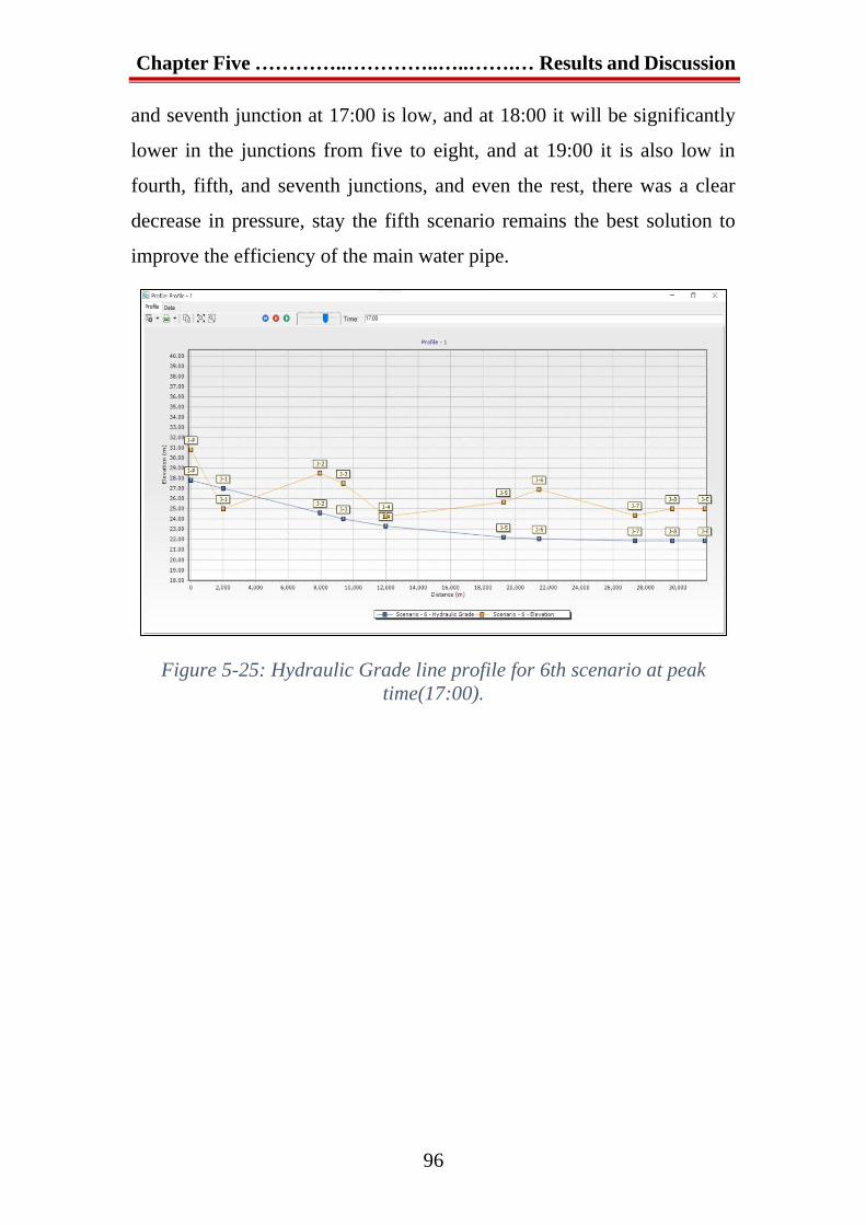
Chapter Five …………..…………..…..…….… Results and Discussion
96
and seventh junction at 17:00 is low, and at 18:00 it will be significantly
lower in the junctions from five to eight, and at 19:00 it is also low in
fourth, fifth, and seventh junctions, and even the rest, there was a clear
decrease in pressure, stay the fifth scenario remains the best solution to
improve the efficiency of the main water pipe.
Figure 5-25: Hydraulic Grade line profile for 6th scenario at peak
time(17:00).

Chapter Five …………..…………..…..…….… Results and Discussion
97
Figure 5-26: Hydraulic Grade line profile for 6th scenario at peak
time(18:00).
Figure 5-27: Hydraulic Grade line profile for 6th scenario at peak
time(19:00).
5.3.7. The summary of scenarios
Finally, after completing the simulation for all the proposed
scenarios, table 5-3 summarizes the advantages and disadvantages of each
scenario.

Chapter Five …………..…………..…..…….… Results and Discussion
98
Table 5-3: summarizes the advantages and disadvantages of scenarios.
Scenario
no. Advantages Disadvantages
1 Do not need an increase in
supply quantities.
Assume ideal customers.
Having a scarcity of 6 hours at peak
times.
2 Increased head pressure in
the last 3 junctions.
Decrease head pressures at the
junctions before the pump.
The continuation of the scarcity
from 7 am to 9 pm.
3 Good performance.
Do not find a scarcity.
Assume ideal customers.
Need an increase in supply
quantities of about 600 m3/hr.
4 Considering the critical
situation of demand for
junctions.
Having a scarcity of 2 hours at peak
times.
Need an increase in supply
quantities of about 600 m3/hr.
Cannot consider any developments
on the main water pipe.
5
Good performance.
Considering the critical
situation of demand for
junctions.
Considering the development
in mainline.
Need an increase in supply
quantities of about 1200 m3/hr. to
improve the efficiency of the main
water pipe.
6 Do not need an increase in
supply quantities.
The difficulty of applying it due to
the nature of the agriculture area
and its continuously need water.

Chapter Six
Conclusion and
Recommendation

Chapter Six …………..………..….. Conclusion and Recommendation
100
Chapter Six: Conclusion and Recommendation
6.1. Conclusions
According to the results of manual analysis on the basis of steady
flow and simulation for the six scenarios for a period of twenty-four hours
on the basis unsteady flow according to the peak hour of the distribution
system of the main water pipe, which operates in the system of branching
tree, the following conclusions were obtained:
1. It was found that the field measurements of the amount of flow coming
out of the pumping station indicated that the amount of discharge is less
than the amount of originally designed discharge of the main water pipe.
The pumped discharge was not exceeded 950 𝑚3/ℎ𝑟 in all seasons and
situations. While the design capacity is 1200 𝑚3/ℎ𝑟 and this is because
of the low performance of the pumps.
2. In the first part of analysis, it was found that there was a clear and large
loss of water at the beginning of the main water pipe, starting from
junction-1 to junction-5, and then there was a clear and large scarcity at
the end of the main water pipe. The total of the loss and scarcity
quantities in the was equal to 326.24 𝑚3/ℎ𝑟 and -113.25 𝑚3/ℎ𝑟,
respectively.
3. The quantities of losses are very large compared to the quantities of
scarcity, so if the quantities of loss were controlled, the quantities
supplied to the main water pipe would be enough to fill the present
scarcities without the need to increase the quantities supplied.
4. In the second part of analysis, based on the simulation of results, it was
found that the water needed to overcome water scarcity was 2400m3/hr.
There is a loss of water in high quantities, especially at the beginning
of the main water pipe, and more specifically in the first five junctions,

Chapter Six …………..………..….. Conclusion and Recommendation
101
and this loss is because of the use of drinking water for irrigation of
gardens and orchards and a large number of illegal connections.
5. Controlling loss rates is almost impossible to achieved because the main
water pipe extends for long distances of agricultural areas that are
difficult to monitor and identify abuses, and because there are no water
meters installed in every house.
6. The presence of a high scarcity in quantities and pressures of the last
three junctions at the end of the main water pipe is because of the high
rates of loss at the beginning of the main water pipe and the insufficient
quantities supplied to the line and the inefficiency of the pumps used.
7. The pressure inside the pumping station did not exceed 1 bar in all
cases, and this is because of the low efficiency of the pumps operating
on the main water pipe. In addition, damage to some parts of the pump
and the effect on the efficiency as well as the field reading pressure at
the junctions are weak, as indicated by the field readings.
8. It was noticed the pumping station level is higher than all the pipe levels
and the junctions branching from it. This is useful when increasing the
capacity of the main water pipe reduces the efforts exerted by the pumps
and raises the value of pressures.
9. It was found that there is no diesel generator to operate pumps when
the national electricity is shut down, Although the project is fed by
emergency lines.
10. The results of the first four scenarios and sixth from some main water
pipe junctions receiving water at low pressure during peak hour
consumption, and in some cases, there is a risk of receiving no water
because the main water pipe pressure is below the acceptable minimum
requirement.
11. The fifth scenario provides sufficient water with proper quantity
pressure of all junctions during peak hour consumption, also there are

Chapter Six …………..………..….. Conclusion and Recommendation
102
quantities of excess water, especially outside peak consumption times.
Excess water can be stored.
6.2. Recommendations
To improve the status of the main water pipe and reduce its deficit
rates to the lowest possible period and percentage, the following
recommendations were developed based on the results of the previous
research and analysis:
6.2.1. Recommendations for operating staff of the main water pipe
1. Controlling losses and replacing pumps in the project, whether they are
working continuously or in standby mode, because they are old and
worn out and do not meet the required flow, as the mainline was
designed based on giving 1200 m3/hour in each case, as mentioned
previously.
2. The change in setting valves in the branch pipes of junctions to provide
the needed amounts of water to the consumers affects the values of
pressure in the mainline, and the closing valves increase the pressure in
the main water pipe.
3. Manage and reduce the water sharing for inhabitants of some junctions,
as shown in the previous simulation, by reducing the consumption rate
to an estimation rate or putting a valve to properly control the amount
of water withdrawal and using a pressure valve to raise pressure more
than the calculated value at junctions that need it. This is especially
important in the summer, with the peak of high consumption of water
withdrawals.
4. It is possible to use the pressure reducer valve and adjust it acceptably
and place it in the junctions close to the pump station, as they are rural
areas and do not need a high increase in pressure. This reduction will

Chapter Six …………..………..….. Conclusion and Recommendation
103
contribute to raising the pressure in the areas that are far from the pump
station to achieve the required flow.
5. Water level monitoring entering the storage tank, affects the water level
in the steel pressure tank through which the water is drawn by pumps
to be pumped into the main water pipe. In addition to the difference in
the efficiency of the pumps being used.
6. The necessity to provide a generator for electric current in anticipation
of emergency situation and power cuts to the pumping station for long
periods, especially in the summer season, leads to the complete
emptying of the main water pipe and the difficulty of filling it again,
since the distance is long and consumption is high in these weather
conditions.
7. Working on the maintenance and cleaning of the intake structure at the
bottom of the river, as they are directly responsible for the quantities
required, and to avoid direct extinguishing of the main water pipe and
its discharge, especially in peak seasons.

Chapter Six …………..………..….. Conclusion and Recommendation
104
6.2.2. Recommendations for future studies
1. Through the analysis scenarios and considering the current and near-
future needs and the importance of the main water pipe to the city of
Karbala, it requires the addition of design capacity to improve the
efficiency of the conveyancer line’s operation, as shown by the results
of the evaluation for the first fiver scenarios with the addition of all the
required accessories, steel tanks, filters, and all that the work requires.
2. During the sixth scenario which is the best, there are quantities of water
above of the needs of the current 8 junctions on the main water pipe.
Also, it can connect to new junctions to feed some nearby areas. In
addition, it is possible to establish a project to collect and pump the
surplus quantities into the center of the holy city of Karbala to fill in
part of the scarcity in the city center.

105
References

References
106
Reference
Abdelbaki, C., Benchaib, M. M., Benziada, S., Mahmoudi, H., & Goosen, M. (2017).
Management of a water distribution network by coupling GIS and hydraulic
modeling: a case study of Chetouane in Algeria. Applied Water Science, 7(3),
1561–1567. https://doi.org/10.1007/s13201-016-0416-1
Agunwamba, J. C., Ekwule, O. R., & Nnaji, C. C. (2018). Performance evaluation of a
municipal water distribution system using waterCAD and Epanet. Journal of
Water Sanitation and Hygiene for Development, 8(3), 459–467.
https://doi.org/10.2166/washdev.2018.262
Al-Barqawi, H., & Zayed, T. (2008). Infrastructure Management: Integrated
AHP/ANN Model to Evaluate Municipal Water Mains’ Performance. Journal of
Infrastructure Systems, 14(4), 305–318. https://doi.org/10.1061/(asce)1076-
0342(2008)14:4(305)
Al-Zahrani, M. A., & Syed, J. L. (2005). etEvaluation of Municipal Water Distribution
System Reliability Using Minimum Cut-set Mhod. Journal of King Saud
University - Engineering Sciences, 18(1), 67–81. https://doi.org/10.1016/S1018-
3639(18)30822-5
Alshammari, M. H. (2000). Analytical Study for Baghdad Water Maintrunks.
University of Technology.
Ang, W. K., & Jowitt, P. W. (2006). Solution for Water Distribution Systems under
Pressure-Deficient Conditions. Journal of Water Resources Planning and
Management, 132(3), 175–182. https://doi.org/10.1061/(asce)0733-
9496(2006)132:3(175)
Archetti, F. (2015). Network Analysis For Resilience Evaluation In Water Distribution
Networks. Environmental Engineering and Management Journal, 14(4), 1261–
1270.
Atiquzzaman, D. (2004). Water distribution network modeling: hydroinformatics
approach.
Balacco, G., Carbonara, A., Gioia, A., Iacobellis, V., & Piccinni, A. F. (2017).
Evaluation of peak water demand factors in puglia (Southern Italy). Water

References
107
(Switzerland), 9(2), 1–14. https://doi.org/10.3390/w9020096
Bhadbhade, M. (2004). Performance Evaluation of a Drinking Water Distribution
System Using Hydraulic Simulation Software for the City of Oilton, Oklahoma.
In Aspectos Generales De La Planificación Tributaria En Venezuela (Vol. 2004,
Issue 75). Oklahoma State University.
Bhave, P. R. (1991). Analysis of Flow in Water Distribution Networks.
Bolouri-Yazdeli, Y., Bozorg Haddad, O., Fallah-Mehdipour, E., & Mariño, M. A.
(2014). Evaluation of real-time operation rules in reservoir systems operation.
Water Resources Management, 28(3), 715–729. https://doi.org/10.1007/s11269-
013-0510-1
Choi, T., & Koo, J. (2015). A water supply risk assessment model for water distribution
network. Desalination and Water Treatment, 54(4–5), 1410–1420.
https://doi.org/10.1080/19443994.2014.892440
Christodoulou, S., Aslani, P., & Deligianni, A. (2006). Integrated GIS-based
management of water distribution networks. International Conference on
Computing and Decision Making in Civil and Building Engineering, 858–865.
Datwyler, T. T. (2012). Hydraulic Modeling : Pipe Network Analysis.
Dave, B. H., Rajpara, G., Patel, A., & Kalubarme, M. H. (2015). Analysis of
Continuous Water Distribution System in Gandhinagar City Using EPANET
Software : A Case Study of Sector-8. National Conference on ‘ Transportation
and Water Resource Engineering, i, 1–6.
Geem, Z. W. (2006). Optimal cost design of water distribution networks using harmony
search. Engineering Optimization, 38(3), 259–277.
https://doi.org/10.1080/03052150500467430
Gomes, R., Marques, A. S., & Sousa, J. (2011). Estimation of the benefits yielded by
pressure management in water distribution systems. Urban Water Journal, 8(2),
65–77. https://doi.org/10.1080/1573062X.2010.542820
Gottipati, P. V. K. S. V., & Nanduri, U. V. (2014). Equity in water supply in intermittent
water distribution networks. Water and Environment Journal, 28(4), 509–515.
https://doi.org/10.1111/wej.12065

References
108
Izinyon, O. C., & Anyata, B. U. (2009a). Use of hydraulic network model for evaluating
fire flow capacity of a water distribution network. Advanced Materials Research,
62–64, 797–801. https://doi.org/10.4028/www.scientific.net/amr.62-64.797
Izinyon, O. C., & Anyata, B. U. (2009b). Water distribution network modelling of a
small community using watercad simulator. Global Journal of Engineering
Research, 10(1–2), 35–47.
Jalal, M. M. (2008). « Performance Measurement of Water Distribution Systems ( WDS
). A critical and constructive appraisal of the state-of-the-art ». University of
Toronto, 157.
Jamieson, D. G., Shamir, U., Martinez, F., & Franchini, M. (2007). Conceptual design
of a generic, real-time, near-optimal control system for water-distribution
networks. Journal of Hydroinformatics, 9(1), 3–14.
https://doi.org/10.2166/hydro.2006.013
Kanakoudis, V., & Tsitsifli, S. (2010). Results of an urban water distribution network
performance evaluation attempt in Greece. Urban Water Journal, 7(5), 267–285.
https://doi.org/10.1080/1573062X.2010.509436
Keedwell, E., & Khu, S. T. (2005). A hybrid genetic algorithm for the design of water
distribution networks. Engineering Applications of Artificial Intelligence, 18(4),
461–472. https://doi.org/10.1016/j.engappai.2004.10.001
Larock, B. E., Jeppson, R. W., & Watters, G. Z. (1999). Hydraulics of Pipeline Systems.
In Hydraulics of Pipeline Systems. https://doi.org/10.1201/9780367802431
López-Ibáñez, M., Prasad, T. D., & Paechter, B. (2008). Ant Colony Optimization for
Optimal Control of Pumps in Water Distribution Networks. Journal of Water
Resources Planning and Management, 134(4), 337–346.
https://doi.org/10.1061/(asce)0733-9496(2008)134:4(337)
Mazumder, R. K., Salman, A. M., Li, Y., & Yu, X. (2018). Performance Evaluation of
Water Distribution Systems and Asset Management. Journal of Infrastructure
Systems, 24(3), 03118001. https://doi.org/10.1061/(asce)is.1943-555x.0000426
Medeiros, E., Da, F., Gallo, S., & Imada, R. (2015). Case Study: WaterCAD modelling
tool to reduce water loss in the city of Pederneiras-São Paulo State, Brazil. July.
Mirzabeygi, M., Naji, M., Yousefi, N., Shams, M., Biglari, H., & Mahvi, A. H. (2016).

References
109
Evaluation of corrosion and scaling tendency indices in water distribution system:
a case study of Torbat Heydariye, Iran. Desalination and Water Treatment, 57(54),
25918–25926. https://doi.org/10.1080/19443994.2016.1162206
Mohammed, S. S. (2017). Optimal Design of Sewer Networks Using Genetic Algorithm.
University of Kerbala.
Muranho, J., Ferreira, A., Sousa, J., Gomes, A., & Sá Marques, A. (2014). Technical
performance evaluation of water distribution networks based on EPANET.
Procedia Engineering, 70, 1201–1210.
https://doi.org/10.1016/j.proeng.2014.02.133
Mutikanga, H. E., Sharma, S. K., & Vairavamoorthy, K. (2013). Methods and Tools for
Managing Losses in Water Distribution Systems. Journal of Water Resources
Planning and Management, 139(2), 166–174.
https://doi.org/10.1061/(asce)wr.1943-5452.0000245
Ostfeld, A., Salomons, E., Skolicki, Z., Wadda, M. M., Houck, M. H., Arciszewski, T.,
Perelman, L., Ostfeld, A., St, S., Water, D. H. I., Alle, A., Ph, D., Asce, M. H. H.
F., Asce, T. A. M., Kroll, D., King, K., Gueli, R., Grayman, W., Murray, R., and
Savic, D., Environmental, W., … Salomons, E. (2013). Building Water
Distribution Network Hydraulic Model by Using WaterGEMS. Journal of Water
Resources Planning and Management, 136(5), 1–10.
Rai, R. K., & Lingayat, P. (2019). Analysis of Water Distribution Network Using
EPANET. SSRN Electronic Journal, 1–7. https://doi.org/10.2139/ssrn.3375289
Rajani, B., & Kleiner, Y. (2001). Comprehensive review of structural deterioration of
water mains: Physically based models. Urban Water, 3(3), 151–164.
https://doi.org/10.1016/S1462-0758(01)00032-2
Robert, E. O. (2019). Evaluation of Municipal Water Distribution Network Using
Watercard and Watergems. 5(2), 147–156.
Rossman. (2000). EPANET 2 Users Manuel. Water supply and water resources division
national risk management research laboratory.
Selvakumar, A., Clark, R. M., & Sivaganesan, M. (2002). Costs for Water Supply
Distribution System Rehabilitation. Journal of Water Resources Planning and
Management, 128(4), 303–306. https://doi.org/10.1061/(asce)0733-

References
110
9496(2002)128:4(303)
Seyoum, A. G., & Tanyimboh, T. T. (2017). Integration of Hydraulic and Water Quality
Modelling in Distribution Networks: EPANET-PMX. Water Resources
Management, 31(14), 4485–4503. https://doi.org/10.1007/s11269-017-1760-0
Shuang, Q., Liu, Y., Tang, Y., Liu, J., & Shuang, K. (2017). System reliability
evaluation in water distribution networks with the impact of valves experiencing
cascading failures. Water (Switzerland), 9(6). https://doi.org/10.3390/w9060413
Sileshi, Y. (2011). ADDIS ABABA UNIVERSITY SCHOOL OF GRADUATE STUDIES
ADDIS ABABA INSTITUTE OF TECHNOLOGY ( AAiT ) Water Supply Coverage
and Water Loss in Distribution System with Modeling ( The Case Study of Addis
Ababa ) A Thesis Submitted to the School of Graduate Studies.
Steel, E. W. (1979). Water Supply and Sewerage (Fifth).
Suribabu, C. R. (2010). Differential evolution algorithm for optimal design of water
distribution networks. Journal of Hydroinformatics, 12(1), 66–82.
https://doi.org/10.2166/hydro.2010.014
Swamee, P. K., & Sharma, A. K. (2008). Design of Water Supply Pipe Networks. In
Design of Water Supply Pipe Networks. https://doi.org/10.1002/9780470225059
Tabesh, M., Asadiyami Yekta, A. H., & Burrows, R. (2009). An integrated model to
evaluate losses in water distribution systems. Water Resources Management,
23(3), 477–492. https://doi.org/10.1007/s11269-008-9284-2
Tricarico, C., Morley, M. S., Gargano, R., Kapelan, Z., De Marinis, G., & Savić, D. A.
(2014). The influence of the existing network layout on water distribution system
redesign analysis. Journal of Hydroinformatics, 16(6), 1375–1389.
https://doi.org/10.2166/hydro.2014.017
Vasan, A., & Simonovic, S. P. (2010). Optimization of Water Distribution Network
Design Using Differential Evolution. Journal of Water Resources Planning and
Management, 136(2), 279–287. https://doi.org/10.1061/(asce)0733-
9496(2010)136:2(279)
Vicente, D. J., Garrote, L., Sánchez, R., & Santillán, D. (2016). Pressure Management
in Water Distribution Systems: Current Status, Proposals, and Future Trends.
Journal of Water Resources Planning and Management, 142(2), 04015061.

References
111
https://doi.org/10.1061/(asce)wr.1943-5452.0000589
Yazdani, A., & Jeffrey, P. (2011). Complex network analysis of water distribution
systems. Chaos: An Interdisciplinary Journal of Nonlinear Science 21, 21(1).
https://doi.org/10.1063/1.3540339
Yunarni Widiarti, W., Wahyuni, S., Utami Agung Wiyono, R., Hidayah, E., Halik, G.,
& Sisinggih, D. (2020). Evaluation of pipe network distribution system using
EPANET 2.0 (a case study of the city of Jember). IOP Conference Series: Earth
and Environmental Science, 437(1), 0–9. https://doi.org/10.1088/1755-
1315/437/1/012043

الخالصة
أ
الخالصة
ئيسية في ستسلط الدراسة الحالية الضوء على تقييم كفاءة أحد أنابيب المياه الر
دًا فهي تعتبر من أهم المحافظات المقدسة في العراق وتشهد أعدا كربالء،محافظة
نابيب أأجريت هذه الدراسة لتقييم كفاءة ذلك،كبيرة من الحجاج كل عام. عالوة على
لتقاطعات االمياه الرئيسية الحالية لتحسين كفاءتها. تم أخذ قراءة ميدانية في مواقع
التي كانت و المختلفة،سي في المواسم السنوية أنبوب الماء الرئي المتفرعة منو المختلفة
ي. في الصيف والخريف والشتاء وساعات مختلفة باستخدام مقياس التدفق فوق الصوت
بيانات التي يتم تحليل أنبوب الماء الرئيسي في جزأين. يتعامل الجزء األول مع تحليل ال
رنامج بوتحليله في ويتم محاكاة الجزء الثاني الثابت،تم جمعها مع افتراض التدفق
WaterCAD وهو افتراض التدفق غير المستقر. ساعة،مع تباين االستهالك لكل
بيرة كوجد أن هناك خسائر اليدوي،بناًء على نتائج الجزء األول من التحليل
5لتقاطع اإلى 1وواضحة للمياه في بداية أنبوب المياه الرئيسي الذي بدأ من التقاطع
يات اضحة وكبيرة في نهاية أنبوب المياه الرئيسي. مجموع الكميصاحبها ندرة و ثم
- / ساعة و 3م 326.24المفقودة والندرة في أنبوب المياه الرئيسي كان يساوي
الندرة،ات كبيرة جدًا مقارنة بكمي مفقودةكميات الال/ ساعة على التوالي. 3م 113.25
ياه الرئيسي فإن الكميات الموردة ألنبوب الم ،ةدمفقوالكميات اللذلك إذا تم التحكم في
لتدفق استكون كافية لسد الندرة دون الحاجة إلى زيادة الكميات الموردة بناًء على
مر المستمر دون أي توسعات مستقبلية للوصالت. يشار إلى أن ضبط كميات الفاقد أ
المياه صعب للغاية بسبب صعوبة كشف التجاوزات على الشبكة وعدم وجود عدادات
في المنازل لتحديد نسبة الفاقد.
WaterCADتمت المحاكاة باستخدام برنامج التحليل،في الجزء الثاني من
والتحكم فيها المستقر،لستة سيناريوهات لتحليل وتحديد مشكلة الندرة وفق التدفق غير
للوصول إلى الحل األفضل. بناًء على محاكاة النتائج وجد أن كمية المياه الالزمة للتغلب
/ ساعة. وال يمكن تجاهل عدم وجود خسائر في 3م 2400على ندرة المياه كانت

الخالصة
ب
وبشكل أكثر تحديدًا في الرئيسي،خاصة في بداية أنبوب المياه كبيرة،المياه بكميات
ـ التقاطعات متر مكعب 326.24الخمسة األولى التي كانت تفقد كميات من المياه تقدر ب
وهذه الخسائر ناتجة عن استخدام مياه الشرب اليدوية،ساعة. بناء على الحسابات /
لري الحدائق والبساتين وعدد كبير من التوصيالت غير القانونية. وهذا باإلضافة إلى
التقاطعات حسب احتياجات اهم في زيادة عدد تسيسي سالسعة الجديدة ألنبوب المياه الرئ
كربالء. اءمديرية م

وزارة التعليم العالي والبحث العلمي
جامعة كربالء
كلية الهندسة
قسم الهندسة المدنية
تأثريات بعض العوامل على كفاءة تشغيل وحتليل تقييمباستخدام برنامج كربالء دينةمانبوب املياه الرئيسي يف
WaterCAD
الى مقدمة رسالة
كربالء جامعة /الهندسة كلية في المدنية الهندسة قسم
الهندسة علوم في الماجستير شهادة نيل متطلبات من كجزء
التحتية البنى هندسة – المدنية
قبل من
حسين علي حسين عبد علي
(2005هندسة مدنية )بكالوريوس
اشراف
أ.د جبار حمود البيضاني
موسى حبيب الشمري أ.د
ـه 1443 م 2021