REPUBLIC OF NAMIBIA - UNFCCC
127
REPUBLIC OF NAMIBIA NATIONAL GHG INVENTORY REPORT NIR3 1994 - 2014 October 2018 PART 1
-
Upload
khangminh22 -
Category
Documents
-
view
5 -
download
0
Transcript of REPUBLIC OF NAMIBIA - UNFCCC
REPUBLIC OF NAMIBIA
NATIONAL GHG INVENTORY REPORT NIR3
1994 - 2014
October 2018
PART 1
REPUBLIC OF NAMIBIA
NATIONAL GHG INVENTORY REPORT NIR3
1994 - 2014
October 2018
PART 1
ii
Copyright 2018 by Government of Namibia
MET, Private bag 13306, Windhoek, Namibia
Phone: +264612842701
All rights reserved
No part of this publication may be reproduced or transmitted in any form or by any means, without the
written permission of the copyright holder.
iii
Hon. Pohamba Shifeta Minister of Environment and Tourism
Foreword
As the minister of the Ministry of Environment and Tourism, it is an
honour and privilege for me to present Namibia’s stand alone
National GHG Inventory (NIR) for the period 1994 to 2014 in
fulfilment of its obligations as a Non-Annex I (NAI) Party to the
United Nations Framework Convention on Climate Change
(UNFCCC) in accordance with the enhanced reporting requirements
adopted at the 16th and 17th Conference of the Parties (COP).
Namibia ratified the UNFCCC in 1995 and thus became obligated to
prepare and submit national communications. Namibia is also a
signatory Party to the Paris Agreement (PA) since 2016. So far
Namibia has prepared and submitted the Initial National
Communication (INC) in 2002, the Second National Communication
(SNC) in 2011, the first BUR in 2014 (BUR 1), the Third National
Communication (TNC) in 2015 and the Second Biennial Update
Report (BUR 2) in 2016. Furthermore, Namibia prepared and
submitted its Intended Nationally Determined Contributions (INDC)
in 2015.
Namibia is currently busy preparing its Fourth National Communication (NC4) which will be submitted in
2019. Namibia became the first Non-Annex I Party to prepare and submit its first Biennial Update Report
at COP 20 and followed by submitting BUR 2 in 2016 making it one of the compliant countries in terms
of reporting obligations. BUR 3 provides an update on Namibia’s Greenhouse Gas (GHG) inventory,
mitigation actions and their effects, including the associated domestic Monitoring, Reporting and
Verification (MRV), and needs and support received, and institutional arrangements. BUR 3 will be
submitted with a stand alone National GHG Inventory (NIR) making it the third NIR Namibia has
submitted to the UNFCCC.
At the national level, Namibia has made numerous strides to further engage itself to play its role in
fighting climate change as outlined in the INDC. In 2014, the Cabinet of the Republic of Namibia
approved the National Climate Change Strategy and Action Plan (NCCSAP). The NCCSAP, which is
currently under its mid-term review, aims at facilitating the realisation of the National Climate Change
Policy (NCCP), which was passed in 2011. The strategy adopted in the document is cross-sectoral and
will be implemented up to the year 2020 and it covers the thematic areas mitigation, adaptation and
related cross cutting issues.
___________________________________
Hon. Pohamba Shifeta
Minister of Environment and Tourism
iv
Acknowledgements
The Ministry of Environment and Tourism, on behalf of the Government of the Republic of Namibia, was
entrusted with the responsibility for computing the National Inventory of Greenhouse Gases, within the
framework of the preparation of the BUR3 to the UNFCCC, for the Republic to meet its obligations as a
signatory Party to the Convention. This Ministry acknowledges the valuable financial support received
from the Global Environment Facility through its implementing agency, the UNDP country office.
Namibia is grateful to all international institutions, namely IPCC, the United Nations Framework
Convention on Climate Change (UNFCCC) secretariat and the Global Support Programme of the UN
Environment and UNDP for providing very useful handbooks, guidelines and the QA exercise for the
preparation of the Inventory and the GSP for reviewing the draft National Inventory Report and making
useful comments for improving the final document towards enhancing the TCCCA standard.
Namibia also wishes to extend its appreciation for the contribution of the representatives of the
institutions and private sector organizations, which collaborated in this work, as well as CLIMAGRIC LTD,
that offered consultancy services for capacity building of the inventory team, the computation of the
GHG Inventory and the preparation of this National Inventory Report.
Name Institution Sector
Mr. Petrus Muteyauli Ministry of Environment and Tourism National Focal Point
Mr. Reagan Chunga Ministry of Environment and Tourism Project Coordinator - NCs/BURs
Mr. Rasack Nayamuth Climagric Resource persons
Ms. Susan Tise Ministry of Mines and Energy
Energy
Mr. Edison Hiwanaame NAMPOWER
Mr. Abednego Ekandjo Ministry of Mines and Energy
Mr. Abraham Hangula Namibia Energy Institute
Mr. Natangwe Nekuiyu
Ministry of Works and Transport Mr. Naville Geiriseb
Ms. Charlene Binga
Mr. Frans Nekuma Ministry of Industralization, Trade & SME Development IPPU
Ms. Amalia Nangolo
Mr. Festus Oscar
Mr. Konzmann Tobias Ohorongo Cement
Mr. Paulus Shikongo
Ministry of Agriculture, Water and Forestry
AFOLU
Ms. Sarafia Ashipala
Mr. Edward Muhoko
Mr. Josephat Katuahupira
Mr. Tony Holbling MEATCO
Mr. Heinrich Lesch Namibia Dairies
Ms. Fransina Angula
Namibia Statistics Agency Data Providers Ms. Saara Niitenge
Mr. Elijah Saushini
Mr. Olavi Makutsi City of Windhoek
Waste Mr. Stellio Tsauseb City of Windhoek
Mr. Clive Lawrence Swakopmund Municipality
v
Table of contents
Foreword ...................................................................................................................................................... iii
Acknowledgements ...................................................................................................................................... iv
Table of contents ........................................................................................................................................... v
List of tables ................................................................................................................................................. ix
List of figures ............................................................................................................................................... xii
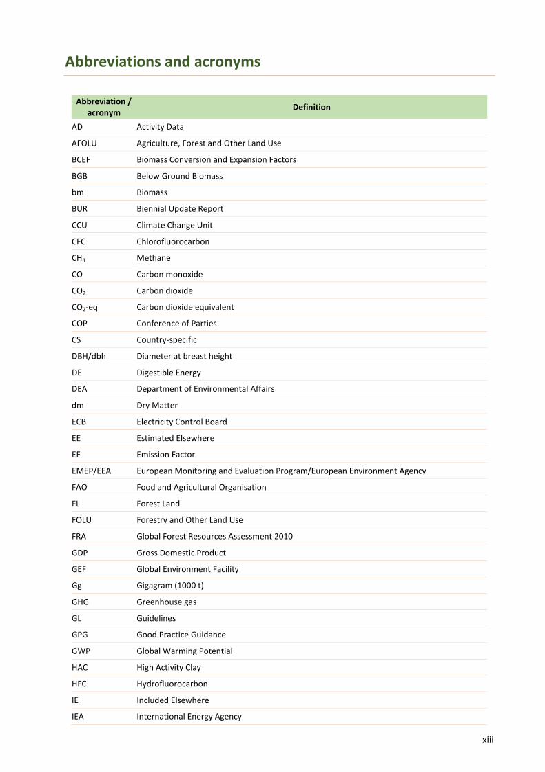
Abbreviations and acronyms ...................................................................................................................... xiii
Executive summary .................................................................................................................................... xvi
ES 1. Introduction ................................................................................................................................ xvi
ES 2. Coverage (period and scope) ..................................................................................................... xvi
ES 3. Institutional arrangements and GHG inventory system ............................................................ xvi
ES 4. Methods .................................................................................................................................... xvii
ES 5. Activity data .............................................................................................................................. xviii
ES 6. Emission factors ....................................................................................................................... xviii
ES 7. Recalculations ........................................................................................................................... xviii
ES 8. Inventory estimates .................................................................................................................. xviii
ES 9. QA/QC....................................................................................................................................... xxiii
ES 10. Completeness ....................................................................................................................... xxiv
ES 11. Uncertainty analysis ............................................................................................................. xxiv
ES 12. Key Category Analysis ............................................................................................................ xxv
ES 13. Archiving ................................................................................................................................ xxv
ES 14. Constraints, gaps and needs................................................................................................. xxvi
ES 15. National inventory improvement plan (NIIP) ....................................................................... xxvi
1. Introduction ...............................................................................................................................................1
1.1. National circumstances ......................................................................................................................1
1.2. Commitments under the Convention ................................................................................................1
2. The inventory process ...............................................................................................................................3
2.1. Overview of GHG inventories .............................................................................................................3
2.2. Institutional arrangements and inventory preparation .....................................................................4
2.3. Key Category Analysis .........................................................................................................................6
2.4. Methodological issues ........................................................................................................................8
2.5. Quality Assurance and Quality Control (QA/QC) ................................................................................9
2.6. Uncertainty assessment .................................................................................................................. 10
2.7. Assessment of completeness .......................................................................................................... 11
2.8. Recalculations .................................................................................................................................. 13
2.9. Time series consistency ................................................................................................................... 14

vi
2.10. Gaps, constraints and needs ......................................................................................................... 14
2.11. National inventory improvement plan (NIIP) ................................................................................ 15
3. Trends in greenhouse gas emissions ...................................................................................................... 17
3.1. Overview.......................................................................................................................................... 17
3.2. The period 1994 to 2014 ................................................................................................................. 17
3.3. Trend of emissions by source category ........................................................................................... 18
3.4. Trend in emissions of direct GHGs .................................................................................................. 19
3.4.1. Carbon dioxide (CO₂) ................................................................................................................ 20
3.4.2. Methane (CH₄) .......................................................................................................................... 21
3.4.3. Nitrous Oxide (N₂O) .................................................................................................................. 22
3.5. Trends for indirect GHGS and SO₂ ................................................................................................... 23
3.5.1. NOₓ ........................................................................................................................................... 23
3.5.2. CO ............................................................................................................................................. 24
3.5.3. NMVOCs ................................................................................................................................... 25
3.5.4. SO₂ ............................................................................................................................................ 25
4. Energy ..................................................................................................................................................... 27
4.1. Description of Energy sector ........................................................................................................... 27
4.1.1. Fuel Combustion Activities (1.A) .............................................................................................. 27
4.2. Methods .......................................................................................................................................... 28
4.3. Activity Data .................................................................................................................................... 29
4.4. Emission factors............................................................................................................................... 30
4.5. Emission estimates .......................................................................................................................... 30
4.5.1. Reference approach ................................................................................................................. 30
4.5.2. Sectoral approach ..................................................................................................................... 32
4.5.3. Evolution of emissions by gas (Gg) in the Energy Sector (1994 - 2014) ................................... 35
4.5.4. Emissions by gas by category for the period 1994 to 2014 ..................................................... 38
4.5.5. Memo Items ............................................................................................................................. 50
4.5.6. Information items ..................................................................................................................... 52
5. Industrial Processes and Product Use (IPPU) ......................................................................................... 53
5.1. Description of IPPU sector ............................................................................................................... 53
5.2. Methods .......................................................................................................................................... 54
5.3. Activity Data .................................................................................................................................... 54
5.3.1. Cement Production (2.A.1) ....................................................................................................... 54
5.3.2. Lime Production (2.A.2) ............................................................................................................ 54
5.3.3. Zinc Production (2.C.6) ............................................................................................................. 55
5.3.4. Lubricant Use (2.D.1) ................................................................................................................ 55
vii
5.3.5. Paraffin Wax Use (2.D.2) .......................................................................................................... 55
5.3.6. Wood Preservation (2.D.3.a) .................................................................................................... 55
5.3.7. Paint application (2.D.3.b) ........................................................................................................ 55
5.3.8. Asphalt and bitumen (2.D.3.c) .................................................................................................. 55
5.3.9. Beer manufacturing (2.H.2.a) ................................................................................................... 56
5.3.10. Bread Making (2.H.2.a) ........................................................................................................... 56
5.4. Emission factors............................................................................................................................... 57
5.5. Emission estimates .......................................................................................................................... 57
Aggregated emissions by gas for inventory year 2014 ...................................................................... 57
5.5.2. Emissions trend of direct GHG and by category for the period 1994 to 2014 ......................... 58
5.5.3. Emissions trend for IPPU sub-categories for inventory period 1994 to 2014 .......................... 60
6. Agriculture, Forest and Other Land Use (AFOLU) .................................................................................. 62
6.1. Description of AFOLU sector ........................................................................................................... 62
6.1.1. Emission estimates for the AFOLU sector ................................................................................ 62
6.2. Livestock .......................................................................................................................................... 65
6.3. Methods .......................................................................................................................................... 65
6.3.1. Activity Data ............................................................................................................................. 65
6.3.2. Emission factors........................................................................................................................ 67
6.4. Results - Emission estimates ........................................................................................................... 69
6.5. Land ................................................................................................................................................. 70
6.5.1. Description ............................................................................................................................... 71
6.5.2. Methods ................................................................................................................................... 72
6.5.3. Activity Data ............................................................................................................................. 72
6.5.4. Generated data and emission factors ...................................................................................... 78
6.6. Aggregated sources and non-CO₂ emission sources on land .......................................................... 82
6.6.1. Description of category ............................................................................................................ 82
6.6.2. Methods ................................................................................................................................... 82
6.6.3. Activity data .............................................................................................................................. 83
6.6.4. Emission factors........................................................................................................................ 84
6.6.5. Emission estimates ................................................................................................................... 84
7. Waste ...................................................................................................................................................... 86
7.1. Description of Waste Sector ............................................................................................................ 86
Uncategorised Waste Disposal Sites .................................................................................................. 86
Open Burning of Waste ...................................................................................................................... 87
Domestic Wastewater Treatment and Discharge .............................................................................. 87
Industrial Wastewater Treatment and Discharge .............................................................................. 88
viii
7.2. Methods .......................................................................................................................................... 88
7.3. Activity Data .................................................................................................................................... 88
7.3.1. Solid waste ............................................................................................................................... 88
7.3.2. Wastewater .............................................................................................................................. 89
7.4. Emission factors............................................................................................................................... 92
7.5. Emission estimates .......................................................................................................................... 92
7.5.1. Aggregated emissions by gas for inventory year 2014 ............................................................ 92
7.5.2. Other emissions by gas for inventory year 2014 ...................................................................... 93
7.5.3. Emission trend by gas for the period 1994 to 2014 ................................................................. 93
7.5.4. Emissions by waste categories for inventory year 2014 .......................................................... 94
7.5.5. Emissions by waste categories – trend for period 1994 to 2014 ............................................. 94
8. References .............................................................................................................................................. 99

ix
List of tables
Table ES 1.1 - National GHG emissions (Gg, CO₂-eq) by sector (1994 - 2014) ............................................................. xx
Table ES 1.2 - National GHG emissions and removals (Gg CO₂-eq) by gas (1994 - 2014) ........................................... xxi
Table ES 1.3 - Emissions (Gg) of GHG precursors and SO₂ (1994 - 2014) ................................................................... xxii
Table ES 1.4. Overall uncertainty (+/-%) .................................................................................................................... xxv
Table 2.1 (a) - Key Category Analysis for the year 2014 - Approach 1 - Level Assessment ........................................... 6
Table 2.1 (b) - Key Category Analysis for the year 2014 - Approach 1 - Level Assessment ........................................... 7
Table 2.2 - Key Category Analysis for the period 1994 - 2014 - Approach 1 - Trend Assessment ................................ 7
Table 2.4 - Global warming potential ............................................................................................................................ 9
Table 2.5. Overall uncertainty (%) ............................................................................................................................... 11
Table 2.6 - Completeness of the 1994 to 2014 inventories ........................................................................................ 11
Table 2.7 - Comparison of original and recalculated emissions, removals and net removals of past inventories presented in national communications ...................................................................................................................... 14
Table 3.1 - GHG emissions (Gg CO₂-eq) characteristics (1994 - 2014) ........................................................................ 17
Table 3.2 - National GHG emissions (Gg, CO₂-eq) by sector (1994 - 2014) ................................................................. 19
Table 3.3 - Aggregated emissions and removals (Gg) by gas (1994 - 2014) ................................................................ 20
Table 3.4 - CO₂ emissions (Gg) by source category (1994 - 2014) .............................................................................. 21
Table 3.5 - CH₄ emissions (Gg) by source category (1994 - 2014)............................................................................... 21
Table 3.6 - N₂O emissions (Gg) by source category (1994 - 2014) .............................................................................. 22
Table 3.7 - Emissions (Gg) of indirect GHGs and SO₂ (1994 - 2014) ............................................................................ 23
Table 3.8 - NOₓ emissions (Gg) by source category (1994 - 2014) .............................................................................. 24
Table 3.9 - CO emissions (Gg) by source category (1994 - 2014) ................................................................................ 24
Table 3.10 - NMVOC emissions (Gg) by source category (1994 - 2014)...................................................................... 25
Table 3.11 - SO₂ emissions (Gg) by source category (1994 - 2014) ............................................................................. 26
Table 4.1 - Summary of data sources .......................................................................................................................... 29
Table 4.2 - Activity data (tonnes) used for Energy Sector ........................................................................................... 31
Table 4.3 - List of emission factors (kg/TJ) used in the Energy sector ........................................................................ 32
Table 4.4 - Comparison of the Reference and Sectoral Approaches (Gg CO₂) (1994 - 2014) ..................................... 32
Table 4.5 - Emissions for Fuel Combustion Activities (Gg CO₂-eq) (1994 - 2014) ....................................................... 33
Table 4.6 - GHG emissions (Gg CO₂-eq) by Energy sub-category (1994 - 2014) .......................................................... 34
Table 4.7 - Emissions (Gg) by gas for the Energy sector (1994 - 2014) ....................................................................... 34
Table 4.8 - CO₂ emissions (Gg) (1994 - 2014) .............................................................................................................. 38
Table 4.9 - CH₄ emissions (Gg) (1994 - 2014) .............................................................................................................. 39
Table 4.10 - N₂O emissions (Gg) (2000 - 2012) ........................................................................................................... 40
Table 4.11 - NOₓ emissions (Gg) (1994 - 2014) ........................................................................................................... 40
Table 4.12 - CO emissions (Gg) (2000 - 2012) ............................................................................................................. 41
Table 4.13 - NMVOCs emissions (Gg) (2000 - 2012) .................................................................................................... 42
Table 4.14 - SO₂ emissions (Gg) (2000 - 2014) ............................................................................................................ 43
Table 4.15 - Emissions (Gg) by gas from energy generation ....................................................................................... 43
Table 4.16 - Emissions (Gg) by gas from the Mining and Quarrying sub-category ..................................................... 44
x
Table 4.17 - Emissions (Gg) by gas from the Non-Specified Industry sub-category .................................................... 45
Table 4.18 - Emissions (Gg) by gas from the Civil Aviation sub-category .................................................................... 45
Table 4.19 - Emissions (Gg) by gas from the Road Transportation sub-category ....................................................... 46
Table 4.20 - Emissions (Gg) by gas from the Railways sub-category .......................................................................... 47
Table 4.21 - Emissions (Gg) by gas from the Residential sub-category ....................................................................... 48
Table 4.22 - Emissions (Gg) by gas from the Fishing sub-category ............................................................................. 48
Table 4.23 - Emissions (Gg) by gas from the Non-Specified sub-category .................................................................. 49
Table 4.24 – Total emissions (Gg CO2-eq) and by gas (Gg) from international bunkers ............................................. 50
Table 4.25 - Total emissions (Gg CO2-eq) and by gas (Gg) from international aviation .............................................. 50
Table 4.26 - Total emissions (Gg CO2-eq) and by gas (Gg) from international water-borne navigation ..................... 51
Table 4.27 - Emissions (Gg CO2-eq) by gas from Biomass Combustion for Energy Production .................................. 52
Table 5.1 - Categories and sub-categories for which emissions are reported ............................................................ 53
Table 5.2 - Activity data for the IPPU sector (1995 - 2014) ......................................................................................... 56
Table 5.3 - References for EFs for the IPPU sector ...................................................................................................... 57
Table 5.4 - Emissions from IPPU Sector for inventory year 2014 ................................................................................ 58
Table 5.5 - Emissions trends of CO₂ by category of IPPU Sector for period 1994 to 2014.......................................... 58
Table 5.6 - NMVOCs emission trends for IPPU sector source categories (1994 - 2014) ............................................. 60
Table 6.1 - Aggregated emissions (CO₂-eq) from the AFOLU sector (1994 - 2014)..................................................... 62
Figure 6.1- Emissions by sub-category (CO₂-eq) in the AFOLU sector (1994-2014) .................................................... 63
Table 6.2 - Emissions (Gg) by gas for AFOLU (1994 - 2014) ........................................................................................ 64
Table 6.3 - Number of animals (1994 - 2014) ............................................................................................................. 66
Table 6.4 - Typical animal mass adopted for the NIR3 ................................................................................................ 67
Table 6.5 - MCF values used for enteric fermentation calculations............................................................................ 67
Table 6.6 - MMS adopted for the different animal categories ................................................................................... 68
Table 6.7 - Emissions (Gg CO₂-eq) from enteric fermentation and manure management of livestock ...................... 69
Table 6.8 - Emissions (Gg) by gas for Livestock (1994-2014) ...................................................................................... 70
Table 6.9 - Reclassification of various land classes into 3 main classes done by FRA for year 2000 .......................... 72
Table 6.10 - Summary of original RCMRD information from maps ............................................................................. 73
Table 6.11 - Total land use adjusted area and annual change used in land matrix (1994 - 2000) .............................. 76
Table 6.12 - Total land use adjusted area and annual change used in land matrix (2001 - 2010) .............................. 76
Table 6.13 - Total land use adjusted area and annual change used in land matrix (2011 - 2014) .............................. 77
Table 6.14 - Importance of different soil types in Namibia ........................................................................................ 77
Table 6.15 - Data from Forest Inventory Reports used to calculate standing biomass in Forests and OWL .............. 79
Table 6.16 - Biomass stock factors used in NIR 3 for FOLU. ........................................................................................ 80
Table 6.17 - Wood removals (t) from various activities .............................................................................................. 80
Table 6.18 - Distribution of annual area disturbed by fire (1994 - 2014) ................................................................... 81
Table 6.19 - Emissions (CO₂) for the LAND sector (1994 - 2014) ................................................................................ 82
Table 6.20: Types of fertilizers used with their assigned N content ........................................................................... 83
Table 6.21 - Amount of N (kg) used from fertilizer application (1994 - 2014) ............................................................ 84
Table 6.22 - Aggregated emissions (Gg CO₂-eq) for aggregate sources and non-CO₂ emissions on Land (1994 - 2014) ........................................................................................................................................................................... 84
xi
Table 6.23 - Emissions (Gg) by gas for aggregate sources and non-CO₂ emissions on Land (2000 - 2012) ................ 85
Table 7.1 - Percentage distribution of households by means of waste disposal (2014) ............................................. 86
Table 7.2 - Estimated percent distribution of household by type of main toilet facility (2014) ................................. 87
Table 7.3 - Activity data for MSW in Waste sector (1994 - 2014) ............................................................................... 89
Table 7.7 - Activity data for industrial wastewater (1994 - 2014)............................................................................... 91
Table 7.8 - Emissions from Waste sector for inventory year 2014 ............................................................................. 94
Table 7.9 - Emissions (Gg CO₂-eq) from Waste sector (1994 - 2014) .......................................................................... 95
Table 7.10 - Emissions (Gg CO₂-eq) from Waste sector (1995 - 2014) ........................................................................ 95
Table 7.11 - Emissions (Gg CO₂-eq) from Waste sector (1995 - 2014) ........................................................................ 97
xii
List of figures
Figure ES 1.1 - National emissions, removals and net removals (Gg CO₂-eq) (1994 – 2014) ...................................... xix
Figure ES 1.2 - Per capita GHG emissions (1994 - 2014) ............................................................................................ xix
Figure ES 1.3 - GDP emissions index (1994 - 2014) .................................................................................................... xix
Figure ES 1.4. Share (%) of emissions by sector .......................................................................................................... xxi
Figure ES 1.5 - Share of aggregated emissions (%) by gas (1994 - 2014) ................................................................... xxii
Figure 2.1 - The inventory cycle of Namibia’s BUR3 GHG inventory............................................................................. 3
Figure 2.2 - Institutional arrangements for the GHG inventory preparation ................................................................ 5
Figure 3.1 - Evolution of national emissions, national removals and the overall (net) situation (Gg CO₂-eq), (1994 - 2014) ........................................................................................................................................................................... 18
Figure 3.2 - Per capita GHG emissions (1994 - 2014) .................................................................................................. 18
Figure 3.3 - GDP emissions index (1994 - 2014) .......................................................................................................... 18
Figure 3.4 - Share of aggregated emissions (Gg CO₂-eq) by gas (1994 - 2014) ........................................................... 20
Figure 4.1 - Share of GHG emissions (Gg CO₂-eq) by Energy sub-category (1994 - 2014) .......................................... 33
Figure 4.2 - Share emissions by gas (%) for the Energy sector (1994 - 2014) ............................................................. 35
Figure 4.3 - Evolution of CO₂ emissions (Gg) in the Energy Sector (1994 - 2014) ....................................................... 36
Figure 4.4 - Evolution of CH₄ emissions (Gg) in the Energy Sector (1994 - 2014) ....................................................... 36
Figure 4.5 - Evolution of N₂O emissions (Gg) in the Energy Sector (1994 - 2014) ...................................................... 36
Figure 4.6 - Evolution of NOₓ emissions (Gg) in the Energy Sector (1994 - 2014)....................................................... 37
Figure 4.7 - Evolution of CO emissions (Gg) in the Energy Sector (1994 - 2014) ........................................................ 37
Figure 4.8 - Evolution of NMVOCs emissions (Gg) in the Energy Sector (1994 - 2014) .............................................. 37
Figure 4.9 - Evolution of SO₂ emissions (Gg) in the Energy Sector (1994 - 2014) ....................................................... 38
Figure 5.1 - Percentage distribution of emissions for IPPU Sector (2014) .................................................................. 58
Figure 5.2 - CO₂-eq emission trends for IPPU sector source categories (1994 - 2014) ............................................... 60
Figure 6.2- Evolution of aggregated emissions (CO₂-eq) in the AFOLU sector (1994 - 2014) ..................................... 64
Figure 6.3 - Extract from Forestland and Woodland of Namibia showing age of major species to reach maturity (30 cm at dbh) ................................................................................................................................................................... 75
Figure 7.1 - Percentage distribution of households by means of waste disposal (2001 – 2014) ................................ 87
Figure 7.2 - Percentage distribution of emissions for waste Sector (2014) ................................................................ 92
Figure 7.3 - Emissions of N₂O, NOₓ, NMVOCs and SO₂ from waste Sector (2014) ...................................................... 93
Figure 7.4 - Percentage distribution of emissions for waste Sector (2014) ................................................................ 93
Figure 7.5 - Evolution of emissions (Gg CO₂-eq.) from Waste sector (1995 – 2014) .................................................. 94
Figure 7.6 - Emissions of CH₄ in CO₂-eq from Solid Waste Disposal (1994 - 2014) ..................................................... 96
Figure 7.7 - Emissions of CH₄ in CO₂-eq from Solid Waste Disposal (1994 - 2014) ..................................................... 97
Figure 7.8 - Emissions of CH₄ in CO₂-eq from Solid Waste Disposal (1994 - 2014) ..................................................... 97
Figure 7.9 - Emissions (Gg) from Industrial Wastewater Treatment and Discharge (1995 – 2014) ............................ 98
xiii
Abbreviations and acronyms
Abbreviation / acronym
Definition
AD Activity Data
AFOLU Agriculture, Forest and Other Land Use
BCEF Biomass Conversion and Expansion Factors
BGB Below Ground Biomass
bm Biomass
BUR Biennial Update Report
CCU Climate Change Unit
CFC Chlorofluorocarbon
CH4 Methane
CO Carbon monoxide
CO2 Carbon dioxide
CO2-eq Carbon dioxide equivalent
COP Conference of Parties
CS Country-specific
DBH/dbh Diameter at breast height
DE Digestible Energy
DEA Department of Environmental Affairs
dm Dry Matter
ECB Electricity Control Board
EE Estimated Elsewhere
EF Emission Factor
EMEP/EEA European Monitoring and Evaluation Program/European Environment Agency
FAO Food and Agricultural Organisation
FL Forest Land
FOLU Forestry and Other Land Use
FRA Global Forest Resources Assessment 2010
GDP Gross Domestic Product
GEF Global Environment Facility
Gg Gigagram (1000 t)
GHG Greenhouse gas
GL Guidelines
GPG Good Practice Guidance
GWP Global Warming Potential
HAC High Activity Clay
HFC Hydrofluorocarbon
IE Included Elsewhere
IEA International Energy Agency

xiv
Abbreviation / acronym
Definition
INC Initial National Communication
INDC Intended Nationally Determined Contribution
IPCC Intergovernmental Panel on Climate Change
IPPU Industrial Processes and Product Use
Iv Annual Growth Rate
LAC Low Activity Clay
LPG Liquefied Petroleum Gas
MAWF Ministry of Agriculture, Water Affairs and Forestry
MeatCo Meat Company of Namibia
MET Ministry of Environment and Tourism
MMS Manure Management System
MODIS Moderate Resolution Imaging Spectroradiometer
MoU Memorandum of Understanding
N Nitrogen
N2O Nitrous oxide
NA Not Applicable
NATIS Namibian Transport Information and Regulatory Services
NC National Communication
NDP4 Fourth National Development Plan
NE Not Estimated
NFI National Forest Inventory
NHIES Namibia Household Income and Expenditure Survey
NGO Non-Governmental Organization
NIIP National Inventory Improvement Plan
NIR National Inventory Report
NMVOC Non-Methane Volatile Organic Compound
NNFU Namibian National Farmers Union
NO Not Occurring
NOX Oxides of nitrogen
NPHC Namibia Population and Housing Census
NSA Namibia Statistics Agency
ODS Ozone Depleting Substances
OL Other Land
OWL Other Wooded Land
PFC Perfluorocarbon
PRP Pasture range and Padlock
QA Quality assurance
QC Quality Control
RCMRD Regional Centre for Mapping Resource for Development
SAN Sandy Mineral

xv
Abbreviation / acronym
Definition
SF6 Sulphur Hexafluoride
SME Small and Medium Enterprises
SNC Second National Communication
SO2 Sulphur dioxide
t Tonnes
TACCC Transparency, Accuracy, Consistency, Completeness, and Comparability
TJ Tera Joule
UNDP United Nations Development Programme
UNE United Nations Environment
UNFCCC United Nations Framework Convention on Climate Change
WD Woodland (Or Wooded Land?)
WET Wetland
X Emission Estimated
xvi
Executive summary
ES 1. Introduction Namibia has been compliant with the Convention with regards to the submission of national inventories
of greenhouse gases (GHGs). Namibia has submitted five inventories as components of its first, second
and third national communications and its first and second Biennial Update Reports. More exhaustive
information on the last inventory can be obtained by perusing the full NIR1 and NIR2 of the country that
has also been submitted to the secretariat of the United Nations Framework Convention on Climate
Change (UNFCCC) as accompanying documents of the Biennial Update Reports. These inventories have
been compiled and submitted in line with Article 4.1 (a) of the Convention which stipulates that each
party has to develop, periodically update, publish and make available to the Conference of the Parties
(COPs), in accordance with Article 12, national inventories of anthropogenic emissions by sources and
removals by sinks of all greenhouse gases not controlled by the Montreal Protocol. These inventories
have been produced according to the capabilities of the country using recommended methodologies of
the IPCC agreed upon by the Conference of the Parties. This exercise of inventory preparation is the
sixth one for the country. This NIR3 supersedes previous inventories and provides for the latest and best
emission estimates of the country compiled with available data and information.
ES 2. Coverage (period and scope) Namibia compiled and published GHG inventories for the years 1994, 2000 and 2010, each of these on a
stand-alone basis, for the requirement of national communications. IPCC methodologies have evolved
to capture the latest scientific advances and as from the fourth inventory, special efforts have been
invested to compile the inventory for a consistent time series and using the latest IPCC 2006 software
and Guidelines. This NIR3 covers the period 1994 to 2014, the latter year to be at least 4 years preceding
the date of submission of the report to be in line with Decisions 2 CP/17 and recalculated inventories
published previously in national communications for the years 1994, 2000 and 2010.
The inventory covered the full territory of the country and the results are presented at the national
level. It addressed all the IPCC sectors and categories subject to Activity Data (AD) availability. The latest
IPCC 2006 Guidelines, revised version of April 2018 and the IPCC Inventory Software (version 2.54
released on July 6, 2017) have been used to estimate emissions for the four sectors, namely, Energy,
Industrial Processes and Product Use (IPPU), Agriculture, Forestry, and Other Land Use (AFOLU) and
Waste.
ES 3. Institutional arrangements and GHG inventory system Namibia outsourced its first two inventories and started to invest in producing its inventories in-house
with the one published in the BUR 1. This capacity building exercise continued with the preparation of
the other inventories to further improve, implement and consolidate the GHG inventory management
system being developed. The process of preparation of GHG inventories, by the newly constituted team,
remained a very laborious exercise as resources and human capacities continued to be limiting factors.
Implementation of the different steps of the inventory cycle was staged over less than a year instead of
a longer period to fit the availability of funds from the GEF for the compilation of this inventory. Due to
this time constraint, it is obvious that there still exist shortcomings in this inventory, but the country is
committed to strive to raise the quality of future GHG inventories through further strengthening of the
GHG inventory system and human capacities.
The Climate Change Unit (CCU) of the Ministry of Environment and Tourism has the responsibility for
overlooking the production of reports to the Convention, including the GHG inventories in its capacity as
xvii
National Focal Point of the Convention. The same framework as in the past was adopted for the present
inventory and all stakeholders agreed to pursue with sharing the responsibilities for the compilation
exercise between different departments of the key ministries as for the BUR2. The exercise of mapping
of national institutions and organizations was renewed to identify any stakeholder that could contribute
in one way or the other for the inventory compilation but is not included in the institutional
arrangements. Thus, data providers and possible institutions and organizations to support derivation of
emission factors (EFs) to suit national circumstances and enable adoption of Tier 2, were consolidated. It
was also decided to maintain existing collaboration streams as they are working satisfactorily and there
is no need for other official formal engagements. An international consultant was appointed to further
capacity building, follow and guide the team until the production of the final output, which is the NIR3
and its summarization into the chapter for the BUR 3. Capacity building of all inventory team members
continued on the different steps of the inventory cycle as well as on data management, running the
2006 IPCC software, analysing the outputs and reporting to the Convention. All members were once
more engaged to ensure consistency of the inventory as the time series is being extended by another 8
years, 1994 to 1999, 2013 and 2014.
ES 4. Methods Guidelines and software
The present national GHG inventory has been prepared in accordance with the latest 2006 IPCC
Guidelines for National Greenhouse Gas Inventories and using the IPCC 2006 software version 2.54 for
the compilations. As the IPCC 2006 Guidelines do not extensively cover all GHGs, it has been
supplemented with the European Monitoring and Evaluation Program/European Environment Agency
(EMEP/EEA) air pollutant emission inventory guidebook 2016 for compiling estimates for nitrogen oxides
(NOₓ), carbon monoxide (CO), non-methane volatile organic compounds (NMVOCs) and sulphur dioxide
(SO₂).
As the IPCC 2006 software is still under development to address compilations at the Tier 2 level,
derivation of national EFs and stock factors for improving estimates to be made at the Tier 2 level for
the Livestock and Land sectors have been done through programming in Excel. Thus, the inventory has
been compiled using a mix of Tiers 1 and 2. This is good practice, improved the accuracy of the emission
estimates and reduced the uncertainty level accordingly.
Gases
The gases covered in this inventory are the direct gases carbon dioxide (CO₂), methane (CH₄) and nitrous
oxide (N₂O) and the indirect gases nitrogen oxides (NOₓ), carbon monoxide (CO), non-methane organic
volatile compounds (NMVOCs) and sulphur dioxide (SO₂).
AD and important information required to allow on the choice of the EFs on the hydro-fluorocarbons
(HFCs) and perfluorocarbons (PFCs) were still lacking and thus estimates of emissions have not been
made for these gases. As well, sulphur hexafluoride (SF6) has not been estimated since AD were not
available. However, work started in these areas and it is hoped that the next inventory will include these
categories.
GWPs
Global Warming Potentials (GWP) as recommended by the IPCC have been used to convert GHGs other
than CO₂ to the latter equivalent. Based on decision 17/CP.8, the values adopted were from the IPCC
Second Assessment Report for the three direct GHGs, namely;
Gas Global Warming
xviii
Potential
Carbon Dioxide (CO₂) 1
Methane (CH₄) 21
Nitrous Oxide (N₂O) 310
ES 5. Activity data Country-specific AD pertaining to most of the socio-economic sectors are collected, quality controlled
and processed to produce official national statistics reports by the National Statistics Agency (NSA) for
use by government and the wider public. These data are then entered in a database and archived within
the existing data archiving system. Thus, data collected at national level from numerous public and
private sector institutions, organizations and companies, and archived by the NSA, provided the basis
and starting point for the compilation of the inventory. Additional and/or missing data, required to meet
the level of disaggregation for higher than the Tier 1 level, were sourced from both public and private
institutions by the inventory team members and coordinators through direct contacts. Data gaps were
filled through personal contacts and/or from results of surveys, scientific studies and by statistical
modelling. Expert knowledge was resorted to as the last option.
In a few cases, data were derived or estimated to fill in the gaps. These were considered reliable and
sound since they were based on scientific findings and other observations. For the Land sector, remote
sensing technology was used whereby maps were produced from Landsat satellite imagery for the years
2000 and 2010 data. These maps, the FAO Forest Resource Assessment reports and other national
studies and scientific publications were then used to generate land cover and land use changes over the
inventory time series.
The methods used to generate missing AD are provided in detail further in this NIR3, under the section
for the individual sectors or categories as applicable.
ES 6. Emission factors Country emission factors were derived for the Tier 2 estimation of GHGs for some animal classes for
enteric fermentation. Similarly, the same exercise was performed for the Land sector where stock
factors have been derived to suit national circumstances. This is Good Practice towards enhancing the
quality of the inventory and especially as these activity areas were major emitters on the basis of
previous inventory results. Additionally, default IPCC EFs for the remaining source categories were
screened for their appropriateness before adoption, on the basis of the situations under which they
have been developed and the extent to which these were representative of national ones. More
information on the country-specific and default EFs are provided under the respective sections on the
different sectors.
ES 7. Recalculations The inventory for the years covered in the previous time series 2000 to 2012, and 1994 was recalculated
to bring them in line with the years 2013 and 2014 being added and to provide for a consistent series in
this inventory report. This is essential as there have been new datasets available and a completely new
approach has been adopted to better reflect the national circumstances. The scope of the inventory has
also been widened to include Solvent Use and Food and Beverages sub-categories of the IPPU sector.
ES 8. Inventory estimates Aggregated emissions
Namibia remained a net GHG sink over the period 1994 to 2014 as a result of the Land sector removals
exceeding emissions. The net removal of CO₂ increased by 20,484 Gg from 77,770 Gg to 98,254 Gg in
xix
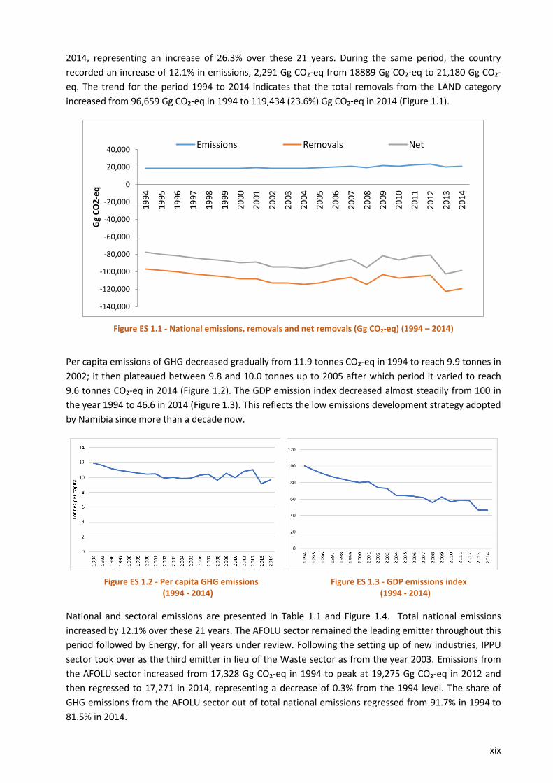
2014, representing an increase of 26.3% over these 21 years. During the same period, the country
recorded an increase of 12.1% in emissions, 2,291 Gg CO₂-eq from 18889 Gg CO₂-eq to 21,180 Gg CO₂-
eq. The trend for the period 1994 to 2014 indicates that the total removals from the LAND category
increased from 96,659 Gg CO₂-eq in 1994 to 119,434 (23.6%) Gg CO₂-eq in 2014 (Figure 1.1).
Figure ES 1.1 - National emissions, removals and net removals (Gg CO₂-eq) (1994 – 2014)
Per capita emissions of GHG decreased gradually from 11.9 tonnes CO₂-eq in 1994 to reach 9.9 tonnes in
2002; it then plateaued between 9.8 and 10.0 tonnes up to 2005 after which period it varied to reach
9.6 tonnes CO₂-eq in 2014 (Figure 1.2). The GDP emission index decreased almost steadily from 100 in
the year 1994 to 46.6 in 2014 (Figure 1.3). This reflects the low emissions development strategy adopted
by Namibia since more than a decade now.
Figure ES 1.2 - Per capita GHG emissions (1994 - 2014)
Figure ES 1.3 - GDP emissions index (1994 - 2014)
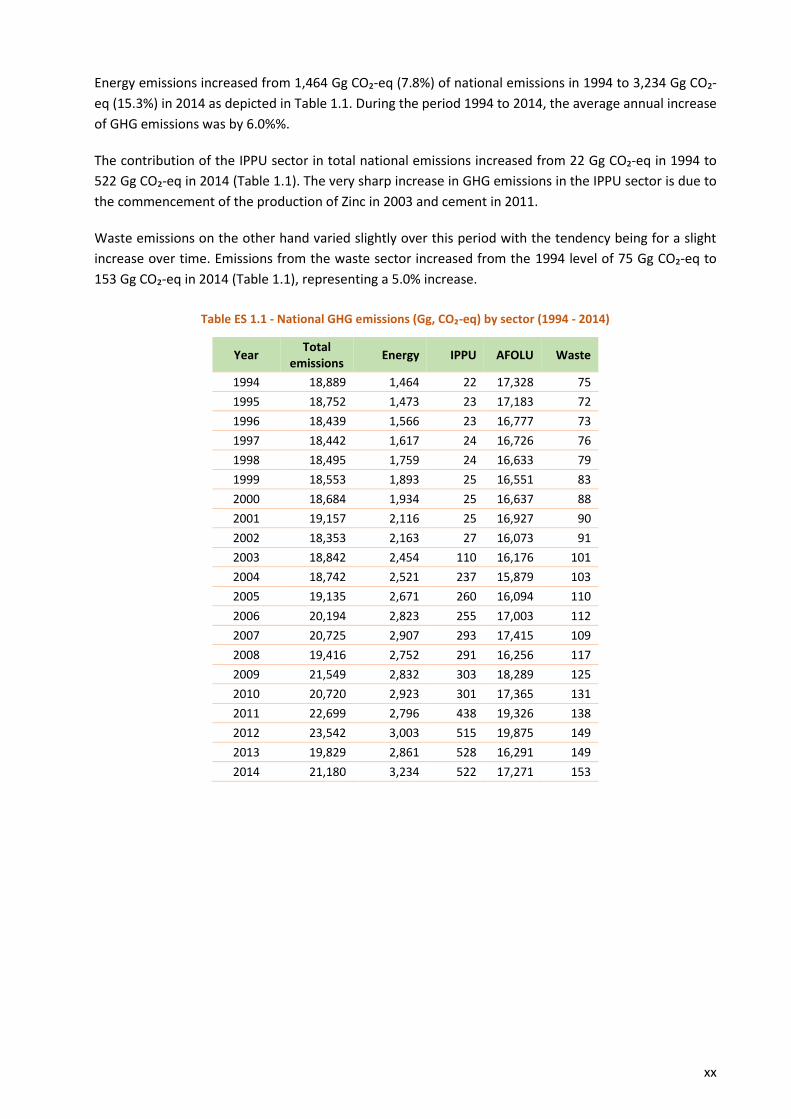
National and sectoral emissions are presented in Table 1.1 and Figure 1.4. Total national emissions
increased by 12.1% over these 21 years. The AFOLU sector remained the leading emitter throughout this
period followed by Energy, for all years under review. Following the setting up of new industries, IPPU
sector took over as the third emitter in lieu of the Waste sector as from the year 2003. Emissions from
the AFOLU sector increased from 17,328 Gg CO₂-eq in 1994 to peak at 19,275 Gg CO₂-eq in 2012 and
then regressed to 17,271 in 2014, representing a decrease of 0.3% from the 1994 level. The share of
GHG emissions from the AFOLU sector out of total national emissions regressed from 91.7% in 1994 to
81.5% in 2014.
-140,000
-120,000
-100,000
-80,000
-60,000
-40,000
-20,000
0
20,000
40,0001
99
4
19
95
19
96
19
97
19
98
19
99
20
00
20
01
20
02
20
03
20
04
20
05
20
06
20
07
20
08
20
09
20
10
20
11
20
12
20
13
20
14
Gg
CO
2-e
q
Emissions Removals Net
xx
Energy emissions increased from 1,464 Gg CO₂-eq (7.8%) of national emissions in 1994 to 3,234 Gg CO₂-
eq (15.3%) in 2014 as depicted in Table 1.1. During the period 1994 to 2014, the average annual increase
of GHG emissions was by 6.0%%.
The contribution of the IPPU sector in total national emissions increased from 22 Gg CO₂-eq in 1994 to
522 Gg CO₂-eq in 2014 (Table 1.1). The very sharp increase in GHG emissions in the IPPU sector is due to
the commencement of the production of Zinc in 2003 and cement in 2011.
Waste emissions on the other hand varied slightly over this period with the tendency being for a slight
increase over time. Emissions from the waste sector increased from the 1994 level of 75 Gg CO₂-eq to
153 Gg CO₂-eq in 2014 (Table 1.1), representing a 5.0% increase.
Table ES 1.1 - National GHG emissions (Gg, CO₂-eq) by sector (1994 - 2014)
Year Total
emissions Energy IPPU AFOLU Waste
1994 18,889 1,464 22 17,328 75
1995 18,752 1,473 23 17,183 72
1996 18,439 1,566 23 16,777 73
1997 18,442 1,617 24 16,726 76
1998 18,495 1,759 24 16,633 79
1999 18,553 1,893 25 16,551 83
2000 18,684 1,934 25 16,637 88
2001 19,157 2,116 25 16,927 90
2002 18,353 2,163 27 16,073 91
2003 18,842 2,454 110 16,176 101
2004 18,742 2,521 237 15,879 103
2005 19,135 2,671 260 16,094 110
2006 20,194 2,823 255 17,003 112
2007 20,725 2,907 293 17,415 109
2008 19,416 2,752 291 16,256 117
2009 21,549 2,832 303 18,289 125
2010 20,720 2,923 301 17,365 131
2011 22,699 2,796 438 19,326 138
2012 23,542 3,003 515 19,875 149
2013 19,829 2,861 528 16,291 149
2014 21,180 3,234 522 17,271 153
xxi
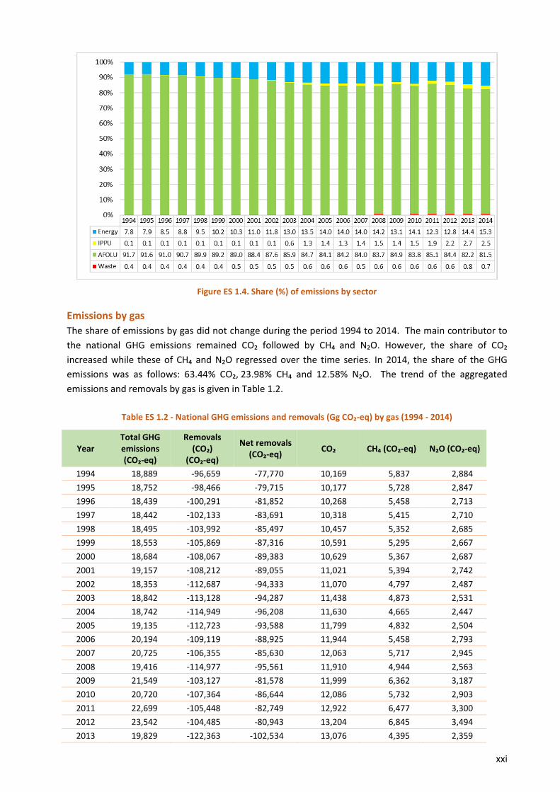
Figure ES 1.4. Share (%) of emissions by sector
Emissions by gas
The share of emissions by gas did not change during the period 1994 to 2014. The main contributor to
the national GHG emissions remained CO₂ followed by CH₄ and N₂O. However, the share of CO₂
increased while these of CH₄ and N₂O regressed over the time series. In 2014, the share of the GHG
emissions was as follows: 63.44% CO₂, 23.98% CH₄ and 12.58% N₂O. The trend of the aggregated
emissions and removals by gas is given in Table 1.2.
Table ES 1.2 - National GHG emissions and removals (Gg CO₂-eq) by gas (1994 - 2014)
Year Total GHG emissions (CO₂-eq)
Removals (CO₂)
(CO₂-eq)
Net removals (CO₂-eq)
CO₂ CH₄ (CO₂-eq) N₂O (CO₂-eq)
1994 18,889 -96,659 -77,770 10,169 5,837 2,884
1995 18,752 -98,466 -79,715 10,177 5,728 2,847
1996 18,439 -100,291 -81,852 10,268 5,458 2,713
1997 18,442 -102,133 -83,691 10,318 5,415 2,710
1998 18,495 -103,992 -85,497 10,457 5,352 2,685
1999 18,553 -105,869 -87,316 10,591 5,295 2,667
2000 18,684 -108,067 -89,383 10,629 5,367 2,687
2001 19,157 -108,212 -89,055 11,021 5,394 2,742
2002 18,353 -112,687 -94,333 11,070 4,797 2,487
2003 18,842 -113,128 -94,287 11,438 4,873 2,531
2004 18,742 -114,949 -96,208 11,630 4,665 2,447
2005 19,135 -112,723 -93,588 11,799 4,832 2,504
2006 20,194 -109,119 -88,925 11,944 5,458 2,793
2007 20,725 -106,355 -85,630 12,063 5,717 2,945
2008 19,416 -114,977 -95,561 11,910 4,944 2,563
2009 21,549 -103,127 -81,578 11,999 6,362 3,187
2010 20,720 -107,364 -86,644 12,086 5,732 2,903
2011 22,699 -105,448 -82,749 12,922 6,477 3,300
2012 23,542 -104,485 -80,943 13,204 6,845 3,494
2013 19,829 -122,363 -102,534 13,076 4,395 2,359
xxii
Year Total GHG emissions (CO₂-eq)
Removals (CO₂)
(CO₂-eq)
Net removals (CO₂-eq)
CO₂ CH₄ (CO₂-eq) N₂O (CO₂-eq)
2014 21,180 -119,434 -98,254 13,436 5,079 2,665
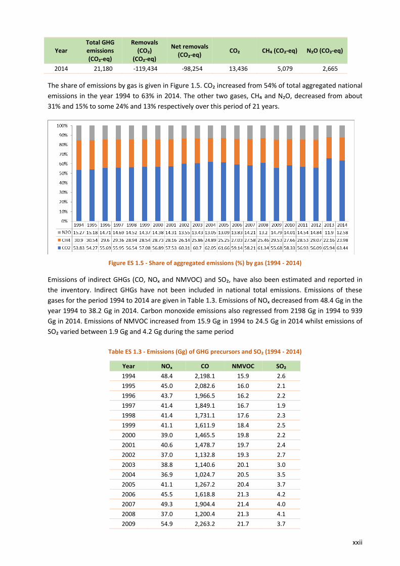
The share of emissions by gas is given in Figure 1.5. CO₂ increased from 54% of total aggregated national
emissions in the year 1994 to 63% in 2014. The other two gases, CH₄ and N₂O, decreased from about
31% and 15% to some 24% and 13% respectively over this period of 21 years.
Figure ES 1.5 - Share of aggregated emissions (%) by gas (1994 - 2014)
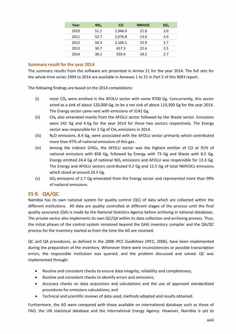
Emissions of indirect GHGs (CO, NOₓ and NMVOC) and SO₂, have also been estimated and reported in
the inventory. Indirect GHGs have not been included in national total emissions. Emissions of these
gases for the period 1994 to 2014 are given in Table 1.3. Emissions of NOₓ decreased from 48.4 Gg in the
year 1994 to 38.2 Gg in 2014. Carbon monoxide emissions also regressed from 2198 Gg in 1994 to 939
Gg in 2014. Emissions of NMVOC increased from 15.9 Gg in 1994 to 24.5 Gg in 2014 whilst emissions of
SO₂ varied between 1.9 Gg and 4.2 Gg during the same period
Table ES 1.3 - Emissions (Gg) of GHG precursors and SO₂ (1994 - 2014)
Year NOₓ CO NMVOC SO₂
1994 48.4 2,198.1 15.9 2.6
1995 45.0 2,082.6 16.0 2.1
1996 43.7 1,966.5 16.2 2.2
1997 41.4 1,849.1 16.7 1.9
1998 41.4 1,731.1 17.6 2.3
1999 41.1 1,611.9 18.4 2.5
2000 39.0 1,465.5 19.8 2.2
2001 40.6 1,478.7 19.7 2.4
2002 37.0 1,132.8 19.3 2.7
2003 38.8 1,140.6 20.1 3.0
2004 36.9 1,024.7 20.5 3.5
2005 41.1 1,267.2 20.4 3.7
2006 45.5 1,618.8 21.3 4.2
2007 49.3 1,904.4 21.4 4.0
2008 37.0 1,200.4 21.3 4.1
2009 54.9 2,263.2 21.7 3.7
xxiii
Year NOₓ CO NMVOC SO₂
2010 51.2 1,946.0 21.8 3.0
2011 52.7 2,076.8 13.0 3.0
2012 56.3 2,166.1 23.9 3.7
2013 30.7 657.3 22.6 2.5
2014 38.2 939.4 24.5 2.7
Summary result for the year 2014
The summary results from the software are presented in Annex 21 for the year 2014. The full sets for
the whole time series 1994 to 2014 are available in Annexes 1 to 21 in Part 2 of this NIR3 report.
The following findings are based on the 2014 compilations:
(i) most CO₂ were emitted in the AFOLU sector with some 9700 Gg. Concurrently, this sector
acted as a sink of about 120,000 Gg, to be a net sink of about 110,300 Gg for the year 2014.
The Energy sector came next with emissions of 3142 Gg.
(ii) CH₄ also emanated mainly from the AFOLU sector followed by the Waste sector. Emissions
were 242 Gg and 6 Gg for the year 2014 for these two sectors respectively. The Energy
sector was responsible for 2 Gg of CH₄ emissions in 2014.
(iii) N₂O emissions, 8.4 Gg, were associated with the AFOLU sector primarily which contributed
more than 97% of national emissions of this gas.
(iv) Among the indirect GHGs, the AFOLU sector was the highest emitter of CO at 91% of
national emissions with 858 Gg, followed by Energy with 73 Gg and Waste with 8.5 Gg.
Energy emitted 24.4 Gg of national NOₓ emissions and AFOLU was responsible for 13.3 Gg.
The Energy and AFOLU sectors contributed 9.2 Gg and 12.5 Gg of total NMVOCs emissions
which stood at around 24.5 Gg.
(v) SO₂ emissions of 2.7 Gg emanated from the Energy sector and represented more than 99%
of national emissions.
ES 9. QA/QC Namibia has its own national system for quality control (QC) of data which are collected within the
different institutions. All data are quality controlled at different stages of the process until the final
quality assurance (QA) is made by the National Statistics Agency before archiving in national databases.
The private sector also implements its own QC/QA within its data collection and archiving process. Thus,
the initial phases of the control system remained beyond the GHG inventory compiler and the QA/QC
process for the inventory started as from the time the AD are received.
QC and QA procedures, as defined in the 2006 IPCC Guidelines (IPCC, 2006), have been implemented
during the preparation of the inventory. Whenever there were inconsistencies or possible transcription
errors, the responsible institution was queried, and the problem discussed and solved. QC was
implemented through:
Routine and consistent checks to ensure data integrity, reliability and completeness;
Routine and consistent checks to identify errors and omissions;
Accuracy checks on data acquisition and calculations and the use of approved standardized
procedures for emissions calculations; and
Technical and scientific reviews of data used, methods adopted and results obtained.
Furthermore, the AD were compared with those available on international database such as those of
FAO, the UN statistical database and the International Energy Agency. However, Namibia is yet to

xxiv
develop and implement a QC management system and this is one of the improvements contemplated in
the future.
QA was undertaken by independent reviewers who were not involved with the compilation of the
inventory, the main objectives being to:
Confirm data quality and reliability from different sources wherever possible;
Compare AD with those available on international websites such as FAO and IEA;
Review the AD and EFs adopted within each source category as a first step; and
Review and check the calculation steps in the software to ensure accuracy.
Namibia requested the UNFCCC and Global Support Programme to undertake a QA exercise on its
inventory compilation process. Unfortunately, the exercise was performed when the inventory report
was not yet completed but on information available at that time. The main conclusions are:
Attempt at collecting missing Ad for improving the completeness of the inventory, namely use
of N₂O for medical applications, ODS and incineration of medical waste;
Improve the Institutional arrangements to ensure annual provision of Ad for preparing the
inventory;
Develop and implement a QC management system;
Improve AD for the AFOLU sector through production of new maps to generate land use
changes, national stock and Emission factors, possible use of Collect earth for confirming the
assumptions and data used;
Develop legal arrangements for securing collaboration of other institutions for AD;
Improve on documentation and archiving; and Capacity building in various areas of inventory
compilation.
The implementing agency of the GEF, UNDP had the draft NIR3 report reviewed by the GSP. The
comments were integrated in the final report as far as possible and those not attended to have been
included in the NIIP for future action.
ES 10. Completeness A source by source category analysis was conducted before the preparation of this inventory and it was
updated by adding two more categories in the IPPU sector. Emissions from HFCs and PFCs have not
been included due to lack of disaggregated data, the information on them being as blends without the
content of the different components.
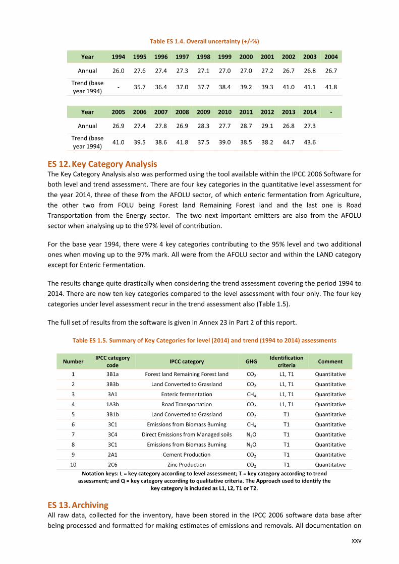
ES 11. Uncertainty analysis For this Inventory, a Tier 1 uncertainty analysis of the aggregated figures as required by the 2006 IPCC
Guidelines, Vol. 1 (IPCC, 2007) was performed. Based on the quality of the data and whether the EFs
used were defaults or nationally derived, uncertainty levels were assigned for the two parameters and
the combined uncertainty calculated. The uncertainty analysis has been performed using the tool
available within the 2006 IPCC Software. The uncertainty in total emissions obtained using the IPCC tool
is presented in Table 1.4 for the individual year of the inventory time series and the trend with the
addition of one year at a time as from 1994 to 2014. Uncertainty levels (+/-) for the individual years of
the period 1994 to 2014 varied from 26.0% to 29.1% while the trend assessment when adding one
successive year on the base year 1994 for the years 1995 to 2014 ranged from 35.7% to 44.7%. The full
set of results from the software is given in Annex 22 of Part 2 of this NIR3 report.
xxv
Table ES 1.4. Overall uncertainty (+/-%)
Year 1994 1995 1996 1997 1998 1999 2000 2001 2002 2003 2004
Annual 26.0 27.6 27.4 27.3 27.1 27.0 27.0 27.2 26.7 26.8 26.7
Trend (base year 1994)
- 35.7 36.4 37.0 37.7 38.4 39.2 39.3 41.0 41.1 41.8
Year 2005 2006 2007 2008 2009 2010 2011 2012 2013 2014 -
Annual 26.9 27.4 27.8 26.9 28.3 27.7 28.7 29.1 26.8 27.3
Trend (base year 1994)
41.0 39.5 38.6 41.8 37.5 39.0 38.5 38.2 44.7 43.6
ES 12. Key Category Analysis The Key Category Analysis also was performed using the tool available within the IPCC 2006 Software for
both level and trend assessment. There are four key categories in the quantitative level assessment for
the year 2014, three of these from the AFOLU sector, of which enteric fermentation from Agriculture,
the other two from FOLU being Forest land Remaining Forest land and the last one is Road
Transportation from the Energy sector. The two next important emitters are also from the AFOLU
sector when analysing up to the 97% level of contribution.
For the base year 1994, there were 4 key categories contributing to the 95% level and two additional
ones when moving up to the 97% mark. All were from the AFOLU sector and within the LAND category
except for Enteric Fermentation.
The results change quite drastically when considering the trend assessment covering the period 1994 to
2014. There are now ten key categories compared to the level assessment with four only. The four key
categories under level assessment recur in the trend assessment also (Table 1.5).
The full set of results from the software is given in Annex 23 in Part 2 of this report.
Table ES 1.5. Summary of Key Categories for level (2014) and trend (1994 to 2014) assessments
Number IPCC category
code IPCC category GHG
Identification criteria
Comment
1 3B1a Forest land Remaining Forest land CO2 L1, T1 Quantitative
2 3B3b Land Converted to Grassland CO2 L1, T1 Quantitative
3 3A1 Enteric fermentation CH4 L1, T1 Quantitative
4 1A3b Road Transportation CO2 L1, T1 Quantitative
5 3B1b Land Converted to Grassland CO2 T1 Quantitative
6 3C1 Emissions from Biomass Burning CH4 T1 Quantitative
7 3C4 Direct Emissions from Managed soils N2O T1 Quantitative
8 3C1 Emissions from Biomass Burning N2O T1 Quantitative
9 2A1 Cement Production CO2 T1 Quantitative
10 2C6 Zinc Production CO2 T1 Quantitative
Notation keys: L = key category according to level assessment; T = key category according to trend assessment; and Q = key category according to qualitative criteria. The Approach used to identify the
key category is included as L1, L2, T1 or T2.
ES 13. Archiving All raw data, collected for the inventory, have been stored in the IPCC 2006 software data base after
being processed and formatted for making estimates of emissions and removals. All documentation on
xxvi
the data processing and formatting have been kept in soft copies in the excel sheets with the summaries
reported in the NIR. These versions will be managed in electronic format in at least three copies, two
stored at the Ministry of Environment and Tourism and a third copy at the National Statistics Agency.
ES 14. Constraints, gaps and needs Namibia, as a developing country, has its constraints and gaps that need to be addressed to improve the
quality of the inventory for reporting to the Convention. Major problems encountered were related to
availability of AD, appropriateness of EFs, background information on technologies associated with
production and national stock factors for the estimation exercise. Additionally, lack of resources - both
technical and financial - coupled to insufficient capacity of national experts to take over the compilation
of the full inventory remained a major issue of concern.
ES 15. National inventory improvement plan (NIIP) Based on the constraints and gaps and other challenges encountered during the preparation of the
inventory, a list of the priority improvements has been identified. The main issues are listed below.
Adequate and proper data capture, QC, validation, storage and retrieval mechanism need to be
improved to facilitate the compilation of future inventories;
Capacity building and strengthening of the existing institutional framework to provide improved
coordinated action for reliable data collection and accessibility is a priority undertaking in the
future;
Improve the existing QA/QC system in order to reduce uncertainty and improve inventory
quality;
Find the necessary resources to establish a GHG inventory unit within DEA to be responsible for
inventory compilation and coordination;
Conduct new forest inventories to supplement available data on the Land sector;
Produce new maps for 1990 to 2015 to refine land use change data over 5 years periods as
opposed to the decadal one available now which is proving inadequate;
Develop the digestible energy (DE) factor for livestock as country-specific data is better than the
default IPCC value to address this key category fully at Tier 2; and
Add the missing years 1990 to 1993 to complete the full time series 1990 to at least 2015 in the
next inventory compilation.
Attempt at estimating emissions for categories not covered yet.

1
1. Introduction
1.1. National circumstances
The Republic of Namibia is situated in South-Western Africa between latitudes 17° and 29°S and
longitudes 11° and 26°E. It extends over 825,608 km2 of land which support a population of some
2.3 million in 2014. In 2014, about 47% of the population of the country inhabited urban areas. The
country is known to be one with a relatively low population density at 2.6 persons per km2.
Namibia’s climate is very variable and is characterized by persistent droughts, unpredictable and
variable rainfall patterns, variability in temperatures and scarcity of water. Natural resources are under
increasing stress. Rainfall ranges from an average of 25 mm in the west to over 600 mm in the
northeast. Apart from the coastal zone, there is a marked seasonal temperature regime, with the
highest temperatures occurring just before the wet season in the wetter areas or during the wet season
in the drier areas. The lowest temperatures occur during the dry season months of June to August.
Mean monthly minimum temperatures do not, on average, fall below 0°C. High solar radiation, low
humidity and high temperature lead to very high evaporation rates, which vary between 3800 mm per
annum in the south to 2600 mm per annum in the north. Over most of the country, potential
evaporation is at least five times greater than rainfall. Thus, only about 1% of rainfall ends up
replenishing the groundwater aquifers. Lack of water is the key limitation factor to Namibia’s
development.
The services sector which accounted for 60% of Gross Domestic Product (GDP) in 2015 is the most
important economic sector of Namibia. Agriculture, fisheries and forestry accounted for 9% and the
manufacturing sector including mining and quarrying another 25%. The primary sector agriculture is one
of the foundations of Namibia’s economy, as it is a vital source of livelihood for most rural families in
term of food generation with approximately 48% of Namibia’s rural households depending on
subsistence agriculture (NDP4).
Mining contributed about 12.3% to the country’s GDP in 2015. The manufacturing sector, a priority
sector under the NDP4, is estimated to have recorded a constant growth of 1.2% in 2011 and 2012 and
contributed some 12.3% to national GDP in 2015. Namibia is highly dependent on imports to meet its
energy requirements. The domestic economy is estimated to have expanded by 3.5% in 2015 (NSA,
2016).
1.2. Commitments under the Convention
The United Nations Framework Convention on Climate Change (UNFCCC) was adopted in 1992 at the UN
Conference on Environment and Sustainable Development in Rio de Janeiro, Brazil. The Convention
came into force on 21 March 1994. The Republic of Namibia ratified the Convention on 16 May 1995 as
a Non-Annex 1 Party and this decision came into effect on 14 August 1995.
Under Article 4.1 (a) of the Convention, each party has to develop, periodically update, publish and
make available to the Conference of the Parties, in accordance with Article 12, national inventories of
anthropogenic emissions by sources and removals by sinks of all greenhouse gases not controlled by the
Montreal Protocol, to the extent its capacities permit, using comparable methodologies to be promoted
and agreed upon by the Conference of the Parties.
2
Moreover, the submissions should also include the following elements amongst others:
a. A general description of steps taken or envisaged by the Party to implement the Convention;
and
b. Any other information that the Party considers relevant to the achievement of the objective of
the convention and suitable for inclusion in its communication, including, if feasible, material
relevant for calculations of global emission trends
In order to meet its reporting obligations, Namibia has submitted three national communications (NCs);
the initial national communication in 2002, the second national communication in 2011 and the third
national communication in 2015. with support from the GEF through UNDP. The Republic of Namibia
was the first developing country to submit its Biennial Update Report in 2014 and the second one in
2016. Thus, Namibia has to-date submitted five GHG inventories detailing its emissions and sinks as
components of the national communications or stand-alone national inventory reports. Namibia has
now prepared a third national inventory report fully detailing the compilation process in the best
transparent manner possible. The summary will constitute the chapter on greenhouse gas inventory of
the third Biennial Update Report (BUR3).
Additionally, Namibia has prepared and submitted its Intended Nationally Determined Contributions
during COP 21 in Paris. The country signed and ratified the Paris Agreement on 22 April 2016 and 21
September 2016 respectively.
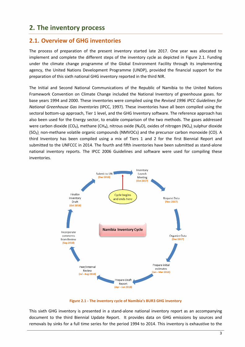
3
2. The inventory process
2.1. Overview of GHG inventories
The process of preparation of the present inventory started late 2017. One year was allocated to
implement and complete the different steps of the inventory cycle as depicted in Figure 2.1. Funding
under the climate change programme of the Global Environment Facility through its implementing
agency, the United Nations Development Programme (UNDP), provided the financial support for the
preparation of this sixth national GHG inventory reported in the third NIR.
The Initial and Second National Communications of the Republic of Namibia to the United Nations
Framework Convention on Climate Change included the National Inventory of greenhouse gases. for
base years 1994 and 2000. These inventories were compiled using the Revised 1996 IPCC Guidelines for
National Greenhouse Gas Inventories (IPCC, 1997). These inventories have all been compiled using the
sectoral bottom-up approach, Tier 1 level, and the GHG Inventory software. The reference approach has
also been used for the Energy sector, to enable comparison of the two methods. The gases addressed
were carbon dioxide (CO₂), methane (CH₄), nitrous oxide (N₂O), oxides of nitrogen (NOₓ), sulphur dioxide
(SO₂), non-methane volatile organic compounds (NMVOCs) and the precursor carbon monoxide (CO). A
third Inventory has been compiled using a mix of Tiers 1 and 2 for the first Biennial Report and
submitted to the UNFCCC in 2014. The fourth and fifth inventories have been submitted as stand-alone
national inventory reports. The IPCC 2006 Guidelines and software were used for compiling these
inventories.
Figure 2.1 - The inventory cycle of Namibia’s BUR3 GHG inventory
This sixth GHG inventory is presented in a stand-alone national inventory report as an accompanying
document to the third Biennial Update Report. It provides data on GHG emissions by sources and
removals by sinks for a full time series for the period 1994 to 2014. This inventory is exhaustive to the
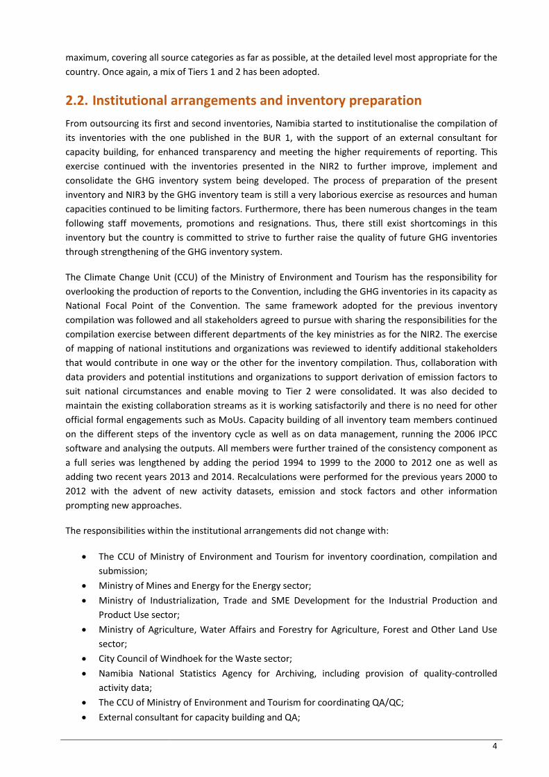
4
maximum, covering all source categories as far as possible, at the detailed level most appropriate for the
country. Once again, a mix of Tiers 1 and 2 has been adopted.
2.2. Institutional arrangements and inventory preparation
From outsourcing its first and second inventories, Namibia started to institutionalise the compilation of
its inventories with the one published in the BUR 1, with the support of an external consultant for
capacity building, for enhanced transparency and meeting the higher requirements of reporting. This
exercise continued with the inventories presented in the NIR2 to further improve, implement and
consolidate the GHG inventory system being developed. The process of preparation of the present
inventory and NIR3 by the GHG inventory team is still a very laborious exercise as resources and human
capacities continued to be limiting factors. Furthermore, there has been numerous changes in the team
following staff movements, promotions and resignations. Thus, there still exist shortcomings in this
inventory but the country is committed to strive to further raise the quality of future GHG inventories
through strengthening of the GHG inventory system.
The Climate Change Unit (CCU) of the Ministry of Environment and Tourism has the responsibility for
overlooking the production of reports to the Convention, including the GHG inventories in its capacity as
National Focal Point of the Convention. The same framework adopted for the previous inventory
compilation was followed and all stakeholders agreed to pursue with sharing the responsibilities for the
compilation exercise between different departments of the key ministries as for the NIR2. The exercise
of mapping of national institutions and organizations was reviewed to identify additional stakeholders
that would contribute in one way or the other for the inventory compilation. Thus, collaboration with
data providers and potential institutions and organizations to support derivation of emission factors to
suit national circumstances and enable moving to Tier 2 were consolidated. It was also decided to
maintain the existing collaboration streams as it is working satisfactorily and there is no need for other
official formal engagements such as MoUs. Capacity building of all inventory team members continued
on the different steps of the inventory cycle as well as on data management, running the 2006 IPCC
software and analysing the outputs. All members were further trained of the consistency component as
a full series was lengthened by adding the period 1994 to 1999 to the 2000 to 2012 one as well as
adding two recent years 2013 and 2014. Recalculations were performed for the previous years 2000 to
2012 with the advent of new activity datasets, emission and stock factors and other information
prompting new approaches.
The responsibilities within the institutional arrangements did not change with:
The CCU of Ministry of Environment and Tourism for inventory coordination, compilation and
submission;
Ministry of Mines and Energy for the Energy sector;
Ministry of Industrialization, Trade and SME Development for the Industrial Production and
Product Use sector;
Ministry of Agriculture, Water Affairs and Forestry for Agriculture, Forest and Other Land Use
sector;
City Council of Windhoek for the Waste sector;
Namibia National Statistics Agency for Archiving, including provision of quality-controlled
activity data;
The CCU of Ministry of Environment and Tourism for coordinating QA/QC;
External consultant for capacity building and QA;
5
The CCU of Ministry of Environment and Tourism for coordinating Uncertainty Analysis; and
The CCU of Ministry of Environment and Tourism to act as GHG inventory specialist to track
capacity building needs, the IPCC process and COP decisions for implementation.
The institutional arrangements for the compilation of the inventory and reporting for the different
sectors are shown in Figure 2.2.
Figure 2.2 - Institutional arrangements for the GHG inventory preparation
The inventory preparation started in January 2018 due to delays in the availability of funds. A work plan
with timeframe and responsibilities was drawn for the preparation of the inventory using a mix of Tiers
1 and 2. AD were collected for the years 1994 to 1999, 2013 and 2014 to update the existing series and
meet the timing requirement for the BUR 3. The collected AD were processed and sectoral experts of
the inventory team computed emissions and performed recalculations as necessary under the
supervision of the external consultant. This exercise took place during a three-day workshop with the
external consultant providing the support for identifying improvement areas relative to data availability
and quality, appropriateness of EFs, gaps and constraints. Drawbacks and shortcomings were addressed
to maintain smooth implementation of the inventory cycle. The 2006 IPCC Guidelines for National
Greenhouse Gas Inventories (IPCC, 2007) were used with the most appropriate IPCC default EFs. Default
EFs were likewise assessed and these were derived or amended in some cases to reflect national
circumstances and conditions, the objective being to estimate emissions as accurately as possible. The
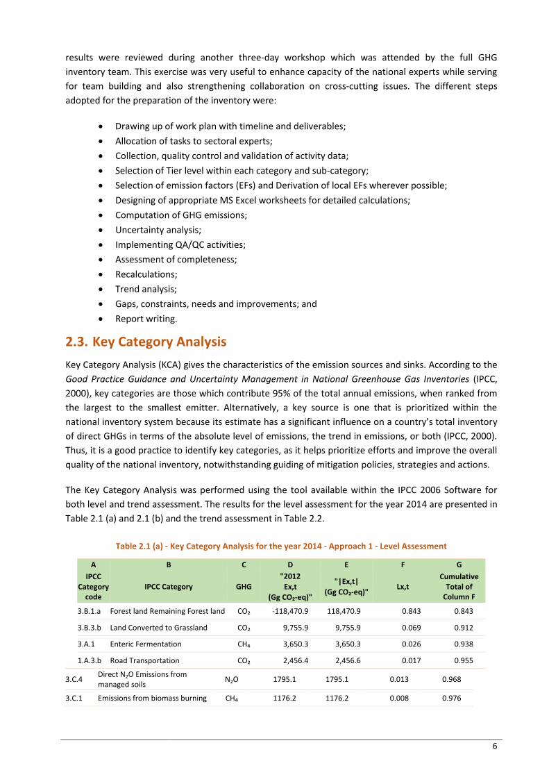
6
results were reviewed during another three-day workshop which was attended by the full GHG
inventory team. This exercise was very useful to enhance capacity of the national experts while serving
for team building and also strengthening collaboration on cross-cutting issues. The different steps
adopted for the preparation of the inventory were:
Drawing up of work plan with timeline and deliverables;
Allocation of tasks to sectoral experts;
Collection, quality control and validation of activity data;
Selection of Tier level within each category and sub-category;
Selection of emission factors (EFs) and Derivation of local EFs wherever possible;
Designing of appropriate MS Excel worksheets for detailed calculations;
Computation of GHG emissions;
Uncertainty analysis;
Implementing QA/QC activities;
Assessment of completeness;
Recalculations;
Trend analysis;
Gaps, constraints, needs and improvements; and
Report writing.
2.3. Key Category Analysis
Key Category Analysis (KCA) gives the characteristics of the emission sources and sinks. According to the
Good Practice Guidance and Uncertainty Management in National Greenhouse Gas Inventories (IPCC,
2000), key categories are those which contribute 95% of the total annual emissions, when ranked from
the largest to the smallest emitter. Alternatively, a key source is one that is prioritized within the
national inventory system because its estimate has a significant influence on a country’s total inventory
of direct GHGs in terms of the absolute level of emissions, the trend in emissions, or both (IPCC, 2000).
Thus, it is a good practice to identify key categories, as it helps prioritize efforts and improve the overall
quality of the national inventory, notwithstanding guiding of mitigation policies, strategies and actions.
The Key Category Analysis was performed using the tool available within the IPCC 2006 Software for
both level and trend assessment. The results for the level assessment for the year 2014 are presented in
Table 2.1 (a) and 2.1 (b) and the trend assessment in Table 2.2.
Table 2.1 (a) - Key Category Analysis for the year 2014 - Approach 1 - Level Assessment
A B C D E F G
IPCC Category
code IPCC Category GHG
"2012
Ex,t
(Gg CO₂-eq)"
"|Ex,t|
(Gg CO₂-eq)" Lx,t
Cumulative Total of
Column F
3.B.1.a Forest land Remaining Forest land CO₂ -118,470.9 118,470.9 0.843 0.843
3.B.3.b Land Converted to Grassland CO₂ 9,755.9 9,755.9 0.069 0.912
3.A.1 Enteric Fermentation CH₄ 3,650.3 3,650.3 0.026 0.938
1.A.3.b Road Transportation CO₂ 2,456.4 2,456.6 0.017 0.955
3.C.4 Direct N2O Emissions from managed soils
N2O 1795.1 1795.1 0.013 0.968
3.C.1 Emissions from biomass burning CH₄ 1176.2 1176.2 0.008 0.976
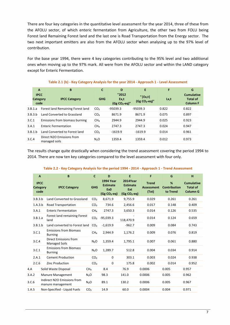
7
There are four key categories in the quantitative level assessment for the year 2014, three of these from
the AFOLU sector, of which enteric fermentation from Agriculture, the other two from FOLU being
Forest land Remaining Forest land and the last one is Road Transportation from the Energy sector. The
two next important emitters are also from the AFOLU sector when analysing up to the 97% level of
contribution.
For the base year 1994, there were 4 key categories contributing to the 95% level and two additional
ones when moving up to the 97% mark. All were from the AFOLU sector and within the LAND category
except for Enteric Fermentation.
Table 2.1 (b) - Key Category Analysis for the year 2014 - Approach 1 - Level Assessment
A B C D E F G
IPCC Category
code IPCC Category GHG
"2012
Ex,t
(Gg CO₂-eq)"
"|Ex,t|
(Gg CO₂-eq)" Lx,t
Cumulative Total of
Column F
3.B.1.a Forest land Remaining Forest land CO₂ -95039.3 -95039.3 0.822 0.822
3.B.3.b Land Converted to Grassland CO₂ 8671.9 8671.9 0.075 0.897
3.C.1 Emissions from biomass burning CH₄ 2944.9 2944.9 0.025 0.923
3.A.1 Enteric Fermentation CH₄ 2747.3 2747.3 0.024 0.947
3.B.1.b Land Converted to Forest land CO₂ -1619.9 -1619.9 0.014 0.961
3.C.4 Direct N2O Emissions from managed soils
N2O 1359.4 1359.4 0.012 0.973
The results change quite drastically when considering the trend assessment covering the period 1994 to
2014. There are now ten key categories compared to the level assessment with four only.
Table 2.2 - Key Category Analysis for the period 1994 - 2014 - Approach 1 - Trend Assessment
A B C D E F G H
IPCC Category
code IPCC Category GHG
1994 Year Estimate
Ex0 (Gg CO₂-eq)
2014Year Estimate
Ext (Gg CO₂-eq)
Trend Assessment
(Txt)
% Contribution
to Trend
Cumulative Total of
Column G
3.B.3.b Land Converted to Grassland CO₂ 8,671.9 9,755.9 0.029 0.261 0.261
1.A.3.b Road Transportation CO₂ 734.6 2,456.6 0.017 0.148 0.409
3.A.1 Enteric Fermentation CH₄ 2747.3 3,650.3 0.014 0.126 0.535
3.B.1.a Forest land remaining Forest land
CO₂ -95,039.3 -
118,470.9 0.014 0.124 0.659
3.B.1.b Land converted to Forest land CO₂ -1,619.9 -962.7 0.009 0.084 0.743
3.C.1 Emissions from Biomass Burning
CH₄ 2,944.9 1,176.2 0.009 0.076 0.819
3.C.4 Direct Emissions from Managed Soils
N₂O 1,359.4 1,795.1 0.007 0.061 0.880
3.C.1 Emissions from Biomass Burning
N₂O 1,289.7 512.8 0.004 0.034 0.914
2.A.1 Cement Production CO₂ 0 303.1 0.003 0.024 0.938
2.C.6 Zinc Production CO₂ 0 175.8 0.002 0.014 0.952
4.A Solid Waste Disposal CH₄ 8.4 76.9 0.0006 0.005 0.957
3.A.2 Manure Management N₂O 98.3 141.0 0.0006 0.005 0.962
3.C.6 Indirect N2O Emissions from manure management
N₂O 89.1 130.2 0.0006 0.005 0.967
1.A.5 Non-Specified - Liquid Fuels CO₂ 14.9 60.0 0.0004 0.004 0.971

8
The summary of Key Categories based on the quantitative level, for year 2014 and trend, period 1994 to 2014, assessments up to the 95% contribution mark is presented in Table 2.3. The number of Key categories increased from four under level assessment to ten with the four recurring in the trend assessment also. The full set of results from the software is provided in Annex 23 of Part 2 of the NIR3 report.
Table 2.3. Summary of Key Categories for level (2014) and trend (1994 to 2014) assessments
Number IPCC category
code IPCC category GHG
Identification criteria
Comment
1 3B1a Forest land Remaining Forest land CO2 L1, T1 Quantitative
2 3B3b Land Converted to Grassland CO2 L1, T1 Quantitative
3 3A1 Enteric fermentation CH4 L1, T1 Quantitative
4 1A3b Road Transportation CO2 L1, T1 Quantitative
5 3B1b Land Converted to Grassland CO2 T1 Quantitative
6 3C1 Emissions from Biomass Burning CH4 T1 Quantitative
7 3C4 Direct Emissions from Managed soils N2O T1 Quantitative
8 3C1 Emissions from Biomass Burning N2O T1 Quantitative
9 2A1 Cement Production CO2 T1 Quantitative
10 2C6 Zinc Production CO2 T1 Quantitative
Notation keys: L = key category according to level assessment; T = key category according to trend assessment; and Q = key
category according to qualitative criteria. The Approach used to identify the key category is included as L1, L2, T1 or T2.
2.4. Methodological issues
This section gives an overview of the methodological approach adopted for all sectors and sub-sectors
covered in this inventory report. These procedures are extensively detailed in the respective section
covering the individual IPCC Key Categories.
Generally, the method adopted to compute emissions involved multiplying activity data (AD) by the
relevant appropriate emission factor (EF), as shown below:
Emissions (E) = Activity Data (AD) x Emission Factor (EF)
All the methods and tools recommended by IPCC for the computation of emissions in an inventory have
been used and followed to be in line with Good Practices.
As the IPCC 2006 Guidelines do not fully address compilations at the Tier 2 level, national emission
factors and stock factors as appropriate have been derived and adopted to compile estimates at the Tier
2 level partially for the Livestock and Land sectors. Thus, the inventory has been compiled using a mix of
Tiers 1 and 2. This is good practice and improved the accuracy of the emission estimates of most of the
key categories and reduced the uncertainty level.
Global Warming Potentials (GWP) as recommended by the IPCC have been used to convert GHGs other
than CO₂ to the latter equivalent. Based on decision 17/CP.8, the values adopted were those from the
IPCC Second Assessment Report for the three direct GHGs, namely carbon dioxide (CO₂), methane (CH₄)
and nitrous oxide (N₂O) (Table 2.4). Additional gases, known as (indirect gases), which affect global
warming, namely oxides of nitrogen (NOₓ), carbon monoxide (CO), non-methane volatile organic
compounds (NMVOCs) and sulphur dioxide (SO₂), have also been computed and reported in the
inventory.
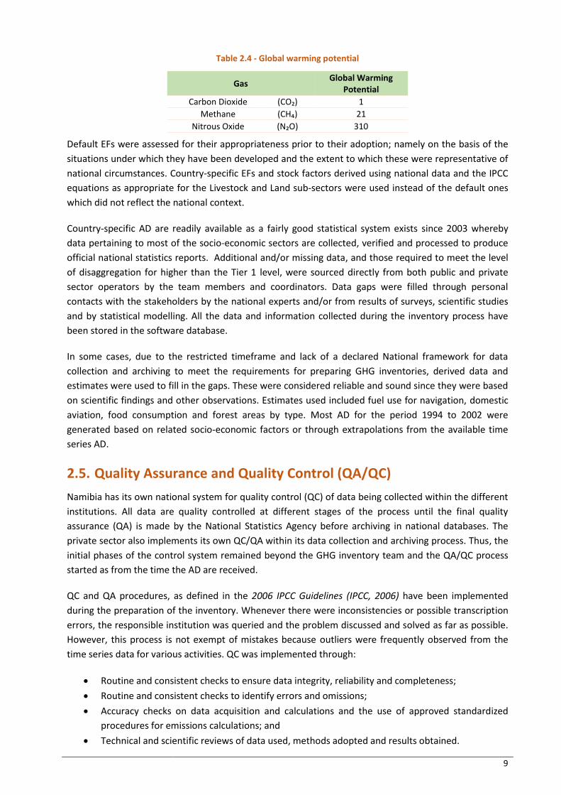
9
Table 2.4 - Global warming potential
Gas Global Warming
Potential
Carbon Dioxide (CO₂) 1
Methane (CH₄) 21
Nitrous Oxide (N₂O) 310
Default EFs were assessed for their appropriateness prior to their adoption; namely on the basis of the
situations under which they have been developed and the extent to which these were representative of
national circumstances. Country-specific EFs and stock factors derived using national data and the IPCC
equations as appropriate for the Livestock and Land sub-sectors were used instead of the default ones
which did not reflect the national context.
Country-specific AD are readily available as a fairly good statistical system exists since 2003 whereby
data pertaining to most of the socio-economic sectors are collected, verified and processed to produce
official national statistics reports. Additional and/or missing data, and those required to meet the level
of disaggregation for higher than the Tier 1 level, were sourced directly from both public and private
sector operators by the team members and coordinators. Data gaps were filled through personal
contacts with the stakeholders by the national experts and/or from results of surveys, scientific studies
and by statistical modelling. All the data and information collected during the inventory process have
been stored in the software database.
In some cases, due to the restricted timeframe and lack of a declared National framework for data
collection and archiving to meet the requirements for preparing GHG inventories, derived data and
estimates were used to fill in the gaps. These were considered reliable and sound since they were based
on scientific findings and other observations. Estimates used included fuel use for navigation, domestic
aviation, food consumption and forest areas by type. Most AD for the period 1994 to 2002 were
generated based on related socio-economic factors or through extrapolations from the available time
series AD.
2.5. Quality Assurance and Quality Control (QA/QC)
Namibia has its own national system for quality control (QC) of data being collected within the different
institutions. All data are quality controlled at different stages of the process until the final quality
assurance (QA) is made by the National Statistics Agency before archiving in national databases. The
private sector also implements its own QC/QA within its data collection and archiving process. Thus, the
initial phases of the control system remained beyond the GHG inventory team and the QA/QC process
started as from the time the AD are received.
QC and QA procedures, as defined in the 2006 IPCC Guidelines (IPCC, 2006) have been implemented
during the preparation of the inventory. Whenever there were inconsistencies or possible transcription
errors, the responsible institution was queried and the problem discussed and solved as far as possible.
However, this process is not exempt of mistakes because outliers were frequently observed from the
time series data for various activities. QC was implemented through:
Routine and consistent checks to ensure data integrity, reliability and completeness;
Routine and consistent checks to identify errors and omissions;
Accuracy checks on data acquisition and calculations and the use of approved standardized
procedures for emissions calculations; and
Technical and scientific reviews of data used, methods adopted and results obtained.
10
QA was undertaken by independent reviewers who were not involved with the preparation of the
inventory, the main objectives being to:
Confirm data quality and reliability from different sources wherever possible;
Compare AD with those available on international websites such as FAO and IEA;
Review the AD and EFs adopted within each source category as a first step; and
Review and check the calculation steps in the software to ensure accuracy.
Even if QA/QC procedures have been followed throughout the inventory process by the inventory
compilers of the different IPCC sectors and the QA officer, a QA/QC plan has yet to be developed to fit
within the Measure, Report and Verify system under implementation. Thus, systematic records as per
the 2006 IPCC Guidelines still have to be developed under a QA/QC coordinator. This resulted from the
lack of personnel, insufficient capacity and since the inventory management system is still being
developed and implemented in the country.
Namibia requested the UNFCCC and Global Support Programme to undertake a QA exercise on its
inventory compilation process. Unfortunately, the exercise was performed when the inventory report
was not yet completed but on information available at that time. The main conclusions are:
Attempt at collecting missing AD for improving the completeness of the inventory, namely use
of N₂O for medical applications, ODS and incineration of medical waste;
Improve the Institutional arrangements to ensure annual provision of AD for preparing the
inventory;
Develop and implement a QC management system;
Improve AD for the AFOLU sector through production of new maps to generate land use
changes, national stock and Emission factors, possible use of Collect earth for confirming the
assumptions and data used;
Develop legal arrangements for securing collaboration of other institutions for AD;
Improve on documentation and archiving; and
Capacity building in various areas of inventory compilation.
2.6. Uncertainty assessment
Uncertainty estimation is an essential element of a complete greenhouse gas emissions and removals
Inventory. The purpose of estimating the uncertainties attached to emission estimates is principally to
provide information on the categories to be prioritized for maximum resources to be allocated to
improve the quality of the inventory. Inventories prepared in accordance with 2006 IPCC guidelines
(IPCC, 2007) will typically contain a wide range of emission estimates, varying from carefully measured
and demonstrably complete data on emissions to order-of-magnitude estimates of highly variable
emissions such as N₂O fluxes from soils and waterways.
For this Inventory, a Tier 1 uncertainty analysis of the aggregated figures as required by the 2006 IPCC
Guidelines, Vol. 1 (IPCC, 2007) was performed. Based on the quality of the data and whether the EFs
used were defaults or nationally derived, uncertainty levels were allocated for the two parameters and
the combined uncertainty calculated. In most instances, the uncertainty values allocated to AD and EFs
from within the range recommended by the IPCC Guidelines. Thus. Lower uncertainties were allocated
to AD obtained from measurements made and recorded, higher values for interpolated and
extrapolated AD and the highest ones in the range when the AD is subject to expert knowledge.
Regarding the EFs, the average value recommended in the IPCC Guidelines were adopted except for
nationally determined EFs when the lower values of the range were adopted. Whenever there was a

11
need to revert to expert judgement, the protocol was to consult with more than one expert from the
typical sector or industry to ascertain on the level of uncertainty to be adopted from within the range
provided in the IPCC guidelines. In cases where IPCC has a particular recommended methodology, the
uncertainty level was derived according to the procedure proposed in the IPCC Guideline and used in
the uncertainty analysis. The uncertainty analysis has been performed using the tool available within the
IPCC 2006 Software. Uncertainties in total emissions based on the IPCC tool including emissions and
removals from the Land sector is presented in Table 2.5. Uncertainty levels for the individual years of
the period 1994 to 2014 varied from 26.0% to 29.1% while the trend assessment when adding one
successive year on the base year 1994 for the years 1995 to 2014 ranged from 35.7% to 44.7%. The full
set of results from the software is given in Annex 22 of Part 2 of this NIR3 report.
Table 2.5. Overall uncertainty (%)
Year 1994 1995 1996 1997 1998 1999 2000 2001 2002 2003 2004
Annual 26.0 27.6 27.4 27.3 27.1 27.0 27.0 27.2 26.7 26.8 26.7
Trend (base year 1994)
- 35.7 36.4 37.0 37.7 38.4 39.2 39.3 41.0 41.1 41.8
Year 2005 2006 2007 2008 2009 2010 2011 2012 2013 2014 -
Annual 26.9 27.4 27.8 26.9 28.3 27.7 28.7 29.1 26.8 27.3
Trend (base year 1994)
41.0 39.5 38.6 41.8 37.5 39.0 38.5 38.2 44.7 43.6
2.7. Assessment of completeness
An assessment of the completeness of the inventory was made for individual activity areas within each
source category and the results are presented within the sections covering the individual sectors. The
methodology adopted was according to the IPCC 2006 Guidelines (IPCC 2007) with the following
notation keys used:
X Estimated
NA Not Applicable
NO Not Occurring
NE Not Estimated
EE Estimated Elsewhere
The level of completeness depicting the scope of the inventory is provided in Table 2.6. In cases where
was no activity for all sub-categories within a category, only the category row was maintained for ease
of presentation and understanding.
Table 2.6 - Completeness of the 1994 to 2014 inventories
Sector / Source category CO₂ CH4 N₂O HFCs PFCs SF6 NOX CO NMV
OC SO₂
1 - Energy
1.A - Fuel Combustion Activities
1.A.1 - Energy Industries X X X NA NA NA X X X X
1.A.2 - Manufacturing Industries and Construction X X X NA NA NA X X X X
1.A.3 - Transport X X X NA NA NA X X X X
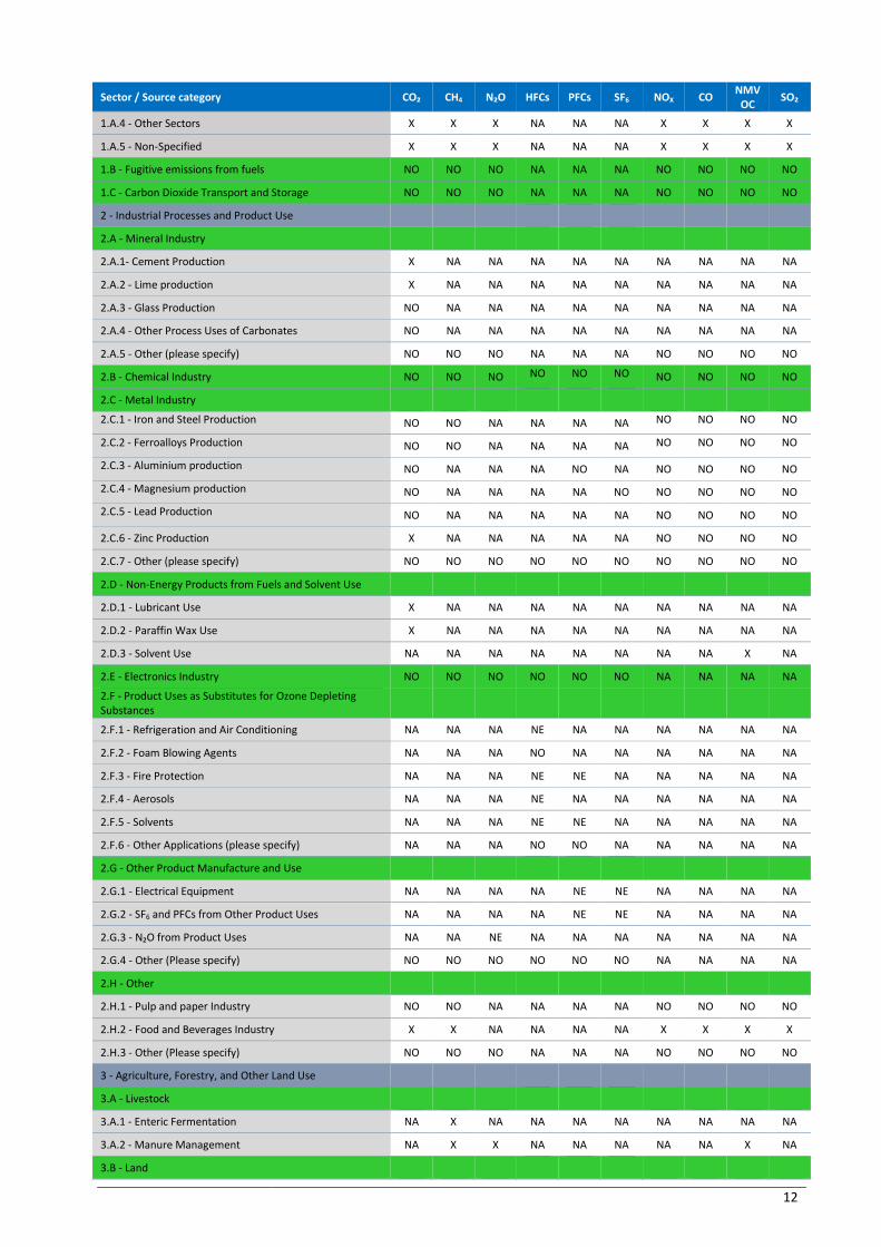
12
Sector / Source category CO₂ CH4 N₂O HFCs PFCs SF6 NOX CO NMV
OC SO₂
1.A.4 - Other Sectors X X X NA NA NA X X X X
1.A.5 - Non-Specified X X X NA NA NA X X X X
1.B - Fugitive emissions from fuels NO NO NO NA NA NA NO NO NO NO
1.C - Carbon Dioxide Transport and Storage NO NO NO NA NA NA NO NO NO NO
2 - Industrial Processes and Product Use
2.A - Mineral Industry
2.A.1- Cement Production X NA NA NA NA NA NA NA NA NA
2.A.2 - Lime production X NA NA NA NA NA NA NA NA NA
2.A.3 - Glass Production NO NA NA NA NA NA NA NA NA NA
2.A.4 - Other Process Uses of Carbonates NO NA NA NA NA NA NA NA NA NA
2.A.5 - Other (please specify) NO NO NO NA NA NA NO NO NO NO
2.B - Chemical Industry NO NO NO NO NO NO NO NO NO NO
2.C - Metal Industry
2.C.1 - Iron and Steel Production NO NO NA NA NA NA NO NO NO NO
2.C.2 - Ferroalloys Production NO NO NA NA NA NA NO NO NO NO
2.C.3 - Aluminium production NO NA NA NA NO NA NO NO NO NO
2.C.4 - Magnesium production NO NA NA NA NA NO NO NO NO NO
2.C.5 - Lead Production NO NA NA NA NA NA NO NO NO NO
2.C.6 - Zinc Production X NA NA NA NA NA NO NO NO NO
2.C.7 - Other (please specify) NO NO NO NO NO NO NO NO NO NO
2.D - Non-Energy Products from Fuels and Solvent Use
2.D.1 - Lubricant Use X NA NA NA NA NA NA NA NA NA
2.D.2 - Paraffin Wax Use X NA NA NA NA NA NA NA NA NA
2.D.3 - Solvent Use NA NA NA NA NA NA NA NA X NA
2.E - Electronics Industry NO NO NO NO NO NO NA NA NA NA
2.F - Product Uses as Substitutes for Ozone Depleting Substances
2.F.1 - Refrigeration and Air Conditioning NA NA NA NE NA NA NA NA NA NA
2.F.2 - Foam Blowing Agents NA NA NA NO NA NA NA NA NA NA
2.F.3 - Fire Protection NA NA NA NE NE NA NA NA NA NA
2.F.4 - Aerosols NA NA NA NE NA NA NA NA NA NA
2.F.5 - Solvents NA NA NA NE NE NA NA NA NA NA
2.F.6 - Other Applications (please specify) NA NA NA NO NO NA NA NA NA NA
2.G - Other Product Manufacture and Use
2.G.1 - Electrical Equipment NA NA NA NA NE NE NA NA NA NA
2.G.2 - SF6 and PFCs from Other Product Uses NA NA NA NA NE NE NA NA NA NA
2.G.3 - N₂O from Product Uses NA NA NE NA NA NA NA NA NA NA
2.G.4 - Other (Please specify) NO NO NO NO NO NO NA NA NA NA
2.H - Other
2.H.1 - Pulp and paper Industry NO NO NA NA NA NA NO NO NO NO
2.H.2 - Food and Beverages Industry X X NA NA NA NA X X X X
2.H.3 - Other (Please specify) NO NO NO NA NA NA NO NO NO NO
3 - Agriculture, Forestry, and Other Land Use
3.A - Livestock
3.A.1 - Enteric Fermentation NA X NA NA NA NA NA NA NA NA
3.A.2 - Manure Management NA X X NA NA NA NA NA X NA
3.B - Land
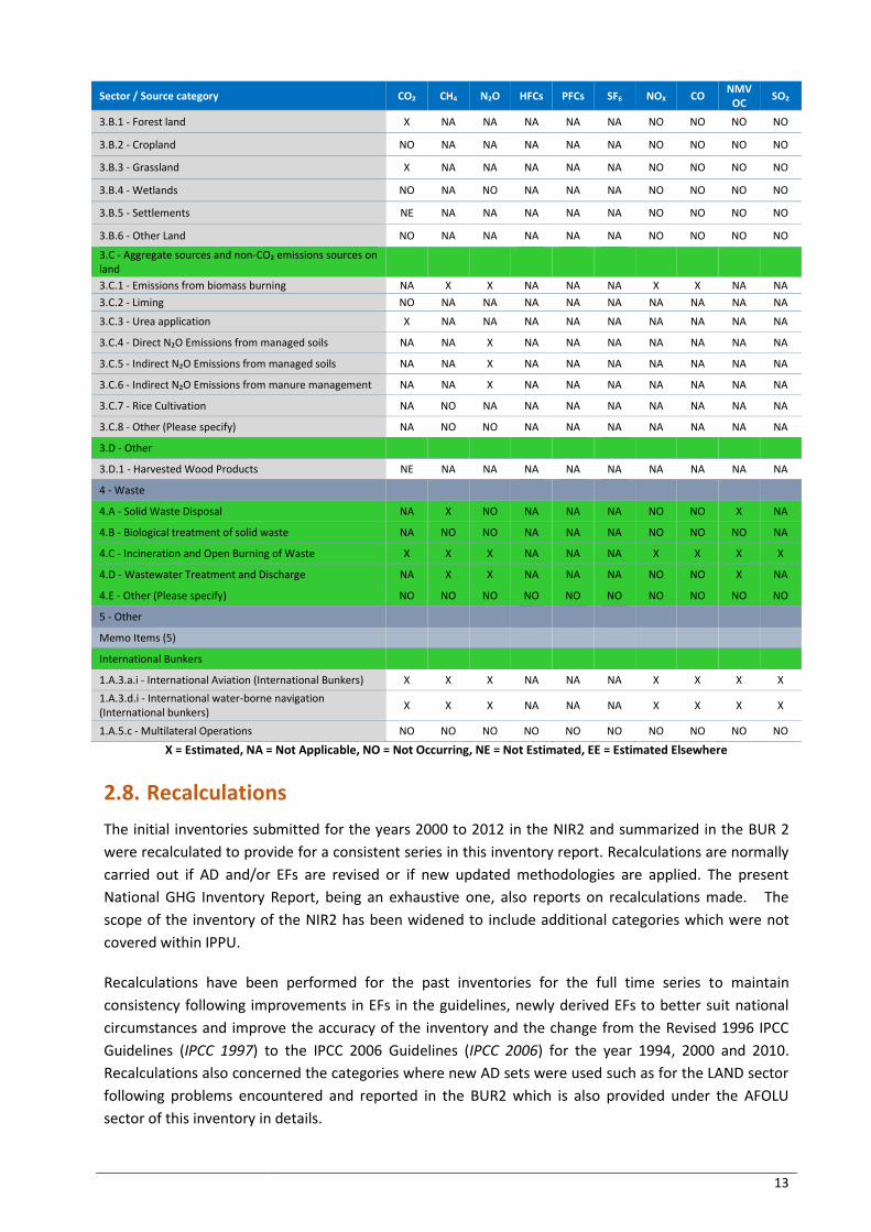
13
Sector / Source category CO₂ CH4 N₂O HFCs PFCs SF6 NOX CO NMV
OC SO₂
3.B.1 - Forest land X NA NA NA NA NA NO NO NO NO
3.B.2 - Cropland NO NA NA NA NA NA NO NO NO NO
3.B.3 - Grassland X NA NA NA NA NA NO NO NO NO
3.B.4 - Wetlands NO NA NO NA NA NA NO NO NO NO
3.B.5 - Settlements NE NA NA NA NA NA NO NO NO NO
3.B.6 - Other Land NO NA NA NA NA NA NO NO NO NO
3.C - Aggregate sources and non-CO₂ emissions sources on land
3.C.1 - Emissions from biomass burning NA X X NA NA NA X X NA NA
3.C.2 - Liming NO NA NA NA NA NA NA NA NA NA
3.C.3 - Urea application X NA NA NA NA NA NA NA NA NA
3.C.4 - Direct N₂O Emissions from managed soils NA NA X NA NA NA NA NA NA NA
3.C.5 - Indirect N₂O Emissions from managed soils NA NA X NA NA NA NA NA NA NA
3.C.6 - Indirect N₂O Emissions from manure management NA NA X NA NA NA NA NA NA NA
3.C.7 - Rice Cultivation NA NO NA NA NA NA NA NA NA NA
3.C.8 - Other (Please specify) NA NO NO NA NA NA NA NA NA NA
3.D - Other
3.D.1 - Harvested Wood Products NE NA NA NA NA NA NA NA NA NA
4 - Waste
4.A - Solid Waste Disposal NA X NO NA NA NA NO NO X NA
4.B - Biological treatment of solid waste NA NO NO NA NA NA NO NO NO NA
4.C - Incineration and Open Burning of Waste X X X NA NA NA X X X X
4.D - Wastewater Treatment and Discharge NA X X NA NA NA NO NO X NA
4.E - Other (Please specify) NO NO NO NO NO NO NO NO NO NO
5 - Other
Memo Items (5)
International Bunkers
1.A.3.a.i - International Aviation (International Bunkers) X X X NA NA NA X X X X
1.A.3.d.i - International water-borne navigation (International bunkers)
X X X NA NA NA X X X X
1.A.5.c - Multilateral Operations NO NO NO NO NO NO NO NO NO NO
X = Estimated, NA = Not Applicable, NO = Not Occurring, NE = Not Estimated, EE = Estimated Elsewhere
2.8. Recalculations
The initial inventories submitted for the years 2000 to 2012 in the NIR2 and summarized in the BUR 2
were recalculated to provide for a consistent series in this inventory report. Recalculations are normally
carried out if AD and/or EFs are revised or if new updated methodologies are applied. The present
National GHG Inventory Report, being an exhaustive one, also reports on recalculations made. The
scope of the inventory of the NIR2 has been widened to include additional categories which were not
covered within IPPU.
Recalculations have been performed for the past inventories for the full time series to maintain
consistency following improvements in EFs in the guidelines, newly derived EFs to better suit national
circumstances and improve the accuracy of the inventory and the change from the Revised 1996 IPCC
Guidelines (IPCC 1997) to the IPCC 2006 Guidelines (IPCC 2006) for the year 1994, 2000 and 2010.
Recalculations also concerned the categories where new AD sets were used such as for the LAND sector
following problems encountered and reported in the BUR2 which is also provided under the AFOLU
sector of this inventory in details.
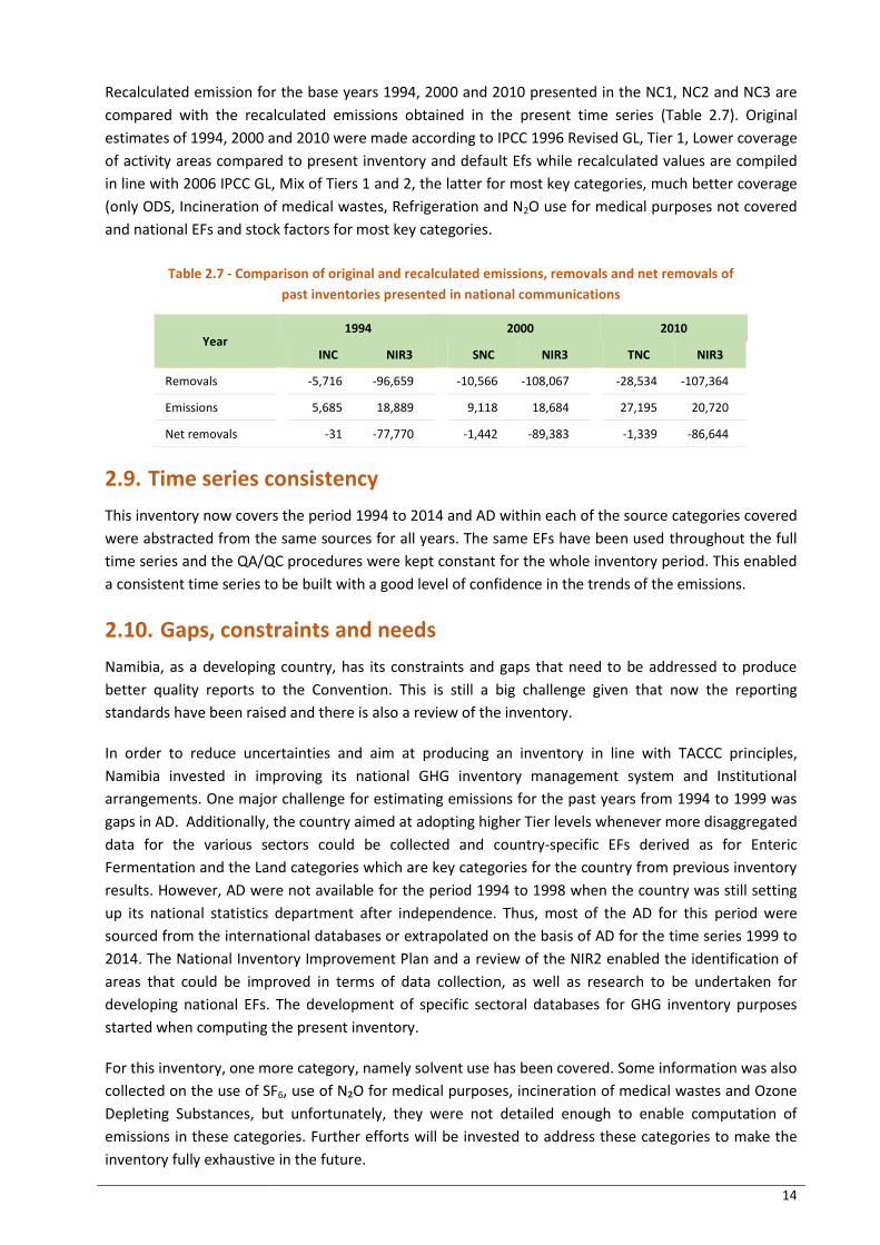
14
Recalculated emission for the base years 1994, 2000 and 2010 presented in the NC1, NC2 and NC3 are
compared with the recalculated emissions obtained in the present time series (Table 2.7). Original
estimates of 1994, 2000 and 2010 were made according to IPCC 1996 Revised GL, Tier 1, Lower coverage
of activity areas compared to present inventory and default Efs while recalculated values are compiled
in line with 2006 IPCC GL, Mix of Tiers 1 and 2, the latter for most key categories, much better coverage
(only ODS, Incineration of medical wastes, Refrigeration and N2O use for medical purposes not covered
and national EFs and stock factors for most key categories.
Table 2.7 - Comparison of original and recalculated emissions, removals and net removals of
past inventories presented in national communications
Year 1994 2000 2010
INC NIR3 SNC NIR3 TNC NIR3
Removals -5,716 -96,659 -10,566 -108,067 -28,534 -107,364
Emissions 5,685 18,889 9,118 18,684 27,195 20,720
Net removals -31 -77,770 -1,442 -89,383 -1,339 -86,644
2.9. Time series consistency
This inventory now covers the period 1994 to 2014 and AD within each of the source categories covered
were abstracted from the same sources for all years. The same EFs have been used throughout the full
time series and the QA/QC procedures were kept constant for the whole inventory period. This enabled
a consistent time series to be built with a good level of confidence in the trends of the emissions.
2.10. Gaps, constraints and needs
Namibia, as a developing country, has its constraints and gaps that need to be addressed to produce
better quality reports to the Convention. This is still a big challenge given that now the reporting
standards have been raised and there is also a review of the inventory.
In order to reduce uncertainties and aim at producing an inventory in line with TACCC principles,
Namibia invested in improving its national GHG inventory management system and Institutional
arrangements. One major challenge for estimating emissions for the past years from 1994 to 1999 was
gaps in AD. Additionally, the country aimed at adopting higher Tier levels whenever more disaggregated
data for the various sectors could be collected and country-specific EFs derived as for Enteric
Fermentation and the Land categories which are key categories for the country from previous inventory
results. However, AD were not available for the period 1994 to 1998 when the country was still setting
up its national statistics department after independence. Thus, most of the AD for this period were
sourced from the international databases or extrapolated on the basis of AD for the time series 1999 to
2014. The National Inventory Improvement Plan and a review of the NIR2 enabled the identification of
areas that could be improved in terms of data collection, as well as research to be undertaken for
developing national EFs. The development of specific sectoral databases for GHG inventory purposes
started when computing the present inventory.
For this inventory, one more category, namely solvent use has been covered. Some information was also
collected on the use of SF6, use of N₂O for medical purposes, incineration of medical wastes and Ozone
Depleting Substances, but unfortunately, they were not detailed enough to enable computation of
emissions in these categories. Further efforts will be invested to address these categories to make the
inventory fully exhaustive in the future.
15
The following problems were encountered during the preparation of this national inventory of GHG:
Information required for the inventory were obtained from various sources as no institution has
yet been endorsed with the responsibility for collection of specific AD needed for the estimation
of emissions according to IPCC on an annual basis;
Almost all of the AD, including those from the NSA are still not yet in the required format for
feeding in the software to make the emission estimates;
End-use consumption data for some of the sectors and categories are not readily available and
had to be generated on the basis of scientific and consumption parameters;
Reliable biomass (bm) data such as timber, fuelwood, wood waste and charcoal consumed or
produced were not available and had to be derived using statistical modelling;
There were frequent inconsistencies when data were collected from different sources;
Appropriate information on some activities such as beverage production and auto-production of
heat and electricity were not always available as these were not released as considered
confidential by the producers;
Lack of solid waste characterization data, amount generated and wastewater generated from
the industrial sector were only partly available and had to be derived on the basis of production
and demographic data amongst others;
Lack of EFs to better represent national circumstances and provide for more accurate estimates
even if this has started to be addressed for some key categories;
Emissions for a few categories have not been estimated due to lack of AD; and
National experts are not yet ready to take over the full inventory compilation process which
dictated the collaboration of an international consultant;
National experts were provided with further capacity building and this will be pursued in the
future until they are fully conversant with the whole process.
2.11. National inventory improvement plan (NIIP)
Based on the constraints, gaps and other challenges encountered during the preparation of the present
inventory, a list of the most urgent improvements has been identified. These are listed below and will be
addressed during the preparation of the next inventory for preparation of the NIR4 within the
framework of the BUR4.
Adequate and proper data capture, QC, validation, storage and retrieval mechanism need to be
improved to facilitate the compilation of future inventories;
Capacity building and strengthening of the existing institutional framework within a GHG
inventory management system to provide improved coordinated action for a smooth
implementation of the GHG inventory cycle for sustainable production of inventories;
Development of emission factors (EFs) more representative of the national context;
Improve the existing QA/QC system including a QA/QC plan in order to reduce uncertainty and
improve inventory quality;
Find the necessary resources to establish a GHG inventory unit within DEA to be responsible for
inventory compilation and coordination;

16
Institutionalize the archiving system;
Pursue efforts for collecting the required AD for categories not covered in this exercise, namely
the use of SF6, use of N₂O for medical purposes, incineration of medical waste and Ozone
Depleting Substances;
Conduct new forest inventories to confirm the new approach adopted for the Land sector;
Produce new maps for 1990 to 2015 to refine land use change data over 5 years periods to
replace the poor-quality maps available now which is proving inadequate;
Refine data collection for determining country-specific (CS) weights for dairy cows, other cattle,
sheep and goats;
Develop the digestible energy (DE) factor for livestock as country-specific data is better than the
default IPCC value to address this key category fully at Tier 2; and
Add the missing years 1990 to 1993 to complete the full time series 1990 to at least 2015 in the
next inventory compilation.
Attempt at estimating emissions for categories not covered yet
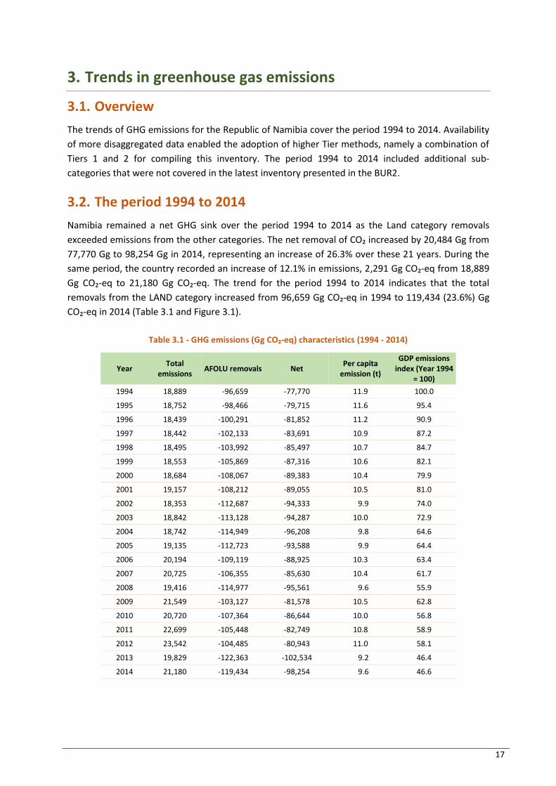
17
3. Trends in greenhouse gas emissions
3.1. Overview
The trends of GHG emissions for the Republic of Namibia cover the period 1994 to 2014. Availability
of more disaggregated data enabled the adoption of higher Tier methods, namely a combination of
Tiers 1 and 2 for compiling this inventory. The period 1994 to 2014 included additional sub-
categories that were not covered in the latest inventory presented in the BUR2.
3.2. The period 1994 to 2014
Namibia remained a net GHG sink over the period 1994 to 2014 as the Land category removals
exceeded emissions from the other categories. The net removal of CO₂ increased by 20,484 Gg from
77,770 Gg to 98,254 Gg in 2014, representing an increase of 26.3% over these 21 years. During the
same period, the country recorded an increase of 12.1% in emissions, 2,291 Gg CO₂-eq from 18,889
Gg CO₂-eq to 21,180 Gg CO₂-eq. The trend for the period 1994 to 2014 indicates that the total
removals from the LAND category increased from 96,659 Gg CO₂-eq in 1994 to 119,434 (23.6%) Gg
CO₂-eq in 2014 (Table 3.1 and Figure 3.1).
Table 3.1 - GHG emissions (Gg CO₂-eq) characteristics (1994 - 2014)
Year Total
emissions AFOLU removals Net
Per capita emission (t)
GDP emissions index (Year 1994
= 100)
1994 18,889 -96,659 -77,770 11.9 100.0
1995 18,752 -98,466 -79,715 11.6 95.4
1996 18,439 -100,291 -81,852 11.2 90.9
1997 18,442 -102,133 -83,691 10.9 87.2
1998 18,495 -103,992 -85,497 10.7 84.7
1999 18,553 -105,869 -87,316 10.6 82.1
2000 18,684 -108,067 -89,383 10.4 79.9
2001 19,157 -108,212 -89,055 10.5 81.0
2002 18,353 -112,687 -94,333 9.9 74.0
2003 18,842 -113,128 -94,287 10.0 72.9
2004 18,742 -114,949 -96,208 9.8 64.6
2005 19,135 -112,723 -93,588 9.9 64.4
2006 20,194 -109,119 -88,925 10.3 63.4
2007 20,725 -106,355 -85,630 10.4 61.7
2008 19,416 -114,977 -95,561 9.6 55.9
2009 21,549 -103,127 -81,578 10.5 62.8
2010 20,720 -107,364 -86,644 10.0 56.8
2011 22,699 -105,448 -82,749 10.8 58.9
2012 23,542 -104,485 -80,943 11.0 58.1
2013 19,829 -122,363 -102,534 9.2 46.4
2014 21,180 -119,434 -98,254 9.6 46.6
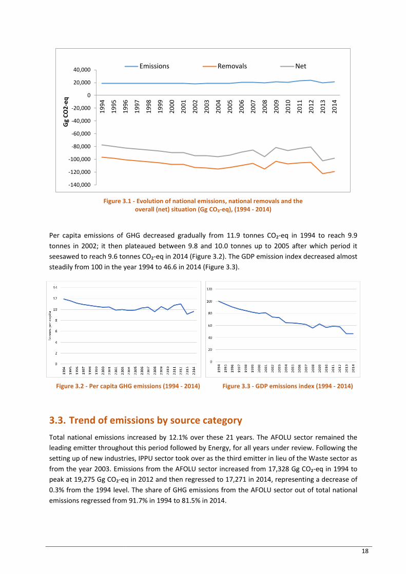
18
Figure 3.1 - Evolution of national emissions, national removals and the overall (net) situation (Gg CO₂-eq), (1994 - 2014)
Per capita emissions of GHG decreased gradually from 11.9 tonnes CO₂-eq in 1994 to reach 9.9
tonnes in 2002; it then plateaued between 9.8 and 10.0 tonnes up to 2005 after which period it
seesawed to reach 9.6 tonnes CO₂-eq in 2014 (Figure 3.2). The GDP emission index decreased almost
steadily from 100 in the year 1994 to 46.6 in 2014 (Figure 3.3).
Figure 3.2 - Per capita GHG emissions (1994 - 2014) Figure 3.3 - GDP emissions index (1994 - 2014)
3.3. Trend of emissions by source category
Total national emissions increased by 12.1% over these 21 years. The AFOLU sector remained the
leading emitter throughout this period followed by Energy, for all years under review. Following the
setting up of new industries, IPPU sector took over as the third emitter in lieu of the Waste sector as
from the year 2003. Emissions from the AFOLU sector increased from 17,328 Gg CO₂-eq in 1994 to
peak at 19,275 Gg CO₂-eq in 2012 and then regressed to 17,271 in 2014, representing a decrease of
0.3% from the 1994 level. The share of GHG emissions from the AFOLU sector out of total national
emissions regressed from 91.7% in 1994 to 81.5% in 2014.
-140,000
-120,000
-100,000
-80,000
-60,000
-40,000
-20,000
0
20,000
40,000
19
94
19
95
19
96
19
97
19
98
19
99
20
00
20
01
20
02
20
03
20
04
20
05
20
06
20
07
20
08
20
09
20
10
20
11
20
12
20
13
20
14
Gg
CO
2-e
q
Emissions Removals Net

19
Energy emissions increased from 1,464 Gg CO₂-eq (7.8%) of national emissions in 1994 to 3,234 Gg
CO₂-eq (15.3%) in 2014 as depicted in Table 3.2. During the period 1994 to 2014, the average annual
increase of GHG emissions was by 6.0%.
The contribution of the IPPU sector in total national emissions increased from 22 Gg CO₂-eq in 1994
to 522 Gg CO₂-eq in 2014 (Table 3.2). The very sharp increase in GHG emissions in the IPPU sector is
due to the commencement of the production of Zinc in 2003 and cement in 2011.
Waste emissions on the other hand varied slightly over this period with the tendency being for a
slight increase over time. Emissions from the waste sector increased from the 1994 level of 75 Gg
CO₂-eq to 153 Gg CO₂-eq in 2014, representing a 5.0% increase.
Table 3.2 - National GHG emissions (Gg, CO₂-eq) by sector (1994 - 2014)
Year Total
emissions Energy IPPU AFOLU Waste
1994 18,889 1,464 22 17,328 75
1995 18,752 1,473 23 17,183 72
1996 18,439 1,566 23 16,777 73
1997 18,442 1,617 24 16,726 76
1998 18,495 1,759 24 16,633 79
1999 18,553 1,893 25 16,551 83
2000 18,684 1,934 25 16,637 88
2001 19,157 2,116 25 16,927 90
2002 18,353 2,163 27 16,073 91
2003 18,842 2,454 110 16,176 101
2004 18,742 2,521 237 15,879 103
2005 19,135 2,671 260 16,094 110
2006 20,194 2,823 255 17,003 112
2007 20,725 2,907 293 17,415 109
2008 19,416 2,752 291 16,256 117
2009 21,549 2,832 303 18,289 125
2010 20,720 2,923 301 17,365 131
2011 22,699 2,796 438 19,326 138
2012 23,542 3,003 515 19,875 149
2013 19,829 2,861 528 16,291 149
2014 21,180 3,234 522 17,271 153
3.4. Trend in emissions of direct GHGs
The share of emissions by gas did not change during the period 1994 to 2014. The main contributor
to the national GHG emissions remained CO₂ followed by CH₄ and N₂O. However, the share of CO₂
increased while these of CH₄ and N₂O regressed over the time series. In 2014, the share of the GHG
emissions was as follows: 63.44% CO₂, 23.98% CH₄ and 12.58% N₂O. The trend of the aggregated
emissions and removals by gas is given in Table 3.3 and Figure 3.4.

20
Table 3.3 - Aggregated emissions and removals (Gg) by gas (1994 - 2014)
Year Total GHG emissions (CO₂-eq)
Removals (CO₂)
(CO₂-eq)
Net removals (CO₂-eq)
CO₂ CH₄ (CO₂-eq) N₂O (CO₂-eq)
1994 18,889 -96,659 -77,770 10,169 5,837 2,884
1995 18,752 -98,466 -79,715 10,177 5,728 2,847
1996 18,439 -100,291 -81,852 10,268 5,458 2,713
1997 18,442 -102,133 -83,691 10,318 5,415 2,710
1998 18,495 -103,992 -85,497 10,457 5,352 2,685
1999 18,553 -105,869 -87,316 10,591 5,295 2,667
2000 18,684 -108,067 -89,383 10,629 5,367 2,687
2001 19,157 -108,212 -89,055 11,021 5,394 2,742
2002 18,353 -112,687 -94,333 11,070 4,797 2,487
2003 18,842 -113,128 -94,287 11,438 4,873 2,531
2004 18,742 -114,949 -96,208 11,630 4,665 2,447
2005 19,135 -112,723 -93,588 11,799 4,832 2,504
2006 20,194 -109,119 -88,925 11,944 5,458 2,793
2007 20,725 -106,355 -85,630 12,063 5,717 2,945
2008 19,416 -114,977 -95,561 11,910 4,944 2,563
2009 21,549 -103,127 -81,578 11,999 6,362 3,187
2010 20,720 -107,364 -86,644 12,086 5,732 2,903
2011 22,699 -105,448 -82,749 12,922 6,477 3,300
2012 23,542 -104,485 -80,943 13,204 6,845 3,494
2013 19,829 -122,363 -102,534 13,076 4,395 2,359
2014 21,180 -119,434 -98,254 13,436 5,079 2,665
Figure 3.4 - Share of aggregated emissions (Gg CO₂-eq) by gas (1994 - 2014)
3.4.1. Carbon dioxide (CO₂)
The most significant anthropogenic GHG was CO₂. In 2014, it contributed the more than half of
national emissions with 13,436 Gg (63.44%). CO₂ emissions increased by 3,268 Gg from the 1994
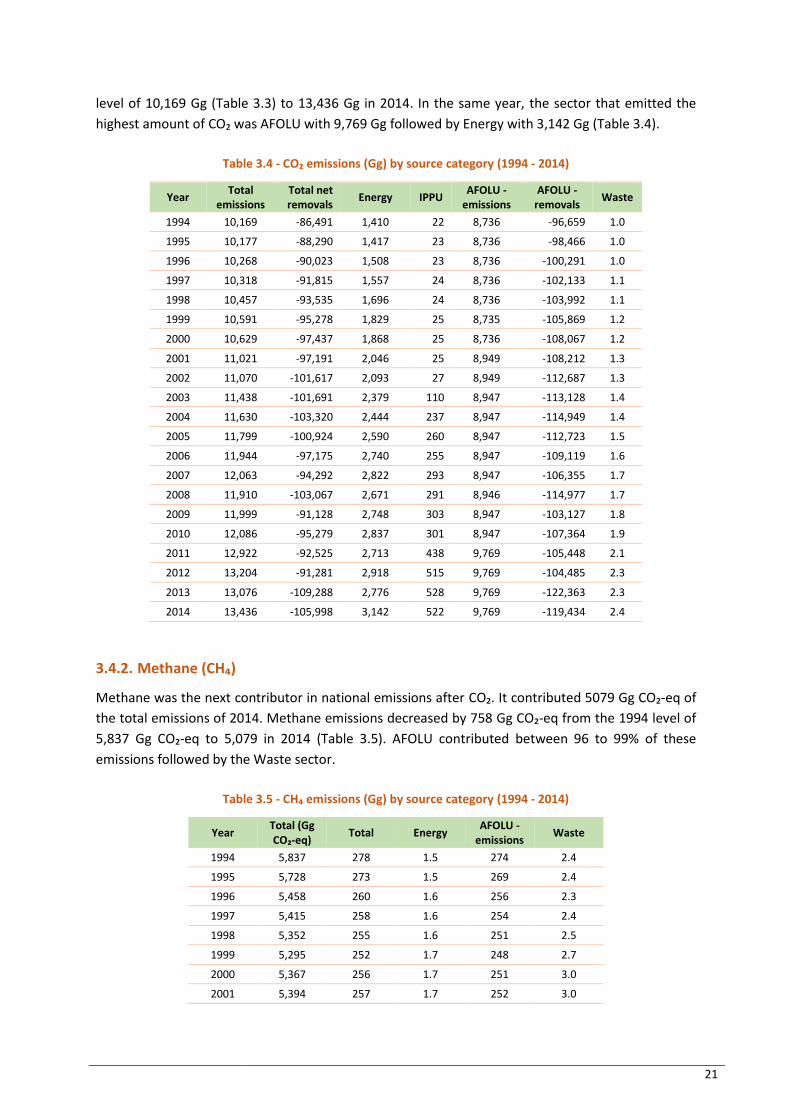
21
level of 10,169 Gg (Table 3.3) to 13,436 Gg in 2014. In the same year, the sector that emitted the
highest amount of CO₂ was AFOLU with 9,769 Gg followed by Energy with 3,142 Gg (Table 3.4).
Table 3.4 - CO₂ emissions (Gg) by source category (1994 - 2014)
Year Total
emissions Total net removals
Energy IPPU AFOLU -
emissions AFOLU -
removals Waste
1994 10,169 -86,491 1,410 22 8,736 -96,659 1.0
1995 10,177 -88,290 1,417 23 8,736 -98,466 1.0
1996 10,268 -90,023 1,508 23 8,736 -100,291 1.0
1997 10,318 -91,815 1,557 24 8,736 -102,133 1.1
1998 10,457 -93,535 1,696 24 8,736 -103,992 1.1
1999 10,591 -95,278 1,829 25 8,735 -105,869 1.2
2000 10,629 -97,437 1,868 25 8,736 -108,067 1.2
2001 11,021 -97,191 2,046 25 8,949 -108,212 1.3
2002 11,070 -101,617 2,093 27 8,949 -112,687 1.3
2003 11,438 -101,691 2,379 110 8,947 -113,128 1.4
2004 11,630 -103,320 2,444 237 8,947 -114,949 1.4
2005 11,799 -100,924 2,590 260 8,947 -112,723 1.5
2006 11,944 -97,175 2,740 255 8,947 -109,119 1.6
2007 12,063 -94,292 2,822 293 8,947 -106,355 1.7
2008 11,910 -103,067 2,671 291 8,946 -114,977 1.7
2009 11,999 -91,128 2,748 303 8,947 -103,127 1.8
2010 12,086 -95,279 2,837 301 8,947 -107,364 1.9
2011 12,922 -92,525 2,713 438 9,769 -105,448 2.1
2012 13,204 -91,281 2,918 515 9,769 -104,485 2.3
2013 13,076 -109,288 2,776 528 9,769 -122,363 2.3
2014 13,436 -105,998 3,142 522 9,769 -119,434 2.4
3.4.2. Methane (CH₄)
Methane was the next contributor in national emissions after CO₂. It contributed 5079 Gg CO₂-eq of
the total emissions of 2014. Methane emissions decreased by 758 Gg CO₂-eq from the 1994 level of
5,837 Gg CO₂-eq to 5,079 in 2014 (Table 3.5). AFOLU contributed between 96 to 99% of these
emissions followed by the Waste sector.
Table 3.5 - CH₄ emissions (Gg) by source category (1994 - 2014)
Year Total (Gg CO₂-eq)
Total Energy AFOLU -
emissions Waste
1994 5,837 278 1.5 274 2.4
1995 5,728 273 1.5 269 2.4
1996 5,458 260 1.6 256 2.3
1997 5,415 258 1.6 254 2.4
1998 5,352 255 1.6 251 2.5
1999 5,295 252 1.7 248 2.7
2000 5,367 256 1.7 251 3.0
2001 5,394 257 1.7 252 3.0
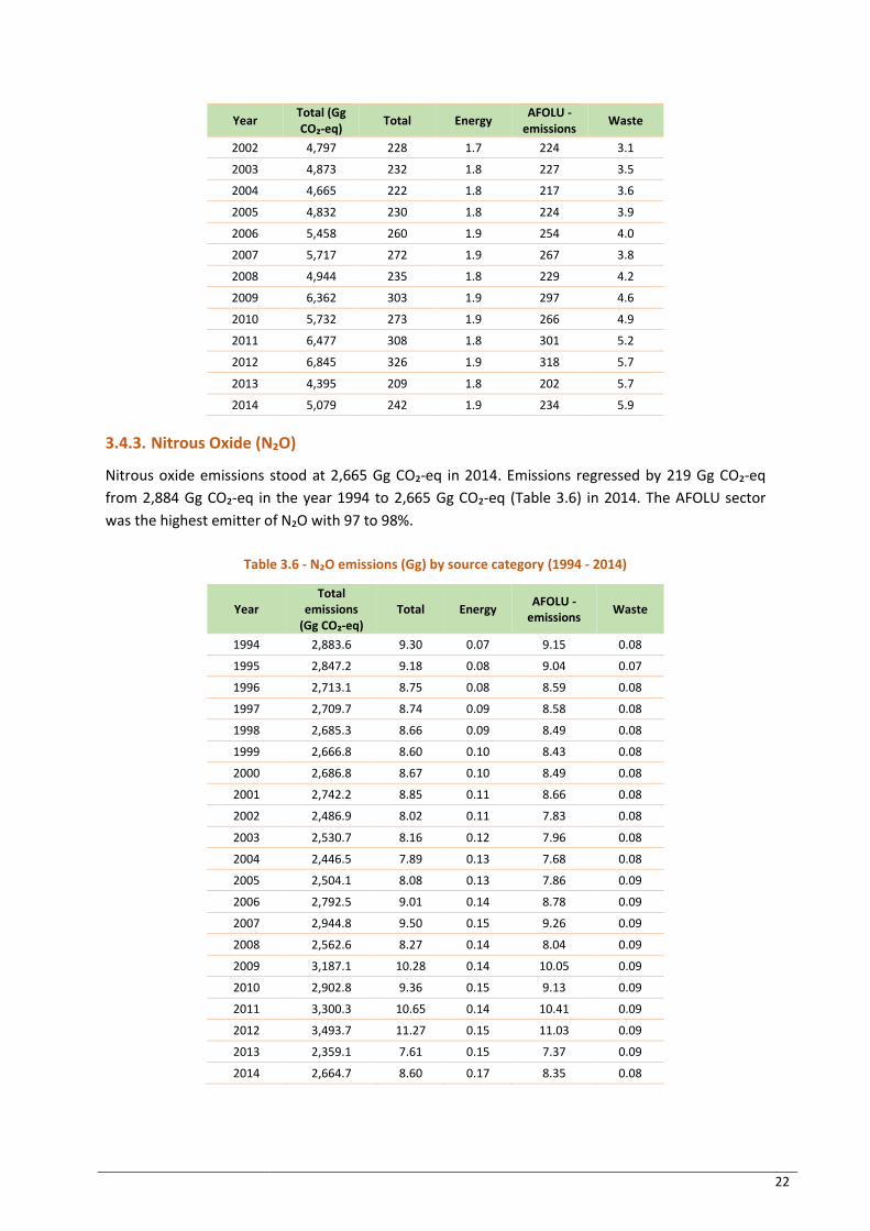
22
Year Total (Gg CO₂-eq)
Total Energy AFOLU -
emissions Waste
2002 4,797 228 1.7 224 3.1
2003 4,873 232 1.8 227 3.5
2004 4,665 222 1.8 217 3.6
2005 4,832 230 1.8 224 3.9
2006 5,458 260 1.9 254 4.0
2007 5,717 272 1.9 267 3.8
2008 4,944 235 1.8 229 4.2
2009 6,362 303 1.9 297 4.6
2010 5,732 273 1.9 266 4.9
2011 6,477 308 1.8 301 5.2
2012 6,845 326 1.9 318 5.7
2013 4,395 209 1.8 202 5.7
2014 5,079 242 1.9 234 5.9
3.4.3. Nitrous Oxide (N₂O)
Nitrous oxide emissions stood at 2,665 Gg CO₂-eq in 2014. Emissions regressed by 219 Gg CO₂-eq
from 2,884 Gg CO₂-eq in the year 1994 to 2,665 Gg CO₂-eq (Table 3.6) in 2014. The AFOLU sector
was the highest emitter of N₂O with 97 to 98%.
Table 3.6 - N₂O emissions (Gg) by source category (1994 - 2014)
Year Total
emissions (Gg CO₂-eq)
Total Energy AFOLU -
emissions Waste
1994 2,883.6 9.30 0.07 9.15 0.08
1995 2,847.2 9.18 0.08 9.04 0.07
1996 2,713.1 8.75 0.08 8.59 0.08
1997 2,709.7 8.74 0.09 8.58 0.08
1998 2,685.3 8.66 0.09 8.49 0.08
1999 2,666.8 8.60 0.10 8.43 0.08
2000 2,686.8 8.67 0.10 8.49 0.08
2001 2,742.2 8.85 0.11 8.66 0.08
2002 2,486.9 8.02 0.11 7.83 0.08
2003 2,530.7 8.16 0.12 7.96 0.08
2004 2,446.5 7.89 0.13 7.68 0.08
2005 2,504.1 8.08 0.13 7.86 0.09
2006 2,792.5 9.01 0.14 8.78 0.09
2007 2,944.8 9.50 0.15 9.26 0.09
2008 2,562.6 8.27 0.14 8.04 0.09
2009 3,187.1 10.28 0.14 10.05 0.09
2010 2,902.8 9.36 0.15 9.13 0.09
2011 3,300.3 10.65 0.14 10.41 0.09
2012 3,493.7 11.27 0.15 11.03 0.09
2013 2,359.1 7.61 0.15 7.37 0.09
2014 2,664.7 8.60 0.17 8.35 0.08
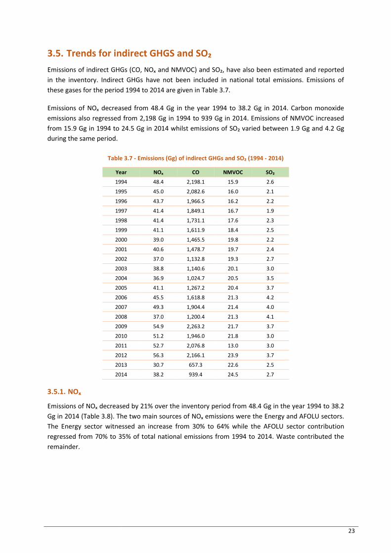
23
3.5. Trends for indirect GHGS and SO₂
Emissions of indirect GHGs (CO, NOₓ and NMVOC) and SO₂, have also been estimated and reported
in the inventory. Indirect GHGs have not been included in national total emissions. Emissions of
these gases for the period 1994 to 2014 are given in Table 3.7.
Emissions of NOₓ decreased from 48.4 Gg in the year 1994 to 38.2 Gg in 2014. Carbon monoxide
emissions also regressed from 2,198 Gg in 1994 to 939 Gg in 2014. Emissions of NMVOC increased
from 15.9 Gg in 1994 to 24.5 Gg in 2014 whilst emissions of SO₂ varied between 1.9 Gg and 4.2 Gg
during the same period.
Table 3.7 - Emissions (Gg) of indirect GHGs and SO₂ (1994 - 2014)
Year NOₓ CO NMVOC SO₂
1994 48.4 2,198.1 15.9 2.6
1995 45.0 2,082.6 16.0 2.1
1996 43.7 1,966.5 16.2 2.2
1997 41.4 1,849.1 16.7 1.9
1998 41.4 1,731.1 17.6 2.3
1999 41.1 1,611.9 18.4 2.5
2000 39.0 1,465.5 19.8 2.2
2001 40.6 1,478.7 19.7 2.4
2002 37.0 1,132.8 19.3 2.7
2003 38.8 1,140.6 20.1 3.0
2004 36.9 1,024.7 20.5 3.5
2005 41.1 1,267.2 20.4 3.7
2006 45.5 1,618.8 21.3 4.2
2007 49.3 1,904.4 21.4 4.0
2008 37.0 1,200.4 21.3 4.1
2009 54.9 2,263.2 21.7 3.7
2010 51.2 1,946.0 21.8 3.0
2011 52.7 2,076.8 13.0 3.0
2012 56.3 2,166.1 23.9 3.7
2013 30.7 657.3 22.6 2.5
2014 38.2 939.4 24.5 2.7
3.5.1. NOₓ
Emissions of NOₓ decreased by 21% over the inventory period from 48.4 Gg in the year 1994 to 38.2
Gg in 2014 (Table 3.8). The two main sources of NOₓ emissions were the Energy and AFOLU sectors.
The Energy sector witnessed an increase from 30% to 64% while the AFOLU sector contribution
regressed from 70% to 35% of total national emissions from 1994 to 2014. Waste contributed the
remainder.
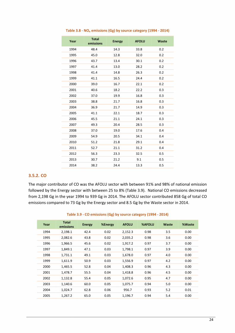
24
Table 3.8 - NOₓ emissions (Gg) by source category (1994 - 2014)
Year Total
emissions Energy AFOLU Waste
1994 48.4 14.3 33.8 0.2
1995 45.0 12.8 32.0 0.2
1996 43.7 13.4 30.1 0.2
1997 41.4 13.0 28.2 0.2
1998 41.4 14.8 26.3 0.2
1999 41.1 16.5 24.4 0.2
2000 39.0 16.7 22.1 0.2
2001 40.6 18.2 22.2 0.3
2002 37.0 19.9 16.8 0.3
2003 38.8 21.7 16.8 0.3
2004 36.9 21.7 14.9 0.3
2005 41.1 22.1 18.7 0.3
2006 45.5 21.1 24.1 0.3
2007 49.3 20.4 28.5 0.3
2008 37.0 19.0 17.6 0.4
2009 54.9 20.5 34.1 0.4
2010 51.2 21.8 29.1 0.4
2011 52.7 21.1 31.2 0.4
2012 56.3 23.3 32.5 0.5
2013 30.7 21.2 9.1 0.5
2014 38.2 24.4 13.3 0.5
3.5.2. CO
The major contributor of CO was the AFOLU sector with between 91% and 98% of national emission
followed by the Energy sector with between 25 to 8% (Table 3.9). National CO emissions decreased
from 2,198 Gg in the year 1994 to 939 Gg in 2014. The AFOLU sector contributed 858 Gg of total CO
emissions compared to 73 Gg by the Energy sector and 8.5 Gg by the Waste sector in 2014.
Table 3.9 - CO emissions (Gg) by source category (1994 - 2014)
Year Total
emissions Energy %Energy AFOLU %AFOLU Waste %Waste
1994 2,198.1 42.4 0.02 2,152.3 0.98 3.5 0.00
1995 2,082.6 43.8 0.02 2,035.2 0.98 3.6 0.00
1996 1,966.5 45.6 0.02 1,917.2 0.97 3.7 0.00
1997 1,849.1 47.1 0.03 1,798.1 0.97 3.9 0.00
1998 1,731.1 49.1 0.03 1,678.0 0.97 4.0 0.00
1999 1,611.9 50.9 0.03 1,556.9 0.97 4.2 0.00
2000 1,465.5 52.8 0.04 1,408.3 0.96 4.3 0.00
2001 1,478.7 55.5 0.04 1,418.8 0.96 4.5 0.00
2002 1,132.8 55.4 0.05 1,072.6 0.95 4.7 0.00
2003 1,140.6 60.0 0.05 1,075.7 0.94 5.0 0.00
2004 1,024.7 62.8 0.06 956.7 0.93 5.2 0.01
2005 1,267.2 65.0 0.05 1,196.7 0.94 5.4 0.00
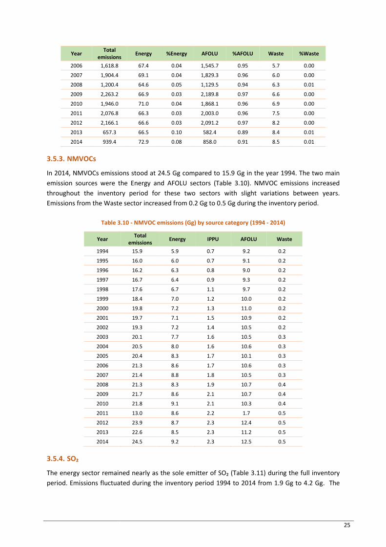
25
Year Total
emissions Energy %Energy AFOLU %AFOLU Waste %Waste
2006 1,618.8 67.4 0.04 1,545.7 0.95 5.7 0.00
2007 1,904.4 69.1 0.04 1,829.3 0.96 6.0 0.00
2008 1,200.4 64.6 0.05 1,129.5 0.94 6.3 0.01
2009 2,263.2 66.9 0.03 2,189.8 0.97 6.6 0.00
2010 1,946.0 71.0 0.04 1,868.1 0.96 6.9 0.00
2011 2,076.8 66.3 0.03 2,003.0 0.96 7.5 0.00
2012 2,166.1 66.6 0.03 2,091.2 0.97 8.2 0.00
2013 657.3 66.5 0.10 582.4 0.89 8.4 0.01
2014 939.4 72.9 0.08 858.0 0.91 8.5 0.01
3.5.3. NMVOCs
In 2014, NMVOCs emissions stood at 24.5 Gg compared to 15.9 Gg in the year 1994. The two main
emission sources were the Energy and AFOLU sectors (Table 3.10). NMVOC emissions increased
throughout the inventory period for these two sectors with slight variations between years.
Emissions from the Waste sector increased from 0.2 Gg to 0.5 Gg during the inventory period.
Table 3.10 - NMVOC emissions (Gg) by source category (1994 - 2014)
Year Total
emissions Energy IPPU AFOLU Waste
1994 15.9 5.9 0.7 9.2 0.2
1995 16.0 6.0 0.7 9.1 0.2
1996 16.2 6.3 0.8 9.0 0.2
1997 16.7 6.4 0.9 9.3 0.2
1998 17.6 6.7 1.1 9.7 0.2
1999 18.4 7.0 1.2 10.0 0.2
2000 19.8 7.2 1.3 11.0 0.2
2001 19.7 7.1 1.5 10.9 0.2
2002 19.3 7.2 1.4 10.5 0.2
2003 20.1 7.7 1.6 10.5 0.3
2004 20.5 8.0 1.6 10.6 0.3
2005 20.4 8.3 1.7 10.1 0.3
2006 21.3 8.6 1.7 10.6 0.3
2007 21.4 8.8 1.8 10.5 0.3
2008 21.3 8.3 1.9 10.7 0.4
2009 21.7 8.6 2.1 10.7 0.4
2010 21.8 9.1 2.1 10.3 0.4
2011 13.0 8.6 2.2 1.7 0.5
2012 23.9 8.7 2.3 12.4 0.5
2013 22.6 8.5 2.3 11.2 0.5
2014 24.5 9.2 2.3 12.5 0.5
3.5.4. SO₂
The energy sector remained nearly as the sole emitter of SO₂ (Table 3.11) during the full inventory
period. Emissions fluctuated during the inventory period 1994 to 2014 from 1.9 Gg to 4.2 Gg. The

26
Waste sector emitted an insignificant amount varying from 0.01 to 0.02 Gg during the inventory
period.
Table 3.11 - SO₂ emissions (Gg) by source category (1994 - 2014)
Year Total emissions Energy Waste
1994 2.6 2.6 0.01
1995 2.1 2.1 0.01
1996 2.2 2.2 0.01
1997 1.9 1.9 0.01
1998 2.3 2.2 0.01
1999 2.5 2.5 0.01
2000 2.2 2.2 0.01
2001 2.4 2.4 0.01
2002 2.7 2.7 0.01
2003 3.0 3.0 0.01
2004 3.5 3.5 0.01
2005 3.7 3.7 0.01
2006 4.2 4.2 0.01
2007 4.0 4.0 0.01
2008 4.1 4.1 0.01
2009 3.7 3.7 0.01
2010 3.0 2.9 0.01
2011 3.0 3.0 0.01
2012 3.7 3.7 0.02
2013 2.5 2.5 0.02
2014 2.7 2.7 0.02
27
4. Energy
4.1. Description of Energy sector
Namibia is concerned only with activities occurring in the Fuel Combustion Category. Activities
occurred under all sub-categories and GHG emissions have been estimated for all of them.
4.1.1. Fuel Combustion Activities (1.A)
4.1.1.1. Energy Industries (1.A.1)
The Energy Industries sub-category covers the production of electricity from a mix of liquid and solid
fossil fuels. The contribution of fossil fuels is however minimal in the national energy balance since
the country generates a high proportion of its electricity from hydro to supplement the imported
power which stands at about 63% of Namibia’s demand from the South African Power Pool (SAPP)
Zambia and Zimbabwe compared to 65% in 2012.
Namibia’s currently total installed electricity generation capacity is about 500 MW for a peak
demand of some 597 MW normally. The biggest generation plant is the Ruacana Hydro Power
station which generates about 332 MW of electricity, Van Eck Coal power station generates about
120 MW and the Paratus and Anixas diesel power stations at the coast with 24 MW and 22.5 MW
respectively (Konrad et al., 2013). The fossil fuel generation plants are mainly used to supplement
the imports and hydro production during peak demand time. Solar and wind potential exists but are
tapped only marginally up to now. The strategy is geared towards penetration of renewable energy
sources and a better idea of the status can be obtained in the mitigation chapter of this report
where actions are more extensively described.
4.1.1.2. Manufacturing Industries and Construction (1.A.2)
Fossil fuel inputs are primarily used for generating process heat within the mining sector and in the
production of cement. The two main mining companies also imported electricity directly from the
neighbouring countries. The construction industry is highly diversified and detailed information was
not available. There are some auto-production of electricity in this sub-category and efforts are
being invested to collect data for estimating emissions from this process separately in the future.
4.1.1.3. Transport (1.A.3)
The transport sector includes domestic aviation, road transportation, railways and domestic water-
borne navigation. Emissions for the three sub-categories domestic aviation, road transportation and
railways have been computed in this inventory. Lack of data prevented estimation of emissions for
domestic water-borne navigation which is of lesser importance compared to the other three areas of
transport. Fuel supplied for international bunkering was also covered.
4.1.1.4. Other Sectors (1.A.4)
The sub-categories included under Other Sectors were the two main GHG contributors Residential
and Fishing. AD for Commercial/Institutional, Stationary combustion and, Off-road vehicles and
other machinery within the Agriculture and Forestry sectors were not available. It should however
be pointed out that the fuels consumed in these sub-categories have been accounted for under
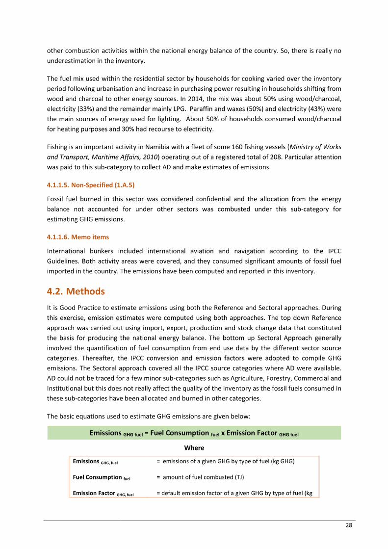
28
other combustion activities within the national energy balance of the country. So, there is really no
underestimation in the inventory.
The fuel mix used within the residential sector by households for cooking varied over the inventory
period following urbanisation and increase in purchasing power resulting in households shifting from
wood and charcoal to other energy sources. In 2014, the mix was about 50% using wood/charcoal,
electricity (33%) and the remainder mainly LPG. Paraffin and waxes (50%) and electricity (43%) were
the main sources of energy used for lighting. About 50% of households consumed wood/charcoal
for heating purposes and 30% had recourse to electricity.
Fishing is an important activity in Namibia with a fleet of some 160 fishing vessels (Ministry of Works
and Transport, Maritime Affairs, 2010) operating out of a registered total of 208. Particular attention
was paid to this sub-category to collect AD and make estimates of emissions.
4.1.1.5. Non-Specified (1.A.5)
Fossil fuel burned in this sector was considered confidential and the allocation from the energy
balance not accounted for under other sectors was combusted under this sub-category for
estimating GHG emissions.
4.1.1.6. Memo items
International bunkers included international aviation and navigation according to the IPCC
Guidelines. Both activity areas were covered, and they consumed significant amounts of fossil fuel
imported in the country. The emissions have been computed and reported in this inventory.
4.2. Methods
It is Good Practice to estimate emissions using both the Reference and Sectoral approaches. During
this exercise, emission estimates were computed using both approaches. The top down Reference
approach was carried out using import, export, production and stock change data that constituted
the basis for producing the national energy balance. The bottom up Sectoral Approach generally
involved the quantification of fuel consumption from end use data by the different sector source
categories. Thereafter, the IPCC conversion and emission factors were adopted to compile GHG
emissions. The Sectoral approach covered all the IPCC source categories where AD were available.
AD could not be traced for a few minor sub-categories such as Agriculture, Forestry, Commercial and
Institutional but this does not really affect the quality of the inventory as the fossil fuels consumed in
these sub-categories have been allocated and burned in other categories.
The basic equations used to estimate GHG emissions are given below:
Emissions GHG fuel = Fuel Consumption fuel x Emission Factor GHG fuel
Where
Emissions GHG, fuel
= emissions of a given GHG by type of fuel (kg GHG)
Fuel Consumption fuel
= amount of fuel combusted (TJ)
Emission Factor GHG, fuel = default emission factor of a given GHG by type of fuel (kg

29
gas/TJ). For CO₂, it includes the carbon oxidation factor, assumed to be 1.
4.3. Activity Data
AD for working out the reference approach was obtained from the energy database of the NSA on
imports and exports of energy products. For the bottom up sectoral approach, AD were sourced
from the end-users of fossil fuels. Data on biomass used were derived from data on consumption of
different fuels by households collected in the censuses conducted by the NSA. The same approach
was used to determine the amount of charcoal used. The data collection covered all solid, liquid and
gaseous fossil fuels, fuelwood and charcoal. In cases where data were missing or to correct for
outliers, the inventory compilers resorted to international databases including those from
International Energy Agency, the United Nations and Food and Agriculture Organisation among
others. These sources provided most of the AD required for the period 1994 to 2002 but to a lesser
extent for the period 2003 to 2014 as the country was still in the process of organising its statistical
organisation after gaining independence. Missing data of these years were thus obtained from the
international databases or from extrapolation of the available time series. Where necessary proxies
such as population, GDP and production data were used to ascertain the generated data.
A summary of data sources of the country is given in Table 4.1.
Table 4.1 - Summary of data sources
Category Fuel type Data source
Energy industries Fuel oil Nampower
Coal Nampower
Mining
Gasolene/Diesel ECB Project “Energy Policy, Regulatory Framework and Energy Future of Namibia (2011-2013)”.
Coal ECB Project “Energy Policy, Regulatory Framework and Energy Future of Namibia (2011-2013)”.
Waste oil National statistics.
Other manufacturing
Gasoline/Diesel Ministry of Industrialization, Trade and SME Development.
Domestic aviation
Aviation Gasoline Airport profile data and national statistics
Jet kerosene Airport profile data and national statistics.
Road Transport Gasoline/Diesel
Gasoline and diesel estimated for the different IPCC vehicles classes in the fleet, mileage run by each and fuel consumption indicators for respective years
LPG Import and export data from NSA
Railways Diesel/residual TransNamib
Residential
Kerosene Import and export data from NSA.
LPG Import and export data from NSA.
Wax candles Ministry of Industrialization, Trade and SME Development and import and export data from NSA
Wood fuel Derived from NSA census data.
Charcoal Derived from NSA census data and import and export data from NSA.
Agriculture/ fishing
Gasoline Import and export data from NSA.
Diesel National statistics on consumption and import and export from NSA.
International aviation bunkers
Jet kerosene Airport profile data and national statistics.
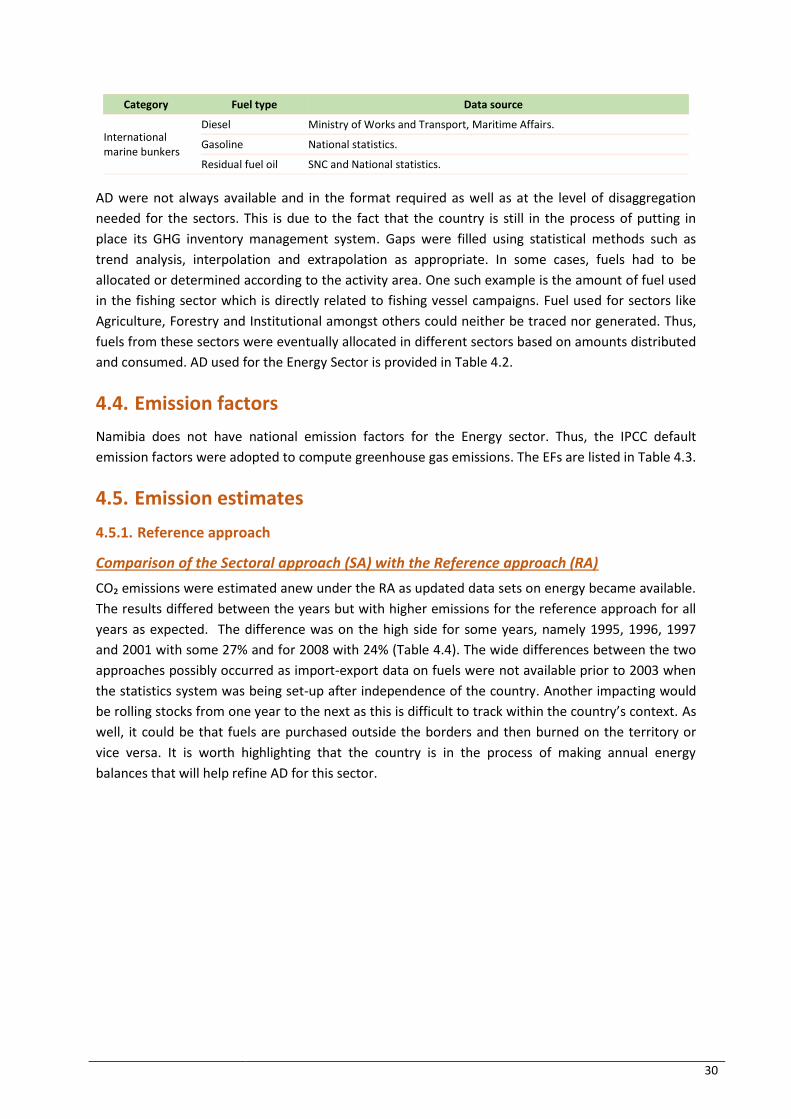
30
Category Fuel type Data source
International marine bunkers
Diesel Ministry of Works and Transport, Maritime Affairs.
Gasoline National statistics.
Residual fuel oil SNC and National statistics.
AD were not always available and in the format required as well as at the level of disaggregation
needed for the sectors. This is due to the fact that the country is still in the process of putting in
place its GHG inventory management system. Gaps were filled using statistical methods such as
trend analysis, interpolation and extrapolation as appropriate. In some cases, fuels had to be
allocated or determined according to the activity area. One such example is the amount of fuel used
in the fishing sector which is directly related to fishing vessel campaigns. Fuel used for sectors like
Agriculture, Forestry and Institutional amongst others could neither be traced nor generated. Thus,
fuels from these sectors were eventually allocated in different sectors based on amounts distributed
and consumed. AD used for the Energy Sector is provided in Table 4.2.
4.4. Emission factors
Namibia does not have national emission factors for the Energy sector. Thus, the IPCC default
emission factors were adopted to compute greenhouse gas emissions. The EFs are listed in Table 4.3.
4.5. Emission estimates
4.5.1. Reference approach
Comparison of the Sectoral approach (SA) with the Reference approach (RA)
CO₂ emissions were estimated anew under the RA as updated data sets on energy became available.
The results differed between the years but with higher emissions for the reference approach for all
years as expected. The difference was on the high side for some years, namely 1995, 1996, 1997
and 2001 with some 27% and for 2008 with 24% (Table 4.4). The wide differences between the two
approaches possibly occurred as import-export data on fuels were not available prior to 2003 when
the statistics system was being set-up after independence of the country. Another impacting would
be rolling stocks from one year to the next as this is difficult to track within the country’s context. As
well, it could be that fuels are purchased outside the borders and then burned on the territory or
vice versa. It is worth highlighting that the country is in the process of making annual energy
balances that will help refine AD for this sector.
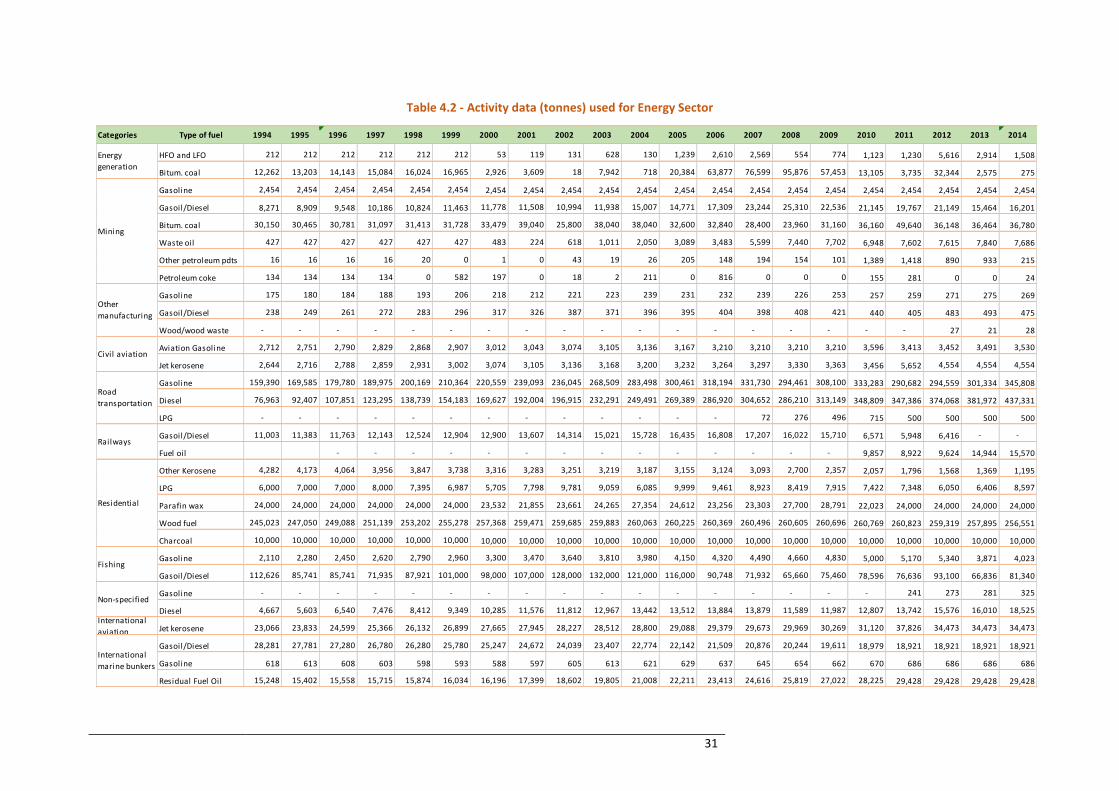
31
Table 4.2 - Activity data (tonnes) used for Energy Sector
Categories Type of fuel 1994 1995 1996 1997 1998 1999 2000 2001 2002 2003 2004 2005 2006 2007 2008 2009 2010 2011 2012 2013 2014
HFO and LFO 212 212 212 212 212 212 53 119 131 628 130 1,239 2,610 2,569 554 774 1,123 1,230 5,616 2,914 1,508
Bitum. coal 12,262 13,203 14,143 15,084 16,024 16,965 2,926 3,609 18 7,942 718 20,384 63,877 76,599 95,876 57,453 13,105 3,735 32,344 2,575 275
Gasoline 2,454 2,454 2,454 2,454 2,454 2,454 2,454 2,454 2,454 2,454 2,454 2,454 2,454 2,454 2,454 2,454 2,454 2,454 2,454 2,454 2,454
Gasoil/Diesel 8,271 8,909 9,548 10,186 10,824 11,463 11,778 11,508 10,994 11,938 15,007 14,771 17,309 23,244 25,310 22,536 21,145 19,767 21,149 15,464 16,201
Bitum. coal 30,150 30,465 30,781 31,097 31,413 31,728 33,479 39,040 25,800 38,040 38,040 32,600 32,840 28,400 23,960 31,160 36,160 49,640 36,148 36,464 36,780
Waste oil 427 427 427 427 427 427 483 224 618 1,011 2,050 3,089 3,483 5,599 7,440 7,702 6,948 7,602 7,615 7,840 7,686
Other petroleum pdts 16 16 16 16 20 0 1 0 43 19 26 205 148 194 154 101 1,389 1,418 890 933 215
Petroleum coke 134 134 134 134 0 582 197 0 18 2 211 0 816 0 0 0 155 281 0 0 24
Gasoline 175 180 184 188 193 206 218 212 221 223 239 231 232 239 226 253 257 259 271 275 269
Gasoil/Diesel 238 249 261 272 283 296 317 326 387 371 396 395 404 398 408 421 440 405 483 493 475
Wood/wood waste - - - - - - - - - - - - - - - - - - 27 21 28
Aviation Gasoline 2,712 2,751 2,790 2,829 2,868 2,907 3,012 3,043 3,074 3,105 3,136 3,167 3,210 3,210 3,210 3,210 3,596 3,413 3,452 3,491 3,530
Jet kerosene 2,644 2,716 2,788 2,859 2,931 3,002 3,074 3,105 3,136 3,168 3,200 3,232 3,264 3,297 3,330 3,363 3,456 5,652 4,554 4,554 4,554
Gasoline 159,390 169,585 179,780 189,975 200,169 210,364 220,559 239,093 236,045 268,509 283,498 300,461 318,194 331,730 294,461 308,100 333,283 290,682 294,559 301,334 345,808
Diesel 76,963 92,407 107,851 123,295 138,739 154,183 169,627 192,004 196,915 232,291 249,491 269,389 286,920 304,652 286,210 313,149 348,809 347,386 374,068 381,972 437,331
LPG - - - - - - - - - - - - - 72 276 496 715 500 500 500 500
Gasoil/Diesel 11,003 11,383 11,763 12,143 12,524 12,904 12,900 13,607 14,314 15,021 15,728 16,435 16,808 17,207 16,022 15,710 6,571 5,948 6,416 - -
Fuel oil - - - - - - - - - - - - - - 9,857 8,922 9,624 14,944 15,570
Other Kerosene 4,282 4,173 4,064 3,956 3,847 3,738 3,316 3,283 3,251 3,219 3,187 3,155 3,124 3,093 2,700 2,357 2,057 1,796 1,568 1,369 1,195
LPG 6,000 7,000 7,000 8,000 7,395 6,987 5,705 7,798 9,781 9,059 6,085 9,999 9,461 8,923 8,419 7,915 7,422 7,348 6,050 6,406 8,597
Parafin wax 24,000 24,000 24,000 24,000 24,000 24,000 23,532 21,855 23,661 24,265 27,354 24,612 23,256 23,303 27,700 28,791 22,023 24,000 24,000 24,000 24,000
Wood fuel 245,023 247,050 249,088 251,139 253,202 255,278 257,368 259,471 259,685 259,883 260,063 260,225 260,369 260,496 260,605 260,696 260,769 260,823 259,319 257,895 256,551
Charcoal 10,000 10,000 10,000 10,000 10,000 10,000 10,000 10,000 10,000 10,000 10,000 10,000 10,000 10,000 10,000 10,000 10,000 10,000 10,000 10,000 10,000
Gasoline 2,110 2,280 2,450 2,620 2,790 2,960 3,300 3,470 3,640 3,810 3,980 4,150 4,320 4,490 4,660 4,830 5,000 5,170 5,340 3,871 4,023
Gasoil/Diesel 112,626 85,741 85,741 71,935 87,921 101,000 98,000 107,000 128,000 132,000 121,000 116,000 90,748 71,932 65,660 75,460 78,596 76,636 93,100 66,836 81,340
Gasoline - - - - - - - - - - - - - - - - - 241 273 281 325
Diesel 4,667 5,603 6,540 7,476 8,412 9,349 10,285 11,576 11,812 12,967 13,442 13,512 13,884 13,879 11,589 11,987 12,807 13,742 15,576 16,010 18,525International
aviation Jet kerosene 23,066 23,833 24,599 25,366 26,132 26,899 27,665 27,945 28,227 28,512 28,800 29,088 29,379 29,673 29,969 30,269 31,120 37,826 34,473 34,473 34,473
Gasoil/Diesel 28,281 27,781 27,280 26,780 26,280 25,780 25,247 24,672 24,039 23,407 22,774 22,142 21,509 20,876 20,244 19,611 18,979 18,921 18,921 18,921 18,921
Gasoline 618 613 608 603 598 593 588 597 605 613 621 629 637 645 654 662 670 686 686 686 686
Residual Fuel Oil 15,248 15,402 15,558 15,715 15,874 16,034 16,196 17,399 18,602 19,805 21,008 22,211 23,413 24,616 25,819 27,022 28,225 29,428 29,428 29,428 29,428
Other
manufacturing
Energy
generation
Mining
Civil aviation
International
marine bunkers
Road
transportation
Non-specified
Railways
Residential
Fishing

32
Table 4.3 - List of emission factors (kg/TJ) used in the Energy sector
Table 4.4 - Comparison of the Reference and Sectoral Approaches (Gg CO₂) (1994 - 2014)
4.5.2. Sectoral approach
Only one category is concerned with emissions in the Energy sector, namely Fuel Combustion
activities. Total aggregated emissions for the three direct GHGs are provided in Table 4.5 while the
share of emissions by category is depicted in Figure 4.1 for the five IPCC source sub-categories falling
under Fuel Combustion activities for the time series 1994 to 2014. Total emissions from Fuel
Combustion Activities varied from 1,464 Gg CO₂-eq in 1994 to 3,234 Gg CO₂-eq in 2014. The
emissions varied between the years under review as fuel combustion is related to economic activity
and other factors. However, the trend is for an increase in consumption of fossil fuels from 1994 to
2014.
CO₂ CH₄ N₂O CO₂ CH₄ N₂O
69,300 3.0 0.6 Vol. 2, table 2.3 Vol. 2, table 2.3 Vol. 2, table 2.3
"" 33.0 3.2 Vol. 2, table 3.2.1 Vol. 2, table 3.2.2 Vol. 2, table 3.2.2
"" 7.0 2.0 Vol. 2, table 3.5.2 Vol. 2, table 3.5.3 Vol. 2, table 3.5.3
"" 10.0 0.6 Vol. 2, table 2.5 Vol. 2, table 2.5 Vol. 2, table 2.5
Aviation gasoline 70,000 0.5 2.0 Vol. 2, table 3.6.4 Vol. 2, table 3.6.5 Vol. 2, table 3.6.5
Jet kerosene 71,500 0.5 2.0 Vol. 2, table 3.6.4 Vol. 2, table 3.6.5 Vol. 2, table 3.6.5
Other kerosene 71,900 10.0 0.6 Vol. 2, table 2.5 Vol. 2, table 2.5 Vol. 2, table 2.5
74,100 3.0 0.6 Vol. 2, table 2.3 Vol. 2, table 2.3 Vol. 2, table 2.3
"" 3.9 3.9 Vol. 2, table 3.2.1 Vol. 2, table 3.2.2 Vol. 2, table 3.2.2
"" 4.15 28.6 Vol. 2, table 3.4.1 Vol. 2, table 3.4.1 Vol. 2, table 3.4.1
"" 7.0 2.0 Vol. 2, table 3.5.2 Vol. 2, table 3.5.3 Vol. 2, table 3.5.3
"" 10.0 0.6 Vol. 2, table 2.5 Vol. 2, table 2.5 Vol. 2, table 2.5
77,400 3.0 0.6 Vol. 2, table 2.2 Vol. 2, table 2.2 Vol. 2, table 2.2
"" 7.0 2.0 Vol. 2, table 3.5.2 Vol. 2, table 3.5.3 Vol. 2, table 3.5.3
"" 4.15 28.6 Vol. 2, table 3.2.1 Vol. 2, table 3.4.1 Vol. 2, table 3.4.1
Liquefied petroleum gases 63,100 5.0 0.1 Vol. 2, table 2.5 Vol. 2, table 2.5 Vol. 2, table 2.5
Liquefied petroleum gases 63,100 62.0 0.2 Vol. 2, table 3.2.1 Vol. 2, table 3.2.2 Vol. 2, table 3.2.2
Petroleum coke 97,500 3.0 0.6 Vol. 2, table 2.3 Vol. 2, table 2.3 Vol. 2, table 2.3
Paraffin waxes 73,300 10.0 0.6 Vol. 2, table 2.5 Vol. 2, table 2.5 Vol. 2, table 2.5
Other petroleum products 73,300 3.0 0.6 Vol. 2, table 2.3 Vol. 2, table 2.3 Vol. 2, table 2.3
94,600 1.0 1.5 Vol. 2, table 2.2 Vol. 2, table 2.2 Vol. 2, table 2.2
"" 10 1.5 Vol. 2, table 2.3 Vol. 2, table 3.4.1 Vol. 2, table 3.4.1
Natural gas l iquids 64,200 10 0.6 Vol. 2, table 2.5 Vol. 2, table 2.5 Vol. 2, table 2.5
Waste oils 73,300 30.0 4.0 Vol. 2, table 2.3 Vol. 2, table 2.2 Vol. 2, table 2.2
Wood fuel 112,000 300.0 4.0 Vol. 2, table 2.5 Vol. 2, table 2.5 Vol. 2, table 2.5
Charcoal 112,000 200.0 1.0 Vol. 2, table 2.5 Vol. 2, table 2.5 Vol. 2, table 2.5
Gasoil/Diesel
Residual fuel oil
Other bituminous coal
Emission factorFuel
Motor Gasoline
Approach 1994 1995 1996 1997 1998 1999 2000 2001 2002 2003 2004 2005 2006 2007 2008 2009 2010 2011 2012 2013 2014
Reference
approach (Gg)1,517 1,806 1,918 1,965 2,022 2,036 2,055 2,607 2,492 2,680 2,838 2,802 2,916 3,266 3,298 3,261 2,912 2,912 3,409 3,028 3,189
Sectoral
approach (Gg)1,410 1,417 1,508 1,557 1,696 1,829 1,868 2,046 2,093 2,379 2,444 2,590 2,740 2,822 2,671 2,748 2,837 2,713 2,918 2,776 3,142
Difference (%) 7.6 27.4 27.2 26.2 19.2 11.3 10.0 27.4 19.1 12.7 16.1 8.2 6.4 15.7 23.5 18.7 2.7 7.3 16.8 9.1 1.5
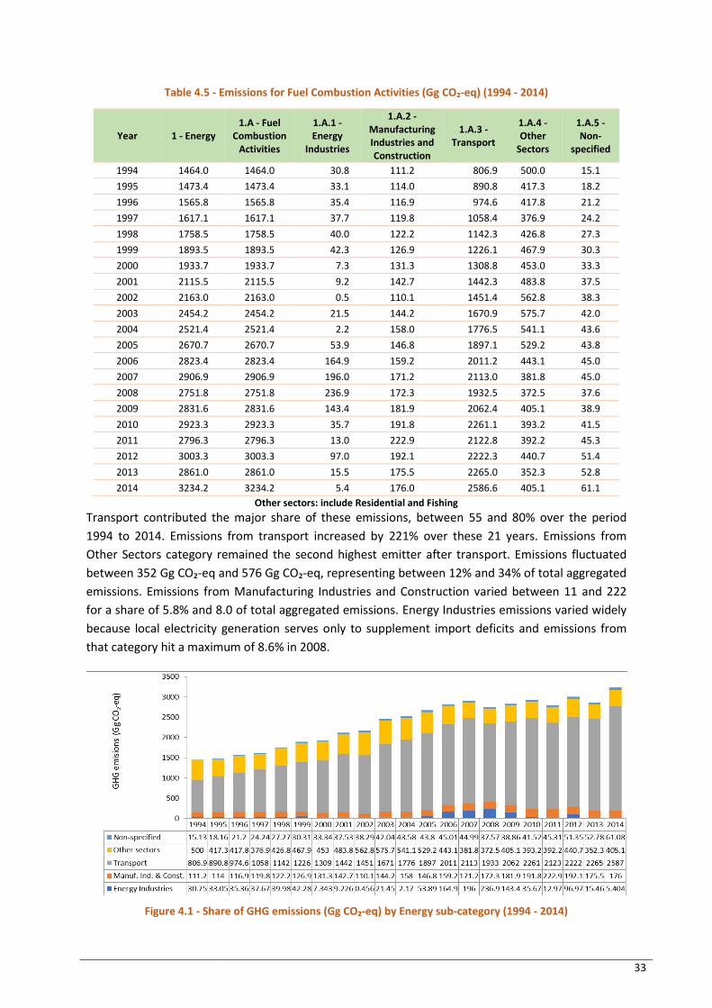
33
Table 4.5 - Emissions for Fuel Combustion Activities (Gg CO₂-eq) (1994 - 2014)
Year 1 - Energy 1.A - Fuel
Combustion Activities
1.A.1 - Energy
Industries
1.A.2 - Manufacturing Industries and Construction
1.A.3 - Transport
1.A.4 - Other
Sectors
1.A.5 - Non-
specified
1994 1464.0 1464.0 30.8 111.2 806.9 500.0 15.1
1995 1473.4 1473.4 33.1 114.0 890.8 417.3 18.2
1996 1565.8 1565.8 35.4 116.9 974.6 417.8 21.2
1997 1617.1 1617.1 37.7 119.8 1058.4 376.9 24.2
1998 1758.5 1758.5 40.0 122.2 1142.3 426.8 27.3
1999 1893.5 1893.5 42.3 126.9 1226.1 467.9 30.3
2000 1933.7 1933.7 7.3 131.3 1308.8 453.0 33.3
2001 2115.5 2115.5 9.2 142.7 1442.3 483.8 37.5
2002 2163.0 2163.0 0.5 110.1 1451.4 562.8 38.3
2003 2454.2 2454.2 21.5 144.2 1670.9 575.7 42.0
2004 2521.4 2521.4 2.2 158.0 1776.5 541.1 43.6
2005 2670.7 2670.7 53.9 146.8 1897.1 529.2 43.8
2006 2823.4 2823.4 164.9 159.2 2011.2 443.1 45.0
2007 2906.9 2906.9 196.0 171.2 2113.0 381.8 45.0
2008 2751.8 2751.8 236.9 172.3 1932.5 372.5 37.6
2009 2831.6 2831.6 143.4 181.9 2062.4 405.1 38.9
2010 2923.3 2923.3 35.7 191.8 2261.1 393.2 41.5
2011 2796.3 2796.3 13.0 222.9 2122.8 392.2 45.3
2012 3003.3 3003.3 97.0 192.1 2222.3 440.7 51.4
2013 2861.0 2861.0 15.5 175.5 2265.0 352.3 52.8
2014 3234.2 3234.2 5.4 176.0 2586.6 405.1 61.1
Other sectors: include Residential and Fishing
Transport contributed the major share of these emissions, between 55 and 80% over the period
1994 to 2014. Emissions from transport increased by 221% over these 21 years. Emissions from
Other Sectors category remained the second highest emitter after transport. Emissions fluctuated
between 352 Gg CO₂-eq and 576 Gg CO₂-eq, representing between 12% and 34% of total aggregated
emissions. Emissions from Manufacturing Industries and Construction varied between 11 and 222
for a share of 5.8% and 8.0 of total aggregated emissions. Energy Industries emissions varied widely
because local electricity generation serves only to supplement import deficits and emissions from
that category hit a maximum of 8.6% in 2008.
Figure 4.1 - Share of GHG emissions (Gg CO₂-eq) by Energy sub-category (1994 - 2014)
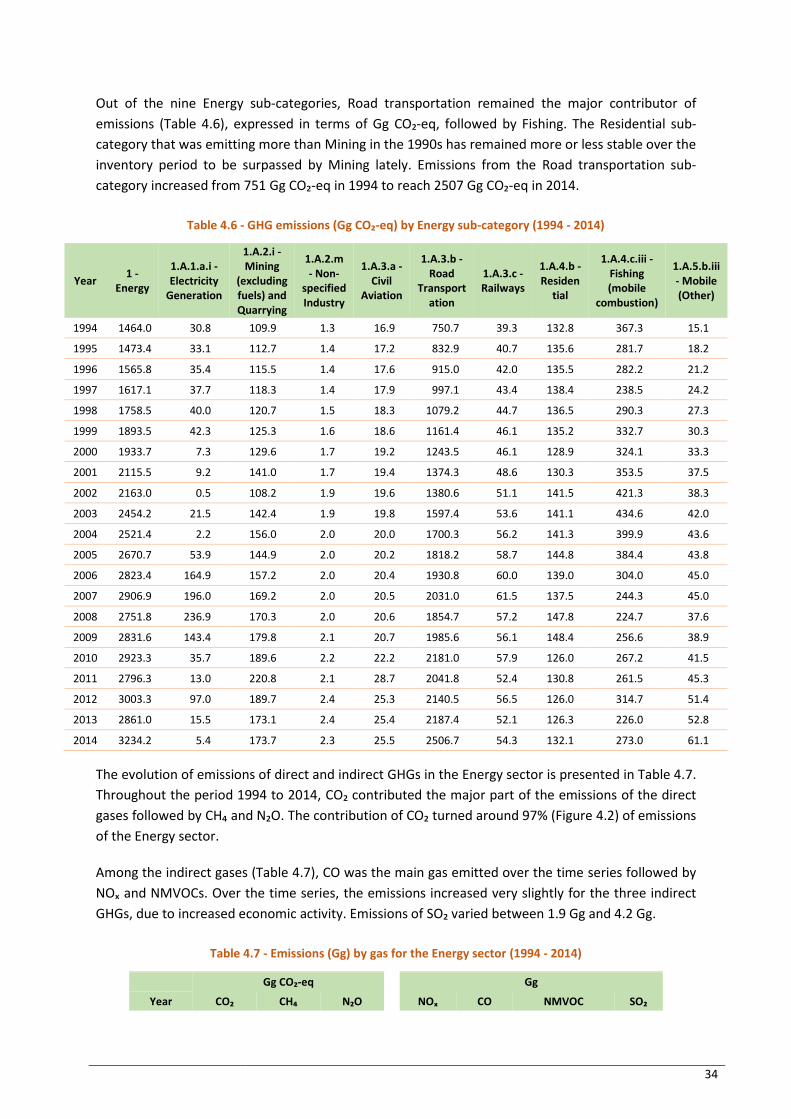
34
Out of the nine Energy sub-categories, Road transportation remained the major contributor of
emissions (Table 4.6), expressed in terms of Gg CO₂-eq, followed by Fishing. The Residential sub-
category that was emitting more than Mining in the 1990s has remained more or less stable over the
inventory period to be surpassed by Mining lately. Emissions from the Road transportation sub-
category increased from 751 Gg CO₂-eq in 1994 to reach 2507 Gg CO₂-eq in 2014.
Table 4.6 - GHG emissions (Gg CO₂-eq) by Energy sub-category (1994 - 2014)
Year 1 -
Energy
1.A.1.a.i - Electricity
Generation
1.A.2.i - Mining
(excluding fuels) and Quarrying
1.A.2.m - Non-
specified Industry
1.A.3.a - Civil
Aviation
1.A.3.b - Road
Transport ation
1.A.3.c - Railways
1.A.4.b - Residen
tial
1.A.4.c.iii - Fishing (mobile
combustion)
1.A.5.b.iii - Mobile (Other)
1994 1464.0 30.8 109.9 1.3 16.9 750.7 39.3 132.8 367.3 15.1
1995 1473.4 33.1 112.7 1.4 17.2 832.9 40.7 135.6 281.7 18.2
1996 1565.8 35.4 115.5 1.4 17.6 915.0 42.0 135.5 282.2 21.2
1997 1617.1 37.7 118.3 1.4 17.9 997.1 43.4 138.4 238.5 24.2
1998 1758.5 40.0 120.7 1.5 18.3 1079.2 44.7 136.5 290.3 27.3
1999 1893.5 42.3 125.3 1.6 18.6 1161.4 46.1 135.2 332.7 30.3
2000 1933.7 7.3 129.6 1.7 19.2 1243.5 46.1 128.9 324.1 33.3
2001 2115.5 9.2 141.0 1.7 19.4 1374.3 48.6 130.3 353.5 37.5
2002 2163.0 0.5 108.2 1.9 19.6 1380.6 51.1 141.5 421.3 38.3
2003 2454.2 21.5 142.4 1.9 19.8 1597.4 53.6 141.1 434.6 42.0
2004 2521.4 2.2 156.0 2.0 20.0 1700.3 56.2 141.3 399.9 43.6
2005 2670.7 53.9 144.9 2.0 20.2 1818.2 58.7 144.8 384.4 43.8
2006 2823.4 164.9 157.2 2.0 20.4 1930.8 60.0 139.0 304.0 45.0
2007 2906.9 196.0 169.2 2.0 20.5 2031.0 61.5 137.5 244.3 45.0
2008 2751.8 236.9 170.3 2.0 20.6 1854.7 57.2 147.8 224.7 37.6
2009 2831.6 143.4 179.8 2.1 20.7 1985.6 56.1 148.4 256.6 38.9
2010 2923.3 35.7 189.6 2.2 22.2 2181.0 57.9 126.0 267.2 41.5
2011 2796.3 13.0 220.8 2.1 28.7 2041.8 52.4 130.8 261.5 45.3
2012 3003.3 97.0 189.7 2.4 25.3 2140.5 56.5 126.0 314.7 51.4
2013 2861.0 15.5 173.1 2.4 25.4 2187.4 52.1 126.3 226.0 52.8
2014 3234.2 5.4 173.7 2.3 25.5 2506.7 54.3 132.1 273.0 61.1
The evolution of emissions of direct and indirect GHGs in the Energy sector is presented in Table 4.7.
Throughout the period 1994 to 2014, CO₂ contributed the major part of the emissions of the direct
gases followed by CH₄ and N₂O. The contribution of CO₂ turned around 97% (Figure 4.2) of emissions
of the Energy sector.
Among the indirect gases (Table 4.7), CO was the main gas emitted over the time series followed by
NOₓ and NMVOCs. Over the time series, the emissions increased very slightly for the three indirect
GHGs, due to increased economic activity. Emissions of SO₂ varied between 1.9 Gg and 4.2 Gg.
Table 4.7 - Emissions (Gg) by gas for the Energy sector (1994 - 2014)
Gg CO₂-eq
Gg
Year CO₂ CH₄ N₂O NOₓ CO NMVOC SO₂

35
Gg CO₂-eq
Gg
Year CO₂ CH₄ N₂O NOₓ CO NMVOC SO₂
1994 1409.8 32.1 22.2
14.3 42.4 5.9 2.6
1995 1417.5 32.4 23.5
12.8 43.8 6.0 2.1
1996 1507.9 33.0 25.0
13.4 45.6 6.3 2.2
1997 1557.2 33.4 26.4
13.0 47.1 6.4 1.9
1998 1696.3 34.2 28.0
14.8 49.1 6.7 2.2
1999 1829.0 34.9 29.6
16.5 50.9 7.0 2.5
2000 1867.5 35.4 30.8
16.7 52.8 7.2 2.2
2001 2045.9 36.4 33.3
18.2 55.5 7.1 2.4
2002 2092.8 36.5 33.7
19.9 55.4 7.2 2.7
2003 2378.9 37.7 37.6
21.7 60.0 7.7 3.0
2004 2443.8 38.2 39.4
21.7 62.8 8.0 3.5
2005 2590.3 38.8 41.6
22.1 65.0 8.3 3.7
2006 2740.3 39.2 43.8
21.1 67.4 8.6 4.2
2007 2821.7 39.6 45.6
20.4 69.1 8.8 4.0
2008 2670.8 38.4 42.7
19.0 64.6 8.3 4.1
2009 2748.3 39.1 44.3
20.5 66.9 8.6 3.7
2010 2836.6 39.9 46.8
21.8 71.0 9.1 2.9
2011 2713.1 38.7 44.5
21.1 66.3 8.6 3.0
2012 2917.6 38.9 46.9
23.3 66.6 8.7 3.7
2013 2775.9 38.7 46.4
21.2 66.5 8.5 2.5
2014 3142.3 40.3 51.6
24.4 72.9 9.2 2.7
Figure 4.2 - Share emissions by gas (%) for the Energy sector (1994 - 2014)
4.5.3. Evolution of emissions by gas (Gg) in the Energy Sector (1994 - 2014)
Emissions of CO₂ in the Energy sector, Fuel Combustion Activities category showed an increase over
the period 1994 to 2014, from 1,410 to 3,142 Gg. The annual increase which was quite sharp up to
2007 and plateaued thereafter until 2014.

36
Figure 4.3 - Evolution of CO₂ emissions (Gg) in the Energy Sector (1994 - 2014)
With regard to CH₄, emissions varied between 1.5 Gg and 1.9 Gg during the period 1994 to 2014
(Figure 4.4). After increasing to 1.9 Gg during the period 1994 to 2007, emissions stabilised between
1.8 Gg and 1.9 Gg until 2014.
Figure 4.4 - Evolution of CH₄ emissions (Gg) in the Energy Sector (1994 - 2014)
Emissions of N₂O increased from 0.10 to 0.2 Gg (Figure 4.5) over the period 1994 to 2014.
Figure 4.5 - Evolution of N₂O emissions (Gg) in the Energy Sector (1994 - 2014)
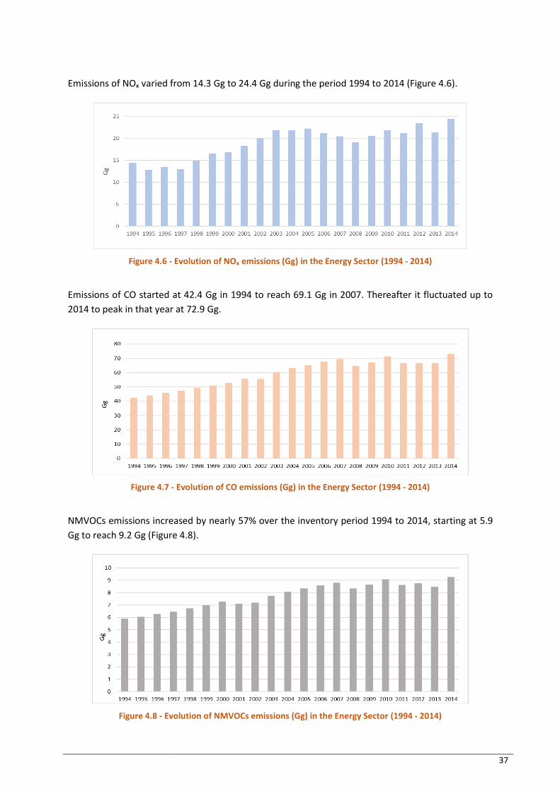
37
Emissions of NOₓ varied from 14.3 Gg to 24.4 Gg during the period 1994 to 2014 (Figure 4.6).
Figure 4.6 - Evolution of NOₓ emissions (Gg) in the Energy Sector (1994 - 2014)
Emissions of CO started at 42.4 Gg in 1994 to reach 69.1 Gg in 2007. Thereafter it fluctuated up to
2014 to peak in that year at 72.9 Gg.
Figure 4.7 - Evolution of CO emissions (Gg) in the Energy Sector (1994 - 2014)
NMVOCs emissions increased by nearly 57% over the inventory period 1994 to 2014, starting at 5.9
Gg to reach 9.2 Gg (Figure 4.8).
Figure 4.8 - Evolution of NMVOCs emissions (Gg) in the Energy Sector (1994 - 2014)
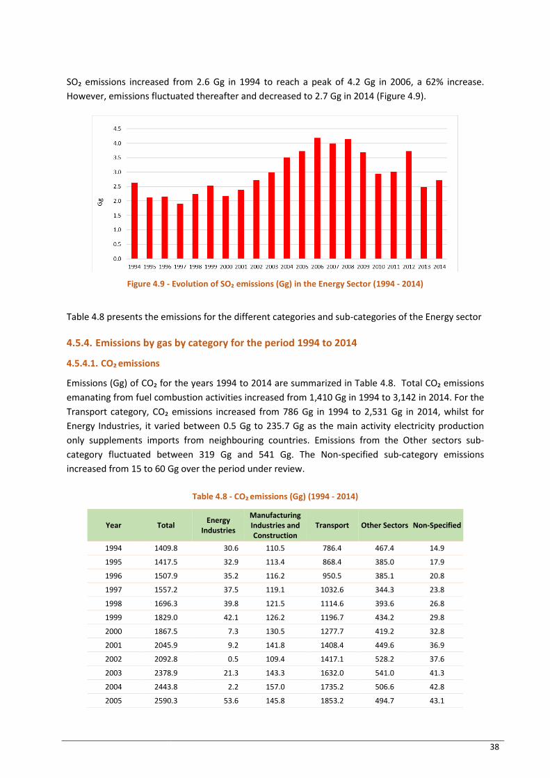
38
SO₂ emissions increased from 2.6 Gg in 1994 to reach a peak of 4.2 Gg in 2006, a 62% increase.
However, emissions fluctuated thereafter and decreased to 2.7 Gg in 2014 (Figure 4.9).
Figure 4.9 - Evolution of SO₂ emissions (Gg) in the Energy Sector (1994 - 2014)
Table 4.8 presents the emissions for the different categories and sub-categories of the Energy sector
4.5.4. Emissions by gas by category for the period 1994 to 2014
4.5.4.1. CO₂ emissions
Emissions (Gg) of CO₂ for the years 1994 to 2014 are summarized in Table 4.8. Total CO₂ emissions
emanating from fuel combustion activities increased from 1,410 Gg in 1994 to 3,142 in 2014. For the
Transport category, CO₂ emissions increased from 786 Gg in 1994 to 2,531 Gg in 2014, whilst for
Energy Industries, it varied between 0.5 Gg to 235.7 Gg as the main activity electricity production
only supplements imports from neighbouring countries. Emissions from the Other sectors sub-
category fluctuated between 319 Gg and 541 Gg. The Non-specified sub-category emissions
increased from 15 to 60 Gg over the period under review.
Table 4.8 - CO₂ emissions (Gg) (1994 - 2014)
Year Total Energy
Industries
Manufacturing Industries and Construction
Transport Other Sectors Non-Specified
1994 1409.8 30.6 110.5 786.4 467.4 14.9
1995 1417.5 32.9 113.4 868.4 385.0 17.9
1996 1507.9 35.2 116.2 950.5 385.1 20.8
1997 1557.2 37.5 119.1 1032.6 344.3 23.8
1998 1696.3 39.8 121.5 1114.6 393.6 26.8
1999 1829.0 42.1 126.2 1196.7 434.2 29.8
2000 1867.5 7.3 130.5 1277.7 419.2 32.8
2001 2045.9 9.2 141.8 1408.4 449.6 36.9
2002 2092.8 0.5 109.4 1417.1 528.2 37.6
2003 2378.9 21.3 143.3 1632.0 541.0 41.3
2004 2443.8 2.2 157.0 1735.2 506.6 42.8
2005 2590.3 53.6 145.8 1853.2 494.7 43.1
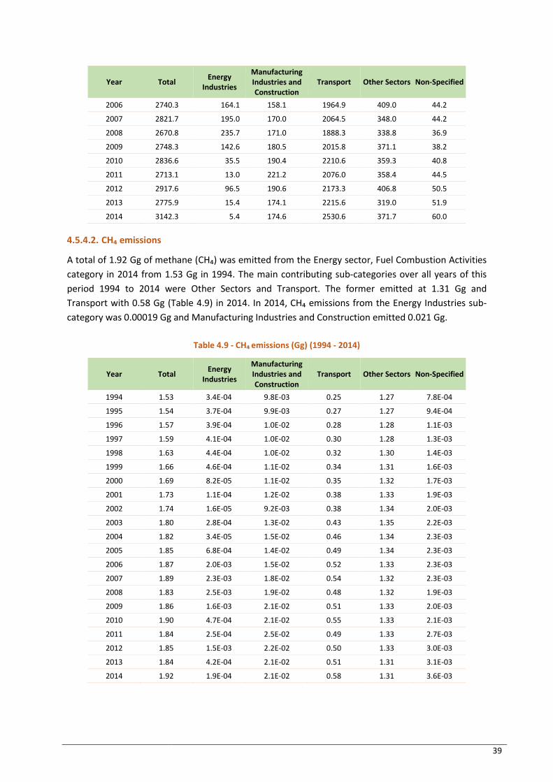
39
Year Total Energy
Industries
Manufacturing Industries and Construction
Transport Other Sectors Non-Specified
2006 2740.3 164.1 158.1 1964.9 409.0 44.2
2007 2821.7 195.0 170.0 2064.5 348.0 44.2
2008 2670.8 235.7 171.0 1888.3 338.8 36.9
2009 2748.3 142.6 180.5 2015.8 371.1 38.2
2010 2836.6 35.5 190.4 2210.6 359.3 40.8
2011 2713.1 13.0 221.2 2076.0 358.4 44.5
2012 2917.6 96.5 190.6 2173.3 406.8 50.5
2013 2775.9 15.4 174.1 2215.6 319.0 51.9
2014 3142.3 5.4 174.6 2530.6 371.7 60.0
4.5.4.2. CH₄ emissions
A total of 1.92 Gg of methane (CH₄) was emitted from the Energy sector, Fuel Combustion Activities
category in 2014 from 1.53 Gg in 1994. The main contributing sub-categories over all years of this
period 1994 to 2014 were Other Sectors and Transport. The former emitted at 1.31 Gg and
Transport with 0.58 Gg (Table 4.9) in 2014. In 2014, CH₄ emissions from the Energy Industries sub-
category was 0.00019 Gg and Manufacturing Industries and Construction emitted 0.021 Gg.
Table 4.9 - CH₄ emissions (Gg) (1994 - 2014)
Year Total Energy
Industries
Manufacturing Industries and Construction
Transport Other Sectors Non-Specified
1994 1.53 3.4E-04 9.8E-03 0.25 1.27 7.8E-04
1995 1.54 3.7E-04 9.9E-03 0.27 1.27 9.4E-04
1996 1.57 3.9E-04 1.0E-02 0.28 1.28 1.1E-03
1997 1.59 4.1E-04 1.0E-02 0.30 1.28 1.3E-03
1998 1.63 4.4E-04 1.0E-02 0.32 1.30 1.4E-03
1999 1.66 4.6E-04 1.1E-02 0.34 1.31 1.6E-03
2000 1.69 8.2E-05 1.1E-02 0.35 1.32 1.7E-03
2001 1.73 1.1E-04 1.2E-02 0.38 1.33 1.9E-03
2002 1.74 1.6E-05 9.2E-03 0.38 1.34 2.0E-03
2003 1.80 2.8E-04 1.3E-02 0.43 1.35 2.2E-03
2004 1.82 3.4E-05 1.5E-02 0.46 1.34 2.3E-03
2005 1.85 6.8E-04 1.4E-02 0.49 1.34 2.3E-03
2006 1.87 2.0E-03 1.5E-02 0.52 1.33 2.3E-03
2007 1.89 2.3E-03 1.8E-02 0.54 1.32 2.3E-03
2008 1.83 2.5E-03 1.9E-02 0.48 1.32 1.9E-03
2009 1.86 1.6E-03 2.1E-02 0.51 1.33 2.0E-03
2010 1.90 4.7E-04 2.1E-02 0.55 1.33 2.1E-03
2011 1.84 2.5E-04 2.5E-02 0.49 1.33 2.7E-03
2012 1.85 1.5E-03 2.2E-02 0.50 1.33 3.0E-03
2013 1.84 4.2E-04 2.1E-02 0.51 1.31 3.1E-03
2014 1.92 1.9E-04 2.1E-02 0.58 1.31 3.6E-03
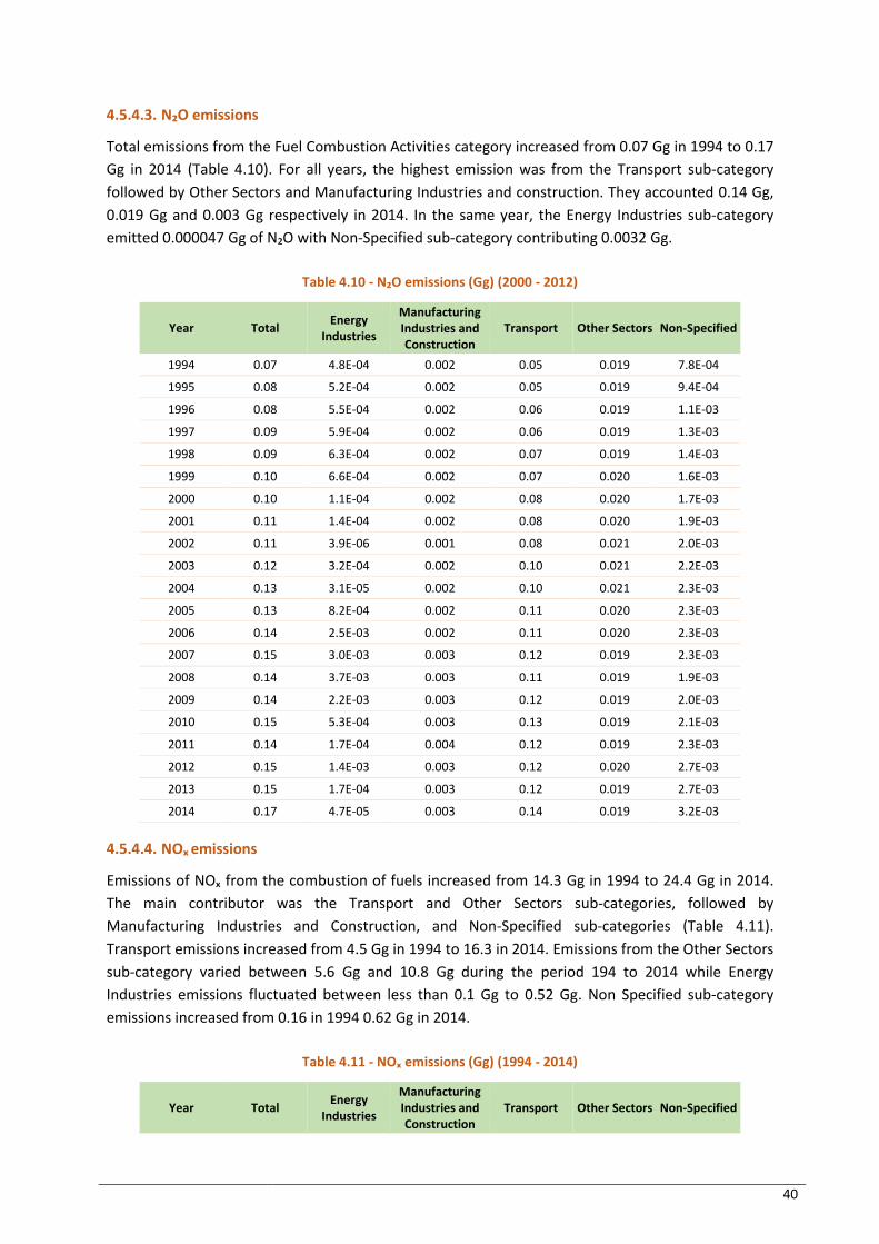
40
4.5.4.3. N₂O emissions
Total emissions from the Fuel Combustion Activities category increased from 0.07 Gg in 1994 to 0.17
Gg in 2014 (Table 4.10). For all years, the highest emission was from the Transport sub-category
followed by Other Sectors and Manufacturing Industries and construction. They accounted 0.14 Gg,
0.019 Gg and 0.003 Gg respectively in 2014. In the same year, the Energy Industries sub-category
emitted 0.000047 Gg of N₂O with Non-Specified sub-category contributing 0.0032 Gg.
Table 4.10 - N₂O emissions (Gg) (2000 - 2012)
Year Total Energy
Industries
Manufacturing Industries and Construction
Transport Other Sectors Non-Specified
1994 0.07 4.8E-04 0.002 0.05 0.019 7.8E-04
1995 0.08 5.2E-04 0.002 0.05 0.019 9.4E-04
1996 0.08 5.5E-04 0.002 0.06 0.019 1.1E-03
1997 0.09 5.9E-04 0.002 0.06 0.019 1.3E-03
1998 0.09 6.3E-04 0.002 0.07 0.019 1.4E-03
1999 0.10 6.6E-04 0.002 0.07 0.020 1.6E-03
2000 0.10 1.1E-04 0.002 0.08 0.020 1.7E-03
2001 0.11 1.4E-04 0.002 0.08 0.020 1.9E-03
2002 0.11 3.9E-06 0.001 0.08 0.021 2.0E-03
2003 0.12 3.2E-04 0.002 0.10 0.021 2.2E-03
2004 0.13 3.1E-05 0.002 0.10 0.021 2.3E-03
2005 0.13 8.2E-04 0.002 0.11 0.020 2.3E-03
2006 0.14 2.5E-03 0.002 0.11 0.020 2.3E-03
2007 0.15 3.0E-03 0.003 0.12 0.019 2.3E-03
2008 0.14 3.7E-03 0.003 0.11 0.019 1.9E-03
2009 0.14 2.2E-03 0.003 0.12 0.019 2.0E-03
2010 0.15 5.3E-04 0.003 0.13 0.019 2.1E-03
2011 0.14 1.7E-04 0.004 0.12 0.019 2.3E-03
2012 0.15 1.4E-03 0.003 0.12 0.020 2.7E-03
2013 0.15 1.7E-04 0.003 0.12 0.019 2.7E-03
2014 0.17 4.7E-05 0.003 0.14 0.019 3.2E-03
4.5.4.4. NOₓ emissions
Emissions of NOₓ from the combustion of fuels increased from 14.3 Gg in 1994 to 24.4 Gg in 2014.
The main contributor was the Transport and Other Sectors sub-categories, followed by
Manufacturing Industries and Construction, and Non-Specified sub-categories (Table 4.11).
Transport emissions increased from 4.5 Gg in 1994 to 16.3 in 2014. Emissions from the Other Sectors
sub-category varied between 5.6 Gg and 10.8 Gg during the period 194 to 2014 while Energy
Industries emissions fluctuated between less than 0.1 Gg to 0.52 Gg. Non Specified sub-category
emissions increased from 0.16 in 1994 0.62 Gg in 2014.
Table 4.11 - NOₓ emissions (Gg) (1994 - 2014)
Year Total Energy
Industries
Manufacturing Industries and Construction
Transport Other Sectors Non-Specified
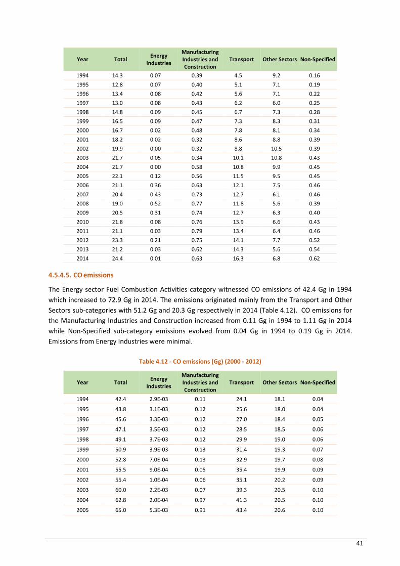
41
Year Total Energy
Industries
Manufacturing Industries and Construction
Transport Other Sectors Non-Specified
1994 14.3 0.07 0.39 4.5 9.2 0.16
1995 12.8 0.07 0.40 5.1 7.1 0.19
1996 13.4 0.08 0.42 5.6 7.1 0.22
1997 13.0 0.08 0.43 6.2 6.0 0.25
1998 14.8 0.09 0.45 6.7 7.3 0.28
1999 16.5 0.09 0.47 7.3 8.3 0.31
2000 16.7 0.02 0.48 7.8 8.1 0.34
2001 18.2 0.02 0.32 8.6 8.8 0.39
2002 19.9 0.00 0.32 8.8 10.5 0.39
2003 21.7 0.05 0.34 10.1 10.8 0.43
2004 21.7 0.00 0.58 10.8 9.9 0.45
2005 22.1 0.12 0.56 11.5 9.5 0.45
2006 21.1 0.36 0.63 12.1 7.5 0.46
2007 20.4 0.43 0.73 12.7 6.1 0.46
2008 19.0 0.52 0.77 11.8 5.6 0.39
2009 20.5 0.31 0.74 12.7 6.3 0.40
2010 21.8 0.08 0.76 13.9 6.6 0.43
2011 21.1 0.03 0.79 13.4 6.4 0.46
2012 23.3 0.21 0.75 14.1 7.7 0.52
2013 21.2 0.03 0.62 14.3 5.6 0.54
2014 24.4 0.01 0.63 16.3 6.8 0.62
4.5.4.5. CO emissions
The Energy sector Fuel Combustion Activities category witnessed CO emissions of 42.4 Gg in 1994
which increased to 72.9 Gg in 2014. The emissions originated mainly from the Transport and Other
Sectors sub-categories with 51.2 Gg and 20.3 Gg respectively in 2014 (Table 4.12). CO emissions for
the Manufacturing Industries and Construction increased from 0.11 Gg in 1994 to 1.11 Gg in 2014
while Non-Specified sub-category emissions evolved from 0.04 Gg in 1994 to 0.19 Gg in 2014.
Emissions from Energy Industries were minimal.
Table 4.12 - CO emissions (Gg) (2000 - 2012)
Year Total Energy
Industries
Manufacturing Industries and Construction
Transport Other Sectors Non-Specified
1994 42.4 2.9E-03 0.11 24.1 18.1 0.04
1995 43.8 3.1E-03 0.12 25.6 18.0 0.04
1996 45.6 3.3E-03 0.12 27.0 18.4 0.05
1997 47.1 3.5E-03 0.12 28.5 18.5 0.06
1998 49.1 3.7E-03 0.12 29.9 19.0 0.06
1999 50.9 3.9E-03 0.13 31.4 19.3 0.07
2000 52.8 7.0E-04 0.13 32.9 19.7 0.08
2001 55.5 9.0E-04 0.05 35.4 19.9 0.09
2002 55.4 1.0E-04 0.06 35.1 20.2 0.09
2003 60.0 2.2E-03 0.07 39.3 20.5 0.10
2004 62.8 2.0E-04 0.97 41.3 20.5 0.10
2005 65.0 5.3E-03 0.91 43.4 20.6 0.10
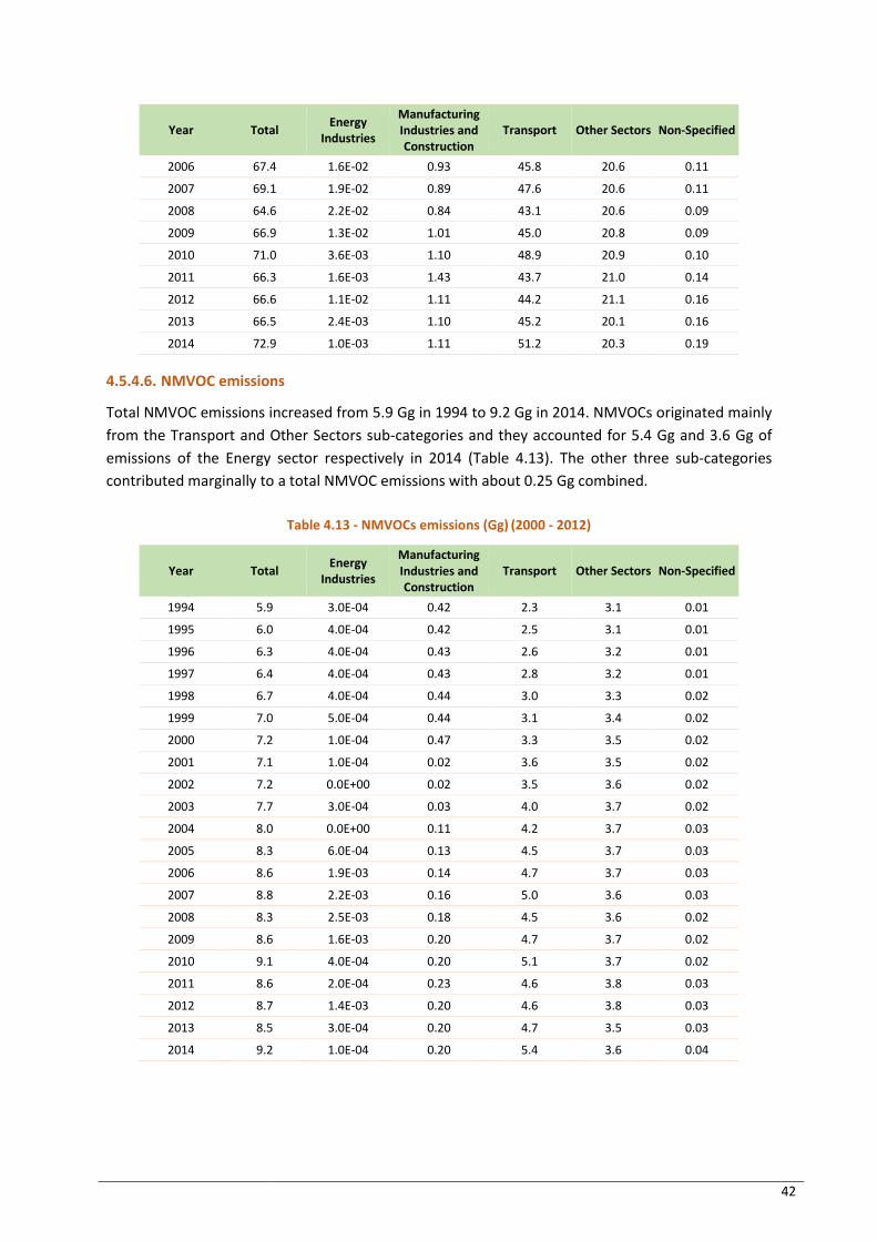
42
Year Total Energy
Industries
Manufacturing Industries and Construction
Transport Other Sectors Non-Specified
2006 67.4 1.6E-02 0.93 45.8 20.6 0.11
2007 69.1 1.9E-02 0.89 47.6 20.6 0.11
2008 64.6 2.2E-02 0.84 43.1 20.6 0.09
2009 66.9 1.3E-02 1.01 45.0 20.8 0.09
2010 71.0 3.6E-03 1.10 48.9 20.9 0.10
2011 66.3 1.6E-03 1.43 43.7 21.0 0.14
2012 66.6 1.1E-02 1.11 44.2 21.1 0.16
2013 66.5 2.4E-03 1.10 45.2 20.1 0.16
2014 72.9 1.0E-03 1.11 51.2 20.3 0.19
4.5.4.6. NMVOC emissions
Total NMVOC emissions increased from 5.9 Gg in 1994 to 9.2 Gg in 2014. NMVOCs originated mainly
from the Transport and Other Sectors sub-categories and they accounted for 5.4 Gg and 3.6 Gg of
emissions of the Energy sector respectively in 2014 (Table 4.13). The other three sub-categories
contributed marginally to a total NMVOC emissions with about 0.25 Gg combined.
Table 4.13 - NMVOCs emissions (Gg) (2000 - 2012)
Year Total Energy
Industries
Manufacturing Industries and Construction
Transport Other Sectors Non-Specified
1994 5.9 3.0E-04 0.42 2.3 3.1 0.01
1995 6.0 4.0E-04 0.42 2.5 3.1 0.01
1996 6.3 4.0E-04 0.43 2.6 3.2 0.01
1997 6.4 4.0E-04 0.43 2.8 3.2 0.01
1998 6.7 4.0E-04 0.44 3.0 3.3 0.02
1999 7.0 5.0E-04 0.44 3.1 3.4 0.02
2000 7.2 1.0E-04 0.47 3.3 3.5 0.02
2001 7.1 1.0E-04 0.02 3.6 3.5 0.02
2002 7.2 0.0E+00 0.02 3.5 3.6 0.02
2003 7.7 3.0E-04 0.03 4.0 3.7 0.02
2004 8.0 0.0E+00 0.11 4.2 3.7 0.03
2005 8.3 6.0E-04 0.13 4.5 3.7 0.03
2006 8.6 1.9E-03 0.14 4.7 3.7 0.03
2007 8.8 2.2E-03 0.16 5.0 3.6 0.03
2008 8.3 2.5E-03 0.18 4.5 3.6 0.02
2009 8.6 1.6E-03 0.20 4.7 3.7 0.02
2010 9.1 4.0E-04 0.20 5.1 3.7 0.02
2011 8.6 2.0E-04 0.23 4.6 3.8 0.03
2012 8.7 1.4E-03 0.20 4.6 3.8 0.03
2013 8.5 3.0E-04 0.20 4.7 3.5 0.03
2014 9.2 1.0E-04 0.20 5.4 3.6 0.04

43
4.5.4.7. SO₂ emissions
Total SO₂ emissions in the Energy sector varied between 1.9 Gg and 4.2 Gg for the time series 1994
to 2014. Emissions of SO₂ across the time period were more important in the Other Sectors sub-
category followed by the Manufacturing Industries and Construction sub-category (Table 4.14).
Emissions in the former sub-category varied between 1.5 Gg and 2.8 Gg while in the Manufacturing
and Construction sub-category, the emissions increased from 0.02 Gg in 1994 to 0.90 Gg in 2014
after a peak of 1.21 Gg in 2011.
Table 4.14 - SO₂ emissions (Gg) (2000 - 2014)
Year Total Energy
Industries
Manufacturing Industries and Construction
Transport Other Sectors Non-Specified
1994 2.6 0.26 0.02 0.01 2.3 1.0E-04
1995 2.1 0.28 0.02 0.01 1.8 1.0E-04
1996 2.2 0.30 0.03 0.01 1.8 1.0E-04
1997 1.9 0.32 0.03 0.01 1.5 1.0E-04
1998 2.2 0.34 0.03 0.02 1.9 1.0E-04
1999 2.5 0.36 0.03 0.02 2.1 1.0E-04
2000 2.2 0.06 0.03 0.02 2.1 2.0E-04
2001 2.4 0.08 0.03 0.02 2.3 2.0E-04
2002 2.7 0.00 0.03 0.02 2.7 2.0E-04
2003 3.0 0.18 0.03 0.02 2.8 2.0E-04
2004 3.5 0.02 0.92 0.02 2.5 2.0E-04
2005 3.7 0.46 0.80 0.02 2.5 2.0E-04
2006 4.2 1.40 0.81 0.02 1.9 2.0E-04
2007 4.0 1.67 0.72 0.02 1.6 2.0E-04
2008 4.1 2.04 0.62 0.02 1.5 2.0E-04
2009 3.7 1.23 0.78 0.02 1.7 2.0E-04
2010 2.9 0.30 0.89 0.02 1.7 2.0E-04
2011 3.0 0.10 1.21 0.02 1.7 2.0E-04
2012 3.7 0.80 0.89 0.02 2.0 3.0E-04
2013 2.5 0.11 0.89 0.02 1.5 3.0E-04
2014 2.7 0.04 0.90 0.03 1.8 3.0E-04
4.5.4.8. Emissions (Gg) by gas from Energy Generation
Within the Energy Generation sub-category, GHG emissions, varied between 0.5 Gg CO₂-eq and
236.9 Gg CO₂-eq (Table 4.15). The largest share of emissions came from CO₂ for all years of the
period 1994 to 2014.
Table 4.15 - Emissions (Gg) by gas from energy generation
Year CO₂-eq CO₂ CH₄ N₂O NOₓ CO NMVOCs SO₂
1994 30.8 30.6 3.4E-04 4.8E-04 0.07 2.9E-03 3.0E-04 0.26
1995 33.1 32.9 3.7E-04 5.2E-04 0.07 3.1E-03 4.0E-04 0.28
1996 35.4 35.2 3.9E-04 5.5E-04 0.08 3.3E-03 4.0E-04 0.30
1997 37.7 37.5 4.1E-04 5.9E-04 0.08 3.5E-03 4.0E-04 0.32
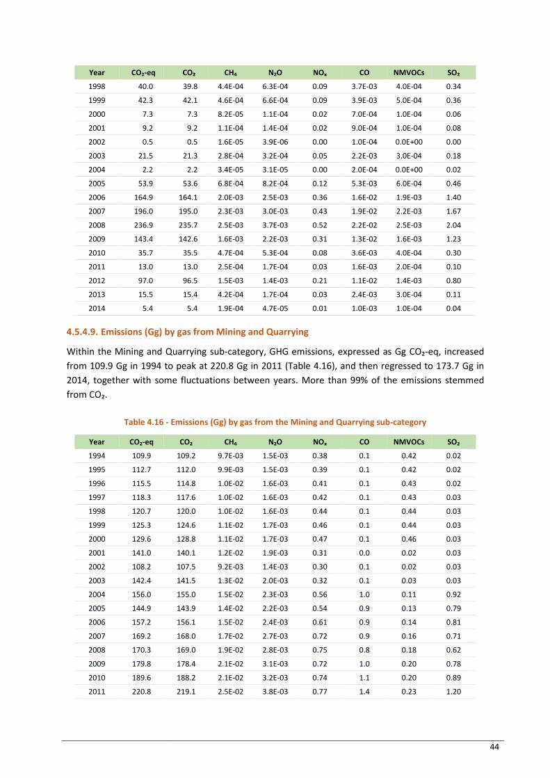
44
Year CO₂-eq CO₂ CH₄ N₂O NOₓ CO NMVOCs SO₂
1998 40.0 39.8 4.4E-04 6.3E-04 0.09 3.7E-03 4.0E-04 0.34
1999 42.3 42.1 4.6E-04 6.6E-04 0.09 3.9E-03 5.0E-04 0.36
2000 7.3 7.3 8.2E-05 1.1E-04 0.02 7.0E-04 1.0E-04 0.06
2001 9.2 9.2 1.1E-04 1.4E-04 0.02 9.0E-04 1.0E-04 0.08
2002 0.5 0.5 1.6E-05 3.9E-06 0.00 1.0E-04 0.0E+00 0.00
2003 21.5 21.3 2.8E-04 3.2E-04 0.05 2.2E-03 3.0E-04 0.18
2004 2.2 2.2 3.4E-05 3.1E-05 0.00 2.0E-04 0.0E+00 0.02
2005 53.9 53.6 6.8E-04 8.2E-04 0.12 5.3E-03 6.0E-04 0.46
2006 164.9 164.1 2.0E-03 2.5E-03 0.36 1.6E-02 1.9E-03 1.40
2007 196.0 195.0 2.3E-03 3.0E-03 0.43 1.9E-02 2.2E-03 1.67
2008 236.9 235.7 2.5E-03 3.7E-03 0.52 2.2E-02 2.5E-03 2.04
2009 143.4 142.6 1.6E-03 2.2E-03 0.31 1.3E-02 1.6E-03 1.23
2010 35.7 35.5 4.7E-04 5.3E-04 0.08 3.6E-03 4.0E-04 0.30
2011 13.0 13.0 2.5E-04 1.7E-04 0.03 1.6E-03 2.0E-04 0.10
2012 97.0 96.5 1.5E-03 1.4E-03 0.21 1.1E-02 1.4E-03 0.80
2013 15.5 15.4 4.2E-04 1.7E-04 0.03 2.4E-03 3.0E-04 0.11
2014 5.4 5.4 1.9E-04 4.7E-05 0.01 1.0E-03 1.0E-04 0.04
4.5.4.9. Emissions (Gg) by gas from Mining and Quarrying
Within the Mining and Quarrying sub-category, GHG emissions, expressed as Gg CO₂-eq, increased
from 109.9 Gg in 1994 to peak at 220.8 Gg in 2011 (Table 4.16), and then regressed to 173.7 Gg in
2014, together with some fluctuations between years. More than 99% of the emissions stemmed
from CO₂.
Table 4.16 - Emissions (Gg) by gas from the Mining and Quarrying sub-category
Year CO₂-eq CO₂ CH₄ N₂O NOₓ CO NMVOCs SO₂
1994 109.9 109.2 9.7E-03 1.5E-03 0.38 0.1 0.42 0.02
1995 112.7 112.0 9.9E-03 1.5E-03 0.39 0.1 0.42 0.02
1996 115.5 114.8 1.0E-02 1.6E-03 0.41 0.1 0.43 0.02
1997 118.3 117.6 1.0E-02 1.6E-03 0.42 0.1 0.43 0.03
1998 120.7 120.0 1.0E-02 1.6E-03 0.44 0.1 0.44 0.03
1999 125.3 124.6 1.1E-02 1.7E-03 0.46 0.1 0.44 0.03
2000 129.6 128.8 1.1E-02 1.7E-03 0.47 0.1 0.46 0.03
2001 141.0 140.1 1.2E-02 1.9E-03 0.31 0.0 0.02 0.03
2002 108.2 107.5 9.2E-03 1.4E-03 0.30 0.1 0.02 0.03
2003 142.4 141.5 1.3E-02 2.0E-03 0.32 0.1 0.03 0.03
2004 156.0 155.0 1.5E-02 2.3E-03 0.56 1.0 0.11 0.92
2005 144.9 143.9 1.4E-02 2.2E-03 0.54 0.9 0.13 0.79
2006 157.2 156.1 1.5E-02 2.4E-03 0.61 0.9 0.14 0.81
2007 169.2 168.0 1.7E-02 2.7E-03 0.72 0.9 0.16 0.71
2008 170.3 169.0 1.9E-02 2.8E-03 0.75 0.8 0.18 0.62
2009 179.8 178.4 2.1E-02 3.1E-03 0.72 1.0 0.20 0.78
2010 189.6 188.2 2.1E-02 3.2E-03 0.74 1.1 0.20 0.89
2011 220.8 219.1 2.5E-02 3.8E-03 0.77 1.4 0.23 1.20
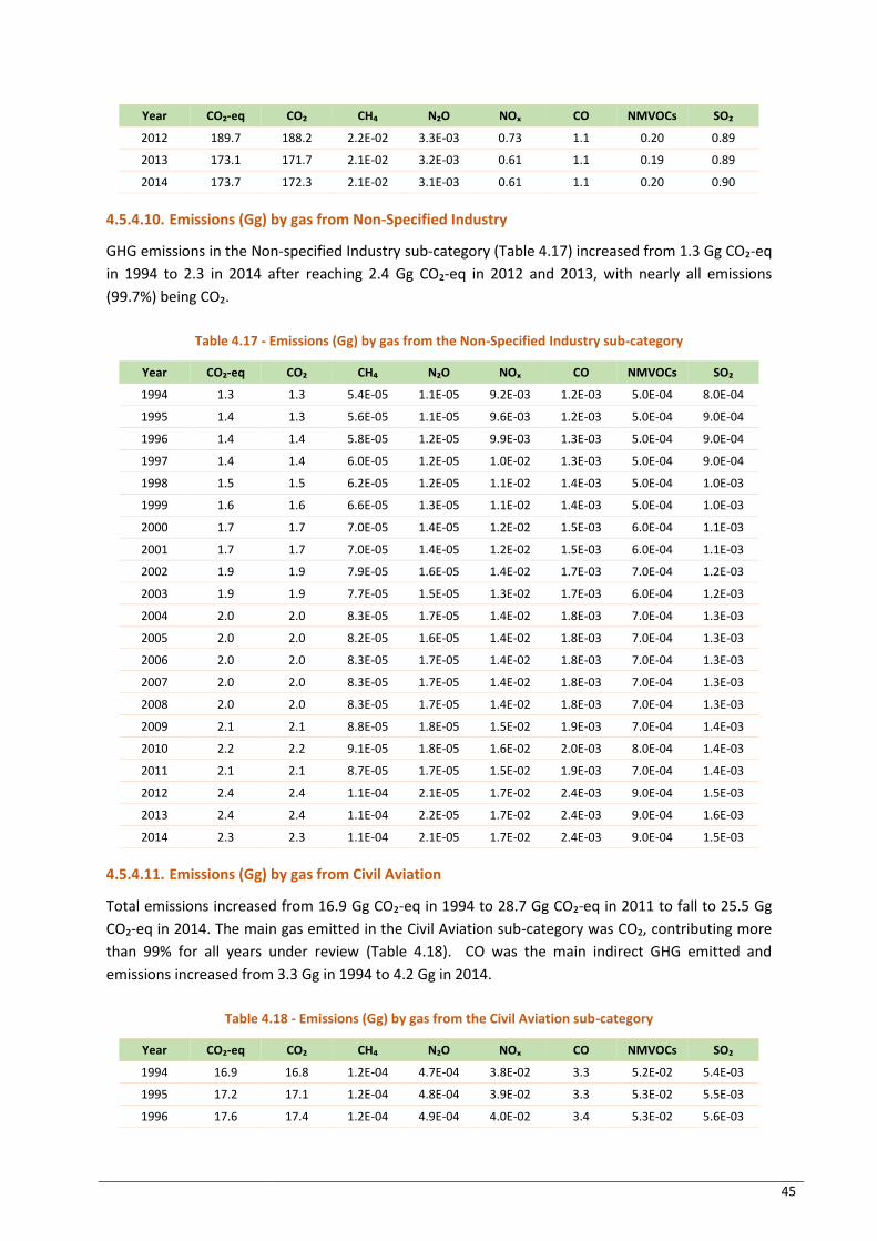
45
Year CO₂-eq CO₂ CH₄ N₂O NOₓ CO NMVOCs SO₂
2012 189.7 188.2 2.2E-02 3.3E-03 0.73 1.1 0.20 0.89
2013 173.1 171.7 2.1E-02 3.2E-03 0.61 1.1 0.19 0.89
2014 173.7 172.3 2.1E-02 3.1E-03 0.61 1.1 0.20 0.90
4.5.4.10. Emissions (Gg) by gas from Non-Specified Industry
GHG emissions in the Non-specified Industry sub-category (Table 4.17) increased from 1.3 Gg CO₂-eq
in 1994 to 2.3 in 2014 after reaching 2.4 Gg CO₂-eq in 2012 and 2013, with nearly all emissions
(99.7%) being CO₂.
Table 4.17 - Emissions (Gg) by gas from the Non-Specified Industry sub-category
Year CO₂-eq CO₂ CH₄ N₂O NOₓ CO NMVOCs SO₂
1994 1.3 1.3 5.4E-05 1.1E-05 9.2E-03 1.2E-03 5.0E-04 8.0E-04
1995 1.4 1.3 5.6E-05 1.1E-05 9.6E-03 1.2E-03 5.0E-04 9.0E-04
1996 1.4 1.4 5.8E-05 1.2E-05 9.9E-03 1.3E-03 5.0E-04 9.0E-04
1997 1.4 1.4 6.0E-05 1.2E-05 1.0E-02 1.3E-03 5.0E-04 9.0E-04
1998 1.5 1.5 6.2E-05 1.2E-05 1.1E-02 1.4E-03 5.0E-04 1.0E-03
1999 1.6 1.6 6.6E-05 1.3E-05 1.1E-02 1.4E-03 5.0E-04 1.0E-03
2000 1.7 1.7 7.0E-05 1.4E-05 1.2E-02 1.5E-03 6.0E-04 1.1E-03
2001 1.7 1.7 7.0E-05 1.4E-05 1.2E-02 1.5E-03 6.0E-04 1.1E-03
2002 1.9 1.9 7.9E-05 1.6E-05 1.4E-02 1.7E-03 7.0E-04 1.2E-03
2003 1.9 1.9 7.7E-05 1.5E-05 1.3E-02 1.7E-03 6.0E-04 1.2E-03
2004 2.0 2.0 8.3E-05 1.7E-05 1.4E-02 1.8E-03 7.0E-04 1.3E-03
2005 2.0 2.0 8.2E-05 1.6E-05 1.4E-02 1.8E-03 7.0E-04 1.3E-03
2006 2.0 2.0 8.3E-05 1.7E-05 1.4E-02 1.8E-03 7.0E-04 1.3E-03
2007 2.0 2.0 8.3E-05 1.7E-05 1.4E-02 1.8E-03 7.0E-04 1.3E-03
2008 2.0 2.0 8.3E-05 1.7E-05 1.4E-02 1.8E-03 7.0E-04 1.3E-03
2009 2.1 2.1 8.8E-05 1.8E-05 1.5E-02 1.9E-03 7.0E-04 1.4E-03
2010 2.2 2.2 9.1E-05 1.8E-05 1.6E-02 2.0E-03 8.0E-04 1.4E-03
2011 2.1 2.1 8.7E-05 1.7E-05 1.5E-02 1.9E-03 7.0E-04 1.4E-03
2012 2.4 2.4 1.1E-04 2.1E-05 1.7E-02 2.4E-03 9.0E-04 1.5E-03
2013 2.4 2.4 1.1E-04 2.2E-05 1.7E-02 2.4E-03 9.0E-04 1.6E-03
2014 2.3 2.3 1.1E-04 2.1E-05 1.7E-02 2.4E-03 9.0E-04 1.5E-03
4.5.4.11. Emissions (Gg) by gas from Civil Aviation
Total emissions increased from 16.9 Gg CO₂-eq in 1994 to 28.7 Gg CO₂-eq in 2011 to fall to 25.5 Gg
CO₂-eq in 2014. The main gas emitted in the Civil Aviation sub-category was CO₂, contributing more
than 99% for all years under review (Table 4.18). CO was the main indirect GHG emitted and
emissions increased from 3.3 Gg in 1994 to 4.2 Gg in 2014.
Table 4.18 - Emissions (Gg) by gas from the Civil Aviation sub-category
Year CO₂-eq CO₂ CH₄ N₂O NOₓ CO NMVOCs SO₂
1994 16.9 16.8 1.2E-04 4.7E-04 3.8E-02 3.3 5.2E-02 5.4E-03
1995 17.2 17.1 1.2E-04 4.8E-04 3.9E-02 3.3 5.3E-02 5.5E-03
1996 17.6 17.4 1.2E-04 4.9E-04 4.0E-02 3.4 5.3E-02 5.6E-03

46
Year CO₂-eq CO₂ CH₄ N₂O NOₓ CO NMVOCs SO₂
1997 17.9 17.8 1.3E-04 5.0E-04 4.1E-02 3.4 5.4E-02 5.7E-03
1998 18.3 18.1 1.3E-04 5.1E-04 4.2E-02 3.4 5.5E-02 5.8E-03
1999 18.6 18.5 1.3E-04 5.2E-04 4.3E-02 3.5 5.6E-02 5.9E-03
2000 19.2 19.0 1.3E-04 5.4E-04 4.4E-02 3.6 5.8E-02 6.1E-03
2001 19.4 19.2 1.4E-04 5.4E-04 4.4E-02 3.7 5.8E-02 6.1E-03
2002 19.6 19.4 1.4E-04 5.5E-04 4.5E-02 3.7 5.9E-02 6.2E-03
2003 19.8 19.6 1.4E-04 5.5E-04 4.5E-02 3.7 5.9E-02 6.3E-03
2004 20.0 19.8 1.4E-04 5.6E-04 4.6E-02 3.8 6.0E-02 6.3E-03
2005 20.2 20.0 1.4E-04 5.7E-04 4.6E-02 3.8 6.1E-02 6.4E-03
2006 20.4 20.2 1.4E-04 5.7E-04 4.7E-02 3.9 6.1E-02 6.5E-03
2007 20.5 20.4 1.4E-04 5.8E-04 4.7E-02 3.9 6.1E-02 6.5E-03
2008 20.6 20.5 1.4E-04 5.8E-04 4.7E-02 3.9 6.1E-02 6.5E-03
2009 20.7 20.6 1.5E-04 5.8E-04 4.8E-02 3.9 6.1E-02 6.6E-03
2010 22.2 22.0 1.6E-04 6.2E-04 5.0E-02 4.3 6.9E-02 7.1E-03
2011 28.7 28.4 2.0E-04 8.0E-04 7.2E-02 4.1 6.5E-02 9.1E-03
2012 25.3 25.1 1.8E-04 7.1E-04 6.1E-02 4.2 6.6E-02 8.0E-03
2013 25.4 25.2 1.8E-04 7.1E-04 6.1E-02 4.2 6.7E-02 8.0E-03
2014 25.5 25.3 1.8E-04 7.1E-04 6.1E-02 4.2 6.8E-02 8.1E-03
4.5.4.12. Emissions (Gg) by gas from Road Transportation
The Road Transportation sub-category emitted 750.7 Gg CO₂-eq in 1994, increasing to 2,506.7 Gg
CO₂-eq in 2014. CO₂ was the main direct GHG emitted. Emissions of NOₓ increased from 3.9 Gg in
1994 to reach 15.5 Gg in 2014. CO and NMVOCs emissions increased over the time period, from 20.7
Gg to 46.8 Gg for CO and from 2.2 Gg to 5.3 Gg for NMVOCs for the years 1994 to 2014 respectively
(Table 4.19).
Table 4.19 - Emissions (Gg) by gas from the Road Transportation sub-category
Year CO₂-eq CO₂ CH₄ N₂O NOₓ CO NMVOCs SO₂
1994 750.7 734.6 0.25 0.04 3.9 20.7 2.2 6.9E-03
1995 832.9 815.1 0.26 0.04 4.4 22.1 2.4 7.5E-03
1996 915.0 895.6 0.28 0.04 5.0 23.5 2.5 8.0E-03
1997 997.1 976.1 0.30 0.05 5.5 24.9 2.7 8.6E-03
1998 1079.2 1056.6 0.32 0.05 6.0 26.3 2.8 9.1E-03
1999 1161.4 1137.1 0.33 0.06 6.5 27.7 3.0 9.7E-03
2000 1243.5 1217.6 0.35 0.06 7.1 29.1 3.2 1.0E-02
2001 1374.3 1345.8 0.38 0.07 7.9 31.6 3.4 1.1E-02
2002 1380.6 1352.1 0.38 0.07 8.0 31.2 3.4 1.1E-02
2003 1597.4 1564.5 0.43 0.08 9.3 35.5 3.9 1.3E-02
2004 1700.3 1665.3 0.46 0.08 9.9 37.3 4.1 1.3E-02
2005 1818.2 1780.8 0.48 0.09 10.6 39.5 4.3 1.4E-02
2006 1930.8 1891.1 0.51 0.09 11.2 41.7 4.6 1.5E-02
2007 2031.0 1989.4 0.54 0.10 11.8 43.5 4.8 1.6E-02
2008 1854.7 1816.8 0.48 0.09 10.9 39.0 4.3 1.4E-02
2009 1985.6 1945.2 0.50 0.10 11.8 41.0 4.6 1.5E-02
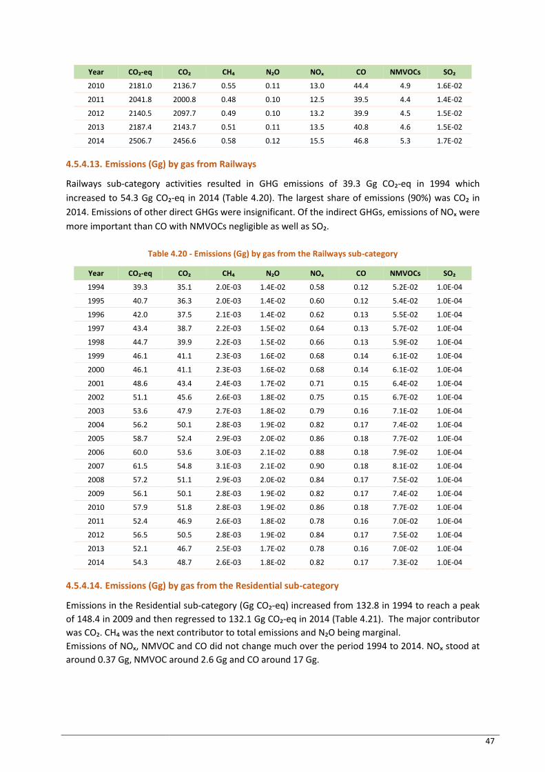
47
Year CO₂-eq CO₂ CH₄ N₂O NOₓ CO NMVOCs SO₂
2010 2181.0 2136.7 0.55 0.11 13.0 44.4 4.9 1.6E-02
2011 2041.8 2000.8 0.48 0.10 12.5 39.5 4.4 1.4E-02
2012 2140.5 2097.7 0.49 0.10 13.2 39.9 4.5 1.5E-02
2013 2187.4 2143.7 0.51 0.11 13.5 40.8 4.6 1.5E-02
2014 2506.7 2456.6 0.58 0.12 15.5 46.8 5.3 1.7E-02
4.5.4.13. Emissions (Gg) by gas from Railways
Railways sub-category activities resulted in GHG emissions of 39.3 Gg CO₂-eq in 1994 which
increased to 54.3 Gg CO₂-eq in 2014 (Table 4.20). The largest share of emissions (90%) was CO₂ in
2014. Emissions of other direct GHGs were insignificant. Of the indirect GHGs, emissions of NOₓ were
more important than CO with NMVOCs negligible as well as SO₂.
Table 4.20 - Emissions (Gg) by gas from the Railways sub-category
Year CO₂-eq CO₂ CH₄ N₂O NOₓ CO NMVOCs SO₂
1994 39.3 35.1 2.0E-03 1.4E-02 0.58 0.12 5.2E-02 1.0E-04
1995 40.7 36.3 2.0E-03 1.4E-02 0.60 0.12 5.4E-02 1.0E-04
1996 42.0 37.5 2.1E-03 1.4E-02 0.62 0.13 5.5E-02 1.0E-04
1997 43.4 38.7 2.2E-03 1.5E-02 0.64 0.13 5.7E-02 1.0E-04
1998 44.7 39.9 2.2E-03 1.5E-02 0.66 0.13 5.9E-02 1.0E-04
1999 46.1 41.1 2.3E-03 1.6E-02 0.68 0.14 6.1E-02 1.0E-04
2000 46.1 41.1 2.3E-03 1.6E-02 0.68 0.14 6.1E-02 1.0E-04
2001 48.6 43.4 2.4E-03 1.7E-02 0.71 0.15 6.4E-02 1.0E-04
2002 51.1 45.6 2.6E-03 1.8E-02 0.75 0.15 6.7E-02 1.0E-04
2003 53.6 47.9 2.7E-03 1.8E-02 0.79 0.16 7.1E-02 1.0E-04
2004 56.2 50.1 2.8E-03 1.9E-02 0.82 0.17 7.4E-02 1.0E-04
2005 58.7 52.4 2.9E-03 2.0E-02 0.86 0.18 7.7E-02 1.0E-04
2006 60.0 53.6 3.0E-03 2.1E-02 0.88 0.18 7.9E-02 1.0E-04
2007 61.5 54.8 3.1E-03 2.1E-02 0.90 0.18 8.1E-02 1.0E-04
2008 57.2 51.1 2.9E-03 2.0E-02 0.84 0.17 7.5E-02 1.0E-04
2009 56.1 50.1 2.8E-03 1.9E-02 0.82 0.17 7.4E-02 1.0E-04
2010 57.9 51.8 2.8E-03 1.9E-02 0.86 0.18 7.7E-02 1.0E-04
2011 52.4 46.9 2.6E-03 1.8E-02 0.78 0.16 7.0E-02 1.0E-04
2012 56.5 50.5 2.8E-03 1.9E-02 0.84 0.17 7.5E-02 1.0E-04
2013 52.1 46.7 2.5E-03 1.7E-02 0.78 0.16 7.0E-02 1.0E-04
2014 54.3 48.7 2.6E-03 1.8E-02 0.82 0.17 7.3E-02 1.0E-04
4.5.4.14. Emissions (Gg) by gas from the Residential sub-category
Emissions in the Residential sub-category (Gg CO₂-eq) increased from 132.8 in 1994 to reach a peak
of 148.4 in 2009 and then regressed to 132.1 Gg CO₂-eq in 2014 (Table 4.21). The major contributor
was CO₂. CH₄ was the next contributor to total emissions and N₂O being marginal.
Emissions of NOₓ, NMVOC and CO did not change much over the period 1994 to 2014. NOₓ stood at
around 0.37 Gg, NMVOC around 2.6 Gg and CO around 17 Gg.

48
Table 4.21 - Emissions (Gg) by gas from the Residential sub-category
Year CO₂-eq CO₂ CH₄ N₂O NOₓ CO NMVOCs SO₂
1994 132.8 102.1 1.2 1.6E-02 0.34 16.0953 2.4 4.4E-02
1995 135.6 104.8 1.2 1.6E-02 0.35 16.1021 2.5 4.4E-02
1996 135.5 104.4 1.2 1.7E-02 0.35 16.4060 2.5 4.5E-02
1997 138.4 107.1 1.2 1.7E-02 0.36 16.4760 2.5 4.5E-02
1998 136.5 104.9 1.3 1.7E-02 0.36 16.7807 2.6 4.6E-02
1999 135.2 103.3 1.3 1.7E-02 0.36 16.8505 2.6 4.6E-02
2000 128.9 96.8 1.3 1.7E-02 0.36 17.0947 2.6 4.7E-02
2001 130.3 98.0 1.3 1.7E-02 0.37 17.1528 2.6 4.7E-02
2002 141.5 109.2 1.3 1.7E-02 0.37 17.1685 2.6 4.7E-02
2003 141.1 108.7 1.3 1.7E-02 0.37 17.2979 2.6 4.8E-02
2004 141.3 108.8 1.3 1.7E-02 0.37 17.3053 2.6 4.8E-02
2005 144.8 112.3 1.3 1.7E-02 0.38 17.3202 2.6 4.8E-02
2006 139.0 106.6 1.3 1.7E-02 0.38 17.4465 2.6 4.8E-02
2007 137.5 105.0 1.3 1.7E-02 0.38 17.4537 2.6 4.8E-02
2008 147.8 115.3 1.3 1.7E-02 0.38 17.4589 2.6 4.8E-02
2009 148.4 115.9 1.3 1.7E-02 0.37 17.4630 2.6 4.8E-02
2010 126.0 93.5 1.3 1.7E-02 0.37 17.4662 2.6 4.8E-02
2011 130.8 98.3 1.3 1.7E-02 0.37 17.4689 2.6 4.8E-02
2012 126.0 93.7 1.3 1.7E-02 0.37 17.3728 2.6 4.8E-02
2013 126.3 94.2 1.3 1.7E-02 0.37 17.4019 2.6 4.8E-02
2014 132.1 100.1 1.3 1.7E-02 0.37 17.4383 2.6 4.8E-02
4.5.4.15. Emissions (Gg) by gas from Fishing (mobile combustion) sub-category
Total GHG emission from the Fishing sub-category increased from 367 Gg CO₂-eq in 1994 to 435 Gg
CO₂-eq in 2003 and then fluctuated to reach 273 Gg CO₂-eq in the year 2014 (Table 4.22). The largest
share of emissions, above 99%, was CO₂. Emissions of all gases, the direct GHGs and precursors as
well as SO₂ followed the same trend as CO₂. SO₂ emissions are relatively more important when
compared with the other sub-categories. This decrease observed up to 2003 is due to lower fishing
activities as a result of the depletion of fish stocks and the fluctuations thereafter attributable to the
imposition of fishing quotas.
Table 4.22 - Emissions (Gg) by gas from the Fishing sub-category
Year CO₂-eq CO₂ CH₄ N₂O NOₓ CO NMVOCs SO₂
1994 367.3 365.3 0.05 3.0E-03 8.9 2.0 0.70 2.3
1995 281.7 280.2 0.04 2.3E-03 6.8 1.9 0.65 1.8
1996 282.2 280.7 0.04 2.3E-03 6.8 2.0 0.68 1.8
1997 238.5 237.3 0.03 1.9E-03 5.7 2.0 0.68 1.5
1998 290.3 288.7 0.04 2.3E-03 6.9 2.3 0.75 1.8
1999 332.7 330.9 0.04 2.7E-03 8.0 2.4 0.82 2.1
2000 324.1 322.4 0.04 2.6E-03 7.7 2.6 0.87 2.0
2001 353.5 351.6 0.05 2.9E-03 8.4 2.8 0.93 2.2
2002 421.3 419.0 0.06 3.4E-03 10.1 3.0 1.02 2.6
2003 434.6 432.3 0.06 3.5E-03 10.4 3.2 1.06 2.7

49
Year CO₂-eq CO₂ CH₄ N₂O NOₓ CO NMVOCs SO₂
2004 399.9 397.8 0.05 3.2E-03 9.5 3.2 1.06 2.5
2005 384.4 382.4 0.05 3.1E-03 9.1 3.2 1.08 2.4
2006 304.0 302.4 0.04 2.5E-03 7.2 3.2 1.04 1.9
2007 244.3 243.0 0.03 2.0E-03 5.7 3.1 1.02 1.5
2008 224.7 223.5 0.03 1.8E-03 5.2 3.2 1.03 1.4
2009 256.6 255.3 0.03 2.1E-03 6.0 3.3 1.09 1.6
2010 267.2 265.8 0.04 2.2E-03 6.2 3.5 1.13 1.7
2011 261.5 260.1 0.04 2.1E-03 6.1 3.5 1.15 1.6
2012 314.7 313.0 0.04 2.5E-03 7.4 3.8 1.23 2.0
2013 226.0 224.8 0.03 1.8E-03 5.3 2.7 0.89 1.4
2014 273.0 271.5 0.04 2.2E-03 6.4 2.9 0.96 1.7
4.5.4.16. Emissions (Gg) by gas from Non-Specified subcategory
Emissions from this sub-category are mainly from mobile sources. Total emissions increased
gradually from 15.1 Gg CO₂-eq in the year 1994 to 61.1 Gg CO₂-eq in 2014 (Table 4.23). CO₂
represented some 98% of these total emissions in 2014. The other two direct GHGs emissions were
marginal. Of the indirect GHGs, emissions of CO and NOₓ were minimal and those of NMVOCS were
insignificant.
Table 4.23 - Emissions (Gg) by gas from the Non-Specified sub-category
Year CO₂-eq CO₂ CH₄ N₂O NOₓ CO NMVOCs SO₂
1994 15.1 14.9 7.8E-04 7.8E-04 0.16 0.04 8.9E-03 1.0E-04
1995 18.2 17.9 9.4E-04 9.4E-04 0.19 0.04 1.1E-02 1.0E-04
1996 21.2 20.8 1.1E-03 1.1E-03 0.22 0.05 1.2E-02 1.0E-04
1997 24.2 23.8 1.3E-03 1.3E-03 0.25 0.06 1.4E-02 1.0E-04
1998 27.3 26.8 1.4E-03 1.4E-03 0.28 0.06 1.6E-02 1.0E-04
1999 30.3 29.8 1.6E-03 1.6E-03 0.31 0.07 1.8E-02 1.0E-04
2000 33.3 32.8 1.7E-03 1.7E-03 0.34 0.08 2.0E-02 2.0E-04
2001 37.5 36.9 1.9E-03 1.9E-03 0.39 0.09 2.2E-02 2.0E-04
2002 38.3 37.6 2.0E-03 2.0E-03 0.39 0.09 2.2E-02 2.0E-04
2003 42.0 41.3 2.2E-03 2.2E-03 0.43 0.10 2.5E-02 2.0E-04
2004 43.6 42.8 2.3E-03 2.3E-03 0.45 0.10 2.6E-02 2.0E-04
2005 43.8 43.1 2.3E-03 2.3E-03 0.45 0.10 2.6E-02 2.0E-04
2006 45.0 44.2 2.3E-03 2.3E-03 0.46 0.11 2.6E-02 2.0E-04
2007 45.0 44.2 2.3E-03 2.3E-03 0.46 0.11 2.6E-02 2.0E-04
2008 37.6 36.9 1.9E-03 1.9E-03 0.39 0.09 2.2E-02 2.0E-04
2009 38.9 38.2 2.0E-03 2.0E-03 0.40 0.09 2.3E-02 2.0E-04
2010 41.5 40.8 2.1E-03 2.1E-03 0.43 0.10 2.4E-02 2.0E-04
2011 45.3 44.5 2.7E-03 2.3E-03 0.46 0.14 3.0E-02 2.0E-04
2012 51.4 50.5 3.0E-03 2.7E-03 0.52 0.16 3.4E-02 3.0E-04
2013 52.8 51.9 3.1E-03 2.7E-03 0.54 0.16 3.5E-02 3.0E-04
2014 61.1 60.0 3.6E-03 3.2E-03 0.62 0.19 4.0E-02 3.0E-04
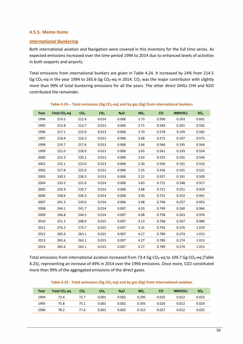
50
4.5.5. Memo Items
International Bunkering
Both international aviation and Navigation were covered in this inventory for the full time series. As
expected emissions increased over the time period 1994 to 2014 due to enhanced levels of activities
in both seaports and airports.
Total emissions from international bunkers are given in Table 4.24. It increased by 24% from 214.5
Gg CO₂-eq in the year 1994 to 265.6 Gg CO₂-eq in 2014. CO2 was the major contributor with slightly
more than 99% of total bunkering emissions for all the years. The other direct GHGs CH4 and N2O
contributed the remainder.
Table 4.24 – Total emissions (Gg CO2-eq) and by gas (Gg) from international bunkers
Year Total CO2-eq CO₂ CH₄ N₂O NOₓ CO NMVOCs SO₂
1994 214.5 212.4 0.014 0.006 3.73 0.590 0.203 0.601
1995 215.8 213.7 0.013 0.006 3.71 0.583 0.201 0.592
1996 217.1 215.0 0.013 0.006 3.70 0.578 0.199 0.582
1997 218.4 216.3 0.013 0.006 3.68 0.572 0.197 0.573
1998 219.7 217.6 0.013 0.006 3.66 0.566 0.195 0.564
1999 221.0 218.9 0.013 0.006 3.65 0.561 0.193 0.554
2000 222.3 220.1 0.013 0.006 3.63 0.555 0.191 0.544
2001 225.1 223.0 0.013 0.006 2.30 0.556 0.191 0.533
2002 227.8 225.6 0.013 0.006 2.25 0.556 0.191 0.521
2003 230.5 228.3 0.013 0.006 2.21 0.557 0.191 0.509
2004 233.2 231.0 0.014 0.006 3.83 0.712 0.248 0.917
2005 235.9 233.7 0.014 0.006 3.88 0.721 0.251 0.929
2006 238.6 236.3 0.014 0.006 3.93 0.731 0.254 0.941
2007 241.3 239.0 0.014 0.006 3.98 0.740 0.257 0.953
2008 244.1 241.7 0.014 0.007 4.03 0.749 0.260 0.964
2009 246.8 244.5 0.014 0.007 4.08 0.758 0.263 0.976
2010 251.3 248.9 0.015 0.007 4.13 0.768 0.267 0.989
2011 276.3 273.7 0.015 0.007 4.31 0.793 0.276 1.019
2012 265.6 263.1 0.015 0.007 4.27 0.789 0.274 1.015
2013 265.6 263.1 0.015 0.007 4.27 0.789 0.274 1.015
2014 265.6 263.1 0.015 0.007 4.27 0.789 0.274 1.015
Total emissions from international aviation increased from 73.4 Gg CO₂-eq to 109.7 Gg CO₂-eq (Table
4.25), representing an increase of 49% in 2014 over the 1994 emissions. Once more, CO2 constituted
more than 99% of the aggregated emissions of the direct gases.
Table 4.25 - Total emissions (Gg CO2-eq) and by gas (Gg) from international aviation
Year Total CO2-eq CO₂ CH₄ N₂O NOₓ CO NMVOCs SO₂
1994 73.4 72.7 0.001 0.002 0.295 0.025 0.012 0.023
1995 75.8 75.1 0.001 0.002 0.305 0.026 0.012 0.024
1996 78.2 77.6 0.001 0.002 0.315 0.027 0.012 0.025
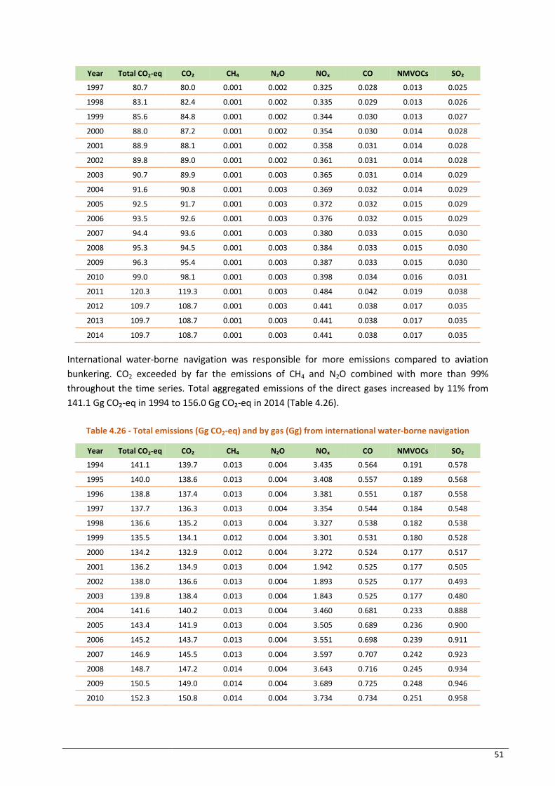
51
Year Total CO2-eq CO₂ CH₄ N₂O NOₓ CO NMVOCs SO₂
1997 80.7 80.0 0.001 0.002 0.325 0.028 0.013 0.025
1998 83.1 82.4 0.001 0.002 0.335 0.029 0.013 0.026
1999 85.6 84.8 0.001 0.002 0.344 0.030 0.013 0.027
2000 88.0 87.2 0.001 0.002 0.354 0.030 0.014 0.028
2001 88.9 88.1 0.001 0.002 0.358 0.031 0.014 0.028
2002 89.8 89.0 0.001 0.002 0.361 0.031 0.014 0.028
2003 90.7 89.9 0.001 0.003 0.365 0.031 0.014 0.029
2004 91.6 90.8 0.001 0.003 0.369 0.032 0.014 0.029
2005 92.5 91.7 0.001 0.003 0.372 0.032 0.015 0.029
2006 93.5 92.6 0.001 0.003 0.376 0.032 0.015 0.029
2007 94.4 93.6 0.001 0.003 0.380 0.033 0.015 0.030
2008 95.3 94.5 0.001 0.003 0.384 0.033 0.015 0.030
2009 96.3 95.4 0.001 0.003 0.387 0.033 0.015 0.030
2010 99.0 98.1 0.001 0.003 0.398 0.034 0.016 0.031
2011 120.3 119.3 0.001 0.003 0.484 0.042 0.019 0.038
2012 109.7 108.7 0.001 0.003 0.441 0.038 0.017 0.035
2013 109.7 108.7 0.001 0.003 0.441 0.038 0.017 0.035
2014 109.7 108.7 0.001 0.003 0.441 0.038 0.017 0.035
International water-borne navigation was responsible for more emissions compared to aviation
bunkering. CO2 exceeded by far the emissions of CH4 and N2O combined with more than 99%
throughout the time series. Total aggregated emissions of the direct gases increased by 11% from
141.1 Gg CO₂-eq in 1994 to 156.0 Gg CO₂-eq in 2014 (Table 4.26).
Table 4.26 - Total emissions (Gg CO2-eq) and by gas (Gg) from international water-borne navigation
Year Total CO2-eq CO₂ CH₄ N₂O NOₓ CO NMVOCs SO₂
1994 141.1 139.7 0.013 0.004 3.435 0.564 0.191 0.578
1995 140.0 138.6 0.013 0.004 3.408 0.557 0.189 0.568
1996 138.8 137.4 0.013 0.004 3.381 0.551 0.187 0.558
1997 137.7 136.3 0.013 0.004 3.354 0.544 0.184 0.548
1998 136.6 135.2 0.013 0.004 3.327 0.538 0.182 0.538
1999 135.5 134.1 0.012 0.004 3.301 0.531 0.180 0.528
2000 134.2 132.9 0.012 0.004 3.272 0.524 0.177 0.517
2001 136.2 134.9 0.013 0.004 1.942 0.525 0.177 0.505
2002 138.0 136.6 0.013 0.004 1.893 0.525 0.177 0.493
2003 139.8 138.4 0.013 0.004 1.843 0.525 0.177 0.480
2004 141.6 140.2 0.013 0.004 3.460 0.681 0.233 0.888
2005 143.4 141.9 0.013 0.004 3.505 0.689 0.236 0.900
2006 145.2 143.7 0.013 0.004 3.551 0.698 0.239 0.911
2007 146.9 145.5 0.013 0.004 3.597 0.707 0.242 0.923
2008 148.7 147.2 0.014 0.004 3.643 0.716 0.245 0.934
2009 150.5 149.0 0.014 0.004 3.689 0.725 0.248 0.946
2010 152.3 150.8 0.014 0.004 3.734 0.734 0.251 0.958
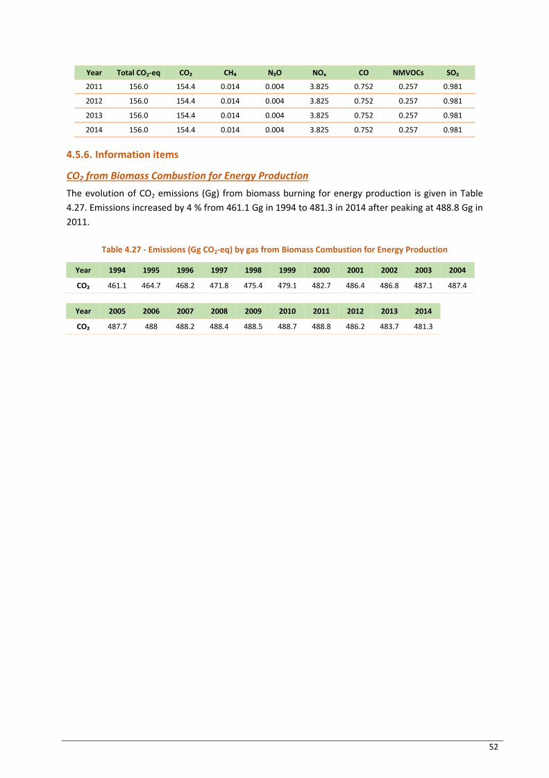
52
Year Total CO2-eq CO₂ CH₄ N₂O NOₓ CO NMVOCs SO₂
2011 156.0 154.4 0.014 0.004 3.825 0.752 0.257 0.981
2012 156.0 154.4 0.014 0.004 3.825 0.752 0.257 0.981
2013 156.0 154.4 0.014 0.004 3.825 0.752 0.257 0.981
2014 156.0 154.4 0.014 0.004 3.825 0.752 0.257 0.981
4.5.6. Information items
CO2 from Biomass Combustion for Energy Production
The evolution of CO2 emissions (Gg) from biomass burning for energy production is given in Table
4.27. Emissions increased by 4 % from 461.1 Gg in 1994 to 481.3 in 2014 after peaking at 488.8 Gg in
2011.
Table 4.27 - Emissions (Gg CO2-eq) by gas from Biomass Combustion for Energy Production
Year 1994 1995 1996 1997 1998 1999 2000 2001 2002 2003 2004
CO₂ 461.1 464.7 468.2 471.8 475.4 479.1 482.7 486.4 486.8 487.1 487.4
Year 2005 2006 2007 2008 2009 2010 2011 2012 2013 2014
CO₂ 487.7 488 488.2 488.4 488.5 488.7 488.8 486.2 483.7 481.3
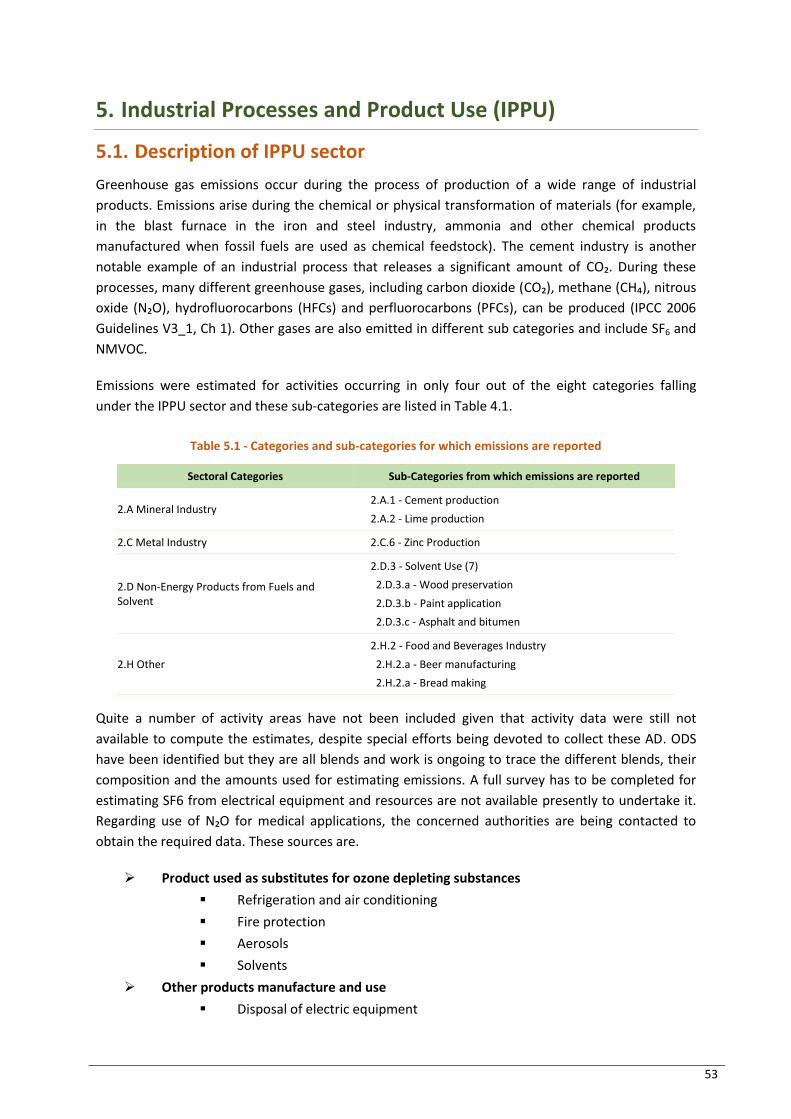
53
5. Industrial Processes and Product Use (IPPU)
5.1. Description of IPPU sector
Greenhouse gas emissions occur during the process of production of a wide range of industrial
products. Emissions arise during the chemical or physical transformation of materials (for example,
in the blast furnace in the iron and steel industry, ammonia and other chemical products
manufactured when fossil fuels are used as chemical feedstock). The cement industry is another
notable example of an industrial process that releases a significant amount of CO₂. During these
processes, many different greenhouse gases, including carbon dioxide (CO₂), methane (CH₄), nitrous
oxide (N₂O), hydrofluorocarbons (HFCs) and perfluorocarbons (PFCs), can be produced (IPCC 2006
Guidelines V3_1, Ch 1). Other gases are also emitted in different sub categories and include SF6 and
NMVOC.
Emissions were estimated for activities occurring in only four out of the eight categories falling
under the IPPU sector and these sub-categories are listed in Table 4.1.
Table 5.1 - Categories and sub-categories for which emissions are reported
Sectoral Categories Sub-Categories from which emissions are reported
2.A Mineral Industry 2.A.1 - Cement production
2.A.2 - Lime production
2.C Metal Industry 2.C.6 - Zinc Production
2.D Non-Energy Products from Fuels and Solvent
2.D.3 - Solvent Use (7)
2.D.3.a - Wood preservation
2.D.3.b - Paint application
2.D.3.c - Asphalt and bitumen
2.H Other
2.H.2 - Food and Beverages Industry
2.H.2.a - Beer manufacturing
2.H.2.a - Bread making
Quite a number of activity areas have not been included given that activity data were still not
available to compute the estimates, despite special efforts being devoted to collect these AD. ODS
have been identified but they are all blends and work is ongoing to trace the different blends, their
composition and the amounts used for estimating emissions. A full survey has to be completed for
estimating SF6 from electrical equipment and resources are not available presently to undertake it.
Regarding use of N₂O for medical applications, the concerned authorities are being contacted to
obtain the required data. These sources are.
Product used as substitutes for ozone depleting substances
Refrigeration and air conditioning
Fire protection
Aerosols
Solvents
Other products manufacture and use
Disposal of electric equipment
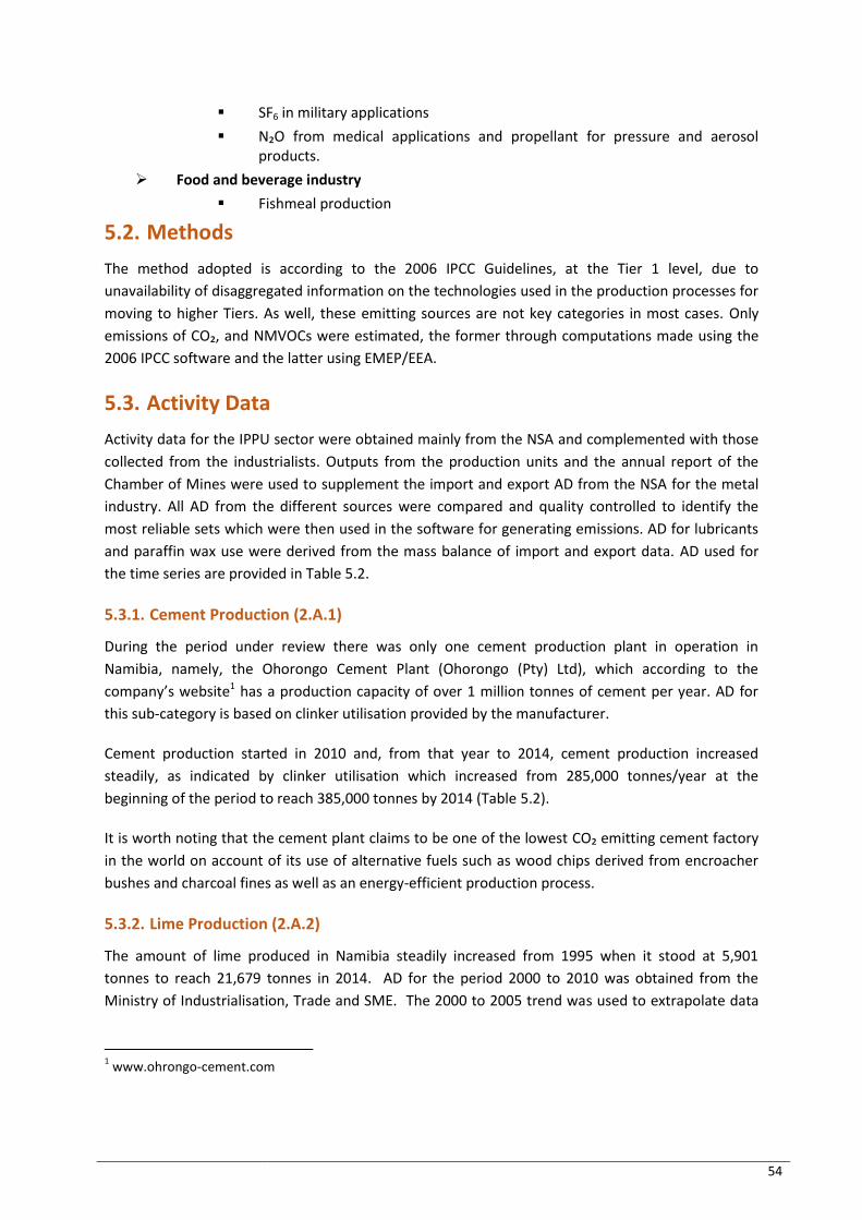
54
SF6 in military applications
N₂O from medical applications and propellant for pressure and aerosol products.
Food and beverage industry
Fishmeal production
5.2. Methods
The method adopted is according to the 2006 IPCC Guidelines, at the Tier 1 level, due to
unavailability of disaggregated information on the technologies used in the production processes for
moving to higher Tiers. As well, these emitting sources are not key categories in most cases. Only
emissions of CO₂, and NMVOCs were estimated, the former through computations made using the
2006 IPCC software and the latter using EMEP/EEA.
5.3. Activity Data
Activity data for the IPPU sector were obtained mainly from the NSA and complemented with those
collected from the industrialists. Outputs from the production units and the annual report of the
Chamber of Mines were used to supplement the import and export AD from the NSA for the metal
industry. All AD from the different sources were compared and quality controlled to identify the
most reliable sets which were then used in the software for generating emissions. AD for lubricants
and paraffin wax use were derived from the mass balance of import and export data. AD used for
the time series are provided in Table 5.2.
5.3.1. Cement Production (2.A.1)
During the period under review there was only one cement production plant in operation in
Namibia, namely, the Ohorongo Cement Plant (Ohorongo (Pty) Ltd), which according to the
company’s website1 has a production capacity of over 1 million tonnes of cement per year. AD for
this sub-category is based on clinker utilisation provided by the manufacturer.
Cement production started in 2010 and, from that year to 2014, cement production increased
steadily, as indicated by clinker utilisation which increased from 285,000 tonnes/year at the
beginning of the period to reach 385,000 tonnes by 2014 (Table 5.2).
It is worth noting that the cement plant claims to be one of the lowest CO₂ emitting cement factory
in the world on account of its use of alternative fuels such as wood chips derived from encroacher
bushes and charcoal fines as well as an energy-efficient production process.
5.3.2. Lime Production (2.A.2)
The amount of lime produced in Namibia steadily increased from 1995 when it stood at 5,901
tonnes to reach 21,679 tonnes in 2014. AD for the period 2000 to 2010 was obtained from the
Ministry of Industrialisation, Trade and SME. The 2000 to 2005 trend was used to extrapolate data
1 www.ohrongo-cement.com

55
for the period 1994 to 1999 while the 2000 to 2010 trend was used to extrapolate data for the
period 2011 to 2014 (Table 5.2).
5.3.3. Zinc Production (2.C.6)
For the purpose of this inventory, only production of metallic zinc is considered. Data obtained from
the Chamber of Mines indicate that though activities were launched in 2002, it was only in 2003 that
commercial production started and by 2004 had reached 119,205 tonnes. Production still grew,
albeit at a slower rate, during the following years to reach 151,688 tonnes in 2010. However,
thereafter production decreased significantly over the years to reach 102,188 tonnes in 2014
(Table 5.2).
5.3.4. Lubricant Use (2.D.1)
Activity data gaps for Lubricant Use were generated from data collected for the period 2000 to 2013
from Trade Statistics and the Ministry of Industrialisation, Trade and SME. The average lubricant use
for 2000 and 2001 was used as a constant for the period 1994 to 1999. Regarding 2014 and since
trade data for that year was not reliable, the average usage during the period 2011 to 2013 was
adopted. The time series thus obtained shows: (i) lubricant use was stable during the 1994 to 1999
period with an annual use of around 854 tonnes, (ii) from 2004 to 2009 lubricant use jumped from
294 tonnes to 15,404 tonnes and (iii) thereafter, with the exception of a drop to 13,896 tonnes in
2010, production stabilised at around 15,400 tonnes per year (Table 5.2).
5.3.5. Paraffin Wax Use (2.D.2)
For the period 2000 to 2010, AD for Paraffin Wax Use were generated by adjusting figures obtained from the Ministry of Industrialisation, Trade and SME with data from Trade Statistics. For the periods 1994 to 1999 and that of 2011 to 2014, an estimate of 30,000 tonnes per year was used (Table 5.2).
5.3.6. Wood Preservation (2.D.3.a)
The utilisation of creosote by the railway network was considered and the assumption made that
over the period under review utilisation was constant given that the railway network did not expand.
Thus, AD for creosote was estimated at 16 tonnes per year based on average trade data (Table 5.2).
5.3.7. Paint application (2.D.3.b)
Since no production data were available from manufacturers of solvent-based paints and lacquers,
the mass balance from import and export data was adopted as AD for this activity. Extrapolation of
data available for the period 1998 to 2014 was adopted to generate data for the period 1994 to
1997. A linear trend was then generated for the whole period to correct the marked highs and lows
of the original trade data (Table 5.2).
5.3.8. Asphalt and bitumen (2.D.3.c)
Asphalt and bitumen import and export data available for the period 1998 to 2014 presented
marked variations between the years. AD for the period 1994 to 1997 was computed as the average
amount of product used during the period 1998 to 2003, export data were retained for the period
1998 to 2002 and linear trending was of import and export data of the period 2003 to 2014 was used
to generate data for completing the time series. Asphalt and bitumen use during the period 1994 to
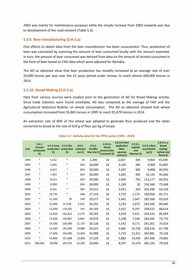
56
2003 was mainly for maintenance purposes while the steady increase from 2004 onwards was due
to development of the road network (Table 5.2).
5.3.9. Beer manufacturing (2.H.2.a)
Past efforts to obtain data from the beer manufacturer has been unsuccessful. Thus, production of
beer was calculated by summing the amount of beer consumed locally with the amount exported.
In turn, the amount of beer consumed was derived from data on the amount of alcohol consumed in
the form of beer based on FAO data which were adjusted for Namibia.
The AD so obtained show that beer production has steadily increased at an average rate of over
20,000 tonnes per year over the 21 years period under review, to reach almost 400,000 tonnes in
2014.
5.3.10. Bread Making (2.H.2.a)
Data from various sources were studied prior to the generation of AD for Bread Making activity.
Since trade statistics were found unreliable, AD was computed as the average of FAO and the
Agricultural Statistical Bulletin on wheat consumption. The AD so obtained showed that wheat
consumption increased from 55,865 tonnes in 1995 to reach 91,879 tonnes in 2014.
An extraction rate of 80% of this wheat was adopted to generate flour produced and the latter
converted to bread at the rate of 610 g of flour per kg of bread.
Table 5.2 - Activity data for the IPPU sector (1995 - 2014)
Year
2.A.1-Cement
production (t)
2.A.2-Lime production
(t)
2.C.6-Zinc production
(t)
2.D.1-Lubricant
use (t)
2.D.2-Paraffin
Wax Use (t)
2.D.3.a-Wood
preservation (creosote) (t)
2.D.3.b-Paint application
(Non-aqueous paint) (t)
2.D.3.c-Asphalt
and bitumen (t)
2.H.2.a-Beer manufacturi
ng (t)
2.D.H.2.a-Bread
making (wheat and
flour) (t)
1994 * 5,152 * 34 1,206 16 2,657 485 9,904 45,939
1995 * 5,901 * 854 30,000 16 3,169 485 9,908 55,865
1996 * 6,651 * 854 30,000 16 3,287 485 9,908 60,950
1997 * 7,401 * 854 30,000 16 3,405 485 42,141 45,646
1998 * 8,151 * 854 30,000 16 2,904 742 113,177 60,953
1999 * 8,900 * 854 30,000 16 5,169 92 156,568 75,648
2000 * 9,161 * 965 29,415 16 3,452 263 202,498 64,218
2001 * 10,735 * 448 27,319 16 3,729 1,175 258,058 65,271
2002 * 11,200 35 294 29,577 16 5,481 1,047 185,268 83,019
2003 * 12,400 47,436 2,022 30,332 16 2,224 2,672 264,395 80,685
2004 * 12,600 119,205 543 34,193 16 3,415 4,297 248,612 88,614
2005 * 13,050 132,813 6,179 30,765 16 3,524 5,921 264,516 85,699
2006 * 13,500 129,897 6,966 29,070 16 5,108 7,546 282,645 73,770
2007 * 14,500 150,080 11,197 29,128 16 5,542 9,171 291,301 74,914
2008 * 15,400 145,396 14,880 34,625 16 4,885 10,796 328,516 67,798
2009 * 17,600 150,400 15,404 35,989 16 5,723 12,421 393,881 70,136
2010 * 19,800 151,688 13,896 27,529 16 5,883 14,045 367,496 74,892
2011 284,000 18,996 144,755 15,205 30,000 16 8,397 15,670 385,193 79,918
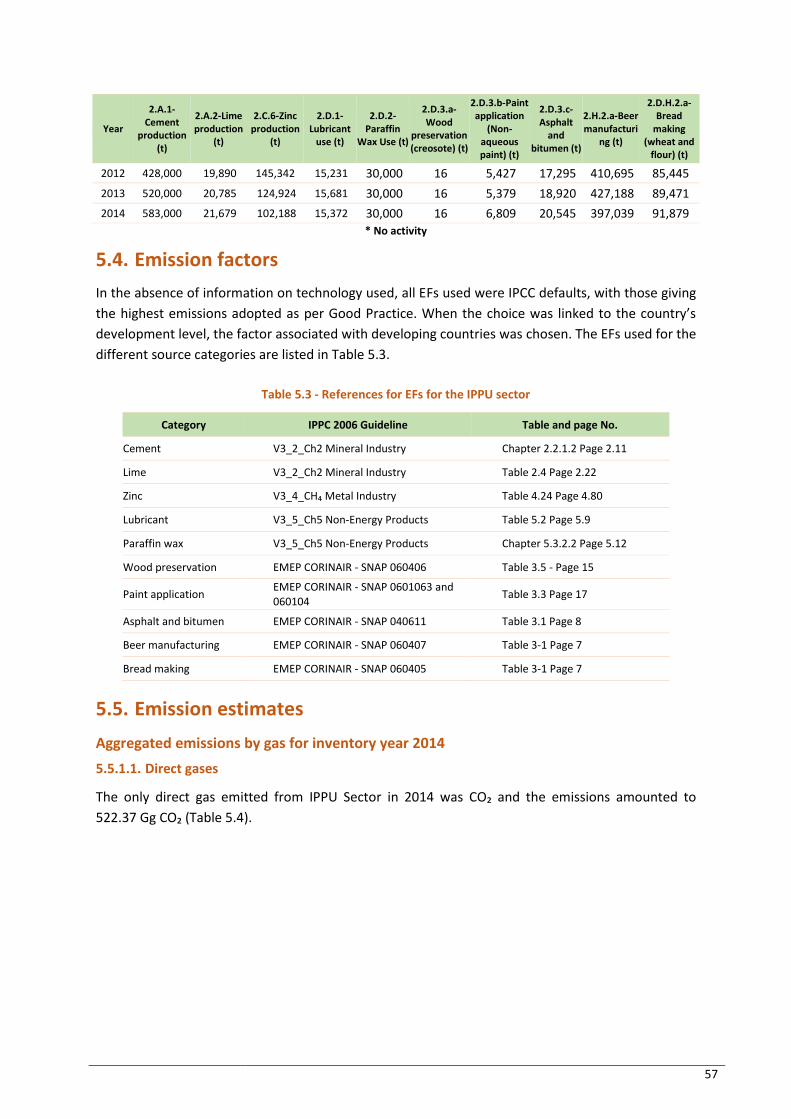
57
Year
2.A.1-Cement
production (t)
2.A.2-Lime production
(t)
2.C.6-Zinc production
(t)
2.D.1-Lubricant
use (t)
2.D.2-Paraffin
Wax Use (t)
2.D.3.a-Wood
preservation (creosote) (t)
2.D.3.b-Paint application
(Non-aqueous paint) (t)
2.D.3.c-Asphalt
and bitumen (t)
2.H.2.a-Beer manufacturi
ng (t)
2.D.H.2.a-Bread
making (wheat and
flour) (t)
2012 428,000 19,890 145,342 15,231 30,000 16 5,427 17,295 410,695 85,445
2013 520,000 20,785 124,924 15,681 30,000 16 5,379 18,920 427,188 89,471
2014 583,000 21,679 102,188 15,372 30,000 16 6,809 20,545 397,039 91,879
* No activity
5.4. Emission factors
In the absence of information on technology used, all EFs used were IPCC defaults, with those giving
the highest emissions adopted as per Good Practice. When the choice was linked to the country’s
development level, the factor associated with developing countries was chosen. The EFs used for the
different source categories are listed in Table 5.3.
Table 5.3 - References for EFs for the IPPU sector
Category IPPC 2006 Guideline Table and page No.
Cement V3_2_Ch2 Mineral Industry Chapter 2.2.1.2 Page 2.11
Lime V3_2_Ch2 Mineral Industry Table 2.4 Page 2.22
Zinc V3_4_CH₄ Metal Industry Table 4.24 Page 4.80
Lubricant V3_5_Ch5 Non-Energy Products Table 5.2 Page 5.9
Paraffin wax V3_5_Ch5 Non-Energy Products Chapter 5.3.2.2 Page 5.12
Wood preservation EMEP CORINAIR - SNAP 060406 Table 3.5 - Page 15
Paint application EMEP CORINAIR - SNAP 0601063 and 060104
Table 3.3 Page 17
Asphalt and bitumen EMEP CORINAIR - SNAP 040611 Table 3.1 Page 8
Beer manufacturing EMEP CORINAIR - SNAP 060407 Table 3-1 Page 7
Bread making EMEP CORINAIR - SNAP 060405 Table 3-1 Page 7
5.5. Emission estimates
Aggregated emissions by gas for inventory year 2014
5.5.1.1. Direct gases
The only direct gas emitted from IPPU Sector in 2014 was CO₂ and the emissions amounted to
522.37 Gg CO₂ (Table 5.4).
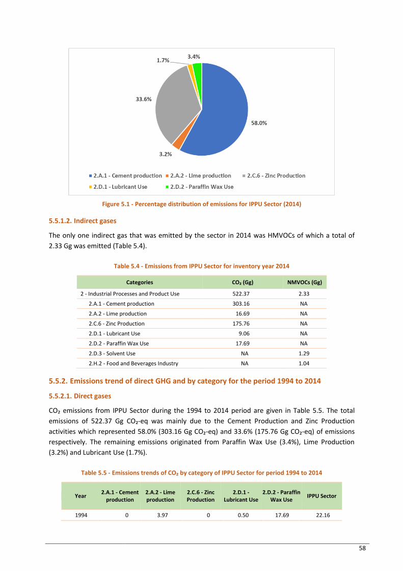
58
Figure 5.1 - Percentage distribution of emissions for IPPU Sector (2014)
5.5.1.2. Indirect gases
The only one indirect gas that was emitted by the sector in 2014 was HMVOCs of which a total of
2.33 Gg was emitted (Table 5.4).
Table 5.4 - Emissions from IPPU Sector for inventory year 2014
Categories CO₂ (Gg) NMVOCs (Gg)
2 - Industrial Processes and Product Use 522.37 2.33
2.A.1 - Cement production 303.16 NA
2.A.2 - Lime production 16.69 NA
2.C.6 - Zinc Production 175.76 NA
2.D.1 - Lubricant Use 9.06 NA
2.D.2 - Paraffin Wax Use 17.69 NA
2.D.3 - Solvent Use NA 1.29
2.H.2 - Food and Beverages Industry NA 1.04
5.5.2. Emissions trend of direct GHG and by category for the period 1994 to 2014
5.5.2.1. Direct gases
CO₂ emissions from IPPU Sector during the 1994 to 2014 period are given in Table 5.5. The total
emissions of 522.37 Gg CO₂-eq was mainly due to the Cement Production and Zinc Production
activities which represented 58.0% (303.16 Gg CO₂-eq) and 33.6% (175.76 Gg CO₂-eq) of emissions
respectively. The remaining emissions originated from Paraffin Wax Use (3.4%), Lime Production
(3.2%) and Lubricant Use (1.7%).
Table 5.5 - Emissions trends of CO₂ by category of IPPU Sector for period 1994 to 2014
Year 2.A.1 - Cement
production 2.A.2 - Lime production
2.C.6 - Zinc Production
2.D.1 - Lubricant Use
2.D.2 - Paraffin Wax Use
IPPU Sector
1994 0 3.97 0 0.50 17.69 22.16
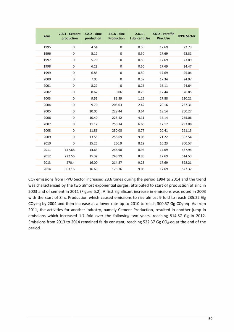
59
Year 2.A.1 - Cement
production 2.A.2 - Lime production
2.C.6 - Zinc Production
2.D.1 - Lubricant Use
2.D.2 - Paraffin Wax Use
IPPU Sector
1995 0 4.54 0 0.50 17.69 22.73
1996 0 5.12 0 0.50 17.69 23.31
1997 0 5.70 0 0.50 17.69 23.89
1998 0 6.28 0 0.50 17.69 24.47
1999 0 6.85 0 0.50 17.69 25.04
2000 0 7.05 0 0.57 17.34 24.97
2001 0 8.27 0 0.26 16.11 24.64
2002 0 8.62 0.06 0.73 17.44 26.85
2003 0 9.55 81.59 1.19 17.88 110.21
2004 0 9.70 205.03 2.42 20.16 237.31
2005 0 10.05 228.44 3.64 18.14 260.27
2006 0 10.40 223.42 4.11 17.14 255.06
2007 0 11.17 258.14 6.60 17.17 293.08
2008 0 11.86 250.08 8.77 20.41 291.13
2009 0 13.55 258.69 9.08 21.22 302.54
2010 0 15.25 260.9 8.19 16.23 300.57
2011 147.68 14.63 248.98 8.96 17.69 437.94
2012 222.56 15.32 249.99 8.98 17.69 514.53
2013 270.4 16.00 214.87 9.25 17.69 528.21
2014 303.16 16.69 175.76 9.06 17.69 522.37
CO₂ emissions from IPPU Sector increased 23.6 times during the period 1994 to 2014 and the trend
was characterised by the two almost exponential surges, attributed to start of production of zinc in
2003 and of cement in 2011 (Figure 5.2). A first significant increase in emissions was noted in 2003
with the start of Zinc Production which caused emissions to rise almost 9 fold to reach 235.22 Gg
CO₂-eq by 2004 and then increase at a lower rate up to 2010 to reach 300.57 Gg CO₂-eq As from
2011, the activities for another industry, namely Cement Production, resulted in another jump in
emissions which increased 1.7 fold over the following two years, reaching 514.57 Gg in 2012.
Emissions from 2013 to 2014 remained fairly constant, reaching 522.37 Gg CO₂-eq at the end of the
period.

60
Figure 5.2 - CO₂-eq emission trends for IPPU sector source categories (1994 - 2014)
5.5.3. Emissions trend for IPPU sub-categories for inventory period 1994 to 2014
5.5.3.1. Indirect gases
NMVOCs emissions came from two sub-categories Solvent Use and Food and Beverages covering
five activities, namely Wood Preservation, Paint Application, Asphalt and Bitumen use, Beer
Manufacturing and Bread Making (Table 5.6).
In 2014, a total amount of 2.33 Gg of NMVOCs were emitted by the IPPU sector, most of which
originating from the use of solvents with 56.2% of emissions (1.29 Gg) and Food and Beverages with
44.8% of emissions at 1.04 Gg. Total emissions of NMVOCs increased by 1.66 Gg from 0.67 in 1994 to
2.33 in 2014. Of this 1.66 Gg, Solvent Use contributed 0.76 Gg and Food and Beverages the
remaining 0.9 Gg.
Table 5.6 - NMVOCs emission trends for IPPU sector source categories (1994 - 2014)
Year 2.D.3 - Solvent 2.H.2 - Food and
Beverages Industry Total IPPU Sector
1994 0.53 0.14 0.67
1995 0.57 0.17 0.74
1996 0.61 0.18 0.79
1997 0.65 0.2 0.85
1998 0.68 0.39 1.07
1999 0.72 0.51 1.23
2000 0.76 0.57 1.33
2001 0.8 0.69 1.49
2002 0.84 0.59 1.42
2003 0.87 0.74 1.61
2004 0.91 0.73 1.64
2005 0.95 0.75 1.7
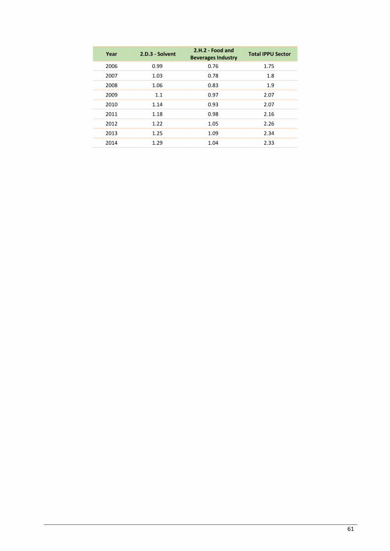
61
Year 2.D.3 - Solvent 2.H.2 - Food and
Beverages Industry Total IPPU Sector
2006 0.99 0.76 1.75
2007 1.03 0.78 1.8
2008 1.06 0.83 1.9
2009 1.1 0.97 2.07
2010 1.14 0.93 2.07
2011 1.18 0.98 2.16
2012 1.22 1.05 2.26
2013 1.25 1.09 2.34
2014 1.29 1.04 2.33
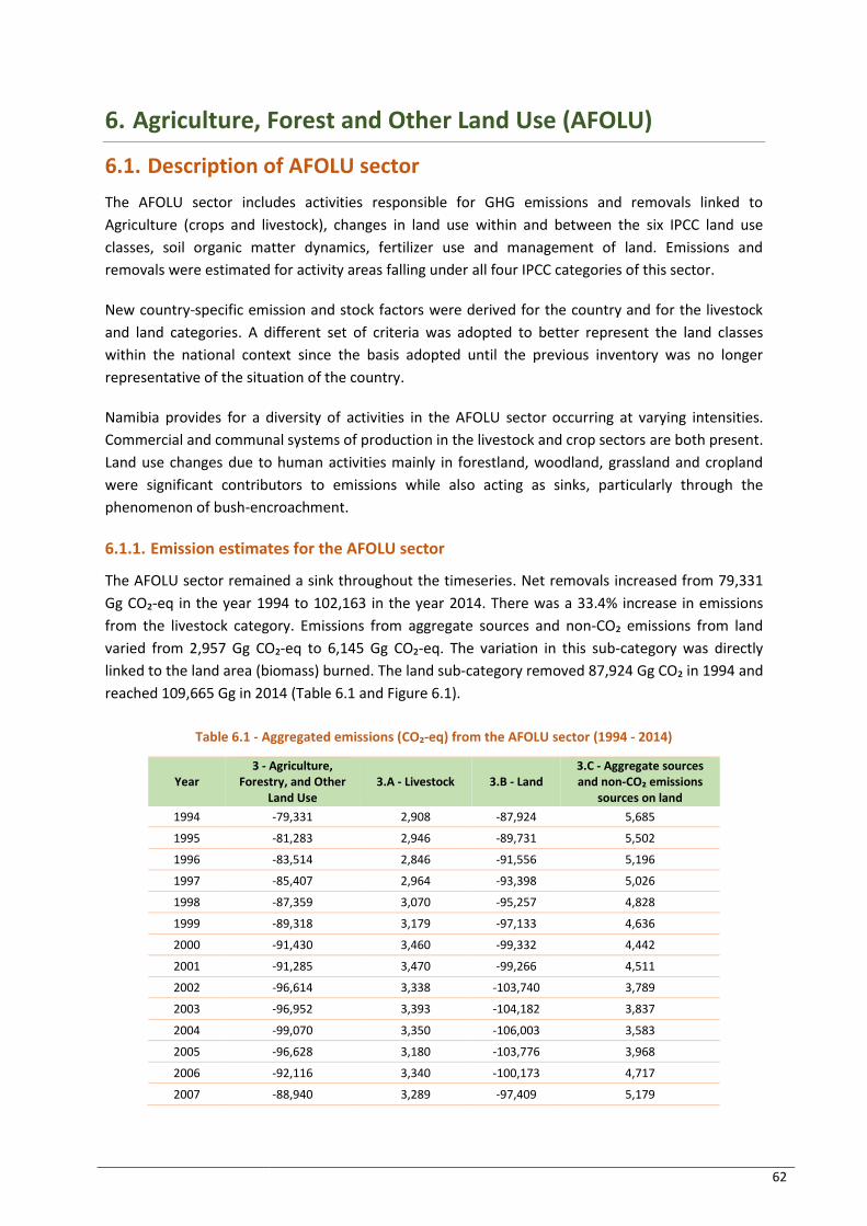
62
6. Agriculture, Forest and Other Land Use (AFOLU)
6.1. Description of AFOLU sector
The AFOLU sector includes activities responsible for GHG emissions and removals linked to
Agriculture (crops and livestock), changes in land use within and between the six IPCC land use
classes, soil organic matter dynamics, fertilizer use and management of land. Emissions and
removals were estimated for activity areas falling under all four IPCC categories of this sector.
New country-specific emission and stock factors were derived for the country and for the livestock
and land categories. A different set of criteria was adopted to better represent the land classes
within the national context since the basis adopted until the previous inventory was no longer
representative of the situation of the country.
Namibia provides for a diversity of activities in the AFOLU sector occurring at varying intensities.
Commercial and communal systems of production in the livestock and crop sectors are both present.
Land use changes due to human activities mainly in forestland, woodland, grassland and cropland
were significant contributors to emissions while also acting as sinks, particularly through the
phenomenon of bush-encroachment.
6.1.1. Emission estimates for the AFOLU sector
The AFOLU sector remained a sink throughout the timeseries. Net removals increased from 79,331
Gg CO₂-eq in the year 1994 to 102,163 in the year 2014. There was a 33.4% increase in emissions
from the livestock category. Emissions from aggregate sources and non-CO₂ emissions from land
varied from 2,957 Gg CO₂-eq to 6,145 Gg CO₂-eq. The variation in this sub-category was directly
linked to the land area (biomass) burned. The land sub-category removed 87,924 Gg CO₂ in 1994 and
reached 109,665 Gg in 2014 (Table 6.1 and Figure 6.1).
Table 6.1 - Aggregated emissions (CO₂-eq) from the AFOLU sector (1994 - 2014)
Year 3 - Agriculture,
Forestry, and Other Land Use
3.A - Livestock 3.B - Land 3.C - Aggregate sources and non-CO₂ emissions
sources on land
1994 -79,331 2,908 -87,924 5,685
1995 -81,283 2,946 -89,731 5,502
1996 -83,514 2,846 -91,556 5,196
1997 -85,407 2,964 -93,398 5,026
1998 -87,359 3,070 -95,257 4,828
1999 -89,318 3,179 -97,133 4,636
2000 -91,430 3,460 -99,332 4,442
2001 -91,285 3,470 -99,266 4,511
2002 -96,614 3,338 -103,740 3,789
2003 -96,952 3,393 -104,182 3,837
2004 -99,070 3,350 -106,003 3,583
2005 -96,628 3,180 -103,776 3,968
2006 -92,116 3,340 -100,173 4,717
2007 -88,940 3,289 -97,409 5,179
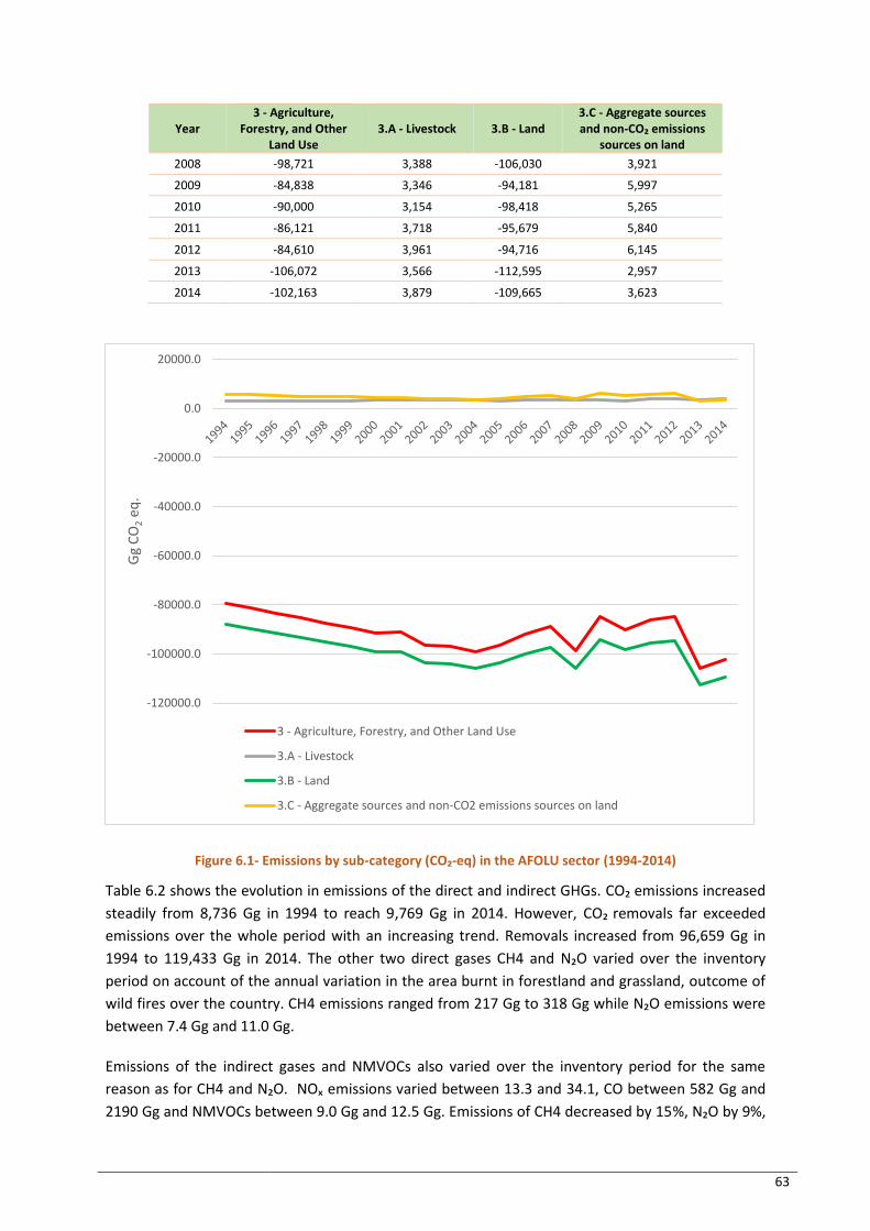
63
Year 3 - Agriculture,
Forestry, and Other Land Use
3.A - Livestock 3.B - Land 3.C - Aggregate sources and non-CO₂ emissions
sources on land
2008 -98,721 3,388 -106,030 3,921
2009 -84,838 3,346 -94,181 5,997
2010 -90,000 3,154 -98,418 5,265
2011 -86,121 3,718 -95,679 5,840
2012 -84,610 3,961 -94,716 6,145
2013 -106,072 3,566 -112,595 2,957
2014 -102,163 3,879 -109,665 3,623
Figure 6.1- Emissions by sub-category (CO₂-eq) in the AFOLU sector (1994-2014)
Table 6.2 shows the evolution in emissions of the direct and indirect GHGs. CO₂ emissions increased
steadily from 8,736 Gg in 1994 to reach 9,769 Gg in 2014. However, CO₂ removals far exceeded
emissions over the whole period with an increasing trend. Removals increased from 96,659 Gg in
1994 to 119,433 Gg in 2014. The other two direct gases CH4 and N₂O varied over the inventory
period on account of the annual variation in the area burnt in forestland and grassland, outcome of
wild fires over the country. CH4 emissions ranged from 217 Gg to 318 Gg while N₂O emissions were
between 7.4 Gg and 11.0 Gg.
Emissions of the indirect gases and NMVOCs also varied over the inventory period for the same
reason as for CH4 and N₂O. NOₓ emissions varied between 13.3 and 34.1, CO between 582 Gg and
2190 Gg and NMVOCs between 9.0 Gg and 12.5 Gg. Emissions of CH4 decreased by 15%, N₂O by 9%,
-120000.0
-100000.0
-80000.0
-60000.0
-40000.0
-20000.0
0.0
20000.0
Gg
CO
2 eq
.
3 - Agriculture, Forestry, and Other Land Use
3.A - Livestock
3.B - Land
3.C - Aggregate sources and non-CO2 emissions sources on land

64
NOₓ by 61% and CO by 61% largely due to the annual variation in the area burnt in forestland and
grassland that had significantly reduced during 2013 and 2014.
Table 6.2 - Emissions (Gg) by gas for AFOLU (1994 - 2014)
Year CO₂ -
Emissions CO₂ -
Removals CO₂ - Net removals
CH4 N₂O NOₓ CO NMVOCs
1994 8,735.6 -96,659.2 -87,923.6 274.0 9.2 33.8 2,152.3 9.2
1995 8,735.6 -98,466.5 -89,730.9 268.8 9.0 32.0 2,035.2 9.1
1996 8,735.6 -100,291.1 -91,555.5 256.1 8.6 30.1 1,917.2 9.0
1997 8,735.6 -102,133.0 -93,397.4 253.8 8.6 28.2 1,798.1 9.3
1998 8,735.5 -103,992.2 -95,256.7 250.7 8.5 26.3 1,678.0 9.7
1999 8,735.5 -105,868.6 -97,133.1 247.8 8.4 24.4 1,556.9 10.0
2000 8,735.8 -108,066.7 -99,330.9 251.0 8.5 22.1 1,408.3 11.0
2001 8,949.5 -108,212.1 -99,262.6 252.1 8.7 22.2 1,418.8 10.9
2002 8,948.5 -112,686.5 -103,738.0 223.6 7.8 16.8 1,072.6 10.5
2003 8,947.3 -113,128.4 -104,181.0 226.7 8.0 16.8 1,075.7 10.5
2004 8,947.0 -114,949.2 -106,002.2 216.7 7.7 14.9 956.7 10.6
2005 8,946.6 -112,722.8 -103,776.1 224.4 7.9 18.7 1,196.7 10.1
2006 8,946.6 -109,118.9 -100,172.3 254.0 8.8 24.1 1,545.7 10.7
2007 8,946.7 -106,355.0 -97,408.2 266.5 9.3 28.5 1,829.3 10.5
2008 8,946.5 -114,976.9 -106,030.4 229.4 8.0 17.6 1,129.5 10.7
2009 8,946.6 -103,127.0 -94,180.4 296.5 10.1 34.1 2,189.8 10.7
2010 8,946.5 -107,364.4 -98,417.9 266.2 9.1 29.1 1,868.1 10.3
2011 9,769.1 -105,447.8 -95,678.6 301.4 10.4 31.2 2,003.0 11.7
2012 9,769.2 -104,484.9 -94,715.6 318.4 11.0 32.5 2,091.2 12.4
2013 9,769.0 -122,363.2 -112,594.1 201.7 7.4 9.1 582.4 11.2
2014 9,769.0 -119,433.7 -109,664.7 234.0 8.3 13.3 858.0 12.5
The evolution of aggregated emissions, excluding removals, of the three direct GHGs is presented in
Figure 6.2. Total emissions fluctuated between 17,328 Gg CO₂-eq and 17,271 Gg CO₂-eq during the
period 1994 to 2014, with a peak of 19,875 Gg CO₂-eq in 2012. Emissions of the three direct GHGs
varied during the inventory period. The major contributor to emissions remained CO₂ contributing to
around 57% of total emissions of this sector followed by CH4 with some 28% and N₂O the remaining
15%.
Figure 6.2- Evolution of aggregated emissions (CO₂-eq) in the AFOLU sector (1994 - 2014)
0
5000
10000
15000
20000
25000
19
94
19
95
19
96
19
97
19
98
19
99
20
00
20
01
20
02
20
03
20
04
20
05
20
06
20
07
20
08
20
09
20
10
20
11
20
12
20
13
20
14
Gg
CO
2-e
q
Total CO2 Total CH4 Total N2O Total GHG emissions
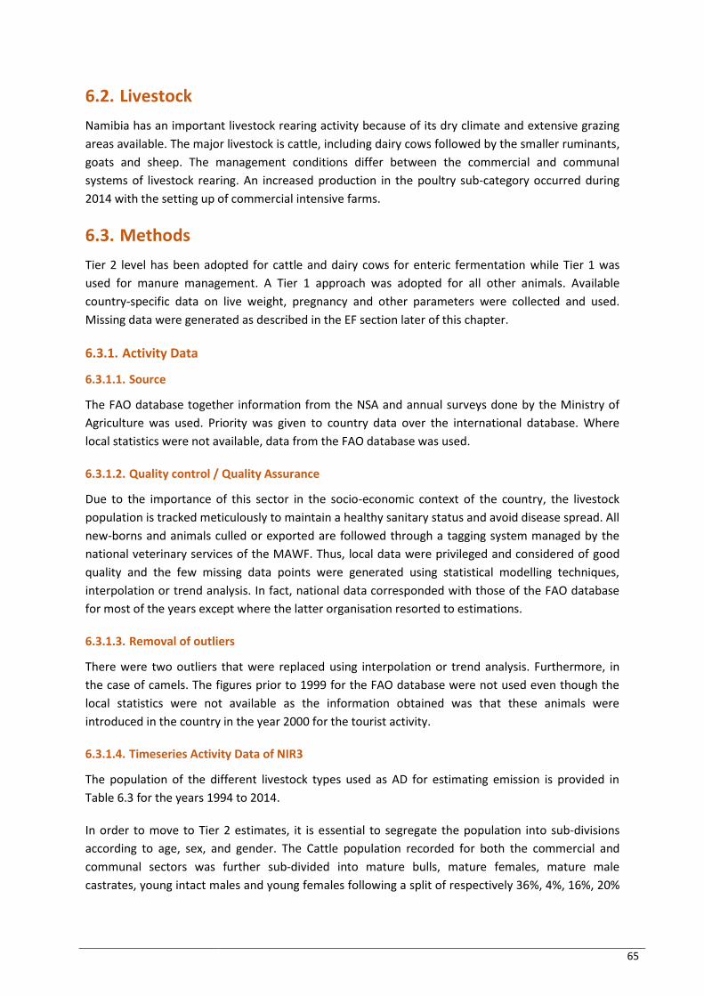
65
6.2. Livestock
Namibia has an important livestock rearing activity because of its dry climate and extensive grazing
areas available. The major livestock is cattle, including dairy cows followed by the smaller ruminants,
goats and sheep. The management conditions differ between the commercial and communal
systems of livestock rearing. An increased production in the poultry sub-category occurred during
2014 with the setting up of commercial intensive farms.
6.3. Methods
Tier 2 level has been adopted for cattle and dairy cows for enteric fermentation while Tier 1 was
used for manure management. A Tier 1 approach was adopted for all other animals. Available
country-specific data on live weight, pregnancy and other parameters were collected and used.
Missing data were generated as described in the EF section later of this chapter.
6.3.1. Activity Data
6.3.1.1. Source
The FAO database together information from the NSA and annual surveys done by the Ministry of
Agriculture was used. Priority was given to country data over the international database. Where
local statistics were not available, data from the FAO database was used.
6.3.1.2. Quality control / Quality Assurance
Due to the importance of this sector in the socio-economic context of the country, the livestock
population is tracked meticulously to maintain a healthy sanitary status and avoid disease spread. All
new-borns and animals culled or exported are followed through a tagging system managed by the
national veterinary services of the MAWF. Thus, local data were privileged and considered of good
quality and the few missing data points were generated using statistical modelling techniques,
interpolation or trend analysis. In fact, national data corresponded with those of the FAO database
for most of the years except where the latter organisation resorted to estimations.
6.3.1.3. Removal of outliers
There were two outliers that were replaced using interpolation or trend analysis. Furthermore, in
the case of camels. The figures prior to 1999 for the FAO database were not used even though the
local statistics were not available as the information obtained was that these animals were
introduced in the country in the year 2000 for the tourist activity.
6.3.1.4. Timeseries Activity Data of NIR3
The population of the different livestock types used as AD for estimating emission is provided in
Table 6.3 for the years 1994 to 2014.
In order to move to Tier 2 estimates, it is essential to segregate the population into sub-divisions
according to age, sex, and gender. The Cattle population recorded for both the commercial and
communal sectors was further sub-divided into mature bulls, mature females, mature male
castrates, young intact males and young females following a split of respectively 36%, 4%, 16%, 20%
66
and 24% based on a study on farming practices (NNFU, 2006). The sub-division into the different
classes was available for communal animals only. The same split was adopted for the commercial
sector as this is the normal situation for cattle rearing.
Table 6.3 - Number of animals (1994 - 2014)
Year Dairy cows Cattle Sheep Goats Horses Mules
and asses Swine Poultry Camels
1994 1,500 2,035,790 2,619,520 1,639,210 58,801 145,607 17,843 464,451 -
1995 1,500 2,031,353 2,409,699 1,616,090 53,217 145,607 19,979 487,031 -
1996 1,500 1,989,947 2,198,436 1,786,150 53,217 145,607 18,923 458,158 -
1997 1,500 2,055,416 2,429,328 1,821,009 53,217 145,607 16,884 522,618 -
1998 1,500 2,192,359 2,086,434 1,710,190 53,217 145,607 14,706 403,937 -
1999 1,500 2,278,569 2,169,651 1,689,770 53,217 145,607 18,731 450,513 -
2000 1,500 2,504,930 2,446,146 1,849,569 61,885 167,548 23,148 476,331 54
2001 1,500 2,508,570 2,369,809 1,769,055 52,502 169,314 21,854 502,356 71
2002 1,500 2,329,553 2,764,253 2,110,092 47,220 134,305 47,805 883,950 88
2003 1,500 2,336,094 2,955,454 2,086,812 47,542 119,828 46,932 894,027 124
2004 1,500 2,349,700 2,619,363 1,997,172 62,726 142,353 52,624 957,966 113
2005 1,500 2,219,330 2,663,795 2,043,479 47,429 140,291 55,931 998,278 63
2006 1,500 2,383,960 2,660,252 2,061,403 46,209 159,948 51,972 923,555 73
2007 1,500 2,353,498 2,652,658 1,926,429 43,863 156,328 51,863 916,991 63
2008 1,500 2,453,097 2,228,059 1,893,387 42,267 165,126 49,187 864,988 43
2009 1,500 2,465,989 1,803,460 1,792,390 38,201 173,923 48,223 843,277 23
2010 1,500 2,389,891 1,378,861 1,690,467 49,852 141,588 63,498 777,480 43
2011 1,500 2,762,240 2,209,593 1,736,565 45,529 105,062 43,865 684,236 69
2012 1,500 2,904,451 2,677,913 1,933,103 46,643 114,591 69,430 940,765 47
2013 2,000 2,634,418 2,188,758 1,693,145 40,265 124,120 69,070 659,033 51
2014 2,000 2,882,489 2,044,156 1,892,439 55,241 159,029 68,710 3,436,430 55
The average live weights of the non-dairy cattle classes were obtained from data of the slaughter
houses of MeatCo and auction of livestock. Information on development and typical animal mass of
the dominant local breeds Brahman and Nguni were used. Daily weight gain was derived from the
live weight and age of the different animal groups at slaughtering or auction time. The data was
compared and aligned with information obtained from breeding studies done on the 2 main species
with various others (S.J. Schoeman, 1996). The live weight for dairy cows has been assumed to be
525 kg based on available information on the race, awaiting confirmation of the current liveweight
of the population from the dairy farms.
For Tier 2 estimations, it is necessary to also assign a typical mature weight for each animal group
and these values for commercial and communal cattle classes were again derived from the weight of
animals slaughtered or sold at auctions. Table 6.4 below depicts the typical mature weight adopted
for the different classes.
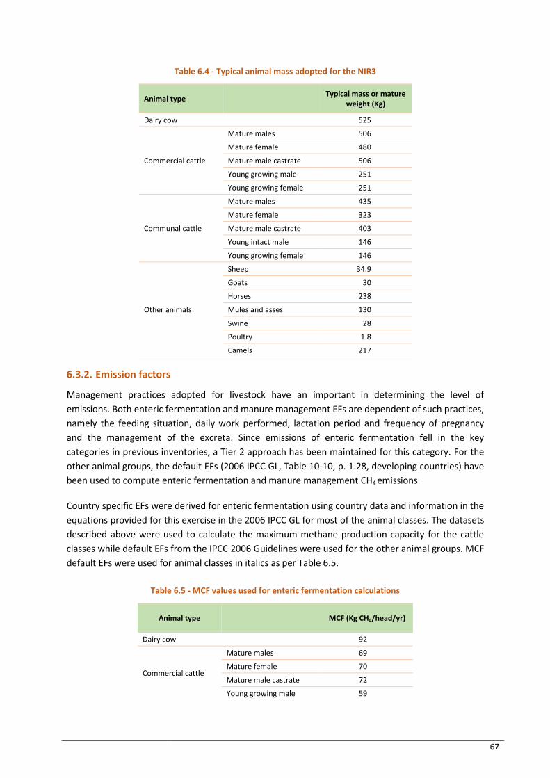
67
Table 6.4 - Typical animal mass adopted for the NIR3
Animal type Typical mass or mature
weight (Kg)
Dairy cow 525
Commercial cattle
Mature males 506
Mature female 480
Mature male castrate 506
Young growing male 251
Young growing female 251
Communal cattle
Mature males 435
Mature female 323
Mature male castrate 403
Young intact male 146
Young growing female 146
Other animals
Sheep 34.9
Goats 30
Horses 238
Mules and asses 130
Swine 28
Poultry 1.8
Camels 217
6.3.2. Emission factors
Management practices adopted for livestock have an important in determining the level of
emissions. Both enteric fermentation and manure management EFs are dependent of such practices,
namely the feeding situation, daily work performed, lactation period and frequency of pregnancy
and the management of the excreta. Since emissions of enteric fermentation fell in the key
categories in previous inventories, a Tier 2 approach has been maintained for this category. For the
other animal groups, the default EFs (2006 IPCC GL, Table 10-10, p. 1.28, developing countries) have
been used to compute enteric fermentation and manure management CH4 emissions.
Country specific EFs were derived for enteric fermentation using country data and information in the
equations provided for this exercise in the 2006 IPCC GL for most of the animal classes. The datasets
described above were used to calculate the maximum methane production capacity for the cattle
classes while default EFs from the IPCC 2006 Guidelines were used for the other animal groups. MCF
default EFs were used for animal classes in italics as per Table 6.5.
Table 6.5 - MCF values used for enteric fermentation calculations
Animal type MCF (Kg CH4/head/yr)
Dairy cow 92
Commercial cattle
Mature males 69
Mature female 70
Mature male castrate 72
Young growing male 59

68
Animal type MCF (Kg CH4/head/yr)
Young growing female 66
Communal cattle
Mature males 59
Mature female 46
Mature male castrate 55
Young intact male 36
Young growing female 40
Other animals
Sheep 5
Goats 5
Horses 18
Mules and asses 10
Swine 1
Camels 46
Table 6.6 below summarizes the manure management systems for the various animal categories.
This is based on information available from the censuses and surveys conducted by the Ministry of
Agriculture, Water Affairs and Forestry and NSA while manure management system (MMS) for cattle
are based on expert judgment and on information from the farming systems guide (NNFU, 2006).
Experts comprised officers of the MAWF, commercial livestock herders and communal farmers. As
manure management is not a key category for all animal classes, the default EFs from the guidelines
were adopted.
The temperature assigned for this sub-category for Namibia in previous inventories was 26oC and
this was amended to 20oC as it was a mistake. In fact, Namibia falls under a temperate climate
according to the IPCC Guideline except for small area classified as Tropical Dry and temperature
cannot be 26oC. This is confirmed from processing of data available on the site
http://sdwebx.worldbank.org/climateportal/index.cfm?page=country_historical_climate&ThisCCode
=NAM for the period 1901 to 2015.
Table 6.6 - MMS adopted for the different animal categories
Type of animal Manure management system
Dairy cows Solid storage
Commercial cattle (All) 100% Pasture-Range-Paddock (PRP)
Communal cattle (All) 50% PRP/ 49% Solid Storage / 1% Burnt for fuel
Sheep 100% PRP
Goats PRP 100%
Horses 100% PRP
Mules and asses 100% PRP
Swine Daily spread 60% and liquid slurry 40%
Poultry Poultry manure with litter 60% and poultry manure without litter 40%
Camels 100% PRP
Pregnancy have been accounted for dairy, commercial and communal cows. The lactation period of
dairy cows is zero day as the calves are severed just after birth. Lactation by commercial and
communal cows have not been integrated in the derivation of the MCFs due to inadequacy of
available information. This improvement has been included in the NIIP.

69
The digestible energy is taken from the 2006 IPCC GL, Chapter 10, annex Table 10A2 for animals in
large grazing areas except for dairy cows for which the factor of 75% for feedlot cattle has been
adopted.
The average daily work for commercial and communal cattle has been assumed as 6 hours/day for
the whole year, based on expert judgment of members of the Namibian GHG inventory team for
mature male castrates only, as the other animal groups do not perform any work. This is being
verified for action in the next inventory.
6.4. Results - Emission estimates
The emission estimates from enteric fermentation and manure management are presented in
Table 6.7.
Enteric fermentation contributed to around 94% of total emissions of CH4 from the livestock
category during the whole time series. Emissions increased from 2,747 Gg CO₂-eq in 1994 to 3,650
Gg CO₂-eq in 2014. The main contributor to this change as from 2011 is due to further development
of the dairy industry with an increase in the number of dairy cows from 1500 to 2000 and a gradual
increase in the population of other cattle from about 2.1 M to 2.8 M during the same period.
Emissions from manure management increased from 161 Gg CO₂-eq to 229 Gg CO₂-eq in 2014 as the
manure management practice did not change much over the inventory period.
Table 6.7 - Emissions (Gg CO₂-eq) from enteric fermentation and manure management of livestock
Year Enteric Fermentation Manure management
1994 2,747.3 160.6
1995 2,793.9 152.0
1996 2,687.2 159.0
1997 2,800.9 163.1
1998 2,898.1 171.6
1999 2,998.4 181.0
2000 3,263.8 195.8
2001 3,272.7 197.5
2002 3,150.0 187.6
2003 3,210.3 182.2
2004 3,163.0 187.4
2005 2,997.6 182.0
2006 3,138.6 201.3
2007 3,091.8 197.5
2008 3,191.4 196.6
2009 3,150.7 195.2
2010 2,957.7 195.8
2011 3,502.3 215.4
2012 3,731.8 229.6
2013 3,358.1 207.6
2014 3,650.3 229.1
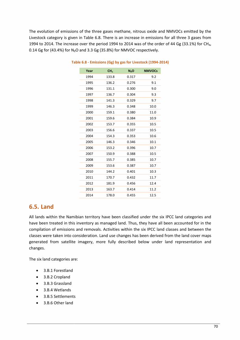
70
The evolution of emissions of the three gases methane, nitrous oxide and NMVOCs emitted by the
Livestock category is given in Table 6.8. There is an increase in emissions for all three 3 gases from
1994 to 2014. The increase over the period 1994 to 2014 was of the order of 44 Gg (33.1%) for CH4,
0.14 Gg for (43.4%) for N₂O and 3.3 Gg (35.8%) for NMVOC respectively.
Table 6.8 - Emissions (Gg) by gas for Livestock (1994-2014)
Year CH4 N₂O NMVOCs
1994 133.8 0.317 9.2
1995 136.2 0.276 9.1
1996 131.1 0.300 9.0
1997 136.7 0.304 9.3
1998 141.3 0.329 9.7
1999 146.3 0.348 10.0
2000 159.1 0.380 11.0
2001 159.6 0.384 10.9
2002 153.7 0.355 10.5
2003 156.6 0.337 10.5
2004 154.3 0.353 10.6
2005 146.3 0.346 10.1
2006 153.2 0.396 10.7
2007 150.9 0.388 10.5
2008 155.7 0.385 10.7
2009 153.6 0.387 10.7
2010 144.2 0.401 10.3
2011 170.7 0.432 11.7
2012 181.9 0.456 12.4
2013 163.7 0.414 11.2
2014 178.0 0.455 12.5
6.5. Land
All lands within the Namibian territory have been classified under the six IPCC land categories and
have been treated in this inventory as managed land. Thus, they have all been accounted for in the
compilation of emissions and removals. Activities within the six IPCC land classes and between the
classes were taken into consideration. Land use changes has been derived from the land cover maps
generated from satellite imagery, more fully described below under land representation and
changes.
The six land categories are:
3.B.1 Forestland
3.B.2 Cropland
3.B.3 Grassland
3.B.4 Wetlands
3.B.5 Settlements
3.B.6 Other land
71
6.5.1. Description
6.5.1.1. Forestland
Forests were divided in two sub-categories and the definitions adopted for the integration of all
information from FRA, RCMRD maps and other reports are provided below:
Forestland (FL): tree height of 5 m and a canopy cover of more than 20%; and
Other Wooded Land (OWL): The are three different land classes in this sub category:
o Woodlands where tree height of 5 m with a canopy cover between 10% and 20%.
o Shrubland where trees and saplings are present as these have been invaded long
ago and trees have grown to a height whereby some areas can now be reclassified
as woodland or forest.
o Savannah grassland where bush invasion is occurring with an increase in woody
biomass.
A major change from the NIR2 is the reclassification and merger of the bush-encroached grassland
with the degraded woodland of Namibia to form the Other Wooded Land sub-class in Forestland.
6.5.1.2. Cropland
Land used for annual cropping has been considered. Main crops are maize, wheat and millet and
sorghum produced under both commercial and communal systems. It is estimated that not all land
cleared for growing crops are used every year. Thus, no more cropland set aside group had to be
created as for the previous NIR.
6.5.1.3. Grassland
Grassland is now redefined as a pure stand without the presence of woody biomass as in the last
NIR. The area of grassland is estimated to be situated between the bush encroachment wetter
Northern part of the country and the desert found on the South Western part.
6.5.1.4. Wetlands
Water bodies, rivers and other marshy areas are considered as Wetlands. The area of this land class
has been kept fixed as no development has been done on Wetlands during the inventory period.
6.5.1.5. Settlements
Land with infrastructures such as roads, buildings, houses and other mad-made structures have been
included under Settlements. Urbanization and development of the road network are the major
contributors to change in this land class.
6.5.1.6. Other Land
All other land present in Namibia and not falling in any of the above categories are included under
this category. Desert, rock outcrops and bare land are the main constituents of Other Land. There
was no change in this land class during the timeseries.
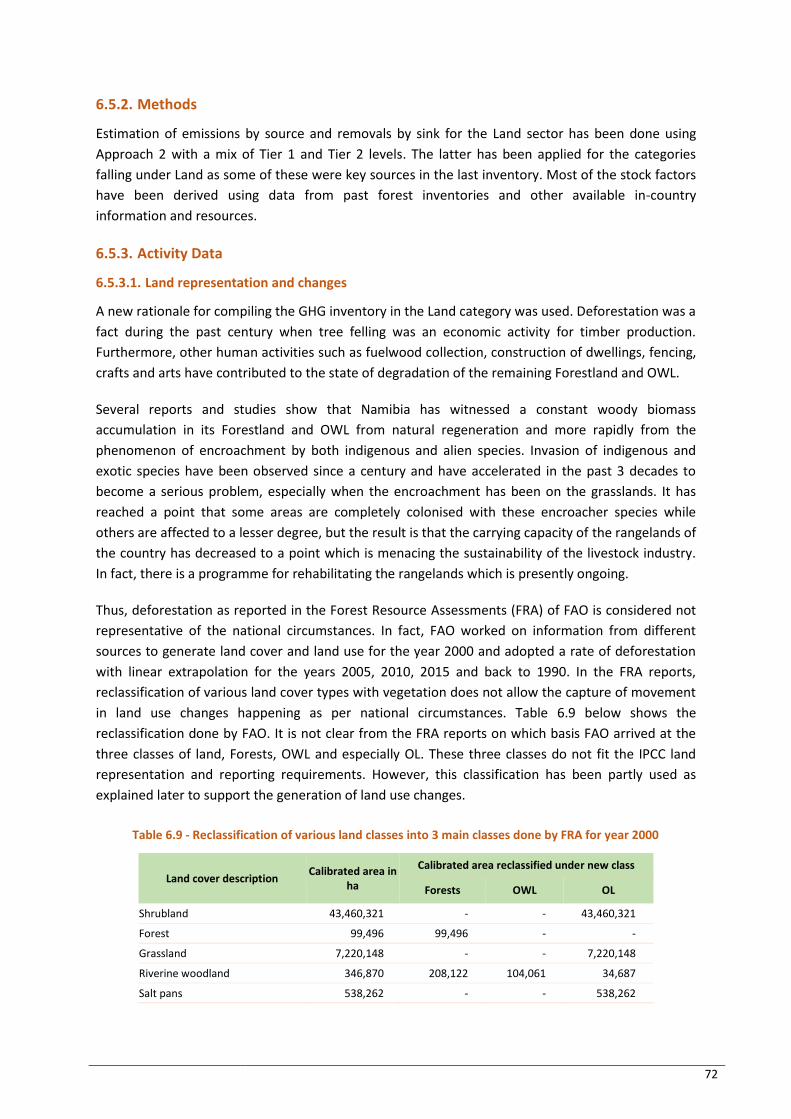
72
6.5.2. Methods
Estimation of emissions by source and removals by sink for the Land sector has been done using
Approach 2 with a mix of Tier 1 and Tier 2 levels. The latter has been applied for the categories
falling under Land as some of these were key sources in the last inventory. Most of the stock factors
have been derived using data from past forest inventories and other available in-country
information and resources.
6.5.3. Activity Data
6.5.3.1. Land representation and changes
A new rationale for compiling the GHG inventory in the Land category was used. Deforestation was a
fact during the past century when tree felling was an economic activity for timber production.
Furthermore, other human activities such as fuelwood collection, construction of dwellings, fencing,
crafts and arts have contributed to the state of degradation of the remaining Forestland and OWL.
Several reports and studies show that Namibia has witnessed a constant woody biomass
accumulation in its Forestland and OWL from natural regeneration and more rapidly from the
phenomenon of encroachment by both indigenous and alien species. Invasion of indigenous and
exotic species have been observed since a century and have accelerated in the past 3 decades to
become a serious problem, especially when the encroachment has been on the grasslands. It has
reached a point that some areas are completely colonised with these encroacher species while
others are affected to a lesser degree, but the result is that the carrying capacity of the rangelands of
the country has decreased to a point which is menacing the sustainability of the livestock industry.
In fact, there is a programme for rehabilitating the rangelands which is presently ongoing.
Thus, deforestation as reported in the Forest Resource Assessments (FRA) of FAO is considered not
representative of the national circumstances. In fact, FAO worked on information from different
sources to generate land cover and land use for the year 2000 and adopted a rate of deforestation
with linear extrapolation for the years 2005, 2010, 2015 and back to 1990. In the FRA reports,
reclassification of various land cover types with vegetation does not allow the capture of movement
in land use changes happening as per national circumstances. Table 6.9 below shows the
reclassification done by FAO. It is not clear from the FRA reports on which basis FAO arrived at the
three classes of land, Forests, OWL and especially OL. These three classes do not fit the IPCC land
representation and reporting requirements. However, this classification has been partly used as
explained later to support the generation of land use changes.
Table 6.9 - Reclassification of various land classes into 3 main classes done by FRA for year 2000
Land cover description Calibrated area in
ha
Calibrated area reclassified under new class
Forests OWL OL
Shrubland 43,460,321 - - 43,460,321
Forest 99,496 99,496 - -
Grassland 7,220,148 - - 7,220,148
Riverine woodland 346,870 208,122 104,061 34,687
Salt pans 538,262 - - 538,262
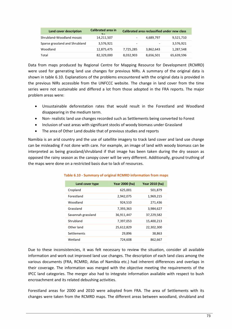
73
Land cover description Calibrated area in ha
Calibrated area reclassified under new class
Shrubland-Woodland mosaic 14,211,507 - 4,689,797 9,521,710
Sparse grassland and Shrubland 3,576,921 - - 3,576,921
Woodland 12,875,475 7,725,285 3,862,643 1,287,548
Total 82,329,000 8,032,903 8,656,501 65,639,596
Data from maps produced by Regional Centre for Mapping Resource for Development (RCMRD)
were used for generating land use changes for previous NIRs. A summary of the original data is
shown in table 6.10. Explanations of the problems encountered with the original data is provided in
the previous NIRs accessible from the UNFCCC website. The change in land cover from the time
series were not sustainable and differed a lot from those adopted in the FRA reports. The major
problem areas were:
Unsustainable deforestation rates that would result in the Forestland and Woodland
disappearing in the medium term.
Non- realistic land use changes recorded such as Settlements being converted to Forest
Inclusion of vast areas with significant stocks of woody biomass under Grassland
The area of Other Land double that of previous studies and reports
Namibia is an arid country and the use of satellite imagery to track land cover and land use change
can be misleading if not done with care. For example, an image of land with woody biomass can be
interpreted as being grassland/shrubland if that image has been taken during the dry season as
opposed the rainy season as the canopy cover will be very different. Additionally, ground truthing of
the maps were done on a restricted basis due to lack of resources.
Table 6.10 - Summary of original RCMRD information from maps
Land cover type Year 2000 (ha) Year 2010 (ha)
Cropland 625,001 501,879
Forestland 2,942,075 1,969,215
Woodland 924,510 271,436
Grassland 7,393,363 3,984,627
Savannah grassland 36,911,447 37,229,582
Shrubland 7,397,053 15,400,213
Other land 25,612,829 22,302,300
Settlements 29,896 38,863
Wetland 724,608 862,667
Due to these inconsistencies, it was felt necessary to review the situation, consider all available
information and work out improved land use changes. The description of each land class among the
various documents (FRA, RCMRD, Atlas of Namibia etc.) had inherent differences and overlaps in
their coverage. The information was merged with the objective meeting the requirements of the
IPCC land categories. The merger also had to integrate information available with respect to bush
encroachment and its related debushing activities.
Forestland areas for 2000 and 2010 were adopted from FRA. The area of Settlements with its
changes were taken from the RCMRD maps. The different areas between woodland, shrubland and
74
savannah grassland was a mix of information from RCMRD and FRA. Cropland and Wetland areas
were taken from RCMRD maps. The extent of Other Land was the remainder after distracting the
other classes from the area of the territory. This was in line with the area classified as Other Land in
Atlas of Namibia (Mendelsohn, et al.,2002)
6.5.3.2. Changes
Forestland
Deforestation
Deforestation is estimated to be under control since the independence of Namibia. Various laws and
regulations have helped to preserve the remaining Forestland of the country. A rise in the standard
of living and urbanization has decreased the pressure for wood resources from forests. A gain of
10,000 ha yearly from OWL has been included on account of bush encroachment since the 1960s
and led to the bush being so thick and more than 5 metres warranting a change in the classification.
De-bushing methods include the use of chemicals and other mechanical means to get rid of the trees
that are affecting farms, particularly with respect to carrying capacity of livestock. It is reported that
80,000 hectares were debushed annually during the 1990s (Routhauge A., 2014). The use of
chemicals for bush control is being discouraged by the authorities. This rate increased to 90,000
hectares during the first decade of the 21st century and 100,000 hectares as from 2011 (De Klerk
J.N., 2004). Added to that, the NGO, the Cheetah Foundation has implemented a project on the
rehabilitation of the natural habitat of the cheetah, a threatened species because of bush
encroachment. This activity produced some 8000 tonnes of bush-block annually (Feller S, et al. 2006)
from the encroached species. They are sold or exported, and the proceeds used to support the
project financially.
Encroachment has nearly peaked as the Grassland are in the drier environment with rainfall
inadequate to support growth of bushes and trees eventually. The aim now is to keep the right
balance for economic activities to be sustainable, preserving the ecosystems and biodiversity
through the control of encroachment by harvesting bush encroached species for use as woody
biomass feedstocks.
Since independence, the Government of Namibia has promulgated many forests as protected areas,
conservancies and community forests with an enhanced management level. This type of
management is preserving the remaining forests and woodlands of the country. The rate of growth
of major species are so slow with a tree taking around 50 years to reach 15 cm diameter at breast
height (dbh) and between 70 to 100 years to reach 30 cm dbh (Mendelson and Obeid, 2004,). This
implies that natural regeneration of these areas will take a long time. However, it is a good sign that
all forest inventories data indicate a high number of seedlings, saplings, and young growing healthy
trees. It is estimated that the clearing and felling of trees when forests were intensively exploited for
timber has resulted in vast extents of the territory without a cover which had taken centuries to
develop and the phenomenon of bush encroachment is the recolonization of those spaces by species
better adapted to the changed climate. An extract of the report by Mendelson and Obeid is given in
figure 6.3. It is to be noted that Caprivi has been renamed as Zambezi now.

75
Figure 6.3 - Extract from Forestland and Woodland of Namibia showing age of major species to reach maturity (30 cm at dbh)
Cropland
A steady decrease in Cropland is estimated as subsistence farming is gradually diminishing. This is
due to migration of the rural population to urban areas, a higher purchasing power for a more varied
food consumption, improved yields from better crop husbandry practices and the combination of
climate change including a higher climate variability.
Grassland
Bush encroachment has led to a rapid decrease in previously classified grassland (shrubland and
savanna) area. These are now under the class OWL as per the presence of enough woody species.
Wetlands
The area of Wetlands is estimated to be constant during the whole time series. The area from the
2000 RCMRD map was used as constant.
Settlements
An increase in Settlement class has been included in the NIR3. Development of infrastructure to
accommodate a growing urban population plus the building of amenities have contributed to this
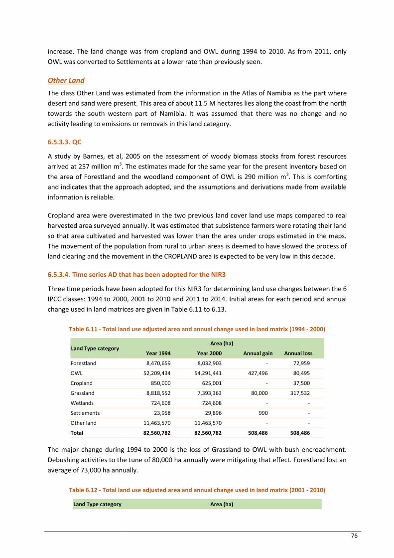
76
increase. The land change was from cropland and OWL during 1994 to 2010. As from 2011, only
OWL was converted to Settlements at a lower rate than previously seen.
Other Land
The class Other Land was estimated from the information in the Atlas of Namibia as the part where
desert and sand were present. This area of about 11.5 M hectares lies along the coast from the north
towards the south western part of Namibia. It was assumed that there was no change and no
activity leading to emissions or removals in this land category.
6.5.3.3. QC
A study by Barnes, et al, 2005 on the assessment of woody biomass stocks from forest resources
arrived at 257 million m3. The estimates made for the same year for the present inventory based on
the area of Forestland and the woodland component of OWL is 290 million m3. This is comforting
and indicates that the approach adopted, and the assumptions and derivations made from available
information is reliable.
Cropland area were overestimated in the two previous land cover land use maps compared to real
harvested area surveyed annually. It was estimated that subsistence farmers were rotating their land
so that area cultivated and harvested was lower than the area under crops estimated in the maps.
The movement of the population from rural to urban areas is deemed to have slowed the process of
land clearing and the movement in the CROPLAND area is expected to be very low in this decade.
6.5.3.4. Time series AD that has been adopted for the NIR3
Three time periods have been adopted for this NIR3 for determining land use changes between the 6
IPCC classes: 1994 to 2000, 2001 to 2010 and 2011 to 2014. Initial areas for each period and annual
change used in land matrices are given in Table 6.11 to 6.13.
Table 6.11 - Total land use adjusted area and annual change used in land matrix (1994 - 2000)
Land Type category Area (ha)
Year 1994 Year 2000 Annual gain Annual loss
Forestland 8,470,659 8,032,903 - 72,959
OWL 52,209,434 54,291,441 427,496 80,495
Cropland 850,000 625,001 - 37,500
Grassland 8,818,552 7,393,363 80,000 317,532
Wetlands 724,608 724,608 - -
Settlements 23,958 29,896 990 -
Other land 11,463,570 11,463,570 - -
Total 82,560,782 82,560,782 508,486 508,486
The major change during 1994 to 2000 is the loss of Grassland to OWL with bush encroachment.
Debushing activities to the tune of 80,000 ha annually were mitigating that effect. Forestland lost an
average of 73,000 ha annually.
Table 6.12 - Total land use adjusted area and annual change used in land matrix (2001 - 2010)
Land Type category Area (ha)
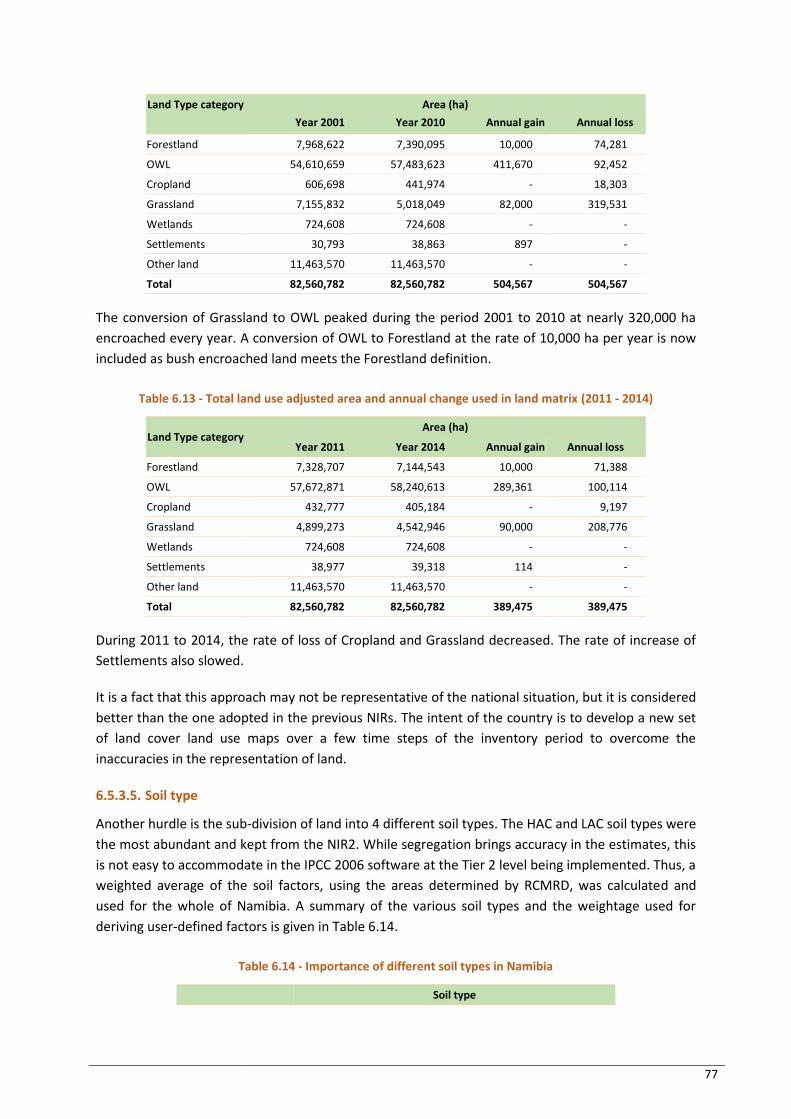
77
Land Type category Area (ha)
Year 2001 Year 2010 Annual gain Annual loss
Forestland 7,968,622 7,390,095 10,000 74,281
OWL 54,610,659 57,483,623 411,670 92,452
Cropland 606,698 441,974 - 18,303
Grassland 7,155,832 5,018,049 82,000 319,531
Wetlands 724,608 724,608 - -
Settlements 30,793 38,863 897 -
Other land 11,463,570 11,463,570 - -
Total 82,560,782 82,560,782 504,567 504,567
The conversion of Grassland to OWL peaked during the period 2001 to 2010 at nearly 320,000 ha
encroached every year. A conversion of OWL to Forestland at the rate of 10,000 ha per year is now
included as bush encroached land meets the Forestland definition.
Table 6.13 - Total land use adjusted area and annual change used in land matrix (2011 - 2014)
Land Type category Area (ha)
Year 2011 Year 2014 Annual gain Annual loss
Forestland 7,328,707 7,144,543 10,000 71,388
OWL 57,672,871 58,240,613 289,361 100,114
Cropland 432,777 405,184 - 9,197
Grassland 4,899,273 4,542,946 90,000 208,776
Wetlands 724,608 724,608 - -
Settlements 38,977 39,318 114 -
Other land 11,463,570 11,463,570 - -
Total 82,560,782 82,560,782 389,475 389,475
During 2011 to 2014, the rate of loss of Cropland and Grassland decreased. The rate of increase of
Settlements also slowed.
It is a fact that this approach may not be representative of the national situation, but it is considered
better than the one adopted in the previous NIRs. The intent of the country is to develop a new set
of land cover land use maps over a few time steps of the inventory period to overcome the
inaccuracies in the representation of land.
6.5.3.5. Soil type
Another hurdle is the sub-division of land into 4 different soil types. The HAC and LAC soil types were
the most abundant and kept from the NIR2. While segregation brings accuracy in the estimates, this
is not easy to accommodate in the IPCC 2006 software at the Tier 2 level being implemented. Thus, a
weighted average of the soil factors, using the areas determined by RCMRD, was calculated and
used for the whole of Namibia. A summary of the various soil types and the weightage used for
deriving user-defined factors is given in Table 6.14.
Table 6.14 - Importance of different soil types in Namibia
Soil type

78
HAC LAC SAN WET
Area (ha) 50,128,385 90,367 32,340,961 1,069
% of total area 60.7% 0.1% 39.2% 0.0%
6.5.3.6. Climate
In the previous NIRs, 2 climate types were allocated by RCMRD in association with the different soil
types. During the review and development of the new approach for the NIR3, it was realized that
Namibia was assigned with the wrong climate type. After confirmation from IPCC map (2006 IPCC
GL, Volume 4, page 3.38, Figure 3.A.5.1), the climate of Namibia is now set as Temperate dry for the
whole country since the small area associated with the Tropical dry climate type is situated in the
Other Land class where there is no activity.
A Tier 2 approach has been maintained but slight changes brought as follows:
(i) This is highly supported from the results of the censuses indicating a much lower use of
local wood resources.
(ii) The lower reliance on local wood resources is attributed to a rise in urbanization rate
accompanied by a fall in woody material used for dwellings coupled with use of alternative
materials for dwellings, imports of wood from neighbouring South Africa, lower use of
wood as fuel for cooking, heating and lighting, and reduced commercial harvest of wood.
(iii) Thus, compared to FRA data, slower rates have been adopted over the 20 years of this time
series (see matrices provided separately).
(iv) Bush encroachment has resulted in vast areas of land previously misclassed as
shrubland/savanna/grassland to be reclassified as forest or dense woodlands now.
(v) Bush encroachment rate and bush clearing have been taken into consideration in the land
use changes.
(vi) Additionally, by combining shrubland, savanna and open woodland under a common class
Other Wooded Land to enable computation of emissions and removals in the software,
compilation has been simplified.
(vii) It is essential to account for the biomass of the bushes properly including their role in wood
removals. Emission and stock factors (Growing stock, annual growth rates, etc) have been
derived for the country based on the latest information available (see worksheets
thereon).
(viii) Most wood removals accounted for in this new OWL as is presently the case for known
uses of woody biomass stocks.
(ix) An increase in Settlement land category is included in the change as population and
urbanization is constantly increasing. This is estimated to be accompanied by a loss in
Cropland area where by subsistence farming is decreasing and villages are also growing.
6.5.4. Generated data and emission factors
6.5.4.1. Biomass stock factors
The standing biomass stock for Forestland was obtained by averaging the data from Forest inventory
reports performed in preserved forests, community forests and conservancies in areas receiving
adequate rainfall to maintain trees. Regarding Other Wooded Land, the standing biomass stocks of
land defined as woodlands, shrubland and savannahs in forest inventories were pooled to provide a
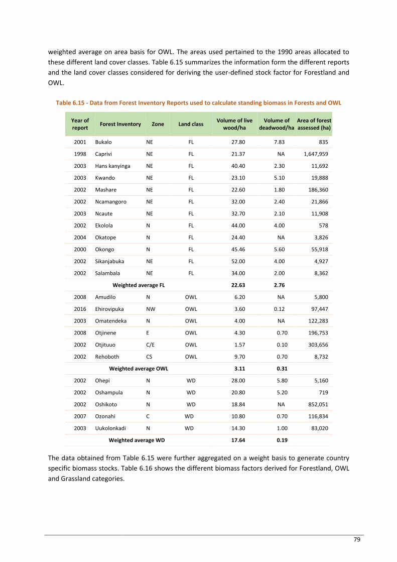
79
weighted average on area basis for OWL. The areas used pertained to the 1990 areas allocated to
these different land cover classes. Table 6.15 summarizes the information form the different reports
and the land cover classes considered for deriving the user-defined stock factor for Forestland and
OWL.
Table 6.15 - Data from Forest Inventory Reports used to calculate standing biomass in Forests and OWL
Year of report
Forest Inventory Zone Land class Volume of live
wood/ha Volume of
deadwood/ha Area of forest assessed (ha)
2001 Bukalo NE FL 27.80 7.83 835
1998 Caprivi NE FL 21.37 NA 1,647,959
2003 Hans kanyinga NE FL 40.40 2.30 11,692
2003 Kwando NE FL 23.10 5.10 19,888
2002 Mashare NE FL 22.60 1.80 186,360
2002 Ncamangoro NE FL 32.00 2.40 21,866
2003 Ncaute NE FL 32.70 2.10 11,908
2002 Ekolola N FL 44.00 4.00 578
2004 Okatope N FL 24.40 NA 3,826
2000 Okongo N FL 45.46 5.60 55,918
2002 Sikanjabuka NE FL 52.00 4.00 4,927
2002 Salambala NE FL 34.00 2.00 8,362
Weighted average FL 22.63 2.76
2008 Amudilo N OWL 6.20 NA 5,800
2016 Ehirovipuka NW OWL 3.60 0.12 97,447
2003 Omatendeka N OWL 4.00 NA 122,283
2008 Otjinene E OWL 4.30 0.70 196,753
2002 Otjituuo C/E OWL 1.57 0.10 303,656
2002 Rehoboth CS OWL 9.70 0.70 8,732
Weighted average OWL 3.11 0.31
2002 Ohepi N WD 28.00 5.80 5,160
2002 Oshampula N WD 20.80 5.20 719
2002 Oshikoto N WD 18.84 NA 852,051
2007 Ozonahi C WD 10.80 0.70 116,834
2003 Uukolonkadi N WD 14.30 1.00 83,020
Weighted average WD 17.64 0.19
The data obtained from Table 6.15 were further aggregated on a weight basis to generate country
specific biomass stocks. Table 6.16 shows the different biomass factors derived for Forestland, OWL
and Grassland categories.

80
Table 6.16 - Biomass stock factors used in NIR 3 for FOLU.
Land classes Woody biomass
(t/ha)
Deadwood (m3)
Above ground Biomass
(t dm/ha)
Age to reach this class (yrs)
Annual growth
(t dm/yr)
Grass layer (t dm/ha)
Forestland 22.63 2.76 38.47 100.0 0.385 0.23
OWL 12.13 1.48 36.38 45.6 0.797 0.69
Grassland
1.15
6.5.4.2. Wood removals
Removal of woodfuel was indexed on the use rate of this fuel by urban and rural population
respectively. Removal of timber and poles were based on number of traditional dwellings and the
amount of woody resources needed to build and maintain these units.
Charcoal produced was estimated from trade statistics and converted to woody biomass and
included in the fuelwood estimates.
The amount of woody biomass removed is shown in Table 6.17.
Table 6.17 - Wood removals (t) from various activities
Year Charcoal
production Fuelwood exported
Fuelwood collected
Poles removal Bushblock production
Industrial consumption
Total
1994 300,000 500 196,018 169,068 * * 665,586
1995 300,000 500 197,640 172,245 * * 670,385
1996 300,000 500 199,270 175,259 * * 675,029
1997 300,000 500 200,911 178,111 * * 679,522
1998 300,000 555 202,562 180,799 * * 683,915
1999 300,000 621 204,223 183,323 * * 688,167
2000 300,000 152 205,894 185,685 * * 691,731
2001 300,000 122 207,577 187,946 8,000 * 703,644
2002 300,000 130 207,748 190,055 8,000 * 705,934
2003 300,000 68 207,906 193,325 8,000 * 709,299
2004 301,044 2,469 208,050 200,640 8,000 * 720,203
2005 294,031 4,486 208,180 194,950 8,000 * 709,647
2006 320,779 7,120 208,296 201,706 8,000 * 745,900
2007 374,117 7,553 208,397 197,702 8,000 * 795,768
2008 523,727 11,651 208,484 198,838 8,000 * 950,700
2009 693,161 14,251 208,557 199,816 8,000 * 1,123,785
2010 621,187 14,467 208,615 200,112 8,000 * 1,052,381
2011 465,524 14,571 208,659 204,371 8,000 * 901,125
2012 471,321 15,116 207,455 201,247 8,000 27,000 930,138
2013 549,841 14,997 206,316 201,552 8,000 30,000 1,010,706
2014 541,410 15,909 205,241 201,631 8,000 27,000 999,191
* Not Occurring
Woody biomass removals were allocated as follows:
1. Charcoal from OWL as de-bushing activities are the major contributor to charcoal production
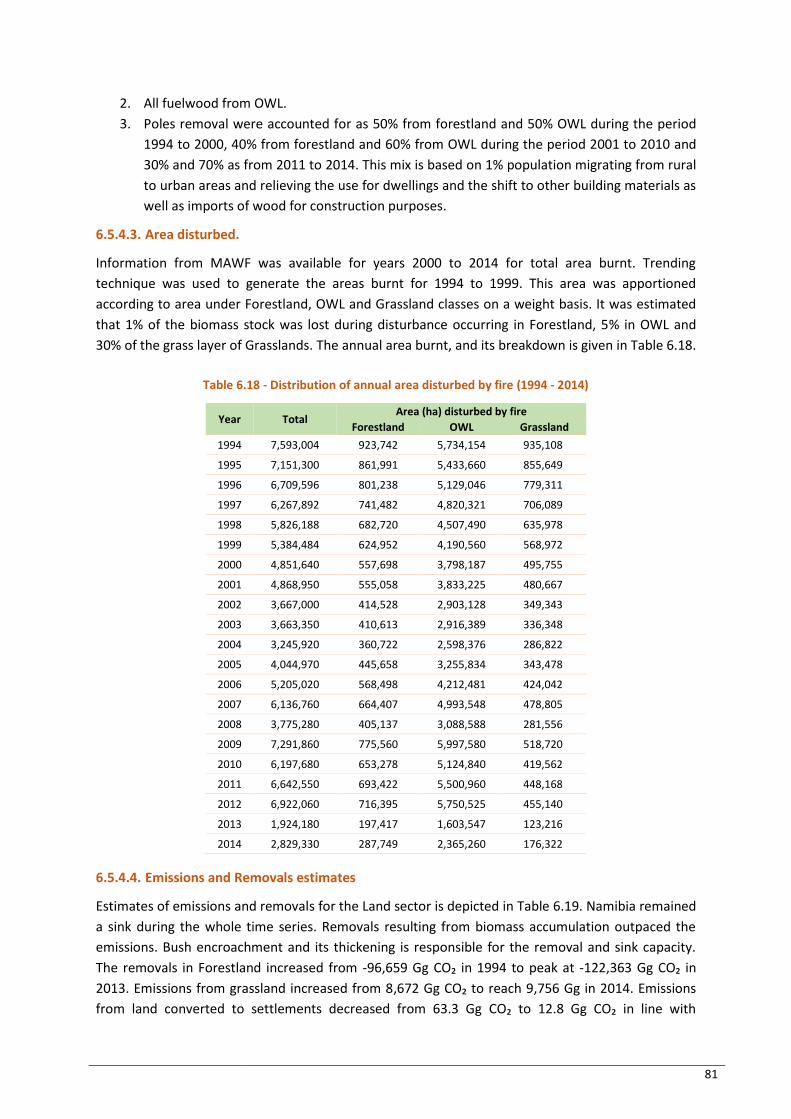
81
2. All fuelwood from OWL.
3. Poles removal were accounted for as 50% from forestland and 50% OWL during the period
1994 to 2000, 40% from forestland and 60% from OWL during the period 2001 to 2010 and
30% and 70% as from 2011 to 2014. This mix is based on 1% population migrating from rural
to urban areas and relieving the use for dwellings and the shift to other building materials as
well as imports of wood for construction purposes.
6.5.4.3. Area disturbed.
Information from MAWF was available for years 2000 to 2014 for total area burnt. Trending
technique was used to generate the areas burnt for 1994 to 1999. This area was apportioned
according to area under Forestland, OWL and Grassland classes on a weight basis. It was estimated
that 1% of the biomass stock was lost during disturbance occurring in Forestland, 5% in OWL and
30% of the grass layer of Grasslands. The annual area burnt, and its breakdown is given in Table 6.18.
Table 6.18 - Distribution of annual area disturbed by fire (1994 - 2014)
Year Total Area (ha) disturbed by fire
Forestland OWL Grassland
1994 7,593,004 923,742 5,734,154 935,108
1995 7,151,300 861,991 5,433,660 855,649
1996 6,709,596 801,238 5,129,046 779,311
1997 6,267,892 741,482 4,820,321 706,089
1998 5,826,188 682,720 4,507,490 635,978
1999 5,384,484 624,952 4,190,560 568,972
2000 4,851,640 557,698 3,798,187 495,755
2001 4,868,950 555,058 3,833,225 480,667
2002 3,667,000 414,528 2,903,128 349,343
2003 3,663,350 410,613 2,916,389 336,348
2004 3,245,920 360,722 2,598,376 286,822
2005 4,044,970 445,658 3,255,834 343,478
2006 5,205,020 568,498 4,212,481 424,042
2007 6,136,760 664,407 4,993,548 478,805
2008 3,775,280 405,137 3,088,588 281,556
2009 7,291,860 775,560 5,997,580 518,720
2010 6,197,680 653,278 5,124,840 419,562
2011 6,642,550 693,422 5,500,960 448,168
2012 6,922,060 716,395 5,750,525 455,140
2013 1,924,180 197,417 1,603,547 123,216
2014 2,829,330 287,749 2,365,260 176,322
6.5.4.4. Emissions and Removals estimates
Estimates of emissions and removals for the Land sector is depicted in Table 6.19. Namibia remained
a sink during the whole time series. Removals resulting from biomass accumulation outpaced the
emissions. Bush encroachment and its thickening is responsible for the removal and sink capacity.
The removals in Forestland increased from -96,659 Gg CO₂ in 1994 to peak at -122,363 Gg CO₂ in
2013. Emissions from grassland increased from 8,672 Gg CO₂ to reach 9,756 Gg in 2014. Emissions
from land converted to settlements decreased from 63.3 Gg CO₂ to 12.8 Gg CO₂ in line with
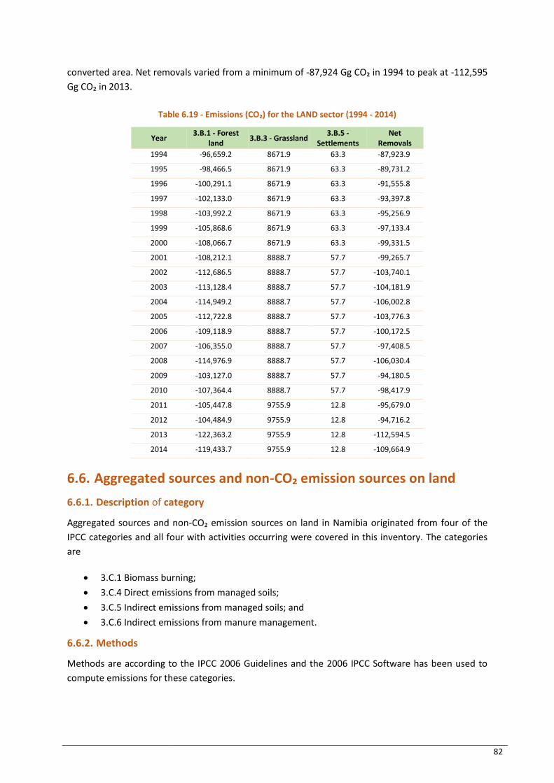
82
converted area. Net removals varied from a minimum of -87,924 Gg CO₂ in 1994 to peak at -112,595
Gg CO₂ in 2013.
Table 6.19 - Emissions (CO₂) for the LAND sector (1994 - 2014)
Year 3.B.1 - Forest
land 3.B.3 - Grassland
3.B.5 - Settlements
Net Removals
1994 -96,659.2 8671.9 63.3 -87,923.9
1995 -98,466.5 8671.9 63.3 -89,731.2
1996 -100,291.1 8671.9 63.3 -91,555.8
1997 -102,133.0 8671.9 63.3 -93,397.8
1998 -103,992.2 8671.9 63.3 -95,256.9
1999 -105,868.6 8671.9 63.3 -97,133.4
2000 -108,066.7 8671.9 63.3 -99,331.5
2001 -108,212.1 8888.7 57.7 -99,265.7
2002 -112,686.5 8888.7 57.7 -103,740.1
2003 -113,128.4 8888.7 57.7 -104,181.9
2004 -114,949.2 8888.7 57.7 -106,002.8
2005 -112,722.8 8888.7 57.7 -103,776.3
2006 -109,118.9 8888.7 57.7 -100,172.5
2007 -106,355.0 8888.7 57.7 -97,408.5
2008 -114,976.9 8888.7 57.7 -106,030.4
2009 -103,127.0 8888.7 57.7 -94,180.5
2010 -107,364.4 8888.7 57.7 -98,417.9
2011 -105,447.8 9755.9 12.8 -95,679.0
2012 -104,484.9 9755.9 12.8 -94,716.2
2013 -122,363.2 9755.9 12.8 -112,594.5
2014 -119,433.7 9755.9 12.8 -109,664.9
6.6. Aggregated sources and non-CO₂ emission sources on land
6.6.1. Description of category
Aggregated sources and non-CO₂ emission sources on land in Namibia originated from four of the
IPCC categories and all four with activities occurring were covered in this inventory. The categories
are
3.C.1 Biomass burning;
3.C.4 Direct emissions from managed soils;
3.C.5 Indirect emissions from managed soils; and
3.C.6 Indirect emissions from manure management.
6.6.2. Methods
Methods are according to the IPCC 2006 Guidelines and the 2006 IPCC Software has been used to
compute emissions for these categories.
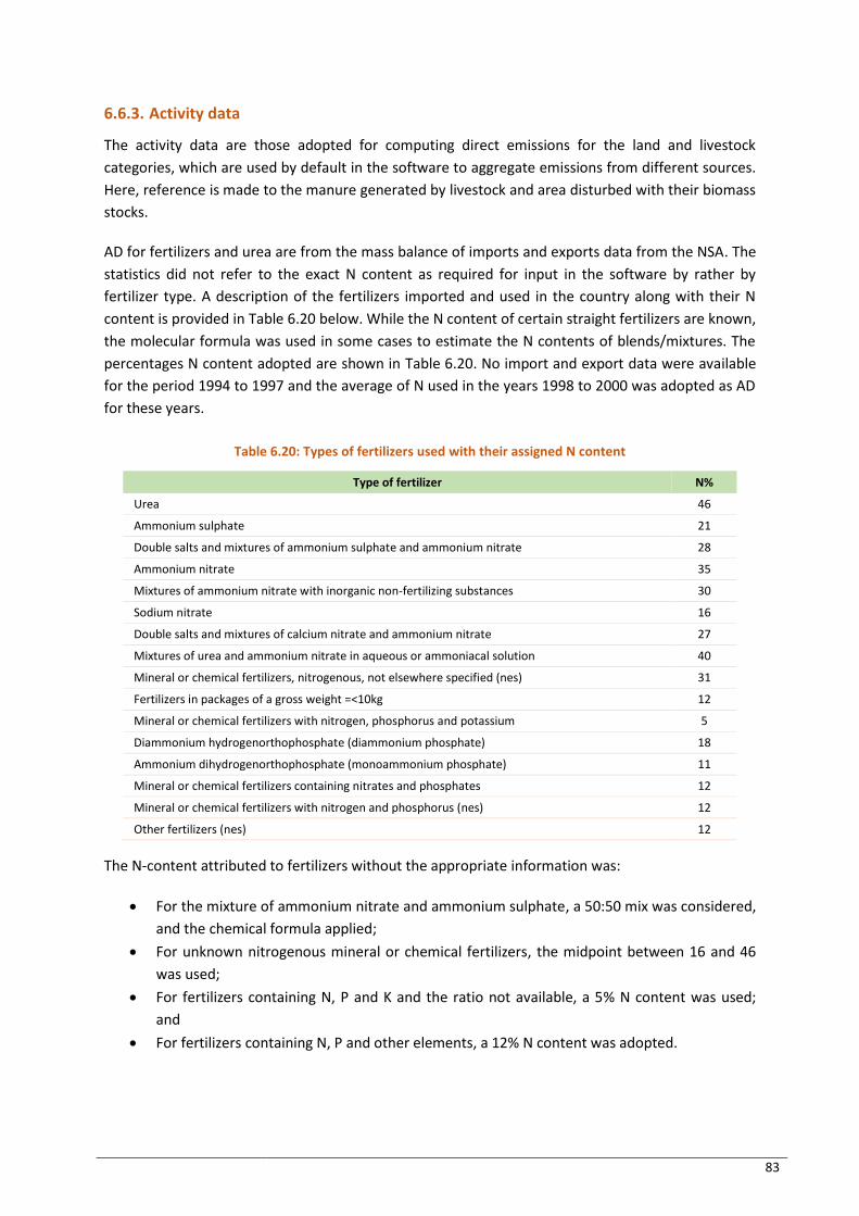
83
6.6.3. Activity data
The activity data are those adopted for computing direct emissions for the land and livestock
categories, which are used by default in the software to aggregate emissions from different sources.
Here, reference is made to the manure generated by livestock and area disturbed with their biomass
stocks.
AD for fertilizers and urea are from the mass balance of imports and exports data from the NSA. The
statistics did not refer to the exact N content as required for input in the software by rather by
fertilizer type. A description of the fertilizers imported and used in the country along with their N
content is provided in Table 6.20 below. While the N content of certain straight fertilizers are known,
the molecular formula was used in some cases to estimate the N contents of blends/mixtures. The
percentages N content adopted are shown in Table 6.20. No import and export data were available
for the period 1994 to 1997 and the average of N used in the years 1998 to 2000 was adopted as AD
for these years.
Table 6.20: Types of fertilizers used with their assigned N content
Type of fertilizer N%
Urea 46
Ammonium sulphate 21
Double salts and mixtures of ammonium sulphate and ammonium nitrate 28
Ammonium nitrate 35
Mixtures of ammonium nitrate with inorganic non-fertilizing substances 30
Sodium nitrate 16
Double salts and mixtures of calcium nitrate and ammonium nitrate 27
Mixtures of urea and ammonium nitrate in aqueous or ammoniacal solution 40
Mineral or chemical fertilizers, nitrogenous, not elsewhere specified (nes) 31
Fertilizers in packages of a gross weight =<10kg 12
Mineral or chemical fertilizers with nitrogen, phosphorus and potassium 5
Diammonium hydrogenorthophosphate (diammonium phosphate) 18
Ammonium dihydrogenorthophosphate (monoammonium phosphate) 11
Mineral or chemical fertilizers containing nitrates and phosphates 12
Mineral or chemical fertilizers with nitrogen and phosphorus (nes) 12
Other fertilizers (nes) 12
The N-content attributed to fertilizers without the appropriate information was:
For the mixture of ammonium nitrate and ammonium sulphate, a 50:50 mix was considered,
and the chemical formula applied;
For unknown nitrogenous mineral or chemical fertilizers, the midpoint between 16 and 46
was used;
For fertilizers containing N, P and K and the ratio not available, a 5% N content was used;
and
For fertilizers containing N, P and other elements, a 12% N content was adopted.

84
The total amount of N obtained from the fertilizers used and keyed in the software for estimating
emissions is provided in Table 6.21. The very high synthetic N fertilizer used for the period 2011 to
2014 was due to a donation from a friendly country.
Table 6.21 - Amount of N (kg) used from fertilizer application (1994 - 2014)
Type of
fertilizer 1994 1995 1996 1997 1998 1999 2000 2001 2002 2003 2004
Urea N 212,650 212,650 212,650 168,158 142,158 327,634 1,888,517 1,291,430 542,740 368,488 212,650
Synthetic
fertilizer N 711,152 711,152 711,152 761,278 579,424 792,753 789,181 1,405,803 1,044,076 4,081,591 711,152
Type of
fertilizer 2005 2006 2007 2008 2009 2010 2011 2012 2013 2014
Urea N 126,153 90,414 173,177 32,491 103,965 50,217 269,867 319,444 212,319 176,470
Synthetic
fertilizer N 4,511,194 5,795,314 6,791,457 4,703,351 7,482,384 10,949,854 12,111,961 12,532,870 9,688,535 5,013,240
6.6.4. Emission factors
Biomass burning is known to occur in the country on account of wildfires. Default EFs were used for
all gases in Forestland, OWL and Grassland burning. Biomass burning is a key category in some years
on account of the vast areas burned rather than the EFs. Thus, it is not contemplated to attempt at
deriving national ones. However, the amount of standing biomass in the different land classes will be
further refined when new forest inventories will be performed. Default EFs were used for estimating
emissions from urea application as well as for estimates of indirect emissions from managed soils
and manure management.
6.6.5. Emission estimates
The emissions for aggregate sources and non-CO₂ emissions on land are given in Table 6.22.
Emissions varied between 3,622 Gg CO₂-eq and 5,685 Gg CO₂-eq for the period 1994 to 2014 with a
peak of 6,145 Gg CO₂-eq in 2012. This high variability in estimates is attributed to the varying areas
disturbed by wild fires between years and this is very difficult to control.
Table 6.22 - Aggregated emissions (Gg CO₂-eq) for aggregate sources and non-CO₂ emissions on Land
(1994 - 2014)
1994 1995 1996 1997 1998 1999 2000 2001 2002 2003 2004
5,685 5,502 5,196 5,026 4,828 4,636 4,442 4,510 3,789 3,837 3,583
2005 2006 2007 2008 2009 2010 2011 2012 2013 2014
3,968 4,717 5,179 3,921 5,997 5,265 5,840 6,145 2,957 3,622
The emissions by gas are given in Table 6.23. The major gas emitted in this category remained CH4
throughout the period followed by N₂O. Carbon dioxide emissions were minimal for all years.
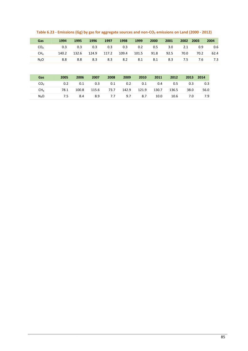
85
Table 6.23 - Emissions (Gg) by gas for aggregate sources and non-CO₂ emissions on Land (2000 - 2012)
Gas 1994 1995 1996 1997 1998 1999 2000 2001 2002 2003 2004
CO₂ 0.3 0.3 0.3 0.3 0.3 0.2 0.5 3.0 2.1 0.9 0.6
CH4 140.2 132.6 124.9 117.2 109.4 101.5 91.8 92.5 70.0 70.2 62.4
N₂O 8.8 8.8 8.3 8.3 8.2 8.1 8.1 8.3 7.5 7.6 7.3
Gas 2005 2006 2007 2008 2009 2010 2011 2012 2013 2014
CO₂ 0.2 0.1 0.3 0.1 0.2 0.1 0.4 0.5 0.3 0.3
CH4 78.1 100.8 115.6 73.7 142.9 121.9 130.7 136.5 38.0 56.0
N₂O 7.5 8.4 8.9 7.7 9.7 8.7 10.0 10.6 7.0 7.9
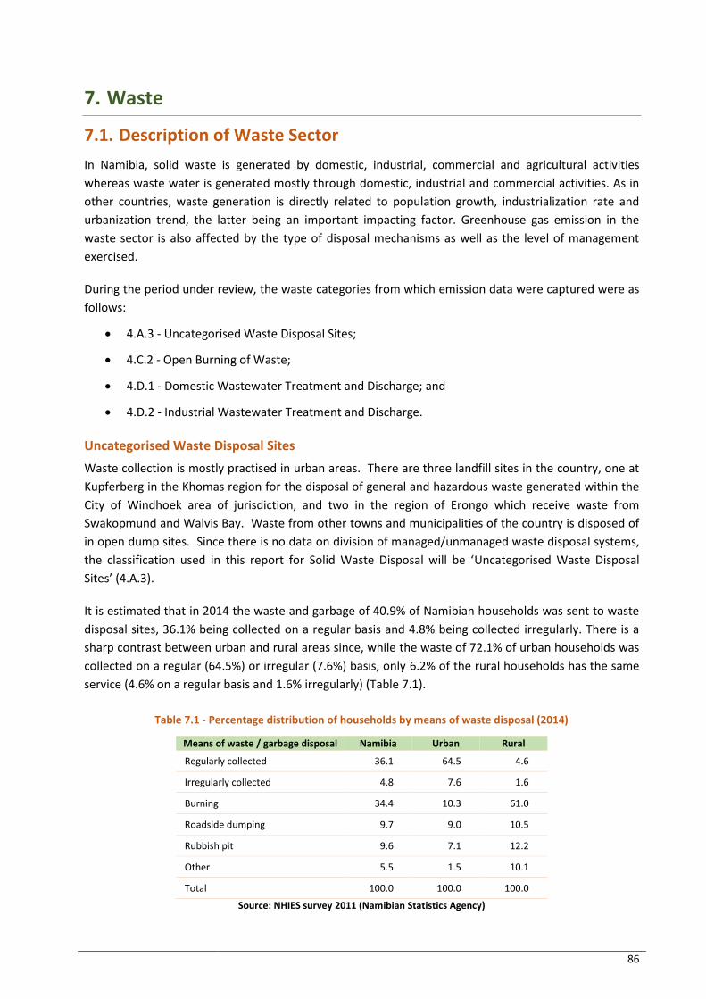
86
7. Waste
7.1. Description of Waste Sector
In Namibia, solid waste is generated by domestic, industrial, commercial and agricultural activities
whereas waste water is generated mostly through domestic, industrial and commercial activities. As in
other countries, waste generation is directly related to population growth, industrialization rate and
urbanization trend, the latter being an important impacting factor. Greenhouse gas emission in the
waste sector is also affected by the type of disposal mechanisms as well as the level of management
exercised.
During the period under review, the waste categories from which emission data were captured were as
follows:
4.A.3 - Uncategorised Waste Disposal Sites;
4.C.2 - Open Burning of Waste;
4.D.1 - Domestic Wastewater Treatment and Discharge; and
4.D.2 - Industrial Wastewater Treatment and Discharge.
Uncategorised Waste Disposal Sites
Waste collection is mostly practised in urban areas. There are three landfill sites in the country, one at
Kupferberg in the Khomas region for the disposal of general and hazardous waste generated within the
City of Windhoek area of jurisdiction, and two in the region of Erongo which receive waste from
Swakopmund and Walvis Bay. Waste from other towns and municipalities of the country is disposed of
in open dump sites. Since there is no data on division of managed/unmanaged waste disposal systems,
the classification used in this report for Solid Waste Disposal will be ‘Uncategorised Waste Disposal
Sites’ (4.A.3).
It is estimated that in 2014 the waste and garbage of 40.9% of Namibian households was sent to waste
disposal sites, 36.1% being collected on a regular basis and 4.8% being collected irregularly. There is a
sharp contrast between urban and rural areas since, while the waste of 72.1% of urban households was
collected on a regular (64.5%) or irregular (7.6%) basis, only 6.2% of the rural households has the same
service (4.6% on a regular basis and 1.6% irregularly) (Table 7.1).
Table 7.1 - Percentage distribution of households by means of waste disposal (2014)
Means of waste / garbage disposal Namibia Urban Rural
Regularly collected 36.1 64.5 4.6
Irregularly collected 4.8 7.6 1.6
Burning 34.4 10.3 61.0
Roadside dumping 9.7 9.0 10.5
Rubbish pit 9.6 7.1 12.2
Other 5.5 1.5 10.1
Total 100.0 100.0 100.0
Source: NHIES survey 2011 (Namibian Statistics Agency)

87
On average, waste collection (regular and irregular basis) remained fairly constant during the 2001 to
the 2011 period, moving from 42.2% of households having access to the service in 2001 to 42.4% in
2011. However, it should be noted, that during the same period, regular collection increased from
30.9% to 37.2% of households while irregular collection decreased from 11.5% to reach only 5.2% of
households. From 2011 to 2014, the percentage of household serviced gradually decreased to reach
40.0%, both regular and irregular collection decreasing slightly to 36.1% and 4.8% of households
respectively (Figure 7.1).
Open Burning of Waste
It is estimated that at national level in 2014, the waste and garbage of 32.4% of Namibian households
were open burnt, a sharp contrast being observed between urban and rural areas, 10.3 % of urban
households being concerned with open burning, while 61.0% of their rural counterparts were concerned
by the same method of waste disposal.
Trend analysis reveals that the percentage households whose waste was open burnt increased from
18.0% in 2001 to 37.8% in 2011 and thereafter decreased to 34.4% in 2014. Data also show that open
burning of waste is a far more frequent practice in rural areas as compared to urban ones (Figure 7.1).
Figure 7.1 - Percentage distribution of households by means of waste disposal (2001 – 2014)
Domestic Wastewater Treatment and Discharge
The estimated percentage distribution of household by type of main toilet facility for the year 2014 is
given in Table 7.2. At the country level, a notable fact is that 47.2 % of the population did not have any
toilet facility. All regions confounded, 40.3% of the households had either a private or shared flush
system, of which around 60% were connected to a sewer system and 3% to a septic tank. The remaining
households used ventilated pits (7.5%), latrines without ventilation system (3.7%), or had recourse to
buckets (1.3%).
Table 7.2 - Estimated percent distribution of household by type of main toilet facility (2014)
Region Namibia Urban Rural
0
10
20
30
40
50
60
70
80
90
100
2001 2002 2003 2004 2005 2006 2007 2008 2009 2010 2011 2012 2013 2014
%D
istr
ibu
tio
n
Regularly collected Irregularly collected Burning Roadside dumping Rubbish pit Other

88
Region Namibia Urban Rural
Private / Shared Flush 40.3 65.4 12.6
Pit Latrine with Ventilation Pipe 7.5 5.5 9.8
Pit Latrine without Ventilation Pipe 3.7 3.1 4.2
Bucket Toilet 1.3 1.2 1.4
Other 47.2 24.8 72.0
Source: Interpolated from Namibia 2011 Population and Housing Census Main Report and Namibia Inter-censal Demographic Survey 2016 Report
Industrial Wastewater Treatment and Discharge
Industrial waste water of relevance to greenhouse gas emissions originates mainly from such activities
as fish processing, slaughter houses, meat conditioning, tanneries and breweries. Because unavailable
data, only the meat sector and fish processing are covered in this inventory. It should be noted that
these two activities account for the major part of industrial waste water in the country.
7.2. Methods
GHG emissions originating from the Waste Sector were estimated following a Tier 1 methodological
approach as per the IPCC 2006 Guidelines for National Greenhouse Gas Inventories and computed using
the IPCC 2006 software.
7.3. Activity Data
7.3.1. Solid waste
Data from municipal councils coupled with population census statistics were first used to estimate solid
waste generation for “high-income” urban and “low-income” urban regions for 2010. The need for this
categorization has been prompted by the sustained and significant population migration from rural to
urban regions with the emergence of fast expanding suburbs to the main cities where the dwellers
lifestyle is of the urban type with a relatively lower purchasing power.
Estimates of solid waste generation for rural regions for 2010 were subsequently worked out by
discounting solid wastes which are typically generated by urban dwellers from the landfills data
available on waste characterization. These solid waste generation potentials were also compared with
those in the 2006 IPCC Guidelines (Volume 5: Waste, Page 2.5, Table 2.1).
Using the 2001, 2006 and 2011 Population and Housing Census Reports (interpolated or extrapolated
for non-census years) and other data source such as the FAO; adjusting for socio-economic factors and
extrapolating waste generation from Windhoek data, estimates for solid waste generation were
calculated for the period 1995 to 2014.
The process of calculating solid waste generation was not straightforward because of the lack of data.
Furthermore, no official data was available on waste categorization which would have enabled more
accurate estimations of GHG emissions. Thus, all the waste from Urban regions were considered as sent
to solid waste disposal sites while 80 % of the waste from the rural regions were open-burned.
The amount of sludge generated per capita for 2010 was estimated using that year’s data for Windhoek
City Council. Using this factor and urban population, the amount of sludge generated for the period
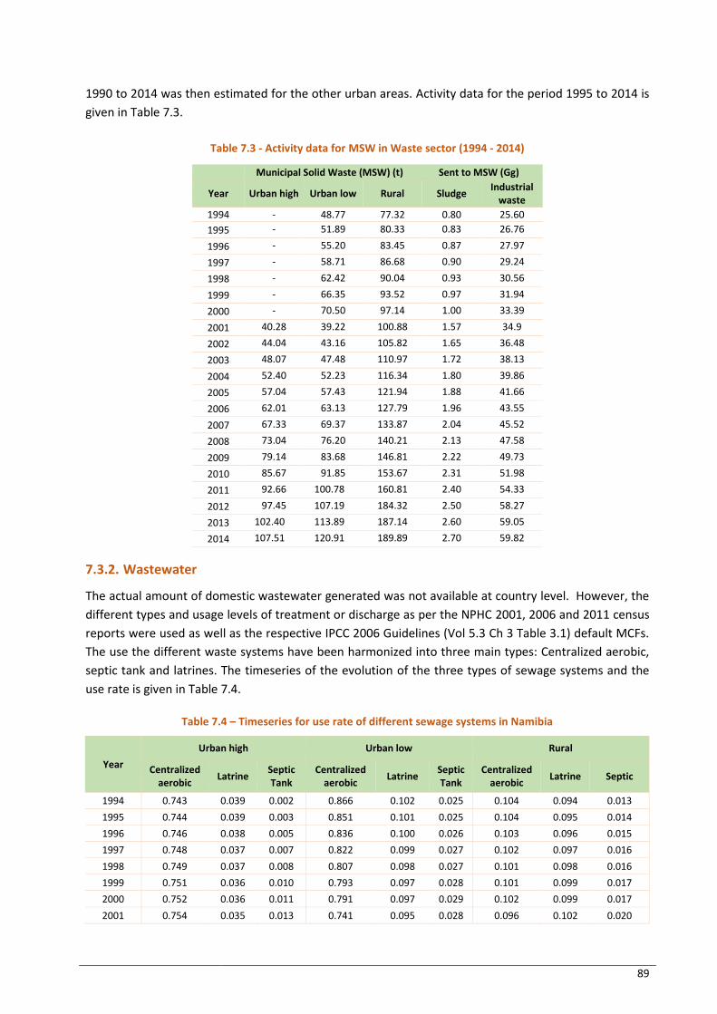
89
1990 to 2014 was then estimated for the other urban areas. Activity data for the period 1995 to 2014 is
given in Table 7.3.
Table 7.3 - Activity data for MSW in Waste sector (1994 - 2014)
Municipal Solid Waste (MSW) (t) Sent to MSW (Gg)
Year Urban high Urban low Rural Sludge Industrial
waste
1994 - 48.77 77.32 0.80 25.60
1995 - 51.89 80.33 0.83 26.76
1996 - 55.20 83.45 0.87 27.97
1997 - 58.71 86.68 0.90 29.24
1998 - 62.42 90.04 0.93 30.56
1999 - 66.35 93.52 0.97 31.94
2000 - 70.50 97.14 1.00 33.39
2001 40.28 39.22 100.88 1.57 34.9
2002 44.04 43.16 105.82 1.65 36.48
2003 48.07 47.48 110.97 1.72 38.13
2004 52.40 52.23 116.34 1.80 39.86
2005 57.04 57.43 121.94 1.88 41.66
2006 62.01 63.13 127.79 1.96 43.55
2007 67.33 69.37 133.87 2.04 45.52
2008 73.04 76.20 140.21 2.13 47.58
2009 79.14 83.68 146.81 2.22 49.73
2010 85.67 91.85 153.67 2.31 51.98
2011 92.66 100.78 160.81 2.40 54.33
2012 97.45 107.19 184.32 2.50 58.27
2013 102.40 113.89 187.14 2.60 59.05
2014 107.51 120.91 189.89 2.70 59.82
7.3.2. Wastewater
The actual amount of domestic wastewater generated was not available at country level. However, the
different types and usage levels of treatment or discharge as per the NPHC 2001, 2006 and 2011 census
reports were used as well as the respective IPCC 2006 Guidelines (Vol 5.3 Ch 3 Table 3.1) default MCFs.
The use the different waste systems have been harmonized into three main types: Centralized aerobic,
septic tank and latrines. The timeseries of the evolution of the three types of sewage systems and the
use rate is given in Table 7.4.
Table 7.4 – Timeseries for use rate of different sewage systems in Namibia
Year
Urban high Urban low Rural
Centralized aerobic
Latrine Septic Tank
Centralized aerobic
Latrine Septic Tank
Centralized aerobic
Latrine Septic
1994 0.743 0.039 0.002 0.866 0.102 0.025 0.104 0.094 0.013
1995 0.744 0.039 0.003 0.851 0.101 0.025 0.104 0.095 0.014
1996 0.746 0.038 0.005 0.836 0.100 0.026 0.103 0.096 0.015
1997 0.748 0.037 0.007 0.822 0.099 0.027 0.102 0.097 0.016
1998 0.749 0.037 0.008 0.807 0.098 0.027 0.101 0.098 0.016
1999 0.751 0.036 0.010 0.793 0.097 0.028 0.101 0.099 0.017
2000 0.752 0.036 0.011 0.791 0.097 0.029 0.102 0.099 0.017
2001 0.754 0.035 0.013 0.741 0.095 0.028 0.096 0.102 0.020
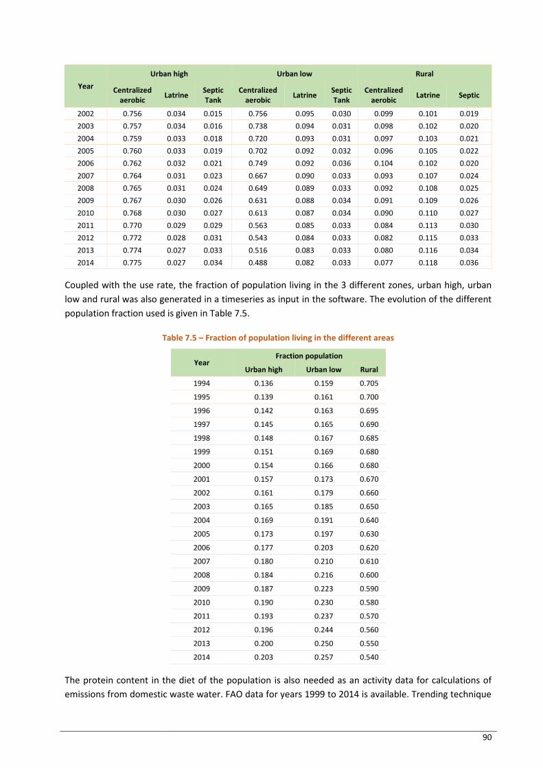
90
Year
Urban high Urban low Rural
Centralized aerobic
Latrine Septic Tank
Centralized aerobic
Latrine Septic Tank
Centralized aerobic
Latrine Septic
2002 0.756 0.034 0.015 0.756 0.095 0.030 0.099 0.101 0.019
2003 0.757 0.034 0.016 0.738 0.094 0.031 0.098 0.102 0.020
2004 0.759 0.033 0.018 0.720 0.093 0.031 0.097 0.103 0.021
2005 0.760 0.033 0.019 0.702 0.092 0.032 0.096 0.105 0.022
2006 0.762 0.032 0.021 0.749 0.092 0.036 0.104 0.102 0.020
2007 0.764 0.031 0.023 0.667 0.090 0.033 0.093 0.107 0.024
2008 0.765 0.031 0.024 0.649 0.089 0.033 0.092 0.108 0.025
2009 0.767 0.030 0.026 0.631 0.088 0.034 0.091 0.109 0.026
2010 0.768 0.030 0.027 0.613 0.087 0.034 0.090 0.110 0.027
2011 0.770 0.029 0.029 0.563 0.085 0.033 0.084 0.113 0.030
2012 0.772 0.028 0.031 0.543 0.084 0.033 0.082 0.115 0.033
2013 0.774 0.027 0.033 0.516 0.083 0.033 0.080 0.116 0.034
2014 0.775 0.027 0.034 0.488 0.082 0.033 0.077 0.118 0.036
Coupled with the use rate, the fraction of population living in the 3 different zones, urban high, urban
low and rural was also generated in a timeseries as input in the software. The evolution of the different
population fraction used is given in Table 7.5.
Table 7.5 – Fraction of population living in the different areas
Year Fraction population
Urban high Urban low Rural
1994 0.136 0.159 0.705
1995 0.139 0.161 0.700
1996 0.142 0.163 0.695
1997 0.145 0.165 0.690
1998 0.148 0.167 0.685
1999 0.151 0.169 0.680
2000 0.154 0.166 0.680
2001 0.157 0.173 0.670
2002 0.161 0.179 0.660
2003 0.165 0.185 0.650
2004 0.169 0.191 0.640
2005 0.173 0.197 0.630
2006 0.177 0.203 0.620
2007 0.180 0.210 0.610
2008 0.184 0.216 0.600
2009 0.187 0.223 0.590
2010 0.190 0.230 0.580
2011 0.193 0.237 0.570
2012 0.196 0.244 0.560
2013 0.200 0.250 0.550
2014 0.203 0.257 0.540
The protein content in the diet of the population is also needed as an activity data for calculations of
emissions from domestic waste water. FAO data for years 1999 to 2014 is available. Trending technique
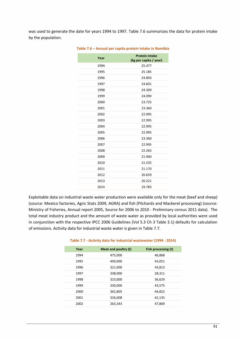
91
was used to generate the date for years 1994 to 1997. Table 7.6 summarizes the data for protein intake
by the population.
Table 7.6 – Annual per capita protein intake in Namibia
Year Protein intake
(kg per capita / year)
1994 25.477
1995 25.185
1996 24.893
1997 24.601
1998 24.309
1999 24.090
2000 23.725
2001 23.360
2002 22.995
2003 22.995
2004 22.995
2005 22.995
2006 23.360
2007 22.995
2008 22.265
2009 21.900
2010 21.535
2011 21.170
2012 20.659
2013 20.221
2014 19.783
Exploitable data on industrial waste water production were available only for the meat (beef and sheep)
(source: Meatco factories, Agric Stats 2009, AGRA) and fish (Pilchards and Mackerel processing) (source:
Ministry of Fisheries, Annual report 2005, Source for 2006 to 2010 - Preliminary census 2011 data). The
total meat industry product and the amount of waste water as provided by local authorities were used
in conjunction with the respective IPCC 2006 Guidelines (Vol 5.3 Ch 3 Table 3.1) defaults for calculation
of emissions. Activity data for industrial waste water is given in Table 7.7.
Table 7.7 - Activity data for industrial wastewater (1994 - 2014)
Year Meat and poultry (t) Fish processing (t)
1994 475,000 46,868
1995 409,000 43,051
1996 321,000 43,813
1997 338,000 28,311
1998 323,000 36,629
1999 330,000 43,575
2000 362,805 44,822
2001 326,008 42,135
2002 263,343 47,869
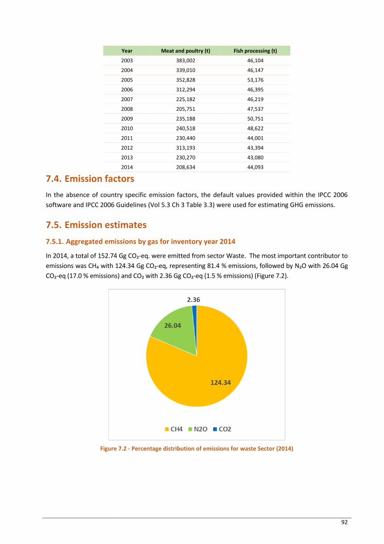
92
Year Meat and poultry (t) Fish processing (t)
2003 383,002 46,104
2004 339,010 46,147
2005 352,828 53,176
2006 312,294 46,395
2007 225,182 46,219
2008 205,751 47,537
2009 235,188 50,751
2010 240,518 48,622
2011 230,440 44,001
2012 313,193 43,394
2013 230,270 43,080
2014 208,634 44,093
7.4. Emission factors
In the absence of country specific emission factors, the default values provided within the IPCC 2006
software and IPCC 2006 Guidelines (Vol 5.3 Ch 3 Table 3.3) were used for estimating GHG emissions.
7.5. Emission estimates
7.5.1. Aggregated emissions by gas for inventory year 2014
In 2014, a total of 152.74 Gg CO₂-eq. were emitted from sector Waste. The most important contributor to
emissions was CH₄ with 124.34 Gg CO₂-eq, representing 81.4 % emissions, followed by N₂O with 26.04 Gg
CO₂-eq (17.0 % emissions) and CO₂ with 2.36 Gg CO₂-eq (1.5 % emissions) (Figure 7.2).
Figure 7.2 - Percentage distribution of emissions for waste Sector (2014)
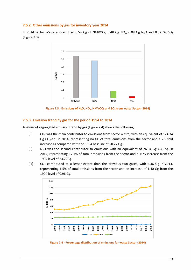
93
7.5.2. Other emissions by gas for inventory year 2014
In 2014 sector Waste also emitted 0.54 Gg of NMVOCs, 0.48 Gg NOₓ, 0.08 Gg N₂O and 0.02 Gg SO₂
(Figure 7.3).
Figure 7.3 - Emissions of N₂O, NOₓ, NMVOCs and SO₂ from waste Sector (2014)
7.5.3. Emission trend by gas for the period 1994 to 2014
Analysis of aggregated emission trend by gas (Figure 7.4) shows the following:
(i) CH₄ was the main contributor to emissions from sector waste, with an equivalent of 124.34
Gg CO₂-eq. in 2014, representing 84.4% of total emissions from the sector and a 2.5 fold
increase as compared with the 1994 baseline of 50.27 Gg.
(ii) N₂O was the second contributor to emissions with an equivalent of 26.04 Gg CO₂-eq. in
2014, representing 17.1% of total emissions from the sector and a 10% increase from the
1994 level of 23.72Gg.
(iii) CO₂ contributed to a lesser extent than the previous two gases, with 2.36 Gg in 2014,
representing 1.5% of total emissions from the sector and an increase of 1.40 Gg from the
1994 level of 0.96 Gg.
Figure 7.4 - Percentage distribution of emissions for waste Sector (2014)

94
7.5.4. Emissions by waste categories for inventory year 2014
The total emissions of 152.74 Gg CO₂-eq. recorded in 2014 represent 0.7 % of national emissions. Solid
Waste Disposal was the most important contributor to total emissions of the sector with 76.86 Gg CO₂-eq.
(50.3% of total), followed by Domestic Wastewater Treatment and Discharge with 34.37 Gg CO₂-eq
(22.5%), Open Burning of Waste with 27.12 Gg (17.8%) and Industrial Wastewater Treatment and
Discharge with 14.38 Gg CO₂-eq (9.4%) (Table 7.8).
During the same inventory year, sector waste also emitted 0.48 Gg NOₓ, 8.48 Gg CO, 0.54 Gg NMVOC and
0.02 Gg SO₂.
Table 7.8 - Emissions from Waste sector for inventory year 2014
Categories
Emissions (Gg CO₂ eq) Emissions (Gg)
CO₂ CH₄ N₂O Total CO₂
eq NOₓ CO NMVOCs SO₂
4 - Waste 2.36 124.34 26.04 152.74 0.48 8.48 0.54 1.67E-02
4.A - Solid Waste Disposal - 76.86 - 76.86 - - 0.36 -
4.A.2 - Unmanaged Waste Disposal Sites - 76.86 - 76.86 - - 0.36 -
4.C - Incineration and Open Burning of Waste 2.36 20.74 4.03 27.12 0.48 8.48 0.19 1.67E-02
4.C.2 - Open Burning of Waste 2.36 20.74 4.03 27.12 0.48 8.48 0.19 1.67E-02
4.D - Wastewater Treatment and Discharge - 26.75 22.01 48.75 - - 1.00E-06 -
4.D.1 - Domestic Wastewater Treatment and Discharge 12.36 22.01 34.37 - - 8.00E-07 -
4.D.2 - Industrial Wastewater treatment and Discharge - 14.38 - 14.38 - - 2.00E-07 -
7.5.5. Emissions by waste categories – trend for period 1994 to 2014
The total emissions of 152.74 Gg CO₂-eq. recorded in 2014 represent an increase of 77.78 Gg CO₂-eq. from
the 1994 estimates of 74.96 Gg CO₂-eq. (Figure 7.5), equivalent to a 103.8% rise.
Figure 7.5 - Evolution of emissions (Gg CO₂-eq.) from Waste sector (1995 – 2014)
The increase in emissions was mainly a result of a significant rise in emissions from Solid Waste Disposal
which increased 9.1 times from 8.43 Gg CO₂-eq. in 1994 to reach 76.85 Gg CO₂-eq in 2014. In fact, the
rise in emissions from Solid Waste Disposal represented as much as 88.0% of the total increase from
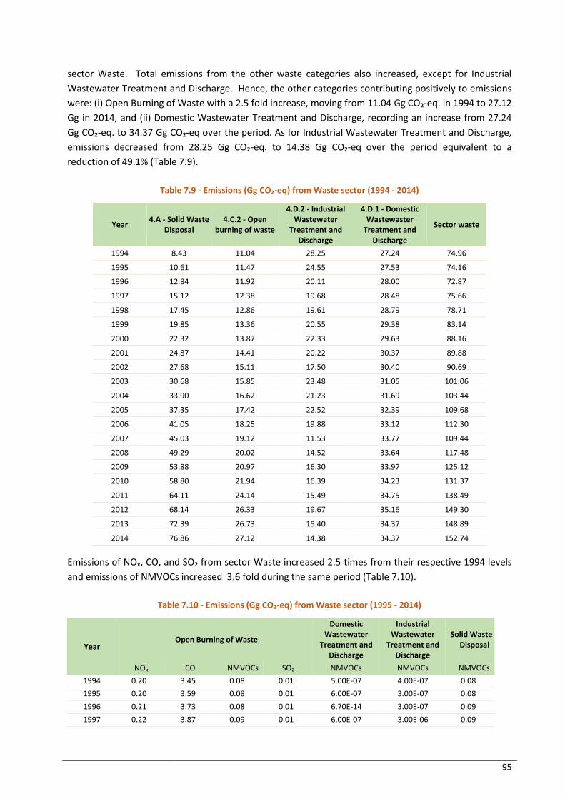
95
sector Waste. Total emissions from the other waste categories also increased, except for Industrial
Wastewater Treatment and Discharge. Hence, the other categories contributing positively to emissions
were: (i) Open Burning of Waste with a 2.5 fold increase, moving from 11.04 Gg CO₂-eq. in 1994 to 27.12
Gg in 2014, and (ii) Domestic Wastewater Treatment and Discharge, recording an increase from 27.24
Gg CO₂-eq. to 34.37 Gg CO₂-eq over the period. As for Industrial Wastewater Treatment and Discharge,
emissions decreased from 28.25 Gg CO₂-eq. to 14.38 Gg CO₂-eq over the period equivalent to a
reduction of 49.1% (Table 7.9).
Table 7.9 - Emissions (Gg CO₂-eq) from Waste sector (1994 - 2014)
Year 4.A - Solid Waste
Disposal 4.C.2 - Open
burning of waste
4.D.2 - Industrial Wastewater
Treatment and Discharge
4.D.1 - Domestic Wastewaster
Treatment and Discharge
Sector waste
1994 8.43 11.04 28.25 27.24 74.96
1995 10.61 11.47 24.55 27.53 74.16
1996 12.84 11.92 20.11 28.00 72.87
1997 15.12 12.38 19.68 28.48 75.66
1998 17.45 12.86 19.61 28.79 78.71
1999 19.85 13.36 20.55 29.38 83.14
2000 22.32 13.87 22.33 29.63 88.16
2001 24.87 14.41 20.22 30.37 89.88
2002 27.68 15.11 17.50 30.40 90.69
2003 30.68 15.85 23.48 31.05 101.06
2004 33.90 16.62 21.23 31.69 103.44
2005 37.35 17.42 22.52 32.39 109.68
2006 41.05 18.25 19.88 33.12 112.30
2007 45.03 19.12 11.53 33.77 109.44
2008 49.29 20.02 14.52 33.64 117.48
2009 53.88 20.97 16.30 33.97 125.12
2010 58.80 21.94 16.39 34.23 131.37
2011 64.11 24.14 15.49 34.75 138.49
2012 68.14 26.33 19.67 35.16 149.30
2013 72.39 26.73 15.40 34.37 148.89
2014 76.86 27.12 14.38 34.37 152.74
Emissions of NOₓ, CO, and SO₂ from sector Waste increased 2.5 times from their respective 1994 levels
and emissions of NMVOCs increased 3.6 fold during the same period (Table 7.10).
Table 7.10 - Emissions (Gg CO₂-eq) from Waste sector (1995 - 2014)
Year Open Burning of Waste
Domestic Wastewater
Treatment and Discharge
Industrial Wastewater
Treatment and Discharge
Solid Waste Disposal
NOₓ CO NMVOCs SO₂ NMVOCs NMVOCs NMVOCs
1994 0.20 3.45 0.08 0.01 5.00E-07 4.00E-07 0.08
1995 0.20 3.59 0.08 0.01 6.00E-07 3.00E-07 0.08
1996 0.21 3.73 0.08 0.01 6.70E-14 3.00E-07 0.09
1997 0.22 3.87 0.09 0.01 6.00E-07 3.00E-06 0.09

96
Year Open Burning of Waste
Domestic Wastewater
Treatment and Discharge
Industrial Wastewater
Treatment and Discharge
Solid Waste Disposal
NOₓ CO NMVOCs SO₂ NMVOCs NMVOCs NMVOCs
1998 0.23 4.02 0.09 0.01 6.00E-07 3.00E-07 0.10
1999 0.24 4.18 0.09 0.01 6.00E-07 3.00E-07 0.10
2000 0.25 4.34 0.10 0.01 6.00E-07 3.00E-07 0.11
2001 0.26 4.51 0.10 0.01 6.00E-07 3.00E-07 0.12
2002 0.27 4.73 0.10 0.01 7.00E-07 2.00E-07 0.14
2003 0.28 4.96 0.11 0.01 7.00E-07 3.00E-07 0.15
2004 0.30 5.20 0.11 0.01 7.00E-07 3.00E-07 0.16
2005 0.31 5.45 0.12 0.01 7.00E-07 3.00E-07 0.18
2006 0.33 5.71 0.13 0.01 7.00E-07 3.00E-07 0.20
2007 0.34 5.98 0.13 0.01 1.00E-06 2.00E-07 0.21
2008 0.36 6.26 0.14 0.01 7.00E-07 2.00E-07 0.23
2009 0.37 6.56 0.14 0.01 7.00E-07 2.00E-07 0.25
2010 0.39 6.86 0.15 0.01 7.00E-07 2.00E-07 0.28
2011 0.43 7.55 0.17 0.01 7.00E-07 2.00E-07 0.30
2012 0.47 8.23 0.18 0.02 8.00E-07 3.00E-07 0.32
2013 0.48 8.36 0.18 0.02 8.00E-07 2.00E-07 0.34
2014 0.48 8.48 0.19 0.02 8.00E-07 2.00E-07 0.36
7.5.5.1. Solid Waste Disposal (4.A)
Solid Waste Disposal was the major contributor to GHG emissions from sector waste as a result of CH₄
emissions of from waste disposal sites. Emissions of CH₄ increased by 9.1 times from 8.43 Gg CO₂-eq in
1994 to reach 76.86 Gg in 2014. (Figure 7.6)
Figure 7.6 - Emissions of CH₄ in CO₂-eq from Solid Waste Disposal (1994 - 2014)
7.5.5.2. Open Burning of Waste (4.C.2)
Emissions from Open Burning of Waste increased from 11.04 Gg CO₂-eq in 1994 to 27.12 Gg CO₂-eq in
2014 – an increase of 16.10 Gg CO₂-eq equivalent 140%. The gases which contributed to the emissions
were, in decreasing order of importance, CH₄ (76.5%), N₂O (14.8%) and CO₂ (8.7%) (Figure 7.7).
-
10
20
30
40
50
60
70
80
90
Gg
CO
₂eq
4.A - Solid Waste Disposal
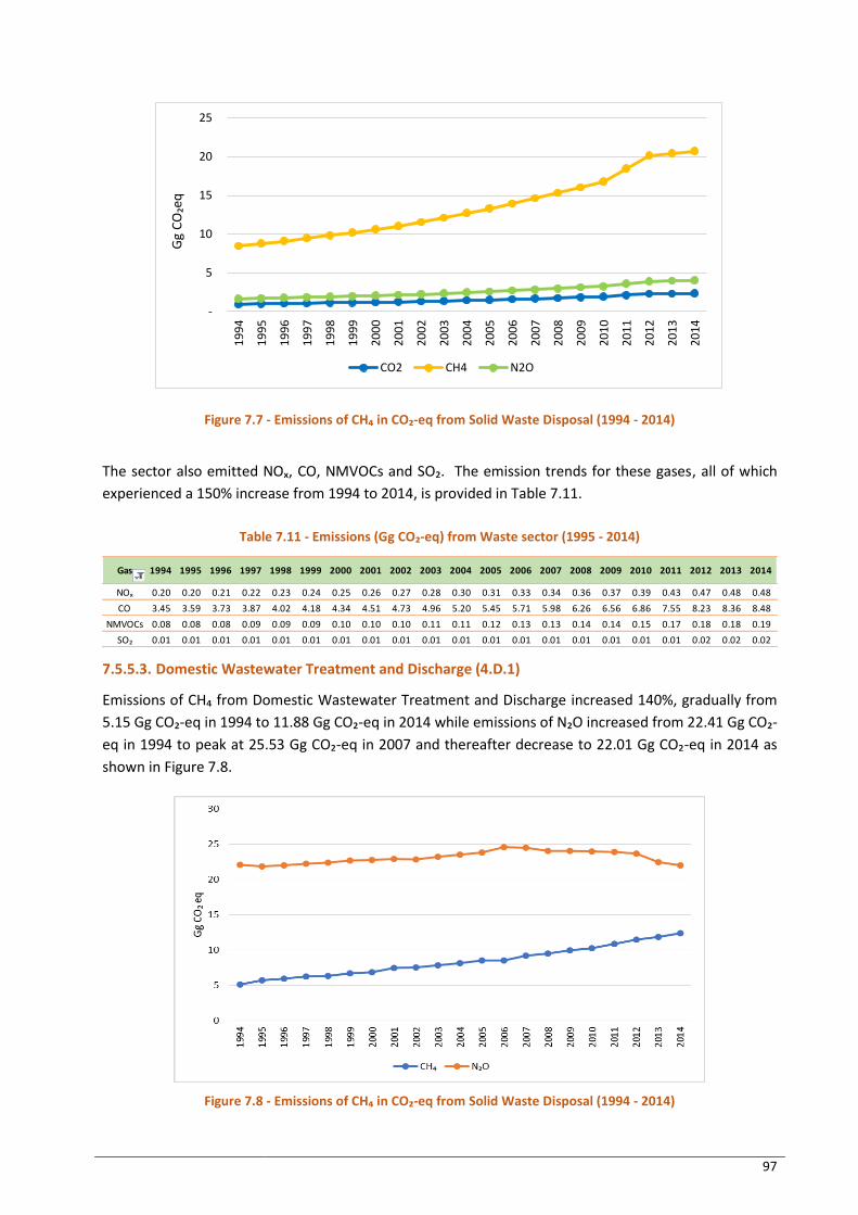
97
Figure 7.7 - Emissions of CH₄ in CO₂-eq from Solid Waste Disposal (1994 - 2014)
The sector also emitted NOₓ, CO, NMVOCs and SO₂. The emission trends for these gases, all of which
experienced a 150% increase from 1994 to 2014, is provided in Table 7.11.
Table 7.11 - Emissions (Gg CO₂-eq) from Waste sector (1995 - 2014)
7.5.5.3. Domestic Wastewater Treatment and Discharge (4.D.1)
Emissions of CH₄ from Domestic Wastewater Treatment and Discharge increased 140%, gradually from
5.15 Gg CO₂-eq in 1994 to 11.88 Gg CO₂-eq in 2014 while emissions of N₂O increased from 22.41 Gg CO₂-
eq in 1994 to peak at 25.53 Gg CO₂-eq in 2007 and thereafter decrease to 22.01 Gg CO₂-eq in 2014 as
shown in Figure 7.8.
Figure 7.8 - Emissions of CH₄ in CO₂-eq from Solid Waste Disposal (1994 - 2014)
-
5
10
15
20
25
19
94
19
95
19
96
19
97
19
98
19
99
20
00
20
01
20
02
20
03
20
04
20
05
20
06
20
07
20
08
20
09
20
10
20
11
20
12
20
13
20
14
Gg
CO
₂eq
CO2 CH4 N2O
Gas 1994 1995 1996 1997 1998 1999 2000 2001 2002 2003 2004 2005 2006 2007 2008 2009 2010 2011 2012 2013 2014
NOₓ 0.20 0.20 0.21 0.22 0.23 0.24 0.25 0.26 0.27 0.28 0.30 0.31 0.33 0.34 0.36 0.37 0.39 0.43 0.47 0.48 0.48
CO 3.45 3.59 3.73 3.87 4.02 4.18 4.34 4.51 4.73 4.96 5.20 5.45 5.71 5.98 6.26 6.56 6.86 7.55 8.23 8.36 8.48
NMVOCs 0.08 0.08 0.08 0.09 0.09 0.09 0.10 0.10 0.10 0.11 0.11 0.12 0.13 0.13 0.14 0.14 0.15 0.17 0.18 0.18 0.19
SO₂ 0.01 0.01 0.01 0.01 0.01 0.01 0.01 0.01 0.01 0.01 0.01 0.01 0.01 0.01 0.01 0.01 0.01 0.01 0.02 0.02 0.02
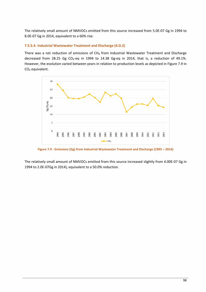
98
The relatively small amount of NMVOCs emitted from this source increased from 5.0E-07 Gg in 1994 to
8.0E-07 Gg in 2014, equivalent to a 60% rise.
7.5.5.4. Industrial Wastewater Treatment and Discharge (4.D.2)
There was a net reduction of emissions of CH₄ from Industrial Wastewater Treatment and Discharge
decreased from 28.25 Gg CO₂-eq in 1994 to 14.38 Gg-eq in 2014, that is, a reduction of 49.1%.
However, the evolution varied between years in relation to production levels as depicted in Figure 7.9 in
CO₂ equivalent.
Figure 7.9 - Emissions (Gg) from Industrial Wastewater Treatment and Discharge (1995 – 2014)
The relatively small amount of NMVOCs emitted from this source increased slightly from 4.00E-07 Gg in
1994 to 2.0E-07Gg in 2014), equivalent to a 50.0% reduction.
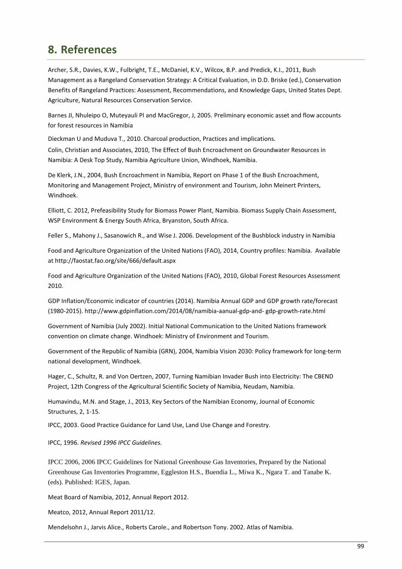
99
8. References
Archer, S.R., Davies, K.W., Fulbright, T.E., McDaniel, K.V., Wilcox, B.P. and Predick, K.I., 2011, Bush
Management as a Rangeland Conservation Strategy: A Critical Evaluation, in D.D. Briske (ed.), Conservation
Benefits of Rangeland Practices: Assessment, Recommendations, and Knowledge Gaps, United States Dept.
Agriculture, Natural Resources Conservation Service.
Barnes JI, Nhuleipo O, Muteyauli PI and MacGregor, J, 2005. Preliminary economic asset and flow accounts
for forest resources in Namibia
Dieckman U and Muduva T., 2010. Charcoal production, Practices and implications.
Colin, Christian and Associates, 2010, The Effect of Bush Encroachment on Groundwater Resources in
Namibia: A Desk Top Study, Namibia Agriculture Union, Windhoek, Namibia.
De Klerk, J.N., 2004, Bush Encroachment in Namibia, Report on Phase 1 of the Bush Encroachment,
Monitoring and Management Project, Ministry of environment and Tourism, John Meinert Printers,
Windhoek.
Elliott, C. 2012, Prefeasibility Study for Biomass Power Plant, Namibia. Biomass Supply Chain Assessment,
WSP Environment & Energy South Africa, Bryanston, South Africa.
Feller S., Mahony J., Sasanowich R., and Wise J. 2006. Development of the Bushblock industry in Namibia
Food and Agriculture Organization of the United Nations (FAO), 2014, Country profiles: Namibia. Available
at http://faostat.fao.org/site/666/default.aspx
Food and Agriculture Organization of the United Nations (FAO), 2010, Global Forest Resources Assessment
2010.
GDP Inflation/Economic indicator of countries (2014). Namibia Annual GDP and GDP growth rate/forecast
(1980-2015). http://www.gdpinflation.com/2014/08/namibia-aanual-gdp-and- gdp-growth-rate.html
Government of Namibia (July 2002). Initial National Communication to the United Nations framework
convention on climate change. Windhoek: Ministry of Environment and Tourism.
Government of the Republic of Namibia (GRN), 2004, Namibia Vision 2030: Policy framework for long‐term
national development, Windhoek.
Hager, C., Schultz, R. and Von Oertzen, 2007, Turning Namibian Invader Bush into Electricity: The CBEND
Project, 12th Congress of the Agricultural Scientific Society of Namibia, Neudam, Namibia.
Humavindu, M.N. and Stage, J., 2013, Key Sectors of the Namibian Economy, Journal of Economic
Structures, 2, 1-15.
IPCC, 2003. Good Practice Guidance for Land Use, Land Use Change and Forestry.
IPCC, 1996. Revised 1996 IPCC Guidelines.
IPCC 2006, 2006 IPCC Guidelines for National Greenhouse Gas Inventories, Prepared by the National
Greenhouse Gas Inventories Programme, Eggleston H.S., Buendia L., Miwa K., Ngara T. and Tanabe K.
(eds). Published: IGES, Japan.
Meat Board of Namibia, 2012, Annual Report 2012.
Meatco, 2012, Annual Report 2011/12.
Mendelsohn J., Jarvis Alice., Roberts Carole., and Robertson Tony. 2002. Atlas of Namibia.
100
Mendelson J. and Obeid, 2004. Forests and woodlands of Namibia
Ministry of Agriculture, Water and Forestry., 2014. Annual report 2013-2014.
Ministry of Agriculture, Water and Forestry., (Personal Communication) Burning AD Dept Forestry.
Ministry of Environment and Tourism, 2010. National Policy on Climate Change for Namibia
Ministry of Fisheries and Marine Resources., 2005. Annual report 2005.
Namibia Statistics Agency (2012). Namibia 2011 Population and Housing Census Main Report. Republic of
Namibia, Windhoek.
Namibia Statistics Agency (2012). Namibia Household Income & Expenditure Survey (NHIES) 2009/2010.
Republic of Namibia, Windhoek.
Namibia Statistics Agency (2014). Namibia Population Projections 2011-2041. Census Main Report.
Republic of Namibia, Windhoek, September 2014.
Namibia Statistics Agency (NSA), 2012, National Household Income and Expenditure Survey.
Namibia Statistics Agency (NSA), 2013, Profile of Namibia.
Namibia Statistics Agency (NSA), 2014a, Namibia 2011 Census Mortality Report.
Namibia Statistics Agency (NSA), 2014b, Namibia 2013 Demographic and Health Survey, Main Report
National Planning Commission (2002). Second National Development Plan (NDP2) 2002/2003 – 2006/2007.
National Planning Commission, Windhoek, Republic of Namibia
National Planning Commission (2008). Third National Development Plan (NDP3) 2007/2008 – 2011/2012.
National Planning Commission, Windhoek, Republic of Namibia
National Planning Commission (2012). Third National Development Plan (NDP3) 2012/2013 – 20161/2017.
National Planning Commission, Windhoek, Republic of Namibia
Republic of Namibia (2004). Namibia Vision 2030 – Policy Framework for Long-term National Development
Main Document. Office of the President. Windhoek, Republic of Namibia.
Republic of Namibia (July 2011) Namibia Second National Communication to the United Nations Framework
Convention on Climate Change. Ministry of Environment and Tourism
Routhauge A., 2014. Baseline Assessment for the De-Bushing Programme in Namibia.
Schoeman S.J., 1996. Characterization of beef cattle breeds by virtue of their performance in the National
Beef Cattle Performance and Progeny Testing Scheme, South African Journal of Animal Science, 1996, 26 (1)
Wikipedia (2015). Demographics of Namibia. http://www.wikipedia.org/wiki.