Representative mass reduction in sampling—a critical survey ...

www.elsevier.com/locate/chemolab

Chemometrics and Intelligent Laboratory Systems 74 (2004) 95–114

Representative mass reduction in sampling—a critical survey of

techniques and hardware

Lars Petersen*, Casper K. Dahl, Kim H. Esbensen

Applied Chemometrics, Analytical Chemistry and Sampling Research Group, ACACSRG, Aalborg University Esbjerg,

Niels Bohrs Vej 8, DK-6700 Esbjerg, Denmark

Received 3 September 2003; received in revised form 16 February 2004; accepted 1 March 2004

Available online 24 June 2004

Abstract

We here present a comprehensive survey of current mass reduction principles and hardware available in the current market. We conduct a

rigorous comparison study of the performance of 17 field and/or laboratory instruments or methods which are quantitatively characterized

(and ranked) for accuracy (bias), reproducibility (precision), material loss (external as well as internal loss), user-dependency, operation time,

and ease of cleaning. Graphical comparison of these quantitative results allow a complete overview of the relative strengths and weaknesses

of riffle splitters, various rotational dividers, the Boerner Divider, the ‘‘spoon method’’, alternate/fractional shoveling and grab sampling.

Only devices based on riffle splitting principles (static or rotational) passes the ultimate representativity test (with minor, but significant

relative differences). Grab sampling, the overwhelmingly most often used mass reduction method, performs appallingly—its use must be

discontinued (with the singular exception for completely homogenized fine powders). Only proper mass reduction (i.e. carried out in

complete compliance with all appropriate design principles, maintenance and cleaning rules) can always be representative in the full Theory

of Sampling (TOS) sense. This survey also allows empirical verification of the merits of the famous ‘‘Gy’s formula’’ for order-of-magnitude

estimation of the Fundamental Sampling Error (FSE).

D 2004 Elsevier B.V. All rights reserved.

Keywords: Mass reduction; Sampling; Riffle splitter; Shoveling; Boerner Divider; Rotational divider; Grab sampling; Representativeness

Sampling is nothing but representative mass reduction. substantial size in order to be representative, and this places

[Pierre Gy]

1. Introduction

The archetype error of ill-reflected sampling is to focus

on getting to the final sample volume much too early in the

sampling process. Instead of only focusing on securing as

quickly as possible the desired representative samples

(which cannot be evidenced from the physical samples

themselves) of the final sample volume/mass, the Theory

of Sampling (TOS) stipulates that only a properly designed

and controlled sampling process can facilitate this. Only

TOS tells comprehensively how and how much material to

extract from a lot. For many types of heterogeneous material

often the extracted primary sample has to be of a quite

0169-7439/$ - see front matter D 2004 Elsevier B.V. All rights reserved.

doi:10.1016/j.chemolab.2004.03.020

* Corresponding author. Tel.: +45-7912-7666; fax: +45-7545-3643.

E-mail address: [email protected] (L. Petersen).

stringent demands on the sampler (the sampling instrument),

for instance if the sample is used for chemical analysis,

where typically only 1 g, or a fraction hereof is required.

Usually, there is a very long way from the size of the initial

lot—via the primary sample—to the final analytical sample

mass (Fig. 1). Typically mass reductions of the order of

1:1000 to 1:100.000 have to be invoked. It is therefore of

the utmost importance that all sampling processes make do

only with representative mass reduction. Unfortunately

many designs and implemented hardware look at mass

reduction as a pure materials handling reduction in terms

of weight per se. It’s quite another thing to be concerned

with the degree of representativity of the reduced mass

fractions.

Also, usually emphasis is on getting a valid analytical

result, in the sense that the amount of the analyte in the final

sample, aS, makes do—while TOS emphasizes that only the

corresponding estimate of the lot concentration, aL, carries

the information sought. There is a world of difference

between these two concentration estimates—the entire

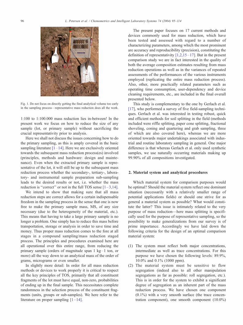
Fig. 1. Do not focus on directly getting the final analytical volume too early

in the sampling process—representative mass reduction does all the work.

L. Petersen et al. / Chemometrics and Intelligent Laboratory Systems 74 (2004) 95–11496

1:100 to 1:100.000 mass reduction lies in-between! In the

present work we focus on how to reduce the size of any

sample (lot, or primary sample) without sacrificing the

crucial representativity prior to analysis.

Here we shall not discuss the issues concerning how to do

the primary sampling, as this is amply covered in the basic

sampling literature [1–14]. Here we are exclusively oriented

towards the subsequent mass reduction process(es) involved

(principles, methods and hardware: design and mainte-

nance). Even when the extracted primary sample is repre-

sentative of the lot, it will still be up to the subsequent mass

reduction process whether the secondary-, tertiary-, labora-

tory- and instrumental sample preparation sub-sampling

leads to the desired results or not, i.e. whether the mass

reduction is ‘‘correct’’ or not in the full TOS sense [1–3,14].

We intend to show that making sure that all mass

reduction steps are correct allows for a certain indispensable

freedom in the sampling process in the sense that one is now

free to make the primary sample mass, MS, of any size

necessary (due to the heterogeneity of the material, etc.).

This means that having to take a large primary sample is no

longer a problem. One simply has to reduce this mass before

transportation, storage or analysis in order to save time and

money. Thus proper mass reduction comes to the fore at all

stages in a compound sampling/mass reduction staged

process. The principles and procedures examined here are

all operational over this entire range, from reducing the

primary sample (orders of magnitude span 1 kg–1 ton, or

more) all the way down to an analytical mass of the order of

grams, micrograms or even smaller.

In slightly more detail: In order for all mass reduction

methods or devices to work properly it is critical to respect

all the key principles of TOS, primarily that all constituent

fragments of the lot must have equal, non-zero, probabilities

of ending up in the final sample. This necessitates complete

randomness in the selection process of the constituent frag-

ments (units, groups or sub-samples). We here refer to the

literature on proper sampling [1–14].

The present paper focuses on 17 current methods and

devices commonly used for mass reduction, which have

been tested and assessed with regard to a number of

characterizing parameters, among which the most prominent

are accuracy and reproducibility (precision), constituting the

definition of representativity [1,2,15–17]. But in the present

comparison study we are in fact interested in the quality of

both the average composition estimates resulting from mass

reduction operations as well as in the variances of repeated

assessments of the performances of the various instruments

employed (replicating the entire mass reduction process).

Also, other, more practically related parameters such as

operating time consumption, user-dependency and device

cleaning requirements, etc., are included in the final overall

presented below.

This study is complementary to the one by Gerlach et al.

[17], who performed a survey of five field-sampling techni-

ques. Gerlach et al. was interested in testing robust, quick

and efficient methods for soil splitting in the field (methods

included were riffle splitting, paper cone splitting, fractional

shoveling, coning and quartering and grab sampling, three

of which are also covered here), whereas we are more

oriented towards major undertakings associated with indus-

trial and routine laboratory sampling in general. One major

difference is that whereas Gerlach et al. only used synthetic

samples, we use naturally occurring materials making up

99.90% of all compositions investigated.

2. Material system and analytical procedures

Which material system for comparison purposes would

be optimal? Should the material system reflect one dominant

situation (necessarily with a relatively smaller range of

potential applications fields) or should one strive for as

general a material system as possible? What would consti-

tute the latter? This issue is intimately related to the very

purpose of mass reduction—here mass splitting is specifi-

cally used for the purpose of representative sampling, so the

possibility to make generalizations from our survey is of

prime importance. Accordingly we have laid down the

following criteria for the design of an optimal comparison

material system:

(1) The system must reflect both major concentrations,

intermediate as well as trace concentrations. For this

purpose we have chosen the following levels: 89.9%,

10.0% and 0.1% (1000 ppm).

(2) The material system must be sensitive to flow

segregation (indeed also to all other manipulation

segregations as far as possible: roll segregation, etc.).

This is in order for the system to exhibit a significant

degree of segregation as an inherent part of the mass

reduction process. We have chosen one component

(0.1%) with a very smooth surface (the trace concen-

tration component), one smooth component (10.0%)

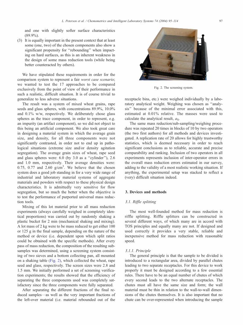
Fig. 2. The screening system.

L. Petersen et al. / Chemometrics and Intelligent Laboratory Systems 74 (2004) 95–114 97

and one with slightly softer surface characteristics

(89.9%).

(3) It is equally important in the present context that at least

some (one, two) of the chosen components also show a

significant propensity for ‘‘rebounding’’ when impact-

ing on hard surfaces, as this is an inherent weakness in

the design of some mass reduction tools (while being

better counteracted by others).

We have stipulated these requirements in order for the

comparison system to represent a fair worst case scenario;

we wanted to test the 17 approaches to be compared

exclusively from the point of view of their performance in

such a realistic, difficult situation. It is of course trivial to

generalize to less adverse situations.

The result was a system of mixed wheat grains, rape

seeds and glass spheres, with concentrations 89.9%, 10.0%

and 0.1% w/w, respectively. We deliberately chose glass

spheres as the trace component, in order to represent, e.g.

an impurity (an artifact component), so we did not object to

this being an artificial component. We also took great care

in designing a material system in which the average grain

size, and density, for all three components were not

significantly contrasted, in order not to end up in patho-

logical situations (extreme size and/or density agitation

segregation). The average grain sizes of wheat, rape seed

and glass spheres were: 6.0 (by 3.0 as a ‘‘cylinder’’), 2.6

and 1.0 mm, respectively. Their average densities were:

0.75, 0.77 and 2.60 g/cm3. We believe that the chosen

system does a good job standing in for a very wide range of

industrial and laboratory material systems of aggregate

materials and powders with respect to these physical design

characteristics. It is admittedly very sensitive for flow

segregation, but so much the better when the objective is

to test the performance of purported universal mass reduc-

tion tools.

Mixing of this lot material prior to all mass reduction

experiments (always carefully weighed in completely iden-

tical proportions) was carried out by randomly shaking a

plastic bucket for 2 min (mechanical shaking and mixing).

A lot mass of 2 kg were to be mass reduced to get either 100

or 125 g in the final sample, depending on the nature of the

method or device (i.e. dependent upon which split ratios

could be obtained with the specific methods). After every

pass of mass reduction, the composition of the resulting sub-

samples was determined, using a screening system consist-

ing of two sieves and a bottom collecting pan, all mounted

on a shaking table (Fig. 2), which collected the wheat, rape

seed and glass, respectively. The screen sizes were 2.8 and

1.5 mm. We initially performed a set of screening verifica-

tion experiments; the results showed that the efficiency of

separating the three components used was completely sat-

isfactory since the three components were fully separated.

After separating the different fractions of the final re-

duced samples—as well as the very important fractions of

the left-over material (i.e. material rebounded out of the

receptacle bins, etc.) were weighed individually by a labo-

ratory analytical weight. Weighing was chosen as ‘‘analy-

sis’’ because of the minimal error associated with this,

estimated at 0.01% relative. The masses were used to

calculate the analytical result, aS.

The same mass reduction/sub-sampling/weighing proce-

dure was repeated 20 times in blocks of 10 by two operators

(the two first authors) for all methods and devices investi-

gated. A replication rate of 20 allows for highly trustworthy

statistics, which is deemed necessary in order to reach

significant conclusions as to reliable, accurate and precise

comparability and ranking. Inclusion of two operators in all

experiments represents inclusion of inter-operator errors in

the overall mass reduction errors estimated in our survey,

adding to the validity of a most realistic working situation. If

anything, the experimental setup was stacked to reflect a

(very) difficult situation indeed.

3. Devices and methods

3.1. Riffle splitting

The most well-founded method for mass reduction is

riffle splitting. Riffle splitters can be constructed in

several different ways, of which many are in accord with

TOS principles and equally many are not. If designed and

used correctly it provides a very stable, reliable and

inexpensive method for mass reduction with reasonable

speed.

3.1.1. Principle

The general principle is that the sample to be divided is

introduced to a rectangular area, divided by parallel chutes

leading to two separate receptacles. For this device to work

properly it must be designed according to a few essential

rules. There have to be an equal number of chutes of which

every second leads to the two alternate receptacles. The

chutes must all have the same size and form; the wall

material must be thin in relation to the wall-to-wall dimen-

sions of the chutes themselves. It is also important that no

chute can be over-represented when introducing the sample

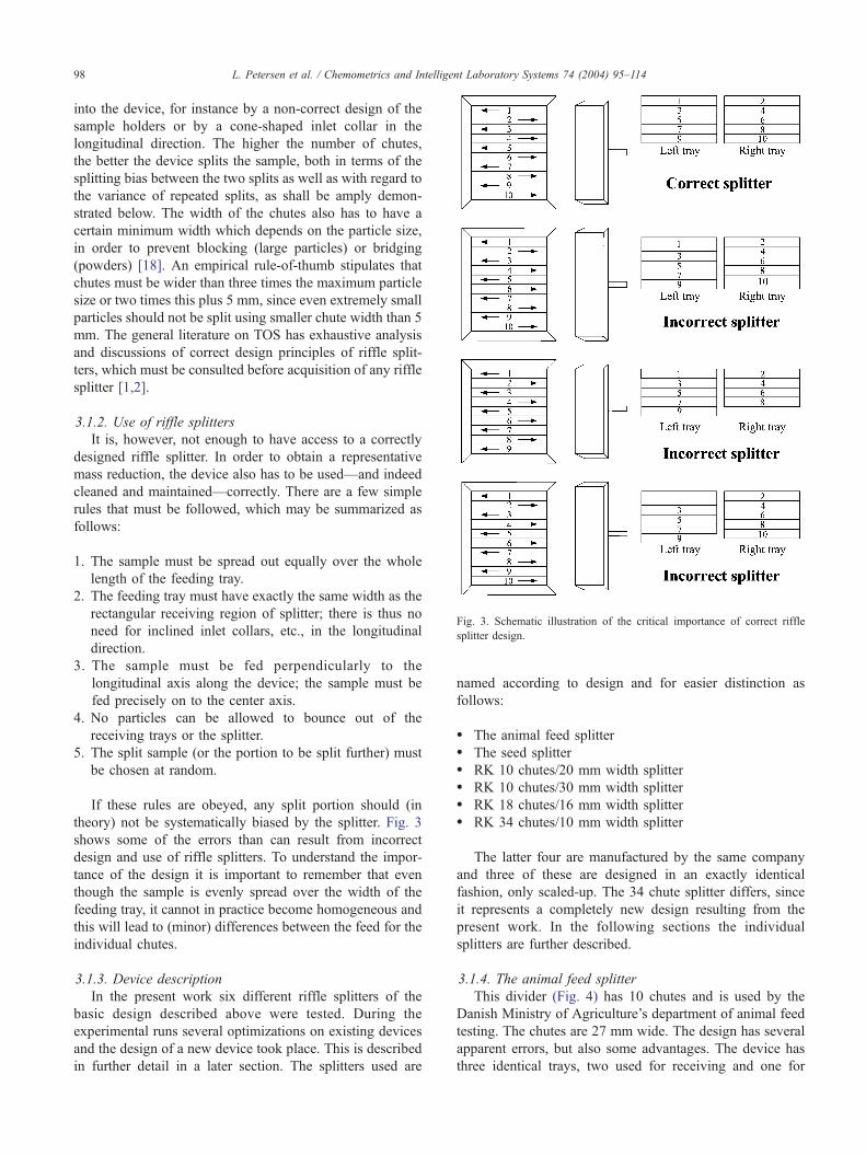
Fig. 3. Schematic illustration of the critical importance of correct riffle

splitter design.


into the device, for instance by a non-correct design of the

sample holders or by a cone-shaped inlet collar in the

longitudinal direction. The higher the number of chutes,

the better the device splits the sample, both in terms of the

splitting bias between the two splits as well as with regard to

the variance of repeated splits, as shall be amply demon-

strated below. The width of the chutes also has to have a

certain minimum width which depends on the particle size,

in order to prevent blocking (large particles) or bridging

(powders) [18]. An empirical rule-of-thumb stipulates that

chutes must be wider than three times the maximum particle

size or two times this plus 5 mm, since even extremely small

particles should not be split using smaller chute width than 5

mm. The general literature on TOS has exhaustive analysis

and discussions of correct design principles of riffle split-

ters, which must be consulted before acquisition of any riffle

splitter [1,2].

3.1.2. Use of riffle splitters

It is, however, not enough to have access to a correctly

designed riffle splitter. In order to obtain a representative

mass reduction, the device also has to be used—and indeed

cleaned and maintained—correctly. There are a few simple

rules that must be followed, which may be summarized as

follows:

1. The sample must be spread out equally over the whole

length of the feeding tray.

2. The feeding tray must have exactly the same width as the

rectangular receiving region of splitter; there is thus no

need for inclined inlet collars, etc., in the longitudinal

direction.

3. The sample must be fed perpendicularly to the

longitudinal axis along the device; the sample must be

fed precisely on to the center axis.

4. No particles can be allowed to bounce out of the

receiving trays or the splitter.

5. The split sample (or the portion to be split further) must

be chosen at random.

If these rules are obeyed, any split portion should (in

theory) not be systematically biased by the splitter. Fig. 3

shows some of the errors than can result from incorrect

design and use of riffle splitters. To understand the impor-

tance of the design it is important to remember that even

though the sample is evenly spread over the width of the

feeding tray, it cannot in practice become homogeneous and

this will lead to (minor) differences between the feed for the

individual chutes.

3.1.3. Device description

In the present work six different riffle splitters of the

basic design described above were tested. During the

experimental runs several optimizations on existing devices

and the design of a new device took place. This is described

in further detail in a later section. The splitters used are

named according to design and for easier distinction as

follows:

� The animal feed splitter� The seed splitter� RK 10 chutes/20 mm width splitter� RK 10 chutes/30 mm width splitter� RK 18 chutes/16 mm width splitter� RK 34 chutes/10 mm width splitter

The latter four are manufactured by the same company

and three of these are designed in an exactly identical

fashion, only scaled-up. The 34 chute splitter differs, since

it represents a completely new design resulting from the

present work. In the following sections the individual

splitters are further described.

3.1.4. The animal feed splitter

This divider (Fig. 4) has 10 chutes and is used by the

Danish Ministry of Agriculture’s department of animal feed

testing. The chutes are 27 mm wide. The design has several

apparent errors, but also some advantages. The device has

three identical trays, two used for receiving and one for

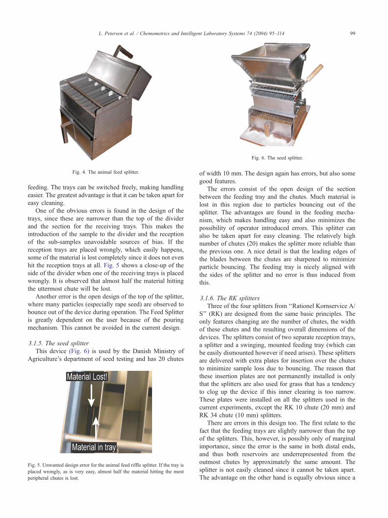
Fig. 6. The seed splitter.

Fig. 4. The animal feed splitter.


feeding. The trays can be switched freely, making handling

easier. The greatest advantage is that it can be taken apart for

easy cleaning.

One of the obvious errors is found in the design of the

trays, since these are narrower than the top of the divider

and the section for the receiving trays. This makes the

introduction of the sample to the divider and the reception

of the sub-samples unavoidable sources of bias. If the

reception trays are placed wrongly, which easily happens,

some of the material is lost completely since it does not even

hit the reception trays at all. Fig. 5 shows a close-up of the

side of the divider when one of the receiving trays is placed

wrongly. It is observed that almost half the material hitting

the uttermost chute will be lost.

Another error is the open design of the top of the splitter,

where many particles (especially rape seed) are observed to

bounce out of the device during operation. The Feed Splitter

is greatly dependent on the user because of the pouring

mechanism. This cannot be avoided in the current design.

3.1.5. The seed splitter

This device (Fig. 6) is used by the Danish Ministry of

Agriculture’s department of seed testing and has 20 chutes

Fig. 5. Unwanted design error for the animal feed riffle splitter. If the tray is

placed wrongly, as is very easy, almost half the material hitting the most

peripheral chutes is lost.

of width 10 mm. The design again has errors, but also some

good features.

The errors consist of the open design of the section

between the feeding tray and the chutes. Much material is

lost in this region due to particles bouncing out of the

splitter. The advantages are found in the feeding mecha-

nism, which makes handling easy and also minimizes the

possibility of operator introduced errors. This splitter can

also be taken apart for easy cleaning. The relatively high

number of chutes (20) makes the splitter more reliable than

the previous one. A nice detail is that the leading edges of

the blades between the chutes are sharpened to minimize

particle bouncing. The feeding tray is nicely aligned with

the sides of the splitter and no error is thus induced from

this.

3.1.6. The RK splitters

Three of the four splitters from ‘‘Rationel Kornservice A/

S’’ (RK) are designed from the same basic principles. The

only features changing are the number of chutes, the width

of these chutes and the resulting overall dimensions of the

devices. The splitters consist of two separate reception trays,

a splitter and a swinging, mounted feeding tray (which can

be easily dismounted however if need arises). These splitters

are delivered with extra plates for insertion over the chutes

to minimize sample loss due to bouncing. The reason that

these insertion plates are not permanently installed is only

that the splitters are also used for grass that has a tendency

to clog up the device if this inner clearing is too narrow.

These plates were installed on all the splitters used in the

current experiments, except the RK 10 chute (20 mm) and

RK 34 chute (10 mm) splitters.

There are errors in this design too. The first relate to the

fact that the feeding trays are slightly narrower than the top

of the splitters. This, however, is possibly only of marginal

importance, since the error is the same in both distal ends,

and thus both reservoirs are underrepresented from the

outmost chutes by approximately the same amount. The

splitter is not easily cleaned since it cannot be taken apart.

The advantage on the other hand is equally obvious since a

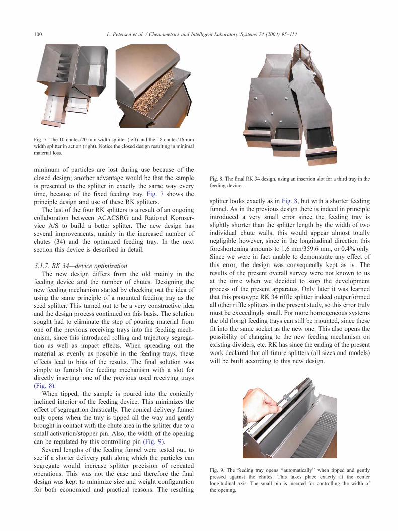
Fig. 7. The 10 chutes/20 mm width splitter (left) and the 18 chutes/16 mm

width splitter in action (right). Notice the closed design resulting in minimal

material loss.

Fig. 8. The final RK 34 design, using an insertion slot for a third tray in the

feeding device.

Fig. 9. The feeding tray opens ‘‘automatically’’ when tipped and gently

pressed against the chutes. This takes place exactly at the center

longitudinal axis. The small pin is inserted for controlling the width of

the opening.


minimum of particles are lost during use because of the

closed design; another advantage would be that the sample

is presented to the splitter in exactly the same way every

time, because of the fixed feeding tray. Fig. 7 shows the

principle design and use of these RK splitters.

The last of the four RK splitters is a result of an ongoing

collaboration between ACACSRG and Rationel Kornser-

vice A/S to build a better splitter. The new design has

several improvements, mainly in the increased number of

chutes (34) and the optimized feeding tray. In the next

section this device is described in detail.

3.1.7. RK 34—device optimization

The new design differs from the old mainly in the

feeding device and the number of chutes. Designing the

new feeding mechanism started by checking out the idea of

using the same principle of a mounted feeding tray as the

seed splitter. This turned out to be a very constructive idea

and the design process continued on this basis. The solution

sought had to eliminate the step of pouring material from

one of the previous receiving trays into the feeding mech-

anism, since this introduced rolling and trajectory segrega-

tion as well as impact effects. When spreading out the

material as evenly as possible in the feeding trays, these

effects lead to bias of the results. The final solution was

simply to furnish the feeding mechanism with a slot for

directly inserting one of the previous used receiving trays

(Fig. 8).

When tipped, the sample is poured into the conically

inclined interior of the feeding device. This minimizes the

effect of segregation drastically. The conical delivery funnel

only opens when the tray is tipped all the way and gently

brought in contact with the chute area in the splitter due to a

small activation/stopper pin. Also, the width of the opening

can be regulated by this controlling pin (Fig. 9).

Several lengths of the feeding funnel were tested out, to

see if a shorter delivery path along which the particles can

segregate would increase splitter precision of repeated

operations. This was not the case and therefore the final

design was kept to minimize size and weight configuration

for both economical and practical reasons. The resulting

splitter looks exactly as in Fig. 8, but with a shorter feeding

funnel. As in the previous design there is indeed in principle

introduced a very small error since the feeding tray is

slightly shorter than the splitter length by the width of two

individual chute walls; this would appear almost totally

negligible however, since in the longitudinal direction this

foreshortening amounts to 1.6 mm/359.6 mm, or 0.4% only.

Since we were in fact unable to demonstrate any effect of

this error, the design was consequently kept as is. The

results of the present overall survey were not known to us

at the time when we decided to stop the development

process of the present apparatus. Only later it was learned

that this prototype RK 34 riffle splitter indeed outperformed

all other riffle splitters in the present study, so this error truly

must be exceedingly small. For more homogeneous systems

the old (long) feeding trays can still be mounted, since these

fit into the same socket as the new one. This also opens the

possibility of changing to the new feeding mechanism on

existing dividers, etc. RK has since the ending of the present

work declared that all future splitters (all sizes and models)

will be built according to this new design.

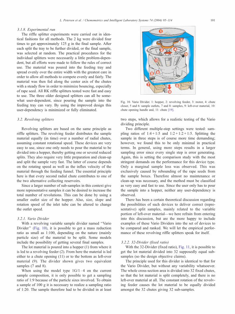
Fig. 10. Vario Divider. 1: hopper, 2: revolving feeder, 3: motor, 4: chute

closer, 5 and 6: sample outlets, 7 and 8: samples, 9: left-over material, 10:

chute opening handle and, 11: chute [19].

elligent Laboratory Systems 74 (2004) 95–114 101

3.1.8. Experimental run

The riffle splitter experiments were carried out in iden-

tical fashions for all methods. The 2 kg were divided four

times to get approximately 125 g in the final sample. After

each split the tray to be further divided, or the final sample,

was selected at random. The practical procedures for the

individual splitters were necessarily a little problem-depen-

dent, but all efforts were made to follow the rules of correct

use. The material was poured into the feeding tray and

spread evenly over the entire width with the greatest care in

order to allow all methods to compete evenly and fairly. The

material was then fed along the center axis of the chutes

with a steady flow in order to minimize bouncing, especially

of rape seed. All RK riffle splitters tested were fast and easy

to use. The three older designed splitters can all be some-

what user-dependent, since pouring the sample into the

feeding tray can vary. By using the improved design this

user-dependency is minimized or fully eliminated.

3.2. Revolving splitters

Revolving splitters are based on the same principle as

riffle splitters. The revolving feeder distributes the sample

material equally (in time) over a number of radial chutes,

assuming constant rotational speed. These devices are very

easy to use, since one only needs to pour the material to be

divided into a hopper, thereby getting one or several reduced

splits. They also require very little preparation and clean-up

and split the sample very fast. The latter of course depends

on the rotating speed as well as the influx velocity of the

material through the feeding funnel. The essential principle

here is that every second radial chute contributes to one of

the two alternative collecting reservoirs.

Since a larger number of sub-samples in this context give

more representative samples it can be desired to increase the

total number of revolutions. This can be done by using a

smaller outlet size of the hopper. Also, size, slope and

rotation speed of the inlet tube can be altered to change

the outlet speed.

3.2.1. Vario Divider

With a revolving variable sample divider named ‘‘Vario

Divider’’ (Fig. 10), it is possible to get a mass reduction

ratio as small as 1:100, depending on the nature (mainly

particle size) of the material to be split. Some models

include the possibility of getting several final samples.

The lot material is poured into a hopper (1) from where it

is led to a revolving feeder (2). From here the material is led

either to a chute opening (11) or to the bottom as left-over

material (9). The divider shown gives two equivalent

samples (7 and 8).

When using the model type 1G/1–4 on the current

sample composition, it is only possible to get a sampling

ratio of 1:9 because of the particle sizes involved. To obtain

a sample of 100 g it is necessary to realize a sampling ratio

of 1:20. The sample therefore had to be divided in at least

L. Petersen et al. / Chemometrics and Int

two steps, which allows for a realistic testing of the Vario

dividing principle.

Two different multiple-step settings were tested: sam-

pling ratios of 1:4 + 1:5 and 1:2 + 1:2 + 1:5. Splitting the

sample in three steps is of course more time demanding;

however, we found this to be only minimal in practical

terms. In general, using more steps results in a larger

sampling error since every single step is error generating.

Again, this is setting the comparison study with the most

stringent demands on the performance for this device type.

Only a marginal sample loss was observed. This was

exclusively caused by rebounding of the rape seeds from

the sample boxes. Therefore almost no maintenance or

clean-up was necessary, and the method must be classified

as very easy and fast to use. Since the user only has to pour

the sample into a hopper, neither any user-dependency is

observed.

There has been a certain theoretical discussion regarding

the possibilities of such devices to deliver correct (repre-

sentative) split samples, mainly related to the variable

portion of left-over material—we here refrain from entering

into this discussion, but are the more happy to include

examples of these Vario Dividers into the set of devices to

be compared and ranked. We will let the empirical perfor-

mance of these revolving riffle splitters speak for itself.

3.2.2. 32-Divider (fixed ratio)

With the 32-Divider (fixed ratio), Fig. 11, it is possible to

get the lot material divided into 32 supposedly equal sub-

samples (so the design objective claims).

The principle used for this divider is identical to that for

the Vario Divider, but without any variability whatsoever.

The whole cross-section area is divided into 32 fixed chutes,

so that the lot material is split completely, and there is no

left-over material at all. The constant rotation of the revolv-

ing feeder causes the lot material to be equally divided

amongst the 32 chutes giving 32 sub-samples.

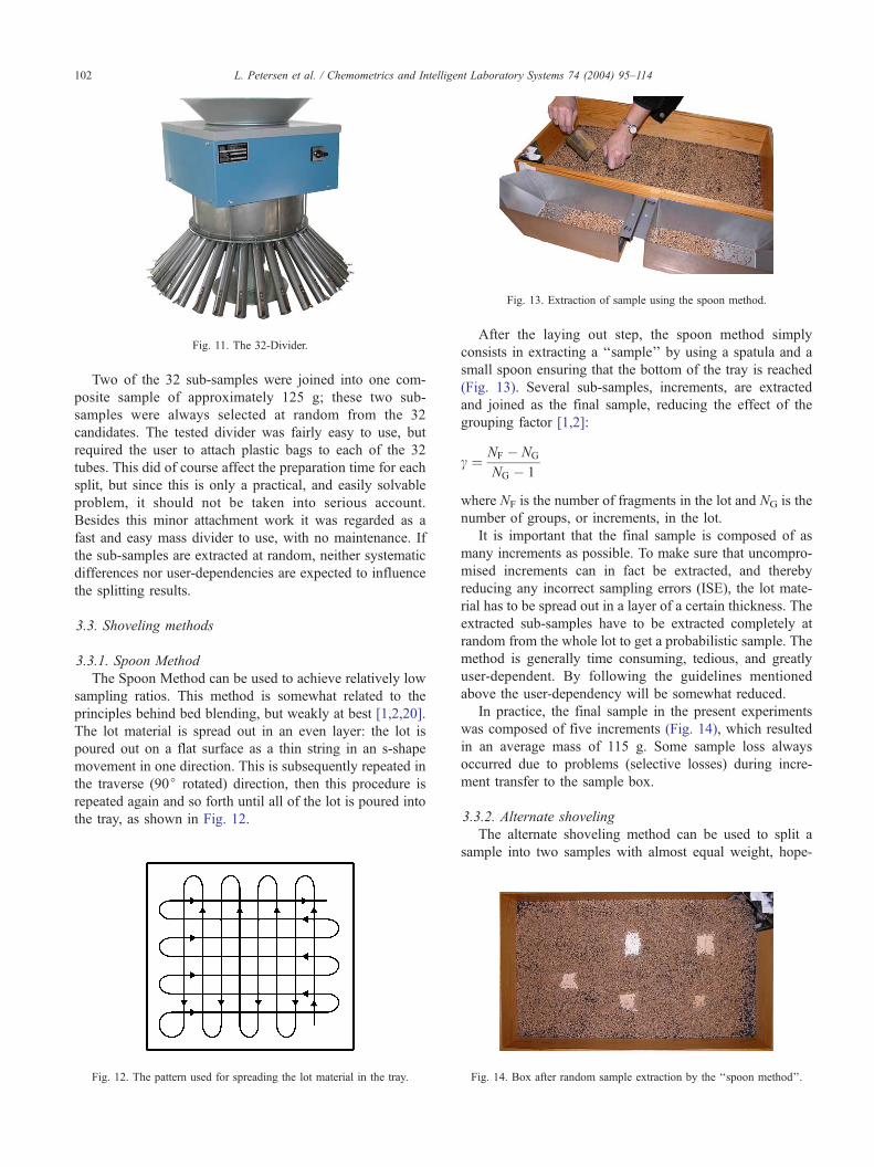
Fig. 13. Extraction of sample using the spoon method.

Fig. 11. The 32-Divider.


Two of the 32 sub-samples were joined into one com-

posite sample of approximately 125 g; these two sub-

samples were always selected at random from the 32

candidates. The tested divider was fairly easy to use, but

required the user to attach plastic bags to each of the 32

tubes. This did of course affect the preparation time for each

split, but since this is only a practical, and easily solvable

problem, it should not be taken into serious account.

Besides this minor attachment work it was regarded as a

fast and easy mass divider to use, with no maintenance. If

the sub-samples are extracted at random, neither systematic

differences nor user-dependencies are expected to influence

the splitting results.

3.3. Shoveling methods

3.3.1. Spoon Method

The Spoon Method can be used to achieve relatively low

sampling ratios. This method is somewhat related to the

principles behind bed blending, but weakly at best [1,2,20].

The lot material is spread out in an even layer: the lot is

poured out on a flat surface as a thin string in an s-shape

movement in one direction. This is subsequently repeated in

the traverse (90j rotated) direction, then this procedure is

repeated again and so forth until all of the lot is poured into

the tray, as shown in Fig. 12.

Fig. 12. The pattern used for spreading the lot material in the tray.

After the laying out step, the spoon method simply

consists in extracting a ‘‘sample’’ by using a spatula and a

small spoon ensuring that the bottom of the tray is reached

(Fig. 13). Several sub-samples, increments, are extracted

and joined as the final sample, reducing the effect of the

grouping factor [1,2]:

c ¼ NF � NG

NG � 1

where NF is the number of fragments in the lot and NG is the

number of groups, or increments, in the lot.

It is important that the final sample is composed of as

many increments as possible. To make sure that uncompro-

mised increments can in fact be extracted, and thereby

reducing any incorrect sampling errors (ISE), the lot mate-

rial has to be spread out in a layer of a certain thickness. The

extracted sub-samples have to be extracted completely at

random from the whole lot to get a probabilistic sample. The

method is generally time consuming, tedious, and greatly

user-dependent. By following the guidelines mentioned

above the user-dependency will be somewhat reduced.

In practice, the final sample in the present experiments

was composed of five increments (Fig. 14), which resulted

in an average mass of 115 g. Some sample loss always

occurred due to problems (selective losses) during incre-

ment transfer to the sample box.

3.3.2. Alternate shoveling

The alternate shoveling method can be used to split a

sample into two samples with almost equal weight, hope-

Fig. 14. Box after random sample extraction by the ‘‘spoon method’’.

Fig. 15. Alternate shoveling.

Fig. 17. Grab sampling.


fully also of almost equal composition. TOS has made

thorough analysis of this general approach [1–3], and there

are many pitfalls which are almost universally unavoidable

in practice. The equality of the final samples obtained by

this method will also be highly dependent on the nature of

the material sampled.

The method is based on the principle that all extracted

shovelfuls from the original sample are deposited sequen-

tially in two alternative heaps as illustrated in Fig. 15.

It is important that all extracted shovelfuls are selected at

random from the initial lot and that all increments have the

same (approximate) size. Each heap should consist of an

equal number of shovelfuls. One heap should only consist of

all even-numbered samples while the other should only

consist of all odd-numbered samples. By ensuring that all

shovelfuls are carefully selected at random, the condition of

sampling equity is preserved thereby minimizing the risk of

a systematic bias to some degree.

Four full splits were necessary to obtain a final sample on

approximately 125 g in our experimental runs. Some sample

loss was observed due to the practical handling of

shovelfuls. Different samplers (operators) will definitely

have unequal impact on the quality of the final reduced

samples, since the shoveling can vary greatly from user to

user.

3.3.3. Fractional shoveling

With true fractional shoveling it is possible to divide the

lot material into N sub-samples instead of only two.

Shovelfuls are extracted from the lot material and deposited

into N distinct heaps. In Fig. 16, true fractional shoveling

with N = 5 is shown.

Fig. 16. Fractional shoveling with N= 5.

The shovelfuls should again all be extracted at random

from the lot material and should be (approximately) equal in

size. Each heap should consist of an equal number of

shovelfuls. All extracted shovelfuls should be alternated

from heap one to heap N.

To reduce the initial 2 kg into approximately 100 g the

sample was first split into five heaps. From these five heaps

one was chosen randomly and further divided into four

samples at approximately 100 g each. This method can also

be slow, tedious and user-dependent.

3.3.4. Grab sampling

Grab sampling is the easy choice for extracting a

‘‘sample’’ and is (unfortunately) very often the preferred

choice in practical sampling situations. One sample only is

extracted to represent the whole lot. Grab sampling is the

archetype sampling error at work. The focus is exclusively

on getting the final sample mass directly in one go!

However, a grab sample may also result from joining

several increments (sub-samples), to produce a composite

sample, which in general should result in a more repre-

sentative sample. Grab samples are typically taken by a

Fig. 18. Boerner Divider.

Fig. 19. Boerner Divider at work.


scoop or a shovel, depending on the size of the original lot,

etc.

To obtain a truly representative sample all virtual units

making up the lot per force must have the same probability

of being selected. With grab sampling this manifestly

neither can be, nor hardly ever is, the case. The singular

sample to be extracted by grab sampling is of course also

often taken from an(y) easily accessible part of a lot, i.e. the

top. Grab sampling is therefore often classified as determin-

istic sampling.

Extracting a sample from the bottom of the lot in Fig. 17

was difficult as in most cases (extraction shown in the

figure). The sample domain was divided into six virtual

areas. Each grab sample was extracted at random from one

of these six areas thereby counteracting unwanted system-

atic bias. It was attempted to extract the sample from the

whole virtual area by pushing the scoop to the bottom and

withdrawing it slowly upwards.

If such ‘‘samples’’ are erroneously accepted, grab sam-

pling is a fast and easy choice. If the final sample is to be a

probabilistic sample it can be time consuming, very often

difficult or downright impossible to get correctly sampled

increments. Lastly grab sampling is always user-dependent.

Following TOS, grab sampling is supposed to perform the

worst of all alternative mass reduction approaches. It was

Fig. 20. Standard deviation of

therefore a natural must for the present comparison purpose,

if nothing else as a (bad) benchmark.

3.4. Other methods

3.4.1. Boerner Divider

Using the Boerner Divider (Figs. 18 and 19) it is possible

to divide a sample into two app. equal half-splits. The

halved samples can iteratively be divided again, etc., until

a satisfactory sample size has been reached.

The initial sample is poured into a hopper. When the

hopper’s bottom-shutter is opened the sample is directed

down onto the top of a cone. Since the sample is flowing

downwards by gravity it should be spread out evenly in all

azimuth directions. At the bottom of the cone the material is

led through a number of alternative chutes which are so

connected so as to lead the alternate part-streams into the

resulting two half-sample splits.

The Boerner Divider is very easy and very fast to use.

Set-up and maintenance is straight forward, but some

sample loss can occur during use, depending greatly on

the nature of the material to be split. Especially bouncing

materials such as rape seed and glass pellets can be a

problem. To avoid any systematic differences from one side

of the splitter (receiving tray) to the other it is also here

important to choose one of the two receptacle trays

randomly.

The initial 2 kg material lots in the present study had to

be divided four times to get a sample size of approximately

125 g. Some loss of material was observed primarily due to

the design of the receptacle tray combined with the nature of

the glass and rape seed used.

Two different Boerner Dividers were tested; one will be

referred to as calibrated, the other as non-calibrated, mean-

the final sample mass.

Fig. 21. Relative bias of the final sample mass.


ing that the hopper was slightly off-centered and that the

receptacle bins where open. For the non-calibrated divider

this could lead to over-representation of some chutes and a

fair amount of lost material. Figs. 18 and 19 show the non-

calibrated divider.

4. Results and discussion

4.1. Characterizing parameters

In order to evaluate and compare the above methods a

system is developed for characterization by a selected set of

Fig. 22. Relative bias for the

mass reduction quality parameters. These parameters are

described shortly below.

4.1.1. Mean and bias (concentration)

After performing the splits or the individual mass reduc-

tions, the results are characterized by the arithmetic average

concentration for all three materials after the universal 20

repetitions. This parameter is very important in practice

since it characterizes the method’s ability to perform splits

and leave the sample with the same composition as the lot

material.

Themean is a measure of the accuracy of the method when

assessed against the true xLot (aL). The bias is simply

concentration of wheat.

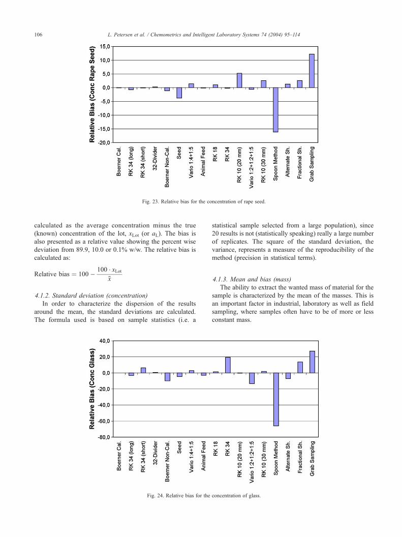
Fig. 23. Relative bias for the concentration of rape seed.


calculated as the average concentration minus the true

(known) concentration of the lot, xLot (or aL). The bias is

also presented as a relative value showing the percent wise

deviation from 89.9, 10.0 or 0.1% w/w. The relative bias is

calculated as:

Relative bias ¼ 100� 100 � xLotx̄

4.1.2. Standard deviation (concentration)

In order to characterize the dispersion of the results

around the mean, the standard deviations are calculated.

The formula used is based on sample statistics (i.e. a

Fig. 24. Relative bias for the

statistical sample selected from a large population), since

20 results is not (statistically speaking) really a large number

of replicates. The square of the standard deviation, the

variance, represents a measure of the reproducibility of the

method (precision in statistical terms).

4.1.3. Mean and bias (mass)

The ability to extract the wanted mass of material for the

sample is characterized by the mean of the masses. This is

an important factor in industrial, laboratory as well as field

sampling, where samples often have to be of more or less

constant mass.

concentration of glass.

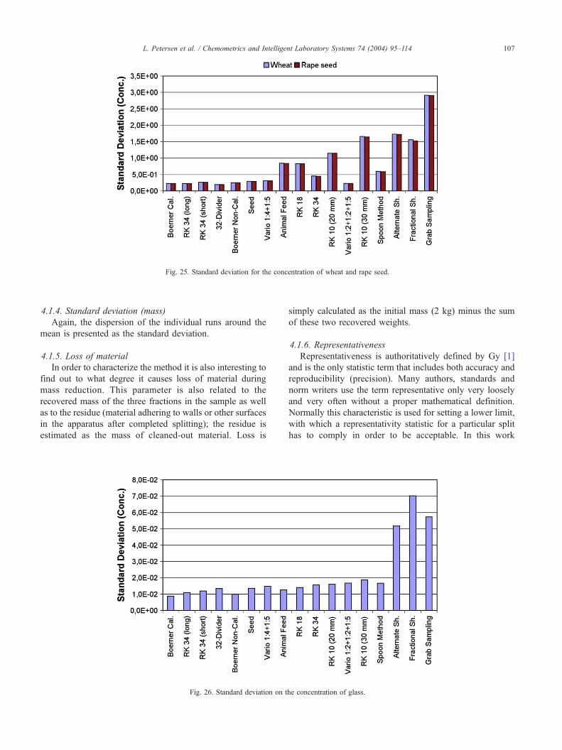
Fig. 25. Standard deviation for the concentration of wheat and rape seed.


4.1.4. Standard deviation (mass)

Again, the dispersion of the individual runs around the

mean is presented as the standard deviation.

4.1.5. Loss of material

In order to characterize the method it is also interesting to

find out to what degree it causes loss of material during

mass reduction. This parameter is also related to the

recovered mass of the three fractions in the sample as well

as to the residue (material adhering to walls or other surfaces

in the apparatus after completed splitting); the residue is

estimated as the mass of cleaned-out material. Loss is

Fig. 26. Standard deviation on t

simply calculated as the initial mass (2 kg) minus the sum

of these two recovered weights.

4.1.6. Representativeness

Representativeness is authoritatively defined by Gy [1]

and is the only statistic term that includes both accuracy and

reproducibility (precision). Many authors, standards and

norm writers use the term representative only very loosely

and very often without a proper mathematical definition.

Normally this characteristic is used for setting a lower limit,

with which a representativity statistic for a particular split

has to comply in order to be acceptable. In this work

he concentration of glass.

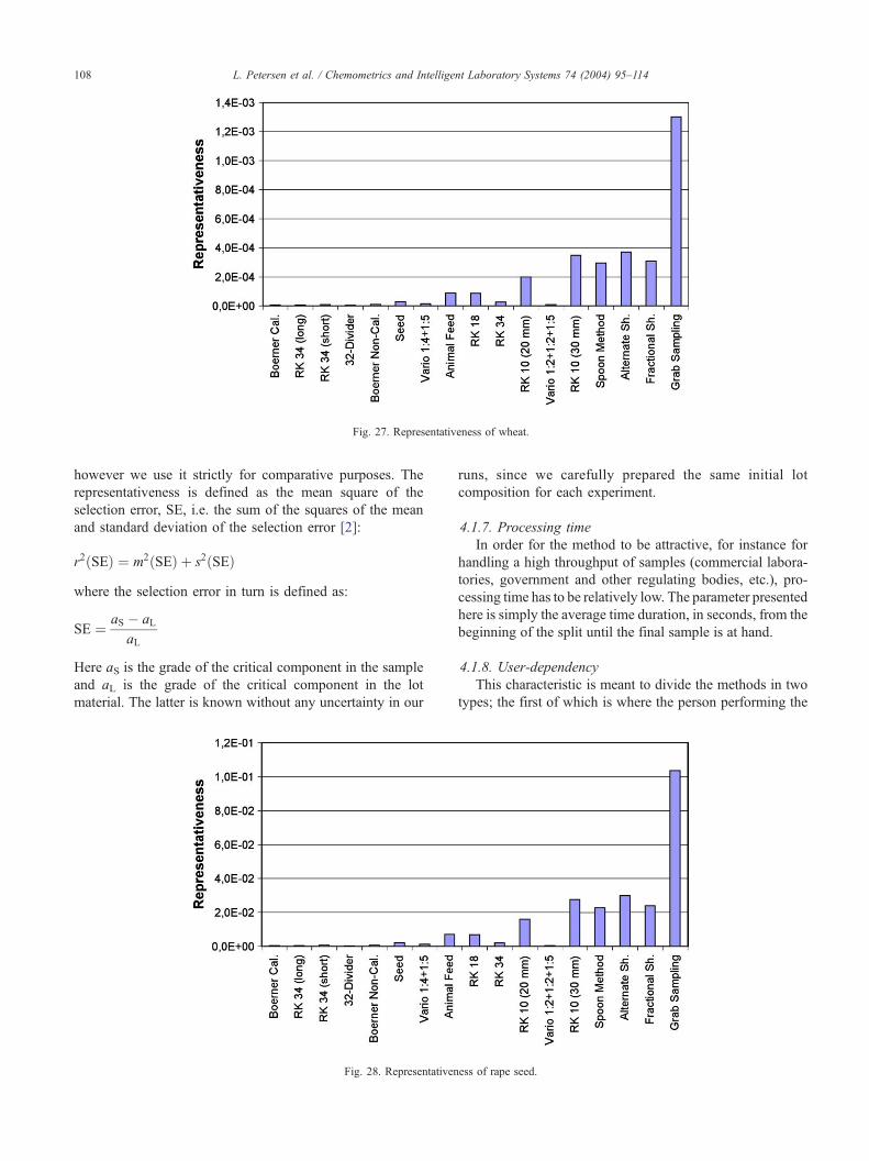
Fig. 27. Representativeness of wheat.


however we use it strictly for comparative purposes. The

representativeness is defined as the mean square of the

selection error, SE, i.e. the sum of the squares of the mean

and standard deviation of the selection error [2]:

r2ðSEÞ ¼ m2ðSEÞ þ s2ðSEÞ

where the selection error in turn is defined as:

SE ¼ aS � aL

aL

Here aS is the grade of the critical component in the sample

and aL is the grade of the critical component in the lot

material. The latter is known without any uncertainty in our

Fig. 28. Representativen

runs, since we carefully prepared the same initial lot

composition for each experiment.

4.1.7. Processing time

In order for the method to be attractive, for instance for

handling a high throughput of samples (commercial labora-

tories, government and other regulating bodies, etc.), pro-

cessing time has to be relatively low. The parameter presented

here is simply the average time duration, in seconds, from the

beginning of the split until the final sample is at hand.

4.1.8. User-dependency

This characteristic is meant to divide the methods in two

types; the first of which is where the person performing the

ess of rape seed.

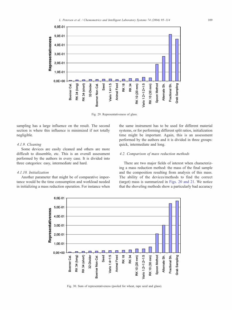
Fig. 29. Representativeness of glass.


sampling has a large influence on the result. The second

section is where this influence is minimized if not totally

negligible.

4.1.9. Cleaning

Some devices are easily cleaned and others are more

difficult to dissemble, etc. This is an overall assessment

performed by the authors in every case. It is divided into

three categories: easy, intermediate and hard.

4.1.10. Initialization

Another parameter that might be of comparative impor-

tance would be the time consumption and workload needed

in initializing a mass reduction operation. For instance when

Fig. 30. Sum of representativeness (poole

the same instrument has to be used for different material

systems, or for performing different split ratios, initialization

time might be important. Again, this is an assessment

performed by the authors and it is divided in three groups:

quick, intermediate and long.

4.2. Comparison of mass reduction methods

There are two major fields of interest when characteriz-

ing a mass reduction method: the mass of the final sample

and the composition resulting from analysis of this mass.

The ability of the devices/methods to find the correct

(target) mass is summarized in Figs. 20 and 21. We notice

that the shoveling methods show a particularly bad accuracy

d for wheat, rape seed and glass).


and precision. Only fractional shoveling seems to have a

relatively good precision. This method is comparable to

alternate shoveling, but differs in having only two mass

reduction steps instead of four, which possibly can explain

the better precision. The rotational dividers and some of the

riffle splitters seem to have good accuracy and precision

throughout in finding the target mass. The RK 10 chute (20

mm splitter), however, differ significantly from the rest of

the riffle splitters (in an adverse sense). The only possible

reason for this must be the missing insertion plates on this

splitter.

With regard to the composition of the final sample, the

methods are evaluated by the standard deviation, relative

bias and the representativeness.

In Figs. 22–24, the methods deviating most from the

rest clearly are the spoon method and grab sampling. This

is understandable since these two methods are both shov-

eling methods, and thus expected to be less precise. In

general, all shoveling methods and some of the riffle

splitters are characterized by bad precision, while all

revolving dividers show good precision. The reason for

this good precision is the large number of rotations

involved, and hence the large number of effective chutes

involved in the mass reduction. When the sample takes

about 1 min to pass through these devices, the number of

revolutions per minute is 40 and the number of openings

eight, the effective number of chutes is actually 320 for the

Vario Dividers and an impressive 1280 for the 32-divider

(which has 32 openings).

The standard deviation is an expression of the precision

of a particular method. Fig. 25 shows the standard devia-

tion of wheat and rape seed, which both are present in

rather large concentrations in the material (89.9 and 10.0%

w/w). All the methods with a large number of chutes or

Fig. 31. Total loss

openings have a low standard deviation on both wheat and

rape seed. The shoveling methods, again, stand out as

terribly imprecise methods, even though the spoon method

would appear just within the window for this parameter

alone. This is possibly due to the bed blending like

preparation of the lot material and the extraction method,

which for the experienced operator ensures nicely delimited

increments (sub-samples).

Glass is present in very low concentration (0.1% w/w) in

the material, and it is expected that the reproducibility

(precision) for this material is substantially worse than the

components present in larger concentrations. The absolute

values in Fig. 26 are not directly comparable with those in

Fig. 25, since the standard deviation is a relative value. It is

noted that the precision of all the methods is more or less

equal for the trace element level, except for the shoveling

methods. The spoon method again seems to have an

acceptable performance, but the rest of the shoveling meth-

ods are distinctly bad, very likely due to the extraction

method.

The overall TOS-measure representativeness takes into

account both accuracy and precision, and will thus express

the overall performance of a method. It is seen in Figs. 27–

30 that the methods with the lowest number of chutes or

openings and the shoveling methods indeed are worst. This

is in accordance with the previous conclusions.

The representativeness of glass has a dominating influ-

ence on the pooled sum, since these values are much larger

than the values for wheat and rape seed. However, the sum

is the best measure for the overall performance of the

methods, since it includes constituents present in both high

and low concentrations. It is observed from Fig. 30 that the

calibrated Boerner Divider has the best overall performance.

There is, however, no large difference to be found between

of material.

0 sof

m

Vario

1:2+1:2

+1:5

RK

10

chutesof

30mm

Spoon

method

Alternate

shoveling

Fractional

shoveling

Grab

sampling

00

��

��

++

��

��

++

+0

0+

�0

0+

++

++

0+

0+

+0

��

��

+0

��

�+

43

�3

�2

�3

1


the 10 best of the methods, meaning that all these methods

in principle are suitable for mass reduction with regard to

representativeness.

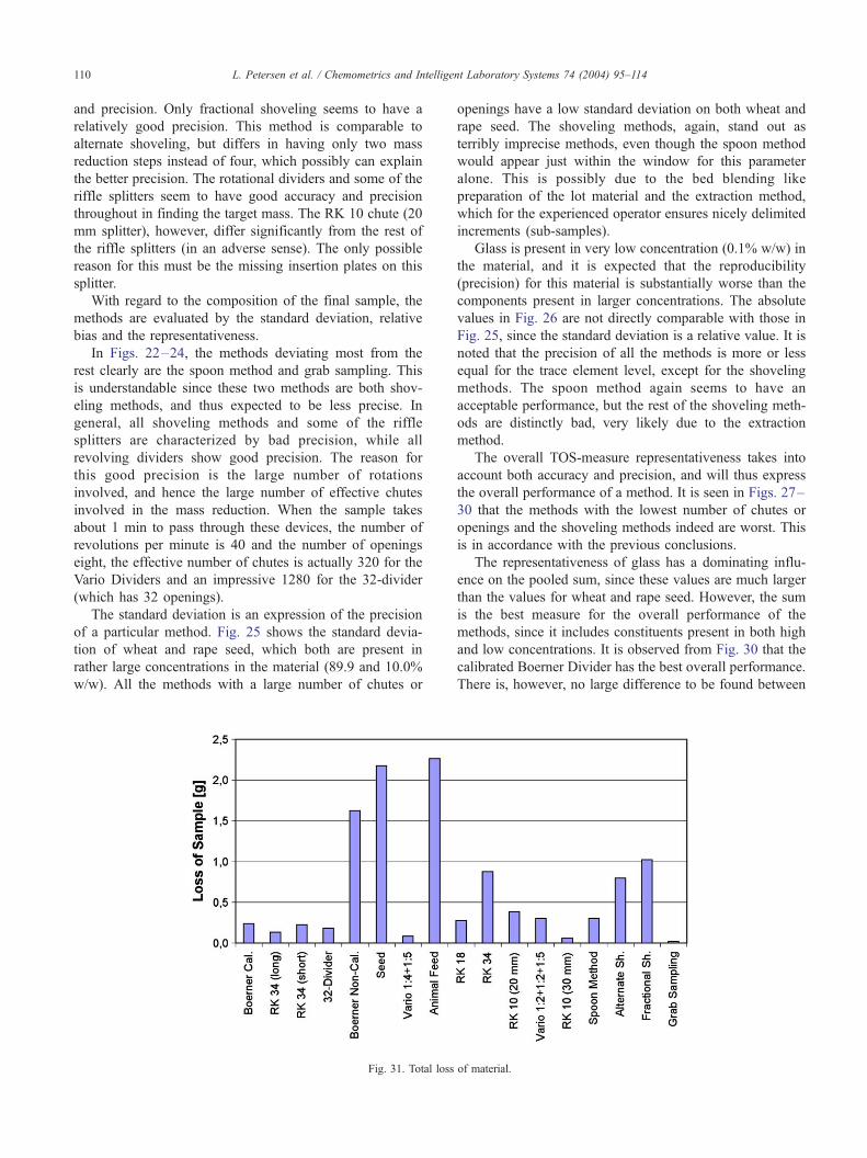
The total loss of material during mass reduction is seen in

Fig. 31. The loss is high for all splitters with open designs,

and for all the shoveling methods with several steps in-

volved. Especially the seed splitter, the animal feed splitter

and the non-calibrated Boerner Divider stand out as spilling

large amounts of material (especially rape seed is seen to

bounce out).

In Table 1, the compound characteristics for the investi-

gated methods are summarized. The different values are

here weighed equally and it is left for the reader to apply

differential weighing to fit his or her own customs or needs.

If for instance operating time is of greater importance than

cleaning, or if it is absolutely crucial to have the correct

mass in the final sample, these parameters can be weighed

on an individual basis.

The resulting sum-scores divide the methods/devices into

three groups:

Table

1

Summaryofthecharacteristicsfortheinvestigated

methods

Boerner

Divider

(Cal)

RK

34

long

RK

34

short

32-D

vider

Boerner

Divider

Seed

splitter

Vario

1:4+1:5

Anim

al

feed

splitter

RK

18

chutesog

16mm

RK

34

Norm

al

RK

1

chute

20m

Composition

++

++

++

++

++

0

Mass

++

++

0+

+0

++

�Loss

++

++

��

+�

+0

+

Cleaning

00

0�

0+

�+

00

0

Initialization

++

++

++

++

++

+

User-dependency

++

++

++

+0

0+

0

Tim

e+

00

+0

0+

�0

0�

Score

55

55

24

51

44

0

Very Good (sum= 5). Boerner Divider (Cal). RK 34 chutes of 10 mm short. RK 34 chutes of 10 mm long. 32-Divider. Vario Divider 1:4 + 1:5

Acceptable (sum= 4, 3 or 2) but only under certain, problem-related

circumstances:. Boerner Divider (Non-cal.). Seed Splitter. Rk 18 chutes of 16 mm. RK 34 chutes of 10 mm normal. Vario Divider 1:2 + 1:2 + 1:5. RK 10 chutes of 30 mm

Poor (sum less than 2) not recommended under any circumstances. Animal feed splitter. RK 10 chutes of 20 mm. Spoon method. Alternate shoveling. Fractional shoveling. Grab sampling

The newly developed riffle splitters, the calibrated

Boerner Divider, the 32-divider and the Vario Divider

outperform all other methods—even though they all can

be difficult to clean. The riffle splitters are in general

rather slow to use, but this is a relative factor, since the

slowest method overall—alternate shoveling—uses only

approximately 200 s to reduce the mass by a factor of

20. The devices in the best group are all really good at

finding the correct target concentration and mass of a final

sample.

This is also the overall conclusion for the intermediate

group. Most of these methods have a significant loss

however and/or are also rather slow to use.

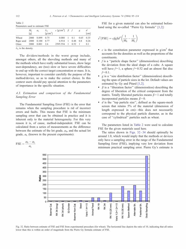
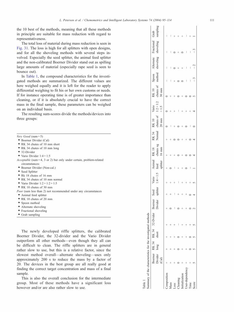
Table 2

Parameters used to estimate FSE

ML

[g]

aL dA[g/cm3]

c [g/cm3] b f g d

[cm]

Wheat 2000 0.899 0.75 0.088 1 0.1 0.65 0.35

Rape seed 2000 0.100 0.77 6.914 1 0.48 0.8 0.26

Glass 2000 0.001 2.6 2595.554 1 0.52 1 0.1

dA is the density.


The dividers/methods in the worst group include,

amongst others, all the shoveling methods and many of

the methods which have really substantial losses, show large

user-dependency, are (too) slow or have severe difficulties

to end up with the correct target concentration or mass. It is,

however, important to consider carefully the purpose of the

method/device, so as to make the correct choice. In this

context users should pay special attention to the parameters

of importance in the specific situation.

4.3. Estimation and comparison of the Fundamental

Sampling Error

The Fundamental Sampling Error (FSE) is the error that

remains when the sampling procedure is rid of incorrect

errors and faults. This means that FSE is the minimum

sampling error that can be obtained in practice and it is

inherent only to the material heterogeneity. For this very

reason it is, of cause, method-independent. FSE can be

calculated from a series of measurements as the difference

between the estimate of the lot grade, aS, and the actual lot

grade, aL (known in the present experiments):

FSE ¼ aS � aL

aL

Fig. 32. Ratio between estimate of FSE and FSE from experimental procedure (for

lower than this is within an order of magnitude from the Pierre Gy formula estim

FSE for a given material can also be estimated before-

hand using the so-called ‘‘Pierre Gy formula’’ [1,2]:

s2ðFSEÞ ¼ cfgbd31

MS

� 1

ML

� �

� c is the constitution parameter expressed in g/cm3 that

accounts for the densities as well as the proportions of the

constituents.� f is a ‘‘particle shape factor’’ (dimensionless) describing

the deviation from the ideal shape of a cube. A square

will have f = 1, a sphere f = 0.52 and an almost flat disc

f = 0.1.� g is a ‘‘size distribution factor’’ (dimensionless) describ-

ing the span of particle sizes in the lot. Default values are

estimated by Gy and Pitard [1,2].� b is a ‘‘liberation factor’’ (dimensionless) describing the

degree of liberation of the critical component from the

matrix. Totally liberated particles means b = 1 and totally

incorporated particles means b = 0.� d is the ’’top particle size’’, defined as the square-mesh

screen that retains 5% of the material (dimension of

length expressed in cm)—this does not necessarily

correspond to the physical particle diameter, as in the

case of ‘‘cylindrical’’ particles such as wheat.

The parameters listed in Table 2 were used to calculate

FSE for the given materials used here.

The ratios shown in Figs. 32–34 should optimally be

around 1.0, which would imply that the methods or devices

only have a sampling error in the range of the Fundamental

Sampling Error (FSE), implying very low deviation from

minimum practical sampling error. Pierre Gy’s estimate is

wheat). The horizontal line depicts the ratio of 10, indicating that all ratios

ate of FSE.

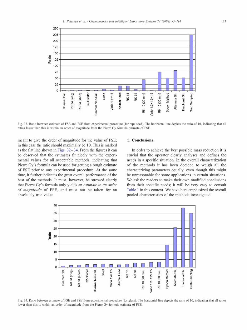
Fig. 33. Ratio between estimate of FSE and FSE from experimental procedure (for rape seed). The horizontal line depicts the ratio of 10, indicating that all

ratios lower than this is within an order of magnitude from the Pierre Gy formula estimate of FSE.


meant to give the order of magnitude for the value of FSE;

in this case the ratio should maximally be 10. This is marked

as the flat line shown in Figs. 32–34. From the figures it can

be observed that the estimates fit nicely with the experi-

mental values for all acceptable methods, indicating that

Pierre Gy’s formula can be used for getting a rough estimate

of FSE prior to any experimental procedure. At the same

time, it further indicates the great overall performance of the

best of the methods. It must, however, be stressed clearly

that Pierre Gy’s formula only yields an estimate to an order

of magnitude of FSE, and must not be taken for an

absolutely true value.

Fig. 34. Ratio between estimate of FSE and FSE from experimental procedure (fo

lower than this is within an order of magnitude from the Pierre Gy formula estim

5. Conclusions

In order to achieve the best possible mass reduction it is

crucial that the operator clearly analyses and defines the

needs in a specific situation. In the overall characterization

of the methods it has been decided to weigh all the

characterizing parameters equally, even though this might

be unreasonable for some applications in certain situations.

We ask the readers to make their own modified conclusions

from their specific needs; it will be very easy to consult

Table 1 in this context. We have here emphasized the overall

pooled characteristics of the methods investigated.

r glass). The horizontal line depicts the ratio of 10, indicating that all ratios

ate of FSE.

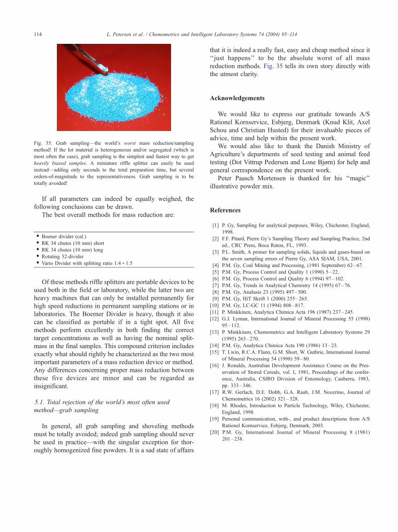
Fig. 35. Grab sampling—the world’s worst mass reduction/sampling

method! If the lot material is heterogeneous and/or segregated (which is

most often the case), grab sampling is the simplest and fastest way to get

heavily biased samples. A miniature riffle splitter can easily be used

instead—adding only seconds to the total preparation time, but several

orders-of-magnitude to the representativeness. Grab sampling is to be

totally avoided!


If all parameters can indeed be equally weighed, the

following conclusions can be drawn.

The best overall methods for mass reduction are:

. Boener divider (cal.)

. RK 34 chutes (10 mm) short

. RK 34 chutes (10 mm) long

. Rotating 32-divider

. Vario Divider with splitting ratio 1:4 + 1:5

Of these methods riffle splitters are portable devices to be

used both in the field or laboratory, while the latter two are

heavy machines that can only be installed permanently for

high speed reductions in permanent sampling stations or in

laboratories. The Boerner Divider is heavy, though it also

can be classified as portable if in a tight spot. All five

methods perform excellently in both finding the correct

target concentrations as well as having the nominal split-

mass in the final samples. This compound criterion includes

exactly what should rightly be characterized as the two most

important parameters of a mass reduction device or method.

Any differences concerning proper mass reduction between

these five devices are minor and can be regarded as

insignificant.

5.1. Total rejection of the world’s most often used

method—grab sampling

In general, all grab sampling and shoveling methods

must be totally avoided; indeed grab sampling should never

be used in practice—with the singular exception for thor-

oughly homogenized fine powders. It is a sad state of affairs

that it is indeed a really fast, easy and cheap method since it

‘‘just happens’’ to be the absolute worst of all mass

reduction methods. Fig. 35 tells its own story directly with

the utmost clarity.

Acknowledgements

We would like to express our gratitude towards A/S

Rationel Kornservice, Esbjerg, Denmark (Knud Klit, Axel

Schou and Christian Husted) for their invaluable pieces of

advice, time and help within the present work.

We would also like to thank the Danish Ministry of

Agriculture’s departments of seed testing and animal feed

testing (Dot Vittrup Pedersen and Lone Bjørn) for help and

general correspondence on the present work.

Peter Paasch Mortensen is thanked for his ‘‘magic’’

illustrative powder mix.

References

[1] P. Gy, Sampling for analytical purposes, Wiley, Chichester, England,

1998.

[2] F.F. Pitard, Pierre Gy’s Sampling Theory and Sampling Practice, 2nd

ed., CRC Press, Boca Raton, FL, 1993.

[3] P.L. Smith, A primer for sampling solids, liquids and gases-based on

the seven sampling errors of Pierre Gy, ASA SIAM, USA, 2001.

[4] P.M. Gy, Coal Mining and Processing, (1981 September) 62–67.

[5] P.M. Gy, Process Control and Quality 1 (1990) 5–22.

[6] P.M. Gy, Process Control and Quality 6 (1994) 97–102.

[7] P.M. Gy, Trends in Analytical Chemistry 14 (1995) 67–76.

[8] P.M. Gy, Analusis 23 (1995) 497–500.

[9] P.M. Gy, HiT Skrift 1 (2000) 255–265.

[10] P.M. Gy, LC-GC 11 (1994) 808–817.

[11] P. Minkkinen, Analytica Chimica Acta 196 (1987) 237–245.

[12] G.J. Lyman, International Journal of Mineral Processing 55 (1998)

95–112.

[13] P. Minkkinen, Chemometrics and Intelligent Laboratory Systems 29

(1995) 263–270.

[14] P.M. Gy, Analytica Chimica Acta 190 (1986) 13–23.

[15] T. Lwin, R.C.A. Flann, G.M. Short, W. Guthrie, International Journal

of Mineral Processing 54 (1998) 59–80.

[16] J. Ronalds, Australian Development Assistance Course on the Pres-

ervation of Stored Cereals, vol. I, 1981, Proceedings of the confer-

ence, Australia, CSIRO Division of Entomology, Canberra, 1983,

pp. 333–346.

[17] R.W. Gerlach, D.E. Dobb, G.A. Raab, J.M. Nocerino, Journal of

Chemometrics 16 (2002) 321–328.

[18] M. Rhodes, Introduction to Particle Technology, Wiley, Chichester,

England, 1998.

[19] Personal communication, with-, and product descriptions from A/S

Rationel Kornservice, Esbjerg, Denmark, 2003.

[20] P.M. Gy, International Journal of Mineral Processing 8 (1981)

201–238.

Representative mass reduction in sampling—a critical survey ...

Documents

Transcript of Representative mass reduction in sampling—a critical survey ...