
Reliability assessment of buried pipelines based on different corrosion rate models
Upload
khangminh22Category
view
2download
0
Reliability-based Analysis and Maintenance
of Buried Pipes Considering the Effect of
Uncertain Variables
ANDREW UTOMI EBENUWA
A thesis submitted in partial fulfilment of the
requirements of the University of Greenwich for the
Degree of Doctor of Philosophy
September 2018

ii
DECLARATION
I certify that the work contained in this thesis, or any part of it, has not been accepted in
substance for any previous degree awarded to me, and is not concurrently being submitted
for any degree other than that of Doctor of Philosophy being studied at the University of
Greenwich. I also declare that this work is the result of my own investigations, except
where otherwise identified by references and that the contents are not the outcome of any
form of research misconduct.
Student: ANDREW UTOMI EBENUWA
Signed: ____________________________
Date: ____________________________
First Supervisor: KONG FAH TEE
Signed: ____________________________
Date: ____________________________

iii
ACKNOWLEDGEMENTS
I would like to express my sincere gratitude and appreciation to my supervisors Dr. Kong
Fah Tee and Prof. Hua-Peng Chen for their guidance and advice from the start to the
completion of the research study.
I am very grateful to the faculty of engineering science, University of Greenwich, which
provided me with the friendly environment needed to carry out the research. My deep
appreciation goes out to Prof. Andrew Chan – University of Tasmania (Australia), Dr. Yi
Zhang - Nanyang Technological University (Singapore), Dr Sabuj Mallik - University of
Derby (UK), Dr Peter Bernasko - University of Greenwich (UK), Elizabeth Daniels –
London South East Colleges (UK), other lecturers in the department of engineering
science and postgraduate research students (University of Greenwich) and friends who
played essential roles during my study.
My sincere gratitude and special thanks go to my family who supported me throughout
this study. Words are not enough to express how grateful I am to my mother, sisters, and
brothers for all the financial sacrifices they made on my behalf. In an exceptional way, I
want to acknowledge my beloved wife Dr. Cynthia Ete Ebenuwa, for her unquantifiable
support, care, prayers and constant encouragement, and my son Nathan Akachi Ebenuwa,
who lightens my life with his smiles and love.

iv
ABSTRACT
The failure of the buried pipeline are rare events, and when it occurs, it poses a significant
threat to the environment, human lives, and nearby assets. The performance of the buried
pipeline is analysed based on the pipe failure modes such as pipe ovality, buckling
pressure, and total axial and circumferential stresses. Also, the input parameters for pipe
and soil properties are affected by imprecision and vagueness, particularly in the process
of estimating the values. In the literature, many researchers have sought for effective
methods to compute the reliability of buried pipe by considering the effect of uncertain
variables. However, the existing methods such as Monte Carlo simulation are limited
because of their computational capability. Often, they can only account for the aleatory
type of uncertainty. Furthermore, with the increasing need in the use of buried pipelines,
developing a robust and effective framework becomes necessary to overcome or mitigate
against the possibility of failure.
In this research, the concept of Line Sampling (LS), Important Sampling (IS) and a
combination of LS and IS have been adapted for time-dependent reliability analysis of
buried pipe. Similarly, a fuzzy-subset simulation framework is developed for the
performance analysis of buried pipe considering aleatory (random) and epistemic (fuzzy)
uncertainty. The structural response of the buried pipe was assessed and quantified based
on the structural failure modes. The methods open a new pathway for a structured
approach with a good computational efficiency based on complete probability and non-
probability description of input parameters. The performance of buried pipe is also
assessed based on fuzzy robustness measure, which is a dimensionless measure used to
account for the impact of the uncertain variables. The approach gains its efficiency by
scrutinising the structural robustness at every membership level with respect to various
degrees of uncertainty. The principle of fuzzy set and a Hybrid GA-GAM optimisation
algorithm is integrated to form a framework employed to determine a robust and
acceptable design for buried pipe. The purpose of the approach is to optimise the design
variable while considering the adverse effect of the uncertain fuzzy variables. The
outcome based on the methods mentioned above demonstrates the importance of
accounting the effects of uncertain variables.

v
The reliability method based on fuzzy approach has been extended to estimate the optimal
time for the maintenance of the buried pipeline. The strategy aimed at assessing the cost-
efficiency required for the determination of the optimal time for maintenance using multi-
objective optimisation based on the fuzzy reliability, risk, and total maintenance cost. The
framework suggested in this study underlines the significance of the analysis of buried
pipe and provides valuable guidance for improving safety in the reliability-based design,
which is demonstrated using a numerical example. The key outcome of this research
shows a new insight into the analysis of buried pipe by considering the effect of aleatory
and epistemic type of uncertainty.

vi
CONTENTS
DECLARATION ........................................................................................................... II
ACKNOWLEDGEMENTS ......................................................................................... III
ABSTRACT .................................................................................................................. IV
CONTENTS .................................................................................................................. VI
LIST OF TABLES ........................................................................................................ XI
LIST OF FIGURES .................................................................................................... XII
ACRONYMS .............................................................................................................. XVI
SYMBOLS ................................................................................................................. XVII
CHAPTER ONE ............................................................................................................. 1
1 INTRODUCTION ....................................................................................................... 1
1.1 BACKGROUND.......................................................................................................... 2
1.2 PROBLEM STATEMENT ............................................................................................. 5
1.3 AIM AND OBJECTIVES .............................................................................................. 8
1.4 RESEARCH CONTRIBUTIONS .................................................................................... 9
1.5 STRUCTURE OF THESIS ........................................................................................... 11
CHAPTER TWO .......................................................................................................... 13
2 LITERATURE REVIEW ......................................................................................... 13
2.1 INTRODUCTION ...................................................................................................... 14
2.2 THE CONCEPT OF UNCERTAINTY ........................................................................... 14
2.2.1 Characterisation of Uncertainties .................................................................. 15
2.3 PHYSICAL AND ENVIRONMENTAL CHALLENGES OF BURIED PIPE .......................... 18
2.3.1 Seismic Action ............................................................................................... 18
2.3.2 Frost Effect .................................................................................................... 20
2.3.3 Thermal Effect ............................................................................................... 21
2.3.4 Corrosion Effect ............................................................................................ 22
2.4 UNCERTAINTY ASSOCIATED WITH THE DESIGN OF BURIED PIPE ........................... 24
2.4.1 The Inherent Variability ................................................................................ 25
2.4.2 Measurement Error ........................................................................................ 25
2.4.3 Transformation Uncertainty (Model Uncertainty) ........................................ 26

vii
2.5 ANALYSIS OF BURIED PIPE .................................................................................... 26
2.5.1 Causes of Pipe Failure ................................................................................... 28
2.5.2 Consequences of Pipe Failure ....................................................................... 30
2.6 RELIABILITY, RISK, AND MAINTENANCE OF BURIED PIPE ..................................... 31
2.6.1 Estimating the Reliability of Buried Pipe ...................................................... 31
2.6.2 Risk Assessment and Maintenance of Buried Pipe ....................................... 33
2.7 RESEARCH GAPS AND LIMITATIONS ...................................................................... 35
2.7.1 Reliability of Buried Pipe Considering Random and Fuzzy Variables ......... 35
2.7.2 Fuzzy-based Robustness Assessment of the Buried Pipeline ........................ 36
2.7.3 Design Optimisation Considering Uncertain Variable .................................. 37
2.7.4 Reliability and Risk-based Maintenance of Buried Pipe ............................... 37
2.8 CHAPTER SUMMARY .............................................................................................. 37
CHAPTER THREE ...................................................................................................... 39
3 RELIABILITY ANALYSIS OF BURIED PIPE BASED ON LINE AND
IMPORTANT SAMPLING METHODS ................................................................... 39
3.1 INTRODUCTION ...................................................................................................... 40
3.2 THE CONCEPT OF PIPE STRUCTURAL RELIABILITY ................................................ 41
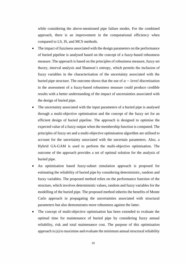
3.2.1 Monte Carlo Simulation ................................................................................ 42
3.2.2 Important Sampling (IS) ................................................................................ 43
3.2.3 Line Sampling ............................................................................................... 44
3.2.4 Methodology .................................................................................................. 49
3.3 APPLICATION TO BURIED PIPE ............................................................................... 53
3.3.1 Pipe Ovality ................................................................................................... 54
3.3.2 Through-wall Bending Stress ........................................................................ 56
3.3.3 Ring Buckling ................................................................................................ 57
3.3.4 Wall Thrust .................................................................................................... 58
3.4 TOTAL CIRCUMFERENTIAL/AXIAL STRESS ............................................................ 59
3.5 PIPE CORROSION .................................................................................................... 62
3.6 LIMIT STATE FUNCTION ......................................................................................... 64
3.7 NUMERICAL EXAMPLE ........................................................................................... 65
3.8 RESULTS AND DISCUSSION .................................................................................... 68
3.8.1 Parametric Studies ......................................................................................... 71

viii
3.9 CHAPTER SUMMARY .............................................................................................. 74
CHAPTER FOUR ........................................................................................................ 76
4 FUZZY-BASED ROBUSTNESS ASSESSMENT OF BURIED PIPE ................. 76
4.1 INTRODUCTION ...................................................................................................... 77
4.2 FUZZY SET AND FUZZY UNCERTAINTY .................................................................. 78
4.2.1 Analysis of Fuzzy Set and α-level Discretisation .......................................... 79
4.3 THE CONCEPT OF ROBUSTNESS MEASURES ........................................................... 81
4.3.1 Deterministic Measures ................................................................................. 81
4.3.2 Probabilistic Measure .................................................................................... 83
4.3.3 Entropy-based Robustness Measure .............................................................. 83
4.3.4 Methodology .................................................................................................. 87
4.4 APPLICATION TO BURIED PIPE ............................................................................... 88
4.4.1 Structural Failure Mode and a Numerical Example ...................................... 88
4.4.2 Damage Modelling of Buried Metal Pipes Under Uniform Corrosion ......... 88
4.5 RESULTS AND DISCUSSION .................................................................................... 90
4.6 CHAPTER SUMMARY .............................................................................................. 99
CHAPTER FIVE ........................................................................................................ 101
5 MULTI-OBJECTIVE OPTIMISATION OF BURIED PIPE BASED ON THE
EXPECTED FUZZY OUTPUT ................................................................................ 101
5.1 INTRODUCTION .................................................................................................... 102
5.2 THE CONCEPT OF ROBUST DESIGN OPTIMISATION .............................................. 103
5.3 FUZZY-BASED MULTI-OBJECTIVE DESIGN OPTIMISATION ................................... 104
5.3.1 Fuzzy Design Optimisation ......................................................................... 104
5.3.2 Fuzzy Variable and the Expected Value ..................................................... 105
5.3.3 Entropy Value of a Fuzzy Variable ............................................................. 106
5.3.4 Formulation of Fuzzy-based Multi-objective Design Optimisation ............ 107
5.4 HYBRID GA-GAM APPROACH ............................................................................ 108
5.4.1 Genetic Algorithm (GA) .............................................................................. 108
5.4.2 Goal Attainment Method (GAM) ................................................................ 108
5.4.3 Hybrid GA-GAM and Multi-objective Design Optimisation ..................... 108
5.4.4 Methodology ................................................................................................ 110
5.5 NUMERICAL EXAMPLE ......................................................................................... 112

ix
5.6 RESULTS AND DISCUSSION .................................................................................. 113
5.7 CHAPTER SUMMARY ............................................................................................ 121
CHAPTER SIX ........................................................................................................... 122
6 RELIABILITY ANALYSIS OF BURIED PIPE BASED ON FUZZY AND
SUBSET SIMULATION ............................................................................................ 122
6.1 INTRODUCTION .................................................................................................... 123
6.2 PROPAGATION OF UNCERTAIN INPUT VARIABLES................................................ 123
6.3 OPTIMISATION BASED FUZZY-SUBSET SIMULATION APPROACH .......................... 125
6.3.1 The Outer Loop: Genetic Algorithm (GA) Approach ................................. 126
6.3.2 The Inner Loop: Subset Simulation (SS) ..................................................... 127
6.3.3 Markov Chain Monte Carlo (MCMC) ........................................................ 130
6.3.4 Proposed Method ......................................................................................... 131
6.3.5 Applicability of the Proposed Method ........................................................ 134
6.4 NUMERICAL EXAMPLE ......................................................................................... 134
6.4.1 Investigation 1 (Pipe Ovality) ..................................................................... 135
6.4.2 Investigation 2 (Through-wall Bending Stress of Buried Pipe) .................. 138
6.4.3 Discussions .................................................................................................. 142
6.5 CHAPTER SUMMARY ............................................................................................ 144
CHAPTER SEVEN .................................................................................................... 146
7 MAINTENANCE OF DETERIORATING BURIED PIPE USING
OPTIMISATION INVOLVING FUZZY RELIABILITY, RISK AND COST .... 146
7.1 INTRODUCTION .................................................................................................... 147
7.2 MAINTENANCE OF BURIED PIPE AND PERFORMANCE INDICATORS ...................... 148
7.3 ANNUAL FUZZY RELIABILITY AND RISK AS PERFORMANCE INDICATORS ............ 151
7.3.1 Procedure for Estimating Reliability ........................................................... 153
7.4 CASE STUDY ........................................................................................................ 154
7.5 PERFORMANCE INDICATORS AND TOTAL COST USING MULTI-OBJECTIVE
OPTIMISATION ........................................................................................................... 156
7.5.1 Annual Fuzzy Reliability and Total Cost of Maintenance .......................... 157
7.5.2 Annual Risk and Total Cost of Maintenance .............................................. 161
7.6 PARAMETRIC STUDY ............................................................................................ 167
7.6.1 The Effect of Pipe Design Variables on Pipe Reliability and Risk ............. 167
x
7.6.2 The Effect of Cost Ratio (Direct and Indirect Cost) .................................... 168
7.7 CHAPTER SUMMARY ............................................................................................ 169
CHAPTER EIGHT .................................................................................................... 171
8 CONCLUSIONS AND RECOMMENDATIONS FOR FUTURE WORK ....... 171
8.1 CONCLUSIONS ...................................................................................................... 172
8.1.1 Reliability of Buried Pipe using a Combination of LS and IS Method ....... 172
8.1.2 Fuzzy-based Robustness Assessment of Buried Pipe ................................. 173
8.1.3 Multi-objective Optimisation of Buried Pipe .............................................. 173
8.1.4 Reliability of Buried Pipe Considering Random and Fuzzy Variable ........ 174
8.1.5 Maintenance Optimisation of Deteriorating Buried Pipe ............................ 175
8.1.6 Concluding Statement ................................................................................. 175
8.2 RECOMMENDATIONS FOR FUTURE WORK ............................................................ 176
REFERENCES ........................................................................................................... 178
LIST OF PUBLICATIONS ....................................................................................... 196

xi
LIST OF TABLES
TABLE 2.1: COMMON PROBABILITY DISTRIBUTION MODELS ............................................ 16
TABLE 2.2: COMMONLY USED SURFACE CORROSION MODEL ........................................... 23
TABLE 2.3: FACTORS THAT AFFECT THE STRUCTURAL DETERIORATION OF THE BURIED PIPE
................................................................................................................................ 29
TABLE 3.1: SUMMARY OF STRESSES/PRESSURES ACTING ON THE BURIED PIPE ................. 61
TABLE 3.2: LIMIT STATE FUNCTIONS FOR THE FAILURE MODES ....................................... 64
TABLE 3.3: STATISTICAL PROPERTIES OF THE INPUT PARAMETERS .................................. 66
TABLE 3.4: MATERIAL PROPERTIES OF THE INPUT PARAMETERS ...................................... 67
TABLE 3.5: FAILURE PROBABILITY OF BURIED PIPE DUE TO TOTAL AXIAL STRESS ........... 69
TABLE 6.1: FAILURE PROBABILITY OF BURIED PIPE AFTER 25-YEARS ............................ 143
TABLE 7.1: STATISTICAL PROPERTIES ............................................................................ 155
TABLE 7.2: PIPE MATERIALS AND LOCATION PROPERTIES .............................................. 156

xii
LIST OF FIGURES
FIGURE 1.1: FACTORS THAT AFFECT THE PERFORMANCE OF THE BURIED PIPE ................... 3
FIGURE 1.2: TYPICAL CORROSION PATTERNS OBSERVED IN WATER MAINS FAILURE (JI ET
AL., 2017) .................................................................................................................. 4
FIGURE 2.1: CAUSES OF PIPE CORROSION ......................................................................... 23
FIGURE 3.1: IMPORTANT UNIT VECTOR AS THE NORMALISED “CENTRE OF MASS” ............ 46
FIGURE 3.2: LS PROCEDURE ............................................................................................ 49
FIGURE 3.3: FLOW DIAGRAM OF THE ADAPTED LS METHOD ............................................ 52
FIGURE 3.4: (A) FLEXIBLE PIPE AND (B) RIGID PIPE ......................................................... 53
FIGURE 3.5: OVALITY OF BURIED PIPE ............................................................................. 55
FIGURE 3.6: THROUGH-WALL BENDING STRESS ............................................................... 56
FIGURE 3.7: RING BUCKLING ........................................................................................... 57
FIGURE 3.8: WALL THRUST.............................................................................................. 59
FIGURE 3.9: INTERNAL AND EXTERNAL CORROSION RATE FOR IRON PIPE ........................ 64
FIGURE 3.10: PROBABILITY OF FAILURE BY CONSIDERING WATER TABLE ABOVE AND BELOW
BURIED PIPE ............................................................................................................. 70
FIGURE 3.11: PROBABILITY OF FAILURE BY CONSIDERING UNDISTURBED SOIL AND
UNDERGROUND WATER TABLE ................................................................................. 70
FIGURE 3.12: THE EFFECT OF DIFFERENT K VALUES ON PROBABILITY OF FAILURE OVER TIME
................................................................................................................................ 72
FIGURE 3.13: THE EFFECT OF DIFFERENT N VALUES ON PROBABILITY OF FAILURE OVER TIME
................................................................................................................................ 73
FIGURE 3.14: THE EFFECT OF DIFFERENT KM VALUES ON PROBABILITY OF FAILURE OVER
TIME ........................................................................................................................ 73
FIGURE 3.15: THE EFFECT OF DIFFERENT KD VALUES ON PROBABILITY OF FAILURE OVER
TIME ........................................................................................................................ 74
FIGURE 4.1: FUZZY TRIANGULAR MEMBERSHIP FUNCTION .............................................. 79
FIGURE 4.2: FUZZY TRAPEZOIDAL MEMBERSHIP FUNCTION ............................................. 79
FIGURE 4.3: THE MEMBERSHIP FUNCTION OF A FUZZY VARIABLE .................................... 81
FIGURE 4.4: FLOW DIAGRAM FOR THE COMPUTATION OF FUZZY-BASED ROBUSTNESS
MEASURE ................................................................................................................. 86

xiii
FIGURE 4.5: FUZZY INPUT MODEL FOR CORROSION LOSS BASED ON MILD STEEL COUPONS
POOLED FROM ALL AVAILABLE DATA SOURCES UNTIL 1994, WITH 5TH AND 95TH
PERCENTILE BANDS. ................................................................................................. 89
FIGURE 4.6: MEMBERSHIP FUNCTIONS DEVELOPED FROM THE IMMERSION CORROSION DATA
OF MILD STEEL COUPONS FOR 4, 8, 12, AND 16 YEARS ............................................. 90
FIGURE 4.7: MEMBERSHIP FUNCTION OF PIPE FAILURE MODE FOR (A) DEFLECTION (B) WALL
THRUST .................................................................................................................... 92
FIGURE 4.8: MEMBERSHIP FUNCTION OF PIPE FAILURE MODE FOR (A) BENDING STRAIN (B)
BUCKLING PRESSURE ............................................................................................... 93
FIGURE 4.9: ENTROPY STATE FOR DIFFERENT FAILURE MODES AFTER 16 YEARS ............. 94
FIGURE 4.10: ENTROPY STATE FOR DIFFERENT FAILURE MODES AFTER 8 YEARS ............. 94
FIGURE 4.11: FUZZY-BASED ROBUSTNESS ASSESSMENT OF BURIED PIPE (A) DEFLECTION (B)
WALL STRESS/THRUST ............................................................................................. 96
FIGURE 4.12: FUZZY-BASED ROBUSTNESS ASSESSMENT OF BURIED PIPE (A) BENDING
STRAIN (B) BUCKLING PRESSURE.............................................................................. 97
FIGURE 4.13: FUZZY-BASED ROBUSTNESS ASSESSMENT OF BURIED PIPE AFTER 16 YEARS98
FIGURE 4.14: FUZZY-BASED ROBUSTNESS ASSESSMENT OF BURIED PIPE AFTER 12 YEARS98
FIGURE 5.1: FLOW DIAGRAM OF FUZZY ENTROPY ANALYSIS USING MULTI-OBJECTIVE
OPTIMISATION ........................................................................................................ 111
FIGURE 5.2: CORROSION PITH DEPTH AT T = 25 YEARS, 50 YEARS AND 100 YEARS ...... 113
FIGURE 5.3: THE PARETO FRONT FOR PIPE DESIGN BASED ON GA AND HYBRID GA-GAM
.............................................................................................................................. 114
FIGURE 5.4: PERFORMANCE OF BURIED PIPE DUE TO BUCKLING PRESSURE AFTER 100 YEARS
.............................................................................................................................. 115
FIGURE 5.5: PERFORMANCE OF BURIED PIPE DUE TO DEFLECTION AFTER 100 YEARS ..... 115
FIGURE 5.6: FUZZY ENTROPY STATE OF BURIED PIPE AFTER 100 YEARS ........................ 116
FIGURE 5.7: PERFORMANCE OF BURIED PIPE DUE TO BUCKLING PRESSURE AFTER 50 YEARS
.............................................................................................................................. 116
FIGURE 5.8: PERFORMANCE OF BURIED PIPE DUE TO DEFLECTION AFTER 50 YEARS ....... 117
FIGURE 5.9: FUZZY ENTROPY STATE OF BURIED PIPE AFTER 50 YEARS .......................... 117
FIGURE 5.10: PERFORMANCE OF BURIED PIPE DUE TO BUCKLING PRESSURE AFTER 25 YEARS
.............................................................................................................................. 118

xiv
FIGURE 5.11: PERFORMANCE OF BURIED PIPE DUE TO DEFLECTION AFTER 100 YEARS ... 118
FIGURE 5.12: FUZZY ENTROPY STATE OF BURIED PIPE AFTER 25 YEARS ........................ 119
FIGURE 6.1: THE PROPAGATION OF INPUT VARIABLES BASED ON FUZZY UNCERTAINTY 125
FIGURE 6.2: FLOW DIAGRAM FOR THE OPTIMISATION BASED FUZZY SUBSET SIMULATION
APPROACH ............................................................................................................. 133
FIGURE 6.3: RELIABILITY OF BURIED PIPE AFTER 25 YEARS DUE TO PIPE OVALITY ........ 136
FIGURE 6.4: RELIABILITY OF BURIED PIPE AFTER 50 YEARS DUE TO PIPE OVALITY ........ 136
FIGURE 6.5: RELIABILITY OF BURIED PIPE AFTER 75 YEARS DUE TO PIPE OVALITY ........ 137
FIGURE 6.6: RELIABILITY OF BURIED PIPE AFTER 100 YEARS DUE TO PIPE OVALITY ...... 137
FIGURE 6.7: PIPE RELIABILITY AFTER 25 YEARS DUE TO THROUGH-WALL BENDING STRESS
.............................................................................................................................. 138
FIGURE 6.8: PIPE RELIABILITY AFTER 50 YEARS DUE TO THROUGH-WALL BENDING STRESS
.............................................................................................................................. 139
FIGURE 6.9: PIPE RELIABILITY AFTER 75 YEARS DUE TO THROUGH-WALL BENDING STRESS
.............................................................................................................................. 139
FIGURE 6.10: PIPE RELIABILITY AFTER 100 YEARS DUE TO THROUGH-WALL BENDING
STRESS ................................................................................................................... 140
FIGURE 6.11: COV VERSUS MEMBERSHIP LEVEL ........................................................... 140
FIGURE 6.12: SENSITIVITY TEST FOR PIPE PERFORMANCE AT 25 YEARS DESIGN LIFE (PIPE
OVALITY) ............................................................................................................... 141
FIGURE 6.13: SENSITIVITY TEST FOR PIPE PERFORMANCE AT 100 YEARS DESIGN LIFE (PIPE
OVALITY) ............................................................................................................... 141
FIGURE 7.1: RELIABILITY AND MAINTENANCE COST OVER TIME (PROBABILISTIC METHOD)
.............................................................................................................................. 150
FIGURE 7.2: RELIABILITY AND MAINTENANCE COST OVER TIME (NON-PROBABILISTIC
METHOD) ............................................................................................................... 150
FIGURE 7.3: PIPE RELIABILITY WITH NO MAINTENANCE ACTION .................................... 160
FIGURE 7.4: RELIABILITY-BASED PARETO FRONT OF BURIED PIPE ................................. 160
FIGURE 7.5: PIPE RELIABILITY WITH MAINTENANCE ACTION ......................................... 161
FIGURE 7.6: FRAMEWORK FOR RISK ASSESSMENT OF BURIED PIPE CONSIDERING THICKNESS
REDUCTION ............................................................................................................ 162
FIGURE 7.7: ANNUAL RISK OF BURIED PIPE WITH NO MAINTENANCE ACTION ................. 165

xv
FIGURE 7.8: RISK-BASED PARETO FRONT OF BURIED PIPE .............................................. 165
FIGURE 7.9: RISK-BASED ASSESSMENT OF BURIED PIPE WITH MAINTENANCE ACTION.... 166
FIGURE 7.10: PIPE RELIABILITY BY VARYING PIPE THICKNESS ....................................... 166
FIGURE 7.11: PIPE RELIABILITY BY VARYING PIPE YIELD STRESS OF PIPE MATERIAL ...... 167
FIGURE 7.12: OPTIMAL PIPE MAINTENANCE TIME USING COST RATIO AND THE PROBABILITY
OF FAILURE ............................................................................................................ 169

xvi
ACRONYMS
AWWA American Water Works Association
CDF Cumulative Distribution Function
COV Coefficient of Variation
CPSA Concrete Pipeline Systems Association
CPU Central Processing Unit
CUI Command User Interface
CWWA Canadian Water and Wastewater Association
DSW Dong, Shah, and Wong
FORM First Order Reliability Method
GA Genetic Algorithm
GAM Goal Attainment Method
IS Important Sampling
LHS Latin Hypercube Sampling
LS Line Sampling
MC Monte Carlo
MCMC Markov Chain Monte Carlo
MCS Monte Carlo Simulation
MFL Magnetic Flux Leakage
MMA Modified Metropolis Algorithm
MOOP Multi-Objective Optimisation Problem
NRC National Research Council
PDF Probability Density Function
PGD Permanent Ground Deformation
RDO Robust Design Optimisation
SORM Second Order Reliability Method
WRC Water Research Centre

xvii
SYMBOLS
𝐴 Effective length of pipe which the load is computed
𝐴𝑠 Cross- sectional area of pipe wall per unit length
𝐵𝑑 The trench width
𝐵′ The empirical coefficient of elastic support
𝐶 Depth of soil cover above the buried pipe
𝐶𝑑 Calculation coefficient for earth load
𝐶𝐹 Future cost
𝐶𝐿 Live load distribution coefficient
𝐶𝑇 Corrosion pit depth
𝐶𝑡 Surface load coefficient
𝐶𝑇𝑂 Total cost
D Pipe diameter
𝐷1 Deflection lag factor
𝑑 Distance from the pipe to the point of application of surface load.
𝑑𝑓 Frost depth
𝐸 The elastic modulus of pipe
𝐸𝑠 Soil modulus
𝐸′ Modulus of soil reaction
𝐹𝑦 The minimum tensile strength of pipe
𝑓𝑓𝑟𝑜𝑠𝑡 Frost load multiple
𝑔(𝑥) Performance function
𝐻 The Bousinesq function to determine the influence of stress
𝐻𝑤 The height of ground water above the pipe and
ℎ𝑓 The total frost heave
idd Independent and identically distributed
𝐼 The moment of inertia
𝐼𝑐 Impact factor
𝑘 Multiplying constant
𝐾𝑠 The backfill sidewall shear stiffness

xviii
𝐾𝑡𝑖𝑝 The stiffness of elastic half-space of unfrozen soil below freezing front
𝐾 Bedding constant
𝐾′ Numerical value which depends on poison ratio
𝐾𝑚 Bending moment coefficient
𝐾𝑑 Deflection coefficient
𝐿𝑊 Live load distribution width
𝑃 Pressure on pipe due to soil load plus live load
𝑝𝑠 Frost load at any point
𝑃𝐹 Probability of failure
𝑃𝐺𝑉 The maximum horizontal ground velocity
𝑃𝑝 Pressure transmitted to the pipe as a result of the concentrated load
𝑃𝑣 Pressure on pipe due to soil load
𝑃𝑠 Live load
𝑃𝑊 Hydrostatic pressure
𝑃𝑠𝑝 Geostatic load
𝑅𝑆𝑅 Reserve strength of a structure
𝑠 The location below the surface where frost load is calculated
𝑆ℎ The hoop stiffness factor
𝑡 Pipe thickness
𝑇 Time of exposure
𝑇𝑜𝑝 Optimised time required for the replacement
𝑇𝑑 The designed life
𝑀𝑠 Secant constrained soil modulus
𝑛 Exponential constant
𝑁𝑇𝑆 Number of time steps
N Number of samples
𝑁𝑠 Sequence of points that lie within the failure domain
𝑁𝑇 Total number of samples
𝑅 The radius of pipe
𝑅w The water buoyancy factor which can be expressed
𝑣𝑠 Poison ratio

xix
𝑣𝑝 Poison ratio of the pipe material
𝑉𝐴𝐹 Vertical arching factor
𝑉0 The initial corrosion rate
𝑊𝐴 Soil arch load
𝛽 The attenuation factor
𝜑𝑝 Capacity modification factor for pipe
𝜑𝑠 Soil capacity modification factor
𝛿 Coefficient of variation
𝛿𝑢 Unitary coefficient of variation
휀𝑔 Ground strain
𝜎𝑏 Through-wall bending stress
𝜎𝐹 Circumferential stress due to internal fluid pressure
𝜎𝑆 Stress due to external soil loading
𝜎𝐿 Stress due to frost action
𝜎𝑉 Stress due to traffic load
𝜎𝑇 Stress due to temperature difference
𝜎𝐹/
Axial stress due to internal fluid pressure
𝜎𝜃 Total circumferential stress
𝜎𝑋 Total axial stress
𝜌 Internal fluid pressure
𝛾 Unit weight of the backfill soil
𝛼𝑝 Expansion coefficient of pipe
𝛼 Important unit vector
∆𝑦 Vertical deflection of the buried pipe
∆𝑇 Temperature difference between the fluid and the surrounding group
∆𝑦 𝐷⁄ Pipe ovality
𝜇(𝑥) Membership function

xx

1
CHAPTER ONE
1 INTRODUCTION

2
1.1 Background
Buried pipe networks are vital engineering infrastructure and are mostly used to transport
crude oil, potable water, sewage sludge, brine and natural gas. The transported fluid and
the pipe, in many instances, are placed or passed under a railway or roadway. Also,
pipelines are buried within the top layer of soil deposits and therefore are affected by the
type of surface loading (cyclic or non-cyclic loading), the geology of the surrounding soil,
corrosion, frost action, thermal effect and environmental hazard such as an earthquake
(Abdoun et al., 2009; Moser & Folkman, 2001; Ogawa & Koike, 2001; Sadiq et al., 2004).
As a result, buried pipelines are designed to resist the adverse effect of the conditions
mentioned above and including the effect of internal pressure.
Furthermore, the geological formation of the soil, frost action and thermal effect are
affected by seasonal climatic changes, which result in variabilities of the design
parameters (Moser & Folkman, 2001; Phoon & Kulhawy, 1999a; Whidden, 2009). For
instance, the annual seasonal variation for the soil moisture content or increase/decrease
in the underground water table can cause significant differences in the soil suction, and
in some cases result in substantial movement of the ground, which affects the soil
parameters. Based on this, the variabilities of the input parameters for a buried pipe can
increase the possibility of pipe failure over time. Figure 1.1 shows some examples of
design parameters including different loading and environmental conditions that affect
the performance of buried pipe over time (St. Clair & Sinha, 2014). The impact of these
design parameters in relation to a particular type of pipe material can lead to the failure
of the buried pipe.
The buried pipeline, like other engineering structures, deteriorates over time (Ahammed,
1998). The deterioration of a metallic pipe usually occurs due to the damaging effect of
the surrounding environment and the mechanism that leads to their failure are often
complex and difficult to completely understand (Kleiner & Rajani, 2001a). For buried
metallic pipe, one of the most predominant deterioration mechanism of the exterior walls
of the pipe is active corrosion effect (Mahmoodian & Li, 2017; Ossai et al., 2015; Sadiq
et al., 2004). This effect is a significant potential threat to the safety of the structure, and
it usually worsens over time. Kleiner & Rajani (2001b) suggested that the operators of
buried pipeline throughout the world are challenged with the costly and risky task of

3
operating and maintaining aged pipelines because of corrosion and the associated
damaging effects.
Figure 1.1: Factors that affect the performance of the buried pipe
The loss of pipe wall thickness due to corrosion is one of the major causes of failure for
the buried pipeline (Ji et al., 2017). The corrosion activity can manifest in various forms
such as uniform or localised and also internally and externally. As suggested in Rajeev et
al. (2014), the loss of thickness as a result of corrosion can be idealised into two patterns:
uniform corrosion and pitting corrosion as illustrated in Figure 1.2. The effect of corrosion
will reduce the resistance of the pipe capacity, which will also decrease the factor of safety
of the buried pipe (Gomes & Beck, 2014; Sadiq et al., 2004). The reduction of the pipe
thickness due to the adverse effect of corrosion can induce the failure of the buried pipe
when structural failure modes such as pipe ovality, through-wall bending stress, ring
buckling, axial and circumferential stresses are examined. Also, the growing uncertainty
Ground water
table
External loads
Dead load: Soil, Structure and Stockpile
Live load: Roadway, Railway and Runway
Trench backfill
Material
Trench width
Trench depth
Construction and Installation
procedure
Pipe properties
Pipe age
Pipe material
Pipe diameter
Pipe thickness
Pipe type
Soil properties
Soil type
Soil corrosively
Moisture content
Temperature
Corrosion
Crack or fracture
Bedding condition Differential Settlement
Ground Movement
Cover depth
Pipe length
Internal corrosion Pressure

4
associated with other design parameters contributes to the failure problem, which leads
to a reduction in the performance and safety level of the buried pipeline. Therefore, for a
buried pipeline in areas that are susceptible to active corrosion effect and in consideration
of other uncertain parameters, a robust and reliable design is required to ensure an
optimum working efficiency, safe operation, and insignificant downtimes during the
designed life.
Figure 1.2: Typical corrosion patterns observed in water mains failure (Ji et al.,
2017)
In recent time, various methods of predicting the reliability of a structure, e.g., First Order
Reliability Method (FORM), Second Order Reliability Method (SORM), Important
Sampling (IS), Latin Hypercube Sampling (LHS), Subset Simulation (SS), and Line
Sampling (LS) have been applied in a range of engineering problems such as building
and aerospace. The methods mentioned above are all available in the literature and can
be found in (Au & Beck, 2001; Koutsourelakis et al., 2004; Melchers, 1999; Olsson et
al., 2003; Schuëller et al., 2004; Zhang & Du, 2010; Zio, 2013). These methods are
powerful tools used to analyse and assess the safety level of structure or systems at the

5
design stage or during operation. For a buried pipeline, the reliability analysis helps to
evaluate and assess the performance of the structure over a specific period in order to
produce an optimum design. Also, the safety assessment of buried pipe structures is
becoming more and more critical because the failure of a buried pipe system may cause
a catastrophic environmental effect, especially when used for the supply of crude oil
(Gomes & Beck, 2014). Halfawy et al. (2008) stated that municipalities are under
increased pressure to adopt proactive and improved strategies that would lessen the risks,
cost and maintain a satisfactory level of performance and service. However, since the
failure of a pipe system may cause disastrous consequences, it is crucial to be able to
assess the reliability and robustness of the pipe system effectively.
Uncertainty associated with design parameters is an unavoidable process that affects the
performance of pipe systems over time. Despite the amount of effort and time put into the
understanding of the causes of pipe failure, through the collecting and processing of data,
the propagation and interpretation of uncertainty will remain an essential aspect of pipe
reliability analysis (Kleiner & Rajani, 2001b; Rajeev et al., 2014). This is because
randomness and fuzziness are often associated with the design parameters of the buried
pipe. However, by studying the reliability and maintenance of a buried pipe system, the
engineer can have a better understanding of the pipe performance at different time and
when to carry out maintenance. By considering various failure modes, environmental
effects such as corrosion and carrying out a parametric study, it is possible to identify and
draw conclusions about which failure mode is the most critical and parameters that are
the most sensitive over time. By considering uncertainty associated with the design
parameters of buried pipe in the computation, intuitions into the effects of the variation
of parameters on the assessment outcomes can be quantified and also useful to the
designer and decision-makers.
1.2 Problem Statement
The study of the reliability of buried pipeline, particularly with the effect of active
corrosion is an area that has attracted so much attention in the literature and which is vital
to many engineers and infrastructure managers (Ahammed & Melchers, 1994, 1997;
Babu & Srivastava, 2010; Caleyo et al., 2009; Sadiq et al., 2004; Tee et al., 2014). Over

6
the years, corrosion effect has affected the safe operation of most engineering structures
(Barone & Frangopol, 2014a; Sadiq et al., 2004). The development of corrosion is a
continuous and time-dependent process and is non-uniform, e.g., pitting corrosion ( Sadiq
et al., 2004; Tee et al., 2013). Undoubtedly, the effect of pipe failure due to corrosion is
significant, and as such, the buried pipe is provided with extra wall thickness, or external
coatings to protect it from the adverse effect of corrosion. Ahammed and Melchers (1997)
pointed out that this practice is not always entirely effective, particularly where pipe
sections are joined.
For a buried pipeline, corrosion will gradually reduce the resistance of the mechanical
and the structural properties, which can increase the possibility of failure over time
(Gomes & Beck, 2014). This can be challenging for design engineers and infrastructure
managers. Due to the nature of the deterioration process of the buried pipeline as a result
of corrosion, the assessment and maintenance would require a robust and reliable
approach to keep the possibility of failure and the risk under control. Therefore, the
development of a reliable and efficient technique for the evaluation of the performance
of buried pipe becomes a vital aspect of this study.
Pipelines are designed to meet a particular standard and to perform safely throughout their
entire design life. During the design life, the buried pipe must be able to deal with the
structural deterioration that diminishes the reliability of the pipe and the ability to
withstand different types of loads and loading conditions. However, the analysis,
assessment, and maintenance of pipeline structures involve uncertainties in the design
parameters. These uncertainties can be due to the randomness of the physical
phenomenon (aleatory uncertainty) and the incomplete knowledge of the physics of some
of this phenomenon (epistemic uncertainty) (Apostolakis, 1990). Sadiq et al. (2004)
suggested that the factors that add to the failure of a buried pipeline are associated with a
high degree of uncertainty, especially corrosion rates because of large spatial and
temporal variabilities. Similarly, Gomes & Beck (2014) and Kleiner & Rajani (2001b)
stated that the deterioration process and the design of buried pipe structures is usually
associated with a significant level of uncertainties due to limited information in the
process of estimating the structural parameters. Therefore, it is necessary to perform the

7
reliability analysis of buried pipe by considering the uncertainties associated with the
design parameters.
In the design of buried pipeline, disregarding the effects of uncertainty is deplorable and
can lead to disastrous consequences. Also, the risk associated with pipe failure involves
high consequences and decisions are made on the basis of quantitative data that is limited
and often expensive to collect. In spite of the availability of detailed physical failure
models, designers need to make explicit judgements based on available information
concerning the design of buried pipe structure. Hence, they must be able to have a high
level of confidence in any proposed or adapted methodology to analyse the safety of the
pipe system and avoid making the wrong decision that can be introduced at the modelling
stage. As a result, a broad modelling approach of uncertainty associated with a buried
pipe, which takes account of the randomness and fuzziness of the design parameters,
offers new insight by helping to effectively evaluate the performance of the pipe structure.
The failure of buried pipe structures are associated with consequences, and as a result,
risk-based assessment becomes necessary, and also, an essential tool for the evaluation
and optimisation of maintenance. The risk is generally defined as the product of the
probability of failure and the expected consequences in monetary terms due to the failure
(Ang & Tang, 1984; Tee et al., 2014). The foreseeable effects are usually quantified in
monetary terms, while the likelihood of failure is calculated using reliability techniques,
and by means of a rigorous mathematical framework. Typically, this requires the
specification of defined probability distribution models for the input parameters. The
analyses of engineering structures including buried pipe are investigated based on
simulation techniques and to obtain a numerical solution, especially where the analytical
approach is considered not efficient. Simulation methods allow explicit consideration of
uncertainty on the investigated problem, which provides a more robust tool for evaluating
the failure probability and allows right decision to be made.
In a nutshell, five challenges need to be addressed in this study to properly analyse the
reliability and robustness of buried pipe while considering the effect of uncertain
variables. These include:

8
For the propagation of uncertainty associated with the input variable due to
randomness, the use of MCS can be computationally expensive. Therefore, the
need to develop or adapt or improve an existing method that is time-dependent
and computationally more efficient to evaluate the reliability of a buried pipe is
essential.
In the design of buried pipe, it is possible for the aleatory and epistemic type of
uncertainties to coexist. Therefore, developing an approach to model the
performance of the buried pipe by considering randomness and fuzziness
associated with the input parameters become vital for a robust analysis.
Buried pipeline have suffered damage due to the effect of corrosion and
imprecision associated with the design parameters. Therefore, how can the
behaviour of the buried pipe be assessed to sustain damage that can be caused by
extreme loads or changes in environmental conditions without disproportionate
failure?
For the design of buried pipe, is it possible to optimise the performance of the
structure by considering the adverse effect of the uncertainty associated with the
input parameters through optimisation?
When evaluating the time to carry out maintenance of a buried pipe based on the
probabilistic approach, it is possible that the pipe segments will not necessarily
fail at the optimal time. Therefore, the use of a non-probabilistic approach can
produce an optimal time interval required to carry out maintenance of the buried
pipe.
1.3 Aim and Objectives
The presented work herein contributes towards the solution of the above challenges, and
this research aims to develop a framework for analysing the reliability and robustness of
buried pipe structure in order to promote safety in reliability-based design and robust
assessment. The framework will be developed using reliability methods, which is based
on probabilistic and non-probabilistic approaches while considering the structural
response. The responses from the failure modes considering uncertain variables will be
extended to compute the corresponding reliability and the robustness of the buried pipe

9
with respect to specific failure modes. However, the aim of this research will be achieved
by pursuing the following specific objectives:
To develop an approach to analysing time-dependent reliability of a buried
pipeline considering the input parameters as random variables and to examine
further the effect of varying some of the parameters.
To develop and analyse the robustness behaviour of the buried pipeline based on
the failure modes and taking into account the uncertainty associated with the
design parameters.
To develop an approach to optimise and analyse the performance of buried pipe
based on the pipe failure mode and the expected value of a fuzzy output.
To develop an approach to analyse the reliability of buried pipeline that
simultaneously considers fuzzy and random variables.
To evaluate the optimal time for the maintenance of buried pipe based on multi-
objective optimisation using fuzzy reliability, risk and cost.
1.4 Research Contributions
This study has developed a robust conceptual framework for analysing and estimating the
reliability and robustness behaviour of buried pipe, which plays an essential role in the
management of pipe systems. The framework would assist in taking a decision at the
design stage and at the point where maintenance interventions may be required to prevent
unexpected failure of the buried pipe subjected to different loading conditions. The
contributions of this research are briefly described as follows:
The structural failure modes of buried pipe such as through-wall bending stress
and total axial stress as explained in Chapter 3, Section 3.3 and 3.4 have been
modified for a time-dependent problem. The rationale is because corrosion, which
is one of the main prevalent challenges that affect the performance of buried pipe
occurs over time. Therefore, the structural reliability of buried pipe has been
analysed while considering the randomness associated with the design parameters
and the modified failure mode formulas using LS and IS. Also, a combination of
LS and IS methods have been adapted to estimate the reliability of a buried pipe
10
while considering the above-mentioned pipe failure modes. For the combined
approach, there is an improvement in the computational efficiency when
compared to LS, IS, and MCS methods.
The impact of fuzziness associated with the design parameters on the performance
of buried pipeline is analysed based on the concept of a fuzzy-based robustness
measure. The approach is based on the principles of robustness measure, fuzzy set
theory, interval analysis and Shannon’s entropy, which permits the inclusion of
fuzzy variables in the characterisation of the uncertainty associated with the
buried pipe structure. The outcome shows that the use of 𝛼 − 𝑙𝑒𝑣𝑒𝑙 discretisation
in the assessment of a fuzzy-based robustness measure could produce credible
results with a better understanding of the impact of uncertainties associated with
the design of buried pipe.
The uncertainty associated with the input parameters of a buried pipe is analysed
through a multi-objective optimisation and the concept of the fuzzy set for an
efficient design of buried pipeline. The approach is designed to optimise the
expected value of a fuzzy output when the membership function is computed. The
principles of fuzzy set and a multi-objective optimisation algorithm are utilised to
account for the uncertainty associated with the uncertain parameters. Also, a
Hybrid GA-GAM is used to perform the multi-objective optimisation. The
outcome of the approach provides a set of optimal solution for the analysis of
buried pipe.
An optimisation based fuzzy-subset simulation approach is proposed for
estimating the reliability of buried pipe by considering deterministic, random and
fuzzy variables. The proposed method relies on the performance function of the
structure, which involves deterministic values, random and fuzzy variables for the
modelling of the buried pipe. The proposed method inherits the benefits of Monte
Carlo approach in propagating the uncertainties associated with structural
parameters but also demonstrates more robustness against the latter.
The concept of multi-objective optimisation has been extended to evaluate the
optimal time for maintenance of buried pipe by considering fuzzy annual
reliability, risk and total maintenance cost. The purpose of this optimisation
approach is (a) to maximise and evaluate the minimum annual structural reliability

11
of buried pipe over a 125 years life cycle, and (b) to minimise the total cost
required to carry out maintenance within the design life. Also, the risk associated
with the possibility of failure is analysed. It is important to note that the annual
failure probability and reliability do not have or contain information concerning
the consequences or severity associated with the pipe failure. Based on this, the
risk associated with the pipe failure is also employed to determine the optimal
maintenance time.
The above-stated contributions can be used to efficiently evaluate and analyse the
performance of buried pipeline and also, serve as a managerial tool for design engineers
in assessing and maintaining the performance of buried pipe. Using the proposed
framework, the reliability and robustness behaviour of buried pipeline considering
uncertainties that exist in the input parameters can be analysed. Also, the influence of
design parameters can be analysed through sensitivity and parametric studies.
1.5 Structure of Thesis
The structure of the thesis is as follows:
CHAPTER 1 - Introduction: This Chapter explains background of the research area
including problem statement, research aims and objectives, research contributions and
structure of thesis.
CHAPTER 2 - Literature review: The concept of uncertainty, physical and environmental
challenges and uncertainties associated with the design parameters of the buried pipe are
explained. Also, the causes and consequences of buried pipe are reviewed including
existing methods used in estimating the reliability, risk and maintenance of buried pipe
and areas where there are gaps in knowledge.
CHAPTER 3 - Reliability analysis of buried pipe based on LS and IS methods: In this
Chapter, LS, IS and a combination of LS and IS has been adapted to estimate the time-
dependent reliability of buried pipe. The failure modes considered include total
axial/circumferential stress and through-wall bending stress.

12
CHAPTER 4 – Fuzzy-based robustness assessment of buried pipe: The robust behaviour
of buried pipeline under the influence of uncertain variables including reduction of pipe
thickness has been analysed considering corrosion-induced failure modes such as pipe
deflection, buckling pressure, wall thrust and bending strain. A numerical example has
been used to elucidate the concept of fuzzy-based robustness measure of the buried pipe
by considering the uncertainty associated with the design parameters.
CHAPTER 5 - Multi-objective optimisation of buried pipe based on the expected fuzzy
output: In this Chapter, a fuzzy-based multi-objective design optimisation approach is
proposed for the optimal analysis of buried pipe based on the expected value of a fuzzy
output when the membership function is computed. A Hybrid GA-GAM is used to
perform the optimisation.
CHAPTER 6 - Reliability analysis of buried pipe based on fuzzy and subset simulation:
This Chapter presents a numerical strategy for estimating the reliability assessment of
buried pipe considering random variables and fuzzy variables. The approach is based
fuzzy set, and subset simulation and the optimisation is performed using GA. The
proposed method relies on the performance function of the structure, which involves
PDFs and fuzzy variables for the modelling of the pipe structure.
CHAPTER 7 - Maintenance of deteriorating buried pipe using optimisation involving
fuzzy reliability, risk and cost: In this Chapter, a maintenance technique is proposed to
determine the optimal time interval for the maintenance of the buried pipeline. The
strategy is aimed at assessing the cost-efficiency required for the determination of the
optimal time for maintenance using multi-objective optimisation based on the annual
fuzzy reliability, risk, and total maintenance cost.
CHAPTER 8 - Conclusions and recommendations for future work: This Chapter presents
a summary of the work and recommendations for potential future work.

13
CHAPTER TWO
2 LITERATURE REVIEW

14
2.1 Introduction
The safety of the structural condition of the buried pipe is crucial to ensure continuity and
the quality of service provided throughout the design life. The cost required for the
replacement, repair, and expansion of existing buried pipe is usually high. However,
targeted research programmes in Canada, Australia, United States and Europe
acknowledge the need for methodologies to assess the level of deterioration and the
possibility of failure (Scheidegger et al., 2015). This is because the complete failure of
buried pipe would have a significant effect on the continuity of service and the
environment. The understanding of the structural condition, physical and environmental
condition, causes and consequences of failure and how it develops over time is essential
to the development of an adequate reliability and maintenance strategies.
In this Chapter, a brief description of the concept of uncertainty and the characterisation
of uncertainty is presented. The physical and environmental challenges of buried pipe are
discussed including the uncertainties associated with the input parameters of the buried
pipeline. Also, the causes and consequences of the failure of the buried pipe are explained.
The existing approaches for the reliability, risk, and maintenance of buried pipeline are
discussed including areas where there are gaps in knowledge.
2.2 The Concept of Uncertainty
The design of engineering structures (e.g., underground pipeline, retaining walls, and
foundation design) is often associated with uncertainties, particularly in estimating the
values of the design parameters (Beer et al., 2013; Möller et al., 2003). The presence of
uncertainties affects the performance of engineering structures throughout the design life.
Zio (2009) suggested that the presences of uncertainties are analysed to gain precise
information on the performance of the system and failure behaviour, and for the purpose
of protecting the system from the uncertain failure scenarios. The uncertainties involved
in the parameter estimation of most engineering structures are classified as aleatory and
epistemic uncertainties (Hanss & Turrin, 2010; Apostolakis, 1990). Although this
classification of uncertainties is not in absolute terms, it makes provision for a proper
distinction to be drawn (Apostolakis, 1990). The classified uncertainties are further

15
described as a property of a structural parameter associated with randomness/variations
(aleatory) and also, as a property linked to the poor understanding of the phenomenon or
lack of knowledge (epistemic) (Hanss & Turrin, 2010).
Aleatory uncertainty is characterised by randomness or natural variability in the
properties of a design parameter, such as the variation in the determination of the elastic
modulus of pipe material or the soil modulus. The aleatory uncertainty is random and can
be related to the outcome of an experiment. Hanss & Turrin (2010) suggested that an
efficient representation of aleatory uncertainties can be realised by the use of random
numbers and their PDFs derived from experimental data. Aleatory uncertainty can be
considered to be intrinsic or inherent uncertainty, which cannot be eliminated from the
associated parameter.
Epistemic uncertainty arises as a result of lack of knowledge or even complete absence
of knowledge concerning the process used in estimating the values of design parameter
(Hanss & Turrin, 2010). This type of uncertainty results from, for example, the vagueness
of parameter definition, subjectivity in numerical implementation, or simplification and
idealisation in the procedure of system modelling (Hanss & Turrin, 2010). Also,
epistemic uncertainty can arise due to imperfect method of estimating a design parameter,
such as the use of faulty instrument due to human error. As a result of the certain character
of epistemic uncertainty, which is entirely different from the aleatory uncertainty,
probability theory may not be suitable to characterise epistemic uncertainties efficiently.
Therefore, an alternative approach of quantifying epistemic uncertainties is by the use of
fuzzy numbers (Hanss & Turrin, 2010; Zadeh, 1965). The impact of all uncertainties on
engineering structures can be performed systematically using the concepts and techniques
that are embodied in the theory of probability (Hanss & Turrin, 2010). However, it is
imperative that the presence of these uncertainties are adequately accounted for in the
design of an engineering structure.
2.2.1 Characterisation of Uncertainties
In most cases, the design of an engineering structure is based on deterministic models,
however, Khemis et al. (2016) and Li et al. (2016) suggested that the limitations of the

16
deterministic approach paved the way for other models in many scientific works.
Uncertainties are associated with engineering structures, therefore, considering their
effect in the analysis becomes crucial for an efficient performance assessment of the
structure. The determination of the actual value of a structural parameter that is random
in nature from a possible range of values can be quantified using a probability distribution
function (Ang & Tang, 2007; Baecher & Christian, 2005). Sriramula &
Chryssanthopoulos (2009) suggested that the probability distributions form an important
part of uncertainty modeling and the selection of a particular distribution may
significantly affect the characteristic values considered in structural design. The
distribution function is used to assign the probability of occurrence for each possible
value. However, a discrete probability distribution is employed if the set of possible
values for a random variable is countable; otherwise, a continuous probability distribution
is used (Ang & Tang, 2007).
Table 2.1: Common probability distribution models
Distribution models
Aleatory Epistemic
Continuous Discrete Continuous Discrete
Normal Poison Interval Real set
Uniform Binomial Fuzzy set Integer set
Weibull Distribution Negative Binomial
Lognormal Geometric
Exponential
Student t-Distribution
In most engineering problems, the continuous probability distribution is often used more
compared to the discrete probability distribution, for example, the design parameters
associated with a mechanical and geometric property of materials (Ang & Tang, 2007).
The continuous probability distribution is described using PDF or Cumulative
Distribution Function (CDF). In the literature, there are several suggestions used to
characterise the probabilistic models of the uncertainties associated with the input

17
parameters (Beer et al., 2013a). Table 2.1 shows some of the common ones. Also, normal
and lognormal distributions are among the most commonly used models, which depends
on the behaviour of the parameter (Beer et al., 2013a; Limpert et al., 2001; Wang et al.,
2016). However, the normal distribution is very popular and often used because of the
central limit theorem (Beer et al., 2013a) and simplicity (Limpert et al., 2001). Limpert
et al. (2001) suggested that the concise description of a normal sample is handy, well-
known, and sufficient to represent the underlying distribution.
The PDFs of the design parameter are usually created from random data, which may not
be available to a considerable extent and quality because of insufficient data and
limitation in the experimental processes (Beer et al., 2013b; Hanss & Turrin, 2010; Li &
Lu, 2014). The scarcity or lack of information concerning the uncertain parameters could
also arise. However, it may be ideal to lessen the assumptions used for some of the well-
defined probabilistic models because of imprecision in the parameters of the model (Beer
et al., 2013a).
Considering a situation where there is an epistemic uncertainty, two different methods
can be used to model the variabilities of the structural parameters based on subjective
probability (Khemis et al., 2016). These include the Bayesian method and the set-
theoretical model. The Bayesian approach relies on the theory of probability and denotes
an excellent way to handle epistemic uncertainty (Beck & Katafygiotis, 1998). The set-
theoretical approach includes fuzzy sets, interval analysis, etc. and is used to model the
epistemic uncertainty based on set values. In recent times, the use of set-theoretical
method has attracted strong consideration especially in the reliability assessment of an
engineering system. The purpose of the fuzzy set permits the simultaneous analysis of
different bound sets, and this is very useful in situations where the set bounds are not
known explicitly to examine the sensitivity of input parameters on the possibility of
failure (Beer et al., 2013a; Beer et al., 2013b; Li & Lu, 2014). In this study, a fuzzy set is
utilised to analyse the performance of a buried pipe. For more information about fuzzy
set, see Chapter 4 and 6.

18
2.3 Physical and Environmental Challenges of Buried Pipe
Buried pipes have sustained substantial physical and environmental damages during the
service life (Kleiner & Rajani, 2001a; O’Rourke & Liu, 2012; Whidden, 2009). As a
result of this, there is growing concern about the structural performance and the physical
mechanism that leads to pipe failure. Kleiner & Rajani (2001a) suggested that the physical
mechanisms that lead to pipe breakage are often very complex and not completely
understood. However, the physical and environmental damages of buried pipe involves
key areas such as: (a) the properties of pipe (e.g. material type and pipe wall thickness)
and pipe-soil interaction; (b) load and loading condition (e.g. operational pressure,
external load such as earth load, traffic load, frost load and seismic effect) and (c)
deterioration of the pipe wall due to active corrosion effect (Kleiner & Rajani, 2001a).
The behaviour and failure modes of sections of buried pipe are somewhat well-known,
and information about them is available in standard textbooks and design codes, e.g.,
(Alliance, 2001; Moser & Folkman, 2001; O’Rourke & Liu, 2012). Also, the traditional
design of buried pipeline has been based on physical behaviour where allowances are
made to provide pipe with the capacity to resist or withstand expected loads such as live
or earth loads and with a sufficient safety margin (Moser & Folkman, 2001). However,
these loads are associated with uncertainties, which affects the performance negatively
over time. Based on this, it is crucial to overcoming the effect of the uncertainty and
imprecision that exist in the design parameters. Hence, prediction of the optimal
performance of buried pipe considering the deterioration of materials requires a good
understanding of several components and causes of failure as briefly reviewed in the
following subsections.
2.3.1 Seismic Action
Buried pipes have sustained substantial damage in the past, following earthquake
occurrence (O’Rourke & Liu, 1999). The damage has been ascribed to the impact of
transient action and permanent ground deformations (Liang & Sun, 2000; O’Rourke &
Liu, 2012). These effects are further reviewed in the subsequent Section, and they are

19
responsible for the majority of the seismic havoc caused in water distribution pipe
network and oil and gas underground pipelines.
2.3.1.1 Transient Action
The transient action as a result of the earthquake effect is called a “wave propagation
hazard,” and is characterised by peak ground acceleration and velocity (Karamanos et al.,
2014). Ground shaking causes the action due to the travelling body and seismic surface
waves (Karamanos et al., 2014; Kouretzis et al., 2006). The transient action is associated
with peak ground acceleration and velocity. The examination of wave impact on the
buried pipeline is complicated, thus requires a wave propagation analysis in a three-
dimensional soil-pipe system (Karamanos et al., 2014). Newmark (1967) developed a
simplified method that can estimate the strain and curvature of the buried pipe that is
caused by the travelling wave of constant shape regarding peak ground motion. Based on
the developed approach, the axial strain that would develop due to longitudinal and bend
deformation triggered by the action of the wave propagating parallel to the pipe can be
estimated. Therefore, the maximum ground strain towards part of wave propagation is
expressed in Eq. (2.1).
휀𝑔 =𝑃𝐺𝑉
𝐶 (2.1)
Where 𝑃𝐺𝑉 is the maximum horizontal ground velocity in the direction of wave
propagation; 𝐶 represents the apparent propagation velocity of the seismic wave.
Yeh (1974) extended the analytical solution of Newmark (1967) in other to account for
obliquely incidence shear and Rayleigh waves. An angle of wave propagation that is
relative to the longitudinal structural axis is introduced as a random problem variable.
The hoop and shear strain developed due to the induced stress were addressed with the
consideration of the time lag that is relative to the axial strains. The uncertainty associated
with the analytical solution is reflected in most of the current design guideline for
structures such as (Alliance, 2001; European Commitee for Standardisation, 2004). The
design guideline for buried pipeline Alliance (2001) called on seismological evidence and
univocally recommend the use of an ‘‘apparent seismic wave velocity of the bedrock’’.
The value suggested for the estimation of the axial strains, regardless of local soil
conditions is equal to 2000 m/s (Kouretzis et al., 2006).

20
2.3.1.2 Permanent Ground Deformation (PGD)
A significant amount of damage to buried steel pipelines are caused as a result of
permanent ground induced actions due to earthquakes, such as landslides, movement of
fault and liquefaction-induced lateral spreading (Dash & Jain, 2007; Datta, 1999, 2010;
Vazouras et al., 2012). The ground induced actions are applied on the buried pipeline in
a quasi-static manner and are not essentially linked with severe seismic shaking, but the
buried pipe could be extremely damaged and evident threats to the environment
(Karamanos et al., 2014). The analysis of PGD depends on the types of action induced.
However, there are different methods presented by researchers for the response of buried
pipeline under seismic event. See the following reference (Alliance, 2001; Dash & Jain,
2007; Karamanos et al., 2014; Kouretzis et al., 2006) for more information.
2.3.2 Frost Effect
The design code (American Water Works Association, 1977) suggested a procedure to
determine earth and traffic load on the buried pipeline but did not include a process to
calculate frost pressure, which affects the performance of the buried pipe. The high
number of water mains breakages in winter has been attributed to the increased earth load
exerted on the walls of the buried pipe (Kleiner & Rajani, 2001b). Rajani & Zhan (1996)
presented a model to estimate frost load on buried pipes in trenches and under roadways.
As described in Kleiner & Rajani (2001b) the frost load in a typical trench can be obtained
using the expression in Eq. (2.2).
𝑝𝑠 = ∑𝛽ℎ𝑓
𝑖
[(1 𝐾𝑡𝑖𝑝⁄ )+(𝐵𝑑 𝐾𝑠𝑑𝑓𝑖⁄ )]
𝑁𝑇𝑖=0 𝐻(𝑠 − 𝑑𝑓
𝑖 , 𝐵𝑑) (2.2)
Where 𝑝𝑠 is the frost load at any point 𝑠, 𝑑𝑓 is the frost depth, 𝑖 is the time step number,
𝑁𝑇 is the number of time steps, ℎ𝑓 is the total frost heave, 𝐵𝑑 is the trench width, 𝐾𝑡𝑖𝑝 is
the stiffness of elastic half-space of unfrozen soil below freezing front, 𝛽 is the
attenuation factor, 𝐾𝑠 is the backfill sidewall shear stiffness, 𝐻 is the Bousinesq function
to determine the influence of stress and 𝑠 is the location below the surface where frost
load is calculated.

21
In the model, the frost load is a function of the trench width, frost depth penetration, and
other soil properties. In a trench, the frost load develops primarily as a result of different
frost susceptibility of the backfill and sidewall of the trench and the interaction at the
trench backfill sidewall interface (Kleiner & Rajani, 2001b). The introduction of a model
for frost load has helped to improve the understanding of the mechanism that leads to the
development of frost load and enabling a mitigation measure. Some of the input
parameters are not readily available, which makes it difficult to use the model. The current
validation data as described in Kleiner & Rajani (2001b) indicates that frost loads could
develop up to twice the geostatic or gravity earth loads. Rajani & Makar (2000) suggested
an alternative and simplistic approach to estimating frost load. Based on the proposed
method, the frost load could be determined as a multiple of the earth pressure. For the
mathematical formulation, see Chapter 3. The typical value of the frost load multiple is
usually between 1 and 2. A value of 1 is used on a condition where there is no frost load,
while the value of 2 is used when there is a maximum frost load acting on a buried pipeline
(Rajani & Makar, 2000). The effect of frost action can lead to further reduction in the
reliability of the buried pipe.
2.3.3 Thermal Effect
The thickness design approach of buried pipe as suggested by American Water Works
Association (1977) does not consider the impact of the difference in temperature of the
water mains and surrounding soil explicitly. Rajani & Makar (2000) suggested that this
difference can lead to a further reduction in the factor of safety as it induces axial stresses
on the pipeline. Failure of the buried pipeline will occur in longitudinal mode if the
induced stresses exceed the axial tensile strength of the pipe. Rajani et al. (1996)
developed an analytical solution for estimating the thermal stress of any pipe material
under pressure and subjected to thermal and other operational loads. Rajani & Makar
(2000) suggested that the analytical equation can be specifically simplified for a metallic
pipe, where the ratio between the soil elastic modulus and the elastic modulus of the pipe
material is slight? Also, the external pressure as a result of the soil reaction may be taken
as zero. For the mathematical formulation, see Chapter 3. However, the reliability of the

22
buried pipe depends on pipe size, the geometry of the trench, soil types, pipe thickness,
and environmental and geo-environmental conditions.
2.3.4 Corrosion Effect
Unlike the loading conditions and the impact of geo-hazards on the buried pipe, corrosion
has proven to be one of the most predominant causes of pipe failures and contributed
significantly to the downtime. Every year, pipeline companies spent huge amount of
money on various forms of corrosion control measures in order to maintain the integrity
of pipelines (Ossai et al., 2015). Regrettably, the difficulties associated with getting an
optimum and robust design, estimation of reliability, and appropriate maintenance
strategies highlight the billions of dollars lost due to corrosion-induced failure (Bhaskaran
et al., 2005; Gomes & Beck, 2014). As suggested in Brown (2014), about 80% per cent
of failed pipelines are monitored in one form or another and between 20% and 65% of
the amount spent on corrosion problems could be saved if there was a better
understanding of corrosion process, protection and control techniques. Corrosion of
buried pipelines can be attributed to various causes and are related to the physical and
chemical factors as a result of corrosive environmental conditions. Figure 2.1 (Ossai et
al., 2015) shows some of the causes of corrosion.
Corrosion of pipe could occur either internally or externally or both ways (Ahammed &
Melchers, 1997; Sadiq et al., 2004). In the literature, there are various models developed
by researchers to model the effect of external corrosion. Some of these models are
reported in Table 2.2. These models are developed from experimental data using
regression analysis. The reduction of buried pipe wall thickness due to corrosion loss can
be relatively uniform or localised (Ahammed & Melchers, 1994). Kleiner & Rajani
(2001a) suggested that the deterioration mechanism on the exterior walls of the cast and
ductile pipes is electrochemical corrosion and the damage occurs in the form of corrosion
pits. Therefore, the physical environmental conditions that surround the buried pipe have
a significant effect on the rate of deterioration. Some of the factors that accelerate the
corrosion of metallic pipes include the characteristic of the soil such as chemical and
biological contents, soil moisture content, electrical resistivity, aeration, etc (Kleiner &
Rajani, 2001a). Also, the interior of a buried metallic pipe can be subjected to erosion and

23
crevice corrosion that may lead to a reduction in the effective inside diameter of the pipe.
The internal corrosion can also reduce the performance of the buried pipe over time.
Pipe Corrosion
Physical factors Chemical Factors Environmental Factor
Structural Properties Product properties
Material properties
Residual and
operating stresses
Design factors
Crevices
Deposites
Inclusions
Interaction of the
above variables
Temperature
Pressure
Flow rate
Entrained solid
and liquid
Flow pattern
Interaction of the
above variables
H20
H2S
C02
Dissolved solids
Organic & inorganic
acids
Sulphur and Sulphur
compounds
Microorganism
Hydrocarbons
pH
Chemical variabilities
Trace elements
Interation of the above
variables
Oil field composition
Soil composition
Temperature and
moisture levels
Nature of operating
area e.g. software,
freshwater, land
Figure 2.1: Causes of pipe corrosion
Table 2.2: Commonly used surface corrosion model
Model Parameters description
𝒅 = 𝑲𝑻𝒏
𝒅𝑻 = 𝒏𝑲𝑻(𝒏−𝟏)
(Kucera and Mattson, 1987)
𝑑 = depth of corrosion pit (mm); 𝐾 = constant
(usually 2); 𝑛 = constant (usually 0.3); 𝑇 =
exposure time (yr); 𝑑𝑇 = corrosion rate (mm/yr)
𝒅 = 𝑲𝒏𝒁𝒏 where
𝒁 = [(𝟏𝟎 − 𝒑𝑯)𝑻
𝝆𝒔𝒐𝒊𝒍]
(Rossum, 1969)
𝐾𝑛 = constant; 𝜌𝑠𝑜𝑖𝑙 = soil resistivity; 𝑝𝐻 = the
acidic or alkaline nature of soil; 𝑛 = related to
soil redox potential;
𝒅 = 𝒂𝑻 + 𝒃(𝟏 − 𝒆−𝒄𝑻)
𝒅𝑻 = 𝒂 + 𝒃𝒄𝒆−𝒄𝑻 (𝒕𝒘𝒐
− 𝒑𝒉𝒂𝒔𝒆 𝒎𝒐𝒅𝒆𝒍)
(Rajani et al, 2000)
𝑎 = final pitting rate constant (typical value; 0.009
mm/yr); 𝑏 = pitting depth scaling constant
(typical value; 6.27 mm); 𝑐 = corrosion rate
inhibition factor (typical value; 0.14 yr−1)

24
2.4 Uncertainty Associated with the Design of Buried Pipe
Buried pipes are designed based on soil and pipe properties, and these properties are used
to model the behaviour of the pipe (Moser & Folkman, 2001; Whidden, 2009). The
analysis of the pipe response due to a particular failure mode is accurate to the point that
the assumptions made in the mathematical representation of the soil and pipe properties
are correct. Indeed, uncertainties affect the performance of a buried pipe and its
modelling. On the one side, there are conditions where the determination of a particular
soil or pipe properties, e.g. the estimation of the elastic modulus of pipe material,
determination of soil modulus, are random. This type of uncertainty for a buried pipe
system is classified as aleatory uncertainty as explained in Section 2.2. Another aspect of
uncertainty comes from the incomplete knowledge concerning the properties of the
design parameters and the conditions in which the phenomena occurs. This type of
uncertainty is classified as epistemic uncertainty, which affects the performance of buried
pipe in the hypotheses assumed and the values of the parameter of the model. Zio &
Pedroni (2009) suggested that model uncertainty arises because mathematical models are
simplified illustrations of real systems and, therefore, their outcomes can be affected by
errors.
In the literature, considerable research has been performed to demonstrate the importance
of considering uncertainties associated with the design parameters of an engineering
structure. For example, Nadim (2015) presented an overview on how uncertainty
associated with mechanical soil properties are dealt with in offshore site investigation and
suggested ways for optimally utilising the reliability tools for this purpose. In the study,
two problems were addressed. The first is the extraction of the maximum amount of
information from site investigation and how to represent soil properties for the purpose
of design while accounting for the uncertainties caused by natural variability of soil
properties and interpretation of lab tests. Also, Lacasse & Nadim (1996) present a review
of the uncertainties in characterising the properties of soil, and stresses the rationale for
characterising the uncertainties for design purpose. Subsequently, the usefulness of
estimating and, where possible reducing, the uncertainties is demonstrated using a case
study. In the following subsection, sources of uncertainties are explained with particular
reference to soil and pipe properties.

25
2.4.1 The Inherent Variability
The properties of soil changes over time due to the natural geologic and environmental
processes that produced and continually modify the soil mass in situ (Phoon & Kulhawy,
1999a). Often, these processes will continue to occur and cause changes in the soil
properties both vertically and horizontally. Soils are formed from weathering of rocks or
weathered rock and minerals transported by water. Therefore, a soil deposit will consist
of different layers of weathered rocks, which has been consolidated over a period and
with different properties. As a result, the soil is seen as a complex engineering material
with an inherent variability (Phoon & Kulhawy, 1999a). The inherent variabilities of soil
properties, e.g., the elastic modulus of soil can be described using statistical parameters
such as the mean, variance, and covariance.
As reported in Phoon & Kulhawy (1999a), if soil samples are collected over a period of
one to two weeks, the properties of the soil can be regarded as time-invariant (Rethati,
1989). Also, if the time periods continue to increase, additional variability may be
introduced into the data set due to the changes in the soil mass. The variation can be rather
significant, in some cases. Unfortunately, the time interval over which the soil samples
will be collected is often not reported. This makes it difficult to evaluate the significance
of the temporal changes.
2.4.2 Measurement Error
For the design of buried pipe, most of the design parameters such as the height of backfill
material and pipe thickness are measured using physical means. The process of
measurement can introduce additional variability. The error generated as a result of
measurement can be attributed to a variety of factors such as human error, equipment
error, and limitations in the experimental process (Fornasini, 2008). Phoon & Kulhawy
(1999a) stated that the effect of equipment error comes from inaccuracies in the
measuring devices and variations in equipment geometries and systems employed for
routine testing while the impact from the operator occurs from the limitations in the
existing test standards and how the procedures are followed. However, an experiment that
depends more on the operator and with a complicated procedure will have higher

26
variability compared to the one with little dependency on the operator and simple
procedure (Kulhawy & Trautmann, 1996; Phoon & Kulhawy, 1999a).
The measurement of uncertainty associated with a particular parameter using specific
equipment can be quantified by taking a repeated measurement of the same parameter.
The data generated from the experiment can be used to quantify the probability
distribution model. Kulhawy & Trautmann (1996) suggested that the use of proper quality
equipment and systematic control of procedure will likely have a small measurement
error. In principle, the error due to measurement can be determined by analysing the
variation of the data obtained through repeated measurement.
2.4.3 Transformation Uncertainty (Model Uncertainty)
Most often, the design parameters that are determined directly from field measurement
may not be directly applicable to the design of the structure. Instead, there may be a need
for the obtained values to be transformed into the appropriate design property using a
mathematical model. In doing this, Phoon & Kulhawy (1999b) suggested that there may
be some form of uncertainties that will be introduced because most transformation models
are determined using empirical data fitting. Because of the simplifications and
approximations, in theory, transformation uncertainty will still be present. Also, an effort
to obtain high-quality data to quantify the uncertainty effect, may not significantly reduce
transformation uncertainty because of the difference between theories and natural
physical behaviour (Phoon & Kulhawy, 1999b). Therefore, transformation uncertainty
occurs as an independent uncertainty in engineering structures. For example, when
evaluating the corrosion empirical constant using values of corrosion pit depth from
different environmental conditions, the transformation uncertainties will depend on the
best fitting line for the regression analysis using different years of corrosion pit depth.
2.5 Analysis of Buried Pipe
The presence of uncertainties will affect the performance of buried pipe overtime if not
accounted for at the preliminary stage of the design. As a result of this, it is crucial to
overcoming the adverse effect of uncertainty in the design of buried pipe. Traditionally,

27
the fundamental criterion used in the design of buried pipe is the resistance to internal
pressure (Moser & Folkman, 2001). Once the criterion is evaluated, the obtained wall
thickness is validated for suitability with regards to other measures such as external loads,
and buckling pressure. This type of design is based on a deterministic approach, and the
limitations have paved the way for other methods. Schuëller & Jensen (2008) suggested
that the determination of structural performance based on the deterministic model is
undoubtedly a simplification because physical measurement always shows variability and
randomness. Furthermore, the analytical expressions used for the design of buried
pipeline are formulated and solved based on physical and experimental models (Kleiner
& Rajani, 2001a). The development of these models is associated with a significant
amount of subjectivity that can lead to the introduction of an aleatory or epistemic form
of uncertainty. Therefore, it is essential to consider the variabilities or randomness
associated with the design parameters of the buried pipe.
The use of structural optimisation has gained an increasing significance in the design of
structures and improving performance (Bucher & Frangopol, 2006; Okasha & Frangopol,
2009; Onoufriou & Frangopol, 2002). Under this trend, substantial progress has been
made towards the design of engineering structures. Considering the importance and
consequences associated with the failure of the pipe network, Sadiq et al. (2004)
suggested that a risk-based maintenance management methodology can be more effective
and independent. The reason is that it allows the optimisation of various types of
structures within a network by considering both the probability of failure and the
consequences of failure. Kleiner et al. (2004) considered the network renewal planning
problem where the structural and the hydraulic capacity deterioration of the network are
considered for the determination of the optimal rehabilitation schedule. In recent time,
considerable attention has been given to the reliability of pipeline systems in conjunction
with optimisation to achieve maximum benefits with the minimum cost (Moneim, 2011).
Halfawy et al. (2008) suggested that an optimum management strategy must ensure
efficient performance after rehabilitation and should provide reliable service with
minimum interruptions. The causes and consequences of the failure of the buried pipe are
reviewed in the following subsections.

28
2.5.1 Causes of Pipe Failure
The selection of the design parameters for buried pipe always varies and depends on the
use (e.g., water supply and crude oil), service life and the nature of the surrounding
environment (Whidden, 2009). Buried pipe have sustained substantial damages due to the
impact of one or more of the aggressive environmental effects such as corrosion, frost
action, and seismic effect (Karamanos et al., 2014; Ossai et al., 2015; Rajani & Zhan,
1996). As a result, there is growing concern about the maintenance of pipe integrity
throughout the designed life. Chughtai & Zayed (2008) suggested that lack of
comprehensive knowledge of the condition of buried pipelines increases chances of a
catastrophic failure. However, it is not possible to completely understand all the
conditions that affect the performance of buried pipe because of lack of knowledge or
information with regards to the processes that are involved. Hence, the consideration of
uncertainty of the design parameter becomes an essential part of the analysis of buried
pipeline. The nature of pipe material, diameter, and age, including factors such as soil
types and corrosion parameters have shown significant influence on pipe failure (Berardi
et al., 2008; Fenner et al., 2000). Ahammed & Melchers (1997) suggested that for an
underground pipe that is subjected to internal and external loading, the primary cause of
failure is the loss of structural strength that is influenced by localised or overall reduction
in pipe wall thickness. Table 2.3 shows some of the factors that affect the structural
deterioration of buried pipelines as defined in Rostum (2000).
Leis & Parkins (1998) stated that the leading causes of damage or failure of the buried
pipeline are stress corrosion cracking, wall thickness reduction, and the presence of stress
concentrators. Corrosion affects buried pipe both internally and externally. In practice,
there are a considerable amount of anticorrosion protection efforts, but the damage due
to corrosion still occurs on a large scale and remains a matter of concern because of the
amount needed for the rehabilitation (Ahammed & Melchers, 1997; Sadiq et al., 2004).
Fares & Zayed (2010) suggested that the magnitude of failure modes is different among
pipelines and varies with the life cycle. Farshad (2006) also pointed out that at a
microscopic level, changes in pipe strength and stiffness are the two most important
aspects that are involved in the long-term behaviour of the pipe. Similarly, as suggested
in (Berardi et al., 2008; Fenner et al., 2000) pipe thickness, pipe elastic modulus, diameter,

29
and age, with or without additional factors such as soil types have contributed to pipe
failure. It is important to note that during installation of buried pipe, other damages such
as mechanical deformations and thermal effect can affect the residual stress and increase
the possibility of pipe failure.
Table 2.3: Factors that affect the structural deterioration of the buried pipe
Structural
variables
External/Environmental
variables
Internal
variables
Maintenance
variables
Location of
pipe
Soil type Passing material
velocity
Date of failure
Diameter loading Passing material
quality
Date of repair
Length Ground condition Internal
corrosion
Location of
failure
Year of
construction
Direct stray current Type of failure
Pipe material Leakage rate Previous
failure history
Joint method Other network
Internal
protection
Salt for de-icing of roads
External
protection
Temperature
Pressure class External corrosion
Wall thickness
Laying depth
Bedding
condition
Ahammed & Melchers (1994) pointed out that the reduction of wall thickness for metal
pipes arises from pitting and crevice corrosion. The study further explains that the

30
decrease in pipe thickness weakens the capacity of the pipe resistance and thus, reduces
the safety of the structure. Also, Gabriel (2011) states that the mechanical strength of a
buried pipe begins to reduce soon after installation. The reduction of pipe wall thickness
due to corrosion could have an adverse impact on the failure modes of buried pipe.
2.5.2 Consequences of Pipe Failure
According to Piratla et al. (2012), a significant portion of the buried pipeline for water
and wastewater in Europe is approaching the end of its service life, and thus, essential
construction works will be required to perform proper rehabilitation or renewal of this
vital infrastructure. The primary design requirement of buried pipeline considering the
physical and environmental challenges and the associated uncertainties is the safety of
the structure during the designed life. In recent time, there is an increase in the structural
performance of a buried pipeline especially in areas that are prone to geo-environmental
hazards (Karamanos et al., 2014). To accurately quantify the extent of damage on the
buried pipe, underground-induced action requires appropriate performance criteria
(Vazouras et al., 2012). However, the consequences of the failure of the buried pipe may
include loss of life, injuries, and environmental contaminations. Although, some of these
consequences cannot be evaluated in monetary terms.
The most common way of quantifying consequences associated with pipe failure is to
evaluate the losses related to the failure regarding cost. The cost related to structural pipe
failure can be a direct cost, e.g., cost of replacing the failed part or indirect cost, e.g.,
environmental contaminations cost. Barone & Frangopol (2014a) suggested that the
direct consequences of structural failure are often associated with repair/replacement cost
of the structural component while the indirect consequence is the estimation cost derived
from failure, which may not strictly be related to rebuilding the structure. In this case, the
indirect effects of pipe failure may contain, for example, injuries, fatalities or
environmental contaminations as a result of the structural failure of the buried pipe. The
failure of the underground pipeline can pose severe health and environmental issues to
the public especially when it is used to transport crude oil.

31
According to Davies et al. (2001), OFWAT, the water services regulation authority in
England and Wales, estimated the length of public sewer to be about 302 000 km and
with a gross replacement cost of £104 billion. The report also suggested that water
companies in England and Wales currently spend approximately £230 million per annum
on sewer maintenance. About £150 million is spent on infrastructure renewals that is
planned while the remaining £80 million is spent on operating expenditure, encompassing
reactive and planned maintenance (Davies et al., 2001). Similarly, in Canada, Canadian
Water and Wastewater Association (CWWA) estimated that CAN $11.5 billion will be
required to upgrade the water main by 2013 (Kleiner et al., 2001). These statements
indicate that a considerable huge amount of money is required to carry pipe maintenance
per annum.
2.6 Reliability, Risk, and Maintenance of Buried Pipe
2.6.1 Estimating the Reliability of Buried Pipe
The reliability estimation of buried pipelines have received greater attention and
traditionally defined by a scalar performance function in a d-dimensional space where
g(x) < 0 denotes the failure domain and g(x) > 0 represents the safe domain. There are so
many methods in the literature on how to estimate the reliability of a structural system
based on limit state function and considering the randomness associated with the
structural parameters. The methods used in the estimation of structural reliability have
been grouped into an approximate method and a simulation-based method (Schuëller et
al., 2004). The approximate method includes FORM and the Second Order Reliability
Methods (SORM). The details of the approximate methods are available in the literature,
for example, (Melchers, 1999; Schuëller et al., 2004). The second method is based on
simulation approach, and examples include Monte Carlo Simulation (MCS), Important
Sampling (IS), Subset Simulation (SS), Latin Hypercube Sampling (LHS), and Line
Sampling (LS), etc. For more information, see (Au & Beck, 2001; Koutsourelakis et al.,
2004; Pradlwarter et al., 2007; Zio, 2013). The challenges with the use of the FORM is
that it ignores all the non-linearity and does not provide information on the accuracy,
which means there is no confidence interval for the estimate that would be determined

32
(Schuëller et al., 2004). On the other hand, SORM does not ignore all the non-linearity.
The use of MCS is not computationally efficient because it takes a long time to calculate
small failure probability due to the required number of samples. However, the advanced
MC methods such as IS, LS, and SS are sometimes called ‘variance reduction techniques’
and are considered more computationally efficient.
For the reliability of buried pipeline, Babu & Srivastava (2010) pointed out that the
reliability factors that represent the combined influence of total variability and derivations
of analytical formulations are often challenging to compute. The prediction of the
reliability of the response of an engineering structure throughout its life cycle depends on
probability modelling of the load and strength of the structural system as well as the use
of appropriate structural reliability methods (Estes & Frangopol, 2001). Fetz & Tonon,
(2008) suggested that the implementation of a probability assessment for a structural
system faces challenges from (1) relationship between random variables, (2) too many
random variables involved, (3) information about the rare scenarios, and (4) too many
interactive response variables. In a simulation-based method for estimating the
probability of failure, the input parameters are treated as continuous random variables
(Sivakumar & Rao, 2005). The performance of the structural system due to different
failure criteria is express in a probabilistic framework (Sivakumar & Rao, 2005). This
probabilistic framework could either be a probability of failure or as a reliability index.
In other to account for different sources of uncertainties involved in the estimation of
input parameters of the buried pipeline and also, the selection of a proper value for the
factor of safety, an adequate level of past experiences and sound engineering judgements
is required (Sivakumar et al., 2006).
Consequently, the approximate and simulation methods are used to capture uncertainty
due to randomness associated with the design parameters and are called the probabilistic
methods. The probabilistic approach has attracted the most attention among researchers
(Kroese & Chan, 2014; Pradlwarter et al., 2005; Schuëller & Jensen, 2008; Tee & Khan,
2014). For a buried pipe, Sivakumar et al. (2006) analysed underground steel pipe
reliability due to deflection, buckling and wall thrust, which is based on pipe installation
time. Sadiq et al. (2004) used MC simulations to estimate the failure probability of buried
pipe for a probabilistic risk analysis while considering a corrosion associated failure.

33
Similarly, Tee et al. (2014) estimated a time-dependent failure probability of buried pipe
considering the failure mode of deflection, buckling bending stress, and wall thrust using
subset simulation.
However, Beer et al. (2013) suggested that the use of the probabilistic technique can be
difficult because the data needed for the estimation of the mathematical statistics are
always not available to a large extent. Therefore, the drawback with the use of the
probabilistic method is the inability to obtain sufficient information to precisely define
the PDF of the uncertain parameter in practice (Yin et al., 2018). Based on this, the
probabilistic method can be used only when there is precise information about the input
variables in order to define their PDFs. In the design of buried pipe, the statistical data to
determine the PDFs of the input variables, e.g., loads and resistance may not be present.
As a result, an alternative non-probabilistic method (e.g., interval modelling and fuzzy
set) can provide the required framework for the reliability assessment of a buried pipeline.
The buried pipe is designed to meet some specific requirement and for a safe operation
throughout their entire design life. To achieve this, the design needs to be robust and to
be able to deal with the uncertainties associated with the design parameters. However, it
is possible for fuzzy variables with membership functions and random variables with
PDFs to occur simultaneously.
2.6.2 Risk Assessment and Maintenance of Buried Pipe
Assessment of risk associated with a buried pipe can be analysed qualitatively or
quantitatively. Qualitative risk assessment deals with simple descriptions of different
types of hazards, the associated consequences and likelihood, and reporting all these
aspects in a constructive and opportunely built risk matrices (Arunraj & Maiti, 2007;
Barone & Frangopol, 2014b). The assessment of risk associated with pipe failure is
crucial for prioritising the renewal of pipeline and also the inspection scheduling and
monitoring of performance (Rahman & Vanier, 2004). Halfawy et al. (2008) suggested
that a risk index that starts from 5 is regarded as the most critical, while 1 is considered
as least critical. The least critical with an index 1 is equivalent to category C manuals,
and an index 5 is equivalent to a risk category A, as reported in (Water Research Centre,
2001). Chughtai & Zayed (2008) analysed risk assessment by using a ‘risk factor’ that is

34
measured on a 1–5 scale, ranging from ‘acceptable’ to ‘critical,’ which reflects the
consequence of pipe failure instead of using a monetary value.
Rajani & Makar (2000) stated that the decision to repair or replace the current pipe is
typically based on the level of performance indicators such as structural integrity,
hydraulic efficiency, and system reliability. However, the planning process for the
renewal of the buried pipeline remains subjective and heuristic, which is considered
mainly as an art as it is science (Halfawy et al. 2008). Water Research Centre (WRC) in
the UK, used a ‘priority index’ to obtain the emergency of pipe management. The ‘priority
index’ is defined for each pipe to illustrate the level of urgency for intervention. The
‘priority index’ ranges from A – F, where index A, denotes an immediate intervention is
required, and index F shows that no action is needed (Water Research Centre, 2001).
Similarly, McDonald & Zhao (2001) suggested a rating system ranging from 1 – 5, which
can be customised to assess the priority index for a group or a particular pipe in the
network, given its condition and risk indexes.
The quantitative risk assessment associated with the failure of the pipe is defined as the
product of the failure probability for each pipe segment at time t and the associated
consequences due to failure. Due to the deteriorating condition of the buried pipeline, the
assessment and maintenance would require proper inspection and maintenance activities
to keep the risk under control. Therefore, the evaluation and determination of the optimal
time for maintenance of engineering structures become an essential research area in the
field of engineering (Faber et al., 1996). Considering the safe operation of the buried pipe,
Hong (1999) stated that the optimal maintenance programme should be defined based on
a minimum acceptable level of failure probability. Similarly, regarding cost Laggoune et
al. (2010) suggested that the optimal maintenance planning should be defined based on
the minimum expected cost. The two viewpoints play a vital role in regards to when
maintenance should be carried out. Also, Barone & Frangopol (2014a) suggested that the
increase in the number of systems that reached critical conditions, due to deterioration of
the structural resistance, has directed the attention of researchers to the development of a
method that would provide cost-effective maintenance approach.
Several techniques are proposed to analyse the structural performance of a deteriorating
buried pipe. These methods are aimed at the assessment of the structure using a robust

35
and comprehensive framework and to ensure the reliability of the structure. Risk
assessment of an engineering structure has been recognised in recent time as a crucial part
of decision making (Barone & Frangopol, 2014b). As a result of this, several performance
indicators have been proposed to evaluate a time-dependent structural performance of
deteriorating buried pipeline structures (Ahammed & Melchers, 1997; Sadiq et al., 2004;
Tee et al., 2014). Over the years, optimisation algorithms are used while considering
maintenance times as design variables and allow the identification of possible opportunity
for maintenance during the design life cycle.
2.7 Research Gaps and Limitations
In Sections 2.2 to 2.6, a detailed review and explanation of uncertainties, physical and
environmental challenges, uncertainties in the design of buried pipe, causes and
consequences of pipe failure and reliability, risk and maintenance of the buried pipeline.
Based on the review, the following areas in the subsections are identified as the research
gaps and have been addressed in the subsequent Chapters.
2.7.1 Reliability of Buried Pipe Considering Random and Fuzzy Variables
In the literature, the reliability prediction of the buried pipeline has been analysed based
on the approximate method (e.g., FORM) and simulation methods (e.g., MCS and Subset
simulation) as explained in Section 2.6.1. While most of the works are based on the
installation time of pipe, few have addressed time-dependent reliability. In all, the
computational efficiency and applicability of the structural reliability methods play a vital
role in choosing a particular method. In such case, the use of advanced Monte Carlo
Simulation such as Line Sampling (LS), Important Sampling (IS), Subset Simulation (SS)
methods, etc. represents a useful option for analysing the reliability of buried pipe. As a
result, this part of the report proposed time-dependent reliability by adapting a
combination of LS and IS to estimate the failure probability of buried pipe while
considering the randomness associated with the design parameters. The adapted approach
increases the computational efficiency and is used to determine the reliability of a buried
pipe considering the randomness of input parameters and the effect of the underground
water table.

36
In most practical engineering design of buried pipeline, fuzzy variables with membership
functions and random variables with PDFs could co-occur. In such a situation, pipe
structures are designed to meet some specific requirement and for a safe operation
throughout their entire design life. To achieve this, the design needs to be robust and to
be able to deal with the uncertainties associated with the design parameters. The presence
of this form of uncertainty makes the analysis more complicated and thus requires a more
robust and efficient modelling approach. Based on this, an optimisation based fuzzy-
subset simulation approach for the reliability analysis of buried pipeline is proposed. The
method has been utilised to deal with the limitations of the probabilistic approach,
especially where the data for proper evaluation of the PDF of the input parameters is
considered not adequate. Also, there is no such work found in the literature for the
reliability analysis of flexible buried pipe considering fuzzy and random variables.
2.7.2 Fuzzy-based Robustness Assessment of the Buried Pipeline
In practice, the sources of uncertainties for the design of buried pipe are quite diverse,
e.g., variations in loading conditions of the structural system, properties of the
engineering material, geometry, and the boundary conditions. So a fuzzy-based robust
assessment of buried pipeline is proposed based on the fuzzy alpha-level set, interval
analysis and evaluation of fuzziness using an analogy to Shannon’s entropy. The aim is
to analyse the capability of the buried pipe system to resist the variabilities associated
with the design parameters and without obvious effects on the serviceability. The
robustness is considered as a measure to assess the ability of buried pipe to sustain damage
that may be caused by extreme loads or changes in environmental conditions without
disproportionate failure. As a result, the structural robustness illustrates a high degree of
objectivity between the variability of the design parameters and the equivalent variability
in the response of the structure. Therefore, a buried pipe structure can be considered as
robust if it can survive dangerous circumstances such as exceptional overloading,
unpredicted events, and severe environmental conditions without any significant damage
to safety and serviceability state of the structure. However, there is no such work found
in the literature with respect to fuzzy-based robustness assessment of buried pipe.

37
2.7.3 Design Optimisation Considering Uncertain Variable
The presence of unavoidable uncertainties in the structural parameters contributed to the
introduction of the concept of “robust design” in the optimisation of engineering structure
to reduce the adverse effect of the uncertain variables (Beyer & Sendhoff, 2007). Marano
& Quaranta (2008) suggested that the standard optimal solutions can be very sensitive to
small parameters variations and because they deal only with the best structural
performances, by minimising a deterministic objective function without taking into
account the parameters of uncertainty. Based on this, fuzzy-based multi-objective design
optimisation is proposed and applied to the design of buried pipe. There is no such work
found in the literature, and the optimisation is performed using a Hybrid GA-GAM.
2.7.4 Reliability and Risk-based Maintenance of Buried Pipe
Structural deterioration of buried pipeline due to adverse corrosion effect is among the
leading causes of increasing possibility of pipe failure. As a result, maintenance
intervention becomes a fundamental task for good engineering management programme.
Also, due to the effect of uncertainty in the design of a buried pipeline, there is a need to
develop a maintenance approach based on the non-probabilistic method that can help to
determine an optimal time interval for maintenance. For this reason, a maintenance
technique is developed to determine the optimal time for the maintenance of buried
pipeline using the fuzzy-based approach as a non-probabilistic method for computing
pipe reliability and risk, based on α-level set. The strategy aimed at assessing the cost-
efficiency required for the determination of the optimal time for maintenance using multi-
objective optimisation based on the fuzzy annual reliability, risk, and total maintenance
cost. Also, there is no such work found in the literature.
2.8 Chapter Summary
In this Chapter, the concept of uncertainty and the characterisation of uncertainties are
explained. An overview of the physical and environmental challenges which affect the
performance of buried pipeline are discussed. These include seismic action, frost effect,
thermal effect, and corrosion effect. Also, the sources of uncertainties associated with the

38
input parameters for the design of buried pipe are explained regarding the inherent
variability, measurement error, and transformation uncertainty. Subsequently, the causes
and consequences of the failure of the buried pipe are reviewed. The understanding of the
challenges and the causes of failure is essential in formulating an approach that will be
used to solve the problem. The adverse effects of these challenges and causes of failure
cannot be undermined in any proper analysis of a buried pipe system. Also, a
comprehensive review of the existing methods used in the design optimisation, reliability,
and maintenance of buried pipeline is reported including areas where there are gaps in
knowledge. The reviewed works cut across other engineering field and in some cases may
not be directly linked to the subject area. However, their importance in engineering
disciplined has been acknowledged. The identified gaps in knowledge have formed the
reason for this research, and they have been addressed in the later Chapters of this Thesis.
In Chapter 3, the reliability of a buried pipeline has been analysed considering an aleatory
type of uncertainty using LS and IS, and a combination of LS and IS. The combined
approach has been utilised to analyse the effect of the underground water table, corrosion
empirical constants, and bending moment coefficient on the performance of buried
pipeline.

39
CHAPTER THREE
3 RELIABILITY ANALYSIS OF BURIED PIPE BASED
ON LINE AND IMPORTANT SAMPLING METHODS

40
3.1 Introduction
A significant level of uncertainties exists in the processes and methods of estimating the
values of the input parameters for the design of buried pipe. The uncertainties can be due
to the imprecision associated with the methods of estimating the values of the parameters
(aleatory uncertainty) or lack of knowledge concerning the processes involved in
estimating the values of the parameter (epistemic uncertainty). However, an aleatory type
of uncertainty due to randomness associated with the input parameters is considered in
this Chapter. Estimating a small failure probability using MCS can be significant because
of the required number of samples. In such a situation, the use of advanced MCS methods
such as LS, IS, and SS methods represent a useful option for evaluating the reliability of
a buried pipeline.
In this Chapter, the reliability of buried pipe is performed by adapting LS, IS and a
combination of LS and IS. For the LS and the combined methods, an “important
direction” that points towards the failure domain of interest is determined. The considered
methods are aimed to reduce the variance of the failure probability estimator while
considering the randomness associated with the input parameters. Also, the methods are
adapted for time-dependent reliability since corrosion, which is one of the main prevalent
challenges that affect the performance of buried pipe occurs over time. The application
to the buried pipe is investigated based on the failure modes of total axial stress and
through-wall bending stress due to concentrated load. In addition, the work performed a
parametric study by analysing the effect of having the underground water table located
above and below the buried pipeline.
The rest of this Chapter is organised as follows. Section 3.2 presents the concept of
structural reliability analysis of buried pipe, which includes methods that can be used to
estimate the reliability of buried pipeline such as MCS, LS and IS. In this Section, the
computational steps for the combination of LS and IS is also presented. Section 3.3
presents an application to the buried pipe and the considered failure modes (pipe ovality,
through-wall bending stress, ring buckling, and wall thrust). Section 3.4 explained the
total circumferential and axial stresses. Section 3.5 explained the pipe corrosion while
Section 3.6 presents the limit state function for the failure mode. In Section 3.7, the

41
numerical example is explained, and Section 3.8 shows the results and discussion
including the parametric studies. Section 3.9 summarises the Chapter.
3.2 The Concept of Pipe Structural Reliability
The structural behaviour of a buried pipeline can be described using a response variable 𝑦.
This response variable can represent the failure mode or displacement of the pipe structure
from the original position. The values of the response variable will depend on the input
variables 𝑥 = (𝑥1, … , 𝑥𝑛), which may represent the material properties of pipe and soil,
and loading conditions. The relationship between the response variable and the input
variables of pipe structure can be expressed as shown in Eq. (3.1)
𝑦 = 𝑔(𝑥1, … , 𝑥𝑛) (3.1)
Where 𝑔(𝑥) denotes the pipe performance function. The performance of the pipe
structure can be measured by comparing the pipe structural response against a particular
critical value 𝑦∗. If the critical value 𝑦∗ is greater than the pipe structural response 𝑦, then
the structure is safe; but, if the critical value 𝑦∗ is less than the pipe structural response 𝑦,
then the structure is considered to have failed. Considering any of the pipe failure
criterion, the failure domain of the pipe can be defined in the input space as expressed in
Eq. (3.2)
𝐹 = {𝑥: 𝑔(𝑥) > 𝑦∗} (3.2)
Based on Eq. (3.2), the failure domain of the pipe structure will comprise a set of values
from the input variables that will lead to the failure of the structure considering the
exceedance of the critical value or threshold. The design of most engineering structure
including a buried pipeline is often based on a deterministic approach, that is the loads,
and the structural parameters are assumed as deterministic values. However, Pradlwarter
et al. (2005) suggested that the deterministic approach is a simplification of the actual
problem because the inherent uncertainties associated with the parameters are not treated
by rational means. This implies that there is a need to account for the uncertainties
associated with the input parameters in analysing the performance of engineering
structure. In this Chapter, the randomness associated with the input parameters are
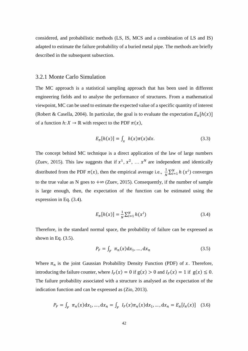
42
considered, and probabilistic methods (LS, IS, MCS and a combination of LS and IS)
adapted to estimate the failure probability of a buried metal pipe. The methods are briefly
described in the subsequent subsection.
3.2.1 Monte Carlo Simulation
The MC approach is a statistical sampling approach that has been used in different
engineering fields and to analyse the performance of structures. From a mathematical
viewpoint, MC can be used to estimate the expected value of a specific quantity of interest
(Robert & Casella, 2004). In particular, the goal is to evaluate the expectation 𝐸𝜋[ℎ(𝑥)]
of a function ℎ: 𝑋 → ℝ with respect to the PDF 𝜋(𝑥),
𝐸𝜋[ℎ(𝑥)] = ∫ ℎ(𝑥)𝜋(𝑥)𝑑𝑥𝑥
. (3.3)
The concept behind MC technique is a direct application of the law of large numbers
(Zuev, 2015). This law suggests that if 𝑥1, 𝑥2, … 𝑥𝑁 are independent and identically
distributed from the PDF 𝜋(𝑥), then the empirical average i.e., 1
𝑁∑ ℎ (𝑥𝑖)𝑁𝑖=1 converges
to the true value as N goes to +∞ (Zuev, 2015). Consequently, if the number of sample
is large enough, then, the expectation of the function can be estimated using the
expression in Eq. (3.4).
𝐸𝜋[ℎ(𝑥)] =1
𝑁∑ ℎ(𝑥𝑖)𝑁𝑖=1 (3.4)
Therefore, in the standard normal space, the probability of failure can be expressed as
shown in Eq. (3.5).
𝑃𝐹 = ∫ 𝜋𝑛(𝑥)d𝑥1, … ,𝐹
d𝑥𝑛 (3.5)
Where 𝜋𝑛 is the joint Gaussian Probability Density Function (PDF) of 𝑥 . Therefore,
introducing the failure counter, where 𝐼𝐹(𝑥) = 0 if g(𝑥) > 0 and 𝐼𝐹(𝑥) = 1 if g(𝑥) ≤ 0.
The failure probability associated with a structure is analysed as the expectation of the
indication function and can be expressed as (Zio, 2013).
𝑃𝐹 = ∫ 𝜋𝑛(𝑥)d𝑥1, … ,𝐹
d𝑥𝑛 = ∫ 𝐼𝐹(𝑥)𝜋𝑛(𝑥)d𝑥1, … ,𝐹
d𝑥𝑛 = 𝐸𝜋[𝐼𝜋(𝑥)] (3.6)

43
With respect to Eq. (3.6), the failure probability can be estimated using MCS as expressed
in Eq. (3.7).
𝑃𝐹 ≈ �̂�𝐹 =1
𝑁∑ 𝐼𝐹(𝑥
𝑖𝑁𝑖=1 ) (3.7)
In analysing the reliability of a structure, the standard measure of the accuracy of the
unbiased estimate of the probability of failure is the coefficient of variation (COV). COV
is a measure of the relative variability and can be defined as the ratio of the standard
deviation to the expected value of �̂�𝐹 , (i.e. 𝛿�̂�𝐹 = √𝑉[�̂�𝐹] 𝐸𝜋[�̂�𝐹]⁄ ) (Zuev, 2015). The
smaller the COV, the more accurate the method used to compute the failure probability.
Therefore, the COV for MCS can be estimated using
𝛿𝑀𝐶𝑆 = √1−�̂�𝐹
𝑁�̂�𝐹 (3.8)
MCS is a very convenient method to estimate the failure probability of a structure, but
the approach requires a significant sample size in order to simulate a small failure
probability. In this study, MCS is used to provide the benchmark result and validate the
outcome of the LS, IS and a combination of LS and IS.
3.2.2 Important Sampling (IS)
In the reliability analysis of a structural system, the estimation of a small failure
probability using MCS, that is, an unacceptable performance is often challenging because
of the required number of samples. Also, the computational process can be time-
consuming due to the sample size. As suggested in the literature, Important Sampling,
which is one of the most prevalent methods in the context of simulation can be used to
assess the reliability of a structure (Schuëller et al., 2004). The underlying theory is to
draw samples of the vector of random parameters from a distribution that is concentrated
in the ‘important region’ of the random parameter, which is the failure domain (Echard
et al., 2013). Based on the rules of IS and considering the weighting of the samples, IS
requires the definition of a joint PDF for the new sampling. Considering that the design
point 𝑥∗ can be identified by FORM, therefore, an auxiliary PDF denoted as the
importance density can be expressed as

44
ℎ𝑥(𝑥) = 𝑓𝑥(𝑥)|𝜇=𝑥∗ (3.9)
This means that the expression ℎ𝑥(𝑥) is similar to the original joint PDF 𝑓𝑥(𝑥) if the
mean values of the input variables is changed as the design point. Therefore, the failure
probability can be expressed as (Der et al., 1987; Echard et al., 2013)
𝑃𝐹 = ∫ 𝐼𝐹(𝑥)𝑓𝑛(𝑥)
ℎ𝑛(𝑥)ℝ𝑛ℎ𝑛(𝑥)𝑑𝑥1… 𝑑𝑥𝑛 (3.10)
Usually, the joint PDF is often taken in the standard space as an n-Gaussian one centred
in the most probable failure point (Echard et al., 2013). Since ℎ(. ) is a PDF, the integral
can be interpreted as an expectation. Therefore, the integral can be estimated using
𝑃𝐹 ≈ �̂�𝐹 =1
𝑁𝐼𝑆∑ 𝐼𝐹(�̃�
𝑖)𝑓𝑛(�̃�
𝑖)
ℎ𝑛(�̃�𝑖)
𝑁𝐼𝑆𝑖=1 (3.11)
The variance and the COV for the probability of failure can be estimated using the
expression in Eq. (3.12) and Eq. (3.13).
V[�̂�𝐹] =1
𝑁𝐼𝑆(
1
𝑁𝐼𝑆∑ (𝐼𝐹(�̃�
𝑖) (𝑓𝑛(�̃�
𝑖)
ℎ𝑛(�̃�𝑖))2
)𝑁𝐼𝑆𝑖=1 − �̂�𝐹
2) (3.12)
𝛿𝐼𝑆 =√V[�̂�𝐹]
�̂�𝐹 (3.13)
3.2.3 Line Sampling
3.2.3.1 General Concept
LS approach was developed by Schuëller et al. (2004) to estimate the reliability of a
structure with high dimension involving linear and non-linear problems. The method uses
lines instead of points to probe the failure space of interest and reduces a high dimensional
problem that is in standard normal space to a number of conditional one-dimensional
problems (Koutsourelakis et al., 2004; Pradlwarter et al., 2007). The conditional failure
probability of the structural systems is computed from the normal cumulative
distribution Φ(. ) (Schuëller et al., 2004). The efficiency of LS has been demonstrated in

45
the literature (Koutsourelakis et al., 2004; Pradlwarter et al., 2007) to estimate the
reliability of linear and non-linear systems associated with the random process.
For the analysis of a structure using LS, the vector 𝑥 = 𝑥1, 𝑥2, … , 𝑥𝑗 , … , 𝑥𝑛 ∈ ℝ𝑛 of an
uncertain parameter defined in the original space can be transformed into the vector
𝜃 ∈ ℝ𝑛 , where each element of the vector 𝜃𝑗 , 𝑗 = 1, 2, 3, … , 𝑛 is associated with the
standard Gaussian distribution (Koutsourelakis et al. 2004; Schuëller et al. 2004; Zio,
2013). Therefore, the joint PDF 𝜃𝑗 , 𝑗 = 1, 2, 3, … , 𝑛, of the random parameter can be
expressed as shown in Eq. (3.14)
φ(𝜃) =∏ 𝜙𝑗(𝜃𝑗)𝑛𝑗=1 (3.14)
Where 𝜙𝑗(𝜃𝑗) =1
√2𝜋𝑒−
𝑥𝑗2
2 , 𝑗 = 1, 2, 3, … , 𝑛. The mapping of the initial physical vector
𝑋 ∈ ℝn to the standard normal vector 𝜃 ∈ ℝ𝑛 is denoted as SXθ(. ) and the inverse
is SθX(. ) . The transformations of the physical space into standard normal space is
generally non-linear and can be obtained by applying Rosenblatt’s or Nataf’s
transformations (Huang & Du, 2006; Zio & Pedroni, 2010). Using transformation, the
limit state function gx(. ) of the structural system define in the physical space can be
transformed into gθ(. ) of the standard normal space.
3.2.3.2 Determination of the “Important Unit Vector”
The use of LS method requires the determination of an “important unit vector” 𝛼. In the
literature, three different methods are available for the determination of the important unit
vector. The methods are the design point direction, the gradient of performance function
in the standard normal space and the normalised centre of mass. For more information,
see (Koutsourelakis et al. 2004; Zio, 2013). Herein, the normalised centre of mass is used
because it provides a good approximation of the important domain of the failure space.
When using the normalised centre of mass approach, a point 𝜃0 , which falls within the
failure space 𝐹 is chosen. This point can be determined using MCS approach and
subsequently used as the initial point of a Markov chain since it lies entirely in the failure
domain. Because of this, a Metropolis–Hastings algorithm can be employed to evaluate a
sequence of 𝑁𝑠 points {𝜃𝑢, 𝑢 = 1, 2, 3, … , 𝑁𝑠} that lie within the failure domain
(Metropolis et al., 1953). The point taken from the failure domain is used as the initial

46
point of a Markov chain and Metropolis– Hastings algorithm is employed to generate a
sequence of 𝑁𝑠 points that lied in the failure domain. The Markov chain simulation
technique is used because it can accelerate the efficiency of exploring the failure region.
Then, the unit vector θu ∥ θu ∥⁄ , u = 1, 2, 3, … , 𝑁𝑠 are averaged to determine the
important unit vector as 𝛼 =1
𝑁𝑠∑ θu ∥ θu ∥⁄𝑁𝑠𝑢=1 as shown in Figure 3.1 (Koutsourelakis
et al., 2004). This method provides a good approximation of the important unit vector by
considering all the relevant samples within the failure region.
Figure 3.1: Important unit vector as the normalised “centre of mass”
3.2.3.3 Formulation of LS Method
Mathematically, the probability of the event F of a structural failure can be expressed as
a multidimensional integral as shown in Eq. (3.15)
𝑃𝐹 = P(𝜃 ∈ 𝐹) = ∫ 𝐼𝐹(𝜃)𝑞𝜃(𝜃)𝑑𝜃 (3.15)
F
𝑔𝜃(𝜃) > 0
“Centre of
mass” for the
failure domain
F
𝛼 =1
𝑁𝑠
𝜃𝑢
𝜃𝑢
𝑁𝑠
𝑢=1
𝜃0
𝜃𝑢
𝜃𝑁𝑠
𝑔𝜃(𝜃)
= 0
𝛼
𝜃2
0 𝜃1

47
Where 𝜃𝑗 , 𝑗 = 1, 2, 3, … , 𝑛 denotes the vector of uncertain input variables in the standard
normal space, 𝑞𝜃: ℝ𝑛 → [0, ∞) is the multidimensional PDF, 𝐹 ⊂ ℝ𝑛 is the failure
domain and 𝐼𝐹 ∶ ℝ𝑛 → {0, 1} is the indicator function. With no loss of generality, the
standard normal random variables in the direction of the important unit vector 𝛼 can be
assured by a suitable rotation of the axes (Koutsourelakis et al., 2004). Therefore, the
failure domain 𝐹 can be expressed alternatively as shown in Eq. (3.16)
𝐹 = {𝜃 𝜖 ℝ𝑛: 𝜃1 𝜖 𝐹1(𝜃2, … , 𝜃𝑛)} (3.16)
Where 𝐹1 is a function define in ℝ𝑛−1 and which takes values on the set of all subsets
of ℝ. Considering an example of a failure domain that corresponds to a performance
function as expressed in Eq. (3.17),
𝑔(𝜃) = 𝑔1(𝜃−1) − 𝜃1 ≤ 0 (3.17)
Where 𝜃−1 denotes the 𝑛 − 1 dimensional vector (𝜃2, … , 𝜃𝑛). In that case, 𝐹1(𝜃−1) is the
half open interval [𝑔1(𝜃−1),∞) (Koutsourelakis et al., 2004). Then, the function that are
similar to 𝐹1 can be defined with respect to any direction in the random parameter space
and for all measurable F. Therefore, combining Eq. (3.15) and Eq. (3.16), the probability
of failure can be expressed as (Koutsourelakis et al., 2004; Zio, 2013):
𝑃𝐹 = ∫ …𝑛
∫ 𝐼𝐹(𝜃)∏ ∅𝑗(𝜃𝑗)𝑑𝜃𝑛𝑗=1 (3.18)
= ∫ …𝑛−1
∫(∫ 𝐼𝐹(𝜃−1) ∅1(𝜃1)𝑑𝜃)∏ ∅𝑗(𝜃𝑗)𝑑𝜃−1𝑛𝑗=2 (3.19)
= ∫ …𝑛−1
∫Φ(𝐹1(𝜃−1))∏ ∅𝑗(𝜃𝑗)𝑑𝜃−1𝑛𝑗=2 (3.20)
= 𝐸𝜃−1[Φ(𝐹1(𝜃−1))] (3.21)
Where Φ(𝐴) = ∫ 𝐼𝐴(𝑥)𝜑(𝑥)𝑑𝑥 is called the Gaussian measure of A. From the Eq.
(3.21), an unbiased MC estimator of 𝑃(𝐹) can be computed as:
�̂�𝐹 =1
𝑁𝑇. ∑ Φ(𝐹1(𝜃−1
𝑘 ))𝑁𝑇𝑘=1 (3.22)

48
Where 𝜃−1𝑘 , 𝐾 = 1, 2, … , 𝑁𝑇 are independent and identically distributed samples in the
standard normal space. The variance of the estimator can be determined by the variance
of Φ(𝐹1(𝜃−1)). It is significant to note that the variance of the estimator takes values in
(0, 1) i.e. 0 ≤ Φ(𝐹1(𝜃−1)) ≤ 1 and Φ2(𝐹1(𝜃−1)) ≤ Φ(𝐹1(𝜃−1)), ∀𝜃−1 ∈ ℝ𝑛−1
(Koutsourelakis et al. 2004; Zio, 2013). This means:
𝑉𝑎𝑟[Φ(𝐹1(𝜃−1))] = 𝐸𝜃−1[Φ2(𝐹1(𝜃−1))] − 𝐸𝜃−1
2 [Φ(𝐹1(𝜃−1))] (3.23)
≤ 𝐸𝜃−1[Φ(𝐹1(𝜃−1))] − 𝐸𝜃−12 [Φ(𝐹1(𝜃−1))] (3.24)
= 𝑃𝐹(1 − 𝑃𝐹) = 𝑉𝑎𝑟[𝐼𝐹(𝜃)] (3.25)
From the derivation, the COV 𝛿𝐿𝑆 = √(𝑉𝑎𝑟[�̂�𝐹] )/𝑃𝐹 of the estimator in equation (3.22)
will be smaller when compare to standard MC (Δ𝑀𝐶) approach (Koutsourelakis et al.
2004; Zio, 2013). This means that the convergence rate that will be achieved using the
LS method will always be smaller than the MC method. The variance of the estimator �̂�𝐹
in LS will always depend on the variability of the random variables Φ(𝐹1(𝜃−1)) instead
of the probability content (Zio, 2013).

49
Figure 3.2: LS procedure
3.2.4 Methodology
The concept of LS, IS, MCS and a combination of LS and IS have been adapted in this
Chapter to estimate the time-dependent reliability of buried pipe and considering the
failure modes explained in Section 3.3 and 3.4. Figure 3.3 shows the flowchart of the
adapted LS method used in the analysis. However, the rationale for combining the LS and
IS techniques is to improve the efficiency of the approach for estimating the reliability of
a structure while considering the randomness associated with the structural parameters.
The computational procedure can be summarised as a two-stage process. The first stage
deals with the determination of the “important unit vector 𝛼” and the second stage
evaluates the probability of failure using the adapted method. The efficiency of the
method will depend on the determination of the important unit vector. Therefore, the
primary step is the searching of the optimal important unit vector and the drawing of the
F
𝑔𝜃(𝜃) > 0
𝑘𝑡ℎ conditional one dimensional
failure probability estimate
�̂�𝑘 = 1 − 𝛷(𝑐−𝑘) = 𝛷(−𝑐−𝑘)
𝛼,𝜃𝑘 𝛼
𝑔𝜃(𝜃)
= 0
𝛼 𝜃2
0 𝜃1
𝜃𝑘,⊥
𝜃𝑘
𝑙𝑘(𝑐𝑘, 𝛼)
𝑐−𝑘
𝑐3𝑘𝛼 + 𝜃𝑘,⊥
𝑐1𝑘𝛼 + 𝜃𝑘,⊥
𝑐2𝑘𝛼 + 𝜃𝑘,⊥

50
samples to estimate failure probability. The computational steps for the combined
methods are summarised briefly below.
1. Generate samples from the PDFs of the input parameters.
2. Using a standard MCS, sample 𝑁𝑇 vectors {𝑥𝑘: 𝐾 = 1,2,3,… , 𝑁𝑇} with 𝑥𝑘 =
{𝑥1𝑘, 𝑥2
𝑘, 𝑥3𝑘, … , 𝑥𝑗
𝑘, … , 𝑥𝑛𝑘 } from the multidimensional joint PDF 𝑞(. ): ℝ𝑛 →
[0, 1) of the input parameters.
3. The transformation of the input vectors. Transform the 𝑁𝑇 sample vectors
{𝑥𝑘: 𝐾 = 1,2,3, … ,𝑁𝑇} defined in the physical space into 𝑁𝑇 samples {𝜃𝑘: 𝐾 =
1,2,3, … ,𝑁𝑇} defined in the standard normal space where each component of the
random variables is associated with an independent central unit Gaussian standard
distribution.
4. In the standard normal space, evaluate the “important unit vector” 𝛼 =
(𝛼1, 𝛼2, … , 𝛼𝑗 , … 𝛼𝑛) that points towards the failure domain of interest, (see
Section 3.2.3.2 and Figure 3.1).
5. Once the “important unit vector” has been determined, then estimate a conditional
one-dimensional failure probabilities {�̂�𝐹𝑘: 𝐾 = 1,2,3, … ,𝑁𝑇} associated with 𝑁𝑇
vectors corresponding to each one of the standard normal samples {𝜃𝑘: 𝐾 =
1,2,3, … ,𝑁𝑇} . For each samples, {𝜃𝑘: 𝐾 = 1,2,3, … ,𝑁𝑇} that falls within the
failure domain, the following steps can be performed, see Figure 3.2.
a. For each sample vectors {𝜃𝑘: 𝐾 = 1,2,3,… , 𝑁𝑇}, determine a vector {�̃�𝑘, 𝐾 =
1,2,3, … ,𝑁𝑇} as the sum of a deterministic multiple of the important unit
vector 𝛼 and a vector 𝜃𝑘,⊥, 𝐾 = 1,2,3, … ,𝑁𝑇 that is perpendicular to the
direction of the important unit vector 𝛼. This can be expressed as:
𝜃𝑘 = 𝑐𝑘𝛼 + 𝜃𝑘,⊥ (3.26)
Where 𝑐𝑘 is a real number with values between −∞ 𝑎𝑛𝑑 +∞.
The relationship for the perpendicular direction is given as:
𝜃𝑘,⊥ = 𝜃𝑘 − 𝛼, 𝜃𝑘 𝛼 (3.27)
Where 𝜃𝑘: 𝐾 = 1,2,3, … ,𝑁𝑇 represents a random realisation of the input
variables and 𝛼, 𝜃𝑘 represents the scaler product between the unit vector 𝛼 and
the random variables 𝜃𝑘, 𝐾 = 1,2,3, … ,𝑁𝑇.

51
b. Calculate the value of 𝑐−𝑘 as the intersection between the limit state function
LSF 𝑔𝜃(�̃�𝑘) = 𝑔𝜃(𝑐
𝑘𝛼 + 𝜃𝑘,⊥) = 0 and the line 𝑙𝑘(𝑐𝑘, 𝛼) passing through
𝜃𝑘 and parallel to the important unit vector 𝛼. The value of 𝑐−𝑘 is determined
by fitting a first or second order polynomial and find its root. For each standard
normal random samples, two or three system performance evaluation is
required.
c. Estimate the conditional one-dimensional probability associated with each
random sample 𝜃𝑘, 𝐾 = 1,2,3, … , 𝑁𝑇 . The associated conditional failure
probability �̂�𝐹𝑘, 𝐾 = 1,2,3, … ,𝑁𝑇 is given as:
�̂�𝐹𝑘 = 𝑃[𝑁(0,1) > 𝑐−𝑘] = 1 − 𝑃[𝑁(0,1) > 𝑐−𝑘] (3.28)
= 1 − 𝛷(𝑐−𝑘) = 𝛷(−𝑐−𝑘) (3.29)
Where Φ(. ) designates the standard normal cumulative density function.
d. Becuase the values of the variables 𝑐−𝑘 follows a standard normal
distribution, the sampling can be carry out in the important domain, rather than
on the origin of the standard space. Therefore, the unbiased estimator of the
failure probability from the important domain �̂�𝐹𝑘, 𝐾 = 1,2,3, … , 𝑁𝑇 can be
estimated using Eq. (3.30).
�̂�𝑓𝑘 = (1 − 𝛷(𝑐−𝑘))
∑ �̂�𝑗(𝑐𝑘𝛼+𝜃𝑘,⊥)𝑒−(𝑐𝑘)2
2⁄𝑁𝑇
𝑗=1
∑ 𝑒−(𝑐𝑘)2
2⁄𝑁𝑇
𝑗=1
(3.30)
6. From the result of the conditional one-dimensional failure probability �̂�𝐹𝑘, 𝐾 =
1,2,3, … ,𝑁𝑇, calculate the failure probability and reliability of the structure using
Eq. (3.31) and Eq. (3.32).
𝑃𝐹 ≈ �̂�𝐹 =1
𝑁𝑇∑ �̂�𝑘(𝐹)𝑁𝑇𝑘=1 (3.31)
𝑃𝑅 = 1 − 𝑃𝐹 (3.32)

52
Figure 3.3: Flow diagram of the adapted LS method
Start
Transform the vectors from physical
space into standard normal space
{𝜃𝑘: 𝐾 = 1,2,3,… ,𝑁𝑇}
Estimate one-dimensional failure
probabilities {�̂�1𝐷,𝑘(𝐹):𝐾 =
1,2,3,… , 𝑁𝑇}
Calculate the unbiased estimator
𝑃𝐹 ≈ �̂�(𝐹) =1
𝑁𝑇
�̂�𝑘(𝐹)
𝑁𝑇
𝑘=1
End
Compute the unit important
direction 𝛼 from the standard
normal space 𝛼 =1
𝑁𝑠∑
𝜃𝑢
𝜃𝑢
𝑁𝑠𝑢=1
For each sample {𝜃𝑘:𝐾 =1,2,3,… , 𝑁𝑇}, determine a vector
{�̃�𝑘 , 𝐾 = 1,2,3,… ,𝑁𝑇} using �̃�𝑘 =
𝑐𝑘𝛼 + 𝜃𝑘,⊥
Evaluate
=
𝑔𝜃(𝑐𝑘𝛼 + 𝜃𝑘,⊥) = 0
𝑔𝜃(𝑐𝑘𝛼 + 𝜃𝑘,⊥) = 0
𝑔𝜃(𝑐𝑘𝛼 + 𝜃𝑘,⊥) = 0
Evaluate �̂�𝑘 = 1 −𝛷(𝑐−𝑘)
Determine the limit state
function in the standard
normal space
Sample 𝑁𝑇 vectors {𝑥𝑘: 𝐾 =
1,2,3,… , 𝑁𝑇} from the input PDF
Current
sample 𝜃1𝑢
Accept/Reject
Precan-
didate
𝜉𝑢+1
Candi-
date
state �̃�𝑢+1
Next
sample
𝜃𝑢+1
Accept/Reject
𝑃1∗(𝜉1|𝜃1
𝑢)
𝑃𝑛∗(𝜉𝑛|𝜃𝑛
𝑢)
𝑃𝑗∗(𝜉𝑗 𝜃𝑗
𝑢)
= 𝜃1𝑢 , . . . , 𝜃𝑗
𝑢, . . . , 𝜃𝑛𝑢
= 𝜉1𝑢+1 , . . . , 𝜉𝑗
𝑢+1, . . . , 𝜉𝑛𝑢+1
= �̃�1𝑢+1 , . . . , �̃�𝑗
𝑢+1, . . . , �̃�𝑛𝑢+1
= �̃�𝑢+1 𝑖𝑓 𝜃 𝑢+1 ∈ 𝐹𝑖
�̃�𝑢 𝑖𝑓 𝜃 𝑢+1 ∉ 𝐹𝑖
Use 𝜃0 as the initial point and
perform MCMC to generate
failure point

53
3.3 Application to Buried Pipe
The design of buried metal pipe can be a fairly complicated process due to the loading
conditions and the geo-environmental effects (Whidden, 2009). Stresses and strains can
develop as a result of the impact of load and will affect the performance of pipe over time.
For underground pipes under pressure, the impact of the load is usually classified into
two broad categories: internal pressure and external loads (Moser & Folkman, 2001). The
internal pressure is made up of the hydrostatic pressure and the surge pressure while the
external loads are those caused by external soil pressure or live loads (Moser & Folkman,
2001). The loads due to differential settlement, longitudinal bending, and shear loadings
are also considered to be external loads. Buried pipes are designed to sustain various loads
that are expected to affect the performance during the intended life.
Figure 3.4: (a) Flexible pipe and (b) Rigid pipe
The classification of the buried pipe is based on their behaviour during installation and
operation. Broadly, the buried pipe is classified as rigid or flexible pipe as shown in Figure
3.4 (Gabriel, 2011). The response of a rigid or flexible pipe to the external loads are
different. Therefore, the failure modes will be different as well. In this study, a buried
flexible metal pipe is considered. Cameron (2005) suggested that the amount of load a
pipe can sustain will depend on the relative height of cover, nature of the backfill material,
geometry of the trench and the relative stiffness of the pipe to the backfill. Similarly,
Marston load theory, as cited by Moser & Folkman (2001), shows that the amount of load

54
taken by a pipe will be affected by settlement or the relative movement of the backfill soil
and the nature of the pipe material.
As a result of the impact of the internal and external loads, failure of buried pipe will
occur when the applied stress (internal or external) exceeds the ultimate strength of the
pipe material. In this case, the applied stress represents the response of the input variables
𝑦 and the ultimate strength of the pipe material represents the critical value or
threshold 𝑦∗. In the literature such as Alliance (2001) and BS EN 1295:1 (1997) different
failure modes has been suggested for the design and assessment of buried pipeline.
However, it is vital to have an approach that will be used to identify the most critical
failure mode in order to avoid accidental economic loss and environmental pollution. The
most critical failure mode will have a more significant contribution to the failure of the
buried pipe structure. This study is concerned about a flexible buried pipe and the
associated dominating failure modes as defined in the literature (Alliance, 2001; Babu &
Srivastava, 2010; Sadiq et al., 2004). The failure modes include pipe ovality, through-
wall bending stress, buckling pressure, wall thrust, and total circumferential and axial
stress. These are succinctly explained in the following subsections.
3.3.1 Pipe Ovality
A buried pipe tends to resist the impact of live and earth load imposed on them, thereby
causing the pipe to ovalise due to the resulting stress from the external pressures as shown
in Figure 3.5. To analyse this effect, the Iowa deflection formula as defined in BS EN
1295:1 (1997) and BS 9295 (2010) can be modified to estimate the pipe ovality under the
influence of earth and live loads. The modified Iowa deflection formula is expressed in
Eq. 3.33. As stated in Gabriel (2011), the critical deflection for a flexible buried pipe can
be estimated using 5% - 7% of the inside diameter.
∆𝑦
𝐷=
𝐷1𝐾𝑃
(𝐸𝐼
𝑅3+0.061𝐸′)
(3.33)
Where ∆𝑦 = deflection of pipe in millimetre, 𝐾 = bedding constant, 𝑃 = the pressure on
pipe due to soil load plus live load i.e. (𝑃𝑣 + 𝑃𝑝), 𝑃𝑝 = pressure transmitted to the pipe as
a result of the concentrated load, 𝑃𝑣= pressure on pipe due to soil load, 𝐷1 = deflection

55
lag factor, 𝑅 = the radius of pipe, 𝐸 = the elastic modulus of pipe, 𝐼 = the moment of
inertia (𝑡^3/12) and 𝐸′ = the modulus of soil reaction and can be expressed as shown in
Eq. (3.34). The modulus of soil reaction 𝐸′ is a measure of the stiffness of the embedment
material surrounding the pipe.
𝐸′ = 𝐾′𝐸𝑠(1−𝑉𝑠)
(1+𝑉𝑠)(1−2𝑉𝑠) (3.34)
Where 𝑣𝑠 is the poison ratio of the soil, 𝐾′ is the numerical value which depends on
poison ratio and 𝐸𝑠 is the modulus of soil.
Buried pipes are also, predisposed to the action of concentrated or distributed live loads.
The effect of concentrated live load on the buried pipe can be enormous, for example,
locomotive loads, railway car, and truck wheel loads. In this situation, Alliance (2001)
stated that Boussinesq’s equation as expressed in Eq. (3.35), can be used to estimate the
pressure of the concentrated surface load exerted on the buried pipe.
𝑃𝑝 =3𝑃𝑠
2𝜋𝐶2[1+(𝑑
𝐶)2]2.5 (3.35)
Where 𝑃𝑝 = pressure transmitted to the pipe, 𝑃𝑠 = concentrated load at the surface, above
pipe, 𝐶 = the depth of soil cover above the buried pipe, 𝑑 = distance from the pipe to the
point of application of surface load.
Figure 3.5: Ovality of buried pipe

56
3.3.2 Through-wall Bending Stress
A buried pipe subjected to live and earth load and a continuous increase in bending will
fail due to increased ovalisation of the pipe cross-section and reduced slope in the stress-
strain curve (Tee & Khan 2014). The bending stress of a buried pipeline depends on the
dead and live loads acting on the pipe wall. For the safe performance of the buried pipe
throughout the design life, the induced through-wall bending stress should not go beyond
the tensile strength of the pipe material. Similarly, the induced longitudinal bending strain
should not exceed the allowable bending strain. For most buried metal pipe, the allowable
bending strain is between 0.15% - 2% and the allowable bending stress is the long-term
tensile strength of the pipe material (Alliance, 2001; Mohr, 2003)
Considering the impact of surface and earth loads, the through-wall bending stress
induced in the buried pipe, distributed as illustrated in Figure 3.6 can be calculated using
the relationship in Eq. (3.36) (Alliance, 2001; BS EN 1295-1:1997).
𝜎𝑏 = 4𝐸 (∆𝑦
𝐷) (
𝑡
𝐷) (3.36)
Where 𝜎𝑏 = through-wall bending stress, ∆𝑦 𝐷⁄ = pipe ovality.
Figure 3.6: Through-wall bending stress

57
3.3.3 Ring Buckling
Ring buckling or buckling pressure of the buried pipe depends on the total vertical
pressure (soil and surface load) that act on the pipe as illustrated in Figure 3.7 (Alliance,
2001). If the total vertical force is excessive, then the pipe can buckle in response to the
applied load. However, with the increase in the vertical pressure, there will be a
corresponding increase in the tangential compressive stress, and this will get to a state
where the pipe will not be able to keep its initial circular shape and buckle as a result.
Ring buckling of buried pipe can occur due to the insufficient stiffness of the pipe
(AWWA, 1999). For the safe performance of buried pipe, the actual buckling pressure
must be less than the critical buckling pressure. Based on the impact of the live and earth
load, the actual and critical buckling pressure can be estimated using Eq. (3.37) and Eq.
(3.38) (AWWA, 1999).
𝑃𝑎 = 𝑅𝑤𝛾𝑠 + 𝛾𝑤𝐻𝑤 + 𝑃𝑠 (3.37)
𝑃𝑐𝑟 = √(32𝑅𝑤𝐵′𝐸𝑠𝐸𝐼
𝐷3) (3.38)
Where 𝑅𝑤 is the water buoyancy factor which can be expressed as 𝑅𝑤 = 1 −
0.33(𝐻𝑤/𝐻), 𝐸𝑠 is the modulus of soil, 𝐻𝑤 is the height of ground water above the pipe
and 𝐵′ is the empirical coefficient of elastic support which can be expressed as 𝐵′ =
1/(1 + 4e−0.213𝐻).
Figure 3.7: Ring buckling

58
3.3.4 Wall Thrust
Wall thrust or crushing of pipe wall is characterised with localised yielding and occurs
when the induced wall stress reaches the yield stress of the pipe material. A buried
pipeline can crush due to earth and surface loading acting on the pipe if burial depth is
not enough (Gabriel 2011). Considering the effect of dead and live load, Gabriel (2011)
suggested two conditions for analysing the wall thrust and they are as follows:
Use short-term material properties if both dead and live loads need to be
accounted for;
Use long-term material properties if only dead load needs to be accounted
for.
Based on the two conditions, the more conservative limit state function value would be
considered for wall thrust analysis. Note that some flexible pipes have both short-term
and long-term material properties (elasticity of modulus), where the short-term value is
higher than long-term value, e.g., polyethylene pipe (Gabriel, 2011). In this case, the two
conditions will be required to analyse the performance of the pipe based wall thrust.
However, for metal pipes, e.g., ductile iron or steel pipe, only the first condition is
considered for the assessment because the short-term and long-term properties of the pipe
material are the same (Gabriel, 2011). The critical and the actual wall thrust can be
evaluated using Eq. (3.39) and Eq. (3.40) respectively (Gabriel, 2011).
𝑇𝑐𝑟 = 𝐹𝑦𝐴𝑠𝜑𝑝 (3.39)
𝑇𝑎 = 1.3(1.5𝑊𝐴 + 1.67𝑃𝑠𝐶𝐿 + 𝑃𝑊)(𝐷𝑜 2⁄ ) (3.40)
Where 𝐹𝑦 denotes the minimum tensile strength of pipe, 𝐴𝑠 = the cross- sectional area of
pipe wall per unit length and 𝜑𝑝 = the capacity modification factor for pipe. 𝐷𝑜 = the pipe
outside diameter, 𝐶𝐿 = live load distribution coefficient (the lesser of 𝐿𝑊 𝐷𝑜⁄ or 1.0),
𝐿𝑊 = live load distribution width. The loads acting on the pipe considered in wall thrust
analysis are soil arch load 𝑊𝐴 , live load, 𝑃𝑠 and hydrostatic pressure 𝑃𝑊. The soil arch
load and hydrostatic pressure can be calculated using Eq. (3.41) and Eq. (3.42).
𝑊𝐴 = 𝑃𝑠𝑝𝑉𝐴𝐹 (3.41)
𝑃𝑊 = 𝛾𝑠𝐻𝑤 (3.42)

59
Where 𝑃𝑠𝑝 = geostatic load (𝑃𝑠𝑝 = 𝛾𝑠(𝐻 + 0.11𝑥10−7(𝐷𝑜)) , 𝑉𝐴𝐹 = vertical arching
factor 𝑉𝐴𝐹 = 0.76 − 0.71(𝑆ℎ−1.17
𝑆ℎ+2.92), 𝑆ℎ = the hoop stiffness factor (𝑆ℎ = 𝜑𝑠𝑀𝑠 𝑅 𝐸𝐴𝑠)⁄ ,
𝜑𝑠 = soil capacity modification factor, 𝑀𝑠 = secant constrained soil modulus, 𝑅 = the
effective radius of pipe.
Figure 3.8: Wall thrust
3.4 Total Circumferential/Axial Stress
The pressurised underground pipeline can continuously be exposed to the action of both
external and internal forces. The forces includes soil/earth load, traffic/vehicular load
(such loads may be from the roadway or railway), the load due to frost action, internal
fluid pressure, and stress due to thermal effect (Sadiq et al., 2004). The adverse impact of
these forces needs consideration at the design stage. The stress produced by the internal
pressure is considered due to uniform circumferential tension generated across the inner
wall of the pipe. For pressurised buried pipelines, the primary stress is produced by
internal pressure (Amirat et al., 2006). Also, the influence of other different forces as
explained in Section 3.3.1 to 3.3.4 can be considered in the analysis of buried pipeline.
Amirat et al. (2006) suggested that internal pressure of a buried pipe produces a uniform
circumferential tension across the pipe wall, while external loads may produce bending
stress in longitudinal and circumferential directions.
The external forces acting on a pressurised pipe can produce stresses in both
circumferential and axial direction (Sadiq et al., 2004). However, Ahammed & Melchers
(1994) suggested that if a pipe is loaded uniformly and supported along its length, then

60
circumferential stresses could be more important than axial stresses. Internal fluid
pressure produces the circumferential bending stresses in a pipe wall (due to external
loads) in addition to the tensile hoop stress. Rajani et al. (2000) suggested a method for
estimating the total external stresses including all circumferential and axial stresses acting
on a buried pipeline. These stresses are shown in Table 3.1. As defined in Rajani et al.
(2000), the circumferential stress 𝜎𝜃 acting on the buried pipe can be expressed as shown
in Eq. (3.43).
𝜎𝜃 = 𝜎𝐹 + 𝜎𝑆 + 𝜎𝐿 + 𝜎𝑉 (3.43)
Where 𝜎𝐹 = stress due to internal fluid pressure; 𝜎𝑆 = stress due to external soil loading;
𝜎𝐿 = stress due to frost pressure and 𝜎𝑉 = stress due to traffic/vehicular load.
Similarly, the axial stress 𝜎𝑋 acting on the pipe can be expressed as shown in Eq. (3.44).
𝜎𝑋 = 𝜎𝑇 + (𝜎𝐹/+ 𝜎𝑆 + 𝜎𝐿 + 𝜎𝑉)𝑣𝑝 (3.44)
Where 𝜎𝑇 = stress as a result of a temperature difference; 𝜎𝐹/ = axial stress due to internal
fluid pressure and 𝑣𝑝 = Poisson’s ratio of the pipe material.

61
Table 3.1: Summary of stresses/pressures acting on the buried pipe
Stresses acting
on Buried Pipe
Model Parameters description
Circumferential
stress due to
internal fluid
pressure 𝝈𝑭
𝜎𝐹 = 𝜌𝐷/2𝑡
Rajani et al. (2000)
𝜌 = internal fluid pressure (MPa);
𝐷 = pipe diameter; 𝑡 = pipe
thickness
Stress due to
external soil
loading 𝝈𝑺
𝜎𝑆 =3𝐾𝑚𝛾𝐵𝑑
2𝐶𝑑𝐸𝑝𝑡𝐷
𝐸𝑝𝑡3 + 3𝐾𝑑𝜌𝐷3
Ahammed and Melchers
(1994)
𝐾𝑚 = bending moment
coefficient; 𝛾 = unit weight of the
backfill soil; 𝐵𝑑 = width of ditch;
𝐶𝑑= calculation coefficient for
earth load; 𝐸𝑝= modulus of
elasticity of pipe material (MPa);
𝐾𝑑 = deflection coefficient
Stress due to
frost action 𝝈𝑳
𝜎𝐿 = 𝑓𝑓𝑟𝑜𝑠𝑡𝜎𝑠
Rajani et al. (2000)
𝑓𝑓𝑟𝑜𝑠𝑡 = frost load multiple; 𝜎𝑆 =
stress due to external soil loading
Stress due to
traffic load 𝝈𝑽
𝜎𝑉
=3𝐾𝑚𝐼𝑐𝐶𝑡𝐹𝐸𝑝𝑡𝐷
𝐴(𝐸𝑝𝑡3 + 3𝐾𝑑𝜌𝐷3)
Ahammed and Melchers
(1994)
𝐼𝑐= impact factor; 𝐶𝑡 = surface
load coefficient; 𝐹 = wheel load
on surface (N); 𝐴 = effective
length of pipe which the load is
computed;
Stress due to
temperature
difference 𝝈𝑻
𝜎𝑇 = −𝐸𝑝𝛼𝑝∆𝑇 − 𝑣𝜎ℎ
Rajani et al. (2000)
𝛼𝑝 = expansion coefficient of
pipe; ∆𝑇 = temperature difference
between the fluid and the
surrounding group; 𝑣 = poison
ratio;
Axial stress due
to internal fluid
pressure 𝝈𝑭/
𝜎𝐹/=𝑣𝑝
2𝜌 (
𝐷
𝑡− 1)
Rajani et al. (2000)
𝑣𝑝 = poison ratio of the pipe
material

62
3.5 Pipe Corrosion
The gradual loss of pipe thickness as a result of corrosion can be relatively uniform or
localised (Ahammed & Melchers, 1997; Sadiq et al., 2004). The rate of corrosion in
uncoated CI pipes is generally high in early age (Sadiq et al., 2004). The corrosion of
underground pipe is a time-variant process, which depends on external factors such as
geo-environmental conditions and internal factors such as chemical composition of the
transported fluid and could be influenced by temperature and flow rate (Mahmoodian &
Li, 2017; Ossai et al., 2015). In the literature, the power law formula as expressed in Eq.
(3.45), can be used for representing both localised and general (uniform) corrosion (Sadiq
et al., 2004).
𝐶𝑇 = 𝑘𝑇𝑛 (3.45)
Where 𝑘 and 𝑛 are empirical constants (𝑛 ≤ 1); and 𝑇 represents the time of exposure.
The rate of corrosion can be calculated from Eq. (3.45) by differentiating with respect to
time. In the literature, the rate of corrosion using Eq. (3.45) has been found to be relatively
high at the beginning of the damage process and attenuates gradually as the service age
increases (Engelhardt & Macdonald, 2004; Wang et al., 2015). As a result, Engelhardt &
Macdonald (2004) suggested a corrosion rate model as shown in Eq. (3.46)
𝑑(𝐶𝑇)
𝑑𝑡= 𝑉0 (1 +
𝑇
𝑇0)𝑛−1
(3.46)
Where 𝑉0 denotes the initial corrosion rate, and 𝑇0 represents constant which has the
effect on the time interval for reaching a stable corrosion rate.
The rate of corrosion as expressed in Eq. (3.46) considers the early stages of corrosion,
and when the metal is exposed to a relatively high concentration of corrosive species
(Wang et al., 2015). However, it requires the determination of the initial corrosion rate.
The depth and location of a possible indicator of corrosion can be measured and obtained
through the use of magnetic flux leakage (MFL) or ultrasonic tools (UTs). Wang et al.
(2015) suggested that because of the cost associated with the direct inspection, which is
typically scheduled at different times, it is highly impractical to apply the technology to

63
obtain the initial corrosion rate. Rajani et al. (2000) proposed a two-phase model
expressed in Eq. (3.47).
𝐶𝑇 = 𝑎𝑇 + 𝑏(1 − 𝑒−𝑐𝑇) (3.47)
Where 𝑎 is the final pitting rate constant (typical value; 0.009 mm/yr); 𝑏 represents the
pitting depth scaling constant (typical value; 6.27 mm); 𝑐 is corrosion rate inhibition
factor (typical value; 0.14 yr-1 ) and 𝑇 is the time.
The effect of corrosion reduces pipe thickness over time. Therefore, pipe thickness
expressed in all the considered failure modes are replaced with a residual pipe thickness.
The residual pipe thickness is the original pipe thickness minus the corrosion model. In
this study, the effect of corrosion is assumed to be uniform over the pipe surface area.
Corrosion of buried pipeline is one of the most critical factors that contribute to the failure
of buried steel pipe. It can occur both internal and external. External corrosion occurs at
the outer surface of the pipe, and it is the most common form of deterioration of the buried
pipeline. The level of the impact of external corrosion on buried pipeline depends on the
surrounding environmental condition and the material properties of the pipe. Internal
corrosion occurs inside the pipe. However, the effect is minimal when compared to the
external corrosion. Figure 3.9 shows an example of internal and external corrosion data
for a buried iron pipe as defined in (Marshall, 2001). Based on Figure 3.9, it can be
deduced that external corrosion is higher than internal corrosion and in both, the rate of
corrosion is high at the early stage.

64
Figure 3.9: Internal and external corrosion rate for iron pipe
Table 3.2: Limit state functions for the failure modes
Failure mode Limit state
Pipe ovality 𝐺𝑃𝑖𝑝𝑒 𝑜𝑣𝑎𝑙𝑖𝑡𝑦 = 6% −
∆𝑦
𝐷
Through-wall bending
stress
𝐺𝐵𝑒𝑛𝑑𝑖𝑛𝑔 𝑠𝑡𝑟𝑒𝑠𝑠 = 𝜎𝑦 − 𝜎𝑏
Ring buckling 𝐺𝑅𝑖𝑛𝑔 𝑏𝑢𝑐𝑘𝑙𝑖𝑛𝑔 = 𝑃𝑐𝑟 − 𝑃𝑎
Wall thrust 𝐺𝑊𝑎𝑙𝑙 𝑡ℎ𝑟𝑢𝑠𝑡 = 𝑇𝑐𝑟 − 𝑇𝑎
Total circumferential
stress
𝐺𝑇𝑜𝑡𝑎𝑙 𝑐𝑖𝑟𝑐𝑢𝑚𝑓𝑒𝑟𝑒𝑛𝑡𝑖𝑎𝑙 𝑠𝑡𝑟𝑒𝑠𝑠
= 𝜎𝑦 − 𝜎𝜃
Total axial stress 𝐺𝑇𝑜𝑡𝑎𝑙 𝑎𝑥𝑖𝑎𝑙 𝑠𝑡𝑟𝑒𝑠𝑠 = 𝜎𝑦 − 𝜎𝑋
3.6 Limit State Function
The reliability analysis of an engineering structure requires the limit state function to
evaluate the performance of the structure. In this study, the method of reliability analysis

65
is applied to a buried pipeline made of steel and considered to be buried under a roadway.
The maximum applied load during the lifetime of the buried pipe is considered to be the
traffic wheel load. However, the effect of the cyclic loading is not considered. The
reliability analysis is carried out through the study of the failure modes as explained in
Section 3.3 and Section 3.4. In all cases, the limit state function that corresponds to the
safety of the pipe structure as defined in the literature is shown in Table 3.2. As reported
in Table 3.2, the limit state function for a particular failure mode can be expressed as
shown in Eq. (3.48). If the outcome of the limit state is positive, that is ( 𝑅 > 𝑆(𝑥)), then
it signifies a safe state and if it is negative, then it indicates a failure state (𝑅 < 𝑆(𝑥)) and
the limit state is denoted as 𝑔(𝑥) = 0.
𝑔(𝑥) = 𝑅 − 𝑆(𝑥) (3.48)
Where 𝑅 represents the strength or resistance; 𝑆(𝑥) is the load term defined in terms of
random variables.
From the limit state function, one can evaluate the failure probability of an engineering
structure by running some random samples to generate different pipeline realisations.
Then, use a Monte Carlo (MC) technique to estimate the probability of failure. However,
the use of the MC approach requires a large number of samples, especially when there is
a need to determine a small failure probability. In order to reduce the computational effort,
advanced MCS are often used.
3.7 Numerical Example
In this example, a pressurised and underground steel pipe is examined and is considered
to be located under a roadway where the groundwater table can rise above or stay below
the buried pipe. The buried pipe is considered to be exposed to corrosion and stresses
from live and earth loads. The pipeline had a diameter of 1.21 m and the pipe wall
thickness of 21.0 mm and considered to be under a heavy traffic condition with a wheel
load of 80 kPa. The remaining numerical values of pipe and soil properties used in the
analyses are listed in Table 3.3 and Table 3.4. The values of the parameters are based on
industry standard and have been acquired from the literature such as Ahammed and
Melchers (1994, 1997); Sadiq et al. (2004); and Tee et al. (2014). This example is to

66
illustrate the confidence level in the analysis of buried pipeline under the influence of
internal and external stresses and to demonstrate the efficiency of the combined approach.
Table 3.3: Statistical properties of the input parameters
Material properties Mean Standard deviation
Elastic modulus of pipe 𝑬𝒑 213.74x10⁶ kPa
(normal)
2.1374x10⁶ kPa
Backfill soil modulus 𝑬𝒔 103kPa (normal) 50 kPa
Unit weight of soil 𝜸𝒔 18.0kN/m3 (normal) 0.45 kN/m3
Wheel load (live load) 𝑷𝒔 150 kN (normal) 15 kN
Thickness of pipe t 0.021 m (normal) 0.00021
Height of backfill H 3.75 m (normal) 0.00375
Internal diameter 0.64 m (normal) 0.01143
Bending moment coefficient
𝑲𝒎
0.235 (lognormal) 0.05
Deflection coefficient 𝑲𝒃 0.108 (lognormal) 0.0216
Calculation coefficient 𝑪𝒅 1.32 (lognormal) 0.20
Surface load coefficient 𝑪𝒕 0.12 (lognormal) 0.024
Width of ditch 𝑩𝒅 0.5 m (normal) 114.3 m
Pipe effective length 𝑨 6.1 m (normal) 0.2 m
Concentrated live load 80 kPa (normal) 2.4 kPa
Internal pressure 𝝆 0.45 MPa (normal) 0.12
Multiplying constant 𝒌 2.0 (normal) 0.1
Exponential constant 𝒏 0.3 (normal) 0.015
In this study, the relationship expressed in Eq. (3.45) is used to model corrosion. Based
on this, the wall thickness t which is a variable in the equations for modelling various
pipe failure modes is replaced with residual wall thickness. This means as the time of
exposure increases, and in consideration of corrosion effect, the thickness of the pipe wall
decreases and the reliability of the buried pipe also decreases. The corrosion effect is
assumed to be uniform over the entire surface area of the pipe and that the pipe is thin-

67
walled and circular. The bending moment coefficient 𝐾𝑚 and deflection coefficient 𝐾𝑏
depends on the distribution of the applied stress across the top of the pipe and the
distribution of the generated reaction across the bottom of the pipe (Ahammed &
Melchers, 1997). The deflection coefficient 𝐾𝑏 accounts for the bedding support which
varies with the bedding angle.
Table 3.4: Material properties of the input parameters
Material properties Value Min Max
Temperature differential - -10.0 (uniform) 0
Frost load multiplier 𝒇𝒇𝒓𝒐𝒔𝒕 - 0 (uniform) 1
Thermal coefficient of pipe 11 x 10−6 - -
Height of water above buried
pipe
1.0 m - -
Unit weight of water 𝜸𝒘 9.81 kN/m3 - -
Yield strength 𝝈𝒚 475 MPa - -
Buoyancy factor 𝑹𝒘 1.0 - -
Trench width 𝑩𝒅 2.0 m - -
Shape factor 𝑫𝒇 4.0 - -
Deflection lag factor 𝑫𝑳 1.0 - -
Capacity modification factor
for soil 𝝋𝒔
0.9 - -
Capacity modification factor
for pipe 𝝋𝒑
1.0 - -
Live load distribution
coefficient 𝑪𝑳
1.0 - -
Poison ratio 𝒗𝒔 0.3 - -
𝒌′ value 1.5 - -
Allowable strain 𝜺𝒄𝒓 0.2 % - -

68
3.8 Results and Discussion
The failure probability of buried pipe is determined based on the total axial stress and the
through-wall bending stress due to pipe ovality. The power law formula as expressed in
Eq. (3.45) is used in the computation to account for the corrosion effect, which denotes
both localised and general (uniform) corrosion. The outcome of the MCS method is
referred to as the benchmark and is used to validate the accuracy of the other methods
such as LS, IS and a combination of LS and IS. The methods were used to evaluate the
reliability of buried pipe by considering the adverse effect of corrosion and the
uncertainties that exist with the pipe and soil parameters. For the through-wall bending
stress, the concentrated live load effect is obtained using Boussinesq’s equation to
estimate the pressure of the load on the buried pipe. The failure criterion utilised in this
study is based on the yield stress of the steel pipe, and the impact of the seasonal change
in the groundwater table is considered in the analysis.
The outcome based on the various methods have been compared with the combined
approach, and Table 3.5 shows the result. From the study, the combined method uses a
total of 𝑁𝑇 = 500 samples, while LS uses a total of 𝑁𝑇 = 600 samples, IS uses a total of
𝑁𝑇 = 10000 samples and MCS uses a total of 𝑁𝑇 = 100,000 samples, to achieve a
small failure probability that is close to 10−3. The number of samples are considered for
the purpose of evaluating and validating the failure probability of buried pipeline. Also,
the various methods have been compared using a numerical index, which is called the
“unitary coefficient of variation 𝛿𝑢” as defined in Zio (2013). The 𝛿𝑢 can be expressed
as 𝛿𝑢 = 𝛿.√𝑁𝑇 =𝜎
�̂�(𝐹). √𝑁𝑇, where 𝜎 is the standard deviation, 𝛿 denotes the coefficient
of variation and �̂�(𝐹) represent the estimate of the probability of failure. For all structural
reliability methods, which is based on MCS technique for estimating the probability of
failure, the standard deviation decays with the rate (1 √𝑁𝑇⁄ ) and 𝛿𝑢 is independent of the
total number of sample 𝑁𝑇 (Zio, 2013). This means that the smaller the value of unitary
coefficient of variation 𝛿𝑢, the variability of the failure probability estimator will be lower
and as a result, the higher the efficiency of the simulation approach. Therefore, the small
number obtained using a combination of LS and IS demonstrates the efficiency and
robustness of the method. Table 3.5 reports the outcome, which shows the efficiency of
the combined approach compared to others. As a result, it can be stated that the combined

69
approach maintains a considerable improvement with regards to efficiency over MCS, IS
and LS when used independently.
Table 3.5: Failure probability of buried pipe due to total axial stress
Methods Failure condition
Total axial stress acting on buried pipeline
𝑃𝑓 𝛿𝑢
MCS 3.1 x 10⁻³ 1.42
IS 2.7 x 10⁻³ 0.36
LS 2.2 x 10⁻³ 0.073
LS & IS 2.0 x 10⁻³ 0.018
The impact of a seasonal change in groundwater level is performed considering the
through-wall bending stress induced on the buried pipe due to pipe ovality. In practice,
this effect is often ignored and in most cases assumed to be inconsequential. Herein, the
study examines the implications of having the underground water table located below and
also, above the buried pipe. Figure 3.10 shows the outcome of this investigation, which
is time dependent. As can be seen, having the underground water table above the buried
pipeline can increase the possibility of pipe failure. Based on Figure 3.10, the probability
of failure started from 25 years when the underground water table is located below the
buried pipe, whereas it started from 18 years when the location of the underground water
table is above the buried pipe. The result shows that the rise in the underground water
table above the buried pipe can affect its performance by increasing the probability of
failure.

70
Figure 3.10: Probability of failure by considering water table above and below
buried pipe
Figure 3.11: Probability of failure by considering undisturbed soil and
underground water table
0 50 100 150
10-2
10-1
100
Time (years)
Pro
ba
bilty
of
failu
re
Buried pipe above water table
Buried pipe below water table
0 50 100 150
10-2
10-1
100
Time (years)
Pro
ba
bilty
of
failu
re
Buried pipe above water table
Buried pipe below water table
Buried pipe in an undisturbed soil

71
Furthermore, another reliability assessment is performed by considering a situation
whereby the buried pipe is jacked into an undisturbed soil as defined by (Moser &
Folkman, 2001). In this case, the buried pipe is assumed to be jacked into an undisturbed
soil as an alternative to being placed in a trench. As a result, the friction and cohesion of
soil on the buried pipe are significantly reduced as against situation where there is a prism
load resting on the buried pipe. The result of this and combined with the water table effect
is illustrated in Figure 3.11. Again, the result indicates a high reduction in the probability
of failure as compared to an open trench where the backfill soil is resting on the buried
pipe.
3.8.1 Parametric Studies
The effect of corrosion empirical constants and soil parameters on the performance of a
buried pipeline have been investigated through parametric studies based on the failure
modes of total axial stress and through-wall bending stress. Sadiq et al. (2004) suggested
that the parameters that have the greatest effect could be those for which a decrease in the
level of uncertainty, would add to reducing the most significant amount of the uncertainty
of the output results. However, this study will assist to identify critical parameters that
affect the performance of buried pipe and the parameters used include the multiplying
constant 𝑘, the exponential constant 𝑛, bending moment coefficient 𝐾𝑚 and deflection
coefficient 𝐾𝑏.
In Figure 3.12 and Figure 3.13, the contribution of the multiplying constant 𝑘 and the
exponential constant 𝑛 on the failure probability of the buried pipe over time are analysed.
The analysis is performed by changing the values of the corrosion parameters (𝑘 and 𝑛)
in order to evaluate their impact on the probability of failure. In Figure 3.12, it can be
deduced that any changes which results in an increase in the values of the 𝑘 (from 1.8 to
2.4) will correspondingly increases the possibility of pipe failure over time. This scenerio
can be visualised by considering different service years between 0 to 150 years. This is
expected because the higher the values of 𝑘 , the greater is the degree of corrosion
penetration which increases the probability of pipe failure. Similarly, Figure 3.13 shows
that a reduction in the values of 𝑛 (from 0.3 to 0.2) could reduce the possibility of pipe
failure over time. Again, this effect is evident by looking at different service years

72
between 0 to 150 years. The two outcome demonstrate the key roles of corrosion
empirical constants 𝑘 and 𝑛 in estimating the failure probability of a corroded, buried
pipeline. Also, the parametric effects of the corrosion empirical constants as reported in
Figure 3.12 and Figure 3.13 shows the dynamic and variable nature of corrosion. Thus, a
good understanding of the corrosion would provide a useful and better analysis of the
reliability of buried pipe.
Figures 3.14 and 3.15 report the impact of the bending moment 𝐾𝑚 and deflection
coefficients 𝐾𝑏 on the reliability of buried pipe over time. In Figures 3.14, the effect of
reasonably varing the values of the bending moment coefficient 𝐾𝑚 is reported and the
outcome shows that the small failure probability increases with an increase in 𝐾𝑚 at
different service years between 0 to 150 years. This scenerio is expected because if the
values of 𝐾𝑚 is high, the bending moment could be high and stress that is induced in the
buried pipe will result in higher failure probability. For the deflection coefficients 𝐾𝑏, a
change in the values results to an insignificant change in the failure probability as shown
in Figures 3.15.
Figure 3.12: The effect of different k values on probability of failure over time
0 50 100 150
10-2
10-1
100
Time (years)
Pro
ba
bilty
of
failu
re
k = 1.8
k = 2.0
k = 2.2
k = 2.4
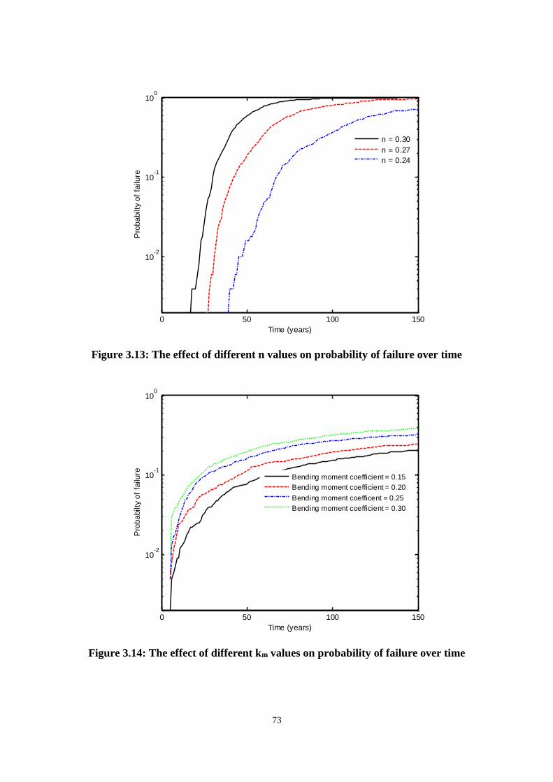
73
Figure 3.13: The effect of different n values on probability of failure over time
Figure 3.14: The effect of different km values on probability of failure over time
0 50 100 150
10-2
10-1
100
Time (years)
Pro
ba
bilty
of
failu
re
n = 0.30
n = 0.27
n = 0.24
0 50 100 150
10-2
10-1
100
Time (years)
Pro
ba
bilty
of
failu
re
Bending moment coefficient = 0.15
Bending moment coefficient = 0.20
Bending moment coefficent = 0.25
Bending moment coefficient = 0.30

74
Figure 3.15: The effect of different kd values on probability of failure over time
3.9 Chapter Summary
In this Chapter, the reliability analysis of buried pipeline is investigated considering the
effect of aleatory uncertainty that is associated with pipe, soil and corrosion parameters.
The failure probability of buried pipe is estimated using an advanced MCS method such
as LS, IS and a combination of LS and IS. The concepts behind the methods are explained,
and the procedure for the implementation of the combined approach are outlined. The
methods are used to estimate the failure probability of buried pipeline subjected to
structural failure modes of total axial stress and through-wall bending stress based on
point load considering the impact of corrosion. The results obtained from the methods
have been compared with the MCS approach for the purpose of estimating small failure
probability. The choice of using the MCS method as a benchmark and for the validation
of the results is due to its general acceptance and efficiency in estimating the failure
probability of an engineering structure.
Also, the effect of groundwater table located below and above the buried pipe is
investigated, and the outcome indicates that undermining this effect could adversely
0 50 100 150
10-2
10-1
100
Time (years)
Pro
ba
bilty
of
failu
re
Deflection coefficient = 0.08
Deflection coefficient = 0.10
Deflection coefficient = 0.12
Deflection coefficient = 0.14

75
decrease the design life of the pipe. Furthermore, another assessment is performed by
considering a situation whereby the buried pipe is jacked into undisturbed soil. In this
case, the buried pipe is considered to be jacked into an undisturbed soil where the friction
and cohesion of soil on the buried pipe are significantly reduced. The result shows a
significant reduction in the probability of failure as compared to an open trench where the
backfill soil is resting on the buried pipe. The result from the parametric studies shows
the dynamic and variable nature of corrosion empirical constants, which indicates that a
slight change in the numerical values can have a significant impact on the pipe failure
probability. Considering the impact of uncertain variables, a fuzzy-based robustness
assessment is presented in Chapter 4 to analyse the robustness behaviour of buried
pipeline. The method is based on the principles of robustness measure, fuzzy set theory,
interval analysis, and Shannon’s entropy. In Chapter 4, both aleatory and epistemic type
of uncertainty are considered.

76
CHAPTER FOUR
4 FUZZY-BASED ROBUSTNESS ASSESSMENT OF
BURIED PIPE

77
4.1 Introduction
The design of buried pipe structure is associated with uncertainties due to randomness
and fuzziness (or vagueness) that exist in the structural parameters. The occurrence of
randomness or fuzziness can be due to manufacturing errors, measurement errors, and
scarceness of information concerning the determination of the input parameter. The
presence of uncertainties has influenced negatively the performance of buried pipe over
time. As a result, it is indispensable to evaluate the performance of the buried pipe
structure by considering the impact of the associated uncertainties.
In this Chapter, a fuzzy-based robustness assessment of buried pipelines is proposed
considering the randomness (aleatory uncertainty) and fuzziness (epistemic uncertainty)
that exist in the structural parameters. The approach utilises the principles of robustness
measure, fuzzy set theory, interval analysis and Shannon’s entropy, which permits the
inclusion of random and fuzzy variables in the quantification of the uncertainty associated
with the performance of buried pipe. Zhang et al., (2015) suggested that robustness
measures analyse robustness as a property of the structure rather than damage. Herein,
robustness is used as a measure to assess the ability of buried pipe to sustain damage that
may be caused by extreme loads or changes in environmental conditions without
disproportionate failure. Therefore, a pipe structure is considered to be robust if it can
survive some extreme conditions such as exceptional overloading, unforeseen events, and
adverse environmental conditions without any substantial loss of safety and
serviceability.
The rest of this Chapter is arranged as follows. Section 4.2 explains an overview of fuzzy
set and fuzzy uncertainty. Section 4.3 gives a review of the literature concerning the
concepts of robustness measure. Section 4.4 provides the application to buried pipe,
which includes the structural failure modes, a numerical example and the damage
modelling of buried metal pipe under uniform corrosion. Section 4.5 discusses the results,
and significant findings from the study and Section 4.6 provides the Chapter summary.

78
4.2 Fuzzy Set and Fuzzy Uncertainty
The uncertainty associated with structural parameters and whose uncertain characteristics
could be identified as fuzziness can be evaluated using fuzzy set theory (Zadeh, 1965). A
fuzzy set is a mathematical tool used in describing an uncertain data whose information
may be described as a set of intervals and their associated gradual assignment (Zadeh,
1965). This definition offers a framework for analysing varieties of information
associated with uncertain parameters starting from discrete data, continuous data, interval
value data and linguistic knowledge. Ross (2010) suggested that a fuzzy set theory allows
an ongoing assessment of the elements in relation to a set. However, in modelling the
uncertainty of a fuzzy variable, an interval value of the uncertain parameter can be
evaluated with the aid of a membership function μ𝑋(𝑥). The membership function of a
fuzzy variable can be represented graphically using different shapes, which helps to
classify the element in the set, whether it is discrete or continuous.
A fuzzy variable with linear membership functions between μX(x) = 0 and μ𝑋(𝑥) = 1
can be represented using fuzzy triangular membership function or a trapezoidal
membership function as illustrated in Figure 4.1 and 4.2 (Möller & Beer, 2004; Ross,
2010). The fuzzy triangular numbers are determined by specifying the smallest 𝑥1 ,
mean 𝑥𝑚 and the largest 𝑥2 values that belong to the functional value. For the trapezoidal,
the interval 𝑥2 and 𝑥3 define the bounds of the interval with the functional value μ𝑋(𝑥) =
1. In the literature, a triangular membership function is generally used to model epistemic
uncertainty. Herein, a triangular membership function is used to describe the uncertain
fuzzy variable because it appears more direct and efficient in modelling epistemic
uncertainties associated with design parameters.

79
Figure 4.1: Fuzzy triangular membership function
Figure 4.2: Fuzzy trapezoidal membership function
4.2.1 Analysis of Fuzzy Set and α-level Discretisation
Usually, the membership function μ𝑋(𝑥) is discretised into ten equal level and denoted
using values between 0 and 1 (Möller & Beer, 2004). The values for the membership
function could be used to signify several practical meanings. For example, the various
level of the membership function of the uncertain parameter could be used to denote the
level of variability associated with the parameter. However, the fuzziness associated with

80
a fuzzy variable can be characterised by its normalised membership function μ𝑋(x) as
expressed in Eq. (4.1).
0 ≤ μ𝑋(𝑥) ≤ 1 ∀𝑥 ∈ ℝ (4.1)
Figure 4.3 shows a typical triangular membership function μ𝑋(𝑥) of a convex fuzzy
variable 𝑥. From Figure 4.3, 𝐿𝑋(𝑥) and 𝑈𝑋(𝑥) denote the lower bound and the upper
bound of the membership function of the fuzzy variable. The 𝐿𝑋(𝑥) and 𝑈𝑋(𝑥) bound are
increasing and decreasing monotonic functions with respect to the fuzzy variable 𝑥. Also,
the fuzzy variable can be expressed as:
μ𝑋(𝑥) =
𝐿𝑋(𝑥) 𝐶1 ≤ 𝑥 ≤ 𝐶𝑚
𝑈𝑋(𝑥) 𝐶𝑚 ≤ 𝑥 ≤ 𝐶2 (4.2)
Other shapes such as Trapezoidal or Gaussian may be selected if considered appropriate
to quantify the uncertainty of a particular structural parameter. As described in the
literature Möller & Reuter (2007), the α-level set of a fuzzy variable can be characterised
with a family of α-level sets 𝑋(𝛼).
𝑋(α) = {[𝑥𝑙(𝛼), 𝑥𝑢(𝛼)], 𝛼 ∈ [0,1]} (4.3)
For each α-level, the set 𝑋(α) is associated with interval values, that is, [𝑥𝑙(𝛼), 𝑥𝑢(𝛼)].
And for every bound 𝑥𝑙(𝛼) and 𝑥𝑢(𝛼) where α ≠ 0, the following expressions exist.
{𝑥𝑙(𝛼) = 𝑚𝑖𝑛[𝑥 ∈ ℝ|𝜇𝑋(𝑥) ≥ 𝛼] = (𝐿𝑋)
−1(𝛼)
𝑥𝑢(𝛼) = 𝑚𝑎𝑥[𝑥 ∈ ℝ|𝜇𝑋(𝑥) ≥ 𝛼] = (𝑈𝑋)−1(𝛼)
(4.4)
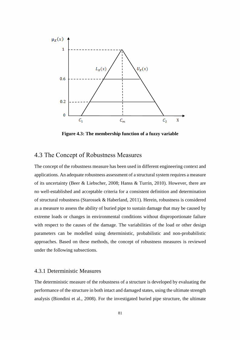
81
Figure 4.3: The membership function of a fuzzy variable
4.3 The Concept of Robustness Measures
The concept of the robustness measure has been used in different engineering context and
applications. An adequate robustness assessment of a structural system requires a measure
of its uncertainty (Beer & Liebscher, 2008; Hanss & Turrin, 2010). However, there are
no well-established and acceptable criteria for a consistent definition and determination
of structural robustness (Starossek & Haberland, 2011). Herein, robustness is considered
as a measure to assess the ability of buried pipe to sustain damage that may be caused by
extreme loads or changes in environmental conditions without disproportionate failure
with respect to the causes of the damage. The variabilities of the load or other design
parameters can be modelled using deterministic, probabilistic and non-probabilistic
approaches. Based on these methods, the concept of robustness measures is reviewed
under the following subsections.
4.3.1 Deterministic Measures
The deterministic measure of the robustness of a structure is developed by evaluating the
performance of the structure in both intact and damaged states, using the ultimate strength
analysis (Biondini et al., 2008). For the investigated buried pipe structure, the ultimate

82
strength will depend on the non-linear response of the pipe structure and the interaction
between the pipe wall, the soil, earth and live loads. However, the concept of reserve
strength and residual strength are considered to evaluate the structural robustness
associated with the buried pipe based on the failure modes. As defined in Zhang et al.
(2015), the reserve strength of a structural system is the ratio between the ultimate
resistance of the intact state structure and the environmental design load that is applied to
measure the residual strength. This can be expressed as shown in Eq. (4.5).
𝑅𝑆𝑅 = 𝑢𝑙𝑡𝑖𝑚𝑎𝑡𝑒 𝑟𝑒𝑠𝑖𝑠𝑡𝑎𝑛𝑐𝑒 𝑜𝑓 𝑖𝑛𝑡𝑎𝑐𝑡 𝑠𝑡𝑟𝑢𝑐𝑡𝑢𝑟𝑒
𝑑𝑒𝑠𝑖𝑔𝑛 𝑒𝑛𝑣𝑖𝑟𝑜𝑛𝑚𝑒𝑛𝑡𝑎𝑙 𝑙𝑜𝑎𝑑 (4.5)
The damage of engineering structures occurs over time. Therefore, Biondini et al. (2008)
suggested a general approach to measure the time-variant structural robustness of
concrete structures subjected to diffusive attacks from aggressive environmental agents
on the ultimate strength analysis. From the expressed measure, the amount of local
damage is first obtained at the member level using dimensionless damage index 0 ≤ δ ≤
1, i.e., associated with the progressive deterioration of the material properties at a spatial
point named x and time t. The global measure of the damaged ∆(t) at the cross-sectional
level can be represented as follows:
∆(t) = [1 − 𝜔(𝑡)]∆𝑐(𝑡) + 𝜔(𝑡)∆𝑠(𝑡) (4.6)
∆𝑐(t) =∫ 𝑊𝑐(𝑥,𝑡)𝛿𝑐(𝑥,𝑡)𝑑𝑥𝐴𝑐
∫ 𝑊𝑐𝐴𝑐(𝑥,𝑡)𝑑𝑥
(4.7)
∆𝑠(t) =∑ 𝑤𝑠𝑚(𝑥,𝑡)𝛿𝑠𝑚(𝑥,𝑡)𝐴𝑠𝑚𝑚
∑ 𝑤𝑠𝑚𝑚 (𝑥,𝑡)𝐴𝑠𝑚 (4.8)
Where 𝜔 = 𝜔(𝑡) , 𝑤𝑐 = 𝑤𝑐(𝑥, 𝑡) and 𝑤𝑠𝑚 = 𝑤𝑠𝑚𝜔(𝑥, 𝑡) are the suitable weight
functions. 𝐴𝑐 is the area of the concrete, and 𝐴𝑠𝑚 is the area of the 𝑚𝑡ℎ steel bar.
The cross-section formulation can be extended at the structural level by integration over
all the members of the system. Therefore, to account for the uncertainties due to
environmental loading and structural resistance for the intact and damaged state, a time-
variant measure of the structural system is expressed in Eq. (4.9) (Biondini et al., 2008).
𝜌(𝑡) = 𝜆𝑐(𝑡)
𝜆𝑐(0) (4.9)

83
Where λ𝑐(t) is the load multiplier that corresponds to the ultimate capacity in a damaged
state and λ𝑐(0) represents the ultimate capacity of the intact state.
4.3.2 Probabilistic Measure
Because of unavoidable uncertainties due to loading conditions and determination of
structural parameters, a probabilistic measure of robustness has been developed based on
system reliability analysis. The probabilistic measure of system redundancy as proposed
in Frangopol & Curley (1987) is based on a reliability index for the full system and the
union of the first member failures. This can be expressed in Eq. (4.10).
𝛽𝑅𝑒𝑑𝑢𝑛𝑑𝑎𝑛𝑐𝑦 = 𝛽𝑖𝑛𝑡𝑎𝑐𝑡
𝛽𝑖𝑛𝑡𝑎𝑐𝑡− 𝛽𝑑𝑎𝑚𝑎𝑔𝑒 (4.10)
Where βdamage denotes the reliability index of the damaged structural system and βintact
represents the reliability index of the intact system. Similarly, Lind (1995) suggested a
probabilistic measure called the damage factor of a system as expressed in Eq. (4.11).
This will assist to assess the capacity of the structure and to withstand damage without
detrimental response. However, these possible approaches are limited to cases in which
probabilistic models can be specified for all the variables with sufficient confidence.
𝑅𝑑𝑓 = 𝑃𝑓,𝑖𝑛𝑡𝑎𝑐𝑡
𝑃𝑓,𝑑𝑎𝑚𝑎𝑔𝑒 (4.11)
4.3.3 Entropy-based Robustness Measure
Entropy-based robustness measure can be used for the assessment of uncertainty specified
with the aid of a fuzzy set (Zhang et al., 2015). The robustness assessment of the fuzzy
uncertainty of structural parameters can be computed based on Shannon’s entropy (Zhang
et al., 2015). The Shannon’s entropy provided the needed information of the total amount
of uncertainty contained in the declared character set (Zimmermann, 2001). Based on
Shannon’s approach, the uncertainty of a fuzzy variable can be quantified. Shannon’s
entropy 𝐻 can be expressed using a probability distribution function 𝑃(𝑥) on a finite set
as shown in Eq. (4.12).

84
𝐻 = −∑ 𝑃(𝑥) log2 𝑃(𝑥)𝑥∈𝑋 (4.12)
𝐻 = −∫ 𝑓(𝑥). log2 𝑓(𝑥)𝑑𝑥+∞
−∞ (4.13)
For an infinite set, the expression in Eq. (4.13) can be applied. In assessing the fuzziness
of the fuzzy set, the functional values of the membership function 𝜇(𝑥) are applied as
measure values of the elements (Zhang et al., 2015). Therefore, an entropy measure of
the fuzziness of an uncertain parameter as defined in Zimmermann (2001) can be
expressed as:
𝐻(�̃�) = −𝐾. ∫ {𝜇(𝑥). ln[𝜇(𝑥)] + [1 − 𝜇(𝑥)]. ln [1 − 𝜇(𝑥)]}𝑑𝑥+∞
−∞ (4.14)
Where �̃� is the fuzzy set which is a subset of the fundamental set X. This entropy
measurement equation evaluates the ‘steepness’ of the membership function μ(x) of �̃�.
The coefficient 𝐾 does not affect the entropy values because entropies appears to be
ratios. Therefore 𝐾 will cancel out. However, 𝐾 was introduced during the
transformation of the dyadic logarithm in Shannon’s entropy in Eq. (4.13) into the natural
logarithm in Eq. (4.14). Based on the expression in Eq. (4.14) for the entropy, the
following properties hold (Zhang et al. 2015):
𝐻(�̃�) = 0 if 𝜇(𝑥) = 0 or 𝜇(𝑥) = 1.0 for all 𝑥;
𝐻(�̃�) reaches maximum if 𝜇(𝑥) = 0.5 for all 𝑥;
If �̃�𝑖 denotes any sharpened version of �̃�𝑗 [i.e., if 𝜇A𝑗(𝑥) ≤ 0.5, then 𝜇A𝑖(𝑥) ≤
𝜇A𝑗(𝑥); and if 𝜇A𝑗(𝑥) ≥ 0.5, then 𝜇A𝑖(𝑥) ≥ 𝜇A𝑗(𝑥)], then 𝐻(�̃�𝑖 ) ≤ 𝐻(�̃�𝑗 ) and
The symmetry property holds, i.e., 𝐻(�̃�) = 𝐻(�̃�𝑐) . Where �̃�𝑐 denotes the
complement of �̃� and can be defined as �̃�𝑐 = {[𝑥, 𝜇𝐴𝑐(𝑥)]|𝑥 ∈ 𝑋; 𝜇𝐴𝑐(𝑥) = 1 −
𝜇𝐴(𝑥).
As defined in Beer & Liebscher (2008), the robustness of a structural system can be
defined as the ratio between the entropy of input parameters and the entropy of associated
structural responses when the uncertainty of structural parameters is quantified as
fuzziness. Using the notation �̃� for the fuzzy input vector for the structural analysis and

85
�̃� for the fuzzy structural response, the structural robustness measure 𝑅(�̃�, �̃�), regarding �̃�
with respect to �̃� can be expressed as:
𝑅(�̃�, �̃�) = 𝐻(�̃�)
𝐻(𝑧) (4.15)
Based on the expression for the robustness of a structure, the following properties hold:
𝑅(. ) ≥ 0 ∀ 𝐻(�̃�), 𝐻(�̃�) > 0;
𝐻(�̃�2) ≤ 𝐻(�̃�1) ⟹ 𝑅2(. ) ≥ 𝑅1(. )|𝐻(�̃�1) = 𝐻(�̃�2);
𝐻(x̃) → 0 ⟹ 𝑅(. ) ⟶ 0 |𝐻(z̃) > 0; and
𝐻(z̃) → 0 ⟹ 𝑅(. ) ⟶ +∞ |𝐻(x) > 0.
Following the properties of the robustness of a structure, the outcome of the robustness
measure can lead to a global statement about the degree of variation in the structural
output with respect to fluctuation in the structural input (Beer & Liebscher, 2008; Zhang
et al., 2015). For example, the second property shows that the smaller the uncertainty
associated with the output in relation to the uncertainty associated with the input
variables, the higher the robustness of the structure. In practice, Zhang et al. (2015)
suggested that this shows that moderate changes applied to structural parameters, e.g.
changes in the design parameters and moderate errors, can affect the structural response
only marginally. Based on the suggestion of Zhang et al. (2015), entropy-based
robustness measure can be assessed at various membership levels with respect to the
degree of imprecision in the fuzzy inputs and the associated imprecision in the fuzzy
outputs. This is realised by considering each component of the structural system. For
instance, for a given fuzzy set �̃� at α-level 𝛼𝑘 ∈ (0,1], a new fuzzy set can be defined as
the intersection of fuzzy set �̃� and the corresponding α-level set �̃�𝛼𝑘. This is expressed in
Eq. (4.16).
�̃�𝛼𝑘 = �̃� ∩ 𝐴𝛼𝑘 (4.16)
Now, the entropy-based robustness assessment can be evaluated at each α-level, as the
ratio of the entropy of the fuzzy input to the entropy of the fuzzy structural response. This
can be expressed as shown in Eq. (4.17).

86
𝑅(𝛼𝑘) = 𝐻(�̃�𝛼𝑘)
𝐻(𝑧𝛼𝑘) (4.17)
Develop triangular membership
function for the fuzzy variable
Discretise the
membership function
Determine the corresponding interval
values for each membership level
Integrate all the interval output results for each α-level
(α1 = 0 < α2 = 0.1 < α3 = 0.3… < α11 = 1)
Compute the entropy of the fuzzy input
and structural response
Normalise the uncertain quantities of the
fuzzy input and the structural response
Compute the robustness measure of the
structural system using Eq.(4.17)
Stage 2
Compute the corresponding response
variables Yα i ,at every level
Repeat this
processes at every
α-level cut until
α11 = 1
Stage 1
Generate N samplesθ0,j(j = 1,2,3,… , N)
from the random normal variable
parameters
Figure 4.4: Flow diagram for the computation of fuzzy-based robustness measure

87
4.3.4 Methodology
In Section 4.3.1 to 4.3.3, various approaches for the assessment of the robustness of a
structure considering different conditions and uncertainties are reviewed. The entropy-
based robustness measure is considered because it provides a potential to assess the
robustness in the form of a function that depends on the magnitude of uncertainty that
exists in the structure. Therefore, the fuzzy-based robustness assessment is developed
based on the concept of the entropy-based robustness measure and the computation is
performed in two stages. The first stage deals with interval analysis concept for the
solution of the α-level cut. This stage is based on the concept of Dong, Shah, and Wong
(DSW) algorithm (Ross, 2004). The method uses the decomposition of a membership
function into a series of α-cut intervals and also uses the full α-cut intervals in a standard
interval analysis. While the second stage takes care of the robustness assessment that is
an analogy to Shannon’s entropy based on the concept of Zhang et al. (2015). Figure 4.4
shows the flow diagram for the two stages and the procedures are summarised as follows:
Stage 1
1. Construct the triangular membership function for a fuzzy set model of the
corrosion loss.
2. Discretise the membership function into 10 parts between 0 and 1, where the
values will be 𝛼1 = 0 < 𝛼2 = 0.1 < 𝛼3 = 0.3… < 𝛼11 = 1.
3. For every 𝛼 − level, determine the corresponding interval values each
membership level 𝛼𝑖, find the correspong interval from the fuzzy sets.
4. Generate N samples 𝜃0,𝑗(𝑗 = 1,2,3,… , 𝑁) from the random normal variable
parameters using their original PDF from the example problem.
5. Using standard interval arithmetic, compute the corresponding response
variables 𝑌𝛼𝑖,(𝑖 = 0, 0.1, 0.2, 0.3… , 1)for the output membership function of the
selected α-level.
6. Repeat the processes from step 3 to 5 at every α-level cut until 𝛼11 = 1.
7. Integrate all the interval output results for each α-level (𝛼1 = 0 < 𝛼2 = 0.1 <
𝛼3 = 0.3… < 𝛼11 = 1) to obtain the overall results of the solution model.

88
Stage 2
1. Normalise the uncertain quantities of the fuzzy input and the structural response
2. Compute the entropy of the fuzzy input and structural response for every α-level
from the analogy Shannon’s entropy using Eq. (4.14)
3. Compute the robustness measure of the structural system using Eq.(4.17)
4.4 Application to Buried Pipe
4.4.1 Structural Failure Mode and a Numerical Example
The numerical example is used to demonstrate the applicability of the method in Section
4.3.4 and the technique is used to assess the structural robustness of a buried pipe while
considering the impact of corrosion and uncertain variables. The considered failure modes
used in the analysis include pipe deflection, buckling pressure (ring buckling), bending
strain and wall thrust as explained in Chapter 3, Section 3.3. The statistical values of the
soil and pipe parameters used in the computation are shown in Table 3.3 and Table 3.4.
The values are based on industry standard and have been obtained from the works of
(Ahammed & Melchers 1994; Sadiq et al., 2004; Tee et al., 2014). As a useful extension,
the effect of corrosion on the buried pipe is assessed herein using the intrinsic features of
a fuzzy set, and modelling of the damage is explained in the subsequent section.
4.4.2 Damage Modelling of Buried Metal Pipes Under Uniform Corrosion
In this numerical example, the buried metal pipe is assumed to undergo gradual
deterioration caused by uniform corrosion. The degradation process can lead to different
failure modes such as pipe deflection, buckling pressure, bending strain and wall thrust.
The investigation of the corrosion effect was performed using the immersion corrosion
data collected by Melchers (2003) as shown in Figure 4.5 to model the corrosion pit depth.
A fuzzy corrosion depth associated with the exposure time is derived from the data based
on a subjective assessment of deterioration of mild steel coupons as shown in Figure 4.6.
Generally, Marano et al. (2008) suggested that it is possible to state that a unitary
approach does not exist for the so-called fuzzification, but different procedures can be

89
adapted for each situation. Therefore, the methods for constructing the membership
function of a fuzzy variable can be direct or indirect with a single expert or multiple
experts (Klir, 2006; Marano et al., 2008).
Figure 4.5: Fuzzy input model for corrosion loss based on mild steel coupons
pooled from all available data sources until 1994, with 5th and 95th percentile
bands.
The membership function for the fuzzy corrosion depth at time T = 4, 8, 12 and 16 years
are subjectively constructed according to the data points plotted in Figure 4.5, and the
developed membership function is shown in Figure 4.6. The membership function is
considered as linear where it connects the 5 percentile, the mean and the 95 percentile
values in the experimental data. In this study, the uncertainty of corrosion pit depth is
considered for the four failure modes of the buried pipeline. For simplicity, the analysis
considers exposure periods of 4, 8, 12, and 16 years (as shown in Figure 4.6). The amount
of damage on the pipe wall or cross-sectional area of the buried pipe is evaluated using
the concept of (Watkins & Anderson, 1999). Therefore, for a flexible metal pipe, the
moment of inertia and the cross-sectional area of the pipe wall per unit length can be
obtained using Eq. (4.18) and Eq. (4.19).
Moment of inertia, 𝐼 = (𝑡 − 𝐶𝑇)3/12 (4.18)
Cross-sectional area 𝐴𝑠 = 𝑡 − 𝐶𝑇 (4.19)

90
Where 𝑡 represents the thickness of the pipe wall, 𝐶𝑇 is the pit depth and 𝑇 is the time of
exposure.
Figure 4.6: Membership functions developed from the immersion corrosion data of
mild steel coupons for 4, 8, 12, and 16 years
4.5 Results and Discussion
The specified fuzzy variable 𝑐 ̃(𝑇 = 4, 8, 12 𝑎𝑛𝑑 16 𝑦𝑒𝑎𝑟𝑠) is employed in modelling
the impact of corrosion pit depth and the impact of other uncertain variables for the
determination of the structural robustness of a buried steel pipe. The external surface area

91
of the buried pipe wall is considered to suffer corrosion loss that is uniform. Four failure
modes are considered in this analysis which includes deflection, wall thrust, bending
strain and buckling pressure (see Chapter 3, Section 3.3 for more information). The
computed membership function outcome for each failure are shown in Figure 4.7 for the
failure modes of pipe deflection and wall stress/thrust, and Figure 4.8 for the failure
modes of bending strain and buckling pressure. The results provide clear information
about transferring the fuzzy corrosion uncertainty to the pipe failure modes. In each
failure mode, the fuzzy model can incorporate and simulate the probabilistic and
vagueness associated with pipe, soil and corrosion parameters for the buried pipe.
However, the degrees of uncertainty increase as the number of service years increases.
The outcome of the entropy values associated with the α-level of the fuzzy output for
different failure modes, normalised by H(p) are reported in Figure 4.9 and Figure 4.10 for
an exposure period of 16 and 8 years, respectively. The result clearly indicates a reduction
of imprecision in the fuzzy input would lead to a reduction of imprecision in the fuzzy
output. It could be noticed from the results that the imprecision associated with the input
parameter has a trade-off in reducing the imprecision associated with the computed output
for different failure modes. However, for the various failure modes, the entropy states
exhibit different characteristics. For example, the imprecision associated with wall thrust
and buckling pressure decreases much faster than the imprecision in deflection and
bending strain when input uncertainty decreases. This indicates that a small reduction of
imprecision in the fuzzy input variable can result in a significant decrease in imprecision
in the failure modes of buried pipe for wall thrust and buckling.

92
(a) Deflection
(b) Wall stress/thrust
Figure 4.7: Membership function of pipe failure mode for (a) deflection (b) wall
thrust

93
(a) Bending strain
(b) Buckling pressure
Figure 4.8: Membership function of pipe failure mode for (a) bending strain (b)
buckling pressure

94
Figure 4.9: Entropy state for different failure modes after 16 years
Figure 4.10: Entropy state for different failure modes after 8 years
0 0.1 0.2 0.3 0.4 0.5 0.6 0.7 0.8 0.9 10
1
2
3
4
5
6
7x 10
-3
Alpha - Level
Entr
opy v
alu
es H
(p)
Deflection
Wall thrust
Bending strain
Buckling
0 0.1 0.2 0.3 0.4 0.5 0.6 0.7 0.8 0.9 10
0.5
1
1.5
2
2.5
3
3.5
4x 10
-3
Alpha - Level
Entr
opy v
alu
e H
(p)
Deflection
Wall thrust
Bending strain
Buckling

95
The entropy state of each failure mode is computed for different α − level with the
intersection of characteristic membership functions of both inputs and outputs. The
intersection is based on the mathematical operations of fuzzy set theory. The outcome of
the corrosion effects of the fuzzy-based robustness measure 𝑅(𝛼𝑘) for different pipe
failure modes of buried pipe are reported in Figure 4.11 and Figure 4.12. This is calculated
based on Eq. (4.14) and (4.17), which is the ratio between the entropy of the fuzzy input
to the entropy of the fuzzy output at each 𝛼 − 𝑙𝑒𝑣𝑒𝑙. The outcome of the pipe robustness
for deflection for the periods of 16 and 12 years demonstrates a close robust behaviour of
the buried pipe when 𝛼𝑘 ≤ 0.2.
On the other hand, as the 𝛼 − 𝑙𝑒𝑣𝑒𝑙 increases, the outcome of pipe deflection for the
period of 12 years continues to display a value that is greater than the case for 16 years.
For the other years (4 and 8 years), the robustness measure of the buried pipe is quite
distinctive. Similarly, for the period of 4 and 8 years, and when the alpha-level 𝛼𝑘 ≥ 0.8,
there is a sudden increase in the robustness value. This could mean that the buried pipe
under deflection failure modes is more robust when the alpha-level 𝛼𝑘 ≥ 0.8 compared
to when the alpha-level 𝛼𝑘 ≤ 0.8 . At this level, it is possible that the robustness
assessment of pipe deflection would require additional information concerning the
corrosion processes. Moreover, as the number of pipe service years increases, the pipe
robustness behaviour tends to normalise and shows a similar trend, which illustrates the
ductility nature of the pipe material. For the other failure modes, the results show similar
behaviour as the number of service years increases

96
(a) Deflection
(a) Wall stress/thrust
Figure 4.11: Fuzzy-based robustness assessment of buried pipe (a) deflection (b)
wall stress/thrust

97
(a) Bending strain
(b) Buckling pressure
Figure 4.12: Fuzzy-based robustness assessment of buried pipe (a) bending strain
(b) buckling pressure

98
Figure 4.13: Fuzzy-based robustness assessment of buried pipe after 16 years
Figure 4.14: Fuzzy-based robustness assessment of buried pipe after 12 years

99
Consequently, the outcome of the four different years (4, 8, 12, and 16 years) shows that
the values evaluated for the pipe robustness measure would continue to decrease as the
number of pipe service years continues to increase. For instance, the pipe robustness
values for the failure mode of deflection for different alpha levels between 𝛼1 to 𝛼11
reduces from (1,139, 1,254, 1,452, 1,184, 1,212, 1,790, 1,207, 745, and 981) in 4 years to
(225, 268, 240, 228, 237, 279, 292, 347, and 351) in 16 years. This demonstrates that the
level of uncertainty based on the adverse effect of corrosion-induced failure could
potentially reduce the performance of the buried pipe. In the same way, for an exposure
time of 4 and 16 years, the pipe failure modes of deflection and bending strain expresses
close behaviour while that of wall thrust and buckling are quite similar. This could mean
that the buried pipe shows more resistance against deflection and bending other than wall
thrust and buckling as illustrated in Figure 4.13 and Figure 4.14.
4.6 Chapter Summary
In this Chapter, a methodological approach for the assessment of fuzzy-based robustness
behaviour of the buried pipe is presented. The concepts behind the method and including
the computational procedure are explained. The fuzzy-based robustness problem is
formulated based on the failure modes of a buried steel pipe and includes pipe deflection,
wall thrust, buckling pressure, and bending strain using the principles of fuzzy set and
Shannon’s entropy. The proposed method gains its effectiveness in the assessment of the
structure by scrutinising the robustness at every membership level. Other pipe failure
modes due to corrosion can be analysed using the proposed method. The fuzziness
associated with the corrosion effects at various times in the life of a buried steel pipe are
quantified using a fuzzy model and based on the immersion corrosion data collected by
Melchers (2003). Corrosion is used as a fuzzy variable in order to account for the
uncertainties that characterise the corrosion processes. The estimation of pipe robustness
is conducted by considering various levels of uncertainties that affect the performance of
the buried pipe, and the modelling of the failure modes based on fuzzy sets, which
considers various levels of the α-level cut. The outcome illustrates that evaluating the
performance of buried steel pipe using the fuzzy-based robustness measure can deliver a
wide-ranging understanding concerning the adverse effect of corrosion uncertainty to the

100
examined pipe failure problems. This result can lead to an optimal decision concerning
buried pipe structures where a degree of accuracy is needed. The proposed method can
be used to assess any type of corrosion-induced failures for buried pipe and also for other
engineering structures. The consequences posed by the uncertain variables for the design
of buried pipeline requires an adequate level of reliability. As a result, a multi-objective
optimisation of buried pipe based on the expected fuzzy output is proposed in Chapter 5.
The formulation is based on fuzzy set and multi-objective optimisation for a robust
analysis of a buried pipeline.

101
CHAPTER FIVE
5 MULTI-OBJECTIVE OPTIMISATION OF BURIED
PIPE BASED ON THE EXPECTED FUZZY OUTPUT

102
5.1 Introduction
Buried pipelines are usually designed based on deterministic parameters and without
considering the randomness and fuzziness associated with the design parameters.
However, the limitation of the deterministic approach has paved the way for other models
in many scientific works. Therefore, the evaluation of the performance of buried pipe
based on the deterministic parameter is undoubtedly a simplification because the
measurement of pipe or soil parameters such as elastic modulus always shows variability
and randomness.
The concept of robust design optimisation (RDO) has been introduced in the literature to
deal with the uncertainties that are random, but the occurrence of variables that are vague
and cannot be ignored from the practical point of view. Considering the consequences
posed by the uncertain variable for the design of buried pipe, an adequate level of
reliability on the performance is required for design purpose. However, given the benefit
of the fuzzy model approach in modelling uncertainties associated with design
parameters, its capability is employed in the multi-objective optimisation of buried pipe.
Therefore, this Chapter presents a formulation based on fuzzy set and multi-objective
optimisation for a robust analysis of a buried pipe structure. The proposed approach
employs the optimal performance of a Hybrid GA-GAM for the optimisation, and the
purpose is to optimise the design variable while considering the adverse effect of the
uncertain fuzzy variables and variability of the structural performance.
The remaining part of this Chapter is summarised as follows: Section 5.2 presents the
concept of robust design optimisation while Section 5.3 describes the fuzzy-based robust
multi-objective design optimisation. Section 5.4 explains the Hybrid GA-GAM, which
include a GA, Goal Attainment Method (GAM), Hybrid GA-GAM and the methodology.
The numerical example is explained in Section 5.5, while Section 5.6 presents the results
and the significant findings from the study. Finally, Section 5.7 shows the Chapter
summary, which summarises the outcome of the study.

103
5.2 The Concept of Robust Design Optimisation
Generally, the optimum design of a structural system can be expressed by the following
expression in Eq. (5.1).
max/min 𝐹(𝑦)
subject to 𝑔𝑖(y, θ) ≤ 0, i = 1,… , I,
ℎ𝑗(y, θ) = 0, j = 1, … , J, (5.1)
𝑠𝑘(y) ≤ 0, k = 1,… , k
Where 𝑦 is the vector of the design variable, θ is the vector of the uncertain structural
parameter, 𝐹(𝑦) is the objective or the cost function, 𝑔𝑖, i = 1,… , I and ℎ𝑗 , j = 1,… , J,
denotes the functions that define a set of inequality and equality constraints, and 𝑠𝑘, 𝑘 =
1, … , 𝑘, are functions that represent the sets of deterministic constraints.
The design variables can be the structural parameters representing or defining the shape
or the dimensions of the structure. The objective and constraint function could represent
the limitations of the structural performance. For the buried pipe problem, the solution to
the problem relating to Eq. (5.1) can be sensitive to changes that may occur from different
sources such as geo-environmental conditions. These include corrosion, temperature
variation, pressure and humidity fluctuation, and changes in material properties. Based
on these issues, the principal target is to provide an optimal design with a high degree of
robustness. The process of finding an optimal solution with some level of robustness is
called RDO. For more information, the reader can refer to the works of (Beyer &
Sendhoff, 2007; Doltsinis & Kang, 2004; Schuëller & Jensen, 2008).
The design of a structure using the principles of robust design is considered as an
optimised design because the technique considered the uncertainties that are explicit in
the optimisation process (Schuëller & Jensen, 2008). In the literature, the concept of RDO
has been used in different engineering applications. The design of engineering structures
always involves a considerable level of uncertainties, and the design engineer needs to
take care of it at the design stage. Many approaches, design guides, and codes have been
developed for different ranges of engineering problems to support the decision of the
designer and also achieve the best solution for a particular case. The structural

104
performance often exhibits high sensitivity to the natural variability of the data.
Therefore, conventional robust design can be formulated as:
min 𝑦{ 𝑓(𝑦, 𝑑) , 𝜎[𝑓(𝑦, 𝑑)]} 𝑠. 𝑡. ℎ̌𝑗(𝑦, 𝑑) ≤ 0 𝑗 = 1,… , 𝐽 𝑦𝑙 ≤ 𝑦 ≤ 𝑦𝑢 (5.2)
Where 𝑓(𝑦, 𝑑) is the performance or objective function, . and 𝜎[. ] are the expected
value and the standard deviation operators; 𝑦 is the design vector and 𝑑 is the vector of
the uncertain variables, 𝑦𝑙 and 𝑦𝑢 are the lower and upper limits.
5.3 Fuzzy-based Multi-objective Design Optimisation
5.3.1 Fuzzy Design Optimisation
Marano & Quaranta (2008) stated that the expected value and the entropy of the fuzzy
variable are often in conflict. As a result, it is ideal to adopt a robust strategy with the
intention of solving the Multi-Objective Optimisation Problem (MOOP) and possibly be
able to define the equivalent Pareto front. However, searching for the Pareto optimal set
for a multi-objective function is the primary goal of the optimisation algorithm. For an
engineering problem, finding an optimum solution of a function based on the single
objective is limited and does not account for other functions in justifying the outcomes
and the evaluation of the optimal design solutions. Therefore, it is important to consider
a multi-objective function in the optimisation process so that an accurate representation
of the structure is reflected in the evaluation of the Pareto front for the design of an
engineering structure.
The use of fuzzy set in the robust design of structures has been studied in the literature
(Fang et al., 2016; Marano & Quaranta, 2008). Herein, fuzzy-based multi-objective
design optimisation is utilised in the structural analysis of buried pipe. A fuzzy variable
can be defined as a function from a possibility space to the set of real numbers (Marano
& Quaranta, 2008) and the membership function of every fuzzy variable could be
expressed from the possibility measure as explained in (Liu, 2004). The computation of
the membership function of a fuzzy variable is one of the challenging factors for a
structural analysis using fuzzy set theory. However, different methods have been adopted

105
in the literature to achieve or construct the membership function. For instance, Klir (2006)
suggested that the construction of the membership function could be done using direct or
indirect information from a single expert or multiple experts. A vector is fuzzy if and only
if all the elements is a fuzzy variable (Liu, 2004).
5.3.2 Fuzzy Variable and the Expected Value
The expected value of a fuzzy output variable plays a vital role in the fuzzy-based multi-
objective design optimisation. If a fuzzy variable and the membership function are
represented as 𝑥 and 𝜇(𝑥), then, the corresponding fuzzy set model can be expressed as
shown in Eq. (5.3)
𝐹 = {((𝑥, 𝜇(𝑥)) 𝑥 ∈ ℝ, 𝜇(𝑥) ∈ [0,1] )} (5.3)
Where ℝ is the universal set.
Also, if a fuzzy variable x with assigned membership function 𝜇(𝑥), is specified, then
the following formula in Eq. (5.4), Eq. (5.5), Eq. (5.6) can be utilised to calculate the
credibility (Liu, 2004; Marano & Quaranta, 2008). The credibility of a fuzzy variable can
be defined as the average between the possibility and the necessity values (Marano &
Quaranta, 2008)
Cr {𝑥 = 𝜌} =1
2(μ(𝜌) + 1 − sup
𝑧≠𝜌{𝜇(𝑧)}) ∀d ϵℝ (5.4)
Cr {𝑥 ≤ 𝜌} =1
2(sup 𝑧≤𝜌
{𝜇(𝑧)} + 1 − sup𝑧>𝜌
{𝜇(𝑧)}) ∀d ϵℝ (5.5)
Cr {𝑥 ≥ 𝜌} =1
2(sup 𝑧≥𝜌
{𝜇(𝑧)} + 1 − sup𝑧<𝜌
{𝜇(𝑧)}) ∀d ϵℝ (5.6)
Based on this concept of credibility measure, the expected value of a fuzzy variable can
be determined using the expression given in Eq. (5.7) (Liu & Liu, 2002).
E[𝑥] = ∫ Cr {𝑥 ≥ 𝜌}𝑑𝜌+∞
0− ∫ Cr {𝑥 ≤ 𝜌}𝑑𝜌
0
−∞ (5.7)
This expression provides a general statement for the expected value of a fuzzy variable.
For a continuous fuzzy variable, if the membership function follows a monotonically

106
increasing law in the range of [−∞, 𝜌𝑜] and a monotonically decrease in the range of
[𝜌𝑜, +∞], therefore a more convenient rule could be adopted as shown in Eq. (5.8) (Liu
& Liu, 2002; Marano & Quaranta, 2008). This expression can be used to evaluate the
expected value of the fuzzy variable.
E[𝑥] = 𝜌𝑜 + 1
2∫ 𝜇(𝜌)𝑑𝜌+∞
𝜌𝑜−
1
2∫ 𝜇(𝜌)𝑑𝜌𝜌𝑜
−∞ (5.8)
5.3.3 Entropy Value of a Fuzzy Variable
The concept of fuzzy entropy can be used to analyse and quantify uncertainties associated
with the design parameters. The fundamentals of Shannon’s entropy could provide the
desired information of the total amount of uncertainty contained in the fuzzy set.
Therefore, Shannon’s entropy can be used as an integral part of information theory to
assess the performance of the structural system. The concept of entropy plays a significant
role in measuring the fuzzy information such as evaluation of fuzzy degree between two
fuzzy sets. In the literature, there are various expressions for computing fuzzy entropy
that has been proposed; however, see the work of (Beer & Liebscher, 2008; Liu, 2007;
Liu & Liu, 2002) for more information.
From Eq. (5.8), if a continuous variable tends to be a crisp number, its entropy tends
towards the minimum value of zero. Herein, the suggestion by Liu (2007) is used, where
the entropy of a continuous fuzzy variable is defined as expressed in Eq. (5.10).
𝐻(𝑥) = ∫ (−𝐶(𝜌) ln 𝐶(𝜌) − (1 − 𝐶(𝜌)) ln(1 − 𝐶(𝜌)))d𝜌+∞
−∞ (5.9)
Where 𝐶(𝜌) = 𝐶𝑟(𝑥 = 𝜌) and for a continuous fuzzy variable 𝑥, 𝐶(𝑟) = 𝐶𝑟(𝑥 = 𝜌) =
1
2𝜇(𝜌), thus
𝐻(𝑥) = −∫ (1
2𝜇(𝜌) ln
1
2𝜇(𝜌) + (1 −
1
2𝜇(𝜌)) ln (1 −
1
2𝜇(𝜌))) d𝜌
+∞
−∞ (5.10)
From Eq. (5.8) and (5.10), the expectation and the entropy of a fuzzy variable can be
computed as soon as the membership function is given.

107
5.3.4 Formulation of Fuzzy-based Multi-objective Design Optimisation
The design of engineering structure has moved from single objective optimisation to
evaluating an optimal solution by considering multi-objective functions. This is because
the design of engineering structures requires a resolution of conflicting objectives. Based
on the fuzziness of the uncertain parameters for a particular structure, the fuzzy-based
multi-objective design optimisation problem can be formulated as expressed in Eq. (5.11).
min𝑦
{𝐸1 𝑓1(𝑦, �̌�) , 𝐸2 𝑓2(𝑦, �̌�) }
𝑆𝑢𝑏𝑗𝑒𝑐𝑡 𝑡𝑜 ℎ̌𝑗(𝑦, �̌�) ≤ 0 𝑗 = 1,… , 𝐽 𝑦𝑙 ≤ 𝑦 ≤ 𝑦𝑢 (5.11)
Where 𝑓1(𝑦, �̌�) and 𝑓2(𝑦, �̌�)represent the performance function based on design and
fuzzy variable for objective 1 and obejective 2; 𝐸1[. ] and 𝐸2[. ] are the expected values
of the fuzzy variable based on objective 1 and obejective 2. �̌� is the fuzzy vector of the
uncertain variable and 𝑦 is the design vector where 𝑦𝑙 𝑎𝑛𝑑 𝑦𝑢 are the lower and upper
values of the design vector. Based on this idea, it is vital to observe that each of the
constraints ℎ𝑗 is a fuzzy variable and it is important to extract a specific value ℎ̌𝑗 from the
fuzzy output variable.
Since most engineering structures are associated with more than one objective, therefore,
employing multi-objective optimisation technique becomes a vital aspect for the optimal
design (Zhang et al., 2017). Also, it is essential to consider the opportune strategies with
the intention of solving the MOOP to obtain the Pareto front. In practice, the decision
with regards to the final solution to be used based on the outcome of the Pareto front is
formulated by the decision maker. However, a preference-based method which allows
preference information to be used in the search to influence the Pareto optimal solution
can be used (Coello, 2000). The search for the Pareto optimal set can be determined
through the use of any multi-objective optimisation algorithm. Herein, the optimisation
is performed using a Hybrid GA-GAM algorithm to determine the Pareto front. This
approach is briefly discussed in the next Section.

108
5.4 Hybrid GA-GAM Approach
5.4.1 Genetic Algorithm (GA)
GA is a population-based metaheuristic algorithm that is widely used for most
optimisation problems because of its robust and independent objective function (Li & Lu,
2014; Garg, 2016; Goldberg, 1989; Fonseca & Fleming, 1993). The concept uses the
survival of the fittest and a biological mechanism to process a set of solutions iteratively
in order to converge and produce an optimum solution. The survival of the fittest which
GA adopts is based on Darwinian’s theory that begins with a set of solutions denoted as
chromosomes, called population. The solutions determined from one population would
be used to form another new population, and that population is motivated based on the
likelihood that the new population will be preferred when compared to the older
population. In addition, the solutions are selected based on their fitness to form a new
solution. The computational steps in executing GA is given in Chapter 6, Section 6.3.1.
5.4.2 Goal Attainment Method (GAM)
GAM is usually employed to solve a MOOP. As suggested by Chankong & Haimes
(1983), GAM is a powerful optimisation tool that can determine the best possible solution
to a multi-objective problem. The GAM approach has the advantage of posing or being
converted as a non-linear programming problem (Fonseca & Fleming, 1993) and the
characteristic of the problem can be exploited in a non-linear programming algorithm.
The GAM method is used as the hybrid solver, and for more information, the reader can
refer to (Fonseca & Fleming, 1993).
5.4.3 Hybrid GA-GAM and Multi-objective Design Optimisation
Multi-objective optimisation is an approach to determine a vector of design variables that
are located within a feasible region, which minimises the vector of the objective function
that could conflict with one another (Cheng & Le, 1997). The optimal solution is called
the Pareto front, and this is obtained based on the concept of dominance. The formulation
of the multi-objective optimisation takes the form of the expression in Eq. (5.12).

109
min {𝑓1(𝑦), 𝑓2(𝑦), … , 𝑓𝑛(𝑦) } 𝑠𝑢𝑏𝑗𝑒𝑐𝑡 𝑡𝑜 𝑔(𝑦) ≤ 0 (5.12)
Where 𝑦 denote the vector of design variables; 𝑓1(𝑦) represents the 𝑖𝑡ℎ objective
function and 𝑔(𝑦) is the constraint vector.
The multi-objective optimisation algorithm tries to locate the best sets of solutions that
could satisfy the various objective/constraint functions to form the Pareto optimal set.
The solution of the multi-objective function is always situated in its Pareto optimal front
set (Cheng & Le, 1997; Deb, 2001). The Pareto optimum gives a set of non-dominated
solutions, which also varies depending on the search technique. These are solutions for
which no objective could be improved without detracting from the other objective
functions. The multi-objective programme does not have a unique solution that can
simultaneously optimise all the objective functions (Cheng & Le, 1997; Deb, 2001).
Therefore, any point located within the Pareto optimal set can become an ‘optimum
solution,’ which invariably depends on the decision of the design engineer. For more
details on multi-objective optimisation, the reader can refer to (Cheng & Le, 1997; Deb,
2001; Tang et al., 2011). The rationale behind the introduction of GAM as the hybrid
solver for the MOOP is to utilise its efficiency in local search and to enable evaluation of
fewer functions in order to achieve convergence. The procedure for evaluating the Hybrid
GA-GAM function is described in the following steps.
1. Define the objective functions, and set the operators of the GA, e.g. population
size, parent/offspring ratio, selection methods, and mutation rate.
2. Initialise the parameters and generate initial population.
3. Set the solution counter 𝑖 = 1.
4. Calculate the number of solutions 𝑛𝑖 that dominates solution 𝑖.
5. Compute the rank 𝑟 of the 𝑖 − th solution as 𝑟𝑖 = 1 + 𝑛𝑖. This will increase the
number of count of the solutions in rank 𝑟𝑖 by one. That is 𝜇(𝑟𝑖) = 𝜇(𝑟𝑖) + 1.
6. If the solution counter 𝑖 is less than the number of population 𝑃𝑛 i.e. 𝑖 < 𝑃𝑛 ,
increase 𝑖 by one and go to step 2. Otherwise, go to step 7.
7. Identify the maximum rank 𝑟𝑚𝑎𝑥 by checking for the biggest 𝑟𝑖 which has 𝜇(𝑟𝑖) >
0. Then, set a rank counter 𝑟 = 1.

110
8. For each solution 𝑖 in the rank 𝑟 , evaluate the niche count 𝑛𝑐𝑖 with the other
solutions of the same rank.
9. If the rank 𝑟 < 𝑟𝑚𝑎𝑥, increase the rank 𝑟 by one and go to step 7. Otherwise, go
to step 10.
10. Perform a local search on each solution using GAM, compute the corresponding
fitness of each new location, and replace the solution if there is a locally improved
option.
11. If convergence is achieved, stop the algorithm. Otherwise, got to step 3.
5.4.4 Methodology
Figure 5.1 shows a flow diagram for the computation. Also, the steps used to determine
the response of the fuzzy-based multi-objective design optimisation of an engineering
structure considering the expected values of the fuzzy output variable based on objective
1 and objective 2 using a Hybrid GA-GAM algorithm are summarised as follows:
Initialise the input parameters.
Evaluate the expectation of the fuzzy structural response based on objective 1 and
objective 2 using Eq. (5.8).
Construct the mathematical formulation for the fuzzy-based multi-objective
design optimisation as explained in Section 5.3.4.
Perform the multi-objective optimisation using the Hybrid GA-GAM algorithm
as explained in Section 5.4.3.
Check whether the constrained is satisfied.
Use the maximum and minimum values in the Pareto front for the computation of
the fuzzy structural response and perform the fuzzy entropy-based analysis.

111
Start
Initialise the input parameters
Evaluate the expectation of the fuzzy
structural response based on objective 1
and objective 2 using Eq. (5.8)
Construct the mathematical
formulation as explained in
Section 5.3.4.
Use Hybrid GA-GAM algorithm to
perform the multi-objective
optimisation
Use the maximum and minimum
values to perform fuzzy entropy-
based analysis
End
Did the optimisation
converge?
Yes
No
Figure 5.1: Flow diagram of fuzzy entropy analysis using multi-objective
optimisation

112
5.5 Numerical Example
The purpose of this numerical example is to demonstrate the applicability and the
confidence level in the design of buried pipeline by incorporating a multi-objective
optimisation approach. The method is used to analyse the performance of buried pipe
structure based on multi-objective functions considering the design variables and the
uncertain fuzzy variables. The possible pipe failure modes used in the analysis include (i)
ovality of pipe, and (ii) buckling pressure. For details concerning the pipe failure, see
Chapter 3, Section 3.3. The statistical values of the soil and pipe parameters used in the
computation are given in Table 3.3 and 3.4. The values are based on industry standard
and have been obtained from the works of (Ahammed & Melchers 1994; Sadiq et al.
2004; Tee et al. 2014).
As a useful extension, the effect of corrosion on the buried pipe is assessed herein using
the intrinsic features of a fuzzy set to develop the membership function. In this case, the
sensitivities of the responses with respect to the uncertainties associated with the
empirical constants are analysed, and an acceptable interval size determined and used to
construct the membership function as illustrated in Figure 5.2 and for the exposure period
of 25, 50 and 100 years. This approach provides the possibility to consider a gradual
assessment of the uncertainties in relation to interval values. Generally, Marano et al.
(2008) suggested that it is possible to state that a unitary approach does not exist for the
so-called fuzzification, but different procedures can be adopted for each situation.
Therefore, the methods for constructing the membership function of a fuzzy variable can
be direct or indirect with a single expert or multiple experts (Klir, 2006; Marano et al.,
2008). For more information, see (Klir & Yuan, 1995; Klir, 2006). Herein, the reason for
treating corrosion as a fuzzy variable is to account for the uncertainties in the values of
the parameters that characterise the environment, variables that affect the time to
corrosion initiation, and the rate of corrosion propagation (Anoop & Balaji, 2007; Marano
et al., 2008).

113
Figure 5.2: Corrosion pith depth at T = 25 years, 50 years and 100 years
5.6 Results and Discussion
The applicability and the usefulness of the proposed method are demonstrated using the
numerical example in Chapter 3, Section 3.7. The output of the multi-objective
optimisation is the Pareto front as shown in Figure 5.3. In this work, a Hybrid GA-GAM
as explained in Section 5.4.3 is used for the multi-objective optimisation, and the outcome
has been compared with the GA. It is clear from Figure 5.3 that the performance of the
two methods is very close. However, for the Hybrid GA-GAM approach, a total of 7255
function evaluations was needed to converge while the GA used a total of 10051 function
evaluations. The two optimisation algorithms have been measured running on a central
processing unit (CPU) time using a 1.60 GHz Pentium 4 computer. The time taken for
the former to converge is 23 minutes while the latter used about 35 minutes. Based on the
execution time, it can be concluded that the difference in time is not significant. However,
the introduction of the Hybrid GA-GAM has enabled evaluation of fewer functions to
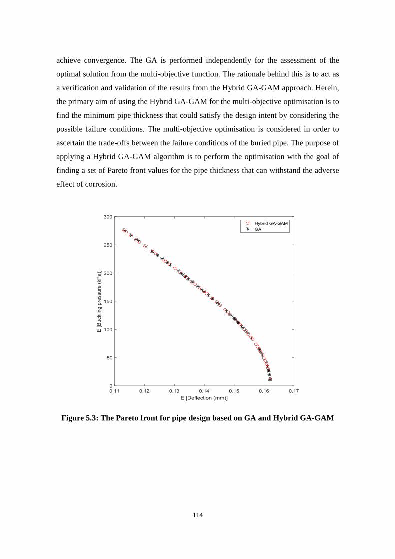
114
achieve convergence. The GA is performed independently for the assessment of the
optimal solution from the multi-objective function. The rationale behind this is to act as
a verification and validation of the results from the Hybrid GA-GAM approach. Herein,
the primary aim of using the Hybrid GA-GAM for the multi-objective optimisation is to
find the minimum pipe thickness that could satisfy the design intent by considering the
possible failure conditions. The multi-objective optimisation is considered in order to
ascertain the trade-offs between the failure conditions of the buried pipe. The purpose of
applying a Hybrid GA-GAM algorithm is to perform the optimisation with the goal of
finding a set of Pareto front values for the pipe thickness that can withstand the adverse
effect of corrosion.
Figure 5.3: The Pareto front for pipe design based on GA and Hybrid GA-GAM

115
Figure 5.4: Performance of buried pipe due to buckling pressure after 100 years
Figure 5.5: Performance of buried pipe due to deflection after 100 years

116
Figure 5.6: Fuzzy entropy state of buried pipe after 100 years
Figure 5.7: Performance of buried pipe due to buckling pressure after 50 years

117
Figure 5.8: Performance of buried pipe due to deflection after 50 years
Figure 5.9: Fuzzy entropy state of buried pipe after 50 years

118
Figure 5.10: Performance of buried pipe due to buckling pressure after 25 years
Figure 5.11: Performance of buried pipe due to deflection after 100 years

119
Figure 5.12: Fuzzy entropy state of buried pipe after 25 years
From the Pareto front, the two extreme values were used in the computation of the fuzzy
structural response of buried pipe, and the results are shown in Figures 5.4 and 5.5 for the
failure mode of buckling pressure and pipe deflection respectively. The first extreme
value of the optimal solution set (black line and circle markers) is characterised by less
performance, less robustness, and more significant variability. The investigated pipe
failure conditions give a small value of the fuzzy output as against the second extreme
value, but also a substantial value of the fuzzy entropy for buckling pressure as shown in
Figure 5.6. Similarly, the second optimum outcome is used in the computation of fuzzy
structural response for the same number of years. The result from this is characterised by
best performance, greater robustness, and less variability. Figures 5.4, 5.5, and 5.6
demonstrate how the expected value of the fuzzy variable and the fuzzy entropy values
vary with regards to the maximum and minimum values for the design variable. The
outcome of this investigation shows that the two failure conditions of the pipe are in
mutual opposition with regards to design variables and the expected entropy values.
Evidently, on the grounds of Figures 5.3, 5.4, 5.5, and 5.6, the designer or decision maker

120
could have the opportunity to decide on the final solution for a buried pipe having 100
years of design life.
Subsequently, for the design life of 50 years and 25 years, a similar analysis was
performed to determine the optimal solution set. Again, the two extreme values were
employed in the computation of the fuzzy structural response of buried pipe and the
outcomes are shown in Figures 5.7, 5.8, 5.10 and 5.11. The first extreme value of the
optimal solution set (black line and circle markers) is characterised by less performance,
less robustness, and more significant variability. Similarly, the second optimum outcome
is used in the computation of fuzzy structural response of buried pipe for the same number
of years. The result from this is characterised by best performance, greater robustness,
and less variability. Again, the investigated pipe failure conditions give a small value of
the fuzzy output as against the second extreme value, but also a significant value of the
fuzzy entropy for buckling pressure as shown in Figures 5.9 and 5.12.
The engineering application of fuzzy-based multi-objective design optimisation has
proved to be an instrumental and vital part of pipe design, especially with corrosion
uncertainty. It is worth stating that the results reported in this study are the primary
motivation. Another contribution of this approach is the importance of analysing the
fuzzy variables. By comparing the results of the fuzzy-based multi-objective design
optimisation for different years of fuzzy variables and their corresponding impact on the
failure conditions, the design engineer would be able to gauge the negative impact on the
safety of the structure. Therefore, reducing the variability of the fuzzy variable, e.g., by
performing more test or collecting additional information, could help to mitigate
structural failure. In addition, a suggestion by Liu (2007) is used to compute the fuzzy
entropy of a structural system. The approach is evaluated along the membership level,
which permits the assessment of the variability and sensitivity of the structural response
concerning various failure modes.

121
5.7 Chapter Summary
In this Chapter, an approach is presented for the optimum design of buried pipes involving
design variables and fuzzy variables, using multi-objective optimisation algorithm. The
method is based on the expected value of a fuzzy output variable for the pipe failure
modes. The concepts and the processes of the proposed algorithm are introduced, and a
numerical example is used to demonstrate its applicability and usefulness in the design of
buried pipe structure. The outcome demonstrates that the uncertainty of the fuzzy
variables for the input parameters could be propagated for the optimal design of buried
pipe structure by employing a multi-objective optimisation algorithm for finding the
optimal solution set. The fuzzy-based multi-objective design optimisation problem has
been expressed by using the expected value of a fuzzy output variable for the pipe failure
modes. The outcome of the expected value controls the performance of the optimal
solution and the entropy deals with the variability and sensitivity of the structural
problem.
Furthermore, a multi-objective optimisation is considered because it offers the potential
to consider several mutually conflicting design requirements that are associated with pipe
failure modes. Based on this, it is essential to locate the Pareto optimal set which plays a
vital role for a pipe designer to decide, because of the opportunity of having a trade-off
kind of analysis. Also, to improve the approach, other improved optimisation and multi-
objective optimisation methods with better computational efficiency and require a lower
number of function evaluations with regards to achieving convergence may exist in
practice and could be used to improve the methodology. The possibility of using up to
four and five objective functions can be included in the optimisation process. In practical
design of buried pipeline, it is possible for fuzzy variables with membership functions
and random variables with PDFs to co-occur. Based on this, the reliability analysis of
buried pipeline based on fuzzy and subset simulation is proposed in Chapter 6. The
method is based on the fuzzy set, subset simulation, and GA. The approach considers
deterministic, random and fuzzy variables.

122
CHAPTER SIX
6 RELIABILITY ANALYSIS OF BURIED PIPE BASED
ON FUZZY AND SUBSET SIMULATION

123
6.1 Introduction
The impact of uncertain variables can be propagated using the probabilistic method (e.g.
MCS, IS, LS, and FORM) or non-probabilistic method (e.g. interval modelling and fuzzy
set). Beer et al. (2013) suggested that the use of the probabilistic technique can be difficult
because the data needed for the estimation of the mathematical statistics are always not
available to a large extent. Therefore, the characterisation of the uncertain parameters
based on PDFs may be subjective due to none availability of the required data in most
cases. Also, the scarcity of information and partial knowledge of design parameters
characterises the design of most engineering structures. Oftentimes, expert knowledge is
usually used to quantify this type of vague information, rather than rigorous analysis.
In most practical engineering design, where there are various parameters involved, fuzzy
variables with membership functions and random variables with PDFs could co-occur.
This type of situation can be found in the design of buried pipes considering different
loading and environmental conditions. As a result, the fuzzy reliability analysis of buried
pipeline considering deterministic, random and fuzzy variables using optimisation based
fuzzy-subset simulation approach is proposed in this Chapter. The approach relies on the
performance function, which involves deterministic values, random and fuzzy variables.
The rationale is to locate a failure domain or region where the objective function is
minimised or maximised and compute the reliability using subset simulation.
The rest of this Chapter is organised as follows: Section 6.2 presents the propagation of
uncertain input variables. Section 6.3 explains optimisation based fuzzy-subset
simulation approach which includes the GA, Subset simulation, Markov Chain Monte
Carlo, the proposed method and the applicability. In Section 6.4, the numerical example
is presented, which includes investigation 1 for pipe ovality, investigation 2 for through-
wall bending stress, and discussion. Section 6.5 presents the Chapter summary.
6.2 Propagation of Uncertain Input Variables
Usually, the uncertain input variables can be dependent or independent normal or non-
normal random variables. The dependent normal random variables can be systematically
transformed into the independent ones, and the dependent non-normal random variables

124
can also be numerically transformed into the independent normal ones using Rosenblatt
or Nataf transformation (Li & Lu, 2014).
The number of input variables 𝜽 = (𝜃1, 𝜃2, … , 𝜃𝑛) is denoted as 𝑛 = 𝑛𝑑 + 𝑛𝑟 + 𝑛𝑓
where 𝑛𝑑 denotes the number of deterministic parameter; 𝑛𝑓 represents the number of
fuzzy parameter; and 𝑛𝑟 is the number of random parameter in a structural system.
Therefore, the number of deterministic parameter 𝑛𝑑 with values 𝜽𝒅 = 𝜃 can be
described in the computational process using their corresponding values. The number
𝑛𝑟 of input parameter (random variable) 𝜽𝒓 = (𝜃1, 𝜃2, … , 𝜃𝑛𝑟) are independent and
random variables with PDFs 𝑓𝜃𝑖(𝜃𝑖)(𝑖 = 1, 2, … , 𝑛𝑟). Similarly, the number 𝑛𝑓 of fuzzy
parameter (fuzzy variable) 𝜽𝒇 = (𝜃𝑛𝑟+1, 𝜃𝑛𝑟+2, … , 𝜃𝑛) are independent fuzzy variables,
which are defined by their associated membership function 𝜇𝜃𝑗(𝜃𝑗)(𝑗 = 𝑛𝑟 + 1, 𝑛𝑟 +
2,… , 𝑛). The performance function 𝐺(𝜃𝑑 , 𝜃𝑅 , 𝜃𝐹) of the structure is the function of 𝜃 =
(𝜃𝑑 , 𝜃𝑅 , 𝜃𝐹), which involves deterministic values, fuzzy variables and random variables.
Since the performance function of the engineering structure is associated with
deterministic values, fuzzy and random variables, therefore the reliability would be fuzzy
and it depends on the fuzziness of the fuzzy input variables. Consequently, the reliability
of the structure is expressed as 𝑃𝑟 = 𝑃{𝐺(𝜃) > 0}.
Figure 6.1 shows the propagation of the input variables based on fuzzy uncertainty in the
determination of fuzzy reliability. For the membership function, the variation of a fuzzy
variable is defined using lower and upper bounds, i.e. 𝜃𝐹(𝛼) ∈ (𝜃𝐹𝑙 (𝛼), 𝜃𝐹
𝑢(𝛼)) for
every α − level. α − levels are used to represent the discretised membership function of
a fuzzy variable i.e. α0, α1, α2, … , α10. Therefore, by mapping 𝑃𝑟 =
𝑃{𝑔(𝜃𝑅(𝛼), 𝜃𝐹(𝛼)) > 0} between 𝜃𝐹(𝛼) and 𝑃𝑟, and the fuzzy reliability of the structure
can be determined using any of the reliability method in the reduced random variable
space at the bounds. The structural reliability can be computed at the bounds on 𝜃𝐹(𝛼)
for every membership level, which would lead to 𝑃𝑟𝑙(𝛼) and 𝑃𝑟
𝑢(𝛼) . So different
membership levels would produce different bounds of reliability.

125
Figure 6.1: The propagation of input variables based on fuzzy uncertainty
6.3 Optimisation Based Fuzzy-subset Simulation Approach
Following the discussion on the propagation processes of the input parameters, it is
evident that at every 𝛼 − 𝑙𝑒𝑣𝑒𝑙, the values of the fuzzy variables turn into sets of intervals.
This means that the challenge of propagating the uncertainties of the fuzzy input variables
becomes an interval analysis. The outcomes are bounding functions and consequently, an
interval for the reliability of the structure. The combination of the interval nature of the
uncertainty and the random parameters is carried out by performing a probabilistic
assessment on every bound of the 𝛼 − 𝑙𝑒𝑣𝑒𝑙 set. As a result of this, the minimum and
maximum values of the membership function of the fuzzy reliability of a structure can be
estimated for every 𝛼 − 𝑙𝑒𝑣𝑒𝑙. The propagation of the uncertainty of the fuzzy input
variables for the determination of the membership function of fuzzy reliability at every
membership level can be seen as a double loop method, where the inner loop evaluates
the fuzzy failure probability and the outer loop searches for the bounds at various alpha
levels. A direct optimisation approach is employed to estimate the extreme values. Herein,

126
a GA is used to compute the outer loop sampling, which would evaluate the desired
interval outcome directly. On this basis, the structural reliability problem can be seen as
a function of the random variable, the lower and upper values of the fuzzy variables and
the deterministic values. Therefore, similar to the works of Eldred et al. (2011) and Li &
Lu (2014), the computation of the fuzzy reliability can be seen as two optimisation
problems and could be expressed as shown in Eq. (6.1) and Eq. (6.2).
min 𝑃𝑅(𝛼) subjected to 𝜽𝐹𝑙 (𝛼) ≤ 𝜽𝐹(𝛼) ≤ 𝜽𝐹
𝑢(𝛼) (6.1)
and
max 𝑃𝑅(𝛼) subjected to 𝜽𝐹𝑙 (𝛼) ≤ 𝜽𝐹(𝛼) ≤ 𝜽𝐹
𝑢(𝛼) (6.2)
6.3.1 The Outer Loop: Genetic Algorithm (GA) Approach
GA is a population-based metaheuristic algorithm that is widely used for most
optimisation problems because of its robust and independent form of the objective
function (Li & Lu, 2014). The concept uses the survival of the fittest and a biological
mechanism to process a set of solutions iteratively in order to converge and produce an
optimum solution. The survival of the fittest which GA adopts is based on Darwinian’s
theory that begins with a set of solutions denoted as chromosomes, called population. The
solutions determined from one population would be used to form another new population,
and that population is motivated based on the likelihood that the new population will be
preferred when compared to the older population. In addition, the solutions are selected
based on their fitness to form a new solution. This process of selection would happen at
every iteration of the algorithm, and this would continue until all the conditions are
satisfied and the best individual is generated. The procedure of GA employed in this study
is summarised below (Haupt & Haupt, 2004; Li & Lu, 2014):
The computational process of GA is outlined below:
Set the solution counter 𝑙 = 0, initialise the parameters and generate an initial
population of the chromosomes 𝜑𝑖(𝑙)
randomly based on the population size 𝑁.

127
Define the objective function 𝑓(𝜑𝑖𝑙) and evaluate the fitness of each chromosomes
in the population. The outcome is used to find the optimum solution (𝜑𝑏𝑒𝑠𝑡) in
the current population.
Create a new sequence of population 𝜑𝑖𝑙+1𝜖 Ω(i = 1,2, … ,𝑁) by repeating steps a
to d. The algorithm uses individuals from the current generation to create the next
population.
a. Select two parent chromosomes from the population 𝜑𝑖𝑙𝜖 Ω(i = 1,2, … ,𝑁)
according to their fitness 𝑓(𝜑𝑖𝑙) 𝜖 Ω(i = 1,2, … ,𝑁). The better the fitness,
the more chances it will have to be the parent.
b. Perform a cross-over probability over the parents to form a new offspring.
However, if there is no cross-over of the offspring by the parent, then
offsprings becomes the exact copy of the parents.
c. Perform mutation probability of the new offsprings at each locus.
d. Place the new offsprings in the new population
If the condition is satisfied, stop the algorithm and return the best individual in the
current population. Otherwise, let 𝑙 = 𝑙 + 1 and start the process again from step
2.
6.3.2 The Inner Loop: Subset Simulation (SS)
Subset simulation (SS) method is an adaptive stochastic simulation approach developed
for estimating efficiently the small failure probabilities of a structural system (Au & Beck,
2001). In the literature, the use of the SS method has shown to be a powerful technique
in structural analysis over the years and it has been successfully applied in different fields
like aerospace, geotechnical engineering and buried pipelines (Schuëller et al., 2004; Tee,
et al., 2014; Zio, 2013). The fundamental concept of SS is to express the failure
probability as a product of conditional probabilities on the intermediate failure events. To
achieve this, the SS approach probes the input space of the structural system by generating
a set of a small number of independent and identically distributed samples and evaluating
the equivalent system response.

128
Based on the framework of subset simulation, Markov Chain Monte Carlo (MCMC) and
Splitting techniques can be used in the conditional sampling of the nested subsets. For the
splitting techniques, the conditional sampling in the nested subsets is determined by
splitting the trajectories that reach each subset instead of using them as seeds to generate
more samples from Markov chains in their stationary state. Therefore, in generating the
number of samples at a level, the splitting technique is slightly more efficient than the
MCMC approach using the Modified Metropolis Algorithm (MMA) because when the
conditional samples are generated, the input offspring trajectories already have available
the first part of the corresponding output trajectories (Beck & Zuev, 2017). However, as
suggested in Beck & Zuev (2017), splitting technique cannot handle parameter
uncertainty in the model since the offspring trajectories must use the same parameter
values as their mothers. As a result, the splitting can only be applied to dynamic problems,
while the MCMC version can be applied to both static and dynamic uncertainty problems
and can handle parameter uncertainty. So, the conditional samples of the target
distribution are generated using a Markov chain. Markov chain is designed in a way that
the limiting stationary distribution would become the conditional distribution of the
adaptive failure event. This would allow the conditional samples to progressively
populate the successive intermediate failure domain and up to the final target failure
domain (Schuëller et al., 2004).
The use of SS simulation approach overcomes the ineffectiveness of direct MC method
in assessing the small failure probability of a structure. The failure probability 𝑃𝐹 can be
expressed as a product of larger conditional probabilities. This is realised by defining a
reducing sequence of failure events F; let 𝐹1 ⊃ 𝐹2 ⊃ 𝐹3 ⊃ ⋯ ⊃ 𝐹𝑚 = 𝐹 be the
decreasing sequence of failure event, so that 𝐹𝑘 = ⋂ 𝐹𝑖, 𝑘 = 1,… , 𝑚.𝑘𝑖=1 If the failure
of a structural system is defined as the exceedance of an uncertain demand 𝐷 over a given
capacity 𝐶, that is, 𝐹 = {𝐷 > 𝐶}, then a sequence of decreasing failure events can simply
be defined as 𝐹𝑖 = {𝐷 > 𝐶𝑖}, where 𝐶1 < 𝐶2 < ⋯ < 𝐶𝑚 = 𝐶. The following expressions
can be derived by considering the definition of conditional probability.
𝑃𝐹 = 𝑃(𝐹𝑚) = 𝑃(⋂ 𝐹𝑖𝑚𝑖=1 ) (6.3)
= 𝑃(𝐹𝑚| ⋂ 𝐹𝑖𝑚−1𝑖=1 )𝑃(⋂ 𝐹𝑖
𝑚−1𝑖=1 ) (6.4)

129
= 𝑃(𝐹𝑚|𝐹𝑚−1)𝑃(⋂ 𝐹𝑖𝑚−1𝑖=1 ) (6.5)
= 𝑃(𝐹𝑖)∏ 𝑃(𝐹𝑖+1|𝐹𝑖)𝑚−1𝑖=1 (6.6)
Eq. (6.6) expresses the failure probability of a structure as a product of a sequence of
conditional probabilities. The conditional probabilities can be made very large, so that the
simulation approach could be employed to evaluate the failure probability (Au & Beck,
2001). To evaluate the probability of failure based on the conditional failure probability,
there is a need to calculate the probabilities of 𝑃(𝐹𝑖) and {𝑃(𝐹𝑖+1|𝐹𝑖): 𝑖 = 1,… ,𝑚 − 1}.
The 𝑃(𝐹𝑖) can be estimated using the expression in Eq. (6.7)
𝑃(𝐹𝑖) ≈ �̅�1 =1
𝑁∑ 𝐼𝐹1(𝜃𝑘)𝑁𝑘=1 (6.7)
Where the set of values {𝜃𝑘: 𝑘 = 1,… ,𝑁} are independent and identically distributed
(i.i.d.) samples simulated according to their corresponding PDF 𝑞 . Similarly, the
conditional probability 𝑃(𝐹𝑖+1|𝐹𝑖) can also be evaluated based on the estimated
probability of failure in Eq. (6.7). It is not efficient to use the same approach because it
takes 1 𝑃(𝐹𝑖)⁄ samples before one of another sample occurs. However, this can be by-
passed by the use of MCMC simulation, which is explained in Section 6.3.3. The
reliability of the structure can be expressed as shown in Eq. (6.8).
𝑃𝑅 = 1 − 𝑃𝐹 (6.8)
The following steps summarise the subset simulation approach as described in (Au &
Beck, 2001; Au & Wang, 2014)
a) Initialise the parameters and generate samples 𝑁 from the original PDF. At this
stage, the subscript ‘0’ represents the samples which correspond to the conditional
level 0 and set 𝑖 = 0.
b) Compute the corresponding response values {�̃�𝑘0 = ℎ(𝑿𝑘
0): 𝑘 = 1,… ,𝑁} from the
structure.
c) Sort the response values {�̃�𝑘0: 𝑘 = 1,… ,𝑁} in ascending order to give the
list {�̃�𝑘0: 𝑘 = 1, … , 𝑁}. The values from the list �̃�𝑘
0 would give the estimate of the
exceedance fuzzy probability 𝑃 𝑘0 = 𝑃(𝑌 > 𝑏) where 𝑃 𝑘
0 = 𝑁−𝑘
𝑁; 𝐾 = 1,… ,𝑁

130
d) The value of �̃�𝑘+1 is chosen as the (1 − 𝑝0)𝑁𝑡ℎ value in the ascending order of
{�̃�𝑘0: 𝑘 = 1,… ,𝑁} . This would allow the sample estimate of �̃�(𝐹𝑖+1) = 𝑃(�̃� >
�̃�𝑘+1) to be always equal to 𝑝0. 𝑝0 and 𝑁 are chosen so that the product 𝑝0𝑁 is
always an integer.
e) If �̃�𝑘+1 ≥ 𝑏𝑚 , proceed to step g. Otherwise, if �̃�𝑘+1 ≤ 𝑏𝑚 identify the 𝑝0𝑁
samples whose response �̃� lies in the (𝐹𝑖+1 = 𝑃(�̃� > �̃�𝑘+1). These samples are at
conditional level 𝑘 + 1 and distributed as 𝑞(. |𝐹𝑘+1).
f) Use one of the samples 𝜃𝑘𝑢(𝑢 = 1, 2, … , 𝑝0𝑁) as the starting point and generate
(1 − 𝑝0)𝑁 additional conditional samples distributed as 𝑞(. |𝐹𝑘+1) using MCMC
simulation. So, there would be a total of 𝑁 conditional samples at conditional
level 𝑘 + 1. Details of the MCMC is given in Section 3.3.
g) Stop the algorithm.
6.3.3 Markov Chain Monte Carlo (MCMC)
The use of MCMC simulation is on the increase, especially the Metropolis approach
which is a robust technique for simulating samples according to their PDFs (Hastings,
1970; Metropolis et al., 1953). In assessing the probability of failure of interest, MCMC
simulation provides an efficient way of generating samples from the multidimensional
conditional PDF 𝜃𝑘(𝑘). To demonstrate the algorithm of MCMC simulation method with
reference to a generic failure region 𝐹𝑖 , let 𝜃−𝑢 = {𝜃1−𝑢, 𝜃2
−𝑢, … , 𝜃𝑗−𝑢, … , 𝜃𝑛
−𝑢} be the
Markov chain sample drawn. Also let 𝑃𝑗∗(𝜉𝑗|𝜃𝑗
𝑢), 𝑗 = 1,2, … , 𝑛, become a 1-dimensional
“proposal PDF” for 𝜉𝑗, which is centred at the value 𝜃𝑗𝑢 and satisfy the symmetry property
in Eq. (6.9) (Au & Beck, 2001).
𝑃𝑗∗(𝜉𝑗 𝜃𝑗
𝑢) = 𝑃𝑗∗(𝜃𝑗
𝑢|𝜉𝑗) (6.9)
The following steps can be used to generate parameter samples from the Markov chain.
1. Generate a candidate from the parameter sample �̅�𝑢+1 =
{�̅�1𝑢+1, �̅�2
𝑢+1, … , �̅�𝑗𝑢+1, … , �̅�𝑛
𝑢+1} for each parameter 𝜃𝑗 , 𝑗 = 1,2,3, … , 𝑛, followed
by:

131
Sample a pre-candidate value 𝜉𝑗𝑢+1 from the proposed distribution
𝑃𝑗∗(. 𝜃𝑗
𝑢)
Compute the acceptance ratio using Eq. (10) below.
𝑟𝑗𝑢+1 =
𝑞𝑗(𝜉𝑗𝑢+1)
𝑞𝑗(𝜃𝑗𝑢)
(6.10)
Then set the new value �̅�𝑗𝑢+1 of the 𝑗𝑡ℎ element �̅�𝑢+1 as follows:
�̅�𝑗𝑢+1 = {
𝜉𝑗𝑢+1 𝑤𝑖𝑡ℎ 𝑝𝑟𝑜𝑏𝑎𝑏𝑖𝑙𝑖𝑡𝑦 min (1, 𝑟𝑗
𝑢+1)
𝜃𝑗𝑢 𝑤𝑖𝑡ℎ 𝑝𝑟𝑜𝑏𝑎𝑏𝑖𝑙𝑖𝑡𝑦 1 − min(1, 𝑟𝑗
𝑢+1) (6.11)
2. Then the candidate samples would be accepted/rejected if:
�̅�𝑗𝑢+1 = 𝜃𝑢 (There are no pre-candidate values accepted), therefore set
�̅�𝑗𝑢+1 = 𝜃𝑢. Check if the sample �̅�𝑗
𝑢+1 belongs to the failure sample space,
i.e. �̅�𝑗𝑢+1 ∈ 𝐹𝑖: if the generated sample belongs to the sample space, then
accept the candidate �̅�𝑗𝑢+1 sample as the next state, i.e. 𝜃𝑗
𝑢+1 = �̅�𝑗𝑢+1 ;
otherwise, reject the sample candidate and take the current sample as the
next one, i.e. 𝜃𝑗𝑢+1 = 𝜃𝑢.
The candidate sample �̅�𝑢+1 is generated from the current sample 𝜃𝑢 . However, the
candidate sample �̅�𝑢+1 or the current sample 𝜃𝑢 is used as the next sample, but depends
on whether the candidate sample �̅�𝑢+1 lies in the failure domain or not.
6.3.4 Proposed Method
For an optimisation problem, finding the maximum or minimum optimum of a function
using MCS is not efficient and involves substantial computational cost (Robert & Casella,
2004). This inefficiency could be attributed to the evaluation of the functions that are
performed in regions which are not close to the maximum. The notion behind the use of
interval optimisation based subset simulation approach of the membership function is to
estimate the corresponding membership interval of the fuzzy variable for structural
reliability assessment. In the value space of fuzzy variable, the lower and upper values of
the reliability problem would be gradually searched by employing the concept of GA and
the highly efficient subset simulation in the reduced domain of the random variables.

132
Figure 6.2 shows the computational steps, and the procedure for computing the
membership function for the failure probability of a structural system based on the
proposed method can be summarised as follows:
Steps
1. Initialise the design variables for deterministic parameters, random and fuzzy
variables and use it to solve the membership function of the structural system. To
achieve this, the fuzzy variable will be developed into a membership function and
then discretise into ten 𝛼 − level cut. The vector of the fuzzy variables 𝛉 could be
expressed as:
𝛉 = [�̃�1, �̃�2, … , �̃�𝑛𝑓 ] = [�̃�11, �̃�1
2, … , �̃�1𝑁; �̃�2
1, �̃�22, … , �̃�2
𝑁; … , �̃�𝑛𝑓1 , �̃�𝑛
2, … , �̃�𝑛𝑓𝑁 ] (6.12)
Where 𝑛𝑓 denotes the number of fuzzy variables for the vector 𝛉 and 𝑁 is the
number of samples for every �̃�𝑖 used in the computation. The membership
interval 𝜽 𝐹(𝛼) ∈ (𝜽 𝐹𝐿(𝛼), 𝜽 𝐹
𝑈(𝛼)), which corresponds to a particular membership
level of a fuzzy variable and can be solved using an inverse function of the fuzzy
variable.
2. Compute the boundaries of performance function at every 𝛼 − level for the lower
and upper bounds of the structural reliability using GA based SS simulation in
each case for 𝜽 𝐹(𝛼) ∈ (𝜽 𝐹𝐿(𝛼), 𝜽 𝐹
𝑈(𝛼)). This will lead to the formulation of the
limit state function 𝑌(𝛼) = 𝑔𝑖(𝜽 𝐹𝐿(𝛼)) and 𝑌(𝛼) = 𝑔𝑖(𝜽 𝐹
𝑈(𝛼)) for every 𝛼 −
level cut. The outcome from the limit state function 𝑌(𝛼) is an interval variable
because 𝜽 𝐹(𝛼) is an interval variable.
3. Compute the fuzzy probability bounds and the corresponding structural reliability
from the real-valued probabilities associated with the originals 𝛉 𝑗(𝛼). Now, at
every alpha-level 𝜽𝐹(𝛼) ∈ (𝜽𝐹𝐿 (𝛼), 𝜽𝐹
𝑈(𝛼)) , the equivalent reliability would
satisfy 𝑃𝑅𝐿(𝛼) ≤ 𝑃𝑅(𝛼) ≤ 𝑃𝑅
𝑈(𝛼) , which is described in this study as two
optimisation problems as expressed in Eq. (6.1) and Eq. (6.2). The minimum
𝑃𝑅𝐿(𝛼) of 𝑃𝑅(𝛼) can be determined using GA and taking (𝜽𝐹
𝐿(𝛼), 𝜽𝐹𝑢(𝛼)) as the
solution domain for every alpha-level. Therefore, during the optimisation, the SS
simulation is called to estimate the reliability whenever the objective function is

133
required in the computational process. However, for the GA, the initial solutions
would be generated uniformly in the solution domain (𝜽𝐹𝐿(𝛼), 𝜽(𝛼)) and these
would be used to form a new set of solutions for the next generation. This process
will continue until the global minimum value of the reliability is converged.
Similarly, to estimate the maximum reliability, that is, 𝑃𝑅𝑢(𝛼) of 𝑃𝑅(𝛼) , the
objective function expressed in Eq. (6.2) is transformed into a minimum
using −𝑃𝑅(𝛼). Then, the minimisation process of GA is applied to search for the
minimum value of −𝑃𝑅(𝛼) , which eventually produce the maximum 𝑃𝑅𝑢(𝛼)
of 𝑃𝑅(𝛼).
Initialise the input parameters
Sample fuzzy variables
Discretised the fuzzy sample
Formulation the limit state
function 𝑌(𝛼) = 𝑔𝑖(𝜽 𝐹𝐿 (𝛼)) and
𝑌(𝛼) = 𝑔𝑖(𝜽 𝐹𝑈(𝛼)) for every
𝛼 − level cut
Compute the boundaries of
performance function at
every 𝛼 − level for the lower
and upper bounds
Compute the fuzzy probability
and the corresponding structural
reliability
Figure 6.2: Flow diagram for the optimisation based fuzzy subset simulation
approach

134
6.3.5 Applicability of the Proposed Method
The proposed method in this study is generally applicable to any engineering structure
associated with parameters such as fuzzy variables, random variables, and deterministic
values. The efficiency of this approach does not depend on a large number of samples
when compared to MC. This feature makes it specially suitable for reliability analysis of
structures and in particular to solve real engineering problems. For a structure that is
characterised by a large number of failure modes, the proposed strategy can be used to
efficiently estimate the fuzzy structural reliability associated with each of the failure
modes. Therefore, the entire system reliability can be evaluated by integrating the
individual failure probability to assess the safety of the structure.
6.4 Numerical Example
The applicability and computational performance of the proposed approach in Section
6.3.4 is demonstrated with a structural failure problem of buried pipes. The random
variable parameters and deterministic values are reported in Table 3.3 and Table 3.4,
which are based on industry standard. These values are obtained from the literature as
reported in (Ahammed & Melchers, 1997; Babu & Srivastava, 2010; Tee et al., 2014;
Sadiq et al., 2004). In this example, corrosion-induced failures for pipe ovality and
through-wall bending stress are considered and for a design life of 25, 50, 75 and 100
years. The proposed approach is employed to capture the impact of uncertain variables
(random and fuzzy variable) on the performance of buried pipelines, where some
probabilistic information is considered not adequate for standard probabilistic analysis.
Two different failure modes as stated earlier are used in this Section to investigate and
demonstrate the performance of the presented approach, which is based on GA, fuzzy set,
and subset simulation. The outcomes of these investigations are validated and compared
with that of the MCS method to ascertain the efficiency of the presented model. To
guarantee and achieve good convergence of the failure probability using the MCS
approach, a large sample size (106) is used at each realisation of the fuzzy variable. The
above-mentioned failure modes are further discussed with the result outcomes as
investigation 1 (Section 6.4.1 for pipe ovality) and investigation 2 (Section 6.4.2 for
through-wall bending stress).

135
6.4.1 Investigation 1 (Pipe Ovality)
A buried steel pipe would tend to ovalise under the action of earth and live load as shown
in Figure 3.5. The modified Iowa equation according to Alliance (2001) and expressed in
Eq. 3.33 is used to analyse the ovality of the buried pipe under the influence of live and
earth load. Table 3.1 shows the PDFs for live load, the elastic modulus of pipe material 𝐸,
backfill soil modulus 𝐸𝑠, and pipe thickness. Other parameters include the pipe deflection
lag factor 𝐷𝐿; the pipe deflection coefficient 𝐾𝑏 and the mean diameter 𝐷 and are defined
as certain deterministic values. The corrosion parameters for final pitting rate constant 𝑎
(Eq. (6.13)), pitting depth scaling constant 𝑏 (Eq. (6.14)), and corrosion rate inhibition
factor 𝑐 (Eq. (6.15)) are modelled using triangular fuzzy membership function. The
reason for treating corrosion as fuzzy variable is to account for the uncertainties in the
values of the parameters that characterise the environment, variables that affect the time
to corrosion initiation, and the rate of corrosion propagation (Anoop & Balaji, 2007;
Marano et al., 2008). The fuzzy variables for the corrosion parameters are combined into
a joint membership function using transformation technique and interval arithmetic. The
study is carried out for the design life of 25, 50, 75, and 100 years.
𝜇𝑎(𝑎) = { (𝑎 − 0.001) 0.008⁄ ; 0.001 ≤ 𝑎 ≤ 0.009
(𝑎 − 0.015) (−0.006)⁄ ; 0.009 ≤ 𝑎 ≤ 0.015 (6.13)
𝜇𝑏(𝑏) = { (𝑏 − 2.5) 3.77⁄ ; 2.5 ≤ 𝑏 ≤ 6.27
(𝑏 − 7.5) (−1.23)⁄ ; 6.25 ≤ 𝑏 ≤ 7.5 (6.14)
𝜇𝑐(𝑐) = {(𝑐 − 0.01) 0.09⁄ 0.01 ≤ 𝑐 ≤ 0.1
(𝑐 − 0.18) (−0.17)⁄ 0.1 ≤ 𝑐 ≤ 0.18 (6.15)
For the computation of fuzzy reliability of the membership function of buried pipe, the
probabilistic and fuzzy alpha-level with GA is applied. Figures 6.3, 6.4, 6.5, and 6.6
shows the membership function of the fuzzy-based reliability of buried pipe after 25, 50,
75 and 100 years, respectively. These results are obtained using the procedure as
explained in Section 6.3.4. It can be deduced from the results (Figures 6.3, 6.4, 6.5 and
6.6) that the performance of the proposed method, shows a good match with that of the
MCS. This illustrates and demonstrates the correctness and applicability of the proposed
method.

136
Figure 6.3: Reliability of buried pipe after 25 years due to pipe ovality
Figure 6.4: Reliability of buried pipe after 50 years due to pipe ovality
MCS Subset - GA
Reliability
(𝑃𝑟)
𝜇𝑃𝑟(𝑃𝑟)
MCS Subset - GA
Reliability
(𝑃𝑟)
𝜇𝑃𝑟(𝑃𝑟)

137
Figure 6.5: Reliability of buried pipe after 75 years due to pipe ovality
Figure 6.6: Reliability of buried pipe after 100 years due to pipe ovality
MCS Subset - GA
𝜇𝑃𝑟(𝑃𝑟)
Reliability
(𝑃𝑟)
MCS Subset - GA
Reliability
(𝑃𝑟)
𝜇𝑃𝑟(𝑃𝑟)

138
6.4.2 Investigation 2 (Through-wall Bending Stress of Buried Pipe)
Figure 3.34 shows the schematic diagram for the through-wall bending stress. The
through-wall bending stress is developed under the impact of earth and the surface load
acting on the buried pipe. The properties of soil and pipe required for this failure condition
are given in Table 3.3 and Table 3.4. Similarly, Figures 6.7, 6.8, 6.9, and 6.10 illustrate
the performance function of the buried pipe for investigation 2 after 25, 50, 75 and 100
years, respectively. These results are obtained using the procedure as explained in Section
6.3.4. The fuzzy reliability of the membership function of the buried pipe is evaluated
using the proposed method and compared with the MCS method. The outcome based on
the proposed method shows satisfactory results with the MCS and demonstrates the
efficiency of the approach in analysing structural engineering problems.
Figure 6.7: Pipe reliability after 25 years due to through-wall bending stress
Reliability
(𝑃𝑟)
MCS Subset - GA
𝜇𝑃𝑟(𝑃𝑟)
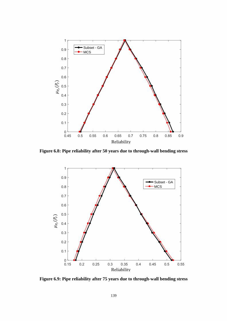
139
Figure 6.8: Pipe reliability after 50 years due to through-wall bending stress
Figure 6.9: Pipe reliability after 75 years due to through-wall bending stress
MCS Subset - GA
Reliability
(𝑃𝑟)
𝜇𝑃𝑟(𝑃𝑟)
Reliability
(𝑃𝑟)
MCS Subset - GA
𝜇𝑃𝑟(𝑃𝑟)

140
Figure 6.10: Pipe reliability after 100 years due to through-wall bending stress
Figure 6.11: COV versus membership level
MCS Subset - GA
Reliability
(𝑃𝑟)
𝜇𝑃𝑟(𝑃𝑟)

141
Figure 6.12: Sensitivity test for pipe performance at 25 years design life (pipe
ovality)
Figure 6.13: Sensitivity test for pipe performance at 100 years design life (pipe
ovality)
Reliability
(𝑃𝑟)
𝜇𝑃𝑟(𝑃𝑟)
= 0.0610
= 0.0605
= 0.0600
= 0.0595
Reliability
(𝑃𝑟)
𝜇𝑃𝑟(𝑃𝑟)
= 0.0610
= 0.0605
= 0.0600
= 0.0595

142
6.4.3 Discussions
As shown in Figures 6.3 - 6.6 and Figures 6.7 – 6.10, the proposed model has been
compared with the MCS approach and the outcome demonstrates that the proposed
approach is robust, reliable and efficient for analysis of engineering structures. The
optimised subset simulation algorithm for the estimation of fuzzy reliability of an
engineering structure has helped to directly solve the reliability problem by focussing on
the maximum of the objective function. In the computation, for each realisation of fuzzy
variables, a total of 106 performance function evaluation counts are required to estimate
the reliability of the structure at each bound when using the MCS, while a total of 650
performance function evaluation counts are needed when using the optimised subset
simulation approach. This clearly demonstrates the computational efficiency of the
proposed method. Also, the computational time for the two methods is assessed, and in
both cases, the expressions are defined in analytical form, which makes the computational
process fast. The two techniques have been measured running on a CPU time using a 1.60
GHz Pentium 4 computer. The computational times required for MCS approach is 281
minutes, while the proposed method is 264 minutes. However, a further computational
assessment based on the COV is reported in Figure 6.11. The COV for MCS is computed
using the expression in Eq. (6.16) and for subset-GA approach, it is estimated using Eq.
(6.17) (Au & Beck, 2001).
√(1 − 𝑃𝑓) 𝑁𝑃𝑓⁄ , (6.16)
√(log(𝑃𝑓))2(1 − 𝑃0)(1 + 𝛾 ) (log(𝑃0))2𝑁𝑃0⁄ (6.17)
Where 𝛾 represents the correlation factor. In Figure 6.11, the assessment is performed on
every membership level, and the result shows that the proposed method can lead to a
substantial improvement in computational efficiency over MCS when estimating small
failure probabilities. However, this advantage begins to narrow down as the probability
of failure approaches unity.

143
Table 6.1: Failure probability of buried pipe after 25-years
Subset-GA
Lower bound Upper bound
0 0.002106 0.445403 0.03688 0.2385
1 0.002547 0.431663 0.033118 0.246276
2 0.002987 0.420146 0.029339 0.255033
3 0.003602 0.406616 0.026285 0.262976
4 0.004196 0.395584 0.023155 0.27214
5 0.005029 0.382497 0.020671 0.280341
6 0.005829 0.371828 0.018137 0.289792
7 0.006928 0.359345 0.016133 0.298254
8 0.008018 0.348784 0.014114 0.307917
9 0.009374 0.337492 0.012431 0.317093
10 0.010957 0.326215 0.010957 0.326215
It is worth mentioning that the engineering application of the proposed model is vital to
structural engineering problems, especially where there are fuzzy and random variables.
Figures 6.12 and 6.13, show the parametric analysis of pipe performance at 25 years and
100 years design life based on pipe ovality failure mode by critically analysing the level
of imprecision on the pipe strength. For instance, the maximum allowable value of pipe
ovality (βovality) is changed using values such as 0.0610, 0.0605, 0.060 and 0.0595. It
can be deduced that after the first 25 years (Figure 6.12), the impact of the changes in
imprecision is insignificant compared to the 100 years (Figure 6.13) design life for fuzzy
reliability assessment. The practical implication of this could mean that the uncertainty
level is high and therefore minor changes in imprecision could lead to a notable change
in the reliability of the structure. Similarly, as shown in Table 6.1, a 3% level of increase
in imprecision leads to upper bound reliability of 0.03688 and lower bound reliability of
0.002106, which is slightly more than one order of magnitude larger than the standard
analysis. Also, in Table 2, as the 𝛼 − 𝑙𝑒𝑣𝑒𝑙 increases, the corresponding failure
probability for the lower and upper bound increases. This feature also demonstrates, how

144
sensitive the interval-based reliability analysis is with respect to the level of imprecision
of the input variables. However, the 𝛼 − 𝑙𝑒𝑣𝑒𝑙 gains its usefulness by examining the
reliability of the structure at different level, which can represent a different degree of
imprecision. Based on this, a better understanding of the impact of uncertainty associated
with the failure of buried pipe can be evaluated. This feature helps to capture and quantify
the negative effects of uncertain variables on the performance of an engineering structure
with regards to estimating the reliability of the structure.
6.5 Chapter Summary
This Chapter analysed the reliability of buried pipe based on fuzzy-subset simulation
approach and considering the effect of uncertain variables. The underlying ideas behind
the proposed algorithm are explained, and an example problem based on the buried
pipeline is used to analyse the applicability and efficiency of the proposed model. The
approach relies on the performance function of the buried pipe, which involves random
and fuzzy variables for the modelling of the pipe structure. The values of the fuzzy
variables for every alpha-level are first obtained using the membership function.
Therefore, the set values of the fuzzy variable bound the reliability of the structure, and
this is evaluated using optimisation and efficient subset simulation approach. The
rationale behind the proposed strategy is to locate a failure domain or region where the
objective function is minimised or maximised and compute the reliability using subset
simulation. The presented approach illustrates that the fuzzy uncertainty of the input
variables could be propagated to determine the fuzzy reliability of the membership
function of a structural system. For the full evaluation of the random variables, the
approach utilised the efficiency and capability of subset simulation. MCS is used to
validate the applicability of the proposed method, and the result shows a very good
agreement. The developed model can accommodate a various degree of uncertainty in the
computation of the fuzzy reliability and can easily be applied to other engineering
structures. Because of the deteriorating condition of the buried pipeline, it is essential to
develop a maintenance strategy in other to keep the risk under control. As a result,
determining the optimal time for maintenance of the buried pipe becomes an important
aspect of this study. Therefore, a maintenance strategy is proposed in Chapter 6 and is

145
designed at evaluating the performance of a buried pipeline using fuzzy reliability, risk,
and cost to predict the optimal time interval for maintenance.

146
CHAPTER SEVEN
7 MAINTENANCE OF DETERIORATING BURIED PIPE
USING OPTIMISATION INVOLVING FUZZY
RELIABILITY, RISK AND COST

147
7.1 Introduction
In this Chapter, a maintenance approach is proposed and is aimed at examining the
performance of a buried pipeline using fuzzy reliability, risk, and total maintenance cost
to predict the optimal time interval for maintenance. The goal is achieved using a multi-
objective optimisation where the first objective is the minimisation of the total cost of
maintenance, while the second objective involves the maximisation or minimisation of
one of the performance indicators (e.g., fuzzy reliability or risk). The maintenance of the
deteriorating pipe segment is considered so that when replaced, there will be a total
restoration of the performance of the pipe segment to the original condition. The pipe
segment with the highest repair priority will be determined using performance indicator,
considering maximum reliability and minimum risk.
The performance of underground pipe network influenced by adverse environmental
effects (e.g., corrosion) and the associated induced failure possibility and risks increases
as the impact of the effects increases. Corrosion effect has affected the safe operation of
most engineering structures over the years. For a buried pipeline, corrosion has gradually
reduced the resistance of the mechanical and the structural properties, which has increased
the possibility of failure over time. Due to the deteriorating condition of the buried
pipeline, the assessment and maintenance would require a proper inspection and
maintenance activities to keep the risk under control. As a result, the evaluation and
determination of the optimal time for maintenance of the buried pipe become an important
research area.
Considering the safe operation of the buried pipe, Hong (1999) stated that the optimal
maintenance programme should be defined based on a minimum acceptable level of
failure probability. Similarly, regarding cost Laggoune et al. (2010) suggested that the
optimal maintenance planning should be defined based on the minimum expected cost.
The two viewpoints play a vital role in regards to when maintenance should be carried
out. Also, Barone & Frangopol (2014a) suggested that the increase in the number of
systems that reached critical conditions, due to deterioration of the structural resistance,
has directed the attention of researchers to the development of a method that would
provide cost-effective maintenance approach. However, this Chapter presents the
development of a cost-effective strategy that would assist the decision-makers with the

148
tool to know the appropriate time interval to carry out maintenance within the design life
of the buried pipe.
The rest of this Chapter is organised as follows: Section 7.2 presents the maintenance of
buried pipe and performance indicators. Section 7.3 explains methods for evaluating
performance indicators and the procedure for estimating the structural reliability. In
Section 7.4, the numerical example is presented, and Section 7.5 explains the performance
indicators and total cost using multi-objective optimisation. Also, the outcome of the
annual fuzzy reliability and total maintenance cost, and the annual risk and total
maintenance cost is presented. Section 7.6 presents a parametric study and Section 7.7
explains Chapter summary.
7.2 Maintenance of Buried Pipe and Performance Indicators
The buried, ageing and deteriorating pipeline network is maintained to ensure safe
operation within the service life. The benchmark for a new service design life of pipeline
is commonly set as 50 years, although other pipe products and design methods under
certain conditions may provide a service life of around 100 years (Najafi, 2011). Also, to
successfully achieve the purpose of pipe maintenance, factors such as the history of the
pipe, possible causes of failure (corrosion, concentrated load, or nearby blasting), leakage,
failure modes, and the nature of the transported fluid should be adequately considered.
Without a proper and detailed understanding of the overall pipeline failure conditions, it
is difficult to select a maintenance approach that would mitigate the problem
appropriately. However, in this study, a corrosion-induced failure is considered based on
the structural failure mode of a buried pipeline. A replacement of a pipe section is deemed
to based on the optimal time and whenever a maintenance action is required relying on
the outcome of the pipe reliability and the associated risk. The objective of pipe
replacement design involves a set of equations that is based on limit state functions and
considering factors such as pipe material properties, soil, traffic loads, and other loading
conditions.
Various techniques considered in assessing the structural performance of buried pipe
throughout the design life may involve the use of performance indicators such as

149
reliability, and risk or lifetime distribution such as hazard function. However, the use of
life cycle maintenance is a fundamental requirement for sustaining and ensuring that the
performance of the engineering structure is above a specific safety level (Barone &
Frangopol, 2014b; Biondini & Frangopol, 2009). Therefore, it is vital for any
maintenance approach to take account of the optimal time for maintenance interventions.
The inspection of the buried pipe during the design life would assist to identify any
structural defects, evaluate the structural performance and, update the structural models
established in the design stage while maintenance interventions are required to maintain,
improve, or restore the structure to the initial state. Barone & Frangopol (2014b),
suggested that the maintenance interventions aimed at slowing down the structural
deterioration process or restoring the resistance of one or more component of the structure
when a specific condition is reached. Slowing down the deterioration process is more of
the preventive maintenance while the restoring the resistance of the part of a structure is
called the essential maintenance (Barone & Frangopol, 2014b). The essential
maintenance is usually performed when one or more of the performance indicators reach
a predefined level.
In the literature, essential maintenance of a structure based on a probabilistic approach is
used for the evaluation of structural reliability as illustrated in Figure 7.1. Herein, the
essential maintenance approach is analysed based on a non-probabilistic method for the
assessment of the structural safety as shown in Figure 7.2. Corrosion is evaluated as fuzzy
variable because of the uncertainty associated with the corrosion parameters. This
approach has helped to capture the variabilities related to corrosion process, which cannot
be obtained using the probabilistic method. The essential maintenance approach assumed
that the reliability of the structure returns to the original condition after repair as
illustrated in Figure 7.1 and Figure 7.2. The time interval used to perform the maintenance
is not considered, and for this reason, the reliability of the structure would suddenly
increase at the time of repair.

150
Figure 7.1: Reliability and maintenance cost over time (probabilistic method)
Figure 7.2: Reliability and maintenance cost over time (non-probabilistic method)

151
Buried pipes are usually affected by corrosion over time, for example, continuous
reduction of pipe walls can lead to failure. Maintenance carried out through replacement
of corroded part would return the pipe segment to its original state, which would enhance
the performance of the pipe network. In some cases, a repair priority can be assigned to
one or more pipe sections, based on their likelihood and consequences of failure. The
decision to carry out a maintenance using different repair options and time will depend
on the performance indicators considered in the analysis.
Maintenance of buried pipeline system requires continuous upkeep of every segment and
components to ascertain a suitable functionality. The terms preventive and essential
maintenance are used to describe different types of maintenance. Preventive maintenance
ensures that the structure does not deteriorate to a critical state before essential
maintenance is carried out. Preventive maintenance is usually performed during the life
cycle before the safety state of the structure is dangerous. Essential maintenance is needed
when the structure has reached suggested performance thresholds, which could threaten
the safety of the structure and cause an environmental hazard (Barone & Frangopol,
2014a). Barone & Frangopol (2014a), suggested that the use of essential maintenance
actions plan provide rescue of the structural performance of engineering structure. On the
other hand, the cost-efficiency of maintenance can be maximised by carrying out
maintenance at an optimal time before failure occurs. Therefore, maintenance of buried
pipeline structure should be formulated as an optimisation problem. A multi-objective
optimisation approach, which uses performance indicator and total maintenance cost as
objective functions are proposed for the maintenance of buried pipe.
7.3 Annual Fuzzy Reliability and Risk as Performance Indicators
There are several probabilistic and non-probabilistic methods that have been proposed to
analyse the performance of deteriorating structures while considering the effect of
uncertain variables. These proposed methods aimed at the assessment of the structure
over the life cycle to ensure the reliability of the structure. While considering the effect
of randomness and fuzziness, a rational way to treat these uncertain variables is to
consider an approach that can simulate the two types of uncertainty. In this context, the

152
failure probability of a structure can be defined as the probability of violating the limit
state associated with the failure mode of the structure as explained in Chapter 3.
For a buried pipe, the deterioration process due to corrosion occurs with time, so the
performance indicator is analysed at a time 𝑡. In this study, the performance indicator for
reliability and risk associated with the failure of the buried pipe is performed annually.
The determination of the failure probability of a structure involving fuzzy and random
variables using optimisation is usually a challenging task because of the computational
cost. For this reason, a simplified approach is proposed as shown in Section 7.3.1
Risk assessment of an engineering structure has been recognised in recent time as a
crucial part of decision making (Barone & Frangopol, 2014a). As a result of this, several
performance indicators have been proposed to evaluate a time-dependent structural
performance of deteriorating buried pipeline (Ahammed & Melchers, 1997; Sadiq et al.,
2004; Tee et al., 2014). Due to the need of taking into account, the consequences
associated with the failure of buried pipeline, making of decisions based on risk has
become an essential tool for optimising the time for maintenance. The assessment of risk
can be either qualitative or quantitative. According to Arunraj & Maiti (2007), qualitative
risk assessment deals with simple descriptions of the types of hazards, their consequences
and likelihood, which are reported in an opportunely built risk matrix In this study, a
quantitative risk assessment is considered, and it is the risk associated with a particular
failure mode of buried pipe. It is defined as the product of the failure probability and the
associated consequences.
Over the years, optimisation algorithms are used while considering maintenance times as
design variables, which allow the identification of possible opportunity for maintenance
during the design life cycle. In this Chapter, two different optimisation problems based
on reliability, risk, and total maintenance cost are utilised for the determination of the
optimal maintenance time of a buried pipe. The failure modes considered herein for the
analysis are briefly described in Chapter 3, Section 3.3. The structural failure modes of
buried pipe have been modelled as a series-series system so that failure will occur when
either of the failure conditions exceeds the safety threshold.

153
7.3.1 Procedure for Estimating Reliability
The propagation of the random and fuzzy variables for the maintenance of a buried pipe
system was performed using fuzzy reliability. Möller et al. (2003) suggested that the
determination of the fuzzy reliability of a structure requires a fundamental stochastic
solution, which means in principle any probabilistic algorithm could be used for this
purpose. In this study, a subset simulation approach is employed and the procedure is
summarised below:
1. Initialise the design parameters and sample random variables and develop the
membership of the fuzzy parameters.
2. Discretise the membership function into ten 𝛼 − level cut. The vector of the fuzzy
variables θ̃ could be expressed as:
θ̃ = �̃�1, �̃�2, … , �̃�𝑛 = �̃�11, �̃�1
2, … , �̃�1𝑁; �̃�2
1, �̃�22, … , �̃�2
𝑁; … , �̃�𝑛1, �̃�𝑛
2, … , �̃�𝑛𝑁 (7.1)
Where n denotes the number of fuzzy variables for the vector θ̃ and 𝑁 is the
number of samples for every �̃�𝑖 used in the computation. For every 𝛼 − 𝑙𝑒𝑣𝑒𝑙 the
fuzzy variable can be decomposed into �̃�𝐹𝐿(𝛼) and �̃�𝐹
𝑈(𝛼). Where �̃�𝐹𝐿(𝛼) denotes
the lower and �̃�𝐹𝑈(𝛼) is the upper value of every 𝛼 − level cut. The membership
interval �̃�𝐹(𝛼) ∈ (�̃�𝐹𝐿(𝛼), �̃�𝐹
𝑈(𝛼)), which corresponds to a particular membership
level of a fuzzy variable.
3. Compute the boundaries of performance function at every 𝛼 − level for lower and
upper bounds of the structural response in each case for �̃�𝐹(𝛼) ∈
( �̃�𝐹𝐿(𝛼), �̃�𝐹
𝑈(𝛼)) . This will lead to the formulation of the limit state
function 𝑌(𝛼) = 𝑔𝑖(�̃�𝐹𝐿(𝛼)) and 𝑌(𝛼) = 𝑔𝑖(�̃�𝐹
𝑈(𝛼)) for every 𝛼 − level cut.
4. Calculate the reliability of the structure for lower 𝑅𝐿and upper 𝑅𝑈 using subset
simulation (SS) (see Chapter 6, Section 6.3.2). Based on the relationship between
the outcomes of subset simulation with the effect of corrosion, the reliability of
the structure considering the lower and upper values for every 𝛼 − level cut can
be expressed as shown in Eq. (7.2) and Eq. (7.3)

154
𝑅𝐿(𝛼𝐿; 𝑇) = 1 − 𝑃(�̃�𝐿)∏ 𝑃(�̃�𝑖+1𝐿 |�̃�𝐿)𝑁−1
𝑖=1 |𝛼𝐿
(7.2)
𝑅𝑈(𝛼𝑈; 𝑇) = 1 − 𝑃(�̃�𝑈)∏ 𝑃(�̃�𝑖+1𝑈 |�̃�𝑈)𝑁−1
𝑖=1 |𝛼𝑈
(7.3)
7.4 Case Study
The investigated problem and the numerical values are obtained from the literature (Khan
& Tee, 2016; Rahman & Vanier, 2004). The total length of the flexible metal pipe is
approximately 789 km, and the pipe network comprises of medium size steel and ductile
iron materials. However, one Section of the medium size steel was used to test the
applicability and the usefulness of the fuzzy-based optimal maintenance approach. The
approach utilised fuzzy reliability and GA to evaluate the optimal time interval to carry
out maintenance of buried pipe network. The pipe material, location, and statistical
properties for the considered segments are reported in Table 7.1 and Table 7.2, with an
assumption that the pipe network is constructed above the underground water table.
Therefore, the effect of subsurface water table was not considered in the analysis. The
corrosion parameters for final pitting rate constant 𝑎, pitting depth scaling constant 𝑏 and
corrosion rate inhibition factor 𝑐 are modelled as fuzzy variable and the values are
expressed in Eq. (7.4), Eq. (7.5), and Eq. (7.6).
𝜇𝑎(𝑎) = { 𝑎 − 0.001 0.008;⁄ 0.001 ≤ 𝑎 ≤ 0.009
𝑎 − 0.015 (−0.006);⁄ 0.009 ≤ 𝑎 ≤ 0.015 (7.4)
𝜇𝑏(𝑏) = { 𝑏 − 2.5 3.77;⁄ 2.5 ≤ 𝑏 ≤ 6.27
𝑏 − 7.5 (−1.23);⁄ 6.25 ≤ 𝑏 ≤ 7.5 (7.5)
𝜇𝑐(𝑐) = { 𝑐 − 0.01 0.09;⁄ 0.01 ≤ 𝑐 ≤ 0.1
𝑐 − 0.18 (−0.17);⁄ 0.1 ≤ 𝑐 ≤ 0.18 (7.6)
In this example, corrosion-induced failures modes as explained in Chapter 3 with limit
state functions are used to evaluate the optimal time for maintenance. The effect of a
continuous reduction of pipe thickness over time due to corrosion is considered over the
service life. Loads acting on the buried pipe are as a result of live and soil load, and they
are considered in the analysis. The failure probability of the pipe segment has been
estimated using fuzzy-subset simulation approach. The approach is employed to capture

155
the impact of corrosion uncertainty on buried pipes, where the probability information is
considered not adequate for standard probability analysis. The reliability and the failure
probability results based on 𝛼 − levels 1, 5 and 8 of the membership function of a fuzzy
variable are reported in Figures 7.3 and Figure 7.7. The various 𝑎 − level sets may
denotes different opinion of engineering judgement or expert knowledge based on the
uncertain fuzzy variables in other to gauge the effect of uncertainties. However, 𝑎 −
levels 8 is used herein to plan the maintenance of buried pipe.
Optimal maintenance plans for the buried pipeline are investigated based on two different
approaches, and these include reliability and risk associated with pipe failure. The
maintenance plans involve essential maintenance actions on any of the pipe segment and
are considered new after repair. The maintenance cost (cost of replacement) is assumed
to be £25,000, and a discount rate r of 2% is used in the analysis. The cost of injuries and
fatalities, environmental damages, and cost of deferred supply during the pipe
maintenance are assumed to be £10,000,000. These costs are obtained based on the case
study of Rahman & Vanier (2004) and Davis et al. (2008) report.
Table 7.1: Statistical properties
Properties Mean value Coefficient of
variation %
Distribution
Elastic modulus of steel
pipe 𝑬
210 GPa 1.0 Normal
Modulus of soil reaction 𝑬′ 2 MPa 5.0 Normal
Unit weight of soil 𝜸𝒔 18.0 kN/m3 2.5 Normal
Backfill soil modulus 𝑬𝒔 103kPa 5.0 Normal
Deflection coefficient 𝑲𝒃 0.11 1.0 Lognormal
Buoyancy factor, 𝑹𝒘 1.0 - -
Yield stress, 𝝈𝒚 475MPa 5.0 Normal
Deflection lag factor, 𝑫𝑳 1 - -

156
Table 7.2: Pipe materials and location properties
Pipe segment A
Material Steel
Location Commercial
Embedment soil Clay
Length (km) 150
Mean diameter (mm) 600
Thickness (mm) 9
Soil height above soil invert (m) 2.0
Wheel load (live load), 𝑷𝒔 100
7.5 Performance Indicators and Total Cost Using Multi-objective
Optimisation
The annual performance indicators for buried pipe usually assumes numerical values,
which represents the performance condition of the buried pipe at a given time during its
life cycle. Traditionally, this can be computed annually, that is a one-year interval. The
performance of an underground pipeline over the design life is evaluated with regards to
a specific limit state. However, this will depend on the design intent of the assessment,
the function and strategic importance of the structure. The soil and pipe parameters are
associated with uncertainties that affect the ultimate performance of pipe structure over
time. Therefore the performance indicators provide a measure of the likelihood of pipe
failure within the service life.
Most engineering parameters associated with a significant amount of uncertainties are as
a result of lack of information or knowledge on how to efficiently estimate the values of
the parameter. In numerical analysis, uncertainties are usually accounted for through the
use of the traditional probabilistic model (Baecher & Christian, 2005). The probabilistic
modelling approach is associated with challenges because of lack of information
particularly with geotechnical engineering parameters (Beer, Zhang, et al., 2013). Also,
the data required for the computation of mathematical statistics are often not available in
157
sufficient quantity and quality. With the lack of information concerning the design
parameters, a non-probabilistic approach, e.g., fuzzy modelling provides the needed
method to capture the impact of the uncertain parameter on the performance of the
structure. In this study, a fuzzy-based model as explained in section 7.3.1 is used to
determine the annual reliability and probability of failure that produces a lower and upper
bound as illustrated in Figure 7.3 and Figure 7.7.
In the literature, annual performance indicators have been used to assess the maintenance
of engineering structure based on reliability index, risk and cost (Dong & Frangopol,
2015; Khan & Tee, 2016). Herein, a non-probabilistic approach is utilised for the
determination of the optimal maintenance time of a buried pipeline. The fuzzy method is
considered in computing the structural reliability so that the effect of the uncertain fuzzy
variable on the overall performance of buried pipeline can be captured. The annual
reliability and risk based on the α − level of the membership function associated with
buried pipe performance are studied. The former is considered due to its direct definition
regarding estimating the failure probability, and the latter due to its increasing importance
in decision making and also, research field.
7.5.1 Annual Fuzzy Reliability and Total Cost of Maintenance
The first method discussed in this study is based on the use of fuzzy annual reliability for
the optimal pipe maintenance. In this approach, a multi-objective optimisation procedure
is used to analyse the optimal maintenance planning of a buried pipeline, and a numerical
application dealing with a series-series connection of the pipe structural failure mode. The
aims of this optimisation approach are (a) to maximise and determine the minimum
annual structural reliability of buried pipe over a 125 years life cycle, and (b) to minimise
the total cost required to carry out maintenance within the design life. This will help to
keep the buried pipe in a safe working condition throughout the design life. The fuzzy
structural reliability-based on lower and upper bounds for the performance of buried
metal pipe is shown in Figure 7.3 for the condition where there are no maintenance
actions. The values of the structural response for the annual reliability have been obtained
using a fuzzy approach that utilised subset simulation for estimating structural reliability.

158
The failure of the buried pipeline will involve a direct economic loss and other financial
consequences as a result of the incident. However, a maintenance action would be
required, and this would be carried out on the pipe segment with the lowest reliability at
the time maintenance is required. The present total cost of maintenance 𝐶𝑇𝑜 for keeping
the each segment of buried pipe in safe working condition is expressed in Eq. (7.7).
𝐶𝑇𝑜 = ∑𝐶𝐹
(1+𝑟)𝑇𝑁𝑖=1 (7.7)
Where 𝑁 denotes the total number of sections that require replacement during the time
for maintenance; 𝐶𝐹 represents the future cost of carrying out the replacement of each
component of the pipe network; and 𝑟 is the annual discount rate.
The formulation of the multi-objective optimisation is described by using the following
minimisation problem.
Given: 𝑔(𝑇), 𝐶, 𝑟, (7.8)
Find 𝑇𝑜𝑝𝑡 = {𝑇1, … , 𝑇𝑛} (7.9)
To minimise: {𝑃𝑟𝐿(T)𝐶𝑇𝑜
0 ≤ T ≤ 125 years (7.10)
And
{𝑃𝑟𝑈(T)𝐶𝑇𝑜
0 ≤ T ≤ 125 years (7.11)
Such that: {0 years ≤ 𝑇opt ≤ 125 years} (7.12)
Where 𝑔(𝑇) represents the limit state functions associated with the structural pipe failure
modes; 𝐶𝑇𝑜 denotes the cost of carrying out maintenance for each of the pipe segment; 𝑟
is the annual money discount rate; 𝑛 is the total number of designed years for the
structure; 𝑇𝑜𝑝𝑡 = {𝑇1, … , 𝑇𝑛} represents the vector of the repair times; 𝑃𝑟𝐿(T) is the
minimum lower bound value of the reliability of pipe over its life cycle, 𝑃𝑟𝑈(𝑇) denotes
the minimum upper bound value of the pipe reliability over its design life and CT is the
total cost of the maintenance plan, evaluated using Eq. (7.7).
The goal of Eq. (7.8) and Eq. (7.11), has been defined regarding the fuzzy annual
reliability for the lower and the upper bound of the buried pipe system, so that a

159
minimisation problem can be achieved with respect to the two objectives. The optimal
solution of the functions is obtained using a GA, and a single cross-over has been adopted,
using an initial population of 200 trial solutions. The formulation and cross-over functions
have been adapted to comply with constraints defined in Eq. (7.12).
Figure 7.3 shows the fuzzy annual reliability for the lower and upper bound of pipe
segment A with no maintenance action, while the Pareto front obtained from the
optimisation is given in Figure 7.4. The first set of the maintenance activities associated
with Figure 7.4 for the pipe segment is characterised by two renewal actions occurring at
different times, for the lower and upper bound reliability. The optimal time determined
based on the optimisation outcome occurred at 60 years and 66 years. However, the
maintenance plan involves essential maintenance, which requires replacement of the pipe
segment with the lowest reliability at the time when pipe maintenance is needed. Because
the failure modes are considered to be connected in series, which means one failure mode
will affect the other and cause the buried pipeline to fail. Therefore, replacement of pipe
segments would provide the needed reliability for the pipe network at the time of
maintenance. By considering Eq. (7.7), the cost of the maintenance plan at 60 years and
66 years will be £82,025 and £92,374 respectively. Also, the fuzzy reliability profile
associated with the optimal time for maintenance of the pipe segment is shown in Figure
7.5. In this case, two maintenance actions time are provided for the maintenance of the
buried pipe.

160
Figure 7.3: Pipe reliability with no maintenance action
Figure 7.4: Reliability-based Pareto front of buried pipe

161
Figure 7.5: Pipe reliability with maintenance action
7.5.2 Annual Risk and Total Cost of Maintenance
The failure of engineering structures are often associated with consequences, and as a
result, risk-based assessment becomes necessary, and also, an essential tool for
optimisation of maintenance. Ang & Tang (1984) defined risk as the product of the
probability of failure and the associated consequences in monetary terms as a result of the
failure. Assessment of risk associated with engineering structures can be analysed
qualitatively or quantitatively. Qualitative risk assessment of structures deals with simple
descriptions of different types of hazards, the associated consequences and likelihood,
and reporting all these aspects in a constructive and opportunely built risk matrices
(Arunraj & Maiti, 2007; Barone & Frangopol, 2014b). However, a quantitative risk
assessment is considered in this study and Figure 7.6, illustrates a flowchart of the
computational process used for the risk assessment of buried pipe considering thickness
reduction due to corrosion. The quantitative risk assessment associated with the failure of
pipe is defined as the product of the failure probability for each pipe segment at time t
and the associated consequences due to failure.

162
Compute or estimate the ultimate pipe
strength (this will depend on the failure
mode)
Compute pipe response based on the
structural failure mode
Evaluate the effect of
thickness reduction by
considering corrosion effect
Compute the annual reliability based
on fuzzy subset simulation approach
Determine the time dependent risk associated with
failure of buried pipe
Evaluate the consequences (i.e.,
direct and indirect cost) associated
with pipe failure
Figure 7.6: Framework for risk assessment of buried pipe considering thickness
reduction
The fuzzy annual failure probability and fuzzy annual reliability do not have or contain
information concerning the consequences or severity associated with the pipe failure. But
considering the risk related to the likelihood of failure, more detailed information for
decision-makers or managers when dealing with issues concerning pipe performance over
the design life is provided. The most common way of quantifying consequences
associated with pipe failure risk is to evaluate the losses associated with the failure
regarding cost. The cost related to structural failure can be a direct cost, e.g., cost of
replacing the failed part or indirect cost, e.g., environmental contaminations cost. Barone
& Frangopol (2014a) suggested that the direct consequences of failure are often

163
associated with repair/replacement cost of the structural component while the indirect
consequence is the estimation cost derived from failure, which may not strictly be related
to rebuilding the structure. In this case, the indirect effects of pipe failure may contain,
for example, injuries, fatalities or environmental contaminations as a result of the
structural failure of the buried pipe. With regards to any segment of the pipe network, the
risk associated with the possibility of pipe failure is expressed in Eq. (7.13).
𝑅(𝑇) = 𝑃𝑓𝐶𝑑𝑖𝑟(𝑇) + 𝐶𝑖𝑛𝑑𝑖𝑟(𝑇) (7.13)
Where 𝑃𝑓 denotes the failure probability of the pipe segment, 𝐶𝑑𝑖𝑟(𝑇) represents the
direct cost of replacing the pipe segment and 𝐶𝑖𝑛𝑑𝑖𝑟(𝑇) is the indirect cost.
Indirect consequences for failure of buried pipe network are estimated as the sum of three
different losses. These include the cost of injuries and fatalities, environmental damages
and cost of deferred supply during the pipe maintenance. By making allowance for the
discount rate of money, the direct and indirect present cost of pipe maintenance can be
obtained using Eq. (7.14) and (7.15).
𝐶𝑑𝑖𝑟(𝑇) =𝐶𝑟
(1+𝑟)𝑇 (7.14)
𝐶𝑖𝑛𝑑𝑖𝑟(𝑇) =𝐶𝑖+𝐶𝑒+𝐶𝑑
(1+𝑟)𝑇 (7.15)
Where 𝐶𝑟 denotes the direct cost of replacing a pipe segment, 𝐶𝑖 represents the cost of
injuries, 𝐶𝑠 is the cost of environmental damages and 𝐶𝑑 is the cost of deferred supply
during maintenance.
The total annual pipe risk (i.e., the sum of direct and indirect risks) for the buried pipeline
structure when there is no maintenance action is shown in Figure 7.7. As observed in
Figure 7.7, the risk associated with pipe failure increases as time increases since
maintenance action is not applied. However, to ensure that the structural performance is
above the recommended safety level during the service life, it is crucial to reduce the risk
associated with pipe failure. Similar to what was used for the reliability case in Section
7.4.1, a multi-objective optimisation procedure is proposed for the determination of
optimal maintenance plan for buried pipe using the same constraints. However, in this

164
investigation, replacement of pipe segment would be performed on the segment
associated with the highest risk. Therefore, the optimisation problem is as follows:
Given: 𝑔(𝑇), 𝐶, 𝑟, (7.16)
Find 𝑇𝑜𝑝𝑡 = {𝑇1, … , 𝑇𝑛} (7.17)
To minimise: {𝑅𝑚𝑎𝑥𝐿 (T)𝐶𝑇𝑜
0 ≤ T ≤ 125 years (7.18)
And
{𝑅𝑚𝑎𝑥𝑈 (T)𝐶𝑇𝑜
0 ≤ T ≤ 125 years (7.19)
Such that: {0 years ≤ Topt ≤ 125 years} (7.20)
Where 𝑅𝑚𝑎𝑥𝐿 (T) is the maximum lower bound value of the annual risk and 𝑅𝑚𝑎𝑥
𝑈 (T) is
the maximum upper bound value of the annual risk over the considered designed life of
the pipe network.
For the risk analysis, the design variable changes during the optimisation, and a Pareto
front, as shown in Figure 7.8, are obtained, containing the dominating solutions for the
various possible time of repairs. Also, the fuzzy risk profile associated with maintenance
action as shown in Figure 7.8 is, instead, shown in Figure 7.9. In this case, two repair
actions are provided for the maintenance of pipe network, which corresponds to the lower
and upper risk. The optimal time for the lower and upper risk happened at 62 years and
69 years and the corresponding cost of carrying out the maintenance is approximately
£85,340 and £98,028 respectively.

165
Figure 7.7: Annual risk of buried pipe with no maintenance action
Figure 7.8: Risk-based Pareto front of buried pipe
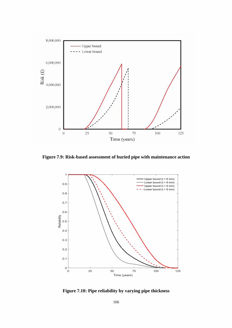
166
Figure 7.9: Risk-based assessment of buried pipe with maintenance action
Figure 7.10: Pipe reliability by varying pipe thickness

167
7.6 Parametric Study
7.6.1 The Effect of Pipe Design Variables on Pipe Reliability and Risk
In this study, the parameters of pipe are considered as deterministic, random and fuzzy
variables as defined in Table 7.1, Table 7.2 and Eq. (7.4) to Eq. (7.6). Figure 7.10 and
Figure 7.11, shows the effect of pipe wall thickness and the yield stress due to pipe
thickness reduction, and with respect to pipe reliability for the service life of 125 years.
The result shows that both can affect pipe reliability, the optimal time for maintenance
and the associated risk. This is demonstrated by varying the mean values of the input
parameters. The increase in pipe thickness and the yield stress increases pipe reliability
and the optimal time for maintenance and the associated risk is reduced. The outcome
also shows that pipe thickness has a significant impact on pipe reliability compared to the
yield stress. This demonstrates the importance of pipe wall thickness in the safety of the
buried pipeline. Also, it could be that the outcome of the thickness reduction of pipe wall
due to corrosion defects that produce the sudden decrease of pipe capacity. Based on this
result, it is important to note that the pipe reliability, risk and optimal time for
maintenance can be influenced significantly by a thickness reduction of the pipe wall.
Figure 7.11: Pipe reliability by varying pipe yield stress of pipe material

168
7.6.2 The Effect of Cost Ratio (Direct and Indirect Cost)
As explained in Section 7.5.2, the direct cost of pipe failure is the cost associated with the
replacement of structural component or segment and the indirect cost involves the cost of
injuries, fatalities or environmental contaminations. Since the risk associated with pipe
failure includes direct and indirect cost, then, their effect including the failure probability
can be analysed with regards to the time of maintenance. Based on Eq. (7.13) and to keep
the buried pipeline safe during the design life, Eq. (7.21) is proposed to minimise the risk
function.
𝑅(𝑇𝑜𝑝) = 𝑃𝑓(𝑇𝑜𝑝)𝐶𝑑𝑖𝑟 +
𝑇𝑑
𝑇𝑜𝑝𝐶𝑖𝑛𝑑𝑖𝑟 (7.21)
Where 𝑇𝑜𝑝 represents the optimised time required for the replacement or maintenance to
be conducted; 𝑇𝑑 denotes the designed life.
The relationship 𝑇𝑑
𝑇𝑜𝑝 represents the frequency of maintenance required during the
designed life. From Eq. (7.21), an optimal time for maintenance can be found as the
minimum of the risk function with respect to optimal time 𝑇𝑜𝑝.
𝑇𝑜𝑝: 𝑅(𝑇𝑜𝑝) → min𝑇𝑜𝑝
. (7.22)
Therefore, the function 𝑅(𝑇𝑜𝑝) is differentiable at any time 𝑇𝑜𝑝, where the residual pipe
thickness is less than the pipe wall thickness and this is expressed in Eq. (7.23).
𝑅𝑇𝑜𝑝′ = 𝑃𝑓(𝑇𝑜𝑝)
′ 𝐶𝑑𝑖𝑟 + (−𝑇𝑑
(𝑇𝑜𝑝)2) 𝐶𝑖𝑛𝑑𝑖𝑟 (7.23)
From Eq. (7.23), the optimal time for maintenance or replacement of pipe segment can
be determined based on the risk function and numerical solution of the equation. Also,
the expression shows that the optimal time for maintenance will depend on the direct and
indirect cost, the designed life and probability of failure. However, the maintenance of
buried pipe by replacing the failed pipe segment is ideal when it is performed before
failure. This will help to save the indirect cost associated with the failure of the pipe. In
Figure 7.12, it can be deduced that as the optimal time required for maintenance increases,
the cost ratio with the probability of failure increases over the designed life. Based on

169
this, it is crucial to quantify efficiently all the aspect of risk that may influence negatively
on the performance of buried pipe.
Figure 7.12: Optimal pipe maintenance time using cost ratio and the probability of
failure
7.7 Chapter Summary
Structural deterioration of buried pipeline due to adverse corrosion effect is among the
leading causes of increasing possibility of pipe failure. As a result, maintenance
intervention becomes a fundamental task for good engineering management programme.
In this Chapter, a new maintenance technique is developed to determine the optimal time
for the maintenance of buried pipeline using the fuzzy-based approach as a non-
probabilistic method for computing pipe reliability and risk, based on α − level cut. The
strategy aimed at assessing the cost-efficiency required for the determination of the
optimal time for maintenance using multi-objective optimisation based on the fuzzy
annual reliability, risk, and total maintenance cost. The time for essential maintenance

170
schedules are obtained based on a particular performance indicator (annual fuzzy
reliability or risk), and the optimisation is performed using a GA.
The applicability is demonstrated with a case study as reported in the literature, and the
method provides engineering technicians with the needed tools for the determination of
optimal time interval required to carry out maintenance of buried pipeline. The
optimisation of the time for maintenance due to corrosion-induced failure has been
analysed using two different multi-objective approaches. In both investigations, annual
performance indicators such as annual reliability and risk based on fuzzy approach with
lower and upper bound are considered. The purpose of the optimisation is aimed to
minimise the total cost of the maintenance and the associated risk. The outcome of the
Pareto fronts obtained using the fuzzy-based reliability and fuzzy-based risk assessment
techniques are marginally different. Although, the same optimisation constraints,
maintenance (replacement) costs and the optimisation method have been considered in
the optimisation process. Therefore, this could mean that the incorporation of
consequences of structural failure plays a vital role in decision making for the
determination of the optimal time for maintenance.
The use of risk as a performance indicator can provide comprehensive and better
understanding of the probability of pipe failure and the associated consequences.
Therefore, the use of risk in the managing pipe systems is imperative and critical to
successful management. The optimal time interval can be determined based on the
proposed optimisation strategy. This would provide the opportunity to have a targeted
maintenance plan with various trade-offs, which will assist maintenance engineers in
taking the needed decision at a point when maintenance is required. However, the fuzzy
risk-based approach requires an initial estimation of the present or future direct and
indirect consequences of failure cost. This additional task increases slightly the
computational effort needed to carry out the optimisation, and this will depend on the
number of the failed pipe segment. A parametric study was carried out on the design
parameters, and the outcome shows that thickness reduction can significantly reduce the
reliability of the buried pipe over the designed life.

171
CHAPTER EIGHT
8 CONCLUSIONS AND RECOMMENDATIONS FOR
FUTURE WORK

172
8.1 Conclusions
The reliability analysis of buried pipeline is usually performed to evaluate the structural
response defined using the limit state function based on the failure modes. Based on this,
there is a need to make informed decisions from the outcome of the buried pipe analysis
to ensure an optimal time for maintenance. In the literature, reliability analysis of buried
pipe system has been presented by a number of published works using probabilistic
methods and considering randomness associated with the input parameters in the
performance assessment. These input parameters are related to the pipe and soil materials
and are associated with uncertainties, particularly in the process of estimating or
determining the values of the parameters. However, the statistical data to determine the
PDFs of some of the input parameter may not be available to define the parameter. Hence,
the presences of fuzziness or vagueness associated with pipe or soil parameters are often
not considered in most computational modelling of buried pipe. Also, the computational
capabilities of some of the existing models require an enormous computational cost in
estimating the reliability of the structure. Therefore, the purpose of this research is to
develop a framework for analysing the reliability and robustness of buried pipe structure
in order to promote safety in reliability-based design and robust assessment for the buried
pipeline.
8.1.1 Reliability of Buried Pipe using a Combination of LS and IS Method
First, this study presents a time-dependent reliability analysis of buried pipeline using LS,
IS, MCS and a combination of LS and IS methods while considering aleatory
uncertainties associated with the input parameters. The structural failure modes of total
axial stress and through-wall bending stress due to concentrated point load and the
adverse effect of active corrosion were considered for the analysis. The outcome based
on the reliability methods demonstrates that the combination of LS and IS shows better
sampling efficiency compared to the other methods. Also, the effect of groundwater table
located below and above the buried pipe was investigated, and the results show that
undermining this effect can affect its performance by increasing the probability of failure.
Furthermore, a situation where the buried pipe is jacked into an undisturbed soil as an
alternative to being placed in a trench is analysed, and the result shows a significant

173
reduction in the probability of failure. For the parametric study, the corrosion empirical
constant shows their variable and dynamic nature. Therefore, a good understanding of the
corrosion parameters can provide a useful and better analysis of the reliability of a buried
pipe.
8.1.2 Fuzzy-based Robustness Assessment of Buried Pipe
As a result of the variabilities and vagueness associated with the input parameters of the
buried pipe, a methodological approach for the assessment of robustness behaviour of the
buried pipe is presented. The robustness of the buried pipe is formulated based on the
pipe failure modes, which include pipe deflection, wall thrust, buckling pressure, and
bending strain using the principles of fuzzy set, Shannon’s entropy, and interval
arithmetic. The entropy-based robustness measure is considered because it provides a
potential to assess the robustness in the form of a function, which depends on the
magnitude of uncertainty that exists in the structure. The modelling of the failure modes
based on fuzzy sets considers the various levels of uncertainties concerning the corrosion
pit depth and other input variables. The outcome shows that as the number of pipe service
years increases, the pipe robustness behaviour tends to normalise and shows a similar
trend, which illustrates the ductility nature of the pipe material. Also, the outcome shows
that the values evaluated for the pipe robustness measure would continue to decrease as
the number of pipe service years continues to increase. By evaluating the performance of
buried steel pipe using the fuzzy-based robustness measure, a wide-ranging
understanding concerning the adverse effect of corrosion uncertainty to the examined
pipe failure problems can be determined. This result can lead to optimal decision making
concerning buried pipe structures and where a degree of accuracy is needed.
8.1.3 Multi-objective Optimisation of Buried Pipe
For optimum design of buried pipes involving design variable and fuzzy variables, a new
approach is presented considering multi-objective optimisation based on the expected
value of a fuzzy output variable for the pipe failure modes. The concepts and the processes
of the proposed algorithm are introduced, and a numerical example is used to demonstrate
its applicability and usefulness. The outcome demonstrates that the uncertainty of the

174
fuzzy variables for the input parameters could be propagated for the optimal design of
buried pipe by employing a multi-objective optimisation algorithm to find the optimal
solution set. The fuzzy-based multi-objective design optimisation problem has been
expressed by considering the expected value of a fuzzy output variable for the pipe failure
modes. The outcome of the expected value controls the performance of the optimal
solution and the entropy deals with the variability of the structural problem. The first
extreme value of the optimal solution set is characterised by less performance, less
robustness, and more significant variability while the second value characterised with the
best performance, greater robustness, and lower variability. The investigated pipe failure
conditions give a small value of the fuzzy output as against the second extreme value, but
also a substantial value of the fuzzy entropy for buckling pressure. Therefore, comparing
the results of the fuzzy-based multi-objective design optimisation for different years of
fuzzy variables and their corresponding impact on the failure conditions, the designer
would be able to gauge the negative impact on the safety of the structure. Furthermore, a
multi-objective optimisation is considered because it offers the potential to consider
several mutually conflicting design requirements that are associated with the failure of
the buried pipe. Based on this, it is essential to locate the Pareto optimal set which plays
a vital role for decision-makers concerning the design of buried pipe.
8.1.4 Reliability of Buried Pipe Considering Random and Fuzzy Variable
Due to the presences of both epistemic and aleatory type of uncertainties in the design of
buried pipe, an optimisation based fuzzy-subset simulation approach for estimating the
reliability of a buried pipe structure is proposed. The purpose is to develop a framework
that is robust and capable of estimating the reliability of buried pipe having parameters
that are random and fuzzy. The underlying ideas behind the proposed framework are
explained, and a numerical example is used to analyse the applicability and efficiency of
the method. The approach shows that the fuzzy uncertainty of the input variables can be
propagated to determine the fuzzy reliability of the membership function of a buried pipe
system. The result shows that as the 𝛼 − 𝑙𝑒𝑣𝑒𝑙 increases, the corresponding failure
probability for the lower and upper bound increases. This outcome demonstrates how
sensitive the interval-based reliability analysis is with respect to the level of imprecision

175
of the input variables. The 𝛼 − 𝑙𝑒𝑣𝑒𝑙 gains its effectiveness by scrutinising the reliability
of the structure at a various level that could represent a different degree of imprecision.
As a result, a better understanding of the impact of uncertainty associated with the failure
of buried pipe can be evaluated. This feature aids to capture and quantify the adverse
effects of uncertain variables on the performance of buried pipeline with regards to
estimating the reliability. Moreover, for the evaluation of the failure probability, the
approach utilised the efficiency and capability of subset simulation. The developed model
can accommodate various types of uncertainty in the computation of fuzzy reliability and
can easily be applied to other engineering structures.
8.1.5 Maintenance Optimisation of Deteriorating Buried Pipe
The reliability of buried pipe based on fuzzy approach has been extended to estimate the
optimal time interval to carry out maintenance using multi-objective optimisation. The
purpose of the optimisation is aimed to minimise the total cost of the maintenance and
the associated risk. The outcome of the Pareto fronts obtained using the fuzzy-based
reliability and fuzzy risk-based techniques are marginally different. Although, the same
optimisation constraints, maintenance (replacement) costs and the optimisation method
have been considered in the optimisation process. Therefore, this could mean that the
incorporation of consequences of structural failure plays a vital role in decision making
for the determination of the optimal time for maintenance. The use of risk as a
performance indicator can provide comprehensive and better understanding of the
probability of pipe failure and the associated consequences. Therefore, the use of risk in
the managing pipe systems is imperative and critical to successful management. Also, the
outcome of a parametric study shows that thickness reduction can significantly reduce the
reliability of the buried pipe over time.
8.1.6 Concluding Statement
In summary, the above-proposed framework can serve as a prudent tool to evaluate and
analyse the performance of buried pipeline efficiently and also, serves as a managerial
tool for design engineers in assessing and maintaining the performance of buried pipe.
Based on the proposed framework, the reliability and robustness behaviour of buried

176
pipeline considering uncertainties that exist in the input parameters can be determined.
Also, the influence of design parameters can be analysed through sensitivity and
parametric studies. The proposed framework for the maintenance of a deteriorating buried
pipe will enable the decision-makers to select appropriate time interval to repair or replace
a particular pipe segment.
8.2 Recommendations for Future Work
The applicability and effectiveness of the presented methods have been exemplified with
numerical examples, and the outcomes demonstrate that these techniques are effective to
perform reliability and robustness analysis of buried pipe considering aleatory and
epistemic uncertainties. However, there are other possible areas for improvement and
extension of this study and here are some of the exciting areas for potential future
research.
The presented framework for the reliability analysis of buried pipe is based on a corrosion
model proposed by Rajani et al. (2000) and the general power law model. However, the
corrosion model relies heavily on the corrosion data, which is highly non-linear and can
be affected by the environmental conditions. Therefore, it is suggested to use an inline
inspection data to quantify the values of corrosion and develop a specific corrosion model
that can be used in conjunction with the proposed framework. This will help to model the
deterioration process of the buried pipe due to corrosion with better precision because of
the data that is tailored to a particular pipeline problem.
It is suggested that more advanced structural failure modes of the buried pipeline should
be investigated using finite element analysis software (e.g., ABAQUS) and experiment.
Practical experience shows that some of the currently available models involve a
considerable model uncertainty. This uncertainty affects the outcome of the existing
structural failure modes, which propagates into the evaluated probability of failure and
can result in over conservative estimate.
The characterisation of the uncertainties associated with the input parameters of the
buried pipeline considering various failure modes is essential because it dictates the
accuracy of the results generated from the methods used in the analysis. Therefore, the

177
need to carry out an experimental update on the data used to model the PDFs of the
uncertain parameters are recommended. This is an important area for future research.
The damage of buried pipe due to the third party is one of the primary causes of pipeline
failure. It is suggested that the damage of buried pipe due to the third party should be
investigated and quantified using structural reliability methods. Also, the preventive
measures used against the damage should be included in the multi-objective optimisation
based maintenance framework.

178
REFERENCES
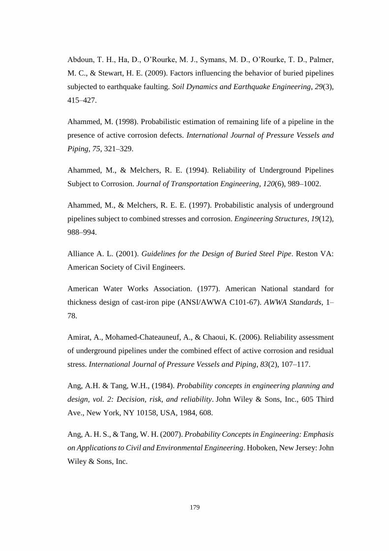
179
Abdoun, T. H., Ha, D., O’Rourke, M. J., Symans, M. D., O’Rourke, T. D., Palmer,
M. C., & Stewart, H. E. (2009). Factors influencing the behavior of buried pipelines
subjected to earthquake faulting. Soil Dynamics and Earthquake Engineering, 29(3),
415–427.
Ahammed, M. (1998). Probabilistic estimation of remaining life of a pipeline in the
presence of active corrosion defects. International Journal of Pressure Vessels and
Piping, 75, 321–329.
Ahammed, M., & Melchers, R. E. (1994). Reliability of Underground Pipelines
Subject to Corrosion. Journal of Transportation Engineering, 120(6), 989–1002.
Ahammed, M., & Melchers, R. E. E. (1997). Probabilistic analysis of underground
pipelines subject to combined stresses and corrosion. Engineering Structures, 19(12),
988–994.
Alliance A. L. (2001). Guidelines for the Design of Buried Steel Pipe. Reston VA:
American Society of Civil Engineers.
American Water Works Association. (1977). American National standard for
thickness design of cast-iron pipe (ANSI/AWWA C101-67). AWWA Standards, 1–
78.
Amirat, A., Mohamed-Chateauneuf, A., & Chaoui, K. (2006). Reliability assessment
of underground pipelines under the combined effect of active corrosion and residual
stress. International Journal of Pressure Vessels and Piping, 83(2), 107–117.
Ang, A.H. & Tang, W.H., (1984). Probability concepts in engineering planning and
design, vol. 2: Decision, risk, and reliability. John Wiley & Sons, Inc., 605 Third
Ave., New York, NY 10158, USA, 1984, 608.
Ang, A. H. S., & Tang, W. H. (2007). Probability Concepts in Engineering: Emphasis
on Applications to Civil and Environmental Engineering. Hoboken, New Jersey: John
Wiley & Sons, Inc.

180
Anoop, M. B., & Balaji Rao, K. (2007). Application of Fuzzy Sets for Remaining Life
Assessment of Corrosion Affected Reinforced Concrete Bridge Girders. Journal of
Performance of Constructed Facilities, 21(2), 166–171.
Apostolakis, G. (1990). The concept of probability in safety assessments of
technological systems. Science (New York, N.Y.), 250(4986), 1359–1364.
Arunraj, N. S., & Maiti, J. (2007). Risk-based maintenance-Techniques and
applications. Journal of Hazardous Materials, 142(3), 653–661.
Au, S. K., & Beck, J. L. (2001). Estimation of small failure probabilities in high
dimensions by subset simulation. Probabilistic Engineering Mechanics, 16(4), 263–
277.
Au, S., & Wang, Y. (2014). Engineering Risk Assessment with Subset Simulation.
John Wiley & Sons.
AWWA (American water works association). 1999. Buried pipe design, Fiberglass
pipe design. AWWA Manual M45, 35–53, Denver, USA.
Babu, G. L. S., & Srivastava, A. (2010). Reliability Analysis of Buried Flexible Pipe-
Soil Systems. Journal of Pipeline Systems Engineering and Practice, 1(1), 33–41.
Baecher, G. B., & Christian, J. T. (2005). Reliability and Statistics in Geotechnical
Engineering. John Wiley & Sons.
Barone, G., & Frangopol, D. M. (2014a). Life-cycle maintenance of deteriorating
structures by multi-objective optimization involving reliability, risk, availability,
hazard and cost. Structural Safety, 48, 40–50.
Barone, G., & Frangopol, D. M. (2014b). Reliability, risk and lifetime distributions
as performance indicators for life-cycle maintenance of deteriorating structures.
Reliability Engineering and System Safety, 123, 21–37.
Beck, J. L., & Katafygiotis, L. S. (1998). Updating models and their uncertainties. I:
bayesian statistical framework. Journal of Engineering Mechanics, 124(4), 463–467.

181
Beck, J.L. & Zuev, K.M., (2017). Rare-Event Simulation. Handbook of uncertainty
quantification, pp.1075-1100.
Beer, M., Ferson, S., & Kreinovich, V. (2013a). Imprecise probabilities in engineering
analyses. Mechanical Systems and Signal Processing, 37(1–2), 4–29.
Beer, M., & Liebscher, M. (2008). Designing robust structures - A nonlinear
simulation based approach. Computers and Structures, 86(10), 1102–1122.
Beer, M., Zhang, Y., Quek, S. T., & Phoon, K. K. (2013b). Reliability analysis with
scarce information: Comparing alternative approaches in a geotechnical engineering
context. Structural Safety, 41, 1–10.
Berardi, L., Giustolisi, O., Kapelan, Z. & Savic, D.A., (2008). Development of pipe
deterioration models for water distribution systems using EPR. Journal of
Hydroinformatics, 10(2), pp.113-126.
Beyer, H. G., & Sendhoff, B. (2007). Robust optimization - A comprehensive survey.
Computer Methods in Applied Mechanics and Engineering, 196(33–34), 3190–3218.
Bhaskaran, R., Palaniswamy, N., Rengaswamy, N.S. & Jayachandran, M. (2005).
Global cost of corrosion - A historical review. Corrosion: Materials, 13, 621–628.
Biondini, F., & Frangopol, D. M. (2009). Lifetime reliability-based optimization of
reinforced concrete cross-sections under corrosion. Structural Safety, 31(6), 483–489.
Biondini, F., Frangopol, D.M. & Restelli, S., (2008). On structural robustness,
redundancy, and static indeterminacy. In Structures Congress 2008: Crossing
Borders (pp. 1-10).
Brown, G.K., (2014). Appendix–internal corrosion monitoring techniques for
pipeline systems. Pipeline integrity handbook. Boston: Gulf Professional Publishing,
pp.255-92.
BS 9295:2010. 2010. Guide to the structural design of buried pipelines. British
Standard Institution, UK.

182
BS EN 1295:1-1997. Structural design of buried pipelines under various conditions
of loading - General requirements. British Standards Institution, UK.
Bucher, C. & Frangopol, D.M., (2006). Optimization of lifetime maintenance
strategies for deteriorating structures considering probabilities of violating safety,
condition, and cost thresholds. Probabilistic Engineering Mechanics, 21(1), pp.1-8.
Caleyo, F., Velázquez, J. C., Valor, A., & Hallen, J. M. (2009). Probability
distribution of pitting corrosion depth and rate in underground pipelines: A Monte
Carlo study. Corrosion Science, 51(9), 1925–1934.
Cameron DA. (2005). Analysis of buried flexible pipes in granular backfill subjected
to construction traffic. PhD Thesis, University of Sydney, Department of Civil
Engineering, Australia.
Chankong, V. & Haimes, Y.Y., (1983). Multiobjective decision making: theory and
methodology. Courier Dover Publications.
Cheng, F. Y., & Le, D. (1997). Multiobjective optimization design with pareto genetic
algorithm. Journal of Structural Engineering, 9(2), 1252–1261.
Chughtai, F. & Zayed, T., (2008). Infrastructure condition prediction models for
sustainable sewer pipelines. Journal of Performance of Constructed Facilities, 22(5),
pp.333-341.
Coello, C. A. C. (2000). Handling preferences in evolutionary multiobjective
optimization: A survey. In Proceedings of the 2000 Congress on Evolutionary
Computation, CEC 2000 (Vol. 1, pp. 30–37).
Dandy, G.C. % Engelhardt, M.O., (2006). Multi-objective trade-offs between cost
and reliability in the replacement of water mains. Journal of water resources planning
and management, 132(2), pp.79-88.
Dash, S.R. & Jain, S.K., (2007). IITK-GSDMA Guidelines for seismic design of
buried pipelines: provisions with commentary and explanatory examples. National
Information Center of Earthquake Engineering, Kanpur, India.

183
Datta, T. (1999). Seismic response of buried pipelines: a state-of-the-art review.
Nuclear Engineering and Design, 192(2–3), 271–284.
Datta, T. K. (2010). Seismic Analysis of Structures. John Wiley & Sons (Asia) Pvt.
Ltd.
Davies, J. P., Clarke, B. A., Whiter, J. T., & Cunningham, R. J. (2001). Factors
influencing the structural deterioration and collapse of rigid sewer pipes. Urban
Water, 3(1–2), 73–89.
Davies, J. P., Clarke, B. A., Whiter, J. T., Cunningham, R. J., & Leidi, A. (2001). The
structural condition of rigid sewer pipes: A statistical investigation. Urban Water,
3(4), 277–286.
Deb, K. (2001). Multi-Objective Optimization Using Evolutionary Algorithms. John
Wiley & Sons.
Der Kiureghian, A., Lin, H., & Hwang, S. (1987). Second‐Order Reliability
Approximations. Journal of Engineering Mechanics, 113(8), 1208–1225.
Doltsinis, I., & Kang, Z. (2004). Robust design of structures using optimization
methods. Computer Methods in Applied Mechanics and Engineering, 193(23–26),
2221–2237.
Dong, Y., & Frangopol, D. M. (2015). Risk-informed life-cycle optimum inspection
and maintenance of ship structures considering corrosion and fatigue. Ocean
Engineering, 101, 161–171.
Earthquake Engineering Research Institute (1999). “Kocaeli, Turkey Earthquake of
August 17”, EERI Special Earthquake Report.
Echard, B., Gayton, N., Lemaire, M., & Relun, N. (2013). A combined Importance
Sampling and Kriging reliability method for small failure probabilities with time-
demanding numerical models. Reliability Engineering and System Safety, 111, 232–
240.

184
Eldred, M. S., Swiler, L. P., & Tang, G. (2011). Mixed aleatory-epistemic uncertainty
quantification with stochastic expansions and optimization-based interval estimation.
Reliability Engineering and System Safety, 96(9), 1092–1113.
Engelhardt, G., & Macdonald, D. D. (2004). Unification of the deterministic and
statistical approaches for predicting localized corrosion damage. I. Theoretical
foundation. Corrosion Science, 46(11), 2755–2780.
Estes, A.C. & Frangopol, D.M., (2001). Bridge lifetime system reliability under
multiple limit states. Journal of bridge engineering, 6(6), pp.523-528.
European Commitee for Standardization. (2004). Eurocode 8: Design of structures for
earthquake resistance - Part 1 : General rules, seismic actions and rules for buildings.
European Committee for Standardization.
Faber, M.H., Kroon, I.B. and Sørensen, J. D. (1996). Sensitivities in structural
maintenance planning. Reliability Engineering and System Safety, 51(3), 317–329.
Fang, Y., Tee, K.F. & Chen, J. (2016). Structural dynamic reliability evaluation under
consideration of fuzzy strength and fuzzy stress. Journal of Vibration Engineering
and Technologies, 4(1), 53–58.
Fares, H. & Zayed, T., (2010). Hierarchical fuzzy expert system for risk of failure of
water mains. Journal of Pipeline Systems Engineering and Practice, 1(1), pp.53-62.
Farshad, M., (2011). Plastic pipe systems: Failure investigation and diagnosis (Vol.
407). Elsevier.
Fenner, R.A., Sweeting, L. & Marriott, M.J., (2000). A new approach for directing
proactive sewer maintenance. In Proceedings of the Institution of Civil Engineers-
Water and Maritime Engineering (Vol. 142, No. 2, pp. 67-77). Thomas Telford Ltd.
Fetz, T. & Tonon, F., (2008). Probability bounds for series systems with variables
constrained by sets of probability measures. International Journal of Reliability and
Safety, 2(4), pp.309-339.

185
Fornasini, P., (2008). The uncertainty in physical measurements: an introduction to
data analysis in the physics laboratory. Springer Science & Business Media.
Fonesca, C.M. and Fleming, P.J. (1993), July. Genetic algorithms for multiobjective
optimization: formulation, discussion and generalization. In Proc of the Fifth Int.
Conf. On genetic Algorithms, Forrest S.(Ed.), San Mateo, CA, Morgan
Kaufmann (pp. 415-423).
Frangopol, D.M. & Curley, J. P. (1987). Effects of damage and redundancy on
structural reliability. Journal of Structural Engineering, 113(7), 1533–1549.
Gabriel, L. H. (2011). Corrugated polyethylene pipe design manual and installation
guide. Plastic Pipe Institute, USA.
Gomes, W. J. S., & Beck, A. T. (2014). Optimal inspection and design of onshore
pipelines under external corrosion process. Structural Safety, 47, 48–58.
Halfawy, M. R., Dridi, L., & Baker, S. (2008). Integrated Decision Support System
for Optimal Renewal Planning of Sewer Networks. Journal of Computing in Civil
Engineering, 22(6), 360–372.
Hand, D. J., & Walley, P. (1993). Statistical Reasoning with Imprecise Probabilities.
Applied Statistics.
Hanss, M., & Turrin, S. (2010). A fuzzy-based approach to comprehensive modeling
and analysis of systems with epistemic uncertainties. Structural Safety, 32(6), 433–
441.
Hastings, W. K. (1970). Monte carlo sampling methods using Markov chains and their
applications. Biometrika, 57(1), 97–109.
Haupt, R. L., & Haupt, S. E. (2004). Practical Genetic Algorithm. John Wiley & Sons.
Hong, H. P. (1999). Inspection and maintenance planning of pipeline under external
corrosion considering generation of new defects. Structural Safety, 21(3), 203–222.

186
Huang, B., & Du, X. (2006). A robust design method using variable transformation
and Gauss-Hermite integration. International Journal for Numerical Methods in
Engineering, 66(12), 1841–1858.
Jayaram, N. & Srinivasan, K., (2008). Performance‐based optimal design and
rehabilitation of water distribution networks using life cycle costing. Water Resources
Research, 44(1).
Ji, J., Robert, D. J., Zhang, C., Zhang, D., & Kodikara, J. (2017). Probabilistic
physical modelling of corroded cast iron pipes for lifetime prediction. Structural
Safety, 64, 62–75.
Karamanos, S.A., Keil, B. & Card, R.J., (2014). Seismic design of buried steel water
pipelines. In Pipelines 2014: From Underground to the Forefront of Innovation and
Sustainability (pp. 1005-1019).
Khan, L.R. & Tee, K.F., (2016). Risk-cost optimization of buried pipelines using
subset simulation. Journal of Infrastructure Systems, 22(2), p.04016001.
Khemis, A., Chaouche, A.H., Athmani, A. & Tee, K.F., (2016). Uncertainty effects
of soil and structural properties on the buckling of flexible pipes shallowly buried in
Winkler foundation. Structural Engineering and Mechanics, 59(4), pp.739-759.
Kleiner, Y., Adams, B.J. & Rogers, J. S. (2001). Water distribution network renewal
planning. Journal of Computing in Civil Engineering, 15(1), 15–26.
Kleiner, Y., & Rajani, B. (2001a). Comprehensive review of structural deterioration
of water mains: physically based models. Urban Water, 3(3), 151-164.
Kleiner, Y., & Rajani, B. (2001b). Comprehensive review of structural deterioration
of water mains: statistical models. Urban Water, 3(3), 131–150.
Kleiner, Y., Rajani, B. & Sadiq, R., (2004). Management of failure risk in large-
diameter buried pipes using fuzzy-based techniques. In 4th International Conference
on Decision Making in Urban and Civil Engineering. Porto Portugal.

187
Klir, G.J. & Yuan, B., (1995). Fuzzy sets and fuzzy logic: theory and
applications. Possibility Theory versus Probab. Theory, 32(2).
Klir, G.J., (2006). Uncertainty and information: foundations of generalized
information theory. John Wiley & Sons.
Kouretzis, G. P., Bouckovalas, G. D., & Gantes, C. J. (2006). 3-D shell analysis of
cylindrical underground structures under seismic shear (S) wave action. Soil
Dynamics and Earthquake Engineering, 26(10), 909–921.
Koutsourelakis, P. S., Pradlwarter, H. J., & Schuëller, G. I. (2004). Reliability of
structures in high dimensions, part I: Algorithms and applications. Probabilistic
Engineering Mechanics, 19(4), 409–417.
Kroese, D. P., & Chan, J. C. C. (2014). Statistical Modeling and Computation. New
York: Springer.
Kulhawy, F. H., & Trautmann, C. H. (1996). Estimation of in situ test uncertainty.
Proceedings of uncertainty in the geologic environment: from theory to practice,
ASCE, Reston, VA, pp. 269–286.
Lacasse S, & Nadim F. (1996). Uncertainties in characterizing soil properties.
Proceedings of uncertainty in the geologic environment: from theory to practice,
ASCE. Reston, VA pp. 49–75.
Laggoune, R., Chateauneuf, A., & Aissani, D. (2010). Impact of few failure data on
the opportunistic replacement policy for multi-component systems. Reliability
Engineering and System Safety, 95(2), 108–119.
Leis, B.N. & Parkins, R. N. (1998). Mechanics and materials aspects in predicting
serviceability limited by stress-corrosion cracking. Fatigue Fract Eng Mater Struct,
21(5), 583–601.
Li, H.S., Zhao, A.L. & Tee, K. F. (2016). Structural reliability analysis of multiple
limit state functions using multi-input multi-output support vector machine. Advances
in Mechanical Engineering, 8(10).

188
Li, L., & Lu, Z. (2014). Interval optimization based line sampling method for fuzzy
and random reliability analysis. Applied Mathematical Modelling, 38(13), 3124–
3135.
Liang, J. & Sun, S. (2000). Site effects on seismic behavior of pipelines: a review.
Journal of Pressure Vessel Technology, 122(4), pp.469-475.
Limpert, E., Stahel, W. a., & Abbt, M. (2001). Log-normal Distributions across the
Sciences: Keys and Clues. BioScience, 51(5), 341.
Lind, N. C. (1995). A measure of vulnerability and damage tolerance. Reliability
Engineering and System Safety, 48(1), 1–6.
Liu, B. (2004). Uncertainty Theory - An Introduction to its Axiomatic Foundations.
New York: Springer-Verlag Berlin Heidelberg.
Liu, B. (2007). A survey of entropy of fuzzy variables. Journal of Uncertain Systems,
1(1), 4–13.
Liu, B., & Liu, Y. K. (2002). Expected value of fuzzy variable and fuzzy expected
value models. IEEE Transactions on Fuzzy Systems, 10(4), 445–450.
Mahmoodian, M., & Li, C. Q. (2017). Failure assessment and safe life prediction of
corroded oil and gas pipelines. Journal of Petroleum Science and Engineering,
151(December 2016), 434–438.
Marano, G. C., & Quaranta, G. (2008). Fuzzy-based robust structural optimization.
International Journal of Solids and Structures, 45(11–12), 3544–3557.
Marano, G. C., Quaranta, G., & Mezzina, M. (2008). Fuzzy Time-Dependent
Reliability Analysis of RC Beams Subject to Pitting Corrosion. Journal of Materials
in Civil Engineering, 20(9), 578–587.
Marshall, P. (2001). The residual structural properties of cast iron pipes: structural
and design criteria for linings for water mains. UK Water Industry Research, UK.

189
McDonald, S. & Zhao, J., (2001). Condition assessment and rehabilitation of large
sewers. In Proceedings of International Conference on Underground Infrastructure
Research (pp. 361-369). Waterloo, Canada: University of Waterloo.
Melchers, R. E. (1999). Structural reliability analysis and prediction (Second ed.).
New York: John Wiley & Sons.
Melchers, R.E., (2003). Probabilistic models for corrosion in structural reliability
assessment—Part 1: empirical models. Journal of Offshore Mechanics and Arctic
Engineering, 125(4), pp.264-271.
Metropolis, N., Rosenbluth, A. W., Rosenbluth, M. N., Teller, A. H., & Teller, E.
(1953). Equation of State Calculations by Fast Computing Machines. The Journal of
Chemical Physics, 21(6), 1087–1092.
Mohr, W., (2003). Strain-based design of pipelines. Edison Welding Institute,
Columbus, OH, Project Report, (45892GTH).
Möller, B. & Beer, M. (2004). Fuzzy randomness: uncertainty in civil engineering
and computational mechanics. New York: Springer.
Möller, B., & Beer, M. (2008). Engineering computation under uncertainty -
Capabilities of non-traditional models. Computers and Structures, 86(10), 1024–
1041.
Möller, B., Graf, W., & Beer, M. (2003). Safety assessment of structures in view of
fuzzy randomness. Computers and Structures, 81(15), 1567–1582.
Möller, B. & Reuter, U., (2007). Uncertain Forecasting in Engineering and
Environmental Science. Uncertainty Forecasting in Engineering, pp.153-191.
Moneim MA. (2011). Modelling reliability based optimisation design for water
distribution networks. Holding Company for Water and Wastewater. Arab Republic
of Egypt.

190
Moser, A. P., & Folkman, S. L. (2001). Buried Pipe Design. New York: McGraw-
Hill.
Nadim, F., (2015), October. Accounting for uncertainty and variability in
geotechnical characterization of offshore sites. In Proc. of the 5th International
Symposium on Geotechnical Safety and Risk (pp. 23-35).
Najafi M. (2011). Pipeline rehabilitation for service life extension. In: Karbhari VM,
Lee LS, editors. Service life estimation and extension of civil engineering structures.
Abington Hall, Cambridge: Woodhead Publishing Limited; pp. 262–89.
Newmark, N. M., (1967). Problems in Wave Propagation in Soil and Rocks.
Proceedings of International Symposium on Wave Propagation and Dynamic
Properties of Earth Materials, Albuquerque, NM, pp. 7-26.
O’Rourke, M.J., Liu, X. (2012). Seismic Design of Buried and Offshore Pipelines.
Multidisciplinary Centre for Earthquake Engineering Research, University at Buffalo.
O’Rourke MJ, Liu X. (1999). Response of buried pipelines subject to earthquake
effects. Monograph Series, Multidisciplinary Centre for Earthquake Engineering
Research (MCEER), University at Buffalo.
Ogawa, Y., & Koike, T. (2001). Structural design of buried pipelines for severe
earthquakes. Soil Dynamics and Earthquake Engineering, 21(3), 199–209.
Okasha, N.M. & Frangopol, D.M., (2009). Lifetime-oriented multi-objective
optimization of structural maintenance considering system reliability, redundancy and
life-cycle cost using GA. Structural Safety, 31(6), pp.460-474.
Olsson, a., Sandberg, G., & Dahlblom, O. (2003). On Latin hypercube sampling for
structural reliability analysis. Structural Safety, 25(1), 47–68.
Onoufriou, T. & Frangopol, D.M., 2002. Reliability-based inspection optimization of
complex structures: a brief retrospective. Computers & structures, 80(12), pp.1133-
1144.

191
Ossai, C. I., Boswell, B., & Davies, I. J. (2015). Pipeline failures in corrosive
environments - A conceptual analysis of trends and effects. Engineering Failure
Analysis, 53, 36–58.
Phoon, K., & Kulhawy, F. H. (1999a). Characterization of geotechnical variability.
Canadian Geotechnical Journal, 36(4), 612–624.
Phoon, K., & Kulhawy, F. H. (1999b). Evaluation of geotechnical property
variability. Canadian Geotechnical Journal, 36(4), 625–639.
Piratla, K.R., Ariaratnam, S.T. & Cohen, A., (2012). Estimation of CO 2 emissions
from the life cycle of a potable water pipeline project. Journal of Management in
Engineering, 28(1), pp.22-30.
Pradlwarter, H. J., Pellissetti, M. F., Schenk, C. A., Schuëller, G. I., Kreis, A.,
Fransen, S., Klein, M. (2005). Realistic and efficient reliability estimation for
aerospace structures. Computer Methods in Applied Mechanics and Engineering,
194(12–16), 1597–1617.
Pradlwarter, H. J., Schuëller, G. I., Koutsourelakis, P. S., & Charmpis, D. C. (2007).
Application of line sampling simulation method to reliability benchmark problems.
Structural Safety, 29(3), 208–221.
Rahman, S. & Vanier, D. J. (2004). Life cycle cost analysis as a decision support tool
for managing municipal infrastructure. In CIB 2004 triennial congress (Vol. 2, pp.
11–8). Ottawa: National Research Council (NRC).
Rajani, B., Zhan, C. & Kuraoka, S. (1996). Pipe soil interaction analysis of jointed
water mains. Canadian Geotechnical Journal, 33(3), 393–404.
Rajani, B. & Makar, J. (2000). A methodology to estimate remaining service life of
grey cast iron water mains. Canadian Journal of Civil Engineering, 27(6), 1259–
1272.
Rajani, B. & Zhan, C. (1996). On the estimation of frost loads. Canadian
Geotechnical Journal, 33(4), 629–641.

192
Rajeev, P., Kodikara, J., Robert, D., Zeman, P., & Rajani, B. (2014). Factors
contributing to large diameter water pipe failure. Water Asset Management
International, 10(3), 9–14.
Robert, C. P., & Casella, G. (2004). Monte Carlo Statistical Methods. Springer, New
York. Sanso, B. and Guenni, L (Vol. 95).
Ross, T.J., (2009). Fuzzy logic with engineering applications. John Wiley & Sons.
Røstum, J. (2000). Statistical Modelling of Pipe Failures in Water Networks (Ph.D.
thesis). Norwegian University of Science and Technology NTNU.
Sadiq, R., Rajani, B., & Kleiner, Y. (2004). Probabilistic risk analysis of corrosion
associated failures in cast iron water mains. Reliability Engineering & System Safety,
86(1), 1–10.
Scheidegger, A., Leitão, J. P., & Scholten, L. (2015). Statistical failure models for
water distribution pipes - A review from a unified perspective. Water Research, 83,
237–247.
Schuëller, G. I., & Jensen, H. A. (2008). Computational methods in optimization
considering uncertainties – An overview. Computer Methods in Applied Mechanics
and Engineering, 198(1), 2–13.
Schuëller, G. I., Pradlwarter, H. J., & Koutsourelakis, P. S. (2004). A critical appraisal
of reliability estimation procedures for high dimensions. Probabilistic Engineering
Mechanics, 19(4), 463–474.
Sivakumar Babu, G.L., Srinivasa Murthy, B.R. & Seshagiri Rao, R. (2006).
Reliability analysis of deflection of buried flexible pipes. Journal of Transportation
Engineering, 132(10), 829–836.
Sivakumar Babu, G.L. & Rao, R.S., (2005). Reliability measures for buried flexible
pipes. Canadian geotechnical journal, 42(2), pp.541-549.

193
Sriramula, S. and Chryssanthopoulos, M.K., (2009). Probabilistic models for spatially
varying mechanical properties of in-service GFRP cladding panels. Journal of
Composites for Construction, 13(2), pp.159-167.
St. Clair, A.M. & Sinha, S., (2014). Development of a standard data structure for
predicting the remaining physical life and consequence of failure of water
pipes. Journal of Performance of Constructed Facilities, 28(1), pp.191-203.
Starossek, U. & Haberland, M., (2011). Approaches to measures of structural
robustness. Structure and Infrastructure Engineering, 7(7-8), pp.625-631.
Tang, X. G., Rezoug, M., Hamzaoui, R., Bassir, D., El Meouche, R., Khreim, J. F., &
Feng, Z. Q. (2011). Multiobjective Optimization on Urban Flooding Using RSM and
GA. Advanced Materials Research, 255–260 (June 2015), 1627–1631.
Tee, K.F., Ebenuwa, A.U. & Zhang, Y., (2018). Fuzzy-based robustness assessment
of buried pipelines. Journal of Pipeline Systems Engineering and Practice, 9(1),
p.06017007.
Tee, K. F., & Khan, L. R. (2014). Reliability analysis of underground pipelines with
correlations between failure modes and random variables. Proceedings of the
Institution of Mechanical Engineers, Part O: Journal of Risk and Reliability, 228(4),
362–370.
Tee, K.F., Khan, L.R. & Chen, H.P., (2013). Probabilistic failure analysis of
underground flexible pipes. Structural engineering and mechanics, 47(2), pp.167-
183.
Tee, K.F., Khan, L.R., Chen, H.P. & Alani, A.M., (2014). Reliability based life cycle
cost optimization for underground pipeline networks. Tunnelling and Underground
Space Technology, 43, pp.32-40.
Tee, K. F., Khan, L. R., & Li, H. (2014). Application of subset simulation in reliability
estimation of underground pipelines. Reliability Engineering & System Safety, 130,
125–131.

194
Vazouras, P., Karamanos, S. A., & Dakoulas, P. (2012). Mechanical behavior of
buried steel pipes crossing active strike-slip faults. Soil Dynamics and Earthquake
Engineering, 41, 164–180.
Velazquez, J.C., Caleyo, F., Valor, A. & Hallen, J.M., (2009). Predictive model for
pitting corrosion in buried oil and gas pipelines. Corrosion, 65(5), pp.332-342.
Wang, H., Yajima, A., Liang, R. Y., & Castaneda, H. (2015). Bayesian modeling of
external corrosion in underground pipelines based on the integration of markov chain
monte carlo techniques and clustered inspection data. Computer-Aided Civil and
Infrastructure Engineering, 30(4), 300–316.
Wang, H., Yajima, A., Liang, R. Y., & Castaneda, H. (2016). Reliability-based
temporal and spatial maintenance strategy for integrity management of corroded
underground pipelines. Structure and Infrastructure Engineering, 12(10), 1281–
1294.
Water Research Centre, (2001). Sewerage rehabilitation manual (Vol. 1). WRC
Publications.
Watkins, R.K. & Anderson, L. R. (1999). Structural mechanics of buried pipes. CRC
press.
Whidden, W. R. (2009). Buried flexible steel pipe: Design and structural analysis.
American Society of Civil Engineers.
Yeh, G.C., (1974). Seismic analysis of slender buried beams. Bulletin of the
Seismological Society of America, 64(5), pp.1551-1562.
Yin, H., Yu, D., Yin, S., & Xia, B. (2018). Possibility-based robust design
optimization for the structural-acoustic system with fuzzy parameters. Mechanical
Systems and Signal Processing, 102, 329–345.
Zadeh, L.A., (1965). Fuzzy sets. Information and control, 8, p.3.

195
Zhang, J., & Du, X. (2010). A Second-Order Reliability Method With First-Order
Efficiency. Journal of Mechanical Design, 132(10), 101006.
Zhang, M. Q., Beer, M., Koh, C. G., & Jensen, H. A. (2015). Nuanced Robustness
Analysis with Limited Information. ASCE-ASME Journal of Risk and Uncertainty in
Engineering Systems, Part A: Civil Engineering, 2(3), B4015001.
Zhang, M. Q., Beer, M., Quek, S. T., & Choo, Y. S. (2010). Comparison of
uncertainty models in reliability analysis of offshore structures under marine
corrosion. Structural Safety, 32(6), 425–432.
Zhang, Y., Kim, C.W., Tee, K.F. and Lam, J.S.L., 2017. Optimal sustainable life cycle
maintenance strategies for port infrastructures. Journal of cleaner production, 142,
pp.1693-1709.
Zimmermann, H. J. (2001). Fuzzy Set Theory and Its Applications. London Kluwer
Academic Publishers.
Zio, E. (2009). Reliability engineering: Old problems and new challenges. Reliability
Engineering and System Safety, 94(2), 125–141.
Zio, E. (2013). The Monte Carlo Simulation Method for System Reliability and Risk
Analysis. London: Springer.
Zio, E., & Pedroni, N. (2009). Functional failure analysis of a thermal-hydraulic
passive system by means of Line Sampling. Reliability Engineering and System
Safety, 94(11), 1764–1781.
Zio, E., & Pedroni, N. (2010). An optimized Line Sampling method for the estimation
of the failure probability of nuclear passive systems. Reliability Engineering & System
Safety, 95(12), 1300–1313.
Zuev, K. (2015). Subset Simulation Method for Rare Event Estimation: An
Introduction. Encyclopedia of Earthquake Engineering, 1–26.

196
LIST OF PUBLICATIONS
Ebenuwa, A.U. & Tee, K.F., (2019). Fuzzy-based optimised subset simulation for
reliability analysis of engineering structures. Structure and Infrastructure Engineering,
pp.1-13.
Ebenuwa, A.U. & Tee, K.F., (2017). Reliability analysis of buried pipes with corrosion
and seismic impact. Geo-Risk 2017 (pp. 424-433).
Tee, K.F., Ebenuwa, A.U. & Zhang, Y., (2018). Fuzzy-based robustness assessment of
buried pipelines. Journal of Pipeline Systems Engineering and Practice, 9(1),
p.06017007.
Tee, K.F. & Ebenuwa, A.U., (2018). Combination of line sampling and important
sampling for reliability assessment of buried pipelines. Proceedings of the Institution of
Mechanical Engineers, Part O: Journal of Risk and Reliability, p.1748006X18764986.
Ebenuwa, A.U. & Tee, K.F., (2016). Reliability Assessment of Buried Pipeline under
Seismic Action. 9th IMA International Conference on Modelling in Industrial
Maintenance and Reliability (MIMAR). London, UK, July 12-14, 2016.
Ebenuwa, A.U. Tee, K.F. & Zhang, Y., (2016). Structural robustness assessment of
corroded buried pipes. High Performance and Optimum Design of Structures and
Materials II, 166, pp.81-92.
Ebenuwa, A.U. & Tee, K.F., (2017). Reliability assessment of buried pipelines for
through-wall bending stress. In 14th International Probabilistic Workshop (pp. 377-387).
Springer, Cham.
Ebenuwa, A.U. & Tee, K.F. Fuzzy-based Multi-Objective Design Optimisation of
Buried Pipelines. International Journal of Uncertainty, Fuzziness and Knowledge-Based
Systems (Under review)

197
Ebenuwa A.U. & Tee, K.F. Reliability-based maintenance of buried pipeline using multi-
objective optimisation involving fuzzy reliability, risk, and cost. Journal of Infrastructure
System (Under review)
Ebenuwa, A.U. and Tee, K.F. Assessment of Buried Pipes under Seismic Action using
Line Sampling. International Journal of Pressure Vessels and Piping (Under review)
Copyright © 2022 FDOKUMEN