ORIGINAL PAPER

Relationship between static and dynamic elastic modulusof calcarenite heated at different temperatures: the SanJulian’s stone

V. Brotons • R. Tomas • S. Ivorra • A. Grediaga

Received: 13 July 2013 / Accepted: 18 February 2014 / Published online: 12 March 2014

� Springer-Verlag Berlin Heidelberg 2014

Abstract The San Julian’s stone is the main material

used to build the most important historical buildings in

Alicante city (Spain). This paper describes the analysis

developed to obtain the relationship between the static and

the dynamic modulus of this sedimentary rock heated at

different temperatures. The rock specimens have been

subjected to heating processes at different temperatures to

produce different levels of weathering on 24 specimens.

The static and dynamic modulus has been measured for

every specimen by means of the ISRM standard and

ultrasonic tests, respectively. Finally, two analytic formulas

are proposed for the relationship between the static and the

dynamic modulus for this stone. The results have been

compared with some relationships proposed by different

researchers for other types of rock. The expressions pre-

sented in this paper can be useful for the analysis, using

non-destructive techniques, of the integrity level of his-

torical constructions built with San Julian’s stone affected

by fires.

Keywords Non-destructive techniques � Calcarenite

stone � Elastic dynamic modulus � Elastic static modulus �San Julian’s stone � Temperature

Introduction

The Young’s modulus, also called elastic modulus, is one

of the most important mechanical characteristic parameters

of the rocks in relation to use as a construction material.

This parameter varies with the degree of weathering of the

rock. As a consequence it is essential in engineering to

state the value of the modulus corresponding to the dif-

ferent weathering states, taking as a reference the unaltered

Young’s modulus. Usually, it is not possible to perform

static laboratory tests from drilled samples (e.g. in histor-

ical buildings) and modulus must be obtained from ultra-

sonic testing. Because the static modulus (Est) is required

for computing the deformations of a building after it comes

into service under the applied loads, the static modulus,

obtained from conventional laboratory procedures, is

required. In these cases in which it is not possible to per-

form destructive tests to determine the characteristics of the

rock, the use of non-destructive techniques using mobile

devices constitutes an alternative option.

The dynamically determined elastic modulus (Edyn) is

generally higher than that statically determined, and both

methods provide high divergent results for low elasticity

modulus rocks (Ide 1936). Several studies (e.g. Ide 1936;

Vanheerden 1987; Al-Shayea 2004; Kolesnikov 2009)

explain these differences by means of the nonlinear elastic

response at different ranges of amplitude of the strains ð2Þinvolved in the distinct techniques. Other authors (Kol-

esnikov 2009; Ciccotti and Mulargia 2004) consider that

the static test is a dynamic test at a very low frequency, and

they highlight the nonlinear elastic response to different

associated frequencies (f). Kolesnikov (2009) uses the

Kjartansson constant Q-model (Kjartansson 1979) to ana-

lyse the effects of intrinsic dispersion of pressure wave

velocities in absorbing media (and it is well known that all

V. Brotons (&) � R. Tomas � S. Ivorra

Departamento de Ingenierıa Civil, Escuela Politecnica Superior,

Universidad de Alicante, P.O. Box 99, 03080 Alicante, Spain

e-mail: vicente.brotons@ua.es

A. Grediaga

Departamento de Tecnologıa Informatica y Computacion,

Escuela Politecnica Superior, Universidad de Alicante,

P.O. Box 99, 03080 Alicante, Spain

123

Bull Eng Geol Environ (2014) 73:791–799

DOI 10.1007/s10064-014-0583-y

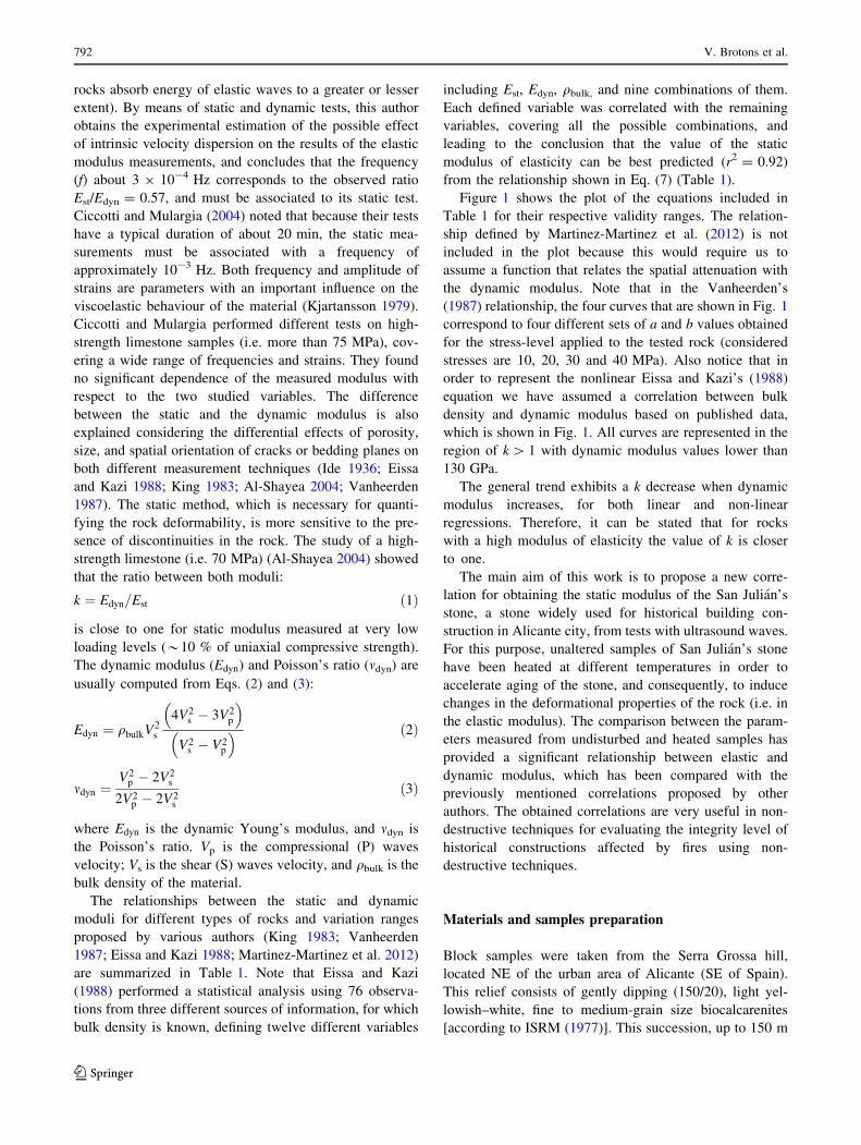
rocks absorb energy of elastic waves to a greater or lesser

extent). By means of static and dynamic tests, this author

obtains the experimental estimation of the possible effect

of intrinsic velocity dispersion on the results of the elastic

modulus measurements, and concludes that the frequency

(f) about 3 9 10-4 Hz corresponds to the observed ratio

Est/Edyn = 0.57, and must be associated to its static test.

Ciccotti and Mulargia (2004) noted that because their tests

have a typical duration of about 20 min, the static mea-

surements must be associated with a frequency of

approximately 10-3 Hz. Both frequency and amplitude of

strains are parameters with an important influence on the

viscoelastic behaviour of the material (Kjartansson 1979).

Ciccotti and Mulargia performed different tests on high-

strength limestone samples (i.e. more than 75 MPa), cov-

ering a wide range of frequencies and strains. They found

no significant dependence of the measured modulus with

respect to the two studied variables. The difference

between the static and the dynamic modulus is also

explained considering the differential effects of porosity,

size, and spatial orientation of cracks or bedding planes on

both different measurement techniques (Ide 1936; Eissa

and Kazi 1988; King 1983; Al-Shayea 2004; Vanheerden

1987). The static method, which is necessary for quanti-

fying the rock deformability, is more sensitive to the pre-

sence of discontinuities in the rock. The study of a high-

strength limestone (i.e. 70 MPa) (Al-Shayea 2004) showed

that the ratio between both moduli:

k ¼ Edyn=Est ð1Þ

is close to one for static modulus measured at very low

loading levels (*10 % of uniaxial compressive strength).

The dynamic modulus (Edyn) and Poisson’s ratio (mdyn) are

usually computed from Eqs. (2) and (3):

Edyn ¼ qbulkV2s

4V2s � 3V2

p

� �

V2s � V2

p

� � ð2Þ

mdyn ¼V2

p � 2V2s

2V2p � 2V2

s

ð3Þ

where Edyn is the dynamic Young’s modulus, and mdyn is

the Poisson’s ratio. Vp is the compressional (P) waves

velocity; Vs is the shear (S) waves velocity, and qbulk is the

bulk density of the material.

The relationships between the static and dynamic

moduli for different types of rocks and variation ranges

proposed by various authors (King 1983; Vanheerden

1987; Eissa and Kazi 1988; Martinez-Martinez et al. 2012)

are summarized in Table 1. Note that Eissa and Kazi

(1988) performed a statistical analysis using 76 observa-

tions from three different sources of information, for which

bulk density is known, defining twelve different variables

including Est, Edyn, qbulk, and nine combinations of them.

Each defined variable was correlated with the remaining

variables, covering all the possible combinations, and

leading to the conclusion that the value of the static

modulus of elasticity can be best predicted (r2 = 0.92)

from the relationship shown in Eq. (7) (Table 1).

Figure 1 shows the plot of the equations included in

Table 1 for their respective validity ranges. The relation-

ship defined by Martinez-Martinez et al. (2012) is not

included in the plot because this would require us to

assume a function that relates the spatial attenuation with

the dynamic modulus. Note that in the Vanheerden’s

(1987) relationship, the four curves that are shown in Fig. 1

correspond to four different sets of a and b values obtained

for the stress-level applied to the tested rock (considered

stresses are 10, 20, 30 and 40 MPa). Also notice that in

order to represent the nonlinear Eissa and Kazi’s (1988)

equation we have assumed a correlation between bulk

density and dynamic modulus based on published data,

which is shown in Fig. 1. All curves are represented in the

region of k [ 1 with dynamic modulus values lower than

130 GPa.

The general trend exhibits a k decrease when dynamic

modulus increases, for both linear and non-linear

regressions. Therefore, it can be stated that for rocks

with a high modulus of elasticity the value of k is closer

to one.

The main aim of this work is to propose a new corre-

lation for obtaining the static modulus of the San Julian’s

stone, a stone widely used for historical building con-

struction in Alicante city, from tests with ultrasound waves.

For this purpose, unaltered samples of San Julian’s stone

have been heated at different temperatures in order to

accelerate aging of the stone, and consequently, to induce

changes in the deformational properties of the rock (i.e. in

the elastic modulus). The comparison between the param-

eters measured from undisturbed and heated samples has

provided a significant relationship between elastic and

dynamic modulus, which has been compared with the

previously mentioned correlations proposed by other

authors. The obtained correlations are very useful in non-

destructive techniques for evaluating the integrity level of

historical constructions affected by fires using non-

destructive techniques.

Materials and samples preparation

Block samples were taken from the Serra Grossa hill,

located NE of the urban area of Alicante (SE of Spain).

This relief consists of gently dipping (150/20), light yel-

lowish–white, fine to medium-grain size biocalcarenites

[according to ISRM (1977)]. This succession, up to 150 m

792 V. Brotons et al.

123

thick, is upper Miocene in age (Montenat 1977; Montenat

et al. 1990).

The rock is locally known as San Julian’s stone and

has been widely used since the Roman period for the

construction of buildings in Alicante city and its sur-

roundings (e.g. Lucentum, the Roman predecessor of the

city of Alicante, Santa Barbara’s Castle, City Council

building, and Gravina Palace). The specimens studied in

this paper were obtained from rock blocks collected from

the dump of a railway tunnel under construction. The

rock blocks were picked up just after the mechanical

excavation and transported to the laboratory, where the

samples were extracted by means of a drill. An X-ray

diffraction analysis was performed and interpreted using

the XPowder software package (Martın 2004). The

qualitative search-matching procedure was based on the

Table 1 Relationship between static (Est) and dynamic (Edyn) moduli proposed by different authors

References Relationship R2 Samples Edyn range (GPa) Rock type

King (1983) Est ¼ 1:26 Edyn � 29:5 ð4Þ 0.82 174 40–120 Igneous-metamorphic

Vanheerden (1987) Est ¼ aEbdyn ð5Þ – – 20–135 Sandstone-granite

Eissa and Kazi (1988) Est ¼ 0:74 Edyn � 0:82 ð6Þ 0.70 342 5–130 All types

Eissa and Kazi (1988) log10Est ¼ 0:77log10 qbulkEdyn

� �þ 0:02 ð7Þ 0.92 76 5–130 All types

Martinez-Martinez et al. (2012) Est ¼ Edyn

3:8a�0:68s

ð8Þ – – 5–50 Limestone-marble

Note that qbulk in Eissa and Kazi’s (1988) equation is originally expressed in grams per cubic centimetre, although in this work it is expressed in

SI units. These equations are plotted in Fig. 1

Fig. 1 Plot of the relationship

between static and dynamic

Young’s modulus shown in

Table 1. Note that the

relationships have been only

represented for their range of

validity

The San Julian’s stone 793

123

ICDD-PDF2 database. The main components derived

from the analysis are: calcite (70 %), iron-rich dolomite

(25 %), quartz (5 %), and traces of clay minerals (illite)

(Brotons et al. 2013). The studied rock corresponds to a

very porous biocalcarenite (a grainstone according to

Dunham 1962). From a textural point of view, this rock

presents abundant allochemicals, generally smaller than

2 mm size, although bands of various grain sizes have

been found. The rock presents a wide variety of fossil

bryozoans, foraminifera, red algae, and echinoderm

fragments. The orthochemical fraction mainly corre-

sponds to sparite (Louis Cereceda et al. 2001). The

studied rock presents medium to high values of open

porosity (20.8 ± 3.3 %) and a bulk density of 21.0 ± 0.7

kN/m3 (according to Spanish standard AENOR 2007).

Complementarily, a mercury intrusion porosimetry test

has been performed over a representative sample of the

studied rock in order to study the pore size distribution.

The test indicates that the rock has a macroporosity

([5 lm) of 55.1 % and a microporosity (\5 lm) of

44.9 %, with a mean pore size of 37.52 lm.

For this study, 24 cylindrical samples of 52 mm in

diameter and 125 mm long were obtained; the choice of a

2.5 slenderness ratio was made to ensure their suitability

for the tests to be conducted according to relevant stan-

dards (ISRM 1979). The bases of the cylinders were treated

to ensure flatness and perpendicularity relative to the

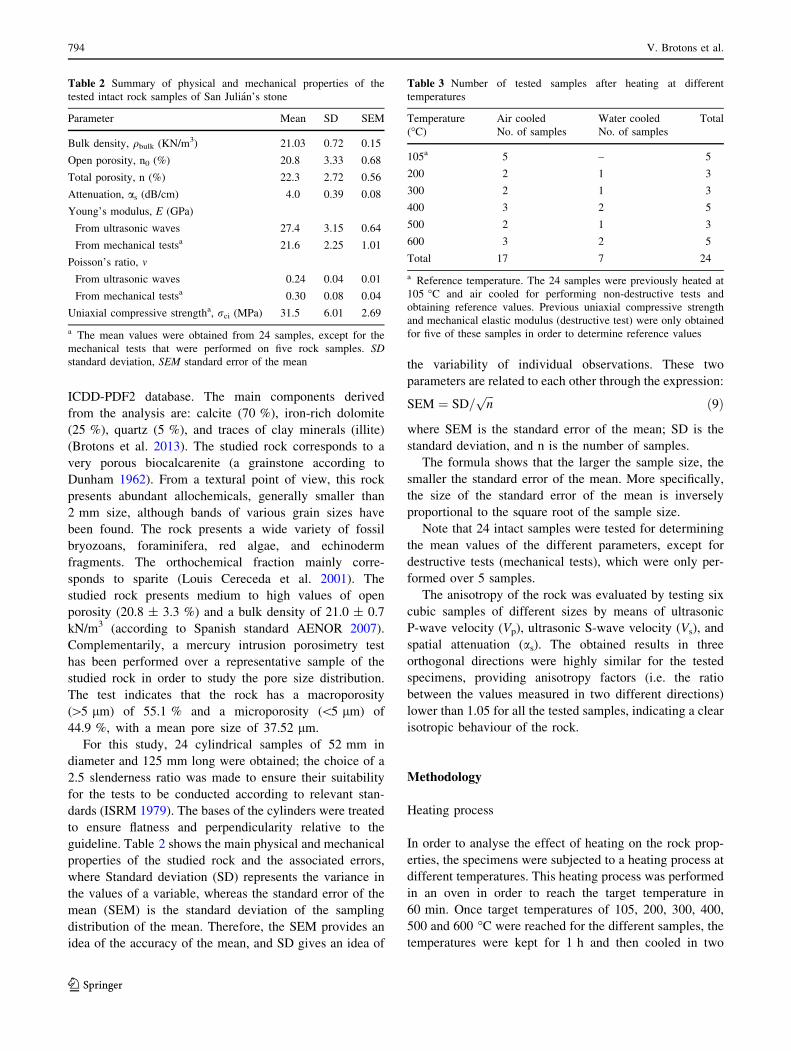
guideline. Table 2 shows the main physical and mechanical

properties of the studied rock and the associated errors,

where Standard deviation (SD) represents the variance in

the values of a variable, whereas the standard error of the

mean (SEM) is the standard deviation of the sampling

distribution of the mean. Therefore, the SEM provides an

idea of the accuracy of the mean, and SD gives an idea of

the variability of individual observations. These two

parameters are related to each other through the expression:

SEM ¼ SD=ffiffiffinp

ð9Þ

where SEM is the standard error of the mean; SD is the

standard deviation, and n is the number of samples.

The formula shows that the larger the sample size, the

smaller the standard error of the mean. More specifically,

the size of the standard error of the mean is inversely

proportional to the square root of the sample size.

Note that 24 intact samples were tested for determining

the mean values of the different parameters, except for

destructive tests (mechanical tests), which were only per-

formed over 5 samples.

The anisotropy of the rock was evaluated by testing six

cubic samples of different sizes by means of ultrasonic

P-wave velocity (Vp), ultrasonic S-wave velocity (Vs), and

spatial attenuation (as). The obtained results in three

orthogonal directions were highly similar for the tested

specimens, providing anisotropy factors (i.e. the ratio

between the values measured in two different directions)

lower than 1.05 for all the tested samples, indicating a clear

isotropic behaviour of the rock.

Methodology

Heating process

In order to analyse the effect of heating on the rock prop-

erties, the specimens were subjected to a heating process at

different temperatures. This heating process was performed

in an oven in order to reach the target temperature in

60 min. Once target temperatures of 105, 200, 300, 400,

500 and 600 �C were reached for the different samples, the

temperatures were kept for 1 h and then cooled in two

Table 2 Summary of physical and mechanical properties of the

tested intact rock samples of San Julian’s stone

Parameter Mean SD SEM

Bulk density, qbulk (KN/m3) 21.03 0.72 0.15

Open porosity, n0 (%) 20.8 3.33 0.68

Total porosity, n (%) 22.3 2.72 0.56

Attenuation, as (dB/cm) 4.0 0.39 0.08

Young’s modulus, E (GPa)

From ultrasonic waves 27.4 3.15 0.64

From mechanical testsa 21.6 2.25 1.01

Poisson’s ratio, m

From ultrasonic waves 0.24 0.04 0.01

From mechanical testsa 0.30 0.08 0.04

Uniaxial compressive strengtha, rci (MPa) 31.5 6.01 2.69

a The mean values were obtained from 24 samples, except for the

mechanical tests that were performed on five rock samples. SD

standard deviation, SEM standard error of the mean

Table 3 Number of tested samples after heating at different

temperatures

Temperature

(�C)

Air cooled

No. of samples

Water cooled

No. of samples

Total

105a 5 – 5

200 2 1 3

300 2 1 3

400 3 2 5

500 2 1 3

600 3 2 5

Total 17 7 24

a Reference temperature. The 24 samples were previously heated at

105 �C and air cooled for performing non-destructive tests and

obtaining reference values. Previous uniaxial compressive strength

and mechanical elastic modulus (destructive test) were only obtained

for five of these samples in order to determine reference values

794 V. Brotons et al.

123

different ways (Table 3): air cooled at laboratory tempera-

ture and by water immersion at laboratory temperature in a

10 l vessel for 5 min. Finally, the samples were kept dry

until the completion of subsequent tests. Table 3 shows the

number of tested samples for each condition.

Ultrasonic test

Ultrasonic waves were measured using a signal emitting-

receiving device (Panametrics-NDT 5058PR) coupled to an

oscilloscope (TDS 3012B-Tektronix), which acquires and

digitalizes waveforms, allowing them to be displayed,

manipulated, and stored.

Two different kinds of Panametrics transducers were

used: a non-polarized transducer couple and an S-polarized

transducer couple. The first couple was used in order to

acquire the ultrasonic waveform and thereafter to study and

quantify the signal in the time domain. The second ultra-

sonic transducer couple was employed exclusively to

measure the S-wave propagation velocity. A visco-elastic

couplant was used to achieve good coupling between the

transducer and the sample. The frequency of both trans-

ducer couples is centred in 1 MHz. Three different ultra-

sonic parameters were computed from each registered

waveform: ultrasonic P-wave velocity (Vp), ultrasonic

S-wave velocity (Vs), and spatial attenuation (as). P-wave

velocity (Vp) is the most widely used ultrasonic parameter,

and it was determined from the ratio of the length of the

specimen to the transit time of the pulse. The obtained

mean values (plus or minus standard deviation) for the 24

tested intact samples were 3.95 ± 0.17 km/s and

2.31 ± 0.12 km/s for the Vp and Vs velocities, respectively,

which correspond to a ‘‘Medium’’ velocity range according

to Anon (1979).

Spatial attenuation (as) quantifies the energy lost during

wave propagation through a material. This quantification

was performed by comparing the amplitude of the signal

emitted (Ae) by the transmitter sensor and the amplitude

recorded (Amx) in the signal received by the receptor sensor

(Martinez-Martinez et al. 2011). Moreover, spatial attenu-

ation was normalized with respect to the distance between

transmitter and receptor sensors (L). as (dB/cm) was then

calculated according to the next expression:

as ¼ 20log Ae

Amx

� �

Lð10Þ

The ultrasonic parameters, ultrasonic P-wave velocity

(Vp) and ultrasonic S-wave velocity (Vs), have been used to

compute the dynamic modulus of the specimens, Young’s

modulus (Edyn) and Poisson’s ratio (mdyn), according to Eqs.

(2) and (3).

Uniaxial compressive strength test

For the mechanical tests, an HBM Spider 8 600 Hz device

was used jointly with HBM strain gauges (120 X, K = 2.1)

and Catman v.5.0 analysis software. Longitudinal and

transverse strain values were obtained for each loading

cycle, up to a maximum value when the applied load is

equal to 40 % of the sample ultimate load as specified by

the suggested test method (ISRM 1979) for the secant

Young’s modulus and corresponding Poisson’s ratio. A

press machine of 200 kN capacity was used for booth

compressive strength and elastic properties tests.

Results: relationship between static and dynamic elastic

modulus

Figure 2 shows the velocities of P and S waves versus

heating temperature for the 24 tested specimens. As it can be

seen, there exists a linear trend of both velocities (vp and vs)

being inversely proportional to temperature (T), with a high

coefficient of determination, R2 [Eqs. (11), (12); Fig. 2]:

vp ¼ 4:291� 0:004T ð11Þ

vs ¼ 2:519� 0:002T ð12Þ

The water-cooled samples show lower propagation

velocities for the different temperatures because quick

water cooling induces a greater degree of weathering. This

weakening and its effect in the wave propagation velocity

is typically due to micro-fissuration of calcite crystals.

Note that, although there are two different origins for the

dispersion values of Edyn (i.e. the dispersion values of the

intrinsic variability from a rock sample to another and the

measurement error), only the measurement error of the

time of flight for the ultrasonic wave can be computed. In

the performed test, the instrumental error is determined by

the error in the measurement of the time of flight through

the specimen which is up to ±200 ns for the used instru-

ments. Consequently, considering the length and the bulk

density of our samples, the error in the estimation of the

time leads to an error in the measurement of the velocity

which depends on its magnitude. In this case, for the

specimen with higher measured velocity values (i.e. with a

lower degree of deterioration), it reached 4.114 km/s for

the P-wave, and 2.279 m/s for the S-wave; hence the

estimation errors for these velocities are ±27 and ±8 m/s.

The velocities for the specimen with the lowest measured

values (i.e. with a higher degree of deterioration) were

1.491 km/s for the P-wave, and 0.972 m/s for the S-wave,

and hence the estimation errors for these velocities are ±4

and ±1 m/s. Thus, considering Eq. (2) these values allow

the determination of an error in the computed module

The San Julian’s stone 795

123

which varies between ±0.24 and ±0.02 GPa (with an

average value of ±0.11 GPa).

Figure 3 shows the plot of the 24 static and dynamic

elastic modules of the different tested samples (blue points)

superimposed to the different relationships proposed by the

authors cited in the introduction section. As can be seen, all

the determined moduli for the San Julian’s stone are lower

than 50 GPa and are comprised between the two correla-

tions proposed by Eissa and Kazi (1988). k equal to 1 line

divides the plotted area, so that the underneath area rep-

resents the cases in which the dynamic values are higher

than the static. This situation occurs for all samples ana-

lysed in this work. We can observe an outlier only in higher

values. The obtained elastic modulus and dynamic modulus

of each sample have been represented and the best fitting

curve has been obtained by means of a least square fitting.

Obtained k-values vary from 1.13 to 2.29. Other authors

obtained values between 0.85 and 1.86 (King 1983;

Vanheerden 1987; Eissa and Kazi 1988; Al-Shayea 2004)

or attributed the differences to natural dispersion of the

tested samples and not to the test type (static or dynamic)

(k = 1) (Ciccotti and Mulargia 2004). Martinez-Martinez

et al. (2012) found k-values between 0.5 and 2.1 for car-

bonate rocks subjected to different aging conditions. This

fact implies that the Edyn measured at 1 MHz can range

from a half to more than double the mechanical tests

measured Est.

In this study the obtained dynamic modulus measured

at 1 MHz varied from 30.8 to 4.2 GPa for intact and aged

rock samples, respectively, showing a clear dependence of

the modulus on aging. The corresponding maximum and

minimum static moduli are 24.2 and 2.0 GPa,

respectively.

Table 4 shows the correlation coefficient matrix, which

shows some significant correlations between the considered

parameters. The functions used for the least squares fit are

linear in the first five rows and columns (coefficients in

bold). In the remaining rows and columns, different func-

tions are used (coefficients in italic).

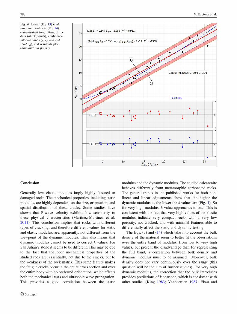
From Table 4 two strong correlations can be derived.

The first one corresponds to the linear correlation between

static modulus and dynamic modulus (both in GPa) that

provides a coefficient of determination 0.961:

Est ¼ 0:867 Edyn � 2:085 ð13Þ

The second significant correlation provides a decimal

logarithm relationship between the static modulus (in GPa),

the bulk density (in kg m-3), and the dynamic modulus (in

Fig. 2 P (triangles) and S

(squares) wave velocities (Vp

and Vs) versus heating

temperature (T) of air-cooled

samples. Note that circles

correspond to P and S wave

velocities of water-cooled

specimens. The decrease of

velocity is typically due to

micro-fissuration of calcite

crystals

796 V. Brotons et al.

123

GPa) with a coefficient of determination of 0.968, similar

to that proposed by Eissa and Kazi (1988):

log10Est ¼ 1:275log10ðqbulkEdynÞ � 4:714 ð14Þ

Note that these two correlations have been computed for a

calcarenite rock and for low dynamic modulus values (i.e.

Edyn from 4 to 30 GPa). Figure 4 shows the plot of the 24

tested samples jointly with the proposed equations [Eqs. (13,

14)]. Regardless of the high value of the coefficient of

determination, the residuals randomly dispersed around the

horizontal axis indicate that a linear regression model is

appropriate for the data. The confidence interval bands of 80

and 95 % are also plotted. The blue dashed line shows the

Eq. (14) or nonlinear fit. Since the correlation between

density and dynamic modulus found in our tests is very poor,

we estimate Eq. (13) is more appropriate than (14) in this

case;moreover that the trend of Eq. (14) extrapolated to high

dynamic modulus values differs from that shown in Fig. 1.

Fig. 3 Representation of the

elastic and dynamic Young’s

modulus relationships proposed

by different authors (see

Table 1) for low elasticity range

(lower than 50 GPa). The

relationships have been only

represented for their range of

validity. Blue points correspond

to the tested samples

Table 4 Matrix of correlation

coefficients

The fitted functions for the first

five columns are linear

(coefficients in bold). For the

remaining columns the fitted

functions are non-linear (in

italic)

R2 k Est Edyn as qbulk m asn log10 Est log10 (qbulk, Edyn)

k 1.000 0.686 0.5687 0.272 0.074 0.268 – –

Est 1.000 0.961 0.397 0.035 0.462 – –

Edyn 1.000 0.404 0.007 0.458 – –

as 1.000 0.001 – – –

qbulk 1.000 0.001 – –

m asn 1.000 – –

log10 Est 1.000 0.968

log10 (qbulk, Edyn) 1.000

The San Julian’s stone 797

123

Conclusion

Generally low elastic modules imply highly fissured or

damaged rocks. The mechanical properties, including static

modulus, are highly dependent on the size, orientation, and

spatial distribution of these cracks. Some studies have

shown that P-wave velocity exhibits low sensitivity to

these physical characteristics (Martinez-Martinez et al.

2011). This conclusion implies that rocks with different

types of cracking, and therefore different values for static

and elastic modulus, are, apparently, not different from the

viewpoint of the dynamic modulus. This also means that

dynamic modulus cannot be used to correct k values. For

San Julian’s stone it seems to be different. This may be due

to the fact that the poor mechanical properties of the

studied rock are, essentially, not due to the cracks, but to

the weakness of the rock matrix. This same feature makes

the fatigue cracks occur in the entire cross section and over

the entire body with no preferred orientation, which affects

both the mechanical tests and ultrasonic wave propagation.

This provides a good correlation between the static

modulus and the dynamic modulus. The studied calcarenite

behaves differently from metamorphic carbonated rocks.

The general trends in the published works for both non-

linear and linear adjustments show that the higher the

dynamic modulus is, the lower the k values are (Fig. 1). So

for very high modulus, k value approaches to one. This is

consistent with the fact that very high values of the elastic

modulus indicate very compact rocks with a very low

porosity, not cracked, and with minimal features able to

differentially affect the static and dynamic testing.

The Eqs. (7) and (14) which take into account the bulk

density of the material seem to better fit the observations

over the entire band of modulus, from low to very high

values, but present the disadvantage that, for representing

the full band, a correlation between bulk density and

dynamic modulus must to be assumed . Moreover, bulk

density does not vary continuously over the range (this

question will be the aim of further studies). For very high

dynamic modulus, the correction that the bulk introduces

provides predictions of k near one, which is consistent with

other studies (King 1983; Vanheerden 1987; Eissa and

Fig. 4 Linear (Eq. 13) (red

line) and nonlinear (Eq. 14)

(blue-dashed line) fitting of the

data (black points), confidence

interval bands (grey and red

shading), and residuals plot

(blue and red points)

798 V. Brotons et al.

123

Kazi 1988; Al-Shayea 2004; Ide 1936). For those appli-

cations in which it is necessary to study the same type of

rock under different weathering degrees, it may be more

convenient to use a linear adjustment, as in Eq. (13), for the

4–30 GPa band, ranging from intact rock to very weakened

rock. In these cases, bulk density exhibits a low variation,

and it is not directly related with the deterioration of

mechanical properties. Note that equations similar to (13)

also implicitly include the bulk density because the

dynamic elastic modulus depends on it [see Eq. (2)].

However, equations similar to (14) are expressed as a

function of the square of the bulk density.

Summarizing, it is concluded that static modulus can be

obtained from dynamic tests, as shown in Eq. (13) for the

studied range (i.e. Edyn values lower than 50 GPa) and for

soft rocks. Furthermore, the dynamic modulus (i.e. ultra-

sonic wave velocity) has been found to be a good indicator

of the material degree of deterioration, in this case poorly

detected by other parameters such as the attenuation of the

ultrasonic wave.

The obtained relationships will allow the computation of

the static modulus of elements of cultural heritage of Ali-

cante city made of San Julian’s stone (e.g. Gravina Palace,

Santa Barbara Castle, City Council building, Lonja, Prin-

cipal Theatre, Cathedral of St. Nicholas, Basilica of Santa

Marıa) from non-destructive field tests, for the analysis of

the integrity level of historical constructions affected by

high temperatures. Furthermore, these results can be

extrapolated, performing the adequate adaptations, for

building stones with similar properties.

Acknowledgments The authors would like to thank Dr. D. Bena-

vente and Dr. J. Martınez from the Earth Sciences Department and

Applied Petrology Laboratory from the University of Alicante for

allowing us to perform ultrasonic tests on their laboratories and Dr.

J. M. Ortega from the Department of Civil Engineering from the

University of Alicante for kindly performing the mercury intrusion

porosimetry test. The companies U.T.E. FCC Construccion, S.A. and

Enrique Ortiz e Hijos Contratistas de Obras, S.A. provided the rock

samples from the TRAM tunnel excavation. This work has been

partially funded by the University of Alicante projects uausti11–11

and gre09–40, the Spanish National project BIA2012-34316, and the

Generalitat Valenciana project gv/2011/044.

References

AENOR (2007) UNE-EN 1936: Metodos de ensayo para piedra natural.

Determinacion de la densidad real y aparente y de la porosidad

abierta y total, vol 1. Asociacion Espanola de Normalizacion y

Certificacion (Ed.), Spain. https://www.aenor.es

Al-Shayea NA (2004) Effects of testing methods and conditions on

the elastic properties of limestone rock. Eng Geol

74(1–2):139–156. doi:10.1016/j.enggeo.2004.03.007

Anon (1979) Classification of rocks and soils for engineering

geological mapping part I: rock and soil materials. Bull Int

Assoc Eng Geol 19(1):364–371. doi:10.1007/bf02600503

Brotons V, Ivorra S, Martınez-Martınez J, Tomas R, Benavente D

(2013) Study of creep behavior of a calcarenite: San Julian’s

stone (Alicante). Mater Constr 62(312). doi:10.3989/mc.2013.

06412

Ciccotti M, Mulargia E (2004) Differences between static and

dynamic elastic moduli of a typical seismogenic rock. Geophys J

Int 157(1):474–477. doi:10.1111/j.1365-246X.2004.02213.x

Dunham RJ (1962) Classification of carbonate rocks according to

depositional texture. Mem Am Assoc Pet Geol 1:108–121

Eissa EA, Kazi A (1988) Relation between static and dynamic

Young’s Moduli of rocks. Int J Rock Mech Min Sci

25(6):479–482. doi:10.1016/0148-9062(88)90987-4

Ide JM (1936) Comparison of statically and dynamically determined

young’s modulus of rocks. Proc Natl Acad Sci USA 22:81–92.

doi:10.1073/pnas.22.2.81

ISRM (1977) Suggested method for petrographic description of rocks.

ISRM Suggest Methods 15:41–45

ISRM (1979) SM for determining the uniaxial compressive strength

and deformability of rock materials. ISRM Suggest Methods

2:137–140

King MS (1983) Static and dynamic elastic properties of rocks from

the Canadian shield. Int J Rock Mech Min Sci 20(5):237–241.

doi:10.1016/0148-9062(83)90004-9

Kjartansson E (1979) Constant Q-wave propagation and attenuation.

J Geophys Res 84(NB9):4737–4748. doi:10.1029/

JB084iB09p04737

Kolesnikov YI (2009) Dispersion effect of velocities on the evalu-

ation of material elasticity. J Min Sci 45(4):347–354

Louis Cereceda M, Garcia-del-Cura MA, Spairani Y, de Blas D

(2001) The civil palaces in Gravina Street, Alicante: building

stones and salt weathering. Mater Constr 51(262):23–37

Martın JD (2004) Using XPowder: a software package for powder

X-ray diffraction analysis. Spain, p 105. http://www.xpowder.

com. ISBN 84-609-1497-6

Martinez-Martinez J, Benavente D, Garcia-del-Cura MA (2011)

Spatial attenuation: the most sensitive ultrasonic parameter for

detecting petrographic features and decay processes in carbonate

rocks. Eng Geol 119(3–4):84–95. doi:10.1016/j.enggeo.2011.02.

002

Martinez-Martinez J, Benavente D, Garcia-del-Cura MA (2012)

Comparison of the static and dynamic elastic modulus in

carbonate rocks. Bull Eng Geol Environ 71(2):263–268. doi:10.

1007/s10064-011-0399-y

Montenat C (1977) Les basins neogenes et quaternaries du Levant

d’Alicante a Murcie (Cordilleres Betiques orientales, Espagne).

Stratigraphie, paleontologie et evolution dynamique. Doc Lab

Geol, Univ Lyon 69, 345 ppMontenat C, Ott d’Estevou P, Coppier G (1990) Les basins neogenes

entre Alicante et Cartagena. Doc Et Trav IGAL 12–13:313–368

Vanheerden WL (1987) General relations between static and dynamic

moduli of rocks. Int J Rock Mech Min Sci 24(6):381–385

The San Julian’s stone 799

123