Recent investigations of the 0–5 Ma geomagnetic fieldrecorded by lava flows

C. L. JohnsonDepartment of Earth and Ocean Sciences, University of British Columbia, 6339 Stores Road, Vancouver, BC,Canada V6T 1Z4 (cjohnson@eos.ubc.ca)

C. G. Constable and L. TauxeScripps Institution of Oceanography, 9500 Gilman Drive, La Jolla, CA 92093, USA (cconstable@ucsd.edu;ltauxe@ucsd.edu)

R. BarendregtDepartment of Geography, University of Lethbridge, 4401 University Drive, Lethbridge, Alberta, Canada TIK 3M4(barendregt@uleth.ca)

L. L. BrownDepartment of Geosciences, 611 North Pleasant Street, 233 Morrill Science, Center University of Massachusetts,Amherst, MA 01003-9297, USA (lbrown@geo.umass.edu)

R. S. CoeEarth and Planetary Sciences Department, University of California, Santa Cruz, CA 95064, USA (rcoe@pmc.ucsc.edu)

P. LayerGeophysical Institute, 903 Koyukuk Drive, University of Alaska, Fairbanks, AK 99775-7320, USA(player@gi.alaska.edu)

V. MejiaUniversidad Nacional de Colombia, Manizales, Colombia (vmejiab@unal.edu.co)

N. D. OpdykeDepartment of Geological Sciences, University of Florida, 241 Williamson Hall, P.O. Box 112120, Gainesville,FL 32611 USA (drno@ufl.edu)

B. S. SingerDepartment of Geology and Geophysics, University of Wisconsin-Madison, 1215 West Dayton Street, Madison,WI 53706, USA (bsinger@geology.wisc.edu)

H. StaudigelScripps Institution of Oceanography, 9500 Gilman Drive, La Jolla, CA 92093, USA (hstaudigel@ucsd.edu)

D. B. StoneGeophysical Institute, 903 Koyukuk Drive, University of Alaska, Fairbanks, AK 99775-7320, USA(dstone@gi.alaska.edu)

G3G3GeochemistryGeophysics

Geosystems

Published by AGU and the Geochemical Society

AN ELECTRONIC JOURNAL OF THE EARTH SCIENCES

GeochemistryGeophysics

Geosystems

Article

Volume 9, Number 4

23 April 2008

Q04032, doi:10.1029/2007GC001696

ISSN: 1525-2027

Copyright 2008 by the American Geophysical Union 1 of 31

[1] We present a synthesis of 0–5 Ma paleomagnetic directional data collected from 17 different locationsunder the collaborative Time Averaged geomagnetic Field Initiative (TAFI). When combined with regionalcompilations from the northwest United States, the southwest United States, Japan, New Zealand, Hawaii,Mexico, South Pacific, and the Indian Ocean, a data set of over 2000 sites with high quality, stable polarity,and declination and inclination measurements is obtained. This is a more than sevenfold increase oversimilar quality data in the existing Paleosecular Variation of Recent Lavas (PSVRL) data set, and hasgreatly improved spatial sampling. The new data set spans 78�S to 53�N, and has sufficient temporal andspatial sampling to allow characterization of latitudinal variations in the time-averaged field (TAF) andpaleosecular variation (PSV) for the Brunhes and Matuyama chrons, and for the 0–5 Ma intervalcombined. The Brunhes and Matuyama chrons exhibit different TAF geometries, notably smallerdepartures from a geocentric axial dipole field during the Brunhes, consistent with higher dipole strengthobserved from paleointensity data. Geographical variations in PSV are also different for the Brunhes andMatuyama. Given the high quality of our data set, polarity asymmetries in PSV and the TAF cannot beattributed to viscous overprints, but suggest different underlying field behavior, perhaps related to theinfluence of long-lived core-mantle boundary conditions on core flow. PSV, as measured by dispersion ofvirtual geomagnetic poles, shows less latitudinal variation than predicted by current statistical PSV models,or by previous data sets. In particular, the Brunhes data reported here are compatible with a wide range ofmodels, from those that predict constant dispersion as a function of latitude to those that predict an increasein dispersion with latitude. Discriminating among such models could be helped by increased numbers oflow-latitude data and new high northern latitude sites. Tests with other data sets, and with simulations,indicate that some of the latitudinal signature previously observed in VGP dispersion can be attributed tothe inclusion of low-quality, insufficiently cleaned data with too few samples per site. Our Matuyama datashow a stronger dependence of dispersion on latitude than the Brunhes data. The TAF is examined usingthe variation of inclination anomaly with latitude. Best fit two-parameter models have axial quadrupolecontributions of 2–4% of the axial dipole term, and axial octupole contributions of 1–5%. Approximately2% of the octupole signature is likely the result of bias incurred by averaging unit vectors.

Components: 13,938 words, 14 figures, 13 tables.

Keywords: paleomagnetic; time-averaged field; paleosecular variation; lavas.

Index Terms: 1522 Geomagnetism and Paleomagnetism: Paleomagnetic secular variation; 1545 Geomagnetism and

Paleomagnetism: Spatial variations: all harmonics and anomalies; 1599 Geomagnetism and Paleomagnetism: General or

miscellaneous.

Received 18 May 2007; Revised 8 August 2007; Accepted 22 October 2007; Published 23 April 2008.

Johnson, C. L., et al. (2008), Recent investigations of the 0–5 Ma geomagnetic field recorded by lava flows, Geochem.

Geophys. Geosyst., 9, Q04032, doi:10.1029/2007GC001696.

1. Introduction

[2] The structure and evolution of the magneticfield is key to understanding the geodynamo andEarth’s deep interior, but many aspects of it remainpoorly documented particularly on timescales of104 to 106 years. While paleomagnetists have madeextensive use of the approximation of the time-averaged geomagnetic field by a geocentric axialdipole (GAD), it has been known for some time[Wilson, 1970], that there are systematic departuresfrom this simple model. The nature of departuresfrom GAD over the past few million years isdebated [Gubbins and Kelly, 1993; Kelly andGubbins, 1997; Johnson and Constable, 1995,

1997; Merrill et al., 1996; McElhinny et al.,1996; Carlut and Courtillot, 1998] (see reviewgiven by Johnson and McFadden [1997]), andcontroversy over field structure extends to time-scales of 108 years and longer [Piper and Grant,1989; Kent and Smethurst, 1998; Van der Voo andTorsvik, 2001; Torsvik and Van der Voo, 2002;McFadden, 2004], for which data sets are evensparser in their geographic and temporal sampling.Experiments with the size and nature of the innercore, and with thermal boundary conditions innumerical dynamo simulations [Hollerbach andJones, 1993a, 1993b; Glatzmaier et al., 1999;Kono and Roberts, 2002; Christensen and Olson,2003], suggest that non-GAD field structure may

GeochemistryGeophysicsGeosystems G3G3

johnson et al.: the 0 – 5 ma geomagnetic field from lavas 10.1029/2007GC001696

2 of 31

persist over timescales governed by the longevityof the boundary conditions and demonstrate theneed to quantify such structure on the basis ofmeasurements of Earth’s magnetic field.

[3] Models of the geomagnetic field can be con-structed using a spherical harmonic representation.The magnetic scalar potential in a source-freeregion due to an internal field obeys Laplace’sequation, and can be written as

Y r; q;f; tð Þ ¼ aX1l¼1

Xl

m¼0

a

r

� �lþ1

gml tð Þ cosmfþ hml tð Þ sinmf� �

� Pml cos qð Þ; ð1Þ

where glm(t) and hl

m(t) are the Schmidt partiallynormalized Gauss coefficients at a time t, a is theradius of the Earth, r, q and f are radius, colatitudeand longitude respectively, and Pl

m are the partiallynormalized Schmidt functions. The magnetic field,~B, is the gradient of the potential Y, and a fieldmodel is specified by the Gauss coefficients gl

m(t)and hl

m(t). The m = 0 terms correspond to sphericalharmonic functions with no azimuthal structure;that is, they are axially symmetric or zonal. Hereg10, g2

0, and g30 are the Gauss coefficients represent-

ing the axial dipole, axial quadrupole and axialoctupole terms, respectively. Time-varying fieldmodels can be constructed from time series ofmagnetic field observations using a parametriza-tion in time (typically cubic b splines). Regulariza-tion of models in both time and space minimizesstructure that is not required by the data [Parker,1994]. Observatory and satellite measurementsprovide (Bx, By, Bz), the north, east, and downwardpointing, locally orthogonal magnetic field compo-nents. Paleomagnetic observations are typicallymeasurements of direction (declination (D) andinclination (I)) and/or intensity jBj, where

D ¼ tan�1 By

Bx

� �;

I ¼ tan�1 Bz

B2x þ B2

y

� �12

0B@

1CA;

jBj ¼ B2x þ B2

y þ B2z

� �1=2: ð2Þ

[4] Over the historical period, 1590–1990 AD,satellite, observatory, and survey measurementsof the geomagnetic field have permitted the con-struction of a spatially detailed, temporally varyingmagnetic field model, GUFM1 [Jackson et al.,2000; see also, e.g., Bloxham et al., 1989; Bloxhamand Jackson, 1992]. Starting in the 1970s, similar

types of models have also been produced overmillenial timescales from compilations of archeo-magnetic directional and paleointensity data, andpaleomagnetic directional data from high accumu-lation-rate sediments [e.g., Hongre et al., 1998](for a review, see Constable [2007]); the mostrecent of these spans the past 7 ka [Korte andConstable, 2005]. Time-varying models, such asGUFM1 and CALS7K.2, can be used to examinethe evolution of the geomagnetic field. Our interesthere is the time-averaged structure: a representationof this is obtained by averaging each of the modelsover their respective time intervals. The radialcomponent of the magnetic field, Br, is shown inFigures 1a and 1b for GUFM1 and CALS7K.2,after downward continuation of the scalar potentialto the surface of Earth’s core under the assumptionthat the mantle is an insulator. GUFM1 showssignificant non-GAD structure, which has beenextensively discussed elsewhere [Jackson et al.,2000], and is generally considered to be stronglyinfluenced by the presence of the inner core and theassociated tangent cylinder. Regions of increasedradial flux at high latitudes, commonly referred toas flux lobes, have persisted in much the samelocations for 400 years. Low radial field over thenorth pole has been interpreted as a manifestationof magnetic thermal winds and polar vorticeswithin the tangent cylinder [Hulot et al., 2002;Olson and Aurnou, 1999; Sreenivasan and Jones,2005, 2006]. Equatorial flux patches that are pro-nounced in the time-varying version of GUFM1and in modern satellite models [e.g., Hulot et al.,2002], and that appear to propagate westward in theAtlantic hemisphere, are attenuated in the 400 yeartemporal average (Figure 1a). When averaged over0–7 ka, CALS7K.2 (Figure 1b) shows longitudinalstructure that suggests the presence of flux lobes seenin the historical field. The radial magnetic field isattenuated in CALS7K.2 compared with GUFM1:the resolution and accuracy is clearly inferior, butaveraging of millennial-scale secular variation alsoplays a major role in subduing the structure.

[5] The time interval 0–5 Ma is our primaryinterest. Three quite different, but representative,field models for this interval are seen in Figures 1c,1d, and 1e. The simplest one, Figure 1c, is basedon the premise that only zonal structure can beresolved, and shows Br at the core-mantle bound-ary due to an axial dipole, with a zonal quadrupolecontribution, g2

0, of 0.05g10. Figures 1d and 1e are

constructed using the same techniques of regular-ized inversion used for GUFM1 and CALS7K.2.These paleofield models are not continuously

GeochemistryGeophysicsGeosystems G3G3

johnson et al.: the 0 – 5 ma geomagnetic field from lavas 10.1029/2007GC001696johnson et al.: the 0 – 5 ma geomagnetic field from lavas 10.1029/2007GC001696

3 of 31

varying in time, owing to the intermittent recordprovided by volcanic rocks and the poor spatialdata distribution. Instead, time-averaged fielddirections are inverted for a time-averaged fieldmodel (see review by Johnson and McFadden[1997]). In Figures 1c–1e, the structure in eachmodel depends on the data sets used: the greatestnumber of paleodata come from sediment pistoncores [Schneider and Kent, 1990] with only incli-nation data and large uncertainties. These arecompatible with very smooth models like thatshown in Figure 1c. When lava flow observationsare combined with sediment data, they suggest themuted nonzonal structure in Figure 1d [Johnsonand Constable, 1997], and lava flow data aloneindicate more complex average field structure(Figure 1e) [Johnson and Constable, 1995].

[6] Figure 2 shows the signal expected at Earth’ssurface for the GUFM1, CALS7K.2 and LSN1average field models, in the form of geographic

variations in departures of inclination and declina-tion from GAD predictions. These are given by theinclination anomaly (DI) and declination anomaly(DD), where

DI ¼ I � IGAD DD ¼ D: ð3Þ

The structure in the archeo and paleofield anoma-lies is rather similar (despite the very different datadistributions from which they are derived) andcontrasts with that seen in GUFM1. Note that themagnitude of the signal decreases over longertimescales. From Figure 2f we see that the averageinclination anomaly in LSN1 is rather small, andwe can expect the largest signal at equatoriallatitudes. If this view of the time-averaged field isapproximately correct, then at mid to high latitudesit will be difficult to detect departures from GADwithout large data sets that provide accuratemeasures of DI.

Figure 1. Time-averaged radial magnetic field, (Br), at the core-mantle boundary (CMB), on different timescales.Units are mT. (a) Historical field: 1590–1990, Model GUFM1 [Jackson et al., 2000], (b) Archeo-Field: 0–7 ka,Model CALS7K.2 [Korte and Constable, 2005], (c) Paleo-Field: 0–5 Ma, axial dipole plus axial quadrupole field(see text), (d) Model LSN1 [Johnson and Constable, 1997], and (e) Model LN1 [Johnson and Constable, 1995].

GeochemistryGeophysicsGeosystems G3G3

johnson et al.: the 0 – 5 ma geomagnetic field from lavas 10.1029/2007GC001696

4 of 31

[7] Figures 1 and 2 provide the motivation forgathering the new lava flow data presented here,and for assembling large regional data sets from thepublished literature. Tantalizing similarities amongthe models averaged on quite different timescalessuggest persistent structure in the time-averagedfield in the form of high-latitude flux lobes, andpossible low radial field in polar regions. Suchstructures are not implausible on several grounds.The inner core tangent cylinder might influencecore flow in such a way as to produce persistentlyhigh values for Br in the latitude band occupied bythe current flux lobes, and lower values close to thepole. It is also possible that these lobes mightexhibit longitudinal bias in their locations as aresult of geographically complex variations inthermal conditions at the core-mantle boundary.However, the major limitations in understandinggeomagnetic field behavior over relevant time-scales (106 years and longer) are the quality,

temporal distribution and spatial coverage of exist-ing paleomagnetic data.

[8] We examine the role of paleomagnetic direc-tions from volcanics in characterizing the 0–5 Matime-averaged field (TAF) and its temporal vari-ability or paleosecular variation (PSV). We focuson these data for several reasons. First, volcanicsprovide geologically instantaneous recordings offield behavior, without the temporal averaginginherent in sedimentary records. Second, measure-ments of absolute declination provide importantconstraints on longitudinal structure in the field(see discussion by Johnson and Constable [1997]),and these are often unavailable from deep seasediment cores. Third, such data are well-suitedto statistical investigations of the paleomagneticfield: they can be used to test the predictions ofstatistical models such as those pioneered byConstable and Parker [1988], the most recent

Figure 2. (a, c, e) Declination and (b, d, f) inclination anomalies in degrees (deviations from GAD direction) atEarth’s surface predicted from models for the three time intervals in Figure 1: Figures 2a and 2b, Model GUFM1;Figures 2c and 2d, CALS7K.2; and Figures 2e and 2f, Model LSN1. The scale bar for the historical field is twice thatfor the archeo-field, and 4 times that for paleofield anomalies.

GeochemistryGeophysicsGeosystems G3G3

johnson et al.: the 0 – 5 ma geomagnetic field from lavas 10.1029/2007GC001696

5 of 31

refinement of which is that of Tauxe and Kent[2004]; to compare with the statistical properties ofdynamo models [e.g., Bouligand et al., 2005]; orultimately can be used to invert for both the time-averaged field and its temporal variability (someprogress in this area has been made by Khokhlov etal. [2001, 2006]). Finally, from a practical perspec-tive, data collection efforts by several groups overthe past decade have resulted in many new high-

quality paleodirections, that can collectively becompared with those used to generate the modelsshown in Figures 1 and 2.

[9] In PSV studies of lava flows, an estimate of thepaleofield at a given location and time is made bysampling what is known as a ‘‘site.’’ At a givensite, multiple samples are collected to reduce theinfluence of measurement error, and these samplesmust be demagnetized in the laboratory to removesecondary remanence. Site mean values of D and Ihave an associated uncertainty that reflects within-site scatter. This is usually quoted as the 95%confidence cone about the mean direction, a95,where a95 140�/

ffiffiffiffiffiffiffikNs

p(for k greater than 25)

and Ns, k are the number of samples and theestimate of the Fisherian precision parameter, krespectively. Within-site scatter is sometimesdescribed by the within-site dispersion, sw, wheresw = 81�/

ffiffiffik

p. Multiple temporally-independent

sites are needed to characterize both the TAF andPSV at a single place. A statistic traditionally usedto describe PSV is SB, the root mean square (rms)angular deviation of virtual geomagnetic poles(VGPs) about the geographic axis,

SB ¼

ffiffiffiffiffiffiffiffiffiffiffiffiffiffiffiffiffiffiffiffiffiffiffiffiffiffiffiffiffiffiffiffiffiffiffiffiffiffiffiffiffiffiffiffiffiffi1

N � 1

XNi¼1

D2i �

S2wi

Nsi

� �vuut : ð4Þ

Table 1. DMAG 4 Data of McElhinny and McFadden[1997]a

Region N Superseded Reference

New Zealand 56 yes this compilation (Table 3)Japan 21 yes this compilation (Table 4)Reunion 27 yes Lawrence et al. [2006]Tahiti 135 yes Lawrence et al. [2006]SW USA 54 yes Tauxe et al. [2003]NW USA 41 yes Tauxe et al. [2004b]Canaries 13 yes Tauxe et al. [2000]Iceland 47 no . . .Total 394

aThese are previously reported data of adequate quality (DMAG 4)

for TAF/PSV modeling [McElhinny and McFadden, 1997]. N is totalnumber of DMAG 4 data for region (no selection based on k or a95).Superseded indicates whether data from McElhinny and McFadden[1997] for that region have been superseded by newer compilationsreported by the cited reference. In the case of the SW USA, NW USA,and the Canaries, the recent published data compilations include newdata collected as part of the TAFI project.

Table 2. TAFI Studiesa

Region l, deg f, deg Ntotal Ndated Reference

Aleutians 54.4 190.1 89 31 Stone and Layer [2006]Nunivak 53.0 �172.0 56 0 Coe et al. [2000], Appendix ABritish Columbia 51.5 �122.4 53 0 Mejia et al. [2002]Snake Riverb 43.0 �113.5 26 21 Tauxe et al. [2004b]San Francisco Volcanicsb 35.3 �111.9 37 0 Tauxe et al. [2003]Azoresc 37.8 �25.4 35 12 Johnson et al. [1998]La Palmab,c 28.8 �17.9 26 8 Tauxe et al. [2000]Mexico 20.1 �99.7 16 7 Mejia et al. [2005]Costa Rica 10.2 �84.4 32 17 Appendix AEcuador �0.4 �78.3 63 13 Opdyke et al. [2006]Atacama �23.3 �67.7 46 23 Appendix AEaster Island �27.1 �109.2 62 0 Brown [2002]Tatara San Pedro, Chile �36.0 �70.9 193 22 Appendix AAustralia �37.7 144.2 38 0 Opdyke and Musgrave [2004]Patagonia �47.0 �71.1 36 34 Brown et al. [2004a]Patagonia �51.2 �70.6 50 20 Mejia et al. [2004]McMurdo �78.1 165.4 36 18 Tauxe et al. [2004a]17 studies total 894 226

aDefinitions are as follows: Region, geographical area of study; l, mean study latitude in degrees (positive north); f, mean study longitude in

degrees (positive east); Ntotal, total number of sites with declination and inclination measurement pairs; Ndated, number of sites for which newradiometric (usually 40Ar/39Ar) dates were obtained; and Reference, publication in which the paleomagnetic study is reported. Data not yetpublished are reported in Appendix A.

bData from the San Francisco volcanics, Snake River plain, and La Palma were included in the regional compilations for the SW USA, NW

USA, and Canaries, respectively (see Table 1).cData sets from the Azores and La Palma were collected prior to the TAFI project but lab protocols followed those of TAFI and so the data sets

are included.

GeochemistryGeophysicsGeosystems G3G3

johnson et al.: the 0 – 5 ma geomagnetic field from lavas 10.1029/2007GC001696

6 of 31

Di represents the angular deviation of the pole forthe ith site from the geographic north pole, N is thenumber of sites, and SB represents the geomagneticsignal remaining after correcting for the within-sitedispersion Swi

determined from Nsisamples. (Note

that this equation corrects an error in equation (4)of Lawrence et al. [2006]). The estimate k fordirections can be converted to an approximation tothe precision parameter for VGPs using thetransformation provided by Creer [1962]. Thestatistical approach inherent in using SB circum-vents the lack of detailed age control and theabsence of time series of observations that areinevitable in working with lava flows fromdisparate locations.

[10] While there have been previous attempts tocompile global data sets suitable for TAF and PSVmodeling [McElhinny and Merrill, 1975; Lee,1983; Quidelleur et al., 1994; Johnson andConstable, 1996], many issues have plagued inter-pretations, notably those of inadequate (or evenunknown) temporal sampling, poor geographicalcoverage, and poor data quality resulting frominferior laboratory methods. These limitations arethe cause of much of the discussion surroundingthe level of complexity in the 0–5 Ma TAF. Themost conservative view is afforded by McElhinnyand McFadden [1997] (hereafter MM97), who inan assessment of a global paleomagnetic databaseconcluded that only 394 D, I pairs would meetmodern standards for paleomagnetic research.These data (designated by a demagnetization code‘DMAG 4’ in work by MM97) are restricted to8 globally distributed locations, and have poor agecontrol (Table 1). This does not necessarily mean

that the older data are unusable, but has provided astrong incentive to understand the influence of dataquality in their interpretation [e.g., Tauxe et al.,2003; Lawrence et al., 2006].

[11] In this paper we provide a synthesis of ongo-ing work toward new global data compilations forTAF and PSV modeling. In particular, we reportthe collective results of a major multi-institutionaleffort, the Time-Averaged Field Investigations(TAFI) project, to improve the characterization of thetime-averaged geomagnetic field and paleosecularvariation over the past 5 million years. Results ofindividual studies from this project have beenreported in several publications (see Table 2); herewe investigate new constraints these data place onglobal paleofield behavior. We summarize thenumbers of data collected, common field andlaboratory procedures, and the resulting temporaland spatial data distribution. We investigate theinfluence of data quality and transitional sites onestimates of the TAF and PSV from the TAFI data.Wesupplement theTAFIdatawithrecentlypublishedregional compilations, and two new compilationsfor New Zealand and Japan that we report here.The resulting data set, while not comprehensive,provides a significant improvement over existingglobal data sets, and we use it to investigate zonal(latitudinal) structure in the TAF and PSV.

2. Time-Averaged Field Investigations(TAFI) Project

[12] Paleomagnetic directions have been obtainedfrom 894 lava flows at 17 locations (Figure 3); we

Figure 3. Locations of TAFI sites (red circles, Table 2) and regional compilations from literature (blue stars, Tauxeet al. [2003, 2004b], Lawrence et al. [2006], and this study, Table 3). Open circle denotes Spitzbergen site, where dataare mostly older than 5 Ma and not reported here.

GeochemistryGeophysicsGeosystems G3G3

johnson et al.: the 0 – 5 ma geomagnetic field from lavas 10.1029/2007GC001696

7 of 31

refer to each location as a study. The TAFI studylocations were chosen to improve the geographicalcoverage of 0–5 Ma paleomagnetic directions athigh latitudes (Spitzbergen, Aleutians, Antarctica),and in the Southern Hemisphere (various SouthAmerican locales, Easter Island and Australia).Samples in four studies, Aleutians [Stone andLayer, 2006; Coe et al., 2000], Antarctica [Tauxeet al., 2004a], and Easter Island [Brown, 2002],were collected in the 1960s and 1970s, but originallaboratory measurements involved minimal de-magnetization. For these studies modern demagne-tization techniques were applied to existingpaleomagnetic cores. For the other 13 studies,new field work was required. New radiometricdates, along with 95% uncertainties were obtainedfor 226 of the TAFI sites (Table 2). Previouslyobtained radiometric dates are available for 88additional flows. Ages were assigned to theremaining sites on the basis of absolute and relativeage data provided in the original TAFI publica-tions. In some cases only the polarity chron isknown, and a median chron age, with uncertaintiescorresponding to half the chron length wereassigned. Thus assignments of age and age uncer-tainty have been made for all TAFI sites. 883 siteshave ages less than 5 Ma, the majority are ofBrunhes (67%) or Matuyama (26%) age (Figure 4).

2.1. Paleomagnetic Field Procedures andLaboratory Methods

[13] Sampling was restricted to lava flows or thindikes: units that cool quickly, and can record theinstantaneous geomagnetic field at the time andlocation of emplacement of the volcanic unit.Standard 2.5-cm-diameter paleomagnetic cores,about 10 cm long, were drilled in the field. Eachsite was determined to be in situ; postemplacementtilting was avoided. Outcrops were surveyed usinga magnetic compass and/or a Bartington magne-tometer to minimize sampling of units subjected tolightning strikes. For each study, as many siteswere sampled as possible during the field season,with a goal of at least 10 sites for a given polarity.On average, about 50 sites were obtained per study(Table 2). A minimum of 10 cores were drilledover a several-meter-extent of outcrop to allowassessment of orientation error at each site. (Thedata set from La Palma [Tauxe et al., 2000]preceded these standards and 5–12 samples persite were drilled.) Each sample was oriented usinga magnetic compass, and where possible a suncompass and/or back-sighting (see Tauxe et al.[2003] for details).

[14] Laboratory methods vary slightly among stud-ies, but a set of minimum criteria were adopted: Inall cases natural remanent magnetizations weremeasured for all specimens, and one specimenper core for at least 5 cores (samples) per site,was subjected to stepwise alternating field orthermal demagnetization. Accompanying rockmagnetic measurements, such as susceptibilityand Curie temperature were also made. New40Ar/39Ar radiometric ages were obtained for lavaflows from twelve studies. Details of the paleo-magnetic and age measurements, and resulting datafor each study are given in the original publicationsof paleomagnetic results [Brown, 2002; Brown etal., 2004a; Johnson et al., 1998; Mejia et al., 2002,2004, 2005; Opdyke and Musgrave, 2004; Opdykeet al., 2006; Stone and Layer, 2006; Tauxe et al.,2000, 2003, 2004a, 2004b]. In this paper we use sitemean directions as follows. Original data, includingall laboratory and field measurements, from theAzores [Johnson et al., 1998], La Palma [Tauxe etal., 2000], Southern Patagonia [Mejia et al., 2004],Antarctica [Tauxe et al., 2004a], Snake River [Tauxeet al., 2004b], San Francisco Volcanics [Tauxe et al.,2003], and Costa Rica (C. G. Constable et al.,manuscript in preparation, 2008, and Appendix A)have been archived in the MagIC database [Solheidet al., 2002] (http://www.earthref.org/MAGIC/).

Figure 4. Age distribution for the 883 TAFI sites withages less than 5 Ma. Average age and an estimate of errorin the age are obtained via one of the following:(1) radiometric dates obtained as part of the TAFI project(226 flows), (2) previous radiometric ages made directlyonTAFI sites (90 flows), or (3) inferred age: stratigraphyand/or polarity chron (remaining flows).

GeochemistryGeophysicsGeosystems G3G3

johnson et al.: the 0 – 5 ma geomagnetic field from lavas 10.1029/2007GC001696

8 of 31

Sample-level directions reported in MagIC useprincipal component analysis and require at least 4demagnetization steps and a maximum angulardeviation of the data about the stable componentof less than 5�. Fisher mean directions were com-puted for all sites with at least 3 samples per site.Over 80% of these sites have site mean directionsderived from at least 5 samples. For all other studies(Aleutians [Stone and Layer, 2006], Nunivak [Coeet al., 2000] (Appendix A), British Columbia [Mejia

et al., 2002], Mexico [Mejia et al., 2005], Atacamaand Tatara San Pedro, Chile [Brown et al., 2004b](Appendix A), Easter Island [Brown, 2002], Pata-gonia [Brown et al., 2004a]) we have used the sitemean directions reported in the original publicationor in Appendix A. In this paper we use onlypaleodirections, as absolute paleointensitymesurements are still underway for several of theTAFI studies. For all TAFI studies, the site-levelresults used in this paper are archived in the MagICdatabase, including the data reported in Appendix A[Solheid et al., 2002] (http://www.earthref.org/MAGIC/).

2.2. Assessment of TAFI Data Quality

[15] As has been discussed extensively [e.g.,McElhinny and McFadden, 1997; Johnson andConstable, 1996; Merrill et al., 1996], assessmentof data quality is critical to accurate identification ofpaleosecular variation and of non-GAD time-averaged field structure. Typically site meandirections with an associated a95 greater than (or kless than) a certain value are excluded from analyses.Recent regional data compilations consist of severalhundred site mean directions, and enable an assess-ment of the behavior of TAF and PSV estimates asincreasingly stringent data quality requirements areimposed. We use a similar approach to that reportedby Tauxe et al. [2003] (hereafter T03) and byLawrence et al. [2006] (hereafter L06).

[16] Our measure of data quality for individualsites is k. We use inclination anomaly, DI, (equa-tion (3)) to characterize the TAF, and between-siteVGP dispersion, SB, (equation (4)), for PSV. Wecalculate DI and SB using site mean directions withvalues of k greater than a cut-off value, denoted bykcut. Increasingly stringent data quality criteriacorrespond to successively larger values of kcut.The approach is discussed in detail by L06 and wedo not repeat it here. The TAFI data set differs fromthose of T03 and L06, having sites from a broadrange of latitudes, and we expect both PSV andTAF estimates to include a latitudinal signature.We investigate the TAFI data set by binning datafrom similar latitudes, but retain a distinctionbetween northern and southern latitudes. Sufficientdata are available at latitudes of approximately50�N, 35�N, 25�S, 35�S, and 50�S to perform aninvestigation of how DI and SB vary with kcut. Weuse only sites for which the number of samples persite, n, is at least 5 because lower n leads to lessreliable estimates of k (see, e.g., T03). The resultsare shown in Figure 5 for normal polarity data

Figure 5. Inclination anomaly (DI) and VGP disper-sion (SB) versus cut-off value of k (kcut) for five latitudebins of the TAFI data set. Normal polarity data areshown, and only sites with n � 5 (at least five samplesper site) are considered. Mean DI, SB (blue curves)along with the bootstrap 95% confidence intervals (redcurves) are shown. Green curves indicate number ofcontributing data at each value of kcut.

GeochemistryGeophysicsGeosystems G3G3

johnson et al.: the 0 – 5 ma geomagnetic field from lavas 10.1029/2007GC001696

9 of 31

only, since these dominate our data set. Normalpolarity is defined here as site mean directions thathave a corresponding positive VGP latitude; thusno distinction between stable polarity and transi-tional data is made in the evaluation of data quality.

[17] Taken together, these regional analyses indi-cate that inclination anomaly is quite robust withrespect to data quality, especially in regions with

large data sets. For example, the latitude band withthe most data, centered on 35�S, shows an averageinclination anomaly that is small (2�) and posi-tive, and does not change significantly as the valueof kcut is varied. For other regions, there is somechange in the estimate of DI at high values of kcutbecause the smaller data sets yield less reliableresults. The behavior of SB with kcut varies fromregion to region. Two latitude bands (50�N and

Figure 6. Equal area projections of site directions for each of the 17 TAFI studies,for sites with n � 5. Solid (open)circles represent projections onto the lower (upper) hemisphere. Sites with estimates of the within-site Fisherprecision parameter k � 50 are shown in green, and those with k > 50 are shown in blue. No VGP latitude cut-off isapplied; that is, transitional directions, if present, are included. The GAD field direction at the mean site location isgiven by the red triangle. North is 0� declination.

GeochemistryGeophysicsGeosystems G3G3

johnson et al.: the 0 – 5 ma geomagnetic field from lavas 10.1029/2007GC001696

10 of 31

35�S) show no change in the estimate of SB at lowk, two latitude bands (25�S and 50�S) show adecrease in SB of 2�–6� at values of kcut around50, and one latitude band (35�N) shows a changein behavior at around kcut = 100. The low-qualitydata can result in overestimates of VGP dispersion.Our current data set is not able to resolve anylatitudinal trend in this bias. For latitudes 50�S,25�S, 35�N, values of kcut of 250 or more result innoisy estimates of SB due to the small number ofdata retained. Analysis of reverse polarity TAFIdata showed similar behavior as a function of kcut,although estimates of both SB and DI display morescatter owing to the much smaller data sets.

[18] On the basis of these results we use thefollowing data selection criteria for further analysesof TAFI data: we require (1) n � 5, (2) k > 50. Theone exception to this is the data set from EasterIsland for which only 4 cores were available for

study. In this case we require n � 4, and k > 50 inorder to retain geographical sampling. The TAFIdata set is summarized in Figure 6 on a study-by-study basis, sites with k � 50 are distinguished(green) from those with k > 50 (blue).

2.3. Effect of Transitional Data

[19] Traditionally, sites with ‘‘low’’ VGP latitudesare removed from studies of PSVand the TAF. Thisapproach has been justified as a means of charac-terizing stable polarity average field geometry andits paleosecular variation, but it is important torecognize that it may well prejudice our view of thephenomena we want to study. In addition, thechoice of which data to exclude is ad hoc. We donot try to resolve this issue here, but show howdifferent criteria for identifying (and excluding)transitional data affect estimates of VGP dispersiondetermined from the TAFI data set. Given thetemporal distribution of the TAFI data (Figure 4),we analyze Brunhes-age normal polarity data,Matuyama-age reverse polarity data, and 0–5 Macombined normal and reverse polarity data. Foreach TAFI study we compute SB using the dataquality criteria above, for 3 different choices ofVGP latitude cut-off (Figure 7). We compare theuse of a constant VGP latitude cut-off (here 45�)with one that is permitted to vary with theempirically derived dispersion as proposed byVandamme [1994]. The Vandamme criterionprescribes a VGP latitude cut-off as

lcut ¼ 90 � 1:8SB þ 5ð Þ : ð5Þ

SB is calculated from the data set, then sites withVGP latitudes less than lcut removed, SB recom-puted, and the procedure repeted; that is, all dataare included.

[20] Figure 7a shows that most Brunhes-age TAFIdata do not include low-latitude VGPs, and esti-mates of SB are in agreement for any choice ofVGP cut-off. Field procedures were deliberatelyfocused on obtaining stable polarity data so this isnot surprising. For the three Brunhes studies wheresome low-VGP-latitude data are present, as seen bythe higher estimates of SB for the green (no cut-offapplied) versus black or blue (cut-off applied)symbols, the use of the Vandamme or constantVGP cut-off criteria does not significantly alter theestimates of dispersion. For the Matuyama-agedata, several studies show high SB when all VGPlatitude data are included. (Note that SB for theChilean data at 36�S is greater than 35�, and soplots off the scale of Figure 7, when either no VGP

Figure 7. Effect of VGP latitude cut-off on estimatesof dispersion for the TAFI studies for (a) Brunhes-agenormal polarity data, (b) Matuyama-age reverse polaritydata, and (c) 0–5 Ma combined normal and reversepolarity data. A constant 45� cut-off (black), theVandamme criterion (blue), and no cut-off (green) areshown.

GeochemistryGeophysicsGeosystems G3G3

johnson et al.: the 0 – 5 ma geomagnetic field from lavas 10.1029/2007GC001696

11 of 31

cut-off or the Vandamme criterion is applied.) Inaddition, two of these studies, Patagonia [Brown etal., 2004a] and Chile (Appendix A) [Brown et al.,2004b], show quite different estimates of SB whenthe Vandamme versus the constant VGP cut-offcriterion is applied. The use of Vandamme’s crite-rion assumes that low latitude VGPs are outliers inthe distribution; if several low-VGP-latitude sitesare present the Vandamme algorithm will convergewithout removing these sites. In the case of theChilean data set, most Matuyama-age sites samplethe Matuyama-Brunhes reversal [Brown et al.,2004b], and in the case of the Patagonia data set[Brown et al., 2004a] 5 of the 14 sites meetingour data quality selection criteria have low VGPlatitudes. Analyses of the 0–5 Ma data setshow several studies for which the Vandammeand constant cut-off criteria give different estimatesof SB. This results from combining normal andreverse polarities that may individually havedifferent estimates of SB and different VGP latitudepopulations.

[21] In summary, Figure 7 shows that most TAFIstudies contain few or no low-VGP-latitude data.However, in the cases where such data are presentthe Vandamme and constant VGP cut-off criterioncan result in different estimates of SB, especiallywhen normal and reverse polarity data are com-bined. Because we wish here to focus on stablepolarity field behavior, we choose to remove low-VGP-latitude sites. On the basis of the aboveanalyses, we choose to use the constant VGP cut-off criterion and exclude sites with VGP latitudesless than 45�. Importantly, we note that in compar-ing the predictions of statistical models with datathe same criterion can be applied to simulationsfrom statistical models as to the data, and so our

choice is not restrictive. After removal of low-k andlow-VGP-latitude sites, our TAFI data contribute661 sites.

3. Additional Data

[22] We supplement the TAFI data with eightregional data sets based on compilations from theliterature; consequently these are more heteroge-neous in associated age information, sampling andlaboratory procedures than our TAFI data set. Sixof the compilations have been described elsewhere:paleomagnetic directions from the NW and SWUSA (Tauxe et al. [2004b] and Tauxe et al. [2003],respectively), Mexico [Mejia et al., 2005; Lawrenceet al., 2006], Hawaii, the South Pacific and Reunion[Lawrence et al., 2006]. In three cases, the SWUSA,the NW USA, and Mexico, the published regionalcompilations included data collected as part of theTAFI project (see Tables 1 and 2). In this paper, weanalyze all TAFI data together because oftheir homogeneity in terms of field work and labprotocols. To avoid duplication, the TAFI data fromthe San Francisco volcanics, Snake River plain, andMexico are thus removed from the SW USA, NWUSA and Mexican regional compilations respec-tively. We add new data sets for New Zealand andJapan, and summarize these here. Sampling inboth Japan and New Zealand has been concentratedon Brunhes or Matuyama age outcrops, and sowe investigate these polarity periods only.Paleomagnetic and age data reported in all studiescontributing to the regional compilations are avail-able from the MagIC database at EarthRef.org(www.earthref.org/MAGIC).

[23] The volcanic centers of the North Island, NewZealand have been extensively sampled for studiesof paleosecular variation, beginning with Cox

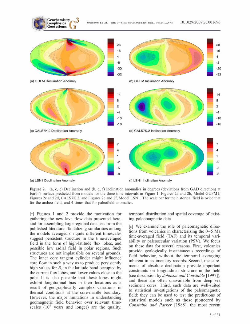
Table 3. New Zealand Studiesa

Location l, deg f, deg NBrunhes NMatuyama Reference

Auckland volcanic province �36.9 174.8 17 . . . Shibuya et al. [1992]South Auckland volcanic province �37.2 174.9 7 10 Briggs et al. [1994]Taupo ignimbritesb �38.5 176.5 15 . . . Shane et al. [1994]Northland �35.4 174.0 9 2 Shibuya et al. [1995]Central Taupoc,d �38.5 176.0 39 14 Tanaka et al. [1996]Taupo, Ruapehu volcanod �39.3 175.6 27 . . . Tanaka et al. [1997]Total 114 26

aDefinitions are as follows: l, mean study latitude in degrees; f, mean study longitude in degrees; NBrunhes/NMatuyama, number of Brunhes/

Matuyama sites with n � 3. There are 92 Brunhes sites with k > 100 and n � 5, with a mean direction, D = 8.2�, I = �56.7� (IGAD = 57.5�) anda95 = 2.1�. There are 14 Matyuama sites with k > 100, n � 5, with a mean direction, D = 180.4�, I = 62.1� (IGAD = 57.5�) and a95 = 6.2�.

bMamaku ignimbrite is excluded since reported directions are anomalous and not well understood.

cDirections from Lake Whakamura are excluded since post emplacement tectonics reported.

dDirections supercede and replace those of Cox [1969, 1971].

GeochemistryGeophysicsGeosystems G3G3

johnson et al.: the 0 – 5 ma geomagnetic field from lavas 10.1029/2007GC001696

12 of 31

[1969, 1971]. Our compilation includes paleodir-ections from all sites, except those suspected oftectonic rotation and those with fewer than 3samples. It comprises 140 sites of Brunhes orMatuyama age: flows, dikes, welded tuffs, weldedignimbrites or small domes (Table 3). Of these 140sites, 112 Brunhes-age sites and 22 Matuyamasites have at least 5 samples and are used here(Figures 8a and 8b). In many studies, radiometricdates were obtained for several of the flows sam-pled for paleomagnetic purposes. We use direc-tional and age data from sites from the Aucklandprovince [Shibuya et al., 1992], South Aucklandprovince [Briggs et al., 1994], Northland [Shibuyaet al., 1995], and the Taupo Volcanic Zone [Shaneet al., 1994; Tanaka et al., 1996, 1997]. We takecare to avoid samples from the Mamaku ignim-

brite, since the origin of anomalous directions fromthis exposure is debated [Shane et al., 1994].

[24] The data set for Japan comprises 176 siteswith at least 3 samples per site, of which 172 areBrunhes age (Table 4). Of these, only 126 Brunhes-age sites have at least 5 samples and are used here(Figures 8c and 8d). As with the New Zealand dataset, many of the paleomagnetic studies also reportnew radiometric dates. The regional tectonics iscomplicated with block rotations likely affectingsome areas including the Izu Peninsula [Kikawa etal., 1989], and we take care not to include suchsites. Notably, we do not include here the studies ofKono [1968, 1971] that were included in ourprevious global PSV data compilation [Johnsonand Constable, 1996]. It is possible that some ofthese sites are tectonically affected. Furthermore,

Figure 8. (a, b) New Zealand and (c, d) Japanese data compilations. Age distributions of contributing sites (n � 5,k > 100) are shown in New Zealand (Figure 8a), and Japan (Figure 8c). Equal area projections (figure format as inFigure 6) of site directions are shown in New Zealand (Figure 8b) and Japan (Figure 8d).

GeochemistryGeophysicsGeosystems G3G3

johnson et al.: the 0 – 5 ma geomagnetic field from lavas 10.1029/2007GC001696

13 of 31

other, more recent studies provide paleomagneticdirections at nearby sites, and use modern labora-tory methods.

[25] We conducted an assessment of data qualityfor these new compilations. Estimates of DI werefound to be robust for all values of kcut. Estimatesof PSVare robust for values of kcut up to about 250(beyond which there are insufficient data to assessPSV), and give SB 16�. Because the data caninclude studies with minimal demagnetization, weconsider sites with k > 100 in our further inves-tigations, for compatibility with the other regionalcompilations used here.

[26] Paleodirections from all contributing sites areshown in Figures 8b and 8d. For New Zealand,92 Brunhes-age stable polarity sites have k > 100and n � 5. The distribution of these directions isnon-Fisherian (Figure 8b): The mean inclination iscompatible with that predicted by GAD, but asignificant positive declination anomaly is ob-served (Table 3). Of the 22 Matuyama sites withn � 5, 14 have a value of k > 100, and the resultingmean direction is compatible with GAD (Table 3).For Japan, 80 Brunhes-age sites have n � 5 and k >100. The distribution of directions is non-Fisherian,with a mean direction indistinguishable from GAD(Table 4).

4. Toward a New Global DataCompilation: Latitudinal Variations inthe TAF and PSV

[27] We combine our TAFI data set with the newcompilations from Japan and New Zealand, andpreviously published compilations for the SW

USA [Tauxe et al., 2003], the NW USA [Tauxeet al., 2004b], and 20� latitude [Lawrence et al.,2006]. For the TAFI data we retain sites with atleast 5 samples, values of k greater than 50 andVGP latitudes higher than 45�. As noted previouslythe one exception to this is Easter Island for whichwe allow 4 samples per site. For the regionalcompilations we retain sites with at least 5 samplesand values of k greater than 100. The higher k cut-off for the regional compilations retains consistencywith the original publications of these data sets,and is more conservative because of minimaldemagnetization at some sites in older studies. Thisresults in a data set of 2107 (D, I) pairs, comparedwith 314 (D, I) pairs meeting both these criteriaand the DMAG 4 criteria of MM97. The new dataset supercedes and replaces all of the MM97DMAG 4 sites, except those from Iceland, andspans latitudes from 78�S to 53�N. In particular,the TAFI data significantly improve coverage inthe Southern Hemisphere. This was previouslyrestricted to 3 locations (Tahiti, Reunion andNew Zealand (Table 1), for which the numbers ofdata have been greatly increased (Table 5)) andnow includes TAFI data from 8 additional locations(Table 2). Site level age information is available forall the regional compilations except that from theSW USA [Tauxe et al., 2003]. In that study siteswith ages less than 5 Ma were retained, but ageinformation is only reported for those sites datedradiometrically; we use only these sites (Table 5).Examination of the temporal distribution of ourdata set (Figure 9 and Table 5) shows that samplingis concentrated in the Brunhes, but suggests thereare also sufficient data to examine behavior duringthe Matuyama chron.

Table 4. Japan Studiesa

Location l, deg f, deg NBrunhes NMatuyama Reference

Higshi-Izu volcano group 34.0 138.0 22 . . . Heki [1983]Kagoshima Prefecture pyroclastics 32.0 131.5 6 . . . Heki [1983]Ashitaka dikes 35.2 138.8 35 . . . Tsunakawa and Hamano [1988]Ashitaka volcano; Izu-Oshima Islb 35.0 139.0 48 . . . Kikawa et al. [1989]Mount Fuji and Mount Oshima 35.4 138.8 6 . . . Tanaka [1990]Goto Islands, Tsushima Strait 32.9 128.9 5 . . . Ishikawa and Tagami [1991]Zao volcanic groupc 38.1 140.5 11 4 Otake et al. [1993]Daisen volcano 35.4 133.6 2 . . . Tanaka et al. [1994]Shikotsu caldera 42.6 141.3 4 . . . Tanaka et al. [1994]Ontake Volcano 35.9 137.5 33 . . . Tanaka and Kobayashi [2003]Total 114 26

aTable format is as in Table 3.

bWe excluded sites from Izu peninsula owing to possible tectonic rotation. There are 80 Brunhes sites with k > 100, with a mean direction,

D = 358.7�, I = 54.6� (IGAD = 54.9�) and a95 = 2.6�.cWe excluded site ZK03, since of Jaramillo age. We also excluded the four reverse polarity sites from our calculations.

GeochemistryGeophysicsGeosystems G3G3

johnson et al.: the 0 – 5 ma geomagnetic field from lavas 10.1029/2007GC001696

14 of 31

[28] The new data set although still not global indistribution, overwhelms previous compilations innumber, quality and age constraints, and substan-tially improves geographical coverage and tempo-ral sampling of the Brunhes and Matuyama chrons.Because there are gaps in data coverage (e.g.,Europe) we restrict ourselves to investigations oflatitudinal structure in the TAF and PSV. Wecorrect for plate motions using the model NUVEL1-A [DeMets et al., 1994] and our estimates of siteage.

4.1. PSV: Latitudinal Variations in VGPDispersion

[29] We first examine latitudinal variations in dis-persion recorded by the individual TAFI studiesand regional compilations (Tables 6 and 7 andFigure 10). SB is calculated using equation (4),and 95% confidence limits estimated using a boot-strap resampling technique. Figure 10 shows lesslatitudinal variation in dispersion during theBrunhes than the Matuyama, and with the excep-tion of the Hawaiian compilation at 20�N, the dataset for the Brunhes suggests a constant dispersionwith latitude of around 16�. The Matuyama data setshows several estimates of SB that are higher thanduring the Brunhes. This difference in SB betweennormal and reverse polarity chrons has been ob-served many times previously and its origin is stillnot understood [McElhinny et al., 1996]. TheMatuyama data display a stronger dependence onlatitude of SB. It is unclear whether SB is symmetricabout the equator; different behavior is seen in theNorthern and Southern Hemispheres, although thiscould be related to differences in spatial andtemporal sampling. We note that the data set from

Easter Island, for which we have only 4 samplesper site, appears to be compatible with otherstudies. The study-by-study comparison of SBindicates regional variations in SB, for example,at 53�N [Coe et al., 2000; Mejia et al., 2002; Stoneand Layer, 2006] and at 50�S [Brown et al., 2004a;Mejia et al., 2004]. However, because the numbersof data from individual studies are rather low (7 outof 13 Matuyama TAFI studies have less than 10contributing sites) detailed comparisons of regionalvariations in SB, and assessment of PSV models arenot possible.

Table 5. Numbers of Data Used in This Studya

Compilation Nused NBru NMat NGau/Gil Reference

TAFIb,c 661 408 194 59 this paperJapan 80 80 . . . . . . this paperNew Zealand 106 92 14 . . . this paperHawaii 727 288 57 382 Lawrence et al. [2006]Mexico 137 44 44 49 Lawrence et al. [2006]South Pacific 209 1 163 45 Lawrence et al. [2006]Reunion 43 31 12 . . . Lawrence et al. [2006]N. W. USA 89 62 11 16 Tauxe et al. [2004b]S. W. USA 55 31 12 12 Tauxe et al. [2003]Totals 2107 1037 507 563

aDefinitions are as follows: Compilation, data compilation reported by cited reference; Nused, all data meeting our selection criteria (sites with at

least five samples per site, k > 100, and VGP latitude greater than 45�); NBru, Brunhes; NMat, Matuyama; NGau/Gil, Gauss and Gilbert age sitescombined.

bNew data from Mexico, the Snake River Plain, and the San Francisco volcanics are included in the TAFI summary numbers and are excluded

from the summary numbers for the Mexican, NW USA, and SW USA compilations.cTAFI data set includes the Easter Island data for which four samples per site are allowed (see text).

Figure 9. Age distribution for the combined data setof 2107 pairs of declination and inclination measure-ments (TAFI data plus regional compilations)used in theremaining analyses.

GeochemistryGeophysicsGeosystems G3G3

johnson et al.: the 0 – 5 ma geomagnetic field from lavas 10.1029/2007GC001696

15 of 31

[30] To improve temporal sampling, we bin ourdata set into latitude bands governed by the distri-bution of sampling sites, and no more than ±5� inspatial extent. SB is reported for latitude bands withmore than 10 sites; the exception is the Matuyamaestimate of SB at Antarctica. This has only 6contributing sites, but the value of SB is supportedby recent measurements on additional data(K. Lawrence et al., unpublished data, 2008), andthis datum provides critical latitudinal coverage.VGP dispersion for the latitudinally binnedBrunhes, Matuyama and 0–5 Ma data sets isshown in Figure 11 (values are given in Table 8),and compared with predictions from two paleosec-ular variation models: Model G [McFadden et al.,1988] and TK03 [Tauxe and Kent, 2004]. The TK03predictions assume a TAF specified by GAD, and10,000 simulations were made at latitude incre-ments of 5�. Sites with VGP latitudes less than 45�

are excluded from the simulated data sets. In addi-tion, for each temporal subset of the data we showthe mean SB calculated from the data. We note thatthe statistical model ofConstable and Parker [1988]predicts almost constant SB with latitude.

[31] The Brunhes age data display little variation inSB versus latitude in the Northern Hemisphere; theonly exception is low secular variation at 20�N thatresults from the Hawaiian data set [Lawrence et al.,2006]. Overall these data are compatible with arange of models, from those that predict a constantSB with latitude to those that show some latitudinalvariation (such as Model G and TK03).

[32] The Matuyama data show some dependence ofSB on latitude, although, given the restricted dataset, it is difficult to discriminate among PSVmodels. None of the existing models appear satis-

Table 6. TAFI Studies: VGP Dispersion Versus Latitude for the 17 TAFI Studiesa

�l, deg NBru SB lo hi NMat SB lo

hi Ntotal SB lo hi

�78.0 27 20.616.124.7 6 26.618.8

33.2 34 21.117.124.6

�51.5 9 16.210.023.7 . . . . . . 35 18.215.4

21.2

�47.1 11 21.715.427.0 9 17.19.6

18.7 25 21.417.425.0

�38.9 . . . . . . 21 12.38.812.6 35 13.810.2

15.6

�36.0 102 16.814.818.6 6 19.715.5

24.3 111 16.714.718.3

�27.0 40 12.88.416.8 – – 40 12.88.4

16.8

�23.5 . . . . . . 12 17.413.321.2 27 19.615.4

22.9

�0.5 13 14.411.917.8 26 14.711.3

19.3 46 14.011.617.0

10.0 18 15.210.620.2 . . . . . . 25 17.412.5

22.5

20.2 . . . . . . 9 11.27.614.7 13 10.68.6

13.4

28.6 . . . . . . 11 16.012.819.7 17 15.612.5

18.8

35.4 12 17.613.419.7 11 11.37.6

14.9 24 14.411.216.2

37.8 19 16.612.319.8 9 17.213.8

20.4 30 16.513.618.8

43.1 10 19.214.822.9 6 18.512.2

23.2 20 17.114.320.4

51.5 50 17.014.219.6 . . . . . . 50 17.014.2

19.6

53.1 36 18.015.321.1 14 27.224.0

31.5 50 20.718.323.4

53.5 47 13.010.814.3 9 32.126.1

40.1 71 16.513.918.9

aDefinitions are as follows: NBru, NMat , and Ntotal , number of Brunhes-age normal polarity, Matuyama-age reverse polarity, or 0 – 5 Ma normal

and reverse polarity data combined; l, mean latitude in degrees for the Brunhes, Matuyama, and 0–5 Ma combined data sets; SB lo hi, the between-site

VGP dispersion in degrees, along with the 95% confidence limits.

Table 7. Regional Compilations: VGP Dispersion Versus Latitude for the Eight Regional Compilations Given inTable 5a

�l, deg NBru SB lo hi NMat SB lo

hi Ntotal SB lo hi

�38.2 92 15.313.117.5 13 16.410.6

23.2 106 15.313.317.6

�20.9 31 12.89.915.6 . . . . . . 43 14.512.2

16.9

�17.9 . . . . . . 81 19.316.422.0 207 17.816.0

19.4

19.9 285 9.99.010.9 23 13.18.5

17.5 681 14.313.515.1

23.6 44 17.313.621.0 21 14.610.8

18.3 123 15.914.017.7

35.2 80 15.113.017.0 . . . . . . 80 15.113.0

17.0

36.1 30 15.913.118.9 12 18.014.2

22.9 53 17.215.019.7

45.5 62 15.113.416.8 . . . . . . 78 14.613.3

16.2

aTAFI data from the Snake River Plain, San Francisco volcanics, and Mexico are excluded from the regional compilations. Table format is as in

Table 5.

GeochemistryGeophysicsGeosystems G3G3

johnson et al.: the 0 – 5 ma geomagnetic field from lavas 10.1029/2007GC001696

16 of 31

factory; Model G and TK03 fit some data, but datasets at around 20�S and 53�N show rather higherdispersion. The data set from the S. Pacific (ap-proximately 17�S) contains a large number oftransitional data, whose effect remains evidenteven when the lowest VGP latitude data areexcluded (our cut-off of 45�). Such oversamplingof transitional data should not be the case howeverfor the latitude bins at 22�S and 50�N.

[33] For the combined 0–5 Ma data set, SB appearsto show less latitudinal variation than predicted byeither Model G or TK03. Reasonable agreement ofthe data with Model G, and in particular, TK03, isseen at mid northern (20� to 50�) and mid southern(20� to 40�) latitudes, but SB estimates for data setsfrom Ecuador, Costa Rica, and the South Pacificare higher than model predictions. Estimates of SBat Costa Rica and Ecuador may be influenced by

the small sample size; additional data are clearlyrequired to better estimate PSV at low latitudes.

[34] Overall our data appear to show differentlatitudinal structure for the Brunhes and Matuyamadata, and analyses of combined normal and reversedata sets are thus difficult to interpret. Theseconclusions are evident in both the unbinned TAFIdata alone, and the latitudinally binned TAFI andregional data sets. In particular, less latitudinalvariation is seen for the Brunhes data set, thetemporal interval best sampled by our data, thanpreviously proposed. We next ask whether appar-ent latitudinal structure in SB can result from theinclusion of lower quality data, because the largenumbers of high-quality data are what distinguishour compilation from those previously published.

Figure 10. VGP dispersion versus latitude for theTAFI studies (black triangles for all sites with n � 5 andstar for Easter Island, where n � 4) and regionalcompilations (blue circles) for (a) Brunhes-age normalpolarity data, (b) Matuyama-age reverse polarity data,and (c) 0–5 Ma combined polarity data. (See alsoTables 6 and 7 and text for data selection criteria.)

Figure 11. VGP dispersion, SB (degrees), versuslatitude for latitudinally binned data (triangles) with95% confidence intervals (error bars) for (a) Brunhes-age normal polarity data; (b) Matuyama-age reversepolarity data; and (c) 0–5 Ma data set, normal andreverse data combined. In each plot, the mean value ofSB averaged over all latitude bins is shown (dotted line)as are predicted dispersions for Model G [McFadden etal., 1988] (dashed line) and TK03 [Tauxe and Kent,2004] (solid line). Numbers of data in each bin areindicated.

GeochemistryGeophysicsGeosystems G3G3

johnson et al.: the 0 – 5 ma geomagnetic field from lavas 10.1029/2007GC001696

17 of 31

[35] We compare VGP dispersion as determinedfrom the TAFI data set alone with that calculatedfor various subsets of the PSVRL database[McElhinny and McFadden, 1997]. Figure 12ashows SB versus latitude for all 0–5 Ma normalpolarity data in the PSVRL database with a DMAGcode of 2 or greater, and with at least 2 samples persite. There are 2033 data, and these have beenbinned in 5 degree latitude bins. No further selec-tion for data quality is made. The results show thewell-known increase of VGP dispersion withlatitude, in both the Northern and SouthernHemispheres. The only data not fit by Model G(TK03 is similar) are those from the S. Pacific(20�S) and about 30 sites from western Canada(58�N). Figure 12b shows the effect of selectingonly data with at least 5 samples per site and with kgreater than 100. The number of data is drasticallyreduced (to 714), as seen by the absence inFigure 12b of 3 of the latitude bins present inFigure 12a, and by the increased uncertainties.Notable though is that in several low to midlatitude bins the mean dispersion has increased.In Figure 12c, the data are further restricted on thebasis of demagnetization procedure: only data witha DMAG code of 3 or greater (i.e., those sites atwhich all samples were demagnetized) are used.(Restriction to only DMAG 4 results in insufficientdata for continued analysis). Only a few latitudebins remain, with a total of 329 data, the dispersionwith latitude is approximately flat and is consistentwith that measured by the Brunhes TAFI studies. Inthe experiments shown inFigure12, the largest effectis contributed by removing sites with inadequatedemagnetization suggesting that viscous remanence

overprints, if not properly removed can contributelatitudinal structure in SB.

[36] In a second experiment we use the statisticalmodel of Constable and Parker [1988] (hereafterCP88) to investigate how estimates of SB might beaffected by the inclusion of low-quality data withinsufficient numbers of samples per site. Wechoose model CP88 because it predicts flat disper-sion with latitude (Figure 13). We simulate 10,000sites at each latitude, noise is prescribed at thewithin-site level, by drawing n samples per site,each from a Fisherian distribution with a meandirection given by GAD, and a within-site preci-sion of k. Again, we exclude site mean directionswith VGP latitudes less than 45�. Figure 14 showsthat with n = 10, k = 100 the expected flat SB withlatitude is recovered. (Figure 14 also shows modelTK03 for reference). Figure 13 shows that as nand/or k are decreased in the simulations, SBincreases (owing to the addition of noisy data),but more importantly apparent latitudinal structurein SB is introduced. An extreme case in which n = 2and k = 30 (for all sites) is shown and indicates thatthe apparent latitudinal variation in SB can be quitelarge (up to 6�). Thus the inclusion of studies withpoor quality data or insufficient samples per sitecould contribute to the observed latitudinal varia-tion in SB in previous studies.

4.2. TAF: Latitudinal Structure inInclination Anomalies

[37] We investigate latitudinal structure in the TAFas measured by DI. In estimating DI, we accountfor variations in site latitude within a given latitude

Table 8. Summary Statistics Versus Latitudea

�l, deg NBru SB lo hi DIlo

hi NMat SB lo hi DIlo

hi Ntotal SB lo hi DIlo

hi

�78.0 27 20.616.124.7 �1.5�4.9

1.6 6 26.618.833.2 1.1�7.6

4.1 34 21.117.124.6 �1.0�4.1

1.7

�51.4 . . . . . . . . . . . . . . . . . . 35 18.215.421.2 0.6�2.0

3.0

�47.2 11 21.715.427.0 �1.3�10.9

3.6 . . . . . . . . . 25 21.417.425.0 1.1�4.8

4.8

�37.3 194 16.114.717.5 1.80.5

3.2 40 14.511.817.4 1.3�2.2

5.0 252 15.714.516.9 1.40.2

2.5

�27.1 40 12.88.416.8 0.0�3.1

1.6 . . . . . . . . . 40 12.88.416.8 0.0�3.1

1.6

�22.1 34 14.110.817.8 �2.4�5.5

1.3 12 17.413.321.2 8.2�1.9

15.1 70 16.514.218.3 �1.4�4.9

1.7

�17.7 . . . . . . . . . 81 19.316.422.0 �0.2�4.5

3.7 207 17.816.019.4 1.3�1.2

3.9

�0.5 13 14.411.917.8 �9.3�17.8

�0.6 27 14.411.018.9 �3.2�9.1

0.9 46 14.011.617.0 �4.9�9.7

�1.5

10.0 18 15.210.620.2 �1.6�9.4

5.1 . . . . . . . . . 25 17.412.522.5 �3.4�10.9

2.8

20.0 329 11.210.112.2 �3.1�4.1

�1.9 53 13.210.715.8 �5.3�8.6

�1.8 817 14.513.815.2 �5.3�6.1

�4.4

28.6 . . . . . . . . . 11 16.012.819.7 �7.9�14.7

�5.8 17 15.612.518.8 �6.0�11.2

�3.0

36.1 141 15.514.016.9 �1.6�3.4

0.1 32 15.212.717.7 �6.3�9.6

�2.7 187 15.714.417.0 �3.0�4.5

�1.2

44.8 72 15.614.016.9 �0.7�2.8

1.6 . . . . . . . . . 98 15.113.716.5 �1.8�3.5

�0.1

52.8 133 15.914.217.3 1.80.9

3.3 23 28.525.132.5 6.01.5

11.2 171 17.816.219.4 2.00.7

3.3

aDefinitions are as follows: NBru, NMat , and Ntotal , number of Brunhes-age normal polarity, Matuyama-age reverse polarity, or 0 – 5 Ma normal

and reverse polarity data combined; �l, mean latitude in degrees; SB lo hi and DIlo

hi, the between-site VGP dispersion and the inclination anomaly indegrees, along with their 95% confidence limits.

GeochemistryGeophysicsGeosystems G3G3

johnson et al.: the 0 – 5 ma geomagnetic field from lavas 10.1029/2007GC001696

18 of 31

band as follows. From the observed (D, I) wecompute the direction (D0, I0) relative to theexpected GAD direction at the site (i.e., the devi-ation from GAD). The mean inclination anomaly iscomputed from the unit vector average of the (D0, I0)in a given latitude band, and plotted at the meanlatitude. The 95% confidence limits on DI arecalculated using a bootstrap resampling technique.We analyze the Brunhes and Matuyama chronsseparately, and the combined normal and reversepolarity data for the 0–5 Ma period. (Normal and

reverse data are combined by using the antipode ofthe reverse polarity directions.)

[38] The results for DI are shown in Figure 14 andTable 8. The best geographical coverage is provid-ed by the 0–5 Ma combined data set; however aswith SB, the Brunhes and Matuyama chrons showquite different behavior. Small negative inclinationanomalies are seen at most latitudes for theBrunhes; the largest signal is at Ecuador (�9�),although the number of contributing data is low(13). Small positive inclination anomalies are seenin the Chilean data set and the binned 50�N dataset. The Matuyama inclination anomalies show aquite different structure with pronounced Northern/Southern Hemisphere asymmetry: dominantly neg-ative inclination anomalies in the Northern Hemi-sphere and zero or positive inclination anomalies inthe Southern Hemisphere.

[39] For each temporal subset of the data in Figure14 we perform a grid search to find the best-fittingtwo parameter zonal field model to the inclinationanomalies. We explore a parameter space in whichthe g2

0 and g30 terms can vary from �50% to 50% of

the g10 term, in increments of 1%. For each (g2

0, g30)

pair we calculate the weighted root mean squaremisfit of the predicted inclination anomaly to theobserved inclination anomaly. (The weights aredetermined by the 95% confidence intervals). Thebest fitting models are provided in Table 9. TheBrunhes inclination anomalies are best fit by g2

0 =0.02g1

0 and g30 = 0.01g1

0, a result that is similar toprevious zonal models for global Brunhes data sets[Johnson and Constable, 1995, 1997; Merrill etal., 1996; Carlut and Courtillot, 1998]. The largeramplitude Matuyama inclination anomalies arebest fit by both larger axial quadrupole and axialoctupole terms, with g2

0 = 0.04g10 and g3

0 = 0.05 g10.

Larger amplitude inclination anomalies during re-verse polarity periods have long been noted, al-though their cause (geomagnetic versus rockmagnetic [see, e.g., Merrill et al., 1996] has beendebated. Large octupole contributions during re-verse polarity periods have also been suggested byrecent high-quality data sets [Opdyke et al., 2006].The 0–5 Ma combined normal and reverse polaritydata are fit by a two parameter model in which g2

0 =0.03g1

0 and g30 = 0.03g1

0. Note that the octupole termhere is smaller than that obtained by Lawrence etal. [2006] for two reasons. First the data set usedhere supercedes that of Lawrence et al. [2006]; themajority of sites are the same but there are somedifferences, notably the inclusion of the NewZealand and Japanese data. Second, here we find

Figure 12. (a) VGP dispersion, SB (degrees), versuslatitude for 0–5 Ma PSVRL normal polarity data binnedin 5� latitude bins. Sites with at least 2 samples per siteand a DMAG code of at least 2 were retained resulting in2033 data. (b) Further selection of data from Figure 12a,at least five samples per site and k > 100 required:714 datum. (c) Further selection of data from Figure 12b,DMAG code of 3 or greater required: 329 data. Forcomparison, SB calculated for the Brunhes from theTAFI studies are shown (gray stars and associated errorbars). Model G [McFadden et al., 1988] (dashed line)and TK03 [Tauxe and Kent, 2004] (solid line) are as inFigure 11.

GeochemistryGeophysicsGeosystems G3G3

johnson et al.: the 0 – 5 ma geomagnetic field from lavas 10.1029/2007GC001696

19 of 31

a best fitting two-parameter model to the meaninclination anomaly, weighted by the uncertaintiesin the mean, whereas Lawrence et al. [2006] fit thesite level inclination data.

[40] It has long been known [Creer, 1983] thatbiased estimates of direction are obtained whenunit vectors are averaged. The bias is manifest asdeviations of inclination from GAD predictionsthat are well approximated by a zonal octupolecontribution. We assess the plausible magnitude ofsuch a signal in our data set using a statisticalmodel for PSV [Constable and Johnson, 1999].The TAF structure in the simulations is prescribedas purely g1

0 (i.e., the time-averaged value of allother spherical harmonic terms is set to zero), andPSV is given by the statistics of the sphericalharmonic coefficients prescribed by Constableand Johnson [1999]. We simulate directions atour observed site locations, by drawing n samplesper site from a Fisherian distribution, with a Fisherprecision parameter given by the observed within-site k. The mean inclination is computed for agiven latitude band in the same way as for our data.Averaging of unit vectors produces an apparentinclination anomaly versus latitude signature that isbest fit (using the grid search algorithm describedabove) by a g2

0 = 0.0 term, and g30 = 0.02 g1

0. Thesame result is obtained if we use the statisticalmodel of Tauxe and Kent [2004]. We note thatalthough these simulations (using our site locationsand within-site k) suggest a similar bias for theBrunhes, Matuyama and the 0–5 Ma combineddata sets, larger bias is incurred if the overall levelof PSV is higher [Johnson and McFadden, 1997].Figure 11 suggests higher SB during the Matuyama,

Figure 13. Simulations from statistical model CP88 [Constable and Parker, 1988] to show how the numbers ofsamples per site, n, and data quality as measured by k can affect the latitudinal variation in VGP dispersion. ModelTK03 [Tauxe and Kent, 2004] is also shown for reference.

Figure 14. Inclination anomaly versus latitude forlatitudinally binned data (triangles) with 95% confi-dence intervals (error bars), and best-fit two-parameterzonal field model (solid line). (a) 0–5 Ma data set,normal and reverse data combined; (b) Brunhes-agenormal polarity data; and (c) Matuyama-age reversepolarity data. Numbers of data in each bin are indicated.

GeochemistryGeophysicsGeosystems G3G3

johnson et al.: the 0 – 5 ma geomagnetic field from lavas 10.1029/2007GC001696

20 of 31

and this could have an associated larger bias in g30.

In addition we have only examined latitudinal con-tributions to PSV and hence to bias. If the observedinclination anomalies are corrected for this bias, thenthe g3

0 contributions for the Brunhes, Matuyama, and0–5 Ma data sets are reduced in amplitude to�0.01g1

0, 0.03g10 and 0.01g1

0, respectively.

5. Summary and Conclusions

[41] The TAFI project has resulted in a new high-quality set of paleodirections from lava flows,suitable for studying the TAF and PSV. Data from17 locations provide significantly enhanced spatialcoverage over previous data sets [Quidelleur et al.,1994; Johnson and Constable, 1996] and over thehighest-quality data (‘DMAG 4’) present in thecompilation of MM97. The TAFI data set com-prises 884 paleodirections in the 0–5 Ma timeinterval, with most data of Brunhes and Matuyamaage (Figure 4 and Table 5). In addition, datacollection efforts by other groups have enabledthe compilation of eight regional data sets [Tauxeet al., 2003, 2004b; Lawrence et al., 2006] (alsothis study), which supercede and replace all but oneof the locations of DMAG 4 data (Tables 1 and 5).The resulting combined data set allows investiga-tion of PSV and the TAF as a function of latitudeduring the Brunhes and Matuyama chrons, and forthe combined normal and reverse data for 0–5 Ma.

[42] Our new data set confirms that PSV and theTAF have been different during normal and reversepolarity chrons over the past 5 Ma (see review byJohnson and McFadden [1997], and specificallyduring the Brunhes andMatuyama. It has frequentlybeen suggested that such differences can be attrib-uted to greater contamination of reverse polaritydata by viscous overprints; this is not the case inour study because all of the TAFI data reportedhere has been subjected to thorough laboratorycleaning. Non-GAD contributions to the time-averaged field during the Brunhes are smallerrelative to g1

0 than during the Matuyama, consistentwith evidence for a stronger virtual axial dipolemoment during this time [Tauxe and Yamazaki,2007; Valet et al., 2005]. In addition, the structure

of the non-GAD field is different for the Brunhesand Matuyama chrons with a significant axialoctupole contribution during the Matuyama.

[43] Best-fit two-parameter zonal models for thetime-averaged field structure indicate axial quad-rupole contributions to the TAF of 2–4% of theaxial dipole term (Figure 9 and Table 7), compat-ible with previous studies [Johnson and Constable,1995, 1997; Carlut and Courtillot, 1998; Merrill etal., 1996]. A substantial axial octupole contribution(5% of the axial dipole) is found for theMatuyama chron, with a smaller contribution dur-ing the Brunhes (1% of the axial dipole). Simu-lations using statistical models for PSV [Constableand Johnson, 1999; Tauxe and Kent, 2004] suggesta g3

0 signature on the order of 2% is attributable tothe bias incurred by the averaging of unit vectors.

[44] Evaluations of VGP dispersion from our newdata set show only modest agreement with existingPSV models (Figure 11). The Brunhes data indi-cate little variation of SB with latitude, the excep-tion being low PSV at Hawaii. The mean value ofSB is 16�. It is difficult to discriminate among arange of PSV models, from those that predict flatdispersion with latitude (such as CP88) to thosethat predict a latitudinal increase in SB (Model Gand TK03). Improved evaluation of existing mod-els would be possible with larger low-latitude datasets and new data from high northern latitudes.

[45] Tests with the PSVRL database [McElhinnyand McFadden, 1997], suggest that differencesbetween previous published results for SB as afunction of latitude and our results here are dueto the inclusion in earlier studies of low-quality,uncleaned sites with less than 5 samples per site. Inaddition simulations with statistical model CP88demonstrate that an apparent latitudinal increase inSB can be imparted by sites with insufficientsamples per site and/or large within-site scatter.

[46] SB for the Matuyama chron suggests reason-able agreement with models predicting an increasein SB with latitude; the Antarctica data set clearlycurrently has insufficient data to assess PSV, butthe result is retained here owing to confirmationfrom more recent work incorporating additionalsites (K. Lawrence, unpublished data, 2008). HighSB at 17�S is due to sampling of transitions inFrench Polynesia, and the use of a VGP cut-offcriterion does not completely remove this over-sampling effect.

[47] Latitudinal structure in both PSV and the TAFfor the 0–5 Ma data sets is compatible with

Table 9. Best-Fitting Zonal TAF Models

Time Period G20 = g2

0/g10 G3

0 = g30/g1

0

Brunhes 0.02 0.01Matuyama 0.04 0.050–5 Ma combined 0.03 0.03

GeochemistryGeophysicsGeosystems G3G3

johnson et al.: the 0 – 5 ma geomagnetic field from lavas 10.1029/2007GC001696

21 of 31

previous studies (see review by Johnson andMcFadden [1997]); however, this data set is dom-inated by Brunhes and Matuyama age sites. Clearlytemporal averaging of the data over 5 Ma affordsincreased numbers of data, and better spatial cov-erage, but the results are difficult to interpret giventhe different TAF and PSV structure during theBrunhes and Matuyama chrons.

[48] The new data set is not complete globally.Existing data from Europe, Iceland, and otherrecent studies still need to be incorporated and itis clear from the results presented here that addi-tional data are needed from several places (notablyequatorial and low latitudes, and high northernlatitudes) to allow even latitudinal trends in theTAF and PSV to be properly characterized. In thispaper we have only considered zonal structure inthe field, although it is evident from the 20�latitude compilation of Lawrence et al. [2006]and from estimates of DI and SB from the TAFIstudies that there are regional differences in theTAF and PSV from data sets at similar latitudes.Rather than excluding lower quality and/or excur-sional data, future studies can use more sophisti-cated weighting schemes to allow the incorporationof all observations. In regions where large data setsare available, progress can be made through inver-sions of regional data sets for TAF and PSVstatistics.

[49] Increasing numbers of high-quality absoluteintensity measurements, along with time series ofrelative paleointensity and inclination from sedi-ments means that in the near future it should bepossible to combine these disparate data types intomore comprehensive models for field behavior.Such studies will require careful internal assess-ment of each contributing data type. Assessment ofone such data type, paleodirections from volcanics,has been reported here, and shows that the com-bined data collection efforts of the paleomagneticcommunity over the past decade have resulted indramatic improvements in spatial and temporalcoverage of 0–5 Ma geomagnetic field behavior.

Appendix A: UnpublishedPaleomagnetic Data Used in OurCompilation

[50] Paleomagnetic directions on flows from Ata-cama in Northern Chile, Costa Rica, and Nunivak(Table 2) have not yet been published elsewhere.We provide a very brief description of results at

each location and tabulate the directions used inour study.

A1. Atacama, Northern Chile

[51] The Central Volcanic Zone of the AndesMountains is composed of subduction-relatedignimbrites and lava flows of andesitic composi-tion erupted during late Tertiary and Quaternarytime. East of the Atacama desert in northern Chile,23�S latitude, lavas and ash flows range in agefrom 8 Ma to Holocene. Included in the samplingwere Recent flows from the currently active LascarVolcano and samples from the famous El Lacomagnetite body. Progressive alternating-field de-magnetization, and principal component analysesyielded directions from 46 sites, with 26 reversed,10 normal, and 10 sites with transitional or excur-sional directions, some with poorly defined direc-tions. All are listed in Table A1. The observeddispersion of the poles is considerably larger thanthat predicted by Model G [McFadden et al.,1988].

A2. Costa Rica

[52] Paleomagnetic samples from Costa Rica werecollected in December 1998 and February 2000. Atleast 10 samples per site were drilled in 33 lavaflows/ignimbrites from the Cordilleras Central andGuanacaste, the underlying Canas, Liberia andBagaces formations and Volcano Arenal. Sampleorientation was with sun or magnetic compass. Oneflow was inadvertently sampled twice and thesamples were merged to form the composite sitecr422_cr423. Data from different parts of cr035were inconsistent, and the flow was resampled in adifferent location as cr405. AF and thermal demag-netization, followed by principal component anal-ysis were used to obtain results from the 32 siteslisted in Table A2. Flow ages range from less than1 ka to about 3 Ma, and there are 27 normal and 5reverse polarity results.

A3. Nunivak

[53] The Nunivak data set used here resulted froma restudy of a 1964 collection by A. Cox of 59oriented cores from Pleistocene lava flows onNunivak Island in the Bering Sea. The 54 origi-nally published paleomagnetic directional resultswere primarily based on NRMs. A modern studyon remaining samples using progressive demagne-tization and principal component analysis has es-sentially confirmed the original results. The newdata are given in Table A3.

GeochemistryGeophysicsGeosystems G3G3

johnson et al.: the 0 – 5 ma geomagnetic field from lavas 10.1029/2007GC001696

22 of 31

Table A1. Atacama Paleomagnetic Sitesa

Site Name ls fs Nsamp Dec Inc k lV fV

AT-1 �23.51 292.31 5 95.2 �38.5 29 4.0 44.2AT-2 �23.65 292.46 8 182.6 41.6 213 �87.6 209.9AT-3 �23.63 292.45 4 161.7 35.3 60 �72.5 32.6AT-4 �23.60 292.44 6 258.1 �39.1 73 �1.4 177.5AT-5 �23.61 292.43 8 198.2 36.7 427 �72.8 195.3AT-6 �23.53 292.38 4 193.3 �19.2 16 �54.1 135.1AT-7 �23.53 292.38 4 349.6 �39.6 112 80.4 206.6AT-8 �23.49 292.27 7 179.3 47.3 257 �85.0 299.3AT-9 �23.50 292.25 7 258.2 44.8 133 �20.2 223.2AT-10 �23.50 292.25 6 250.4 �2.2 76 �17.5 193.1AT-11 �23.45 292.22 7 312.1 �18.6 72 42.3 210.8AT-12 �23.34 292.19 7 230.7 �52.7 19 �15.6 154.4AT-13 �23.35 292.19 3 299.2 �36.7 143 33.9 192.5AT-15 �23.85 292.50 5 162.3 48.3 575 �73.3 359.7AT-16 �23.85 292.50 6 182.5 66.9 517 �64.2 288.8AT-17 �23.85 292.50 3 351.1 �50.0 986 79.5 159.3AT-18 �23.86 292.51 6 180.0 30.0 142 �82.2 112.5AT-19 �23.91 292.44 9 181.2 20.6 1338 �76.7 117.6AT-20 �23.91 292.44 7 171.8 8.8 1095 �69.0 89.1AT-21 �23.90 292.45 7 82.2 20.5 33 2.7 9.6AT-22 �23.91 292.45 5 236.9 44.0 9 �38.7 217.2AT-23 �23.93 292.34 5 255.0 �5.7 414 �12.5 193.5AT-24 �23.93 292.34 6 161.7 32.0 171 �71.7 39.9AT-25 �22.85 292.25 4 195.7 23.6 110 �71.7 169.7AT-26 �22.72 292.20 7 178.1 23.5 472 �79.4 102.1AT-27 �22.60 292.44 8 320.7 �46.5 295 54.2 185.8AT-28 �22.66 292.44 10 178.6 21.7 361 �78.5 105.5AT-29 �22.87 291.73 4 31.9 �49.1 28 60.7 42.6AT-30 �22.87 291.73 7 333.8 �49.2 56 65.5 179.0AT-31 �22.88 291.97 8 342.4 �53.5 175 71.0 162.2AT-32 �23.32 292.17 9 178.4 25.0 261 �79.7 103.4AT-33 �23.28 292.01 10 185.8 67.2 514 �63.0 283.8AT-34 �23.21 292.83 8 202.9 46.2 32 �68.9 219.5AT-35 �23.12 292.50 8 188.3 44.5 156 �81.9 226.2AT-36 �22.96 292.33 3 202.0 13.7 102 �63.5 168.7AT-37 �22.92 292.29 6 184.3 29.6 176 �81.9 142.9AT-38 �22.92 292.23 6 195.4 43.5 102 �75.7 215.3AT-39 �23.33 292.22 5 347.3 �33.7 238 77.2 222.2AT-40 �23.32 292.22 4 192.5 33.3 25 �77.2 180.8AT-42 �22.40 291.97 5 152.7 30.1 100 �63.5 30.7AT-43 �22.45 292.00 9 317.8 �44.9 185 51.5 187.2AT-44 �22.59 291.99 7 177.5 20.8 192 �77.9 100.2AT-49 �23.91 292.32 7 355.4 �46.6 53 84.3 157.6AT-50 �23.49 292.01 8 181.3 18.6 300 �76.0 117.3AT-52 �22.69 292.01 6 23.9 �21.1 91 64.3 358.7AT-53 �22.73 291.96 5 203.8 16.7 308 �63.1 173.9

aDefinitions are as follows: ls, site latitude; fs, site longitude; Nsamp, number of samples at the site; k, estimated Fisherian precision parameter;

lV, VGP latitude; fV, VGP longitude.

GeochemistryGeophysicsGeosystems G3G3

johnson et al.: the 0 – 5 ma geomagnetic field from lavas 10.1029/2007GC001696

23 of 31

Table A2. Costa Rica Paleomagnetic Sitesa

Site Name ls fs Nsamp Dec Inc k lV fV

cr017 10.4967 �85.2290 6 15.1 18.1 685 75.1 8.1cr035 9.9707 �84.1800 10 345.9 9.8 9 75.1 167.0cr036 9.9707 �84.1798 6 354.6 25.0 133 83.8 217.1cr037 9.9707 �84.1800 8 359.1 26.8 360 85.7 264.1cr401 10.0592 �84.0393 7 346.3 �7.3 704 70.6 141.5cr402 10.0547 �84.0387 4 0.9 �27.6 199 65.3 93.9cr404 9.8905 �83.8552 8 347.8 5.9 337 76.0 157.2cr405 9.9718 �84.1801 9 355.6 22.4 562 85.4 207.4cr406 10.0703 �83.9848 6 0.9 23.1 1797 87.8 300.1cr407 10.1103 �83.9745 9 218.7 24.0 457 �45.4 215.7cr408 9.7570 �84.1999 6 14.2 5.1 136 74.2 31.9cr409 9.9162 �84.4594 8 342.6 23.3 144 72.8 194.6cr410 9.7480 �84.4435 10 351.5 24.1 142 81.2 205.3cr411 9.8847 �83.8944 6 23.3 �15.1 788 60.9 42.4cr412 9.8847 �83.8944 9 30.6 �6.6 113 56.8 28.0cr414 9.8156 �83.8633 7 6.7 �15.6 81 71.0 75.3cr415 9.9692 �84.0849 6 358.4 8.1 259 83.9 111.1cr416 9.9828 �84.3464 8 170.0 �7.7 15 �78.3 334.7cr417 10.2889 �84.8336 6 23.4 36.6 103 65.3 338.3cr418 10.4738 �85.0726 8 180.9 �7.5 1302 �83.2 267.3cr419 10.4710 �85.0748 5 354.0 32.7 233 80.6 237.2cr420 10.7293 �85.1796 8 7.1 31.3 681 80.7 322.1cr421 10.4578 �84.6432 4 343.3 30.8 477 72.7 207.9cr422_cr423 10.4618 �84.6840 12 347.5 33.2 300 75.7 219.2cr424 10.4587 �84.6793 6 5.7 11.9 1114 82.8 43.1cr425 10.7838 �85.4258 5 184.7 �17.5 314 �85.0 205.7cr426 10.4744 �85.0460 8 173.8 7.5 296 �74.5 298.7cr427 9.9724 �83.7844 7 359.6 44.5 525 73.8 274.9cr428 10.2594 �84.1769 7 292.2 3.2 86 22.1 183.4cr429 10.2080 �84.1635 5 355.3 32.6 1190 81.2 245.2cr430 10.1909 �84.2334 7 356.7 24.9 878 85.7 227.7cr431 10.0601 �84.0800 6 11.6 34.2 2 75.8 326.8

aDefinitions are as follows: ls, site latitude; fs, site longitude; Nsamp, number of samples at the site; k estimated Fisherian precision parameter;

lV, VGP latitude; fV, VGP longitude.

GeochemistryGeophysicsGeosystems G3G3

johnson et al.: the 0 – 5 ma geomagnetic field from lavas 10.1029/2007GC001696

24 of 31

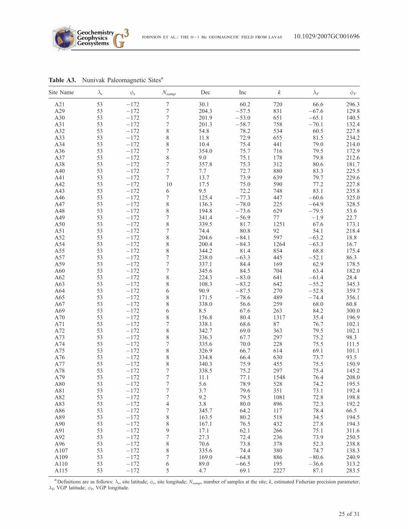
Table A3. Nunivak Paleomagnetic Sitesa

Site Name ls fs Nsamp Dec Inc k lV fV

A21 53 �172 7 30.1 60.2 720 66.6 296.3A29 53 �172 7 204.3 �57.5 831 �67.6 129.8A30 53 �172 7 201.9 �53.0 651 �65.1 140.5A31 53 �172 7 201.3 �58.7 758 �70.1 132.4A32 53 �172 8 54.8 78.2 534 60.5 227.8A33 53 �172 8 11.8 72.9 655 81.5 234.2A34 53 �172 8 10.4 75.4 441 79.0 214.0A36 53 �172 7 354.0 75.7 716 79.5 172.9A37 53 �172 8 9.0 75.1 178 79.8 212.6A38 53 �172 7 357.8 75.3 312 80.6 181.7A40 53 �172 7 7.7 72.7 880 83.3 225.5A41 53 �172 7 13.7 73.9 639 79.7 229.6A42 53 �172 10 17.5 75.0 590 77.2 227.8A43 53 �172 6 9.5 72.2 748 83.1 235.8A46 53 �172 7 125.4 �77.3 447 �60.6 325.0A47 53 �172 8 136.3 �78.0 225 �64.9 328.5A48 53 �172 8 194.8 �73.6 629 �79.5 53.6A49 53 �172 7 341.4 �56.9 77 �1.9 22.7A50 53 �172 8 339.5 81.7 1251 67.6 173.1A51 53 �172 7 74.4 80.8 92 54.1 218.4A52 53 �172 8 204.6 �84.1 597 �63.2 18.8A54 53 �172 8 200.4 �84.3 1264 �63.3 16.7A55 53 �172 8 344.2 81.4 854 68.8 175.4A57 53 �172 7 238.0 �63.3 445 �52.1 86.3A59 53 �172 7 337.1 84.4 169 62.9 178.5A60 53 �172 7 345.6 84.5 704 63.4 182.0A62 53 �172 8 224.3 �83.0 641 �61.4 28.4A63 53 �172 8 108.3 �83.2 642 �55.2 345.3A64 53 �172 6 90.9 �87.5 270 �52.8 359.7A65 53 �172 8 171.5 �78.6 489 �74.4 356.1A67 53 �172 8 338.0 56.6 259 68.0 60.8A69 53 �172 6 8.5 67.6 263 84.2 300.0A70 53 �172 8 156.8 80.4 1317 35.4 196.9A71 53 �172 7 338.1 68.6 87 76.7 102.1A72 53 �172 8 342.7 69.0 363 79.5 102.1A73 53 �172 8 336.3 67.7 297 75.2 98.3A74 53 �172 7 335.6 70.0 228 75.5 111.5A75 53 �172 8 326.9 66.7 614 69.1 101.1A76 53 �172 8 334.8 66.4 630 73.7 93.5A77 53 �172 8 340.3 75.9 455 75.5 150.9A78 53 �172 7 338.5 75.2 297 75.4 145.2A79 53 �172 7 11.1 77.1 1548 76.4 208.0A80 53 �172 7 5.6 78.9 528 74.2 195.5A81 53 �172 7 3.7 79.6 351 73.1 192.4A82 53 �172 7 9.2 79.5 1081 72.8 198.8A83 53 �172 4 3.8 80.0 896 72.3 192.2A86 53 �172 7 345.7 64.2 117 78.4 66.5A89 53 �172 8 163.5 80.2 518 34.5 194.5A90 53 �172 8 167.1 76.5 432 27.8 194.3A91 53 �172 9 17.1 62.1 266 75.1 311.6A92 53 �172 7 27.3 72.4 236 73.9 250.5A96 53 �172 8 70.6 73.8 378 52.3 238.8A107 53 �172 8 335.6 74.4 380 74.7 138.3A109 53 �172 7 169.0 �64.8 886 �80.6 240.9A110 53 �172 6 89.0 �66.5 195 �36.6 313.2A115 53 �172 5 4.7 69.1 2227 87.1 283.5

aDefinitions are as follows: ls, site latitude; fs, site longitude; Nsamp, number of samples at the site; k, estimated Fisherian precision parameter;

lV, VGP latitude; fV, VGP longitude.

GeochemistryGeophysicsGeosystems G3G3

johnson et al.: the 0 – 5 ma geomagnetic field from lavas 10.1029/2007GC001696

25 of 31

Table A4. Tatara San Pedro, Chile, Paleomagnetic Sitesa

Site Name ls fs Nsamp Dec Inc k lV fV

EMU23 �36 289 5 17.4 �46.2 911 73.0 354.2EMU22 �36 289 5 17.4 �50.6 624 74.8 6.2EMU21 �36 289 5 17.0 �48.1 488 74.1 358.3EMU20 �36 289 5 7.4 �42.5 396 77.0 320.4EMU19 �36 289 3 8.8 �46.8 728 79.1 334.7EMU18 �36 289 5 12.1 �45.0 639 76.0 340.0EMU17 �36 289 4 14.0 �45.8 877 75.2 346.6EMU16 �36 289 5 10.5 �50.3 295 80.0 352.7EMU15 �36 289 4 17.7 �49.8 833 74.3 4.2EMU14 �36 289 5 16.6 �51.4 849 75.7 7.9EMU13 �36 289 5 16.3 �52.6 502 76.3 12.0EMU12 �36 289 5 11.6 �49.5 892 78.8 352.2EMU11 �36 289 5 20.4 �46.9 396 71.0 0.3EMU10 �36 289 5 16.5 �49.9 1055 75.3 2.8EMU9 �36 289 5 20.9 �56.4 600 73.2 28.6EMU8 �36 289 5 11.8 �41.7 550 74.3 332.7EMU7 �36 289 5 16.9 �47.2 606 73.8 355.8EMU6 �36 289 4 359.9 �69.5 410 72.8 109.3EMU5 �36 289 3 4.8 �35.3 858 73.0 304.7EMU1 �36 289 5 6.8 �43.8 406 78.1 320.3EPW-6-13 �36 289 5 336.2 �79.4 401 54.1 123.1EPW-6-12 �36 289 4 34.9 �74.7 978 56.5 79.3EPW-6-11 �36 289 4 26.8 �82.5 402 48.8 99.1EPW-6-10 �36 289 4 37.6 �79.9 807 50.2 90.4EPW-6-9 �36 289 5 45.0 �69.5 293 54.4 62.4EPW-6-8 �36 289 5 350.2 �75.3 1000 63.0 119.1EPW-6-7 �36 289 6 219.6 �86.5 279 30.5 114.3EPW-6-5 �36 289 5 14.5 �76.0 312 61.1 95.7EPW-6-4 �36 289 5 40.4 �84.9 214 43.4 100.1EPW-6-3 �36 289 5 14.8 �79.5 342 55.4 100.1EPW-6-2 �36 289 5 353.8 �83.4 252 48.9 111.2EPW-6-1 �36 289 4 31.1 �80.4 625 51.1 93.8ESPE-I-38 �36 289 5 11.8 �51.1 499 79.3 359.2ESPE-I-33 �36 289 4 16.4 �37.1 175 69.0 336.7ESPE-I-32 �36 289 6 11.5 �39.3 293 73.0 328.3ESPE-I-31 �36 289 6 16.7 �38.9 589 69.8 339.7ESPE-I-30 �36 289 6 12.2 �36.5 320 71.0 326.6ESPE-I-29 �36 289 6 14.2 �40.2 194 72.0 336.2ESPE-I-28 �36 289 5 16.5 �37.0 361 68.9 336.8ESPE-I-27 �36 289 6 1.4 �73.0 180 67.4 107.2ESPE-I-23 �36 289 5 8.4 �31.7 531 69.7 312.9ESPE-I-22 �36 289 4 14.2 �36.9 359 70.2 331.8ESPE-I-21 �36 289 4 2.1 �30.4 402 70.3 295.1ESPE-I-19 �36 289 5 4.8 �47.8 374 81.8 320.1ESPE-I-18 �36 289 4 356.4 �55.9 908 87.1 189.3ESPE-I-17 �36 289 4 357.3 �47.8 697 82.5 270.6ESPE-I-16 �36 289 4 16.7 �59.0 622 76.3 40.1ESPE-I-15 �36 289 5 10.3 �49.0 635 79.4 346.8ESPE-I-13 �36 289 4 23.6 �44.0 191 67.4 358.8ESPE-I-12 �36 289 3 22.5 �51.0 485 70.9 12.6ESPE-I-11 �36 289 4 14.1 �56.3 1886 78.6 27.6ESPE-I-10 �36 289 5 2.2 �40.5 92 77.0 298.1ESPE-I-90 �36 289 5 3.5 �46.3 354 81.1 309.6ESPE-I-9 �36 289 6 358.7 �46.9 226 82.0 280.8ESPE-I-8 �36 289 6 5.4 �40.3 675 76.2 310.4ESPE-I-7 �36 289 5 356.3 �43.7 353 79.1 271.2ESPE-I-6 �36 289 6 18.2 �56.4 498 75.4 28.3ESPE-I-5 �36 289 6 5.3 �54.8 441 85.6 11.8ESPE-I-4 �36 289 6 355.3 �54.9 361 86.1 206.2ESPE-I-2 �36 289 6 352.7 �49.6 233 81.7 239.4ESPE-I-1 �36 289 5 1.8 �47.4 252 82.4 301.1ESPE-II-7 �36 289 4 343.4 �55.7 1391 76.6 193.2

GeochemistryGeophysicsGeosystems G3G3

johnson et al.: the 0 – 5 ma geomagnetic field from lavas 10.1029/2007GC001696

26 of 31

Site Name ls fs Nsamp Dec Inc k lV fV

ESPE-II-6 �36 289 6 352.4 �56.6 237 83.8 186.0ESPE-II-4 �36 289 6 6.5 �57.1 308 84.5 39.1ESPE-II-3 �36 289 5 355.9 �54.3 161 86.5 217.2ESPE-II-2 �36 289 3 359.3 �55.0 990 89.3 238.5ESPE-II-1 �36 289 5 1.8 �68.3 239 74.5 104.9QTW-10-48 �36 289 5 11.5 �22.2 40 63.4 315.0QTW-10-46 �36 289 4 10.6 �51.2 378 80.3 357.0QTW-10-45 �36 289 5 359.2 �57.3 5162 88.0 127.4QTW-10-44 �36 289 5 331.0 �54.7 762 66.5 192.4QTW-10-43 �36 289 6 354.1 �55.4 596 85.2 198.2QTW-10-42 �36 289 6 5.1 �60.8 210 83.0 76.4QTW-10-41 �36 289 5 357.9 �55.7 454 88.3 190.4QTW-10-40 �36 289 5 352.0 �50.8 144 82.0 230.9QTW-10-39 �36 289 5 354.9 �52.1 854 84.7 235.6QTW-10-38 �36 289 5 1.9 �61.9 91 82.7 98.1QTW-10-37 �36 289 5 2.7 �52.0 471 85.9 323.3QTW-10-36 �36 289 5 355.3 �54.6 148 86.1 210.6QTW-10-35 �36 289 4 2.3 �50.5 1072 84.9 311.7QTW-10-34 �36 289 5 1.8 �54.0 246 89.0 84.4QTW-10-33 �36 289 5 1.2 �52.9 599 87.3 310.8QTW-10-32 �36 289 6 3.9 �53.8 1217 86.4 352.7QTW-10-30 �36 289 5 0.5 �58.1 262 87.2 101.1QTW-10-29 �36 289 5 5.8 �55.8 470 85.3 25.0QTW-10-28 �36 289 4 345.9 �46.4 440 75.5 229.9QTW-10-27 �36 289 5 343.9 �50.1 176 75.6 215.4QTW-10-26 �36 289 4 340.8 �47.2 183 72.1 218.9QTW-10-25 �36 289 5 347.2 �49.9 305 78.1 221.8QTW-10-24 �36 289 5 344.2 �47.7 145 74.9 223.1QTW-10-23 �36 289 5 345.0 �49.5 693 76.3 219.1QTW-10-22 �36 289 5 347.7 �49.5 272 78.3 224.4QTW-10-21 �36 289 4 350.0 �49.2 806 79.7 231.5QTW-10-20 �36 289 4 350.0 �52.3 357 81.2 216.8QTW-10-19 �36 289 5 344.7 �43.7 762 73.2 233.5QTW-10-18 �36 289 4 341.6 �41.7 308 70.1 231.1QTW-10-18s �36 289 6 324.1 �50.1 100 59.8 198.4QTW-10-17 �36 289 3 325.6 �50.2 226 61.0 199.1QTW-10-16 �36 289 4 355.4 �40.4 179 76.5 270.8QTW-10-15 �36 289 5 5.6 �26.7 179 67.5 303.5QTW-10-14 �36 289 5 359.2 �40.2 267 76.9 285.9QTW-10-13 �36 289 4 354.9 �45.0 100 79.6 263.0QTW-12-10 �36 289 6 337.4 �56.7 199 71.9 188.3QTW-12-9 �36 289 6 350.4 �59.1 266 81.5 169.1QTW-12-8 �36 289 7 333.1 �53.6 489 68.0 196.0QTW-12-7 �36 289 6 315.8 �56.4 26 54.8 184.1QTW-12-6 �36 289 4 345.9 �44.2 286 74.3 235.1QTW-12-5 �36 289 7 338.7 �44.5 699 69.3 221.6QTW-12-4 �36 289 6 336.1 �48.9 170 69.1 209.4QTW-12-3 �36 289 6 339.7 �49.3 1313 72.1 212.3QTW-12-2 �36 289 7 350.9 �52.9 503 82.1 215.2QTW-12-1 �36 289 6 327.4 �53.4 200 63.3 193.9QTW-12-0 �36 289 8 334.3 �63.9 27 68.4 164.8QTE-2-5 �36 289 4 160.7 33.7 65 �65.5 59.9QTE-2-4 �36 289 7 175.9 43.3 385 �78.7 89.9QTE-2-3 �36 289 7 170.1 45.8 134 �77.8 62.6QTE-2-2 �36 289 6 198.7 48.7 138 �73.1 182.4QTE-2-1 �36 289 7 181.5 45.0 39 �80.5 117.3LV-1-21 �36 289 3 8.6 �66.5 693 75.6 85.9LV-1-20 �36 289 5 5.4 �64.5 446 78.9 89.4LV-1-19 �36 289 4 6.4 �55.8 499 84.8 24.8LV-1-18 �36 289 5 357.9 �55.1 277 88.3 210.7LV-1-17 �36 289 5 353.1 �55.2 791 84.4 199.8LV-1-16 �36 289 5 323.9 �53.5 207 60.5 192.2

Table A4. (continued)

GeochemistryGeophysicsGeosystems G3G3

johnson et al.: the 0 – 5 ma geomagnetic field from lavas 10.1029/2007GC001696

27 of 31

A4. Tatara San Pedro, Chile

[54] Tatara San Pedro, Chile, is an eruptive com-plex of the volcanic front of the Andean southernvolcanic zone, with at least three central ventregions. Quaternary volcanism began about930 ka, and both mafic and silicic lavas are present.The geology and chronology of the region isdescribed in detail by Singer et al. [1997]. Paleo-magnetic data were collected over several fieldseasons by L. Brown, B. Singer and colleaguesand directional data from 193 sites are available forour study. K-Ar radiometric ages are available for22 of these sites [Singer et al., 1997, Table 1], withone site having both a K-Ar and Ar-Ar [Singer etal., 1997, Table 2] age. Paleomagnetic data are

from the following sections: Estero Molino, EsteroPellado, Estero San Pedro, Quebrada Turbia andLaguna Verde. The Matuyama-Brunhes transitionis recorded in two sections of the Quebrada Turbiasequence, and paleomagnetic data from 32 sitesfrom these sections is reported by Brown et al.[2004b]. Data from the additional 161 sites aregiven in Table A4.

Acknowledgments

[55] This work was supported under NSF grants EAR-

9805164 (Tauxe), EAR-0337712 (C. Johnson, C. Constable),

EAR-0516760, EAR-0337684, EAR-9909309 (B. Singer),

EAR-0608998 and EAR-0229130 (N. Opdyke), EAR-

9870309 and EAR-9943700 (D. Stone and P. Layer), and

EAR-04400018 (L. Brown), and by NSERC (R. Barendregt).

Table A4. (continued)

Site Name ls fs Nsamp Dec Inc k lV fV

LV-1-15 �36 289 5 2.1 �53.9 690 87.7 337.4LV-1-14 �36 289 5 349.0 �49.5 371 79.2 227.6LV-1-13 �36 289 3 8.1 �39.4 1647 74.6 318.6LV-1-12 �36 289 3 5.5 �41.2 262 76.8 311.7LV-1-11 �36 289 4 4.7 �38.6 512 75.2 306.4LV-1-10 �36 289 5 8.7 �35.6 634 72.0 316.6LV-1-9 �36 289 5 0.5 �30.2 218 70.2 290.5LV-1-7 �36 289 4 3.9 �39.6 593 76.1 304.2LV-1-6 �36 289 5 4.8 �29.9 1881 69.6 302.5LV-1-5 �36 289 4 4.7 �58.3 831 85.2 59.3LV-1-4 �36 289 4 11.3 �42.7 306 75.2 333.1LV-1-3 �36 289 5 20.8 �55.2 331 73.2 24.4LV-1-2 �36 289 5 14.4 �54.2 1217 78.2 17.2LV-1-1 �36 289 5 27.7 �60.2 436 67.8 40.9EML-1-22 �36 289 5 0.4 �26.5 27 68.0 290.2EML-1-21 �36 289 5 359.7 �39.7 221 76.5 287.9EML-1-20 �36 289 5 15.4 �24.2 39 62.9 323.7EML-1-19 �36 289 5 2.5 �45.3 99 80.6 302.9EML-1-18 �36 289 6 10.0 �35.5 283 71.4 320.0EML-1-17 �36 289 4 349.9 �39.7 53 73.9 253.3EML-1-16 �36 289 4 2.9 �42.8 387 78.6 302.5EML-1-15 �36 289 4 347.6 �67.2 293 73.4 138.1EML-1-14 �36 289 6 341.2 �51.6 169 74.0 207.3EML-1-13 �36 289 5 347.7 �46.9 102 76.9 232.8EML-1-12 �36 289 4 356.9 �43.5 139 79.1 274.2EML-1-11 �36 289 5 1.8 �44.1 184 79.7 298.2EML-1-10 �36 289 6 355.8 �55.4 166 86.6 199.0EML-1-7 �36 289 5 336.0 �49.3 417 69.1 208.4EML-1-6 �36 289 5 23.1 �50.0 6 70.1 10.6EML-1-5 �36 289 5 46.2 �47.8 436 50.7 22.2EML-1-4 �36 289 4 11.5 �59.8 135 79.9 50.0EML-1-3 �36 289 4 11.1 �69.6 92 71.0 88.5EML-1-0 �36 289 5 6.6 �54.5 179 84.5 10.8QCN-1-3 �36 289 4 7.0 �40.2 593 75.6 315.9QCN-1-2 �36 289 5 2.7 �53.7 858 87.2 341.4QCN-1-1 �36 289 5 28.2 �67.9 179 64.9 64.5QC-1 �36 289 4 317.6 �66.3 118 56.7 163.3

aDefinitions are as follows: ls, site latitude; fs, site longitude; Nsamp, number of samples at the site; k, estimated Fisherian precision parameter;

lV, VGP latitude; fV, VGP longitude.

GeochemistryGeophysicsGeosystems G3G3

johnson et al.: the 0 – 5 ma geomagnetic field from lavas 10.1029/2007GC001696

28 of 31

C. Johnson acknowledges the Institut de Physique du Globe de

Paris for support as a visiting researcher during preparation of

this manuscript. We thank Kristin Lawrence for input on the

20� latitude regional compilation. Comments by J. Tarduno

and reviews from R. Van der Voo, J.-P. Valet, and an

anonymous reviewer are much appreciated.

References

Bloxham, J., and A. Jackson (1992), Time-dependent mappingof the magnetic field at the core-mantle boundary, J. Geo-phys. Res., 97, 19,537–19,563.

Bloxham, J., D. Gubbins, and A. Jackson (1989), Geomagneticsecular variation, Philos. Trans. R. Soc., Ser. A, 329, 415–502.

Bouligand, C., G. Hulot, A. Khokhlov, and G. A. Glatzmaier(2005), Statistical paleomagnetic field modelling and dyna-mo numerical simulation, Geophys. J. Int., 161, 603–626.

Briggs, R. M., T. Okada, T. Itaya, H. Shibuya, and I. E. M.Smith (1994), K-Ar ages, paleomagnetism, and geochemis-try of the South Auckland volcanic field, North Island, NewZealand, N. Z. J. Geol. Geophys., 37, 143–153.

Brown, L. (2002), Paleosecular variation from Easter Islandrevisited: Modern demagnetization of a 1970s data set, Phys.Earth Planet. Inter., 133, 73–81.

Brown, L. L., B. S. Singer, and M. Gorring (2004a), Paleo-magnetism and 40Ar/39Ar chronology of lavas from Mesetadel Lago Buenos Aires, Patagonia, Geochem. Geophys. Geo-syst., 5, Q01H04, doi:10.1029/2003GC000526.

Brown, L. L., B. S. Singer, J. C. Pickens, and B. R. Jicha(2004b), Paleomagnetic directions and 40Ar/39Ar ages fromthe Tatara San Pedro volcanic complex, Chilean Andes: Lavarecord of a Matuyama-Brunhes precursor?, J. Geophys. Res.,109, B12101, doi:10.1029/2004JB003007.

Carlut, J., and V. Courtillot (1998), How complex is the time-averaged geomagnetic field over the last 5 million years?,Geophys. J. Int., 134, 527–544.

Christensen, U. R., and P. Olson (2003), Secular variaiton innumerical geodynamo models with lateral variations ofboundary heat flow, Phys. Earth Planet. Inter., 138, 39–54.

Coe, R. S., X. Zhao, J. J. Lyons, C. J. Pluhar, and E. A.Mankinen (2000), Revisiting the 1964 collection of Nunivaklava flows, Eos Trans. AGU, 81(48), Fall Meeting Suppl.,Abstract GP62A-06.

Constable, C. G. (2007), Centennial to millennial-scale geo-magnetic field variations, in Treatise on Geophysics, vol. 5,Geomagnetism, edited by M. Kono, chap. 9, Elsevier, NewYork.

Constable, C. G., and C. L. Johnson (1999), Anisotropic pa-leosecular variation models: Implications for geomagneticobservables, Phys. Earth Planet. Inter., 115, 35–51.

Constable, C. G., and R. L. Parker (1988), Statistics of thegeomagnetic secular variation for the past 5 m.y., J. Geo-phys. Res., 93, 11,569–11,581.

Cox, A. (1969), A paleomagnetic study of secular variation inNew Zealand, Earth Planet. Sci. Lett., 6, 257–267.

Cox, A. (1971), Remanent magnetization and susceptibility oflate Cenozoic rocks from New Zealand, N. Z. J. Geol. Geo-phys., 14, 192–207.

Creer, K. M. (1962), The dispersion of the geomagnetic fielddue to secular variation and its determination from remotetimes from paleomagnetic data, J. Geophys. Res., 67, 3461–3476.

Creer, K. M. (1983), Computer synthesis of geomagneticpaleosecular variations, Nature, 304, 695–699.

DeMets, C., R. G. Gordon, D. F. Argus, and S. Stein (1994),Effect of recent revisions to the geomagnetic reversal timescale on estimates of current plate motions, Geophys. Res.Lett., 21, 2191–2194.

Glatzmaier, G. A., R. S. Coe, L. Hongre, and P. H. Roberts(1999), The role of the Earth’s mantle in controlling thefrequency of geomagnetic reversals, Nature, 401, 885–890.

Gubbins, D., and P. Kelly (1993), Persistent patterns in thegeomagnetic field over the past 2.5 Myr, Nature, 365,829–832.

Heki, K. (1983), Paleomagnetic study of the Higashi-Izu Vol-cano Group and pyroclastics flow deposits in KagoshimaPrefecture: Paleosecular variation during the last 40,000years, J. Geomagn. Geoelectr., 35, 383–390.

Hollerbach, R., and C. Jones (1993a), A geodynamo modelincorporating a finitely conducting inner core, Phys. EarthPlanet. Inter., 75, 317–327.

Hollerbach, R., and C. Jones (1993b), Influence of Earth’sinner core on geomagnetic fluctutations and reversals,Nature, 365, 541–543.

Hongre, L., G. Hulot, and A. Khokhlov (1998), An analysis ofthe geomagnetic field over the past 2000 years, Phys. EarthPlanet. Inter., 106, 311–335.

Hulot, G., C. Eymin, B. Langlais, M. Mandea, and N. Olsen(2002), Small-scale structure of the geodynamo inferred fromOersted and Magsat satellite data, Nature, 416, 620–623.

Ishikawa, N., and T. Tagami (1991), Paleomagnetism andfission-track geochronology on the Goto and TsushimaIslands in theTsushimaStrait area: Implications for theopeningmode of the Japan Sea, J. Geomagn. Geoelectr., 43, 229–253.

Jackson, A., A. R. T. Jonkers, and M. R. Walker (2000), Fourcenturies of geomagnetic secular variation from historicalrecords, Philos. Trans. R. Soc., Ser. A, 358, 957–990.

Johnson, C. L., and C. G. Constable (1995), The time-averaged geomagnetic field as recorded by lava flows overthe past 5 Myr, Geophys. J. Int., 122, 489–519.

Johnson, C. L., and C. G. Constable (1996), Paleosecular var-iation recorded by lava flows over the last 5 Myr, Philos.Trans. R. Soc., Ser. A, 354, 89–141.

Johnson, C. L., and C. G. Constable (1997), The time-averaged geomagnetic field: Global and regional biases for0–5 Ma, Geophys. J. Int., 131, 643–666.

Johnson, C. L., and P. McFadden (1997), The time-averagedfield and paleosecular variation, in Treatise on Geophysics,vol. 5, Geomagnetism, edited by M. Kono, chap. 11,Elsevier, New York.

Johnson, C. L., J. R. Wijbrans, C. G. Constable, J. Gee,H. Staudigel, L. Tauxe, V.-H. Forjaz, andM. Salgueiro (1998),40Ar/39Ar ages and paleomagnetism of Sao Miguel lavas,Azores, Earth Planet. Sci. Lett., 160, 637–649.

Kelly, P., and D. Gubbins (1997), The geomagnetic field overthe past 5 Myr, Geophys. J. Int., 128, 315–330.

Kent, D. V., and M. A. Smethurst (1998), Shallow bias ofinclinations in the Paleozoic and Precambrian, Earth Planet.Sci. Lett., 160, 391–402.

Khokhlov, A., G. Hulot, and J. Carlut (2001), Towards a self-consistent approach to palaeomagnetic field modelling,Geophys. J. Int., 145, 157–171.

Khokhlov, A., G. Hulot, and C. Bouligand (2006), Testingstatistical palaeomagnetic field models against directionaldata affected by measurement errors, Geophys. J. Int., 167,635–648.

Kikawa, E., M. Koyama, and H. Kinoshita (1989), Paleomag-netism of Quaternary volcanics in the Izu Peninsula andadjacent areas, Japan, and its tectonic significance, J. Geo-magn. Geoelectr., 41, 175–201.

GeochemistryGeophysicsGeosystems G3G3

johnson et al.: the 0 – 5 ma geomagnetic field from lavas 10.1029/2007GC001696

29 of 31

Kono, M. (1968), Paleomagnetism of Pleistocene UsamiVolcano, Izu Peninsula, Japan—Intensity of the Earth’smagnetic field in geological time II, J. Geomagn. Geoelectr.,20, 353–366.

Kono, M. (1971), Intensity of the Earth’s magnetic field ingeological time III. Pleistocene and Pliocene data from Ja-panese volcanic rocks, J. Geomagn. Geoelectr., 23, 1–9.

Kono, M., and P. H. Roberts (2002), Recent geodynamosimulations and observations of the geomagnetic field, Rev.Geophys., 40(4), 1013, doi:10.1029/2000RG000102.

Korte, M., and C. G. Constable (2005), Continuousgeomagnetic models for the past 7 millennia: 2. CALS7K,Geochem. Geophys. Geosyst., 6, Q02H16, doi:10.1029/2004GC000801.

Lawrence, K., C. G. Constable, and C. L. Johnson (2006),Paleosecular Variation and the average geomagnetic fieldat ±20� latitude, Geochem. Geophys. Geosyst., 7, Q07007,doi:10.1029/2005GC001181.

Lee, S. (1983), A study of the time-averaged paleomagneticfield for the past 195 million years, Ph.D. thesis, Aust. Natl.Univ., Canberra, ACT, Australia.

McElhinny, M. W., and P. L. McFadden (1997), Palaeosecularvariation over the past 5 Myr based on a new generalizeddatabase, Geophys. J. Int., 131, 240–252.

McElhinny,M.W.,andR.T.Merrill (1975),Geomagneticsecularvariation over the past 5 my, Rev. Geophys., 13, 687–708.

McElhinny, M. W., P. L. McFadden, and R. T. Merrill (1996),The time-averaged paleomagnetic field 0–5 Ma, J. Geophys.Res., 101, 25,007–25,027.

McFadden, P. L. (2004), Is 600 Myr long enough for the ran-dom paleogeographic test of the geomagnetic axial dipoleassumption?, Geophys. J. Int., 158, 443–445.

McFadden, P. L., R. T. Merrill, and M. W. McElhinny (1988),Dipole/quadrupole family modelling of paleosecularvariation, J. Geophys. Res., 93, 11,583–11,588.

Mejia, V., R. W. Barendregt, and N. D. Opdyke (2002),Paleosecular variation of brunhes age lava flows from BritishColumbia, Canada, Geochem. Geophys. Geosyst., 3(12),8801, doi:10.1029/2002GC000353.

Mejia, V., N. D. Opdyke, J. F. Vilas, B. S. Singer, and J. S.Stoner (2004), Plio-Pleistocene time-averaged field in south-ern Patagonia recorded in lava flows, Geochem. Geophys.Geosyst., 5, Q03H08, doi:10.1029/2003GC000633.

Mejia, V., H. Bohnel, N. D. Opdyke, M. A. Otega-Rivera, J. K.W. Lee, and J. J. Aranda-Gomez (2005), Paleosecular varia-tion and time-averaged field recorded in late Pliocene–Holocene lava flows from Mexico, Geochem. Geophys.Geosyst., 6, Q07H19, doi:10.1029/2004GC000871.

Merrill, R. T., M. W. McElhinny, and P. L. McFadden (1996),The Magnetic Field of the Earth: Paleomagnetism, the Coreand the Deep Mantle, Academic Press, San Diego, Calif.

Olson, P., and J. Aurnou (1999), A polar vortex in the Earth’score, Nature, 402, 170–173.

Opdyke, N., and R. Musgrave (2004), Paleomagnetic resultsfrom the Newer Volcanics of Victoria: Contribution to theTime Averaged Field Initiative, Geochem. Geophys.Geosyst., 5, Q03H09, doi:10.1029/2003GC000632.

Opdyke, N. D., M. Hall, V. Mejia, K. Huang, and D. A. Foster(2006), The time-averaged field at Ecuador: Results from theequator, Geochem. Geophys. Geosyst., 7, Q11005,doi:10.1029/2005GC001221.

Otake, H., H. Tanaka, M. Kono, and K. Saito (1993), Paleomag-netic study of Pleistocene lavas and dikes of the Zao VolcanicGroup, Japan, J. Geomagn. Geoelectr., 45, 595–612.

Parker, R. L. (1994), Geophysical Inverse Theory, PrincetonUniv. Press, Princeton, N. J.

Piper, J. D. A., and S. Grant (1989), A paleomagnetic test ofthe axial dipole assumption and implications for continentaldistributions through geological time, Phys. Earth Planet.Inter., 55, 37–53.

Quidelleur, X., et al. (1994), Long-term geometry of thegeomagnetic field for the last 5 million years: An updatedsecular variation database from volcanic sequences,Geophys. Res. Lett., 21, 1639–1642.

Schneider, D. A., and D. V. Kent (1990), The time-averagedpaleomagnetic field, Rev. Geophys., 28, 71–96.

Shane, P., T. Black, and J. Westgate (1994), Isothermal plateaufission-track age for a paleomagnetic excursion in theMamakuIgnimbrite, NewZealand, and implications for late Quaternarystratigraphy,Geophys. Res. Lett., 21, 1695–1698.

Shibuya, H., J. Cassidy, I. E. M. Smith, and T. Itaya (1992), Ageomagnetic excursion in the Brunhes chron recorded inNew Zealand basalts, Earth Planet. Sci. Lett., 111, 41–48.

Shibuya, H., J. Cassidy, I. E. M. Smith, and T. Itaya (1995),Paleomagnetism of young New Zealand basalts and long-itudinal distribution of paleosecular variation, J. Geomagn.Geoelectr., 47, 1011–1022.

Singer, B. S., R. A. Thompson, M. A. Dungan, T. C. Feeley,S. T. Nelson, J. C. Pickens, L. L. Brown, A. W. Wulff, J. P.Davidson, and J. Metzger (1997), Volcanism and erosionduring the past 930 k.y. at the Tatara San Pedro complex,Chilean Andes, GSA Bull., 109, 127–142.

Solheid, P., C. Constable, A. Koppers, M. Jackson, andS. Banerjee (2002), Research-oriented data base for rock andpaleomagnetism to be developed, Eos Trans. AGU, 83(48),560.

Sreenivasan, B., and C. A. Jones (2005), Structure anddynamics of the polar vortex in the Earth’s core, Geophys.Res. Lett., 32, L20301, doi:10.1029/2005GL023841.

Sreenivasan, B., and C. A. Jones (2006), Azimuthal winds, con-vection and dynamo action in the polar region of the planetarycores,Geophys. Astrophys. Fluid Dyn., 100, 319–339.

Stone, D. B., and P. W. Layer (2006), Paleosecular variationand GAD studies of 02 Ma flow sequences from the AleutianIslands, Alaska, Geochem. Geophys. Geosyst., 7, Q04H22,doi:10.1029/2005GC001007.

Tanaka, H. (1990), Paleointensity high at 9000 years ago fromvolcanic rocks in Japan, J. Geophys. Res., 95, 17,517–17,531.

Tanaka, H., and T. Kobayashi (2003), Paleomagnetism of thelate Quaternary Ontake Volcano, Japan: Directions, intensi-ties, and excursions, Earth Planets Space, 55, 189–202.

Tanaka, H., A. Otsuka, T. Tachibana, and M. Kono (1994),Paleointensities for 10–22 ka from volcanic rocks in Japanand New Zealand, Earth Planet. Sci. Lett., 122, 29–42.

Tanaka, H., G. M. Turner, B. F. Houghton, T. Tachibana,M. Kono, and M. O. McWilliams (1996), Palaeomagnetismand chronology of the central Taupo Volcanic Zone,Geophys.J. Int., 124, 919–934.

Tanaka, H., K. Kawamura, K. Nagao, and B. F. Houghton(1997), K-Ar ages and paleosecular variation of directionand intensity from Quaternary lava sequences in theRuapehu Volcano, New Zealand, J. Geomagn. Geoelectr.,49, 587–599.

Tauxe, L., and D. Kent (2004), A simplified statistical modelfor the geomagnetic field and the detection of shallow bias inpaleomagnetic inclinations: Was the ancient magnetic fielddipolar?, in Timescales of the Internal Geomagnetic Field,Geophys. Monogr. Ser., vol. 145, edited by J. E. T. C.Channell et al., pp. 101–115, AGU, Washington, D. C.

Tauxe, L., and T. Yamazaki (2007), Paleointensities, inTreatise on Geophysics, Geomagnetism, edited by M. Kono,chap. 13, Elsevier, New York.

GeochemistryGeophysicsGeosystems G3G3

johnson et al.: the 0 – 5 ma geomagnetic field from lavas 10.1029/2007GC001696

30 of 31

Tauxe, L., H. Staudigel, and J. Wijbrans (2000), Paleomagnet-ism and 40Ar/39Ar ages from La Palma in the CanaryIslands, Geochem. Geophys. Geosyst., 1(9), doi:10.1029/2000GC000063.

Tauxe, L., C. Constable, C. L. Johnson, A. A. P. Koppers,W. R. Miller, and H. Staudigel (2003), Paleomagnetism ofthe southwestern U.S.A. recorded by 0–5 Ma igneous rocks,Geochem. Geophys. Geosyst., 4(4), 8802, doi:10.1029/2002GC000343.

Tauxe, L., P. Gans, and E. A. Mankinen (2004a), Paleomag-netism and 40Ar/39Ar ages from volcanics extruded duringthe Matuyama and Brunhes Chrons near McMurdo Sound,Antarctica, Geochem. Geophys. Geosyst., 5, Q06H12,doi:10.1029/2003GC000656.

Tauxe, L., C. Luskin, P. Selkin, P. Gans, and A. Calvert(2004b), Paleomagnetic results from the Snake River Plain:Contribution to the time-averaged field global database,Geochem. Geophys. Geosyst., 5, Q08H13, doi:10.1029/2003GC000661.

Torsvik, T. H., and R. Van der Voo (2002), Refining Gondwanaand Pangea paloegeography: Estimates of Phanerozoic non-dipole (octupole) fields, Geophys. J. Int., 151, 771–794.

Tsunakawa, H., and Y. Hamano (1988), Paleomagnetic studyof the Ashitaka Dike Swarm in central Japan, J. Geomagn.Geoelectr., 40, 221–226.

Valet, J. P., L. Meynadier, and Y. Guyodo (2005), Geomag-netic dipole strength and reversal rate over the past twomillion years, Nature, 435, 802–805.

Vandamme, D. (1994), A new method to determine paleose-cular variation, Phys. Earth Planet. Inter., 85, 131–142.

Van der Voo, R., and T. H. Torsvik (2001), Evidenceforlate Paleozoic and Mesozoic non-dipole fields provides anexplanation for the Pangea reconstruction problems, EarthPlanet. Sci. Lett., 187, 71–81.

Wilson, R. L. (1970), Permanent aspects of the Earth’s non-dipole magnetic field over Upper Tertiary times, Geophys.J. R. Astron. Soc., 19, 417–439.

GeochemistryGeophysicsGeosystems G3G3

johnson et al.: the 0 – 5 ma geomagnetic field from lavas 10.1029/2007GC001696

31 of 31