ANALYTICAL INTERPRETATION OF GEOMAGNETIC FIELDANOMALY ALONG THE DIP EQUATOR

ANALYTICAL INTERPRETATION OF GEOMAGNETIC FIELDANOMA LY ALONG THE

DIP EQUATOR

RIDWAN AGBOOLA

Department of Physics, Al-Hikmah University Ilorin, Nigeria,

ABSTRACT

The variation of the magnetic H- field in the equatorial electrojet (EEJ) regions along the dip equator have been

studied, using five international Quiet Days (IQD’s) of each month for the years 2005 to 2007. The hourly mean values

were used to study the variations in the component (H) at the equatorial electrojet regions. The results of the

analysisrevealed average constant diurnal variations in all, while the amplitude of dH variation peaks during the day at

about local noon (12.00h) in all the eight equatorial electrojet regions used. This diurnal variation in H with Sq (H)

enhancement in all the eight regions are attributed partly to ionospheric plasma irregularities as well as the enhanced

dynamo action in the ionosphere.

KEYWORDS: Magnetic Field, Dip Equator, Equatorial Electroject, Diurnal

INTRODUCTION

Earth is the third planet from the Sun, the densest and Fifth-largest of the eight planets in the Solar system.

It is also the largest of the Solar System's four terrestrial planets. It is sometimes referred to as the World, the Blue Planet

or by its Latin name, Terra, Denni et. al. (1995). It is home to millions of species including humans, Earth is currently the

only place in the universe where life is known to exist. The planet formed 4.54 billion years ago and life appeared on its

surface within a billion years Williams. D (2004). Since then, Earth's biosphere has significantly altered the atmosphere

and other abiotic conditions on the planet, enabling the proliferation of aerobic organism as well as the formation of the

ozone layer which, together with Earth’s magnetic field, blocks harmful solar radiation, permitting life on land.

It has been a long established fact that variations in ground magnetic records are caused by the dynamo action in

the upper atmosphere. These daily variations in the geomagnetic fields at the earth’s surface during geomagnetically quiet

conditions are known to be associated with the dynamo currents which are driven by winds and thermal tidal motions in

the E-region of the ionosphere (Chapman, 1919). At the magnetic dip equator the mid day eastward polarization field

generated by global scale dynamo action gives rise to a downward Hall current. A strong vertical polarization field is set

up which opposes the downward flow of current due to the presence of non-conducting boundaries. This field in turn gives

rise to the intense Hall current which Chapman (1951) named the equatorial electrojet (EEJ). The phenomenon has been

given various attention and has attracted several research workers both in the past and recent times. There still exists a

controversy as to whether the EEJ current system and the WSq current system are independent. Hence, Ogbuehi et al.

(1976) suggested that the EEJ is a current circuit whose strength changes independent of the WSq strength.

Onwumechili (1985), noted that the observed field at the dip equator was made of two components and separable

parts: the WSq and electrojet fields. Okeke et al. (1998) showed that the variabilities of the current intensities of the EEJ

and WSq current layers are mostly independent. Earlier works of Bartels and Johnson (1940), Egedal (1947), found that

the diurnal ranges of H at the stations near the equator peaks around the dip equator with assumption that the amplitudes of

the daily variation in D and Zwere unaffected. Forbush and Casaverde(1961) studied the features of EEJ in dH and Z

BEST: International Journal of Humanities, Arts, Medicine and Sciences (BEST: IJHAMS) ISSN 2348-0521 Vol. 3, Issue 3, Mar 2015, 29-44 © BEST Journals

30 Ridwan Agboola

across the dip equator, and assumed that EEJ produced none or very negligible D field. However, recent work of Rastogi

(1998),Onwumechili (1997) and Okeke et al. (1998) has shown that D field of EEJ does exist. Patil et al. (1983), described

the mean daily variations of different component of the geomagnetic field, declination(D),horizontal component field (H)

and vertical field (Z),using the Indian observatories combined with those in the U.S.S.R. Patil et al.(1990) studied the

average latitudinal profile of dH and dZ in the Indian and American zone. Fambitakoye (1971) gave the first latitudinal

profiles of dH and dZ due to normal and counter electroject event using nine equatorial stations in central Africa.

Rastogi (1974)Fambitakoye and Mayaud(1976a,b)described profile of dH and dZ on individual days. Studies

have been carried out on the seasonal variation of dH in other EEJ regions which reveals equinoctial maximum and solistiti

alminimum in these regions, these include the works of Chapman and Rajarao (1965), Tarpley (1973) and Doumouya et al.

(1998).The characteristic signature of the EEJ, ∆H field is a sharp negative V shaped curve attaining its minimum within

0.5° of the magnetic dip equator.

However, due to the structure of the Earth and its content, the present work examines the disturbance daily

variation of Horizontal component H along the dip equator at the unique set of EEJ stations such as: Adis Ababa, Ilorin,

Ancon, Darwin, Cebu, Davao, Yap Island and Manado.

MATERIALS AND METHODS

Theory

Figure 1:-D Representation of Geomagnetic Elements

So � = �� + ��

�, and = ��

�

F is the total geomagnetic field, H and Z are horizontal and vertical components of the earth’s field; and I and D

are the dip/inclination and declination angles.

At geomagnetic equator I tend to zero hence � ≅ �; thus, horizontal component is measured in all the

observatories used.

The aims and objective of this project is to study, observe and predict the magnetic variation along the dip

equator. The detailed of the stations used are shown in the table 1

Table 1

Abbrev. Station Name Nation GG Lat. GG Lon. GM Lat. GM Lon. L Dip Lat. AAB Adis Ababa Ethiopia 9.04 38.77 0.18 110.47 1.00 0.57 ILR Ilorin Nigeria 8.50 4.68 -1.82 76.80 1.00 -2.96 ANC Ancon Peru -11.77 -77.15 0.77 354.33 1.00 0.74 DAW Darwin Australia -12.41 130.92 -21.91 202.81 1.18 CEB Cebu Philippine 10.36 123.91 2.53 195.06 1.00 2.74

Analytical Interpretation of Geomagnetic Fieldanomaly along the Dip Equator

DAV Davao PhilippineYAP Yap Island FSMMND Manado Indonesia

Instrument

The instrument used for the collection of data was MAGDAS/CPMNSystem. MAGDAS (MAGnetic Data

Acquisition system)/CPMN (Circum-

MAGDAS-A system is a new magnetometer system installed

and monitoring system installed at SERC. The new MAGDAS

thermometer in sensor unit, fluxgate –

Figure 2.

Magnetic field digital data (H, D, Z, and F.) are obtained with the sampling rate of 1/16 seconds and then the

1-sec average data are transferred from the overseas stations to the SERC, Japan in real time. The ambient magnetic fields

expressed by horizontal (H), declination (D) and vertical (z) components, are digitized by using the field

for the dynamic range of±64,000nT/16bit. The resolutions of MAGDAS data are

±2,000nT and ± 1,000nT range, respectively.

MAGDAS system can obtain amplitude

variations. The ordinary data (i.e MAGDAS data(1)) can be used for studies of long

Auroral sub-storms, Sq. etc while the induction

transient and impulsive phenomena. By using these new MAGDAS data, a real

global 3-dimensional current system and (2) the ambient plasma density for understanding the global electromagnetic and

plasma environmental changes in geo-space.

Source of Data

The data used were obtained from MAGDAS station for the year 2005, 2006and 200

Abbrev. Station Name NationAAB Adis Ababa EthiopiaILR Ilorin NigeriaANC Ancon PeruDAW Darwin Australia

Analytical Interpretation of Geomagnetic Fieldanomaly along the Dip Equator

Table 1: Contd., Philippine 7.00 125.40 -1.02 196.54

FSM 9.50 138.08 1.49 209.06Indonesia 1.44 124.84 -6.91 196.06


-pan Pacific Magnetometer Network) IS roughly divided into two portion:

system is a new magnetometer system installed at the CPMN stations, while MAGDAS

and monitoring system installed at SERC. The new MAGDAS-A system consists of 3-axial ring core sensor, tiltmetres and

–type magnetometer, data logger/transfer units and the power unit as shown in the

Figure 2: Magnetometer


sec average data are transferred from the overseas stations to the SERC, Japan in real time. The ambient magnetic fields

expressed by horizontal (H), declination (D) and vertical (z) components, are digitized by using the field

dynamic range of±64,000nT/16bit. The resolutions of MAGDAS data are 0.061Nt/LS

±2,000nT and ± 1,000nT range, respectively.

MAGDAS system can obtain amplitude-time records of 4-componentordinary and induction

(i.e MAGDAS data(1)) can be used for studies of long- term variations, e.g Magnetic storm,

etc while the induction-type data (i.e MAGDAS data(2)) is useful for the studies of ULF waves,

phenomena. By using these new MAGDAS data, a real-time monitoring and modeling of (1) the

dimensional current system and (2) the ambient plasma density for understanding the global electromagnetic and

space.

The data used were obtained from MAGDAS station for the year 2005, 2006and 200

Table 2

Nation GG Lat. GG Lon. GM Lat. GM Lon.Ethiopia 9.04 38.77 0.18 110.47Nigeria 8.50 4.68 -1.82 76.80

Peru -11.77 -77.15 0.77 354.33Australia -12.41 130.92 -21.91 202.81

31

196.54 1.00 -0.65 209.06 1.00 1.70 196.06 1.01


pan Pacific Magnetometer Network) IS roughly divided into two portion:

at the CPMN stations, while MAGDAS-B is data acquisition

axial ring core sensor, tiltmetres and

ts and the power unit as shown in the


sec average data are transferred from the overseas stations to the SERC, Japan in real time. The ambient magnetic fields

expressed by horizontal (H), declination (D) and vertical (z) components, are digitized by using the field-cancelling coils

0.061Nt/LS Band 0.031Nt/LSB for

componentordinary and induction-type magnetic field

term variations, e.g Magnetic storm,

type data (i.e MAGDAS data(2)) is useful for the studies of ULF waves,

time monitoring and modeling of (1) the

dimensional current system and (2) the ambient plasma density for understanding the global electromagnetic and

The data used were obtained from MAGDAS station for the year 2005, 2006and 2007as indicated in the table 2

GM Lon. L Dip Lat 110.47 1.00 0.57 76.80 1.00 -2.96 354.33 1.00 0.74 202.81 1.18

32 Ridwan Agboola

Table 2: Contd., CEB Cebu Philippine 10.36 123.91 2.53 195.06 1.00 2.74 DAV Davao Philippine 7.00 125.40 -1.02 196.54 1.00 -0.65 YAP Yap Island FSM 9.50 138.08 1.49 209.06 1.00 1.70 MND Manado Indonesia 1.44 124.84 -6.91 196.06 1.01

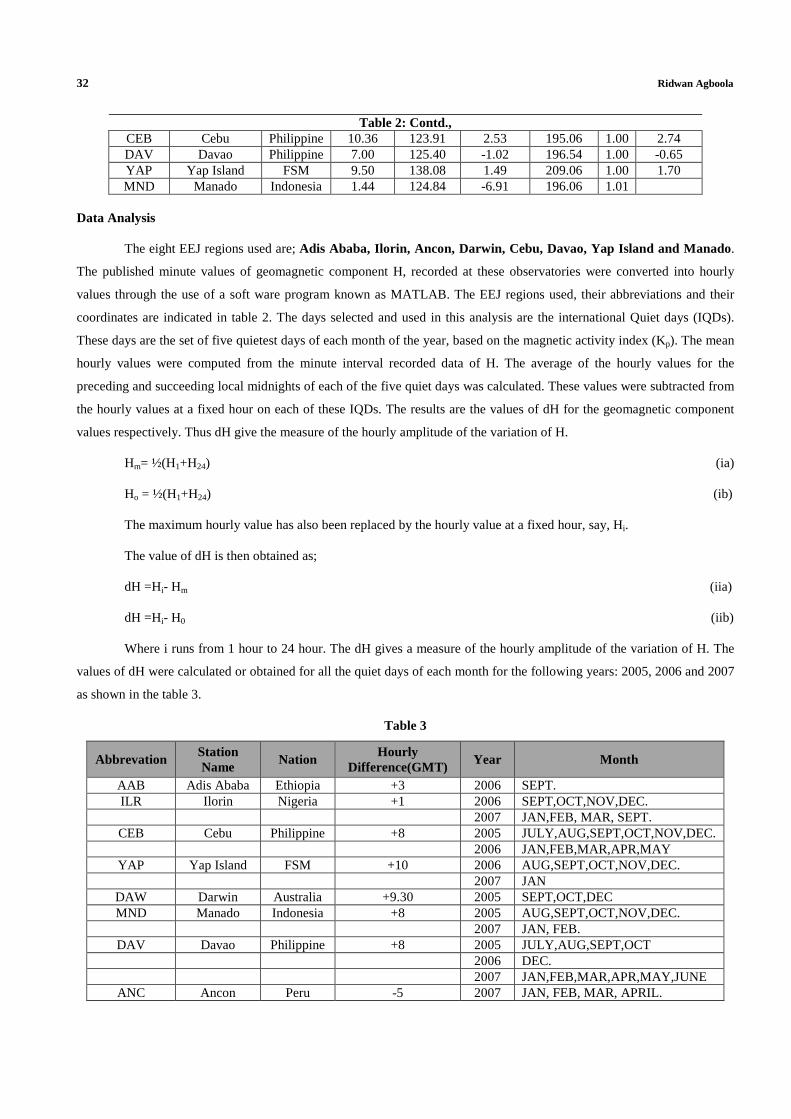
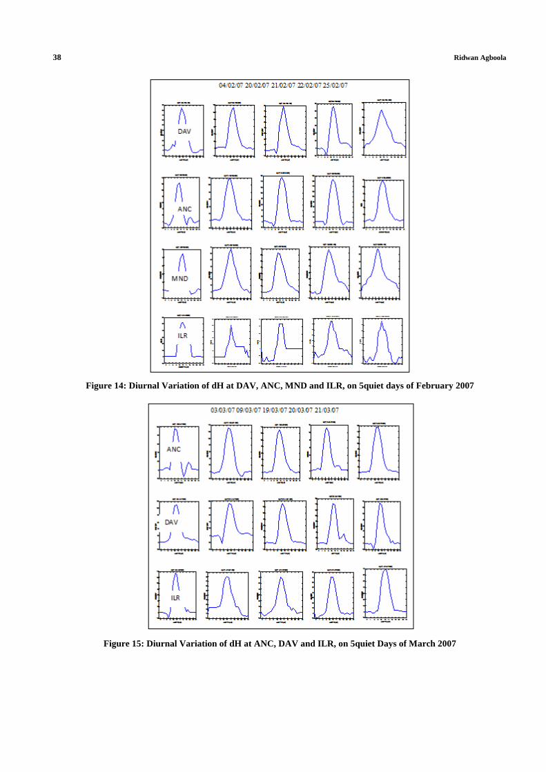
Data Analysis

The eight EEJ regions used are; Adis Ababa, Ilorin, Ancon, Darwin, Cebu, Davao, Yap Island and Manado.

The published minute values of geomagnetic component H, recorded at these observatories were converted into hourly

values through the use of a soft ware program known as MATLAB. The EEJ regions used, their abbreviations and their

coordinates are indicated in table 2. The days selected and used in this analysis are the international Quiet days (IQDs).

These days are the set of five quietest days of each month of the year, based on the magnetic activity index (Kp). The mean

hourly values were computed from the minute interval recorded data of H. The average of the hourly values for the

preceding and succeeding local midnights of each of the five quiet days was calculated. These values were subtracted from

the hourly values at a fixed hour on each of these IQDs. The results are the values of dH for the geomagnetic component

values respectively. Thus dH give the measure of the hourly amplitude of the variation of H.

Hm= ½(H1+H24) (ia)

Ho = ½(H1+H24) (ib)

The maximum hourly value has also been replaced by the hourly value at a fixed hour, say, Hi.

The value of dH is then obtained as;

dH =Hi- Hm (iia)

dH =Hi- H0 (iib)

Where i runs from 1 hour to 24 hour. The dH gives a measure of the hourly amplitude of the variation of H. The

values of dH were calculated or obtained for all the quiet days of each month for the following years: 2005, 2006 and 2007

as shown in the table 3.

Table 3

Abbrevation Station Name

Nation Hourly

Difference(GMT) Year Month

AAB Adis Ababa Ethiopia +3 2006 SEPT. ILR Ilorin Nigeria +1 2006 SEPT,OCT,NOV,DEC.

2007 JAN,FEB, MAR, SEPT. CEB Cebu Philippine +8 2005 JULY,AUG,SEPT,OCT,NOV,DEC.

2006 JAN,FEB,MAR,APR,MAY YAP Yap Island FSM +10 2006 AUG,SEPT,OCT,NOV,DEC.

2007 JAN DAW Darwin Australia +9.30 2005 SEPT,OCT,DEC MND Manado Indonesia +8 2005 AUG,SEPT,OCT,NOV,DEC.

2007 JAN, FEB. DAV Davao Philippine +8 2005 JULY,AUG,SEPT,OCT

2006 DEC. 2007 JAN,FEB,MAR,APR,MAY,JUNE

ANC Ancon Peru -5 2007 JAN, FEB, MAR, APRIL.

Analytical Interpretation of Geomagnetic Fieldanomaly along the Dip Equator 33

Program Modification

The software (MATLAB) used was properly modified taking into account the hourly difference between the

Geographic Longitudes of each of the station and GMT.

RESULTS AND DISCUSSIONS

Results

The results obtained in this study are presented graphically in the table 3 to 20.

Figure 3: Diurnal Variation of dH at CEB and DAV, on 5quiet Days of July 2005

Figure 4: Diurnal Variation of dH at CEB, DAV and M ND, on 5quiet Days of August 2005

34 Ridwan Agboola

Figure 5: Diurnal Variation of dH at CEB, DAV,MND a nd DAW, on 5quiet Days of September 2005

Figure 6: Diurnal Variation of dH at CEB,MND and DA W, on 5quiet Days of October 2005


Figure 7: Diurnal Variation of dH at CEB and MND, on 5quiet Days of November 2005

Figure 8: Diurnal Variation of dH at CEB, MND and DAW, on 5quiet Days of December 2005

36 Ridwan Agboola

Figure 9: Diurnal Variation of dH at YAP, and ILR, on 5quiet Days of September 2006

Figure 10: Diurnal Variation of dH at YAP and ILR, on 5quiet days of October 2006

Figure 11: Diurnal Variation of dH at YAP and ILR, on 5quiet Days of November 2006


Figure 12: Diurnal Variation of dH at DAV, YAP and ILR, on 5quiet Days of December 2006

Figure 13: Diurnal Variation of dH at DAV, MND, ANC , YAP and ILR, on 5quiet Days of January 2007

38 Ridwan Agboola

Figure 14: Diurnal Variation of dH at DAV, ANC, MND and ILR, on 5quiet days of February 2007

Figure 15: Diurnal Variation of dH at ANC, DAV and ILR, on 5quiet Days of March 2007


Figure 16: Diurnal Variation of dH at ANC and DAV, on 5quiet Days of April 2007

Figure 17: Diurnal Variation of dH at CEB, on 5quiet Days of Jan, Feb, Mar, April and May 2006

40 Ridwan Agboola

Figure 18: Diurnal Variation of dH at YAP, on 5quiet Days of AUG. 2006

Figure 19: Diurnal Variation of dH at DAV, on 5quiet Days of May, June AUG. 2007

Figure 20: Diurnal Variation of dH at ILR, on 5quiet Days of Sept. 2007

DISCUSSIONS

Day-to-Day Variability

It is clear from the figures (3 - 20) and appendix 2 that, the diurnal variations of solar quiet daily variations (H),

exist in the element (H) on the quiet days of each month. The figures (3 - 20) showed the mass plots of daily hourly

variation of the solar daily variation of Horizontal intensity on these days. The absolute value of Sq (H) daily variation

rises from 006 hrs LT., reaches the peak at about 12noon and declines to low level at 1800hrs LT. In general, the day time

(0700-2000hours) magnitudes are much greater than the night time (2000-0700 hours through2400 hour) magnitudes for

all the months studied in the element H. This is quite in agreement with the diurnal variation pattern of Sq in the earlier

works of Onwumechili (1960) and Matsuskhita (1969) which showed that the maximum intensity of Sq occurs around the

local noon. Emilia and Last (1977) reported a similar diurnal variation pattern of Sq in H. This implies that there is day-to-

day variability in the ionospheric conditions in the regions studied, such as Adis Ababa,Ilorin, Ancon, Darwin, Cebu,

Davao, YapIsland and Manado stations all at dip equator.


The diurnal variation of day-to-day variability, which followed the variation pattern of Sq, can be attributed to the

variability of the ionospheric process and physical structure such as conductivity and wind structure, which are responsible

for the Sq variation.

Night –TimeVariation

Figures (3 - 20) also indicate that there is Night time (2000-0700 hours through 2400 hours) variation of day-to-

day variability in the element H. This night- time geomagnetic variation has also been noticed in Sq, even when Campbell

(1973) used only 37 of the quietest days of the solar activity minimum year of 1965, the variation still persisted at midnight

(Campbell, 1979). Hence it is not generally accepted that ionospheric currents do not flow at night outside the auriora and

polar regions. Rabiu(1996) found a consistent night time variation in horizontal magnetic field component at mid-latitudes

and attributed same to distant magnetospheric sources after Matveyenkov(1983). The variability of the night time field

may thus be as a result of the variability of the night time distant currents, Been given to explain these night-time

variations, which include convective drift currents in the magnetosphere and the asymmetric ring current in the

magnetospheric currents, magnetospheric effects like the westward ring current even during fairly quiet periods.

Forbes (1981) noted that the seasonal variability could be partially explained by the seasonal variation of lunar

semi-diurnal tide. Seasonal change in the Sq variation isattributed to a seasonal shift in the mean position of the Sq

currentsystem of the ionospheric Electrojet (EEJ), Hutton (1962). The electrodynamics effect of local winds can also

account for seasonal variability, since the winds are subjected to day-to-dray and seasonal variability.

The results of the research work can be summarized as;

The equatorial electroject exhibits diurnal variations on quiet days of the Months studied. The daytime magnitude

of the solar daily variation magnetic field is greater than the night time magnitudes for the days of the months studied in

the element, H. The diurnal variation of solar daily variation in the earlier works (Onwumechili and Ezema 1977;Emilla

and Last 1977) can be attributed to the variability of the ionospheric processes and physical structures such as conductivity

and winds structure.

• The rate of building up of ionospheric Sq current is faster than its rate of decay afternoon time maximum.

• The variation of the night time may be as a result of the variability of the night - time distant current.

• The seasonal variation is attributed to seasonal shift in the mean position of Sq current system and the

electrodynamics effect of local winds. The verticalday time E X B drift velocity in the ionospheric F-region is

inferred to have seasonal variation.

• The details of how high energy particles are generated during geomagnetic storms constitute an entire discipline

of space science.

However the basic idea is that the earth magnetic field or geomagnetic field is responding to outwardly propagating

disturbances from the sun. As the geomagnetic field adjust to this disturbances, various components of the earth field range

form, releasing magnetic energy and thereby accelerating charged particles to high energies. These particles being charged

are forced to stream along the geomagnetic field lines, some end up in the upper part of the earth neutral atmosphere and

the aurora mechanism begins.

42 Ridwan Agboola

CONCLUSIONS

From the work carried out on the study of day to day variability of geomagnetic field variation, by examining the

variability of Sq (H) amplitude at a fixed local time from one day to the next, the results shows that the values of

geomagnetic field at a particular hour vary from one day to another.

Finally, the result of this research shows a regular pattern of Sq (H) enhancement at the EEJ regions, the results of the

analysis carried out revealed that the amplitude of dH has diurnal variation which peaks during the day at about local noon

in all the eight equatorial electrojet regions. The diurnal variation so observed was attributed to ionospheric plasma

irregularities as well as the dynamo action in the ionosphere.

REFERENCES

1. A.B Rabiu., I.A Adimula, J.O Adeniyi, G.Maeda MAGDAS/CPMN Project group Preliminary Result from the

magnetic field measurement Using MAGDAS at Ilorin, Nigeria

2. R, G. Rastogi: A new aspect of daily variation of the geomagnetic field in low latitudes.

3. J. Bartels and H.F. Johnson: Geomagnetic tidea in Horizontal intensity at Huancayo-part 1 Geophysics. Res., 45,

264-308, 1940.

4. Chapman. S: The equatorial electrojet as detected from the abnormal electric current Distribution above

Hucanayo, Peru. Geophys. 4,368-390,1951.

5. Standish, E. Myles; Williams, James C. "Orbital Ephemerides of the Sun, Moon, and Planets" International

Astronomical Union Commission 3.

6. Staff (2007-08-07). "Useful Constants" International Earth Rotation and Reference Systems Service (IERS-

7. Williams, David R. (2004-09-01). "Earth Fact Sheet

8. Allen, Clabon Walter; Cox, Arthur N. (2000).

9. Ronal T. Merrill (2010), Our Magnetic Earth The Science of Geomagnetism

10. Dennis D.; Petit, Gérard, Cazenave, Anny (1995). Ahrens, Thomas J. ed (PDF). Global earth physics a handbook

of physical constants. Washington, DC: American Geophysical Union.

11. Rosenberg, Matt. "What is the circumference of the earth?". About.com.

12. Pidwirny, Michael (2006-02-02). Surface area of our planet covered by oceans University of British Columbia,

Okanagan.

13. Staff (2008-07-24). "World". The World Factbook. Central Intelligence Agency.

14. Yoder, Charles F. (1995). T. J. Ahrens. ed. Global Earth Physics Washington: American Geophysical Union.

pp. 12.

15. Allen, Clabon Walter; Cox, Arthur N. (2000). Allen's Astrophysical Quantities. Springer.

16. Arthur N. Cox, ed (2000). Allen's Astrophysical Quantities (4th ed.). New York: AIP Press.

17. National Climatic Data Center. August 20, 2008.

18. Kinver, Mark (10 December 2009). "Global average temperature may hit record level in 2010".


19. May, Robert M. (1988). "How many species are there on earth?". Science 241.

20. Neil. F. Comins (2001): Discovering the essential universe.

21. J.N. Towle (1984) “The Anomalous Geomagnetic variation field and Geomagnetic Structure’

22. J. Egbedal: The magnetic diurnal variation of the Horizontal force near the magnetic equator; Terr. Magn. Atmos.

Electr; 52,449-451, 1947

ANALYTICAL INTERPRETATION OF GEOMAGNETIC FIELDANOMALY ALONG THE DIP EQUATOR

Documents

Transcript of ANALYTICAL INTERPRETATION OF GEOMAGNETIC FIELDANOMALY ALONG THE DIP EQUATOR