Cracking in Hot-dip Galvanized Welded Joints of Steel Platform

Structures

by

Christopher T. DiGiovanni

A thesis submitted in partial fulfillment of the requirements for the degree of

Master of Science

in

Welding Engineering

Department of Chemical and Materials Engineering

University of Alberta

©Christopher T. DiGiovanni, 2017

Abstract

In a recent construction project, a platform structure made up of 350W and 300W steel un-

derwent a double dip galvanizing process. Prior to the galvanizing process, the platform was

fabricated to completion, which included numerous welds throughout the design. After galva-

nizing, cracks were found originating in the welds and propagating into the base material. To

the steel designer, this posed a new and curious problem. Previously, similar structures had

undergone the same processing with no cracking.

This research project began by investigating the metallurgy and microstructure of the base

material, the welds, and of the crack sites. Two key features that were noted were the thicker and

inclusion-rich grain boundaries in the base material, and the cracking appeared with little or no

deformation of the grains. In addition, the fracture surfaces were studied at high magnification

levels and showed features of brittle fracture, which is uncharacteristic of the 350W and 300W

steels used. Studies were carried out to asses the material’s susceptibility to both hydrogen

embrittlement and temper embrittlement, both of which are known to potentially occur during

galvanizing.

Tension test samples were sectioned from the base material and were charged with hydrogen.

During the tension testing, the samples charged with hydrogen did not show any different

behavior from the regular samples. All the fracture surfaces were ductile and did not match

the surfaces from the galvanizing cracks. Furthermore, hardness levels were too low to be

deemed susceptible to hydrogen cracking according to the values seen in literature. Similarly,

samples were sectioned from the base material and notched for temper embrittlement testing.

The samples were heated to the galvanizing temperature and then fractured. The samples

broke suddenly and showed little signs of ductile fracture and, more significantly, had a fracture

surface matching the original cracks. To support the notion of temper embrittlement, material

chemistry testing found high levels of phosphorus. Phosphorus is a key culprit in temper

embrittlement, and given the elevated temperature and stress of the double dip process, it would

have been able to diffuse to the grain boundaries causing brittle grain boundary separation.

Finally, to quantify the thermal stresses induced from galvanizing, a three dimensional finite

element analysis model was created to simulate the double dip process. The model found

relatively high stresses but not enough to reach the yield point without an embrittlement factor

present.

ii

Preface

The material presented in this thesis are parts of the research project under the supervision of

Dr. Leijun Li, which was funded by Waiward Steel LLP and MITACS. This thesis is the study

that was completed to provide Waiward Steel with a full scale examination and explanation for

the cracking that occurred in one of their construction projects. The study and results were

condensed into a research article submitted to the Engineering Failure Analysis Journal.

Chapter 3 of this thesis includes a 3-dimensional model of the steel structure that was studied.

The design of the structure is the intellectual property of Waiward Steel LLP.

Chapters 4 and 5 of this thesis involve original and unique test experiments developed by

the author. The tests were developed to thoroughly and empirically test the material for

embrittlement susceptibility, in accordance to the material and equipment that was available.

All testing was done on samples provided by Waiward Steel LLP.

iii

Acknowledgement

I would like to thank Dr. Leijun Li for giving me the amazing opportunity to be a part of his

research group in physical and welding metallurgy. His love and enthusiasm for metallurgy has

been truly inspiring throughout my degree and has driven me to reach further in my academic

and professional life. On the numerous occasions I showed up unannounced in Dr. Li’s office I

was always greeted with a smile, and my questions were always greeted with patience. I would

also like to thank Dr. Robert Driver for introducing myself and Dr. Li to the project my thesis

is based on, and making me feel welcome in the Steel Centre’s group. His wisdom, insight and

understanding have been irreplaceable throughout my graduate studies. As the next stage of

my career is ahead, I hope to keep in touch and a maintain a friendship with both Dr. Li and

Dr. Driver in the years to come.

I would like to recognize MITACS for their funding to make this research project possible.

Without their contribution the research and student stipend costs would not have been met.

Along with MITACS I would like to thank Waiward Steel LLP and Logan Callele for giving

us the opportunity to work on this project, and for their contribution to the project’s funding.

They also provided all the samples used in this thesis and gave valuable insight into the project’s

background.

I would like to thank everyone involved in Dr. Li’s research group including Jason Wang,

Rangasayee Kannan, Neil Anderson, and Daniel Yang. Their patience in teaching me to use

the metallography equipment and operating the SEM with me in the evenings can not be over

stated. Their warm reception when I first moved to Alberta from Ontario was welcoming and

kind. Attending conferences with them has easily been the highlights of my degree, not only

for the memories and laughs we shared, but also because it was an opportunity to see them

present their work with admirable passion. I would also like to include Victoria Buffan and

Riley Quinton of The Steel Centre group in the thanks of my colleagues. They were both

always a reliable source for guidance using Abaqus, and our rants and stories of frustration over

the software were always appreciated.

My family has supported me throughout my degree and has made my life insurmountably

better. They have always supported my decisions and encouraged me to follow my dreams and

desires. Their unconditional love, patience, and care have helped me throughout my entire life

and words cannot express my gratitude.

iv

Contents

Abstract ii

Preface iii

Acknowledgement iv

List Of Figures . . . . . . . . . . . . . . . . . . . . . . . . . . . . . . . . . . . . . . . . . . . . . . viii

List Of Tables . . . . . . . . . . . . . . . . . . . . . . . . . . . . . . . . . . . . . . . . . . . . . . . ix

1 Introduction. . . . . . . . . . . . . . . . . . . . . . . . . . . . . . . . . . . . . . . . . . . . . . 1

1.1 Introduction . . . . . . . . . . . . . . . . . . . . . . . . . . . . . . . . . . . . . . . 1

1.2 Thesis Objective . . . . . . . . . . . . . . . . . . . . . . . . . . . . . . . . . . . . 3

1.3 Thesis Outline . . . . . . . . . . . . . . . . . . . . . . . . . . . . . . . . . . . . . 3

2 Metallography, Microstructure, and Fractography. . . . . . . . . . . . . . . . . . . 4

2.1 Introduction . . . . . . . . . . . . . . . . . . . . . . . . . . . . . . . . . . . . . . . 4

2.2 Methods and Experimental Setup . . . . . . . . . . . . . . . . . . . . . . . . . . . 5

2.3 Results and Discussion . . . . . . . . . . . . . . . . . . . . . . . . . . . . . . . . . 7

2.3.1 Metallography . . . . . . . . . . . . . . . . . . . . . . . . . . . . . . . . . 7

2.3.2 Fractography . . . . . . . . . . . . . . . . . . . . . . . . . . . . . . . . . . 16

2.4 Conclusions . . . . . . . . . . . . . . . . . . . . . . . . . . . . . . . . . . . . . . . 22

3 Finite Element Analysis Model . . . . . . . . . . . . . . . . . . . . . . . . . . . . . . . . 23

3.1 Introduction . . . . . . . . . . . . . . . . . . . . . . . . . . . . . . . . . . . . . . . 23

3.2 Model Methodology and Setup . . . . . . . . . . . . . . . . . . . . . . . . . . . . 24

3.3 Results and Discussion . . . . . . . . . . . . . . . . . . . . . . . . . . . . . . . . . 29

3.4 Conclusions . . . . . . . . . . . . . . . . . . . . . . . . . . . . . . . . . . . . . . . 33

4 Hydrogen Embrittlement Study. . . . . . . . . . . . . . . . . . . . . . . . . . . . . . . . 35

4.1 Introduction . . . . . . . . . . . . . . . . . . . . . . . . . . . . . . . . . . . . . . . 35

4.2 Experimental Setup . . . . . . . . . . . . . . . . . . . . . . . . . . . . . . . . . . 36

4.3 Results and Discussion . . . . . . . . . . . . . . . . . . . . . . . . . . . . . . . . . 39

4.3.1 Hardness Testing . . . . . . . . . . . . . . . . . . . . . . . . . . . . . . . . 39

4.3.2 Tension Testing . . . . . . . . . . . . . . . . . . . . . . . . . . . . . . . . . 40

4.4 Conclusions . . . . . . . . . . . . . . . . . . . . . . . . . . . . . . . . . . . . . . . 43

5 Temper Embrittlement Study . . . . . . . . . . . . . . . . . . . . . . . . . . . . . . . . . 45

5.1 Introduction . . . . . . . . . . . . . . . . . . . . . . . . . . . . . . . . . . . . . . . 45

5.2 Experimental Setup . . . . . . . . . . . . . . . . . . . . . . . . . . . . . . . . . . 46

v

5.3 Results and Discussion . . . . . . . . . . . . . . . . . . . . . . . . . . . . . . . . . 48

5.4 Conclusions . . . . . . . . . . . . . . . . . . . . . . . . . . . . . . . . . . . . . . . 53

6 Conclusions and Future Work . . . . . . . . . . . . . . . . . . . . . . . . . . . . . . . . . 54

6.1 Conclusions and Summary Findings . . . . . . . . . . . . . . . . . . . . . . . . . 54

6.2 Future Work . . . . . . . . . . . . . . . . . . . . . . . . . . . . . . . . . . . . . . 56

7 References . . . . . . . . . . . . . . . . . . . . . . . . . . . . . . . . . . . . . . . . . . . . . . . 57

References . . . . . . . . . . . . . . . . . . . . . . . . . . . . . . . . . . . . . . . . . . . . . . . . . 57

Appendix A: Experimental Equipment . . . . . . . . . . . . . . . . . . . . . . . . . . . . . 60

A.1 Base Material Images . . . . . . . . . . . . . . . . . . . . . . . . . . . . . . . . . 60

A.2 Weld Images . . . . . . . . . . . . . . . . . . . . . . . . . . . . . . . . . . . . . . 63

vi

List of Figures

2.1 Sample cutting . . . . . . . . . . . . . . . . . . . . . . . . . . . . . . . . . . . . . 6

2.2 Base material of the T-joint . . . . . . . . . . . . . . . . . . . . . . . . . . . . . . 8

2.3 Base material of the corner joint . . . . . . . . . . . . . . . . . . . . . . . . . . . 9

2.4 Images showing the same location with the different etchants . . . . . . . . . . . 10

2.5 SEM images of the T joint base material . . . . . . . . . . . . . . . . . . . . . . . 10

2.6 AES carbon mapping . . . . . . . . . . . . . . . . . . . . . . . . . . . . . . . . . . 11

2.7 EDS line scans of site A . . . . . . . . . . . . . . . . . . . . . . . . . . . . . . . . 12

2.8 EDS line scans of site B . . . . . . . . . . . . . . . . . . . . . . . . . . . . . . . . 13

2.9 EDS mapping of inclusions . . . . . . . . . . . . . . . . . . . . . . . . . . . . . . 15

2.10 Crack initiation site . . . . . . . . . . . . . . . . . . . . . . . . . . . . . . . . . . 16

2.11 Crack arrest site 5X . . . . . . . . . . . . . . . . . . . . . . . . . . . . . . . . . . 17

2.12 EDS mapping of the crack arrest . . . . . . . . . . . . . . . . . . . . . . . . . . . 18

2.13 As received fracture samples . . . . . . . . . . . . . . . . . . . . . . . . . . . . . . 19

2.14 SEM of received fracture surfaces . . . . . . . . . . . . . . . . . . . . . . . . . . . 20

2.15 Fresh fracture surface . . . . . . . . . . . . . . . . . . . . . . . . . . . . . . . . . 21

3.1 Platform assembly drawing . . . . . . . . . . . . . . . . . . . . . . . . . . . . . . 25

3.2 3D model of the platform and joint constraint . . . . . . . . . . . . . . . . . . . . 26

3.3 Location of boundary condition . . . . . . . . . . . . . . . . . . . . . . . . . . . . 27

3.4 Galvanizing bath convection area . . . . . . . . . . . . . . . . . . . . . . . . . . . 28

3.5 Node chosen for mesh refinement study . . . . . . . . . . . . . . . . . . . . . . . 29

3.6 Plot of nodal stress versus number of elements . . . . . . . . . . . . . . . . . . . 30

3.7 Mesh applied to the model . . . . . . . . . . . . . . . . . . . . . . . . . . . . . . . 30

3.8 Nodes selected for stress analysis . . . . . . . . . . . . . . . . . . . . . . . . . . . 31

3.9 Stress at the crack locations during galvanizing by the FEA model . . . . . . . . 31

3.10 Contour stress plot of the entire model . . . . . . . . . . . . . . . . . . . . . . . . 32

3.11 T-joint stress distribution and actual crack location . . . . . . . . . . . . . . . . . 33

3.12 Corner joint stress distribution and actual crack location . . . . . . . . . . . . . . 33

4.1 Location of hydrogen embrittlement samples . . . . . . . . . . . . . . . . . . . . . 38

4.2 Hardness measurements across weld cross sections . . . . . . . . . . . . . . . . . 39

4.3 Fracture surfaces of hydrogen-charged samples . . . . . . . . . . . . . . . . . . . 41

4.4 Tension test results of hydrogen-charged samples . . . . . . . . . . . . . . . . . . 42

5.1 Temper Embrittlement Sample . . . . . . . . . . . . . . . . . . . . . . . . . . . . 47

vii

5.2 Fracture surfaces of temper embrittlement test . . . . . . . . . . . . . . . . . . . 50

5.3 Comparison of 200X & 500X SEM images of the received fracture surface and

lab fracture surface . . . . . . . . . . . . . . . . . . . . . . . . . . . . . . . . . . . 52

5.4 Comparison of 500X SEM images of the ambient fracture surface and galvanizing

temperature fracture surface . . . . . . . . . . . . . . . . . . . . . . . . . . . . . . 52

A.1 5X, 10X and 100X of T-joint horizontal member’s base material . . . . . . . . . . 60

A.2 5X, 10X and 100X of T joint vertical member’s base material . . . . . . . . . . . 61

A.3 5X, 10X and 100X of T-joint horizontal member’s base material . . . . . . . . . . 62

A.4 5X, 10X and 100X of T-joint vertical member’s base material . . . . . . . . . . . 63

A.5 Different weld cross sections in the platform . . . . . . . . . . . . . . . . . . . . . 64

A.6 Fusion zone and heat affected zone of the corner joint’s weld . . . . . . . . . . . . 65

A.7 Side view of the corner joint weld . . . . . . . . . . . . . . . . . . . . . . . . . . . 66

A.8 Side view of the upper cracks in the corner joint weld . . . . . . . . . . . . . . . 67

A.9 Side view of the lower cracks in the corner joint weld . . . . . . . . . . . . . . . . 67

viii

List of Tables

4.1 Test cases . . . . . . . . . . . . . . . . . . . . . . . . . . . . . . . . . . . . . . . . 37

5.1 Compositional analysis . . . . . . . . . . . . . . . . . . . . . . . . . . . . . . . . . 49

5.2 Element Diffusivity . . . . . . . . . . . . . . . . . . . . . . . . . . . . . . . . . . . 49

ix

1. Introduction

1.1. Introduction

For almost two hundred and fifty years galvanization has been used as the primary procedure to

protect steels from the corrosive atmosphere [1, 2]. The process involves applying a protective

and thin layer of zinc to a thicker base material, typically steel. Without the protective zinc

layer, the steel would form rust (a type of iron oxide) in the open air atmosphere [3]. However,

the corrosion of zinc occurs significantly slower which makes it a good protective layer and

lengthens the product life of the covered base material. In addition to its anti-corrosive proper-

ties, zinc will also act as a sacrificial anode. This advantage is what makes galvanizing superior

to something like painting, since exposed areas do not need immediate touch ups, because the

sacrificial zinc anode will protect the base material [4].

There are three different types of processes used to apply the zinc layer to the base material.

The first and most widely used process is hot-dip galvanizing. This is the process of submerging

the base material in a bath of molten zinc. However, the surface must cleaned entirely and

rid of any oxides to ensure a strong metallic bond is formed [5, 6]. This is also the most

cost-effective process. The next type is pre-galvanizing. Pre-galvanizing is similar to hot-dip

galvanizing, except it occurs at the steel mill, where the rolled metal sheets are put through

the same cleaning process followed by a bath of molten zinc. This process allows for a more

uniform coat, but if the sheets are cut for fabrication, large sections of the base material can be

exposed to the atmosphere [3]. The last process is electrogalvanizing. Unlike the previous two

processes, electrogalvanizing does not rely on a molten zinc bath, but rather applies the zinc

layer using an electric current in electrolyte solution to apply zinc ions. This process gives the

greatest degree of control on the coating thickness and gives a much more uniform coat [3].

In the case of larger steel assemblies, a double dip process may be used. This is a variant

to hot-dip galvanizing, in which the structure is too large to be fully submerged in the zinc

bath. Instead, half of the structure is dipped and coated with zinc, followed by the remaining

half. A concern when using a double dip procedure is the large temperature gradient across

the structure, since half the structure will be exposed to the ambient air while the other half is

submerged in the molten bath. The thermal stresses induced could be considerable depending

1

on the design of the structure.

In a construction project in the Edmonton area, a platform structure was going into service

outdoors and, since it was fabricated from 350W and 300W structural steel, required corrosion

protection. However, due to the size of the structure and its fabrication prior to galvanizing,

it also required a double dip procedure. The structure was made up of various wide-flanged

beams, T-beams and C-channels (the C-channels were the 300W components). The beams

were welded using a metal core arc welding process for the flanges and a flux core arc welding

process for the webs of the beams. After fabrication, the platform had exterior dimensions of

approximately 3m x 7m.

The steel platforms underwent the typical procedure for double dip galvanizing. They were

first processed with the caustic cleaning to remove any contaminants such as oil, grease, paint

or dirt. Next, it was cleaned in the pickling bath to remove any oxides or rust from the base

material’s surface. Finally, before being submerged in the molten zinc bath, the structure

underwent fluxing which removes any oxides still present and deposits a protective layer to

shield the structure before being put into the zinc bath.

Upon inspection after galvanizing, numerous cracks were found initiating in the welded joints

and propagating into the base material. Cracking was found across several different platforms

and in different types of joints. To the steel structure designers this was an unexpected compli-

cation to the project. Previous projects with similar designs that had also undergone a double

dip galvanizing procedure did not experience any cracking. The welds were inspected after

fabrication and no signs of a pre-existing crack or defect were found. A third party consulting

company was brought in to investigate the cracking, but strong conclusive results were not

found.

The galvanizing company however did not claim this was an outlandish result. Cracking during

hot dip galvanizing, especially double dip galvanizing, is a known phenomenon. Several types

of embrittlement can occur during galvanizing, including liquid metal embrittlement (LME),

hydrogen embrittlement, and temper embrittlement [7–10]. Also, the double dip process can

lead to thermal stresses potentially exceeding the yield strength under certain designs. Explor-

ing each embrittlement type and understanding what makes a material susceptible is key to

understanding the cracking situation studied, and cracking during galvanizing as a whole.

2

1.2. Thesis Objective

The objective of this thesis is to assist the galvanizing and steel structures industry by uncovering

the cause of cracking in this incident, and demonstrating the methods used. The thesis aims

to show what factors of the galvanizing process and material made the structure susceptible to

cracking, which can be carried forward by industry in future projects.

1.3. Thesis Outline

Each chapter of the thesis is a study of a different aspect of interest, including its own back-

ground, experimental procedures, and conclusions. Each chapter builds on the knowledge base

which is used in the succeeding chapters, until an overall and final conclusion can be drawn.

Chapter 2 focuses on the metallurgy of the steel, along with the fractography of the original

cracks and lab-produced cracks. This study establishes a base of information from which the

experimental direction can be drawn.

Chapter 3 shows the creation of the finite element model to simulate the double dip process.

The stress and temperature readings from the model indicate that an embrittlement factor must

have been present since the thermal stress did not exceed the yield point. They also show a

stress distribution matching the crack shape indicating the double dip process was the driving

force for cracking.

Chapter 4 outlines a study on hydrogen cracking susceptibility by measuring hardness and

more explicitly by mechanically testing and fracturing samples charged with hydrogen. The

low hardness and absence of any difference in the charged samples implies the material is not

susceptible to hydrogen cracking in this case and can be eliminated as a possibility.

Finally in Chapter 5 temper embrittlement susceptibility is tested by heating samples to the

galvanizing temperature and fracturing them, along with studying the material chemistry. The

results show features similar to those found in the original cracks.

3

2. Metallography, Microstructure, and Fractography

2.1. Introduction

Metallography is the study of the structure and distribution of components, at a microscopic

level. Metallography is typically carried out using microscopy techniques along with appropriate

sample preparation. For example, using a different etchant on a metal can show different

phase structures of interest. Metallography serves as the cornerstone in understanding material

properties, and can even be used to predict material behaviors and characteristics [11].

Surface preparation for a metallographic study is critical. If the surface is not prepared properly,

or is prepared poorly, the features of the microstructure will not be clear and furthermore will

not look presentable. The sample surfaces are typically prepared mechanically, using a finer

and finer abrasive until the surface is completely flat. The surface is then burned with a

select etchant to show the features of interest. Metallography is carried out using an optical

microscope or an electron microscope. An optical microscope is more desirable for low level

magnification images, and the natural colour of the sample can also still be seen. However, for

more detailed and higher level magnification images a scanning electron microscope (SEM) is

the optimal choice. If the SEM is also equipped with energy dispersive spectrometer, chemical

compositional analysis can be carried out by excitation of the outer orbit electron. Although

energy dispersive spectroscopy (EDS) is not useful for compositional analysis smaller elements,

it can still give a relative reading showing which areas have a higher concentration. Similar to

EDS, Auger electron spectroscopy (AES) uses the Auger effect instead which makes it more

suitable and more accurate in identifying smaller elements.

In the case of the cracked steel frames, understanding the microstructure of the base material,

along with the weld zone, is a critical first step in developing a direction for experimental

testing. The embrittlement types of interest (liquid metal, hydrogen, and temper) all rely

on the metallurgy of the material to some degree. Furthermore, the metallography of the

material would show if there were any irregularities in the structure leading to embrittlement

susceptibility. It is impossible to discuss the cause of cracking without first understanding the

structure and constituents of the material.

In addition to metallography, fractography also serves as a backbone of knowledge on which

4

further studies are based. Fractography is the study of a material’s fracture surface. It is a

routine practice in the world of failure analysis, and similarly to metallography, is heavily based

on imaging and recognizing characteristics [12]. Different failure types exhibit different features

on the fracture surface created by the crack [13]. This helps engineers target the cause of failure

and the fracture mode that occurred.

Similar microscopy techniques from metallography are also used in fractography. Once again,

optical microscopes are often used as the baseline tool. However, SEMs are still extensively

used since more often than not, higher level magnification images of the fracture surface are

needed [12]. SEM imaging used in conjunction withe EDS is particularly useful since it can

help identify any constituents on the fracture surface that may lead to the cause of cracking.

Even something as simple as a visual inspection for plastic deformation is very beneficial to the

case of the cracked steel platforms. Plastic deformation of the material would be an expected

feature of the fracture of a structural steel. However, the absence of deformation and relatively

flat fracture surfaces would indicate some sort of embrittlement phenomenon is at play, rather

than a simple case of plastic collapse. Further details of the surface can be observed under the

SEM such as grain deformation, and elemental analysis can be done by EDS. Altogether, the

metallography and fractography studies were a cornerstone in the investigation of the cracked

steel frames, and gave valuable knowledge into structural steel metallurgy and fracture modes.

2.2. Methods and Experimental Setup

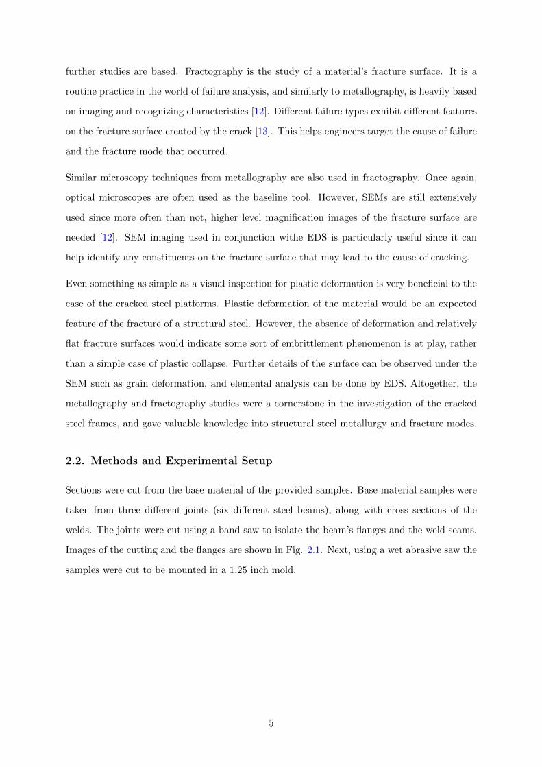
Sections were cut from the base material of the provided samples. Base material samples were

taken from three different joints (six different steel beams), along with cross sections of the

welds. The joints were cut using a band saw to isolate the beam’s flanges and the weld seams.

Images of the cutting and the flanges are shown in Fig. 2.1. Next, using a wet abrasive saw the

samples were cut to be mounted in a 1.25 inch mold.

5

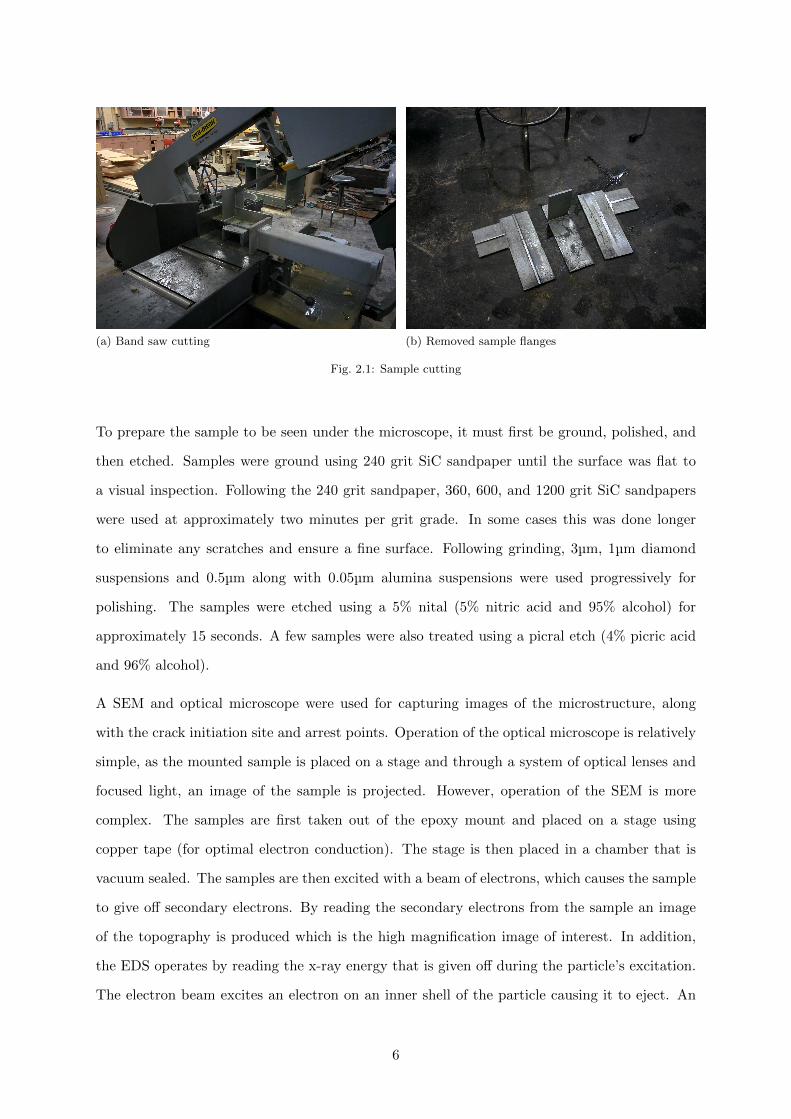
(a) Band saw cutting (b) Removed sample flanges

Fig. 2.1: Sample cutting

To prepare the sample to be seen under the microscope, it must first be ground, polished, and

then etched. Samples were ground using 240 grit SiC sandpaper until the surface was flat to

a visual inspection. Following the 240 grit sandpaper, 360, 600, and 1200 grit SiC sandpapers

were used at approximately two minutes per grit grade. In some cases this was done longer

to eliminate any scratches and ensure a fine surface. Following grinding, 3µm, 1µm diamond

suspensions and 0.5µm along with 0.05µm alumina suspensions were used progressively for

polishing. The samples were etched using a 5% nital (5% nitric acid and 95% alcohol) for

approximately 15 seconds. A few samples were also treated using a picral etch (4% picric acid

and 96% alcohol).

A SEM and optical microscope were used for capturing images of the microstructure, along

with the crack initiation site and arrest points. Operation of the optical microscope is relatively

simple, as the mounted sample is placed on a stage and through a system of optical lenses and

focused light, an image of the sample is projected. However, operation of the SEM is more

complex. The samples are first taken out of the epoxy mount and placed on a stage using

copper tape (for optimal electron conduction). The stage is then placed in a chamber that is

vacuum sealed. The samples are then excited with a beam of electrons, which causes the sample

to give off secondary electrons. By reading the secondary electrons from the sample an image

of the topography is produced which is the high magnification image of interest. In addition,

the EDS operates by reading the x-ray energy that is given off during the particle’s excitation.

The electron beam excites an electron on an inner shell of the particle causing it to eject. An

6

electron from a higher energy outer shell fills the electron hole left by the ejected electron, and

the difference in energy is the x-ray given off. The difference in energy between two shells is

indicative of the particle’s atomic structure and can thus be used to determine the elements

[14].

Auger electron spectroscopy functions using a similar concept of excitation through an electron

beam and ejecting a core electron. However, the difference between AES and EDS is that

instead of measuring the energy difference in the form of X-rays it is measured by the emittance

of a second electron called the Auger electron. This process is called the Auger effect [15]. AES

is a more suitable option for measuring smaller elements such as carbon and was used for carbon

mapping and sulfur mapping. The surface of the samples analyzed by AES were prepared in the

same way as the SEM samples. In addition, the surface cleaned with ion sputtering to expose

a fresh surface for elemental mapping [16, 17].

Unlike the metallography samples, the fractography samples did not require the same amount

of preparation since the fresh fracture surface is the area of interest. The cracks were cut open

to expose the fracture surface. The surfaces were first inspected visually for any macroscopic

features such as plastic deformation or beach marks. The fracture samples were then cut

to an appropriate size to fit on to the SEM stage and were mounted using the same copper

tape process. The fracture surface was observed at high magnification using the SEM and

constituents were studied using EDS.

2.3. Results and Discussion

2.3.1. Metallography

Images showing the microstructure of the samples taken from a T-joint are given in Fig. 2.2.

These images show the samples etched with a 5% nital mixture to give a well defined image

of the grain structure, size, and any inclusions. The lighter grains are ferrite, since the nital

etch would not corrode the ferrite quickly. The darker grains are a carbide formation, but there

are also inclusions present. It is also interesting to note that in the 50X magnification images,

some grain boundaries appear thicker than usual or than expected. This implies the presence

of carbides and inclusions in the grain boundaries.

7

(a) Horizontal member at 20X (b) Horizontal member at 50X

(c) Vertical member at 20X (d) Vertical member at 50X

Fig. 2.2: Base material of the T-joint

The corner joint samples show similar features and the same carbide formation. Images show-

ing the base material at different magnifications are displayed in Fig. 2.3. Similar thick grain

boundaries or small carbide formations are seen in image Fig. 2.3(c). Further optical micro-

scope images of the base material’s microstructure and varying magnifications can be found in

Appendix A.

8

(a) Corner joint base material at 5X (b) Corner joint base material at 20X

(c) Corner joint base material at 50X

Fig. 2.3: Base material of the corner joint

To definitively determine the carbide structure that makes up the darker grains, the picral etch

was used was used on the corner joint base material. Images showing the same location with

the nital etch and picral etch for comparison are shown in Fig. 2.4.

9

(a) C-channel base material using nital etch (b) C-channel base material using picral etch

Fig. 2.4: Images showing the same location with the different etchants

As expected, the picral etch shows pearlitic grains as the structure of carbide formation. This

is evident by the somewhat lighter colour carbides meaning ferrite is present, and in the grains

that were exceptionally well captured a layered structure can be seen [18]. The final and most

definitive step to confirm the pearlite grain is to analyze the samples with the SEM for highly

detailed topographic image. Two images showing the grain structure from the SEM can be seen

in Fig. 2.5. Fig. 2.6 also shows a carbon map produced by AES. It should be noted there is a

high carbon concentration in the grain boundaries as well as the pearlite grain.

(a) Horizontal member 2000X (b) Vertical member 2000X

Fig. 2.5: SEM images of the T joint base material

10

(a) AES Location (b) AES Carbon Map

Fig. 2.6: AES carbon mapping

The thicker grain boundaries are an interesting observation and could be a critical clue in the

investigation of the cracked platforms. Once again in Fig. 2.5, thicker grain boundaries are

seen. Grain boundary segregation is an important factor for temper embrittlement; however,

key elements must be present. To analyze the make up of the thicker grain boundaries, EDS

line scans were used. EDS line scans do not give an exact composition of the grain boundary

(which may be considered inaccurate for smaller elements anyway), but it will give a relative

reading, in case the concentration of certain elements is higher at the grain boundary. This will

give an idea of what elements the grain boundaries are composed of. Two different sites and

their EDS scans are shown in Fig. 2.7 and Fig. 2.8.

11

(a) EDS line scan site A

(b) Fe EDS line scan site A

(c) C EDS line scan site A

(d) Mn EDS line scan site A

(e) P EDS line scan site A

Fig. 2.7: EDS line scans of site A

12

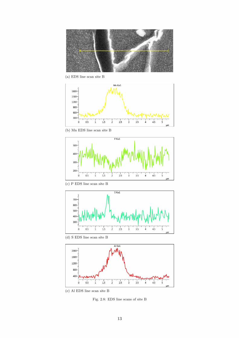
(a) EDS line scan site B

(b) Mn EDS line scan site B

(c) P EDS line scan site B

(d) S EDS line scan site B

(e) Al EDS line scan site B

Fig. 2.8: EDS line scans of site B

13

When looking at the results of site A in Fig. 2.7, there is a clear dip in the iron content at both

grain boundaries. This is expected as the ferrite grains would have much higher iron content

than the grain boundaries, but also shows it is not cementite that has formed. Carbon however

has a large spike on the first grain boundary and a relatively smaller spike on the second. In

contrast, both manganese and phosphorus only spike on the second grain boundary. These

results would indicate that some type of carbide has formed on the first grain boundary and the

second grain boundary is made up of segregated impurities. The rise of phosphorus content in

the second grain boundary is a significant finding, however, since it is directly related to temper

embrittlement. Manganese is also reported to be a culprit element in temper embrittlement

susceptibility; however, it is well documented that phosphorus is the main element of concern

when dealing with temper embrittlement [10, 19–24]. To study this further, a separate site on

a separate sample was used. Site B shows not only a line scan across a grain boundary, but

also across an inclusion. It can be seen from the results that going across the inclusion spikes

aluminum, manganese, and sulfur towards the edge. However, the grain boundary once again

appears to spike the phosphorus content. The manganese content may also be higher in the

grain boundary, but due to the large amount of manganese in the inclusion, the spike may not

be detectable from the scan. Overall, the phosphorus content spiking at the grain boundary is

a key finding and is cause for further investigation and testing into temper embrittlement.

To follow up with the line scans of the inclusion in site B, an area of the base material was

found with several inclusions present. An EDS element map was created for the area to identify

which elements the inclusions are composed of. The images of the EDS mapping as well as the

inclusions are shown in Fig. 2.9

14

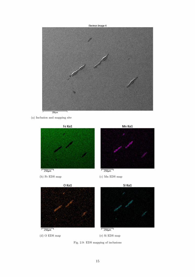
(a) Inclusion and mapping site

(b) Fe EDS map (c) Mn EDS map

(d) O EDS map (e) Si EDS map

Fig. 2.9: EDS mapping of inclusions

15

The inclusions are mainly composed of manganese, silicon and oxygen. This is typical of 350W

steel and is not a cause for concern. Other inclusions may be found within the steel composed

of manganese and sulfur (as perhaps in Fig. 2.8) which is also typical of structural steel since

the manganese will bond and consume the excess sulfur.

2.3.2. Fractography

When turning our attention towards the crack themselves, it is logical to first analyze the

initiation site. Unfortunately, due to the crack opening in the galvanizing bath, the surface

of the primary (macroscopically visual) crack’s initiation is covered with zinc. However, Fig.

2.10 shows the crack initiation site and more specifically a secondary crack that microscopi-

cally formed alongside the primary crack, with a separation along the grain boundaries. This

secondary crack is useful for analysis since the primary crack’s initiation site cannot be seen.

When zooming in on the secondary crack, as seen in Fig. 2.10(b), there is no deformation of

the grains and the crack appears as if it could fit back together. It appears the crack is a

result of separation along the grain boundary with no considerable plastic deformation. Each

of these samples was sectioned and processed the same as the base material samples using a

5% nital etch. More images of the crack initiation site can be found in Appendix A. They are

accompanied by images of the weld cross section, side view, and microstructure.

(a) Crack initiation site 10X (b) Crack initiation site 50X

Fig. 2.10: Crack initiation site

Along with the crack initiation site, the arrest site is also of interest. An image showing the

crack arrest is shown in Fig. 2.11. It can be seen that the crack has the same feature of grain

16

boundary separation with little to no distortion. This would imply the mode of fracture stayed

the same throughout the crack propagation. An EDS map was done directly at the crack arrest,

where from the microscope image it looks as though there may be something in the crack. The

EDS map results are shown in Fig 2.12.

Fig. 2.11: Crack arrest site 5X

17

(a) Crack arrest site

(b) Fe EDS map (c) O EDS map

(d) Zn EDS map

Fig. 2.12: EDS mapping of the crack arrest

18

The results shown in Fig. 2.12 do not show anything irregular or noteworthy. There is no

increase of zinc content in the crack, which suggests LME may not be the embrittlement case

[8, 25]. Also, there seems to be a build up of oxidation in the crack, which is the inclusion that

was seen from the optical microscope images. This may be due to the water used while grinding

the sample or from exposure to the air, but in either case it is not unexpected.

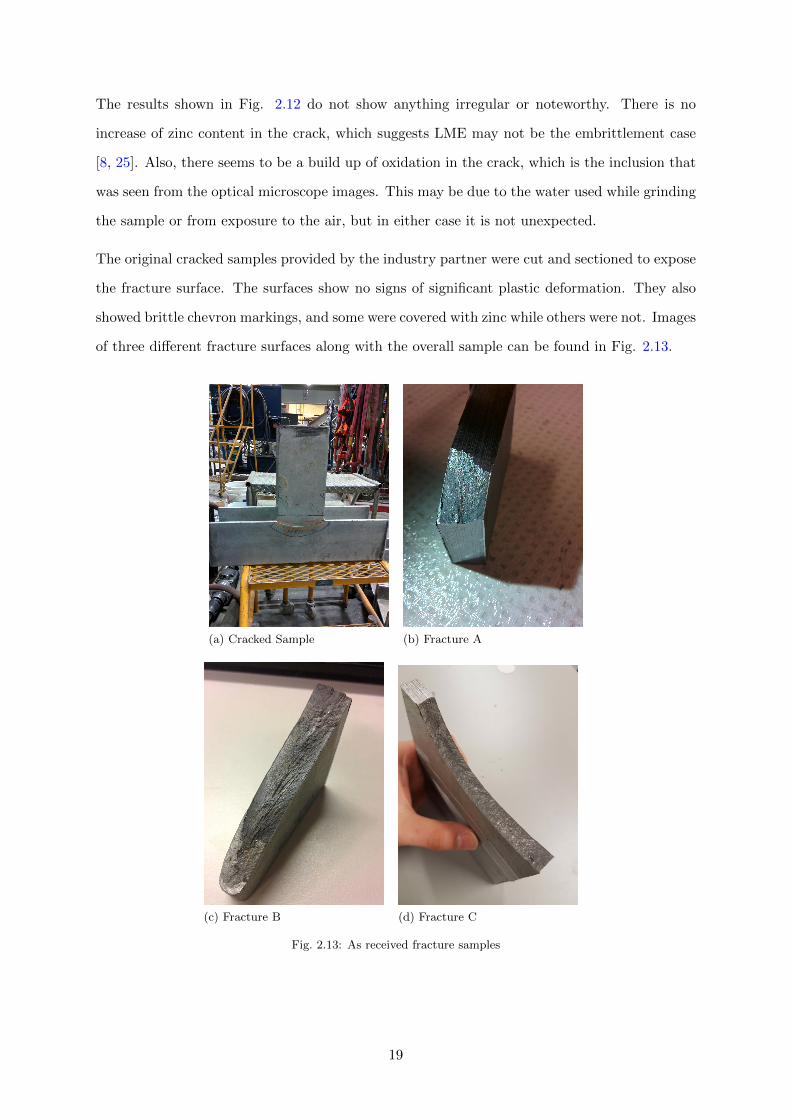
The original cracked samples provided by the industry partner were cut and sectioned to expose

the fracture surface. The surfaces show no signs of significant plastic deformation. They also

showed brittle chevron markings, and some were covered with zinc while others were not. Images

of three different fracture surfaces along with the overall sample can be found in Fig. 2.13.

(a) Cracked Sample (b) Fracture A

(c) Fracture B (d) Fracture C

Fig. 2.13: As received fracture samples

19

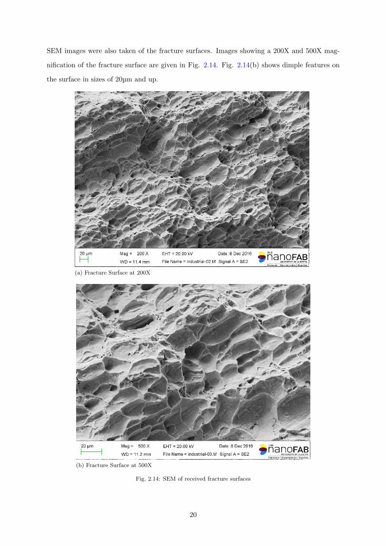
SEM images were also taken of the fracture surfaces. Images showing a 200X and 500X mag-

nification of the fracture surface are given in Fig. 2.14. Fig. 2.14(b) shows dimple features on

the surface in sizes of 20µm and up.

(a) Fracture Surface at 200X

(b) Fracture Surface at 500X

Fig. 2.14: SEM of received fracture surfaces

20

In comparison, a fresh crack was made by fracturing the same base material at ambient tem-

perature. An SEM image of 500X magnification is shown in Fig. 2.15. In comparison to the

features seen in Fig. 2.14(b), the dimple features are much smaller. The largest dimples are

about 10µm with many smaller dimples across the surface.

Fig. 2.15: Fresh fracture surface

Looking at the images of the provided samples, it can be seen there is little to no deformation

of the steel on the fracture surface. It does not show any characteristics of ductile fracture, such

as cup and cone features or plastic deformation. Furthermore, when examining the fracture

surface under the SEM there is no evidence of deformation of the grains, the dimples seen are

the same size as the grains (20µm), and the surface shows smooth areas between the grain

boundaries. Even more explicitly in Fig. 2.15, microvoids can be seen across the surface.

Given the distinction in these features, the difference in fracture mode can be seen directly

when comparing Fig. 2.13 and Fig. 2.15. Given that 350W is expected to have very ductile

behavior, the brittle fracture mode in the provided samples is critical to determining why the

steel platforms cracked and supports the notion of an embrittlement factor present.

With the findings of this chapter, it is clear experimental testing is needed to further explore

the embrittlement factor at play. There is evidence to suggest temper embrittlement may be

21

the case but testing is also needed on hydrogen embrittlement. Also, a FEA model is needed

to place metrics on the stresses of the double dip galvanizing process. The conclusions of this

chapter have given a base of knowledge and clues into the cracking of the steel platforms which

can now be followed up with experimental lab testing.

2.4. Conclusions

The microstructure of the steel base material was analyzed using an optical microscope and

SEM. The images show a typical ferritic and pearlitic steel microstructure which is expected

of 350W and 300W steel. However, a closer inspection shows thicker grain boundaries with

potential grain boundary segregation. EDS analysis shows the thicker grain boundaries are

composed of either carbides, manganese, or phosphorus. EDS analysis also showed the inclusions

were not composed of anything detrimental.

When analyzing the cracks that occurred during galvanizing the most outstanding result is

the absence of any ductile features. There are no visual signs of plastic deformation, which is

very uncharacteristic of the steel. It can be said the fracture during galvanizing was brittle.

However, when the steel is fractured at the ambient temperature, it is ductile. Therefore,

an embrittlement factor must have been present during the cracking of the steel platforms. In

addition, the cracks showed little to no zinc on the crack surface. Zinc is only found consistently

at the opening of the crack. This suggests LME was not the cause.

22

3. Finite Element Analysis Model

3.1. Introduction

Finite element analysis is a numerical method for solving complex mathematical problems in

engineering as well as physics. In engineering it is typically used for problems involving struc-

tural analysis, fluid mechanics, or heat transfer. The basic concept revolves around dividing the

existing problem into a discrete simpler problems called finite elements. The finite elements are

solved individually by developing an equation for each element. Then once each element has

an associated equation, they are put together as a global system of equations that models the

original larger problem [26, 27]. The equations are simple local approximations of the original

complex equation, which is usually in the form of a partial differential equation. In FEA this

simplification is done using Galerkin’s method [26]. To solve the system of equations, FEA

relies on the boundary conditions. These must be known and accurately modeled for FEA to

be useful. FEA can be used for static cases as well as transient cases.

The subdivision is often referred to as meshing. In the case of structural analysis, the mesh is

the subdivision of the structure’s geometry into smaller and standard geometric elements. The

types of elements typically used in FEA meshing are tetrahydra, pyramids, prisms or hexahedra,

for continuum models. Each meshing type has its own number of nodes, which is a point used for

calculation during the FEA calculations [28]. Nodes are placed at the corners of the elements, on

the elements faces, or in some cases, within the element. Elements are connected by the corner

nodes, and when the nodes displace that will distort the connected elements in accordance to

the inputted properties [29]. The nodal displacement is the basis from which outputs such as

stress are drawn.

In some cases the nodes are the points being used for calculation, and the nodes cannot cover

the entire model, the output may have a dependency on the mesh size. However, the critical

mesh size for acceptable accuracy can be easily assessed. It is done by a mesh refinement study,

which includes taking an important metric and studying the change of the result as the mesh

refines. Once the result shows little change with large changes in the mesh refinement, the result

is deemed independent of the mesh and of acceptable accuracy [30].

Use of FEA to model the hot dip galvanizing process it seems it is sparsely reported in literature.

23

Modeling the hot dip galvanizing process would include the self weight of hoisting the object,

but it is primarily a heat transfer problem. Therefore the thermal stresses and their distribution

would depend on the geometry of the hoisted item. For this reason, literature available does

not focus on what kinds of stresses are expected during galvanizing. Instead studies have been

found analyzing the beam distortion during galvanizing, and investigating the heat transfer

that takes place. Although this study, along with others, does not give an idea of the stresses

of galvanizing, the heat transfer properties are very useful for creating an FEA model of the

cracked steel platform structures.

Abaqus FEA is one of the largest and most widely available software packages to conduct an

FEA study. Although FEA is a numerical method, the user interaction with Abaqus is largely

visual. A two or three dimensional model is created and the boundary conditions are visually

applied by selecting the node, line, or surface for their location. Loading is done in a similar

fashion, whether it is mechanical or thermal. The intricacies and complete details of the Abaqus

software functions are beyond the scope of this chapter, however the visual operation and results

of the software are greatly valued in the case of the cracked steel platforms. The shape of the

stress distribution across the structure is just as significant as the stress values themselves.

Using FEA to analyze the cracked platforms gives many insightful results in terms of what

the platforms experienced during the double dip galvanizing process. Using the Abaqus FEA

software, a solid model of the platform can be created and analyzed for the stress experienced

during the dipping procedure.

3.2. Model Methodology and Setup

Along with the physical joint samples, plenty of documentation and drawings were provided of

the steel platform structures by the industry partner. These drawings were important initially

to determine where the samples had been sectioned from. However, the drawings include di-

mensions as well as the assembly list which includes the individual beam dimensions and profile

type. There is also many section views available to fully understand the connections and fit

between beams. An image of the drawing is shown in Fig. 3.1.

24

Fig. 3.1: Platform assembly drawing

This first step to creating an FEA model in Abaqus is to create a three dimensional solid model.

The drawing seen in Fig. 3.1 was the schematic used for creating the solid model, and the

model was made to match the drawing exactly. Each beam profile was first sketched, and then

each beam in the assembly was extruded in accordance to the listed length, and the material

properties of the structural steel were applied to each section. Once all the parts were created,

the connections could be modeled. The drawing shows that all the joints are done via welding,

however given the complexity of modeling a weld in FEA it is a common assumption to assume

it as an ideal connection. Once the FEA is carried out, this will show the stresses at each

joint without any independent movement of the members. This will keep the deformation of

the frame as a cohesive unit, which is how it is assumed a perfectly welded structure would be

behave. This connection is modeled using a tie constraint in the software. The tie constraint

requires selecting a master surface and slave surface, where the nodes of the slave surface are

adjusted to match the master surface. This allows for the seamless connection between the two

parts. Fig. 3.2 shows the assembled three dimensional model along with a close up of a T-joint

25

and the tie constraint.

(a) 3D model

(b) T-joint connection (c) Tie constraint

Fig. 3.2: 3D model of the platform and joint constraint

Once the three dimensional model has been created, the frame work of the FEA model can be

set. First, to create a time dependent model the steps must be created as transient. Steps are

generally used to separate different phases within the model. For example, in the double dip of

the steel platforms, four steps were used: the hoisting of the platform, the first dip, the cool off

between dips, and the second dip. As a transient step, the time period must be inputted from

which the software creates incrementation to show the frames that best capture the changing

states. The increments have a minimum value (such as 0.0001) and the maximum value is equal

to the time period (in the case that nothing changes throughout the time period). For the

26

double dip process a time period of five minutes was used for the submersion time and the cool

off was extended until the frame returned to the ambient temperature. This is assumed given

that the workers would need to be able to work around the structure and handle it before doing

the second dip.

After putting the steps in place, the boundary conditions and loads can be created and applied

to the structure. The first step only included the hoisting of the frame, and was created to be

able to see the stresses of hoisting alone. In this step the loading is purely mechanical and is

a result of the self-weight of the platform. According to the commercial galvanizing company,

the structure was hoisted using two chains around the corners of the structure. To model this

as a boundary condition the line of nodes at the corners was fixed to have zero displacement.

Fig. 3.3 shows the application of the boundary condition to the platform’s corner. The software

has a loading function available that is self-weight of the structure (assuming the density of the

parts is inputted) where the only input needed is the acceleration due to to gravity which was

set at 9.81m/s2.

Fig. 3.3: Location of boundary condition

The remaining steps focus heavily on modeling the heat transfer of the dipping process. The

27

parameters that are known about the heating during galvanizing are only the dwell time in the

molten zinc bath and the temperature of the bath at 450 °C. Thermal loading in Abaqus is

done by different forms of heat fluxes, however given the information that is available, modeling

the heat transfer directly as a flux would be very difficult. Instead, the software has another

option to create an interaction between the structure and the inputted environment. Using

an interaction, a convection heat transfer can be modeled. With the convection coefficient of

1350 Wm−2K−1 from the study of beam distortion during galvanizing, all the required inputs

are known for the model [31]. A partition line is used to separate the model into two halves

along the double dip line shown in the drawing. During the second step, the convection of the

galvanizing bath is applied to half of the structure, while the convection of the ambient air is

applied to the other half. A visual of the application area is given in Fig. 3.4. During the

third step, the convection of the ambient air applied to the whole structure and finally in the

last step the inverse of the first dip interactions were applied. It should also be mentioned that

during the second dip the boundary conditions of the hoist are moved to the other ends of the

structure and the force of gravity is reversed since it is being hoisted on its opposite side. The

different interactions, loading and boundary conditions are activated and deactivated as the

model progresses through the steps.

Fig. 3.4: Galvanizing bath convection area

28

Finally, a mesh must be created and refined for accurate results. Initially a coarse mesh is created

for easy and quick computation. Tetrahedral elements were used since they are required for a

thermo-displacement coupled computation. From there a node of significant interest is chosen

and the results of that node are tracked as the mesh refines. For the steel platform model,

a node in the area of cracking at the T-joint was chosen. Given this is a transient case, the

peak stress during the whole galvanizing process was taken as the tracked metric. Once the

peak stress was approximately stable and independent of the number of elements, the results

were deemed reliable and accurate. This occurred with approximately 204 000 elements in the

model.

3.3. Results and Discussion

The results of the mesh refinement study must be shown first, before analyzing the stress and

temperature results. For this study, a node on the T-joint was chosen. Fig. 3.5 shows the

T-joint with the node highlighted. It is important to note that the node at the exact edge

where the cracking initiated can not be used for the study. Due to the method of computation

of the software, edge nodes do not converge.

Fig. 3.5: Node chosen for mesh refinement study

29

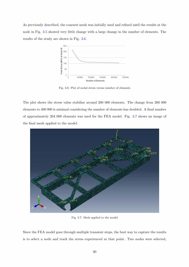
As previously described, the coarsest mesh was initially used and refined until the results at the

node in Fig. 3.5 showed very little change with a large change in the number of elements. The

results of the study are shown in Fig. 3.6.

Fig. 3.6: Plot of nodal stress versus number of elements

The plot shows the stress value stabilize around 200 000 elements. The change from 200 000

elements to 400 000 is minimal considering the number of elements has doubled. A final number

of approximately 204 000 elements was used for the FEA model. Fig. 3.7 shows an image of

the final mesh applied to the model.

Fig. 3.7: Mesh applied to the model

Since the FEA model goes through multiple transient steps, the best way to capture the results

is to select a node and track the stress experienced at that point. Two nodes were selected,

30

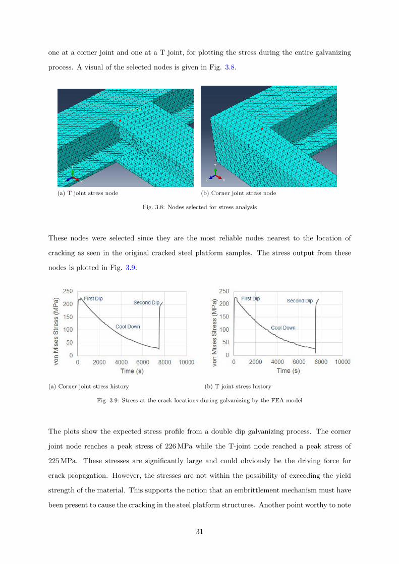
one at a corner joint and one at a T joint, for plotting the stress during the entire galvanizing

process. A visual of the selected nodes is given in Fig. 3.8.

(a) T joint stress node (b) Corner joint stress node

Fig. 3.8: Nodes selected for stress analysis

These nodes were selected since they are the most reliable nodes nearest to the location of

cracking as seen in the original cracked steel platform samples. The stress output from these

nodes is plotted in Fig. 3.9.

(a) Corner joint stress history (b) T joint stress history

Fig. 3.9: Stress at the crack locations during galvanizing by the FEA model

The plots show the expected stress profile from a double dip galvanizing process. The corner

joint node reaches a peak stress of 226 MPa while the T-joint node reached a peak stress of

225 MPa. These stresses are significantly large and could obviously be the driving force for

crack propagation. However, the stresses are not within the possibility of exceeding the yield

strength of the material. This supports the notion that an embrittlement mechanism must have

been present to cause the cracking in the steel platform structures. Another point worthy to note

31

is the stresses of hoisting the platform proved minuscule in comparison to the thermal stresses.

The stress of hoisting reached approximately 10 MPa in the corner joint, which accounts for

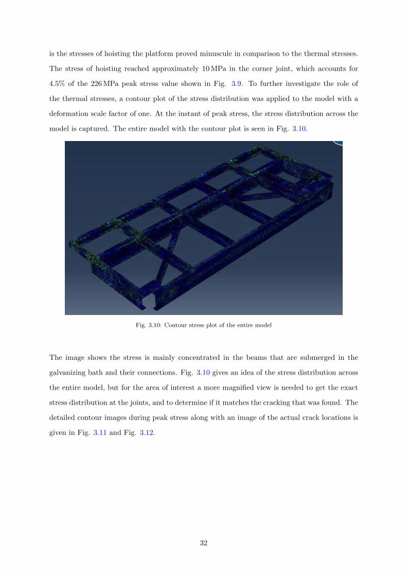
4.5% of the 226 MPa peak stress value shown in Fig. 3.9. To further investigate the role of

the thermal stresses, a contour plot of the stress distribution was applied to the model with a

deformation scale factor of one. At the instant of peak stress, the stress distribution across the

model is captured. The entire model with the contour plot is seen in Fig. 3.10.

Fig. 3.10: Contour stress plot of the entire model

The image shows the stress is mainly concentrated in the beams that are submerged in the

galvanizing bath and their connections. Fig. 3.10 gives an idea of the stress distribution across

the entire model, but for the area of interest a more magnified view is needed to get the exact

stress distribution at the joints, and to determine if it matches the cracking that was found. The

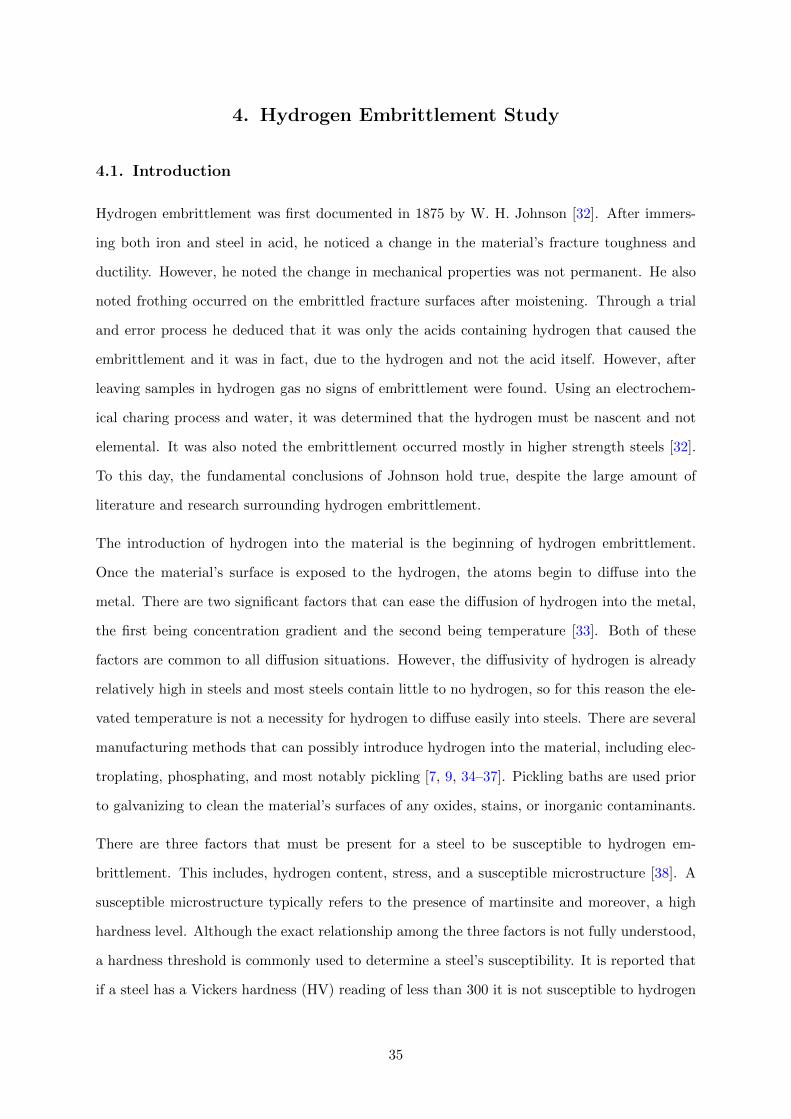
detailed contour images during peak stress along with an image of the actual crack locations is

given in Fig. 3.11 and Fig. 3.12.

32

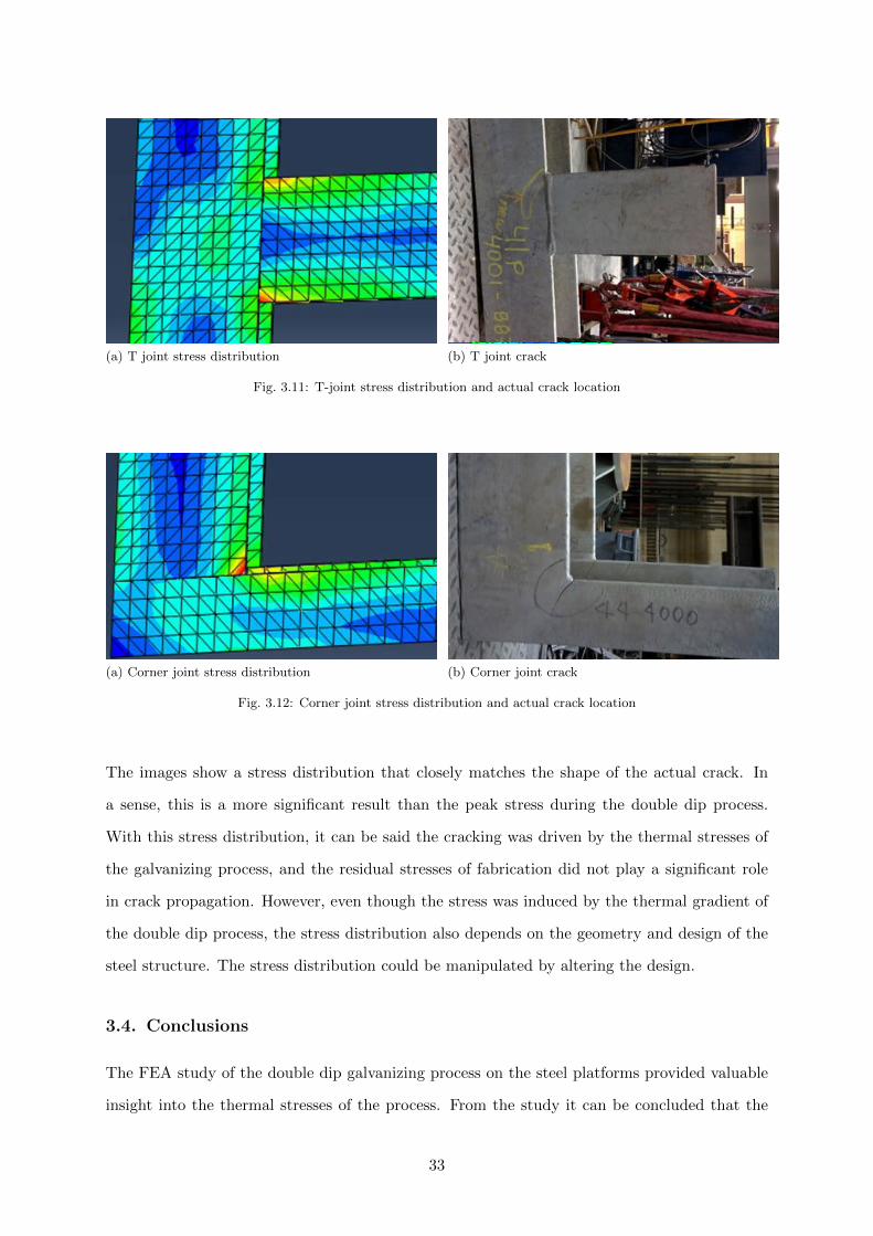
(a) T joint stress distribution (b) T joint crack

Fig. 3.11: T-joint stress distribution and actual crack location

(a) Corner joint stress distribution (b) Corner joint crack

Fig. 3.12: Corner joint stress distribution and actual crack location

The images show a stress distribution that closely matches the shape of the actual crack. In

a sense, this is a more significant result than the peak stress during the double dip process.

With this stress distribution, it can be said the cracking was driven by the thermal stresses of

the galvanizing process, and the residual stresses of fabrication did not play a significant role

in crack propagation. However, even though the stress was induced by the thermal gradient of

the double dip process, the stress distribution also depends on the geometry and design of the

steel structure. The stress distribution could be manipulated by altering the design.

3.4. Conclusions

The FEA study of the double dip galvanizing process on the steel platforms provided valuable

insight into the thermal stresses of the process. From the study it can be concluded that the

33

stresses reached a considerable magnitude but did not exceed the yield strength of the steel. In

addition, the thermal stresses were the driving force for crack propagation.

Although this study did not directly build on the results of Chapter 2 and operated indepen-

dently, it once again helped build the knowledge base and understanding of the problem and

supported the conclusions of Chapter 2 by showing evidence that an embrittlement factor was

needed for the cracking to occur. In the following two chapters of the thesis, the most common

embrittlement types during hot-dip galvanizing will be explored and the steel’s susceptibility

will be tested by lab experiments.

34

4. Hydrogen Embrittlement Study

4.1. Introduction

Hydrogen embrittlement was first documented in 1875 by W. H. Johnson [32]. After immers-

ing both iron and steel in acid, he noticed a change in the material’s fracture toughness and

ductility. However, he noted the change in mechanical properties was not permanent. He also

noted frothing occurred on the embrittled fracture surfaces after moistening. Through a trial

and error process he deduced that it was only the acids containing hydrogen that caused the

embrittlement and it was in fact, due to the hydrogen and not the acid itself. However, after

leaving samples in hydrogen gas no signs of embrittlement were found. Using an electrochem-

ical charing process and water, it was determined that the hydrogen must be nascent and not

elemental. It was also noted the embrittlement occurred mostly in higher strength steels [32].

To this day, the fundamental conclusions of Johnson hold true, despite the large amount of

literature and research surrounding hydrogen embrittlement.

The introduction of hydrogen into the material is the beginning of hydrogen embrittlement.

Once the material’s surface is exposed to the hydrogen, the atoms begin to diffuse into the

metal. There are two significant factors that can ease the diffusion of hydrogen into the metal,

the first being concentration gradient and the second being temperature [33]. Both of these

factors are common to all diffusion situations. However, the diffusivity of hydrogen is already

relatively high in steels and most steels contain little to no hydrogen, so for this reason the ele-

vated temperature is not a necessity for hydrogen to diffuse easily into steels. There are several

manufacturing methods that can possibly introduce hydrogen into the material, including elec-

troplating, phosphating, and most notably pickling [7, 9, 34–37]. Pickling baths are used prior

to galvanizing to clean the material’s surfaces of any oxides, stains, or inorganic contaminants.

There are three factors that must be present for a steel to be susceptible to hydrogen em-

brittlement. This includes, hydrogen content, stress, and a susceptible microstructure [38]. A

susceptible microstructure typically refers to the presence of martinsite and moreover, a high

hardness level. Although the exact relationship among the three factors is not fully understood,

a hardness threshold is commonly used to determine a steel’s susceptibility. It is reported that

if a steel has a Vickers hardness (HV) reading of less than 300 it is not susceptible to hydrogen

35

embrittlement. The most conservative value for the hydrogen susceptibility range were found to

be 275 HV [7, 9, 36, 39]. Therefore the first step to assessing a steel’s susceptibility to hydrogen

embrittlement is to study the its hardness.

Hydrogen embrittlement is commonly associated with hot dip galvanizing. This is due to the

pickling process prior to being hot dipped, which contains a hydrogen chloride solution. This is

an excellent opportunity for active, diffusible hydrogen to enter into the steel [7, 9, 34–37, 39, 40].

Pickling is a long standing culprit in causing hydrogen embrittlement, however coupled with

the stresses of hot-dip galvanizing almost all of the factors to cause hydrogen embrittlement are

present from the processing alone. However, studies showing hydrogen embrittlement during

the galvanizing process are usually done with steels that fall within the susceptible hardness

range. It would be very uncharacteristic for 350W or 300W steel to show hardness levels that

high.

When relating hydrogen embrittlement back to the cracked steel platforms, it is reasonable to

suspect this embrittlement type as the cause of cracking. Given the large amount of literature

and research that suggests cracking during galvanizing is hydrogen related, it is an embrittlement

type that must be tested and explored. Also, when reflecting back on results from Chapter 2, it

was seen there were some irregularities with thicker-than-usual grain boundaries that contained

carbides. This may act as a susceptible microstructure. For this reason, actual testing for

hydrogen embrittlement by charging samples with hydrogen must be carried out. Hardness

testing will also be done to check for any irregularities in the base material or weld that cause

the material to be in the susceptible range. Hardness testing will also give an idea if liquid

metal embrittlement is at play at all, even though no signs of zinc were found in the crack, as

discussed in Chapter 2.

4.2. Experimental Setup

Given the hardness threshold for susceptibility to hydrogen embrittlement (along with LME

[8, 25]) hardness testing was carried out on the weld cross sections, which included some of the

base material outside of the weld zone. For the hardness testing, four samples were used and

taken from four different welds. The samples were mounted and ground in the same fashion as

the metallography samples discussed in Chapter 1. Vickers hardness was measured using a 0.3N

force with a dwell time of 10 seconds, done with a Tukon 2500 automatic hardness mapper.

36

The orientation of the indentation points and the number of indentations is inputted in the

software. In this case, the indentations are oriented in a straight line across the weld with most

cases having 75 indentation points. The hardness reading and indentation number was then

processed into a comprehensive plot.

An experimental procedure was developed to test the hydrogen embrittlement susceptibility of

the base material and welds. The premise of the test is to mechanically test samples that were

put through the pickling process in comparison to samples that were not pickled. Any difference

in the fracture mode or the material’s strength would indicate hydrogen does impact the material

properties. For the mechanical testing and fracture a standard tension test procedure was

selected. To accurately gather all the desired information four test cases were developed as

summarized in Table 4.1. Samples of the base material and of the weld were sectioned from

a T-joint and cut into standard sizes for tension testing according to ASTM A370 [41]. The

general location of the samples is shown in Fig. 4.1.

Table 4.1: Test cases

Test Case Description

1 Not pickled base material

2 Pickled base material

3 Not pickled weld

4 Pickled weld

37

Fig. 4.1: Location of hydrogen embrittlement samples

The samples were transported to the same commercial galvanizing company that worked on

the steel platforms. The tension samples were put through the same processing as the steel

platforms except they did not get galvanized. However, they did undergo the pickling process

to be charged with hydrogen. The pickling bath has a hydrogen chloride concentration of 13%.

To prevent the hydrogen from diffusing out of the steel while being transported back to the

lab, the samples were transported at -78.5°C in a polystyrene cooler filled with dry ice pellets.

The tension tests were carried out with a strain rate of 0.25mm/min in the elastic region and

2.5mm/min in the plastic region until fracture occurred. The input force data was recorded

along with the displacement data taken from a 1” gauge extensometer. The fracture mode,

surfaces, and size of the ductile region would determine the potential presence of embrittlement

(loss of ductility and fracture toughness).

38

4.3. Results and Discussion

4.3.1. Hardness Testing

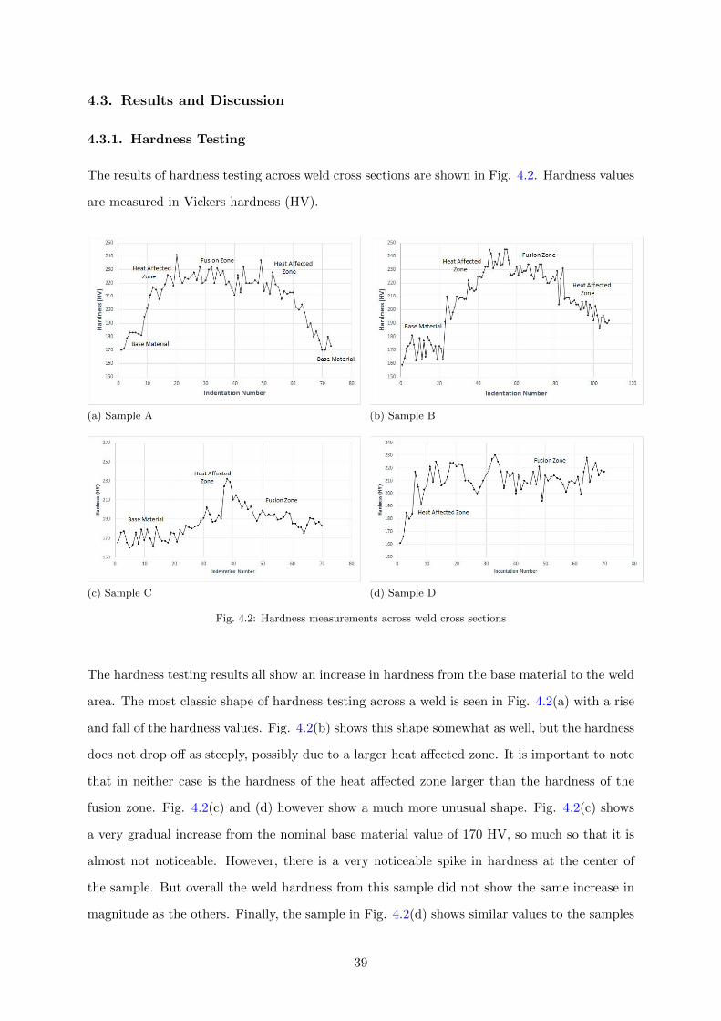
The results of hardness testing across weld cross sections are shown in Fig. 4.2. Hardness values

are measured in Vickers hardness (HV).

(a) Sample A (b) Sample B

(c) Sample C (d) Sample D

Fig. 4.2: Hardness measurements across weld cross sections

The hardness testing results all show an increase in hardness from the base material to the weld

area. The most classic shape of hardness testing across a weld is seen in Fig. 4.2(a) with a rise

and fall of the hardness values. Fig. 4.2(b) shows this shape somewhat as well, but the hardness

does not drop off as steeply, possibly due to a larger heat affected zone. It is important to note

that in neither case is the hardness of the heat affected zone larger than the hardness of the

fusion zone. Fig. 4.2(c) and (d) however show a much more unusual shape. Fig. 4.2(c) shows

a very gradual increase from the nominal base material value of 170 HV, so much so that it is

almost not noticeable. However, there is a very noticeable spike in hardness at the center of

the sample. But overall the weld hardness from this sample did not show the same increase in

magnitude as the others. Finally, the sample in Fig. 4.2(d) shows similar values to the samples

39

in Fig. 4.2(a) and (b) and also the same large increase as the indentations move into the weld

zone on the left side of the plot. The hardness does not drop on the right but this is likely due

to hardness mapping not reaching outside the weld zone.

The most significant data from the hardness testing is the peak value. In Fig. 4.2(a), (b), (c),

and (d) the maximum hardness readings are 241 HV, 245 HV, 232 HV, and 230 HV respectively.

It is also important to note that the hardness of the base material consistently reads 170 - 180

HV. These values are expected for 350W and 300W steel along with their welds. Ultimately

these results show that there is nothing irregular with the hardness levels of the material, which

is supported by the typical pearlitic carbide structure seen in Chapter 2.

As previously noted, both LME and hydrogen embrittlement depend heavily on a susceptible

microstructure which is measured by hardness testing. But even the peak hardness values in any

region are very short of the minimum hardness values reported for susceptibility to LME and

hydrogen cracking. Given these hardness results and the lack of zinc found in the mid-crack and

near the crack arrest, LME is not a reasonable explanation for cracking. This also eliminates one

of the three contributing factors for hydrogen embrittlement. This makes the notion of hydrogen

cracking unlikely. It would be very unusual and perhaps even extraordinary to discover hydrogen

cracking in a case with such low hardness. But the considerable stresses induced by the double

dip galvanizing process must still be considered, along with the hydrogen that is charged into

the material during pickling. Further investigation into hydrogen embrittlement is warranted.

4.3.2. Tension Testing

Despite the results of the hardness testing, the experimental study on hydrogen embrittlement

was still carried out through tension testing. The fracture surfaces of the tension tests with

hydrogen-charged samples is shown in Fig. 4.3. Fig. 4.3(a) and (b) shows the fracture surface

of the base material sample not pickled and pickled. Similarly, Fig. 4.3(b) and (c) show the

sample across the weld pickled and not pickled. It should also be noted that in Fig. 4.3(c) and

(d) the fracture did not occur in the weld, but in the base material.

40

(a) Base material, not pickled (b) Base material, pickled

(c) Across weld, not pickled (d) Across weld, pickled

Fig. 4.3: Fracture surfaces of hydrogen-charged samples

41

The main purpose of this experiment is to compare the fracture surface of the samples that

were pickled against the samples that were not. However, a visual inspection of all four samples

fracture surfaces shows no significant difference. Similar features are found on each surface

and more significantly they all share ductile features. Evidence of ductile fracture is shown by

the cup and cone features and plastic deformation. The pickling process and introduction of

hydrogen into the steel had no impact on the mechanical properties. Overall it can be said

there is no difference in fracture mode among the different samples.

(a) Base material, not pickled (b) Base material, pickled

(c) Across weld, not pickled (d) Across weld, pickled

Fig. 4.4: Tension test results of hydrogen-charged samples

To support the discussion of the visual inspection of the fracture surface, the data from the

tension tests were also analyzed. The numerical stress–strain data from the tension testing is

graphically shown in Fig. 4.4 for each different type of sample, which includes the pickled base

material and weld samples, and the unpickled base material and weld samples. The images show

no change between the samples that were pickled and the samples that were not. The ductile

behavior is the same with both types of samples showing a large plastic region and necking

before the final fracture. The only difference between the samples is the welded samples did

not have as large a plastic region as the base material samples, since they did not experience as

42

much strain before fracture. This is an interesting result since the welded samples both broke in

the base material. In any case, all the graphs show the typical behavior of an elastic region and

large plastic region, meaning deformation along with necking and ductile fracture. It appears

the pickling process and introduction of hydrogen into the steel or welds has no effect on the

material’s fracture toughness or tensile behavior.

From the results of Chapters 2 and 3 it is seen that an embrittlement mechanism is needed

for the material to crack in the brittle manner that occurred during galvanizing. However the

results of this chapter conclude that it was not a case of hydrogen embrittlement. The pickling

process does allow for hydrogen to diffuse into steel, however the material is not susceptible.

Although hydrogen embrittlement can be removed from the list of possible factors, this does

not determine the cause of cracking. Literature has also stated that temper embrittlement may

be a possibility, which is the next logical study to conduct.

4.4. Conclusions

Hardness testing of the base material and welds, along with tension testing of pickled samples,

was used determine to the material’s susceptibility to hydrogen embrittlement. The results of the

hardness testing were compared to the values reported in literature to determine susceptibility.

The results from the tension testing of the pickled samples were compared to those of regular

samples. The tension testing determined if the hydrogen introduced into the steel during pickling

had any impact on the mechanical properties.

From the results of the hardness testing, the steel platform’s base material and welds are not

within the range of susceptibility. This leads to the conclusion that hydrogen embrittlement

was not the mechanism that caused cracking in the steel platform structures. As one of the

three factors needed is not present. The hardness testing results from this chapter and the lack

of zinc seen in the fractography study in Chapter 2 both indicate the LME can be eliminated

as a possible cause for cracking as well.

The fracture surfaces of the tension testing all showed signs of ductile fracture and no resem-

blance to the fracture surfaces of the cracked samples. Charging the samples with hydrogen and

fracturing them failed to recreate the fracture surface from the galvanizing cracking, and more-

over the fracture surfaces of the pickling samples matched the ductile surfaces of the unpickled

43

samples. Once again the material exhibited ductile behavior instead of the brittle behavior seen

from the original incident of cracking. From these tests, in conjunction with the results of the

hardness testing, it can be stated that hydrogen embrittlement was not the cause of cracking

in the steel frames and can be eliminated as an option.

44

5. Temper Embrittlement Study

5.1. Introduction

Temper embrittlement is traditionally used to describe an embrittlement phenomenon during

the tempering of quenched steels. Temper embrittlement typically occurs while aging a steel

through a susceptible temperature range, or when slowly cooling steel through that range. For

carbon steel, this range is 370 °C – 560 °C [7, 10, 19, 20, 22]. Recent research using AES has

shown that the exact mechanism of embrittlement is a migration of impurities to the grain

boundaries [42, 43]. The impurity-rich grain boundaries cause a weakness in the structure.

This results in a decrease in the material’s ductility and fracture toughness [21, 23, 24, 44, 45].

The main element to cause weakness in the grain boundaries is phosphorus, however elements

such as nickel, chromium, and manganese promote the segregation of impurities to the grain

boundary [10, 19–23]. When evaluating the susceptibility of a material and process to temper

embrittlement, the two main factors to consider are the chemistry of the material (if the culprit

elements are present) and if the process temperature is within the susceptible range.

Temper embrittlement has been reported in a few incidents of galvanizing. However, because

it is not a tempering process, it is sometimes given a different name. Overall it is the same

mechanism of embrittlement. The galvanizing bath sits at approximately 450 °C, which is

within the temper embrittlement range [10, 22]. It should also be noted that the galvanized

parts or structures cool slowly from 450 °C, which for some portion, falls within the temper

embrittlement range. The embrittlement is not related to the molten zinc or galvanizing process

directly, but rather the heating cycle and thermal stresses make temper embrittlement a concern

[22]. This is particularly relevant in the case of a double dipping process, where the thermal

gradient across the structure is large, which creates significant thermal stresses in the structure.

The main factor influencing susceptibility to temper embrittlement during galvanizing is the

material’s chemistry. The external factors are all provided by the galvanizing process.

The cracking that occurred in the steel platforms may be related to the mechanisms of temper

embrittlement, especially after the EDS results seen in Chapter 2. EDS line scans consistently

showed spikes in phosphorus content in the grain boundary. Manganese and carbon spikes

were found as well. All of this makes a temper embrittlement study beneficial. The first

45

step in the study is to conduct a compositional analysis of the material. Under the G40.21

specifications set for Canadian structural steel, there should be no cause for concern of temper

embrittlement. However, under the right balance of elements temper embrittlement can still

occur. The composition of the base material along with the steel mill’s chemistry reports will

show if there is anything out of the ordinary in the steel. Secondly, an experiment can be

developed to try to recreate the fracture surface found in the original cracks. This should be

similar to the hydrogen embrittlement tension testing done in Chapter 4. The fracture surface

is once again the result of interest and studied for similarities or differences to the original

surfaces. Lastly, a review and minor study of the diffusivity of phosphorus in steel can show

the mobility of the phosphorous in steel during galvanizing.

5.2. Experimental Setup

The cornerstone of temper embrittlement susceptibility is the material’s chemistry. Two meth-

ods of composition analysis were used in this study, X-ray florescence (XRF) and optical emission

spectroscopy (OES). For the XRF analysis three samples were used, and tested on 3 different

locations per sample. Similarly, for the OES three samples were used which were taken from

the center of the base material’s thickness. Along with the measured composition analysis, the

mill chemistry reports for select beams of interest were gathered. It is unknown exactly how

the mills tested the material’s composition.

XRF operates on a similar principle to EDS in that the sample is excited to cause the release

of a lower level electron and a higher level electron to fill the hole. The energy or radiation

released during this ionization is matched with it’s atomic characteristic. However the major

difference comes into play during the excitation process. XRF uses a secondary target that

is excited by the source, but the florescence given off from exciting the secondary target then

excites the sample [46]. This is in contrast to the direct excitation of EDS. Another difference

with regards to the excitation is that unlike EDS, XRF does not use a high energy electron

beam for the excitation. Rather, a photon source is used, which is more bulk sensitive than

using a high energy electron beam source and EDS.

OES operates by applying electrical energy, in various forms, to the sample and vaporizing

the atoms. The vaporized atoms form a discharged plasma and the atoms are brought to a

high energy state. A unique spectrum discharge is produced, which is matched to its uniquely

46

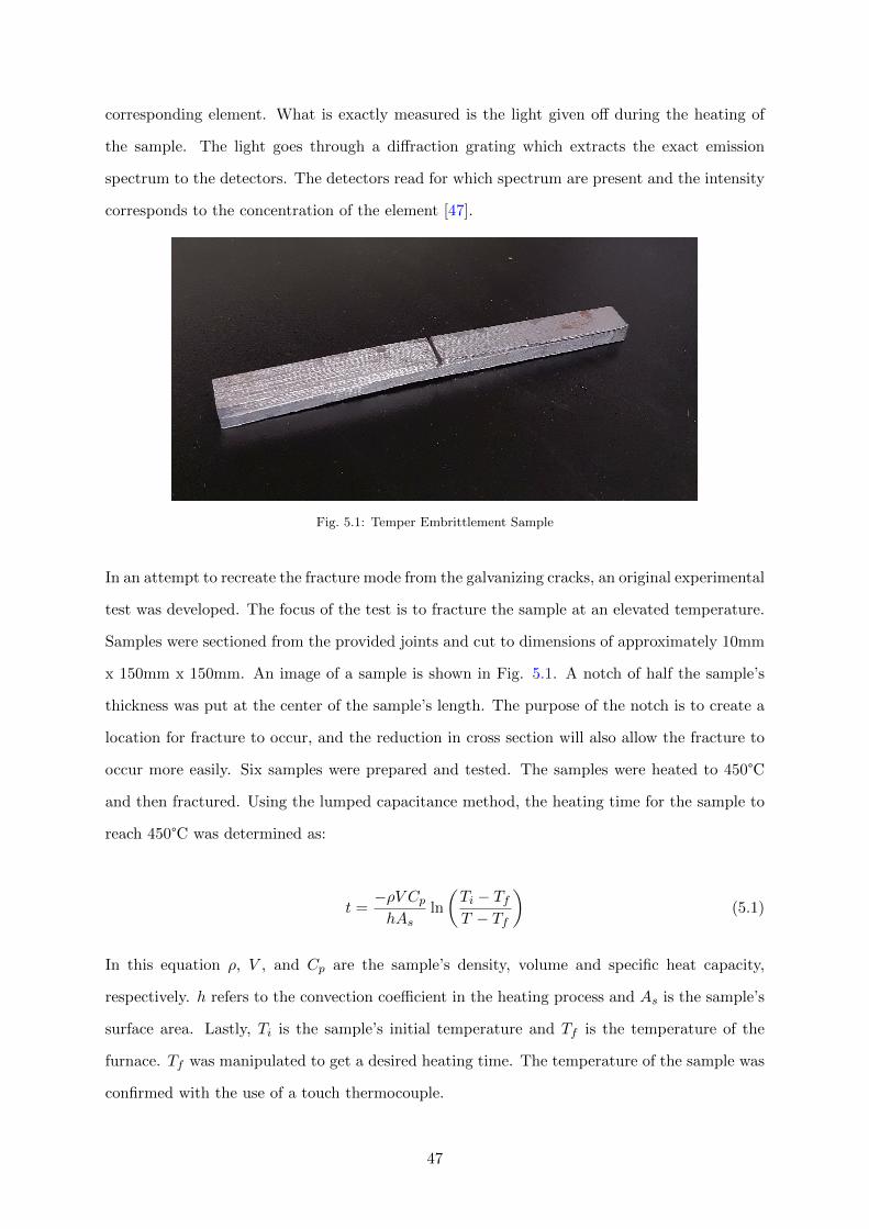
corresponding element. What is exactly measured is the light given off during the heating of

the sample. The light goes through a diffraction grating which extracts the exact emission

spectrum to the detectors. The detectors read for which spectrum are present and the intensity

corresponds to the concentration of the element [47].

Fig. 5.1: Temper Embrittlement Sample

In an attempt to recreate the fracture mode from the galvanizing cracks, an original experimental

test was developed. The focus of the test is to fracture the sample at an elevated temperature.

Samples were sectioned from the provided joints and cut to dimensions of approximately 10mm

x 150mm x 150mm. An image of a sample is shown in Fig. 5.1. A notch of half the sample’s

thickness was put at the center of the sample’s length. The purpose of the notch is to create a

location for fracture to occur, and the reduction in cross section will also allow the fracture to

occur more easily. Six samples were prepared and tested. The samples were heated to 450°C

and then fractured. Using the lumped capacitance method, the heating time for the sample to

reach 450°C was determined as:

t =−ρV Cp

hAsln

(Ti − TfT − Tf

)(5.1)

In this equation ρ, V , and Cp are the sample’s density, volume and specific heat capacity,

respectively. h refers to the convection coefficient in the heating process and As is the sample’s

surface area. Lastly, Ti is the sample’s initial temperature and Tf is the temperature of the

furnace. Tf was manipulated to get a desired heating time. The temperature of the sample was

confirmed with the use of a touch thermocouple.

47

The fracture was created by supporting the sample on both of its ends, with the notch facing

downwards. An impact force, created by a chisel and hammer, was applied to the side opposite

of the notch. This is a similar test set up to a 3-point bend test, but an impact force was applied

in a fashion similar to Charpy impact testing. However, in the end the result of interest is the

fracture surface, since the test objective is to determine if the elevated temperature causes a

brittle fracture. Thus, as long as a fracture surface is produced the results of the test can be

analyzed. The fracture surfaces were analyzed by SEM as well as visually.

5.3. Results and Discussion

All of the compositional analysis of the base material along with the chemistry specifications

in accordance to the G40.21 standards are summarized in Table 5.1. The steel mill’s chemistry

report data was provided for several beams used in the steel structure. According to the G40.21

structural steel chemistry standards, the beams are within specification [48]. To confirm the

analysis of the steel mill, an XRF study was done on three different samples and three different

locations per sample. The results shown from the XRF analysis in Table 5.1 are fairly different

from the values reported by the steel mill. Most obviously is the aluminum, and perhaps more

significantly the sulfur content. The specification for sulfur content is 0.05 wt% maximum [48]

and a sulfur content of 0.228 wt% is very uncharacteristic for structural steel and questionable.

To gather more data along with the XRF readings, an OES analysis was carried about on three

samples. Given the accepted accuracy of OES for trace elements [49] and the closeness to the

values of the steel mill reports, the OES readings are taken as the most accurate. However,

it should be noted the high phosphorus content reported by the OES, which is slightly out

of the specification of 0.04 wt% maximum [48]. The steel mill reports show a relatively high

phosphorus content as well, but not quite as high and not outside of the specification. It

should be noted that phosphorus is a key culprit in susceptibility to temper embrittlement. In

addition to phosphorus, elements such as silicon and manganese create susceptibility to temper

embrittlement, which are both shown to be present within the susceptible range [34]. The

results of the composition study show a susceptibility to temper embrittlement. However, if the

results of the XRF analysis are true, this leaves the steel susceptible to hot short [50]. In either

case, the results point towards a type of embrittlement that is temperature activated.

To explore the notion of grain boundary segregation, the bulk diffusivity of elements of interest

48

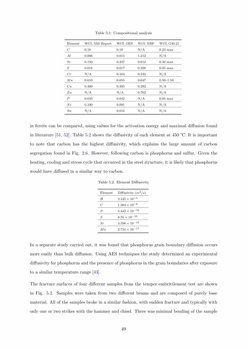
Table 5.1: Compositional analysis

Element Wt% Mill Report Wt% OES Wt% XRF Wt% G40.21

C 0.18 0.19 N/A 0.23 max

Al 0.006 0.015 1.212 N/A

Si 0.150 0.237 0.612 0.40 max

S 0.018 0.017 0.228 0.05 max

Cr N/A 0.164 0.242 N/A

Mn 0.610 0.655 0.647 0.50–1.50

Cu 0.300 0.305 0.292 N/A

Zn N/A N/A 0.702 N/A

P 0.033 0.042 N/A 0.04 max

Ni 0.100 0.091 N/A N/A

Sn N/A 0.016 N/A N/A

in ferrite can be compared, using values for the activation energy and maximal diffusion found

in literature [51, 52]. Table 5.2 shows the diffusivity of each element at 450 °C. It is important

to note that carbon has the highest diffusivity, which explains the large amount of carbon

segregation found in Fig. 2.6. However, following carbon is phosphorus and sulfur. Given the

heating, cooling and stress cycle that occurred in the steel structure, it is likely that phosphorus

would have diffused in a similar way to carbon.

Table 5.2: Element Diffusivity

Element Diffusivity (m2/s)

H 3.125 × 10−5

C 1.384 × 10−8

P 5.442 × 10−16

S 8.55 × 10−16

Si 4.598 × 10−18

Mn 2.734 × 10−17

In a separate study carried out, it was found that phosphorus grain boundary diffusion occurs

more easily than bulk diffusion. Using AES techniques the study determined an experimental

diffusivity for phosphorus and the presence of phosphorus in the grain boundaries after exposure

to a similar temperature range [43].

The fracture surfaces of four different samples from the temper embrittlement test are shown

in Fig. 5.2. Samples were taken from two different beams and are composed of purely base

material. All of the samples broke in a similar fashion, with sudden fracture and typically with

only one or two strikes with the hammer and chisel. There was minimal bending of the sample

49

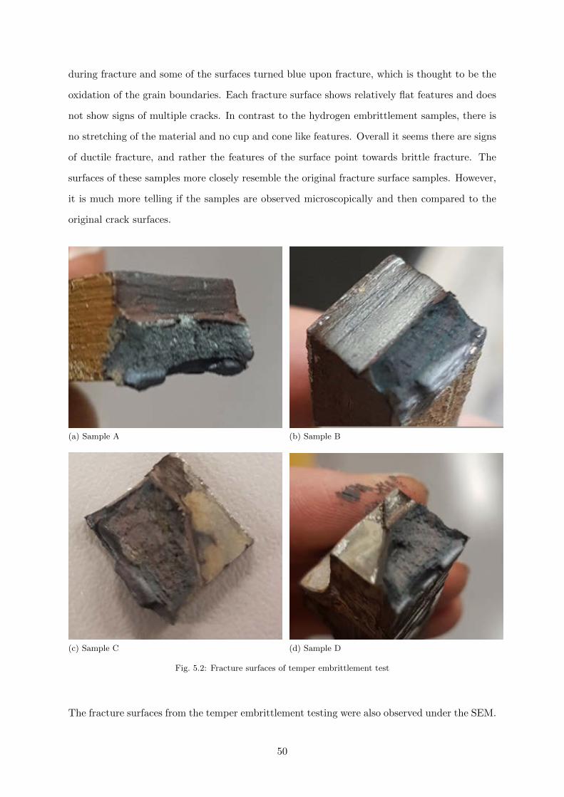
during fracture and some of the surfaces turned blue upon fracture, which is thought to be the

oxidation of the grain boundaries. Each fracture surface shows relatively flat features and does

not show signs of multiple cracks. In contrast to the hydrogen embrittlement samples, there is

no stretching of the material and no cup and cone like features. Overall it seems there are signs

of ductile fracture, and rather the features of the surface point towards brittle fracture. The

surfaces of these samples more closely resemble the original fracture surface samples. However,

it is much more telling if the samples are observed microscopically and then compared to the

original crack surfaces.

(a) Sample A (b) Sample B

(c) Sample C (d) Sample D

Fig. 5.2: Fracture surfaces of temper embrittlement test

The fracture surfaces from the temper embrittlement testing were also observed under the SEM.

50

In Fig. 5.3(b) and (d) the images of the lab sample fracture surface are shown at 200X and

500X respectively. The lab surfaces show the same features, grain boundary separation and

similar dimple sizes as the received fracture surfaces. Fig. 5.3(a) and (c) give a comparison

to the provided sample’s fracture surfaces from Fig. 2.14. The similarities between the two

fractures is stunning. The only noticeable difference in the images is that in Fig. 5.3(d) there

are a few microvoids present, which seem to all be along the grain edges.

Similarly, in Fig. 5.4 a comparison is shown of the ambient lab fracture sample in Fig. 5.4(a)

and the temper embrittlement testing fracture sample in Fig. 5.4(b). Both images are shown at

500X. The difference in the deformation of the surface is apparent as there are many microvoids

and the grain boundaries are not recognizable in Fig. 5.4(a). The obvious differences in this

comparison also reinforces the idea of how stark the similarities are between the surfaces in

Fig. 5.3. For the same material to behave so differently under different temperature conditions

is a key finding. The similarities and differences between the comparisons shows that the

original fracture is recreated by elevated temperature fracture. The increase in the material’s

temperature clearly has an impact on its fracture toughness, thought to be caused by the

diffusion of phosphorus and other impurities to the grain boundaries. Overall, the temper

embrittlement testing proved a temperature activated embrittlement mechanism is present.

51

(a) Received surface 200X (b) Lab surface 200X

(c) Received surface 500X (d) Lab surface 500X

Fig. 5.3: Comparison of 200X & 500X SEM images of the received fracture surface and lab fracture surface

(a) Ambient temperature fracture surface (b) Elevated temperature fracture surface

Fig. 5.4: Comparison of 500X SEM images of the ambient fracture surface and galvanizing temperature fracturesurface

52

Chemical composition and elevated temperature fracture testing, along with a study on the

diffusivity of different elements in ferritic steel was used to investigate the notion of temper em-

brittlement susceptibility in the steel. The results of the chemical composition testing showed

unusually high levels of phosphorus, relative to the Canadian standards. The phosphorus con-

tent along with the low diffusivity and tendency for phosphorus to diffuse to the grain boundaries

agree with the EDS scans of Chapter 2. The results of the elevated temperature fracture test-

ing showed vastly different results from the ambient fracture testing. It also showed a different

fracture surface features compared to what was seen in the hydrogen embrittlement testing

5.4. Conclusions

The definitive conclusion that can be drawn from the chemical composition analysis is that phos-

phorous content is higher than what is acceptable. The mill test reports show high phosphorous

content and the OES testing shows a phosphorous weight percentage outside the chemistry stan-

dards. The presence of phosphorous in the grain boundaries is strongly supported with the EDS

scans of Chapter 2 and the diffusivity coefficients explored in this chapter.

The brittle fracture results of the elevated temperature testing confirmed that embrittlement is

activated by the exposure to the heat of the galvanizing bath. Given that the fracture surface

of the original cracks could not be reproduced until the elevated temperature testing, and the

fracture surfaces of the elevated temperature test samples closely matched, it can be concluded

that the embrittlement mechanism is temperature activated and can be considered a type of

temper embrittlement. Even though there is strong evidence to suggest phosphorus was the

critical impurity in the steel, further study could be completed to explore its role.

With the conclusions of this chapter, a final overall project conclusion can be reached. With

the elimination of hydrogen embrittlement as a failure mechanism, along with the successful

results of this chapter an explanation for the cracking of the steel platforms can be proposed.

Furthermore, this project also opens many doors to explore temper embrittlement mechanisms

during galvanizing, particularly with regards to 350W and 300W steel.

53

6. Conclusions and Future Work

6.1. Conclusions and Summary Findings

Using the twelve cracked samples provided by the industry partner, an extensive study of the

material’s metallurgy and fracture surface was done. The most significant finding across the

whole study may have been the lack of ductile features on the fracture surface. The crack

appeared brittle which is uncharacteristic for 350W and 300W steel. Even more interestingly,

the brittle fracture could not be recreated in the lab. Each attempt showed a typical ductile

fracture, without any of the features from the provided sample. However, on the metallurgy side

of the study, another significant finding was the thicker grain boundaries containing impurities

and carbides. EDS scans found the grain boundaries were rich in carbon, phosphorus and in

some cases manganese as well. This discovery shaped the next steps of this research project and

thesis. Altogether though, the microstructure of the base material and weld was as expected,

showing ferrite grains and a pearlitic carbide structure.

An FEA study to model the galvanizing process had several benefits. The FEA was able to put

metrics to the thermal stresses of the double dip process. The stresses showed a considerable

load on the structures joints, however they were not enough to surpass the yield strength of

the material. For failure to occur, an embrittlement mechanism would be needed to weaken

the material. The stress distribution also showed the highest stresses occurring in the joints

that experienced cracking, and the shape of the distribution matched the shape and orientation

of the cracks. From this another major conclusion can be drawn: the thermal stresses of the

galvanizing process were the driving force for crack propagation.

Given the results of the metallography, fractography, and the FEA, two experimental studies

were done to evaluate the material’s susceptibility. Given the history and commonly reported

incidents of hydrogen embrittlement it was studied first. The hardness testing showed nothing

abnormal in the base material or in the weld zone, with relatively low readings in comparison

to steels where hydrogen embrittlement usually occurs. The hardness of the samples was out-

side the specified range for hydrogen embrittlement, but in the case the material still had a

susceptibility a further experimental test was done. The samples were charged with hydrogen

and fractured, however the fractures of the samples with hydrogen had the same behavior and

54

features as the regular samples. The hydrogen did not affect the mechanical properties of base

material or weld and therefore, hydrogen embrittlement can be eliminated as a possible cause

of cracking.

In a similar fashion, an experimental study was done on temper embrittlement susceptibility.

First, the chemical composition of the material was studied using two different analysis methods

and by reviewing the data given by the steel mill. Phosphorus was found to be relatively high

while the other elements were all well within the material’s chemical specification. However, it

should also be noted that certain elements such as manganese were measured within required

range for temper embrittlement. Overall from the compositional analysis, it can be concluded

the material shows signs of susceptibility to temper embrittlement. To determine the impact

an elevated temperature has on the material’s mechanical properties, samples were heated to

the galvanizing temperature and fractured. Unlike previous fractures, the surface from the

elevated temperature testing showed features resembling the provided sample’s cracks. The

definitive conclusion that can be drawn from this study, is that the elevated temperature has

a negative impact on the material’s fracture toughness and ductility. Given the evidence for

temper embrittlement, such as high phosphorus content and grain boundary segregation, it is

beyond a reasonable doubt that it was the embrittlement mechanism that lead to cracking in

the steel platform structure.

The studies performed in this project all built on each other to reach a final conclusion. To

ensure consistency in the test results all the testing and analysis was done exclusively on the steel

that was used to construct the steel platforms. The steel metallurgy, chemical composition, and

mechanical behavior in difference circumstances were all used to showcase that a temperature

activated embrittlement mechanism was the cause of cracking. The findings of this thesis

contribute valuable knowledge in the area of cracking during galvanizing, and may prompt

further study of temper embrittlement cases during galvanizing.

For the industry parter, there are several options for developing a mitigation plan. When dealing

with an elevated temperature process, such as double dip galvanizing, the elements of temper

embrittlement (especially phosphorus) should be given extra consideration. Although it would

be unreasonable to perform OES on top of every MTR, the MTRs should be examined closely

for not only higher content elements, but the combination of culprit elements in high amounts.

55

Another approach may be to redesign the structure to manipulate the stress distribution and

reduce the stress concentrations. Without the driving force to cause crack initiation or propa-

gation, the cracking would not occur. In addition, if it is possible, eliminating the double dip

process for a complete submersion of the structure would get rid of the thermal gradient, and

thus the thermal stresses. Finally, and perhaps the most difficult to implement, if the diffusivity

of the impurities could be reduced they would not be able to segregate to the grain boundaries.

For example, the addition of molybdenum to the steel inhibits phosphorus’ diffusivity Without

elements such as phosphorus in the grain boundaries the fracture toughness and ductility of the

material would not be affected.

6.2. Future Work

• The diffusion of phosphorus in ferritic steel was briefly covered in this thesis. However

further research and experimental study would greatly benefit the field of temper embrit-

tlement. A study on the diffusivity of phosphorus-rich mild steel during galvanizing would

be an excellent contribution to knowledge base of cracks related to galvanizing.

• Since temper embrittlement commonly occurs in alloyed steels, many susceptibility tests

and equations exist only for those steels. Temper embrittlement occurring in mild steel

with impurities could be expanded by developing a governing equation for susceptibility.

• Although an elevated temperature fracture test was conducted in this thesis, the test did

not have any data acquisition. This experiment could be expanded to further to collect

metrics on the impact force that caused the fracture in the samples. Furthermore, this test

could be modified to heat the sample for a tension test as opposed to an impact test. The

material’s tensile behavior could then be analyzed and compared to the ambient tensile

behavior and properties.

56

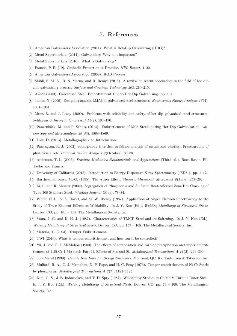
7. References

[1] American Galvanizers Association (2011). What is Hot-Dip Galvanizing (HDG)?

[2] Metal Supermarkets (2014). Galvanizing: Why is it important?

[3] Metal Supermarkets (2016). What is Galvanizing?

[4] Francis, P. E. (19). Cathodic Protection in Practise. NPL Report , 1–22.

[5] American Galvanizers Association (2009). HGD Process.

[6] Shibli, S. M. A., B. N. Meena, and R. Remya (2015). A review on recent approaches in the field of hot dip

zinc galvanizing process. Surface and Coatings Technology 262, 210–215.

[7] AZoM (2003). Galvanised Steel Embrittlement Due to Hot Dip Galvanising. pp. 1–4.

[8] James, N. (2009). Designing against LMAC in galvanised steel structures. Engineering Failure Analysis 16 (4),

1051–1061.

[9] Mraz, L. and J. Lesay (2009). Problems with reliability and safety of hot dip galvanized steel structures.

Soldagem & Inspecao (Impresso) 14 (2), 184–190.

[10] Panzenbock, M. and P. Schutz (2014). Embrittlement of Mild Steels during Hot Dip Galvanization. Mi-

croscopy and Microanalysis 20 (S3), 1868–1869.

[11] Diez, D. (2013). Metallography - an Introduction.

[12] Parrington, R. J. (2002). ractography is critical to failure analysis of metals and plastics . Fractography of

plastics is a rel-. Practical Failure Analysis 2 (October), 33–38.

[13] Anderson, T. L. (2005). Fracture Mechanics Fundamentals and Applications (Third ed.). Boca Raton, FL:

Taylor and Francis.

[14] University of California (2015). Introduction to Energy Dispersive X-ray Spectrometry ( EDS ). pp. 1–12.

[15] Barthes-Labrousse, M.-G. (1995). The Auger Effect. Microsc. Microanal. Microsruct 6 (June), 253–262.

[16] Li, L. and R. Messler (2002). Segregation of Phosphorus and Sulfur in Heat-Affected Zone Hot Cracking of

Type 308 Stainless Steel. Welding Journal (May), 78–84.

[17] White, C. L., S. A. David, and M. W. Richey (1987). Application of Auger Electron Spectroscopy to the

Study of Trace Element Effects on Weldability. In J. Y. Koo (Ed.), Welding Metallurgy of Structural Steels,

Denver, CO, pp. 101 – 114. The Metallurgical Society, Inc.

[18] Youn, J. G. and K. H. J. (1987). Characteristics of TMCP Steel and its Softening. In J. Y. Koo (Ed.),

Welding Metallurgy of Structural Steels, Denver, CO, pp. 157 – 168. The Metallurgical Society, Inc.

[19] Materia, T. (2003). Temper Embrittlement.

[20] TWI (2010). What is temper embrittlement, and how can it be controlled?

[21] Yu, J. and C. J. McMahon (1980). The effects of composition and carbide precipitation on temper embrit-

tlement of 2.25 Cr-1 Mo steel: Part II. Effects of Mn and Si. Metallurgical Transactions A 11 (2), 291–300.

[22] SorelMetal (1999). Ductile Iron Data for Design Engineers. Montreal, QC: Rio Tinto Iron & Titanium Inc.

[23] Mulford, R. A., C. J. Mcmahon, D. P. Pope, and H. C. Feng (1976). Temper embrittlement of Ni-Cr Steels

by phosphorus. Metallurgical Transactions A 7 (7), 1183–1195.

[24] Kim, G. S., J. E. Indacochea, and T. D. Spry (1987). Weldability Studies in Cr-Mo-V Turbine Rotor Steel.

In J. Y. Koo (Ed.), Welding Metallurgy of Structural Steels, Denver, CO, pp. 79 – 100. The Metallurgical

Society, Inc.

57

[25] Kikuta, Y., T. Araki, and M. Yoneda (1986). Liquid Metal Embrittlement Cracking By Molten Zinc

Structural Steel HAZ. Technical report, Oksaka University.

[26] Thomee, V. (2006). Galerkin Finite Element Methods for Parabolic Problems (Second ed.). Berlin: Springer.

[27] Szabo, B. and I. Babuska (1991). Finite Element Analysis (First ed.). New York, NY: John Wiley & Sons.

[28] Niazy, A. M. (1997). Type of Finite Elements and Steps in. Machine Design, 54–58.

[29] Cook, R. D., D. S. Malkus, M. E. Plesha, and R. J. Witt (2007). Concept and Applications of Finite Element

Analysis. New York, NY: John Wiley & Sons.

[30] Autodesk Knowledge (2015). How to Perform and Mesh Convergence Study.

[31] Cresdee, R., W. Edwards, P. Thomas, and G. Voss (1992). Analysis of beam distortion during hot dip

galvanizing. Materials Science and Technology 9 (2), 161–162.

[32] Johnson, W. H. (1875). On some remarkable Changes Produced in Iron and Steel by the Action of Hydrogen

and Acids. In Proceedings of the Royal Society of London, London, pp. 168. Taylor and Francis.

[33] Louthan, M. R. J. (2008). Hydrogen Embrittlement of Metals: A Primer for Failure Analyst.

[34] Kinstler, T. J. (2005). Current knowledge of the cracking of steels during galvanizing a synthesis of the

available technical literature and collective experience.

[35] Marcelo, A. L., R. C. Tokimatsu, and I. Ferreira (2009). Hydrogen embrittlement in an AISI 1045 steel

component of the sugarcane industry. Engineering Failure Analysis 16 (1), 468–474.

[36] Yu, H., D. Zeng, and Z. Liu (2010). Failure analysis on the rivet. Materials Science Forum 654-656 (June).

[37] lei Xu, X., Z. wei Yu, Z. Yang, and Y. zhen Chen (2011). Intergranular brittle cracking of truck diesel fuel

filter-cases. Engineering Failure Analysis 18 (8), 2054–2063.

[38] Brahimi Eng, S., S. Brahimi -, and S. Brahimi (2014). HYDROGEN EMBRITTLEMENT IN STEEL FAS-

TENERS Fundamentals of hydrogen embrittlement in steel fasteners Fundamentals of hydrogen embrittlement

in steel fasteners. pp. 1–23.

[39] Brahimi, S., S. Rajagopalan, S. Yue, and J. Szpunar (2009). Effect of Surface Processing Variables on

Hydrogen Embrittlement of Steel Fasteners Part 1 : Hot Dip Galvanizing. 48 (3), 293–301.

[40] Recio, F. J., M. C. Alonso, L. Gaillet, and M. Sanchez (2011). Hydrogen embrittlement risk of high strength

galvanized steel in contact with alkaline media. Corrosion Science 53 (9), 2853–2860.

[41] ASTM Internatinal (2017). Standard Test Methods and Definitions for Mechanical Testing of Steel Products.

[42] Ding, R., A. Islam, S. Wu, and J. Knott (2005). Effect of phosphorus segregation on fracture properties of

two quenched and tempered structural steels. Materials Science and Technology 21 (4), 467–475.

[43] Christien, F., R. Le Gall, and G. Saindrenan (2003). Phosphorus grain boundary segregation in steel 17-4

PH. Scripta Materialia 48 (3), 301–306.

[44] Borges, D., V. D. Castro, J. M. Ventura, C. Olivio, F. Terra, S. Paulo, A. T. Sao-carlense, P. A. Schmidt,

and S. Carlos (2010). Influence of Phosphorus Content and Quenching / Tempering Temperatures on Fracture

Toughness and Fatigue Life of SAE 5160 Steel. Materials Research 13 (4), 445–455.

[45] Matsuyama, T., H. Hosokawa, and H. Suto (1983). Tracer Diffusion of P in Iron and Iron Alloys. Transactions

of the Japan Institute of Metals 24 (8), 589–594.

[46] Beckhoff, B., B. Kanngieber, N. Langhoff, R. Wedell, and H. Wolff (2006). Handbook of Practical X-Ray

Fluorescence Analysis (First ed.). Berlin: Springer.

[47] Shimadzu (2014). Principle of Optical Emission Spectrometry.

[48] CSA Group (2013). Standard G40.20/G40.21 General requirements for rolled or welded structural quality

steel / Structural quality steel.

58

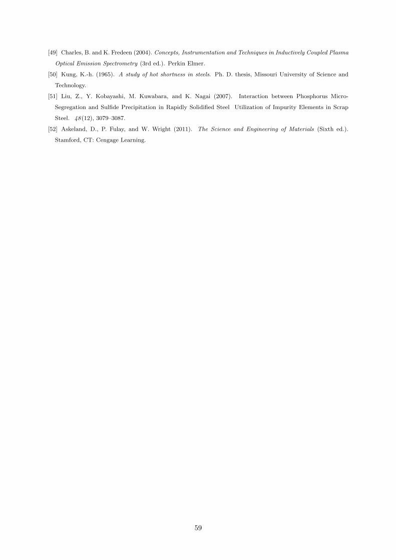
[49] Charles, B. and K. Fredeen (2004). Concepts, Instrumentation and Techniques in Inductively Coupled Plasma

Optical Emission Spectrometry (3rd ed.). Perkin Elmer.

[50] Kung, K.-h. (1965). A study of hot shortness in steels. Ph. D. thesis, Missouri University of Science and

Technology.

[51] Liu, Z., Y. Kobayashi, M. Kuwabara, and K. Nagai (2007). Interaction between Phosphorus Micro-

Segregation and Sulfide Precipitation in Rapidly Solidified Steel Utilization of Impurity Elements in Scrap

Steel. 48 (12), 3079–3087.

[52] Askeland, D., P. Fulay, and W. Wright (2011). The Science and Engineering of Materials (Sixth ed.).

Stamford, CT: Cengage Learning.

59

Appendix A: Base Material and Weld Images

This appendix provides further microscope images of the base material from Chapter 2 and

introduces images of the weld cross section, both macroscopically and microscopically.

A.1. Base Material Images

Higher and lower magnification images of the T-joint base material section, shown in Chapter

2, are given in Fig. A.1 and Fig. A.2.

(a) Horizontal member at 5X (b) Horizontal member at 10X

(c) Horizontal member at 100X

Fig. A.1: 5X, 10X and 100X of T-joint horizontal member’s base material

60

(a) Vertical member at 5X (b) Vertical member at 10X

(c) Vertical member at 100X

Fig. A.2: 5X, 10X and 100X of T joint vertical member’s base material

Another T-joint was sectioned and cut to prepare samples for further mechanical testing. How-

ever, base material samples were still taken from this T-joint for analysis. Images of the mi-

crostructure of the horizontal and vertical members are shown in Fig. A.3 and Fig. A.4. The

features of the microstructure were similar to what shown in the previous base material samples

in Chapter 2 and in Fig. A.1 and Fig. A.2.

61

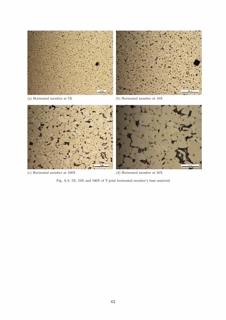
(a) Horizontal member at 5X (b) Horizontal member at 10X

(c) Horizontal member at 100X (d) Horizontal member at 50X

Fig. A.3: 5X, 10X and 100X of T-joint horizontal member’s base material

62

(a) Vertical member at 5X (b) Vertical member at 10X

(c) Vertical member at 100X (d) Vertical member at 50X

Fig. A.4: 5X, 10X and 100X of T-joint vertical member’s base material

A.2. Weld Images

The welded joints were also prepared and analyzed in the same fashion as the base material.

The cross section of the welds was the surface of study, and images of the different cross sections

can be seen in Fig. A.5.

63

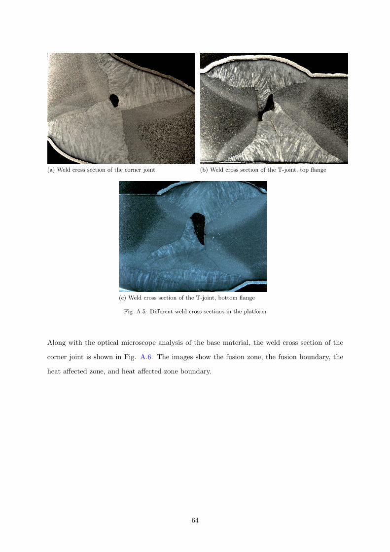
(a) Weld cross section of the corner joint (b) Weld cross section of the T-joint, top flange

(c) Weld cross section of the T-joint, bottom flange

Fig. A.5: Different weld cross sections in the platform

Along with the optical microscope analysis of the base material, the weld cross section of the

corner joint is shown in Fig. A.6. The images show the fusion zone, the fusion boundary, the

heat affected zone, and heat affected zone boundary.

64

(a) Fusion zone boundary at 5X (b) Fusion zone at 20X

(c) Heat affected zone boundary at 10X (d) Heat affected zone at 20X

Fig. A.6: Fusion zone and heat affected zone of the corner joint’s weld

Images of the side view of the weld were also captured at the crack initiation site. As an

extension to the images in Fig. 2.10, lower magnification pictures are shown in Fig. A.7, Fig.

A.8, and Fig. A.9.

65

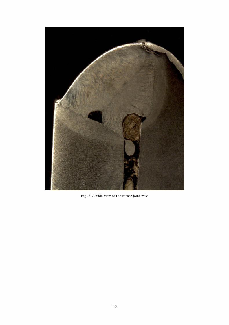
Fig. A.7: Side view of the corner joint weld

66

(a) Crack initiation site and upper secondary crack (b) 5X of upper secondary crack

Fig. A.8: Side view of the upper cracks in the corner joint weld

(a) Lower secondary crack (b) 5X of lower secondary crack

Fig. A.9: Side view of the lower cracks in the corner joint weld

67