Review

Recent Developments of Computational Methods for pKa PredictionBased on Electronic Structure Theory with Solvation Models

Ryo Fujiki 1, Toru Matsui 2 , Yasuteru Shigeta 3 , Haruyuki Nakano 1 and Norio Yoshida 1,*

�����������������

Citation: Fujiki, R.; Matsui, T.;

Shigeta, Y.; Nakano, H.; Yoshida, N.

Recent Developments of

Computational Methods for pKa

Prediction Based on Electronic

Structure Theory with Solvation

Models. J 2021, 4, 849–864.

https://doi.org/10.3390/j4040058

Academic Editor: Johan Jacquemin

Received: 24 November 2021

Accepted: 7 December 2021

Published: 10 December 2021

Publisher’s Note: MDPI stays neutral

with regard to jurisdictional claims in

published maps and institutional affil-

iations.

Copyright: © 2021 by the authors.

Licensee MDPI, Basel, Switzerland.

This article is an open access article

distributed under the terms and

conditions of the Creative Commons

Attribution (CC BY) license (https://

creativecommons.org/licenses/by/

4.0/).

1 Department of Chemistry, Graduate School of Science, Kyushu University, Fukuoka 819-0052, Japan;rfjk@ccl.scc.kyushu-u.ac.jp (R.F.); nakano@ccl.scc.kyushu-u.ac.jp (H.N.)

2 Department of Chemistry, Graduate School of Pure and Applied Sciences, University of Tsukuba,Tsukuba 305-8577, Japan; matsui@chem.tsukuba.ac.jp

3 Center for Computational Sciences, University of Tsukuba, Tsukuba 305-8577, Japan;shigeta@ccs.tsukuba.ac.jp

* Correspondence: noriwo@chem.kyushu-univ.jp

Abstract: The protonation/deprotonation reaction is one of the most fundamental processes insolutions and biological systems. Compounds with dissociative functional groups change theircharge states by protonation/deprotonation. This change not only significantly alters the physicalproperties of a compound itself, but also has a profound effect on the surrounding molecules. Inthis paper, we review our recent developments of the methods for predicting the Ka, the equilibriumconstant for protonation reactions or acid dissociation reactions. The pKa, which is a logarithm ofKa, is proportional to the reaction Gibbs energy of the protonation reaction, and the reaction freeenergy can be determined by electronic structure calculations with solvation models. The charge ofthe compound changes before and after protonation; therefore, the solvent effect plays an importantrole in determining the reaction Gibbs energy. Here, we review two solvation models: the continuummodel, and the integral equation theory of molecular liquids. Furthermore, the reaction Gibbs energycalculations for the protonation reactions require special attention to the handling of dissociatedprotons. An efficient method for handling the free energy of dissociated protons will also be reviewed.

Keywords: pKa; pKw; PCM; 3D-RISM; DFT; solvation

1. Introduction

The protonation and deprotonation reactions of dissociative functional groups insolvated compounds often play essential roles in chemical and biological processes, suchas solvation, protein–ligand binding, and the higher-order structure formation of pro-teins. Such processes occur in complex environments, where the functional groups aresurrounded by other molecules, ions, and water. The equilibrium of the pronation anddeprotonation states is governed by the Gibbs energy change of the reaction; thus, it can bestated that the process is fully thermodynamic.

The equilibrium constants of the protonation/deprotonation reaction, or the aciddissociation reaction, Ka, or its logarithm, pKa, can be measured experimentally by titrationcombined with pH electrode measurement, vibrational spectroscopy, neutron diffraction,and nuclear magnetic resonance. However, experimental values are not always available;hence, highly accurate prediction by computational means is most desirable [1].

Currently, one of the most successful methods for predicting the pKa values of aminoacids in proteins is PROPKA, an empirical method based on the three-dimensional (3D)protein structure [2]. The method can estimate the pKa value, or the charged states of theamino acids in target proteins, within a reasonable computational time and with accuracy.However, to understand the mechanism of the protonation reactions and the pKa shiftsdue to the environment, a nonempirical approach based on molecular theory is effective.

J 2021, 4, 849–864. https://doi.org/10.3390/j4040058 https://www.mdpi.com/journal/j

J 2021, 4 850

An accurate estimation of the free-energy change in the protonation process is indis-pensable for quantitative pKa prediction. Therefore, estimating the energy change beforeand after dissociation using quantum chemistry calculations is a very effective approach.

In this paper, we review our recent developments of the computational methods forpredicting pKa values, which are based on quantum chemical electronic structure methodscombined with solvation models. Here, we review the methods employed. Specifically, wereview two different solvation models: the polarizable continuum model (PCM) and thereference interaction site model (RISM) theories.

Quantum chemical calculations, such as density functional theory (DFT), can oftenbe used to avoid the computational parameter dependence. For the pKa values of smallcompounds, a number of studies using quantum chemical calculations have been reported,and the details of their accuracy are discussed in a review by Ho and Coote [3]. To es-timate reliable pKa values, it is necessary to obtain the solvation free-energy differenceof the molecules in aqueous solution, due to acid dissociation, as accurately as possible.Sprik and coworkers proposed a method for obtaining the free-energy profile due to aciddissociation from DFT-based ab initio molecular dynamics (AIMD) simulations and suc-cessfully obtained the pKa values of many compounds, including amino acids in aqueoussolution [4]. Although this method is highly accurate for pKa prediction, long computa-tion times are required to obtain the solvation free-energy difference, thus indicating thatit is only applicable to small molecules. To avoid these high computational costs, it is,therefore, essential to employ solvation free-energy calculation methods that are based onstatic quantum chemical methods. Recently, combinations of various quantum chemicalcalculation methods and the PCM have been explored in considering the solvent effects.High-precision solvation free-energy calculations can be used to discuss deprotonationtrends in aqueous solutions [5–10]. The accuracy is in good agreement with experimentalvalues, as reported by Takano and Houk [11].

However, even in pKa calculations using the static DFT calculations with the PCMmodel, one often encounters several problems when adopting the conventional methods.One such problem is the choice of methodology (combinations of quantum chemicalcalculation methods, basis functions, cavity models, and the parameters of the PCM), andthe error can vary greatly depending on the choice. An additional problem is that thesolvation free energies of similar molecules, having the same chemical groups, tend to havecorrelations among them, while this rule is not applicable for all molecules. Because ofsuch a methodology and the chemical group dependence, the calculated pKa values scattertoward the corresponding experimental values.

One of the root causes in this complex issue is the treatment of the proton’s solvationfree-energy value. Conventional methods adopt some reference value (e.g., values fromexperimental values) and assume that it is a constant value in the calculation of the pKafor any type of molecule. Unlike an arbitrary molecule, the solvation free energy of oneproton (H+), Gsolv

(H+), cannot be directly calculated because the proton has no electrons.

Instead, Gsolv(H+)

is sometimes calculated from the dissociation of a proton from thehydronium ion, H3O+, Gsolv

(H+)= Gsolv

(H3O+

)− Gsolv(H2O). The hydronium ion

is surrounded by many water molecules and forms a hydrogen-bonding network withthem; hence, it is desirable to use larger proton solvation clusters and/or other protonexchange reactions involving protonated/deprotonated compounds, except for H2n+1O+

nclusters. However, the computational costs increase exponentially when the size of theclusters increases because of the vast configurations of the water clusters, as in the AIMDcalculations. Therefore, it is extremely difficult to obtain the solvation free energy of theproton with high accuracy, which indicates that, in many cases, it has not been possible toquantitatively reproduce pKa values.

In efforts to address the above, we have developed a methodology- and chemical-group-dependent approach for the evaluation of pKa values using PCM-based meth-ods [12–15]. This method refers to the experimental data of representative molecules withspecific chemical groups, such as COOH, OH (alcohol), OH (phenol), SH, and NH2, among

J 2021, 4 851

others. As noted earlier, the Gsolv(H+)

value depends strongly on the choice of method-ology. Thus, the correction terms for the Gsolv

(H+)

value should be evaluated for eachmethodology and chemical group considered. Our linear scaling scheme, mentioned inSection 3.2, provided the error within 0.25 pKa units for standard PCM–DFT calculations.The details of this scheme are reported later.

The success of the abovementioned method allows us to adopt other static solvationmodels that differ from the PCM. The RISM theory is a statistical mechanics integralequation theory of molecular liquids, derived from the density functional derivative ofthe grand potential under a solute–solvent molecular pair interaction [16–19]. Unlikethe PCM, the theory now allows us to consider molecular interaction, such as hydrogenbonding, which plays an important role in the acid dissociation reaction. In addition, theanalytical solvation free-energy formula is known and can be evaluated on the basis of thefirst-principles approach. Although the computational cost is somewhat higher than that ofthe PCM, it has, nonetheless, been used to analyze various chemical processes in solutionbecause of the above advantages. An extension of the RISM theory that is applicable tohighly complex molecules, such as proteins, is the so-called 3D-RISM theory [20–22]. Thelatter can be derived from the six-dimensional molecular Ornstein–Zernike equation byapplying the interaction site model for solvent molecules. The hybrid methods of the RISM,or the 3D-RISM theory with the quantum chemical electronic structure theory, are referredto as the RISM self-consistent field (SCF), or as the 3D-RISM-SCF theories [23–25].

In this paper, we review two types of approaches that are based on the RISM-SCF/3D-RISM-SCF theory: namely, the first-principles approach and the data-driven approach.In their pioneering work, Sato and coworkers applied the first-principles approach formeasuring the pKw, which is the equilibrium constant of the autoionization reaction ofwater [26,27]. Their method has been applied to studies of the pKa of various systems inefforts to improve the accuracy. These studies have revealed that the most serious problemto be addressed, namely, improving the accuracy, is the estimation of the free energy ofthe dissociated protons. As mentioned above, Matsui et al. proposed a method to avoidthis difficulty by using a data-driven approach with the PCM method [14]. Fujiki et al.extended their method by combining the 3D-RISM-SCF and Matsui’s method and achievedquantitative accuracy of the predicted pKa values [28].

The organization of this review is as follows: Section 2 provides a general backgroundto pKa computation. In Sections 3 and 4, theoretical studies, based on the PCM and RISM,respectively, are reviewed. In Section 5, we include a summary and offer some futureperspectives pertaining to computational pKa prediction.

2. Basics of pKa Computation

The pKa value is proportional to the Gibbs energy change of the protonation reaction,or the acid dissociation reaction, ∆G, given by:

pKa =∆G

(ln 10)RT(1)

where R and T denote the gas constant and absolute temperature, respectively. The Gibbsenergy change, ∆G, is:

∆G = G(A−)+ G

(H+)− G(HA) (2)

= ∆Ggas + ∆GsolvA− + ∆Gsolv

H+ − ∆GsolvHA (3)

where G(A−), G(HA), and G

(H+)

denote the Gibbs energy of the unprotonated andprotonated states of an acid, A, and that of a dissociated proton, respectively (See Figure 1).If we consider a thermodynamic cycle of the reaction, Equation (2) can be written asEquation (3), using the gas-phase reaction Gibbs energy, ∆Ggas, and the solvation freeenergy of the A−, H+, and HA, namely, ∆Gsolv

A−, ∆Gsolv

H+ , ∆GsolvHA , respectively. These Gibbs

energy terms can be evaluated by quantum chemical electronic structure calculations,such as the ab initio molecular orbital (MO) theory, or the Kohn–Sham DFT (KS-DFT).

J 2021, 4 852

As mentioned earlier, since a compound/an acid, A, rearranges its electronic structurebecause of the protonation/deprotonation, a precise treatment of the electronic structureof the target compounds is highly anticipated. Furthermore, the solvent environmentsurrounding the target compounds must be considered. The most popular way to takesolvent effects into account is to implement the PCM, one of the implicit solvation models,which is implemented in all the popular quantum chemical software packages, such asGaussian and GAMESS. The computational methods employing the PCM will be reviewedin Section 3. Other candidates applicable to the consideration of the solvent effects on theelectronic structure of solvated molecules are the integral equation theories of molecularliquids, namely, the RISM and 3D-RISM theories, which allow us to treat the solvent effectson the basis of the statistical mechanics theory on the molecular level, unlike the PCM. ThepKa computation method based on the RISM/3D-RISM will be reviewed in Section 4.

J 2021, 4 FOR PEER REVIEW    4  

If we consider a thermodynamic cycle of the reaction, Equation (2) can be written as Equa‐

tion (3), using the gas‐phase reaction Gibbs energy,  Δ𝐺 , and the solvation free energy 

of  the  A , H , and HA, namely,  Δ𝐺 , Δ𝐺 , Δ𝐺 ,  respectively. These Gibbs energy 

terms can be evaluated by quantum chemical electronic structure calculations, such as the 

ab initio molecular orbital (MO) theory, or the Kohn–Sham DFT (KS‐DFT). As mentioned 

earlier, since a compound/an acid, A, rearranges  its electronic structure because of  the 

protonation/deprotonation, a precise  treatment of  the electronic  structure of  the  target 

compounds is highly anticipated. Furthermore, the solvent environment surrounding the 

target compounds must be considered. The most popular way to take solvent effects into 

account is to implement the PCM, one of the implicit solvation models, which is imple‐

mented  in all the popular quantum chemical software packages, such as Gaussian and 

GAMESS. The computational methods employing the PCM will be reviewed in Section 3. 

Other candidates applicable to the consideration of the solvent effects on the electronic 

structure of solvated molecules are  the  integral equation  theories of molecular  liquids, 

namely, the RISM and 3D‐RISM theories, which allow us to treat the solvent effects on the 

basis of the statistical mechanics theory on the molecular level, unlike the PCM. The  p𝐾  

computation method based on the RISM/3D‐RISM will be reviewed in Section 4. 

 

Figure 1. Schematic description of thermodynamic cycle of the acid dissociation reaction. 

3. Polarizable Continuum Model‐Based Approach 

3.1. Basics of the Polarizable Continuum Model 

Among the methods that incorporate solvent effects, the dielectric model is a rela‐

tively simple method that is installed in many quantum chemistry program packages. In 

this section, we present a basic concept of the PCM for describing solvent effects and the 

results using this model. 

In the continuum model, a cavity is created around a molecule filled with a dielectric 

medium with a dielectric constant,  𝜀. We refer to the change in properties caused by this 

effect as the “solvent effect”. This effect can be described as in Equation (4): 

Δ𝐺 Δ𝐺 Δ𝐺 Δ𝐺   (4)

In this equation, the latter two terms are obtained by the empirical method obtained 

from the volume/surface of a solute. For further details, see the following references by 

Mennucci’s group and the references therein [29,30]. In the dielectric model,  𝑉 𝒓   con‐sists of two types of potential. One is the electrostatic potential,  𝑉   from  𝜌 𝒓 . The other 

is  the  reaction potential,  𝑉 , generated by  the polarization emanating  from  the solvent 

molecules: 

𝑉 𝒓 𝑉 𝒓 𝑉 𝒓   (5)

In  the dielectric model, a vacancy  in  the  form of a solute molecule  is  formed  in a 

continuous dielectric, and the solute molecule is placed in the vacancy, using the polari‐

zation surface charge density,  𝜎 𝒔 , at the boundary of the vacancy. When  𝑑   expresses 

an area integral,  𝑉 𝒓   can be written as follows: 

𝑉 𝒓 𝑑 𝒔𝜎 𝒔𝒓 𝒔

  (6)

Figure 1. Schematic description of thermodynamic cycle of the acid dissociation reaction.

3. Polarizable Continuum Model-Based Approach3.1. Basics of the Polarizable Continuum Model

Among the methods that incorporate solvent effects, the dielectric model is a relativelysimple method that is installed in many quantum chemistry program packages. In thissection, we present a basic concept of the PCM for describing solvent effects and the resultsusing this model.

In the continuum model, a cavity is created around a molecule filled with a dielectricmedium with a dielectric constant, ε. We refer to the change in properties caused by thiseffect as the “solvent effect”. This effect can be described as in Equation (4):

∆Gsolv = ∆Gelec + ∆Gcavity + ∆Gdispersion (4)

In this equation, the latter two terms are obtained by the empirical method obtainedfrom the volume/surface of a solute. For further details, see the following references byMennucci’s group and the references therein [29,30]. In the dielectric model, V(r) consistsof two types of potential. One is the electrostatic potential, VR from ρ(r). The other is thereaction potential, Vσ, generated by the polarization emanating from the solvent molecules:

V(r) = VR(r) + Vσ(r) (5)

In the dielectric model, a vacancy in the form of a solute molecule is formed in a con-tinuous dielectric, and the solute molecule is placed in the vacancy, using the polarizationsurface charge density, σ(s), at the boundary of the vacancy. When d2 expresses an areaintegral, Vσ(r) can be written as follows:

Vσ(r) =∫

Γd2s

σ(s)r− s

(6)

This surface integral is obtained by dividing the whole into smaller parts, Ak, andfinding the sum of them:

Vσ(r) ≈∑k

σ(s)Akr− sk

= ∑k

qkr− sk

(7)

J 2021, 4 853

The qk in Equation (7) depends on the overall charge, which is calculated from theelectrostatic potential obtained when the solute molecules are assumed to be in a vacuum. Wemust consider the following equation to satisfy the boundary condition mentioned earlier:

σ(s) =ε− 14πε

∂

∂n(VR + Vσ)s (8)

where n is the unit vector of the normal vector at a point, s, on the surface, and the directionis from inside the cavity to the outside. When we define the integral operator, D∗, theabove equation can be rewritten as follows:(

2πε + 1ε− 1

I − D∗)

σ(s) =∂

∂n(VR)s (9)

where I is the unit operator. The conductor-like screening model [5] is based on the idea thatthe dielectric constant, ε, is now assumed, but, because of the effect of the solvent–soluteinteraction, it does not actually shield the charge effect, as per the value of ε. In this model,the following equation is assumed:

Sσ(s) = − f (ε)VR(s) =∫

Γd2s′

1|s− s′|σ

(s′)

(10)

The f (ε) in the following equation is an artificial function specific to this model:

f (ε) =ε− 1ε + x

(11)

where there is an arbitrariness in the value of x. In the PCM, x = 0 is used, and the modelis referred to as a conductor-like PCM. As an alternative to this type of shielding, one cansolve the integral equation by another method, the integral equation formulation of thePCM [7]: (

2πε + 1ε− 1

I −D)

Sσ(s) = −(2π I − D)(VR)s (12)

By replacing each of these, we obtain what is called the PCM formation:

Tσ(s) = −RVR(s), (13)

Obtaining VR(s) is similar to the SCF calculations performed, where the interactionenergy, Vσ(r), is obtained by iteratively calculating σ(s) and then adding the energy of thevacancy formation, etc., as an empirical value, to obtain the overall energy.

The calculation results are poor in many cases because of the addition of parametersunder the assumption of an ideal gas. The solvation model of Truhlar and coworkersimproved this term by calling it “cavitation”, “dispersion”, and “solvent structural ef-fects” [31]. The most commonly used model is its density version (SMD, often referred toas “PCM-SMD”). By setting the structural information of a molecule into a parameter, thismodel reproduces the solvation energy of many types of solvents very well. Although theother parts are based on the derivation method of the PCM, the SMD is the most frequentlyused solvent model in quantum chemistry calculations.

3.2. The AKB Scheme

We now briefly summarize the “appropriate pKa estimation with benchmark molecules”(AKB) scheme, the details of which were reported previously [14,32,33].

As noted earlier, the difference between the computed and observed pKa valuesdepends on the computational methods, such as the functional of DFT, the basis set,and the cavity of the PCM method; hence, the error should be systematic within similar

J 2021, 4 854

reactions. In computing the pKa with the AKB scheme, the Gibbs energy difference betweenthe reactant and the product is scaled by s as follows:

pKmodifieda =

s∆G(ln 10)RT

=s{

Gsolv(A−)− Gsolv(HA)}

(ln 10)RT+

Gsolv(H+)

(ln 10)RT(14)

The scaling factor, s, corresponds not only to an activity coefficient of the deproto-nation reaction, but also to an error correction for a given computational method. Weregard Gsolv

(H+)

and s as constants, both of which depend on the approximation levels.Equation (14) then becomes:

pKmodifieda = k

{Gsolv(A−)− Gsolv(HA)

}+ C0 = k∆G0 + C0 (15)

where ∆G0 is defined as Gsolv(A−) − Gsolv(HA). Equation (15) results in an apparentlinear correlation between the ∆G0 and pKa values. Therefore, it is possible to compute anunknown pKa by fitting k and C0 for reference molecules. We computed ∆G0 for severalcompounds that have either COOH, OH (phenol), or NH2 (aniline) groups, and plottedit with the experimental pKa values, where linear regression curves were estimated byleast-squares analysis (see Figure 2). The calculations by B3LYP/6-31++G(d, p) with thePCM-SMD provide a good result, within 0.2 pKa units (mean absolute error) in aqueoussolution [32]. Note that, here, the slopes (k) for the COOH, OH (phenol), and NH2 (aniline)groups differ from each other, indicating that the curves also exhibit the chemical-groupdependence. Once the linear regression curve is obtained, from Equation (14), one canestimate the Gibbs energy of the proton in aqueous solution using the slope and the abscissa,as follows:

Gsolv(H+)=

C0

k(16)

J 2021, 4 FOR PEER REVIEW    6  

As noted earlier, the difference between the computed and observed  p𝐾   values de‐

pends on the computational methods, such as the functional of DFT, the basis set, and the 

cavity of the PCM method; hence, the error should be systematic within similar reactions. 

In computing  the  p𝐾  with  the AKB scheme,  the Gibbs energy difference between  the 

reactant and the product is scaled by s as follows: 

p𝐾𝑠Δ𝐺

ln 10 𝑅𝑇𝑠 𝐺 A 𝐺 HA

ln 10 𝑅𝑇𝐺 Hln 10 𝑅𝑇

  (14)

The scaling factor, s, corresponds not only to an activity coefficient of the deprotona‐

tion reaction, but also to an error correction for a given computational method. We regard 

𝐺 H   and s as constants, both of which depend on the approximation levels. Equation 

(14) then becomes: 

p𝐾 𝑘 𝐺 A 𝐺 HA 𝐶 𝑘Δ𝐺 𝐶   (15)

where  Δ𝐺   is defined as  𝐺 A 𝐺 HA . Equation (15) results in an apparent lin‐

ear correlation between the  Δ𝐺   and  p𝐾   values. Therefore, it is possible to compute an 

unknown  p𝐾   by fitting  𝑘  and  𝐶   for reference molecules. We computed  Δ𝐺   for sev‐

eral compounds that have either COOH, OH (phenol), or NH2 (aniline) groups, and plot‐

ted it with the experimental  p𝐾   values, where linear regression curves were estimated 

by least‐squares analysis (see Figure 2). The calculations by B3LYP/6‐31++G(d, p) with the 

PCM‐SMD provide a good result, within  0.2 p𝐾   units (mean absolute error) in aqueous 

solution [32]. Note that, here, the slopes (𝑘   for the COOH, OH (phenol), and NH2 (ani‐

line) groups differ from each other, indicating that the curves also exhibit the chemical‐

group dependence. Once the linear regression curve is obtained, from Equation (14), one 

can estimate the Gibbs energy of the proton in aqueous solution using the slope and the 

abscissa, as follows: 

𝐺 H𝐶𝑘  (16)

The 𝐺 H   for  the COOH, OH  (phenol), and NH2  (aniline) groups are 1115.71, 

1065.32, and 1094.92 kJ/mol, respectively. This result indicates that, if one adopts the same 

𝐺 H   value for evaluating the  p𝐾   values of these compounds, a large error  is ob‐

tained when using Equation (2). The AKB scheme complements the errors arising from 

both a difference in the method and the chemical groups, simultaneously. 

 

Figure 2. Example of linear fitting at B3LYP/6‐31++G(d, p) + PCM‐SMD level. Three chemical groups 

(COOH, phenol, and aniline) were considered. R2 is the coefficient of determination. 

   

Figure 2. Example of linear fitting at B3LYP/6-31++G(d, p) + PCM-SMD level. Three chemicalgroups (COOH, phenol, and aniline) were considered. R2 is the coefficient of determination.

The Gsolv(H+)

for the COOH, OH (phenol), and NH2 (aniline) groups are 1115.71,1065.32, and 1094.92 kJ/mol, respectively. This result indicates that, if one adopts thesame Gsolv(H+

)value for evaluating the pKa values of these compounds, a large error is

obtained when using Equation (2). The AKB scheme complements the errors arising fromboth a difference in the method and the chemical groups, simultaneously.

3.3. Some Applications of the AKB Scheme

The linear scaling method is a very powerful scheme because it enables us to computethe pKa values for many compounds.

J 2021, 4 855

3.3.1. Application to Salicylic Acid

Salicylic acid (2-hydroxybenzoic acid) has a COOH group and an OH (phenol) group;hence, two different regioisomers exist (3- and 4-hydroxybenzoic acid) (see Figure 3).Experimentally, the first pKa value of salicylic acid is lower than the values of benzoic acid(pKa = 4.20) and phenol (pKa = 9.95) because the hydrogen bond between the neighboringCOO− and OH groups stabilizes the deprotonated compound. This detail is presumedfrom the structures and experimental results, but it has not yet been accurately confirmedby theory. Although salicylic acid has good analgesic action, it can simultaneously cause theperforation of stomach ulcers as one of its adverse effects because of the low pKa. To reducethe adverse effect while retaining the medicinal action, acetylsalicylic acid (commerciallyknown as aspirin) was synthesized. Here, we examine both the first and second pKa valuesof the hydroxybenzoic acids, and the pKa value of the acetylsalicylic acid, to clarify therelationship between the pKa and the structure of the conformers.

J 2021, 4 FOR PEER REVIEW    8  

     (a)  (b)  (c) 

Figure 3. Two conformers of salicylic acid. Conformer (a) forms a hydrogen bond between a phenol OH and a COOH 

group (shown by the broken line), conformer (b) does not form a hydrogen bond, and conformer (c) is aspirin. The black, 

red, and white balls represent carbon, oxygen, and hydrogen atoms, respectively. 

3.3.2. Solvent Dependence 

We next investigated the solvent dependencies on  p𝐾   using various solvents [35–

37]. Table 2 shows the results of the fitting and the estimated Gibbs energy of a proton of 

each solvent molecule. Again, the AKB method provided very good results. Interestingly, 

the experimental  p𝐾   value is very different because of the  𝐺 H   for acetonitrile and 

DMSO, which have  similar dielectric  constants. The  same  also  applies  to  aniline. The 

deprotonation Gibbs energy decreases as the dielectric constant decreases. This is why the 

p𝐾   values in THF are too low, even though the proton affinity of THF and acetonitrile is 

similar. Conversely, in the case of acids, such as carboxylic acids, the deprotonation Gibbs 

energy increases as the dielectric constant decreases. Table 2 shows the results for aniline. 

There are two different experimental results for THF; therefore, two results from the AKB 

scheme are independently shown. One of the problems associated with the AKB scheme 

is that we are unable to judge whether the experimental results are reliable or not when 

there is not much data available. 

Table 2. Solvent dependence on the scaling factor,  𝑘, Gibbs energy of a proton, and mean absolute 

error (MAE) in computing  p𝐾   for aniline derivatives. 𝑁  indicates the samples of aniline deriva‐

tives that have experimental  p𝐾   values for the solvents. 

Solvent  ε  N  Ref.  k  G(H+)  MAE 

Water  78.4  14  [35]  0.09641  –1094.9  0.38 

Methanol  32.7  6  [35]  0.09454  –1080.5  0.19 

DMSO  46.7  4  [35]  0.11580  –1112.2  0.22 

Acetonitrile  36.0  9  [35]  0.10487  –1046.3  0.50 

THF a  7.58  4  [36]  0.11712  –1066.4  0.19 

THF b  7.58  7  [37]  0.05938  –988.7  0.42 

Acetone b  20.7  5  [37]  0.06186  –1042.7  0.25 

Nitromethane b  35.9  6  [37]  0.09395  –1048.2  0.23 a  p𝐾   is listed. b  p𝐾   is listed. 

4. Integral Equation‐Based Approach 

In  this section, computational methods based on  integral equation  theories, RISM, 

and 3D‐RISM, are reviewed. A comparison between the PCM‐based method and the 3D‐

RISM‐based method will also be discussed. 

4.1. Basics of RISM‐SCF and 3D‐RISM‐SCF 

In  this subsection,  the basics of  the RISM‐SCF and 3D‐RISM‐SCF methods are ex‐

plained. Since the formalisms of these two methods are very similar, that of RISM‐SCF 

will be explained  first,  followed by a brief description of  the 3D‐RISM‐SCF  formalism 

later. 

Figure 3. Two conformers of salicylic acid. Conformer (a) forms a hydrogen bond between a phenol OH and a COOHgroup (shown by the broken line), conformer (b) does not form a hydrogen bond, and conformer (c) is aspirin. The black,red, and white balls represent carbon, oxygen, and hydrogen atoms, respectively.

For simplicity, we considered two conformations (Figure 3). Conformer (a) has ahydrogen bond between the phenol and carboxyl groups, whereas conformer (b) does nothave any hydrogen bonds. Because of this difference, conformer (a) is more stable thanconformer (b), by 22.1 kJ/mol, at the computational level. Hence, in the case of the salicylicacid, the existence of (b) is negligibly small, judging from the Boltzmann distribution.Table 1 provides the calculated ∆G and pKa values for each conformer. It was found thatboth of the pKa values for conformer (a) agree well with the experimental values: 2.97 and13.4 [34]. However, the pKa values for conformer (b) are similar to those of the benzoicacid (pKa = 4.20) and phenol (pKa = 9.95). This difference is ascribed to the effect ofthe presence of a hydrogen bond in conformer (a). Specifically, the first deprotonatedcompound is stabilized by the hydrogen bond in conformer (a), which decreases the pKavalue by 1.5 units in the first deprotonation and increases the pKa value by 2.5 units inthe second deprotonation. These results indicate how the hydrogen bond strongly affectsthe pKa value in small molecules, such as those of the salicylic acid. Furthermore, tounderstand this effect, we then examined (c) (aspirin), which has no explicit intramolecularinteraction (see Figure 3). The corresponding results are also shown in Table 1. Here, thepKa values of the regioisomers differ from the value of the salicylic acid. Because of theabsence of an intramolecular hydrogen bond, the pKa values of these isomers are alsofound to be close to the pKa values of each chemical group. In the case of aspirin, thepKa value is lower than that of the benzoic acid, but higher than that of the salicylic acid.Therefore, the neighboring acetyl group also affects the pKa of the COOH group through aweaker hydrogen bond than that of the salicylic acid, or through a secondary hydrogenbond via water molecules. Our scheme can also consider the effect of the acetylation,compared with the salicylic acid alone, the effect of which is not fully treated in empirical

J 2021, 4 856

approaches, such as PROPKA and H++. Our results demonstrate that our scheme is safelyand accurately applicable to the evaluation of the pKa of arbitrary molecules.

Table 1. Deprotonation Gibbs energy (in kJ/mol) and estimated pKa in each conformer of salicylicacid. Numbers in parentheses indicate experimental values.

Compound ∆G0,a1 pKa1 ∆G0,a2 pKa2

(a) 1157.9 2.69 (2.97) 1271.4 13.29 (13.40)(b) 1180.0 4.10 (2.97) 1232.1 10.76 (13.40)(c) 1174.6 3.76 (3.49) - -

pKa1 is from the COOH group, and pKa2 is from the phenol group.

3.3.2. Solvent Dependence

We next investigated the solvent dependencies on pKa using various solvents [35–37].Table 2 shows the results of the fitting and the estimated Gibbs energy of a proton of eachsolvent molecule. Again, the AKB method provided very good results. Interestingly, theexperimental pKa value is very different because of the Gsolv(H+

)for acetonitrile and

DMSO, which have similar dielectric constants. The same also applies to aniline. Thedeprotonation Gibbs energy decreases as the dielectric constant decreases. This is why thepKa values in THF are too low, even though the proton affinity of THF and acetonitrile issimilar. Conversely, in the case of acids, such as carboxylic acids, the deprotonation Gibbsenergy increases as the dielectric constant decreases. Table 2 shows the results for aniline.There are two different experimental results for THF; therefore, two results from the AKBscheme are independently shown. One of the problems associated with the AKB scheme isthat we are unable to judge whether the experimental results are reliable or not when thereis not much data available.

Table 2. Solvent dependence on the scaling factor, k, Gibbs energy of a proton, and mean absoluteerror (MAE) in computing pKa for aniline derivatives. N indicates the samples of aniline derivativesthat have experimental pKa values for the solvents.

Solvent ε N Ref. k G (H+) MAE

Water 78.4 14 [35] 0.09641 −1094.9 0.38Methanol 32.7 6 [35] 0.09454 −1080.5 0.19

DMSO 46.7 4 [35] 0.11580 −1112.2 0.22Acetonitrile 36.0 9 [35] 0.10487 −1046.3 0.50

THF a 7.58 4 [36] 0.11712 −1066.4 0.19THF b 7.58 7 [37] 0.05938 −988.7 0.42

Acetone b 20.7 5 [37] 0.06186 −1042.7 0.25Nitromethane b 35.9 6 [37] 0.09395 −1048.2 0.23

a pKa is listed. b pKb is listed.

4. Integral Equation-Based Approach

In this section, computational methods based on integral equation theories, RISM,and 3D-RISM, are reviewed. A comparison between the PCM-based method and the3D-RISM-based method will also be discussed.

4.1. Basics of RISM-SCF and 3D-RISM-SCF

In this subsection, the basics of the RISM-SCF and 3D-RISM-SCF methods are ex-plained. Since the formalisms of these two methods are very similar, that of RISM-SCF willbe explained first, followed by a brief description of the 3D-RISM-SCF formalism later.

Similar to the PCM, the total free energy of solvated molecules is given by:

G = Ggas + ∆Gsolv (17)

J 2021, 4 857

where Ggas is the free energy of the molecule in an isolated system or gas phase, which isevaluated as an expected value of the gas-phase Hamiltonian with respect to the solvatedwave function, Ggas = Ψsolute

∣∣Hgas |Ψ solute . It is noted that the Ψsolute is an eigen functionof the solvated Hamiltonian, which includes the solvent electrostatic potential as an externalfield. ∆Gsolv is the solvation free energy, expressed by:

∆Gsolv = 4π ∑i∈solute

∑j∈solvent

ρj

∫ [12(hij(r)

)2Θ(−hij(r)

)− cij(r)−

12

hij(r)cij(r)]

r2dr (18)

where ρj is the number density of the solvent site, j. The summations of i and j are runningover the interaction sites in the solute and solvent molecules, respectively. The hij(r) andcij(r) are the total and direct correlation functions, evaluated by solving the RISM integralequation. These are the function of the distance between two interaction sites, i and j. Toderive Equation (18), the Kovalenko–Hirata (KH) closure equation is employed [24,38]. Ifone employs the hypernetted chain (HNC) closure, instead of the KH closure, the Heavisidestep function, Θ, is replaced by 1. The RISM/KH equation is solved under the followingsolute–solvent interaction potential:

uij(r) = 4εij

[(σij

r

)12−(

σij

r

)6]+

qiqj

r(19)

where εij and σij are the Lennard–Jones parameters, with the usual meanings. qi and qjdenote point charges on the solute site, i, and solvent site, j, respectively. The solute pointcharge, qi, is determined to reproduce the electrostatic potential, due to the solute electronicstructure, by the least-squares fitting method, known as the “restrained electrostatic poten-tial” method. The solute wave function depends on the solvent distribution, which dependson the solute wave function through the solute–solvent interaction potential. Therefore,the quantum chemical electronic structure and the RISM calculations were performed untilthe solute wave function and solvent distribution were unchanged iteratively.

In the case of the 3D-RISM-SCF, ∆Gsolv is given by:

∆Gsolv = ∑j∈solvent

ρj

∫ [12(hj(r)

)2Θ(−hj(r)

)− cj(r)−

12

hj(r)cj(r)]

dr (20)

where hj(r) and cj(r) are the total and direct correlations in 3D format, respectively. Thesefunctions are obtained as the results of the 3D-RISM calculation coupled with the 3D-KHclosure. In contrast to the correlation functions of the RISM, the hj(r) in the 3D-RISMis related to the special distribution of solvent species. The solute–solvent interactionpotential is given by:

uj(r) = ∑i∈solute

4εij

[(σij

r

)12−(

σij

r

)6]−∫ |Ψsolute(r′)|

2qj

|r− r′| dr + ∑i∈solute

Ziqj∣∣ri − rj∣∣ (21)

where Ψsolute is the wave function of a solute molecule, and Zi is the nucleus charge of asolute atom, i. Unlike the RISM case, the electrostatic potential, due to the solute molecule,can be evaluated from the solute wave function directory, which is a great advantage ofthe 3D-RISM-SCF theory over the RISM-SCF theory. Therefore, since the 3D-RISM canincorporate anisotropic solvent distribution under the spatial distribution of solute electrondensity, it is suitable for handling complex solutes, such as biomolecules.

4.2. First-Principles Calculation of pKa and pKw

The pKa can be determined by first-principles calculations, such as evaluating thefree energy of the reactant and the product species of the acid dissociation reaction usingRISM-SCF or 3D-RISM-SCF theories.

J 2021, 4 858

The pioneering work using the first-principles calculation by the RISM-SCF wasperformed by Sato et al. [27], who investigated the temperature and density dependencesof the pKw, where Kw is an equilibrium constant of the autoionization reaction of water:

2H2O � OH− + H3O+

They performed the RISM-SCF calculation of the pKw for a wide range of temperaturesand densities. Following them, Yoshida et al. [26] extended the range of the applicationsof the temperature and density by using the KH closure, and also investigated the tem-perature and density dependences of the pKw, including the supercritical region. Figure 4shows the RISM-SCF results of the changes in the density and temperature dependencesof the pKw, ∆pKw(ρ, T) = pKw(ρ, T)− pKw

(1.0 g cm−3, 273.15 K

), compared with exper-

imental results. The computational values show a qualitatively similar tendency withthe values of the experiments, namely, the ∆pKw decreases with increasing density andtemperature, although, quantitatively, there are significant deviations. A detailed analysisof the free-energy components revealed the origin of these monotonical changes. Thebehavior is essentially determined by the difference in the solvation free energy, which isaffected by two major effects: electrostatic stabilization and cavity formation. The balancebetween them determines the change in the pKw.

J 2021, 4 FOR PEER REVIEW    10  

4.2. First‐Principles Calculation of pKa and pKw 

The  p𝐾   can be determined by first‐principles calculations, such as evaluating  the 

free energy of the reactant and the product species of the acid dissociation reaction using 

RISM‐SCF or 3D‐RISM‐SCF theories. 

The pioneering work using the first‐principles calculation by the RISM‐SCF was per‐

formed by Sato et al. [27], who investigated the temperature and density dependences of 

the  p𝐾 , where 𝐾   is an equilibrium constant of the autoionization reaction of water: 

2H O ⇄ OH H O  

They performed the RISM‐SCF calculation of the  p𝐾   for a wide range of tempera‐

tures and densities. Following them, Yoshida et al. [26] extended the range of the applica‐

tions of the temperature and density by using the KH closure, and also investigated the 

temperature and density dependences of the  p𝐾 , including the supercritical region. Fig‐

ure 4 shows the RISM‐SCF results of the changes in the density and temperature depend‐

ences  of  the  p𝐾 ,  Δp𝐾 𝜌, 𝑇 p𝐾 𝜌, 𝑇 p𝐾 1.0 g cm , 273.15 K ,  compared with 

experimental  results. The  computational values  show  a qualitatively  similar  tendency 

with the values of the experiments, namely, the  Δp𝐾   decreases with increasing density 

and  temperature,  although, quantitatively,  there  are  significant deviations. A detailed 

analysis of the free‐energy components revealed the origin of these monotonical changes. 

The behavior  is  essentially determined by  the difference  in  the  solvation  free  energy, 

which is affected by two major effects: electrostatic stabilization and cavity formation. The 

balance between them determines the change in the  p𝐾 . 

 

Figure  4. Density  and  temperature dependences of  Δp𝐾 ,  the difference of  the  p𝐾 𝜌, 𝑇   from 

p𝐾 (1.0 g cm−3, 273.15 K). The computational and experimental values are provided in panels (a) 

and (b), respectively. These figures are reprinted with permission from [26]. 

Kido et al. performed  first‐principles calculations  for  the  p𝐾   of glycine using  the 

RISM‐SCF extended to mixed solvent systems [39]. In this calculation, not only water, but 

also self‐dissociated OH   and H O  were considered as solvents, making it possible to 

analyze the pH‐dependent protonation state of glycine. Later, to further improve the ac‐

curacy, Kido et al. applied and assessed the RISM‐SCF spatial electron density distribution 

(SEDD) method, which can take into account the spatial distribution of the electron den‐

sity in the solute–solvent interaction [40]. As shown in Equation (19), the RISM‐SCF re‐

quires the use of effective point charges for the solute–solvent interaction, which is one of 

the reasons for errors. The restraint electrostatic potential (RESP) method is usually used 

to determine the point charges, but it is known that the fitting accuracy of the RESP dete‐

riorates when “rich” basis functions, such as those used in accurate electronic structure 

calculations, are required. The assessment by Kido et al. reveals that the RISM‐SCF‐SEDD 

Figure 4. Density and temperature dependences of ∆pKw, the difference of the pKw(ρ, T) from pKw

(1.0 g cm−3, 273.15 K). The computational and experimental values are provided in panels (a) and(b), respectively. These figures are reprinted with permission from [26], Copyright 2014, AmericanChemical Society.

Kido et al. performed first-principles calculations for the pKa of glycine using theRISM-SCF extended to mixed solvent systems [39]. In this calculation, not only water,but also self-dissociated OH− and H3O+ were considered as solvents, making it possibleto analyze the pH-dependent protonation state of glycine. Later, to further improvethe accuracy, Kido et al. applied and assessed the RISM-SCF spatial electron densitydistribution (SEDD) method, which can take into account the spatial distribution of theelectron density in the solute–solvent interaction [40]. As shown in Equation (19), theRISM-SCF requires the use of effective point charges for the solute–solvent interaction,which is one of the reasons for errors. The restraint electrostatic potential (RESP) method isusually used to determine the point charges, but it is known that the fitting accuracy of theRESP deteriorates when “rich” basis functions, such as those used in accurate electronicstructure calculations, are required. The assessment by Kido et al. reveals that the RISM-SCF-SEDD can perform accurate calculations using “rich” basis functions by consideringthe spatial charge distribution.

J 2021, 4 859

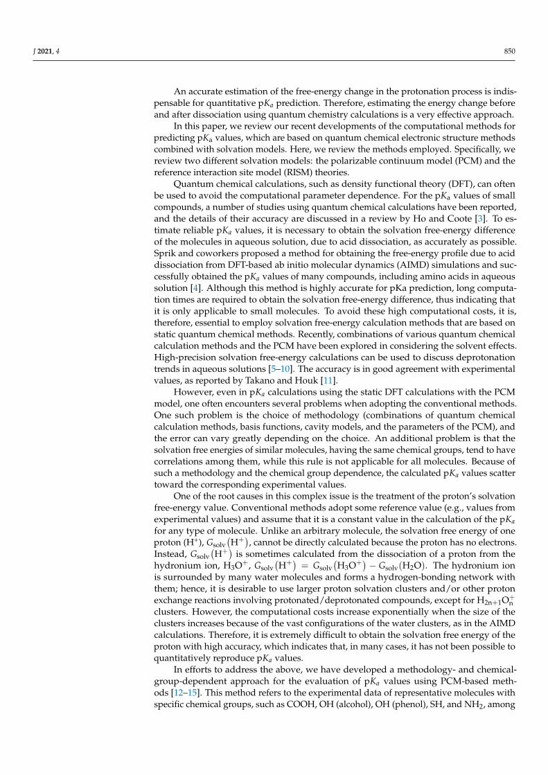
A more straightforward way to consider the spatial charge distribution is to employ the3D-RISM-SCF. As shown in Equation (21), the 3D-RISM-SCF can take into account the spa-tial distribution of the electron density derived from the solute wave function in the solute–solvent interaction. Seno et al. [41,42] calculated the pKa of p-carboxybenzeneboronic acid(PCBA), and its complex, with a monosaccharide, using the 3D-RISM-SCF, and clarifiedthe mechanism of a pKa shift due to complex formation. PCBA is a drug candidate usedin boron neutron capture therapy for skin cancer. The pKa change is utilized upon thecomplex formation with monosaccharides to increase solubility.

In aqueous solution at physiological pH, PCBA exists in equilibrium as:

J 2021, 4 FOR PEER REVIEW    11  

can perform accurate calculations using “rich” basis functions by considering the spatial 

charge distribution. 

A more straightforward way to consider the spatial charge distribution is to employ 

the 3D‐RISM‐SCF. As shown in Equation (21), the 3D‐RISM‐SCF can take into account the 

spatial distribution of the electron density derived from the solute wave function in the 

solute–solvent  interaction.  Seno  et  al.  [41,42]  calculated  the  p𝐾   of  p‐carboxyben‐

zeneboronic acid (PCBA), and its complex, with a monosaccharide, using the 3D‐RISM‐

SCF, and clarified  the mechanism of a  p𝐾   shift due  to complex  formation. PCBA  is a 

drug candidate used in boron neutron capture therapy for skin cancer. The  p𝐾   change 

is utilized upon the complex formation with monosaccharides to increase solubility. 

In aqueous solution at physiological pH, PCBA exists in equilibrium as: 

 

and under higher pH conditions, the following equilibrium forms: 

 

where 𝐾   and 𝐾   denote the dissociation constants of the corresponding reactions. The 

estimated  p𝐾   and  p𝐾   values are shown in Table 3. The results reveal that the  p𝐾  

was greatly reduced by the complex formation. Note that the adjusted values provided in 

Table 3 were evaluated on the basis of: 

p𝐾 p𝐾 p𝐾  

where  p𝐾   is a parameter for calibrating the  p𝐾   values. The parameter was deter‐

mined by performing similar calculations  for various carboxylic acids  to fit  the experi‐

mental  p𝐾   values. On the basis of the computed  p𝐾 , the molar fraction of each species 

of PCBA and its complex are plotted against the pH in Figure 5. The results indicate that, 

at physiological pH (7.4), the fraction of dissociated species with high solubility increases 

in the complex. 

As mentioned above, the RISM‐SCF and the 3D‐RISM‐SCF can be used to calculate 

the  p𝐾   using a first‐principles method, and to understand the mechanism at the molec‐

ular level. However, accuracy remains at a qualitative level, and corrections are necessary 

for quantitative discussions. 

Table 3. Reaction free energies and  p𝐾   values for PCBA and its complex. This table is reprinted 

with permission from [42]. 

Reaction  𝚫𝑮  [kcal mol−1]  𝐩𝑲𝐚 𝐜𝐨𝐦𝐩  𝐩𝑲𝐚  b 

PCBA + H2OPCBA− + H3O+  28.74  21.1    4.7 

PCBA− + 2H2OPCBA2− + H3O+  36.76  26.9  (8.7 a)  10.6 

PCBA‐complex + H2OPCBA‐complex− + H3O+  28.13  20.6    4.3 

PCBA‐complex− + 2H2OPCBA‐complex2− + H3O+  31.22  22.9    6.5 a Experimental value taken from [41]. b Adjusted  p𝐾   values. 

and under higher pH conditions, the following equilibrium forms:

J 2021, 4 FOR PEER REVIEW    11  

can perform accurate calculations using “rich” basis functions by considering the spatial 

charge distribution. 

A more straightforward way to consider the spatial charge distribution is to employ 

the 3D‐RISM‐SCF. As shown in Equation (21), the 3D‐RISM‐SCF can take into account the 

spatial distribution of the electron density derived from the solute wave function in the 

solute–solvent  interaction.  Seno  et  al.  [41,42]  calculated  the  p𝐾   of  p‐carboxyben‐

zeneboronic acid (PCBA), and its complex, with a monosaccharide, using the 3D‐RISM‐

SCF, and clarified  the mechanism of a  p𝐾   shift due  to complex  formation. PCBA  is a 

drug candidate used in boron neutron capture therapy for skin cancer. The  p𝐾   change 

is utilized upon the complex formation with monosaccharides to increase solubility. 

In aqueous solution at physiological pH, PCBA exists in equilibrium as: 

 

and under higher pH conditions, the following equilibrium forms: 

 

where 𝐾   and 𝐾   denote the dissociation constants of the corresponding reactions. The 

estimated  p𝐾   and  p𝐾   values are shown in Table 3. The results reveal that the  p𝐾  

was greatly reduced by the complex formation. Note that the adjusted values provided in 

Table 3 were evaluated on the basis of: 

p𝐾 p𝐾 p𝐾  

where  p𝐾   is a parameter for calibrating the  p𝐾   values. The parameter was deter‐

mined by performing similar calculations  for various carboxylic acids  to fit  the experi‐

mental  p𝐾   values. On the basis of the computed  p𝐾 , the molar fraction of each species 

of PCBA and its complex are plotted against the pH in Figure 5. The results indicate that, 

at physiological pH (7.4), the fraction of dissociated species with high solubility increases 

in the complex. 

As mentioned above, the RISM‐SCF and the 3D‐RISM‐SCF can be used to calculate 

the  p𝐾   using a first‐principles method, and to understand the mechanism at the molec‐

ular level. However, accuracy remains at a qualitative level, and corrections are necessary 

for quantitative discussions. 

Table 3. Reaction free energies and  p𝐾   values for PCBA and its complex. This table is reprinted 

with permission from [42]. 

Reaction  𝚫𝑮  [kcal mol−1]  𝐩𝑲𝐚 𝐜𝐨𝐦𝐩  𝐩𝑲𝐚  b 

PCBA + H2OPCBA− + H3O+  28.74  21.1    4.7 

PCBA− + 2H2OPCBA2− + H3O+  36.76  26.9  (8.7 a)  10.6 

PCBA‐complex + H2OPCBA‐complex− + H3O+  28.13  20.6    4.3 

PCBA‐complex− + 2H2OPCBA‐complex2− + H3O+  31.22  22.9    6.5 a Experimental value taken from [41]. b Adjusted  p𝐾   values. 

where Ka1 and Ka2 denote the dissociation constants of the corresponding reactions. Theestimated pKa1 and pKa2 values are shown in Table 3. The results reveal that the pKa2was greatly reduced by the complex formation. Note that the adjusted values provided inTable 3 were evaluated on the basis of:

pKa = pKa comp − pKa calib

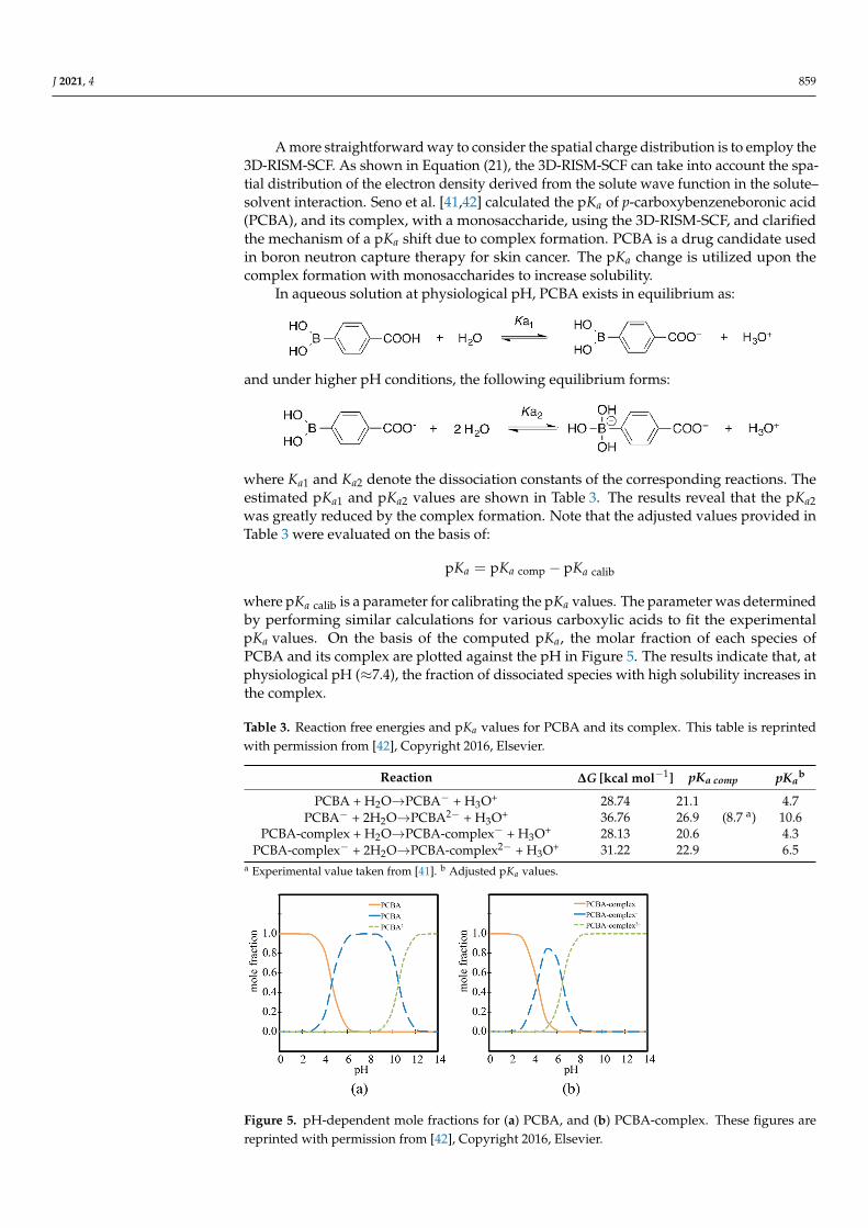
where pKa calib is a parameter for calibrating the pKa values. The parameter was determinedby performing similar calculations for various carboxylic acids to fit the experimentalpKa values. On the basis of the computed pKa, the molar fraction of each species ofPCBA and its complex are plotted against the pH in Figure 5. The results indicate that, atphysiological pH (≈7.4), the fraction of dissociated species with high solubility increases inthe complex.

Table 3. Reaction free energies and pKa values for PCBA and its complex. This table is reprintedwith permission from [42], Copyright 2016, Elsevier.

Reaction ∆G [kcal mol−1] pKa comp pKab

PCBA + H2O→PCBA− + H3O+ 28.74 21.1 4.7PCBA− + 2H2O→PCBA2− + H3O+ 36.76 26.9 (8.7 a) 10.6

PCBA-complex + H2O→PCBA-complex− + H3O+ 28.13 20.6 4.3PCBA-complex− + 2H2O→PCBA-complex2− + H3O+ 31.22 22.9 6.5

a Experimental value taken from [41]. b Adjusted pKa values.

J 2021, 4 FOR PEER REVIEW    12  

 

Figure 5. pH‐dependent mole fractions for (a) PCBA, and (b) PCBA‐complex. These figures are re‐

printed with permission from [42]. 

4.3. Data‐Driven Approach for pKa Prediction with 3D‐RISM‐SCF 

As mentioned in the previous subsection, it was difficult to achieve quantitative ac‐

curacy  in  the  first‐principles  p𝐾   calculations of  the RISM‐SCF and  the 3D‐RISM‐SCF. 

Possible sources of the error include the accuracy of the empirical parameters used in the 

Lennard‐Jones potential, the functional and basis functions in the electronic structure cal‐

culations, and, most seriously, the accuracy of the free‐energy values of the dissociated 

protons. 

A data‐driven method, to avoid the calculation of the free energy of a proton and to 

improve the quantitative accuracy, was proposed by Fujiki et al. [28]. This is an extension 

of  the AKB method, proposed by Matsui et al.  (explained  in Section 3),  to use  the 3D‐

RISM‐SCF method instead of the PCM [14]. Here, the method of Matsui et al. will be re‐

ferred to as the  linear fitting correction (LFC) method, which  is referred to as the AKB 

method in Section 3. For the LFC method, the  p𝐾   is provided by Equation (14). 

The parameters  introduced  here,  𝑘   and  𝐶 ,  are determined  by  the data‐learning 

method.  In  this work, Fujiki et al. employed  simple  least‐square  fitting  for  the experi‐

mental  p𝐾   values of training molecules. In this way, the free energy of a proton is buried 

in the parameter,  𝐶 , and only  Δ𝐺   is required by the 3D‐RISM‐SCF. Furthermore, errors 

based on functional dependence and basis functions are mitigated by the parameter,  𝑠, included in  𝑘  and  𝐶 . Fujiki et al. determined these parameters by data learning for each 

of the following functional groups: alcohol, amine, imidazole, thiol, phenol, and carboxyl. 

Figure 6 compares the accuracy of the  p𝐾   of the LFC/3D‐RISM‐SCF, with the  p𝐾 deter‐mined using the first‐principles method, as described in the previous subsection. On the 

one hand, the first‐principles method shows a good correlation, qualitatively, but a large 

error, quantitatively. On  the other hand, quantitative  accuracy was achieved with  the 

LFC/3D‐RISM, enabling highly accurate prediction. 

The method employing the continuum model introduced in the previous section is 

also capable of predicting the  p𝐾  with high accuracy. However, it is difficult to apply 

this method to systems with strong heterogeneity, such as the inside of a protein, where 

it is difficult to define the dielectric constant. By using the 3D‐RISM‐SCF, the solvent ef‐

fects  in heterogeneous  systems  can be  incorporated with high  accuracy. The LFC/3D‐

RISM‐SCF method is, therefore, expected to be applicable to complex biomolecular sys‐

tems. 

Figure 5. pH-dependent mole fractions for (a) PCBA, and (b) PCBA-complex. These figures arereprinted with permission from [42], Copyright 2016, Elsevier.

J 2021, 4 860

As mentioned above, the RISM-SCF and the 3D-RISM-SCF can be used to calculatethe pKa using a first-principles method, and to understand the mechanism at the molecularlevel. However, accuracy remains at a qualitative level, and corrections are necessary forquantitative discussions.

4.3. Data-Driven Approach for pKa Prediction with 3D-RISM-SCF

As mentioned in the previous subsection, it was difficult to achieve quantitative accu-racy in the first-principles pKa calculations of the RISM-SCF and the 3D-RISM-SCF. Possiblesources of the error include the accuracy of the empirical parameters used in the Lennard-Jones potential, the functional and basis functions in the electronic structure calculations, and,most seriously, the accuracy of the free-energy values of the dissociated protons.

A data-driven method, to avoid the calculation of the free energy of a proton andto improve the quantitative accuracy, was proposed by Fujiki et al. [28]. This is an exten-sion of the AKB method, proposed by Matsui et al. (explained in Section 3), to use the3D-RISM-SCF method instead of the PCM [14]. Here, the method of Matsui et al. will bereferred to as the linear fitting correction (LFC) method, which is referred to as the AKBmethod in Section 3. For the LFC method, the pKa is provided by Equation (14).

The parameters introduced here, k and C0, are determined by the data-learningmethod. In this work, Fujiki et al. employed simple least-square fitting for the experimentalpKa values of training molecules. In this way, the free energy of a proton is buried inthe parameter, C0, and only ∆G0 is required by the 3D-RISM-SCF. Furthermore, errorsbased on functional dependence and basis functions are mitigated by the parameter, s,included in k and C0. Fujiki et al. determined these parameters by data learning foreach of the following functional groups: alcohol, amine, imidazole, thiol, phenol, andcarboxyl. Figure 6 compares the accuracy of the pKa of the LFC/3D-RISM-SCF, with thepKa determined using the first-principles method, as described in the previous subsection.On the one hand, the first-principles method shows a good correlation, qualitatively, but alarge error, quantitatively. On the other hand, quantitative accuracy was achieved with theLFC/3D-RISM, enabling highly accurate prediction.

J 2021, 4 FOR PEER REVIEW    13  

 

Figure 6. Comparison of the computed  p𝐾   values with the experimental values determined using 

(a) the LFC/3D‐RISM‐SCF, and (b) first‐principles approach of the 3D‐RISM‐SCF. These figures are 

reprinted with permission from [28]. 

5. Summary 

This review addresses computational methods used to evaluate  p𝐾   values that are 

based on the first‐principles quantum chemical electronic structure theory, coupled with 

two different solvation models, the PCM and RISM/3D‐RISM methods. 

The strategy common to the methods presented in this review is the use of quantum 

chemical electronic structure theory to determine the free‐energy change of the deproto‐

nation reaction of a target system. The most serious difficulty associated with achieving 

quantitative accuracy is the estimation of the free energy of dissociated protons in solution. 

To avoid this, the free energy of the dissociated proton was replaced by an empirical pa‐

rameter, using a linear relationship between the free‐energy change and the actual  p𝐾  

value. The method proposed by Matsui et al. [28], which used the PCM as a solvent model, 

was reviewed in detail. On the one hand, several studies reveal that it has both quantita‐

tive accuracy and a reasonable computational cost. Their method was extended to the use 

of the 3D‐RISM as a solvent model by Fujiki et al. [28]. On the other hand, first‐principles 

computational methods  that are without empirical parameters are also  important. The 

first‐principles approach of the RISM/3D‐RISM‐SCF allows the qualitative prediction of 

the  p𝐾   in various solution environments, such as with mixed solvents and in supercriti‐

cal conditions. In the future, it is expected that methods for the quantitative prediction of 

the  p𝐾   in such complex solution environments will be developed on the basis of the ap‐

proaches reviewed in this paper. 

Here, we mainly reviewed examples of research related to  p𝐾   prediction by the au‐

thors’ group. Further developments of  p𝐾   prediction methods or theories are ongoing 

within the science community, with a variety of approaches being used [1,2,43–48]. The 

conductor‐like screening model for real solvents (COSMO‐RS) is one such method [49,50]. 

COSMO‐RS‐based methods have also been successfully applied to predict the  p𝐾   and 

p𝐾   for various systems, including proteins [51–54]. 

The prediction of the  p𝐾   is considered  important for drug design and for under‐

standing biomolecular functions; thus, computer‐aided prediction methods will become 

increasingly important. In order to predict the pKa of biomolecular systems, the electronic 

structure  theory  for  large‐scale molecules,  such  as quantum mechanics/molecular me‐

chanics  (QM/MM) or fragment molecular orbital  (FMO) methods, has been  introduced 

[55–58]. In addition, it is essential to consider the structural fluctuations of biomolecules, 

which were not addressed in this review. Indeed, the Boltzmann average of the  p𝐾   val‐

ues are, in principle, evaluated for all possible conformations. However, it is quite time‐

consuming and rather difficult to explore all of the stable structures for a given molecule, 

especially for biomolecules. Therefore, an efficient structural sampling method based on 

Figure 6. Comparison of the computed pKa values with the experimental values determined using(a) the LFC/3D-RISM-SCF, and (b) first-principles approach of the 3D-RISM-SCF. These figures arereprinted with permission from [28], Copyright 2018, Royal Society of Chemistry.

The method employing the continuum model introduced in the previous section isalso capable of predicting the pKa with high accuracy. However, it is difficult to apply thismethod to systems with strong heterogeneity, such as the inside of a protein, where it isdifficult to define the dielectric constant. By using the 3D-RISM-SCF, the solvent effects inheterogeneous systems can be incorporated with high accuracy. The LFC/3D-RISM-SCFmethod is, therefore, expected to be applicable to complex biomolecular systems.

J 2021, 4 861

5. Summary

This review addresses computational methods used to evaluate pKa values that arebased on the first-principles quantum chemical electronic structure theory, coupled withtwo different solvation models, the PCM and RISM/3D-RISM methods.

The strategy common to the methods presented in this review is the use of quantumchemical electronic structure theory to determine the free-energy change of the deproto-nation reaction of a target system. The most serious difficulty associated with achievingquantitative accuracy is the estimation of the free energy of dissociated protons in solution.To avoid this, the free energy of the dissociated proton was replaced by an empiricalparameter, using a linear relationship between the free-energy change and the actual pKavalue. The method proposed by Matsui et al. [28], which used the PCM as a solvent model,was reviewed in detail. On the one hand, several studies reveal that it has both quantitativeaccuracy and a reasonable computational cost. Their method was extended to the use ofthe 3D-RISM as a solvent model by Fujiki et al. [28]. On the other hand, first-principlescomputational methods that are without empirical parameters are also important. Thefirst-principles approach of the RISM/3D-RISM-SCF allows the qualitative prediction ofthe pKa in various solution environments, such as with mixed solvents and in supercriticalconditions. In the future, it is expected that methods for the quantitative prediction ofthe pKa in such complex solution environments will be developed on the basis of theapproaches reviewed in this paper.

Here, we mainly reviewed examples of research related to pKa prediction by theauthors’ group. Further developments of pKa prediction methods or theories are ongoingwithin the science community, with a variety of approaches being used [1,2,43–48]. Theconductor-like screening model for real solvents (COSMO-RS) is one such method [49,50].COSMO-RS-based methods have also been successfully applied to predict the pKa and pKbfor various systems, including proteins [51–54].

The prediction of the pKa is considered important for drug design and for under-standing biomolecular functions; thus, computer-aided prediction methods will becomeincreasingly important. In order to predict the pKa of biomolecular systems, the electronicstructure theory for large-scale molecules, such as quantum mechanics/molecular mechan-ics (QM/MM) or fragment molecular orbital (FMO) methods, has been introduced [55–58].In addition, it is essential to consider the structural fluctuations of biomolecules, whichwere not addressed in this review. Indeed, the Boltzmann average of the pKa values are, inprinciple, evaluated for all possible conformations. However, it is quite time-consumingand rather difficult to explore all of the stable structures for a given molecule, especially forbiomolecules. Therefore, an efficient structural sampling method based on molecular simu-lation is necessary. The constant pH (CpH) MD is one such method, which is widely usedand equipped in major program packages [59,60]. By combining the methods described inthis review with CpHMD, it is expected that a method will be developed that describes thechanges in the electronic structure and that also takes structural fluctuations into account.The development of such a method is in progress in the authors’ group. It is desirable thatwe continue to improve the methods that can provide accuracy, computational speed, anda detailed molecular picture.

Author Contributions: R.F. and H.N. contributed for the Sections 1 and 4. T.M. and Y.S. contributedfor the Sections 1 and 2. N.Y. contributed for the Sections 1 and 3–5. All authors have read and agreedto the published version of the manuscript.

Funding: We are grateful for the financial support from the Japan Society for the Promotion ofScience (JSPS), KAKENHI (Grant Nos. 18K05036 and 19H02677).

Acknowledgments: Norio Yoshida would like to thank Sato (Kyoto University, Japan) and Hirata(Institute for Molecular Science, Japan) for their contributions in writing some of the original papersreferred to in this review. We would like to dedicate this work to the late Yukako Kasai (1990–2020)for her significant contributions to the development of the LFC/3D-RISM-SCF method.

J 2021, 4 862

Conflicts of Interest: The authors declare no conflict of interest.

References1. Navo, C.D.; Jiménez-Osés, G. Computer Prediction of pKa Values in Small Molecules and Proteins. ACS Med. Chem. Lett. 2021, 12,

1624–1628. [CrossRef]2. Li, H.; Robertson, A.D.; Jensen, J.H. Very Fast Empirical Prediction and Rationalization of Protein pKa Values. Proteins Struct.

Funct. Genet. 2005, 61, 704–721. [CrossRef] [PubMed]3. Ho, J.M.; Coote, M.L. A universal approach for continuum solvent pKa calculations: Are we there yet? Theor. Chem. Acc. 2010,

125, 3–21. [CrossRef]4. Mangold, M.; Rolland, L.; Costanzo, F.; Sprik, M.; Sulpizi, M.; Blumberger, J. Absolute pKa Values and Solvation Structure

of Amino Acids from Density Functional Based Molecular Dynamics Simulation. J. Chem. Theory Comput. 2011, 7, 1951–1961.[CrossRef] [PubMed]

5. Klamt, A.; Schuurmann, G. Cosmo—A New Approach to Dielectric Screening in Solvents with Explicit Expressions for theScreening Energy and Its Gradient. J. Chem. Soc. Perkin Trans. 2 1993, 799–805. [CrossRef]

6. Barone, V.; Cossi, M. Quantum calculation of molecular energies and energy gradients in solution by a conductor solvent model.J. Phys. Chem. A 1998, 102, 1995–2001. [CrossRef]

7. Cances, E.; Mennucci, B.; Tomasi, J. A new integral equation formalism for the polarizable continuum model: Theoreticalbackground and applications to isotropic and anisotropic dielectrics. J. Chem. Phys. 1997, 107, 3032–3041. [CrossRef]

8. Mennucci, B.; Tomasi, J. Continuum solvation models: A new approach to the problem of solute’s charge distribution and cavityboundaries. J. Chem. Phys. 1997, 106, 5151–5158. [CrossRef]

9. Foresman, J.B.; Keith, T.A.; Wiberg, K.B.; Snoonian, J.; Frisch, M.J. Solvent effects. 5. Influence of cavity shape, truncation ofelectrostatics, and electron correlation ab initio reaction field calculations. J. Phys. Chem. 1996, 100, 16098–16104. [CrossRef]

10. Pliego, J.R.; Riveros, J.M. Gibbs energy of solvation of organic ions in aqueous and dimethyl sulfoxide solutions. Phys. Chem.Chem. Phys. 2002, 4, 1622–1627. [CrossRef]

11. Takano, Y.; Houk, K.N. Benchmarking the conductor-like polarizable continuum model (CPCM) for aqueous solvation freeenergies of neutral and ionic organic molecules. J. Chem. Theory Comput. 2005, 1, 70–77. [CrossRef] [PubMed]

12. Matsui, T.; Oshiyama, A.; Shigeta, Y. A Simple scheme for estimating the pKa values of 5-substituted uracils. Chem. Phys. Lett.2011, 502, 248–252. [CrossRef]

13. Matsui, T.; Miyachi, H.; Baba, T.; Shigeta, Y. Theoretical Study on Reaction Scheme of Silver(I) Containing 5-Substituted UracilsBridge Formation. J. Phys. Chem. A 2011, 115, 8504–8510. [CrossRef] [PubMed]

14. Matsui, T.; Baba, T.; Kamiya, K.; Shigeta, Y. An accurate density functional theory based estimation of pKa values of polar residuescombined with experimental data: From amino acids to minimal proteins. Phys. Chem. Chem. Phys. 2012, 14, 4181. [CrossRef]

15. Baba, T.; Matsui, T.; Kamiya, K.; Nakano, M.; Shigeta, Y. A Density Functional Study on the pKa of Small Polyprotic Molecules.Int. J. Quantum Chem. 2014, 114, 1128–1134. [CrossRef]

16. Hirata, F. (Ed.) Molecular Theory of Solvation; Kluwer: Dordrecht, The Netherlands, 2003.17. Chandler, D.; Andersen, H.C. Optimized Cluster Expansions for Classical Fluids. 2. Theory of Molecular Liquids. J. Chem. Phys.

1972, 57, 1930–1937. [CrossRef]18. Andersen, H.; Chandler, D.; Weeks, J. Optimized Cluster Expansions for Classical Fluids. 3. Applications to Ionic Solutions and

Simple Liquids. J. Chem. Phys. 1972, 57, 2626–2631. [CrossRef]19. Andersen, H.; Chandler, D. Optimized Cluster Expansions for Classical Fluids. 1. General Theory and Variational Formulation of

Mean Spherical Model and hard-sphere Percus-Yevick Equations. J. Chem. Phys. 1972, 57, 1918–1929. [CrossRef]20. Beglov, D.; Roux, B. An Integral Equation to Describe the Solvation of Polar Molecules in Liquid Water. J. Phys. Chem. B 1997, 101,

7821–7826. [CrossRef]21. Beglov, D.; Roux, B. Solvation Of Complex Molecules in A Polar Liquid: An Integral Equation Theory. J. Chem. Phys. 1996, 104,

8678–8689. [CrossRef]22. Kovalenko, A.; Hirata, F. Three-Dimensional Density Profiles of Water in Contact with A Solute of Arbitrary Shape: A RISM

Approach. Chem. Phys. Lett. 1998, 290, 237–244. [CrossRef]23. Ten-No, S.; Hirata, F.; Kato, S. A Hybrid Approach for the Solvent Effect on the Electronic Structure of A Solute Based on the

RISM and Hartree-Fock Equations. Chem. Phys. Lett. 1993, 214, 391–396. [CrossRef]24. Kovalenko, A.; Hirata, F. Self-Consistent Description of A Metal-Water Interface by the Kohn-Sham Density Functional Theory

and the Three-Dimensional Reference Interaction Site Model. J. Chem. Phys. 1999, 110, 10095–10112. [CrossRef]25. Sato, H.; Kovalenko, A.; Hirata, F. Self-Consistent Field, Ab Initio Molecular Orbital and Three-Dimensional Reference Interaction

Site Model Study for Solvation Effect on Carbon Monoxide in Aqueous Solution. J. Chem. Phys. 2000, 112, 9463–9468. [CrossRef]26. Yoshida, N.; Ishizuka, R.; Sato, H.; Hirata, F. Ab initio theoretical study of temperature and density dependence of molecular and

thermodynamic properties of water in the entire fluid region: Autoionization processes. J. Phys. Chem. B 2006, 110, 8451–8458.[CrossRef] [PubMed]

27. Sato, H.; Hirata, F. Theoretical study for autoionization of liquid water: Temperature dependence of the ionic product (pKw). J.Phys. Chem. A 1998, 102, 2603–2608. [CrossRef]

J 2021, 4 863

28. Fujiki, R.; Kasai, Y.; Seno, Y.; Matsui, T.; Shigeta, Y.; Yoshida, N.; Nakano, H. A computational scheme of pKa values based on thethree-dimensional reference interaction site model self-consistent field theory coupled with the linear fitting correction scheme.Phys. Chem. Chem. Phys 2018, 20, 27272–27279. [CrossRef]

29. Tomasi, J.; Mennucci, B.; Cammi, R. Quantum Mechanical Continuum Solvation Models. Chem. Rev. 2005, 105, 2999–3093.[CrossRef]

30. Mennucci, B. Polarizable continuum model. WIREs Comput. Mol. Sci. 2012, 2, 386–404. [CrossRef]31. Marenich, A.V.; Cramer, C.J.; Truhlar, D.G. Universal Solvation Model Based on Solute Electron Density and on a Continuum

Model of the Solvent Defined by the Bulk Dielectric Constant and Atomic Surface Tensions. J. Phys. Chem. B 2009, 113, 6378.[CrossRef] [PubMed]

32. Matsui, T.; Shigeta, Y.; Morihashi, K. Assessment of Methodology and Chemical Group Dependences in the Calculation of thepKa for Several Chemical Groups. J. Chem. Theory Comput. 2017, 13, 4791–4803. [CrossRef]

33. Hengphasatporn, K.; Matsui, T.; Shigeta, Y. Estimation of Acid Dissociation Constants (pKa) of N-Containing Heterocycles inDMSO and Transferability of Gibbs Free Energy in Different Solvent Conditions. Chem. Lett. 2020, 49, 307–310. [CrossRef]

34. Dawson, R.M.C.; Elliott, D.C.; Elliott, W.H.; Jones, K.M. Data for Biochemical Research; Clarendon Press: Oxford, UK, 1969; Volume 316.35. Kaljurand, I.; Kutt, A.; Soovali, L.; Rodima, T.; Maemets, V.; Leito, I.; Koppel, I.A. Extension of the self-consistent spectrophoto-

metric basicity scale in acetonitrile to a full span of 28 pKa units: Unification of different basicity scales. J. Org. Chem. 2005, 70,1019–1028. [CrossRef]

36. Garrido, G.; Roses, M.; Rafols, C.; Bosch, E. Acidity of several anilinium derivatives in pure tetrahydrofuran. J. Solut. Chem. 2008,37, 689–700. [CrossRef]

37. Jover, J.; Bosque, R.; Sales, J. QSPR Prediction of pK for Aliphatic Carboxylic Acids and Anilines in Different Solvents. QSARComb. Sci. 2008, 27, 1204–1215. [CrossRef]

38. Kovalenko, A.; Hirata, F. First-principles realization of a van der Waals-Maxwell theory for water. Chem. Phys. Lett. 2001, 349,496–502. [CrossRef]

39. Kido, K.; Sato, H.; Sakaki, S. First Principle Theory for pKa Prediction at Molecular Level: pH Effects Based on Explicit SolventModel. J. Phys. Chem. B 2009, 113, 10509–10514. [CrossRef] [PubMed]

40. Kido, K.; Sato, H.; Sakaki, S. Systematic Assessment on Aqueous pKa and pKb of an Amino Acid Base on RISM-SCF-SEDDMethod: Toward First Principles Calculations. Int. J. Quantum Chem. 2012, 112, 103–112. [CrossRef]

41. Islam, T.M.B.; Yoshino, K.; Sasane, A. 11B NMR study of p-carboxybenzeneboronic acid ions for complex formation with somemonosaccharides. Anal. Sci. 2003, 19, 455–460. [CrossRef]

42. Seno, Y.; Yoshida, N.; Nakano, H. Theoretical analysis of complex formation of p-carboxybenzeneboronic acid with a monosac-charide. J. Mol. Liq. 2016, 217, 93–98. [CrossRef]

43. Radak, B.K.; Chipot, C.; Suh, D.; Jo, S.; Jiang, W.; Phillips, J.C.; Schulten, K.; Roux, B. Constant-PH Molecular DynamicsSimulations for Large Biomolecular Systems. J. Chem. Theory Comput. 2017, 13, 5933. [CrossRef]

44. Tielker, N.; Eberlein, L.; Gussregen, S.; Kast, S.M. The SAMPL6 challenge on predicting aqueous pKa values from EC-RISM theory.J. Comput.-Aided Mol. Des. 2018, 32, 1151–1163. [CrossRef]

45. Tielker, N.; Tomazic, D.; Heil, J.; Kloss, T.; Ehrhart, S.; Gussregen, S.; Schmidt, K.F.; Kast, S.M. The SAMPL5 challenge forembedded-cluster integral equation theory: Solvation free energies, aqueous pKa, and cyclohexane-water log D. J. Comput.-AidedMol. Des. 2016, 30, 1035–1044. [CrossRef]

46. Matos, M.J.; Oliveira, B.L.; Martínez-Sáez, N.; Guerreiro, A.; Cal, P.M.S.D.; Bertoldo, J.; Maneiro, M.; Perkins, E.; Howard, J.; Deery,M.J.; et al. Chemo- and Regioselective Lysine Modification on Native Proteins. J. Am. Chem. Soc. 2018, 140, 4004. [CrossRef]

47. Isık, M.; Rustenburg, A.S.; Rizzi, A.; Gunner, M.R.; Mobley, D.L.; Chodera, J.D. Overview of the SAMPL6 PKa Challenge:Evaluating Small Molecule Microscopic and Macroscopic PKa Predictions. J. Comput.-Aided Mol. Des. 2021, 35, 131. [CrossRef]

48. Li, M.; Zhang, H.; Chen, B.; Wu, Y.; Guan, L. Prediction of PKa Values for Neutral and Basic Drugs Based on Hybrid ArtificialIntelligence Methods. Sci. Rep. 2018, 8, 3991. [CrossRef]

49. Klamt, A. Conductor-Like Screening Model for Real Solvents—A New Approach to the Quantitative Calculation of SolvationPhenomena. J. Phys. Chem. 1995, 99, 2224–2235. [CrossRef]

50. Klamt, A.; Eckert, F.; Diedenhofen, M.; Beck, M.E. First principles calculations of aqueous pKa values for organic and inorganicacids using COSMO-RS reveal an inconsistency in the slope of the pKa scale. J. Phys. Chem. A 2003, 107, 9380–9386. [CrossRef][PubMed]

51. Eckert, F.; Klamt, A. Accurate prediction of basicity in aqueous solution with COSMO-RS. J. Comput. Chem. 2006, 27, 11–19.[CrossRef] [PubMed]

52. Eckert, F.; Leito, I.; Kaljurand, I.; Kutt, A.; Klamt, A.; Diedenhofen, M. Prediction of Acidity in Acetonitrile Solution withCOSMO-RS. J. Comput. Chem. 2009, 30, 799–810. [CrossRef]

53. Toure, O.; Dussap, C.G.; Lebert, A. Comparison of Predicted pKa Values for Some Amino-Acids, Dipeptides and Tripeptides,Using COSMO-RS, ChemAxon and ACD/Labs Methods. Oil Gas Sci. Technol. 2013, 68, 281–297. [CrossRef]

54. Andersson, M.P.; Jensen, J.H.; Stipp, S.L.S. Predicting pKa for proteins using COSMO-RS. PeerJ 2013, 1, e198. [CrossRef] [PubMed]55. Kitaura, K.; Ikeo, E.; Asada, T.; Nakano, T.; Uebayasi, M. Fragment Molecular Orbital Method: An Approximate Computational

Method For Large Molecules. Chem. Phys. Lett. 1999, 313, 701–706. [CrossRef]

J 2021, 4 864

56. Fedorov, D.G.; Kitaura, K.; Li, H.; Jensen, J.H.; Gordon, M.S. The Polarizable Continuum Model (PCM) Interfaced With TheFragment Molecular Orbital Method (FMO). J. Comput. Chem. 2006, 27, 976–985. [CrossRef]

57. Yoshida, N. Efficient implementation of the three-dimensional reference interaction site model method in the fragment molecularorbital method. J. Chem. Phys. 2014, 140, 214118. [CrossRef]

58. Yoshida, N.; Kiyota, Y.; Hirata, F. The Electronic-Structure Theory Of A Large-Molecular System In Solution: Application to TheIntercalation of Proflavine With Solvated DNA. J. Mol. Liq. 2011, 159, 83–92. [CrossRef]

59. Mongan, J.; Case, D.A.; McCammon, J.A. Constant pH molecular dynamics in generalized born implicit solvent. J. Comput. Chem.2004, 25, 2038–2048. [CrossRef]

60. Itoh, S.G.; Damjanovic, A.; Brooks, B.R. pH replica-exchange method based on discrete protonation states. Proteins 2011, 79,3420–3436. [CrossRef]