1  

Real-time shape approximation and 5-D fingerprinting of single proteins Erik C. Yusko1,†,ǂ, Brandon R. Bruhn1,†, Olivia Eggenberger1, Jared Houghtaling1, Ryan C. Rollings2, Nathan C. Walsh2, Santoshi Nandivada2, Mariya Pindrus3, Adam R. Hall4, David Sept1,5, Jiali Li2, Devendra S. Kalonia3, Michael Mayer1,6,*

Affiliations: 1Department of Biomedical Engineering, University of Michigan, Ann Arbor, MI 48109, USA 2Department of Physics, University of Arkansas, Fayetteville, Arkansas 72701, USA 3Department of Pharmaceutical Sciences, University of Connecticut, Storrs, CT 06269, USA 4Department of Biomedical Engineering and Comprehensive Cancer Center, Wake Forest University School of Medicine, Winston Salem, NC 27157, USA 5Center for Computational Medicine and Biology, University of Michigan, Ann Arbor, MI 48109, USA 6Biophysics Program, University of Michigan, Ann Arbor, MI 48109, USA

†These authors contributed equally to this work. ǂCurrent address: Department of Physiology and Biophysics, University of Washington, Seattle, WA 98195, USA *Correspondence should be addressed to M.M. (mimayer@umich.edu)

This work exploits the zeptoliter sensing volume of electrolyte-filled nanopores to determine,

simultaneously and in real time, the approximate shape, volume, charge, rotational diffusion

coefficient, and dipole moment of individual proteins. We have developed the theory for a

quantitative understanding and analysis of modulations in ionic current that arise from rotational

dynamics of single proteins as they move through the electric field inside a nanopore. The

resulting multi-parametric information raises the possibility to characterize, identify, and quantify

individual proteins and protein complexes in a mixture. This approach interrogates single

proteins in solution and determines parameters such as the approximate shape and dipole

moment, which are excellent protein descriptors and cannot be obtained otherwise from single

protein molecules in solution. Taken together, this five-dimensional characterization of

biomolecules at the single particle level has the potential for instantaneous protein identification,

quantification, and possibly sorting with implications for structural biology, proteomics,

biomarker detection, and routine protein analysis.

2  

Methods to characterize, identify, and quantify unlabeled, folded proteins in solution on a single

molecule level do not currently exist1. If available, such methods would have a disruptive impact on the

life sciences and clinical assays by simplifying routine protein analysis, enabling rapid and ultra-sensitive

biomarker detection2, and allowing the analysis of personal proteomes3. Furthermore, if such methods

instantly provided low-resolution approximations of shape, they could help to reveal the conformation of

transient protein complexes or large assemblies that are not accessible by electron microscopy, NMR

spectroscopy, X-ray crystallography, or small-angle X-ray scattering4. Here, we demonstrate that

interrogation of single proteins or protein-protein complexes during their passage through the electric

field inside a nanopore can enable characterization of these particles based on spheroidal approximations

of their shape, as well as their volume, charge, rotational diffusion coefficient, and dipole moment.

Dipole moment has mostly been neglected as a protein descriptor. Despite the pioneering work by

Debye5 and Oncley6, neither the usefulness of this parameter for protein identification nor its importance

for concentrated protein solutions has hitherto been widely appreciated, and existing methods for

determining protein dipole moments are tedious and limited to ensemble measurements. We propose,

however, that dipole moment provides a powerful dimension for label-free protein analysis since its

magnitude is widely distributed among different proteins (absolute values typically range from 0 to 4,000

Debye)7. Dipole moment may therefore approach the usefulness of protein size for identification and

would likely exceed the usefulness of protein charge (whose values are less distributed, typically ranging

from -40e to +40e)7. Moreover, the pharmaceutical industry is increasingly recognizing the importance of

dipole moment for antibody formulations8, in part because subcutaneous injection of highly concentrated

solutions of monoclonal antibodies (the fastest growing class of therapeutics) can be impractical due to

high viscosity and aggregation resulting from dipole alignment8-10. Measurements of antibody dipole

moments could therefore provide a criterion to select early candidates in the drug discovery process and

reduce development costs11.

3  

Interrogating single protein particles during their passage through a pore is simple in principle12-16. It

requires a single electrolyte-filled pore that connects two solutions across a thin insulating membrane and

serves as a conduit for ions and proteins (Fig. 1a). Electrodes connect the solutions on both sides of the

membrane to a high-gain amplifier that applies a constant electric potential difference while measuring

the ionic current through the nanopore. This arrangement ensures that virtually the entire voltage drop

occurs within the pore, rendering this zone supremely sensitive to transient changes in its ionic

conductivity. Consequently, each protein that is driven electrophoretically through the pore displaces

conductive electrolyte, distorts the electric field, and reduces the ionic current through the pore. If the

volume of the electrolyte-filled pore is sufficiently small compared to the volume of the particle, then the

change in ionic current due to the translocating particle is measurable and characterized by its magnitude,

ΔI, and duration, td17-23; this current signature is referred to as a resistive pulse. In addition to its exquisite

sensitivity to conductivity changes, this small volume transiently separates single proteins from other

macromolecules in solution, enabling, for the first time, that rotational dynamics of one protein can be

interrogated without artifacts from other macromolecules. For this reason, time-dependent modulations

of ionic current as a single protein passes through a nanopore can, under appropriate conditions, relate

uniquely to the time-dependent molecular orientation of that protein as well as its shape, volume, charge,

rotational diffusion coefficient, and dipole moment (Fig. 1b-e, Supplementary Notes 1-3, and

Supplementary Figs. 1-9). Several groups have recently considered, in qualitative terms, the effect of a

protein’s17,18,20,24-28 or nanoparticle’s shape when analyzing distributed ΔI signals29 as well as the effect of

a protein’s dipole moment on its translocation through an alpha-hemolysin pore in the presence of an AC

field30. The work presented here develops the theory for a quantitative understanding of the dependence

of measured ΔI values on the shape, dipole, and rotational dynamics of a protein inside a nanopore and

makes it possible to estimate the volume, approximate shape, rotational diffusion coefficient, and dipole

moment of non-spherical proteins in real time (Supplementary Figure 10). We suggest that this ability to

measure five parameters simultaneously on single proteins in real time has fundamental implications. For

instance, analyzing individual proteins one-by-one may inherently mean that these proteins do not have to

4  

be purified for determining their approximate shape or the other four parameters. This consequence

would be a paradigm shift compared to existing methods for determining the shape or structure of

proteins, which either require purified, concentrated, or crystallized protein samples or cannot examine

protein dynamics.

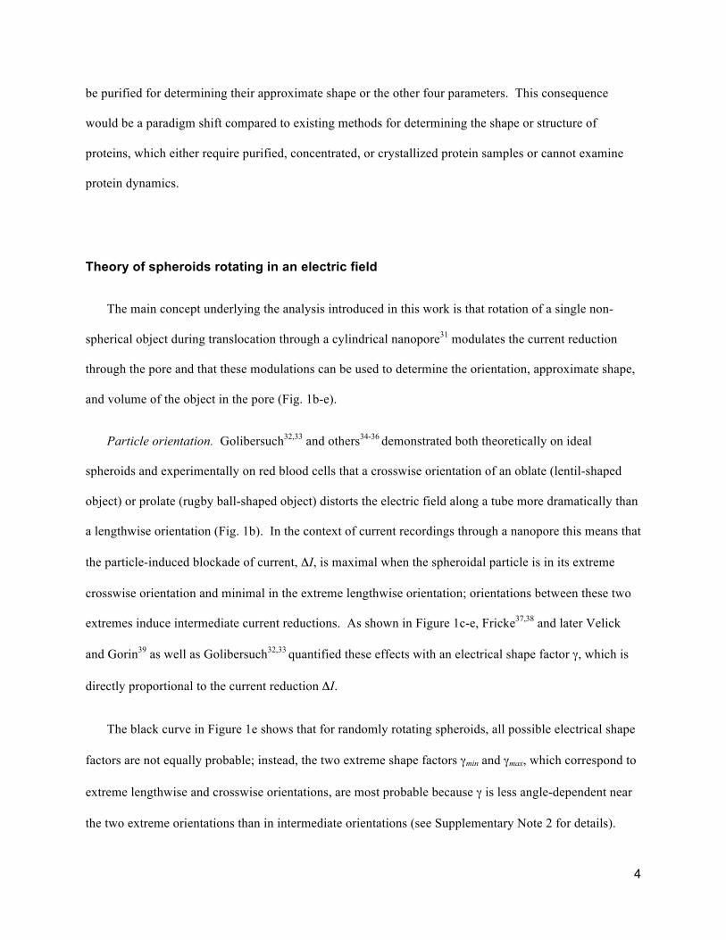
Theory of spheroids rotating in an electric field

The main concept underlying the analysis introduced in this work is that rotation of a single non-

spherical object during translocation through a cylindrical nanopore31 modulates the current reduction

through the pore and that these modulations can be used to determine the orientation, approximate shape,

and volume of the object in the pore (Fig. 1b-e).

Particle orientation. Golibersuch32,33 and others34-36 demonstrated both theoretically on ideal

spheroids and experimentally on red blood cells that a crosswise orientation of an oblate (lentil-shaped

object) or prolate (rugby ball-shaped object) distorts the electric field along a tube more dramatically than

a lengthwise orientation (Fig. 1b). In the context of current recordings through a nanopore this means that

the particle-induced blockade of current, ΔI, is maximal when the spheroidal particle is in its extreme

crosswise orientation and minimal in the extreme lengthwise orientation; orientations between these two

extremes induce intermediate current reductions. As shown in Figure 1c-e, Fricke37,38 and later Velick

and Gorin39 as well as Golibersuch32,33 quantified these effects with an electrical shape factor γ, which is

directly proportional to the current reduction ΔI.

The black curve in Figure 1e shows that for randomly rotating spheroids, all possible electrical shape

factors are not equally probable; instead, the two extreme shape factors γmin and γmax, which correspond to

extreme lengthwise and crosswise orientations, are most probable because γ is less angle-dependent near

the two extreme orientations than in intermediate orientations (see Supplementary Note 2 for details).

5  

This U-shaped probability distribution means that the translocation of randomly rotating spheroidal

proteins through a nanopore should result in a distribution of ΔI values with two maxima, one

corresponding to ΔI(γmin) and one to ΔI(γmax). In contrast, spherical proteins, with a γ value of 1.5 that is

independent of orientation, should result in Normal distributions of ΔI values.

Particle shape. In addition to these orientation-dependent effects, the particle’s volume and shape

also affect the extent of electric field line distortion (Fig. 1c). For example, when comparing two oblates

of equal volume in a cross-wise orientation, the particle that deviates most from a perfect sphere (i.e. the

flatter oblate) distorts the field lines more dramatically than the rounder object. Conversely, in a

lengthwise orientation, the flatter of these two particles distorts the field lines less dramatically than the

rounder object. In other words, particles with increasingly non-spherical shapes result in a more extreme

ratio between the current blockage in their crosswise versus lengthwise orientation.

Particle volume. For translocation of two particles with the same shape but different volume, both

the orientation-dependent minimal and maximal current reductions have larger magnitudes for the larger

particle compared to the smaller one. Therefore, the magnitude of the current reduction depends on

particle volume, while the ratio between the minimal and maximal current reduction depends on particle

shape.

General implications for nanopore recordings of non-spherical particles. The dependence of ∆I

values on the shape and orientation of translocating particles has generally been neglected in nanopore-

based protein characterization, thereby introducing uncertainty in measurements of volume for particles

that are not perfect spheres. Considering these shape-dependent effects, as proposed here, will likely

increase the accuracy of nanopore-based particle characterization as most particles and proteins are not

perfect spheres.

6  

RESULTS

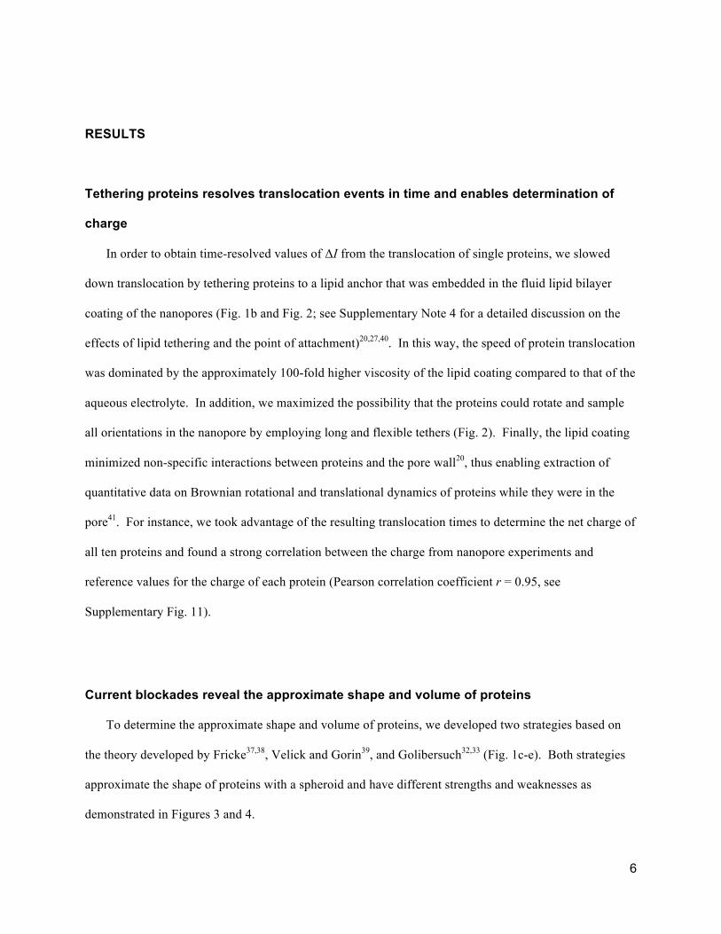
Tethering proteins resolves translocation events in time and enables determination of

charge

In order to obtain time-resolved values of ΔI from the translocation of single proteins, we slowed

down translocation by tethering proteins to a lipid anchor that was embedded in the fluid lipid bilayer

coating of the nanopores (Fig. 1b and Fig. 2; see Supplementary Note 4 for a detailed discussion on the

effects of lipid tethering and the point of attachment)20,27,40. In this way, the speed of protein translocation

was dominated by the approximately 100-fold higher viscosity of the lipid coating compared to that of the

aqueous electrolyte. In addition, we maximized the possibility that the proteins could rotate and sample

all orientations in the nanopore by employing long and flexible tethers (Fig. 2). Finally, the lipid coating

minimized non-specific interactions between proteins and the pore wall20, thus enabling extraction of

quantitative data on Brownian rotational and translational dynamics of proteins while they were in the

pore41. For instance, we took advantage of the resulting translocation times to determine the net charge of

all ten proteins and found a strong correlation between the charge from nanopore experiments and

reference values for the charge of each protein (Pearson correlation coefficient r = 0.95, see

Supplementary Fig. 11).

Current blockades reveal the approximate shape and volume of proteins

To determine the approximate shape and volume of proteins, we developed two strategies based on

the theory developed by Fricke37,38, Velick and Gorin39, and Golibersuch32,33 (Fig. 1c-e). Both strategies

approximate the shape of proteins with a spheroid and have different strengths and weaknesses as

demonstrated in Figures 3 and 4.

7  

The first strategy estimates shape and volume from distributions of maximum ΔI values from many

translocation events that were obtained from a pure protein solution. In other words, only the peak value

of ΔI from each resistive pulse is used for analysis. Maximum ΔI values have been employed in almost

all nanopore-based resistive pulse analyses of protein volume to date combined with the assumption of a

perfectly spherical particle shape (i.e. γ = 1.5), thereby foregoing the opportunity to evaluate protein

shape. In contrast, Golibersuch showed by examining red blood cells that maximum ΔI values could also

be used to approximate the shape of particles.32 Here, we adopted this concept for the first time to

proteins in nanopores. An advantage of using maximum ΔI values to estimate protein shape and volume

is that the ratio between the extreme values of current reduction, ΔI(γmax) and ΔI(γmin), is relatively

insensitive to deviations in pore geometry from a perfect cylinder. A disadvantage of this approach is that

shape and volume cannot be determined from a single translocation event because only the maximum ΔI

value from each translocation event is analyzed and thus many translocations are required to sample all

possible electrical shape factors (see Supplementary Note 2 for discussion).

Determining the shape and volume of spheroids from distributions of maximum ∆I values proceeds in

three steps; Figure 3 shows the results from each step (see Supplementary Note 2 and Supplementary

Figs. 5-8 for details). First, an algorithm detects resistive pulses from the translocation of hundreds to a

few thousands copies of the same protein and determines the maximum amplitude of the current

modulation, ΔI, with respect to the baseline current for each pulse (Fig. 3a,b). As predicted theoretically

in Fig. 1c-e, the resulting distribution of maximum ΔI values is either Normal for spherical proteins (Fig.

3c) or bimodal for non-spherical proteins (Fig. 3d-f as well as Supplementary Fig. 6 and Supplementary

Note 2). Second, in order to circumvent binning effects encountered with probability distributions20, the

experimentally determined distribution of ΔI values is converted to an empirical cumulative density

function, CDF (Fig. 3c,d, insets), and fit iteratively with an equation that describes the variation in ΔI due

to rotation of proteins with non-spherical shape (Supplementary Note 2, Equation 13a,b). We refer to

this equation as the convolution model since it also accounts for broadening of the ΔI distribution due to

8  

convolution of the true signal with noise (Supplementary Fig. 5) and for bias towards either the crosswise

or lengthwise orientation as a result of the electric-field-induced torque on the protein’s dipole moment.42

The bias in a distribution of maximum ΔI values, however, may also be affected by other factors than the

dipole moment (as discussed in Supplementary Note 2), which are all accounted for by the same fitting

parameter. The values of ΔI(γmin) and ΔI(γmax) returned by the fitting procedure reflect the two extreme

orientations of the protein (red dashed curves in Fig. 3d-f). Third, based on the direct proportionality

between ΔI and γ and the geometrical relationship between γ and the length-to-diameter ratio m of a

spheroid (Supplementary Note 2, Equations 1 and 4-7), we determine the shape and volume that agree

best with the experimental distribution of ΔI values for the protein.

Figure 3g shows the spheroidal approximation of the shape of ten different proteins compared to the

respective crystal structure for each protein, illustrating that this analysis yields excellent estimates of

protein shape, particularly for proteins that closely resemble a spheroid. Figure 3h,i, for instance, shows

that the volume and m values agree well with the expected reference values; the average deviation of both

parameters is less than 20% (Supplementary Tables 1-4 list the results of this analysis as well as reference

values). These results also show that two proteins with a similar molecular weight and volume but

different shape are clearly distinguishable by this analysis; for instance, compare the ellipsoids

determined for the IgG1 antibody and GPI-AChE in Fig. 3g.29

Independent from these experimental results, we confirmed the accuracy of this approach for shape

and volume determination using simulated data that was generated from the theory of biased one-

dimensional Brownian diffusion and convolved with current noise. Fitting the simulated data with the

convolution model, just as with the experimental data, returned values of shape and volume that were in

excellent agreement with the input parameters (Supplementary Note 5 and Supplementary Fig. 12).

Compared to other methods for determining the shape and volume of proteins in aqueous solution

such as solution-state NMR spectroscopy, analytical ultracentrifugation, and dynamic light scattering, the

9  

nanopore-based approach is faster (seconds to minutes), requires smaller sample volumes (≤10 µL) and

lower protein concentrations (pM to nM), and may perform better as the size of proteins or protein

complexes increases due to the concomitant potential increase in signal-to-noise ratio. While the

resolution of shape is significantly lower than that of NMR spectroscopy for small proteins (<80 kDa), it

is higher than the resolution of analytical ultracentrifugation and dynamic light scattering. In addition,

although the limited time-resolution of currently available amplifiers requires tethering proteins to the

lipid coating (a reaction that occurs in situ on the nanopore chip), the nanopore-based approach does not

require extensive modification of pure proteins by isotope labeling as it is the case for protein NMR

spectroscopy.

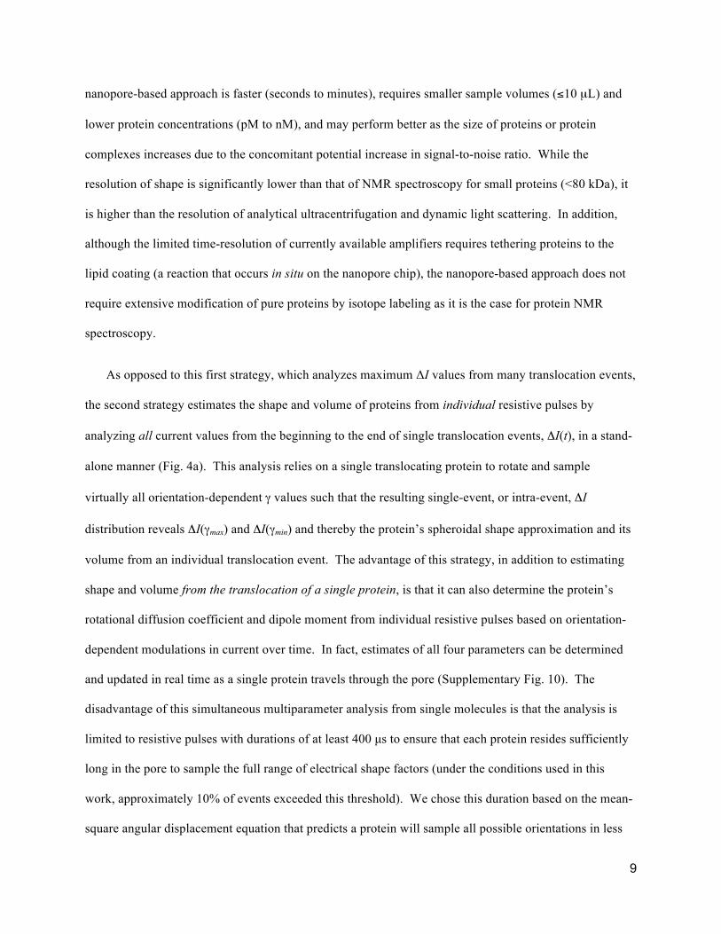
As opposed to this first strategy, which analyzes maximum ΔI values from many translocation events,

the second strategy estimates the shape and volume of proteins from individual resistive pulses by

analyzing all current values from the beginning to the end of single translocation events, ΔI(t), in a stand-

alone manner (Fig. 4a). This analysis relies on a single translocating protein to rotate and sample

virtually all orientation-dependent γ values such that the resulting single-event, or intra-event, ΔI

distribution reveals ΔI(γmax) and ΔI(γmin) and thereby the protein’s spheroidal shape approximation and its

volume from an individual translocation event. The advantage of this strategy, in addition to estimating

shape and volume from the translocation of a single protein, is that it can also determine the protein’s

rotational diffusion coefficient and dipole moment from individual resistive pulses based on orientation-

dependent modulations in current over time. In fact, estimates of all four parameters can be determined

and updated in real time as a single protein travels through the pore (Supplementary Fig. 10). The

disadvantage of this simultaneous multiparameter analysis from single molecules is that the analysis is

limited to resistive pulses with durations of at least 400 µs to ensure that each protein resides sufficiently

long in the pore to sample the full range of electrical shape factors (under the conditions used in this

work, approximately 10% of events exceeded this threshold). We chose this duration based on the mean-

square angular displacement equation that predicts a protein will sample all possible orientations in less

10  

than 400 µs, on average, as long as its rotational diffusion coefficient exceeds 3,000 rad2 s-1, which was

clearly the case for all tethered proteins examined here (Supplementary Table 4). Other disadvantages of

this analysis include that it is more sensitive to deviations of the pore geometry from a perfect cylinder

than the multi-event analysis of maximum ΔI values (see Supplementary Note 6) and that the analysis of

individual resistive pulses is associated with relatively high uncertainty as with other single-molecule

measurements.

Figure 4 shows estimates of the shape and volume of proteins obtained from fitting distributions of

intra-event ΔI(t) values from individual resistive pulses with the convolution model in the same way as

the distributions of maximum ΔI values from hundreds of pulses (see Supplementary Note 6 and

Supplementary Fig. 15). We find that the intra-event ΔI distributions from translocations of individual

proteins retain their key features (e.g. minimal and maximal ΔI values) although the current recordings

are smoothed due to filtering (see Supplementary Fig. 21). The median protein shapes obtained from this

analysis are in reasonable agreement with their crystal structure (Fig. 4d), although the analysis of

maximum ∆I values yielded more accurate shapes (Supplementary Note 6 discusses potential reasons for

the discrepancy between the two approaches). With regard to the robustness of each stand-alone single

molecule measurement, more than half of all measurements yielded values of the length-to-diameter ratio

and of volume that were within ± 35% of the median value (Supplementary Fig. 15). Based on this result

and the expectation that further improvements are possible, we propose that intra-event analysis has the

potential to yield good estimates of shape and volume of single proteins from individual translocation

events. Moreover, this strategy of analyzing intra-event ΔI distributions introduces, to the best of our

knowledge, the only existing method for estimating, in real time, the shape and volume of single protein

molecules in solution. Shape and volume determination on a single particle level is particularly

advantageous for analysis of samples with large heterogeneity in size and shape (such as amyloids);

ensemble methods such as dynamic light scattering are not well suited for such samples.27,43 Other

techniques for analyzing the shape and volume of single proteins such as cryo-electron microscopy and

11  

atomic force microscopy either require freezing or surface immobilization that fixes the orientation of the

proteins; therefore, these methods are not well suited for tracking protein dynamics.

Current fluctuations reveal the rotational diffusion coefficient of single proteins

Figure 4 shows that monitoring the time-dependent modulations of ΔI while a single particle moves

through a nanopore makes it possible to measure its rotational diffusion coefficient, DR, by tracking its

rotation over short time scales and therefore over small fluctuations in angle (Supplementary Note 6 and 7

and Supplementary Fig. 18-20). We carried out this analysis in three steps by transforming the intra-

event current signal into an angle (i.e. orientation) versus time curve (Supplementary Note 6), calculating

the mean-square angular displacement over various time intervals, τ, and fitting its initial slope with a

model for rotational diffusion about a single axis (Fig. 4c). Figure 4f shows that the most probable DR

values for tethered proteins obtained from many intra-event analyses of individual resistive pulses were

strongly correlated with the expected values of DR in bulk solution (Pearson’s r = 0.93). As expected, the

presence of the lipid tether and close proximity of the proteins to the bilayer coating reduced DR

significantly;44,45 this tether-induced attenuation of rotation was consistent with an apparent viscosity

increase by a factor of 211 compared to the viscosity in bulk solution (Supplementary Fig. 18). This

value is in excellent agreement with fluorescence polarization measurements of GPI-anchored AChE by

Yuan and Axelrod, which revealed that the rotational diffusion coefficient of tethered AChE is 199 times

smaller than its expected value in bulk solution.46 For analyzing the rotational dynamics of proteins in

real time as presented here, this tether-induced reduction of DR was critical as it enabled changes in

protein orientation to be resolved in time (Supplementary Figs. 10 and 21).

With regard to the robustness of these measurements, we found that, on average, the relative standard

deviation of the most probable value of DR from distributions of measured single molecule values was

46% from experiment-to-experiment or day-to-day; however, as is typical for many single molecule

12  

measurements, the variation from event-to-event was large with a mean absolute deviation of 403% (see

Supplementary Fig. 18).

To the best of our knowledge, this approach is the fastest method (sub-millisecond) for estimating the

rotational diffusion coefficient of single proteins in solution, albeit with considerable uncertainty at this

initial stage of the technology; it is also the only non-fluorescent method to determine DR.47 While the

requirement for tethering proteins precludes direct determination of the bulk value of DR by this approach,

the good correlation shown in Figure 4f demonstrates that bulk DR values can be estimated from the

measured DR values of tethered proteins.

Bias in a protein’s orientation in a nanopore reveals its dipole moment

Monitoring the rotational dynamics of proteins at long time scales and hence over large changes in

angle shows theoretically (Fig. 2c) and experimentally (Fig. 4c,e) that proteins with a dipole moment do

not rotate randomly when they experience the MV m-1 electric field intensity inside the pore; instead, the

proteins undergo biased Brownian rotation due to electric-field-induced torque on their dipole moment.5,6

Quantifying this bias in orientation by fitting the intra-event ΔI distribution from an individual resistive

pulse with the convolution model made it possible to calculate a protein’s dipole moment by considering

the potential energy landscape of a dipole in an electric field (Fig. 4b; see Supplementary Notes 2 and 6

and Supplementary Figs. 16 and 17). In this analysis, the fitting parameter µ of the convolution model is

equivalent to the dipole moment and therefore yields its magnitude. In contrast, in the analysis of

maximum ΔI values, the same parameter encompasses additional factors, as discussed before, and hence

precludes estimation of dipole moment (Supplementary Note 2).

Fig. 4e shows that the most probable values of dipole moment from this nanopore-based analysis

agree well with expected values; the average deviation is less than 25%. With regard to the robustness of

this method from experiment-to-experiment or day-to-day: the relative standard deviation of the most

13  

probable value from distributions of measured single molecule values was 12% and compares well with

dielectric impedance spectroscopy measurements;48 however, as is typical for many single molecule

measurements, the variation from event-to-event was large with a mean absolute deviation of 227% (see

Supplementary Fig. 16).

While the uncertainty in each stand-alone single molecule measurement of dipole moment will have

to be reduced in order to realize the full potential of this approach, this technique introduces the first

experimental method for determining the dipole moment of individual proteins in solution. To this end it

exploits a fundamental advantage of single molecule techniques, namely that statistical fluctuations of one

particle are easier to interpret and to compare with theoretical models than it would be of an ensemble of

particles. An additional advantage of this single particle analysis is that it can estimate dipole moments in

real time (Supplementary Fig. 10) and requires only pico- to nanomolar concentrations of proteins. In

contrast, the standard method for measuring dipole moment, dielectric impedance spectroscopy, requires

micromolar protein concentrations and significantly larger sample volumes.48

Simulations confirm that the shape, volume, rotational diffusion coefficient, and dipole

moment of single proteins can be estimated in real time

An analysis on simulated intra-event data with the convolution model returned values of the

determined shape, volume, dipole moment, and rotational diffusion coefficient that were in excellent

agreement with the input parameters for the simulation (Supplementary Figs. 10, 13, and 14). These

purely theoretical results provide strong complementary evidence for the effectiveness of the methods

developed in this work.

14  

Multiparameter characterization of individual proteins improves protein classification

To assess the potential of nanopore-based identification and characterization of different proteins in a

mixture, we repeated the characterization of glucose-6-phosphate dehydrogenase described in Fig. 3f and

added an anti-G6PDH IgG antibody. Thus, in the same experiment, single proteins of G6PDH and

protein-protein complexes of G6PDH-IgG were passing through the nanopore. Analysis of intra-event ΔI

distributions from individual resistive pulses returned an estimate of the volume, shape, charge, rotational

diffusion coefficient, and dipole moment for single particles passing through the pore. Figure 5 shows

that this multiparameter-fingerprinting approach made it possible to distinguish G6PDH from the

G6PDH-IgG complex by using a clustering algorithm to classify each translocation event (Fig. 5b; see

Supplementary Note 8 and Supplementary Fig. 22 for details)27,49. This analysis returned excellent

estimates of the size and shape of G6PDH and the G6PDH-IgG complex (Fig. 5a and 5c). In contrast,

employing the current standard practice of distinguishing proteins by the ΔI values and translocation

times of individual resistive pulses50,51 underestimated the amount of the G6PDH-IgG complex formed by

90% and overestimated its volume by 70% (Supplementary Note 8). Figure 5b also confirms several

expectations with regard to the difference between G6PDH and its complex with IgG. For instance,

individual resistive pulses assigned to the complex correspond to significantly larger molecular volumes

and smaller rotational diffusion coefficients than resistive pulses assigned to G6PDH by itself. In

addition, the dipole moment of G6PDH is relatively clustered as expected for a protein with well-defined

shape and position of amino acids. In contrast, the dipole moment of the complex between G6PDH and

the polyclonal anti-G6PDH IgG antibody varies widely as expected for a complex that involves a protein

antigen with multiple binding sites and binding of a relatively floppy IgG molecule. This analysis,

therefore, provides proof-of-principle for nanopore-based characterization, identification, and

quantification at the single protein level and demonstrates the advantage of simultaneous multiparameter

characterization for identifying individual proteins or protein-protein complexes over single-variate or bi-

variate characterization.

15  

These first results also raise the fundamental question, what benefit may be gained by determining

additional descriptors for distinguishing individual molecules in a mixture of hundreds of different

proteins. Figure 6 takes a bioinformatics-based approach to address this question. Every pixel in this plot

represents the normalized distance between one protein-protein pair in either two or five dimensions. The

normalized distances between most protein pairs shift from less than one standard deviation in the two

dimensional analysis (lower left corner of the plot) to more than three standard deviations in the five

dimensional analysis (upper right corner). The graph therefore illustrates that additional descriptors of

proteins beyond the oft-employed protein size and charge make it significantly easier to distinguish

proteins from each other. Another question is which protein descriptors are most useful for distinguishing

proteins from each other. Ideal descriptors are not correlated with each other and therefore provide

orthogonal distinguishing power. Analysis of 780 randomly sampled proteins from the Protein Data Bank

revealed that mass, volume, and rotational diffusion constant of proteins are strongly correlated with each

other (see Supplementary Fig. 23 and 24), while protein size (i.e. mass or volume) did not correlate

strongly with protein charge, shape factor m, or dipole moment. Protein charge spanned a range from -

40e to +40e with a majority between -10e and +10e and is therefore a somewhat degenerate descriptor. In

contrast, dipole moment and the length-to-diameter ratio, m – the descriptors made accessible on a single

molecule level by the work introduced here – are both widely distributed. Hence, dipole moment and

protein shape are compelling candidates for the identification of single proteins by multidimensional

fingerprinting.

DISCUSSION

The work presented here extends the potential of nanopore-based DNA sequencing to five-

dimensional characterization and fingerprinting of proteins and protein complexes. Unlike standard bulk

methods, this technique interrogates individual proteins one-at-a-time by taking advantage of the

molecular scale volume of the nanopore. This zeptoliter volume (10-21 L) temporarily separates

16  

individual proteins from other proteins in the bulk solution and inherently forms a focal point for

measuring protein-induced changes in ionic conductance with exquisite sensitivity. Hence, only the

protein residing in the nanopore modulates the electrical signal. This arrangement together with the lipid

coating, which minimizes non-specific interactions and slows down the translocation and rotation of

lipid-anchored proteins, enables examination of the translational and rotational dynamics of single

proteins long enough in time to determine their approximate shape, volume, charge, rotational diffusion

coefficient, and dipole moment. We showed that this approach has advantages in distinguishing a protein

from its complex with another protein in a binary mixture.

Based on the spectacular progress in nanopore-based DNA sequencing in the last 17 years3,52-54, we

predict that improvements to the approach introduced here will increase the potential of nanopore-based

protein characterization55. For instance, the single event (intra-event) analysis likely suffers from

deviations in the pore geometry from a perfect cylinder. These irregularities, which are a consequence of

the current state of the art fabrication methods, affect the local resistance along the lumen of the pore and

hence affect the precision with which the maximum and minimum ΔI value can be determined. Novel

fabrication methods such as He-ion beam fabrication produce pores that are almost perfectly cylindrical

and should therefore minimize possible artifacts from this source of error56. In addition, the recent

development of integrated CMOS current amplifiers57, which can be produced in parallel to record from

hundreds of nanopores simultaneously while reaching at least ten-times higher bandwidth and three-times

higher signal to noise ratio compared to the amplifier used in this work57, will increase the throughput and

improve the precision and accuracy of determining the rotational dynamics of proteins on their journey

through the pore. Such fast amplifiers may eliminate the need for tethering proteins to lipid anchors40

while their improved signal to noise ratio combined with the recent development of low-noise nanopore

chips58 will likely reduce the uncertainty in each determined parameter57,59. Furthermore, computational

approaches that can model proteins with shapes more complex than simple spheroids may increase the

resolution of shape determination, while the capability to monitor current modulations with MHz

17  

bandwidths40,57 may open up the possibility to follow transient changes in protein conformation and

folding as well as to determine the shape of short-lived protein complexes whose structure and dynamics

are not accessible by existing techniques.

We suggest that the ability to measure five parameters simultaneously on single proteins in real time,

including parameters that can otherwise not be obtained on a single molecule level, has transformative

potential for the analysis and quantification of proteins as well as for the characterization of nanoparticle

assemblies. For instance, fast protein identification and quantification in complex mixtures is an

unsolved problem2. Despite its tremendous capabilities, mass spectrometry has currently limited

throughput and is not broadly applicable to meet demand for routine protein analysis1,2. Two-dimensional

gel electrophoresis remains one of the most important techniques for analyzing complex protein samples,

but its reproducibility is limited, and the method is slow and semi-quantitative60. We propose that multi-

dimensional analysis and fingerprinting of single proteins in nanoscale volumes may be one alternative.

The work presented here is only a first step in this direction; if improvements similar to the ones made in

nanopore-based DNA sequencing can be realized, we think it has the potential to replace methods such as

2-D gel electrophoresis by providing additional protein descriptors, improved quantification, increased

sensitivity, reduced analysis time, and lower cost. Such a capability may ultimately make it feasible to

characterize and monitor an individual’s proteome with significant implications for personalized

medicine1. Multiparameter protein characterization on a single molecule level may also reveal

biochemically- or clinically-relevant static or dynamic heterogeneities, such as sub-populations of

phosphorylated proteins, that are often hidden in ensemble measurements61. Moreover, real-time

identification of single proteins might ultimately enable single molecule sorting in a fashion analogous to

cell sorting.

Finally, this work focused on one of the most relevant and challenging applications of nanoscale

shape approximation, namely the characterization of single proteins. The same approach may, however,

apply to particles such as DNA origami62, synthetic nanoparticles63,64, and nanoparticle assemblies65,

18  

whose characterization on a single particle level is important since they are typically more heterogeneous

than proteins and since their charge, shape, volume, and dipole moment affect their assembly

characteristics and function66-68.

References:

1 Picotti, P. & Aebersold, R. Selected reaction monitoring-based proteomics: Workflows, potential, pitfalls and future directions. Nat. Methods. 9, 555-566 (2012).

2 Herr, A. E. Disruptive by design: A perspective on engineering in analytical chemistry. Anal. Chem. 85, 7622-7628 (2013).

3 Rusk, N. Disruptive nanopores. Nat. Methods. 10, 35-35 (2013). 4 Sali, A., Glaeser, R., Earnest, T. & Baumeister, W. From words to literature in structural

proteomics. Nature 422, 216-225 (2003). 5 Debye, P. Polar molecules. 1 edn, (Dover Publications Inc., 1929). 6 Oncley, J. L. The investigation of proteins by dielectric measurements. Chem. Rev. 30, 433-450

(1942). 7 Felder, C. E., Prilusky, J., Silman, I. & Sussman, J. L. A server and database for dipole moments

of proteins. Nucleic Acids Research 35, W512-W521 (2007). 8 Chari, R., Jerath, K., Badkar, A. V. & Kalonia, D. S. Long- and short-range electrostatic

interactions affect the rheology of highly concentrated antibody solutions. Pharm. Res. 26, 2607-2618 (2009).

9 Mehl, J. W., Oncley, J. L. & Simha, R. Viscosity and the shape of protein molecules. Science 92, 132-133 (1940).

10 Bonincontro, A. & Risuleo, G. Dielectric spectroscopy as a probe for the investigation of conformational properties of proteins. Spectrochim. Acta. A. 59, 2677-2684 (2003).

11 Hughes, J. P., Rees, S., Kalindjian, S. B. & Philpott, K. L. Principles of early drug discovery. Br. J. Pharmacol. 162, 1239-1249 (2011).

12 Movileanu, L., Howorka, S., Braha, O. & Bayley, H. Detecting protein analytes that modulate transmembrane movement of a polymer chain within a single protein pore. Nat. Biotechnol. 18, 1091-1095 (2000).

13 Siwy, Z. et al. Protein biosensors based on biofunctionalized conical gold nanotubes. J. Am. Chem. Soc. 127, 5000-5001 (2005).

14 Han, A. et al. Sensing protein molecules using nanofabricated pores. Appl. Phys. Lett. 88, 093901 (2006).

15 Dekker, C. Solid-state nanopores. Nat. Nanotechnol. 2, 209-215 (2007). 16 Wei, R., Gatterdam, V., Wieneke, R., Tampe, R. & Rant, U. Stochastic sensing of proteins with

receptor-modified solid-state nanopores. Nat. Nanotechnol. 7, 257-263 (2012). 17 Qin, Z. P., Zhe, J. A. & Wang, G. X. Effects of particle's off-axis position, shape, orientation and

entry position on resistance changes of micro Coulter counting devices. Meas. Sci. Technol. 22 (2011).

18 Fologea, D., Ledden, B., David, S. M. & Li, J. Electrical characterization of protein molecules by a solid-state nanopore. Appl. Phys. Lett. 91, 053901 (2007).

19 Sexton, L. T. et al. Resistive-pulse studies of proteins and protein/antibody complexes using a conical nanotube sensor. J. Am. Chem. Soc. 129, 13144-13152 (2007).

19  

20 Yusko, E. C. et al. Controlling protein translocation through nanopores with bio-inspired fluid walls. Nat. Nanotechnol. 6, 253-260 (2011).

21 Robertson, J. W. F. et al. Single-molecule mass spectrometry in solution using a solitary nanopore. Proc. Natl. Acad. Sci. U. S. A. 104, 8207-8211 (2007).

22 Reiner, J. E., Kasianowicz, J. J., Nablo, B. J. & Robertson, J. W. F. Theory for polymer analysis using nanopore-based single-molecule mass spectrometry. Proc. Natl. Acad. Sci. 107, 12080-12085 (2010).

23 Reiner, J. E. et al. Disease detection and management via single nanopore-based sensors. Chem. Rev. 112, 6431-6451 (2012).

24 Raillon, C. et al. Nanopore detection of single molecule RNAP-DNA transcription complex. Nano. Lett. 12, 1157-1164 (2012).

25 Soni, G. V. & Dekker, C. Detection of nucleosomal substructures using solid-state nanopores. Nano. Lett. (2012).

26 Di Fiori, N. et al. Optoelectronic control of surface charge and translocation dynamics in solid-state nanopores. Nat. Nanotechnol. 8, 946-951 (2013).

27 Yusko, E. C. et al. Single-particle characterization of Aβ oligomers in solution. ACS Nano 6, 5909-5919 (2012).

28 German, S. R., Hurd, T. S., White, H. S. & Mega, T. L. Sizing individual au nanoparticles in solution with sub-nanometer resolution. ACS Nano (2015).

29 Nir, I., Huttner, D. & Meller, A. Direct sensing and discrimination among ubiquitin and ubiquitin chains using solid-state nanopores. Biophys. J. 108, 2340-2349 (2015).

30 Stefureac, R. I., Kachayev, A. & Lee, J. S. Modulation of the translocation of peptides through nanopores by the application of an ac electric field. Chem. Comm. 48, 1928-1930 (2012).

31 Li, J. et al. Ion-beam sculpting at nanometre length scales. Nature 412, 166-169 (2001). 32 Golibersuch, D. C. Observation of aspherical particle rotation in Poiseuille flow via the resistance

pulse technique. Part 1. Application to human erythrocytes. Biophys. J. 13, 265-280 (1973). 33 Golibersuch, D. C. Observation of aspherical particle rotation in Poiseuille flow via the resistance

pulse technique. Part 2. Application to fused sphere dumbbells. J. Appl. Phys. 44, 2580-2584 (1973).

34 DeBlois, R. W., Uzgiris, E. E., Cluxton, D. H. & Mazzone, H. M. Comparative measurements of size and polydispersity of several insect viruses. Anal. Biochem. 90, 273-288 (1978).

35 Deblois, R. W. & Wesley, R. K. A. Viral sizes, concentrations, and electrophoretic mobilities by nanopar analyzer. Biophys. J. 16, A178-A178 (1976).

36 Smythe, W. R. Flow around a spheroid in a circular tube. Phys. Fluids 7, 633-638 (1964). 37 Fricke, H. The electric permittivity of a dilute suspension of membrane-covered ellipsoids. J.

Appl. Phys. 24, 644-646 (1953). 38 Fricke, H. A mathematical treatment of the electrical conductivity of colloids and cell

suspensions. J. Gen. Physiol. 6, 375-384 (1924). 39 Velick, S. & Gorin, M. The electrical conductance of suspensions of ellipsoids and its relation to

the study of avian erythrocytes. J. Gen. Physiol. 23, 753-771 (1940). 40 Plesa, C. et al. Fast translocation of proteins through solid state nanopores. Nano. Lett. 13, 658-

663 (2013). 41 Hernandez-Ainsa, S. et al. Lipid-coated nanocapillaries for DNA sensing. Analyst, 104-106

(2013). 42 Woodside, M. T. et al. Direct measurement of the full, sequence-dependent folding landscape of

a nucleic acid. Science 314, 1001-1004 (2006). 43 Berge, L. I., Feder, J. & Jossang, T. in Particle size analysis (eds N.G. Stanley-Wood & R. W.

Lines) 374-383 (The Royal Society of Chemistry, 1992). 44 Deen, W. M. Hindered transport of large molecules in liquid-filled pores. AIChE Journal 33,

1409-1425 (1987).

20  

45 Happel, J. & Brenner, H. Low reynolds number hydrodynamics: With special applications to particulate media. 1 edn, (Springer Netherlands, 1983).

46 Yuan, Y. & Axelrod, D. Subnanosecond polarized fluorescence photobleaching - rotational diffusion of acetylcholine-receptors on developing muscle-cells. Biophys. J. 69, 690-700 (1995).

47 Weiss, S. Fluorescence spectroscopy of single biomolecules. Science 12, 1676-1683 (1999). 48 Singh, S., Yadav, S., Shire, S. & Kalonia, D. Dipole-dipole interaction in antibody solutions:

Correlation with viscosity behavior at high concentration. Pharm. Res. 31, 2549-2558 (2014). 49 Rousseeuw, P. J. & Kaufman, L. Finding groups in data: An introduction to cluster analysis.

(John Wiley & Sons, Inc., 1990). 50 Venkatesan, B. M. & Bashir, R. Nanopore sensors for nucleic acid analysis. Nat. Nanotechnol. 6,

615-624 (2011). 51 Li, W. et al. Single protein molecule detection by glass nanopores. ACS Nano 7, 4129-4134

(2013). 52 Kasianowicz, J. J., Brandin, E., Branton, D. & Deamer, D. W. Characterization of individual

polynucleotide molecules using a membrane channel. Proc. Natl. Acad. Sci. U. S. A. 93, 13770-13773 (1996).

53 Manrao, E. A. et al. Reading DNA at single-nucleotide resolution with a mutant MspA nanopore and phi29 DNA polymerase. Nat. Biotechnol. 30, 349-353 (2012).

54 Branton, D. et al. The potential and challenges of nanopore sequencing. Nat. Biotechnol. 26, 1146-1153 (2008).

55 Nivala, J., Marks, D. B. & Akeson, M. Unfoldase-mediated protein translocation through an [alpha]-hemolysin nanopore. Nat. Biotechnol. 31, 247-250 (2013).

56 Jijin, Y. et al. Rapid and precise scanning helium ion microscope milling of solid-state nanopores for biomolecule detection. Nanotechnology 22, 285310 (2011).

57 Rosenstein, J. K., Wanunu, M., Merchant, C. A., Drndic, M. & Shepard, K. L. Integrated nanopore sensing platform with sub-microsecond temporal resolution. Nat. Methods. 9, 487-492 (2012).

58 Lee, M.-H. et al. A low-noise solid-state nanopore platform based on a highly insulating substrate. Sci. Rep. 4 (2014).

59 Uram, J. D., Ke, K. & Mayer, M. Noise and bandwidth of current recordings from submicrometer pores and nanopores. ACS Nano 2, 857-872 (2008).

60 Issaq, H. J. & Veenstra, T. D. Two-dimensional polyacrylamide gel electrophoresis (2d-page): Advances and perspectives. Biotechniques 44, 697 - 700 (2008).

61 De Pascalis, A. R. et al. Binding of ferredoxin to ferredoxin: Nadp+ oxidoreductase: The role of carboxyl groups, electrostatic surface potential, and molecular dipole moment. Protein Sci. 2, 1126-1135 (1993).

62 Dietz, H., Douglas, S. M. & Shih, W. M. Folding DNA into twisted and curved nanoscale shapes. Science 325, 725-730 (2009).

63 Jin, R. et al. Photoinduced conversion of silver nanospheres to nanoprisms. Science 294, 1901-1903 (2001).

64 Cecchini, M. P. et al. Rapid ultrasensitive single particle surface-enhanced raman spectroscopy using metallic nanopores. Nano. Lett. 13, 4602-4609 (2013).

65 Auyeung, E. et al. Synthetically programmable nanoparticle superlattices using a hollow three-dimensional spacer approach. Nat. Nanotechnol. 7, 24-28 (2012).

66 Alivisatos, A. P. Semiconductor clusters, nanocrystals, and quantum dots. Science 271, 933-937 (1996).

67 Kalsin, A. M. et al. Electrostatic self-assembly of binary nanoparticle crystals with a diamond-like lattice. Science 312, 420-424 (2006).

68 Yoo, J. & Aksimentiev, A. In situ structure and dynamics of DNA origami determined through molecular dynamics simulations. Proc. Natl. Acad. Sci. U. S. A. 110, 20099-20104 (2013).

21  

69 Pedone, D., Firnkes, M. & Rant, U. Data analysis of translocation events in nanopore experiments. Anal. Chem. 81, 9689-9694 (2009).

70 Talaga, D. S. & Li, J. L. Single-molecule protein unfolding in solid state nanopores. J. Am. Chem. Soc. 131, 9287-9297 (2009).

71 Maxwell, J. C. A treatise on electricity and magnetism. 3rd edn, 435-441 (Clarendon Press, 1904).

METHODS Materials. All phospholipids were obtained from Avanti Polar Lipids. Bis(succinimidyl)

penta(ethylene glycol) (21581) was purchased from Thermo Scientific. Monoclonal anti-biotin

IgG1 (B7653), GPI-anchored acetylcholinesterase (C0663), glucose-6-phosphate dehydrogenase

(G5885), L-lactate dehydrogenase (59747), bovine serum albumin (A7638), α-amylase (A4551),

and streptavidin were purchased from Sigma Aldrich, Inc. Polyclonal anti-biotin IgG-Fab

fragments (800-101-098) were purchased from Rockland and β-phycoerythrin (P-800) was

purchased from Life Technologies.  

Methods of Nanopore-Based Sensing Experiments. To sense proteins, we first formed a

supported lipid bilayer containing either 0.15 mol% 1,2-dipalmitoyl-sn-glycero-3-

phosphoethanolamine-N-capbiotinyl (biotin-PE) lipids or 1 mol% 1-palmitoyl-2-oleoyl-sn-

glycero-3-phosphoethanolamine (POPE) lipid in a background of 1-palmitoyl-2-oleoyl-sn-

glycero-3-phosphocholine (POPC) lipids (Avanti Polar Lipids, Inc.). We described details of the

bilayer formation in Yusko et al.20 The dimensions of all nanopores are shown in Supplementary

Fig. 25. When biotin-PE lipids were present in the bilayer, we added a solution containing anti-

biotin IgG1, Fab, or GPI-anchored acetylcholinesterase to the top solution compartment of the

fluidic setup such that the final concentration of protein ranged from 5 pM to 10 nM. When

sensing GPI-anchored acetylcholinesterase, we started recording resistive pulses after incubating

the bilayer-coated nanopore for 1 h with GPI-anchored acetylcholinesterase (where the solution

was 150 mM KCl, 10 mM HEPES, pH = 7.4) to allow time for the GPI-lipid anchor of the

protein to insert into the fluid lipid bilayer coating. When POPE lipids were present in the

bilayer, we first dissolved bis(succinimidyl) penta(ethylene glycol), a bifunctional crosslinker, in

a buffer containing 2 M KCl and 100 mM KHCO3 (pH = 8.4) and immediately added this

22  

solution to the top compartment of the fluidic setup such that the final concentration of

crosslinker was 10 mg/mL. After 10 min, we rinsed away excess crosslinker and subsequently

added β-phycoerythrin, glucose-6-phosphate dehydrogenase, L-lactate dehydrogenase, bovine

serum albumin, α-amylase, or butyrylcholinesterase dissolved in the same buffer as the

preceding step to the top compartment such that final protein concentration ranged from 1 to 3

µM. After at least 30 min, we rinsed away excess protein and began recording. We recorded

resistive pulses at an applied potential difference of -0.04 to -0.115 V with the polarity referring

to the top fluid compartment relative to the bottom fluid compartment, which was connected to

ground. The electrolyte contained 2 M KCl with either 10 mM HEPES at pH 6.5 for

experiments with GPI-anchored acetylcholinesterase; 10 mM HEPES at pH 7.4 for experiments

with IgG, Fab, α-amylase, butyrylcholinesterase, and streptavidin; 10 mM C6H7KO7 at pH 5.1

for experiments with β-phycoerythrin; 10 mM C6H7KO7 at pH 5.2 for experiments with bovine

serum albumin; or 10 mM C6H7KO7 at pH 6.1 for experiments with glucose-6-phosphate

dehydrogenase and L-lactate dehydrogenase. We used Ag/AgCl pellet electrodes (Warner

Instruments) to monitor ionic currents through electrolyte-filled nanopores with a patch-clamp

amplifier (Axopatch 200B, Molecular Devices Inc.) in voltage-clamp mode (i.e. at constant

applied voltage). We set the analog low-pass filter of the amplifier to a cutoff frequency of 100

kHz. We used a digitizer (Digidata 1322) with a sampling frequency of 500 kHz in combination

with a program written in LabView to acquire and store data59. To distinguish resistive pulses

reliably from the electrical noise, we first filtered the data digitally with a Gaussian low-pass

filter (fc =15 kHz) in MATLAB and then used a modified form of the custom written MATLAB

routine described in Pedone et al.69,70. We calculated the translocation time, td, as the width of

individual resistive-pulse at half of their peak amplitude, also known as the full-width-half-

maximum value20,70. From this analysis we obtained the ΔI and td values for each resistive pulse,

and we only analyzed ΔI values for resistive-pulses with td values greater than 50 µs, since

resistive pulses with translocation times faster than 50 µs have attenuated ΔI values due to the

low-pass filter20,69.

With regard to the success rate of the experiments reported here, we used a total of 68

different nanopores for this work and 21 of these nanopores (31%) yielded measurements.

Experiments generally failed due to one of three reasons: First, the baseline current was lower

than expected based on pore geometry and electrolyte conductivity prior to coating the nanopore

23  

with a lipid bilayer (Ibaseline < 0.9 * Iexpected), second, the nanopore did not coat, or third, the

baseline current after coating was too noisy to detect translocation events. For the 68 nanopores,

we obtained the expected baseline current in 73% of attempts, successfully coated the pore in

37% of attempts (cumulative success rate = 27%), and achieved sufficiently low noise for

recording after successfully coating the pore in 46% of attempts (cumulative success rate =

12%). These statistics indicate that approximately 1 in 10 experiments yielded a measurement,

on average. The success rate was, however, highly dependent on the nanopore chip being used:

A subset of approximately 10 nanopores coated successfully in ~80% of attempts until they

abruptly failed irreversibly at the first stage described above; on average this failure occurred

after 16 experiments. Supplementary Text and Figures are available in the online version of the paper. ACKNOWLEDGEMENTS We thank C.L. Asbury for several helpful discussions and review of the manuscript. This work was supported by a Miller Faculty Scholar Award (M.M), the Air Force Office of Scientific Research (M.M. and D.S., grant number 11161568), Oxford Nanopore Technologies (M.M., grant number 350509-N016133), the National Institutes of Health (M.M., grant number 1R01GM081705), the National Human Genome Research Institute (J.L., grant numbers HG003290 and HG004776),  Professor J.Golovchenko's Harvard nanopore group for FIB pore preparation (J.L.), a Rackham Pre-Doctoral Fellowship from the University of Michigan (E.C.Y), and the Microfluidics in Biomedical Sciences Training Program from the NIH and BIBIB (B.R.B). AUTHOR CONTRIBUTIONS E.C.Y., B.R.B, and M.M conceived and designed experiments, analyzed data, and co-wrote the manuscript. E.C.Y., B.R.B., and O.M.E. performed nanopore experiments. R.R, N.W., N.S., A.R.H., and J.L fabricated nanopores. M.P, D.S.K., and B.R.B. measured the dipole moments of proteins with impedance spectroscopy and provided constructive feedback on the manuscript. D.S. performed computational analyses of several protein crystal structures and provided guidance on statistical methods used in the manuscript.  

 

24  

Figure 1. Rotational dynamics of individual proteins inside a nanopore reveal a spheroidal approximation of the protein’s shape. (a) Experimental setup to measure resistive pulses from the translocation of individual proteins. (b) Top and side views of a nanopore illustrating the two extreme orientations of a spheroidal protein that is anchored to a fluid lipid coating on the pore wall. A crosswise orientation disturbs the field lines inside the pore more than a lengthwise orientation due to the angle-dependent electrical shape factor γ.36 (c) Electrical shape factor γ of spheroids (prolates in blue curves and oblates in red curves) as a function of their aspect ratio, m, for two extreme orientations: when the angle, θ, between the axis of rotation of the ellipsoid relative to the electric field is 0, i.e. θ = 0 (solid curves), and when θ = π/2 (dashed curves). For reference, a sphere has a m value equal to 1, and an electrical shape factor γ of 1.5 that is independent of its angle θ (grey line).32-34,36-38,71 (d) Shape factor as a function of θ for prolates with a defined m value of 2.5 and oblates with an m value of 0.4. (e) Bimodal probability distribution of shape factors, p(γ), for spheroids without a dipole moment as predicted by Golibersuch (black curve)32,33 and for spheroidal proteins with a dipole moment of 500 and 1500 Debye pointed parallel to the longest axis of the protein (dashed curves). For the different magnitudes of the dipole moment, the energy difference between θ = 0 and θ = π/2 is listed in units of kBT for a typical electric field of 2×106 V m-1. See Supplementary Notes 2 and 9 for details.

25  

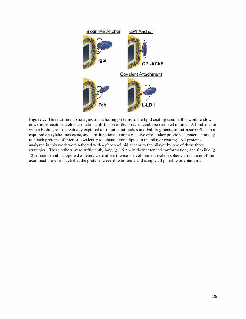
Figure 2. Three different strategies of anchoring proteins to the lipid coating used in this work to slow down translocation such that rotational diffusion of the proteins could be resolved in time. A lipid anchor with a biotin group selectively captured anti-biotin antibodies and Fab fragments, an intrinsic GPI anchor captured acetylcholinesterase, and a bi-functional, amine-reactive crosslinker provided a general strategy to attach proteins of interest covalently to ethanolamine lipids in the bilayer coating. All proteins analyzed in this work were tethered with a phospholipid anchor to the bilayer by one of these three strategies. These tethers were sufficiently long (≥ 1.5 nm in their extended conformation) and flexible (≥ 12 σ-bonds) and nanopore diameters were at least twice the volume-equivalent spherical diameter of the examined proteins, such that the proteins were able to rotate and sample all possible orientations.

26  

Figure 3. Determination of approximate protein shape and volume from histograms of maximum ΔI values from resistive pulse recordings. (a, b) Examples of original current traces as a function of time: upward spikes indicate individual resistive current pulses towards zero current due to the translocation of single streptavidin (a) or IgG (b) proteins. Resistive pulses marked by an asterisk are shown in detail above. (c-f) Histograms of maximum ΔI values from resistive pulse recordings with streptavidin (c), IgG1 (d), GPI-AChE (e), and G6PDH (f) proteins. Black curves show the solution of the convolution model, p(ΔI), after a non-linear least squares fitting procedure, and red dashed curves show the estimated distribution of ΔI values due to the distribution of shape factors, p(ΔIγ). Supplementary Table 1 lists the values of all fitting parameters and the electric field strength used in each experiment. Supplementary Note 2 and Supplementary Fig. 5-7 explain the convolution model and fitting procedure in detail and extend the analyses to all proteins characterized in this work. (g) Comparison of the approximate shape of ten proteins as determined by analysis of resistive pulses (blue spheroids) with crystal structures from the Protein Data Bank in red (streptavidin: 3RY1, anti-biotin immunoglobulin G1: 1HZH, GPI-anchored acetylcholinesterase: 3LII, anti-biotin Fab fragment: 1F8T, β-phycoerythrin: 3V57, glucose-6-phosphate dehydrogenase: 4EM5, L-lactate dehydrogenase: 2ZQY, bovine serum albumin: 3V03, α-amylase: 1BLI, and butyrylcholinesterase: 1P0I). (h) Comparison of the measured volume by nanopore-based analysis with the expected reference volume. (i) Comparison of the measured length-to-diameter ratios m of all proteins with the expected reference values of m. Error bars in h,i represent the standard deviation in most probable values from experiment-to-experiment or day-to-day.

27  

 

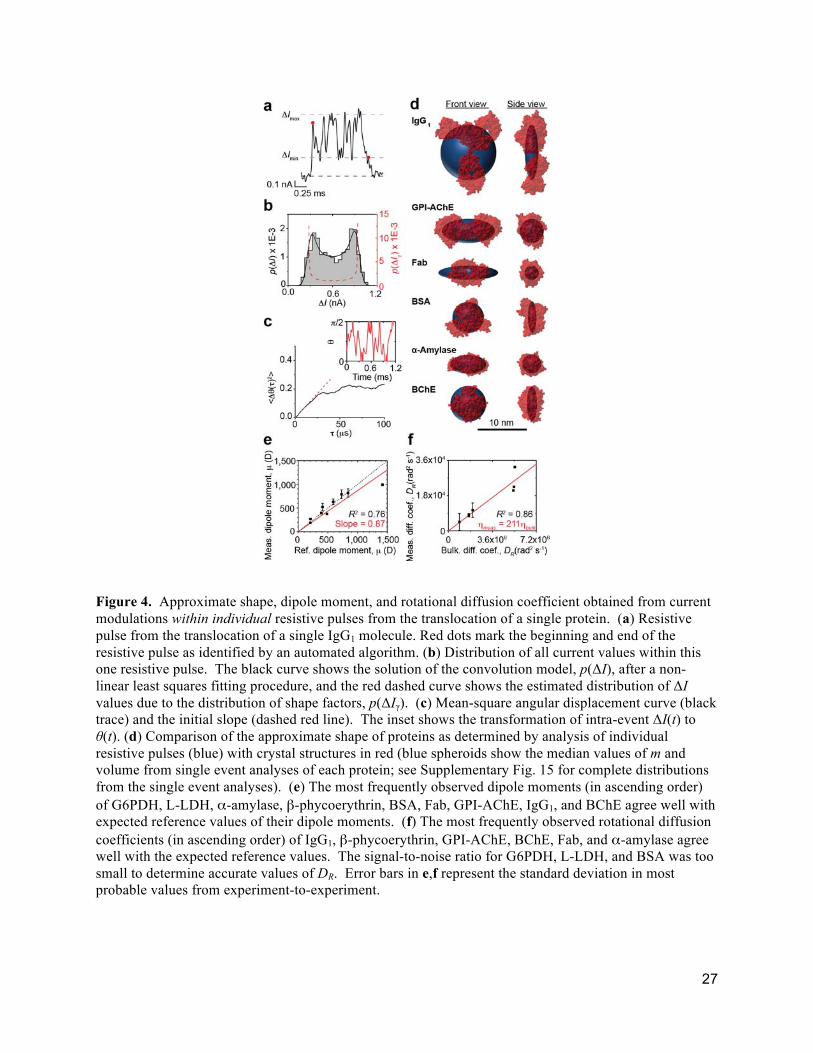
Figure 4. Approximate shape, dipole moment, and rotational diffusion coefficient obtained from current modulations within individual resistive pulses from the translocation of a single protein. (a) Resistive pulse from the translocation of a single IgG1 molecule. Red dots mark the beginning and end of the resistive pulse as identified by an automated algorithm. (b) Distribution of all current values within this one resistive pulse. The black curve shows the solution of the convolution model, p(ΔI), after a non-linear least squares fitting procedure, and the red dashed curve shows the estimated distribution of ΔI values due to the distribution of shape factors, p(ΔIγ). (c) Mean-square angular displacement curve (black trace) and the initial slope (dashed red line). The inset shows the transformation of intra-event ΔI(t) to θ(t). (d) Comparison of the approximate shape of proteins as determined by analysis of individual resistive pulses (blue) with crystal structures in red (blue spheroids show the median values of m and volume from single event analyses of each protein; see Supplementary Fig. 15 for complete distributions from the single event analyses). (e) The most frequently observed dipole moments (in ascending order) of G6PDH, L-LDH, α-amylase, β-phycoerythrin, BSA, Fab, GPI-AChE, IgG1, and BChE agree well with expected reference values of their dipole moments. (f) The most frequently observed rotational diffusion coefficients (in ascending order) of IgG1, β-phycoerythrin, GPI-AChE, BChE, Fab, and α-amylase agree well with the expected reference values. The signal-to-noise ratio for G6PDH, L-LDH, and BSA was too small to determine accurate values of DR. Error bars in e,f represent the standard deviation in most probable values from experiment-to-experiment.

28  

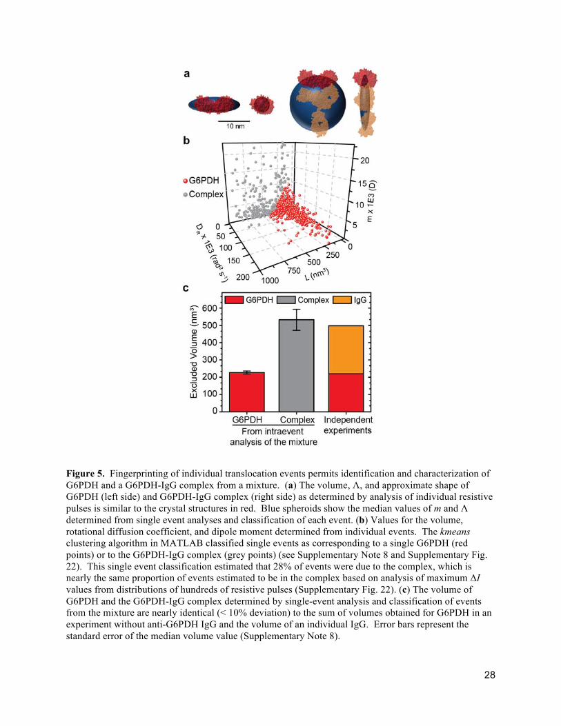
Figure 5. Fingerprinting of individual translocation events permits identification and characterization of G6PDH and a G6PDH-IgG complex from a mixture. (a) The volume, Λ, and approximate shape of G6PDH (left side) and G6PDH-IgG complex (right side) as determined by analysis of individual resistive pulses is similar to the crystal structures in red. Blue spheroids show the median values of m and Λ determined from single event analyses and classification of each event. (b) Values for the volume, rotational diffusion coefficient, and dipole moment determined from individual events. The kmeans clustering algorithm in MATLAB classified single events as corresponding to a single G6PDH (red points) or to the G6PDH-IgG complex (grey points) (see Supplementary Note 8 and Supplementary Fig. 22). This single event classification estimated that 28% of events were due to the complex, which is nearly the same proportion of events estimated to be in the complex based on analysis of maximum ΔI values from distributions of hundreds of resistive pulses (Supplementary Fig. 22). (c) The volume of G6PDH and the G6PDH-IgG complex determined by single-event analysis and classification of events from the mixture are nearly identical (< 10% deviation) to the sum of volumes obtained for G6PDH in an experiment without anti-G6PDH IgG and the volume of an individual IgG. Error bars represent the standard error of the median volume value (Supplementary Note 8).

29  

Figure 6. Advantage of 5-D fingerprinting over the standard 2-D characterization for protein identification. Using structural and sequence data from the Protein Data Bank, we randomly selected a group of proteins and determined their mass, volume, rotational diffusion constant, shape factor, dipole moment, and charge. Each parameter can be thought of as a dimension, and the heat map shows the separation between each pair of 100 randomly sampled proteins for two dimensions (lower left corner) or five dimensions (upper right corner) calculated using standard normal distributions for each descriptor.

This separation is calculated as where n is the number of dimensions and di is the difference

between the values of two different proteins in one parameter. Red squares mark protein-protein pairs that are similar in all descriptors (i.e. closely spaced), while yellow and green squares indicate increasing separation. Physical descriptors beyond protein charge and mass such as shape and dipole moment create additional dimensions and facilitate protein identification by increasing the separation between each protein-protein pair.

2

1

n

iid

=∑

1    

Supplementary Text and Figures:  

Real-time shape approximation and 5-D fingerprinting of single proteins Erik C. Yusko1,†,ǂ, Brandon R. Bruhn1,†, Olivia Eggenberger1, Jared Houghtaling1, Ryan C. Rollings2, Nathan C. Walsh2, Santoshi Nandivada2, Mariya Pindrus3, Adam R. Hall4, David Sept1,5, Jiali Li2, Devendra S. Kalonia3, Michael Mayer1,6,*

Affiliations: 1Department of Biomedical Engineering, University of Michigan, Ann Arbor, MI 48109, USA 2Department of Physics, University of Arkansas, Fayetteville, Arkansas 72701, USA 3Department of Pharmaceutical Sciences, University of Connecticut, Storrs, CT 06269, USA 4Department of Biomedical Engineering and Comprehensive Cancer Center, Wake Forest University School of Medicine, Winston Salem, NC 27157, USA 5Center for Computational Medicine and Biology, University of Michigan, Ann Arbor, MI 48109, USA 6Biophysics Program, University of Michigan, Ann Arbor, MI 48109, USA

†These authors contributed equally to this work. ǂCurrent address: Department of Physiology and Biophysics, University of Washington, Seattle, WA 98195, USA *Correspondence should be addressed to M.M. (mimayer@umich.edu)

Table of Contents Supplementary Note 1. Control experiments indicate that broad distributions of ∆I values were not due to impurities or simultaneous translocations .................................................................... 4 Supplementary Note 2. Determining the volume and shape of proteins from fitting distributions of maximum ΔI values .................................................................................................................. 6

Equation relating the amplitude of resistive pulses to the volume and electrical shape factor of particles ..................................................................................................................................... 6 Electrical shape factor and distributions of shape factors ......................................................... 7 Fitting the convolution model to distributions of ΔI values ...................................................... 12 Using ΔImin and ΔImax to solve for the volume and shape of proteins ...................................... 12 Estimating the volume of spheroidal proteins via dynamic light scattering ............................. 14 Low applied potentials yield consistent estimates of protein shape ........................................ 15 Forces acting on proteins in a nanopore ................................................................................. 15 Description of the assumptions underlying the convolution model ......................................... 17

Supplementary Note 3. Interpretation of the observed bimodal distributions of ΔI values from the translocation of non-spherical proteins ................................................................................. 18 Supplementary Note 4. Effect of lipid anchoring on the measurement of protein properties ... 20 Supplementary Note 5. Simulating translocation events due to spheroidal particles ............... 21 Supplementary Note 6. Analysis of intra-event ΔI values ......................................................... 22

2    

Distributions of m and Λ determined from fitting intra-event ΔI values ................................... 22 Determining the dipole moment of a protein from fitting intra-event ΔI values ........................ 23 Determining the rotational diffusion coefficient of a protein in a nanopore ............................. 24

Supplementary Note 7. Bivalently-bound IgG1 rotates slower than monovalently-bound IgG1 25 Supplementary Note 8. Distinguishing an antigen and antibody-antigen complex in a single nanopore experiment .................................................................................................................. 26 Supplementary Note 9. Derivation of probability distribution of shape factors for proteins with a dipole moment ............................................................................................................................ 27 Supplementary Figure 1. Most probable td values for the monoclonal anti-biotin IgG1 antibody and GPI-AChE as a function of the voltage drop, VP, across a bilayer-coated nanopore containing biotin-PE .................................................................................................................... 31 Supplementary Figure 2. Detection of monoclonal anti-biotin IgG1 antibody with a bilayer-coated nanopore and dynamic light scattering experiments ....................................................... 32 Supplementary Figure 3. Solutions containing GPI-AChE contained the dimeric, prolate shaped form of GPI-AChE .......................................................................................................... 33 Supplementary Figure 4. Histograms of the ΔI values due to the translocation of the IgG1 antibody (150 kDa) and GPI-anchored acetylcholinesterase (160 kDa) through the same nanopore ..................................................................................................................................... 34 Supplementary Figure 5. Example convolution of the probability distribution of ΔI values one expects due to the distribution of shape factors, p(ΔIγ) (equations (13a) and (13b)), and the error in determining individual ΔI values, p(ΔIσ) (a Normal distribution function) ................................ 35 Supplementary Figure 6. Empirical cumulative distributions of ΔI values due to the translocation of non-spherical proteins compared to a best-fit Normal distribution (red curves) and the solution to the convolution model, p(ΔI) ......................................................................... 36 Supplementary Figure 7. Estimating the excluded volume as a function of m using ΔImin and ΔImax values illustrates that there are two solutions to equations (14) and (15) for prolate shaped proteins ....................................................................................................................................... 38 Supplementary Figure 8. The dependence of a protein’s length-to-diameter ratio, m, on the applied potential, VA, for IgG1 and GPI-AChE ............................................................................. 39 Supplementary Figure 9. Finite-element simulations indicate that local variations in the conductivity of the solution are negligible under the experimental conditions used in this work 40 Supplementary Figure 10. Analysis of intra-event ∆I signals can yield parameter estimates in real-time ...................................................................................................................................... 41 Supplementary Figure 11. Determining the charge of proteins by fitting translocation time distributions with a first-passage-time model .............................................................................. 42 Supplementary Figure 12. Distributions of maximum ∆I values from simulated translocation events ......................................................................................................................................... 43 Supplementary Figure 13. Distributions of the length-to-diameter ratio, m, and excluded volume, Λ, determined from fitting the convolution model to simulated intra-event ∆I signals ... 44 Supplementary Figure 14. Dipole moments, µ, and rotational diffusion coefficients, DR, determined from analyzing simulated translocation events due to spheroidal particles ............. 45

3    

Supplementary Figure 15. Distributions of the length-to-diameter ratio, m, and excluded volume, Λ, determined from fitting the convolution model to all intra-event ∆I signals longer than 0.4 ms for IgG1, GPI-AChE, Fab, BSA, α-Amylase, and BChE .................................................. 46 Supplementary Figure 16. Dipole moments, µ, of IgG1, GPI-AChE, Fab, β-PE, G6PDH, L-LDH, BSA, α-amylase, and BChE determined from fitting intra-event ΔI values with the convolution model .......................................................................................................................................... 47 Supplementary Figure 17. Variation of the dipole moment, µ, of β-phycoerythrin (β-PE) as a function of pH. ............................................................................................................................. 49 Supplementary Figure 18. Rotational diffusion coefficients, DR, of IgG1, GPI-AChE, Fab, β-PE, α-Amylase, and BChE determined from analysis of intra-event ΔI values ................................. 50 Supplementary Figure 19. The measured rotational diffusion coefficient, DR, of lipid-anchored IgG1 decreases with the ratio of bivalently-bound to monovalently-bound IgG1 ......................... 52 Supplementary Figure 20. The distribution of maximum ∆I values for IgG1 is more biased toward low values when the fraction of bivalently-bound IgG1 is relatively high ......................... 53 Supplementary Figure 21. Effect of the recording electronics and low-pass filtering on intra-event ∆I values ........................................................................................................................... 54 Supplementary Figure 22. Determining the volume and shape of an antibody-antigen complex from individual resistive-pulses ................................................................................................... 55 Supplementary Figure 23. Histograms, boxplots, and density distributions of calculated physical descriptors for 780 proteins .......................................................................................... 56 Supplementary Figure 24. A scatter plot matrix showing the relationships between the log-normalized quantities in Supplementary Figure 23 ..................................................................... 57 Supplementary Figure 25. Transmission electron micrographs of the nanopores used in this work ............................................................................................................................................ 58 Supplementary Table 1. Values of fitting parameters determined from fitting the convolution model to the empirical distributions of ΔI values (Fig. 3 and 4 in the main text) as well as the resulting calculations of protein volume, Λ, and shape parameter, m ........................................ 59 Supplementary Table 2. Estimated hydration shell thickness of proteins detected in this work .................................................................................................................................................... 60 Supplementary Table 3. Estimated volume of proteins detected in this work from dynamic light scattering (DLS) measurements ................................................................................................. 61 Supplementary Table 4. Average volumes, length-to-diameter ratios, m = A/B, most probable dipole moments, rotational diffusion coefficients, and charges of proteins determined by analysis of resistive pulses and other methods ........................................................................................ 62 Supplementary References ..................................................................................................... 64

   

4    

Supplementary Note 1. Control experiments indicate that broad distributions of ∆I values were not due to impurities or simultaneous translocations

To confirm that the distributions of ΔI values during experiments with monoclonal anti-biotin IgG1 antibodies were not affected by potential impurities in the solution, we performed three control experiments. In one control experiment, we competitively inhibited the binding of IgG1 antibodies to the biotin-PE lipids on the surface by adding an excess concentration of soluble biotin to the aqueous solution of an ongoing experiment (Supplementary Fig. 2a and 2b). Fifteen minutes after the addition of the soluble biotin we observed the frequency of resistive pulses decrease from 34 s-1 to 1.3 s-1. In the second control experiment, we generated a lipid bilayer coated nanopore that did not contain biotin-PE lipids in the coating and therefore was not specific for the translocation of IgG1 antibodies (Supplementary Fig. 2c). In this experiment, the concentration of the IgG1 antibody was even higher (25 nM compared to 20 nM) than in the original experiment (Supplementary Fig. 2a), and the frequency of translocation events was 2 s-1. Since the frequency of events is proportional to concentration, we estimated that if the concentration of IgG1 in this control experiment was 20 nM, we would expect to observe an event frequency of approximately 1.6 s-1. From these two control experiments, we estimated that during experiments with biotin-PE lipids in the bilayer coating only 3.8 to 4.7 % of translocation events were due to proteins that were not bound to biotin-PE lipids. Furthermore, almost all (~90%) of the translocation times calculated from resistive-pulses observed in control experiments (where binding to biotin-PE was not possible) were less than 50 µs, and we did not include resistive-pulses with translocation times less than 50 µs in the analysis of ΔI distributions because the amplitude would be attenuated due to electronic filtering1,2. Consequently, we concluded that the protein we detected in the solution of anti-biotin IgG1 antibodies was bound to biotin-PE lipids specifically. In the final control experiment, we removed any fragments of IgG proteins (i.e. Fab fragments) or other proteins in the IgG stock solution by purifying the solution with a Protein A spin column (Thermo Scientific 89952). Using this purified solution in a nanopore-based sensing experiment, we observed distributions of ΔI values similar to those seen with the stock solution, and we determined the same volume and shape of anti-biotin IgG1, within error (Supplementary Table 1). Results from these three control experiments indicate that the resistive pulses in experiments with IgG1 were due to anti-biotin IgG1 proteins and not due to the presence of other proteins or Fab fragments.

Since IgG antibodies can occasionally form dimers3, we performed dynamic light scattering (DLS) experiments to characterize the hydrodynamic diameter of the IgG1 antibodies. If dimers of IgG1 antibodies were present in solution and contributing to the bimodal distribution of ΔI values in Fig. 3 of the main text, we would expect them to be reflected in DLS experiments in a significant fraction because approximately ½ of the resistive pulses had ΔI values that can be attributed to either of the bimodal peaks in the distribution of ΔI values. Consequently, if dimers were present, we would expect to observe two peaks in the distributions of estimated hydrodynamic diameters of the particles (proteins in this case) in DLS experiments3. Supplementary Fig. 2d shows that we only observed one peak corresponding to a hydrodynamic diameter of 10.5 ± 2.0 nm. This value is in good agreement with previously published hydrodynamic diameters of IgG antibodies of 10.9 to 11.0 nm, which were determined in physiologic buffers3,4. As additional evidence, we added urea to a concentration of 8 M to denature the IgG protein and disassociate potential aggregates. Again we only observed one peak corresponding to a hydrodynamic diameter of 12.9 ± 2.7 nm (Supplementary Fig. 2d). This hydrodynamic diameter is larger because of the random-coil and ball-like structure of denatured

5    

IgG1 antibodies compared to their native, oblate-shaped structures3. Thus, the results presented in Supplementary Fig. 2 confirm that dimers of IgG1 antibodies were not responsible for the bimodal distribution of ΔI values and that the IgG1 antibodies were stable and functional in the buffered solutions used here. GPI-anchored acetylcholinesterase purified from human erythrocyte membranes naturally occurs in a dimeric, prolate-shaped form that is held together by disulfide bonds near the C-terminal tail of the protein5-9. To confirm that the GPI-AChE used in this work remained in dimeric form and to detect impurities in solution, we performed a SDS-PAGE experiment. We ran three lanes on the SDS-PAGE gel corresponding to three different treatments of the protein: incubation with SDS, incubation with SDS and β-mercaptoethanol to dissociate the disulfide bond, and incubation with only β-mercaptoethanol to assess whether the disulfide bond in the folded protein was accessible to β-mercaptoethanol as reported in literature9. After staining, we observed only one protein band in each lane. When the protein was denatured with only SDS, we observed the dimeric form that ran with an apparent molecular weight of ~140 kDa. In both lanes where the protein was treated with β-mercaptoethanol, we observed only one protein band, running at an apparent molecular weight of ~60 kDa. These apparent molecular weights are lower than the values in reported literature of 160 kDa for the dimer and 80 kDa for the monomer because GPI-AChE is an amphiphilic protein and likely has a higher binding capacity for SDS than more commonly run soluble proteins5-11. This increased binding of SDS yields a greater charge to mass ratio and therefore greater migration speed of the protein compared to most soluble proteins, causing GPI-AChE to migrate in the gel as if it had a lower molecular weight. This phenomenon is well known for amphiphilic proteins12.

The fact that we only observe one band in each lane of the gel indicates that our samples contained high concentrations of GPI-AChE relative to other contaminants. In the lanes treated with β-mercaptoethanol the absence of a band at ~140 kDa coincident with the appearance of a band at ~60 kDa is consistent with breakage of the disulfide bond holding the dimer together. Moreover, as reported in literature, the disulfide bond was accessible in the native structure of the protein, as indicated by the appearance of a single band at the monomer molecular weight when the protein was treated only with β-mercaptoethanol (and no SDS) prior to running the gel9. Consequently, this gel confirms that the GPI-AChE protein in our sample was in its natural dimeric, prolate-shaped form. Moreover, the control experiments in Supplementary Fig. 2a-c indicate that if there were soluble (i.e. not lipid-anchored) contaminants in the solution, they would not be detected, since soluble proteins would not be concentrated on the lipid surface or slowed during translocation through the nanopore.

To rule out the possibility that the widely distributed ΔI values were due to two proteins passing through the nanopore simultaneously, we compared the frequency of translocation events with the translocation times for each protein13. In the case of streptavidin translocations, we observed approximately 45 translocation events per second and a most-probable translocation time of about 115 µs. Consequently, on average there was a 0.52% probability of a molecule occupying the nanopore at any time, and the probability of two streptavidin proteins occupying the nanopore at the same time would be 0.003%. In the case of the IgG1 translocation events, the maximum frequency we observed was approximately 30 events per second and a most probable translocation time of about 55 µs. Consequently, on average there was a 0.16% probability of an IgG1 protein occupying the nanopore at any time, and the probability of two IgG1 proteins occupying the nanopore at the same time would then be 0.0027%. Even if the first translocation event of an IgG antibody would be exceptionally long lived (e.g. 1000 µs), the probability of a

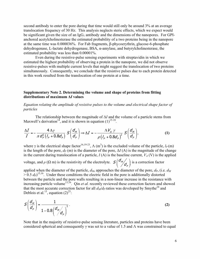
6    

second antibody to enter the pore during that time would still only be around 3% at an average translocation frequency of 30 Hz. This analysis neglects steric effects, which we expect would be significant given the size of an IgG1 antibody and the dimensions of the nanopores. For GPI-anchored acetylcholinesterase the estimated probability of a two proteins being in the nanopore at the same time was 0.000036%. For Fab fragments, β-phycoerythrin, glucose-6-phosphate dehydrogenase, L-lactate dehydrogenase, BSA, α-amylase, and butyrylcholinesterase, the estimated probability was less than 0.00001%.

Even during the resistive-pulse sensing experiments with streptavidin in which we estimated the highest probability of observing a protein in the nanopore, we did not observe resistive-pulses with multiple current levels that might suggest the translocation of two proteins simultaneously. Consequently, we conclude that the resistive pulses due to each protein detected in this work resulted from the translocation of one protein at a time.

Supplementary Note 2. Determining the volume and shape of proteins from fitting distributions of maximum ΔI values

Equation relating the amplitude of resistive pulses to the volume and electrical shape factor of particles

The relationship between the magnitude of ΔI and the volume of a particle stems from Maxwell’s derivation14, and it is shown in equation (1)15-18.

( ) ( )γγ

π ρ

⎛ ⎞ ⎛ ⎞ΛΔ Λ=− ⇒Δ = −⎜ ⎟ ⎜ ⎟

+ +⎝ ⎠ ⎝ ⎠2 2

40.8 0.8

M A M

P PP P P P P

d V dI S I SI d dd l d l d

, (1)

where γ is the electrical shape factor16,19-23, Λ (m3) is the excluded volume of the particle, lP (m) is the length of the pore, dP (m) is the diameter of the pore, ΔI (A) is the magnitude of the change in the current during translocation of a particle, I (A) is the baseline current, VA (V) is the applied

voltage, and ρ (Ω m) is the resistivity of the electrolyte. ⎛ ⎞⎜ ⎟⎝ ⎠M

P

dS d is a correction factor

applied when the diameter of the particle, dM, approaches the diameter of the pore, dP, (i.e. dM > 0.5 dP)15,16. Under these conditions the electric field in the pore is additionally distorted between the particle and the pore walls resulting in a non-linear increase in the resistance with increasing particle volume15,16. Qin et al. recently reviewed these correction factors and showed that the most accurate correction factor for all dM/dP ratios was developed by Smythe24 and Deblois et al.15, equation (2)25:

⎛ ⎞=⎜ ⎟

⎛ ⎞⎝ ⎠ − ⎜ ⎟⎝ ⎠

3

1

1 0.8

M

P M

P

dSd d

d

. (2)

Note that in the majority of resistive-pulse sensing literature, particles and proteins have been considered spherical and consequently γ was set to a value of 1.5 and Λ was constrained to equal

7    

316 Mdπ . Substituting these values into equation (1) simplifies it to the more commonly seen

form in equation (3)14,15,17,18,23,25:

( ) ( )π

ρ

⎛ ⎞ ⎛ ⎞Δ=− ⇒Δ =−⎜ ⎟ ⎜ ⎟

+ +⎝ ⎠ ⎝ ⎠

3 3

2 20.8 4 0.8M M A M M

P PP P P P P

d d V d dI S I SI d dd l d l d

, (3)

Since in this work we analyzed resistive-pulses due to the translocation of non-spherical proteins and we expected dM to be less than ½ dP, we set the correction factor to a value of 12,17,18. We used equation (1) and expressed the impeded flow of ions through the nanopore during protein translocation events as reductions in current, ΔI. The volume exclusion model shown in equation (1) has yielded accurate estimates of volume in a number of prior publications17,22,26-30; however, it has also been inadequate under a variety of different experimental conditions31-35. The model fails to describe certain current pulses because it does not account for heterogeneity in the distribution of ions, and thus the conductivity of the solution, in the nanopore. Heterogeneity in the distribution of ions results from electrostatic interactions with the surface of the pore and translocating particle. For instance, Lan et al. observed biphasic current pulses resulting in part from the accumulation of chloride ions on one side of the particle31. In this case, the flow of chloride ions around the particle was inhibited as the particle and pore were both negatively charged. To determine whether such effects are likely to occur under the experimental conditions used here, we performed finite-element simulations nearly identical to those described by Lan et al. Supplementary Fig. 9a shows similar local variations in the conductivity of the solution to those reported by Lan et al. at a low ionic strength of 10 mM KCl due to the accumulation and depletion of chloride ions on opposite sides of the protein. In contrast, the conductivity of the solution is nearly constant at the high ionic strength of 2 M KCl that we used in the experiments presented here (Supplementary Fig. 9b). In this case, the ∆I signature (see Supplementary Fig. 9c) is well described by the volume exclusion model shown in equation (1). Consequently, the volume exclusion model is appropriate under the experimental conditions used in this work.

Electrical shape factor and distributions of shape factors

The electrical shape factor has been reported in literature since Maxwell derived equations to describe the conductance of solutions that contain insulating (i.e. non-conducting) spheres14. Maxwell considered both the volume fraction of the spheres in solution and the deformation of the electric field around these spheres. To account for the distortion of the electric field, Maxwell derived a scaling factor that is dependent on the shape of the insulating particles (i.e. electrical shape factor) and equal to 3/2 or 1.5 for spheres. Several years later, Fricke derived the electrical shape factor for spheroids, and Velick and Gorin developed analytical equations to describe the shape factor for ellipsoids of a general shape36-38. In 1954, Smythe numerically tested Maxwell’s theory for the specific case of a particle residing in a pore; this work verified the electrical shape factor of 1.5 for spheres as well as the methods described by Fricke, Velick, and Gorin24. Around the same time, many groups experimentally proved these theories during resistive-pulse sensing experiments with holes that were micrometers in diameter while sensing various micrometer-sized particles16,19,23,39,40. In 1973, Golibersuch observed the rotation of red blood cells within the pore of a resistive-pulse sensor and derived the

8    

distribution for electrical shape factors to explain the periodic variations in ΔI that occurred during the rotation of the blood cell.

The mathematical descriptions for shape factors are analogous among many systems and can be used to describe how electric and magnetic fields deform around insulating particles as well as how ideal fluids flow around obstacles in wind tunnels or in aqueous solutions with laminar flow19,24,39. Spheres alter flow and electric fields to the same extent regardless of their orientation; however, spheroid particles alter these fields to a different extent depending on their orientation relative to the direction of the field. Thus, the electrical shape factor is a function of a particle’s shape and orientation.

To relate the value of ΔI to the volume and shape of non-spherical proteins, we considered the possible values of the electrical shape factor, γ, with the condition that a protein may have an oblate, prolate, or spherical shape. Oblates and prolates have an axis of revolution (shown as the dashed blue line in Fig. 1 of the main text) with length A and secondary axes with length B. Golibersuch elegantly pointed out that equation (4) describes the electrical shape factor, γ, for these ellipsoids as a function of the angle between the axis of symmetry and the electric field, θ, (Fig. 1)19,39:

( ) ( ) ( )γ θ γ γ γ θ⊥ ⊥= + − 2II cos (4)

where IIγ

and γ ⊥ are the electrical shape factors when the axis of symmetry is parallel to the

electric field (i.e. θ = 0, π, ...) and perpendicular to the electric field (i.e. θ = π/2, 3π/2, …), respectively. Equation (4) implies that the shape factor for any orientation will range between the values of IIγ

and γ ⊥ . These factors, IIγ

and γ ⊥ , are related to the well-described

depolarization factors for ellipsoids, IIn and n⊥ , by equation (5) and are a function of the length to diameter ratio, m = A/B, of an ellipsoid19,20,40,41.

IIII

11 n

γ =−

and 11 n

γ ⊥⊥

=−

(5)

where IIn for a prolate spheroid with m = A/B > 1 is described by equation (6):

( )2II 2 2

1 ln 1 11 1

mn m mm m

⎡ ⎤= + − −⎢ ⎥− −⎣ ⎦

(6)

and IIn for an oblate spheroid with m = A/B < 1 is described by equation (7):

( )1II 2 2

1 1 cos1 1

mn mm m

−⎡ ⎤= −⎢ ⎥− −⎣ ⎦

(7)

and n⊥ = (1 - IIn )/219,23,41. To derive the distribution of shape factors, we assume that ellipsoidal proteins rotate

freely such that all angles of θ are equally likely when ΔI is measured. By symmetry, values of θ range between 0 and π/2. According to Golibersuch, these assumptions enable using substitution of variables to write a probability distribution function for electrical shape factors P(γ) based on

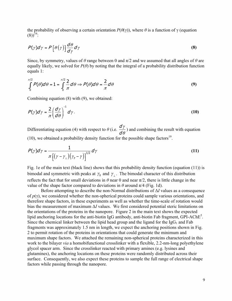
9    

the probability of observing a certain orientation P(θ(γ)), where θ is a function of γ (equation (8))19:

( )( )dP d P ddθ

γ γ θ γ γγ

⎡ ⎤= ⎣ ⎦

(8)

Since, by symmetry, values of θ range between 0 and π/2 and we assumed that all angles of θ are equally likely, we solved for P(θ) by noting that the integral of a probability distribution function equals 1:

/2 /2

0 0

2 2( ) 1 ( )P d d P d d

π π

θ θ θ θ θ θπ π

= = ⇒ =∫ ∫ (9)

Combining equation (8) with (9), we obtained:

12

( )dP d ddγ

γ γ γπ θ

−⎛ ⎞

= ⎜ ⎟⎝ ⎠

. (10)

Differentiating equation (4) with respect to θ (i.e. ddγθ

) and combining the result with equation

(10), we obtained a probability density function for the possible shape factors19.    

( )( )γ γ γ

π γ γ γ γ⊥

=⎡ ⎤− −⎣ ⎦P

1/2

1( )P d d (11)

Fig. 1e of the main text (black line) shows that this probability density function (equation (11)) is bimodal and symmetric with peaks at IIγ

and γ ⊥ . The bimodal character of this distribution

reflects the fact that for small deviations in θ near 0 and near π/2, there is little change in the value of the shape factor compared to deviations in θ around π/4 (Fig. 1d).

Before attempting to describe the non-Normal distributions of ΔI values as a consequence of p(γ), we considered whether the non-spherical proteins could sample various orientations, and therefore shape factors, in these experiments as well as whether the time-scale of rotation would bias the measurement of maximum ΔI values. We first considered potential steric limitations on the orientations of the proteins in the nanopore. Figure 2 in the main text shows the expected lipid anchoring locations for the anti-biotin IgG antibody, anti-biotin Fab fragment, GPI-AChE5. Since the chemical linker between the lipid head group and the ligand for the IgG1 and Fab fragments was approximately 1.5 nm in length, we expect the anchoring positions shown in Fig. 2 to permit rotation of the proteins in orientations that could generate the minimum and maximum shape factors. We attached the remaining non-spherical proteins characterized in this work to the bilayer via a homobifunctional crosslinker with a flexible, 2.2-nm-long polyethylene glycol spacer arm. Since the crosslinker reacted with primary amines (e.g. lysines and glutamines), the anchoring locations on these proteins were randomly distributed across their surface. Consequently, we also expect these proteins to sample the full range of electrical shape factors while passing through the nanopore.

10    

We next examined whether the dipole moment of a protein may align completely in the large electric field in the nanopore (~106 V m-1). Combining the potential energy, ΔU, of a dipole moment in an electric field and the Boltzmann distribution of energies while assuming that the dipole moment was pointed parallel to one of the principal axes of the protein, we expanded on Golibersuch’s probability distribution of shape factors to develop a p(γ) for a protein with a dipole moment (Fig. 1e in the main text and Supplementary Note 9). To expand on the theories developed by Golibersuch, we considered the possible probability distribution of shape factors if the orientation of the protein were biased by the electric field in the nanopore. The electric field in the nanopore is on the order of 106 V m-1

, and consequently, we expect the orientation of a protein to be biased by alignment of its dipole moment, µv (Debye ≈ 3.33564×10−30 C m), in the electric field,

vE ( V m-1). Taking into account the potential energy of

a dipole in an electric field, ( )µ µ φΔ = = −v vg cosU E E , using the Boltzmann distribution of

energies, and assuming the dipole was aligned along the symmetry or equatorial axis, we derived equations (12a) and (12b), respectively (Supplementary Note 9). Equations (12a) and (12b) describe probability distribution functions of shape factors for spheroid proteins when their orientation is biased by the dipole energy in an electric field.

( ) ( )

γ γµ

γ γ γγ γπ γ γ γ γ

⊥

⊥

⊥

⎡ ⎤⎛ ⎞ ⎡ ⎤−⎢ ⎥⎜ ⎟ ⎢ ⎥⎜ ⎟= −⎢ ⎥⎝ ⎠ ⎢ ⎥⎡ ⎤− −⎢ ⎥ ⎢ ⎥⎣ ⎦⎣ ⎦⎣ ⎦

P

P

1/2

1/2

1 1( ) cosh

B

EP d dA

k T

(12a)

( ) ( )

γ γµ

γ γ γγ γπ γ γ γ γ

⊥

⊥

⎡ ⎤⎛ ⎞− ⎡ ⎤⎢ ⎥⎜ ⎟ ⎢ ⎥⎜ ⎟= −⎢ ⎥⎝ ⎠ ⎢ ⎥⎡ ⎤− −⎢ ⎥ ⎢ ⎥⎣ ⎦⎣ ⎦⎣ ⎦

P

P

P

1/2

1/2

1 1( ) cosh

B

EP d dA

k T

(12b)

In equations (12a) and (12b), A is a normalization constant described in Supplementary Note 9. Fig. 1e of the main text demonstrates that for spheroid proteins with dipoles of several thousand Debyes, it is theoretically possible to observe a bimodal distribution of shape factors. The average dipole moments of proteins is approximately 550 Debye (http://bioinfo.weizmann.ac.il/dipol/indexj.html), suggesting that many non-spherical proteins should generate a skewed bimodal distribution of shape factors. Additional factors may bias the orientation of proteins in the nanopore including steric effects, interactions with the pore wall, and alignment of slender proteins prior to entering the nanopore. All of these factors could affect the estimated value of ΔU or µ in this model. Therefore, an alternative interpretation of these parameters is that they describe the overall bias of the protein’s orientation toward θ = 0 or π/2. Equations (12a) and (12b) cannot describe distributions of ΔI accurately for proteins that are significantly biased (i.e. ΔU > ~4 kBT or µ > ~3000 D for a typical pore at 100 mV applied potential) toward intermediate orientations relative to the electric field (i.e. θ = π/4). Under these circumstances, the model would not resolve ΔImin and ΔImax accurately, underestimating the shape of the protein (i.e. m would approach 1) and overestimating the volume of the protein. Consequently, equations (12a) and (12b) are an approximation of how the orientation, and therefore distribution of shape factors, of a protein with a dipole moment may be biased, and they allow the theoretical distribution of shape factors to become asymmetric.

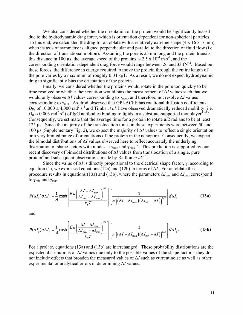
11    

We also considered whether the orientation of the protein would be significantly biased due to the hydrodynamic drag force, which is orientation dependent for non-spherical particles. To this end, we calculated the drag for an oblate with a relatively extreme shape (4 x 16 x 16 nm) when its axis of symmetry is aligned perpendicular and parallel to the direction of fluid flow (i.e. the direction of translational motion). Assuming the pore is 25 nm long and the protein transits this distance in 100 µs, the average speed of the proteins is 2.5 x 10-4 m s-1, and the corresponding orientation-dependent drag force would range between 26 and 33 fN42. Based on these forces, the difference in energy required to move the protein through the entire length of the pore varies by a maximum of roughly 0.04 kBT. As a result, we do not expect hydrodynamic drag to significantly bias the orientation of the protein. Finally, we considered whether the proteins would rotate in the pore too quickly to be time resolved or whether their rotation would bias the measurement of ΔI values such that we would only observe ΔI values corresponding to γmax, and therefore, not resolve ΔI values corresponding to γmin. Axelrod observed that GPI-AChE has rotational diffusion coefficients, DR, of 10,000 ± 4,000 rad2 s-1

and Timbs et al. have observed dramatically reduced mobility (i.e. DR ≈ 0.003 rad2 s-1) of IgG antibodies binding to lipids in a substrate-supported monolayer43-45. Consequently, we estimate that the average time for a protein to rotate π/2 radians to be at least 125 µs. Since the majority of the translocation times in these experiments were between 50 and 100 µs (Supplementary Fig. 2), we expect the majority of ΔI values to reflect a single orientation or a very limited range of orientations of the protein in the nanopore. Consequently, we expect the bimodal distributions of ΔI values observed here to reflect accurately the underlying distribution of shape factors with modes at γmin and γmax

19. This prediction is supported by our recent discovery of bimodal distributions of ΔI values from translocation of a single, pure protein2 and subsequent observations made by Raillon et al.22. Since the value of ΔI is directly proportional to the electrical shape factor, γ, according to equation (1), we expressed equations (12a) and (12b) in terms of ΔI. For an oblate this procedure results in equations (13a) and (13b), where the parameters ΔImin and ΔImax correspond to γmin and γmax.

( ) ( )γ γ γ

µ

π

⎡ ⎤⎛ ⎞Δ − Δ ⎡ ⎤⎢ ⎥⎜ ⎟ ⎢ ⎥Δ Δ = ΔΔ − Δ⎢ ⎥⎝ ⎠ ⎢ ⎥⎡ ⎤Δ − Δ Δ − Δ⎢ ⎥ ⎣ ⎦⎣ ⎦⎣ ⎦

1/2

max

1/2min max

max min

1 1( ) cosh

B

I IEP I d I d II IA I I I Ik T

(13a)

and

( ) ( )γ γ γ

µ

π

⎡ ⎤⎛ ⎞Δ − Δ ⎡ ⎤⎢ ⎥⎜ ⎟ ⎢ ⎥Δ Δ = ΔΔ − Δ⎢ ⎥⎝ ⎠ ⎢ ⎥⎡ ⎤Δ − Δ Δ − Δ⎢ ⎥ ⎣ ⎦⎣ ⎦⎣ ⎦

1/2

min

1/2max min

max min

1 1( ) cosh

B

I IEP I d I d II IA I I I Ik T

. (13b)

For a prolate, equations (13a) and (13b) are interchanged. These probability distributions are the expected distributions of ΔI values due only to the possible values of the shape factor – they do not include effects that broaden the measured values of ΔI such as current noise as well as other experimental or analytical errors in determining ΔI values.

12    

Fitting the convolution model to distributions of ΔI values

  To account for experimental and analytical errors in determining ΔI values, we convolved the expected distribution of ΔI values due to variation in the electrical shape factor, p(ΔIγ) (equations (13a) and (13b)), with a Normal distribution, p(ΔIσ), to generate the a distribution of ΔI values that one expects to observe experimentally, p(ΔI). We used this theoretical distribution (herein referred to as the “convolution model”) to fit all of the empirical distributions of ΔI values presented in this work. Supplementary Figure 5 illustrates this method.

When constructing empirical distributions of ∆I values from many translocation events, we represented each event by its maximum ∆I value as opposed to its average (e.g. Fig. 3 in the main text). We followed this strategy because representing events by their average value causes bias towards intermediate ∆I values and may introduce an additional mode besides the two expected modes at ∆Imin and ∆Imax, which would result in an improper fit with the convolution model (Supplementary Fig. 5). On the other hand, representing events by their maximum value likely biases the distribution of ΔI values toward ΔImax such that the amplitude of the peak corresponding to ∆Imax increases. In this instance, however, the location of ΔImax and ΔImin should be preserved such that the shape of the protein can still be determined accurately.

Since the distribution of ∆I values resulting from the distribution of shape factors, p(ΔIγ), is different depending whether the dipole moment is assumed to be parallel to the symmetry or equatorial axis of the protein (equations (13a) and (13b), respectively), we fit each empirical distribution of ∆I values, P(ΔI), with both of the resulting solutions to the convolution model. Subsequently, we selected the fit that yielded the larger adjusted R2 value as the correct solution. Since the orientation of the dipole moment dictates the preferred orientation of the protein, this procedure effectively determined whether the distribution of ∆I values was skewed towards ∆Imin or ∆Imax.  

When fitting the distributions of ∆I values for Fab, α-amylase, and BChE, we excluded outliers from the upper end of the distributions to determine their shape correctly. For each distribution, we excluded ∆I values that were greater than a threshold value, which we chose such that the R2 value of the fit with the convolution model was maximized. Conversely, ∆I values were not excluded for any of the other proteins detected in this work. Finally, we low-pass filtered the data for BChE at 10 kHz as opposed to 15 kHz in order to improve the signal-to-noise ratio.

Using ΔImin and ΔImax to solve for the volume and shape of proteins

Given that the probability distribution of shape factors has modes at IIγ

and γ ⊥

corresponding to either ΔImin or ΔImax values according to equation (1), we expected that if the value of ΔImin and ΔImax could be determined quantitatively from the empirical distribution of ΔI values then the volume and shape of a protein could also be determined. For example, the minimum shape factor for an oblate spheroid occurs at θ = π/2 and has a value of γ ⊥ (m) (equation (4)). Thus, according to equation (1), the minimum mode in the bimodal ΔI distribution, ΔImin, is a function of Λ and γ ⊥ (m), and the maximum mode in the bimodal ΔI distribution, ΔImax, is a function of Λ and IIγ (m). Since both IIγ

and γ ⊥ are solely a function of

m, we developed the system of equations (14) and (15) in which the values of m and Λ are the only two unknowns and the values of ΔImin and ΔImax are determined from fitting the empirical

13    

distributions of ΔI with the convolution model. By rearranging equation (3), we can write for oblate spheroids with m < 1:

( )( )( )

min

II max

( ),if 1

( ),

m Im m

m I

γ

γ⊥⎧Λ Δ⎪

Λ = <⎨Λ Δ⎪⎩

, (14)

and for prolate spheroids with m > 1:

( )( )( )II min

max

( ),if 1

( ),

m Im m

m I

γ

γ ⊥

⎧Λ Δ⎪Λ = >⎨

Λ Δ⎪⎩. (15)

Since this system of equations has a piecewise dependence on the value of m, we substituted the determined values of ΔImin and ΔImax into equations (14) and (15) and used MATLAB to solve the system for the excluded volume of the protein, Λ, and the value of m. For all prolates and relatively spherical oblates, two solutions to this system of equations exist as shown in Supplementary Fig. 7. The solutions for all experiments are summarized in Supplementary Table 1.  

For many of the fits, the value of σ is reasonable given the standard deviation of the baseline noise, which was typically between 20 and 60 pA. On the other hand, several of the fits returned relatively low estimates of σ (e.g. α-Amylase using Pore 10), which may be a result of using maximum ∆I values to represent long events or due to partial truncation of the ∆I distributions since only values larger than a certain threshold were detected. Nevertheless, the excellent agreement between the estimated volume of the proteins and their respective shapes (Supplementary Table 4) provide strong evidence that this procedure enables one to approximate the shape and determine the volume of non-spherical proteins by analyzing the distributions of maximum ΔI values. This method does not assume any information about the protein to extract the parameters shown in Supplementary Table 1.

While results for m and Λ from different pores are in good agreement for G6PDH and BSA (<10% difference in m and <20% difference in Λ), we observed significant pore-to-pore variability for GPI-AChE and IgG1 (Supplementary Table 4). Using all of the 9 possible pore-to-pore comparisons from the results presented in Supplementary Table 1, we found that pore-to-pore variability in m and Λ is weakly correlated with differences in pore diameter and length (i.e. -0.3 ≤ Pearson’s r ≤ 0.3). In fact, we observed the lowest pore-to-pore variability in m for G6PDH despite the fact that the pores used to characterize this protein have the largest difference in radii of any of the possible pore-to-pore comparisons. Based on these results, it appears that pore-to-pore variability of determined m- and Λ-values does not depend on pore diameter or length. This variability is likely due to variations in the pore geometry that are not accounted for in the model. The model assumes that the pore is perfectly cylindrical (i.e. constant diameter); however, nanopores prepared by ion-beam sculpting generally have an hourglass shape46. Even if the maximum ∆I value for each event is obtained when the protein is centered about the narrowest constriction of the pore, ∆Imin and ∆Imax will vary with the degree of pore tapering. Moreover, sterics may also introduce pore-to-pore variability by restricting certain protein orientations or conformations, particularly for IgG1 since it is a relatively large protein and composed of three domains that move relative to one another. Based on these arguments, it is perhaps unsurprising that we find the largest pore-to-pore variability for the determination of the

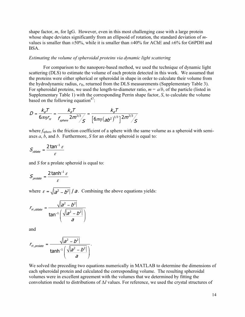
14    

shape factor, m, for IgG. However, even in this most challenging case with a large protein whose shape deviates significantly from an ellipsoid of rotation, the standard deviation of m-values is smaller than ±50%, while it is smaller than ±40% for AChE and ±6% for G6PDH and BSA.

Estimating the volume of spheroidal proteins via dynamic light scattering

For comparison to the nanopore-based method, we used the technique of dynamic light scattering (DLS) to estimate the volume of each protein detected in this work. We assumed that the proteins were either spherical or spheroidal in shape in order to calculate their volume from the hydrodynamic radius, rH, returned from the DLS measurements (Supplementary Table 3). For spheroidal proteins, we used the length-to-diameter ratio, m = a/b, of the particle (listed in Supplementary Table 1) with the corresponding Perrin shape factor, S, to calculate the volume based on the following equation47:

( )πη πη= = =

⎡ ⎤⎣ ⎦2/3 2/31/326 2 26

B B B

H sphere

k T k T k TD

r m mf abS S

where fsphere is the friction coefficient of a sphere with the same volume as a spheroid with semi-axes a, b, and b. Furthermore, S for an oblate spheroid is equal to:

εε

−

=12 tan

oblateS

and S for a prolate spheroid is equal to:

εε

−

=12 tanh

prolateS

where ε = −2 2 / aa b . Combining the above equations yields:

2 2

,2 21tan

H oblatea bra ba

−

−=⎛ ⎞−⎜ ⎟⎝ ⎠

and

2 2

,2 21tanh

H prolatea bra ba

−

−=⎛ ⎞−⎜ ⎟⎝ ⎠

.

We solved the preceding two equations numerically in MATLAB to determine the dimensions of each spheroidal protein and calculated the corresponding volume. The resulting spheroidal volumes were in excellent agreement with the volumes that we determined by fitting the convolution model to distributions of ΔI values. For reference, we used the crystal structures of

15    

these proteins to determine their length-to-diameter ratio, m, and subsequently determine their spheroidal volume; these volumes were also in excellent agreement with volumes obtained from analysis of DLS and resistive-pulse sensing experiments (Supplementary Table 3). In contrast, if we assumed the particles were a perfect sphere, the volumes that we determined from the hydrodynamic radius were overestimated for every non-spherical protein. These experiments provide additional evidence that the methods we present in this paper accurately describe the distribution of ΔI values for determining the shape and volume of spheroidal proteins.

Low applied potentials yield consistent estimates of protein shape

  The value of the shape parameter, m, determined from fitting distributions of maximum ∆I values for IgG1 and GPI-AChE is consistent at relatively low applied potentials but decreases or increases, respectively, as the applied potential is increased (Supplementary Fig. 8). This deviation might result from deformation of the protein due to the electrophoretic force acting on it while in the nanopore as was observed by Freedman et al.48; however, the amount of deformation that is expected based on theory (see proceeding subsection) is not large enough to account for the change in m observed here. Furthermore, Pelta et al. have previously shown that proteins do not change shape under similar electric field intensities49. Alternatively, this deviation could be due to changes in the size and shape of the hydration shell surrounding the protein or increasing alignment of the protein in the electric field gradient prior to entering the pore with increasing field intensity. In response to this observation, we limited our analyses to distributions of ∆I values that were obtained at relatively low potentials where the distributions appeared to be resolved fully. This approach consistently returned accurate estimates of the shape and volume of non-spherical proteins (Supplementary Table 1).

Forces acting on proteins in a nanopore

  Since the magnitude of the electric field is on the order of 106 V m-1 in the nanopore, we considered theoretically whether it was possible for the shape of proteins to be affected by forces in the nanopore. In this work, we expect proteins in the nanopore to be subjected to the following forces:

1) Instantaneous forces due to collisions with water will be on the order of ~500 pN with a net force equal to 0 on time scales of roughly 1 ps50.

2) Net torque due to the dipole moment in the electric field will have magnitudes similar to thermal energy. Fig. 1e in the main text shows that we expect the torque on a protein to be on the order of 0 to 4 kBT in this work.

3) Average force due to the net charge of the protein in the electric field, Fq, is in the range of 0.1 to 4 pN for the electric field strengths and net charges of proteins used in this work.

4) Average force on the protein due to viscous drag in the aqueous solution, Fw, which opposes the electrophoretic force. We approximated this force to range from about 0.026 to 0.033 pN.

5) Average force on the lipid anchor, FL, which also opposes the electrophoretic force, is thus on the order of 0.1 to 4 pN, since the force due to drag in the aqueous solution is negligible (i.e. F = 0 = Fq - Fw - FL).

Since we expect these five forces to be nearly constant through the length of the nanopore, the shape of proteins in the nanopore should also be constant. This expectation is

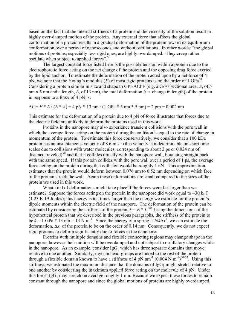
16    

based on the fact that the internal stiffness of a protein and the viscosity of the solution result in highly over-damped motion of the protein. Any external force that affects the global conformation of a protein results in a gradual deformation of the protein toward its equilibrium conformation over a period of nanoseconds and without oscillations. In other words: “the global motions of proteins, especially less rigid ones, are highly overdamped: They creep rather oscillate when subject to applied forces”.50

The largest constant force listed here is the possible tension within a protein due to the electrophoretic force acting on the net charge of the protein and the opposing drag force exerted by the lipid anchor. To estimate the deformation of the protein acted upon by a net force of 4 pN, we note that the Young’s modulus (E) of most rigid proteins is on the order of 1 GPa50. Considering a protein similar in size and shape to GPI-AChE (e.g. a cross sectional area, A, of 5 nm x 5 nm and a length, L, of 13 nm), the total deformation (i.e. change in length) of the protein in response to a force of 4 pN is:

ΔL = F * L / (E * A) = 4 pN * 13 nm / (1 GPa * 5 nm * 5 nm) = 2 pm = 0.002 nm

This estimate for the deformation of a protein due to 4 pN of force illustrates that forces due to the electric field are unlikely to deform the proteins used in this work.

Proteins in the nanopore may also experience transient collisions with the pore wall in which the average force acting on the protein during the collision is equal to the rate of change in momentum of the protein. To estimate this force conservatively, we consider that a 100 kDa protein has an instantaneous velocity of 8.6 m s-1 (this velocity is indeterminable on short time scales due to collisions with water molecules, corresponding to about 2 ps or 0.024 nm of distance traveled)50 and that it collides directly with the nanopore wall, bouncing straight back with the same speed. If this protein collides with the pore wall over a period of 1 ps, the average force acting on the protein during that collision would be roughly 1 nN. This approximation estimates that the protein would deform between 0.076 nm to 0.52 nm depending on which face of the protein struck the wall. Again these deformations are small compared to the sizes of the protein we used in this work.

What kind of deformations might take place if the forces were far larger than we estimate? Suppose the forces acting on the protein in the nanopore did work equal to ~30 kBT (1.23 E-19 Joules); this energy is ten times larger than the energy we estimate for the protein’s dipole moments within the electric field of the nanopore. The deformation of the protein can be estimated by considering the stiffness of the protein, k = E * L.50 Using the dimensions of the hypothetical protein that we described in the previous paragraphs, the stiffness of the protein to be k = 1 GPa * 13 nm = 13 N m-1. Since the energy of a spring is ½kΔx2, we can estimate the deformation, Δx, of the protein to be on the order of 0.14 nm. Consequently, we do not expect rigid proteins to deform significantly due to forces in the nanopore.

Proteins with multiple domains and flexible connecting regions may change shape in the nanopore, however their motion will be overdamped and not subject to oscillatory changes while in the nanopore. As an example, consider IgG1 which has three separate domains that move relative to one another. Similarly, myosin head-groups are linked to the rest of the protein through a flexible domain known to have a stiffness of 4 pN nm-1 (0.004 N m-1)50-52. Using this stiffness, we estimated the maximum distance that the domains of IgG1 might stretch relative to one another by considering the maximum applied force acting on the molecule of 4 pN. Under this force, IgG1 may stretch on average roughly 1 nm. Because we expect these forces to remain constant through the nanopore and since the global motions of proteins are highly overdamped,

17    

especially for flexible proteins, this deformation would be nearly constant through the length of the nanopore.

Based on the magnitude of the forces discussed above, we do not expect the proteins used in this work to change shape significantly while in the nanopore. This expectation is supported by the accurate measurements of the size and shape of the ten different proteins detected in this work compared to the size and shape of these proteins as determined from crystal structures (Fig. 3 in the main text and Supplementary Table 4). In further support of this expectation, proteins that bound non-covalently to biotinylated lipids (IgG1, Fab, and streptavidin) translocated through pores in the bound, lipid-anchored state as confirmed by their distributions of translocation times and measured charges (see Supplementary Fig. 11); if the binding pockets were denatured, antigen-binding would likely not occur.

Description of the assumptions underlying the convolution model

  The following section describes the primary assumptions underlying the convolution model in particular with regard to their validity. To derive this model (i.e. equation), we made four key assumptions:

1) The protein is a spheroid. 2) The dipole moment of the spheroidal protein is aligned with one of the principal axes. 3) While residing in the nanopore, the orientation of the protein is only biased due to its

dipole moment. 4) The pore is perfectly cylindrical.

The first assumption states that the protein is a spheroid with principle axes having lengths A, B, and B (see Fig 2a). We examined approximately 1,000 randomly sampled proteins from the Protein Data Bank and found that the lengths of two of the three principal axes are less than 20% different on average, indicating that most proteins can be approximated as spheroids. Based on our results for IgG1, we have also shown that our approach can be used to characterize proteins with highly irregular shapes. Although the complexity of the shape of IgG1 is not captured in full, our approach still provides low-resolution shape information and yields accurate values for the dipole moment and rotational diffusion coefficient of the protein. The second assumption is based on the expectation that the dipole moment is most often aligned with a principle axis of a spheroidal protein. For an asymmetrical protein, we expect the dipole moment to be aligned along the longest axis of the protein because the residues that are furthest from the center of the protein contribute most to the magnitude of the dipole moment. For a multimeric protein with rotational symmetry, such as GPI-AChE or β-PE, we expect the dipole moment to lie along the axis of symmetry since the off-axis components of the dipole moment from each subunit cancel each other out. Thus, in both cases it seems reasonable that the dipole moment will be in near alignment with one of the principal axes of the protein. In support of this expectation, we found that the dipole moment was aligned close to one of the principal axes for each of the nine non-spherical proteins examined here by using the Weizmann server to analyze the protein crystal structures. The third assumption states that the orientation of a protein in the nanopore is only biased by its dipole moment. We expect this to be true since we coated the nanopores with a lipid bilayer to eliminate non-specific interactions2, anchored the proteins to the coating via long (≥ 1.5 nm) and flexible (≥ 12 σ-bonds) tethers so they could sample most orientations, and used

18    

nanopore diameters that were at least twice the volume-equivalent spherical diameter of the proteins to minimize steric effects. Under these conditions, we obtained dipole moment measurements for nine different proteins that were in excellent agreement with reference values (see Fig. 4e), supporting our assumption. We expect this assumption to be valid as long as the protein being characterized does not interact with lipids in the nanopore coating. In such cases, however, interactions with the coating could likely be avoided by modifying the bilayer composition (e.g. including a small fraction of PEG-conjugated lipids). The fourth assumption is that the pore is cylindrical. This assumption does not depend on the protein under investigation and, consequently, does not limit the general applicability of our approach toward other proteins. The good agreement between the measured and expected values of volume for the ten different proteins examined here (see Fig. 3h) supports this assumption. Additionally, the change in the baseline current observed upon coating a nanopore is generally close to the value predicted by theory in which the pore geometry is assumed to be cylindrical2, further supporting this assumption. Regardless, we discuss how pores that are not perfectly cylindrical may affect the analysis of intra-event ∆I values in Supplementary Note 6 below.

Supplementary Note 3. Interpretation of the observed bimodal distributions of ΔI values from the translocation of non-spherical proteins

To determine whether any explanation might exist for the bimodal distributions of ΔI values observed here besides the theory presented in Supplementary Note 2, we closely examined the literature to ascertain whether other groups had observed similar signals in nanopore-based sensing experiments resulting from alternative mechanisms. To the best of our knowledge, there is only one such report. In this study, Spiering et al. used optical tweezers to characterize the force response of threading a protein bound to a negatively-charged DNA molecule through a nanopore53. For a finite range of optical trap positions, the authors found that the potential landscape “exhibits two minima (potential wells), corresponding to two metastable “states”… with the charged protein on either side of the membrane,” resulting in bimodal force versus time signals. Since the protein is located outside of the pore in both of these states (i.e. where the electric field is negligible), the resulting ∆I values should be close to zero in resistive-pulse sensing experiments. Hence, we do not think that these two states do not correspond to the two modes in the ∆I distributions that we observe. The potential landscape in our experiments is different than that described by Spiering et al. due to the following reasons: (1) the lipid tethers are shorter (length ~1.5 nm) than the pore length (~30 nm) and hence cannot contract and extend to allow a protein to transition from one side of the pore to the other, (2) the charge of the protein-lipid complex is dominated by the charge of the protein rather than the tether, whereas in the case of a DNA tether, the opposite is true, (3) the lipid tethers only extend on one side of the protein instead of both sides as with the DNA tethers, and (4) there is no optical trap potential present in our experiments. Hence, it is extremely unlikely that the two metastable states described by Spiering et al. exist under the experimental conditions used in our work. Skewed and bimodal distributions of ΔI values have been observed with increasing frequency in the last few years and in each instance the authors suggested that the shape of the ΔI distributions may have been influenced by the shape and orientation of the macromolecule. For example, early indications that the shape and orientation of a macromolecule can affect the ΔI signal were reported by Mathé et al., who observed orientation-dependent translocation signals

19    

of DNA through α-hemolysin pores54, and Fologea et al. who observed a unimodal but skewed distribution of ΔI values due to the translocation of nodular fibrinogen proteins through nanopores26. More recently, Raillon et al. observed distributions of ΔI values that appeared to be bimodal due to the translocation of an untethered, non-spherical RNA polymerase through a nanopore; without additional quantification, the authors attributed this result to different orientations of the RNA polymerase22. Finally, Fiori et al. observed a bimodal distribution of ∆I values due to the translocation of untethered, prolate-shaped protein ubiquitin55. Together, these reports indicated that the bimodal distributions presented in our work do not result from the effect of the lipid tether on the potential landscape but rather the shape and orientation of the translocating proteins. Until the work presented here, however, the origin of these biomodal distributions was not understood and it was unknown whether useful information could be obtained from the shape of these distributions of ΔI values. While we considered a number of other possible explanations for the current signatures that we observe (see Supplementary Note 1 and the subsection titled “Forces acting on proteins in a nanopore” in Supplementary Note 2), eight observations indicate that ∆I reflects the rotational dynamics of proteins passing through the nanopore:

1) Streptavidin, which is spherical with a shape factor, m, of 1.1, yielded a Normal distribution of ∆I values (Fig. 3c in the main text).

2) The values of ∆Imin and ∆Imax that we determined for each protein are consistent with the values predicted by established theory for large particles; Golibersuch originally developed this theory to describe the periodic variations in ∆I that occurred during the rotation of a red blood cell within a resistive-pulse sensor.

3) Simulations based on a spheroidal particle undergoing biased random rotation in one dimension yield ∆I signals that are comparable to those that we obtained experimentally (Supplementary Note 5).

4) The values of volume (Λ), length-to-diameter ratio (m), rotational diffusion coefficient (DR), and dipole moment (µ) that we determined for 9 different proteins are in good agreement with expected values (Fig. 3g-i and Fig. 4e-f); the methods used to determine these parameters critically depend on the assumption that ∆I reflects the orientation of non-spherical proteins, as described by the theory in Supplementary Note 2.

5) DR of bivalently-bound IgG1 is significantly less than DR of monovalently-bound IgG1 (see Supplementary Note 7), indicating that ∆I reflects the rotational dynamics of the protein in the nanopore.

6) Translocation of IgG1 and GPI-AChE through the same nanopore result in markedly different distributions of ∆I values despite their similar molecular weights, indicating that ∆I is related to the shape of the protein.

7) Kolmogorov Smirnov (KS) tests indicate that the convolution model, which incorporates the effect of protein shape and orientation combined with noise to predict distributions of ∆I values, is not significantly different from the empirical distribution in 11 out of 13 cases (Supplementary Fig. 6), indicating that the model that underlies our analysis and employs the effect of protein orientation and shape on ΔI describes the data very well.

8) From a fundamental physical chemistry perspective it is also reasonable to assume that proteins rotate while moving through the pore. In the case of non-spherical proteins this rotation will change the electric field lines and hence modulate the current based on Maxwell’s and Golibersuch’s equations. This expectation is supported by simulations

20    

(see Point 3 of this list). We think it is extremely unlikely that proteins translocate through the pores in one constant orientation over several hundreds of microseconds given that we demonstrated before that the fluid bilayer coating circumvents non-specific protein adsorption to the pore walls.

Supplementary Note 4. Effect of lipid anchoring on the measurement of protein properties

Since we anchored each protein to a lipid in the bilayer coating of the nanopore to slow down translocation, we considered whether anchoring may have any other effects on the five parameters measured in this work. First, we do not expect protein shape or volume to be affected by anchoring. As discussed in Supplementary Note 2, the force exerted by the lipid anchor that opposes the electrophoretic force is unlikely to deform the protein. In addition, the chemical modifications involved in the crosslinking procedure are unlikely to cause denaturation as such modifications are standard practice in various biochemical assays that rely on retention of protein function. Our expectation that protein shape and volume are unaffected by anchoring is supported by the excellent agreement between the measured size and shape of the ten different proteins detected in this work with reference values (Fig. 3g-i in the main text). We do expect the distribution of translocation times to reflect the net charge, z, of the protein-lipid complex as a whole. Hence, we subtracted 1 from the expected value of z (Supplementary Figure 11j and Table 4) for each protein (except GPI-AChE) to correct for the net charge of the lipid anchor. For each protein that was crosslinked to the bilayer, we also subtracted 0.93 from the expected value of z based on the “charge regulation” model by Menon and Zydney56 to account for the consumption of a positively charged amine group. Tethering a protein to a lipid anchor is known to slow rotation significantly, which we exploited in order to resolve in time the rotational dynamics of proteins residing in the nanopore. Proteins in free solution generally have rotational diffusion coefficients, DR, that are on the order of 106 to 107 rad2 s-1 57,58, while lipid anchored proteins have been shown to rotate over 2 orders of magnitude more slowly43-45. For instance, GPI-AChE rotates about 199 times slower when tethered to the bilayer than in bulk (see Supplementary Table 4). Likewise, our measurements indicate that the proteins examined here rotate 211 times slower on average when tethered (see Fig. 4f). There is a strong correlation (Pearson’s r = 0.93) between the measured and bulk values of DR, indicating that the factor by which tethering slowed rotation was comparable between proteins. This result is likely due to the fact that all proteins were attached to the bilayer by similarly long and flexible tethers. We do not expect the tether itself to bias protein orientation and thereby affect the measurements of dipole moment, µ; however, the crosslinking reaction consumes a positively charged amine and thus will affect µ. To determine the extent by which crosslinking and removal of the positively charged amine affect µ, we modified the crystal structure for BSA (PDB ID: 3V03) by replacing a single, randomly-chosen lysine residue on the protein surface with a glycine residue and calculated µ for the modified protein using the Weizmann server (http://bioinfo.weizmann.ac.il/dipol/). We found that the median percent difference between µ for the native protein and 10 modified versions of the protein was approximately 12 percent and ranged from 1 to 38 percent. In line with this relatively small change, we observed good agreement between the values of µ determined in nanopore experiments and those measured with impedance spectroscopy (Fig. 4e).

21    

Finally, we examined whether the point of attachment of the lipid anchor may affect the ability of the proteins to sample all possible electrical shape factors (corresponding to 0 ≤ θ ≤ π/2 in Fig. 1c). To maximize the possibility that the proteins could sample all orientations (θ) regardless of the method or point of attachment, we used long (≥ 1.5 nm in their extended conformation) and flexible (≥ 12 σ-bonds) lipid tethers as well as nanopore diameters that were at least twice the volume-equivalent spherical diameter of the examined proteins. Despite these precautions, we do expect points of attachment near the axis of symmetry on oblates to restrict certain orientations and thereby introduce some degree of error into our approach. While such cases are possible when using our crosslinking strategy in which the point of attachment is approximately random, we expect these cases to occur relatively infrequently. For instance, we anticipate that these cases occur in ~20% of the attachments for L-LDH assuming that all points on the surface of the protein are equally likely to serve as the point of attachment. Hence, we expect the point of attachment to have a relatively minor effect on the most probable values of the parameter distributions. The assumption that the proteins are able to sample the full range of electrical shape factors is supported by the good agreement between the measured and expected values for the parameters examined in this work (Fig. 3g-i and Fig. 4e,f). The point of attachment is, however, likely to contribute to the uncertainty in a fraction of the stand-alone single protein measurements.

Supplementary Note 5. Simulating translocation events due to spheroidal particles

We numerically simulated translocation events due to spheroidal particles in MATLAB in order to provide support for the analysis methods developed in this work. Input parameters for the simulations included ∆Imin, ∆Imax, the dipole moment or µ, the rotational diffusion coefficient or DR, pore geometry (i.e. length and diameter), the resistivity of the solution, the standard deviation of the noise, and the duration of each event or td. To generate an intra-event ∆I signal, we first simulated a spheroidal particle undergoing a biased random walk in one dimension by adapting the model developed by Gauthier and Slater for translational motion59. In our model, bias is introduced solely due to the electric field acting on the dipole moment of the particle, which was assumed to be pointed parallel to one of the principal axes. We simulated discrete 1-ns-long time steps in which the angle of the particle relative to the electric field, θ, changed by a fixed step size, ∆θ = 2DR∆t. For each time step, the following equation gives the probability that the particle will move in the positive or negative direction:

( ) ( )µ θ θ θ θΔ ⎡ ⎤⎣ ⎦

± ± −−Δ +Δ+= =

+/ /(2k )cos cos

11

1

1B BU k T TEe

pe

(16)

which was implemented in the simulations via the random number generator in MATLAB. Note that the change in potential energy, ∆U, is divided by a factor of 2 since the particle is initially located halfway in between the two possible final orientations. After simulating the entire event, we converted θ(t) to ∆I(t) based on equation (4) and sampled the signal at a rate of 500 kHz to mimic the sampling conditions of the real electronic recordings. Finally, we added Gaussian noise to the signal (unless indicated otherwise) and proceeded with analyzing these simulated signals in the same manner as the resistive-pulse signals obtained during an experiment.

22    

Supplementary Figure 12 shows results from fitting the convolution model to a cumulative distribution of maximum ∆I values from simulated translocation events. The convolution model described the experimental data extremely well (R2 = 0.999) and yielded estimates of the length-to-diameter ratio, m, and excluded volume, Λ, that were within 10% of their expected values. As hypothesized in Supplementary Note 2, the distribution was biased toward ∆Imax more than expected (i.e. based on the dipole moment only), which is likely a result of representing each event by its maximum value. These results suggest that fitting distributions of maximum ∆I values yields accurate estimates of shape and volume but not dipole moment.

Supplementary Figure 13 shows distributions of the length-to-diameter ratio, m, and excluded volume, Λ, determined from fitting the convolution model to simulated intra-event ∆I signals (analysis of intra-event ∆I values is presented in Supplementary Note 6). The median values of m and Λ exactly match the expected values despite the relatively low signal-to-noise ratio of the data (SNR = [IRMS, Signal / IRMS, Noise]2), which is lower than that observed in any of the experiments summarized in Supplementary Figure 15 wherein the signal-to-noise ratio was at least 1.4 and the noise was also Gaussian. These results suggest that the error in determining m and Λ from fitting experimental intra-event ∆I signals, as described in Supplementary Note 6, is not due to low signal-to-noise ratios. Furthermore, these results highlight the ability of the convolution model to account for the presence of noise. Supplementary Figure 14 shows the distribution of µ and DR that we obtained from analyzing simulated intra-event ∆I signals. These distributions were described well by a lognormal distribution (R2 > 0.98) similar to our experimental results. The most probable value of µ determined from fitting each intra-event ∆I signal with the convolution model was in excellent agreement with the expected (i.e. input) value over the range of values measured in this work (Supplementary Fig. 14c). Similarly, the most probable value of DR determined from analyzing each intra-event ∆I signal similarly was in agreement with the input value; however, our analysis methods systematically underestimated DR by about 10 percent (Supplementary Fig. 14d). This underestimation is likely due to a slight leveling off of the MSAD curve between the first two points (an example MSAD curve is shown in Fig. 4 in the main text), which might be rectified by increasing the sampling frequency of the signal. Regardless, these results suggest that the analysis methods developed in this work yield accurate estimates of the dipole moment and rotational diffusion coefficient of a spheroidal particle as long as its orientation is biased purely by its dipole moment.

We want to emphasize that these simulation results were not acquired by performing a simple backwards calculation. The data used here was simulated based on the probability of the particle rotating in one direction or another (equation (16)), and thus it is accomplished in a manner that is independent from the analysis methods described in equations (8) through (13).

Supplementary Note 6. Analysis of intra-event ΔI values

Distributions of m and Λ determined from fitting intra-event ΔI values

Supplementary Figure 15 shows distributions of the length-to-diameter ratio, m, and excluded volume, Λ, determined from fitting the convolution model to all intra-event ∆I signals longer than 0.4 ms from experiments with IgG1, GPI-AChE, Fab, BSA, α-amylase, and BChE. In general, the median value of m from each experiment corresponds to a shape that is more elongated than we expect (i.e. the median values were less than expected for oblates and greater

23    

than expected for prolates), and the median value of Λ is lower than the results we obtained by analyzing distributions of maximum ∆I values and also lower than what is expected from the crystal structure of each protein (Supplementary Table 1). The discrepancy between the values of these parameters obtained by the two different analysis strategies may result from the shape of the nanopore, which the model assumes is perfectly cylindrical (i.e. constant diameter); however, the pore may have a varying diameter. The intra-event ∆I signal would be expected to reflect changes in pore diameter60 and will include ∆I values from when the protein is in the widest regions of the pore. In contrast, the maximum ∆I value from each event most likely occurs when the protein is near the narrowest constriction of the pore. One might also expect low ∆I values as the protein enters and exits the nanopore; however, the electric field is highly non-uniform and dense at the edges of the pore, which is thought to offset this effect or even result in larger than expected ∆I values61,62. In the current model, the effect of pore shape and the non-uniformity of the electric field near the pore entrance and exit are not considered and could result in lower than expected ∆I values. For the intra-event (i.e. single-event) analysis, these low ∆I values would yield more elongated shapes and lower volumes than expected. If these hypotheses are true, this single-event analysis could be improved by (1) using pores that more closely match a perfect cylinder, (2) by excluding ∆I values from the beginning and end of the signals, and (3) by knowing the exact geometry of the nanopore in combination with an improved description of the electric-field in and around the pore. Despite the increased uncertainty in the results from the single-event analysis compared to the analysis of distributions of maximum ∆I values from many events, the values m and Λ determined from fitting intra-event ∆I signals still can be used to identify and characterize proteins as evidenced by the repeatability between different experiments for IgG1, Fab, BSA, and α-amylase.

Determining the dipole moment of a protein from fitting intra-event ΔI values

In the main text, we plotted the most probable value of the biasing parameter or dipole moment, µ, determined from fitting the convolution model to all intra-event signals longer than 0.4 ms for IgG1, GPI-AChE, Fab, β-PE, G6PDH, L-LDH, BSA, α-amylase, and BChE (Fig. 4e in the main text). Supplementary Figure 16 shows histograms of the values of µ that were returned from fitting each event in all experiments. In every case, the distribution of µ was described well by a lognormal distribution (R2 > 0.94); we expected distributions of this shape based on simulations (see Supplementary Note 5). Moreover, the most probable value of µ in each distribution was indicative of the dipole moment of the protein. Only the permanent dipole moment of a protein biases its orientation inside the nanopore as the dipole moment induced by the electric field is roughly parallel to the field and hence does not affect the torque exerted on the protein63. The dipole moment estimates were in good agreement with measurements from dielectric impedance spectroscopy and calculations from crystal structures returned by the software HydroPro and the Weizmann server (Supplementary Table 4). Dielectric impedance spectroscopy was performed as described previously64 using a buffer of 1 mM KCl and 1 mM HEPES (pH = 7.4) for IgG1 and Fab or 1 mM phosphate (pH = 5.2) for BSA. Moreover, these results were repeatable between different nanopores; the difference in the estimated dipole moment (i.e. most probable values of µ) from experiments with different nanopores was always less than 20 percent, indicating that, with bilayer coated walls, pore-dependent effects did not significantly bias the orientation of the protein.

24    

Determining the rotational diffusion coefficient of a protein in a nanopore

To determine the rotational diffusion coefficient, DR, of a protein during a translocation event, we first fit the convolution model to the intra-event ∆I signal at a bandwidth of 15 kHz to estimate ∆Imin and ∆Imax. Using these values, we determined the volume and shape of the protein as described in Supplementary Note 2; this procedure also reveals the maximum and minimum shape factors of the protein based on equations (5) through (7). Using these values we calculated θ(t) based on equation (4). From this trajectory, we calculated the mean-squared-angular displacement (MSAD) of the protein using overlapping time intervals (i.e. 0 to 4 µs, 2 to 6 µs, 4 to 8 µs, etc.). Since θ(t) can be “clipped” (i.e. equation (4) yields imaginary values of θ(t) for ∆I values that are not between ∆Imin and ∆Imax), we only calculated angular displacement between two non-clipped values when computing the MSAD. By symmetry of the spheroid, multiple orientations of the particle are equivalent to θ in the range of 0 to π/2 (for example, the orientation of 3π/2 is equivalent in this equation to the orientation of π/2). This degeneracy in the estimate of θ means that the trajectory of the MSAD will fail to describe the rotation of the protein accurately for long time scales; rather, the trajectory of θ(t) should be used only to estimate changes in θ over short time scales. This degeneracy, combined with the periodicity of rotation, causes the MSAD curve to level off asymptotically (see Fig. 4c in the main text for an example). Hence, we only fit the MSAD curve with a tangent line that passes through the origin to estimate the initial slope of the MSAD curve and reveal the rotational diffusion coefficient, DR. According to the Langevin torque equation, DR is equal to the initial slope of the MSAD curve divided by 2 for rotation around a single axis65. Since filtering attenuates frequency components of the ∆I signal at which rotation occurs, we calculated DR at various cut-off frequencies and fit this data with the logistic equation to estimate the value of DR at infinite bandwidth, which corresponds to the upper horizontal asymptote of the fit (Fig. 18a shows an example). On average, these fits described the experimental data extremely well (R2 > 0.96). We calculated the overall bandwidth of the signal according to the following equation66:

⎡ ⎤= +⎣ ⎦2 21 21 / 1 / f 1 / fc c cf

where 1cf is the cutoff frequency of the recording electronics (57 kHz)1 and 2cf is the cutoff frequency of the digital Gaussian filter (ranges from 15 to 57 kHz). Note that the diffusion coefficients determined in this analysis describe rotation about the equatorial axes of the protein since rotation about the axis of symmetry is not reflected in the intra-event ∆I signal. The diffusion coefficient that describes rotation about the equatorial axes of a spheroid is within 10 percent of the average diffusion coefficient for length-to-diameter ratios (m) that are less than 1.5. Supplementary Figure 18 shows histograms of the values of DR that were returned from fitting all events longer than 0.4 ms for experiments with IgG1, GPI-AChE, Fab, β-PE, α-amylase, and BChE. We excluded all other experiments (10 of 26) from this analysis due to their relatively low signal-to-noise ratios, which yielded values of DR that were erroneously high and similar to values obtained from analyzing signals consisting of only Gaussian noise (~50,000 rad2 s-1). As with the distributions of µ, each distribution of DR was described well by a lognormal distribution (R2 > 0.96), wherein the most probable value was strongly correlated (Pearson’s r = 0.93) with the theoretical rotational diffusion coefficient for each protein in bulk solution (Fig. 4f and Supplementary Table 4). The most probable values measured here were

25    

211 times lower on average than the values of DR in bulk solution, which is consistent with previous findings for GPI-AChE (see Supplementary Table 4). The rotational diffusion coefficient of the relatively flexible IgG1 antibody was similar in two of the three nanopores; this result suggests that additional pore-dependent effects (e.g. steric effects) not taken into account by this model might impact the rotation of proteins in a nanopore. Supplementary Note 5 shows results from simulated data that support the methods described in this section.

Supplementary Note 7. Bivalently-bound IgG1 rotates slower than monovalently-bound IgG1

To provide additional evidence that ∆I values reflect the orientation of a non-spherical protein residing in the nanopore, we measured resistive-pulses resulting from the translocation of anti-biotin IgG1 bound to one or two biotin-PE lipids in the nanopore coating. Bivalently-bound IgG1 should have reduced translational and rotational diffusion coefficients compared to monovalently-bound IgG1 due to the additional drag associated with the second lipid anchor. To test this hypothesis, we performed an experiment in which the conditions initially favored bivalent binding of IgG1 to the lipid coating, and gradually throughout the experiment, we changed the conditions to favor monovalent binding of IgG1. To favor bivalent binding of IgG1, we used a ratio of lipid-anchored biotin to IgG1 that was 33-fold greater than that used in other experiments involving the same protein (i.e. 2 nM IgG1 and 1 mol% biotin-PE versus 10 nM IgG1 and 0.15 mol% biotin-PE). To shift toward conditions favoring monovalent binding, we introduced soluble biotin at sequentially increasing concentrations (1, 10, and 100 nM for 30 min each) to out-compete the lipid-anchored biotin in binding IgG1, thereby reducing the fraction of bivalently-bound IgG1 and increasing the fraction of monovalently-bound IgG1 throughout the course of the experiment. IgG1 proteins that were not bound to a lipid-anchored ligand were not detected2.

To determine the translational diffusion coefficient of lipid-anchored IgG1 in the presence of 0 and 100 nM of soluble biotin, we fit each distribution of translocation times with Schrödinger’s first-passage probability density function. In the absence of soluble biotin wherein bivalent binding is favored, the translational diffusion coefficient was 1.05 nm2 µs-1, whereas in the presence of 100 nM of soluble biotin wherein monovalent binding is favored, the diffusion coefficient increased to 1.37 nm2 µs-1

. This increase by a factor of 1.3 is in agreement with work by van Lengerich et al., who previously estimated that a particle with a single lipid anchor should diffuse laterally about 1.5 times faster than a particle with two lipid anchors67. This result supports our expectation that the ratio of bivalently-bound to monovalently-bound IgG1 decreases with the concentration of soluble biotin. We also found that the charge of the protein-lipid complex changed from -3.25 in the absence of soluble biotin (i.e. conditions favoring bivalent binding) to -1.53 in the presence of 100 nM of soluble biotin (i.e. conditions favoring monovalent binding); this change in the value of the charge by -1.7 is slightly larger in magnitude than the theoretically expected value of -1 (the expected charge of one biotin-PE lipid) but this deviation is likely within the error of the measurement. The main aspect for the discussion here is that the negative charge decreased in magnitude as expected when fewer IgG molecules are bound bivalently.

We next obtained distributions of rotational diffusion coefficients (DR) by analyzing intra-event ∆I values (see Supplementary Note 6) for IgG1 in the presence of increasing

26    

concentrations of soluble biotin (Supplementary Figure 19). The most probable value of DR increases with the concentration of soluble biotin as expected for conditions that favor monovalent over bivalent binding (Supplementary Figure 19c; Pearson’s correlation coefficient r = 1.00). In the absence of soluble biotin, DR was approximately 100 rad2 s-1. In the presence of 100 nM of soluble biotin, DR increased more than an order of magnitude to 1,744 rad2 s-1, approaching the expected value for monovalently-bound IgG1 of 4,500 rad2 s-1 (see Supplementary Table 4). As with the results for the translational diffusion coefficient, this trend indicates that the ratio of bivalently-bound to monovalently-bound IgG1 decreases with the concentration of soluble biotin. Together, these results provide strong evidence that ∆I values reflect the rotational dynamics of the protein since we observed more than 17-times faster rotational diffusion in the same nanopore as we change the experimental conditions from favoring bivalent binding to favoring monovalent binding. The distribution of maximum ∆I values is also affected by the ratio of monovalently-bound to bivalently-bound IgG1, as shown in Supplementary Figure 20. The distribution becomes more biased toward low ∆I values as the fraction of bivalently-bound IgG1 increases, suggesting that bivalently-bound IgG1 is less likely to sample cross-wise orientations during a translocation event than monovalently-bound IgG1. One likely explanation for this bias in orientation is that non-spherical proteins orient length-wise prior to entering the pore due to the strong electric field gradient that they experience once they approach the pore61,68 and as a consequence of the reduced rotational diffusion coefficient of bivalently-bound IgG1 compared to monovalently-bound IgG1, bivalently-bound IgG1 is less likely to reorient by Brownian motion with dipole-induced bias during an event of a given duration. Alternatively, the bias toward low ∆I values might result from steric effects that limit crosswise orientations since the second lipid anchor of bivalently-bound IgG1 may restrict the possible range of configurations the protein can assume for a given position of the first lipid anchor. Regardless, the results of increased bias as a consequence of two lipid anchors strongly support the conclusion that ∆I reflects the orientation and shape of non-spherical protein residing in the nanopore.

Supplementary Note 8. Distinguishing an antigen and antibody-antigen complex in a single nanopore experiment

Supplementary Figure 22 illustrates the ability of the methods developed in this work to characterize and identify a single protein, G6PDH, and a protein-protein complex, G6PDH-IgG, in the same solution. Supplementary Fig. 22a-i shows results from analysis of maximum ΔI values (the procedures for this analysis are described in the figure caption). Supplementary Fig. 22j-l shows results from analysis of all intra-event ΔI values.

To classify each translocation event as either G6PDH or G6PDH-IgG, we analyzed intra-event ΔI values as described in Supplementary Note 6 to determine the volume, shape, charge-related td value, rotational diffusion coefficient, and dipole moment from each protein or protein complex moving through the nanopore. This procedure identified 787 translocation events that were longer than 400 µs. We normalized the values for each parameter by their standard deviations and classified each event using the clustering algorithm kmeans in MATLAB69,70. Briefly, the kmeans clustering algorithm minimizes, across all clusters, the sum of the distance between all points in the cluster to the centroid of the cluster. To assess the quality of all cluster analyses and provide an error for the values assigned to parameters, we ran a bootstrap method in

27    

which 1,000 datasets were created by random resampling with replacement of the original dataset71. We then ran the cluster analysis on these 1,000 datasets. The clustering procedure was always robust with approximately 90% of the data (727 events) consistently being classified as either G6PDH or G6PDH-IgG (at least 95% of the time).

We performed the cluster analysis on several combinations of these five parameters and found that a 3D cluster analysis based on the volume, dipole moment, and rotational diffusion coefficient provided the best separation between clusters as well as the most accurate characterization of the volumes for G6PDH (3% difference) and the G6PDH-IgG complex (7% difference). For instance, Fig. 5c in the main text shows that this technique determined a volume for G6PDH of 227 ± 9 nm3 compared to the volume of 220 nm3 determined from distributions of maximum ΔI values in an independent experiment; similarly, this analysis determined the volume of the complex to be 530 ± 64 nm3, and we expected a volume for the complex of 497 nm3 (the volume of G6PDH plus the volume of an IgG protein). The volume of the complex determined from this intra-event analysis was also in excellent agreement with that determined from analysis of distributions of maximum ΔI values, which is shown in Supplementary Fig. 22i. Furthermore, both the analysis of maximum ΔI values (Supplementary Fig. 22f) and analysis of intra-event ΔI values followed by cluster analysis revealed that after the addition of anti-G6PDH IgG, the proportion of events due to the G6PDH-IgG complex was between 27 to 28 percent. The agreement between these two values provides additional evidence that the classification of events from single-event analysis was accurate. For reference, two-dimensional projections of the 3D scatter plot in Fig. 5b of the main text are shown in Supplementary Fig. 22j-l. Prior to this work, the standard practice for distinguishing between proteins in a mixture would have been to analyze scatter plots of td values vs. ΔI values. To illustrate the benefits of the multi-parameter characterization based on methods developed in this work, we performed a two-dimensional cluster analysis on the same data set used above, using only td values and average ΔI values. This analysis found that the protein complex represented only 2.5 ± 0.5 % of events, which is ~90% lower than the values determined by single-event analysis or analysis of distributions of maximum ΔI values (Supplementary Fig. 22). Moreover, this analysis failed to determine the volume of the complex accurately as it returned a value of 833 ± 50 nm3, which is 68% greater than the estimated volume of the complex of 497 nm3 determined from independent experiments.

 

Supplementary Note 9. Derivation of probability distribution of shape factors for proteins with a dipole moment

To derive a probability distribution of shape factors that takes into account a bias for a specific orientation based on the dipole moment of a protein and the electric field, we used the Boltzmann distribution of energies:

−⎡ ⎤⎢ ⎥⎣ ⎦=−⎡ ⎤⎢ ⎥⎣ ⎦

∑

exp

exp

ii

Bi

jj

B

Ug k TNUN g k T

(17)

28    

where gi is the number of states that have the same energy level, Ui is the energy level of state i, Ni is the number of molecules with energy level i, N is the total number of molecules in the system, and kBT is the thermal energy. The denominator of equation (17) is the partition function, and we will label it Z. Assuming that all of the energy affecting the orientation of the protein is in the form of the potential energy of a dipole in an electric field, then gi is constant for all energy states and cancels out of equation (17). The potential energy of a dipole in an electric field is:

( )µ µ φΔ = = −v vg cosU E E (18)

where E is the electric field, µ is the dipole moment, and ϕ is the angle between the moment and the electric field. Combining equations (17) and (18), the proportion of molecules at an angle, ϕ, is:

( )φ µ φ⎡ ⎤= ⎢ ⎥

⎢ ⎥⎣ ⎦

cos1exp

B

N EN Z k T

(19)

and therefore the probability of observing an angle ϕ is:

( )φ

µ φ⎡ ⎤= ⎢ ⎥

⎢ ⎥⎣ ⎦

cosexp

B

EcPZ k T

(20)

where c is a normalization constant. Considering a simple scenario in which the dipole moment is parallel with the symmetry or equatorial axis and accounting for the two possible orientations of the dipole moment relative to the electric field for a given orientation (i.e. θ) due to symmetry, we obtained equations (21a) and (21b) for ϕ = θ and θ + π/2 from equation (20):

( ) ( ) ( )θ

µ θ µ π θ µ θ⎡ ⎤ ⎡ ⎤ ⎡ ⎤−= + =⎢ ⎥ ⎢ ⎥ ⎢ ⎥

⎢ ⎥ ⎢ ⎥ ⎣ ⎦⎣ ⎦ ⎣ ⎦

cos cos cosexp exp cosh

B B B

E E Ec c cPZ k T Z k T Z k T

(21a)

and

( )( ) ( )θ

π πµ πµ θ µ θθ−+ +

= + =

⎡ ⎛ ⎞ ⎤ ⎡ ⎤ ⎡ ⎤⎜ ⎟⎢ ⎥ ⎢ ⎥⎝ ⎠ ⎢ ⎥⎢ ⎥ ⎢ ⎥ ⎣ ⎦⎣ ⎦⎣ ⎦

coscos sinexp exp cosh2 2

BBB

EE Ec c cP

k TZ Z Zk Tk T

(21b)

To express cos(ϕ) in terms of the electrical shape factor we first rearranged equation (4), which describes γ as a function of θ, to obtain:

( ) γ γθ

γ γ⊥

⊥

⎛ ⎞−= ⎜ ⎟⎜ ⎟−⎝ ⎠P

1/2

cos

(22)

Substituting equation (22) into equations (21a) and (21b), we obtain:

29    

θ

γ γµ

γ γ⊥

⊥

⎡ ⎤⎛ ⎞−⎢ ⎥⎜ ⎟⎜ ⎟= −⎢ ⎥⎝ ⎠⎢ ⎥⎣ ⎦

P

1/2

cosh

B

c EPZ

k T

(23a)

and

θ

γ γγ γµ µγ γ γ γ

− ⊥

⊥ ⊥

⎡ ⎤⎛ ⎞⎡ ⎤ ⎡ ⎤⎛ ⎞ ⎛ ⎞−−⎢ ⎥⎜ ⎟⎢ ⎥ ⎢ ⎥⎜ ⎟ ⎜ ⎟⎜ ⎟ ⎜ ⎟= =⎢ ⎥⎜ ⎟− −⎢ ⎥ ⎢ ⎥⎝ ⎠ ⎝ ⎠⎣ ⎦⎝ ⎠⎢ ⎥ ⎢ ⎥⎢ ⎥ ⎣ ⎦⎣ ⎦

P

P P

1/2 1/2

1sin coscosh cosh

BB

Ec c EPZ Z

k Tk T

(23b)

Equations (23a) and (23b) express the probability of observing an angle θ as a function of the shape factor, P(θ(γ)). As in the derivation by Golibersuch, we used substitution of variables to transform P(θ(γ)) into P(γ):

θ θ

θ γγ γ γ γ

γ θ

−⎛ ⎞

= = ⎜ ⎟⎝ ⎠

1

( )d dP d P d P dd d

(24)

and differentiated equation (4) with respect to θ, ddγθ

. Substituting this result into equation (24),

we obtained equations (25a) and (25b):

( ) ( )

γ γµγ γ γγ γ

π γ γ γ γ

⊥

⊥

⊥

⎡ ⎤⎡ ⎤⎛ ⎞ ⎢ ⎥⎢ ⎥⎜ ⎟ ⎢ ⎥⎢ ⎥⎜ ⎟⎢ ⎥⎢ ⎥⎝ ⎠ ⎡ ⎤⎢ ⎥⎢ ⎥ ⎢ ⎥⎣ ⎦⎣ ⎦ ⎣ ⎦

−= −

− −P

P

1/2

1/21( ) cosh

B

c EP d dZk T

(25a)

and

( ) ( )

γ γµγ γ γγ γ

π γ γ γ γ⊥

⊥

⎡ ⎤⎡ ⎤⎛ ⎞ ⎢ ⎥⎢ ⎥⎜ ⎟ ⎢ ⎥⎢ ⎥⎜ ⎟⎢ ⎥⎢ ⎥⎝ ⎠ ⎡ ⎤⎢ ⎥⎢ ⎥ ⎢ ⎥⎣ ⎦⎣ ⎦ ⎣ ⎦

−= −

− −

P

P

P

1/2

1/21( ) cosh

B

c EP d dZk T

(25b)

To solve for the normalization constants, we integrated equations (25a) and (25b) and set each

equation equal to 1 (i.e. ( ) 1P dγ

γ

γ γ⊥

=∫P

). This procedure cancels out the partition function Z and

yields:

( ) ( )

γ γµ

γ γ γγ γπ γ γ γ γ

⊥

⊥

⊥

⎡ ⎤⎛ ⎞ ⎡ ⎤−⎢ ⎥⎜ ⎟ ⎢ ⎥⎜ ⎟= −⎢ ⎥⎝ ⎠ ⎢ ⎥⎡ ⎤− −⎢ ⎥ ⎢ ⎥⎣ ⎦⎣ ⎦⎣ ⎦

P

P

1/2

1/2

1 1( ) cosh

B

EP d dA

k T

(26a)

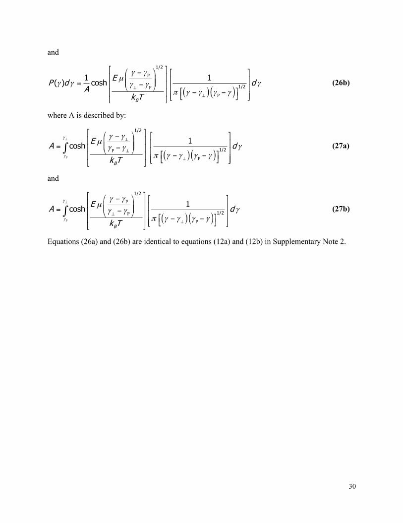
30    

and

( ) ( )

γ γµ

γ γ γγ γπ γ γ γ γ

⊥

⊥

⎡ ⎤⎛ ⎞− ⎡ ⎤⎢ ⎥⎜ ⎟ ⎢ ⎥⎜ ⎟= −⎢ ⎥⎝ ⎠ ⎢ ⎥⎡ ⎤− −⎢ ⎥ ⎢ ⎥⎣ ⎦⎣ ⎦⎣ ⎦

P

P

P

1/2

1/2

1 1( ) cosh

B

EP d dA

k T

(26b)

where A is described by:

( ) ( )

γ

γ

γ γµ

γγ γπ γ γ γ γ

⊥ ⊥

⊥

⊥

⎡ ⎤⎛ ⎞ ⎡ ⎤−⎢ ⎥⎜ ⎟ ⎢ ⎥⎜ ⎟= −⎢ ⎥⎝ ⎠ ⎢ ⎥⎡ ⎤− −⎢ ⎥ ⎢ ⎥⎣ ⎦⎣ ⎦⎣ ⎦

∫P

P

P

1/2

1/2

1cosh

B

EA d

k T

(27a)

and

( ) ( )

γ

γ

γ γµ

γγ γπ γ γ γ γ

⊥

⊥

⊥

⎡ ⎤⎛ ⎞− ⎡ ⎤⎢ ⎥⎜ ⎟ ⎢ ⎥⎜ ⎟= −⎢ ⎥⎝ ⎠ ⎢ ⎥⎡ ⎤− −⎢ ⎥ ⎢ ⎥⎣ ⎦⎣ ⎦⎣ ⎦

∫P

P

P

P

1/2

1/2

1cosh

B

EA d

k T

(27b)

Equations (26a) and (26b) are identical to equations (12a) and (12b) in Supplementary Note 2.

31    

 

Supplementary Figure 1. Most probable td values for the monoclonal anti-biotin IgG1 antibody (a) and GPI-AChE (b) as a function of the voltage drop, VP, across a bilayer-coated nanopore containing biotin-PE. The inverse relationship between translocation time and applied voltage as well as the excellent agreement between theory (red curve) and experiment indicate that the lipid-anchored proteins completely passed through the nanopore. The red curve was obtained by a best-fit of equation

( )2d P B p Lt l k T z eV D= as described in Yusko et al.2, where the only fitting parameter is the net charge of

the protein, z. lP is the length of the nanopore with the bilayer coating, kBT is the thermal energy (1.38E-23 J K-1 × 295 K), Vp is the voltage drop across the nanopore, and DL is the diffusion coefficient of the lipids in the bilayer as determined from FRAP experiments. For the IgG1 antibody (a), the fit returned a value for z of -3.5 ± 0.1 (in 2 M KCl with pH = 7.4 in 10 mM HEPES) with R2 = 0.98, p-value < 0.001 (N = 8), which is the expected value for the charge of this monoclonal antibody based on capillary electrophoresis experiments2. The value used for DL was 1.35E-12 m2 s-1 determined from FRAP experiments2, and the value of lP was 24 nm. For the GPI-AChE (b), the fit returned a value for z of -2.7 ± 0.1 (in 2 M KCl with pH = 6.1 in 10 mM HEPES) with R2 = 0.99, p-value < 0.001 (N = 4). For comparison, the theoretical charge of GPI-AChE at zero ionic strength and pH 7.4 is -12 to -167,10. DL was 1.6 E-12 m2 s-1 and lP = 24 nm. The bilayer coating in (a) contained 0.15% biotin-PE, 0.8% Rh-PE, and ~99% POPC, and the bilayer coating in (b) contained only 0.8% Rh-PE, and ~99.2% POPC.

 

a b

32    

Supplementary Figure 2. Detection of monoclonal anti-biotin IgG1 antibody with a bilayer-coated nanopore and dynamic light scattering experiments. a) Current versus time trace showing resistive pulses due to translocation of IgG1 antibodies that were bound to biotin-PE lipids in the bilayer coating. Resistive pulses occurred at a frequency of 34 s-1. b) Current versus time trace recorded after the addition of excess biotin (10 µM) to the solution and containing a reduced frequency of resistive pulses (1.3 s-1). c) Current versus time trace recorded using the same nanopore as (a) and (b) but with a bilayer coating that did not contain biotin-PE lipids. Resistive-pulses occurred at a frequency of 2 s-1

. The experiments were performed using pore 2 (Supplementary Fig. 25). d) Hydrodynamic diameter of IgG1 antibodies determined from dynamic light scattering experiments. IgG1 antibodies were at a concentration of 500 nM in aqueous solutions identical to the recording electrolyte (2 M KCl and 10 mM HEPES at pH = 7.4) during the dynamic light scattering experiment. Where indicated, 8 M of urea was added to the solution in order to denature all proteins. The dynamic light scattering results are the combination of 5 runs, each 60 s in duration. Results show the intensity-weighted calculation for the hydrodynamic diameter. The instrument was a Brookhaven 90Plus Particle Sizer and used a 658 nm laser at an angle of 90º to the detector. The absence of a second peak indicates that IgG1 antibodies were not fragmented or present in dimers in 2 M KCl even at concentrations 500 fold greater than in the resistive-pulse sensing experiments.    

a d

b

c

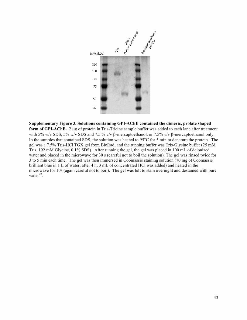
33    

Supplementary Figure 3. Solutions containing GPI-AChE contained the dimeric, prolate shaped form of GPI-AChE. 2 µg of protein in Tris-Tricine sample buffer was added to each lane after treatment with 5% w/v SDS, 5% w/v SDS and 7.5 % v/v β-mercaptoethanol, or 7.5% v/v β-mercaptoethanol only. In the samples that contained SDS, the solution was heated to 95°C for 5 min to denature the protein. The gel was a 7.5% Tris-HCl TGX gel from BioRad, and the running buffer was Tris-Glysine buffer (25 mM Tris, 192 mM Glycine, 0.1% SDS). After running the gel, the gel was placed in 100 mL of deionized water and placed in the microwave for 30 s (careful not to boil the solution). The gel was rinsed twice for 3 to 5 min each time. The gel was then immersed in Coomassie staining solution (70 mg of Coomassie brilliant blue in 1 L of water; after 4 h, 3 mL of concentrated HCl was added) and heated in the microwave for 10s (again careful not to boil). The gel was left to stain overnight and destained with pure water72.

   

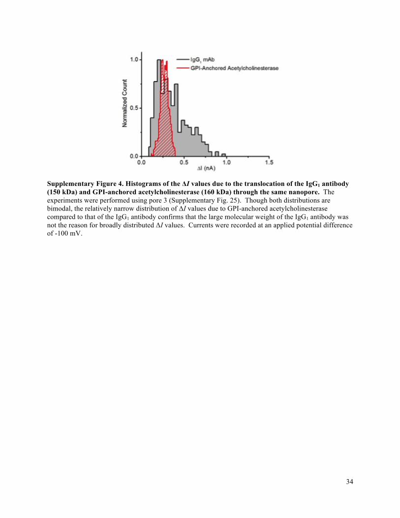
34    

 

Supplementary Figure 4. Histograms of the ΔI values due to the translocation of the IgG1 antibody (150 kDa) and GPI-anchored acetylcholinesterase (160 kDa) through the same nanopore. The experiments were performed using pore 3 (Supplementary Fig. 25). Though both distributions are bimodal, the relatively narrow distribution of ΔI values due to GPI-anchored acetylcholinesterase compared to that of the IgG1 antibody confirms that the large molecular weight of the IgG1 antibody was not the reason for broadly distributed ΔI values. Currents were recorded at an applied potential difference of -100 mV.

   

35    

Supplementary Figure 5. Example convolution of the probability distribution of ΔI values one expects due to the distribution of shape factors, p(ΔIγ) (equations (13a) and (13b)), and the error in determining individual ΔI values, p(ΔIσ) (a Normal distribution function). The solution to the convolution is the probability distribution of ΔI values one expects to observe, p(ΔI). During the fitting procedure, the theoretical cumulative distribution, p(ΔI), is compared to the empirical cumulative distribution of ΔI values, P(ΔI), and the Levenberg-Marquardt non-linear least squares fitting algorithm in MATLAB generates new values for the fitting parameters ΔImin, ΔImax, µ, and σ, thereby creating new iterations of p(ΔIγ) and p(ΔIσ). This process repeats until the fit converges, which typically takes around 20 iterations.

   

σ

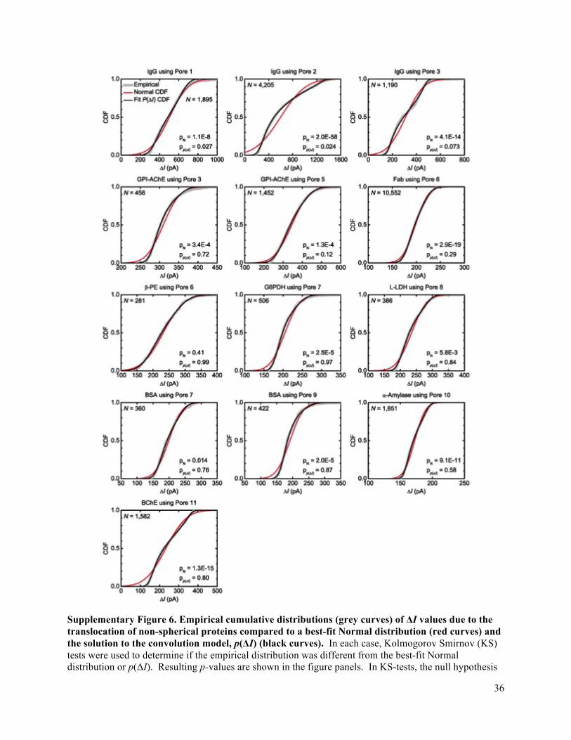
36    

Supplementary Figure 6. Empirical cumulative distributions (grey curves) of ΔI values due to the translocation of non-spherical proteins compared to a best-fit Normal distribution (red curves) and the solution to the convolution model, p(ΔI) (black curves). In each case, Kolmogorov Smirnov (KS) tests were used to determine if the empirical distribution was different from the best-fit Normal distribution or p(ΔI). Resulting p-values are shown in the figure panels. In KS-tests, the null hypothesis

37    

is that the two distributions are the same, and therefore, a p-value ≤ 0.05 indicates that the difference between two distributions is statistically significant at the α = 0.05 level. For all of the non-spherical proteins except β-phycoerythrin, the distribution of ΔI values was different from a Normal distribution (pN < 0.05). In contrast, the difference between the empirical distribution and convolution model, p(∆I), was not statistically significant in 11 out of 13 cases (p-value ≥ 0.05).

   

38    

 

Supplementary Figure 7. Estimating the excluded volume as a function of m using ΔImin and ΔImax values illustrates that there are two solutions to equations (14) and (15) for prolate shaped proteins. This figure shows this result graphically by plotting the estimated volume of GPI-anchored acetylcholinesterase as a function of m for Pore 5. The two red dots indicate the two solutions to the system of equations (m = 0.50, Λ = 222 nm3 and m = 3.1, Λ = 259 nm3). In order to simplify the graph,

we described the electrical shape factor with the notation MAXγ or MINγ . We used this notation because for

prolates (m > 1) MAXγ = γ ⊥ and for oblates (m < 1) MAXγ = IIγ

(see equations (14) and (15)). The opposite

is true for MINγ .

   

39    

 

Supplementary Figure 8. The dependence of a protein’s length-to-diameter ratio, m, on the applied potential, VA, for IgG1 (a) and GPI-AChE (b). We determined the value of m at different applied potentials by fitting the convolution model to distributions of maximum ∆I values. Interestingly, m is consistent at low potentials, while its value changes to indicate an increasingly elongated protein (i.e. m approaches 0 for oblates or approaches ∞ for prolates) with increasing potential. To clearly illustrate this trend, we fit the results with an exponential growth function, ( )τ= + ⋅0 exp Am m A V where A may

be positive or negative. Considering that the fits asymptotically approached m ≈ 0.26 for IgG1 and m ≈ 2.9 for GPI-AChE and the expected value of m is between 0.2 and 0.5 for IgG1 and 2.9 for GPI-AChE (Supplementary Table 4), this result suggests that low potentials yield accurate estimates of the protein shape.

   

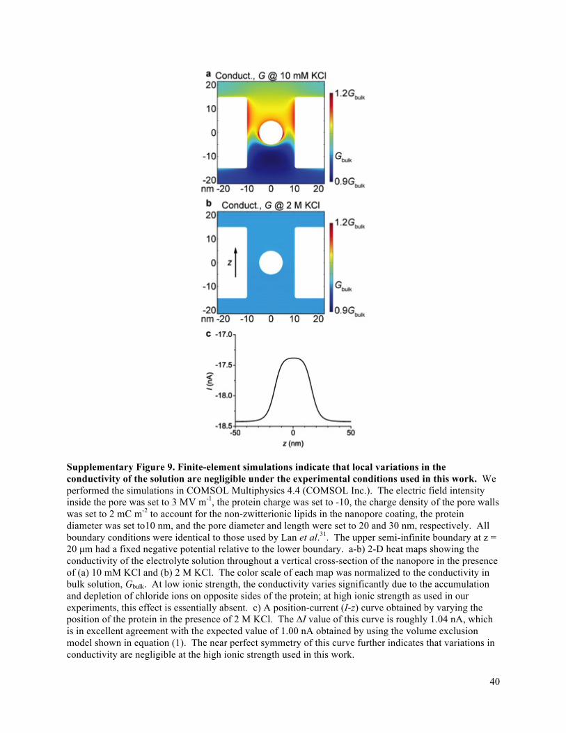
40    

Supplementary Figure 9. Finite-element simulations indicate that local variations in the conductivity of the solution are negligible under the experimental conditions used in this work. We performed the simulations in COMSOL Multiphysics 4.4 (COMSOL Inc.). The electric field intensity inside the pore was set to 3 MV m-1, the protein charge was set to -10, the charge density of the pore walls was set to 2 mC m-2 to account for the non-zwitterionic lipids in the nanopore coating, the protein diameter was set to10 nm, and the pore diameter and length were set to 20 and 30 nm, respectively. All boundary conditions were identical to those used by Lan et al.31. The upper semi-infinite boundary at z = 20 µm had a fixed negative potential relative to the lower boundary. a-b) 2-D heat maps showing the conductivity of the electrolyte solution throughout a vertical cross-section of the nanopore in the presence of (a) 10 mM KCl and (b) 2 M KCl. The color scale of each map was normalized to the conductivity in bulk solution, Gbulk. At low ionic strength, the conductivity varies significantly due to the accumulation and depletion of chloride ions on opposite sides of the protein; at high ionic strength as used in our experiments, this effect is essentially absent. c) A position-current (I-z) curve obtained by varying the position of the protein in the presence of 2 M KCl. The ∆I value of this curve is roughly 1.04 nA, which is in excellent agreement with the expected value of 1.00 nA obtained by using the volume exclusion model shown in equation (1). The near perfect symmetry of this curve further indicates that variations in conductivity are negligible at the high ionic strength used in this work.  

41    

Supplementary Figure 10. Analysis of intra-event ∆I signals can yield parameter estimates in real-time. Measurements of the (a) length-to-diameter ratio, (b) excluded volume, (c) dipole moment, and (d) rotational diffusion coefficient obtained by progressively analyzing the current modulations (i.e. intra-event ∆I values) of a single resistive-pulse resulting from the translocation of an individual anti-biotin Fab fragment. The red lines are moving 10th and 90th percentiles (smoothing window = 50 points). As the protein spends additional time in the pore, more data is acquired and analyzed; consequently, the spread in the determined parameter values narrows and the determined magnitudes of each parameter converge to their final values. The figure also shows that, for this particular event due to the translocation of a single anti-biotin Fab fragment, the variation in each parameter had narrowed to about 20% of its initial spread after approximately 550 µs before the end of the resistive-pulse. These results show that by analyzing a translocation event as it is occurring, it is possible to obtain parameter estimates while the protein still resides in the pore.

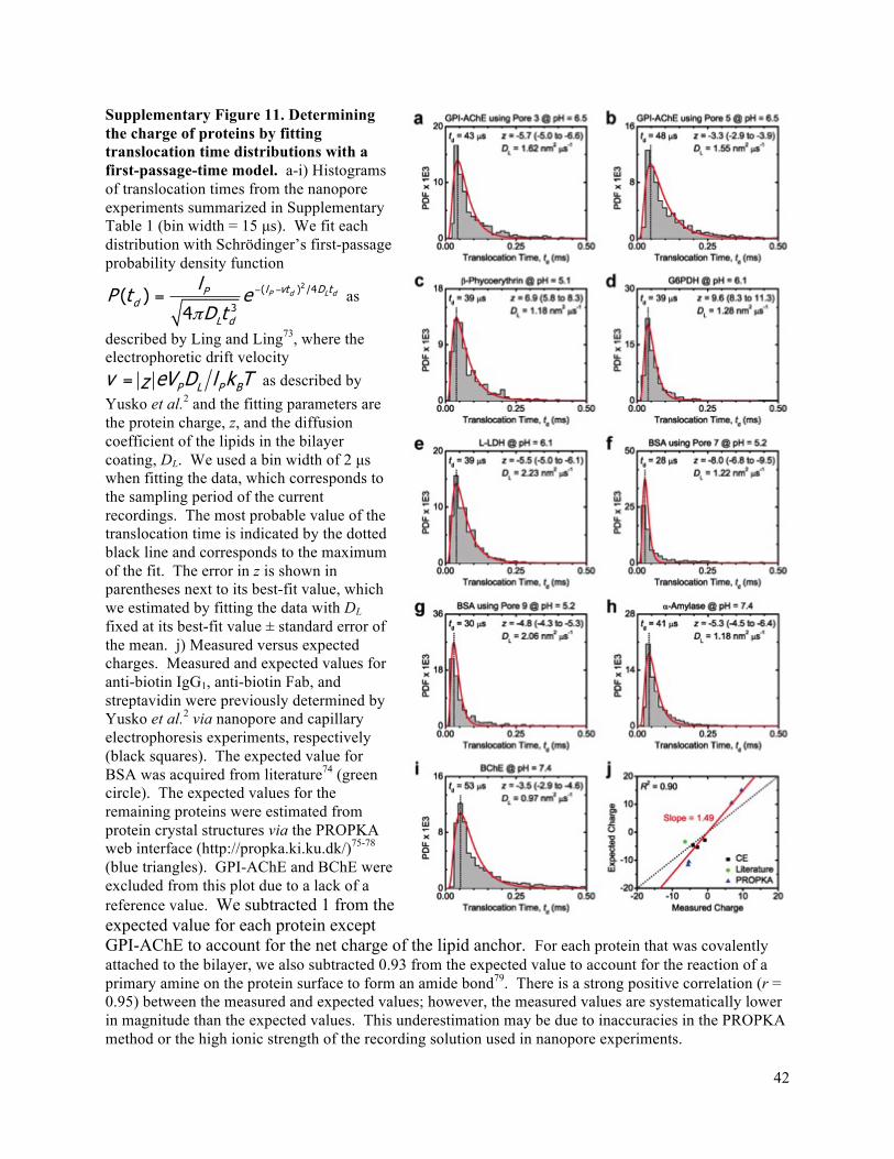
42    

Supplementary Figure 11. Determining the charge of proteins by fitting translocation time distributions with a first-passage-time model. a-i) Histograms of translocation times from the nanopore experiments summarized in Supplementary Table 1 (bin width = 15 µs). We fit each distribution with Schrödinger’s first-passage probability density function

2( ) /4

3( )

4P d L dl vt D tP

d

L d

lP t e

D tπ

− −= as

described by Ling and Ling73, where the electrophoretic drift velocity

P L P Bv eV D l k Tz= as described by Yusko et al.2 and the fitting parameters are the protein charge, z, and the diffusion coefficient of the lipids in the bilayer coating, DL. We used a bin width of 2 µs when fitting the data, which corresponds to the sampling period of the current recordings. The most probable value of the translocation time is indicated by the dotted black line and corresponds to the maximum of the fit. The error in z is shown in parentheses next to its best-fit value, which we estimated by fitting the data with DL fixed at its best-fit value ± standard error of the mean. j) Measured versus expected charges. Measured and expected values for anti-biotin IgG1, anti-biotin Fab, and streptavidin were previously determined by Yusko et al.2 via nanopore and capillary electrophoresis experiments, respectively (black squares). The expected value for BSA was acquired from literature74 (green circle). The expected values for the remaining proteins were estimated from protein crystal structures via the PROPKA web interface (http://propka.ki.ku.dk/)75-78 (blue triangles). GPI-AChE and BChE were excluded from this plot due to a lack of a reference value. We subtracted 1 from the expected value for each protein except GPI-AChE to account for the net charge of the lipid anchor. For each protein that was covalently attached to the bilayer, we also subtracted 0.93 from the expected value to account for the reaction of a primary amine on the protein surface to form an amide bond79. There is a strong positive correlation (r = 0.95) between the measured and expected values; however, the measured values are systematically lower in magnitude than the expected values. This underestimation may be due to inaccuracies in the PROPKA method or the high ionic strength of the recording solution used in nanopore experiments.  

43    

Supplementary Figure 12. Distributions of maximum ∆I values from simulated translocation events. a) A histogram of maximum ∆I values from simulated translocation events. The black curve shows the solution of the convolution model, p(ΔI), after a non-linear least squares fitting procedure, and the red dashed curve shows the estimated distribution of ΔI values due to the distribution of shape factors, p(ΔIγ). b) The cumulative distribution of the same data shown in (a) (grey curve) compared to a best-fit Normal distribution (blue curve) and the solution to the convolution model (black curve). p-values shown in the figure resulted from Kolmogorov Smirnov (KS) tests that compared the simulated, empirical cumulative distribution to the model Normal distribution, pN, or the convolution model, pp(ΔI). Since, the value pN was less than 0.05, the KS-test indicated that the distribution was not Normal at the α = 0.05 level. In contrast, the value of pp(ΔI) was greater than 0.05 and therefore not significantly different from the convolution model; this result indicates that the model describes the empirical distribution well. For the simulations, we used input parameters that were based on the experiment done with IgG1 in pore 1 (e.g. ∆Imin and ∆Imax were 329 and 678 pA, corresponding to values of m and Λ of 0.37 and 292 nm3). We simulated 2,000 events with translocation times that were sampled from Schrödinger’s first-passage probability density function73. The signal processing algorithm detected 1,922 events wherein 1,665 of these events were fully time resolved (i.e. td > 50 µs). From the fit, we calculated values for m and Λ of 0.38 (2.7% greater than the expected value) and 310 nm3 (6.2% greater than the expected value).

   

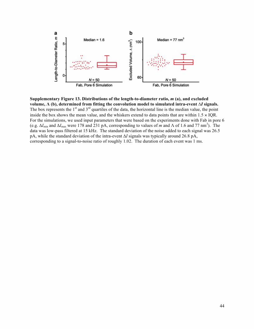
44    

Supplementary Figure 13. Distributions of the length-to-diameter ratio, m (a), and excluded volume, Λ (b), determined from fitting the convolution model to simulated intra-event ∆I signals. The box represents the 1st and 3rd quartiles of the data, the horizontal line is the median value, the point inside the box shows the mean value, and the whiskers extend to data points that are within 1.5 × IQR. For the simulations, we used input parameters that were based on the experiments done with Fab in pore 6 (e.g. ∆Imin and ∆Imax were 178 and 231 pA, corresponding to values of m and Λ of 1.6 and 77 nm3). The data was low-pass filtered at 15 kHz. The standard deviation of the noise added to each signal was 26.5 pA, while the standard deviation of the intra-event ∆I signals was typically around 26.8 pA, corresponding to a signal-to-noise ratio of roughly 1.02. The duration of each event was 1 ms.

   

45    

Supplementary Figure 14. Dipole moments, µ, and rotational diffusion coefficients, DR, determined from analyzing simulated translocation events due to spheroidal particles. a-b) Distributions of dipole moments and rotational diffusion coefficients determined from analyzing simulated, 1-ms-long translocation events. The inset in each plot shows the empirical cumulative distribution (black squares) fit with a lognormal cumulative distribution function (CDF) (red line). KS-tests indicated the difference between the empirical distribution and best-fit curve was not significant in all cases at a confidence level of α = 0.10. The derivative of the CDF is the probability density function (PDF), which is plotted in red with the histograms of dipole moments and rotational diffusion coefficients. The most probable value is indicated by the dotted black line and corresponds to the maximum of the lognormal fit. c-d) Measured versus expected (i.e. input) dipole moments and rotational diffusion coefficients. The ideal outcome wherein the measured values are equal to the input values is shown in black and the best fit line is shown in red. For the simulations where we varied µ, we used input parameters that were based on the experiment done with IgG1 in pore 1. For the simulations where we varied DR, we kept µ fixed at 500 Debyes and did not add noise to the signal; lower signal-to-noise ratios resulted in additional error as expected. Furthermore, we calculated DR at bandwidths ranging up to 60 kHz for each event to determine the value of DR at infinite bandwidth, as illustrated in Supplementary Fig. 18a.

   

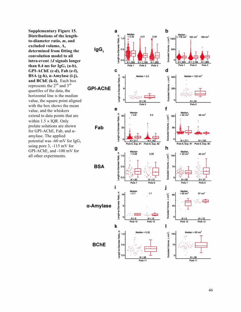
46    

Supplementary Figure 15. Distributions of the length-to-diameter ratio, m, and excluded volume, Λ, determined from fitting the convolution model to all intra-event ∆I signals longer than 0.4 ms for IgG1 (a-b), GPI-AChE (c-d), Fab (e-f), BSA (g-h), α-Amylase (i-j), and BChE (k-l). Each box represents the 2nd and 3rd quartiles of the data, the horizontal line is the median value, the square point aligned with the box shows the mean value, and the whiskers extend to data points that are within 1.5 × IQR. Only prolate solutions are shown for GPI-AChE, Fab, and α-amylase. The applied potential was -60 mV for IgG1 using pore 3, -115 mV for GPI-AChE, and -100 mV for all other experiments.

   

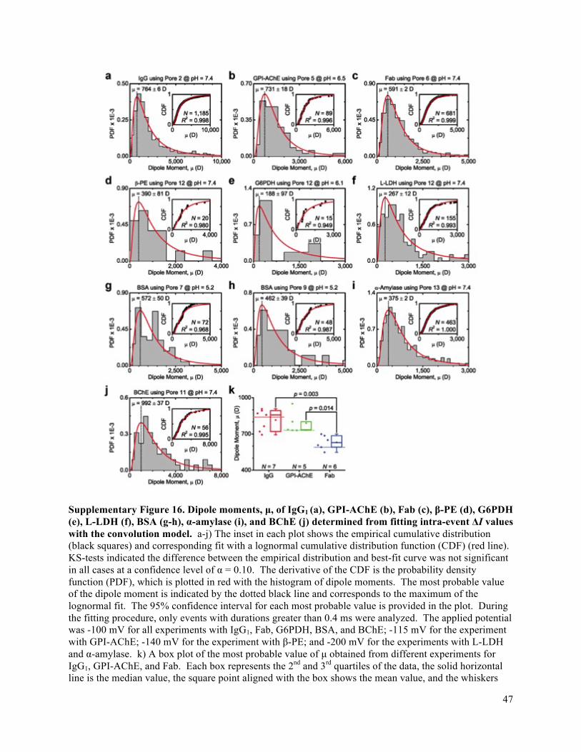
47    

Supplementary Figure 16. Dipole moments, µ, of IgG1 (a), GPI-AChE (b), Fab (c), β-PE (d), G6PDH

(e), L-LDH (f), BSA (g-h), α-amylase (i), and BChE (j) determined from fitting intra-event ΔI values with the convolution model. a-j) The inset in each plot shows the empirical cumulative distribution (black squares) and corresponding fit with a lognormal cumulative distribution function (CDF) (red line). KS-tests indicated the difference between the empirical distribution and best-fit curve was not significant in all cases at a confidence level of α = 0.10. The derivative of the CDF is the probability density function (PDF), which is plotted in red with the histogram of dipole moments. The most probable value of the dipole moment is indicated by the dotted black line and corresponds to the maximum of the lognormal fit. The 95% confidence interval for each most probable value is provided in the plot. During the fitting procedure, only events with durations greater than 0.4 ms were analyzed. The applied potential was -100 mV for all experiments with IgG1, Fab, G6PDH, BSA, and BChE; -115 mV for the experiment with GPI-AChE; -140 mV for the experiment with β-PE; and -200 mV for the experiments with L-LDH and α-amylase. k) A box plot of the most probable value of µ obtained from different experiments for IgG1, GPI-AChE, and Fab. Each box represents the 2nd and 3rd quartiles of the data, the solid horizontal line is the median value, the square point aligned with the box shows the mean value, and the whiskers

48    

extend to data points that are within 1.5 × IQR. The dotted horizontal line indicates the reference value for each protein (see Supplementary Table 4). A Tukey test indicated the distribution for Fab is significantly different than the distributions for the other two proteins (p-values are indicated on the plot). For IgG1, we obtained the following values: 908 D in pore 1, 764 D in pore 2, 894 D in pore 3, 871 D in pore 8, 720 D in pore 16, 858 D in pore 17, and 694 in pore 18. For GPI-AChE, we obtained the following values: 731 in pore 5, 736 D in pore 16, 730 D in pore 20, and 950 and 802 D in pore 21. For Fab, we obtained the following values: 548 and 591 D in pore 6, 686 D in pore 11, 699 and 650 D in pore 13, and 607 D in pore 14.

   

49    

 

Supplementary Figure 17. Variation of the dipole moment, µ, of β-phycoerythrin (β-PE) as a function of pH. The inset in each plot shows the empirical cumulative distribution (black squares) and corresponding fit with a lognormal cumulative distribution function (CDF) (red line). The derivative of the CDF is the probability density function (PDF), which is plotted in red with the histogram of dipole moments. The most probable value of the dipole moment is indicated by the dotted black line and corresponds to the maximum of the lognormal fit. The 95% confidence interval for each most probable value is provided in the plot. Based on theory, β-PE’s expected values of µ are 395 D at pH 7.4 and 489 D at pH 5.1, which are in reasonable agreement with the measured values. An additional measurement at pH 5.1 obtained using pore 19 yielded a most probable value with relatively high uncertainty of 774 ± 371 D (N = 10). During the fitting procedure, only events with durations greater than 0.4 ms were analyzed. The applied potential was -100 mV in all cases.

   

50    

Supplementary Figure 18. Rotational diffusion coefficients, DR, of IgG1 (a-b), GPI-AChE (c), Fab

(d), β-PE (e-f), α-Amylase (g), and BChE (h) determined from analysis of intra-event ΔI values. a) Rotational diffusion coefficient versus the low-pass cutoff frequency for a single event due to IgG1 in pore 1. The curve was fit with the logistic equation to determine DR at infinite bandwidth, which is denoted by the dotted black line. We used this procedure to determine the values of DR for all proteins and subsequently generate the histograms in panes (b) through (i). b-h) The inset in each plot shows the empirical cumulative distribution (black squares) fit with a lognormal cumulative distribution function (CDF) (red line). KS-tests indicated the difference between the empirical distribution and best-fit curve was not significant in every case except for the experiment with Fab using Pore 6 (panel (f)) at a confidence level of α = 0.10. The derivative of the CDF is the probability density function (PDF), which is plotted in red with the histogram of rotational diffusion coefficients. The most probable value of the rotational diffusion coefficient is indicated by the dotted black line and corresponds to the maximum of the lognormal fit. The 95% confidence interval for each most probable value is provided in the plot. Only events with durations greater than 0.4 ms were analyzed. The applied potential was -100 mV for all experiments with the IgG1 antibody, Fab, and BChE; -115 mV for the experiment with GPI-AChE; -140

51    

mV for the experiment with β-PE; and -200 mV for the experiment with α-amylase. i) A box plot of the most probable value of DR obtained from different experiments for IgG1 and GPI-AChE. Each box represents the 2nd and 3rd quartiles of the data, the solid horizontal line is the median value, the square point aligned with the box shows the mean value, and the whiskers extend to data points that are within 1.5 × IQR. The dotted horizontal line for GPI-AChE indicates its reference value. A t-test indicated the two distributions are significantly different (the p-value is indicated on the plot). For IgG1, we obtained the following values: 14,262 rad2 s-1 in pore 1; 2,414 rad2 s-1 in pore 2; 3,227 rad2 s-1 in pore 3; 2,934 rad2 s-1 in pore 8; 2,958 rad2 s-1 in pore 16; 2,680 rad2 s-1 in pore 17; and 3,727 rad2 s-1 in pore 18. For GPI-AChE, we obtained the following values: 11,732 rad2 s-1 for pore 5; 4,725 rad2 s-1 for pore 16; 9,456 rad2 s-1 for pore 20; and 13,630 and 13,446 rad2 s-1 for pore 21. j) A fit of the Stokes-Einstein equation for rotational diffusion, DR = kBT / (8πηrH,eff

3), to the measured most probable values of DR. The only fitting parameter was apparent viscosity, η, which had a best-fit value that was 211 times higher than the viscosity of water.

   

52    

Supplementary Figure 19. The measured rotational diffusion coefficient, DR, of lipid-anchored IgG1 decreases with the ratio of bivalently-bound to monovalently-bound IgG1. a) Histograms of DR values determined from analysis of intra-event ∆I values. We analyzed 179, 343, 382, and 739 events obtained in the presence of 0, 1, 10, and 100 nM free biotin, respectively. b) Lognormal fits of the DR distributions. We fit each empirical cumulative distribution with a lognormal cumulative distribution function (not shown). The R2 values of the fits are 0.989, 0.998, 0.987, and 0.996 for 0, 1, 10, and 100 nM free biotin, respectively. The legend displays the most probable value of each fit. c) The most probable value of DR as a function of the concentration of free biotin. We attribute the increase in DR with the concentration of free biotin to a decrease in the ratio of bivalently-bound to monovalently-bound IgG1. All recordings were obtained with pore 13 at an applied potential of -100 mV and pH of 7.4.

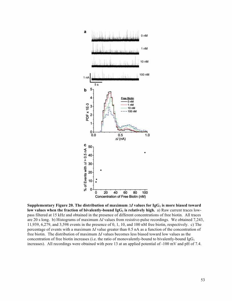
53    

Supplementary Figure 20. The distribution of maximum ∆I values for IgG1 is more biased toward low values when the fraction of bivalently-bound IgG1 is relatively high. a) Raw current traces low-pass filtered at 15 kHz and obtained in the presence of different concentrations of free biotin. All traces are 20 s long. b) Histograms of maximum ΔI values from resistive-pulse recordings. We obtained 7,243, 11,939, 6,279, and 3,598 events in the presence of 0, 1, 10, and 100 nM free biotin, respectively. c) The percentage of events with a maximum ∆I value greater than 0.5 nA as a function of the concentration of free biotin. The distribution of maximum ∆I values becomes less biased toward low values as the concentration of free biotin increases (i.e. the ratio of monovalently-bound to bivalently-bound IgG1 increases). All recordings were obtained with pore 13 at an applied potential of -100 mV and pH of 7.4.

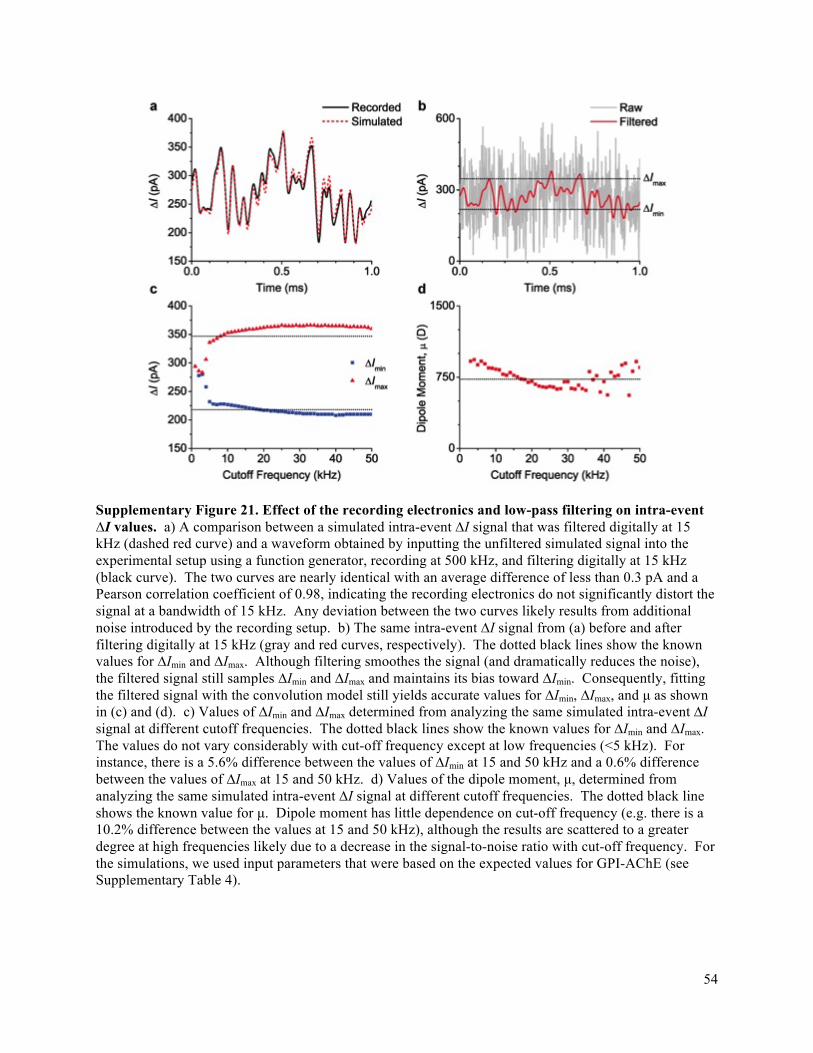
54    

Supplementary Figure 21. Effect of the recording electronics and low-pass filtering on intra-event ∆I values. a) A comparison between a simulated intra-event ∆I signal that was filtered digitally at 15 kHz (dashed red curve) and a waveform obtained by inputting the unfiltered simulated signal into the experimental setup using a function generator, recording at 500 kHz, and filtering digitally at 15 kHz (black curve). The two curves are nearly identical with an average difference of less than 0.3 pA and a Pearson correlation coefficient of 0.98, indicating the recording electronics do not significantly distort the signal at a bandwidth of 15 kHz. Any deviation between the two curves likely results from additional noise introduced by the recording setup. b) The same intra-event ∆I signal from (a) before and after filtering digitally at 15 kHz (gray and red curves, respectively). The dotted black lines show the known values for ∆Imin and ∆Imax. Although filtering smoothes the signal (and dramatically reduces the noise), the filtered signal still samples ∆Imin and ∆Imax and maintains its bias toward ∆Imin. Consequently, fitting the filtered signal with the convolution model still yields accurate values for ∆Imin, ∆Imax, and µ as shown in (c) and (d). c) Values of ∆Imin and ∆Imax determined from analyzing the same simulated intra-event ∆I signal at different cutoff frequencies. The dotted black lines show the known values for ∆Imin and ∆Imax. The values do not vary considerably with cut-off frequency except at low frequencies (<5 kHz). For instance, there is a 5.6% difference between the values of ∆Imin at 15 and 50 kHz and a 0.6% difference between the values of ∆Imax at 15 and 50 kHz. d) Values of the dipole moment, µ, determined from analyzing the same simulated intra-event ∆I signal at different cutoff frequencies. The dotted black line shows the known value for µ. Dipole moment has little dependence on cut-off frequency (e.g. there is a 10.2% difference between the values at 15 and 50 kHz), although the results are scattered to a greater degree at high frequencies likely due to a decrease in the signal-to-noise ratio with cut-off frequency. For the simulations, we used input parameters that were based on the expected values for GPI-AChE (see Supplementary Table 4).

55    

Supplementary Figure 22. Determining the volume and shape of an antibody-antigen complex from individual resistive-pulses. a) Current trace showing resistive pulses due to the translocation of G6PDH in the absence of antibody. b) Current trace recorded after incubation with 15 µM polyclonal anti-G6PDH IgG for 1 hr. After incubation, we rinsed the chip with recording buffer to remove unbound IgG. c-d) Histograms of maximum ∆I values recorded before and after incubation with anti-G6PDH IgG. Insets show the same data over a reduced y-axis scale. We observed a significant increase in the number of events with large ∆I values after incubation with IgG (e.g. the percentage of events with values larger than 500 pA increased from 0.01 to 9 percent). e) Empirical cumulative distribution (CDF) of ∆I values due to the translocation of G6PDH (grey curve) and the fit of this data to the convolution model (black curve). f) Empirical CDF of ∆I values due to the translocation of both G6PDH and the antibody-antigen complex (red dotted curve). To generate a CDF due to the translocation of the complex only (i.e. remove ∆I values due to the translocation of unbound G6PDH), we subtracted the CDF due to the translocation of G6PDH only (e) after scaling this distribution such that the difference between the two empirical CDFs was minimized at low ∆I values (250 to 350 pA). We expect the majority of ∆I values in this range to result from the translocation of unbound G6PDH. The optimal scaling factor was 0.73, suggesting that roughly 27 percent of translocation events were due to the antibody-antigen complex. g-h) Blue spheroids show the volume and shape of G6PDH and the antibody-antigen complex determined by fitting the empirical CDFs shown in panes (e) and (f). The crystal structure of G6PDH and IgG are shown in red and orange, respectively. i) Bar plot showing excellent agreement between the volume of the antibody-antigen complex determined from analyzing maximum ∆I values from this experiment and the sum of the volumes of G6PDH and IgG determined that were determined individually in other nanopore experiments (see Supplementary Table 1). j-i) Scatter plots showing the 2D projections of the 3D plot in Fig 5c of the main text. These plots show that resistive pulses assigned to the complex correspond to larger molecular volumes and smaller rotational diffusion coefficients than resistive pulses assigned to G6PDH. The dipole moment of G6PDH is relatively clustered as expected for a protein with well-defined shape and position of amino acids. In contrast, the dipole moment of the complex between G6PDH and the polyclonal anti-G6PDH IgG antibody varies widely as expected since IgG may bind at multiple locations and is a relatively floppy molecule. All recordings were obtained with pore 15 at an applied potential of -100 mV and pH of 6.1. We purchased polyclonal anti-G6PDH IgG (A9521) from Sigma Aldrich, Inc.

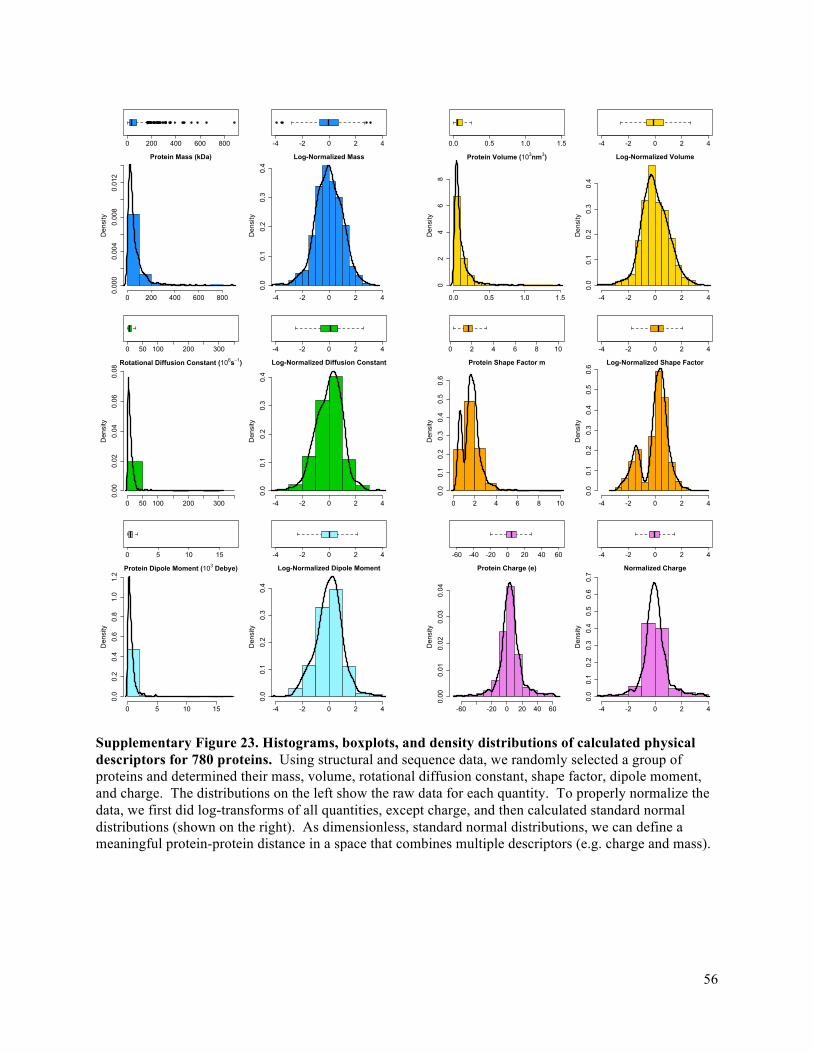
56    

 

Supplementary Figure 23. Histograms, boxplots, and density distributions of calculated physical descriptors for 780 proteins. Using structural and sequence data, we randomly selected a group of proteins and determined their mass, volume, rotational diffusion constant, shape factor, dipole moment, and charge. The distributions on the left show the raw data for each quantity. To properly normalize the data, we first did log-transforms of all quantities, except charge, and then calculated standard normal distributions (shown on the right). As dimensionless, standard normal distributions, we can define a meaningful protein-protein distance in a space that combines multiple descriptors (e.g. charge and mass).

0 200 400 600 800 -4 -2 0 2 4 0.0 0.5 1.0 1.5 -4 -2 0 2 4

Protein Mass (kDa)

Density

0 200 400 600 800

0.000

0.004

0.008

0.012

Log-Normalized Mass

Density

-4 -2 0 2 4

0.0

0.1

0.2

0.3

0.4

Protein Volume (103nm3)

Density

0.0 0.5 1.0 1.5

02

46

8

Log-Normalized Volume

Density

-4 -2 0 2 4

0.0

0.1

0.2

0.3

0.4

0 50 100 200 300 -4 -2 0 2 4 0 2 4 6 8 10 -4 -2 0 2 4

Rotational Diffusion Constant (106s−1)

Density

0 50 100 200 300

0.00

0.02

0.04

0.06

0.08

Log-Normalized Diffusion Constant

Density

-4 -2 0 2 4

0.0

0.1

0.2

0.3

0.4

Protein Shape Factor m

Density

0 2 4 6 8 10

0.0

0.1

0.2

0.3

0.4

0.5

0.6

Log-Normalized Shape Factor

Density

-4 -2 0 2 4

0.0

0.1

0.2

0.3

0.4

0.5

0.6

0 5 10 15 -4 -2 0 2 4 -60 -40 -20 0 20 40 60 -4 -2 0 2 4

Protein Dipole Moment (103 Debye)

Density

0 5 10 15

0.0

0.2

0.4

0.6

0.8

1.0

1.2

Log-Normalized Dipole Moment

Density

-4 -2 0 2 4

0.0

0.1

0.2

0.3

0.4

Protein Charge (e)

Density

-60 -20 0 20 40 60

0.00

0.01

0.02

0.03

0.04

Normalized ChargeDensity

-4 -2 0 2 4

0.0

0.1

0.2

0.3

0.4

0.5

0.6

0.7

57    

Supplementary Figure 24. A scatter plot matrix showing the relationships between the log-normalized quantities in Supplementary Figure 23. Mass, volume, and rotational diffusion constant show a high-degree of correlation; however charge, the length-to-diameter ratio (m), and the dipole moment show little correlation with any other descriptor.

log(mass)-4 -2 0 2 -4 -2 0 2 4 -4 -2 0 2 4

-4-2

01

23

-4-2

02 log(volume)

log(Dr)

-4-2

02

4

-4-2

02

4

charge

log(m)

-3-2

-10

12

3-4 -2 0 1 2 3

-4-2

02

4

-4 -2 0 2 4 -3 -2 -1 0 1 2 3

log(dipole)

58    

Supplementary Figure 25. Transmission electron micrographs of the nanopores used in this work. The brightest part in the center of each image depicts the shape and size of the nanopore and the surrounding circle with reduced brightness reflects the channel leading to the nanopore2,80. All scale bars are 50 nm. Nanopores shown are pore 1(a), pore 2 (b), pore 3 (c), pore 4 (d), pore 5 (e), pore 6 (f), pore 7 (g), pore 8 (h), pore 9 (i), pore 10 (j), pore 11 (k), pore 12 (l), pore 13 (m), and pore 14 (n). The dimensions of the nanopores (in units of nm) without the lipid bilayer coating were: for pore 1 rP = 16.1 and lP = 21.3; for pore 2 rP = 16.4 and lP = 17.3; for pore 3 rP = 22.7 and lP = 16.2; for pore 4 rP = 9.6 and lP = 18.0; for pore 5 rP = 16.0 and lP = 15.0; for pore 6 rP = 14.2 and lP = 10.0; for pore 7 rP = 14.0 and lP = 15.4; for pore 8 rP = 17.8 and lP = 15.5; for pore 9 rP = 14.7 and lP = 18.0; for pore 10 rP = 13.6 and lP = 14.0; for pore 11 rP = 16.0 and lP = 12.0; for pore 12 rP = 14.5 and lP = 10.0; for pore 13 rP = 15.7 and lP = 12.0; for pore 14 rP = 15.0 and lP = 10.9; for pore 15 rP = 21.3 and lP = 19.7; for pore 16 rP = 16.4 and lP = 30.0; for pore 17 rP = 18.5 and lP = 30.0; for pore 18 rP = 18.0 and lP = 30.0; for pore 19 rP = 16.5 and lP = 30.0; for pore 20 rP = 15.5 and lP = 30.0; and for pore 21 rP = 15.5 and lP = 6.0.  

59    

Supplementary Table 1. Values of fitting parameters determined from fitting the convolution model to the empirical distributions of ΔI values (Fig. 3 and 4 in the main text) as well as the resulting calculations of protein volume, Λ, and shape parameter, m. Experiment E† (MV m-1) ΔImin

(pA) ΔImax (pA) σ (pA) µ (D) R2 Λ* (nm3) m*

IgG1, Pore 1 -1.5 329 678 58 596 0.998 292 0.37

IgG1, Pore 2 -1.6 258 1,320 65 1,911 1.000 223 0.13

Intra-event (Fig. 4) -1.6 281 938 48 302 0.998 232 0.21

IgG1, Pore 3 -0.6 164 483 21 2,020 0.997 319 0.24

IgG1, Pore 8 -1.4 266 1132 64 1,493 0.999 217 0.16

GPI-AChE, Pore 3 -1.0 280 375 14 3,530 0.999 278 or 306 0.64 or 1.8

GPI-AChE, Pore 5 -1.3 279 451 40 1,712 0.999 222 or 259 0.50 or 3.1

Fab, Pore 6 -2.1 178 231 11 972 1.000 71 or 77 0.67 or 1.6

β-PE, Pore 6 -0.8 181 302 31 2,125 0.999 192 or 227 0.48 or 3.5

G6PDH, Pore 7 -1.0 178 264 12 3,590 0.999 193 or 220 0.56 or 2.3

G6PDH, Pore 15 -1.1 169 254 58 2,822 0.997 181 or 207 0.55 or 2.4

L-LDH, Pore 8 -0.8 195 296 16 2,802 0.999 267 or 307 0.54 or 2.5

BSA, Pore 7 -1.9 165 258 17 1,263 0.998 91 or 105 0.52 or 2.7

BSA, Pore 9 -1.7 165 276 13 2,925 0.998 110 or 130 0.48 or 3.5

α-Amylase, Pore 10 -1.6 157 196 5 1,243 1.000 92 or 99 0.71 or 1.5

BChE, Pore 11 -1.7 150 364 18 1,007 1.000 82 0.30 † The electric field intensity was calculated according to the following equation: E = VA * Rp / (Rtotal * lp), where Rp is the resistance of the pore, Rtotal is the total resistance of the circuit, and lp is the length of the pore. * Values of Λ and m shown in bold are those corresponding to the correct shape (i.e. the shape that matches the crystal structure).    

60    

Supplementary Table 2. Estimated hydration shell thickness of proteins detected in this work. Based on the difference between the volume that we measured and the volume determined from crystal structures, we estimated the thickness of the hydration shell and the average number of water molecules required in this ordered water layer. The average hydration shell thickness is 0.34 ± 0.14 nm, which closely matches reported values that range from 0.3 to 0.5 nm81-84. An alternative explanation for the difference between the measured and crystal structure volumes is that counter ions, rather than water molecules, bind tightly to the proteins85.

Volume, Λ (nm3)

Hydration Shell Thickness

Protein Measured Crystal Structure (nm) NH2O†

IgG1 278 174 0.37 1.3

GPI-Acetylcholinesterase 283 145 0.53 1.9

Fab Fragment 77 56 0.21 0.8

β-Phycoerythrin 192 139 0.29 1.0

Glucose-6-Phosphate Dehydrogenase 220 135 0.40 1.4

L-Lactate Dehydrogenase 267 160 0.46 1.6

Bovine Serum Albumin 101 78 0.19 0.7

α-Amylase 99 65 0.29 1.0

Butyrylcholinesterase 82 69 0.12 0.4

Streptavidin 110 61 0.53 1.9 † The number of water molecules was calculated by dividing the thickness by the diameter of a water molecule (0.28 nm)86.

   

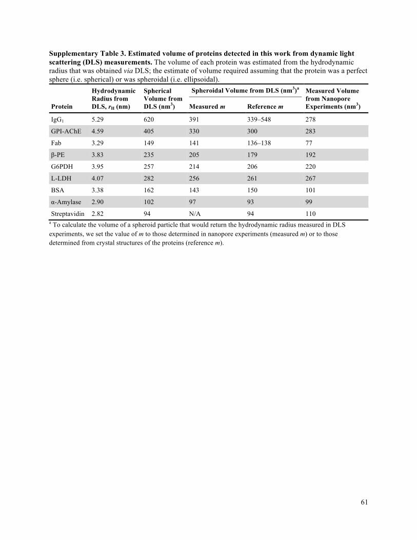
61    

Supplementary Table 3. Estimated volume of proteins detected in this work from dynamic light scattering (DLS) measurements. The volume of each protein was estimated from the hydrodynamic radius that was obtained via DLS; the estimate of volume required assuming that the protein was a perfect sphere (i.e. spherical) or was spheroidal (i.e. ellipsoidal).

Protein

Hydrodynamic Radius from DLS, rH (nm)

Spherical Volume from DLS (nm3)

Spheroidal Volume from DLS (nm3)a

Measured Volume from Nanopore Experiments (nm3) Measured m Reference m

IgG1 5.29 620 391 339–548 278

GPI-AChE 4.59 405 330 300 283

Fab 3.29 149 141 136–138 77

β-PE 3.83 235 205 179 192

G6PDH 3.95 257 214 206 220

L-LDH 4.07 282 256 261 267

BSA 3.38 162 143 150 101

α-Amylase 2.90 102 97 93 99

Streptavidin 2.82 94 N/A 94 110 a To calculate the volume of a spheroid particle that would return the hydrodynamic radius measured in DLS experiments, we set the value of m to those determined in nanopore experiments (measured m) or to those determined from crystal structures of the proteins (reference m).

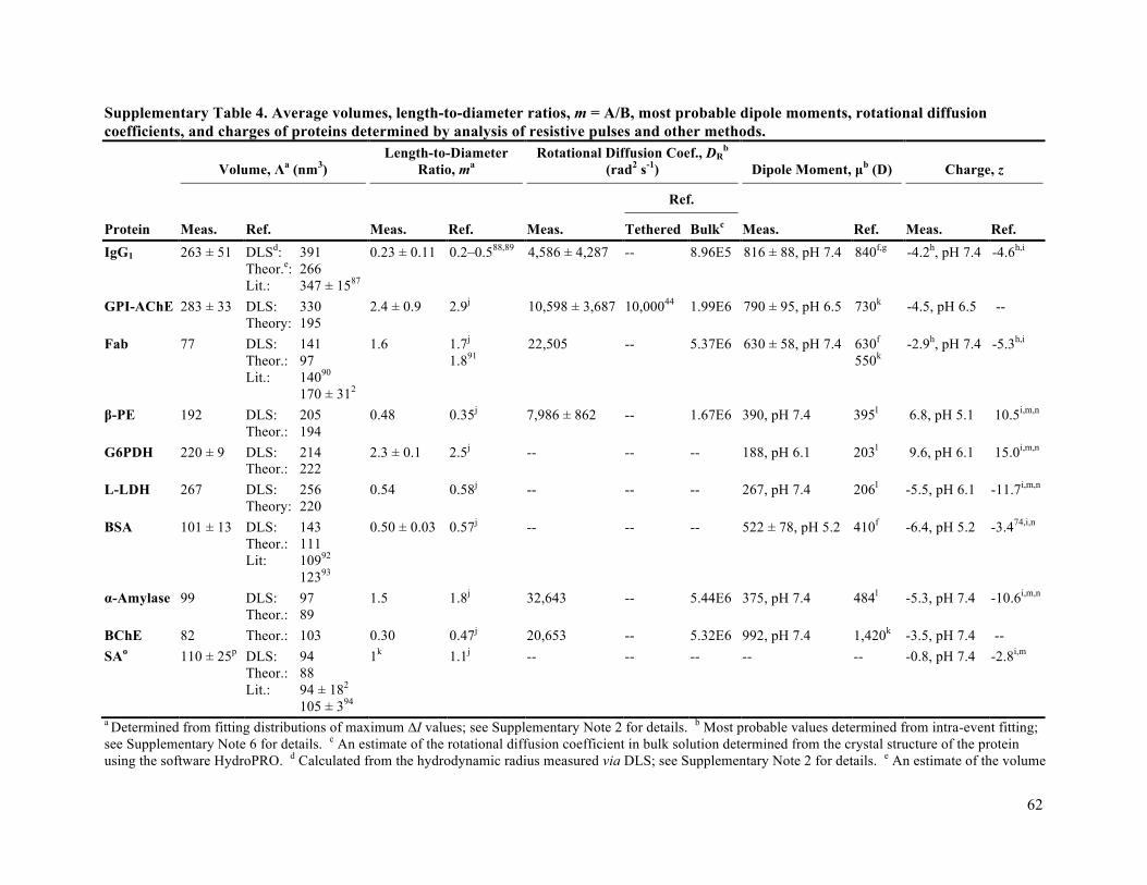
62    

Supplementary Table 4. Average volumes, length-to-diameter ratios, m = A/B, most probable dipole moments, rotational diffusion coefficients, and charges of proteins determined by analysis of resistive pulses and other methods.

Protein

Volume, Λa (nm3)

Length-to-Diameter Ratio, ma

Rotational Diffusion Coef., DRb

(rad2 s-1)

Dipole Moment, µb (D)

Charge, z

Meas. Ref. Meas. Ref. Meas.

Ref. Meas. Ref. Meas. Ref. Tethered Bulkc

IgG1 263 ± 51 DLSd: 391

Theor.e: 266 Lit.: 347 ± 1587

0.23 ± 0.11 0.2–0.588,89 4,586 ± 4,287 -- 8.96E5 816 ± 88, pH 7.4 840f,g -4.2h, pH 7.4 -4.6h,i

GPI-AChE 283 ± 33 DLS: 330 Theory: 195

2.4 ± 0.9 2.9j 10,598 ± 3,687 10,00044 1.99E6 790 ± 95, pH 6.5 730k -4.5, pH 6.5 --

Fab 77 DLS: 141 Theor.: 97 Lit.: 14090 170 ± 312

1.6 1.7j

1.891 22,505 -- 5.37E6 630 ± 58, pH 7.4 630f

550k -2.9h, pH 7.4 -5.3h,i

β-PE 192 DLS: 205 Theor.: 194

0.48 0.35j 7,986 ± 862 -- 1.67E6 390, pH 7.4 395l 6.8, pH 5.1 10.5i,m,n

G6PDH 220 ± 9 DLS: 214 Theor.: 222

2.3 ± 0.1 2.5j -- -- -- 188, pH 6.1 203l 9.6, pH 6.1 15.0i,m,n

L-LDH 267 DLS: 256 Theory: 220

0.54 0.58j -- -- -- 267, pH 7.4 206l -5.5, pH 6.1 -11.7i,m,n

BSA 101 ± 13 DLS: 143 Theor.: 111 Lit: 10992 12393

0.50 ± 0.03 0.57j -- -- -- 522 ± 78, pH 5.2 410f -6.4, pH 5.2 -3.474,i,n

α-Amylase 99 DLS: 97 Theor.: 89

1.5 1.8j 32,643 -- 5.44E6 375, pH 7.4 484l -5.3, pH 7.4 -10.6i,m,n

BChE 82 Theor.: 103 0.30 0.47j 20,653 -- 5.32E6 992, pH 7.4 1,420k -3.5, pH 7.4 -- SAo 110 ± 25p DLS: 94

Theor.: 88 Lit.: 94 ± 182 105 ± 394

1k 1.1j -- -- -- -- -- -0.8, pH 7.4 -2.8i,m

a Determined from fitting distributions of maximum ∆I values; see Supplementary Note 2 for details. b Most probable values determined from intra-event fitting; see Supplementary Note 6 for details. c An estimate of the rotational diffusion coefficient in bulk solution determined from the crystal structure of the protein using the software HydroPRO. d Calculated from the hydrodynamic radius measured via DLS; see Supplementary Note 2 for details. e An estimate of the volume

63    

of the hydrated protein determined from the crystal structure of the protein using the software HydroPRO. f Measured via dielectric impedance spectroscopy. g

This value should be used as a loose approximation due to the low signal-to-noise ratio of the measurement. h Results from Yusko et al.2. i Values were reduced by 1 to account for the charge of the lipid anchor. j Estimated from the crystal structure of the protein. k Calculated from the crystal structure of the protein using the software HydroPRO. l Calculated from the crystal structure of the protein using the Weizmann server (http://bioinfo.weizmann.ac.il/dipol/). m Estimated using the PROPKA web interface (http://propka.ki.ku.dk/)75-78  . n Values were reduced by 0.93 to account for the reaction of a primary amine on the protein surface with an NHS ester on the crosslinker molecule to form an amide bond79. All estimates were done in the absence of ligands except for G6PDH. o

Parameters determined using pore 4. p Since the distribution of ΔI values due to streptavidin translocations was unimodal and Normal, we assumed that streptavidin had a spherical shape, and therefore m = 1; to calculate the excluded volume of streptavidin, we solved equation (1) with γ set to a value of 1.5.

64    

Supplementary References

1   Uram, J. D., Ke, K. & Mayer, M. Noise and bandwidth of current recordings from submicrometer pores and nanopores. ACS Nano 2, 857-872 (2008).

2 Yusko, E. C. et al. Controlling protein translocation through nanopores with bio-inspired fluid walls. Nat. Nanotechnol. 6, 253-260 (2011).

3 Bermudez, O. & Forciniti, D. Aggregation and denaturation of antibodies: A capillary electrophoresis, dynamic light scattering, and aqueous two-phase partitioning study. J. Chromatogr. B 807, 17-24 (2004).

4 Jossang, T., Feder, J. & Rosenqvist, E. Photon-correlation spectroscopy of human-IgG. J. Protein Chem. 7, 165-171 (1988).

5 Goodsell, D. Acetylcholinesterase. June 2004 molecule of the month., <http://www.rcsb.org/pdb/101/motm.do?momID=54> (2004).

6 Sigma-Aldrich. Product information: Acetylcholinesterase from human erythrocytes (c0663), <http://www.sigmaaldrich.com/catalog/product/sigma/c0663> (2012).

7 Tan, R. C., Truong, T. N., McCammon, J. A. & Sussman, J. L. Acetylcholinesterase: Electrostatic steering increases the rate of ligand binding. Biochemistry 32, 401-403 (1993).

8 Antosiewicz, J., Wlodek, S. T. & McCammon, J. A. Acetylcholinesterase: Role of the enzyme's charge distribution in steering charged ligands toward the active site. Biopolymers 39, 85-94 (1996).

9 Luk, W. K. W., Chen, V. P., Choi, R. C. Y. & Tsim, K. W. K. N-linked glycosylation of dimeric acetylcholinesterase in erythrocytes is essential for enzyme maturation and membrane targeting. Febs J. 279, 3229-3239 (2012).

10 Porschke, D. et al. Electrooptical measurements demonstrate a large permanent dipole moment associated with acetylcholinesterase. Biophys. J. 70, 1603-1608 (1996).

11 Parihar, M. S. & Hemnani, T. Alzheimer's disease pathogenesis and therapeutic interventions. J. Clin. Neurosci. 11, 456-467 (2004).

12 Rath, A. & Deber, C. M. Correction factors for membrane protein molecular weight readouts on sodium dodecyl sulfate-polyacrylamide gel electrophoresis. Anal. Biochem. 434, 67-72 (2013).

13 Skinner, G. M., van den Hout, M., Broekmans, O., Dekker, C. & Dekker, N. H. Distinguishing single- and double-stranded nucleic acid molecules using solid-state nanopores. Nano. Lett. 9, 2953-2960 (2009).

14 Maxwell, J. C. A treatise on electricity and magnetism. 3rd edn, 435-441 (Clarendon Press, 1904).

15 Deblois, R. W. & Bean, C. P. Counting and sizing of submicron particles by resistive pulse technique. Rev. Sci. Instrum. 41, 909-915 (1970).

16 Grover, N. B., Naaman, J., Ben-sasson, S. & Doljansk, F. Electrical sizing of particles in suspensions. I.Theory. Biophys. J. 9, 1398-1414 (1969).

17 Han, A. P. et al. Label-free detection of single protein molecules and protein-protein interactions using synthetic nanopores. Anal. Chem. 80, 4651-4658 (2008).

18 Ito, T., Sun, L. & Crooks, R. M. Simultaneous determination of the size and surface charge of individual nanoparticles using a carbon nanotube-based Coulter counter. Anal. Chem. 75, 2399-2406 (2003).

19 Golibersuch, D. C. Observation of aspherical particle rotation in Poiseuille flow via the resistance pulse technique. Part 1. Application to human erythrocytes. Biophys. J. 13, 265-280 (1973).

20 Hurley, J. Sizing particles with a Coulter counter. Biophys. J. 10, 74-79 (1970). 21 Soni, G. V. & Dekker, C. Detection of nucleosomal substructures using solid-state nanopores.

Nano. Lett. (2012). 22 Raillon, C. et al. Nanopore detection of single molecule RNAP-DNA transcription complex.

Nano. Lett. 12, 1157-1164 (2012).

65    

23 DeBlois, R. W., Uzgiris, E. E., Cluxton, D. H. & Mazzone, H. M. Comparative measurements of size and polydispersity of several insect viruses. Anal. Biochem. 90, 273-288 (1978).

24 Smythe, W. R. Flow around a spheroid in a circular tube. Phys. Fluids 7, 633-638 (1964). 25 Qin, Z. P., Zhe, J. A. & Wang, G. X. Effects of particle's off-axis position, shape, orientation and

entry position on resistance changes of micro Coulter counting devices. Meas. Sci. Technol. 22 (2011).

26 Fologea, D., Ledden, B., David, S. M. & Li, J. Electrical characterization of protein molecules by a solid-state nanopore. Appl. Phys. Lett. 91, 053901 (2007).

27 Soni, G. V. & Dekker, C. Detection of nucleosomal substructures using solid-state nanopores. Nano. Lett. 12, 3180-3186 (2012).

28 Wei, R., Gatterdam, V., Wieneke, R., Tampe, R. & Rant, U. Stochastic sensing of proteins with receptor-modified solid-state nanopores. Nat. Nanotechnol. 7, 257-263 (2012).

29 Han, A. et al. Sensing protein molecules using nanofabricated pores. Appl. Phys. Lett. 88, 093901 (2006).

30 Sexton, L. T. et al. Resistive-pulse studies of proteins and protein/antibody complexes using a conical nanotube sensor. J. Am. Chem. Soc. 129, 13144-13152 (2007).

31 Lan, W.-J., Kubeil, C., Xiong, J.-W., Bund, A. & White, H. S. Effect of surface charge on the resistive pulse waveshape during particle translocation through glass nanopores. J. Phys. Chem. C. 118, 2726-2734 (2014).

32 Fan, R. et al. DNA translocation in inorganic nanotubes. Nano. Lett. 5, 1633-1637 (2005). 33 Chang, H. et al. DNA-mediated fluctuations in ionic current through silicon oxide nanopore

channels. Nano. Lett. 4, 1551-1556 (2004). 34 Das, S., Dubsky, P., van den Berg, A. & Eijkel, J. Concentration polarization in translocation of

DNA through nanopores and nanochannels. Physical Review Letters 108, 138101 (2012). 35 Japrung, D. et al. Single-molecule studies of intrinsically disordered proteins using solid-state

nanopores. Anal. Chem. 85, 2449-2456 (2013). 36 Fricke, H. The electric permittivity of a dilute suspension of membrane-covered ellipsoids. J.

Appl. Phys. 24, 644-646 (1953). 37 Fricke, H. A mathematical treatment of the electrical conductivity of colloids and cell

suspensions. Journal of General Physiology 6, 375-384 (1924). 38 Velick, S. & Gorin, M. The electrical conductance of suspensions of ellipsoids and its relation to

the study of avian erythrocytes. Journal of General Physiology 23, 753-771 (1940). 39 Golibersuch, D. C. Observation of aspherical particle rotation in Poiseuille flow via the resistance

pulse technique. Part 2. Application to fused sphere dumbbells. J. Appl. Phys. 44, 2580-2584 (1973).

40 Deblois, R. W. & Wesley, R. K. A. Viral sizes, concentrations, and electrophoretic mobilities by nanopar analyzer. Biophys. J. 16, A178-A178 (1976).

41 Osborn, J. A. Demagnetizing factors of the general ellipsoid. Physical Review 67, 351-357 (1945).

42 Vogel, S. Life in moving fluids: The physical biology of flow. (Princeton University Press, 1994). 43 Axelrod, D., Koppel, D. E., Schlessinger, J., Elson, E. & Webb, W. W. Mobility measurement by

analysis of fluorescence photobleaching recovery kinetics. Biophys. J. 16, 1055-1069 (1976). 44 Yuan, Y. & Axelrod, D. Subnanosecond polarized fluorescence photobleaching - rotational

diffusion of acetylcholine-receptors on developing muscle-cells. Biophys. J. 69, 690-700 (1995). 45 Timbs, M. M. & Thompson, N. L. Slow rotational mobilities of antibodies and lipids associated

with substrate-supported phospholipid monolayers as measured by polarized fluorescence photobleaching recovery. Biophys. J. 58, 413-428 (1990).

46 Liu, S., Yuzvinsky, T. D. & Schmidt, H. Effect of fabrication-dependent shape and composition of solid-state nanopores on single nanoparticle detection. ACS Nano 7, 5621-5627 (2013).

47 Jr., I. T., Sauer, K., Wang, J. C. & Puglisi, J. D. Physical chemistry: Principles and applications in biological sciences., (Pearson Education, 2002).

66    

48 Freedman, K. J., Haq, S. R., Edel, J. B., Jemth, P. & Kim, M. J. Single molecule unfolding and stretching of protein domains inside a solid-state nanopore by electric field. Sci. Rep. 3 (2013).

49 Oukhaled, A. et al. Dynamics of completely unfolded and native proteins through solid-state nanopores as a function of electric driving force. ACS Nano 5, 3628-3638 (2011).

50 Howard, J. Mechanics of motor proteins and the cytoskeleton. (Sinauer Associates Inc. , 2001). 51 Ishijima, A. et al. Multiple- and single-molecule analysis of the actomyosin motor by nanometer

piconewton manipulation with a microneedle: Unitary steps and forces. Biophys. J. 70, 383-400 (1996).

52 Lewalle, A., Steffen, W., Stevenson, O., Ouyang, Z. & Sleep, J. Single-molecule measurement of the stiffness of the rigor myosin head. Biophys. J. 94, 2160-2169 (2008).

53 Spiering, A., Getfert, S., Sischka, A., Reimann, P. & Anselmetti, D. Nanopore translocation dynamics of a single DNA-bound protein. Nano. Lett. 11, 2978-2982 (2011).

54 Mathé, J., Aksimentiev, A., Nelson, D. R., Schulten, K. & Meller, A. Orientation discrimination of single-stranded DNA inside the alpha-hemolysin membrane channel. Proc. Natl. Acad. Sci. U. S. A. 102, 12377-12382 (2005).

55 Di Fiori, N. et al. Optoelectronic control of surface charge and translocation dynamics in solid-state nanopores. Nat. Nanotechnol. 8, 946-951 (2013).

56 Menon, M. K. & Zydney, A. L. Effect of ion binding on protein transport through ultrafiltration membranes. Biotechnol. Bioeng. 63, 298-307 (1999).

57 Tao, T. Time-dependent fluorescence depolarization and brownian rotational diffusion coefficients of macromolecules. Biopolymers 8, 609-632 (1969).

58 Garcı ́a de la Torre, J., Huertas, M. L. & Carrasco, B. Hydronmr: Prediction of NMR relaxation of globular proteins from atomic-level structures and hydrodynamic calculations. Journal of Magnetic Resonance 147, 138-146 (2000).

59 Gauthier, M. G. & Slater, G. W. Exactly solvable ogston model of gel electrophoresis. Ix. Generalizing the lattice model to treat high field intensities. The Journal of Chemical Physics 117, 6745-6756 (2002).

60 Davenport, M. et al. The role of pore geometry in single nanoparticle detection. ACS Nano (2012).

61 Ai, Y. & Qian, S. Direct numerical simulation of electrokinetic translocation of a cylindrical particle through a nanopore using a poisson-boltzmann approach. Electrophoresis 32, 996-1005 (2011).

62 Lines, R. W. in Particle size analysis (eds N. G. Stanley-Wood & R. W. Lines) 352 (The Royal Society of Chemistry, 1992).

63 Atkins, P. & Paula, J. d. Elements of physical chemistry. 357 (Oxford University Press, 2012). 64 Chari, R., Singh, S. N., Yadav, S., Brems, D. N. & Kalonia, D. S. Determination of the dipole

moments of rnase sa wild type and a basic mutant. Proteins: Structure, Function, and Bioinformatics 80, 1041-1052 (2012).

65 Cheng, Z., Chaikin, P. M. & Mason, T. G. Light streak tracking of optically trapped thin microdisks. Physical Review Letters 89 (2002).

66 Sakmann, B. & Neher, E. (Springer, 2009). 67 van Lengerich, B., Rawle, R. J. & Boxer, S. G. Covalent attachment of lipid vesicles to a fluid-

supported bilayer allows observation of DNA-mediated vesicle interactions. Langmuir 26, 8666-8672 (2010).

68 Solomentsev, Y. & Anderson, J. L. Electrophoresis of slender particles. J. Fluid Mech. 279, 197-215 (1994).

69 Rousseeuw, P. J. & Kaufman, L. Finding groups in data: An introduction to cluster analysis. (John Wiley & Sons, Inc., 1990).

70 Yusko, E. C. et al. Single-particle characterization of Ab oligomers in solution. ACS Nano 6, 5909-5919 (2012).

67    

71 Kerr, M. K. & Churchill, G. A. Bootstrapping cluster analysis: Assessing the reliability of conclusions from microarray experiments. Proc. Natl. Acad. Sci. 98, 8961-8965 (2001).

72 Lawrence, A.-M., Besir, H. & seyin. Staining of proteins in gels with coomassie g-250 without organic solvent and acetic acid. J Vis Exp, e1350 (2009).

73 Daniel, Y. L. & Xinsheng Sean, L. On the distribution of DNA translocation times in solid-state nanopores: An analysis using schrödinger’s first-passage-time theory. Journal of Physics: Condensed Matter 25, 375102 (2013).

74 Yadav, S., Shire, S. & Kalonia, D. Viscosity analysis of high concentration bovine serum albumin aqueous solutions. Pharm. Res. 28, 1973-1983 (2011).

75 Li, H., Robertson, A. D. & Jensen, J. H. Very fast empirical prediction and rationalization of protein pka values. Proteins: Structure, Function, and Bioinformatics 61, 704-721 (2005).

76 Bas, D. C., Rogers, D. M. & Jensen, J. H. Very fast prediction and rationalization of pka values for protein–ligand complexes. Proteins: Structure, Function, and Bioinformatics 73, 765-783 (2008).

77 Olsson, M. H. M., Søndergaard, C. R., Rostkowski, M. & Jensen, J. H. Propka3: Consistent treatment of internal and surface residues in empirical pka predictions. Journal of Chemical Theory and Computation 7, 525-537 (2011).

78 Søndergaard, C. R., Olsson, M. H. M., Rostkowski, M. & Jensen, J. H. Improved treatment of ligands and coupling effects in empirical calculation and rationalization of pka values. Journal of Chemical Theory and Computation 7, 2284-2295 (2011).

79 Gitlin, I., Mayer, M. & Whitesides, G. M. Significance of charge regulation in the analysis of protein charge ladders. J. Phys. Chem. B. 107, 1466-1472 (2003).

80 Li, J. et al. Ion-beam sculpting at nanometre length scales. Nature 412, 166-169 (2001). 81 Fogarty, A. C., Duboue-Dijon, E., Sterpone, F., Hynes, J. T. & Laage, D. Biomolecular hydration

dynamics: A jump model perspective. Chem. Soc. Rev. 42, 5672-5683 (2013). 82 Merzel, F. & Smith, J. C. Is the first hydration shell of lysozyme of higher density than bulk

water? Proc. Natl. Acad. Sci. 99, 5378-5383 (2002). 83 Austin, R. H., Beeson, K. W., Eisenstein, L., Frauenfelder, H. & Gunsalus, I. C. Dynamics of

ligand binding to myoglobin. Biochemistry 14, 5355-5373 (1975). 84 Steinhoff, H. J., Kramm, B., Hess, G., Owerdieck, C. & Redhardt, A. Rotational and translational

water diffusion in the hemoglobin hydration shell: Dielectric and proton nuclear relaxation measurements. Biophys. J. 65, 1486-1495 (1993).

85 Balijepalli, A., Robertson, J. W. F., Reiner, J. E., Kasianowicz, J. J. & Pastor, R. W. Theory of polymer–nanopore interactions refined using molecular dynamics simulations. J. Am. Chem. Soc. 135, 7064-7072 (2013).

86 Arrigo, J. S. Screening of membrane surface charges by divalent cations: An atomic representation. American Journal of Physiology - Cell Physiology 235, C109-C117 (1978).

87 Schneider, S. W., Larmer, J., Henderson, R. M. & Oberleithner, H. Molecular weights of individual proteins correlate with molecular volumes measured by atomic force microscopy. Pflugers Arch. 435, 362-367 (1998).

88 Ozinskas, A. J. in Topics in fluorescence spectroscopy Vol. 4 (ed Joseph R. Lakowicz) 487 (Kluwer Academic Publishers, 1994).

89 Carrasco, B. et al. Crystallohydrodynamics for solving the hydration problem for multi-domain proteins: Open physiological conformations for human IgG. Biophysical Chemistry 93, 181-196 (2001).

90 Janeway, C. A. Immunobiology: The immune system in health and disease. 5th edn, (Garland Publishing, 2001).

91 de la Torre, J. G. & Carrasco, B. Hydrodynamic properties of rigid macromolecules composed of ellipsoidal and cylindrical subunits. Biopolymers 63, 163-167 (2002).

68    

92 Singh, M., Chand, H. & Gupta, K. C. The studies of density, apparent molar volume, and viscosity of bovine serum albumin, egg albumin, and lysozyme in aqueous and rbi, csi, and dtab aqueous solutions at 303.15 k. Chemistry & Biodiversity 2, 809-824 (2005).

93 El Kadi, N. et al. Unfolding and refolding of bovine serum albumin at acid ph: Ultrasound and structural studies. Biophys. J. 91, 3397-3404 (2006).

94 Neish, C. S., Martin, I. L., Henderson, R. M. & Edwardson, J. M. Direct visualization of ligand-protein interactions using atomic force microscopy. Br. J. Pharmacol. 135, 1943-1950 (2002).