Applied Soft Computing 9 (2009) 896–905

Real options approach to evaluating genetic algorithms

Sunisa Rimcharoen a, Daricha Sutivong b,*, Prabhas Chongstitvatana a

a Department of Computer Engineering, Chulalongkorn University, Bangkok 10330, Thailandb Department of Industrial Engineering, Chulalongkorn University, Bangkok 10330, Thailand

A R T I C L E I N F O

Article history:

Received 8 February 2008

Received in revised form 30 October 2008

Accepted 15 November 2008

Available online 25 November 2008

Keywords:

Real options

Estimation of distribution algorithm

Optimal stopping time

A B S T R A C T

The real options technique has emerged as an evaluation tool for investment under uncertainty. It

explicitly recognizes future decisions, and the exercise strategy is based on the optimal decisions in

future periods. This paper employs the optimal stopping policy derived from real options approach to

analyze and evaluate genetic algorithms, specifically for the new branches namely Estimation of

Distribution Algorithms (EDAs). As an example, we focus on their simple class called univariate EDAs,

which include the population-based incremental learning (PBIL), the univariate marginal distribution

algorithm (UMDA), and the compact genetic algorithm (cGA). Although these algorithms are classified in

the same class, the characteristics of their optimal stopping policy are different. These observations are

useful in answering the question ‘‘which algorithm is suitable for a particular problem’’. The results from

the simulations indicate that the option values can be used as a quantitative measurement for comparing

algorithms.

� 2008 Elsevier B.V. All rights reserved.

Contents lists available at ScienceDirect

Applied Soft Computing

journal homepage: www.elsev ier .com/ locate /asoc

1. Introduction

The real options approach has been applied to many economicand financial problems. It helps investors evaluate investment riskand guides them when to take an opportunity. Its advantages inmanagerial flexibility have been widely recognized in theliterature. The novelty of this work lies in applying real optionsto a computational problem, namely to analyze an optimalstopping policy of the evolutionary algorithms.

Evolutionary algorithms are becoming a common technique tosolve difficult real-world problems. In spite of many usefulpractical applications, there are little knowledge about theirbehavior. Many approaches have been presented in order tounderstand how evolutionary algorithms work. The analysis isusually based on Markov chain model [34]. Time complexity hasbeen studied [16,22] and the first hitting time are derived [23,24].The results lead to the question of what kinds of problems are easyor hard for the evolutionary algorithms. Various techniques havebeen proposed to measure their difficulties, such as epistasisvariance [12], fitness distance correlation [26,38], NK landscapes[28], fitness distribution [9] and information landscape [8].Unfortunately, these predictive measures still have a problem inreliability, which are reported in [1,27,39,43]. The comparison

* Corresponding author. Tel.: +66 2 2186830; fax: +66 2 2186813.

E-mail address: daricha.s@chula.ac.th (D. Sutivong).

1568-4946/$ – see front matter � 2008 Elsevier B.V. All rights reserved.

doi:10.1016/j.asoc.2008.11.002

results from the study of Naudts and Kallel [32] show that thevalues of the measures can be completely unreliable. A few yearslater, He et al. [21] show rigorous proof that finding a generaldifficulty measure is impossible.

The problem of GA-easy and GA-hard is closely related to thestopping problem. The first hitting time analysis [24] yields animportant insight in more understanding what makes a problemhard for an evolutionary algorithm. The two conditions that leadevolutionary algorithms to an exponential time are presented tocharacterize what problems are hard. Similarly, the stopping timeanalysis gives bounds on running an evolutionary algorithm. Aytugand Koehler [4,5] estimated an upper bound of the number ofiterations required to achieve a level of confidence to guaranteethat a simple genetic algorithm converges. However, characteriz-ing the hard problem is not mentioned in the paper. A criticalreview of the state-of-the-art in the design of terminationconditions can be found in Safe et al. [44].

Theoretical bounds on running an evolutionary algorithm giveus a large picture of the ability to solve a problem. In practice,evolutionary algorithms may stop early or they may not haveenough computational effort to achieve it. We typically accept agood result with a given effort. With limited resources, theefficiency of computation is essential. Using the real optionstechnique, it facilitates analyzing an optimal stopping time usingan economic approach. The analysis offers us two things: astopping criterion based on the bound of fitness value in eachgeneration and a quantitative value indicates the efficiency of the

S. Rimcharoen et al. / Applied Soft Computing 9 (2009) 896–905 897

algorithm under investigation. In a complex algorithm, which ishard to analyze analytically, this approach gives us a method toinvestigate its behavior in searching for a solution. We propose thereal options technique as a tool to evaluate algorithms byanalyzing an optimal stopping time. It focuses on a computationalapproach rather than the theoretical analysis. In computationalapproach, the algorithm is run several times and its profile iscollected. From these data, the benefit of an algorithm can becalculated. It takes a computational cost, time and the possibility tofind a solution into account. The obtained value can be used tocompare different evolutionary algorithms for their efficiency.

The optimal stopping problem is an important class of astochastic control problem that arises in economics and finance,such as finding optimal exercise rules for financial options.Fortunately, there are similarities in the problem of finding anoptimal stopping time in genetic algorithms and finding optimalexercise rules for financial options. The concept behind thistechnique is that finding an optimal stopping time of the algorithmcan be viewed as deciding when to exercise a call option. Note thata call option is the right to buy an asset at a certain price. In thiscase, exercising a call option is analogous to stopping an algorithm,or buying an asset, same as quitting an algorithm, ignores all futurepossibilities. To explore this approach, Rimcharoen et al. [42]proposed finding an optimal stopping time in the compact geneticalgorithm. Using the compact genetic algorithm, a special class ofgenetic algorithms, the underlying uncertainty can be viewed as aprobability distribution. This distribution automatically capturesthe underlying uncertainty of the problem, which can be simulatedto obtain an evolutionary process of the algorithm. This forms abasis in using the real options valuation in order to determinewhen it is worth stopping the algorithm. The extensions of thiswork which improved solution’s quality on the deceptive problemwere published in [40,41].

In this paper, the analysis and evaluation of univariate EDAs arepresented as an example. They include the population-basedincremental learning (PBIL) [6], the univariate marginal distribu-tion algorithm (UMDA) [30], and the compact genetic algorithm(cGA) [19]. The different behaviors among these algorithms arealso discussed. Although they belong to the same class, they havetheir own characteristic in searching for solution, which can bespecified by their optimal stopping policies.

2. Estimation of distribution algorithm

Genetic algorithms (GAs) have been developed by Holland [25],who was motivated to study the behavior of complex and adaptivesystems. The genetic algorithms, the branches of evolutionarycomputation, are based upon the principle of natural evolution andthe principle of survival of the fittest. Evolutionary computationtechniques abstract these evolutionary principles into algorithms.In an evolutionary algorithm, a representation scheme is chosen bya researcher to define a set of solutions which form the searchspace for the algorithm. The representation of genetic algorithm isa fixed-length bit string. A number of candidate solutions arecreated and evaluated using a fitness function that is specific to theproblem being solved. A number of solutions are chosen using theirfitness values to be parents for creating new individuals oroffspring to form a new population of the next generation.

Goldberg [17] introduced a simple genetic algorithm (sGA),which is a simple binary coding using two genetic operators:mutation and one-point crossover. A selection operator is appliedto the population and the appropriate solutions will survive. Therehave been numerous extensions and modifications of the simplegenetic algorithm thus far.

Recently, the probabilistic model-building genetic algorithms(PMBGAs) or the estimation of distribution algorithms (EDAs) have

been proposed. These models generalize genetic algorithms byreplacing the crossover and mutation operators with the prob-ability model estimation. The probability distribution of thesolutions is estimated by adjusting the model according to thegood solutions. New solutions are generated from the constructedmodel. The simplest way to design the distribution of promisingsolutions is to assume that the variables are independent, which iscalled univariate EDAs. These models include the PBIL, the UMDA,and the cGA.

The population-based incremental learning was introduced byBaluja [6]. It uses a probability vector to represent its population.At each generation, using the probability vector, M individuals areobtained. Each of these M individuals is evaluated and the N best ofthem are selected to update the probability vector. The pseudocode of the PBIL is shown below. The parameter is the learning rate(a) where a 2 (0, 1], and xk is a value of each position in the bitstring (0 or 1).

1. Initialize probability vector (p) with 0.5 at each position.2. Generate M individuals from the vector.3. Select N best individuals, where N �M.4. Update the probability vector p.

for i = 1 to l do

pi ¼ ð1� aÞpi þ a1

N

XN

k¼1

xk

5. Go to step 2 until a termination criterion is met.

The univariate marginal distribution algorithm was proposedby Muhlenbein and Paaß [30]. It maintains a population andcreates a new population based on the frequency of each gene. Thepseudo code of UMDA is shown below.

1. Randomly generate M individuals.2. Select N individuals according to a selection method, where

N �M.3. Estimate univariate marginal probabilities (pi) for each xk.

for i = 1 to l do

pi ¼1

N

XN

k¼1

xk

4. Go to step 2 until a termination criterion is met.

Another type of this class, the cGA, was proposed by Harik et al.[19]. It represents the population as a probability distribution overthe set of solutions. In each generation, the compact geneticalgorithm samples individuals according to the probabilitiesspecified in the probability vector. The individuals are evaluatedand the probability vector is updated towards the betterindividual. The compact genetic algorithm has an advantage ofusing a small amount of memory and achieving comparablequality with approximately the same number of fitness evalua-tions as the simple genetic algorithm. The pseudo code of the cGAis shown below. The parameters are the updating step size (n) andchromosome length (l). Notice that the parameter n is related tothe population size in the simple genetic algorithm. The detail isprovided in the original paper [19].

1. Initialize probability vector (p).for i :¼ 1 to l do p[i] :¼ 0.5;

2. Generate two individuals from the vector.a :¼ generate (p);b :¼ generate (p);

3. Let them compete.winner, loser :¼ compete(a, b);

S. Rimcharoen et al. / Applied Soft Computing 9 (2009) 896–905898

4. Update the probability vector towards the better one.

5. Check if the vector has converged.

Harik et al. also proposed a modification of cGA that used largerpopulation. A tournament selection, which is one of many selectionmethods in GA, is used in this modification. A few individuals arechosen at random from the population and compete, after whichonly the winner survives. It allows the algorithm to simulatehigher selection pressure, which adds an intensity of a selectionmechanism. Selection pressure can be easily adjusted by changingthe tournament size, i.e. the number of individuals chosen tocompete. The larger the tournament size, the smaller chance weakindividuals have to survive.

For the modified cGA, if we would like to simulate a tournamentof size s, steps 2–4 of the above cGA’s pseudo code would bereplaced by the following procedures.

1. Generate s individuals from the vector and store them in S.

2. Rearrange S so that S[1] is the individual with higher fitness, andlet S[1] compete with the other individuals.

3. Real options approach

Real options approach is a financial concept that applies afinancial option theory to investments in real assets (as opposed tofinancial assets that are traded in the market). A financial option isthe right, but not an obligation, to buy or sell an asset. An option thatgives the holder the right to purchase an asset at a specified price is acall option, while an option that gives the holder the right to sell anasset at a specified price is a put option. The financial options areuseful for managing risks in the financial world. For example, a calloption limits possible loss by paying an upfront premium to havethis right, and it opens the possibility to unlimited gains. Black andScholes [7] and Merton [29] have inspired the rapid development infinancial option pricing. For example, the two widely used methodsfor pricing financial options are the binomial lattice [11] and theBlack–Scholes formula [7].

The financial option concept was extended to real assets whenMyers [31] identified the fact that many corporate real assets canbe viewed as call options. The real options approach addresses aninvestment decision problem by analyzing not only the expectednet present value (NPV), but also considering the value of an optionto wait, expand, abandon, etc.

One of the techniques to find an option value is a dynamicprogramming method. The idea of dynamic programming is tosplit a whole sequence of decisions into two parts: the immediate

choice and the remaining decisions. The detailed technique isdescribed in Dixit and Pindyck [13].

The value Ft(xt) is the expected NPV when the firm makes all thedecisions optimally from this point onwards. The value functioncalled Bellman equation or the fundamental of optimality is shownin Eq. (1).

FtðxtÞ ¼maxut

ptðxt;utÞ þ1

1þ ret½Ftþ1ðxtþ1Þ�

� �(1)

At each period t, choices available to the firm are represented bythe control variable(s) ut. The value ut must be chosen using onlythe information available at the time t, namely xt. When the firmchooses the control variables ut, it gets an immediate profit flowpt(xt, ut). The discount factor between any two periods is 1/(1 + r),where r is the discount rate. The term et[Ft+1(xt+1)] is the expectedvalue from time t + 1 on called a continuation value.

An optimal stopping time is found by selecting the maximumvalue between the termination payoff V(x) and the continuationvalue. The Bellman equation becomes

FðxÞ ¼ max VðxÞ;pðxÞ þ 1

1þ re½Fðx0Þjx�

� �: (2)

From Eq. (2), there is a payoff value as a function of x achievedby termination and a payoff value as a function of x achievedthrough continuation. The x values that produce the boundarypayoff values, where termination is optimal on one side andcontinuation is on the other, form an exercise region. This alsoprovides a guideline for making decision optimally called anexercise policy.

4. Proposed option-based methodology

We employ the real options approach to determine when tostop running a genetic algorithm, which is analogous to decidingwhen to exercise a call option. In each generation, the algorithmcan stop or continue running. If the algorithm decides to stop, thepayoff from stopping is obtained. If the algorithm decides tocontinue, further computation may add the value, while it mustincur a computational cost. To determine when to terminate, thealgorithm needs to know the probability distribution of the fitnessvalue (underlying uncertainty) and the payoff model (valuefunction of option). At every generation, we compute the expectedpayoff from stopping and continuing using the underlyinguncertainty and the value function of option. The algorithmshould continue if the expected payoff from continuing is higherthan that of stopping. The stop or continue decision is solvedstarting from the last time step and working backward to the firstgeneration, as in dynamic programming.

The methodology of finding an optimal stopping time in geneticalgorithm described above can be summarized in the followingprocess.

4.1. Modeling underlying uncertainty

In this step, we need to know the movement of fitness values ineach generation. We can obtain this distribution by running thegenetic algorithms many times. For example, suppose the averagefitness value in the first generation is 5.0. Assume that the fitnessvalue increases to 7.0 in the first run and falls to 4.0 in the secondrun. The fitness movement of these two runs can be shown in Fig. 1.From this example, it means that the fitness value in the secondgeneration is 7.0 with probability 0.5 and 4.0 with probability 0.5.

By running the genetic algorithms many times, we have fitnessvalues in each generation (time step). We accumulate the possiblechanges of fitness values in each generation over many runs and

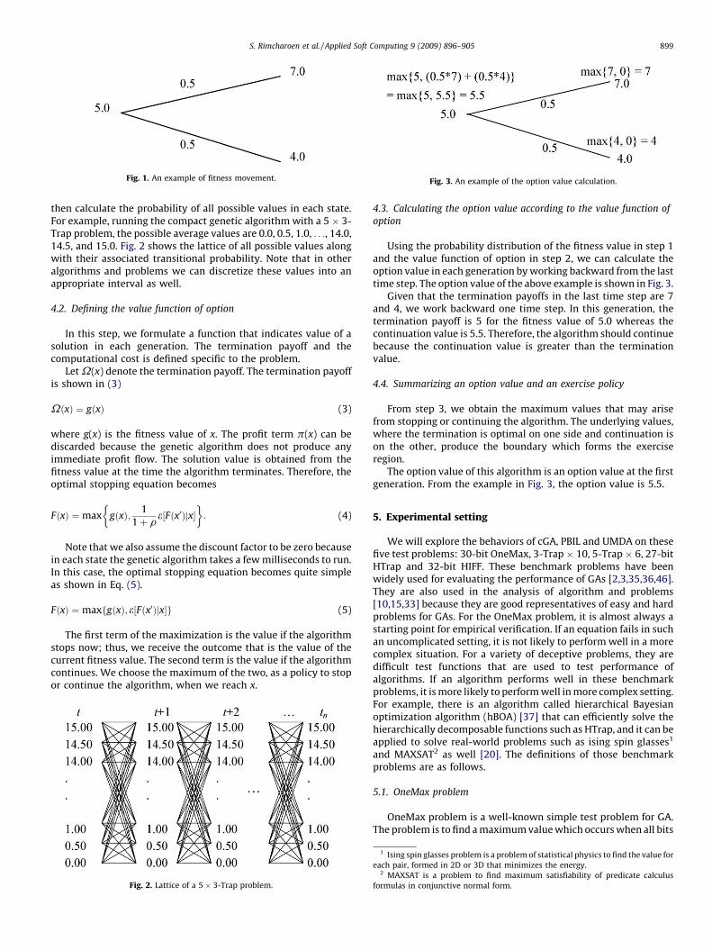
Fig. 1. An example of fitness movement. Fig. 3. An example of the option value calculation.

S. Rimcharoen et al. / Applied Soft Computing 9 (2009) 896–905 899

then calculate the probability of all possible values in each state.For example, running the compact genetic algorithm with a 5 � 3-Trap problem, the possible average values are 0.0, 0.5, 1.0, . . ., 14.0,14.5, and 15.0. Fig. 2 shows the lattice of all possible values alongwith their associated transitional probability. Note that in otheralgorithms and problems we can discretize these values into anappropriate interval as well.

4.2. Defining the value function of option

In this step, we formulate a function that indicates value of asolution in each generation. The termination payoff and thecomputational cost is defined specific to the problem.

Let V(x) denote the termination payoff. The termination payoffis shown in (3)

VðxÞ ¼ gðxÞ (3)

where g(x) is the fitness value of x. The profit term p(x) can bediscarded because the genetic algorithm does not produce anyimmediate profit flow. The solution value is obtained from thefitness value at the time the algorithm terminates. Therefore, theoptimal stopping equation becomes

FðxÞ ¼max gðxÞ; 1

1þ re½Fðx0Þjx�

� �: (4)

Note that we also assume the discount factor to be zero becausein each state the genetic algorithm takes a few milliseconds to run.In this case, the optimal stopping equation becomes quite simpleas shown in Eq. (5).

FðxÞ ¼maxfgðxÞ; e½Fðx0Þjx�g (5)

The first term of the maximization is the value if the algorithmstops now; thus, we receive the outcome that is the value of thecurrent fitness value. The second term is the value if the algorithmcontinues. We choose the maximum of the two, as a policy to stopor continue the algorithm, when we reach x.

Fig. 2. Lattice of a 5 � 3-Trap problem.

4.3. Calculating the option value according to the value function of

option

Using the probability distribution of the fitness value in step 1and the value function of option in step 2, we can calculate theoption value in each generation by working backward from the lasttime step. The option value of the above example is shown in Fig. 3.

Given that the termination payoffs in the last time step are 7and 4, we work backward one time step. In this generation, thetermination payoff is 5 for the fitness value of 5.0 whereas thecontinuation value is 5.5. Therefore, the algorithm should continuebecause the continuation value is greater than the terminationvalue.

4.4. Summarizing an option value and an exercise policy

From step 3, we obtain the maximum values that may arisefrom stopping or continuing the algorithm. The underlying values,where the termination is optimal on one side and continuation ison the other, produce the boundary which forms the exerciseregion.

The option value of this algorithm is an option value at the firstgeneration. From the example in Fig. 3, the option value is 5.5.

5. Experimental setting

We will explore the behaviors of cGA, PBIL and UMDA on thesefive test problems: 30-bit OneMax, 3-Trap � 10, 5-Trap � 6, 27-bitHTrap and 32-bit HIFF. These benchmark problems have beenwidely used for evaluating the performance of GAs [2,3,35,36,46].They are also used in the analysis of algorithm and problems[10,15,33] because they are good representatives of easy and hardproblems for GAs. For the OneMax problem, it is almost always astarting point for empirical verification. If an equation fails in suchan uncomplicated setting, it is not likely to perform well in a morecomplex situation. For a variety of deceptive problems, they aredifficult test functions that are used to test performance ofalgorithms. If an algorithm performs well in these benchmarkproblems, it is more likely to perform well in more complex setting.For example, there is an algorithm called hierarchical Bayesianoptimization algorithm (hBOA) [37] that can efficiently solve thehierarchically decomposable functions such as HTrap, and it can beapplied to solve real-world problems such as ising spin glasses1

and MAXSAT2 as well [20]. The definitions of those benchmarkproblems are as follows.

5.1. OneMax problem

OneMax problem is a well-known simple test problem for GA.The problem is to find a maximum value which occurs when all bits

1 Ising spin glasses problem is a problem of statistical physics to find the value for

each pair, formed in 2D or 3D that minimizes the energy.2 MAXSAT is a problem to find maximum satisfiability of predicate calculus

formulas in conjunctive normal form.

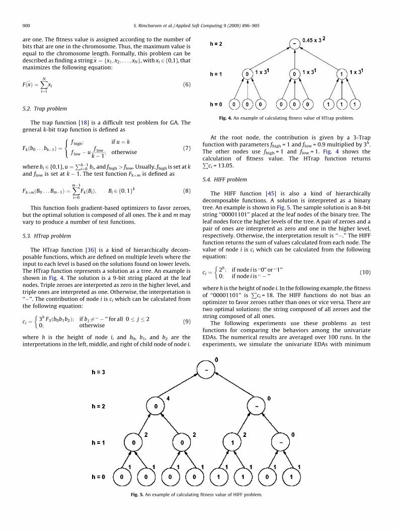
Fig. 4. An example of calculating fitness value of HTrap problem.

S. Rimcharoen et al. / Applied Soft Computing 9 (2009) 896–905900

are one. The fitness value is assigned according to the number ofbits that are one in the chromosome. Thus, the maximum value isequal to the chromosome length. Formally, this problem can bedescribed as finding a string x

*¼ fx1; x2; . . . ; xNg, with xi 2 (0,1), that

maximizes the following equation:

Fðx*Þ ¼

XN

i¼1

xi (6)

5.2. Trap problem

The trap function [18] is a difficult test problem for GA. Thegeneral k-bit trap function is defined as

Fkðb0 . . . bk�1Þ ¼f high; if u ¼ k

f low � uf low

k� 1; otherwise

8<: (7)

where bi 2 {0,1}, u ¼Pk�1

i¼0 bi, and fhigh > flow. Usually, fhigh is set at k

and flow is set at k � 1. The test function Fk�m is defined as

Fk�mðB0 . . . Bm�1Þ ¼Xm�1

i¼0

FkðBiÞ; Bi 2f0;1gk (8)

This function fools gradient-based optimizers to favor zeroes,but the optimal solution is composed of all ones. The k and m mayvary to produce a number of test functions.

5.3. HTrap problem

The HTrap function [36] is a kind of hierarchically decom-posable functions, which are defined on multiple levels where theinput to each level is based on the solutions found on lower levels.The HTrap function represents a solution as a tree. An example isshown in Fig. 4. The solution is a 9-bit string placed at the leafnodes. Triple zeroes are interpreted as zero in the higher level, andtriple ones are interpreted as one. Otherwise, the interpretation is‘‘�’’. The contribution of node i is ci which can be calculated fromthe following equation:

ci ¼ 3h F3ðb0b1b2Þ; if b j 6¼ ‘‘� ’’ for all 0 � j � 20; otherwise

�(9)

where h is the height of node i, and b0, b1, and b2 are theinterpretations in the left, middle, and right of child node of node i.

Fig. 5. An example of calculating fi

At the root node, the contribution is given by a 3-Trapfunction with parameters fhigh = 1 and flow = 0.9 multiplied by 3h.The other nodes use fhigh = 1 and flow = 1. Fig. 4 shows thecalculation of fitness value. The HTrap function returnsP

ci = 13.05.

5.4. HIFF problem

The HIFF function [45] is also a kind of hierarchicallydecomposable functions. A solution is interpreted as a binarytree. An example is shown in Fig. 5. The sample solution is an 8-bitstring ‘‘00001101’’ placed at the leaf nodes of the binary tree. Theleaf nodes force the higher levels of the tree. A pair of zeroes and apair of ones are interpreted as zero and one in the higher level,respectively. Otherwise, the interpretation result is ‘‘�.’’ The HIFFfunction returns the sum of values calculated from each node. Thevalue of node i is ci which can be calculated from the followingequation:

ci ¼ 2h; if node i is ‘‘0’’ or ‘‘1’’0; if node i is ‘‘� ’’

�(10)

where h is the height of node i. In the following example, the fitnessof ‘‘00001101’’ is

Pci = 18. The HIFF functions do not bias an

optimizer to favor zeroes rather than ones or vice versa. There aretwo optimal solutions: the string composed of all zeroes and thestring composed of all ones.

The following experiments use these problems as testfunctions for comparing the behaviors among the univariateEDAs. The numerical results are averaged over 100 runs. In theexperiments, we simulate the univariate EDAs with minimum

tness value of HIFF problem.

Fig. 6. Exercise regions from simulating cGA and PBIL with minimum population size. The left column shows the results from simulating the cGA and the right column is the

results from simulating the PBIL. The curves are plotted using an average value of 100 runs. The standard deviations are shown in gray color.

S. Rimcharoen et al. / Applied Soft Computing 9 (2009) 896–905 901

population size in order to study behaviors of algorithm in thesimplest setting. The results are presented in Section 6. Thebehaviors when using larger population size are also provided inSection 7.

6. Univariate EDAs with minimum population

Experimenting with minimum population helps us understandthe basic behavior of algorithms. The original cGA employs

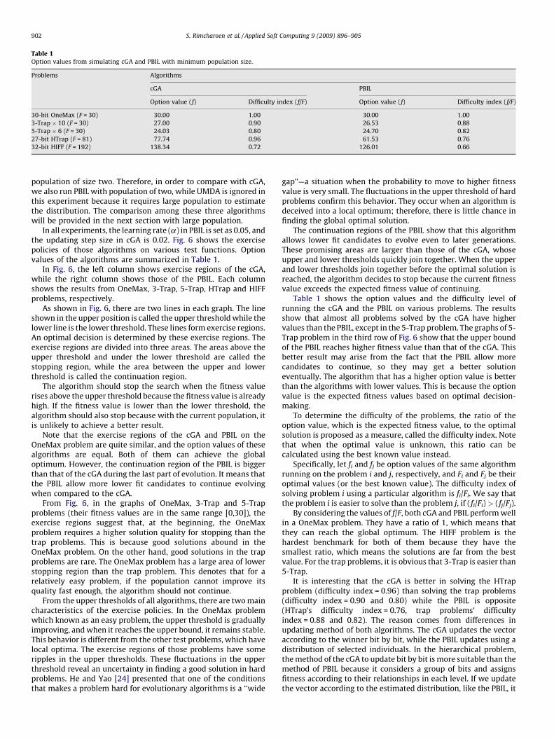
Table 1Option values from simulating cGA and PBIL with minimum population size.

Problems Algorithms

cGA PBIL

Option value (f) Difficulty index (f/F) Option value (f) Difficulty index (f/F)

30-bit OneMax (F = 30) 30.00 1.00 30.00 1.00

3-Trap � 10 (F = 30) 27.00 0.90 26.53 0.88

5-Trap � 6 (F = 30) 24.03 0.80 24.70 0.82

27-bit HTrap (F = 81) 77.74 0.96 61.53 0.76

32-bit HIFF (F = 192) 138.34 0.72 126.01 0.66

S. Rimcharoen et al. / Applied Soft Computing 9 (2009) 896–905902

population of size two. Therefore, in order to compare with cGA,we also run PBIL with population of two, while UMDA is ignored inthis experiment because it requires large population to estimatethe distribution. The comparison among these three algorithmswill be provided in the next section with large population.

In all experiments, the learning rate (a) in PBIL is set as 0.05, andthe updating step size in cGA is 0.02. Fig. 6 shows the exercisepolicies of those algorithms on various test functions. Optionvalues of the algorithms are summarized in Table 1.

In Fig. 6, the left column shows exercise regions of the cGA,while the right column shows those of the PBIL. Each columnshows the results from OneMax, 3-Trap, 5-Trap, HTrap and HIFFproblems, respectively.

As shown in Fig. 6, there are two lines in each graph. The lineshown in the upper position is called the upper threshold while thelower line is the lower threshold. These lines form exercise regions.An optimal decision is determined by these exercise regions. Theexercise regions are divided into three areas. The areas above theupper threshold and under the lower threshold are called thestopping region, while the area between the upper and lowerthreshold is called the continuation region.

The algorithm should stop the search when the fitness valuerises above the upper threshold because the fitness value is alreadyhigh. If the fitness value is lower than the lower threshold, thealgorithm should also stop because with the current population, itis unlikely to achieve a better result.

Note that the exercise regions of the cGA and PBIL on theOneMax problem are quite similar, and the option values of thesealgorithms are equal. Both of them can achieve the globaloptimum. However, the continuation region of the PBIL is biggerthan that of the cGA during the last part of evolution. It means thatthe PBIL allow more lower fit candidates to continue evolvingwhen compared to the cGA.

From Fig. 6, in the graphs of OneMax, 3-Trap and 5-Trapproblems (their fitness values are in the same range [0,30]), theexercise regions suggest that, at the beginning, the OneMaxproblem requires a higher solution quality for stopping than thetrap problems. This is because good solutions abound in theOneMax problem. On the other hand, good solutions in the trapproblems are rare. The OneMax problem has a large area of lowerstopping region than the trap problem. This denotes that for arelatively easy problem, if the population cannot improve itsquality fast enough, the algorithm should not continue.

From the upper thresholds of all algorithms, there are two maincharacteristics of the exercise policies. In the OneMax problemwhich known as an easy problem, the upper threshold is graduallyimproving, and when it reaches the upper bound, it remains stable.This behavior is different from the other test problems, which havelocal optima. The exercise regions of those problems have someripples in the upper thresholds. These fluctuations in the upperthreshold reveal an uncertainty in finding a good solution in hardproblems. He and Yao [24] presented that one of the conditionsthat makes a problem hard for evolutionary algorithms is a ‘‘wide

gap’’—a situation when the probability to move to higher fitnessvalue is very small. The fluctuations in the upper threshold of hardproblems confirm this behavior. They occur when an algorithm isdeceived into a local optimum; therefore, there is little chance infinding the global optimal solution.

The continuation regions of the PBIL show that this algorithmallows lower fit candidates to evolve even to later generations.These promising areas are larger than those of the cGA, whoseupper and lower thresholds quickly join together. When the upperand lower thresholds join together before the optimal solution isreached, the algorithm decides to stop because the current fitnessvalue exceeds the expected fitness value of continuing.

Table 1 shows the option values and the difficulty level ofrunning the cGA and the PBIL on various problems. The resultsshow that almost all problems solved by the cGA have highervalues than the PBIL, except in the 5-Trap problem. The graphs of 5-Trap problem in the third row of Fig. 6 show that the upper boundof the PBIL reaches higher fitness value than that of the cGA. Thisbetter result may arise from the fact that the PBIL allow morecandidates to continue, so they may get a better solutioneventually. The algorithm that has a higher option value is betterthan the algorithms with lower values. This is because the optionvalue is the expected fitness values based on optimal decision-making.

To determine the difficulty of the problems, the ratio of theoption value, which is the expected fitness value, to the optimalsolution is proposed as a measure, called the difficulty index. Notethat when the optimal value is unknown, this ratio can becalculated using the best known value instead.

Specifically, let fi and fj be option values of the same algorithmrunning on the problem i and j, respectively, and Fi and Fj be theiroptimal values (or the best known value). The difficulty index ofsolving problem i using a particular algorithm is fi/Fi. We say thatthe problem i is easier to solve than the problem j, if (fi/Fi) > (fj/Fj).

By considering the values of f/F, both cGA and PBIL perform wellin a OneMax problem. They have a ratio of 1, which means thatthey can reach the global optimum. The HIFF problem is thehardest benchmark for both of them because they have thesmallest ratio, which means the solutions are far from the bestvalue. For the trap problems, it is obvious that 3-Trap is easier than5-Trap.

It is interesting that the cGA is better in solving the HTrapproblem (difficulty index = 0.96) than solving the trap problems(difficulty index = 0.90 and 0.80) while the PBIL is opposite(HTrap’s difficulty index = 0.76, trap problems’ difficultyindex = 0.88 and 0.82). The reason comes from differences inupdating method of both algorithms. The cGA updates the vectoraccording to the winner bit by bit, while the PBIL updates using adistribution of selected individuals. In the hierarchical problem,the method of the cGA to update bit by bit is more suitable than themethod of PBIL because it considers a group of bits and assignsfitness according to their relationships in each level. If we updatethe vector according to the estimated distribution, like the PBIL, it

Fig. 7. Exercise regions from simulating cGA, PBIL and UMDA with larger population. The results from cGA, PBIL and UMDA are presented in the left, middle and right columns,

respectively. The curves are plotted using an average value of 100 runs. The standard deviations are shown in gray color.

S. Rimcharoen et al. / Applied Soft Computing 9 (2009) 896–905 903

is more likely to guide every bit toward that distribution, so it losesdiversity. Note that, in this case where the population size is two,only the best individual is used to estimate the distribution, thevector is biased by this solution. The experiments using largerpopulation are provided in the next section.

7. Simulating with larger population

The behaviors of the univariate EDAs with large population areprovided in this section. We simulate cGA and PBIL with largerpopulation size in order to compare with UMDA, which is a

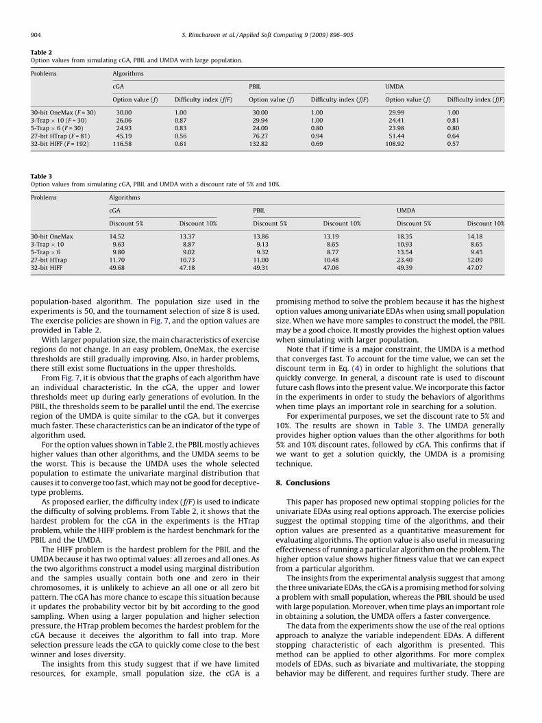
Table 2Option values from simulating cGA, PBIL and UMDA with large population.

Problems Algorithms

cGA PBIL UMDA

Option value (f) Difficulty index (f/F) Option value (f) Difficulty index (f/F) Option value (f) Difficulty index (f/F)

30-bit OneMax (F = 30) 30.00 1.00 30.00 1.00 29.99 1.00

3-Trap � 10 (F = 30) 26.06 0.87 29.94 1.00 24.41 0.81

5-Trap � 6 (F = 30) 24.93 0.83 24.00 0.80 23.98 0.80

27-bit HTrap (F = 81) 45.19 0.56 76.27 0.94 51.44 0.64

32-bit HIFF (F = 192) 116.58 0.61 132.82 0.69 108.92 0.57

Table 3Option values from simulating cGA, PBIL and UMDA with a discount rate of 5% and 10%.

Problems Algorithms

cGA PBIL UMDA

Discount 5% Discount 10% Discount 5% Discount 10% Discount 5% Discount 10%

30-bit OneMax 14.52 13.37 13.86 13.19 18.35 14.18

3-Trap � 10 9.63 8.87 9.13 8.65 10.93 8.65

5-Trap � 6 9.80 9.02 9.32 8.77 13.54 9.45

27-bit HTrap 11.70 10.73 11.00 10.48 23.40 12.09

32-bit HIFF 49.68 47.18 49.31 47.06 49.39 47.07

S. Rimcharoen et al. / Applied Soft Computing 9 (2009) 896–905904

population-based algorithm. The population size used in theexperiments is 50, and the tournament selection of size 8 is used.The exercise policies are shown in Fig. 7, and the option values areprovided in Table 2.

With larger population size, the main characteristics of exerciseregions do not change. In an easy problem, OneMax, the exercisethresholds are still gradually improving. Also, in harder problems,there still exist some fluctuations in the upper thresholds.

From Fig. 7, it is obvious that the graphs of each algorithm havean individual characteristic. In the cGA, the upper and lowerthresholds meet up during early generations of evolution. In thePBIL, the thresholds seem to be parallel until the end. The exerciseregion of the UMDA is quite similar to the cGA, but it convergesmuch faster. These characteristics can be an indicator of the type ofalgorithm used.

For the option values shown in Table 2, the PBIL mostly achieveshigher values than other algorithms, and the UMDA seems to bethe worst. This is because the UMDA uses the whole selectedpopulation to estimate the univariate marginal distribution thatcauses it to converge too fast, which may not be good for deceptive-type problems.

As proposed earlier, the difficulty index (f/F) is used to indicatethe difficulty of solving problems. From Table 2, it shows that thehardest problem for the cGA in the experiments is the HTrapproblem, while the HIFF problem is the hardest benchmark for thePBIL and the UMDA.

The HIFF problem is the hardest problem for the PBIL and theUMDA because it has two optimal values: all zeroes and all ones. Asthe two algorithms construct a model using marginal distributionand the samples usually contain both one and zero in theirchromosomes, it is unlikely to achieve an all one or all zero bitpattern. The cGA has more chance to escape this situation becauseit updates the probability vector bit by bit according to the goodsampling. When using a larger population and higher selectionpressure, the HTrap problem becomes the hardest problem for thecGA because it deceives the algorithm to fall into trap. Moreselection pressure leads the cGA to quickly come close to the bestwinner and loses diversity.

The insights from this study suggest that if we have limitedresources, for example, small population size, the cGA is a

promising method to solve the problem because it has the highestoption values among univariate EDAs when using small populationsize. When we have more samples to construct the model, the PBILmay be a good choice. It mostly provides the highest option valueswhen simulating with larger population.

Note that if time is a major constraint, the UMDA is a methodthat converges fast. To account for the time value, we can set thediscount term in Eq. (4) in order to highlight the solutions thatquickly converge. In general, a discount rate is used to discountfuture cash flows into the present value. We incorporate this factorin the experiments in order to study the behaviors of algorithmswhen time plays an important role in searching for a solution.

For experimental purposes, we set the discount rate to 5% and10%. The results are shown in Table 3. The UMDA generallyprovides higher option values than the other algorithms for both5% and 10% discount rates, followed by cGA. This confirms that ifwe want to get a solution quickly, the UMDA is a promisingtechnique.

8. Conclusions

This paper has proposed new optimal stopping policies for theunivariate EDAs using real options approach. The exercise policiessuggest the optimal stopping time of the algorithms, and theiroption values are presented as a quantitative measurement forevaluating algorithms. The option value is also useful in measuringeffectiveness of running a particular algorithm on the problem. Thehigher option value shows higher fitness value that we can expectfrom a particular algorithm.

The insights from the experimental analysis suggest that amongthe three univariate EDAs, the cGA is a promising method for solvinga problem with small population, whereas the PBIL should be usedwith large population. Moreover, when time plays an important rolein obtaining a solution, the UMDA offers a faster convergence.

The data from the experiments show the use of the real optionsapproach to analyze the variable independent EDAs. A differentstopping characteristic of each algorithm is presented. Thismethod can be applied to other algorithms. For more complexmodels of EDAs, such as bivariate and multivariate, the stoppingbehavior may be different, and requires further study. There are

S. Rimcharoen et al. / Applied Soft Computing 9 (2009) 896–905 905

also non-classical EDAs such as the eigen decomposition EDA (ED-EDA) [14]. Its procedure on tuning eigenvalue to influence theevolution process is complicated. The optimal stopping timeanalysis of these classical and non-classical EDAs is currently anopen problem. As we mentioned earlier, in the situation thatanalytical method is hard, analyzing the optimal stopping timeusing the real options approach is an alternative. It does not requireprior knowledge about algorithms and problems, and uses only thefitness movement to analyze the optimal stopping time. Anyalgorithms that have a fitness value in each time step can utilizethis technique, while the main evolution process remainsuntouched.

The proposed method can be used as an analysis tool toinvestigate the behavior of an algorithm. As a practical tool, it ishard to accept a large number of runs required in collecting thefitness data. As shown in the experiments, the optimal stoppingtime and its policy are only obtained after performing many runs.Future work will focus on incorporating this approach directly intothe evolutionary process so that there is no need to perform manyruns beforehand.

Nonetheless, the proposed method helps us understand thebehavior of genetic algorithms. From the experiments, the exerciseregions are the characteristics of the algorithm type. The optionvalue can also be used as a quantitative measurement forcomparing algorithms in terms of their effectiveness in solvingproblems. The sensitivity analysis can be studied by adding costsinto Eq. (5). The analysis on discount rates can be performed as wellwithout requiring additional runs. We can use the obtained fitness-movement profile and re-calculate option value with various costsand discount rates. This opens up a new way to explore behaviorsof the algorithm in various situations.

References

[1] L. Altenberg, Fitness distance correlation analysis: An instructive counterexample,in: Proceedings of the 7th International Conference on Genetic Algorithms, 1997,pp. 57–64.

[2] C. Aporntewan, P. Chongstitvatana, Building-block identification by simultaneitymatrix, Soft Computing 11 (2007) 541–548.

[3] C. Aporntewan, P. Chongstitvatana, Chi-square matrix: an approach for building-block identification, ASIAN (2004) 63–67.

[4] H. Aytug, G.J. Koehler, New stopping criterion for genetic algorithm, EuropeanJournal of Operational Research 126 (2000) 662–674.

[5] H. Aytug, G.J. Koehler, Stopping criterion for finite length genetic algorithms,INFORMS Journal on Computing 8 (1996) 183–191.

[6] S. Baluja, Population-based incremental learning: a method for integratinggenetic search based function optimization and competitive learning, TechnicalReport CMU-CS-95-163, Carnegie Mellon University, 1994.

[7] F. Black, M. Scholes, The pricing of options and corporate liabilities, Journal ofPolitical Economy 81 (1973) 637–654.

[8] Y. Borenstein, R. Poli, Information landscapes and problem hardness, in: Proceed-ings of the 2005 Genetic and Evolutionary Computation Conference, 2005, pp.1425–1431.

[9] Y. Borenstein, R. Poli, Fitness distributions and GA hardness, in: Proceedings of the8th International Conference on Parallel Problem Solving from Nature, 2004, pp.11–20.

[10] M. Clergue, P. Collard, GA-hard functions built by combination of trap functions,in: Proceedings of the IEEE Congress on Evolutionary Computation, 2002, pp.249–254.

[11] J.C. Cox, S.A. Ross, M. Rubinstein, Option pricing: a simplified approach, Journal ofFinancial Economics 7 (1979) 229–263.

[12] Y. Davidor, Epistasis variance: a viewpoint on GA-hardness, in: G.J.E. Rawlins(Ed.), Foundations of Genetic Algorithms, Morgan Kaufmann, San Mateo, CA,1991 , pp. 23–35.

[13] A.K. Dixit, R.S. Pindyck, Investment Under Uncertainty, Princeton UniversityPress, NJ, 1994.

[14] W. Dong, X. Yao, Unified eigen analysis on multivariate Gaussian based estima-tion of distribution algorithms, Information Sciences 178 (2008) 3000–3023.

[15] S. Droste, A rigorous analysis of the compact genetic algorithm for linear func-tions, Natural Computing 5 (2006) 257–283.

[16] S. Droste, T. Jansen, I. Wegener, On the analysis of the (1 + 1) evolutionaryalgorithm, Theoretical Computer Science 276 (2002) 51–81.

[17] D.E. Goldberg, Genetic Algorithms in Search Optimization and Machine Learning,Addison Wesley, 1989.

[18] D.E. Goldberg, Simple genetic algorithms and the minimal deceptive problem, in:Genetic Algorithms and Simulated Annealing, Morgan Kaufmann Publisher, 1987.

[19] G.R. Harik, F.G. Lobo, D.E. Goldberg, The compact genetic algorithm, IEEE Transac-tions on Evolutionary Computation 3 (1999) 287–297.

[20] M. Hauschild, M. Pelikan, C.F. Lima, K. Sastry, Analyzing probabilistic models inhierarchical BOA on traps and spin glasses, in: Proceedings of the Genetic andEvolutionary Computation Conference, 2007, pp. 523–530.

[21] J. He, C. Reeves, C. Witt, X. Yao, A note on problem difficulty measures in black-boxoptimization: classification, realizations and predictability, Evolutionary Com-putation 15 (2007) 435–443.

[22] J. He, X. Yao, Drift analysis and average time complexity of evolutionary algo-rithms, Artificial Intelligence 127 (2001) 57–85.

[23] J. He, X. Yao, From an individual to a population: an analysis of the first hittingtime of population-based evolutionary algorithms, IEEE Transactions on Evolu-tionary Computation 6 (2002) 495–511.

[24] J. He, X. Yao, Towards an analytic framework for analysing the computation timeof evolutionary algorithms, Artificial Intelligence 145 (2003) 59–97.

[25] J. Holland, Adaptation in Natural and Artificial Systems, University of MichiganPress, 1975.

[26] T. Jones, S. Forrest, Fitness distance correlation as a measure of problem difficultyfor genetic algorithms, in: Proceedings of the 6th International Conference onGenetic Algorithms, 1995, pp. 184–192.

[27] L. Kallel, B. Naudts, M. Schoenauer, On functions with a fixed fitness-distancerelation, in: Proceedings of the 1999 Congress on Evolutionary Computation,1998, pp. 1910–1916.

[28] S. Kauffman, The Origins of Order: Self-Organization and Selection in Evolution,Oxford University Press, Oxford, 1993.

[29] R.C. Merton, Theory of rational option pricing, Bell Journal of Economics andManagement Science 4 (1973) 141–183.

[30] H. Muhlenbein, G. Paaß, From recombination of genes to the estimation ofdistributions. I. Binary parameters, in: Parallel Problem Solving from Nature—PPSN IV, 1996, 178–187.

[31] S.C. Myers, Determinants of corporate borrowing, Journal of Financial Economics5 (1977) 147–175.

[32] B. Naudts, L. Kallel, A comparison of predictive measure of problem difficulty inevolutionary algorithms, IEEE Transactions on Evolutionary Computation 4(2000) 1–15.

[33] S. Nijssen, T. Back, An analysis of the behaviour of simplified evolutionaryalgorithms on trap functions, IEEE Transactions on Evolutionary Computation7 (2003) 11–22.

[34] A.E. Nix, M.D. Vose, Modeling genetic algorithms with Markov chains, Annals ofMathematics and Artificial Intelligence 5 (1992) 79–88.

[35] M. Pelikan, D.E. Goldberg, E. Cantu-Paz, BOA: the bayesian optimization algo-rithm, in: Proceedings of the Genetic and Evolutionary Computation Conference,1999, pp. 525–532.

[36] M. Pelikan, D.E. Goldberg, Escaping hierarchical traps with competent geneticalgorithm, in: Proceedings of the Genetic and Evolutionary Computation Con-ference, 2001, pp. 511–518.

[37] M. Pelikan, Hierarchical Bayesian Optimization Algorithm: Toward a New Gen-eration of Evolutionary Algorithms, Springer, 2005.

[38] R.J. Quick, V.J. Rayward-Smith, G.D. Smith, Fitness distance correlation and ridgefunctions, in: Proceedings of the 5th Conference on Parallel Problem Solving fromNature, 1998, pp. 77–86.

[39] C. Reeves, C. Wright, Epistasis in genetic algorithms: an experimental designperspective, in: Proceedings of the 6th International Conference on GeneticAlgorithms, 1995, pp. 217–230.

[40] S. Rimcharoen, D. Sutivong, P. Chongstitvatana, A synthesis of optimal stoppingtime in compact genetic algorithm based on real options approach, in: Proceed-ings of the Genetic and Evolutionary Computation Conference, 2007, p. 630.

[41] S. Rimcharoen, D. Sutivong, P. Chongstitvatana, Optimal stopping time of compactgenetic algorithm on deceptive problem using real options analysis, in: Proceed-ings of the IEEE Congress on Evolutionary Computation, 2007, pp. 4668–4675.

[42] S. Rimcharoen, D. Sutivong, P. Chongstitvatana, Real option approach tofinding optimal stopping time in compact genetic algorithm, in: Proceedingsof IEEE International Conference on Systems, Man, and Cybernetics, 2006, pp.215–220.

[43] S. Rochet, G. Venturini, M. Slimane, E.M. El Kharoubi, A critical and empiricalstudy of epistasis measures for predicting GA performances: a summary, ArtificialEvolution (1998) 275–285.

[44] M. Safe, J. Carballido, I. Ponzoni, N. Brignole, On stopping criteria for geneticalgorithms, SBIA (2004) 405–413.

[45] R.A. Watson, G.S. Hornby, J.B. Pollack, Modeling building-block interdependency,in: Parallel Problem Solving from Nature PPSN V, 1998, 97–106.

[46] R.A. Watson, J.B. Pollack, Hierarchically consistent test problems for geneticalgorithms, in: Proceedings of the IEEE Congress on Evolutionary Computation,1999, pp. 292–297.