Reaction kinetics of cellulose hydrolysis in subcritical and ...

-

Reaction kinetics of cellulose hydrolysis insubcritical and supercritical waterOlanrewaju, Kazeem Bodehttps://iro.uiowa.edu/discovery/delivery/01IOWA_INST:ResearchRepository/12730666050002771?l#13730822550002771

Olanrewaju. (2012). Reaction kinetics of cellulose hydrolysis in subcritical and supercritical water[University of Iowa]. https://doi.org/10.17077/etd.vq2ldcuy

Downloaded on 2022/07/31 01:17:49 -0500Copyright 2012 Kazeem Bode OlanrewajuFree to read and downloadhttps://iro.uiowa.edu

-

REACTION KINETICS OF CELLULOSE HYDROLYSIS IN SUBCRITICAL AND

SUPERCRITICAL WATER

by

Kazeem Bode Olanrewaju

An Abstract

Of a thesis submitted in partial fulfillment of the requirements for the Doctor of

Philosophy degree in Chemical and Biochemical Engineering in the Graduate College of

The University of Iowa

May 2012

Thesis Supervisors: Adjunct Associate Professor Gary A. Aurand Professor David Rethwisch

1

ABSTRACT

The uncertainties in the continuous supply of fossil fuels from the crisis-ridden

oil-rich region of the world is fast shifting focus on the need to utilize cellulosic biomass

and develop more efficient technologies for its conversion to fuels and chemicals. One

such technology is the rapid degradation of cellulose in supercritical water without the

need for an enzyme or inorganic catalyst such as acid. This project focused on the study

of reaction kinetics of cellulose hydrolysis in subcritical and supercritical water.

Cellulose reactions at hydrothermal conditions can proceed via the homogeneous

route involving dissolution and hydrolysis or the heterogeneous path of surface

hydrolysis. The work is divided into three main parts. First, the detailed kinetic analysis

of cellulose reactions in micro- and tubular reactors was conducted. Reaction kinetics

models were applied, and kinetics parameters at both subcritical and supercritical

conditions were evaluated. The second major task was the evaluation of yields of water

soluble hydrolysates obtained from the hydrolysis of cellulose and starch in hydrothermal

reactors. Lastly, changes in molecular weight distribution due to hydrothermolytic

degradation of cellulose were investigated. These changes were also simulated based on

different modes of scission, and the pattern generated from simulation was compared

with the distribution pattern from experiments.

For a better understanding of the reaction kinetics of cellulose in subcritical and

supercritical water, a series of reactions was conducted in the microreactor. Hydrolysis of

cellulose was performed at subcritical temperatures ranging from 270 to 340 °C (τ =

0.40-0.88 s). For the dissolution of cellulose, the reaction was conducted at supercritical

temperatures ranging from 375 to 395 °C (τ = 0.27 - 0.44 s). The operating pressure for

2

the reactions at both subcritical and supercritical conditions was 5000 psig. The results

show that the rate-limiting step in converting cellulose to fermentable sugars in

subcritical and supercritical water differs because of the difference in their activation

energies.

Cellulose and starch were both hydrolyzed in micro- and tubular reactors and at

subcritical and supercritical conditions. Due to the difficulty involved in generating an

aqueous based dissolved cellulose and having it reacted in subcritical water, dissolved

starch was used instead. Better yields of water soluble hydrolysates, especially

fermentable sugars, were observed from the hydrolysis of cellulose and dissolved starch

in subcritical water than at supercritical conditions.

The concluding phase of this project focuses on establishing the mode of scission

of cellulose chains in the hydrothermal reactor. This was achieved by using the simulated

degradation pattern generated based on different scission modes to fingerprint the

degradation pattern obtained from experiment.

Abstract Approved: ______________________________________________ Thesis Supervisor

______________________________________________ Title and Department

______________________________________________ Date

______________________________________________ Thesis Supervisor

______________________________________________ Title and Department

______________________________________________ Date

REACTION KINETICS OF CELLULOSE HYDROLYSIS IN SUBCRITICAL AND

SUPERCRITICAL WATER

by


A thesis submitted in partial fulfillment of the requirements for the Doctor of

Philosophy degree in Chemical and Biochemical Engineering in the Graduate College of

The University of Iowa

May 2012

Thesis Supervisors: Adjunct Associate Professor Gary A. Aurand Professor David Rethwisch

Graduate College The University of Iowa

Iowa City, Iowa

CERTIFICATE OF APPROVAL

_______________________

PH.D THESIS

_______________

This is to certify that the Ph.D. thesis of


has been approved by the Examining Committee for the thesis requirement for the Doctor of Philosophy degree in Chemical and Biochemical Engineering at the May 2012 graduation.

Thesis Committee: ___________________________________ Gary A. Aurand, Thesis Supervisor

___________________________________ David Rethwisch, Thesis Supervisor

___________________________________ Alec Scranton

___________________________________ Julie L.P Jessop

___________________________________ Daniel M.Quinn

ii

To GOD the Father, the Son, the Holy Spirit and to my loving mother and my late father

iii

ACKNOWLEDGEMENTS

First and foremost, I wholeheartedly acknowledged GOD ALMIGHTY for

making it possible for me to complete this project and for showering upon me HIS

boundless grace, mercy and wisdom during my studies at the University of Iowa. The

success of this project is without doubt a result of the unwavering effort of my advisor,

Prof. Gary Aurand, who took courage to get me on board his research group at a time

when the prospect of continuing the Ph.D programme appear bleak. Words will not be

enough to express my immense appreciation for what you did Sir. Thus, I will like to

thank Prof. David Rethwisch for accepting to serve as co-chair on my Ph.D thesis defense

committee and for offering valuable contributions during and after the defense.

I will like to express my deepest appreciation to Prof. Daniel Quinn, Prof. Alec

Scranton, and Prof. Julie Jessop, for willing to be on my thesis defense committee and for

offering valuable contribution during and after the thesis defense. I will forever be

grateful to the Iowa Energy Center and the University of Iowa graduate college for their

financial support. It is no gainsaying that the completion of this project would have been

met with serious hitch without these monetary supports.

My sincere gratitude goes to the entire staff of the department of chemical and

biochemical engineering, University of Iowa. Honor they say should be given to whom is

due and that explain why I will like to specially thank Ms.Linda and Ms.Natalie for the

amazing work they do in the department such as helping in acquiring chemical and

materials for research, offering administrative assistance where necessary and a desire to

see us finished our degree programs in accolade. I will like to say a big thank you to Mr.

Steve Struckman and his late co-worker Mr. Herbert Dirks, in the machine shop for

iv

helping with quick repair and machining of metallic parts of some of the equipment used

in the laboratory. I owe a lot of debt of appreciation to my colleagues in the biorenewable

and supercritical fluid reaction research group, Ashley D’Ann Koh and Kehinde Bankole

for their academic and moral support. I also wish to express my gratitude to friends in

Iowa City including the Alarapes, the Onwuamezes, the Ajiboyes, the Goshits, the

Vasciks, Chioma Ibeawuachi, Patience Ezenwanne, and members of international and

living spring fellowships for their camaraderie and social support in the course of my

study. However, my compliments will be incomplete without expressing my profound

gratitude to my Aunty in New York, Mrs Bosede Otulaja and her Husband, Dr. Femi

Otulaja for their parental advice and support this couple of years spent so far in the US of

A.

I will like to thank my siblings, Mrs Oluwatoyin Akintomide, Mrs Oluwabunmi

Oloruntoba, Mr Abiola Adeniji, Miss Oluwabukola Adeniji and Mrs Lara for their moral

and prayer supports. Lastly, many thanks to my late father, Pa Olatunji Olanrewaju (who

died midway into my Ph.D programme) and my mother, Mrs Oluwakemi Olanrewaju for

instilling in me, through GOD’s grace, the values that have carried me through these

years.

v

ABSTRACT

The uncertainties in the continuous supply of fossil fuels from the crisis-ridden

oil-rich region of the world is fast shifting focus on the need to utilize cellulosic biomass

and develop more efficient technologies for its conversion to fuels and chemicals. One

such technology is the rapid degradation of cellulose in supercritical water without the

need for an enzyme or inorganic catalyst such as acid. This project focused on the study

of reaction kinetics of cellulose hydrolysis in subcritical and supercritical water.

Cellulose reactions at hydrothermal conditions can proceed via the homogeneous

route involving dissolution and hydrolysis or the heterogeneous path of surface

hydrolysis. The work is divided into three main parts. First, the detailed kinetic analysis

of cellulose reactions in micro- and tubular reactors was conducted. Reaction kinetics

models were applied, and kinetics parameters at both subcritical and supercritical

conditions were evaluated. The second major task was the evaluation of yields of water

soluble hydrolysates obtained from the hydrolysis of cellulose and starch in hydrothermal

reactors. Lastly, changes in molecular weight distribution due to hydrothermolytic

degradation of cellulose were investigated. These changes were also simulated based on

different modes of scission, and the pattern generated from simulation was compared

with the distribution pattern from experiments.

For a better understanding of the reaction kinetics of cellulose in subcritical and

supercritical water, a series of reactions was conducted in the microreactor. Hydrolysis of

cellulose was performed at subcritical temperatures ranging from 270 to 340 °C (τ =

0.40-0.88 s). For the dissolution of cellulose, the reaction was conducted at supercritical

temperatures ranging from 375 to 395 °C (τ = 0.27 - 0.44 s). The operating pressure for

vi

the reactions at both subcritical and supercritical conditions was 5000 psig. The results

show that the rate-limiting step in converting cellulose to fermentable sugars in

subcritical and supercritical water differs because of the difference in their activation

energies.

Cellulose and starch were both hydrolyzed in micro- and tubular reactors and at

subcritical and supercritical conditions. Due to the difficulty involved in generating an

aqueous based dissolved cellulose and having it reacted in subcritical water, dissolved

starch was used instead. Better yield of water soluble hydrolysates, especially

fermentable sugars, were observed from the hydrolysis of cellulose and dissolved starch

in subcritical water than at supercritical conditions.

The concluding phase of this project focuses on establishing the mode of scission

of cellulose chains in the hydrothermal reactor. This was achieved by using the simulated

degradation pattern generated based on different scission modes to fingerprint the

degradation pattern obtained from experiment.

vii

TABLE OF CONTENTS

LIST OF TABLES ...............................................................................................................x

LIST OF FIGURES ........................................................................................................... xi

CHAPTER 1. PROJECT INTRODUCTION ......................................................................1 1.1 Project Overview ........................................................................................1 1.2 A Transition from Petroleum-based to Biobased Economy .......................2 1.3 Biomass Model Compounds .......................................................................7 1.4 Subcritical and Supercritical Phases: Hydrolysis Media ............................9

CHAPTER 2. RESEARCH BACKGROUND ..................................................................17 2.1 Cellulose Dissolution and Hydrolysis ......................................................17 2.2 Reaction Kinetics of Cellulose Hydrolysis in Different Media ................20

2.2.1 Acidic Media ..................................................................................20 2.2.2 Enzymatic Media ............................................................................22 2.2.3 Hydrothermal Media ......................................................................23 2.2.4 Disadvantages of Conventional Hydrolysis Media ........................27

2.3 Polymer Molecules Characterization ........................................................28 2.3.1 Dilute Solution Viscometry ............................................................30 2.3.2 Size Exclusion Chromatography ....................................................35 2.3.3 Effect of Hydrolysis on Molecular Weight Distribution and Degree of Polymerization ........................................................................38 2.3.4 Hydrolysis Rate of Crystalline Cellulose Based on Glycosidic Bond Concentration .................................................................................39

2.4 Degradation Pattern and Mode of Scission ..............................................41 2.4.1. Pattern of Degradation ...................................................................41 2.4.2 Mode of Scission of Polymer Degradation ....................................42 2.4.3. MATLAB ......................................................................................48

CHAPTER 3. RESEARCH OBJECTIVES .......................................................................50 3.1 Reaction Kinetics Analysis of Crystalline Cellulose in Subcritical and Supercritical Water ..................................................................................51 3.2 Hydrolysis of Dissolved Starch used as a Surrogate for Dissolved Cellulose in Subcritical Water ........................................................................52 3.3 Determining the Degradation Pattern and Mode of Scission of Cellulose Hydrolysis in Subcritical and Supercritical Water .........................53

CHAPTER 4. KINETICS ANALYSIS OF CELLULOSE REACTION IN SUBCRITICAL AND SUPERCRITICAL WATER .....................................54 4.1 Experimental Methods ..............................................................................55

4.1.1 Experimental Setup and the Processing Steps ................................55 4.1.2 Product Sample Analysis Method ..................................................59

4.1.2.1 Materials ...............................................................................59 4.1.2.2 Aqueous Products (Water Soluble Hydrolysate) .................59 4.1.2.3 Water Insoluble Hydrolysate. ...............................................60

4.1.3 Data Analysis Method ....................................................................61 4.2 Conversion of Crystalline Cellulose in Subcritical and Supercritical Water ...............................................................................................................63

viii

4.2.1 Conversion of Crystalline Cellulose in Subcritical Water .............63 4.2.1.1 Experimental Description .....................................................64 4.2.1.2 Cellulose Residue Data Analysis ........................................64 4.2.1.3 Results and Discussions .......................................................65 4.2.1.4 Conclusion ............................................................................67

4.2.2 Dilute Solution Viscometry Analysis of Crystalline and Unreacted Cellulose .................................................................................68

4.2.2.1 Experimental Description .....................................................68 4.2.2.2 Results and Discussions .......................................................69 4.2.2.4 Conclusion ............................................................................74

4.2.3 Hydrolysis of Glycosidic Bonds of Cellulose ................................74 4.2.3.1 Experimental Description .....................................................74 4.2.3.2 Sample Analysis ...................................................................75 4.2.3.3 Results and Discussions .......................................................76 4.2.3.4 Conclusion ............................................................................81

4.3 Conversion of Crystalline Cellulose in Supercritical Water .....................82 4.3.1 Experimental Setup and the Processing Steps ................................83 4.3.2 Sample Analysis .............................................................................85 4.3.3 Results and Discussions .................................................................86 4.3.4 Conclusions ....................................................................................89

4.4 Kinetic Analysis of the Conversion of Crystalline Cellulose in Subcritical and Supercritical Water ................................................................89

4.4.1 Shrinking Core Model ....................................................................90 4.4.2 First Order and Shrinking Core Models .........................................93

4.5 Summary of Experiments .........................................................................96

CHAPTER 5. INVESTIGATING YIELD OF WATER SOLUBLE HYDROLYSATE IN HYDROTHERMAL MEDIA .....................................99 5.1 Experimental Methods ............................................................................100

5.1.1 Experimental Setup and the Processing Steps ..............................100 5.1.2 Sample Product Analysis Method ................................................103

5.1.2.1 Materials. ...........................................................................103 5.1.2.2 Aqueous products (water soluble hydrolysate). .................103 5.1.2.3 Water Insoluble Hydrolysate. .............................................104

5.1.3 Data Analysis Method ..................................................................104 5.2 Yield of Water Soluble Hydrolysates in the Hydrothermal Reactor ......105

5.2.1 Yield of Water Soluble Hydrolysates in the Tubular Reactor ......106 5.2.1.1 Experimental Description ...................................................106 5.2.1.2 Sample Analysis .................................................................107 5.2.1.3 Results and Discussions .....................................................107 5.2.1.4 Conclusions ........................................................................110

5.2.2. Hydrolysates Yield from Crystalline Cellulose Hydrolysis in the Microreactor at Subcritical Condition of water ...............................111

5.2.2.1 Experimental Description ...................................................112 5.2.2.2 Sample Analysis .................................................................112 5.2.2.3 Results and Discussions .....................................................113 5.2.2.4 Conclusions ........................................................................116

5.2.3. Hydrolysates Yield from Dissolved Starch Hydrolysis in the Microreactor at Subcritical Condition of Water ....................................117

5.2.3.1 Experimental Description ...................................................118 5.2.3.2 Sample Analysis .................................................................118 5.2.3.3 Results and Discussions .....................................................119 5.2.3.4 Conclusions ........................................................................127

ix

5.2.4 Hydrolysates Yield from Crystalline Cellulose Hydrolysis in the Microreactor at Supercritical Condition of Water ...........................128

5.2.4.1 Experimental Description ...................................................128 5.2.4.2 Sample Analysis .................................................................129 5.2.4.3 Results and Discussions .....................................................129 5.2.4.4. Conclusions .......................................................................133

5.3. Summary of Experiments ......................................................................134 5.4. Comparison of the Monosaccharide Yields Obtained at Subcritical and Supercritical Conditions of Water in the Microreactor ..........................136

CHAPTER 6. DEGRADATION PATTERN AND MODE OF SCISSION OF CELLULOSE HYDROLYSIS IN HYDROTHERMAL SYSTEMS ..........138 6.1. Analysis of the Molecular Weight Distribution of Crystaline Cellulose .......................................................................................................140

6.1.1. Materials. .....................................................................................140 6.1.2 Hydrolysates Analysis. .................................................................141 6.1.3 SEC Calibration. ...........................................................................142

6.2 Degradation Pattern ................................................................................142 6.2.1 Experimentally Generated Degradation Pattern ...........................143 6.2.2 Experimental Description .............................................................144 6.2.3 Sample Analysis ...........................................................................145 6.2.4 Results and Discussions ...............................................................145 6.2.5 Conclusion ....................................................................................154

6.3 Simulation of the Different Mode of Scission ........................................154 6.3.1 Importation and Analysis of Experimental Data in the Simulation Environment ........................................................................156 6.3.2 A Step-by-Step Algorithm for the Matlab Code .........................159 6.3.3 Simulation Results and Discussion ..............................................161

6.4 Comparison of the Degradation Pattern from Experiment and Simulation .....................................................................................................167 6.5 Conclusions.............................................................................................173

CHAPTER 7. IMPACT AND FUTURE WORK ............................................................175

APPENDIX A: RATE CONSTANTS FOR THE ARRHENIUS PLOTS ......................178

APPENDIX B. CALIBRATION CURVE FOR THE PULLULAN STANDARD ........179

APPENDIX C: MATLAB CODE FOR THE ALGEBRAIC EXACT STATISTICAL SIMULATION ...................................................................180

APPENDIX D: MATLAB CODE FOR THE MONTE CARLO SIMULATION ..........198

REFERENCES ................................................................................................................217

x

LIST OF TABLES

Table 1: Amount of Biomass utilized from various sources in 2003 ..................................4

Table 2. Energy Potential of Selected Biomass in Iowa ......................................................5

Table 3. Critical Temperatures, Pressures, and Densities of Selected Fluids ....................11

Table 4. Conversion of 1 wt% Cellulose Suspension at Subcritical Temperatures in Microreactor..............................................................................................................66

Table 5. Viscosity-Average Degree of Polymerization of Cellulose Residues at Subcritical Temperatures ..........................................................................................70

Table 6. Kinetics Parameters obtained for the Glycosidic Bond Hydrolysis based on bond concentration evaluated from the DP of cellulose residues obtained from dilute solution viscometry and SEC..........................................................................80

Table 7. Conversion of Cellulose Suspension at Supercritical Temperatures in Microreactor..............................................................................................................87

Table 8. Summary of the Water Soluble Hydrolysates Yields obtained from Cellulose and Starch ...............................................................................................126

Table 9. Molecular weight averages and wt fraction for cellulose residue obtained at 270 °C in the microreactor ..................................................................................147

Table 10.Molecular weight averages and wt fraction for cellulose residue obtained at 280 °C in the microreactor ..................................................................................149




xi

LIST OF FIGURES

Figure 1. Crystalline Layers of Cellulose Structure (Department of Biology, University of Hamburg, Germany) .............................................................................9

Figure 2. Pressure-Temperature Phase Diagram for Pure Water ......................................10

Figure 3. Pressure-Density Phase Diagram for Pure Water ...............................................12

Figure 4. Variation of the Dielectric Constant (ε) of Water with Temperature and Pressure (NBS/NRC steam tables) ...........................................................................14

Figure 5. Ion Product of Water at Low Pressure ...............................................................15

Figure 6. Ion Product of Water at High Pressure ...............................................................16

Figure 7. Arrangement of hydrogen bonds and cellulose molecules in fibrils (Cellulose Hydrolysis by Fan et al.) .........................................................................18

Figure 8. Schematic diagram of crystalline cellulose dissolution and hydrolysis .............19

Figure 9. Rates of Cellobiose Hydrolysis and Glucose Decomposition ............................25

Figure 10. Plot of ηinh (lnηr/c) and ηred (ηsp/c) versus c for a crystalline cellulose in cupriethylenediamine at 25 °C with shared intercept as [η] .....................................35

Figure 11. Illustrative diagram of separation mechanism in SEC column ........................37

Figure 12. Chromatograms of cellulose residue (cotton linters) degraded with 1 N HCl at 80 °C. After the original sample on the far left, samples converted from left to right correspond respectively to the treatment times of 6 min, 18 min, 60 min, 4 h, 11 h, 24 h and 120 h. ....................................................................39

Figure 13. Molecular weight distribution of birch pulp (fibrous cellulose) with different alkaline concentration ................................................................................42

Figure 14. Experimental setup of the microreactor: 1) sampling bottle; 2) gas-liquid separator; 3) back pressure regulator; 4) stirrer plate; 5)cellulose suspension; 6) deionized water; 7) pumps; 8) insulated microreactor; 9) furnace; 10) pressure gauge; 11) temperature reader; 12) platform; 13)stopwatch ......................56

Figure 15. Schematic of cellulose hydrolysis in microreactor ...........................................57

Figure 16. Schematic flow detail of reaction in microreactor ...........................................58

Figure 17. Relationship between 1-(1-X)1/2 and the residence time ..................................66

Figure 18. Arrhenius plot of the rate constant of the conversion of crystalline cellulose in subcritical water and at 5000 psig based on grain/shrinking core model ........................................................................................................................67

xii

Figure 19. Plot of ηinh (ln(ηr/c)) and ηred (ηsp/c) versus c for cellulose residues obtained at 270 °C and at flow rates of 8 ml/min and dissolved in cupriethylenediamine at 25 °C. The shared intercept is [η]......................................71


Figure 21.Plot of ηinh (ln(ηr/c)) and ηred (ηsp/c) versus c for cellulose residues obtained at 290 °C and at flow rates of 9 ml/min and dissolved in cupriethylenediamine at 25 °C. The shared intercept is [η]......................................72


Figure 23.Plot of ηinh (ln(ηr/c)) and ηred (ηsp/c) versus c for cellulose residues obtained at 300 °C and at flow rates of 9 ml/min and dissolved in cupriethylenediamine at 25 °C. The shared intercept is [η]......................................73

Figure 24. Conversion term based on bond concentration vs the residence time ..............77

Figure 25. Arrhenius plot of the rate constant of crystalline cellulose hydrolysis in subcritical water and at 5000 psi based on bond concentration (DPv from dilute solution viscometry experiment) ....................................................................77

Figure 26. Arrhenius plot of the rate constant of crystalline cellulose hydrolysis in subcritical water and at 5000 psi based on bond concentration (DPp from size exclusion chromatography experiment)....................................................................78

Figure 27. Arrhenius plot of the rate constant of crystalline cellulose hydrolysis in subcritical water and at 5000 psi based on bond concentration (DPn from size exclusion chromatography experiment)....................................................................78

Figure 28. Arrhenius plot of the rate constant of crystalline cellulose hydrolysis in subcritical water and at 5000 psi based on bond concentration (DPw from size exclusion chromatography experiment)....................................................................79

Figure 29. Arrhenius plot of the rate constant of crystalline cellulose hydrolysis in subcritical water and at 5000 psi based on bond concentration (DPv from size exclusion chromatography experiment)....................................................................79

Figure 30. Arrhenius plot comparing rate constant of crystalline cellulose hydrolysis based on bond concentration with oligomers hydrolysis in subcritical water ........................................................................................................80

Figure 31. Schematic chart of the conversion of crystalline cellulose in microreactor at supercritical condition .....................................................................84

Figure 32. Microreactor system set-up for cellulose conversion at supercritical condition ...................................................................................................................85

Figure 33. Conversion plot for the rate constant of cellulose reaction in supercritical water..........................................................................................................................88

xiii

Figure 34. Arrhenius plot for the conversion of crystalline cellulose in supercritical water..........................................................................................................................88

Figure 35. Shrinking Core Model: Separated Arrhenius plot for the conversion of crystalline cellulose in subcritical and supercritical water with conversion plot of cellulose reaction in subcritical water passing through the origin .......................91

Figure 36. Shrinking Core Model: Separated Arrhenius plot for the conversion of crystalline cellulose in subcritical and supercritical water without forcing the conversion plot of cellulose reaction in subcritical to pass through the origin.........92

Figure 37. Shrinking Core Model: Combined Arrhenius plot for the conversion of crystalline cellulose in subcritical and supercritical water with conversion plot of cellulose reaction in subcritical water passing through the origin .......................92

Figure 38. Shrinking Core Model: Combined Arrhenius plot for the conversion of crystalline cellulose in subcritical and supercritical water without forcing the conversion plot of cellulose reaction in subcritical water to pass through the origin .........................................................................................................................93

Figure 39. First Order Model: Separated Arrhenius plot for the conversion of crystalline cellulose in subcritical and supercritical water with conversion plot of cellulose reaction in subcritical water being forced through the origin ..............94

Figure 40. First Order Model: Separated Arrhenius plot for the conversion of crystalline cellulose in subcritical and supercritical water without allowing the conversion plot of cellulose reaction in subcritical water not being forced through the origin......................................................................................................95

Figure 41.First Order Model: Combined Arrhenius plot for the conversion of crystalline cellulose in subcritical and supercritical water with conversion plot of cellulose reaction in subcritical being forced through the origin .........................95

Figure 42. First Order Model: Combined Arrhenius plot for the conversion of crystalline cellulose in subcritical and supercritical water without allowing the conversion plot of cellulose reaction in subcritical not being forced through the origin ...................................................................................................................96

Figure 43. Schematic flow process for cellulose hydrolysis in hydrothermal tubular reactor .....................................................................................................................101

Figure 44. Fractional yield of water soluble hydrolysates in hydrothermal tubular reactor at 10 ml/min ................................................................................................108

Figure 45. Fractional yield of water soluble hydrolysates obtained from starch in a hydrothermal tubular reactor at 5ml/min ................................................................109

Figure 46.Fractional yield of water soluble hydrolysates obtained from cellulose in a hydrothermal tubular reactor at 5ml/min .............................................................109

Figure 47. Fractional yield of water soluble hydrolysates obtained from cellulose at 280 °C in microreactor ............................................................................................113

xiv

Figure 48.Fractional yield of water soluble hydrolysates obtained from cellulose at 290 °C in microreactor ............................................................................................114




Figure 52.Fractional yield of water soluble hydrolysates obtained from starch at 270 °C in microreactor ............................................................................................120

Figure 53. Fractional yield of water soluble hydrolysates obtained from starch at 280 °C in microreactor ............................................................................................121





Figure 58. Fractional yield of monosacchride obtained at 375 °C in the microreactor ............................................................................................................130

Figure 59. Fractional yield of monosaccharide obtained at 380 °C in the microreactor ............................................................................................................131




Figure 63. Molecular weight distribution for cellulose and residue obtained at 270 °C ............................................................................................................................147

Figure 64.Molecular weight distribution for cellulose and residue obtained at 280 °C ............................................................................................................................149

Figure 65.Molecular weight distribution for cellulose and residue obtained at 290 °C ............................................................................................................................150

xv



Figure 68. Random Scission -1000 simulated number of scissions ................................163

Figure 69. Random Scission -500 simulated number of scissions ..................................163

Figure 70. Center Scission -1000 simulated number of scissions ...................................164

Figure 71. Center Scission- 500 simulated number of scissions .....................................165

Figure 72. Unzip Scission- 1000 simulated number of scissions ....................................166

Figure 73. Unzip Scission- 500 simulated number of scissions ......................................166

Figure 74. Plot of experimental, fitted (866.37), and fitted (643.32) distributions .........169

Figure 75. Experimental degradation pattern and simulated pattern based on random scission.......................................................................................................171

Figure 76. Experimental degradation pattern and simulated pattern based on center scission ....................................................................................................................172

Figure 77.Experimental degradation pattern and simulated pattern based on unzip scission ....................................................................................................................173

1

CHAPTER 1. PROJECT INTRODUCTION

1.1 Project Overview

This project investigates the detailed reaction kinetics of crystalline cellulose in

subcritical and supercritical water. These media offer conversion of cellulose to

fermentable sugars via two routes: 1) a homogenous route involving dissolution and

hydrolysis or 2) a heterogeneous route involving surface hydrolysis. Information obtained

from the mechanism of cellulose conversion in these routes will aid in the design of a

reaction flow path that will improve yield of fermentable sugars.

Extracting valuable products such as fermentable sugars and chemicals from cellulose

has always been challenging. The challenges are largely connected to the structural

integrity and recalcitrant nature of cellulose. As a result, the reaction kinetics describing

the various methods of deconstructing its bonds, both on the intra- and intermolecular

levels, will undoubtedly be complicated. Some of these methods include hydrolysis, ionic

pretreatment, mechanical degradation, ammonia fiber explosion, and a thermochemical

process.1, 2 Thus, for any method adopted, a detailed understanding of its reactive

behavior must be a necessary prerequisite. In this project, hydrolysis of cellulose in a

hydrothermal environment will be adopted, and as a result the project will be guided by

the following aims:

1. To conduct kinetics driven experiments on the conversion of cellulosic biomass to

fermentable sugars following the dissolution and the hydrolysis routes.

2. To analyze the kinetics detailed of each step involved in the two reaction routes.

3. To design a reaction flow system that will be suited for optimizing yield of

fermentable sugars.

2

4. To establish modes of scission of cellulose chains in a hydrothermal system by

comparing its distribution pattern from modeling with the experimentally generated

pattern.

To date, some questions regarding the hydrothermolytic conversion of cellulose to

fermentable sugars still remain unresolved and, for this purpose, this research project has

been designed to fill some of these gaps:

1. There are few scientific studies that adequately address characterization of the

cellulose chains and their mode of scission in a hydrothermal system. Many

studies on this subject have been conducted with such systems as enzymatic,

acidic, and alkaline media but with the hydrothermal system, information is still

very sparse.

2. There is still a substantial lack of clarity with respect to which of the steps along

the route of cellulose dissolution and hydrolysis is rate-limiting. Is it the

dissolution or the hydrolysis step? This work is set to contribute to the

understanding and clarification of the kinetic details describing these reactions.

1.2 A Transition from Petroleum-based to Biobased Economy

The challenge posed to the socioeconomic and political stability of many nations

by the crises-ridden oil-rich regions of the world is paving the way for an urgent

transition from a petroleum-based to a biobased economy. This paradigm shift in the

United States is largely driven by the need to avoid reliance on foreign oil and the

accompanying national security risks. For some other regions such as the European

Union, the shift is not only orchestrated by the need to reduce petroleum dependency but

by an unwavering interest in environmental sustainability. A biobased economy utilizes

3

natural resources (biomass) as surrogates to all fossil-based feedstocks to generate valued

end-products such as fuels and chemicals.3 Table 1 shows the amounts of biomass

utilized from various sources in 2003. A significant portion of it is from the forest

products industry, which consists of wood residues and pulping liquors while the source

with the least amount of biomass resources is from recycled or reused bioproducts.

Biomass transformation results in far less emission of CO2 to the atmosphere when

compared with the fossil stock that releases CO2 in excess of what is needed to maintain

the greenhouse effect. Thus, excessive CO2 loading on the atmosphere contributes to a

phenomenon known as global warming.

In an effort to mirror every component describing the current petroleum based

economy in the biobased economy, resources are being invested to design and construct a

biorefinery∗ that will generate products that are ordinarily obtained from the traditional

petroleum refinery. Adoption of the biorefinery is currently being viewed in phases based

on the complexity and flexibility of the plant to process feedstock at a lower volume to a

more complicated unit of processing lignocellulosic biomass at a higher volume. Phases

in a biorefinery plant are described by the degree of complexity, level of flexibility and

number of products being generated from the plant. For example, corn dry-mill ethanol

process plant, designed solely to produce ethanol, is consider a phase I biorefinery unit

because of its flexibility in generating other co-product, distiller’s dry grains (DDG) used

for animal feed. A corn wet milling ethanol plant, which is a bit more complex than the

dry-mill, is portrayed as a phase II biorefinery because of its flexibility in generating

∗ A biorefinery is a facility that integrates biomass conversion processes and equipment

to produce fuels, power, and chemicals from biomass4

4

Table 1: Amount of Biomass utilized from various sources in 2003 ______________________________________________________________________ Biomass Consumption Million dry tons/year ______________________________________________________________________ Forest products industry

Wood residues 44

Pulping liquors 52

Urban wood and food & other process residues 35

Fuelwood (residential/commercial & electric utilities) 35

Biofuels 18

Bioproducts 6

_______________________________________________________________________

Total 190

Source: U.S.D.A & U.S.D.O.E (2005) Biomass as Feedstock for a Bioenergy and Bioproducts Industry

multiple products including ethanol, starch, high fructose corn syrup, corn oil, and corn

gluten meal.4 As of now, corn is one of the strongest viable feedstock candidates in the

emerging biorefinery plant. But the ultimate goal is to be able to utilize a wider range of

biomass feedstocks to generate all products made available to us by the traditional

petroleum-based refinery through biorefinery.

The future prospect of the current biofuel (bioethanol) generated from corn-starch

is questionable due to speculated negative impact on food production5. The idea of corn

starch utilization encroaching on the cost of the food supply is still not well founded as

enough data have not been put together to support this trend. However, current efforts are

channeled towards exploring cellulosic biomass as an alternative to increase the resource

base for biofuel feedstock production and lessen the use of corn starch for ethanol

production. Cellulosic biomass is grouped among feedstocks driving the current

5

advanced biofuel initiative for the expansion of biofuel production. Advanced biofuel is

defined as biofuel generated from biorenewable sources other than corn starch, with the

potential of emitting as much as 50% less greenhouse gases compared to the traditional

fuel being replaced.6 Cellulosic biomass, the most natural occuring organic matters, is

seen as a strong prospect for salvaging future paucity of fossil fuel and a support for the

ever increasing energy demand.

At the end of the twentieth century, it was estimated that 7% of total global

biomass production, with an estimated record amount of 6.9 x 1017 kcal/yr, was utilized7

while worldwide production of terrestial biomass was recently estimated to be 220 billion

tons. Total energy content from this quantity (based on the analysis of heat of

combustion) is roughly five times the energy content of the total crude oil consumed

worldwide4. Table 2 depicts the relative abundance of different forms of biomass in Iowa,

their equivalent energy content and potential.

Table 2. Energy Potential of Selected Biomass in Iowa Material Annual Amount

(tons)

Energy Content

(Btu/lb)

Energy Potential (109

Btu)

Switchgrass 11,200,000 8,000 179,200

Row crop residue 10,000,000 5,337 106,000

Wood and wood waste 165,000 4,800 1,580

Livestock byproducts 2,330,000 97 452

Cattle manure (dry basis) 1,600,000 6,760 21,600

Hog manure (dry basis) 2,700,000 7,300 39,400

Source : Iowa Biomass Energy Plan, 1994.

6

Gasification of biomass to produce energy building blocks such as syngas (carbon

monoxide and hydrogen) and biogas (methane) is one way of expanding biomass energy

potential. Liquefaction of biomass through the hydrothermolysis process (subcritical and

supercritical conditions), acidic hydrolysis, or enzymatic hydrolysis, is another route of

generating fermentable sugars necessary for the production of liquid fuel used to power

energy driven devices.

All the preceding indicators are currently driving the United States Department of

Energy (USDOE) on a multiyear program3, 8 focused at better understanding and utilizing

biomass efficiently. USDOE is exploring potential technologies and improving on current

techniques in transforming biomass to economically valuable products such as biofuels,

and other bioproducts. One of the most crucial valued end points in the conversion of

biomass to usable form is energy. As of 2008, about 93% of the energy supply in the

United States is from non-renewable sources while 7% is from renewable sources.

Roughly 50% of the renewable energy is biomass based and more than half of the

biomass resources utilized, as indicated on Table 1, are from wood residues and pulping

liquors.9

The renewed vision of USDOE is to reduce consumption of fossil fuel by 33%

from 2010 to 2022, while investing more resources into biofuel production8. This vision

presents itself as a modification of the initial goal of reducing fossil fuel consumption by

20 % from 2007 to 20173 which was the previously tagged vision “20 in 10”. The

possibility of reaching this feat is further encouraged by the introduction of the advanced

biofuel initiative which expands resources for biofuel production. While there is this

strong initiative to meet the above stated goal as a nation (USA), the techniques of

7

converting some of the newly adopted feedstock, such as cellulosic biomass, a highly

recalcitrant feedstock, to valuable products, is of great concern.

To achieve this goal, efficient technology and approachs should be investigated to

generate and optimize the yields of fermentable sugars from cellulosic biomass. The

mode of converting biomass and the kinetics describing the conversion are essential in

understanding ways of improving yield and selectivity of fermentable sugars. As of now,

biomass, though thermally pretreated, is largely transformed biochemically10 ; a process

that is far more kinetically limited when compared with transforming biomass to

fermentable sugars in an absolute hydrothermal process11. It is hereby proposed in this

research work to investigate the kinetics of cellulose conversion in subcritical and

supercritical water.

1.3 Biomass Model Compounds

The term “biomass” can be defined specifically as the total mass of living or

recently dead (unfossilized) organic matter within a given environment12. More

pertinently, biomass refers to all organic matter available on a renewable or recurring

basis, including dedicated energy crops and trees, agricultural food and feed crops,

animal waste, agricultural crop waste, wood and wood waste, aquatic plants, municipal

wastes and other waste materials13. Plant biomass is an abundant renewable natural

resource consisting mainly of crude organic matter such as cellulose, hemicellulose,

lignin and starch14. Biomass model compounds that will be investigated in this work are

cellulose and starch.

Cellulose is a long linear chain polymer of several monomeric D-glucose units

linked by β-1,4-glycosidic bonds. It is the most abundant organic compound in nature and

8

does exist in the cell wall of plants as complex fibrous carbohydrates. Starch is formed

by α-1, 4 and/or α-1, 6 glycosidic bonding of several glucose units. The strength and

chemical stability of these biopolymers differs due to different glycosidic bond types at

the anomeric carbon. The β-type is more stable due to hydroxyl (-OH) group equatorial

orientation at the anomeric carbon while the α-type, with a hydroxyl (OH) group axially

positioned at the anomeric carbon and beneath the hemiacetal ring, displays less

stability15. Their stability is ranked by resistance to biodegradability from microbes and

enzymes.

Raw biomass (e.g. corn stover) comprises mainly cellulose, lignin, and

hemicellulose. The biomass is deconstructed to produce chemical compounds such as

cellulose, starch, ethanol, methanol, and other biomass-based chemicals. Some of the

extracted macromolecular compounds, cellulose and starch, are further degraded to

smaller chemical compounds such as glucose, maltose, cellobiose, maltotriose,

cellotriose, etc. The degradation involves breaking of the glycosidic bond (primary

covalent bond) between the monomeric residues and disruption of both the intra and

inter-molecular hydrogen bonding amidst the polymer chains. Intra-hydrogen bonding in

cellulose is responsible for its chain stiffnes16while inter-hydrogen bonding establishes its

crystallinity. In Figure 1, the red dotted lines indicate the intra-chain hydrogen bonding

while the blue dotted lines depict the inter-chain hydrogen bonding.

9

Figure 1. Crystalline Layers of Cellulose Structure (Department of Biology, University of Hamburg, Germany)

1.4 Subcritical and Supercritical Phases: Hydrolysis Media

In a pressure-temperature phase diagram, the critical point is the point where the

equilibrium line for coexisting liquid and vapor ends. The region extending upwards,

with temperatures and pressures exceeding their respective critical values,17 as indicated

in Figure 2, is depicted as the supercritical fluid. However, subcritical condition of the

fluid describes a zone slightly below or near its critical pressure, and a temperature lower

than its critical point. The data used for generating the equilibrium line on Figure 2 were

obtained from the Chemistry WebBook published by the National Institute of Standard

and Technology (NIST) for calculating thermophysical properties.18, 19

Most solvents can be characterized by their critical temperature and pressure 20-22.

For instance, water has a critical temperature and pressure of 374 °C and 22.1 MPa

respectively. Ethanol and methanol also exhibit unique critical values despite belonging

to the same aliphatic alcohol group. Table 3 displays critical temperatures, pressures and

10

densities for different solvents. Supercritical fluids have been used extensively in a

number of applications ranging from supercritical fluid chromatography, supercritical

fluid extraction, polymer processing, hydrothermal processing, and hydrothermal

destruction of hazardous waste 23. Supercritical water has been a primary medium for

nuclear waste diminution and oxidative detoxification of organic waste 24.

Figure 2. Pressure-Temperature Phase Diagram for Pure Water

-1

4

9

14

19

24

29

34

39

-50 150 350 550 750

Pre

ssur

e, M

Pa

Temperature, °C

Gas (Steam)

Solid

(ice

)

Pc

Supercritical Fluid

Critical Point

Tc

11

Table 3. Critical Temperatures, Pressures, and Densities of Selected Fluids

Substance Tc (°C) Pc ( atm) ρc (kg m-3)

Ethylene 9.4 49.7 214

Trifluoromethane 26.1 48.1 322

Carbon dioxide 31.2 72.8 468

Sulfur hexafluoride 45.7 37.1 735

Propane 96.8 41.9 217

Ammonia 132.6 111.3 235

Methyl amine 157.0 73.6 222

Acetone 235.1 46.4 269

i-Propanol 235.3 47.0 273

Methanol 239.6 79.9 272

Ethanol 243.2 63.0 276

Water 374.3 217.6 322

Industrial applications of supercritical water started in 1994 when Eco Waste

Technologies, a Canadian company, developed the first industrial-scale supercritical

water oxidation (SCWO) process specifically to treat organic waste generated from a

Huntsman petrochemical plant located in Austin, Texas25.

The uniqueness of supercritical fluid (SCF) is portrayed by displaying both gas-

like and liquid-like properties. The gas-like properties, including high diffusivity and low

viscosity, enhance SCF mass transfer rates 20, while high density atypical of a gaseous

compound characterizes its liquid-like behavior. Physical properties of most liquid

solvents at ambient conditions (significantly below the critical point) display slight

12

variation with respect to corresponding changes in pressure and temperature. However,

density and properties such as solubility parameter, partition coefficient, and viscosity

change immensely at a slight variation in pressure and temperature both on short and long

range within the critical region.22, 26-28 The significant change in density at a slight change

in pressure is due to the compressible nature of the supercritical fluid.

Thus, variation in macroscopic density-dependent solvent properties creates room

for the tunability of subcritical and supercritical fluid physico-chemical properties to suit

in-situ applications such as microscopic dissolution27, 29 of cellulose. Invariably, the

ability of fine a tuning supercritical fluid (SCF), by switching it on and off to a density

suitable for dissolving and precipitating out the solute, makes SCF a perfect candidate in

extraction processes and is mostly applied in the food industry. Figure 3 shows the phase

diagram depicting variation of density of pure water with pressure. The data used for

generating the plot were obtained from NIST Chemistry WebBook.18, 19

Figure 3. Pressure-Density Phase Diagram for Pure Water

0

5

10

15

20

25

30

35

40

0 200 400 600 800 1000 1200

Pre

ssur

e, M

Pa

Density, kg/m3

260 °C

280 °C

320 °C

340 °C

360 °C

374 °C

380 °C

390 °C

400 °C

13

The dome shape as depicted in Figure 3 is the region of a mixture of liquid and

gaseous phases while the equilibrium lines from both left and right ends of the plot and

merging to form a plateau at the critical point describe the saturation curves from the

gaseous and liquid ends respectively. At an isothermal condition outside of the dome

shape, increasing pressure results in a corresponding increase in the density. Also within

the dome shape there is still a significant increase in the density of the liquid-gaseous

mixture while maintaining a constant saturation pressure along an isotherm line. Moving

beyond the critical point into the supercritical region, increasing pressure at a constant

temperature leads to an increase in density while increasing temperature at constant

pressure leads to a decrease in density of the fluid.

Modification of the dielectric constant opens opportunities for a normally polar

solvent such as water to dissolve organic compounds.24 For supercritical water, the

dielectric constant is significantly lower and resides within the range common to most

organic solvents. Figure 4 shows that the dielectric constant of supercritical water at a

pressure of 300 bar and temperature of 375 °C is 12.03. Bewteen 2 and 30 , is a range

typical for most organic solvents for dissolving organic macromolecules such as

cellulose. Water at normal condition of 25 °C and pressure of 1 bar has a dielectric

constant of about 78. From Figure 4, there is little or no change in the dielectric constant

of water with respect to changes in pressure while following each isotherm except for 400

°C which displays some measurable direct variation with pressure in the range of 300 bar

to close to 400 bar. However, at a constant pressure, changes in temperature reflect a

significant change in the dielectric constant.

14

Figure 4. Variation of the Dielectric Constant (ε) of Water with Temperature and Pressure (NBS/NRC steam tables)

The ion product exhibited by supercritical water enhances the solvating power27

needed to dissolve the compound in the medium. The ionic product is denoted as Kw and

mathematically expressed as the product of the molar concentration of [OH-] and [H+]

(Kw = [H+][OH-]). At neutral pH each has a value of 10-7mol/l. At room temperature and

pressure, the ion product of water is 10-14(mol/l)2 with a pH of 7 while at critical

temperature and pressure its ion product is 10-11(mol/l)2 with a pH of 5.5. Figures 5 and 6

display the variation of the ion product of water at low and high pressure, respectively. In

Figure 5, ion products appear to decrease monotonically as pressure increases except for

isotherms of the four lowest temperatures in which the ionic product (10-12.06(mol/l)2 )

remains constant for pressure ranging from 200 bar to 500 bar. While at constant

pressure, ion product increases with increase in temperature. Following the isotherms,

400 – 1000 °C, Figure 6 reflects a decreasing pattern in the ion product with pressure

0

20

40

60

80

100

300 350 400 450 500

Die

lect

ric c

onst

ant

Pressure (Bar)

0 °C

25 °C

75 °C

100 °C

175 °C

250 °C

275 °C

300 °C

375 °C

400 °C

15

within the range of 250 bar to about 3000 bar, while increasing pressure beyond this

value, ion product decreases slightly. The effect of temperature on the ionic product of

water in the high pressure region and at temperature range of 400 – 1000 °C, is less

significant as portrayed in Figure 6. The ion product of water at a supercritical condition

of about 3500 bar and 400 °C will be 10-9.5 (mol/l)2, and the pH at this condition is 4.75.

Both of these values, i.e. at critical and supercritical conditions, connote that water at

these conditions will be slightly acidic. All the physico-chemical properties displayed by

water at subcritical and supercritical conditions make it an excellent medium for

converting macromolecular compounds to smaller valuable compounds.

Figure 5. Ion Product of Water at Low Pressure

0

5

10

15

20

25

30

35

40

0 100 200 300 400 500

Ion

Pro

duc

t (-lo

gKw

)

Pressure (Bar)

340 °C

360 °C

380 °C

400 °C

440 °C

480 °C

520 °C

560 °C

600 °C

16

Figure 6. Ion Product of Water at High Pressure

In this age of environmental sustainability where most solvents that are toxic to

the environment are being replaced with greener ones, supercritical fluids will be a very

good replacement for many reactions and processes that involve solvents.

0

5

10

15

20

25

0 2000 4000 6000 8000 10000

Ion

Pro

duct

(-lo

gK

w)

Pressure (bar)

200 °C250 °C300 °C400 °C500 °C800 °C1000 °C

17

CHAPTER 2. RESEARCH BACKGROUND

In this chapter, the fundamentals of cellulose dissolution and hydrolysis will be

discussed while exploring previous work on the reaction kinetics of cellulose hydrolysis

in different media. Two of the different techniques of characterizing macromolecular

compounds such as cellulose will be reviewed. Lastly, a thorough reviewed of the mode

of scission of polymer molecules and the accompanying molecular weight distribution

patterns in both organic and inorganic media will be conducted.

2.1 Cellulose Dissolution and Hydrolysis Cellulose, a bioorganic linear polymer15 and the most abundant renewable

resource30, is composed of D-glucose monomer units joined by β-1,4-glycosidic bonds.

Native cellulose is built from several thousands (~10,000) of β-anhydroglucose residues

to form a long linear chain molecule and that explains why its molecular weight is above

1.5 million. The linearly configured and highly dense cellulose chain molecules give rise

to fibrillar structured material stabilized by inter-chain hydrogen bonding. The cellulosic

fibril is a macro-picture of a smaller scaled unit called a microfibril31 for all

lignocellulosic biomass. This micro-scale unit, microfibril, is composed of orderly

arranged crystallites with a cylindrical conformational structure.32 The arrangement of

cellulose molecules and the hydrogen bonding in fibrils are illustrated in Figure 7. The

inter-chain hydrogen bonding between layers of longitudinally arranged microfibrils33,34

establishs their crystallinity while intra-chain hydrogen bonding results in cellulose chain

stiffness16. These properties justify why cellulose is ranked among recalcitrant

compounds: substances that are very difficult to degrade. For most of these compounds, a

special solvent or fluid such as supercritical fluid is needed for their dissolution.

18

Cellulose fibrils, though largely crystalline, exhibit amorphous structure at the ends of

two adjoining microfibrils.

Figure 7. Arrangement of hydrogen bonds and cellulose molecules in fibrils (Cellulose Hydrolysis by Fan et al.)

Cellulose dissolution involves disengaging the inter-chain hydrogen bonding

between layers of cellulose chains thereby making the hydroxyl (OH) on each of the

glucose units available for bonding with the component of the dissolving solvent. The

dissolution is preceded by swelling of the cellulose chain thereby facilitating accessibility

of the degradative agent in breaking apart the inter-chain hydrogen bonding within the

crystalline structure31. The dissolved cellulose can be further converted to lower

molecular compounds such as the oligomers and fermentable sugars. Dissolution and

hydrolysis of crystalline cellulose in media such as acid or supercritical water involve

solvation of hydronium ions (protonated water molecules) around cellulose molecules.

This process initiates protonation of either the cyclic oxygen (on one of the monomers) or

19

acyclic oxygen (glycosidic binding oxygen) along the polymeric chain33. The combined

effect of solvation and protonation initiates rupturing of the inter-molecular hydrogen

bonding (dissolution) and cleavage of intra-glycosidic and intra-hydrogen bonds

(hydrolysis). The diagram below illustrates the dissolution and hydrolysis of crystalline

cellulose.

Figure 8. Schematic diagram of crystalline cellulose dissolution and hydrolysis

As depicted in the diagram above, direct hydrolysis of crystalline cellulose to

smaller compounds such as glucose and water soluble oligosaccharides of DP less than

10 is probable but with relatively large cellulose chains yet undissolved. This type of

Crystalline Cellulose Dissolved Cellulose

Monosaccharide

Supercritical/Subcriticalmedium

Dissolution

20

hydrolysis is termed heterogeneous while homogeneous hydrolysis is connoted by a

complete dissolution of the crystalline cellulose35. The key issue which remains

unresolved by most previous studies is a detailed kinetics evaluation of the rate of

dissolution and rate of hydrolysis of crystalline cellulose under hydrothermal conditions.

Considering the conversion of crystalline cellulose to simple sugars and water soluble

oligosaccharides; which of the two steps could be considered rate limiting? Is it the

dissolution step or hydrolysis step? This is one major aspect of reaction kinetics of

cellulose in hydrothermal conditions yet to receive serious attention by researchers but

considered due for investigation in this research project.

2.2 Reaction Kinetics of Cellulose Hydrolysis in Different Media

The hydrolysis rate of cellulose largely depends on the medium of degradation. In

other words, the rate at which cellulose and starch depolymerize in acidic, enzymatic and

hydrothermal media differ.

2.2.1 Acidic Media

Degradation of celluloses in an acidic medium was enhanced by its ability to

hydrolyze both the glycosidic bond and break the intra- and inter-molecular hydrogen

bonding33. Acid-aided cellulose hydrolysis can either occur in a homogeneous or

heterogeneous phase. Different models have been developed to better understand the

kinetics of homogeneous and heterogeneous hydrolysis of cellulose and starch in acid.

Cellulose hydrolysis is classically defined by a pseudo-homogeneous kinetics model, a

term that in reality reflects that the hydrolysis process is heterogeneous. A very good

example of such a model is the kinetics model36 of Saeman et al. (1945) proposed for the

hydrolysis of cellulosic wood biomass. The model assumed that the amount of cellulose

21

was the same as an equivalent quantity of dissolved glucose and that the reaction

proceeds in two successive steps. A similar model approach was adopted in a study

conducted by Girisuta et al. (2007).37

ecosgluDecomposedecosGluCelluloseCBA

→→ (1)

The kinetics expression of the schematic process above is as follows:

AA Ck

dt

dC1−= (2)

BAB CkCk

dt

dC21 −= (3)

Bc Ck

dt

dC2= (4)

Lack of detailed understanding of the kinetics of heterogeneous hydrolysis of

celluloses in acid explains the rationale behind developing different forms of empirical

and diffusion models33. These representative models are mostly predicated on significant

experimental observations. Xiang et al. (2003)38 developed exploration tools to

understand the heterogeneous hydrolysis of microcrystalline cellulose in dilute acid by

designing a simplistic modeling approach that coupled intrinsic, heterogeneous

hydrolysis and transport rates together. The model was developed based on two

assumptions: 1) total surface concentration of glucopyranose rings is constant and 2)

glucopyranoses are considered part of either glucan or sugar. Transport rates of

solubilized sugars (dissolved saccharides) and hydrolysis rates of glucan (undissolved

saccharides) were used as parameters in simplifying the complexity surrounding the

heterogeneous hydrolysis of microcrystalline cellulose in acid. The measured hydrolysis

22

profile of the cellulosic compounds correlated well with simulated hydrolysis profiles but

caution should be exercised with high conversions obtained from simulation.

The use of acid as a hydrolytic medium for degrading compounds such as

cellulose has been discouraged in recent times. This is because the corrosiveness of the

acid requires the use of an expensive corrosion-resistant stainless steel reactor. The

problem of acid disposal from an environmental perspective is also an issue of thoughtful

consideration33.

2.2.2 Enzymatic Media

Enzymatic degradation as reflected from the study conducted by Knauf, et al.

(2004) was considered a promising option for depolymerizing pretreated cellulosic

biomass and other carbohydrate macromolecules10. Complete biohydrolysis of cellulose

requires combined influence of the complex cellulase system39. The cellulolytic enzyme

formulations comprise exoglucanases (otherwise called cellobiohydrolase, CBH),

endoglucanases (EG), and β-glucosidases. Exoglucanases degrade cellulose from either

ends of the chain to release cellobiose while endoglucanases degrade the polymer chain

randomly. The cellobiose produced by cellobiohydrolases is further hydrolyzed by β-

glucosidases to generate glucose ( the most desired product for fermentation). Due to

substrate specificity of enzymes, starch is degraded by a different set of biohydrolytic

catalysts such as bacterial thermophilic α-amylase, β-amylase, amyloglucosidase, and

maltogenase40.

Without prior treatment of cellulose for de-crystallization and gelatinization,

bioconversion time for complete enzymatic hydrolysis of cellulose is quite long. Fan et

al. (1987)33 reported 30% conversion of cellulose in an optimal batch time of 16 h while

23

Eremeeva et al.41 observed, in a 10% NaOH enzymatic medium, 75% formation of

cellulose hydrolysate in 42 h. Another issue of concern in biohydrolysis is the huge cost

incurred in the procurement of the enzymes. On this premise and other related matters,

Genencor International, with the support of USDOE, embarked several years ago on

developing low cost cellulases and thermophilic enzymes for ethanol production.10

The reaction in enzymatic hydrolysis sequentially occurs in about four to five

stages depending on the enzyme-substrate interaction with solvent-medium. These stages

include (1) diffusion of enzymes onto the substrate, (2) adsorption of enzymes by

substrate, (3) enzymatic reaction on the substrate, (4) desorption of enzymes back into the

bulk solution.33, 42 The kinetics of the cellulose-enzyme system could be explained

theoretically by Michaelis-Menten or McLaren models. The rate limiting step is mass

transfer of enzymes from the bulk solution to the substrates. A further problem is

inhibition33 after formation of hydrolysate such as cellobiose. The disaccharide competes

for enzymes needed to further hydrolyze the remaining cellulose residues.

2.2.3 Hydrothermal Media

To investigate the rate of cellulose depolymerization in a non-catalyzed high

temperature and high pressure medium, Saka et al. (1999)43 dissolved various cellulosic

compounds in supercritical water. These celluloses were hydrolyzed in a reaction vessel

immersed in a preheated tin or salt bath and subsequently quenched in a water bath. The

study indicated an appreciable yield of glucose and other products of decomposition

within a very short supercritical water treatment time ranging from 3-10 s. Many of the

studies 35, 43-46 reviewed by Matsumura et al. (2006)47 on the hydrothermolytic recovery

24

of energy and material from biomass support high hydrolysis rates of cellulose and starch

in subcritical and supercritical water.

Studies conducted by Yesodharan,24 Sasaki et al.35, and Sasaki et al.46 generally

support that the decomposition rate of hydrolysate (e.g., glucose) is higher than its

formation in the subcritical phase, while in the supercritical phase, the rate of hydrolysate

formation is reported to be faster than the rate at which it decomposes. Ehara et al.11

investigated the decomposition trend of cellulose in a two-step treatment, with a first step

in supercritical water (400 oC, 40 MPa) and a subsequent subcritical phase treatment (280

oC,40 MPa). To avoid excessive decomposition of the hydrolysate in the first phase

(supercritical), a short reaction tube was used. The aim was to first dissolve cellulose

before saccharifying it in a long reaction tube where subcritical condition is maintained.

Combined yields of hydrolysate and monomeric pyrolysate (93.9%) were observed to be

higher in the supercritical phase than what was obtained under subcritical conditions

(82.7%). However, the selectivity of pyrolysate generated via isomerization (fructose),

fragmentation and dehydration48 in the two phases differs. According to Ehara et al.11 ,

fragmentation dominates pyrolysis of glucose in supercritical water and dehydration

mainly dictates glucose decomposition in subcritical phase. Products of dehydration as

stated by Ehara and Saka,11 Sasaki et al.35, and Matsumura et al.47 are levoglucosan (1,6-

anhydroglucose), 5-hydroxymethylfurfural (5-HMF), and furfural while most of the

remaining pyrolysate such as erythrose, methylglyoxal (pyruvaldehyde), glycolaldehyde,

glyceraldehydes, and dihydoxyacetone are obtained from fragmentation.

Taiying Zhang’s recent work14 tends to disagree with the idea of an increase in

the hydrolysis rate compared to the hydrolysate decomposition rate in hydrothermal

25

conditions, (380-400 °C). Maximum glucose yield was observed at temperatures ranging

from 260 – 300 °C for most of the reaction scenarios, while at higher temperatures (370-

400 °C) glucose degradation was dominant due to high activation energy. Figure 9

reveals that the hydrolysis rate of cellobiose is higher than the decomposition rate of

glucose within the subcritical temperatures ranging from 260 °C to 340 °C.49 Extending

beyond the subcritical temperature range to supercritical region (400 °C) as indicated by

the extrapolated dashed line, decomposition rate of glucose is higher than the hydrolysis

rate of cellobiose.

Figure 9. Rates of Cellobiose Hydrolysis and Glucose Decomposition

Nagamori et al.50 hydrolyzed starch in a batch reactor at hydrothermal conditions

of temperature ranging from 180-240 °C. An increase in yield in the decomposition

product of glucose (e.g. HMF) at 220 °C was observed throughout the heating period

-2

-1

0

1

2

3

4

5

6

1.40 1.50 1.60 1.70 1.80 1.90

lnk

1000/T (K)

Cellobiose

Glucose

26

while glucose yield started to plummet after 50 % of the heating period had been

expended. The decomposition behavior of cellulose and starch in subcritical and

supercritical water is believed to be strongly influenced by an increase in the

accessibility of the protonated water molecule to the various bonds32, 34 and effectiveness

of these hydrolytic agents in breaking these bonds.31 Most of the work reviewed above

revealed an in-depth understanding of the dynamics and kinetics of monosaccharide

degradation, most especially in hydrothermal media. But much uncertainty still remains

regarding the kinetics of the different stages that describe the monomerization of

crystalline cellulose in subcritical and supercritical water. These stages include 1)

dissolution of crystalline cellulose, 2) saccharification of dissolved cellulose, and 3)

decomposition of saccharification product.

However, in an effort to offer insight to some of these ambiguities, Sasaki et al.32

adopted a kinetics model that addresses both heterogeneous and homogeneous hydrolysis

of crystalline cellulose at sub- and supercritical condition of water in a micro-reactor. The

model which elucidates the mechanism of reaction on the surface of a solid particle is

described as a shrinking core or grain model. They observed that heterogeneous

hydrolysis of crystalline cellulose dominates under subcritical conditions in water, while

homogeneous hydrolysis of crystalline cellulose prevails in supercritical water. The

reason is that the solubility of macro-organic molecules such as crystalline cellulose

increases as the phase condition of water changes from subcritical condition to

supercritical condition. The low solubility level of crystalline cellulose in subcritical

water results in surface hydrolysis of cellulose chains within the crystalline matrix to

form water soluble cellooligosaccharide and simple sugars. As a result of swelling that

27

predominates on the surface of the cellulose chain while in supercritical water, the rate of

dissolution is so high and rapid that the hydrolytic degradation of cellulose in this

medium occurs homogeneously. The shrinking core model is thus expressed by the

following equations.

)()(

XSkdt

XdVs ⋅−= (5)

where V and S are the volume and surface area of the cellulose particles respectively;

and sk is the surface reaction constant. The two size parameters (V and S) are both

functions of conversion, X, and are mathematically related to V as )0()(1 VXVX −= .

The conversion, X, is afterward coupled into Equation (5) to obtain Equation (6).

2/1

0,

)1(2 Xr

k

dt

dX

g

s −⋅=

(6)

The shape of the cellulose particle is considered cylindrical and 0,gr is the initial

radius of the cellulose particle before hydrolysis. Equation 6 is integrated to obtain the

following equation

τ

2/1

0,

)1(1 X

r

kk

g

s −−== (7)

where k (s-1) is the overall conversion rate constant of the micro-crystalline cellulose and

τ is the residence times.

2.2.4 Disadvantages of Conventional Hydrolysis Media

As interest continues to grow in bioenergy generation and biochemical production

from biomass, more efforts are being put into researching other techniques in

28

transforming biomass to valuable end-points. These techniques, some of which have

proven practicable on an industrial scale, include biomass gasification, hydrothermolysis

of cellulose and starch, and pyrolysis of biomass. Excellent transport properties and fast

reaction rate (low residence time) that characterized hydrolysis of cellulose and starch in

a supercritical phase give it an edge over enzymatic hydrolysis. The problem of inhibition

and mass transfer limitation (diffusion) in enzymatic hydrolysis are completely avoided

in hydrothermolytic degradation of celluloses. Bottlenecks associated with acid

hydrolysis such as waste disposal are avoided also in the hydrolytic depolymerization of

cellulose in subcritical and supercritical water.

However, the quantity of heat required to power this reaction is a drawback for

the hydrothermolysis process over enzymatic hydrolysis. But this issue could be resolved

by way of process heat integration and recycling of waste heat from the boiler plant.

2.3 Polymer Molecules Characterization

Characterization of polymeric materials in terms of their molecular weight

distribution, compositional and microstructural heterogeneity and degree of

polymerization is challenging. This work will focus on the molecular weight distribution

and the degree of polymerization. Molecular weight distribution is brought about by the

variability in the molecular weights and chain lengths of the different molecules that

constitute the polymer itself while the degree of polymerization describes the number of

monomer units in a polymer chain. As polymer degrades, the degree of polymerization

(DP) decreases. Therefore DP serves as a strong parameter in evaluating the extent of

hydrolysis of cellulose and starch in a hydrothermal reactor. Degree of polymerization is

evaluated in terms of molecular weight of the polymer per molecular weight of the

29

monomer. The molecular weight of polymer can be expressed34, 51 as viscosity-average

molecular weight ( vM ), weight-average molecular weight (wM ), or number-average

molecular weight ( nM ) and these reflect the three basic formats of expressing DP.

n

nm

MDP

MW=

(8)

w

wm

MDP

MW= (9)

v

vm

MDP

MW= ` (10)

Where MWm is the molecular weight of the monomer and the molecular weight averages,

nM , wM , and vM are mathematically expressed as follows:

1

1

i ii

n

ii

N MM

N

∞

=∞

=

=∑

∑ (11)

2

1

1

i ii

w

i ii

N MM

N M

∞

=∞

=

=∑

∑ (12)

1/

1

1

1

a

ai i

iv

i ii

N MM

N M

∞+

=∞

=

=

∑

∑ (13)

30

Where i depicts each polymer molecule size, iN is the number of molecules of size i, iM

is the mass of each polymer molecule and a is the Mark-Houwink constant that is

polymer-solvent-temperature dependent. Degree of polymerization (DP) of cellulose can

be obtained experimentally from the dilute solution viscometry method, size exclusion /

gel permeation chromatography and other techniques ranging from light scattering to end

group analysis and osmotic pressure.

2.3.1 Dilute Solution Viscometry

Dilute solution viscometry is a characterization technique for establishing the

average molecular weight of polymer molecules based on their impact in changing the

viscosity of the solvent. Studies have shown that the viscosity of a solvent is significantly

altered by the introduction of a strand of polymer chain. Thus, the two major steps in

evaluating the molecular weight of polymer molecules via dilute solution viscometry

method are : 1) to determine the intrinsic viscosity of the dissolved polymer and next is 2)

to introduce the value of the intrinsic viscosity into the Mark-Houwink-Sakurada

Equation and then solve for the average molecular weight.

For a fluid flowing through a capillary tube, its viscosity can be evaluated by

Equation 14.

cl

rp

t

V

ηπ8

4= (14)

Where V is the volume of the liquid, t is the flow (efflux) time through the capillary, lc is

the length of the capillary, η is the viscosity of the liquid, and p which is expressed

below in Equation 15 is the average hydrostatic pressure.

31

hgp ρ= (15)

Introducing Equation 15, into Equation 14 and re-arranging to obtain t as depicted in

Equation 16

(16)

Where ρ is the density of the liquid, g is the acceleration due to gravity and h is the

average value of the liquid head. All the variables in Equation 16 are constant except for t

and η. Thus, Equation 16 can be simplified as :

ρη Ct= (17)

where C is a constant for a particular viscometer and is commonly referred to as the

viscometer constant. For example, a Cannon Fenske viscometer of size 50 (a size defined

based on the Cannon Fenske calibration) typically has a viscometer constant of about

0.004 (centistokes/second). Equation 17 will only be valid if the total pressure difference

applied across the column overcomes the viscous force, meaning that, the potential

energy of the liquid in capillary tube should not at any rate affect the kinetic energy to the

efflux. But in the real sense, this is not true. To correct for this contribution, Equation 17

is rewritten in a new form as depicted in Equation 18 and the second term on the right is

the term responsible for the correction.

2t

DC

t−=

ρη

(18)

The flow of liquid in the capillary is assumed laminar with a no-slip boundary condition

on the capillary wall. This is an accurate assumption for the case of a dilute polymer

solution. Most commercial viscometers are designed to minimize the effect of the kinetic

πρ

η4

8

rhg

lVt c=

32

energy constant D so that Equation 17 can be applied. After measuring the viscosity η of

a polymer solution, the next step is to calculate the intrinsic viscosity [η ] of a dilute

polymer solution. This involves evaluating the increase in the viscosity of a solvent

brought about by the introduction of polymer molecules. The first step is to solve for the

relative viscosity which is the ratio of the viscosity of the solvent and polymer solution

with respect to the viscosity of the solvent only. Relative viscosity symbolically denoted

as ηr, expressed as

0ηη

η =r (19)

Where 0η is the viscosity of the solvent without polymer (solute). Following the format

of Equation 17, Equation 19 can be rewritten in the form

00ρ

ρη

t

tr = (20)

At an extremely dilute solution, the density of the polymer solution will be

approximately equal to the density of the solvent, so that Equation 20 can be reduced to

0t

tr =η (21)

Infinite dilution is a way of approximating the effect of the increase in the viscosity of the

solvent caused by the polymer presence to the barest minimum, so that the value of rη

approaches unity. Specific viscosity (spη ) is therefore evaluated on the basis of this

condition and is mathematically expressed in Equation 22.

33

0

01t

ttrsp

−=−=ηη (22)

The next step is to obtain the reduced viscosity (ηred) which is defined simply as the ratio

of the specific viscosity to the concentration of the polymer solution;

c

spred

ηη = (23)

Physically, this ratio (ηsp/c) evaluates the specific capacity of the solute (polymer) to

augment the relative viscosity. To finally set the stage for the evaluation of the intrinsic

viscosity[η], inherent viscosity must be calculated. Inherent viscosity (ηinh) is defined as

the ratio of the natural logarithm of relative viscosity (ηr) to the concentration c.

( )

cr

inhη

ηln

= (24)

Due to the logarithmic component of Equation 24, it is referred to, following the IUPAC∗

terminology, as the logarithmic viscosity number.

Reduced and inherent viscosities are the two respective independent variables in

Huggins and Kraemer equations, as depicted in

[ ] [ ] ckcsp 2' ηη

η+= (25)

[ ] [ ] ckc

r 2''ln

ηηη

+= (26)

∗ IUPAC: International Union of Pure and Applied Chemistry

34

Where 'k and ''k are Huggins and Kraemer coefficients. After obtaining the intrinsic

viscosity, it is then coupled into the Mark-Houwink-Sakurada (MKS) equation as

expressed in Equation 27 to obtain the viscosity average degree of polymerization (DPv)

of the polymer.

[ ] αη )( vDPK= (27)

Where K and α are constants specific for a particular polymer, solvent and temperature.

Equations 25 and 26, needed to graphically solve for the intrinsic viscosity. Intrinsic

viscosity [η] can be describe as the limit at infinite dilution of the polymer solution and it

is portrayed by simply setting the limit of concentration terms in Equations 25 and 26 to

approaching zero. In essence, it is expressed mathematically as (ηsp/ c)c→0 and (ln ηr/c

)c→0. Therefore, intrinsic viscosity is evaluated, following Huggins or Kraemer equations,

respectively, as the average of the intercepts obtained after extrapolating the plots of

ηsp/c and ln(ηr/c) with the polymer concentration c onto the ordinate axis.

An example is shown in Figure 10, which relates how the value of intrinsic

viscosity was obtained in this research work for crystalline cellulose (as received) in

cupriethylenediamine hydroxide and at 25 °C. The intrinsic viscosity which is the

average of the two intercepts (1.30 and 1.31 g/dl) is 1.305 g/dl . The intrinsic viscosity is

introduced into the MKS equation, i.e. Equation 27, to obtain 228 as the average DPv of

polymer (crystalline cellulose as received). Details of the experiment will be discussed

later in the results section.

35

Figure 10. Plot of ηinh (lnηr/c) and ηred (ηsp/c) versus c for a crystalline cellulose in cupriethylenediamine at 25 °C with shared intercept as [η]

2.3.2 Size Exclusion Chromatography

Size-exclusion chromatography was a scientific breakthrough in the field of

analytical techniques of separating macromolecular compounds in the mid twentieth

century52. The name has always been gel permeation chromatography (GPC) but not until

recently that researchers adopted size exclusion chromatography (SEC) as a name as

definitive and descriptive as GPC. According to Varian Incorporation, the term “GPC53

is used to describe the analysis of polymers in organic solvents such as tetrahydrofuran

while SEC is used to describe the analysis of polymers in water and water-based solvents

(buffer solutions)”. It is applied in analyzing the molecular weight distribution of

synthetic polymers and oligomers, lipids, natural macromolecules such as proteins,

0

0.5

1

1.5

2

2.5

3

0 0.5 1 1.5 2

ηsp

/c o

r lnη

r/c

Concentration c, g/dl

Reduce Viscosity Inherent Viscosity

36

glucans, and cellulose derivatives. SEC is extremely useful in studying processes

accompanied by changes in the hydrodynamic volume of polymers. These processes

include hydrolysis of biopolymers (cellulose and starch), polymerization, and refolding of

protein molecules.

SEC separates macromolecular chains or polymer chains according to their size or

hydrodynamic volume.51 The normal chromatographic column is packed with spherical

microporous material (rigid) and the material most often used for packing is crosslinked

polystyrene particles with pore sizes ranging from 3 to 20 µm. The sample solutes are

dissolved in a suitable eluting solvent (mobile phase), and partitioning is created between

the mobile phase flowing within the interstitial spaces and the mobile phase stationary

within the volume of the particle pores. The larger the size of the sample solutes

(polymer) within the eluting media, the more probably it is to flow past many porous

volumes and the less it is for the solute to be retained within the column. Larger

molecules (larger sizes) flow more within the interstitial mobile phase than the porous

mobile phase while the smaller molecules ( smaller sizes) partition more into the porous

mobile phase than the interstitial mobile phase within the column. These exclusion

activities exhibited by both large and small sized molecules determine their retention time

and volume within the column. Large molecules meander less within pores of the

stationary phase thereby eluting faster than small molecules which spend more time

within the porous volume than in the interstitial spaces. Eluting solutes are sensed by a

detector or a series of detectors connected to the outlet of the SEC column. The diagram

below illustrates SEC separation process.54

37

Figure 11. Illustrative diagram of separation mechanism in SEC column

Most commonly used detectors in size exclusion chromatography include a

differential refractometer and/or a light scattering detector. The laser light scattering

technique will directly measure the average molecular weight while a differential

refractometer will aid in generating a chromatogram for the molecular weight

distribution. A differential refractometer operates by measuring the difference in the

refractive index of the pure solvent (mobile phase) and the polymer solution eluting from

the column.

Time Sequence

Retention time

38

2.3.3 Effect of Hydrolysis on Molecular Weight Distribution and Degree

of Polymerization

Chang et al.55 performed gel permeation experiments to investigate cellulose

degradation in acid while establishing a connection between the hydrolysis rate of

cellulose, its molecular weight distribution and the degree of polymerization (DP).

Cellulosic material, cotton linter, was subjected to periodic hydrolysis in 1 N

hydrochloric acid at 80 oC. The end products of the hydrolysis, the polymeric residues,

and the acid-soluble hydrolysate were analyzed for molecular weight distribution using

gel permeation chromatography. Figure 12 depicts the hydrolysate chromatogram at

different time intervals. Considering the DP with the corresponding peak maxima as

reflected on the chromatograms, it could be observed that at the initial stage of the

degradation, the hydrolysis rate was high. But as the degradation continues and

hydrolysis time increases, the hydrolysis rate gradually slows due to a limiting DP value

as indicated by clustered peak maxima of the chromatograms on the extreme right of the

plot. The point at which there is little or no change in the DP is referred to as the

leveling-off degree of polymerization (LODP). On the chromatogram, after the original

sample on the far left, the degraded samples from left to right correspond respectively to

the treatment times of 6 min, 18 min, 60 min, 4 h, 11 h, 24 h, and 120 h.

39

DP

Figure 12. Chromatograms of cellulose residue (cotton linters) degraded with 1 N HCl at 80 °C. After the original sample on the far left, samples converted from left to right correspond respectively to the treatment times of 6 min, 18 min, 60 min, 4 h, 11 h, 24 h and 120 h.

2.3.4 Hydrolysis Rate of Crystalline Cellulose Based on Glycosidic Bond

Concentration

Hydrolysis rates of crystalline cellulose can be addressed more specifically by

looking at changes in bond concentration with respect to time while degrading cellulose

in a hydrothermal system. Bond concentration (Cb) as expressed in this work is the

number of bonds of polymer molecule per volume of solution. Number of bonds can be

expressed mathematically as DP-1, but the DP used in this study is based on viscosity

average. The bond concentration is given by

Nor

mal

ized

Ref

ract

ive

Inde

x D

iffer

ence

Elution Volume

40

Moles of polymer Number of bonds

CbVolume Chain

=

(28)

For a more useful representation, Equation 28 can be expressed as follows:

( )1ce

s

ce

MV

Cb DPMW

= −

(29)

Where Mce is the mass of cellulose, Vs is the volume of sample solution, DP is the degree

of polymerization, and MWce is the average molecular weight of cellulose which can be

expressed as:

( *162) 18ceMW DP= + (30)

Mass of cellulose and volume of sample solution are measured; viscosity-average degree

of polymerization is experimentally determined, while viscosity-average molecular

weight is evaluated using Equation 30.

First order kinetics are assumed for the hydrolytic splitting of the β-glycosidic bonds and

the rate equation for the reaction is expressed by

dCb

kCbdt

− = (31)

Equation 31 is integrated to obtain a relationship between Cb and t

dCb

kdtCb

− =∫ ∫ (32)

yielding

c – lnCb = kt (33)

The integration constant c is obtain by solving for the bond concentration Cbo when t =

0. Final expression between Cb and t is

41

nCb

l ktCbo

− = (34)

2.4 Degradation Pattern and Mode of Scission

Molecular weight distribution is one way of characterizing polymeric material.

Polymer molecules of the same repeat unit often exhibit varied chain lengths and this

explains why their weights are often expressed in a distributional form. Once any point

along the polymer chain is broken, the distribution will be altered and the need to re-

evaluate their molecular weight distribution will arise. However, this breakage or scission

can take different modes. Thus, in this section, the effect of different modes of scission

on changing the molecular weight distribution (degradation pattern) will be reviewed.

2.4.1. Pattern of Degradation

The degradation patterns of cellulose hydrolysis in acidic/alkaline and enzymatic

media have been explored with limited understanding. The degradation pattern of

polymeric chains is deduced from changes in the graphical display of the molecular

weight distribution while undergoing degradation. Berggren et al.56 studied the

implication of cellulose degradation in pulp fibers on its molar mass distribution. Cotton

linters and several pulps collected from industry and laboratory were subjected to

different forms of degradation which include ozonation, acid hydrolysis, alkaline

degradation, alkaline pulping (delignification), and soda anthraquinone degradation of

wood polymer beads. Figure 13 shows the degradation pattern of cellulose and

hemicellulose while delignifying wood. The initial bimodal molecular weight distribution

changes into a monomodal distribution as alkaline concentration increases. The initial

lower and higher peaks indicate hemicellulose and cellulose fractions respectively.

42

Figure 13. Molecular weight distribution of birch pulp (fibrous cellulose) with different alkaline concentration

2.4.2 Mode of Scission of Polymer Degradation

Modes of scission describe different ways of breaking bonds along the polymer

chain and also aid in understanding the level of susceptibility of these bonds to cleavage.

Enzymatic hydrolysis offers a much clearer view of the scission mode by virtue of the

different type of enzymes and their specific activity34, 57 in degrading biopolymer

molecules. Two major categorized groups of enzymes used in cellulose depolymerization

are: 1) exoglycosidases, that attack glycosidic bonds of cellulose from reducing ends,

while 2) endoglycosidases, which randomly break any glycosidic bond of the cellulose

chain.

43

Some studies33, 56 reported that breakage of the glycosidic bond in acid follows a

specific scission mode while other investigators indicated that hydrolysis of cellulose in

acid occurs randomly. The mode of scissioning cellulose chains in alkaline medium is

categorically reported as non-random: end-wise depolymerization.33 Mechanical

degradation of polymer, initiated by influence of shear forces on the polymer molecule,

produced a non-random systematic scission at the center of the chain.58 Guaita et al.59

and Emsley et al.60 both investigated polymer degradation based on Monte Carlo

procedures using a BASIC program designed to systematically simulate polymer

degradation. The latter studied different scission processes such as simple scission and

scission with coupling, adopting polydispersity index (PI) as a tool to establish the

randomness of bond scission along the polymer chain. The polydispersity index, a

measure of spread of molecular weight distribution of polymer chains, is expressed as

follows:

n

w

M

MPI = (35)

Where wM is weight-average molecular weight and nM is the number-average

molecular weight. It is random if the polydispersity index, after several stages of

degradation, with respect to number of scissions per initial molecule approaches 2 and

nonrandom if PI deviates from this limiting value. The number of scissions per initial

molecule ( )S is mathematically represented as

1−=

n

no

DP

DPS (36)

44

where noDP denotes initial number-average degree of polymerization and nDP is the

number-average degree of polymerization after Sscissions occur.

However, Emsley et al.60 describe randomness to be a measure of linearity of the

plot of the reciprocal of DP (1/DP) with respect to degradation time. Berggren et al.56

tends to disagree with one of the definitions of Emsley et al., which states that slight

variations in the position of the molecular weight distribution as degradation continues is

indicative of a totally random scission. Berggren et al.56 expounded that a significant shift

in the molecular weight distribution from its distribution status to a lower molecular

weight range typifies equal susceptibility of the cellulosic bonds to cleavage. Most

studies56, 59-61 agreed that broadening of the molecular weight distribution towards a peak

higher than the mode of the initial molecular weight distribution is a result of coupling of

the fragmented polymer chain molecules.

Montroll and Simha62, one of the earliest groups investigating bond scission rate

on a statistical basis, developed a depolymerization theory that is based on equal

susceptibility of bonds to cleavage in long polymer chains. The theory was premised on

three assumptions: 1) all intial polymer molecules have equal weight, 2) accessibility to

reaction is independent of bond positions, and 3) all chains have equal access to reaction.

A probability based expression relating average size distribution of polymeric chains as a

function of initial polymer chain length and number of bonds split per molecule was

developed. The average molecular weight of the degraded polymers was also expressed

as a function of the number of bonds split per molecule. This work only addressed the

probability of random scission but did not offer insight into situations where polymers of

45

varied chain length display unequal bond susceptibility to scission and the rate under

those circumstances.

These issues were substantially addressed when Basedow et al.63 and Mostafa et

al.64 developed similar kinetics schemes to evaluate analytically the degradation rate of

polymers of different chain length. In this line of interest, Glynn et al.65 designed a

numerical scheme that fits molecular weight distributions generated by three different

probability based breakage models (random, center, and Gaussian) with experimentally

determined MWD. Ballauf et al.66, 67 advanced further on the Basedow et al. kinetics

schemes63 by not only formulating an exact solution to obtain the rate constants for

degrading individual polymer chains, but also generating scission rate constants for each

bond in the polymer chain. The general kinetics equation for individual polymer chains is

( )

1

1,1 1, 1 , , 11

....... ( )i

iij i i i i i r i r r r

j

dnk n k k n k k n

dt

−

+ + + −=

= − + + + + +

∑ (37)

where idn

dt is the rate of depolymerization of polymer i, ijk is the individual rate constant

of polymer i at bond point j , ni is the number of molecules of polymer i, while r indicates

the highest degree of polymerization of polymers under investigation. Individual rate

constants were subsequently modeled for the three modes of scission which include

random scission, central scission and Gaussian scission; the last two can be categorized

as non-random.

The recent work on the mode of scission and probability rate of scission is the

study conducted by Bose and Git on mathematical modeling and computer simulation of

linear polymer degradation.61 In this study, two different algorithms, a Monte Carlo

method and an algebraic exact statistical formulation, were explored and developed.

46

Both, though different in their approach in estimating periodic scission outcome, are

based on binary tree chain cleavage models. The model depicts chain rupturing as a

sequence of probabilistic events and as a non-linear function of time. It assumes that one

bond is broken at each step of degradation. The latter algorithm, which is the algebraic

exact statistical formulation, is adopted and served as the mathematical formulation basis

for the simulation in this research project. This approach utilizes an algebraic equation to

express the expected fragmentation outcome of finite sets of chains from a large

population. The equations are formulated from a list of logically defined degradation

schemes that are specific to a particular mode of scission. Under this formulation, two

probability-based criteria of selecting the affected polymer chain were considered: 1)

chain length frequency, and 2) bond density. Highlighted below are the probability-based

mathematical models describing each criterion.

Chain length Frequency:

( ) ( )( ) ( )

,,1

,,

tdtT

tndtnP

−= 2 Nn≤≤ (38)

Bond density :

( ) ( ) ( )

( ) ( )∑=

−

−=

N

i

tidi

tndntnP

1

,1

,1, ,1 Nn≤≤ Ni ≤≤1 (39)

At the end of each cycle of degradation the total probability must be 1:

( )∑

=

=N

n

tnP2

1, (40)

P(n,t) is the probability of selecting polymer chain of size (DP) n at cycle t for scission,

while d(n,t) is the number of molecules of size n at cycle t and T(t) is the number of

molecules of all sizes in the system at cycle t .The size of the molecule is denoted with i.

47

These concepts were used in developing models used to simulate different types of

scission such as unzip (peeling–off of polymer ends), midpoint, percent cut, and random

scission. The algebraic equations representative of the different modes of scission

formulated by Bose and Git can be expressed as follows:

Random scission:

1,1

),(2),1()1,1(

2

=−

+=+ ∑=

nk

tkPtdtd

N

k

(41)

1

2 ( , )( , 1) ( , ) ( , ) , 1 1

1

N

k n

P k td n t d n t P n t n N

k= +

+ = − + ≤ ≤ −−∑ (42)

(43)

Midpoint Scission:

( , 1) ( , ) ( , ) (2 1, ) 2 (2 , ) (2 1, ); (1 )d n t d n t P n t P n t P n t P n t n n N+ = − + − + + + < < (44)

Percent Cut Scission

( , 1) ( , ) ( , ) , , , (1 ) 1

n nd n t d n t P n t P t P t n n N

p p

+ = − + + < < −

(45)

Unzip Scission

( , 1) ( , ) ( , ) ( , ); (1 )d n t d n t P n t P n z t n z N+ = − + + < < (46)

Quantity d(n,t+1) is the number of molecules of size n at cycle t+1, i.e. after one

degradation cycle, while p and z assume a fixed percent and fixed number of monomers

( , 1) ( , ) ( , ) ,d n t d n t P n t n N+ = − =

48

to be unzipped from either end of the polymer chain. Mode of scission was used in line

with the formulation to simulate an array of polymer chains that were ruptured and was

also used to generate molecular weight distribution patterns specific to each scission

mode. The initial distribution function for the simulated molecular weight distribution is

normal distribution.

Extensive studies have been conducted on the mechanism and dynamics of

converting oligosaccharides and simple sugars to simpler compounds, but yet to be fully

resolved is an adequate understanding of the mode of scissioning of cellulose molecules

and the subsequent molecular weight distribution of the degraded molecules in a

hydrothermal medium. This research work is aimed at answering some of the questions

attributable to cellulose conversion in such media.

2.4.3. MATLAB

The programming language adopted for the simulation part of this project is

MATLAB which is an abridged form of Matrix Laboratory. The name reflects the

original design and purpose of the language, which was to perform matrix calculations.

As times progressed, its capability and scope was further expanded to perform a range of

scientific and engineering calculations and solve virtually any technical problem. The

advantages of MATLAB over other programming languages such as Fortran, or C

include: 1) ease of use, 2) platform independence, which affords MATLAB the

opportunity of being supported on virtually any operating system including Macintosh,

Linux, Unix, Microsoft Windows and 3) availability of many predefined functions such

as mean, mode, and standard deviation. Other advantage of programming in MATLAB

include device-independent plotting that offers many integral plotting and imaging

49

commands and tools that makes it possible for MATLAB programmers to create an

interactive graphical user interface (GUI). This feature enhances analysis and monitoring

of sophisticated data.

50

CHAPTER 3. RESEARCH OBJECTIVES

Most pretreatment methods2 such as autohydrolysis, steam explosion, liquid hot

water, wet oxidation, ammonia fiber explosion, comminution, ball milling, and radiation

are designed to streamline generation of biofuel precursors or fermentable sugars from

biomass. The main goal of all pretreatment methods is to create a platform for optimizing

yield of fermentable sugars from biomass while invariably increasing biofuel production.

In the long run, proponents of biofuel believe if all relevant resources are well channeled

that biofuel will, in the foreseeable future, rise to becoming a very strong competitor to

fossil fuel. However, research is still ongoing with the development of cost effective

pretreatment methods. This project is intended to contribute resourcefully to this on-

going research and will be addressed holistically in three separate parts: 1) reaction

kinetics analysis of crystalline cellulose hydrolysis in the hydrothermal reactor, 2)

hydrolysis of dissolved starch (which will be used as a surrogate for dissolved cellulose)

in subcritical and supercritical water, and 3) the degradation pattern and mode of scission

of cellulose hydrolysis in subcritical and supercritical water.

Therefore, the overall objectives of this project are: 1) to conduct a detailed

reaction kinetics study of the conversion of crystalline cellulose to fermentable sugars in

subcritical and supercritical water and 2) to determine the mode and rate of scission of

crystalline cellulose in the hydrothermal reactor by fingerprinting experimentally

determined degradation patterns with a probabilistic based model-generated pattern. To

put things in perspective, this research opens up the possibility of developing and

designing a fast reaction pathway contrary to a much slower conventional enzymatic

approach while enhancing yield of fermentable sugars.

51

The reaction kinetics at each phase will be investigated while product and

molecular weight distribution at different temperatures will be studied by size exclusion

and ion exchange chromatography. An algebraic exact statistical formulation coded in

MATLAB is adopted to model hydrolytic degradation of polymer chains, and the

molecular weight distribution obtained from this simulation will be compared with the

experimental distribution. Finally, adequate understanding of the reaction kinetics,

product distribution at the different critical temperatures, degradation pattern, and mode

of scission will help to facilitate the development of a comprehensive kinetics model.

This research is driven by the following hypotheses:

1. Cellulose dissolution is a limiting step in the overall reaction kinetics of

crystalline cellulose hydrolysis in supercritical water.

2. Glucose formation from dissolved cellulose is better optimized in subcritical

water than supercritical water

3. Bond scission of cellulose in sub- and supercritical water is nonrandom.

Descriptions of the specific aims to address each hypothesis are briefly stated

respectively in 3.1, 3.2, and 3.3, while detailed descriptions will be elucidated in

Chapters 4, 5, and 6, respectively.

3.1 Reaction Kinetics Analysis of Crystalline Cellulose in Subcritical and Supercritical

Water

The reaction kinetics analysis of crystalline cellulose in a hydrothermal reactor

will focus on the detailed reaction kinetics model describing cellulose hydrolysis. The

kinetics parameters describing the overall conversion of crystalline cellulose in

subcritical water based on a shrinking core model were explored. To establish the rate

52

limiting step of crystalline cellulose conversion in subcritical and supercritical water, the

dissolution and the hydrolysis rate constants of crystalline cellulose conversion in these

media were determined. The hydrolysis rate is based on the rate at which the glycosidic

bonds break, while the dissolution rate is described by the amount of cellulose dissolved

in supercritical water.

3.2 Hydrolysis of Dissolved Starch used as a Surrogate for Dissolved Cellulose in

Subcritical Water

Data obtained from previous work reveal a better yield of glucose from

hydrolysis of crystalline cellulose in subcritical water than in supercritical water. To

improve glucose yield in the overall reaction, a reaction sequence is intended to first

dissolve cellulose and later hydrolyze the dissolved cellulose in subcritical water. As

dissolving cellulose is difficult, dissolved starch will be used as a surrogate for initial

hydrolysis studies in subcritical water. This approach is adopted as a result of the

similarities in the hydrolytic rate behavior of maltosaccharides and cellosaccharides in

subcritical media as observed in the studies conducted by Taiying Zhang.49 It does

indicate that due to proximity in values of the activation energies for the two saccharides

that hydrolysis rate of maltosaccharides and cellosaccharides in subcritical water could

be predicted similarly. Based on these findings, hydrolysis reactions of starch and

cellulose in subcritical water are invariably predicted to be similar. Dissolved starch will

be hydrolyzed separately in subcritical water, and its yields evaluated. The water soluble

product (hydrolysate) obtained in the course of these reactions will be analyzed with

high performance liquid chromatography (HPLC).

53

3.3 Determining the Degradation Pattern and Mode of Scission of Cellulose Hydrolysis

in Subcritical and Supercritical Water

The goal of this section is to determine the pattern of cellulose degradation and

its mode of scission in subcritical and supercritical water. The most feasible way of

approaching this task is modeling cellulose chain degradation based on different modes

of scission, and simultaneously simulating the molecular weight distribution of the

degraded chains. The modeled molecular weight distribution will be used to fingerprint

the molecular weight distribution generated from experimentally degraded cellulose

chains at the subcritical and supercritical conditions of water. MATLAB based code was

used for the simulation, and size exclusion chromatography was used to generate the

molecular weight distribution for the degraded cellulose chains in subcritical and


54

CHAPTER 4. KINETICS ANALYSIS OF CELLULOSE REACTION IN

SUBCRITICAL AND SUPERCRITICAL WATER

In this chapter, the kinetic parameters describing the reaction of crystalline

cellulose in subcritical and supercritical water will be investigated. Studies from previous

work11, 32, 35 have shown that dissolution of crystalline cellulose dominates in supercritical

water, while surface hydrolysis largely dictates the order of its reactive behavior in

subcritical water. Figure 8 in Chapter 2 presents a pictorial view of how these reactions

can proceed in two different routes: 1) a homogeneous route (dissolution and hydrolysis)

and 2) a heterogeneous route (surface hydrolysis).

Due to the surface-based heterogeneous nature of cellulose reactions in subcritical

water, detailed kinetic parameters describing its overall conversion will be investigated

based on a shrinking core model. The next step will be to evaluate the kinetic parameters

guiding the glycosidic bond hydrolysis of crystalline cellulose in the hydrothermal

medium. However, unlike heterogeneous hydrolysis, that uses a shrinking core kinetics

model, the glycosidic bond hydrolysis rate will be evaluated based on the bond

concentration rate equation given in Equations 28 - 34. Lastly, the kinetics details

expressing the dissolution of crystalline cellulose in supercritical water will be

investigated.

The rate constants for the overall conversion of crystalline cellulose and

hydrolysis of the glycosidic bonds in subcritical water and dissolution of crystalline

cellulose in supercritical water will be obtained by plotting their respective conversion

terms with residence times. The conversion term is a reflection of the kinetic rate

equation adopted for each reaction. A first order rate equation, as it is applied to the

55

hydrolysis of the glycosidic bond, will be adopted for the dissolution rate. However, the

hydrolysis rate will be based on bond concentration, while dissolution rate will be based

on mass concentration. The glycosidic bond concentration analysis will be conducted by

experimentally determining the degree of polymerization (DP) via dilute solution

viscometry analysis and later solved for the number of bonds per volume of solution. The

dissolution rate will be approached based on the amount of crystalline cellulose dissolved

in supercritical water. The rate constants obtained from the conversion-residence time

plots for these reactions will be introduced into the Arrhenius equation to obtain the

kinetic parameters. To establish the rate limiting step in the dissolution-hydrolysis

(homogeneous) route, the activation energy obtained for the dissolution will be compared

with the energy needed to activate the hydrolysis of glycosidic bonds. The step with the

higher activation energy is considered the limiting step following the homogeneous route:

dissolution- hydrolysis.

4.1 Experimental Methods

The experimental methods present a detailed description of the experimental setup

and the processing steps, sample product analysis and data analysis methods.

4.1.1 Experimental Setup and the Processing Steps

Cellulose reactions were conducted in the microreactor. Figure 14 is a photograph

of the experimental setup for the reaction of crystalline cellulose in the microreactor. The

same setup was used for the cellulose reaction in the tubular reactor; the only difference

is the point at which feedstock is fed into the process stream. For the microreactor, the

feedstock which is crystalline cellulose in water (slurry solution) is fed into the

microreactor positioned midway along the process flow path. A schematic chart of the

56

process for the microreactor can be seen in Figure 15. Most of the reactions that will be

discussed in this chapter will be cellulose slurry reactions in the microreactor.

Figure 14. Experimental setup of the microreactor: 1) sampling bottle; 2) gas-liquid separator; 3) back pressure regulator; 4) stirrer plate; 5)cellulose suspension; 6) deionized water; 7) pumps; 8) insulated microreactor; 9) furnace; 10) pressure gauge; 11) temperature reader; 12) platform; 13)stopwatch

Deionized water obtained from a Nanopure infinity water purification system was

fed by Lab Alliance series II pump at flow rates ranging from 5 ml/min to 10 ml/min into

a tube enclosed within a tube furnace (Thermolyne 79400). Subsequently, the deionized

water was heated to subcritical temperatures ranging from 280 °C to 340 °C for separate

experimental runs. The pressure of the fluid was about 5000 psig and was set and

controlled by a 15,000 psig capacity Tescom back pressure regulator downstream. The

5

2

1

4

3

6

7

8

9

10

12

11

13

57

pressure gauge displays the operating pressure. Just after the pressure gauge is a rupture

disc. This safety device, unlike the relief valve which opens when the maximum pressure

is exceeded, is ruptured when the operating pressure exceeds its limit. In this

experimental setup, the rupture disc can support a maximum pressure of 9000 psi, so

therefore, any pressure beyond this limit can lead to rupture of the disc.

Figure 15. Schematic of cellulose hydrolysis in microreactor

The subcritical water exited into the glass fiber insulated microreactor and served

as both hydrolytic agent and the reaction medium for the 2 wt% cellulose slurry

solutions. The feedstock was fed into the microreactor at the upper inlet port closer to the

outlet of the tube furnace. The temperature the furnace can support ranges from room

temperature to 1200 °C. The cellulose slurry solution mixed with the subcritical water at

equal volumetric flow rate, thereby diluting the slurry concentration to 1 wt%. The

reaction was quenched by the deionized water entering from the other upper inlet port of

58

the microreactor and also by the shell and tube heat exchanger just at the outlet end of the

microreactor. With the rapid heating and quick quenching of the cellulose reaction in the

microreactor, the reacting volume within the microreactor is estimated to be 0.17 ml. The

schematic flow detail in the microreactor can be seen in Figure 16. To address the

dissolution rate of crystalline cellulose in supercritical water, some changes were made to

the orientation of the microreactor, and variables such as the reacting volume,

temperature, and wt% were altered. Detailed descriptions of these alterations will be

elucidated in the dissolution rate section of this chapter. The samples were collected in

the gas-liquid separator and analyzed for cellulose conversion, and weight and degree of

polymerization of unreacted cellulose.

Figure 16. Schematic flow detail of reaction in microreactor

Supercritical/subcritical water

Cellulose slurry solution, 2 wt% Cooling water

Thermocouple

Sample product

Reaction zone Diluted 1 wt%

59

4.1.2 Product Sample Analysis Method

4.1.2.1 Materials Sample solution of cellulose suspension in deionized water, and dissolved

cellulose in bis(ethylenediamine)copper(II)hydroxide solution are the reactant and

reagent solutions used in this section of the research project. The chemical

compounds used for the experiments and standard solutions for calibration curves

were all obtained from Sigma-Aldrich® and they are highlighted as follows:

crystalline (sigmacell cellulose type, 20 µm),

bis(ethylenediamine)copper(II)hydroxide solution, cellobiose (>98 %), maltose

monohydrate (>98%), glucose (>99.5%), fructose (>98%), 5-(hydroxymethyl)-2-

furfural and furfural .

4.1.2.2 Aqueous Products (Water Soluble Hydrolysate) Cellulose were not subject to any pre-analytical test before being fed into the

hydrothermal reactor. The products obtained from the hydrolysis reaction, which

included water soluble, water insoluble, precipitate, and some gases, were

analyzed by different analytical instruments. Water soluble hydrolysate was

analyzed by ionic chromatography comprising: high performance liquid

chromatography pump (LC-10ADvp), refractive index detector (RID-10A), SSI

505 LC column oven, aminex HPX-87H & HPX-42A (300 x 7.8 mm); mobile

phase (5 mmol/L H2SO4 and water). The mobile phase operated at a flow rate of

0.6 ml/min and the oven temperature was set at 50 oC. Hydrolysate was quantified

based on a standard calibration and identified by its characteristic retention time.

60

4.1.2.3 Water Insoluble Hydrolysate. These are the solid portions of the sample products obtained from the hydrolysis

reaction. The insoluble hydrolysate was mainly unreacted cellulose which is

sometimes refered to as cellulose residue. These products were analyzed

gravimetrically by 1) filtering the hydrolysate via Stericup® 0.22 µm Millipore GV

PVDF membrane, 2) by centrifugation and decantation. The solid residues left after

filtration were dried at room temperature till weight of the solid product remained

constant. This method was adopted for knowing the mass (g) of unreacted cellulose

per liter (L) of the hydrolysate solely for evaluating the conversion of crystalline

cellulose in subcritical water. This gravimetric method was quite similar to how

mass concentration of unreacted cellulose was assessed for the purpose of

dissolution rate of crystalline cellulose in supercritical water. The only exceptions

are 1) in place of the Stericup® 0.22 µm Millipore, a 15 ml centrifuge bottle was

used and 2) samples in this case were not filtered but centrifuged and decanted to

set the cellulose residue up for drying. The solid residues left after centrifugation

and decantation were dried at a temperature of about 67 °C until the weight of the

solid product remained constant.

For the viscometry analysis for cellulose characterization, the solid

components of the hydrolysate were centrifuged and freeze dried with a 4.5

Labconco freeze dryer. Samples obtained from reaction were centrifuged to

separate cellulose residue from the hydrolysate. The cellulose residue, after

decanting the supernatant from the centrifuge bottle, was frozen at -20 °C and later

freeze dried by the freeze drying system to obtain dried cellulose residue and

weighed thereafter. The reason for freeze drying the cellulose residue needed for the

61

viscosity analysis is to avoid caking of the cellulose residue that may occur during

drying in an oven or desiccator. In the case of freeze drying, the cellulose residue is

obtained in powdery form which does allow for easy dissolution in

bis(ethylenediamine)copper(II)hydroxide. The only disadvantage with freeze drying

is the tendency to lose some residue during handling.

4.1.3 Data Analysis Method

In the microreactor, the average times the reactants spend in the reacting volume

is referred to as residence time (τ ) and can be expressed mathematically as:

τ = ρcV/ρrFr (47)

where ρc is the density of the reactant mixture at reactor conditions, V is the volume of

the microreactor, and ρr is the density of the reactant mixture at room temperature. Fr is

the volumetric flow rate of the reactant solution being fed into the reactor. Other

descriptive data analysis parameters include conversion, yield, and bond concentration.

Conversion is denoted symbolically as X and is defined as the amount of solute (in

solution/suspension) reacted with respect to the initial amount. It can be expressed by

Initial Mass Final MassX

Initial Mass

−= (48)

Yield, commonly denoted as Y, is mathematically defined as

Mass of productY

Mass of the feed= (49)

Product in this case could be glucose, cellobiose, fructose, 5-(hydroxymethyl)-2-furfural

(HMF), furfural, and organic acids while feed could either be cellulose suspension or

starch solution. Cellulose and starch are polymers of glucose, and obtaining their

62

concentration in mole/liter may prompt an initial line of thought of finding the DP to

obtain the molecular weight so as to obtain the moles of the polymer. The approach is

logical but not necessary because these polysaccharides are polymers of glucose and

concentration can be based on the mass of glucose units in the polysaccharides.

Approximating the density of dilute aqueous solution at room conditions to be 1000g/L,

the composition (mass ratio) of solute in terms of wt% is given by

( / )100 %

1000 /

mass concentration g Lmass ratio wt

g L= × (50)

Bond concentration is another variable used in analyzing and describing some of the

results obtained in this chapter. The detailed description of the theoretical approach of

obtaining bond concentration in this research project was discussed in Chapter 2.

The Arrhenius equation is used significantly in this chapter:

EaRTk Ae

−= (51)

where k is the rate constant, Ea is the activation energy, and A is the pre-exponential

factor. Equation 51 can be expressed in linear form as:

ln ln aEk A

RT= − (52)

A plot of lnk versus 1/T yields a slope of -Ea/R and an intercept of lnA.

63

4.2 Conversion of Crystalline Cellulose in Subcritical and Supercritical Water

This section explores the reaction of crystalline cellulose in the microreactor at

subcritical and supercritical conditions of water. As stated earlier, there are essentially

two routes of hydrolyzing cellulose in hydrothermal media. It can either follow the

homogeneous route (complete solubilization of the crystalline cellulose in supercritical

water) or heterogeneous route (incomplete solubilization of the crystalline cellulose in

subcritical water). For complete solubilization, two steps are involved and these steps

include: 1) dissolution and 2) hydrolysis, while incomplete solubilization involves mainly

surface hydrolysis.

Conversion of crystalline cellulose in subcritical water was studied with much

emphasis on the kinetic detail describing the reaction in this medium. Thereafter,

characterization of cellulose residues obtained from conversion of crystalline cellulose in

subcritical water was conducted via dilute solution viscometry. The DP of unreacted

cellulose was used to evaluate the rate of hydrolysis of glycosidic bonds. Lastly,

conversions of crystalline cellulose in supercritical water were measured.

4.2.1 Conversion of Crystalline Cellulose in Subcritical Water

Reaction of crystalline cellulose in subcritical water is heterogeneous. This is due

to the low solubility level of crystalline cellulose in subcritical water. Therefore, from a

particulate standpoint, surface hydrolysis of crystalline cellulose is presumed to dominate

in subcritical water. To describe the detail of this heterogeneous reaction at this

particulate level, a rate equation based on the shrinking core model reported by Yoshioka

et al.68, 69and later adopted by Sasaki et al.32 was used. The conversion term based on this

64

reaction and its relationship with the residence time were established. The kinetics

parameters were subsequently evaluated.

4.2.1.1 Experimental Description

Double distilled (deionized) water was fed into a tube enclosed within a tuber

furnace at flow rates ranging from 5 ml/min to 10 ml/min. Subsequently, the temperature

of the deionized water was raised from room temperature to subcritical temperatures

ranging from 270 °C to 340 °C for separate experimental runs. The pressure of the fluid

in the tube which was about 5000 psi was set and controlled by a back pressure regulator

downstream. The subcritical water from the tube entered the microreactor and served as

both the hydrolytic agent and reacting medium for the 2 wt% cellulose suspension. The

cellulose suspension entered from the upper inlet port of the reactor closer to the tube

furnace outlet. The 2 wt% cellulose suspension mixed with the subcritical water at an

equal volumetric flow rate, thereby diluting it to 1 wt%. The reaction was quenched by

the deionized water entering from the other upper inlet port of the microreactor and also

by the heat exchanger just at the outlet end of the microreactor.

4.2.1.2 Cellulose Residue Data Analysis

Conversion was subsequently evaluated based on the amount of cellulose reacted

with respect to the initial quantity of cellulose fed. The values obtained for the conversion

at the different subcritical temperatures were coupled into the conversion term

(numerator of Equation 7) and plots of the conversion term with residence times were

made. The overall surface hydrolysis rate constants obtained from these plots were

introduced into the Arrhenius equation to obtain the kinetics parameters.

65

4.2.1.3 Results and Discussions

The concentrations in g/l of the insoluble hydrolysates sampled at the subcritical

condition were measured in accordance with the gravimetric analysis method discussed

above in the sampling analysis section. The conversions obtained at each subcritical

temperature per range of residence times can be seen in Table 4. At each subcritical

temperature, conversion as observed from Table 4 increases generally with the residence

times. Maximum conversion of 92.2 % is seen at a residence time of 0.56 s and at 320

°C. At residence times higher than 0.56 s at 320 °C, complete liquefaction of the 1 wt%

cellulose suspension was observed. This explains why there are no experimental data (no

residue to measured) due to complete conversion of the crystalline cellulose at 320 °C for

residence times higher than 0.56 s.

As stated earlier in this section, the dominant reaction mechanism describing the

conversion of crystalline cellulose to fermentable sugars in subcritical water is surface

hydrolysis. The kinetics behind this mechanism are modeled after the shrinking core or

grain model and detailed kinetics equations are expressed in Equations 5 to 7. The

conversion term as shown in Figure 17 is plotted against the residence times to obtain the

overall rate constants, k, for each subcritical temperature. The natural log of the rate

constant was plotted with the reciprocal of the temperature to generate the Arrhenius plot

as depicted in Figure 18. The kinetic parameters were subsequently evaluated.

66

Table 4. Conversion of 1 wt% Cellulose Suspension at Subcritical Temperatures

in Microreactor 270 °C 280 °C 290 °C 295 °C 300 °C 320 °C

τ X τ X τ X τ X τ X τ X

0.00 0.00 0.00 0.00 0.00 0.00 0.00 0.00 0.00 0.00 0.00 0.00

0.445 0.165 0.437 0.234 0.438 0.330 0.424 0.316 0.402 0.465 0.400 0.723

0.498 0.257 0.489 0.262 0.469 0.324 0.453 0.431 0.494 0.487 0.437 0.831

0.537 0.186 0.559 0.177 0.545 0.455 0.525 0.377 0.534 0.306 0.495 0.868

0.601 0.202 0.606 0.237 0.612 0.431 0.623 0.581 0.582 0.464 0.555 0.922

0.725 0.289 0.712 0.327 0.745 0.553 0.691 0.855 0.684 0.565

0.877 0.342 0.832 0.402 0.870 0.631 0.808 0.691 0.788 0.698

Figure 17. Relationship between 1-(1-X)1/2 and the residence time

0.000

0.100

0.200

0.300

0.400

0.500

0.600

0.700

0.000 0.200 0.400 0.600 0.800 1.000

1-(

1-X

)1/2

Residence time, τ (s)

270 °C

280 °C

290 °C

295 °C

300 °C

320 °C

67

Figure 18. Arrhenius plot of the rate constant of the conversion of crystalline cellulose in subcritical water and at 5000 psig based on grain/shrinking core model

The activation energy, EA, and the frequency factor, A, evaluated based on the

plot in Figure 18 are 99 ± 29 kJmol-1 and 108.9±2.7 s-1 which are lower than146 ± 5 kJ

mol-1 and 4.09.1110 ± s-1 the values reported by Sasaki et al. 32under subcritical condition.

The error values were estimated based on 95 % confidence intervals.

4.2.1.4 Conclusion

Conversion of crystalline cellulose in subcritical water is heterogeneous due to its

low solubility in this reaction medium. The reaction mechanism is surface based

hydrolysis and can be best modeled after a shrinking core or grain model equation. The

-1.800

-1.300

-0.800

-0.300

0.200

0.700

1.650 1.700 1.750 1.800 1.850

lnk

1000/T, 1/K

68

kinetic parameters, including the activation energy and pre-exponential factor, obtained

for the overall conversion of crystalline cellulose are 99 ± 29 kJmol-1 and 108.9±2.7 s-1,

respectively. There is almost complete liquefaction of 1 wt % cellulose suspension at

subcritical temperature of 320 °C and at a residence of 0.56 s in the microreactor. It is

logical to categorically state that, all things being equal, if a residence time is increased

above 0.56 s while at 320 °C, it is very possible to have 100 % liquefaction of the 1 wt %

cellulose suspension. Thus, solubility of crystalline cellulose in subcritical water

increases as the temperature increases.

4.2.2 Dilute Solution Viscometry Analysis of Crystalline and Unreacted Cellulose

To assess hydrolysis rates of glycosidic bonds in cellulose chains, the degree of

polymerization (DP) of the crystalline cellulose as received and cellulosic residues

obtained after reaction must be known. There are different characterization methods for

knowing the DP of a polymer; examples include size exclusion chromatography,

osmometry, dilute solution viscometry, and low-angle laser light scattering, to mention

but a few. However, the characterization method adopted in this section of the project is

dilute solution viscometry. The viscosity-average DP is obtained by dividing the

viscosity-average molecular weight of the cellulose molecules with the molecular weight

of the monomer, which is dehydrated glucose. A fundamental description of this

characterization has been elucidated in Chapter 2.


The ASTM International standard (ASTM 1795-96) for measuring intrinsic

viscosity of cellulose70 was adopted in evaluating the viscosity–average molecular weight

69

(MWv) and viscosity-based degree of polymerization (DPv) of cellulose. Crystalline

cellulose as received was dissolved in the ASTM recommended reagent, 0.5 M

cupriethylenediamine hydroxide solution (CED). After hydrolysis, cellulose residues left

unreacted were separated from hydrolysate suspension through centrifugation,

decantation and the solid residue was subsequently freeze-dried. The dried cellulose

residue follows the same ASTM recommended steps for dissolution in 0.5 M CED. The

dissolved cellulose was injected into a size 100 calibrated Cannon-Fenske viscometer

from the bigger open end and suctioned up to cross over the marked line between the two

smaller bulbs of the viscometer and later released to flow through the viscometer

capillary passage. Viscosities were obtained for concentrations ranging from 0.1 to 3 g/dl.

Similar procedure was followed for obtaining the kinematic viscosity (η0) of the solvent

(CED) void of any solid cellulose but with viscometer of size 50. The experimental

procedure for evaluating the DP of unreacted cellulose was followed in like manner for

cellulose residues obtained after hydrolysis in the microreactor.


Based on these data, intrinsic viscosity was deduced from the average of the

intersection points resulting from the extrapolation of both inherent-viscosity-

concentration and reduced-viscosity-concentration curves onto the ordinate axis. Figure

10 in Chapter 2 depicted the plot obtain for evaluating the intrinsic viscosity of crystalline

cellulose as received from Sigmal Aldrich®.

Intrinsic viscosity obtained from Figure 10 is 1.31 dl/g and was subsequently

introduced into the MKS equation (Equation 27) to evaluate the degree of polymerization

(DP). The empirical Mark-Houwink constants are polymer-solvent specific and for

70

cellulose-cupriethylenediamine at dissolution temperature of 25 °C, their values71 are K

=1.7 cm3/g and, α = 0.8. The DPv evaluated for crystalline cellulose as received was

approximately 228, and the viscosity-average molecular weight (MWv) calculated for the

cellulose was approximately 37 KDa. This average molecular weight agrees with the

Sigma-Aldrich certified average molecular weight for cellulose which ranges between 36

and 40 KDa. The DPv(s) evaluated for cellulose residues at different residence times and

different subcritical temperatures during hydrolysis are highlighted on Table 5. A

decreasing trend in the chain length of the cellulose molecules as temperature increases

was observed with the lowest DPv range obtained at 295 °C and 300 °C. The decrease in

the chain length can be attributed to the reaction of the crystalline cellulose in subcritical

water in the microreactor.

Table 5. Viscosity-Average Degree of Polymerization of Cellulose Residues at Subcritical Temperatures

270 °C 280 °C 290 °C 295 °C 300 °C

τ(s) DPv τ (s) DPv τ (s) DPv τ(s) DPv τ(s) DPv

0.00 228 0.00 228 0.00 228 0.00 288 0.00 228

0.445 78 0.437 125 0.438 90 0.424 47 0.402 89

0.498 87 0.489 108 0.469 68 0.453 42 0.494 43

0.537 91 0.556 115 0.545 76 0.525 42 0.534 55

0.601 85 0.606 127 0.612 73 0.623 26 0.582 49

0.725 69 0.712 57 0.745 72 0.691 7 0.684 39

0.877 53 0.832 50 0.870 72 0.808 13

71

Figures 19 - 23 present some plots depicting how the value of intrinsic viscosity

was obtained for cellulose residues obtained at subcritical water reaction temperature in

the microreactor. The intrinsic viscosity, which is the average of the two intercepts on the

ordinate axis, was introduced into the MKS Equation ( Equation 27) to obtain the average

DPv of the cellulose residues as delineated on Table 5 for different residence times and at

different subcritical temperatures.

Figure 19. Plot of ηinh (ln(ηr/c)) and ηred (ηsp/c) versus c for cellulose residues obtained at 270 °C and at flow rates of 8 ml/min and dissolved in cupriethylenediamine at 25 °C. The shared intercept is [η].

0

0.2

0.4

0.6

0.8

1

1.2

0 0.5 1 1.5 2 2.5 3

ηsp

/c o

r lnη

r/c

Concentration c, (g/dl)

Reduced viscosity Inherent viscosity

72


Figure 21.Plot of ηinh (ln(ηr/c)) and ηred (ηsp/c) versus c for cellulose residues obtained at 290 °C and at flow rates of 9 ml/min and dissolved in cupriethylenediamine at 25 °C. The shared intercept is [η].

0

0.2

0.4

0.6

0.8

1

1.2

1.4

1.6

0 0.5 1 1.5 2 2.5

ηsp

/c o

r lnη

r/c



0

0.1

0.2

0.3

0.4

0.5

0.6

0.7

0 0.5 1 1.5 2 2.5 3 3.5

ηs

p/c o

r lnη

r/c



73


Figure 23.Plot of ηinh (ln(ηr/c)) and ηred (ηsp/c) versus c for cellulose residues obtained at 300 °C and at flow rates of 9 ml/min and dissolved in cupriethylenediamine at 25 °C. The shared intercept is [η].

00.050.1

0.150.2

0.250.3

0.350.4

0.450.5

0 0.5 1 1.5 2 2.5 3

ηs

p/c o

r lnη

r/c



0

0.05

0.1

0.15

0.2

0.25

0.3

0.35

0.4

0 0.5 1 1.5 2 2.5

ηs

p/c o

r lnη

r/c



74

4.2.2.4 Conclusion

Crystalline cellulose as received and cellulose residues obtained from reaction

were characterized by dilute solution viscometry. The viscosity-average degree of

polymerization (DPv) obtained for the crystalline cellulose was 228 while the DPv

obtained for the cellulose residues ranged from 127 to 7 for the temperature and flow

rates considered. Having obtained the DP for the crystalline cellulose as received and for

the cellulose residue obtained from reaction, we could then proceed to the next important

step of evaluating the rate of hydrolysis of glycosidic bonds of the cellulose.

4.2.3 Hydrolysis of Glycosidic Bonds of Cellulose

The most logical approach to investigate the hydrolysis of crystalline cellulose in

any medium, be it enzymatic, acidic, or hydrothermal, is to look at it from the standpoint

of breaking its glycosidic bonds. To assess this hydrolysis rate, the initial and final

number of bonds, and bond concentration must be known. Initial number of bonds is

obtained from the DP of crystalline cellulose as received while the final number of bonds

is obtained from the DP of cellulose residue after reaction. A detailed description of how

the bond concentration is evaluated is discussed in section 2.3.4. The first order rate

equation guiding the reactive behavior of breaking the glycosidic bonds was elucidated in

the same section (2.3.4). This reaction was conducted in the subcritical phase, and based

on the temperature range considered, it was largely heterogeneous.


Deionized water was fed into a tube enclosed within a tube furnace at flow rates

ranging from 5 ml/min to 10 ml/min. Subsequently, the water temperature was raised

75

from room temperature to subcritical temperatures ranging from 270 °C to 300 °C for

separate experimental runs. The pressure of the fluid in the tube was about 5000 psig and

was controlled by a back pressure regulator downstream. The subcritical water was

injected into the microreactor and served as the reacting medium for the 2 wt% cellulose

suspension entering from the upper inlet port of the reactor closer to the tube furnace

outlet. The 2 wt% cellulose suspension mixed with the subcritical water at an equal

volumetric flow rate thereby diluting it to 1 wt %. The reaction is quenched by the

deionized water entering from the other upper inlet port of the micro-reactor and also by

the heat exchanger just at the outlet end of the micro-reactor. The samples were collected

in the gas-liquid separator and were analyzed.

4.2.3.2 Sample Analysis

The hydrolysate products were collected at different subcritical temperatures and

the water insoluble portion were centrifuged, dried, and characterized. Centrifugation was

conducted with SORVALL® RC 5B plus and samples were centrifuged at a speed of

8000 rpm and at duration of 10 min. The supernatant obtained after centrifugation were

decanted leaving behind some cellulose residue which was later freeze dried with

labconco freeze dryer. The dried cellulose residue was then dissolved in CED at 25 °C

and subsequently characterized for viscosity-average degree of polymerization via dilute

solution viscometry. Some of the cellulose residues were subject to size exclusion

chromatography (SEC) analysis. The chromatography analysis allow for determination of

the degree of polymerization and molecular weight distribution.

76


Figure 24 depicts the rate of cellulose hydrolysis at subcritical conditions of water

in the microreactor. The –ln(Cb/Cbo) values were plotted against residence times, τ, at

subcritical temperatures ranging from 270 °C to 300 °C and at a pressure of 5000 psi.

Rate constants, k, were evaluated at each reaction condition. Figures 25-29 show the

Arrhenius plot for the k values obtained for the temperatures, 270 °C – 300 °C. The k

values were introduced into the Arrhenius equation to obtain the activation energy (EA)

and pre-exponential factor (A) based on the different DPs used in calculating the bond

concentrations. The activation energy and pre-exponential factors obtained for the bond

concentration resulting from the DP(s) of cellulose residue evaluated experimentally from

dilute solution viscometry and SEC are shown on Table 6. DPp is the peak average degree

of polymerization from the molecular weight distribution obtained in SEC. It is simply

the molecular weight corresponding to the peak of the distribution. The idea of solving

for the activation energy based on DP of cellulose residues obtained by these different

characterization techniques is to validate that the activation energy corresponding to the

DP obtained from dilute solution viscometry analysis. There is no significant difference

in the activation energy obtained via both the dilute solution viscometry (DSV) and SEC.

The corresponding activation energies for the viscosity average degree of polymerization

obtained via DSV and SEC are quite close. Observing Arrhenius plots for each

corresponding DP, there is a striking similarity in these plots and similar error bars; this

further conferred a high level of confidence on the values of DPv obtained via dilute

solution viscometry.

77

Figure 24. Conversion term based on bond concentration vs the residence time

Figure 25. Arrhenius plot of the rate constant of crystalline cellulose hydrolysis in subcritical water and at 5000 psi based on bond concentration (DPv from dilute solution viscometry experiment)

0

0.5

1

1.5

2

2.5

0.000 0.200 0.400 0.600 0.800 1.000

-ln(C

b/C

bo)

270 °C

280 °C

290 °C

295 °C

300 °C

-1.5

-1

-0.5

0

0.5

1

1.72 1.74 1.76 1.78 1.8 1.82 1.84 1.86

lnk

(s-1

)

1000/T (K)

78

Figure 26. Arrhenius plot of the rate constant of crystalline cellulose hydrolysis in subcritical water and at 5000 psi based on bond concentration (DPp from size exclusion chromatography experiment)

Figure 27. Arrhenius plot of the rate constant of crystalline cellulose hydrolysis in subcritical water and at 5000 psi based on bond concentration (DPn from size exclusion chromatography experiment)

-1.5

-1

-0.5

0

0.5

1

1.72 1.74 1.76 1.78 1.8 1.82 1.84 1.86

lnk

(s-1

)

1000/T (K)

-1.5

-1

-0.5

0

0.5

1

1.72 1.74 1.76 1.78 1.8 1.82 1.84 1.86

lnk

(s-1

)

1000/T (K)

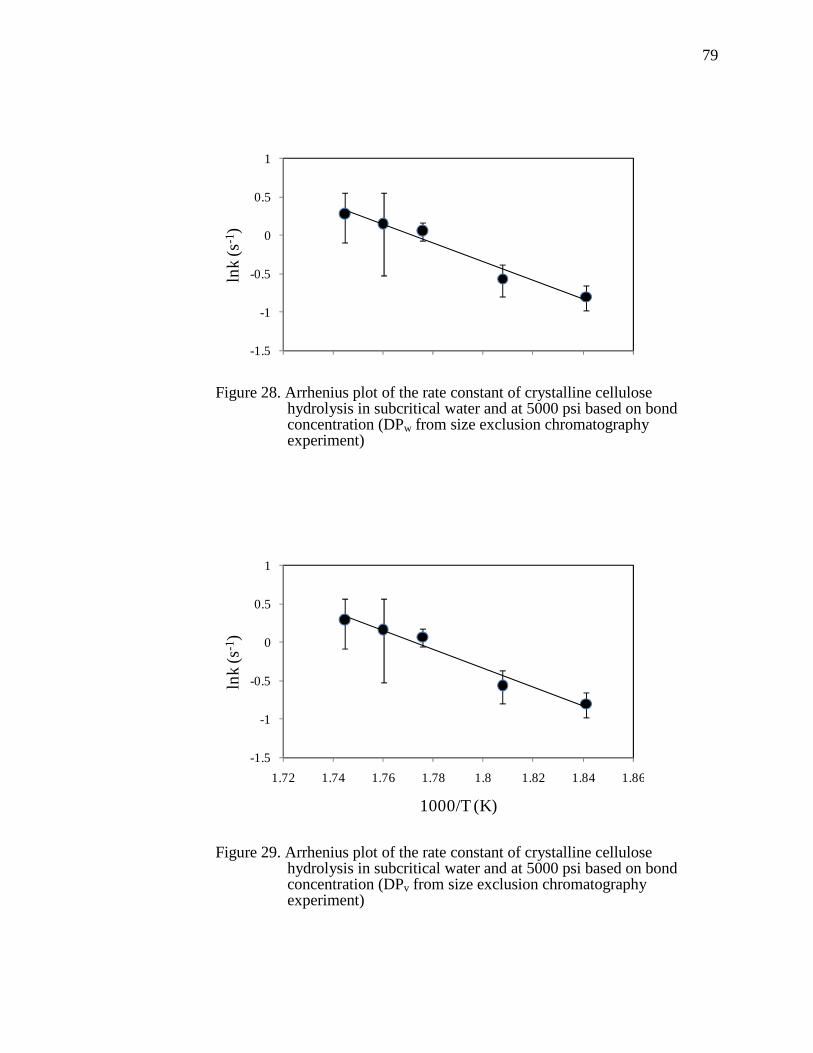
79

Figure 28. Arrhenius plot of the rate constant of crystalline cellulose hydrolysis in subcritical water and at 5000 psi based on bond concentration (DPw from size exclusion chromatography experiment)

Figure 29. Arrhenius plot of the rate constant of crystalline cellulose hydrolysis in subcritical water and at 5000 psi based on bond concentration (DPv from size exclusion chromatography experiment)

-1.5

-1

-0.5

0

0.5

1

lnk

(s-1

)

-1.5

-1

-0.5

0

0.5

1

1.72 1.74 1.76 1.78 1.8 1.82 1.84 1.86

lnk

(s-1

)

1000/T (K)

80

Figure 30. Arrhenius plot comparing rate constant of crystalline cellulose hydrolysis based on bond concentration with oligomers hydrolysis in subcritical water

Table 6. Kinetics Parameters obtained for the Glycosidic Bond Hydrolysis based on bond concentration evaluated from the DP of cellulose residues obtained from dilute solution viscometry and SEC

Degree of

Polymerization

Characterization

techniques

Activation Energy,

EA (kJ/mol)

Pre-exponential

factor, A (s-1)

DPv Dilute solution

viscometry

108.24±89.09 1010.04±4.65

DPp Size exclusion

chromatography

104.98±36.48 109.75±1.91

DPw Size exclusion

chromatography

101.17±35.46 109.36±1.85

DPv Size exclusion

chromatography

102.04±34.59 109.45±1.81

-2.00

-1.00

0.00

1.00

2.00

3.00

4.00

5.00

1.60 1.65 1.70 1.75 1.80 1.85 1.90

ln k

(s-

1 )

1000/T(K)

Cellobiose

Cellotriose

Maltose

Maltotriose

Maltotetraose

Cellulose

81

Figure 30 displays an Arrhenius plot depicting the rate constants obtained for the

hydrolysis of oligomers and cellulose in subcritical water. Hydrolysis rate constants for

the oligomers are obtained from Taiying Zhang’s PhD work14 while hydrolysis rate

constants for the cellulose are obtained from Figure 25. The activation energies obtained

for the oligomers: maltose (93 kJ/mol), cellobiose (82 kJ/mol), cellotriose (65 kJ/mol),

maltotriose (65 kJ/mol), and maltotetraose (52 kJ/mol), decreases with increase in the

size of the monomeric units while activation energy for the hydrolysis of cellulose in

subcritical water is higher than that of the oligomers.

4.2.3.4 Conclusion

Hydrolysates obtained as a result of hydrolyzing crystalline cellulose in

subcritical water contained unreacted cellulose. These hydrolysates were centrifuged to

separate the water soluble part via decantation from the sample as a whole. Subsequently,

the cellulose residue was freeze dried and characterized to obtain the degree of

polymerization (DPv). Bond concentrations based on the DP(s) obtained from DSV and

SEC were calculated and the detailed kinetics parameters based on a first order bond-

concentration rate equation were evaluated. The activation energies (EA) and pre-

exponential factors (A) obtained for the hydrolysis rate of breaking the glycosidic bonds

in cellulose are 108±89 kJ/mol and 1010.0±4.6 s-1 for DPv obtained via DSV and 101±35

kJ/mol and 109.4±1.9 s-1 for DPv obtained from SEC. The rate of breaking the glycosidic

bonds is crucial to understanding the kinetics of converting crystalline cellulose to

fermentable sugars.

82

4.3 Conversion of Crystalline Cellulose in Supercritical Water

Conversion of crystalline cellulose occurs by disintegrating the intermolecular

hydrogen bonding binding each layer of cellulose chains within the crystal structure. As a

result of the disintegration, the hydroxyl (OH) group on each of the glucose units reacts

with the protonating component of the solvent. In this section, we shall be investigating

the kinetics parameter defining the conversion of crystalline cellulose in supercritical

water.

Considering the reaction volume of the microreactor (0.17 ml) coupled with the

maximum flow rate the available pumps at our disposal could deliver, it proved to be

unrealistic to obtain unreacted cellulose in supercritical water. Therefore, to obtain some

cellulose residue after reacting crystalline cellulose in the microreactor at supercritical

condition of water, there is the need to either significantly increase the maximum

deliverable flow rates or substantially reduce the reaction volume. The latter option based

on the available resources was chosen. The modification also involves changing the

orientation of the microreactor. Details of the modification will be elucidated in the

experimental set-up and processing steps. Experimental description of the conversion of

cellulose in the microreactor and at the supercritical condition of water will be discussed.

Subsequently, methods adopted in analyzing the sample will be presented while results

and discussion section will follow immediately. Lastly, conclusions based on findings

and a summary of experiments will complete this chapter.

83


This section describes the experimental setup and processing steps of converting

crystalline cellulose in the microreactor in supercritical water. The essence of this

reaction is to have some quantity of the crystalline cellulose reacted and leaving behind

some residues. The experimental setup for the reaction of crystalline cellulose in the

microreactor is similar to the experimental setup in Figure 14, the only difference is the

orientation of the microreactor and extra heat exchanger unit in the setup for this

experiment. The feedstock (slurry solution) is fed into the microreactor positioned

midway along the process flow path. A schematic chart of the process for the reaction in

the microreactor can be seen in Figure 31.

Deionized water (18 mohm) obtained from a Nanopure infinity water purification

system was fed into a tube enclosed within a tube furnace (Thermolyne79400) by Lab

Alliance series II pumps at flow rates ranging from 9 ml/min to 14 ml/min. Subsequently,

the water was heated to supercritical temperatures ranging from 374 °C to 390 °C for

separate experimental runs. The pressure of the fluid in the tube was about 5,000 psig and

was controlled downstream by a 15,000 psig capacity Tescom back pressure regulator.

The pressure gauge displays the operating pressure. Just after the pressure gauge is a

rupture disc. This safety device, unlike the relief valve which opens when the maximum

pressure is exceeded, is ruptured when the operating pressure exceeds its limit. In this

experimental setup, the rupture disc can support a maximum pressure of 9000 psig, so

therefore, any pressure beyond this limit can lead to rupture of the disc.

84

Figure 31. Schematic chart of the conversion of crystalline cellulose in microreactor at supercritical condition

The supercritical water exited into the glass fiber insulated microreactor and

served as both hydrolytic agent and the reaction medium for the 2 wt% cellulose slurry

solutions. The feedstock was fed into the microreactor at the inlet port oriented upward

and located midway in the microreactor. The maximum temperature limit the furnace

could support was 1200 °C. The cellulose slurry solution with flow rates ranging from 9

to 14 ml/min mixed with the supercritical water with a constant flow rate of 10 ml/min,

thereby diluting the slurry concentration to values ranging from 0.947 to 1.167 wt%. The

reaction was quenched by a heat exchanger just at the outlet port of the microreactor and

also by the shell and tube heat exchanger placed just downstream from the first heat

exchanger. With the rapid heating and quick quenching of the cellulose reaction in the

microreactor, the reaction volume within the microreactor is estimated to be 0.088 ml.

The schematic flow detail in the microreactor can be seen in Figure 28. Alterations made

to the microreactor were mainly to reduce the reaction volume and allow the reaction to

occur as indicated in Figure 32.

85

The reaction volume for the conversion of cellulose at supercritical conditions is

this low because of the need to allow the reaction to occur at very low residence times to

avoid complete disappearance of the crystalline cellulose in supercritical water. Cellulose

residues left behind were measured gravimetrically. Detail of the gravimetric analysis for

the sole purpose of evaluating the rate of cellulose conversion in supercritical water will

be discussed in the subsequent sections. The samples were collected in the gas-liquid

separator and analyzed for conversion and weight of unreacted cellulose (residue).

Figure 32. Microreactor system set-up for cellulose conversion at supercritical condition

4.3.2 Sample Analysis The hydrolysate products were collected at different supercritical temperatures,

and the water insoluble portions were centrifuged, dried, and analyzed gravimetrically.

Centrifugation was conducted with SORVALL® RC 5B plus and samples were

centrifuged at a speed of 8000 rpm for 10 min. The supernatant obtained after

Sample products

Thermocouple Thermocouple

Supercritical water

Cellulose suspension 2wt %

Diluted to 0.947-1.167 wt %

86

centrifugation was decanted leaving behind the cellulose residue, which was later dried in

an oven within the temperature range of 42 °C – 67 °C . Cellulose residues were

measured gravimetrically to determine the mass that reacted. The results were used to

calculate the conversion.

4.3.3 Results and Discussions The concentrations in g/l of the insoluble hydrolysates sampled at the supercritical

conditions were evaluated by gravimetrically measuring the amount of cellulose residue

contained within the volume of the sampled hydrolysate. Conversions were evaluated and

the values obtained at each supercritical temperature per residence times can be seen on

Table 7. At each supercritical temperature, conversion as observed from Table 7

increases generally with the residence times. Maximum conversion of 90 % is seen at

residence time of 0.154 s and at supercritical temperature of 390 °C, while a minimum

conversion of 38.5% was observed at 374 °C and residence time of 0.142 s.

87

Table 7. Conversion of Cellulose Suspension at Supercritical Temperatures in Microreactor

374 °C 378 °C 380 °C 382 °C 388 °C 390 °C

τ(s) X τ(s) X τ(s) X τ(s) X τ(s) X τ(s) X

0.00 0.00 0.00 0.00 0.00 0.00 0.00 0.00 0.00 0.00 0.00 0.00

0.142 0.368 0.139 0.414 0.137 0.413 0.135 0.526 0.129 0.538 0.126 0.560

0.145 0.460 0.142 0.394 0.140 0.415 0.138 0.452 0.132 0.642 0.129 0.715

0.149 0.411 0.145 0.484 0.143 0.404 0.141 0.543 0.135 0.510 0.132 0.620

0.152 0.412 0.149 0.557 0.147 0.472 0.145 0.617 0.138 0.684 0.136 0.715

0.156 0.458 0.152 0.531 0.150 0.482 0.148 0.654 0.141 0.520 0.139 0.572

0.160 0.572 0.154 0.588 0.165 0.750 0.149 0.692 0.154 0.895

0.169 0.629 0.158 0.571 0.157 0.885

Conversion of cellulose in this medium is modeled after a first order reaction rate

equation. The conversion term, –ln(1-X), as shown in Figure 33 is plotted against the

residence times to obtain the rate constants, k, for each supercritical temperature

considered. The natural log of rate constants was plotted with the reciprocal of the

temperature to generate the Arrhenius plot as depicted in Figure 34. The kinetic

parameters were subsequently evaluated by equating the slope and the intercept of the

Arrhenius plot with –EA/R and lnA respectively (Equation 52).

88

Figure 33. Conversion plot for the rate constant of cellulose reaction in supercritical water

Figure 34. Arrhenius plot for the conversion of crystalline cellulose in supercritical water

The activation energy, Ea, and the pre-exponential or frequency factor, A, evaluated

based on Figure 31 are 290 ± 160 kJ mol-1 and 1024±13 s-1. The error values were

estimated based on 95 % confidence intervals. From the activation energy obtained for

0.000

0.500

1.000

1.500

2.000

2.500

0.120 0.130 0.140 0.150 0.160 0.170 0.180

-ln(1

-X)

Residence times (s)

374

378

380

382

388

390

0.000

1.000

2.000

3.000

4.000

5.000

1.500 1.510 1.520 1.530 1.540 1.550

lnk

(s-1

)

1000/T (K)

-∞

89

the conversion of cellulose in supercritical water (a mixture of hydroysis and dissolution)

as compared with the activation energy obtained for the conversion in subcritical water, it

seems that the conversion of cellulose has different rate-limiting steps under the two

conditions.

4.3.4 Conclusions Hydrolysates obtained as a result of dissolving crystalline cellulose in

supercritical water contain unreacted cellulose. These hydrolysates were centrifuged to

separate the water soluble part via decantation from the sample as a whole. Subsequently,

the unreacted cellulose or cellulose residues were dried and analyzed gravimetrically.

Conversion was calculated and the detail kinetics parameters based on a first order rate

equation were evaluated. The activation energy (EA) and pre-exponential factor (A)

obtained for the dissolution rate are 290 ± 160 kJmol-1 and 1024±13s-1 respectively.

Comparatively, the activation energy obtained for the conversion of cellulose in

supercritical water (dissolution/hydrolysis) is higher than the activation energy obtained

when cellulose is reacted in subcritical water. Thus, it appears that conversion of

cellulose in subcritical and supercritical water has different rate-limiting steps.

4.4 Kinetic Analysis of the Conversion of Crystalline Cellulose in

Subcritical and Supercritical Water

In this section, the kinetic parameters obtained based on the two kinetic models

adopted in this project for the conversion of cellulose in a hydrothermal system were

compared. Arrhenius trends for the conversion of crystalline cellulose in subcritical and

supercritical water based on first order and shrinking core models were compared with

results of similar work by Sasaki et al. (2004). The conversion plots that result in the

90

Arrhenius plot of cellulose reaction in supercritical water for both the first order and

shrinking core models were not allowed to go through the origin. The reason is because

the intercepts of these plots are not anywhere near the origin. Error estimation in this

study was based on a 95 % confidence interval and this perhaps may explain why the

margin of error is quite significant relative to what was obtained in Sasaki et al’s. It is not

certain what level of confidence is the estimated error in Sasaki et al but is likely to be

based on standard error estimation. Also, error estimation in the plots forced through the

origin is less in value compared with the margin of error in the plots that are not forced

through the origin and the reason is based on the degree of freedom. A critical review of

this observation revealed that the former has more degrees of freedom than the latter. The

values of the kinetics parameters and their errors from Sasaki et al. are left as they were

reported while in this study, the kinetic values are rounded to 2 significant figures.

4.4.1 Shrinking Core Model

Figure 35 depicts the Arrhenius plots of cellulose conversion in subcritical and

supercritical water obtained from this study and the study conducted by Sasaki et al. The

trends for the two separate studies appear to closely follow each other in the supercritical

region though at the high end they seems to widen while a clear difference in their trends

was observed in the subcritical region. The kinetic parameters obtained in the

supercritical region were found to be, Ea =290 ± 160 kJ mol-1 , A= 1024±13 s-1 for this

study, and Ea=547.9 ± 27.8 kJ mol-1 , A=1044.6±2.2 s-1 for Sasaki et al. respectively. In the

subcritical region, the kinetic parameters obtained were found to be, Ea =99 ± 29 kJ mol-

1, A=108.9±2.7 s-1 for this study, and Ea=145.9 ± 4.6 kJ mol-1 , A=1011.9±0.4 s-1 for Sasaki et

al. Figure 36 seems to portray the same trend as observed in Figure 35 but the only

exception is the difference in the error margin in the subcritical region. A larger error

range in the subcritical region was observed in Figure 36 than in Figure 35. The

91

corresponding conversion plots upon which k-values in Figure 36 were estimated weren’t

forced through the origin. The kinetic parameters obtained in this case were found to be

Ea =110 ± 57 kJ mol-1, A=109.5±5.3 s-1 . In Figure 37, the Arrhenius trend across the

critical regions, i.e. the subcritical and supercritical regions, reflects a much better fit of

the data in this study than in the study conducted by Sasaki et al. In Figure 37, the kinetic

parameters obtained in this study across the critical region were found to be, Ea=92 ± 13

kJ mol-1 , A=108.1±1.1 s-1 While in Sasaki’s work, the kinetic parameters were found to be

Ea=210 ± 86 kJ mol-1 and A=1011.9±0.4 s-1 . Thus, the kinetic parameters obtained for this

study, in Figure 38, were estimated to be Ea=88 ± 15 kJmol-1 , A=107.8±1.3 s-1. There is no

kinetic data trend for Sasaki et al in Figure 38 and the reason is because the conversion

plots reported by Sasaki et al., only pass through the origin. Therefore, we were

constrained to only estimate the kinetic parameters from Sasaki’s work for plots passing

through the origin.

Figure 35. Shrinking Core Model: Separated Arrhenius plot for the conversion of

crystalline cellulose in subcritical and supercritical water with conversion plot of cellulose reaction in subcritical water passing through the origin

-5.000-4.000-3.000-2.000-1.0000.0001.0002.0003.0004.0005.000

1.500 1.550 1.600 1.650 1.700 1.750 1.800 1.850 1.900

lnk

(s-1

)

1000/T (K)

This study sup

This study sub

Sasaki et al sup

Sasaki et al sub

-∞

-∞

92

Figure 36. Shrinking Core Model: Separated Arrhenius plot for the conversion of

crystalline cellulose in subcritical and supercritical water without forcing the conversion plot of cellulose reaction in subcritical to pass through the origin

Figure 37. Shrinking Core Model: Combined Arrhenius plot for the conversion of

crystalline cellulose in subcritical and supercritical water with conversion plot of cellulose reaction in subcritical water passing through the origin

-5.000-4.000-3.000-2.000-1.0000.0001.0002.0003.0004.0005.000

1.500 1.550 1.600 1.650 1.700 1.750 1.800 1.850 1.900

lnk

(s-1

)

1000/T (K)

This study sup

This study sub

Sasaki et al sup

Sasaki et al sub

-∞

-∞

-∞-∞

-5.000-4.000-3.000-2.000-1.0000.0001.0002.0003.0004.0005.000

1.500 1.550 1.600 1.650 1.700 1.750 1.800 1.850 1.900

lnk

(s-1

)

1000/T (K)

This study

Sasaki et al

-∞

-∞

93

Figure 38. Shrinking Core Model: Combined Arrhenius plot for the conversion of

crystalline cellulose in subcritical and supercritical water without forcing the conversion plot of cellulose reaction in subcritical water to pass through the origin

4.4.2 First Order and Shrinking Core Models

Figure 39 depicts the Arrhenius plots of cellulose conversion in subcritical and

supercritical water obtained based on first order and shrinking core models. The trends

for the two models appear to roughly parallel each other in both regions with lower k-

values for the shrinking core model. The kinetic parameters obtained in the supercritical

region were found to be Ea =420 ± 140 kJ mol-1, A= 1034±11 s-1 for first order, and Ea=290

± 160 kJ mol-1, A=1024±13s-1 for shrinking core. In the subcritical region, the kinetic

parameters obtained for the first order and the shrinking core were found to be, Ea =150 ±

67 kJ mol-1, A=1015±6.2 s-1, and Ea=99 ± 29 kJ mol-1, A=108.9±2.7 s-1, respectively. Similar

trends as observed in Figure 39 were displayed in Figure 40 except that the k-values for

the first order and shrinking core models do not parallel each other as much as in the

former, and a slightly higher difference in the k-values was observed on the high side of

both regions. A much wider error range in the subcritical region was observed in Figure

40 than in Figure 39. The corresponding conversion plots for which k-values in Figure 40

-5.000

-4.000

-3.000

-2.000

-1.000

0.000

1.000

2.000

3.000

4.000

1.500 1.550 1.600 1.650 1.700 1.750 1.800 1.850 1.900

lnk

(s-1

)

1000/T (K)

This study

-∞

-∞

-∞-∞

94

were estimated weren’t forced through the origin. The kinetic parameters obtained for

first order in this case were found to be Ea =120 ± 39 kJ mol-1, A=1011±3.6 s-1 while

corresponding kinetic parameters for the shrinking core model were estimated to be Ea

=110 ± 57 kJ mol-1 and A=109.5±5.3 s-1.

In Figure 42, the corresponding conversion plot for the Arrhenius plots for either

the subcritical or supercritical region per each of the models were not forced through the

origin while opposite is the case in Figure 41. In Figure 41 and 42, the Arrhenius trend

across the subcritical and supercritical regions display similar trends but with higher k-

values for the first order than their corresponding shrinking core values. In Figure 41, the

kinetics parameters obtained for first order across the critical region were found to be

Ea=100 ± 18 kJ mol-1, and A=109.5±1.6 s-1 while in Figure 42, the kinetic parameters were

found to be , Ea=94±23 kJ mol-1, and A=108.9±2.0 s-1 . The kinetic parameter for shrinking

core were found both in Figure 40 and 42 to be Ea=92 ± 13 kJ mol-1, A=108.1±1.1 s-1, and

Ea=88 ± 15 kJ mol-1, A=107.8±1.3 s-1.

Figure 39. First Order Model: Separated Arrhenius plot for the conversion of crystalline

cellulose in subcritical and supercritical water with conversion plot of cellulose reaction in subcritical water being forced through the origin

-2.000

-1.000

0.000

1.000

2.000

3.000

4.000

5.000

1.500 1.550 1.600 1.650 1.700 1.750 1.800 1.850 1.900

lnk

(s-1

)

1000/T (K)

First Order sup

First Order sub

Shrinking Core sup

Shrinking Core sub

-∞

95

Figure 40. First Order Model: Separated Arrhenius plot for the conversion of crystalline cellulose in subcritical and supercritical water without allowing the conversion plot of cellulose reaction in subcritical water not being forced through the origin

Figure 41.First Order Model: Combined Arrhenius plot for the conversion of crystalline

cellulose in subcritical and supercritical water with conversion plot of cellulose reaction in subcritical being forced through the origin

-4.000

-3.000

-2.000

-1.000

0.000

1.000

2.000

3.000

4.000

5.000

1.500 1.550 1.600 1.650 1.700 1.750 1.800 1.850 1.900

lnk

(s-1

)

1000/T (K)

First Order sup

First Order sub

Shrinking Core sup

Shrinking Core sub

-∞

-∞-∞

-2.000

-1.000

0.000

1.000

2.000

3.000

4.000

5.000

1.500 1.550 1.600 1.650 1.700 1.750 1.800 1.850 1.900

lnk

(s-1

)

1000/T (K)

First Order

Shrinking Core

-∞

96

Figure 42. First Order Model: Combined Arrhenius plot for the conversion of crystalline

cellulose in subcritical and supercritical water without allowing the conversion plot of cellulose reaction in subcritical not being forced through the origin

4.5 Summary of Experiments

In this chapter, a kinetics analysis describing the reactive behavior of cellulosic

biomass in a hydrothermal microreactor has been discussed. The most important

conclusions from the various experiments conducted can be summarized as the

following:

1. The hydrolysis of crystalline cellulose in subcritical water is best explained by

the low solubility level of cellulose in subcritical water resulting in

heterogeneous reaction. The hydrolysis is surface based and its kinetics is

modeled after the shrinking core or grain model. The solubilization or

solvation effect of subcritical water on crystalline cellulose increases as the

subcritical temperature increases. Kinetic parameters for the overall

conversion of crystalline cellulose include the activation energy and the pre-

-4.000

-3.000

-2.000

-1.000

0.000

1.000

2.000

3.000

4.000

5.000

1.500 1.550 1.600 1.650 1.700 1.750 1.800 1.850 1.900

lnk

(s-1

)

1000/T (K)

First Order

Shrinking Core

-∞

-∞-∞

97

exponential factor and were evaluated respectively as 99 ± 29 kJ mol-1 and

108.9±2.7 s-1.

2. Dilute solution viscometry analysis was conducted to evaluate the DP of

cellulose as received and cellulose residue obtained from hydrolysis. As the

subcritical temperature increases at similar residence time, a decreasing trend

of the DP of the cellulose chain is observed. The degree of polymerization

(DP) is observed to drastically reduce from the initial DP of 228 to as low as

7.

3. Hydrolysis of cellulose in subcritical water was investigated. A first order

bond concentration rate equation was employed in assessing the hydrolysis.

The activation energy and the pre-exponential factor obtained for the

hydrolysis of the glycosidic bonds evaluated from DPv(s) obtained via DSV

and SEC are 110±89 kJ/mol, 1010±4.7 s-1 and 102±35 kJ/mol, 109.5±1.8 s-1.

4. Conversion of crystalline cellulose in supercritical water proceeds in a two-

steps reaction. In supercritical water, the reaction proceeds very fast and the

liquefaction is so drastic that it gives little or no room for unreacted cellulose

to survive after reaction. Maximum conversion of 89.5 % was obtained at

supercritical temperature of 390 °C and residence time of 0.154 s. Minimum

conversion of 36.8 % was obtained at supercritical temperature of 374 °C and

residence time of 0.142 s. At supercritical conditions, the kinetic parameters

for the conversion of crystalline cellulose in the microreactor were

experimentally determined. Activation energy and pre-exponential factor

obtained for the first order cellulose conversion in supercritical water are 290

± 160 kJ mol-1 and 1024±13s-1 respectively.

5. Arrhenius trend obtained based on shrinking core model from this study and

Sasaki et al are quite similar in the supercritical region using rate plots going

through the origin. While the trends for the two separate studies appear to

98

closely follow each other in the supercritical region, a clear difference in their

trends was observed in the subcritical region. The trends for the first order and

shrinking core models appear to parallel each other in both critical regions

with lower k-values for the shrinking core model.

99

CHAPTER 5. INVESTIGATING YIELD OF WATER SOLUBLE

HYDROLYSATE IN HYDROTHERMAL MEDIA

Previous studies showed a better monosaccharide yield from cellulose hydrolysis

in subcritical water 14, 50 than in supercritical water. This trend is caused by the relatively

higher hydrolysis rate of crystalline cellulose compared to the decomposition rate of the

hydrolysate in subcritical water. But in supercritical water, the hydrolysis rate proceeds

at a slower pace than the decomposition rate. This understanding is considered helpful in

the design of a process path that can potentially improve the yield of fermentable sugars

from crystalline cellulose. The process path entails setting up a reaction sequence

intended to first dissolve cellulose and subsequently hydrolyze the dissolved cellulose in

subcritical water.

Since dissolving cellulose is difficult, dissolved starch will be use as a surrogate

for cellulose in the hydrolysis reaction in subcritical water. The rationale behind this

approach is seen from the observation made from one of Taiying Zhang’s works14

(Figure 30) that hydrolysis of maltosaccharides and cellosaccharides in subcritical water

are similar. Dissolved starch, at subcritical conditions of water, will be hydrolyzed

within the reaction volume of the microreactor. The water soluble product (hydrolysate)

obtained from the reaction will be analyzed with high performance liquid

chromatography (HPLC).

Decoupling the dissolution of cellulose from its hydrolysis could be approached

by dissolving cellulose under a very short time (0.01-0.2 s) in supercritical water and

afterward, hydrolyze the dissolved cellulose in subcritical water at a relatively longer

residence time. Before coming up with the idea of decoupling the reaction, the

100

conventional way has always been to dissolve and hydrolyze crystalline cellulose within

the same hydrothermal reactor while allowing the reaction conditions to change from

subcritical to supercritical phase. The notion of sequencing the two phases, subcritical

and supercritical, per experimental degradation is similar to the study conducted by Ehara

and Saka11 on phase-separating the reaction media to improve yield and selectivity of

target products.

Another approach is in-situ pretreatment of crystalline cellulose in an ionic liquid

or non-derivatizing solvent.71-73 As it has been discussed extensively,74-76 ionic liquid

will deconstruct the crystallinity of the cellulose to a far less crystalline structure.

Dissolved cellulose in the ionic liquid will subsequentlybe precipitated at the introduction

of an anti-solvent (water or aliphatic alcohol) via preferential solute-displacement

mechanism.74 Non-volatile ionic liquid is afterward recovered by stripping off the anti-

solvent via flash distillation. Thereafter, decrystallized cellulose will be hydrolyzed in the

hydrothermal (subcritical) reactor.

5.1 Experimental Methods

The experimental methods present a detailed description of the experimental setup

and the processing steps, sample product analysis, and data analysis methods.


Hydrolysis of starch and cellulose were conducted both in the microreactor and

the tubular reactor. Figure 14 depicts the experimental setup for the reaction of crystalline

cellulose and dissolved starch in the microreactor. The same setup was used for the

polysaccharide reactions in the tubular reactor but the only difference is the point at

101

which feedstock is fed into the process stream. With the microreactor, the feedstock is fed

into the reactor positioned midway along the process flow path while for the tubular

reactor, the feedstock solution is fed at the starting point of the process stream. A

schematic chart of the process for the microreactor can be seen in Figure 15, while

Figures 43 is a schematic diagram of the tubular reactor.

Figure 43. Schematic flow process for cellulose hydrolysis in hydrothermal tubular reactor

For microreactor experiments, deionized water obtained from a nanopure Infinity

water purification system was fed into a tube enclosed within a tube furnace

(Thermolyne79400) by Lab Alliance series II pump at flow rates ranging from 5 ml/min

to 10 ml/min. Subsequently, the deionized water was heated to subcritical temperatures

ranging from 280°C to 340°C for separate experimental runs. The pressure of the fluid

was about 5,000 psig was set and control by a 15,000 psig capacity Tescom back pressure

regulator downstream. The pressure gauge displays the operating pressure. Just after the

pressure gauge is a rupture disc. This safety device, unlike the relief valve which opens

when the maximum pressure is exceeded, is ruptured when the operating pressure

102

exceeds its limit. In this experimental setup, the rupture disc can support a maximum

pressure of 9000 psi, so therefore, any pressure beyond this limit can lead to rupture of

the disc.

The subcritical water exited into the microreactor insulated with fiber glass and

served as both hydrolytic agent and the reaction medium for the 2 wt % polysaccharide

solutions entering the upper inlet port of the microreactor just at the outlet of the tube

furnace. The temperature the furnace can support range from room temperature to 1200

°C. The cellulose slurry/dissolved starch solutions was mixed with the subcritical water at

equal volumetric flow rate, thereby diluting the cellulose slurry/dissolved starch

concentration to 1 wt%. The reaction was quenched by the deionized water from the

other upper inlet port of the microreactor and also by the shell and tube heat exchanger

just at the outlet end of the microreactor. With the rapid heating and quick quenching of

the polysaccharides reaction in the microreactor, the reacting volume within the

microreactor is estimated to be 0.17ml. The schematic flow detail in the microreactor can

be seen in Figure 16 of chapter 4.

For the tubular reactor, cellulose/starch slurry (2 wt %) solution was fed into the

hydrothermal tubular reactor at temperatures ranging from 200 °C- 400 °C and pressure

of about 5000 psig. The reactions were conducted at flow rates of 5 ml/min and 10

ml/min and were quenched by the heat exchanger downstream of the reactor. The

reacting volume for the tubular reactor is 2.13 ml, while residence times due to

temperature range span between 12 – 23 s for 5 ml/min and 6 – 11 s for 10 ml/min. The

product samples which flow via the back-pressure regulator are collected downstream in

the gas-liquid separator. The water soluble part of the hydrolysate was analyzed with

103

HPLC. The insoluble part obtained from the unreacted cellulose was either centrifuged or

filtered and subsequently dried for further analysis.

5.1.2 Sample Product Analysis Method

5.1.2.1 Materials.

Cellulose suspensions and starch solutions in deionized water are the reactant

mixture used in this section of the research project. The chemical compounds

used for the experiments and the standard solutions for calibration curves were

all obtained from Sigma-Aldrich and they are highlighted as follows: crystalline

cellulose (sigmacell type 20), cellobiose (>98 %), maltose monohydrate (>98

%), glucose (>99.5 %), fructose (>98 %), 5-(hydroxymethyl)-2-furfural, and

furfural .

5.1.2.2 Aqueous products (water soluble hydrolysate).

Water soluble hydrolysate was analyzed by ionic HPLC comprising: pump (LC-

10ADvp), refractive index detector (RID-10A), SSI 505 LC column oven,

Aminex HPX-87H & HPX-42A columns (300 x 7.8 mm), mobile phase (0.1

mmol/L H2SO4 & Water). A large percentage of the samples was analyzed with

HPLC using auto sampler injection, but for the latter part of the project manual

injection was used. The mobile phase flow rate was of 0.6 ml/min and the

column oven temperature was 50 °C. Hydrolysate quantification and

identification were obtained based on hydrolysate standard calibration and

characteristics retention time respectively.

104

5.1.2.3 Water Insoluble Hydrolysate.

This is the solid portion of the product samples obtained from the hydrolysis

reaction. These products were analyzed gravimetrically by filtering the

hydrolysate via Stericup® 0.22 µm Millipore GV PVDF membrane. The solid

residues left after filtration were dried at room temperature until the weight of

the solid products remained constant. This method was used to find the mass of

unreacted cellulose per volume of the product mixture solely for evaluating the

conversion of crystalline cellulose under hydrothermal conditions.

5.1.3 Data Analysis Method

In the hydrothermal (micro and tubular) reactor, the average time the reactants

spend in the reacting volume is refers to as the residence time (τ) and can be expressed

mathematically as:

τ = ρcV/ρrFr (47)

where ρc is the density of the reactant mixture at reactor conditions, V is the

reacting volume of the hydrothermal reactor, and ρr is the density of the reactant mixture

at room temperature. Fr is the volumetric flow rate of the reactant mixture being fed into

the reactor. Other descriptive data analysis variables include conversion and yield.

Conversion is denoted symbolically as X and is define as the amount of solute (in

solution/suspension) reacted with respect to the initial amount. Yield is the amount of the

product formed with respect to the initial amount of the reactant fed. The mathematical

representation of both the conversion and yield are expressed as Equations 48 and 49 in

chapter 4.

105

Products in this case could be glucose, cellobiose, maltose, fructose, 5-

(hydroxymethyl)-2-furfural (HMF), furfural, and organic acids while reactants could be

either cellulose suspension or starch solution. Cellulose and starch are polymers of

glucose, and obtaining their concentration in mole/litre may prompt an initial line of

thought of finding the DP to obtain the molecular weight so as to obtain the moles of the

polymer. The approach is logical but not necessary because these polysaccharides are

polymer of glucose and concentration can be based on the mass of glucose units in the

polysaccharides. Approximating the density of the dilute aqueous solution at room

conditions to be 1000g/L, the composition (mass ratio) of solute in terms of wt% was

expressed in Equation 50.

5.2 Yield of Water Soluble Hydrolysates in the Hydrothermal Reactor

Hydrolysis of starch and crystalline cellulose were conducted in both tubular

reactor and microreactor at subcritical and supercritical conditions of water. The yields of

water soluble hydrolysates such as glucose, cellobiose, and furfural vary as the

temperature and residence times are altered. The thing to look out for in this section is the

residence time and the temperature at which optimum yield of fermentable sugars are

attained. The reason is because some of the fermentable sugars formed during reaction

degrade to other compounds that perhaps could serve as inhibitors in the fermentation

stage of biofuel production. Thus, the yield of water soluble hydrolysates in both the

tubular reactor and the microreactor will be investigated. Finally, a detailed comparison

of the water soluble hydrolysate yields obtained at subcritical conditions for dissolved

starch, a surrogate for the dissolved cellulose, will be compared with yields obtained

106

from the hydrolysis of crystalline cellulose in subcritical and supercritical water. This

section of the project is largely driven by hypothesis No. 2 in Chapter 3 which propounds

that: glucose formation from dissolved cellulose is better optimized in subcritical water

than in supercritical water.

5.2.1 Yield of Water Soluble Hydrolysates in the Tubular Reactor

Hydrolysis of cellulose and starch in the hydrothermal tubular reactor results in

the formation of water soluble and insoluble hydrolysates. Unreacted cellulose primarily

constitutes the insoluble hydrolysates while soluble hydrolysates for both starch and

cellulose include fermentable sugars and hydrolysate decomposition products. Cellulose

slurry solution or starch solution were fed to the process unit, and products resulting from

the reaction were collected downstream. The sampled hydrolysate products were

analyzed with HPLC and the yield of the water soluble hydrolysates were evaluated.


Figure 35 shows a schematic flow process of cellulose hydrolysis in the tubular

reactor. Cellulose slurry (2 wt%) was fed into the hydrothermal tubular reactor at

temperatures used ranged from 200 °C to 400 °C. The reactor pressure of about 5000

psig. The reactions were conducted at flow rates of 5 ml/min and 10 ml/min and were

quenched by the heat exchanger after exiting the reactor. The sample products which

flow via the back-pressure regulator were collected downstream in the gas-liquid

separator.

107


Water soluble hydrolysates collected at the different subcritical temperatures and

at different residence times were analyzed with HPLC. Hydrolysate quantification was

based on hydrolysate standard calibration and species identification was determined by

characteristic retention time. The quantification was established based on the peak areas

of HPLC compared against a known standard.


Figure 44 depicts the fractional yield of water soluble hydrolysate obtained in the

hydrothermal tubular reactor at a flow rate of 10 ml/min. Crystalline cellulose was

reacted at subcritical and supercritical conditions of water, and yields of water soluble

hydrolysates at temperature ranging from 300 °C to 400 °C were obtained. Glucose yield,

showed a maximum of 15 % at the lowest subcritical temperature of 300 °C, and

decreased appreciably as temperatures increased. The same trend was observed with

cellobiose and fructose which peak at 2.5 % and 7 % yield and subsequently decreases as

reaction temperature increased. While experiencing a drastic decrease in the percent yield

of sugars, a net formation of 5-(hydroxymethyl)-2-furfural (HMF) and furfural were

observed. Yield of HMF and furfural which peak at about 6.7 % and 8.6 % and at

subcritical temperatures of 310 °C and 330 °C, respectively decrease subsequently as

temperatures increase from subcritical to supercritical. However, the decomposition of

HMF and furfural is not as pronounced as what was observed with the decomposition of

monosaccharides and cellobiose as reaction temperature increased. The significant

reduction in the quantity of sugars is strongly believed to have contributed relatively to a

considerable amount of the furanic compounds at high temperature.

108

Figure 44. Fractional yield of water soluble hydrolysates in hydrothermal tubular reactor at 10 ml/min

Figures 45 and 46 portray fractional yield of water soluble hydrolysates obtained

from starch and cellulose in the hydrothermal tubular reactor at 5 ml/min. Figure 45

reflects an increase in the yield of glucose and fructose as the exit temperature rises from

200 °C up until 250 °C, where yield for both monosaccharide peak at about 35% and

5.3% respectively. Monosaccharide yield decreases after the reactor exit temperature

increases from subcritical temperature to supercritical temperature. While similar trend,

though at a relatively lower yield when compared with glucose, was observed with

maltose. Maximum yield for maltose was obtained at 7.6% and at subcritical temperature

of 230 °C. Maltose yield subsequently decreased as temperature increased. However, the

temperature at which maximum glucose yield was obtained is 20 °C lagging the

temperature at which yield of maltose is at the maximum. This trend maybe indicative of

the fact that some glucose was formed as result of the hydrolysis of maltose.

0

0.02

0.04

0.06

0.08

0.1

0.12

0.14

0.16F

ract

ion

al Y

ield

Cellobiose

Glucose

Fructose

HMF

Furfural

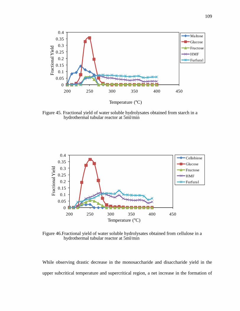
109

Figure 45. Fractional yield of water soluble hydrolysates obtained from starch in a hydrothermal tubular reactor at 5ml/min

Figure 46.Fractional yield of water soluble hydrolysates obtained from cellulose in a hydrothermal tubular reactor at 5ml/min

While observing drastic decrease in the monosaccharide and disaccharide yield in the

upper subcritical temperature and supercritical region, a net increase in the formation of

0

0.05

0.1

0.15

0.2

0.25

0.3

0.35

0.4

200 250 300 350 400 450

Fra

ctio

nal Y

ield

Temperature (°C)

Maltose

Glucose

Fructose

HMF

Furfural

0

0.05

0.1

0.15

0.2

0.25

0.3

0.35

0.4

200 250 300 350 400 450

Fra

ctio

nal Y

ield

Temperature (°C)

Cellobiose

Glucose

Fructose

HMF

Furfural

110

HMF and furfural was observed. Maximum HMF and furfural yield was observed at

7.2% and at 270 °C and subsequently remain constant for furfural as temperature

increased while some of the HMF decomposes further perhaps to furfural and other

compounds.

Yields evaluated for all the soluble hydrolysates portray on Figure 45, follow

similar trend as delineated in Figure 44 with just two exceptions and they are 1) the

temperature at which each hydrolysate yield peaks and 2) the percent yield. Both

Glucose and fructose yields increase as the reactor exit temperature increases from 200

°C and peak at subcritical temperature of 250 °C and at percent yields of 36.7% and 6.7%

respectively. Yields for the glucose and fructose (monosaccharides isomers) decreased

after the reactor exit subcritical temperature increased past the 250 °C and approach

temperature in the supercritical region. Cellobiose yields do follow similar trend with

maximum percent yield of 2.9% obtained at subcritical temperature of 230 °C. As yields

for simple sugars decreased with increasing temperature, a net formation of HMF and

furfural were observed. The maximum yield obtained for HMF and furfural and at

subcritical temperature of 320 °C are 9.4% and 12.9%. There is a substantial presence of

HMF and furfural relative to simple sugars at supercritical condition of water. This trend

is obviously connected to excessive net decomposition of the monosaccharide at high

temperature to HMF, furfural and other compound such as organic acids.

5.2.1.4 Conclusions

Water soluble hydrolysates yield obtained while reacting crystalline cellulose and

starch at 5 ml/min in the hydrothermal tubular reactor follow similar trend with the 10

ml/min flow rates. The only two features distinguishing each trend are the maximum

111

yields obtained for each hydrolysate and the temperature at which these maximum yields

were obtained. For the 10 ml/min flow rates, more simple sugars were formed at

subcritical temperature than at supercritical temperature. At high temperature, more of

the simple sugars decompose into HMF, furfural and other compounds. An aggregated

sum of maximum glucose (15%) and fructose (7%) yield obtained at 10 ml/min is 22%.

However, at 5 ml/min, it is interesting to observe maximum glucose yield from starch

(35% glucose) and cellulose (36.7% glucose) occurring at the same temperature and

virtually exhibiting same maximum yields. Similar trend was observed for the

temperature at which fructose, cellobiose and maltose peaked though with different

yields. But with furanic compounds, the temperatures at which HMF and furfural peaked

for the 5 ml/min flow rate are totally different. An aggregated sum of the maximum

glucose and fructose yield obtained from the hydrothermolytic conversion of crystalline

cellulose and starch at 5 ml/min are 43.4% and 40.3% respectively.

5.2.2. Hydrolysates Yield from Crystalline Cellulose Hydrolysis in the Microreactor at

Subcritical Condition of water

Hydrolysis of cellulose in the hydrothermal microreactor results in the formation

of water soluble and insoluble hydrolysates. Samples obtained from the reaction consist

of unreacted cellulose and water soluble hydrolysates. Unreacted cellulose primarily

constitutes the insoluble hydrolysates while soluble hydrolysates include fermentable

sugars and hydrolysate decomposition products. Cellulose suspensions were fed to the

process unit, and products resulting from the reaction were collected downstream. The

112

sampled hydrolysate products were analyzed with HPLC and the yield of the water

soluble hydrolysates were evaluated.


Cellulose suspension was fed into a tube enclosed within the tube furnace at flow

rates ranging of 5 ml/min and 10 ml/min. Subsequently, the deionized water was heated

to subcritical temperatures ranging from 280°C to 340°C. The pressure of the fluid was

about 5000 psig was set and controlled by a back pressure regulator downstream. The

subcritical water exit into the glass fiber insulated microreactor serving both as hydrolytic

agents and reaction medium for the 2 wt % cellulose suspension entering from the upper

inlet port of the reactor just at the tube furnace outlet. The 2 wt% cellulose suspension

was mixed with the subcritical water at equal volumetric flow rate, thereby diluting it to 1

wt%. The reaction was quenched by the deionized water entering the other upper inlet

port of the microreactor closer to the heat exchanger. The samples were collected in the

gas-liquid separator and were analyzed.







113


Figures 47 – 51, depict yield of water soluble hydrolysate obtained along side the

cellulose residue evaluated for conversion. Figure 47 shows apparently low yield in

water soluble hydrolysate production at 280 °C. Fractional yields for each hydrolysate

increases with residence time with maximum glucose yield of 2.2% at 0.83 s , while at

the same residence time, fructose and cellobiose yield peak at about 2.0% and 4.4%.

Figure 48 unfolds a slight increase in water soluble hydrolysate yield at 290 °C than at

280 °C. Maximum yields of glucose and fructose obtained under this condition and at

residence time of 0.61 s are 3.1% and 1.9% respectively. Cellobiose displays better yield

(with maximum yield of 5.2% at the same residence time) than the yield of the

monosaccharides.

Figure 47. Fractional yield of water soluble hydrolysates obtained from cellulose at 280 °C in microreactor

0

0.01

0.02

0.03

0.04

0.05

0.000 0.200 0.400 0.600 0.800 1.000

Fra

ctio

nal y

ield

Residence time (s)

Cellobiose

Glucose

Fructose

T= 280 °CP= 5000 psi

114

Figure 48.Fractional yield of water soluble hydrolysates obtained from cellulose at 290 °C in microreactor

Figure 49. Fractional yield of water soluble hydrolysates obtained from cellulose at 300 °C in microreactor

0

0.01

0.02

0.03

0.04

0.05

0.06

0.000 0.200 0.400 0.600 0.800 1.000

Fra

ctio

nal y

ield

Residence time (s)

Cellobiose

Glucose

Fructose

T= 290 °CP= 5000 psi

0

0.02

0.04

0.06

0.08

0.1

0.12

0.000 0.200 0.400 0.600 0.800 1.000

Fra

ctio

nal y

ield

Residence time (s)

Cellobiose

Glucose

Fructose

HMF

T= 300 °CP= 5000 psi

115

Figure 50. Fractional yield of water soluble hydrolysates obtained from cellulose at 320

°C in microreactor

Figure 51. Fractional yield of water soluble hydrolysates obtained from cellulose at 340

°C in microreactor

However, formation of hydroxymethylfurfural (5-HMF), one of glucose

decomposition products, started becoming apparent at 300 °C, while at 320 °C and 340

°C, a relatively higher HMF yields were observed. In Figure 49, yield of water soluble

0

0.04

0.08

0.12

0.16

0.2

0.000 0.200 0.400 0.600 0.800 1.000

Fra

ctio

nal y

ield

Cellobiose

Glucose

Fructose

HMF

T= 320 °CP= 5000 psi

0

0.05

0.1

0.15

0.2

0.25

0.000 0.200 0.400 0.600 0.800 1.000

Fra

ctio

nal y

ield

Residence time (s)

Cellobiose

Glucose

Fructose

HMF

Furfural

T= 340 °CP= 5000 psi

116

hydrolysates obtained at 300 °C increased with residence times. More monosaccharide

are generated at this temperature with almost 10% maximum glucose yield, 4%

maximum fructose and HMF yields while cellobiose has a better yield of 11.1% . Figure

50 reflects at 320 °C an increase in glucose yield with residence time, while cellobiose

decreased as residence time increased. It is most likely that some of the cellobiose are

further hydrolyzed to form glucose. Amount of fructose and HMF formed remain

relatively constant across the residence time. This contrasting variation of cellobiose and

glucose yields with residence time, explains why their respective maximum yields of

about 14.4% and 19% occur at the lowest and highest residence time. Figure 51,

displays a steady but not apparent increasing trend in hydrolysates yield with residence

time at 340 °C. This trend includes cellobiose yield which decreases as residence time

increases. Reduction in the quantity of cellobiose, as stated earlier, is due to further

hydrolysis to glucose and other simpler compounds. Quantity of furfural formed, which

though becomes only measurable under this reaction condition, exceed the respective

yields of HMF, fructose, and cellobiose. Overall maximum glucose yield of 22.5% was

obtained at 340 °C which exceeded yields obtained at any of the operating temperature

considered in this experiment. As temperatures increased within the subcritical phase

(280 °C – 340 °C) more glucose are formed possibly from hydrolysis of soluble

oligosaccharide such as cellobiose, cellotriose, and heterogeneous hydrolysis of

insoluble cellulose.

5.2.2.4 Conclusions

Hydrolysis of crystalline cellulose was conducted in a hydrothermal microreactor

at subcritical temperature ranging from 280 °C to 340 °C and at 5000 psig. Sample

117

contain water soluble hydrolysates were obtained and subsequently analyzed with HPLC.

Water soluble hydrolysates analyzed consist of glucose, fructose, cellobiose, HMF, and

furfural. More cellobiose yield relative to the yield of other hydrolysates were obtained at

subcritical temperature ranging from 280 °C to 300 °C. But at 320 °C, the yield which is

more than what was obtained at 280 °C to 300 °C, is relatively less than the glucose yield

and decreased as the residence time increased. At 340 °C, cellobiose yields are almost

equal with the yield obtained for fructose. Glucose yield at all subcritical temperature in

question increased with residence times. In this experiment, maximum glucose yield of

22.5% was obtained at 340 °C and at residence time of 0.615 s, while in the case of

fructose, maximum yield of 8.03% was obtained at 340 °C and at 0.468 s. The maximum

aggregate sum of the monosaccharide yield which is 30.4% was obtained at 340 °C and

at residence time of 0.615 s. Formation of HMF and furfural began formation at 300 °C

with maximum HMF yield of 4.6% occurring at residence time of 0.615 s and at

subcritical temperature of 340 °C. While maximum furfural yield of 14% was obtained at

340 °C and at 0.745 s. The maximum of the sum of the aggregate yields of the two

furanic compounds at 340 °C and residence time of 0.745s is 18.4 %.

5.2.3. Hydrolysates Yield from Dissolved Starch Hydrolysis in the Microreactor at

Subcritical Condition of Water

Hydrolysis of dissolved starch in the hydrothermal microreactor results in the

formation of water soluble hydrolysates. These soluble hydrolysates from starch include

fermentable sugars and hydrolysate decomposition products. Dissolved solution of starch

was fed to the process unit, and products resulting from the reaction were collected

118

downstream. The sampled hydrolysate products were analyzed with HPLC and the yield

of the water soluble hydrolysates obtained were evaluated.


Dissolved starch solution was fed into a tube enclosed within the tube furnace at

flow rates ranging of 5 ml/min and 10 ml/min. Subsequently, the deionized water was

heated to subcritical temperatures ranging from 280°C to 340°C. The pressure of the fluid

was about 5000 psig was set and controlled by a back pressure regulator downstream.

The subcritical water exit into the glass fiber insulated microreactor serving both as

hydrolytic agents and reaction medium for the 2 wt % starch solution entering from the

upper inlet port of the reactor just at the tube furnace outlet. The starch solution was

mixed with the subcritical water at equal volumetric flow rate, thereby diluting it to 1

wt%. The reaction was quenched by the deionized water entering the other upper inlet

port of the microreactor closer to the heat exchanger. The samples were collected in the

gas-liquid separator and were analyzed.







119


Figures 52 – 57 showed yields of water soluble hydrolysates obtained from the

hydrolysis of dissolved starch in subcritical water. Maltose, as shown in Figure 52,

displays a better yield at 270 °C than the yield obtained for glucose and fructose. Percent

yields for each of the hydrolysates.i.e. maltose, glucose, and fructose decreased within

the residence time range of 0.45s and 0.57s, and subsequently increased as the residence

time increased. Maximum percent yield for maltose, glucose and fructose which

occurred at residence times of 0.847s are 3.1%, 1.04% and 0.4% respectively. Though

the percent yield for each hydrolysate are significantly small but the plots showing the

variation of their respective yields with residence time follow the same trend. This

similarity in trend could be indicative of the fact that glucose was formed from the

hydrolysis of maltose and not directly from starch. In otherword, maltose was formed

from starch hydrolysis before hydrolyzing into glucose. As glucose is formed,

simultaneously, is also getting isomerized into fructose. Figure 53 displays a better yield

performance for the hydrolysate than the yield portrayed in Figure 52. Therefore, at 280

°C which is the reaction temperature depicted in Figure 53, hydrolysates yield increased

with residence time with maximum percent yield of 9.6% for maltose, 5.5% for glucose

and 3.6% for fructose, occuring at 0.804 s. A similar trend is observed with the variation

of the percent yields with residence time for each of the hydrolysate. This observation

further confimed a direct connection between the amount of glucose formed in the

course of the reaction and the quantity of maltose generated from the hydrolysis of starch.

Hydrolysates yield obtained at this reaction condition increased with the residence time.

Worthy of note, at these two subcritical temperatures, 270 °C and 280 °C, is the rate of

120

formation of maltose and glucose with regard to their rate of disppearance. The fact that

maltose has a better yield thus far, clearly shows that rate of hydrolyzing maltose to

glucose is lower than the rate at which maltose is being formed from the hydrothermal

conversion of starch. Also noted is the isomerization of glucose to fructose which occurs

at a slower pace than fructose isomerizing back to glucose.

Figure 52.Fractional yield of water soluble hydrolysates obtained from starch at 270 °C in microreactor

0

0.005

0.01

0.015

0.02

0.025

0.03

0.035

0.000 0.200 0.400 0.600 0.800 1.000

Fra

ctio

nal y

ield

Residence time (τ)

Maltose

Glucose

Fructose

T=270 °CP=5000 psi

121

Figure 53. Fractional yield of water soluble hydrolysates obtained from starch at 280 °C in microreactor

The fractional yield as shown in Figure 54, displayed an improved yield as

compare with the hydrolysates yield in Figures 52 and 53. At 290 °C, hydrolysates yield

initially increase with residence times and subsequently decrease slightly after 0.505 s.

Maximum percent yields obtained for maltose, glucose and fructose are 11.5%, 11.9%

and 6.2% respectively and the residence times at which the optimum yields occurred are

0.505 s for the disaccharide and 0.563 s for the monosaccharides. In the two previous

temperatures (270 °C and 280 °C), maltose yields are often significantly higher than

glucose yields but at 290 °C, the yields appear very close. This strongly indicate that, as

the temperature is increasing, the rate at which maltose hydrolyzes to glucose is

increasing faster relative to the rate of its formation. Other reason could be that formation

of glucose is not only limited to maltose hydrolysis but also from hydrolysis of some

other oligomers formed during the reaction. Figure 55 unfolds a clear deviation from a

better yield of maltose relative to other hydrolysate yields to a better yield of glucose. At

0

0.02

0.04

0.06

0.08

0.1

0.12

Fra

ctio

nal y

ield

Maltose

Glucose

Fructose

T=280 °CP=5000 psi

122

300 °C, HMF formation started becoming apparent and fractional yields of glucose and

fructose including HMF are relatively constant over the residence times. However,

maltose yields display some significant variation with residence time. In spite of the level

of steadiness in the monosaccharide yield with residence times, maximum percent yield

of 14.4%, 9.3%, and 1.5% respectively glucose, fructose, and HMF could still be

identified at a residence time of 0.439s. Maximum percent yield of maltose which

occurred at a residence time of 0.507 s is 10.9%. One thing to note in Figure 55 is that at

300 °C, yield of fructose is increasingly matching up to maltose yield, meaning that the

rate of glucose-fructose isomerization which is often significantly slower than the

fructose-glucose isomerization rate is occurring at a rate close in comparison with the net

formation rate of maltose.


0

0.02

0.04

0.06

0.08

0.1

0.12

0.14

0.000 0.200 0.400 0.600 0.800 1.000

Fra

ctio

nal y

ield

Residence time (τ)

Maltose

Glucose

Fructose

T=290 °CP=5000 psi

123


Figure 56 depicts the plot of the hydrolysate yields with residence times at 320 °C. At

residence time of 0.392s to 0.526s, glucose display better yield than the yields obtained

for fructose and maltose but as the residence times increased, glucose and fructose yields

equilibrate. These trends depicting the fractional yields of glucose and fructose with

residence time reflect a decrease in the fractional yield of glucose with residence times

until 0.526 s and subsequently remain constant. And with fructose yields, the reverse is

the case but remain constant also after 0.526 s. However, fractional yields for maltose

and HMF are constant over the residence times and their respective percent yields ranges

from 6.3% to 7.4%, and 1.0% to 1.2 %. The equilibration of the fractional yield of

glucose and fructose after 0.526 s tends to suggest that the rate of glucose to fructose

isomerization and fructose to glucose isomerization is equal. Maximum percent yields of

13.7% and 12.5% were obtained at a residence time of 0.472 s for glucose and fructose

respectively.

Figure 57 unveils the plots of the hydrolysate yields with residence times at 340

°C. A better and an improved yield was observed for fructose over the residence times

00.020.040.060.080.1

0.120.140.16

0.000 0.200 0.400 0.600 0.800 1.000

Fra

ctio

nal y

ield

Maltose

Glucose

Fructose

HMF

T=300 °CP=5000 psi

124

ranging from 0.370 s to 0.629 s but afterwards fructose yield decreases and equilibrates

with the yield obtained for glucose. Invariably, yields of glucose increased with residence

times but after 0.757 s it decreased. A more improved yield was seen with HMF over

maltose from residence times ranging between 0.536 s to 0.948 s. The same reason cited

earlier could be the cause of the equilibration of glucose yield with the yield obtained for

fructose. Maximum yield obtained for fructose, glucose, HMF, and maltose are 13.4%,

10.3 %, 2.9% and 2.5 % respectively. While the residence times at which these respective

percent yields were obtained are 0.629 s, 0.757 s, 0.757 s and 0.413 s.


0

0.02

0.04

0.06

0.08

0.1

0.12

0.14

0.16

0.000 0.200 0.400 0.600 0.800

Fra

ctio

nal y

ield

Residence time (τ)

Maltose

Glucose

Fructose

HMF

T=320 °CP=5000 psi

125


0

0.02

0.04

0.06

0.08

0.1

0.12

0.14

0.16

0.000 0.200 0.400 0.600 0.800 1.000

Fra

ctio

nal Y

ield

Maltose

Glucose

Fructose

HMF

T=340 °CP=5000 psi

126

Table 8. Summary of the Water Soluble Hydrolysates Yields obtained from Cellulose and Starch

Reaction in Microreactor Starch Soluble Hydrolysates Cellulose Soluble

Hydrolysates

At 270 °C – 290 °C Better yields of maltose than

glucose

Better yields of cellobiose

than glucose

Maximum glucose yield

obtained at what temperature

and residence time?

14.4 %, 300 °C, 0. 370 s 22.5 %, 340 °C, 0.615 s

Formation of furfural and

HMF started becoming

apparent

At 300 °C At 300 °C

Glucose to fructose

isomerization

Increasing rate when compare

with cellulose

Relative slower rate when

compare with starch

Maximum fructose yield

obtained at what temperature

and residence time?

13.4 %, 340 °C, 0.629 s 7.9 %, 340 °C, 0.539 s

Comparing yields of glucose

with disaccharide above 300

°C

Better glucose yields Better glucose yields

127

5.2.3.4 Conclusions

Hydrolysis of dissolved starch was conducted in a hydrothermal microreactor at

the subcritical temperatures ranging from 270 °C to 340 °C and at 5000 psi. Samples

containing water soluble hydrolysates were obtained and subsequently analyzed with

HPLC. The hydrolysates in question consist of glucose, fructose, maltose, and HMF.

Maltose yield exceeded the yield obtained for the other hydrolysates analyzed at the

subcritical temperatures ranging from 270 °C to 290 °C. But at 300 °C, the disaccharide

yield is relatively less than the glucose yield and decreases as the residence time

increases. While at 320 °C, yield obtain for maltose is apparently constant but relatively

less than the yield generated for the monosaccharides. At 340 °C, maltose yield is not

only less than the monosaccharide yields but also less than the HMF yield. One

interesting trend in this experiment is the isomeric behavior of glucose and fructose.

Fructose yields improve significantly as temperature increases and this is largely due to

an increase in the isomerization rate of glucose to fructose with temperature. The climax

of increasing rate in glucose to fructose isomerization was made evident when fructose

yield at 340 °C and residence times ranging between 0.370s and 0.629s exceeded glucose

yield. In this experiment, maximum glucose yield of 14.4 % was obtained at 300 °C and

residence time of 0.370 s while in the case of fructose, maximum yield of 13.4 % was

obtained at 340 °C and at 0.629 s. The maximum aggregate sum of the monosaccharide

yield which is 26.3 % was obtained at 320 °C and at residence times of 0.472s. Formation

of HMF began manifesting at 300 °C with maximum HMF yield of 2.9 % occurring at

residence time of 0.757 s and at subcritical temperature of 340 °C.

128

5.2.4 Hydrolysates Yield from Crystalline Cellulose Hydrolysis in the Microreactor at

Supercritical Condition of Water

Hydrolysis of cellulose in a hydrothermal microreactor results in the formation of

water soluble hydrolysates. Soluble hydrolysates include fermentable sugars and

hydrolysate decomposition products. Cellulose suspensions were fed to the process unit

and products resulting from the reaction were collected downstream. The sampled

hydrolysate products were analyzed with HPLC and the yield of the water soluble

hydrolysates obtained were evaluated.


Cellulose suspension was fed into a tube enclosed within a tube furnace at flow

rates ranging from 5 ml/min to 10 ml/min. Subsequently, the deionized water was heated

to supercritical temperatures ranging from 375 °C to 395 °C per experimental run. The

pressure of the fluid was 5000 psig and was set and controlled by a back pressure

regulator downstream. The supercritical water exit into the glass fiber microreactor and

serve as both hydrolytic agents and reaction medium for the 2 wt% cellulose suspension

entering from the upper inlet port of the reactor closer to the tube furnace outlet. The 2

wt% cellulose suspension mixed with the supercritical water at constant volumetric flow

rate of 10 ml/min thence diluting it to weight percent ranging from 0.67 to 1 wt%. The

reaction is quenched by the deionized water entering from the other upper inlet port of

the microreactor and also by the heat exchanger downstream. The samples were collected

in the gas-liquid separator and were analyzed.

129








Figure 58 – 62 unveil the fractional yields of monosaccharide formed from the

hydrolysis of crystalline cellulose in the hydrothermal microreactor at temperature

ranging from 375°C to 395°C and 5000 psi. The reactions were conducted at supercritical

condition and dissolution dominates the reaction of crystalline cellulose at this condition.

The yield of the monosaccharides obtained at each supercritical temperature considered

decreased with increasing residence time except at 395 °C. Decomposition products of

glucose such as HMF and furfural were sampled but at a very negligible amount.

In Figure 58, Glucose yield decreased from 6.5% to 1.8% as residence time

changes from 0.318 s to 0.442 s while fructose yields with the exception of percent yield

at 0.347 s ranges between 2.5% and 2.8% over the residence times. Thus, fructose yield

obtained at 0.347 s is 4.3%. Figure 59, reveal similar trend with the yield of glucose as

depicted in Figure 58 with the residence time but the only difference is that glucose yield

decreased from 5.0% to 1.5% as residence time changes from 0.308 s to 0.429 s . While

Fructose yield ranges between 3.14 % and 1.38 % as over the residence time with

maximum yield of 3.14 % occurring at 0.336 s.

130

Figure 60 unveils both yields of the monosaccharide decreasing as the residence

times increases from 0.297 s to 0.413 s. However, it is interesting to observe glucose and

fructose displaying about the same yields over the residence time. Maximum fructose

yield of 5.3% was obtained at 0.297 s, while 1.2%, the minimum fructose yield, was

obtained at 0.361 s. Maximum and minimum yields obtained for glucose are 5.0% and

1.4% and at the residence times of 0.297 s and 0.413 s respectively.

Figure 58. Fractional yield of monosacchride obtained at 375 °C in the microreactor

0

0.01

0.02

0.03

0.04

0.05

0.06

0.07

0.200 0.250 0.300 0.350 0.400 0.450 0.500

Fra

ctio

nal y

ield

Residence time (τ)

Glucose

Fructose

T=375 °CP= 5000 psi

131

Figure 59. Fractional yield of monosaccharide obtained at 380 °C in the microreactor


Figure 61 displays yields of glucose and fructose with residence times at 390 °C.

Glucose yield decreased with increasing residence times (0.284 s to 0.398 s) while

fructose yield decreased with increased residence times. But after 0.346 s, the quantity of

0

0.01

0.02

0.03

0.04

0.05

0.06

Fra

ctio

nal y

ield

Glucose

Fructose

T=380 °CP= 5000 psi

0

0.01

0.02

0.03

0.04

0.05

0.06

0.200 0.250 0.300 0.350 0.400 0.450

Fra

ctio

nal y

ield

Residence time (τ)

Glucose

Fructose

T=385 °CP= 5000 psi

132

fructose formed relative to the feed increased with the residence times. The minimum

yield obtained for fructose at a residence time of 0.346 s is 1.3%, while maximum

fructose yield of 2.7% was obtained at a residence of 0.284 s. For glucose, maximum and

minimum yields of 3.9% and 1.4% were obtained at residence times of 0.284 s and 0.398

s respectively. Figure 51 portray yields of glucose and fructose with residence times at

395 °C. Glucose and fructose yields increased as residence time increased but decreased

after 0.329 s. The minimum yield obtained for fructose at a residence time of 0.342 s is

1.2% while maximum fructose at a residence time of 0.329 s yield is 2.9%. Maximum

and minimum glucose yields obtained at residence times of 0.329 s and 0.378 s are 3.3%

and 1.6% respectively.


00.0050.01

0.0150.02

0.0250.03

0.0350.04

0.045

0.200 0.250 0.300 0.350 0.400 0.450

Fra

ctio

nal y

ield

Residence time (τ)

Glucose

Fructose

T=390 °CP= 5000 psi

133


5.2.4.4. Conclusions

The residence times depicted at the supercritical temperature appears lower and

shorter in range than what was obtained at subcritical conditions. The reason is because

of the density of the supercritical water which is lower than the subcritical water.

Keeping all other variables in calculating residence time aside from density constant,

density of the fluid at reaction condition is obviously going to alter the residence times

evaluated at subcritical and supercritical conditions of water.

Unlike monosaccharide yield obtained at subcritical condition which increases

relatively with residence times, the yield obtained for the monosaccharide at supercritical

condition decreased with the residence time and with increasing temperatures. The

Maximum glucose yield of 6.2% occurs at a residence time of 0.318 s while minimum

glucose yield of 1.3% occurs at a residence time of 0.413 s. However, the maximum

fructose yield of 5.2% occurs at a residence time of 0.297 s.

0

0.005

0.01

0.015

0.02

0.025

0.03

0.035

0.100 0.200 0.300 0.400

Fra

ctio

nal y

ield

Residence time (τ)

Glucose

Fructose

T=395 °CP= 5000 psi

134

5.3. Summary of Experiments

This chapter explored yields obtained from the hydrothermal conversion of

crystalline cellulose and starch in tubular and micro- reactors. The range of reaction was

done under different reaction conditions and the yields generated as per the hydrolysate

have been extensively discussed. The most important conclusions from the various

experiments conducted can be summarized as the following: 1. In the tubular reactor and at subcritical temperature, hydrolysates such as

glucose, fructose and cellobiose exhibit better product yield than

decomposition products of the hydrolysates. But as temperature increased,

hydrolysates including monosaccharide start experiencing net decomposition

rate. For 10 ml/min, maximum glucose and fructose yields are 15% and 7%

and are obtained at 300 °C. As temperature increased past 300 °C and began

approaching supercritical condition, less monosaccharide were formed as a

result of an increase in the net decomposition rate of glucose to HMF and

furfural. In other word, more furanic compounds and other decomposition

product were formed in the supercritical region. For 5 ml/min, maximum

glucose and fructose yields obtained from hydrolysis of starch are 35% and

5.3% while maximum glucose and fructose yields obtained from hydrolysis of

crystalline cellulose are 36.7% and 6.7%. These maximum yields were

obtained at subcritical temperatures of 250 °C but as temperatures increased

and approach supercritical region the same scenario that was observed for 10

ml/min also unfolded. That is, a net decomposition rate of the hydrolysate as

against its formation occurred thus giving rise to more HMF, furfural and

135

array of other decomposition product. Better monosaccharide yields are

observed for 5 ml/min than 10 ml/min.

2. Hydrolysis of crystalline cellulose in the microreactor revealed an increase in

the monosaccharide yield relative to other hydrolysate and decomposition

products present as temperature increased from a lower subcritical

temperature (280 °C) to a higher subcritical temperature (340 °C). Maximum

glucose and fructose yield in this experiment are 22.5% and 8.03% and both

yields were obtained at 340 °C. As temperature move toward a higher

subcritical temperature, to be precise 300 °C, HMF start becoming apparent

while at 340 °C formations of HMF and furfural became visible. These trends

further underscore this fact that, increasing temperature towards a near

supercritical region will certainly increase the net decomposition rate of

glucose and fructose via their formation rate to an array of decomposition

products. Cellobiose yield, though increases as temperature increases,

relatively decreases with the yield of other hydrolysates. The reason is due to

an increase in its hydrolysis rate to glucose as temperature increases.

3. Hydrolysis of dissolved starch was aim at serving as surrogate for hydrolyzing

dissolved cellulose. More formation of monosaccharide was observed as

temperature increase from 270 °C to 340 °C. The same trend of increasing

formation rate of the monosaccharide as observed in the hydrolysis of

crystalline cellulose was also noticed in this experiment. One trend in this

experiment is the increase in the isomerization rate of glucose to fructose as

temperature increased. Thus, opening up opportunity for fructose at some

136

temperature to have a better yield than glucose. Maximum glucose and

fructose yields are 14.4% and 13.4%; the former is quite lower than its

counterpart obtained from cellulose hydrolysis while the latter is not. HMF

also becomes apparent at 300 °C while no measurable furfural was obtained at

any of the subcritical temperature. Maltose yield though increase as

temperature increases but relatively decreases when compared with other

hydrolysates. The reason is due to more of it hydrolyzing to glucose. The

lowest array of maltose yield was obtained at 340 °C.

4. Due to the lower density characteristics of supercritical water, the average

residence time in this experiment is than the average residence time observed

at subcritical condition of water. The yield obtained for the monosaccharide

decreased with residence time and with increasing supercritical temperature.

5.4. Comparison of the Monosaccharide Yields Obtained at Subcritical and Supercritical

Conditions of Water in the Microreactor

To compare monosaccharide yield obtained at supercritical condition with the

yield obtained at subcritical temperature will be relatively skewed except to look at the

residence times that can be accommodated at the two conditions. Thus, at supercritical

condition, maximum glucose yield obtained at 0.318 s is 6.2% while maximum fructose

yield obtained at 0.297 s is 5.2%. Thus yield obtained within residence time ranging

from 0.270 s to 0.442 s and at subcritical condition for dissolved starch is consider

qualified for comparison. Maximum glucose yield obtained from the hydrolysis of

dissolved starch within the ballpark residence times range is 14.4% and the residence

137

time is 0.439 s . While maximum fructose yield is 12.1 % and the residence times is

0.413 s. For the hydrolysis of crystalline cellulose, maximum glucose and fructose yields

obtained within the stipulated ballpark residence times are 21 % and 7.9 %. The latter

was at residence times of 0.378 s while the former was at residence times of 0.437 s. It is

clear that a better glucose yield is highly plausible for the hydrolysis of dissolved starch

and even crystalline cellulose than glucose yield from hydrolysis of cellulose in


138

CHAPTER 6. DEGRADATION PATTERN AND MODE OF SCISSION

OF CELLULOSE HYDROLYSIS IN HYDROTHERMAL SYSTEMS

Cellulose is a bioorganic polymer formed from condensation polymerization of

glucose. Polymerization often commences by an initiator propelling the monomer to

action and after the initiation, a chain reaction of monomers combining with one another

will be invoked until terminated. The termination step is a pointer to the fact that there is

no limit to the number of monomers that can get polymerized until reaction is terminated.

Thus, a polymer can be formed from varying numbers of monomers as long as the chain

reaction is still active. In a simpler term, a polymer is a compound which does exhibit the

ability to be defined by a range of molecular weights and as a result, the need to express

their weights in a distribution format is necessary. Thus, the distributive nature of the

weights of the polymer molecule best explained why averaging the molecular weight is a

reasonable step in ascribing one single molecular weight to the polymer. The molecular

weight average can be depicted, as indicated in Chapter 2, as viscosity average molecular

weight, number average molecular weight, or weight average molecular weight.

Polymeric compounds can also be characterized by chemical structure, average molecular

size, degree of branching, stereoregularity (tacticity) and crystallinity. To alter both the

physical and chemical properties of a polymeric compound, reaction such as hydrolysis,

ozonolysis, mechanical degradation, and hydrothermolysis need to be applied to it. The

main effect of some of these processes on the array of polymer molecules is to scission or

break their chains thereby altering the molecular weights distribution.

As explained in Chapter 2, continuous changes in the molecular weight

distribution pattern due to scission or recombination of polymer molecules is referred to

139

as the degradation pattern. There are different modes of scissioning polymer chains and

these include center scission, unzip scission, and random scission. Once the polymer

molecules are scissioned, the molecular weight distribution changes. As for bioorganic

polymer molecules such as cellulose and starch, hydrolysis is often the common way of

scissioning the molecules. Characteristic features of cellulose such as molecular weight

distribution, molecular weight average, and crystallinity are altered when its chains are

scissioned. To assess these changes, characterization methods such as size exclusion

chromatography, osmometry, ultracentrifugation, and mass assisted laser desorption and

Ionization (MALDI) mass spectroscopy, and multiangle laser light scattering (MALLS)

can be applied.

This section of the proposed research is focus at determining mode of scission

(random or nonrandom) and the degradation pattern of cellulose in subcritical and

supercritical phase. Till date, it is rare to see in the literature any work done on the study

of molecular weight distribution pattern of cellulose residue obtained from hydrothermal

reaction. And that explains the drive behind conducting a detail study on the changes in

the molecular weight characterization of cellulose residue obtained from hydrothermal

reaction. Size exclusion chromatography (SEC) method will be adopted to unveil the

molecular weight distribution (MWD) pattern before and after stages of hydrolysis in the

hydrothermal reactor. Subsequently, the degradation pattern currently being simulated

based on different mode of scission such as random scission, unzip (end-wise) scission,

and mid-point or center scission, will be used to fingerprint experimentally generated

degradation patterns obtained from SEC.

140

6.1. Analysis of the Molecular Weight Distribution of Crystaline Cellulose

Molecular weight distribution analysis of crystalline cellulose as received and

cellulose residue obtained from the hydrothermal reaction was conducted. The reaction

entails the hydrolysis of crystalline cellulose at subcritical conditions of water in the

microreactor. The characterization method used for the molecular weight distribution

analysis is the size exclusion chromatography. The detail procedure of the hydrolysis

experiment was well explained in section 4.1.1 of chapter 4 while the detail procedure for

the SEC experiment will be presented in this chapter.

6.1.1. Materials.

Materials. Most of the chemical compounds used for the molecular weight

distribution experiments were obtained from Sigma-Aldrich and are highlighted

as follows: crystalline cellulose (sigmacell type 20), N,N-dimethylacetamide

(99 %), lithium chloride. Pullulan standards with peak molecular weights (Mp),

180, 667, 5900, 11100, 21100, 47100, 107100, 200000, were purchased from

Polymer Laboratories. These standards were used to generate the calibration

curve for the molecular weight distribution. Lithium chloride (5g) was oven

dried before being dissolved in 1 litre of N,N-dimethylacetamide (DMAc). The

method involve in mixing the relative quantity of LiCl in DMAc (DMAc/0.5%

LiCL) was stated in the procedure adopted in this project for the dissolution of

the polysaccharides (cellulose and pullulan). This procedure was published in

an article73 written by Striege and Timpa.

141

6.1.2 Hydrolysates Analysis.

The sampled products from the hydrolysis reaction which includes water

soluble and water insoluble (cellulose residue) were analyzed by different

analytical instruments. The insoluble hydrolysate which is our main concern

here is the unreacted cellulose generated after the hydrolysis reaction and can

simply be refers to as the cellulose residue. They were not filtered but

centrifuged and decanted to be set up for drying. The solid residues left after

centrifugation and decantation are freeze dried with a 4.5 Labconco freeze

dryer. The reason for freeze drying the cellulose residue needed for the SEC is

to avoid caking of the cellulose residue which is common with drying maybe in

an oven or desiccators. But in the case of freeze drying, the cellulose residue is

obtained in powdery form which does allow for easy dissolution in

DMAc/0.5%LiCl. The only disadvantage with freeze drying is the tendency of

losing some residue in the process and after drying. But with conventional

method of drying via oven or at room temperature the likelihood of losing any

of the solid residues in the process and after drying is greatly reduced. After the

freeze-dried cellulose residue is finally dissolved in DMAc/0.5%Licl, the next

step is to perform the size-exclusion chromatography experiment. The

chromatography set-up is not significantly different from HPLC’s. The only

unit in the two set-ups that is different is the column. Thus, the SEC used in

this experiment consist of the pump (LC-10ADvp), Refractive index detector

(RID-10A), SSI 505 LC column oven, PLgel 5µm MIIXED-D (300 x 7.5 mm);

mobile phase (DMAC/0.1% Licl ). The mobile phase operates at a flow rate of

142

1.0 ml/min and the oven temperature was set at 70 oC. The sample was

manually injected and the chromatograms were analyzed and converted to

molecular weight distribution plot with CIRRUS GPC Software. Detail of the

software will be presented later.

6.1.3 SEC Calibration.

Different polymers of the same molecular weight will display unique

hydrodynamic volume and conformation when dissolved in a given solvent.

The hydrodynamic volume which is a measure of the intrinsic viscosity and

molecular weight forms the basis of the universal calibration. Cellulose and

pullulan are both polysaccharides but with different hydrodynamic behavior in

DMAc/liCl. Pullulan is a polymer of maltotriose unit while cellulose is formed

from glucose polymerization. To accurately assess the MW of cellulose based

on calibration developed through pullulan standard, the following equation built

on the premise of universal calibration is applied.

1 12 1

2 2 2

1 1log log log

1 1

a KM M

a a K

+= + + +

(53)

Where M2 is the molecular weight of cellulose, M1 is the molecular weight

obtained based on pullulan standard calibration; a1, K1 and a2, K2 are Mark-

Houwink constants for the two polymers in question.

6.2 Degradation Pattern

Degradation pattern, as defined earlier, describes continuous changing in the

molecular weight distribution plots as a result of changes in the chain length of the

143

polymer molecules constituting the distribution. Changes in chain length are brought by

either breaking the bonds binding the polymer chain or by recombination of the polymer

molecules/monomers present in the distribution. In this study, we will only be looking at

the former, i.e. breaking or scissioning of the bonds. Degradation pattern can be assessed

by either conducting molecular weight distribution experiments on the size of the

polymer at each stage of a reaction or by simulating these changes in chain length and re-

making the distribution plots. In this chapter, degradation pattern of cellulose residue

obtained from hydrolysis will be generated via SEC. Thereafter, degradation pattern

generated from simulation will be explored. Finally, a detail comparison of the

degradation pattern from experiment and simulation will be conducted. The comparison

is necessitated because of the need to establish the scission mode that does transpire

during hydrothermal reaction of crystalline cellulose.

6.2.1 Experimentally Generated Degradation Pattern

Hydrolysis of crystalline cellulose in the hydrothermal microreactor results in the

formation of water soluble and insoluble hydrolysates. Unreacted cellulose which most

often will be refers to as cellulose residue, constitutes the insoluble hydrolysates.

Cellulose slurry solution was fed upstream the process unit and products resulting from

the reaction were collected downstream. Cellulose as received and the cellulose residues

from the samples were analyzed with high performance size exclusion chromatography

(HPSEC) or simply size exclusion chromatography. The chromatograms obtained were

analyzed and converted to molecular weight distribution plots.

144

6.2.2 Experimental Description

Hydrolysates samples were centrifuged and the supernatant decanted. After

decantation, the cellulose residues after centrifugation were frozen and subsequently

freeze dryed in 4.5 labconco Freeze Dryer. Cellulose as received and dried cellulose

residue were subsequently dissolved in DMAc. To prepare standard solution for

calibration, 30 mg of the pullulan was dissolved in 5ml DMAc in 10 ml sample tube. The

tube was seated in a heating block placed on magnetic stirrer plate and heated, after

ensuring that the temperature of the sample is 150 °C, for 1 hr. After an hour of heating

and stirring with an egg-shaped magnetic stirrer expires, the sample temperature is

allowed to cool to 100 °C and then, 0.250 g of LiCl was added. Subsequently, the sample

is made to stay at 100 °C for the next 1 hr, and afterwards left overnight or for 6 to 7 hrs

at 50 °C. The sample solution is finally emptied into a 50 ml volumetric flask and diluted

with the DMAc solvent up to the 50 ml mark. The last step is done at room temperature

and the final concentration is 0.6 mg/ml in DMAc/0.5% LiCl. The same procedure was

followed for the dissolution of cellulose as received and cellulose residue in DMAc, but

with different final concentrations. The starting masses use for the cellulose as received

and cellulose residue ranges between 30 mg and 120 mg and 25 ml volumetric flask was

used in lieu of the 50 ml volumetric flask. Major reasons for these differences are 1) a

more final concentrated solution is desired and 2), the quantity of some of the residue

obtained after hydrolysis is limited.

The sample solution of the polysaccharide is manually injected into the size

exclusion chromatography unit and chromatogram were subsequently generated and

reflected on the readout computer. The chromatograms were exported as a CDF

145

(common data format) file and imported into a GPC analytical software obtained from

Polymer Laboratory now part of a larger company called Varian Inc. The software only

support single channel chromatogram for conventional SEC/GPC analytical methods. It

is designed to analyzed and processed data from a good numbers of chromatography

system. Some of the major features of the Cirrus GPC software includes user interface,

single analysis program, workbook, GPC calibration options, GPC analysis option,

processed data, user definable MW range to mention a few. The Cirrus GPC software

converts the CDF file back into chromatogram, and then analyzed the data by making a

plot of the molecular weight distribution.

6.2.3 Sample Analysis

After exporting the chromatograms into Cirrus, a calibration curve was generated

for the molecular weight distribution analysis. Subsequently chromatograms obtained for

the cellulose as received and cellulose residue were imported and molecular weight

distribution were generated for each chromatograms based on the calibration curve. The

calibration curve can be seen in Appendix.

6.2.4 Results and Discussions Figure 63-67 show the molecular weight distribution plots for the cellulose as

received and cellulose residue obtained from the hydrothermal conversion. The number

on the legend with a dash in between respectively depicts the temperature and flow rates

at which the cellulose suspension is fed into the reactor. Table 9-13 unfold molecular

weight averages and polydispersity index calculated by Cirrus GPC software while wt

fraction was calculated with excel. The essence of showing the average on a table is to

avoid crowding the plots with marks indictating these relevant molecular weight

146

averages. It also affords us the opportunity to compare these weight averages and also be

able to compare the weight fraction alongside with the respective distribution after

reaction.

A good number of the molecular weight (MW) distributions in Figure 63 appear

changing from a monomodal distribution as displayed by the Initial MW distribution to

biomodal distribution. Molecular weight distributions for cellulose residue obtained at

270 °C and flow rates at 5, 6,and 7 ml/min seem to follow a similar pattern but differ in

their respective peak average molecular weight and differential weight fraction (y-axis).

However, cellulose residue obtained at 270 °C and feed flow rate of 5 ml/min has the

lowest peak avearge molecular weight but with the highest differential weight fraction.

This is supportive of the fact that, more cellulose chain are broken to lower molecules at

the lowest flow rate (5 ml/min) relative to other flow rates. The distribution with the

maximum peak average molecular weight portrayed by MW distribution of cellulose

before undergoing any reaction and its peak average molecular weight is approximately

49,987 Da. The MW distribution with the lesser number of smaller molecules but the

highest peak average molecular weight has the widest distribution(PDI= 4.01) while MW

distribution with narrowest distribution (PDI=2.86) has the highest number of smaller

molecules though with the lowest peak average molecular weight of 2,675 Da. This

maybe pointing to an increase in the hydrolysis rate of cellulose to forming molecules

with lower degree of polymerization as flow rate reduces.

147

Figure 63. Molecular weight distribution for cellulose and residue obtained at 270 °C

Table 9. Molecular weight averages and wt fraction for cellulose residue obtained at 270 °C in the microreactor

Sample Name Mp Mn Mw Mv PD WT

fraction

cellulose_residue270_5 2675 4702 14280 11915 2.86 0.658 cellulose_residue270_6 2895 5261 19835 16115 3.52 0.711 cellulose_residue270_7 11117 5788 23218 18916 3.75 0.798 cellulose_residue270_8 11371 7156 21667 18598 2.88 0.814 cellulose_residue270_9 13618 7199 27773 23214 3.63 0.743 cellulose_residue270_10 10468 5801 24252 19762 3.90 0.835

cellulose as received 49987 13660 58051 49032 4.01 1.000

0

0.1

0.2

0.3

0.4

0.5

0.6

0.7

0.8

0.9

1

dw

/dlo

gM

Initia l270_5270_6270_7270_8270_9270_10

148

Figure 64 and Table 10 unveil the molecular weight distribution and range of

molecular weight averages obtained based on the chromatogram generated for cellulose

residue sampled at 280 °C. As flow rates decreases, peak average molecular weight

shifted from a higher value of 49,987 Da for cellulose as received to a lower value of

2,119 Da for cellulose residue obtained at 280 °C and 5 ml/min. A similar trend of an

increased in the formation of smaller cellulose chain molecules could be observed as

residence times increased. At this operating condition, the highest PDI was observed for

280_5 (i.e. the molecular weight distribution with the lowest peak average molecular

weight), while MW distribution with the lowest PDI is displayed by cellulose residue

obtained at 280 °C and 8 ml/min. As observed at 270 °C, where it is presumed that higher

number of shorter cellulose chain is being formed, more smaller cellulose chains are seen

emerging at 280 °C and 5 ml/min. The MW distribution patterns of cellulose residue

obtained at 280 °C and at 9 and 10 ml/min are almost alike. This could be indicative of

why the two distributions having almost equal PDI and a close peak average molecular

weights of 13,116 Da and 12,491 Da.

149

Figure 64.Molecular weight distribution for cellulose and residue obtained at 280 °C

Table 10.Molecular weight averages and wt fraction for cellulose residue obtained at 280 °C in the microreactor

Sample Name Mp Mn Mw Mv PD WT fraction

cellulose_residue280_5 2119 2136 10592 8048 4.54 0.598 cellulose_residue280_8 6495 5427 25151 20206 4.31 0.823 cellulose_residue280_9 13116 7155 29841 24663 3.91 0.738 cellulose_residue280_10 12491 6814 29702 24486 4.08 0.766


Figure 65 depicts the molecular weight distribution for cellulose as received and cellulose

residue obtained at 290 °C. While Table 10 reflects molecular weight averages, PDI, and

weight percents for cellulose as received and cellulose residue. Almost all MW

0

0.2

0.4

0.6

0.8

1

1.2

dw

/dlo

gM

Initia l280_5280_8280_9280_10

150

distributions depicted for the cellulose residues seem to portray a mirror-like image of the

MW distribution of the cellulose as received. A significant shift was observed for the

peak average molecular weights of all the molecular weight distributions from initial

distribution. The differential weight fraction increased as the flow rate decreased. Thus,

there is an increase in the hydrolytic conversion of cellulose to lower molecules as flow

rate reduces. Detail information on the values of the molecular weight averages such as

number average molecular weight, weight average molecular weight, and viscosity

average molecular weight can be seen on Table 10. About 73 % of cellulose as received

were hydrolyzed at 290 °C and flow rate of 5 ml/min, 50 % more when compare with

flow rates at 9 and 10 ml/min. But with that, the areas depicted by the 9 and 10 ml/min

MW distribution do not reflect a significant difference in the area portrayed by the MW

of the flow rate at 5 ml/min.

Figure 65.Molecular weight distribution for cellulose and residue obtained at 290 °C

0

0.2

0.4

0.6

0.8

1

1.2

100 1000 10000 100000 1000000

dw

/dlo

gM

MW

Initia l

290_5

290_9

290_10

151



cellulose_residue290_5 1851 1812 12253 8909 6.09 0.369 cellulose_residue290_9 2381 2516 12214 9358 4.46 0.676 cellulose_residue290_10 2453 3025 14874 11405 4.51 0.670


Figure 66 depicts the molecular weight distribution for cellulose as received and

cellulose residue obtained at 295 °C. While Table 11 reflects molecular weight averages

and weight percent for cellulose as received and cellulose residue. Molecular weight

distributions depicted for the cellulose residues appear to portray images similar to what

was obtained in Figure 65. In essence, similar trends with the molecular weight

distribution shifting to a lower peak average molecular weight could also be observed.

The differential weight fraction appear very close for 7, 8, and 9 ml/min though the

lowest flow rate among these three still possesses more of smaller cellulose chain

molecules. Hydrolytic conversion of cellulose to lower molecules at the three penultimate

flow rate does not present a significant change relative to one another. One interesting

observation is that, there is an increase in the number of oligomers and some measurable

amount of glucose at this temperature. This observation could also be supported by the

sizes of the PDIs obtained at this temperature. The bigger the PDI the more variable the

sizes of the molecules represented in the distribution. Detail information on the values of

152

the molecular weight averages such as number average molecular weight, weight average

molecular weight, and viscosity average molecular weight can be seen on Table 11.



Sample Name Mp Mn Mw Mv PD WT

fraction

cellulose_residue295_7 2675 2501 9223 7506 3.45 0.419 cellulose_residue295_8 3017 3872 12800 10154 3.07 0.623 cellulose_residue295_9 3051 3716 12081 9608 3.02 0.569 cellulose_residue295_10 3028 3893 14428 11293 3.42 0.684


0

0.2

0.4

0.6

0.8

1

1.2

100 1000 10000 100000 1000000

dw

/dlo

gM

MW

Initia l

295_7

295_8

295_9

295_10

153

Figure 67 depicts the molecular weight distribution for cellulose as received and

cellulose residue obtained at 300 °C. While Table 13 reflects molecular weight averages

and weight percent for cellulose as received and cellulose residue. A significant shift was

observed in the peak average molecular weights of the distribution of the unreacted

cellulose to the MW distributions of the cellulose residue with lower peaks average

molecular weight. The differential weight fraction increases with decreases in the flow

rates. Increase in the differential weight fraction at lower peak average molecular weight

indicates an increase in the hydrolytic conversion of cellulose chain to molecules with

smaller chain length such as oligomers. The small spikes at molecular weight slightly

higher than 100 Da perhaps between 100 and 300 Da, reflect a measurable formation of

glucose as oppose to what was obtain at other temperatures.


0

0.2

0.4

0.6

0.8

1

1.2

1.4

1.6

1.8

100 1000 10000 100000 1000000

dw

/dlo

gM

MW

Initia l

300_5

300_6

300_7

300_8

300_9

300_10

154



cellulose_residue300_5 1528 926 1971 1783 2.06 0.302 cellulose_residue300_6 1557 712 1574 1440 2.14 0.435 cellulose_residue300_7 1575 834 2179 1869 2.48 0.536 cellulose_residue300_8 1483 1107 6796 4716 5.47 0.694 cellulose_residue300_9 1749 1301 4591 3568 3.25 0.513 cellulose_residue300_10 1987 1443 6801 5127 4.30 0.535


6.2.5 Conclusion

Changes in the molecular weight distribution pattern for cellulose residue relative

to the initial distribution of cellulose as received have been explored. The shift in the

peak average molecular weight of the initial MW distribution to a lower peak average

molecular weight increases as temperature increases and flow rate are reduced. An

increasing trend is observed with differential weight fraction at the lower end of the peak

average molecular weight spectrum. This is suggestive of an increase in the formation of

lower sized molecules such as oligomers and monomer precisely glucose. One last thing

that was hardly mention in the result and discussion section is the mode at which

cellulose chain scissioned. It is almost impossible to ordinarily look at experimentally

generated molecular weight distribution and be able to predict the scission mode. To

perform this task, a simulated molecular weight distribution modeled after a scission

mode will be needed. This is why in the next section, scission mode and simulated

degradation pattern will be addressed extensively.

6.3 Simulation of the Different Mode of Scission

Mode of scissions describe the different ways by which a polymer chain is broken

or the bonds binding the monomers together are disengaged. It can occur at the center or

155

at the end of the chain or at any point along the polymeric chain. To determine the mode

of scission by mere observing experimentally generated MW distribution looks highly

uncertain. However, modeling the MW distribution based on different modes of scission

and then compare it with the experimentally generated distribution is perceived to be

highly feasible and doable. Detail reviewed on theories and concepts describing the

different mode of scission have been performed in Section 2.4.2 of Chapter 2. Therefore,

in this Section, we shall be applying one of the major concepts elucidated in Chapter 2

and that is the Algebraic Exact Statistical Formulations. It is based on binary tree chain

cleavage model which depicts chain rupturing as sequence of probabilistic events and as

a non-linear function of time. It assumes that one bond is broken at each step of

degradation. The latter algorithm, which is the algebraic exact statistical formulation, is

adopted and served as the mathematical formulation basis for the simulation in this

research project. This approach utilizes an algebraic equation to express the expected

fragmentation outcome of finite sets of chains from a large population. The equations are

formulated from a list of logically defined degradation schemes that are specific to a

particular mode of scission. Under this formulation, two probability-based criteria of

selecting the affected polymer chain were considered: 1) chain length frequency, and 2)

bond density. The probability-based mathematical models describing each criterion and

the different modes of scission ( random, center, and unzip) are expressed in Equation 38-

46. These equations will be incorporated into the simulation, and it will be coded in

MATLAB. Monte Carlo simulation was also adopted as an alternative to the algebraic

exact statistical simulation. The problem with the Monte Carlo is the time it takes for the

simulation to converge specifically for the random scission which is set to randomly

select a bond for example from several tens of thousands of bonds within a matrix of

5902 by 5624. The column and row of the bond matrix are number of bonds per size of

molecule (DP) and number of molecules per DP respectively. For instance, it takes

roughly 7 hours for 0.2 % of the bonds to be broken from a population size of 1175

156

molecules with 41,953 bonds. The simulation was run on one of the Hewlett-Packard

personal computers (PC) in the engineering computer laboratory. The components of the

computer include an intel(R) Core(TM) i7 CPU 860 @ 2.80GHz processor, a memory

ram of 8.00 GB and a 64-bit operating system. The rating of the computer was in the

range of 7.5 to 5.9.

Therefore, due to time constraint, Monte Carlo simulation will be put on hold for

future work. The Matlab codes for the algebraic exact statistical formulation and Monte

Carlo method for the simulation of the scission modes can be seen in Appendices C and

D respectively.

6.3.1 Importation and Analysis of Experimental Data in the Simulation Environment

The simulation environment is the MATLAB code written and run within the

MATLAB environment. Experimental data is the data based on the chromatogram

generated in the high performance size exclusion chromatography. The chromatogram

was exported from HPSEC as CDF file format into Cirrus. The CDF format is converted

within Cirrus software environment back into chromatogram with Response (mV) on the

y-axis and retention time (min) on the x-axis. The chromatogram is further processed and

re-modified into molecular weight distribution plots. Re-modification of the

chromatogram is done based on the calibration curve generated from the pullulan

standard. The curve can be seen in appendix B. Y-axis on the calibration curve reads MW

while RT which means retention times is the x-axis.

There are different ways of representing the y-axis and x-axis of a molecular

weight distribution. It can be by dw/dlogM vs MW mostly on a semilog plot or by weight

fraction or number fraction vs DP or MW on a normal plot. However, representation of

the molecular weight distribution with dw/dlogM vs MW on a semilog plot is often

preferred and Cirrus GPC software is no exception. The dw/dlogM simply mean the

157

differential weight fraction of the polymer with respect to change in natural log of the

mass of the polymer.

To generate the MW distribution from chromatogram and depict it using

dw/dlogM as the y-axis and MW as the x-axis, the reciprocal of the gradient of the

calibration must be multiplied with the normalized height of the chromatogram. This is

simply the height of the chromatogram response (mV) at each RT divided by the sum of

the heights at all the RTs. The reason is because each chromatogram response (mV) per

RT represents the refractive index detector effect on the concentration of a definite

molecular weight. Thus, the normalized height can also be seen as the change in weight

fraction of the polymer per retention volume (dw/dv). Meanwhile the calibration equation

for the molecular distribution weight can be expressed in the format as follows:

Log M = A +BX (54)

Where M is the mass of the polymer, A is the intercept, B is the gradient and X

can either be retention time or retention volume. Let assume X is retention volume, v,

differentiating Equation 54 with respect to X will result in:

log

= Bd M

dv (55)

To obtain dw/dlogM, normalized height or change in differential weight fraction per the

retention volume, v, is multiplied with the reciprocal of the gradient of Equation 55.

Therefore, dw/dlogM is thus evaluated as follows in Equation 56.

log log

dw dw dv

d M dv d M= × (56)

The reason for going through the task of explaining the connection between these

variables is because of their significance in evaluating the various calculations performed

in the simulation.

158

Once Cirrus GPC software finished analyzing the chromatogram, the data are

extracted into ten columns which include retention time (RT), chromatogram response,

normalized height, MW, dw/dlogM and some other columns of variables not particularly

needed in the simulation. Cirrus does not calculate the number of molecules but from the

data we were able to generate the number of molecules by dividing the dw/dlogM with

the corresponding molecular weight (MW). The dw/dlogM which depicts mathematically

the differential of weight fraction per differential of the logarithms of molecular weight is

a product of the number of molecules and molecular weight. In other words, it typifies

the total mass of each molecule size present in the distribution. Below is the equation

reflecting the description.

log

dwNM

d M= (57)

Where N is the number of molecules and M is the molecular weight.

The initial molecular weight distribution was developed based on raw data

obtained from the experiment with DP ranging from 2.7003 to 5721.6436 as opposed to a

unit increase stepsize integer DP. Problem of establishing the correctness of the algebraic

exact statistical equation as per each mode of scission was encountered due to uneven

distribution in the stepsize increase of DP and the real number format of the DP obtained

from raw experimental data and. For every run, one bond must be broken and the number

of molecules in the whole population must be increase by one. Thus, with the raw DP

data, instead of breaking one bond for very run, roughly 14 bonds were recorded broken

and tens of molecules were added. A critical evaluation of this anomaly shows a

cumulative effect of the fractional part of the real number DP on the number of bond

broken and the increment in the number of molecules. But when the DP was normalized

into an integer with a uniform stepsize increase of 1, this anomaly was corrected

especially with random scission. Though for center and unzip scission, increase in the

159

number of molecules was not exactly 1. Increase in the number of molecules for center

scission was 1.025 as opposed to 1. The 0.025 may account for a fractional part of the

molecule while breaking the polymer chain with even number of bonds at the center.

To normalized the real number DP into integer, the initial dw/dlogM per MW

generated based on the raw data was fitted with a smoothing spline function. The

function evaluated from curve fitting tool box with a command function of “cftool.m” is

a piecewise polynomial computed from p. It is thus represented mathematically in

Equation 58 as follows: .

( )f x piecewise polynomial computed from p=

(58)

Where the smoothing parameter p equals 0.000798699 and the details of the goodness fit

is presented as: R-square =1; Adjusted R-square = 1; Summation of Square Error(SSE) =

7.305e-5;and Root Mean Square Error (RMSE)=0.0003112. While f(x) is dw/dlogM and

the piecewise polynomial is varing polynomial equations with MW as the independent

variable. The DP obtained from the MW ranges from 1 to 5636 with a stepsize increase

of 1.

Relevant data from Cirrus were manually exported into Excel. But for the

simulation, Matlab code was written to export these data from excel.

6.3.2 A Step-by-Step Algorithm for the Matlab Code

Below are the highlighted steps of the matlab-based computer code for simulating

the different mode of scission and subsequently generating the degradation pattern:

1. Import molecular weight of the polymer, normalized height, chromatogram

response from excel files

160

2. Divide the molecular weight of the polymer (cellulose) with the molecular weight

of the monomer (anhydroglucose) to obtain the degree of polymerization

3. Set the counter for number of scission.

4. Set another counter for when to make the distribution plot. It may be at every 10

multiples for the number of scission or any other multiple convenient for the

person running the script.

5. Set the options for the mode of scissions.

6. Generate the Chromatogram plot.

7. Calculate the initial total number of molecules

8. Generate the initial distribution from the experiment

9. Generate a semilog plot for the initial distribution with dw/dlogM on the y-axis

and MW on the x-axis

10. Store initial DP values in an array tag “ iDP”.

11. Import number of molecules from excel files

12. Set-up series of mathematical models (Algebraic Exact Statistical Algorithm

Scheme) or develop a Monte Carlo scheme for the scissioning of the polymer

chain based on different modes of scission highlighted below:

a. Random scission model

b. Center scission model

c. Unzipping scission model

13. After ensuring the above steps are successful, the next line of action is to conduct

series of calculations as expressed in the governing equations (38-46) for the

161

breaking of the polymer chain based on the scission mode in question and

afterwards generate a new DP or MW distribution (dw/dlogM vs MW).

14. After each counter for the number of scission, the number of molecule is increase

by one. This is because for each counter in the number of scission one new

molecule is expected to be formed and one scission is expected to take place.

15. Calculate the new total number of molecules and re-introduce the array of the

number of molecule back into the module section of the scission mode in question

and let another scission take place.

16. The next step is to generate a new molecular weight distribution.

17. This cycle maybe repeated as many times as possible in order to evaluate pattern

of degradation and be able to connect these patterns with mode of scission.

18. Series of calculation conducted in the simulation is based on the Algebraic exact

statistical method and according to Bose and Grit61 it “introduces a totally new

approach to mathematically modeling of the degradation process with

statistically perfect expected instant calculation of MWD without error or

approximation”.

The molecular weight distribution pattern obtain after a predetermine time interval

for each cycle of degradation as coded in the simulation will be utilized as a fingerprint

for the mode of scission displayed by the experimentally generated molecular weight

distribution of hydrolyzed cellulose in the reactor.

6.3.3 Simulation Results and Discussion

Figure 68 unveils changing in the molecular weight distribution based on random

scission. The counter for number of scission was set to 1000 and at every multiple of 100

162

a new molecular weight distribution emerges. As the number of scission increases, the

peak average molecular weight decreases with increasing dw/dlogMW. The molecular

weight distribution get narrower as more bonds are broken which then results in shifting

the peak average molecular weight from an approximately value of 39000 Da to roughly

6336 Da. Simultaneously, a net increase in the number of polymer chains with molecular

weight lower than 6336 Da was observed relative to initial distribution.

Figure 69 unveils changing in the molecular weight distribution based on random

scission. The counter for number of scission was set to 500 and at every multiple of 50 a

new molecular weight distribution emerges. The peak average molecular weight

decreases as the number of scissions and dw/dlogMW increases. A lower amount of

glucose and oligosaccharides relatively to what was produced in Figure 68 was observed.

The molecular weight distribution pattern was similar to the distribution depicted in

Figure 68 but the only difference is the resultant peak average molecular weights and

their corresponding total mass (dw/dlogMW) which are observed to be respectively 100

% higher and 50 % lower than its counterpart in Figure 68.

163

Figure 68. Random Scission -1000 simulated number of scissions

Figure 69. Random Scission -500 simulated number of scissions

Figure 70 unveils changing in the molecular weight distribution based on center

scission. The counter for number of scission was set to 1000 and at every multiple of 100;

1

2

3

4

5

6

7

8

dw/d

logM

Initial100 runs200 runs300 runs400 runs500 runs600 runs700 runs800 runs900 runs1000 runs

0

0.5

1

1.5

2

2.5

3

3.5

4

4.5

100 1000 10000 100000 1000000

dw/d

logM

MW


164

a new molecular weight distribution emerges. As the number of scissions increases, the

distribution changes from a broader monomodal distribution to a bimodal distribution.

The shape of the initial distribution started out with a monomodal distribution and as

scission increases, the effect of the bimodality shape of the distribution becomes more

apparent. The emerging peak averages MW on the medium end of the distribution

decreases with increasing number of scissions while on the lower end, a constant peak

average MW was observed at 180 Da (glucose). The differential weight fraction with

respect to log of MW (dw/dlogMW) or the total mass increases with increasing scission

number for both peaks, with maximum dw/dlogMW occurring at the peak average of

roughly 1800 Da. Similar trend regarding the shape of the molecular weight distribution;

variation of peak average molecular weight and dw/dlogMW with number of scission or

runs was also observed in Figure 71. The only exception is the point at which peak

average MW emerges on the distribution and the peak average at which maximum

dw/dlogMW was obtained. The final bimodal peak average MW in Figure 71 occurs at

4554 Da and 180 Da.

Figure 70. Center Scission -1000 simulated number of scissions

0

0.5

1

1.5

2

2.5

3

3.5

4

4.5

100 1000 10000 100000 1000000

dw/d

logM

MW


165

Figure 71. Center Scission- 500 simulated number of scissions

Figure 72 and 73 unveil changing in the molecular weight distribution based on

unzip scission. The counter for number of scission was set to 1000 and 500 respectively

and at every multiple of 100 and 50 a new molecular weight distribution emerges. As

number of scission increases in Figures 72 and 73, a very slight change was observed in

the MW distributions. The slight variation in the distribution is indicative of why the

peak average molecular weight for the entire runs does change appreciably. One

significant observation in the two distributions is the sizeable increase in the number of

monomer molecules. Monomer generation is more pronounce for the 1000 scissions than

the 500 scission and the reason is clear; more scissions more unzipping at the reducing

ends for the former than the latter. The maximum dw/dlogMW obtain in Figure 72 is 0.83

at peak average molecular weight of roughly 44730 Da while maximum dw/dlogMW for

the 500 simulated scissions is also 0.62 with peak average molecular weight of 38898 Da.

0

0.5

1

1.5

2

2.5

3

100 1000 10000 100000 1000000

dw/d

logM

MW


166

Figure 72. Unzip Scission- 1000 simulated number of scissions

Figure 73. Unzip Scission- 500 simulated number of scissions

0.1

0.2

0.3

0.4

0.5

0.6

0.7

0.8

0.9

1

dw/d

logM


0

0.1

0.2

0.3

0.4

0.5

0.6

0.7

0.8

0.9

1

100 1000 10000 100000 1000000

dw/d

logM

MW


167

6.4 Comparison of the Degradation Pattern from Experiment and Simulation

This section compares the degradation pattern obtained from simulation with

pattern generated from experiment. Since simulated pattern are based on a specific mode

of scission, the goal is to see the possibility of fingerprinting the degradation pattern from

experiment with the pattern generated from simulation. This approach is designed to

establish the mode of scission characteristic of cellulose reaction in the hydrothermal

system. Changes in the molecular weight distribution are largely due to alteration in the

chain length of the various molecules in the distribution. The alteration can be by

breaking the bonds or recombination of the bonds. In other words, changes in the number

of bonds could be seen as directly related to changes in the molecular weight distribution.

In view of this understanding, it is logical to use percent change in the number of bonds

broken as a common criterion for comparison between simulated and experimentally

generated pattern. Before finally delving into the comparison, some key observations in

the course of the simulation need be stated to better understand why visually, the area of

the simulated distribution appears bigger than the distributions from experiment.

a. The total mass (dw/dlogM) of the distribution from experiment is 643.31986 with

an irregular stepsize increase in the MW of the polymer. The irregular stepsize

differences in the MW or DP across the size range prohibit the simulation from

breaking one single bond per run. Thus, for each scission, the number of molecule

and the number of bonds are expected to increase and decrease by 1 respetively.

But under this scenario, it is a different ball game as noted above in section

6.3.2.1.

b. To avoid the issue raised above, a smooth spline function was used to fit the

initial distribution plot (MW vs dw/dlogM) so as to have a regular stepsize of 1 in

the case of the DP and 162 in the case of MW. A perfect fit was generated with

R2 = 1. Thus, the number of molecule and the number of bonds, as expected,

increases and decreases by 1 as noted in section 6.3.2.1. However, while trying to

168

resolve this problem, it is observed that extra DP or MW sizes of about 3600 were

added which meant more masses to the whole distribution as a whole. The total

mass (dw/dlogM) obtained from the fitted curve with DP ranging from 1 to 5636

and stepsize increase of 1 is 866.3658 Da. The difference in the total mass of the

experimental distribution and the fitted distribution is 223.0459 Da.Worthy of

note, is that, in the simulation, mass of water molecules which was inherently

accounted for, was deducted from the total mass by the Matlab code shown below

per scission or run: dMH20=(t*18/Mf)*(dw_dlogMW/sum(dw_dlogMW) );

Where dMH20 is the accumulated mass of H20 per run; t is the number of run,

Mf is the multiplication factor used for the number of molecules while

dw_dlogMW is the same as dw/dlogM.

c. After addressing accumulated mass of water molecule, the sum total mass for

each run which was 866.3658 Da, was observed constant throughout the

simulation. After thorough review of the distribution pattern obtain from

simulation vis-avis the distribution pattern from experiment, the relative larger

plot from simulation is caused by the mass generated from the extra 3600 DPs

obtained from the fitted distribution. Attempt was made to weightedly reduce the

total mass of the fitted distribution from 866.36583 Da to 643.31986 Da but the

plot obtained no longer reflects the same peak height and as such result in an R2

of about 0.6. The plots of the experimental, fitted with total of 866.3658 Da and

fitted with total mass of 643.31986 Da is shown in Figure 74.

169

Figure 74. Plot of experimental, fitted (866.37), and fitted (643.32) distributions

d. Percentage bond broken was estimated based on Equation 59

1 *100bt

bi

NPercent bond broken

N

= −

(59)

Where Nbt is the number of bonds at run cycle t and Nbi is the initial total number

of bonds.

Figure 75 depicts the molecular weight distributions for cellulose as received and

cellulose residue obtained at 270 °C. The simulated pattern reflected on this same plot

was generated based on random scission. The total number of bonds in the simulation is

53314 bonds and a bond is broken per run.The legend for the experimental distribution

show the temperature, flow rates, and percent bonds broken as one word with dash in

between. But for the simulation, it shows number of runs and percent bonds broken as

one word with a dash in between also. The molecular weight distribution for the same

percent bond broken on both sides of the aisles .i.e., experiment and simulation, were

compare to observe their level of matchness in terms of shapes and pattern. Experimental

distribution start off with the monomodal curve but as flow rates decreases and residence

0.1

0.2

0.3

0.4

0.5

0.6

0.7

0.8

0.9

1

dw/d

logM

Experimental

Fitted(866.37)

Fitted (643.32)

170

time increases, more scission occur which thus lead to the shifting of the distribution to

the lower end of the MW. However, as the scission increases, the shapes of the initial

momodal distribution changes to a not-too visible bimodal distributions. On the

simulation end, the initial monomodal distribution which gets narrower as the scission

increases maintains it modality throughout the simulation. There is hardly any correlation

in the molecular weight distribution pattern for the same percent bond broken with

regards to the simulated and the experimentally pattern. The simulated patterns portray a

higher differential weight fraction with respect to the molecular weight and a higher peak

average MW than the experimentally generated pattern. This significant difference is as a

result of the accumulation of more molecules generated based on DP accounted for in the

simulation and not in the experiment. The DP considers in the simulation ranges from 1

to 5636 with one step increase while DP from the experiment ranges from 2.7 to 5721.6

with an irregular step-size increase and a size bins of about 2027. Thus, roughly 3600

more DPs were accounted for in the simulation than in the experiment. Based on these

observations, simulated pattern obtained on the premise of random scission is far from

modeling well the MW distribution pattern obtained from experiment.

171

Figure 75. Experimental degradation pattern and simulated pattern based on random scission



was generated based on center scission. One common observation is the shifting of the

peak average molecular weight of the distribution to a much lower end of the MW. But

one major difference is the difference in the differential weight fraction per MW

(dw_dlogMW) and the peak average MW. The simulated pattern display a higher

dw/dlogMW and peak average MW when compare with the distribution pattern obtain

from experiment. This significant difference could be attributed to the same scenario

observed under random scission. The shapes of the experimentally determined and

simulated distributions differs with the former displaying a not-too apparent bimodal

distribution as scission increases while the latter clearly show the emergence of bimodal

type MW distributions as simulation runs proceed. With these changes in the shape and

modality of the distribution for the same percent bond broken on the simulation and

0

1

2

3

4

5

6dw

/dlo

gMInitial270_5_1.95%270_6_1.65%270_7_1.42%270_8_0.94%270_9_0.93%270_10_1.41%774runs_1.95%655runs_1.65%563runs_1.42%562runs_1.41%374runs_0.94%373runs_0.93%

172

experimental end, center scission also fail the test of fingerprinting the degradation

pattern obtained from the experiment.

Figure 76. Experimental degradation pattern and simulated pattern based on center scission



was generated based on unzip scission. As the scission increases (i.e increase in residence

times), peak average MW in the distribution obtained from experiment shifted towards a

lower MW end. However, the peak average MW on the simulation front virtually remains

unchanged but with a very quasi-decrease in the height (dw/dlogM) of the plot as

simulation runs progress. More so, monomer (glucose) concentration increases as

scission increases. The shape of the experimentally determined distribution changes from

unimodal distribution to bimodal distribution especially at 5 ml/min, 6 ml/min, and 7

ml/min but for the other flow rates, a slight multimodal curve appears emerging. The

distribution evolving as simulation runs increase virtually remains the same though with

0

0.5

1

1.5

2

2.5

3

3.5

4

100 1000 10000 100000 1000000

dw/d

logM

MW

Initial270_5_1.95%270_6_1.65%270_7_1.42%270_8_0.94%270_9_0.93%270_10_1.41%774runs_1.95%655runs_1.65%563runs_1.42%562runs_1.41%374runs_0.94%373runs_0.93%

173

increasing glucose molecules spike. With these observations, unzip scission could also

be seen as not helping the matter of establishing what scission is largely taking place in

the hydrothermal reaction of cellulose.

Figure 77.Experimental degradation pattern and simulated pattern based on unzip scission

6.5 Conclusions Molecular weight distribution changes when bonds are broken. In this study, SEC

was used to analyze the molecular weight distribution obtained from hydrolysis of

crystalline cellulose in the hydrothermal system at temperatures ranging from 270 °C to

300 °C and at a pressure 5000 psig. The flow rates consider in this analysis range from 5

ml/min to 10 ml/min. Divers molecular weight distribution patterns emerge as operating

conditions such as residence time and temperature change. On the other hand, raw

molecular weight distribution data obtained from experiment was fed into a simulation

environment to evaluate the effect of random, center and unzip scission on the

distribution. The simulation were coded in Matlab and algebraic statistical formulations

0

0.1

0.2

0.3

0.4

0.5

0.6

0.7

0.8

0.9

1

100 1000 10000 100000 1000000

dw/d

logM

MW

Initial270_5_1.95%270_6_1.65%270_7_1.42%270_8_0.94%270_9_0.93%270_10_1.41%774runs_1.95%655runs_1.65%563runs_1.42%562runs_1.41%374runs_0.94%373runs_0.93%

174

were used to evaluate the different mode of scissions (random, center, unzip). Unique

molecular distribution patterns were displayed by the different mode of scissions. It is

observed that none of the molecular weight distributions obtained based on the different

modes of scission was able to fingerprint the corresponding MW distributions obtained

from the experiment. The shrinking effect of crystalline cellulose in subcritical water may

affect proper representation of the different sizes of the cellulose chains in the molecular

weight distribution from experiment. As a result, molecular weight distribution from

experiment may be at a disadvantage for reasonable correlation with molecular weight

distributions from simulation.

175

CHAPTER 7. IMPACT AND FUTURE WORK

The enormous availability of cellulosic biomass is increasingly gaining interest

from both public and private organizations as a viable alternative to the current biofuel

feedstocks. Government and private sectors are putting initiatives and programs in place

to investigate ways of utilizing this rife organic matter with a view to promoting

economic growth. One of such is the advanced biofuel initiative which is focus at

exploring range of technologies for converting cellulosic biomass to fuel and chemicals.

But the major reason why some are still skeptical of its potential to compete in a

hydrocarbon-based economy is due to its recalcitrant nature which still remains an issue

that must be thoroughly addressed. To address it will mean to come up with an effective

pretreatment method, plausible degradation techniques and understanding its reactive

mechanism at the morphologic level. The latter reason seems to be the most interesting

and the most important of the three and why? It addresses the root cause of the problem:

cellulose recalcitrance.

This work emphasizes the reaction kinetics of cellulose conversion which is very

critical in designing a reaction pathway that can better optimized glucose production.

Conventional method has been to thermally pretreat cellulosic biomass before hydrolytic

degradation in enzymes10. In a complete thermo-transformation process, with subcritical

and supercritical as reacting media, dissolution and hydrolysis of cellulosic biomass

could be achieve under a very short time window unlike enzymatic degradation.

Moreover, decomposition of hydrolysate is less pronounced than its formation in

subcritical water, therefore dissolved cellulose in subcritical water gives a better glucose

selectivity and yield than in supercritical water14. Two steps were involved in the

176

homogeneous conversion of crystalline cellulose to fermentable sugars. The steps are

dissolution and hydrolysis. In this work, it has been established that the conversion of

cellulose both in subcritical and supercritical water is limited by the concurrent reactions

of hydrolysis and dissolution. This understanding is very useful in the optimization of

target products such as glucose and also providing better control over product that may be

inhibitory to the production of biofuel feedstock.

However, mode of scission of cellulose in a hydrothermal reactor unlike any other

reacting media such as enzymatic and acidic media still appear complicated without a

modeling tool that will predict its pattern of degradation within high temperature and

high pressure environment. As a macromolecule compound, cellulose is better

characterized by its molecular weight distribution. Therefore degradation of cellulose in

any media is depicted strongly by pattern with which its molecular weight is being

distributed at the different time interval. Range of molecular weight distribution pattern

of cellulose residue obtained in a hydrothermal system has been conducted. Also

addressed is the simulation of the changes in the molecular weight distribution due to the

different mode of scission. There has not been any extensive work perform on this

subject matter until now. This research project will remain one of its kinds and can also

be consider a very good resource for any further work on the degradation pattern of

cellulose in a hydrothermal system.

Detail work was conducted on the simulation aspect of the degradation pattern of

bioorganic polymer such as cellulose in hydrothermal media. This facilitate our

understanding of the degradation of cellulose in a hydrothermal media and invariably

offers us pattern that can be utilized as tools to fingerprint61 mode of scission in this

177

environment. It was established that none of the mode of scissions (random, center,

unzip) was able to fingerprint the degradation pattern obtained from the experiment. The

shrinking effect of crystalline cellulose in subcritical water may affect proper

representation of the different sizes of the cellulose chains in the molecular weight

distribution from experiment. Thus, further studies should be conducted to investigate

the effect of shrinking core model on the molecular weight distribution of crystalline

cellulose after hydrolysis.

Finally, Hydrothermolytic degradation of cellulose in subcritical and supercritical

is energy intensive. Thus, improved understanding of the reaction kinetics, products

distribution at the different critical temperatures, degradation pattern and mode of

scission will aid the development of a comprehensive kinetics model and also help in

designing an efficient reactor system that minimize cost (energy) and maximize yield of

target product such as glucose and other valuable precursors in the emerging

bioeconomy.

178

APPENDIX A: RATE CONSTANTS FOR THE ARRHENIUS PLOTS

SURFACE HYDROLYSIS IN SUBCRITICAL WATER

Temperature(K) Rate Constants (s-1)

543.150 0.210

553.150 0.246

563.150 0.436

568.150 0.597

573.150 0.510

593.150 1.285

GLYCOSIDIC BONDS HYDROLYSIS IN SUBCRITICAL WATER

DPv from Dilute Solution Viscometry


543.150 0.450

553.150 0.555

563.150 1.060

568.150 1.708

573.150 1.174

GLYCOSIDIC BONDS HYDROLYSIS IN SUBCRITICAL WATER

DPv from Size Exclusion Chromatography


543.150 0.449

553.150 0.571

563.150 1.069

568.150 1.176

573.150 1.324

CONVERSION OF CELLULOSE IN SUPERCRITICAL WATER


647.150 11.010

651.150 14.318

653.150 14.352

655.150 20.483

661.150 28.147

663.150 34.451

179

APPENDIX B. CALIBRATION CURVE FOR THE PULLULAN

STANDARD

Retention time Peak Average Molecular Weight

of Pullulan

5.596 200000 5.833 107000 6.198 47100 6.248 36000 6.571 21100 6.874 11100 7.138 5900 8.185 667 8.822 180

1

10

100

1000

10000

100000

1000000

5 6 7 8 9 10

Pea

k A

vera

ge M

olec

ular

Wei

ght

of P

ullu

lan

Retention times (min)

180

APPENDIX C: MATLAB CODE FOR THE ALGEBRAIC EXACT

STATISTICAL SIMULATION

close all clear all % Importing data from Excel file: DP_cellulose_from _experiment.xlsx %================================================== ======================== % Molecular weight : MW= xlsread('C:\MATLAB\DP_cellulose_from_experiment','s heet3','BE127:BE5762'); %sheet 1 %Normalized height: Weight fraction of each MW in t he distribution NH = xlsread('C:\MATLAB\DP_cellulose_from_experiment','s heet3','AX127:AX5751');% sheet 1 % Sum of all Molecular Weight SWM = sum(MW); %Chromotogram %======================= Chromresp=xlsread('C:\MATLAB\DP_cellulose_from_expe riment','sheet3','AW127:AW5762');% sheet1 Mf=1E4; % Simulated Data %=========================== % Number of molecules for each Molecular Weight in the Distribution d =xlsread('C:\MATLAB\DP_cellulose_from_experiment',' sheet3','BG127:BG5762')*Mf; %initial_d initial_d=d; % Array of DP generated from Experiments %======================================== DP = ((MW)-18)/162; x=DP;

181

testDP=DP; pause on warning off %Counter for number of runs: scissions %========================================== dc=1E4; % dcc is dc counter cystp=1E3; % cycle step ( for the mod function) for plotting every "cystp" iDP=DP; plotlabel={'-r' '-b' '-r' '--r' '--k' '-k' '-g' '-- g' '-m' '-y' '--y'}; plotlabel_run={'Initial' 'plot1' 'plot2' 'plot3' 'p lot4' 'plot5' 'plot6'... 'plot7' 'plot8' 'plot9' 'Final'}; lg=1; % legend indices for plotlabel lw=1; lk=1; lh=1; %Mode of scission options: random_scission=0; center_scission=1; unzip_scission=0; percent_cut_scission=0; %Plotting chromatogram %============================================= figure(1) semilogx(MW,Chromresp); title('Chromatogram response vs MW'); xlabel('MW'); ylabel('mV'); %pause %TN1=sum(d); % Affirming the Total number of molecu les TN=sum(d); %pause % Initial total number of bonds inumbond=sum((DP-1).*d); figure(2) semilogx(MW,d); title('Experimental MW Distribution '); xlabel('MW'); ylabel('# of Molecules'); %hold on

182

%number average degree polymerization or average bo nd length n_average(1)=(sum(DP.*d)/sum(d)); % Calibration equation from experiment is of the fo rm logMW = A + Bv; % where: A and B are intercept and gradient respect ively; v is elution volume; % dv/dlogMW equals the reciprocal of the gradient ( constant- linear) % therefore to obtain dw/dlogMW, we multiply dw/dv with dv/dlogMW % dw/dlogMW = dw/dv * dv/dlogMW %dv_dlogMW = 643; %dw_dlogMW = dw_dv*dv_dlogMW; dw_dlogMW = xlsread('C:\MATLAB\DP_cellulose_from_experiment','s heet3','BF127:BF5762'); %sheet 1; ini_dw_dlogMW=dw_dlogMW; ChromrespE=flipud(xlsread('C:\MATLAB\DP_cellulose_f rom_experiment','sheet4','C101:C2333')); MWE= flipud(xlsread('C:\MATLAB\DP_cellulose_from_experim ent','sheet4','F101:F2333')); dw_dlogMWE= flipud(xlsread('C:\MATLAB\DP_cellulose_from_experim ent','sheet4','G101:G2333')); figure(3) semilogx(MW,dw_dlogMW,'--b')%,plotlabel{lh})%'-g')% ,DP,d,'-b'); %title(strcat('DP Distribution after Scission (rand om)',numberm_str)); xlabel('MW'); ylabel('dw/dlogMW'); hold on %initial_d initial_d=d; % Number average MW: iMn=sum(d/Mf.*MW)/sum(d/Mf); % DPn iDPn = (iMn-18)/162; dw_dlogMWA=dw_dlogMW; countd=d; % Percentage number of bonds broken Theoreticalpercent_bond_broken=(dc/inumbond)*100; imassmonomer=sum((DP).*d); %d=Sd;

183

m=1; % DP with number of molecules > zero %DP=[DP(6:end)]; %MW=MW-18; % POLYMER DEGRADATION SECTION %========================================== %(1) Random scission: %***************************************** % dc : degradation cycle if random_scission ==1 %dc=1; fprintf('==================================='); fprintf('\nRunning random scissioning'); fprintf('\n===================================\n'); % DP is the degree of polymerization mkdir('C:\MATLAB','Random_scission'); randomscission_files=('C:\MATLAB\Random_scission'); mkdir('C:\MATLAB','Random_scission_rawdata'); randomscission_rawdata=('C:\MATLAB\Random_scission_ rawdata'); % DP=M/162; to=0; % to : initial t % step1 : randomly select a polymer chain for sciss ioning: for t=1:dc % Calculating total number of bonds sTb=sum((DP-1).*d); % Checking number of bonds at every cycle CsTb(t)=sum((DP-1).*d); percentscissioned(t)=((inumbond-CsTb(t))/inumbo nd)*100; %sTb=sum(d)-d(1); clear r; %pause on % Probability based on number of bonds % Solving for probability for all DP sizes P=((DP-1).*d)/sTb; % Probability , P %Pini=initial_d./sum(initial_d); %P= d./sum(d);

184

% number of bonds as degradation progresses numbond=sum((DP-1).*d); massmonomer=sum((DP).*d); CP=vertcat(Chromresp,d,DP); for n=1:length(DP) %2<n<N if n==1 sTbK=sum((DP(2:end)-1).*d(2:end)); % Solving for P(k,t) Pk=((DP(2:end)-1).*d(2:end))/sTb; % Solving for sum of 2P(k,t)/k-1, range k=2 to N --Max(DP) Sk=sum(2*Pk./(DP(2:end)-1)); % Equation for when n=1 dt(n)= d(n) + Sk; elseif n==max(DP) % Equation for when n=N dt(n)= d(n)-P(n); elseif n~=1 && n~=max(DP) %P(n) =((n-1)*d(n))/(sTb) %P(n,t); k=n+1; %P=((DP-1).*d)/sTb; % Probability ,P sTbk=sum((DP(k:end)-1).*d(k:end)); % Solving for P(k,t) pk=((DP(k:end)-1).*d(k:end))/sTb; % Solving for sum of 2P(k,t)/k-1, range k=n+1 to N --Max(DP) sk=sum(2*pk./(DP(k:end)-1)); % Equation for when 1<=n<=N dt(n)= d(n)-P(n) + sk; end

185

end m=m+1; d=dt'; % array of new values for the number of molecules Number_m1(:,t)=d; % Solving MW based response and number of molec ules %MW=Chromresp/d; %MW=MW-18; %Number average MW: Mn(t)=sum((d/Mf).*MW)/sum(d/Mf); %Weight average MW: Mw(t)=sum(d/Mf.*MW.^2)/sum(d/Mf.*MW); % DPn DPn(t) = (Mn(t)-18)/162; % Percentage of average bonds broken Percent_bond_broken(t) = ((iMn-Mn(t))/iMn)*100; fracbondbroken(t)=((inumbond-CsTb(t))/inumbond) *100; %Weight fraction in Dp wt_frac=(DP.*d/Mf)/sum(DP.*d/Mf); %Weight fraction in Mw Mwt_frac=((DP*162+180).*d)/sum((DP*162+180).*d) ; % Normalized height h/total_h also refers to dw /dv dw_dv=(d.*MW)/sum(d.*MW); %dw_dv=(NMW)/sum(NMW); %dw_dv=Mwt_frac; % Calibration equation from experiment is of th e form logMW = A + Bv; % where: A and B are intercept and gradient res pectively; v is elution volume; % dv/dlogMW equals the reciprocal of the gradie nt (constant- linear) % therefore to obtain dw/dlogMW, we multiply dw /dv with dv/dlogMW % dw/dlogMW = dw/dv * dv/dlogMW % dw_dlogMW = MW.*(d/Mf);

186

% Mass of accumulated water molecules %============================================= =============== dMH20=(t*18/Mf)*(dw_dlogMW/sum(dw_dlogMW)); %Deducting mass of accumulated water molecules from the total mass in %the distribution as scission increases %============================================= ================== dw_dlogMW=dw_dlogMW-dMH20; %dw_dlogMW=dw_dlogMW-dSEM; dw_dlogMWA(1:end,t)=dw_dlogMW; countd(1:end,t)=d; xlcol={'B' 'C' 'D' 'E' 'F' 'G' 'H' 'I' 'J' 'K' 'L' 'M' 'N' 'O' 'P' 'Q'}; xlcol_num=2:5636; if mod(t,cystp)==0 %|| %t==1 figure(3) %semilogx(MW,wt_frac,plotlabel{lh})%'-g')%, DP,d,'-b'); semilogx(MW,dw_dlogMW,plotlabel{lh})%'-g')% ,DP,d,'-b'); %title(strcat('DP Distribution after Scissi on (random)',numberm_str)); xlabel('MW'); ylabel('dw/dlogMW'); legend(plotlabel_run); hold on %figname=strcat('random',numberm_str); cd(randomscission_files); % saveas(gcf, figname, 'pdf'); % saveas(gcf, figname, 'fig'); % saveas(gcf, figname, 'jpeg'); % MW % Storing data in Excel %============================== %dw_dlogMW_SUCCESS = xlswrite('C:\MATLAB\Random_scission_rawdata\Randoms cissiondata.xlsx',dw_dlogMW,'dw_dlogMW5000_500AA',... % strcat(xlcol{lh},num2str(xlcol_num(1)),:,xlcol{lh}, num2str(xlcol_num(5624)))); %MW_SUCCESS = xlswrite('C:\MATLAB\Random_scission_rawdata\Randoms cissiondata.xlsx',MW,'dw_dlogMW5000_500AA','A2:A5625');

187

%========================================== ====== lh=lh+1; %hold off % figure(4) semilogx(DP,wt_frac,plotlabel{lg})%'-g')%,D P,d,'-b'); %title(strcat('DP Distribution after Scissi on (random)',numberm_str)); xlabel('DP'); ylabel('Weight Fraction'); legend(plotlabel_run); hold on %figname=strcat('random',numberm_str); cd(randomscission_files); % saveas(gcf, figname, 'pdf'); % saveas(gcf, figname, 'fig'); % saveas(gcf, figname, 'jpeg'); % %Storing data in Excel % ============================== % WTFRAC_SUCCESS = xlswrite('C:\Users\Kazee m\Documents\My Documents\MATLAB\Random_scission_rawdata\Randomscis siondata.xls',wt_frac','weightfraction',... % strcat(xlcol{lg},num2str(xlcol_num(1)),:,xlcol{lg}, num2str(xlcol_num(end)))); % DP_SUCCESS = xlswrite('C:\Users\Kazeem\Do cuments\My Documents\MATLAB\Random_scission_rawdata\Randomscis siondata.xls',DP','weightfraction','A2:A454'); % %======================================== ======== lg=lg+1; %hold off % end %MW=NMW; TN(t)=sum(d); % Caculating the new total number of molecues after each cycle %d=TN*Probdf; %pause(4) end cd('..'); % clear i j

188

end %% center scission session %========================================== %%(2)center scission: %***************************************** %polymer chain to be scissioned at the center %%================================================= ========================= % dc : degradation cycle if center_scission==1 %dc=1; % DP is the degree of polymerization %dc=1; fprintf('==================================='); fprintf('\nRunning center scissioning'); fprintf('\n===================================\n'); % DP is the degree of polymerization mkdir('C:\MATLAB','Center_scission'); centerscission_files='C:\MATLAB\Center_scission'; mkdir('C:\MATLAB','Center_scission_rawdata'); randomscission_rawdata=('C:\MATLAB\Center_scission_ rawdata'); % DP=M/162; to=0 % to : initial t % step1 : randomly select a polymer chain for sciss ioning: for t=1:dc % Calculating total number of bonds sTb=sum((DP-1).*d); % Checking number of bonds at every cycle CsTb(t)=sum((DP-1).*d); %sTb=sum(d)-d(1); clear r; % Average bond length per cycle: DP(1:10) are molecules assume to be % soluble in solvent(water) at room condition n_average(t+1)=(sum(DP.*d)/sum(d))-(sum((DP(1:1 0)-1).*d(1:10)))/sum(d(1:10)); % Probability based on number of molecules of a particular size(DP) % over total number of molecules %P= d./(TN1-d(1));

189

pause off % Probability based on number of bonds % Solving for probability for all DP sizes %P=((DP-1).*d)/sTb; % Probability , P % Probability based on chain length %P=d/(TN-d(1)); %P(n) =((n-1)*d(n))/(sTb) %P(n,t); % number of bonds as degradation progresses numbond=sum((DP-1).*d); %P=((DP-1).*d)/sTb; % Probability , P %CP=vertcat(Chromresp,P,d,DP); for n=1:length(DP) %2<n<N if n==1 sTbK=sum((DP(2:end)-1).*d(2:end)); % Solving for P(k,t) %Pk=((DP(2:end)-1).*d(2:end))/sTb; % Solving for P(k,t) Pk=d(2:end)/(TN-d(1)); % Solving for sum of 2P(k,t)/k-1, range k=2 to N --Max(DP) Sk=sum(2*Pk./(DP(2:end)-1)); % Equation for when n=1 dt(n)= d(n) + Sk; elseif n==max(DP) % Equation for when n=N dt(n)= d(n)-P(n); elseif n~=1 && n~=max(DP) %P(n) =((n-1)*d(n))/(sTb) %P(n,t); k=n; sTbk=sum((DP(k:end)-1).*d(k:end)); %P=((DP-1).*d)/sTb; % Probability , P

190

P=d/(TN-d(1)); % Probability , P % Solving for P(2n-1,t) if k<=median(DP) %p2n11(n)=((((2*n)-1)-1)*d((2*k)-1) )/sTb; p2n11(n)=d((2*k)-1)/(TN-d(1)); else p2n11(n)=0; end % Solving for P(2n,t) if k<=median(DP)-1 %p2n12(n)=(((2*n)-1)*d(2*k))/sTb; p2n12(n)=d(2*k)/(TN-d(1)); else p2n12(n)=0; end % Solving for P(2n+1,t) if k<=median(DP)-1 %p2n13(n)=((((2*n)+1)-1)*d((2*k)+1) )/sTb; p2n13(n)=d((2*k)+1)/(TN-d(1)); else p2n13(n)=0; end % Equation for when 1<=n<=N dt(n)= d(n)-P(n) + p2n11(n) + 2*p2n12(n ) + p2n13(n); end end d=dt'; % array of new values for the number of molecules Number_m1=d; % Solving MW based response and number of molec ules %MW=Chromresp/d; %Number average MW: Mn(t)=sum(d/Mf.*MW)/sum(d/Mf); % DPn DPn(t) = (Mn(t)-18)/162; % Percentage of average bonds broken Percent_bond_broken(t) = ((iMn-Mn(t))/iMn)*100;

191

fracbondbroken(t)=((inumbond-CsTb(t))/inumbond) *100; %Weight fraction wt_frac=(DP.*d)/sum(DP.*d); % Normalized height h/total_h also refers to dw /dv dw_dv=(d.*MW)/sum(d.*MW); %dw_dv=Mwt_frac; % Calibration equation from experiment is of th e form logMW = A + Bv; % where: A and B are intercept and gradient res pectively; v is elution volume; % dv/dlogMW equals the reciprocal of the gradie nt (constant- linear) % therefore to obtain dw/dlogMW, we multiply dw /dv with dv/dlogMW % dw/dlogMW = dw/dv * dv/dlogMW % dw_dlogMW = MW.*(d/Mf); % Mass of accumulated water molecules %============================================= =============== dMH20=(t*18/Mf)*(dw_dlogMW/sum(dw_dlogMW)); %Deducting mass of accumulated water molecules from the total mass in %the distribution as scission increases %============================================= ================== dw_dlogMW=dw_dlogMW-dMH20; %dw_dlogMW=dw_dlogMW-dSEM; dw_dlogMWA(1:end,t)=dw_dlogMW; countd(1:end,t)=d; xlcol={'B' 'C' 'D' 'E' 'F' 'G' 'H' 'I' 'J' 'K' 'L' 'M' 'N' 'O' 'P' 'Q'}; xlcol_num=2:5636; if mod(t,cystp)==0 || t==1 figure(3) semilogx(MW,dw_dlogMW,plotlabel{lh})%'-g')% ,DP,d,'-b'); %title(strcat('DP Distribution after Scissi on (random)',numberm_str)); xlabel('MW'); ylabel('dw/dlogMW'); legend(plotlabel_run); hold on

192

% figname=strcat('center',numberm_str); cd(centerscission_files); % saveas(gcf, figname, 'pdf'); % saveas(gcf, figname, 'fig'); % saveas(gcf, figname, 'jpeg'); % % Storing data in Excel %============================== dw_dlogMW_SUCCESS = xlswrite('C:\MATLAB\Center_scission_rawdata\Centers cissiondata.xlsx',dw_dlogMW,'dw_dlogMW5000_500',... strcat(xlcol{lh},num2str(xlcol_num(1)),:,xlcol{lh}, num2str(xlcol_num(5624)))); MW_SUCCESS = xlswrite('C:\MATLAB\Center_scission_rawdata\Centers cissiondata.xlsx',MW,'dw_dlogMW5000_500A','A2:A5625'); %========================================== ====== lh=lh+1; %hold off % end %TN(dc)=sum(d); % Caculating the new total numb er of molecues after each cycle TN=sum(d); TN1(t)=sum(d); %d=TN*Probdf; %pause(4) end cd('..'); % clear i j end %% unzip scission session %========================================== %%(2)unzip scission: %***************************************** %polymer chain to be scissioned at the end (reducin g end) %%================================================= ========================= % dc : degradation cycle if unzip_scission==1

193

%dc=1; % DP is the degree of polymerization %dc=1; fprintf('==================================='); fprintf('\nRunning unzip scissioning'); fprintf('\n===================================\n'); % DP is the degree of polymerization mkdir('C:\MATLAB','Unzip_scission') unzipscission_files='C:\MATLAB\Unzip_scission'; mkdir('C:\MATLAB','Unzip_scission_rawdata'); randomscission_rawdata=('C:\MATLAB\Unzip_scission_r awdata'); % DP=M/162; to=0 % to : initial t % step1 : randomly select a polymer chain for sciss ioning: for t=1:dc % Calculating total number of bonds sTb=sum((DP-1).*d); % Checking number of bonds at every cycle CsTb(t)=sum((DP-1).*d); %sTb=sum(d)-d(1); clear r; % Average bond length per cycle: DP(1:10) are molecules assume to be % soluble in solvent(water) at room condition n_average(t+1)=(sum(DP.*d)/sum(d))-(sum((DP(1:1 0)-1).*d(1:10)))/sum(d(1:10)); % Probability based on number of molecules of a particular size(DP) % over total number of molecules %P= d./(TN1-d(1)); pause off % Probability based on number of bonds % Solving for probability for all DP sizes %P=((DP-1).*d)/sTb; % Probability , P %P=d/(TN-d(1)); % Probability based on chain le ngth , P % number of bonds as degradation progresses

194

numbond=sum((DP-1).*d); % unzipping involves scissioning of z-mer(s) s uch as monomer, dimers,etc % at either end of the polymer chain % selection of arbitrary z-mers that one desire to scission at either % end of the polymer chain z=1; az=num2str(z); %CP=vertcat(Probdf,P,d,DP); %CP=vertcat(Chromresp,P,d,DP); for n=1:length(DP) %2<n<N if n==1 sTbK=sum((DP(2:end)-1).*d(2:end)); % Solving for P(k,t) %Pk=((DP(2:end)-1).*d(2:end))/sTb; % Solving for P(k,t) Pk=d(2:end)/(TN-d(1)); % Solving for sum of 2P(k,t)/k-1, range k=2 to N --Max(DP) Sk=sum(2*Pk./(DP(2:end)-1)); % Equation for when n=1 dt(n)= d(n) + Sk; elseif n==max(DP) % Equation for when n=N dt(n)= d(n)-P(n); elseif n~=1 && n~=max(DP) %P(n) =((n-1)*d(n))/(sTb) %P(n,t); k=n; sTbk=sum((DP(k:end)-1).*d(k:end)); %P=((DP-1).*d)/sTb; % Probability , P P=d/(TN-d(1)); % Probability , P % Solving for P(n+z,t) if k<=max(DP)-z && k>z %pnz(n)=(((n+z)-1)*d(n+z))/sTb; pnz(n)=d(n+z)/(TN-d(1)); else

195

pnz(n)=0; end % Equation for when 1<=n<=N dt(n)= d(n)-P(n) + pnz(n); end end d=dt'; % array of new values for the number of molecules Number_m1=d; % Solving MW based response and number of molec ules %MW=Chromresp./d; %Weight fraction wt_frac=(DP.*d)/sum(DP.*d); %Number average MW: Mn(t)=sum(d/Mf.*MW)/sum(d/Mf); % DPn DPn(t) = (Mn(t)-18)/162; % Percentage of average bonds broken Percent_bond_broken(t) = ((iMn-Mn(t))/iMn)*100; fracbondbroken(t)=((inumbond-CsTb(t))/inumbond) *100; % Normalized height h/total_h also refers to dw /dv dw_dv=(d.*MW)/sum(d.*MW); %dw_dv=Mwt_frac; % Calibration equation from experiment is of th e form logMW = A + Bv; % where: A and B are intercept and gradient res pectively; v is elution volume; % dv/dlogMW equals the reciprocal of the gradie nt (constant- linear) % therefore to obtain dw/dlogMW, we multiply dw /dv with dv/dlogMW % dw/dlogMW = dw/dv * dv/dlogMW % % dw_dlogMW = MW.*(d/Mf);

196

% Mass of accumulated water molecules %============================================= =============== dMH20=(t*18/Mf)*(dw_dlogMW/sum(dw_dlogMW)); %Deducting mass of accumulated water molecules from the total mass in %the distribution as scission increases %============================================= ================== dw_dlogMW=dw_dlogMW-dMH20; %dw_dlogMW=dw_dlogMW-dSEM; dw_dlogMWA(1:end,t)=dw_dlogMW; countd(1:end,t)=d; xlcol={'B' 'C' 'D' 'E' 'F' 'G' 'H' 'I' 'J' 'K' 'L' 'M' 'N' 'O' 'P' 'Q'}; xlcol_num=2:5636; if mod(t,cystp)==0 || t==1 % figure(3) semilogx(MW,dw_dlogMW,plotlabel{lg})%'-g')% ,DP,d,'-b'); %title(strcat('DP Distribution after Scission(unzip',az,'mer)',numberm_str)); xlabel('MW'); ylabel('dw/dlogMW'); legend(plotlabel_run); hold on %figname=strcat('unzip_',az,'mers',numberm_ str); cd(unzipscission_files); % saveas(gcf, figname, 'pdf'); % saveas(gcf, figname, 'fig'); % saveas(gcf, figname, 'jpeg'); % Storing data in Excel %============================== WTFRAC_SUCCESS = xlswrite('C:\MATLAB\Unzip_scission_rawdata\Unzipsci ssiondata.xlsx',dw_dlogMW,'dw_dlogMW2000_200',... strcat(xlcol{lg},num2str(xlcol_num(1)),:,xlcol{lg}, num2str(xlcol_num(5624)))); DP_SUCCESS = xlswrite('C:\MATLAB\Unzip_scission_rawdata\Unzipsci ssiondata.xlsx',MW,'dw_dlogMW2000_200','A2:A2050'); %========================================== ====== lg=lg+1;

197

% % end %TN(dc)=sum(d); % Caculating the new total numb er of molecues after each cycle TN=sum(d); % TN1(t)=sum(d); %d=TN*Probdf; %pause(4) end % figure(3) % %plot(x,fracpdfNormal2); % plot(DP,d,'-r')%,DP,d,'-b'); % title('DP Distribution after Scission'); % xlabel('DP'); % ylabel('# of Molecules and Probability'); % hold on cd('..'); % clear i j end % Percentage number of bonds broken percent_bond_broken=((inumbond-numbond)/inumbond)*1 00; % LIBRARY OF CODE % ================================================= % histc(testDP,unique(testDP(1:end)))'; % unique(testDP(1:end))';

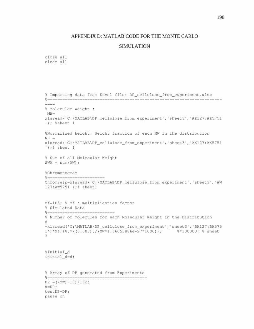
198

APPENDIX D: MATLAB CODE FOR THE MONTE CARLO

SIMULATION

close all clear all % Importing data from Excel file: DP_cellulose_from _experiment.xlsx %================================================== ======================== % Molecular weight : MW= xlsread('C:\MATLAB\DP_cellulose_from_experiment','s heet3','AZ127:AZ5751'); %sheet 1 %Normalized height: Weight fraction of each MW in t he distribution NH = xlsread('C:\MATLAB\DP_cellulose_from_experiment','s heet3','AX127:AX5751');% sheet 1 % Sum of all Molecular Weight SWM = sum(MW); %Chromotogram %======================= Chromresp=xlsread('C:\MATLAB\DP_cellulose_from_expe riment','sheet3','AW127:AW5751');% sheet1 Mf=1E5; % Mf : multiplication factor % Simulated Data %=========================== % Number of molecules for each Molecular Weight in the Distribution d =xlsread('C:\MATLAB\DP_cellulose_from_experiment',' sheet3','BA127:BA5751')*Mf;%%.*((0.003)./(MW*1.66053886e-27*1000)); %*100000; % sheet 3 %initial_d initial_d=d; % Array of DP generated from Experiments %======================================== DP =((MW)-18)/162; x=DP; testDP=DP; pause on

199

warning off %========================================== %Counter for number of runs: scissions %========================================== % dc=1000; % dcc is dc counter % cystp=100; % cycle step ( for the mod function) f or plotting every "cystp" %Counter for number of runs: scissions %========================================== dc=Mf;%sum(d); % dcc is dc counter cystp=dc/10;% cycle step ( for the mod function) fo r plotting every "cystp" %Mode of scission options: random_scission=1; center_scission=0; unzip_scission=0; %Plotting chromatogram %============================================= figure(1) semilogx(MW,Chromresp); title('Chromatogram response vs MW'); xlabel('MW'); ylabel('mV'); %pause %TN1=sum(d); % Affirming the Total number of molecu les TN=sum(d); %pause % Initial total number of bonds inumbond=sum((DP-1).*d); figure(2) semilogx(MW,d); title('Experimental MW Distribution '); xlabel('MW'); ylabel('# of Molecules'); %number average degree polymerization or average bo nd length

200

n_average(1)=(sum(DP.*d)/sum(d)); %Weight fraction in Mw %Mwt_frac=((DP*162+180).*d)/sum((DP*162+180).*d); % Normalized height h/total_h also refers to dw/dv %dw_dv=(d.*MW)/sum(d.*MW); dw_dv=NH; % Calibration equation from experiment is of the fo rm logMW = A + Bv; % where: A and B are intercept and gradient respect ively; v is elution volume; % dv/dlogMW equals the reciprocal of the gradient ( constant- linear) % therefore to obtain dw/dlogMW, we multiply dw/dv with dv/dlogMW % dw/dlogMW = dw/dv * dv/dlogMW dv_dlogMW = 643; dw_dlogMW = dw_dv*dv_dlogMW; ini_dw_dlogMW=dw_dlogMW; figure(3) semilogx(MW,dw_dlogMW)%'-g')%,DP,d,'-b'); %title(strcat('DP Distribution after Scission (rand om)',numberm_str)); xlabel('MW'); ylabel('dw/dlogMW'); hold on % figname=strcat('random',numberm_str); % cd(randomscission_files); % saveas(gcf, figname, 'pdf'); % saveas(gcf, figname, 'fig'); % saveas(gcf, figname, 'jpeg'); iDP=DP; plotlabel={'-r' '-b' '-r' '--r' '--k' '-k' '-g' '-- g' '-m' '-y' '--y'}; plotlabel_run={'Initial' 'plot1' 'plot2' 'plot3' 'p lot4' 'plot5' 'plot6'... 'plot7' 'plot8' 'plot9' 'Final'}; lg=1; % legend indices for plotlabel lw=1; lk=1; lh=1; dw_dlogMWA=dw_dlogMW; % Number of molecules for each Molecular Weight in the Distribution %d =flipud(xlsread('C:\Users\Kazeem\Documents\My Documents\MATLAB\DP_cellulose_from_experiment','she et3','O130:O2152'))*100000; % sheet 3 %initial_d initial_d=d;

201

% % Number average MW: iMn=sum(d/Mf.*MW)/sum(d/Mf); % % % DPn iDPn = (iMn-18)/162; % Percentage number of bonds broken Theoreticalpercent_bond_broken=(dc/inumbond)*100; imassmonomer=sum((DP).*d); %d=Sd; % DP with number of molecules > zero %DP=[DP(6:end)]; % POLYMER DEGRADATION SECTION %========================================== %(1) Random scission: %***************************************** % dc : degradation cycle if random_scission ==1 %dc=1; fprintf('==================================='); fprintf('\nRunning random scissioning'); fprintf('\n===================================\n'); % DP is the degree of polymerization mkdir('C:\MATLAB','Random_scission'); randomscission_files=('C:\MATLAB\Random_scission'); mkdir('C:\MATLAB','Random_scission_rawdata'); randomscission_rawdata=('C:\MATLAB\Random_scission_ rawdata'); % DP=M/162; to=0; % to : initial t % step1 : randomly select a polymer chain for sciss ioning: for t=1:dc % Calculating total number of bonds sTb=sum((DP-1).*d); % book keeping number of bonds at every cycle CsTb(t)=sum((DP-1).*d); %sTb=sum(d)-d(1); clear r;

202

CP=vertcat(Chromresp,d,DP); DP=DP'; % % randomly selecting chain length for scissio n % SDP=DP(1,ceil(length(DP)*rand)); % CSDP(t)=SDP; %Extracting the nonzeros elements.i.e. molecule s with bonds [rDPb cDPb]=size(nonzeros(DPb)); % randomly selecting bond to break from the who le molecules Pb=[ceil(rand*rDPb) ceil(cDPb*rand)]; [i j]=find(DPb==Pb(1));% noting bond point wit hin the matrix SDPb=DPb(i,j); CSDPb(t)=SDPb; % A(ceil(rand*4),ceil(5*rand)) ; A is a matri x of 4 by 5 %============================================= ============ if SDPb==0 d=d; DP=DP'; else % %Randomly selecting bond from the bondmat rix % Pb=DPb(1,ceil([rDPb,cDPb]*rand)); %To know the randomly selected bond %SDPb=DPb(Pb(1),Pb(2)); % To know all the bonds in the array where the bond is selected LDPb=nonzeros(DPb(i,1:end)); %The corresponding chain length from where the bond was randomly %selecetd within bondmatrix SDP=length(LDPb)+1; % finding the spot at which the randomly se lected bond is broken SB=find(LDPb==SDPb); % Two different chains from scission SB1=SDP-SB; CDP=[SB SB1]; DP1=CDP(1); DP2=CDP(2);

203

% Adding one more molecule to the number of molecules corresponding to DP with equal size to the two % new DPs formed d=d'; dp=find(DP==SDP); dp1=find(DP==DP1); dp2=find(DP==DP2); %increasing number of molecules by 1 for ea ch new chain %length formed which if DP1==DP2 || d(dp1)+2<d(dp1+1) d(dp1)=d(dp1)+2; elseif DP1~=DP2 || d(dp1)+1<d(dp1+1) d(dp1)=d(dp1)+1; elseif DP1~=DP2 && d(dp2)+1<d(dp2+1); d(dp2)=d(dp2)+1; else end MW=MW'; % decreasing number of molecules by 1 from the chain length % selected scissioned and if a polymer chai n has one molecule and % is scissioned removed from the distributi on to avoid % spikes between DP if isempty(dp)==1 elseif d(dp)>=1 && d(dp)-1<1 %d(dp)=0; %DP(dp)=0; %MW(dp)=0; %dw_dlogMWA(dp,t)=[]; d(dp)=d(dp); elseif d(dp)<1 d(dp)=d(dp); else d(dp)=d(dp)-1; end if SB==1 || SB==length(LDPb) ntzero=SDP-1; DPb(i,1:ntzero)=0; DPb(i,1:ntzero-1)=LDPb(1:length(LDPb)-1 )';

204

DPbr=DPb(DPb>max(LDPb))-1; DPb(DPb>max(LDPb))=DPbr; else ntzero=SDP-1; [ii jj]=size(DPb); DPb(i,1:ntzero)=0; DPb(i,1:SB-1)=LDPb(1:SB-1)'; DPb(ii+1,1:DP2-1)=LDPb(SB:length(LDPb)- 1); DPbr=DPb(DPb>max(LDPb))-1; DPb(DPb>max(LDPb))=DPbr; %maxnzero=max(nonzeros(DPb)); %maxnzero:maxnzero+DP1-2; %DPb(ii+2,1:DP2-1)=maxnzero+DP1-1:(maxn zero+DP1-1)+DP2-2; end DP=DP'; d=d'; MW=MW' end d=d; % array of new values for the number of mo lecules %Number_m1(:,t)=d; %Weight fraction in Dp wt_frac=(DP.*d)/sum(DP.*d); %Weight fraction in Mw Mwt_frac=((DP*162+180).*d)/sum((DP*162+180).*d) ; % Normalized height h/total_h also refers to dw /dv dw_dv=(d.*MW)/sum(d.*MW); %Number average MW: Mn(t)=sum(d/Mf.*MW)/sum(d/Mf); % DPn DPn(t) = (Mn(t)-18)/162;

205

% Percentage of average bonds broken Percent_bond_broken(t) = ((iMn-Mn(t))/iMn)*100; %dw_dv=(NMW)/sum(NMW); %dw_dv=Mwt_frac; % Calibration equation from experiment is of th e form logMW = A + Bv; % where: A and B are intercept and gradient res pectively; v is elution volume; % dv/dlogMW equals the reciprocal of the gradie nt (constant- linear) % therefore to obtain dw/dlogMW, we multiply dw /dv with dv/dlogMW % dw/dlogMW = dw/dv * dv/dlogMW %dv_dlogMW = 643.3198705; %dw_dlogMW = dw_dv*dv_dlogMW; %dw_dlogMWA(1:end,t)=dw_dlogMW; dw_dlogMW = MW.*(d/Mf); %Differential fraction dw_frac=(log(10))*(DP).*Mwt_frac; lgMw=log10(DP*162); %MW=MW; xlcol={'B' 'C' 'D' 'E' 'F' 'G' 'H' 'I' 'J' 'K' 'L' 'M' 'N' 'O' 'P' 'Q'}; xlcol_num=2:2050; if mod(t,cystp)==0 || t==1 figure(3) %semilogx(MW,wt_frac,plotlabel{lh})%'-g')%, DP,d,'-b'); semilogx(MW,dw_dlogMW,plotlabel{lh})%'-g')% ,DP,d,'-b'); %title(strcat('DP Distribution after Scissi on (random)',numberm_str)); xlabel('MW'); ylabel('dw/dlogMW'); legend(plotlabel_run); hold on %figname=strcat('random',numberm_str); cd(randomscission_files); % saveas(gcf, figname, 'pdf'); % saveas(gcf, figname, 'fig'); % saveas(gcf, figname, 'jpeg'); % MW % Storing data in Excel %============================== dw_dlogMW_SUCCESS = xlswrite('C:\MATLAB\Random_scission_rawdata\Randoms cissiondata.xlsx',dw_dlogMW,'dw_dlogMW1000_100A',...

206

strcat(xlcol{lh},num2str(xlcol_num(1)),:,xlcol{lh}, num2str(xlcol_num(end)))); MW_SUCCESS = xlswrite('C:\MATLAB\Random_scission_rawdata\Randoms cissiondata.xlsx',MW,'dw_dlogMW1000_100A','A2:A2050'); %========================================== ====== lh=lh+1; %hold off %wt_frac=wt_frac*643; figure(4) semilogx(DP,wt_frac,plotlabel{lg})%'-g')%,D P,d,'-b'); %title(strcat('DP Distribution after Scissi on (random)',numberm_str)); xlabel('DP'); ylabel('Weight Fraction'); legend(plotlabel_run); hold on %figname=strcat('random',numberm_str); cd(randomscission_files); % saveas(gcf, figname, 'pdf'); % saveas(gcf, figname, 'fig'); % saveas(gcf, figname, 'jpeg'); % %Storing data in Excel % ============================== % WTFRAC_SUCCESS = xlswrite('C:\Users\Kazee m\Documents\My Documents\MATLAB\Random_scission_rawdata\Randomscis siondata.xls',wt_frac','weightfraction',... % strcat(xlcol{lg},num2str(xlcol_num(1)),:,xlcol{lg}, num2str(xlcol_num(end)))); % DP_SUCCESS = xlswrite('C:\Users\Kazeem\Do cuments\My Documents\MATLAB\Random_scission_rawdata\Randomscis siondata.xls',DP','weightfraction','A2:A454'); % %======================================== ======== lg=lg+1; hold off % % end %MW=NMW;

207

TN(t)=sum(d); % Caculating the new total number of molecues after each cycle % end DW_DLOGMWA = xlswrite('C:\MATLAB\Random_scission_rawdata\Randoms cissiondata.xlsx',dw_dlogMWA,'dw_dlogMWA'); %AREA_A = xlswrite('C:\Users\Kazeem\Documents\My Documents\MATLAB\Random_scission_rawdata\Randomscis siondata.xlsx',SMWC','SMWCT1000_100'); % figure(3) % %plot(x,fracpdfNormal2); % plot(DP,d,'-r')%,DP,d,'-b'); % title('DP Distribution after Scission'); % xlabel('DP'); % ylabel('# of Molecules and Probability'); % hold on %cd('..'); % clear i j end %% center scission session %========================================== %%(2)center scission: %***************************************** %polymer chain to be scissioned at the center %%================================================= ========================= % dc : degradation cycle if center_scission==1 %dc=1; % DP is the degree of polymerization %dc=1; fprintf('==================================='); fprintf('\nRunning center scissioning'); fprintf('\n===================================\n'); % DP is the degree of polymerization mkdir('C:\MATLAB','Center_scission'); centerscission_files='C:\MATLAB\Center_scission'; mkdir('C:\MATLAB','Center_scission_rawdata'); randomscission_rawdata=('C:\MATLAB\Center_scission_ rawdata');

208

% DP=M/162; to=0 % to : initial t % step1 : randomly select a polymer chain for sciss ioning: for t=1:dc % Calculating total number of bonds sTb=sum((DP-1).*d); % book keeping number of bonds at every cycle CsTb(t)=sum((DP-1).*d); %sTb=sum(d)-d(1); clear r; CP=vertcat(Chromresp,d,DP); DP=DP'; % randomly selecting chain length for scission SDP=DP(1,ceil(length(DP)*rand)); CSDP(t)=SDP; if SDP==1 d=d; DP=DP'; else SDP > 1 ; % Forming an array out of the selected DP ( SDP) SBDP=1:SDP; % Forming an array of number of bonds from the selected DP (SDP) NSBDP=1:SDP-1; % Checking if selected DP is odd or even an d selecting bond to % break from the selected chain if mod(max(NSBDP),2)==0 % for even number o f bonds SB=max(NSBDP)/2; SB1=SB-1; CDP=[SB+1 SB1+1];% DP=number of bonds + 1; that is why SB+1 or SB1+1 are the new DPs else PSB=median(NSBDP); % for odd number of bonds SB=length(NSBDP)-PSB; SB1=SB;

209

CDP=[SB+1 SB1+1]; % two new chains form ed with DPs : SB+1 ans SB1+1 end DP1=CDP(1); DP2=CDP(2); % Adding one more molecule to the number of molecules corresponding to DP with equal size to the two % new DPs formed d=d'; dp=find(DP==SDP); dp1=find(DP==DP1); dp2=find(DP==DP2); % decreasing number of molecules by 1 from the chain length selected scissioned if d(dp)>=1 d(dp)=d(dp)-1; else d(dp)=d(dp); end %increasing number of molecules by 1 for ea ch new chain %length formed which if DP1==DP2 d(dp1)=d(dp1)+2; else d(dp1)=d(dp1)+1; d(dp2)=d(dp2)+1; end DP=DP'; d=d'; end d=d; % array of new values for the number of mo lecules %Number_m1(:,t)=d; %Weight fraction in Dp wt_frac=(DP.*d)/sum(DP.*d); %Weight fraction in Mw

210

Mwt_frac=((DP*162+180).*d)/sum((DP*162+180).*d) ; % Normalized height h/total_h also refers to dw /dv dw_dv=(d.*MW)/sum(d.*MW); %Number average MW: Mn(t)=sum(d/1E9.*MW)/sum(d/1E9); % DPn DPn(t) = (Mn(t)-18)/162; % Percentage of average bonds broken Percent_bond_broken(t) = ((iMn-Mn(t))/iMn)*100; %dw_dv=(NMW)/sum(NMW); %dw_dv=Mwt_frac; % Calibration equation from experiment is of th e form logMW = A + Bv; % where: A and B are intercept and gradient res pectively; v is elution volume; % dv/dlogMW equals the reciprocal of the gradie nt (constant- linear) % therefore to obtain dw/dlogMW, we multiply dw /dv with dv/dlogMW % dw/dlogMW = dw/dv * dv/dlogMW dv_dlogMW = 643.3198705; dw_dlogMW = dw_dv*dv_dlogMW; dw_dlogMWA(1:end,t)=dw_dlogMW; %Differential fraction dw_frac=(log(10))*(DP).*Mwt_frac; lgMw=log10(DP*162); % Number fraction num_frac = d/sum(d); xlcol={'B' 'C' 'D' 'E' 'F' 'G' 'H' 'I' 'J' 'K' 'L' 'M' 'N' 'O' 'P' 'Q'}; xlcol_num=2:5625; if mod(t,cystp)==0 || t==1 figure(3) semilogx(MW,dw_dlogMW,plotlabel{lh})%'-g')% ,DP,d,'-b'); %title(strcat('DP Distribution after Scissi on (random)',numberm_str)); xlabel('MW'); ylabel('dw/dlogMW'); legend(plotlabel_run); hold on % figname=strcat('center',numberm_str);

211

cd(centerscission_files); % saveas(gcf, figname, 'pdf'); % saveas(gcf, figname, 'fig'); % saveas(gcf, figname, 'jpeg'); % % Storing data in Excel %============================== dw_dlogMW_SUCCESS = xlswrite('C:\MATLAB\Center_scission_rawdata\Centers cissiondata.xlsx',dw_dlogMW,'dw_dlogMW42000_4200C',... strcat(xlcol{lh},num2str(xlcol_num(1)),:,xlcol{lh}, num2str(xlcol_num(5624)))); MW_SUCCESS = xlswrite('C:\MATLAB\Center_scission_rawdata\Centers cissiondata.xlsx',MW,'dw_dlogMW42000_4200C','A2:A5625'); %========================================== ====== lh=lh+1; %hold off % % end %TN(dc)=sum(d); % Caculating the new total numb er of molecues after each cycle TN=sum(d); TN1(t)=sum(d); %d=TN*Probdf; %pause(4) end % end %% unzip scission session %========================================== %%(2)unzip scission: %***************************************** %polymer chain to be scissioned at the end (reducin g end) %%================================================= ========================= % dc : degradation cycle if unzip_scission==1 %dc=1;

212

% DP is the degree of polymerization %dc=1; fprintf('==================================='); fprintf('\nRunning unzip scissioning'); fprintf('\n===================================\n'); % DP is the degree of polymerization mkdir('C:\Users\Kazeem\Documents\My Documents\MATLA B','Unzip_scission') unzipscission_files='C:\Users\Kazeem\Documents\My Documents\MATLAB\Unzip_scission'; mkdir('C:\Users\Kazeem\Documents\My Documents\MATLAB','Unzip_scission_rawdata'); randomscission_rawdata=('C:\Users\Kazeem\Documents\ My Documents\MATLAB\Unzip_scission_rawdata'); % DP=M/162; to=0 % to : initial t % step1 : randomly select a polymer chain for sciss ioning: for t=1:10 % Calculating total number of bonds sTb=sum((DP-1).*d); % book keeping number of bonds at every cycle CsTb(t)=sum((DP-1).*d); %sTb=sum(d)-d(1); clear r; CP=vertcat(Chromresp,d,DP); DP=DP'; % randomly selecting chain length for scission SDP=DP(1,ceil(length(DP)*rand)); CSDP(t)=SDP; if SDP==1 d=d; DP=DP'; else SDP > 1 ; % Forming an array out of the selected DP ( SDP) SBDP=1:1:SDP;

213

% Breaking off one bond from the end of the selected chain uzb=1; % number of unzip bonds from any of the chain ends SB=length(SBDP)-uzb; SB1=uzb; % Two different chains from scission CDP=[SB SB1]; DP1=CDP(1); DP2=CDP(2); % Adding one more molecule to the number of molecules corresponding to DP with equal size to the two % new DPs formed d=d'; dp=find(DP==SDP); dp1=find(DP==DP1); dp2=find(DP==DP2); % decreasing number of molecules by 1 from the chain length selected scissioned if d(dp)>=1 d(dp)=d(dp)-1; else d(dp)=d(dp); end %increasing number of molecules by 1 for ea ch new chain %length formed which if DP1==DP2 d(dp1)=d(dp1)+2; else d(dp1)=d(dp1)+1; d(dp2)=d(dp2)+1; end DP=DP'; d=d'; end d=d; % array of new values for the number of mo lecules %Number_m1(:,t)=d; %Weight fraction in Dp wt_frac=(DP.*d)/sum(DP.*d);

214

%Weight fraction in Mw Mwt_frac=((DP*162+180).*d)/sum((DP*162+180).*d) ; % Normalized height h/total_h also refers to dw /dv dw_dv=(d.*MW)/sum(d.*MW); %dw_dv=(NMW)/sum(NMW); %dw_dv=Mwt_frac; % Calibration equation from experiment is of th e form logMW = A + Bv; % where: A and B are intercept and gradient res pectively; v is elution volume; % dv/dlogMW equals the reciprocal of the gradie nt (constant- linear) % therefore to obtain dw/dlogMW, we multiply dw /dv with dv/dlogMW % dw/dlogMW = dw/dv * dv/dlogMW dv_dlogMW = 643.3198705; dw_dlogMW = dw_dv*dv_dlogMW; dw_dlogMWA(1:end,t)=dw_dlogMW; %Differential fraction dw_frac=(log(10))*(DP).*Mwt_frac; lgMw=log10(DP*162); % Number fraction num_frac = d/sum(d); xlcol={'B' 'C' 'D' 'E' 'F' 'G' 'H' 'I' 'J' 'K' 'L' 'M' 'N' 'O' 'P' 'Q'}; xlcol_num=2:2050; if mod(t,cystp)==0 || t==1 % figure(3) % %plot(x,fracpdfNormal2); % plot(DP,Number_m1); % title('DP Distribution after Scission (un zip)'); % xlabel('DP'); % ylabel('Number of molecules'); % hold on % % figure(4) % %plot(x,fracpdfNormal2); % plot(DP,P,'-r')%,DP,d,'-b'); % title('DP Distribution after Scission (un zip)'); % xlabel('DP');

215

% ylabel('Probability'); % hold on figure(3) semilogx(MW,dw_dlogMW,plotlabel{lg})%'-g')% ,DP,d,'-b'); %title(strcat('DP Distribution after Scission(unzip',az,'mer)',numberm_str)); xlabel('MW'); ylabel('dw/dlogMW'); legend(plotlabel_run); hold on %figname=strcat('unzip_',az,'mers',numberm_ str); cd(unzipscission_files); % saveas(gcf, figname, 'pdf'); % saveas(gcf, figname, 'fig'); % saveas(gcf, figname, 'jpeg'); % Storing data in Excel %============================== WTFRAC_SUCCESS = xlswrite('C:\Users\Kazeem\ Documents\My Documents\MATLAB\Unzip_scission_rawdata\Unzipscissi ondata.xlsx',dw_dlogMW,'dw_dlogMW2000_200',... strcat(xlcol{lg},num2str(xlcol_num(1)),:,xlcol{lg}, num2str(xlcol_num(end)))); DP_SUCCESS = xlswrite('C:\Users\Kazeem\Docu ments\My Documents\MATLAB\Unzip_scission_rawdata\Unzipscissi ondata.xlsx',MW,'dw_dlogMW2000_200','A2:A2050'); %========================================== ====== lg=lg+1; % end %TN(dc)=sum(d); % Caculating the new total numb er of molecues after each cycle TN=sum(d); % TN1(t)=sum(d); %d=TN*Probdf; %pause(4) end % figure(3) % %plot(x,fracpdfNormal2); % plot(DP,d,'-r')%,DP,d,'-b'); % title('DP Distribution after Scission'); % xlabel('DP');

216

% ylabel('# of Molecules and Probability'); % hold on cd('..'); % clear i j end

217

REFERENCES

(1) Simmons, B. A.; Singh, S.; Holmes, B. M.; Blanch, H. W. Ionic Liquid Pretreatment. CEP 2010, 106, 50-55.

(2) Ladisch, M. R.; Mosier, N. S.; Kim, Y.; Ximenes, E.; Hogsett, D. Converting Cellulose to Biofuels. CEP 2010, 106, 56-62.

(3) U.S.D.O.E Biomass Multi-Year Program Plan Report. http://www1.eere.energy.gov/biomass/pdfs/biomass_program_mypp.pdf2007).

(4) Himmel, M. E., Ed.; In Biomass Recalcitrance; 2008; Vol. 1, pp 495.

(5) Ziegler, J. The Right to Food,". United Nations General Assembly Report 2007, A/62/289.

(6) Cortes-Caminero, M. Engineering Advanced Biofuels. CEP 2010, 106, 35.

(7) E.E.R.E PLANT/CROP-BASED RENEWABLE RESOURCES 2020. 1998, DOE/GO-10097-385, 1-24.

(8) U.S.D.O.E Biomass Multi-Year Program Plan Report. http://www1.eere.energy.gov/biomass/pdfs/biomass_program_mypp.pdf (accessed 03/25, 2010).

(9) U.S.D.A & U.S.D.O.E (2005) Biomass as Feedstock for a Bioenergy and Bioproducts Industry: The Technical Feasibility of a Billion-Ton Annual Supply. http://www1.eere.energy.gov/biomass/pdfs/final_billionton_vision_report2.pdf (accessed 11, 2007).

(10) Knauf, M.; Moniruzzaman, M. Lignocellulosic Biomass Process: A Perspective. International Sugar Journal 2004, 106, 147-150.

(11) Ehara, K.; Saka, S. Decomposition Behavior of Cellulose in Supercritical Water, Subcritical Water, and their Combined Treatments. Journal of Wood Science 2005, 51, 148-153.

(12) NEED In Biomass; Secondary Energy Infobook; Manassas, VA, 2007; pp 12-15.

(13) 106th Congress Public Law 106-224. 2000, 301-310.

(14) Zhang, T. Glucose Production from Cellulose in Subcritical and Supercritical Water, The University of Iowa, 2008.

218

(15) Bruice, P. Y. In Carbohydrates; Folchetti, N., Mullaney, R., Kaveney, D., Lerner-Nelson, M. and Richards, M. J., Eds.; Organic Chemistry; Pearson Prentice Hall: Upper Saddle River, NJ, 2007; pp 1-2-1317.

(16) Krassig, H. A. In The Fiber Structure; Cellulose; Gordon and Breach Science: Amsterdam, The Netherlands, 1993; Vol. 11, pp 6-7-42.

(17) Jessop, P. G.; Leitner, W. In Supercritical Fluids as Media for Chemical Reactions; Jessop, P. G., Leitner, W., Eds.; Chemical Synthesis Using Supercritical Fluids; Wiley-VCH: Weinheim, Germany, 1999; pp 1-2-65.

(18) Linstrom, P. J.; and Mallard, W. G. National Institute of Standards and Technology, Gaithersburg MD, 20899. http://webbook.nist.gov (accessed 4/30, 2010).

(19) Linstrom, P. J.; and Mallard, W. G., Eds.; In NIST Chemistry WebBook, NIST Standard Reference Database .; Lemmon, E. W., McLinden, M. O. and and Friend, D. G., Eds.; "Thermophysical Properties of Fluid Systems"; .

(20) Baiker, A. Supercritical Fluids in Heterogeneous Catalysis. Chem. Rev. 1999, 99, 453-473.

(21) Li, L.; Kiran, E. Gas-Liquid Critical Properties of Methylamine + Nitrous-Oxide and Methylamine + Ethylene Binary-Mixtures. J. Chem. Eng. Data 1988, 33, 342-344.

(22) Savage, P. E.; Gopalan, S.; Mizan, T. I.; Martino, C. J.; Brock, E. E. Reactions at Supercritical Conditions - Applications and Fundamentals. AICHE J. 1995, 41, 1723-1778.

(23) Kiran, E., Debenedetti, P. G., and Peters, C. J., Ed.; In Supercritical Fluids (Fundamentals and Applications); Kluwer Academic Publishers: Dordrecht, The Netherlands, 1999; Vol. 366, pp 591.

(24) Yesodharan, S. Supercritical Water Oxidation: An Environmentally Safe Method for the Disposal of Organic Wastes. Curr. Sci. 2002, 82, 1112-1122.

(25) Schmieder, H.; Abeln, J. Supercritical Water: State of the Art. Chem. Eng. Technol 1999, 22, 903-904-908.

(26) Mesiano, A. J.; Beckman, E. J.; Russell, A. J. Supercritical Biocatalysis. Chem. Rev. 1999, 99, 623-633.

(27) Kajimoto, O. Solvation in Supercritical Fluids: Its Effects on Energy Transfer and Chemical Reactions. Chem. Rev. 1999, 99, 355-389.

(28) Jessop, P. G.; Ikariya, T.; Noyori, R. Homogeneous Catalysis in Supercritical Fluids. Chem. Rev. 1999, 99, 475-493.

219

(29) Brennecke, J. F.; Chateauneuf, J. E. Homogeneous Organic Reactions as Mechanistic Probes in Supercritical Fluids. Chem. Rev. 1999, 99, 433-452.

(30) Arthur E. Humphrey In The Hydrolysis of Cellulosic Materials to Useful Products; Brown, R. D., Jurasek, L., Eds.; Hydrolysis of Cellulose: Mechanisms of Enzymatic and Acid Catalysis; American Chemical Society: Washington, D. C., 1979; pp 25-53.

(31) Lipinsky, E. S. In Perspectives on Preparation of Cellulose for Hydrolysis; Brown, R. D., Jurasek, L., Eds.; Hydrolysis of Cellulose: Mechanisms of Enzymatic and Acid Catalysis; American Chemical Society: Washington, D. C., 1979; pp 1-24.

(32) Sasaki, M.; Adschiri, T.; Arai, K. Kinetics of Cellulose Conversion at 25 MPa in Sub- and Supercritical Water. AICHE J. 2004, 50, 192-202.

(33) Fan, L. T.; Gharpuray, M. M.; Lee, Y. -. In Cellulose Hydrolysis; Aiba, S., Fan, L. T., Fiechter, A., Klein, J. and Schugerl, K., Eds.; Springer-Verlag: Berlin Heidelberg, New York, 1987; Vol. 3, pp 197.

(34) Zhang, Y. P.; Lynd, L. R. Toward an Aggregated Understanding of Enzymatic Hydrolysis of Cellulose: Noncomplexed Cellulase Systems. Biotechnol. Bioeng. 2004, 88, 797-798-824.

(35) Sasaki, M.; Fang, Z.; Fukushima, Y.; Adschiri, T.; Arai, K. Dissolution and Hydrolysis of Cellulose in Subcritical and Supercritical Water. Ind Eng Chem Res 2000, 39, 2883-2890.

(36) Saeman, J. F. Kinetics of Wood Saccharification - Hydrolysis of Cellulose and Decomposition of Sugars in Dilute Acid at High Temperature. Industrial and Engineering Chemistry 1945, 37, 43-52.

(37) Girisuta, B.; Janssen, L. P. B. M.; Heeres, H. J. Kinetic Study on the Acid-Catalyzed Hydrolysis of Cellulose to Levulinic Acid. Ind Eng Chem Res 2007, 46, 1696-1708.

(38) Xiang, Q.; Lee, Y. Y.; Pettersson, P. O.; Torget, R. Heterogeneous Aspects of Acid Hydrolysis of Alpha-Cellulose. Appl. Biochem. Biotechnol. 2003, 105, 505-514.

(39) Wood, T. M.; McCrae, S. I. In Synergism Between Enzymes Involved in the Solubilization of Native Cellulose; Brown, R. D., Jurasek, L., Eds.; Hydrolysis of Cellulose: Mechanisms of Enzymatic and Acid Catalysis; American Chemical Society: Washington, D. C., 1979; pp 181-210.

(40) Kearsley, M. W.; Dziedzic, S. Z. In Handbook of Starch Hydrolysis Product and their Derivatives; Blackie Academy and Professional: 1996; , pp 275.

220

(41) Eremeeva, T.; Bikova, T.; Eisimonte, M.; Viesturs, U.; Treimanis, A. Fractionation and Molecular Characteristics of Cellulose during Enzymatic Hydrolysis. Cellulose 2001, 8, 69-79.

(42) Wald, S.; Wilke, C. R.; Blanch, H. W. Kinetics of the Enzymatic-Hydrolysis of Cellulose. Biotechnol. Bioeng. 1984, 26, 221-230.

(43) Saka, S.; Ueno, T. Chemical Conversion of various Celluloses to Glucose and its Derivatives in Supercritical Water. Cellulose 1999, 6, 177-191.

(44) Antal, M. J.; Allen, S. G.; Schulman, D.; Xu, X. D.; Divilio, R. J. Biomass Gasification in Supercritical Water. Ind Eng Chem Res 2000, 39, 4040-4053.

(45) Minowa, T.; Ogi, T.; Yokoyama, S. Hydrogen-Production from Wet Cellulose by Low-Temperature Gasification using a Reduced Nickel-Catalyst. Chem. Lett. 1995, 937-938.

(46) Sakaki, T.; Shibata, M.; Miki, T.; Hirosue, H.; Hayashi, N. Decomposition of Cellulose in Near-Critical Water and Fermentability of the Products. Energy Fuels 1996, 10, 684-688.

(47) Matsumura, Y.; Sasaki, M.; Okuda, K.; Takami, S.; Ohara, S.; Umetsu, M.; Adschiri, T. Supercritical Water Treatment of Biomass for Energy and Material Recovery. Combustion Sci. Technol. 2006, 178, 509-536.

(48) Kabyemela, B. M.; Adschiri, T.; Malaluan, R. M.; Arai, K. Glucose and Fructose Decomposition in Subcritical and Supercritical Water: Detailed Reaction Pathway, Mechanisms, and Kinetics. Ind Eng Chem Res 1999, 38, 2888-2895.

(49) Zhang, T. Glucose Production from Cellulose in Subcritical and Supercritical Water, The University of Iowa, Iowa City, Iowa, USA, 2008.

(50) Nagamori, M.; Funazukuri, T. Glucose Production by Hydrolysis of Starch Under Hydrothermal Conditions. Journal of Chemical Technology and Biotechnology 2004, 79, 229-233.

(51) Rosen, S. L. In Characterization of Molecular Weight; Fundamental Principles of Polymeric Materials; John Wiley & Sons, Inc.: New York, 1993; pp 53-78.

(52) Trathnigg, B. In Size-exclusion Chromatography of Polymers; Encyclopedia of Analytical Chemistry; John Wiley & Sons Ltd: Chichester, 2000; pp 8008-8008.

(53) VARIAN, I. GPC/SEC Reference Guide. 2010.

(54) Synder, L.; Kirkland, J. J. In Introduction to Modern Liquid Chromatography; John Wiley & Sons, Inc.: New York, 1979; .

221

(55) Chang, M.; Pound, T. C.; Manley, R. S. J. Gel-Permeation Chromatographic Studies of Cellulose Degradation .1. Treatment with Hydrochloric-Acid. Journal of Polymer Science Part B-Polymer Physics 1973, 11, 399-411.

(56) Berggren, R.; Berthold, F.; Sjoholm, E.; Lindstrom, M. Improved Methods for Evaluating the Molar Mass Distributions of Cellulose in Kraft Pulp. J Appl Polym Sci 2003, 88, 1170-1179.

(57) Kanda, T.; Nakakubo, S.; Wakabayashi, K.; Nisizawa, K. In The Mode of Enzymatic Degradation of Cellulose Based on the Properties of Cellulase Components; Brown, R. D., Jurasek, L., Eds.; Hydrolysis of Cellulose: Mechanisms of Enzymatic and Acid Catalysis; American Chemical Society: Washington, D. C., 1979; pp 211-236.

(58) Schnabel, W. In Mechanistic Aspects; Polymer Degradation, Principles and Practical applications; Macmillan Publishing Co., Inc.: New York, 1981; pp 13-24.

(59) Guaita, M.; Chiantore, O.; Luda, M. P. Monte-Carlo Simulations of Polymer Degradations .1. Degradations without Volatilization. Macromolecules 1990, 23, 2087-2092.

(60) Emsley, A. M.; Heywood, R. J. Computer Modeling of the Degradation of Linear-Polymers. Polym. Degrad. Stab. 1995, 49, 145-149.

(61) Bose, S. M.; Git, Y. Mathematical Modelling and Computer Simulation of Linear Polymer Degradation: Simple Scissions. Macromolecular Theory and Simulations 2004, 13, 453-473.

(62) Montroll, E. W.; Simha, R. Theory of Depolymerization of Long Chain Molecules. Journal of Chemical Physics 1940, 8, 721-722-727.

(63) Basedow, A. M.; Ebert, K. H.; Fosshag, E. Ultrasonic Degradation of Polymers in Mixed-Solvents. Makromolekulare Chemie-Macromolecular Chemistry and Physics 1978, 179, 2565-2568.

(64) Mostafa, M. A. K. Degradation of Addition Polymers by Ultrasonic Waves. Journal of Polymer Science 1956, 22, 535-548.

(65) Glynn, P. A. R.; Vanderho.Bm; Reilly, P. M. General Model for Prediction of Molecular-Weight Distributions of Degraded Polymers - Development and Comparison with Ultrasonic Degradation Experiments. Journal of Macromolecular Science-Chemistry 1972, A 6, 1653-1664.

(66) Ballauff, M.; Wolf, B. A. Degradation of Chain Molecules .1. Exact Solution of the Kinetic-Equations. Macromolecules 1981, 14, 654-658.

222

(67) Ballauff, M.; Wolf, B. A. Degradation of Chain Molecules .2. Thermodynamically Induced Shear Degradation of Dissolved Polystyrene. Macromolecules 1984, 17, 209-216.

(68) Yoshioka, T.; Motoki, T.; Okuwaki, A. Kinetics of Hydrolysis of Poly(Ethylene Terephthalate) Powder in Sulfuric Acid by a Modified Shrinking-Core Model. Ind Eng Chem Res 2001, 40, 75-79.

(69) Yoshioka, T.; Okayama, N.; Okuwaki, A. Kinetics of Hydrolysis of PET Powder in Nitric Acid by a Modified Shrinking-Core Model. Ind Eng Chem Res 1998, 37, 336-340.

(70) ASTM Standard D 1795-96 In Standard Test Method for Intrinsic Viscosity of Cellulose; Annual Book of ASTM Standards; 1997; Vol. 05.01, pp 345-350.

(71) He, C.; Wang, Q. Viscometric Study of Cellulose in PF/DMSO Solution. J. M. S. -Pure Appl. Chem. , 1999, A36, 105-114.

(72) Merienne, S.; Busnel, J. P.; Fricoteaux, F.; Prudhomme, J. C. Size Exclusion Chromatography of Dextrans in DMSO as Eluent. J. Liq. Chromatogr. Rel. Technol. 2000, 23, 1745-1746-1756.

(73) Striegel, A. M.; Timpa, J. D. Size Exclusion Chromatography of Polysaccharides in Dimethylacetamide-Lithium Chloride. Strategies in Size Exclusion Chromatography 1996, 635, 366-378.

(74) Dadi, A. P.; Varanasi, S.; Schall, C. A. Enhancement of Cellulose Saccharification Kinetics using an Ionic Liquid Pretreatment Step. Biotechnol. Bioeng. 2006, 95, 904-910.

(75) Kamiya, N.; Matsushita, Y.; Hanaki, M.; Nakashima, K.; Narita, M.; Goto, M.; & Takahashi, H. Enzymatic in Situ Saccharification of Cellulose in Aqueous-Ionic Liquid Media. Biotechnol. Lett. 2008, 30, 1037-1038-1040.

(76) Remsing, R. C.; Swatloski, R. P.; Rogers, R. D.; Moyna, G. Mechanism of Cellulose Dissolution in the Ionic Liquid 1-n-Butyl-3-Methylimidazolium Chloride: A C-13 and Cl-35. Chemical Communications 2006, 1271-1273.

Reaction kinetics of cellulose hydrolysis in subcritical and ...

Documents

Transcript of Reaction kinetics of cellulose hydrolysis in subcritical and ...