The University of Alberta

RATIONAL DESIGN OF PRESTRESSED AND REINFORCED

CONCRETE TANKS

- - Abdelazîz Abdo Rashed . S.,

L'

A thesis submitted to the Faculty of Graduate Studies and Research

in partial fulfillment of the requirements for the degree of

Doctor of Philosophy

in

Structural Engineering

Department of Civil and Environmental Engineering

Edmonton, Alberta

Spring, 1998

National Library 1 . canada Biblioth ue nationale du Cana '2 a

Acquisitions and Acquisitions et Bibliographie Services services bibliographiques 395 Wellington Street 395, rue Wellingtoci OttawaON K 1 A W ûttawaON K1A O N 4 Canada Canada

The author has granted a non- L'auteur a accorde une licence non exclusive licence allowing the exclusive permettant à la National Library of Canada to Bibliothèque nationale du Canada de reproduce, loan, distribute or sel reproduire, prêter, distribuer ou copies of this thesis in microform, vendre des copies de cette thèse sous paper or electronic formats. la fome de rnicrofiche/fïlm, de

reproduction sur papier ou sur format électronique.

The author retains ownership of the L'auteur conserve la propriété du copyright in this thesis. Neither the droit d'auteur qui protège cette thèse. thesis nor substantial extracts fiom it Ni la thèse ni des extraits substantiels may be printed or otherwise de celle-ci ne doivent être imprim6s reproduced without the author's ou autrement reproduits sans son permission. autozisation.

Abstract

The structural design of environmental concrete structures such as water reservoirs

and sewage treatment tanks is not covered explicitly in Canadian design standards. A

variety of foreign sources are frequently used. While al1 these sources purport to produce

safe, leak resistant and durable tanks, the various design standards require significantly

different arnounts of reinforcement and concrete. The most significant difference appears

between the design of reinforced concrete and prestressed concrete tanks. The lack of

agreement between the major sources implies that the profession has yet to converge

upon a rational solution. The objective of this snidy is to rationaiize the design procedures

for reinforced and prestressed concrete tanks so that an applicable Canadian design

standard be developed. The study investigates the concept of partial prestressing in liquid

containment structures. This concept is currently used successhilly in the design of other

types of structures. Understanding the behaviour of partially prestressed tanks is the key

for providing rational solutions ranging from reinforced concrete at one end of the design

spectrum to fùlly prestressed concrete at the other.

The present study included experirnental and analytical phases. In the experimental

phase a toiai of eight full-scaie specimens, representing segments fiom typical tank walls.

were subjected to load and leakage tests. The test specimens covered a range of

prestressed and non-prestressed reinforcernent ratios and were subjected to various

combinations of loads. Also, while the specimens were under load, leakage tests were

conducted to obtain leakage rates through the cracks. The results of both tests are

described. The ability of a flexural compression zone to prevent leakage. and the ability

of fine cracks to seal themselves (autohealing) are discussed. They appear to be important

design parameters that are not explicitly recognized in current design standards.

In the analytical study a computer model that can predict the response of tank wall

segments is described and calibrated against the test results. The model is used to carry

out a pararnetric study which investigates additional combinations of reinforcement and

loading. The combination of the physical experiments, and the numerical experiments is

used to develop a design procedure. The proposed design procedure addresses the leakage

limit state directly. It is applicable for fully prestressed, fully reinforced and partially

prestressed concrete water tanks.

The author wishes to express his deep appreciation and sincere gratitude to his

research supervisors. Professors David M. Rogowsky and Alaa E. Elwi for their

consistent guidance, valuable comments and suggestions, and constructive

encouragement throughout the course of this study.

The assistance and cooperation of Lany Burden and Richard Helfrich of the I.F.

Momsion Structural Laboratory, University of Alberta. in the expenmental prograrn are

gratefully acknowledged. The assistance provided by Dr. Scon D. B. Alexander with

the data acquisition system and by the author's colleagues with the concrete casting is

deeply appreciated.

The author would like to acknowledge the following organizations for their

financial support: the Natural Sciences and Engineering Research Council of Canada.

the Province of Alberta. and the University of Alberta Faculty of Graduate Studies and

Research. The donations of materials and components by VSL Corporation. Lafarge

Canada Inc.. and Inland Cernent for the experimental program are gratefully

acknowledged.

The author deeply appreciates the support and patience of his wife and children

throughout the course of this study.

1 - INTRODUCTION .................................................................................................................................. 1

1.1 GENERAL ............................................................................................................................................ 1 ................................................................................................................ 1.2 OBJECTIVES OF THIS STUDY 2

...................................................................................................................... 1.3 SCOPE OF THE THESIS 3 ........................................................................................................... 1 . 4 ORGANIZATION OF THE THESIS 3

2- PRELIMINARY REVIEW .................................................................................................................... 6

................................................................................................................................... 2.1 ~NTRODUCTION 6 ...................................................... ....................... 2.2 DESIGN APPROACHES - A LITERATURE REVIEW ..., 6

2.2.1 Design Philosophy ...................................................................................................................... 6

A Cl 350R ( 1 989) "Environmental Engineering Concrete Structures" ............................................... .............................................................................................................. Portland Cernent Association 8

. 4 CI 3.14 "Design and Construction of Circular Prestressed Concrete Structures" and Presrressed Concrete Institute ................................................................................................................................ 9 BS 8007 "Design of Concrete Structures for Retaining Aqueous Liquids " ........................................ 9 2.2. t Crack Width Calcularion .......................................................................................................... I O

2.3 CASE STUDIES ................................................................................................................................ I I 2.4 PARTIAL PRESTRESSING - A LITERATURE REVIEW ............................................................................ 14

2.4.1 Buckground .............................................................................................................................. 14 2.4.2 Partial Prestressing in Water tanks ....................................................................................... 16 1.4.3 Crack Width Calculutions for Partiaiiy Prestrased Concrete ............................................... / - 2.4.4 E~perimental Studies on Partial Prestressing .......................................................................... 18

2.5 WATERTIGHTNESS ...................................~....................................................................................... 20 2.3. i I.l.'atertightnerss Criteria ............................................................................................................ 20 7.5. i A utogenous Healing ...................................... ..... ..................................................................... 24

2.6 CRACK WIDTH AND STEEL CORROSION .......................................................................................... 26 2.7 SUMMARY ......................................................................................................................................... 26

3- EXPERIMENTAL STUDY ..~.............................................................................................................. 33

3.1 IKTRODUCTION ............................................................................................................................. 33 . * 3.2 TEST SPECIMENS ............................................................................................................................... JJ

3.3 FABRICATION OF SPECIMEBS ............................................................................................................ 35 3.3.1 Casting and Curing .................................................................................................................. 32 3.3.2 Prestressing the Specimens ...................................................................................................... 36 3.3.3 Grouting the Specimens ...................... ... ................................................................................ 31

3 -4 MATEMAL PROPERTIES ..................................................................................................................... 37 3 . -1.1 Cancrete ........................................................................................ ... ........................................ 37

3.4.2 Non- Prestressed Sted ..............................~..~............................................................................. 38

3.4.3 Prestressing Tendons ...................~................................-.............................-........................ 38 3.5 TESTS SET-UP ................................................................................................................................... 39

3 . 5 I Eccentric Load Test Set-up ....................................................................................................... 39 3 . 5 2 Axial4 oad Tesr Set-up ............................................................................................................. 39

................................................................................................................. 3.5.3 Flexural Test Set-up 40

3.6 LEAUGE TEST ................................................................................................................................ 41 ............................................................................................................................... 3.6.1 Test Set-up 41

........................................................................................................................... 3.7 INSTRUMENTATION 42 ................................................................................................... . 3 7.1 Non-Prestressed Steel Sirain 42

....................................................................................................................... 3.7.2 Concrete Strain. 42 ........................................................................................................................................ 3.7.3 Loads 43

3 . 7 . J Specimen Rotation .................................................................................................................... 43 3.7.5 Crack Measurements ................................................................................................................ -13

............................................................................................................................ 3.7.6 Leakuge Rate 44 ............................................................................................... 3.7.7 Variations in Instrumentation 34

3.8 CONCRETE AND REMFORCEMMT INITIAL STRAMS ........................................................................ 44 3.8.1 Initial Strain in Concrete ............................. ... ........................................................................ 34

3.8.2 Non-prestressed Steel Strain .................................................................................................... 45 ............................................................................................................ 3.8.3 Prestressed Steel Strain 46

4- TEST RESULTS ................O......e.... .......,,.... .......................................................................................... 62

4.1 INTRODUCTION ................................................................................................................................. 62 4.2 CRACK PATTERNS AND SPECIMEN RESPONSE ................................................................................... 62

4 .21 Specimens Tested under Eccentric Loud ................................................................................. 67

4.2.2 Sprcinren Tesrd under ..l xial L aad ......................................................................................... 68 3.2.3 Specimen Tested under Flexure ................................................................................................ '0

4.3 MOMENT-CURVATURE CHARACTERISTICS ....................................................................................... 71 4.4 LEAKAGE TEST RESULTS .................................................................................................................. 72 4.5 EVALUGTION OF TEST RESULTS .................................................................................................... 78

4 .51 Crucking of Concrete ............................................................................................................... -8 3.5.2 hlornenr-Curvarurr Characteristics .......................................................................................... 80

4.5.3 Leakage Throzcgh Cracks ......................................................................................................... SI

5- ANALYTICAL MODEL ................................................................................................................... I l 1

5.1 INTRODUCTION ............................................................................................................................... I I I .................................................................................... 5.2 DESCRIPTION OF THE ANALYTICAL MODEL 1 1 1

5.3 MATERIAL CONSTITUT~VE LAWS .................................................................................................... 112 5.3.1 Concrete in Compression ....................................................................................................... 112 53 .2 Concrete in Tension ................. ... ..................................................................................... I l 2 5.3.3 Effect of Creep and Shrinkage ................................................................................................ I I J 53 .4 Non-Prestressed Steel ............................................................................................................. I I 5 5.3. j Prestress ing Steel ................................................................................................................... I l 6

5.4 VER~FICATION OF THE ANALY~CAL MODEL .......................... ,., ................................................. 116 5.5 TENSION S~FFENING MODEL ......................................................................................................... 117 5.6 COMPARISON BFIWEEN ANALYTICAL PREDIcTIONS AND TEST RESULTS ....................................... 120

................................... 5.7 COMPARISON OF A N A L ~ C A L P R E D ~ O N S WITH OTHERS TEST mULTS 123

................................................................................................................. 6- PARAMETRIC STUDIES 149

....................................................................... 6 . 2 PARAMETRIC STUDY OF STRUCTURAL BEHAVIOUR 149

............................................. 6.3 RESULTS OF THE PARAMETRIC STUDY OF STRUCTURAL BEHAVIOUR 150

6.3.1 Moment versus Curvature .................................................................................................... 1% ............................................................................................... 6.3.2 Depth of Compression Zone 132

..................................................................................................... 6.3.3 Concrete Residual Stresses 153 6.4 SUMMARY OF THE PARAMETRIC STUDY ON STRUCTURAL BEHAVIOUR .......................................... 154

.................................................................................... 6.4 HYDRAULIC CONDUCTlVlTY OF CONCRETE 156

7- LIMtT STATES DESIGN FOR LIQUID CONTAINING TANKS ............................................... 175

.............................................................................................................................. 7.1 INTRODUCTION 178 ................................................................................................ 7.2 ULT~MATE STRENGTH L ~ M I T STATE 179

................................................................................................................. 7.3 LEAMGE LIMIT STATE 181 ................................................................................................................................. 7.3.1 General 181

..................................................................................................................... 7.3.2 Direct tension 187 ................................................................................................................. 7.3.2.1 Prrvent Crucking 182

............................................. 7.3.2 2 Limiting Throicgh Crack Widths Such Thar Cracks Self-Seal. 184

73.2.2 Limit ing Through Crack Widrhs Such That Leukage Rates are Acceptable .................S.,... 184 ........................................................................ 7 3 . 2 . 4 Design to Satisfi Permissible Crack Widths 183

3.3.3 Cont bined Tension and Bending ............................................................................................. 191 ? . 3.3.1 Prevent Cracking Cornpiete /y ............................................................................................. 191 * . 3.3.2 :Claintuin ~tlinimum Depth of Compression Zone ................................................................ 191

7.4 TRIAL DESIGNS .................... .. ................................................................................................. 194

8- SUMMARY. CONCLUSION. AND RECOMMENDATIONS ................................................. 206

8.1 S ~ M M A R V ....................................................................................................................................... 206 8.2 CONCLUSIONS ................................................................................................................................. 207

8 . 7.1 Conclttsions from Cornparison of Extsting Spec flcarions ...................................................... 20' 8 -22 Findings fion1 Tesrs ................................................................................................................ 208 8 . 2.2.1 Structrrral Response of tt'all Panels ................................................................................... 208 8.2.2.2 Leakage Tests ..................................................................................................................... 208 8 . 2.3 Conclusions from [he Purametric Studies .............................................................................. 209 8 -24 Conclusions fiom the Proposed Design Approuch ................................................................. 210

8.3 RECOMMMDATIONS FOR FUTURE RESEARCH .............................................................................. 210

REFERENCES ...................................................................................................................................... 212

APPENDIX A: LISTING OF THE COMPUTER PROÇRAM ....................................................... 218

APPENDIX B: TIME-DEPENDENT STRESS AND STRAIN ......................................................... 233 ............... APPENDIX C: SOLVED EXAMPLES ................................................................................. 236

EXAMPLE 1 . OPEN TOPPED CIRCULAR TANK ........................ .. ........................................................... 237 EXAMPLE 2 . OPEN TOPPED RECTANGULAR TANK ............................................................................... 243

List of Tables

Table . Title . Page

........... 2.1 Corn parison of crack widths determined using different approaches 17 3 3 ..................................... ... Cornparison between the various codes, WSD 28

.................................... 2.3 Cornparison between the various codes, USD 18 .......................................................... 2 $4 kï values for different crack 29

....................... ..... ............. 2.5 Permissible crack widths for water tanks , , 30

................................. 3.1 The variables of the experimental test specimens 45 3.3 Results of ancillary tests of concrete at time of stressing and testing the

............................................................................... specimens 46

............................................................. 3.3 Reinforcement properties 47

...................... 5 . 1 Sumrnary of shrinkage and creep effects on the specimens 133 5 2 Material properties for the concrete used in simulating test results ............. 124 5.3 Specimens tested by Alvarez and Marti ............................................. 124 5.4 The material properties used in Alvarez and Marti specimens .................. 125

6.1 Surnrnary of the variables of the parametric study ................................ 157 6.2 Temperature required to equate evaporation and ieakage rates .................. 157

.................. 7 . I Cornparison between failure and design (coded) ultimate load 195 7.2 W idth of pre.openin p. crack for different partial prestressing ratios ............ 195 7 . j Permissible crack widths for water tanks ........................................... 196

List of Figures

Figure . Title Page ................................. 2.1 The finite element mesh of the large circuiar tank 31

............................................................ 2.2 Distribution of hoop force 31

Specimens configurations ............................................................ Schematic details of specimen 1 C40 ............................................... Details of end anchorage

(a) Typical specimen .......................................................... (b) Specimen 2A ................ ..... ..........................................

Schematic details of specimen 3C (a) Longitudinal section ....................................................... (b) Plan .........................................................................

......................................................... End details of specimen 3C ................................ Distribution of prestressing force along the stand

Eccentric loading test set-up .................................................................. (a) Side view

(b) Plan view .................................................................. 3.8 Whiffletree end fitting ................................................................ 3.9 Specimen 3C in MTS test machine ............................... .. ............... 3.10 Flesure test set-up

.................................................................. (a) Side view .................................................................. (b) End view

3.1 1 Leakage test set-up ............................................................... (a) Section A-A

(b) Section B-B ............................................................... 3.12 Leakage test set-up for specimen 3C ............................................... 3.13 Location of the instruments for a typical specimen ...............................

Crack pattern of specimen iC40 ................................................. 81 Crack pattern of specimen 2A ...................................................... 81 Crack pattem and mode of faiiure of specimen 2B

............................................................... (a) Crackpattern 82

(b) Mode of failure ........................................................... 82 Crack pattern of specimen 3A ....................................................... 83 Crack pattern of specimen 3B ....................................................... 83

Figure Titte . 4.6 Load versus gross concrete strain for specimen IC40

(a) Tensile strain ............................................................. (b) Compressive strain ...,..................................................

Load versus gross concrete strain for specimen 1 C20 (a) Tensile strain ............................................................. (b) Compressive strain ......................................................

Load versus gross concrete strain for specimen 2A (a) Tensile strain ............................................................. (b) Compressive strain ......................................................

Load versus gross concrete strain for specimen 26 (a) Tende strain ............................................................. (b) Compressive strain ......................................................

Load versus gross concrete strain for specimen 3A (a) Tensile strain ............................................................. (b) Compressive main ......................................................

Load versus gross concrete strain for specimen 38 (a) Tensile strain ............................................................. (b) Compressive strain ......................................................

Load versus non-prestressed steel stress for specimen 1 C40 ................... Load versus non-prestressed steel stress for specimen 1 C20 ................... Load versus non-prestressed steel stress for specirnen 2A ...................... Load versus non-prestressed steel stress for specimen 28 ...................... Load versus non-prestressed steel stress for specimen 3B ...................... The rotation of the eccentric loading bracke* in specimen IC40

during the test ......................................................................... Mode of failure of specimen 1C20

(a) Viewed from the side .................................................... (b) Viewed from the compression side ....................................

Large deformation of specimen 2A during the test ............................... Wide cracks in specimen 3A ......................................................... Crack pattern for specimen 3C ...................................................... Load versus gros concrete main for specimen 3C .............................. Failure mode of specimen 2C

(a) Crack pattern ............................................................... (b) Concrete spalling on the compression side ............................

Load versus gross concrete m i n for specimen 2C (a) Tende strain ............................................................. (b) Compressive main ......................................................

Page

Figure Title . Page

.................. Moment versus non-prestnssed steel strain for specimen 1C

Examples of strain distribution plotted at each load level using ................................... Demec and LVDT readings for specimen lC40

.................................. Moment versus curvature for specimen 1 C4O

.................................... Moment versus curvature for specimen 1 C20

.................................. Moment versus curvature for specimen 2A

................................... Moment versus curvature for specimen 2B

................................... Moment versus curvature for specimen 3A

................................... Moment versus curvature for specimen 38

................................. Moment versus curvature for specimen 2C ............................ Leakage rate for the through cracks in specirnen 3C

Effect of level of partial prestressing on crack width ............................ Effect of level of concrete cover of non-prestressed steel on crack width ......................................................................... Effect of load eccentricity on crack width

(a) Moment .................................................................... ........................................................................ (b) Load

Effect of bond characteristic of tendons on crack width .......................... Effect of level of partial prestressing on the relation between crack width and steel stress ........................................................................ Non-prestressed steel stress versus crack width for fiexural and through cracks .................................................................................. Effect of load eccentricity on moment-curvature relationship ................. Effect of partial prestressing level on moment-curvature relationship ......... Effect of tendon bond characteristic on moment-curvature relationship ...... Effect of non-prestressed steel concrete cover on moment-cuwature relationship ............................................................................

Concrete stress-main curves ......................................................... Tension stiffening models ............................................................ Stress-strain curve for non-prestressed steel ....................................... Stress-strain curve for prestressed steel ............................................ Moment versus curvature for specimen lC40 obtained frorn the current prograrn and program RESPONSE ................... .. ............................ Moment versus curvature for specimen 2A obtained fiom the current program and program RESPONSE ................................................. Moment versus curvature for specimen 3B obtained from the current program and program RESPONSE .................................................

Figure

5.8

Title - Moment versus curvature responses for specimen 3A obtained from

................................................. different tension stiffening models

Page

Moment venus curvature responses for specimen lC40 obtained from ................................................. different tension stiffening models

Moment versus curvature responses for specimen 2A obtained from ................................................. different tension stiffening models

Load venus strain response for specimen 3C obtained from different tension st iffening models

.............................................................. (a) Full response .................................................... (b) Response up to yield

Load versus strain response for specimen 3C obtained from the suggested tension stiffening mode1

.............................................................. (a) Full response (b) Response up to yield .................... .... .........................

Observed and predicted moment versus curvature responses for specimen

Moment versus depth of compression zone for specimen 1 CJO ................ Moment versus non-prestressed steel stress for specimen 1C40 ............... Load versus concrete tensile strain for specimen lC40 .......................... Load versus concrete compressive strain for specimen 1 C40 .................. Observed and predicted moment versus curvature responses for specimen

.................................................................................... 1 C20

Moment versus depth of compression zone for specimen ICZO ................ Observed and predicted moment versus curvature responses for specimen SA ........................................................................... Load versus concrete tensile strain for specimen ZA ............................. Observed and predicted moment versus curvature responses for specimen 28 ........................................................................... Observed and predicted moment versus curvature responses for specimen 2C ........................................................................... Observed and predicted moment versus curvature responses for specimen 3A ......................................,................................. Moment versus depth of compression zone for specimen 3A ................... Observed and predicted moment venus curvature responses for specimen 3 B ...........................................................................

Figure Title Page

7.5 Prestressed reinforcement versus steel ratio for a crack width of O. 15 mm . . . 198

7.6 The minimum depth of compression zone required to control leakage . . . . . . .. 199

7.7 Non-prestressed steel stress versus eccentricity for different depths of compression zones .. . .. . . .. . . . .. . . . . . . . .. . .. . . . . . .. . . , .. , . . . . . . . . , . . . . . . .. . . . . . . . . . . .. 200

7.8 Non-prestressed steel stress versus steel ratio for different depths of compression zone . . . ... .. . . . . . .. . . . . . . .. . . . . . .. . . . . . . .. . . . . . . . . .. . . . . . . . .. . . . . .. . . . . . . 20 1

7.9 Steel stress obtained using the proposed equation for different prestressing degrees . . . . . . . . . . . . . . . . . . . . . . . . . . . . . . . . . . . . . . . . . . . . . . . . . . . . . . . . . . . . . . . . . . . . . . , . . . . . . . . . . . 202

7.10 Steel stress obtained using the proposed equation for different load eccentricities . . . . . . , . . . . . . . . . . . . . . . . . . . . . . . . . . . . . . . . , . . . . + . . . . . . . . . . . . . . . . . . . . . . . . . . . . 302

A spreadsheet contains the input data and part of the output results . . . .. . . . . .. 128

List of Symbols

Crack friction coefficient

Effective tension concrete area

Area of prestressed tendon

Area of non-prestressed reinforcement (bar)

Depth of the rectangular compression block

Intemal compressive force

Depth of compression zone

Diame ter

Effective depth for non-prestressed steel

Effective depth for prestressed steel

Elastic modulus of concrete

Elastic modulus of non-prestressed steel

Elastic modulus of prestressed steel

Load eccentncity

Concrete strength

Concrete cracking stress

Concrete tensile stress

Modulus of rupture

Splitting stress

Uniaxial cracking stress

Prestressed reinforcement ultimate strength

Prestressed reinforcement stress

Non-prestressed reinforcement stress

Non-prestressed reinforcement yield stress

Water head

Thic kness

Hydraulic gradient

Permeability coefficient for concrete

Pemeability coefficient for cracks

Ratio between effective and surface crack width

Maximum crack spacingq

Crack length

Service moment due to dead load

Service moment due to water pressure

Tensile force

Initial prestressing force

Effective prestressing force

Leakage rate

Radius

Crack spacing

Axial tensile force

Factored mial tensile force

Resistance axial tensile force

Crack width

Effective rack width

Characteristic rack width

Dynarnic liquid viscosity

S train

Concrete strain

Concrete cracking strain

Prestressed steel strain

Non-prestressed steel snsiin

The difference in water head at the crack

Strength reduction factor

Diarneter of bar / strand

Modular ratio

cP Creep coefficient

P Liquid density

Ptuiai Total steel ratio

Plat. cm Total effective steel ratio

rn Asf + 4 (0*9f,)

5 Percentage of water loss

V Bond coefficient as defined by CEB-FIP Mode1 Code 1990

1- Introduction

1.1 General

Concrete is ideally suited for environmental engineering structures such as water

reservoirs and sewage treatment tanks. Consequently reinforced and prestressed concrete

are the preferred materials for environmental engineering structures. While cylindrical

shapes may be stnicturally best for tank construction, rectangular tanks are frequently

preferred for process related reasons.

The structural design of these environmental concrete structures is not covered in

Canadian design standards. A variety of foreign sources are frequently used. While al1

the sources purport to produce safe, leak resistant and durable tanks, the various design

standards require significantly different amounts of reinforcement and concrete. The

most significant difference appears between the design of reinforced concrete and

prestressed concrete tanks. While in the former a significant concrete tensilr stress is

allowed. a residual net compressive stress is required in the latter. The jack of agreement

betwern the major sources implies that the profession has yet to converge upon a rational

solution.

Serviceability limit states are the most important limit states for tanks and they

invariably govem the design. Of these, the leakage limit state generally govems over the

other serviceability limit states such as deflection. The existing design approaches

attempt to convol leakage by either completely preventing cracking in prestressed tanks

or by limiting cracking to specific widths in reinforced concrete tanks. The various

design approaches implement different crack width equations yielding significantly

di fferent predictions.

In his historical review, Gogate (1981) stated that one of the earliest documents

on the design of concrete liquid retaining structures is due to Gray (1948) who pubiished

a textbook about reinforced concrete reservoirs. The book provided convincing

arguments for the use of low stresses in the steel reinforcement (80 MPa to 120 MPa) in

the working stress design format. One of the first Arnerican documents on the subject

appeared in 1942 as a structural design bulletin of the Portland Cernent Association

ST57 (1942) for the design of circular concrete tanks. This was followed by PCA

bulletin ST63 (1963) for the design of rectangular concrete tanks. Many design

approaches have evolved since these early references. They are distantly related but with

little agreement on design philosophy .

1.2 Objectives of this Study

At a preliminary stage of this research, the existing design approaches for water

containment stnictures were critically reviewed and trial designs were carried out to

investigate the practical implications of these design approaches. This preliminary study

showed the differences between the existing approaches especially those between the

design of reinforced concrete and prestressed concrete tanks. The study also showed the

advantages of partial prestressing in water tanks. This is not covered in the current watrr

tank design approaches. It also reveaied a growing understanding of phenomena such as

watertightness and sel f-healing of cracks.

As a result of the preliminary study. the objectives of this study were set:

to develop a ntional design procedure for both reinforced and prestressed concrete

tanks that assure a safe leak resistant structure.

to investigate the concept of partial prestressing in liquid storage tanks. This concept

is currently used successfilly in the design of other types of structures such as

bridges and buildings. Understanding the behavior of partially prestressed tanks is

the key for providing rational solutions ranging from reinforced concrete at one end

of the design spectrum to fùily prestressed concrete at the other.

1.3 Scope of the Thesis

The scope of this thesis includes a literature review and subsequent trial designs

to develop an understanding for the current state of the art. This was followed by an

expenmental program and subsequent analytical studies.

In the expenmental phase a total of eight hll-scale specimens. representing

segments from typical tank walls, were subjected to load and leakage tests. The test

specimens covered a range of prestressed and non-prestressed reinforcement ratios and

were subjected to various combinations of axial tension and bending. In the analytical

phase a computer mode1 that predicts the response of' tank wall segments was written and

calibrated against the test results. The mode1 was used to investigate additional factors

and to conduct a parametric study. The combination of the experiments and the

analytical results were used to propose a tentative design procedure that satisfies the

different limit States.

Providing comprehensive design recommendations for water containment

structures is beyond the scope of this thesis. Design considerations such as defiections.

seismic design. and design of joints are not covered. but their importance should not be

underestimated.

1.4 Organization of the Thesis

This thesis consists of eight chapters and three appendices

Chapter 1 provides a general introduction.

Chapter 2 contains a critical review of the literature and trial designs using the

various existing approaches. The results of the trial designs illustrate the practical

differences between the various approaches. The concept of partial prestressing in water

tanks, watertightness critena for tanks and durability of tanks are aiso discussed.

Chapter 3 presents a detailed description or the test specimens, the experimental

set-up, and the test procedure.

Chapter 4 provides the detailed test results as weli as evaluation of the observed

behaviour of al1 the specimens throughout the course of both loading and leakage tests.

Chapter 5 includes a detailed description of the analytical model employed to

simulate the test specimens. Verification of the suggested model against the experimental

results and third party test results are also presented in this chapter.

A parametric study is presented in Chapter 6. The analytical mode1 was the basis

for this study. The chapter also describes the results of a study conducted to investigate

the leakage of concrete tank wail sections.

In Chapter 7. the design limit States for water tanks are discussed in the light of

the experimental and the analytical results. A unified approach for the design of water

tanks ranging from reinforced concrete at one end of design spectrum to fully prestressed

concrete at the other is proposed.

Chapter 8 provides a summary of the research and the conclusions drawn

thrrefrom. Recomrnendations for future study are also noted.

In Appendix A. a listing of the cornputer program is given as well as an esample

of input data and program output.

In Appendix B. the procedure used to calculate time-dependant stresses and

strains is illustrated.

Appendix C, contains solved examples to illustrate the application of the

suggested design procedure.

This thesis generally uses the SI system of units. Unless othenvise indicated. the

moments are in kNm, forces are in kN and lengths are in millimeters.

The symbols that are used throughout this thesis are included in the List of

Symbols. Some symbols. which are only used in one location and are defined there? are

not included in the List of Symbols. It should be noted that the notations of some

equations from other resources, have been modified to make the notations consistent

with those used in this thesis. For example, some authors use "d" for the total thickness.

This was replaced by "h" the more commonly used symbol to avoid confusion with the

comrnon use of "d" for the effective depth of the reinforcement.

2- Preliminary Review

2.1 Introduction

In this chapter, a critical review of the commonly used design approaches for

concrete water tanks is provided. The design philosophy and crack width calculations for

each method are cornpared. This is followed by a description of case studies (trial

designs) conducted to illustrate the practical differences between the various approaches.

The results of these case studies are then presented. The concept of partial prestressing in

concrete members is discussed with ernphasis on its application to water tanks.

Experimental studies and crack width calculations in partially prestressed concrete

rnembers are also presented. Next, the cnterion for watertightness in water tanks is

described along with the phenornenon of autogenous healing in concrete cracks. FinaIly

the relationship between crack width and reinforcement corrosion is discussed.

The review presented is this chapter focuses on design rather than analysis.

Existing Standards and design recornmendations used in practice are reviewed. The

structural analysis of tanks is also excluded from the scope of this chapter because

Wilby's (1977) comprehensive literature survey on that subject showed that elastic

(linear) structural analysis is the most common approach.

2.2 Design Approaches - a literature review

2.2.1 Design Philosophy

The limit states for tanks are the ultimate limit state and serviceability limit states

which include leakage, durability and deflection limit states. The serviceability

requirements invariably govem the design. Within the sewiceability requirements.

leakage and durability generally govem over deflection limitations. Various design

strategies rnay be used to create a structure that will satisQ al1 limit state requirements.

This will now be explored.

AC1 350R ( 7 989) "Environmental Engineering Concrete Structures"

Recognizing the need for an organization to provide guidance for the design of

environmental engineering structures, AC1 formed Cornmittee 350 in 1964. Since its first

report in 197 1, AC1 350 committee reports have become the most widely used references

for the design of reinforced concrete tanks in Canada, the USA, and perhaps the world.

The basic philosophy used is to limit the reinforcing steel stresses under normal working

loads. This was done exclusively, and explicitly. through working stress design

procedures in the early committee reports. In more recent reports, this is done implicitly

through a modi fied ultimate strength procedure. AC1 350 supports both procedures. and

has "calibrated" (hem to produce similar but not necessarily identical designs.

A modified ultimate strength procedure was introduced into AC1 350 in response

io changes in the rducation of Amencan engineers. In the mid 1970's. North American

universities stopped teaching working stress design in favour of ultimate strength design.

In order to accommodate designers who were unfamiliar with working stress design

procedures. Committee 350 introduced an additional load factor called the "sanitary

durability coefficient". The demand side of the ultimate limit state equation was

artificially increased. A designer using regular ultimate strength design aids would arrive

at steel quantities that would produce satisfactory service load stresses in the

reinforcement.

AC1 350 contains tables and charts with conservative steel stress limits for

specific situations. A modem crack control formulation based on the Gergely-Lutz

equation was introduced to permit designers to take advantage of the benefits of using

smaller bars at closer spacing. Rather than calculating an explicit crack width, the "Z-

factor" approach from AC1 318 was followed. The permissible Z depends upon the

severity of the exposure conditions. The more aggressive the exposure. the more

restrictive the Z value. This approach can be used to refine designs based on either the

working stress or modified ultimate strength approaches. However, the working stress

method is more convenient because it does not require iteration processes to achieve an

acceptable value of Z.

AC1 350 recognizes that direct tension is more severe than flexure. In the former.

a through crack leading to significant leakage can occur. in the latter, a compression zone

on one face of the member reduces the potential for a through crack and significant

leakage. These differences are recognized through the use of different allowable working

stresses and sanitary durability coefficients.

Shrinkage and temperature related stresses are generally not considered explicitly

in AC1 350. Details that reduce these stresses are recommended. More importantly, the

minimum shrinkage and temperature reinforcernent requirements Vary from 0.28% to

0.6% and are thus significantly greater than in AC1 3 18. The minimum reinforcement is

a function of the yield strength of the reinforcement and the distance between shrinkage

dissipating joints (e.g. construction joints).

Portland Cemen t Association

Over the years. Portland Cernent Association PCA has published reports on the

design of rectangular and circular reinforced concrete tanks (PCA 1942. 1963, 198 1. and

1993). They provide tables that assist with the structural analysis of the various tanks

(i.e. plate and shell tables). After the appearance of AC1 350, PCA reports tended to

support AC1 350 recornmendations. The most important difference in the PCA

documents is in the establishment of the minimum wall thickness for circular tanks. In

addition to a minimum thickness based on constructability, PCA suggests that the wall

thickness be such that, in the hoop direction, the wall does not crack under normal

service loads. PCA includes an explicit allowance for concrete shnnkage in the

calculations.

AC1 344 "Design and Construction of Circuler Prestressed Concrete Structures"

and Prestressed Concrete lnstitute

Circular prestressed concrete tanks in North America are generally designed in

accordance with the requirements of AC1 344 (1989) or PCI (1987). These documents

are rather similar and are based on the philosophy of maintaining the concrete in

compression. With this fully prestressed philosophy, concrete tensile stresses are

prevented under normal service loads. In general, a residual compression stress of 1.38

MPa (200 psi) is required in the hoop direction under service load. This prevents the

formation of through cracks due to direct tension. Tensile stresses due to thermal and

moisture gradients are not explicitly calculated. Where these stresses are most important,

such as in the upper region of the walls in open-topped above-ground tanks. the nominal

residual compression is increased to 2.8 MPa (400 psi).

One of the consequences of the full prestressing philosophy is that there is no

benefit of' providing non-prestressed reinforcement and additional concrete wall

thickness. Ln fact. one pays a penalty in that additional prestressing is rrquired. Designers

are indirectly encouraged to design thin walls with linle if any non-prestressed

reinforcement.

To resist tensile stresses from vertical bending moments the walls rnay be

prestressed vertically or reinforced with non-prestressed reinforcement. A combination

of prestressed and non-prestressed reinforcement may be used. When vertical

prestressing is used, AC1 344 requires an average vertical compressive stress of at least

1.3 8 MPa due to prestressing after al1 losses.

BS 8007 "Design of Concrete Structures for Retaining Aqueous Liquids"

British Standard BS 8007 (1987) is used occasionally in Canada. From a legal

point of view, this is a standard written in mandatory language. The other documents that

have been previousiy discussed are "good practice guides" that offer many helpfùl

suggestions and hints.

BS 8007 is based on limit state design concepts. The basic philosophy is to assess

reinforcement requirernents on the basis of the crack width limit state under service load.

The design is then checked for other limit States. There is no distinction made between

crack widths for flexure and direct tension or restrained temperature and moisture effects.

For reinforced concrete tanks, the maximum design surface crack widths are limited to

0.2 mm for severe or very severe exposuce and 0.1 mm for critical aesthetic appearance

situations.

In circular prestressed concrete tanks, zero tension is allowed in the hoop

direction while 1.0 MPa flexural tensile stress is allowed due to vertical flexure, In

prestressed tanks that are other than circular, the design is based on a 0.1 mm crack width

for very aggressive environrnents and 0.3 mm crack width for other exposures.

2.2.2 Crack Width Calculation

While AC1 344 requires residual compression stress to prevent the formation of

cracks. both AC1 350 and BS 8007 standards limit the maximum crack width at the

concrete surface to 0.1 or 0.3 mm. However. since each document adopts a different

crack width equation. they have different degrees of conservatism. In AC1 350. the

Gergely-Lutz equation is the ba i s of the Z parameter. while in BS 8007 the calculation

of the crack width is based on a different ernpirical approach that is detailed in Appendix

B of BS 8007.

A numerical comparison between the two approaches is given in Table 2.1 for

typical wall thicknesses subjected to Bexure using No. 15 bars at various spacings with

50 mm clear concrete cover. The comparison is extended to inciude the crack width

equations provided by CEB78 (1985) and CEB-FIP Mode1 Code 1990 (1993). Predicted

crack widths can Vary by more than 200%, with Gergely-Lutz predicting the largest

crack widths. For typical practical cases with steel ratios smaller than 1% or with M/M,,

smaller than 1 S. the differences in crack width prediction are significant.

2.3 Case Studies

To identiS, the practical differences between the existing design approaches, two

open topped circular tanks were designed. The two tanks have capacities of 650 and

7900 m3 respectively (diameters of 12 and 36 m and heights of 6 and 8 m respectively).

The tanks rest on soi1 and have a membrane floor which is thickened beneath the wall.

The structural analysis of each tank was conducted using the finite element prograrn.

FEPARCS92 (Elwi l992), employing a two-dimensional cubic, 4-noded. beam element

with axisymrnetric formulation. To simulate the soi1 reaction under the floor, a vertical

spring was anached to each node of the Boor elements. Figure 2.1 shows the finite

element mode1 for the large tank. Each tank was designed as a non-prestressed tank

following the requirements of both AC1 350R and BS 8007. The tanks were also

designed as prestressed tanks following the requirements of AC1 344. PCI and BS 8007

respectively. The wall was considered hinged at the floor in the non-prestressed tanks. In

the prestressed tanks designed by either AC1 344 or PCI. the wall was allowed to slide

during prestressing, taking into account the friction of the suppon pad. A coefficient of

friction of 0.2 was assumed. During the application of water pressure on the tank, the

wall was considered hinged at the bottom. This is consistent with common construction

practices. Figure 7.3 shows the significantly different distributions of the prestressing

force in the large tank that result from AC1 344 and BS 8007. The design was conducted

with both the ultimate strength design method. USD. and working stress design method.

WSD.

In total, 20 tank designs were generated. Concrete quantities, steel arnounts. the

calculated crack widths due to applied loads and an approximate estimate of the costs are

presented in Tables 2.2 and 2.3 for WSD and USD respectively. The cost calculations

assumed; S 1 /kg of non-prestressed steel, b4kg of prestressing steel, S 1 3 0/m3 of concrete

and f SOI contact m' of form. To ensure consistent comparisons, the BS 8007 crack width

prediction equations were used in al1 cases.

Detailed cornparison of the resdts leads to the following observations.

1. AC1 350's WSD and USD procedures produce similar results.

2. In small prestressed tanks vertical non-prestressed steel and wall thickness are

govemed by the minimum value required by each code.

3. In al1 cases, other than those mentioned in items 1 and 2, WSD requires more non-

prestressed reinforcement than USD. Simple tabulated working stresses give

conservative crack widths. Mile the reduction in the arnount of steel required by

USD causes negligible reduction in the total cost (less than two percent) it results in a

significant increase in crack widths. Crack widths are doubled in some cases.

4. Required concrete volumes depend primarily on the minimum wail thickness

required for constructability. These minimum thicknesses were sufficient for strength

requirements even for the large tank. BS 8007 does not specify a minimum wall

thickness. Therefore. a reasonable wall thickness was used to satisfy ease of

construction. strength requirements. and the allowed crack width.

5 . AC1 350 required 9 percent less nonprestressed reinforcement than "the simple

BS 8007" WSD but 20 percent more than "the refined BS 8007" design based on

crack widths. This difference is because steel stresses smaller than those used by AC1

350 are used in simple BS 8007 WSD, while in the refined BS 8007 design the crack

width limits are specifically achieved. The uitimate limit state was checked, but

never govemed.

6. In prestressed tanks, AC1 344 produces the largest vertical non-prestressed steel

arnount when using WSD. This is in part due to the low stee1 mess of 124 MPa

(18 ksi) it recommends. The minimum vertical reinforcement ratio of 0.005 A,

required to resist moments from temperature and moisture gradients is a reason for

the high steel quantities. Using AC1 344 USD requires slightly larger amounts of

steel than the other USD approaches because it suggests greater minimum vertical

steel reinforcement be used.

7. In prestressed tanks BS 8007 requires significantly less prestressing than the other

applicable documents, especially in smaller tanks. BS 8007 does not require residual

compression in the circumferential direction.

8. Ln the prestressed tanks, al1 approaches produce a crack free small tank, but al1

produce horizontal cracks due to vertical moments in the large tank. AC1 344 always

produces the narrowest crack width, especially in US9. In the circumferential

direction of prestressed tanks there were no cracks. By contrast, a residual

compression existed in AC1 344 and PCI solutions as indicated in the last line of

Tables 2.2 and 2.3,

9. The crack width in nonprestressed tanks relates to the arnount of reinforcement

provided. Designs that economized on reinforcement had iarger crack widths.

10. In the small tanks. designs that include no prestressing are slightly less expensive

than those that use prestressing (2 to 9 percent). For large tanks. prestressing is more

economical.

1 1. When tanks are compared on a crack width basis, prestressed tanks are better. The

residual compression stresses. in prestressed tanks. provide additional safety against

cracking due to temperature and moisture gradients.

12. For floors, AC1 344 requires the largest amount of reinforcement and BS 8007

requires the smallest. This is because both AC1 350 and PCI require a minimum

reinforcement of about 0.003 A, while AC1 344 requires a minimum of 0.005 A, for

membrane slabs and 0.006 A, for thickened slabs. In BS 8007 no bottom

reinforcement is required for floors of thickness less han 300 mm. Also.

A, = 0.003 5 A, based of one-half the floor thickness.

2.4 Partial Prestressing - a literature review

2.4.1 Background

Around 1940, Abeles (1 945) introduced the concept of using a small amount of

tensioned high-strength steel to control deflection and crack width while permitting high

working stress in the main reinforcement of reinforced concrete. Based on his studies.

Abeles advocated that in many designs it is unnecessary to completely elirninate the

tensile stress and possible cracking in the concrete. Prestress of a limited magnitude ma-

be applied to counteract only part of the service Ioad so that tensile stress or even hairline

cracks could occur in the concrete under full service load. This design approach was

termed by Abeles as "partially prestressed concrete". In generai. partial prestressing may

mean either or both of the following two conditions:

1. Flexural tensile stresses are permitted in the concrete under service loads. These

stresses may be lower than or lead to cracking.

2. A combination of prestressed and non-prestressed reinforcement is employed in the

member to resist extemal loads. The non-prestressed reinforcement may be either

ordinary reinforcing steel or non-stressed prestressing steel.

Naaman (1 981) proposed that "A necessary and sufficient condition for a member

to be called partially prestressed is to contain prestressed and non-prestressed

reinforcement intended to resist external loads of the same nature1'.

Since the 1970's the Canadian concrete design code has permitted partial

prestressing based on condition 2. CAN-A23.3-M77 (1977), clause 16.6 ailows the use

of partially prestressed concrete members "which derive rheir strength partiy fiom rhe

use of reinforcernent and p u d y j - o m prestressed tendons ... l' This clause has disappeared

fiom the code. The cornmentary on clause 18.4.3 of the curent M3.3-94 (1 994) defines

partially prestressed rnembers as memben in which tensile stress exceeds O ~ K . Clause

18.9 of the same code requires minimum bonded non-prestressed reinforcernent to

control cracking in pariially prestressed members.

The American concrete design code provisions have permitted partial

prestressing if the concept is defined on the basis of allowing tensile stresses in the

concrete under service loads. AC1 318 Building Code implicitly allows partial

prestressing. by permitting tensile stresses at service load that started with 0 5 6 MPa in

1958 and then increased to I.O& MPa in 197 1 if immediate and long-term deflections

comply with code limits. The latter value is higher than concrete cracking stresses. which

means that cracks are allowed. Partial prestressing is also addressed in the European

Specifications (CEB. BS 8 1 10, FIP, SLA).

Partial prestressing has been implemented successfully in buildings and bridges

because it utilizes the advantages of both reinforced and fully prestressed concrete.

Compared to reinforced concrete it offers better cracking and deflection control and

better econorny. Compared to full prestressing, partial prestressing also offers bet~er

control of carnber. a simple layout of prestressing tendons. a higher ductility and energy

absorption to failure. Non-prestressed reinforcernent used in partial prestressing controls

crack width. On the other hand, partially prestressed bearns are generally more

susceptible to fatigue failure than fully prestressed or reinforced concrete bearns.

Naaman ( 1 982) indicated that there can be large stress changes in the steel ar concrete

cracks due to repetitive loads on partially prestressed concrete. In hlly prestressed

members which by definition are uncracked. the steel stress ranges are small. Brandum-

Nielsen (1984) stated that the stress limits ensuring safety against fatigue may be

satisfied even if moderate crack widths are presented. Brmdurn-Nielsen argued that the

fatigue strength of the anchorage and joints in the tendons is considerably lower than that

of the tendons. The fatigue strength of a structure can thus be improved by placing

anchorage and joints in zones with smdl stress variations provided an efficient bond

between tendons and concrete is ensured. In addition, durability is a problem for partially

prestressed members in cornparison to fully prestressed members since they are

presurned to be cracked under full service load. The durability concem can usually be

addressed with proper design and detailing of the non-prestressed reinforcement.

2.4.2 Partial Prestressing in Water tanks

Unlike buildings and bridges, partial prestressing is not cornmonly used for liquid

retaining structures. AC1 344 (1989) implicitly allows partial prestressing in the vertical

direction of circular tanks. In clause 2.3.8 it allows using a combination of prestressed

and non-prestressed reinforcernent to resist vertical moments. It also states that "non-

prestressed reinforcement should be provided near wall faces in ail locarions subjected

IO net [ensile stress (afrr allowing for vertical presrressing, if any) from primary

moments ". AC1 344 does not give any guidance on the crack widths. BS 8007 ( 1 987)

appears to allow partial prestressing For non-cylindrkal tanks as long as the crack width

limits are satisfied (same limits as in reinforced concrete). Partial prestressing does not

require additional prestressing when wall thicknesses are increased for constructability.

and recognizes the benefits of non-prestressed reinforcement.

To study the influence of using partial prestressing in water tanks. trial designs

were carried out. In these studies an 920 m3 open topped rectangular tank (8x20 m and 6

m height) was analyzed using SAP80 (Habib-Allah and Wilson 1984) employing a two

dimensional 4noded shell element. Soi1 reaction and the wall-tloor joints were treated as

explained earlier in the circular tanks. The tank was designed as reinforced concrete.

full' prestressed and partially prestressed. The structural analysis showed the benefits of

providing an edge horizontal beam at the top of the wall. In the case study the presence

of that beam reduces the connecting moments in the horizontal direction ai wall mid-

height from 223 to 153 kNm (40 %) but only increases the maximum vertical moment

from 1 15 to 124 kNm (7.6 %). In the prestressed tanks, prestressing was provided in the

vertical direction as well as in the horizontal direction due to the presence of high

vertical moments. Since there are no cunently available design recomrnendations for

rectangular prestressed tanks, a minimum average prestress of 1.4 MPa was provided in

the venical direction to be consistent with AC1 344. In the horizontal direction, high

axial tension accompanies the high bending moments, especially in shallow tanks. This

combination rnakes it impractical to provide full horizontal prestressing sufficient to

produce a residual compression as would be used in the hoop direction of circular tanks.

In the case of partial prestressing, the amount of prestressing was adjusted such that the

maximum hypothetical tensile stress may exceed the cracking stresses but within the

limits specified in BS 8 1 10's (1985) Table 4-2, class 3 prestressing (3.2 to 7.3 MPa).

The estirnated cost, using the values stated earlier, for the three (non-prestressed.

partially prestressed and fully prestressed) tanks are $88,350 ($96/m3water), $86.350

($94/mbater) and $103,650 ($1 1 3/m3 water) respectively . In this erample, the partially

prestressed tank is the least cost solution. The cost study also shows that, for the size

studied. the rectangular tanks were generally more expensive than the circular tanks. The

crack width calculations showed that. while the crack widths approached 0.15 mm in

both the vertical and horizontal directions of reinforced concrete tanks, there were no

cracks in the case of partially prestressed tanks. The procedure used in the crack width

calculations was based on Tadros (1982) with minor modifications to suit the load cases

found in tanks. Even though the partially prestressed tank was designed with tensile

stresses that exceed the cracking stresses. the refined crack width calculations based on

Tadros ( 1982) showed that cracks did not form. The above case studies showed the merit

of using partial prestressing in water tanks.

2.4.3 Crack Width Calculations for Partially Prestressed Concrete

For partially prestressed members. the presence of prestressed steel complicates

crack width calculations by adding more variables affecting the crack width. Prestressed

steel type, strands, bars or wires, type of prestressing, pre-tensioned or post-tensioned

and level of prestressing are exarnples of these variables. Krishna Rao and Dilger (1992)

presented a critical review of crack-width equations for partially prestressed members. In

these members the estimation of non-prestressed steel stress is facilitated by the

definition of a fictitious force called the "decompression force". Several researchers use

this approach for partially prestressed bearns subjected to flexure. The methods need to

be extended to combine flexure and tension to suit the loading conditions commonly

found in tanks.

2.4.4 Experimental Studies on Partial Prestressing

Because of the importance of serviceability behaviour of partially prestressed

elements. many experimental investigations have been undertaken. A selection of

experimental programs that dealt with flexure, tension, and static loads (rather than

seismic) are presented here.

Stevens (1969) tested three series of fully prestressed, partially prestressed and

reinforced concrete simply supported bearns designed to have sirnilar ultimate resistance.

He proposed the design of partially prestressed beams as fully prestressed up to the point

of decompression at the sofit of the beam and as reinforced concrete after that point. He

stated that cracking. fatigue and ultimate limit states are Iikely to be satisfied. when the

non-prestressed reinforcement stress under service loads does not exceed 228 MPa or

0.55 times the yield stress.

Bennett and Veerasu bramanian ( 1972) tested thirty-four simply supported 6.0 m

beams. with four different cross-sections: rectangular. 1-section, T-section and composite

T-section. They investigated the effect of the shape of the cross-section and the non-

prestressed steel on the flexunl behaviour of partially prestressed bearns, with particular

referencr to the deflection. cracks size and the ultimate strength. They concluded that the

shape has no effect on flexural cracks and that nonprestressed steel afforded satisfactory

control of cracking, even in beams with unbonded prestressed suands, provided that the

bonded reinforcement does not yield. They proposed a formula for crack width

calculation.

Raju et al (1 973) tested eight 2.7 m span simply supported pretensioned concrete beams

with non-prestressed reinforcement. They proposed a formula to caiculate crack width

considering the percentage of non-prestressed reinforcement.

Harajli and Naaman (1984, 1989) tested twelve different sets of simply-supported

beams. Each set comprised two identical beams. One beam was tested to failure under

monotonie loading, while the second beam was tested in fatigue at a constant load range

simulating full live load. Based on test results they developed a model for cornputing the

increase in crack width under cyclic fatigue loading.

Hassoun and Sabebjam ( 1989) conducted tests on simpl y supported partiall y

prestressed beams to study the effect of non-prestressed steel on the cracking behaviour.

They used test results to develop an expression to calculate the maximum crack width.

Nawy (1989) conducted tests on twenty simply supported pre-tensioned 2.7 rn span

beams, four two-span continuous beams and twenty-two simply supported posi-

iensioned beams of 2.3 m span. The major controlling parameters were the amounts of

prestressed and non-prestressed reinforcement. Experiments illustrated that the prrsence

of nonprestressed steel in partially prestressed members has a significant effect on crack

control such that the cracks become more evenly distributed and the crack spacing and

widths become smaller. They also illustrated that an increase in the total steel ratio

decreases the crack width and spacing in partiall y prestressed members.

Based on test results. Nawy proposed a mathematical expression for evaluating

crack widths in partially prestressed beams.

Unlike a11 the above experiments which were conducted on beams. Alvarez and

Marti (1996) canied out axial tension tests on seven conventionally reinforced and two

partially prestressed concrete wall elements. They investigated the influence of some

selected parameters on the deformation behaviour and the deformation capacity of

structural elements in pure tension. Partial prestressing of the longitudinal reinforcement

was one of these selected parameters. They reported the deformation behaviour of each

specimen and surnmarized the effect of the different parameters on the plastic

deformation. These tests were used in Section 5.7 to validate the analytical model

developed in this thesis. Further details can be found there.

2.5 Watertightness

2.5.1 Watertig htness Criteria

Watertightness is essential for water containment structures. No concrete

structure will be perfectly watertight. Some loss of water will occur through uncracked

concrete due to pemeability, cracks, joints, finings and incidental defects. The

pemeability of concrete normally used for water containment structures will result in a

very small loss of water (AC1 350/AWWA 400, 1993). On the other hand, joints have a

large potential for leakage. Therefore joints require more careful attention during design

and construction than other concrete areas. AC1 350IAWWA 400 (1993) states that an

expansion joint is more apt to le& than a contraction or control joint, and that al1 are

more apt to leak than a construction joint. Fittings refer to foreign or different matenals

inserted in. embedded in. or passing through the concrete such as piping. Fittings have

the potential for allowing water to follow along the contact surface between the fitting

and the concrete. Watertightness criteria usuaily recognize this potential by not allowing

visible leakage at fittings.

Bomhard ( 1986) differentiates between local and global watertightness. For local

tightness, the outer surface of the container may exhibit moist or wet spots at no point.

No moist spots implies that the water must evaporate faster than it can pemcate through

concrete. For global tightness, a specific leakage rate m u t not be exceeded.

Each of the existing standards specifies certain global leakage rates and requires

le& testing to measure the actual leakage rate. The leakage rate is measured by the drop

in the water level during the test period. AC1 35O/AWWA 400 (1993) allows loss of

0.025 to 0.1 percent of water volume in 24 hours. The specific rate depends upon the

water depth and whether the concrete is lined or not. BS 8007 (1987) allows a drop in

water level of 1/500h of the average water depth of the full tank (0.2% of water volume)

over 7 days.

M i l e both local and global tightness requirements should be met, the global

requirements are more important. Satisfying local tightness at al1 the locations can be

done, but at markedly higher costs.

Bomhard States that watertightness requirements could be met by one or a

combination of three methods: limiting concrete tensile stress, specifying a minimum

depth of concrete compression zone or iimiting crack width. Since concrete tensile

strength varies considerably, he considers it an unsuitable measure. Bomhard defined

three regions in the load-moment interaction diagrarn. In the first region there are

separation (through) cracks. in the second region there is a very small compression zone.

and in the third region there is a large compression zone. Prestressing has a considerable

effect in preventing leakage in the first two regions. For the region with a sufficiently

thick compression zone. Bomhard suggested that tightness will be reached without any

tensile stress or crack width limitations and that the watertightness will be more reliable.

Bomhard provided equations to calculate leakage rate Q through uncracked

concrete and through cracks given by the following two equations respectively:

where,

k is the permeability coefficient for concrete (m'), - k is the permeability coeflicient for the crack (non-dimensional),

x is the dynarnic liquid viscosity (1.06~10" Nseclm' for water),

AF is the pressure drop through the wall,

h is the wall thickness (m),

A is the flow-through surface area in (m'),

L is the crack length (m), and

w, is the effective width of the cracks (m) taken as:

w , and iv? are crack widths from the inner and the outer faces of the wall (m).

Bomhard suggested that k c m be taken as 10'16 to 10'" nrL depending upon the

required degree of watertightness, and that L will be less than IO-', which corresponds to

laminar flow. He suggested that Eq. 2.2 may be used for open joints. He compared the

leakage due to porosity (per unit area) with leakage through a crack (of 0.1 or 0.2 mm

width) and found that the ratio varies from 10.' to 10". He also compared them to leakage

through an open joint (considering joint width 100 times the crack width) and found the

ratios will be: 1 : 10' : 10" for porosity. cracks and joints respectively. Finally. he

proposed using 50 mm as a minimum for the compression zone and below this minimum

the crack width should be limited to either 0.1 or 0.2 mm.

Imhof-Zeitler ( 1 996) studied the flow of liquids having different viscosity

(acetone. water. gas oil, motor oil) in through-cracked structures. He developed the

following relationship to predict leakage rate through penetration cracks:

where,

A is a fiction coefficient = 12h; ( llm'),

w is the crack width (mm),

g is the gravity acceleration and.

p is the density of the Iiquid (1000 kg/m3 for water).

Equation 2.4 is based on flow through slot with plane and parallel walls. Comparing Eqs.

2.4 and 2.2 shows that the coefficient k in Eq. 2.2 is approxirnately replaced by 1 112

(0.083) in Eq. 2.3.

Based on experimental investigation for the flow through cracks. Irnhof-Zeitler

changed the friction coefficient A to consider the roughness of the crack. He proposed

the following two values of A for crack widths greater than or Iess than 0.1 mm

respectively :

where,

I is the hydraulic gradient (M/h).

c = 1 for water soluble liquids and 1.89 for other liquids and,

Irv is the crack width in mm.

To account for the presence of longitudinal steel. he multiplied A by 1.43 for w < 0.1 mm

and for steel ratio > 0.3%.

Irnho f-Z eider's experimental results showed that flow behaviour through cracks

depends primarily on crack width and roughness. It also depends on liquid propenies

(viscosity, density, and water solubility) and on the pressure gradient. He concluded that

watertightness can not be fulfilled for liquids with low viscosity through separation

cracks wider than 0.1 mm. This conclusion is based on testing specimens with thickness

of 200 mm under a water head of 1.4 rn for 72 hours. He also tested small specimens

with a flexural crack and precracked compression zone. He stated that in this case

loading conditions and the presence of compression stresses affect watertightness. Tests

showed that the penetration behaviour is influenced also by the percentage of

longitudinal reinforcement

2.5.2 Autogenous Healing

The ability of srnaIl cracks in concrete to heal thernselves in the presence of

moisture is called autogenous healing. Autogenous healing reduces and sometimrs stops

leakage through cracks.

Neville (198 1) proposed that autogenous healing is due to the hydration of the

unhydrated cernent, and may also be aided by carbonation. He stated that the younger the

concrete. i.e. the more unhydrated cernent it contains, the faster the healing. but healing

has been observed at ages up to three years. Neville noted that the application of pressure

across the cracks assists in healing.

Murray (198 1) conducted experiments to detenine a relationship between crack width

and the hy draulic conductivity of the crack. The test specimens were 1 501 1 50~730 mm

blocks of plain concrete cracked in tension and opened to various crack widths ranging

from 0.14 to 2.3 mm. Water flow through the crack was recorded but it was allowed to

stabil ize before recording. so the e ffect of autogenous healing was not ascenai ned. The

results indicated that parallel-plate theory significantly overestimates the flow rate

through a crack. He used the obtained values of hydraulic conductivity for different crack

widths as input to a numerical model. He presented a tentative expression that enables

one to calculate the maximum allowable crack width that will satisQ certain flow rate

limit.

Clear (1985) carried out experiments to investigate the phenornenon of autogenous

healing and to detemine the relationship between the surface width of a crack in

concrete and its effective width. The effective width is defmed as the width of a smooth

parallel-sided slot that provides equivalent flow through the concrete. Clear defined the

factor k, as the ratio between the effective crack width. Table 2.4 gives values of k, for

some simple crack geometries. The experiments showed that parallel-sided cracks.

subjected to a hydraulic gradient of 22.5 with characteristic surface widths up to 0.2 mm

heal autogenously such that leakage becomes practicaliy unmeasurable within one week.

Tests also showed that the heaiing mechanism is a combination of mechanical blocking

and chernical precipitation of calcium carbonate. Thus filling that the reservoir slowly

allows autogenous healing to take place before large pressure gradients develop.

Edvardsen (1 996) performed comprehensive and accurate experimental and theoretical

studies. He tested small specimens with a single crack as well as 2500x1 000x400 mm

concrete slabs. He examined rnany variables include crack width. water pressure.

concrete composition. water hardness, skin reinforcement and water additives such as

bentonite and silika fume. Experimental results proved that the formation of calcium

carbonate crystals in the crack is almost the sole cause of autogenous healing and that the

crystal formation is not affected by either concrete composition, or water hardness. Skin

reinforcement proved to be highly effective in supporting the autogenous healing

process. Edvardsen developed an algorithm that c m be used to estimate the reduction in

flow rate through a crack as a result of autogenous healing. He finally proposed

permissible crack widths for autogenous healing in water-retaining structures vary

between 0.05 and 0.2 mm according to the hydraulic gradient as given in Table 2.5. It is

noted that there is a distinguish between stationary cracks that do not change width over

time and other cracks.

Bick er al. (1997) investigated the penetration of fluids through cracks in concrete. They

tested two simply supported 5 m prestressed beams under Cpoint loading. The beams

were loaded until stabilize cracks were formed. The flow rate h o u & these cracks was

exarnined. They also examined the peneuation of eight different liquids through cracks?

formed due to axial tension. in 200x200~700 mm concrete prisms. They proposed that

the Ieakage through crack widths up to 0.2 mm can be estimated for a parallel-sided slot

with smooth walls multiplied by a reduction factor. Test results suggested that the factor

varies from 0.015 to 0.067 with a mean of 0.04. This factor was higher in unreinforced

cracks (0.004 to 0.1 36 with a mean of 0.085). They noted that these values are valid for

liquids that do not react with the hardened cernent paste and do not contain suspended

particles. In the case of water, the flow rate is considerably smaller due to self healing of

the cracks.

2.6 Crack Width and Steel Corrosion

Codes and design spccifications have traditionally related durability and

reinforcement corrosion to crack width. They specify crack width limits and provide

formulas for calculating crack widths. These formulas usually produce different crack

widths for the same case as illustrated earlier in the case studies. Beeby (1983), presented

a survey of the research cwried out on this subject in different countries in Europe and

North America. Beeby concluded that crack widths have linle influence on corrosion and

that the major parameters controlling corrosion are cover and concrete quaiity. The

detailed calculations for crack width as a corrosion control rneasure in many design

recommendations are unnecessary. Brmdum-Nielsen (1 984) noted that cracks parallel to

the tendons are more dangerous than cracks perpendicular to the tendons. and that the

former type is usually not eliminated by prestressing. Naaman (1984) also stated that

corrosion may be due to many causes, most of which do not need cracking to be

activated and that the best protection against reinforcement corrosion is good quality

concrete.

The conclusion is perhaps best stated by Mathieu (1984) as " Thus. since rhe vent

foundation of the cracking serviceability criteria has disappeared. some fresh thinking of

this subject is required'.

2.7 Summary

The literature and the case studies presented in this chapter show the differences

between the existing approaches for the design of water containment structures. The

chapter shows the advantages of implementing the concept of partial prestressing in

water tanks. It also presents the trend towards the explicit consideration of watenightness

and self-heaiing of cracks in the design of water tanks.

The experimental and the theoretical work presented in the rest of this thesis is a

step towards the development of a rational design procedure for both reinforced and

prestressed concrete leak-resistant tanks. The investigation of partial prestressing in

liquid containing structures is included.

Table 2.1 Comparison of crack widths determined using different approaches

CEB 78

Group (1) : MM,,= 1.25 & AS is variable Croup (II) : As 4 6 0 0 mm- & M/Mo is variable Croup (III) : M / M c ï 1.25 , As =2600 mm2& h is variable. p % =(As/ A c ) ~ l O O

Table 2.2 Comparison between the various codes, WSD

AC1 350 AC1 344 PCI A* 1 B" A I E 3 A r B

Concrete volume (m3 ) wall

total Rein forcement

(kg) wall floor total

Prrstressed stcel (kg)

The cost ($)

Wall cost Floor cost Total cost ~ o s t / m 3 watrr

Crack width(mm) Flrxure cnck Direct tension

A 8: A* : The prestressed and the nonprcstressed c o n c t e t e ~ l l water tanks respcctivcly 0 & 8' : The prrstressed and the nonprestrcsxd concretelargc water tanks rcspcctively * rrs.comp : The midual cornprcssion in circlimferrntial direction afier al1 losses of presuess.

: Concrete [ensile surss in the circumfercntial direction rathcr than rcsidual compression.

Table 2.3 Comparison between the various codes, üSD

PCI BS 8007

Concretc volume

Reinforcement

floor

Prestressed stcel

The cost (5) wall cost fioor cost 05 130 total cost JO 130

cos~rn3 watrr 1 61.7 L

Crack width( mm) fleure crack - 0.12 - 0.18 direct tension 0.06 0.1 1 - -- res.comp* (MPa) 0.8* 2.6* 1.40-8 I 4/28

The m e footnotes as in Table 2.2

Table 2.4 k, values for different crack geometries (after Clear)

Table 2.5 Permissible crack widths for watcr tanks (after Edvardsen)

1 Ï&nissible crack width (mm)

Hydraulic gradient 1 1 Tanks with active cracks 1 Tanks with siationary

Aw I 10% Aw s 30% hw s 50% cracks

h r . is the variation in crack width with iime

. Nodal Point

an axial spring is attached to each node in the floor

Al1 dimensions in meters

Typical soi1 spring

Figure 2.1. The finite element mesh of the large circular tank

\ b

5 b

b

-AC1 344 prestress force b

b . - - Bwater pressun + residual compression, ' . free/hinged base

. - O water pressure + free base

4 6 s 8007 pnstress force

O 200 400 600 800 1000 1200 1400 1600

hoop force (Wm)

Figure 2.2 Distribution of hoop force

3- Experimental Study

3.1 Introduction

This chapter presents a detailed description of the test specimens, the

experimental set-up, and the test procedure. The experimental program consisted of two

phases. The first phase addressed the structural response of wall panels representing a

typical wall segment from a tank with varying reinforcement patterns, prestressing ratios

and loading. The second phase addressed leakage rates through cracked wall panels.

Eight specimens in al1 were tested. Six of those were subjected to leakage tests

concurrently with structural load application. The goal of the experimental program was

to provide data, that does not already exist in the literature, that will be used to deveiop

and calibrate an analytical model.

3.2 Test specimens

The test specimens were selected to represent a typical wall segment from a tank.

A typical wall in a tank may be subjected to either flexure, axial tension or both. For that

reason three different specimen configurations were chosen, as s h o m in Fig. 3.1. The

test region of the specimen was the central 1.2 m. The central test region was sufficiently

far from the end regions to produce a uniform stress srate. Table 3.1 shows the details of

al1 specimens and load types.

Six specimens were built with configuration C-1, as s h o w in Fig. 3.l(a). Al1 had

the same dimensions showri except that the height of the eccentnc loading brackets was

520 mm in five specimens and 240 mm in specimen 3B. Two 60 mm diameter holes

were formed in each eccentric loading bracket spaced at 500 mm centre-to-centre. The

"standard" specimen for corQuration C-1 was lC40. Figure 3.2 shows schematic details

of specimen 1 C40 which was reinforced wîth one layer of non-prestressed reinforcement

comprised of four No. 15 bars in the longitudinal direction with 40 mm of concrete

cover. Transverse steel of the same diameter spaced at 300 mm was placed above the

main steel. The prestressed steel was six 7-wire size 13 bonded strands. Two strands

were placed in each of three metal ducts spaced at 333 mm. The ducts sat on the

transverse steel and had a concrete cover of 72 mm. Special reinforcement was added at

each end for end anchorage effect as shown in Fig. 3.3. This end anchorage

reinforcement consisted of No. 10 closed stimps surrounding the ducts. Each eccentric

loading bracket was provided with vertical reinforcement. This vertical reinforcement

was eight 15 mm diameter high-strength threaded rods placed in vertical holes fonned in

the eccentric loading bracket. Each rod was provided with a lOOxlOOx 20 mm steel plate.

washer and nut at each end. The eccentric loading bracket was also provided with four

No. 10 vertical stimps.

AI1 the specimens of configuration C-I had the sarne reinforcement and concrete

cover except as noted in Table 3.1. The concrete cover of specimen 1 C20 was 20 mm

rather than JO mm. The reinforcement of specimen 2A was five No. 15 bars. That

specimen also had only two strands placrd into two ducrs. The reinforcement of

specimen 3A was only nine strands placed in three ducts with no ordinary reinforcement.

The ducts of specimen ZB were not grouted.. Note that the specimens were fabricated

and cast upside d o m and inverted for testing.

Only one specimen. 3C, was cast in configuration C-II. Fig.j.l(b). It was a panel

wiih side dimensions of 1000x3 160 mm and a thickness of 250 mm reinforced with top

and botton layers of non-prestressed reinforcernent each comprised of two full lenpth

No. 15 bars in the longitudinal direction for which the concrete cover was 40 mm.

Transverse steel of the same diameter was spaced at 300 mm and tied to the main steel.

The prestressed steel was six 7-wire size 13 bonded strands. The strands were fit into

three metal ducts spaced at 333 mm, two s m d s per duct, placed at rnid-height with a

concrete cover of 105 mm. No. 10 closed stimps sunounding the ducts were added at

each end for end anchorage effect. Before casting the specimen, a 1000~280~25.4 mm

steel end plate was placed at each end as shown in Figs. 3.4 and 3.5. The prestressing

strands passed though holes dnlled in that plate. The four No. 15 non-prestressed

longitudinal reinforcing bars also passed through holes ddled in the end plates and then

welded to the plate. To prevent preiature failtue close to the end-fitting, eight No. 10

bars, four 600 mm long and four 480 mm long, were added symmetrically to the

specimen at each end and were welded to the plate in the same maMer as the No. 15

bars. Figures 3.4 and 3.5 show these details.

Only specimen 2C was cast in configuration C-III. It was a 1000x3 160 mm panel

250 mm thick. The non-prestressed longitudinal reinforcement. the transverse steel and

the prestressed steel were sirnila. in arnount, size, distribution and end anchorage detail

to that of specimen 1 C40.

3.3 Fabrication of Specimens

3.3.1 Casting and Curing

All specimens were cast flat on wooden forms. The specimens of configuration

C-1 were cast inverted such that the top surface during casting was the bottom during the

test. The vertical and the horizontal holes in the eccentric loading brackets were fomed

by installing plastic tubes in the formwork. Pior to casting. 5 mm diameter plugs were

silver soldered to two of the reinforcing bars. Two plugs long enough to project about

40 mm from the form holes and spaced at 800 mm were soldered to each bar. They were

enclosed in rubber tubes with 10 mm outside diameter. M e r the concrete had hardened

this tube was removed Ieaving a gap around the plug so that if the reinforcement moved

relative to the concrete during testing the plug would not bear on the concrete. Durinp

the test a linear voltage differential transducer, LVDT. was connected between the two

plugs soldered to one bar.

After casting, the specimens were lefi to allow for partial set then the exposed

surfaces were trowled. The specimens remained exposed for a few hours. and then

covered with plastic sheets. After one or two days the sides of the forms were removed.

The concrete cylinders and modulus of rupture beams were stripped and placed on top of

the specimens. The specimens were then covered for about one week with wet burlap

and plastic sheets. During that week it was ensured that the specimen were kept wet.

Afler that the specimens were lifted fiom the forms and cured in air.

3.3.2 Prestressing the Specimens

After the curing penod the specimens were placed in the test hune where

prestressing was to take place. Applying the prestressing force at one end results in a

nonunifonn strand force distribution because of end anchorage (wedge setting) losses

and because of fiction along the duct, as shown in Fig. 3.6. To determine that

distribution a special procedure is followed. A prestressing chair was supported against

the bearing plates embedded in the specirnen ends. The prestressing force was applied

through a centre-hole hydraulic ram and measured by a centre-hole load cell. A small

force was applied and the distance between a mark on the strand and the specimen edge

was recorded at both the stressing and fixed ends. The force was increased in steps and at

each step the distance at each end was recorded. When the prestressing force reached

80% of the ultimate load of the strand, the end anchorage wedges were seated manually

by tapping into place. A 0.12 mm thick trial steel shim was placed between the bearing

plate and the wedge anchor. The prestressing force was then reduced by approximately

50% in steps and the strand shortening was rneasured.

The force was next increased gradually up to the point where the shims could be

lified-off by hand. The difference between that force and the design initial suessing force

of 70% of stand ultirnate load deiermined the required thickness of the shims to be added

to compensate wedge setting assurning linear response of the strand. The load was then

increased to slightly more than the target initial force and the required shims were placed

between the bearing plate and the wedge anchor. The 0.12 mm trial shim was introduced

again. The force was dropped and then increased again gradually. The force at which the

0.12 mm shim was removed was recorded. This force. Pl , was considered the initial load

at the stressing end of the strand after lock-off. The load was then released completely

and the final distance between the reference mark on the strand and the edge of the

specimen was rneasured. The above procedure was repeated for al1 the strands from one

end.

The stressing set-up was transferred to the other end of the specimen. Each strand

was tensioned gradually until the 0.12 mm shim, placed before stressing, could be

removed. The load was recorded and considered as the initial force P2 at the dead end.

After thar the load in the ram was released gradually.

The above stressing procedure was followed to allow: accurate tracing of the

strand elongation during stressing; determination of the final elongation; compensation

for the wedge-setting losses; and determination of the forces P l and P2 at each end of the

strand afier lock-off and before long-tenn losses.

The stressing sequence of the strands was approximately syrnrnetric with respect

to the longitudinal axis of the specimen. Stressing started at the outside strands and

moved to die inside strands altemating fom side to side.

3.3.3 Grouting the Specimens

All the specimens were grouted except specimen 2B. The grouting mix consisted

of water and Portland cernent in ratios that varied from 0.40 to 0.12. The grout was

injected using a manual pump with reasonable pressure. less than 1 MPA. through a

19 mm hole dRlled in the bearing plate. The injection continued from one end until pure

grout flowed fiorn the other end. 102x204 mm cylinders were prepared by pouring grout

into molds. These cylinders were tested in compression just before testing the specimens

to ensure that the grout had adequate strength.

3.4 Material Properties

3.4.1 Concrete

Normal density concrete fiom a readimix supplier was used. Three loads of

concrete were used. Specimens 1C20 and 1 C40 were cast in the fint placement. 2A. 2B.

and 2C were cast next, and 3A, 3B, and 3C were cast 1st. The mix had a specified 28

day compressive strength of 35 MPa, maximum size of aggregate of 20 mm. Type 50

cement, a 100 mm slump and was non-air entrained. Although the same concrete mix

was ordered each time, the concrete compressive strength at the time of testing the

specimen varied from 48 to 53 MPa.

Concrete test cylinders and modulus of rupture beams were cast at the same time

as the specimens. Eight 152x304 mm cylinders and two l52x 1 52x584 mm beams were

cast for each specimen. Three cylinders were tested in compression, one was used for a

split cylinder test, and one bearn was used for a modulus of rupture test at specimen

stressing and testing days.

Details of the concrete strengths for each specimen are given in Table 5.2. The

best estirnates for the concrete tende strength were found to be f,,, = 0.53fiand

f, = 0 . 7 0 E . The tende strengths are consistent with what one would expect for

ordinary concrete. The stress versus strain responses for the concrete are reported in

Section 5.3.1 where they are compared with a numerical simulation.

3.4.2 Non-Prestressed Steel

Longitudinal and transverse steel used in al1 the specimens consisred of No. 15

deformed bars. The stimps were dl No. 10 deformed bars. Three tension tests for each

size were performed on samples in an MTS 1000 kN universal testing machine in

general accordance with CSA G3O. l8-M92. The tests were stroke controlled. At selected

points in the test the stroke was held constant pennitting the load to drop to the static

value.

3.4.3 Prestressing Tendons

7-wire Size 13 low relaxation strands were used in al1 the specimens. Three

tension tests were performed on samples in the above-mentioned testing machine in

general accordance with ASTM.A370-92 The tests were stroke controlled with static

readings.

Both reinforcement properties are reported in Table 3.3. while the stress versus

strain responses are reported in Sections 5.3.4 and 5.3.5 for non-prestressed and

presuessed reinforcement, respectively.

3.5 Tests Set-up

3.5.1 Eccentric Load Test Set-up

The specimens were supported horizontally, as s h o w in Fig. 3.7 (a) and (b), on

roller and knife edge bearings as s h o w to create a centre-to-centre span of 2500 mm.

The specimens were placed between two steel h e s 1829 mm apart. Each Frame

consisted of two W 250x80 bearns of span 3962 mm spanning between two W 3 10x97

steel columns 2134 mm high. Back-to-back C3 10x32 lateral beam spanned horizontally

between the columns to provide reaction points for the loading jacks. Two Dywidag

threaded bars of 26 mm nominal diameter were passed through this lateral beam and into

the two 60 mm diarneter holes formed in each eccentric loading bracket. Each of the two

Dywidag bars on the East end was pulled with a 980 kN centre-hole hydraulic jack

supportcd against the lateral beam. The loads were measured using 490 kN centre-hole

Ioad cells. On the West end, each of the bars was aiso connected to 490 kN centre-hole

load ce11 to determine the load. The load was applied simultaneously to both hydraulic

jacks with a manually controlled system which used air pressure to activate the hydraulic

fluid.

3.5.2 Axial-Load Test Set-up

Specimen 3C was tested verticdly in an MTS 6000 W universal testing machine.

The load was transferred between the machine head and the specimen using "clevises

and whiffletree" type fittings as shown in Figs. 3.8 and 3.9. These fittings were

developed and used by Sirnrnonds et al. (1979) with some modifications. These special

fittings were connected to a 280~1000~25.4 mm steel end plate at each end of the

specimen fitting using eight 19 mm diameter and eight 16 mm diameter bolts. The heads

of these bolts were partially embedded in concrete. Before casting concrete a spot of

weld was provided to each head to fix the bolts in their positions perpendicular to the

steel plate.

3.5.3 Flexural Test Set-up

Specimen 2C was tested in flexure. It was tested as a simply supported beam

under a two-line load system to produce a constant moment region in the middle. The

specimen was tested with the tension side up to facilitate taking the readings and

conducting the leakage test. The test set-up is shown in Fig. 3.10 (a) and (b). The

specimen was held down at both ends using a roller unit consisting of a 25 mm diarneter

high strength rod between two 30x100~1000 plates. The roller unit was placed under a

38 mm thick steel plate that in turn was placed under a 2-MC 460x86 beam supported on

two steel columns. The two upward line loads were located symmetrically and spaced at

1500 mm. Each load was applied through a roller unit similar to that used as a bearing.

Each roller unit sat on a 2-C3 10x45 spreader bearn 1200 mm long. At each end two

15 mm diameter high strength threaded bars were passed through the spreader bearn to

the top of ihe test set-up and were bolted to 490 kN centre hole load cells bearing on the

ends of a 2-50x200~1200 mm plate bearn. A 980 kN load ce11 was centred under that

beam. The load cell sat on top of a 980 kN hydraulic jack. The two jacks. one at each line

load. were supponed on a built-in distrîbuting beam 470mm deep that in tum sat on two

2-MC 460x86 beams rnentioned above. The load was monitored with the two 980 kN

load cells placed above the jacks and the four small load cells attached to the four 25 mm

rods.

As a safety provision, two beams consisting of 2-MC 460x86. 300 mm apart

were placed longitudinally at the level of the jacks and supported on 75x50~13 HSS

spanning between the two columns. These beams were completely separated and had no

eEect on the loading system. They are not shown in Fig. 3.10 for clarity.

3.6 Leakage Test

3.6.1 Test Set-up

A 300x1000 mm pressure chamber was placed on the top of the concrete

specimen as show in Fig. 3.1 1. The four sides of the pressure chamber were C10x8

sections covered with 25 mm thick plexi-glass to permit the observation of any cracking

in concrete. A rubber gasket was placed between the chamber and the concrete surface to

provide a water tight seal and to eliminate the effect of specimen deformation on the

charnber during the test. The chamber was held down by two HSS 76~51~3.8 bearns

along the long edges of the chamber from the top and two HSS 7 6 ~ 5 1 ~ 3 . 8 beams in the

same direction undemeath the specimen. The top and the bottom HSS beams were

connected at each end by a 19 mm diarneter steel rod and were tightened together to

resist the uplift pressure. Spacen were placed between the bottom HSS beam and the

specimen to allow the flow of any leaked water. A drip pan larger than the pressure

chamber was placed undemeath the specimen at the location of the chamber to collect

the leaked water into a graduated cylinder for leakage measurements.

The chamber was filled with pressurized water coming from a 520 mm diameter.

540 mm high cylindrical steel container. Air pressure was applied to the water surface

inside the cylindrical steel container through a pressure regulator that controlled the

water pressure. The applied air pressure was equivalent to an 8 to 10 m head of water.

The water container was centred on a load ce11 calibrated to measure the change in water

weight with an accuracy of 10 gm (equivalent to a water volume of 10 ml or 0.00001

m3).

Silicon caulking was applied to the specimen side edges at the location of the

chamber to prevent leakage from the slab edges. The caulking layer was covered by steel

plates shimmed against the steel rods connecting the top and the bottom HSS bearns.

In specimen 3C. which was tested vertically, the pressure charnber was anached

to the vertical side of the specimen. The charnber was held in place by running two HSS

76x5 1x3.8 along each long side of the charnber and running two HSS 76x5 1 x3.8 in the

same direction from the opposite side of the specimen then were c o ~ e c t e d together with

19 mm diameter steel rods. To ensure collecting any water leaking, a sheet steel channel

was fabricated and surrounded the specimen directly below the location of the chamber

with a slope towards one corner where a graduated cylinder was placed to collect water.

Figure 3.17 shows that set-up.

3.7 Instrumentation

For each specimen approximately 50 measurements were recorded at each load

level. The measurements included load, elongation, rotation. leakage rate, strain and

crack width. Some of these rneasurements were taken electronically and processed

directly using the data acquisition system in the laboratory. Other measurements such as

mechanical strain gauges (Demec gauges), crack widths and air pressure were read and

recorded manually. Instrumentation for a typical specimen is s h o w in Fig. 3.13.

3.7.1 Non-Prestressed Steel Strain

Two plugs spaced at 800 mm were silver soldered to each of two reinforcing ban

as mentioned in Section 3.3. The change in plug spacing d u h g the test was recorded

electronically using a linrar variable displacement transducer (LVDT) co~ec t ing the

two plugs. The average non-prestressed steel strain dong the 800 mm gauge length was

calculated fiom LVDT readings. Dividing LVDT readings by the exact gauge length was

assumed to produce the strain at the level of the LVDT. The strain at the level of the non-

prestressed steel was obtained assurning a linear strain distribution and using the

measured strains at the level of the LVDT and the concrete compressive strain at the

extreme sofit from Demec gauge readings.

3.7.2 Concrete Strain

Demec discs with a gauge length of 254 mm were glued to the concrete surface

as shown in Fig. 3.13. At each load level, ali gauges were read twice and reported

manually. If the readings differed significantly, a third reading was taken. The average

reading was used in the calculations. The accuracy of the Demec gauge was k 8.1

microstrain (as reported by the manufacture).

Concrete strain at the specimen mid-height was obtained using the LVDT's 5

and 6 connected between two plugs spaced at 800 mm projected from the concrete. The

two plugs were partially embedded in the concrete prior to casting.

3.7.3 Loads

In the eccentric load tests, configuration C-1, the load applied to each of the two

East Dywidag bars was measured using the 490 kN centre-hole load ce11 attached to each

rod. The 490 IiN centre-hole load ce11 attached to each of the two West bars measured the

force developed in each of these two bars. The four loads were electronically recorded.

In the axial load test. configuration C-II. the load applied to the specimen by the

MTS machine was measured by differential pressure transducers contained in the

machine.

In the flexure test. the load applied by each of the two 980 W hydraulic jacks

was measured by a 980 kN load ce11 located above each jack. The force in each of the

four rods was measured by a 490 kN centre-hole load ceIl connected to each rod.

3.7.4 Specimen Rotation

Two electronic rotation meters were mounted on the two eccentric loading

brackets of the specimen at the same level of the Dywidag bars.

3.7.5 Crack Measurements

Crack widths were measured at each load level after cracking using a microscope

with an optical scale graduated to 0.0254 mm (0.001 in.). The cracks were marked during

the test. A 1 OOx 100 mm grid was marked on the specimen and the crack profile was

mapped after the test.

3.7.6 Leakage Rate

Two estimates for the leakage rate were obtained. One estimate came from the

volume of water that was collected in the graduated cylinder. The other estimate came

from the change in weight of the cylindncal water supply container. The accuracy of the

leakage rate estimates is discussed in Section 4.4.

3.7.7 Variations in Instrumentation

The instrumentation of al1 specimens was similar with the following exceptions.

The spacing between the two top LVDTs in specimen 2A was 400 mm because the

specimen had five No. 15 bars rather than 4 bars. The two rotation meters in specimen

2 C . which was a panel tested in flexure. were mounted at the mid-depth above the

supports. There were no top LVDTs in specirnen 3A because there was no non-

prestressed longitudinal steel. Specimen K. which was a panel tested vertically under

axial load. was reinforced with non-prestressed steel in both faces. Hence. two LVDTs

were used to rneasure the strain of the bars in each face.

3.8 Concrete and Reinforcement Initial Strains

3.8.1 Initial Strain in Concrete

The specimens were covered with wet burlap and plastic sheets for about one

week after casting. It was ensured during that week that the specimens were kept wet.

After that. the specimens were lified nom the wooden form and the Demec strain gauges

were installed. Curing in air was continued until the specimens were prestressed. The

tests were conducted a few weeks after stressing. Concrete age varied from 60 to 170

days at testing. A series of Demec readings was taken as follows:

reading # 1 : immediately afker Demec installation while the specimen still wet;

reading #2: imrnediately before tendons stressing;

reading #3: immediately after tendons stressing;

reading #4: 24 hours after stressing;

reading # 5 : 72 hours after stressing;

reading #6: at the day of testing, before start of loading,

reading # 7: at each load level.

The above Demec readings were used to trace the strain history of the specimen

as follows:

reading # I was considered as the initial reading;

sîuinkage strain of concrete before stressing = reading #2 - reading # 1

concrete strain due to stressing = reading # 3 - reading # 2

24 hour creep and shrinkage strain in concrete = reading # 4 - reading 3 3

readings taken 72 hours after stressing were identical with those taken 24 hours

afier the stressing.

shnnkage and creep strain of concrete after stressing = reading # 6 - reading % 3

initial strain in concrete at testing = reading # 6 - reading # 1

actual concrete strain at any load level = reading # 7 - reading # 1

3.8.2 Non-prestressed Steel Strain

Non-prestressed steel strain at the beginning of the test was determin O r n

Demec reading # 6 - # 1 and an asumed linear strain distribution. This initiai steel strain.

which was compressive. was algebraically added to the steel main obtained fiom LVDT

readings at any load step.

3.8.3 Prestressed Steel Strain

The prestressing force, Pl and P2, at each end was obtained immediately after the

prestressing process as explained in Section 3.3.2. The average of these two forces. P 1

and P2. was considered as the prestressing force in the strand. The forces in al1 the

strands were averaged to get the average strand force in the specimen. The corresponding

stress was calculated. The strand stress-strain curve was then used to obtain the initial

strain in the strand before long-ten losses.

The prestressing losses due to shrinkage and creep of concrete were considered

from the concrete strains at the level of the tendons resulting from Demecs reading # 6 - # 3. This strain was subtracted from the initial suain in the tendon to produce the

average strain in the strand at the beginning of the test.

Table 3.1 Thc variables of the expcrimental test spccimens

Configuration

C-II

Load 1 Concrete 1 Reinforcemen t Bond of

Specimen IType

Notes: M : Bending moment T : Tensile axial load

530 40 4No. 15

530 20 4No. 15

530 40 5No 15

530 40 4 No. 15

530 40 - 260 40 4No. 15

0.0 40 4 No. 15

- 40 4No. 15

tendons strarids

6 in 2 ducts 1 bonded

2 in 2 ducts 1 bonded

6 in 2 duc& bonded

6 in 2 ducts 1 bonded

'T'lie distinguishing variable of each specimen (related to spcciiiicn lC'40) is shaded

Table 3.3 Reinforcement properties

No. 10 bar

Modulus of elasticity ( M W

Y ieid stress ( MPa)

Static yield stress (MPa)

Ultimate strength (Mfa)

Strain hardening strain (microstrain)

Ultimate strain (microstrain)

Size 13 strand

taken as the stress at an elongation of 1.0% as defined by CSA G279

80 rccontric lording bncket ------ Test Zone 1 240

3700

(a) Configuration C-1 (eccentric load)

(b) Configuration C-II (axial load)

(o) Configuration C-III (flexwe)

Ail iprcimoni 1.0 m wide

Figure 3.1 Specimena configuration8

(a) Typical specimen

(b) Spechen 2A

Figure 3.3 Details of end anchorage

3 No. 10. 3 metal ducts 2 No.15 No. 15 @ 300 mm 1 I

1 000x280~254 mm bearing plate

l , / /

1 2 No. 15 No.I.55 300 mm

(a) Longitudinal section

8 No.10 each duct contains 2 strands

@) Pian

Figure 3.4 Schematic details of specimen 3C

Force P

effect of wedge setting

change in dope due to inclination of the strand .-.. .-.-

*-* - * - . - .-.-. *. # C d C + .-*- - - . - --.-.-.,., ----.-._

d # # - 1 - -

Figure 3.5 End details of specimen 3C

u Length of the strand s

Figure 3.6 Distribution of prestressing force along the strand

54

Roller and knik edge system

(a) Side view

(b) Plan view

Figure 3.7 Eccentric loading test set-up

Figure 3.8 Whiffletree end fitting Figure 3.9 Specimen 3C in MTS test machine

Roller assernblf Spreader beam

Figure 3.10 (b) End view of flexure test set-up

Pressure chamber

Section A-A

A Pressure Chamber

F

Section B-B

Figure 3.11 Leakage test set-up

59

two

Press

Wai

WSS be

ure char

:er conta

wo HSS beams

Figure 3.12 Leakage test set-up for specimen 3C

Elevation

Top Plan

X LVDTpoint for concrete

0 Demec point

LVDTpoint for non-prestressed s tee l

0 Rotation transducer

Figure3.13 Location of instruments for a typical specimen

61

4- Test Results

4.1 Introduction

This chapter presents the test results and the observed behaviour of al1 the

specimens. Test variables included concrete cover, load eccentricity, prestressed to

non-prestressed steel ratios and bond of tendons. Crack patterns and structural response

of the individual specimens are presented in Section 4.2. ïhe specimens are classified

into three categories according to the nature of the test. The first category includes

specimens tested under eccentric load starting with the standard specimen 1C40. The

second category includes specimen 3C tested under axial tension and the third includes

specimen 2C tested under flexure only. Moment-curvature characteristics are discussed

in Section 4.3 followed by leakage test results given in Section 1.4. Finally. Section 4.5

presents an evaluation of test results.

4.2 Crack Patterns and Specimen Response

4.2.1 Specimens Tested under Eccentric Load

In this group of specimens a tensile load was appiied to the Dywidag bars

attached to the eccentric load brackets. The test zone in the middle of the specimen was

thus subjected to that tensile force accompanied by a bending moment equal to the force

times the eccentricity. The eccentricity was approximately 520 mm in al1 the specimens

of this category except specimen 3 8 which had an eccentricity of 260 mm. The self-

weight of each specimen in this group produced a bending moment at the mid-span of

3.6 kNm that counteracts the moments due to the applied load. Demec and LVDT

readings at zero applied load were considered the initial strains. Hence. the strains due to

this latter moment were not considered and consequently the self weight moment is not

included in the figures of Chapter 4 or this discussion. The effect of the dead load is

considered in Section 5.6 in which the results of the analyticd mode1 are compared with

test results.

Figures 4.1 through 4.5 show some signi ficant crack features at the temination of

the tests. Figures 4.6 through 4.1 1 show the gross concrete tensile and compressive strain

histories versus the applied test load obtained from the Demec points s h o w in Fig. 3.1 3.

Figures 4.17 through 4.16 show the non-prestressed steel strain history obtained form

LVDT readings. The strains are thus the average steel strain within the gauge length of

the LVDT. A detailed description of the response of each specimen is given below.

4.2.1 .1 Specimen 1 C4O

Specimen 1C40 is considered the standard specimen. The load was applied in

incremrnts of 10 kN. The first observed transverse crack occurred on the tension side at a

load level of 157 kN in the middle zone of the specimen. When the load was kept

constant at 160 kN to take a set of readings. other transverse cracks spaced at 300 mm

started to appear. These cracks formed at the location of the transverse steel. Some of

these cracks estended to the full width of the specimen when the load was increased.

Observation of the edges (sides) of the specimen showed that these cracks penetrated

partially through the thickness of the specimen. The depth of prnetration increased with

increasing load. At a load level of 320 kN a new crack formed between cach of the

existing cracks. With increasing load. no new cracks were observed but existinp cracks

continued to widen. A crack that formed at the intersection with the eccentric loading

brackets becarne very wide by the end of the test. as shown in Fig. 1.17. and

consequently the rotation of these two brackets increased. Because of that rotation. a

local bend of the Dywidag rods was noticed at a load of 365 Id\l where the rods touched

the edges of the 60 mm holes formed in the brackets. It was decided to terminate the load

and reposition Dywidag rods in the holes to eliminate the contact. The specimen was

reloaded and at 405 kN. the loading was terminated due to spalling of the concrete at the

bottom of the specimen under the crack at the eccentric load bracket. The crack pattern at

the temination of the test is s h o w in Fig. 4.1. The regularity of the cracks is clear from

the figure. The depth of the compression zone at the cracks at the termination of the test

was an average of 65 mm. Due to the uncertainty in identifying the precise crack tip

location. The compression zone depths are considered to be accurate within * 10 mm.

The load versus gross concrete tensile strain plots are given in Fig. 4.6(a). The

influence of crack propagation on gross concrete strain is clearly seen. The plot obtained

from Demec 1T is stiffer than the other two cunres. The cracks at 1T formed at a higher

load and were narrower than the cracks forrned at the location of the other two Demecs.

However. each of the three curves generally has three stages. ïhe first stage is linear op

to first cracking. The second stage is from first cracking up to yielding of the prestressed

steel. The third stage is from steel yield to concrete failure. It can also be observed from

Fig. 4.6(a) that the three curves at the cracking load are still on the negative side of the

strain axis which means that the concrete strain is still compressive. This is because the

plotted strain includes also concrete strain due to stressing and time effects. shrinkage

and creep. If concrete strain due to tirne effects was excluded from the plot. the strain at

cracking would be tensile and in the range of concrete tensile strain. To do that the

vertical asis was shified to the lefi by an amount equal to that due to shrinkage and

creep. This s h o w by the vertical dashed line in Fig. 4.G(a).

Load versus concrete compressive strain curves are given in Fig. 4.6(b). The

three curvcs are very close since no crack effect is involved.

Figure 4.12 shows a clear sudden change in the non-prestressed steel strain

curves at cracking but no such change cm be seen at yield of the non-prestressed steel. It

is thought that at that loading level the prestressed steel is canying most of the applied

load. Hence, the effect of non-prestressed steel is insignificant. For that reason the

second cusp of the c w e occurred at a main equivalent IO yield of the prestressed steel.

The vertical dashed line to the lefi of the origin accounts for creep and shrinkage strains

as was in Fip. 4.6(a).

4.2.1.2 Specimen 1 C20

Unlike the other specimens in which the concrete cover to the non-prestressed

steel was JO mm. specimen 1C20 had a concrete cover of 20 mm. During the test, the

behaviour of specimen 1C20 was sirnilar to that of specimen 1C40 except that the

cracking load and the failure load were slightly higher. This slight difference is expected

since the effective depth of the non-prestressed steel in specimen lC20 is 20 mm larger.

The first crack occuned at a load of 170 IrN and was located exactly at the mid-span.

Similar to specimen 1C40, a small increment of the load caused a set of additional cracks

with a unifom spacing. At a load of 240 kN a new crack formed between each of the

existing cracks. The test was terminated at a load of 420 kN when spalling of the

concrete occurred close to the eccenuic loading bracket as shown in Fig. 4.18. At the end

of the test the average depth of the compression zone, as observed from the crack

penetration on the edges of the specimen. was 80 mm. The camber was 16 mm at the end

of the test.

The concrete strains in Fig. 4.7(a) show that the plot obtained from Demec 1T is

much sofier than the other two plots. Three cracks occurred in 1T. while only one crack

occurred in each of the other two locations (2T and 1 ' T).

Figure 4.7(b) shows that the concrete compression strain curves are very close

due to the absence of cracking on the compression face of the specimen.

Figure 4.13 shows that the non-prestressed steel behaviour is similar to that in

specirnen lC40, but it seems that a sudden movement occurred in LVDT # 8 afier

cracking. This movement affected that LVDT readings.

4.2.1.3 Specimen 2A

The variable in specimen 2A was the reinforcement. It had five No. 15 bars and

two strands instead of four No. 15 bars and 6 strands as used in the other specimens. This

significant reduction in prestressed steel led to a significant reduction in both cracking

and ultimate loads. First cracking occurred at a load of 80 kN. The test was terminated at

a load of 290 kN due to large deformation of the specimen. At a load of 80 kN a set of

cracks formed at the location of the transverse steel. With increased load. the cracks

extended until a load of 140 kN at which a new crack appeared between each existing

crack. With subsequent load, no more cracking was observed but rather only the

widening of the existing cracks. Figure 4.19 shows the large deformation and crack

widths of the specimen during the test. The depth of the compression zone was as small

as 30 mm. Figure 4.2 shows the regular crack pattern that developed. The crack widths

reached 5 mm before termination of the test.

In Fig. 4.8 (a). the Demec 2T was lost when a crack occurred at the location of

one of the Demec points, and the point fell off. It should also be noted that Demec 1T is

softer between 120 kN to 200 kN. In this range Demec 1T include one more crack than

the other demec gauges and the common crack was approximately 0.12 mm wider at 1T

location.

Figure 4.14 shows that the non-prestressed average steel strain for the two

LVDTs are in good agreement escept for the last few readings where one LVDT

deviated.

4.2.1.4 Specimen 28

This specirnen is similar to specimen IClO except that the tendons were not

grouted. Unbonding affected the behaviour of this specimen during the test. The first

cracking was observed at a load of 150 W. At a load of 160 kN. more cracks appeared.

For purposes of the leakage test, the specimen was unloaded then reloaded in the next

day . More cracks occurred when the load was increased beyond 160 kN. Unlike the other

specimens, the cracks were random and wider. There was no apparent relationship

between the cracks and the location of transverse reinforcement. At a load of 100 kN? the

test was terminated after spalling of the concrete on the compression side at the location

of the leakage test set-up as s h o w in Fig. 4.3. Figure 4.3 aiso shows the crack pattern at

the end of the test. The average depth of the compression zone at the end of the test was

about 50 mm. It can be concluded that unbonding the strands, in the specimen studied.

had no effect on the cracking load or on ultimate load but it affected the specimen's

behavior after cracking.

The effect of cracking on load versus gross concrete tensile strain curves is

shown in Fig. 49(a). The response obtained from Demec 1'T is softer than Demec 1T

response than that of 21. One crack was formed at Demec 2T while two cracks were

formed at the location of both 1T and 1 'T. Those at 1 'T were wider. Load versus average

non-prestressed steel strain plots are given in Fig. 4.15. There is very good agreement

between the gauges.

4.2.1.5 Specimen 3A

This specimen was reinforced with 9 prestressed strands and no non-prestressed

longitudinal steel. It represents fùlly prestressed concrete. One crack occurred at a load of

180 kN. At 190 kN. a set of additional cracks were observed. They were regular and

formed at the location of the transverse steel. Unlike al1 the previous specimens no

additional cracks occurred with increasing load. The cracks merely widened with

additional load. Figure 1.20 shows the wideness of the cracks during the test. Figure 1.4

shows the crack pattern afier the termination of the test.

The crack penetration into the specimen showed a cracking phenornena unique to

specimen 3A. As evident in Fig. 4.4, every crack branched into two cracks at a load of

230 kN. This happened at approximately the same level as the bottom of the metal duct.

The two branches of the original crack continued penetrating with increased load. Sorne

of them branched again into two cracks. I w o crack branches fiom different original

cracks extended until intersecting. The concrete spalled at this location along the entire

width of the specimen at a load of 410 kN. The test was terminated. At failure, the

average depth of compression zone was 45 mm except at the location of the crushing

where it was 30 m. The cracks were as wide as 8 mm.

The load versus gross concrete tensile strain cuves given in Fig. 4.1 O(a) coincide

because one crack formed at a load of 130 kN along the full width of the specimen and

passed through the three Demecs locations. No more cracks formed at Demecs locations

other than this pnmary crack. Figure 4.10(b) shows that the three compressive strain

responses are very close but two of the three Demecs detached at a load of 380 kN. The

remaining Dernec recorded concrete compressive strain that reached 4500 microstrain.

4.2.1.6 Specimen 38

The load eccentncity of 260 mm in this specimen was one-half of the eccentricity

in the other specimens. The first cracking was observed at a load of 300 kN. This load

produces the same moment resulting frorn a load of 150 kN in specimen 1C40 which

means that cracking started approximately at the same moment in both specimens. A set

of transverse cracks occurred along the specimen span at load of 300 kN. This set of

cracks was spaced at 300 mm and was aligned with the transverse reinforcement. By

increasing the load new cracks formed but unlike the other specimens. the new cracks

were random and occurred at different loads and at different spacing. The last crack

forrned at a load of 580 kN. Afier that. the cracks extended and widened. The test was

terminated at a load of 860 kN when it was noticed that two of the Dywidag bars had

elongated significantly. The cracks were 7 mm wide. the rotation of the eccentric load

brackets was 6.5". and the average depth of the compression zone was 50 mm. The

cracks pattern after the termination of the test is shown in Fig. 4.5.

As with the other specimens. the concrete strains and non-prestressed steel strain

are shown in Figs. 4.1 1 and 4.16.

4.2.2 Specimen Tested under Axial Load

Specimen 3C was tested in axial tension using the MTS 6000 Wu universal test

machine as described in Section 3.7.2. This test lasted for eight days due to leakage tests

that were peIformed on this specimen while under load. On the first day, the load was

applied gradually. The eight LVDTs readings were recorded electronically every 40 kN.

or less. while Demec readings were taken every 200 W. The first cracking appeared at a

load of 1040 kN. It consisted of two through transverse cracks. labeled A and B in Fig.

1.21, located at transverse steel bar positions 900 mm apart. The load was increased to

1090 1drI at which point a new through crack, Iabeled C, occurred following the

transverse steel. The load was released gradually. After unloading. the cracks did not

close cornpletely. Permanent crack widths varied from 0.025 mm to 0.10 mm. The

leakage test followed at this point with the full details in Section 4.4. For four days part

of the leakage test was conducted and on the fifih day the specimen was reloaded. n i e

load was increased and kept constant on the specimen at a level of 730 kN for another

iwo days for leakage test purposes. During these two days the load was decreased to

580 kN. After that the load was increased again. Widening of the existing cracks was

observed. At a load of 1100 kN a new transverse through crack, Labeled F. occurred. as

s h o w in Fig. 4.2 1 . Another transverse through crack. labeled G, occurred at a load of

1160 W. With increasing the load the existing cracks became wider and new irregular

cracks occurred near the ends of the specimen. At a load of 1600 kN a loud bang was

heard from the specimen indicating a fracture of the reinforcement afier which the load

dropped. The load was released gradually.

The srrain of some non-presuessed steel bars at failure measured with the LVDTs

reached 30.000 microsuain. The strain of the prestressed strands was 36.200 microstrain.

the difference arising from the initial prestressing strain. The stress-strain curves of the

No. 15 bars and the 7-wire size 13 strands used in this test indicate that while this

measured strain is less than 25% of the ultirnate strain of No. 15 bars. it exceeds 58% of

the ultimate strain of the strands. Similar failures occurred in tension tests of strand

coupons. Some coupons failed at a strain lower than 30.000 microstrain due to fracture ai

the ends of the sample (at the grip with the machine head). This cornparison suggests thai

the fracture occurred to one or more wires in the strands and most probably at the ends.

Figures 4.2 1 presents the crack pattern of the specimen after the test.

LVDT readings were close at al1 six locations. Similar behaviour was obsenfed

Frorn the Demec readings. Figure 4.22 represents average readings of al1 sis LVDTs as

well as a plot representing average readings of the six Demec gauges. The last readings

of Demec strain gauges were taken at a load of 1500 W. Very significant elongation

occurred for the specimen beyond that load until steel fracture took place at a load of

1600 kN. The curves are linear up to cracking. After cracking and due to unloading and

reloading processes and the creep of concrete. a horizontal shift is observed followed by

strain hardening up to a strain equivalent to yielding of the prestressed steel where a

rapid reduction in the slope of curves is observed. The curves continue with that slope

until fracture occurs.

4.2.3 Specimen Tested under Flexure

Specimen 2C was tested under pure flexure as a simply supponed slab 1000 mm

wide with a 2900 mm span. It was loaded with two line loads 1500 mm apart giving

700 mm shear span on each end. According to the chosen structural system the bending

moment due to the applied load along the middle half-span of the specimen is assumed

to be constant with a value of (0.70 x jack load) kN. The pressure on the two hydraulic

jacks was controlled manually. hence the two loads were not exactly equal. Therefore.

the moment in the test region was calculated using the average load. The Demec and

LVDT readings give the values of gross strain at the mid-span. The specimen self-weight

and the loading apparatris produced a bending moment of 6.3 kNm that counteracts the

moments due to the applied load. Demec and LVDT readings at zero applied load were

considered the initial strains. Hence. the strains due to this latter moment were not

considered and consequently the self weight moment is not included in the figures of

Chapter 4 or this discussion. The effect of the dead load is considered in Section 5.6 in

which the results of the analytical mode1 are compared with test results. The first

observed cracking occurred on the tension side at a bending moment of 104 kNm in the

middle zone of the specimen. The cracks fonned in the transverse direction at spacing of

300 mm. coinciding with the locations of the transverse steel. The Load was terminated

for leakage test purpose. Afier two days the specimen was reloaded. With increasing the

load. some of the eristing cracks extended tu the full width. The crack depth increased

with increasing load. At a moment of 11 8 kNm new crack fonned on each side of the

central crack. The two new cracks extended to the full width of the specimen at a

moment of 141 kNm. With increasing load, additional cracks occurred outside the

central 600 mm portion of the span. The new group of cracks occurred between the first

set of cracks in an irregular inclined pattern. As the moment increased beyond 187 kNm.

no new cracking was observed but rather only the widening of existing cracks. At a

moment of 262 W m the load was teminated because of spalling of the concrete on the

compression side within the middle zone of the specimen next to the location of the East

line load. The crack pattern at the termination of the test is shown in Fig. 4.23. The crack

depths indicated that the average depth of the compression zone after the termination of

the test was 68 mm along one side of the specimen and 92 mm along the other.

Moment at mid-span versus gross concrete tensile and cornpressiw strains are

plotted in Fie. 4.21. The concrete strains in these plots were obtained from Demecs

readings. The three plots in Fig. 4.24(a) are very close except three readings of Demec

I'T. Crack widths readings showed that even though one crack passed by the three

Demecs. it was wider at the location of 1'T during that load range. Compressive strain

plots are very close due to the absence of cracking.

Figure 4.25 shows moment versus non-prestressed steel suain responses. There is

a difference between the responses of the two LVDTs which starts from the beginning

and reduces gradually through the test. This suggests that cracking had noihing to do

with that difference. Rather. ir seems that there was a problern with one of the LVDTs.

4.3 Moment-Curvature Characteristics

The concrete strain distribution was measured at three locations across the mid-

span of the specimen. on the centre and at each edge, using Demec strain gauges. The

Demecs rnounted on the top and the bottom sutfaces on the centre gave the strain

distribution at this location. The strain distribution at each edge was obtained from four

Demecs mounted at the top. at the bonorn and 40 mm above and below the mid-depth.

For each specimen the three strain distributions were plotted at each load level. The

non-prestressed steel strains obtained from the LVDT readings at the same load levels

were plotted in the sarne plots at the position of the non-prestressed steel. Samples of

these plots are given in Fig. 4.26.

n i e strain distributions obtained from the three sets of Demec gauges were used

to calculate three different values of curvatures at each moment level. Two other

cwature values were calculated using the strain values obtained from LVDT readings

(LVDT 7 and 8). LVDT readings were considered as an extension of the concrete strain

at the level of the LVDT and were used in conjunction with concrete compressive strain

obtained from Demecs strain gauges. Figures 4.27 through 4.33 give moment-curvature

diagrarns for al1 the specimens except specimen 3C, which was tested under axial tensile

load. The moment versus curvature response for the different specimens eshibit sirnilar

features. Each diagram is essentially linear up to cracking. Beyond cracking a change of

the slope is observed. The second reduction of slope occurs due to yielding of the

prestressed steel. In most specimens yielding of the non-prestressed steel has no

significant effect on the response since the force carried by the non-prestressed steel is

small comparable to that carried by prestressed steel. Only the moment-curvature

response of specimen 2A , given in Fig. 4.29. shows the influence of yielding of the

non-prestressed steel. The area of the non-prestressed steel in this specimen was more

than five times that of the prestressed steel.

4.4 Leakage Test Results

After testing the first two specimens 1C40 and 1C20. it was noted fiom the

measured crack widths that the cracks pattern and widths were in generd syrnrnetric with

respect to the specimen mid-span. It was also noted that the cracks occurred at the

location of the transverse steel as described in the proceeding Sections. Hence, it was

decided to conduct leakage tests on the subsequent specimens such that a steel "water"

charnber was placed at the location of the first transverse bar outside the gauge length of

the LVDTs in order not to interfere with strain readings taken at mid-span. It was also

decided to rely on the symrnetry of the crack pattern and assume that the width of the

concrete cracks occurring inside the charnber were equal to the corresponding crack on

the other side of mid-span. The leakage tests were conducted on the remaining six

specimens during the course of the loading tests described in Section 4.2. This section

presents a detailed description of the leakage test results for the individual specimens

presented in the same order in which they were tested.

The first leakage test was conducted on specimen 2A. Before the loading portion

of the test was staned the water chamber was filled with water under a pressure of 35

kPa and left for 24 hours to ensure that the concrete inside the charnber was saturated. At

the start of the load test the pressure was increased to 80 kPa which is equivalent to about

an 8 m head of water. A crack formed inside the charnber at a load of 80 kN as a pan of

the first set of cracks. The second set of cracks in the specimen occurred. as mentioned in

Section 4.1.1.3. at a load of 140 kN. No leakage was observed until a load of 180 B. At

that load the width of the crack inside the charnber at the surface was estimated to vary

from 0.30 to 0.48 mm with an average of 0.39 mm. At that load water started leaking

from the nonh vertical edge of the specimen at the location of the chamber. The leaking

water was collected and the corresponding time was recorded. Leakage continuçd frorn

this side with a flow rate increased fiom 7 mllmin at a load of 200 kN to 150 mllmin at a

load of 232 kN. At the sarne time the average width of the crack inside the chamber

increased fkom 0.5 to 1.7 mm respectively. At that load the pressure on the water was

released. It was discovered after the test that when the crack penetrated through the depth

of the specimen it caused a cut in the silicon "caulking" which started to leak through

that cut. Leakage occurred despite the presence of the sheet of steel clarnped against this

membrane. However, throughout the test there was no sign of water leakage or even

wetness at the bonom of the specimen, the compression side. This means that although

the water was able to overcome the resistance of the caulking membrane and the sheet of

steel, it was not able to flow through the concrete compression zone.

It was noted that the crack inside the chamber did not close cornpletely after the

termination of the load in almost al1 the specimens and that it was wider than any other

crack. Hence. the width of the crack inside the chamber was estimated using the width of

the similar crack from the other half of the specimen. The effect of lateral water pressure

on the crack surface is believed to be small.

In specimen ?B. the same procedure of filling the charnber with pressurized water

was followed. The concrete crack inside the chamber was observed at the cracking load

of 150 kN. Once the crack occurred a limited leakage was observed from one vertical

edge. It was decided to shut off the water pressure and terminate the load to fix this side

by adding more caulking material. A steel plate was also added to increase the support of

the steel sheet. On the next day. water pressure was applied and the specimen was

reloaded. At a load of 160 kN the existing crack inside the chamber extended to the full

width of the specimen and changed direction running diagonally to the corner of the

chamber. When this crack approached the edge of the specimen and passed under one

corner of the water charnber water started leaking from the gasket and continued with an

almost constant flow rate of 35 mllmin. At a load of 200 kN. a second main crack

occurred inside the charnber followed by a group of random short cracks. At a load of

280 kN one of these small cracks extended outside the chamber. Water started to flow

profusely from this crack causing the leakage test to be terminated. At the maximum

load. the average width of the crack inside the chamber was estimated to be 0.38 mm. No

sign of leaking or wetness was observed at the bottom of the specimen. That is. there was

no leakage through the specimen. Al1 of the leakage was through breaches in the sealing

system.

The third leakage test was conducted on specimen 3A. In that specimen more

precautions were taken to avoid leaking from the vertical sides of the specirnen. Two

layers of the caulking material were applied on the concrete sides and left for six hours to

set. A third layer was applied on the steel sheet, then the sheet was compressed against

the specimen side to ensure good contact. A steel plate was used to apply compression to

the steel sheet. As in the previous tests the pressurized water was applied to the specimen

24 hours before the test and increased to 80 kPa at the time of the test.

At a load of 190 kN a crack occurred inside the charnber. The width of this crack

was estimated at that load to be only 0.05 mm. At a load of 240 kN. with the crack width

estimated to be 0.34 mm. slight leakage was observed through the north side of the

specimen. The precautions taken to prevent such leakage were not entirely successful.

but they did reduce the rate of leakage significantly. Leakage fiom that side continued at

an almost constant rate of 27 ml/min. Continuous observation for the bottom of the

specimen showed no leakage and the surface was completely dry. At a very high load of

340 kN, a diagonal crack fomed inside the chamber extended to the corner of the

chamber and a considerable leakage was observed. The crack inside the charnber was

wider than 1.25 mm at that load. The water pressure was released and the ieakage test

was terrninated.

The nest specimen tested was specimen 3B. In this specimen the load eccentricity

was small. Cracking inside the chamber occurred at a load of 300 kN. With increasing

load. a crack. K. running in the longitudinal direction of the specimen was obsented

inside the chamber at a load of 500 W. This crack extended outside the chamber and

staned leaking at a load of 540 kN. The pressure was temporarily released. The pan of

that crack outside the charnber was dned then sealed using epoxy. After drying the epoxy

was covered with a steel plate held in place with weights. The water pressure was applied

again and the loading increased. This treatment was successful in preventing leakage

fiom that spot. Also there was no leakage fiom the vertical sides in that specimen. At a

load of 700 kN crack K extended and water started to flow through it with high rate. The

leakage test was terrninated at that load with an estimated surface width of the crack

inside the charnber of 3.0 mm. Again no sign of leakage or wetness was observed on the

compression side.

The last leakage test on a specimen

specimen ZC. which was tested under flexure

with flexural cracks was conducted on

only. A new procedure was followed in

this test to ensure that the chamber would be centered on a crack. The specimen was

loaded f'rst without the water charnber. The load was increased until first cracking was

observed at a bending moment of 104 Wm. It was decided to place the water chamber

on a crack occurred within the zone of constant moment but outside the zone in which

strain measurements are taken. While the specimen was under load and the crack was

open, the vertical part of the crack from each side were filled with caulking matenal.

After removing the loads the verticai crack closed with that material inside it. Afier

removing the loads fiom the specimen the water charnber was centered on the chosen

crack. The two vertical sides of the specimen at the location of the chamber were sealed

as described for specimen 3A. AAer one day with the sides dry, the chamber was filled

with water under a pressure of 35 kPa and lefi for one day. The next day the specimen

was reloaded and the load increased gradually. At the same moment at which cracking

started during the first loading cycle. 104 kNm, a diagonal crack formed inside the

chamber and estended to the outside. Leakage started through this crack. The water

pressure was temporary shut off to permit sealing of this crack. The pan of the crack

outside the charnber was dried then sealed with epoxy and covered with a steel plate held

in place with weights. The water pressure was applied again but once the load \vas

increased. the diagonal crack extended to intersect with the closest main crack and

leaking started along this main crack. It was decided then to terminate the leakage test.

There was no leaking from compression side of the specimen at any time during the test.

Al1 the previously descnbed leakage tests were conducted on flexural cracks with

compression zones. In specimen 3C leakage through a "through crack" was investigated.

To ensure that the water charnber would 'ae centered on a crack, the specimen was loaded

first without the water chamber. At a load of 1040 kN two through cracks occurred.

crack A and B shown in Fig. 4.21. By increasing the load to 1090 IrN a third through

crack, crack C, occurred. Crack C was chosen to be in the centre of the water chamber

because it does not interfere with LVDTs and Demec strain gauges. The average width

of crack C at a load of 1 100 kN was 0.43 mm on the north of the specimen and 0.21 mm

on the south face. It was decided to place the water chamber on the north side where the

crack was wider. The specimen was unloaded and the average width of crack C was

measured. It was O. 1 O mm from the north side and 0.03 mm h m the south side. The two

sides of the specimen at the location of the water charnber were sealed as described for

specimen 3A. The sides were left to dry and after two days the charnber was filled with

water under a pressure of 70 kPa while the specimen is unloaded. A few minutes after

filling the chamber. water started to leak from the crack inside the charnber. Due to a

problem occurred in the pressure regulator. water pressure increased to 120 kPa for about

20 minutes. The leaking water was collected and leaking rate was recorded. Leakage rate

was low and significantly reduced until leaking completely stopped at 330 minutes from

the start of the leakage test.

It was intended to investigate the phenornena of autogenous healing (sealing) of

the crack. Hence. afier the crack self sealed for the first time, it was lefi for 48 hours

under the sarne water pressure without load on the specimen. After 18 houn the

specimen was loaded gradually. The crack started to leak once the load reached 730kN.

At that load. the width of the crack inside the chamber was estimated to be 0.25 mm at

the waterside and 0.01 mm at the other side. The testing machine pressure valve was

locked to keep the same load of 730 kN acting on the specimen. Leaking water was

collected and leakage rate svas recorded. Leakage rate gradually reduced. and after 48

hours with the specimen still loaded the crack sealed itself again and leakage completely

stopped. During that per-iod it was o b s e ~ e d that the load reduced to 580 kN.

The load was increased gradually. At a load of 840 kN the leakage started again

and there was a spot dong the crack where something like a hole in concrete occuned.

Water jetted through this hole. Leakage test was terminated because of the very high

flow. At that load, 840 Dl, the width of the crack inside the charnber uras estimated to be

0.36 mm at water side and 0.14 mm at the other side. The estimation of the width of the

crack inside the chamber was based on measuring the width of crack A. Crack width

readings taken after removing the chamber showed that cracks A and C generally had the

same width at the sarne loads.

Figure 4.34 shows autogenous healing of the crack inside the chamber in the two

cases described above. The readings of the load cell, on which the water container was

supported. were very accurate (A 10 gm). It was also sensitive to any change in the

pressure on the water surface. Water was moving back and forth between the container

and the chamber, due to any minor change in air pressure, causing fluctuations in load

ce11 readings. Any sudden change in air pressure, caused a jump in load ce11 readings.

Hence. the ploned leakage rate recorded manually was more useful. It was based on the

volume of water collected in the graduated cylinder.

4.5 Evaluation of Test Results

In this section an evaluation and comparison of test results will be presented. The

evaluation wi Il address the cracking behaviour of the specimrns em phasizing the effec t

of the different variables investigated in the experimental study. Leakage through cracks

and moment-cunrature relationships of the specimens will be also evaluated. Other

aspects of test results will be presented later through a comparison with the analyticai

model.

4.5.1 Cracking of Concrete

4.5.1.1 Effect of Partial Prestressing Level on Cracking

Figure 4.35 shows the relationship between crack width and bending moment for

three levels of partial prestressing (A&, = 0, 1.3,S.l). It is noted that although the crack

initiation in the hilly prestressed specimen, 3A ( A 4 4 = O), was delayed due to

prestressing, once it cracked the cracks were always wider than those of partially

prestressed specimen. This would be expected since the transformed cracked stiffness is

smailer. The rate of crack width increase, described by the slope of the curve. was also

higher in the fully prestressed. On the other hand, specimen 2A (AJA, = 5. l), that had

loa prestressing started cracking at the lowest moment but the rate of crack width

increase was low prior to yielding of the steel and significantly increased after that.

Generally at the same load, the crack widths in the case of partial presvessing (AJA, =

1.3) were narrower than those of the fully prestressed case or the very lightly prestressed

case (A,/A, = 5.1). The above observations show the ment of partial prestressing in

controlling the cracking behaviour of concrete.

4.5.1.2 Effect of Concrete Cover on Cracking

Figure 4.36 shows that the crack width versus moment plots for the case of 20

and 40 mm concrete covers are very close. This suggests that, at the same moment. the

effect of the concrete cover on crack width for partially prestressed concrete is not

significant. However, that conclusion cari not be generalized because it is based on only

one test with specific partial prestressing level and load eccentricity.

4.5.1.3 Effect of Eccentricity on Cracking

Figure 1.37 (a) and (b) show the effect of eccentricity on crack behaviour. In Fig.

4.37(a) for the same moment the smaller the eccentricity. the higher the axial tension.

and the wider the cracks. In addition. the rate of crack width increasc is highest for the

specimen of smallest eccentricity. In Fig. 4.37(b). which gives the relationship between

crack width and load. the cornparison between through and flesural cracks is not

necessarîly realistic because. as described eariier. specimen 3C that had through cracks

was loaded. unloaded. and reloaded. The load was kept constant for two days then

increased. The other two specimens with flexural cracking were subjected to only one

cycle of loading. If specimen 3C were loaded like the others for only one cycle. the crack

widths would be less. This aiso indicates that one should not be relied on crack widths

taken fiom first cycle of loading since the reopened cracks are generally wider. In either

case of loading, it is clear that through cracks occurred at higher axial load but once they

occurred they become wide. Testing the specimen with through cracks showed that pre-

cracking effects significantly affects the cracking behaviour of the specimen. In the test

the first crack occurred at a load of 1040 kN with a width of 0.10 mm but afier reloading

the width of the pre-opened crack was 0.20 mm at a load level of 600 M.

4.5.1.4 Effect of Bond Characteristic of Tendons on Cracking

Figure 4.38 shows the relationship between crack width and moment for two

specimens. In one specimen the tendons were ungrouted. Even though the cracking

moment and the ultimate moment were almost the sarne for the two specimens, the

behaviour of the two specimens between these two limits was different. The cracks in the

case of unbonded tendons were significantly wider and the crack pattern was completely

different as described in Section 4.2.1.4.

4.5.1.5 Effect of Non-prestressed Steel Stress on Cracking

Figure 4.39 shows the crack width versus non-prestressed steel stress relationship

for two different partial prestressing levels, namely A& = 5.1 and 1.3. respectively.

The figure shows that partial prestressing Ievel has an insignificant effect. This

conclusion is expecred because it has been shown (Gergely and Lutz. 1968. and Na.

and Huang. 1977) that a crack width can be expressed as a direct function of the average

strain in the steel and crack spacing. Hence for the same crack spacing and the same steel

strain. the crack width should be the sarne.

Figure 4.40. in contrast to Fig. 4.39. presents the significant difference in crack

width at the same steel stress between flexural cracks and through cracks. Again. this

difference may be due to the loading procedure followed in testing the specimen with the

through crack. The plot shows that for similar steel stresses, the through cracks are much

wider than the flexural cracks.

4.5.2 Moment-Curvature C haracteristics

The moment curvature plots show the same trends as load-strain plots. Figures

4.41 through 4.44 show the effect of the different variables on the moment-curvature

responses.

In Fig. 4.41 the effect of the axial tension in increasing the specimen ductility is

shown. This is expected since the axial tension reduces the depth of the neutral avis and

hence the compression zone.

Figure 4.42 shows the effect of partial prestressing. Comparing the two plots of

the fùlly prestressed case and the case of AjA,, of 1.3 shows that while the maximum

moment of the fully prestressed specimen is slightly higher, the curvature. which reflects

ductility, in the case of partial prestressing is generally higher. The moment capacity of

the fully prestressed case was slightly higher because its reinforcing index was higher.

The reinforcing index is a direct hinction of the surnmation of the yield force of the

non-prestressed steel and the yield stress of the prestressed steel. The ductility of

concrete elements depends globally on the ductility of the reinforcement: prestressing

steel is less ductile than non-prestressed steel. Therefore, the hlly prestressed spacernen

was less ductile. This decrease in ductility favors partial prestressing which combines the

advantages of both fully prestressing and fully reinforcing. The specimen with very light

prestressing. As/Ap = 5 . l . (close to reinforced concrete) was the most ductile but its

flexural capacity was significantly lower. II also cracked earlier.

The effect of bond c haracteristics of the tendons on the moment-cunrature

diagrarn is shown in Fig. 4.43. It is obsewed that the specimen with unbonded tendons is

slightly more ductile due to the wide cracks that occurred in it. It can be also obsewed

from Fie. 1.41 that increasing the concrete cover increases ductility.

4.5.3 Leakage Through Cracks

Leakage tests were conducted on six specimens. In five specimens the cracks

were flexural with a compression zone. In the pure tension specimen. a h o u & crack

peneuated the whole depth. In the case of flexural cracks. there was no leakage from the

compression side in dl five specimens tested. Even when water leaked from either the

top or the sides of the specimens, the crack widths that leaked were very wide. The load

that caused leakage was beyond the service load. It is also well known that water always

follows the path of least resistance. Since water was able to overcome the resistance

provided by the caulking. sheet steel and steel plate. this may indicate that flow through

these constraints was easier than leaking through the compression zone. From these

observations it can be concluded that the presence of the compression zone, in the tested

specimens, prevented leakage. Thus, a design strategy for flexural memben may be

based on providing a minimum thickness of compression zone rather than lirniting steel

stresses or crack widths.

In the case of through cracks, autogenous healing occurred for the pre-opened

crack within five hours during which rate of leaking was very low. For a crack width of

0.35 mm from the water side and 0.1 mm from the other side. autogenous healing

occurred in less than two days and the leakage rate decreased dramatically in the fint few

hours of that period. Thus. design strategy for tension members that develop through

cracks rnay be based on restricting the crack widths so that autogenous healing can

occur. Also. one rnay design so that while leakage rnay occur. the rate is within

acceptable values.

Figure 4.1 Crack pattern of specimen lC40

Figure 4.2 Crack pattern of specimen 2A

(a) Crack pattern

(b) Mode of failure

Figure 4.3 Crack pattern and mode of failure of specimen 2B

84

Figure 4.4 Crack pattern of specimen 3A

Figure 4.5 Crack pattern of specimen 3B

+ Demec 2T -a- Demec l T

Gross concrete strain (microstrain)

(a) Tensile strain

--

+ Demec 28 -p-- Demec 1 B

Gross concrete strain (microstrain)

(b) Compressive strain

Figure 4.6 Load versus gross concrete strain for specimen 1C40

- - O --Demec I ' T

+ Demec 2T

+ Demec 1 T

Gross concrete strain (microstrain)

(a) Teasile strain

Gross concrete strain (microstrain)

(b) Compressive strain

Figure 4.7 load versus gross concrete strain for specimen 1C20

- O - - D e m e c I 'T . - . - - -. . - -

Gross concrete strain (microstrain)

(a) Tensile strain

+Demec 1 B

+ Demec 2 B

-+--Demec I ' B

Gross concrete strain (microstrain) (b) Compressive strain

Figure 4.8 Load versus gross concrete strain for specimen 2A

400 -1

.

-& ~ e m e i I T

+ Demec 2 T

- -0-Demec 1' T

Gross concrete strain (microstrain) (a) Tensile strain

- - .

+Demec 1 B

+ Demec 2 B

0-+-Dernec 1' B

-5000 -4000 -3000 -2000 -1 000 O

Gross concrete strain (microstrain)

(b) Compressive strain

Figure 4.9 Load versus gross concrete strain for specimen 2B

- - O - - D e m e c l ' T

+ Demec 2T

+ Demec 1 T - . . - - - .

(a) Tensile Strain

-B- Demec 1 B

+ Demec 28

- - 0 - - D e m e c l t B

Gross concrete strain (microstrain)

-5000 -4000 -3000 -2000 -4 000 O

Cross concrete strain (microstrain)

(b) Compressive Strain

Figure 4.10 Load versus eoncrete strain for specimen 3A

.. .

+ Demec 1 T

Gross concrete strain (microstrain)

(a) Tensile strain

+ Dernec 1 B

--c- Demec 2 6

- - O - - D e m e c l ' B

-3500 -3000 -2500 -2000 -1500 -1000 -500 O

Gross coocrete strain (microstrain)

(b) Compressive strain

Figure 4.1 1 Load versus Gross concrete strain for specimen 3B

< non-pnstressed a , steel yield I I

, I

a t cracking

* I

b I

Steel straio (microstrain)

Figure 4.12 Load versus non-prestressed steel stress for specimen 1C40

--..a. LVDT # 7

LVDT # 8

Steel strain (microstrain)

Figure 4.13 Load venus non-prestressed steel stress for specimen lC2O

LVDT # 8

.o. 0 . 0 LVDT # 7

Steel strain (microstrain)

Figure 4.14 Load versus non-prestressed steel stress for specimen 2A

- LVDT # 7

. . . * * . LVDT # 8

Steel strain (microstrain)

Figure 4.15 Load versus non-prestressed steel stress for specimen 2B

Figure 4.16 Load versus non-prestressed steel strain for specimen 3 B

Figure 4.17 The rotation of the eccentric Ioading bracket in specimen 1C40 during the test

(a) Viewed from the side

(b) Viewed from the compression side

Figure 4.18 Mode of failure for specimen 1C20

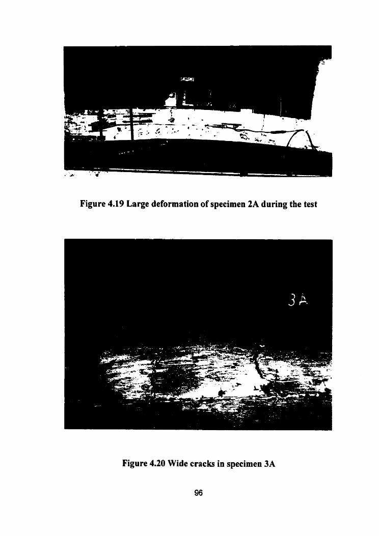
Figure 4.19 Large deformation of specimen 2A during the test

Figure 4.20 Wide cracks in specimen 3A

Figure 4.21 Crack pattern for specimen 3C

- . . *--h.**, ----- .

t

'6 1

* L

1

I I

,

O 1

O

8 -- - ....-- average LVDTs

+Average dernec -- y-- . 8

. t L . . t * L . ~ - * . D . . l . . . i

O

I 1 1

Gross strriin (microstrain)

Figure 4.22 Load versus gross concrete strain for specimen 3C

(a) Crack pattern

(b) Concrete spaHing on the compression side

Figure 4.23 Failure mode of specimen 2C

98

+ Demec 1T

+demec 2T

=-*- -Demec 1'T

Gross concrete strain (microstrain)

(a) Tensile Strain

i -50 Gross concrete strain (microstrain)

(b) Compressive Strain

Figure 4.24 Moment versus gross concrete strain for specimen 2C

+ LVDT # 8

+LVDT# 7 .

t

-1000 O 1000 2000 3000 4000 5000 6000 7000 8000 9000 10000 Steel strain (microstrain)

Figure 4.25 Moment versus non-prestressed steel strain for specimen 2C

-1 000 O 1 O00 2000 3000 -2000 O 2000 4000 6000 8000 Cross strain (microstrain) Cross strain (microstrain)

Load 220 kN Load 340 kN -. . .-- - - - .. - - -

Figure 4.26 Examles of strain distribution plotted at each load level using Demec and LVDT readings for specimen 1C40

+ Demec 1 '

+ Demec 1

+ Demec 2

---I€--LVDT# 7

- - + - - L V D T # 8 - - - - - - . - - - . . -

- 10 O 1 O 20 30 40 50 60 70

Curvature xlO" (llm)

Figure 4.27 Moment versus curvature for specimen 1C40

Figure 4.28 Moment versus curvature for specimen lC2O

+Demec 1'

+Dernec 1

+Demec 2

..a-. LVDT # 7

- - + - - L V D T # 8

-20 i

Figure 4.29 Moment venus cuwature for specimen 2A

+ Demc 2

+Demec 1 - - . --

-10 O 10 20 30 40 50 60 70 80 90 100

Curvature x 10-~ (l/m)

Figure 4.30 Moment versus curvature for specimen 2B

Curvature x 10'~ (I/m)

Figure 4.31 Moment versus curvature for specimen 3A

+ Demec 1

+ Demcs 2

+Demec 1'

---X--LVDT#7

L V D T 3 8 -

I I 1

Curvature x 10"' (Ilm)

Figure 4.32 Moment versus cuwature for specimen 3B

10 20 30 40 5 0 60 70

curvnture x 1oo3 (~/rn)

Figure 4.33 Moment versus curvature for specimen 2C

+crack width: wet face 0.25 mm dry face 0.1 0 mm

4 crack width: wet face 0.10 mm dry face 0.03 mm

a- -

O 5 10 15 20 25 30 35 40 45 Time (hours)

Figure 4.34 Leakage rate for the through cracks in specimen 3C

1 O4

Crack Width (mm)

Figure 4.35 Effect of level of partial prestressing on crack width

- +- - 20 mm cover -40 mm cover

-- -

Figure 4.36 Effect of concrete eover of non-prestressed steel on crack width

+e = 0.52 m +e = 0.25 m - - + - - 2C (flexure)

Crack width (mm)

(a) Moment

L œ

œ

O I i i i i , . r k i , i i i . , . i i . ~ L I , ,

I 1 t 1 I

O 0.5 1 1.5 2 2.5 3

Crack width (mm)

(b) Load

Figure 4.37 Effect of load eccentricity on crack width

- + - - unbonded . . - . - -

25

Crack width (mm)

Figure 1.38 Effect of bond characteristic of tendons on crack width ( the last data point at crack width 8 mm is not shown)

crack width (mm)

Figure 4.39 Effect of level of prestressing on the relation between crack width and steel stress

Crack width (mm)

Figure 4.40 Non-prestressed steel stress versus crack width for flexural and through cracks

+ flexu re - - * - - e l h = 1.04

-1 O O 10 20 30 40 50 60 70 80 90

Curvature x lo5 ( l h )

Figure 4.41 Effect of load eccentricity on moment-cuwature relationship

1 " ' r i i l . r i i I i i i i ~ t i i n ~ riii.riiliiiiltii.iii..LLI,,,~LI

r I 1 1 1 i I . , . l I I I I I . . . . I t I

-1 0 O 10 20 30 40 50 60 70 80 90

Curvature x 105 ( lh)

Figure 4.42 Effect of partial prestressing level on moment-cuwature

relations hip

-4- bonded

Curvature x 10'' (Ilrn)

Figure 4.43 Effect of tendon bond characteristics on moment-curvature relationship

-1 O O

Figure 4.44

1 O 20 30 40 50 60 70

Curvature r 105 (Ilm)

Effect of non-prestressed steel concrete cover ou

moment-curvature relationship

110

5- Analytical Model

5.1 Introduction

This chapter presents a description of an analpical model written using Visual

Basic to analyze partially prestressed concrete sections. Description of the model. the

material constitutive laws used in it and a verification of it are given in Sections 5.2

through 5.5. The mode1 was employed to simulate the experimental test specimens. The

results of the simulations are presented in Section 5.6. It was also used to model third-

party test specimens. which are presented in Section 5.7.

5.2 Description of the Analytical Model

A Visual Basic computer program was developed to perform a plane section

analysis of reinforced. prestressed and partially presuessed concrete sections. In

performing this analysis. a linear strain distribution is assumed over the cross section at

al1 load levels. The corresponding stresses are obtained from stress-strain relationships.

The cross section is divided into 100 layers and a numerical integration is used to obtain

the corresponding forces and moments.

The prograrn starts by calculating concrete strains corresponding to zero extemal

loading then increases the concrete strain at the extreme fibre on the compression side.

by increments of 25 microstrain (compression) until failure. For each increment. the

model calculates. by trial and enor. the other extreme fibre strain that satisfies a given

eccentricity. Consequently, for this strain distribution. the program calculates moment.

axial load, curvature. concrete compressive stress at extreme fibre. non-prestressed and

prestressed steel stresses and the depth of the compression zone. The program recognizes

failure when the strain at any of the concrete extreme fibres. non-prestressed steel or

prestressing steel. exceeds its uitimate strain. The program considers the effecr of creep

and shrinkage of concrete and calculates deformations and forces before and after

considering this effect. The program displays the results directly on a spreadsheet and

automatically creates plots for moment versus curvature and other responses.

The input of the prograrn includes: section and matenal properties. reinforcement

area, load eccentricity. initial strain in concrete due to shrinkage and creep. creep

coefficient, free shrinkage strain and prestressing steel initial strain. The material models

for concrete. non-prestressed steel and prestressed steel are grouped in a separate module

as separate functions to facilitate modifjing any one of them without affecting the rest of

the program. A listing of the program is provided in Appendix A.

5.3 Material Constitutive Laws

5.3.1 Concrete in Compression

Compressive tests were conducted on three concrete cylinders for each specimen

on the same day as the test. as described in Chapter 3. In addition to concrete strength.

the full response of the cylinder was obtained for each compression test. Two and

sometimes three stress-strain curves were obtained for each specimen from the cylinder

compression tests. Curve fitting was used to produce relationships simulating an average

stress-strain response for each specimen. This average curve was unique for each

specimen and used in the analytical study. Each c w e consists of different cubic

relationships for ascending and descending branches. Figure 5.1 shows exarnples of these

cuves.

5.3.2 Concrete in Tension

While tensile behavior in concrete usually does not significantly affect the

ultimate strength of a member, the effect of tensile stresses in concrete must be taken

into account when the serviceability charactenstics of a member are needed. It is known

that reinforced concrete c m display sipifkant additional stifiess afier cracking due to

tension stiffening. This effect is simulated using stress-strain relationships for concrete in

tension so that the strain and curvatures obtained would represent average values in the

cracked zone rather than the peak values at crack locations.

Several tension stiffening models are proposed in the literature. Three models

were examined in the present study. These three models are those of Vecchio and Collins

(1986). Massicotti er al. (1990) and Foster (1992). The three models are ploned in Fig.

5.2 for three different partial prestressing ratios. A description of these models is given

below.

Vecchio and Collins (1986) proposed the following equation to simulate the post-

cracking behaviour of reinforced concrete based on correlation with test data:

This equation was modified later as given by Collins and Mitchell ( 1987) to

The factors a, and al represent bond characteristics of tendons and load history

respectively. Collins and Mitchell (1987) suggested that the cracking stress of concrete

be taken as:

Massicotte er al. (1990) derived stress-strain relationships modeling the post-

cracking behavior. Equilibrium of forces between the cracked and the uncracked regions

is considered at control points that represent the States of stabilized cracking and yielding

of reinforcement at the crack. The curve is assumed to be quadratic between these two

points. Concrete tensile stress is considered zero when the average strain in tLie member

reaches the reinforcement yield strain. ï h e c w e is considered linear between this point

and the point of yielding of reinforcement at the crack. Detailed equations can be found

in Massicotte et al. (1 990).

Foster (1992) rnodified the linear relationships suggested by Al-Manaseer and

Phillips (1987) to recognize the fact that concrete cracking ma! occur at values

considerably lower than the uniaxial cracking stress, f;' . The stress-strain curve afler

cracking is defined by:

for E, 2alo,,

In this equation the factors al and a? are material constants. different than those

used by Vecchio and Collins. In using this mode1 to simulate his own test results. Foster

used a, = 10.0 and a? = 0.3 and he estimated the concrete cracking stress to be in the

range of 0.3& to OAK to best match the observed test results. Funhermore. when

Foster used the mode1 to sirnulate others test results he aluays usrd a, as 10.0 but

changed a, in the range of 0.2 to 0.8 to match test results. This wide range of

a2 implies that Foster considered that the average tensile stress could remain higher than

0.8 of the cracking stress at fairly high average strains.

The three tension stiffening models were incorporated in the developed analytical

mode1 to simulate the response of some tested specimens. The results are presented in

Section 5.5.

5.3.3 Effect of Creep and Shrinkage

Creep and shrinkage of concrete directly affect the strain and consequently the

curvature of a member. Creep and shrinkage also induce stresses in a restrained concrete

member producing additional axial forces and moments. This effect is calculated in the

analytical model by employing the method described by Ghali and Favre (1986).

However. there was no need to calculate theoretical values for the creep coefficient. cp. or

shrinkage strain. E , of the tested specimens. The change of concrete strain due to

shnnkage and creep was already measured during the test as explained in Chapter 3.

Therefore. the measured strains were used to calculate realistic values of 9 and E,, that

were used in the analytical model in conjunction with the measured strains to calculate

the change in stresses and consequently moments and loads. A summary of the effeci of

shrinkage and creep on the tested specimens is given in Table 5.1 and the procedure used

in these calculations is explained in Appendix B.

It should be noted that in the test results the initial load was considered zero

while the effect of shrinkage and creep of concrete was included in initial strain readings.

This means that shnnkage and creep effects were considered only on deformations not

loads. Therefore. in comparing analytical and expenmental results. the predicted values

of loads and moment were those without shnnkage and creep effects while the predicted

values for deformations and stresses were those including that effect.

5.3.4 Non-Prestressed Steel

The two stress-strain curves obtained from tension tests on coupon samples of the

reinforcement were simulated in the analytical study by a model consisting of three

stages described by the following relationship:

Equation 5.5 is ploned in Fig. 5.3 against tension test results. Equation 5.5 is

shified from the test results by the difference between the observed yield stress and the

static yield stresses.

5.3.5 Prestressing Steel

The stress-strain response for prestressing steel obtained from the tension tests

described in Chapter 3 was modeled using the modified Ramberg-Osgood function

recommended by Mattock (1979) up to a strain of 38000. Afier that strain the dope of

the curve. obtained fiom the test, reduces. The part of stress-strain response between a

strain of 28000 until ultimate saah was modeled using a quadratic function.

The modulus of elasticity E, is 200000 MPa. The three constants A, B and C

which define the Ramberg-Osgood function are taken as 0.03. 116.5. and 10

respectively . Figure 5.4 shows a plot of this equation against the curves obtained from

the tension tests.

5.4 Verification of the Analytical Model

Specific problems were analyzed manually in a spreadsheet and the results of

each step were verified carefully against that obtained using the developed model. The

rnodel was also verified against the program RESPONSE (Collins and Mitchell. 199 1 ).

Some tested specimens were simulated using both RESPONSE and the developed

model. During this cornparison, the material constitutive laws used in the developed

model were chosen to be the same as üsed in RESPONSE. The simulation was

performed for three specimens subjected to eccentric tension. With two different partial

prestressing ratios. A&,, of 1.3 and 5.0, and two different eccentncities of 520 and

260 mm for specimens 1C40 and 2A, and specimens 1C40 and 3B. respectively.

Moment versus curvature diagrams resulting fiom the two programs for the h e e

specimens are plotted against the corresponding experimental results and s h o w in Figs.

5.5 through 5.7. It is clear that responses obtained fiom the hhio programs completely

coincide. However. responses obtained from both prograrns are stiffer than the response

of the tested specimens in the range between cracking and yielding and sofier after that.

This discrepancy was the reason that led to the development of the analytical rnodel

rather than relying on an existing program Iike RESPONSE. It is believed that using

appropriate material models, particularly the tension stiffening model, can produce better

results.

5.5 Tension Stiffening Model

The three tension stiffening models described in Section 5.3 were incorporated in

the developed analytical model to simulate the response of four tested specimens. Three

of these specimens, specimens 3A. 1C40 and 2A. were tested under eccentric tension

with the same load eccentncity but with three different partial prestressing ratios. A JA,.

of 0.0. 1.3 and 5.0. respectively. Specimen 3C tested under axial tension was also

simulated. Figures 5.8 to 5.10 give moment versus curvature diagrarns for the three

specimens 3A. lC40 and ZA respectively. The curves obtained using the three tension

stiffening models are plotted in each figure together with two additional plots. One plot

represents the experimental results (the average of Demecs and LVDT readings) and the

second gives the analytical rnodel results neglecting the contnbuti~n of concrete after

cracking. The figures show that the predicted responses by al1 the three tension stiffening

models are stiffer than the expenmentai results in the region of service loading. between

cracking and yielding. At higher loads the three models predict an sofier response than

the tests, with the Massicone model producing the lowest moments and the Foster model

producing the highest moments. Figure 5.2 explains this difference since the descending

part of Massicotte's model has the steepest dope and vanishes completely when the

average concrete strain equds the non-prestressed yield strain, while the Vecchio and

Collins and the Foster models continued beyond this strain with a considerable concrete

tensile stress. Vecchio and Collins (1986) stated that significant tensile stresses were

found in the concrete between the cracks even at very high average tensile strain.

Expenments conducted by Gilbert and Warner (1978) showed also that concrete

maintains an average tensile stress varying between 0.3 to 0.7 f, even at high average

tensile strain.

Figure 5.1 1(a) shows load versus gross concrete strain diagram for specimen 3C

obtained by using the three tension stiffening models and fiom expenmental test data. In

this case Foster also significantly overestimates the section capacity while Massicotte

underestimates it. Vecchio and Collins model on the other hand accurately predict the

ultimate capacity of the section. The first part of the load-strain c w e s are enlarged in

Fig. 5.1 1 (b) to study the impact of using these models on the prediction of the

serviceability response of the mernber subjected to axial load. The figure yields many

observations. The predicted cracking load, which is the sarne for the three models

depending on the value specified for concrete cracking stress, was higher than that

obtained from the test. The discontinuity of Vecchio and Collins model at cracking stress

led to a drop in the load-strain curve which is inconsistent with test results. On the other

hand. the constant concrete stress after cracking in the Foster model led to an increase

and then a gradual decrease in the load. which also is inconsistent with test results. The

steep decrease in concrete stress in the' Massicotte rnodel and neglecting the concrete

contribution afier yielding of the reinforcement affected the global behaviour.

The above observations led to the developing of a tension stiffening mode1 that

better simulates the present test results. This mode1 has the following features: a lower

cracking stress than 033& suggested by Mitchell and Collins. and concrete tensile

stresses that gradually decrease after cracking without a sudden drop. Concrete still has

some tension stress afier the yielding of steel but not as high as in the Foster model.

With al1 the difierences among the existing tension stiffening rnodels and the

scatter in test data collected by Vecchio and Collins (1986), there was no need to

complicate the model. Therefore, the suggested tension stiffening rnodel consists of two

parts describing the post-cracking behaviour. The first part is non-linear and represents

the gradual reduction in concrete tensile stress during the progress of cracks until a state

of stabilized cracking is achieved. The second part represents the stress history after that

and c m be constant or linear with a very flat dope. The model is ploned in Fig. 5.2

against the other three models and is given by the following equation:

In this equation the constant p, represents the extension of the non-linear part of

the curve beyond the concrete cracking strain while P, represents the portion of cracking

stress that remains after stable cracking. It was found from simulating the present

experiments with this tension stiffening model that P? cm be taken in the range of 0.3 to

0.5. while P, can be approximately taken as 15. and can be increased if the eccentricity or

the ratio AjA, increases. lncreasing the ratio between the load at which stable cracking

occurs and the cracking load is the reason for increasing B,. On the other hand. a

significant reduction in P, should be considered in either partial prestressing with

unbonded tendons or full prestressing.

As detailed in Chapter 1, in rnost specimens. a second and final set of cracking

occurred after the first set. The ratio between the two loads at which theses two sets

occurred was about 1.4. In specimen 2A where AJA,, was high and in specimen 2C

tested under flexure the ratio was about 1.75. In the case of full prestressing, specimen

3A. no second set of cracking occurred and in specimen lB. unbonded tendons. random

and very wide cracks occurred at different load levels due to lack of bond.

This model was used to predict the response of specimen 3C tened under axial

tension. and the results are plotted in Fig. 5.12. Figure 5.12 (a) shows the full Ioad verses

concrete strain diagram, while Fig. 5.12 (b) shows the response to approximately the

level of the service load. In general. the two figures exhibit good agreement between the

suggested model and test results.

The proposed tension stiffening model was incorporated in the proposed

analytical model which was used to predict the response of al1 the tested specimens. The

response predictions are presented in the next section.

5.6 Comparison between Analytical Predictions and Test Results

The eight tested specimens were modeled using the analytical model described

earlier. The material properties for concrete used in this study and the parameters of the

tension stiffening model are given in Table 5.2. The results for individual tests are

presented below. The comparison between predicted and observed values included

failure loads. moment versus curvature response, moment versus depth of compression

zone. moment versus non-prestressed steel stresses and concrete tensile and compressive

strains versus load. Detailed cornpansons are provided for the standard specimen lC40.

For al1 the other specimens. only moment versus curvature response is shown unless

certain response eshibits certain features. To account for the effect of dead load. the

stresses due to the dead load moments were theoretically calculated for the uncracked

transformed section. The corresponding strains were obtained by dividing these stresses

by the concrete modulus of elasticity used in the analytical model. The obtained strains at

the extreme fibres were approximately 11 microstrain for configuration C-1 specimens

and 20 microstrain for specimen 2C. These strain values are a result of a bending

moment at the mid-span due to dead load of 3.6 and 6.3 kNm respectively. These dead

load moment and the corresponding strains (and the curvatures) are added aigebraically

to the test results presented in the figures of this chapter to insure a consistent

comparison with the analyticd model. The latter predicts the total resistance of the wall

section. The failure moments described beiow are those indude the dead load moment.

For specimen 1C40. the andytical model predicted failure at a load of 404 kN

when the concrete compressive strain exceeded the ultimate strain. This compares

favourably with the observed failure load of 405 kN that occurred due to crushing of the

concrete on the compression side. The moment versus cwature, moment versus depth

of compression zone and moment versus non-prestressed steel stresses are plotted in

Figs. 5.1 3 through 5.1 5 respectively . Frorn the results presented in these figures it can be

seen that a good correlation exists between the test and the analytical model. Plots of the

rneasured and the modeled concrete tensile and compressive strains venus load are given

in Fig. 5.1 6 and 5.1 7 respectively.

The model predicted failure for specirnen 1 C20 by crushing of the concrete at a

load of 393 kN. This load is 6S% less than the observed failure load of 420 kN which

occurred due to concrete crushing. The moment versus curvature and moment versus the

depth of the compression zone graphs are given in Fig. 5.18 and 5.19. where it can be

seen that the model was slightly stiffer than the test for a limited range of loading but in

general a good correlation exists between the analytical and test results. Plots of concrete

r'rtremr fibre strain versus load produce the same conclusion.

For specimen 2A. where AJA, = 5.0. the predicted failure of 794 kN due to

crushing of concrete compares favourably with the observed failure load of 390 kN

which occurred due to crushing of concrete. In both cases failure occurred well afier

yield of the non-prestressed steel. Comparing the predicted moment versus curvature

graph with the experimental curve given in Fig. 5.20 shows that excellent correlation

exists up to yielding of the non-prestressed steel where the modeled curve became sofier.

The load versus concrete tensile stress plots in Fig. 5.21 give similar results. Test results

showed that tensile strains measured using Demec strain gauges were lower than tensile

strains obtained fiom LVDT readings. Hence, concrete tensile strains at the extreme

fibres obtained by interpolated LVDT readings were plotted on the same graph. The

interpolated LVDT readings show better correlation than Demec points readings.

For specimen 2B, where the tendons were unbonded. the analficd model

predicted failure at a load of 398 kN when the concrete compressive strain exceeded the

ultimate strain. This compares favorably with the observed failure load of 400 kN ;Nat

occurred due to crushing of concrete on the compression side. However. the model was

initiaily stiffer but became softer at high loads as shown in Fig. 5 .E.

For specimen 2C tested under flexure, the predicted failure moment, 242 kNm.

was slightly less than the observed value of 260 kNm. However both of them were due to

crushing of concrete on the compression side. Figure 5.23 that shows plots of moment

versus curvature indicates good agreement between test and analytical model although

the rnodel is slightly softer at high moments.

In specimen 3A. which was fully prestressed, the model predicted failure due to

crushing of concrete at a load level of 385 kN which is only 6% less than the observed

failure load of 410 kN. The moment versus curvature and moment versus depth of

compression zone are given in Figs. 5.24 and 5.25 respectively. An excellent agreement

c m be seen in the latter figure while in the former the model predicted stiffer response

for a range of load aher cracking. It should be noted that during the test. the Demec

points became loose during the last three load increments.

When modeling specimen 38 that had a load eccentricity half that of the othrr

specirnens. it was found that using the concrete cracking stress. f,,. as 023& predicted a

significantly low failure load. Therefore. unlike the other specimens, fer. was taken as

0 2 3 6 and the tension stiffening parameter p, was taken as 0.6. This slightly increased

the predicted failure load to 760 kN due to concrete crushing while the observed failure

load was 860 kN with a difference of 13%. Increasing the value of f,, used in the

analysis, however, made the response of the specimen stiffer than the observed behaviour

as shown in Fig. 5.26. The cornparison presented in this figure indicates that. in general.

a p o d correlation exists between the experimental test and the analfical model within

the service load only. This implies that the model predicts the serviceability behaviour

well. It should be noted that the rotation of the eccentric loading brackets reached 6.5 O

by the end of the test. which reduced the eccentricity and consequently increased the

ultimate load.

5.7 Cornparison of Analytical Predictions with Others Test Results

Some of the experimental studies carried out to investigate the serviceability of

reinforced. prestressed and partially prestressed concrete members are presented in

Chapter 2. Most of these studies were concemed about crack widths and the parameters

affecting cracking. Most of the tests were conducted on beams subjected to bending

moment and reported only crack widths and the bearn deflection. Among the few tests

conducted on specimens subjected to axial tension, those conducted by Alvarez and

Marti ( 1996) were rnodeled and the results are presented in this section.

Alvarez and Marti (1996) carried out tension tests on seven conventionally

reinforced and two prestressed concrete wall elements to investigate the influence of

some selected parameters on the deformation behaviour and the deformation capacity of

structural elements in pure tension. Partial prestressing of the longitudinal reinforcement

was one of these selected parameters. Al1 nine test specimens were 1000x3000 mm.

220 mm thick rectangular panels. The characteristics of the specimens are given in Table

5.3. Table 5.3 indicates that the non-prestressed reinforcement had high ductility in seven

specimens and low ductility in two specimens. ZJ and 25. The propenies of the

materials used in these specimens are given in Table 5.4. The four reinforced concrete

specimens 21, 22, 28 and Z9 that were reinforced with high ductility non-prestressed

steel and the iwo partially prestressed concrete specimens 26 and 27 were chosen for

anaiylicai modeling.

It was reported that failure of specimens Z1,22 and 28 was caused by rupture of

the longitudinal reinforcing bars while in test 29 some bar couplen at the edges of the

specimen broke before reaching the expected mode. Failure of the partially prestressed

test specimens 26 and 27 was initiated by rupture of wires in the post-tensioning tendon.

The reinforcing bars failed only afier a furdier increase of the imposed elongation. It was

also reported that specimens Z1,W and 28 failed at an average concrete strain Less than

one half of the ultimate strain of steel. In the two partially prestressed test specimens 26

and 27 the strain at failure was only 20% of the non-prestressed steel ultimate strain and

approximately 53% of the prestressed steel ultimate strain.

The concrete cracking stress used in the model varied between 023Jfi and

0 . 2 0 c to match test results. The tension stiffening parameter P, was taker, 15 and

varied between 0.2 and 0.35. Figures 5.27 through 5.32 show load versus elongation

plots for specimens Z1, Z2, 26, 27, 28 and 29 respectively. The elongation was

measured for a gauge length of 1800 mm. In general, a good correlation exists between

test and modeled values keeping in mind that the modeled non-prestressed steel stresses

were the static values. For the prestressed steel, only the dynamic stresses were reponed

and were used in the model. Hence, the model c w e s are closer to the static readings in

the load-elongation plots for reinforced concrete specimens Z1, Z2, and 28 as shown in

Fig. 5.27. 5.28 and 5.3 1 respectively. In the partially prestressed specimens 26 and 27,

that had AJA, of 1.173 and 0.587 respectively. the mode1 curves. shown in Figs. 5.29

and 5.30. are closer to the dynamic readings especially in specimen 27. The model cune

continued until the axial load became equal to the steel area times the ultimate steel

stress, which means that steel strain at a crack reached the ultimate strain, The reinforced

concrete specimens 21. Z2, and 28 failed at a gross strain less than one half the steel

ultimate strain due to strain localization. The partially prestressed specimens 26 and 27

also failed at a low gross strain due to rupture of wires in the tendons. The cornparison

between model and test responses for specimen 29, shown in Fig. 5.32. is only for the

response before yield since specimen Z9 failed in this load range when some bar

couplers at the edges of the specimen broke.

Table 5.1 Summary of shrinkagc and crecp effects on the spccimcns

ni icrostrain

I C4O 0.401 8 -385

Afs change in non-presiressed steel stress

ANs change in steel interrial force

AMs change in steel interrial moment

ANc change in concretc iriternal farce

AMc changc in concrete infernal moment

ANtota~ change in total interrial force

AMtotal change in total interiial iiiotnent cÇS shriiikage strairi

0 crcep coefficieiit

Table 5.2 Material properties for the concrete used in simulating test results

fc' ECO Ec f" : J;; P 1 P2 MPa MPa

Specimen

Table 5.3 Specimens tested by Alvarez and Marti

Test Specimen

Non-prestressed Steel

As [mm'] Prestressed Steel

A, [mm?]

Type of steel

Transverse reinforcement Ast [mm']

Target sttength of concrete fi [ M W

The variable in each specimen is shaded H : Highly ductile non-presnessed steel N & L : rwo types of low ductile non-prestressed steel

Table 5.4 The Mater id properties used in Alvarez and Mar t i spccimens

S pec i iiicn

Concrcle: Agc of spcc inicn Ilensity

.L Tensile sireiigt h Splitiiiig stress

Eco t

Modulus of elasiicity Non-prest ressed steel:

2

h, Diameter -J Y ield stress

Static yield stress Ultininie streiigth Stalic ul~iniate s~rengtli

Y ield straiii IJltiiiiate strain Modulus of elasiicity Frest rosscd sf eel -- Y icld stress (0.2% offset) IJIlitiialc strengili

IJItiniatc straiii

Moduhs of elasiicity 1 G Pa 1

strain x 1oa3 -4.5 -4 -3.5 -3 -2.5 -2 -1.5 -1 -0.5 O

(a) specirnen 36

strain x 10" -4.5 -4 -3.5 -3 -2.5 -2 -1.5 -1 -0.5 O

(b) specimen 3A

Figure 5.1 Concrete stress-strain curves

128

-.-. test 1

- Eq. 5.5

O 20000 40000

Figure 5.3 Stress-strain

60000 80000 100000 120000 140000

Strain (microstrain)

curve for non-prestressed steel

- Eq. 5.6

- * m . . - Test

Strain (microstrain)

Figure 5.4 Stress-strain curve for prestressing steel

130

Curvature x 10-3 (l lm)

Figure 5.5 Moment versus curvature for specimen 1C40 obtained from the current program and program RESPONSE

Y current prog ram

- - + - - RESPONSE

Curvature x 1q3 (llm)

Figure 5.6 Moment versus curvature for specimen 2A obtained from the current program and program RESPONSE

225 7

200 - =

+ current program - - Q - - RESPONSE -

-

experimental -

Curvature x 10-3 (l/rn)

Figure 5.7 Moment versus curvature response for specimen 3B obtained from the current program and RESPONSE

- c

Vecchio & Collins 100 Massicotte et al. ...... Massicotte et al.

E f 75

* experirnental x Foster

50 + no tension stiffening --

Figure 5.8 Moment versus Curvature response for Specimen 3A obtained using different tension stiffening models

Veccho & Collins ...... Massicotte et al. * exaerimental

Figure 5.9 Moment versus curvature response for specimen 1C40 obtained using different tension stiffening models

- Vecchio & Collins ..-..- Massicotte et al.

r Y experirnental P

x Foster + no tension stiffening

- . - _ _ . . - - - - - - - - -- -

Figure 5.10 Moment versus curvature response for specimen 2A obtained using different tension stiffening models

.

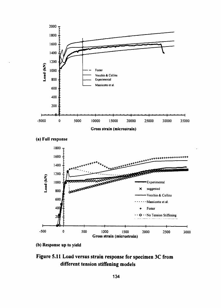
- - Foster

Vccchio & Collins

Massicone ct al. 600

Cross strain (microstrain)

(a) Full response

+++++-kt++++

E x p e r i m e n t a l

X supgested

- Vccchio & Collins

- - - - - -Massicotte et al.

+ Foster

- - O - -No Tension Stiffening - - - - - - . - . - - -- . -

-500 O 500 1 O00 1500 2000 2500 3000 Cross strain (microstrain)

(b) Response up to yield

Figure 5.11 Load versus strain response for specimen 3C from different tension stiffening models

1800 -

bare reinforcernent

-5000 O 5000 10000 15000 20000 25000 30000 35000 Gross strain (microstrain)

(a) Full response

- LVDT 's

- - - - - - bare reinforcement

- suggested - - - - - -. - -A- - - - -- . -

-500 O 500 1 O00 1500 2000 2500 3000

Gross strain (microstrain)

(b) Response before yield

Figure 5.12 Load versus strain response for specimen 3C obtained from the suggested tension stiffening mode1

+ Demec I '

+ Demec 1

-+- Demec 2

---*--LVDT#7

--*--LVDT#8

- predicted - -- - - - - -

-10 O 1 O 20 30 40 5 O 60 70 80 90

Curvature xloJ (llm)

Figure 5.13 Observed and predicted moment versus curvature respouses for specimen 1C40

O 25 50 75 1 O0 125 150 175 200

Moment (mm)

Figure 5.14 Moment versus depth of compression zone for specimen IC40

- predicted

-a--LVDT#7

-11- LVDT # 8 . -

Figure 5.15 Moment versus non-prestressed steel stress for specimen 1C40

+ Demec 2T -Q- Demec 1T

- e- -Demec 1' T - predicted

t . . . . . . . . . . . , . . . , . . , . , , , , ~ ~ , 1 1 I 1 I

-2000 O 2000 4000 6000 8000 10000 12000 14000 Gross concrete strain (microstrain)

Figure 5.16 Load versus concrete tensile strain for specimen 1C40

+ Demec 26 4 Demec 16 - Q- Demec 1' B - pred icted

- -

4000 -3500 -3000 -2500 -2000 -1500 -1000 -500 O

Grogs concrete strain (microstrain)

Figure 5.17 Load versus concrete compressive strain for specimen lC4O

--c- Demec 2

60

Curvature r 10-3 (ltm)

Figure 5.18 Obsewed and predicted moment versus cuwature responses for specimen lC2O

1 - - predicted 0.9 -: . --- Demec 2 0.8 -: ..... - Demec 1

-.-. Demec 1'

0.3 -1 .

0.3 -:

0.1 -:

O 2 5 50 7 5 1 O0 125 150 175 200 225

Moment (mm)

Figure 5.19 Moment versus depth of compression zone for specimen lCZO

L . b

.....- Demec 1'

+Demec 1

+Demec 2

- LVDT#7

- LVDT#8

- pred icted - . . . . . . - - . - . -- . . -

Cu~ature x loJ (llm)

Figure 5.20 Observed and predicted moment versus cuwature

responses for specimen 2A

-

Dernec 1

Demec 2

Demec 1'

predicted

I interpolation from L U T

Cross concrete strain (microstrain)

Figure 5.21 Load versus concrete tensile strain for specimen 2A

Demc 2

- predicted - - -- - -

i . . i * r . i , i i t . i . i . . . * l l , * ~ , l , , l I , , , I I 1 I I I 1 I 1 1

L i i i i 1 i i i i 1 i I I i

-10 O IO 30 30 40 50 60 70 80 90 100 110 120 Curvature x 10" (l/m)

Figure 5.22 Observed and predicted moment versus curvature responses for specimen 2B

+Demec I

+ Demec 2

+ Demec 1 '

-*X--LVDT#7

--0--LVDT# 8 - Predicted

Figure 5.23 Observed and predicted moment versus cuwature responses for specimen 2C

4 .

4 Demec 1

4 Demec 1 '

-+ Demc 2 - predicted - - - - - - - .- - - -

Curvature x loJ (llm)

' Figure 5.24 Obsewed and predicted moment versus curvature responses for specimen 3A

- - 4 - - Demec 1

- - Demec 1'

- -* - Demc 2 - predicted

- - -. - --

O 25 50 75 1 O0 135 1 50 175 200 225

Moment (mm)

Figure 5.25 Moment venus compression zone depth for specimen 3A

predicted

Figure 5.26 Obsewed and predicted moment versus cuwature responses for specimen 3B

t 0 r I L . , l . , . . f . . I I . ' O 25 50 75 1 O0 125 150 A/[mm]

(a) Full Response NIA, [MPaI

l I .

O O 1 2 3 4 5 A1 [mm]

(b) Response before yielding

d Zr: Alvarez & Marti -

Figure 5.27 Observed and predicted load versus elongation for specimen 21 tested by Alvarez & Marti

N [kW NIA, [Mh]

A 600

1 1

; 500

. 7 400

'1 I

- 300

Alvarez & Marti - 200

-----------. Present study - 100

1 O b .

l , . , r L . , . - l . , l

O 25 50 75 100 1 25 150 A l [mm]

(a) Full Response NIA, [hiPa]

- 0'

- 200 Alvarez & Marti

(b) Response before yielding

Figure 5.28 Observed and predicted load versus eiongation for specimen 22 tested by Alvarez & Marti

(a) Full Response N jk!]

(b) Response before yielding

Figure 5.29 Observed and predicted load venus elongation for specimen 26 tested by Alvarez & Marti

Alvarez & Marti

--*--------a Present study

0 ' t . ,

O 1 O 20 30 40 50 60 Ai [mm]

(a) Full Response

Alvarez & Marti

------______ Pment study

0 2 3 4 5 6 Ai[mm]

(b) Responae before yieldiag

Figure 5.30 Observed and predicted load versus elongation for specimen 27 tested by Alvarez & Marti

Alvarez & Marti -1 200

------------ Present study i lo0 (a) Full Response

NIA, [MPa]

-1 500 -- - -y

1 . - Y /; 0 400

/ j 1 i 300 l i I --- 1

1 1 2,

Alvarez & Marti

------------ Present study

! 1 t . ! i

(b) Response befon yielding

Figure 5.31 Observed and predicted load versus elongation for specimen 28 tested by Alvarez & Marti

- 200

Alvarez & Marti - 100

Figure 5.32 Observed and predicted load versus elongation for specimen 29 tested by Alvarez & Marti

6- Pararnetric Studies

6.1 Introduction

Two parametric studies are presented in this chapter. Fint, the developed

analytical model was used to carry out a parametric study of the structural response of

wall panels to extend the range of the available test results. Section 6.2 gives the basic

variables studied followed by the results given in Section 6.3. This study is surnmarized

in Section 6.4. Finally, Section 6.5 describes a study conducted to investigate the

hydraulic conductivity through cracks and the compression zone of the concrete section.

6.2 Parametric Study of Structural Behaviour

The experimental study investigated the effect of four parameters on the

behaviour of partially prestressed wall segments in concrete water tanks. These four

parameters are:

1. The effective depth of non-prestressed steel. Two values for concrete covrr were

tested. namely 20 mm and 40 mm (Le. d = 232 and 207 mm respectively).

2. The partial prestressing ratio expressed as the ratio between non-presuessed and

prestressed steel area A,/% for which three ratios were tested namely 0.0. 1.3 and

5 .o. 3. Load eccentricity. e; for which four eccentricities were tested. namely pure moment.

e= 520 mm. e = 260 mm and axial tension (eh = m. 2.08. 1 .O4 and 0.0 respectively).

4. Bond characteristics of tendons; bonded and unbonded.

The restrictions on the number of physical tests limited the nurnber of values

studied for each of the four parameters not to mention other pararneters. The present

analyticai model. which yielded satisfactory agreement with test results. was used to

generate a pararnetric study. With the exception of bond characteristics of tendons, the

pararnetric study addressed the sarne parameters invenigated in the experimental tests

with more values and wider range. In addition to these parameters, the effects of the

effective depth of prestressed steel and the concrete wall thickness were studied. The

parametric study did not address some parameters such as the method of prestressing.

post-tensioning versus pre-tensioning, and type of tendons; strands versus wires or bars.

The basic concrete section used in this pararneuic study had a width of 1000 mm

and a thickness of 250 mm which is the minimum thickness required by the North

American standards and recommendations for constnictability. The section was

reinforced with non-prestressed steel of area A, = 800 mm2 at an effective depth. d of

200 mm and prestressed steel of area A, = 800 mmL ai an effective depth, dp, of 150 mm.

The stress-strain relationships for both steel types were those used in modeling the

experimental tests. The concrete uniaxial compressive strength f ; was selected equal to

45 MPa. a cracking stress of concrete of 023& was used. and the concrete

compressive strain corresponding to A'. E, , was set to 0.0023. A summary of the

variables studied in the parametric study is given in Table 6.1. The table indicates that a

total of 5 1 wall sections were analyzed. For each case the analytical mode1 generated

several relationships including moment versus curvature. moment versus depth of

compression zone (c). load versus c. extreme fiber concrete compressive stress j; versus

c. non-prestressed steel stressf, versus c and concrete stress at mid-depth versus c. The

results of the parametnc study are presented in several forms to delineate the behaviour

of each parameter.

6.3 Results of the Parametric Study of Structural Behaviour

6.3.1 Moment versus Cunrature

Figures 6.1 through 6.5 show the effect of the different studied parameters on

moment-curvature relationships. Figure 6.1 indicates that the non-prestressed steel

effective depth. d, has no effect before cracking. Reducing d stightly softens the response

after cracking. This slight effect is due to the fact that the contribution of non-prestressed

steel on the total moment is insignificant in the partially prestressed concrete sections

studied. On the other hand, the same figure shows the significant effect of increasing

prestressed steel effective depth, 4, on increasing the cracking moment and post-

cracking moments. In the case studied the ultimate moment is increased by about 70%.

Because, in this example, the prestressing steel contributes about 80% of the tensile

force. increasing its effective depth improves the moment resistance more than

increasing the effective depth of the non-prestressed reinforcement. The significant effect

of wall thickness on the moment is clear in Fig. 6.2; increasing the thickness by 20%,

from 250 to 300 mm. increased the moments by about 40% for the case studied.

It can be observed from Fig. 6.3 that load eccentricity. e, has a great effect on the

ultimate curvature; reducing the eccentricity dramatically increased the section

deformation but decreased the moment resistance. The effect of partial prestressing on

moment-curvature relationships is demonstrated in Figs. 6.4 and 6.5 for two partial

prestressing ratios. The first is the AJA, ratio that satisfies the condition that the total

steel in the section. A, + A,. is constant. i.e. p,,,, = constant. The second is the AJA, ratio

that satisfies the relationship: n = AJ + 4 (0.9&) = constant. Here the ultimate

capacity of the section is the same for any AJA, ratio. The case of steel ratios that satisfy

p,,,, = constant. Fig. 6.4. exhibits the well-known difference between reinforcement and

prestressing steel. The former produces larger deformation with lower moment capacity

In the case of the steel ratios that satisfy a = constant. Fig. 6.5 (a). al1 A/Ap ratios

achieved the same ultimate ductility but do not have the same ultimate moment. Al1 of

the curves intersect at a moment of 156 kNm. At that momentf,jdJf;jd= 0.9&, //;. and

since al1 the steel ratios satisfy the relationship: A, + 4 (0.9fpu4) = constant. the

resulting moment is constant for ail steel ratios. The ultirnate moments vary because the

effective depth for non-prestressed steel and prestressed steel were not the same. To

overcome this difference the section was reanalyzed with d = d, = 200 mm. The resulting

moment versus curvature diagrarns are given in Fig. 6.5 (b). The small differences which

still exist in ultimate moments are because the ratio between fp and f, at ultimate is not

exactly 0.9fp /$ due primarily to the strain hardening of non-prestressed steel.

6.3.2 Depth of Compression Zone

Test results indicate that no leakage occurs through flexural cracks as long as a

compression zone exists. The depth of the compression zone seems to be an effective

parameter in preventing leakage.

Figures 6.6 through 6.9 give the depth of the compression zone. c, versus

moment for the studied parameters. It can be observed from the figures that while

changing d has almost no effect on c, increasing d, significantly increases c. Figure 6.7

indicates that even after cracking members with e h > 0.5 still have a considerable

compression zone. Figures 6.8 and 6.9 illustrate the efficiency of prestressed tendons in

increasing c for steel ratios with P,,,~, = constant and a = constant respectively.

Some design procedures such as AC1 350 (1989) are based on limiting the non-

prestressed steel stress under service loads. The limiting stress typically varies from 100

MPa to 200 MPa depending upon the exposure conditions, bar size and whether the

section is subjected to direct tension or flexure. The limiting stress does not depend on

load eccentricity or partial prestressing ratio. For this range of steel stress Fig. 6.10

shows that for a constant e h . there is virtually no difference in the dep~h of the

compression zone. It also shows that e/h has a considerable influence on the depth of the

compression zone. Figure 6.1 1 shows that for the typical steel stress limit. the impact of

AJAp is less significant than that of eh .

Figure 6.12 shows the effect of increasing the allowable steel stress on the depth

of the compression zone. Doubling the steel stress reduces c by only 25%. Figure 6.12

also shows that the value of c becomes constant for each steel stress when e exceeds

about four times the thickness. The same effect is illustrated in Fig. 6.13 for different

A 4 4 with constant m. The reduction in c in this case is less than 20% with a

considerable compression zone for al1 steel ratios.

6.3.3 Concrete Residual Stresses

In the design of circular prestressed concrete tanks, AC1 344 requires that full

prestressing be used in the circurnferential direction, subjected to axial tension, with a

residual compressive stress in concrete of 1.38 MPa (200 psi). AC1 344 allows partial

prestressing in the vertical direction but specifies that the average compressive stress due

to prestressing after al1 losses is 1.38 MPa. Since the section is only subjected to

moment, the concrete compressive stress at mid-thickness must be less than 1.38 MPa.

This indicates that a residual compressive stress is also required in the vertical direction

at the section mid-thickness.

The concrete stress at mid-thickness is plotted versus depth of compression zone

c and shown in Figs. 6.14 through 6.17 for different load eccentricities. steel ratios with

constant m. wall thickness, d and dp respectively. Figure 6.14 shows thar for a specific

residual concrete stress (RCS). for instance -1.38 MPa, the depth of the compression

zone is greater for smaller eccentricities. This is rational since the stress gradient is small

when load eccentricity is small. Figure 6.15 shows that a RCS of -1.38 MPa c m not be

achieved beyond a certain partial prestressing ratio, AJAp = 8 in the figure. Below this

limiting ratio. the change in steel ratio slightly affects the depth of the compression zone

corresponding to RCS of -1.38 MPa. Figures 6.16 and 6.17 show that the effect of wall

thickness on c is signifiant and that both of d and d, have linle effect on c. At a RCS of - 1.38 MPa. increasing the wall thickness fiom 190 to 300 mm caused a 70 mm increase in

the depth of the compression zone.

M i l e it ensures that most or al1 of the section is in compression, a RCS of -1.38

MPa yieided, in the studied cases, a steel stress, f,, ranging Crom 0.03 to 0.12 of the yield

stress. The smaller the eccentricity, or the larger the A 4 4 ratio, the lower is f,. On the

other hand. a RCS of -1.38 MPa yielded in the cases studied cases a reasonable concrete

compressive stressf, that ranged between 0.2 and 0.4f,'.

In order to overcome the drawbacks resulting from specibing a RCS of -1.38

MPa, two alternative values for residual concrete stresses (RCS) at mid-depth were

investigated. Figures 6.18 and 6.19 present the impact of changing RCS from -1.38 to

0.0 and 1 .O MPa on f, andf, for different load eccentricities and mechanical steel ratios

respectively. It can be observed fiom the figures that this change in RCS increased f,.

70% in the first figure. The percentage of increasing f , in Fig. 6.19 varies from 50 to

500%. This change in RCS also increased f, by smaller percentages. However, both f,

and f, are stiil within reasonable lirnits. The effect on bending moment and depth of

compression zone c is illustrated in Figs. 6.20 and 6.21 for different load eccentricities

and steel ratios with constant ar respectively. Reducing RCS increased the carried

moment which, with the exception of the cases with very small eccentricities. is still in

the acceptable stage between cracking and yielding moments particularly for high partial

prestressing ratios. Furthemore, this change in RCS does not significantly reduce c

which is still more than 110 mm in the studied cases.

For the case of axial tension. Fig. 6.22 shows plots for load versus concrete main

for different steel ratios with constant a. The plots indicate that while the ultimate

capacity is the sarne for al1 steel ratios, the cracking load increases and the deformation

reduces with increasing prestressed steel in the section. It should also be realized that

specifjing a residual compressive or even zero stress in the concrete means that the stress

in the non-prestressed steel will be either compressive or zero. The only way to utilize

the presence of non-prestressed steel in the section is by allowing some tensile stress in

the concrete. For instance allowing only 1 .O MPa tensile stress, although it produces f , of

only 8.0 MPa, significantly increases the capacity as s h o w in the Fig. 6.23. It should be

noticed that concrete, non-prestressed and prestressed steel al1 contributed in diis

increment in load.

6.4 Summary of the Parametric Study on Structural Behaviour

The aim of this parametric study was to provide M e r insight into the

behaviour of partially prestressed sections subjected to combinations of axial load and

moment. A second objective was to examine existing codes recommendations on

behaviour in order to try to identify a rationai design method for concrete water tanks.

Fifty-one cases were analyzed in the pararnetric study and based on the behaviour

observed in these cases the following conclusion are drawn:

1. The non-prestressed steel stress f, recommended by AC1 350 appears to be very

conservative, especially in the case of partial prestressing or an axial load with a

small eccentricity. A design method based on limiting the steel stress, f,, does not

produce consistent crack or compression zone depths.

2. The residual compressive concrete stress of 1.38 MPa required by ACI 344 produces

very low steel stress. f,. for small load eccentricities. A design method based on

providing a residual compressive stress in the concrete does not utilize non-

prestressed reinforcement effectively.

3. Relaxing the residual compressive stress requirement permits a more efficient design.

The stresses in steel are higher, but below yield so less reinforcement is used.

Reasonable values of concrete stresses and considerable depths of compression zone

c m be achieved.

4. Load eccentricity significantly affects the behaviour of the partially prestressed

concrete sections. The behaviour with a small load eccentricity, less than about half

the thickness, is close to that of pure axial tension. At a load eccentricity larger than

about four times the thickness, the section may be treated as a flexurai member.

5. The ratio of steel in a panidly prestressed concrete section has a significant effect on

the member serviceability and strength. Choosing the steel ratio such that both non-

prestressed and prestressed steel reach their strength simdtaneously is effective in

utilizing both types of steel at the ultimate limit state. Increasing the arnount of

prestressed steel increases the cracking load and the depth of the compression zone.

6. Increasing the wall thickness is very effective in increasing the capacity of the

section and improving its serviceability by increasing the compression zone and

reducing the deformations. However, according to the existing specifications this

requires the use of more prestressing steel to achieve the required residual

compression. The existing specifications appear to be irrational because adding

concrete to the section should not require additional reinforcement.

6.4 Hydraulic Conductivity of Concrete

As presented in Chapter 3, leakage tests showed that leakage does not occur

through the concrete section as long as a compression zone exists. A separate numerical

study was performed to investigate the effect of the uncracked compression zone on the

rate of water leakage through the concrete. In this study a 255 mm thick wall segment

was subjected from one side to an 8 m head of water and leakage of water through the

section was studied. These values were chosen to represent the experimental leakage test.

Laplace's equation for steady-state flow which states that:

was used to find the distribution of hydraulic pressure through the section. where u in

this case is the hydraulic pressure. This equation was solved numerically using a finite

difference technique. Darcy's law for larninar flow in porous media was used to calculate

leakage through the wall thickness. Darcy's law (Cedergreen 1989) states that:

where, Q is the quantity of seepage or leakage (m3) through a media with a coefficient of

permeability k and a cross section with an area A normal to the direction of flow, under a

hydraulic gradient i, during a time pexiod t.

A cornputer program was written to perform this study. The numerical solution

for Laplace's equation is found in Gerald (1980). The finite difference mesh used in the

analysis is shown in Fig. 6.24. The shaded area in the middle of the mesh represents a

crack that varies in depth. The mesh extends horizontally to the mid-point between

cracks. An additional line of nodes at each side was used to apply the boundary condition

of zero flow in the horizontal direction along the vertical edges. The hydraulic pressure

on the top row of nodes and on al1 the nodes located on the perimeter of the crack was

taken equal to 8 metres. Zero pressure was considered on the lower row of nodes. located

on the soffit of the section. A coefficient of permeability for concrete of 3Ox 10'" m/s was

used in this study. This value was taken from Neville (1981) and is conservative since it

was originally obtained from concrete with a waterlcement ratio of 0.47 used in dams.

The concrete coefficient of permeability can also be obtained from CEB-FIP Mode1

Code 1990 Eq. 2.1 - 103 (1 993), which gives significantly srnaller value. The depth of the

crack was changed from 0.0 to 250 mm and leakage in each case was calculated.

In Fig 6.25 the nodal vertical flow rate through the thickness. at the vertical line

directly below the crack. is plotted for different depths of compression zone. It cm be

obsewed from the figure that increasing the depth of the compression zone reduces the

80w rate. The horizontal distribution of flow rate for a 135 mm crack depth is plotted in

Fig. 6.26 at three different horizontal layers; one just below the crack. other at the soffit

and a third layer mid-way between these two layers. It can be seen that within the

120 mm compression zone. the distribution of flow becomes more uniform as one moves

away from the crack. Finally, the volume of water that leaks through the thickness from

one square metre of wall per week is plotted in Fig. 6.27 for different depths of

compression zone. The leakage quantity Q can be calculated using a simple but

conservative approach. In this approach the hydraulic gradient i is assumed to Vary

linearly within the compression zone which means that: i = WC. Water head H is

assumed to be constant on a horizontal layer located at the top of the compression zone.

In other words. the section is assumed uncracked with a thickness equal to the

compression zone depth c. With these assumptions Eq. 6.2 becomes:

The dashed curve in Fig. 6.27 gives the values obtained frorn this approximate

method. The significant effect of increasing the depth of compression zone on reducing

leakage is clear in the figure. Furthemore, it is obvious from Fig. 6.27 that the quantity

of leakage in either case is negligible particularly when compared to the allowable

leakage rate in various standards. AC1 344 allows about Hl300 per week. while BS8007

allows loss of H/500 per week. The value of Q that corresponds with the allowable

leakage rates in BS8007 is plotted in Fig. 6.27 for two rectangular tanks.

If the water fast evaporates fiom the wall surface than it flows through the wall.

the surface will stay dry. Water evaporation can be estimated using mass-transfer method

given by Ponce ( 1 989):

where. r, = 6.1 1 esp i where.

E, is mass-transfer evaporation rate. in centimeten per day per square meue.

v is wind velocity. in kilometers per day.

e, is saturation vapor pressure in millibars at the overlying air temperature T in

RH is the relative humidity in percent.

For the conditions of a relative humidity, RH, of 75% and a wind velocity of 5

km/hr. the air temperature T necessary to give a dry surface are given in Table 6.2 for

various points in Fie. 6.27.

This section studied the leakage through cracks with compression zone. Leakage

through through-cracks is discussed in Section 2-51

The above analysis for the cases studied shows that vimüilly any compression

zone depth will give adequate leakage control. While a compression zone thickness of 5

mm may be theoretically adequate, bug holes, honey combing and other small voids

greater than 5mm may cause a breach of the compression zone. A practical minimum

design thickness for the compression zone should account for these possible defects.

Table 6.1 Summary of the variables for the parametrie study

Case No.

Load eccentricity (e)

Wall thickness (h)

Effective depth (d) for

non-prestressed steel Effective depth (4)

for prestressed steel

steel ratio AJA, with

hou, = constant

steel ratio A,!A, with

O = constant

L The last variable. steel ratio with n = constant. was repeatcd for pure moment (cases 33 to 40). for axial tension (cases 4 I to 18) and for d = dp = 200 mm (cases 49 to 56). The variable of cach case is shaded

Table 6.2 Temperature required to equate evaporation and leakage rates

The values of Q are those obtained from the finite difference analysis.

160

c (mm)

255

I 80

120 60

Evaporation calculations assumes: wind speed = 5 km/hr. RH = 75%

Q (m3/ week) = E. (m3/ week)

0.000579 0.000658 0.000849 0.00 1279

Temperature ( O C )

7.2 9.2 13

19.5

. .' /- J

--.--t---

Plots from top to bottom are: d,=200mm&d=200rnrn d,=150rnm&d=225mrn

Curvature x IO^ (ilni)

Figure 6.1 Effect of effective depth ou moment venus cuwature response

-1 0 O 10 20 30 40 50 60 70 80 90

Curvature x loJ (l/m)

Figure 6.2 Moment versus cuwature for different wall thicknesses

Plots from t o ~ to bottom are: pure moment elh = 10.00 e/h = 4.40 elh = 1.60 elh = 0.40 elh = O. 16

- - . - - - - -

cases 2 to 7 . l t ' C

. 1 . i * i * i i l * i r l i . i l i * , I , , , 1 I 1 I 1 1

Figure 6.3 Moment versus cuwature for different load eccentricities

Plots from top to bottorn are: A, only

A,/& = 0.07 A& = 0.33 ASA, = 1.00 &/A, = 3.00 &/A, = 15.00

A, only

cases 17 to 23 I --

b

I " " " ~ : ' b ' : ' ~ l : * * ~ : * d m : B a n ; l n m ; * * * ; a L * I

-20 O 20 40 60 80 100 120 140 160 180

Curvature x 1 0 ~ (llm)

Figure 6.4 Effect of steel ratio on moment versus cuwature response for constant p,,,

plots from t o ~ to bottom at riaht are:

A, only A&, = 11.90 &/Ap = 8.00 A& = 4.00 A,/& = 2.66 A,/&= 1.71 A,/&= 1.00 &/& = 0.44

-1 O O 10 20 30 40 50 60 70 80 90 Curvature x IO*' (llm)

(a) d, = 150 mm & d = 200 mm

A E 250 t 0 Plots fforn top to bottom at riaht are:

2C" 5 e

t i I . l l i I L 1 i ~ , 1 I I t I I 1

-1 0 O 10 20 30 40 50 60 70 80 90 Curvature x 10'' (llrn)

(b) d = d, = 200 mm

Figure 6.5 Effect of steel ratio on moment versus curvature for constant m

4

v . Plots from ton to bottom are: d,= 200 mm & d = 200 mm

. d,= 150 mm&d=225mrn . . d,= 150 mm&d=200mm dP=150mm&d=175mm

C

4

3 -

- - - -

Cases (1 1 to 16)

1 I I I * 1 I

1 1

1

I 1 I

O 50 100 1 50 200 250 300 Moment (mm)

Figure 6.6 Effect of effective depth on compression zone depth

O 50 100 150 200 250 Moment (Mm)

Figure 6.7 Effect of load eccentricity on compression zone depth

Plots from top to bottom.

cases 17 to 23

O 50 100 150 200 250 300 350 Moment (Mm)

Figure 6.8 Effect of steel ratio on compression zone depth for constant p,,,,,

Moment (Mm)

Figure 6.9 Effect of steel ratio on compression zone depth for constant a

Plots from t o ~ to bottom are: pure moment e/h = 10.00 e/h = 4.40 e/h = 1.60 e/h = 0.40 e/h = 0.16

- cases 2 to 7

Stress (MPa)

Figure 6.10 Effect of load eccentricity on compression zone depth versus non-prestressed steel stress

Plots from t o ~ to bottorn: 4 O"Y &/Ap = 0.44 &/Ap = 1.00 &/Ap = 1.71 AJ4 = 2.66 &/A, = 4.00

A

E A&, = 8.00

E C/I& = 11.9 u Pd

cases 24 to32 ----

Stress (MPa)

Figure 6.1 1 Effect of steel ratio on compression zone depth versus non-prestressed steel stress (m = constant)

- fs = 200 MPa

+ fs= 110 MPa

Figure 6.12 Effect of increasing steel stress on depth of compression zone for different load eccenrricities

- fs = 200 MPa

fs= 110 MPa -

25 - - - A - cases 24 to 32

Figure 6.13 Effect of increasing steel stress on depth of compression zone for different steel ratios (m = constant)

250 - . .

Plots from lefi to right are: pure moment

e/h = 10.00 e/h = 4.40 e h = 1.60 e h = 0.40 e/h= 0.16

cases 2 to 7

Figure 6.14 Compression zone depth versus residual stress at centroid for different load eccen tricities

As/% = 4.00 AJ4 = 8.00 A& = 11.9 cases 24 to 32 A, only - -

Figure 6.15 Compression zone depth versus residual stress at centroid for different steel ratios (a = constant)

. - - - - . . . - . -

cases 8 to IO . - -

Figure 6.16 Compression zone depth versus residual stress at centroid for different waIl thicknesses

Figure 6.1 7 Compression zone depth versus residual stress at centroid for different effective depths

(a) Concrete extreme fibre stress

20 -r L . . .

(b) Non-prestressed steel stress

A

g 10 w

c"

Figure 6.18 Effect of chaaging concrete residual stress for different load eccen tricities

.: L

9

5 . -- - - 1.38 MPa

- - .- - - - - - - - - rn 0.0 MPa cases 2 to 7

++l.O MPa O 1 I I

1 i . , 1 i , r i I r r i t

v 1 4

- -1 -38 MPa 4 0.0 MPa 4 +1 .O MPa - - - .-

(a) Concrete extreme fibre stress

A - - - -1.38 M P ~ 4 0.0 MPa 4- +1 .O MPa

m - # P . cases 24 to 32

(b) Non-prestressed steel stress

Figure 6.19 Effect of changing concrete residual stress for differeot steel ratios (a = constant)

* - - *

cases 2 to 7 ++ 0.0 MPa - -.-- - .. -.* *+1.0 MPa

- - - - - - . . - - - - . . - . - - - . 1 * a . a , i l 1

1 . 1 a . . . . . a i l T 1 I

(a) Moment

200 -

160 --

120 -- Ê E v V

80 * -

---- . -

40 -- - -1.38 MPa

+ 0.0 MPa

- 4 H . O MPa

- - -

O L . 1 1 1.1.

1 . . L i , i l

I I r L L L LI..#

I 'i

(b) depth of compression zone

-- cases 2 to 7

Figure 6.20 Effect of changing concrete residual stress on moment and depth of compression zone for different load eccenricities

Yielding - . * - - -

MPa

-Mt 0.0 MPa

.+M, +?.O MPa - - - - -

Cracking Moment - * - - - - - - - - - - -

cases 24 to 32

(a) Moment

- -1.38 MPa 4 0.0 MPa + +1 .O MPa

(b) Depth of compression zone

Figure 6.21 Effect of changing concrete residual stress on moment and depth of compression zone for different steel ratios

L

3000 -- b

L

cases 41 to 48 ta = constant

1 n 1 1 1 1 1 1 1

1 1 1

r 1 1 1 i I v

1 1

1

-2500 O 2500 5000 7500 10000 12500 15000 17500 20000 22500 25000 Axial strain (microstrain)

Plots frorn top to bottom (at left) are: A, only N A p = 0.44 N A p = 1 &/b = 1.71

= 2.66 AsJAp = 4 &/Ap = 11 -9

A, only

Figure 6.22 Load versus strain for axially loaded member with different steel ratios

1400 f*.. cases 41 to 48 - .-

- 1.38 MPa

Figure 6.23 Axial tension versus steel ratio for different concrete residual stresses

Ar=5mni The crack

Spacing between cracks = 270 mm

Figure 6.24 Finite difference mesh

Figure 6.25 Nodal flow rate below cracks of compression zone

1 1 1 just below the crack , ,

for different depths

I 1

O 45 90 135 180 225 270

Distance (mm)

Figure 6.26 Horizontal distribution of the flow at different depths

7- Limit States Design for Liquid Containing Tanks

7.1 Introduction

Limit states design for liquid containing tanks is discussed in this chapter in the

light of the results drawn in the preceding chapters. A unified limit states design

approach for the design of water tanks ranging from reinforced concrete at one end of the

design spectmm to fully prestressed concrete at the other is proposed.

In concrete structures, "design" is the selection of dimensions and details for

concrete and reinforcement. "A limit state" is defined as the condition at which the

structure or structural element becomes unfit for its intended use. "Limit states design" is

defined as a process that involves identification of d l potential modes of failure.

detemination of acceptable levels of safety against occurrence of each limit state and

then consideration of the significant limit states. For normal structures, the acceptable

levels of safety against limit states are determined by the building code authorities.

Frequently for buildings, a lirnit state design is carried out by proportioning members for

the ultimate limit state followed by a check of the serviceability limit states (MacGregor.

1997). The iimit states for tanks are the ultimate strength limit state and serviceability

limit states that include leakage. durability and deflection limit states. Cracking is not a

real lirnit state in itself; limiting cracking is an indirect method used to control leakage

and enhance durability. This thesis focuses only on the leakage limit state and on the

resistance side of ultimate strength limit state. Within the ultimate strength limit state,

this thesis does not cover aspects such as shear and flotation of the tank. Within the

serviceability limit states, this thesis does not cover deflection and durability limit states.

The following sections include detailed discussions of the ultimate strength and

leakage lirnit states with emphasis on the leakage limit state.

7.2 Ultimate Strength Limit State

The ultimate limit state involves a structural collapse of part or al! of the

structure. The structure should be designed such that:

Fuctored resisiance 2 Effect offctored loads (7- 1)

The effect of the factored loads includes moment, axial load, shear, and torsion.

The load factors for liquid containing structures are addressed in the different building

codes. AC1 3 18-95 (1995) recornmends a load factor of 1.7 (live load) for earth pressure.

ground water pressure and granula materials pressure. The Code specifies a factor of 1.4

(dead load) for liquids with well-defined densities and controllable maximum heights.

AC1 344 (1 988) recommends a load factor of 1.5 for fluid pressure and 1.7 for earth

pressure. AC1 350 (1989) recornmends a load factor of 1.7 for both lateral liquid and

earth pressures. Note that AC1 350 increases the load factor by the sanitary durability

coefficient (1.3 for flexure and 1.65 for direct tension). The final load factors are 2.21

and 2.7 for flexure and direct tension respectively. This was done to accommodate

designers who were unfamiliar with working stress design procedures as explained in

Section 2.2.1. ïhe National Building Code of Canada (NBCC 1995) recommends a load

factor of 1.5 for hydrostatic and earth pressures (live load). However. it is stated in

Commentary F of NBCC that a load factor of 1 2 5 (dead load) is appropriate for fluids in

storage tanks. The load factors discussed above are not adequate for significant increases

in liquid heights. The ultimate limit state should be checked with the maximum possible

heights rather than with the normal operating liquid levels.

n i e resistance of an element subjected to bending and eccentric tension is

conservatively predicted by CSA A23,3-94. Table 7.1 compares the test results with

predictions based on CSA A23.3-94 (with material resistance factors set equal to 1.0).

and the proposed model. The proposed model is a better predictor than the code mode1

because it includes strain hardening and the real stress-saain c w e s for the materials

used.

The ultimate limit state equations for Amencan and Canadian codes will now be

presented for pure tension, pure moment and combined tension and moment.

For direct tension, the basic design equation as expressed in ACI-3 18-95 is:

where;

4 is the strength reduction factor (0.9 for direct or eccentnc tension and for flexure),

T, is the nominal strength (nominal axial tension in this case),

T, is the Bctored axial tension.

For water. and for concrete section with low-relaxation tendons, Eq. 7.2 becomes:

For the same conditions, CSA A23.3-94 (1 994) gives:

Cornparison of Eqs. 7.3 and 7.4 shows that CSA A23.3-94 is slightly less

conservative than ACI 3 18-95. For the sarne concrete section, the service axial tensile

load that cm be carried according to Eq. 7.4 is 5 to 12% more than that given by Eq. 7.3

for reinforced and prestressed concrete respectively.

For fiexure. the design equation for a rectangular section according to AC1 3 18-95 is:

In this equationf, and f,' are the tensidh and compression non-prestressed reinforcement

stresses determined fiom strain compatibility. The stress in tendons&, at ultimate may be

obtained fiom strain compatibility or empirical equations contained in the code.

CSA A23 3-94 produces a simila. equation:

180

Again CSA A23.3-94 is less conservative than ACI-3 18-95.

For eccentric tension the ultirnate limit state, Eq. 7.1, can not be expressed as

simply as in Eqs. 7.3 through 7.6. In the case of ACI-3 18, the nominal strength (Mn and

T,,) of the concrete section can be caiculated for different load eccentricities. The nominal

strength is then multiplied by 4 = 0.9 to produce the design strength (the factored

resistance). The different values of #Mn and #T, obtained for different load eccentricities

are used to plot the interaction diagram for the concrete section. The strength ultimate

limit state is satisfied when the point representing the factored moment and the factored

tension is located on or inside the interaction diagram. When using CSA A23.3-94. the

interaction diagram is produced with O,, 0, and 4,.

7.3 Leakage Limit State

7.3.1 General

Existing codes when dealing with leakage express it as watertightness (or

leakage) criteria. Watertightness can be defined locally and globally. Local

watertightness requires that the surface of the wall, at no point, exhibit moist or wet

spots. Global watertightness requires that leakage rate must not exceed a specified

leakage rate. These two definitions for watertightness can be translated into two limit

states for leakage:

1. leakage rate evaporation rate,

2. leakage rate water Ioss (during certain period) expressed as a specific percentage

of water volume

The above two limit states can be written in a general form as:

Predicted leakage rate 5 Allowable Ierrkage rate

The "allowable Ieakage rate" is obtained fiom the leakage test criterion that is

contained in the design standards for liquid containment structures. "The predicted

leakuge raie " has not been calculated explicitly and is not well defined in the literature.

The remaining portion of this section discusses the leakage limit state with

emphasis on 'rhe predicted Ieakuge rate ". It should be noted that the leakage limit state

is under normal operating conditions, therefore service loads and stresses are used.

The design strategies for the leakage limit state range fiom preventing cracking

completely to limiting through-crack widths such that leakage rates are acceptable.

Experimental and theoretical evidence in the preceding chapters suggest that a separate

design procedure should be followed to control leakage from each of direct tension,

which produces through-cracks, and eccentric tension or flexure, which produces cracks

with compression zones. The two load cases are discussed individually in the following

sections.

7.3.2 Direct tension

The leakage rate in sections subjected to axial tension is govemed mainly by the

width of the through-cracks. The tests conducted in this study showed that:

if there was no through-crack there was no leakage,

if the through-cracks were narrower than 0.15 mm, the cracks leaked initially but

then self-sealed.

if the through-cracks were wide, water flowed through the cracks continuously

There are three strategies for satisQing the leakage limit state.

7.3.2.1 Prevent Cracking

Prevent cracking completely gives a zero leakage rate. A conservative approach

is to prohibit any tensile stresses in concrete, or even require some residual compressive

stresses. This c m be only done by prestressing. This approach is suficient but excessive.

It can not be applied to reinforced concrete sections. It also ignores the presence of non-

prestressed steel. The trial designs presented in Chapter 2 showed that the requirement of

residual concrete compressive stress uses more prestressing, does not benefit from the

thick walls require for constnictability.

Preventing cracking rnay theoretically be done by keeping the tensile stresses in

concrete below the cracking stress. This cm be done in reinforced concrete by increasing

the dimensions of the concrete section, which may produce thick walls. This was the

basis behind the PCA reinforced concrete circular tank design as discussed in Section

2.2. In prestressed concrete, allowing low tensile stresses in the concrete has advantages

that were discussed in the parametric study presented in Chapter 5 . It effectively reduces

the amount of prestressing and utilizes the presence of non-prestressed steel in the

section. Unfortunately, if the concrete ever develops a crack due to temporary overload

or siuinkage and temperature effect, this approach may not work. To examine this

approach trial designs were c h e d out on four 1 m wide sections of 250 mm thick wall

as s h o w in Table 7.2. The sections were subjected to an axial tension. The steel areas

were chosen such that al1 sections have the same ultimate capacity and have a concrete

tensile stress of 1 .O MPa under service loads. Although the chosen tensile stress

(1 .O MPa) is small compared with the concrete cracking stress, it affects the width of any

working joint or pre-opened through crack that occurred due to secondary effects such as

shrinkage and creep. The widths of working (cold) joint or pre-opened crack for the four

cases were calculated employing crack width calculation in CEB-FIP Mode1 Code 1990

( 1993).

The results are presented in Table 7.2 which shows that the width of the pre-

opened crack varies fiom 0.03 mm for reinforced concrete section to 0.38 mm for fidly

prestressed concrete. Specifying a certain residual tensile stress produces different crack

widths, and significantly different leakage rates. Thus, while specifying a minimum

residual compression stress prevents through cracks, allowing a tensile stress in the

concrete does not necessary guarantee satisfactory leakage behaviour.

7.3.2.2 Limiting Through Crack Widths Such That Cracks Self-Seal

In this approach through-cracks are allowed but limited such that cracks self-seal

to produce a zero leakage rate. Edvardsen (1996) recommended crack widths for

autogenous healing and self-sealing as indicated in Table 7.3. Such values can be used as

the permissible through crack widths. This approach is applicable to reinforced and

prestressed concrete. The design procedure to be followed afier determining that

permissible through crack widths is explained in Section 7.3.2.4.

7.3.2.2 Limiting Through Crack Widths Such That Leakage Rates are Acceptable

Through-cracks are allowed and the predicted leakage rate is explicitly calculated

to satisQ Eq. 7.7. Knowing the effective crack width, water head, and the wall thickness,

the leakage rate can be calculated.

Equations 2.4 through 2.6 proposed by Irnhof-Zeitler can be used for the leakage

rate predictions. The equations can be re-written for water as:

With the friction coefficient .4 :

where.

Q is the leakage rate in m31m'/s,

I is the hydraulic gradient = &Ph,

LW is the water head in m,

h is the wall thickness in m,

for w 2 0.000 1

for w < 0.000 1

S is the expected crack spacing in m (assuming parallel cracks in one direction only),

c = 1 for water soluble liquids and 1/0.53 for other liquids,

w is the crack width in rnetre.

The value of Q obtained from Eq. 7.8 can bc used to apply the leakage limit state

as:

Q x wetred sur/ace area of the tank I The qllowabie loss of waier volume per second

The crack width that satisfies this condition can be obtained for any tank with

known dimensions. However, the effect of self-sealing is considemd in the fiction

coefficient, A, for crack width less than O. 1 mm, Eq. 7.9 b. Therefore it was noted from

applying the above equations on some numerical exarnples that a crack width < 0.1 mm

satisfies the above condition in al1 the cases.

In using Eqs. 7.8 and 7.9 to determine the leakage rate through the wall. one-half

and one-third of the hydraulic gradient 1 should be used for w < 0.1 mm and IV 2 0.1

respectively. This is because the water head varies linearly along the wall height which

makes Q varies linearly along the height for w c 0.1 and varies quadraticlly for ir 2 0.1.

The approach presented in this section is applicable for both reinforced and

prestressed concrete. The design procedure to be followed after determinhg the

permissible through-crack widths is explained below.

7.3.2.4 Design to Satisfy Pemissible Crack Widths

Having determined the permissible through-crack width, either as in Section

7.3.3.2 or 7.3.2.3, there is a direct design procedure that will produce the desired crack

width. The CEB-FIP Mode1 Code 1990 (1993) crack width approach is used. This

procedure tries to obtain steel stresses that satisfy certain crack widths in reinforced.

partially prestressed and hlly prestressed concrete members.

The relation after cracking between non-prestressed steel stress f, and total steel

ratio in the section ~ t , c effor a specific characteristic crack width w, can be derived

from CEB-FIP Mode1 Code 1990 equations as follows:

The maximum crack spacing after cracking is given by CEB-FIP Eq. 7.4-1 1 as:

The average steel strain within 1,. is given by CEB-FIP Eq. 3 2- 1 1 as

where, E,,, is the steel strain at the point of zero slip (mid-way between two cracks) under

cracking force reachingf,. At the point of zero slip the steel strain is equal to the

concrete strain. hence:

The reinforcement strain, E,,. at the crack under cracking forces reachingf,, is:

The concrete strain after cracking within 2, ,, varies from zero at the crack to the

concrete cracking strain E,, at the point of zero slip with an average of E, where:

CEB-FIP Eq. 7.4-2 gives the characteristic crack width w, as the crack spacing times the

difference between average steel strain and average concrete strain, i.e.

The charactenstic crack width, w,, is the 95% fractile of the crack widths could be

expected on a member (CEB, 1985).

Substituting Eqs 7.10 through 7.14 into 7.15 neglecting the term (1 + rlp,u,bcfl ) for

simplicity and rearranging the equation yields:

where,

w, is the characteristic crack width in mm,

q is the modular ratio = EJEc

Es is the Modulus of Elasticity of non-prestressed steel (bars) in MPa,

Ec is the tangential Modulus of Elasticity of concrete in MPa

p i s an integration factor for strain distribution between cracks(CEB-FIP Table 7.4.2).

f,, is the cracking tensile stress in concrete in MPa.

pi,^, eff is the total effective reinforcement ratio = pst e f f + y@, efl

-4 , P . effand 4, effare - respectively: and -

4 . t f i 4 . t ~

Q and QP are non-prestressed and prestressed reinforcement diameters respectively.

A , ,nis the effective area of concrete in tension as shown in Fig. 7.1 adapted fiom

CEB-FIP Model Code 1990;

0 3 v is the bond coefficient = - x - :

s,, and t, : bond stresses for tendons and bars respectively. The ratio between them is

given by CEB-FIP Model Code 1990 for different combinations as follows:

rbp I r,, = 0.40 for post-tensioned tendons, indented bars or strands

rbp / r,, = 0.60 for post-tensioned tendons, ribbed bars

rbp / r, = 0.60 for pre-tensioned tendons, indented bars or strands

r , / r,, = 0.80 for pre-tensioned tendons, ribbed bars

If Es is taken equal to 200,000 MPa, E, = 4500fi MPa, P = 0.38 for long-term

or repeated load and f , is conservatively taken as 0 2 5 c MPa, (as observed in the

expenmental tests) then Eq. 7.16 can be used to plot a serirs of cuves that give the

relationship betweenf, and f lot, e f f f ~ r different bar sizes for each design characteristic

crack width w, and concrete compressive strength f,. Figures 7.2 and 7.3 show two

groups of curves for/,' = 35 MPa and w, = 0.1 0 and 0.15 mm respectively. Increasing the

total steel ratio and reducing bar diameter allow increased steel stresses for a given crack

width. CEB-FIP Mode1 Code 1990 crack width equation is based on multiplying the

crack spacing times the difference between average steel strain and average concrete

strain within crack spacing. Very small steel ratios produce unrealistically large crack

spacings and very small differences in strain between steel and concrete. Equation 7.16

should not be used for small steel ratios. Equation 7.16 produces sagging curves with

minimum values at approximate 1% total steel ratio in Figs. 7.2 and 7.3. The values to

the lefi of the minimum point are uncertain and therefore ignored. One of the ignored

portion of the curves is shown dashed. The chosen steel areas should be checked to

ensure that the steel does not yield at the onset of cracking. The following equation can

be used for that purpose:

where.

$, and 4, are the strength reduction factors specified by CSA A23.3-94 for

non-prestressed steel and tendons respectively (0.9 and 0.89,

f, is the effective prestressing stress after ail losses,

f , is the ultimate strength of prestressed tendons.

The CEB-FIP Mode1 Code 1990 gives the width of working joints (or pre-opened

through cracks). The Code uses the same equations replacing the steel stress at cracking

(which does not occur yet) by the actual steel stress at the joint. The following equation,

which gives f, corresponding to working joints of width w,, can be easily derived from

Code equations:

This equation is independent of the total steel ratio and gives the horizontal lines shown

in Figs. 7.2 and 7.3.

Equations 7.17 and 7.18 and Figs. 7.2 and 7.3 are applicable to reinforced or

prestressed concrete members. For prestressed concrete mernbers without non-

prestressed steel. a similar relationship between the allowable increment of prestressed

steel stress after decompression, A + , and the effective steel ratiop,,. ,, for a characteristic

crack width wk is given by the following equation:

Equation 7.19 is piotted in Figs. 7.4 and 7.5 for f; = 35 MPa and w, = 0.10 and

O. 15 mm respectively. In these plots, E,, = 195000 MPa., P = 0.38. andf,, = 0 . 2 5 f i .

For fully prestressed concrete with working joints and w, of 0.10 or 0.1 5 mm, the

equation corresponding to Eq. 7.18 is:

In this equation, it is assumed that the member is post-tensioned with strand tendons.

This gives a strand bond stress oE

Equation 7.20 produces the horizontal lines in Figs. 7.4 and 7.5.

Equation 7.16 (curves plotted in Figs. 7.2 and 7.3), can be used in conjunction

with the following equation (CEB-FIP Eq. 7.4-8) to calculate the required reinforcement

in a reinforced concrete or partially prestressed concrete section:

where.

T is the applied axial tension under service loads in N,

fpe is the effective prestress stress after losses in MPa

The procedure is to select a suitablej; fiom Fig. 7.2 O s appropriate for the

design 11, obtained from the leakage limit state. Knowingf, and either A, or 4 solve for

4 or A, respectively using Eq. 7.32. Once both A, and A,, are determined, one should

return to Fig. 7.2 or 7.3 to confirm that f, is appropriate to the total steel ratio. In trial

designs conducted. the convergence was achieved from two or three circles. If the design

is based on pre-existing cracks, the value off, is independent on the total steel ratio and

no iteration is required.

For a prestressed member without non-prestressed reinforcement, Eq. 7.19

(curves plotted in Figs. 7.4 and 7.9, can be used in conjunction with the following

equation (CEB-FIP Eq. 7.4-9) to calculate the required prestressed steel area.

7.3.3 Combined Tension and Bending

This section deals with combined flexure and tension (Le. eccentric tension) that

produces cracking a compression zone. Two strategies c m be followed to satisfy leakage

limit state,

7.3.3.1 Prevent Cracking Completely

Cracking can be prevented by allowing zero tensile stress in concrete. The

cracking may also be prevented by allowing tensile stresses in concrete below the

concrete cracking stress. The fust option can only be done with prestressing. Therefore,

it is not applicable for reinforced concrete. It also does not recognize the benefits of non-

prestressed reinforcement in the section. It requires large arnounts of prestress. Ailowing

low tensile stresses in the concrete section can be done in reinforced concrete by

increasing the dimensions of the concrete section, but this may produce very thick walls.

Also. cracks due to shrinkage or temperature effect cm be problematic as illustrated in

Section 7.3 2 . 1 for the case of through-cracks.

7.3.3.2 Maintain Minimum Depth of Compression Zone

Recognizing the dificuity of the above approach, the existing specifications for

the design of water containing structures allow cracking in the case of flexure. This

applies to both reinforced concrete (AC1 350) and prestressed concrete (AC1 344). The

1.38 MPa average compressive stress due prestressing required by AC1 344 in the

vertical direction, subjected to flexure, is not always sufficient to prevent cracking. The

parametric study proved that this requirement gives very low steel stress f ; and requires

more prestressing.

The tests conducted show that the presence of a compression zone prevents

leakage even if cracks are present. The leakage limit state can be satisfied by maintainhg

an adequate compression zone under service load. The depth of the compression zone

must be chosen to satisfi each of the two leakage limit States mentioned in Section 7.3.1.

The minimum depth of compression zone can be determined by equating the predicted

leakage rate with the allowable loss of water volume. The minimum compression zone

depth for a given leakage rate can be obtained from refined methods such as the finite

difference simulation used in Section 6.5. Altemativeiy, Eq. 6.3 can be used.

For a circular tank of a diameter D and a water head H, the minimum depth of the

compression zone c can be obtained fiom Eq. 6.3 as:

and for an L, x L? rectangular tank:

where,

k is the coefficient of permeability of concrete (rn/s),

5 is the allowed percentage of water loss per second (expressed as a decimal number).

In Eqs. 7.24 (a) and 7.24 (b), one-half the hydraulic gradient is used in

calculating leakage rate through the wall to consider the average water head on the wall.

Equation 7.24(a) is plotted in Fig. 7.6 for different water heads considering 6 = 0.05 %

per day as specified by AC1 350 (1989) and k = 3x10'" m/s. Fig. 7.6 and Eq. 7.24(a)

show that for diameters greater than the height, the minimum compression zone depth is

less than 1 5.6 rniliimeters.

The minimum depth of the compression zone can be also obtained by equating

the predicted leakage rate with the evaporation rate. ï h e evaporation rate, given by Eq.

6.4, depends on the weather. The water needs months (or even years) to penetrate the

compression zone. Therefore, the average weather conditions (air temperature, wind

speed, and relative humidity) for long periods (one year or many months) shodd by used

ui Eq. 6.4. The Q obtained from Eq. 6.3 (or the refmed approach) gives the velocity of

water assuming uniform flow through one squared meter of the concrete. To account for

the presence of aggregate in concrete, Q is divided by the voids ratio of the concrete. The

time in which the water penetrates the compression zone is obtained by dividing the

compression zone depth, c, by the water velocity. Detailed calculations are given in the

second example in Appendix C.

The minimum thickness of the compression zone obtained from the leakage limit

state should be increased to provide a margin of safety and to account for any possible

honey combing, bug holes or other shallow surface defects in the concrete.

Having determined the minimum depth of the compression zone, the structural

design of the wall section can be performed. First. the prestressed steel should be

determined. Prestressed steel could be chosen to balance a portion or al1 of the extemal

tensile force. The maximum spacing between tendons should be considered. The

permissible compression stresses in concrete specified by the general codes immediately

after prestressing transfer and after allowance for al1 prestressing losses should be

satisfied. The working stress design method can be used to determine the area of the non-

prestressed steel. The chosen non-prestressed steel area must be larger than the minimum

required by the codes for shnnkage and temperature effects. It must also satisfi the

constructive requirements for minimum bar sizes and maximum bar spacing. Small

diameter. closely spaced bars should be used for better crack control. The concrete

section can then be analyzed as a transformed cracked section to determine the actuai

depth of compression zone and compare it with the minimum required for the leakage

limit state.

A constant allowable non-prestressed steel stress 1; gives different depths of

compression zone for the different load eccentricities or steel ratios, as shown in Figs.

6.10 and 6.1 1. However, for eccentricities greater than ten times the wall thickness a

constantf, gives almost the same depth of compression zone. This conclusion is based on

the case of AJ% = 1.0. Figure 7.8 shows that the steel stress for the same compression

zone depth insignificantly changes for high steel ratios, approximately greater than A 4 4

= 12. This conclusion is based on the cases of e h = 4.4 and pure flexure. The permissible

values off, should reflect these changes. A form of equation similar to the following can

be used:

f' = 1[25- $) log(20 x i ) for 0 . 4 ~ - c l 0 e h and - c l 2 4 AP

f T = 120 MPa

e for 4 -110 and - 4 2

h AP

e As for 0 . 4 ~ - c l 0 and -212

h A,

for e As -210 and -112 h 4

Equations 7.23 (a) through 7.25 (d) are plotted in Figs 7.9 and 7.10 for different

load eccentricities and partial prestressing ratios respectively. Equations 7.25 (a) through

7.25 (d) are also plotted in Figs. 7.7 and 7.8. Cornparing these plots with the responses

obtained fiom the parametric study shows that these equations produce compression

zones of depth ranging from 85 to 100 mm. The purpose of these equations is to provide

values forf; to be used in the calculation of the non-prestressed reinforcement directly.

Equations 7.25 (a) through 7.25 (d) do not replace the calculation of the compression

zone depth and cornparison with the minimum depth required for leakage control. These

tentative equations are based on the limited parametric study carried out in this thesis.

7.4 Trial Oesigns

The circular and the rectangular tanks designed in Section 2.3 using the existing

specifications are designed in Appendix C using the proposed approach. Some

conclusions fiom the triai designs are discussed below.

For the case of a section subjected to an axial tension, it is s h o w in Section 7.2

that the ultimate limit state accordhg to CSA A23.3-94, Eq. 7.4, is less conservative than

that according to AC1 3 1 8-95, Eq. 7.3. If the approach of preventing cracks, discussed in

Section 7.3.2.1, was chosen and the prestress force is selected to give zero concrete

tensile stress under service load:

where,

P, andfp, are the effective prestressing force and stress afier al1 losses respectively.

Cornparing Eqs. 7.3 and 7.26, shows that the ultimate strength limit state is

satisfied if:

There is no need to check the ultimate limit state iffpe satisfies Eq. 7.27 providing that

the same water height. H. is used to detenine T in serviceability and ultirnate limit

States.

If the design is based on a 0.1 mm wide pre-existing crack, the ultimate limit

state is autornatically satisfied if:

Equation 7.28 can be derived as follows:

Equation 7.22 cm be rearranged as:

Comparing Eqs. 7.3 and 7.29, shows that the ultimate strength limit state is satisfied iE

Figure 7.2 shows that Eq. 7.30(a) will always be satisfied.

For Eq. 7.30(b),f, corresponding to pre-existing crack or working joints of width

w, is given in Eq. 7.18. Hence:

For the values used in plotting Figs. 7.2 and 7.3:

f v f i , = 78.4 and 85.2 MPa for strands sizes 13 and 11. For /pu = 1860 MPa these

values are 0.042 1 and 0.0458fpu respectively. Hence, Eq. 7.30 b can be rewritten as:

fPe 5 0.536 f,,,, for strand size 13 (7.32a)

f, < 0.533 f p u for strand size 1 1 (7.32a)

Equation 7.32 cm be approximated as by Eq. 7.28 which is applicable to both stand

sizes. The difference due to this approximation is less than 0.8%fpl,

Equations similar to Eqs. 7.27 and 7.28 cm be obtained using CSA A23.3-94 for

the two cases of zero tensile stress and 0.1 mm crack width respectively as:

An equation similar to Eq. 7.28 or 7.34 can be developed for a crack width of

0.15 mm. Such equations can Save the effort of checking the ultimate suength limit state

providing that the same water height H is used in both ultimate and serviceability

calculations. If Eq. 7.28 or 7.34 is not satisfied, the ultimate suength limit state must be

checked but this still does not mean that it will govem the design.

It is dificult to obtain an equation similar to Eq. 7.28 or 7.34 that eliminates the

need for checking for flexure or eccentric tension. The ultimate strength limit state does

not govern in the second example of Appendix C.

Comparing the trial designs presented in Section 2.3 with those presented in

Appendix C, shows that the proposed design approach requires less reinforcement,

especially less prestressed steel. The reinforcement of the circular tank designed in

Appendix C is 21% less expensive than that of the tank designed using AC1 344. This

presents 4.4% reduction in the total cost. The total cost of the rectangular tank designed

in Appendix C is 14% less than the hlly prestressed tank designed in Section 2.3. The

proposed design procedure addresses the leakage limit state directly. It recognizes the

benefits of increasing wall thickness and non-prestressed reinforcement. The proposed

design approach offers smooth and logical transition between the design of fully

prestressed and fully reinforced concrete water tanks.

Table 7.1 Cornparison between failure and design (coded) ultimate Ioad

Specimen

Ultirnate Moment (kNm)

- --

Predicted (model)

Observed (test)

mean

Coefficient of variation Note: - - -

For specimen 3C. Pu is the ultirnate load in kN.

Table 7.2 Width of pre-opened crack for different partial prestressing ratios.

As/Ap = 2

A JAp = 1

Fully prestressed

1680

1010

-

840

1010

1265

1 .O 20 13

13

13

0.8

0.5

- -

0.10

0.15

0.38

20 -

Table 7.3 Permissible crack widths for water tanks (afier Edvardsen) - 1 - -

Permissible crack width (mm)

Hydraulic gradient )Tanks& active cracks 1 Tanks with

Aw is the variation of crack width with time

I

beam

Lesser of 2.5(c + 412 ) and t12

member in tension

stationary cracks

sla b

Aw < 50% Aw 5 10%

Figure 7.1 Effective tension area as defined by CEB-FIP Mode1 1990

Aw S 30%

1 - - 1 - 1 I r-- -- 1 - - 1 1

O 0.5 I 1.5 2 2.5 3 3.5 4 4.5

P ioui,rîï.

Figure 7.2 Non-prestressed steel stress versus total reinforcement ratio for a crack width of 0.10 mm

for pre-existing crack or joint

Figure 7.3 Non-prestressed steel stress venus total reinforcement ratio for a crack width of 0.15 mm

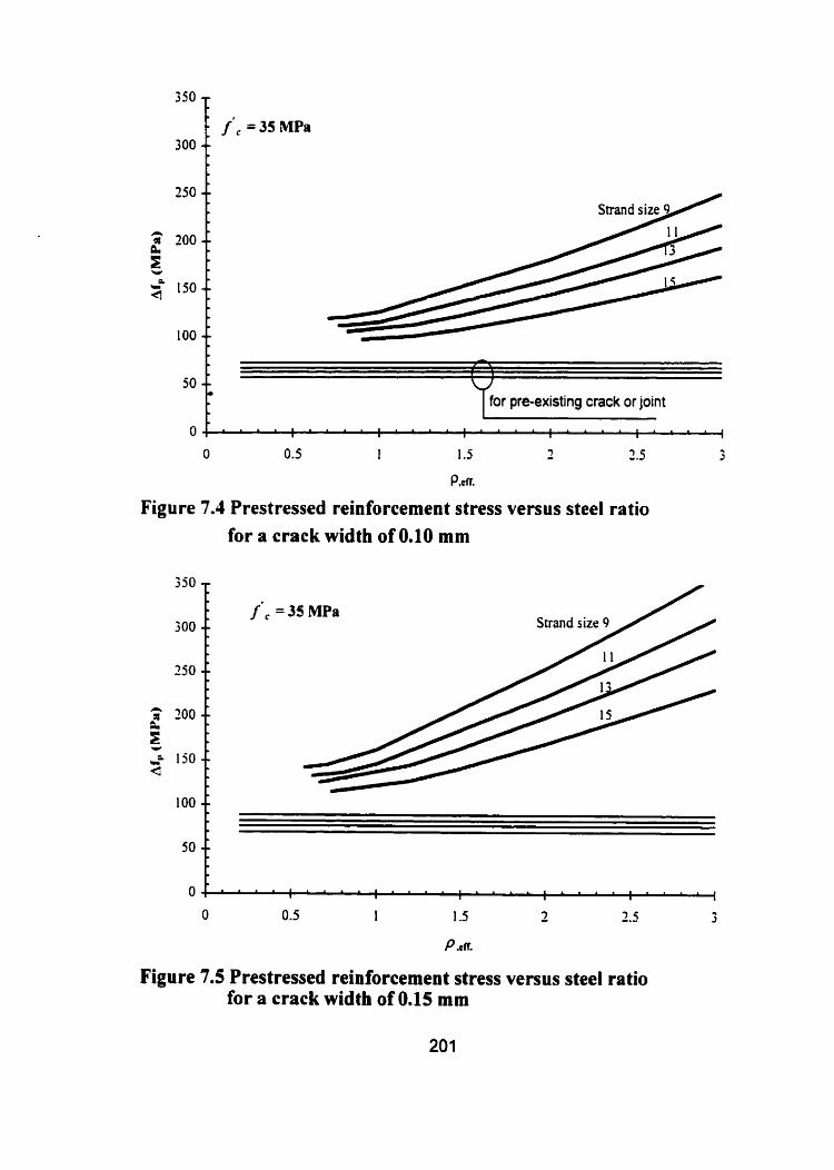
for pre-existing crack or joint

O , ' ~ L L : i . A * : L * ~ l : ~ A i i : i i ~ * : l ~ L L (

O 0.5 I 1.5 7 2.5 3

P,cfr.

Figure 7.4 Prestressed reinforcement stress versus steel ratio for a crack width of 0.10 mm

Figure 7.5 Prestressed reinforcement stress versus steel ratio for a crack width of 0.15 mm

. - -

+As/Ap = 0.2 + AslAp = 2

4 - A s l A p = 6 -0- AslAp = 9

Figure 7.9 Steel stress obtained using the proposed equation for different partial prestressing degrees

Figure 7.10 Steel stress obtained using the proposed equation for different load eccentricities

8- Summary, Conclusion, and Recommendations

8.1 Summary

The design of concrete water containment structures is studied in this thesis with

the aim of developing a rational design procedure for both reinforced and prestressed

concrete tanks that assure a safe leak resistant structure. In particular, the concepts of

partial prestressing and watertightness in liquid retaining structures are investigated.

A critical review of the existing design approaches for liquid containing

structures was carried out. The review together with design trials illustrated the

differences between the existing approaches especially those between the design of

reinforced concrete and prestressed concrete tanks. The review and the design tnals

highlighted the advantages of partial prestressing in the design of water tanks. The

literature review also revealed a growing understanding of the phenornena of

watertightness and self-sealing of cracks.

The experimental program consisted of two phases. The first phase addressed the

structural response of wall panels representing a typical wall segment from a tank with

varying reinforcement patterns. presuessing ratios and loading. The second phase

addressed leakage rates through cracked wall panels. Eight full-scale specimens. which

had three different configurations. were tested. Six specimens were subjected to leakage

tests concurrently with structural load application. The goal of the experimental program

was to provide new data that was used to develop and calibrate an analytical model.

An analytical model was written to anal yze partial1 y prestressed concrete

sections. The mode1 considen the acnial measured stress-strain relationships for the

different materials. The analytical model uses a tension stiffening description based on

the test results. The analytical model was used to simulate the test specimens. The

response predictions were satisfactory. The analytical model was then used to cany out a

p m e t r i c study on stnicturai behaviour. The aim of this parametric study was to

provide further insight into the behaviour of partially prestressed sections subjected to

combinations of axial load and moments. A fiirther objective was to examine the existing

code recornmendations in order to identify a rational method for the design of concrete

water tanks. Another limited parametric study was conducted to investigate hydraulic

conductivity through cracks and the compression zone of a cracked concrete section.

Various design strategies for the leakage limit state are next discussed. These

strategies range from preventing cracking completely to limiting through-crack widths

such that leakage rates are acceptable. Based on the results of physical and numerical

experiments. a unified limit States design approach for the design of water tanks is

proposed. The proposed approach covers water tank designs ranging from reinforced

concrete at one end of the design spectmm to fully prestressed concrete at the other. Two

design examples that illustrate the practical implementation of this proposed approach

are provided.

8.2 Conclusions

8.2.1 Conclusions from Comparison of Existing Specifications

The broad general conclusions that c m be drawn from the experience of doing 23

different designs based on the existing specifications for the design of water containment

structures are:

Ultimate strength never govems the design based on existing specifications.

Choosing the reinforcement to meet specific crack width limits requires the least

reinforcement but requires the most design calculations.

Working stress design is the easiest and produced structures only slightly more

expensive than structures designed on the basis of explicit crack width calculations.

Existing design standards are based on either hlly prestressed or fd ly non-

prestressed concepts.

The existing specifications for prestressed tanks require the use of more prestressing

steel for thicker walls to achieve the required residual compression. The existing

specifications appear to be irrational because adding concrete to the section should

not require additional reinforcement. The exishg specifications also do not provide

a recognized benefit for additional non-prestressed reinforcement.

There appears to be merit in a design based on partial prestressing concepts since ir

would recognize the benefits of additional wall thickness and additional non-

prestressed reinforcement

8.2.2 Findings from Tests

8.2.2.1 Structural Response of Wall Panels

1. Non-prestressed steel improves the cracking behaviour and increases the ductility of

the prestressed member.

2. Unbonded tendons produced the same cracking and ultimate moments as bonded

tendons in the specimens tested. The cracks in the specimen with unbonded tendons

were significantly wider and had an irregular crack pattern. The large in-plane

tension was such that the tendons yielded at ultimate.

3. In the case of eccentric tension or flexure the cracks formed at a low load level but

did not progress quickly. Under pure axial tension through-cracks occurred at higher

load level but once they occurred they become wide and progressed through the

section rapidly.

8.2.2.2 Leakage Tests

In the absence of through-cracks there was no leakage. The presence of the

compression zone prevented leakage regardless of the crack widths.

If the effective width of a through-crack was narrower than 0.15 mm. the cracks

would leak initially and then self-sed.

If the through-cracks were wide, water flowed through the cracks continuously

The pre-opened cracks self-sealed within a few hours.

8.2.3 Conclusions from the Parametric Studies

A design method based on limiting the steel stress, f,, does not produce consistent

crack or compression zone depths under the application of partial prestressing nor

under a combination of axial load and moment,

A design method based on providing a residual compressive stress in the concrete

does not utilize non-prestressed reinforcement effectively.

Relaxing the residual compressive stress requirement permits a more efficient design.

The stresses in the non-prestressed steel are higher, but remain below yield under

service load. Therefore, less reinforcement is required.

Load eccentricity significantly affects the behaviour of the partially prestressed

concrete sections. The behaviour with a small load eccentricity. less than about half

the thickness. is close to that of pure axial tension. At a load eccentricity larger than

about four times the thickness. the section may be treated as a flexural member.

The ratio of non-prestressed steel to prestressed steel in a partially prestressed

concrete section has a significant effect on the member serviceability and strength.

Choosing the ratio such that both non-prestressed and prestressrd steel reach rheir

strength simultaneously utilizes both types of steel at the ultimate lirnit state

effectively .

Increasing the wail thickness is very effective in increasing the capacity of the

section and improving its serviceability by increasing the compression zone depth

and reducing the deformations.

Virtually any compression zone depth will give adequate leakage control. While a

compression zone thickness of 5 mm may be theoretically adequate. a practical

minimum design thickness for the compression zone should account for the possible

defects in concrete surface.

8.2.4 Conclusions from the Proposed Design Approach

Design trials show that the proposed design approach has the following features:

1. Less reinforcement, especially less prestressed steel, is required.

2. n i e leakage limit state is addressed directly.

3. The benefits of increasing wall thickness and non-prestressed reinforcement are

recognized.

4. The proposed approach also offen a smooth and logical transition between the

design of fùlly prestressed and hlly reinforced concrete water tanks.

8.3 Recommendations for Future Research

The study of partially prestressed water tanks is relatively a new research field.

Many experimental and analytical research topics can be suggested such as:

Additional experimental investigation of full-scale specimens subjected to axial

tension is needed. The investigation should include parameters such as partial

prestressing ratios. crack widths. and elongation. Non-prestressed reinforcement

stress should be also obtained to validate a design equation which gives f, depending

on the partial prestressing level and the crack width. which in tum depends on

leakage limit state. Leakage rate through the cracks formed in these specimens

should also be investigated. This load case governs the design of the circular tanks.

Only one specirnen subjected to an axial tension was tested in the current study.

Leakage tests should be conducted on small specimens to investigate aspects such as

cracks that change their width with time (active cracks), variable water head, and

closed pre-existing cracks. These aspects may have effect on the leakag and the self-

sealing behaviour of through cracks.

A design aid, such as tables. should be generated to give the minimum compression

zone depth for a given leakage rate using an accurate approach, e.g. the finite

difference simulation. The variables in these tables are the wall thickness and the

water pressure. These tables can be prepared for a specific location for a given

allowable loss of water volume and the average annual weather conditions. The

designer can obtained the minimum depth of compression zone directly from these

tables.

4. Deflection of partially prestressed tanks should be investigated. This cm be done on

two levels. On the simple level, shell and plate theory equations can be used to

prepare tables, similar to the PCA tables, that give deformations. The equations given

by the building codes for the effective moment of inertia can be used to calculate the

deflection. At an advanced level, a computer pmgrarn which considers cracking and

non-linearity in concrete sections and has the ability to mode1 both types of

reinforcement, can be used in a parametric study to investigate the deformation of

partially prestressed water tanks. Deflection is critical in situations such as walls that

support roofs or are attached to any mechanical or structural element which rnight be

affected by the large deflection.

References

Abeles, P. W., 1945. Fully and Partially Prestressed Reinforced Concrete. ACI Journal.

Vol. 41, No. 3, January 1945, pp. 18 1-2 14.

AC1 Cornmittee 350, 1989. Environmental Engineering Concrete Structures (AC1 350R-

89). American Concrete Institute, Detroit, 24 pp.

AC1 Cornrninee 344. 1989. Design and Construction of Circular Prestressed Concrete

Structures (AC1 344). Amencan Concrete Institute, Detroit. 38 pp.

AC1 350.lR-93lAWWA 400-93, 1993. Testing Reinforced Concrete Structures for

Watertightness. Amencan Concrete Institute, Detroit. October 1993.

Al-Manasrer. A.A. and Philips. D.V.. 1987. Numerical Study of Some Post-Cracking

Material Parameters Affecting Nonlinear Solutions in RC Deep Beam. Canadian

Journal of Civil Engineering. Vol. 14. pp. 655-666.

Alvarez. M. and Marti, P.. 1996. Versuche zum Verbundverhalten von Bewehrungsstahl

Bei plastischen Verformungen. IBK Bericht Nr. 222, Sept. 1996. 135 pp.

Berby. A. W.. 1983. Cracking. Cover. and Corrosion of Reinforcement. Concrete

International. Vol. 5 . No. 2, Feb. 1983. pp 35-40

Bennett, E.W. and Veerasubramanian. N.' 1972. Behaviour of Nonrectangular iiearns

with Limited Prestress after FleMiral Cracking. AC1 Journal Sept. 1972. pp. 533-542.

Bick. D.. Cordes, H.. and Trost, H.? 1997. Eindnng- und Durchstr~mungsvorgiinge

umweltgefahrdender Stoffe an feinen T r e n ~ s s e n in Beton. Deutscher Ausschuss Für

Stahibeton. Heft 475. Berlin, pp. 10 1 - 17 1.

Bomhard. H.. 1986. Concrete Tanks for Water Storage - a Conceptional Approach.

Proceedings of the Tenth International Congress of the FIP. New Delhi, India. pp 55-

77.

Brmdum-Nielsen, T., 1984. On the Problems of Partial Prestressing. The Proceedings of

NATO Advanced Research Workshop. Paris. France. June 1 8-22. Vol. 2. pp. 5- 13.

BS 8 1 1O:Part 1 : 1985. Structural Use of Concrete. British Standard Institute, London.

BS 8007: 1987. Code of Practice for the Design of Concrete Structures for Retaining

Aqueous Liquids. British Standard Institute, London.

CAN ,423.3-M77. 1977. Code for the Design of Concrete Structure for Buildings.

Canadian Standard Association, CSA. Rexdale, Ontario. 13 1 pp.

CEB. 1985. CEB Manual on Cracking and Deformations. Bulletin D'Information

No 158-E. Comite Euro-International du Beton, EPF Lausanne, Swizerland. 65 pp.

CEB-FIP Mode1 Code 1990. 1993. Comite' Euro-International du Beton. EPF Lausanne,

Swizerland.

Cedergreen. H. R.. 1989. Seepage, Drainage, and Flow Nets. Third Edition. John Wiley

& Sons. New York. 465 pp.

Clear. C.A.. 1985. The Effect of Autogenous Healing upon the Leakage of Water

through Cracks in Concrete. Cernent and Concrete Association. Report No. 559. May

1985.31 pp.

Collins. M.P. and Mitchell. M.) 1987. Prestressed Concrete Basics. Canadian Prestressed

Concrete Institute. 6 14 pp.

Collins, M.P. and Mitchell, M., 1991. Prestressed Concrete Structures. Prentice Hall.

CSA M3.3-94. 1994. Design of Concrete Structures. Canadian Standard Association.

Rexdale. Ontario.

Dunne. T. and Leopold, L.B., 1978. Water in Environmental Planning. W. H. Freernan

and Company. San Francisco. 8 18 pp.

Edvardsen. C.K.. 1996. Wasserdurchlbsigkeit und Selbstheilung von Trennrissen in

Beton. Deutscher Ausschuss Für Stahlbeton. Heft 455. Berlin, 134 pp.

Elwi, A. E., 1992. FEPARCS 92- A Finite Element Program for the Analysis of

Axisymmetric Reinforced Concrete Structures. Department of Civil Engineering.

University of Alberta.

Foster, S. J., 1992. The Structural Behaviour of Reinforced Concrete Deep Beams. Ph.D.

thesis. University of New South Wales. Australia.

Gerald. C. F.. 1980. Applied Numerical Analysis. Second Edition. Addison-wesley

Publishing Company. Massachusetts. 5 18 pp.

Gergely. P. and Lutz. L. A.. 1968. Maximum Crack Width in Reinforced Concrete

Flexural Members. Causes, Mechanism. and Control of Cracking in Concrete. SP-20.

American Concrete Institute? Detroit, pp. 87-1 17.

Ghali. A. and Favre. R.. 1986. Concrete Stnictures: Stresses and Deformations. Chapman

and Hall. London. 352 pp.

Gilbert. R. 1. and Warner. R. F., 1978. Tension Stiffening in Reinforced Concrete Slabs.

Journal of the Structural Division? ASCE, Vol. 104, No. ST12: pp. 1885-1 900.

Gogate. A.B.' 198 1. Structural Design of Reinforced Concrete Sanitary Structures- Past.

Present, and Future. Concrete International, Vol. 3, No. 4, April 198 1. pp. 21-28.

Gray, W. S.. 1948. Reinforced Concrete Reservoirs and Tanks. Concrete Publications

Limited. London, 189 pp.

Habib-Allah. A., and Wilson, E.L., 1984. SAPIO- A Cornputer Program for the Finite

Element Analysis of Structures," Berkeley, California.

Harajli, M.H. and Naaman. A.E., 1984. Deformation and Cracking of Partially

Prestressed Concrete Beams under Static and Cyclic Fatigue Loading. Report No.

UMEE 84R1. Department of Civil Engineering. The University of Michigan, Ann

Arbor. Aug. 1984. 177 pp.

Harajli, M.H. and Naaman, A.E., 1989. Cracking in Partially Prestressed Beams under

Static and Fatigue Loading. AC1 Publication SP-113, Detroit. Michigan pp. 29-56.

Hassoun, M.N. and Sahebjam, K., 1989. Cracking of Partially Prestressed Concrete

Beams. AC1 Publication SP-113, Detroit, Michigan. pp. 57-78.

Imhof-Zeitler. C.. 1996. Fliebverhalten von Flüssigkeiten in durchgehend gerissenen

Betonkonstruktionen. Deutscher Ausschuss Für Stahlbeton. Hefi 460. Berlin. 199 pp.

Krishna Mohan Rao. S.V. and Dilger. W.H.. 1992. Control of Flexural Crack Width in

Cracked Prestressed Concrete Members," AC1 Structural Journal. V. 89. No. 2. pp.

127-1 38.

MacGregor. J.G.. 1997. Reinforced Concrete Mechanics and Design. Third edition.

Prentice Hall. 939 pp.

Massicotte. B.. Elwi. A.E.. and MacGregor, J.G., 1990. Tension-Stiffening Model for

Planar Reinforced Concrete Members. ASCE. Journal of Structural Engineering. Vol.

116. No. 11. Nov. 1990. pp 3039- 3057.

Mathieu. H.. 1984. Importance of Serviceability. Reexamination of Cracking Criteria.

The Proceedings of NATO Advanced Research Workshop. Puis, France. June 18-22.

Vol. 2. pp. 15-28.

Mattock. A.H.. 1979. Flexurai Strength of Prestressed Concrete Section by

Programmable Calculator. Journal of Prestressed Concrete Institute, Vol. 24. No. 1.

Jan-Feb., pp. 32-54.

Murray. M.H., 1981. Crack Widths in Water Retaining Structures. The 10n Biennial

Conference. Concrete Institute of Australia, Adelaide, Australia.

Naaman. A.E.. 1982. Fatigue in Partially Prestressed Concrete Beams. AC1 Publication

SP-75. Detroit, Michigan. pp. 25-46.

Naaman. A.E.. 1984. Partially Prestressed Concrete Members under Static Loading:

American Perspective. The Proceedings of NATO Advanced Research Workshop.

Paris. France. June 18-22. Vol. 1. pp. 79- 124.

Na-. E.G. and Huang, P.T., 1977. Crack and Deflection Control of Pretensioned

Prestressed Beams. PCI Journal may/June 1977. Pp. 30-47.

Nawy. E.G.. 1984. Flexural Cracking of Pre- and Post-Tensioned Flanged Bearns. The

Proceedings of NATO Advanced Research Workshop. Paris, France. June 18-22.

Vol. 2. pp. 137-156.

Na-. E.G.. 1989. Cracking Behaviour of Partially Prestressed Pretensioned and Post

tensioned Beams - state of the Art. AC1 Publication SP-113. Detroit. Michigan. pp.

1-28.

NBCC. 1995. National Building Code of Canada 1995. National Research Council of

Canada. Ottawa.

Seville. AM.. 198 1. Properties of Concrete. Third edition. PITMAN Publication

Limited. London. 779 pp.

PCA. 1 942. Circular Concrete Tanks without Prestressing. Portland Cernent Association.

Skokie. (revised 1993).

PCA. 1963. Rectangular Concrete Tanks. Portland Cernent Association, Skokie, (revised

198 1).

PCI Cornmittee on Precast Prestressed Concrete Storage Tanks. 198% Recommended

practice for precast concrete circular storage tanks. PCI journal, pp. 80- 125.

Ponce, V.M., 1989. Engineering Hydrology Principles and Practices. Prentice Hall.

Raju, N. K., Basavarajaiah, B. S., and Kutty. U. C., 1973. Flexural Behaviour of

Pretensioned Concrete Beams with Limited Prestress. Building Science. Progarnon

Press, Vol. 8, pp. 179- 1 85.

Simrnonds, S. H.. Rizkalla, S. H., and MacGregor, J. G., 1979. Tests of Walls Segments

from Reactor Containment. Structural Engineering Report No. 8 1, Vol. 1. Department

of Civil Engineering, University of Alberta. 207 pp.

Stevens. R.F., 1969. Tests on Prestressed Concrete Bearns. Concrete November 1969.

pp. 457-462.

Tadros. M. K.. 1982. Expedient Service Load Analysis of Cracked Prestressed Concrete

Sections. PCI Journal. V. 27. No. 6. Dec. 1982. pp. 50-63.

Vecchio. F.J. and Collins. M.P.. 1986. The Modified Compression-Field theory for

Reinforced Concrete Elements Subjected to Shear. AC1 Journal March/Apnl 1986.

Pp. 2 19-23 1.

Wilby. A.C.. 1977. Structural Analysis of Reinforced Concrete Tanks. Journal of the

Structural Division. ASCE, V. 103, No. STS. May 1977, pp. 989- 1004.

Appendix A: Listing of the Cornputer Program

The cornputer prograrn was written using Visual Basic. The program consists of

main subroutine, MAMI, and six subroutines. The main subroutine reads the data and

calls the other subroutines then writes the output. Subroutine MACR02 calculates the

strain distribution resulting from the prestressing force only before applying the extemal

loads. FIRSTVALUE calculates stresses and deformations corresponding to that strain

distribution. MACROl calculates stress resultants, stresses and deformations for each

strain increment until failure. Subroutine S H W K calculates the effect of creep and

shnnkage. Subroutine PLOTTING automatically prepares moment versus curvature

plots. Subroutine MYDATA opens and prepares new spreadsheet to inter the data and

print the results in it. The different materiai rnodels were expressed as functions grouped

in a separate subroutine. Only one subroutine was written for the case of axial load.

Listing of the complete program is below. An example for a spreadsheet that

contains the input date and a part of the output results is given in Fig. A. 1.

' This is the main subroutine, which calls the other subroutines. I

Public CS As Double, Ntotl, Mtotl, cforcel, cmoml As Double Public ecc, ecco, bottstrain, phi, cstre, topstrain, y, H As Double Public bottp, eccp, bott7, psfo, pA As Double Public topinitial, botinitial, psinitial, ds, dps As Double Public sstrain, pstrain, sstre, pstre, sforce As Double Public sarea, pforce, parea, spforce, smoment As Double Public 1, KI , K2, IayerN As lnteger Public a, b l l , b12, bto, dl1 , d12, dto, roll ro2. compl As Double Public tcon, ts, tps, fcun, phiun, phicr As Double Public creep, shstrain, tertop. zerbot, deltop, delbot As Double Public delMtot1, deliütotl , delsstra, delsstre, delsforc As Double Public delsmome, delcforc, delcmoml, delcs, zercs, redcrnod As Double Public delcstre, Mtot2, Ntot2, cstre2, sstre2 As Double '

Sub main1 () topinitial = [dZ].VaIue: botinitial = (D31,Value psinitial = [D4].Value: parea = [M].Value: sarea = [BS].Value ds = [FZ].Value: dps = (F11.Value: H = [bl ].Value 6 = [bZ].Value: Bt = [B3].Vaiue fcc = [J2].Value: cso = [J3].Value

ccrack = [J4].Value: cmod = [JS].VaIue ecco = [F 51.Value: creep = [ml ].Value shstrain = [m2].Value: zertop = [m3].Value zerbot = [m4].Value: deltop = [mS].Value deibot = [rnG].Value pA = psinitial 1 1000000 psfo = 200000 pA ' (0.026 + 0.974 1 (1 + (1 17.3 ' PA) A 10) A 0.1) ' parea

For K I = 1 To 350 topstrain = -0.005 ' (KI + 4300) Macro2

Cells(8, 2).Value = K1 If Ntotl c -psfo Then Exit For Next K I Celts(8, 3).Value = ecc Cells(8,4).Value = Ntotl / 1000 'initial normal force Cells(8, S).Value = Mtotl / 1000000 'initial moment Cells(8, 6).Value = (bottp - topstrain) / H 'phi Cells(8, 7).Value = topstrain: Cetls(8, 8).Value = bottp Cells(8, 9).Value = (-Ntotl - psfo) I psfo * 100 ecco = [FSj.Value

I

Subroutine to calculate the first values of moment and N firstvalue I

topstrain = O For K2 = 1 To 200 topstrain = -25 ' K2

Macro1 Cells(11 + K2, 2).Value = K2 Next K2

plotting End Sub

Subroutine calculates strain distribution equivalent to zero external moment Sub Macf020

l = 1 H = [bi].Value ecc = O: bottp = O Do Ntotl = O Mtotl = O Cells(8, 1).Value = I If I = 1 Then ' first estimate of bottom strain bottstrain = 3 ' topstrain Else End If sstrain = (bottstrain + (topstrain - bottstrain) ds / H) / 1000000 'rebar strain pstrain = (bottstrain + (topstrain - bottstrain) dps I H) I 1000000 'pis strain sstre = sstress(sstrain) 'rebar stress

' PIS stress using Osgood func. wl ultimate stress of 1860 MPa pstre = 200000 " pstrain (0.026 + 0.974 l ( 1 + (1 17.3 ' pstrain) A 10) A 0.1) i f pstre > 1860 Then Exit Sub sforce = sstre ' sarea ' rebar force

pforce = pstre + parea ' pis force spforce = sforce + pforce ' total steel force

' total steel moment @ the mid-height of the section smoment = sforce (H 1 2 - ds) + pforce ' (H 1 2 - d ps) cforcel = O cmoml = O For layerN = 1 To 100 'concrete strain at the centroid of the layer CS = (bottstrain - (IayerN - 0.5) 1 100 ' (bottstrain - topstrain)) 1 1000000 ' If CS < -0.0033 Then Exit Sub 'Distance between layer's centmid and section mid-height y = (H 12) - (IayerN - 0.5) H 1 100

'Concrete stress cstre = cstresl (fcc, CS, cso, ccrack, cmod)

' cstress & cstre are concrete stress formula and value respectively cforcel = cforce(cs, cstre, ccrack. H, 6, Bt) ' concrete forcellayer cmoml = cforcel y ' concrete momentllayer Ntotl = Ntotl + cforcel Mtotl = Mtotl + cmoml cforcel = O cmom? = O Next IayerN cforcel = 0 cmoml = O Ntotl = spforce + Ntotl ' total steel & concrete tension Mtotl = smoment + Mtotl ' total steel & concrete moment ecc = Mtotl 1 Ntotl ecco = H 12 - dps I = 1 + 1 If I = 2 Then bottp = bottstrain eccp = ecc bottstrain = bottstrain + Mtotl * 2 / (25 ' 389) ' (1 1 ecco - 1 1 ecc) End If If 1 > 2 And eccp = ecc Then bott7 = bottstrain + 200 ' (1 + 1) bottp = bottstrain bottstrain = bott7 eccp = ecc End If If I > 2 And eccp - ecc Then boW= bottstrain + (1 / ecco - 1 I ecc) 1 (1 1 ecc - 1 1 eccp) ' (bottstrain - bottp) bottp = bottstrain bottstrain = bon7 eccp = ecc End If Loop Until (Abs(ecc - ecco)) c 0.07 End Sub

*

' This module contains the different material models 1

Public ss As Double, CS As Double, cstre As Double, ecc As Double Public fcc As Double, cso As Double, ccrack As Double, cmod As Double Public H As Double, B As Double, Bt As Double, cforcl As Double, y As Double Public cmoml As Double, Mtotl As Double I

'The following function calculates steel stress (sstress)knowing steel strain (ss) 'yield stress = 417 MPa, Es = 190000 MPa, strain hardening strain = 0.00512 ' stress after strain hardening found by best fitting of the actual stress-strain curve 1

Public Function sstress(ss) As Double If ss <= (417 / 190000) And ss >= (-417 1 190000) Then sstress = ss ' 190000 Elself ss > (41 7 1 190000) And ss <= 0.00512 Then sstress = 4 17 Elself ss > 0.00512 And ss <= 0.125 Then sstress = ss A 3 369604 - 105391 ss A 2 + 10015 ' ss + 368 Elseif ss c (-41 7 1 190000) And ss >= -0.00512 Then sstress = -4 1 7 Elself ss c -0.00512 And ss >= -0.125 Then sstress = 369604 ss A 3 + 105391 ss A 2 + 10015 ss - 368 End If End Function I

' The following function calculates concrete stress (cstress) knowing concrete strain (CS) M o parabolic eqns. fit the stress-strain cuwe of specimen 1C40

0

'Public Function cstresl (fcc, CS, cso, ccrack, crnod) As Double ft1 = 0.22 ' Sqr(-fcc) ccrack = ft? 1 cmod I f O >= CS And CS > cso Then ' concrete in compression cstresl = 0.0135 + 27450 ' cs + 322142W CS A 2 Elself cso >= CS And CS >= -0.0033 Then cstresl = 59.04 + 97530 CS + 2264400W CS A 2 Elself CS > O And CS <= (ftl 1 cmod) Then cstresl = CS ' cmod 'cmod is the concrete modules of elasticity Elself CS > (ft l 1 cmod) And CS <= (3 ftl 1 cmod) Then cstresl = (0.4 + 0.25 14 " (3 - CS 1 ccrack) A 2) ' ft l Else cstresl = 0.4 f t l End If End Function ,

' The following function calculates concrete force (cforce) knowing concrete stress 0

Public Function cforce(cs, cstre, ccrack, H, 0, Bt) As Double If CS < ccrack Then cforce = cstre 0 H 1 100 Else cforce = cstre 8t H 1 100 End If End Function 1

" In the case of axial tension the section was divided only into 4 layers 9

Public Function cforceX(cs, cstre, ccrack, H, B, 61) As Double If CS < ccrack Then cforceX = cstre B ' H 1 4 Else cforce X= cstre ' Bt H 1 4 End If End Function

Public CS As Double, Ntotl , Mtotl , cforcel , cmoml As Double Public ecc, ecco, bottlstrain, phi, cstre, toplstrain, y, H As Double Public 1, IayerN As lnteger Public bottp, eccp, bott7 As Double Sub firstvalue()

H = [bt ).Value ecc = O: bottp = O Ntotl = O: Mtotl = O topl strain = [g8].Value: bottl strain = [h8].Value sstrain = (bottl strain + (topl strain - bottl strain) ds 1 H) 1 1000000 'rebar strain pstrain = (psinitial + (bottlstrain + (toplstrain - bottlstrain) dps 1 H)) 1 1000000 'pls strain sstre = sstress(sstrain) 'rebar stress

' PIS stress using Osgood func. wl ultimate stress of 1860 MPa pstre = 200000 ' pstrain ' (0.026 + 0.974 1 (1 + (1 17.3 " pstrain) A 10) A 0.1) If pstre > 1860 Then Exit Sub sforce = sstre " sarea ' rebar force pforce = pstre " parea ' pls force spforce = sforce + pforce ' total steel force

' total steel moment @ the mid-height of the section smoment = sforce ' (H 12 - ds) + pforce (H 12 - dps) cforcel = O: cmoml = O For IayerN = 1 To 100 'concrete strain at the centroid of the layer CS = (bottl strain - (IayerN - 0.5) 1 100 (bottl strain - toplstrain)) 1 1000000

' If CS c -0.0033 Then Exit Sub ' distance between layets centroid and section mid-height y = (H / 2) - (IayerN - 0.5) ' H 1 100 cst re = cstres 1 (fcc, CS, cso, ccrack, cmod) 'concrete stress ' cstress & cstre are concrete stress formula and value respectively cforcel = cforce(cs, cstre, ccrack, H, B, Bt) ' concrete forcellayer cmoml = cforcel ' y ' concrete momentllayer Ntotl = Ntott + cforcel Mtotl = Mtotl + cmoml cforcel = O: cmoml = O Next IayerN Ntotl = spforce + Ntotl ' total steel & concrete tension Mtotl = smoment + Mtotl ' total steel & concrete moment ecc = Mtotl / Ntotl 8

'shrinkage and creep effect 1

H = (bt ].Value Shrink

Ntot2 = Ntotl + delNtotl Mtot2 = Mtotl + delMtotl cstre2 = cstre + delcstre sstre2 = sstre + delsstre CelIs(l1, 3).Value = ecc 'final eccentricity Cells(11, 4).Value = Ntotl / 1000 'final normal force Cells(l1, S).VaIue = Mtotl 1 1000000 'final moment Cells(11, 6).Value = (bottl strain - top1 strain) I H 'phi Cells(l1, 7).Value = top1 strain Cells(11, 8).Value = bottl strain compzone = -top1 strain H 1 (bottlstrain - toplstrain) If Abs(compzone) > H Then compzone = H Cells(l1, 9).Value = compzone Cells(l1, 1 O).Value = sstre Cells(11, 1 l).Value = pstre Cells(11, 16),Value = Ntot2 / 1000 'final normal force Cells(l1, 17).Value = Mtot2 / 1000000 'final moment Cells(l1, 18).Value = ((bottl strain + delbot) - (topl strain + deltop)) / H Cells(l1, 19).Value = (topl strain + deltop) Cells(l1, 20).Value = (bottl strain + delbot) compzone = -(top1 strain + deltop) H 1 (bottl strain + delbot - toplstrain - deltop) If Abs(compzone) > H Then compzone = H Cells(l1, 21).Value = cornpzone CelIs(l1, 22).Value = sstre2 Cells(l1, 23).Value = cstre2 End Sub

' Macrol Macro ' This rnacro conducts structural analysis for the concrete section I

Public CS As Double, Ntotl, Mtotl, cforcel, cmoml As Double Public ecc, ecco, bottstrain, phi, cstre, y, Hl compzone As Double Public 1, IayerN As lnteger Public bottp, eccp, bott7 As Double Public a, bll, bl2, bto, dl1 , d12, dto, ro l , ro2, compl As Double Public tcon, ts, tps, fcun, phiun, phicr As Double Sub Macrol()

I = 1 H = [bl].Value

'Shrinkage and crrep effect Shrink 1

ecc = O: bottp = O Do Ntotl = O Mtotl = O Cells(K2 + 1 1, 1).VaIue = I If I = 1 Then ' first estimate of bottom strain topstrain = topstrain 'top strain bottstrain = -3 topstrain Else End If sstrain = (bottstrain + (topstrain - bottstrain) ds I H) 1 1000000 'rebar strain

pstrain = (psinitial + (bottstrain + (topstrain - bottstrain) dps 1 H)) I 1000000 'pis strain sstre = sstress(sstrain) 'rebar stress

' PIS stress using Osgood func. wl ultimate stress of 1860 MPa pstre = 200000 ' pstrain ' (0.026 + 0.974 1 (1 + (1 17.3 pstrain) A 10) A 0.1) If pstre > 1860 And topstrain < -3000 Then Exit Sub sforce = sstre sarea ' rebar force pforce = pstre parea ' pls force spforce = sforce + pforce ' total steel force

' total steel moment @ the mid-height of the section smoment = sforce (H / 2 - ds) + pforce (H / 2 - dps) cforcel = O cmoml = O For IayerN = 1 To 100

' concrete strain at the centroid of the layer CS = (bottstrain - (IayerN - 0.5) / 100 ' (bottstrain - topstrain)) / 1000000 If CS c -0.006 Then Exit Sub

' Distance between layef s centroid and section mid-height y = (ti / 2) - (IayerN - 0.5) H 1 100

' Concrete stress cstre = cstresl(fcc, CS, cso, ccrack, cmod)

' cstress & cstre are concrete stress formula and value respectively cforcel = cforce(cs, cstre, ccrack, Hl 6, Bt) ' concrete forceltayer cmoml = cforcel ' y ' concrete momenUlayer Ntotl = Ntotl + cforcel Mtotl = Mtotl + cmoml cforcel = O cmoml = O Next IayerN cforcel = O cmoml = O Ntotl = spforce + Mot1 ' total steel 8 concrete tension Mtotl = smoment + Mtotl ' total steel & concrete moment ecc = Mtoti / Ntotl ecco = [F5].Value If (eccoJH) > 200 GoTo linel 1=1+1 If 1 = 2 Then bottp = bottstrain eccp = ecc bottstrain = bottstrain + Mtotl 2 1 (25 389) (1 1 ecco - 1 1 ecc) End If If I > 2 And eccp = ecc Then bott7 = bottstrain + 200 ' (1 + 1) bottp = bottstrain bottstrain = bott7 eccp = ecc End If If 1 > 2 And eccp - ecc Then batt? = bottstrain + (1 1 ecco - 1 1 ecc) 1 (1 I ecc - 7 1 eccp) (bottstrain - bottp) bottp = bottstrain bottstrain = bott? eccp = ecc End If

Loop Until (Abs(ecc - ecco)) c 4 GoTo line2

L

Linel : I = l + ?

If I > 600 Then Exit Sub If I = 2 Then bottp = bottstrain bottstrain = bottstrain - 2 1 (25 ' 389) ' Ntotl Ntotp = Ntotl End If If I > 2 And Ntotp = Ntotl Then bott7 = bottstrain + 100 (1 + 1 ) bottp = bottstrain bottstrain = bott7 Ntotp = Ntotl End If If I > 2 And Ntotp - Ntotl Then bott7 = bottstrain + Ntotl 1 (Ntotp - Ntotl) (bottstrain - bottp) bottp = bottstrain bottstrain = botti Ntotp = Ntotl End If Loop Until (Abs(Ntot1)) c 5 'the loop ends GoTo line2 Line2: Mot2 = Ntotl + delNtotl Mtot2 = Mtotl + delMtotl cstre2 = cstre + delcstre sstre2 = sstress(sstrain + delsstra) 1

'Printing the calculated values I

If (ecco1H) > 200 GoTo line3 CeIls(l1 + K2, 3).Value = ecc 'final eccenricity Line3: Cells(1l + K2, 4)Yalue = Ntotl 1 1000 'final normal force Cells(1 l + K2, S),Value = Mtotl 1 1000000 'final moment Cells(1l + K2,6).Value = (bottp - topstrain) 1 H 'phi phicr = Cells(l1 + K2, 6).Value Cells(l1 + K2, 7).Value = topstrain Cells(l1 + K2, 8).Value = bottp compzone = 4opstrain H 1 (bottp - topstrain) If Abs(compzone) > H Then compzone = H Cells(11 + K2, 9).Value = compzone Cells(l1 + K2, 1 O).Value = sstre CeIls(l1 + K2, 1 1 ).Value = pstre

' The following are values after considering creep and shrinkage effect L

Cells(l1 + K2, 12).Value = Ntot2 1 1000 'final normal force Cells(i1 + K2, 13)Yalue = Mtot2 1 1000000 'final moment Cells(l1 + K2, 14).Value = ((bottp + delbot) - (topstrain + deltop)) 1 H

Cells(11 + K2, 1 S).Value = (topstrain + deltop) Cells(l1 + K2, 16).Value = (bottp + delbot) compzone = -(topstrain + deltop) ' H 1 (bottp + delbot - topstrain - deltop) If Abs(compzone) > H Then compzone = H Cells(11 + K2, l7).Value = compzone Cells(l1 + K2, 18).Value = sstre2 Cells(l1 + K2, 19).Value = cstre2 End Sub

1

' Subroutine to calculate the change in concrete stress, steel stress, total moment ' and total axial force due to shrinkage and creep strains 8

Sub Shrink() H = [bl].Value delNtot1 = 0: delMtot1 = Q delsstra = (delbot + (deltop - delbot) + ds I H) 1 1000000 'rebar strain delsstre = delsstra + 190000 'rebar stress delsforc = delsstre sarea ' rebar force

' total steel moment @ the mid-height of the section delsmome = delsforc ' (H / 2 - ds) delcforc = O delcmoml = O For IayerN = 1 To 100 Concrete strain at the centroid of the layer delcs = (delbot - (IayerN - 0.5) 1 100 (delbot - deltop)) 1 1000000 zercs = (zerbot - (IayerN - 0.5) 1 1 O0 ' (zerbot - zertop)) l 1000000 ' distance between layer's centroid and section mid-height y = (H 12) - (IayerN - 0.5) ' H 1 100 Concrete stress redcmod = cmod 1 (1 + 0.8 ' creep) delcstre = redcmod ' (-creep zercs - shstrain / 1000000 + delcs) delcforc = delcstre H 1 100 B ' concrete force/layer delcmoml = delcforc ' y ' concrete momentllayer delNtotl = delNtotl + delcforc delMtot1 = delMtotl + delcmoml delcforc = O delcmoml = O Next IayerN delcforc = O delcmoml = O delNtotl = delsforc + delNtotl ' total steel & concrete tension delMtot1 = delsmome + deIMtot1 ' total steel & concrete moment End Sub

' Mydata Macro ' this macro prepare the input to start new problem in new sheet #

Sub Mydata() Windows("M0D-1 cAO.XLS').Activate S heets("Sheet3).Select Range("A1 :wl O).Select Selection-Copy Workbooks-Add

ActiveSheet. Paste Range("K12).Select

' plotting Macro Macro plots moment-curvature diagram

I

Sub plotting() Range("E11: Ç260)Select Charts.Add ActiveChart. ChartWizard Source:=Sheets("Sheetl ").Range("El 1 :F260), -

Gallery:=xlXYScatter, Format:=6, PlotBy:=xlColurnns, - Category Labels:=l , SeriesLabels:=O, HasLegend:=2, Title:= - "Moment vs Curvature", CategoryTitle:="cu~ature", ValueTitle: = - "moment (kN m)", ExtraTitle:=""

ActiveChart. PlotArea.Select With Selection. Border

.Weight = x l f hin

.LineStyle = xlNone End With Selection. lnterior.Colorlndex = xINone ActiveC hart.SeriesColIection(1 ).Select ActiveChart.SeriesCollection(1 ).XValues = "=Sheetl !RI 1 C6:R260C6" With ActiveC hart.SeriesCoIlection(1)

.Name = ""

.Values = "=Sheetl !RI 1 C5:R260C5" End With ActiveChart. PlotArea.Select With ActiveChart.Axes(xlCategory)

.HasMajorGridlines True End With

With ActiveChart.Axes(xlValue) .HasMajorGridlines = True

End With ActiveChaf?.Axes(xIValue).MajorGridlines.Select With Selection. Border

.Colorlndex = 4

.Weig ht = xlHairline

.LineStyle = xlDot End With ActiveChart.Axes(xlCategory).MajorGridlines.Select With Selection. Border

.Color1 ndex = 4

.Weight = xlHairline -1ineStyle = xlDot

End With End Sub This is the main subroutine used for axial loading I

Public cs As Double, Ntotl , cforcel As Double Public bottstrain, cstre, topstrain, H As Double Public topinitial, botinitial, psinitial, ds, dps As Double

Public sstrain, pstrain, sstre, pstre, sforce As Double Public sarea, pforce, parea, spforce As Double Public creep, shstrain, zertop, zerbot. deltop, delbot As Double Public delNtotl , delsstra, delsstre, delsforc As Double Public delcforc, delcs, zercs, redcmod As Double Public delcstre, Ntot2, cstre2, sstre2 As Double Public K, IayerN As lnteger Sub main20 topinitial = [D2].Value: botinitial = [D3].Value psinitial = [D4].Value parea = [B4].Value: sarea = [BS].Value ds = [F2].Value: dps = [Fl].Value H = [BI].Value B = [BZ].Value: Bt = (B3J.Value fcc = [J2].Value: cso = [J3].Value ccrack = [J4].Value: cmod = [JS].Value

creep = [ml].Value: shstrsin = [m2].Value zertop = [m3].Value: zerbot = [m4].Value deltop = [mS].Value: delbot = [mG].Value

Determine the strain corresponding to zero external load H = [Bl].Value topstrain = -149.69 Do

Ntotl = O bottstrain = topstrain sstrain = (bottstrain + (topstrain - bottstrain) ds 1 H) 1 1000000 'rebar strain pstrain = (psinitial + (bottstrain + (topstrain - bottstrain) dps / H)) 1 1000000 'pls strain sstre = sstress(sstrain) 'rebar stress

' PIS stress using Osgood func. wl ultimate stress of 1860 MPa pstre = 200000-* ~strain ' (0.026 + 0.974 1 (1 + (1 17.3 pstrain) A 10) A 0.1) If pstre > 1860 Then Exit Sub sforce = sstre ' sarea ' rebar force pforce = pstre ' parea ' pls force spforce = sforce + pforce ' total steel force cforcel = O For IayerN = 1 To 4 ' the section is divided into four layers concrete strain at the centroid of the layer CS = (bottstrain - (IayerN - 0.5) 1 4 " (bottstrain - topstrain)) 1 1000000 If CS c -0.0045 Then Exit Sub If cs > -0.00009 Then Exit Do concrete stress cstre = cstresl (fcc, CS, CSO, ccrack, crnod) cstress 8 cstre are concrete stress formula and value respectively cforcel = cforce(cs, cstre, ccrack, H, B, Et) ' concrete forcellayer Ntotl = Ntotl + cforcel cforce 1 = 0 Next IayerN cforcel = O Ntotl = spforce + Ntotl ' total steel & concrete tension If Abs(Ntot1) > 2W Then topstrain = topstrain + 0.005 Else

End If Loop Until Abs(Ntot1) <= 2W 'effect of shrinkage and creep

1

S hrin k 1

Cells(1 1 , 2).Value = Ntotl / 1000 'final normal force Cells(l1, 3).Value = topstrain Celts(î 1, 4).Value = bottstrain Cells(11, S).Value = sstre Cells(11, 6).Value = pstre Cells(l1, 7).Value = (Ntotl + delNtot1) 1 1000 'final normal force Cells(l1, 8)Yalue = (topstrain + deltop) Cells(11, 9).Value = (bottstrain + delbot) Cells(l1, 10).Value = sstress(sstrain + delsstra) Celis(l1, 1 1 ).Value = (cstre + delcstre)

topstrain = O For K = 1 To 700 topstrain = -50 (3 - K) ' For K = 200 To 320 'topstrain = K 1 2 Macrol

CelIs(l1 + K. 1 ).Value = K Next K

End Sub 1

' Macrol Macro I

Su b Macrol () H = [Bl].Value Ntotl = O topstrain = topstrain 'top strain bottstrain = topstrain sstrain = (bottstrain + (topstrain - bottstrain) " ds 1 H) 1 1000000 'rebar strain pstrain = (psinitial + (bottstrain + (topstrain - bottstrain) ' dps 1 H)) 1 1000000 'pls strain sstre = sstress(sstrain) 'rebar stress

' PIS stress using Osgood func. w l ultimate stress of 1860 MPa pstre = 200000 ' pstrain (0.026 + 0.974 1 (1 + (1 17.3 ' pstrain) A 10) A 0.1) If pstre > 1860 Then Exit Sub sforce = sstre ' sarea ' rebar force pforce = pstre parea ' pis force spforce = sforce + pforce ' total steel force cforcel = O For IayerN = 1 To 4

' concrete strain at the centroid of the layer cs = (bottstrain - (IayerN - 0.5) / 4 (bottstrain - topstrain)) / 1000000 If CS c -0.0045 Then Exit Sub

' Concrete stress cstre = cstresl (fcc, CS, cso, ccrack, crnod) cstress 8 cstre are concrete stress formula and value respectively

cforcel = cforce(cs, cstre, ccrack, Hl B, Et) ' concrete forcellayer Ntotl = Ntotl + cforcel cforcel = O Next IayerN cforcel = O Ntotl = spforce + Ntotl ' total steel & concrete tension Ntot2 = Ntotl - delNtot1 cstre2 = cstre + delcstre sstre2 = sstre + delsstre Cells(11 + K, 2)Yatue = Ntotl 1 1000 'final normal force Cells(11 + K, 3)Yalue = topstrain Cells(l1 + K. 4).Value = bottstrain Cells(l1 + KI S).Value = sstre Cells(1 l + K, 6).Value = pstre Cells(l1 + K, 7).Value = Ntot2 1 1000 'final normal force Cells(l1 + K, 8).Value = (topstrain + deltop) Cells(l1 + KI 9).Value = (bottstrain + delbot) Cells(1l + K, 1 O).Value = sstress(sstrain + delsstra) Cells(l1 + K. 11 ).Value = cstre2 End Sub

C 1 D 1 E 1 F 1 G 1 H I 1 J 1 K L Initial strains (pc) dp = 90 mm (irom bottom) concrefe (a-e)

I 1

E in,, = O d = 48 mm (from bottom) f,, = -51.85 MPa

I PIS = 6064 1 E,, = 8.75E-05 e I l%(mm)= 520 mm 1 E,= 27143.55 MPa

1

6 1 I 7 strain corresponding @CC N M 4 c top E bottom % o f d m . - 8 to zero external load 33.95883 -239.378 -8.12898 -0.21 1321 -7.535 -59.94264 0.0020483

9 #of lter. Counter 1 eccen. totaitorce total mom. 4 Ew &mlmm cmp. um fs L fc

i K 1 mm kN kNm @mm CIE CLE mm MPa MPa MPa

Figure A.1 A spreadsheet contains the input data and part of the output results

M 1 N O 1 P 1 Q 1 R 1 S 1 T 1 U - + c m p - 0.665

- œ -147.47 -

Eotop - -8.1 œ

&O bot - -59

A Etop ' -145 A &bot ' -1 78

lincluding cresp & shrinkrge effect

total force total mom. + E mp ~ 1 . m c ~ n p . zone fs fc clh kN kNrn @mm LU; UT. mm MPa MPa

Figure A. I (con t.)

Appendix B: Time-dependent Stress and Strain

The concrete strain at the centroid E, and the curvature y due to the specimen

stressing and the change in these two quantities between casting and testing the specimen

due to time effects Ac, and Ay were obtained fiom Demecs readings as described in

Section 3.10. These actual values were first used to obtain the corresponding values of

the creep coefficient cp and the fiee shrinkage strain E,, that are usually obtained from

empirical equations. Ghali and Favre ( 1986) approach for calculating time-dependent

stress and strain was used as follows:

The relation between the changes in strain and curvature and the restraining force

is given by Ghali and Favre's Equation 2.35 as :

The restraining axial force LW and the restraining moment M a r e those due to

creep and shrinkage that their values are given by Ghali and Favre Equations 2.37 and

2.3 8 respective1 y. Hence. the restraining force can be expressed as:

Substituting in Eq. B-1 yields:

Reananging Equation B-3 yields:

where.

E,, AG,. y and Ay are the initial and the change in concrete axial strain at the centroid and

the initial and the change in the curvature respectively. They are

obtained from Demecs readings,

Ac and are the area and moment of inertia of uncracked concrete section, 4

A and Î are the area and the moment of inertia of the uncracked transformed section.

In the above equations the section was considered symmetric, i.e. the small shifi

in the centroid of the transformed section than the centroid of the concrete section due to

the presence of the reinforcement was neglected. This srnall shift slightly affects 7 .

The stress increment that develops during the period between casting and testing

at any fibre in concrete at a distance y from the centroid is given by Ghali and Favre

Equation 3.4 1 as:

Hence.

and Ag , , ,=E , (A&, )

where.

E, and As, are the initial and the change in concrete main at any fibre at a distance y

fiom the centroid,

AD, and AE, are the change in non-prestressed steel stress and main respectively.

Ac, and Ac, can be obtained from the strain distribution defined by A&, and Ay.

AAer calculating A&, and Ay using Equation B-4 the changes in non-prestressed

steel and concrete stresses and the changes in the axial force and the bending moment

were cakulated. This was done in the cornputer program in the subroutine called

"Shrink". in which the concrete section was divided into 100 layer. These changes were

calculated for each layer then nurnerically integrated for the whole section.

Appendix C: Solved Examples

This appendix contains two solved examples. The aim of these two examples is

to illustrate the application of the water containment structures design approach proposed

in Chapter 7. The complete design of the tank is beyond of the scope of these solved

examples. The first example presents the design of the wall of a 7900 m3 open topped

circular tank of 36 m diameter and 8 m height. The tank rests on soil and has a

membrane floor thickened beneath the wall. The thickness of the wall is taken as 250

mm. PCA (1 942) tables for circular tanks are used for the structural analysis.

The second exarnple presents the design of the wall of a 920 m' open topped

rectangular tank. The length of the shon wall = 8 m, the length of the long wall = 20 m

and the wall height = 6 m. The wall thickness is taken as 300 mm. The tank rests on soil

and has a membrane floor thickened beneath the wall. The structural analysis was

performed with SAP80 (Habib-Allah and Wilson 1984).

Zero free board was used for each design. Therefore. the water height is

considered the sarne in both the ultimate strength and the serviceability design.

Normally. the water height with a fiee board of approximately 0.3 m is considered for

the serviceability limit States while the maximum possible height of the water is

considered for the ultimate strength.

When applicable A23.3-94 is used. Some of AC1 350 recommendations (e.p. the

ailowable water loss in leakage test and temperature reinforcement) are followed in the

examples.

Example 1 - Open Topped Circular Tank (H = 8 m & D = 36 m)

water pressure from PCA Table A-5 T = coeff. (9.81 x8xI 8) = 1412.64 coeff. from PCA Table A-7 M = coeff. ( 9.81 ~8~ ) = 5022.72 coeff.

height

top O 0.8 1.6 2.4 3.2 4

4.8 5 -6 6.4

coeff. for T

-0.01 3 O. 1

0.216 0.334 0.453 0.565 0.65 0.67 0.584 0.3565

O

Coeff. for M T (kN/m)

O -18.4 O 141.3 O 305.1 O 471.8

0.0004 639.9 0.001 3 798.1 0.003 918.2

Maximum water pressure = 946.5 kN Maximum vertical moment = 33.9 kNm

T - distribution M - distribution

Prestressing

Consider the average initial stress in the strand (after initial losses) = 0.6 f ,

and that the long term tosses are 8% of that stress. Hence: P,= 0.6 x 1860xA,= 1116%

P,= 0.92 x 0.6 x 1860 x % = 1026.7 4

During prestressing the wall is free to slide. The friction with the wall pad is considered.

Wall base friction only affects the region near the base of the wall.

Therefore the ring compression due to prestressing is approximately = the prestressing force.

Choosing A,

qshould not be less than No 15 @ 300 mm each way each face (A, = 1333.33 mm2 I m = 0.0053 AJ

[A, ,,, for temperature effects required by AC1 350 varies from 0.0028 to 0.006 A, ]

Try using No. 15 @ 200 mm each face (As = 2000 mm2 1 rn = 0.008 AJ

Desian for leakaae limit state

For direct tension

Consider the allowed water loss as 0.05 % of water volume / day as specified by AC1 350

Therefore, Q ,,o.,,,c = 0.0005 x ? H /( 24 x 60 x 60) =4.71x104 m3ls

The predicted leakage rate from a through crack can be calculated using Eqs 7.8 and 7.9. In these equations, crack spacing can be calculated using CEB-FI? Model Code 1990 as

S = @, 1 3.6 p,, ,otei = 509 mm = 0.509 m

(it was noted from experiments that cracks occurred at the location of transverse steel

which means that crack spacing is likely to be 300 mm. However, S is taken = 0.509 m because this crack spacing equation was used to obtain the equations and the curves

that are used to get steel stress.

for w = 0.1 mm

.4 = 2.25 x l o 4 / (1 x 0 .0001~~) =

for wall: Q = (9.25 x [ 1 - I/2 ] w f (S A)) .u (2xrH) = 4.95~1 o4 rn31s

for floor p = (9.23 x [ I - 1 ] w 1 (S A)) x (d) = 10.8~1 o4 m31s 1 . ~ 7 ~ 1 0 ~ ~ m3/s = 33% Q , , , ~ ~

for w = 0.1 5 mm

forwall .4=6.1x10"/(1~0.0001~'x(14I/3-20))=1184~n~

Q = (9.25 x [ 1 - 1/3 ] w / (S A)) x (27trH) = 16.2~10' m3/s

for floor .4 =6.1 s 1 O d ! ( I ~ 0 . 0 0 0 1 ~ ~ ~ ( 1 4 I - 2 0 ) ) = 35800.3111~

Q = (9.25 x [ I - I ] w / (S A)) x (nr2) = 70.6~1 O= m31s

86.8~1 O~ not acceptable

Hence, u is taken 0.1 mm

In the above equations, I = 810.25 = 32. For the wall, 0.5 and 0.33 I are considered for M.

= 0.1 and 0.15 mm respectively, as explained in Section 7.3.2.2.

Alternative approach to detemin the permissible crack width W , is to obtaîned w directly

from Table 7.3 for the case of self-healing.

For w = 0.10 mm, and considering the probability of having preopened cracks,

Fig. 7.2 gives the permissible steel stress f s for No. 15 ban as 90 MPa.

The maximum ring tension in the wall (service load) is approximately = 946469 - P, = 946469 - 1026.7 A,

This force is considered as the net axial tension acting on the section and is resisted at

the crack locations by both prestressed and non-prestressed steel. The non-prestressed steel stress f , given by Eq. 7.22 is: f, = T 1 (A, +sqrt(w) Ap)

90 = ( 946469 - 1026.7 A, ) 1 (2000 tsqrt(0.4 x 15 1 1 1 ) Ap)

from which, A, = 643.20 mm2

Use 10 size 11 strands per metre grouped into multi-strand tendons (ducts) as desired for constructability . bu,= 10x74=740 mm2/m

Check the ultimate strennth limit state

There was no need to check the ultimate limit state because f, = 0.552 f,

Le. < O 6 O as explained in Section 7.4.

Interna1 forces due to prestressina force

for 10 strands : P,= 825.8 kN & P, = 759.8.0 kN

The wall weight = 0.25 x 24 x 8 = 48 kNI m of perimeter

Assuming coefficient of friction for the pad = 0.15

Friction force V = O. 15 x 48 = 7.2 kN/m

The number of strands should be reduced towards the top and the bottom. CPA tables can not be used in this case. In this example, 4 is taken constant along the wall. It is also more

accurate to consider the effect of creep and relaxation on the stress resultants for the chosen

structural system. This effect is beyond the scope of this exarnple.

Axial force

The axial force in the horizontal direction is the resultant of the prestressing force (for free base)

and force resulting fram the friction force which c m be obtained from PCA Table A-8

prestress force (kW

top O 0.8 1.6 2.4 3 3

3.2 4

4.8 5.6 6.4

7 7

7.2 bottom 8

ftee base (compression)

friction = coeff. (4) r 1 H total force coefficient

O 0.0 1 0.1 3 0.3 0.48 0.48 0.5 0.63 0.48 -0.26 -2.06 -4.4 -4.4 -5.27 -9.72

force

O -0.162 -2.1 O6 -4.86 -7.776 -7.776 -8.1

-1 0.206 -7.776 4.212 33,372 71.28 71.28 85.374 157.464

friction

coefficient top O -0.003

0.8 -0.003 1.6 -0.003 2.4 -0.001 3.2 0.003 4 0.0125

4.8 0.028 5.6 0.048 6.4 0.064 7.2 0.06

bottom 8 O

moment (kNm) O. 173 0.173 0.173 0.058 -0.173 -0.720 -1.61 3 -2.765 -3.686 -3 -456

O

1 -770.21 1= max. C -767.78

Vertical moments are due to the friction force only

Moment due to friction = coeff.(Table A-9) x (4) H

total (compression)

Case of fuH tank

consider water pressure and the effective prestressing force (after al1 losses)

Horizontal axial force heig ht

O 0.8 1.6 2.4 3 3

3.2 4

water pressure -1 8.4 141.3 305.1 471.8 598.0 598.0 639.9 798.1

prestressing -760.0 -760.2 -762.1 -764.9 -767.8 -767.8 -768.1 -770.2

total (kN) -778.4 -61 8.9 -457.0 -293. O -169.8 -1 69.8 -128.2 27.9

Ring Tension in the case of full tank

Vertical bending moment

height water prestressing total (kNm) O O 0.173 0.173

0.8 O 0.173 0.173 1.6 O 0.173 0.173 2.4 0.000 0.058 0.058

Check of stresses

maxT = 190.7 kN f, =190700 1 (2000 +sqrt(OJ x 15 1 1 1) 740) = 74.9 MPa

< 90 MPa

max compression = 778.4 x 759.8 1 825.8 = 846.09 kN (before tosses}

f , = 846090 1 (250 x 1000 x 0.97) = 3.49 MPa very srnall

(concrete area is reduced by 3% for ducts area)

Check that reinforcement will not yield at cmckina (Ea. 7.171

Cracking force = 0.25 sqrt(35) x (250000) = 369.755 kN 4, A, f , + (0.9 Ip - f p l f p r ) Ap fpr = 0.85 ~ 2 0 0 0 ~ 4 0 0 + (0.9 ~ 0 . 9 - 0.552 ) 1860 x 740:

= 1051.628 kN > cracking force

Vertical Direction

Maximum Moment = 30.2 kNm (from the case of full tank)

This moment is small and produces compression on water side of the wall. Hence the wall will

be non-prestressed. Ultimate strength design may be used to calculate As required

Mf = 1.25 x 30.2 = 37.75

As required = 617 mm2 / m (use No. 15 bar @ 300 mm 1 rn . A, = 667 mm2)

Example 2 - Open Topped Rectangular Tank

L, = 20 m L2=8 m wall thickness = 300 mm

Water pressure The stress resultants at the critical sections :

- Horizontal direction at the mid-height of the wail sec. 1-1 connecting moment = 220 kNm & T = 129 kN sec. 2-2 mid-span moment = 116 kNm 8 T = 120 kN

- Vertical direction at the mid-length of long wall sec. 3-3 maximum vertical moment = 1 15 kNm

i -1 16.6 I Horizontal moment distribution at the mid-height of long wall

Vertical moments at the mid-tength of long wall

Prestressins force

Due to the high bending moments, prestressing is used in both vertical and horizontal directions use 7-wire site 11 low relaxation strands, for which A,., = 74 mm2

effective prestressing force, P, = 0.92 ( 0.6 x 1860 ) ( 74 ) = 75.98 kN 1 strand

Vertical prestressing

Try using 8 straight strandslm with a constant eccentricity of 45 mm (outward) P, = 8 x 7 6 = 608 kN and M, = 608 x 0.045 = 27.4 kNm

The number of strands were reduced away from the long wall mid-span because the vertical moments become smaller toward wall ends. The vertical prestressing for short wall was also less

Horizontal prestressing

Try using 8 defiected strandslm with an eccentricity of 25 mm (outward) at rnid-span and 50 mm (inward) at ends. The number of strands was reduced toward the top and the bottom where moments are smaller

The tank was analyzed for both full and empty conditions.

Full Tank

Stress resultants are: sec. 1-1 connecting moment = 145 kNm 8 N = -416 kN sec. 2-2 rnid-span moment = 73 kNm & N = -145 kN sec. 3-3 maximum vertical moment = 103 kNrn 8 N = -624 kN

Empty tank

S . 1 connecting moment = -75 kNm & N = -545 kN sec. 2-2 mid-span moment = -43 kNm & N = -256 kN sec. 3-3 maximum vertical moment = -12 kNm & N = -624 kN

The minimum depth of com~ression zone which satisfies leakaae limit state

(1) Allowable Leakaae rate = Lois of water volume ~ennitted bv AC1 350 Take the allowed water loss as 0.05 % of water volume per day as specified by AC1 350

The minimum depth of the compression zone can be obtained using Eq. 7.24 (b) as:

c = 3 x 1 0 " ' { 6 ( 2 0 + 8 ) + 2 0 x 8 } 1 ( ~ 2 0 x 8 ) = 10.63 mm

(2) Allowable Leakacie rate = Eva~oration Rate

Assuming that the weather conditions on a given day are: Air temperature. T = 5 O C Wind velocity = 5 km/h Relative humidity, RH = 70°h

The evaporation rate can be calculated using Eq. 6.4 as:

e, = 6.11 exp (1 7.27 T 1 (237.3 + T) ) = 8.726

E,=e, (0.013 + 0 .00016~5 x24) (100-RH)/100 =0.0843 crntday

= 9.76 x 10-'O rnfs

At the wall base, the leakage rate through the compression zone = 3 x IO-" ( 6 1 C ) m/s

Therefore. c = 18 x 10'" 1 (9.76 x 1 O-'') = 184 mm

However. the critical section (Section 1-1) is located at the mid-height (AH = 3 m) Therefore. c = 9 x 10"' 1 (9.76 x 10-'O) = 92 mm

The velocity of the water through the compression zone at Section 1-1 = ( 3 x IO-" ) x (310.092) 10.3 =3.26 x 10~rnls

The 0.3 in this equation is the assumed void ratio of the concrete

The time required for the water to pass through the compression zone = 0.092 1 ( 3.26 x 10'' ) 1 ( 3600 124 1365 ) = 0.895 year = 10.7 months

Hence, it is more appropriate to consider the annual weather conditions to calculate the evaporation rate. For instance, if the average annual conditions are:

Air temperature, T = 14 OC Wind velocity = 13 kWh Relative humidity, RH = 70%

The minimum c required at Section 1-1 = 51.5 mm (103 mm at the wall base)

In this example, the evaporation rate govems the minimum depth of compression zone.

This depth should be increased to provide a margin of safety against any defects in concrete

Analyze the critical sections

For section 1-1 & full tank: M = 145 kNm & N = - 416 kN

Estimation of 4 h = 300 mm, d = 250 mm, d, = 200 mm use Eq. 7.18, to estimate non-prestressed steel stress f , Assuming that 4 1 4 is approximately 2. For M/T = 2201129 = 1.7, e h = 5.7

f,= 192 MPa Consider equilibrium equations:

C=N+T=N+A, f , (A)

M = C (jd) - N (d, - h12) (B) (in Eq. B, the moments are taken at the location of As. The contribution of prestressed steel after decompression is neglected for simplicity since it is just a primary estimation)

Substitute Eq. A into B

A,= [ M + N (d,-h12)]/fsjd,- N/fs

and assume jd = 0.85 d A, = [145 +416 (0.25-0.312)j x 1061(192 xO 85 x250) - 4160001 192 =2407 mm2

use 8 - No. 20 lm (2400 mm2)

Analvsis of the cracked transforrned section under the effect of M = 145 kNm & N = 416 kN

Consider Es = Ep = 200000 MPa, hence q = Es 1 Ec = 7

N = C - T p - T S 416000 = 0.5 f, c (1000) - 7 x 592 fc ( 2 0 0 ~ ) l ~ - 7 x 2400 fc ( 2 5 0 ~ ) k

f, = 832 c l [c' - 8.29 (200 - C) - 33.6 (250 c)] ( c l moments about A, location:

[ M + N (d, - hi2) ] 1 o6 = C (ds - d3) - % x 7 fc (200-C)~C (50)

186600000 = 0.5 f, x c (1000) (250 - d 3 ) - 592 x 7 f, (200~) lc (50) -- ( d )

Solving the two equations gives:

c = 103.93 mm f, = 16.96 MPa = 0.42 f, Hence. f, = 7 (16.96) (250 - 103.93)/103.93 = 167 MPa = 0.41 f,

and, A/, = 7 (16.96) (200 - 1 O3.93)llO3.93 = 109.7 MPa = 0.06 f,"

Therefore the actual depth of compression zone satisfies leakage limit state.

For the same section & empty tank: M = - 75 kNm & N = - 545 kN

Stresses distribution assuming uncracked section and considering only the concrete section for simplicity:

f, = NIA + MII y = -5450001300000 - 75000000 1 (1000 .300216) = -6.8 MPa = 0.17f,

f2 = NIA - MI1 y = -545000/300000 + 75000000 l(1000 . 300~1 6) = 3.18 MPa = 0.5 sqrt (/'c)

- Considering the transformed section yields smaller stresses. However any reduction in concrete area (e.g. at water stops) should also be considered.

- The stresses before long-terrn losses are 8% higher (8% is the percentage of long-term losses with respect to the initial prestressing force after lock-ofF)

- Although the section is uncracked, it is preferable to add non-prestressed steel in tension side, the area of this steel can be calculated to resist tensite force = area under tension in stresses distribution on the section. Steel stress may be taken around 0 .51 ,

depth of tension zone = 300 x 3.18 1 ( 3.18+6.8 ) = 95.6 mm T = 0.5 x 95.6 x3.18 x 1000 = 151990 N A, = 151990 l(0.5 x 400) = 759.9499 mm2

use 4 - No. 15 lm

Check the strenath of the section Lultimate limit state)

Factored forces resulting from water pressure:

The given cross section was analyzed using CS4 A23.3-94 equations and gives:

M, = 300.5 kNm > M,

T, = 176.7 kN > Tf

For section 3-3 & full tank: M = 103 kNm & N = - 624 kN

This section is not as critical as section 1-1 because the stress resultants are smaller.

The same procedure followed in section 1-1 can be used here to calculate the required As Estimation of A,

h = 300 mm, d, = 250 mm. d, = 195 mm use Eq. 7.18, to estimate non-prestressed steel stress f ,

and assume that &/A,, will be approximtely 2, and for fiexure

f,= 210 MPa

consider equilibrium equations: A, = [IO3 + 624 (0.25 - 0.312)J x 106 1 (210 x 0.85 x 250) - 624000 1210 = 735 mm2

use 4 - No. 15 lm (800 mm2)

Analvsis of the cncked transfonned section under the effect of M = 103 kNm 6 N = - 624 kN

fc= 1248 c 1 [c2 - 8.29 (195 - C) - 11.2 (250 c ) ]

moments at A, location:

( M + N (ds - hl2) ] 1 o6 = C (d, - d3) - Ap x 7 fc ( 1 9 5 ~ ) l ~ (50)

165400000 = 0.5 f, c (1000) (250 - d 3 ) - 592 x 7 fc (200-C)IC (50)

solving the two equations by trial and error yields:

c = 106.6 mm f, = 14.74 MPa = 0.37 f '. for the same section & empty tank: M = + 12 kNrn & N = - 624 kN

stresses distribution assuming uncracked section and consider only the concrete section for simplicity:

f, = NIA + Ml1 y = -624000/300000 - 12000000 1 (1000 . 300~1 6) = -2.88 MPa = 0.07 f

f2 = NIA - MI1 y = -624000/300000 + 12000000 1 (1000 . 3002/ 6) = -1.28 MPa

A, for section 2-2, and fcr the critical sections of the short wall should also be calculated.

The wall is 300 mm thick reinfotced at the critical section 1-1 with: eight 7-wire size 11 strands and 8 No. 20 1 m from inside and 4 No. 1 Slm from outside

IMAGE EVALUATION TEST TARGET (QA-3)

APPLIED IMAGE. lnc 1653 Easî Main Street - Rochester, NY 14609 USA . Phone: 7181482-0300 =-= F :ax: 7161288-5989