Journal of the Optical Society of America, 15(7):1777-1786, 1988.

Range Estimation by Optical Differentiation

Hany Farid Eero P. Simoncelli

Perceptual Science Group Center for Neural Science, andDepartment of Brain and Cognitive Sciences Courant Inst. of Mathematical Sciences

Massachusetts Institute of Technology New York UniversityCambridge, MA 02139 New York, NY 10003-6603

farid@persci.mit.edu eero.simoncelli@nyu.edu

Abstract

We describe a novel formulation of the range recovery problem based on computation of the differen-tial variation in image intensities with respect to changes in camera position. This method uses a singlestationary camera and a pair of calibrated optical masks to directly measure this differential quantity.We also describe a variant based on changes in aperture size. The subsequent computation of the rangeimage involves simple arithmetic operations, and is suitable for real-time implementation. We presentthe theory of this technique and show results from a prototype camera which we have constructed.

1

1 Introduction

Visual images are formed via the projection of lightfrom the three-dimensional world onto a two di-mensional sensor. In an idealized pinhole camera,all points lying on a ray passing through the pin-hole will be projected onto the same image posi-tion. Thus, information about the distance to ob-jects in the scene (i.e., range) is lost. Range informa-tion can be recovered by measuring the change inappearance of the world resulting from a changein viewing position (i.e., parallax). Traditionally,this is accomplished via simultaneous measurementswith two cameras at different positions (binocularstereo), or via sequential measurements collectedfrom a moving camera (structure from motion).

The recovery of range in these approaches fre-quently relies on the assumption of brightness con-stancy [1]: the brightness of the image of a pointin the world is constant when seen from differentviewpoints. Consider the formulation of this as-sumption in one dimension (the extension to twodimensions is straightforward). Let f(x; v) describethe intensity function, as measured through a pin-hole camera system. The variable v corresponds tothe pinhole position (along an axis perpendicularto the optical axis). The variable x parameterizesthe position on the sensor. This configuration isillustrated in Figure 1. According to the assump-tion, the intensity function f(x; v) is of the form:

f(x; v) = I�x� vd

Z(x)

�; (1)

where d is the distance between the pinhole andthe sensor and Z(x) is the range (distance from thepinhole to a point in the world). That is, the imageof a point in the world appears at a position thatdepends on both the pinhole position (v) and therange of the point, but always has the same inten-sity.

For the purpose of recovering range, we are in-terested in computing the change in the appear-ance of the world with respect to change in view-ing position. It is thus natural to consider differ-ential measurement techniques. Taking the partialderivative of f(x; v) with respect to viewing posi-

Zd

V=0

V=v

f(x;v)

I(x) = f(x;0)

x=vd/Z

x=0

V

x=0

Figure 1: Geometry for a binocular stereo sys-tem with pinhole cameras. The variable V

parameterizes the position of the camera pin-holes. According to the brightness constancyconstraint, the intensity of a point in the world,as recorded by the two pinhole cameras, shouldbe the same.

tion, and evaluating at v = 0 gives:

Iv(x) � @f(x;v)@v jv=0

= � dZ(x)I

0(x); (2)

where I 0(�) indicates the derivative of I(�) with re-spect to its argument. Consider next the partialderivative with respect to the spatial parameter:

Ix(x) � @f(x;v)@x jv=0

= I 0(x): (3)

Combining these two differential measurements gives:

Iv(x) = � dZ(x)Ix(x): (4)

Clearly, an estimate of the range,Z(x), can be com-puted using this equation. With this formulation,the difficulty typically lies in obtaining an accu-rate and efficient measurement of the viewpointderivative, Iv(x).

Many traditional range algorithms may be framedin terms of this differential formalism. The view-point derivatives are typically computed by cap-turing images from a set of discrete viewpoints, ei-ther simultaneously (using two or more cameras),

2

or sequentially (using a single moving camera). Inthe case of binocular stereo (e.g., [2]), Iv(x) is ap-proximated as the difference of two images takenfrom cameras at different viewpoints. Similarly,differences of consecutive images are often used tocompute viewpoint derivatives for structure frommotion. However, these differences are generallya poor approximation to the viewpoint derivative.In addition, these approaches require precise knowl-edge of the camera position associated with eachimage.

In this paper, we describe a technique for directmeasurement of the viewpoint derivative using asingle camera at a fixed location. We begin by de-scribing the conceptual framework for a simplifiedworld consisting of a single point-source. Theseconcepts are then generalized in Section 3, and arefollowed by a description of the implementationand results from a prototype camera.

2 Optical Differentiation

We now show a direct method for the measure-ment of the required derivatives (Equation (4)) froma single stationary camera and a pair of optical at-tenuation masks. Conceptually, this is made possi-ble by replacing the pinhole camera model with amore realistic “thin lens” model, in which the cam-era collects light from a range of viewpoints. Thisviewpoint information is lost once the light is im-aged on the sensor plane. Nonetheless, at the frontof the lens, the information is available. It is pre-cisely this information that we exploit.

Consider a world consisting of a single pointlight source and a lens-based imaging system witha variable-opacity optical mask, M(u), placed di-rectly in front of the lens (left side, Figure 2). Thelight striking the lens is attenuated by the valueof the optical mask function at that particular spa-tial location (we assume that the values of such amask function are real numbers in the range [0,1],and that the optical transfer function of the imag-ing system is constant). With such a configuration,the image of the point source will be a scaled and

-I (x) = 1/α M’(x/α) v

M’(u)M(u)

Point Light Source

Optical Mask

Lens

Sensor

Z

α

d/dx

I(x) = 1/α M(x/α)

I (x) = 1/α M’(x/α)2x

Figure 2: Illustration of direct differential rangedetermination for a single point source. Imagesof a point light source are formed using two dif-ferent optical masks, corresponding to the func-tion M(u) and its derivative, M 0(u). In eachcase, the image formed is a scaled and dilatedcopy of the mask function (by a factor �). Com-puting the spatial (image) derivative of the im-age formed under mask M(u) produces an im-age that is identical to the image formed underthe derivative mask, M 0(u), except for a scalefactor �. Thus, � may be estimated as the ra-tio of the two images. Range is then computedfrom � using the relationship given in Equa-tion (6).

dilated version of the optical mask function:

I(x) = 1�M( x� ); (5)

as illustrated in Figure 2. The scale factor, �, isa monotonic function of the distance to the pointsource, Z , and is easily derived from the imaginggeometry and the lens equation:

� = 1� df + d

Z ; (6)

where d is the distance between lens and sensor,and f is the focal length of the lens.

2.1 Optical Viewpoint Differentiation

In the system shown on the left side of Figure 2,the effective viewpoint may be altered by translat-ing the mask, while leaving the lens and sensor

3

stationary. For example, consider a mask with asingle pinhole; different views of the world are ob-tained by sliding the pinhole across the front of thelens. The generalized image intensity function fora mask centered at position v is written as:

f(x; v) = 1�M

� x� � v

�; (7)

assuming that the non-zero portion of the maskdoes not extend past the edge of the lens.

The differential change in the image with respectto a change in the mask position is obtained by tak-ing the derivative of this equation with respect tothe mask position, v, and evaluating at v = 0:

Iv(x) � @@v f(x; v)jv=0

= � 1�M

0 � x�

�; (8)

where M 0(�) is the derivative of the mask functionM(�) with respect to its argument. Observe thatthis equation is of the same general form as Equa-tion (5). Thus, the derivative with respect to view-ing position, Iv(x), may be measured directly by imag-ing with the optical mask M0(�). The spatial deriva-tive of I(x) may also be written in terms of M 0(�):

Ix(x) � @@x f(x; v)jv=0

= 1�2M

0 � x�

�(9)

Combining these two equations gives a relation-ship between the two derivatives:

Ix(x) = � 1�Iv(x): (10)

From this relationship, the scaling parameter �may be computed as the ratio of the spatial deriva-tive of the image formed through the optical maskM(u), and the image formed through the deriva-tive of that optical mask, M 0(u). This computa-tion is illustrated in Figure 2. The distance to thepoint source can subsequently be computed from� using the monotonic relationship given in Equa-tion (6). Note that the resulting equation for dis-tance is identical to that of Equation (4) when d =f (i.e., when the camera is focused at infinity). Inpractice, the mask M 0(u) cannot be directly usedas an attenuation mask, since it contains negativevalues. This issue is addressed in Section 5.2.

2.1.1 Least-Squares Solution

The relationship in Equation (10) holds at all im-age positions, x, within the image. In order tocompute a reliable estimate of the distance to thepoint source (and avoid problems with localizedsingularities where Ix(x) = 0 in Equation (10)),information can be combined over image positionusing a least-squares estimator (e.g., [2]). Specifi-cally, an error measure is defined as follows:

E(�) =Xx2P

(Iv(x) + �Ix(x))2; (11)

whereP is a set of image positions in a local neigh-borhood around the origin. This assumes that theparameter � (and therefore range) is constant overthis neighborhood. Taking the derivative with re-spect to �, setting equal to zero and solving for �yields the minimal solution:

� = �

Px2P Iv(x)Ix(x)P

x2P I2x(x)

: (12)

By integrating over a small patch in the image, theleast-squares solution avoids singularities at loca-tions where the spatial derivative, Ix(x), is zero.However, since the denominator still contains anIx(x) term (integrated over a small image patch),a singularity still exists when Ix(x) is zero overthe entire image patch. This singularity may beavoided by considering a maximum a posteriori(MAP) estimator with a Gaussian prior on � (asin [3]). For a prior variance of �2, the resulting es-timate is:

� = �

Px2P Iv(x)Ix(x)Px2P [Ix(x)]

2 + �2: (13)

This algorithm extends to a two-dimensional im-age plane: we need only consider two-dimensionalmasks M(u;w), and the horizontal partial deriva-tive Mu(u;w) � @M(u;w)=@u. For a more robustimplementation, the vertical partial derivative mask,Mv(u;w) � @M(u;w)=@w, may also be included.The least-squares error function becomes:

E(�) =X

(x;y)2P

[Iu(x; y) + �Ix(x; y)]2

+[Iw(x; y) + �Iy(x; y)]2: (14)

4

As above, the MAP estimator gives:

� = �

P(x;y)2P

Iu(x; y)Ix(x; y) + Iw(x; y)Iy(x; y)P(x;y)2P

[Ix(x; y)]2 + [Iy(x; y)]2 + �2:(15)

2.2 Optical Aperture Size Differentiation

Here we show a similar technique for estimatingrange that is based on the derivative with respectto aperture size. Discrete versions of this concepthave been studied and are generally called “rangefrom defocus” (e.g., [4, 5, 6, 7, 8, 9]). The gener-alized intensity function for a mask with aperturesize A is written as:

f(x;A) = 1A�M

� xA�

�: (16)

The 1A factor is included to ensure that the changes

in the aperture size do not change the mean inten-sity of the image.

The differential change in the image with respectto aperture size may be computed by taking thederivative of this equation with respect to aperturesize, A, evaluated at A = 1:

IA(x) � @@A f(x;A)jA=1

= � 1�M

� x�

�� x

�2M0 � x

�

�= � 1

�

�M

� x�

�+ x

�M0 � x

�

��: (17)

Since this equation is again of the general form ofEquation 5, the derivative with respect to aperturesize, IA(x), may be computed directly by imaging withthe optical mask �(M(u) + uM0(u)). Similar to theviewpoint derivative, one can compute a relatedimage by spatial differentiation. In particular, theimage formed using the optimal mask �uM(u) is:

J(x) = � x�2M

�x�

�; (18)

and the spatial derivative of this image is:

Jx(x) = � 1�2

�M

�x�

�+ x

�M0 � x

�

��; (19)

which is equal to Equation (17) with an additionalfactor of �. Thus, the ratio of these two image mea-surements could be used to compute � (and thusrange).

A particularly interesting choice for a mask func-tion is a Gaussian:

M(u;A) = 1A exp

�� u2

2A2

�;

for which

IA(x) = 1�M

00 � x�

�(20)

which may be related to the spatial second deriva-tive:

Ixx(x) = 1�3M

00 �x�

�= 1

�2 IA(x) (21)

Similar relationships are derived in [7, 9]. Thisequation may be used to compute the square ofthe scaling parameter � as the ratio of a spatialand aperture size derivative. Again, the importantpoint is that the derivative with respect to aperturesize is measured directly by imaging through theappropriate optical mask.

As in the previous section, this formulation canbe extended to 2-D and a least-squares formula-tion can be used to combine information over spa-tial location. We write an error function of theform:

E(�2) =X

(x;y)2P

�IA(x; y)� �

2(Ixx(x; y) + Iyy(x; y))�2;(22)

and solving for the minimizing �2 gives:

�2 =

P(x;y)2P

IA(x; y)[Ixx(x; y) + Iyy(x; y)]P(x;y)2P

[Ixx(x; y) + Iyy(x; y)]2 + �2: (23)

There are several notable differences betweenthis formulation based on aperture size derivativesand the previous formulation based on viewpointderivatives. First, a second-order spatial deriva-tive is required. Second, the ratio of the aperturesize derivative and spatial derivative is proportionalto the square of the parameter �. As such, only theabsolute value of � can be determined. A secondlook at the optical masks reveals why this must beso. Whereas the viewpoint derivative mask is anti-symmetric with respect to the center of the lens,the aperture size derivative mask is symmetric. Asa result, points positioned on opposite sides of thefocal plane will differ by a sign in the case of the

5

anti-symmetric mask, but could appear identicalin the case of the symmetric mask. This ambigu-ity may be eliminated by focusing the camera atinfinity, thus ensuring that � > 0.

3 Range Map Estimation by OpticalDifferentiation

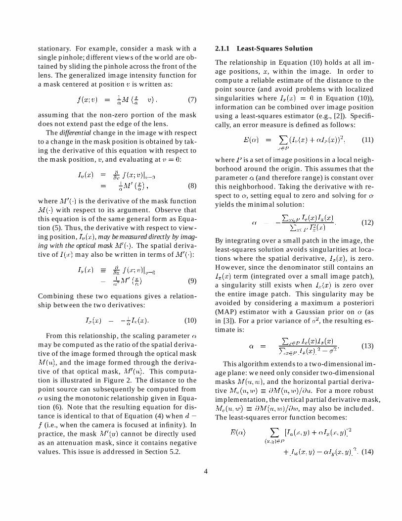
Equations (10) and (21) embody the fundamentalrelationships used for the optical differential com-putation of range for a single point light source.A world consisting of a collection of many suchpoint sources imaged through an optical mask willproduce an image consisting of a superposition ofscaled and dilated versions of the masks. In par-ticular, in the case of the viewpoint derivative, anexpression for the image can be written by inte-grating over the images of the visible points, p, inthe world:

f(x; v) =

Zdxp

1�(xp)

M

�x�xp�(xp)

� v

�L(xp); (24)

where the integral is performed over the variablexp, the position in the sensor of a point p projectedthrough the center of the lens. The intensity ofthe world point p is denoted as L(xp), and �(xp)is monotonically related to the distance to p (as inEquation (6)). Note that each point source is as-sumed to produce a uniform light intensity acrossthe optical mask (i.e., brightness constancy). Again,consider the derivatives of f(x; v) with respect toviewing position, v, and image position, x, evalu-ated at v = 0:

Iv(x) � @@vf(x; v) jv=0

= �

Zdxp

1�(xp)

M0

�x�xp�(xp)

�L(xp); (25)

and

Ix(x) � @@xf(x; v) jv=0

=

Zdxp

1�2(xp)

M0

�x�xp�(xp)

�L(xp): (26)

An exact solution for �(xp) is nontrivial, since it isembedded in the integrand and depends on the in-tegration variable. Nevertheless, the computationof Equation (10) gives an estimate:

�̂(xp) � �Iv(x)

Ix(x)

= �

Rdxp �(xp)

1�2(xp)

M 0

�x�xp�(xp)

�L(xp)R

dxp1

�2(xp)M 0

�x�xp�(xp)

�L(xp)

:(27)

The estimate �̂(xp) is seen to be a local average of�(xp), weighted by 1

�2(xp)M 0

�xp

�(xp)

�L(xp). In

particular, the more out of focus the image, thelarger the magnitude of �, and the larger the sizeof this averaging region. Of course, if the points ina local region lie on a frontal-parallel plane relativeto the sensor, the estimate will be exact.

4 Related Work

The idea of optical differentiation and its appli-cation to range estimation is novel to this work,however the concept of single-lens range imagingis not. Below are brief descriptions of several suchsystems.

The use of optical attenuation masks for rangeestimation has been considered in the work of Dowskiand Cathey [10] and Jones and Lamb [11]. The for-mer employs a sinusoidal aperture mask and com-putes range by searching for zero-crossings in thelocal frequency spectra. The latter system employsan aperture mask consisting of a pair of spatiallyoffset pinholes. Imaging through such a mask pro-duces a superimposed pair of images from differ-ent viewing positions. Range is determined us-ing standard stereo matching or visual echo tech-niques. The masks used in both these systems arenot based on differential operations. Furthermore,these systems operate on a single image and musttherefore rely on assumptions regarding the spec-tral content of the scene.

Adelson and Wang [12] describe a single-lens,single-image range camera, termed the “plenopticcamera”. This approach is based on the same un-derlying principles as our own, but is quite differ-ent in implementation. The authors place a lentic-ular array (a sheet of miniature lenses) over thesensor, allowing the camera to capture images fromseveral viewpoints. More specifically, a group of

6

5�5 pixels under each lenticule (termed a macropixel)captures a unique viewpoint. From only a singleimage, a viewpoint derivative can be computedacross several macropixels. An image derivativeis computed on the mean values of the macropix-els, and range is determined by the familiar ratioof these derivative measurements. Note however,that the viewpoint derivative is computed from adiscrete set of viewpoints. The authors noted sev-eral technical difficulties with this approach, mostnotably, aliasing and the difficulty of precisely align-ing the lenticular array with the CCD sensor.

A series of single-lens stereo systems have alsobeen developed [13, 14, 15]. In the first of thesesystems, a stereo pair of images is generated bytwo fixed mirrors, at a 45� angle with the camera’soptical axis and a rotating mirror made parallel toeach of the fixed mirrors. In the second system,a rotating glass plate placed in front of the mainlens, shifts the optical axis, simulating two cam-eras with parallel axis. The last system places twoangled mirrors in front of a camera producing animage where the left and right half of the imagecorrespond to the view from a pair of verged vir-tual cameras. In each case, range is calculated us-ing standard stereo matching algorithms. The ben-efit of these approaches is that they eliminate theneed for extrinsic camera calibration (i.e., deter-mination of the relative positions of two or morecameras), but they do require slightly more com-plicated intrinsic calibration of the camera optics.

5 Experiments

We have verified the principles of optical differ-entiation for range estimation both in simulationand experimentation [16]. This section discussesthe construction of a prototype camera, and showsexample range maps computed using this camera.

5.1 Prototype Camera

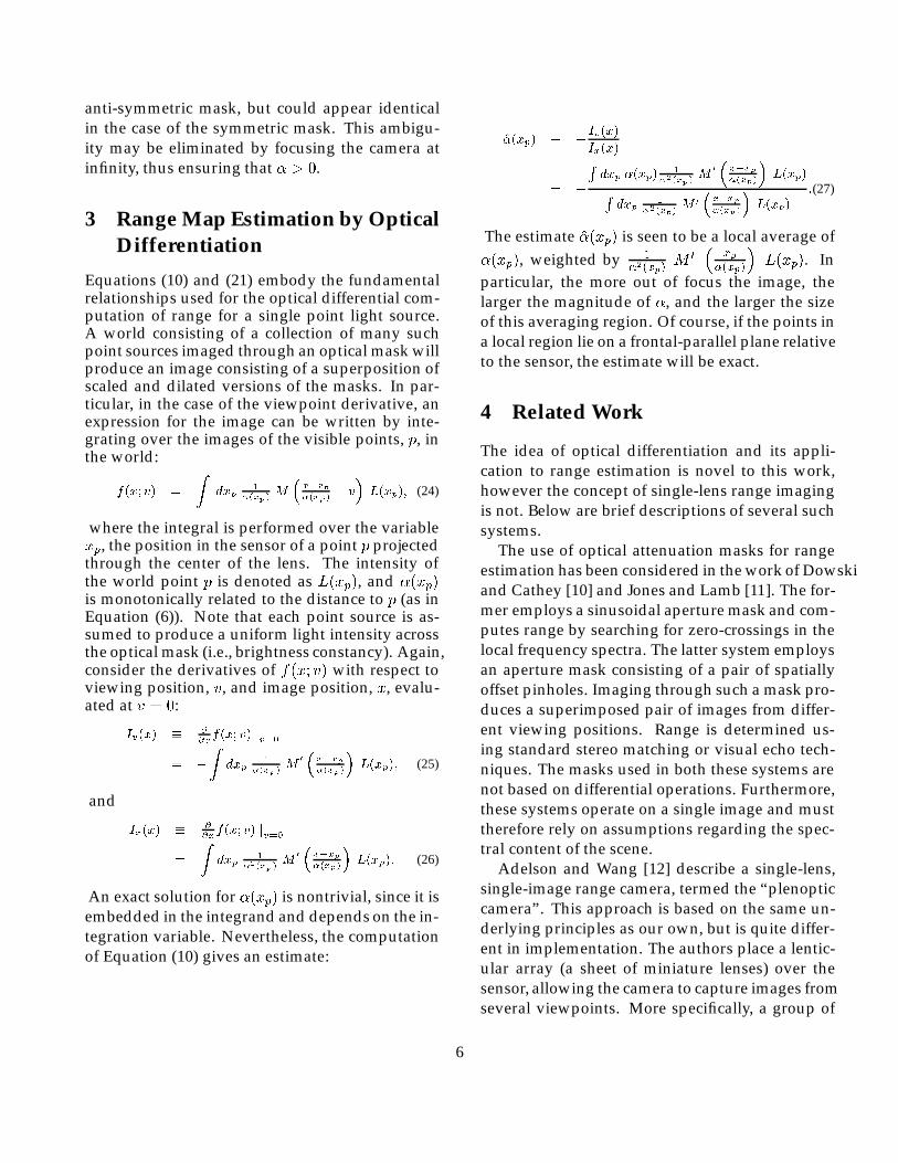
We have constructed a prototype camera for val-idating the differential approach to range estima-tion. As illustrated in Figure 3, the camera con-sists of an optical attenuation mask sandwiched

between a pair of planar-convex lenses, and placedin front of a CCD camera. This arrangement placesthe mask at the center of the optical system, wherethe viewpoint information is isolated. The cam-era is a Sony model XC-77R, the lenses are 25mmin diameter, 50mm focal length, and were placed31mm from the sensor. Thus, the camera was fo-cused at a distance of 130mm. We have employeda liquid crystal spatial light modulator (LC SLM),purchashed from CRL Smectic Technology (Mid-dlesex, UK), for use as an optical attenuation mask,also shown in Figure 3. This device is a fully pro-grammable, fast-switching, twisted nematic liquidcrystal display measuring 38mm (W) � 42mm (H)� 4.3mm (D), with a display area of 28.48mm (W)� 20.16mm (H). The spatial resolution is 640� 480pixels, with 4 possible transmittance values. Thedisplay is controlled through a standard VGA videointerface, supplied by the manufacturer. The LCSLM refreshes its display at 30 Hz; when synchro-nized with the camera, the pair of images may beacquired by temporal interleaving at a rate of 15Hz. Alternatively, a pair of images could be ac-quired simultaneously (i.e., 30 Hz), by employingan additional camera, some beam-splitting optics,and two fixed optical masks, as in [8]. The subse-quent processing (i.e., convolutions and arithmeticcombinations) can be performed in real-time on ageneral-purpose DSP chip or perhaps even on afast RISC microprocesser.

5.2 Optical Masks

The most essential component of our range cam-era is the optical attenuation mask. The functionalform of any such mask must only contain valuesin the range [0; 1], where a value of 0 correspondsto full attenuation and a value of 1 correspondsto full transmittance. The viewpoint and aperturesize derivative masks both contain negative val-ues, and thus may not be used directly. Further-more, adding a positive constant to the derivativemask destroys the derivative relationship. Nonethe-less a pair of non-negative masks can be constructedby taking the appropriate linear combination ofthe original masks. In particular, consider the fol-

7

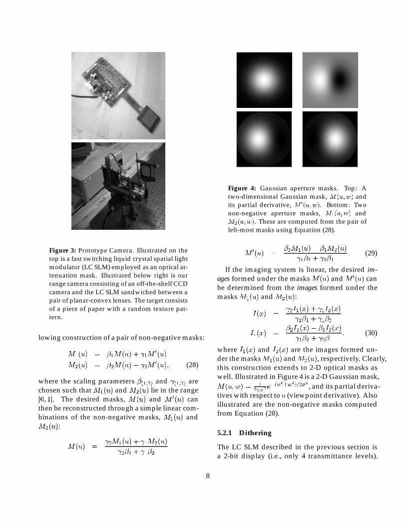
Figure 3: Prototype Camera. Illustrated on thetop is a fast switching liquid crystal spatial lightmodulator (LC SLM) employed as an optical at-tenuation mask. Illustrated below right is ourrange camera consisting of an off-the-shelf CCDcamera and the LC SLM sandwiched between apair of planar-convex lenses. The target consistsof a piece of paper with a random texture pat-tern.

lowing construction of a pair of non-negative masks:

M1(u) = �1M(u) + 1M0(u)

M2(u) = �2M(u)� 2M0(u); (28)

where the scaling parameters �(1;2) and (1;2) arechosen such that M1(u) and M2(u) lie in the range[0; 1]. The desired masks, M(u) and M 0(u) canthen be reconstructed through a simple linear com-binations of the non-negative masks, M1(u) andM2(u):

M(u) = 2M1(u) + 1M2(u)

2�1 + 1�2

Figure 4: Gaussian aperture masks. Top: Atwo-dimensional Gaussian mask, M(u;w) andits partial derivative, M 0(u;w). Bottom: Twonon-negative aperture masks, M1(u;w) andM2(u;w). These are computed from the pair ofleft-most masks using Equation (28).

M 0(u) =�2M1(u)� �1M2(u)

1�2 + 2�1: (29)

If the imaging system is linear, the desired im-ages formed under the masks M(u) and M 0(u) canbe determined from the images formed under themasks M1(u) and M2(u):

I(x) = 2I1(x) + 1I2(x)

2�1 + 1�2

Iv(x) =�2I1(x)� �1I2(x)

1�2 + 2�1: (30)

where I1(x) and I2(x) are the images formed un-der the masksM1(u) andM2(u), respectively. Clearly,this construction extends to 2-D optical masks aswell. Illustrated in Figure 4 is a 2-D Gaussian mask,M(u;w) = 1

2��2e�(u

2+w2)=2�2 , and its partial deriva-tives with respect to u (viewpoint derivative). Alsoillustrated are the non-negative masks computedfrom Equation (28).

5.2.1 Dithering

The LC SLM described in the previous section isa 2-bit display (i.e., only 4 transmittance levels).

8

In order to minimize the quantization effects dueto this low resolution, a standard stochastic errordiffusion dithering algorithm based on the Floyd/Steinberg algorithm [17] was employed. The valueof a pixel is first quantized to one of the four avail-able levels. The difference between the quantizedpixel value and the desired value is computed anddistributed in a weighted fashion to its neighbors.In [17], the authors suggest distributing the errorto four neighbors with the following weighting:

116 �

�� 7

3 5 1

�;

where the � represents the quantized pixel, andthe position of the weights represent spatial posi-tion on a rectangular sampling lattice. Since thisalgorithm makes only a single pass through theimage, the neighbors receiving a portion of the er-ror must consist only of those pixels not alreadyvisited (i.e., the algorithm should be causal). In or-der to avoid some of the visual artifacts due to thedeterministic nature of this algorithm, stochasticvariations may be introduced. Along these lines,we have taken the standard error diffusion algo-rithm and randomized the error (by a factor dis-tributed uniformly between 90% and 110%) beforedistributing it to its neighbors, and alternated thescanning direction (odd lines are scanned from leftto right, and even lines are scanned from right toleft).

5.2.2 Calibration

In our system, there are at least two potential non-linearities that need to be eliminated. The first isthe non-linearity in the light transmittance of theoptical attenuation masks. A non-linearity at thisstage will affect the derivative relationship of theoptical masks. As illustrated in Figure 5, the LCSLM used to generate the optical masks is highlynon-linear. Shown in the first panel of this figureis the light transmittance (measured with a pho-tometer) through a uniform mask set to each of thefour LCD levels. If this device were linear, thenthese measurements would lie along a unit-slopeline. Clearly they do not.

This non-linearity may be corrected in the dither-ing process. More specifically, in the dithering al-gorithm the error between the quantized pixel valueand the desired value is distributed to its neigh-bors. In order to correct for the non-linearity in theLC SLM, the diffused error may be assigned thedifference between the desired and measured lighttransmittances of the quantized pixel. Note thatwe are assuming that the LC SLM pixels are in-dependent (i.e., there are no interactions betweenneighboring transmittance values). Illustrated inFigure 5 is the measured light transmittance through32 constant masks, dithered using to this technique.The data are seen to be much more linear than theoriginal measurements.

The second potential non-linearity to consideris in the imaging sensor. With the optical masklinearized, it is possible to test the linearity of theimaging sensor by measuring the pixel intensity ofthe image of a point light source imaged through aseries of (dithered) uniform gray masks. As shownin Figure 5, the imaging sensor is fairly linear. Inparticular, the data in this figure closely resemblesthe measured light transmittance of the LC SLMafter linearization (Figure 5). Thus, it is assumedthat the imaging sensor is linear, and a second lin-earization correction is not necessary.

The final calibration that needs to be consideredis that of the camera’s intrinsic point spread func-tion (PSF). More specifically, in describing the for-mation of an image through an optical attenuationmask we have been assuming that the camera’sPSF is constant across the lens diameter (i.e., theimage of a point light source is assumed to be ahard-edged rectangular function). This is gener-ally not the case in a real camera: the PSF typicallytakes on a Gaussian-like shape. The PSF and theoptical mask will be combined in a multiplicativefashion. Whereas before, we employed a matchedpair of masks,M(u) andM 0(u), with dM(u)

du = M 0(u),we now require a pair of masks, M(u) and M̂(u),that obey the following constraint:

M̂(u)H(u) =d(M(u)H(u))

du; (31)

where H(u) is the camera PSF. That is, the deriva-

9

0

0.5

1

Nor

mal

ized

Lig

ht T

rans

mitt

ance

0 0.5 1LCD Value

0

0.5

1

Nor

mal

ized

Lig

ht T

rans

mitt

ance

0 0.5 1Dithered LCD Transmittance

0

0.5

1

Nor

mal

ized

CC

D In

tens

ity

0 0.5 1Dithered LCD Transmittance

Figure 5: Calibration of LCD mask and CCDsensor. Shown in the top left panel is thenormalized light transmittance (in cd/m2, asmeasured with a photometer) through constantmasks set to each of the four LCD values.Shown in top right panel is the normalized lighttransmittance measured through each of 32 uni-form dithered and gamma-corrected masks, av-eraged over five trials. If our dithering andgamma-correction were perfect, the measure-ments (circles) would lie along a unit-slope line(dashed line). Shown in the lower panel is thenormalized CCD pixel intensity of a point lightsource as imaged through a series of 32 uni-form, dithered optical masks (with gamma cor-rection), averaged over five trials, and spatiallyintegrated over a 5 � 5 pixel neighborhood. Ifboth the optical mask and imaging sensor werelinear, then these measurements (circles) wouldlie along a unit-slope line (dashed line).

tive relationship should be imposed on the prod-uct of the optical mask and the PSF. We have notincluded this calibration in our experiments.

5.3 Results

We have verified the principles of range estima-tion by optical differentiation with a prototype cam-era which we have constructed (see Figure 3). Ac-cording to our initial observation we expect thatthe image of a point light source to be a scaled anddilated copy of the mask function. Illustrated inFigure 6 is an example of this behavior: shown are

Figure 6: Illustrated in the top two panelsare 1-D slices of the image of a “point lightsource” taken through a pair of non-negativeGaussian-based masks, I1 and I2. Shown inthe bottom left panel are 1-D slices of the linearcombination of the measurements (see Equa-tion (30)). Shown in the bottom right panel are1-D slices of the resulting images Ix (solid) and�Iv (dashed). These images should be relatedto each other by a scale factor of � (see Equa-tion (10)).

1-D slices of images taken through a pair of non-negative Gaussian-based optical masks printed ontoa sheet of transparent plastic (later experiments uti-lized the LC SLM described above). The appropri-ate linear combination of these slices (Equation (30)),and the resulting slices of Ix(x) and Iv(x).

In the remaining experiments the target consistedof a sheet of paper with a random texture patternand back-illuminated with an incandescent lampto help counter the low light transmittance of theLC SLM optical mask. Spatial derivatives werecomputed using a pair of 5-tap filter kernels de-scribed in [18]. For example, the x-derivative iscomputed via separable convolution with the one-dimensional derivative kernel in the x direction,and with a one-dimensional blurring kernel in they direction. The viewpoint derivative was filteredwith the blurring kernel in both spatial directions.Range was estimated using the least-squares for-mulation (Equations (15) or (23)), with a spatial in-tegration neighborhood of 31 � 31 pixels.

10

Illustrated in Figures 7 and 8 are a pair of re-covered range maps for frontal-parallel surfacesplaced at distances of 11 and 17 cm from the cam-era. These figures illustrate the range maps com-puted using optical viewpoint and aperture sizedifferentiation, respectively. The camera is focusedat a distance of 13 cm. In the case of the viewpointdifferentiation, the recovered range maps had amean of 10.9 and 17.0 cm, with a standard devia-tion of 0.27 and 0.75 cm, and a minimum/maximumestimate of 10.1/11.8 cm and 15.1/19.4 cm, respec-tively. In the case of the aperture size differen-tiation, the recovered range maps had a mean of11.0 and 17.0 cm, with a standard deviation of 0.06and 0.16 cm and a minimum/maximum estimateof 10.8/11.2 cm and 16.5/17.5 cm, respectively. Itwas somewhat surprising to discover that the aper-ture size differentiation gave significantly betterresults than the viewpoint differentiation (in termsof standard deviation). We suspect that one possi-ble reason for this is that the aperture size maskshave a higher total light transmittance: for the Gaussian-based optical masks, the mean light transmittanceis 0.37, as compared to a mean of 0.20 for the view-point masks. Increased light transmittance pro-duces a higher signal-to-noise ratio in the measure-ments. Although the aperture size differentiationhas smaller errors in this example, it suffers froma sign ambiguity (i.e., surfaces on either side of thefocal plane can be equally defocused). Illustratedin Figure 9 is a recovered range map for a planersurface oriented approximately 30 degrees relativeto the sensor plane, with the center of the plane14 cm from the camera, and a pair of occludingsurfaces placed at 11 and 17 cm. The recoveredrange maps in this figure were determined usingthe viewpoint differentiation formulation. Quali-tatively, these range maps look quite reasonable.

5.4 Sensitivity

As with most other techniques, the inherent sensi-tivity of our method of range estimation is depen-dent on the basic rules of triangulation. In par-ticular, from classical binocular stereo we knowthat range is inversely proportional to disparity:

0

10

20

0

10

20

Figure 7: Illustrated are the recovered rangemaps using optical viewpoint differentiationfor a pair of frontal-parallel surfaces at a dis-tance of 11 and 17 cm from the camera. Thecomputed range maps have a mean of 10.9 and17.0 cm with a standard deviation of 0.27 and0.75 cm, respectively.

0

10

20

0

10

20

Figure 8: Illustrated are the recovered rangemaps computed using optical aperture size dif-ferentiation for a pair of frontal-parallel sur-faces at a distance of 11 and 17 cm from the cam-era. The computed range maps have a mean of11.0 and 17.0 cm with a standard deviation of0.06 and 0.16 cm, respectively.

Z = dbD , where d is the distance between lens and

sensor, b is the distance between the stereo camerapair (i.e., the “baseline”), and D is the measureddisparity. The sensitivity in estimating range withrespect to errors in the disparity estimate can bedetermined by differentiating with respect to thisparameter:

����@Z@D���� =

���� dbD2

����/

Z2

db: (32)

In our system, � plays the role of disparity, andeffective baseline is proportional to lens diameter

11

0

10

20

0

10

20

Figure 9: Illustrated on the left is the recoveredrange map computed using optical viewpointdifferentiation for a slanted surface oriented ap-proximately 30 degrees relative to the sensorplane with the center of the plane at a depth of14 cm. Illustrated on the right is the recoveredrange map for a pair of occluding surfaces at adepth of 11 and 17 cm.

and dependent on the choice of optical masks.In addition, errors in estimating � will be pro-

portional to �2. More specifically, we consider theeffects of additive noise in the differential measure-ments:

�̂ = �Iv +�v

Ix +�x

= �1�M

0 +�v1�2M 0 +�x

= ��+ �2�v

M 0

1 + �2�x

M 0

: (33)

Expanding the denominator as a polynomial se-ries in �x, the leading error terms of the full ex-pression are seen to scale as the square of�. Rewrit-ing in terms of depth (using Equation (6)) and in-coporating with the above, we expect errors in thedifferential measurements to produce range errorsof the form:

�Z /Z2

db

�1� d

f + dZ

�2�fv;xg: (34)

That is, measurement errors lead to range errorsthat scale as the square of the distance from thefocal plane.

6 Discussion

We have presented the theory, analysis, and im-plementation of a novel technique for estimatingrange from a single stationary camera. The com-putation of range is determined from a pair of im-ages taken through one of two optical attenuationmasks. The subsequent processing of these imagesis simple, involving only a few 1D convolutionsand arithmetic operations.

The simplicity of this technique has some clearadvantages. In particular, the use of a single sta-tionary camera reduces the cost, size and calibra-tion of the overall system, and the simple and fastcomputations required to estimate range makes thistechnique amenable to a real-time implementation.In comparison to classical stereo approaches, ourapproach completely avoids the difficult and com-putationally demanding “correspondence” prob-lem. In addition, with only a single stationary cam-era, we avoid the need for extrinsic camera calibra-tion. There are some disadvantages as well. Mostnotably, the construction of a non-standard imag-ing system, and the limited range accuracy due tothe small effective baseline.

A counterintuitive aspect of our technique is thatit relies on the defocus of the image. In particu-lar, a perfectly focused image corresponds to � =0, leading to a singularity in Equation (10). Wehave partially overcome this problem by impos-ing a prior density on � that biases solutions to-ward the focal plane. But in general, accuracy willbe best for surfaces outside of the focal plane.

The results presented here can be improved ina number of ways. A better mask design, whichincludes the effects of the PSF of the camera opticsand optimizes light transmittance while satisfyingthe desired derivative relationship could have alarge effect on the quality of the estimator. In theproposed camera, a pair of images are acquired ina temporally interleaved fashion, so that motion inthe scene will be misinterpreted as false range in-formation. A more sophisticated algorithm shouldbe developed that compensates for any inter-framemotion. Alternatively, the technique could be mod-ified to measure the two images simultaneously

12

(using a beamsplitter, as in [8]). Finally, as withall intensity-based range imaging approaches, theresults may be improved by illuminating the scenewith structured light.

Acknowledgments

This research was performed while HF was in theGRASP Laboratory at the University of Pennsyl-vania, where he was supported by ARO DAAH04-96-1-0007, DARPA N00014-92-J-1647, and NSF SBR89-20230. HF is currently at MIT where he is sup-ported by NIH Grant EY11005-04 and MURI GrantN00014-95-1-0699. This research was performedwhile EPS was in the GRASP Laboratory at theUniversity of Pennsylvania, where he was partiallysupported by ARO/MURI DAAH04-96-1-0007. EPSis currently at NYU, where he is partially supportedby NSF CAREER grant 9624855. Portions of thiswork have appeared in [19, 20, 21, 16].

References

[1] B.K.P. Horn. Robot Vision. MIT Press, Cam-bridge, MA, 1986.

[2] B.D. Lucas and T. Kanade. An iterative imageregistration technique with an application tostereo vision. In Proceedings of the 7th Interna-tional Joint Conference on Artificial Intelligence,pages 674–679, Vancouver, 1981.

[3] E.P. Simoncelli, E.H. Adelson, and D.J.Heeger. Probability distributions of opti-cal flow. In Proc Conf on Computer Visionand Pattern Recognition, pages 310–315, Mauii,Hawaii, June 1991. IEEE Computer Society.

[4] A.P. Pentland. A new sense for depth of field.IEEE Transactions on Pattern Analysis and Ma-chine Intelligence, 9(4):523–531, 1987.

[5] M. Subbarao. Parallel depth recovery bychanging camera parameters. In Proceedingsof the International Conference on Computer Vi-sion, pages 149–155, Tampa, FL, 1988. IEEE,New York, NY.

[6] Y. Xiong and S. Shafer. Depth from focus-ing and defocusing. In Proceedings of theDARPA Image Understanding Workshop, pages967–976, New York, NY, 1993. IEEE, Piscat-away, NJ.

[7] A.M. Subbarao and G. Surya. Depth fromdefocus: A spatial domain approach. Inter-national Journal of Computer Vision, 13(3):271–294, 1994.

[8] S.K. Nayar, M. Watanabe, and M. Noguchi.Real-time focus range sensor. IEEE Transac-tions on Pattern Analysis and Machine Intelli-gence, 18(12):1186–1198, 1995.

[9] M. Watanabe and S. Nayar. Minimal oper-ator set for passive depth from defocus. InProceedings of the Conference on Computer Vi-sion and Pattern Recognition, pages 431–438,San Francisco, CA, 1996. IEEE, Los Alasmi-tos, CA.

[10] E.R. Dowski and W.T. Cathey. Single-lenssingle-image incoherent passive-ranging sys-tems. Applied Optics, 33(29):6762–6773, 1994.

[11] D.G. Jones and D.G. Lamb. Analyzing the vi-sual echo: Passive 3-d imaging with a multi-ple aperture camera. Technical Report CIM-93-3, Department of Electrical Engineering,McGill University, 1993.

[12] E.H. Adelson and J.Y.A. Wang. Single lensstereo with a plenoptic camera. IEEE Trans-actions on Pattern Analysis and Machine Intelli-gence, 14(2):99–106, 1992.

[13] W. Teoh and X.D. Zhang. An inexpensivestereoscopic vision system for robots. In Inter-national Conference on Robotics, pages 186–189,1984.

[14] Y. Nishimoto and Y. Shirai. A feature-basedstereo model using small disparities. In Pro-ceedings of the Conference on Computer Visionand Pattern Recognition, pages 192–196, Tokyo,1987.

13

[15] A. Goshtasby and W.A. Gruver. Design ofa single-lens stereo camera system. PatternRecognition, 26(6):923–937, 1993.

[16] H. Farid. Range Estimation by Optical Differen-tiation. PhD thesis, Department of Computerand Information Science, University of Penn-sylvania, Philadelphia, PA., 1997.

[17] R.W. Floyd and L. Steinberg. An adaptive al-gorithm for spatial grey scale. Proceedings ofthe Society for Information Display, 17(2):75–77,1976.

[18] H. Farid and E.P. Simoncelli. Optimallyrotation-equivariant directional derivativekernels. In Computer Analysis of Images andPatterns, Kiel, Germany, 1997.

[19] E.P. Simoncelli and H. Farid. Direct differ-ential range estimation from aperture deriva-tives. In Proceedings of the European Conferenceon Computer Vision, pages 82–93 (volume II),Cambridge, England, 1996.

[20] E.P. Simoncelli and H. Farid. Single-lens range imaging using optical derivativemasks, 1995. U.S. Patent Pending (filed14 Nov 1995). International Patent Pending(filed 13 Nov 1996).

[21] H. Farid and E.P. Simoncelli. A differentialoptical range camera. In Proceedings of the An-nual Meeting of the Optical Society of America,Rochester, NY, 1996.

14