RAILWAY BRIDGE CONDITION MONITORING AND FAULT ...

The University of Nottingham

Department of Civil Engineering

Resilience Engineering Research Group

RAILWAY BRIDGE CONDITION

MONITORING AND FAULT

DIAGNOSTICS

Matteo Vagnoli

A Doctoral Thesis

Thesis submitted to the University of Nottingham for the degree of

Doctor of Philosophy

November 2018

Abstract

The European transportation network is ageing continuously due to environmental

threats, such as traffic, wind and temperature changes. Bridges are vital assets of the

transportation network, and consequently their safety and availability need to be

guaranteed to provide a safe transportation network to passenger and freights traffic.

The main objective of this thesis is to develop a bridge condition monitoring and

damage diagnostics method. The main element of the proposed Structural Health

Monitoring (SHM) method is to monitor and assess the health state of a bridge

continuously, by taking account of the health state of each element of the bridge. In

this way, an early detection of the ongoing degradation of the bridge can be achieved,

and a fast and cost-effective recovery of the optimal health state of the infrastructure

can be achieved.

A BBN-based approach for bridge condition monitoring and damage diagnostics is

proposed and developed to assess and update the health state of the bridge

continuously, by taking account of the health state of each element of the bridge. At

the same time, the proposed BBN approach allows to detect and diagnose damage of

the bridge infrastructure.

Firstly, the BBN method is developed for monitoring the condition of two bridges,

which are modelled via two Finite Element Models (FEMs). The Conditional

Probability Tables (CPTs) of the BBN are defined by using an expert knowledge

elicitation process. Results shows that the BBN allows to detect and diagnose damage

of the bridges, however the performance of the BBN can be improved by pre-

processing the data of the bridge behaviour and improving the definition of the CPTs.

A data analysis methodology is then proposed to pre-process the data of the bridge

behaviour, and to use the results of the analysis as an input to the BBN. The proposed

data analysis methodology relies on a five-step process: i) remove of the outlier of the

bridge data; ii) identify of the free-vibration of the bridge; iii) extract statistical,

frequency-based and vibration -based features from the free-vibration behaviour of the

bridge; iv) assess the features trend over time, by using the extracted features as an

input to an Empirical Mode Decomposition (EMD) algorithm; v) evaluate of the

Health Indicator (HI) of the bridge element. The proposed data analysis methodology

is tested on two in-field bridges, a steel truss bridge and a post-tensioned concrete

bridge, which are subject to a progressive damage test.

A machine learning method is also developed in order to assess the health state of

the bridge automatically. A Neuro Fuzzy Classifier (NFC) is adopted for this purpose.

The results of the NFC can potentially be used as an input to the BBN nodes, to select

the states of the BBN nodes, and improve the BBN performance. In fact, the NFC

shows high accuracy in assessing the health state of bridge elements. An optimal set

of HIs, which allows to maximize the accuracy of the NFC, is identified by adopting

an iterative Modified Binary Differential Evolution (MBDE) method. The NFC is

applied to the post-tensioned concrete in-field bridge that is subject to a progressive

damage test.

Hence, the performance of the BBN is improved significantly by pre-processing the

bridge data, but also by developing a novel method to continuously update the CPTs

of the BBN. The CPTs update process relies on the actual health state of the bridge

element, and the knowledge of bridge engineers. Indeed, the CPT updating method

aims to merge the expert knowledge with the analysis of the bridge behaviour. In this

way, the diagnostic ability of the BBN is improved by merging the expertise of bridge

engineer, who can analyse hypothetical damage scenarios of the bridge, and the

analysis of a database of known bridge behaviour in different health states. The method

is verified on the post-tensioned concrete in-field bridge, by developing a BBN to

monitor the health state of the bridge continuously. The damages of the bridge are

diagnosed by the proposed BBN.

Finally, a method to analyse database of unknown infrastructure behaviour is finally

proposed. An ensemble-based change-point detection method is presented to analyse

a database of past unknown infrastructure behaviour. The method aims to identify the

most critical change of the health state of the infrastructure, by providing the

characteristics of such a change, in terms of time duration and possible causes. The

method is applied to a database of tunnel behaviour, which is subject to renewal

activities that influence the health state of the infrastructure.

To my Family…

“…Laugh as we always laughed at the little jokes that we enjoyed together…

...Play, smile, think of me…It is the same as it ever was...

…How we shall laugh at the trouble of parting when we meet again!”

Acknowledgements

The acknowledgement section is usually the most boring and most important part

of a thesis. It is boring because it’s merely a list of thank-you’s, yet it’s important

because most of the people that will read a thesis would never go beyond this section.

For this reason, I will try to be as boring as possible, to sincerely thank all the people

that I have met throughout my PhD. To any readers that are scrolling this thesis

casually, please consider this as your final warning.

I will start my acknowledgments by thanking the European Union, which allows

thousands of students to experience a fantastic journey of personal and technical

growth through the Marie-Curie Fellowship. If such an experience would have been

available for more people, who would have had the possibility of experiencing

different cultures and make new friends from all over the word, we would be more

united, and we would probably have less brexiters-style of people.

I sincerely thank Prof. John Andrews, for giving me this opportunity after a short,

fun and constructive skype interview. At the same time, I have really appreciated his

wise managing style of the Research Engineering Research Group (RERG).

It is difficult to find enough words to thank Dr. Rasa Remenyte-Prescott adequately.

I am grateful to have had such a great, smart and patient supervisor, who gave me

precious and intelligent technical suggestions continuously, while also helping me in

growing as a Man. Thank you Rasa. I recognise I was not the easiest PhD student of

your career, and I am sorry for all the unrequested comments, ideas, actions, etc. I have

learnt a lot as a person thanks to your guidance. I would like also to thank you for

being part of my kidnap during February 2017, when I left home for going to the

grocery shop, and I ended up in Iceland.

Obviously, I need to thank the whole TRUSS crew, from the project coordinator

Prof. Arturo Gonzalez (who also shared some data to validate the method developed

in this thesis) to Loreto and Parisa, who magnificently organized each TRUSS event.

Similarly, all the Professors (with a special mention for Prof. Juan Ramon Casas) and

people of the TRUSS consortium need my warmest acknowledgment.

I’ll skip the acknowledgments to the TRUSS ESRs, they already know that they

rock, all of them. Similarly, the RERG and NTEC PhD students and researchers are

among the smartest and funniest people that I have ever met.

AECOM needs to be warmly recognized for allowing me to experience the consulting

world, for having hosted me for four months during my PhD and having provided data

and case studies. Particularly, I would thank Matt Brough, Paul Clarke, Neil Atkinson

(even if I am still waiting his reply to my emails) and Daniel Thompson. I hope you

are doing a great job with the codes that we developed together.

Last but not least (a classic closing remark in any well-respected acknowledgement

section), for the PhD-related appreciation, I would like to thank Network Rail, for

giving me the opportunity to take part in some visual inspections of railway bridges

along with the engineering team.

All my dear friends in Nottingham are worth to be mentioned, for their continuous

support, time and friendship: thank you Federico and Kamila for Michelin star home

cooked dinners, thanks to Francesco for (almost) continuously loosing squash matches

against me, and to his awesome girlfriend Roberta, who bakes the best mascarpone

and the best parigina of the world. Thanks also to Alberto and Francesca for lovely

feeding the ducks of the Nottingham Canal, we will conquer them one day. The

Brazilian couple Gustavo and Emily is one of the best couples that I ever seen, and I

would like to thank them for their delicious mayonnaise with potatoes. Andrea, thank

you for your pesto-, risotto-, lasagna-, whatever-nights, you are great. Francesco

Cannarile, Silvia Marino and Claudia Picoco are worth mentioning for hours of

chatting and ideas sharing.

Finally, I must thank my whole family, Sonja and Mario, Filippo and Monica. We

have spent hours face-timing each other to minimize the distance between us, and to

talk and support each other for any decision we were facing. We are a great Team,

which is able to face and solve everything, without losing our smiles. I am grateful to

have a family like ours. Similarly, Fabio, Nicoletta, Francesco, Lorenzo, Elvira and

Rossano have been a strong column that kept me motivated and happy.

The very last person to acknowledge is the one that is sitting right next to me during

this Rome to Liverpool Sunday morning flight. I have sincerely lost the count of how

many flights we have caught together during these three years. We should be co-

owners of EasyJet, for having flown with them from Luton to Paris CDG every single

weekend from September 2015 to February 2017. All that travelling was hard,

exhausting and a great moment of excitement (on Friday) and solitude (on Sunday),

but it was worth every second. It is just thank to you if I am here writing this thesis, as

you have been supporting me since the application phase. You have challenged me

every single second throughout the journey, even going against me in order to allow

me to see the bigger picture. Thank you for this, it allowed me to grow and view

different unknown prospective. Thank you, Allegra, let’s keep exploring the world

with last minute unpredictable and unscheduled journeys, together.

i

Table of Contents

Introduction ........................................................................................ 1

Introduction .................................................................................................. 1

Introduction to Structural Health Monitoring .......................................... 1

Structural Health Monitoring desiderata .................................................. 2

The need of a Bayesian Belief Network (BBN) approach ....................... 5

Data analysis methodology, machine learning methods and BBN .......... 6

A method to update the CPTs of the BBN by taking account of expert

judgment and bridge behaviour data .................................................................... 7

A method to analyse a database of infrastructure behaviour ................... 8

Research aims and objectives....................................................................... 8

Research aims........................................................................................... 8

Research objectives .................................................................................. 9

Thesis Outline ............................................................................................ 10

Structural Health Monitoring of bridges ....................................... 11

Introduction to literature review................................................................. 11

Model-based condition monitoring and damage detection methods.......... 12

FEM updating methods .......................................................................... 12

Non-Model-based methods ........................................................................ 16

Artificial Neural Network based methods ............................................. 17

Other non-model-based methods ........................................................... 21

Bayesian Belief Network methods ......................................................... 25

Requirements for a new detection and diagnostics of bridge deterioration

method .................................................................................................................... 27

The proposed Bayesian Belief Network approach ........................ 29

Introduction ................................................................................................ 29

Background of the Bayesian Belief Network method................................ 31

The structure of the BBN ....................................................................... 31

Bayes theorem and CPTs ....................................................................... 31

ii

Chain rule and update of the conditional probabilities .......................... 33

BBN used to decompose systems into smaller parts .............................. 34

The proposed methodology for building a Bayesian Belief Network for

detection and diagnostics of bridge deterioration .................................................. 36

The method of building the BBN ........................................................... 37

The method of CPT definition ............................................................... 39

BBN model for a steel truss bridge and its application in detection and

diagnostics of bridge deterioration ......................................................................... 45

FEM of a steel truss railway bridge ....................................................... 45

Development of the BBN model ............................................................ 49

BBN model usage for detection and diagnostics of bridge deterioration ..

................................................................................................................ 60

Analysis of the performance of the BBN model .................................... 63

Discussion of the proposed BBN method .............................................. 65

BBN model for a beam-and-slab bridge .................................................... 67

The FEM of the beam-and-slab bridge .................................................. 68

The BBN of the beam-and-slab bridge .................................................. 70

Analysis of the BBN performance in detecting and diagnosing damage

of the beam-and-slab bridge ............................................................................... 72

Discussion of the proposed BBN method for the beam-and-slab bridge75

Summary .................................................................................................... 75

A data analysis methodology and a machine learning approach

for processing the data on bridge behaviour ......................................................... 77

Introduction ................................................................................................ 77

The proposed data analysis methodology .................................................. 78

Overview of the methodology ................................................................ 80

Step 1 - Data cleansing ........................................................................... 81

Step 2 - Identification of the bridge free-vibration behaviour ............... 82

Step 3 - Feature extraction ..................................................................... 82

Step 4 - Assessment of the feature trend ................................................ 85

iii

Step 5 - Definition and selection of the bridge Health Indicators (HIs) ....

................................................................................................................ 87

Application of the proposed data analysis methodology to an in-field post-

tensioned concrete bridge ....................................................................................... 89

Description of the post-tensioned concrete bridge and the progressive

damage test ......................................................................................................... 89

Step 1- Data cleansing ............................................................................ 91

Step 2 - Identification of the bridge free-vibration behaviour ............... 92

Step 3 - Feature extraction ..................................................................... 93

Step 4 - Assessment of the feature trend ................................................ 94

Step 5 - Bridge Health Indicators definition .......................................... 95

Summary of the data analysis methodology .............................................. 98

A machine learning approach for automatic identification of the bridge

health state .............................................................................................................. 99

Introduction ............................................................................................ 99

The Neuro-Fuzzy Classifier (NFC) ...................................................... 100

Application of the NFC to the post-tensioned concrete bridge ............ 104

Influence of the size of bridge behaviour data and of the HIs set on the

performance of the NFC....................................................................................... 110

NFC performance analysis by using the whole set of bridge health states

and HIs ............................................................................................................. 111

NFC performance analysis by using the damage health state of the

bridge and the whole set of HIs for damage characterization .......................... 115

Summary of the NFC ............................................................................... 117

Application of the proposed data analysis methodology to an in-field steel

truss bridge ........................................................................................................... 118

Introduction .......................................................................................... 118

Description of the steel truss bridge and the progressive damage test . 119

Step 1 and 2 - Data cleansing and free-vibration bridge behaviour

identification .................................................................................................... 120

Step 3 - Feature extraction ................................................................... 121

iv

Step 4 and 5- Feature trend, Health Indicators (HI) definition and

selection............................................................................................................ 122

Summary of the application of the proposed data analysis methodology

to an in-field steel truss bridge ......................................................................... 124

Summary .................................................................................................. 124

CPTs updating method by merging expert judgment and bridge

behaviour analysis .................................................................................................. 127

Introduction .............................................................................................. 127

The method to merge expert judgment and bridge behaviour analysis ... 128

The method........................................................................................... 129

The definition of the HI cumulative distribution function ................... 132

Analysis of the HI of the post-tensioned bridge ...................................... 137

The assessment of AICc and Q-Q plot ................................................. 139

The K-S test to verify the hypothesis of using the best fitting pdf ...... 145

Summary of the proposed method to merge expert judgment and bridge

behaviour analysis ................................................................................................ 148

A method to data-mine the behaviour of the infrastructure ..................... 150

Introduction .......................................................................................... 150

The proposed ensemble-based change-point detection method ........... 152

A case study: data mining technique applied to a railway tunnel ........ 159

Summary of the proposed ensemble-based change-point detection

method .............................................................................................................. 178

Summary .................................................................................................. 179

The application of the BBN method to the in-field post-tensioned

bridge .......................................................................................................... 180

Introduction .............................................................................................. 180

The BBN of the post-tensioned bridge .................................................... 180

The BBN model building ..................................................................... 181

Development of the CPTs .................................................................... 185

BBN model usage for detection and diagnostics of bridge deterioration 187

v

BBN performance when the CPTs are defined by considering the

proposed updating strategy and varies over time ......................................... 188

Comparison of BBN performance by using different CPTs definition

strategies ........................................................................................................... 193

BBN performance by using the CDFs retrieved by the K-S test ......... 200

Summary .................................................................................................. 205

Conclusions and future work ........................................................ 207

Conclusions .............................................................................................. 207

Research contributions ............................................................................. 209

Future work .............................................................................................. 212

References ............................................................................................................... 214

Appendix A – The Modified Binary Differential evolution ................................ 233

Appendix B – Analysis of nine distributions for fitting the bridge HI values .. 236

B.1 Weibull vs Generalized Extreme value distribution for HIs ......................... 240

Appendix C – Comparison between the optimal HI of the post-tensioned bridge

for different τ* ......................................................................................................... 242

Appendix D – Plots of the HIs of each extracted feature for the post-tensioned

concrete bridge ....................................................................................................... 244

vi

List of Figures

Figure 1-1 . Flowchart of a comprehensive SHM analysis ......................................... 5

Figure 3-1. Proposed methodology for BBN-based condition monitoring and

degradation diagnostics of bridges ............................................................................ 30

Figure 3-2. Example of relationship between parent and child node ........................ 31

Figure 3-3. Example of complex system for OOBN ................................................... 35

Figure 3-4. Example of OOBN................................................................................... 36

Figure 3-5. Evidence nodes of the OOBN .................................................................. 36

Figure 3-6. Triangular fuzzy membership function to represent the linguistic scale 43

Figure 3-7. The FEM of the steel truss bridge. Overview, top, lateral and bottom view

of the steel truss bridge, in figure (a), (b), (c) and (d) respectively ........................... 47

Figure 3-8. Displacement of the third and fourth joints of the top chord at y=0m as the

loss of area increase figures (a) and (b), respectively; effect of the degradation over

time on the third (c) and fourth (d) joints, respectively ............................................. 49

Figure 3-9. First draft of the BBN of the steel truss bridge ....................................... 51

Figure 3-10. BBN that considers the interdependencies among minor (major) bridge

elements ...................................................................................................................... 52

Figure 3-11. Percentage of variation of the displacement of TCR elements, when

E_1_TCR is degrading ............................................................................................... 53

Figure 3-12. Influence of TCR degradation on TCL ................................................. 54

Figure 3-13. Updated BBN after the bridge behaviour analysis ............................... 54

Figure 3-14. Final BBN for condition monitoring and degradation diagnostics of the

steel truss bridge ........................................................................................................ 55

Figure 3-15. Evolution over time of the health state of the whole bridge

(BridgeHealthState node). The time represents consecutive simulations .................. 61

Figure 3-16. Evolution over time of the health state of the whole bridge

(BridgeHealthState node) and its parent nodes, i.e. the top and bottom chords nodes

.................................................................................................................................... 62

Figure 3-17. Evolution over time of the health state of the TCR_1 node and its parents,

i.e. the top and bottom chords on the right-hand side of the bridge, respectively ..... 63

Figure 3-18. Evolution over time of the health state of the fourth element of the top

chord on the right-hand side of the bridge, which is the degraded element of the bridge

.................................................................................................................................... 63

vii

Figure 3-19. Plan view of the beam-and-slab bridge ................................................ 68

Figure 3-20. BBN of a longitudinal beam of the bridge ............................................ 71

Figure 3-21. OOBN of the beam-and-slab bridge ..................................................... 72

Figure 4-1. Flowchart of the proposed methodology ................................................ 81

Figure 4-2. The post-tensioned concrete bridge [Siringoringo et al., 2013] ............ 91

Figure 4-3. Raw and processed acceleration of the bridge ....................................... 92

Figure 4-4. Identification of the bridge free-vibration behaviour ............................. 93

Figure 4-5. Example of feature extracted from the free-vibration behaviour of the

bridge ......................................................................................................................... 94

Figure 4-6. Example of a feature trend at consecutive τ* ......................................... 95

Figure 4-7. GI values at varying τ and τ* .................................................................. 96

Figure 4-8. HIs evolution of the optimal features ...................................................... 97

Figure 4-9. Example of NFC algorithm ................................................................... 102

Figure 4-10. Iterative algorithm to select the optimal HIs ...................................... 104

Figure 4-11. NFC accuracy values at varying τ and τ* ........................................... 106

Figure 4-12. Evolution of the fitness function during the HIs selection process ..... 108

Figure 4-13. Selected HIs by using the optimization algorithm for bridge condition

monitoring and damage diagnostics ........................................................................ 109

Figure 4-14. NFC accuracy values at varying τ and τ* ........................................... 111

Figure 4-15. Evolution of the fitness function during the HIs selection process ..... 113


monitoring and damage diagnostics ........................................................................ 114

Figure 4-17. Selected HIs by using the optimization algorithm for bridge damage

diagnostics ............................................................................................................... 116

Figure 4-18. The truss steel bridge .......................................................................... 120

Figure 4-19. Bridge acceleration and free vibration identification ........................ 121

Figure 4-20. Example of features extraction ........................................................... 122

Figure 4-21. GI values at varying τ and τ* .............................................................. 123

Figure 4-22. Evolution of the optimal HIs ............................................................... 124

Figure 5-1. Flowchart of the proposed method to continuously updating the CPTs

.................................................................................................................................. 129

Figure 5-2. Example of increase of the linear combination weight ......................... 131

Figure 5-3. Flow-graph of the method to identify the pdf that describes the optimal HI

.................................................................................................................................. 134

file:///F:/fUpdate_RAILWAY%20BRIDGE%20CONDITION%20MONITORING%20AND%20FAULT%20DIAGNOSTICS%20(5).docx%23_Toc1507394

file:///F:/fUpdate_RAILWAY%20BRIDGE%20CONDITION%20MONITORING%20AND%20FAULT%20DIAGNOSTICS%20(5).docx%23_Toc1507394

viii

Figure 5-4. Considered health states scenarios of the post-tensioned bridge for the

BBN analysis ............................................................................................................ 138

Figure 5-5. AICc values and Q-Q plots of the three health states of the bridge for

sensor A. ................................................................................................................... 140

Figure 5-6. AICc values and Q-Q plots of the three health states of the bridge for

sensor B. ................................................................................................................... 142

Figure 5-7. Possible best fitting pdfs and CDFs according to the AICc and Q-Q plot

analysis to model the HI values for sensor A ........................................................... 143

Figure 5-8. Possible best fitting pdfs and CDFs according to the AICc and Q-Q plot

analysis to model the HI values for sensor B ........................................................... 143

Figure 5-9. Possible best pdfs and CDFs according to K-S test to model the HI values

for sensor A .............................................................................................................. 147

Figure 5-10. Possible best pdfs and CDFs according to K-S test to model the HI values

for sensor B .............................................................................................................. 147

Figure 5-11. Graphical relationship between the monitored behaviour of the system,

y(t), and its samples, Y(t) [Liu et al., 2013] ............................................................. 154

Figure 5-12. Example of clearance problem (a), and SAA monitoring system (b) .. 162

Figure 5-13. Displacements before (a-c) and after the off-set correction (b-d) ...... 164

Figure 5-14. Feature definition and selection process ............................................ 165

Figure 5-15. Optimal features (a) and grouped behaviours of the tunnel (b) measured

by the SAA installed 30m inside the tunnel .............................................................. 167

Figure 5-16. Optimal features (a) and clustered behaviours of the tunnel (b) measured

by the SAA installed 80m inside the tunnel .............................................................. 168

Figure 5-17. Change-point detection of the SAA30_13 by using the proposed

ensemble-based method and each individual change-point method (a), and the

corresponding work activities (b) ............................................................................ 173

Figure 5-18. Change-point detection of the SAA80_19 by using the proposed

ensemble-based method and each individual change-point method (a), and the

corresponding work activities (b). ........................................................................... 175

Figure 6-1. First BBN draft of the post-tensioned concrete bridge ......................... 182


elements .................................................................................................................... 183

Figure 6-3. Updated BBN of the post-tensioned bridge after the bridge behaviour

analysis ..................................................................................................................... 184

ix


post-tensioned concrete bridge ................................................................................ 185

Figure 6-5. Evolution over time of the health state of the whole bridge when varies

over time, as shown in Eq. (5-2) (Deck node) .......................................................... 189

Figure 6-6. Evolution over time of the health state of the whole bridge (Deck node)

and its parent nodes, i.e. left, right and main span, when varies over time, as shown

in Eq. (5 2) ............................................................................................................... 190

Figure 6-7. Evolution over time of the health state of the minor elements of the post-

tensioned bridge when varies over time, as shown in Eq. (5 2) ........................... 191

Figure 6-8. Evolution over time of the health state of the most degraded elements of

the post-tensioned bridge when CPTs are defined by the proposed updating strategy

and the expert knowledge elicitation process .......................................................... 194

Figure 6-9. Comparison between different CPT definition strategies for the severely

degraded probability of the most degraded bridge element when varies over time

.................................................................................................................................. 196


the post-tensioned bridge when CPTs are defined by the proposed updating strategy

by using different values ...................................................................................... 198


degraded probability of the most degraded bridge element when is constant and

equals to 0.1 ............................................................................................................. 199


degraded probability of the most degraded bridge element when is constant and

equals to 0.5 ............................................................................................................. 200


tensioned bridge when varies over time and Weibull distributions are used ....... 201



and the Weibull distributions are used..................................................................... 202


the post-tensioned bridge when CPTs are updated by using a uniform or a Weibull

distribution ............................................................................................................... 204

x


degraded probability of the most degraded bridge element when uniform or Weibull

distribution are adopted ........................................................................................... 205

xi

List of Tables Table 2-1. FE model updating literature examples ................................................... 12

Table 2-2. Examples of condition monitoring methods based on the ANN ............... 17

Table 2-3. Condition monitoring analysis using data-driven methods ...................... 21

Table 2-4. Condition monitoring strategies based on BBN ....................................... 25

Table 3-1. CPT for the node C of Figure 3-2 ............................................................. 33

Table 3-2. Linguistic scale for assessing the interdependencies between different

bridge elements .......................................................................................................... 40

Table 3-3. Individual and aggregated FAHP results ................................................. 57

Table 3-4. Pairwise comparison matrix with respect to the influences among the bridge

major elements ........................................................................................................... 58

Table 3-5. CPT of a child node with three health states and two parent nodes with 3

health states each ....................................................................................................... 60

Table 3-6. Damage detection and diagnostic performance of the proposed BBN

method ........................................................................................................................ 65

Table 3-7. Degraded scenarios of the beam-and-slab bridge ................................... 70

Table 3-8. Performance of the proposed BBN method in monitoring the beam-and-

slab bridge .................................................................................................................. 74

Table 4-1. Optimal HIs to assess the health state of the bridge ................................ 96

Table 4-2. Accuracy performance of the NFC for bridge condition monitoring and

damage diagnostics .................................................................................................. 110

Table 4-3. Performance of the NFC for bridge condition monitoring and damage

diagnostics ............................................................................................................... 115

Table 4-4. Performance of the NFC for damage characterization .......................... 117

Table 5-1. Parameters of the best distributions according to AICc and Q-Q plots

analysis ..................................................................................................................... 144

Table 5-2. K-S test results for the CDFs with the lowest value of AICc .................. 146

Table 5-3. K-S results for the CDFs with the second lowest value of AICc ............ 146

Table 5-4. Parameters of the best distributions according to the K-S test .............. 148

Table 5-5. Analysis of the critical SAAs ................................................................... 168

Table 5-6. Result for each change-point detection strategy. ................................... 177

Table 6-1. CPT of node E_4_1 by relying on the expert knowledge elicitation process

.................................................................................................................................. 192

xiii

Publication based on the thesis work

Journal papers:

1. Vagnoli, M., Remenyte-Prescott, R., Andrews, J., “Railway bridge structural

health monitoring and fault detection: state-of-the-art methods and future

challenges”, Structural Health Monitoring, 17 (4), pp. 971-1007, 2018.

2. Vagnoli, M., Remenyte-Prescott, R., “An ensemble-based change-point

detection method for identifying unexpected behaviour of railway tunnel

infrastructures”, Tunnelling and Underground Space Technology Journal, 81,

pp. 68-82, 2018.

3. Vagnoli, M., Remenyte-Prescott, R., Andrews, J., “Condition monitoring and

deterioration diagnostics of bridges: a Bayesian belief network approach”,

under review, Structural Control and Health Monitoring Journal.

4. Vagnoli, M., Remenyte -Prescott, R., Andrews, J., “A data-driven methodology

for bridge condition monitoring and damage diagnostics”, under review,

Structural control and health monitoring journal, since 26/07/2018.

5. Vagnoli, M., Remenyte -Prescott, R., Andrews, J., “A Bayesian Network

method for real-time bridge structural health monitoring”, being drafted and

going to be submitted to Reliability Engineering & System Safety Technology

Journal.

Conference papers:

1. Vagnoli, M., Remenyte-Prescott, R., Andrews, J., “Railway bridge fault

detection using Bayesian belief network”, the Stephenson conference (London,

25-27 April 2017).

2. Vagnoli, M., Remenyte-Prescott, R., Andrews, J., “Towards a continuous

Structural Health Monitoring of railway bridges”, the 52nd European Safety,

Reliability & Data Association (ESReDA) seminar (Kaunas, 30-31 May 2017).

3. Vagnoli, M., Remenyte-Prescott, R., Andrews, J., “A fuzzy-based Bayesian

Belief Network approach for railway bridge condition monitoring and fault

detection”, the European Safety and RELiability (ESREL) conference

(Portoroz, 18-22 June, 2017).

4. Vagnoli, M., Remenyte-Prescott, R, Thompson, D., Andrews, J., Clarke, P.,

Atkinson, N., “A data mining tool for detecting and predicting abnormal

behaviour of railway tunnels”, 11th International Workshop of Structural

Health Monitoring (IWSHM) (Stanford, 12-14 September, 2017).

5. A. González, F. Huseynov, B. Heitner, M. Vagnoli, J.J. Moughty, A. Barrias,

D. Martinez, S. Chen, E. OBrien, D. Laefer, J.R. Casas, R. Remenyte-Prescott,

T. Yalamas, J. Brownjohn, “Structural Health Monitoring Developments in

TRUSS Marie Skłodowska-Curie Innovative Training Network”, The 8th

xiv

International Conference on Structural Health Monitoring of Intelligent

Infrastructure (Brisbane, Australia, 5-8 December 2017).

6. Vagnoli, M., Remenyte -Prescott, R., Andrews, J., “Structural health

monitoring of bridges: a Bayesian approach”, the Sixth International

Symposium on Life-Cycle Civil Engineering (IALCCE 2018) (Gent, 28-31

October 2018).

7. Vagnoli, M., R. Remenyte-Prescott, J. Andrews, “A machine learning

classifier for condition monitoring and damage detection of bridge

infrastructure”, Civil Engineering Research in Ireland conference

(CERI2018), Dublin, 29-30 August 2018.

xv

Funding

This project has received funding from the European Union’s Horizon 2020 research

and innovation programme under the Marie Skłodowska-Curie grant agreement No.

642453.

xvi

List of Abbreviations

ABNN - Acceleration-Based Neural Networks

AIC - Akaike Information Criterion

AICc - Akaike Information Criterion corrected

ANNs - Artificial Neural Networks

BBN - Bayesian Belief Network

CPTs - Conditional Probability Tables

CI - Consistency Index

CR - Consistency Ratio

CAV - Cumulative Absolute Velocity

CDF - Cumulative Distribution Function

CUSUM - Cumulative Sum

DI - Damage Indexes

DPI - Damage Potential Indicator

DBN - Dynamic Bayesian Network

EMD - Empirical Mode Composition

EEMD - Ensemble Empirical Mode Composition

FFT - Fast Fourier Transform

FT - Fault Tree

FEM - Finite Element Model

FAHP - Fuzzy Analytic Hierarchy Process

GA - Genetic Algorithm

GI - Goodness Index

GVW - Gross Vehicle Weights

HI - Health Indicators

IMF- Intrinsic Mode Functions

MAC - Modal Assurance Criterion

MBNN - Modal feature-Based Neural Network

MBDE - Modified Binary Differential Evolution

MPCA - Moving Principal Component Analysis

MEMD - Multivariate Empirical Mode Composition

NFC - Neuro-Fuzzy Classifier

OOBN - Objected Oriented Bayesian Network

xvii

OLE - Overhead Line Equipment

PD - Partially Degraded

PCA - Principal Component Analysis

PELT - Pruned Exact Linear Time

RI - Random Index

RuLSIF - Relative Unconstrained Least-Squares Importance Fitting

RMS - Root Mean Square

SD - Severely Degraded

SAA - Shape Accel Array

SHM - Structural Health Monitoring

SVD - Singular-Value Decomposition

1

Introduction

Introduction

This thesis investigates methods for bridge condition monitoring and damage

(degradation) diagnostics, in order to propose a methodology that can be used to

monitor and assess the health state of an infrastructure continuously. Degradation

detection and diagnostics strategies are needed to guarantee the safety, reliability and

availability of the infrastructure during the life-cycle of the asset. Structural Health

Monitoring (SHM) strategies rely on the analysis of the infrastructure behaviour,

which is measured by sensors installed on the infrastructure. A large amount of data is

usually generated by sensors, and as a consequence, SHM methods are required in

order to transform the recorded data into valuable information for decision-makers.

Introduction to Structural Health Monitoring

The size of the European railway network is expected to continuously increase in

order to transport most of the long-distance passengers and freight by 2030 [IRA,

2015]. Railways are, indeed, among the most emission-efficient transportation

systems, and electric trains can offer a carbon-free journey (if they are powered using

nuclear or renewable power sources). More than one million of bridges are present on

the European transportation network, which is composed of highways and railways

[European Commission, 2012]. These assets are continuously deteriorating due to

aging, traffic load (which nowadays exceeds original design criteria of bridges), and

environmental effects [Moughty et al., 2017]. Time-consuming and expensive visual

inspection techniques are widely adopted to assess the health state of bridges, at fixed

time intervals, ranging from one to six years [Wellalage et al., 2015]. Furthermore,

visual inspections are based on expert knowledge, and consequently the outcomes can

be significantly variable in terms of structural condition assessment, due to subjectivity

of the assessor [Phares et al., 2004; Stajano et al., 2010]. In order to overcome the

limitations of visual inspections, SHM methods are used to assess the health state of

civil infrastructure (including bridges) accurately, remotely and continuously, by

2

relying on the analysis of static and dynamic responses of the infrastructure [Lynch et

al., 2006]. In fact, SHM methods allows to define a damage detection strategy for

assessing the health state of structures, by analysing the structure response that is

monitored via sensors installed on the structures. Therefore, a SHM strategy consist of

a measurement system, which measures the behaviour of the structure, and a data

analysis method, that allows to analyse the structure behaviour to assess the health

state of the structure and point out damage of the structure promptly. In this way,

maintenance costs can be reduced dramatically when the degradation of the

infrastructure is identified at an early stage. Conversely, visual inspections might

identify the degradation years after its first occurrence, and therefore maintenance

costs can increase accordingly.

SHM methods can monitor the health state of the infrastructure continuously, and

thus the ongoing degradation can be detected promptly. As a result, information about

the health state of the bridge can help in finding an optimal maintenance schedule,

which would result in minimizing the whole life cycle cost of the asset [Frangopol et

al., 2012; Webb et al., 2015; Zhao et al., 2015]. At the same time, SHM methods,

which are able to detect and diagnose sudden and unexpected changes of the

infrastructure health state (i.e. damage of the infrastructure), are needed to guarantee

the safety and reliability of the asset [Moughty et al., 2017]. Therefore, SHM methods

for analysing bridge behaviour data are presented in this thesis in order to assess the

health state of bridges.

Structural Health Monitoring desiderata

According to the definition of SHM given by [Andersen et al., 2006], “Structural

Health Monitoring (SHM) aims to give, at every moment during the life of a structure,

a diagnosis of the “state” of the constituent materials, of the different parts, and of the

full assembly of these parts constituting the structure as a whole”, different individual

elements of the infrastructure influence the health state of the whole asset. Therefore,

the health state of each element of the system should be assessed simultaneously.

Following this definition, the desiderata of the SHM can be given as follows:

• Real-time monitoring of the structure. In order to achieve a continuous SHM

(i.e. “at every moment during the life of a structure, a diagnosis of the “state””

[Andersen et al., 2006]), a continuous flow of data, which measures changes in

the behaviour of the monitored asset, is needed [Yeung et al., 2005; Nair et al.,

3

2010]. Indeed, continuous SHM methods can allow an early identification of a

degradation process, and as a result a reduction of the direct life cost of the

asset can be achieved by performing maintenance activities when early signs

of degradation are identified [Adey et al., 2004; Sekuła et al., 2012; Yi et al.,

2013; Chang et al., 2014].

• A cost-effective monitoring system. Sensors need to be installed on the most

informative position, i.e. the location that provides the least uncertainty in the

evaluations of the bridge parameters, in order to optimize the cost and quality

of the retrieve information [Liu et al., 2008]. The sensor position is usually

determined using expert knowledge; however, for a structure that has not been

monitored before, it may be difficult to determine the optimal sensor location,

based on the expert knowledge [Li et al., 2004]. Some studies have been

proposed in order to find the best configuration of the measurement system, in

terms of the appropriate number of sensors and the most informative locations

[Meo & Zumpano, 2005; Liu et al., 2008; Laory et al., 2012].

• Mathematical methods for exhaustive SHM process. Once sensor data is

transmitted through the communications network, it has to be then analysed by

a mathematical method in order to automatically, remotely and rapidly assess

the level of degradation of the asset [Soyoz et al., 2009]. The main objective of

the SHM method is to detect and diagnose a degradation mechanism during its

early stage, so that the maintenance crew can go to the site, knowing the

required level of maintenance or repair to be carried out [Katipamula et al.,

2005]. Furthermore, the assessment of possible future damage of the

infrastructure elements can be desired by an SHM method, in order to prevent

undesired and unscheduled bridge closure. Basically, an SHM method is

required to meet all the four requirements of the damage detection process: i)

identification of the damage (degradation) existence; ii) identification of the

damage (degradation) location; iii) identification of the damage (degradation)

magnitude and causes; iv) assessment of the residual useful life (RUL) of the

structure, i.e. the period of time during which the reliability of the asset is

guaranteed [Wang et al., 2009]. However, it should be noted that the fourth

requirement, iv), of the damage detection process is usually used by

prognostics strategies, such as Prognostics and Health Management (PHM)

strategies, which aim to predict the future health state of the infrastructure,

4

based on its current state (SHM). Finally, an optimal SHM method is required

to be adaptive to environmental changes in order to detect only actual changes

to the infrastructure health state, without activating false alarms due to changes

in environmental conditions [Cao et al., 2011; Zhou & Yi, 2014].

Graphically, the desiderata of a comprehensive SHM procedure for a bridge

infrastructure can be depicted as proposed in Figure 1-1. The bridge performance is

influenced by environmental conditions, such as weather condition and traffic load,

which influence the vibration properties of the bridge. The climate change can also

influence the future performance of the bridge, e.g. more than 3,000 hours of delays

have been experienced during two particularly hot summers in 2003 and 2004 in the

UK railway network [Hooper et al., 2012; Santillán et al., 2015]. Therefore, the

variability of environmental conditions under current and future scenarios, e.g. climate

and traffic scenarios, has to be considered in the SHM analysis. Once the bridge is

excited by an external disturbance (such as passing train, wind, etc.), the response of

the bridge is recorded by sensors, which are installed in the optimal position. Sensor

data is then pre-processed in order to remove noise and any influence of changing

environmental condition. Then, processed data is used as input data to the SHM

method, such as a Finite Element Model (FEM) updating (where, for example, the

initial FEM is based on the blueprint of the bridge and on the historical visual

inspection reports) or a data-driven (non-model-based) SHM method. If the bridge is

in a good condition, damages do not occur, and the next set of measurements can be

analysed. At the same time, the prognostic analysis of the bridge can be carried out,

i.e. the degradation mechanism and the bridge behaviour can be predicted and

simulated, by relying on both environmental and bridge behaviour data. In this way,

the future expected health state of the bridge can be assessed. It should be noted,

however, that SHM mainly aims to assess the current health state of the infrastructure,

whereas similar disciplines, such as Prognostics and Health Management (PHM), aim

to predict the residual useful life of the infrastructure. Therefore, a comprehensive

analysis of the infrastructure health state would require both the assessment of the

current and future condition of the infrastructure.

If degradation is detected (level i) [Wang et al., 2009]), a diagnostic analysis has to

be performed. During the degradation diagnostic step, level ii) and level iii) of the

degradation analysis evaluation are investigated, through the assessment of the

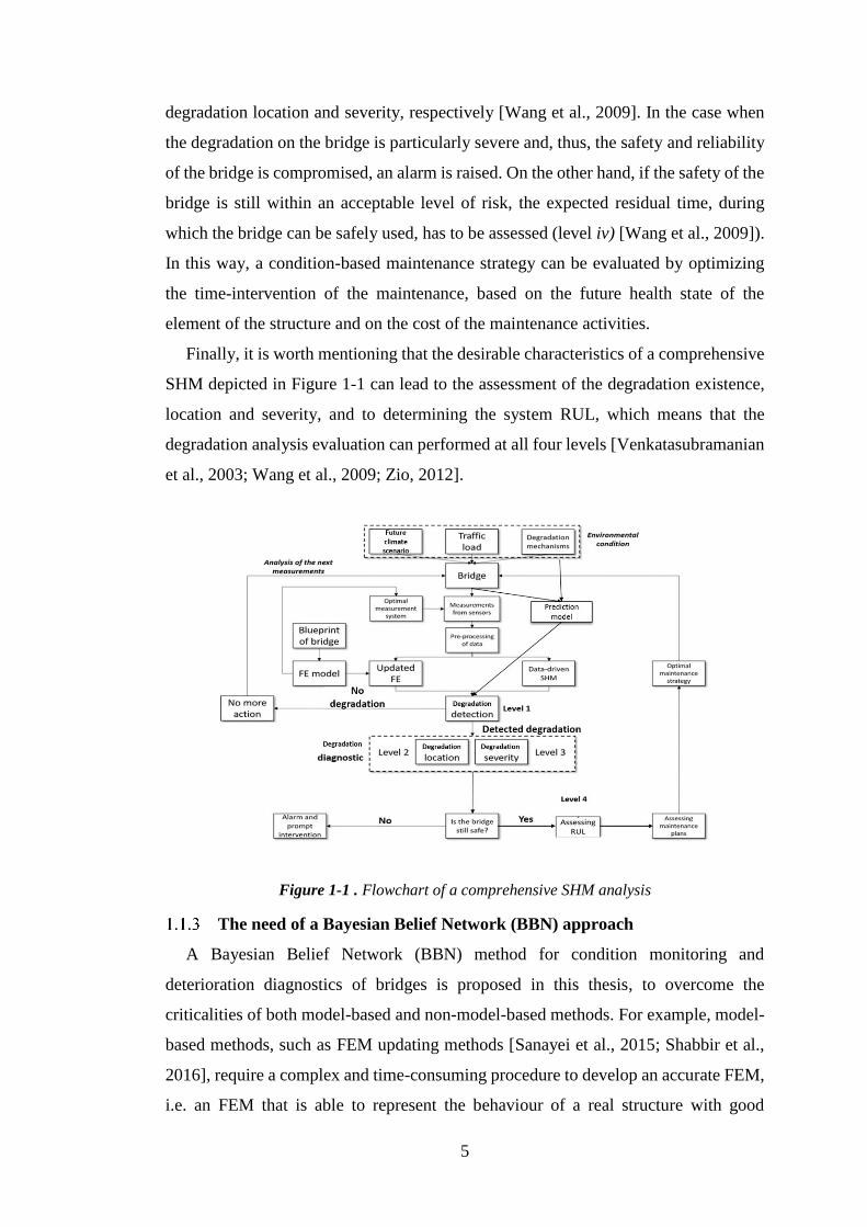
5

degradation location and severity, respectively [Wang et al., 2009]. In the case when

the degradation on the bridge is particularly severe and, thus, the safety and reliability

of the bridge is compromised, an alarm is raised. On the other hand, if the safety of the

bridge is still within an acceptable level of risk, the expected residual time, during

which the bridge can be safely used, has to be assessed (level iv) [Wang et al., 2009]).

In this way, a condition-based maintenance strategy can be evaluated by optimizing

the time-intervention of the maintenance, based on the future health state of the

element of the structure and on the cost of the maintenance activities.

Finally, it is worth mentioning that the desirable characteristics of a comprehensive

SHM depicted in Figure 1-1 can lead to the assessment of the degradation existence,

location and severity, and to determining the system RUL, which means that the

degradation analysis evaluation can performed at all four levels [Venkatasubramanian

et al., 2003; Wang et al., 2009; Zio, 2012].

Figure 1-1 . Flowchart of a comprehensive SHM analysis

The need of a Bayesian Belief Network (BBN) approach

A Bayesian Belief Network (BBN) method for condition monitoring and

deterioration diagnostics of bridges is proposed in this thesis, to overcome the

criticalities of both model-based and non-model-based methods. For example, model-

based methods, such as FEM updating methods [Sanayei et al., 2015; Shabbir et al.,

2016], require a complex and time-consuming procedure to develop an accurate FEM,

i.e. an FEM that is able to represent the behaviour of a real structure with good

6

accuracy [Vagnoli et al., 2018]. In contrast, non-model-based methods, such as

Artificial Neural Networks (ANNs) [Hakim et al., 2013], Principal Component

Analysis (PCA) [Hsu et al., 2010; Cavadas et al., 2013], supervised and unsupervised

clustering techniques [Alves et al., 2016; Santos et al., 2016], show promising results

for continuous condition monitoring of bridges. However, the performance of non-

model-based methods strongly depends on the quality of available data [Kim et al.,

2007; Casas et al., 2017; Moughty et al., 2017]. At the same time, non-model-based

methods do not take into account the knowledge of structural engineers that design

and maintain bridges, and the influence of degradation of individual elements on the

health state of the whole bridge.

Hence, bridge managers are in need of SHM methods that are able to: i) assess the

health state of the bridge by taking account of influences between different elements

of the bridge; ii) take account of the expertise of bridge engineers without requiring

time-consuming process to develop the SHM method; iii) manage different sources of

data, such as evidence of the bridge behaviour provided by sensors and visual

inspection reports; iv) update the assessment of the bridge health state every time when

new evidence of the behaviour becomes available; v) detect and diagnose slow

degradation mechanism and sudden changes of the bridge condition (damage), in order

to provide rapid information about the health state of the bridge to bridge managers. A

BBN approach can satisfy these requirements, by providing a graphical interface to

bridge managers, who can interact with the BBN model to assess the health state of

the bridge and the influence between different elements of the bridge [Fenton et al.,

2013; Rafiq et al., 2015; Kabir et al., 2016].

Data analysis methodology, machine learning methods and BBN

The BBN method is able to assess the health state of a railway infrastructure, and

of its elements, at the same time. However, pre-processing of data of the infrastructure

behaviour is needed to remove the data noise, which is usually present in the

measurement of the infrastructure behaviour. In this way, crisp information about the

behaviour of the bridge elements is provided to the BBN. In fact, when the behaviour

of an in-field bridge is monitored, it is difficult to clearly point out changes in the

bridge health states, due to the statistical variability of the measurements and changing

environmental conditions [Kim et al., 2007; Santos et al., 2016]. For these reasons, in

this thesis a data analysis methodology is proposed, in order to analyse vibration

7

behaviour of the bridge and monitor the health state of bridge. The main novelty of the

proposed methodology lies in the use of the Empirical Mode Composition (EMD),

which is adopted to assess the trend of time and frequency-domain features of the

bridge behaviour. The trend of the extracted features is then lumped into Health

Indicators (HIs) of the bridge.

The EMD is generally adopted in the SHM framework to identify structural changes

by analysing the bridge dynamic behaviour directly, i.e. the dynamic behaviour of the

bridge is used as an input to the EMD process, rather than the extracted features [Cahill

et al., 2018; Han et al., 2014]. Eventually, HIs can be used as an input to a Neuro-

Fuzzy Classifier (NFC), which is able to automatically assess the health state of bridge

elements [Cetişli & Barkana, 2010]. This information is finally used as an input to the

BBN, which assess the health state of the whole bridge by taking account of influences

between different bridge elements.

A method to update the CPTs of the BBN by taking account of expert

judgment and bridge behaviour data

The Conditional Probability Tables (CPTs) represent the quantitative part of the

BBN and allow to define the dependencies between connected nodes of the BBN. An

expert knowledge elicitation process is usually adopted to define the CPTs, if no data

about the bridge behaviour are available [Loughney & Wang, 2017]. Therefore,

experts are interviewed to retrieve the values of conditional probabilities. However,

such an approach can be subjective. On the contrary, when data of the bridge behaviour

are available, the CPTs can be defined by using learning methods [Sun et al., 2006].

This latter approach requires a large amount of data.

For these reasons, in this thesis, a method to merge the expert judgments with the

analysis of a small amount of bridge behaviour data is proposed. The method aims to

define the CPTs by the means of the expert knowledge elicitation process, and then to

update the CPTs every time when a new measurement of the bridge behaviour is

available. The updating process requires the knowledge of Cumulative Distribution

Function (CDF) of an optimal HI, which is used to monitor the evolution of the bridge

health state. The CDF is retrieved by analysing a database of bridge behaviour, when

the bridge behaviour in different health states of the bridge is known.

8

A method to analyse a database of infrastructure behaviour

The analysis of a database of unknown infrastructure behaviour requires a robust

data mining technique to analyse the data automatically, accurately and rapidly [Duan

and Zhang, 2006]. In this way, the data of the infrastructure behaviour can be

transformed into valuable information for decision makers, by pointing out past

abnormal behaviour of the infrastructure.

In this thesis, an ensemble-based change-point detection method is proposed in

order to identify changes of the condition of railway infrastructure. This information

can be used to: i) help the construction of the quantitative part of the BBN, by

providing insights about interdependencies between different elements of the asset and

(or) changes of environmental condition; ii) identify the time when the most severe

change of the asset health state occurred, and consequently diagnose the causes of such

changes.

An ensemble of change-point detection method is needed due to the fact that

individual change-point methods, such as Cumulative Sum (CUSUM)-based [Carslaw

et al., 2006] or probability distributions-based [Liu et al., 2013] methods, are able to

detect only abrupt changes in the data, without pointing out the most severe changes.

As a result, the most severe changes in the data can be lost among all the change-points

[Killick et al., 2012]. Furthermore, individual change-point methods are also usually

unable to identify the duration of the most critical system behaviour, as their objective

is to point out the moment when the data deviates from the average behaviour.

Research aims and objectives

Research aims

The main goal of this thesis is to a bridge condition monitoring and damage

diagnostics method of a critical infrastructure continuously. The focus is on the

continuous monitoring, by taking account of the interdependencies between different

elements of the infrastructure and diagnosing the damage of the structure. At the same

time, methods to analyse database of infrastructure behaviour are investigated, and a

method to analyse database of unknown infrastructure behaviour is proposed.

The goals of the thesis are to:

• Propose a method for bridge condition monitoring and damage diagnostics, to

assess the health state of a bridge and its elements simultaneously.

9

• Analyse the performance of the proposed method, by assessing the health state

of both in-field bridges and FEM of bridges.

• Achieve a robust assessment of the bridge health state by pre-processing data

of bridge behaviour to remove the noise.

• Assess the health state of a bridge in an automatic manner, by taking account

of the past behaviour of the bridge.

• Merge the expertise of bridge engineer with the analysis of the bridge

behaviour during the assessment of the bridge health state.

• Analyse a database of unknown infrastructure behaviour, with the aim of

pointing out changes of the health state of the infrastructure.

Research objectives

The following objectives have been fulfilled in this thesis:

• A BBN-based approach is developed for monitoring the condition of a bridge

and diagnosing its damage. The main element of the proposed method is to

monitor and assess the health state of a bridge continuously, by taking account

of the health state of each element of the bridge and without requiring a time-

consuming process for its development. The BBN method is verified by

monitoring and diagnosing the health state of two bridges, which are modelled

via FEMs, and of an in-field bridge.

• A data analysis methodology is proposed to pre-process the bridge behaviour

data. The proposed data analysis methodology allows to assess HIs of the

bridge. The HIs are identified by extracting statistical, frequency-based and

vibration-based features from the vibration behaviour of the bridge, and using

the extracted features as an input to an EMD method to assess the trend of the

features over time. In this way, the noise of the data is removed, and HIs of the

bridge are provided to allow a robust assessment of the bridge health state.

• A machine learning method, which relies on an NFC, is introduced to assess

the health state of a bridge element automatically. The method is trained on

past behaviour of the bridge and allows to assess the health state of the bridge

in an automatic manner.

• A method to update the CPTs of the BBN nodes, by merging the expert

knowledge elicitation process and the analysis of a database of bridge

10

behaviour is proposed. This method allows to update the CPTs of the BBN

nodes by taking account of the current health state of the bridge elements.

• A method to analyse database of unknown infrastructure behaviour is

proposed. This method relies on an ensemble-based change-point detection

algorithm, which is developed to identify the most critical change of the health

state of an infrastructure.

Thesis Outline

The thesis is organized as follows:

• Chapter 2 provides a detailed literature review analysis. Previous researches on

SHM are reviewed, by describing model-based methods and non-model-based

methods. The advantages and disadvantages of each method are discussed.

• Chapter 3 introduces the proposed BBN method for bridge condition

monitoring and damage diagnostics. The theoretical background of the BBN is

presented. A step-by-step process is introduced in order to develop the BBN

structure and define its CPTs. The BBN is applied using information from the

FEMs of two bridges.

• Chapter 4 discusses the data analysis methodology and the machine learning

method. The data analysis methodology is applied to two in-fields bridges to

assess their health states. Similarly, the machine learning method is applied to

an in-field bridge to assess the health state of the bridge automatically.

• Chapter 5 presents the method for defining and updating the CPTs of the BBN

by merging the expert judgment with the analysis of the bridge behaviour. The

method is applied to an in-field bridge.

• Chapter 6 presents the application of the proposed methods to an in-field

bridge. The bridge is monitored by the means of a BBN, whose CPTs are

updated by using the proposed method. The results of the data analysis

methodology are used as an input to the BBN, to achieve the robust assessment

of the bridge health state.

• Chapter 7 discusses the conclusion of the thesis, by highlighting the

contributions and the future work.

11

Structural Health

Monitoring of bridges

Introduction to literature review

An extensive literature review was carried out in this study and is presented in this

section, in order to identify the methods used for condition monitoring and damage

detection of railway infrastructure, by pointing out the advantages and disadvantages

of each method. The literature review focuses on the first three steps of the degradation

(damage) analysis process, i.e. degradation identification, diagnostics of degradation

location and severity. This is due to the fact that the aim of the thesis is to develop a

SHM methodology that fulfils these first three requirements. The fourth point of the

degradation (damage) analysis process, i.e. the prediction of the residual life of the

bridge, is out of the scope of this thesis. However, the BBN method, which has been

scarcely adopted in literature, has been used in few cases as Dynamic BBN (DBN), to

predict the future condition of bridges. Although many SHM methods have been

developed and applied for bridge condition monitoring, the research is still ongoing to

fulfil the four requirements of the fault detection methods.

In the next sections, SHM methods are discussed by grouping them into two

categories: model-based and non-model-based methods. A description of each

category is provided, and furthermore, several methods for each category are presented

individually by emphasizing: i) the infrastructure that is monitored; ii) how the method

works; iii) the monitored variables of the infrastructure; iv) the results obtained with

the considered method.

The requirements for a new condition monitoring and fault detection method are

then discussed, with the aim of highlighting the need of an SHM method that has the

advantages of both categories.

The content of this chapter has been published in the “Structural health monitoring

journal”, with the aim of discussing and analysing a comprehensive review of SHM

methods [Vagnoli et al., 2018]. The tables of this chapters have been extracted from

[Vagnoli et al., 2018].

12

Model-based condition monitoring and damage detection methods

A model-based condition monitoring and damage detection method aims to assess

the condition of a bridge, by comparing the bridge behaviour that is simulated by a

FEM of the bridge, with the behaviour of the real structure. FEMs are adopted usually

to simulate the bridge behaviour under different environmental conditions, due to their

computational and modelling capacity. However, during the development of the FEM,

many model parameters (such as material properties, geometric properties and

boundary conditions) are unknown and, thus, several assumptions and simplifications

need to be made [Mottershead & Friswell, 1993]. An updating process of the bridge

FEM parameters is then carried out, in order to obtain the FEM responses to be as

similar as possible to the real measured responses of the bridge, and to increase the

FEM accuracy by reducing the model uncertainties [Schlune et al., 2009]. This process

of developing and updating the FEM can be complex and time-consuming. However,

many authors have developed techniques to update FEM for damage detection

analysis. In what follows, a description of FEM updating strategies is provided in

section 2.2.1, and a discussion of the model-based methods is presented in section

2.2.1.1.

FEM updating methods

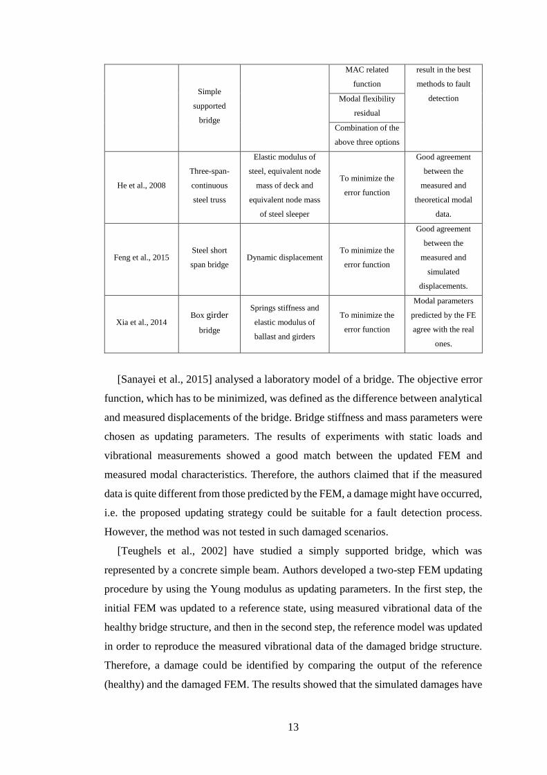
In this section FEM updating methods are described by highlighting the type of

bridge that was analysed, the choice of the updating parameters and by describing the

updating strategy. Finally, the results of each work are presented. Table 2-1 shows the

information of the works presented in this section.

Table 2-1. FE model updating literature examples

Reference Type of bridge Updating

parameter(s) Updating strategy Results

Sanayei et al.,

2015

Bridge model

that was

designed as a

grid system.

Bending rigidity, area

mass and boundary

link stiffness

To minimize the

error function

High correlation

between the

empirical and

analytical data

Teughels et al.,

2002

Reinforced

concrete beam Young module

Global damage

function

High correlation

between the

empirical and

analytical data

Jaishi & Ren, 2005 Young module and

moment of inertia

Frequency

residuals

MAC and modal

flexibility residuals

13

Simple

supported

bridge

MAC related

function

result in the best

methods to fault

detection Modal flexibility

residual

Combination of the

above three options

He et al., 2008

Three-span-

continuous

steel truss

Elastic modulus of

steel, equivalent node

mass of deck and

equivalent node mass

of steel sleeper

To minimize the

error function

Good agreement

between the

measured and

theoretical modal

data.

Feng et al., 2015 Steel short

span bridge Dynamic displacement

To minimize the

error function

Good agreement

between the

measured and

simulated

displacements.

Xia et al., 2014 Box girder

bridge

Springs stiffness and

elastic modulus of

ballast and girders

To minimize the

error function

Modal parameters

predicted by the FE

agree with the real

ones.

[Sanayei et al., 2015] analysed a laboratory model of a bridge. The objective error

function, which has to be minimized, was defined as the difference between analytical

and measured displacements of the bridge. Bridge stiffness and mass parameters were

chosen as updating parameters. The results of experiments with static loads and

vibrational measurements showed a good match between the updated FEM and

measured modal characteristics. Therefore, the authors claimed that if the measured

data is quite different from those predicted by the FEM, a damage might have occurred,

i.e. the proposed updating strategy could be suitable for a fault detection process.

However, the method was not tested in such damaged scenarios.

[Teughels et al., 2002] have studied a simply supported bridge, which was

represented by a concrete simple beam. Authors developed a two-step FEM updating

procedure by using the Young modulus as updating parameters. In the first step, the

initial FEM was updated to a reference state, using measured vibrational data of the

healthy bridge structure, and then in the second step, the reference model was updated

in order to reproduce the measured vibrational data of the damaged bridge structure.

Therefore, a damage could be identified by comparing the output of the reference

(healthy) and the damaged FEM. The results showed that the simulated damages have

14

been correctly identified through an asymmetrical distribution of the updating

parameter at the damaged location. The magnitude of the damage was not analysed.

[Jaishi & Ren, 2005] analysed a simply supported bridge. They proposed a

sensitivity-based updating strategy using four different objective functions: i)

frequency residuals, i.e. the residuals between the natural frequencies provided by the

FEM and those measured; ii) a Modal Assurance Criterion (MAC) related function;

iii) modal flexibility residual; iv) combination of the first three options.

The MAC related function has been defined as follows:

i

i

MAC

MACif

2)1()(

−=

(2-1)

where )(if is the MAC related function at step i . The method has been tested on a

laboratory bridge model. The results showed that in each case of the four objective

functions, an accurate damage detection becomes more difficult, as the number of

updating parameters increases. Furthermore, the objective function based on the

combination of frequency residuals, MAC and modal flexibility residuals, improves

the performance of damage detection. Therefore, the results of the FEM updating

strategy depends on the choice of the number and type of updating parameters. In fact,

both physical (such as boundary and material properties) and numerical (such as

mathematical modelling and numerical solution) parameters of the FEM are uncertain,

and such uncertainty needs to be reduced, by choosing optimal updating parameters

that allow a fast and reliable updating process [Başaĝa et al., 2011].

[He et al., 2008] studied a three-span continuous steel truss bridge. Authors

proposed to optimize an objective function based on the difference between analytical

and measured natural frequency of the bridge. A simple method of model updating

was adopted by using the elastic modulus of steel, the equivalent node mass of deck

and the equivalent node mass of steel sleeper as updating parameters. Results showed

that there is a good agreement between the data provided by the FEM and those

retrieved by the sensors, i.e. a maximum error of frequency is 4.09% and the minimum

value of MAC is 85.92%. Hence, the method proposed by the authors can be adopted

to monitor the evolution of the bridge condition over time, and point out unexpected

behaviour of the bridge accordingly. However, the authors did not test the method in

any damaged scenario of the bridge.

15

[Feng et al., 2015] have analysed a single-span railway steel bridge. They proposed

an updating strategy of the FE model by optimizing an objective function, which was

based on the difference between simulated and measured dynamic displacements of

the bridge. The results showed that the displacements of the real bridge and those

predicted using the updated FE model were in good agreement. However, the authors

pointed out that in order to simulate the behaviour of the real bridge with good

accuracy, the interaction between the bridge and the train needs to be modelled and

updated accurately. As a result, a set of new variables is introduced in the updating

process by resulting in an increase of computational time and uncertainty of the

process.

[Xia et al., 2014] monitored a box-girder railway bridge. The authors proposed an

FEM updating strategy based on the optimization of an objective function that aimed

to minimize the differences between the real and simulated modal properties of a

railway bridge. Results showed a good match between the predicted and measured

modal parameters of the railway bridge. The optimization problem proposed by the

authors showed good results when high modal parameters of the bridge were used to

update the FEM characteristics, e.g. from the 6th to the 11th mode shapes. However,

high modal parameters of the bridge, which are more sensitive to damage, are difficult

to extract from the data measured in an in-field bridge in a reliable manner. As a

consequence, the reliability of the condition monitoring process can be threatened

[Casas et al., 2017].

2.2.1.1 Summary of the FEM updating strategy

FEM updating strategies are one of the most common techniques adopted for

monitoring and assessing the health state of a bridge. In fact, an FEM method allows

to simulate the behaviour of the bridge under changing environmental conditions.

Furthermore, as soon as new information regarding the health state of the bridge, such

as visual inspection reports of the bridge, or new measurement of the bridge behaviour,

is available, the FEM can be updated accordingly. However, the development of an

FE model can be complex and time-consuming. The choice of the updating parameters

is a challenge, due to the fact that different updating parameters lead to different

accuracy and computational time of the updating process. For example, it has been

shown that the higher the complexity of the structure, the larger the number of updating

16

parameters: [Teughels et al., 2002; Jaishi & Ren, 2005] have studied a simple

supported span bridge and beams, and consequently, only one or two updating

parameter(s) have been selected; [He et al., 2008; Sanayei et al., 2015] have studied a

more complex bridge structure, such as a three-span continuous bridge, and the number

of updating parameter was consequently increased. The increase of the number of the

updating parameters can lead to a reduction of the performance of the condition

monitoring method, due to an increase of uncertainty and computational time of the

updating process [Jaishi & Ren, 2005]. It is worth noting that, even if the initial FEM

may not represent the real structural behaviour accurately due to modelling

uncertainties, the responses provided by the initial FEM before the updating procedure

need to be relatively similar to those provided by the real measured bridge responses,

in order to avoid a long updating process, which might have no optimal solutions. The

size and complexity of the FEM and its updating strategy can be a challenge for

achieving a continuous SHM. Finally, the magnitude of the damage and the effect of

environmental condition on the modal parameters of the bridge are not considered

generally. Consequently, only the first two requirements of the damage detection

process (identification of the damage existence and damage location) are satisfied.

Non-Model-based methods

Non-model-based methods can provide information about the health state of the

bridge rapidly, by analysing the bridge behaviour directly, without requiring a

development of an FEM of the structure. In literature, non-model-based methods have

demonstrated to be suitable for real-time monitoring of complex systems, such as

nuclear systems [Zio et al., 2010], industrial processes (including chemicals,

microelectronics manufacturing, iron and steel, pharmaceutical processes, and power

distribution networks) [Qin, 2012; Yin et al., 2014], petroleum and natural gas systems

[Galotto et al., 2015] and electric vehicles [Rigamonti et al., 2016]. For these reasons,

in what follows a survey of non-model-based methods for bridge condition monitoring

and damage detection is provided. Particularly, ANN methods have been intensively

used as a condition monitoring and damage detection method in the structural

engineering framework, and as a result section 2.3.1 presents the analysis of these

ANN-based methods. At the same time, other non-model-based methods have been

presented in literature, such as unsupervised clustering methods or statistical

approaches. These latter methods are presented and discussed in section 2.3.2. Finally,

17

section 2.3.3 shows some works based on BBNs, which can evaluate the condition of

individual elements on the bridge as well as considering the structure as a whole.

Artificial Neural Network based methods

In this section ANN-based methods applied to monitor the condition of bridges are

described. Table 2-2 shows the main characteristics of the works discussed in this

section, by highlighting the type of the bridge under analysis, the nature of the ANN,

the monitored behaviours of the bridge and the results of the considered method.

Table 2-2. Examples of condition monitoring methods based on the ANN

Reference Type of

bridge

Type of

NN

Number

of input

nodes

Number of

hidden

nodes

Number of

output

nodes

Type of input

data Results

Shu et al.,

2013

FE model

of Banafjäl

bridge,

Sweden

Back

propagation

single layer

Not

explained

19 for fault

detection

Not

explained

Displacements

and acceleration

Results

strongly

depend on the

position of

the fault and

on the load

and velocity

of the train

23 for fault

diagnostic

Lee et al.,

2005

FE model

of a beam

Back

propagation

multi layers

20

20 first

layer 8

Mode shape,

mode shape

difference

before and after

failure and

mode shape

ratio for the first

four modes

Generally, the

method

shows good

accuracy with

some false

alarms in the

laboratory

and Hannam

bridge case

study

20 second

layer

FE model

of single

span bridge

98

60 first

layer 40

40 second

layer

Laboratory

model of

bridge

24

24 first

layer 8

8 second

layer

Hannam

Grand

bridge,

South

Korea

80

60 first

layer 40

60 second

layer

6 19 5

Park et al.,

2009

FE and

laboratory

model of

simply

supported

beam

Back

propagation

50 50

Depending

on the case

study

Acceleration

Good

accuracy as

sequential FD

method:

acceleration-

based NN

monitors the

bridge in real

Dependin

g on the

Depending

on the case

study

Depending

on the case

study

Modal data

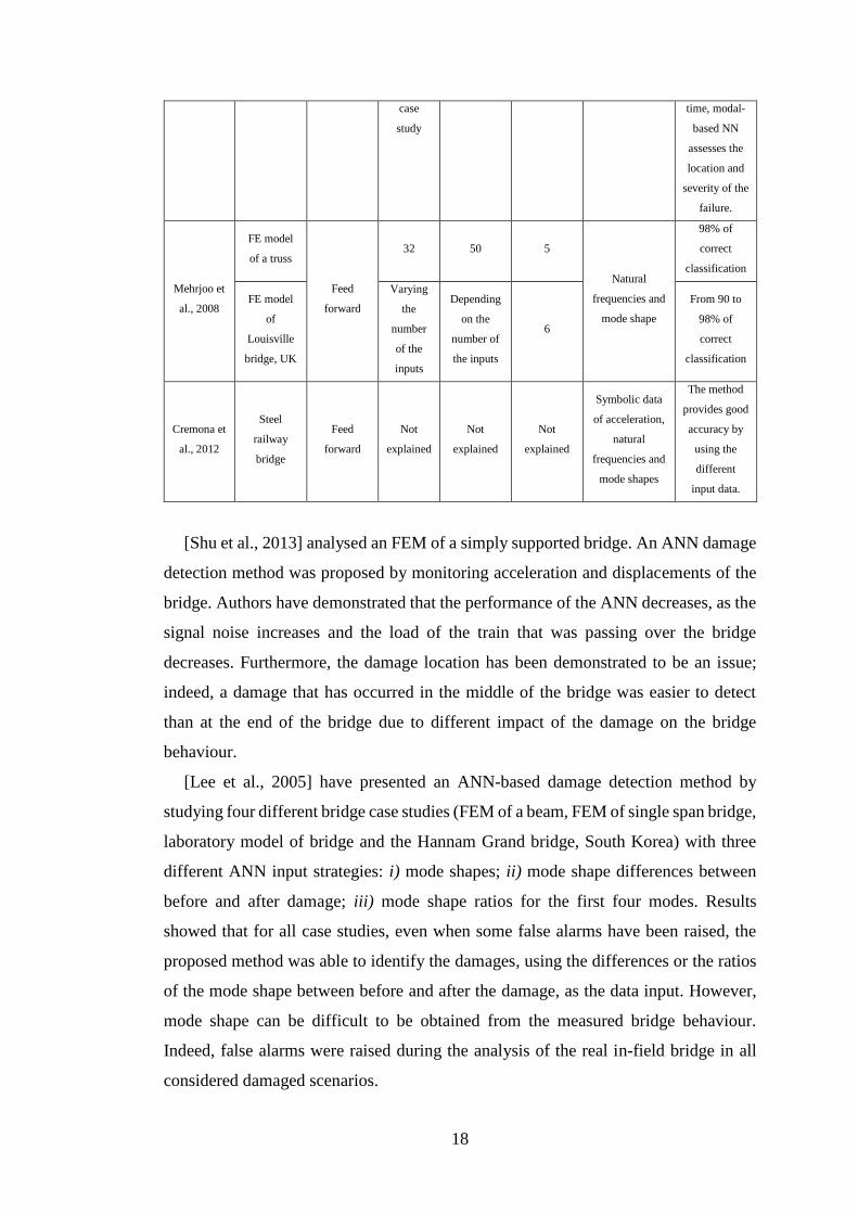
18

case

study

time, modal-

based NN

assesses the

location and

severity of the

failure.

Mehrjoo et

al., 2008

FE model

of a truss

Feed

forward

32 50 5

Natural

frequencies and

mode shape

98% of

correct

classification

FE model

of

Louisville

bridge, UK

Varying

the

number

of the

inputs

Depending

on the

number of

the inputs

6

From 90 to

98% of

correct

classification

Cremona et

al., 2012

Steel

railway

bridge

Feed

forward

Not

explained

Not

explained

Not

explained

Symbolic data

of acceleration,

natural

frequencies and

mode shapes

The method

provides good

accuracy by

using the

different

input data.

[Shu et al., 2013] analysed an FEM of a simply supported bridge. An ANN damage

detection method was proposed by monitoring acceleration and displacements of the

bridge. Authors have demonstrated that the performance of the ANN decreases, as the

signal noise increases and the load of the train that was passing over the bridge

decreases. Furthermore, the damage location has been demonstrated to be an issue;

indeed, a damage that has occurred in the middle of the bridge was easier to detect

than at the end of the bridge due to different impact of the damage on the bridge

behaviour.

[Lee et al., 2005] have presented an ANN-based damage detection method by

studying four different bridge case studies (FEM of a beam, FEM of single span bridge,

laboratory model of bridge and the Hannam Grand bridge, South Korea) with three

different ANN input strategies: i) mode shapes; ii) mode shape differences between

before and after damage; iii) mode shape ratios for the first four modes. Results

showed that for all case studies, even when some false alarms have been raised, the

proposed method was able to identify the damages, using the differences or the ratios

of the mode shape between before and after the damage, as the data input. However,

mode shape can be difficult to be obtained from the measured bridge behaviour.

Indeed, false alarms were raised during the analysis of the real in-field bridge in all

considered damaged scenarios.

19

[Park et al., 2009] have studied an FEM and laboratory model of simply supported

bridge. The authors proposed a sequential damage detection method based on an

acceleration-based ANN (ABNN) and on a modal feature-based ANN (MBNN). The

ABNN was used to monitor the behaviour of the bridge and to detect the occurrence

of a damage by using acceleration data as input; whilst the MBNN was used to estimate

the location and the severity of the occurred damage by using modal parameters, such

as mode shapes, as input. Results showed that the occurrence, the location and

magnitude of damage is correctly identified by firstly adopting the ABNN and,

sequentially, the MBNN. Although, the method shows good performance, it should be

mentioned that the identification of modal parameters can be difficult for an in-field

bridge [Casas et al., 2017].

[Mehrjoo et al., 2008] have analysed two FEMs of two steel truss bridges. They

proposed an ANN-based method to detect damage of the bridge, by using natural

frequencies and mode shape as input to the ANN. The accuracy detection of the

proposed method was higher than 90%. However, the accuracy of the results and the

architecture of the ANN strongly depended on the number of vibration modes, i.e.

natural frequencies and mode shapes that have been considered as input of the ANN.

At the same time, the accuracy of the ANN depended on the numbers of input and

hidden neurons, i.e. the performance of the method depended on the structure of the

ANN.

[Cremona et al., 2012] discussed a NN-based classification method in order to

assess the condition of a steel railway bridge over time. Particularly, strengthening

works were carried out on the bridge, and the authors aimed to assess the health state

of the strengthened bridge. Therefore, symbolic data of the measured acceleration,

natural frequencies and mode shapes were used as the input to an ANN, which has

been trained using historical measurements. Results showed that when a new and

unknown measurement was available, the proposed method was able to correctly

assess the condition of the bridge up to 93% of the tested scenarios. It should be noted

that due to the availability of a vast database of recorded behaviour of a real bridge,

good results in terms of assessment of the condition of the bridge were achieved.

20

2.3.1.1 Summary of ANN-based methods

One of the most important issues of the ANN strategy is the selection of the model

structure, i.e. the number of hidden layers and neurons. The number of the input

neurons is, generally, taken to be equal to the number of the monitored variables of the

system, e.g. [Mehrjoo et al., 2008] changed the number of input neurons based on the

number of input variables. A general rule to select the optimal number of input nodes

is not available, and thus, the optimal number of input nodes is defined by trial and

error procedure usually. The number of hidden neurons is usually kept to as low as

possible, in order to reach the best solution in terms of computational time cost and

residual error. This procedure is one of the most critical aspects of the use the ANN,

and it is generally addressed by using a trial and error procedure [Lee et al., 2005;

Mehrjoo et al., 2008; Park et al., 2009]. Although a methodological criterion to choose

the optimal ANN structure has not been proposed yet, Bayesian processes can be

adopted to investigate how a different number of hidden layers and nodes influences

the accuracy of the ANN-based method [Arangio et al., 2014]. Generally speaking, the

accuracy increases as the number of hidden layer and neurons increases, however, an

over-parameterization may be achieved. Indeed, if the ANN is over-parameterized, i.e.

the number of hidden neurons is too high, the ANN is optimal to mimic the training

set, but it is unable to manage new and unknown patterns. Furthermore, the best ANN

structure is chosen for a particular case study usually, and as a consequence, it has to

be changed if the case study changes (i.e. the bridge model under study or the number

of the modal properties is changed), as demonstrated by [Lee et al., 2005; Mehrjoo et

al., 2008; Park et al., 2009].

The performance of the ANN in terms of accuracy depends on the data used in the

training set. For example, [Mehrjoo et al., 2008] have demonstrated that the ANN

damage detection accuracy decreases and, thus, the number of false alarms increases,

as the number of the considered modal characteristics (e.g., the number of considered

natural frequencies or mode shapes) decreases and the noise of the data increases.

Moreover, [Shu et al., 2013] have shown that the accuracy of the ANN is affected by

the damage location: a failure close to the end of the bridge is more difficult to be

detected than a failure in the middle of the bridge.

Finally, although the ANN method has been applied in a number of studies, it has

three main limitations:

21

i) the ANN methods are able to approximate any function, but they are not

directly correlated to the bridge model, and thus they do not represent the

physical structure of the bridge. A model with the properties showed by the

ANN is also called black-box model usually. Thus, the expertise of the

structural engineers that have developed the FEM of the bridges is lost, as

the damage detection methods based on the ANN rely only on the data

retrieved by the bridge.

ii) there is no standard method to choose the optimal structure of the ANN. At

the same time, a criterion to rigorously define how much and what type of

training data are required, has to be defined in order to achieve a fast and

reliable training process [Lee et al., 2014; Kan et al., 2015].

iii) there is a need of a large amount of data, which contains the behaviour of

the bridge under changing environmental scenarios, in order to correctly

assess the health state of the bridge.

Other non-model-based methods

Non-model-based methods can be based on a variety of different mathematical

models, such as regression model, machine learning methods, genetic algorithm

methods, clustering methods, etc. In what follows, a survey of non-model-based

methods for bridge SHM is provided by describing unsupervised clustering methods

or statistical approaches, such as regression and PCA methods. The unsupervised

clustering methods are thoroughly described due to the fact that they are able to

monitor the health state of the bridge in an unsupervised way by aiming to group

different bridge behaviours in separate, well distanced and compact clusters. In this

way, the distance between different clusters (between-cluster variance) is maximized,

whilst the distance between behaviours of the bridge that have similar properties

(within-cluster variance) is minimized. Table 2-3 shows the methods described in this

section.

Table 2-3. Condition monitoring analysis using data-driven methods

Reference Type of bridge Monitoring method Type of input data Results

Kim et al., 2015 Seven-span plate

bridge Bayesian regression

Acceleration of the

bridge

Depends on the

environmental

conditions, such as

traffic load

22

Laory et al., 2013

Steel truss railway

bridge Moving Principal

component analysis

coupled with

regression methods

Quasi-static

measurement

The coupling of

MPCA and regression

methods shows better

results than the

singular methods.

Five spans box

girder bridge

Cury et al., 2012 Steel bridge

Hierarchy-divisive

and a dynamic clouds

clustering method

Symbolic

acceleration, natural

frequencies and mode

shapes

Good assessment of

the health state of the

bridge with very low

false alarms raised.

Guo et al., 2012 Steel bridge K-means clustering Sorted acceleration

data

Good performance in

the analysis of the FE

model. However, false

alarms are raised in the

analysis of the real

bridge.

Langone et al., 2017 Concrete bridge adaptive kernel

spectral clustering Natural frequencies

Good detection ability

of the method, that

decrease as the

environmental

condition changes.

Alves et al., 2016

Steel railway bridge

and concrete

highway bridge

K-means, hierarchy-

agglomerative and

fuzzy c-means

clustering methods

Acceleration data

Good results for the

railway bridge. Many

misclassifications for

the highway bridge

due to changing

environmental

condition.

[Kim et al., 2015] studied a seven-span plate bridge. The authors used coefficients

of an autoregressive model of the bridge acceleration as Damage Indexes (DI). The

behaviour of the bridge is monitored by an online Bayesian updating process of the

DIs, and consequently, if the value of the DIs changes suddenly, the health state of the

bridge experienced a change. Acceleration data over one year have been used as input

to the method. Three different data strategies have been considered: a) complete

environmental change scenario, where acceleration, temperature and vehicle weight

data have been used; b) temperature change scenario, where acceleration and

temperature data have been used; c) no environmental change scenario, where only

acceleration data without considering environmental changes have been used. Results

showed that the analysis, considering both temperature and vehicle weight as

environmental effects (case a), led to more accurate results than case b) and c).

Therefore, a more accurate and reliable assessment of the bridge health state is

achieved when changes of environmental condition are considered into the analysis,

and not only the behaviour of the bridge (e.g. acceleration).

23

[Laory et al., 2013] analysed an FEM of a steel truss bridge. Authors developed a

damage detection method by coupling a Moving PCA (MPCA) and regression

methods. The performance of the proposed method was compared with those of the

individual methods, i.e. MPCA and regression method alone. The results showed that

the proposed method had better performance in terms of damage identification. The

method was also tested on a real five-span box girder bridge, and it provide better

results of each individual method. Although the method showed good performance,

the data used for the analysis are quasi-static measurement, i.e. the excitation of the

bridge was so small that the dynamical effects of the bridge were negligible.

[Cury et al., 2012] analysed a steel bridge by comparing the performance of a

hierarchy-divisive and a dynamic clouds clustering method. Acceleration and natural

frequencies of the bridge were used as the input to the analysis. During a pre-

processing analysis, the acceleration and natural frequencies data were transformed

into symbolic data by the means of a frequentist analysis. The condition monitoring of

the bridge was carried out by assigning each new measurement to the cluster with the

minimum distance. Results showed a very low rate of misclassification by using the

acceleration data as the input to both clustering methods, i.e. the condition of the bridge

were assessed correctly. However, when the analysis was performed by using the

natural frequencies as the input to the clustering methods, misclassifications were

identified due to noisy data.

[Guo et al., 2012] presented a K-means-based clustering method in order to assess

the condition of a steel railway bridge (FEM and real in-field bridge). Acceleration

data are used as input to the clustering method. The K-means algorithm was used in

order to group the measured data into different groups. The method showed good

performance in identifying damages when the FEM was analysed, however, when the

real steel railway bridge was analysed, several false alarms were raised, due to the

impact of environmental condition, which led to a noisy measurement of the bridge

behaviour.

[Langone et al., 2017] analysed a concrete bridge. An unsupervised adaptive kernel

spectral clustering method was proposed to monitor the health state of bridge

infrastructure. Natural frequencies of the bridge were used as input to the proposed

method. Results showed that damages of the bridge were identified correctly.

However, when the environmental conditions changed, such as variation of the air

temperature, the accuracy of the proposed method decreased.

24

[Alves et al., 2016] presented a study in order to compare the performance of three

clustering algorithms, K-means, hierarchy-agglomerative and fuzzy c-means

clustering methods, in two different case studies: a steel railway bridge and a concrete

highway bridge. The symbolic values of the acceleration data were used for the

analysis, i.e. the acceleration data were transformed into symbolic variable by the

means of a frequentist analysis. The three methods showed good results when the steel

railway bridge was analysed, where the K-means algorithm outperformed the other

methods in identifying the changes of the stiffness of the bridge. On the other hand,

the analysis of the highway bridge showed that the fuzzy c-means method was able to

provide the best classification results. However, the changing environmental

conditions led to a high number of misclassification (over 40%).

2.3.2.1 Discussion of other non-model-based methods

The presented non-model-based methods have demonstrated the ability to detect

failures in the considered case study efficiently. However, false alarms and

misclassification were obtained mainly due to changing environmental condition that

led to the presence of noise in the data, particularly in the modal parameters of the

bridge. [Kim et al., 2015] have pointed out that the understanding of how ambient

temperature and traffic effects influence the behaviour of the bridge is of vital

importance for bridge SHM. In fact, the impact of environmental variations on the

bridge modal properties can lead the developed condition monitoring algorithms to

raise many false alarms. The non-model-based methods are usually optimized for a

specified structure that is subject to known environmental and operational conditions.

Therefore, good performance for new and previously unknown environmental and

operational conditions, which have been not included in the database used, cannot be

guaranteed [Zio, 2012]. The methods presented in this section are mainly focused on

the first two requirements of the damage detection process, i.e. failure existence and

failure location. The magnitude of the damage is not assessed usually due to a lack of

adequate dataset to develop the methods. Hence, a vast database that contains both

healthy and degraded behaviours of the bridge is needed, in order to develop a reliable

non-model-based condition monitoring and damage detection method.

Finally, the results provided by these methods need to be evaluated by an expert, in

order to assess the actual health state of the bridge. In fact, these methods are only able

25

to point out a change of the bridge behaviour without diagnosing its causes, and

without considering interdependencies between different elements of the

infrastructure.

Bayesian Belief Network methods

In structural engineering framework, the BBN method has been mainly used in

reliability assessment studies, e.g. probability of failure due to the scour phenomena

[Salamatian et al., 2013], fragility of the reinforced concrete bridges [Franchin et al.,

2016] and assessment of technical causes of that can lead to a catastrophic bridge

downfall [Holický et al., 2013], and for prediction of future residual life of the bridge.

Although the use of the BBN methods for condition monitoring and damage

diagnostics of bridge is limited, BBN-based methods can be a great candidate for the

real time SHM, due to the fact that BBN gives the opportunity to assess the health state

of the whole bridge and its elements at the same time, by managing complex

information from different sources, such as sensors and visual inspection reports.

Furthermore, the extension of the BBN, called DBN, can be used to analyse problems

with time varying domains. Table 2-4 shows the papers that have adopted a BBN-

based strategy for SHM, by highlighting the strategy adopted to define the CPT of the

network.

Table 2-4. Condition monitoring strategies based on BBN

Reference Type of bridge Proposed

method

Definition of

CPTs Type of input data Results

Rafiq et al., 2015 50 Masonry arch

bridges

Condition

modelling of the

bridge based on

BBN and DBN

methods

Expert judgment

Bridge visual

inspection results

(SCMI)

Condition of

the bridge over

time

Attoh-Okine &

Bowers, 2006

Single span steel

girder, reinforced

concrete deck

bridge

Deterioration

modelling of the

bridge based on

BBN

Expert judgment Expert judgment

Probability of

the bridge

health state

Wang et al., 2012 Girder steel

bridge

Condition

modelling of the

bridge based on

DBN

Expert judgment

Simulated

observations of the

bridge

Condition of

the bridge over

time

Kosgodagan-

Dalla Torre et al.,

2017

4 steel

bridges

Deterioration

modelling of the

bridge based on

DBN

Expert judgment

Traffic and load

data from a weigh-

in-

motion (WIM)

system

The predicted

useful life of

the bridge

strongly relies

on the available

information

26

[Rafiq et al., 2015] showed how a BBN method could be used as a condition-based

deterioration modelling methodology for a bridge management system. The data used

as the input to the BBN model were visual inspection reports of 50 masonry arch

railway bridges. The condition of the whole bridge was obtained by considering the

health state of each element of the bridge, i.e. the minor elements influences the major

elements of the bridge, which influence the health state of the whole bridge. A DBN

was developed to model and predict the future degradation level of the masonry

bridges. CPTs of the network were defined by the means of the information provided

by the visual inspection reports. Results showed that the BBN is able to assess how

the health state of the whole bridge is influenced by the degradation of its elements,

whereas the DBN was able to predict the health state of the bridge over time by

highlighting the ability of the DBN in updating the bridge health state when new

evidence of the bridge health state are available.

[Attoh-Okine & Bowers, 2006] built a BBN using a Fault Tree (FT) for a railway

bridge [LeBeau et al., 2000]. The authors presented a qualitative case study in order to

investigate the feasibility of SHM by using a BBN method. Consequently, the

behaviour of a bridge was not considered in the analysis. The CPTs for the overall

bridge deterioration process were described by using engineering judgment. The input

data to the BBN were obtained by interviewing seven bridge engineers and inspectors

in order to analyse three ‘what if’ scenarios, e.g. the authors analysed a scenario where

the bridge joints are all in the acceptable condition state with the aim of analysing how

the health state of the bridge is influenced by this information.

[Wang et al., 2012] studied the main girder of a steel railway bridge. Authors

proposed a DBN to predict the condition of bridge elements. The deterioration process

of bridge elements was modelled using maintenance actions, environmental effects

(i.e. traffic volumes and loads, temperature, humidity). Evidence of the bridge

behaviour were used as DBN input at each time step. The CPTs were estimated using

the expertise knowledge. Results showed how the evolution of the bridge future

condition changes significantly, when new bridge condition information, i.e. the visual

inspection records, became available.

[Kosgodagan-Dalla Torre et al., 2017] presented a DBN to model and predict the

degradation of a bridge network when limited data about the bridge behaviour are

available. The authors considered a network of four steel bridges. The transaction

27

probabilities of the DBN, i.e. the probability that a bridge of the network improves or

decreases its health state, are defined by using an expert knowledge elicitation process.

Results showed that the accuracy of the prediction of the future degradation level of

the bridge increases, when more information about environmental condition of the

bridges are available.

2.3.3.1 Discussion on Bayesian Belief Network

Generally, the BBN method describes the deterioration process of the bridge by

considering the effects of each individual bridge element on the health state of the

whole bridge. Expert knowledge and bridge response data are merged in a BBN, and

consequently the results of the BBN rely on the strength of the expert knowledge, and

the comprehensive information regarding the behaviour of the bridge. However, the

structural behaviour of the bridge is usually not considered as the input to the presented

BBN-based methods. Instead, visual inspection reports are used as evidence of the

bridge behaviour. The definition of the CPTs is one the major issues for the BBN

application. The usual practice is to define CPTs by using an expert knowledge

elicitation process. However, this process can be time-consuming and subjective.

Furthermore, the size of the CPT can increase considerably with the number of parents,

which can make the process of populating the CPTs intractable. This problem can be

avoided using fewer states for each node and the divorcing node technique [Chen &

Pollino, 2012].

Requirements for a new detection and diagnostics of bridge

deterioration method

The literature review of model-based and non-model-based methods shows that

several methods have been proposed to fulfil the requirements of the first three steps

of the degradation (damage) analysis [Wang et al., 2009]. However, model-based and

non-model-based methods show criticalities in monitoring the health state of a bridge

continuously, by taking account of the influences between different elements of the

bridge, managing different source of data (such as bridge behaviour and expert

knowledge) and diagnosing the location and level of severity of the bridge degradation.

Therefore, taking account of the criticalities of the reviewed approaches, the

requirements for a new condition monitoring and damage detection method for bridge

infrastructure can be defined as follows:

28

• Able to consider the knowledge of bridge engineers;

• Do not require time-consuming process to be developed;

• Able to update the health state of the bridge by taking account of the health

state of each element of the bridge;

• Able to consider influences between different bridge elements;

• Able to monitor the health state of the bridge continuously;

• Able to use different source of information about the health state of the bridge,

such as data provided by a measurement system installed on the bridge and

visual inspection reports;

• Able to identify unexpected behaviour of the bridge (Level i) of the damage

detection process [Wang et al., 2009]);

• Able to diagnose the unexpected behaviour of the bridge (Level ii) and iii) of

the damage detection process [Wang et al., 2009]);

• Able to provide rapid information about the health state of the bridge to bridge

managers;

• Able to assess the health state of the bridge under unknown environmental

condition.

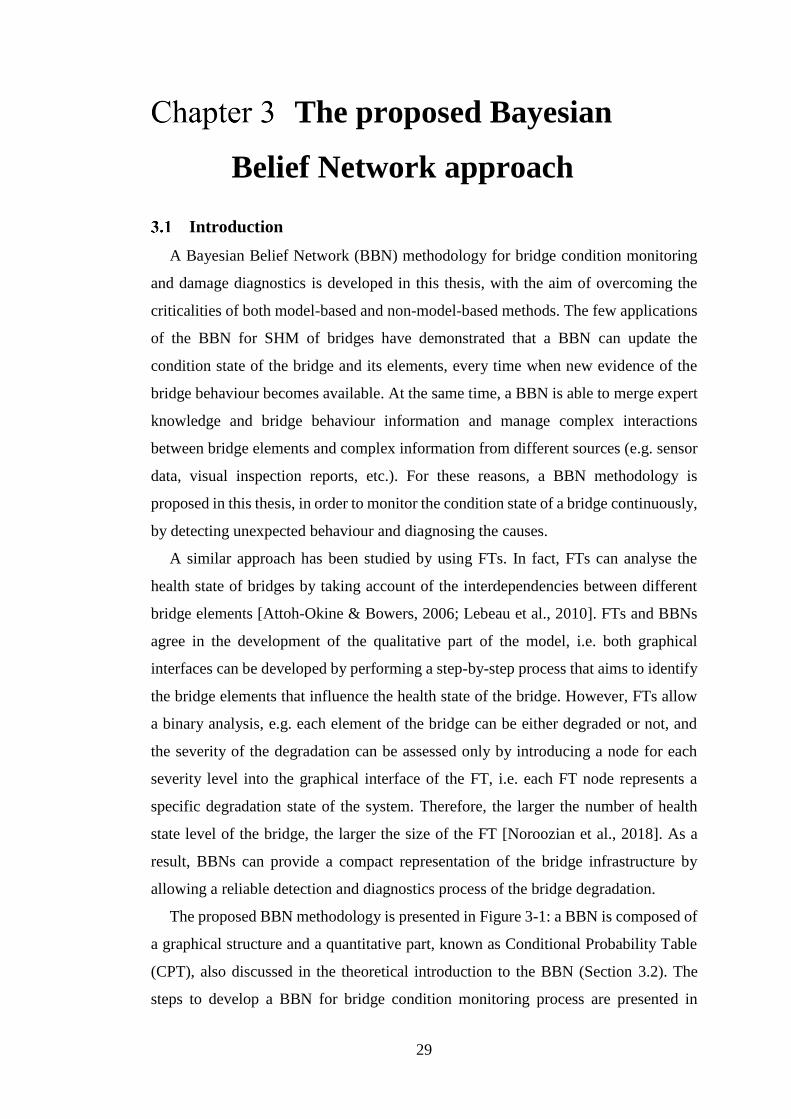
29

The proposed Bayesian

Belief Network approach

Introduction

A Bayesian Belief Network (BBN) methodology for bridge condition monitoring

and damage diagnostics is developed in this thesis, with the aim of overcoming the

criticalities of both model-based and non-model-based methods. The few applications

of the BBN for SHM of bridges have demonstrated that a BBN can update the

condition state of the bridge and its elements, every time when new evidence of the

bridge behaviour becomes available. At the same time, a BBN is able to merge expert

knowledge and bridge behaviour information and manage complex interactions

between bridge elements and complex information from different sources (e.g. sensor

data, visual inspection reports, etc.). For these reasons, a BBN methodology is

proposed in this thesis, in order to monitor the condition state of a bridge continuously,

by detecting unexpected behaviour and diagnosing the causes.

A similar approach has been studied by using FTs. In fact, FTs can analyse the

health state of bridges by taking account of the interdependencies between different

bridge elements [Attoh-Okine & Bowers, 2006; Lebeau et al., 2010]. FTs and BBNs

agree in the development of the qualitative part of the model, i.e. both graphical

interfaces can be developed by performing a step-by-step process that aims to identify

the bridge elements that influence the health state of the bridge. However, FTs allow

a binary analysis, e.g. each element of the bridge can be either degraded or not, and

the severity of the degradation can be assessed only by introducing a node for each

severity level into the graphical interface of the FT, i.e. each FT node represents a

specific degradation state of the system. Therefore, the larger the number of health

state level of the bridge, the larger the size of the FT [Noroozian et al., 2018]. As a

result, BBNs can provide a compact representation of the bridge infrastructure by

allowing a reliable detection and diagnostics process of the bridge degradation.

The proposed BBN methodology is presented in Figure 3-1: a BBN is composed of

a graphical structure and a quantitative part, known as Conditional Probability Table

(CPT), also discussed in the theoretical introduction to the BBN (Section 3.2). The

steps to develop a BBN for bridge condition monitoring process are presented in

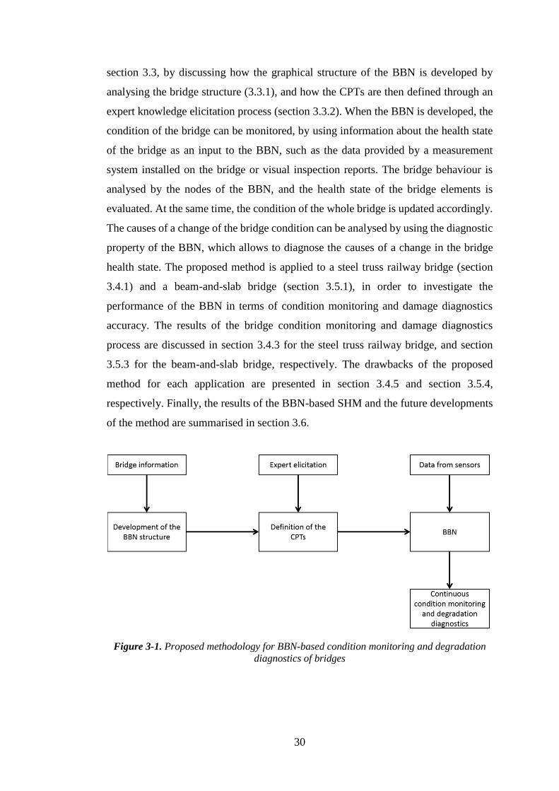
30

section 3.3, by discussing how the graphical structure of the BBN is developed by

analysing the bridge structure (3.3.1), and how the CPTs are then defined through an

expert knowledge elicitation process (section 3.3.2). When the BBN is developed, the

condition of the bridge can be monitored, by using information about the health state

of the bridge as an input to the BBN, such as the data provided by a measurement

system installed on the bridge or visual inspection reports. The bridge behaviour is

analysed by the nodes of the BBN, and the health state of the bridge elements is

evaluated. At the same time, the condition of the whole bridge is updated accordingly.

The causes of a change of the bridge condition can be analysed by using the diagnostic

property of the BBN, which allows to diagnose the causes of a change in the bridge

health state. The proposed method is applied to a steel truss railway bridge (section

3.4.1) and a beam-and-slab bridge (section 3.5.1), in order to investigate the

performance of the BBN in terms of condition monitoring and damage diagnostics

accuracy. The results of the bridge condition monitoring and damage diagnostics

process are discussed in section 3.4.3 for the steel truss railway bridge, and section

3.5.3 for the beam-and-slab bridge, respectively. The drawbacks of the proposed

method for each application are presented in section 3.4.5 and section 3.5.4,

respectively. Finally, the results of the BBN-based SHM and the future developments

of the method are summarised in section 3.6.

Figure 3-1. Proposed methodology for BBN-based condition monitoring and degradation

diagnostics of bridges

31

Background of the Bayesian Belief Network method

BBNs have been developed in the 80s, when a novel approach to represent the

expert knowledge within a computational architecture has been proposed by [Pearl,

1986]. In that work, Pearl developed a graphical interface between expert knowledge,

statistics and computers, by linking nodes, which represent the object under study and

its properties. Given a system that needs to be analysed, Pearl proposed to firstly

identify the relevant system variables and the (causal) relations among them. In this

way, the qualitative part of the BBN is developed by the means of a graphical interface.

The quantitative part of the network is defined by assessing a set of conditional

probability distributions in order to quantify the interdependencies between different

connected nodes.

The structure of the BBN

The graphical interface of a BBN is made of a set of variables (called nodes) and a

set of directed links (called arcs) between system variables of interest. The arcs

represent a causal relationship between variables of interest of the system. For

example, Figure 3-2 shows a directed graph from variables A and B to C, i.e. the

directed arcs start from nodes A and B and end with node C, and as a consequence A

and B are parent nodes of C, and C is a child node of A and B. BBNs are acyclic graphs,

i.e. connections between nodes nAAAA ,...,,, 321 , such as 1AAn = , are not permitted

[Jensen & Nielsen, 2007].

Figure 3-2. Example of relationship between parent and child node

Bayes theorem and CPTs

Generally speaking, the conditional probability of a variable X that is conditioned on

the occurrence of another variable Y is defined as follows:

zYXP =)|( (3-1)

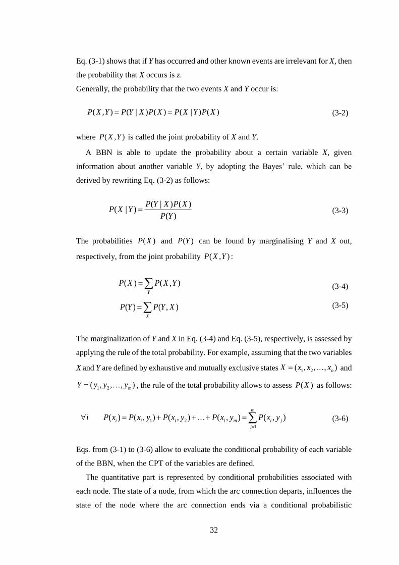
32

Eq. (3-1) shows that if Y has occurred and other known events are irrelevant for X, then

the probability that X occurs is z.

Generally, the probability that the two events X and Y occur is:

)()|()()|(),( XPYXPXPXYPYXP == (3-2)

where ),( YXP is called the joint probability of X and Y.

A BBN is able to update the probability about a certain variable X, given

information about another variable Y, by adopting the Bayes’ rule, which can be

derived by rewriting Eq. (3-2) as follows:

)(

)()|()|(

YP

XPXYPYXP = (3-3)

The probabilities )(XP and )(YP can be found by marginalising Y and X out,

respectively, from the joint probability ),( YXP :

=Y

YXPXP ),()( (3-4)

=X

XYPYP ),()( (3-5)

The marginalization of Y and X in Eq. (3-4) and Eq. (3-5), respectively, is assessed by

applying the rule of the total probability. For example, assuming that the two variables

X and Y are defined by exhaustive and mutually exclusive states ),,,( 21 nxxxX = and

),,,( 21 myyyY = , the rule of the total probability allows to assess )(XP as follows:

=

=+++=m

j

jimiiii yxPyxPyxPyxPxPi1

21 ),(),(),(),()( (3-6)

Eqs. from (3-1) to (3-6) allow to evaluate the conditional probability of each variable

of the BBN, when the CPT of the variables are defined.

The quantitative part is represented by conditional probabilities associated with

each node. The state of a node, from which the arc connection departs, influences the

state of the node where the arc connection ends via a conditional probabilistic

33

relationship [Lampis et al., 2009]. Continuous or discrete conditional probability

distributions can be used to describe the conditional probabilistic relationship between

two connected nodes [Morales-Nápoles et al., 2014]. A set of exhaustive and mutually

exclusive possible states has to be adopted when the nodes of the BBN are described

through discrete conditional probability distributions [Vileiniskis et al., 2016]. The

CPTs can be described by considering the network in Figure 3-2.

Assume that each node is described by two mutually exclusive states, such as

21,aaA = , 21,bbB = and 21,ccC = . The parent nodes are not conditioned, and thus

their CPTs coincide with the probability of each individual state: 21, aa and 21,bb . The

child node C is conditioned by the known state of its parent nodes, A and B, and

therefore its CPT is as shown in Table 3-1. The sum of the conditional probabilities

),|( kji bBaAcCP === , where j and k are fixed, for all states of i has to be equal to 1,

i.e. each column of the CPT must sum to 1.

Table 3-1 shows an important property of the CPTs: the size of the CPT increases

with the number of parent nodes and the number of the states of both parent and child

nodes. Indeed, a child node with K states and N parents with H states is described by

a CPT with NK H entries. In fact, node C, which is described by 2 states and has 2

parent nodes with 2 states each, is described by a CPT that requires 22 2 8 = entries.

Table 3-1. CPT for the node C of Figure 3-2

1bB = 2bB =

1aA = 2aA = 1aA = 2aA =

1cC = ),|( 111 bBaAcCP === ),|( 121 bBaAcCP === ),|( 211 bBaAcCP === ),|( 221 bBaAcCP ===

2cC = ),|( 112 bBaAcCP === ),|( 122 bBaAcCP === ),|( 212 bBaAcCP === ),|( 222 bBaAcCP ===

Chain rule and update of the conditional probabilities

In the BBN framework, each node Xi is conditioned on its parent nodes, pa(Xi), and

thus the probability )(XP can be decomposed into a product of conditional probability

distributions by using Eq.(3-2) repetitively:

==

+ ==

n

i

ii

n

i

nii XpaXPXXXPXP

11

1 ))(|(),,|()( (3-7)

34

where n is the number of nodes of the BBN. Eq. (3-7) is known as the probability chain

rule and allows to assess the joint distribution of each set of BBN variables by using

only conditional probabilities. Therefore, given a set of nodes U=nAAAA ,...,,, 321 within

the BBN, every time when new evidence me , with 1,2,...,m M= , about the state of the

nodes of the BBN become available, the BBN is able to update the degree of belief of

the node states by computing the posterior probability distribution of each node as

follows:

)(

),(

)|(eP

eUP

eAP UA

= (3-8)

where ),( eUP is the updated joint probability:

==

=M

m

m

n

i

ii eApaAPeUP11

))(|(),( (3-9)

Eq. (3-8) shows that the probability of each node, A, is updated given the evidence e,

by applying the Bayes’ rule (Eq. (3-3)), whereas Eq. (3-9) shows that the joint

probability of the each BBN node is updated by applying the chain rule (Eq. (3-7)).

Finally, it is worth noting that the evidence me is introduced into the BBN as a vector

of zeros and ones, where the zeros represent the fact that the state of the node has not

occurred, whilst the ones represent the fact that the state has occurred.

BBN used to decompose systems into smaller parts

The BBN also allows to decompose a complex system into smaller parts. In fact,

the BBN of a complex and large system, such as a bridge, can result in a large and

complex BBN structure. Consequently, the graphical representation of the BBN can

become ineffective due to a large number of nodes of the BBN. Furthermore, some

systems can consist of a number of similar elements installed next to each other, e.g.

multiple similar beams of a bridge. In these cases, the BBN allows to decompose the

system into Objected Oriented Bayesian Network (OOBN). From the graphical point

of view, the OOBN allows to define a new separate BBN in order to represent all the

elements of a part of the complex BBN system. Subsequently, the part of the BBN of

the system is replaced by a single evidence node, which represents each element of the

35

considered part. For example, Figure 3-3 shows a BBN of a system that is composed

of three components, A, B and C. Each component is made of five elements. The

dependencies between different elements of the system can be difficult to be identified

due to the high number of connections between different nodes. The OOBN allows to

simplify the BBN, as shown in Figure 3-4.

Figure 3-3. Example of complex system for OOBN

Figure 3-4 shows the OOBN of the system. The graphical view of the network is

clearer than the one in Figure 3-3. In fact, the connections between the different

components of the system are pointed out more clearly. Each node within a rectangular

node represents evidence introduced to the BBN. For example, Figure 3-5 shows the

BBN for the components A and C. It should be noted that the BBN of each component

in Figure 3-5 is made of the same connections as in Figure 3-3. However, Figure 3-5b

shows that the BBN of component C has an additional node, which is depicted by a

dashed node and represents the evidence of the BBN about component A, i.e. the BBN

of Figure 3-5a. In this way, the graphical view of the BBN can be simplified, and each

component of the system can be analysed separately.

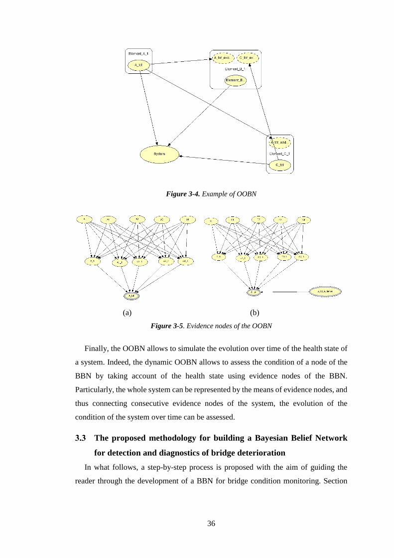
36

Figure 3-4. Example of OOBN

(a) (b)

Figure 3-5. Evidence nodes of the OOBN

Finally, the OOBN allows to simulate the evolution over time of the health state of

a system. Indeed, the dynamic OOBN allows to assess the condition of a node of the

BBN by taking account of the health state using evidence nodes of the BBN.

Particularly, the whole system can be represented by the means of evidence nodes, and

thus connecting consecutive evidence nodes of the system, the evolution of the

condition of the system over time can be assessed.

The proposed methodology for building a Bayesian Belief Network

for detection and diagnostics of bridge deterioration

In what follows, a step-by-step process is proposed with the aim of guiding the

reader through the development of a BBN for bridge condition monitoring. Section

37

3.3.1 describes the steps to develop the graphical interface of the BBN, whereas section

3.3.2 describes the steps necessary to define the CPT.

The method of building the BBN

A step by step process to develop the structure of the BBN for condition monitoring

and degradation diagnostics of a bridge infrastructure is hereafter described. The

following steps are proposed:

1. Identify the type of the bridge and its major and minor elements of

interest. Several types of bridge structure, such as box-girder, cable stayed,

truss, arch, suspension, etc., are usually found within the transportation

network [Catbas et al., 2008; Arangio et al., 2014; Xia et al., 2014; Ni, 2014;

Gentile et al., 2015]. The analysis of the bridge structure helps to identify the

bridge components (major elements) and sub-components (minor elements) of

which a bridge manager needs to monitor the condition [LeBeau et al., 2000].

The identification of the elements of the bridge can be as detailed as the bridge

manager requires. Indeed, each minor element is made of relatively small

elements, such as smaller beams, joints, etc. However, a balance between the

number of elements of interest and the size of the BBN needs to be reached,

due to the fact that the size of the BBN increases as the number of the bridge

elements of interest increases. Finally, it should be noted that sometimes

guidelines that describe the bridge structure, i.e. major and minor elements of

the bridge, can be provided by the bridge owner [Gangone et al., 2011].

2. Define the BBN structure. When the bridge elements of interest are identified,

the structure of the BBN can be developed, i.e. the set of nodes and arcs can be

defined. The nodes of the BBN represent the major and minor elements,

whereas the arcs represent the interdependencies between the nodes of the

BBN. The construction of the BBN should follow the same order as for the

construction of the real bridge, i.e. from minor to major elements. In fact, the

condition of a major element of the bridge is influenced by the condition of its

minor elements, and thus each major element is child node of its minor element

nodes. The health state of the whole bridge can be then evaluated by

introducing a child node to the major elements of the bridge [Attoh-Okine &

Bowers, 2006].

38

3. Upgrade the BBN model to take account of the interdependencies among

major/minor elements. The health state of a major (minor) element depends

also on the condition of the other major bridge (minor) elements. Thus, the

BBN structure can be further developed in order to take into account the

interdependencies between major (minor) elements of the bridge. As the BBN

is an acyclic graph, additional nodes are introduced in order to evaluate

interdependencies between different elements of the bridge that belong to the

same class, i.e. major or minor elements.

4. Choose the number of health states of each node. An element of the bridge

experiences different health states during its life time, such as good and

degraded conditions. Therefore, each BBN node should be described by a set

of mutually exclusive discrete states to describe these conditions. The number

of states can be as large as the bridge manager would require. However, the

size of the CPTs increases as the number of states increase. Bridge owners can

usually provide information about the possible conditions of a bridge. For

example, Network Rail, which is the owner of the UK railway network,

assesses the condition of bridges by considering three classes: i) good

condition, if the element is in good condition and maintenance actions are not

required; ii) partially degraded, if maintenance action are required, but they can

be postponed due to budgeting reasons, without compromising the safety of the

asset; iii) severely degraded, if essential maintenance actions, i.e. that cannot

be postponed, are required [Rafiq et al., 2015].

5. Define nodes to represent the measurement system of the bridge. If a

measurement system is installed on the bridge, sensors, such as accelerometers,

strain gauges, tiltmeters, etc., are used to monitor the bridge behaviour under

changing environmental conditions [Roberts et al., 2004]. The data provided

by the sensors is evidence of the bridge behaviour, and, as a consequence, a

node for each sensor can be added to the BBN. The nodes representing the

sensors are introduced as parent nodes of the bridge element(s) on which the

sensors are installed. If a measurement system is not installed on the bridge,

the BBN approach can be still adopted, by relying on different sources of

information on the bridge behaviour, such as visual inspection reports.

6. Review the BBN structure by analysing the bridge behaviour. When the

BBN is developed, its structure can be updated by analysing the behaviour of

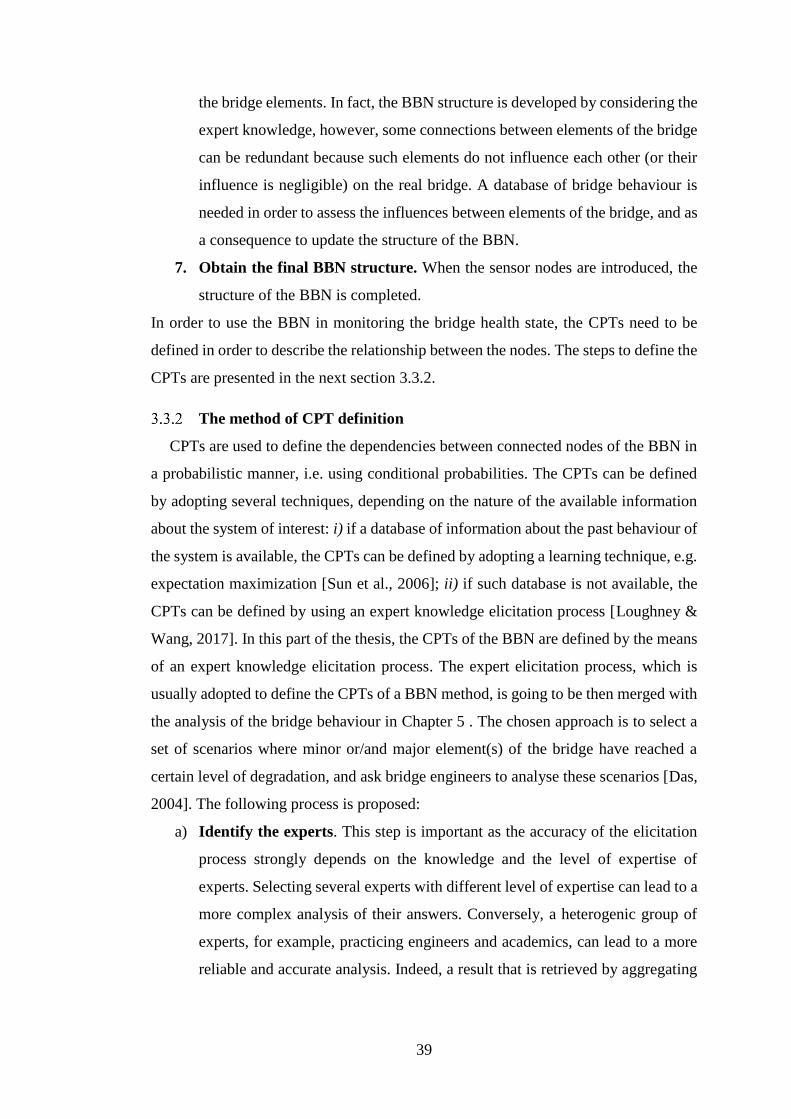
39

the bridge elements. In fact, the BBN structure is developed by considering the

expert knowledge, however, some connections between elements of the bridge

can be redundant because such elements do not influence each other (or their

influence is negligible) on the real bridge. A database of bridge behaviour is

needed in order to assess the influences between elements of the bridge, and as

a consequence to update the structure of the BBN.

7. Obtain the final BBN structure. When the sensor nodes are introduced, the

structure of the BBN is completed.

In order to use the BBN in monitoring the bridge health state, the CPTs need to be

defined in order to describe the relationship between the nodes. The steps to define the

CPTs are presented in the next section 3.3.2.

The method of CPT definition

CPTs are used to define the dependencies between connected nodes of the BBN in

a probabilistic manner, i.e. using conditional probabilities. The CPTs can be defined

by adopting several techniques, depending on the nature of the available information

about the system of interest: i) if a database of information about the past behaviour of

the system is available, the CPTs can be defined by adopting a learning technique, e.g.

expectation maximization [Sun et al., 2006]; ii) if such database is not available, the

CPTs can be defined by using an expert knowledge elicitation process [Loughney &

Wang, 2017]. In this part of the thesis, the CPTs of the BBN are defined by the means

of an expert knowledge elicitation process. The expert elicitation process, which is

usually adopted to define the CPTs of a BBN method, is going to be then merged with

the analysis of the bridge behaviour in Chapter 5 . The chosen approach is to select a

set of scenarios where minor or/and major element(s) of the bridge have reached a

certain level of degradation, and ask bridge engineers to analyse these scenarios [Das,

2004]. The following process is proposed:

a) Identify the experts. This step is important as the accuracy of the elicitation

process strongly depends on the knowledge and the level of expertise of

experts. Selecting several experts with different level of expertise can lead to a

more complex analysis of their answers. Conversely, a heterogenic group of

experts, for example, practicing engineers and academics, can lead to a more

reliable and accurate analysis. Indeed, a result that is retrieved by aggregating

40

the analysis from a group of experts is usually more reliable than each

individual analysis [Surowiecki, 2004; Kabir et al., 2016].

b) Identify the degraded scenarios. The definition of the CPTs can be an

extremely time-consuming process, due to the number of scenarios that the

experts need to analyse. As a result, the uniformity and consistency of the

expert knowledge elicitation process might not be achieved [Elmasry et al.,

2017]. A smaller number of scenarios can be presented to the expert by

considering scenarios that are physically consistent. For instance, if a minor

element of a bridge is degraded in a specified health state, the major element,

which contains that minor element, is expected to be in a similar health state

[Das, 2004; Rafiq et al., 2015].

c) Present the scenarios to the experts. The set of degraded scenarios is

presented to experts through interviews and online surveys [Perkusich et al.,

2013]. Each scenario needs to be described accurately, by explaining the health

state of the element of interest and its possible influence on the health state of

the connected nodes.

d) Provide a scale for answers. A linguistic scale can be provided to the experts

in order to answer the questions. In fact, experts can be more comfortable in

providing a linguistic answer rather than a precise numerical value of the

probability, due to the fact that the linguistic answer allows to take account of

some uncertainty [Torfi et al., 2010]. An example of a linguistic scale is shown

in Table 3-2.

Table 3-2. Linguistic scale for assessing the interdependencies between different bridge

elements Linguistic

scale Meaning

very unlikely

it is highly unlikely that the health state of the considered element

would be influenced by the described critical scenario of the bridge

element

unlikely

it is unlikely but possible that the health state of the considered

element would be influenced by the described critical scenario of the

bridge element

even chance

the likelihood that the health state of the considered element would be

influenced by the described critical scenario of the bridge element is

even chance

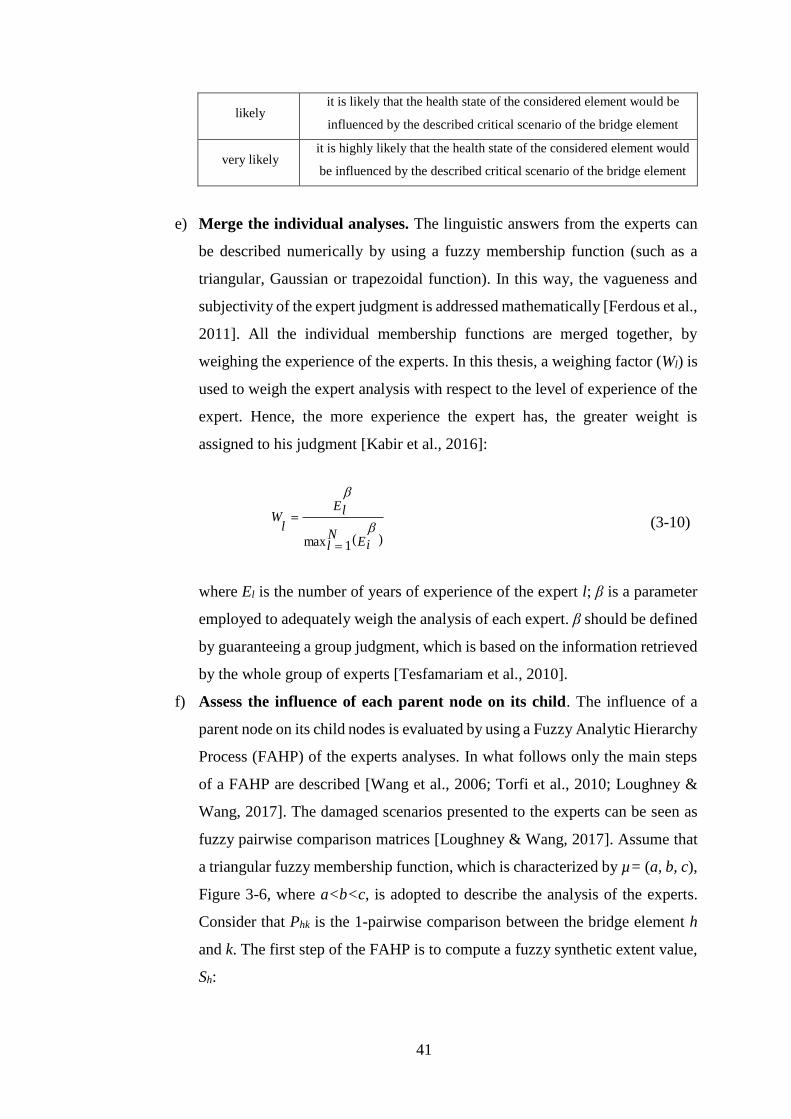
41

likely it is likely that the health state of the considered element would be

influenced by the described critical scenario of the bridge element

very likely it is highly likely that the health state of the considered element would

be influenced by the described critical scenario of the bridge element

e) Merge the individual analyses. The linguistic answers from the experts can

be described numerically by using a fuzzy membership function (such as a

triangular, Gaussian or trapezoidal function). In this way, the vagueness and

subjectivity of the expert judgment is addressed mathematically [Ferdous et al.,

2011]. All the individual membership functions are merged together, by

weighing the experience of the experts. In this thesis, a weighing factor (Wl) is

used to weigh the expert analysis with respect to the level of experience of the

expert. Hence, the more experience the expert has, the greater weight is

assigned to his judgment [Kabir et al., 2016]:

)(max 1 EiNl

El

lW

=

= (3-10)

where El is the number of years of experience of the expert l; β is a parameter

employed to adequately weigh the analysis of each expert. β should be defined

by guaranteeing a group judgment, which is based on the information retrieved

by the whole group of experts [Tesfamariam et al., 2010].

f) Assess the influence of each parent node on its child. The influence of a

parent node on its child nodes is evaluated by using a Fuzzy Analytic Hierarchy

Process (FAHP) of the experts analyses. In what follows only the main steps

of a FAHP are described [Wang et al., 2006; Torfi et al., 2010; Loughney &

Wang, 2017]. The damaged scenarios presented to the experts can be seen as

fuzzy pairwise comparison matrices [Loughney & Wang, 2017]. Assume that

a triangular fuzzy membership function, which is characterized by µ= (a, b, c),

Figure 3-6, where a<b<c, is adopted to describe the analysis of the experts.

Consider that Phk is the 1-pairwise comparison between the bridge element h

and k. The first step of the FAHP is to compute a fuzzy synthetic extent value,

Sh:

42

1

1 11

−

= =

=

=

D

h

C

khk

PC

khk

Ph

S (3-11)

where D is the number of rows of the pairwise comparison matrix, i.e. the

number of bridge elements that influence the health state of other bridge

elements, and C is the number of columns of the pairwise comparison, i.e. the

number of bridge elements that are influenced by a selected bridge element.

The sum of the pairwise comparison of each child node (the first term of Eq.

(3-11)) can be easily computed as:

===

=

=

C

kk

cC

kk

bC

kk

aC

khk

P

1

,

1

,

11

(3-12)

whereas the second term of Eq. (3-11) is computed following the modified

Chang extend analysis, which has been demonstrated to perform better than the

original Chang extend analysis [Wang et al., 2006]. An integral value of each

synthetic extend value is then evaluated as follows:

( )hhhh abcI )1(2

1 −++= (3-13)

where α ϵ [0,1] is the optimism of the expert on the results of his analysis, and

(ah, bh, ch) are the fuzzy membership of the h-th fuzzy synthetic extent [Kabir

et al., 2016]. Finally, the importance weight vector (wh) of each parent node on

its child nodes can be assessed as:

=

=D

h

h

hh

I

Iw

1

(3-14)

where h = 1, 2, …, D.

g) Assess the consistency of the expert analysis. The expert knowledge

elicitation process can be a long task for the experts. Consequently, the

consistency of the expert analysis needs to be verified by assessing a

Consistency Ratio (CR). Therefore, the fuzzy pairwise comparison matrix is

defuzzified, and then a Consistency Index (CI) is computed as follows:

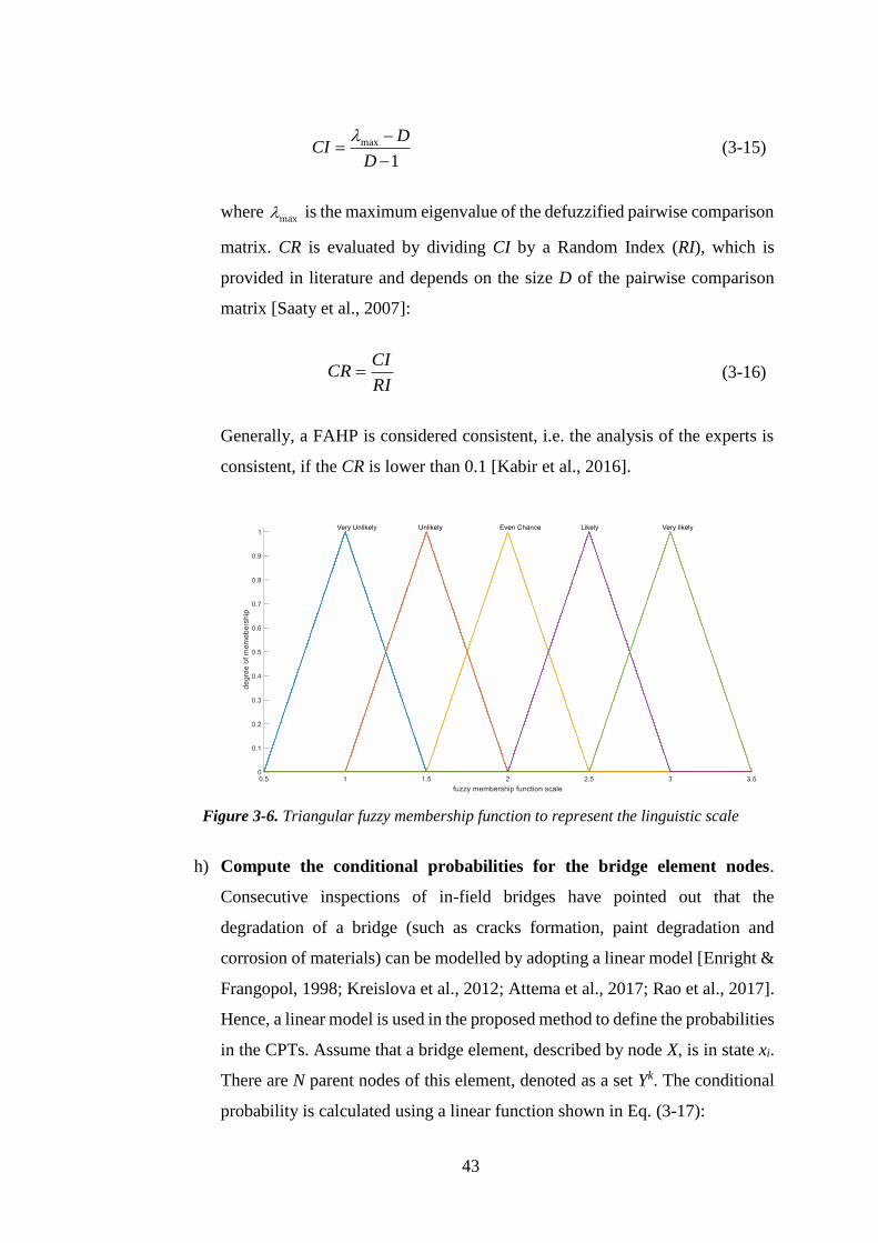
43

1

max

−

−=

D

DCI

(3-15)

where max is the maximum eigenvalue of the defuzzified pairwise comparison

matrix. CR is evaluated by dividing CI by a Random Index (RI), which is

provided in literature and depends on the size D of the pairwise comparison

matrix [Saaty et al., 2007]:

RI

CICR = (3-16)

Generally, a FAHP is considered consistent, i.e. the analysis of the experts is

consistent, if the CR is lower than 0.1 [Kabir et al., 2016].

Figure 3-6. Triangular fuzzy membership function to represent the linguistic scale

h) Compute the conditional probabilities for the bridge element nodes.

Consecutive inspections of in-field bridges have pointed out that the

degradation of a bridge (such as cracks formation, paint degradation and

corrosion of materials) can be modelled by adopting a linear model [Enright &

Frangopol, 1998; Kreislova et al., 2012; Attema et al., 2017; Rao et al., 2017].

Hence, a linear model is used in the proposed method to define the probabilities

in the CPTs. Assume that a bridge element, described by node X, is in state xi.

There are N parent nodes of this element, denoted as a set Yk. The conditional

probability is calculated using a linear function shown in Eq. (3-17):

44

11 1 1

( ) ( 1) ( 1)m m

N N NMk k k

i k i k i k h p imk k k

P x Y y P x Y y P x Y y w f p == = =

= = = = + = = (3-17)

where 1

( )N

ki k

k

P x Y y=

= is the probability of the child node in state xi, with a

condition that the health states of the parent nodes are known, denoted as yk;

1

( 1)N

ki k

k

P x Y y=

= = is the probability of the child node X in state xi, with a

condition that all parent nodes are in the healthy state, yk=1, i.e. the parent

nodes show no degradation; M is the number of degraded parent nodes; mhw

is the importance weight vector used to assess the influence of each degraded

parent node on the state of the child node, note that mhw is calculated using

Eq. (3-14); mpf is a penalty factor that increases as the condition of the bridge

element(s) deteriorates; 1−= if the child node is in the healthy state, xi=1,

and 1= if the child node is in the degraded state; ip is a vector used to

normalise the respective column of probabilities in the CPT and it depends on

the state of the child node.

Overall, Eq. (3-17) shows that the probability of the child node being in state

xi, with a condition that M parent nodes are degraded, is computed as the total

mm p

M

m

h fw=1

decrease or increase of 1

( 1)N

ki k

k

P x Y y=

= = , caused by the influence of

M degraded parent nodes. M can be between 0 to N, i.e. if M=0 (there are no

degraded parent nodes), then 1

( 1)N

ki k

k

P x Y y=

= = does not change; if M=N (all

parent nodes are degraded), then 1

( 1)N

ki k

k

P x Y y=

= = experiences its maximum

variation.

Finally, when the CPTs are defined, the BBN is ready to be used to monitor the

health state of the bridge and diagnose its unexpected behaviour.

In the next section, an FEM of a steel truss railway bridges is introduced, with the

aim of simulating the beahviour of the bridge under changing condition, and to test the

45

proposed BBN method in monitoring the behaviour of the bridge in detecting and

diagnosing its unexpected behaviour.

BBN model for a steel truss bridge and its application in detection and

diagnostics of bridge deterioration

In this section, the proposed BBN methodology is applied to monitor the health

state of a steel truss bridge, which is subject to a gradual degradation mechanism of its

element(s). The aim of this case study is the testing of the updating capability of the

BBN with respect to the bridge condition monitoring and damage diagnostics process.

An FEM of a steel truss bridge is developed with the aim of simulating the behaviour

of the bridge under an ongoing degradation mechanism, which leads to a gradual

decrease of the bridge health state. The BBN is required to monitor the health state of

the steel truss bridge continuously, by pointing out changes of the bridge condition and

diagnosing the causes of such changes. The FEM is presented in section 3.4.1. The

step by step process to develop the BBN is discussed in section 3.4.2, whereas its

performance in monitoring the bridge condition is presented in section 3.4.3. Section

3.4.4 evaluates the performance of the proposed BBN method. The results of the

proposed method are discussed in section 3.4.5.

FEM of a steel truss railway bridge

An FEM of a steel truss bridge is developed in order to test the proposed BBN

methodology in monitoring the condition of the bridge over time, using a model. An

FEM is required due to the fact that data from an in-field bridge are difficult to retrieve,

because a bridge is a critical infrastructure of the transportation network, and thus

usually bridge owners are not willing to share the data. Moreover, a laboratory model

of a bridge is not available, and it would be more expensive and time-consuming to

develop a laboratory model of a bridge, rather than an FEM.

The FEM model that is described in this section is developed by assuming that the

boundary conditions are fixed, i.e. air temperature is fixed, wind is not present, and no

traffic is passing over the bridge, and only a static uniform load is applied to the bridge.

Although many bridge of the transportation network are more than 50 years old, and

therefore they are built using old materials (such as iron), the materials of the

developed FEM are defined by following the “Innovative Bridge Design Handbook”

[Pipinato & Patton, 2016]. The aim of the FEM is not to simulate the behaviour of a

real in-field bridge accurately, but rather to simulate the bridge behaviour under

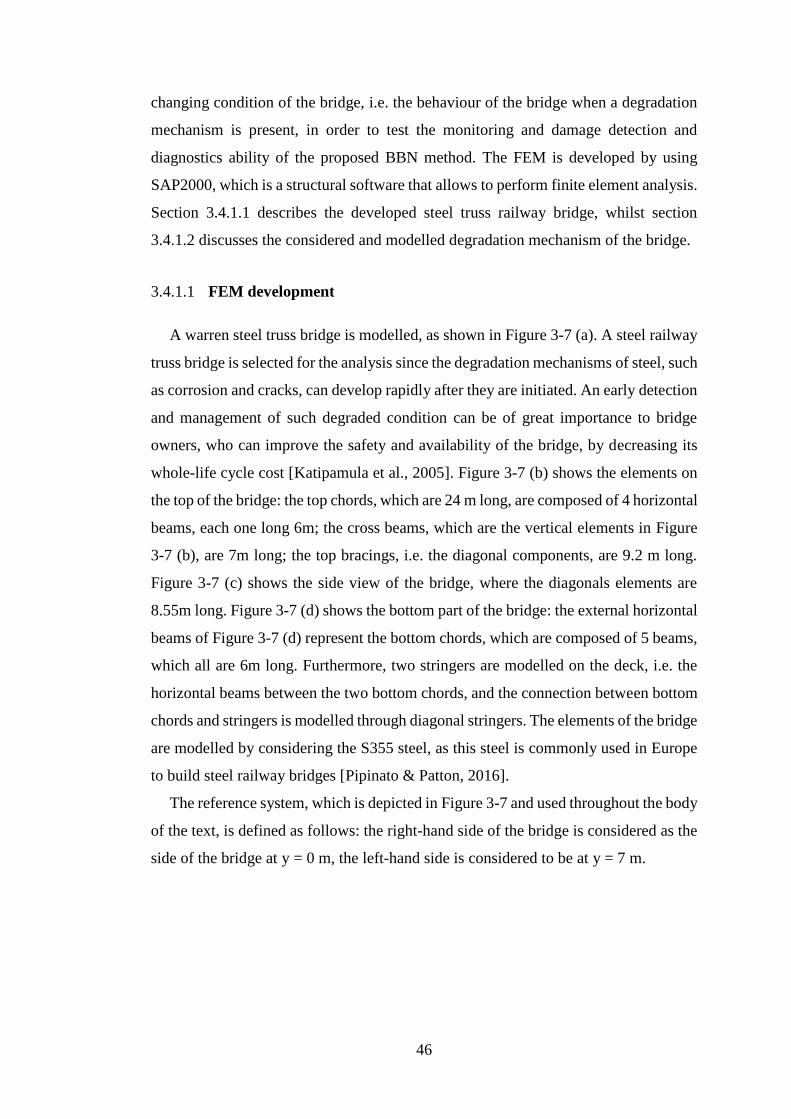
46

changing condition of the bridge, i.e. the behaviour of the bridge when a degradation

mechanism is present, in order to test the monitoring and damage detection and

diagnostics ability of the proposed BBN method. The FEM is developed by using

SAP2000, which is a structural software that allows to perform finite element analysis.

Section 3.4.1.1 describes the developed steel truss railway bridge, whilst section

3.4.1.2 discusses the considered and modelled degradation mechanism of the bridge.

3.4.1.1 FEM development

A warren steel truss bridge is modelled, as shown in Figure 3-7 (a). A steel railway

truss bridge is selected for the analysis since the degradation mechanisms of steel, such

as corrosion and cracks, can develop rapidly after they are initiated. An early detection

and management of such degraded condition can be of great importance to bridge

owners, who can improve the safety and availability of the bridge, by decreasing its

whole-life cycle cost [Katipamula et al., 2005]. Figure 3-7 (b) shows the elements on

the top of the bridge: the top chords, which are 24 m long, are composed of 4 horizontal

beams, each one long 6m; the cross beams, which are the vertical elements in Figure

3-7 (b), are 7m long; the top bracings, i.e. the diagonal components, are 9.2 m long.

Figure 3-7 (c) shows the side view of the bridge, where the diagonals elements are

8.55m long. Figure 3-7 (d) shows the bottom part of the bridge: the external horizontal

beams of Figure 3-7 (d) represent the bottom chords, which are composed of 5 beams,

which all are 6m long. Furthermore, two stringers are modelled on the deck, i.e. the

horizontal beams between the two bottom chords, and the connection between bottom

chords and stringers is modelled through diagonal stringers. The elements of the bridge

are modelled by considering the S355 steel, as this steel is commonly used in Europe

to build steel railway bridges [Pipinato & Patton, 2016].

The reference system, which is depicted in Figure 3-7 and used throughout the body

of the text, is defined as follows: the right-hand side of the bridge is considered as the

side of the bridge at y = 0 m, the left-hand side is considered to be at y = 7 m.

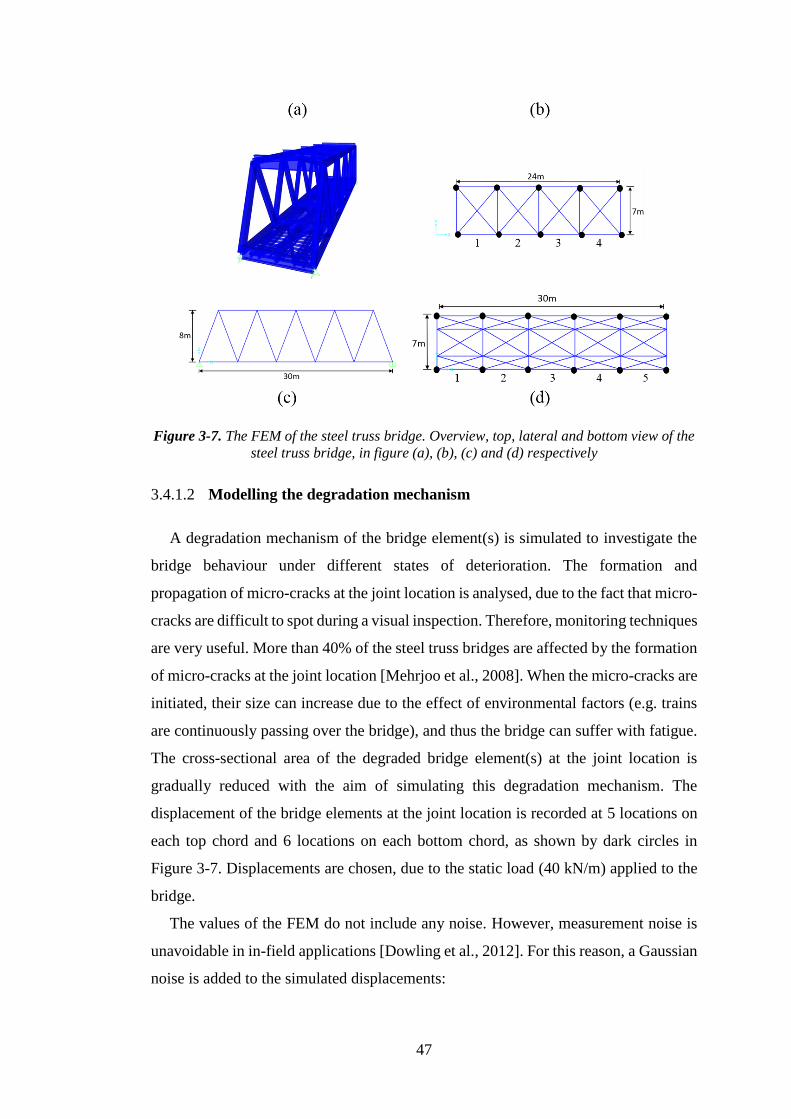
47

Figure 3-7. The FEM of the steel truss bridge. Overview, top, lateral and bottom view of the

steel truss bridge, in figure (a), (b), (c) and (d) respectively

3.4.1.2 Modelling the degradation mechanism

A degradation mechanism of the bridge element(s) is simulated to investigate the

bridge behaviour under different states of deterioration. The formation and

propagation of micro-cracks at the joint location is analysed, due to the fact that micro-

cracks are difficult to spot during a visual inspection. Therefore, monitoring techniques

are very useful. More than 40% of the steel truss bridges are affected by the formation

of micro-cracks at the joint location [Mehrjoo et al., 2008]. When the micro-cracks are

initiated, their size can increase due to the effect of environmental factors (e.g. trains

are continuously passing over the bridge), and thus the bridge can suffer with fatigue.

The cross-sectional area of the degraded bridge element(s) at the joint location is

gradually reduced with the aim of simulating this degradation mechanism. The

displacement of the bridge elements at the joint location is recorded at 5 locations on

each top chord and 6 locations on each bottom chord, as shown by dark circles in

Figure 3-7. Displacements are chosen, due to the static load (40 kN/m) applied to the

bridge.

The values of the FEM do not include any noise. However, measurement noise is

unavoidable in in-field applications [Dowling et al., 2012]. For this reason, a Gaussian

noise is added to the simulated displacements:

48

)( FEpFEpol yNqyy += (3-18)

where poly is the displacement of a bridge element when the noise is added, FEy is

the displacement value provided by the FEM, pq is the ratio of standard deviation

between the noise and the FEM displacement FEy and is equal to 5%. N is a standard

normal distribution of mean 0 and standard deviation 1, and )( FEy is the standard

deviation of the results of the FEM [Shu et al., 2013].

The deterioration mechanisms of the bridge element(s) is studied by developing 28

deterioration scenarios:

• 22 individual deterioration mechanism scenarios, where each joint of the top

chords (10 scenarios) and bottom chords (12 scenarios) is individually

degraded. The cross-sectional area of the corresponding minor elements at the

joint location is gradually decreased down to the 70% of its initial value. The

minor elements of the top and bottom chords are chosen due to the fact that

they have shown the highest stresses during the service of a steel truss bridge

[Ni et al., 2012].

• 6 multiple deterioration mechanism scenarios, where two or three joints of the

top/bottom chords are degraded, by decreasing the cross-sectional area of the

corresponding minor elements at the joint location.

For example, Figure 3-8 shows the evolution of the displacement of the third and

fourth joints of the top chord on the right-hand side of the bridge, when the fourth joint

is degraded over time, i.e. a gradual degradation of the joint is simulated by the means

of consecutive simulations. The displacements provided by the FEM for the two joints,

when a static uniform load of 40kN/m is applied to the bridge, are depicted by the solid

lines in Figure 3-8 (a) and (b) for the third and fourth joint, respectively. The dotted

lines of Figure 3-8 represent the displacement of the two elements of the bridge when

the Gaussian noise is added. Figure 3-8 shows that with the same static load that is

applied to the bridge, the higher the loss of cross-sectional area (i.e. the more

degradation has occurred), the higher (in terms of absolute value) the displacement of

the bridge elements. In a similar way, Figure 3-8(c) and (d) show that the displacement

of the two joints increase as the joint degradation increases over time (i.e. consecutive

49

simulations time). Therefore, the displacements can be used as an indicator of the

health condition of the bridge over time.

In what follows, the proposed BBN method is developed in order to test its

performance in monitoring the condition of the presented FEM, by diagnosing the

degraded element(s) of the bridge.

(a) (b)

(c) (d)

Figure 3-8. Displacement of the third and fourth joints of the top chord at y=0m as the loss

of area increase figures (a) and (b), respectively; effect of the degradation over time on the

third (c) and fourth (d) joints, respectively

Development of the BBN model

The proposed BBN-based condition monitoring and fault detection method is

evaluated by analysing the developed FEM of the steel truss bridge. Particularly, the

condition of the bridge is monitored during the 28 degradation scenarios, in order to

point out the ongoing degradation of the bridge, by detecting and diagnosing the

ongoing degradation of the bridge.

In what follows, the process to define the BBN structure is presented in section

3.4.2.1, whilst section 3.4.2.2 presents the process to define the CPTs of the BBN.

50

Section 3.4.3 presents a detailed analysis of the bridge condition monitoring during a

degradation scenario, with the aim of illustrating how a bridge manager can adopt, and

interact with, the BBN in order to monitor the bridge health state and diagnose its

unexpected condition. The analysis of the BBN performance is then discussed in

section 3.4.4 in order to point out the accuracy of the proposed method in analysing

the 28 degraded scenarios, by highlighting its advantages and disadvantages. Finally,

the proposed method is discussed in section 3.4.5 by pointing out the drawbacks of the

proposed method, which are then managed in the following chapters of the thesis.

3.4.2.1 The BBN model building

The development of the structure of the BBN is carried out by following the 7 steps

proposed in Section 3.3:


interest. The bridge is a warren steel truss, and its major elements are identified

as the deck, the top and bottom chords, the diagonals and the stringers. The

minor elements of the bridge are represented by each individual beam that

belongs to a major element and by the joints that connect each minor beam.

Hereafter, only the condition of the top and bottom chords of the bridge are

considered. Therefore, we assume that the health state of the whole bridge

depends only on the health state of these two major elements. This assumption

is due to the fact that the chords of the bridge show the highest stresses during

the service of a steel truss bridge usually [Ni et al., 2012].

2. Define the BBN structure. Each top chord is made of 4 beams, as shown in

Figure 3-7(a). Therefore, 4 nodes are used in the BBN framework to

characterize these four elements: each E_j_TCR node in Figure 3-9 represents

the condition of the minor elements j, where j=1, 2, 3, 4, of the top chord on

the right hand side of the bridge (parent nodes of TCR node in Figure 3-9).

Similarly, each bottom chord is made of 5 beams, as shown in Figure 3-7(c).

Thus, 5 nodes representing the minor elements of the bottom chords are

introduced in the BBN: each E_i_BCR represents the minor element i, where i

=1, 2, 3, 4, 5, of the bottom chord on the right hand side of the bridge (parent

nodes of BCR in Figure 3-9). The same definition is true for the left-hand side

of the bridge, as shown in Figure 3-9 by the nodes ending with “L”. Each minor

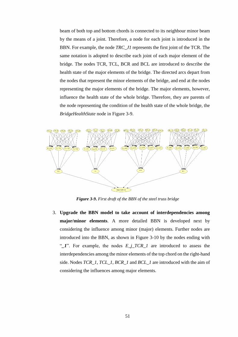
51

beam of both top and bottom chords is connected to its neighbour minor beam

by the means of a joint. Therefore, a node for each joint is introduced in the

BBN. For example, the node TRC_J1 represents the first joint of the TCR. The

same notation is adopted to describe each joint of each major element of the

bridge. The nodes TCR, TCL, BCR and BCL are introduced to describe the

health state of the major elements of the bridge. The directed arcs depart from

the nodes that represent the minor elements of the bridge, and end at the nodes

representing the major elements of the bridge. The major elements, however,

influence the health state of the whole bridge. Therefore, they are parents of

the node representing the condition of the health state of the whole bridge, the

BridgeHealthState node in Figure 3-9.

Figure 3-9. First draft of the BBN of the steel truss bridge

3. Upgrade the BBN model to take account of interdependencies among

major/minor elements. A more detailed BBN is developed next by

considering the influence among minor (major) elements. Further nodes are

introduced into the BBN, as shown in Figure 3-10 by the nodes ending with

“_1”. For example, the nodes E_j_TCR_1 are introduced to assess the

interdependencies among the minor elements of the top chord on the right-hand

side. Nodes TCR_1, TCL_1, BCR_1 and BCL_1 are introduced with the aim of

considering the influences among major elements.

52


elements

4. Review the BBN structure by analysing the bridge behaviour. A database

of bridge behaviour is needed to carry out this step and optimize the structure

of the BBN. Displacement of the joints is used as an input to the BBN nodes,

i.e. the displacements is used to assess the condition of the bridge elements.

The analysis of the bridge behaviour in different conditions of the bridge

elements can provide information about the strength of the influence between

different bridge elements, and the structure of the BBN can be updated

accordingly. The strength of the influence of a degrading bridge element (A)

on the health state of another healthy bridge element (B) is assessed by

computing the percentage of variation (with respect to the healthy bridge) of

the displacement of the element B. We assume a threshold of 0.5% to take

account of a possible influence between different bridge elements. The value

of the threshold is retrieved by analysing the behaviour of the developed FEM

in different health states of the bridge elements. The FEM displacements are

6mm generally, and as a result the resolution of a real displacement

measurement system, which best resolution is up to is 0.08mm, is not

considered during the threshold definition process [Vicente et al., 2018]. For

example, Figure 3-11 shows the percentage of variation of the BCR joints

displacement, when joint 1 or joint 2 of BCR are degrading. When joint 1 is

degrading, i.e. the cross-sectional area of the first BCR element is decreased at

the joint location, the displacements of the other BCR joints are slightly

influenced (the maximum percentage variation is equal to 0.25%). Therefore,

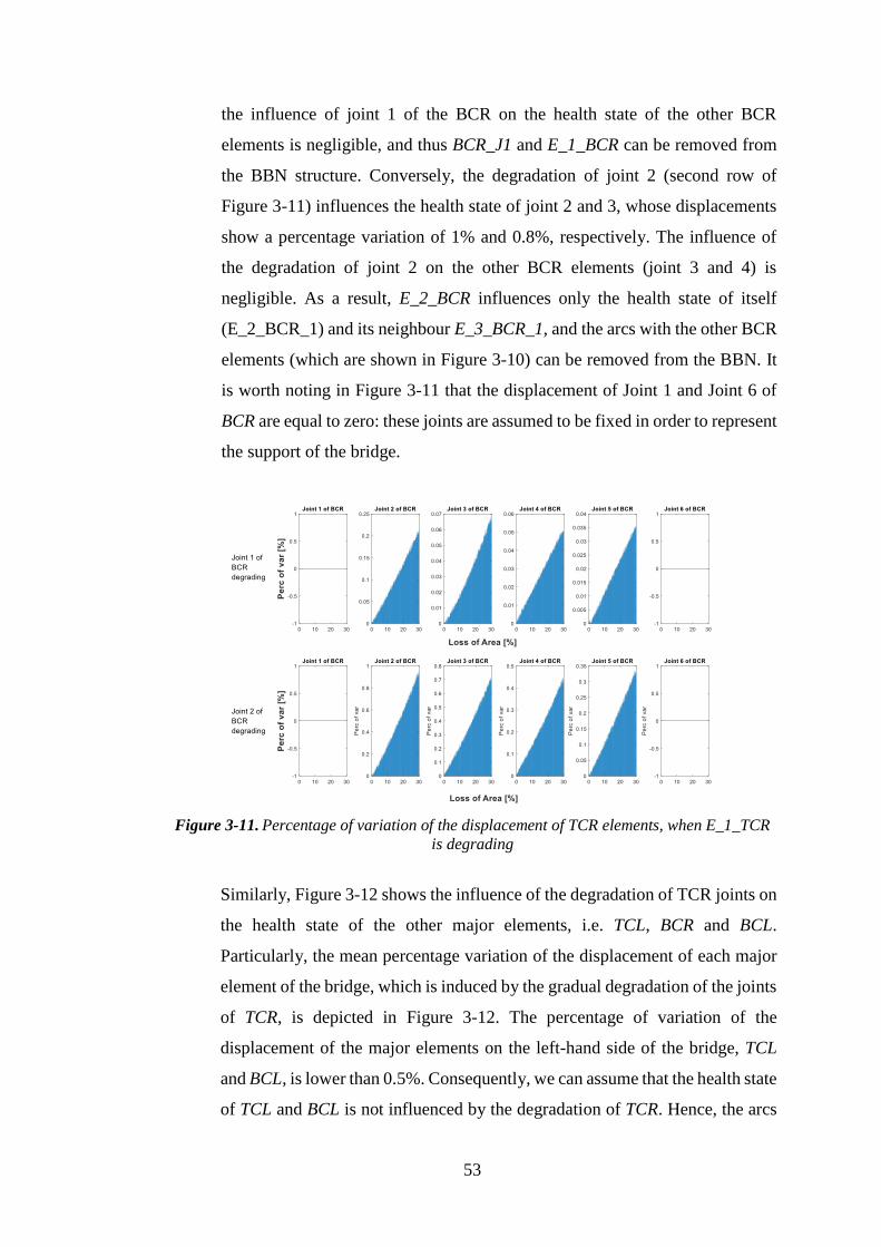
53

the influence of joint 1 of the BCR on the health state of the other BCR

elements is negligible, and thus BCR_J1 and E_1_BCR can be removed from

the BBN structure. Conversely, the degradation of joint 2 (second row of

Figure 3-11) influences the health state of joint 2 and 3, whose displacements

show a percentage variation of 1% and 0.8%, respectively. The influence of

the degradation of joint 2 on the other BCR elements (joint 3 and 4) is

negligible. As a result, E_2_BCR influences only the health state of itself

(E_2_BCR_1) and its neighbour E_3_BCR_1, and the arcs with the other BCR

elements (which are shown in Figure 3-10) can be removed from the BBN. It

is worth noting in Figure 3-11 that the displacement of Joint 1 and Joint 6 of

BCR are equal to zero: these joints are assumed to be fixed in order to represent

the support of the bridge.

Figure 3-11. Percentage of variation of the displacement of TCR elements, when E_1_TCR

is degrading

Similarly, Figure 3-12 shows the influence of the degradation of TCR joints on

the health state of the other major elements, i.e. TCL, BCR and BCL.

Particularly, the mean percentage variation of the displacement of each major

element of the bridge, which is induced by the gradual degradation of the joints

of TCR, is depicted in Figure 3-12. The percentage of variation of the

displacement of the major elements on the left-hand side of the bridge, TCL

and BCL, is lower than 0.5%. Consequently, we can assume that the health state

of TCL and BCL is not influenced by the degradation of TCR. Hence, the arcs

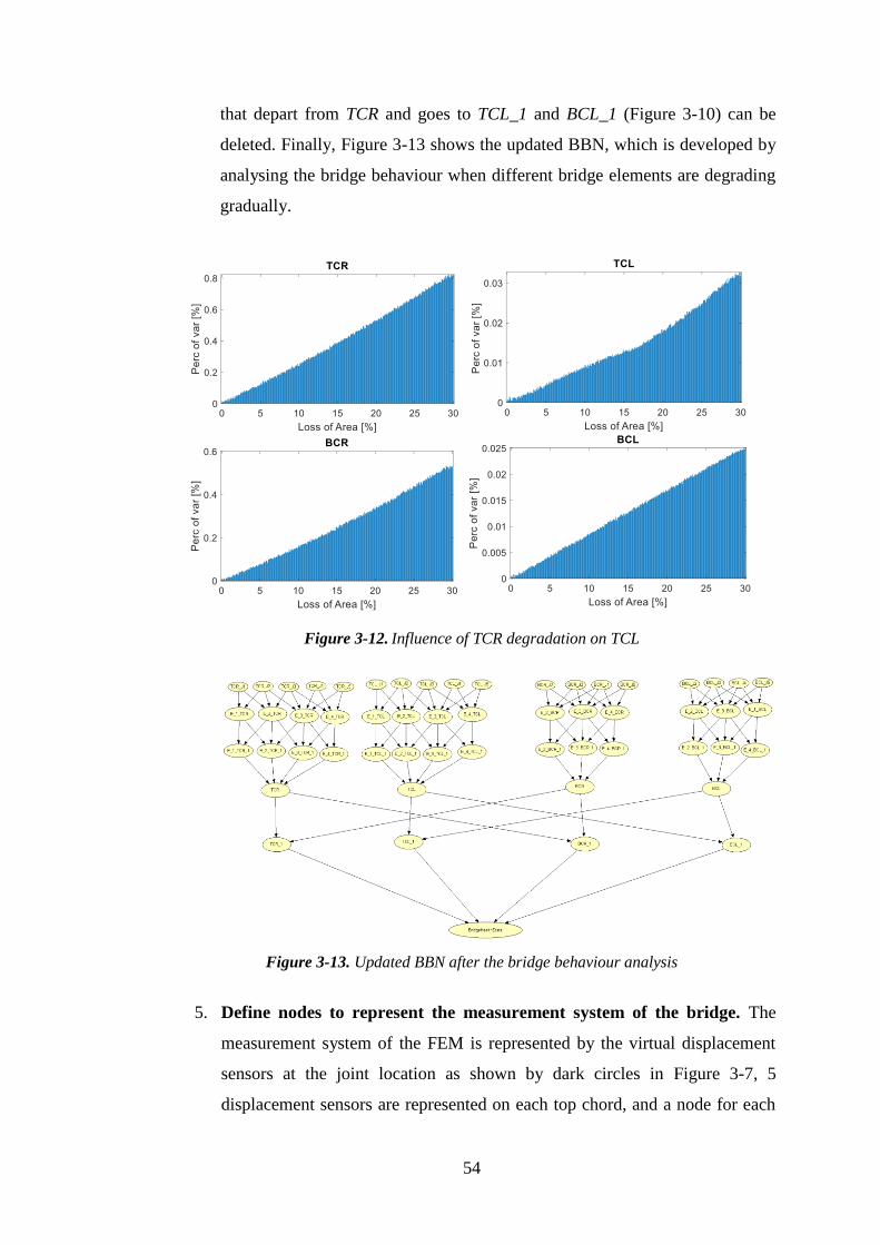
54

that depart from TCR and goes to TCL_1 and BCL_1 (Figure 3-10) can be

deleted. Finally, Figure 3-13 shows the updated BBN, which is developed by

analysing the bridge behaviour when different bridge elements are degrading

gradually.

Figure 3-12. Influence of TCR degradation on TCL

Figure 3-13. Updated BBN after the bridge behaviour analysis

5. Define nodes to represent the measurement system of the bridge. The

measurement system of the FEM is represented by the virtual displacement

sensors at the joint location as shown by dark circles in Figure 3-7, 5

displacement sensors are represented on each top chord, and a node for each

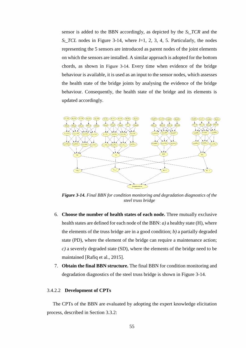
55

sensor is added to the BBN accordingly, as depicted by the Sl_TCR and the

Sl_TCL nodes in Figure 3-14, where l=1, 2, 3, 4, 5. Particularly, the nodes

representing the 5 sensors are introduced as parent nodes of the joint elements

on which the sensors are installed. A similar approach is adopted for the bottom

chords, as shown in Figure 3-14. Every time when evidence of the bridge

behaviour is available, it is used as an input to the sensor nodes, which assesses

the health state of the bridge joints by analysing the evidence of the bridge

behaviour. Consequently, the health state of the bridge and its elements is

updated accordingly.


steel truss bridge

6. Choose the number of health states of each node. Three mutually exclusive

health states are defined for each node of the BBN: a) a healthy state (H), where

the elements of the truss bridge are in a good condition; b) a partially degraded

state (PD), where the element of the bridge can require a maintenance action;

c) a severely degraded state (SD), where the elements of the bridge need to be

maintained [Rafiq et al., 2015].

7. Obtain the final BBN structure. The final BBN for condition monitoring and

degradation diagnostics of the steel truss bridge is shown in Figure 3-14.

3.4.2.2 Development of CPTs

The CPTs of the BBN are evaluated by adopting the expert knowledge elicitation

process, described in Section 3.3.2:

56

a) Identify the experts. Three bridge experts were interviewed: i) Expert 1 is a

principal engineer of an engineering firm with 8 years of experience in SHM;

ii) Expert 2 is a director of an engineering consultancy group with over 28 years

of experience in structural assessment of civil infrastructure; iii) Expert 3 is a

professor of structural engineering in a top ranked UK university, with more

than 25 years of experience in SHM.

b) Identify the degraded scenarios. The experts were interviewed to evaluate 4

scenarios: i) the influence of the degradation of a minor element on the health

state of a neighbouring minor element; ii) the influence of the degradation of a

minor element on the condition of a major element; iii) the influence of the

degradation of a major element on the health state of a different major element;

iv) the influence of the degradation of a major element on the health state of

the whole bridge.

c) Present the scenarios to the experts. The four scenarios are presented to the

experts by the means of questions. Without loss of generality, the influence of

a major element on the condition of the other major elements is hereafter

discussed and analysed, i.e. scenario iii) is investigated using questions to the

experts. For instance, the influence of the top chord on the right hand side on

the health state of other major elements (scenario iii)) can be analysed by the

means of three questions: let us consider a truss steel bridge, shown in Figure

3-7. The bridge can be divided into major elements (top and bottom chords)

and minor elements (such as an individual steel beam).

1. Referring to your expertise, if essential maintenance actions, such as

repair, are required in the top chord on the right-hand side, i.e. the

maintenance cannot be postponed, how likely would the overall condition

of the bottom chord on the same hand side of the bridge be influenced by

the degraded state of the top chord on the right-hand side?


repair, are required in top chord on the right-hand side, i.e. the


of the top chord on the left-hand side of the bridge be influenced by the

degraded state of the top chord on the right-hand side?


repair, are required in the top chord on the right-hand side, i.e. the

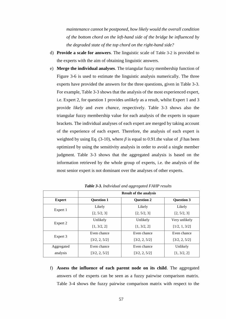
57


of the bottom chord on the left-hand side of the bridge be influenced by

the degraded state of the top chord on the right-hand side?

d) Provide a scale for answers. The linguistic scale of Table 3-2 is provided to

the experts with the aim of obtaining linguistic answers.

e) Merge the individual analyses. The triangular fuzzy membership function of

Figure 3-6 is used to estimate the linguistic analysis numerically. The three

experts have provided the answers for the three questions, given in Table 3-3.

For example, Table 3-3 shows that the analysis of the most experienced expert,

i.e. Expert 2, for question 1 provides unlikely as a result, whilst Expert 1 and 3

provide likely and even chance, respectively. Table 3-3 shows also the

triangular fuzzy membership value for each analysis of the experts in square

brackets. The individual analyses of each expert are merged by taking account

of the experience of each expert. Therefore, the analysis of each expert is

weighted by using Eq. (3-10), where β is equal to 0.91.the value of β has been

optimized by using the sensitivity analysis in order to avoid a single member

judgment. Table 3-3 shows that the aggregated analysis is based on the

information retrieved by the whole group of experts, i.e. the analysis of the

most senior expert is not dominant over the analyses of other experts.

Table 3-3. Individual and aggregated FAHP results

Result of the analysis

Expert Question 1 Question 2 Question 3

Expert 1 Likely

[2, 5/2, 3]

Likely

[2, 5/2, 3]

Likely

[2, 5/2, 3]

Expert 2 Unlikely

[1, 3/2, 2]

Unlikely

[1, 3/2, 2]

Very unlikely

[1/2, 1, 3/2]

Expert 3 Even chance

[3/2, 2, 5/2]

Even chance

[3/2, 2, 5/2]

Even chance

[3/2, 2, 5/2]

Aggregated

analysis

Even chance

[3/2, 2, 5/2]

Even chance

[3/2, 2, 5/2]

Unlikely

[1, 3/2, 2]

f) Assess the influence of each parent node on its child. The aggregated

answers of the experts can be seen as a fuzzy pairwise comparison matrix.

Table 3-4 shows the fuzzy pairwise comparison matrix with respect to the

58

influences among the major elements of the bridge. The FAHP is then used to

evaluate the weight of a major element on the health state of other major

elements of the bridge. The fuzzy synthetic extend (Eq. (3-11)), which was

computed by using Eq. (3-12) for the first term of Eq. (3-11) and the modified

Chang extend for the second term [Wang et al., 2006; Kabir et al., 2014], of

TCR is equal to:

( ) ( ) ( )0.333 0.300, 0.222,0.055 0.060, 0.055,6,5,4 =TCR

S (3-19)

The integral value of each synthetic extend is computed by using Eq. (7). The

integral value for the TCR is equal to:

( )( ) 2889.00.22210.300 333.02

1=−++=

TCRI (3-20)

where α= 0.5.

Finally, the weight of each major element on the health state of another major

element is obtained by applying Eq. (3-14), and thus

( )Tw 0.200 0.2497, 0.2497, 0.3007,= .

Table 3-4. Pairwise comparison matrix with respect to the influences among the bridge

major elements TCR TCL BCR BCL

TCR [1, 1, 1] [1, 3/2, 2] [1, 1, 1] [1, 3/2, 2]

TCL [1/2, 2/3, 1] [1,1,1] [1, 3/2, 2] [1, 1, 1]

BCR [1,1,1] [1/2, 2/3, 1] [1, 1, 1] [1, 3/2, 2]

BCL [1/2, 2/3, 1] [1, 1, 1] [1/2, 2/3, 1] [1, 1, 1]

g) Assess the consistency of the expert analysis. The consistency of the expert

analysis is verified by evaluating the CR. For the comparison matrix of Table

3-4, the CR index is equal to:

0.030.9000

1

3

4-4.0837===

RI

CICR (3-21)

where max = 4.0837 is retrieved by using the maximum centroid of area

method to defuzzify the pairwise matrix. RI is equal to 0.9 and is obtained by

59

using a table from literature [Kabir et al., 2014]. Eq. (3-21) shows a CR ratio

lower than 0.1, and thus the analysis of the experts is consistent.

h) Compute the conditional probabilities for the bridge element nodes. The

first step is to define the conditional probability that the condition of a child

node of the BBN is influenced by knowledge of the health state of its parents,

1

( 1)N

ki k

k

P x Y y=

= = , with i = H, PD, SD. This means that the probability of

having a child node in a state i, conditional on the knowledge that its parent

nodes are in the healthy state (no degradation is present). In this thesis, we

assume that the health state of each node of the BBN when no degradation is

present is equal to 1

( 1)N

ki k

k

P x Y y=

= = =[ 95.0)1(1

====

k

kN

k

H yYxP ,

025.0)1(1

====

k

kN

k

PD yYxP , 025.0)1(1

====

k

kN

k

SD yYxP ]. For example, the CPTs of

the TCR_1 node of the BBN is shown in Table 3-5. The states of the node

TCR_1 are influenced by two parent nodes, the TCR and BCR nodes, as shown

in Figure 3-14. Each node is described with 3 health states, and thus the CPT

requires 24 entries )23( 3 . The probability of having TCR_1 in state i,

conditional on the knowledge that both its parents are in the healthy state, is

defined as 1

( _1 1) [ 0.95, 0.025, 0.025]N

ki k

k

P TCR Y y=

= = = . The CPT is then

thoroughly defined by using Eq. (3-17), where ip and

mpf depend on the

health state of the parent nodes k:

=

==

SDkif

PDkifp

T

T

i]75.0,25.0,1[

]3.0,7.0,1[

(3-22)

1

1.1mp

if k H or PDf

if k SD

==

= (3-23)

Eq. (3-22) shows that pi is equal to 1 if TCR_1 is in state i=H, 0.7 if i=PD, etc.

In this way, the decrease of 1

( _1 1)N

ki k

k

P TCR Y y=

= = is shared between the

states PD and SD, and the whole probability is normalized to 1.

60

An example of this process is presented in Eq. (3-24) and Eq. (3-25). The

weight of the parent nodes on the child node is equal to ( )0.2497 0.3007,=w , as

shown in step f). For instance, the bold probabilities of Table 3-5 are computed

by using Eq. (3-17), where the number of degraded parent nodes is equal to 1,

M=1, Eq. (3-24), or 2, M=2, Eq. (3-25), respectively:

( )

( )

( )

=+=

=+=

=−+=

==

==

==

11.00.1107 113.03007.095.0025.0),1_(

25.00.2250 117.03007.095.0025.0),1_(

66.00.6647 1113007.095.095.0),1_(

BCRHk

TCRPDkSD

BCRHk

TCRPDkPD

BCRHk

TCRPDkH

YYTCRP

YYTCRP

YYTCRP

(3-24)

( )

( )

( )

=++=

=++=

=−++=

==

==

==

0.430.4386 175.0)12497.01.13007.0(95.0025.0),1_(

0.160.1629 125.0)12497.01.13007.0(95.0025.0),1_(

0.390.3986 11)12497.01.13007.0(95.095.0),1_(

BCRPDk

TCRSDkSD

BCRPDk

TCRSDkPD

BCRPDk

TCRSDkH

YYTCRP

YYTCRP

YYTCRP

(3-25)

Table 3-5. CPT of a child node with three health states and two parent nodes with 3 health

states each

BCR H PD SD

TCR H PD SD H PD SD H PD SD

TCR_

1

H 0.95 0.66 0.63 0.71 0.42 0.39 0.68 0.40 0.3

PD 0.025 0.22 0.10 0.19 0.39 0.16 0.09 0.16 0.16

SD 0.025 0.11 0.26 0.09 0.18 0.43 0.22 0.43 0.45

BBN model usage for detection and diagnostics of bridge deterioration

The 28 simulated degradation scenarios are presented randomly to the BBN. In this

way, the nature of the scenario is not known a-priori, and the BBN needs to assess the

health state of the bridge. The displacement of the bridge joints is used to monitor the

bridge condition, and thus as an input to the BBN nodes. Three health states of the

bridge are defined, by assessing the percentage of the joint displacement variation

during the degradation process. A bridge manager can interact with the BBN during

the bridge condition monitoring process. As a result, when a change of the condition

of the bridge is identified, the bridge manager can diagnose the causes of such change.

The bottom-up diagnostic process of the BBN can be a one-step process, i.e. the bridge

manager can directly observe the most degraded element of the bridge, or a step by

step process, i.e. the bridge manager diagnoses the cause of the change of the bridge

condition by analysing the health state of each node of the BBN. In this example, this

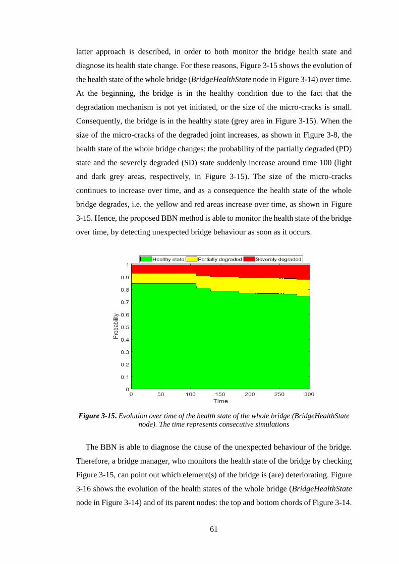
61

latter approach is described, in order to both monitor the bridge health state and

diagnose its health state change. For these reasons, Figure 3-15 shows the evolution of

the health state of the whole bridge (BridgeHealthState node in Figure 3-14) over time.

At the beginning, the bridge is in the healthy condition due to the fact that the

degradation mechanism is not yet initiated, or the size of the micro-cracks is small.

Consequently, the bridge is in the healthy state (grey area in Figure 3-15). When the

size of the micro-cracks of the degraded joint increases, as shown in Figure 3-8, the

health state of the whole bridge changes: the probability of the partially degraded (PD)

state and the severely degraded (SD) state suddenly increase around time 100 (light

and dark grey areas, respectively, in Figure 3-15). The size of the micro-cracks

continues to increase over time, and as a consequence the health state of the whole

bridge degrades, i.e. the yellow and red areas increase over time, as shown in Figure

3-15. Hence, the proposed BBN method is able to monitor the health state of the bridge

over time, by detecting unexpected bridge behaviour as soon as it occurs.

Figure 3-15. Evolution over time of the health state of the whole bridge (BridgeHealthState

node). The time represents consecutive simulations

The BBN is able to diagnose the cause of the unexpected behaviour of the bridge.

Therefore, a bridge manager, who monitors the health state of the bridge by checking

Figure 3-15, can point out which element(s) of the bridge is (are) deteriorating. Figure

3-16 shows the evolution of the health states of the whole bridge (BridgeHealthState

node in Figure 3-14) and of its parent nodes: the top and bottom chords of Figure 3-14.

62

Figure 3-16 allows to identify directly that the top chord on the right-hand side of the

bridge (TCR_1) is more degraded than the other major elements, i.e. the light and dark

grey areas of TCR_1 are higher than those of the other chords.

Figure 3-16. Evolution over time of the health state of the whole bridge (BridgeHealthState

node) and its parent nodes, i.e. the top and bottom chords nodes

The diagnostic property of the BBN allows to investigate the degradation level of

the bridge elements at each level of the BBN. For example, Figure 3-17 shows the

evolution of the health state of the TCR_1 node and its parent nodes, which are the top

and bottom chord on the right-hand side of the bridge, TCR and BCR node in Figure

3-14, respectively. Figure 3-17 depicts that the top chord on the left-hand side of the

bridge is more degraded than the right one. The cause of the decrease of the bridge

health state can be thus identified among the elements of the top chord on the right-

hand side of the bridge. The probability of each parent node of the top chord on the

right-hand side of the bridge can be then observed and analysed by the bridge manager,

with the aim of pointing out the most degraded element of the chord. Figure 3-18

shows the evolution of the health state probabilities of the most degraded element of

the top chord, i.e. the joint between the third and fourth elements of the top chord on

the right-hand side of the bridge. Therefore, the element of the bridge that was

degrading is identified correctly, due to the fact that the degradation of the joint

between the third and fourth elements of the top chord on the right-hand side of the

bridge was simulated using the FEM. The oscillations of the conditional probability of

the health states of the most degraded element in Figure 3-18 are due to the added

noise of the data. It should be noted that the proposed approach allows the bridge

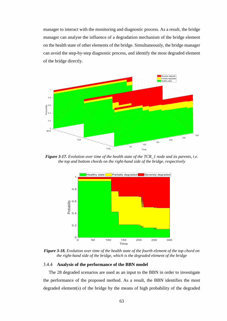
63

manager to interact with the monitoring and diagnostic process. As a result, the bridge

manager can analyse the influence of a degradation mechanism of the bridge element

on the health state of other elements of the bridge. Simultaneously, the bridge manager

can avoid the step-by-step diagnostic process, and identify the most degraded element

of the bridge directly.

Figure 3-17. Evolution over time of the health state of the TCR_1 node and its parents, i.e.

the top and bottom chords on the right-hand side of the bridge, respectively

Figure 3-18. Evolution over time of the health state of the fourth element of the top chord on

the right-hand side of the bridge, which is the degraded element of the bridge

Analysis of the performance of the BBN model

The 28 degraded scenarios are used as an input to the BBN in order to investigate

the performance of the proposed method. As a result, the BBN identifies the most

degraded element(s) of the bridge by the means of high probability of the degraded

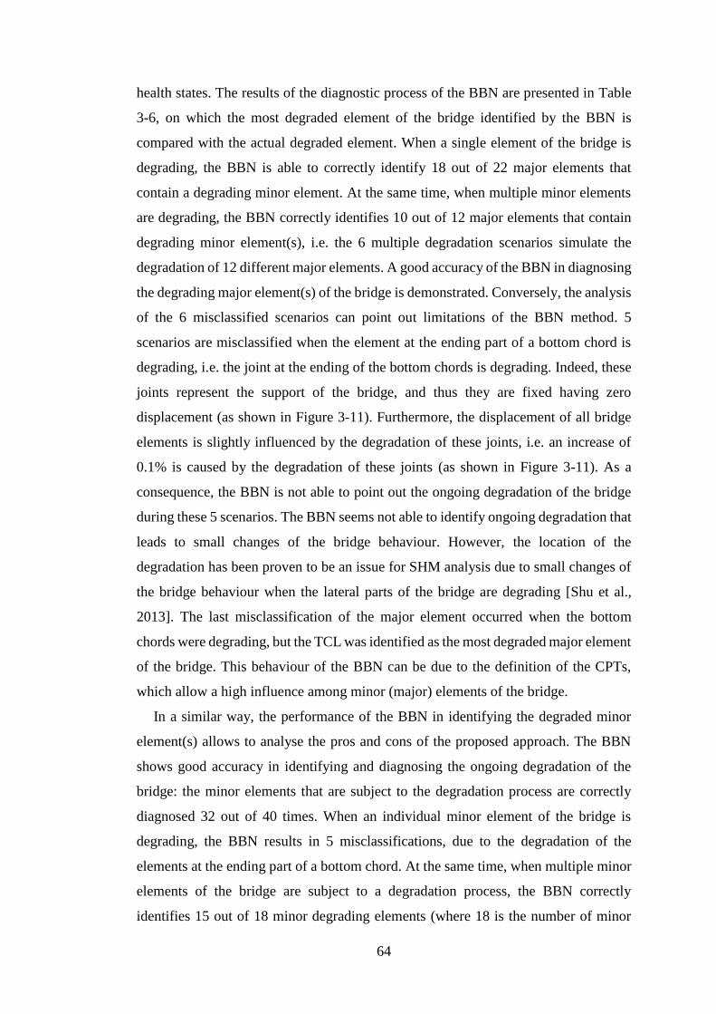
64

health states. The results of the diagnostic process of the BBN are presented in Table

3-6, on which the most degraded element of the bridge identified by the BBN is

compared with the actual degraded element. When a single element of the bridge is

degrading, the BBN is able to correctly identify 18 out of 22 major elements that

contain a degrading minor element. At the same time, when multiple minor elements

are degrading, the BBN correctly identifies 10 out of 12 major elements that contain

degrading minor element(s), i.e. the 6 multiple degradation scenarios simulate the

degradation of 12 different major elements. A good accuracy of the BBN in diagnosing

the degrading major element(s) of the bridge is demonstrated. Conversely, the analysis

of the 6 misclassified scenarios can point out limitations of the BBN method. 5

scenarios are misclassified when the element at the ending part of a bottom chord is

degrading, i.e. the joint at the ending of the bottom chords is degrading. Indeed, these

joints represent the support of the bridge, and thus they are fixed having zero

displacement (as shown in Figure 3-11). Furthermore, the displacement of all bridge

elements is slightly influenced by the degradation of these joints, i.e. an increase of

0.1% is caused by the degradation of these joints (as shown in Figure 3-11). As a

consequence, the BBN is not able to point out the ongoing degradation of the bridge

during these 5 scenarios. The BBN seems not able to identify ongoing degradation that

leads to small changes of the bridge behaviour. However, the location of the

degradation has been proven to be an issue for SHM analysis due to small changes of

the bridge behaviour when the lateral parts of the bridge are degrading [Shu et al.,

2013]. The last misclassification of the major element occurred when the bottom

chords were degrading, but the TCL was identified as the most degraded major element

of the bridge. This behaviour of the BBN can be due to the definition of the CPTs,

which allow a high influence among minor (major) elements of the bridge.

In a similar way, the performance of the BBN in identifying the degraded minor

element(s) allows to analyse the pros and cons of the proposed approach. The BBN

shows good accuracy in identifying and diagnosing the ongoing degradation of the

bridge: the minor elements that are subject to the degradation process are correctly

diagnosed 32 out of 40 times. When an individual minor element of the bridge is

degrading, the BBN results in 5 misclassifications, due to the degradation of the

elements at the ending part of a bottom chord. At the same time, when multiple minor

elements of the bridge are subject to a degradation process, the BBN correctly

identifies 15 out of 18 minor degrading elements (where 18 is the number of minor

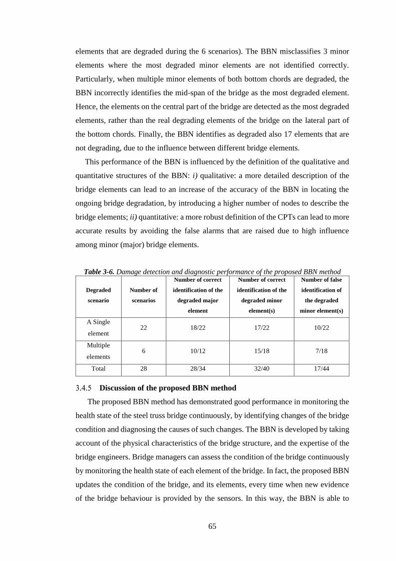
65

elements that are degraded during the 6 scenarios). The BBN misclassifies 3 minor

elements where the most degraded minor elements are not identified correctly.

Particularly, when multiple minor elements of both bottom chords are degraded, the

BBN incorrectly identifies the mid-span of the bridge as the most degraded element.

Hence, the elements on the central part of the bridge are detected as the most degraded

elements, rather than the real degrading elements of the bridge on the lateral part of

the bottom chords. Finally, the BBN identifies as degraded also 17 elements that are

not degrading, due to the influence between different bridge elements.

This performance of the BBN is influenced by the definition of the qualitative and

quantitative structures of the BBN: i) qualitative: a more detailed description of the

bridge elements can lead to an increase of the accuracy of the BBN in locating the

ongoing bridge degradation, by introducing a higher number of nodes to describe the

bridge elements; ii) quantitative: a more robust definition of the CPTs can lead to more

accurate results by avoiding the false alarms that are raised due to high influence

among minor (major) bridge elements.

Table 3-6. Damage detection and diagnostic performance of the proposed BBN method

Degraded

scenario

Number of

scenarios

Number of correct

identification of the

degraded major

element

Number of correct

identification of the

degraded minor

element(s)

Number of false

identification of

the degraded

minor element(s)

A Single

element 22 18/22 17/22 10/22

Multiple

elements 6 10/12 15/18 7/18

Total 28 28/34 32/40 17/44

Discussion of the proposed BBN method

The proposed BBN method has demonstrated good performance in monitoring the

health state of the steel truss bridge continuously, by identifying changes of the bridge

condition and diagnosing the causes of such changes. The BBN is developed by taking

account of the physical characteristics of the bridge structure, and the expertise of the

bridge engineers. Bridge managers can assess the condition of the bridge continuously

by monitoring the health state of each element of the bridge. In fact, the proposed BBN

updates the condition of the bridge, and its elements, every time when new evidence

of the bridge behaviour is provided by the sensors. In this way, the BBN is able to

66

detect and diagnose unexpected behaviour of the bridge as soon as it occurs. However,

some drawbacks have been found:

1. The FEM of the steel truss bridge has been developed with the aim of testing

and stressing the BBN ability of monitoring a bridge under ongoing

degradation mechanisms. As a result, assumptions have been made during the

development of the FEM: i) only a static uniform load has been applied to the

FEM; ii) fixed environmental conditions; iii) the traffic is not present, and thus

interactions between the bridge and the vehicles that are passing over the bridge

are neglected. Therefore, the good performance of the BBN might not be

guaranteed in a more complex case study, where the bridge is subject to traffic,

for example. Traffic and changing environmental conditions can lead to a noisy

response of the bridge, due to different vehicles that run over the bridge, and

thus misclassifications of the bridge health state might be obtained. The effects

of traffic and changing environmental conditions on the performance of the

proposed BBN approach are investigated in the next section, by analysing an

FEM that is excited by moving vehicles rather than static loads.

2. The accuracy of the BBN damage detection process decreased when the

degradation of the bridge elements led to small changes of the bridge

displacements. As a consequence, the BBN was not able to detect small

changes of the bridge behaviour. The behaviour of a real in-field bridge is

expected to experience small changes when a degradation mechanism is

ongoing on some bridge elements. Therefore, the BBN should be able to detect

small changes of the bridge behaviour, which may be hidden by the noise of

the data, in order to accurately assess the health state of the bridge. A pre-

processing analysis of the bridge behaviour can tackle this problem, by

providing crisp information about the bridge behaviour to the BBN.

3. The diagnostics performance of the BBN seems to depend on the number of

nodes that are used to describe the bridge elements of interest, i.e. the higher

the number of nodes of the BBN, the higher the accuracy of the BBN in

identifying the degraded element(s) of the bridge. In fact, the discussion of the

performance of the BBN in section 3.4.4 has shown that when the number of

degraded elements of the bridge increases, the BBN identifies the central

elements of the bridge as degraded. These issues can be resolved by

introducing more nodes, i.e. by describing each element of the bridge with

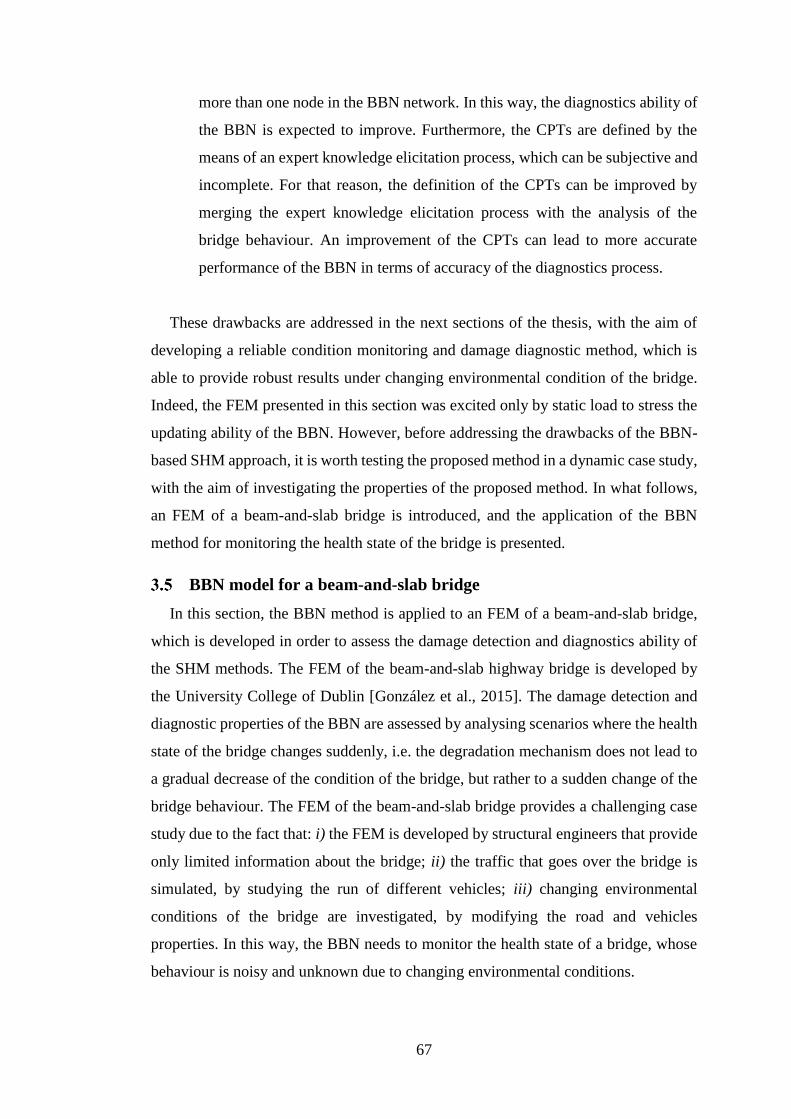
67

more than one node in the BBN network. In this way, the diagnostics ability of

the BBN is expected to improve. Furthermore, the CPTs are defined by the

means of an expert knowledge elicitation process, which can be subjective and

incomplete. For that reason, the definition of the CPTs can be improved by

merging the expert knowledge elicitation process with the analysis of the

bridge behaviour. An improvement of the CPTs can lead to more accurate

performance of the BBN in terms of accuracy of the diagnostics process.

These drawbacks are addressed in the next sections of the thesis, with the aim of

developing a reliable condition monitoring and damage diagnostic method, which is

able to provide robust results under changing environmental condition of the bridge.

Indeed, the FEM presented in this section was excited only by static load to stress the

updating ability of the BBN. However, before addressing the drawbacks of the BBN-

based SHM approach, it is worth testing the proposed method in a dynamic case study,

with the aim of investigating the properties of the proposed method. In what follows,

an FEM of a beam-and-slab bridge is introduced, and the application of the BBN

method for monitoring the health state of the bridge is presented.

BBN model for a beam-and-slab bridge

In this section, the BBN method is applied to an FEM of a beam-and-slab bridge,

which is developed in order to assess the damage detection and diagnostics ability of

the SHM methods. The FEM of the beam-and-slab highway bridge is developed by

the University College of Dublin [González et al., 2015]. The damage detection and

diagnostic properties of the BBN are assessed by analysing scenarios where the health

state of the bridge changes suddenly, i.e. the degradation mechanism does not lead to

a gradual decrease of the condition of the bridge, but rather to a sudden change of the

bridge behaviour. The FEM of the beam-and-slab bridge provides a challenging case

study due to the fact that: i) the FEM is developed by structural engineers that provide

only limited information about the bridge; ii) the traffic that goes over the bridge is

simulated, by studying the run of different vehicles; iii) changing environmental

conditions of the bridge are investigated, by modifying the road and vehicles

properties. In this way, the BBN needs to monitor the health state of a bridge, whose

behaviour is noisy and unknown due to changing environmental conditions.

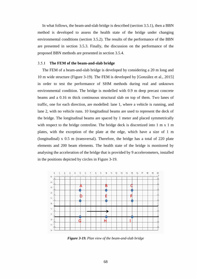
68

In what follows, the beam-and-slab bridge is described (section 3.5.1), then a BBN

method is developed to assess the health state of the bridge under changing

environmental conditions (section 3.5.2). The results of the performance of the BBN

are presented in section 3.5.3. Finally, the discussion on the performance of the

proposed BBN methods are presented in section 3.5.4.

The FEM of the beam-and-slab bridge

The FEM of a beam-and-slab bridge is developed by considering a 20 m long and

10 m wide structure (Figure 3-19). The FEM is developed by [González et al., 2015]

in order to test the performance of SHM methods during real and unknown

environmental condition. The bridge is modelled with 0.9 m deep precast concrete

beams and a 0.16 m thick continuous structural slab on top of them. Two lanes of

traffic, one for each direction, are modelled: lane 1, where a vehicle is running, and

lane 2, with no vehicle runs. 10 longitudinal beams are used to represent the deck of

the bridge. The longitudinal beams are spaced by 1 meter and placed symmetrically

with respect to the bridge centreline. The bridge deck is discretized into 1 m x 1 m

plates, with the exception of the plate at the edge, which have a size of 1 m

(longitudinal) x 0.5 m (transversal). Therefore, the bridge has a total of 220 plate

elements and 200 beam elements. The health state of the bridge is monitored by

analysing the acceleration of the bridge that is provided by 9 accelerometers, installed

in the positions depicted by circles in Figure 3-19.

Figure 3-19. Plan view of the beam-and-slab bridge

69

3.5.1.1 The model of the vehicle

A model of a typical European 5-axle articulated truck is modelled in order to

simulate the traffic over the bridge. The length of the truck is assumed to be 14.9 m,

and the direction of the truck is assumed to be from left to right, with inner and outer

wheels located along the path at 0.5 m and 2.5 m, respectively, from bridge centreline,

as shown in Figure 3-19 [González et al., 2015]. A single tyre is assumed for the 1st

axle while two tyres are considered for other axles. The distances between the

consecutive axles is 3.6, 6.33, 1.31 and 1.31 m, respectively. The transverse distance

between two wheels of an axle is 2 m. Two different Gross Vehicle Weights (GVWs)

are tested: i) a fully-loaded condition, where the GVW is equal to 40 tons (truck A);

ii) a half-loaded condition, where the GVW is 25 tons (truck B).

3.5.1.2 Degradation mechanism

The degradation of the bridge is modelled as a sudden loss of stiffness at selected

beam elements. The location and magnitude of the simulated damages of the bridge is

presented in Table 3-7. The damage location in Table 3-7 corresponds to the distance

from the first support of the bridge on the left-hand side. The loss of stiffness extends

1.5 m longitudinally at both sides of the location shown in Table 3-7, and its width is

given in Table 3-7. The percentage of loss of stiffness in Table 3-7 represents the loss

of stiffness of the entire damaged area of the bridge. The 16 damage scenarios illustrate

that the change of the bridge behaviour can be caused by: i) loss of stiffness of bridge

element(s); ii) changes of the road roughness, i.e. the bridge is in a healthy condition,

but the roughness of the road is changed, as shown by the road type column in Table

3-7; iii) changes of the vehicle properties (such as dynamic properties, speed, mass),

i.e. the bridge is in the good condition, but the properties of the vehicles are changed,

as shown by the vehicle type column in Table 3-7. Therefore, the BBN needs to be

able to manage these different environmental conditions in order to assess the

condition of the bridge correctly, by detecting and diagnosing its damaged health

states.

70

Table 3-7. Degraded scenarios of the beam-and-slab bridge

Test

number

Vehicle

speed

Vehicle

type

Road

type

Damage

location

(m)

Damage

width

(m)

Damage

severity

(%)

Damaged

lane

1 20 A 2 15 5 8 2

2 30 B 3 Healthy Healthy Healthy Healthy

3 30 A* 1 5 5 6 2

4 20 B* 2 Healthy Healthy Healthy Healthy

5 20 A 1 12.5 5 8 1

6 30 B 1 2.5 5 12.1 1

7 30 A 1 10 5 10 2

8 20 B 1 10 5 6 2

9 20 A 1 7.5 5 12.1 1

10 30 B 1 13.3 10 16 1, 2

11 22.5 A 1 6.6 10 20.1 1, 2

12 27.5 B 1 6.6 5 10 1

13 30 A 1 12.5 5 8 2

14 20 B 1 12.5 10 16 1, 2

15 20 A 1 6.6 10 11.9 1, 2

15 5 12.1 1

16 30 B 1 7.5 10 24.2 1, 2

13.3 5 8 2

*The dynamic properties of the vehicle are modified in test 3 and 4 by modifying the values

of the stiffness of the suspensions.

The BBN of the beam-and-slab bridge

The BBN is developed by following the methodology described in section 3.3. The

aim of this section is to analyse the performance of the proposed method, and thus the

step-by-step process that leads to the development of the BBN is briefly described in

section 3.5.2.1 (BBN structure) and section 3.5.2.2 (CPTs of the BBN), whereas the

performance of the BBN is analysed in detail in section 3.5.3.

3.5.2.1 The structure of the BBN

The step-by-step process presented in section 3.3.1 is adopted in order to develop

the structure of the BBN to assess the health state of the beam-and-slab bridge. Major

and minor elements of the beam-and-slab bridge are identified as follows: each

longitudinal beam is identified as a major element of the bridge, whereas two

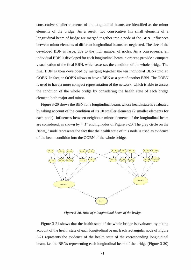
71

consecutive smaller elements of the longitudinal beams are identified as the minor

elements of the bridge. As a result, two consecutive 1m small elements of a

longitudinal beam of bridge are merged together into a node of the BBN. Influences

between minor elements of different longitudinal beams are neglected. The size of the

developed BBN is large, due to the high number of nodes. As a consequence, an

individual BBN is developed for each longitudinal beam in order to provide a compact

visualization of the final BBN, which assesses the condition of the whole bridge. The

final BBN is then developed by merging together the ten individual BBNs into an

OOBN. In fact, an OOBN allows to have a BBN as a part of another BBN. The OOBN

is used to have a more compact representation of the network, which is able to assess

the condition of the whole bridge by considering the health state of each bridge

element, both major and minor.

Figure 3-20 shows the BBN for a longitudinal beam, whose health state is evaluated

by taking account of the condition of its 10 smaller elements (2 smaller elements for

each node). Influences between neighbour minor elements of the longitudinal beam

are considered, as shown by “_1” ending nodes of Figure 3-20. The grey circle on the

Beam_1 node represents the fact that the health state of this node is used as evidence

of the beam condition into the OOBN of the whole bridge.

Figure 3-20. BBN of a longitudinal beam of the bridge

Figure 3-21 shows that the health state of the whole bridge is evaluated by taking

account of the health state of each longitudinal beam. Each rectangular node of Figure

3-21 represents the evidence of the health state of the corresponding longitudinal

beam, i.e. the BBNs representing each longitudinal beam of the bridge (Figure 3-20)

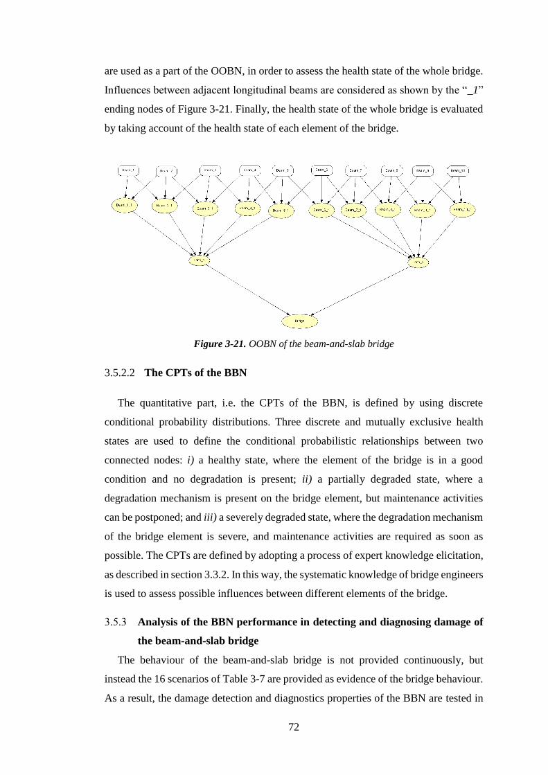
72

are used as a part of the OOBN, in order to assess the health state of the whole bridge.

Influences between adjacent longitudinal beams are considered as shown by the “_1”

ending nodes of Figure 3-21. Finally, the health state of the whole bridge is evaluated

by taking account of the health state of each element of the bridge.

Figure 3-21. OOBN of the beam-and-slab bridge

3.5.2.2 The CPTs of the BBN

The quantitative part, i.e. the CPTs of the BBN, is defined by using discrete

conditional probability distributions. Three discrete and mutually exclusive health

states are used to define the conditional probabilistic relationships between two

connected nodes: i) a healthy state, where the element of the bridge is in a good

condition and no degradation is present; ii) a partially degraded state, where a

degradation mechanism is present on the bridge element, but maintenance activities

can be postponed; and iii) a severely degraded state, where the degradation mechanism

of the bridge element is severe, and maintenance activities are required as soon as

possible. The CPTs are defined by adopting a process of expert knowledge elicitation,

as described in section 3.3.2. In this way, the systematic knowledge of bridge engineers

is used to assess possible influences between different elements of the bridge.

Analysis of the BBN performance in detecting and diagnosing damage of

the beam-and-slab bridge

The behaviour of the beam-and-slab bridge is not provided continuously, but

instead the 16 scenarios of Table 3-7 are provided as evidence of the bridge behaviour.

As a result, the damage detection and diagnostics properties of the BBN are tested in

73

this case study. A Damage Potential Indicator (DPI) is assessed from each sensor of

the bridge, i.e. every time when a new evidence of the acceleration of the bridge is

available, the DPI is assessed. The DPI is then used as an input to the BBN in order to

assess the health state of the bridge. The DPI is a vibration-based index that takes

account of the frequency content of the bridge acceleration in the time interval t, and

of the bridge vibration energy [Moughty & Casas, 2017]. The DPI is assessed as

follows:

2

0

2

0

( )2

t

pi

a t dtg

D

=

(3-26)

where a(t) is the acceleration of the bridge in the time interval t, g is equal to the gravity

constant and2

0 represents the number of zero crossings per unit of time of the bridge

acceleration. The bridge response frequency and energy absorption are represented by

the DPI.

The performance of the BBN in analysing the 16 test scenarios of the bridge

behaviour are presented in Table 3-8. It is shown that in most cases the BBN is able to

detect and diagnose damages of the bridge correctly. However, two false alarms are

raised by the BBN, as shown by test 2 and 4 in Table 3-8: tests 2 and 4 simulate a

change of the environmental condition of the bridge (road roughness and dynamic

properties of the vehicle), but the BBN assigns such changes to the change in the health

state of the bridge. The lane where the loss of stiffness occurred is correctly identified

in 13 out of 14 remaining damaged test scenarios. The lane is identified correctly

partially in Test 16: the BBN is able to correctly identify the damage from 5m to 7m

that extends over the complete width of the bridge, whereas the loss of stiffness of lane

2 at 11.5m is not identified. The longitudinal damaged elements of the bridge are

correctly identified on average, but, in some test scenarios healthy elements of the

bridge, which are close to the damaged ones, are identified as damaged by the BBN.

For example, the transversal extension of the damage of Test 9 is correctly identified,

as well as the longitudinal extension from 6.5m to 9m. However, the healthy

longitudinal elements from 5.5m to 6.5 and from 9m to 12m are also identified as

damaged by the BBN. This behaviour of the BBN can be caused by the definition of

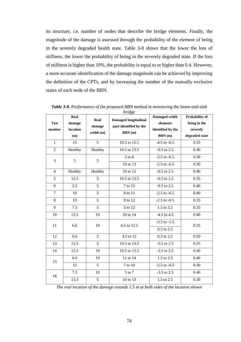
74

its structure, i.e. number of nodes that describe the bridge elements. Finally, the

magnitude of the damage is assessed through the probability of the element of being

in the severely degraded health state. Table 3-8 shows that the lower the loss of

stiffness, the lower the probability of being in the severely degraded state. If the loss

of stiffness is higher than 10%, the probability is equal to or higher than 0.4. However,

a more accurate identification of the damage magnitude can be achieved by improving

the definition of the CPTs, and by increasing the number of the mutually exclusive

states of each node of the BBN.

Table 3-8. Performance of the proposed BBN method in monitoring the beam-and-slab

bridge

Test

number

Real

damage

location

(m)

Real

damage

width (m)

Damaged longitudinal

part identified by the

BBN (m)

Damaged width

elements

identified by the

BBN (m)

Probability of

being in the

severely

degraded state

1 15 5 10.5 to 15.5 -4.5 to -0.5 0.35

2 Healthy Healthy 10.5 to 13.5 -0.5 to 2.5 0.40

3 5 5 3 to 6 -2.5 to -0.5 0.30

10 to 13 -2.5 to -0.5 0.30

4 Healthy Healthy 10 to 12 -0.5 to 2.5 0.40

5 12.5 5 10.5 to 13.5 -0.5 to 2.5 0.35

6 2.5 5 7 to 15 -0.5 to 2.5 0.40

7 10 5 8 to 11 -2.5 to -0.5 0.40

8 10 5 9 to 12 -2.5 to -0.5 0.35

9 7.5 5 5 to 12 1.5 to 3.5 0.35

10 13.3 10 10 to 14 -4.5 to 4.5 0.40

11 6.6 10 4.5 to 12.5 -3.5 to -1.5

0.35 0.5 to 2.5

12 6.6 5 4.5 to 12 0.5 to 2.5 0.50

13 12.5 5 10.5 to 13.5 -3.5 to 2.5 0.35

14 12.5 10 10.5 to 13.5 -3.5 to 2.5 0.40

15 6.6 10 11 to 14 1.5 to 2.5 0.40

15 5 7 to 10 -2.5 to -0.5 0.30

16 7.5 10 5 to 7 -3.5 to 2.5 0.40

13.3 5 10 to 13 1.5 to 2.5 0.30

The real location of the damage extends 1.5 m at both sides of the location shown

75

Discussion of the proposed BBN method for the beam-and-slab bridge

The proposed BBN method has shown good performance in analysing the beam-

and-slab bridge, which consisted in challenging and realistic damaged scenarios. In

fact, the health state of the bridge was modified at the same time with changes of the

environmental conditions of the bridge. Therefore, a change of the bridge behaviour

can be caused either by a damage or (and) by a change of the environmental conditions.

However, the method has confirmed the drawbacks identified in section 3.4.5:

1. False alarms have been activated when the environmental conditions of the bridge

changed. A pre-processing analysis of the bridge behaviour would improve the

performance of the BBN analysis by allowing to analyse only the structural

behaviour of the bridge. In this way, the proposed BBN-based SHM method can

assess the health state of the bridge under changing environmental conditions.

2. The accuracy of the damage detection and diagnostic process was inaccurate in

some scenarios. The performance of the BBN can be enhanced by improving the

method for defining the CPTs, e.g. if a database of bridge behaviour, such as bridge

acceleration, displacement, natural frequencies, etc., is available, such data would

help to define the influences between different elements of the bridge more

accurately, and, as a consequence, the diagnostics process of the BBN could be

more accurate. At the same time, a higher number of the discrete mutually

exclusive states, which describe the node of the BBN, can lead to a more accurate

diagnosis of the magnitude of the damage. However, the size of the CPTs increases

with the number of the mutually exclusive health states.

Summary

A BBN-based method for bridge condition monitoring has been presented in this

chapter. The BBN model is composed of two parts: i) a structural part, which is defined

by analysing the structure of the bridge, represents the connection between the

different elements of the bridge; ii) a quantitative part, which is defined by using an

expert knowledge elicitation process, defines the influences between different

connected elements of the bridge.

The method has been demonstrated to be able to monitor the health state of a bridge

continuously, by updating the health state of the bridge, and its elements, every time

when new evidence of the bridge behaviour becomes available. In this way, when the

76

health state of the bridge changes, the BBN allows to diagnose the causes of such a

change, by pointing out the degrading element(s) of the bridge.

At the same time, the damage detection and diagnostics abilities of the BBN have been

investigated, by analysing damaged scenarios of a bridge. The results of the analysis

have shown that the proposed method allows to accurately detect and diagnose damage

of the bridge structure, however false alarms and misclassification have been detected.

The analysis of the BBN results suggest that its performance can be improved by:

1. Introducing pre-processing of the data with the aim of managing the noise of

the data and taking account of the effects of the changes in the environmental

condition experienced by the bridge.

2. Updating the CPTs by merging together the expert knowledge with the analysis

of the bridge behaviour. In this way, the CPTs of the BBN can be defined in a

more robust way, and, thus, the accuracy of the diagnostics analysis of the BBN

is expected to improve.

3. Introducing a higher number of nodes in order to describe the bridge elements

in a more detailed manner. Similarly, the increase of the number of the

mutually exclusive discrete states, which describe each node of the BBN, can

lead to an improvement of the diagnostics property of the BBN. However, the

increase of both number of nodes and health states would lead to an increase

in the size of the CPTs.

In what follows, these drawbacks are handled by proposing a robust and reliable

BBN-based method for SHM in the further chapters.

77

A data analysis methodology

and a machine learning approach

for processing the data on bridge

behaviour

Introduction

The analysis of the BBN performance in Chapter 3 has shown that pre-processing

of the bridge behaviour is needed to improve the accuracy of the BBN analysis.

Particularly, the data on the behaviour of the bridge needs to be processed to remove

noise of the data, which then can be used to identify the condition of bridge elements.

In this way, the results of the pre-processing data analysis can be used as an input to

the BBN nodes in order to select the condition of the bridge element in a reliable way.

The BBN is then able to update the health state of the bridge by taking account of the

condition of its elements. The pre-processing of the bridge behaviour is of particular

importance when an in-field bridge is analysed, due to the noise and uncertainties that

affect its behaviour.

In this chapter, monitoring data from a post-tensioned concrete in-field bridge is

analysed with the aim of identifying the bridge health state. Consequently, a data

analysis methodology for pre-processing the bridge behaviour is proposed by relying

on a multi-step method that is presented in section 4.2. Since, sensors can provide large

amounts of data, the adoption of machine learning methods in the SHM of

infrastructure is becoming more popular. For this reason, a machine learning approach

is proposed in section 4.5 to achieve an automatic assessment of the health state of the

bridge elements, by the means of a NFC [Cetişli & Barkana, 2010]. The assessment of

the health state of the bridge elements provided by the NFC can be used as an input to

the BBN nodes, in order to update the health state of the whole bridge.

In what follows, the proposed data analysis methodology is introduced in section

4.2, then the methodology is applied to the post-tensioned concrete bridge in section

4.3. The summary of the data analysis methodology is presented in section 4.4. The

NFC machine learning method to automatically identify the health state of the bridge

78

element is presented in section 4.5, whereas the influence of the size of the feature

training set on the performance of the NFC is discussed in section 4.6. The conclusive

discussion of the results is given in section 4.7.

Finally, it is worth noting that the proposed data analysis methodology is also

applied to an in-field steel truss bridge, which is subject to a progressive damage test,

in order to identify and diagnose the health state of the steel truss bridge. In this way,

the proposed data analysis methodology and its performance are verified using a

different in-field bridge, which shows a different behaviour from the post-tensioned

concrete bridge, e.g. the steel truss bridge is excited by a moving vehicle rather than

changing environmental condition. However, only a small amount of data is available

for the steel truss bridge, and thus the NFC cannot be verified for this second case

study. The results of the data analysis methodology of this latter case study are

presented in section 4.8.

The proposed data analysis methodology

Several methods for analysing the raw data of bridge behaviour are presented in

literature, such as clustering techniques, PCA and ANN models [Fan et al., 2011;

Moughty et al., 2017; Vagnoli et al., 2018]. These methods showed promising

performance in identifying the health state of bridge elements, however two main

drawbacks are: a) the methods are often verified by using an FEM, which is unable to

reproduce all the data noise and uncertainties affecting an in-field bridge [Limongelli

et al., 2017]; b) modal parameters of the bridge are usually monitored [Han et al., 2014;

Sadhu, 2017; Khan et al., 2018]. To expand on the second point, modal parameters of

the bridge can be difficult to assess in a fast and reliable manner. In fact, lower modal

parameters of the bridge, i.e. the first natural frequencies and mode shapes, are both

strongly influenced by changes in environmental conditions and usually are of low

sensitivity to bridge infrastructure damage. Higher modal parameters of the bridge are

more sensitive to damage, but more difficult to extract from the measured bridge data

in a reliable manner [Kim et al., 2007; Casas et al., 2017]. For these reasons, in this

thesis a data analysis methodology is proposed to process the bridge behaviour by

removing noise of the data and to identify the health state of bridge elements. The

methodology rely on two main steps: i) extraction of statistical, frequency-based and

vibration-based features from the bridge behaviour, to reduce the dimension of the

bridge behaviour data into valuable information, with respect to the bridge condition

79

[Moughty & Casas, 2017; Lei et al., 2018]; ii) assessment of the features’ trend and of

bridge HIs, by applying the EMD method to the extracted features [Huang et al., 1998].

The main novelty of the proposed data analysis methodology lies on the second step

of the methodology ii). In fact, the EMD is generally adopted in the SHM framework

to identify structural changes by analysing the bridge dynamic behaviour directly, i.e.

the dynamic behaviour of the bridge is used as input to the EMD process [Cahill et al.,

2018; Han et al., 2014]. Such applications have shown good results when an FEM is

analysed [Han et al., 2014; Aied et al., 2016]; conversely, misclassifications of the

bridge health state were observed due to a mode-mixing problem when an in-field

large structure was monitored [Barbosh et al., 2018; Khan et al., 2018]. Variations of

the EMD process, such as Ensemble EMD (EEMD) and Multivariate EMD (MEMD),

can be adopted in order to overcome the mode-mixing problem and achieve good

assessment of the bridge condition [Wu & Huang, 2009; Rehman & Mandic, 2010].

The application of the EEMD and the MEMD to a large bridge structure provides

better results than the EMD, by being able to detect changes of the bridge health state

(but not to diagnose the nature of the occurred damages) and reducing the mode-

mixing problem. However, the EEMD and the MEMD require higher computational

time than the EMD, and the mode-mixing problem is not fully addressed [Sadhu, 2017;

Barbosh et al., 2018]. For these reasons, we adopt the EMD method to assess the trend

of the extracted features, not the raw data, of the bridge behaviour. Indeed, several

studies showed that the trend of statistical, frequency-based and vibration-based

features can provide valuable information with respect to the level of degradation of

components of rotary machinery [Mosallam et al., 2014; Cannarile et al., 2017].

Furthermore, the literature review of Chapter 2 has shown that when the health state

of a bridge has been evaluated by monitoring raw bridge behaviour, or slightly

processed (e.g. transformation of the bridge acceleration to symbolic values based on

a frequentist analysis [Cury et al., 2012]), promising results were obtained in a fast and

reliable way [Langone et al., 2017].

The proposed methodology is developed and optimized by analysing the

acceleration of the bridge, which is provided by accelerometers installed on the bridge

infrastructure. Therefore, if different parameters are monitored, such as displacements

of the bridge, some of the features introduced in the next sections cannot be adopted

due to their nature that aims to analyse bridge vibration only. As a consequence, if

80

different parameters are monitored, the proposed methodology can be still applied to

the bridge, but the set of extracted features needs to be defined accurately.

In what follows, the proposed methodology is presented in section 4.2.1, and each

step of the methodology is discussed in the following sections.

Overview of the methodology

The proposed data analysis methodology is depicted in Figure 4-1. The vibration

behaviour (i.e. acceleration) of the bridge is recorded by a measurement system

(accelerometers) that is installed on the bridge infrastructure. Every time when a new

set of raw bridge acceleration is provided by the sensors, the raw acceleration is pre-

processed with the aim of removing outliers of the data (i.e. the noise) and obtaining

the free vibration behaviour of the bridge. This data allows to assess the condition of

the bridge by avoiding any potential noise from excitation sources [Chang & Kim,

2016; Cao et al., 2017]. A feature extraction process is then developed, to reduce the

dimensionality of the free-vibration bridge behaviour. Indeed, the sensors can provide

thousands of values of the bridge acceleration at each time second, whereas features

can extract relevant information regarding the bridge health state, by merging together

the thousands sensor values into a lumped assessment [Chalouli et al., 2017].

Statistical features (such as mean value, standard deviation, kurtosis, root mean square,

etc.), frequency-domain features (such as peaks and amplitudes of the bridge

frequencies that are obtained by using the Fast Fourier Transform (FFT)) and vibration

parameters (such as peak acceleration, Arias intensity, cumulative absolute velocity,

etc.) are assessed at each τ time step in order to extract information from the free-

vibration behaviour of the bridge [Mosallam et al., 2014; Moughty & Casas, 2017].

The obtained features usually show a high level of oscillations, and a robust and

reliable assessment of the bridge condition can be threatened. A further step of data

processing is introduced in this thesis with the aim of computing the feature trend over

the time interval τ*, by assessing the residuals of the EMD of each extracted feature. A

set of bridge HIs, which provides information with respect to the health state of the

monitored bridge, can then be obtained by calculating statistical parameters (such as

standard deviation and skewness) of the feature trend.

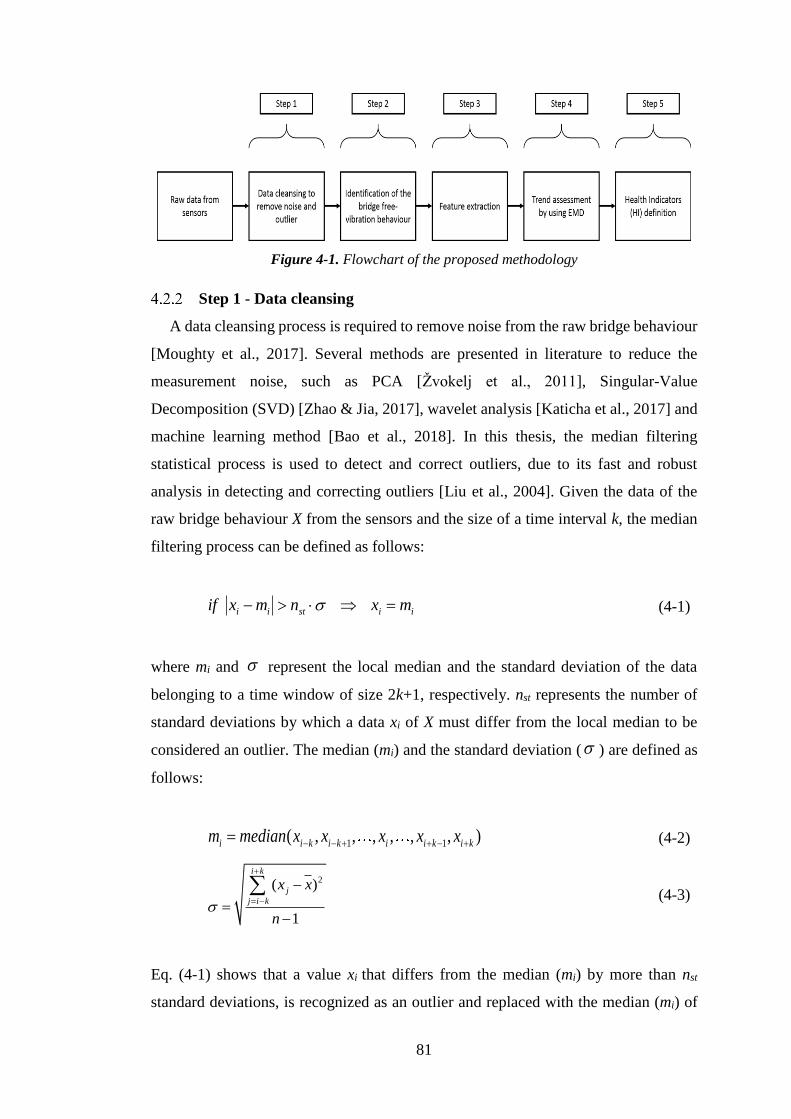
81

Figure 4-1. Flowchart of the proposed methodology

Step 1 - Data cleansing

A data cleansing process is required to remove noise from the raw bridge behaviour

[Moughty et al., 2017]. Several methods are presented in literature to reduce the

measurement noise, such as PCA [Žvokelj et al., 2011], Singular-Value

Decomposition (SVD) [Zhao & Jia, 2017], wavelet analysis [Katicha et al., 2017] and

machine learning method [Bao et al., 2018]. In this thesis, the median filtering

statistical process is used to detect and correct outliers, due to its fast and robust

analysis in detecting and correcting outliers [Liu et al., 2004]. Given the data of the

raw bridge behaviour X from the sensors and the size of a time interval k, the median

filtering process can be defined as follows:

i i st i iif x m n x m− =

(4-1)

where mi and represent the local median and the standard deviation of the data

belonging to a time window of size 2k+1, respectively. nst represents the number of

standard deviations by which a data xi of X must differ from the local median to be

considered an outlier. The median (mi) and the standard deviation ( ) are defined as

follows:

1 1( , , , , , , )i i k i k i i k i km median x x x x x− − + + − +=

(4-2)

2( )

1

i k

j

j i k

x x

n

+

= −

−

=−

(4-3)

Eq. (4-1) shows that a value xi that differs from the median (mi) by more than nst

standard deviations, is recognized as an outlier and replaced with the median (mi) of

82

that time window of size 2k+1. The size of the time interval k is defined by the user

depending on the nature of the considered case study, e.g. the sampling rate of the

sensors influences the definition of k: a higher sampling rate would require a smaller

size of k. Indeed, the higher the number of data points provided by the sensors, the

higher the number of possible outliers that can influence the assessment of the local

median (mi). The number of standard deviations (nst) that defines the acceptable

deviation of a point from the local median is defined by the user according to the

chosen confidence interval.

Step 2 - Identification of the bridge free-vibration behaviour

The free-vibration behaviour of the bridge is analysed with the aim of assessing the

bridge health state, and avoiding any influence of the excitation source, which can lead

to incorrect condition assessment [Chang & Kim, 2016; Cao et al., 2017]. The bridge

free-vibration, which can be defined as the vibration of the bridge that decays in an

approximately exponential form following an external excitation, can be extracted

from the vibration data by analysing the available information: i) if a bridge is excited

by a moving vehicle, the free-vibration behaviour can be identified by knowing when

the vehicle leaves the bridge [Chang & Kim, 2016]; ii) if the bridge is excited by

changing environmental condition, such as wind, the free-vibration behaviour of the

bridge can be identified as the decreasing bridge vibration behaviour that follows a

peak value of the bridge vibration behaviour [Cunha et al., 2001]. This second

approach can also be used when information about moving vehicles is not available.

Step 3 - Feature extraction

Large data storage capacity and high computational power are required to

efficiently store and analyse the data provided by the sensors: each sensor provides N

values of the bridge behaviour for each second, i.e. each sensor has a sampling rate of

N Hz. Conversely, the dimension of the bridge behaviour data can be reduced into

more valuable information, with respect to the bridge health state, by extracting

features from the acceleration data. For this reason, 18 features are extracted from the

free-vibration behaviour of the bridge every τ seconds, by reducing the dimensionality

of the data from N • τ to 18 for each sensor, i.e. every τ seconds the 18 features are

evaluated for each sensor and stored to monitor the evolution of the bridge condition

over time. τ can be defined by optimizing the monotonicity and trendability values of

the features. The features are extracted from both time domain (such as mean value,

83

standard deviation, etc.) and the frequency domain by using an FFT approach (such as

amplitude and peak of the first harmonic). In this way, statistical, frequency-based and

vibration parameters of the bridge are evaluated in order to assess the condition of the

bridge. In fact, changes in statistical and vibration features of the bridge behaviour can

identify a damage of the bridge structure: an increase of the bridge vibration behaviour

can be caused by a reduction of bridge stiffness, which leads to a lower structural

ability in resisting to external excitation in a static and stable manner [Moughty &

Casas, 2017]. Similarly, a change in the frequency-based feature, which estimates

modal and vibration characteristics of the bridge, can represent changes in bridge

physical characteristics, such as stiffness, mass, etc. [Han et al., 2014; Khan et al.,

2018]. The 18 features are chosen due to their ability in describing the health state of

a system during different system health states [Mosallam et al., 2014; Moughty &

Casas, 2017].

The 18 features are defined as follows:

1. Mean value (statistical) is the mean value of the bridge acceleration in the

interval τ;

2. Standard deviation (statistical) represents how much the bridge acceleration

in the interval τ differs from the mean value;

3. Skewness (statistical) measures the asymmetry of the bridge acceleration in

the interval τ;

4. Kurtosis (statistical) measures the shape of the distribution of the bridge

acceleration in the interval τ;

5. Root Mean Square (RMS) (statistical) is the root mean square of the bridge

acceleration in the interval τ;

6. Median (statistical) is the median value of the bridge acceleration in the

interval τ;

7. Coefficient of variation (statistical) is the ratio between the standard deviation

and the mean value of the bridge acceleration in the interval τ;

8. Euclidean Norm (statistical) is the length of the bridge acceleration vector in

the interval τ;

9. Frequency of the first harmonic (frequency-based) represents the frequency

value of the first harmonic of the FFT spectrum, which is obtained by using the

bridge acceleration in the interval τ as input to the FFT algorithm;

84

10. Amplitude of first harmonic (frequency-based) represents the amplitude of

the first harmonic of the FFT spectrum, which is obtained by using the bridge

acceleration in the interval τ as input to the FFT algorithm;

11. Mean period of the bridge behaviour (frequency-based) in the interval τ is

defined as follows:

2

2

1( )

0.25 20i

ii

i

m

i

i

T

Af

for Hz f HzA

=

(4-4)

where iA represents the amplitude values of the discrete frequencies if that

belong to the interval between 0.25Hz and 20Hz. Tm evaluates a weighted

average period of the bridge between 0.25Hz and 20Hz [Rathje et al., 2004].

12. Mean frequency of the bridge behaviour (frequency-based) is the inverse of

the mean period value determined by applying Eq. (4-4);

13. Cumulative velocity of the bridge (vibration) computes the approximate

velocity of the bridge in the interval τ;

14. Peak acceleration (vibration) is the maximum value of the bridge acceleration

in the interval τ;

15. Peak displacement (vibration) is the maximum value of the bridge

displacement in the interval τ, which is estimated by integrating the bridge

acceleration twice;

16. Arias intensity (vibration) represents the cumulative value of the bridge

vibration energy in the interval τ. The Arias intensity index is evaluated as

follows:

2

0

( )2

t

AI a t dtg

= (4-5)

where a(t) is the acceleration of the bridge in the time interval τ and g is equal

to the gravity constant. The Arias intensity has been defined by [Arias, 1970]

in order to describe the potential destructiveness of an earthquake, by assessing

the energy content of the earthquake. Therefore, the Arias intensity of the

bridge represents the energy content of the bridge when the bridge is excited.

85

17. Damage Potential Indicator (DPI) (vibration) is an adaptation of Arias

Intensity, which takes account of the frequency content of the bridge

acceleration in the time interval τ, in addition to the bridge vibration energy

[Moughty & Casas, 2017]:

2

0

2

0

( )2

t

pi

a t dtg

D

=

(4-6)

where 2

0 represents the number of zero crossings per unit of time of the bridge

acceleration. The bridge response frequency and energy absorption are

represented by the Damage Potential Indicator.

18. Cumulative Absolute Velocity (CAV) (vibration) is the sum of all absolute

bridge acceleration values in the interval τ:

2

0( )

t

CAV a t dt= (4-7)

Step 4 - Assessment of the feature trend

The features extracted from the bridge acceleration every τ seconds can show a high

level of oscillations, due to changing response of the bridge and noisy data provided

by the sensor. [Mosallam et al., 2014; Cannarile et al., 2017] have shown that a robust

and reliable assessment of the system health state can be threatened if noisy features

are evaluated. Similarly, the assessment of the bridge health state can be threatened by

evaluating features that show oscillation. Hence, a further step of data processing is

introduced in this thesis by using the features as an input to the EMD process. The

features that are extracted during an interval [0, τ*] are used as an input to the EMD

process to assess their trend. The interval [0, τ*] is chosen to monitor the health state

of the bridge continuously, i.e. the trend of the features is evaluated and updated each

time when τ* new features are extracted from the free-vibration of the bridge. The

value of τ* can be identified by maximizing the monotonicity and trendability values

of the features.

86

The EMD is able to provide a smooth monotonic trend of the features, and as a

consequence, the health state of the bridge can be assessed in a robust way. The EMD

is a data-driven decomposition method that is able to decompose the feature pattern

(F) in the interval τ* into multiple simple harmonics of various frequencies, called

Intrinsic Mode Functions (IMFs) [Huang et al., 1998]. The EMD process can be

applied to any oscillatory and non-stationary time series as follows:

I. Identify all maxima and minima of the feature pattern (F) to be decomposed

in the interval τ*.

II. Connect peaks using a polynomial spline fitting to enhance interpolation.

III. Assess the mean value of both maxima and minima spline envelope.

IV. Subtract the mean of the envelope from the original feature pattern.

V. Perform steps I to IV until the following two criteria are satisfied: i) the

number of extrema and number of zero crossings is either equal or differ at

most by one; ii) a zero-mean of the envelope is obtained. The resulting time-

series is the first IMF, denoted as h1.

VI. Perform steps I to V to the obtained IMFs, known as shifting process, until a

monotonic function remains, or a stopping criterion is reached. This final

time-series is known as residuals (r) which represent the trend of the

decomposed feature pattern.

In this thesis, the shifting process of the EMD is stopped when the difference

between residuals of successive IMFs is lower than a predetermined threshold, which

is set to equal to 0.2 on the Matlab® data processing toolbox.

The EMD decomposition can be represented as shown in Eq. (4-8): the feature pattern,

denoted as F, in the interval τ* is decomposed into multiple IMFs (hi) and a residual

curve (r).

1

M

i

i

F h r=

= + (4-8)

where M is the number of IMFs.

87

Step 5 - Definition and selection of the bridge Health Indicators (HIs)

The trend of the proposed feature provides information about the condition of the

bridge. Such information can be lumped into a set of HIs, which represent the health

state of the bridge by defining a set of parameters. The HIs are defined by evaluating

four statistical parameters of each feature trend: a) the standard deviation of the trend

(HI1), in order to take account of the variability of the feature trend; b) the intercept of

a linear polynomial fitting of the feature trend (HI2), which has demonstrated to be

informative with respect to the heath state of a system [Cannarile et al., 2017]; c) the

normalized cumulative sum of the feature trend (HI3), to take account of the

positive/negative monotonicity of the feature trend; d) the skewness of the feature

trend (HI4), in order to take account of the trend asymmetry. A set of 72 HIs (18 feature

trends and 4 statistical parameters for each trend) is computed each time τ* when a new

assessment of the feature trend is carried out. The HIs are selected to consider the

variability of the features trend, the trend monotonic behaviour over time and the trend

shape. Other HIs can be used to represent other characteristics of the features trend in

a lumped manner. For example, both the trendability and monotonicity, which are

introduced in what follows, can be used directly to monitor the evolution the bridge

health state over time.

Some of the 72 HIs can be non-informative in respect to the health state of the

bridge [Hoell & Omenzetter, 2017]. In a similar way, the value of τ and τ* can

influence the performance of the proposed method, due to the amount of data of the

bridge behaviour that are considered to assess the features and the HIs.

The HI selection process and the optimization of τ and τ* is carried out by

maximizing the HIs trendability and monotonicity. In fact, the trendability (Eq. (4-9)),

which belongs to the interval [-1, 1], represents the correlation between the feature

trend and the time: a feature with constant trend has a zero correlation, whereas a

feature with a trend that linearly increases over time has a strong positive correlation.

The monotonicity (Eq. (4-10)), which belongs to [0, 1], represents the positive or

negative trend of a feature trend: the higher the monotonicity, the higher the monotonic

behaviour of the feature trend, i.e. the feature increases (decreases) as the degradation

of the bridge increases. Both trendability and monotonicity are important in the health

monitoring framework due to the fact that a system is generally unable to repair itself

after that a degradation process is initiated, and thus the HIs should be able to represent

the decreasing condition of the system in a monotonic manner [Duan et al., 2018]:

88

( ) ( )( )

( ) ( )2 2

2 2

n xt x tTrendability

n x x n t t

−=

− −

(4-9)

. 0 . 0

1 1

d dno of no ofdtMonotonicit dt

ny

n

= −

− − (4-10)

where x is the value of the HI, t is the time, n is the length of the available data being

analysed, and . dno ofdt

represents the number of points such that the first derivative

of the HI is positive/negative.

The higher the trendability and monotonicity of a HI, the higher the ability of that

HI in representing the changing health state of the bridge. Hence, we merge these two

metrics into a Goodness Index (GI) that accounts for both trendability and

monotonicity, as shown in Eq. (4-11). The HIs with the highest value of GI are chosen

as the optimal bridge HIs, whilst the values of τ and τ* that allow to maximize the GI

of the HI set are set as optimal values.

GI Trendability Monotonicity= + (4-11)

The health state of the bridge is monitored by assessing the value of the optimal HIs

every τ* time when a new set of feature assessment is available. A set of HIs is adopted

to monitor the health state of the bridge with the aim of tackling the uncertainties that

can affect the assessment of the bridge HIs. Indeed, an HI can provide reliable

information about the health state of the bridge in terms of healthy or damaged bridge

but can be unable to diagnose the nature of the bridge damage. On the contrary, if a

set of optimal HIs is used to monitor the condition of the bridge, each HI can provide

valuable information about the condition of the bridge and the characteristics of its

damage scenarios. Finally, the application of this data analysis methodology within

the BBN approach is expected to improve the performance of each individual method

in terms of both damage detection and diagnostics ability.

In what follows, the proposed method for data processing is applied to a post-

tensioned concrete bridge that is subjected to a progressive damage test, and as a

89

consequence, the ability of the proposed method in monitoring the health state of the

bridge by identifying the health state of the bridge elements is tested.

Application of the proposed data analysis methodology to an in-field

post-tensioned concrete bridge

The performance of the proposed data analysis methodology is verified by assessing

the condition of a post-tensioned concrete bridge [Siringoringo et al., 2013]. The

bridge is subjected to a damage test, i.e. the infrastructure of the bridge is intentionally

damaged in order to study how the bridge behaves in different conditions. The post-

tensioned concrete bridge is excited by changing environmental conditions. The aim

of the proposed method is to monitor the behaviour of the bridge and detect and

diagnose the damaged bridge elements.

Description of the post-tensioned concrete bridge and the progressive

damage test

The post-tensioned concrete bridge has the main span of 32 m, side spans of 12 m,

and its width is 6.6 m (Figure 4-2a). The bridge was subject to a vibration measurement

test before being demolished in order to obtain the bridge behaviour in different health

states. The acceleration of the bridge was monitored by a measurement system made

of 2 reference sensors, and 4 sensors that were moved periodically along the bridge

length to obtain a complete modal description of the bridge. In this thesis, we consider

the acceleration provided by the 2 reference sensors, which were kept fixed throughout

the duration of the test that allows a robust calibration of the data analysis methodology

by providing the behaviour of the same section of the bridge throughout the

progressive damage test. The sampling rate of the sensors was 100 Hz and they were

installed at locations, shown by circles in Figure 4-2b. The main excitation source of

the bridge was due to changing environmental conditions. A progressive damage test

was performed by cutting a pier of the bridge, as shown in Figure 4-2c. The bridge

acceleration of during 6 different health states of the bridge were monitored (Figure

4-2c):

• Class 1, the undamaged (healthy) condition of the bridge was monitored for

50 minutes;

90

• Class 2, the pier was cut by 5cm and a steel column was installed to have a

temporary support of the bridge, while studying different damage scenarios.

This state was monitored for 5 minutes.

• Class 3, the pier was cut by 5 additional cm, and the bridge health state during

this scenario was monitored for 20 minutes.

• Class 4, the steel column was lowered by 1 cm and the bridge deck settled at

1 cm lower of its starting position. This scenario was monitored for 20

minutes.

• Class 5, the steel column was further lowered by 1 cm and the bridge deck

settled at 2 cm lower of its starting position. The acceleration of the bridge

during this scenario was recorded for 50 minutes.

• Class 6, the steel column was lowered by 3cm and the bridge deck settled at

2.7 cm lower of its starting position. The bridge acceleration was monitored

during this scenario was recorded for 20 minutes.

• Class 7, the pier of the bridge was retrofitted by installing a steel plate to fill

the gap between the pier and footing. The bridge acceleration was monitored

for 20 minutes during this scenario.

The behaviour of the bridge in the different scenarios was recorded for different

time intervals. For this reason, Class 2 is not considered in this thesis due to the low

amount of data available, which does not allow to adequately assess the bridge health

state. Class 7 is also not considered due to the focus on the fault detection and

diagnostic ability of the proposed methods. Furthermore, 20 minutes of acceleration

data are considered for each remaining class, in order to analyse scenarios that have

the same amount of data and to verify the ability of the proposed method in identifying

different health states of the bridge. The retrieved database of bridge behaviour is

divided in two smaller groups of data: a) the first group (group 1) contains 10 minutes

of data, and is used in this chapter, and also chapter 5 to present the proposed data

analysis method and define the CPTs of the bridge BBN; b) the second group (group

2) is made of 10 minutes of data, and is used to verify the performance of both the

NFC (section 4.5) and the BBN method (Chapter 6 ) in identifying the bridge

condition. This second group of data is not labelled, i.e. the class of the data is not

91

known a-priori, and thus the ability of the proposed method in assessing the health

state of the bridge can be verified.

Finally, all groups of data are used as an input to the proposed methodology, in

order to remove the data noise (step 1), extract the features (step 2), define the features

(step 3) and their trend (step 4) and compute the bridge HIs set (step 5).

(a)

(b)

(c)

Figure 4-2. The post-tensioned concrete bridge [Siringoringo et al., 2013]

Step 1- Data cleansing

The bridge is excited randomly by unknown changes in wind and traffic, which is

passing on the road under the bridge. As a result, the bridge acceleration can show

sudden spikes due to external unknown sources of excitation. For example, Figure 4-3

(top) shows the raw data of the bridge acceleration provided by a sensor during a time

interval of 300 seconds. The raw acceleration shows high level of noise, such as sudden

increases and spikes, e.g. the spike at time 240 seconds, where the acceleration of the

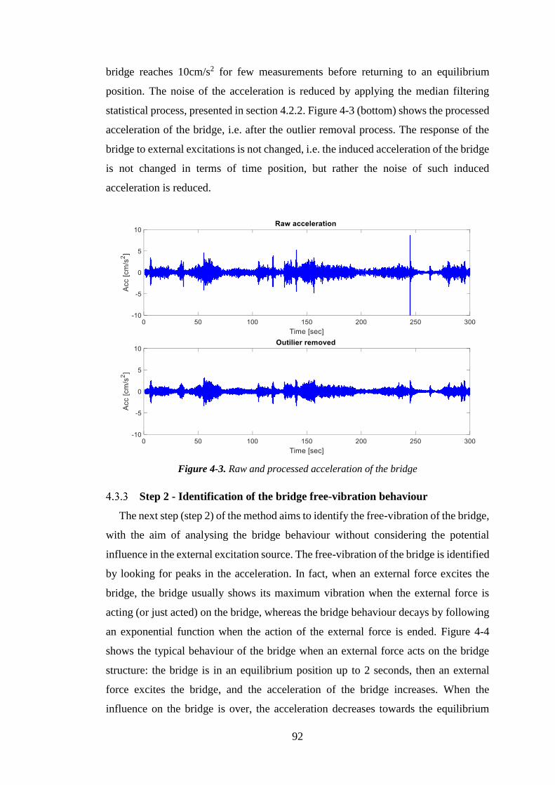
92

bridge reaches 10cm/s2 for few measurements before returning to an equilibrium

position. The noise of the acceleration is reduced by applying the median filtering

statistical process, presented in section 4.2.2. Figure 4-3 (bottom) shows the processed

acceleration of the bridge, i.e. after the outlier removal process. The response of the

bridge to external excitations is not changed, i.e. the induced acceleration of the bridge

is not changed in terms of time position, but rather the noise of such induced

acceleration is reduced.

Figure 4-3. Raw and processed acceleration of the bridge

Step 2 - Identification of the bridge free-vibration behaviour

The next step (step 2) of the method aims to identify the free-vibration of the bridge,

with the aim of analysing the bridge behaviour without considering the potential

influence in the external excitation source. The free-vibration of the bridge is identified

by looking for peaks in the acceleration. In fact, when an external force excites the

bridge, the bridge usually shows its maximum vibration when the external force is

acting (or just acted) on the bridge, whereas the bridge behaviour decays by following

an exponential function when the action of the external force is ended. Figure 4-4

shows the typical behaviour of the bridge when an external force acts on the bridge

structure: the bridge is in an equilibrium position up to 2 seconds, then an external

force excites the bridge, and the acceleration of the bridge increases. When the

influence on the bridge is over, the acceleration decreases towards the equilibrium

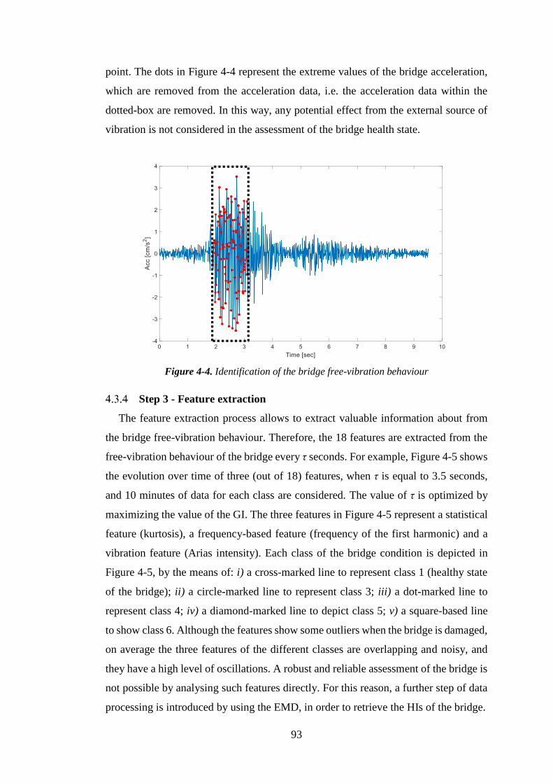
93

point. The dots in Figure 4-4 represent the extreme values of the bridge acceleration,

which are removed from the acceleration data, i.e. the acceleration data within the

dotted-box are removed. In this way, any potential effect from the external source of

vibration is not considered in the assessment of the bridge health state.

Figure 4-4. Identification of the bridge free-vibration behaviour


The feature extraction process allows to extract valuable information about from

the bridge free-vibration behaviour. Therefore, the 18 features are extracted from the

free-vibration behaviour of the bridge every τ seconds. For example, Figure 4-5 shows

the evolution over time of three (out of 18) features, when τ is equal to 3.5 seconds,

and 10 minutes of data for each class are considered. The value of τ is optimized by

maximizing the value of the GI. The three features in Figure 4-5 represent a statistical

feature (kurtosis), a frequency-based feature (frequency of the first harmonic) and a

vibration feature (Arias intensity). Each class of the bridge condition is depicted in

Figure 4-5, by the means of: i) a cross-marked line to represent class 1 (healthy state

of the bridge); ii) a circle-marked line to represent class 3; iii) a dot-marked line to

represent class 4; iv) a diamond-marked line to depict class 5; v) a square-based line

to show class 6. Although the features show some outliers when the bridge is damaged,

on average the three features of the different classes are overlapping and noisy, and

they have a high level of oscillations. A robust and reliable assessment of the bridge is

not possible by analysing such features directly. For this reason, a further step of data

processing is introduced by using the EMD, in order to retrieve the HIs of the bridge.

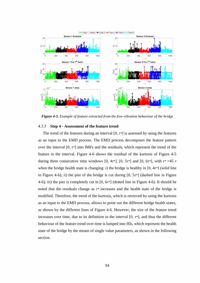
94

Figure 4-5. Example of feature extracted from the free-vibration behaviour of the bridge

Step 4 - Assessment of the feature trend

The trend of the features during an interval [0, τ*] is assessed by using the features

as an input to the EMD process. The EMD process decomposes the feature pattern

over the interval [0, τ*] into IMFs and the residuals, which represent the trend of the

feature in the interval. Figure 4-6 shows the residual of the kurtosis of Figure 4-5

during three consecutive time windows [0, 4τ*], [0, 5τ*] and [0, 6τ*], with τ* =45 τ

when the bridge health state is changing: i) the bridge is healthy in [0, 4τ*] (solid line

in Figure 4-6); ii) the pier of the bridge is cut during [0, 5τ*] (dashed line in Figure

4-6); iii) the pier is completely cut in [0, 6τ*] (dotted line in Figure 4-6). It should be

noted that the residuals change as τ* increases and the health state of the bridge is

modified. Therefore, the trend of the kurtosis, which is retrieved by using the kurtosis

as an input to the EMD process, allows to point out the different bridge health states,

as shown by the different lines of Figure 4-6. However, the size of the feature trend

increases over time, due to its definition in the interval [0, τ*], and thus the different

behaviour of the feature trend over time is lumped into HIs, which represent the health

state of the bridge by the means of single value parameters, as shown in the following

section.

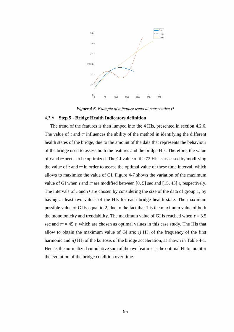
95

Figure 4-6. Example of a feature trend at consecutive τ*

Step 5 - Bridge Health Indicators definition

The trend of the features is then lumped into the 4 HIs, presented in section 4.2.6.

The value of τ and τ* influences the ability of the method in identifying the different

health states of the bridge, due to the amount of the data that represents the behaviour

of the bridge used to assess both the features and the bridge HIs. Therefore, the value

of τ and τ* needs to be optimized. The GI value of the 72 HIs is assessed by modifying

the value of τ and τ* in order to assess the optimal value of these time interval, which

allows to maximize the value of GI. Figure 4-7 shows the variation of the maximum

value of GI when τ and τ* are modified between [0, 5] sec and [15, 45] τ, respectively.

The intervals of τ and τ* are chosen by considering the size of the data of group 1, by

having at least two values of the HIs for each bridge health state. The maximum

possible value of GI is equal to 2, due to the fact that 1 is the maximum value of both

the monotonicity and trendability. The maximum value of GI is reached when τ = 3.5

sec and τ* = 45 τ, which are chosen as optimal values in this case study. The HIs that

allow to obtain the maximum value of GI are: i) HI3 of the frequency of the first

harmonic and ii) HI3 of the kurtosis of the bridge acceleration, as shown in Table 4-1.

Hence, the normalized cumulative sum of the two features is the optimal HI to monitor

the evolution of the bridge condition over time.

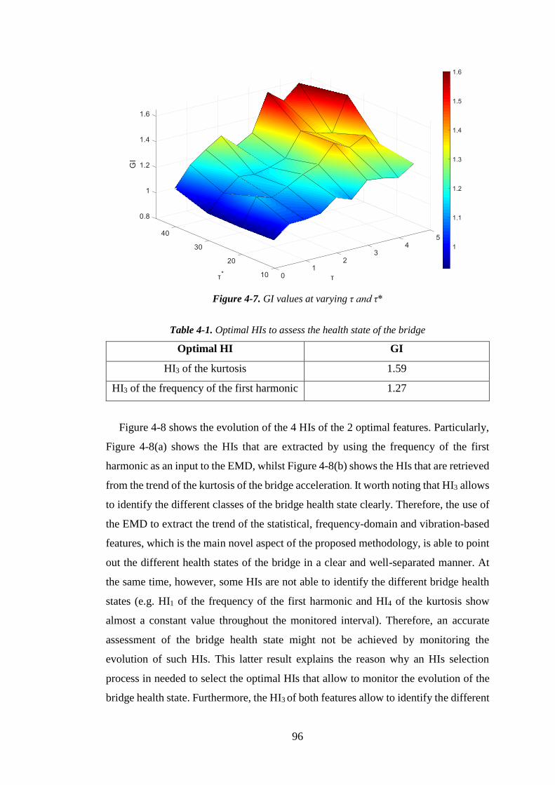
96

Figure 4-7. GI values at varying τ and τ*

Table 4-1. Optimal HIs to assess the health state of the bridge

Optimal HI GI

HI3 of the kurtosis 1.59

HI3 of the frequency of the first harmonic 1.27

Figure 4-8 shows the evolution of the 4 HIs of the 2 optimal features. Particularly,

Figure 4-8(a) shows the HIs that are extracted by using the frequency of the first

harmonic as an input to the EMD, whilst Figure 4-8(b) shows the HIs that are retrieved

from the trend of the kurtosis of the bridge acceleration. It worth noting that HI3 allows

to identify the different classes of the bridge health state clearly. Therefore, the use of

the EMD to extract the trend of the statistical, frequency-domain and vibration-based

features, which is the main novel aspect of the proposed methodology, is able to point

out the different health states of the bridge in a clear and well-separated manner. At

the same time, however, some HIs are not able to identify the different bridge health

states (e.g. HI1 of the frequency of the first harmonic and HI4 of the kurtosis show

almost a constant value throughout the monitored interval). Therefore, an accurate

assessment of the bridge health state might not be achieved by monitoring the

evolution of such HIs. This latter result explains the reason why an HIs selection

process in needed to select the optimal HIs that allow to monitor the evolution of the

bridge health state. Furthermore, the HI3 of both features allow to identify the different

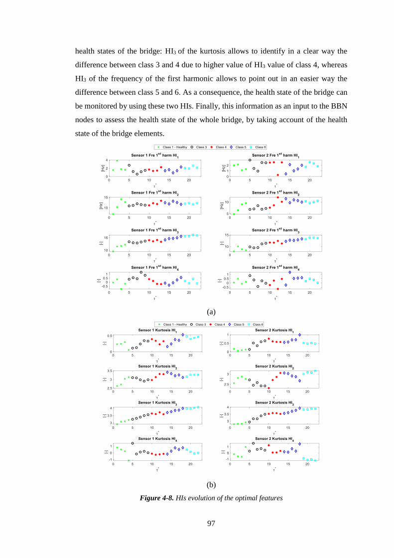
97

health states of the bridge: HI3 of the kurtosis allows to identify in a clear way the

difference between class 3 and 4 due to higher value of HI3 value of class 4, whereas

HI3 of the frequency of the first harmonic allows to point out in an easier way the

difference between class 5 and 6. As a consequence, the health state of the bridge can

be monitored by using these two HIs. Finally, this information as an input to the BBN

nodes to assess the health state of the whole bridge, by taking account of the health

state of the bridge elements.

(a)

(b)

Figure 4-8. HIs evolution of the optimal features

98

Finally, it should be noted that the evolution of the HIs for each feature is presented in

Appendix D.

Summary of the data analysis methodology

The proposed data-driven methodology allows to monitor the condition of the post-

tensioned concrete bridge elements by relying on the data analysis of its vibration

behaviour. Statistical, frequency-based and vibration-based features are extracted from

the data, and the trend of these features is assessed by the means of the EMD approach.

HIs of the bridge are evaluated by computing four statistical parameters of the features

trend. The optimal HIs to monitor the bridge health state are identified by optimizing

the value of a GI, which allows to identify the HIs with the highest values of

monotonicity and trendability over time. In this way, the degrading health state of the

bridge is monitored by monotonic HIs that are able to clearly represent the different

conditions experienced by the bridge. Different health states of the bridge are

identified by the proposed HIs, and therefore such information can be used as an input

to the BBN nodes in order to select the state of the BBN nodes in a reliable manner.

In this way, the BBN can assess the condition of the whole bridge, by taking account

of the health state of each element of the bridge, by monitoring the optimal HIs that

allow to point out the changing health state of the bridge.

The proposed methodology relies on vibration parameters of the bridge, which can

be assessed only when the vibration behaviour of the bridge is monitored by the

measurement system that is installed on the bridge. Hence, if other behaviour of the

bridge is monitored, the methodology needs to be modified accordingly, by computing

different features of the bridge behaviour. Furthermore, the proposed HIs can be

replaced by other statistical parameters that assess other characteristics of the features

trend. In fact, the proposed HIs do not represent the optimal set of HIs for monitoring

the health state of any bridge, due to the fact that each bridge presents unique

characteristics and behaviour, and thus its different health states can be represented by

different optimal HIs. However, when the proposed data analysis methodology is

applied to different bridges, the changing health state of the bridges can be identified

by the proposed methodology, as shown in section 4.8. Future research activities

should consider these initial results in order to identify an optimal set of HIs for SHM.

The proposed data analysis methodology is represented by a deep data analysis, which

starts using raw bridge acceleration data and their features, and results in HIs whose

99

physical meaning is not straightforward to explain. For example, HI3 of the kurtosis

represents the normalized cumulative sum of the trend of the kurtosis of the bridge

acceleration over time. The increase of this HI of the kurtosis represents the increase

of the trend of the kurtosis of the bridge acceleration over time, and consequently an

increase of the outliers of the bridge acceleration. Hence, the extreme values of the

bridge vibration are increasing over time, which can be expected due to the cut of the

pier of the bridge that leads to a reduced capacity of the bridge in responding to

external forces. The optimal value of τ and τ* and the optimal set of HIs depend on the

case study and the available data. Therefore, an optimization process needs to be

carried out in order to point out the optimal value of these parameters.

Finally, although the retrofitting of the bridge, i.e. when the cut pier is repaired,

allows to restore the condition of the bridge, it can be worth adding the data of class 7

when analysing the data in future work, in order to verify if the maintenance action is

able to restore the as-good-as-new condition of the bridge.

The proposed data analysis method is used in Chapter 6 of this thesis to process the

raw acceleration of the bridge and be incorporated in the BBN method. The proposed

methodology can be integrated with a machine learning method, which allows to

automatically assess the health state of the bridge elements by relying on the analysis

of the bridge HIs, as shown in the next section.

A machine learning approach for automatic identification of the

bridge health state

Introduction

An automatic assessment of the bridge health state is proposed by the means of an

NFC, which is trained in a supervised manner by using a dataset of bridge behaviour

in different health states [Cetişli & Barkana, 2010]. Machine learning methods are

being used more frequently in different data analysis frameworks, such as system

health monitoring, infrastructure health monitoring, natural language processing, etc.

due to the availability of large quantities of data. For this reason, we propose a NFC-

based method to assess the health state of the bridge elements in a fast and automatic

manner. In this way, the proposed machine learning method can provide information

about the health state of the bridge elements to the BBN, which is then able to

propagate such information throughout the BBN network and update the health state

of the whole bridge.

100

The NFC is adopted to automatically assess the health state of the bridge by using

an optimal subset of HIs as an input to the NFC. Conversely to the HI selection process

of section 4.2.6, here the optimal subset of HIs is retrieved by using an optimization

differential evolution algorithm [Di Maio et al., 2016], which aims to optimize the

accuracy performance of the NFC. The NFC is selected among the machine learning

classifiers due to the fact that it combines fuzzy classification techniques with learning

capabilities of the Neural Networks. As a consequence, the network structure is

developed by the means of if-then fuzzy rules, which are initially defined by using a

K-means clustering algorithm. Conversely to ANNs, which require the optimization

of the number of hidden layers and hidden nodes, the NFC requires only the

optimization of the number of clusters of the K-means algorithm, and the performance

of the NFC is slightly influenced by the number of the cluster. Moreover, good

performance can also be achieved with a small dataset of the system behaviour [Cetişli

& Barkana, 2010]. NFC has been adopted to diagnose the damage of system

components, such as wind turbine blades [Hoell & Omenzetter, 2017] and rotor bars

[Dias & De Sousa, 2018], but not for bridge damage diagnostics, where ANNs and

clustering techniques have been mostly applied, as discussed in Chapter 2 . The NFC

can be used to automatically assess the health state of the bridge by providing robust

results without requiring a time-consuming trial and error procedure to optimize its

parameters, as a step needed in the ANN method. The proposed method of automatic

health state identification based on the NFC also contributes to the novelty of this

thesis.

In what follows, the NFC is introduced (section 4.5.2), followed by the HIs

selection process (section 4.5.2.2) and the analysis of the post-tensioned bridge using

this method (section 4.5.3). Finally, the influence of different datasets and of the size

of the HIs set on the performance of the NFC method is investigated (section 4.6).

The Neuro-Fuzzy Classifier (NFC)

The NFC requires a database of historical behaviour of the bridge in different health

states, in order to perform the training process. The NFC is trained by using a

supervised process, that is, the condition of the bridge is known when the database of

bridge behaviour is analysed. The NFC is trained with the HIs values that represent

each health state experienced by the bridge. In this way, when a new set of unknown

HIs is available, it is used as an input to the NFC, which is able to assess the health

101

state of the bridge elements automatically. An HIs selection process is necessary to

find, among the HIs, a subset of optimal HIs that are informative with respect to the

health state of the bridge [Hoell & Omenzetter, 2017]. In what follows, the main steps

of the NFC are presented in section 4.5.2.1, whereas the HIs selection process is

presented in section 4.5.2.2.

4.5.2.1 The main steps of the NFC

The detail description of the NFC is out of the scope of this thesis, and an interested

reader can find more information in [Cetişli & Barkana, 2010]. An example of the

NFC structure is depicted in Figure 4-9, for an NFC with 3 fuzzy rules (clusters of the

K-means algorithm) and two classes. In what follows the main steps of the NFC

(Figure 4-9) are presented:

1) a database of set of HIs is used as an input to the NFC. The target class of each

set of HIs, i.e. the bridge health state corresponding to each set of HIs, is also

provided to the NFC due to the fact that a supervised training process is carried

out.

2) a K-means clustering method is applied to the HI data of each class with the

aim of defining fuzzy if-then rules. This means that the HIs of each health state

class are separated into different clusters, in order to describe the relation

between HIs belonging to the same class. For example, a fuzzy rule can be

defined as follows: if the HI1 belongs to cluster 1, and the HI2 belongs to cluster

2, then the bridge health state belongs to class 1.

3) the weight of each cluster of each class is assessed by evaluating the ratio

between the size of each cluster with respect to the size of that class.

4) a Gaussian probability density membership function is defined for each cluster,

by using the centre of each cluster as the mean value of the Gaussian

distribution, whereas the standard deviation of the membership function is

equal to the standard deviation of the HIs that belong to that cluster.

5) a fuzzification process is developed by assessing the membership value of each

HI to each Gaussian probability distribution.

6) a defuzzification and normalization process is finally carried out in order to

assign each HI to a class, i.e. each HI is assigned to the class with the higher

membership value.

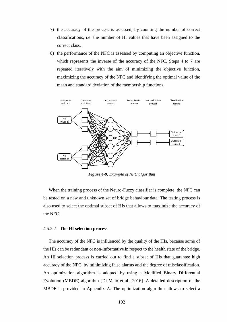
102

7) the accuracy of the process is assessed, by counting the number of correct

classifications, i.e. the number of HI values that have been assigned to the

correct class.

8) the performance of the NFC is assessed by computing an objective function,

which represents the inverse of the accuracy of the NFC. Steps 4 to 7 are

repeated iteratively with the aim of minimizing the objective function,

maximizing the accuracy of the NFC and identifying the optimal value of the

mean and standard deviation of the membership functions.

Figure 4-9. Example of NFC algorithm

When the training process of the Neuro-Fuzzy classifier is complete, the NFC can

be tested on a new and unknown set of bridge behaviour data. The testing process is

also used to select the optimal subset of HIs that allows to maximize the accuracy of

the NFC.

4.5.2.2 The HI selection process

The accuracy of the NFC is influenced by the quality of the HIs, because some of

the HIs can be redundant or non-informative in respect to the health state of the bridge.

An HI selection process is carried out to find a subset of HIs that guarantee high

accuracy of the NFC, by minimizing false alarms and the degree of misclassification.

An optimization algorithm is adopted by using a Modified Binary Differential

Evolution (MBDE) algorithm [Di Maio et al., 2016]. A detailed description of the

MBDE is provided in Appendix A. The optimization algorithm allows to select a

103

subset of HIs iteratively, and assess the accuracy of the NFC by using only the selected

subset of HIs as an input to the NFC both during the training and testing phase, as

shown in Figure 4-10. The group of possible subsets of HIs is comprehensively

represented by 2#HIs-1, where #HIs represents the number of HIs used to describe the

condition of the bridge. A multi-objective optimization process is performed to

minimize the fitness function, which is defined as follows:

fit = {(∑ (𝐿𝑅𝑒𝑎𝑙

𝑇𝑟𝑎𝑖𝑛−𝐿𝑁𝐹𝐶𝑇𝑟𝑎𝑖𝑛)

𝑇𝑇𝑟𝑎𝑖𝑛𝑖=1

×100

𝑇𝑇𝑟𝑎𝑖𝑛)

−1

, (∑ (𝐿𝑅𝑒𝑎𝑙

𝑇𝑒𝑠𝑡−𝐿𝑁𝐹𝐶𝑇𝑒𝑠𝑡)

𝑇𝑇𝑒𝑠𝑡𝑖=1

×100

𝑇𝑇𝑒𝑠𝑡)

−1

}

(4-12)

where TrainT and TestT

represent the size of the target vectors for the training and test

processes, respectively, Re

Train

alL and Re

Test

alL represent the real health state of the bridge for

each bridge behaviour belonging to the training and testing target vectors, respectively.

Train

NFCL and

Test

NFCL represent the health state assigned to each bridge behaviour by the NFC

during the training and testing process, respectively. Eq. (4-12) shows that the fitness

function is minimized when the performance of the NFC is maximized, i.e. the higher

the number of correct classification of the NFC, the lower the value of the fitness

function. The training process is carried out in a supervised manner, whereas the test

process is carried out by analysing a new and unknown set of bridge data. The

optimization algorithm proceeds iteratively until a maximum number of iterations is

reached, the accuracy of the NFC is maximised and the optimal subset of HIs is fixed.

The optimal set of HIs can then be used to validate the proposed NFC, by monitoring

the health state of the bridge when new and unknown behaviour of the bridge is

provided by the sensors.

In the next sections, the proposed NFC method is tested in monitoring and assessing

the health state of an in-field bridge.

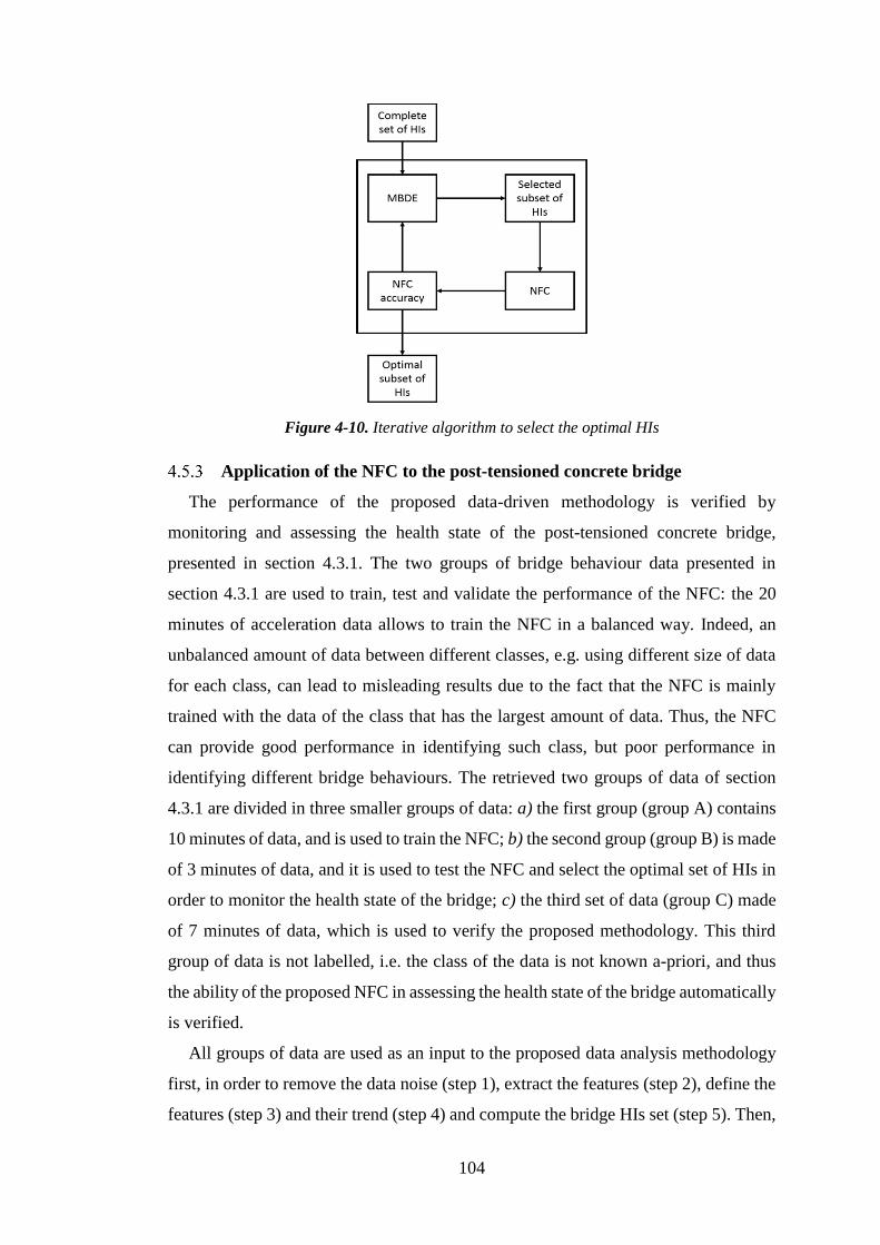
104

Figure 4-10. Iterative algorithm to select the optimal HIs

Application of the NFC to the post-tensioned concrete bridge

The performance of the proposed data-driven methodology is verified by

monitoring and assessing the health state of the post-tensioned concrete bridge,

presented in section 4.3.1. The two groups of bridge behaviour data presented in

section 4.3.1 are used to train, test and validate the performance of the NFC: the 20

minutes of acceleration data allows to train the NFC in a balanced way. Indeed, an

unbalanced amount of data between different classes, e.g. using different size of data

for each class, can lead to misleading results due to the fact that the NFC is mainly

trained with the data of the class that has the largest amount of data. Thus, the NFC

can provide good performance in identifying such class, but poor performance in

identifying different bridge behaviours. The retrieved two groups of data of section

4.3.1 are divided in three smaller groups of data: a) the first group (group A) contains

10 minutes of data, and is used to train the NFC; b) the second group (group B) is made

of 3 minutes of data, and it is used to test the NFC and select the optimal set of HIs in

order to monitor the health state of the bridge; c) the third set of data (group C) made

of 7 minutes of data, which is used to verify the proposed methodology. This third

group of data is not labelled, i.e. the class of the data is not known a-priori, and thus

the ability of the proposed NFC in assessing the health state of the bridge automatically

is verified.

All groups of data are used as an input to the proposed data analysis methodology

first, in order to remove the data noise (step 1), extract the features (step 2), define the

features (step 3) and their trend (step 4) and compute the bridge HIs set (step 5). Then,

105

the HIs are used as an input to the NFC that assesses the health state of the bridge (step

6).

The performance of the NFC strongly depends on the quality and amount of data

available for the training process and on the selection of the subset of HIs performed

by the MBDE. The amount of data is limited in this case study and the set of 72 HIs is

represented by 272-1 possible combinations. Such large set of combination would

require a large number of iteration in order to point out the optimal subset of HIs, and

thus in this section only two HIs are considered to train, test and validate the NFC to

obtain faster results based on the analysis of the HIs. Hence, HI1 and HI3 of the features

trend are considered to monitor the health state of the bridge over time, and to train,

test and validate the NFC. These two HIs are chosen due to their ability in identifying

the different health states of the bridge, as discussed in section 4.3.6. Section 4.6

discusses the performance of the NFC when the whole set of bridge health state classes

and of the 72 HIs are used to train, test and validate the NFC, and demonstrates that

such performance is comparable to the results of other machine learning methods

presented in literature.

In what follows, the performance of the NFC when only 2 HIs are used as an input

to the method is investigated, by discussing the NFC training process (section 4.5.3.1),

the HIs selection process (section 4.5.3.2) and the performance of the NFC (section

4.5.3.3).

4.5.3.1 NFC training

The NFC is adopted to automatically assess the health state of the bridge, by

analysing the extracted HIs. The data of group A are used to train the NFC in a

supervised manner, i.e. the health state of the bridge during the training process is

known, and it is used as target results for the NFC. The training process aims to set the

NFC parameters (number of clusters, mean and standard deviation of the Gaussian

membership functions) to optimize the accuracy of the classification process. The

number of clusters is assumed to be equal to the number of classes used as input to the

NFC (5) and it is kept constant during the analysis. At the same time, the parameters τ

and τ* are optimized during the training process: the HIs of the data in group A are

used as an input to the NFC by modifying either τ or τ*, as shown in Figure 4-11. For

example, when τ* is equal to 30 τ, the NFC shows higher accuracy. The highest

106

accuracy is achieved when τ is equal to 2 seconds, which is chosen as the optimal τ.

The optimal values of τ* and τ are then used for the HIs selection process, to train the

NFC with a dataset of 100 values of each HIs and to monitor the health state of the

bridge.

Figure 4-11. NFC accuracy values at varying τ and τ*

4.5.3.2 HIs selection process

The selection process of the HIs is carried out by adopting the MBDE optimization

algorithm, presented in section 4.5.3.2 and given Appendix A. The MBDE performs

an iterative optimization by selecting a subset of HIs and evaluating the NFC

performance by using the selected subset of HIs as an input to the NFC during both

training and testing phases. The training process is carried out in a supervised manner,

and the testing process is performed by using unlabelled data of group B, which are

used as an input of the proposed method to assess the HIs values during these time

intervals. A dataset of 30 values for each HIs is used for the HIs selection process. The

aim of the MBDE is to maximize the accuracy of the NFC, and, thus, to identify the

subset of HIs that allows to monitor the health state of the bridge reliably. The iterative

process of the MBDE terminates when the maximum number of 2500 iterations is

reached. The MBDE parameters (weighting factor, control parameter and size of the

population as shown in Appendix A) are chosen by performing a trial and error

procedure, and are equal to 0.8, 0.3 and 20 respectively, whereas 2500 iterations are

chosen as trade-off between the high computational-time required by the MBDE and

the number of iterations performed.

107

The evolution of the inverse of the fitness function of Eq. (4-12) is depicted in

Figure 4-12: the higher the number of iteration, the higher the accuracy of the NFC

(the lower the fitness function of the MBDE). Therefore, the MBDE is able to select

subsets of HIs that lead to an improvement of the NFC accuracy. The dotted line in

Figure 4-12 shows the improvement in the performance of the NFC during the testing

phase: the accuracy of the NFC during the first iteration of the MBDE, when the subset

of HIs is randomly selected by the MBDE, is 27%, whereas at generation 2500 it is

77%, due to the MBDE search that is able to select the possible optimal HIs.

The dotted line in Figure 4-12 shows a rapid increase of the NFC accuracy during

the first 400 iterations, which is followed by 1000 ca. iterations that do not improve

the accuracy of the NFC. This result can be due to the definition of the MBDE

parameters, that lead the optimization research into a local minimum of the fitness

function. The local minimum is erroneously identified as a global minimum of the

MBDE fitness function, and the population of the selected HIs is slightly modified

during these iterations. However, at iteration 1500 the MBDE is able to leave the local

minimum, and the NFC accuracy increases accordingly. Finally, at iteration 2300 a

new subset of HIs that allows to increase the accuracy of the NFC is found.

The accuracy of the NFC during the supervised training phase is always close to

98%. This latter performance of the NFC can be explained by considering the fact that,

for each subset of HIs chosen by the MBDE, the NFC is able to set the value of its

parameters in order to optimize the classification of the data during the training phase.

The optimal subset of HIs is identified during the testing phase, as shown in Figure

4-13. The optimization algorithm, which is implemented in Matlab, requires 1 hour

and 10 minutes to be completed by using an Intel core i3-4130 with CPU @ 3.4Hz.

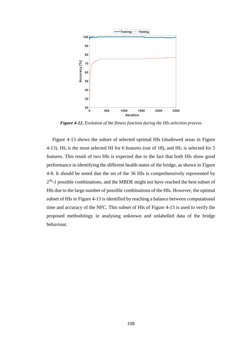
108

Figure 4-12. Evolution of the fitness function during the HIs selection process

Figure 4-13 shows the subset of selected optimal HIs (shadowed areas in Figure

4-13). HI1 is the most selected HI for 6 features (out of 18), and HI3 is selected for 5

features. This result of two HIs is expected due to the fact that both HIs show good

performance in identifying the different health states of the bridge, as shown in Figure

4-8. It should be noted that the set of the 36 HIs is comprehensively represented by

236-1 possible combinations, and the MBDE might not have reached the best subset of

HIs due to the large number of possible combinations of the HIs. However, the optimal

subset of HIs in Figure 4-13 is identified by reaching a balance between computational

time and accuracy of the NFC. This subset of HIs of Figure 4-13 is used to verify the

proposed methodology in analysing unknown and unlabelled data of the bridge

behaviour.

109


monitoring and damage diagnostics

4.5.3.3 Results of the proposed methodology for bridge condition monitoring

and damage diagnostics

The unlabelled data of group C are used to verify the accuracy of the proposed

methodology. The acceleration of the bridge of group C are used in the methodology

in the chronological order, i.e. the 7 minutes of acceleration of the healthy bridge (class

1), followed by the 7 minutes of acceleration of class 3, etc. In this way, the real-time

monitoring of the bridge is simulated. A dataset of 70 values for each optimal HI is

used to assess the performance of the NFC. The accuracy of the methodology is

assessed by comparing the health state of the bridge assigned by the NFC with the real

bridge health state.

Table 4-2 shows the results of the accuracy of the NFC as a condition monitoring

and diagnostic tool. The overall accuracy of the NFC is 78.3%, i.e. 78.3% of the

considered scenarios of group C are correctly identified by the proposed NFC. The

lowest accuracy of the NFC is obtained for class 3 and 5, i.e. the fully cut of the pier,

and when the pier is fully cut, and the deck is settled 2 cm lower of its starting position,

respectively. The fully cut of the bridge pier (class 3) is correctly recognized with

66.67% accuracy, and as a result 37.4% of class 3 scenarios are misclassified as class

4 scenarios. Class 5 is misclassified 41.6% of times to be either class 3 or class 6.

Therefore, the NFC is able to identify the damage of the bridge structure, however,

110

some misclassifications of the nature of the damage are shown due to small changes

of the bridge structural behaviour during these scenarios, i.e. a small loss of stiffness

of the bridge, as pointed out by the modal analysis of the bridge by [Siringoringo et

al., 2013].

Table 4-2 suggests that the proposed NFC can be used as both bridge condition

monitoring and damage diagnostic tool, in order to identify anomalies in bridge

behaviour and point out their causes. In fact, the accuracy of identifying the presence

of the damage is higher than 90% (class 1), whereas the nature of the bridge damage

is correctly identified 75% of times (average of results for classes 3 and higher).

Table 4-2. Accuracy performance of the NFC for bridge condition monitoring and damage

diagnostics

Case study Overall

accuracy Class 1 Class 2 Class 3 Class 4 Class 5 Class 6

Condition

monitoring

and

diagnostics

78.3% 91.67% n/a 66.67% 83.33% 58.34% 91.67%

Influence of the size of bridge behaviour data and of the HIs set on the

performance of the NFC

In this section, the post-tensioned concrete bridge of presented in section 4.3.1 is

analysed by using the NFC approach where a set of four HIs is considered. Particularly,

the NFC is applied to each class of the bridge health state that has at least 20 minutes

of data, and consequently, the data of class 1 (healthy bridge), class 3, 4, 5, 6 and 7 are

used to train, test and validate the NFC in this section. In this way, the influence of

different amount of data on the performance of the NFC is investigated. At the same

time, the whole set of HIs is used as an input to the NFC, with the aim of assessing

how a different set of HIs influences the performance of the NFC.

The data of the bridge health states are divided into the three groups of section 4.5.3

and are used as an input to the proposed data analysis methodology to assess the HIs,

which are then used as input to the NFC.

In what follows, the influence of the size of the HIs set on the performance of the

NFC is investigated in section 4.6.1, where how the size of the bridge behaviour data

influences the NFC performance is analysed in section 4.6.2.

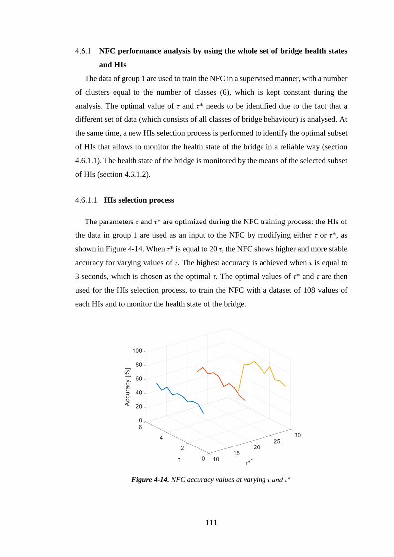
111

NFC performance analysis by using the whole set of bridge health states

and HIs

The data of group 1 are used to train the NFC in a supervised manner, with a number

of clusters equal to the number of classes (6), which is kept constant during the

analysis. The optimal value of τ and τ* needs to be identified due to the fact that a

different set of data (which consists of all classes of bridge behaviour) is analysed. At

the same time, a new HIs selection process is performed to identify the optimal subset

of HIs that allows to monitor the health state of the bridge in a reliable way (section

4.6.1.1). The health state of the bridge is monitored by the means of the selected subset

of HIs (section 4.6.1.2).


The parameters τ and τ* are optimized during the NFC training process: the HIs of

the data in group 1 are used as an input to the NFC by modifying either τ or τ*, as

shown in Figure 4-14. When τ* is equal to 20 τ, the NFC shows higher and more stable

accuracy for varying values of τ. The highest accuracy is achieved when τ is equal to

3 seconds, which is chosen as the optimal τ. The optimal values of τ* and τ are then

used for the HIs selection process, to train the NFC with a dataset of 108 values of

each HIs and to monitor the health state of the bridge.

Figure 4-14. NFC accuracy values at varying τ and τ*

112

The selection process of the HIs is carried out by adopting the MBDE optimization

algorithm. A dataset of 30 values for each HIs is used for the HIs selection process.

The iterative process of the MBDE terminates when a maximum number of 5000

iterations is reached. The MBDE parameters (weighting factor and control parameter,

as shown in Appendix A) are kept constant to the previous analysis, and are equal to

0.8 and 0.3 respectively, whereas 5000 iterations are chosen as trade-off between the

high computational-time required by the MBDE and the number of iteration

performed. A higher number of MBDE iteration, with respect to the analysis of section

4.5.3, is chosen in order to take account of the increased set of HIs.

The evolution of the inverse of the fitness function is depicted in Figure 4-15. The

dotted line in Figure 4-15 shows the improvement in the performance of the NFC

during the testing phase: the accuracy of the NFC during the first iteration of the

MBDE, when the subset of HIs is randomly selected by the MBDE, is equal to 27%,

whereas at generation 5000 it is equal to 76%, due to the MBDE search that is able to

select the possible optimal HIs. Furthermore, the dotted line in Figure 4-15 shows a

rapid increase of the NFC accuracy during the first 1100 iterations, which is followed

by a 3000 ca. iterations that do not improve the accuracy of the NFC. This result can

be due to the definition of the MBDE parameters, that lead the optimization research

into a local minimum of the fitness function. The local minimum is erroneously

identified as a global minimum of the MBDE fitness function, and the population of

the selected HIs is slightly modified during these iterations. However, at iteration 4000

the MBDE is able to leave the local minimum, and the NFC accuracy increases

accordingly.

The accuracy of the NFC during the supervised training phase is always close to

98%. This latter performance of the NFC can be explained by considering the fact that,

for each subset of HIs chosen by the MBDE, the NFC is able to set the value of its

parameters in order to optimize the classification of the data during the training phase.

The optimal subset of HIs is identified during the testing phase, as shown in Figure

4-16. The optimization algorithm, which is implemented in Matlab, requires 3 hours

and 40 minutes to be completed by using an Intel core i3-4130 with CPU @ 3.4Hz. It

should be noted that, despite an increase of the number of iteration of the MBDE, the

accuracy of the NFC during the testing process is lower than the performance shown

in section 4.5.3.2. Furthermore, the increase of the maximum number of generation,

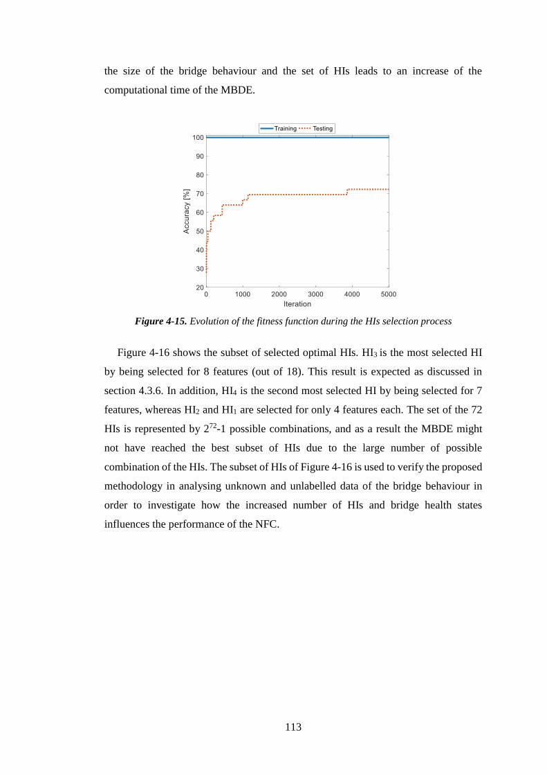
113

the size of the bridge behaviour and the set of HIs leads to an increase of the

computational time of the MBDE.

Figure 4-15. Evolution of the fitness function during the HIs selection process

Figure 4-16 shows the subset of selected optimal HIs. HI3 is the most selected HI

by being selected for 8 features (out of 18). This result is expected as discussed in

section 4.3.6. In addition, HI4 is the second most selected HI by being selected for 7

features, whereas HI2 and HI1 are selected for only 4 features each. The set of the 72

HIs is represented by 272-1 possible combinations, and as a result the MBDE might

not have reached the best subset of HIs due to the large number of possible

combination of the HIs. The subset of HIs of Figure 4-16 is used to verify the proposed

methodology in analysing unknown and unlabelled data of the bridge behaviour in

order to investigate how the increased number of HIs and bridge health states

influences the performance of the NFC.

114


monitoring and damage diagnostics

4.6.1.2 Performance of the NFC by analysing the whole set of HIs for bridge

condition monitoring and damage diagnostics

The unlabelled data of group 3 are used to verify the accuracy of the NFC. A dataset

of 78 values for each optimal HI is used to assess the performance of the NFC. The

accuracy of the methodology is assessed by comparing the health state of the bridge

assigned by the NFC with the real bridge health state.

Table 4-3 shows the results of the accuracy of the NFC as a damage detection and

diagnostic tool. The overall accuracy of the NFC is equal to 72.2%, i.e. 72.2% of the

considered scenarios of group 3 are correctly identified by the proposed NFC. The

lowest accuracy of the NFC is obtained for class 1 and 6, i.e. the healthy state of the

bridge and when the pier is fully cut, and the deck is settled 2.7 cm lower of its starting

position, respectively. The healthy state of the bridge (class 1) is correctly recognized

with 66.6% accuracy, and as a result 37.4% of the healthy scenarios are misclassified

as damaged scenarios. Class 6 is misclassified to be class 3. The misclassification of

class 6 is not straightforward to explain due to the fact that class 6 represents a scenario

in which the pier of the bridge is completely suspended, whereas class 3 represents a

scenario in which the pier is completely cut but not suspended. Therefore, the

structural behaviour of the bridge is expected to be different in these two scenarios.

The misclassification of class 6 can be caused by both non-optimal HIs and small

changes of the structural behaviour of the bridge.

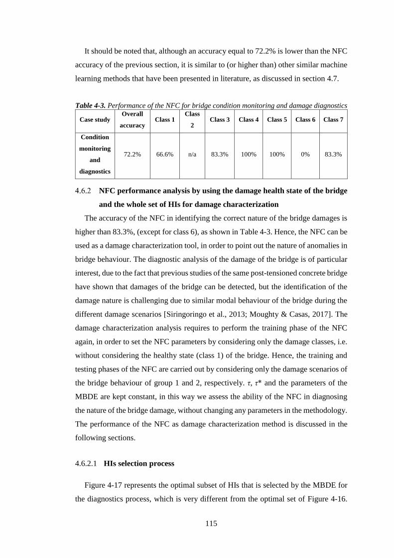
115

It should be noted that, although an accuracy equal to 72.2% is lower than the NFC

accuracy of the previous section, it is similar to (or higher than) other similar machine

learning methods that have been presented in literature, as discussed in section 4.7.

Table 4-3. Performance of the NFC for bridge condition monitoring and damage diagnostics

Case study Overall

accuracy Class 1

Class

2 Class 3 Class 4 Class 5 Class 6 Class 7

Condition

monitoring

and

diagnostics

72.2% 66.6% n/a 83.3% 100% 100% 0% 83.3%

NFC performance analysis by using the damage health state of the bridge

and the whole set of HIs for damage characterization

The accuracy of the NFC in identifying the correct nature of the bridge damages is

higher than 83.3%, (except for class 6), as shown in Table 4-3. Hence, the NFC can be

used as a damage characterization tool, in order to point out the nature of anomalies in

bridge behaviour. The diagnostic analysis of the damage of the bridge is of particular

interest, due to the fact that previous studies of the same post-tensioned concrete bridge

have shown that damages of the bridge can be detected, but the identification of the

damage nature is challenging due to similar modal behaviour of the bridge during the

different damage scenarios [Siringoringo et al., 2013; Moughty & Casas, 2017]. The

damage characterization analysis requires to perform the training phase of the NFC

again, in order to set the NFC parameters by considering only the damage classes, i.e.

without considering the healthy state (class 1) of the bridge. Hence, the training and

testing phases of the NFC are carried out by considering only the damage scenarios of

the bridge behaviour of group 1 and 2, respectively. τ, τ* and the parameters of the

MBDE are kept constant, in this way we assess the ability of the NFC in diagnosing

the nature of the bridge damage, without changing any parameters in the methodology.

The performance of the NFC as damage characterization method is discussed in the

following sections.


Figure 4-17 represents the optimal subset of HIs that is selected by the MBDE for

the diagnostics process, which is very different from the optimal set of Figure 4-16.

116

HI1 is the most selected HI, followed by HI2, whereas HI3 and HI4 are chosen only to

represent three and two features, respectively. The number of HIs that belong to the

optimal subset is also different: for the damage characterization case study 18 HIs

represent the optimal subset, whilst 23 HIs represent the optimal subset for the damage

detection and diagnostics case study. The different subset of optimal HIs is due to the

different case study being considered.

4.6.2.2 Performance of the NFC by analysing the whole set of HIs for bridge

damage characterization

The unlabelled data of the damages of group 3 are used as an input to the

methodology, in order to automatically characterize the nature of a bridge damage by

the means of the NFC. Table 4-4 shows the accuracy of the NFC in diagnosing the

nature of the bridge damage. The overall accuracy is equal to 85%: 3 out of 5 classes

(class 3, 4 and 7) of the bridge damage are correctly identified all the time, whilst class

5 is correctly identified with an accuracy of 75% and class 6 with an accuracy of 50%.

The analysis of the misclassifications points out that class 5 is misclassified as class 3,

and class 6 as class 4. The misclassifications can be explained due to a low change of

the bridge structural behaviour between the two classes.

The accuracy of the NFC in this case study outperforms the accuracy of the previous

sections. This result can be explained by pointing out that when only the damage

scenarios of the bridge are analysed, the proposed data analysis methodology provides

HIs values of the damage scenarios that are different from each other. Furthermore, as

the healthy state is not considered in the damage characterization analysis, the

Figure 4-17. Selected HIs by using the optimization algorithm for bridge damage

diagnostics

117

misclassifications of the healthy state that the NFC showed in section 4.6.1.2 are not

present.

Table 4-4. Performance of the NFC for damage characterization

Case study Overall

accuracy Class 1

Class

2 Class 3 Class 4 Class 5 Class 6 Class 7

Diagnostics 85% n/a n/a 100% 100% 75% 50% 100%

Summary of the NFC

The NFC for bridge elements condition monitoring and damage diagnostics showed

a good accuracy in identifying and diagnosing the damages of the bridge structure

automatically. It should be noted that an overall accuracy that ranges from 72.2% to

85% is a good result in assessing the health state of an in-field bridge, due to the

unknown source of uncertainty and changing environmental conditions. Indeed,

similar machine learning methods, which are based on ANNs and verified on FEMs

by adding white Gaussian noise to the simulated bridge behaviour, have shown an

average accuracy of 65% [Shu et al., 201352; Zhou et al., 2014; Yeung et al., 2005],

whereas clustering techniques, which were verified on in-field bridges, have shown an

average accuracy of 68%, with a maximum accuracy of 75% [Alves et al., 2016]. At

the same time, [Siringoringo et al., 2013] performed a modal analysis of the bridge

during each health state of the bridge, and showed that the modal parameters of the

bridge are slightly modified by the first inflicted damages (class 2 to class 5), whereas

the most severe damage (class 6) modified the modal parameters of the bridge

significantly, and, as a consequence, it is possible to identify such a damage clearly,

and the accuracy for class 6 is high.

The performance of the NFC strongly depends on the quality and amount of data

available for the training process, which is limited in this case study. As a consequence,

the performance of the proposed NFC is expected to improve by increasing the size

and quality (in terms of different behaviour of the bridge) of the training (group A),

testing (group B) and validation (group C) sets. At the same time, as the size of data

of the bridge behaviour and the set of HIs increases, the time required to identify the

optimal set of HIs increases, due to the increases of the set of possible optimal solutions

of the optimization problem. Therefore, a balance between the amount of data and the

118

size of the HIs set needs to be reach in order to guarantee robust results without being

penalizing by large computational time of the analysis.

The NFC approach is proposed in this thesis as a possible method to assess the

health state of the bridge elements automatically, and then use such information as an

input to the BBN. Due to the limited amount of data that is available in this case study,

in the remaining of this thesis the data analysis approach of section 4.2 is used to

process the raw bridge behaviour with the aim of identifying the health state of the

bridge elements. The main drawback of the NFC is that it requires a large amount of

data for the training and testing processes, and, as a result, it can be used in case study

with large amount of data. Furthermore, the bridge behaviour for different health states

of the bridge is required to adequately train the NFC. Such data are not usually

available, and the NFC is only able to identify and diagnose available bridge damages,

i.e. the damages of the bridge whose behaviour is available within the training data set.

However, the larger the availability of the data, the more accurate the results provided

by the NFC, due to its learning ability.

Application of the proposed data analysis methodology to an in-field

steel truss bridge

Introduction

In this section, the proposed data analysis methodology to process the raw bridge

behaviour and assess the health state of the bridge is applied to an in-field steel truss

bridge. The bridge is subjected to a progressive damage test that aims to study the

bridge behaviour during different health states of the bridge. The bridge is excited by

a moving vehicle that runs over the bridge at almost constant speed throughout the test.

Three runs of the vehicle for each health state of the bridge are available, and thus a

very limited amount of data is available in this case study. Despite the limited

availability of data of the bridge behaviour, the proposed data analysis methodology

is able to point out the different health states of the bridge. Finally, it should be

mentioned that the machine learning approach that relies on the NFC is not applied to

this case study due to the limited amount of data.

The steel truss bridge is described in section 4.8.2, and the steps of the proposed

method for analysing the bridge behaviour are presented in the following sections.

119

Description of the steel truss bridge and the progressive damage test

A simply-supported steel Warren truss bridge is considered in this analysis. The

length of the bridge is 59.2 m, with 3.6 m width and 8 m of maximum height, as shown

in Figure 4-18 [Chang & Kim, 2016]. The bridge was demolished in 2012. However,

progressive damage tests were carried out while the bridge was closed to the public in

order to develop a dataset of bridge behaviour under changing health states of the

bridge. The dynamic behaviour of the bridge was collected by 8 accelerometers,

denoted as Ai (i = 1, 2, …, 8) circles in Figure 4-18, whose sample rates was equal to

200 Hz. Five different health state classes of the bridge were analysed by damaging

the bridge infrastructure progressively (Figure 4-18): i) intact bridge scenarios, with

no damage of the bridge infrastructure (healthy bridge); ii) a half cut of the mid-span

vertical member (DMG1); iii) a complete cut of the mid-span vertical member

(DMG2); iv) retrofitted scenarios in which the cut of the mid-span vertical member is

repaired (RCV, retrofitted); v) a complete cut of the vertical member at 5/8th span

(DMG3). The data of the bridge behaviour during the five health states are analysed

in two separated groups: a) the first group (group A) considers the intact bridge

scenarios (healthy), followed by DMG1 and DMG2; b) the second group (group B)

consists of the data of the bridge during the retrofitted and the DMG3 scenarios. The

separation between the two groups is assumed due to the repair of the bridge damage

that retrofits the bridge to a healthy state after DMG2. Indeed, the repair of the bridge

after DMG2 considers that the damage scenarios of the bridge are identified, and

maintenance actions are taken on the bridge. Finally, the scenarios of the bridge are

analysed by considering the chronological order of the events, i.e. the healthy scenarios

are the first data to be used as an input to the data analysis methodology, followed by

DMG1 and DMG2 data, respectively, etc. In this way, the evolution over time of the

bridge health state is considered.

For each health state, the vehicle used for the experiment was a two-axle vehicle,

with a total weight of about 21kN. The vehicle was driven across the bridge three times

for each scenario at a speed ranging from 36 to 41 km/hr to induce excitation.

The acceleration of the bridge is recorded by the 8 sensors and used as an input to

the proposed data analysis method.

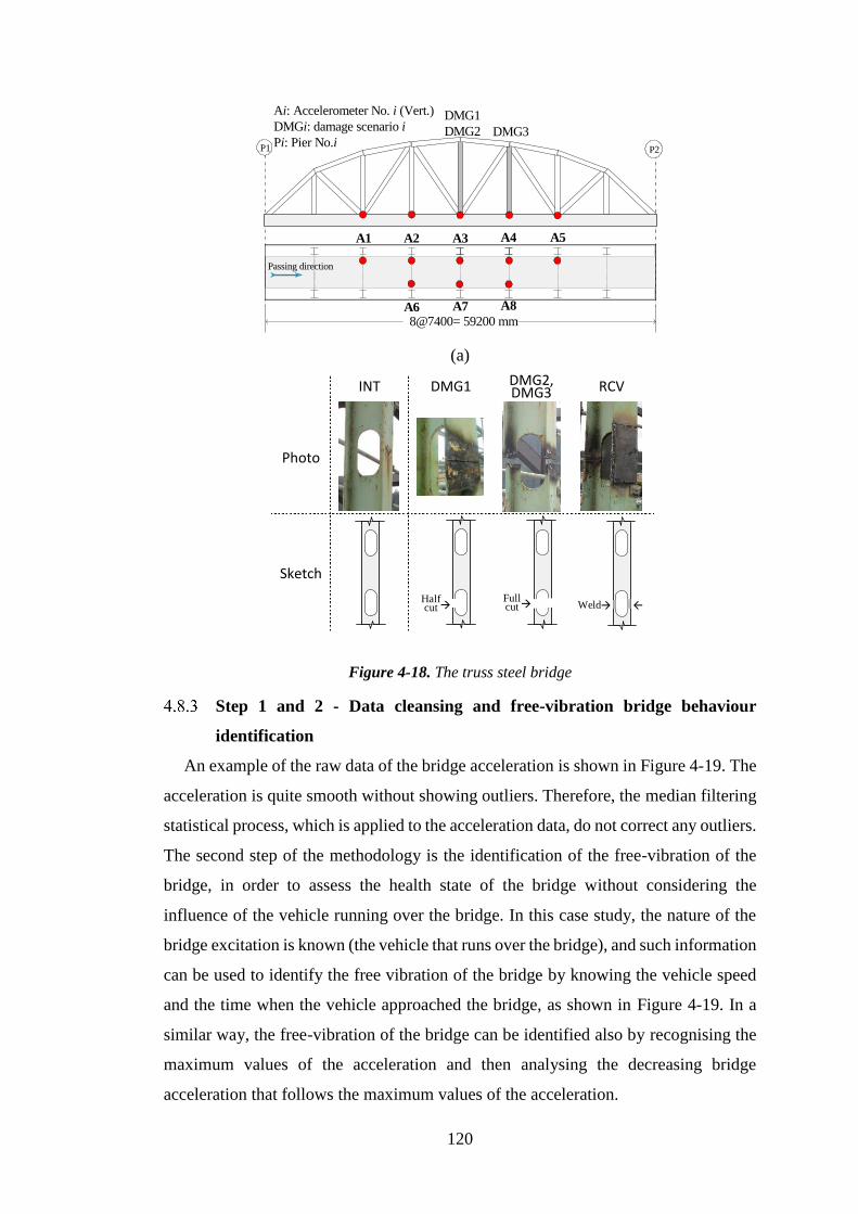
120

(a)

Figure 4-18. The truss steel bridge

Step 1 and 2 - Data cleansing and free-vibration bridge behaviour

identification

An example of the raw data of the bridge acceleration is shown in Figure 4-19. The

acceleration is quite smooth without showing outliers. Therefore, the median filtering

statistical process, which is applied to the acceleration data, do not correct any outliers.

The second step of the methodology is the identification of the free-vibration of the

bridge, in order to assess the health state of the bridge without considering the

influence of the vehicle running over the bridge. In this case study, the nature of the

bridge excitation is known (the vehicle that runs over the bridge), and such information

can be used to identify the free vibration of the bridge by knowing the vehicle speed

and the time when the vehicle approached the bridge, as shown in Figure 4-19. In a

similar way, the free-vibration of the bridge can be identified also by recognising the

maximum values of the acceleration and then analysing the decreasing bridge

acceleration that follows the maximum values of the acceleration.

8@7400= 59200 mm

P1 P2

A1 A2 A3 A4 A5

A6 A7 A8

DMG1

DMG2 DMG3

Passing direction

Ai: Accelerometer No. i (Vert.)

DMGi: damage scenario i

Pi: Pier No.i

INT DMG1 DMG2, DMG3 RCV

Photo

Sketch

INT

→

DMG2

DMG3

Full cut

DMG1

→Half cut →

RCV

Weld

INT

→

DMG2

DMG3

Full cut

DMG1

→Half cut →

RCV

Weld

INT

→

DMG2

DMG3

Full cut

DMG1

→Half cut →

RCV

Weld

INT

→

DMG2

DMG3

Full cut

DMG1

→Half cut →

RCV

Weld

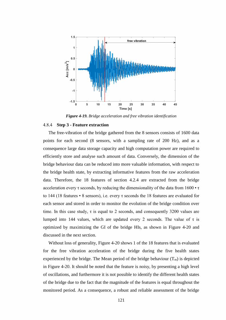
121

Figure 4-19. Bridge acceleration and free vibration identification


The free-vibration of the bridge gathered from the 8 sensors consists of 1600 data

points for each second (8 sensors, with a sampling rate of 200 Hz), and as a

consequence large data storage capacity and high computation power are required to

efficiently store and analyse such amount of data. Conversely, the dimension of the

bridge behaviour data can be reduced into more valuable information, with respect to

the bridge health state, by extracting informative features from the raw acceleration

data. Therefore, the 18 features of section 4.2.4 are extracted from the bridge

acceleration every τ seconds, by reducing the dimensionality of the data from 1600 • τ

to 144 (18 features • 8 sensors), i.e. every τ seconds the 18 features are evaluated for

each sensor and stored in order to monitor the evolution of the bridge condition over

time. In this case study, τ is equal to 2 seconds, and consequently 3200 values are

lumped into 144 values, which are updated every 2 seconds. The value of τ is

optimized by maximizing the GI of the bridge HIs, as shown in Figure 4-20 and

discussed in the next section.

Without loss of generality, Figure 4-20 shows 1 of the 18 features that is evaluated

for the free vibration acceleration of the bridge during the five health states

experienced by the bridge. The Mean period of the bridge behaviour (Tm) is depicted

in Figure 4-20. It should be noted that the feature is noisy, by presenting a high level

of oscillations, and furthermore it is not possible to identify the different health states

of the bridge due to the fact that the magnitude of the features is equal throughout the

monitored period. As a consequence, a robust and reliable assessment of the bridge

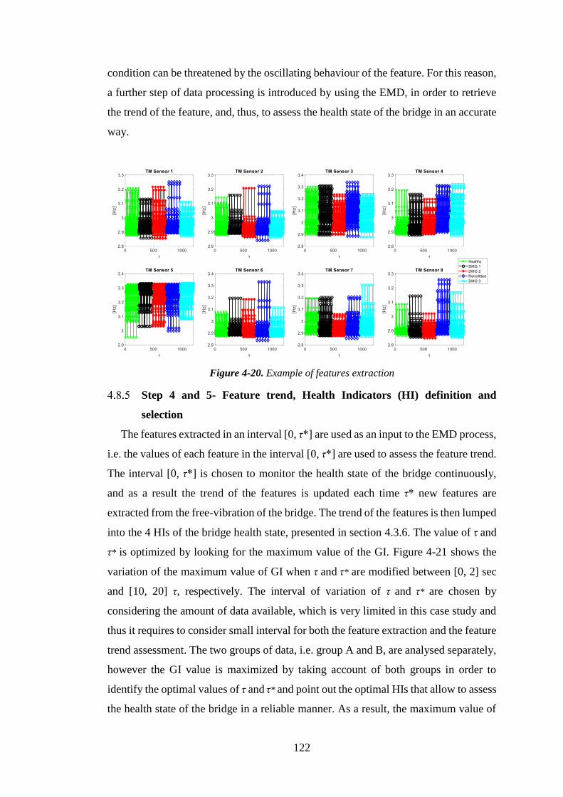
122

condition can be threatened by the oscillating behaviour of the feature. For this reason,

a further step of data processing is introduced by using the EMD, in order to retrieve

the trend of the feature, and, thus, to assess the health state of the bridge in an accurate

way.

Figure 4-20. Example of features extraction

Step 4 and 5- Feature trend, Health Indicators (HI) definition and

selection

The features extracted in an interval [0, τ*] are used as an input to the EMD process,

i.e. the values of each feature in the interval [0, τ*] are used to assess the feature trend.

The interval [0, τ*] is chosen to monitor the health state of the bridge continuously,

and as a result the trend of the features is updated each time τ* new features are

extracted from the free-vibration of the bridge. The trend of the features is then lumped

into the 4 HIs of the bridge health state, presented in section 4.3.6. The value of τ and

τ* is optimized by looking for the maximum value of the GI. Figure 4-21 shows the

variation of the maximum value of GI when τ and τ* are modified between [0, 2] sec

and [10, 20] τ, respectively. The interval of variation of τ and τ* are chosen by

considering the amount of data available, which is very limited in this case study and

thus it requires to consider small interval for both the feature extraction and the feature

trend assessment. The two groups of data, i.e. group A and B, are analysed separately,

however the GI value is maximized by taking account of both groups in order to

identify the optimal values of τ and τ* and point out the optimal HIs that allow to assess

the health state of the bridge in a reliable manner. As a result, the maximum value of

123

GI is equal to 4, i.e. the monotonicity and trendability of the two groups are summed

into the GI. Figure 4-21 shows that the maximum value of GI is reached when τ = 2

sec and τ* = 20 τ, which are chosen as optimal values. The HI that allows to obtain the

maximum value of GI is the HI3 of the Mean period of the bridge behaviour (Tm), as

shown in Table A. 1.

Figure 4-21. GI values at varying τ and τ*

Table A. 1. Optimal HIs to assess the health state of the steel truss bridge

Optimal HI GI

HI3 of the mean period of the bridge

behaviour (Tm) 3.5811

Figure 4-22 shows that the HI3 of Tm for both groups of data is able to point out

clearly the different health states of the steel truss bridge for both groups of data, i.e.

each damage scenario of the bridge (DMG1 and DMG2 of group A, and DMG3 of

group B) is identified by the optimal HIs, due to an increase of its value with respect

to the healthy (retrofitted) value of the HI. The HI3 of Tm allows to identify the location

of the damages: the maximum value of the HI is shown by sensor 5 and sensor 3 for

damages DMG1 and DMG2, which are installed at the damage location, whereas the

maximum value for damage DMG3 is shown by sensor 4 that is exactly the location

where the cut of the vertical element is applied.

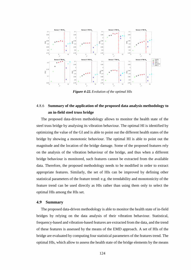
124

Figure 4-22. Evolution of the optimal HIs

Summary of the application of the proposed data analysis methodology to

an in-field steel truss bridge

The proposed data-driven methodology allows to monitor the health state of the

steel truss bridge by analysing its vibration behaviour. The optimal HI is identified by

optimizing the value of the GI and is able to point out the different health states of the

bridge by showing a monotonic behaviour. The optimal HI is able to point out the

magnitude and the location of the bridge damage. Some of the proposed features rely

on the analysis of the vibration behaviour of the bridge, and thus when a different

bridge behaviour is monitored, such features cannot be extracted from the available

data. Therefore, the proposed methodology needs to be modified in order to extract

appropriate features. Similarly, the set of HIs can be improved by defining other

statistical parameters of the feature trend: e.g. the trendability and monotonicity of the

feature trend can be used directly as HIs rather than using them only to select the

optimal HIs among the HIs set.

Summary

The proposed data-driven methodology is able to monitor the health state of in-field

bridges by relying on the data analysis of their vibration behaviour. Statistical,

frequency-based and vibration-based features are extracted from the data, and the trend

of these features is assessed by the means of the EMD approach. A set of HIs of the

bridge are evaluated by computing four statistical parameters of the features trend. The

optimal HIs, which allow to assess the health state of the bridge elements by the means

125

of a monotonic behaviour that increases/decreases according to the degradation of the

bridge elements, are identified by optimizing the value of a GI.

The proposed methodology is able to provide optimal HIs to clearly identify the

different health states of the bridge elements, and such information can be used as an

input to the BBN nodes to assess the state of the BBN nodes in a reliable manner. As

a consequence, the BBN can assess the health state of the whole bridge, by taking

account of the health state of each element of the bridge, by monitoring the optimal

HIs that allow to point out the changing health state of the bridge.

The proposed methodology shows some drawbacks:

1. The vibration features that are extracted from the bridge behaviour can be

assessed only when the vibration behaviour of the bridge is monitored by the

measurement system. Hence, if other behaviour of the bridge is monitored, the

methodology needs to be modified accordingly, by computing different

features of the bridge behaviour.

2. The feature trend is lumped into four HIs, which do not represent the optimal

set of HIs for monitoring the health state of any bridge. In fact, other statistical

parameters (such as the trendability and monotonicity of the feature trend) of

the feature trend can be used in order to monitor the health state of the bridge

in a reliable and effective manner.

3. The optimal values of τ and τ* and the optimal set of HIs depend on the case

study and the available data, and, as a result, an optimization process needs to

be carried out in order to point out the optimal value of these parameters for

each case study.

The information provided by the proposed data analysis methodology, by using the

HIs can be used as an input to a machine learning method, in order to identify the

health state of the bridge elements automatically. The proposed NFC showed a good

accuracy in identifying and diagnosing the damages of the bridge structure

automatically. However, the NFC shows some drawbacks:

• The performance of the NFC relies on the quality and amount of data available

for the training process, which need to be as high as possible, in order to train

the NFC with lot of data of different behaviour of the bridge.

• The set of possible HIs is identified by applying the MBDE algorithm, whose

computational time increases when the set of possible optimal solutions of the

optimization problem increases.

126

The NFC approach is proposed in this thesis as a possible method to automatically

asses the health state of the bridge elements, and then use such information as an input

to the BBN. Due to the limited amount of data that is available in this case study, in

the remaining of this thesis the data analysis methodology of section 4.2 is used to

process the raw bridge behaviour with the aim of identifying the health state of the

bridge elements.

In what follows, the optimal HI is used to define the CPTs of the BBN of the bridge,

by merging the expert judgement analysis with the analysis of the bridge behaviour in

order to define reliable CPTs.

127

CPTs updating method by

merging expert judgment and

bridge behaviour analysis

Introduction

The CPTs represent the quantitative part of the BBN and allow to define the

dependencies between connected nodes of the BBN, by using conditional

probabilities. The analysis of bridge behaviour, if a database of information about the

past behaviour of the bridge is available, or an expert elicitation process, if such

database is unavailable, can be used to define the CPTs. In Chapter 3 the latter

approach has been used to define the CPTs of the BBN by interviewing three experts.

However, the results of the BBN analyses in Chapter 3 showed that the diagnostic

performance of the BBN was limited. Therefore, an increase of the BBN diagnostic

performance is expected when the CPTs are defined in a more accurate manner, by

using the bridge behaviour data to assess the influences between different elements of

the bridge. For this reason, an approach to update the CPTs by merging the expert

elicitation process, which allows to define the CPTs at first, with the analysis of the

bridge behaviour is proposed in this thesis. The proposed method requires the

availability of bridge behaviour data for different known health states of the bridge

elements, in order to assess the dependencies between different bridge elements, using

CDFs.

However, when a database of behaviour of the infrastructure is analysed, the

infrastructure health state is not always known a-priori. As a consequence, a method

to analyse the database of infrastructure behaviour is also proposed in this chapter with

the aim of identifying the point when the health state of the infrastructure changes. At

the same time, the characteristics of this change, in terms of change duration and

possible causes, are pointed out.

In what follows, the method to define the CPTs by merging the expert judgement

elicitation process and the analysis of the bridge behaviour is presented in section 5.2.

The proposed method is applied to the presented post-tensioned bridge in section 5.3,

and the results of the method for updating the CPTs are summarized in section 5.4.

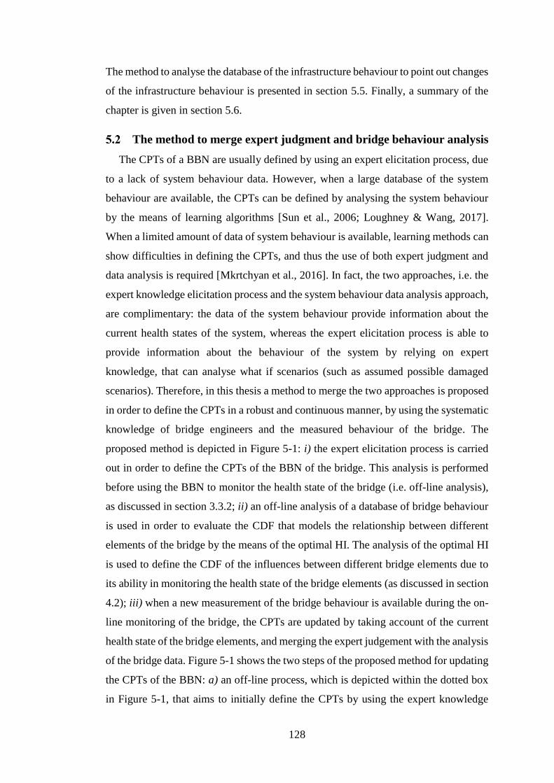
128

The method to analyse the database of the infrastructure behaviour to point out changes

of the infrastructure behaviour is presented in section 5.5. Finally, a summary of the

chapter is given in section 5.6.

The method to merge expert judgment and bridge behaviour analysis

The CPTs of a BBN are usually defined by using an expert elicitation process, due

to a lack of system behaviour data. However, when a large database of the system

behaviour are available, the CPTs can be defined by analysing the system behaviour

by the means of learning algorithms [Sun et al., 2006; Loughney & Wang, 2017].

When a limited amount of data of system behaviour is available, learning methods can

show difficulties in defining the CPTs, and thus the use of both expert judgment and

data analysis is required [Mkrtchyan et al., 2016]. In fact, the two approaches, i.e. the

expert knowledge elicitation process and the system behaviour data analysis approach,

are complimentary: the data of the system behaviour provide information about the

current health states of the system, whereas the expert elicitation process is able to

provide information about the behaviour of the system by relying on expert

knowledge, that can analyse what if scenarios (such as assumed possible damaged

scenarios). Therefore, in this thesis a method to merge the two approaches is proposed

in order to define the CPTs in a robust and continuous manner, by using the systematic

knowledge of bridge engineers and the measured behaviour of the bridge. The

proposed method is depicted in Figure 5-1: i) the expert elicitation process is carried

out in order to define the CPTs of the BBN of the bridge. This analysis is performed

before using the BBN to monitor the health state of the bridge (i.e. off-line analysis),

as discussed in section 3.3.2; ii) an off-line analysis of a database of bridge behaviour

is used in order to evaluate the CDF that models the relationship between different

elements of the bridge by the means of the optimal HI. The analysis of the optimal HI

is used to define the CDF of the influences between different bridge elements due to

its ability in monitoring the health state of the bridge elements (as discussed in section

4.2); iii) when a new measurement of the bridge behaviour is available during the on-

line monitoring of the bridge, the CPTs are updated by taking account of the current

health state of the bridge elements, and merging the expert judgement with the analysis

of the bridge data. Figure 5-1 shows the two steps of the proposed method for updating

the CPTs of the BBN: a) an off-line process, which is depicted within the dotted box

in Figure 5-1, that aims to initially define the CPTs by using the expert knowledge

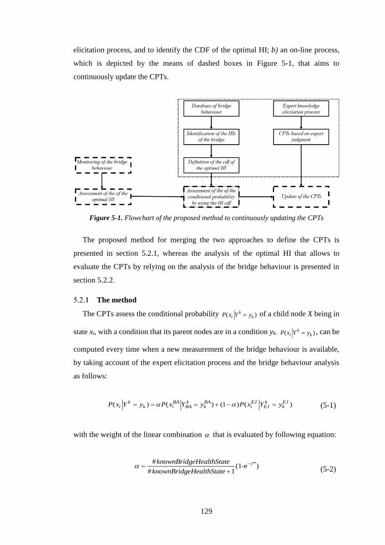
129

elicitation process, and to identify the CDF of the optimal HI; b) an on-line process,

which is depicted by the means of dashed boxes in Figure 5-1, that aims to

continuously update the CPTs.

Figure 5-1. Flowchart of the proposed method to continuously updating the CPTs

The proposed method for merging the two approaches to define the CPTs is

presented in section 5.2.1, whereas the analysis of the optimal HI that allows to

evaluate the CPTs by relying on the analysis of the bridge behaviour is presented in

section 5.2.2.

The method

The CPTs assess the conditional probability ( )ki kP x Y y= of a child node X being in

state xi, with a condition that its parent nodes are in a condition yk. ( )ki kP x Y y= , can be

computed every time when a new measurement of the bridge behaviour is available,

by taking account of the expert elicitation process and the bridge behaviour analysis

as follows:

( ) ( ) (1 ) ( )k BA k BA EJ k EJi k i BA k i EJ kP x Y y P x Y y P x Y y = = = + − = (5-1)

with the weight of the linear combination that is evaluated by following equation:

*(1-e#

)#

1

knownBridgeHealthState

knownBridgeHealthState

−

+=

(5-2)

130

Eq. (5-1) shows that the conditional probability that the child node X is in state xi, with

a condition that its parent nodes are in a condition yk, is evaluated by a linear

combination with weight [0, 0.9] , of the conditional probabilities assessed by

analysing the bridge behaviour, ( )BA k BAi BA kP x Y y= , and considering the expert

knowledge elicitation process, ( )EJ k EJi EJ kP x Y y= . The process to assess the conditional

probability, ( )BA k BAi BA kP x Y y= , is presented in the following section, whereas the

approach to compute the conditional probability ( )EJ k EJi EJ kP x Y y= has been introduced

in section 3.3.2.

Eq. (5-2) displays that the weight of the linear combination, [0, 0.9] , depends on

both the number of the identified health states experienced by the bridge (which are

labelled as #knownBridgeHealthState ) and the time interval * during which the bridge

behaviour is monitored. In fact, the larger the monitoring interval of the bridge

behaviour, the more reliable the assessment of ( )BA k BAi BA kP x Y y= , and thus the higher

the weight of ( )BA k BAi BA kP x Y y= . Conversely, the smaller the length of the

monitoring time, the smaller the weight and the higher the importance of

( )EJ k EJi EJ kP x Y y= . Furthermore, Eq. (5-2) shows also that the weight of the linear

combination increases when the number of known health states experienced by the

bridge increases. In fact, the definition of assumes that the knowledge acquired by

analysing the bridge behaviour data can reach a saturation level, if different health

states of the bridge are not monitored. This assumption is introduced to consider the

ability of the expert knowledge elicitation process in investigating what-if scenarios,

i.e. the scenarios in which the influence of a supposed damaged element of the bridge

on the health state of other elements is evaluated. Indeed, although data analysis

methods (such as Expectation Maximization) can estimate the value of the CPTs for

missing data, when an off-line CPTs definition is carried out, a continuous CPTs

definition requires a low computational-time approach. Consequently, the traditional

data analysis methods for retrieving CPTs values from incomplete database might not

be applied [Ji et al., 2015].

For example, Figure 5-2 depicts the evolution of when the monitoring time *

increases (where * can have the time unit of interest to the user). At the beginning of

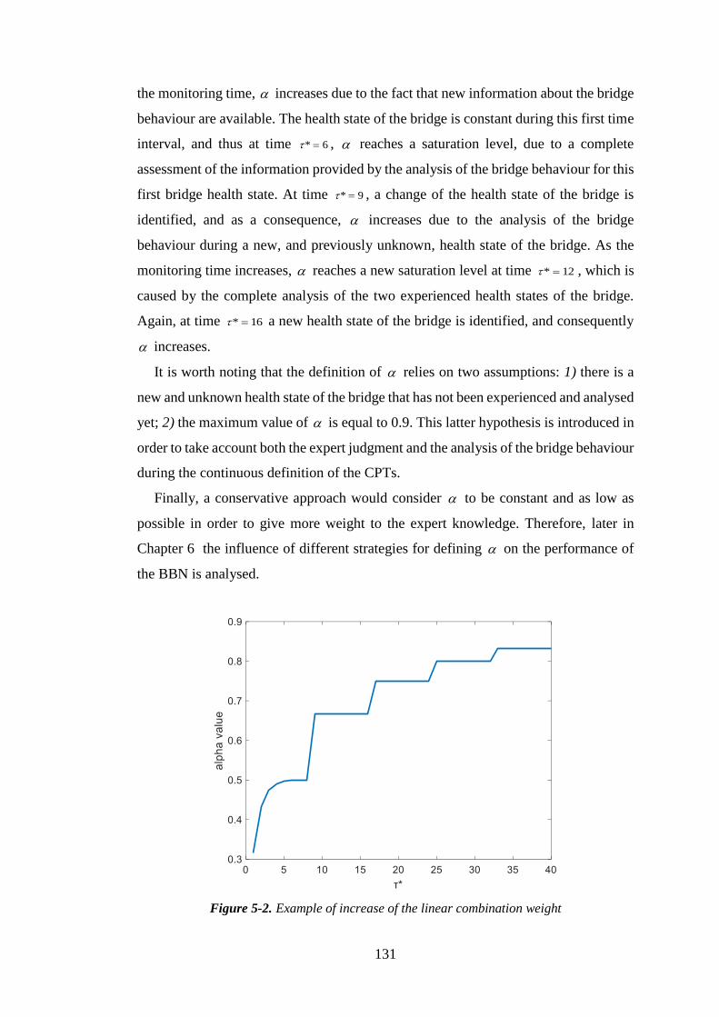
131

the monitoring time, increases due to the fact that new information about the bridge

behaviour are available. The health state of the bridge is constant during this first time

interval, and thus at time * 6 = , reaches a saturation level, due to a complete

assessment of the information provided by the analysis of the bridge behaviour for this

first bridge health state. At time * 9 = , a change of the health state of the bridge is

identified, and as a consequence, increases due to the analysis of the bridge

behaviour during a new, and previously unknown, health state of the bridge. As the

monitoring time increases, reaches a new saturation level at time * 12 = , which is

caused by the complete analysis of the two experienced health states of the bridge.

Again, at time * 16 = a new health state of the bridge is identified, and consequently

increases.

It is worth noting that the definition of relies on two assumptions: 1) there is a

new and unknown health state of the bridge that has not been experienced and analysed

yet; 2) the maximum value of is equal to 0.9. This latter hypothesis is introduced in

order to take account both the expert judgment and the analysis of the bridge behaviour

during the continuous definition of the CPTs.

Finally, a conservative approach would consider to be constant and as low as

possible in order to give more weight to the expert knowledge. Therefore, later in

Chapter 6 the influence of different strategies for defining on the performance of

the BBN is analysed.

Figure 5-2. Example of increase of the linear combination weight

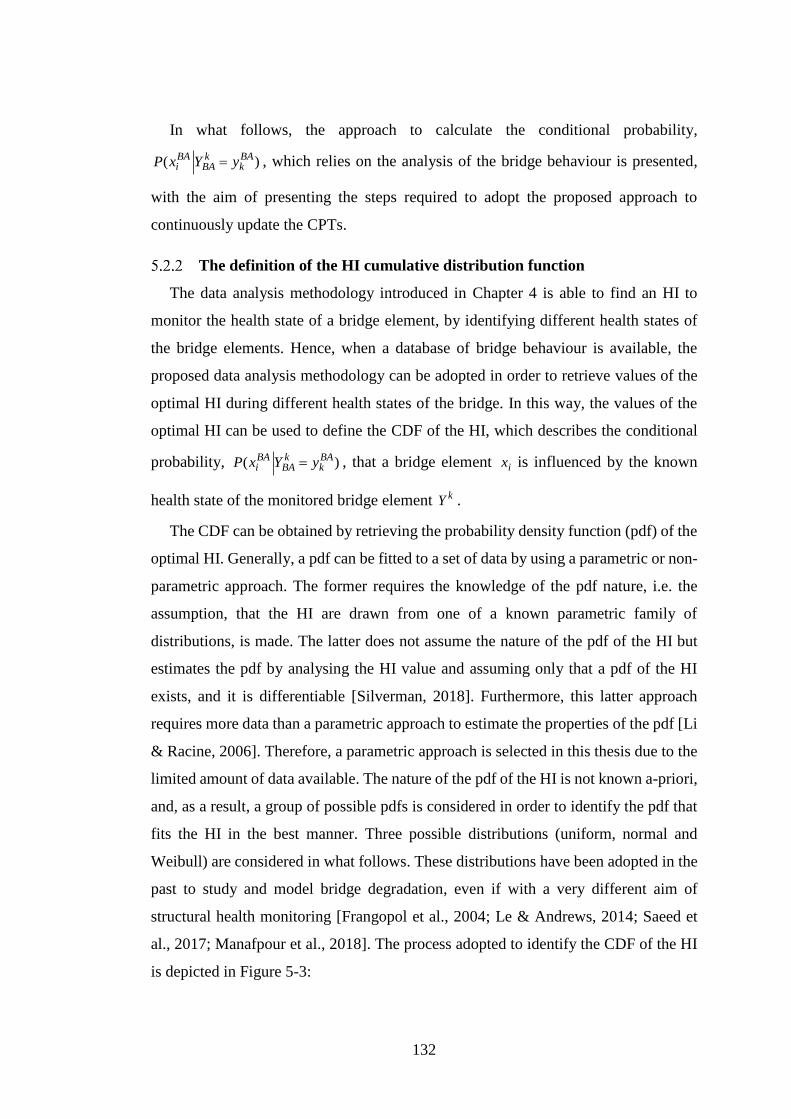
132

In what follows, the approach to calculate the conditional probability,

( )BA k BAi BA kP x Y y= , which relies on the analysis of the bridge behaviour is presented,

with the aim of presenting the steps required to adopt the proposed approach to

continuously update the CPTs.

The definition of the HI cumulative distribution function

The data analysis methodology introduced in Chapter 4 is able to find an HI to

monitor the health state of a bridge element, by identifying different health states of

the bridge elements. Hence, when a database of bridge behaviour is available, the

proposed data analysis methodology can be adopted in order to retrieve values of the

optimal HI during different health states of the bridge. In this way, the values of the

optimal HI can be used to define the CDF of the HI, which describes the conditional

probability, ( )BA k BAi BA kP x Y y= , that a bridge element ix is influenced by the known

health state of the monitored bridge element kY .

The CDF can be obtained by retrieving the probability density function (pdf) of the

optimal HI. Generally, a pdf can be fitted to a set of data by using a parametric or non-

parametric approach. The former requires the knowledge of the pdf nature, i.e. the

assumption, that the HI are drawn from one of a known parametric family of

distributions, is made. The latter does not assume the nature of the pdf of the HI but

estimates the pdf by analysing the HI value and assuming only that a pdf of the HI

exists, and it is differentiable [Silverman, 2018]. Furthermore, this latter approach

requires more data than a parametric approach to estimate the properties of the pdf [Li

& Racine, 2006]. Therefore, a parametric approach is selected in this thesis due to the

limited amount of data available. The nature of the pdf of the HI is not known a-priori,

and, as a result, a group of possible pdfs is considered in order to identify the pdf that

fits the HI in the best manner. Three possible distributions (uniform, normal and

Weibull) are considered in what follows. These distributions have been adopted in the

past to study and model bridge degradation, even if with a very different aim of

structural health monitoring [Frangopol et al., 2004; Le & Andrews, 2014; Saeed et

al., 2017; Manafpour et al., 2018]. The process adopted to identify the CDF of the HI

is depicted in Figure 5-3:

133

1) the three pdfs (uniform, normal and Weibull) are fitted to the available HIs

that are retrieved by analysing a database of bridge behaviour data. A

Maximum Likelihood Estimation (MLE) method is adopted to estimate

the parameters of each distribution;

2) the goodness of the fitting is assessed by evaluating the performance of

two criterion: i) the Akaike Information Criterion corrected (AICc)

[Akaike, 1974; Burnham & Anderson, 2004]; and ii) the quantile-quantile

(Q-Q) plot [Djurovic et al., 2000; Loy et al., 2016]. The two criteria are

selected due to their ability in comparing different fitting models when a

small dataset is used (AICc) and representing the goodness of each fitting

model graphically (Q-Q plot);

3) the pdf that outperforms the others in terms of AICc (i.e. the pdf with the

lowest AICc) and Q-Q plot is selected as a possible best available pdf;

4) the Kolmogorov-Smirnov test (K-S test) [Zeng et al., 2015] is adopted to

verify if the available sample of HI data can be described by the selected

best pdf. If the null hypothesis that the HI values belong to the selected pdf

is not rejected, then the pdf is verified as optimal and its CDF is assessed.

Otherwise, when the null hypothesis is rejected, the pdf with the second

lowest value of AICc is tested by using the K-S test. This process is

assumed to reliably identify a pdf to fit the HI data. In fact, a small

difference of the AIC value between two possible pdfs can show some

evidence that both pdfs perform a good fit [Burnham & Anderson, 2004].

The iterative process in Figure 5-3 is introduced due to the limited amount of data

available for this thesis, which can lead to misinterpretation of the selected pdf.

Therefore, the robustness of the pdf selection is expected to increase by evaluating the

performance of three criteria to assess the goodness of the fitting process.

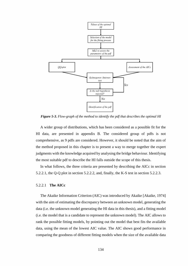
134

Figure 5-3. Flow-graph of the method to identify the pdf that describes the optimal HI

A wider group of distributions, which has been considered as a possible fit for the

HI data, are presented in appendix B. The considered group of pdfs is not

comprehensive, as 9 pdfs are considered. However, it should be noted that the aim of

the method proposed in this chapter is to present a way to merge together the expert

judgments with the knowledge acquired by analysing the bridge behaviour. Identifying

the most suitable pdf to describe the HI falls outside the scope of this thesis.

In what follows, the three criteria are presented by describing the AICc in section

5.2.2.1, the Q-Q plot in section 5.2.2.2, and, finally, the K-S test in section 5.2.2.3.

5.2.2.1 The AICc

The Akaike Information Criterion (AIC) was introduced by Akaike [Akaike, 1974]

with the aim of estimating the discrepancy between an unknown model, generating the

data (i.e. the unknown model generating the HI data in this thesis), and a fitting model

(i.e. the model that is a candidate to represent the unknown model). The AIC allows to

rank the possible fitting models, by pointing out the model that best fits the available

data, using the mean of the lowest AIC value. The AIC shows good performance in

comparing the goodness of different fitting models when the size of the available data

135

is large. However, when only few data are available the AIC shows incorrect

performance by usually choosing the model with the highest number of parameters

[Burnham & Anderson, 2004]. Hence, the AIC corrected (AICc) can be introduced in

order to take account of a low amount of data. Generally, AICc is recommended when

40n

k , where n is the number of available data from the unknown generating model

and k is the number of parameters of the fitting model (e.g. k= 2 for the normal

distribution, where the mean value and the standard deviation need to be evaluated to

represent the distribution) [Burnham & Anderson, 2004].

The AICc is defined as follows:

22 22 2ln( )

1

k kAICc k L

n k

+= − +

− − (5-3)

where k is the number of parameters of the fitting model, L the maximum likelihood

of the fitting model and n the number of available data. The correction factor is

represented by the last positive term of Eq. (5-3), which tends to zero as the number

of available data increases.

Eq. (5-3) shows that AICs depends linearly on the number of parameters of the

fitting model, k, and consequently, the higher the number of parameters of the fitting

parameters the higher the value of AICc. Therefore, AICc aims to reward fitting

models that are described by a low number of parameters.

5.2.2.2 The Q-Q plot

The Q-Q plot is probably the most commonly used graphical method to assess if a

set of data belongs to a specified distribution. The Q-Q plot aims to plot the sorted data

to be fitted, i.e. the data generated by the unknown model are sorted in an ascending

order, against the expected quantile of the theoretical specified distribution [Loy et al.,

2016]. Therefore, given a dataset of n values, e.g. the n values of the optimal HI in this

thesis, a Q-Q plot can be constructed by: i) sorting the n values in an ascending order,

i.e. from the smallest to the largest, in order to obtain the quantiles of the dataset to be

fitted; ii) finding the quantile of the theoretical specified distribution by dividing its

area into n+1 equally-sized areas, i.e. find the quantile of the theoretical distribution;

iii) plot the quantile of the data (y-axis) against the quantile of the theoretical specified

136

distribution (x-axes). If the plotted points belong to a straight line y x= , then the data

can be represented by the selected distribution, i.e. if Q-Q plot shows a linear

behaviour, the selected distribution fits the data accurately [Djurovic et al., 2000].

5.2.2.3 The K-S test

The K-S test is a nonparametric test that aims to verify the null hypothesis that a

dataset belongs to a selected CDF [Zeng et al., 2015]. Given a dataset of n data, the K-

S test is carried out as follows:

• Define the null hypothesis (H0) that the n data are described by a specified CDF

*G . Therefore, if H0 is not rejected, the n data actually belong to the specified

CDF.

• Find the empirical CDF, ( )o iF n , of the n data of the dataset, by considering

that for any value ni of the dataset, ( )o iF n is proportional to the number of data

of the dataset having a value lower or equal to ni. Formally, the empirical CDF,

( )o iF n , is obtained as follows:

1

1

0,

( ) ,

1,

i

paro i par i par

i N

if n n

nF n if n n n

n

if n n

+

=

(5-4)

where n1 is the lowest value of the dataset, npar is any data of the database

between the minimum and maximum dataset value, and nN is the maximum

value of the dataset.

• Assess the K-S test statistic, D, which is defined as:

( )1

*sup ( ) ( )

i N

on n n

D F n G n

= − (5-5)

Eq. (5-5) shows that the K-S test statistic is equal to the maximum (vertical)

distance between the empirical CDF, ( )o iF n , and the specified CDF *G .

• Compare the computed K-S test statistic with the critical value of the K-S test

statistics, D*, which is obtained from tables defined in literature, for specified

137

CDF and significance level sl . In this thesis, a significance level of 5% is

chosen, due to the fact that 0.005sl = is commonly adopted. The null

hypothesis H0 is rejected if the computed H-S test statistics D is greater than

the critical value D*, i.e. if D>D*, and, as a consequence, the p-value of the

dataset is lower than the significance level. Otherwise, if the null hypothesis is

not rejected, the data belong to the hypothesized CDF, *G , which can be then

used to fit the data and model the system under study.

The K-S test allows to find out whether if the data belong to a specified CDF.

In what follows, the proposed method for continuously updating the CPTs of an BBN

is applied to the post-tensioned concrete bridge, which was presented in Chapter 4.

Analysis of the HI of the post-tensioned bridge

The data of the first group (group 1) of the post-tensioned concrete bridge are used

as an input to the data analysis methodology presented in Chapter 4 , with the aim of

retrieving the optimal HIs to monitor the condition of the bridge elements over time.

The analysis of the bridge behaviour in Chapter 4 showed that two optimal HIs are

able to point out the different health states of the bridge elements clearly: the HI3 of

the Kurtosis of the free vibration of the bridge, and HI3 of the frequency of the

estimated first harmonic of the bridge. In what follows, only the HI3 of the Kurtosis of

the free vibration of the bridge, which is the HI of the bridge that shows the highest GI

index, is considered in order to monitor the evolution of the health state of the bridge

elements. The adoption of a single HI allows to have a simpler method for bridge

condition monitoring, rather than using two (or more) HIs. However, a single HI can

increase the number of misclassifications of assessment of the bridge health state, due

to oscillations of the HI, which could be damped by using two (or more) HIs to monitor

the bridge health state.

The health states of the bridge, which have been introduced in section 4.3.1, are

grouped as depicted in Figure 5-4: a) the data of the HI3 of the Kurtosis of class 1, i.e.

the healthy state of the bridge, represent the healthy state of the bridge, as shown by

the solid box in Figure 5-4; b) the data of HI3 of the Kurtosis of class 3 and class 4, i.e.

when the pier of the bridge has been cut by 10cm and the deck has been lowered by 1

cm (class 4), represent a partially degraded health state of the bridge, as shown by the

dotted box in Figure 5-4; and c) the data of HI3 of the Kurtosis of class 5 and class 6,

i.e. when the pier of the bridge has been cut by 10 cm and the deck has been lowered

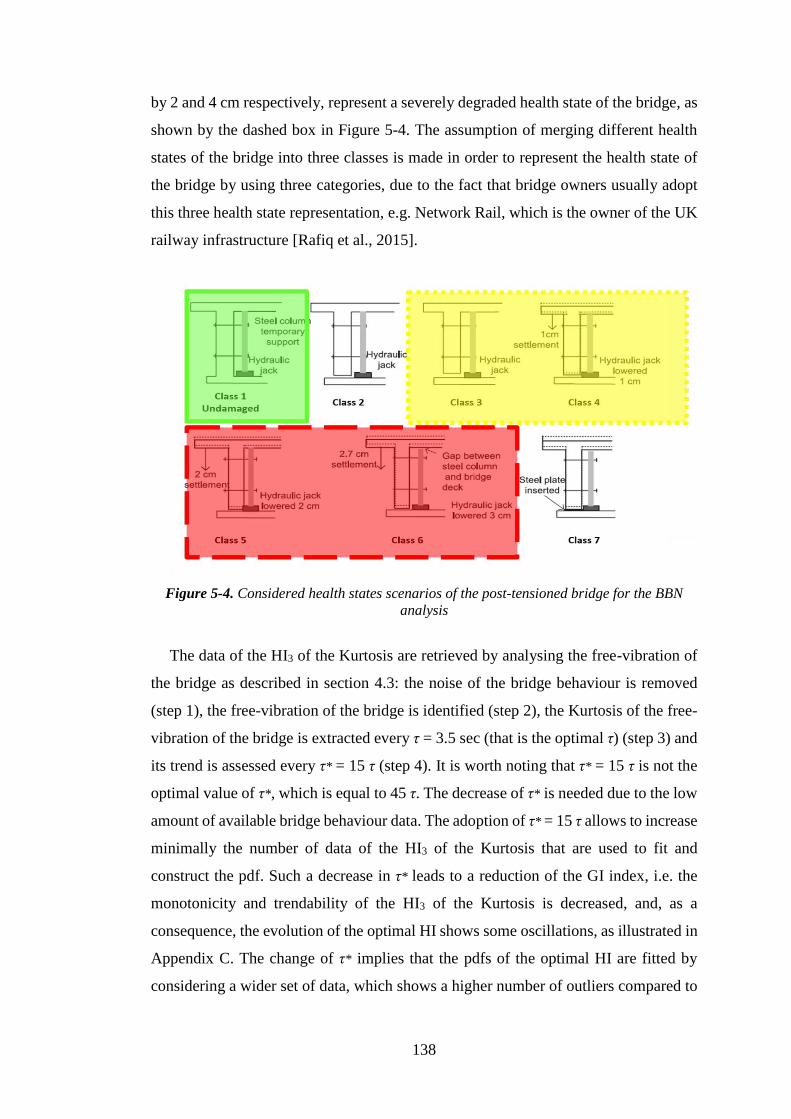
138

by 2 and 4 cm respectively, represent a severely degraded health state of the bridge, as

shown by the dashed box in Figure 5-4. The assumption of merging different health

states of the bridge into three classes is made in order to represent the health state of

the bridge by using three categories, due to the fact that bridge owners usually adopt

this three health state representation, e.g. Network Rail, which is the owner of the UK

railway infrastructure [Rafiq et al., 2015].

Figure 5-4. Considered health states scenarios of the post-tensioned bridge for the BBN

analysis

The data of the HI3 of the Kurtosis are retrieved by analysing the free-vibration of

the bridge as described in section 4.3: the noise of the bridge behaviour is removed

(step 1), the free-vibration of the bridge is identified (step 2), the Kurtosis of the free-

vibration of the bridge is extracted every τ = 3.5 sec (that is the optimal τ) (step 3) and

its trend is assessed every τ* = 15 τ (step 4). It is worth noting that τ* = 15 τ is not the

optimal value of τ*, which is equal to 45 τ. The decrease of τ* is needed due to the low

amount of available bridge behaviour data. The adoption of τ* = 15 τ allows to increase

minimally the number of data of the HI3 of the Kurtosis that are used to fit and

construct the pdf. Such a decrease in τ* leads to a reduction of the GI index, i.e. the

monotonicity and trendability of the HI3 of the Kurtosis is decreased, and, as a

consequence, the evolution of the optimal HI shows some oscillations, as illustrated in

Appendix C. The change of τ* implies that the pdfs of the optimal HI are fitted by

considering a wider set of data, which shows a higher number of outliers compared to

139

the optimal value of τ*. However, the different health states of the bridge can be still

pointed out by using this definition of τ*.

In what follows, the data of HI3 of the Kurtosis are used to estimate the parameters

of the three pdfs, and then the goodness of the fit is evaluated in order to identify the

optimal CDF to update the CPTs of the BBN.

The assessment of AICc and Q-Q plot

The three considered models (uniform, normal and Weibull) are adopted as possible

distributions to fit the data of the optimal HI. Therefore, the possibility that the optimal

HI is described by one of these three CDF is investigated. The data of each health state

of the bridge elements, i.e. healthy state, partially degraded and severely degraded

states of the bridge elements, are used as an input to the MLE algorithm in order to

assess the parameters of each model. As a result, three pdfs for each health state of the

bridge are fitted. The goodness-of-fit process is analysed by assessing the AICc of the

three pdfs for each health state of the bridge elements. Similarly, the Q-Q plot of the

three pdfs for each health state of the bridge elements is analysed in order to

graphically point out which selected pdf fits the data in the best manner.

Figure 5-5 shows the three pdfs fitted on the HI values retrieved by analysing the

bridge behaviour provided by sensor A. Figure 5-5a, i.e. the three Q-Q plots on the top

within the solid line box, represents the analysis of the HI of the healthy bridge. The

uniform distribution shows the lowest AICc and almost linear behaviour on its Q-Q

plot, with a small deviation from the linearity at the centre of the HI data, i.e. at the

middle of the Q-Q plot. The Weibull distribution shows the second lowest AICc, but

its Q-Q plot departs from the linearity at high values of the HI. Finally, the normal

distribution shows the highest AICc and almost linear behaviour on its Q-Q plot. The

analysis of Figure 5-5a shows that the uniform distribution seems to be the distribution

that fits the HI values in the best possible way. However, the AICc of the three

distributions is similar, and thus the K-S test needs to be adopted in order to verify

whether the HI values really belong to the uniform distribution.

Similarly, Figure 5-5b, i.e. the three Q-Q plots on the middle within the dotted line

box, represents the analysis of the HI of the partially degraded bridge. Again, the

normal distribution shows the lowest AICc and a linear behaviour on its Q-Q plot,

whereas the Weibull distribution shows the second lowest AICc and non-linear

behaviour of the Q-Q plot for large values of the HI. Finally, the normal distribution

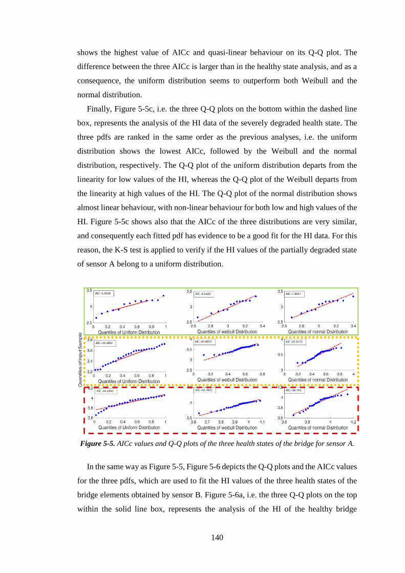
140

shows the highest value of AICc and quasi-linear behaviour on its Q-Q plot. The

difference between the three AICc is larger than in the healthy state analysis, and as a

consequence, the uniform distribution seems to outperform both Weibull and the

normal distribution.

Finally, Figure 5-5c, i.e. the three Q-Q plots on the bottom within the dashed line

box, represents the analysis of the HI data of the severely degraded health state. The

three pdfs are ranked in the same order as the previous analyses, i.e. the uniform

distribution shows the lowest AICc, followed by the Weibull and the normal

distribution, respectively. The Q-Q plot of the uniform distribution departs from the

linearity for low values of the HI, whereas the Q-Q plot of the Weibull departs from

the linearity at high values of the HI. The Q-Q plot of the normal distribution shows

almost linear behaviour, with non-linear behaviour for both low and high values of the

HI. Figure 5-5c shows also that the AICc of the three distributions are very similar,

and consequently each fitted pdf has evidence to be a good fit for the HI data. For this

reason, the K-S test is applied to verify if the HI values of the partially degraded state

of sensor A belong to a uniform distribution.

Figure 5-5. AICc values and Q-Q plots of the three health states of the bridge for sensor A.

In the same way as Figure 5-5, Figure 5-6 depicts the Q-Q plots and the AICc values

for the three pdfs, which are used to fit the HI values of the three health states of the

bridge elements obtained by sensor B. Figure 5-6a, i.e. the three Q-Q plots on the top

within the solid line box, represents the analysis of the HI of the healthy bridge

141

provided by sensor B. The Weibull distribution shows the lowest AICc, even though

its Q-Q plot shows non-linear behaviour at low values of HI. The uniform distribution

provides the second lowest AICc and almost linear Q-Q plot, and the normal

distribution shows the highest AICc and a Q-Q plot that departs from the linearity at

low values of the HI. Figure 5-6a suggests that the Weibull distribution is the pdf that

best fits the HI values for the healthy state of the bridge recorded by sensor B.

However, the three AICc values are close, and therefore the K-S test needs to be

applied in order to verify if these HI values can be represented by a Weibull

distribution.

Figure 5-6b and Figure 5-6c, i.e. the three Q-Q plots in the middle within the dotted

line box and the three Q-Q plots on the bottom within the dashed line box, respectively,

show the analysis of the HI values for the partially degraded and the severely degraded

health states. In both health states of the bridge elements, the uniform distribution

shows the lowest AICc and almost linear behaviour in the Q-Q plot, whereas the

partially degraded health states (Figure 5-6b) show a departure from the linearity on

the middle of the Q-Q plot. The Weibull distribution provides the second lowest values

of AICc in both Figure 5-6b and Figure 5-6c. However, the analysis of the partially

degraded health state of the bridge in Figure 5-6b shows that the AICc of the Weibull

distribution is much higher than the AICc of the uniform distribution. Furthermore,

the Q-Q plot of the Weibull in Figure 5-6b depicts a departure from the linearity at

high values of the HI. As a result, the uniform distribution seems to outperform the

other two distributions in terms of fitting model for the partially degraded health state

values. The K-S test in the next section would verify if the HI of this health state of

the bridge can be effectively represented by the uniform distribution. Finally, the AICc

of the pdfs in Figure 5-6c is similar, and thus the K-S test will help in assessing which

pdf allows to fit the HI vales in the best way.

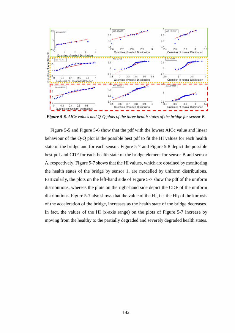
142

Figure 5-6. AICc values and Q-Q plots of the three health states of the bridge for sensor B.

Figure 5-5 and Figure 5-6 show that the pdf with the lowest AICc value and linear

behaviour of the Q-Q plot is the possible best pdf to fit the HI values for each health

state of the bridge and for each sensor. Figure 5-7 and Figure 5-8 depict the possible

best pdf and CDF for each health state of the bridge element for sensor B and sensor

A, respectively. Figure 5-7 shows that the HI values, which are obtained by monitoring

the health states of the bridge by sensor 1, are modelled by uniform distributions.

Particularly, the plots on the left-hand side of Figure 5-7 show the pdf of the uniform

distributions, whereas the plots on the right-hand side depict the CDF of the uniform

distributions. Figure 5-7 also shows that the value of the HI, i.e. the HI3 of the kurtosis

of the acceleration of the bridge, increases as the health state of the bridge decreases.

In fact, the values of the HI (x-axis range) on the plots of Figure 5-7 increase by

moving from the healthy to the partially degraded and severely degraded health states.

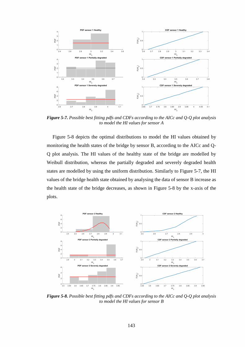
143

Figure 5-7. Possible best fitting pdfs and CDFs according to the AICc and Q-Q plot analysis

to model the HI values for sensor A

Figure 5-8 depicts the optimal distributions to model the HI values obtained by

monitoring the health states of the bridge by sensor B, according to the AICc and Q-

Q plot analysis. The HI values of the healthy state of the bridge are modelled by

Weibull distribution, whereas the partially degraded and severely degraded health

states are modelled by using the uniform distribution. Similarly to Figure 5-7, the HI

values of the bridge health state obtained by analysing the data of sensor B increase as

the health state of the bridge decreases, as shown in Figure 5-8 by the x-axis of the

plots.

Figure 5-8. Possible best fitting pdfs and CDFs according to the AICc and Q-Q plot analysis

to model the HI values for sensor B

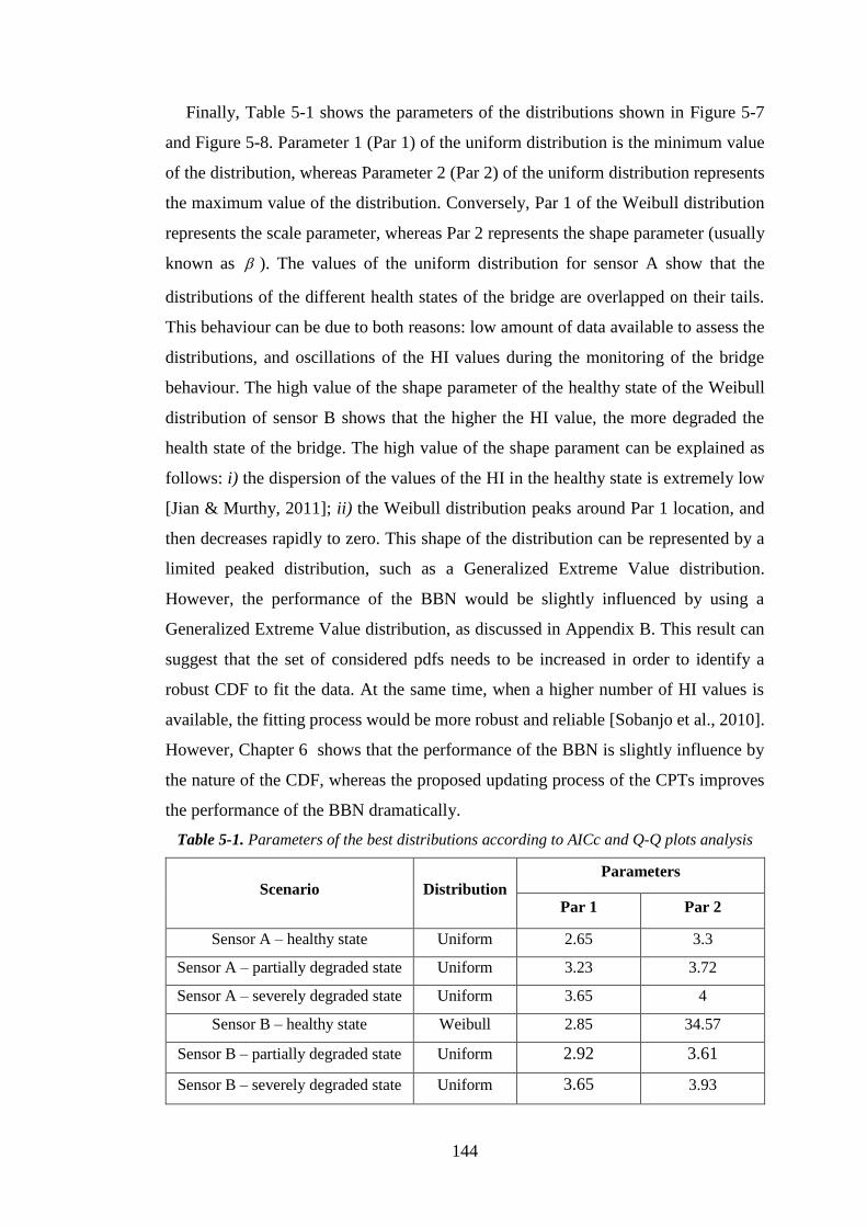
144

Finally, Table 5-1 shows the parameters of the distributions shown in Figure 5-7

and Figure 5-8. Parameter 1 (Par 1) of the uniform distribution is the minimum value

of the distribution, whereas Parameter 2 (Par 2) of the uniform distribution represents

the maximum value of the distribution. Conversely, Par 1 of the Weibull distribution

represents the scale parameter, whereas Par 2 represents the shape parameter (usually

known as ). The values of the uniform distribution for sensor A show that the

distributions of the different health states of the bridge are overlapped on their tails.

This behaviour can be due to both reasons: low amount of data available to assess the

distributions, and oscillations of the HI values during the monitoring of the bridge

behaviour. The high value of the shape parameter of the healthy state of the Weibull

distribution of sensor B shows that the higher the HI value, the more degraded the

health state of the bridge. The high value of the shape parament can be explained as

follows: i) the dispersion of the values of the HI in the healthy state is extremely low

[Jian & Murthy, 2011]; ii) the Weibull distribution peaks around Par 1 location, and

then decreases rapidly to zero. This shape of the distribution can be represented by a

limited peaked distribution, such as a Generalized Extreme Value distribution.

However, the performance of the BBN would be slightly influenced by using a

Generalized Extreme Value distribution, as discussed in Appendix B. This result can

suggest that the set of considered pdfs needs to be increased in order to identify a

robust CDF to fit the data. At the same time, when a higher number of HI values is

available, the fitting process would be more robust and reliable [Sobanjo et al., 2010].

However, Chapter 6 shows that the performance of the BBN is slightly influence by

the nature of the CDF, whereas the proposed updating process of the CPTs improves

the performance of the BBN dramatically.

Table 5-1. Parameters of the best distributions according to AICc and Q-Q plots analysis

Scenario Distribution Parameters

Par 1 Par 2

Sensor A – healthy state Uniform 2.65 3.3

Sensor A – partially degraded state Uniform 3.23 3.72

Sensor A – severely degraded state Uniform 3.65 4

Sensor B – healthy state Weibull 2.85 34.57

Sensor B – partially degraded state Uniform 2.92 3.61

Sensor B – severely degraded state Uniform 3.65 3.93

145

In what follows, the K-S test is applied to the possible best pdf for each health state

of the bridge of each sensor, i.e. the pdf that provides the best AICc value is assumed

to be the best pdf, and this hypothesis is verified by the means of the K-S test.

The K-S test to verify the hypothesis of using the best fitting pdf

The CDF of Figure 5-7 and Figure 5-8 are used as an input to the K-S test in order

to verify if the HI values can be represented by the considered CDF. Hence, the K-S

test is carried out for each health state of the bridge and each sensor, by assuming that

for each health state of each sensor, its HI values belong to the corresponding CDF

shown in Figure 5-7 and Figure 5-8.

The K-S test verifies the null hypothesis (H0) that the HI values of the specified

health state of the bridge follow the selected CDF. If H0 is not rejected, then the HI

values can be modelled by the CDF shown in Figure 5-7 and Figure 5-8. Otherwise,

the distribution with the second lowest AICc is used to describe the HI values, and the

K-S test is then performed again in order to test if the HI values follow the second

ranked distribution (in terms of AICc value).

Table 5-2 shows the results of the K-S test for each health state and for both sensors

at a significance level of 5%. The null hypothesis that the HI values of the healthy state

of the bridge follow a uniform distribution (sensor A) and a Weibull distribution

(sensor B) is not rejected (p-values higher than the significance level for both cases),

and thus the CDF of the healthy state depicted in Figure 5-7 and Figure 5-8 are used

to model the HI during the healthy state of the bridge. Similarly, the null hypothesis

that the HI values of sensor A of the partially degraded health state of the bridge

elements follow a uniform distribution is not rejected, by obtaining a p-value higher

than the significance level. Therefore, the uniform distribution shown in Figure 5-7 is

adopted to model the HI of the partially degraded health state for sensor A.

The null hypothesis that the HI values of the severely degraded state for sensor A

follows a uniform distribution is rejected (p-value lower than the significance level),

as well as the null hypothesis that the HI values of the partially and severely degraded

states for sensor B follow the uniform distributions. For these three scenarios, the

values of the HI are then assumed to follow the distribution that shows the second

lowest AICc, i.e. the Weibull distribution for all scenarios. The K-S test is performed

146

again for these three cases, in order to verify if the HI values follows the Weibull

distribution.

Table 5-2. K-S test results for the CDFs with the lowest value of AICc

Scenario H0 p-value

Sensor A – healthy state Not rejected 0.4144

Sensor A – partially degraded state Not rejected 0.2931

Sensor A – severely degraded state Rejected 0.0401

Sensor B – healthy state Not rejected 0.9121

Sensor B – partially degraded state Rejected 0.0002

Sensor B – severely degraded state Rejected 0.0496

Table 5-3 shows the results of the K-S test for the HI values of the three health

states that are rejected in Table 5-2. For each scenario, the null hypothesis (H0) is that

the HI values of the three health states of the bridge belong to Weibull distribution,

which is the distribution with the second lowest AICc. The null hypothesis (H0) is not

rejected in all three cases, due to the fact that the p-values are higher than the

significance level. As a result, the HI values of the degraded health state of the bridge

shown in Table 5-3 follow Weibull distribution. The pdfs and CDF of Figure 5-7 and

Figure 5-8 need thus to be updated in order to take account of the K-S test results.

Table 5-3. K-S results for the CDFs with the second lowest value of AICc

Scenario H0 p-value

Sensor A – severely degraded state Not rejected 0.7544

Sensor B – partially degraded state Not rejected 0.0790

Sensor B – severely degraded state Not rejected 0.4125

Figure 5-9 and Figure 5-10 show the possible best pdf and CDF for the HI values

of each health state of the bridge for sensor A and sensor B, respectively, by accounting

for the results of the K-S test. Figure 5-9 shows that the HI values of the partially

degraded health state obtained by monitoring the health states of the bridge by sensor

A are modelled by the Weibull distributions. The HI values of the healthy state and

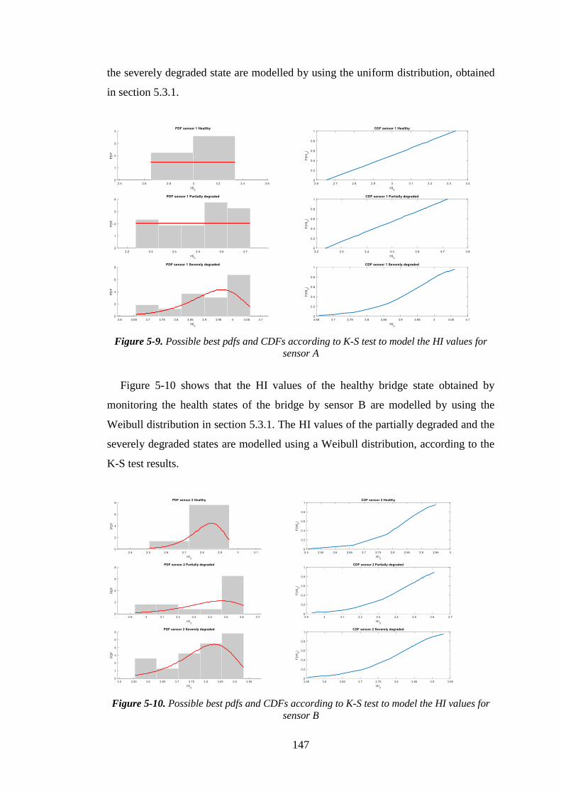
147

the severely degraded state are modelled by using the uniform distribution, obtained

in section 5.3.1.

Figure 5-9. Possible best pdfs and CDFs according to K-S test to model the HI values for

sensor A

Figure 5-10 shows that the HI values of the healthy bridge state obtained by

monitoring the health states of the bridge by sensor B are modelled by using the

Weibull distribution in section 5.3.1. The HI values of the partially degraded and the

severely degraded states are modelled using a Weibull distribution, according to the

K-S test results.

Figure 5-10. Possible best pdfs and CDFs according to K-S test to model the HI values for

sensor B

148

Table 5-4 shows the values of the parameters of the best distribution according to

the K-S test. The distributions of the healthy state for both sensors of the partially

degraded state for sensor A are the same as in section 5.3.1. The distributions of the

severely degraded state for both sensors and of the partially degraded state for sensor

B are modified to Weibull distributions. Again, the high value of the shape parameter

shows that the health state of the bridge decreases when the HI value increases.

Furthermore, such high value of the shape parameter leads to a distribution that peaks

at the location of Par 1, and then decrease suddenly to zero. The high value of the shape

parameter can be caused by the low variability of the small set of HI data and due to a

non-optimal selection of the set of the pdfs, which, however, influences the

performance of the BBN slightly.

It is worth mentioning that, when more data of the bridge behaviour are available,

the fitting process needs to be performed again, in order to point out the distribution

of the optimal HI in a more reliable manner.

Table 5-4. Parameters of the best distributions according to the K-S test

Scenario Distribution Parameters

Par 1 Par 2

Sensor A – healthy state Uniform 2.65 3.3

Sensor A – partially degraded state Uniform 3.23 3.72

Sensor A – severely degraded state Weibull 3.96 46.68

Sensor B – healthy state Weibull 2.85 34.57

Sensor B – partially degraded state Weibull 3.47 21.11

Sensor B – severely degraded state Weibull 3.83 45.92

In what follows, the CDF of both Table 5-1 and Table 5-4 are used to update the

CPTs in order to compare the performance of the BBN when different CDFs are

adopted.

Summary of the proposed method to merge expert judgment and

bridge behaviour analysis

A method to merge the expert elicitation process with the analysis of the bridge

behaviour is proposed, with the aim of updating the CPTs of a BBN in a reliable and

149

continuous manner. The CPT values are updated by considering an weighted

combination of the expert knowledge and the bridge behaviour analysis. The expert

knowledge elicitation process and the bridge behaviour analyses are carried out off-

line in order to initially define the CPTs and identify a set of CDFs to model the optimal

HI of the bridge elements, respectively. The expert knowledge process has been

discussed in section 3.3.2. The assessment of the CDF of the HI that monitors the

health state of the bridge elements is proposed by analysing the HI of different health

state of the bridge elements. Particularly, for each health state of the bridge elements,

its HI values are fitted to a set of three possible pdfs, and the goodness-of-fit process

is then evaluated. The AICc index and Q-Q plot approaches are used to select the pdf

that fits the HI values in the best manner. The selected pdf is then verified by adopting

a K-S test, which aims to verify if the HI values belongs to the specified distribution.

The low amount of available data of HI led to different results, i.e. the distributions

selected by analysing the AICc and the Q-Q plot are not verified by using the K-S test.

Therefore, in the following of the thesis both distributions are adopted as an input to

the CPTs of the BBN in order to take account of the uncertainties in the CDF

distributions and to analyse how different CDFs influence the performance of the

BBN.

The presented method shows some drawbacks:

• the weight of the combination is defined by considering that the bridge

behaviour data can give more reliable information than the expert knowledge.

Therefore, the higher the amount of data of the bridge behaviour, the higher

and the more important the analysis of the bridge behaviour. As a consequence,

the importance of the information provided by the expert knowledge process

decreases over time, due to the fact that the monitoring process of the bridge

provides more and more data. However, a conservative approach would

suggest giving more importance to the expert knowledge, as the experts can

investigate what-if scenarios and the analysis of the bridge behaviour data

depends on the quality of the available data. In the following of the thesis,

different strategies for the definition of are investigated, with the aim of

assessing how the performance of the BBN is affected.

• the fitting process to identify the best CDF is carried out with a parametric

approach and a small amount of data. The parametric approach considered only

150

three different CDFs (9 CDFs considering also Appendix B). As a result, the

optimal CDF to describe the optimal HI values might not be considered within

the group of 9 CDFs. Therefore, future work should analyse how to identify

the best CDF to model the HI of the bridge elements, in order to model the

bridge behaviour changes in a reliable manner.

• the analysis of the bridge behaviour data assumes that the health state of the

bridge is known a-priori, i.e. the data of bridge behaviour are labelled in order

to point out the health state of the bridge at that moment. However, the health

state of the bridge is not always known a-priori and such labels might be

unavailable. As a consequence, a method to analyse database of infrastructure

behaviour is needed in order to point out the changes of the health state of the

infrastructure. In this way, this information can be used as an input to the

proposed method with the aim of updating the definition of the CPTs of the

BBN. Such a method is proposed in the following section. Furthermore, data

of a damaged bridge is not usually available, and it might require the adoption

of an FEM to retrieve data of the bridge behaviour.

In what follows, a method to analyse unknown database of infrastructure behaviour

is presented in order to assess changes of the health state of the infrastructure, and

investigate the characteristics of such changes.

A method to data-mine the behaviour of the infrastructure

Introduction

SHM systems generate a large amount of data and, as a consequence, processing

and interpreting this data can be difficult and time consuming. Particularly, when

decision makers need to analyse a database of infrastructure behaviour in order to

analyse the past behaviour of an infrastructure, robust data mining techniques are

required to analyse this data automatically, accurately and rapidly [Duan and Zhang,

2006]. Indeed, data mining techniques are able to transform the recorded data into

valuable information for decision makers, by pointing out past changes of the health

states of the infrastructure.

In this thesis, an ensemble-based data mining method is proposed in order to detect

the past unexpected behaviour of civil infrastructure. The proposed method relies on

an ensemble-based change-point detection analysis, which aims to identify the time

when the infrastructure behaviour starts to change rapidly and point out the duration

151

of the health state change. The ensemble-based change-point detection method is

needed due to the fact that single change-point methods, such as Cumulative Sum

(CUSUM)-based [Carslaw et al., 2006] or probability distributions-based [Liu et al.,

2013] methods, are able to detect only abrupt changes in the data, without pointing out

the most severe changes. Furthermore, the longer the duration of the monitored

behaviour of the system, the higher the number of the abrupt changes, which are

identified by an individual change-point method. Thus, the most severe change in the

data can be lost among all the change-points [Killick et al., 2012]. Individual change-

point methods are also usually unable to identify the duration of the most critical

system behaviour. Conversely, the proposed ensemble-based of change-point methods

is able to identify the most critical change in the data, by highlighting its start and end

time. In this way, only the information regarding the most critical behaviour of the

tunnel is provided to the decision maker.

In what follows, the proposed data mining method is presented. First of all, the

proposed method would be applied to the HI of a bridge infrastructure. Then, the past

bridge behaviour would be analysed to identify the HIs of the bridge health state over

time, and the optimal HI, which is the HI with the highest GI, would be analysed by

the proposed data mining method in order to detect changes of the HI pattern.

Therefore, when the HI changes, the health state of the bridge changes accordingly. In

this way, different health state of the bridge can be identified and analysed. However,

low amount of data about bridge behaviour was available for this study, and, as a

consequence, the proposed data mining method was tested on a different case study of

a railway tunnel. Furthermore, the case study considered in this thesis showed the

potential of the proposed method, which can be applied to every system that has

monotonic behaviour as the degradation increases.

For these reasons, the proposed data mining method is applied to a real in-field

railway tunnel, which is subject to renewal activities. As described also above, this

case study is selected due to the limitation of the scarce amount of bridge behaviour

data, and due to the needs of the industrial collaborator, AECOM, to analyse a database

of tunnel behaviour in order to detect when the health state of the tunnel changes.

Indeed, the tunnel data shows noisy measurements that are caused by the working

activities, and the decision makers need information about the changes of the tunnel

health states rapidly, in order to guarantee the safety of the asset and the workforce.

152

The content of this chapter has been published in “Tunnelling and Underground Space

Technology Journal” with the aim of proposing a novel ensemble-based change point

detection method for identifying changes of infrastructure health state [Vagnoli &

Remenyte-Prescott, 2018]. Particularly, section 5.5.2 and section 5.5.3 are extracted

from [Vagnoli & Remenyte-Prescott, 2018].

The proposed ensemble-based change-point detection method

Change-point methods aim to identify the exact moment when the monitored

variable of a system starts to deviate abruptly from an equilibrium level. Change-point

detection algorithms are adopted in several frameworks, such as SHM and prognosis

of gas turbines [Maleki et al., 2016], variation of air pollution concentration [Carslaw

et al., 2006], variation of climate parameters in order to monitor climate change

characteristics [Reeves et al., 2007], failure of pipes in chemical industries [Tickle et

al., 2010]. However, change-point methods are usually unable to point out the most

critical change-point clearly, i.e. the change-point where the monitored variable

experiences the highest variation. In fact, the most critical change point is identified

among all the change-points of the system. The duration of the unexpected changes is

also not assessed. Furthermore, the choice of an individual change-point algorithm can

jeopardize the reliability and robustness of the data analysis, due to different results of

the individual change-point detection methods.

In this thesis, a novel ensemble-based change-point method is proposed to analyse

database of infrastructure behaviour, by coupling the performance of four individual

change-points methods. In this way, the proposed ensemble-based method is able to

point out the most critical change-point of the infrastructure, providing its duration

and, eventually, possible causes. As a consequence, the reliability and robustness of

the data mining analysis are expected to improve accordingly. Decision makers can

then schedule future monitoring and work activities by using the results of the

ensemble-based change-point method.

In what follows, the theoretical background of the four individual change-point

algorithms is presented briefly in section 5.5.2.1, and then the proposed ensemble-

based method is introduced in section 5.5.2.2.

153

5.5.2.1 Change-point methods: theoretical background

The change-point analysis can be divided in two groups - real-time and

retrospective detection: the former aims to identify a change-point of system behaviour

as soon as it occurs; the latter aims to identify a change-point of system behaviour by

analysing the history of the monitored parameter. The focus in this thesis is on the

retrospective change-point analysis, which usually provides a more robust and

accurate detection than the real-time analysis [Liu et al., 2013]. Particularly, the aim is

to identify the most critical change-point of the system health state, by assessing its

duration and diagnosing its possible causes. In order to achieve this aim, an ensemble-

based change-point method is developed by coupling the performance of four of the

most commonly adopted change-point algorithms: i) a change-point detection method

that relies on a relative probability density ratio, which is computed by using the

Relative Unconstrained Least-Squares Importance Fitting (RuLSIF) [Liu et al., 2013].

The RuLSIF method has demonstrated to provide very good results in identifying

change-points through the assessment of a relative probability density-ratio; ii) a

Cumulative Sum (CUSUM) change-point detection algorithm [Carslaw et al., 2006].

The CUSUM is one of the most popular change-point method that has been adopted

in many different research framework, such as air pollution concentration [Carslaw et

al., 2006], failures of computer networks [Montes De Oca et al., 2010], functionality

of animal brain activity [Koepcke et al., 2016]; iii) a change-point detection method

that relies on the identification of changes of the mean value of the monitored system

behaviour, by defining a penalty cost function [Lavielle, 2005]; iv) a change-point

detection method that relies on the identification of changes of the slope of the

monitored system behaviour, by using a Pruned Exact Linear Time (PELT) method

[Killick et al., 2012]. The change-point methods iii) and iv), which rely on the same

theoretical basis, have been chosen due to their efficiency and low computational

burdensome. Indeed, as the length of the monitored parameters increases, the number

of possible change-points also increases, and thus an efficient and fast detection of

change-point is needed [Harchaoui and Levy-Leduc, 2010; Killick & Eckley, 2014].

A brief description of each individual change-point detection method is presented

in what follows, by discussing the RuLSIF method in section 0, the CUSUM in section

0, the mean-based change-point detection in section 0 and the PELT-based change-

point detection method in section 0.

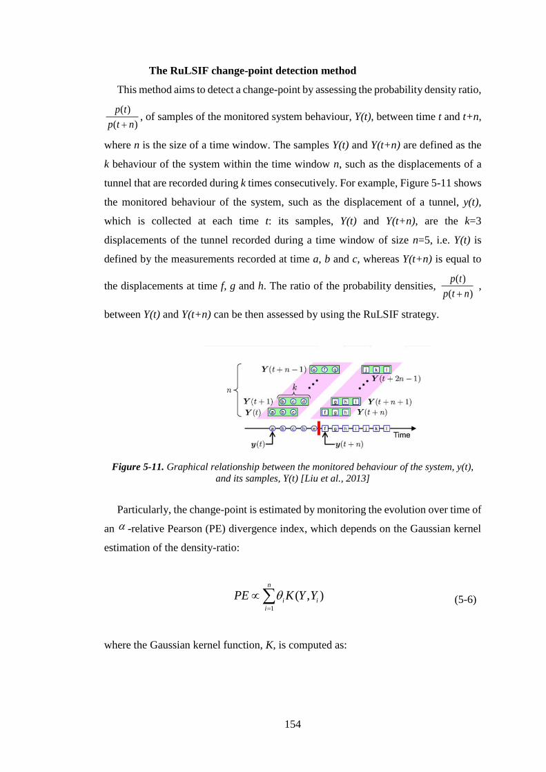
154

The RuLSIF change-point detection method

This method aims to detect a change-point by assessing the probability density ratio,

( )

( )

p t

p t n+, of samples of the monitored system behaviour, Y(t), between time t and t+n,

where n is the size of a time window. The samples Y(t) and Y(t+n) are defined as the

k behaviour of the system within the time window n, such as the displacements of a

tunnel that are recorded during k times consecutively. For example, Figure 5-11 shows

the monitored behaviour of the system, such as the displacement of a tunnel, y(t),

which is collected at each time t: its samples, Y(t) and Y(t+n), are the k=3

displacements of the tunnel recorded during a time window of size n=5, i.e. Y(t) is

defined by the measurements recorded at time a, b and c, whereas Y(t+n) is equal to

the displacements at time f, g and h. The ratio of the probability densities, ( )

( )

p t

p t n+ ,

between Y(t) and Y(t+n) can be then assessed by using the RuLSIF strategy.

Figure 5-11. Graphical relationship between the monitored behaviour of the system, y(t),

and its samples, Y(t) [Liu et al., 2013]

Particularly, the change-point is estimated by monitoring the evolution over time of

an -relative Pearson (PE) divergence index, which depends on the Gaussian kernel

estimation of the density-ratio:

1

( , )n

i i

i

PE K Y Y=

(5-6)

where the Gaussian kernel function, K, is computed as:

155

2

'

2( , ) exp

2

iY Y

K Y Y

− = −

(5-7)

in Eq. (5-7) is the width of the kernel.

The parameters, i

, are to be found from the data [Liu et al., 2013]. Eq. (5-6) and Eq.

(5-7) show that the PE index increases as the distance between the samples Y and Yi

increases, i.e. the probability that a change-point occurred increases as the difference

between the two samples of the monitored system behaviour increases.

The CUSUM change-point detection algorithm

Given a time series of monitored behaviour of the system, such as the displacement

of a tunnel at consecutive times 1, 2, …, m, y(t)= [y1, y2,…, ym], where m is the size of

the measured behaviour of the system, the CUSUM chart is developed by assessing

the cumulated difference between each value yi of y(t) and the mean value of the

displacement pattern, mean

y :

1 ( ) 1, 2, ,

i m ani eiS S y y for i m

−= + − = (5-8)

Eq. (5-8) shows that when the system behaviour is measured, the cumulative

difference, Si, is computed as the difference between the mean value of the measured

behaviour of the system, mean

y , (e.g. the mean value of the recorded displacement of a

tunnel) and the value of the system behaviour at each time, yi, (e.g. the displacement

of the tunnel at each time step).

The difference between the maximum value of Eq. (5-8), Smax, and the minimum

cumulated difference, Smin, is the maximum variation of the CUSUM, ΔSmax. ΔSmax is

used in order to evaluate if a change of the monitored behaviour of the system has

occurred. Indeed, once ΔSmax for the original recorded data is computed, the values of

the monitored behaviour of the system, y(t), are randomly resampled for 1000 times,

and the CUSUM process is repeated for each resampled trial. As proposed by [Carslaw

et al., 2006], we consider that a change has occurred on the recorded data y(t) when

the ΔSmax of y(t) is higher than the ΔSmax of the 95% of the randomly resampled trials.

Therefore, a change point is estimated to have occurred at the time of occurrence of

the maximum CUSUM value, ΔSmax, if a 95% confidence level is achieved. Finally,

multiple change-points can be detected by dividing the monitored behaviour data y(t)

156

in two parts, one for each side of the identified change-point, and repeating the

CUSUM analysis for each part. The CUSUM analysis is terminated when no change-

point is detected in each analysed part of y(t).

The penalty cost function-based change-point detection method

The existence of change-points of the monitored behaviour of the system is

investigated by minimising an objective cost function, C. Particularly, assume that the

monitored behaviour, y(t), shows l change-points, which occur at time

1: 1 2( , , , )

l l = . The monitored behaviour, y(t), is divided in l+1 segments,

1( 1):j jy − + . The cost function for each segment, which needs to be minimized, can be

defined as follows:

1

1

( 1):

1

( ) ( )j j

l

j

C y f l −

+

+

=

+ (5-9)

where ( )f l is a penalty function that is usually linear with the number of the change-

points, ( )f l l = [Killick et al., 2012]. The cost function C is defined by using

features of the monitored system behaviour. For example, the mean value, the root

mean square, the standard deviation, the slope of a linear fitting model, etc. of the

system behaviour can be used as features that define the objective of the cost function

C. A change-point is identified at time when the cost function is minimized, i.e. at time

when the chosen feature of the system behaviour changes suddenly. In this thesis, a

cost function that aims to detect change-points by looking for changes of the mean

value of the system behaviour is presented. The penalty parameter is optimized by

using an iterative procedure with the aim of minimizing the cost function, C [Lavielle,

2005]. However, the optimal choice of the penalty function, ( )f l , and the penalty

parameter, , depend on several parameters that are unknown a-priori, such as the

length of the data and number of change-points [Killick & Eckley, 2014]. In this thesis,

the penalty parameter, , and the penalty function, ( )f l , are automatically selected

by the software (MatLab®).

The PELT-based change-point detection method.

This method identifies the change-points of the monitored behaviour of the system,

y(t), by relying on the same theoretical approach described for method of section 0, i.e.

157

by minimizing the cost function, C. However, a pruning strategy is applied in order to

improve the computational speed and efficiency of the change-point search. Hence,

the values of the monitored behaviour of the system, y(t), that cannot minimize the

cost function, C, are removed from the analysis. In this thesis a cost function that aims

to detect change-points by identifying changes on the slope of the system behaviour

by considering an autoregressive linear model for the individual change-point method

is presented.

5.5.2.2 The proposed ensemble-based change-point detection method

The individual change-point methods described in section 5.5.2.1, are able to

identify efficiently abrupt change-points of the monitored variable of the system.

However, the most critical change-point, which occurs when the monitored variable

experiences the highest variation, is identified among all the change-points

experienced by the system. The performance of each individual change-point method

is different, and consequently the reliability and robustness of the change-point

detection analysis is influenced by the choice of a change-point method. The duration

of the change of the system is also not assessed by these individual methods. The four-

individual change-point detection algorithms are then merged together in an ensemble

strategy, in order to point out the most critical change-point of the monitored behaviour

of the system, and identify its duration. The following criteria for identifying the start

and end of the change-point are proposed Eqs. (5-10)-(5-11) and (5-12)-(5-13),

respectively:

11:( )

maxP

y

t

(5-10)

where P is defined as follows:

( ) 1 1 1 1min , | , 1, ..., 1; 1, ...,k q k q

Pwith k M q k M = + − = − = + (5-11)

158

*1 1:

( )min l l P

y

t

− +

(5-12)

where *P is defined as follows:

( )*

*

*

*

1

min , | ,

1, ..., 1; 1, ...

1, max

,

k q k q

l l l lnP

N

n

with k M k k M

tN

=

= + + −

= − = +

(5-13)

where M is the number of the individual change-point algorithms adopted, i.e. four in

this example; N in Eq. (5-13) is the length of the interval, where PE ; ,

1

k q and

,k q

l represent the first and l-th change-point identified by each individual change-point

algorithm, respectively. Finally, , and are constants that need to be defined

by the user. is a threshold for the PE coefficient that needs to be chosen in order to

emphasise the detection ability of the most critical change-point in the behaviour of

the system, by neglecting other small changes [Liu et al., 2013]. The constants and

need to be defined by the user when considering the nature of the case study. For

example, if the ensemble-based method is applied for monitoring the existence of

change in behaviour in a computer network, and need to be as low as possible,

i.e. one second or less. Indeed, a computer network system manages large amount of

information continuously, at each second or a fraction of a second. On the contrary, if

the ensemble-based method is to be applied to monitor possible changes of the

behaviour of a civil infrastructure, such as a bridge or tunnel, and will be set to

larger values. In fact, the SHM measurement system can provide a measurement of the

infrastructure behaviour every hour. As a result, and require to be optimized by

considering the nature of the case study and using expert knowledge elicitation.

Eq. (5-10) shows that the ensemble-based strategy is able to identify the initial

change-point of the most critical unexpected behaviour of the system, by looking for

the maximum variation of the monitored system behaviour at time P

(Eq. (5-11)). P

is the first change-point that is identified by at least two different individual change-

point methods within time of each-other, plus a constant .

159

Eq. (5-12) shows that the final point of the most critical change-point of the

behaviour of the system, i.e. the point where the critical unexpected behaviour ends, is

identified by looking for time *P . The point, *P

, in Eq. (5-13), is identified by looking

for the minimum value between: i) the mean value of the time interval, where the PE

coefficient is higher than the threshold ; ii) the time where a change-point is

identified by at least two different individual change-point methods within time of

each other, plus a constant . Again, and depend on the nature of the system

analysed, and they are optimized considering the nature of the system under analysis.

The ensemble-based method merges the performance of each individual change-point

method in order to improve the reliability of the data analysis process. At the same

time, the ensemble-based method is able to detect and diagnose the most critical

change-point, by providing a robust and reliable analysis. Each individual change-

point method identifies different change-points of the monitored behaviour of the

system, and so a reliable and robust analysis of the system behaviour can be influenced

by the choice of the change-point algorithm. On the contrary, the proposed ensemble-

based change-point method is able to provide the most critical change of the system

behaviour, by coupling the results of the individual change-points methods. Therefore,

the reliability and robustness of the identified change-point is improved. In what

follows, the performance of the individual methods is compared with the performance

of the ensemble-based strategy, in order to demonstrate the more robust and reliable

results of the proposed strategy.

A case study: data mining technique applied to a railway tunnel

The proposed ensemble-based change-point method is applied to a database of real-

time recorded displacements of a railway tunnel, which is subjected to electrification

works. Particularly, during the electrification works, the track and the ballast of the

rail are removed in order to excavate the sub-formation towards a new lowered level

of the track, which provides the necessary clearance for the OLE system. However,

when the track and the ballast are removed, the tunnel can start to converge due to

changes of its support. A real-time SHM system is thus needed with the aim of

monitoring the behaviour of the tunnel. A large amount of data is available from the

SHM measurement system. Hence, a robust and rapid analysis of the recorded

displacements of the tunnel is needed, in order to eventually identify unexpected

changes of the behaviour of the tunnel. With this aim, a data mining procedure is

160

proposed aiming to detect unexpected displacements of the tunnel during the works,

by pointing out the time duration and the work activity at the tunnel at the moment of

the unexpected behaviour. The proposed method relies on three steps:

1. Step 1. A data pre-processing process that aims to delete the noise of the

measurements.

2. Step 2. A feature definition and selection process are carried out, in order to

identify, by the means of a K-means clustering algorithm, the locations where

unexpected tunnel behaviour is measured.

3. Step 3. The critical behaviour is analysed by the means of the proposed

ensemble-based change-point detection method, with the aim of identifying the

duration of the unexpected variation of the tunnel displacements. The work

activities that are carried out at the tunnel site at that moment are also provided.

The electrification works are presented in section 5.5.3.1, and each step of the analysis

in discussed in the following section, by presenting step 1 in section 5.5.3.2, step 2 in

section 5.5.3.3 and, step 3 in section 5.5.3.5.

Finally, it should be noted that if a large database of bridge behaviour were

available, and as a consequence a large number of optimal HI values could be

calculated to represent the evolution of the health state of the bridge over time, the

proposed method would be applied with the same aforementioned steps. In fact, if a

high number of optimal HI values were available, such values would show oscillations

due to noise of the data and biased assessment of the optimal HI. Therefore, Step 1

would be applied to smooth the optimal HI pattern over time. Similarly, when multiple

sensors are used to monitor a bridge, Step 2 would be used to identify which sensors

monitored a change of the bridge health state, by identifying the sensors with the

highest HI value. Step 3 would be finally adopted to identify the time when the HI

changes in order to point out changes of the bridge health state.

5.5.3.1 Introduction to the tunnel electrification works and the SHM system

The electrification process of the UK railway network aims to develop a cheaper

and cleaner railway system. For example, a reduction of maintenance activities is

expected due to less wear of the railway track caused by electric trains, which are

lighter than diesel trains, and also carbon-free journeys are provided by electric trains

[Baxter, 2015]. One of the biggest challenges of the electrification process is the

161

installation of the Overhead Line Equipment (OLE) system on aging railway lines.

Figure 5-12(a) shows a tunnel where the OLE system cannot be installed. The

following three main activities are scheduled in order to install the OLE: i) to remove

the track, sleepers and ballast; ii) to excavate into the sub-formation in order to obtain

a new lowered ground; iii) to re-establish the ballast, sleepers and track to the new

lower level that provides the necessary clearance for the OLE system. The works are

carried out at intervals between 20 to 100 meters on the approach of the tunnel and

inside the tunnel, in order to avoid a sudden sharp step in the track level. During these

works, a real-time monitoring system is needed in order to continuously monitor the

behaviour of the tunnel, by comparing the real convergence movements of the tunnel

with those predicted by an FEM [Ordoñez et al., 2016]. The convergence of the tunnel

can be measured by the means of optical and mechanical measurement systems: the

former can rely on total stations and laser scan systems [Lato & Diederichs, 2014],

whereas the latter can use fiber optical sensors [Mohamad et al., 2012]. However, the

electrification works are carried out by working on two sets of tracks at different times.

For example, whilst the track on the right hand-side of the tunnel is lowered, the track

on the left hand-side needs to be accessible by trains in order to remove the ballast and

move work materials. A measurement system that requires line-of sight within the

tunnel or across the tunnel, such as laser distance measurement or total station, cannot

be adopted. For these reasons, Shape Accel Array (SAA) sensors [Abdoun et al., 2009]

are chosen by the contractor of the monitoring, which was appointed to study and

install a monitoring system of the tunnel. Ten SAA sensors are installed within the

first 100 meters of the tunnel, spaced at regular intervals along the tunnel length, in

order to monitor a critical area of the tunnel where a void behind a section of the tunnel

wall is discovered. Each SAA sensor is made of 23 orthogonally aligned

accelerometers. Particularly, the sensors provide the relative displacement of the

tunnel with respect to a reference point that measures zero always and has been

numbered as sensor zero, as shown in Figure 5-12(b). The frequency of the sensors is

changed based on the type of the works that are carried out on the site, i.e. when the

electrification works are carried out within the tunnel, the frequency is higher than

when the works are carried out on the approaching of the tunnel. However, in this case-

study a measurement of the displacement of the tunnel is provided for each hour, and,

as a result, the frequency of the SAA is constant. An illustration of SAA sensor, which

is composed of 23 accelerometers installed on the control points of the tunnel

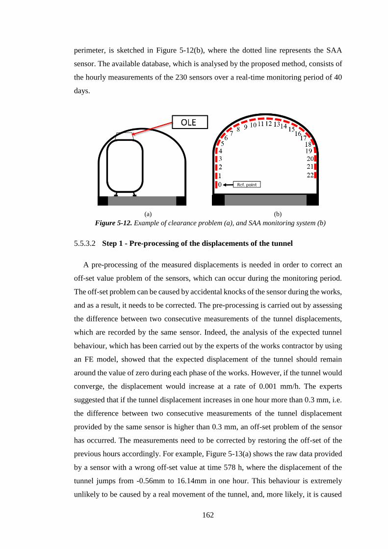
162

perimeter, is sketched in Figure 5-12(b), where the dotted line represents the SAA

sensor. The available database, which is analysed by the proposed method, consists of

the hourly measurements of the 230 sensors over a real-time monitoring period of 40

days.

(a) (b)

Figure 5-12. Example of clearance problem (a), and SAA monitoring system (b)

5.5.3.2 Step 1 - Pre-processing of the displacements of the tunnel

A pre-processing of the measured displacements is needed in order to correct an

off-set value problem of the sensors, which can occur during the monitoring period.

The off-set problem can be caused by accidental knocks of the sensor during the works,

and as a result, it needs to be corrected. The pre-processing is carried out by assessing

the difference between two consecutive measurements of the tunnel displacements,

which are recorded by the same sensor. Indeed, the analysis of the expected tunnel

behaviour, which has been carried out by the experts of the works contractor by using

an FE model, showed that the expected displacement of the tunnel should remain

around the value of zero during each phase of the works. However, if the tunnel would

converge, the displacement would increase at a rate of 0.001 mm/h. The experts

suggested that if the tunnel displacement increases in one hour more than 0.3 mm, i.e.

the difference between two consecutive measurements of the tunnel displacement

provided by the same sensor is higher than 0.3 mm, an off-set problem of the sensor

has occurred. The measurements need to be corrected by restoring the off-set of the

previous hours accordingly. For example, Figure 5-13(a) shows the raw data provided

by a sensor with a wrong off-set value at time 578 h, where the displacement of the

tunnel jumps from -0.56mm to 16.14mm in one hour. This behaviour is extremely

unlikely to be caused by a real movement of the tunnel, and, more likely, it is caused

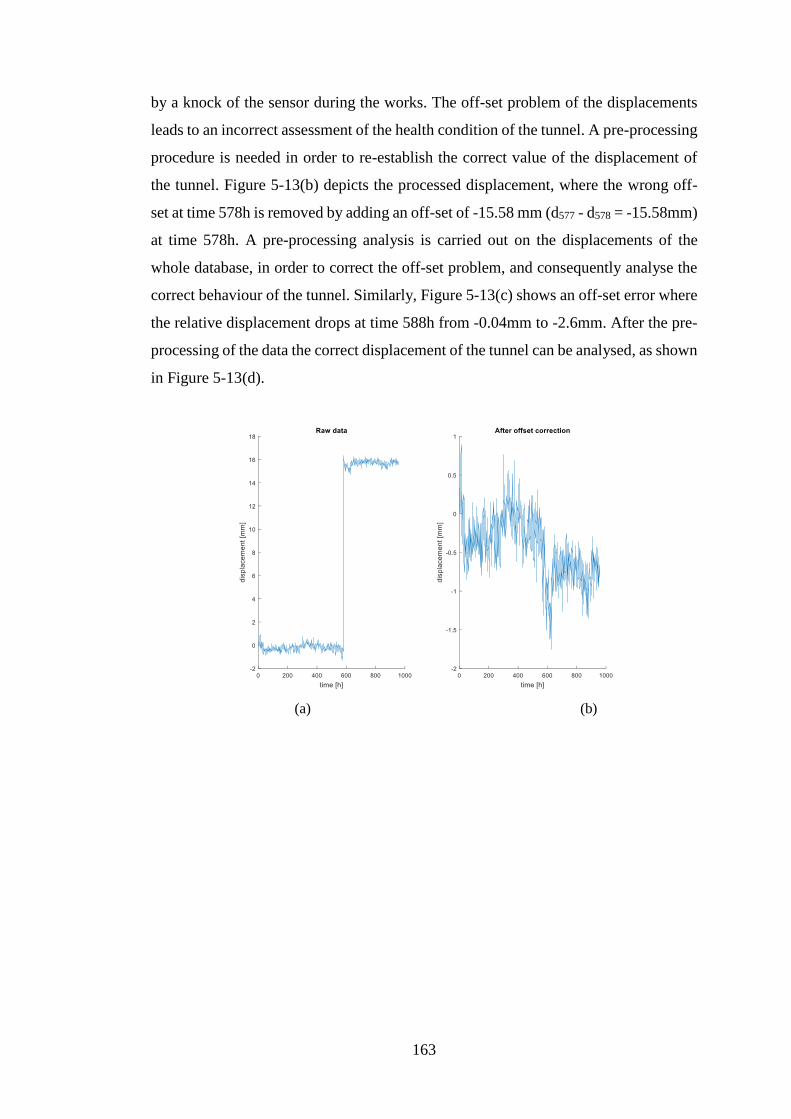
163

by a knock of the sensor during the works. The off-set problem of the displacements

leads to an incorrect assessment of the health condition of the tunnel. A pre-processing

procedure is needed in order to re-establish the correct value of the displacement of

the tunnel. Figure 5-13(b) depicts the processed displacement, where the wrong off-

set at time 578h is removed by adding an off-set of -15.58 mm (d577 - d578 = -15.58mm)

at time 578h. A pre-processing analysis is carried out on the displacements of the

whole database, in order to correct the off-set problem, and consequently analyse the

correct behaviour of the tunnel. Similarly, Figure 5-13(c) shows an off-set error where

the relative displacement drops at time 588h from -0.04mm to -2.6mm. After the pre-

processing of the data the correct displacement of the tunnel can be analysed, as shown

in Figure 5-13(d).

(a) (b)

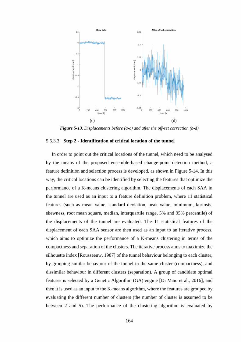
164

(c) (d)

Figure 5-13. Displacements before (a-c) and after the off-set correction (b-d)

5.5.3.3 Step 2 - Identification of critical location of the tunnel

In order to point out the critical locations of the tunnel, which need to be analysed

by the means of the proposed ensemble-based change-point detection method, a

feature definition and selection process is developed, as shown in Figure 5-14. In this

way, the critical locations can be identified by selecting the features that optimize the

performance of a K-means clustering algorithm. The displacements of each SAA in

the tunnel are used as an input to a feature definition problem, where 11 statistical

features (such as mean value, standard deviation, peak value, minimum, kurtosis,

skewness, root mean square, median, interquartile range, 5% and 95% percentile) of

the displacements of the tunnel are evaluated. The 11 statistical features of the

displacement of each SAA sensor are then used as an input to an iterative process,

which aims to optimize the performance of a K-means clustering in terms of the

compactness and separation of the clusters. The iterative process aims to maximize the

silhouette index [Rousseeuw, 1987] of the tunnel behaviour belonging to each cluster,

by grouping similar behaviour of the tunnel in the same cluster (compactness), and

dissimilar behaviour in different clusters (separation). A group of candidate optimal

features is selected by a Genetic Algorithm (GA) engine [Di Maio et al., 2016], and

then it is used as an input to the K-means algorithm, where the features are grouped by

evaluating the different number of clusters (the number of cluster is assumed to be

between 2 and 5). The performance of the clustering algorithm is evaluated by

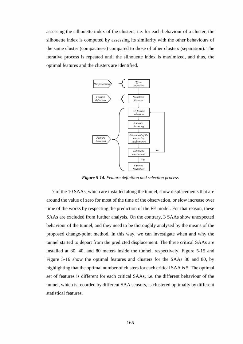
165

assessing the silhouette index of the clusters, i.e. for each behaviour of a cluster, the

silhouette index is computed by assessing its similarity with the other behaviours of

the same cluster (compactness) compared to those of other clusters (separation). The

iterative process is repeated until the silhouette index is maximized, and thus, the

optimal features and the clusters are identified.

Figure 5-14. Feature definition and selection process

7 of the 10 SAAs, which are installed along the tunnel, show displacements that are

around the value of zero for most of the time of the observation, or slow increase over

time of the works by respecting the prediction of the FE model. For that reason, these

SAAs are excluded from further analysis. On the contrary, 3 SAAs show unexpected

behaviour of the tunnel, and they need to be thoroughly analysed by the means of the

proposed change-point method. In this way, we can investigate when and why the

tunnel started to depart from the predicted displacement. The three critical SAAs are

installed at 30, 40, and 80 meters inside the tunnel, respectively. Figure 5-15 and

Figure 5-16 show the optimal features and clusters for the SAAs 30 and 80, by

highlighting that the optimal number of clusters for each critical SAA is 5. The optimal

set of features is different for each critical SAAs, i.e. the different behaviour of the

tunnel, which is recorded by different SAA sensors, is clustered optimally by different

statistical features.

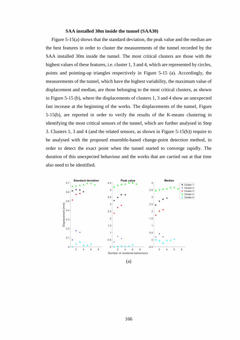
166

SAA installed 30m inside the tunnel (SAA30)

Figure 5-15(a) shows that the standard deviation, the peak value and the median are

the best features in order to cluster the measurements of the tunnel recorded by the

SAA installed 30m inside the tunnel. The most critical clusters are those with the

highest values of these features, i.e. cluster 1, 3 and 4, which are represented by circles,

points and pointing-up triangles respectively in Figure 5-15 (a). Accordingly, the

measurements of the tunnel, which have the highest variability, the maximum value of

displacement and median, are those belonging to the most critical clusters, as shown

in Figure 5-15 (b), where the displacements of clusters 1, 3 and 4 show an unexpected

fast increase at the beginning of the works. The displacements of the tunnel, Figure

5-15(b), are reported in order to verify the results of the K-means clustering in

identifying the most critical sensors of the tunnel, which are further analysed in Step

3. Clusters 1, 3 and 4 (and the related sensors, as shown in Figure 5-15(b)) require to

be analysed with the proposed ensemble-based change-point detection method, in

order to detect the exact point when the tunnel started to converge rapidly. The

duration of this unexpected behaviour and the works that are carried out at that time

also need to be identified.

(a)

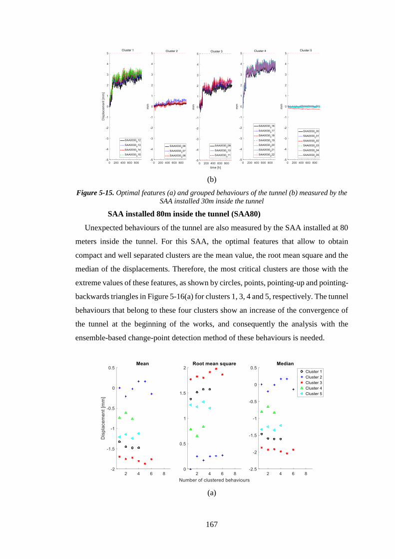
167

(b)

Figure 5-15. Optimal features (a) and grouped behaviours of the tunnel (b) measured by the

SAA installed 30m inside the tunnel

SAA installed 80m inside the tunnel (SAA80)

Unexpected behaviours of the tunnel are also measured by the SAA installed at 80

meters inside the tunnel. For this SAA, the optimal features that allow to obtain

compact and well separated clusters are the mean value, the root mean square and the

median of the displacements. Therefore, the most critical clusters are those with the

extreme values of these features, as shown by circles, points, pointing-up and pointing-

backwards triangles in Figure 5-16(a) for clusters 1, 3, 4 and 5, respectively. The tunnel

behaviours that belong to these four clusters show an increase of the convergence of

the tunnel at the beginning of the works, and consequently the analysis with the

ensemble-based change-point detection method of these behaviours is needed.

(a)

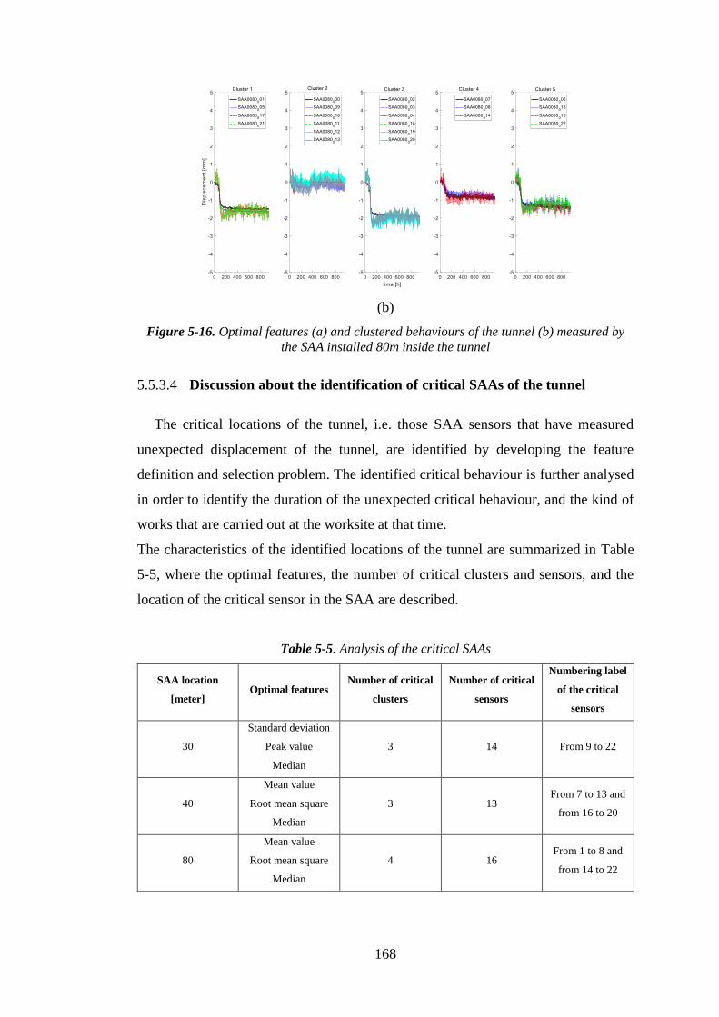
168

(b)

Figure 5-16. Optimal features (a) and clustered behaviours of the tunnel (b) measured by

the SAA installed 80m inside the tunnel

5.5.3.4 Discussion about the identification of critical SAAs of the tunnel

The critical locations of the tunnel, i.e. those SAA sensors that have measured

unexpected displacement of the tunnel, are identified by developing the feature

definition and selection problem. The identified critical behaviour is further analysed

in order to identify the duration of the unexpected critical behaviour, and the kind of

works that are carried out at the worksite at that time.

The characteristics of the identified locations of the tunnel are summarized in Table

5-5, where the optimal features, the number of critical clusters and sensors, and the

location of the critical sensor in the SAA are described.

Table 5-5. Analysis of the critical SAAs

SAA location

[meter] Optimal features

Number of critical

clusters

Number of critical

sensors

Numbering label

of the critical

sensors

30

Standard deviation

Peak value

Median

3 14 From 9 to 22

40

Mean value

Root mean square

Median

3 13 From 7 to 13 and

from 16 to 20

80

Mean value

Root mean square

Median

4 16 From 1 to 8 and

from 14 to 22

169

The analysis of the critical clusters of the three SAAs shows that the sensors that

have high numbering label (from 9 to 22), i.e. those on the right hand-side of the tunnel,

as shown in Figure 5-12(b), are those with the higher value of displacement, as shown

in Table 5-5. However, the SAA installed at 80m inside the tunnel, Figure 5-16(b),

shows high values of displacement on both sides of the tunnel, and as a result the

infrastructure of the tunnel might have unknown critical issues at this point. This

common behaviour can mean that the works are carried out on the right-hand side of

the tunnel, and as a result the displacement of the tunnel on the right hand-side is higher

than on the left-hand side, due to the temporary lack of the track and the excavation

process. However, such detail information is not available on the database of the work

activities, as only the information about the main work activity (e.g. excavation of the

zone between 80 and 100 meters) is available.

In what follows, the behaviour of the critical clusters, which are identified by using

the feature definition and selection process, are analysed further, in order to point out

the time of occurrence, the duration and the possible causes of the unexpected fast

convergence of the tunnel.

5.5.3.5 Step 3 – Change-point identification using the proposed ensemble-based

methodology

The measurements that have been identified to describe the critical behaviour of the

tunnel are further analysed with the aim of identifying the time when the unexpected

behaviour of the tunnel has started, its duration and pointing out its possible causes.

The duration of the unexpected tunnel behaviour is identified by the means of the

proposed ensemble-based change-point detection method, whose performance is

compared with the results of each individual change-point method. Once the most

critical change-point is identified, the works that are carried out at the tunnel site are

investigated by automatically analysing the database of the work activities. However,

hard copies of the spreadsheets of the works are usually used by the contractor of the

works, and an electronic version is prepared only at a later date. Hence, some

information about the works might be omitted. Other possible causes that can lead to

unexpected behaviour of the tunnel, such as geophysics of the ground around the

tunnel or geometry of the tunnel, are neglected due to the lack of such technical

170

information about the tunnel. The works that are carried out at the tunnel are

investigated by using the results of each change-point algorithm.

In this case study, the values of the time constants , , , and , which have

been introduced in section 5.5.2.2, are optimized by expert knowledge elicitation, and

they are equal to -7h, 15h, 10h and 0.75, respectively.

In this thesis, two particular penalty functions are considered in order to detect

change-points of the monitored variable:

• a cost function, C, that aims to detect change-points by identifying changes on

the mean value of the monitored variable:

1

1

21 _

( 1):

1 1

1( )

j

j j

j

l

q j

j q

C y y ym

−

−

+

+

= = +

= −

(5-14)

where _

jy is the empirical mean value of the monitored behaviour of the tunnel

in the segment j, qy is the monitored variable of the tunnel at time q, m is the

time duration of the monitored behaviour of the tunnel and j is a change-point

of the tunnel behaviour.

• a cost function, C, which aims to identify change-points of the tunnel behaviour

by pointing out changes on the slope of the system behaviour by considering

an autoregressive linear model for the PELT-based individual change-point

method. The cost function is then defined as follows

1

1 * 2

( 1): 1 1

3( ) log( ) log(2 (1, 1, ) )

2 2j j

j j

j j j jC y

−

−

+ − −

−= − + + (5-15)

where * is the estimation of the variance of the monitored data in the segment

1[ , ]

j j

− , i.e. 1( 1):j j

y − + , j is a change-point of the tunnel behaviour.

In what follows, without loss of generality, among the critical sensors of the clusters

that have been identified in section 5.5.3.3, two critical scenarios of the tunnel are

presented, in order to discuss the performance of the proposed ensemble-based change-

point method with respect to the individual change-point methods.

171

Change-point analysis of SAA30

Figure 5-17(a-1) shows the displacement measured by sensor SAA30_13 (i.e. the

sensor number 13 of the SAA installed at 30m inside the tunnel). An increase of the

displacements around time 100h is recorded, as shown in Figure 5-17(a-1). Figure

5-17(a) depicts the performance of each individual change-point method by comparing

it with the result of the proposed ensemble-based method. Each individual change-

point methods is able to point out this change-point generally, as shown in Figure

5-17(a-2), (a-3), (a-4) and (a-5) by the means of vertical lines and the probability of

change being higher than = 0.75 for the RuLSIF method. The change-point is

identified around time 130h by the RuLSIF method, which results to be at a later time

than the actual initial change-point (Figure 5-17(a-2)). The CUSUM, the penalty cost-

function-based and the PELT-based methods are able to identify the change-point

effectively around time 80h, as shown in Figure 5-17(a-3), (a-4) and (a-5),

respectively. However, each individual change-point method is not able to identify the

duration of the unexpected behaviour of the tunnel, i.e. the time when the unexpected

behaviour ends is not found. A second and small change-point around time 400h is

identified by the CUSUM, the penalty cost-function-based and the PELT-based

methods, Figure 5-17(a-3), (a-4) and (a-5), and a third one at time 600h by the CUSUM

method (Figure 5-17(a-3)). The change-point at time 80h can be caused by the works

that are carried out in the first 50m inside the tunnel. In a similar way, the change-point

at time 130h, which is identified by the RuLSIF method, is due to the works in the first

50m inside the tunnel. The change-point at time 400h can be caused by work activities

that are carried out at between 340 to 420m inside of the tunnel, as reported in the

database of the work activities for that time. However, the change-point at time 400h

is not the most critical change-point of the tunnel behaviour, which is the one where

the tunnel shows the highest change of its convergence. The most critical change-point

is not identified by each individual change-point algorithm, i.e. the start and ending

time and the duration of the most critical change are not identified.

Oppositely, the proposed ensemble-based change-point method is able to identify

the time when the tunnel started to converge rapidly at time 74h. At the same time, the

final time of the unexpected behaviour, i.e. when the fast convergence of the tunnel

ends, is pointed out at time 161h, as shown in Figure 5-17(a-6). The most critical

unexpected behaviour of sensor SAA30_13, and its duration, is identified by the

proposed method correctly, accordingly to the safety reports of the tunnel. The

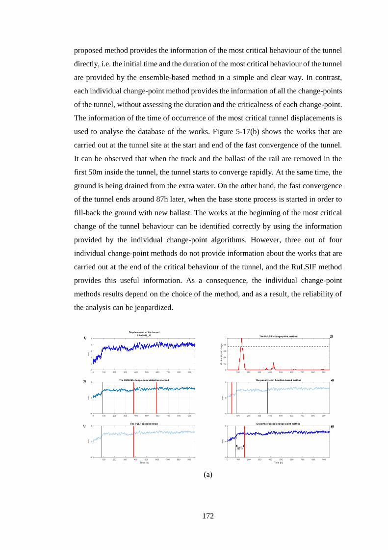
172

proposed method provides the information of the most critical behaviour of the tunnel

directly, i.e. the initial time and the duration of the most critical behaviour of the tunnel

are provided by the ensemble-based method in a simple and clear way. In contrast,

each individual change-point method provides the information of all the change-points

of the tunnel, without assessing the duration and the criticalness of each change-point.

The information of the time of occurrence of the most critical tunnel displacements is

used to analyse the database of the works. Figure 5-17(b) shows the works that are

carried out at the tunnel site at the start and end of the fast convergence of the tunnel.

It can be observed that when the track and the ballast of the rail are removed in the

first 50m inside the tunnel, the tunnel starts to converge rapidly. At the same time, the

ground is being drained from the extra water. On the other hand, the fast convergence

of the tunnel ends around 87h later, when the base stone process is started in order to

fill-back the ground with new ballast. The works at the beginning of the most critical

change of the tunnel behaviour can be identified correctly by using the information

provided by the individual change-point algorithms. However, three out of four

individual change-point methods do not provide information about the works that are

carried out at the end of the critical behaviour of the tunnel, and the RuLSIF method

provides this useful information. As a consequence, the individual change-point

methods results depend on the choice of the method, and as a result, the reliability of

the analysis can be jeopardized.

(a)

173

(b)

Figure 5-17. Change-point detection of the SAA30_13 by using the proposed ensemble-

based method and each individual change-point method (a), and the corresponding work

activities (b)

Change-point analysis of SAA80

An increase of the displacements of the tunnel is also measured by SAA80. The

feature definition and selection process of Section 5.5.3.3 showed that the SAA80 is

particularly critical, due to the fact that high values of displacement are measured all

along the section of the tunnel. Indeed, almost all the sensors of the SAA80 measure

an increase of the convergence of the tunnel at the beginning of the works. For

example, Figure 5-18(a-1) shows the displacement recorded by sensor 19 of the

SAA80. Therefore, the analysis of this behaviour with the ensemble-based change-

point method is needed in order to point out the time duration of this unexpected fast

convergence of the tunnel, and the works that are carried out at the tunnel at that time.

Figure 5-18(a-2), (a-3), (a-4) and (a-5) show the analysis of the displacements of the

tunnel by the means of each individual change-point method. Again, the RuLSIF

method detects the change-point at a later time than the actual initial point of the

unexpected behaviour, as shown in Figure 5-18(a-2). The CUSUM and the penalty

cost-function-based agree in pointing out the first change-point around 50h (Figure

5-18(a-3) and (a-4)), whereas the PELT-based method identifies the first change-point

around 80h, Figure 5-18(a-5). Furthermore, the CUSUM, the penalty cost-function-

based and the PELT-based methods identifies a second change-point of the

displacement of the tunnel around 100h, i.e. before that the tunnel stops to converge,

as shown in Figure 5-18(a-3), (a-4) and (a-5), respectively. The analysis of the database

of the work activities shows that no information is available at time 50h, when the first

174

change-point is identified by each individual change-point method. At time 100h, the

works are carried out in the first 50m inside the tunnel, and, especially, the base stone

process of this section has been started. Conversely, the proposed ensemble-based

change-point method identifies a change-point interval that starts at time 50h and ends

at time 169h (Figure 5-18(a-6)). In this way, the initial point where the tunnel

displacement starts to increase, and the end point of the critical convergence are

identified. The analysis of the database of the work activities shows that no information

is available at the beginning of the critical behaviour of the tunnel. On the contrary,

the tunnel stops to converge when the works are carried out at 50 to 100 meters inside

the tunnel, as shown in Figure 5-18(b). The base stone process of this section of the

tunnel is initiated when the fast convergence of the tunnel ends, and subsequently we

can conclude that when the ground is back filled with new ballast, the tunnel stops to

show the unexpected fast increase of the displacement. The works identified by using

the results provided by the ensemble-based method are different from those retrieved

by using the results of the individual change-point algorithms. Particularly, at time

100h, i.e. the change-point identified by the individual change-point methods, the

behaviour of the tunnel is still changing rapidly, as shown in Figure 5-18, and the

works are carried out in the first 50m inside the tunnel. In contrast, the ensemble-based

method points out that the fast convergence of the tunnel ends at time 160h, when the

works are carried out at 50 to 100 meters inside the tunnel.

Note that similar results in terms of the performance of the proposed method,

described in this section, have also been achieved during the analysis of other critical

sensors, as identified in Table 5-5 of Section 5.5.3.3.

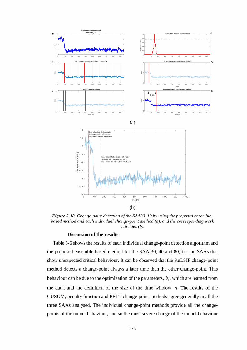
175

(a)

(b)

Figure 5-18. Change-point detection of the SAA80_19 by using the proposed ensemble-

based method and each individual change-point method (a), and the corresponding work

activities (b).

Discussion of the results

Table 5-6 shows the results of each individual change-point detection algorithm and

the proposed ensemble-based method for the SAA 30, 40 and 80, i.e. the SAAs that

show unexpected critical behaviour. It can be observed that the RuLSIF change-point

method detects a change-point always a later time than the other change-point. This

behaviour can be due to the optimization of the parameters, i , which are learned from

the data, and the definition of the size of the time window, n. The results of the

CUSUM, penalty function and PELT change-point methods agree generally in all the

three SAAs analysed. The individual change-point methods provide all the change-

points of the tunnel behaviour, and so the most severe change of the tunnel behaviour

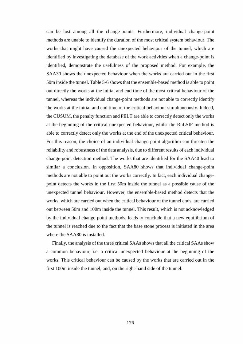
176

can be lost among all the change-points. Furthermore, individual change-point

methods are unable to identify the duration of the most critical system behaviour. The

works that might have caused the unexpected behaviour of the tunnel, which are

identified by investigating the database of the work activities when a change-point is

identified, demonstrate the usefulness of the proposed method. For example, the

SAA30 shows the unexpected behaviour when the works are carried out in the first

50m inside the tunnel. Table 5-6 shows that the ensemble-based method is able to point

out directly the works at the initial and end time of the most critical behaviour of the

tunnel, whereas the individual change-point methods are not able to correctly identify

the works at the initial and end time of the critical behaviour simultaneously. Indeed,

the CUSUM, the penalty function and PELT are able to correctly detect only the works

at the beginning of the critical unexpected behaviour, whilst the RuLSIF method is

able to correctly detect only the works at the end of the unexpected critical behaviour.

For this reason, the choice of an individual change-point algorithm can threaten the

reliability and robustness of the data analysis, due to different results of each individual

change-point detection method. The works that are identified for the SAA40 lead to

similar a conclusion. In opposition, SAA80 shows that individual change-point

methods are not able to point out the works correctly. In fact, each individual change-

point detects the works in the first 50m inside the tunnel as a possible cause of the

unexpected tunnel behaviour. However, the ensemble-based method detects that the

works, which are carried out when the critical behaviour of the tunnel ends, are carried

out between 50m and 100m inside the tunnel. This result, which is not acknowledged

by the individual change-point methods, leads to conclude that a new equilibrium of

the tunnel is reached due to the fact that the base stone process is initiated in the area

where the SAA80 is installed.

Finally, the analysis of the three critical SAAs shows that all the critical SAAs show

a common behaviour, i.e. a critical unexpected behaviour at the beginning of the

works. This critical behaviour can be caused by the works that are carried out in the

first 100m inside the tunnel, and, on the right-hand side of the tunnel.

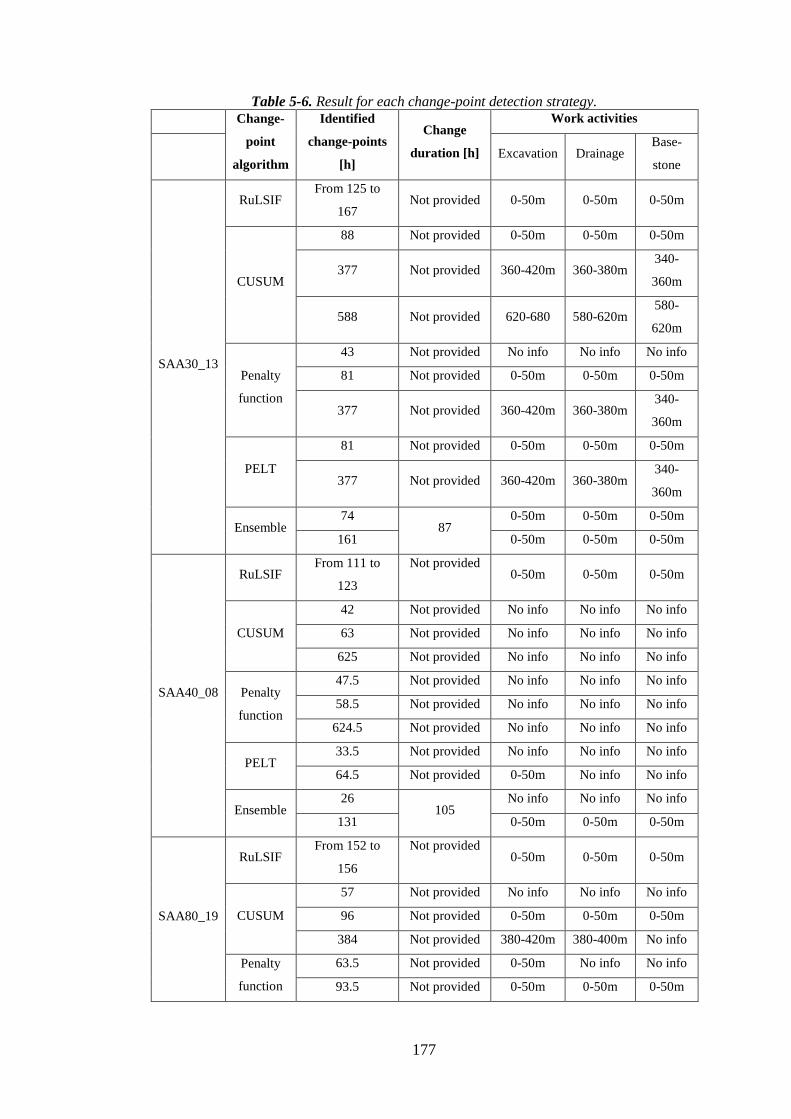
177

Table 5-6. Result for each change-point detection strategy. Change-

point

algorithm

Identified

change-points

[h]

Change

duration [h]

Work activities

Excavation Drainage Base-

stone

SAA30_13

RuLSIF From 125 to

167 Not provided 0-50m 0-50m 0-50m

CUSUM


377 Not provided 360-420m 360-380m 340-

360m

588 Not provided 620-680 580-620m 580-

620m

Penalty

function

43 Not provided No info No info No info


377 Not provided 360-420m 360-380m 340-

360m

PELT


377 Not provided 360-420m 360-380m 340-

360m

Ensemble 74

87 0-50m 0-50m 0-50m

161 0-50m 0-50m 0-50m

SAA40_08

RuLSIF From 111 to

123

Not provided 0-50m 0-50m 0-50m

CUSUM




Penalty

function

47.5 Not provided No info No info No info



PELT 33.5 Not provided No info No info No info

64.5 Not provided 0-50m No info No info

Ensemble 26

105 No info No info No info

131 0-50m 0-50m 0-50m

SAA80_19

RuLSIF From 152 to

156

Not provided 0-50m 0-50m 0-50m

CUSUM



384 Not provided 380-420m 380-400m No info

Penalty

function

63.5 Not provided 0-50m No info No info

93.5 Not provided 0-50m 0-50m 0-50m

178

PELT

80.5 Not provided 0-50m 0-50m No info

107.5 Not provided 0-50m 0-50m 0-50m

397.5 Not provided 380-400m 420-440m No info

Ensemble 50

119 No info No info No info

169 50-100m 50-100m 50-100m

Summary of the proposed ensemble-based change-point detection method

An ensemble-based change-point detection method is proposed in order to identify

and diagnose the most critical change of the behaviour of a railway infrastructure. For

example, the proposed method can be applied both to bridge vibration behaviour with

the aim of assessing when the HI of the bridge changed over time, and to infrastructure

that shows monotonic behaviour over time, such as the presented tunnel case study.

The proposed ensemble-based change-point detection method has been developed to

overcome the limitation of the individual change-point methods. In fact, individual

change-point methods can only detect abrupt changes of the behaviour of the

infrastructure, without providing information regarding the severity and the duration

of the identified change-points of the infrastructure behaviour.

The behaviour of a tunnel during renewal activities has been analysed to assess the

performance of the proposed method. The proposed ensemble-based change-point

method outperforms each individual change-point method, in identifying the most

critical behaviour of the tunnel, by pointing out the time, when the tunnel starts to

converge rapidly, its duration and possible causes. Particularly, the proposed method

outperforms each individual method when severe unexpected behaviour is

experienced, i.e. when the displacements of the tunnel increase suddenly and rapidly.

The ensemble-based change-point detection method, however, has some

drawbacks:

• only the most critical change-point of the system is pointed out, without

providing further information regarding other smaller change-points. Decision

makers can be interested in identifying and analysing the most critical

behaviour of the system firstly, and once immediate actions are taken, minor

changes in the system behaviour can also be analysed. In that case, a

comprehensive analysis of the data can be carried out and all the vulnerabilities

of the system can be identified. If all the change-points were to be analysed,

the proposed ensemble-based change-point method can be used for this

purpose by modifying its rules appropriately. For example, a decision maker

179

can look for each change-point that has been identified by at least two

individual change-point methods, rather than for the change-point where the

tunnel behaviour experiences its highest variation.

• the performance of the proposed method relies on the assessment of time-

constants, i.e. , , , which are defined by using an expert knowledge

elicitation process. When the time constants are set, the identification of the

change-points depends on the values of these parameters, and consequently the

expert knowledge elicitation process can lead to misleading results if the

considered system is new and unknown for the experts.

Summary

A method to merge the expert elicitation process with the analysis of the bridge

behaviour has been proposed, with the aim of updating the CPTs of a BBN in a reliable

and continuous manner. The CPT values are updated by considering an -weighted

combination of the conditional probabilities obtained by analysing both: i) the expert

knowledge; and ii) the bridge behaviour data. Particularly, the latter analysis requires

data of different health states of the bridge elements to define a CDF for each health

state of the bridge. An approach to assess the CDF by relying on the analysis of the HI

of the bridge has been proposed by fitting a set of possible pdfs and choosing the

optimal distribution by evaluating the goodness of the fit.

In addition, an ensemble-based change-point detection method has been introduced

in order to analyse a database of past infrastructure behaviour to identify when the

health state of the infrastructure changed. The results of the proposed ensemble-based

method can then be used to analyse different health states of the infrastructure, and

thus define the CDF of each health state to update the CPTs of a BBN.

In what follows, the CDFs that have been defined in this chapter are used in order

to update the CPTs of a BBN continuously, by taking account of the actual health state

of the bridge elements in Chapter 6 . The performance of the BBN by using the

proposed method to update the CPTs and the performance without using the proposed

method is evaluated in order to investigate the potential of the CPTs updating strategy

are also analysed in Chapter 6 .

180

The application of the BBN

method to the in-field post-

tensioned bridge

Introduction

In this chapter, the BBN approach that is introduced in Chapter 3 is applied to the

in-field post-tensioned bridge, which is presented in section 4.3.1. In this way, the

condition monitoring and damage detection capability of the BBN is verified by

assessing the health state of the bridge and its elements.

The bridge behaviour data of group 2, which are not labelled (i.e. the health state of

the bridge elements is assumed to be unknown), are used as an input to the data analysis

methodology of section 4.2, in order to assess the optimal HI of the bridge. The HI is

then used as an input to the BBN to assess the health state of the whole bridge.

Therefore, a bridge manager, that is monitoring the bridge health state by the means

of the proposed BBN, is able to find changes of the bridge health state, by identifying

the degrading elements of the bridge.

The BBN of the bridge is developed by following the step-by-step procedure

presented in section 3.3, whereas different strategies to define the CPTs of the BBN

are analysed in Chapter 5 . Particularly, the CPTs are firstly defined by adopting an

expert knowledge elicitation process, and then the proposed strategy to update the

CPTs by merging expert judgements and bridge behaviour analysis is used.

The developed BBN is presented in section 6.2, whereas the performance of the BBN

by using different CPT definition strategies is analysed in section 6.3. Conclusions and

remarks are discussed in section 6.4.

The BBN of the post-tensioned bridge

In section 4.3.1, the post-tensioned concrete bridge is described. Before introducing

the BBN that aims to monitor and assess the health state of the bridge, the main

characteristics of the bridge are recalled. The post-tensioned concrete bridge has the

main span of 32 m and two side spans of 12 m each. The bridge was subject to a

vibration measurement test before being demolished to obtain the bridge vibration

behaviour in different health states. The acceleration of the bridge was monitored by a

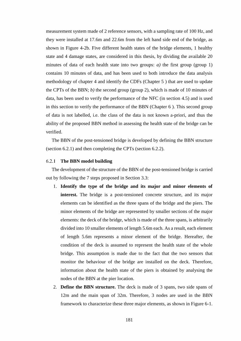
181

measurement system made of 2 reference sensors, with a sampling rate of 100 Hz, and

they were installed at 17.6m and 22.6m from the left hand side end of the bridge, as

shown in Figure 4-2b. Five different health states of the bridge elements, 1 healthy

state and 4 damage states, are considered in this thesis, by dividing the available 20

minutes of data of each health state into two groups: a) the first group (group 1)

contains 10 minutes of data, and has been used to both introduce the data analysis

methodology of chapter 4 and identify the CDFs (Chapter 5 ) that are used to update

the CPTs of the BBN; b) the second group (group 2), which is made of 10 minutes of

data, has been used to verify the performance of the NFC (in section 4.5) and is used

in this section to verify the performance of the BBN (Chapter 6 ). This second group

of data is not labelled, i.e. the class of the data is not known a-priori, and thus the

ability of the proposed BBN method in assessing the health state of the bridge can be

verified.

The BBN of the post-tensioned bridge is developed by defining the BBN structure

(section 6.2.1) and then completing the CPTs (section 6.2.2).

The BBN model building

The development of the structure of the BBN of the post-tensioned bridge is carried

out by following the 7 steps proposed in Section 3.3:


interest. The bridge is a post-tensioned concrete structure, and its major

elements can be identified as the three spans of the bridge and the piers. The

minor elements of the bridge are represented by smaller sections of the major

elements: the deck of the bridge, which is made of the three spans, is arbitrarily

divided into 10 smaller elements of length 5.6m each. As a result, each element

of length 5.6m represents a minor element of the bridge. Hereafter, the

condition of the deck is assumed to represent the health state of the whole

bridge. This assumption is made due to the fact that the two sensors that

monitor the behaviour of the bridge are installed on the deck. Therefore,

information about the health state of the piers is obtained by analysing the

nodes of the BBN at the pier location.

2. Define the BBN structure. The deck is made of 3 spans, two side spans of

12m and the main span of 32m. Therefore, 3 nodes are used in the BBN

framework to characterize these three major elements, as shown in Figure 6-1.

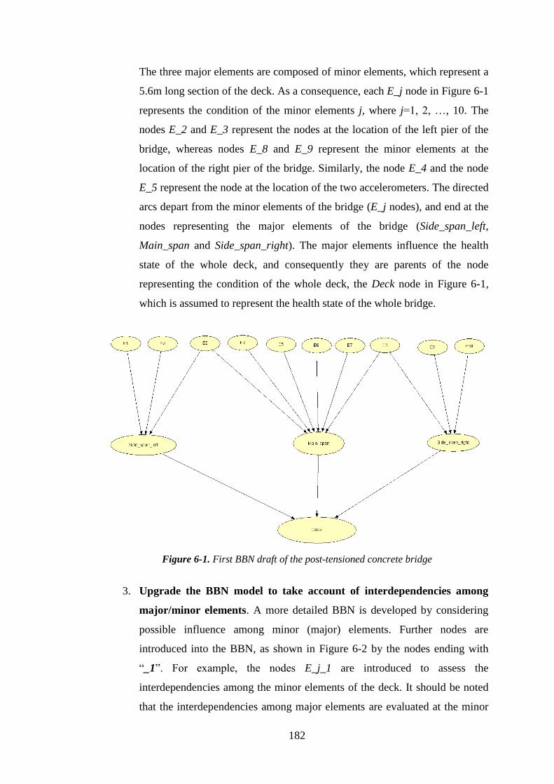
182

The three major elements are composed of minor elements, which represent a

5.6m long section of the deck. As a consequence, each E_j node in Figure 6-1

represents the condition of the minor elements j, where j=1, 2, …, 10. The

nodes E_2 and E_3 represent the nodes at the location of the left pier of the

bridge, whereas nodes E_8 and E_9 represent the minor elements at the

location of the right pier of the bridge. Similarly, the node E_4 and the node

E_5 represent the node at the location of the two accelerometers. The directed

arcs depart from the minor elements of the bridge (E_j nodes), and end at the

nodes representing the major elements of the bridge (Side_span_left,

Main_span and Side_span_right). The major elements influence the health

state of the whole deck, and consequently they are parents of the node

representing the condition of the whole deck, the Deck node in Figure 6-1,

which is assumed to represent the health state of the whole bridge.

Figure 6-1. First BBN draft of the post-tensioned concrete bridge

3. Upgrade the BBN model to take account of interdependencies among

major/minor elements. A more detailed BBN is developed by considering

possible influence among minor (major) elements. Further nodes are

introduced into the BBN, as shown in Figure 6-2 by the nodes ending with

“_1”. For example, the nodes E_j_1 are introduced to assess the

interdependencies among the minor elements of the deck. It should be noted

that the interdependencies among major elements are evaluated at the minor

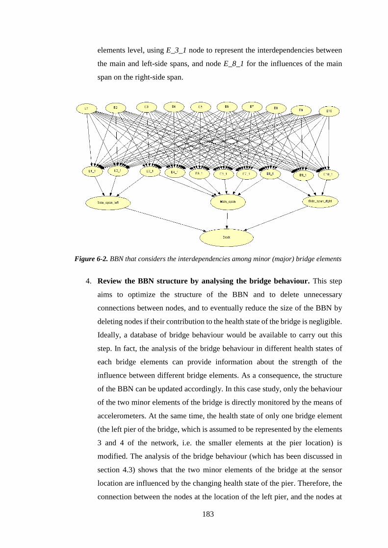
183

elements level, using E_3_1 node to represent the interdependencies between

the main and left-side spans, and node E_8_1 for the influences of the main

span on the right-side span.

Figure 6-2. BBN that considers the interdependencies among minor (major) bridge elements

4. Review the BBN structure by analysing the bridge behaviour. This step

aims to optimize the structure of the BBN and to delete unnecessary

connections between nodes, and to eventually reduce the size of the BBN by

deleting nodes if their contribution to the health state of the bridge is negligible.

Ideally, a database of bridge behaviour would be available to carry out this

step. In fact, the analysis of the bridge behaviour in different health states of

each bridge elements can provide information about the strength of the

influence between different bridge elements. As a consequence, the structure

of the BBN can be updated accordingly. In this case study, only the behaviour

of the two minor elements of the bridge is directly monitored by the means of

accelerometers. At the same time, the health state of only one bridge element

(the left pier of the bridge, which is assumed to be represented by the elements

3 and 4 of the network, i.e. the smaller elements at the pier location) is

modified. The analysis of the bridge behaviour (which has been discussed in

section 4.3) shows that the two minor elements of the bridge at the sensor

location are influenced by the changing health state of the pier. Therefore, the

connection between the nodes at the location of the left pier, and the nodes at

184

the location of the two sensors is validated. Further analysis based on the data

cannot be carried out, due to a lack of bridge behaviour data. However, the

BBN of Figure 6-2 is a complex model, due to all the connections between the

minor elements, which lead to large CPTs of the BBN. Subsequently, only

connections between neighbour minor elements are considered. This

assumption is based on the performance of both the BBN of the steel truss

bridge (section 3.4) and of the beam-and-slab bridge (section 3.5.2), which

have shown to be able to monitor and assess the health state of each bridge.

Figure 6-3 shows the BBN structure after the bridge behaviour analysis and the

abovementioned assumptions.

Figure 6-3. Updated BBN of the post-tensioned bridge after the bridge behaviour analysis

5. Define nodes to represent the measurement system of the bridge. The

measurement system of the bridge is represented by two accelerometers that

are installed at 17.6m and 22.6m from the left ending if the bridge, as shown

in Figure 4-2. The two sensors are introduced into the BBN structure

accordingly, as depicted in Figure 6-4. The nodes representing the 2 sensors

are introduced as a parent of the minor elements on which the sensors are

installed. Every time when evidence of the bridge vibration is available, it is

analysed by the proposed data analysis methodology and the resulting optimal

HI value is used as an input to the sensor nodes, which assess the health state

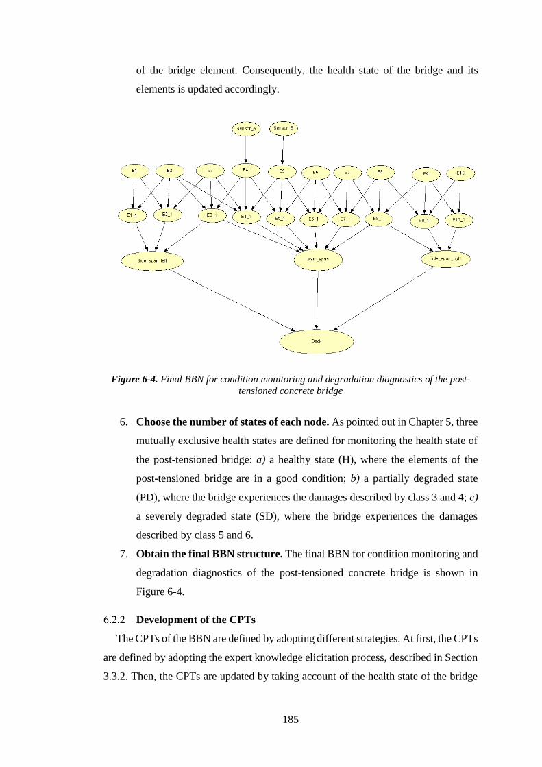
185

of the bridge element. Consequently, the health state of the bridge and its

elements is updated accordingly.

Figure 6-4. Final BBN for condition monitoring and degradation diagnostics of the post-

tensioned concrete bridge

6. Choose the number of states of each node. As pointed out in Chapter 5, three

mutually exclusive health states are defined for monitoring the health state of

the post-tensioned bridge: a) a healthy state (H), where the elements of the

post-tensioned bridge are in a good condition; b) a partially degraded state

(PD), where the bridge experiences the damages described by class 3 and 4; c)

a severely degraded state (SD), where the bridge experiences the damages

described by class 5 and 6.

7. Obtain the final BBN structure. The final BBN for condition monitoring and

degradation diagnostics of the post-tensioned concrete bridge is shown in

Figure 6-4.

Development of the CPTs

The CPTs of the BBN are defined by adopting different strategies. At first, the CPTs

are defined by adopting the expert knowledge elicitation process, described in Section

3.3.2. Then, the CPTs are updated by taking account of the health state of the bridge

186

elements, as described in section 5.2. The BBN is analysed by comparing its

performance when both CPTs strategies are adopted

The expert knowledge elicitation process is assumed to be the same as presented in

section 3.3.2. This assumption is needed due to a lack of experts to be interviewed

about the post-tensioned concrete bridge. Such an assumption influences the

assessment of the exact value of the probability of BBN nodes describing each state.

However, the damage detection ability of the BBN is not influenced by this

assumption, since the detection ability of the BBN depends on how the different states

of the nodes are selected, rather than on the values the CPTs. As a consequence, this

assumption allows to point out different health states of the bridge, and its elements,

but it may impact the diagnostic ability of the BBN. Indeed, conservative results (such

as a larger probability that the bridge is in a degraded health state than the actual health

state of the bridge) or misleading results (such as a much lower probability that the

bridge is in a degraded health state than the actual health state of the bridge) can be

achieved due to this assumption. The updating process of the CPTs, however, is able

to define the value of the conditional probabilities of the CPTs by taking account of

the actual health state of the bridge elements. Consequently, the values of the updated

CPTs are expected to provide an optimal assessment of the bridge health state, due to

the fact that the actual health state of the bridge elements is considered during the

definition of the CPTs. It should be noted that two sensors are available to monitor the

behaviour of the bridge, and thus the CPTs updating strategy is performed for the two

nodes where evidence are provided, i.e. nodes E_4_1 and E_5_1.

Different strategies to define the CPTs are compared in what follows:

a. CPTs are defined by considering only the expert knowledge elicitation process.

b. CPTs are defined by considering the proposed updating strategy (section 5.2)

with the weight of the linear combination [0, 0.9] that varies over time, by

taking account of the number of identified health states of the bridge elements

and the monitoring time. In this way, the analysis of the bridge behaviour data

has more importance than the expert knowledge elicitation process, due to the

fact that increases over time towards 0.9.

c. CPTs are defined by considering the proposed updating strategy (section 5.2)

with the weight of the linear combination that is constant and equals to 0.1.

In this way, a possible conservative scenario is analysed by giving the more

187

importance to the expert knowledge rather than to the bridge behaviour

analysis.

d. CPTs are defined by considering the proposed updating strategy (section 5.2)

with the weight of the linear combination that is constant and equals to 0.5.

In this way, the expert knowledge elicitation process and the bridge behaviour

analysis have the same importance.

The performance of the BBN in monitoring the health state of the post-tensioned

bridge by using these four CPTs strategy is compared in terms of the conditional

probability value of the most degraded elements of the bridge. Therefore, the aim of

the comparison is to point out which strategy allows to describe the health state of the

bridge, and its elements, in the most accurate way.

Finally, it is worth noting that the CDFs of the optimal HI for each sensor are used

to updated the CPTs of the two minor nodes of the BBN: section 6.3.1 and section

6.3.2 show the performance of the BBN by using the CDFs that are retrieved by using

the AICc to update the CPTs, and compare the performance of the BBN with the results

of the BBN analysis when the CPTs are defined by using the expert knowledge

elicitation process only. Then, in section 6.3.3, the performance of the BBN is

evaluated by taking account of the CDFs that are retrieved by using the results of the

K-S test. This latter performance of the BBN is compared to the results of the BBN

that relies on the CDFs retrieved by using the AICc analysis.

BBN model usage for detection and diagnostics of bridge

deterioration

The acceleration data are used as an input to the data analysis methodology

presented in section 4.2, in order to assess the value of the optimal HI of the bridge.

The value of the optimal HI is then used as an input to the BBN nodes, with the aim

of assessing the health state of the whole bridge, by taking account of the health state

of each element of the bridge.

The analysis of the BBN is presented by considering the bottom-up diagnostic

process of the BBN, which allows a bridge manger to interact with the BBN to

diagnose the cause of a change of the health state of the bridge. The step-by-step

bottom-up diagnostic process is proposed in this section to describe the results of the

BBN. In this way, the health state of the whole bridge is monitored and the causes of

the change of its health state can be diagnosed.

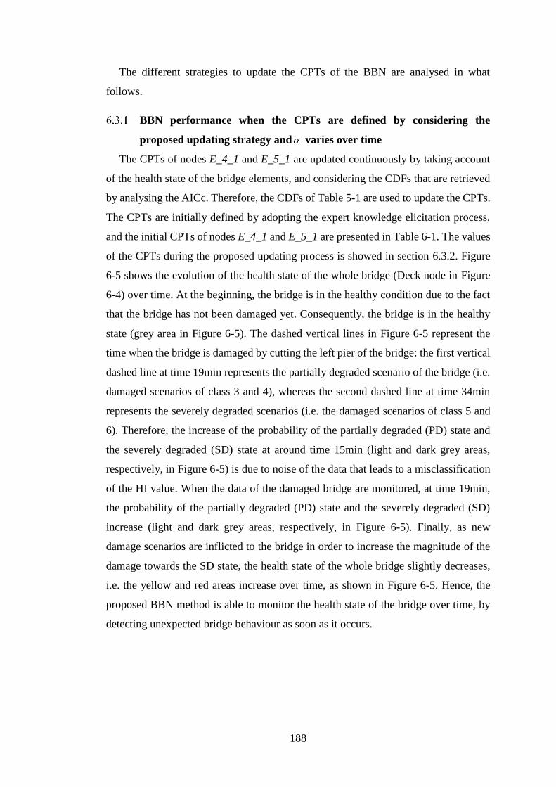
188

The different strategies to update the CPTs of the BBN are analysed in what

follows.

BBN performance when the CPTs are defined by considering the

proposed updating strategy and varies over time

The CPTs of nodes E_4_1 and E_5_1 are updated continuously by taking account

of the health state of the bridge elements, and considering the CDFs that are retrieved

by analysing the AICc. Therefore, the CDFs of Table 5-1 are used to update the CPTs.

The CPTs are initially defined by adopting the expert knowledge elicitation process,

and the initial CPTs of nodes E_4_1 and E_5_1 are presented in Table 6-1. The values

of the CPTs during the proposed updating process is showed in section 6.3.2. Figure

6-5 shows the evolution of the health state of the whole bridge (Deck node in Figure

6-4) over time. At the beginning, the bridge is in the healthy condition due to the fact

that the bridge has not been damaged yet. Consequently, the bridge is in the healthy

state (grey area in Figure 6-5). The dashed vertical lines in Figure 6-5 represent the

time when the bridge is damaged by cutting the left pier of the bridge: the first vertical

dashed line at time 19min represents the partially degraded scenario of the bridge (i.e.

damaged scenarios of class 3 and 4), whereas the second dashed line at time 34min

represents the severely degraded scenarios (i.e. the damaged scenarios of class 5 and

6). Therefore, the increase of the probability of the partially degraded (PD) state and

the severely degraded (SD) state at around time 15min (light and dark grey areas,

respectively, in Figure 6-5) is due to noise of the data that leads to a misclassification

of the HI value. When the data of the damaged bridge are monitored, at time 19min,

the probability of the partially degraded (PD) state and the severely degraded (SD)

increase (light and dark grey areas, respectively, in Figure 6-5). Finally, as new

damage scenarios are inflicted to the bridge in order to increase the magnitude of the

damage towards the SD state, the health state of the whole bridge slightly decreases,

i.e. the yellow and red areas increase over time, as shown in Figure 6-5. Hence, the

proposed BBN method is able to monitor the health state of the bridge over time, by

detecting unexpected bridge behaviour as soon as it occurs.

189

Figure 6-5. Evolution over time of the health state of the whole bridge when varies over

time, as shown in Eq. (5-2) (Deck node)

The BBN allows to diagnose the cause of the change of the bridge health state, by

pointing out the evolution over time of the health state of the parent nodes of the Deck

node (note that the Deck node represents the health state of the whole bridge). Figure

6-6 shows the evolution of the health states of the whole bridge (Deck node in Figure

6-4) and of its parent nodes: the left, main and right spans of the bridge, as shown in

Figure 6-4. Figure 6-6 allows to directly identify that the left and main spans of the

bridge are damaged, and that the main span is more degraded than the other major

elements, i.e. the light and dark grey areas of Main_span node are higher than those of

the other major elements. This result is because evidence of the bridge behaviour is

provided by the two sensors that are installed on the main span of the bridge.

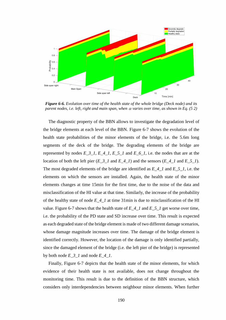
190

Figure 6-6. Evolution over time of the health state of the whole bridge (Deck node) and its

parent nodes, i.e. left, right and main span, when varies over time, as shown in Eq. (5 2)

The diagnostic property of the BBN allows to investigate the degradation level of

the bridge elements at each level of the BBN. Figure 6-7 shows the evolution of the

health state probabilities of the minor elements of the bridge, i.e. the 5.6m long

segments of the deck of the bridge. The degrading elements of the bridge are

represented by nodes E_3_1, E_4_1, E_5_1 and E_6_1, i.e. the nodes that are at the

location of both the left pier (E_3_1 and E_4_1) and the sensors (E_4_1 and E_5_1).

The most degraded elements of the bridge are identified as E_4_1 and E_5_1, i.e. the

elements on which the sensors are installed. Again, the health state of the minor

elements changes at time 15min for the first time, due to the noise of the data and

misclassification of the HI value at that time. Similarly, the increase of the probability

of the healthy state of node E_4_1 at time 31min is due to misclassification of the HI

value. Figure 6-7 shows that the health state of E_4_1 and E_5_1 get worse over time,

i.e. the probability of the PD state and SD increase over time. This result is expected

as each degraded state of the bridge element is made of two different damage scenarios,

whose damage magnitude increases over time. The damage of the bridge element is

identified correctly. However, the location of the damage is only identified partially,

since the damaged element of the bridge (i.e. the left pier of the bridge) is represented

by both node E_3_1 and node E_4_1.

Finally, Figure 6-7 depicts that the health state of the minor elements, for which

evidence of their health state is not available, does not change throughout the

monitoring time. This result is due to the definition of the BBN structure, which

considers only interdependencies between neighbour minor elements. When further

191

information about the possible interdependencies between non-neighbour minor

elements (e.g. the influence of E_1_1 on the health state of E_10_1) is available, the

structure of the BBN can be updated. Consequently, when evidence of a bridge

element is available, the health state of each minor element is updated accordingly.

In what follows, the performance of the BBN with different CPTs definition strategies

is analysed.


tensioned bridge when varies over time, as shown in Eq. (5 2)

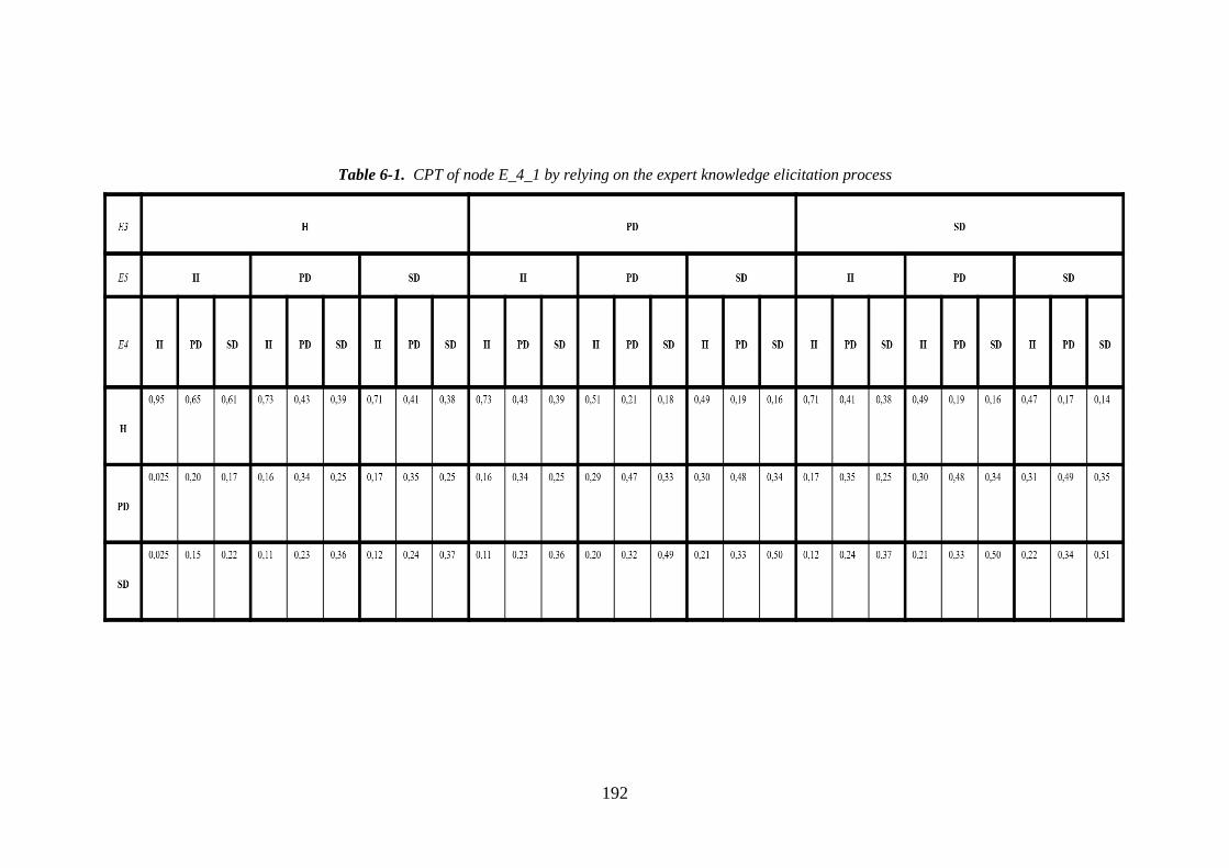
192

Table 6-1. CPT of node E_4_1 by relying on the expert knowledge elicitation process

193

Comparison of BBN performance by using different CPTs definition

strategies

The performance of the BBN by using the proposed strategy to update the CPTs is

compared with the performance of the BBN that relies on the expert knowledge

elicitation process. At the same time, the performance of the BBN is investigated by

considering different strategies of definition.

6.3.2.1 Expert knowledge elicitation process-based CPTs vs CPTs based on the

proposed updating strategy with time varying

The performance of the BBN for different scenarios is evaluated in this section. The

structure of the BBN is the same during the comparison scenarios, whereas the strategy

to define the CPTs is changed. Particularly, two CPTs definition strategies are

compared: i) the expert knowledge elicitation process; and ii) the proposed updating

strategy for CPT, by taking account of both expert judgement and bridge behaviour

analysis, with a value of that changes over time based on the health state of the

bridge element. The comparison of the BBN performance is made by considering the

evolution over time of the health state of the most degraded element of the bridge that

has been identified, i.e. E_4_1 and E_5_1.

Figure 6-8 shows the evolution of the health state of nodes E_4_1 and E_5_1 when

the proposed strategy for updating the CPTs is used (Figure 6-8 top), and when the

CPTs are defined by using the expert knowledge elicitation process (Figure 6-8

bottom). Both strategies allow to point out the different health states of the bridge

elements, by increasing the probability of the PD and SD states when damages are

inflicted to the bridge (light and dark grey areas, respectively, in Figure 6-8). Figure

6-8 top, i.e. when the CPTs are updated by adopting the proposed strategy, shows that

the probability of the PD and SD states increases more than the correspondent PD and

SD probabilities in Figure 6-8 bottom (i.e. when the CPTs are defined by using the

expert judgement). Therefore, the BBN that relies on the proposed strategy to update

the CPTs is able to diagnose the damage states of the bridge in a clearer manner.

Furthermore, the probability of the PD and SD states increase over time in Figure 6-8

top, which means that the health state of the bridge elements decrease over time. In

fact, the health state of the bridge decreases over time, due to the different damages

that are inflicted to the bridge pier: both the PD and the SD state are made of two

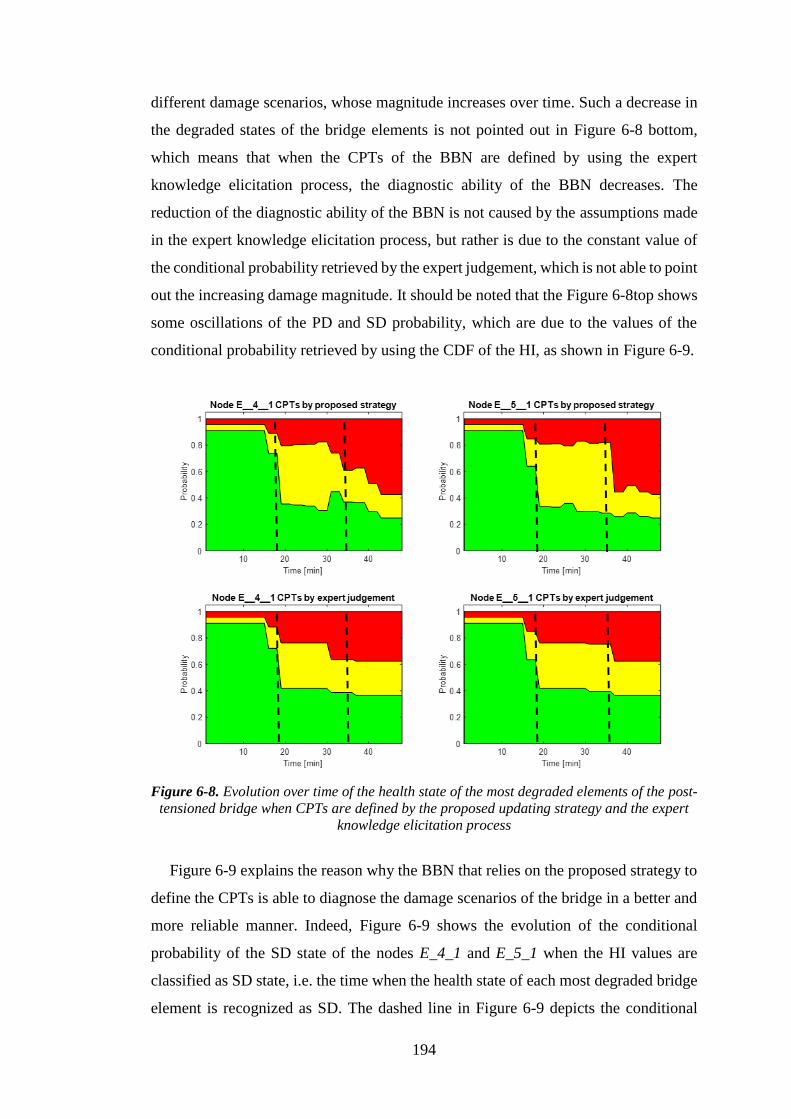
194

different damage scenarios, whose magnitude increases over time. Such a decrease in

the degraded states of the bridge elements is not pointed out in Figure 6-8 bottom,

which means that when the CPTs of the BBN are defined by using the expert

knowledge elicitation process, the diagnostic ability of the BBN decreases. The

reduction of the diagnostic ability of the BBN is not caused by the assumptions made

in the expert knowledge elicitation process, but rather is due to the constant value of

the conditional probability retrieved by the expert judgement, which is not able to point

out the increasing damage magnitude. It should be noted that the Figure 6-8top shows

some oscillations of the PD and SD probability, which are due to the values of the

conditional probability retrieved by using the CDF of the HI, as shown in Figure 6-9.

Figure 6-8. Evolution over time of the health state of the most degraded elements of the post-

tensioned bridge when CPTs are defined by the proposed updating strategy and the expert

knowledge elicitation process

Figure 6-9 explains the reason why the BBN that relies on the proposed strategy to

define the CPTs is able to diagnose the damage scenarios of the bridge in a better and

more reliable manner. Indeed, Figure 6-9 shows the evolution of the conditional

probability of the SD state of the nodes E_4_1 and E_5_1 when the HI values are

classified as SD state, i.e. the time when the health state of each most degraded bridge

element is recognized as SD. The dashed line in Figure 6-9 depicts the conditional

195

probability of both E_4_1 and E_5_1 nodes when the CPTs are defined by the expert

knowledge process: the expert judgement is a constant value, which cannot be changed

during the monitoring process of the bridge. As a consequence, when the magnitude

of a damaged health state of the bridge increases, the BBN is not able to point out such

a decrease of the bridge health state by using an expert-based CPTs definition.

Conversely, the dotted line in Figure 6-9 shows the evolution of the conditional

probability of the SD state of the two nodes that is retrieved by using the CDFs of the

optimal HI. This dotted line shows some oscillations due to the value of the HI, which

is used as an input to the CDF. The conditional probability of the SD states that is

assessed by using the CDFs of the optimal HI increases over time. Consequently,

different degraded scenarios of the bridge can be pointed out by using the CDFs of the

optimal HI, which are retrieved by analysing the bridge behaviour, as discussed in

section 5.2. Finally, the solid line in Figure 6-9 shows the evolution of the conditional

probability of the SD state of the two nodes when the expert judgement and the bridge

behaviour analysis are merged by using the proposed method to update the CPTs. The

value of changes over time, according to the number of health states of the bridge

and the time of the monitoring process, as shown in Eq. (5-2). Therefore, the proposed

strategy to update the CPTs of the nodes of the BBN allows to diagnose different

damage health states of the bridge elements, by increasing the probability of the

damage states based on the actual health state of the bridge elements.

Different strategies to define the weight of the combination of the expert knowledge

and the bridge behaviour analysis can be used. In what follows, three different

strategies to define are analysed and compared.

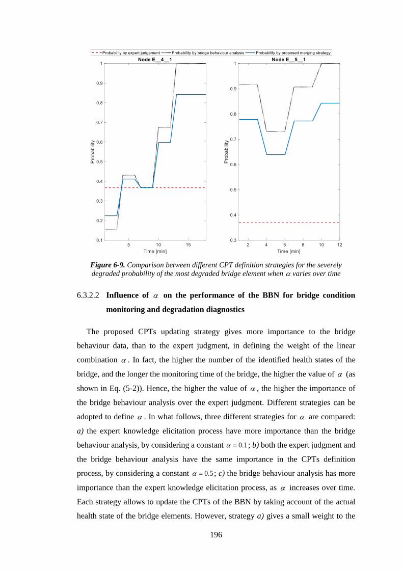
196



6.3.2.2 Influence of on the performance of the BBN for bridge condition

monitoring and degradation diagnostics

The proposed CPTs updating strategy gives more importance to the bridge

behaviour data, than to the expert judgment, in defining the weight of the linear

combination . In fact, the higher the number of the identified health states of the

bridge, and the longer the monitoring time of the bridge, the higher the value of (as

shown in Eq. (5-2)). Hence, the higher the value of , the higher the importance of

the bridge behaviour analysis over the expert judgment. Different strategies can be

adopted to define . In what follows, three different strategies for are compared:

a) the expert knowledge elicitation process have more importance than the bridge

behaviour analysis, by considering a constant 0.1 = ; b) both the expert judgment and

the bridge behaviour analysis have the same importance in the CPTs definition

process, by considering a constant 0.5 = ; c) the bridge behaviour analysis has more

importance than the expert knowledge elicitation process, as increases over time.

Each strategy allows to update the CPTs of the BBN by taking account of the actual

health state of the bridge elements. However, strategy a) gives a small weight to the

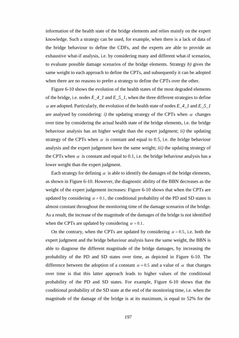
197

information of the health state of the bridge elements and relies mainly on the expert

knowledge. Such a strategy can be used, for example, when there is a lack of data of

the bridge behaviour to define the CDFs, and the experts are able to provide an

exhaustive what-if analysis, i.e. by considering many and different what-if scenarios,

to evaluate possible damage scenarios of the bridge elements. Strategy b) gives the

same weight to each approach to define the CPTs, and subsequently it can be adopted

when there are no reasons to prefer a strategy to define the CPTs over the other.

Figure 6-10 shows the evolution of the health states of the most degraded elements

of the bridge, i.e. nodes E_4_1 and E_5_1, when the three different strategies to define

are adopted. Particularly, the evolution of the health state of nodes E_4_1 and E_5_1

are analysed by considering: i) the updating strategy of the CPTs when changes

over time by considering the actual health state of the bridge elements, i.e. the bridge

behaviour analysis has an higher weight than the expert judgment; ii) the updating

strategy of the CPTs when is constant and equal to 0.5, i.e. the bridge behaviour

analysis and the expert judgement have the same weight; iii) the updating strategy of

the CPTs when is constant and equal to 0.1, i.e. the bridge behaviour analysis has a

lower weight than the expert judgment.

Each strategy for defining is able to identify the damages of the bridge elements,

as shown in Figure 6-10. However, the diagnostic ability of the BBN decreases as the

weight of the expert judgement increases: Figure 6-10 shows that when the CPTs are

updated by considering 0.1 = , the conditional probability of the PD and SD states is

almost constant throughout the monitoring time of the damage scenarios of the bridge.

As a result, the increase of the magnitude of the damages of the bridge is not identified

when the CPTs are updated by considering 0.1 = .

On the contrary, when the CPTs are updated by considering 0.5 = , i.e. both the

expert judgment and the bridge behaviour analysis have the same weight, the BBN is

able to diagnose the different magnitude of the bridge damages, by increasing the

probability of the PD and SD states over time, as depicted in Figure 6-10. The

difference between the adoption of a constant 0.5 = and a value of that changes

over time is that this latter approach leads to higher values of the conditional

probability of the PD and SD states. For example, Figure 6-10 shows that the

conditional probability of the SD state at the end of the monitoring time, i.e. when the

magnitude of the damage of the bridge is at its maximum, is equal to 52% for the

198

0.5 = strategy and 58% for the proposed strategy with that varies over time.

Although the difference between the value of the conditional probability is small, this

can result in a change of the diagnostic ability of the BBN. In fact, when a high number

of different damage scenarios of the bridge are considered, each damage scenario may

be recognized by a value of the conditional probability of the SD state. Consequently,

the best strategy can be the one that is able to assign the highest value of conditional

probability of the SD to the most degraded scenario of the bridge.

Figure 6-10. Evolution over time of the health state of the most degraded elements of the

post-tensioned bridge when CPTs are defined by the proposed updating strategy by using

different values

Finally, Figure 6-11 and Figure 6-12 show the evolution of the conditional

probability of the being in the SD state for nodes E_4_1 and E_5_1, when the two

strategies for updating the CPTs with a constant are considered. Both figures show

the evolution of the conditional probability of SD when the health state of the two

bridge elements is recognized as SD.

Figure 6-11 shows that the conditional probability assigned by the expert

knowledge elicitation process is constant during the time when the elements are

identified as SD, as depicted by the dashed line in Figure 6-11. On the contrary, the

conditional probability obtained by the CDFs of the optimal HI increases as the

condition of the bridge elements gets worse, as shown by the dotted line in Figure

6-11. The solid line in Figure 6-11 shows the evolution of the combination of the two

strategies when a constant 0.1 = is considered. It should be noted that the solid line

is closer to the conditional probability obtained by the expert judgment, rather than to

199

the probability retrieved by analysing the bridge behaviour. Furthermore, the CPTs

updating strategy allows to increase the probability of the SD state of the bridge

elements when the magnitude of the bridge damage increases. However, the value of

the PD and SD states is close to the expert judgment values, and thus the diagnostic

ability of the BBN can be limited.


degraded probability of the most degraded bridge element when is constant and equals to

0.1

Figure 6-12 shows the evolution of the combination of the two strategies when a

constant 0.5 = is considered, by the means of a solid line. The conditional probability

of the SD state of the two BBN nodes increases over time, as the magnitude of the

bridge damages increase. Furthermore, the solid line is closer to the probability

obtained by analysing the bridge behaviour (i.e. by assessing the CDFs of the optimal

HI), than the solid line in Figure 6-11. However, the solid line in Figure 6-12 is closer

to the probability retrieved by the expert judgment than the solid line in Figure 6-9,

where changes based on the length of the monitoring time and the number of

identified health states of the bridge. Again, it is worth mentioning that the proposed

strategy to update the CPTs allows to increase the probability of the SD state when the

magnitude of the damages of the bridge increases.

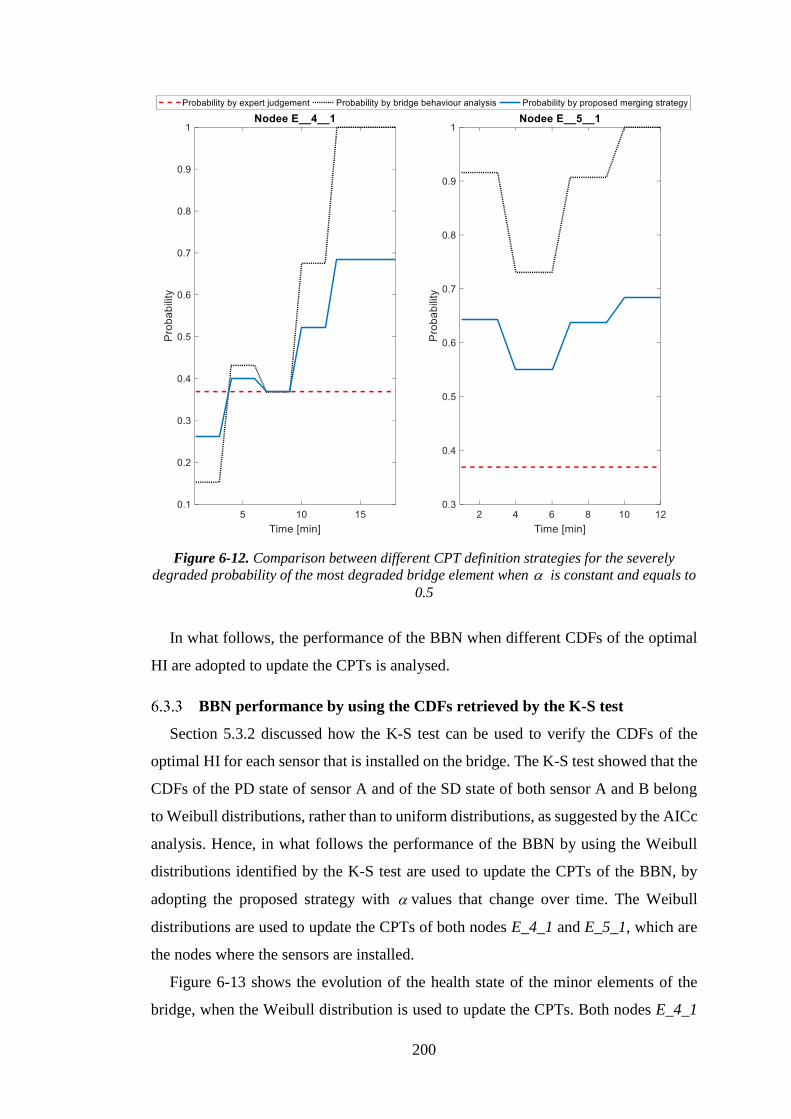
200


degraded probability of the most degraded bridge element when is constant and equals to

0.5

In what follows, the performance of the BBN when different CDFs of the optimal

HI are adopted to update the CPTs is analysed.

BBN performance by using the CDFs retrieved by the K-S test

Section 5.3.2 discussed how the K-S test can be used to verify the CDFs of the

optimal HI for each sensor that is installed on the bridge. The K-S test showed that the

CDFs of the PD state of sensor A and of the SD state of both sensor A and B belong

to Weibull distributions, rather than to uniform distributions, as suggested by the AICc

analysis. Hence, in what follows the performance of the BBN by using the Weibull

distributions identified by the K-S test are used to update the CPTs of the BBN, by

adopting the proposed strategy with values that change over time. The Weibull

distributions are used to update the CPTs of both nodes E_4_1 and E_5_1, which are

the nodes where the sensors are installed.

Figure 6-13 shows the evolution of the health state of the minor elements of the

bridge, when the Weibull distribution is used to update the CPTs. Both nodes E_4_1

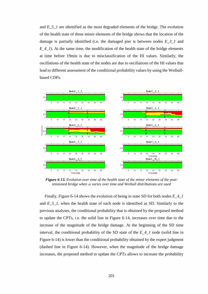
201

and E_5_1 are identified as the most degraded elements of the bridge. The evolution

of the health state of these minor elements of the bridge shows that the location of the

damage is partially identified (i.e. the damaged pier is between nodes E_3_1 and

E_4_1). At the same time, the modification of the health state of the bridge elements

at time before 19min is due to misclassification of the HI values. Similarly, the

oscillations of the health state of the nodes are due to oscillations of the HI values that

lead to different assessment of the conditional probability values by using the Weibull-

based CDFs.


tensioned bridge when varies over time and Weibull distributions are used

Finally, Figure 6-14 shows the evolution of being in state SD for both nodes E_4_1

and E_5_1, when the health state of each node is identified as SD. Similarly to the

previous analyses, the conditional probability that is obtained by the proposed method

to update the CPTs, i.e. the solid line in Figure 6-14, increases over time due to the

increase of the magnitude of the bridge damage. At the beginning of the SD time

interval, the conditional probability of the SD state of the E_4_1 node (solid line in

Figure 6-14) is lower than the conditional probability obtained by the expert judgment

(dashed line in Figure 6-14). However, when the magnitude of the bridge damage

increases, the proposed method to update the CPTs allows to increase the probability

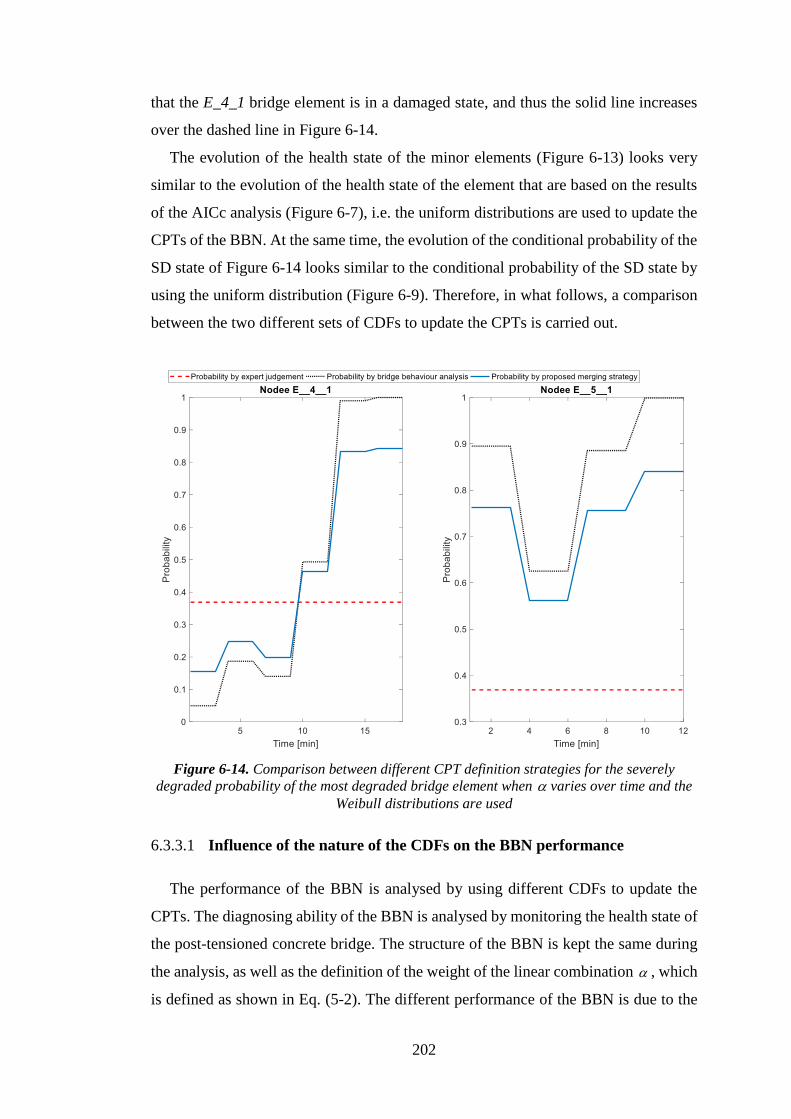
202

that the E_4_1 bridge element is in a damaged state, and thus the solid line increases

over the dashed line in Figure 6-14.

The evolution of the health state of the minor elements (Figure 6-13) looks very

similar to the evolution of the health state of the element that are based on the results

of the AICc analysis (Figure 6-7), i.e. the uniform distributions are used to update the

CPTs of the BBN. At the same time, the evolution of the conditional probability of the

SD state of Figure 6-14 looks similar to the conditional probability of the SD state by

using the uniform distribution (Figure 6-9). Therefore, in what follows, a comparison

between the two different sets of CDFs to update the CPTs is carried out.


degraded probability of the most degraded bridge element when varies over time and the

Weibull distributions are used

6.3.3.1 Influence of the nature of the CDFs on the BBN performance

The performance of the BBN is analysed by using different CDFs to update the

CPTs. The diagnosing ability of the BBN is analysed by monitoring the health state of

the post-tensioned concrete bridge. The structure of the BBN is kept the same during

the analysis, as well as the definition of the weight of the linear combination , which

is defined as shown in Eq. (5-2). The different performance of the BBN is due to the

203

different CDFs that are used to update the CPTs of nodes E_4_1 and E_5_1. In fact,

the CDFs of the PD state for sensor A and of the SD states for both sensor A and B are

retrieved by using: i) the AICc analysis, which leads to three uniform distributions; ii)

the K-S test, which leads to three Weibull distributions. The comparison between the

different CDFs is carried out by analysing the evolution of the identified most

degraded element of the bridge, i.e. nodes E_4_1 and E_5_1 of the BBN.

Figure 6-15 shows the evolution of the health states of nodes E_4_1 and E_5_1

when the Weibull or the uniform distributions are used to update the CPTs. The

evolution of the health state of the nodes is similar when using both CDFs updating

strategies. However, the evolution of the PD state for node E_4_1 (light grey area in

Figure 6-15) shows higher probability values when the Weibull distribution is used to

update the CPTs of the BBN. For example, from time 32min to time 39min, the

Weibull distribution provides a PD probability slightly larger than the other health

states of the bridge elements. On the other hand, the uniform distribution-based BBN

shows a similar value of the PD state from time 31min to time 34min, however, after

time 34min, the value of the SD state (dark grey area in Figure 6-15) becomes the

largest one. At the end of the monitoring time, the value of the conditional probability

of each state is the same for both CDFs-updating strategies. Therefore, the updating of

the health state of the bridge elements appears to happen more slowly, when the

Weibull distribution is adopted. This behaviour can be due to the shape of the CDF of

the Weibull distribution, which increases slowly of the tail on the distribution. On the

contrary, the uniform distribution increases linearly throughout the interval of the

distribution, and consequently the transition between different health states of the

bridge can be faster. The evolution of the health state of node E_5_1 is mainly the

same for both CDFs strategies, as shown in Figure 6-15.

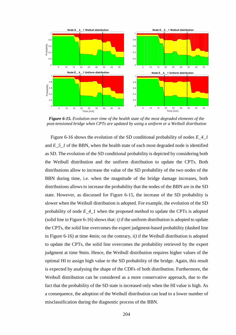
204

Figure 6-15. Evolution over time of the health state of the most degraded elements of the

post-tensioned bridge when CPTs are updated by using a uniform or a Weibull distribution

Figure 6-16 shows the evolution of the SD conditional probability of nodes E_4_1

and E_5_1 of the BBN, when the health state of each most degraded node is identified

as SD. The evolution of the SD conditional probability is depicted by considering both

the Weibull distribution and the uniform distribution to update the CPTs. Both

distributions allow to increase the value of the SD probability of the two nodes of the

BBN during time, i.e. when the magnitude of the bridge damage increases, both

distributions allows to increase the probability that the nodes of the BBN are in the SD

state. However, as discussed for Figure 6-15, the increase of the SD probability is

slower when the Weibull distribution is adopted. For example, the evolution of the SD

probability of node E_4_1 when the proposed method to update the CPTs is adopted

(solid line in Figure 6-16) shows that: i) if the uniform distribution is adopted to update

the CPTs, the solid line overcomes the expert judgment-based probability (dashed line

in Figure 6-16) at time 4min; on the contrary, ii) if the Weibull distribution is adopted

to update the CPTs, the solid line overcomes the probability retrieved by the expert

judgment at time 9min. Hence, the Weibull distribution requires higher values of the

optimal HI to assign high value to the SD probability of the bridge. Again, this result

is expected by analysing the shape of the CDFs of both distribution. Furthermore, the

Weibull distribution can be considered as a more conservative approach, due to the

fact that the probability of the SD state is increased only when the HI value is high. As

a consequence, the adoption of the Weibull distribution can lead to a lower number of

misclassification during the diagnostic process of the BBN.

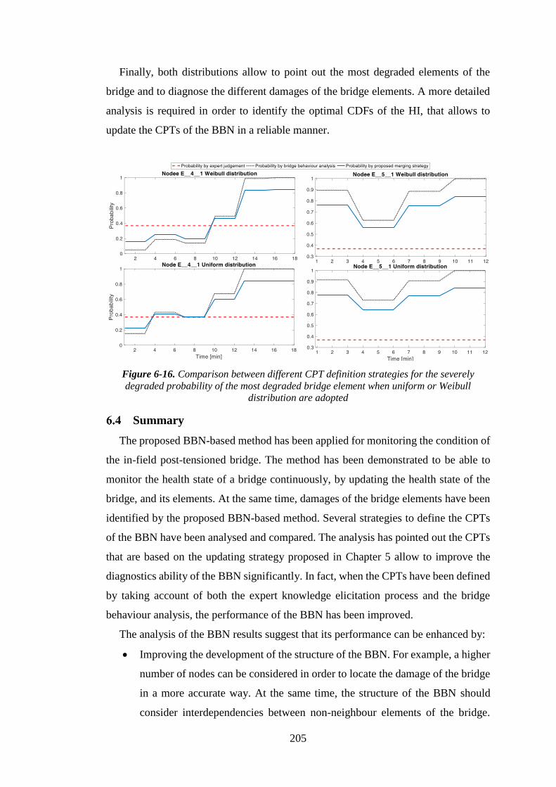
205

Finally, both distributions allow to point out the most degraded elements of the

bridge and to diagnose the different damages of the bridge elements. A more detailed

analysis is required in order to identify the optimal CDFs of the HI, that allows to

update the CPTs of the BBN in a reliable manner.


degraded probability of the most degraded bridge element when uniform or Weibull

distribution are adopted

Summary

The proposed BBN-based method has been applied for monitoring the condition of

the in-field post-tensioned bridge. The method has been demonstrated to be able to

monitor the health state of a bridge continuously, by updating the health state of the

bridge, and its elements. At the same time, damages of the bridge elements have been

identified by the proposed BBN-based method. Several strategies to define the CPTs

of the BBN have been analysed and compared. The analysis has pointed out the CPTs

that are based on the updating strategy proposed in Chapter 5 allow to improve the

diagnostics ability of the BBN significantly. In fact, when the CPTs have been defined

by taking account of both the expert knowledge elicitation process and the bridge

behaviour analysis, the performance of the BBN has been improved.

The analysis of the BBN results suggest that its performance can be enhanced by:

• Improving the development of the structure of the BBN. For example, a higher

number of nodes can be considered in order to locate the damage of the bridge

in a more accurate way. At the same time, the structure of the BBN should

consider interdependencies between non-neighbour elements of the bridge.

206

However, a database of bridge behaviour is needed in order to validate such

connections between non-neighbour bridge elements. Similarly, the number of

states of the BBN nodes can be increased with the aim of improving the

diagnostic ability of the BBN. However, the higher the number of state of the

BBN nodes, the higher the size of the CPTs.

• Interviewing a group of experts in order to retrieve a set of CPTs that relies on

the analysis of the post-tensioned bridge. In fact, this process can improve the

diagnostic ability of the BBN slightly, when the CPTs are based on the expert

knowledge elicitation process. However, when the CPTs are based on the

expert judgements, a small deterioration of the bridge health state is not

identified. For example, if the magnitude of bridge damage increases, the BBN

that relies on expert judgement-based CPTs is not able to point out the decrease

of the bridge health state, due to the constant value of the CPTs.

• Optimizing the definition of the CDFs of the optimal HI of the bridge. In this

way, the diagnostic ability of the BBN can be optimized by taking account of

the actual health state of the bridge elements.

• Optimizing the strategy to define the weight of the linear combination .

Indeed, the analysis of the BBN when different values of have been

considered showed that the diagnostic ability of the BBN strongly rely on the

value of . Therefore, a rigorous way to define needs to be proposed in

order to optimize the performance of the BBN.

In what follows, the conclusions of the thesis and future work are discussed.

207

Conclusions and future

work

Conclusions

The European transportation network has more than one million bridges. These

assets are continuously deteriorating due to aging, traffic load (which nowadays

exceeds original design criteria of bridges), and environmental effects, such as wind,

and changing temperatures. Commonly, the health state of bridges is assessed by time-

consuming, expensive and subjective visual inspections at fixed time intervals, ranging

from one to six years. As a consequence, the degradation of the bridge health state can

increase undetected, by reducing the safety, reliability and availability of both the

bridge and the corresponding transportation network.

In this thesis, the literature review process showed that a clear majority of the

analysed condition monitoring and damage detection methods have deficiencies in

monitoring the health state of a bridge continuously, by taking account of the

influences between different elements of the bridge. Model-based methods allow to

consider interdependencies between different elements of a bridge, but a time-

consuming process is required for their development. At the same time, the reviewed

methods presented difficulties in managing different sources of data (such as bridge

behaviour data and expert knowledge) and diagnosing the location and level of severity

of the bridge damage. Furthermore, most of the reviewed non-model-based methods

are verified on FEMs of bridges, which are not able to represent the data uncertainties

and noise of an in-field bridge.

Several objectives have been achieved in this thesis:

• The main objective of this thesis was to develop a bridge condition monitoring

and damage diagnostics method. The main element of the proposed method

was to monitor and assess the health state of a bridge continuously, by taking

account of the health state of each element of the bridge and without requiring

a time-consuming process for its development. This method has been

developed by proposing a BBN-based approach. First of all, the CPTs of the

BBN have been defined by adopting an expert knowledge elicitation process.

Such a BBN method has shown to be able to monitor the health state of two

208

bridges (a steel truss bridge and a beam-and-slab bridge), modelled using

FEMs, continuously, by accounting for the interdependencies between

different elements of the bridge. The BBN allowed also to identify damages of

the bridge, and to diagnose the causes of such damages by pointing out the

damaged minor element(s) of the bridge. However, in terms of the diagnostic

ability of the BBN there were some cases of misclassification. Consequently,

several methods have been introduced in this thesis to improve the performance

of the BBN analysis, by pre-processing the data of the bridge behaviour and

improving the definition of the CPTs, as discussed below.

• A data analysis methodology has been developed in order to pre-process the

bridge behaviour data. The data analysis methodology allowed to assess HIs of

the bridge elements. The HIs have been identified by using statistical,

frequency-based and vibration-based features as an input to an EMD method,

which allowed to assess the trend of the features over time. The optimal HI to

represent the health state of the bridge elements has been identified by looking

for the HI with the highest values of trendability and monotonicity. The optimal

HI has been then used as an input to the BBN nodes, in order to assess the

health state of the whole bridge. The proposed data analysis methodology has

been verified on two in-field bridges, a steel truss bridge and a post-tensioned

concrete bridge. Both bridges were subjected to a progressive damage test

under unknown environmental conditions. A good performance has been

achieved in monitoring the health state of the bridges and diagnosing their

damages in terms of location and magnitude.

• A machine learning method, which relies on an NFC, has been introduced to

assess the health state of a bridge element automatically. The results of the

NFC can potentially be used as an input to the BBN nodes, to select the states

of the BBN nodes. An optimal set of HIs has been identified to assess the health

state of the bridge elements automatically, by relying on an MBDE method.

The optimal set of HIs allowed to achieve good performance in assessing the

health state of the post-tensioned concrete bridge (an in-field bridge)

automatically.

• A method to update the CPTs of the BBN nodes, by merging the expert

knowledge elicitation process and the analysis of a database of bridge

behaviour has been proposed. This method allows to update the CPTs of the

209

BBN nodes by taking account of the actual health state of the bridge elements.

The method has been tested on the post-tensioned concrete in-field. The

analysis of the results showed that a significant improvement of the diagnostic

ability of the BBN is achieved, when the proposed method to update the CPTs

is adopted.

• A method to analyse database of unknown infrastructure behaviour has been

proposed. This latter method relies on an ensemble-based change-point

detection algorithm, which has been developed to identify the most critical

change of the health state of the infrastructure. The proposed method has been

confirmed by analysing the database of a real in-field tunnel infrastructure. The

method allowed to identify when the health state of the infrastructure changes,

by providing the characteristics of such changes of the infrastructure health

state. In this way, information about different health states of the infrastructure

can be identified and analysed. As a result, useful information for defining the

CPTs of the BBN, by relying on both expert judgment and bridge behaviour

analysis, can be retrieved.

Overall, the proposed BBN-based method, with the integration of the other developed

methods, allows to monitor the health state of a bridge continuously. The health state

of the bridge is assessed by taking account of the interdependencies between different

elements of the bridge. Different sources of information, such as visual inspection

reports and bridge behaviour data, can be used as an input to the BBN. Moreover, the

proposed BBN method allows to identify and diagnose damage of the bridge elements.

In this way, the health state of the bridge is monitored continuously, and consequently

the safety, reliability and availability of the bridge are improved. At the same time,

continuous information about the health state of the bridge, and its elements, is

provided to bridge managers, who can optimize the maintenance budget by scheduling

maintenance activities based on the actual health state of the bridge.

Research contributions

The developed thesis makes several contributions to the SHM framework:

• A better understanding of the SHM needs. A vast number of SHM methods

for bridge condition monitoring and damage detection has been reviewed in

this thesis. The advantages and disadvantages of each condition monitoring

method have been identified and discussed. The needs of a comprehensive

210

bridge SHM strategy have been proposed and discussed. The output of this

literature review analysis has been published in the Structural health

monitoring journal [Vagnoli et al., 2018].

• Assessment of the bridge health state by considering the health state of its

elements. Many bridge condition monitoring, and damage diagnostics

methods do not consider the interdependencies between different elements of

the bridge. Hence, the influence of a damaged element on the health state of a

different bridge element is neglected. The BBN method proposed in this thesis

allows to assess the interdependencies between different elements of the

bridge. The BBN method can be applied directly on any infrastructure, by

following the proposed step-by-step process to define both the BBN structure

and its CPTs. This will allow bridge engineers to monitor the behaviour of a

bridge, by pointing out and diagnosing its unexpected behaviour. The proposed

method allows to satisfy the first three level of the damage detection process.

However, a rigorous way to define the BBN structure, and the number of states

of the BBN nodes require to be analysed further. The proposed method has

been described in a paper, which is currently under review at the Structural

Control and Health Monitoring Journal.

• Merging the expert knowledge and the bridge behaviour analysis. Bridge

engineers and bridge managers have a lot of experience in knowing the most

critical elements of a bridge, and in providing insights about possible

relationships between the different elements. At the same time, the data of the

bridge behaviour also provides information about interdependencies between

different elements of the bridge. In this thesis, these two sources of information

have been analysed together in order to improve the reliability of the condition

monitoring process using the BBN. The proposed method can be applied in a

framework where a BBN method is used to monitor the health state of a system.

In fact, such method has been demonstrated to enhance the diagnostic

performance of the BBN significantly. However, the expert elicitation process

requires further analysis, in order to provide a reliable assessment of the

interdependencies between different system elements. At the same time, the

definition of the CDFs of the bridge behaviour needs to be analysed further, to

provide a robust assessment of the CPTs. The method for analysing both the

211

expert judgment and the bridge behaviour is being described in a paper, which

is going to be submitted to the Reliability Engineering & System Safety journal.

• Assessment of the health state of the bridge elements by relying on data-

driven methods. Measurement systems are becoming cheap, and thus sensors

are installed on an increasing number of infrastructures. Therefore, two data-

driven methods have been proposed to assess the health state of the bridge

elements in a fast and reliable manner. A data analysis methodology showed

how to analyse the data of the bridge behaviour by adopting several steps: i)

the removal of the noise; ii) identification of the free-vibration of the bridge;

iii) extraction of statistical, frequency-based and vibration-based features; iv)

assessment of the features trend by using the EMD method; v) assessment of

the health state of the bridge elements. Features of the bridge behaviour data

have been analysed. A machine learning method showed how the past

behaviour of the bridge can be used to assess the health state of the bridge

elements in a fast and automatic way. Furthermore, the performance of the

machine learning method is expected to increase when the availability of the

bridge behaviour data increases. Consequently, in the future, when more bridge

behaviour data is available, machine learning methods can be applied to

automatically monitor the health state of bridge infrastructure in a fast and

reliable way. The two data-driven methods can be applied to any system that

is monitored by the means of vibration data. Particularly, the data analysis

methodology would allow to identify unexpected behaviour of the system as

soon as it occurs, whereas the machine learning method would require a

database of past behaviour of the system for the training process. However, the

set of proposed HIs may require further analysis in order to increase the set of

possible HIs to describe the health state of different systems. The developed

data-driven methods have been described in a research article, which is under

review at the Structural Control and Health Monitoring Journal .

• Analysis of database of infrastructure behaviour for change identification.

A method to analyse vast database of past infrastructure behaviour has been

proposed, in order to identify the most critical change of the health state of the

infrastructure. In fact, structural engineers would use this method for

identifying the most critical change of behaviour of the infrastructure. Such

information can be used to analyse the critical behaviour experienced by the

212

infrastructure and diagnose possible causes of the changes of the infrastructure

health. The proposed method can be applied to any system that has monotonic

behaviour as the degradation increases. Further analysis of the time constant

definition may be required in order to identify a rigorous method for their

definition. The developed method has been published in the Tunnelling and

Underground Space Technology Journal [Vagnoli & Remenyte-Prescott,

2018].

Future work

The proposed method-based on BBN is suitable for monitoring the health state of

real in-field bridge continuously, by diagnosing damage of the bridge elements. At the

same time, the other methods proposed in this thesis to analyse the data of bridge

behaviour showed good performance in assessing changes of the health state of real

infrastructures. However, there are some aspects of the proposed methods that require

further analysis to improve the robustness of the methods in real applications:

• A step-by-step process to define the structure of the BBN has been proposed,

by identifying major and minor elements of the bridge. Eventually, the minor

elements of the bridge have been identified by dividing the major elements into

smaller parts. Therefore, a rigorous method to divide major (minor) elements

into smaller elements, and thus to define an optimal number of nodes of the

BBN, needs to be proposed. For example, an optimization analysis can be

carried out in order to evaluate how different structure of the BBN influences

the BBN performance. In this way, an optimal structure of the BBN may be

identified, by optimizing both the diagnostics performance of the BBN and the

size of the network, which can influence the computational time of the analysis.

• The number of states of the nodes in the proposed BBN is three in this thesis:

i) a healthy state; ii) a partially degraded state; and iii) a severely degraded

state. However, a higher number of states of the BBN allows to increase the

damage detection and diagnostics ability of the BBN, by pointing out small

changes of the bridge damage magnitude. It should be noted that the size of the

CPT increases with the number of states of the nodes, and, as a consequence,

a balance between number of states and size of the CPTs needs to be obtained.

A possible solution to this problem can be the adoption of continuous nodes of

213

the BBN, which might also help in identifying smaller changes of the health

state of the bridge, by avoiding the issue of the CPTs size.

• The proposed data analysis methodology provides HIs of the health state of the

bridge, by lumping together the information of the trend of the features into the

HI. However, the proposed set of HIs is not exhaustive, i.e. more HIs can be

used to represent the health state of the bridge. Therefore, several statistical

parameters, such as the mean value, the peak value, the interquartile range, etc.,

could be analysed in order to identify an optimal set of HIs, which is able to

monitor the health state of the bridge by minimizing the number of

misclassification of the bridge health state.

• The proposed method to update the CPTs of the BBN by merging expert

knowledge elicitation process and the bridge behaviour analysis requires

further analysis to: i) improve the robustness of the expert knowledge

elicitation process by interviewing a wider group of experts; ii) improve the

definition of the weight of the linear combination , by considering also the

robustness of the expert judgment; iii) define the CDFs of the bridge behaviour

in a robust manner, by considering a wider set of possible distributions to fit

the optimal HI values.

• The performance of the proposed ensemble-based change-point detection

method relies on the value of three time-constants, i.e. , , . These

constants are defined by using an expert knowledge elicitation process. Further

analysis needs to be carried out in order to assess the value of the time constant

in a more robust manner.

214

References

[Abdoun et al., 2009] Abdoun, T., Bennett, V., Thevanayagam, S., Dobry, R.,

Shantz, T., Jang, D., 2009. “Wireless MEMS-based system for real-time

geotechnical instrumentation of active slopes”, WIT Transactions on the Built

Environment, 108, pp. 617-624.

[Rousseeuw, 1987] Rousseeuw, P.J., 1987. “Silhouettes: A graphical aid to the

interpretation and validation of cluster analysis”, Journal of Computational and

Applied Mathematics, 20 (C), pp. 53-65.

[Adey et al., 2004] Adey, B., Hajdin, R., Brühwiler, E., “Effect of common cause

failures on indirect costs”, Journal of Bridge Engineering, 9 (2), pp. 200-208, 2004.

[Aied et al., 2016] Aied, H., González, A., Cantero, D., “Identification of sudden

stiffness changes in the acceleration response of a bridge to moving loads using

ensemble empirical mode decomposition”, Mechanical Systems and Signal

Processing, 66-67, pp. 314-338, 2016.

[Akaike, 1974] Akaike, H., “A New Look at the Statistical Model Identification”,

IEEE Transactions on Automatic Control, 19 (6), pp. 716-723, 1974.

[Alves et al., 2016] Alves, V., Cury, A., Cremona, C., “On the use of symbolic

vibration data for robust structural health monitoring”, Proceedings of the Institution

of Civil Engineers: Structures and Buildings, 169 (9), pp. 715-723, 2016.

[Anastasopoulos et al., 2015] Anastasopoulos, I., Anastasopoulos, P.C.,

Agalianos, A., Sakellariadis, L., “Simple method for real-time seismic damage

assessment of bridges”, Soil Dynamics and Earthquake Engineering, 78, pp. 201-

212, 2015.

[Andersen et al., 2006] Andersen, J.E. and Fustinoni, M., “Structural Health

Monitoring Systems”, L&S S.r.l. Servizi Grafici, 2006.

[Arangio et al., 2014] Arangio, S., Bontempi, F., “Structural health monitoring

of a cable-stayed bridge with Bayesian neural networks”, Structure and

Infrastructure Engineering, Article in Press, 2014.

[Arias, 1970] A. Arias, “A Measure of Earthquake Intensity”, R.J. Hansen, ed.

Seismic Design for Nuclear Power Plants, MIT Press, Cambridge, Massachusetts,

pp. 438-483, 1970.

215

[Attema et al., 2017] Attema, T., Kosgodagan Acharige, A., Morales-Nápoles,

O., Maljaars, J., “Maintenance decision model for steel bridges: a case in the

Netherlands”, Structure and Infrastructure Engineering, 13 (2), pp. 242-253, 2017.

[Attoh-Okine & Bowers, 2006] Attoh-Okine, N.O., Bowers, S., “A Bayesian

belief network model of bridge deterioration”, Proceedings of the Institution of Civil

Engineers: Bridge Engineering, 159 (2), pp. 69-76, 2006.

[Bao et al., 2018] Bao, Y., Tang, Z., Li, H., Zhang, Y., “Computer vision and

deep learning–based data anomaly detection method for structural health

monitoring”, Structural Health Monitoring, DOI 10.1177/1475921718757405,

2018.

[Barbosh et al., 2018] Barbosh, M., Sadhu, A., Vogrig, M., “Multisensor-based

hybrid empirical mode decomposition method towards system identification of

structures”, Structural Control and Health Monitoring, 25 (5), art. no. e2147, 2018.

[Başaĝa et al., 2011] Başaĝa, H.B., Türker, T., Bayraktar, A., “A model updating

approach based on design points for unknown structural parameters”, Applied

Mathematical Modelling, 35 (12), pp. 5872-5883, 2011.

[Bhalla et al., 2005] Bhalla, S., Yang, Y.W., Zhao, J., Soh, C.K., 2005.

“Structural health monitoring of underground facilities - Technological issues and

challenges”, Tunnelling and Underground Space Technology, 20 (5), pp. 487-500.

[Burnham & Anderson, 2004] Burnham, K.P., Anderson, D.R., “Multimodel

inference: Understanding AIC and BIC in model selection”, Sociological Methods

and Research, 33 (2), pp. 261-304, 2004.

[Cahill et al., 2018] Cahill, P., Hazra, B., Karoumi, R., Mathewson, A., Pakrashi,

V., “Vibration energy harvesting based monitoring of an operational bridge

undergoing forced vibration and train passage”, Mechanical Systems and Signal

Processing, 106, pp. 265-283, 2018.

[Cannarile et al., 2017] Cannarile, F., Baraldi., P., Compare, M., Borghi, D.,

Capelli, L., Cocconcelli, M., Lahrac, A., Zio, E., “An unsupervised clustering

method for assessing the degradation state of cutting tools in the packaging

industry”, Safety and Reliability: Theory and Application- Proceedings of the

European Safety and Reliability Conference, ESREL 2017, Portroz, Slovenia, 2017.

216

[Cao et al., 2011] Cao, Y., Yim, J., Zhao, Y., Wang, M.L., “Temperature effects

on cable stayed bridge using health monitoring system: A case study”, Structural

Health Monitoring, 10 (5), pp. 523-537, 2011.

[Cao et al., 2017] Cao, M.S., Sha, G.G., Gao, Y.F., Ostachowicz, W., “Structural

damage identification using damping: A compendium of uses and features”, Smart

Materials and Structures, 26 (4), art. no. 043001, 2017.

[Carslaw et al., 2006] Carslaw, D.C., Ropkins, K., Bell, M.C., “Change-point

detection of gaseous and particulate traffic-related pollutants at a roadside location”,

Environmental Science and Technology, 40 (22), pp. 6912-6918, 2006.

[Casas et al., 2017] Casas, J.R., Moughty, J. J., “Bridge Damage Detection Based

on Vibration Data: Past and New Developments”, Front. Built Environ. 3:4., doi:

10.3389/fbuil.2017.00004, 2017.

[Catbas et al., 2008] Catbas, F.N., Susoy, M., Frangopol, D.M., “Structural

health monitoring and reliability estimation: Long span truss bridge application with

environmental monitoring data”, Engineering Structures, 30 (9), pp. 2347-2359,

2008.

[Cavadas et al., 2013] Cavadas, F., Smith, I.F.C., Figueiras, J., “Damage

detection using data-driven methods applied to moving-load responses”,

Mechanical Systems and Signal Processing, 39 (1-2), pp. 409-425, 2013.

[Cetişli & Barkana, 2010] Cetişli, B., Barkana, A., “Speeding up the scaled

conjugate gradient algorithm and its application in neuro-fuzzy classifier training”,

Soft Computing, 14 (4), pp. 365-378, 2010.

[Chalouli et al., 2017] Chalouli, M., Berrached, N.-E., Denai, M., “Intelligent

Health Monitoring of Machine Bearings Based on Feature Extraction”, Journal of

Failure Analysis and Prevention, 17 (5), pp. 1053-1066, 2017.

[Chang & Kim, 2016] Chang, K.-C., Kim, C.-W., “Modal-parameter

identification and vibration-based damage detection of a damaged steel truss

bridge”, Engineering Structures, 122, pp. 156-173, 2016.

[Chang et al., 2014] Chang, K.-C., Kim, C.-W., Kawatani, M., “Feasibility

investigation for a bridge damage identification method through moving vehicle

laboratory experiment”, Structure and Infrastructure Engineering, 10 (3), pp. 328-

345, 2014.

217

[Chen & Pollino, 2012] Chen, S.H., Pollino, C.A., “Good practice in Bayesian

network modelling”, Environmental Modelling and Software, 37, pp. 134-145,

2012.

[Cremona et al., 2012] Cremona, C., Cury, A., Orcesi, A., “Supervised learning

algorithms for damage detection and long term bridge monitoring”, Bridge

Maintenance, Safety, Management, Resilience and sustainability - Proceedings of

the Sixth International Conference on Bridge Maintenance, Safety and

Management, pp. 2144-2151, 2012.

[Cunha et al., 2001] Cunha, A., Caetano, E., Delgado, R., “Dynamic Tests on

Large Cable-Stayed Bridge”, Journal of Bridge Engineering, 6.

10.1061/(ASCE)1084-0702(2001)6:1(54), 2001.

[Cury et al., 2012] Cury, A., Crémona, C., “Assignment of structural behaviours

in long-term monitoring: Application to a strengthened railway bridge”, Structural

Health Monitoring, 11 (4), pp. 422-441, 2012.

[Das, 2004] Das, B., “Generating conditional probabilities for Bayesian

networks: Easing the knowledge acquisition problem”, arXiv preprint cs/0411034,

2004.

[Di Maio et al., 2016] Di Maio, F., Vagnoli, M., Zio, E., “Transient identification

by clustering based on Integrated Deterministic and Probabilistic Safety Analysis

outcomes”, Annals of Nuclear Energy, 87, pp. 217-227, 2016.

[Dias & De Sousa, 2018] Dias, C.G., de Sousa, C.M., “A Neuro-Fuzzy Approach

for Locating Broken Rotor Bars in Induction Motors at Very Low Slip”, Journal of

Control, Automation and Electrical Systems, 29 (4), pp. 489-499, 2018

[Djurovic et al., 2000] Djurovic, Z., Kovacevic, B., Barroso, V., “QQ-plot based

probability density function estimation”, IEEE Signal Processing Workshop on

Statistical Signal and Array Processing, SSAP, pp. 243-247, 2000.

[Dowling et al., 2012] Dowling, J., Obrien, E.J., González, A., “Adaptation of

Cross Entropy optimisation to a dynamic Bridge WIM calibration problem”,

Engineering Structures, 44, pp. 13-22, 2012.

[Duan and Zhang, 2006] Duan Z, Zhang K., “Data Mining Technology for

Structural Health Monitoring”, Pacific Science Review, 8, 2006.

218

[Duan et al., 2018] Duan, L., Zhao, F., Wang, J., Wang, N., Zhang, J., “An

Integrated Cumulative Transformation and Feature Fusion Approach for Bearing

Degradation Prognostics”, Shock and Vibration, 2018, art. no. 9067184, 2018.

[Elmasry et al., 2017] Elmasry, M., Hawari, A., Zayed, T., “Defect based

deterioration model for sewer pipelines using bayesian belief networks”, Canadian

Journal of Civil Engineering, 44 (9), pp. 675-690, 2017.

[Enright & Frangopol, 1998] Enright, M.P., Frangopol, D.M., “Probabilistic

analysis of resistance degradation of reinforced concrete bridge beams under

corrosion”, Engineering Structures, 20 (11), pp. 960-971, 1998.

[European Commission, 2012] European Commission, “EU transport in

figures”, statistical pocketbook, 2012.

[Fan et al., 2011] Fan, W., Qiao, P., “Vibration-based damage identification

methods: A review and comparative study”, Structural Health Monitoring, 10 (1),

pp. 83-111, 2011.

[Feng et al., 2015] Feng, D., Feng, M.Q., “Model Updating of Railway Bridge

Using in Situ Dynamic Displacement Measurement under Trainloads”, Journal of

Bridge Engineering, 20 (12), art. no. 04015019, 2015.

[Fenton et al., 2013] Fenton, N., Neil, M., “Risk assessment and decision analysis

with Bayesian networks”, 1st ed. Oxford: Taylor & Francis, 2013.

[Ferdous et al., 2011] Ferdous, R., Khan, F., Sadiq, R., Amyotte, P., & Veitch,

B., “Fault and event tree analyses for process systems risk analysis: Uncertainty

handling formulations”, Risk Analysis, 31, 86–107, 2011.

[Franchin et al., 2016] Franchin, P., Lupoi, A., Noto, F., Tesfamariam, S.,

“Seismic fragility of reinforced concrete girder bridges using Bayesian belief

network”, Earthquake Engineering and Structural Dynamics, 45 (1), pp. 29-44,

2016.

[Frangopol et al., 2004] Frangopol, D.M., Kallen, M.J. and Noortwijk, J.M.V.,

“Probabilistic models for life‐cycle performance of deteriorating structures: review

and future directions”, Progress in Structural Engineering and Materials, 6(4),

pp.197-212, 2004.

[Frangopol et al., 2012] Frangopol, D.M., Saydam, D., Kim, S., “Maintenance,

management, life-cycle design and performance of structures and infrastructures: a

brief review”, Structure and Infrastructure Engineering, 8 (1), pp. 1-25, 2012.

219

[Galotto et al., 2015] Galotto, L., Brun, A.D.M., Godoy, R.B., Maciel, F.R.R.,

Pinto, J.O.P., “Data based tools for sensors continuous monitoring in industry

applications”, IEEE International Symposium on Industrial Electronics, 2015-

September, art. no. 7281536, pp. 600-605, 2015.

[Gangone et al., 2011] Gangone, M.V., Whelan, M.J., Janoyan, K.D., “Wireless

monitoring of a multispan bridge superstructure for diagnostic load testing and

system identification”, Computer-Aided Civil and Infrastructure Engineering, 26

(7), pp. 560-579, 2011.

[Gentile et al., 2015] Gentile, C., Saisi, A., “Continuous dynamic monitoring of

a centenary iron bridge for structural modification assessment”, Frontiers of

Structural and Civil Engineering, 9 (1), pp. 26-41, 2015.

[González et al., 2015] González, A., Covián, E., Casero, M., “Impact of super-

imposed and truck live load on modal characteristics of short-span bridges”,

Operational Modal Analysis Conference (IOMAC 2015); Proc. 6th intern. Confer.,

Gijon (Spain), 10-14 May 2015.

[Guo et al., 2012] Guo, W., Orcesi, A.D., Cremona, C.F., Santos, J.P., Yang, S.,

Dieleman, L., “A vibration-based framework for structural health monitoring of

railway bridges”, Life-Cycle and Sustainability of Civil Infrastructure Systems –

Proceedings of the 3rd International Symposium on Life-Cycle Civil Engineering,

IALCCE 2012, pp. 1118-1125, 2012.

[Hakim et al., 2013] Hakim, S.J.S., Abdul Razak, H., “Structural damage

detection of steel bridge girder using artificial neural networks and finite element

models”, Steel and Composite Structures, 14 (4), pp. 367-377, 2013.

[Han et al., 2014] Han, J., Zheng, P. & Wang, H., “Structural modal parameter

identification and damage diagnosis based on Hilbert Huang transform”, Earthquake

Engineering & Engineering Vibration, Vol. 13, (1) pp 101-111, 2014.

[He et al., 2008] He, X.-H., Yu, Z.-W., Chen, Z.-Q., “Finite element model

updating of existing steel bridge based on structural health monitoring”, Journal of

Central South University of Technology (English Edition), 15 (3), pp. 399-403,

2008.

[Hoell & Omenzetter, 2017] Hoell, S., Omenzetter, P., “Fukunaga-Koontz

feature transformation for statistical structural damage detection and hierarchical

220

neuro-fuzzy damage localisation”, Journal of Sound and Vibration, 400, pp. 329-

353, 2017.

[Holický et al., 2013] Holický, M., Marková, J., Sýkora, M., “Forensic

assessment of a bridge downfall using Bayesian networks”, Engineering Failure

Analysis, 30, pp. 1-9, 2013.

[Hooper et al., 2012] Hooper, E., Chapman, L., “The impacts of climate change

on national road and rail networks”, Transport and Sustainability, 2, pp. 105-136,

2012.

[Hsu et al., 2010] Hsu, T.-Y., Loh, C.-H., “Damage detection accommodating

nonlinear environmental effects by nonlinear principal component analysis”,

Structural Control and Health Monitoring, 17 (3), pp. 338-354, 2010.

[Huang et al., 1998] Huang, N.E., Shen, Z., Long, S.R., Wu, M.C., Snin, H.H.,

Zheng, Q., Yen, N.-C., Tung, C.C., Liu, H.H., “The empirical mode decomposition

and the Hubert spectrum for nonlinear and non-stationary time series analysis”,

Proceedings of the Royal Society A: Mathematical, Physical and Engineering

Sciences, 454 (1971), pp. 903-995, 1998.

[IRA, 2015] International railway association, community of European railway

and infrastructure, “Rail transport and environment, facts and figure”, ISBN 976-2-

7461-2400-4, 2015.

[Jaishi & Ren, 2005] Jaishi, B., Ren, W.-X., “Structural finite element model

updating using ambient vibration test results”, Journal of Structural Engineering,

131 (4), pp. 617-628, 2005.

[Jensen & Nielsen, 2007] Jensen, F.V., Nielsen, T. D., “Bayesian Networks and

Decision Graphs”, Information Science and Statistics, Springer, 2007.

[Ji et al., 2015] Ji, Z., Xia, Q., Meng, G., “A review of parameter learning

methods in bayesian network”, Lecture Notes in Computer Science (including

subseries Lecture Notes in Artificial Intelligence and Lecture Notes in

Bioinformatics), 9227, pp. 3-12, 2015.

[Jian & Murthy, 2011] Jiang, R., Murthy, D.N.P., “A study of Weibull shape

parameter: Properties and significance”, Reliability Engineering and System Safety,

96 (12), pp. 1619-1626, 2011.

221

[Kabir et al., 2016] Kabir, G., Sadiq, R., Tesfamariam, S., “A fuzzy Bayesian

belief network for safety assessment of oil and gas pipelines”, Structure and

Infrastructure Engineering, 12 (8), pp. 874-889, 2016.

[Kan et al., 2015] Kan, M.S., Tan, A.C.C., Mathew, J., “A review on prognostic

techniques for non-stationary and non-linear rotating systems”, Mechanical Systems

and Signal Processing, 62, pp. 1-20, 2015.

[Katicha et al., 2017] Katicha, S.W., Flintsch, G., Bryce, J., Ferne, B., “Wavelet

denoising of TSD deflection slope measurements for improved pavement structural

evaluation”, Computer-Aided Civil and Infrastructure Engineering, 29 (6), pp. 399-

415, 2014.

[Katipamula et al., 2005] Katipamula, S., Brambley, M.R., “Methods for fault

detection, diagnostics, and prognostics for building systems - A review, Part I”,

HVAC and R Research, 11 (1), pp. 3-25, 2005.

[Khan et al., 2018] Khan, I., Shan, D., Li, Q., Jie, H., “Continuous modal

parameter identification of cable-stayed bridges based on a novel improved

ensemble empirical mode decomposition”, Structure and Infrastructure

Engineering, 14 (2), pp. 177-191, 2018.

[Killick et al., 2012] Killick, R., Fearnhead, P., Eckley, I.A., “Optimal detection

of changepoints with a linear computational cost”, Journal of the American

Statistical Association, 107 (500), pp. 1590-1598, 2012.

[Kim et al., 2007] Kim, J.-T., Park, J.-H., Lee, B.-J., “Vibration-based damage

monitoring in model plate-girder bridges under uncertain temperature conditions”,

Engineering Structures, 29 (7), pp. 1354-1365, 2007.

[Kim et al., 2015] Kim, C.-W., Morita, T., Oshima, Y., Sugiura, K., “A Bayesian

approach for vibration-based long-term bridge monitoring to consider

environmental and operational changes”, Smart Structures and Systems, 15 (2), pp.

395-408, 2015.

[Koepcke et al., 2016] Koepcke, L., Ashida, G., Kretzberg, J., 2016. “Single and

multiple change point detection in spike trains: Comparison of different CUSUM

methods”, Frontiers in Systems Neuroscience, 10 (JUN), art. no. 51.

[Lavielle, 2005] Lavielle, M., 2005. “Using penalized contrasts for the change-

point problem”, Signal Processing, 85 (8), pp. 1501-1510.

222

[Killick & Eckley, 2014] Killick, R. and Eckley, I., 2014. “Changepoint: An R

package for changepoint analysis”, Journal of Statistical Software, 58(3), pp.1-19.

[Baxter, 2015] Alan Baxter, 2015. “Network Rail A Guide to Overhead

Electrification”, 132787-ALB-GUN-EOH-000001, February 2015 Rev 10.

[Ordoñez et al., 2016] Ariznavarreta-Fernández, F., González-Palacio, C.,

Menéndez-Díaz, A., Ordoñez, C., 2016. “Measurement system with angular

encoders for continuous monitoring of tunnel convergence”, Tunnelling and

Underground Space Technology, 56, pp. 176-185.

[Lato & Diederichs, 2014] Lato, M.J. and Diederichs, M.S., 2014. “Mapping

shotcrete thickness using LiDAR and photogrammetry data: Correcting for over-

calculation due to rockmass convergence”, Tunnelling and Underground Space

Technology, 41, pp.234-240.

[Mohamad et al., 2012] Mohamad, H., Soga, K., Bennett, P.J., Mair, R.J., Lim,

C.S., 2012. “Monitoring twin tunnel interaction using distributed optical fiber strain

measurements”, Journal of Geotechnical and Geoenvironmental Engineering, 138

(8), pp. 957-967.

[Kosgodagan-Dalla Torre et al., 2017] Kosgodagan-Dalla Torre, A., Yeung,

T.G., Morales-Nápoles, O., Castanier, B., Maljaars, J., Courage, W., “A Two-

Dimension Dynamic Bayesian Network for Large-Scale Degradation Modeling

with an Application to a Bridges Network”, Computer-Aided Civil and


[Kreislova et al., 2012] Kreislova, K., Geiplova, H., “Evaluation of corrosion

protection of steel bridges”, Procedia Engineering, 40, pp. 229-234, 2012.

[Lampis et al., 2009] Lampis, M., Andrews, J.D., “Bayesian belief networks for

system fault diagnostics”, Quality and Reliability Engineering International, 25 (4),

pp. 409-426, 2009.

[Langone et al., 2017] Langone, R., Reynders, E., Mehrkanoon, S., Suykens,

J.A.K., “Automated structural health monitoring based on adaptive kernel spectral

clustering”, Mechanical Systems and Signal Processing, 90, pp. 64-78, 2017.

[Laory et al., 2012] Laory, I., Hadj Ali, N.B., Trinh, T.N., Smith, I.F.C.,

“Measurement system configuration for damage identification of continuously

monitored structures”, Journal of Bridge Engineering, 17 (6), pp. 857-866, 2012.

223

[Laory et al., 2013] Laory, I., Trinh, T.N., Posenato, D., Smith, I.F.C.,

“Combined model-free data-interpretation methodologies for damage detection

during continuous monitoring of structures”, Journal of Computing in Civil

Engineering, 27 (6), pp. 657-666, 2013.

[Le & Andrews, 2014] Le, B.L., Andrews, J.D., “Modelling railway bridge asset

management using Petri-Net modelling techniques”, Civil-Comp Proceedings, 104,

2014.

[LeBeau et al., 2000] LeBeau, K., Wadia-Fascetti, S., “A fault tree model of

bridge deterioration”, 8th ASCE conference on probabilistic mechanics and

structural reliability, Indiana, USA, 2000.

[Lebeau et al., 2010] Lebeau, K., Wadia-Fascetti, S., “Predictive and diagnostic

load rating model of a prestressed concrete bridge”, Journal of Bridge Engineering,

15 (4), pp. 399-407, 2010.

[Lee et al., 2005] Lee, J.J., Lee, J.W., Yi, J.H., Yun, C.B., Jung, H.Y., “Neural

networks-based fault detection for bridges considering errors in baseline finite

element models”, Journal of Sound and Vibration, 280 (3-5), pp. 555-578, 2005.

[Lee et al., 2014] Lee, J., Wu, F., Zhao, W., Ghaffari, M., Liao, L., Siegel, D.,

“Prognostics and health management design for rotary machinery systems -

Reviews, methodology and applications”, Mechanical Systems and Signal

Processing, 42 (1-2), pp. 314-334, 2014.

[Lei et al., 2018] Lei, Y., Li, N., Guo, L., Li, N., Yan, T., Lin, J., “Machinery

health prognostics: A systematic review from data acquisition to RUL prediction”,

Mechanical Systems and Signal Processing, 104, pp. 799-834, 2018.

[Li & Racine, 2006] Li, Q. & Racine, J. S., “Nonparametric Econometrics

Theory and Practice”, Princeton university press, ISBN 9781400841066, 2006.

[Li et al., 2004] Li, Z.N., Tang, J., Li, Q.S., “Optimal sensor locations for

structural vibration measurements”, Applied Acoustics, 65 (8), pp. 807-818, 2004.

[Li et al., 2016] Li, H. N., Ren, L., Jia, Z. G., Yi, T. H., & Li, D. S., “State-of-

the-art in structural health monitoring of large and complex civil infrastructures”,

Journal of Civil Structural Health Monitoring, 6(1), 3-16, 2016.

[Limongelli et al., 2017] Limongelli, M. P., Tirone, M., Surace, C., "Non-

destructive monitoring of a prestressed bridge with a data-driven method", Proc.

SPIE 10170, Health Monitoring of Structural and Biological Systems 2017,

224

1017033 (5 April 2017); doi: 10.1117/12.2258381;

https://doi.org/10.1117/12.2258381, 2017

[Liu et al., 2008] Liu, W., Gao, W.-c., Sun, Y., Xu, M.-j., “Optimal sensor

placement for spatial lattice structure based on genetic algorithms”, Journal of

Sound and Vibration, 317 (1-2), pp. 175-189, 2008.

[Liu et al., 2013] Liu, S., Yamada, M., Collier, N., Sugiyama, M., “Change-point

detection in time-series data by relative density-ratio estimation”, Neural Networks,

43, pp. 72-83, 2013.

[Loughney & Wang, 2017] Loughney, S., Wang, J., “Bayesian network

modelling of an offshore electrical generation system for applications within an

asset integrity case for normally unattended offshore installations”, Proceedings of

the Institution of Mechanical Engineers, Part M: Journal of Engineering for the

Maritime Environment, p.1475090217704787, 2017.

[Loy et al., 2016] Loy, A., Follett, L. and Hofmann, H., “Variations of Q–Q

Plots: The Power of Our Eyes!”, The American Statistician, 70(2), pp.202-214,

2016.

[Lynch et al., 2006] Lynch, J. P., Loh, K. J., “A summary review of wireless

sensors and sensor networks for structural health monitoring”, Shock and Vibration

Digest, 38(2), pp. 91–128, 2006.

[Maleki et al., 2016] Maleki, S., Bingham, C., Zhang, Y., 2016. “Development

and Realization of Changepoint Analysis for the Detection of Emerging Faults on

Industrial Systems”, IEEE Transactions on Industrial Informatics, 12 (3), art. no.

7458838, pp. 1180-1187.

[Reeves et al., 2007] Reeves, J., Chen, J., Wang, X. L., Lund, R., and Lu., Q.,

2007. “A review and comparison of changepoint detection techniques for climate

data”, Journal of Applied Meteorology and Climatology, 46(6):900–915.

[Tickle et al., 2010] Tickle, A.J., Harvey, P.K., Smith, J.S., 2010. “Applications

of a Morphological Scene Change Detection (MSCD) for visual leak and failure

identification in process and chemical engineering”, Proceedings of SPIE - The

International Society for Optical Engineering, 7833, art. no. 78330W.

[Montes De Oca et al., 2010] Montes De Oca, V., Jeske, D.R., Zhang, Q.,

Rendon, C., Marvasti, M., 2010. “A cusum change-point detection algorithm for

225

non-stationary sequences with application to data network surveillance”, Journal of

Systems and Software, 83 (7), pp. 1288-1297.

[Manafpour et al., 2018] Manafpour, A., Guler, I., Radlińska, A., Rajabipour, F.,

Warn, G., “Stochastic Analysis and Time-Based Modeling of Concrete Bridge Deck

Deterioration”, Journal of Bridge Engineering, 23 (9), art. no. 04018066, 2018.

[Mehrjoo et al., 2008] Mehrjoo, M., Khaji, N., Moharrami, H., Bahreininejad,

A., “Damage detection of truss bridge joints using Artificial Neural Networks”,

Expert Systems with Applications, 35 (3), pp. 1122-1131, 2008.

[Meo & Zumpano, 2005] Meo, M., Zumpano, G., “On the optimal sensor

placement techniques for a bridge structure”, Engineering Structures, 27 (10), pp.

1488-1497, 2005.

[Mkrtchyan et al., 2016] Mkrtchyan, L., Podofillini, L., Dang, V.N., “Methods

for building Conditional Probability Tables of Bayesian Belief Networks from

limited judgment: An evaluation for Human Reliability Application”, Reliability

Engineering and System Safety, 151, pp. 93-112, 2016.

[Morales-Nápoles et al., 2014] Morales-Nápoles, O., Delgado-Hernández, D.J.,

De-León-Escobedo, D. and Arteaga-Arcos, J.C., “A continuous Bayesian network

for earth dams' risk assessment: methodology and quantification”, Structure and

Infrastructure Engineering, 10(5), pp.589-603, 2014.

[Mosallam et al., 2014] Mosallam, A., Medjaher, K., Zerhouni, N., “Time series

trending for condition assessment and prognostics”, Journal of Manufacturing

Technology Management, 25 (4): 550-567, 2014.

[Mottershead & Friswell, 1993] Mottershead, J.E. and Friswell, M.I., “Model

updating in structural dynamics: a survey”, Journal of Sound and Vibration, 167(2),

347–375, 1993.

[Moughty & Casas, 2017] Moughty, J.J., Casas, J.R., “Performance Assessment

of Vibration Parameters as Damage Indicators for Bridge Structures under Ambient

Excitation”, Procedia Engineering, 199, pp. 1970-1975, 2017.

[Moughty & Casas, 2017b] Moughty, J., Casas, J., “Evaluation of the Hilbert

Huang transformation of transient signals for bridge condition assessment”,

European Safety and Reliability Conference. “Safety and Reliability: Theory and

Applications”. Portoroz: CRC Press, p. 2741-2749, 2017.

226

[Moughty et al., 2017] Moughty, J.J., Casas, J.R., “A state of the art review of

modal-based damage detection in bridges: Development, challenges, and solutions”,

Applied Sciences (Switzerland), 7 (5), art. no. 510, 2017.

[Muin & Mosalam, 2017] Muin, S. & Mosalam, K., “Cumulative Absolute

Velocity as a Local Damage Indicator of Instrumented Structures”. Earthquake

Spectra. 33. 641-664. 10.1193/090416EQS142M, 2017.

[Nair et al., 2010] Nair, A., Cai, C.S., “Acoustic emission monitoring of bridges:

Review and case studies”, Engineering Structures, 32 (6), pp. 1704-1714, 2010.

[Ni et al., 2012] Ni, Y.Q., Xia, H.W., Wong, K.Y., Ko, J.M., “In-service

condition assessment of bridge deck using long-term monitoring data of strain

response” Journal of Bridge Engineering, 17 (6), pp. 876-885, 2012.

[Ni, 2014] Ni, Y. Q., “Structural health monitoring of cable-supported bridges

based on vibration measurements”, Proceedings of the 9th International Conference

on Structural Dynamics, EURODYN 2014 Porto, Portugal, 2014.

[Noroozian et al., 2018] Noroozian, A., Kazemzadeh, R.B., Niaki, S.T.A., Zio,

E., “System Risk Importance Analysis Using Bayesian Networks”, International

Journal of Reliability, Quality and Safety Engineering, 25 (1), art. no. 1850004,

2018.

[Park et al., 2009] J.H. Park, J.T. Kim, D.S. Honga, D.D. Hoa, J.H. Yib,

“Sequential damage detection approaches for beams using time-modal features and

artificial neural networks”, Journal of Sound and Vibration, 323, 451–474, 2009.

[Pearl, 1986] Pearl, J., “Fusion, propagation, and structuring in belief networks”,

Artificial Intelligence, 29 (3), pp. 241-288, 1986.

[Perkusich et al., 2013] Perkusich, M., Perkusich, A., De Almeida, H.O., “Using

survey and weighted functions to generate node probability tables for Bayesian

networks”, Proceedings - 1st BRICS Countries Congress on Computational

Intelligence, BRICS-CCI 2013, art. no. 6855848, pp. 183-188, 2013.

[Phares et al., 2004] Phares, B. M., Washer, G. A., Rolander, D. D., Graybeal,

B. A. Moore, M., “Routine highway bridge inspection condition documentation

accuracy and reliability”, Journal of Bridge Engineering, 9 (4), pp. 403–13, 2004.

[Pipinato & Patton, 2016] Pipinato, A., Patton, R., “Chapter 19 – Railway

bridges”, Innovative Bridge Design Handbook Construction, Rehabilitation and

Maintenance, Pages 509–527, 2016

227

[Qin, 2012] Qin, S.J., “Survey on data-driven industrial process monitoring and

diagnosis”, Annual Reviews in Control, 36 (2), pp. 220-234, 2012.

[Rafiq et al., 2015] Rafiq, M.I., Chryssanthopoulos, M.K., Sathananthan, S.,

“Bridge condition modelling and prediction using dynamic Bayesian belief

networks”, Structure and Infrastructure Engineering, 11 (1), pp. 38-50, 2015.

[Rajabi et al., 2017] Rajabi, M., Rahmannejad, R., Rezaei, M., Ganjalipour, K.,

“Evaluation of the maximum horizontal displacement around the power station

caverns using artificial neural network”, Tunnelling and Underground Space

Technology, 64, pp. 51-60, 2017.

[Rao et al., 2017] Rao, A.S., Lepech, M.D., Kiremidjian, A., “Development of

time-dependent fragility functions for deteriorating reinforced concrete bridge

piers”, Structure and Infrastructure Engineering, 13 (1), pp. 67-83, 2017.

[Rathje et al., 2004] Rathje, E.M., Faraj, F., Russell, S., Bray, J.D., “Empirical

Relationships for Frequency Content Parameters of Earthquake Ground Motions”,

Earthquake Spectra, 20 (1), pp. 119-144, 2004.

[Rehman & Mandic, 2010] Rehman, N., Mandic, D.P., “Multivariate empirical

mode decomposition”, Proceedings of the Royal Society A: Mathematical, Physical

and Engineering Sciences, 466 (2117), pp. 1291-1302, 2010.

[Rigamonti et al., 2016] Rigamonti, M., Baraldi, P., Zio, E., Alessi, A.,

Astigarraga, D., Galarza, A., “Identification of the degradation state for condition-

based maintenance of insulated gate bipolar transistors: A self-organizing map

approach”, Microelectronics Reliability, 60, pp. 48-61, 2016.

[Roberts et al., 2004] Roberts, G.W., Meng, X., Dodson, A.H., “Integrating a

global positioning system and accelerometers to monitor the deflection of bridges”,

Journal of Surveying Engineering, 130 (2), pp. 65-72, 2004.

[Saaty et al., 2007] Saaty, T.L., Tran, L.T., “On the invalidity of fuzzifying

numerical judgments in the Analytic Hierarchy Process”, Mathematical and

Computer Modelling, 46 (7-8), pp. 962-975, 2007.

[Sadhu, 2017] Sadhu, A., “An integrated multivariate empirical mode

decomposition method towards modal identification of structures”, JVC/Journal of

Vibration and Control, 23 (17), pp. 2727-2741, 2017.

[Saeed et al., 2017] Saeed, T.U., Qiao, Y., Chen, S., Gkritza, K., Labi, S.,

“Methodology for probabilistic modeling of highway bridge infrastructure

228

condition: Accounting for improvement effectiveness and incorporating random

effects”, Journal of Infrastructure Systems, 23 (4), art. no. 04017030, 2017.

[Salamatian et al., 2013] Salamatian, S.A., Zarrati, A.R., Banazadeh, M.,

“Assessment of bridge safety due to scour by Bayesian network”, Proceedings of

the Institution of Civil Engineers: Water Management, 166 (6), pp. 341-350, 2013.

[Sanayei et al., 2015] Sanayei, M., Khaloo, A., Gul, M., Necati Catbas, F.,

“Automated finite element model updating of a scale bridge model using measured

static and modal test data”, Engineering Structures, 102, pp. 66-79, 2015.

[Santillán et al., 2015] Santillán, D., Salete, E., Toledo, M.Á., “A methodology

for the assessment of the effect of climate change on the thermal-strain-stress

behaviour of structures”, Engineering Structures, 92, pp. 123-141, 2015.

[Santos et al., 2016] de Oliveira Dias Prudente dos Santos, J.P., Crémona, C., da

Silveira, A.P.C., de Oliveira Martins, L.C., “Real-time damage detection based on

pattern recognition”, Structural Concrete, Article in Press, 2016.

[Schlune et al., 2009] Schlune, H., Plos, M., Gylltoft, K., “Improved bridge

evaluation through finite element model updating using static and dynamic

measurements”, Engineering Structures, 31 (7), pp. 1477-1485, 2009.

[Sekkal et al., 2017] Sekkal, M.C., Berrached, N., Medjaher, K., Varnier, C.,

“Skeleton of a generic approach for the generation of health indicators of physical

systems”, Colloquium in Information Science and Technology, CIST, art. no.

7804960, pp. 621-626, 2017.

[Sekuła et al., 2012] Sekuła, K., Kołakowski, P., “Piezo-based weigh-in-motion

system for the railway transport”, Structural Control and Health Monitoring, 19 (2),

pp. 199-215, 2012.

[Shabbir et al., 2016] Shabbir, F., Omenzetter, P., “Model updating using genetic

algorithms with sequential niche technique”, Engineering Structures, 120, pp. 166-

182, 2016.

[Shu et al., 2013] Shu, J., Zhang, Z., Gonzalez, I., Karoumi, R., “The application

of a damage detection method using Artificial Neural Network and train-induced

vibrations on a simplified railway bridge model”, Engineering Structures, 52, pp.

408-421, 2013.

[Silverman, 2018] Silverman, B.W., “Density estimation for statistics and data

analysis”, Routledge, ISBN 9781351456173, 2018.

229

[Siringoringo et al., 2013] Siringoringo, D.M., Fujino, Y., Nagayama, T.,

“Dynamic characteristics of an overpass bridge in a full-scale destructive test”,

Journal of Engineering Mechanics, 139 (6), pp. 691-701, 2013.

[Sobanjo et al., 2010] Sobanjo, J., Mtenga, P., Rambo-Roddenberry, M.,

“Reliability-based modeling of bridge deterioration hazards”, Journal of Bridge

Engineering, 15, 671-683, 2010.

[Soyoz et al., 2009] Soyoz, S., Feng, M.Q., “Long-term monitoring and

identification of bridge structural parameters”, Computer-Aided Civil and


[Stajano et al., 2010] Stajano, F., Hoult, N., Wassell, I., Bennett, P., Middleton,

C., Soga, K., “Smart bridges, smart tunnels: Transforming wireless sensor networks

from research prototypes into robust engineering infrastructure”, Ad Hoc Networks,

8 (8), pp. 872-888, 2010.

[Sun et al., 2006] Sun, S., Zhang, C., Yu, G., “A Bayesian network approach to

traffic flow forecasting”, IEEE Transactions on Intelligent Transportation Systems,

7 (1), pp. 124-133, 2006.

[Surowiecki, 2004] Surowiecki, J., "The Wisdom of Crowds: Why the many are

smarter than the few and how collective wisdom shapes business, economies,

societies and nations". Brown, Little, 2004, ISBN: 0-316-86173-1, 2004.

[Tesfamariam et al., 2010] Tesfamariam, S., Sadiq, R., & Najjaran, H.,

“Decision-making under uncertainty – An example for seismic risk management”

Risk Analysis, 30, 78–94, 2010.

[Teughels et al., 2002] Teughels, A., Maeck, J., De Roeck, G., “Damage

assessment by FE model updating using damage functions”, Computers and

Structures, 80 (25), pp. 1869-1879, 2002.

[Torfi et al., 2010] Torfi, F., Farahani, R.Z., Rezapour, S., “Fuzzy AHP to

determine the relative weights of evaluation criteria and Fuzzy TOP-SIS to rank the

alternatives”, Applied Soft Computing Journal, 10 (2), pp. 520-528, 2010.

[Vagnoli & Remenyte-Prescott, 2018] Vagnoli, M., Remenyte-Prescott, R., “An

ensemble-based change-point detection method for identifying unexpected

behaviour of railway tunnel infrastructures”, Tunnelling and Underground Space

Technology Journal, 81, pp. 68-82, 2018.

230

[Vagnoli et al., 2018] Vagnoli, M., Remenyte-Prescott, R., Andrews, J.,

“Railway bridge structural health monitoring and fault detection: State-of-the-art

methods and future challenges”, Structural Health Monitoring, 17 (4), pp. 971-1007,

2018.

[Venkatasubramanian et al., 2003] Venkatasubramanian, V., Rengaswamy, R.,

Yin, K., Kavuri, S.N., “A review of process fault detection and diagnosis part I:

Quantitative model-based methods”, Computers and Chemical Engineering, 27 (3),

pp. 293-311, 2003.

[Vicente et al., 2018] Vicente, M.A., Gonzalez, D.C., Minguez, J., Schumacher,

T., “A novel laser and video-based displacement transducer to monitor bridge

deflections”, Sensors (Switzerland), 18 (4), art. no. 970, 2018.

[Vileiniskis et al., 2016] Vileiniskis, M., Remenyte-Prescott, R., Rama, D.,

Andrews, J., “Fault detection and diagnostics of a three-phase separator”, Journal of

Loss Prevention in the Process Industries, 41, pp. 215-230, 2016.

[Wang et al., 2006] Wang, Y.-M., Elhag, T.M.S., “On the normalization of

interval and fuzzy weights”, Fuzzy Sets and Systems, 157 (18), pp. 2456-2471,

2006.

[Wang et al., 2009] Wang, L., Chan, T.H.T., “Review of vibration-based fault

detection and condition assessment of bridge structures using structural health

monitoring”, the Second Infrastructure Theme Postgraduate Conference,

Queensland University, 2009.

[Wang et al., 2012] Wang, R., Ma, L., Yan, C., Mathew, J., “Condition

deterioration prediction of bridge elements using Dynamic Bayesian Networks

(DBNs)”, ICQR2MSE 2012, art. no. 6246298, pp. 566-571, 2012.

[Webb et al., 2015] Webb, G.T., Vardanega, P.J., Middleton, C.R., “Categories

of SHM deployments: Technologies and capabilities”, Journal of Bridge

Engineering, 20 (11), art. no. 04014118, 2015.

[Wellalage et al., 2015] Wellalage, N.K.W., Zhang, T., Dwight, R., “Calibrating

Markov chain-based deterioration models for predicting future conditions of railway

bridge elements”, Journal of Bridge Engineering, 20 (2), art. no. 04014060, 2015.

[Wu & Huang, 2009] Wu, Z. and Huang, N.E., “Ensemble empirical mode

decomposition: a noise-assisted data analysis method”, Advances in adaptive data

analysis, 1(01), pp.1-41, 2009.

231

[Xia et al., 2014] Xia, C., De Roeck, G., “Modal analysis of the Jalon Viaduct

using FE updating”, Proceedings of the International Conference on Structural

Dynamic, EURODYN, 2014-January, pp. 2311-2317, 2014.

[Yang & Lee, 2018] Yang, J.P., Lee, W.-C., “Damping Effect of a Passing

Vehicle for Indirectly Measuring Bridge Frequencies by EMD Technique”,

International Journal of Structural Stability and Dynamics, 18 (1), art. no. 1850008,

2018.

[Yeung et al., 2005] Yeung, W.T., Smith, J.W., “Fault detection in bridges using

neural networks for pattern recognition of vibration signatures”, Engineering

Structures, 27 (5), pp. 685-698, 2005.

[Yi et al., 2013] Yi, T.-H., Li, H.-N., Gu, M., “Experimental assessment of high-

rate GPS receivers for deformation monitoring of bridge”, Measurement: Journal of

the International Measurement Confederation, 46 (1), pp. 420-432, 2013.

[Yin et al., 2014] Yin, S., Ding, S.X., Xie, X., Luo, H., “A review on basic data-

driven approaches for industrial process monitoring”, IEEE Transactions on

Industrial Electronics, 61 (11), art. no. 6717991, pp. 6414-6428, 2014.

[Zeng et al., 2015] Zeng, X., Wang, D. and Wu, J., “Evaluating the three methods

of goodness of fit test for frequency analysis”, Journal of Risk Analysis and Crisis

Response, 5(3), pp.178-187, 2015.

[Zhao & Jia, 2017] Zhao, M., Jia, X., “A novel strategy for signal denoising using

reweighted SVD and its applications to weak fault feature enhancement of rotating

machinery”, Mechanical Systems and Signal Processing, 94, pp. 129-147, 2017.

[Zhao et al., 2015] Zhao, X., Liu, H., Yu, Y., Xu, X., Hu, W., Li, M., Ou, J.,

“Bridge displacement monitoring method based on laser projection-sensing

technology”, Sensors, 15 (4), pp. 8444-8643, 2015.

[Zhou & Yi, 2014] Zhou, G.-D., Yi, T.-H., “A summary review of correlations

between temperatures and vibration properties of long-span bridges”, Mathematical

Problems in Engineering, 2014, art. no. 638209, 2014.

[Zhou et al., 2014] Zhou, X.T., Ni, Y.Q., Zhang, F.L., “Damage localization of

cablesupported bridges using modal frequency data and probabilistic neural

network”, Mathematical Problems in Engineering, 2014, art. no. 837963, 2014.

232

[Zhou et al., 2015] Zhou, F., Zhang, W., Sun, K., & Shi, B., “Health state

evaluation of shield tunnel SHM using fuzzy cluster method”, Nondestructive

Evaluation and Health Monitoring pp. 94371J, 2015.

[Zio et al., 2010] Zio, E., Di Maio, F., “A data-driven fuzzy approach for

predicting the remaining useful life in dynamic failure scenarios of a nuclear

system”, Reliability Engineering and System Safety, 95 (1), pp. 49-57, 2010.

[Zio, 2012] Zio, E., “Prognostic and health management of industrial

equipment”, Diagnostic and Prognostic of Engineering Systems: Methods and

Techniques, IGI Global, pp. 333-356, 2012.

[Žvokelj et al., 2011] Žvokelj, M., Zupan, S., Prebil, I., “Non-linear multivariate

and multiscale monitoring and signal denoising strategy using Kernel Principal

Component Analysis combined with Ensemble Empirical Mode Decomposition

method”, Mechanical Systems and Signal Processing, 25 (7), pp. 2631-2653, 2011.

233

Appendix A – The Modified Binary

Differential evolution

The Modified Binary Differential Evolution (MBDE) is an evolutionary algorithm,

which has shown good performance in tackling optimization problems with high

number of variables [Di Maio et al., 2016]. Given a space of size R of HIs (in this case

study), the solution space is formed by 2R-1 possible solutions (by excluding the

solution where no HIs are chosen). Hence, each possible solution is represented by a

specific combination of HIs that is represented by a binary R-dimensional vector

1 2( , ,..., )

Rx x x x= , usually called chromosome. Each xi of the chromosome is known as

gene. A chromosome x allows to choose a subset of HIs: if a 1 is present in the i-th

gene of the vector xi, the HIth is chosen in the possible solution x ; otherwise the HIth

is not chosen and the value of the i-th gene position xi is equal to 0.

The MBDE assess the goodness of each chromosome of each population (a group

of NP chromosome) iteratively for a maximum number of generation Gmax, where the

following generation provides better results, or at least equal, to the previous

generation due to the definition of the population at G+1. For each generation G, the

MBDE performs three phases to define the chromosome population: i) mutation; ii)

crossover; iii) selection.

i) Mutation. Given the population of NP different chromosomes

1 2( , ,..., )

G R Gx x x x= at generation G, the chromosomes at the G+1-th generation

are obtained by adding to gene xi of the chromosome vector 1 2( , ,..., )

G R Gx x x x=

a noisy gene vi of the noisy vector 1 1 2 1( , ,..., )

G R Gv v v v

+ += . The noisy vector

1 1 2 1( , ,..., )

G R Gv v v v

+ += is obtained as follows: a probability estimation operator

(Eq. (A.1)) is introduced to generate mutated genes, by accounting for the

information of the parent population:

( ) ( )( )2 0.5

1 2

1( )

1

i il i mk

ib x F x x

F

P x

e

+ − −

−

+

=

+

(A.1)

234

where b is a positive real constant, usually set to the value of 6; [0,2]F is

known as weighting factor. F is defined by the user and kept constant during

the optimization. Finally, ( ) ( ) ( )

, andl k mi i ix x x , with , , 1,2,...,l k m NP , are the

i-th genes of three randomly chosen chromosome of the population NP.

The corresponding genes of the noisy vector 1Gv

+ of the current target individual

Gx are generated as follows:

1 if ( )

0 otherwise

i

i

rand P xv

=

where ( )i

P x is the probability estimation operator of the i-th gene and rand is

a random number drawn from the standard uniform distribution on the open

interval (0,1).

ii) Crossover. The noisy vector 1Gv

+ obtained by Eq. (A.2) is not directly

compared with Gx , but it is modified with the aim of having a diversity of

chromosome inside the perturbed population G+1. The crossover phase aims

to mix 1Gv

+ and Gx according to Eq. (A.3) in order to create a trial vector 1G

u+

, which is formed by different pieces of chromosome of 1Gv

+ and Gx . The genes

of the trial individual 1Gu

+ can be obtained by the crossover operator through

Eq. (A.3):

if or ( )

otherwise

i

i

i

v rand CR i irand Ru

x

==

where [0,1]CR is known as control parameter, and it is defined by the user.

CR influences the probability for 1Gv

+ to be selected for the mutation process.

irand(R) is a number randomly sampled from and uniform discrete distribution

1,2,..., R .

iii) Selection. The objective function of the MBDE (fitness function, e.g. inverse

of the accuracy of the NFC in this thesis) is evaluated by using the trail vector

(A.3)

(A.2)

235

1Gu

+ as input of the objective function. The aim of the MBDE is to minimize

the objective function, and consequently if the objective function of 1Gu

+ is

lower than the objective function of , the trail vector 1Gu

+ will be a

chromosome of the next population G+1, by replacing the chromosome .

1 1

1

( ) ( )

G G G

G

G

u if fitness u fitness xx

x otherwise

+ +

+

=

Gx

Gx

(A.4)

236

Appendix B – Analysis of nine

distributions for fitting the bridge

HI values

In section 5.2.2 a set of three pdfs is introduced in order to identify a distribution to

fit the data of the optimal HI of a bridge. In this way, the CPTs of a BBN can be

updated by taking account of both the expert knowledge and the bridge behaviour

analysis. A wider group of pdfs is analysed in this Appendix, in order to evaluate

whether the HI values can be fitted by a different distribution in a better way, by

providing more reliable results. The set of nine distribution contains the three

distributions presented in section 5.2.2 (uniform, Weibull and normal), plus 6

arbitrarily chosen pdfs (gamma, inverse Gaussian, log-normal, logistic, log-logistic

and Generalized Extreme Value (GEV)). The considered group of pdfs is not

comprehensive, and further analysis could to be carried out in the future in order to

identify the most suitable pdf to model the HI values of a bridge.

In what follows, the nine pdfs are fitted to the data of the optimal HI of the post-

tensioned bridge for each health state of the bridge (i.e. healthy, partially degraded and

severely degraded). The goodness of the fitting process is evaluated by considering

both the AICc index and the Q-Q plot. The K-S test is not considered due to the fact

that the three pdfs considered in section 5.2.2 outperform the other 6 distributions

generally. However, the GEV distribution is selected as the possible best fitting model

for three health states of the bridge. Therefore, in section B.1 Weibull vs Generalized

Extreme value distribution for HIs the CDFs of the GEV and of the Weibull

distribution are compared in order to show that the influence of the difference between

these two distributions on the performance of the BBN is negligible.

The HI values of each health state of the bridge are analysed as follows:

1. HI values of the healthy bridge. The HI values obtained by analysing the

bridge acceleration provided by both sensor A and sensor B are fitted by

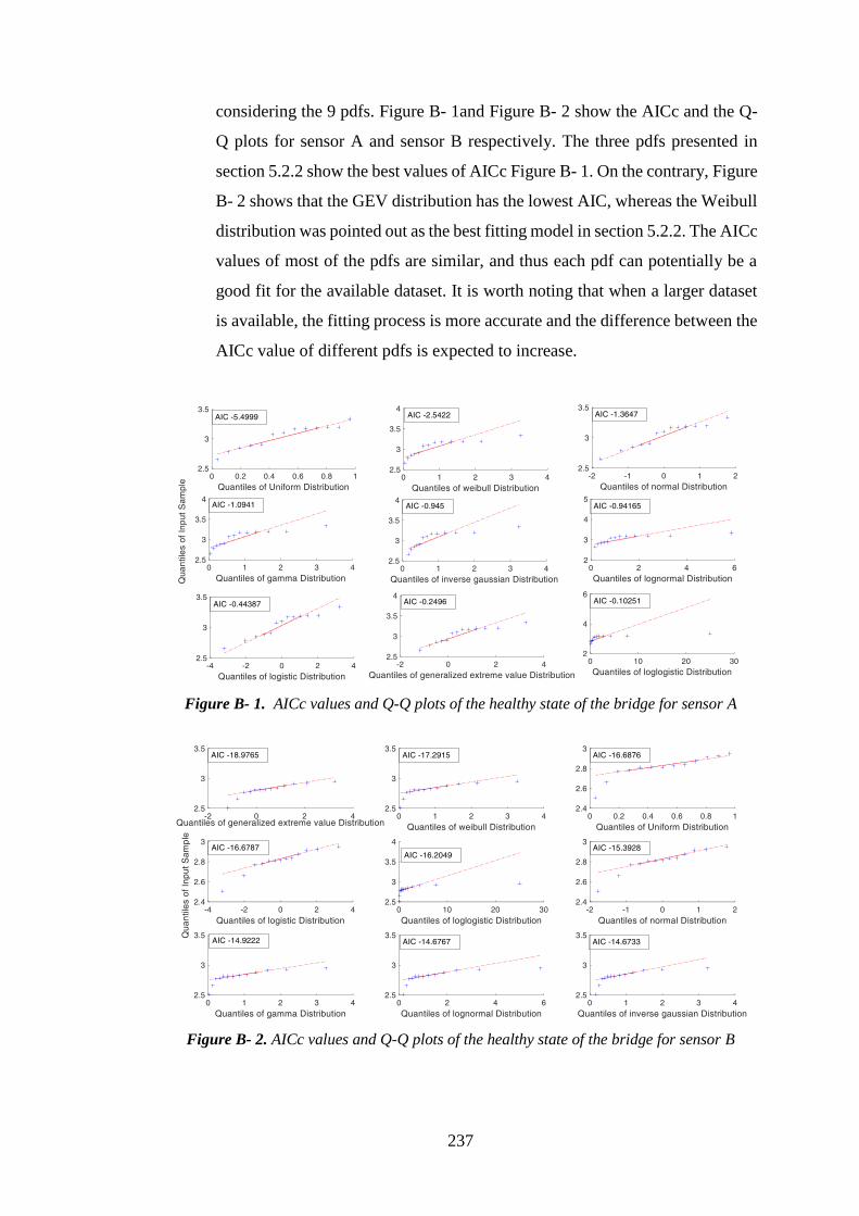
237

considering the 9 pdfs. Figure B- 1and Figure B- 2 show the AICc and the Q-

Q plots for sensor A and sensor B respectively. The three pdfs presented in

section 5.2.2 show the best values of AICc Figure B- 1. On the contrary, Figure

B- 2 shows that the GEV distribution has the lowest AIC, whereas the Weibull

distribution was pointed out as the best fitting model in section 5.2.2. The AICc

values of most of the pdfs are similar, and thus each pdf can potentially be a

good fit for the available dataset. It is worth noting that when a larger dataset

is available, the fitting process is more accurate and the difference between the

AICc value of different pdfs is expected to increase.

Figure B- 1. AICc values and Q-Q plots of the healthy state of the bridge for sensor A

Figure B- 2. AICc values and Q-Q plots of the healthy state of the bridge for sensor B

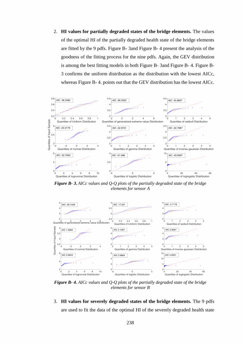
238

2. HI values for partially degraded states of the bridge elements. The values

of the optimal HI of the partially degraded health state of the bridge elements

are fitted by the 9 pdfs. Figure B- 3and Figure B- 4 present the analysis of the

goodness of the fitting process for the nine pdfs. Again, the GEV distribution

is among the best fitting models in both Figure B- 3and Figure B- 4. Figure B-

3 confirms the uniform distribution as the distribution with the lowest AICc,

whereas Figure B- 4. points out that the GEV distribution has the lowest AICc.

Figure B- 3. AICc values and Q-Q plots of the partially degraded state of the bridge

elements for sensor A

Figure B- 4. AICc values and Q-Q plots of the partially degraded state of the bridge

elements for sensor B

3. HI values for severely degraded states of the bridge elements. The 9 pdfs

are used to fit the data of the optimal HI of the severely degraded health state

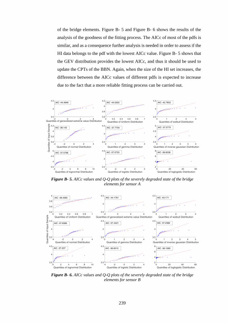
239

of the bridge elements. Figure B- 5 and Figure B- 6 shows the results of the

analysis of the goodness of the fitting process. The AICc of most of the pdfs is

similar, and as a consequence further analysis is needed in order to assess if the

HI data belongs to the pdf with the lowest AICc value. Figure B- 5 shows that

the GEV distribution provides the lowest AICc, and thus it should be used to

update the CPTs of the BBN. Again, when the size of the HI set increases, the

difference between the AICc values of different pdfs is expected to increase

due to the fact that a more reliable fitting process can be carried out.

Figure B- 5. AICc values and Q-Q plots of the severely degraded state of the bridge

elements for sensor A

Figure B- 6. AICc values and Q-Q plots of the severely degraded state of the bridge

elements for sensor B

240

B.1 Weibull vs Generalized Extreme value distribution for HIs

The GEV distribution provides the minimum value of AICc for three health states

of the bridge elements: i) the healthy state of the values recorded by sensor A; ii) the

partially degraded state of the values recorded by sensor B; iii) the severely degraded

state of the values recorded by sensor B. As a consequence, the GEV distribution

should be adopted to update the CPTs of the BBN, in order to assess the health state

of the bridge by considering both the bridge expert judgment and the analysis of the

bridge behaviour. Section 6.3.3 has discussed the performance of the BBN when the

uniform and the Weibull distributions are used to update the CPTs. The analysis of the

BBN performance showed that the diagnostic ability of the BBN is influenced by the

shape of the CDF. For example, the CDF of the uniform distribution increases rapidly

than the CDF of the Weibull, and thus the probability of the damaged BBN node of

being in a degraded state is higher when the uniform distribution is adopted, rather

than the Weibull CDF. Therefore, Figure B- 7 shows the CDF of the Weibull (by using

a solid blue line) and of the GEV distribution (by the means of a dotted red line) for

the three health states in which the GEV distribution provides the lowest AICc. The

CDF of the Weibull and the GEV distribution increase in a similar manner, when the

HI values increase. Therefore, the diagnostic performance of the BBN would be

indistinguishable when the Weibull or the GEV distributions are adopted.

However, it is worth mentioning that the nature of the CDF needs to be pointed out

in a reliable and robust manner, in order to increase the accuracy of the BBN

performance. Therefore, as discussed in the future work session, the analysis of the

fitting model needs to be further considered.

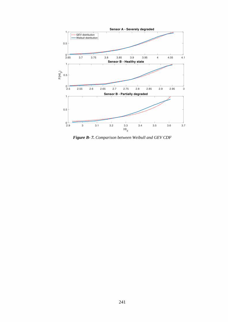
241

Figure B- 7. Comparison between Weibull and GEV CDF

242

Appendix C – Comparison between

the optimal HI of the post-tensioned

bridge for different τ*

In section 5.3 a τ* = 15 τ has been considered in order to obtain a set of HI values

for updating the CPTs of a BBN. The optimal value of τ* is equal to 45 τ, as shown in

section 4.3.6. Figure C- 1 shows the evolution of the optimal HI for monitoring the

health state of the post-tensioned bridge elements when different values of τ* and τ are

considered: Figure C- 1(a) shows the evolution of the HI when τ=0.5sec and τ* = 15 τ,

Figure C- 1(b) shows the evolution of the HI when τ=3.5sec and τ* = 15 τ, and Figure

C- 1(c) shows the evolution of the optimal HI when τ=3.5sec and τ* = 45 τ. Figure C-

1(c) represents the optimal configuration to monitor and assess the health state of the

bridge, as shown in section 4.3.6, i.e. the definition of τ=3.5sec and τ* = 45 τ allows to

maximize the GI. It should be noted that the lower the value of both τ and τ*, the higher

the number of assessments of the HI. As a consequence, although the three plots are

based on the analysis of the same set of data, the range τ* decreases when both τ and

τ* increases.

The comparison between the three figures shows two main results: i) the higher the

values of both τ and τ*, the higher the value of the optimal HI, due to the assessment

of a higher number of bridge vibration data. This can be behaviour of the HI can be

due to the amount of energy of the bridge that is analysed and lumped into the

assessment of the optimal HI. For example, the minimum value of the optimal HI

increases from 2.2 in Figure C- 1(a) to 2.7 in Figure C- 1(c); ii) Figure C- 1(b) and

Figure C- 1(c) show the same range of values for the HI, and a similar evolution over

time of the HI, which allows to point out the different health states of the bridge

elements. Figure C- 1(c) allows to point out the different health states of the bridge

elements in a clearer manner than the HI values in Figure C- 1(b). However. Figure C-

1(b) shows that the evolution of the optimal HI of the bridge when τ=3.5sec and 5sec

and τ* = 15 τ is very similar to the evolution of the HI in Figure C- 1(c). The analysis

of the two plots justify the hypothesis that the HI values of Figure C- 1(b) are used to

define the CDF of the bridge health states. The main difference between Figure C- 1(b)

and Figure C- 1(c) is that the HI values of Figure C- 1(b) show higher oscillations that

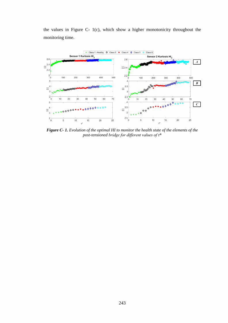
243

the values in Figure C- 1(c), which show a higher monotonicity throughout the

monitoring time.

Figure C- 1. Evolution of the optimal HI to monitor the health state of the elements of the

post-tensioned bridge for different values of τ*

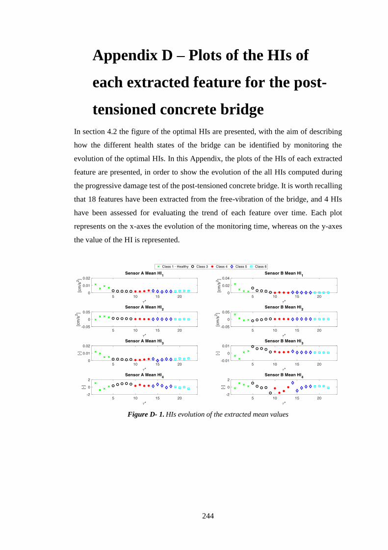
244

Appendix D – Plots of the HIs of

each extracted feature for the post-

tensioned concrete bridge

In section 4.2 the figure of the optimal HIs are presented, with the aim of describing

how the different health states of the bridge can be identified by monitoring the

evolution of the optimal HIs. In this Appendix, the plots of the HIs of each extracted

feature are presented, in order to show the evolution of the all HIs computed during

the progressive damage test of the post-tensioned concrete bridge. It is worth recalling

that 18 features have been extracted from the free-vibration of the bridge, and 4 HIs

have been assessed for evaluating the trend of each feature over time. Each plot

represents on the x-axes the evolution of the monitoring time, whereas on the y-axes

the value of the HI is represented.

Figure D- 1. HIs evolution of the extracted mean values

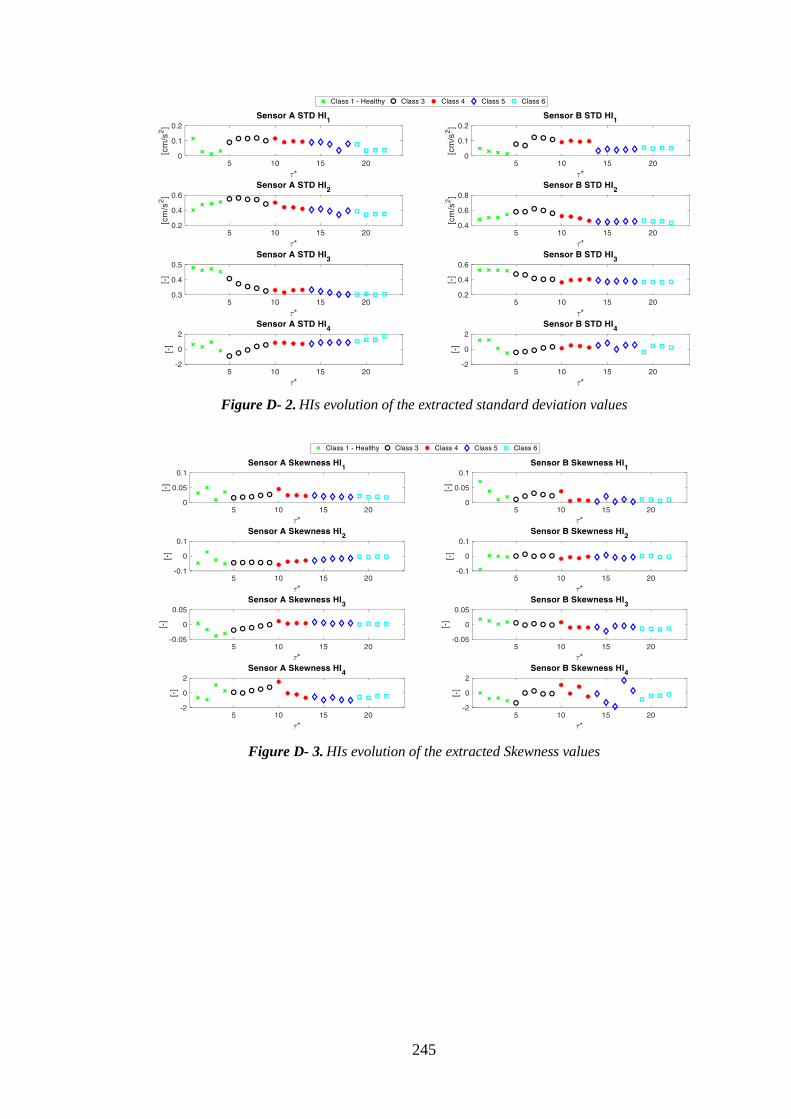
245

Figure D- 2. HIs evolution of the extracted standard deviation values

Figure D- 3. HIs evolution of the extracted Skewness values

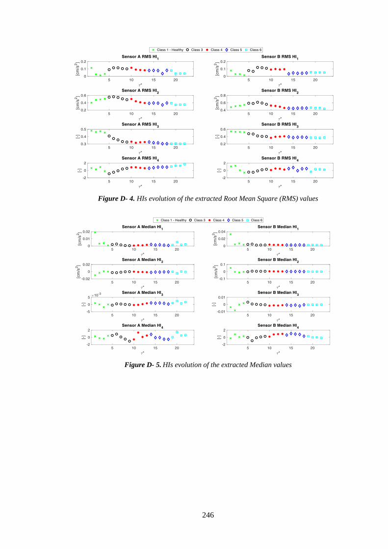
246

Figure D- 4. HIs evolution of the extracted Root Mean Square (RMS) values

Figure D- 5. HIs evolution of the extracted Median values

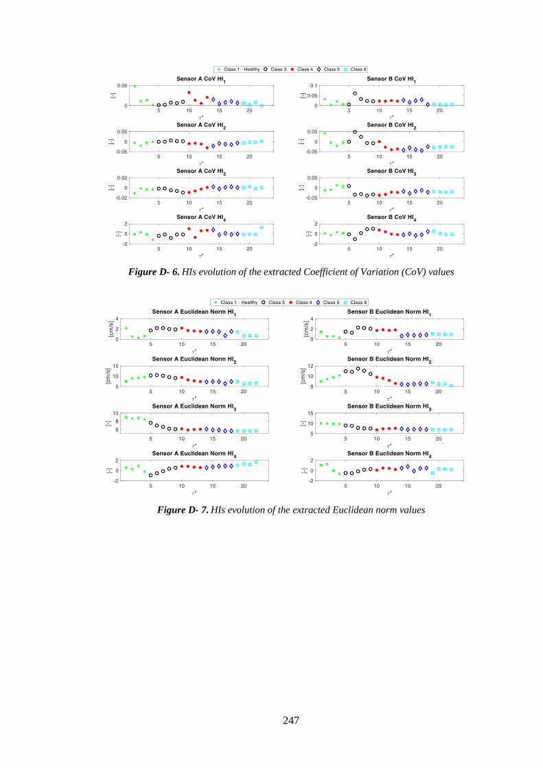
247

Figure D- 6. HIs evolution of the extracted Coefficient of Variation (CoV) values

Figure D- 7. HIs evolution of the extracted Euclidean norm values

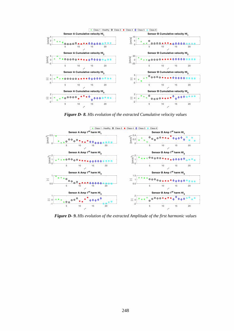
248

Figure D- 8. HIs evolution of the extracted Cumulative velocity values

Figure D- 9. HIs evolution of the extracted Amplitude of the first harmonic values

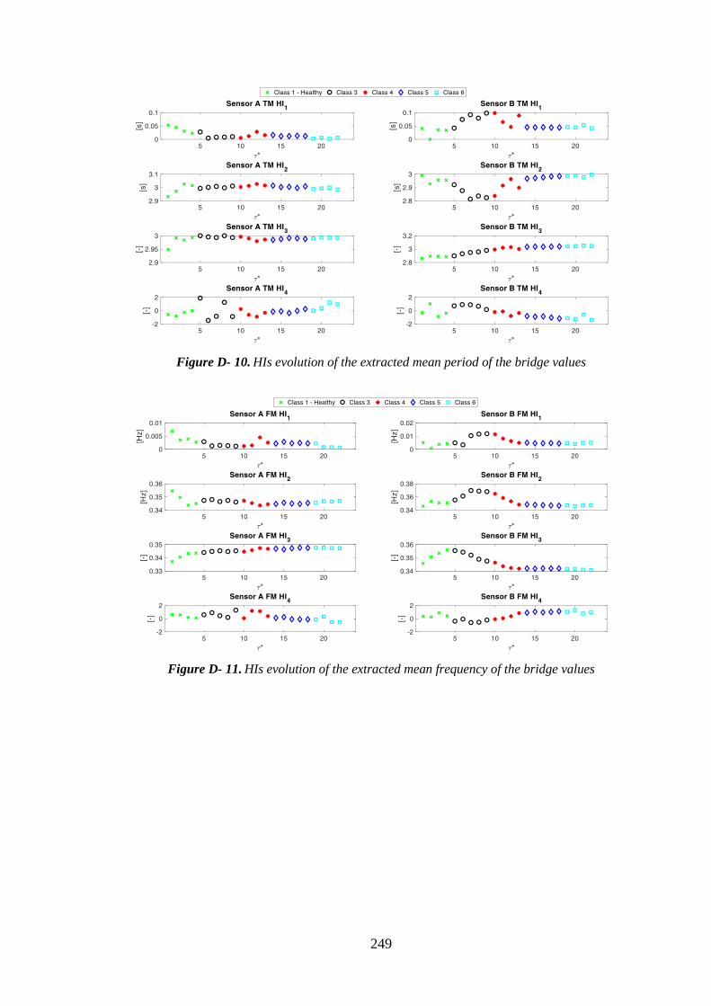
249

Figure D- 10. HIs evolution of the extracted mean period of the bridge values

Figure D- 11. HIs evolution of the extracted mean frequency of the bridge values

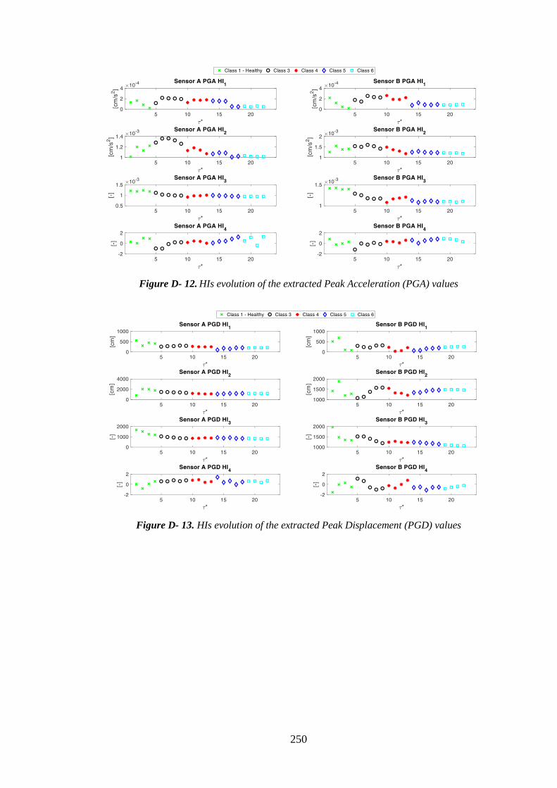
250

Figure D- 12. HIs evolution of the extracted Peak Acceleration (PGA) values

Figure D- 13. HIs evolution of the extracted Peak Displacement (PGD) values

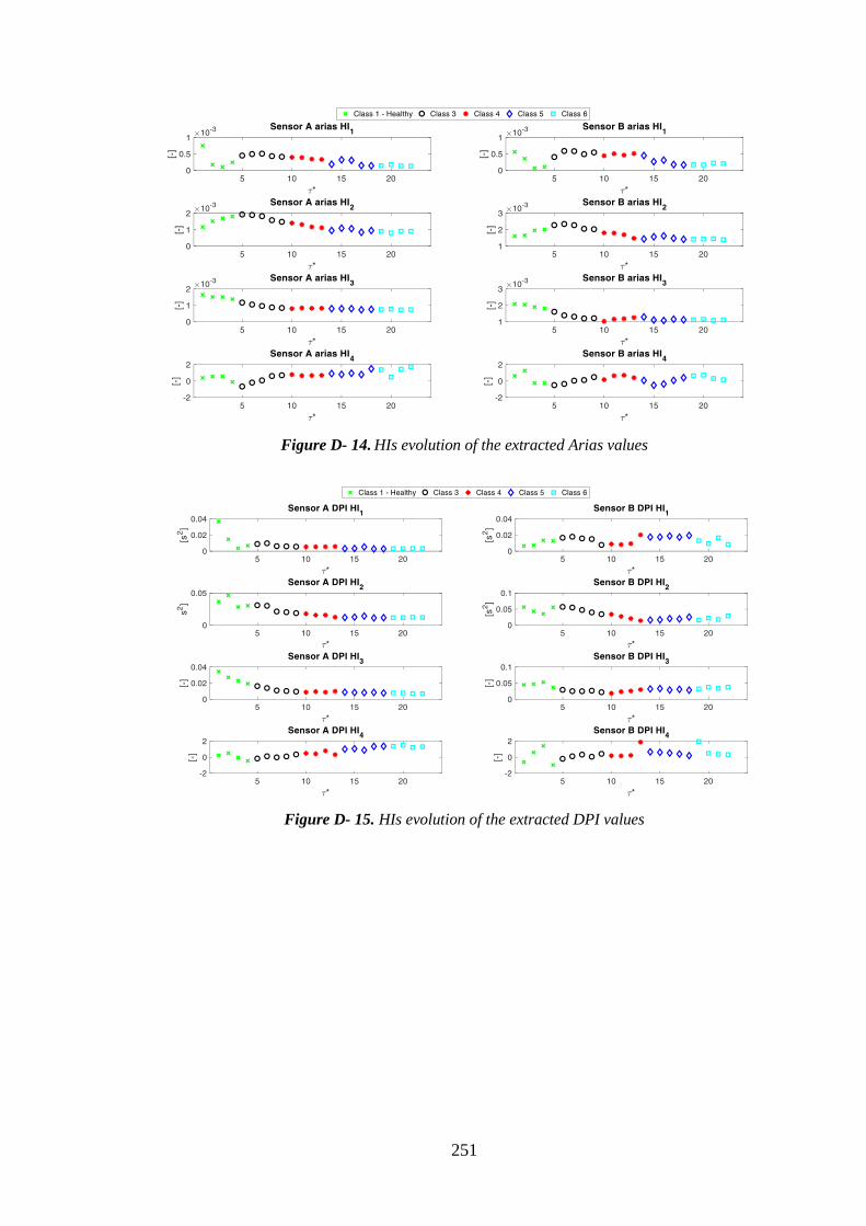
251

Figure D- 14. HIs evolution of the extracted Arias values

Figure D- 15. HIs evolution of the extracted DPI values

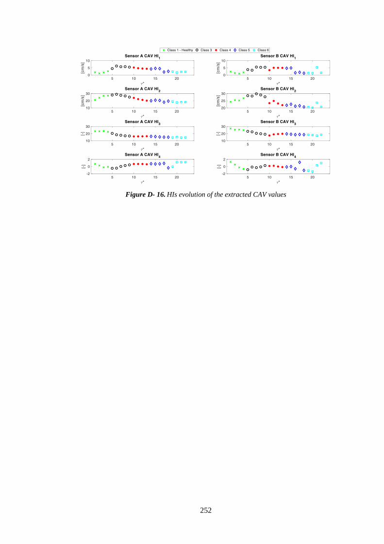
252

Figure D- 16. HIs evolution of the extracted CAV values

RAILWAY BRIDGE CONDITION MONITORING AND FAULT ...

Documents

Transcript of RAILWAY BRIDGE CONDITION MONITORING AND FAULT ...