Radioecological Models for Inland Water Systems - CORE

Forschungszentrum Karlsruhe Technik und Umwelt

Wissenschaftliche Berichte FZKA 6089

Radioecological Models for Inland Water Systems

W. Raskob, A. Popov, M. J. Zheleznyak, R.Heling Institut für Neutronenphysik und Reaktortechnik Projekt Nukleare Sicherheitsforschung

April1998

Forschungszentrum Karlsruhe

Technik und Umwelt

Wissenschaftliche Berichte

FZKA 6089

Radioecological models for in land water systems

W. Raskob* A. Popov**

M.J. Zheleznyak*** R. Heling****

Institut für Neutronenphysik und Reaktortechnik Projekt Nukleare Sicherheitsforschung

*D.T.I. Dr. Trippe Ingenieurgesellschaft m.b.H., Karlsruhe **Scientific Production Association TYPHOON, Obninsk, Russia

***Cybernetics Centre of the Ukrainian Academy of Sciences, Kiev, Ukraine ****NV KEMA, Arnhem, Netherlands

Forschungszentrum Karlsruhe GmbH, Karlsruhe 1998

Die im vorliegenden Bericht beschriebenen Untersuchungen wurden im Rahmen des Vertrags St.Sch.4089 "Radioökologische Modelle der Binnengewässer" mit dem Bundesministerium für Umwelt, Naturschutz und Reaktorsicherheit durchgeführt. Der Bericht gibt die Auffassung und die Meinung des Auftragnehmers wieder und muß nicht mit der Meinung des Auftraggebers übereinstimmen.

Als Manuskript gedruckt Für diesen Bericht behalten wir uns alle Rechte vor

Forschungszentrum Karlsruhe GmbH Postfach 3640, 76021 Karlsruhe

Mitglied der Hermann von Helmholtz-Gemeinschaft Deutscher Forschungszentren (HGF)

JSSN 0947-8620

Radioecological models for inland water systems

Individual final reports on runoff, river and lakemodeHing for: BMU-Vorhaben St.Sch 4089 August 1997

Authors:

Editor: W. Raskob1

Forschungszentrum Karlsruhe GmbH, Institut für Neutronenphysik und Reaktortechnik, Postfach 3640, D-76021 Karlsruhe

1 D.T.I. Dr. Trippe Ingenieurgesellschaft m.b.H., Amalienstr. 63/65, 76133 Karlsruhe

Runoff modelling: A. Popov

Scientific Production Association TYPHOON, Lenin str 82, Obninsk, Kaluga Region, 249020, Russia

River modeHing M. J. Zheleznyak

Cybemetics Centre of the Ukrainian Academy of Sciences, Institute of Mathematical Machirresand Systems, Prospect Glushkova42, Kiev, 252207, Ukraine

Lake modeHing R. Reling

NV KEMA, P.O. Box 9035, Amhem, Netherlands

Abstract

Following a nuclear accident, radioactivity may either be directly discharged into rivers, lakes and reservoirs or - after the re-mobilisation of dry and wet deposited material by rain events - may result in the contamination of surface water bodies. These so-called aquatic exposure pathways are still missing in the decision support system IMIS/P ARK. Therefore, a study was launched to analyse aquatic and radioecological models with respect to their applicability for assessing the radiation exposure of the population. The computer codes should fulfil the following requirements:

1. to quantify the impact of radionuclides in water systems from direct deposition and via runoff, both dependent on time and space,

2. to forecast the activity concentration in water systems (rivers and lakes) and sediment, both dependent on time and space, and

3. to assess the time dependent activity concentration in fish.

To that purpose, a Iiterature survey was conducted to collect a list of all relevant computer models potentially suitable for these tasks. In addition, a detailed overview of the key physical processes was provided, which should be considered in the models. Based on the three main processes, 9 codes were selected for the runoff from large watersheds, 19 codes for the river transpoft and 14 for lakes. During the investigations, it became obvious that currently none of the tested codes fulfils all the requirements setout above. However, those computer programs incorporated in the hydrological model chain of the decision support system RODOS meet most of the selection criteria.

Radioökologische Modelle itir Binnengewässer

Zusammenfassung

Nach einem kerntechnischen Unfall kann Radioaktivität direkt in stehende bzw. fließende Gewässer gelangen, oder aber auch durch atmosphärischen Transport großräumig verteilt, auf dem Erdboden deponiert, durch Niederschläge wieder remobilisiert und in Oberflächenwasser transportiert werden. Diese sogenannten aquatischen Expositionspfade sind im Entscheidungshilfesystem IMIS/P ARK bisher nicht explizit berücksichtigt. Deshalb wurde eine Untersuchung mit der Zielsetzung durchgeführt, aquatische und radioökologische Modelle hinsichtlich ihrer Eignung :fiir eine zuverlässige Abschätzung der Strahlenexposition der Bevölkerung zu analysieren. Mit Hilfe der Modelle soll es möglich sein:

• den Eintrag von Radionukliden in Gewässer durch direkte Ablagerung und durch Runoff in Abhängigkeit von der Zeit und vom Ort zu quantifizieren,

• den Aktivitätsverlauf im Wasser und im Sediment in Abhängigkeit von der Zeit und vom Ort zu prognostizieren und

• den zeitlichen Verlauf der Kontamination in Fischen abzuschätzen.

Zu diesem Zweck wurde eine Literaturrecherche durchgeführt, um alle relevanten Modelle zu identifizieren, die :fiir die obige Problemstellung in Frage kommen könnten. Weiterhin wurden die wichtigsten physikalischen Prozesse beschrieben, die in einem geeigneten Computercode modelliert sein sollten. Entsprechend der drei identifizierten Hauptprozesse wurden 9 Computerprogramme im Bereich des Oberflächenabflusses, 19 im Bereich des Transports in Fließgewässern und 14 bezüglich des Verhaltens von Radionukliden in Seen :fiir die Untersuchungen ausgewählt. Im Verlauf der Arbeiten wurde festgestellt, daß keines der getesteten Programme zur Zeit allen Anforderungen gewachsen ist, daß aber die Rechenprogramme der im Entscheidungshilfesystem RODOS-System integrierten hydrologischen Modellkette die meisten Auswahlkriterien erfüllen.

1 INTRODUCTION 1

2 GENERIC EQUATIONS 2

2.1 REFERENCES 5

3 SURFACE RUNOFF (A. POPOV) 6

3.1 Introduction 6

3.2 Physico - chemical processes governing the behaviour of radionuclides in the watershed 6 3.2.1 Formation ofthe radioactive fallout and mass balance in the watershed 6 3.2.2 Physico-chemical processes goveming radionuclide wash-off 7 3.2.3 Hydrological and erosion processes determining the migration ofradionuclides in watershed 9

3.3 Characterisation of the computer codes 10 3.3 .1 Short model description 10

3.4 Criteria for a model intercomparison 15

3.5 AGNPS Model 19 3.5 .1 Criteria of adequate radionuclide wash-off simulation 19 3.5.2 Criteria ofpractical applicability in connection with the system IMIS/PARK 19

3.6 HSPF Model 21 3.6.1 Criteria of an adequate radionuclide wash-off simulation 21 3.6.2 Criteria ofpractica1 applicability in connection with the system IMIS/PARK 22

3. 7 MARTE Model 24 3. 7.1 Criteria of an adequate radionuclide wash-off simulation 24 3.7.2 Criteria ofpractical applicability in connection with the system IMIS/PARK 25

3.8 RETRACE 26 3 .8.1 Criteria of an adequate radionuclide wash-off simulation 26 3.8.2 Criteria ofpractical applicability in connection with the system IMIS/PARK 27

3.9SWRRB 29 3.9 .1 Criteria of adequate radionuclide wash-off simulation. 29 3.9.2 Criteria ofpractical applicability in connection with the system IMIS/PARK 30

3.10 Comparison ofthe selected models 32 3.10.1 The conclusions for HSPF 33 3.10.2 The conclusions for SWRRB and AGNPS 33 3.10.3 The conclusions forMARTE 33 3.10.4 The conclusions for RETRACE 34

3.11 Conclusions and proposal of a runoff model 34

3.12 References 36

4 RIVER SYSTEMS (MARK J. ZHELEZNYAK) 41

4.1 Introduction 41

4.2 ldentification of the key processes 42 4.2.1 Overview of the processes 42 4.2.2 Radionuclide transformation in river water: contemporary view and modeHing approaches 44 4.2.3 Sediment transpürt and hydrüdynamic processes and models 47

4.3 ldentification of models available for describing the radionuclide transport in rivers 48 4.3.1 ModeHing Approach 48 4.3.2 Descriptiün ofthe radionuclide transport models 49

4.4 Comparison ofthe models with respect to their applicability in the IMIS/PARK system 55

4.5 Selection of a river model for use in IMIS/P ARK 57

4.6 REFERENCES 64

5 LAKES AND RESERVOIRS (R. HELING) 72

5.1 lntroduction 72

5.2 PROCESSES 73

5.3 Parameters 75 5.3 .1 Chemical parameters and trophic level classification 7 6 5.3.2 Physical parameters 76 5.3.3 Biological parameters 77

5.4 Models 77 5.4.1 Types oflake/reservoir müdels 77 5.4.2 Existing models and their applications 79

5.5 Comparison of the models 86

5.6 Model selection 87 5.6.1 Validation and flexibility 87 5.6.2 Complexity 88 5.6.3 Applicability 88 5.6.4 Availability 89

5. 7 Final advice on the selection of a Iake model for the IMIS/P ARK system. 89

5.8 REFERENCES 92

6 FINAL CONCLUSIONS AND MODEL PROPOSAL 94

APPENDIX ON INDIVIDUAL MODEL DESCRIPTIONS 96

APPENDIX ON RUNOFF MODELLING (A. POPOV) 97

THE MAIN CHARACTERISTICS OF AGNPS 97

Description of the processes controlling the radionuclide wash-off from watersheds 97 Descriptiün ofthe hydrülogical processes 97 Description üf the sediment yield and transport 97 Descriptiün üfpoHutant transpürt 98

Applicability of the model in Europe, in particular in Germany Temporal and spatial ranges Interface with in-stream transport models Data availability for European conditions Validations, testing and applications performed Model software and documentation availability

Data assimilation

Software requirements

THE MAIN CHARACTERISTICS OF HSPF

Description of the processes controlling the radionuclide wash-off from watersheds Description of the hydrological processes Description oftransport and sediment yield Description ofthe transport ofpollutants

Applicability of the model in Europe, in particular in Germany Temporal and spatial ranges Interface with in-stream transport models Data for European conditions Validation, testing and application Model software and documentation availability

Data assimilation

Software possibilities and requirements

THE MAIN CHARACTERISTICS OF MARTE

Description of the processes controlling the radionuclide wash-off from watersheds Hydrological processes Sedimenttransport Pollutant transport processes

Applicability of the model in Europe, in particular in Germany Temporaland spatial ranges ofthe model Interface with in-stream transport models Data for European conditions Testing and validation Model software and documentation

Data assimilation Software requirements

THE MAIN CHARACTERISTICS OF RETRACE

Description of processes controlling the radionuclide wash-off from watersheds Description of the hydrological processes Description of transport and sediment yield Description of the pollutant transport

Applicability of the model in Europe, in particular in Germany Temporal and spatial rang es of model validity Interface with in-stream transport models

99 99

101 101 101 101

102

102

103

103 103 105 105

105 105 106 106 106 106

107

107

108

108 108 108 108

109 109 110 110 110 110

110 110

111

111 111 112 113

114 114 115

Data availability for European conditions Validations, testing and applications performed

Data assimilation


THE MAIN CHARACTERISTICS OF SWRRB

Description of processes controlling the radionuclide wash-off from watersheds Description of the hydrological processes Description oftransport and sediment yield Description ofthe pollutant transport

Applicability of the model in Europe, in particular in Germany Temporal and spatial ranges Interface with in-stream transport models Data availability for the European conditions Validations, testing and applications performed Model software and documentation Data assimilation


REFERENCES FOR RUNOFF MODELS

APPENDIX ON RIVER MODELLING (M. ZHELEZNIAK)

HOFFER&BAYER MODEL

HSPF

River Transport Submodel - RCHRES

RCHRES structure and main processes

Submodel HYDR- flow simulation

Simulation of sediments and hydrophysical parameters

Simulation of pollutant transport

Software environment

MIKE 11

Model overview

Submodels Hydrological processes Submodel ofunsteady flow dynamics in river channels Submodel of non-cohesive sediment transport Submodel of advection-dispersion and cohesive sediment transport. Submodel ofwater quality

115 115

115

115

116

117 117 118 118

119 119 119 119 119 120 120

120

121

123

123

127

127

127

128

129

129

130

132

132

132 132 133 134 134 136

L. MONTE RIVER RESERVOIR MODEL

Appendix with symbols and parameter values

RIVTOX

Model overview

Submodels Submodel of the unsteady flow in river channels Submodel of suspended sediment transport Submodel of radionuclides transport

Software environment of RIVTOX

Validation sturlies

Input data Geographical data (river net) Hydrological data Radiological data

TOD AM

Submodels Sediment transport Sediment-associated contaminant transport Dissolved contaminant transport Bed materials Contaminant movement within the bed material

Boundary conditions for channel branching

Software realisation

WATOX

Model overview

Model equations

Software and model implementation

REFERENCES FOR RIVER MODELS

APPENDIX ON LAKE MODELLING (R. HELING)

Introduction on detailed model descriptions

VAMP MODEL

Hydrological processes Sedimentation processes

138

142

144

144

145 145 147 148

149

149

150 150 150 151

152

152 152 154 155 155 157

159

160

161

161

161

163

165

168

168

169

170 171

The biological uptake model ModeHing more nuclides

Possibility to apply the model in Central Europe Temporaland spatial ranges ofthe model Flexibility and generic character ofthe model Required input data and availability

Validation and test exercises

The model software and documentation availability

Criteria for implementation into a decision support system Interface to radiological models and output ofthe model Data assimilation The implementation of countermeasures

Conclusion

LAKECO MODEL

Hydrological processes

Sedimentation processes Remobilisation Fuel particles

Biological uptake modelling The foodweb model Parametrisation and submodels ModeHing more nuclides

Possibility to apply the model in Central Europe Temporaland spatial ranges ofthe model Required input data and availability



Criteria for implementation into a decision support system Interface to radiological models and output of the model Data assimilation The implementation of countermeasures

Conclusion

DELWAQ/IMPAQT MODEL

Introduction

Hydrological processes (IMP AQT)

Sedimentation processes Processes for poHutants

173 174

174 174 175 175

176

176

176 176 177 177

177

179

180

180 182 182

183 183 183 185

186 186 186

187

187

187 187 187 188

188

189

189

190

190 191

Biological uptake modelling The foodweb model

Modelling more nuclides

Possibility to apply the model in Central Europe Temporaland spatial ranges ofthe model Required input data and availability



Criteria for implementation into a decision support system Interface to radiological models and output of the model Data assirnilation The irnplementation of countermeasures

Conclusion

BIOPATH MODEL


Sedimentation processes

Biological uptake modelling


Possibility to apply the model in Central Europe Temporaland spatial ranges ofthe model Flexibility and generic character of the model Required input data and availability



Criteria for implementation into a decision support system Interface to radiological models and output of the model Data assimilation The irnplementation of countermeasures

Conclusion

DETRA



Comparison of planktonic uptake in DETRA with other models Composition ofthe suspended matter Uptake in organisms

192 192

194

194 194 194

195

196

196 196 196 196

197

198

198

199

199

202

202 202 202 202

203

203

204 204 204 204

204

206

206 206

207

208 209 210


Possibility to apply the model in Central Europe Temporaland spatial ranges ofthe model Flexibility and generic character of the model Required input data and availability




Conclusion

MARTE




Possibility to apply the model in Central Europe Temporaland spatial ranges ofthe model Flexibility and generic character ofthe model Required input data and availability




Conclusion

REFERENCES ON LAKE MODELLING

211

211 211 212 212

213

213

213 213 213 214

214

215

215 216

217

219

219 219 219 220

220

220

221 221 221 221

221

223

1 lntroduction

The aim of this study is to analyse the qualification of radiological models with respect to the application in the system IMIS/P ARK for the assessment of the impact of contamination of large watersheds after the deposition of radionuclides over a large area on the population. This part of the report comprises the individual reports of the three subcontractors responsible for the modelling of runoff, rivers, and lakes. Based on the initial definition, the task was divided into the above mentioned three parts to answer the following questions concerning the capabilities of radiological models in detail:

1. Quantifying the impact of radionuclides in water systems from direct deposition and via runoff; both as a function of time and space.

2. Forecasting the activity concentration in water systems (rivers and lakes) and sediment; both as a function of time and space.

3. Assessing the time dependent activity concentration in fish.

To answer the questions, a detailed overview of the physical key processes, which should be considered in the models, is provided. Based on a Iiterature survey, a list of computer models was drawn up and analysed with respect to the requirements of the task. As the processes can be divided into three parts , also the models were selected and investigated for:

• runoff, • river transport and • lakes.

In total, 9 codes were considered for the runoff from large watersheds, 19 codes for the river transport and 14 for lakes. Based on key criteria, which are described separately in the individual sections, the number ofthe modelswas reduced for the final selection. Thesecodes were analysed and described in more detail. The main criteria for the code intercomparison have been:

• consideration of the relevant processes, • the temporal and spatial ranges of validity of the models, • the kind and amount of input data and the results obtainable, • validation studies performed, • operational applicability, experience, accessibility, maintenance, • computation requirements ( calculation times, storage requirements, etc.) • availability of documentation, • applicability in Central Europe and • interface to radioecological models.

Furthermore, the capabilities of the computer codes with respect to data assimilation were included. As result, a detailed analysis of the individual models is provided together with a proposal as to which of the investigated models might be implemented into the system IMIS/PARK.

1

2 Generic equations

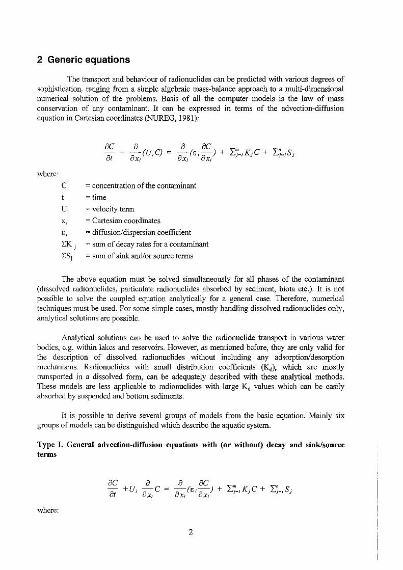
The transport and behaviour of radionuclides can be predicted with various degrees of sophistication, ranging from a simple algebraic mass-balance approach to a multi-dimensional numerical solution of the problems. Basis of all the computer models is the law of mass conservation of any contaminant. It can be expressed in terms of the advection-diffusion equation in Cartesian coordinates (NUREG, 1981 ):

ac a 8t + 8xi (UiC)

where:

C = concentration of the contaminant

t =time

Ui = Velocity term

xi = Cartesian coordinates

Ei = diffusion/dispersion coefficient

l:K j = sum of decay rates for a contaminant

l:Sj = sum of sink and/or source terms

The above equation must be solved simultaneously for all phases of the contaminant (dissolved radionuclides, particulate radionuclides absorbed by sediment, biota etc.). It is not possible to solve the coupled equation analytically for a general case. Therefore, numerical techniques must be used. For some simple cases, mostly handling dissolved radionuclides only, analytical solutions are possible.

Analytical solutions can be used to solve the radionuclide transport in various water bodies, e.g. within lakes and reservoirs. However, as mentioned before, they are only valid for the description of dissolved radionuclides without including any adsorption/desorption mechanisms. Radionuclides with small distribution coefficients (K<J), which are mostly transported in a dissolved form, can be adequately described with these analytical methods. These models are less applicable to radionuclides with large Kd values which can be easily absorbed by suspended and bottom sediments.

It is possible to derive several groups of models from the basic equation. Mainly six groups of models can be distinguished which describe the aquatic system.

Type I. General advection-diffusion equations with ( or without) decay and sink/source terms

where:

2

C = concentration of the contaminant

t =time

ui = velocity term

xi = Cartesian coordinates

Bi = diffusion/dispersion coefficient

LKj = sum of decay rates for a contaminant

LSj = sum of sink and/or source terms

This equation includes the basic transport mechanisms of advection and diffusion for both conservative and nonconservative substances, and is the most complete form of a water quality model. The model, however, is in principle only valid for dissolved radionuclides with decay and source (sink) terms representing radionuclide decay and reduction of dissolved concentrations by non-moveable sediment of biota. This type of model cannot handle dissolved radionuclide transport coupled with particulate radionuclide transport, e.g. adsorption and/or desorption of radionuclides by sediments and biota, transport, deposition, and resuspension of contaminated sediments. This Type I is generally applicable to aquatic systems.

In the equations of type II to V (Type VI is not based on the diffusion/dispersion equation) some parts of the basic formula are omitted when the code is applied to a specific aquatic system.

Type II General advection-diffusion equations with ( or without) decay and sink/source terms

In this type, the dispersion term is omitted. Therefore,the equation can only be applied to predict the behaviour of radionuclides in fast-moving rivers.

Type 111. Langrangian routing models with decay and source/sink term

In this type the dispersion and the advection term are omitted, as a result of which the equation can only be applied to predict the behaviour of radionuclides in uniform, non-tidal nvers.

This type calculates the concentration in a Langrangian system, i.e. the longitudinal coordinate is moving with the flow velocity. Although the governing equation does not seems to have spatial coordinates, the solution is unsteady, one-dimensional, with decay, and sink/source occurring during the travel time throughout the system. The advantage of the Type III is that the

3

equation is simpler to handle than type li. A disadvantage is the one-dimensional character of the equation. Type 111 is suited to calculate the transport of dissolved nuclides with decay and adsorption and of other substances with constant adsorption rates, however, the particulate nuclide concentrations need to be precalculated.

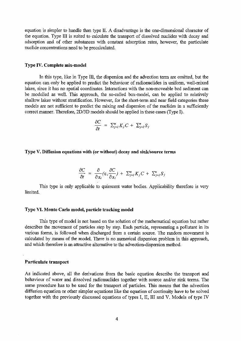
Type IV. Complete mix-model

In this type, like in Type 111, the dispersion and the advection term are omitted, but the equation can only be applied to predict the behaviour of radionuclides in uniform, well-mixed lakes, since it has no spatial coordinates. lnteractions with the non-moveable bed sediment can be modelled as weil. This approach, the so-called box-model, can be applied to relatively shallow lakes without stratification. However, for the short-term and near field categories these models are not sufficient to predict the mixing and dispersion of the nuclides in a sufficiently correct manner. Therefore, 2D/3D models should be applied in these cases (Type 1).

Type V. Diffusion equations with ( or without) decay and sink/source terms

This type is only applicable to quiescent water bodies. Applicability therefore is very limited.

Type VI. Monte Carlo model, particle tracking model

This type of model is not based on the solution of the mathematical equation but rather describes the movement of particles step by step. Each particle, representing a pollutant in its various forms, is followed when discharged from a certain source. The random movement is calculated by means of the model. There is no numerical dispersion problern in this approach, and which therefore is an attractive alternative to the advection-dispersion method.

Particulate transport

As indicated above, all the derivations from the basic equation describe the transport and behaviour of water and dissolved radionuclides together with source and/or sink terms. The same procedure has to be used for the transport of particles. This means that the advection diffusion equation or other simpler equations like the equation of continuity have to be solved tagether with the previously discussed equations of types I, II, 111 and V. Models of type IV

4

and VI are able to handle the transport and behaviour of particles by a simple parametrisation (type IV) or by treating it as another form ofthe discharged pollutant.

2.1 REFERENCES

NUREG (1981) Onishi Y, Seme R J, Arnold E M, Cowan CE and Thompson F L. Critical

Review: Radionuclide transport, sediment transport, and water quality mathematical modelling;

and radionuclide adsorption/desorption mechanisms. NUREG/CR-1322 PNL-2901.

5

3 Surface runoft (A. Popov)

3.1 lntroduction

The first analysis of the computer codes shows that specialised models describing the complex processes of the behaviour of radionuclides in the watershed are practically not available in the free literature. The models presented in this study were mostly developed for the prediction of agricultural runoff. Nevertheless, the physical concepts and mathematical techniques used in these models their application for radionuclides as well, but modification ofthe modelsoften seems tobe necessary.

Main emphasis was put on investigating the completeness of the consideration of all the relevant processes, the spatial and temporal characteristics, the practicability and applicability ofthe computer codes. The main features ofthe computer codes are summarised in Tables. In a first step, the physico - chemical processes have been described and, in further steps, the selection criteria have been applied to the individual models. A final decision is provided at the end of this section.

3.2 Physico - chemica/ processes governing the behaviour of radionuc/ides in the watershed

3.2.1 Formation of the radioactive fallout and mass balance in the watershed

In case of a nuclear accident, radionuclides are released mostly in molecular and aerosol form. The aerosol phase consists of fuel particles, structural elements and condensation particles. During the atmospheric transport of the cloud, sorption on aerosols and water droplets occurs.

The contamination of the soil surface occurs as a result of dry and wet deposition. The intensity of the deposition flux depends on the atmospheric turbulence and the properties of the underlying surface. Therefore, even if the contamination is nearly uniform by distributed in the cloud, the surface properties such as urban area, forest, field, open surface of water bodies or snow determine completely different deposition rates, in particular in case of the dry deposition process. For example, the depletion over a forest canopy can be very high and contamination ofthe soil surface is very low (Tikhomirov, 1994). Later on, due to wind, rain or vegetation change, radionuclides can reach the soil surface, i.e. the forest litter where they can stay for a long time and become available for surface wash-off.

Urban buildings as well as forests, cause a more intense radioactive fallout due to the induced higher turbulence. Furthermore, wash-off of radionuclides may become more organised, given a channelled runoff.

One issue which is still poorly understood is the contamination of surface water as a consequence of the deposition onto snow covers. If the contaminated area is rather small, decontamination can be performed quickly and effectively. When larger areas are contaminated (in terms of decontamination capabilities), consequences may be quite significant due to flooding events caused by snow melting. There is one documented event, where radionuclides were deposited on the snow surface after an accident which occurred at a chemical plant in Tomsk, Russia (Tomsk- 7) (Shershakov, 95). No significant contamination of water bodies due to radionuclides wash-off has been reported.

6

Figure 1 shows a flow chart of the different forms of the radionuclides including the above mentioned phases, the transformation processes and the migration pathways on the watershed.

3.2.2 Physico-chemical processes governing radionuclide wash-off

Deposition of radionuclides onto the underlying surface may occur in different chemical forms such as dissolved, sorbed and vapour phase (this phase is primarily characteristic of tritium and iodine isotopes) or in the form of aerosols reaching the soil solution by leaching (e.g. Konoplev et al., 1991, Borzilov et al., 1991). The relation between these phases, in particular in the early stage after deposition, depends on the physico-chemical properties of the fallout, on the surface properties and on the type of soil. It was demonstrated on the basis of 1aboratory experiments with the Chemobyl fall out (V ozzhennikov et al., 1996) that the exchange processes of freshly deposited radionuclides between soil and water differ significantly from those which are important later on.

The leaching rate of radionuclides in aerosol form is mostly determined by their destruction due to chemical reactions and due to the activity of the soil micro-organisms (Konoplev et al., 1996a). According to the available data after the Chemobyl accident, the leaching rate is in the order of about 1 0"3

- 10-4 per day (Konop1ev et al., 1996a) .

ATMOSP

LAND

.. HERE

I Fu~l particl~s I I Mol~cular phas~ 1 - . A~rosol I -f w ~~ f w f w ~ur a a V a a a a I ~

I s a I s I s n s I h p I h I h d LI

----------- ------------ ----- ----------- -------0

0 0 r 0

u u a LI

t t t t

i 0 ,, n ,,

Fu~l particl~s

l~aching

0

LI

t

0 0

u u t t

H

s

p ~

n s i 0

I I I I I I I I I I I I I I I I n

f-L-'~~.c.L«--, t) '--,.------,----' I

I I I

1----'=.:..~::....::...::..:.:........J d ~sor ti on : I I

Fig.i. Radlonuolide mlgratlon soheme

Radiom1clid~

wash-off to dralnag~

systerns

The wash-off of radionuclides can be divided into two components: "liquid" and "solid". The liquid wash-off is the result of the passage of soluble radionuclides from pore water to the surface runoff as well as of the desorption from the soil matrix. The solid wash-off can be regarded as a flow of radionuclides sorbed (particulate) on suspended sediments which were formed by surface forces such as wind and heavy rain and transported by overland water flow. It is important to note that the particle size distribution in solid runoff differs from the mechanical soil composition (Konoplev et al., 1996b). This may have a noticeable effect on the activity of the solid runoff if the irreversible sorption of the radionuclide has occurred on

7

those soil fractions entrained in the sediment flow. This phenomenon is nonnally described using the enrichment coefficient which can vary within one order of magnitude ( e.g. Bulgakov et al., 1992).

The wash-off of the dissolved phase is often described with the so called "sheet flow" approach (Maidment, 1992). This means that the advective and diffusive exchange of radionuclides occurs between the surface runoff water above and the soil water below the soil boundary (see e.g. Ahuja et al., 1983, Ahuja, 1990, Wallachet al., 1988). In other publications (Borzilov et al., 1988 and 1991, Vozzhennikov et al., 1990, WMO, 1992) it is assumed that the exchange of radionuclides with the surface runoff water occurs in the upper soillayer only (several millimetres). Additionally, newly developed approaches describe the fast subsurface runoffby a network of soil macropores (Hadley et al., 1985). In this case it seems tobe more realistic to use the whole depth of the upper soil layer as the one which interacts with surface runoff water.

Qualitative characterisation of the radionuclides in soil is based on their division into several groups depending on their ability to exchange with the water phase ( dissolved, reversibly sorbed, irreversibly sorbed or fixed fonns).

Sorption of radionuclides occurs both on the organic matter and on the mineral components of the soil (Prochorov, 1081, Konoplev et al., 1996b, Onishi et al., 1981). Moreover, characteristic sorption and desorption rates may differ significantly depending on the physical and chemical properties of both sorbent and sorbate. Sorption and desorption processes may last up to several months and more (Konoplev et al., 1996b). Therefore, for short-tenn forecast long-tenn processes can be neglected by assuming a constant amount of fixed or irreversibly sorbed radionuclides in the soil matrix. The occurrence of this form is explained by the ability of the radionuclide to be nearly completely integrated into the soil matrix (Konoplev et al., 1996b, Onishi et al., 1981).

Mainly three groups of interactions with the soil solution and the soil matrix can be distinguished: alkaline and alkaline earth metals (e.g. K, Sr, Cs), transitionmetals (e.g. Co, Ru, plutonium and uranium isotopes) and non-metals (e.g. iodine and sulphur).

The first group is characterised by its occurrence in the soil solution as cations, which means that sorption takes place on the negatively charged sorption sites. Fonnation of organic complexes with huniic and fulvic acids and inorganic ligands can be regarded as not typical for this group (Fried et al., 1988, Konoplev et al., 1996b, Onishi et al., 1981).

Transition metals form complexes with humic acids and inorganic anions, both in the soil solution and the soil matrix. They are primarily present in the solution as anions and are chemically bound to other elements ofthe soil matrix (Onishi et al., 1981).

Non-metals occur either in molecular andlor anion state in the solution. They are characterised by covalent bounds with the soil organic matter (Onishi et al., 1981).

Another form of radionuclide interaction with the soil surface can be referred to as reversibly sorbed. The bi-directional processes ofthe interaction ofthe radionuclides with the soil matrix are quite rapid in this case (minutes for the ion exchange and hours for the fonnation of complexes). As the characteristic half-time of the radionuclide removal from soil often is much Ionger than the characteristic half-times of sorption and desorption, the approximation of an instantaneous equilibrium between water and soil can be used. Therefore, the relation between the sorbed and dissolved phases of the reversible form of the radionuclide can be written as (see e.g. Borzilov et al., 1991, Konoplev et al., 1996b):

Cs =Kd ·Cw (1) where C s is the concentration of the radionuclide in the sorbed state,

8

Cw is the activity in the soil solution,

Kd is the distribution coefficient of the radionuclide in the "soil matrix - soil solution" system.

This relation is used to describe only the reversibly sorbed parts of the radionuclides. Their transformation into irreversibly sorbed form can be accounted for by equations of first-order decomposition kinetics (Konoplev et al., 1991, Fried et al., 1988). Furthermore, it is proposed in (Vozzhennikov et al., 1994, WMO, 1992) that the increase in the fraction ofradionuclides which are irreversible fixed can be described by an increase in the distribution coefficient between the dissolved and sorbed phases.

Experimental work performed on runoff plots in the 30-km zone around the Chemobyl NPP have shown that the instantaneous sorption equilibrium approach can be used for short term wash-off events. However, for long-term predictions of wash-off or flooding events, which occur on a yearly basis, migration of radionuclides down the soil column and kinetics of "slow' sorption - desorption processes may considerably influence the activity in the washoff water (Vozzhennikov et al., 1994 and 1996).

3.2.3 Hydrological and erosion processes determining the migration of radionuclides in watershed

As mentioned above, the wash-off process of radionuclides can take place in soluble form and in particulate form, both together with the runoff water. Therefore, all hydrological processes controlling the transport of water and particles also influence the transport of radionuclides in the watershed. As there are many references available describing the relevant transport processes and their modeHing in detail (Vinogradov et al., 1988, Maidment, 1992), in this report shall concentrate on a brief list of the most essential ones. It should be stressed that the individual processes are usually considered and modelled independently, but do strongly interact in reality .

The Iist of individual processes determining water runoff includes: • Evapotranspiration. • Infiltration. • Precipitation (rainfall and snowfall ). The aggregate state of precipitation determines the

different fate of water during the initial period of its presence in the watershed. • Interception ofprecipitation by the canopy. • Snow melting, including processes of snow cover formation, heat transport in snow cover,

phase transformation process ofwater and water escape from snow cover. • Surface runoff caused by liquid precipitation together with processes of surface

transformation of surface runoff (ponding and discharge from puddies and surface depressions) as well as retention of a part of the surface runoff in depressions.

• Transformation ofwater in a drainage network. • Transport of ground water.

Soil erosion also is a very complex process, and there are still gaps in the present knowledge. The following properties of the watershed determine the soil erosion process (Maidment, 1992, Hadley et al., 1985): • physical structure and chemical properties of soil, • properties ofliquid precipitation (size and energy of droplets, time distribution ofrain), • hydrodynamic properties of the surface and subsurface flows,

9

• relief of the watershed, • land use of soil, • types and seasonal characteristics of the vegetation on the watershed.

One of the main problems is the absence of reliable data to calibrate models for large watersheds. Therefore, difficulties arise when determining the necessary erosion parameters. This has led to the fact, that most of the present models use empirical approaches in case of large watersheds (Hadley et al., 1985). However, physically based models were successfully applied to smaller catchments (Hadley et al., 1985). At present, it is accepted to distinguish between the following soil erosion mechanisms, which complete the Iist of processes determining the radionuclide migration in watershed: • Splash detachment and soil splash transport actions caused by rain droplets, • Soil detachment and soil transport of inter-rill flows or sheet flows, • Soil detachment and soil transport of rill flows of overland runoff and subsurface runoff. • Pipe flow.

It should be noted that the concept of rapid subsurface flow (pipe flow) is relatively new in hydrology and soil erosion investigations. However, several studies proved the significance of the following features of the pipe flow ( e.g. Hadley et al., 1985): • its geographical distribution is much wider, • pipe flow can be regarded more like a channel flow and is a more rapid flow through the

"normal" porous media (interflow), • pipe flow is less dependent on watershed topography (hill slopes) and takes place in all

topographic locations of the watershed, • pipe flow may effectively lengthen the stream network and provide a suitable explanation

for the quick response to storm channel flow, • pipe flow may be directly fed by crack flow, rill flow or overland flow. • Quantitative data and field observations of subsurface erosion are still rare. There is no

theoretical model to describe the soil detachment and soil transport by pipe flow. Therefore, pipe flow is rarely seen in the present modelling.

3.3 Characterisation of the computer codes

3.3.1 Short model description

As mentioned in the introduction, there are not many watershed models which are basically designed for describing radionuclide transport. Therefore, also computer codes developed for conventional pollutants were considered.

AGNPS (Agricultural Non-f_oint S.ource Pollution Model) AGNPS is a distributed parameter, event-based model (Young et al. 1987). It simulates

surface runoff, sediment, and nutrient transport primarily from agricultural watersheds. The nutrients considered include nitrogen (N), phosphorous (P), and pesticides, the contributors to surface water pollution. Basic model components include hydrology, erosion, sediment and chemical transport. In addition, the model considers point sources of water, sediment, nutrients, and chemical oxygen demand (COD) from animal feedlots, and springs. Water impoundment, such as tile-outlet terraces, also are considered as deposition areas of sediment and sediment-associated nutrients.

The AGNPS model has been used in many US states and several countries to prioritize watersheds for severity ofwater quality problems, to pinpoint critical areas within a watershed

10

contributing to pollution, and to evaluate the effects of applying alternative management practices.

AGNPS is under on-going improvements. The main purposes ofthe current developing are to provide the ability for a continuous simulation, to include an urban runoff component, to link with a Iake submodel and a pesticide submodel and to include an economic component (Young et al. 1995).

ARM ARM ( Agricultural Runoff Model ) (Onishi et al., 1982) was developed to simulate the

wash-off of fertilisers and pesticides from a small watershed ( which can be also an urban one ). The hydrological submodel of ARM is based on the Stanford Watershed Model originally

developed in 1959 (Crawford et al., 1966). This submodel is a lumped conceptual model, based on several empirical relationships. The model uses rainfall data with a 5 minute time-step and daily averaged evaporation rates.

The erosion submodel of ARM is based on a model described in (Negev, 1967). This submodel considers the formation of suspended sediments (basically clay and silt fractions) caused by rain droplet splashes.

The contaminant transport submodel uses the approach of an instantaneous sorption equilibrium between the contaminant in the overland runoff and the water in the soil pores. Sorption in soil is described by Freundlich isotherms with an additive, describing irreversible sorption. The process of contaminant degradation is described by equations of first order kinetics.

All three submodels require calibration work. It should be mentioned that the ARM model was successfully used for the interpretation of

wash-off experiments in 30 plots near the Chernobyl NPP (Borzilov et al., 1991). Furthermore, ARM was applied to simulate 239Pu wash-off in the USA (Onishi et al., 1982)

CREAMS CREAMS ("A field scale model for Chemicals, Runoff, and Erosion from Agricultural

Management Systems" ) was developed by scientists of the US Department of Agriculture in 1980 (CREAMS, 1980). The model is designed to control the water quality of overland runoff and of the subsurface flow in the root zone of the soil. Nitrate and pesticides are considered as pollutants. F orecasts range from one day up to several years. If detailed data on rain intensities are available, a special version of the model can predict the water quality for a separate rain event.

CREAMS is a conceptual model and was designed for the use in agricultural management. Therefore, the quantity of model parameters was minimised and an opportunity of using the model without preliminary calibration is provided. However, this mode of operation is highly questionable.

The model simulates the water balance in a near-surface layer and in the root zone of the soil. It considers the process of precipitation (rain and snow), insolation, evapotranspiration, however in most cases in a rather simple manner and only with the help of empirical relationships. It has to be mentioned that parameters of the empirical relationships were tabulated for each of the principal states of the USA.

The erosion part of the model permits to consider up to five different fractions of sediments (primary silt, primary clay, primary sand, small aggregate and large aggregate). An opportunity, in particular for agricultural purposes, to model the erosion under various agricultural practices (terracing, temporary impoundment) was included in the model.

11

The pollution part of CREAMS contains a submodel for pesticides which considers physical and chemical transformations similar to those required for the modeHing of radionuclides. The kci approach, often applied for radionuclides, is also used in CREAMS. Liquid and particulate wash-off of pesticides is taken into account.

The model contains many parameters, which requires a Iot of work on calibration for the selected watershed.

EPIC The EPIC ( Erosion I froductivity Impact Calculator ) model was developed by the US

Department of Agriculture (EPIC, 1990) and designed to determine the relationship between soil erosion and soil productivity throughout the United States. EPIC contains (a) physically based components for simulating erosion, plant growth and related processes and (b) economic components for assessing the cost of erosion, determining optimal management strategies, and others. The physical components of EPIC include hydrology, weather simulation, erosionsedimentation, nutrient cycling, plant growth, tillage, and soil temperature.

The spatial scale of the model applicability is about 1 ha. The simulation time of the model ranges from one day up to several centuries. The hydrological part of the model permits to calculate not only the surface, but also the subsurface runoff. In the vertical direction the model is able to work with changing soil properties. The soil profile can be divided into a maximum of 10 layers.

EPIC considers in particular the nutrient fate in soil such as nitrogen N and phosphorus P. Both fertilisers N and P are assumed to dissolve very fast and contribute to the mineral fraction of N and to the labile pools of P. The fraction of the fertiliser P which is labile or active is estimated from the chemical and taxonomic characteristics of the soil.

Some similarities exist between the fate of radionuclides and nutrients in soil but as far as the authors know, EPIC has never been applied to simulate the runoff of radionuclides.

HSPF The HSPF ( Hydrological Simulator frogram - EORTRAN ) model simulates both the

watershed hydrology and the water quality (Johanson et al., 1981, Donigan et al., 1982). It allows an integrated simulation of the contaminant runoff process with in-stream hydraulics and sediment-chemical interactions. The program provides the time history of the runoff rate, the sediment Ioad and nutrient and pesticide concentrations, together with a time history of the water quality and quantity at specific points in a watershed. HSPF simulates sand, clay and silt sediments and one organic chemical together with transformation products ofthat chemical. The considered transformation and chemical processes are hydrolysis, oxidation, biodegradation, volatilisation and sorption. The model permits to consider resuspension and settling processes in streamflows. Calibration of the model requires data for each of the sediment types. Exchanges of chemieals between bottom sediments and the overlying water column are also allowed.

HSPF computes a continuous hydrograph of the stream flow at the outlet of the catchment. Input is a continuous record of rain and potential evaporation data. Rainfall is divided into fractions for interception loss, for rainfall on impervious areas (a model ofurban territory) which contributes directly to the runoff, and for infiltration. Infiltration is then divided into (1) surface runoff and interflow which moves through the upper soil zone towards the channel and (2) flow into the lower soil zone or into groundwater storage which contribute to active and inactive groundwater storage. The model contains three soil moisture zones: an upper soillayer, a lower soil layer and a groundwater storage zone. Total runoff is the combination of overland flow, interflow and ground water flow.

12

The model. contains a high nurober of parameters, which requires extensive work on calibration for the selected watershed.

Lumped models (MARTE, CalTOX, RESRAD) Many lumped contaminant transport models exist which include the characteristics of

contaminant transport for a territory ofinterest (BIOMOVS II Tech. Report No. 4 1995, Yu et al. 1993, Joshi et al. 1991, Shukla 1993, Carlsel et al. 1984, Monte 1996). A specific feature of these models is the operation with spatially averaged (in horizontal directions and /or vertical direction) environmental parameters, which means that these model are lumped. This method enables to construct a system of ordinary differential equations (Monte 1996, Joshi and Shukla 1991) or algebraic relationships. The coefficients of these equations are based on empirical data and therefore these models need calibration. However, the simplifications in the transport process is often compensated by including all significant processes concerning the behaviour of radionuclides.

The main aim of these ecological models is to provide the simulation of the behaviour of radionuclides for long time periods (years, dozens of years and even more ). The Uranium Mill Tailings Group of the BIOMOVS II project has tested several models (BIOMOVS II Tech. Report No. 4, 1995). It should be mentioned that in some models the attempt was made to take into account lateral dispersion and spatial heterogeneity (e.g., RESRAD - see Yu et al. 1993).

These lumped ecological models can be useful to predict the environmental behaviour of the radionuclides for long times and homogeneously contaminated watersheds.

RETRACE RETRACE (Zheleznyak et al., 1996) is under development at SP A TYPHOON in particular

for the modeHing of radionuclide wash-off from the surface of large watersheds such as the River Rhine watershed.

The hydrological submodel is based on the conceptual model described in (Vinogradov et al., 1967 and 1988). It is capable to simulate the complete hydrological cycle of a watershed. However, up to now only the model for rain runoff is implemented in RETRACE. The hydrological submodel was designed to maintain the spatially distributed characteristics of the watershed. This was achieved by using the concept of runoff forming complexes (RFC), which are similar to the concept of hydrologic response units (HRU) (Alley et al., 1982) or the approach used in HSPF (Donigan et al., 1982).

The main parameters of RFC are the surface roughness, the mean slope, the soil type, the vegetation type, and the evaporation characteristics. The water and energy balance are computed daily for each RFC. The total discharge in the drainage system is calculated on the basis of the discharge from each RFC. The parameters of each RFC have to be calibrated by test simulations and comparisons with measurements.

Input data for the modeHing of the water runoff are daily averages of precipitation and air humidity which are distributed over the watershed. For the connection with an in-stream transport model geographical information on the drainage network is needed.

The erosion submodel of RETRACE is based on the equation of conservation of mass for the top layer of the soil. The complexity of this submodel is in accordance with the complexity of the hydrological submodel. The erosion submodel requires the same effort in calibration as the hydrological part.

13

RETRACE takes into account most of the relevant processes of transformation of radionuclides in soil. The scheme of radionuclide transformation in soil, which is described in (Konoplev et al, 1991, Bulgakov et al., 1992), is used. The exchange water - soil of the exchangeable form of the activity is described by the ~ approach. The vertical migration of the activity is described by either analytical solutions of the diffusion equation or a numerical solution of the advective-diffusion equations.

The results of RETRACE are time series of lateral in:flows of water and washed-off radionuclides (dissolved and particulate) in predefined branches ofthe drainage network (rivers).

At present, RETRACE is tightly connected with the river transport model RIVTOX (Zheleznyak et al., 1996). Furthermore it has been designed and developed to be part of the hydrological module of an integrated and comprehensive real-time on-line decision support system (RODOS) for nuclear emergencies in Europe (Zheleznyak et al., 1996). RETRACE was tested within several seenarios based on Chemobyl data.

Systeme Hydrologique Europeen (SHE), SHETRAN and MIKE SHE The Systeme Hydrologique Europeen or European Hydrological System (SHE) has been

jointly produced by the Danish Hydraulic Institute (DHI), the British Institute of Hydrology and SOGREAH (France) with the financial support of the Commission of the European Communities (Abbott et al. 1986a and 1986b ). SHE includes an integrated surface and subsurface representation of water movement through a river basin, incorporating the major elements of the land phase of the hydrological cycle. It is a general, physically based, spatially distributed modelling system: this means that it can be used to model the whole or any part of the land phase of the hydrological cycle for any geographical area.

The decision to develop SHE was taken in 1976 and the first version became operational in 1982. Further extensive testing and development increased the reliability of the system, running speed and general efficiency, and broadened its scope.

SHE can be applied to a wide range of water resources and environmental problems related to surface water and groundwater systems and the dynamic interaction between them. Typical areas of application are:

• river basin planning; • water supply; • irrigation and drainage; • contamination from waste disposal sites; • impacts of farming practices (including the use of agrochemieals and fertilisers); • soil and water management; • effects of changes in land use; • effects of changes in climate; • ecological evaluations, including this associated with wetland areas.

In the UK, following the concentration of the activities concerning SHE at the Water Resource Systems Research Unit (WRSRU), University of Newcastle upon Tyne, the soil erosion and sediment yield component SHESED was developed (Bathurst et al. 1995). The combination of SHE and SHESED provides a general system for modelling water flow and sediment transport on the basin scale. Later on the SHE/SHESED combination was upgraded to take into account the migration of contaminants. The upgraded model was named SHETRAN. This development has taken place as one project within a large research program, funded mainly by UK Nirex Ltd and concemed with establishing a safety case for deep underground disposal of low and intermediate level radioactive waste in the UK. The basis of

14

the work was discussed in detail in several UK Nirex reports (Ewen 1990, Purnarna et al. 1991a and 1991b).

MIKE SHE is a derivation of SHE in the Danish Hydraulic Institute (Refsgaard et al. 1995). This version of SHE tends to use models and software developed by DHI. MIKE SHE has been applied to a large number of projects during the past decade. A list of MIKE SHE applications (Refsgaard et al. 1995) includes the EU research project "Modelling of the nitrogen and pesticide transport and transformation on catchment scale" (1991-94), several Danish projects on "Optimisation of remedial measures for safeguarding groundwater resources from pollution from waste disposal sites" and the Hungarian project "Assessment of pollution hazards in groundwater supplies".

Therefore, both versions of SHE were improved to consider the contaminant transport and obviously could be applied in Europe. But both models are restricted to smaller catchment sizes as foreseen by IMIS/P ARK.

SWRRB The SWRRB (Simulator for Water Resources in Rural Basins) model (Amold et al. 1987 and 1995) was developed for simulating hydrological and other related processes in rural basins. The objective was to predict the effect of management decisions on water, sediment and pollution yields with reasonable accuracy for engaged basins throughout the US. Recently, most of the development focused on problems involving water quality. These additions include the GLEAMS (Leonard et al. 1987) pesticide fate component, optional SCS (Soil Conservation Service) technology for estimating peak runoff rates and newly developed sediment yield equations. The major process included in the model are

• surface runoff, • transmission losses, • pond and reservoir storage, • sedimentation, • pesticide fate, • nutrient cycle and • crop growth.

The model contains an extended database which allows to use this model inside the USA without calibration.

3.4 Criteria for a model intercomparison To allow for an intercomparison ofthe models described above, a Table has been drawn up,

which includes the key processes necessary to successfully describe the relevant processes of the movement ofthe activity in large catchments. This includes:

• hydrology • eroswn • radionuclide transport and transformation, • key pararneters and practical applicability of the models.

The sign of a + indicates whether a model considers a certain process or contains a certain key pararneter. The sign of a - describes a lacking feature which has been identified to be important for the modelling.

As a representative of a lumped model, the properties of the MARTE model (Monte, 1996) are tabulated.

15

Table 1: Comparison of runoff models by selected criteria

A A c E H L R s s G R R p s u E H w N M E I p M T E R p A c F p R R s M E A B

s D c E

Criteria for hydrological processes

The model includes description of hydrological process of:

vertical migration of water - + + + + - + + + surface runoff + + + + + - + + + subsurface runoff - + - + + - + + + interception by plants - + - - + - + + -evapotranspiration - + + + + - + + + snow melting - + + + + - - + +

Criteria for soil erosion processes The model comprises description of erosion process of: sediment transport + + + + + - + + + transport of specific sediment fractions - + + - + - - + +

Criteria for processes of radionuclide transport and transformation

The model comprises description of transport and transformation processes of contaminant:

vertical migration - + - - + + + + + surface wash-off of soluble phase + + + + + + + + + surface wash-off of particulate phase + + + + + - + + + degradation + + + + + + + + + transformation of species + - - + - + + ?') -equilibrium sorption + + + - + + + ? 1) + sorption kinetics - - - - + - - ? 1) -distribution coefficient modelling - - - - + - - ? l) -

I Criteria for practical applicability of model

Model can be applied for non-uniform spatial distribution of + - - - + - + + + precipitation describing time variations of precipitation + + + - + - - + + field scale + + + + + + + + +

watershed + + - - + + + + + time period as large as period of hydrological + + + - + - - + -event (rainfall) time period as long as a season I year - + + + + + + + +

16

Table 1 ( continued). Comparison of runoff models by selected criteria

A A c E H L R s s G R R p s u E H w N M E I p M T E R p A c F p R R s M E A B

s D c E

simulation period as long as a period of a - - + + + - - + + complete hydrological cycle or Ionger non-uniform spatial contamination + - - - + - + + + urban areas + + - - + - - + -

Model minimum time step to provide output data 1 5 -"'' -"') 20 1 1 1 h 1

day mm min day day day has been applied in Europe - + - - + - + + -available on software market + + + + + - '+) - '+} - '+} + has been applied for predicting radionuclide - + - - - + + + -wash-off requires calibration before use + + - - + + + + + is designed to be used tagether with + - J) - - + + + - U) + contaminant in-stream transport model can be adapted to model various + +') +'' - +') + + +0) +')

radionuclides

I) Model description not published yet in the open literature. 2

) The duration of a hydrological event like rain-storm runoff or flood runoff. 3

) In different versions, the model has a time step of either 1 day or of the duration of an hydrological event. :t) RETRACE will be available in the RODOS PRTY 3.0 version (July 1997), MARTE and SHE are research models. S) ARM has been included in the series of models accounting for both wash-off and river transport of Pu-239 (Onishi et al., 1982). 6

) The SHE system includes a river model (e.g. MIKE11, see river section). ?) Models do not consider radionuclides but can be improved as the contaminant submodel is similar. &) SHETRAN version of SHE includes a radionuclide transport submodel.

17

To reduce the number of models which should be investigated in more detail, a list of key parameters was defined. This included that the model should be able to consider

• spatially distributed contamination and runoff, • large watersheds and • time steps of 12 to 24 hours.

Basedonthese criteria, only HSPF, SWRRB, AGNPS and RETRACE have tobe investigated in detail. The model SHE, which seems to be one of the most developed systems existing at present (see e.g. Abbott, 1996) was also excluded due to its enormous data requirements. Additionally, it's application is, at present, limited to catchment sizes smaller than 2500 km2

.

Also the simple models - here represented by CalTOX I MARTE - do not fulfil the requirements, as they are designed for homogeneaus watersheds. Recent publications demonstrated, however, that also these models can be applied rather successfully but for averaged conditions (Monte, 1996). On the other hand, these simple models are, besides RETRACE, the only ones which were specially developed to cope with radionuclides. Therefore, also CalTOX I MARTE will be considered for the final decision.

Based on the description of the work, the following criteria were derived for each of the five models. These criteria were divided into two groups:

• criteria of an adequate wash-off simulation of radionuclides and • criteria related to the application in IMISIP ARK.

The criteria arelistedas follows: I. Criteria of an adequate radionuclide wash-off simulation:

A. The model should consider all relevant processes B. The model should be tested and validated C. The model predictions should have a reasonable accuracy

II. Criteria of practical applicability in connection with the system IMIS/P ARK: A. The model area should be distributed in space B. The spatial resolution should be in the order of several km C. The model should be applicable for Central Europe, in particular, the German

territory D. The leadtime ofthe model should range from 1 day to years E. The time step of the model should not exceed 1 day F. The model should be operational and should have the possibility to consider

results of measurements and recalculate the predictions on the basis of these measurements

G. The model should provide an interface with radioecological codes H. The model should not be too complex I. The amount of input data should be not too high J. The model should be flexible and not fixed to site-specific measurements K. The model should be easy to handle L. The model should be available M. The model should include documentation N. The computational requirements should be reasonable

18

3.5 AGNPS Model A detailed description of the AGNPS model is included in the Appendix on model descriptions. In the following sections the results conceming the criteria mentioned above are presented.

3.5.1 Criteria of adequate radionuclide wash-off simulation

3.5.1.1 The model should consider allrelevant processes

Findings: AGNPS considers most of the relevant processes for modelling the wash-off of pesticides. However, the AGNPS model has not been applied to radionuclide wash-off simulations, but there it is at least possible to modify the code in this direction. Comments: The AGNPS model like SWRRB uses the SCS curve number (CN) method to simulate the formation of runoff. The main advantages and disadvantages of these hydrological approach are discussed elsewhere. But percolation, subsurface flow, evapotranspiration and snow melt processes were not simulated in AGNPS, as the model was developed to consider short-term storm events only and, therefore, all intermediate or longterm runoffprocess arenot considered by AGNPS. Thus, the hydrological simulation approach used in AGNPS: 1. is robust for the US territory, but there do not seem to be any applications outside the USA; 2. was developed for a short Iead time ("event scale model"). The AGNPS model includes up-to-date submodels to simulate soil erosion and sediment transport. To obtain reliable results outside the USA, "more work is required to investigate the need to modify the values ofthe coefficients" ofthe model (Hadley and al., 1985). The chemical transport processes were simulated based on empirical and physical relationships and might be in general adequate for the use in IMIS/P ARK, however radionuclides are not considered.

3.5.1.2 The model should be tested and validated

Findings: This requirement is fulfilled. Comments: The model has been validated using field data from 20 agricultural watersheds in several states of the USA (Young et al., 1987 and 1995). The model has been tested with respect to estimations of sediment yield, comparing it with experimental watersheds located in Iowa, US (see Y oung et al., 1995). The agreement between predictions and measurements was rather good.

3.5.1.3 The model predictions should have a reasonable accuracy

Findings: The model has a reasonable accuracy.

3.5.2 Criteria of practical applicability in connection with the system IMIS/P ARK

3.5.2.1 The model area should be distributed in space

Findings: This requirement is fulfilled. Comments: AGNPS uses a "numerical" method to consider the spatial heterogeneity of the watershed.

19

3.5.2.2 The spatial resolution should he in the order of several km

Findings: This requirement is not fulfilled. Comments: The AGNPS operates with smaller, but variable spatial steps. The upper limit of a cell area is defined as 40 acres (0.004 km2

).

3.5.2.3 The model should he applicahle for Central Europe, in particular the German territory

Findings: It is very difficult to transfer the runoff simulation method used in the AGNPS to Europe. Comments: There is no information on available applications of AGNPS in Europe. The model application outside the USA is difficult due to an intensive use of empirical relations developed for the US territory.

3.5.2.4 The Iead time ofthe model should rangefrom 1 day to years

Findings: The temporal range ofthe model ranges from days up to several years.

3.5.2.5 The time step ofthe model should not exceed I day

Findings: This requirement is fulfilled.

3.5.2.6 The model should he operational and should have the possihility to consider results of measurements and recalculate the predictions on the hasis of these measurements

Findings: AGNPS does not include data assimilation. Comments: Though the AGNPS is not operational, it has a user-friendly interface which allows to re-arrange inputrather quickly.

3.5.2. 7 The model should provide an interface with radioecological codes

Findings: The AGNPS model is not connected with any radioecological model.

3.5.2.8 The model should not he too complex

Findings: The model complexity is adequate with respect to the problern under consideration.

3.5.2.9 The amount ofinput data should he not too high


3.5.2.10 The model should hejlexihle and notfvced to site-specific measurements

Findings: In principle, the flexibility ofthe model can be estimated tobe good; however, the model is site-specific for the USA. Comments: The software flexibility of the UNIXversion of the model can be regarded as very good as it provides an interface with an geographical information system (GIS) (Young et al., 1995). But applications abroad the USA are difficult due to the dependence on particular parameter databases (e.g. site-specific CN measurements).

3.5.2.11 The model should he easy to handle

Findings: The AGNPS model is easy to handle. Comments: The MS-DOS software is realised as a spread-sheet. The graphical representation of the processes is very limited.

20

3.5.2.12 The model should be available

Findings: AGNPS files (program and user manual) can be downloaded for the MS-DOS system at: "ftp://witch.cee.odu.edu/pub/model/agnps/dos/agdos500.exe" (2.45 MB) AGNPS files (pro gram and sample I/0 data) for UNIX ( compiled for the CEE UNIX Lab's Solaris 2.5) can be downloaded at: "ftp://witch.cee.odu.edu/pub/model/agnps/unix/agnps500.solaris_2.5.tar.gz" A comprehensive model description and also the software (on CD-ROM) can be purchased with the monograph ofSingh (1995).

3.5.2.13 The model should include documentation

Findings: This requirement is fulfilled. Comments: A complete list of references and the AGNPS software ( on CD-ROM) 1s provided in the monograph of Singh (1995).

3.5.2.14 The computational requirements should be reasonable

Findings: This requirement is fulfilled. Comments: AGNPS is designed to run on any IBM compatible personal computers with MSDOS version 3.0 and later. It requires 2MB of either extended or expanded memory, a hard disk with 3MB or more offree space, a 80286 processor or higher, and a graphics adapter and monitor (CGA minimum). A 80287 math co-processor is highly recommended. A UNIX version ofthe model is available for the use with a geographical information system (GIS) but it requires an extemal input data file. Also, the graphical output of the PC-version is not compatible with the UNIX version.

3. 6 HSPF Model A detailed description of the HSPF model is included in the Appendix on model descriptions. In the following sections, the results concerning the criteria mentioned above are presented.

3.6.1 Criteria of an adequate radionuclide wash-off simulation


Findings: The HSPF model considers most ofthe relevant processes for modelling the washoff of pesticides. However, the HSPF model has not been applied to radionuclide wash-off simulations, but it is at least possible to modify the code in this direction. Comments: The HSPF enables to simulate all necessary hydrologic, sediment transport and pesticide wash-off processes. The model can be applied for various seenarios and complex watersheds including rural and urban territories.


Findings: This requirement is fulfilled. Comments: The hydrologic part ofHSPF has been applied in various climatic regionssuch as tropical rain forests of the Caribbean, arid conditions of Saudi Arabia and South-westem US, the humid Eastem US and Europe, and snow covered regions of Eastem Canada (Donigian et al., 1991 and 1995). It was also applied to pesticide contamination ofwatersheds (Donigian et al., 1995).

21

Although HSPF was never applied to radionuclide wash-off simulation the stand alone version of the surface runoff submodelARM was used to investigate radionuclide wash-off problems in the US as weil as in the Chernobyl area.


Findings: Appropriate calibration of the model parameters ensures a reasonable accuracy of the predictions. Comments: Many validation studies were carried out with HSPF and its submodels (ARM, HSP, NPS). HSPF is mostly used as a planning tool. This means that mostly not a very high accuracy is necessary, but the predictions have to show the trend of the problem. It seems reasonable to consider HSPF as a model which has sufficient accuracy to solve the relevant tasks.

3.6.2 Criteria of practical applicability in connection with the system IMIS/P ARK


Findings: This requirement is fulfilled. Comments: The HSPF Model uses a "hydrological" method to consider the spatial heterogeneity of the parameters of the watershed. The lower Iimits of the spatial validity can be estimated as a small watershed or agricultural production area (as for ARM). The upper Iimit of the spatial validity is not a priori defined and dependent on the spatial variability of the contamination. But there is an upper Iimit for the number ofunits (UNS) considered. Assuming that the all UNSs are as large as 1,000 km2

( equivalent to the maximum segment size in the application of HSPF to the Iowa River (Donigian et al., 1982), the upper Iimit for Release 11 can be estimated to be about 200,000 km2

• (Note that for the Iowa River application the simulation area of was only about 7,000 km\ However, when using a more realistic size of the UNS of about 10 km2 for heterogeneaus radionuclide contamination, the upper Iimit of an application of HSPF can be estimated tobe 2,000 km2

•

3.6.2.2 The spatial resolution should be in the order ofseveral km

Findings: This criteria is fulfilled.

3.6.2.3 The model should be applicable for Central Europe, in particular, the German territory

Findings: The methods used in HSPF allow to apply the model all over the world. Comments: There is only one reference (Donigian et al., 1995) of the HSPF being used in Europe. However, there seems tobe no reason preventing such an application, but the tuning and calibration procedures of the HSPF model in Europe could be difficult (see also model description).


Findings: The temporal range ofvalidity is from several hours up to several years.

3.6.2.5 The time step ofthe model should not exceed 1 day

Findings:. Such a resolution is provided. Comments: The minimumtime step is 20 minutes

22

3.6.2.6 The model should be operational and should have the possibility to consider results ofmeasurements and recalculate the predictions on the basis ofthese measurements

Findings: The HSPF model does not provide such a possibility. Comments: In general, use of the HSPF model is embarrassing due to the representation of the watersheds as a steady set of homogeneaus segments. Another reason to consider the HSPF as not operational is the complex way of preparing the input data.


Findings: The HSPF model is not connected with any radioecological model.

3.6.2.8 The model should not be too complex


3.6.2.9 The amount ofinput data should be not too high

Findings: This requirement is fulfilled. Comments: HSPF is designed in a way that it can be applied to most watersheds by using existing meteorological and hydrological data, soil and topographical information; land-use data, drainage data, and system (physical and man-made) characteristics. The inputs required by HSPF do not differ significantly from those needed by most other simpler model. The primary difference is that Ionger-term averages, rather than short-time records are preferred. Typicallong-time series include precipitation, waste discharges, and calibration data such as stream flow and sediment concentrations.

At least 6 main parameters exist which have to be calibrated in the hydrological submodel for each UNS. Similarly, at least 4 parameters need tobe calibrated for the sediment yield simulation. For pesticides, there are at least 3 additional parameters which have to be calibrated. Though the amount of parameters for calibration could not be considered to be very large, the total amount of HSPF parameters is extremely large ( about 1000 parameters.) Therefore, application of the HSPF model on a new site can be a very complex task.

It should be noted that special software, called HSPEXP, was developed to calibrate HSPF. This expert system is based on over 35 rules including over 80 conditions to recommend parameter adjustments. Additional information is available via http://water.usgs.gov/cgi-bin/man _ wrdapp?hspexp

3.6.2.10 The model should bejlexible and notflXed to site-specific measurements

Findings: The flexibility ofthe model can be estimated tobe very good. Comments: The model can be applied for many different scenarios. However, such applications outside the USA are difficult due to the huge amount of parameters which have to be tuned and calibrated.

3.6.2.11 The model should be easy to handle

Findings: Until Release 10, the HSPF model was not easy to handle. But starting with Release 11 (1995) HSPF becomes part of a comprehensive system for water management and water-quality control. It seems to be reasonable to assume that being part of the new system, HSPF has become more easy to handle. Comments: Significant efforts were spent to eliminate the complexity when applying HSPF. Thereto, special training courses for HSPF users have been organised. At present the

23

complicated interaction with HSPF is smoothed by using tools such as ANNIE, IOWDM, HSPEXP with the Release 11 of HSPF.


Findings: HSPF is distributed by the US-EP A and the US Geologica1 Survey Hydrological Analysis Software Support Team. Information can be obtained from

http:/ /water .usgs.gov/cgi-bin/man _ wrdapp?hspf Comments: The Release 10 and documentation arealso supplied by CD-ROM which is an annex to the monograph of Singh (1995).


Findings: A large number of documentation reports exists for HSPF and its application. Among them are the User's Manual (about 700 pages) (Bicknell, et al., 1993), the Application Guide (Donigian, et al., 1984) and an Exposure Assessment Methodology for Agricultural Pesticide Runoff (Donigian, Jr., and Mulkey , 1992). Comments: The list of references and documentation (on CD-ROM) is provided in the monograph of Singh (1995).


Findings: This requirement is fulfilled. Comments: For the installation ofthe DOS Version ofRelease 11 ofHSPF, 7.7 megabytes of free disk space are necessary. To run HSPF, the following is necessary: - 386 or larger processor, - math coprocessor, - 17.3 megabytes of combined free extended memory and free disk space on installationdrive (the greater proportion is available as memory, the better performancewill be), and - at least 1.5 megabytes free disk space in current working directory, computations requirements are low- IPM PC AT-386 with 4MB RAM, MS-DOS version 3.3 or later.

Also available is a UNIX version of HSPF via http://water.usgs.gov/cgibin/man _ wrdapp?hspf

3. 7 MARTE Model

MAR TE (Model for Assessing Radionuclide Iransport in Aquatic Environment) (Monte 1996) was developed to predict the concentration of dissolved radionuclides in rivers collecting water from a catchment. The objective of its development was to explain features of radionuclide wash-off which were not explained by other lumped models developed earlier (McDougal et al. 1991, Korhonen 1990, Sautchi et al. 1990, Joshi et al. 1991). A detailed descriptions of MARTE is included in the Appendix on model descriptions. In the following section, the results conceming the criteria mentioned earlier are presented

3. 7.1 Criteria of an adequate radionuclide wash-off simulation

3. 7.1.1 The model should consider allrelevant processes

Findings: This requirement is not completely fulfilled. MARTE does not calculate hydrological processes. It can be either linked with hydrological models or measurements can

24

be used to obtain the necessary hydrological input. As MARTE is developed to simulate the wash-off of the soluble form of radionuclides only, it does not consider the soil erosion process and sediment transport explicitly. Comments: MARTE was developed in particular to describe the wash-off of the soluble fraction of radionuclides for various European watersheds contaminated by the Chemobyl fall out.

3. 7.1.2 The model should be tested and validated

Findings: This requirement is fulfilled. Comments: MARTE contains values of radionuclide transfer functions as reported from various measurements (Monte 1996).

3. 7.1.3 The model predictions should have a reasonable accuracy

Findings: Appropriate calibration of the model parameters ensures a reasonable accuracy of the predictions. Comments: MARTE is a conceptual model on a watershed scale. In general, conceptual models such as MAR TE can provide reasonable results when the application takes place inside the range of conditions for which the calibration was performed.

3.7.2 Criteria ofpractical applicability in connection with the system IMIS/PARK

3. 7.2.1 The model area should be distributed in space

Findings: This requirement is not fulfilled.

3. 7.2.2 The spatial resolution slwuld be in the order of several km

Findings: This resolution is not possible for large watersheds at present. Comments: MARTE can be used for hydrologically homogeneaus watersheds or parts of it. However, watershed characteristics vary in space and, therefore, a detailed set of data has to be available for the selection of the appropriate model parameters. Furthermore, there are several examples (Kozhanovskoe and Svyatoe lakes, Russia, Devoke Iake, UK) where the wash-off also from small watersheds being very difficult to estimate (Sansone et al. 1996). However, it seems tobe questionable, whether more sophisticated models may provide better results without calibration.

3. 7.2.3 The model should be applicable for Centrat Europe, in particular, the German territory


3. 7.2.4 The Iead time of the model should range from 1 day to years

Findings: This requirement seems tobe fulfilled. Comments: The maximum Iead time is in the order of a few years (Monte 1996). The minimum Iead time is not reported, but 1 day seems to be possible.

3. 7.2.5 The time step ofthe model should not exceed 1 day

Findings: This requirement is fulfilled. Comments: The structure of the model allows to conclude that a daily time ·step can be used.

25

3. 7.2.6 The model should be operational and should have the possibility to consider results ofmeasurements and recalculate the predictions on the basis ofthese measurements

Findings: MARTE does not provide such a possibility. Comments: At present MARTE is a research tool. Data assimilation is not considered at all.

3. 7.2. 7 The model should provide an inteiface with radioecological codes

Findings: MARTE is not connected with any radioecological model.

3. 7.2.8 The model should not be too complex

Findings: The model structure is simple.

3. 7.2.9 The amount ofinput data should be not too high

Findings: This requirement is fulfilled. Comments: MARTE uses about 30 parameters and 3 inputtime sets (radionuclide deposition, water flux on the watershed and the water outflow). The model parameters need calibration.

3. 7.2.1 0 The model should be flexible and not fzxed to site-specific measurements

Findings: The flexibility ofthe model can be estimated tobe good. Comments: The model transfer 'function can be used for different medium-sized and also large watersheds.

3. 7.2.11 The model should be easy to handle

Findings: This requirement is fulfilled. Comments: At present MARTE uses a commercial software environment which is userfriendly and easy to handle.

3. 7.2.12 The model slwuld be available

Findings: MARTE's description is available, but the software is not distributed.

3. 7.2.13 The model should include documentation

Findings: MARTE is described in detail in (Monte 1993 and 1996).

3. 7.2.14 The computational requirements should be reasonable

Findings: This requirement is fulfilled. Comments: MARTE can operate on an average PC.

3.8 RETRACE A detailed description of the RETRACE model is included in the Appendix on model descriptions. In the following sections, the results conceming the criteria mentioned above are presented.

3.8.1 Criteria of an adequate radionuclide wash-off simulation


Findings: RETRACE considers most ofthe relevant processes.

26

Comments: The hydrologic submodel ofRETRACE has the following advantages: using of either empirical or statistically based relations flexibility of the UNS structure flexibility of the watershed representation applicability to large watersheds (as large as River Rhine watershed)

A disadvantage exists: the Iack of snow melt modelling in the present version ofRETRACE.

As in other watershed models calibration ofthe key parameters is necessary. The description of the radionuclide transport by runoff is based on the present understanding of the process. The transformation of the physical and chemical properties of the radionuclides in soil enables to apply RETRACE to several radioecologically significant radionuclides such as strontium and caesium. Since RETRACE was developed as an assessment tool up to seven radionuclides can be treated within one run of the model. At present the following nuclides are considered in RETRACE:

90 1. Sr; 2. I37Cs; 3. 1311; 4. 3H;

60 5. Co; 6. I06Ru;

7. 239Pu.


Findings: This requirement is fulfilled. Comments: As the development of RETRACE started in 1993, this model was not as often tested and validated as older models ( e.g. HSPF is based on the NPS model which was developed in the mid-1970's). However, RETRACE was tested mostly on Chemobyl data. The first validation was performed with data from the Ilia River basin, which were measured in 1988. (Zheleznyak, 1996, Popov and Reling, 1996) At present, two tests with data from the Rhine River watershed have been started. The first scenario is based on data of the flood event Dec. 1993 - Jan 1994 and the second simulates the wash-off of radionuclides in May-June 1986. Both validation studies have not yet been completed. The description ofthe validations was published within the framework ofthe RODOS project in several Technical Documents (e.g. Raskob (ed.), 1997). A test of the submodel for the vertical migration in soil was performed in the frame of the BIOMOVS II project. (BIOMOVS, 1996)


Findings: The model has a reasonable accuracy .

. 3.8.2 Criteria of practical applicability in connection with the system IMIS/P ARK


Findings: This requirement is fulfilled. Comments: The RETRACE model uses at the same time both "hydrological" and "numerical" methods to consider the spatial heterogeneity of the watershed.

27

3.8.2.2 The spatial resolution should be in the order of several km

Findings: Such a resolution is provided. Comments: The spatial step can range from about 0.5 km up to 5 km with an optimal value around 1-2 km.

3.8.2.3 The model should be applicable for Central Europe, in particular the German territory

Findings: This requirement is fulfilled. Comments: Validation studies have been carried for the Rhine River basin. The preliminary results have shown a principel applicability of the model to such a large basin.

3.8.2.4 The Iead time ofthe model should rangefrom I day to years

Findings: This requirement is fulfilled. Comments: Calculations were performed for a 90 days' period within the test on the Ilia River water.shed. The hydrologic model-part was applied for periods of several years.

3.8.2.5 The time step ofthe model should not exceed I day

Findings:. Sucharesolution is provided. Comments: RETRACE operates on the basis of a daily time step.

3.8.2.6 The model should be operational and should have the possibility to consider results of measurements and recalculate the predictions on the basis of these measurements

Findings: The RETRACE model is operational, however data assimilation is not yet implemented. Comments: The possibility exists to obtain input data from atmospheric dispersion models operating in the RODOS system. Special tools of RETRACE allow to use additionally measurements as input data. Work on data assimilation will start at the end of 1997.


Findings: RETRACE as part of the hydrological chain of RODOS is connected with radioecological models operating in the RODOS system.


Findings: The model complexity is adequate regarding the problern under consideration.


Findings: This requirement is fulfilled. Comments: Care was taken to use the only widely available hydrometeorological data in RETRACE. Additional tools were included in the RETRACE software to facilitate data preparation.

3.8.2.IO The model should bejlexible and notftxed to site-specijic measurements

Findings: The model flexibility can be estimated tobe good. Comments: The present version of RETRACE can be applied to different types of rural watersheds. Some specific features of urban watersheds (such as the impermeability of the soil surface) can be considered by choosing appropriate parameter values. The final version of RETRACE, which will be ready in 1999, will be able to take into account other features of urban wash-off such as sewage systems and water treatment plants.

28


Findings: The RETRACE model is easy to handle. Comments: The RETRACE software operates under a UNIX XWindows system implemented in HP-9000 workstations. It provides several modes of operation, error management, an on-line help system and a graphical presentation system.


Findings: RETRACE is under development as a part of the RODOS system. Both the documentation and software ofthe version 3.0 will be published in July/August 1997.


Findings: The full RETRACE documentation is published as a Technical Document within the framewerk ofthe RODOS project (e.g. Raskob et al., 1997).


Findings: This requirement is fulfilled. Comments: A workstation is required to run RETRACE. About 10 MB space on the hard disk is needed for the executable module. Additional hard disk storage dependent on the size and the spatial resolution of the watershed is needed for I/0 data storage. Nevertheless, the computational speed of the model is sufficient.

3.9 SWRRB A detailed description of the SWRRB model is included in the Appendix on model descriptions. In the following sections, the results conceming the criteria mentioned above are presented.

3.9.1 Criteria of adequate radionuclide wash-off simulation.

3.9.1.1 The model should consider allrelevant processes.

Findings: The SWRRB model considers most of the relevant processes for modelling the wash-off of pesticides. However, the SWRRB model has not been applied to radionuclide wash-off simulations, but it is at least possible to modify the code in this direction.


Findings: This requirement is fulfilled. Comments: SWRRB has been tested on 11 watersheds throughout the United States (Amold and Williams, 1987). There seems tobe no application ofthe model in Europe.


Findings: The model has a reasonable accuracy. The results show that SWRRB can realistically simulate water and sediment yields under a wide range of soil, climate, topography, and management conditions.

29

3.9.2. Criteria of practical applicability in connection with the system IMIS/P ARK


Findings: This requirement is fulfilled. Comments: The SWRRB Model uses "hydrological" methods to consider the spatial variability of the watershed. Currently, the UNS amount is very limited- only ten subbasins can be considered. Taking a spatial step of 1-10 km as a size of UNS, the upper Iimit of the watershed for which SWRRB could be applied is 1000 km2

.

3.9.2.2 The spatial resolution should be in the order ofseveral km

Findings: Such a resolution is provided.

3.9.2.3 The model should be applicable for the Central Europe conditions, in particular, the German territory

Findings: It is very difficult to transfer the runoff simulation method used in the SWRRB to Europe. Comments: The problern to use SWRRB outside the USA is due to the use of the SCS CN method which is specific for the USA. There are many reasons to use this technique: (1) it is reliable and has been used for many years in the United States; (2) it is computationally efficient; (3) the inputs are generally available; and ( 4) it connects runoff to parameters such as soil types, land use, and management practices. However, this method is not used in Europe, thus the database is missing.


Findings: The temporal range ofthe model ranges from days up to several years.

3.9.2.5 The time step ofthe model should not exceed 1 day

Findings:. Sucharesolution is provided. Comments: SWRRB operates with a daily time step.

3.9.2.6 The model should be operational and should have the possibility to consider results ofmeasurements and recalculate the predictions on the basis ofthese measurements

Findings: SWRRB does not meet these requirements. Comments: Though SWRRB is not operational, the small amount of UNS units and the present user interface make it possible to re-arrange inputsrather quickly.

3.9.2. 7 The model should provide an intetface with radioecological codes

Findings: SWRRB is not connected with any radioecological model.




Findings: This requirement is fulfilled. Comments: There are two ways to interact with the SWRRB model via the user interface -(1) the "interpreter regime" and (2) the "compilator regime". In the first one, the necessary input data will be prepared and subsequently the program will be executed. In the second one

30

a previously prepared data file is used as input and the program is applied to answer the problern under consideration. The arnount of input pararneters in a test simulation, including the software package, exceeds 200.

3.9.2.10 The model should bejlexible and notfiXed to site-specific measurements

Findings: The model depends on site-specific measurements ofthe SCS-CN curve numbers. Comments: The model can be applied for different seenarios including rural and urban watersheds. But the applications outside the USA are very limited due to the dependence on particular parameter databases (e.g. site-specific CN measurements).


Findings: SWRRB is easy to handle. Comments: The SWRRB software operates under MS Windows 3.x and is user-friendly. The features of the user interface contain an input menu, error management and on-line help systems as well as graphics and plain text as output.


Findings: A comprehensive model description and the model software (on CD-ROM) can be purchased with the monograph of Singh (1995). Another possibility is provided via the INTERNET address: http://dino.wiz.uni-kassel.de/model_db/server.html


Findings: The full list of references can be found in the model description (Arnold and Williams, 1995).


Findings: This requirement is fulfilled. Comments: The total disk space needed for software is about 6.2 MB. The execution time of the model is very high.

31

3. 10 Camparisan af the se/ected madels A summary of the criteria of the individual models can be found in following Table.

H s A M R s w G A E p R N R T F R p T R

B s E A c E

Criteria of an adequate radionuclide wash-off simulation The model should consider all relevant processes ±1) ±1) ±1) + + The model should be tested and validated + + + + + The predictions should have reasonable accuracy + + + + +

Criteria of practical applicability in connection with the system IMIS/P ARK The model area should be distributed in space + + The spatial resolution should be in the order of several km + + The model should be applicable for Central Europe, ±.<.) -·n particular the German territory The lead time should range from 1 day to years + + The time step should not exceed 1 day + + The model should be operational and should have he possibility to consider results of measurements and - -o recalculate the predictions nterface with radioecological models - -

The model should not be too complex + + The amount of input data should be not too high + + The model should be flexible + -The model should be easy to handle +OJ + The model should be available + + [The model should include documentation + + The computational requirements should be reasonable +1'+) +i.t)

Table 2: Summary ofthe intercomparison ofrunoffmodels

I) This model was not applied to the radionuclide wash-off simulation. 2) In general, such a possibility exists but severe adaptation problems could arise.

3) MARTE is designed to apply for the first few years.

4) Until 1998 RETRACE can be applied for rainfall runoff only.

s) Should be ready up to the fmal version( Dec. 1999).

+ - + - - + - + +

- ±"') ±'+)

- + +

- - ±5)

- - +0)

+ +'' + + + +

- + + + + + + ±:1) ±1VJ

+ ±11) + +i'+J +l.t) +U)

6) This connection is realized only within the framework ofthe ofRODOS decision support system.

7) MARTE and other lumped models need little input data (mostly empirical)

S) This criterion is satisfied by HSPF only together with the additional software ANNIE and HSPEXP. 9) MARTE has pre-operational status.

IO) RETRACE will be available in RODOS PRTY 3.0 (Jul. 1997). ll) Only one model description is available. 12

) Only DOS software is available. 13

) Only UNIX software is available. 14

) Both DOS and UNIX software are available.

32

3.10.1 The conclusions for HSPF

The analysis ofthe HSPF model shows: 1. HSPF is a distributed watershed model, applicable to large watersheds, if the

spatial resolution is low and to small and medium-sized watersheds when the spatial resolution is in the order of about 1-10 km. The number of UNSs is still limited (200 for Release 11 ).

2. HSPF is designed to model pesticide wash-off, but must be modified to consider radionuclides.

3. HSPF is transferable, but the implementation in Europe requires the estimation of about 1000 parameters of the model.

4. The HSPF model is not operational, but it is possible to use it with other software tools developed by USGS and US EPA (ANNIE, IOWDM, HSPEXP). Data assimilation is not considered in HSPF.

5. HSPF is reliable and reasonably precise. 6. The present HSPF software requires the development of additional utilities to

facilitate the model management. Therefore, the HSPF model (Release 11) can be used only after significant modifications and for simple accident seenarios only:

1. heterogeneaus contamination of small watershed 2. almost homogeneaus contamination of large watershed.

The use of HSPF for the general case (large watershed, heterogeneaus contamination) hardly seems tobe possible, however, and major modifications will be required.

3.10.2 The conclusions for SWRRB and AGNPS

The analysis for SWRRB and AGNPS show: 1. Both models are distributed, but applicable only to the territory of the USA due to

the use of the SCS curve number method. Large watersheds can be modelled, if the spatial resolution is low, and small and medium-sized watersheds, if the spatial resolution is in the order of about 1-10 km. The leadtime of AGNPS is too short (only one rainstorm event).

2. Both models are designed to simulate the pesticide wash-offand modifications are necessary to cover radionuclides as well.

3. Both models are not transferable as they are based on US specific hydrological approaches.

4. Both models are reliable and reasonably precise. 5. The software environment ofboth models is up-to-date and user-friendly.

SWRRB and AGNPS cannot be recommended as too many modifications seem to be necessary to improve the models in such a way that they can meet all the requirements.

3.10.3 The conclusions forMARTE

The analysis of MAR TE and several similar models (in the following list, MAR TE is used as a collective name forthistype ofmodels) shows:

1. MARTE is a lumped and not a distributed model; it does include neither a hydrological nor a soil erosionlsediment transport submodel explicitly. Therefore, it needs detailed

33

measurements of this process for a certain watershed. The range of the spatial applicability depends on the level of heterogeneity of the contamination. It seems to be possible to apply MARTE tosmall or medium-size watersheds.

2. MARTE considers physico-chemical processes governing the radionuclide transport on watersheds. In some lumped models also dose assessment submodels ( e.g., RESRAD; see Yu et al. 1993) and in-stream transport models (Monte 1996, Joshi et al. 1991, Shukla 1993) are included.

3. MARTE is easy to transfer, but needs a Iot ofmeasurements tobe calibrated. 4. MARTE is not operative at present, but could be improved as the code is simple. 5. The software is available on PC.

MARTE is one ofthe models which have been developed in particular for assessing the runoff of radionuclides. It has some drawbacks such as the simplicity of the runoff component and its non-operational status, however, it can be applied successfully if a detailed database on runoff and washeut of particles is available for a certain catchment. Nevertheless, it has to be improved to consider larger catchments and data assimilation.

3.10.4 The conclusions for RETRACE

The analysis ofRETRACE shows: 1. RETRACE is specially developed as a distributed watershed model, applicable to

simulate the wash-off of radionuclides from large watersheds with a spatial resolution ranging from about 1 to 10 km

2. RETRACE is able to simulate the radionuclide wash-off for up to 7 species simultaneously

3. RETRACE is transferable 4. RETRACE is operative, however, data assimilation is under development 5. RETRACE is reliable and reasonably precise 6. The RETRACE software needs a workstation such as the HP-9000 series.

It is necessary to mention that up to now RETRACE was mostly used by its developers. Therefore feedback by other users is still missing. The improvement of the code is an ongoing task which includes also tools for data assimilation. As a conclusion, RETRACE is that model which seems to be closest to the requirements by the system IMIS/P ARK.

3.11 Conclusions and proposal of a runoff model The analysis of the five models leads to the following conclusions:

1. Though the problern of radionuclide wash-off is considered important, in particular in all countries affected by the Chemobyl accident, many processes are yet not completely understood and realised in the mathematical models. As a consequence, only a limited number of models exists at present which are capable to simulate radionuclide wash-off from non-uniformly contaminated large watersheds.

2. At the same time, the number of models applicable for the simulation of radionuclide wash-off from homogeneously contaminated watersheds, is greater. Many of these models are able to assess also the doses to the population. These models are lumped and modifications are necessary for the use on large watersheds.

3. The similarity between the behaviour of radionuclides and pesticides in the "soilwater" system makes it - in principle - possible to apply water quality models to

34

the problern of radionuclide wash-off. Several comprehensive water quality models have been developed by the US Department of Agriculture (US-DA), US Oeological Survey (USOS) and US Environmental Protection Agency (US-EP A). Some of them were used for the simulation of pesticide and only one - ARM - was applied to the problern of radionuclide wash-off. The crucial disadvantage of most of these models is the impossibility to easily transfer them to Europe as they use the US SCS methodology for surface runoff simulation.

4. HSPF (US-EPA and USOS) is not based on the US SCS methodology and, in principle, this model can be applied for Central European conditions. But the need for software modifications to consider radionuclides and the methodology to divide the watershed into individual subareas are disadvantages of this code.

5. None of the investigated models includes data assimilation, however, RETRACE will be improved with this feature within the next two years.

6. The analysis has shown that RETRACE can fulfil most of the criteria due to the following reasons: (1) RETRACE was developed in particular to solve the problern of radionuclide wash-off, (2) RETRACE was designed to be used in the on-line decision support system RODOS which has some common features with IMIS/P ARK, and (3) the model development started recently, which allows to consider the present knowledge of the prob lern.

7. The last point also includes one disadvantage (typical for a new model) as until now RETRACE has been applied and tested by its developers only. Butthis will change as the version 3.0 of the RODOS systemwill be widely distributed in the middle of 1997.

Based on this analysis, there seem to be two models which might be considered in the future. If the database (water discharge, erosion, radionuclide transfer) of a particular watershed is outstanding, simple models such as MARTE can be easily adapted and applied to smaller subbasins. Large watersheds, however, require significant modification of the simple models, in particular the rooting of water and sediments from one subbasin to the another one has to be added. On the other hand, the RETRACE code meets most of the criteria used for the investigations. It can be applied for any type of watershed and considers short-term as well as long-term events. Both codes need improvements, in particular with respect to data assimilation. One of the important advantages of RETRACE is also the fact that the code is under development for the RODOS system which requires similar solutions as the system IMIS/P ARK. Therefore, in any case the database is not sufficient and RETRACE seems to be the better choice for the integration into IMIS/P ARK..

Nevertheless, further development of the model system SHE should be considered a potential candidate for the future. At present, the SHE/SHETRAN system is being expanded by the UP system which is less comprehensive and detailed but more flexible as it can simulate very large basins (> 50000 km2

) over a long time period with a time step of 1 hour (Ewen, 1997). After completion, test and validation of this model system, UP might be considered as the next step model in the system IMIS/P ARK.

35

3. 12 References

Abbott, M.B., Bathurst, J.C., Cunge, J.A., O'Connell, P.E. and Rasmussen, J. 1986a. An introduction to the European Hydrological System - Systeme Hydrologique Europeen. "SHE", 1: History and philosophy of a physically-based, distributed modelling system. J. Hydro!., 87:45-59.

Abbott, M.B., Bathurst, J.C., Cunge, J.A., O'Connell, P.E. and Rasmussen, J. 1986b. An introduction to the European Hydrological System - Systeme Hydrologique Europeen. "SHE", 2: Structure of a physically-based, distributed modelling system. J. Hydro!., 87:61-77.

Abbott, M.B. and Refsgaard J.C.,(eds.), 1996, Distributed Hydrological Modelling, Kluwer Academic Publishers

Ahuja L.R., Lehman O.R., 1983, Extent and nature of rainfall-soil in the release of soluble chemieals to runoff, J. Environ. Qual., Vol. 12, No 1, pp. 35-39

Ahuja L.R., 1990, Modeling soluble chemical transfer to runoff with impact as a diffusion process- Soil Sei. Soc. Am. J., Vol. 54, pp. 312-321

Alley W.M., Smith P.E., 1982, "Distributed Routing Rainfall-RunoffModel- Version II". US Geological Survey open file report 82-344

Arnold, J. G .. and J. R. Williams. 1987. Validation ofSWRRB- Simulator ofWaters in rural basins. J. Water Resources Planning and Management. ASCE, 113(2):243-246.

Arnold, J. G .. and J. R. Williams. 1995. SWRRB - A Watershed Scale Model for Soil and Water Resource Management. In: Computer Models of Watersheds Hydrology. V.P.Singh, ed. Water Resource Publications, Highlands Ranch, Colorado. pp.l001-1020.

Bathurst, J.C. 1986a. Physically-based distributed modelling ofan upland catchment using the Systeme Hydrologique Europeen. J. Hydro!., 87:79-102.

Bathurst, J.C. 1986b. Sensitivity analysis of the Systeme Hydrologique Europeen for an upland catchment. J. Hydro!., 87:103-123.

Bathurst, J.C., J.M. Wicks, and P.E. O'Connell. 1995. The SHE/SHESED basin scale water flow and sediment transport modelling system. In: Computer Models of Watersheds Hydrology. V.P.Singh, ed. Water Resource Publications, Highlands Ranch, Colorado. pp.563-594.

BIOMOVS II. October 1993. Wash-Off of Sr90 and Cs137 from Two Experimental Plots Established in the Vicinity of the Chemobyl Reactor. Description of Scenario W (Version 1.02), published as Technical report Nr. 9, Swedisch Radiation Protection Institute, Sweden, 1996

BIOMOVS II, 1995, Long Term Contaminant Migration and Impacts from Uranium Mill Tailings. Comparison of computer models using a hypothetical dataset. BIOMOVS II Tech. Report No.4, IAEA, Vienna, 1995

Bicknell, B.R., J.C.Imhoff, J.L.Kittle Jr., A.S.Donigian, Jr. and R.C.Joahanson. 1993. Hydrological Simulator Program - Fortran. User's Manual for Release 10. U.S. EPA Environmental Research Laboratory, EP A/600/R-93/174, Athens, GA. 660 pp.

Borzilov V.A. et al., 1988, Physico-mathematical modeling of the processes determining the long-lived radionuclide wash-off from watersheds located in 30-km zone of Chemobyl NPP.- Meteorology and Hydrology (in Russian), NI, pp. 5-13

36

Borzilov V.A., Vozzhennikov O.I., Novitsky, M.A and Dragolyubova, LV. 1991. Radionuclide Wasoff Simulation Caused by Runoff and Snowmelt. Vodnie Resursi (in Russian), 3:103-108.

Bulgakov A.A., Konoplev A.V., Popov V.E. 1992. Prognosis ofSr-90 and Cs-137 behavior in soil-water system after Chemobyl accident. In: Ecological and geophysical aspects of nuclear accidents (in Russian), Moscow, Hydrometeorological Publishing House, pp.21-42.

CalTOX: A Multimedia Total Exposure Model for Hazardous-Waste Sites, 1993, EPA Tech. Rep. Sacramento, California, December 1993

Carlsel, R.F. et al. 1984. Usersmanual for the Pesticide Root Zone Model (PRZM). Release 1. EP A -600/3-84-1 09.

Crawford N.H. and R.K.Linsley. 1966. Digital Simulation in Hydrology: Stanford Watershed Model IV Department of Civil Engineering, Stanford University, Tech. Report No.39.

CREAMS, 1980. CREAMS: A field-scale model for chemicals, runoff and erosion from agricultural management systems. US Department of Agriculture, Conservation Research ReportN26

Dingman,S.L., 1994, Physical Hydrology. ISBN 0-02-329745-X, Prentice-Hall, Inc. Donigian,A.S.Jr. and H.H.Davis. 1978. User's Manual for Agricaltural Runoff Management

(ARM) Model. EPA-600/3-78-080. U.S.EPA Environmental Research Laboratory, Athens, GA.

Donigian A.S., Jr., J.C.Imhoff, B.R.Bicknell, J.L.Kittle. 1982. Guide to the Application ofthe Hydrological Simulator Program - Fortran (HSPF) Contract No. 68-01-6207, US Environmental Protection Agency, Athens, GA.

Donigian A.S., Jr., J.C.Imhoff, B.R.Bicknell and J.L.Kittle. 1984. Application Guide for the Hydrological Simulator Program - FORTRAN. U.S. EPA Environmental Research Laboratory, EP A 600/3-84-066, Athens, GA.

Donigian, A.S.,Jr., and L.A.Mulkey. 1992. STREAM, An Exposure Assessment Methodology for Agricultural Pesticide Runoff. In: Fate of Pesficides and Chemieals in the Environment. J.L.Schnoor (ed.) John Wiley & Sons, Inc., New York. pp.297-330.

Donigian, A.S.,Jr., B.R.Bicknell and J.C.Imhoff. 1995. Hydrological Simulation Program -FORTRAN (HSPF). In: Computer Models of Watersheds Hydrology. V.P.Singh, ed. Water Resource Publications, Highlands Ranch, Colorado. pp.395-442.

Ehrhardt, J. and V.M.Shershakov. 1996. Real-time on-line decision support systems (RODOS) for off-site emergency management following a nuclear accident. Joint study project No 1, Final report EUR 16533 En., ISBN 92-827-5203-8

EPIC, 1990, EPIC - Erosion/Productivity Impact Calculator. Model Documentation. US Department of Agriculture, Agricultural Research Service, Technical Bulletin Number 1768

Ewen, J. 1990. Basis for the subsurface contaminant migration components of the catchment flow, sediment transport, and contaminant migrationmodeHing system SHETRAN-UK. UK Nirex Ltd Rep. NSS/R229, Harwell, UK

Ewen, J., 1997, Personal communications Frid A.S., Grakovsy V.G., 1988, 137Cs Diffusion in Soils. - Soil science (in Russian), N2,

pp.78-93 Hadley R.F., Lal R., Onstad C.A., Walling D.E., Yair A. 1985. Recent developments in

erosion and sediment yield studies. UNESCO, Technical Documents in Hydrology, IHP-11 Project A.l.3.1, Paris 128 pp.

37

Hummel,P.R., A.S.Donigian and B.R.Bicknell. 1993. STREAM(PC) - An Interactive PCBased Implementation of the STREAM Methodology for the Exposure Assessment of Agricultural Pesticide Runoff. EPA Environmental Research Brief, U.S.EPA, Environmental Research Laboratory, Athens, GA.

IMPACT (Integrated Model for the Probabilistic Assessment of Contaminated Transport) User Manual. BEAK 1994, Report to Atomic Energy Control Board, UK

Johanson, J, Imhoff, R.C. Davis, H.H., Kittle J.L. and Donigian, A.S. Jr. 1981. User's Manual for the Hydrological Simulator Program - Fortran (HSPF): Version 7.0 US Environmental Protection Agency, Athens, GA.

Joshi, S.R. and Shucla, B.S. 1991. The role of water/soil distribution coefficient in the watershed transport of environmental radionuclide. Earth Planetary Sei. Lett. 105:314-318.

Knisel, W.G. 1980. CREAMS, A field-scale model for chemicals, runoff and erosion from agricultural management systems U.S. Dept. of Agric. Conser. Res. Rept. No. 26.

Konoplev A.V., Golubenkov A.V., 1991, Simulation of the radionuclide vertical migration in soil. - Meteorology and Hydrology (in Russian), N1 0, pp. 62-68.

Konoplev A.V., Bulgakov A.A, 1996a, Kinetics ofradionuclides leaching from fuel particles in the soil around the Chemobyl nuclear power plant. Proceedings of the International Symposium "Ten Years Terrestrial Radioecological Research Following the Chemobyl Accident:, Vienna, 22-24 April1996

Konoplev A.V., Bulgakov A.A., Popov V.E., Hilton J. , Comans R.N.J., 1996b, Long-term kinetics of 137Cs fixation by soils. Sei. Tot. Env., 1996, in press

Korhonen, R. 1990. Modeling transfer of 137Cs fallout in a large Finnish watercourse. Health Phys., 59:443-454.

Leonard, R.A., W.G.Knisel, and D.A.Still. 1987. GLEAMS: Groundwater loading effects on agricultural management systems. Trans. ASAE, 30(5):1403-1428.

Maidment, David, R. (editor in chief), Handbook of hydrology, 1992. ISBN 0-07--39732-5, McGraw-Hill, Inc.

McDougall, S., Hilton,J., Jenkis,A. 1991. A dynamic model of caesium transport in lakes and their catchments. Health Phys., 65:288-294.

Monte, L. 1993. A predictive model for the behaviour of radionuclides in lake systems. Health Phys., 65:288-294

Monte, L. 1995. Evaluation of Radionuclide Transfer Functions from Drainage Basins of Fresh Water Systems. J.Environ. Radioactivity, 26:71-82

Monte, L. 1996. Analysis of models assessing the radionuclide migration from catchments to water bodies. Health Physics, 70:227-237.

Negev M. A. 1967. Sediment Model on Digital Computer. Department of Civil Engineering, Stanford University, Tech. Rep. 76, Stanford, CA. 109 pp.

Onishi Y. et al., 1981, Critical Review: Radionuclide Transport, Sediment Transport, and Water Quality Mathematical Modeling; and Radionuclide Adsorption/Desorption Mechanisms. NUREG/CR-1322 PNL-2901

Onishi Y.,Whelan G., Skaggs R.L. 1982. Development of a Multimedia Radionuclide Exposure Assessment Methodology for Low-Level Waste Management PNL 3370.

Popov, A.G. and R. Reling. 1996. Aquatic Transfer Models to Predict Wash-Off from Watersheds and the Migration of Radionuclides in Lakes for Implementation in RODOS. In: Proc. First Int. Conf. "The radiological consequences of the Chemobyl accident", ISSN 1018-5593, pp. 1189-1192.

38

Prochorov V.M., 1981, Radionuclide contaminant migration in soils. Physical and chemical mechanisms and simulations. - Moscow, Energoaomizdat

Purnama, A. and Bathurst, J.C. 1991a. Basis for the ground surface and stream channel radionuclide transport components of the catchment modelling system SHETRAN-UK including a review of sorption. Draft UK Nirex Ltd Rep. NSS/R232, Harwell, UK, 136 pp.

Purnama, A. and Bathurst, J.C. 1991b. A review of three features of sediment transport in stream channels: dynamics of cohesive sediment, infiltration of transported sediment into the bed, and stream bank erosion. Draft UK Nirex Ltd Rep. NSS/R233, Harwell, UK, 124 pp.

Raskob, W., ed., 1997, The Hydrological Model Chain of RODOS, report: RODOS(WG4)TN(97)04, Draft, May 97

Refsgaard, J.C. and Storm, B. 1995. MIKE SHE - In: Computer Models of Watersheds Hydrology. V.P.Singh, ed. Water Resource Publications, Highlands Ranch, Colorado, pp. 809-846.

Sansone, U. and O.Voitsekhovitch, eds., 1996. Modelling and study ofthe mechanisms ofthe transfer of radioactive material from terrestrial ecosystems to and in water bodies around Chemobyl. ECP-3 Final report, EUR 16529

Santchi, P.H., Bolhander, S., Zings, S., Luck, A., Farrenkothen, K. 1990. The self-cleaning capacity of surface waters after radioactive fallout. Evidence from European waters after Chemobyl, 1986-1988. Environ. Sei. Techno!, 24:519-527.

Sharpley, A.N. and J.R. Williams, eds. 1990 EPIC- Erosion/Productivity Impact Calculator. Model Documentation. U.S. Dept. Agric.Tech. Bull. No. 1768.

Shershakov V.M. et al., 1995, Analysis and prognosis of radiation exposure following the accident at the Siberian chemical combine Tomsk-7, Rad. Protection Dosimetry, 1995, -Vol. 59, No 2, pp. 93-126

Shukla, B.S., 1993. Watershed, river and lake modeling through environmental radioactivity. Environmental Research & Publications Inc., Hamilton, Ontario ISBN 0-9696383-0-2.

Singh, V.P., ed., 1995. Computer Models of Watersheds Hydrology. Water Resource Publications, Highlands Ranch, Colorado, 1130 pp.

Tikhomirov F .A., Scheglov A.I., 1994, Radioecological impact of Kyshtym and Chemobyl accidents on forest ecosystems. - Ecology of the nuclear plant regions (in Russian), Moscow

Vinogradov Yu. B. 1967. Rainstarm flood hydrological problems for small catchments of Middle Asia and South Kazachstan. (In Russian). Leningrad, Hydrometeorological Publishing House, 263 pp.

Vinogradov Yu. B. 1988. Mathematical modelling of runoff formation. Critical review. (In Russian). Leningrad, Hydrometeorological Publishing House, 312 pp.

Vozzhennikov O.I. et al., 1990, Boxmodel to forecast the water bodies contamination. - Water Resources (in Russian), N6, pp. 94-97

Vozzhennikov O.I., Burkov A.I., Moroz'ko E.N., 1994, A model for long-scale prediction of radionuclides wash-off coefficient, Ekologia regionov atomnih stanciy, Moscow (in Russian)

Vozzhennikov O.I., Burkov A.I., Moroz'ko E.N., 1996, Desorption of long-lived radionuclides from land flooded after Chemobyl accident -Rad. Protection Dos.,Vol. 64, No 1/2, pp. 19-22

Wallach R. et al., 1988, Transfer of chemieals from soil solution to surface runoff: a diffusion based soil model- Soil Sei. Soc. Am. J., Vol. 52, pp. 612-618

39

Warner, F. and Harrison, R.M. (Eds.) 1993. SCOPE 50: Radioecology after Chemobyl. Biogeochemical Pathways of Artificial Radionuclides. John Wiley & Sons, Ltd., Chichester, 368 pp.

Wicks, J.M. 'Physically-based mathematical modelling of catchment sediment yield.' PhD thesis, University ofNewcastle upon Tyne, Newcastle upon Tyne, UK, 1988.

Wicks, J.M. and Bathurst, J.C. 'SHESED: A physically-based, distributed erosion and sediment yield component for the SHE hydrological modelling system.', J. Hydrol., in press.

Wicks, J.M., Bathurst, J.C. and Johnson, C.W. 'Calibrating SHE soil-erosion model for different land covers.' Proc.Am.Soc.Civ.Engrs., J.Irrig.Drain.Engrg., 118, 708-723, 1992.

Williams, J.R., A.D.Nicks and J.G.Amold. 1985. Simulator for water resources in rural basins. ASCE J. Hydr. Engr., 111(6):970-986.

WMO. 1975. Intercomparison of conceptual models used in operating hydrological forecasting. WMO Operational hydrol. Re. No.7, 172 pp.

WM0,1992, Hydrological Aspects Of Aceidental Pollution Of Water Bodies, Operational Report No.37, 209 pp.

Young, R.A., C.A. Onstad, D.D. Bosch, and W.P. Anderson. 1987. AGNPS: An agricultural non-point source pollution model: A watershed analysis tool. USDA Conservation Research Report 35. 77 pp.

Young, R.A., C.A. Onstad, and D.D. Bosch. 1995. AGNPS: Agricultural Non-Point Source Pollution Model. In: Computer Models ofWatersheds Hydrology. V.P.Singh, ed. Water Resource Publications, Highlands Ranch, Colorado, pp.1001-1020.

Yu, C., Zielen, A.J., Cheng, J.J., et al. 1993. Manual for Implementing Residual Radioactive Material Guidelines Using RESRAD, Version 5.0. ANL/EAD/LD-2, Argonne National Laboratory, Argonne Ill.

Zheleznyak M., Reling R., Raskob W., Popov A., eds. 1996. Modeling of Hydrological Pathways in RODOS. Proc. First Int. Conf. "The radiological consequences of the Chemobyl accident", ISSN 1018-5593, pp.1139-1148.

40

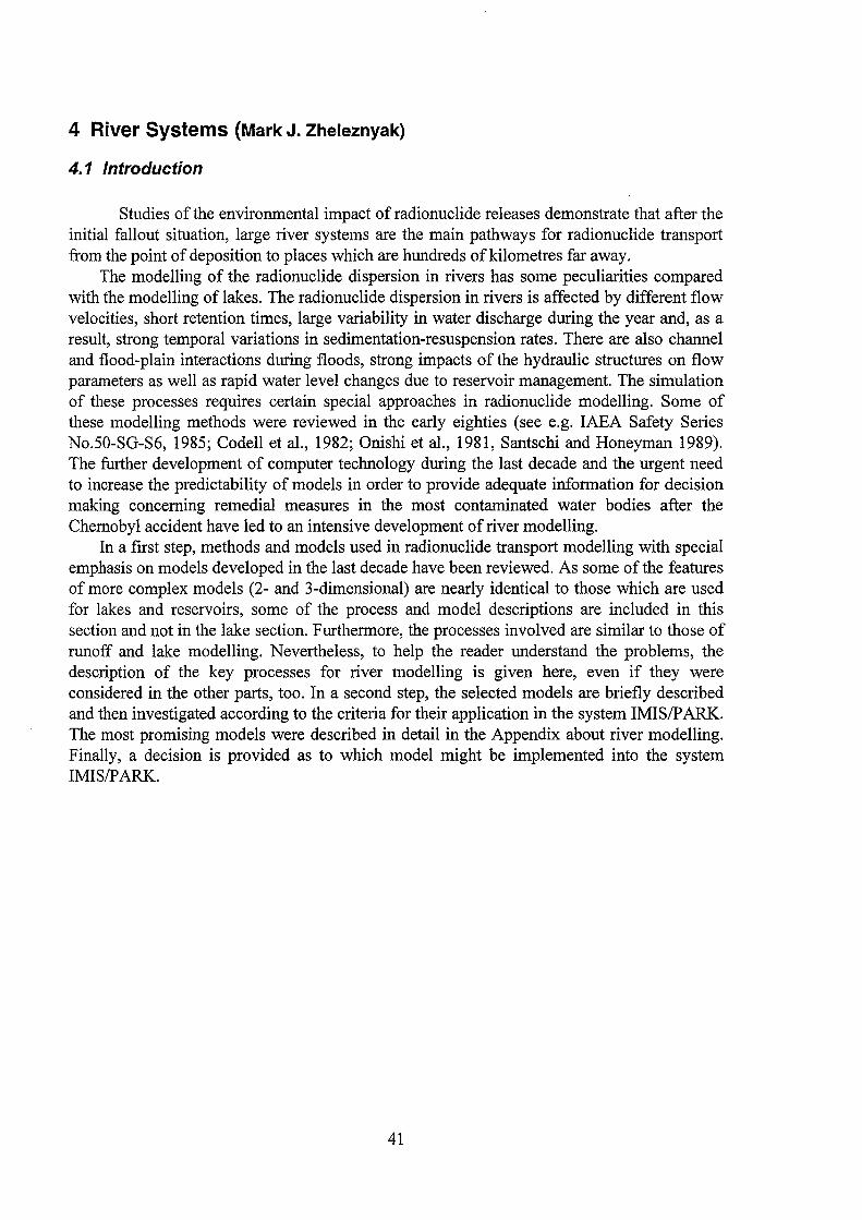
4 River Systems (Mark J. Zheleznyak)

4.1 lntroduction

Studies of the environmental impact of radionuclide releases demonstrate that after the initial fallout situation, large river systems are the main pathways for radionuclide transport from the point of deposition to places which are hundreds of kilometres far away.

The modelling of the radionuclide dispersion in rivers has some peculiarities compared with the modelling of lakes. The radionuclide dispersion in rivers is affected by different flow velocities, short retention times, large variability in water discharge during the year and, as a result, strong temporal variations in Sedimentation-resuspension rates. There are also channel and flood-plain interactions during floods, strong impacts of the hydraulic structures on flow parameters as well as rapid water level changes due to reservoir management. The simulation of these processes requires certain special approaches in radionuclide modelling. Some of these modelling methods were reviewed in the early eighties (see e.g. IAEA Safety Series No.50-SG-S6, 1985; Codell et al., 1982; Onishi et al., 1981, Santschi and Honeyman 1989). The further development of computer technology during the last decade and the urgent need to increase the predictability of models in order to provide adequate information for decision making conceming remedial measures in the most contaminated water bodies after the Chemobyl accident have led to an intensive development of river modelling.

In a first step, methods and models used in radionuclide transport modelling with special emphasis on models developed in the last decade have been reviewed. As some of the features of more complex models (2- and 3-dimensional) are nearly identical to those which are used for lakes and reservoirs, some of the process and model descriptions are included in this section and not in the lake section. Furthermore, the processes involved are similar to those of runoff and lake modelling. Nevertheless, to help the reader understand the problems, the description of the key processes for river modelling is given here, even if they were considered in the other parts, too. In a second step, the selected models are briefly described and then investigated according to the criteria for their application in the system IMIS/P ARK. The most promising models were described in detail in the Appendix about river modelling. Finally, a decision is provided as to which model might be implemented into the system IMIS/PARK.

41

4.2 ldentification of the key processes

4.2.1 Overview of the processes The main processes goveming radionuclide transport in river systems are presented in

Fig. 2. The pollutants in rivers are transported by the water flow (advection processes) with the simultaneaus influence of the turbulent diffusion processes. The radionuclides can interact with the suspended sediments and bottom depositions. A pollutant transfer between river water and suspended sediment is described by the adsorption-desorption processes. The transfer between river water and upper layer of the bottom deposition is under the influence of adsorption-desorption and diffusion processes. The Sedimentation of contaminated suspended sediments and the bottom erosion are also important pathways of the "water column-bottom" radionuclides exchange. All above mentioned processes are reflected in Eq. 1 of chapter 2 (Generic Equations). Differenttypes of river models describe these processes with a different level of parametrisation.

River models, independently of their spatial resolution, include two main types of submodels -hydraulic ones, describing water, suspended sediment and bottom dynamics, and submodels conceming the fate of radionuclides in different phases driven by these hydraulic processes.

Hydraulic submodels may include mathematical descriptions of the following processes:

• wind circulation including seiches* , and circulation driven by inflow/outflow currents;

• turbulent transport; • suspended sediment transport; • sedimentation, resuspension and erosion; • wind wave propagation and transformation*; • wave-driven near-shore circulation*; • dynamics of temperature and density stratification *;

The asterisks indicate processes that may only be important for reservoirs. For longterm projections, precipitation and evaporation should also be taken into account as well as water loss due to irrigation and industrial and municipal purposes.

The fate of radionuclides in general may be determined by the following processes: • dissolved contaminant transport by the river/reservoir flow, • particulate contaminant (pollution absorbed by sediment) transport by the

river/reservoir flow (this includes a separate description of the contaminants transported by clay, silt, mud and sand with different grain size);

• contamination dynamics in the upper active layer ofbottom sediments; • contamination dynamics in deeper buried sediment layers ; • contaminant transfer in interstitial waters; • contaminant transfer by bioturbation in bottom sediments; and • contaminant transfer by biota.

42

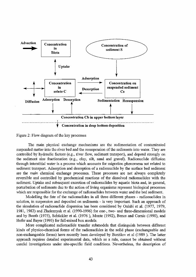
Advection ..

'

'

Concentration in

Biota

1 Uptake

Concentration in

solnte C

Adsorption

Desorption

Concentration of sediment S

l Concentration on

suspended sediment Cs

Diffusion Adsorption Sedimentation Resuspension

~ 1 ~ Concentration Cb in upper bottom layer

----------------------~-------------------------------------------------------------' Concentration in deep bottom deposition

Figure 2: Flow diagram ofthe key processes

The main physical exchange mechanisms are the Sedimentation of contaminated suspended matter into the river bed and the resuspension of the sediments into water. They are controlled by hydraulic factors (e.g., river flow, sediment transport), and depend strongly on the sediment size fractionation (e.g., clay, silt, sand and gravel). Radionuclide diffusion through interstitial water is a process which accounts for migration phenomena not related to sediment transport. Adsorption and desorption of a radionuclide by the surface bed sediment are the main chemical exchange processes. These processes are not always completely reversible and controlled by geochemical reactions of the dissolved radionuclides with the sediment. Uptake and subsequent excretion of radionuclides by aquatic biota and, in general, perturbation of sediments due to the action of living organisms represent biological processes which are responsible for the exchange of radionuclides between water and the bed sediment.

ModeHing the fate of the radionuclides in all three different phases - radionuclides in solution, in suspension and deposited on sediments - is very important. Such an approach of the simulation of radionuclide dispersion has been considered by Onishi et al. (1977, 1979, 1981, 1982) and Zheleznyak et al. (1990-1996) for one-, two- and three-dimensional models and by Booth (1975), Schückler et al. (1976 ), Monte (1992), Benes and Cernie (1990), and Hoferand Bayer (1993) for full-mixed box models.

More complicated radionuclide transfer submodels that distinguish between different kinds of physico-chemical forms of the radionuclides in the solid phase ( exchangeable and non-exchangeable forms) have recently been developed by Borzilov et al (1989 ). The latter approach requires detailed experimental data, which as a rule, cannot be obtained without careful investigations under site-specific field conditions. Nevertheless, the description of

43

these processes is necessary for the understanding of the Ievel of process simplification which is part ofmost ofthe commonly used models.

4.2.2 Radionuclide transformation in river water: contemporary view and modelling approaches

The geochemical modelling is a separate branch of the aquatic modelling activities. Many efforts have been made since the early eighties to improve the modelling of the transport and fate of contaminants by coupling transport models with geochemical models (Chapman, 1982; Felmy et al. 1983). Geochemical models solve various chemical reaction equations based on the mass conservation and chemical equilibrium principles with the aids of thermodynamic laws. Some of the geochemical models, such as MINEQL (Westall et al., 1976) and MINTEQ (Felmy et al., 1984) also calculate adsorption/desorption and precipitation/ dissolution.

F or example, the transport model EXAMS was coupled with MINTEQ to form the model MEXAMS (Felmy et al. 1983), which considers several chemical species of heavy metals, their amounts of adsorption/desorption, precipitation/dissolution, and migration.

Mathematical models describing sorption of metals on homogeneaus solid surfaces, which are primarily metal hydroxides and reference clay minerals, are based on surface complexation and ion-exchange theories. However, the traditional approach in describing and predicting the fate of radionuclides on heterogeneaus solids such as soil, suspended and bottom sediments is mainly empirical and still based on the use of the distribution coefficients Kd.

Kd = ( amount of contaminant sorbed by sediment) I ( amount of contaminant left in solution)

The popularity of Kd models can be also explained by the ease of determination of the distribution coefficient from simple laboratory experiments and field data. Although this approach has some practical benefit, the data are usually site-dependent and seldom have predictive value for other places. The distribution coefficient Kd, which is dependent on liquid and solid phase characteristics, is the integrated result of various physical-chemical processes controlling the retention of the radionuclides. This approach assumes a complete sorption equilibrium, which is seldom the case under natural conditions

Literature data from laboratory experiments and field measurements indicate that sorption of radionuclides by clay minerals, soil and sediments depends on the nature of the clay minerals and is a kinetically controlled process which may continue over time scales up to several years. A kinetic approach of the sorption phenomena therefore is necessary for various reasons. Thus, for realistic modelling of the vertical transport of radionuclides and heavy metals in soil and the aquatic environment, knowledge is needed not only about the sorption equilibrium, but also about the sorption kinetics.

Konoplev et al. (1990 - 1992) have investigated the role of the physico-chemical forms of radionuclides and their transformation processes. The dissolved fraction of a radionuclide can exist either as cations, as neutrally or as negatively charged complexes with dissolved organic substances, or as a mineral component of the soil moisture. The cation form of a radionuclide in solution is in equilibrium with the fraction of the radionuclide absorbed onto the solid particles. In the solid phase, radionuclides can be in exchangeable and nonexchangeable form. In its exchangeable form the radionuclide is sorbed by an ion exchange

44

mechanism. The non-exchangeable form consists of radionuclides originating from nuclear fuel particles or are radionuclides absorbed by a mechanism of irreversible sorption (i.e. incorporation into a mineral crystal lattice, formation of radionuclide-organic in soluble compounds etc.)

The transformation processes of radionuclides in a water body may be represented schematically as follows:

k12 ~'<:;:__ ~ Ac)

k24 A K ~

* A;_

Figure 3: Transformation process of the radionuclide (A 1 + A2 + A * 2 + A 3 + A4 = A0 )

where: Ao Al

A2

A*2

A3

A4

K kij

is the total content of the radionuclides; is the fraction of radionuclides included as part of the fuel particles;

is the cation form of the radionuclide in solution;

are radionuclides sorbed on soil by an ion exchange mechanism;

is an irreversibly sorbed form of a radionuclide;

are radionuclides which are part of the soluble complex compound;

is the constant of ion-exchange equilibrium, and is the rate constant of a corresponding transformation process.

Benes et al. (1992) describe the sorption of the radionuclides by means of two parallel or consecutive ion exchange reactions with two elements bound at two different sites on the solid phase. The equation and parameters for all kinetic models were derived for general ion exchange reactions.

Comans (1990) studied the caesium sorption on potassium and calcium saturated illite. Applying the linearisation method developed by Jannasch et al. (1988) to detennine the number of processes, three consecutive reactions can be distinguished: one fast, instantaneous reaction and two distinct slow processes. For investigating the sorption of caesium on time scales of days to weeks which is most relevant for natural systems, two-box and three- box models were suggested and the isotherm of Freundlich was assumed to describe the equilibrium. Intercamparisen with experimental data for periods Ionger than two weeks showed that reversible reaction on calcium-illite was too slow, whereas the secend process (irreversible reaction) was too fast. Therefore, a more complicated three- box model was used. This model assumed the existence of the easily accessible sorption sites and sorption sites, where the kinetically controlled process are followed by irreversible sorption. The three-box model is presented schematically in Fig. 4:

45

r

II Yt

II --------> k

X K --------> <------>

II y2

II Figure 4: Schematic view ofthe mass balance of a three-box model

with X,X0

YI> Y2o '

Y2, Y2o Z,Z0

Kandn r k Cp

[X]+([Y 1 ]+[Y 2]+[ Z])Cp=[X]0 +([Y 1 ]0 +[Y 2]0 +[Z]0 )Cp

activity in the liquid phase

activity in the equilibrium sites at the time t and t=O

activity in the slow sorption site at the time t and t=O

activity in the irreversible sorption sites at t and t=O

parameters ofthe Freundlich isotherm rate constants of reversible reaction irreversible rate constant particle concentration

z

Two above mentioned models have been proposed for cases where fixation is treated as an irreversible reaction. Data conceming long-term transformation of radionuclides in soil, indicate, however, the existence of demobilisation processes which are reverse to fixation.

Taking into account the reversibility of fixation and two mechanisms of fixation -selective adsorption and diffusion into the solid phase of soil and bottom sediments, the transformation of the chemical forms of the radionuclides was summarised in the ECP-3 Report (1996) and can be represented by the following scheme:

Ke ~

kl p EF==EJ FD

kr

Ks

I FS I

Figure 5: Improved scheme for the transformation process ofthe radionuclides in soil solution

where p is the radionuclide in fuel particles;

46

W,E

FS,FD

are the water-soluble and exchangeable form, respectively. Equilibrium between the water soluble and exchangeable form is reached relatively quickly and it is reasonable to consider them as a single mobile form, are radionuclides, fixed as a result of selective sorption and diffusion into solid phase respectively, the equilibrium constant for non-selective and selective sorption, and are first order rate constants of the radionuclide leaching from fuel particles,

fixation and remobilisation, respectively. There is no unified mathematical description of the sorption process goveming the

behaviour of metals and particulate radionuclides which is demonstrated by the above mentioned articles. Further detailed study of the sorption kinetics of radionuclides will allow to examine existing concepts in terms of a more fundamental description of the underlying processes.

In general, models of radionuclide transport in the rivers/reservoirs do not include the above presented kinetics in their complete details. However, a reasonable level of model complexity which may reflect the main features of the exchange processes (radionuclides transfer in the system "water - suspended sediments - bottom depositions" - transition from a non-equilibrium to an equilibrium state, different Kd value for bottom deposition and suspended sediments, different rates of sorption and desorption) seems to be represented by a "Kd- exchange rate" approach which is used in practically all contemporary models (Onishi et al., Smitz, Zheleznyak et al. ).

4.2.3 Sediment transport and hydrodynamic processes and models

To simulate radionuclide transport in rivers, it is necessary to estimate in advance the river flow and suspended sediment transport driven by the river hydrodynamic processes. There are a lot of models to simulate river hydraulics and hydrodynamics. Overviews are presented in e.g. Cunge J., Holly F. and Verwey A., 1986; and Orlob, 1983. The contemporary "state-of-the-art" in the field is presented by Rutherford, 1994. In our report we will describe only hydrodynamic models which are coupled with sediment and radionuclide transport submodels.

Suspended sediments act as a carrier of radionuclides in river/reservoir flow. The amount of radionuclides transported by the sediments depends on the suspended sediment concentration in the river flow and the Kd value. After the Chemobyl accident, for example, up to half of the Cs-13 7 transported by the Pripyat River from the vicinity of the Chemobyl NPP was bound to suspended sediments (V oitsekhovitch et al., 1992). The Sedimentation and bottom erosion processes play a key role in flow self-purification and for secondary contamination.

The mathematical modeHing of sediment and transport is a large branch of hydraulics where overviews could be found in Ackersand White (1973), Grishanin (1976), Cunge, Holly and Verwey (1986), Engelund and Fredsoe (1976), Holly et al. (1990), Karim et al. (1981,1987), Mehta et al. (1989), Onishi (1993), Raudkivi (1967), van Rijn (1984). For steady state conditions, the sediment discharges are calculated by empirical and semi-empirical formulae which connect sediment discharge with sediment parameters, flow velocities and river cross-section characteristics or shear stress acting on the bed. In the case of cohesive sediments (finest silt and clay) also cohesive bonds between the particles have tobe taken into account (Mehta et al. 1989). The variability of streams and sediment parameters lead to the situation that up to now several different formulae have been used for practical applications. It

47

was demonstrated by validation studies (Onishi, 1993) that the approaches of Ackers -White, Engelund-Hansen, Rijn and Toffaleti show the most acceptable results for non-cohesive sediments over a wide range of flow and sediment conditions. However, for an individual river, the best result can be obtained also by empirical formulae especially tuned for this river.

The sediment transport models are based on the suspended sediment-mass conservation equation (advection-diffusion equation with the sink-source term describing Sedimentation resuspension rate) and the equation of bottarn deformation (Exner equation). The most important problern for modeHing is the parametrisation of the sedimentation and resuspension rates. A physically based approach calculates these rates as a function of the difference between the actual and the equilibrium concentration of suspended sediments. This is often referred to as "suspended sediment capacity" and can be derived on the base of the above mentioned formulae.

One-dimensional models based on cross-sectionally averaged variables seem to be the most important ones to determine the river flow. Well known are computer codes such as HEC-6 and HEC-2SR (Hydrological Engineering Center, 1977, 1982), REDSED (Chen, 1988), PLUVIAL 11 (Chang, 1988), !ALLUVIAL (Karim et al., 1981, 1987) and CHARIMA (Holly et al., 1990) which extends the !ALLUVIAL approaches as well as MIKE-11 (Danish Hydraulics Institute), and TELMAC (Laboratory of Hydraulics, EDP, Prance ). The two last ones are commercially distributed modeHing systems which include models of different dimensions. HEC-2SR, PLUVIAL 11, CHARIMA, MIKE-11, and TELMAC contain river hydraulics modules based on a numerical solution of the Saint-Venant equation. The possibility of an efficient estimation of river hydraulics on the base of a numerical solution of the "diffusive wave" equation, a simplified version of the Saint-Venant equation, was demonstrated by Jobson, 1989, Zheleznyak and Marinets, 1993.

Suspended sediments models include different formulae for calculating the equilibrium sediment concentration. The most comprehensive model (e.g. CHARIMA) contains modules of river hydraulics computation and methods to simulate the bottarn erosion as a function of the sediment grain distribution in the upper bottarn layer (bottom armouring calculation) and to calculate the bottarn friction in dependence of the simulated dynamics of the bottarn forms.

The sediment transport models are also part of the radionuclide transport models described by Onishi et al. (TODAM, SERATRA, PETRA, PLESQOT) and Zheleznyak et al. (RIVTOX, COASTOX, WATOX, THREETOX), all described in more detail below.

4.3 ldentification of mode/s availab/e for describing the radionuc/ide transport in rivers

4.3.1 Modelling Approach

Mathematical models describing the radionuclide transport and dispersion in rivers and reservoirs can be classified according to two different approaches - (1) spatial averaging of the variables and (2) individual treatment of variables describing radionuclides in different physical-chemical forms.

Variables averaged over compartments represent the highest level of averaging and, as a result, are used in models of the lowest spatial dimension. These box-type (zero dimension) models treat the entire body ofwater (including the sediment layer, etc.) or apart ofthe entire body (e.g. one box for water and one for sediments) as a homogeneaus compartment.

48

Cross-sectionally averaged variables are often used in channel models and in models for narrow reservoirs. These 1-D modelsalso have zero dimension for steady state flow (plug flow models), and there are one-dimensional models for unstable flows.

Two dimensional (2-D) vertical models operate with width averaged variables. These models are used to describe current, suspended sediment and radionuclide transport in cases of a significant variability with respect to the channel depth.

Depth averaged variables are used in the lateral-longitudinal 2-D models which describe flow pattem and radionuclide dispersion in shallow reservoirs, river channels and flood plains.

The lowest level of averaging takes place in 3-D models solving primitive or basic goveming equations. The real spatial averaging scale of these models is only based on the width of the computational grid but not on a certain parametrisation or averaging procedure.

However, modelling of radionuclides dispersion in water bodies is also apart of the more general problern of modelling of the water quality, including the estimation of hydrodynamic (hydraulic) processes, and the simulation of sediment and pollutant transport driven by such hydrodynamics (see, e.g., Orlob, 1983). Therefore, the above derived model classification in terms of scale averaging may be considered as a general one for water quality modelling.

Models can be also classified in terms of the consideration of radionuclide concentrations in different phases (in solution, attached to suspended clay, silt, sand, mud, biota, contained in upper Sedimentation layer, buried sediments, etc.) and in different physical-chemical forms (exchangeable and non-exchangeable forms on solid particles, colloidal forms).

The early models for the radionuclide transport in water bodies described only the total concentration of the radionuclides in water, and did not distinguish its forms. A first step to improve those models was to develop water-sediment interaction submodels. Codes that include a reasonable mathematical description of the radionuclide interactions with the solid phase, i.e., with the bottom deposition and with suspended sediments, have demonstrated to be more successful in predicting the aquatic transport of radionuclides (see reviews by Codell et al., 1982; Onishi et al., 1981; Santschi and Honeyman, 1989).

The river and reservoir models will be classified below according to the level of averaging (model dimension) and subsequently according to the number of considered phases and physical-chemical forms of the radionuclide.

4.3.2 Description of the radionuclide transport models

4.3.2.1 3-D jlow and transport models

It is reasonable to provide three-dimensional modelling of the transport of radionuclides in rivers and reservoirs in conditions of large vertical and lateral gradients of the hydrodynamical fields. Such conditions may occur close to the point of the release of radioactive material into water bodies, in the vicinity of heavily contaminated bottom areas, and in stratified water bodies.

The FLESCOT model (Onishi and Trent 1982) is an unsteady, three-dimensional, finite difference model. It consists of submodels of hydrodynamics, turbulence, water temperature, salinity, sediments (both cohesive and noncohesive) and contaminants (both dissolved and sorbed on sediments). The FLESCOT model also simulates the behaviour of sediments and contaminants in the river bed, affected by erosion/deposition, direct

49

adsorption/desorption between water and bottom sediments, and bioturbation. It can calculate wind-induced flow and wave-induced sediment transport, thus affecting radionuclide transport in shallow water. The model has been applied to the Hudson River estuary in New York for Cs-137 migration and accumulation, to Buzzards Bay/New Bedford Harbor in Massachusetts for PCBs and heavy metals assessing their transport and potential remediation activities, and to a hypothetical 3000m deep ocean for low-level radioactive waste disposal assessment. FLESCOT, as other models of Onishi of lower dimensions presented below (TODAM, FETRA, SERATRA), uses multiple bed layers. The first layer (usually taken as a few cm thick) implicitly includes a very thin top layer (assigned as twice the bed sediment grown size) characterised by the chemical equilibrium between the attached and interstitial dissolved form of the radionuclide. Onishi's models also calculate sedimentation and erosion rates for different sediment size fractions taking into account the water flow and sediment characteristics.

The three-dimensional model THREETOX was developed recently at the Cybemetics Center, Kiev and applied to several water bodies. (Zheleznyak and Margvelashvili, 1995). THREETOX was developed to simulate 3-D hydrodynamic fields, suspended sediment transport and radionuclide transport in water bodies. Fluid dynamics are simulated on the basis of a three-dimensional, time-dependent, free surface primitive equation. The prognostic variables of the hydrodynamic part of the model are the three components of the velocity fields, the temperature, salinity and the surface elevation. The concepts of eddy viscosity/diffusivity and Prandtl's hypothesis with a variable turbulence scaling length are used to define the turbulence stresses.

Suspended sediment transport is described by the advection- diffusion equation, taking into account the deposition velocity ofthe sediment particles. The bottom boundary condition describes sediment resuspension or settling dependent on the ratio between equilibrium and the actual near-bottom suspended sediment concentration.

The equations of the transport of the radionuclides describe the concentration of the radionuclides in solution, in suspended sediments and in bottom depositions. The exchange between these variables is described as a adsorption-desorption and Sedimentationresuspension process.

The goveming equations together with the boundary conditions are solved by finite difference techniques. A horizontally and vertically staggered mesh of grid points is used for the computation. The use of a splitting technique with an implicit scheme results in a threediagonal matrix which is solved by a Gaussian elimination method.

The influence of water stratification on radionuclide transport was studied for the Dniepr - Bug Estuary. The dispersion of radionuclides discharged from this estuary to the Black Sea was simulated with this model.

4.3.2.2 2-D vertical-longitudinal models

The SERATRA codewas developed at the Pacific Northwest Laboratory (Onishi and Trent, 1982, Onishi et al., 1981). The model describes width-averaged concentrations of radionuclides and other sediment adherent pollutants in river channels and reservoirs. The Kd and exchange rate coefficients for "water-suspended sediment" and "water-bottom deposition" are used. The code includes a submodel for the suspended sediment transport simulation for cohesive and non-cohesive sediments.

The VERTOX code (Zheleznyak, 1990 ; Zheleznyak et al., 1991 ) has been derived from 3-D models by averaging the equations over the flow width, resulting in a 2-D

50

vertical-longitudinal model. The model structure is similar to SERATRA. The main difference regarding the submodel of radionuclide transport is that VERTOX contains two different Kd values for suspended and bottom sediments, and individual exchange rate coefficients for the adsorption and desorption processes. The main objects of the application of VERTOX are zones of abrupt changes in flow parameters. An important example is the flow over bottom traps which were made for settling down of contaminated suspended sediments.

The equations goveming the current flow is derived by using the hydrostatic approximation. The advection-diffusion equation for suspended sediment transport is used, describing the deposition and erosion rates by the suspended sediment capacity of the flow. The submodel of the transport of radionuclides describes the radionuclide concentration in solution, the concentration in suspended sediments and the concentration in the bottom sediment. The exchanges between these phases are described by absorption-desorption and Sedimentation-resuspension processes.

A verification of the hydrodynamics and the sediment submodels was performed (Demchenko, Zheleznyak 1990, Demchenko, Koziy, Zheleznyak, 1994) by using laboratory data for dredged trenches (van Rijn, 1981) and experimental data on radionuclide deposition in bottom traps ofthe Pripyat River.

4.3.2.3 2-D lateral-longitudinal models

2-D lateral-longitudinal models are widely used to simulate the flow and dispersion of pollutants in shallow reservoirs, floodplains and coastal areas (e.g. Orlob, 1983). The model equations may be derived by averaging the primitive 3-D equations over the depth.

The FETRA code (Onishi, 1981) is based on the unsteady two-dimensional equations which simulate the transport, deposition and resuspension of sediments and contaminants together with their interactions. The model describes the transport of cohesive and noncohesive sediments by using the Du Boy formula. FETRA was validated on the basis of experimental data for the James River estuary, Virginia ,USA. Recently, FETRA was applied to simulate Sr-90 wash-out from the Pripyat River flood plain (Onishi, 1995, personal information).

The COASTOX modelwas developed at the Cybemetics Center, Kiev (Zheleznyak, 1990, Zheleznyak et al., 1991-1996) to simulate the transport and dispersion ofpollutants in the Dniepr reservoirs and in the Pripyat River. It contains radionuclide transport submodels similar to those used in FETRA. The model includes sediment transport, transport by advection-diffusion, and radionuclide - sediment interactions. It considers the dynamics of the bottom depositions and describes the rate of sedimentation and resuspension as a function of the difference between the actual and the equilibrium concentration of suspended matter depending on the transport capacity of the flow. The latter is calculated on the basis of semiempirical relationships. The Kd approach has been used for describing the adsorption/desorption and diffusion transfer of the radionuclides in the systems "solution -suspended sediments" and "solution - bottom deposition". The exchange rates between the solution and the particles is taken into account to obtain a more realistic simulation of the kinetics of the processes. The adsorption and desorption rates are assumed to be not equal. Finite difference methods are used to solve the equations. The two main differences between FETRA and COASTOX is that the latter has the possibility to calculate non-reversible adsorption processes and that it contains a hydrodynamic submodel. In contrast, FETRA can only be used in combination with some other hydrodynamical computer code. COASTOX

51

was applied and validated for the Kiev Reservoir, the Pripyat River flood plain, the Kralova Reservoir, and the Vakh River. It is implemented into the hydrological module ofthe RODOS European decision support system (Ehrhardt et al. 1996, Zheleznyak et al., 1996, Gofman et al., 1996)

4.3.2.4 1-D channel models

1-D models describe the cross-sectionally averaged flow in water bodies. This type of models is widely used to simulate the dynamics of the radionuclide transport in networks of river channels. A simplified approach of radionuclide-sediment interaction was used in models of White and Gloyna (1969), Shih and Gloyna (1970), CHNSED (Fields, 1976), HOTSED (Fields, 1977).

The one-dimensional channel model TODAM has been used to simulate radionuclide transport in several rivers ofthe United States (Onishi et al., 1982 ). TODAMis based on the same approaches as the other 2-D and 3-D models of Onishi, characterised above. The model describes the radionuclide transport for three typical suspended sediments, - sand, silt and clay - with individual Kd values for each of them. The radionuclide transport module is supported by a comprehensive suspended sediment transport module that describes the transport of cohesive and non-cohesive sediments. TODAM does not include a module estimating the hydrodynamics of the river. It was always applied for precalculated hydrodynamic fields (DKWA V or HEC-2 or CHARIMA). TOD AM was used to simulate Pu-239 transport during flush-flood events in the Mortandad Canyon, New Mexico, USA (Whelan and Onishi, 1983), to reconstruct the bottom contamination of the Clinch-River- Tennessee River System from releases of the Oak Ridge National Laboratory (Onishi, private communication), and to simulate Sr-90 and Cs-1237 transport in the Dniepr Reservoir after the Chemobyl accident (Zheleznyak, Blaylock and al., 1995).

The 1-D model of the SP A "TYPHOON" State Hydrometeorological Committee of USSR (Borzilov et al., 1989 ) uses empirical data on sedimenttransportrate and flow. The model includes detailed descriptions of the transfer between different forms of radionuclides. Model parameters have been identified on the basis of experimental data of Pripyat River spring floods.

The 1-D model by Smitz and Everbecq (1986) considers kinetics of radionuclide interaction with two size fractions of suspended solids. The model was verified for the migration of radionuclides in the Meuse River and subsequently applied elsewhere to a large extent (Smitz, private communication).

The Hydrological Simulation Program - FORTRAN (HSPF) (Bicknell et al., 1993, Donigian et al., 1995) does not consider radionuclides however it is included in this review as it is a comprehensive model that contains a watershed contaminant transport module -presented in chapter 3 of the runoff section - and a module that describes the transport of pollutants in rivers and reservoirs.

MIKEll developed in the River Hydraulics Division ofthe Danish Hydraulic Institute (Havno et al., 1995) is a one-dimensional modelling system for the simulation of flows, sediment transport and water quality in estuaries, rivers, irrigation systems and other water bodies. This modelling package is designed for micro-computers with DOS or UNIX operating systems and provides the user with an interactive menu and a graphical support system with logical and systematic Iayouts and sequencing of the menus. MIKE11 has been designed to have an integrated modular structure with basic computational modules for hydrology, hydrodynamics, advection-dispersion, water quality and cohesive and non-

52

cohesive sediment transport. It also includes modules for surface runoff. MIKE11 has not yet been applied for modeHing radionuclide transport in river systems.

The one-dimensional model RIVTOX developed at IPMMS, Cybemetics Centre, Kiev (Zheleznyak et al. 1992, 1993, Tkalich et al. 1994, Zheleznyak et al., 1996, Gofman et al., 1996) simulates the radionuclide transport in networks of river channels. Sources can be a direct release into the river or the runoff from the catchment. In the latter case the output from the RETRACE model of SP A TYPHOON (Zheleznyak et al., 1996) is used as the input of RIVTOX. The stream function, the transport of suspended sediments and radionuclide dynamics are averaged over the cross-section of the river. A 'diffusion wave' model, derived from the one-dimensional Saint-Venant equation describes water discharge. An advectiondiffusion equation calculates the transport of the suspended sediments in the river channel. Its sink/source terms describe the rate of Sedimentation and resuspension as a function of the difference between the actual and the equilibrium concentration of suspended matter with respect to the transport capacity of the flow. The latter is calculated on the basis of semiempirical relations - Bijker formula (Bijker, 1968) or van Rijn formula (Rijn, 1984). The dynamics of the upper contaminated river bed is characterised by an equation for the erosion ofthe bottom layer.

The radionuclide transport submodel of RIVTOX describes the dynamics of the crosssectionally averaged concentrations of radionuclides in solution, in suspended sediments and in bottom depositions. The adsorption/desorption and diffusion contamination transfer in the systems "solution- suspended sediments" and "solution- bottom deposition" is treated by the Kd approach for the equilibrium state, additionally taking into account the exchange rates between the solution and particles for a more realistic simulation of the kinetics of the processes. The adsorption and desorption rates are assumed to be not equal, which is the difference between this approach and the one realised in TODAM.

A finite difference method is used to solve the "diffusion wave" equation and the advection-diffusion equations which describe the transport of the suspended sediments, the radionuclides in solution and the radionuclides adherent to suspended sediments. An ordinary differential equation simulates the dynamics of the radionuclides in the upper contaminated bottom layer.

The model was validated on the basis of data for the radioactive contamination of the Dniepr River and the Clinch River within the IAEA/CEC VAMP program (Zheleznyak et al., 1995), for the Ilya River in the Chemobyl zone within the RODOS-JSP-1 project (Zheleznyak et al. 1996), and recently, the model was successfully applied for the simulation of the early post-release stage of Cs-137 in rivers on the basis of data for the Dudvakh River, Slovakia (Zheleznyak, unpublished).

4.3.2.5 Box type models

Boxmodels (other names- compartment models or 0-D models) are wide spread tools for ecological modeHing in aquatic systems (see e.g. Orlob, 1983). Some ofthe models which were developed to simulate different kinds of pollutants can be also applied for the simulation ofthe transport ofradionuclides in rivers- e.g. EXAMS (Bumas and Cline, 1982; Felmy et al, 1983), WASP4 (Ambrose et al. 1988). Early radionuclide transport models were constructed as box models (see overviews of Onishi et al., 1981, Codell et al., 1982, Santchi and Honeyman, 1989) and were applied mainly for lakes. The application of box-type models for rivers is constrained by the assumption of complete mixing in the compartment. On the other

53

hand, box models can be considered as the finite-difference approximation of 1-D river models, however mostly applied on a coarse computational grid only.

The two-phase box model (radionuclides in bottom sediments and radionuclides in water) developed by the United States Nuclear Regulatory Commission (USNRC, 1978) is a simplification of the five-phase model proposed by Booth (1975). The model has been used for Clinch and Tennessee Rivers case studies (USNRC, 1978; IAEA, 1985).

The SMC model (Benes and Cemik, 1990) describes the transport ofradionuclides in suspended and dissolved forms in river channels. It consists of hydrodynamic, sediment transport and radionuclide transport submodels. Distribution of the radionuclide between the water and the suspended solids is described by a kinetic equation for a two-step reversible reaction. The deposition of radionuclides in the bottom sediments depends on the exchange between suspended solids and bottom sediments characterised by an exchange coefficient. The model was used for modelling of the migration of Cs-13 7 accidentally released into the Dudvakh River (Benes et al., 1994). The Sedimentation rate is a parameter of the modeland can be tuned during the calculations.

Monte's box-model (Monte, 1993) is based on the subdivision ofthe water body into a set of sub-systems corresponding to the set of reservoirs. In each sub-system the following processes are considered: radionuclide transport due to the horizontal movement of water and suspended matter; radionuclide interaction with suspended matter and with the top sediment layer; migration of radionuclides through the sediment; Sedimentation and resuspension. The model accounts for three layers: a first thin top layer in which the radionuclides are in chemical equilibrium with the overlying water; a second layer Gust below the first) exchanging radionuclides with the overlying water through the top layer and/or with the deeper layer which acts as an ultimate radionuclide sink. The suspended sediment transport and sedimentation rate is not calculated in the model. These values are taken from measured data.

The equations are solved by using a set of first order differential equations. The model demonstrated reasonable good results in a validation study for the Dniepr reservoir cascade within the VAMP program.

The WATOX model (Zheleznyak, 1990, Zheleznyak et al., 1991, 1994) isabox-type model based on a set of first order differential equations describing water, sediment and radionuclide transport. Dissolved contamination, contamination on suspended sediment and the contamination of the bottom sediment are considered with a special treatment of the contamination-sediment interaction. The parametrisation of these processes is similar to those used by Schückler et al. (1976), however, some further processes are included. Additionally, a supplementary submodel to simulate the temporal variations of Sedimentation-resuspension rates during flood events in reservoirs is included. As described for RIVTOX, COASTOX and THREETOX, also W ATOX takes into account different Kd values for suspended and bottom sediments, together with different exchange rate coefficients for adsorption and desorption. Model verification shows the high significance of this mechanism for the fate of Cs-137 in reservoirs. The model was tested and calibrated on the basis of post-Chemobyl data for the Dniepr reservoir cascade.

The Hoferand Bayermodel (1993) is a dynamic extension ofthe above-mentioned stea:dy state (static) model developed by Schückler et al. The dynamics of radionuclide concentrations in filtrated water, on suspended sediments and bottom sediments is described by the set of ordinary differential equations on the basis of two different Kd values for adsorption and desorption and exchange rate coefficients. The model coefficients were not calibrated on the basis of measurements.

54

In the box model of Mundschenk (1988), the processes of direct adsorption and diffusion exchange between water and bottom depositions is omitted. It is assumed that the radionuclides interact directly with suspended matter only.

4.3.2. 6 Analytical models

This type of models describes the radionuclide fate in rivers on the basis of analytical solutions of the equations valid for box model or 1-D models with respect to several simplifying assumptions ( e.g. flow parameters are constant within the river branch, waterbottom radionuclide exchange processes could be described by one parameter only and so on). Examples ofthis approach are presented by Coppa (1992); IAEA (1985); and USNRC (1975). The oversimplification in these approaches ends up in the fact that the parameters of an analytical model calibrated for one water body cannot be used for another one without significant recalibration. Further development of computer technology nowadays allows to use numerical models which describe the main significant processes in more detail based on the physical characteristics of the site. Analytical models can be used mainly as a first estimation of the situation - for example as a conservative upper estimation of the radionuclide concentration after accidental releases. Therefore, they will not be considered in the further discussion.

4.4 Comparison of the mode/s with respect to their applicability in the IMIS/PARK system

The processes goveming the transport of radionuclides in the river flow have been subdivided into hydraulic and radionuclide exchange processes.

A summary of the analysis of the hydraulic transport processes in the models considered in this study is presented in Table 3. The two main hydraulic processes such as the advection and diffusion/dispersion of the pollutant can be described rather accurately in 3-D, 2-D and 1-D models, however with a different Ievel of complexity (averaging).

One-dimensional river models seem to be most appropriate to simulate the dynamics of the radionuclide transport for distances !arger than 10 times the river width and for time scales from seconds till one year. 2-D lateral-longitudinal models can be used for the simulation of the radionuclides distribution near the release point. For reservoirs with a complex bathymetry and where effects of stratification can be significant, 3-D models might be a useful tool to simulate the complex distibution of radionuclides. Box models, based on the assumption of full mixing in one individual compartment, and thus simplifying the transport processes, can be applied usefully mainly for long-term estimations in particular.

Computer codes which include the simulation of the dynamics of suspended sediment are preferable as it is very difficult to measure accurately the temporal variations of the concentration of suspended sediment as well as the rate of sedimentation/resuspension. Furthermore, the transport of radionuclides should be coupled with the modelling of the flow and the transport of suspended sediment. This allows the consideration of instantaneous changes in the water flow and the impact of engineering structures such as dams and waterworks. Therefore, in particular with respect to the dynamics in the discharge, and due to the required time scales of at least several days and a spatial gridding in the order of

55

kilometres, 1-D models are preferable. 2-D and 3-D models are too complex and require too many data and computational resources.

Five 1-D models (TODAM, Smith & Everbeq model, RIVTOX, HPSF and MIKE11) are considered in the study. TODAMis limited by the absence of a hydrodynamic (hydraulic) submodel. Information in the open Iiterature about the Smith & Everbeq model is not sufficient to consider it for the final decision. HPSF was developed only for pesticides and not for radionuclides, however, taking into account that HPSF includes both river and watershed submodels, it seems to be necessary to include it into further consideration. RIVTOX does not include such a detailed description ofthe sedimentationlerosion processes as TODAM and MIKEll, however, it has the advantage of coupling the hydrodynamic, sedimentation and radionuclide transport submodels. MIKEll does not consider radionuclides, the heavy metal transport submodel, however, includes all features for a modification to describe the transport of radionuclides as weil.

Some of the box models such as the model of Monte, W ATOX and the Hofer & Bayer model have been also selected for further analyses, taking into account that the simplified description of the hydrodynamic processes can be particularly compensated by a comprehensive approach for the description of the radionuclide exchange (see Table 4). Models which describe the processes properly should include the fate of the radionuclides in the solute, bound on suspended sediment and bound on bottom depositions. The radionuclide transfers in this system "water - suspended sediments - bottom depositions" can be adequately described on the basis of parameter distribution coefficients and exchange rates coefficients. This approach is used in these box models as weil as in the 1-D models TODAM and RIVTOX. Further improvements in the realisation of the chemical transfer processes, in particular the consideration of exchangeable and non-exchangeable forms of the radionuclides adherent to sediments, are under development now. A first approach was implemented recently in RIVTOX. The possibility to use different transfer rates for adsorption and desorption processes now exist for the two codes W ATOX and RIVTOX.

The temporal and spatial ranges of applicability of the models depends on either the type and amount of input data or the requested spatial resolution of the results. Table 5 shows a summary ofthe temporaland spatial characteristics ofthe models. The 1-D models seem to be best balanced with respect to the amount of input data against resolution and possibilities for short-term/medium-term modelling. The box model developed by Hoferand Bayer was also applied for short-term (hours) simulations, however, it is not possible to consider changing hydrological properties, such as additional runoff water following a heavy storm event. To allow for such a dynamical modelling, the structure of the box models has to be modified considerably, which, nevertheless, is in principle possible.

From the seven models which were top-ranked based on the analysis presented above (TODAM, RIVTOX, MIKEll, HPSF, Monte's model, WATOX and the Hofer & Bayer model) five codes were validated by comparison calculations with measured radionuclide concentrations (see Table 6). It should be stressed that only RIVTOXIRETRACE has been tested and validated for the short range (hours- days; on Dudvah data).

The applicability to Central European conditions has been demonstrated by validation studies performed with RIVTOX (various temporal ranges) and particularly by the Hofer & Bayer model for the long-term predictions.

Table 6 also includes information on the operational status of the computer codes. Three ofthe programs contain a special user interface for data input, however, only RIVTOX include tools that simplify the process of the data preparation, support the execution of the model and provide detailed graphical analyses of the results.

56

As far as the availability and accessibility of input data are concemed, 1-D models seem to be the best choice, in particular, taking into account that hydrological data of open publications is often sufficient for model tuning for various river systems. Box models which need even less data cannot provide such an adequate description of the dynamic hydrological processes, in particular, on a short time scale.

None of the investigated computer codes contain tools for data assimilation. In the case ofRIVTOX, work started recently to use updated on-line monitaring data. This tool will provide the possibility to use any measurement in the river as an updated source term for the further calculations downstream. There might be also the possibility to tune model parameters based on these measurements.

None of the models except for RIVTOX provides an interface to radiological models. Within the framewerk of the RODOS project, RIVTOX is connected to a special version of the ECOSYS model which is also implemented in the IMIS/P ARK system.

4.5 Se/ection of a river model for use in IMIS/PARK

On the basis of the discussion presented above, 1-D computer codes seem to be the most appropriate choice for use in IMIS/PARK. With 1-D models it is possible to consider changing hydrological conditions. They can be applied for nearly all temporal and spatial scales without too many input data being required. However, the hydrological part of such a code has to be closely connected to the chemical part describing the behaviour of the radionuclides. It is also possible to connect those codes with runoff models as demonstrated by HSPF and RIVROX. None ofthe mathematical models considers all the features which are required by the IMIS/P ARK system, but it is possible to improve the models if necessary. HSPF has the advantage to be part of a model system which also includes a runoff component. But radionuclides are not considered explicitly in this system. Modifications are needed for a comprehensive user interface and data assimilation. MIKE 11 Iacks the chemical submodel for radionuclides. TOD AM contains a very detailed description of the behaviour of the radionuclides, but does not include a hydrological component. Such a model has to be added together with a user interface and tools for data assimilation. None of the models HSPF, MIKE11 and TODAM are connected to radioecological models. RIVTOX on the other hand, only has data assimilation as a missing feature, however, work in this area started recently. Therefore, the 1-D RIVTOX code might be the most adequate one for the integration into the IMIS/P ARK system for the following reasons:

• close coupling of the simulation of hydraulic, sediment and radionuclide transport processes,

• adequate description of the processes, • temporaland spatial ranges of applicability, • available and accessible input data, • wide range of validation studies performed, • moderate computational requirements, • interface with the watershed model RETRACE for the simulation of aerial

contamination of a river basin, • interface with the Iake model LAKECO, • interface with a radioecological model, • interface with a GIS system (in development) that should simplify the procedures

of the adaptation for different river basins,

57

• operational status (mid 1997) including a user interface and interaction with a "real-time database" (in progress). and

• ongoing improvement of the model and in particular of the tool for data assimilation.

As a second choice, TODAM tagether with a hydrological submodel might be considered, too. However, this code does not meet as many criteria as RIVTOX.

58

Table 3: Features ofthe hydraulic transport simulation in river/reservoir models

Dimension

1 2 3 1 FLESCOT 3-D

2-D vertical 5 FETRA 2-D lateral-

longitudinal

6 COASTOX 2-D lateral-

13

rodynamic submo

was used with TEMPEST 3-D hydrodynamic transport code

was used with 2-D hydrodynamic transport codes R2-M and others

"+"

59

Wayof hydrodynamic transport

Table 4: Features ofthe physical/chemical (radionuclide) submodels in river/reservoir models

No. Model Radionuclidesuspended sediment

interaction "-" steady (only Kd)

"+" unsteady

Interaction of nuclides in solute

and bottom deposition

60

Possibility to take into account the amount of

exchangeable forms and/or non-reversible

Table 5: Input and output infonnation ofthe river/reservoir models

1

3

6 COASTOX

bottom bathymetry map

same as 1

same as 1

same as 1

same as 1

compartment ofriver channel

of radionuclide concentra-tion

distribution ofwidth-averaged concentra-tion along the stream same as 2-d distribution of depth-averaged concentra-tion same as 5

tion

61

x, y directions: tens- hundreds ofmetres; z direction: centimetres-metres

x directions: tens - hundreds ofmetres; z direction: centimetres-metres

3

x, y directions: tens- hundreds ofmetres;

same as 5

metres, km.

ter Iangterm (weeks- (years)

+ +

+ +

+ +

+ +

+ +

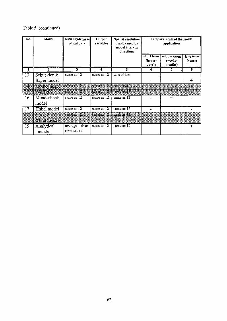
Table 5: (continued)

No.

same as 12

Bayermodel same as 12

62

term (years)

+

Table 6: Validation ofmodels and computer codes

No. Model Computer code Validation studies

UNIX PCversion User environment interfaces

1 2 6 7 8

1 TOD AM + - -2 RIVTOX + + + 3 HPSF - + + 4 Monternodei - + -5 WATOX + + + 6 Hofer & Bayer - + -

model 7 MIKEll + + +

Case studies: Clinch River-Tennessee River ,Oak-Ridge releases (column 8)

models 1 ), 2) Dniepr River, Chernobyl accident (column 7, 8)

models 1), 2), 4), 5). Rhine basin -Rhine, Neckar -Chernobyl accident (column 7)

model2) Uzh River- Chemobyl area (column 7)

model2)

short term medium ter (hours- (weeks-

days) months)

6 7

- + + +

+* +*

- +

- +

- +

+* +*

Dudvakh River, Slovakia, aceidentat release from Bohunice NPP ( column 6) model2).

Weser River, release from NPP Würgassen (column 7) model6).

*For HSPF and MIK.Ell validation studies only for non-radioactive pollutants

63

Iong term (years)

8

+ +

-+ +

-

4.6 REFERENCES

Ackers, P., White, R. Sediment transport: new approach and analyses. J.Hydr.Div. ASCE, v99, No.ll, 2041-2060 (1973).

Ambrose, R.B., Wool, T.M., Connolly, J.P., Schanz, R.W. WASP4, a Hydrodynamic and Water Quality Model - Model Theory, User Manual and Programmer's Guide. EPA/600/3-87/039, U.S. Environmental Protection Agency, Environmental Research Laboratory, Athens, Georgia. 1988.- 663 pp.

ANONYMOUS, Guidelines for calculating derived release limits for radioactive material in airbome and liquid effluents for normal operation of nuclear facilities, CAN/CSA-N288.1-M87, Canadian Standards Association Ed., Toronto, Ontario, Canada, 69 pp. (1987).

ANONYMOUS, Methodology for evaluating the radiological consequences of radioactive effluents released in normal operations, National Radiological Protection Board, Chilton, United Kingdom (1994).

Beck, M.B., Water Quality Management: A Review of the Development and Application of Mathematical Models. Lecture Notes in Engineering, IIASA,11(1985)108.

Benes, P., Cemik, M., Model Calculations and Experimental Analysis of Transport of Radiocesium in the System Wastewater Channel- Dudvah (in Czech Republic). Report of the Faculty of Nuclear Seiences and Physical Engineering, Czech Technical University, Prague 1990.

Benes, P., Cernik, M., Slavik, 0. ModeHing ofMigration of 137cs Accidentally Released into a Small River. J. Environ. Radioactivity 22, 279-293 (1994).

Benes, P., Picat, P., Cemik, M., Quinalt, J.M. Kinetics of radionuclide interaction with suspended solids in modeling the migration of radionuclides in river. Parametres for twostep kinetics. J. Radioanalytical and Nuclear Chemistry, (1992)Vol. 159, N2, 175-186

Berkovski, V., Voitsekhovitch, 0., Nasvit, 0, Zheleznyak, M., Sansone, U. Exposures from aquatic pathways. The radiological consequences of the Chemobyl accident. Proceedings of the first international conference. Minsk, Belarus 18 - 22 March 1996. Editors A.Karaoglou, G.Desmet, G.N.Kelly and H.G.Menzel, European Commission. Luxembourg,1996, pp. 283-294.

Bicknell, B.R., Imhoff, J.C., Kittle Jr. J.L., Jr., Donigian A.S., Jr. and Johanson, R.C.. 1993. Hydrological Simulator Program - Fortran. User's Manual for Release 10. U.S. EPA Environmental Research Laboratory, EP A/600/R-93/174, Athens, GA. 660 pp.

BIOMOVS-II, Technical Report N 1, Guidance for Uncertainty Analyses, July, 1993, Publ. BIOMOVS li Steering Committee, Swedish Radiation Protection Institute,1993

Bijker, E.W, Some considerations about scales for coastal models with movable bed, Delft Hydr. Lab., Publ. No 50, 1968.

Bijker, E.W. Littoral drift as a function of waves and currents. 11th Coastal Engineering Conference, London, 1968, pp. 34-48.

64

Booth, R.S A systems analysis model for calculating radionuclide transport between receiving water and bottom sediments, Oak Ridge National Lab., ORNL-TM-4751, 1975, 37pp.

Borzilov, V.A., Konoplev, A.V. Experimental investigation of radionuclides washing out, falled out on earth after accident on Chernobyl NPP, Meteorologia and Gidrologia, 11(1988)(In Russian).

Borzilov, V.A., Sedunov, Yu.S., Novittsky, M.A., et al. Forecasting of secondary radioactive contamination of the rivers in 30 kilometres zone of the Chernobyl NPP, Meteorologia i Gidrologia, 2, 5-13 (1989) (In Russian).

Burkov, A., Gerasimenko, A., Jobson, H., Novitsky, M., Voszhennikov, 0., Zheleznyak, M. Methods of calculating and forecasting pollutant transport in water bodies. Hydrological aspects of accidental pollution of water bodies. Operational Hydrological Report No.37, WMO -No 754, Geneva, Switzerland, pp.65-92, 1992.

Bums, L.A., Cline, D.M. Exposure analysis modeling system- reference manual for EXAMS li. EP A/600/3-85/038, U.S. Environmental Protection Agency, Environmental Research Laboratory, Athens, Georgia., 1985.- 402 pp.

Callendar, E., Robbins, J. Transport and accumulation of radionuclides and stable elements in a Missouri River Reservoir.- Water Resources Research, No.62, 1992

Chang, H.H. Pluvial processes in river engineering.- New York: Wilcy, 1988.- 105 pp.

Chapman, B.M. Numerical simulation of the transport and speciation of non-conservative chemical reactions in rivers. Water Resources Research, Vol. 18, No.l, 1982, pp. 155-167.

Chen, Y.H. Development of a quasi-nonequilibrium reservoir Sedimentation model: REDSED. In: Twelve Selected Computer Stream Sedimentation Models Developed in the United States, edited by S-S. Fan, Federal Energy Regulatory Commition, Washington, D.C., 1988, pp. 491-510.

Codell, R.B., Key, K.T., Whelan, G. Collection of mathematical models for radionuclide dispersion in surface water and groundwater. NUREG- 0868, 1982.- 271 pp.

Colon, R., McMahon, G.F. BRASS model: application to Savannah river system reservoirs. J. Water Resour. Plann. Manage., 1987, vol. 113, no. 2, pp. 177-190.

Comans, R.N.J. Sorption of cadmium and cesium at mineral/water interfaces. Ph.D. thesis, Rijksuniversiteit Utrecht. (1990 )

Comans, R.N.J., Haller, M., DePreter, P. Sorption of Cesium on IIlite; nonequilibrium behaviour and reversibility, Geochim.Cosmochim.Acta, 55, 433-440 (1991)

Coppe, P ., Estimated models of impact used by Electricite de France within the framework of the French and European regulations, Radioprotection, Special issue, Proc. of the joint seminary from September 15th to 18th 1992, Fribourg, Switzerland, 185-189 (1993).

Cunge, J.A., Holly, F.M., Verwey, A. Practical Aspects of Computational River Hydraulics, Pitman Publ., London, 250pp., 1986.

Demchenko, R.l., Zheleznyak, M.J. Numerical modeHing of suspended sediments vertical distribution above uneven bottom In: System Analysis and Methods of Mathematical Modelling in Ecology, V.Glushkov Institute of Cybernetics Publ., Kiev, 1990 ,66-72. (in Russian)

65

Demchenko, R., Zheleznyak, M., Koziy, L. Modelling of Sedimentation and Radionuclides Deposition in a Bottom Trap. A. Peters et al.( eds.), Computational Methods. in: Water Resources X, vol. 2, Kluwer Academic Publishers, Dordrecht, The Netherlands, 1994, pp. 1341-1348.

Donigian, A.S.,Jr., B.R.Bicknell and J.C.Imhoff. 1995. Hydrological Simulation Program -FORTRAN (HSPF). In: Computer Models ofWatersheds Hydrology. V.P.Singh, ed. Water Resource Publications, Highlands Ranch, Colorado. pp.395-442

Gofman, D., Lyashenko, G., Marinets, A., Mezhueva, I., Shepeleva, T., Tkalich, P., Zheleznyak, M. Implementation of the Aquatic Radionuclide Transport Models RIVTOX and COASTOX into the RODOS System. The radiological consequences ofthe Chernobyl accident. Proceedings of the first international conference. Minsk, Belarus 18 to 22 March 1996. Editors A.Karaoglou, G.Desmet, G.N.Kelly and H.G.Menzel. European Commission. Luxembourg,1996, pp.1181-1184, EUR16544EN.

Ehrhardt, J., Shershakov, V, Zheleznyak, M., Mikhalevich, A., RODOS: decision support system for off-site emergency management in Europe. The radiological consequences of the Chernobyl accident. Proceedings of the first international conference. Minsk, Belarus 18 -22 March 1996. Editors A.Karaoglou, G.Desmet, G.N.Kelly and H.G.Menzel. European Commission. Luxembourg, 1996, pp. 1087-1096, EUR16544EN.

Engelund, F., Fredsoe, J. A sediment transport model for straight alluvial channels. -Nordic Hydrology, 7, (1976), pp.293-306

Eraslan, A.H., Akin, E.J., Barton, J.M., Bledsoe, J.L., Cross, K.E., Diament, H., Fields, D.E., Fisher, S.K., Harris, J.L., Hetrick, D.M., Holdeman, J.T., Kim, K.K., Lietzke, M.H., Park, J.E., Pattersom, M.R., Sharp, R.D., Themas, B. Development of a unified transpoft approach for the assessment of power plant impact. ORNL/NUREG/TM-89, Oak Ridge National Laboratory, Oak Ridge, Tennessee, 1977.- 409 pp.

Eraslan, A.H., Lin, W.L., Sharp, R.D. FLOWER: a computer code for simulation threedimensional flow, temperature and salinity conditions in rivers, estuaries and oceans. NUREG/CR-3172, U.S. Nuclear Regulatory Commision, Washington, D.C., 1983. - 231 pp.

Felmy, A.R., Brown, S.M., Onishi, Y., Argo, R.S., Yabusaki, S.B. MEXAMS - the metals exposure analysis modeling system. Prepared for the U.S. Environmental Protection Agency by Battelle, Pacific Northwest Laboratories, Richland, Washington, 1983. - 295 pp.

Felmy, A.R., Girvin, D.C., Jenne, E.A. MINTEQ - a computer program for calculating aqueous geochemical equilibrium. EPA 600-3-84-032, U.S. Environmental Protection Agency, Athens, Georgia, 1984.- 279 pp.

Fields, D.E. CHNSED: simulation of sediment and trace contaminant transport with sediment/ contaminant interaction. 0 RNL/NSF /EATC-19, Oak Ridge National Labaratory, Oak Ridge, Tennessee, 1976.- 170 pp.

Fields, D.E. HOTSET: a one-dimensional, tidal-transient, discrete element model for simulating hydrodynamic conditions and absorbed and dissolved radioisotope concentration in controlled rivers and estuaries. ORNL/CSD-16, Oak Ridge National Laboratory, Oak Ridge, Tennessee, 1977.- 227 pp.

Fread, D.L. The NWS DAMBRK model: theoretical background I user documentation. HRL-

66

256, Hydrologica Research Laboratory, National Weather Service, Silver Spring, Md., 1988.- '189pp.

Fread, D.L., Lewis, J.M. FLDWAV: a generalized flood routing model. Proc. National Conference on Hydraulic Engineering, ASCE, Colorade Springs, Colo., 1988. pp. 688-673.

Fread, D.L. Flow routing. Handbock ofhydrology /D.R. Maidment (ed.), McGraw-Hill, 1992, pp. 10.1-10.36.

Grishanin, K.V. River flow dynamics. Hydrometizdat, Leningrad, 1976 (In Russian)

Hakanson, L., Ecometric and dynamic modelling. Springer Verlag, Berlin, Heidelberg, New York, London, Paris, Tokyo, 162 pp. (1991)

Handbock of parameter values for the prediction of radionuclide transfer in temperature environments. IAEA Technical Report No. 364, Vienna, 1994.-284 pp.

Havno, K., Madsen, M.N., Dorge, J. MIKE 11 - a generalized river modelling package. in: Computer Models of Watershed Hydrology (Ed., V.P. Singh), Water Resources Publications, USA, pp. 733-782, 1995

Hofer, H., Bayer, A. Calculation of radionuclide dispersion in flowing waters with a dynamic model, Kerntechnik, v.58, No3, (1993) 164-169

Holly, F.M., Yang, J.C., Schwarz, P., Schaefer, J., Hsu S.H., Einhellig R. CHARIMA: numerical simulation on unsteady water and sediment movement in multiply connected networcs of mobile-bed channels. IIHR Report No. 343, Iowa Institute of Hydraulic Research, University oflowa, Iowa City, Iowa. 1990. - 327 pp.

Holly, F.M Dispersion in rivers and coastal waters. -l.Phisical principles and dispersion equations. Developments in Hydraulic Engineering., 3(1987)1-37.

Hydrologie Engineering Center. HEC-6 scour and deposition in rivers and reservoirs. U.S. Army Corps ofEngineering, Davis, Califomia. 1977.- 295 pp.

Hydrologie Engineering Center. HEC-2 water-surface profiles users manual. U.S. Army Corps ofEngineering, Davis, Califomia. 1982.- 402 pp.

IAEA, Safety Series N50-SG-S6, Hydrological Dispersion of Radioactive Material in Relation to Nuclear Power Plant Siting, Vienna, 116 pp. (1985).

IAEA, Safety Series N 100, Evaluation the Reliability of Predictions Made Using Environmental Transfer Models, IAEA, Vienna, 1989;

Jannasch, H.W., Honeyman, B.D., Balistrieri, L.S. and Murray, J.W. (1988) Kinetics oftrace element uptake by marine particles. Geochim. Cosmochim. Acta 52, 567-577.

Jobson, H.E. Usersmanualfora flow model based on the diffusion analogy. U.S. Geological Survey, Resfton; Virginia, 1989.- 56 pp.

Karim, M.F., Kennedy, J.F. Computer-based predictors for sediment discharge and friction factor of alluvial streams. IIHR Report No. 242, Iowa Institute of Hydraulic Research, University oflowa, Iowa City, Iowa, 1981.- 273 pp.

Karim, M.F., Holley, F.M., Yang, J.C. !ALLUVIAL numerical simulation of mobile-bed rivers, part theoretical and numerical principles. IIHR Report No. 309, Iowa Institute of Hydraulic Research, University oflowa, Iowa City, Iowa, 1987.- 198 pp.

67

Konoplev, A.V., Bulgakov, A.A., Popov, V.E., Bobovnikova, Ts. I. Behaviour of Long-lived Chemobyl Radionuclides in a Soil-Water System. Analyst ill, 1041 (1992).

Konoplev, A.V., Bulgakov, A.A and Shuratova, I.T., in: Migration in soil and surface flow of the some radioactive products in the zone of Chemobyl NPP, Meteorologia and Gidrologia,6(1990) 119-121(in Russian)

Konoplev, A.V., Bulgakov, A.A., Popov, V.E., Bobovnikova, Ts. I. Behaviour of Long-lived Chemobyl Radionuclides in a Soil-Water System. Analyst 117, 1041 (1992).

Konoplev, A.V., Golubenkov, A.V. Modelling of the vertical migration in soil as result of a nuclear accident. Meteorologia i Gidrologia. v. 10, 62-68 (1991)

Mehta, J., Hayter, P., Parker, W., Krone, R., Teeter, A. Cohesive sediment transport. I:Process description. J.Hydraul.Eng.,115 (1989) 1076-1093

Marinets, A., Gofman, D., Zheleznyak, M. Using GIS for modelling radionuclide transport in complex river-reservoir network. - HydroGIS 96: Application of Geographical Information Systems in Hydrology and Water Resources Management (Proc.of Vienna Conf.1996) IAHS Publ. No. 235, 1996, 325- 330.

ModeHing and study of the mechanisms of the transfer of radioactive material from terrestrial ecosystems to water bodies, (1996) Final report ECP-3 Project, CEC- Belarus, Russia, Ukraine Programme on the radiological consequences ofthe Chemobyl accident.

Monte, L. - A predictive model for the behavior of radionuclides in Iake system. Health Physics 65(3):288-294; 1993

Morozov, A., Zheleznyak, M., Aliev, K., Bilotkach, U., Votsekhovitch, 0. Prediction of radionuclide migration in the Pripyat River and Dniepr Reservoirs and decision support of water protection measures on the basis of mathematical modelling. - Book of Extennded Synopsis, International Conference "One Decade after Chernobyl: Surnming up the Radiological Consequences ofthe Accident", Vienna, Austria 8-12 April1996

Mundschenk, H., Tolksdorf, W. Methodische Unterschungen zur Sedimentation mit Hilfe radioaktiver Leitstoffe am Beispei eines Kleinhafens am Mittelrhein. Deutsche Gewässerkundliehe Mitteilungen 32 (1988) 110-119

Orlob, G.T(Ed.) Mathematical Modeling of Water Quality: Streams,Lakes,and Reservoirs, International Series. on Applied Systems Analysis, IIASA, Pitman Press, 12 (1983) -518 pp.

Onishi, Y., Mathematical simulation of sediment and radionuclide transport in the Columbia River, Batteile Pacific Northwest Lab., Richland, Washington D.C., Rep. BNWL-2228, (August 1977).

Onishi, Y., Sediment and Contaminant Transport Model, Journal of the Hydraulic Division, American Society of Civil Engineers, 107 (HY9) 1089-11 07 (September 1981 ).

Onishi, Y. Sedimenttransportmodels and their testing.- In NATO Advanced Studies Institute Lecture Series, Pullman, W A, 1993

Onishi, Y., Seme, J., Amold, E., Cowan, C., Thompson, F., Critical review: radionuclide transport, sediment transport, water quality, mathematical modeling and radionuclide adsorption I desorption mechanism, NUREG/CR-1322, Pacific Northwest Laboratory, Richland, 1981, 512 pp.

68

Onishi, Y., Trent, D., Mathematical Simulation of Sediment and Radionuclide Transport in Surface Waters, NUREG/CR-1034, Washington D.C., 1979.

Onishi, Y., Trent, D.S. Mathematical Simulation of Sediment and Radionuclide Transport in Estuaries, NUREG/CR-2423, PNL-4109, Pacific Northwest Laboratory, Richland, Washington D.C. (1982).

Onishi, Y., Wheelan, G., Skaggs, R.L., Development of a Multi-media Radionuclide Exposure Assessment Methodology for Low-Level Waste Management, PNL-3370, Pacific Northwest Laboratory, Richland, Washington D.C., (1982).

Raudkivi, A. Loose boundary hydraulics, Pergarnon Press, N.Y., (1967)

Rijn, van L.C. Model for Sedimentation predictions In: XIX Congr. International Association for Hydraulic Research, Congress Proceedings, New Delhi, India, 3(1981) 321-328.

Rijn, van L.C., Sediment transport, Part I: Bed load transport. J. Hydraul. Engineering, 110(1984), pp 1431- 1456.

Rijn, van L.C., Sediment transport, Part II: Suspended load transport. J. Hydraul.Engineering, 110(1984) 1613- 1641.

Rutherford, J.C., River mixing, John Wiley and Sons, England, 1994

Santschi, P.H., Honeyman, B.D., Radionuclides in aquatic environments. Radiation Phys. and Chem., v.34, 2(1989) 213-240&

Schuckler, M., Kalckbrenner, R., Bayer, A. Zukünftige radiologische Belastung durch kerntechnische Anlagen im Einzugsgebiet des Oberrheins, T.2, Belastung über den Wasserweg, Conference Düsseldorf, Proceedings, ZAED, Eggenstein-Leopoldshafen, 1976.

Shin, C.S., Gloyna, E.F. Mathematical model for the transport of radionuclides in stream system. Environmental surveillance in the vicinity of a nuclear facility. /Reinig W.C., Charles C. ed., Thomas Publishing Co., Springfield, Illinois, 1970, pp. 518-532.

Smitz, Y., Everbecq, E. Modelling the Behaviour of Radionuclides in Aquatic Ecosystems, Paper presented at CEC Seminar on Cycling of Long-Lived Radionuclides in the Biosphere: Observations and Models, Madrid, September 1986.

Tkalich, P., Zheleznyak, M., Lyashenko, G., Marinets, A. RIVTOX - Computer Code to Simulate Radionuclides Transport in Rivers, A. Peters et al.( eds.) , Computational Methods in Water Resources X, vol. 2, Kluwer Academic Publishers, Dordrecht, The Netherlands, 1994, pp. 1173-1180.

USNRC Liquid pathway generic study. Impact of accidental radioactivity releases to the hydrosphere from floating and land-based nuclear power plants. United States Nuclear Regulatory Commission. USNRC, NUREG-0440, 1978.-212 pp.

Voitsekhovitch, O.V., Zheleznyak, M.J., Onishi, Y. Chernobyl nuclear accident hydrological analyses and emergency evaluation of radionuclide distribution in the Dniepr River, Ukraine during the 1993 summer flood. - Pacific Northwest Laboratories, Battelle, PNL-9980, Richland, Washington, June 1994,- 96 pp.

Voitsekhovitch, 0., Sansone, U., Zheleznyak, M., Bugai, D. Water quality management of contaminated areas and its effect on doses from aquatic pathways. The radiological

69

consequences of the Chernobyl accident. Proceedings of the first international conference. Minsk, Belarus 18 - 22 March 1996. Editors A.Karaoglou, G.Desmet, G.N.Kelly and H.G.Menzel, European Commission. Luxembourg,1996, pp. 401-410, EUR16544EN.

Westall, I.C., Zachary, J.L., Morel, F.M. MINEQL: a computerprogram for the calculation of chemical equilibrium composition of aqueous systems. Tech. Note 18, Dept. Civil Eng., Massachusetts Institute ofTechnology, Cambridge, Massachusetts, 1976.- 102 pp.

White, A., Gloyna, E.F. Radioactivity transport in water-mathematical simulation. EHE-70-04, Technical report No. 19, prepared for the U.S. Atomic Energy Commission by the University ofTexas, Austin, Texas, 1969.-231 pp.

Zheleznyak, M.J., Mathematical models of radionuclide dispersion in a reservoir set In: System Analysis and Methods of Mathematical Modelling in Ecology, V.Glushkov Institute of Cybernetics, Kiev, 1990, 48-58 (in Russian).

Zheleznyak, M., Vojtsekhovich, 0., Demchenko, R., Kuzmenko, Yu., Tkalich, P., Khursin, S., Simulating the effectiveness of measures to reduce the transport of radionuclides in the Pripyat-Dniepr- Proc. International Seminar on Intervention Levelsand Countermeasures for Nuclear Accidents. Cadarache, France, 7-11 October 1991.-Commission of the European Communities, Radiation Protection-54, EUR 14469, 1992, pp.336-362.

Zheleznyak, M., Demchenko, R., Khursin, S., Kuzmenko, Yu., Tkalich, P., Vitjuk, N. Mathematical modeling of radionuclide dispersion in the Pripyat-Dniepr aquatic system after the Chernobyl accident. -The Science ofthe Total Environment. 1992, v.l12, pp.89-114.

Zheleznyak, M., Demtchenko, R., Kuzmenko, Yu., Tkalich, P., Dzuba, N., Mezhueva, I. Mathe-matical modelling of radionuclide dispersion in the water bodies of the Chernobyl NPP zone and in the Dniepr Reservoirs.- Hydrological Impact of Nuclear Power Plants. Proc. UNESCO Workshop-92, UNESCO Press, Paris,1993, pp.l73-185

Zheleznyak, M., Marinets, A. Modelling of long wave propagation in river channels on the basis of "diffusion wave" equation, In book: Computational Technologies, v.2, N 6, 1993, Novosibirsk, Institute of Computational Technologies of Russian Academy of Sciences, pp.14 7-154 (In Russian)

Zheleznyak, M.J., Tkalich, P.V., Lyashenko, G.B., Marinets, A.V. Radionuclide aquatic dispersion model-first approach to integration into the decision support system on a basis ofpost-Chernobyl experience.- Radiation Protection Dosimetry, N6, 1993, pp.37-43.

Zheleznyak, M., Kuzmenko, Yu., Tkalich, P., Dzuba, N., Gofman, D., Golovanov, I., Marinets, A. , Mezhueva, I. Modelling of Radionuclides Transport in the Set of River Reservoirs. in: A. Peters et al.( eds.), Computational Methods in Water Resources X, vol. 2, Kluwer Academic Publishers, Dordrecht, The Netherlands, 1994, pp. 1189- 1196

Zheleznyak, M., Blaylock, G., Gontier, G., Konoplev, A. et al. Modeling of radionuclide transfer in rivers and reservoirs: validation study whithin the IAEA \CEC VAMP Programme. International Symposium on Environmental Impact of Radioactive Releases, IAEA, Vienna, 8-12 May 1995, IAEA-SM-339, IAEA, 1995, pp.330-331

70

Zheleznyak, M., Reling, R., Raskob, W., Popov, A., Borodin, R., Gofman, D., Lyashenko, G., Marinets, A., Pokhil, A., Shepeleva, T., Tkalich, P. Modelling ofHydrological Pathways in RODOS. The radiological consequences of the Chemobyl accident. Proceedings of the first international conference. Minsk, Belarus 18 - 22 March 1996. Editors A.Karaoglou, G.Desmet, G.N.Kelly and H.G.Menzel. European Commission. Luxembourg, 1996, pp. 1139-1148 EUR16544EN.

71

5 Lakes and reservoirs (R. Heling)

5. 1 lntroduction

This part of the report discusses models for lakes and reservoirs which can be used to simulate the migration of contaminants for both continuous and accidental releases. The mechanisms which result in the transport of contaminants differ from the mechanisms in rivers or estuaries. In lakes and reservoir systems, biotic interactions become more important and physical movement of the water tends to be less important than for other types of water bodies. The main physical and biological processes in lake ecosystems are presented and a short description of lake models and their applications is provided thereafter. There are many overlapping features with other parts ofthe hydrological system, in particular with the modelling of rivers. Therefore, if models are also considered in the river section, no individual further description is provided here. A further chapter deals with the selection of models for the use in IMIS/P ARK. At the end, a final decision concerning the most appropriate code will be given.

72

5.2 PROCESSES

In many lakes wind-induced waves, turbulence, stratification, and seiches are the most important reasons for mixing and ,thus, dilution of the contaminant, in the lake water. Windinduced currents result from the piling up of water on the leeward side of a lake. Equalisation of the pressure head results in return flow currents. Seiches, or periodic currents, might be due to continuously or persistently blowing winds. Both types cause a movement of bottom material from shore areas to deeper sections.

Stratification is another important feature in a lake system. Stratification is caused by solar insolation on the lake surface. In a deep, medium-sized or large lake, temperature stratification may induce a definite and abrupt thermocline which is stable over periods of months. In freshwater systems the layer above the thermocline is referred to as the epilimnion, and below as the hypolimnion. Mixing of both layers occurs mainly in spring and late autumn. The epilimnion can be treated as a separate layer as there is hardly any transfer of radionuclides over the thermocline during stratification. Even when water reaches the hypolimnion due to the density gradient, no backward flux and thus no real mixing between the two layers will occur.

Stratification restricts the transfer of radionuclides and limits the dilution to the epilimnion only when deposition of radionuclides occurs on the lake surface. Later on, when mixing occurs, the concentration may decrease dramatically especially when the depth of the epilimnion is relatively low in comparison with the total depth of the lake. In very deep lakes like the Italian mountain lakes (Monte, 1991 ), the mixing with the hypolimnion causes a more rapid decline in the concentration than the outflow from the epilimnion. This is also the reason for observations that nuclides remain in the lake ecosystem for a very long time. Residence time of hundreds of year for the totallake volume are possible. Consequently, the main process reducing the inventory of the lake is the physical decay.

The trophic status is of great importance for the behaviour of radionuclides in the system. Lakes can be categorised into several trophic levels, varying from oligotrophic, via mesotrophic and eutrophic to hypertrophic. Eutrophie lakes are often shallow, while oligotrophic lakes are often deep, have rocky sides and a low amount of organic matter. Without measuring of the acidity or ion strength, this lake type may be recognised by its fish population. The more eutrophic the lake is, the more complex is the food chain. Oligotrophie lakes have a very short food chain, whereas eutrophic lakes contain very complex foodwebs. Therefore, when the foodweb or the fish species are known, the tropic status of the lake can be estimated.

A major part of the inventory is adsorbed on particles. Therefore, inflow of suspended sediments and the interactions between water and sediment are very important. Suspended matter entering the lake via the water inflow will settle due to the relatively low flow velocities in a lake. However, as mentioned earlier, resuspension may cause the remobilisation of the activity from the bed sediments. Studies performed after the Chemobyl accident highlighted the important role of sedimentation. It was demonstrated by Hilton et al. 1988 that 40-80% of the radiocaesium which deposited on the lake surface was found in the bottom sediments.

The significance of sedimentation is govemed by the adsorption to particles and the sedimentation rate in the lake. High adsorption and a high amount of particulate matter cause rapid removal of the activity from the water column by the scavenging process. However the content of suspended matter and the sedimentation rate are not totally independent. Both are often high for eutrophic lakes, whereas for oligotrophic lakes these factors are both low. In the latter case, however, due to the low levels of ions in the lake, the adsorptionrate is increased,

73

which also increases the transfer to the sediments. In general it can be stated that the sedimentation rate and the overall removal effect is higher in eutrophic lakes than in oligotrophic lakes.

The opposite process, resuspension, dominates the remobilisation of particles towards the water column in shallow lakes. This resuspension is caused by both physical and biological processes. Wind induced waves and bioturbation ( disturbance of the lak:e bottom by sediment eating organisms - benthos and fish) can mix the top sediment layer up to a depth of 10 cm. This effect clearly is a function of the depth of the lake. In deep parts of the lake, sedimentation dominates the burial of nuclides, whereas the resuspension dominates in the shallow parts. Therefore, two different types of lak:e bottoms may be distinguished such as erosion areas (shallow) and accumulation areas (deep). In deep lakes the remobilisation of nuclides :from the sediment bed is very low and mainly govemed by the diffusion process. Large shallow lakes like the Dutch IJsselmeer are totally dominated by resuspension, while in the shallow Cumbrian lakes in England (Devoke, Windermere, and Eastwaithe) resuspension hardly plays any role, as the lake surface I lak:e depth ratio is relatively low. Hak:anson classified nine Swedish lakes on the basis of the lak:e surface I lak:e depth ratio into various groups (Hak:anson, 1989). At the upper range, refereed to as 'resuspension lakes', mostly eutrophic shallow lakes can be found, and at the lower end, referred as 'accumulation lak:es', deep mountain lakes have been sorted. This classification is a good tool to predict the significance of resuspension in an individuallake ecosystem.

The residence time of the lake water as a result of inflow and by outflow rates in general is one of the most important factors affecting the activity concentration in many lakes. After accidental releases about 50% ofthe total nuclide budget is removed by the water tumover (Hilton et al, 1988). An exception are very deep lakes in which the total residence time hardly has any significant effect on the outflow. This is due to the effect of the stratification of the lak:e as in this case the dilution due to mixing in the late autumn and late spring can be more effective for the decline of the activity than the outflow.

Besides drinking water, uptake of radionuclides by aquatic organisms might be one of the dominating pathways in aquatic dose assessments. Therefore, it is important to know the transfer of the radionuclides throughout the aquatic food chain. An important role in this uptake is the trophic status of the lake and the fraction of nuclides dissolved in the water. The bio availability of the activity in the lak:e water controls the uptake by lower organisms such as phytoplankton. The concentration factor between water and lower organisms is of major importance, as it controls for almost 1 00% the contamination of fish. In oligotrophic lakes the uptake by lower organisms is high, due to the high dissolved fraction caused by low amounts of suspended matter and low ion concentrations.

The bioaccumulation in fish is govemed by the retention time or biological half-time of a nuclide in fish. The biological half-time is the time an aquatic organism needs to lose 50% of its body burden of activity. The higher the biological half-life of a nuclide in a specific organism, the later the concentration peak of this radionuclide occurs in the aquatic organism. The half-time also seems to be proportional to the body weight, i.e. small organisms show short half-times, and bigger organisms show Iongerhalf-times (Reichle, 1970). One reason f.or this might be that smaller organisms have a higher metabolic rate resulting in a relatively high growth rate. This causes rapid uptake and rapid removal of the nuclides :from the body of the fish. The biological half-time is also directly related to the lak:e temperature, i.e. lower temperatures cause lower metabolic rates. In Nordic lakes the biological half-time of the activity in fish seems to be Ionger as compared to that of fish in lakes located at lower latitudes. Furthermore, the target tissue plays an important role in the retention time in fish. Cs-13 7, for

74

instance remains in the flesh, while Sr-90 remains in the fish bones (Blaylock, 1982). Lanthanides and actinides are stored mostly in the organs like the kidney and the liver.

The important processes are summarised in Table 7 below:

Table 7 Important processes in lakes and reservoirs

Process

Aquatic processes Residence time of water in lake Inflow Sedimentation I resuspension Adsorption and desorption processes

Sediment processes Bioturbation Resuspension Diffusion Burial

Biological Processes (Dynamic modelling) Biological half time Foodweb composition Consumption rate organisms

lmportance

High High Low Moderate

Low High Low Low

High Moderate High

In principle, the significance of the processes is related with the characteristics of the lake and the required output of the computer code. Additionally, the number of the processes which have to be considered and the complexity of the model applied depend on the available data. F or predicting the activity concentration in a certain fish species like trout with a complex model, the exact information about the species such as body weight and consumption rate is required. If the required site-specific information is not available, or only data from the literature, more simple approaches might be used with the same range of uncertainty.

5.3 Parameters

In this section the parameters necessary for the application of lake ecosystem models are listed briefly. Before lake models can be applied within a decision support system these parameters should be collected. These parameters belong to the environmental or site-specific parameters. Model specific parameters - if a model already contains these parameter - are not mentioned here. The parameters related to runoff models which are implemented in some of the lake models are also not mentioned here. The reason is that is it assumed that separated runoff models will be implemented.

This chapter contains the required parameters without giving default values or a classification. The collection of these parameters is a task for experts implementing the lake models on a certain area. It must be noted that not all parameters are required in each of the

75

mode1s, but to be complete as possib1e, the Iist presents an extended range of parameters. The parameters are re1ated to compartment mode1s only. 2D and 3D 1ake mode1s require additional1y extensive sets of input parameters.

5.3.1 Chemical parameters and trophic Ievel classification

Chemical parameters are necessary for mode1s which include the effect of the 1ake chemistry on the dispersion of nuclides, in particular if biological processes are considered. Lakes can be classified roughly on the basis ofthe trophic status which means, that it is based on the nutrient 1eve1s in the 1ake water. The throphic status is re1ated to the 1ocation of the 1ake. Lakes in mountainous regions are mostly oligothrophic, whi1e lakes 1ocated at 1ower altitudes are generally eutrophic. The lack of sufficient nutrients in 1akes causes that the aquatic food chains to be shorter and 1ess comp1ex than in eutrophic 1akes. (Häkanson & Jansson, 1983) Furthermore, oligotrophic 1akes genera11y are more sensitive to radioactive pollution than eutrophic lakes, since the 1evels of competitive ions are low. Adsorption to sediment particles and uptake in the food chain is therefore maximised. The following chemical parameters might be required:

• Calcium (Ca2+) in mg/1 • Potassium concentration in lake water (K+) (mg/1). • Potassium concentration in sediments (K+) (mg/1). • Ammonium concentration in lake water (mg/1) • Ammonium concentration in sediments (mg/1) • Suspended matter concentration in lake water (mg/1). • Primary conductivity (g C m-2 y"1

)

• Chlorophyll-a concentration (mg m"3)

• Trophic level of the 1ake ( oligotrophic, mesotrophic, eutrophic, hypertrophic) • TotalP (mg m"3

)

• Total N (mg m-3)

• Lake pH (acidity)

5.3.2 Physical parameters

Physical parameters comprise all parameters which are related to hydro1ogical, sedimentological, and morphological conditions of a lake. Hydro1ogical processes govem the residence time of nuclides in an aquatic system, whereas sedimentological parameters are of importance to calculate the loss of nuclides to the bottom sediments after an accidental re1ease. Furthermore, sediment related parameters are important to calculate the effects of these bottom sediments on the remobilisation to the lake water in the long term. The bathymetry of the lake is important for the calculation of the activity concentration and affects the sediment - water interaction. The following physical parameters are required:

• Mean depth ofthe lake (m) • Max depth ofthe 1ake (m) • Surface area ofthe lake (km2

)

• Dischargerates (inflow/outflow) (m3 /y) • Mean annual hydrological residence time (y) • Sedimentation rate (kg m-2 y"1

) or

76

• Setding rate ofparticles (m/y) or • Sediment layer growth (cm/y) • Resuspension rate (kg m-2 y"1

)

• Distribution coef:ficient for all nuclides (l/k:g) • Fraction lutum (fine particles) in bottom sediments • Stratification ( dimictic/cold monomictic/warm monomictic) or fully mixed • Iee cover (months per year, ice-break-up; ice-freeze-up) • Mean summer temperature ( epilimnion) (°C) • Rainfall rate (mmly)

5.3.3 Biological parameters

Biological parameters are related to biological processes particularly when describing the aquatic organisms of the foodweb of a lake. These parameters are important for the calculation of the retention of nuclides in the various organisms especially with respect to the contamination of fishery products. Biological parameters are:

• Biological half-life of organisms (predatory fish, prey fish, molluscs) ( d) • Concentration factor of phytoplankton, zooplankton, and benthos (l/k:g) • Composition ofthe foodweb (trophic levels, predator-prey relations) • Uptake rate of radionuclides for various organisms ( often organism dependent

default values possibly based on respiration and growth) d-1

• Biomass (kg) of the entire population of each organism

5.4 Models

5.4.1 Types of Iake/reservoir models

The selection of the type of model depends on the demands of the user in combination with the infonnation available on the lake system. In this chapter, the most commonly used Iake/reservoir computer codes are described briefly taking into account their availability and applicability in Europe.

5.4.1.1 Boxmodels

Box models are often used to calculate the concentration in a lake ecosystem assuming complete mixing ofthe lake water. The basic principles ofthe box models are similar: the lake is subdivided into several boxes in which homogeneaus concentrations are assumed, and in which the transfer of radionuclides is based on a linear relationship between the concentration and removal rates. This relationship can be described by differential equations of first order and solved numerically.

Although the basic principles of box-models are similar, the models may differ in complexity, predictive power and flexibility. The extent to which the model is govemed by easy to be obtained environmental parameters for instance is an important quality indication. First of all, the number of equations and parameters differs among the box models described in the following. The most complex model is not necessarily the best model, and often the optimum

77

size of a model for a certain lake system must be determined. When the model structure is exceeding the optimum complexity, the uncertainty of the model predictions increases significantly. A second important evaluation criteria is the number of environmental or sitespecific parameters. The predictive power increases when the ratio between model specific parameters and environmentally specific parameters is low. A great number of model-specific parameters which are mostly based on expert judgements or generic literature data willlead to uncertain model outcomes. Models with a high number of physically or empirically based processes will provide good predictions, whereas models with a high number of model-specific parameters, of no physical meaning cannot guarantee reliable model outcomes. These type of models may better be referred to as descriptive models with fitting parameters, while decisions supports systems require models with a high predictive power.

The biological component can be modelled basically by two distinct approaches. The concentration factor approach, where the level of a pollutant in the biota is described by multiplying the concentration in lake water by a so called Concentration Factor (CF). This is a convenient method for steady state conditions, for instance to describe the concentration in biota due to regular discharges on a lake ecosystem. However, for pulsed releases which occur quite often after accidents a dynamic approach is required to predict the levels in fish properly.

By combining the CF- method with the biological half-life ofthe fish, a more accurate prediction can be obtained. By introducing the biernass of the different fish species, the total transfer of nuclides between the predator and prey fish can be assessed. The most complex method is to model the levels in biota by means of biological half-life and the position in the feodweb (predator-prey relation). In these types of models all predator-prey relationships are described mathematically and therefore the food preference for each organism has to be known and available when applied to a certain lake.

Forthis latter type of model a relatively high amount of site-specific data is required, although a generic approach based on the lake type can be adapted. The composition of the feodweb for instance can be derived from the location ofthe lake and the lake type. Oligotrophie lakes have a short aquatic food chain and a variation of fish types, while eutrophic lakes have a relatively short food chain characterised by a low diversity of fish types.

Here again, the rule can be applied that models which describe the processes based on physical and/or empirical relationships have a higher predictive power than only descriptive models. The use of mathematical transfer rates without any physical meaning will lead to inflexible models with a low predictive power.

5.4.1.2 2-D and 3-D models

As the processes and model approaches for the more complex models are covered by the description about river modelling, it is not necessary to repeat it at this place. Therefore the reader is requested to have a look on the river section in chapter 4.

78

5.4.2 Existing models and their applications

In this chapter several computer codes, mostly box-type models, are briefly reviewed. In Table 8, the main features of the models are summarised for the future step of model intercomparison and of identification of the model most suitable for application in IMIS/P ARK.

1) DELWAQ (Delft Hydraulics, 1985)

DEL WAQ (DElft WAter Quality) is a three-dimensional model originally developed to model dissolved toxic compounds in aquatic systems. Later, also submodu1es for the transport of sediments have been added. DEL W AQ is a compartment model in which the computation elements may have any possible shape. DEL W AQ is in fact a computation method and the quality of model prediction depends on the processes implemented by the user. DEL WAQ has been applied on lakes, rivers and estuaries. A 2-D model release was applied to calculate the dispersion of tritium. The hydrodynamic pattern is calculated by means of other Delft Hydraulics models such as WAQUA and HYDSIM. In the model the following processes are described:

* * * * * * * * *

Sedimentationiresuspension Burlallerosion Dispersion! diffusion Interaction porewater-surface water Coagulation Bioturbation Non-linear degradation ofthe toxic components Chemical reactions Volatilisation

Several applications of DEL W AQ were developed in the previous 10 years. DELWAQIIMPAQT (Integral Modelling ofthe Pollution of Aquatic Systems by Toxic Chemicals) is a special release developed at Delft Hydrau1ics, Delft, The Netherlands (Laheij et al., 1994) to model the dispersion of pollutants in aquatic systems. Besides IMPAQT, the model UPTAQE was developed to model dynamically the accumu1ation of micropollutants in aquatic organisms. IMP AQT was originally developed to model the transpoft and accumu1ation of pesticides in aquatic systems. In 1992 the processes were extended to model the behaviour of nuclides in lake ecosystems. DEL W AQ!IMP AQT is in itself a method based on differential equations and can be used as box model or as 2D model. Under several names it has been applied to model heavy metals, chlorohydrocarbons and radionuclides in lakes, estuaries and rivers. F or rivers and estuaries the aquatic system is subdivided into compartments for which the dispersionladvection equation is solved numerically.

The first IMPAQT application (HCB and PCB153) was on the lakes Ketelmeer and IJsselmeer (De Vries & De Vries, 1988). Various applications of IMPAQT on the lake IJsselmeer system were released in the period 1988-1992. As a four-box model the dispersion of cadmium (De Vries & Kroot, 1989; Smits & Kroot, 1990) was modelled by IMPAQT, Furthermore the bioaccumulation of mercury in fish (De Vries & Pieters, 1989) was modelled by IMP AQT in combination with the UPTAQE biological uptake model. In 1992, IMP AQT

79

was modified to deal with the dispersion of radionuclides such as caesmm in the Lake IJsselmeer (Kroot, 1992).

The abiotic part of the box-model of DEL WAQ contains four compartments for the water column, and a sediment layer. This sediment layer is again subdivided into four layers; three layers are in contact with the water column, the fourth layer is the deep layer, where the sediment is irreversibly buried.

2) BILTH (1991)

This box-model BILTH (BILTHoven) was developed at the National Institute ofPublic Health and Environmental Protection, Bilthoven, The Netherlands. It was applied in the intercomparison study BIOMOVS I (BIOlogical MOdel Validation Study phase 1, BIOMOVS, 1991) to predict the levels of radiocaesium in the Swedish lake Hillesjon. The model is a box model in which many parameters are based on expert judgement and not on physically or empirically based data. Nevertheless, rather good results were obtained in the blind test scenario. The abiotic part of the box-model contains Sedimentation, resuspension, in- and outflow. The output ofthe model consists ofthe levels ofradiocaesium in the dissolved, adsorbed and precipitated phases. The food chain model was based on a semi-dynamic approach, in which the biological half-time of the fish species was combined with the concentration factor approach to obtain a better dynamic response for the initial pulse of radionuclides released into the lake.

3) Hübel model (BMU-1991-320)

Shortly after the Chemobyl accident, a box model for applications on Bavarian lakes was developed by the Bayrisches Landesamt für Wasserforschung, Germany. The model is designed to study accidental releases into lakes and considers 5 different compartments such as water, tripton, plankton, sediment and fish. The transfer rates are treated as of first order, and the 5 time dependent first order differential equations were solved analytically. The constant transfer rates were derived from measurements. The model was applied for the 'Staroberger See, a lake located in southem Germany.

4) BIOLAKE (1991)

The BIOLAKEmodel was developed at the Chalk River Nuclear Laboratories, Canada. The model contains a relatively simple description for the sediment layer; one single box with no burial to deeper layers. Processes in the model are: Sedimentation, resuspension, in- and outflow. As a special nature of this model the biological concentration factor depends on the potassium levels in the lake, which means that higher potassium levels lead to lower CF values. No prey-predator relationship is modelled in BIOLAKE, but the semi-dynamic method is selected to model the levels in fish.

80

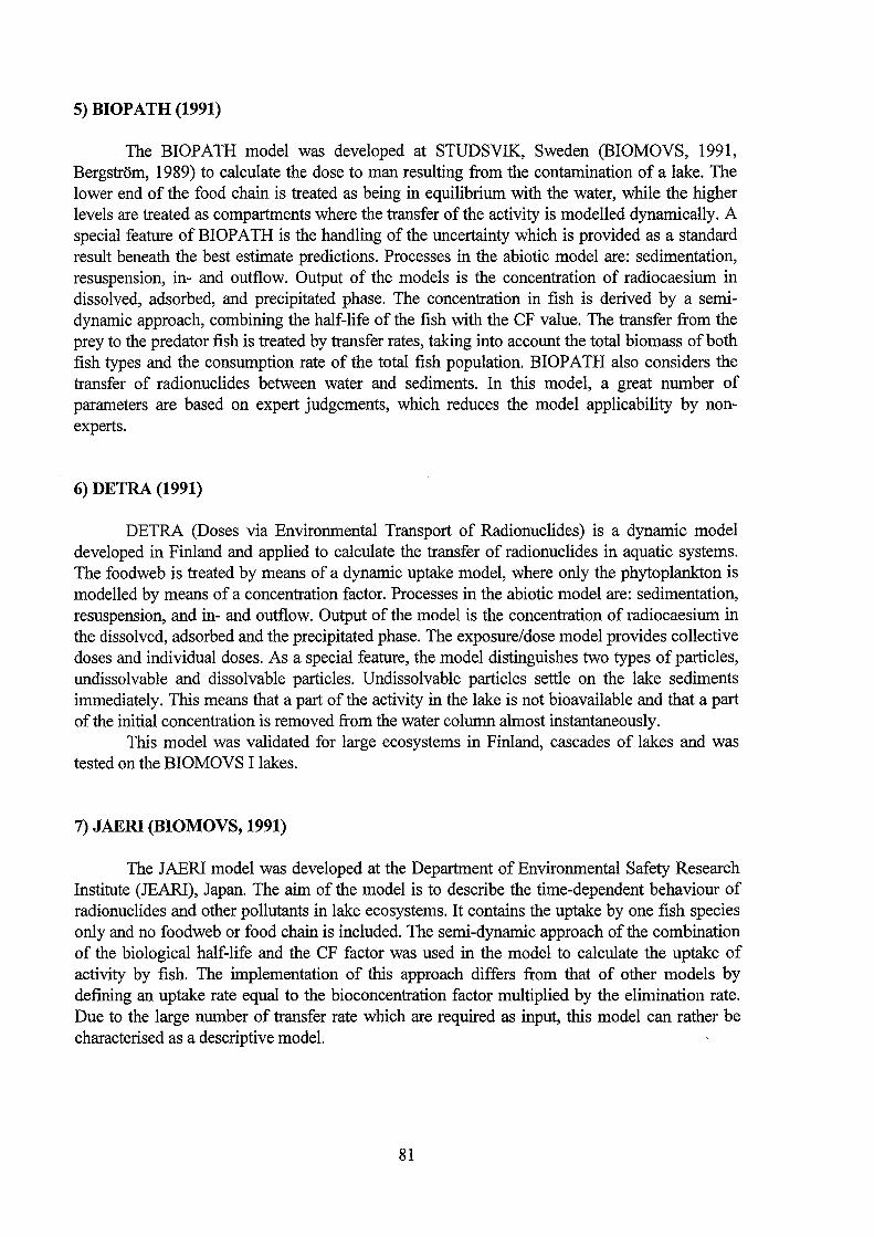
5) BIOPATH (1991)

The BIOPATH model was developed at STUDSVIK, Sweden (BIOMOVS, 1991, Bergström, 1989) to calculate the dose to man resulting from the contamination of a Iake. The lower end of the food chain is treated as being in equilibrium with the water, while the higher Ievels are treated as compartments where the transfer of the activity is modelled dynamically. A special feature ofBIOPATH is the handling ofthe uncertainty which is provided as a standard result beneath the best estimate predictions. Processes in the abiotic model are: Sedimentation, resuspension, in- and outflow. Output of the models is the concentration of radiocaesium in dissolved, adsorbed, and precipitated phase. The concentration in fish is derived by a semidynamic approach, combining the half-life of the fish with the CF value. The transfer from the prey to the predator fish is treated by transfer rates, taking into account the total biomass of both fish types and the consumption rate ofthe total fish population. BIOPATH also considers the transfer of radionuclides between water and sediments. In this model, a great number of parameters are based on expert judgements, which reduces the model applicability by nonexperts.

6) DETRA (1991)

DETRA (Doses via Environmental Transport of Radionuclides) is a dynamic model developed in Finland and applied to calculate the transfer of radionuclides in aquatic systems. The foodweb is treated by means of a dynamic uptake model, where only the phytoplankton is modelled by means of a concentration factor. Processes in the abiotic model are: sedimentation, resuspension, and in- and outflow. Output of the model is the concentration of radiocaesium in the dissolved, adsorbed and the precipitated phase. The exposure/dose model provides collective doses and individual doses. As a special feature, the model distinguishes two types of particles, undissolvable and dissolvable particles. Undissolvable particles settle on the Iake sediments immediately. This means that a part of the activity in the Iake is not bioavailable and that a part ofthe initial concentration is removed from the water column almost instantaneously.

This model was validated for large ecosystems in Finland, cascades of lakes and was tested on the BIOMOVS I lakes.

7) JAERI (BIOMOVS, 1991)

The JAERI model was developed at the Department of Environmental Safety Research Institute (JEARI), Japan. The aim of the model is to describe the time-dependent behaviour of radionuclides and other pollutants in Iake ecosystems. It contains the uptake by one fish species only and no foodweb or food chain is included. The semi-dynamic approach of the combination of the biological half-life and the CF factor was used in the model to calculate the uptake of activity by fish. The implementation of this approach differs from that of other models by defming an uptake rate equal to the bioconcentration factor multiplied by the elimination rate. Due to the large number of transfer rate which are required as input, this model can rather be characterised as a descriptive model.

81

8) NRIRR (BIOMOVS, 1991)

The NRIRR model was developed at the National Research Institute of Radiobiology and Radiohygiene, Rungary .. The modelwas designed for a case study to assess the radiological effects of an accident of a nuclear power plant in Rungary. Processes in the abiotic model are: Sedimentation, resuspension and in- and outflow. Output of the model is the concentration of radiocaesium in the dissolved, adsorbed, and the precipitated phase, and the concentration in fish and aquatic plants. One fish species was modelled dynamically. The transfer rates from water to fish, and from plant to fish are derived by means of the ratio between the biomass of the fish species and the mass of the water. In this model fish plants are treated as individual compartments. The transfer rates are based on CF values from literature.

9)COASTOX

See the section ofthe river model description (chapter 4)

10)WATOX


11) THREETOX


12) LAKECO (Reling 1996)

The box model LAKECO (1994) has been developed at KEMA, Arnhem, The Netherlands. The model was originally developed in 1989 to predict the behaviour of radiocaesium in Iake IJsselmeer in the Netherlands (Reling, 1990). The model concept ofthe abiotic part is based on the COLDOS code (MacKenzie & Nicholson, 1987). The biological part was based on a biological uptake model developed to predict the mercury accumulation in fishin the Iake IJsselmeer (De Vries & Pieters, 1989). A modifiedrelease ofLAKECO, LAKECO-B, was validated within the framework of the VAMP project with caesium data on various lakes in Europe (IAEA, in press). In LAKECO-B new submodules for the behaviour of caesium in sediments and biota have been implemented. Within the BIOMOVS II programme LAKECO-B was successfully applied to the Cooling Pond Scenario (Reling, 1994). LAKECO-B is an integral part of the hydrological model chain of the RODOS decision support system(Popov & Reling, 1996; Zheleznyak et al., 1996).

Processes in the abiotic model are: Sedimentation, resuspension, bioturbation, porewater and particle exchange between the sediments and the water column, diffusion, and in- and outflow. Output ofthe model is the concentration ofradiocaesium in the dissolved, adsorbed and the precipitated phase and in fish species.

In LAKECO-B the transfer throughout the food chain is modelled dynamically (method 2b ). The model contains a large number of physically and empirically based equations, with the

82

emphasis on predicting the important parameters beforehand. V alidated in VAMP and tested on blind data in BIOMOVS II, the model demonstrated the flexibility required in decision support systems.

13) MARTE (Monte, 1991; IAEA, in press)

This box-type model is being developed at ENEA, Italy, (Monte, 1991). It was designed to model the behaviour of radionuclides in lakes. A special release was developed to model the behaviour of radionuclides in very deep mountain lakes, in which the activity may stay over a time period due to the long water turnever time. The model can handle stratified lakes, which is often a weak point of other box models, that assume vertical mixing. The abiotic part considers adsorption/desorption processes and interaction with sediments. Processes related with stratification are described extensively. Other processes included in the abiotic part are: Sedimentation, diffusion, and in- and outflow. It uses the semi-dynamic approach of the biological half-life and the CF factor. The model had been applied to model the behaviour of radiocaesium in the lakes Bracciano, Vico and Trasimeno in Italy. Within the framewerk of the VAMP project (IAEA, in press), the MARTE model had been tested successfully on a wide range of lakes varying in trophic status, food chain composition and environmental circumstances.

14) VAMP (IAEA, in progress; Häkanson et al., 1996)

The VAMP model is an aquatic model for the transfer of radiocaesium within lakeecosystems developed within the framewerk of the VAMP project co-ordinated by the IAEA. The model is based on the model and process descriptions of the aquatic models of the VAMP project group. It is an attempt to develop a radioecological model with an optimum size and with a high predictive power. To achieve this, a large nurober ofprocesses ofminor importance have been omitted or simplified. To increase the flexibility of the model, seasonal and site-specific moderators based on empirical data have been introduced.

The model has been extensively tested on the VAMP lakes. The results showed a high model accuracy for these lakes. The biological uptake is modelled dynamically and seasonal parameters govem the elimination and uptake rates of the aquatic organisms, the transfer :from the catchment and the hydrological turnever time.

83

Table 8: Main characteristics of Iake models

~- -~

MODEL DELWAQ LAKE CO DELWAQ BILTH BIOLAKE BIOPATH DETRA JAERI HÜBEL NRIRR COASTOX WATOX MARTE JTOX VAMP RODOS Box RODOS RODOS

AQUATIC PART

Dimension 2-D Box Box Box Box Box Box Box Box Box 2D Box Box 3D Box

Residence time - + + + + + + + + + - + + - +

Adsorption/ desorption - - - - - - - - - - + + - + -dynamic

Adsorption/ desorption + + + + + + + + + + - - + - + equilibrium

SEDIMENTPART

Bioturbation - + + - - - - - - - - - - - -

Porewater turnover - + + - - - - + - - + + - + -

Particle turnover - + + - + - - - - - + + - + -Resuspension - + + + - + + + + + + + + + +

Burial - + + - - + + + + + - + + + +

BIOLOGICAL PRO-CESSES

I Biological half-life - + + - - + + - + - - - - - +

Foodweb composition - + + - - + + - + - - - - - +

BCFmethod - - - - + - - - + + - - - - -

Semi-dynamic method - - - + - - - + ? - - - + - -

can be APPLIED :

Shortterm + - - - - - - - - - + + - + -Mediumterm + + + + + + + + + + + + + - +

84

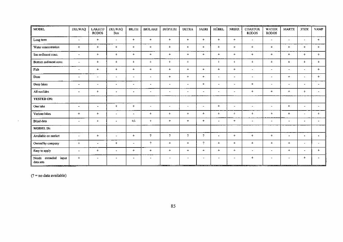
MODEL DELWAQ LAKE CO DELWAQ BILTH BIOLAKE BIOPATH DETRA JAERI HÜBEL NRIRR COASTOX WATOX MARTE 3TOX VAMP RODOS Box RODOS RODOS

Longterm - + - + + + + + + + - - - - +

Water concentration + + + + + + + + + + + + + + +

Sus sediment conc. - + + + + + + + + + + + + + +

Bottom sediment conc. - + + + + + + + + + + + + +

Fish - + + + + + + + + + - - - - +

Dose - - - - - + + + - - - - + - +

Deeplakes - - - - - - - + - - + - - - -All nuclides - + - - - - - - - - + + + + -

TESTEDON:

Onelake - - + + - - - - + - - - + - -

Various lakes + + - - + + + + + + + + + - +

Blind data - + - +!- + + + + - + - - - - -i MODELlS:

Available on market - + - + ? ? ? ? - + + + - - -

Owned by company + - + - ? + + ? + + + + + - -

Easy to apply - + - + + + + + + + - - + - +

Needs extended input + - - - - - - - - - + - - + -datasets

(? = no data available)

85

5.5 Comparison of the models

In the following, the models will be analysed with respect to the criteria listed below. As the number of 14 lak:e models is too high to analyse in all detail, a preliminary selection of the most promising codes according to key parameters was necessary and is described in the next chapter. The criteria for the selection are based on demands made by the IMIS/P ARK system. After comparison of the models with respect to their properties, these demands must be used as the final filter.

The models must be compared with respect to: • The processes • Temporaland spatial ranges ofvalidity • The required input data • The output of the model • The reliability ofthe model (validation studies) • Computational requirements • A vailability of documents

Further criteria include: 1. The models should be capable to deal with countermeasures (must be able to be

linked to countermeasure models); 2. Data assimilation. The model should perform recalculations on the basis of incoming

measurements; 3. The model should have an optimum size, i.e. the level of complexity must yield the

highest possible predictive power; 4. The spatial scale must cover whole Germany. The lak:e model must not be site

specific, but generic, with a wide applicability.

Some aspects must be considered when applying the criteria list: 1. The list of criteria cannot be applied simply in sequence. It is possible that if the

model passes the first list, it does not meet the demands of the second list. The list of criteria is in fact an attempt to trace the most ideal model. The most obvious criteria with high weight factors should govem the selection.

2. The items listed in the previous chapter regarding processes may be in contradiction with the selection criteria. Thus, a model which includes many processes may not be necessarily the most applicable one; but applicability is a very important selection criteria.

3. Most of the listed codes are designed to be applied to model the behaviour of radionuclides in lak:es. Nevertheless, a large number of computer codes of a high quality is present in the Iiterature to model nutrients, micropollutants such as heavy metals, and pesticides. Pesticide dispersion models could be suitable since the biodegradation of pesticides is a linear process of first order like the physical decay of radionuclides. The presented models, however, are only selected with respect to the validity and proven expertise in the field of the behaviour of radionuclides in the aquatic environment.

86

4. Descriptive models which can only be operated by experts due to the relatively large number of model-specific parameters might be interesting from the scientific point of view, however, these models must be filtered out due to their low flexibility.

5. 6 Model se/ection

Without an extensive comparison of the selected models by means of the above mentioned lists of criteria, a number of models can be excluded :from further evaluation on the basis of some obvious criteria: validation, complexity, applicability and to a lesser extent, availability. After this rough selection, the models are evaluated by means of the criteria Iist of the German government. Additionally a detailed description of the selected models is provided in the Appendices.

5.6.1 Validation and flexibility

A very important selection criterion is the reliability of the model. A large number of the presented models were developed for one special study or for a special environmental circumstance. This was more or less the case for models applied in the BIOMOVS-I validation study. Furthermore, within BIOMOVS-I the models were applied to up to three lakes only. The models within the VAMP study in most cases were not developed for the validation study, but had been operated at the various institutes before the start of the project. Only the VAMP model was developed within the study. The validity of all models applied in the VAMP study was proven within and outside the VAMP project. Validation on data sets of seven lakes, with a wide range of environmental and ecological circumstances proved the quality of the codes. Therefore, the VAMPmodelsare in general more reliable than the models ofthe BIOMOVS-I study.

A disadvantage of most computer codes is that even valid models have only been developed and tested on radiocaesium, in particular from the Chemobyl release. It is obvious that countermeasure implementation based on any criteria should take a large set of nuclides into account. Even if the models have been enabled to cope with other nuclides than caesium, e.g. strontium, cobalt, ruthenium and plutonium, the validation is less reliable due to the Iack of extensive data sets. In general, institutes associated with nuclear facilities are more experienced in the application of risk assessment models for other radionuclides than radioceasium.

All models validated within the framework of the VAMP project (VAMP, LAKECO, BIOPATH, DETRA and MARTE) can meet the demands of the validation criteria. Among these, the VAMP model and the LAKECO model have the lowest amount of model-specific parameters. One of the releases of the DEL W AQ computation scheme, the box model release, combined with the foodweb model UPTAQE meets the demands to a lesser extent. It was only tested on radiocaesium for one single Iake in the Netherlands. However, the expertise of Delft Hydraulics in the field of hydrodynamic modeHing is very high, and therefore the DEL W AQ model concept, to be referred to as DEL WAQ/UPTAQE, is also included as a possible model for the IMIS/P ARK system.

87

5.6.2 Complexity

Complex 2-D and 3-D hydrodynamic models were excluded in the selection for obvious reasons. The large number of input parameter sets and the site-specific data needed to calibrate the models and its processes cause an inflexibility and results in unnecessary detailed information. These model types can be applied in special case studies and are less useful in emergency management systems.

5.6.3 Applicability

ated: When determining the applicability of the selected codes, several aspects must be evalu-

1. The degree of expert judgement. Flexibility decreases with an increasing amount of model-specific parameters. The model should be govemed by easily accessible environmental parameters.

2. The applicability of the model on lake-ecosystems with a large range of environmental, ecological and climatological properties. For the application in Germany the latter are of less importance.

3. The user friendliness of the model. Most of the scientific model tools are merely designed for individual applications and not for operational use.

Table 9: Aspects ofapplicability oflake models

VAMP LAKE CO DELWAQ ROD OS UPTAQE

MARTE BIOPATH DETRA

Controlled by env1-renmental parame- ++1) +2) - - - -ters

Generle character3)

widely applicable to + ++ -I+ + + + various lake types

User friendliness + ++4) - - - -

(1) All model or expert parameters are omitted. Therefore, the model has a high predictive power.

(2) The foodweb model is less flexible, field data are required to evaluate the food web transfer.

(3) All models are highly applicable for radiocaesium. This is excluded in the judgement under point 2.

( 4) LAKECO within the RODOS system is the only operational model with a user friendly interface. The other models are scientific tools.

88

Some remarks should be kept in mind: 1. All listed models emphasize on the modeHing of radiocaesium only. LAKECO

govems seven nuclides (137Cs, 239Pu, 1311, 6°Co, 90Sr, 106Ru and 3H). The reliability of the model predictions is highest for caesium; the same can be concluded for alllisted models.

2. None ofthe models is operational and user friendly except LAKECO, since most of the computer codes are tools resulting from scientific research without any need for user friendliness.

3. The VAMP model has a proven predictive power and should not be excluded due to its present scientific character. One of the powerful aspects is that this model contains a large number of dimensionless parameters to deal with seasonal effects of most of the biological and hydrodynamic processes.

4. LAKECO at present is connected with runoff and river models and thus embedded into an hydrological model chain inside the RODOS system. This chain of aquatic models is applied to the Rhine catchment area. This set of models is available, tested on a large part of the German territory and therefore directly applicable in the IMIS/P ARK system.

5.6.4 A vailability

An important and obvious criterion is the availability of the models. Most of the models are available, but not in all cases meant to be distributed as commercial software. High costs can be expected in the case of the models of Delft Hydraulics. These model applications were developed for the Dutch govemment to evaluate the fluvial marine and marine dispersion of pollutants. These projects were collaborative in a sense that Delft Hydraulics treated the application as a scientific project. The product was not sold as a commercial product, but transferred to a govemmental institute as a result ofthe joint research. The lake ecological model LAKECO, integrated into the RODOS system, is available via the European Commission.

5. 7 Final advice on the selection of a Iake model for the IMISIPARK system.

This section deals with the final ranking on the basis of the second Iist of criteria which are most important for the applicability in the IMIS/P ARK system. The final selection can be based on criteria 3 and 4. None ofthe models can perform recalculations automatically (criterion 2). The coupling with countermeasure models is principally possible when output files are produced. Only LAKECO is fully in operation in a software tool and also designed to establish the connection with countermeasure modules. Hydrological countermeasure models such as chemical treatment of the contaminated lakes have not been included in LAKECO yet. The VAMP model at present is extended by submodels to calculate the effect of a chemical treatment to diminish the uptake in the biota. DELWAQ/UPTAQE is, despite ofits positive performance, rather complex to handle since it is not a commercial software product. VAMP and LAKECO are very applicable. The applicability ofDETRA, MARTE and BIOPATH is limited because of the extensive need of expert judgement necessary to implement the three codes.

89

Table 10: Model comparison on the basis ofthe demands oftheGerman Government.

VAMP LAKE CO DELWAQ MARTE BIOPATH DETRA

RODOS UPTAQE

1 Coupling with + + - - - -countermeasure modules

2 Recalculations +1- +I- +I- -I+ -I+ +I-based on incoming measurements

3 Optimum size ++ + - + + + high predictive power

4 Generally ++ ++ + +!- +!- +I-applicable

The most flexible lake ecosystem models are LAKECO and VAMP. Drawback of the VAMP model is its focusing on the fate and behaviour of radiocaesium in lake ecosystems. This is not only reflected by the type of submodels, but also by the process descriptions which are often empirically based on data about radiocaesium. Rearranging the VAMP model for other nuclides would need a lot of efforts. This is partly the case for LAKECO, too. This model has some caesium-specific submodels, but the process description is basically nuclide-independent. The reason for this situation can be seen in the fact that the VAMP model has been made flexible during its development to such an extent that processes are described assuming specific physical-chemical properties of caesium. Therefore, the extension to other nuclides would require structural changes tobe closer to a generic model approach. In LAKECO, the description in general is less nuclide specific, thus, modifications for other nuclides are already implemented. Both models also contain nuclide-independent submodels to estimate important parameters. An advantage of LAKECO as compared to the VAMP model is its integration into a decision support system (RODOS) written in FORTRAN and completed with a userfriendly input and output management. But the VAMP model contains a very strong submodel which is lacking in LAKECO: the temperature and stratification submodel. Here, LAKECO's only restriction becomes obvious, modeHing of deep lakes cannot be performed with LAKECO.

Should LAKECO be selected, there are two possibilities to cope with this drawback. The first solution is to implement a second lake model to be used for stratified lakes. This could be for example MARTE which is applicable for deep stratified lakes, but would have the disadvantage to collect many input parameters to model the stratification. Besides this problem, most of the parameters of MARTE - also for the unstratified model release - are mathematical rates without any physical correlation, which, as described above is not a favoured solution.

A second - preferred - solution might be to implement the present powerful submodel of VAMP for stratification, into LAKECO. This submodel needs minimum input data in centrast to the MARTE model. This solution would nearly solve the main disadvantage of LAKECO, even if the stratification submodel still has some restrictions as it only can be applied to dimictic lakes.

90

Additionally, the selected Iake model system should govem a large number of lakes on the German territory. For the application to such a large number of lakes, the authors would recommend to classify the lakes into a set of standard lakes to Iimit the amount of input parameters. At present LAKECO as part of the hydrological module of the RODOS system will be expanded to deal with a great number of lakes. These modifications are not restricted by the structure of the Iake model, but changes are necessary in the graphic interface and in the intemal structure ofthe operating system ofthe hydrological model chain inside RODOS.

At present the Finnish institute VTT is improving the DETRA model by a classification scheme for lakes typical for Finland (first release is expected in 1998). The large number of lakes on the Finnish territory is sorted into a limited group of standard lakes. This classification is related to the trophic status of the Iake, which is often easily available. Each Iake type in the classification has its own set of standard parameters. This classification tool could be coupled to LAKECO to support and to improve the application for a larger number of lakes also on the German territory.

To conclude, the best choice for the IMIS/PARK system seems to be an improved version ofLAKECO followed by the VAMPmodel which, however, needs many modifications and improvements with regard to its structure and contents.

91

5.8 REFERENCES

Bergström, U and Nordlinder, S., 1989, Comparison of predicted and measured Cs-137 concentrations in a Lake Ecosystem. In: Feldt W, Radioecology of Natural and Artificial Radionuclides - Proceedings of XV Regional Conf of IRP A.

BIOMOVS, 1991, Dynamics within lake ecosystems. Technical report 12, scenario AS. Blaylock, B.G., 1982, Radionuclide Databases Available of Bioaccumulation Factors for

Freshwater Biota. Nuclear Safety, vol. 23, no 4. De Vries D.J., De Vries M.B., 1988, Modelling the fate of RCB and PCB153 in the lakes

Ketelmeer and IJsselmeer. Report T250 Delft Rydraulics. De Vries, M.B., Pieters, H., 1989, Accumulation ofheavy metals in organisms. Bioaccumulati

on of mercury in pikeperch. Data analysis on IJsselmeer, Ketelmeer, and Markermeer. Delft Rydraulics. Report T 250

De Vries, D.J., Kroot, M.P., 1989, ModeHing the behaviour and fate ofheavy metals in aquatic systems with IMPAQT. Process descriptions and application to Ketelmeer and IJsselmeer. (In Dutch). Delft Rydraulics, report number T0250.

Delft Rydraulics, 1985, Discharges ofnuclear power plants located at the IJsselmeer, and at the Rollandsch Diep. Dispersion and accumulation of radioactivity in the aquatic environment. (In Dutch). Report R2112/R2152

Räkanson L, Jansson, M., 1983 Principles ofLake Sedimentology. Reling, R., 1990, ModeHing the ecological consequences of an accidental release on the lake

IJsselmeer. KEMA Report 931 05-MOS 90-3468 (In Dutch). Reling, R., 1994, LAKECO, the ecological consequences of an accidental release of

radionuclides on a lake ecosystem and its integration into the real-time on-line decision support system for the off-site Emergency Management foHowing a Nuclear Accident (RODOS). KEMA report. Nr. 40352-NUC 93-5852.

Reling, R., 1996, Off Site Emergency Planning Support. The validation ofthe Lake Ecosystem Model LAKECO. KEMAreportNr. 40901-NUC 95-9113.

IAEA, (in press). VAMP Aquatic Work Group I. Modelling of Radionuclide Transfer into Lakes.

Korhonen, R., 1990, Modelling the Transfer of 137Cs Fallout in a large Finnish Watercourse. Realth Physics 59, 4, 1990 pp. 443-454.

Kroot, M.P.J.M., 1992, Behaviour of radionuclides. Part of the issue "Description of the modifications ofthe model IMPAQT. T740.01. Delft Rydraulics Delft (In Dutch).

Laheij, G. M. R, Blaauboer, R. 0. and Lembrechts, J. F. M. M., 1994, Risc calculations for discharges ofradionuclides into the environment. RIVM report 610053001 (in Dutch).

MacKenzie, J., Nicholson, S., 1987, COLDOS, a computer code for the estimation of coHective doses from radioactive wastes to the sea. Implications for the coHective dose assessment. Safety and ReHability Directorate. UKAEA, W arrington.

McDougaH, S., Rilton, J. and Jenkins, A., 1991, A dynamic model of caesium transport in lakes and their catchments. Water Research 25 (4), 437-445.

Monte, L., Frararcangeli, S., Quaggia, S., Pompei, F. and Andrasi, G., 1991, A predictive model for the behaviour of dissolved radioactive substances in stratified lakes. Journal of Environmental radioactivity 13, 297-308.

NUREG, 1981, Onishi, Y., Seme, R. J., Amold, E. M., Cowan, C. E. and Thompson, F. L., Critical Review: Radionuclide transport, sediment transport, and water quality mathematical

92

modelling; and radionuclide adsorption/desorption mechanisms. NUREG/CR-1322 PNL-2901.

Popov, AG, Reling, R., 1996, Aquatic models to predict wash-off from watersheds and the migration of radionuclides in lakes for implementation in RODOS. In: Proceedings of the Conference on Radiological Consequences of the Chemobyl Accident held at Minsk. March 1996.

Reichle, D. Dunaway, P.B., Nelson, D.J., 1970 Tumover of Radionuclides on Food Chains. Nuclear Safety, vol. 11, no.l.

Smits, J.G.C., Kroot, M.P.J.M., 1990, Application ofiMPAQT on Cadmium in the lakes system Ketelmeer-IJsselmeer. Report T632. Delft Rydraulics (In Dutch).

Zheleznyak, M., Reling, R., Raskob, W., Popov, A., Borodin, R., Gofinan, D., Lyashenko, G., Marinets, A., Pokhil, A., Shepeleva, T., Tkalich, P., 1996, ModeHing of Rydrological Pathways in RODOS. In: Proceedings of the Conference on Radiological Consequences of the Chemobyl Accident held at Minsk. March 1996.

93

6 Final conclusions and model proposal

In each of the three areas of surface runoff, river transport and lakes, computer programs have been identified, which might be integrated into the IMIS/P ARK system as they fulfil most of the criteria applied. However, it was also concluded that none of the tested models meets all the requirements at present. There is no model which includes data assimilation or recalculations of the predictions based on on-line measurements, as it is requested by the IMIS/PARK system. Only those computer programs developed within the framework of the RODOS project ( further indicated with the extension /RODOS) will be improved by this feature till 1999. Nevertheless, the following programs seem to be applicable in general, however, with modifications:

• surface runoff RETRACE/RODOS MONTE (limited)

• river transport RIVTOX/RODOS TOD AM

• lakes LAKECO/RODOS VAMP

A further question is related with the coupling of the computer programs of the individual areas as the IMIS/P ARK system requires an integrated solution for all the transport and exchange processes. This is one of the advantages of the three programs of the hydrological model chain of the RODOS system as they contain defined interfaces with each other. Additionally this model chain also contains an interface to the RODOS version of the radioecological model ECOSYS. All other computer programs require extended modifications and programming efforts either to realise the coupling or the interface with a radiological program. None of the investigated models exceptfor those of RODOS have been applied to catchments as large as required for IMIS/P ARK. Only this hydrological chain was implemented for the Rhine catchment. This also allowed to study the difficulties in obtaining the necessary input data; difficulties which always exist for any of the selected models.

Despite the problems and shortages of the models mentioned above, it is recommended to use mathematical models in IMIS/P ARK as this seems to be the only way to obtain reliable forecasts of highly contaminated areas and proposals of which measures might be applied at which location. This may also be the basis for decisions to perform further measurements to finally quantify the contamination pattem. Only prognostic computer programs are able to quantify events such as the recent floods of winter 1993/94 and winter 1995 in the Rhine catchment. A further advantage of a complete set of atmospherical, terrestrial and hydrological mathematical models can be seen in the identification ofthose pathways- terrestriallatmospheric or aquatic - which contribute most to a measured contamination in foodstuffs. This allows the decision maker to apply better directed measures.

Assuming that hydrological models will be implemented into IMIS/P ARK, further aspects have to be considered:

1. Development of a concept for the operation of the hydrological models inside IMIS/PARK.

2. Further development of the selected models to meet all the requirements of IMIS/PARK (at least data assimilation).

94

3. Adaptation of the models to the computational requirements of the IMIS/P ARK system (e.g. different computer or UNIX systems)

4. Development of an interface to operate the models and to handle data transfer between the system and the hydrological models - including data exchange with the radioecological model.

5. Data acquisition. 6. Coupling of the hydrological models with the forecasts from the German weather

service (DWD) - time dependent and spatially distributed fields of precipitation -including statistical data for long-term prognoses.

Taking these six criteria into account additionally, the hydrological models integrated into RODOS show advantages as the points two, four five and six are partly solved and will be further considered in the development of the RODOS system. The authors therefore suggest a close cooperation with RODOS to participate in the present and future knowledge gained within this project. This would also avoid a duplication of work and enhance the 'know-how' transfer into the IMIS/P ARK system. The aspect of a potential coupling of the two systems IMIS/P ARK and RODOS additionally supports the selection of the models RETRACE, RIVTOX and LAKECO.

95

Appendix on individual model descriptions

This section of the report contains the extended description of the models which have been identified for the final selection. Depending on the available sources, the models are described in more or less detail. Emphasis has been put on the basic features of the models which are not necessarily identical to the requirements of the IMIS/P ARK system. This section also reflects the view of the individual contractors regarding the models. Therefore, the style and degree of details may differ from author to author.

To have an idea about the applicability of the model in the IMIS/P ARK system, the reader is requested to refer to the appropriate chapters in the main report.

96

Appendix on runoft modelling (A. Popov)

The main characteristics of AGNPS

AGNPS (Agricultural Non-Point Source Pollution Model) is an event-based model that - simulates surface runoff, sediment and nutrient transport primarily from agricultural

watersheds. The nutrients considered include nitrogen (N), phosphorus (P) and pesticides, the contributors to surface water pollution. Basicmodel components include hydrology, erosion and sediment and chemical transport. In addition, the model considers point sources of water, sediment, nutrients and chemical oxygen demand (COD) from animal feedlots, and springs. Water impoundment, such as tile-outlet terraces, are also considered as deposition areas of sediment and sediment-associated nutrients.

Description of the processes controlling the radionuc/ide wash-off from watersheds

Description of the hydrological processes

Interception by Plants and Suiface Retention Infiltration Suiface Runoff

The model components use equations and methodologies that have been well established and are extensively used by agencies such as the USDA Soil Conservation Service. Runoff volume and peak flow rate are estimated using the SCS (Soil Conservation Service) runoff curve number method. The peak runoffrate for each cell is estimated using an empirical relationship proposed by Smith and Williams (1980), which is also used in CREAMS (Frere et al., 1980).

The rainfall excess method known as USDA SCS Runoff Curve Number Model is used in AGNPS. Abrief discussion ofthis method is included in the description ofSWRRB.

Perco/ation and Lateral Subsuiface Flow Evapotranspiration SnowMelt

These processes were not simulated since the model can consider one event only and, therefore, alllonger term hydrological processes are beyend the scope of AGNPS.

Description of the sediment yield and transport

Upland erosion and sediment transport is estimated using a modified form of the Universal Soil Loss Equation, USLE (Wischmeier and Smith, 1978). Eroded soil and sediment yield are subdivided into five particle fractions- clay, silt, small aggregates, large aggregates, and sand. A brief discussion of this method is included in the SWRRB model description.

97

Sediment is routed from cell to cell through the watershed to the outlet using a sediment transport and depositionrelationship described by Poster et al. (1981), which is based on a steady-state continuity equation.

Description of pollutant transport

Chemical transport is calculated based on the relationships adapted from CREAMS and a feedlot evaluation model (Young et al., 1982). Feedlots are treated as point sources and chemical contributions are estimated using the feedlot pollution model developed by Y oung et al. Other point-source inputs of water and nutrients, such as springs and wastewater treatment plant discharges are accounted for by inputting incoming flow rates and concentrations of nutrients to the cells where they occur.

Chemical transport calculations are divided into soluble and sediment adsorbed phases.

Nutrient Transport The pollutant transport part of the model estimates the transport of nitrogen, phosphorus

and the chemical oxygen demand (COD) throughout the watershed. The pollutant transport portion is subdivided into one part handling soluble pollutants and another part handling sediment-attached pollutants. Pollutant transport of soluble nitrogen and phosphorus is calculated using a relationship adapted from CREAMS (Frere et al., 1980) and a feedlot evaluation model by Y oung et al. (1982). Soluble nitrogen and phosphorus in runoff waters represent the effects of rainfall, fertilisation, solid waste and leaching from the soil in each cell. The nutrient yield associated with the sediment is calculated using the total sediment yield from each cell and by relationships proposed in the CREAMS nutrient submodel (Frere et al., 1980).

The contributions of soluble nitrogen and phosphorus from each of the cells are calculated first and routed into the channel. Once soluble nutrients reach concentrated flow, they are assumed to remain constant. That is, the amount entering in the overland flow from any particular cell is simply added to what is already present in the channel, with no losses of soluble nutrients in the channel allowed.

Pesticide A menu-driven interactive pesticide submodel has been developed. It allows the

evaluation of different management methods of pesticide runoff and leaching. {pesticides are divided into 6 categories: herbicides, insecticides, fungicides, nematicides, growth regulators and desiccants/defoliants. Pesticides are selected from databases containing both common and trade names. Default inputs are suggested depending on the pesticide selected and the method of application. Inputs include

l.the time of pesticide application, 2.application rate, 3 .application efficiency, 4.percent ground cover, 5.soil and foliar pesticide residues, 6.soil and foliar pesticide half-life, 7 .incorporation depth and efficiency, 8.water solubility, 9 .organic carbon sorption coefficient (Koc ).

98

An enrichment ratio approach is used to estimate pesticide yield from the adsorbed phase. The submodel calculates the mass (lb./acre) of pesticide lost in the runoff and sediment yield. Outputs are both tabular and graphical, including areas of pesticide Iosses within watershed. Radionuclides were not considered, however, modifications of the existing submodels are possible.

App/icability of the model in Europe, in particular in Germany

Temporal and spatial ranges

AGNPS is a distributed, event-based model. The model operates on a cell basis. Cells are uniformly square areas subdividing the watershed, allowing analysis at any point within the watershed. All watershed characteristics and inputs are expressed at the cell Ievel. Potential pollutants are routed through cells from the watershed and spread to the outlet in a stepwise manner such that flow may be examined at any point between the cells. All watershed characteristics and inputs are expressed at the celllevel.

The model has the ability to output water quality characteristics at intermediate points throughout the watershed network. This capability is based on the model's implementation of the 'cell'. The model operates on a geographic cell basis (Dirichlet tessellation) that is used to represent upland and channel conditions. Dirichlet tessellation is a process of splitting up and grouping a· study area into cells or tiles, also known as Thiessen or Voronoi polygons. Cells are uniformly square areas subdividing the watersheds, allowing analyses at any point within the watershed. Potential pollutants are routed through cells from the watershed and spread to the outlet in a stepwise manner such that flow can be examined at any point between the cells. All watershed characteristics and inputs are expressed at the celllevel.

Model requirements on tlte input data and especially on meteorological data The computations in AGNPS occur in three stages based on twenty three items of

information per cell. Initial calculations for all cells in the watershed are made in the first stage. These calculations include estimates for upland erosion, overland runoff volume, time until overland flow becomes concentrated, Ievel of soluble pollutants leaving the watershed via overland runoff, sediment and runoff leaving impoundment-terrace systems and pollutants coming from point source inputs such as feedlots.

The second stage calculates the runoff volume leaving the cells containing impoundments and the sediment yields for primary cells. A primary cell is one that no other cell drains into. The sediment from these and other cells is broken down into five particle-size classes: clay, silt, small aggregates, large aggregates, and sand.

The sediment and nutrients are routed through the rest of the watershed in stage three. Calculations are made to establish the concentrated flow rates, to derive the channel transport capacity, and to calculate the actual sediment and nutrient flow rates.

99

AGNPS Input Parameters 1. cell number (from) 2. receiving cell number (to) 3. SCS curve number 4. land slope 5. land slope shape factor 6. field slope length 7. channel slope 8. channel side slope 9. Manning's roughness coefficient 10. soil erodibility factor 11.cover and management factor 12.support practice factor 13.surface condition constant 14.aspect (direction of drainage) 15. so il texture 16.fertilisation Ievel 17.fertilisation availability factor 18.point source indicator 19.gully source Ievel 20.chemical oxygen demand (COD) factor 21.impoundment factor 22.channel indicator

Nitrogen 1. sediment associated mass (lbs/acre) 2. concentration of soluble material (ppm) 3. mass of soluble material in runoff

(lbs/acre) 4. Phosphorus 5. sediment associated mass (lbs/acre) 6. concentration of soluble material (ppm) 7. mass of soluble material in runoff

(lbs/acre) 8. chemical oxygen demand 9. concentration (ppm) 10.mass (lbs/acre)

100

AGNPS Output at the Watershed Outlet or for Whole Watershed

Output values for the whole watershed 1.watershed description 2.area (acres) 3 .area of each cell ( acres) 4.characteristic storm precipitation (inches) 5.storm energy-intensity (EI) value

Output values at the watershed outlet 1. hydrology 2. runoffvolume (inches) 3. peak runoffrate ( cfs) 4. fraction of runoff generated within the

cell 5. sediment (by particle size and in total) 6. sediment yield (tons) 7. sediment concentration (ppm) 8. sediment particle size distribution 9. upland erosion (tons/acre) 1 O.channel erosion (tons/acre) 11.amount of deposition (%) 12.sediment generated within the cell (tons) 13.enrichment ratio 14.delivery ratio

Space and time steps and ranges of validity of the model A single cell or a data unit can have resolutions of 2.5 acres to 40 acres. Smaller cell

sizes such as 10 acres are recommended for watersheds of less than 2000 acres. For watersheds exceeding 2000 acres, cell sizes of 40 acres are normally used to pixelise the watershed. In a 40-acre main unit cell segmentation scheme, other and cell sizes smaller than 40 acres can also be used to meet the further resolution needs for complex topography or smaller-than-40-acre watershed characteristic unit. Accuracy of results can be increased by reducing the cell size, but this increases the time and labour required to run the model.

Conversely, enlarging the cell size reduces time and labour, but the savings must be balanced against the loss of accuracy resulting from treating larger areas as homogeneous units.

The model uses the balance method for one runoff event. So there is no explicit time step in the model. The applicability ranges from hours up to 1 day (24 hours).

Interface with in-stream transport models

The structure of the model allows for linkage with in-stream transport models at the outlet of the watershed as weil as in the outlet of each cell.

Data availability for European conditions

The main problern for the application of AGNPS in Europe is the need for data on surface hydrology (SCS curve number). A second critical point are data bases on soil erosion.

Validations, testing and applications performed

The model has been validated using field data from 20 agricultural watersheds in several states of the US (Young et al., 1987, Mitchel et al., 1993).The model has been tested for accuracy of sediment yield estimation with data from experimental watersheds located in Iowa, US (USDA, AS, 1970, USDA, ARS, 1967, Koelliker and Humbert, 1989, Lee, 1989).

The AGNPS model has been used in many states and several countries to prioritise watersheds for severity of water quality problems, to pinpoint critical areas within a watershed contributing to pollution, and to evaluate the effects of applying alternative management practices (German and Dingels, 1984, Dingels, 1986).

Model software and documentation availability

The following AGNPS model files (program and user manual) can be downloaded for the MS-DOS system.

ftp:/ /witch.cee.odu.edu/pub/modeVagnps/dos/agdos500 .exe AGNPS model system (program and user manual, 2.45 MB)

AGNPS model files (pro gram and sample 1/0 data) for UNIX ( compiled for CEE UNIX Lab's Solaris 2.5) can be downloaded at:

ftp ://witch.cee.odu.edu/pub/modeVagnps/unix/agnps500 .solaris _ 2.5. tar .gz

Data assimilation

As there exists some experience in applications of AGNPS together with the GRASP (Geographical Resotrrces Analysis Support System) GIS, it seems tobe very likely that AGNPS can be improved to assimilate measurements.


AGNPS is designed to run on any IBM compatible personal computers with MS-DOS versions 3.0 and later. It requires 2MB available of either extended or expanded memory, a hard disk with 3 MB or more of free space and an 80286 or later processor as weil as a graphics adapter and monitor (CGA minimum). An 80287 math co-processor is highly recommended.

A UNIX version of the model is available for use with a geographical information system (GIS) but it requires an extemal input data file. Also, the graphical output is not compatible with the MS-DOS version.

102

The main characteristics of HSPF

Description of the processes controlling the radionuc/ide wash-off from watersheds


The HSPF model is a conceptual spatially distributed model designed to model hydrological processes at the watershed scale under due consideration of the water quality. Considered are conventional pollutants (sediments) only such as pesticides, nutrients and toxic substances. Potential applications are:

• flood control planning and operation; • hydropower studies; • river basin and watershed planning • storm drainage analyses • water quality planning and management • point and nonpoint source pollution analyses • soil erosion and sediment transport studies • evaluation ofurban and agricultural best management practices (BMP's) • fate, transport, exposure assessment and control of pesticides, nutrients, and toxic

substances • storage oftime-series, analysis and display.

In order to solve the listed problems for large inhomogeneaus areas, the watershed can be considered as a set of homogeneaus parts interacting via a drainage system. Such a homogeneaus part ofthe watershed is called "segment". As defined in the HSPF user manual (p.9) "a segment is a portion of the land assumed to have really uniform properties". Furthermore, each segment or element may contain several zones with different hydrological behaviour. Suchalandsegment- Pervious Land Segment (PLS)- may contain zones such as a ·snow area, surface area, upper layer of soil, lower layer of soil and groundwater zone.

The parameter selection for each segment ( e.g. area, storage, slope, coefficients in empirical relations) is made by experts on the basis of the available data. One important feature of HSPF is the variable size and the form of the segments. The Iowa River watershed with an area of 7236 km2 was represented by 13 PLS ranging from 122 km2 up to 1109 km2

(Donigian et al., 1982). The hydrological processes are represented by boxes (storage) which interact among the

individual subareas and with the connected PLSs. The flux into and out of such a storage box is described by empirical relations. The total amount of model parameters is above 1000. Certainly, not all parameters always have to be changed. However, to apply the model to a pesticide transportproblern there is a set of at least 13 parameters for each PLS, demanding specific input during the model calibration.

Historically, the HSPF model was developed as an extension and improvement of the EPA Agricultural Runoff Management (ARM) model (Donigian and Davis, 1978), the EPA Nonpoint Source Runoff (NPS) model (Donigian and Crawford, 1979- Unpublished) and the Hydrologie Simulation Program (HSP) (Hydrocomp, 1977). Therefore, many of the present features were taken from those existing codes. However, a new essential feature of HSPF, which was not present in those previous models, is the use of a system approach to

103

programming, allowing to develop flexible program systems to solve hydrological and water quality problems on a watershed scale.

Infiltration This process is described on the basis of empirical relations which have been widely

tested. Initially, those relations were obtained by Philip (1957) and were applied in the models ARM, NPS, HSP, LANDS and PTR.

lt is weil known that the spatial variability of the hydrological properties, in particular the infiltration capacity, is very high and therefore difficult to describe in mathematical models. The approach in HSPF is simple, as it is supposed that the soil infiltration capacity is randomly and uniformly distributed over the whole watershed area. Thus, the infiltration Iosses were calculated by using such a probability distribution. However, the applicability of such a hypothesis is not discussed by the authors and in particular for inhomogeneous contamination fields this method might be questionable.

Only extensive calibration efforts ailow to avoid errors connected with such an approach. That is the reason why the calibration of the infiltration parameters is always necessary (Donigian et al., 1982).

Suiface Runoff The main sources of water loss such as interception of vegetation and the retention in

surface depressions are considered in HSPF. The velocity of the overland water flow is determined with the help ofManning's approach. The hill slopes are considered as plain with an effective steepness and length. This again can Iead to systematic errors, but again calibration may provide the opportunity to achieve correct results.

Subsuiface Flow There is only one type of subsurface runoff in the vadose zone: the interflow. But from

the present understanding of the processes also the so cailed 'pipe' (tunnel) subsurface runoff may be very important in particular for storm runoff events.

It is assumed in HSPF that the interflow runoff depends on the inflow into the storage as weil as the amount of water stored in the upper soil zone.

The description of the groundwater flow is based on a simple approach which ailows to consider a variable groundwater table. This ailows for the consideration of the long-term behaviour of groundwater.

Evapotranspiration The modeiling of the evapotranspiration (ET) in HSPF is treated in a rather complex

way assuming this is an essential component of the watershed hydrology. ET from all zones was taken into account. The method used is based on data on potential ET as weil as on the simulation of the actual water status in the different compartments.

The model considers different types of vegetation, rooting depth, density of the vegetation, and the aerial distribution of these properties for each segment. But as realised in the case of water infiltration, a uniform probability distribution of the ET over the segment is applied

Interception by Plants and Suiface Retention Rather simple and flexible approaches to describe interception by plants and surface

water retention were used. The user may supply the interception capacity on a monthly basis

104

to account for seasonal variations or one value designating a fixed capacity. The balance method was used for both types of losses.

SnowMelt An approach developed by the US Anny Corps of Engineers (Snow Hydrology,

Summary Report ofthe Snow Investigations. North Pacific Division, 1956) is implemented in HSPF.

Description of transport and sediment yield

The complexity of the description of the water erosion and sediment transport is similar to the description of the hydrological processes.

The equations used in HSPF to generate and to remove sediments are modifications of the soil and gully erosion equations developed by Negev (1967) and influenced by Meyer and Wischmeier (1969) and Onstad and Fester (1975). Many of the parameters of the sediment submodel are derived from the Universal Soil Loss Equation (Wischmeier and Smith, 1978). Removal of sediment by water is simulated as washeut of sediment located in the storage area of the soil matrix. Sedimentation is modelled as a function of rainfall, land cover, land management practice and soil properties. Removal of sediments by surface water is modelled empirically as a function of surface water storage and surface water outflow.

The calibration of the submodel for soil erosion and sediment transport is a necessary step after model implementation. As mentioned in the "Guide to Application of the HSPF" (Donigian et al., 1982), the calibration ofthe sediment transport submodels shows, as a rule, large difficulties and brings in large uncertainties to results of the simulation. The same may be the fact for the hydrological submodel due to a general lack of data necessary for the calibration.

Description of the transport of pollutants

HSPF does not consider radionuclides explicitly. However, the ARM model, as a separate code, was successfully applied in the USAandin the Chemobyl zone.

HSPF considers liquid and particulate wash-off. The Kd approach as well as kinetic transfer rates are applied for sorption process. Only the enrichment ratio is not included in HSPF. This shortcoming may be significant if a large fraction of the deposited material is bound on large particles which cannot be removed by wash-off.

According to the PLS structure, the pesticide can be located in any of the four storage compartments: surface, upper soil, lower soil and groundwater. The exchange of contamination between these compartments is completely determined by the flow of water, calculated by the hydrological submodel. It is possible to simulate simultaneously up to 3 different types of pesticides.

App/icability of the model in Europe, in particular in Germany


HSPF represents the watershed by several (not more that 200) homogeneaus segments. A complete set of model parameters has to be collected for each segment.

105

lnputdata HSPF requires inputs similar to most of the other watershed models. One difference is

associated with the fact that long-term time series are preferred. Typical records include precipitation, waste discharges and calibration data such as streamflow and concentration of the pollutant.

Space and time steps of the model There is no fixed spatial resolution in HSPF. However, the codewas never applied to

watersheds as large as the Rhine catchment. The timestep of the model is equal to 15 minutes. The code can be applied for

predictions over several years. Application of HSPF shows, that the model can be used for large territories, thus the

lead time of the forecast is limited only by the presence of meteorological input data.


The HSPF model system also contains an in-stream submodel. Additionally, the results can be (probably) transferred into any other in-stream transport model, as the watershed structure is appropriate for this purpose.

The HSPF in-stream submodel is rather simple and effective and operates on the same level, as the whole model (see also the description ofHSPF in the river section).

Data for European conditions

There is one reference in (Singh, 1995) that HSPF was applied in Europe, but the reference was not available. The analysis of the model, however, Ieads to the conclusion that HSPF is transferable and data are available for the calibration ofthe model.

Validation, testing and application

The hydrologic part of HSPF has been applied in various climatic regions such as tropical rain forests of the Caribbean, arid conditions of Saudi Arabia and South-westem US, the humid Bastern US and Europe and snow covered regions ofEastem Canada (Singh, 1995; Nichols and Timpe, 1985; Donigian et al., 1991). It was also applied to pesticide contamination of watersheds (e.g. Singh, 1995). Although HSPF was never applied to radionuclide wash-off simulation, the stand-alone version of the surface runoff submodel ARM was used to investigate the radionuclide wash-off problern in the US as well as in the Chemobyl zone.

Model software and documentation availability

There is a large number of reports describing HSPF and its application. Among them are the User's Manual (about 700 pages) (Bicknell, B.R. et al., 1993), the Application Guide (Donigian, A.S., et al., 1984) and an Exposure Assessment Methodology for Agricultural Pesticide Runoff (Donigian, A.S., Jr., and L.A. Mulkey , 1992). The code is also available via the Internet:

http://www.epa.gov/software.html

106

The software implementation as weil as the input and output can be characterised as outdated. For example, HSPF Release 10 limits the maximum number of UNS (PLS and IMPLS) to 75, whereas in HSPF Release 11 (planned) this number might be increased up to 200. This Iimitation might be also the reason for the development of such a scheme to divide one model area into various segments. Another problern concerning the preparation of the input data and for the processing and representation of results was solved by the development of the special utility ANNIE (Lumb et al., 1990). Until now, HSPF operates as a "batch" program, only auxiliary programs (ANNIE, HSPEXP, Scenario Generators) allow the interactive execution ofthe code (see Singh, p.437). Additionally, it seems tobe very difficult to include atmospheric fallout into the model (see Singh, p.429).

As noted in (Singh, 1995, p.433), there are several categories ofpotential improvements of the HSPF software:

• provide capability to define the physical setting ofthe modelling effort via GIS; • graphical representation of important environmental state variables and processes; • representation of man-made effects on environmental state variables and processes

(i.e. countermeasure ); • the better use of available data (digital elevation data, remote sensing data on

precipitation, satellites data).

Data assimilation

HSPF does not contain any tool for data assimilation.

Software possibilities and requirements

The implementation of HSPF is rather difficult and a special training is highly recommended. Model and documentation are available.

Maintenance is not easy since HSPF still is a batch program. An interface has been developed by the ANNIE program which is now considered as a necessary tool of HSPF.

The computational requirements are low: IPM PC AT-386 with 4MB RAM, MS-DOS version 3.3 or later.

107

The main characteristics of MARTE

MARTE (Model for Assessing Radionuclide Iransport in an Aquatic Environment) (Monte 1996) was developed to predict the concentration of dissolved radionuclides in rivers collecting water from a catchment. The objective of its development was to explain features of radionuclide wash-off which were not explained by the other lumped models developed earlier (McDougal et al. 1991, Korhonen 1990, Santchi et al. 1990, Joashi et al. 1991).

Description of the processes controlling the radionuclide wash-off from watersheds Hydrological processes

MARTE does not calculate hydrological processes. It can either be linked with hydrological models or measurements can be used to obtain the necessary hydrological input.

Sediment transport

As MARTE is developed to simulate only the wash-off of the soluble form of radionuclides, it does not consider the soil erosion process and sediment transport explicitly. However, this fraction is implicitly considered in the overall equations of the mass balance of the radionuclides. This allows to consider erosion without including an individual transport model.

Pollutant transport processes

MARTE is based on the equations of mass conservation for the soluble form of radionuclides which are situated in the upper soil layers (submodel A as used in the description). It should be noted that the vertical structure of contamination of the soil corresponds to the situation after the Chemobyl fallout.

The following control processes are tak:en into account: • direct interception of deposited radionuclide; • radioactive decay; • removal of radionuclides due to runoff (the upper 10 cm of the soil are assumed tobe

contaminated); • vertical migration of radionuclides from the first layer to the second and then from the

second layer to deeper layers; • reversible interaction of dissolved radionuclides with soil particles ( only in the second

layer); • irreversible processes of radionuclide fixation on the soil matrix which decreases the

wash-out ofthe dissolved radionuclides (only in the second layer). This structure allows the radionuclide from the first layer to reach the watercourse

without retention caused by sorption on the soil matrix. It should be noted that such a model structure provides the possibility to consider short-term and long-term components in simulating wash-off. This might be the reason, why the model predictions are close to measurements performed in Italy (Monte 1995, 1996).

The vertical migration of the radionuclides is proportional to the infiltration rates of water. They have to be estimated or measured, but are assumed to be constant in time and space. This is one of the drawbacks, as these rates depend on the soil characteristics, soil

108

water content, vegetation as well asonother parameters. Additionally, they vary in time and space. Other parameters of the model need the presence of an extended data base for calibration:

• water flux in the catchment per square meter (which is the water flux available for runoff and infiltration, i.e. rain water which remains after losses by interception, evapotranspiration and depression losses);

• fluxes of runoff water in the first and in the second layer; • rate constant of the irreversible process of radionuclide removal from the second layer

(which depends on the soil and the chemical form ofthe radionuclide); • rate constant of the removal of the radionuclide from the first layer due to mechanical

actions other than rain ( erosion and wash-off of particles ); • radionuclide partition (distribution) coefficient soil/water (which depends on soil

properties).

Further model parameters can be estimated from the properties of the watershed and those of the radionuclide. They are:

• amount of water in the first and the second layer expressed as the fraction of the saturation thickness (i.e. percent saturation);

• soil density; • radionuclide deposition rate.

An attractive feature of MARTE is its combination with a river transport submodel (referred to here as submodel B). This feature allows to calibrate model parameters against measurements at the outlet of the watershed. The following processes are taken into account in submodel B:

• flux of radionuclides from the watershed into the watercourse; • the direct deposition of the radionuclide onto the water surface; • the outflow of dissolved and particulate radionuclides; • the radioactive decay; • the removal of radionuclides from the water column by Sedimentation; • the radionuclide exchange with bottom sediments and deeper sediment layers.

The Kd approach is used to describe the distribution of dissolved and particulate radionuclides in the water column. The main disadvantage of submodel B is the same as for submodel A: an extended database has to be available for the selection of parameter values suchas:

• exchange rates between the "interface layer" and the first sediment layer of the bottom; • exchange rates between the first bottom layer and the deep sediments; • sedimentation rate; • turbidity of the watercourse.

Applicability of the model in Europe, in particular in Germany

Temporal and spatial ranges of the model

Inputdata As mentioned earlier, MARTE requires a lot of input parameters which are directly

based on either measured data ( extended database) or on the evaluation of the hydrological and physical/chemical characteristics of the watershed. Other parameters such as the surface

109

area of the watershed, the properties of the watercourse, the soil water content, the density of soil and sediment and others can be assigned by using maps, handbooks or other digital data bases. MARTE does not consider detailed meteorological data as it does not contain a surface runoff submodel.

Space and time steps MARTE's time step was not explicitly mentioned in the documentation (Monte 1996).

But the structure of the model allows to conclude that a daily time step can be used in the model. The model may predict the time-dependent concentration of radionuclides up to several years in the future. There is no spatial resolution except for that of the watershed in the model. In general, conceptual modelssuch as MARTE can provide reasonable results when the application takes place inside the range of conditions for which the calibration was performed.

It should be mentioned that wash-off from large (like Rhine) and medium sized (like Uzh and Teterev, Ukraine) watersheds show a similar time behaviour as assumed in MARTE (Monte 1995). This supports to use lumped models for watersheds of different characteristics. However, heavy rain events may be underestimated as the transfer parameters are far from the averaged values used in general within the lumped models.


As mentioned above, MARTE is linked with an in-stream radionuclide transport model (submodel B).

Data for European conditions

MARTE has been applied in Europe, but data bases have to be available for the selected catchment.

Testing and Validation

MARTE was tested and validated agairrst radionuclide transfer functions obtained for several European watersheds contaminated by fallout from Chemobyl (Monte 1994, 1996).

Model software and documentation

As it is used only as a research tool at present, MARTE is not documented with a special user guide. As a drawback, MAR TE is implemented in a special commercial software package and needs to be rewritten for the use in the IMIS/P ARK system (Monte 1996).

Data assimilation There is no on-line data assimilation feature available inside MARTE.


MAR TE requires a PC.

110

The main characteristics of RETRACE

Description of processes controlling the radionuc/ide wash-off from watersheds


RETRACE can be characterised as a conceptual spatially distributed model for radionuclide wash-off in rural basins. The basic conceptual unit of RETRACE is the RunoffEonning Complex (RFC) which describes a part of an inhomogeneaus watershed as homogeneous. This means that an inhomogeneaus watershed is constructed by a number of homogeneaus parts, as it is often dorre in conceptual models. Soil types, vegetation and topography are considered as the main features to represent a watershed by a set of RFCs. Although the subdividing can be made automatically, the final definition of the RFCs and their distribution in the watershed should be a task of expert judgement. Additionally, the definition of the RFCs and their spatial boundaries can drastically aceeierate the identification of other important model parameters. It should be noted that

• the subdivision of a watershed is typical for and widely used by conceptual hydrologic models and

• many ofthe watershed models (in this study HSPF, SWRRB and AGNPS) contain the process of the spatial dividing at the stage where the set of subbasins ( or segments as in HSPF) are defined.

But RETRACE uses a further step of spatial partitioning ofthe surface ofthe watershed. Here, the whole surface is divided into a reetangular grid based on geographical information. This procedure of subdivision is based only on the relief and topography for the hydrological part and on the contamination data for water quality assessment. It should also be mentioned that the use of a reetangular ( or triangular) grid is a common feature for physically based models. But in contrast to fully distributed models, each grid cell of RETRACE has identical parameters if it belongs to the same RFC. This smallest unit in RETRACE, the reetangular cell, is called the Simulation Cell (SC). Thus each SC has the same hydrological and physical/chemical properties as the RFC to which it belongs. But in contrary to HSPF and similar models, each SC can be connected to a river (or Iake) and is considered individually by the exchange of water and pollutant. Therefore, RETRACE exhibits the advantages of both the traditional hydrological conceptual and the physically based approaches.

Each RFC can be regarded as a set of "boxes", exchanging water, pollutant and heat with neighbouring "boxes" and with connected parts of a river. Each box is characterised by a specific type of runoff (surface or subsurface) and has its own appropriate hydrological characteristics. The parameter values of the RFC are specified within the calibration process when adapting the model for a certain watershed. As a minimum ( default value) a set of 3 boxes (like in HSPF) is selected: surface runoff box, interflow box and ground water box.

RETRACE was designed to account for water exchange processes in the whole hydrological cycle. Thus, the time step of input and output data was set to one day (24 h). In order to cover also the subdynamics of the precipitation and runoff events, special statistical methods are applied which split up the data (process) into shorter time intervals. These statistical relationships were tested and validated on the basis of experimental observations and during the testing of the model prototype (Vinogradov, 1967; Vinogradov, 1981; Vinogradov et al., 1985; 1990).

111

Infiltration The infiltration of water is described by an empirical infiltration model (Vinogradov,

1967), which has been confirmed by experiments. This model seems to be more reliable than the model developed by Horton. The maximum infiltration capacity of each RFC is a model parameter which has to be calibrated.

Suiface Runoff Interception by Plants and Suiface Retention

RETRACE considers interception and surface runoff on the basis of: • empirical relationships for these processes and • statistical characteristics of these processes.

The rate of the surface as well as of the subsurface runoff is approximated by a simple two-parametric formula, that allows to obtain an analytical solution of the system of water balance equations.

Perco/ation and Lateral Subsuiface Flow It is possible to consider 2 different surface boxes and up to 7 different subsurface boxes

in RETRACE. The velocity of the subsurface water movement can be defined by the use of (1) hydraulic conductivity ofsoil and (2) by expertjudgement. Therefore, it is possible to take into account not only the "ordinary" interflow but also the rapid component ( concentrated) of the subsurface flow. However, the parameters based on expert judgement have to be tested and calibrated.

It should be noted that the vertical structure of soil layers used in the hydrologic submodel of RETRACE only corresponds to the hydrological characteristics of the soil column.

Evapotranspiration RETRACE uses simple but reliable empirical formulas to account for daily

evapotranspiration from soiVvegetation as well as from water stored in surface depressions. The daily moisture deficit of air is needed as input data. The evapotranspiration submodel should be calibrated when sufficient data are available, as the actual status of the soil water is very important at the time of the potential accident.

SnowMelt At present, RETRACE does not consider snow melting. But the prototype of the model

(Vinogradov et al., 1985; 1990) includes a detailed description of the formation and melting of a snow pack. The adaptation ofthis approach within RETRACE is planned for mid 1997.


The complexity of the sediment yield and transport in RETRACE is similar to the complexity of the description of the hydrological processes. The assumptions are:

1. sediment transport occurs only via overland flow, 2. the turbidity of the overland flow always has its maximum possible value, i.e. is

equal to the transport capacity of the flow and 3. only the fine fraction of the particles with a diameter less than 0.005 mm can be

transported to the river without deposition; coarser fractions remain on the SC surface during the whole simulation period.

112

A set of empirical relationships for the transport capacity of the overland flow is used for the simulation. The transport capacity of the overland flow is one of the important parameters of the RFC. As the transport capacity of RFC can vary significantly, this parameter should be calibrated whenever appropriate experimental data on water erosion and sediment transport are available. Again, it must be mentioned that the simulation of erosion and sediment transport on a watershed scale is far from a really correct description. Therefore, empirical relationships such as the MUSLE (see SWRRB description) and calibration methods seem tobethebest way at present to cope with the problem.

Description of the pollutant transport

The radionuclide transport submodel of 90Sr and 137 Cs shows most details as these radionuclides are very important with respect to the consequences and have been extensively investigated after the Chemobyl accident. A submodel for the wash-off and transformation processes was developed based on the work of (e.g. Konoplev, 1996). It is also assumed that the behaviour of all the other radionuclides can be described by using the same scheme with the appropriate transfer parameters. At present, RETRACE considers the following seven radionuclides within one run:

• 90Sr

• 137Cs

• 1311

• 3H • 60Co • 106Ru • 239Pu

Liquid and particulate washoff is considered in RETRACE. Accordingly the activity balance of the radionuclides is calculated for:

1. the dissolved form (pore water, overland flow and interflow water) and 2. the particulate form ( deposited aerosol, sediment and soil particles with absorbed

radionuclides). The Kd-approach is used to describe the partition soil/water of the exchangeable form of

the radionuclide. As the Kd value for selectively sorbing radionuclides such as Cs is not weil defined, an appropriate Kd can be added manually and is also one of the most important parametertobe calibrated. The Kd value for non-selectively sorbed radionuclides such as Sr, is calculated by equations based on soil characteristics. A further parameter is the fraction of the exchangeable firm which changes with time. The loss of radionuclides due to evaporation and biodegradation is included by using quasi-first order kinetics.

The process of the vertical movement is very important for the long-term behaviour of the radionuclides as it defines the amount available for the wash-off by the overland flow. To consider vertical migration, two submodels were implemented in RETRACE which are based on:

• (main variant) an analytical solution of the diffusion equation for the vertical migration by using empirical values of an effective diffusion coefficient and

• (second variant) a numerical solution of the advection - diffusion equation for all radionuclide species by using empirical rate constants.

Only the upper soillayer, also called the layer of full mixing or the layer of interaction with the runoff water, can exchange with the surface water. The width of this layer is estimated based on empirical data. It is assumed that the total amount of dissolved

113

radionuclides can be transported to the river without losses. This assumption can be characterised as conservative.

The wash-off ofparticles is based on the following assumptions: 1. aerosols from the fall out are homogeneously distributed in the layer of full mixing, 2. the fine particles can have another specific concentration than the average

concentration in the layer of full mixing (a special enrichment coefficient is introduced to take this effect into account), and

3. the overland flow is the only pathway for particulate runoff (the subsurface sediment transport through pipe networks is not considered).

Applicabi/ity of the model in Europe, in particular in Germany

Temporal and spatial ranges of model validity

Spatially distrihuted wash-off processes The spatial characteristics of the watershed are represented by an appropriate selection

ofRCFs. The parameters ofthe RFC can be obtained on the basis of available data sets or via the calibration process. The method of the subdivision was described above. Again it should be noted that this approach couples the advantages of the conceptual hydrologic approach with those of distributed physically based models.

Special investigations of the sensitivity of the variation in the spatial resolution are still missing. However, the optimum resolution may range from 0.5 km up to 5 km spacing (about 1 km for the TOPMODEL, Singh, 1995).

Assuming a large watershed in Europe (such as the watershed of the Rhine) which does not exceed 1 000 km in length, an upper Iimit of about 1 000 000 grid points might be considered during the simulations. In a real test for the Rhine River with 2 km resolution, about 114 000 grid points have been used. Therefore, high-end PCs or workstations are required to execute RETRACE.

Data requirements RETRACE requires two types of data such as basic data on the watershed transport

process and meteorological and radiological forecasts. Basic data do not vary during the simulation. These data can be obtained i.e. from maps, handbooks and from calibration of the model. RETRACE was specially designed to use only the standard meteorological observation data available from the global network and with resolutions which are in general provided at least once a day (12 h or 24 h).

Spatial and time steps As mentioned above, the spatial resolution of an individual grid cell may range from 0.5

km up to 5 km. The optimum value seems tobe 1-2 km. The size ofthe watershed is basically unlimited, only dependent on the available amount of computer memory.

The time step is set to one day (24 h). It should be mentioned that RETRACE is a deterministic model and, hence, can be used for short-term and medium term predictions (i.e. for periods not Ionger than one year). For long-term predictions the Ievel of details of RETRACE is not Ionger required.

RETRACE was applied on the Ilia River watershed for forecasts over three months. The hydrologic model prototype has been used for periods of several years.

114


RETRACE is integrated into the hydrological model chain of RODOS, including the 1-D river model RIVTOX and the 0-D (compartment) Iake model LAKECO. An agreed interface exists to transfer hydrological data and radionuclide concentrations at selected points. For this purpose, the river network of the watershed is shared by the hydrological models of the chain.

Data availability for European conditions

The application of the hydrological model chain of RODOS to the Rhine River has shown that the data, necessary for RETRACE are available in general. However, detailed information on the soil type, vegetation cover and Kd is partly difficult to obtain. The main problern seems tobe to calibrate the sediment transport submodeland the Kd parameters.


RETRACE has been applied to various watersheds in Europe. Validation effort was spent on the Ilia River basin (1600 km2

) for a period of three months in 1988. At present, RETRACE is being tested on the flood event ofDec. 1993 - Jan. 1994 (Rhine watershed) and on wash-off measurements from May-June 1986 (Rhine watershed). All these validation studies will be finished till end of 1997. The description ofthe results will be published in the Technical Documentswithin the framewerk ofthe RODOS project (see list ofreferences).

Validation of the vertical migration submodel was performed by using of the Scenario W ofthe BIOMOVS II project.

Model software and documentation availability RETRACE is developed as a part of the RODOS project. Both the documentation and

the softwarewill be published in July/August 1997.

Data assimilation

RETRACE contains many features which are typical for GIS-based systems. The manipulation of data (inputloutput) is therefore rather simple. However, there exists no procedure which allows for an automatic update of measured radionuclide concentration in soil and runoffwater. Work on this topic was started recently.


The RETRACE software was realised by using rather modern standards (e.g. C Language, XMotif). There are some GIS features implemented into the software. An advanced menu system as well as text and graphical output are available.

RETRACE requires a Iot of disk space, computer memory and processor speed. The present version operates on HP-9000 work stations. lt uses the X-Window system and is based on Xt-Intrinsic and XMotiftools

115

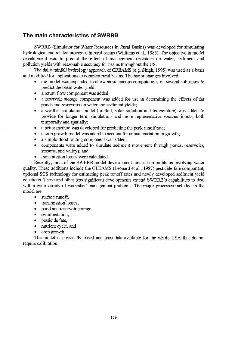
The main characteristics of SWRRB

SWRRB (.S.imulator for Water Resources in ,Rural Basins) was developed for simulating hydrological and related processes in rural basins (Williams et al., 1985). The objective in model development was to predict the effect of management decisions on water, sediment and pollution yields with reasonable accuracy for basins throughout the US.

The daily rainfall hydrology approach of CREAMS ( e.g. Singh, 1995) was used as a basis and modified for applications to complex rural basins. The major changes involved:

• the model was expanded to allow simultaneaus computations on several subbasins to predict the basin water yield;

• a return flow component was added; • a reservoir storage component was added for use in determining the effects of far

ponds and reservoirs on water and sediment yields; • a weather simulation model (rainfall, solar radiation and temperature) was added to

provide for Ionger term simulations and more representative weather inputs, both temporally and spatially;

• a better method was developed for predicting the peak runoff rate; • a crop growth model was added to account for annual variation in growth; • a simple flood routing component was added; • components were added to simulate sediment movement through ponds, reservoirs,

streams, and valleys; and • transmission losses were calculated. Recently, most ofthe SWRRB model development focused on problems involving water

quality. Theseadditions include the GLEAMS (Leonard et al., 1987) pesticide fate component, optional SCS technology for estimating peak runoff rates and newly developed sediment yield equations. These and other less significant developments extend SWRRB's capabilities to deal with a wide variety of watershed management problems. The major processes included in the model are

• surface runoff, • transmission.losses, • pond and reservoir storage, • Sedimentation, • pesticide fate, • nutrient cycle, and • crop growth. The model is physically based and uses data available for the whole USA that do not

require calibration.

116

Description of processes controlling the radionuclide wash-off from watersheds


Interception by Plants and Surface Retention Infiltration Surface Runoff

SWRRB uses the SCS curve number technique (USDA - SCS, 1972). This technique was selected because:

• it is reliable and has been used for many years in the United States, • it is computationally efficient, • the required inputs are generally available in the USA and • it relates runoff to soil type and management practice. The SCS runoff equation can be written as:

where Q - runoff, [in] P- rainfall, [in] S - potential maximum retention after runoff begins, [in] Ia - initial abstraction, [in]

The initial abstraction describes all Iosses before the overland runoff starts. It includes water retained in surface depressions, water intercepted by vegetation, evaporation and infiltration. Ia is highly variable but experimentally determined such that it can be approximated by the following empirical equation:

The use of readily available daily rainfall data is a particularly important attribute of the curve number technique because rainfall data with time increments of less than 1 day are not available for many locations. Also, rainfall data manipulations and runoff computations are more efficient for data taken daily than at shorter intervals.

There are two options for estimating peak runoff rates - the modified Rational formula and the SCS TR-55 method (USDA- SCS, 1986). A stochastic element is included into the Rational equation to allow a realistic simulation of peak runoff rates, given only daily rainfall and monthly rainfall intensity.

As specially mentioned in the Handbock of Hydrology (Maidment, 1992) the approximation "in urban application ... can imply a significant initial loss that may not take place". And later- "goodjudgement and experience based on stream gauge records are needed to adjust CNs as conditions warrant".

Perco/ation and Lateral Subsurface Flow The percolation component of SWRRB uses a storage routing technique combined with a

crack-flow model to predict flow through each soillayer. It is assumed that outflow from a soil

117

layer occurs when the soil water content exceeds field capacity. The parameters for percolation (saturated conductivity, travel time through a layer, field capacity, etc.) are estimated by using a set of empirical relationships based on the grain size distribution of a given soil. It should be mentioned that SWRRB explicitly considers water movement through soil cracks which is relatively unusual in present runoff models.

A kinematic storage model developed by Sloan et al. (1983) is implemented in SWRRB. This approach uses the mass continuity equation together with the soil profile as the control volume.

Evapotranspiration The model offers two options for estimating potential evaporation - Hargreaves and

Samani (1985) and Priestly-Taylor (1972). The Priestly-Taylor method requires solar radiation and air temperature as input; the Hargreaves method requires air temperature only.

The model computes evaporation and transpiration separately, as described by Ritchie (1972). Potential soil water evaporation is estimated as a function of potential evaporation and leaf area index (LAI, area of plant leaves relative to the soil surface area). Actual soil water evaporation is estimated by using exponential functions of soil depth and water content. Plant water evaporation is simulated as a linear function of potential evaporation and LAI.

SnowMelt To consider the snow melt process, a set of empirical equations for the vertical distribution

of soil temperature is used. It was necessary that the form of the equations allows to use artificial data produced by a weather generator included in SWRRB. It is assumed that snow melt takes place if the temperature of the second soillayer exceeds 0° C. The snow melt rate is assumed to be proportional to the mean daily air temperature. Such assumptions are typical for empirical approaches and were derived from the energy balance of the snow pack.


Sediment yield is calculated for each subbasin with the Modified Universal Soil Loss Equation (MUSLE) (Williams and Brandt, 1977). This approach allows to consider not only wash-off of eroded soil but also the transport of the sediments to the outlet of the basin. As mentioned in an UNESCO review (Hadley and al., 1985), there were encouraging results obtained with the MUSLE for 102 small but very different basins (with areas ranging from 0.01 up to 234 km2

) in the USA. Thus, the MUSLE can be regarded as a significant improvement of the USLE for use on the watershed scale.

In SWRRB the MUSLE approach was further developed by adding an empirical relationship for the effective slope length and a steepness factor. This improved version contains parameters which are collected in the USDA Handbook (Wischmeier and Smith, 1978). But again, it must be pointed out that to obtain reliable results outside the US, "more work is required to investigate the need to modify the values of the coefficients of the model" (Hadley and al., 1985).

Description of the pollutant transport

The approach frrst realised in GLEAMS (Leonard et al., 1987) for simulating pesticide transport by runoff, percolation, evaporation and sediment transport is implemented in SWRRB. Pollutants may be applied at any time and rate to the plant foliage, to the soil surface or below

118

the soil surface at any depth. It is assumed that there exists an equilibrium for the sorption!desorption process (Kd approach). This allows in principle to consider radionuclides which are at present not included in SWRRB. Pereclation of soluble pollutants is based on the mass balance for soil water.

Applicability of the mode/ in Europe, in particu/ar in Germany


Spatially distributed wash-off processes The basic simulation unit inside SWRRB is an homogeneaus subbasin. SWRRB includes

features for subdividing the watershed into several subbasin. Each subbasins can include more than one raingauge. The definition of a subbasin is mainly based on variations in soil properties, land use, crops, topography, rainfall and temperature. But with a maximum number of 10 subbasins, the representation of large watersheds seems to be questionable.

Inputdata SWRRB requires the usual amount of data necessary to characterise a watershed (soil,

vegetation, erosion, etc.). The weather generator uses a set of statistical weather characteristics such as rainfall probabilities. The data acquisition of the weather generator might be difficult, as these parameters should be calculated from long-term observations (typically over 20 years).

Time step and spatial range SWRRB operates on a daily time step. Daily weather data (rainfall, air temperature, etc.)

has to be provided by forecast modeHing or by the weather generator. At present, SWRRB can handle only ten subbasins which might limit its application to small or medium sized watersheds.


SWRRB is realised as an integrated basin model which means that it simulates the transport of water and pollutants throughout the whole drainage net. Additionally, as described before, the model includes modifications of the mass balance caused by percolation, Sedimentation and others. But SWRRB does not provide a complete hydrograph at the outlets of the subbasins. It only estimates the yields of water, sediments and pollutants at discrete points ( again a very limited maximum number of 10 points) of the drainage net.

Data availability for the European conditions

As mentioned for other models, a crucial point for the application in Europe is the missing data on surface hydrology (SCS curve number), specially developed for the USA. A second critical point are data bases on soil erosion.


SWRRB has been tested on 11 large watersheds throughout the United States (see e.g. Singh, 1995). The results show that SWRRB can realistically simulate water and sediment

119

yields tu1der a wide range of soil, climate, topography, and management conditions. There seems to be no applications of the model in Europe.

Model software and documentation

A comprehensive description of model approaches and a demo-version of the software are available in the monograph of Singh (1995) and are provided with a CD-disk as part of this book.

Data assimilation

The arrangement and control ofthe structure ofthe subbasins is realised via a user-friendly interface, however, the basic method requires input by hand. Additionally, data files can be used as input. Data assimilation, as required by the IMIS/P ARK system, is not included at all.


The code requires a modern IBM-compatible PC with moderate equipment. The software is user-:friendly. It provides input menus, error management and an on-line help system as well as output of graphics and plain text. The execution speed of SWRRB is high.

120

References for runoft models

Arnold, J. G. and J. R. Williams. 1987. Validation of SWRRB- Simulator ofwaters in rural basins. J. Wafer Resources Planning and Management. ASCE, 113(2):243-246.

Arnold, J. G. and J. R. Williams. 1995. SWRRB - A Watershed Scale Model for Soil and Water Resource Management. In: Computer Models of Watersheds Hydrology. V.P. Singh, ed. Water Resource Publications, Highlands Ranch, Colorado. p.1001-1020.

BIOMOVS II. October 1993. Wash-Off of Sr90 and Cs137 from Two Experimental Plots Established in the Vicinity of the Chemobyl Reactor. Description of Scenario W (Version 1.02),

BIOMOVS II Tech. Report No.4, 1995. Long Term Contaminant Migration and Impacts from Uranium Mill Tailings. Comparison of computer models using a hypothetical data set.

Bicknell, B.R., J. C. Imhoff, J. L. Kittle Jr., A. S. Donigian, Jr. and R. C. Joahanson. 1993. Hydrological Simulator Program - Fortran. User's Manual for Release 10. U.S. EPA Environmental Research Laboratory, EPA/600/R-93/174, Athens, GA. 660 pp.

Crawford N. H. and R. K. Linsley. 1966. Digital Simulation in Hydrology: Stanford Watershed Model IV Department of Civil Engineering, Stanford University, Tech. Report No.39.

Donigian,A.S.Jr. and H.H. Davis. 1978. User's Manual for Agricaltural Runoff Management (ARM) Model. EP A-600/3-78-080. U.S.EP A Environmental Research Laboratory, Athens, GA.

Donigian, A. S., Jr., J. C. Imhoff, B. R. Bicknell, J.L.Kittle. 1982. Guide to the Application of the Hydrological Simulator Program - Fortran (HSPF) Contract No. 68-01-6207, US Environmental Protection Agency, Athens, GA.

Donigian, A. S., Jr., J. C. Imhoff, B. R. Bicknell and J. L. Kittle. 1984. Application Guide for the Hydrological Simulator Program- FORTRAN. U.S. EPA Environmental Research Laboratory, EPA 600/3-84-066, Athens, GA.

Donigian, A. S.,Jr., and L. A. Mulkey. 1992. STREAM, An Exposure Assessment Methodology for Agricultral Pesticide Runoff. In: Fate of Pesficides and Chemieals in the Environment. J.L.Schnoor (ed.) John Wiley & Sons, Inc., New York. pp.297-330.

Donigian, A. S.,Jr., B. R. Bicknell and J. C. Imhoff. 1995. Hydrological Simulation ProgramFORTRAN (HSPF). In: Computer Models of Watersheds Hydrology. V.P.Singh, ed. Water Resource Publications, Highlands Ranch, Colorado. pp.395-442.

Hadley, R. F., Lal R., Onstad C. A., Walling, D.E., Yair A. 1985. Recent developments in erosion and sediment yield studies. UNESCO, Technical Documents in Hydro1ogy, IHP-II Project A.l.3.1, Paris 128 pp.

Hummel,P. R., A. S. Donigian and B. R. Bicknell. 1993. STREAM(PC)- An Interactive PCBased Implementation of the STREAM Methodology for the Exposure Assessment of Agricultural Pesticide Runoff. EPA Environmental Research Brief, U.S. EPA, Environmental Research Laboratory, Athens, GA.

Johanson ,R.C., Imhoff, H.H., Davis, J.L., Kittle, A.S. and Donigian, Jr. 1981. User's Manual for the Hydrological Simulator Program - Fortran (HSPF): Version 7.0 US Environmental Protection Agency, Athens, GA.

Knisel, W.G. 1980. CREAMS, A field-scale model for chemicals, runoff and erosion from agricultural management systems U.S. Dept. of Agric. Conser. Res. Rept. No. 26.

Leonard, R.A., W.G. Knisel, and D.A. Still. 1987. GLEAMS: Groundwater loading effects on agricultural management systems. Trans. ASAE, 30(5):1403-1428.

121

Monte, L. 1993. A predictive model for the behaviour of radionuclides in lake systems. Health Phys., 65:288-294

Monte, L. 1995. Evaluation of Radionuclide Transfer Functions from Drainage Basins of Fresh Water Systems. J.Environ. Radioactivity, 26:71-82.

Negev, M. A. 1967. Sediment Model on Digital Computer. Department of Civil Engineering, Stanford University, Tech. Rep. 76, Stanford, CA. 109 pp.

Popov, A.G. and R. Reling 1996. Aquatic Transfer Models to predict Wash-Off from Watersheds and the Migration of Radionuclides in Lakes for Implementation in RODOS. In: Proc. First Int. Conf. "The radiological consequences of the Chemobyl accident", ISSN 1018-5593, pp. 1189-1192.

Sansone, U. and O.Voitsekhovitch, eds. 1996. Modelling and study ofthe mechanisms ofthe transfer of radioactive material from terrestrial ecosystems to and in water bodies around Chemobyl. ECP-3 Final report, EUR 16529 en

Singh, V.P., ed., 1995. Computer Models of Watersheds Hydrology. Water Resource Publications, Highlands Ranch, Colorado, 1130 pp.

Vinogradov, Yu. B. 1967. Rainstorm flood hydrological problems for small catchments of Middle Asia and South Kazachstan. (In Russian). Leningrad, Hydrometeorological Publishing House, 263 pp.

Vinogradov, Yu. B. 1988. Mathematical modelling of runoff formation. Critical review. (In Russian). Leningrad, Hydrometeorological Publishing House, 312 pp.

Williams, J.R., A.D. Nicks and J.G. Arnold. 1985. Simulator for water resources in rural basins. ASCE J. Hydr. Engr., 111(6):970-986.

Williams, J.R., 1975. Sediment-yield predictions with Universal Equation using runoff energy factor. in: Proceedings of Sediment-Yield Workshop, USDA Sedimentary Lab., Nov. 28.-30. 1972

Young, R.A., C.A. Onstad, D.D. Bosch, and W.P.Anderson. 1987. AGNPS: An agricultural nonpoint source pollution model: A watershed analysis tool. USDA Conservation Research Report 35. 77 pp.

Young, R.A., C.A. Onstad, and D.D. Bosch 1995. AGNPS: Agricultural Non-Point Source Pollution Model. In: Computer Models ofWatersheds Hydrology. V.P.Singh, ed. Water Resource Publications, Highlands Ranch, Colorado, pp.1 001-1020.

122

Appendix on river modelling (M. Zhelezniak)

Hoffer&Bayer Model

This model (Hoffer&Bayer, 1993) is a further development of the static approach (Schückler and Bayer, 1978) - introducing dynamics -, that was used in the computer code KIRMES. This box model is designed to calculate the concentration of radionuclides in water, suspended matter and sediments as a function of time and space, following a release into the river water. For this purpose the river is subdivided into defined longitudinal sections according to its flow direction. The model describes both the interaction of the three subcompartments within a river section and the exchange with other sections.

The radionuclides are assumed to be instantaneously and homogeneously mixed within each river section. Mathematically, the model represents a system of three coupled ordinary differential equations of first order. It is possible to include data on the behaviour of the radionuclide and the river water for each individual section, i.e., it is basically possible to adapt the code to real conditions.

The equation for the water filtrate (FW) can be written as:

8CFW,n =Qn-1CFW,n-1 _QnCFW,n -'AC a V V

FW,n f FW,n FW,n

- g(KdC FW,n - C SM,n )K FW-SM (KdC FW,n - C SM,n )SM"

+ g(CsM,n- Kd,deCFw,")KsM-FW(CsM,n- Kd,deCFw,")SMn (1)

- g(KdC FW n - CS'E ,,)K FW-S'E (KdC FW n - C S'E 11 ) M S'Ea,n , , , , V FW,n

where n - is the number of the river section;

CFw n - is the active concentration offiltrated water, (Bqjm 3);

Qn - is the runoffrate ,(m 3 /s);

VFw,n - is the volume offiltrated water, (m 3);

'A - is the radioactive decay constant, (s-1) ;

K d - is the distribution coefficient for adsorption, ( m 3/ kg) g - is a function controlling the direction of adsorption and desorption;

CsM,n - is the specific activity ofsuspended matter,(Bqjkg) ;

Ki,j - is the rate oftransfer from subbox i to subboxj, (s-1);

Kd,de - is the distribution coefficient for desorption, (m 3 jkg);

SM" - is the concentration ofsuspended matter in water, (kg/m 3);

123

M SEa,n - is the mass of active sediment layer, (kg) ;

Si,n - is the source term ofthe subbox i ,(Bqls).

The terms on the right-hand side ofthis equation represent, in the first line, the activity load from the preceding section, the activity discharge into the following section and the radioactive decay. The terms in the second, third, fourth and fifth lines represent the adsorption to suspended matter, the desorption from suspended matter, the adsorption to sediments and the desorption from sediments together with the source term, respectively.

The equation for suspended matter (SM) can be written as:

acSM,n M".CsMn-1 M"acSMII = ' ' ' ' +K C -K C ßt SM V SM V SE-SM,II SE,11 SM-SE,n SM,n n FW,n n FW,n

- 'ACSM,11 + g(KdCFW,11- CSM,11)KFW-SM(KdCFW,11- CSM,11) (2)

-g(C -K C )K (C -K C )+ SSM,II SM,11 d,de FW,11 SM-FW SM,11 d,de FW,11 SM V 11 FW,11

where

M 11 ,e - is the rate of transfer of suspended matter into the river section, ( kg I s) ;

M 11 a - is the rate of transfer of suspended matter out of the river section, ( kg I s) .

The terms on the right-hand side of equation two represent, in the first line, the activity load from the preceding section, the activity discharge into the following section, erosion, and Sedimentation. The terms in the second line represent the radioactive decay and adsorption from water. The following term represent desorption to water, and the last term is the source term.

The equation for sediments (SE) are written as:

ac SE,II =K C -K C -A,C ßt SM-SE,n SM,11 SE-SM,II SE,11 SE,11

+ g(KdCFW 11- CSE II)KFW-SE(KdCFW 11

- CsE 11 ) MSEa,ll , , , , M SEb,n

(3)

where

M sEb,n - is the bed sediment considered, as explained below.

The terms on the right-hand side in the first line of equation three represent Sedimentation, erosion, and radioactive decay, resprctively. The terms in the following lines represent the adsorption from water, the desorption to water and the source term.

The function g is defined as:

124

sgna + 1 g(a) = sgna

2 {

+ 1,a >0

sgna= O,a=O

-1,a <0

In the second line of equation (1) the function g is applied to the difference Kd

C Fw,n- C SM,n. The entire term is unequal to 0 only, if this difference is positive. This means

that radionuclides dissolved in water will only be adsorbed to suspended particles when the state of equilibrium, represented by the Kd value, is not reached with respect to adsorption. The third line in equation one also implies that desorption back into water occurs only in the

case ofa positive difference cSM,n- Kd,de CFW,n.

This model provides the possibility to consider different distribution coefficients for adsorption and desorption, if available. Radionuclides dissolved in water will be adsorbed to suspended matter until an equilibrium value is reached (dynamic approach ), i.e., until

CSM,n=Kd CFw,n. The back reaction, i.e., desorption back to water, occurs when the

concentration in the water C FW,n is smaller than Kd,de C SM,n .

In equation (3) a distinction is made between the mass of the active sediment layer,

M SEa,n, and the mass of the sediment layer accounted for, M sEh,n • The active sediment layer

isthat layer in which adsorption and desorption processes occur. As a result of sedimentation and erosion, however, the mass ofthe sediment layer involved in the exchange process varies such that a greater layer with the mass M SEh is accounted for when calculating the specific activity concentration of the sediments.

The mass ofthe active sediment layer is defined as:

where

Pn - is the density ofthe bed sediments, (kg/m 3);

P11

- is the interstitial water fraction of the bed sediments;

dan - is the depth ofthe active sediment layer, (m);

B11

- is the width ofthe volume element n, (m);

L11

- is the length ofthe volume element n, (m).

The mass of the sediment layer is defined as:

where dh,n is the depth ofthe sediment layer considered, (m).

125

The transfer rates KSM-sE and KsE-SM, describing the process of sedimentation and erosion, are obtained from the equations

K - Ra,nBnLn SM-SE,n- M.

J

where

Ra,n is the depositionrate ofsuspended matter, (kgjm 2 s);

Rr,n is the resuspension rate ofthe sediment, (kgjm 2 s);

Mj is the mass ofthe subbox considered, (kg).

Equations (1)-(3) can be re-arranged for the steady state case so that the following system of three coupled differential equations of first order with constant coefficients a 1 , ••• , a 4 , b1 , •• , b 4 , c 1 , ••• , c 4 has to be solved for each volume element:

CFw =aiCFw +a2CSM +a3CSE +a4

The modelwas applied to simulate release from NPP Würgassen to the Weser River (Hofer H., Bayer A., 1993). The model exists as a FORTRAN program, but its operational status is questionable.

126

HSPF

River Transport Submodel- RCHRES

The Hydrological Simulation Program - FORTRAN (HSPF) (Bicknell et al., 1993, Donigian, et al., 1995) is a comprehensive model that includes a watershed contaminant transport module and a module that describes the transport of pollutants in rivers and reservoirs. The watershed module is described in the section about runoff modelling. Here, the river/reservoir module ofHSPF which is called RCHRES will be presented (Fig. 1).

RCHRES

I Simulate a reach or mixed reservoir I I

HYDR ADCALC CONS HTRCH

Simulate Estimate Simulate Simulate

hydraulic advective conservative heat exchange

behavior behavior of constituents andwater constituents temperatilre

SEDTRN I GQUAL I RQUAL I '

Simulate Simulate Simulate inor2anic 2eneralized constituents

sediment quality involvedin consntüimts biochemical

transformations

Figure 1: HPSF - RCHRES Structure Chart.

RCHRES structure and main processes

RCHRES is used to route runoff and water quality constituents simulated by PERLND and IMPLND through stream channel networks and reservoirs. The module simulates the processes that occur in a series of open or closed channel reaches or a completely mixed lake. Flow is modelled as unidirectional. A nurober of processes can be modelled, including:

• hydraulic behaviour, • heat balance processes that determine water temperature, • inorganic sediment deposition, scour and transport by particle size, • chemical partitioning, hydrolysis, volatilisation, oxidation,

127

• biodegradation and generalised first-order (e.g. radionuclides) decay, parent chemical /metabolite transformation,

• DO and BOD balances, • inorganic nitrogen and phosphorus balances, • plankton population, • pH, carbon dioxide, total inorganic carbon and alkalinity.

Figure 1 shows the structure and basic features of the RCHRES module. The module contains individual submodels for calculating hydraulics (HYDR), constituent advection (ADCALC), conservatives (CONS), water temperature (HTRCH), inorganic sediments (SEDTRN), generalised quality constituents (GQUAL), specific constituents involved in biochemical transformations (RQUAL), and acid mine drainage phenomena (ACIDPH). Because the ACIDPH part has not yet been finally field-tested, it is not a documented feature of Release 10 and therefore not included into Fig. 1.

Submodel HYDR - jlow simulation

HYDR simulates the processes that occur in a single reach of an open channel or a completely mixed Iake. Hydraulic behaviour is modelled using the kinematic wave assumption. All inflows into a reach are assumed to enter at a single upstream point. The outflow of a reach may be distributed across several targets that might represent normal outflows, diversions and multiple gates of a reservoir. In HSPF, outflows can be represented by either or both of two methods;

1. Outflow can be modelled as a function of the volume of the reach for situations where there is no control of the water or the gate settings are only a function of the water Ievel.

2. Outflow can be modelled as a function of time to represent demands for municipal, industrial or agricultural use. To do so, the modeler must provide a time series of outflow values for the outflow target that is time-dependent and independent of the reach volume.

If an outflow demand has both volume-dependent and time-dependent components, the modeler can, and must, specify how the components are combined to define the resulting outflow demand. HSPF allows the modeler to define the resulting demand in one of three manners: (1) as the minimum of the two components, (2) as the maximum of the two components, or (3) as the sum ofthe two components.

HSPF makes no assumptions regarding the shape of a reach; however, the following assumptions are made:

1. There is a fixed, user-defined relation between water depth, surface area, volume, and discharge. This is specified in a Function Table ( or FT ABLE) defined for each reach by the user.

2. For any outflow demand with a volume-dependent component, the relation between the above variables is constant in time. (This assumption precludes modelling flow reversals.)

In addition to calculating outflow rates and reach water volumes, HYDR computes the values for additional hydraulic parameters that are used in the other code sections of RCHRES including depth, stage, surface area, average depth, top width, hydraulic radius, bed shear stress and shear velocity.

128

Simulation of sediments and hydrophysical parameters

ADCALC calculates values for variables that are necessary to simulate the longitudinal advection of dissolved and entrained constituents. These variables are all dependent on the volume and outflow values computed in the hydraulics compartment (HYDR).

In HTRCH, the temperature is simulated by using a heat balance approach. Five time series of meteorological data are required to simulate the temperature balance within a reach. These are solar radiation, cloud cover, air temperature, dew point temperature and wind speed. HTRCH considers two major processes: heat transfer by advection and heat transfer across the air-water interface. Heat transfer by advection is accomplished by treating water temperature as a thermal concentration and using the standard advection computations contained in CONS. The net transport of heat across the air-water interface is computed as the sum of a number of mechanisms, each of which is evaluated individually. Sources of heat that are computed include absorption of short-wave solar radiation, absorption of long-wave radiation, and conduction-convection. Sinks of heat that are computed are emission of long-wave radiation, conduction-convection, and evaporation.

The approach taken by the SEDTRN submodule to compute the transport of the channel sediment is based on the SERA TRA model developed by Batteile Laboratories (Onishi and Wise, 1979). Both noncohesive (sand) and cohesive (silt, clay) sediments are simulated in SEDTRN; migration of each sediment fraction between the suspension in water and the bed is modelled by balancing deposition and resuspension. The code allows the modeler to compute the deposition or scour of noncohesive sediment by selecting one of three empirical formulations:

1. a user-defined power function of streamflow velocity, 2. a relationship (Toffaleti method) dependent on the median sand particle diameter,

average stream velocity, reach hydraulic radius, reach slope, settling velocity for sand (user-specified) and water temperature, or

3. a relationship (Golby method) dependent on the median sand particle diameter, average stream velocity, reach hydraulic radius, fine sediment Ioad concentration, and water temperature.

The simulation of cohesive sediment transport consists of two steps. First, advective transport is calculated; then deposition and scour are calculated based on the calculated bed shear stress. To evaluate deposition, the modeler is required to provide values for settling velocity and critical shear stress for deposition of each fraction (silt, clay) of cohesive sediment that is modelled. To evaluate resuspension, or scour, the modeler must provide values for the erodibility coefficient and critical shear stress of scour for each fraction.

Simulation of pollutant Iransport

CONS simulates constituents which for all practical purposes, do not decay with time or leave the reach by any other mechanism than advection. Typical constituents that are modelled as conservatives include chlorides, total dissolved solids and hydrophilic chemieals which decay very slowly.

The focus of the GQUAL code development was to allow simulation of agricultural pesticides and other synthetic organic chemicals. Given the diversity of pesticides that might

129

be modelled , the code provides the user with the capability to model any subset of the following generalised processes: advection of dissolved material; decay of dissolved material by hydrolysis, oxidation by free radical oxygen, photolysis, volatilisation, biodegradation, and/or generalised first-order decay; production of one modelled constituent as a result of decay of another constituent; advection of adsorbed suspended material; deposition and scour of adsorbed material; and adsorption/desorption between dissolved and sediment-associated phases. Using the GQUAL section in conjunction with the sediment transport code (SEDTRN), adsorbed chemieals may settle or resuspend during each simulation time step depending on hydrodynamic conditions. Decomposition of adsorbed chemieals may be simulated, both in suspended materials and in the bed, by using a first-order, temperaturecorrected decay formulation.

The RQUAL code provides detailed simulation of constituents involved in biochemical transformations. Included are dissolved oxygen, BOD, ammonia, nitrite, nitrate, phosphate, phytoplankton, benthic algae, zooplankton, refractory organic, and pH. The primary dissolved oxygen and biochemical oxygen demand balances are simulated with provisions for decay, settling, benthal sinks and sources, reaeration, and sinks and sources related to plankton. The primary nitrogen balance is modelled as sequential reactions from ammonia through nitrate. Ammonia volatilisation, ammonification, denitrification, and ammonium adsorption/desorption interactions with suspended sediment fractions are also considered. Both ammonium and phosphate adsorption/desorption to suspended sediment fractions are modelled using an equilibrium linear isotherm approach. Both nitrogen and phosphorus species are considered in modelling three types of plankton - phytoplankton, attached algae and zooplankton. Phytoplankton processes that are modelled include growth, respiration, sinking, zooplankton predation and death; zooplankton processes include growth, respiration and death; and benthic algae processes modelled are growth, respiration and death. Hydrogen ion activity (pH) can be calculated by two independent code sections. The first, named PHCARB, is contained within the RQUAL section and computes pH by considering carbon dioxide, total organic carbon and alkalinity. In doing so, the code considers the effects on the carbon dioxide-bicarbonate system of carbon dioxide invasion, zooplankton respiration, BOD decay, net growth of algae and benthal releases.

ACIDPH is a general module for performing user-defined instream chemical computations. Its intended application primarily is to model acid mine drainage and acid rain affected waters, where the pH computations in the PHCARB module, which are based solely on carbonate system equilibrium, cannot adequately represent the processes which determine pH.

Software environment

Five utility modules are used to access, manipulate and analyse time series information stored by the user in HSPF's TSS (Time Series Store) and WDM (Watershed Data Management) files. These time series, such as hourly precipitation, daily evaporation, daily streamflow are used by the application modules and are often a valuable resource in the analysis of watershed's characteristics. The five utility modules and their functions are as follows:

1. COPY - Copies data in the TSS or WDW to another file. The user can change the time step of the time series during the COPY operation; for example, a five-minute rainfall record can be aggregated to an hourly time interval.

130

2. PL TGEN - Generates a specially formatted ASCII file for subsequent data display on a platter or input to other software.

3. DISPLY - Creates data display tables. Aggregated values as well as summary information can be generated.

4. DURANL - Performs frequency, duration and excursion analyses; computes statistics; and performs toxicity/lethality analysis. DURANL can be used to answer such questions as: "How often does dissolved oxygen stay below 4 mg/1 for 4 consecutive hours?"

5. GENER - Transform one or two time series to produce a new or different time series. GENER is a powerful tool that allows the user to perform any of 22 optional transformations ( e.g., absolute value, truncation, division, logarithm).

Recently, release 10.0 of HSPF (Bicknell et al., 1993) was published and made available through the U.S. EPA. This most current release of HSPF reflects recent improvements in database and input management as well as improved algorithms for such processes as instream sediment-nutrient interactions and acid mine drainage. In addition to improvements to the batch version of HSPF, a stand-alone expert system for hydrologic calibration using the HSPF water budget computations in the PERLND module has been developed by the U.S. Georgical Survey and made available to the public.

The United States Georgical Survey has sponsored the development of interactive preand post-processing capabilities to facilitate applications of HSPF and other hydrologic models. ANNIE (Lumb et al., 1990) is an interactive computerprogram written in FORTRAN and designed for portability to mainframe computers, minicomputers and microcomputers (i.e., PC's and workstations). ANNIE helps users to interactively store, retrieve, list, plot, check and update spatial, parametric, and time-series data for hydrologic models and model analyses. A binary, direct-access file is used to store data in a logical, well-defined structure and is called a Watershed Data Management (WDM) file. HSPF and a number of other hydrologic and water quality models and analysis tools developed by the USGS currently use either ANNIE or the WDM file, or both. The WDM file provides the user with a common data base for many applications, thus eliminating the need to reformat data from one application to another.

A new section, called the FILES block, was added to the input file in Release 10 to facilitate interaction with all other input and output files. Previously, all I/0 file definition in the input file was accomplished with file unit numbers which were associated with actual disk file names using an extemal operating system-specific "command" file such as a DOS batch file. The FILES block allows the user to accomplish the correspondence between file unit numbers and file names entirely within the input file, and reduces any confusion created by using separate command files.

The river/reservoir module of HPSF is a good example of a sufficiently simple but comprehensive model that describes pollutant transport both on watersheds and in river systems. HSPF contains no submodels for the simulating the behaviour of radionuclides. Nor is there any special graphical interface. However, the pre-processing of input data and postprocessing of the output results are provided by stand-alone software packages as described above ( e.g. ANNIE).

131

MIKE 11

Model overview

MIKE11, developed at the River Hydraulics Division ofthe Danish Hydraulic Institute (Havno et al., 1995) is a one-dimensional modelling system for the simulation of flows, sediment transport and water quality in estuaries, rivers, irrigation systems and other water bodies. This modelling package is designed for micro-computers with a DOS or UNIX operating systems and provides the user with an interactive menu and a graphical support system with logical and systematic Iayouts and sequencing of the menus.

MIKE 11 has been designed to have an integrated modular structure with basic computational modules for hydrology, hydrodynamics, advection-dispersion, water quality and cohesive and non-cohesive sediment transport. It also includes modules for surface runoff. MIKE 11 has not yet been applied for modelling of radionuclide transport in river systems.

Submodels


Rainfall-runoff processes can be modelled using either the NAM module or the Unit Hydrograph Module (UHM). Whereas the NAM model is used to simulate rural catchment runoff based on a representation of the land phase of the hydrological cycle, the UHM model is used to describe the runoff from a single storm event using the unit hydrograph technique.

The mathematical submodel NAM contains a set of equations which describe in a simplified quantitative form the rainfall-runoff process in rural catchments. The model can be characterised as deterministic, conceptual and lumped with moderate input data requirements. The model simulates the rainfall-runoff process in rural catchments. It considers the water content in four different and mutually interrelated storages such as snow storage, surface storage, lower-zone storage and groundwater storage.

The model area can be divided into a number of subcatchments. As each subcatchment is treated as one unit the parameters and variables should be averages, representative for the entire subcatchment.

The input data to the model are: precipitation, potential evapotranspiration and temperature (for the snow routine). The primary results are mean daily values of streamflow and information about other elements such as the temporal variation of the soil moisture content and the groundwater recharge.

If the runoff and groundwater recharge of any of the catchments are affected by irrigation schemes, separate calculations can be performed on each irrigation area defined within a catchment. A modified description of the infiltration is used and the time series of irrigation water is specified as additional water supply to the surface storage.

Unit Hydrograph Module (UHM) is used to simulate the runoff from single storm events using unit hydrograph techniques. Excess rainfall is routed to the river using unit hydrograph or time area methods including the SCS dimensionless and SCS triangular synthetic unit hydrographs, or user-defined hydrographs.

The input data required include data describing the properties of the catchment and time series of rainfalL

132

The coupling of MIKE 11 with the more comprehensive hydrological model SHE ( called MIKE -SHE) is also possible.

Submodel of unsteady flow dynamics in river channels

Basedon topographical and time series data (model boundary conditions), the model computes water Ievels, discharges and flow velocities at all intemal model grid points.

The hydrodynamics model is based on the one-dimensional Saint-Venant equations. The two equations representing conservation of mass and momentum are respectively :

8Q 8A -+-=q ax 8t

where Q d. h 3 -1 - 1sc arge, m s A - flow area, m2

1 1 . fl 2 -1 q- atera m ow, m s h - stage above datum, m C eh . f~ . 112 -1 - ezy res1stance coe !lCient, m s R - hydraulic or resistance radius, m a - momentum distribution coefficient

Wind friction on the free surface is taken into account by adding a wind friction term to the right hand side of the momentum equation above.

The computational grid comprises altemating Q (discharge) and h (water Ievel) points. It is automatically generated with Q-points placed midway between neighbouring h-points and at structures. H points are placed at locations where cross-sectional data are available.

The differential equations are solved in a 6-point implicit finite difference scheme with altemating Q and h points, known as the Abbot-Ionescu scheme. The momentum equation is conveniently centred at Q points whereas the continuity equation is centred at h points.

The generalised matrix solution procedure applies to simply as weil as rnultiply connected regions (looped and branched networks). The same solution method can be applied to subcritical and supercritical flow conditions, by ascribing the centring of the scheme to a function of the flow state (i.e. Freude number). This is essential when both sub- and supercritical flow situations have to be described within the same model simulation, as is frequently the case for rivers and flood plains.

In order to incorporate the effects of local energy Iosses associated with flows through narrow cross sections or flow at hydraulic structures such as weirs, movable gates, culverts, etc. it is necessary to substitute the momentum equation by an energy equation.

The simulation of flow over wide flood plains is of a two-dimensional nature. Several descriptions can be formulated with MIKE 11 to simulate areas which become inundated during flooding. One method is to establish a quasi two-dimensional description by dividing the inundated area into a number of cells or separate flood plains. This approach corresponds

133

to a looped network of one-dimensional branches. The division of flood plains may be based on natural features, such as elevated roads, embankments, dikes, etc. The flow between two cells or to the main river may be specified using a broad crested weir, culvert formulation or river channel description.

Submodel of non-cohesive sediment transport

The description of non-cohesive sediment transport can be based on four different models for the calculation of sediment transport rate and alluvial roughness. These are the Engelund-Hansen modeland the Ackers-White model (Ackers, 1973) for the calculation of the totalload, and the Engelund-Fredsoe (Engelund, 1976) and van Rijn (van Rijn, 1984a, b) models for the calculation of bed load and suspended load separately. The non-cohesive sediment transport can be computed in one oftwo modes; explicitly and morphologically.

In the explicit mode, output is required from the hydrodynamic module (HD) in terms of discharge, water levels, (cross-sectional area and hydraulic radius) bothin time and space. There is no feedback from the sediment transport calculations to the HD module. Results are in the form of volume transport rates and accumulated volumes of deposition or erosion. The explicit mode is useful where significant morphological changes are unlikely to occur.

In the morphological mode, sediment transport is calculated in parallel with the HD module. Communication between the sediment transport calculations and the HD module is achieved through the solution of the sediment continuity equation and through updating the bed resistance and the following sediment transport calculation. Results are in the form of sediment transport rates, bed level changes, resistance number and dune dimension ( depending on the transport relationship adopted).

Submodel of advection-dispersion and cohesive sediment transport.

The pure advection-dispersion model, i.e. without inclusion of biological and chemical processes, is used to simulate the advection and dispersion of conservative materials or materials with a simple first order decay only.

Typical applications include studies of saline intrusion or the behaviour of cohesive sediment. The latter requires the inclusion of erosion and deposition of fine sediments in the advection-dispersion equations.

Advection-dispersion. The one-dimensional (vertically and laterally integrated) equation for the conservation of mass of a substance in solution, i.e. the one-dimensional advectiondispersion equation, can be written as:

a AC a QC a ( a c) --+---- AD- =-AKC+C2q Bt Bx Bx Bx

where: C- concentration (arbitrary unit) D- dispersion coefficient (m2/s) A- cross-sectional area (m2

)

K -linear decay coefficient (s-1)

C2 - source/sink concentration

134

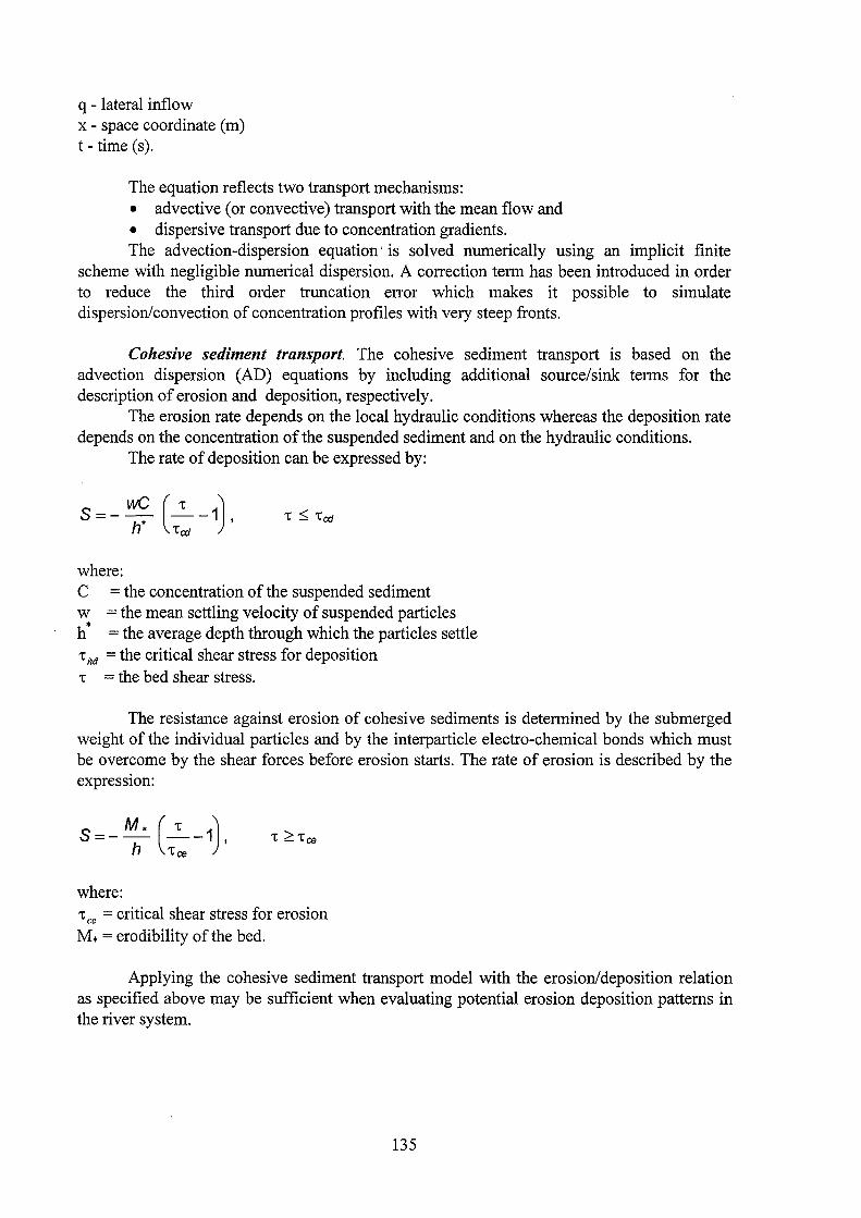
q - lateral inflow x- space coordinate (m) t- time (s).

The equation reflects two transport mechanisms: • advective ( or convective) transport with the mean flow and • dispersive transport due to concentration gradients. The advection-dispersion equation · is solved numerically using an implicit finite

scheme with negligible numerical dispersion. A correction term has been introduced in order to reduce the third order truncation error which makes it possible to simulate dispersion/convection of concentration profiles with very steep fronts.

Cohesive sediment transport. The cohesive sediment transport is based on the advection dispersion (AD) equations by including additional source/sink terms for the description of erosion and deposition, respectively.

The erosion rate depends on the local hydraulic conditions whereas the deposition rate depends on the concentration of the suspended sediment and on the hydraulic conditions.

The rate of deposition can be expressed by:

s = - wC (_2_ -1) h• ' 'tcd

where: C = the concentration of the suspended sediment w = the mean settling velocity of suspended particles h * = the average depth through which the particles settle 't M = the critical shear stress for deposition 't = the bed shear stress.

The resistance against erosion of cohesive sediments is determined by the submerged weight of the individual particles and by the interparticle electro-chemical bonds which must be overcome by the shear forces before erosion starts. The rate of erosion is described by the expression:

where: 't ce = critical shear stress for erosion M* = erodibility of the bed.

Applying the cohesive sediment transport model with the erosion/deposition relation as specified above may be sufficient when evaluating potential erosion deposition pattems in the river system.

135

Submodel of water quality

The water quality model in MIKE 11 consists of several modules describing different aspects of water quality in areas influenced by human activities, e.g. pollution with organic matter and subsequent oxygen depletion, pollution with heavy metals or problems with unnaturally high production of algae ( eutrophication).

The water quality models are based on the one-dimensional equation of conservation of mass of a dissolved or suspended material, i.e. the advection-dispersion equation, combined with a system of coupled differential equations describing the physical, chemical and biological interactions in the modelled water systems.

The BOD/DO and bacterial fate model deals with the basic aspects of river water quality in areas influenced by human activities, e.g. oxygen depletion and ammonia Ievels as a result of organic matter loading. Good oxygen conditions are essential for the diversity of the animal community and ammonia, in its non-ionised form, is highly toxic to fish and fish larvae.

The state variables in the BOD/DO model are dissolved oxygen (DO), water temperature, organic matter ( expressed as dissolved, suspended and deposited BOD5),

ammonia/ammonium (NH4 - N) and nitrate (N03 - N). The decay of bacteria (faecal and total coliform bacteria) are included in the standard

water quality model. Eschericia coli is one of the dominant species in faeces from man and warm blooded animals. The organism itself is normally considered non-pathogenic, but is very often used as an indicator of faecal pollution and, hence, a potential of real pathogenic organisms (e.g. other bacteria and viruses).

Enteric bacteria die-off can be modelled very weil by the first order decay reaction. The die-off constant or decay rate is highly variable due to interaction by environmental factors on bacterial die-off. The main factors accounted for the model are light, temperature and salinity variations.

Phosphorus components are modelled using a special version of the BOD/DO model, where BOD/DO relations tagether with nitrogen and phosphorus dynamics are calculated. The processes influencing the concentration of dissolved phosphorus (DP) are: release of inorganic phosphorus, adsorption of dissolved phosphorus, phosphorus uptake by vegetation and degradation of BOD. The processes influencing the concentration of particulate inorganic phosphorus (PP) are its deposition and resuspension and the release and adsorption of dissolved phosphorus. Particulate organic phosphorus is not described explicitly as a state variable but related to the concentration of organic material measured as BOD which is itself expressed as a function of the BOD decay rate and the suspension and deposition of sediment with attached BOD. The total phosphorus concentration is given as the sum of the dissolved inorganic and organic particulate phosphorus.

An eutrophication model is used to investigate pollution sources ( e.g. domestic and industrial sewage, agricultural runoff) with particular emphasis on the process of eutrophication (nutrient enrichment) and its effects. The model describes nutrient cycling, growth of phytoplankton and zooplankton (including nutrient dynamics) and elements of the oxygen balance. The eutrophication model consists of 12 coupled first order differential equations describing the above processes. The transport process for the pelagic components and the biological processes are coupled and solved simultaneously.

A heavy metal model is used in investigations of heavy metal pollution (industrial or urban) and dispersion of heavy metal due to its release from polluted sediments. The interaction between metals and particles, both in the water phase and in the bed, is simulated using a kinetic description of the adsorption/desorption processes. Heavymetals exist either

136

dissolved in the water or attached to suspended matter in the aquatic environment. The extent to which heavy metal in bound to suspended matter differs from metal to metal and also depends on the nature of the particles. Adsorption of heavy metals to suspended matter Ieads to their removal from the water column due to the deposition of the suspended material, but transfers the problern to the bed sediments. Differences between the concentration of heavy metal in the porewater of the sediment and in the water column result in a diffusive transport of heavy metal from the polluted sediments to the cleaner water. Another transport mechanism is resuspension of the sediments. The heavy metal submodel could be used for the simulation of the radionuclide fate if appropriate values for the model parameters would be identified.

The MIKE 11 models have been widely used for different validation and case studies. However, no information exists for its application for the simulation of the transport of radionuclides in rivers.

137

L. Monte River Reservoir Model

The model is an extension ofthe lake model developed by (Monte 1993)and serves to simulate radionuclide transport in a cascade of reservoirs. The model was applied to the Dniepr reservoir cascade within the framewerk of the IAEA VAMP programme. Each compartment is divided into a set of subsystems consisting of the following box es:

• suspended matter, • "interface" layer sediments-water, • bottom sediments, and • deep sediments.

The following equations are solved for each subsystem (the index "i" refers to the subsystem; a list of symbols is given in the Appendixtothis chapter):

dC; = !tot + D;(t) _ C;Q;(t) _ KdC;SQ;(t) _ a13KdC;ZePe _ A C dt VR Rh VR VR hR ri

_ KdC;q, + a31ZhphCh; _ C;_1QH(t) + KdCi-ISQi-l(t) hR hR VR VR

(1)

and

(2)

The retardation factor R is equal to

(3)

The terms of the formula (1) are, respectively: • the change ofthe concentration ofthe radionuclide in water (dissolved form); • the input ofthe radionuclide from the catchment basin to the subsystem (upstream

contribution not included); • the direct deposition ofthe radionuclide onto the water surface (D(t) = rate of

deposition of radionuclide on lake water); • the outflow ofthe radionuclide in dissolved form; • the outflow of the radionuclide attached to suspended particles; • the migration of the radionuclide from the sediment interface layer to the bottom

sediment; • the radioactive decay; • the removal ofthe radionuclide from the bottom sediment to the "interface layer"; • the radionuclide (dissolved form) input to the subsystem "i" from the subsystem

"i-1 "; and • the radionuclide (suspended form) input to the subsystem "i" from the subsystem

"i-1" .

138

The tenns on the right hand side of eq. (2) are: • the radioactive decay; • the migration of the radionuclide to the deep sediment; • the migration of the radionuclide from the bottom sediment to the "interface

layer"; • sedimentation; • migration of the radionuclide to deep sediment as a result of the upward

movement, due to the sedimentation, of the interface and bottom sediment layers; and

• the migration of the radionuclide from the "interface layer" to the bottom sediment.

The following figure shows the considered processes as a flow diagram.

Uepos1t1on {Ui{t)) ,J, Deposition

Cathment area (Dl (t)) (upstream not included)

I I ... Outflow

ltot/(VR) Water .....

from I , to S

Subsystem i-1 l i ._/ (upstream) Suspended a 13 a31""

ubsystem i+1

matter Sediment l -"'- "interface

Sedimentation layer"

J Bottom sediment

to deep J seidment,,

Structure of the model - Subsystem i

Figure 1- Model structure ofa watercourse segment

139

The following equation is used to calculate the total deposition ofthe radionuclide

onto the sediments (Sdi):

(4)

where

(5)

The three terms on the righthand side of equation (4) are the deposition ofthe radionuclide onto the interface layer, the deposition onto the bottom sediments and the deposition onto deep sediments, respectively. The total concentration ofthe radionuclide in

water ( Cti) was calculated according to the following formula:

(6)

A detailed algebraic derivation ofthese equations is presented for example in (Monte, 1993). All the parameters used in equations (1), (2), (3), (4) and (5) may depend on the specific subsystem (e.g. Kd, K~R1 can have different values for each reservoir). The modelwas created by using the STELLA (Richmond et al. 1987) software, running on a Macintosh computer.

Equation (1) may be considered as the solution (finite-difference scheme) ofthe following partial differential equation:

oC(x,t) _ 9(x,t) D(x,t) _ _Q_(C(x,t)Q(x,t)) _ _Q_(KdSC(x,t)a(x,t)) ot - RW(x) + Rh(x) iJx RW(x) iJx RW(x)

where e(x1t)dx is the runofffrom the catchment (upstream concentration not included) to the

segment ofthe watercourse having an infinitesimallength dx. C(x,t) is the radionuclide concentration in water ( dissolved form) at time t and at distance x from an origin arbitrarily chosen. W(x) and h(x) are the area ofthe section and the average depth ofthe watercourse at point x, respectively. The various symbols used in equation (7) may be easily related to the terms in formula (1) considering that index 'i' is substituted by the functional dependence on x. All the parameters in equation (7) have to be considered as a function of x. The term

2 Lxc(x,t) Ox

represents the effect of diffusion ofthe radionuclide in water. This term is considered tobe negligible; in fact, the model is based on the following hypotheses:

• the radionuclide concentration is homogeneously distributed in each reservoir (it is supposed that the time of diffusion of the radionuclide through a reservoir is small as compared to the observation period);

• the diffusion from one reservoir to another is negligible as compared to the transport phenomena.

140

The results of the model only represent the average concentration of the radionuclide in each reservoir. Thus to obtain reliable results for short-term predictions, the number of compartments has tobe increased drastically.

The model was successfully applied to simulate the transport of radionuclides in the Dniepr reservoirs after the Chernobyl accident.

141

Appendix with symbols and parameter va/ues

Symbols used in the subsystem model

Cbi = radionuclide concentration in bottarn sediment (Bq kg - 1 );

Cti = concentration oftotal radionuclide in water (Bq m-3);

Ci = concentration of dissolved radionuclide in water (Bq m-3 );

Di(t) = depositionrate of radionuclide (Bq m -2 s-1 );

Ze = thickness of sediment" interface layer" (m);

zb = thickness ofbottom sediment (m); h = mean depth of watercourse subsystem (m); 1101 = total rate of input of radionuclide from the catchment basin, upstream not

included (Bq s-1);

a1,3 = transferrate of radionuclide from sediment " interface layer" to bottarn

sediment (s-1 );

a3,1 = transferrate of radionuclide from bottarn sediment to " interface layer" ( s-1 );

kct = partition coefficient suspended matter/water ( m3 kg - 1 );

a3,4 = transferrate ofradionuclide from bottarn to deep sediments (s-1);

Me = total mass ofthe "interface layer" of sediment (kg);

M8 = total mass of suspended matter (kg); R = retardation factor;

q 8 = sedimentationrate (kg m-2 s-1 );

Sdi = radionuclide deposit in sediment (Bq m-2);

t = time (s);

V = volume ofwater ofthe subsystem (m3);

S = weight of suspended matter per unit volume of water (kg m -3 );

Qi(t) = water outflow from subsystem 'I' (m3 s-1);

Ai = lost deposit ofradionuclide per unit surface (Bq m-2);

'Ar = radioactivity decay constant (s-1);

Pe = density of "interface layer" (kg m-3);

Pb = density ofbottom sediment (kg m-3);

142

Symbols used in the partial differential equation (7)

C(x, t) = concentration ofradionuclide (dissolved form) at timet and point x (Bq m-3);

Cd ( x, t) = concentration of radionuclide in bottom sediment at time t and point x

D(x,t) h(x)

W(x) X

e(x, t)

X

(Bq kg- 1);

= depositionrate at timet and point x (Bq m-2 s-1 );

= watercourse depth at point x (m);

= watercourse section at point x ( m -2 );

= downstream distance from an arbitrary origin (m);

= radionuclide input into watercourse (upstream not included) per unit time and

unit length ofwatercourse (B g s-1 m-1 );

= diffusion coefficient ( m2 s-1 );

Q(x, t) = water flow at timet and point x · ( m3 s-1 );

TABLE 1 - Values of model parameters.

Parameter Units l.J Cs ~vSr

Zi = Dbs m 0.1 0.1

ZePeKd = DaePaeKd m 10 5

a13 = Kaed -1 4.6 X 10-8 4.6 X 10-8 , s

a3,1 = Kbae s -1 2.9 x 10-8 2.9 X 10-8

kd 3 k -1 m g 20 2

a3.4 = Ksd s -1 8.7 X 10-9 5.8 X 10-9

bb kg m-3 1000 1000

143

RIVTOX

Model overview

The one-dimensional model RIVTOX was developed at IPMMS, Cybemetics Centre, Kiev, Ukraine to solve water contamination problems in Ukrainian rivers after the Chemobyl accident (Zheleznyak at al., 1992, Tkalich et al. 1994). The radionuclide transport part of the model is similar to TODAM, however simplifications have been introduced to receive a more applicable model which does not need too many input parameter. On the other hand RIVTOX includes a more detailed description of the adsorption-desorption processes ( e.g. non equal rates of desorption and adsorption, different Kds for bottom sediments and suspended sediments) which was implemented into the model on the basis of validation studies carried out on Chemobyl data. RIVTOX was also tested and validated for the Clinch River -Tennessee River system within the framework of the IAEA VAMP program (Zheleznyak et al., 1995) and for the Dudvah River- Vah River system, tributaries of the Danube (Slavik et al., 1997). Within the later study, the possibility to use a two-step kinetics in RIVTOX was analysed.

RIVTOX is part of the hydrochain of the EC real-time on-line decision support system for nuclear accidents- RODOS (Zheleznyak et al., 1993; Zheleznyak, Reling, Raskob, Popov at al., 1996). In this hydrochain, RIVTOX is used to simulate the transport ofradionuclides in networks of river channels caused by direct release into the river or by washout of radionuclides from the catchment. In the latter case, the output from the runoff model RETRACE is used as input. The variables in RIVTOX which describe the dynamics of the flow, of suspended sediments and of the radionuclides are averaged over the cross section of the river channel. A 'diffusion wave' modelthat has been derived from the one-dimensional Saint-Venant equations is used to describe the water discharge and the surface elevation dynamics. The hydraulics submodel has been verified on data of the Tvertsa and Dniester Rivers (Marinets and Zheleznyak, 1993). An advection-diffusion equation is used to describe the transport of suspended sediments in the river channel. Its sink/source term describes the rate of sedimentation and the resuspension rate as the function of the difference between the actual suspended sediment concentration and an equilibrium concentration related to the transport capacity ofthe flow. The latter is calculated on the basis of semi-empirical relations. The dynamics of the upper contaminated bottom layer Z* is govemed by the equation of bottom erosion.

The transport submodel of RIVTOX describes the dynamics of the cross-sectionally averaged concentrations of the radionuclide in solution, in suspended sediments and in bottom depositions. The transfer via adsorption/desorption and diffusion in the systems "solution -suspended sediments" and "solution- bottom deposition" is treated via the Kd approach for the equilibrium state. But additionally, the exchange rates between solution and particles is taken into account to simulate also the kinetics of the processes. The adsorption and desorption rates are assumed to be not equal.

The exchange of contamination between bottom deposition and suspended sediment is described considering sedimentation and also resuspension processes. Finite-difference methods of high order accuracy are used to solve the "diffusion wave" equation and also the advection-diffusion equations which describe the transport of suspended sediments, radionuclides in dilution and radionuclides bound to suspended sediments. Ordinary differential equation were used for the simulation of the radionuclide dynamics in the upper bottom layer.

144

The model requires the following input data: • the river channel network including the length of the branches and position of the

junction, the area of the channel cross sections dependent on water surface elevation, the bottom roughness and a typical set of discharge rates,

• the mean grain size distribution of suspended sediments and the size of bottom depositions and

• the dynamics of a point sources for the simulation of a direct release and/or the results from RETRACE as lateral inflow for the modeHing of the fate of pollutants washed out from the watershed.

Submodels

Submodel of the unsteady flow in river channels

RIVTOX includes two submodels for simulating the cross sectional averaged flow velocity and water elevation in a network of river canals. The first one is based on the complete set of the Saint-Venant equations whereas the second one is a simplified form of the Saint-Venant equations, the "diffusive wave" approach. The latter, as was demonstrated (e.g. Marinets, Zheleznyak 1993), can provide good results for the flood routing in a river net that does not include structures ( e.g. dams and gates) which could have significant upstream influence on the flow parameters. The complete Saint-Venant equations should be used in situations with significant upstream influence of the river structure, including e.g. pumping of water to irrigation channels and others.

The original Saint-Venant equations include an equation for mass conservation:

a ( A V ) + BA _ q = O ax at (1)

and the momentum equation,

~ + v ~ + g ( 8

h + s 1 ) = o (2) at ax ax in which t is time, x is the distance along the longitudinal axis of the watercourse, A is the cross-sectional area, V is the velocity, q is the lateral inflow distributed along the x axis of the watercourse, g is the gravity acceleration constant, h is the water-surface elevation above an arbitrary datum such that

8hj8x = ay ;ax - s 0 (3)

in which y is the flow depth and S0 is the bottom slope of the watercourse and Sr is the friction slope which may be evaluated using a uniform, steady-state-flow empirical resistance equation such as Chezy's or Manning's. Equations (1) and (2) are quasi-linear hyperbolic partial differential equations with two dependent parameters (V and h) varying in one dimension only (the x direction) and with two independent parameters (x and t). A and Sr are known functions of h and/or V. There is no analytical solution available for most of the practical applications.

The numerical solution of the complete Saint-Venant equations needs a lot of computational effort. Therefore, several simplified distributed routing models have been

145

developed which are based on the mass conservation equation (1) and various simplifications ofthe momentum equation (2). They are called 'kinematic wave' and 'diffusion wave' model; the latter is more precise.

The hydrological model is based on Saint-Venant equations which can be simplified for plain rivers (Cunge et al., 1980) by neglecting the inertial and acceleration terms.

8h + s = 0 ax f (4)

In this case, the following approximation can be written in the form ofthe "diffusive wave":

with initial conditions:

Q(t = O,x) = Q(x) A(t = O,x) = A(x) B(t = O,x) = B(x)

and upper boundary condition:

Q(t, X = 0) = Q(t)

where:

(5)

(6)

(7)

C =BQ - velocity ofwater wave propagation (wave celerity) [rn/sec], aA

D = __Q_ - dispersion coefficient [sq. rn/sec], 2BS

Q- water discharge [cub. rn/sec], A- cross sectional area ofthe stream [sq. m], B- width ofthe stream [m], S - bed slope, q -lateral inflow [sq. rn/sec] t- time [sec], x- distance along the stream [m].

The simulation of flood plains and harbours close to the main river channel is considered in RlVTOX on the basis of a commonly used approach: the introduction of supplementary channels and by "dead volumes" (Cunge et al., 1980). The numerical solution of the complete Saint-Venant equation is obtained on the basis of the explicit HollyPreismann scheme (Cunge et al., 1980) similar to the one which was used in the CHARlMA code ( Holly et al., 1990). The numerical solution of the "diffusive wave" approximation is obtained on the basis of a finite difference scheme of fourth order.

At present, the UNIX version of RlVTOX as implemented into the RODOS hydrochain only includes the "diffusive wave" module, the PC version includes both. It is planned to include the complete Saint-Venant module into RlVTOXIRODOS till the end of 1997.

146

Submodel of suspended sediment transport

The suspended sediment transport in river channels is described by the advection -diffusion equation that includes sedimentation and resuspension rates and the laterally distributed inflow of radionuclides as a sink-source term. This equation can be presented in the following form:

where

Q(x, t) h(x, t) A(x, t; h) E s

(8)

- the flow discharge (cub. rn/sec), - the river depth (m), - the cross sectional area (sq. m), - the dispersion coefficient (sq. rn/sec), - suspended sediment concentration (kg/1),

SR (kglm ) - the concentration of suspended sediments in the lateral inflow,

z* - effective thickness ofthe contaminated, upper bottom deposition layer, that is simulated by the equation:

(1 ) az· s b

Ps -8 -=q -q' 8t

(9)

where qs and qb are the vertical fluxes of sediments (kg/sq. rn/sec), i.e. sedimentation and resuspension rates which are calculated as a function of the flow parameters:

(10)

b { 0, q = Erw0 (S* -S),

where

S* _ equilibrium suspended sediment concentration (flow capacity),

w 0 - deposition velocity (function ofthe suspended sediment grain diameter D),

Er - coefficient ofbottom erodibility (armouring coefficient) which may vary from 0 to 1.

The equilibrium suspended sediment concentration (flow capacity) S* can be calculated on the basis ofvarious semi-empirical hydraulic approaches. The methods ofBijker (Bijker, 1968) and Van Rijn (Van Rijn, 1984a, b) are used in the present version to calculate the suspended sediment concentration.

147

Submodel of radionuclides transport

The dispersion block of RIVTOX for the aquatic pollutants describes the dynamics of crosssectionally averaged values of the radionuclide concentration in the solute C, radionuclide concentration on suspended sediments es and radionuclide concentration in bottom deposition cb by the following system of equations :

BC + Q Be= _!_~(AEBe) -A.e+!L(eR -e)-Bt A Bx A Bx Bx A (11)

-a1,2S(Kdse-es)-a1,3(Kde-eb)ps(l-s)Z* I h

aes + Q aes = _!_~(AEaes) +qSR(e~ -es)I(AS)-Bt A Bx A Bx Bx (12)

-A.es +a1,2(Kdse-e8 )+qh(eh -e8 )/(hS)

where

C - concentration of radionuclide in solution (Bq/1),

es - concentration of radionuclide on Sediments (Bq/kg),

eh - concentration of radionuclide in bottom deposition (Bq/kg),

q - laterally distributed inflow to the channel river (sq. rn/sec);

eR - the concentration ofradionuclides in solution in lateral inflow (Bq/rn),

e~- the concentration ofradionuclides on sediments in lateral inflow (Bq/kg).

The model parameters are:

p s - the density of the bottom sediments (kg/m ), 8 - the porosity of the bottom deposition,

A. - the decay constant (1/sec), Kds and a1,2 are the distribution coefficient (m /kg) and the exchange rate parameter for the system "water-suspended sediment" (1/sec), respectively, Kd, a1 3- are the same parameters for the system "waterbottom sediment".

'

The present version of RIVTOX uses different values of sorption and desorption rates a1,2 and a2,1 for the system "water-suspended sediment" and a1,3 and a3,1 for the system "waterbottom deposition" because this fits better to the real physical-chemical behaviour of radionuclides in water systems. Furthermore, the use of different exchange rates gives better results in the simulations.

148

Software environment of RIVTOX

RIVTOX is running on workstations under the HP-UNIX operational system. A user friendly graphical interface was developed to operate the model inside the hydrological model chain of RODOS. The interface provides the possibility to easily access all the information necessary to run the individual models ( e.g. river model RIVTOX and watershed model RETRACE) as well as displaying the results in a way decision makers can handle them. The interface was designed as a stand-alone program and allows: • to integrate modules on the basis of a RODOS-like technology with the possibility to

allocate only as much shared memory as the program really uses for a simulation, • to input end edit data and parameters through a system of user-configured dialogues and

input windows, • to run models of the chain separately or simultaneously with the possibility to exchange

data between individual modules via shared memory, • to manage the database and to create predefined scenarios, • to present database information and on-line results of the simulations in graphs and maps

of the contamination and • to receive data from other RODOS modules e.g. results of atmospheric dispersion. New ideas realised in the RODOS Hydrological Module interface are • creation of predefined scenarios, • different automatic and manual modes for different categories of RODOS users, • the users configured system of input windows and dialogues and • new techniques of integration of extemal programs.

The PC version of RIVTOX is operating under MS WINDOWS by using a different graphical user interface.

Software tools for data assimilation are under development for RIVTOX. It is planned to release a first version of these tools at the end of 1997, additionally with software tools for estimating the uncertainty of the model.

Validation studies The hydrological module of RIVTOX has been tested and validated on data from the

Tvertsa (Russia) and Dniestr Rivers (Moldova-Ukraine) (Marinets, Zheleznyak, 1993). RIVTOX was successfully applied to simulate the propagation of pollutants in the Rhine River as the result of a chemical spill near Basle, Switzerland (Zheleznyak et al., 1993)

Within the framework of the IAEA \CEC VAMP programme, RIVTOX was tested and validated on contamination data ofthe Clinch-Tennessee Rivers (releases from Oak Ridge). The VAMP scenario of the radioactive contamination of the Dniepr River after the Chemobyl accident was used to calibrate 137Cs and 90Sr parameters (Zheleznyak et al., 1995, Marinets et al., 1995).

A special study was performed within the RODOS project to validate RIVTOX on the basis of post-Chemobyl data of the Rhine basin. Reasonable agreementwas obtained with data measured in the two rivers Neckar and Mosel (RODOS Report 4, 1997).

A validation study for the chain of RETRACE-RIVTOX has been performed for the Ilya River (Chemobyl Nuclear Power Plant zone) (Zheleznyak et al. 1996) and this will be repeated in the future for the whole Rhine River watershed.

149

A validation study on data covering the first post-accidental period was perfonned recently on the basis of a unique set of data from the Dudvah River - V ah River system (Slovakia, Danube basin) following an accidental release from the Bohunice Nuclear Power Plant (Slavik et al., 1997).

RIVTOX was used in Ukraine in summer 1995 to evaluate the consequences of an accidental but continuous release of municipal waste water from Kharkov to a near river system. Within several days, the model as part of the RODOS hydrological chain was customised and adopted by IMMS to simulate the chemical and bacteriological contamination ofthe Udy River- Siversky Donets River aquatic system. Basedon the request from the State Emergency Commission, several calculations were provided to evaluate the amount of water that should be pumped to the Siversky Donets through the channel from the Dniepr River to improve the water quality, to at least the maximum pennissible levels. This countenneasure based on calculations with the hydromodule ofRODOS was successfully implemented by the Ukrainian State Committee on Water Resources.

Input data The Program "RIVTOX" requires the following sets of input data which can be

defined via the RODOS hydromodule interface for every point of the river net:

• geographical data (river net); • hydrological data; • toxicological data.

Geographical data (river net)

The river net must be created as a connected set of points with geographical Coordinates which correspond to the real points of the main river and its tributaries. Software tools for the preparation of the river net file on the basis of standard GIS infonnation is under development now.

It is necessary to obtain data about the dependence of the cross sectional area of the river from the water elevation. This data should in general be available from the local hydrological service or can also be calculated from cross sections of the river channel.

For small rivers where these detailed data are not available, the dependencies can be simulated by default relationships.

If the river contains dams, it is necessary to include operational parameters of the dams such as the water discharge/elevation and others.

Hydrological data

Important for the creation of the basic hydrodynamical fields are data about the discharge and cross sections at the outlets from the tributary to the main river channel. Additionally, values of the suspended sediment concentration and sediment grain size distribution are necessary. Also the infonnation about the size of the bottom sediments is an input parameter.

150

Radiological data

At present, RIVTOX can handle up to seven radionuclides including H-3, Co-60, Sr-90, Ru-106, I-131, Cs-137 and Pu-239. Most important are data about the distribution coefficients of the system "water - suspended sediment" and the system "water - bottom sediment". Additionally, concentration data in the various media are required for the calculations.

151

TODAM

TODAM was developed by Yasuo Onishi (Pacific National Laboratories, WA, USA) to simulate the transport of sediments and contaminants (mainly radionuclides) in open channels. The sediment is divided into three size classes: sand, silt and clay. The transport of each sediment class is simulated independently. Contaminant transport is simulated as both dissolved and sediment-associated. Contaminants can be associated with any of the sediment size classes and bed materials. The Galerkin FEM scheme is used for solving the equations for the sediment and contaminant transport.

Submodels

Sediment transport

The sediment transport in the water column is represented by:

(1)

where

S j = the concentration ofthe sediment ofthe j - th size fraction (kg/m 3);

A = channel cross sectional flow area (m2);

B = channel bed width (m); Q = sediment contribution of the j - th size fraction from a tributary and/ or the

Sj

lateral inflow (kg m "1 day "1);

q8j = deposition rate of sediment (); qRj = scouring rate of sediment (); U = longitudinal flow velocity (); a x = longitudinal diffusion coefficient ();

Q1 = net lateral inflow ().

TODAM simulates the transport of the three separate sediment size classes using equation 1. These classes can be characterised as "sand" , "silt" and "clay". The "sand" class is considered to be non-cohesive; "silt" and "clay" are both considered to be cohesive. Erosion and deposition, represented by ~ and q0 in equation 1, are computed differently for cohesive and non-cohesive sediment classes. For non-cohesive sediment ("sand"), qR and qD are computed as

(2)

and

152

where

Ka = an armouring coefficient ranging from 0.0 to 1.0; QT = the (non-cohesive) sediment transport capacity (kg m -1 day "1);

QT. = the actual sedimenttransportrate (kg m -1 day -\ a

~x = the length of the stream segment under consideration (m).

(3)

The erosion rates are, of course, limited by the available amount of the bed sediments. A choice of three methods is available in TODAM to compute the sediment transport capacity. Erosion and deposition ofthe cohesive sediment fraction is estimated as:

{K M(-"--1) for 't h :2: 't R a t Re ' c (4) qR =

0.0, for 't b <'t Re

and r, (!--"-) for 't h ~'t D s t D '

qs = c c (5)

0.0, for 't h >'t D c

where

M = erodibility (kg m -2 day·\ 't b = the bed shear stress (kg m -2

);

'tn = the critical bed shear stress for erosion (kg m -2 );

c

'tRc= = the critical bed shear stress for deposition (kg m "2 );

Vs = the effective particle settling velocity (m day -\

In TODAM, the bed shear stress, 'tb, can be input as part ofthe hydrodynamic data or may be estimated in two ways. The first is applied for running streams with a non zero slope:

't b = p!R

where

't b = bed shear stress (newton day "1).

p = the density of water (nominally 1 000) (kg m -3 );

I = the channel bottom slope; R = the channel's hydraulic radius (m).

153

(6)

The second method should be used for reservoirs, for example, where the energy slope is much lower than the channel slope:

where

g = the acceleration of gravity (m s "2);

U* = the shear Velocity (m S "1)

which is computed by Graf, 1971, as

u* = u 17.66+

2"/ log( 96 .~ka)

D = the flow depth (m);

(7)

ka = the Nikuradse sand roughness (m), = the median bed sediment diameter, according to Chow, 1959 (pg. 202);

k = the Karman value (= 0.4).

Sediment-associated contaminant transport

The transport of a contaminant associated with sediments is modelled as:

(8)

where

C j s = contaminant concentration associated with the j-th sediment fraction (Ci m "\ /.., = contaminant radioactive decay rate (day -\ C8 . =the contaminant concentration in the bed sediment ofthe j-th :fraction (Ci kg "\

J

Q P j = the contribution of the contaminant associated with the j-th sediment fraction

from tributary and lateral inflow (Ci m -1 day "1);

K j = mass transfer rate for dissolved contaminant adsorption to and

desorption from suspended sediment ofthe j-th fraction (day "1); Kd· = distribution coefficient between dissolved contaminant and sediment

J

associated contaminant ofthe j-th sediment fraction (both suspended and bed) (m 3 kg "1);

C = the dissolved contaminant concentration (Ci m -\

TODAM simulates the transport of a contaminant associated with three separate sediment size classes using equation (8).

154

Dissolved contaminant transport

The dissolved contarninant is described as:

where

A oc +UAac = .E...{s A ac) at ax ax x ax 5

-'AAC- LKc1AC-Q1C+Qw

i=l

NI

- IAKj(Kdjsjc-c;) j=l

NI

-2:By j(1-n)djKb(KdjCCBj) j=l

(9)

Kc. = first order reaction rates of dissolved contarninant degradation from 1

causes other than radioactive decay ( day-1 );

Q w = the contribution of dissolved contarninant from tributary and lateral . f1 (C' -1 d -1) m ow 1m ay ;

y j = the solids density of the j-th sediment size fraction (kg m -3);

n = bed sediment porosity; d j = (median) particle diarneter ofthe j-th sediment fraction (m);

Kb· = mass transferrate for dissolved contarninant adsorption to and J

desorption from the j-th bed sediment fraction ( day-1 );

The Kci rate constant used in equation (9) considers the chemical degradation due to:

1. hydrolysis, 2. oxidation, 3. photolysis, 4. biological activities and 5. volatilisation.

These processes are important mainly for non-radioactive contarninants.

Bed materials

TODAM also considers bed materials such as gravel and stones. Thesematerials are affected by erosion/deposition and adsorption/desorption predicted by the sediment and contarninant transport submodels. Bed materials are conceptualised as a series of horizontal material layers, of some "standard" thickness, T, lying above an unerodable bed rock. The thickness of the standard layer is constant within a segment but may vary from segment to segment. It is assumed that the layer in a segment has a constant porosity completely filled with water.

155

The subroutines for the bed materials are first executed when all the transport equations have been solved. The calculations are performed in the following steps (andin this order):

1. Sediment erosion computed by the transport submodels is removed from the bed materials. Any particulate contaminant associated with the sediment is included.

2. Sediment deposition computed by the transport submodels is added to the bed materials. Any particulate contaminant associated with the sediment is included.

3. Contaminant adsorption to bed material, as predicted by the dissolved contaminant transport submodel, is added to the top layer of the bed material.

4. Contaminant diffusion within the bed material is computed. 5. Contaminant radioactive decay is computed.

Erosion rates are computed for the sediment and particulate contaminant transport submodels as described in the section about sediment transport. These rates are limited by the availability of bed material. The following rules are used to determine how particles are eroded from the bed (and hence to adjust q ri):

• If deposition of a given sediment fraction occurs, no erosion is allowed and if erosion occurs, no deposition is allowed.

• Any amount of any sediment fraction may be eroded from the top bed layer. • The sand sediment (non-cohesive) fraction may be eroded from any bed layer, e.g.,

sand may be eroded from the third layer down, even though there is silt and clay in the first and second layers above.

• The silt and clay ( cohesive) fraction can be eroded from a layer only if the sand fraction has been completely eroded from the layer above, i.e. sand armours silt and clay.

The reduced erosion rates are used for the solution of the transport submodel. After the completion of the transport computations for one time step, the consideration of bed material is performed in the following order:

• Eroded material is removed from the current bed materials based on the computed erosion rates for each sediment fraction. This may affect several bed layers.

• Bed material is resettled so that all layers, except for the top, are of the specified standard thickness.

• Material is deposited on top of the resettled bed materials based on the computed deposition rates for each sediment fraction. The deposited material is added to the top layer and, ifnecessary, new layers are created to accommodate it. Note that the contaminant concentration of the new material corresponds to that computed in the particulate contaminant submodel.

• Any contaminant which adsorbs or desorbs from the bed sediment, as computed in the dissolved contaminant transport submodel, is added to the top layer of bed materials.

The order of computation may or may not be important. In reality, resuspension and deposition occur simultaneously, but for the mathematical description of the process a certain order is necessary. However, the order here was chosen arbitrarily.

156

Contaminant movement within the bed material

The movement of contaminants within the bed material is typically negligible. It can, however, become significant over a long period oftime (tens ofyears). TODAM uses a rather crude approach to move a contaminant within the bed material, emulating diffusion. The process uses a fictitious concentration of a dissolved contaminant as a basis for the movement. The concentration is "fictitious" since there is no storage considered for dissolved contaminants as there is for particulate contaminants. The dissolved contaminant in the bed material is used only as a mechanism to disperse it within the bed layers. It is assumed that the entire pore space ofthe bed is filled with water. The mass ofthe dissolved contaminant within a given bed layer would then be:

(10)

where

Md= the mass of dissolved contaminant within a layer (Ci);

Gd = the concentration of dissolved contaminant in the pore space of the bed (kg m -3);

n = the bed sediment porosity; T = the thickness ofthe layer (m); L = the length ofthe channel segment (m); B = the average bed width of the channel segment (m).

It is also assumed that the particulate and dissolved contaminant within the bed is always in equilibrium. Thus:

(11)

where

Kd = the distribution coefficient between dissolved contaminant and 1

sediment ofthe j-th sediment fraction (m3 kg); N 1 = the nurober of sediment size fraction.

This is in terms of mass of the contaminant:

Using this relationship and the statement ofthe conservation ofmass, one can obtain:

Mo=Md+MP +MP+ ... +MP 1 2 NI

(13)

where

Mo = the total mass of contaminant within the bed layer (kg).

The (fictitious) mass ofthe dissolved contaminant within the bed layer is:

157

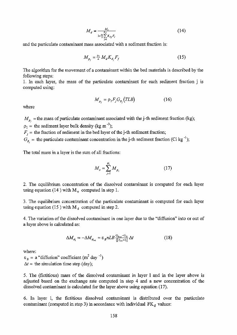
(14)

and the particulate contaminant mass associated with a sediment fraction is:

(15)

The algorithm for the movement of a contaminant within the bed materials is described by the following steps: 1. In each layer, the mass of the particulate contaminant for each sediment fraction j 1s computed using:

(16)

where

MP1

=the mass ofparticulate contaminant associated with thej-th sediment fraction (kg);

p1 = the sediment layer bulk density (kg m -\ Fj = the fraction of sediment in the bed layer ofthe j-th sediment fraction;

GB. = the particulate contaminant concentration in the j-th sediment fraction (Ci kg "1); J

The total mass in a layer is the sum of all fractions:

N,

Mo= LMPJ j=l

(17)

2. The equilibrium concentration of the dissolved contaminant is computed for each layer using equation (14) with M 0 computed in step 1.

3. The equilibrium concentration of the particulate contaminant is computed for each layer using equation (15 ) with Md computed in step 2.

4. The variation ofthe dissolved contaminant in one layer due to the "diffusion" into or out of a layer above is calculated as:

where: 8 B = a "diffusion" coefficient (m2 day "1)

f:..t = the simulationtime step (day);

(18)

5. The (fictitious) mass of the dissolved contaminant in layer 1 and in the layer above is adjusted based on the exchange rate computed in step 4 and a new concentration of the dissolved contaminant is calculated for the layer above using equation (17).

6. In layer 1, the fictitious dissolved contaminant is distributed over the particulate contaminant (computed in step 3) in accordance with individual FKd values:

158

(19)

7. Steps 4 through 6 are repeated for each bed layer, except for layer one (top layer).

Boundary conditions for channel branching

TODAM is able to consider a river net. A "junction" of a river is represented as a collection of nodes. At a junction, the mass of sediments and contaminants is balanced in a way that the sum ofboth the advective and convective flux into the junction is zero:

(20)

where

~ = the number of nodes in the junction (Figure 1 ).

The concentration gradient at the node has to be estimated. This is clone by using the concentration at the neighbouring node. For example, the concentration gradient for node 3 in Figure 1 (a) would be estimated as

(21)

Applying the mass balance to the confluence situation shown in Figure 1 results in

(22)

This equation is used to replace the equation of the outflow node in the system matrix. In fact, this equation becomes a boundary condition, in which the concentration at node two is specified:

159

Legend: I Node 06 Segment-a- JWlction•

6\\ /b 4 ~~. 3

2

1

(a) confluence

Figure 1: Schematics of two cases where junctions are used (see the text for an explanation of the computation of this particular situation)

Software realisation

TODAMis realised as a FORTRAN program and also exists in a version for UNIX workstations. In its newest version graphical interfaces were added to the main program. All input infonnation has to be provided in special input files. Further graphical processing of the output data can be perfonned with commercial packages, but is not included into TODAM itself.

To use TODAM, it is necessary to obtain infonnation about flow parameters (cross sectionally averaged velocities, cross section area) that should be the result of a onedimensional hydraulic code. At PNL, TODAM obtained this infonnation provided beforehand by the hydraulic codes RMA -1 or CHARIMA.

160

WATOX

Model overview The box model W ATOX (Zheleznyak et al., 1992) describes a system of rivers/reservoirs as a set ofboxes (compartments). Initially, the modelwas developed to simulate seasonal and longterm dynamics of radionuclides in the set of the Dniepr reservoirs. The transport submodule is a dynamic extension of the static model proposed by Schückler et al., 1978, extended by the description of several supplementary processes (different rates of desorption/adsorption and others). A set of the ordinary differential equations describes the dynamics of the water volume in a box, the mean - averaged over the volume - suspended sediment concentration and the mean concentration of the radionuclides in solution, on suspended sediments and in bottom deposition.

Model equations The water balance equations for a set of compartments can be written as:

dV. In QJ'. - Qwi -~=Q -Q+R+ dt i-1 i i j=m

where Vi = volume of compartment i; Q i = water discharge into the next compartment; Q i-1 = discharge from the previous compartment;

Q~ = discharges from the n(i)-(i)+ 1 tributary to the compartment;

Q ~ = total discharges; Ri = difference between precipitation and evaporation rate.

(1)

The suspended sediment transport equation averaged over the compartment taking into account sources as a boundary condition is written as:

m

Qi_1Sj.1 - Qisi + q~ - q~ + R~ - siQi + I Q~S~ j-1

where,

R~ = sediment flux into the compartment due to coastal erosion processes,

S~ = sediment concentration in tributaries,

(2)

q; and q; = averaged rates of resuspension and sedimentation are calculated as a functions of

the equilibrium suspended sediment concentration (flow capacity) s.

(3)

161

where

w0 =fall velocity (function ofthe suspended sediment grain diameter D), B = resuspension coefficient, F i = free surface area.

The compartmentally averaged value of the equilibrium concentration S. is defined by the Bijker (Bijker, 1968) approach through the compartmentally averaged water velocity Ui = QiLi I Vi (here Li= compartment length), the average depth hi = Vi I Fi and sediment grain size. The mean value of the bottom roughness parameter, z0 , is calculated using the Manning friction coefficient n. The temporal dynamics of the mass of the contaminated bottom deposition

M~ = p s(l - s )Z.Fi is described as:

(4)

The radionuclide transport in the compartment is described by the equations of the dynamics of the radionuclide concentration in the solute - Ci , the radionuclide concentration on

suspended sediments - c: and the radionuclide concentration in the upper bottom layer - C~. Taking into account the boundary sources and the above mentioned exchange processes, the set of corresponding equations may be written as:

m

Qi-1Ci-1 - QiCi - a1.2CKsCi - Cf) + LQ:c~ j=n (5)

m (6)

+ L(QjSjCj) + R~C~ + C~q~ - C~q~ - Q~C~Si j=n

(7)

where

C ~= concentration in the tributaries,

C~ = radionuclide concentration on the sediments discharged into the compartment due to coastal erosion mechanisms.

The exchange rate coefficients in this model are:

a = visi (8 1,2 + 8 2,1) 1'2 1 + K S s i 'ts 'tds

where

162

M~ b (8 1,3

1 + K M; 'tsb d V,

I

(8)

't5

, 'tds = the time scale ofthe adsorption and desorption processes, respectively, for the system water - suspended sediments,

't sb , 't d, b - the same parameters for the system water - bottom depositions.

The parameters ö l,p and ö p,l determine the direction ofthe contamination transfer and can be

written as:

{1, Kcl. > c~

ö - I

l,p - 0, KCi < er {1, KCi < er

ö p,l = 0, KCi > Cf

(9)

where

p =1,2,3 for the contamination C in the Solution, the Centamination on Sediments Cs and the

Centamination in bottom deposition Cb, respectively.

The radionuclide transport submodel contains the following constants: A, = ln2 I T., where T. = the half-life ofthe radionuclide, K 5 , Kd , 't, , 'tds , 't,b and 'tdsb. For the cascade of the Dniepr reservoirs, WATOX was applied with the following set of parameters values:

Radionuclide K.J L!kg 't, days 't ds days KdL!kg 't sb days 't dsb .days z.m

90Sr 600 1 100 600 1 100 0.1

137Cs 20,000 1 100 20,000 25 100 0.1

Software and model implementation The numerical solutions of the model equations are obtained by the Runge-Kutta method. W ATOX is integrated in a system of PC-compatible software where transport models are combined with optimisation models for water management of the reservoir and modules for parameter identification. A menu-driven user interface provides the interaction between the simulation and optimisation models, their databases and the graphics system.

The database of the simulation models includes the compartmentally averaged information on hydrology and contamination for the reservoirs as well as various seenarios ofwater, sediment and contamination input from the tributaries. The database of the optimisation module also includes information about hydropower, water supply and the environmental constraints on reservoir management.

In 1997, work started to implement WATOX into the UNIXenvironment and to use it in the hydrochain of RODOS as a long-term simulation model. Till the end of 1997, the implementation of W ATOX will be completed for the Rhine River basin.

The model has been used since 1987 for the preparation of seasonal forecasts of the radionuclide transport in the Dniepr reservoirs. Furthermore, W ATOX was applied within IAEAN AMP validation studies. W ATOX has also been used successfully for prediction of

163

the long-term dynamics of radionuclides in the Dniepr reservoirs (Zheleznyak et al., 1992; Zheleznyak et. al., 1994; Golovanov et al., 1996).

164

REFERENCES for river models

Ackers, P., White, R. Sediment transport: new approach and analyses. J.Hydr.Div. ASCE, vol. 99, No.ll, 2041-2060 (1973).

Bicknell, B.R., J.C. Imhoff, J.L. Kittle Jr., A.S. Donigian, Jr. and R.C. Johanson. 1993. Hydrological Simulation Program- FORTRAN. User's Manual for Release 10. U.S. EPA Environmental Research Laboratory, Athens, GA.

Bijker, E.W, Some considerations about scales for coastal models with movable bed, Delft Hydr. Lab., Publ. No 50, 1968.

Bijker, E.W. Littoral drift as a function of waves and currents. 11th Coastal Engineering Conference, London, 1968, pp. 34-48.

Codell, R.B., Key, K.T., Whelan, G. Collection of mathematical models for radionuclide dispersion in surface water and ground water. NUREG- 0868, 1982.-271 pp.

Colon, R., McMahon, G.F. BRASS model: application to Savannah river system reservoirs. J. Water Resour. Plann. Manage., 1987, vol. 113, No. 2, pp. 177-190.

Cunge, J.A., Holly, F.M., Verwey A., Practical Aspects of Computational River Hydraulics, Pitman Publ., London, 250 pp., 1986.

Donigian, A.S., Jr., B.R. Bicknell and J.C. Imhoff. 1995. Hydrological Simulation ProgramFORTRAN (HSPF). Computer Models of Watershed Hydrology. Water Resources Publications, Colorado.

Engelund, F., Fredsoe, J., A sediment transport model for straight alluvial channels. -Nordic Hydrology, 7, (1976), pp. 293-306

Golovanov I., Sizonenko, V., Zheleznyak, M." Modeling of Strategies of Water Reservoir Management under the Impact of Aceidental Radioactive Contamination" - Proc. of the

. Conference on Aspects of Conflicts in Reservoir Development and Management, 3-5 September 1996, City University, London, 1996, pp. 433- 442

Havno, K., Madsen, M.N., Dorge, J. MIKE 11 - a generalized river modelling package. in: Computer Models of Watershed Hydrology (Ed., V.P. Singh), Water Resources Publications, USA, pp. 733-782, 1995

Hofer, H., Bayer, A. Calculation of radionuclide dispersion in flowing waters with a dynamic model, Kerntechnik, v.58, No3, (1993) 164-169

Holly, F.M., Yang, J.C., Schwarz, P., Schaefer, J., Hsu, S.H., Einhellig, R. CHARIMA: numerical simulation of unsteady water and sediment movement in multiply connected networks of mobile-bed channels. IIHR Report No. 343, Iowa Institute of Hydraulic Research, University oflowa, Iowa City, Iowa. 1990. - 327 pp.

Lumb, A.M., J.L. Kittle and K.M. Flynn. 1990. Users Manual for ANNIE, A Computer Program for Interactive Hydrologie Analyses and Data Management, Water-Resources Investigations Report 89-4080, U.S. Geological Survey, Reston, VA.

Marinets, A., Sizonenko, V., Papush, L., Tschurlovits, M., Zheleznyak, M. Validation of models for radionuclide migration in rivers and reservoirs, - Environmental Impact of Radioactive Releases, Proc.of International Symposium, IAEA, Vienna, 8-12 May 1995, IAEA-SM-339, IAEA, 1995 pp.822-824

165

Marinets, A.,Gofman, D., Zheleznyak, M. Using GIS for modelling radionuclide transport in complex river-reservoir network. - HydroGIS 96: Application of Geographical Information Systems in Hydrology and Water Resources Management (Proc.of Vienna Conf.1996) IAHS Publ.No.235, 1996, 325- 330.

Monte, L. - A predictive model for the behavior of radionuclides in lakes system. Health Physics 65(3):288-294; 1993.

Onishi, Y. and S.E. Wise. User's Manual for the Instream Sediment-Contaminant Transport Model, SERATRA. Draft Report prepared by Batteile Laboratories, Richland, Washington for U.S. EPA Environmental Research Laboratory, Athens, GA, (1979)

Rijn van L.C., Sediment transport, Part 1: Bed Ioad transport. J. Hydraul. Engineering, 110(1984a), pp 1431- 1456.

Rijn van L.C., Sediment transport, Part II: Suspended Ioad transport. J. Hydraul. Engineering, 110(1984b) 1613- 1641.

Richmond, B., Vescuso, P., Peterson, S. - User's guide to STELLA™. Software from High Performance Systems. Dartmouth, New Hampshire: High Performance Systems; 1987.

Schückler, M., Kalckbrenner, R., Bayer, A., Zukünftige radiologische Belastung durch kerntechnische Anlagen im Einzugsgebiet des Oberrheins, T.2, Belastung uber den Wasserweg, Conference Düsseldorf, Proceedings, ZAED, Eggenstein-Leopoldshafen, 1976.

Slavik, 0., Zheleznyak, M., Dzuba, N., Marinets, A., Lyashenko, G., Papush, L., Shepeleva, T., Mihaly, B., lmplementation of the decision support system for the river-reservoir network affected by releases from the Bohrmice NPP, Slovakia - - Radiation Protection Dosimetry, 1997

Tkalich, P., Zheleznyak, M., Lyashenko, G., Marinets, A. RIVTOX- Computer Code to Simulate Radionuclides Transport in Rivers, A. Peters et al.( eds.) , Computational Methods in Water Resources X, vol. 2, Kluwer Academic Publishers, Dordrecht, The Netherlands, 1994, pp. 1173-1180.

Zheleznyak, M., Demchenko, R., Khursin, S., Kuzmenko, Yu., Tkalich, P., Vitjuk, N. Mathematical modeling of radionuclide dispersion in the Pripyat-Dniepr aquatic system after the Chernobyl accident. -The Science ofthe Total Environment. 1992, v.ll2, pp.89-114.

Zheleznyak, M., Demtchenko, R., Kuzmenko, Yu., Tkalich, P., Dzuba, N., Mezhueva, I. Mathematical modelling of radionuclide dispersion in the water bodies of the Chernobyl NPP zone and in the Dniepr Reservoirs.- Hydrological Impact of Nuclear Power Plants. Proc. UNESCO Workshop-92, UNESCO Press, Paris,1993, pp.173-185

Zheleznyak, M., Marinets, A. ModeHing of long wave propagation in river channels on the base of"diffusion wave" equation, In book: Copmputational Technologies, v.2, N 6, 1993, Novosibirsk, Institute of Computational Technologies of Russian Academy of Sciences, pp.147-154 (In Russian)

Zheleznyak, M.J., Tkalich, P.V., Lyashenko, G.B., Marinets, A.V. Radionuclide aquatic dispersion model-first approach to integration into the decision support system on a basis ofPost-Chernobyl experience.- Radiation Protection Dosimetry, N6, 1993, pp.37-43.

Zheleznyak, M., Kuzmenko, Yu., Tkalich, P., Dzuba, N., Gofman, D., Golovanov, I., Marinets, A. , Mezhueva, I. Modelling of Radionuclides Transport in the Set of River

166

Reservoirs. in: A. Peters et al.( eds.), Computational Methods in Water Resources X, vol. 2, Kluwer Academic Publishers, Dordrecht, The Netherlands, 1994, pp. 1189 - 1196

Zheleznyak, M., Blaylock, G., Gontier, G., Konoplev, A. et al. Modeling of radionuclide transfer in rivers and reservoirs: validation study within the IAEA\CEC VAMP Programme. International Symposium on Environmental Impact of Radioactive Releases, IAEA, Vienna, 8-12 May 1995, IAEA-SM-339, IAEA, 1995, pp.330-331

Zheleznyak, M., Heling, R., Raskob, W., Popov, A., Borodin, R., Gofman, D., Lyashenko, G., Marinets, A., Pokhil, A., Shepeleva, T., Tkalich, P. Modelling ofHydrological Pathways in RODOS. The radiological consequences of the Chernobyl accident. Proceedings of the first international conference. Minsk, Belarus 18 - 22 March 1996. Editors A. Karaoglou, G. Desmet, G.N. Kelly and H.G. Menzel. European Commission. Luxembourg, 1996, pp. 1139-1148 EUR16544EN.

167

Appendix on Iake modelling (R. Heling)

lntroduction on detai/ed model descriptions

Within the analysing procedure, six models have been identified which might be suitable for the integration into the IMIS/PARK system. To have a better insight into these models, they will be discussed in detail with respect to flexibility, reliability and applicability as these seem tobe the most important criteria and determine the final selection.

To each modelaseparate section is devoted. Each section starts with a list of items describing features which increase the flexibility. Besides that, details on processes, on the possibility to apply the model in Central Europe and on the extent to which the model meets the other implementation criteria are described. The emphasis in the process descriptions is put on the deviations from an average Iake model. To reduce the text, the common equations for Iake modelling are not repeated per section. Only when the equations deviate from the average approach, they are explicitly mentioned or discussed. In addition, a computer code is discussed in more detail, when it contains remarkable features which enables the model to be attached to an expert system.

The models which will be discussed in more detail are: • VAMP • LAKECO • DELWAQ/UPTAQE • BIOPATH • DETRA • MARTE

For the complete set of equations, we refer to the literature, manuals and/or documentation of the models (see References).

168

VAMPmodel

The VAMP model has been developed within the framewerk of the international VAMP (Validation of Model Predictions) project as a result of model intercomparison exercises among various lake models. During this project a new model, - simple, general, predictive and state-of-the-art-, was developed on the basis of all the models of the participants. The aim was to produce a model for decision support systems which is as flexible as possible and applicable to a wide range of lake ecosystems. The model therefore an optimum size and a high predictive power. By the introduction of a number of powerful submodels, there is a minimum amount of expert judgement required to operate the model. A typical feature of the VAMP model is the presence of moderators to take seasonal effects on a number of biological and hydrological processes into account. They relate these processes with the geographical location of the lake. This increases the flexibility and applicability to a high extent.

Specific submodels, which distinguish the VAMP model from other generic radioecological lake codes are used to predict the following parameters in advance:

1. uptake rate from water to phytoplankton based on lake pH and potassium concentra-tion,

2. the fraction of dissolved radiocaesium in the lake water on the basis of lake pH, 3. the biological half-life offish based on lake temperature and body weight, 4. the resuspension rate and transfer of radionuclides from the sediments to the lake

with a moderater controlled by lake bathymetry, 5. discharge from the lake based on catchment area information modified with a

seasonal moderater, governing the lake water retention time, 6. the total biernass of the aquatic organisms on the basis of primary production of

phytoplankton, 7. the lake water temperature on the basis of the geographical location. This

information is used to calculate the presence of stratification and also the depth of the stratified layers and

8. the transferrate from the catchment to the lake (secondary load).

The model is flexible and widely applicable. Although most of the processes of the VAMP model are empirically based, the quality and quantity of the data on which these processes have been derived determine the effectiveness of the submodel. The transfer of nuclides to phytoplankton, for instance, is based on field data by means of a dimensionless moderater and not on laboratory studies on the uptake behaviour in aquatic plants cells under various conditions. A strong advantage above most of the other compartment models can be seen in the fact that VAMP may be applied to deep lakes. A temperature moderater was designed to deal with the dispersion of nuclides in deep lakes. This approach is kept relatively simple to avoid high uncertainties and the need of extensive sets of data (the case with most of the model developed for deep lakes). Because ofthese features, VAMP can cover a large range oflake types.

169

Hydrologica/ processes

The hydrological residence time is an important variable which controls the behaviour of nuclides in the lakes significantly. The hydrological residence time or Iake water retentiontime is modelled in a generic way, expressed by the following equation:

T=V/Q 1

where Q is the discharge in m3/d ofthe inflowing or outflowing water and V is the volume ofthe Iake in m3

. In the VAMP model this equation is made generally applicable by means of a seasonal moderator to take the fluctuations of the discharge Q during the year into account.

Q(t) = Seasonal moderator * Qmean 2

Qmean is expressed by the following equation:

Qmean = ADA * Precipitation *SR 3

where precip is the ratio between the actual precipitation, mm year-1 and the mean annual precipitation, mm year-1

, ADA is the size of the catchment area in m2 and SR is the specific ff . 3 th-1 -2 runo mm mon m .

The seasonal moderator for the discharge is a function of altitude, latitude, Iake catchment area, precipitation, Iake volume and of the 'seasonal variability norm'. This seasonal variability norm is a function of the season and expresses the fluctuations of discharge under most extreme circumstances. The other parameters smooth ( or minimise) this function controlled by the two parameters of latitude and longitude. For Nordic lakes, for instance, the seasonal variability of discharge will be more extreme than for a Iake system in Central Europe. By means of this moderator it is no Ionger required to have sets of seasonally dependent data of a Iake system as the average values are now sufficient to calculate the mean discharge. The fluctuations are subsequently calculated by means of this seasonal moderator.

After calculation of the time dependent discharge Q, the seasonally dependent Iake residence timeT (or retention in the Iake water) can be obtained by means of equation (1).

There are various methods to calculate the retention rate from the Iake residence time. The commonly used methods are 1/T(t) or 0.693/(0.S*T(t)) or 1/TYDm (where YDm is a moderator for the mean depth). A more complex approach is to apply the equation 0.693/(0.5 * Tr), where Tr is the retention of radiocaesium in lakes. Tr is defined as T/(1 + KT * T), where KT is the settling rate for particulate radiocaesium.

In the VAMP model, the following equation has been applied based on model calibrations for various lakes in the validation study:

1 Ret Rate = --3"""0--rr (l'+29/o.5J11.5

4

This equation is generally applicable. In deep lakes with stratification, T is the total residence time ofthe entire lake. The resulting retention rate, however, is only predicted for the epilimnion

170

or active volurne. The VAMP model includes a depth model in which the depth of the epilimnion is calculated on the basis of the average depth of the Iake, the mean depth of the Iake and the Iake temperature. A submodel has been included to predict the mean annual temperature in the Iake water on the basis of latitude, altitude and continentality ( distance from the ocean). A seasonal moderater has been introduced related to the same parameters and the Iake volurne to calculate the monthly temperature changes. The seasonal moderater contains, like the discharge moderater, a 'seasonal variability norm' and a smoothing function. The smoothing function in the moderater for the Iake temperature causes lower temperature fluctuations in lakes on lower altitudes and latitudes. Both in the epilimnion and the hypolimnion (if present), the temperature is calculated. The depth of the epilimnion and hypolimnion are calculated on the basis of bathymetry data combined with information on the geographicallocation of the Iake.

The VAMP model also contains a submodel to govem the leakage of nuclides from the catchment in the long term. This process is not of high importance in a Iake model, since the concentration in the Iake ecosystem is govemed by the initial transfer of nuclides, both from the deposition and from the initial runoff to the Iake. Sensitivity tests with the VAMP model on severallakes demonstrated the minor role ofthe long-term runoffto the concentration in the Iake ecosystem.

The secondary Ioad, the transfer from the catchment, is modelled by means of a simple function expressing the time-dependent outflow rate. In the VAMP model, the catchment is subdivided into different areas, the inflow and the outflow areas. The percentage of outflow areas, generally the wet part of the catchment, is set to 20% for reasons of the simplicity. Furthermore it is assumed that the transfer from the inflow areas, generally dry areas, is negligible and it is set to zero percent. An initiallass from the catchment of 4% per year is assurned for the outflow areas which is in accordance with studies done by Bergström (1989), where a value for the wet areas or bog areas of 1% was assumed. This outflow rate is modified by means of the seasonal moderater for Q and further modified by the division of the square root of the month nurnber, a rather empirical method to take into account other processes than decay such as fixation and vertical migration in the catchment.


The Iake model describes the dissolved and the particulate radiocaesiurn as separate compartments. This separate treatment has no further advantage above the single-compartment-method except for the behaviour of the different phases of radiocaesiurn being made more explicitly visible. A separate rate is governing the transfer from one of these two phases, while in the one compartment method, - regarding the Iake water as one compartment - the description of each transferrate takes both phases into account implicitly. But the VAMPmodel yields the totallake water concentration as final output similar to other compartments models.

The distinction between the dissolved phase and the particulate phase is normally described in the following way expressing the dissolved fraction as a function of the suspended sediment concentration and distribution coefficient ofthe nuclide:

5

171

where Kct is the distribution coefficient, defined as the ratio of the nuclide concentration in the particulate phase (Bq/kg) and the concentration in the dissolved phase (Bq/1), in 1 kg-1 and SS is the suspended matter concentration in kg r 1

•

Higher Kct values give a lower dissolved :fraction and at a constant Kct the dissolved fraction decreases when the suspended sediment concentration increases. The VAMP model and also other lake models are extremely sensitive regarding this Kct value. Site-specific data on the Kct value or expert judgements are required to deal with this problern of high sensitivity. Generic Iiterature values are not sufficient for all lake ecosystems. The VAMP model, however, deals with this problern using an empirical, not physically based moderater, derived from data of many lakes, with the lake pH as a driving variable (see equation 6). The initial dissolved fraction is fixed to 0.5, assuming that after deposition 50% ofthe radiocaesium is in the dissolved phase.

1 F = ---------;:;

w 1.04 + [1. 75(pH I 4) -1 f 6

It is obvious that the Kct approach is omitted in the VAMP model: it is assumed that this overall equation is sufficient to describe the dissolved phase. Note that for instance the potassium concentration has no effect on the dissolved fraction according to this approach, which is not likely (Comans et al., 1989). The potassium effect is implicitly included, since this approach is based on a statistical correlation indicating the lake pH as the most important parameter influencing the fraction of dissolved radiocaesium. Probably, lakes with high pH are usually eutrophic lakes, where high values for high hardness and other ion concentrations such as potassium may be expected. In the VAMP model, the dissolved fraction is a very important moderater, since only dissolved radionuclides are transferred to pelagic organisms and only adsorbed nuclides are transferred to the sediment layers. In the VAMP model it is assumed that there are no processes of importance, which transfer nuclides via the dissolved phase to the porewater of the sediments.

The transfer of nuclides from the lake water to the sediments is considered by modeHing the scavenging process in a general way:

Rate = dm

(J

7

where cr is the Sedimentation rate in kg m-2 d-1 and dm is the mean depth ofthe lake in m.

The Sedimentation rate can be expressed as:

=v*SS 8

where SS is the suspended sediment concentration in kg m-3 and v the settling rate in m d-1. In

the VAMP model, the settling rate on carrier particles for radiocaesium is set to 1 m/d.

The aim of the VAMP model is the prediction of the radiocaesium concentration in the hydrological part of the lake ecosystem. The behaviour of radionuclides in the sediment layers was therefore generally regarded as a necessary module important for the levels in lake water

172

and biota, but is not the main goal. The transfer from the water layer to the sediment layers and vice versa, are described by means of one rate for each direction. The main processes included into the water-sediment interactions are burial and resuspension. The burial was modelled by dividing the scavenging rate by the depth of the active layer of sediments.

Resuspension is modelled by means of a fixed rate govemed by a moderater called Dynamic Ratio. The Dynamic Ratio (DR = Lake Surface (km2

) o.s /depth (m)) relates the extent of resuspension takes place with the lake bathymetry. An alternative method used in VAMP, instead of a fixed value, is a function, governing the transfer from the sediments to the Iake water, which is driven by the ratio between the depth of the epilimnion and the hypolimnion. There is a deep sediment layer modelled which acts as a sink only, no transfer to from this layer to the active layer is taken into account. Diffusion among the sediment layers and between the sediment layers and the water column is not taken into account.

The biological uptake model

Foodweb modelling in the VAMPmodel is treated in such a way that the user has to provide as less as possible parameters. Each group of organisms is treated as a compartment. Between the individual compartments transfer takes place. The biomass of all organisms is assessed on the basis of an empirical function calibrated on a set of lakes, with the primary production of phytoplankton as key parameter.

The foodweb description is extremely generic; it consists of one top predator ( defmed as piscivorous fish), prey (including non-piseivoraus fish, zooplankton and benthos) and phyto- . plankton. Depending on the foodweb composition in a particular Iake, this basic chain is followed. Fora Nordic Lake, for instance, the top predator is trout, the prey is benthos. For an eutrophic Iake such as the IJsselmeer in the Netherlands, the predator fish is perch and the prey fish is smelt. Into the foodweb model a number of empirical moderators have been introduced to reduce the number of input parameters.

The way the aquatic organisms are modelled is in accordance with the standard way adopted in most ofthe bio-uptake models:

dc organism _ * * dt - A uptake.jood C food + A uptake, water C water - A half /ife C organism 9

where Iambda represents the transfer rates and C the nuclide concentration in fish, food and water, respectively. Generally, the main problern in aquatic radioecology models is to describe the biological transfer rates properly by physical or empirical approaches.

It is also important in modeHing that most parameters are depending on physiological (body weight, type of organism) and environmental conditions (chemical composition of the Iake water, Iake temperature). A model without submodels to take the variation among the various Iake ecosystems into account, is very difficult to apply by a non-expert. A model is more powerful when empirical, or better, physiological submodels assess the important rates and correlate these rates to environmental conditions. Too many submodels on the other hand, lower the predictive power and for insensitive parameters fixed values, based on validation tests are the

173

best solution to avoid extensive sets of input parameters. In the VAMP model, the road of the empirical submodels was selected. Since physiological processes are not introduced, the flexibility of the biological uptake model is related to the number of lak:es and the reliability of the data sets which are the basis of these empirical relations.

The uptak:e of nuclides into phytoplank:ton is often based on Concentration Factors. In the VAMP model, the uptak:e rate is related with the lak:e pH and the potassium concentration. The retention or biological half life is related to the mean weight of the fish and the lak:e temperature, based on literature data (Reichle, 1970; Ugedal, 1992; IAEA, 1996). The uptak:e rates for prey and predator fish were not modified by lak:e temperature or body weight, as the predictive power was lowered in this case. The uptake rate to benthos is modified by means ofthe Dynamic Ratio. The uptak:e :from sediments to benthos is tak:en into account, although this seems to be of minor importance, since radiocaesium is hardly transferred :from particles to benthos (Kolehmainen, 1972). In the benthic uptake it was assumed that 100% of the nuclides are in particulate form; no uptak:e from the porewater is tak:en into account and no reduction of the sediment load is assumed. This is understandable, since about 99% of the radiocaesium are adsorbed to particles, also when the porewater fraction or porosity is about 0.9.

F or organisms, both the direct uptak:e of nuclides from the water and from the food is taken into account. The direct uptak:e might play a minor role, however, it plays a role under specific conditions, such as in the initial phase after the accident (IAEA, in press; Hinton & Scott, 1990; Morgan, 1994). The uptak:e rate for fish is modelled applying the same moderater as for the plank:tonic uptak:e rate. This moderater is govemed by the potassium concentration and the Iake pH. The direct uptak:e water to fish is lowered by one order of magnitude in comparison with the plank:tonic uptake rate of nuclides from the water.

In the VAMP model, the uptak:e ratesarenot physically, but empirically based and to keep the model simple, there is no distinction made in respiration and growth rate in the organisms for instance, nor are the pharmokinetic equations applied.


The VAMP model is designed, validated and tested for radiocaesium. A lot of modifications are necessary in the case of the model being applied to other nuclides than caesium. All nuclidespecific submodels have to be omitted or substituted; the biological, hydrological and sedimentological submodels can be maintained. This will lower the predictive power of the code.

Possibility to apply the model in Centrat Europe


The VAMP model is a compartment model. The model can be applied to predict the behaviour of radiocaesium in lak:e ecosystems with different environmental properties. The size of the lake may vary :from 1 km2 up to 1000 km2

. For smaller lak:es, in the order ofhectares (e.g. ponds) and larger lakes in the order of 10000 km2 (the Great Lak:es) the predictions will be less reliable. Due to some special subroutines for deep lak:es, applicable for latitudes ranging from 30 - 60° N and

174

altitudes between 0 - 4000 m a.s.l., the VAMP model can easily be applied to deep lakes where stratification occurs. Considering the Iake ecosystems in Central Europe and in particular the German territory, deep lakes like the Lake Constance connected with a river system and relatively small lakes in Bavaria can be analysed. A disadvantage or restriction of this code is that the Iake model as a compartment model is not designed to supply reliable information on the dispersion of nuclides in the aquatic phase in the first days after an initial deposition, as this requires 2-D models. Especially the initial dispersion is of importance when the lake is contaminated by runoff or inflow and not by direct deposition of nuclides. Nevertheless, for the biouptak:e the concentration differences in the lake are of minor importance, as it is assumed that fish migrates in general all over the Iake. Only when lake water is used as a drinking water resource, the non-homogeneaus contamination might be of importance.

The time step or spatial resolution of the model system is days, however, the model is a compartment model and therefore assumes immediate mixing. F or the prediction of the radioactive contamination of the biota, a time scale of weeks up to years is sufficient. In validation tests, the model has shown reliable predictions for up to 10 years.

Flexibility and generic character of the model

The VAMP model is, as stated above, very flexible, relatively simple in its design and created as a small and fast tool to be applied in radiological studies. Most of the important parameters are derived from generic data from Iake ecosystems. Difficult-to-obtain information on model specific parameters is set to default values based on model experience. Lake specific parameters are assessed based on very obvious site information such as bathymetry and Iake chemistry. Therefore, the model can be applied by non-experts and model adjustment is not necessary.

Required input data and availability

The required input of the model is listed below. The geographical information can readily be obtained from information ofthe catchment area and bathymetric maps.

• Geographical and hydrological information • Altitude (ma.s.l.) • Latitude ( degrees) • Size ofthe catchment area (m2

)

• Lake volume (m3)

• Water residence time ( d) • Precipitation (annual mean or monthly mean, ifpresent) in mm i 1 or mm month"1

• Mean depth, maximum depth ( d)

Chemical information • Lake pH • Potassium concentration in Iake water (mg/1)

Sedimentological information • Sedimentation rate of suspended matter (g m·2 year-1

) or • Growth ofthe sediment layer (cm year-1

)

175

Biological information • Aquatic food chain information

Predator and prey fish Predator-prey relation Mean body weight of target fish

• Primary production oflake system (C m-2 year-1)

Radiological information • Atmospheric load (both lake and catchment) in KBq m2

• Month offallout


The VAMP model has been tested on seven lakes in Europe within the framewerk of the VAMP project; the results are published by Häkanson et al (1996) and in the IAEA Techdoc (IAEA, in press). These tests demonstrated the high predictive power of the model. The cases of mispredictions could be explained by two reasons. The first was the presence of old caesium in the water phase in the case of the very deep lake Bracciano, a lake with a high retention time of 137 years (weapon testing caesium is transferred to the epilimnion after the mixing period). The second reason is the uncertainty ofthe empirical (measurement) data.

The model software and documentation avai/ability

The VAMP model is written in the specific graphical simulation language !Think for the Macintosh computer, which identifies it as a stand-alone model system. At present a release is available written in Powersim, another simulation language for the Windows environment. By means of the Powersim simulation language, a runtime release has been created to be built in the C++ environment and to link the VAMP code to other modules, input/output management is then possible.

At present, a scientific publication is available in which the specific features of the VAMP model are explained (Häkanson, 1996).

Criteria for implementation into a decision support system

Interface to radiological models and output of the model

As output the model provides the time-dependent concentration of radiocaesium in lake water, in sediments and in prey and predator fish. In the present version, the output is listed as graphs and tables within the !Think environment. In the Powersim release under development within the framewerk of the EC project "MOIRA, a model based computer system to support the implementation of countermeasures into aquatic systems", the VAMP model is attached to a graphical environment, displaying the output in a graphical interface. The Powersim release of

176

the VAMP model too might be applied in a chain of models similar to that of the MOIRA system.

Data assimilation

At present, the VAMP models is not designed to read incoming hydrological or radiological data, nor is it designed to adjust the model results on the basis of these data.

The implementation of countermeasures

The original VAMP model has no tool to implement countermeasures and to perform recalculations as a result of selected countermeasures. But at present some chemical countermeasure models are under development for radiocaesiurn (Abrahamson & Häkanson; in press; Fredriks & Häkanson, in press) to govem the effects of chemical treatments of a lake, such as lake liming and potash treatment, after accidental releases of radiocaesiurn. Both approaches are now included into the MOIRA system to evaluate the effectiveness of countermeasures on the basis of economic, radiological and social criteria.

Conc/usion

VAMP is a very powerfullake model to be applied on radiocaesiurn (not on other nuclides) on a large range of lake ecosystems. Its flexibility is its most important feature and was in fact the main goal of the model developers. The objective was certainly not the creation of another scientific and complex model to govem all possible processes in Iake ecosystems, but to keep the model as small as possible, keeping in mind that the dose to the population from water and fish consurnption is the target output. Aspects such as detailed profiles of nuclides in the sediment layers and the distribution of radioactivity over the fish organs were not the aim. During the development, model approaches were modified if it served the main goal of the model, the reliable prediction of the nuclide Ievels in compartments of importance for the assessment of the dose to the population.

The code contains no countermeasure module, nor can it perform recalculations on the basis of incoming data automatically. The model, in the present release, cannot be attached to an existing computerised emergency system, nor can it communicate with extemal dose and countermeasures models. However, an enhanced release is under construction. It is prograrnmed in a simulation toollanguage which makes linking to other models possible.

The VAMP code contains a good model to predict the hydrological budgets depending on hydrological behaviour of the catchment. This is a strong feature as the VAMP model is a chain of models in itself, which is not necessarily required when put into a chain of models. Both a runoff model and a river model are expected to supply reliable information on the transfer of nuclides to the lake and on hydrological budgets to and also from the lake. The presence of a Iake catchment model therefore is not a comparison criterion.

As a final conclusion, the VAMP code may be characterised to be a very good model, although small, based on empirical or statistical information, but lacking, in the present release, the

177

possibility to be built into a decision support system. A major drawback is that the model is totally designed to describe the behaviour of radiocaesium only, adjustment to other nuclides would make the modelless reliable and not the powerfiil tool as it is now. On the other hand, the fact that the VAMP model is released in another simulation language and implemented in a computerised expert system (MOIRA), coupled to a lake countermeasure model, promises a high applicability. This fact should be kept in mind when the final selection for the IMIS/P ARK system is made.

178

LAKECO model

The LAKECO model was originally developed at KEMA on the basis of Iiterature on aquatic dispersion modelling of radionuclides and biouptake modeHing of mercury in fish (MacKenzie & Nicholson, 1978; De Vries & Pieters, 1989). It is described in several reports (Heling, 1994; Heling, 1996; IAEA, in press).

The LAKECO release was enhanced by a number of submodels to improve the flexibility and the applicability to a wide range of lake ecosystems. This release was called LAKECO-B. Validation results were reported in various documents (Heling, 1996; Popov & Heling, 1996, Heling, in press).

The aim of the LAKECO-B release was to develop a tool that could be applied generally to a wide range of ecosystems, without the need of experts to calibrate and adapt the model. A large number of submodels, mostly physically based, some empirically based, improved the predictive power and reduced the amount ofparameters tobe supplied by the user significantly. The original models on which LAKECO was based were lacking this flexibility, or were complex in such a way that intensive site studies and analyses were required.

LAKECO-B has various degrees of application based on the information the user supplies. When e.g. data on the aquatic feodweb are lacking, average and generic levels are supplied for biological half lives. In the case lake temperature and mean body weight are known, a submodel supplies information on the expected biological half-life of fish. These submodels are extensively described in the report ofthe validation study VAMP (IAEA, in press).

New submodels in LAKECO-B are used to predict the following parameters in advance. • concentration factor water phytoplankton, • the distribution coefficient of radiocaesium on the basis of potassium and arnmonium

concentrations, • the size of the sediment accumulation area based on the lake bathymetry, • the biological halflife offish based on lake temperature and body weight, • the reworking rate, the transfer of radionuclides from the sediments to the lake and • the distribution coefficient in the sediment layers, when the cation concentration in the

sediments is not known and when the nuclide to be modelled is not caesium.

And the following processes were taken into account ( optional): • the leaching of fuel particles or insoluble particles and • the delay ofthe transfer ofnuclides due to ice cover.

The model is physically reasonable since most of the new processes of LAKECO-B are physically and not empirically based. The transfer to phytoplankton, for instance, is based on laboratory studies on the uptake behaviour in plant cells under various conditions and not on the statistical analysis of field measurements. LAKECO, however, is not designed for deep lakes and a more sophisticated submodel should be introduced to cover this. It should be noted that deep lake models are in most cases rather complex and detailed information on mixing periods, temperature regimes over the years and on vertical migration or turbulent diffusion in the vertical direction of the water column is required as input.

179

The aim of the LAKECO developers was to form a lake model as applicable as possible, which can easily be coupled to other models or data. LAKECO was enhanced to be flexible and to be implemented into the RODOS decision support system, and therefore little attention was paid to an extension with a catchment model. Simple equations were added, but they are absolutely not required when LAKECO is linked with other aquatic models. Therefore this is not a selection criterion or an aspect of the further discussions.


It is of great importance to know the discharge from and to the lake. This value determines the lake or hydrological residence time. The lake residence time in LAKECO-B is calculated in a generic way, by dividing the lake volume (V) by the mean discharge (Q). When information on the time-dependent flow is available or river models provide this figure, the time-dependent residence time can be calculated by the following equation T=Q(t)N, where T is the hydrological residence time in days, V the lake volume and Q(t) the discharge rate in m3 /day. The retention rate is calculated on the basis of this equation simply by the reciprocal of the residence time (i.e. Lake Water Retention= 1/T(t)). This approach is rather straight forward, but convenient enough when the discharge is known. The modelling of the transfer of the secondary load from the catchment to the lake is not present in the standard release of LAKECO-B. In a special release, however, it was modelled and appeared to be of no great importance for the prediction of the peak levels in fish. The levels in the water in the long term tend to be somewhat underestimated when this submodel is not applied. This is also demonstrated in publications on the behaviour of radiocaesium in lakes in Cumbria (McDougall, 1991). In this optional submodel it is assumed that about one percent of the mobile nuclide inventory of the nuclides in a bog area and 0.1% of the nuclides from the dry area is transferred to the lake each year. The amount of mobile nuclides decreasing by fixation is simply described by a default rate.


The LAKECO-B model is excellent in its description ofthe sediment-water interaction. A large number of processes of importance in the transfer are taken into account: scavenging, burial, porewater exchange, particle reworking, diffusion and bioturbation.

These processes describe the transfer from and to the sediments in both the dissolved and the particulate phase. Considering the dissolved phase might be of minor importance for radiocaesium - almost 99% percent are adsorbed in the sediments - but it might be of great importance for nuclides with a higher fraction in the dissolved phasesuch as Tc-99 or I-129.

The sediment consists ofthree layers, an active layer, a passive layer and a deep layer which acts as a sink. The considered interaction processes between the dissolved phase and the lake water are porewater exchange and diffusion, which also take place into both directions between the active and the passive layer. Burial transports particles from the active sediment layer to the passive layer and particles aretransferred by particle reworking from and to the sediments. Note that there is one type of transport from the second, passive, sediment layer to the upper layer: diffusion. The particle reworking and porewater exchange are caused by physical and biological effects, wind induced waves and bioturbation. This complex sediment model is suitable for nuclides with different adsorbing properties.

180

The most important parameter for radiocaesium is the lake water Kct· It is assessed by a submodel govemed by the competitive cations potassium and ammonium and by the fraction of the FES, the so-called "frayed edge absorption sites", determining radiocaesium adsorption (Comans et al., 1989). For the bottom sediments in the LAKECO model, there are two methods to calculate the sediment Kct. The sediment Kct can be estimated by the same submodelas for the lake water Kd or can be based on a model considering two different types of particles in the sediments, coarse sandy particles with low adsorbing capacity and fine nuclide carrier particles which are settled down from the lake water and with the lake Kct·

1. Bothin the sediment and in the water column compartment, Kd is assessed by the Kct submodel govemed by the potassium and ammonium concentration.

2. In the water column the Kct is assessed; in the ·sediment, the overall Kd is a result from the Kct of the deposited particles and sandy particles with a lower Kct.

In case 1, the following equation is applied based on studies of the adsorption of radiocaesium on illite (Cremers et al; 1988; Comans & Hockley, 1992) and on personal communication with Comans (Comans, 1994) about default values for the parameters. Here, the specific adsorption sites are taken into account by a measurable parameter, the cation exchange capacity (CEC).

The following equation is derived on measurements ofthe Kct:

1000 Kd = Fr FES* CEC *

5 M

MK+ NH./ 10

Where Kct is the distribution coefficient (m3 kg-1), CEC is the cation exchange capacity (meq g·

1), FrFES is the fraction ofthe "frayed edge sites", MK the molarity ofpotassium ions (mM) and

MNH4 the molarity of ammonium ions (mM).

If no information on the CEC is available, a default value of 0.1 meq g"1 is selected from a spectrum of CEC ranges ofvarious sediment types (De Preter, 1990). The potassium concentration in the lake is mostly known, the CEC is not always available. If not measured, the ammonium concentration in the lake water is generally set to zero due the oxidic conditions of the active layer ofthe water column. In case of stratification, a value of 0.4 mg/1 is assumed for ammonium in the lake water. For the sediments, adefault value of 4 mg/1 is taken. A standard fraction of 1.5% of the CEC is defined as default (Comans, 1994). The above-mentioned equation then changes into a function where the Kct is inversely proportional to the potassium concentration.

In case 2, the same procedure with the similar generic ammonium concentration will be carried out as in case 1 for assessing the lake water Kct, but for the sediments the following method to calculate the Kct value has been applied, derived under the assumption that the Kct for sandy particles is smaller by one order of magnitude than the Kct for small particles:

Kct sediment = Kd lake water (0.9 * a + 0.1),

where a is the fraction of small particles in the sediment layer, usually set to 0.1 (1 0%).

181

Due to this submodel(s), the user ofthe code has to provide the potassium concentration as the only parameter. If this is not available, the trophic status can be an indication. High potassium levels often occur, where the pH is high, the hardness is high and the conductivity is high. In hardwater lak:es with a high trophic status as eutrophic lak:es, the potassium levels are often above 3 - 4 mg/1 causing relatively low Kd values. Lower concentrations of potassium may be expected in oligotrophic lak:es with low pH (Häkanson & Jansson, 1988).

F or other nuclides there are no special submodels available to predict the Kd. F or the lak:e water Kd, generic Iiterature values have to be applied, while for the sediment Kd subsequently the dilution by coarse particles can be applied to calculate the Kd.

Remobilisation

The remobilisation of particulate and dissolved nuclides from the sediment layers depends on the bioturbation and physical effects of wind induced waves. This effect is determined by the ratio between the surface and the mean depth. Large shallow lak:es are generally resuspension lak:es, while deep mountain lak:es are sediment accumulators. In LAKECO the morphology influences the remobilisation of nuclides from the sediments to the extent of wind effects and bioturbation disturbing the sediment. This moderator is called the Dynamic Ratio (dimensionless), as proposed by Häkanson & Jansson (1983).

Fuel particles

One of the major characteristics of the Chemobyl accident is the dominating presence of fuel particles in the vicinity of the Chemobyl reactor. This is highly associated with the reactor type and less expectable for other reactors in Europe. This special accident caused that the dissolved fraction in the initial phase to be relatively low, while in a later stage the dissolved fraction increased due to leaching of radionuclides from the fuel particles. Insoluble particles or fuel particles both diminish the bioavailability of caesium in the water column and reduce the retention time of radiocaesium in the lak:e water. However, also at long distances from Chemobyl, these particles were a significant part ofthe fallout. For instance, for Finnish lak:es a fraction of 50% of insoluble particles was assumed in model studies presented by Korhonen (Korhonen, 1990) to explain the levels of radiocaesium in the lak:e water and in the biota. In the BIOMOVS II study (BIOMOVS, 1991) for the Swedish lak:e Hillesjön, a fraction of 75% was selected. One of the reasons to introduce this insoluble fraction in Korhonen's study, was the discrepancy between measurements and predicted values. In the work of Salbu (Salbu, 1988), it was suggested that in the Norwegian area about 75% of the caesium deposited was bound to colloids or particles in as insoluble form. The phenomena of hot particles and their behaviour near the reactor site is described by several other authors (Al Rayyes et al., 1993; Tcherkezian, 1994).

When LAKECO is applied to the - unique - Chemobyl type of reactor accident, the problern of fuel particles is solved by means of a simple fuel particle submodel. In order to simulate the leaching of radiocaesium from fuel particles, a leaching rate of 1 o-2 per year is assumed. Again, the necessity is strongly dependent on the type of reactor accident and the distance between the source and the lak:e. However, the presence of fuel particles should not be excluded beforehand. So, a special release ofLAKECO can handle this fuel particle problem.

182

Bio/ogical uptake modelling

The foodweb model

LAKECO was originally developed to model the transfer of radiocaesium in the aquatic food chains. However, the description of the foodweb is based on the pharmokinetic equation, in which all processes are based on nuclide independent ecological and physiological parameters. In LAKECO, this equation is adapted also to other nuclides (see below) or may be adapted to any toxic element (micropollutants such as heavy metals and organic compounds such as PCB's).

In ecological modelling often the pharmokinetic equation is used (see equation 11), while in most of the models in radioecology generic equations with generic rates from literatme are applied. These rates often have no physical meaning, which limits the application range. In equation 11, the elimination rate and the extractability a and b are substance specific.

M dC C dM - ( ) * * * * b M dt + dt - r respiration + r growth c jood a + r uptake, water c water - k excrelioll c organism

(11)

Where the coefficients r describe the uptake rates for growth, respiration and for water (passing via the gills) in kg d"1 and k is the eliminationrate due to excretion at zero growth in d-1 and a and b are extraction coefficients from food and water, respectively. After rearranging equation 11, the following differential equation can be obtained for the description of the concentration C in an organism:

dCorganism _ * * * * dt - a ( Kresp + Kgrowth) C Jood + b Kwater Cwater- 'Ahalflife Corganism (12)

where Kresp and Kgrowth are the food uptake rate for respiration (maintenance) and growth, respectively in d-1

, Kwater is the uptake rate directly from lake water (via the gills) in 1 d"1 and a and b are the dimensionless extraction coefficients from food in the guts and from water passing the gills, respectively.

The application of the above described equation in LAKECO implies that each organism is modelled on an individual basis and not as a simple compartment as it is commonly done in radioecology. The use of different, when necessary standard, physiological parameter values for the various groups of organisms - detritus feeders (benthos ), zooplankton, phytoplankton, filter feeders (molluscs), predator and prey fish,- allows to apply LAKECO under various conditions (De Vries & Pieters, 1989; J0rgenson et al., 1991).

Parametrisation and submodels

The LAKECO foodweb model is very sophisticated and complex and for proper application foodweb information and nuclide-specific parameters should be collected. In validation studies, radiological databases have been regarded as a unique chance to obtain information on the

183

transfer of radiocaesium in aquatic food chains. A reliable set of parameters is based on validation tests with radiocaesium measurements from various European lakes. On the basis of these validation tests and of literature values, standard values for radiocaesium specific parameters such as extraction coefficients were derived for radiocaesium. A set of standard physiological parameters for the different organisms was derived from literature and from data sets on growth curves of fish in various lakes (Willemsen, 1977; De Vries & Pieters, 1989; J0rgenson et al., 1991; Cazemier, 1986).

To make the application ofLAKECO easier in different lake ecosystems, two submodels for the transfer of radiocaesium in lake water to phytoplankton and a submodel to assess the biological half life in fish on the basis of the mean body weight and the lake water temperature were added. For small fish types, the biological half-life submodel differs from the submodel for large fish types in its parametrisation.

As the phytoplankton uptake is a very dominant parameter at least in the case of radiocaesium, two special submodels have been implemented into LAKECO to predict the uptake as a function ofthe potassium concentration in the lake water. For concentrations below 4 mg/1 the MichaelisMente equation is applied and above this concentration the Nemst equation. Both are process based equations, the parameters of which are determined in laboratory studies (Femandez, personal com., 1994). For the uptake of radiostrontium, a submodel is present to calculate the effect of the lake water hardness on the uptake in phytoplankton. The uptake is reduced significantly when the calcium concentration is high. Significant strontium uptake in plankton can be expected in acid lakes such as the Scandinavian forest lakes. The Concentration Factor for phytoplankton is an empiricallinear power equation ofthe form CF= a * (Ca2+)-b, where b varies between 0.8 and 1.35.

Moreover, the differential equation for biouptake is principally meant to describe the behaviour of nuclides in the accumulation (target) tissue; each nuclide has its own preference organ or tissue for accumulation. F or calculating the dose effect of fish consumption for large fish, the nuclide concentration in the flesh is of importance, while for small fish types the total body concentration is of importance when consumed as a whole. Therefore, a procedure is introduced to modify the above mentioned equation for this target tissue effect.

The following aspects are considered in the calculation of the concentration in fish:

1. Only the tissue where the radionuclide is accumulated and transferred from prey fish to predator fish, assuming zero concentration in the non-accumulating fish organs. This means that the concentration in the food of the predator fish is lowered by the weight fraction of the target tissue.

2. The above mentioned concentration in the food is applied to calculate the concentration in the target tissue. The various tissues have a nuclide independent biological half life. The organ type determines the half life of the nuclide in fish.

3. T o calculate finally the total body concentration from the concentration in the target tissue, the target tissue concentration is multiplied by the weight fraction of the target tissue. The following equation is applied: C(total) = C(tissue, predicted) * weight fraction of target tissue.

4. When the concentration in fish flesh must be calculated, a target tissue dependent modifier is applied, based on measurements reported in literature on the observed difference in nuclide concentration in flesh and target tissue of fish. With this modifier

184

the nuclide concentration in the flesh is calculated from the concentration in the target tissue.

This modification, not described here in detail, improves LAKECO-B significantly since the range of nuclides on which calculations can be performed is in fact limitless. This approach only requires the knowledge of which organ is the 'target' tissue of a specific nuclide.

Thus, the foodweb description is extremely generic. Any nuclide or any foodweb type can be modelled. In its standard release, LAKECO contains a simple foodweb: one top predator ( defined as piscivorous fish), one type of prey fish, zooplankton and phytoplankton. Depending on the foodweb composition in a particular lake, this chain can be modified for any given lake ecosystem. In the case of no specific foodweb information being available, the default food chain is applied. In the standard case a predator fish represents fish like perch, pikeperch and pike and standard prey is small fish such as smelt, minnow and roach under the assumption that prey fish consumes zooplankton.

The retention or biological half-life is related to the mean weight of the fish and the lake temperature, based on literatme (Reichle, 1970; Ugedal, 1992; IAEA, 1996). As in the VAMP model, the uptake rates for prey and predator fish are not modified for lake temperature or body weight, since the predictive power of the model will be lowered when introducing this feature.

There is no uptake to benthos assumed, as this pathway seems to be of minor importance since radiocaesium is hardly transferred from particles (Kolemainen, 1972) to benthos. In the LAKECO model,. benthic uptake is associated with the consumption of phytoplankton and zooplankton.

F or organisms both the direct uptake of nuclides from water and food is taken into account. The direct uptake from water might play a minor role, however, it plays a role under specific conditions, such as in the initial phase after the accident (Morgan, 1994; Hinton & Scott, 1990). In LAKECO, the uptake rate directly from the water is organism-dependent and not nuclidedependent.


LAKECO is able to predict the behaviour of radionuclides in the lake water, the sediments and in the biota for any nuclide. Although the highest reliability can be expected for predicting the radiocaesium dispersion, other radionuclides can be modelled due to the process-based model description. At present, LAK.ECO as built in the RODOS decision support system, is able to perform predictions for Cs-137, Sr-90, I-131, Pu-239, Co-60, Ru-106 and H-3.

185

Possibility to apply the model in Centra/ Europe

Temporaland spatial ranges ofthe model

LAKECO is a compartment model and therefore not primarily designed to perform reliable calculations for the first days after an atmospheric release. The model can be applied to predict the behaviour of radiocaesium in lake ecosystems with different environmental properties. The size ofthe lake may vary from 1 km2 up to 1000 km2

, for smaller lakes in the order ofhectares (e.g. ponds) and larger lakes in the order of 10000 km2 (the Great Lakes) the predictions will be less reliable. To avoid mispredictions, the size ofthe lake system should be under a certain upper limit. LAKECO in its present form is not able to predict the behaviour of nuclides in lakes deeper than 20 m. In this case more compartments in the vertical direction are required. The implementation of vertical compartments would increase the applicability of LAKECO, but this would also require a lot of additional input data on stratification periods, mixing periods and on vertical dispersion. These additional site-specific parameters will decrease the predictive power in parallel with the construction of more vertical compartments. Extension in this direction is only efficient if submodels can predict the temperature regime and subsequently the depth of the stratified layers.

Considering the lake ecosystems in Central Europe and in particular on the German territory, LAKECO should be extended by a stratification submodel to consider deep lakes like Lake Constance, connected with a river system, whereas for the relatively smalllakes in Bavaria, the standard version of LAKECO might be sufficient.

As in most compartment models, the time step or spatial resolution of the model system is days, however, immediate mixing is assumed. But to predict the concentration in fish, the behaviour in the next weeks, months and up to years is required. The model has proven to give reliable predictions up to 1 0 years after a contamination.


The required input of the model is listed below. The geographical information can readily be obtained from information ofthe catchment area and bathymetric maps.

Geographical and hydrological information • Lake volume (m3

)

• Water residence time ( d) • Mean depth (m) Chemical information • Potassium concentration lake water (mg/1) • Calcium concentration (mg/1)

Sedimentological information • Sedimentation rate of suspended matter (g m2 year-1

)

Biological information

186

• Aquatic food chain information Predator and prey fish Predator prey relation Mean body weight of target fish

Radiological information • Atmospheric load (lake) in K.Bq m2

• Month offallout • Physical half life of radionuclides • Concentration Factor Phytoplankton (1/kg) for other nuclides than radiocaesium and

radiostrontium


The LAKECO model has been tested within the :framework ofthe VAMP project on seven lakes in Europe with a wide range of environmental and climatological circumstances. The results are reported in an IAEA Techdoc (IAEA, in press). Thesetests showed a high predictive power of the model. Furthermore, LAKECO has been successfully applied on blind data within the :framework ofthe international BIOMOVS II scenario (BIOMOVS II TechDoc, 1996; Kryshev et al., in press). In this study only global input information was supplied, which might be a normal situation when the code is applied to many lakes in one country.


The standard release ofLAKECO is written in FORTRAN available on PC and UNIX systems. At present, the standard release in RODOS is applied for the Dutch lake IJsselmeer. Documentation, with model background, validation tests and sensitivity analysis, is reported and available. (Reling, 1994; Reling, 1996).



As output LAKECO provides the time-dependent concentration of nuclides in lake water, sediments and biota. This output is transferred to the graphical rautirres of the interface of the hydrological module of RODOS and presented as graphs. LAKECO is designed to be integrated into a user interface, as it does not contain any graphical output in its standard version written in FORTRAN.

Data assimilation

At present, the LAKECO model is not designed to read incoming hydrological or radiological data :from the network, nor is it able to adjust the model results on the basis of such data.

187


LAKECO can recalculate the effect of hydrological countermeasures when implemented at the Iake boundary, such as higher discharge from the river by sluices or protection of the flood plains with dams to diminish the land-to-water transfer. LAKECO considers these actions as incoming data. No special submodels are present to deal with chemical countermeasures such as liming or potash treatment to reduce the uptake of nuclides in the biota. The necessity of the implementation of food bans, drinking water bans or irrigation restrictions is evaluated outside LAKECO, for example, in the countermeasure, food chain and dose models of RODOS. This proves that LAKECO, in connection with runoff and river models, is already designed to communicate with radioecological models - in case of RODOS with a special version of ECOSYS.

Conc/usion

LAKECO is a very powerful lake model to be applied to radiocaesium and other nuclides in a wide range of Iake ecosystems. As the VAMP model, flexibility is its most important feature and was in fact the main aim of the developer. Due to the generic design of the code, reasonable predictions can be supplied on lakes with different environmental and climatological conditions.

The target variables are the concentration of the radionuclide in water, biota and sediments. The transfer between the compartments is described by means of physical and biological processes with physically based parameters. Purely mathematical rates are excluded in LAKECO to avoid the necessity of tuning and the need of expert judgement each time the model is applied to another lake ecosystem. Special attention is paid to the sediment model in order to achieve reliable predictions for nuclides with different chemical-physical properties. For dissolvable radionuclides such as iodine, bottom sediments play a minor role and conservative behaviour can be expected. For highly adsorbing elements such as caesium and plutonium, enhanced sediment models is of importance.

The biological uptake model, although rather extended, is flexible due to a set of submodels. An important modification in LAKECO is the general approach for various nuclides. Due to the classification into four groups of nuclides representing the accumulation tissue in fish, it is no Ionger required to collect the biological parameters for each nuclide independently. Only the identification of the accumulation tissue is required.

The model contains no countermeasure module nor can it perform recalculations on the basis of incoming data automatically. The model is, in the present release, attached to an existing computerised emergency system (RODOS) and it communicates with extemal radioecological models. As a final conclusion, LAKECO can be characterised as a very good model, based on physical rather than empirical or statistical information. The drawback can be seen, that the model is not designed to describe the behaviour of nuclides in deep lakes with stratification. But as LAKE CO has been applied with good results in international validation and model testing projects and, in particular, as LAKECO is part of the RODOS decision support system - with connections to other hydrological and radiological models -, LAKECO seems to be a reasonable choice to be integrated into the IMIS/P ARK system.

188

DELWAQ/IMPAQT model

lntroduction

DEL W AQ is a computational method to solve sets of differential equations in defined 'computed volumes' (compartments), developed by Delft Hydraulics. IMPAQT is a special release of the application of DEL WAQ to lakes and rivers restricted to 1D and 2D modelling ( depth averaged) by means of the compartment structure. IMP AQT is not suitable for stratified lakes. UPTAQE, also developed by Delft Hydraulics, is a model describing the dynamic uptake of nuclides in biota. The sediment layers are modelled by regarding the cohesive sediments, neglecting the non-cohesive sediments; erosion and Sedimentation areas are identified by the model. These two codes, IMP AQT and UPTAQE, are separate stand-alone models, but can be applied consecutively.

IMPAQT and UPTAQE were defined to serve as research and support tools for water management. The scope was broader than radionuclides only; originally, the IMPAQT model was developed to model micropollutants. The aim ofiMPAQT was defined as:

• increase ofunderstanding ofproblems and the fate-determining processes, • supply exposure Ievels for aquatic organisms (bio-availability ofpollutants), • development of a quantitative approach for water management support and • optimisation of monitaring programs.

The use of IMP AQT and UPTAQE is obviously linked to intensive studies of the aquatic environment, aquatic food chains and sediment composition. The models are always applied as a part of countermeasure (remedial actions) and evaluation studies. IMPAQT is not designed with the goal to have a small input parameters Iist and all required parameters are collected in the field.

Originally developed to describe the behaviour of organic micropollutants such as PCB's and heavy metals (De Vries & De Vries, 1988; De Vries & Kroot, 1989), IMPAQT was extended and modified for radiocaesium and radioactive iodine in 1992 (Kroot, 1992). The development of the IMP AQT scheme in fact is mostly user-defined and model application determines whether a process is included or excluded.

Specific features ofthe IMPAQT model are: • Process description for the adsorption rates of radiocaesium to suspended sediments. • Irreversible and reversible adsorption of radiocaesium on sediment particles. • Phytoplankton and suspended particles are treated as sources of nuclides due to

elimination and particle erosion. • Phytoplankton and sediment concentration can be modelled or regarded as input

functions. • Phytoplankton is treated as 'suspended matter' with different physical and chemical

properties. • In IMP AQT, two sources of suspended matter are modelled: the resuspended particles

and detritus ( coming from phytoplankton degradation).

189

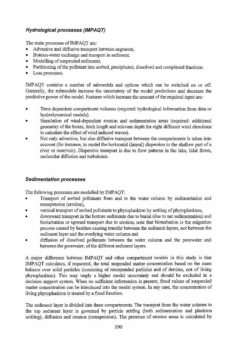
Hydro/ogica/ processes (IMPAQT)

The main processes ofiMP AQT are: • Advective and diffusive transport between segments. • Bottom-water exchange and transport in sediment. • ModeHing of suspended sediments. • Partitioning ofthe pollutant into sorbed, precipitated, dissolved and complexed fractions. • Loss processes.

IMP AQT contains a number of submodels and options which can be switched on or off. Generally, the submodels increase the uncertainty of the model predictions and decrease the predictive power ofthe model. Features which increase the amount üfthe required input are:

• Time dependent compartment volumes (required: hydrological information from data or hydrodynamical models).

• Simulation of wind-dependent erosion and sedimentation areas (required: additional geometry of the boxes, fetch length and relevant depth for eight different wind directions to calculate the effect ofwind induced waves).

• Not only advective, but also diffusive transport between the compartments is taken into account (for instance, to model the horizontal (lateral) dispersion to the shallow part of a river or reservoir). Dispersive transpürt is due to flow pattems in the lake, tidal flows, molecular diffusion and turbulence.


The following processes are modelled by IMP AQT: • Transport of sorbed pollutants from and to the water column by Sedimentation and

resuspension ( erosion), • vertical transport of sorbed püllutants to phytoplankton by settling of phytoplankton, • downward transport in the bottom sediments due to burial ( due to net sedimentation) and

bioturbation or upward transport due to erosion; note that bioturbation is the migration process caused by benthos causing transfer between the sediment layers, not between the sediment layer and the overlying water column and

• diffusion of dissolved pollutants between the water column and the porewater and between the porewater, ofthe different sediment layers.

A major difference between IMPAQT and other compartment models in this study is that IMP AQT calculates, if requested, the total suspended matter concentration based on the mass balance over solid particles ( consisting of resuspended particles and of detritus, not of living phytoplankton). This may imply a higher model uncertainty and should be excluded in a decision support system. When no sufficient information is present, fixed values of suspended matter concentration can be introduced into the model system. In any case, the cüncentration of living phytoplankton is treated by a fixed function.

The sediment layer is divided into three compartments. The transpürt from the water column to the top sediment layer is govemed by particle settling (both sedimentation and plankton settling), diffusion and erosion (resuspension). The presence of erosion areas is calculated by

190

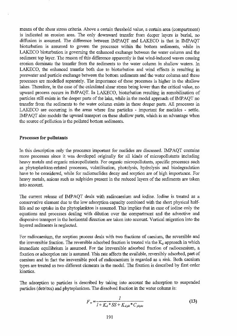
means of the shear stress criteria. Above a certain threshold value, a certain area ( compartment) is indicated as erosion area. The only downward transfer from deeper layers is burial, no diffusion is assumed. The difference between IMP AQT and LAKECO is that in IMP AQT bioturbation is assumed to govem the processes within the bottom sediments, while in LAKECO bioturbation is goveming the enhanced exchange between the water column and the sedimenttop layer. The reason of this difference apparently is that wind-induced waves causing erosion dominate the transfer from the sediments to the water column in shallow waters. In LAKECO, the enhanced transfer both due to bioturbation and wind effects is resulting in porewater and particle exchange between the bottom sediments and the water column and these processes are modelled separately. The importance of these processes is higher in the shallow lakes. Therefore, in the case of the calculated shear stress being lower than the critical value, no upward process occurs in IMPAQT. In LAKECO, bioturbation resulting in remobilisation of particles still exists in the deeper parts of the Iake, while in the model approach of IMP AQT no transfer from the sediments to the water column exists in these deeper parts. All processes in LAKECO are occurring in the areas where fine particles - important for nuclides - settle. IMP AQT also models the upward transport on these shallow parts, which is an advantage when the source of pollution is the polluted bottom sediments.

Processes for pollutants

In this description only the processes important for nuclides are discussed. IMPAQT contains more processes since it was developed originally for all kinds of micropollutants including heavy metals and organic micropollutants. For organic micropollutants, specific processes such as phytoplankton-related processes, volatilisation, photolysis, hydrolysis and biodegradation have to be considered, while for radionuclides decay and sorption are of high importance. F or heavy metals, anions such as sulphides present in the reduced layers of the sediments are taken into account.

The current release of IMP AQT deals with radiocaesium and iodine. Iodirre is treated as a conservative element due to the low adsorption capacity combined with the short physical halflife and no uptake in the phytoplankton is assumed. This implies that in case of iodirre only the equations and processes dealing with dilution over the compartment and the advective and dispersive transport in the horizontal direction are taken into account. Vertical migration into the layered sediments is neglected.

For radiocaesium, the sorption process deals with two fractions of caesium, the reversible and the irreversible fraction. The reversible adsorbed fraction is treated via the Kd approach in which immediate equilibrium is assumed. F or the irreversible adsorbed fraction of radiocaesium, a fixation or adsorptionrate is assumed. This rate affects the available, reversibly adsorbed, part of caesium and in fact the irreversible pool of radiocaesium is regarded as a sink. Both caesium types are treated as two different elements in the model. The fixation is described by first order kinetics.

The adsorption to particles is described by taking into account the adsorption to suspended particles (detritus) and phytoplankton. The dissolved fraction in the water column is:

Fw 1 + Kd * SS + Kd,ph * C phyto

1 (13)

191

where Kd is the traditional adsorption or distribution coefficient in m3 /kg and Kd ph the adsorption coefficient for caesium on phytoplankton in m3 /kg, SS the suspended sedime~t concentration in m3 /kg and Cphyto the phytoplankton concentration in the water column in kg/m3

.

In IMPAQT, the Kd of solid particles is expressed in relation to the lutum content (particles smaller than 2 ~-tm), the illite content and the concentration of competitive ions for adsorption on illite. This is based on the idea of selective adsorption at specific sites of the clay minerals. Principally, this is similar to the approach applied in LAKECO, but there the relationship between the parameters is linear, whereas in IMP AQT a linear-power relation is used. In case of the IMP AQT model, the expression is generally described according to equation 14.

- jr jr b*NH4 c*K+ Kd - a X il/ite X lutum X I 0 X I 0 (14)

where a is a coefficient for illite (1/kg illite)"1, b the coefficient for ammonium in (g N/m3

)"\ c the coefficient for potassium (g/m3

)"1, Frmite the fraction of illite in lutum, Fr1utum the fraction of

lutum in the sediment layer, NH4 is the ammonium concentration in the sediment layer or water column in g N/m3 and K+ the potassium concentration in the layer in g/m3

.

In IMPAQT, the fraction of irreversible adsorbed caesium is assumed nottobe present in the dissolved phase and not to be bioavailable. This is realised by setting the fraction of irreversibly adsorbed caesium in the dissolved phase (both in the water column andin the sediment layer) andin phytoplankton (in the water column) to zero.


The model for the biological uptake is called UPTAQE and was tested in the Netherlands, for the accumulation of mercury in fish in the Iake IJsselmeer (De Vries & Pieters, 1989). The model has been applied for various micropollutants with the objective to analyse the effect of remedial measures to improve the quality of the aquatic environment. For specific lake ecosystems various pollutants affected the composition ofthe biota. This UPTAQE modelwas applied e.g. by Delft Hydraulics to evaluate the effects of removal of sediments on the Ievels of micropollutants in the various species of the aquatic foodweb in freshwater systems such as the lake Ketelmeer and the Holland' s Diep in the Netherlands.

The foodweb model

UPTAQE is a dynamic foodweb modeland was originally developed to model the transfer of micropollutants in aquatic food chains. However, the description ofthe foodweb is based on the pharmokinetic equation, in which all processes are based on nuclide-independent ecological and physiological parameters. The approach is therefore flexible and any foodweb can be constructed to model the transfer of nuclides in the aquatic food chain.

So far, UPTAQE has not been applied to radionuclides, but KEMA used this model principle also in its LAKECO model developed parlicularly for radionuclides.

192

Contrary to LAKECO, UPTAQE can only be applied as a descriptive model due to the lack of powerful submodels. UPTAQE has been applied mostly to support field studies and feasibility studies on sanitation measures (remedial measures). UPTAQE was not developed as a predictive tool, but can be applied to evaluate the actual situation of a lake ecosystem. In these cases, the simplified steady state release ofUPTAQE, CHEOPS, is applied.

When UPTAQE is applied with a standard set of nuclide independent parameter values for various groups of organisms such as detritus feeders (benthos), Zooplankton, phytoplankton, filter feeders (molluscs), predator and prey fish, the number of model-specific parameters is reduced, which increases the flexibility of the model. As input, the CHEOPS or UPTAQE model requires biomass and food preference which is obtained by Delft Hydraulics by means of the carbon flux model MC2

. Delft Hydraulics applies MC2 to calculate the biomass and changes in the biomasses after remedial measures or after increasing pollution. For radionuclides, changes of the biomass resulting from the concentration in the environment are of minor importance. However, remedial measures such as lowering the uptake ofradionuclides by potash treatment, liming or fertilisation (Abrahamson & Häkanson, in press; Fredriks & Häkanson, in press) could affect the biomass of the aquatic species and the foodweb composition by changing the trophic status of the lake. For the application in a decision support system, these kinds of complicated models, where the levels in the biota are calculated, cannot be recommended. Eventually, the change in the food pattem as a consequence of countermeasures can be modelled by MC2 or by simpler equations derived from literature (Peters and Häkanson, 1996). It must be noted that Delft Hydraulics often uses the biomass model not only to support the uptake model with food preferences and biomass, but also to answer the question as to which extent the biomass recovers after remedial measures when toxic concentration are lowered. In case of radionuclides, MC2

could be used to construct the foodweb composition, but the foodweb can also be constructed on the basis of field data on stomach contents of fish, or based on generic data of a lake ecosystem (eventually classified by the trophic status).

The disadvantage of UPTAQE (or CHEOPS) is that the model was never developed as a predictive tool to be used when a minimum amount of input data is available. However, UPTAQE can be used in its most simplified release with standard values for all biological parameters. The model was mostly applied by Delft Hydraulics: 1. to calculate the actual situation of the toxic levels in biota in steady-state situations and 2. to calculate the effect of potential countermeasures on the concentration of toxicants in

the biota.

Since the model approach is strongly related to biophysical processes, it can be applied for radionuclides, too. The use of standard sets of input values for nuclide independent parameters for each group of organisms seems tobe sufficient. When using similar equations in LAKECO, sufficiently precise results for various radionuclides were obtained. LAKECO in fact is an UPTAQE release adapted to radionuclides and tested on accidental releases to lake ecosystems in entire Europe.

Therefore, UPTAQE can be regarded as a comprehensive tool which can be used, possibly in combination with the Delft Hydraulics' carbon flux model MC2

, to describe the uptake of pollutants in biota. It could be modified to radionuclide uptake modelling, if required. However, it might be too complex for the application in decision support systems. Therefore - as in IMP AQT - the most simplified release must be used, in combination with standard sets of input

193

values. In addition, predictive tools should be developed to assess all relevant parameters based on the prevailing environmental conditions.

Modelling more nuc/ides

At present, IMP AQT has been developed to model radiocaesium and iodirre in the aquatic environment. The model is principally designed in a way to deal with more nuclides, but has not been applied for a wider range of nuclides yet. The UPTAQE biological uptake model has not yet been modified to perform calculations for the transfer of nuclides throughout the aquatic food chain.

Possibi/ity to app/y the model in Centra/ Europe


The temporal and spatial ranges of the IMP AQT and UPTAQE models are dependent on the compartimentation chosen for a certain lake area. It is obvious that selecting of a large number of compartments, enables IMPAQT/UPTAQE tobe applied in the short termandin the near field. This is in fact similar to 2-D modelling. However, in this case also hydrodynamic models, also available at Delft Hydraulics, should be applied to predict the transfer between the individual compartments. To cover lakes in large areas such as the German territory, the simplified release of IMP AQT should be used to reduce the required input data sets per lake ecosystem.


The required input of IMPAQT, the dispersion model and UPTAQE, the biological uptake model, is listed below. It must be noted that IMP AQT has a large number of submodels which can be switched off to use predefined functions, field data or simply constants. For comparison reasons, it is assumed in this list that a lake is modelled by means of a single compartment (no hydrodynamic model necessary) and that most ofthe additional models, requiring extensive data sets, are switched off.

Required input data ofthe IMPAQT and UPTAQE models:

Geographical and hydrological information • Lake volume (m3

)

• Water residence time ( d) • Meandepth

Chemical information • Potassium and ammonium concentration in lake water and bottom sediments (mg/1)

Sedimentological information • Settling rate suspended sediment (m/d) • Resuspension coefficient (mg m"3 dag "1

)

194

• Wind speed coefficient (-) • Windspeed (m/s) • Mortality rate phytoplankton (d-1

)

• Temperature coefficient (-) • Temperature (°C) • Concentration phytoplankton (mg/1) • Phytoplankton settling rate (m/d) • Fraction oflutum (small particles) in bottom sediments (-) • Fraction of illite in bottom sediments (-) • Coefficients of ammonium, potassium and illite ( see section above)

Radiological information • Atmospheric load (lake) in KBq m2

• Month offallout • Physical half-life of radionuclides • Concentration Factor Phytoplankton (1/kg) for other nuclides than radiocaesium and

radiostrontium (used in IMPAQT as ~,phyt) • Fixation rate (from reversible to irreversible) ofradiocaesium in particles (d-1

)

Biological information • Aquatic food chain information

Predator and prey fish Predator prey relations

• Biological half-life for organisms in the food chain ( d) • Growth and respiration rates of organisms (d-1

)


IMPAQT was applied by Delft Hydraulics on the lakes Ketelmeer, IJsselmeer and Markermeer, on the Scheldt Estuary and on the Rhine - Meuse estuary to model the dispersion of organic micropollutants and heavy metals. The high quality of the model system was demonstrated by its good results. IMP AQT has been modified for iodine and radiocaesium, but no validation studies have been reported yet (manual Delft Hydraulics, 1993) on radiocaesium. Certainly, it could be expected that radiocaesium and other nuclides could be modelled without significant problems.

CHEOPS (in combination with IMP AQT and with a hydrodynamic model called ZWENDL) the steady-state release of the biouptake model, was validated on mercury for the lakes IJsselmeer, Ketelmeer and Markermeer for the accumulation in perch and pikeperch (De Vries & Pieters, 1989). lt was successfully applied in an ecotoxicological study on the possible effects of sediment dredging and the construction of a harbour sludge depository in the contaminated 'Hollandsch Diep' (Delft Hydraulics, 1992). lt is not clear whether UPTAQE was tested and validated for radiocaesium and iodine.

In this section no real conclusions can be drawn regarding the validity of IPMAQT and UPTAQE for radionuclides. The models were generally applied to toxic pollutants and used as descriptive or environmental assessment tools rather than as predictive tools. Nevertheless it can be assumed that these models, in their simplified form, can be applied for radionuclides, too.

195


The software of Delft Hydraulics computer codes is an institute property. The software is designed as a tool to solve sets of differential equations and has the possibility to implement any user defined process. The software was applied in and transferred to governmental institutes in the Netherlands in various joint projects in which Delft Hydraulics remained the owner. Excellent manuals and documentation are -mostly freely- available at the Delft Hydraulics institute.



As output IMP AQT provides the time dependent concentration of suspended matter in the water column (including detritus), the concentration in phytoplankton (when calculated), the total concentration of nuclides in Iake water (the sum of dissolved and particulate concentration; suspended matter and phytoplankton) and the concentration in the bottom sediments. This output is post processed and presented in curves within the software structure of IMP AQT. This software is developed by Delft Hydraulics and contains a user interface running under DOS on a PC.

There seems to be no Windows or UNIX environment around the IMP AQT model. There are no radiological models present or linked with IMP AQT to calculate dose effects of discharged radionuclides (IMP AQT is a dispersion model in the first place ). The modularisation of IMP AQT provides a good input - output management. By means of these output files, other models can calculate further dose consequences. For the implementation into IMIS/P ARK, the model should be embedded into a more user-friendly software environment.

As output UPTAQE (CHEOPS) provides the concentration ofpollutants in aquatic organisms of a Iake ecosystem.

Data assimilation

At present, the IMPAQT hydrological modeland the UPTAQE biological uptake model arenot designed to read incoming hydrological or radiological data, nor are these models able to adjust the model results on the basis of such data.


IMPAQT and UPTAQE belong to a set ofmodels developed at Delft Hydraulics to evaluate the ecological effects of releases of pollutants to the aquatic environment. One of the applications of these models is the evaluation of countermeasures such as dredging of contaminated sediments in terms of sedimentological, ecological and ecotoxicological consequences. This application, however, is rather complex and intensive field studies are needed to support the model

196

calculations. Additionally, expert knowledge is required to obtain reliable results. In case of radionuclides, ecotoxicological effects on aquatic organisms and subsequent shifts in the food availability and biomass are not expected, but certain countermeasures such as fertilisation could affect the biomass and food availability. Delft Hydraulics' biomass model MC2 could then be applied. Nevertheless, it is doubtful whether such a detailed model is useful in a decision support system for real-time management after nuclear accidents. It can be assumed that a fixed foodweb composition neglecting the biomass and changes in the biomass is appropriate for the purpose of the IMIS/P ARK system.

GoneJusion

The aquatic dispersion models of Delft Hydraulics, evaluated in this study are of high quality and complexity and suitable for use in ecotoxicological studies on lakes and reservoirs. The structural approach of the computer codes allows to link them to other aquatic models such as river and runoff models. The disadvantage is that they have never been developed as predictive tools to be used when a minimum amount of input data is available. Finding the optimum model size was never a goal within the development of IMP AQT. When applying IMP AQT in a decision support system, its flexibility has to be increased. The need of intensive food-web studies to support the application of the biological uptake model is a similar kind of disadvantage. Here too, the flexibility of the model should be increased before it can be applied to aquatic food chains under various environmental and ecological conditions.

Nevertheless, powerful submodels to assess important parameters are present in some cases (in IMP AQT). Both models IMP AQT and UPTAQE, can be applied in a mode in which many submodules are switched off and substituted by constant values for the relevant parameters. This minimises the model effort, but it has not been proven, whether this action increases the predictive power.

For the UPTAQE model, there is no Validation study performed on nuclides, although the generic character ofthe equations makes it easy to apply UPTAQE to radionuclides. It does not include countermeasures, nor is there a defined interface to other radioecological computer codes. Both models arenot implemented into a decision supportsystemsuch as P ARKIIMIS.

One can conclude that the IMPAQT-UPTAQE model system could be applied in a decision support system, but since these models were rather complex and never developed to be applied for radionuclides, model testing, validation and subsequent modifications should be performed to increase the flexibility and predictive power before IMPAQT-UPTAQE can meet the criteria of the IMIS/P ARK system.

197

BIOPATH model

The BIOPATH model was developed at STUDSVIK institute, Sweden and applied in the BIOMOVS I project (BIOMOVS, 1991). Later, this model was applied in the IAEA coordinated project VAMP under the name ECOLAKE. The aim was to develop a model that should be applied to a wide range of lake ecosystems. The models were validated mainly on Chernobyl fallout on Swedish lakes and later within the VAMP project on lakes in entire Europe.

Model specifications are: 1. Possibility to apply BIOPATH to a wide range of lake ecosystems. 2. Possibility to perform uncertainty analysis as a structural part of the model: uncertainty

bounds araund model predictions. 3. Uncertainty analysis identifies which parameters are dominant. Site specific data should

then be collected to improve the model results.


In BIOPATH, the outflow rate is calculated on the basis of the hydrological residence time in the standard way: Rate= 1/Tresidence· The residence time is calculated using the generic expressIOn:

V T= Q(t) (1)

where Q(t) is the discharge in m3/d ofthe inflowing or outflowing water and V is the volume of the lake in m3

.

When no information on the seasonal fluctuation in the discharge is available, the mean annual discharge rate Q is used. F or deep lakes with depths of more than 10 m, the volume of the epilimnion is used instead of the entire lake volume.

The secondary load of the lake, which is caused by catchment runoff, is described in a generic way. Specific in this model is the modification by a function to consider a higher land-to-lake transfer in the case oflakes in the Nordic areas (equation 16).

Outjlowrate = 1 o-.t * D * ADA * EXP(-"A * t) * MOD (2)

where Disdepositionon the catchment area in Bq m·2, ADA is the drainage area in m2, "Ais the

decay constant for the radionuclide and MOD is a moderator to correct for Nordic lakes of high altitude: MOD is equal to 10 for Nordic lakes and equal to 1 in other areas.

198


The sedimentation process in BIOPATH and ECOLAKE is modelled by the following generic equation as e.g. in LAKECO:

(3)

where Kd is the distribution coefficient defined as the ratio of nuclide concentration in the particulate phase (Bq/kg) and concentration in the dissolved phase (Bq/1), in 1 kg-1 and SS is the suspended matter concentration in kg/1.

In BIOPATH and ECOLAKE, the presence ofinsoluble particles (or fuel particles) is treated by modifying the Sedimentation rate by means of a 'distance moderater'. It is assumed that the sedimentation rate is higher closer to the source of radionuclides due to the fact that settling of fuel particles is a relatively fast process.

The sediment model of BIOPATH and ECOLAKE is kept as simple as possible in terms of processes. The sediment is subdivided into two layers, the top and the deep sediment layer. The transfer between the top sediment layer and the overlying water column as weil as between the top sediment layer and the deep sediment layer is described by a single rate without physical meaning. This rate is mostly derived by fitting the model to measurements. The second deeper sediment layer is regarded as a sink, since no transfer from this deep layer to the top layer is assumed.


The feodweb modelling in BIOPATH (ECOLAKE) is treated by a set of differential equations of first order, representing each group of organisms as a single compartment with input and output fluxes. In the code, the total biernass of the organisms in the lake is required but no predictive submodel to assess this parameter is present. To increase the flexibility of the computer model, some empirical moderators are included into the process descriptions of the various trophic Ievels to deal with different Iake types.

BIOPATH was tested on data sets on radiocaesium in Swedish lakes with two distinct releases, BIOPATH 1 and BIOPATH 2. In BIOPATH 2, planktonwas taken into account as food for the top predator, while in BIOPATH 1 the top predator was strictly piscivorous and the prey fish was contaminated directly by water and not by the consumption of food. Since the approach used in BIOPATH 1 is based on a too simplified foodweb, it is not discussed here any further. BIOPATH 2, later called ECOLAKE in the VAMP study, therefore showed better predictions.

ECOLAKE uses a generic feodweb description for the transfer of nuclides in various types of aquatic foodwebs. The radionuclide uptake in plankton, benthos, predatory fish and prey fish is calculated by means of differential equations. For plankton and benthos a steady-state situationequilibrium with the water - is assumed.

The basic equation for the generic modeHing of the biological uptake in organisms is:

199

dMB organism _ * * dt - Auptake.jood MF food + Auptake, water MWwater- Ab,organism MB organism ( 4)

where /... represents the rates on a total mass basis (d-1) and MB, MF, MW are the total amount of

nuclides in the compartments fish, food and water, respectively. One ofthe problems, in aquatic radioecology models, however is to describe the biological transfer rates properly by physical or empirical approaches.

Since ECOLAKE/BIOPATH was originally developed for Swedish lakes with similar environmental properties and was used by experts only (developer ofthe model), the modelwas lacking powerft.ll submodels to deal with lakes with a wide range of environmental and climatological properties. BIOPATH in its original form (BIOMOVS I) therefore was a descriptive and not a predictive tool. To reduce the need of expert judgement and to make the model more widely applicable, some moderators where added to the foodweb model. Generally, these moderators are described as 'switches', were the user has to turn the switch after identification of the lake type as oligothrophic or eutrophic, the season as winter or summer and depending on the potassium content in the lake. These switches are in fact based on expert experience in applying the model to various lake ecosystems and are more or less multiplication or fitting coefficients. This method is far :from process-based and therefore not really suitable for the use in a decision support system. Reliable moderators to increase the flexibility should be empirically or physically based submodels and not simple switches.

The amount of nuclides in plankton is described by the steady state solution of the differential equation 18:

MP L = CF* MMp1

A.b,p * MW * (1- exp(- Ab,p t)) w

(5)

where MPL is the nuclide amount in the total biomass of phytoplankton in Bq, MW the total amount of the nuclide in the lake, MP1 is the total plankton biomass in kg, Mw the lake volume in kg ( or 1), CF the concentration factor water phytoplankton in 1/kg and Ab the biological half life phytoplankton. This method is more reliable than applying the traditional Concentration Factor method only.

The total biomass of the phytoplankton in this equation is an input parameter. This is a logical consequence of the introduction of the generally used CF approach, which is mass unit-based, while the solution of the differential equation expresses the transfer between the total amount of lake water and the total mass of plankton. The planktonic uptake rate ApJ is therefore substituted by the expression CF*A.b *MP11Mw as a consequence of the solution of the differential equation. The Concentration Factor is introduced to substitute the variable Apl,uptake• the planktonic uptake rate.

The uptake in phytoplankton is modified by three moderators to take the seasonal effects in the planktonic uptake, the lake type and the potassium concentration into account. The concentration factor phytoplankton is not - as in LAKECO, or VAMP - govemed by a processbased submodel, but only by a multiplier dependent on the above-mentioned conditions. Thus, these moderators are, as stated before, discrete numbers and no functions or mathematical

200

expressions. The planktonie uptake moderater dependent on three distinet moderators 1s expressed in the following equation:

MOD = MOD/aketype * MQD K

MODseason (6)

MODseason is equal to 1 in the summer period and 5 in the winter period, MOD1ake type is equal to 1 in the ease of an eutrophie lake, 2 in a mesotrophie lake and 3 for an oligotrophie lake. MODK is equal to 2 in lakes with a potassium eoneentration below 0.5 mg/1 and 1 at a eoneentration higher than 0.5 mg/1. For instanee, in a eutrophie lake with a potassium eoneentration higher than 0.5 mg/1 andin the summer period the value for MOD is 1, in an oligotrophie lake in the summer with a potassium eoneentration lower than 0.5 mg/1 the moderater is equal to 6, whieh implies an inerease of the planktonie uptake by a faetor of 6.

In ECOLAKE, the uptake of radionuclides in benthos is deseribed, assuming the transfer of nuclides from sediment particles via benthie organisms to higher organisms. Experiments, however, demonstrated that a minor fraetion ofthe particle bound eaesium (detritus) eonsumed by benthie organisms was transferred to fish, due to the low bioavailability of the adsorbed particles (Kolehmainen, 1973).

The benthonie uptake rate is deseribed in a similar way as the planktonie uptake; in this ease the transfer to benthos from sediments instead of water is modelled. A relatively low transfer, as indieated above, is eonsidered by assuming a low Coneentration Faetor for benthos to sediments. And again, the uptake is modified by means of a moderater in a similar way as for the planktonie uptake.

The uptake of nuclides in fish is assumed to oeeur via food ingestion only (Hewett & Jefferies, 1976); the direet uptake via the gills is negleeted. Instead of using the eoneentration faetor predator- prey, the uptake rate by eonsumption is deseribed as in LAKECO, without substituting the uptake rate as in the ease of planktonie and benthie uptake rates.

The uptake rate in predator fish is deseribed in the generie way, but modified with a temperature moderater in the following way:

'\ *K Mprea *MOD 1\,uptake = a 1-- temp Mprey

(7)

where a is the uptake fraetion, MC is the dimensionless temperature moderater, Mpred and Mprey are the biomass of the predator and the prey, respeetively, in kg and K1 is the eonsumption rate in kg ki1 month"1

.

The biologieal half-lives for the organisms in the foodweb are based on expertjudgement for the various organisms related to the eeosystem eonditions. No submodel to assess this important parameter for fish was introdueed. The eoneentration faetors for plankton and benthos in ECOLAKE are based on literature values and on baekfitting ofthe model to measurement data.

201

Modelling more nuc/ides

As most ofthe lake models evaluated in this study, ECOLAKE and BIOPATH were originally designed, validated and tested to describe the distribution of radiocaesium in lake ecosystems. Since these computer codes are designed in a generic way with a relative low amount of nuclide specific processes, the model could be modified easily for other nuclides. The caesium specific moderators are to be substituted and validation tests are required to find new nuclide specific moderators. But it is necessary to increase the number of processes considered and also the amount of easily measurable environmental parameters to improve the model flexibility and applicability and not to rely on expert judgement only. Then the model could have a higher predictive power which is necessary as a predictive tool.

Possibility to app/y the model in Centra/ Europe


The ECOLAKE/BIOPATH model is a compartment model. The model can be applied to predict the behaviour of radiocaesium in lake ecosystems with different environmental properties. The size of the lake is restricted to lakes with a lake volume in which mixing can be assumed. F or considerations of the general applicability of compartment models in terms of temporal and spatial resolution, we refer to the section in which the compartment model VAMP is evaluated in terms of applicability in Central Europe (see this Appendix).

ECOLAKE and BIOPATH are not developed to be applied to deep lakes with stratification periods. When ECOLAKE is applied to deep lakes, as was clone within the framework of the VAMP project, the rapid decrease of the nuclide concentration during the mixing period could not be reproduced by the model.


The BIOPATHIECOLAKE model is, as mentioned earlier in this section, a generic model including some moderators which relate various model-specific parameters to environmental conditions. But these moderators are in fact fitting parameters or conceptual multipliers based on expert knowledge and validation experience. They are not based on processes or empirical and statistical relationships as it is the case for the models VAMP and LAKECO. As a result, ECOLAKE can be applied to a wide range of ecosystems, but expert knowledge is necessary to obtain reliable predictions. The STUDSVIK models, although modified on the basis of validation tests to improve the flexibility, cannot be recommended asthebest predictive tool in this study due to the descriptive character ofthe codes.


The required input ofECOLAKE is listed below.

202

Required input data ofthe ECOLAKE model: Environmental, geographical and hydrological information • Altitude (high altitude/low altitude) • Size ofthe catchment area (m2

)

• Lake volume (m3)

• Water residence time ( d) • Mean depth ofthe lake (m) • Discharge rate (lake outtlow) in m3 /d

Chemical information • Trophic status of the lake (lake type: oligotrophic/mesotrophic/eutrophic) • Potassium concentration in lake water (mg/1)

Sedimentological information • Sedimentation rate of suspended matter (g m-2 year-1

)

Biological information • Aquatic food chain information • Predator and prey fish • Predator prey relations • Total biomass of plank:ton, benthos, prey and predator fish in the lake. • Concentration Factor plank:ton and benthos (to sediment)

Radiological information • Atmospheric load (both lake and catchment) in K.Bq m2


ECOLAKE was tested on seven lakes in Europe within the framework ofthe VAMP project; the results are published in the IAEA Techdoc (IAEA, in press). These tests showed a relatively good agreement between predictions and measurements. The earlier release of ECOLAKE, BIOP ATH, was tested on data sets from two Swedish and one American lake within the framework of BIOMOVS I, an international validation study with blind data sets. But STUDSVIK was mentioned in the final report tobe the data supplier (BIOMOVS I, 1991) and reported that the model had been calibrated on these measurement data in an earlier stage. The model concept was also successfully tested on the transfer of radiocaesium in Nordic lakes (Nordlinder et al., 1993). Generally, model predictions varied within a factor of two from the observed values.


ECOLAKE, developed at STUDSVIK, is an institute-owned package to solve differential equations. The code is used in combination with the statistical package PRISM. This package enables the user to perform uncertainty analysis as an integrated part of the calculations. Predictions are presented with the uncertainty bounds and PRISM gives a ranking of the

203

sensitivity of the parameters as a function of time. This is a powerful part of the ECOLAKE model.

The codes and the documentation are institute property and probably not :freely available. The codes were not developed as user-friendly tools for commercial distribution, but as scientific tools to evaluate the radiological impact of accidental and regular releases of radionuclides into the environment. The software package is developed for the PC environment (DOSenvironment).



As output the model provides the time-dependent concentration of radiocaesium in lake water, in sediments, in prey and predator fish together with the uncertainty ranges of these variables. The computer code calculates: • the mean values, • the standard deviation, • the coefficient of variation, • the geometric mean and • the percentages In its present version, the model output is listed as tables (stored in files) presented within the user environment. The models are stand-alone codes, with no links to other aquatic and dose models nor to graphical interfaces.

Data assimilation

At present, the STUDSVIK models ECOLAKE and BIOPATH are not designed to read incoming hydrological or radiological data and to adjust the model results on the basis of such data.


No countermeasures are treated in ECOLAKE and BIOPATH.

GoneJusion

ECOLAKE is an appropriate model to predict the behaviour of radiocaesium when sufficient measurements on nuclide concentrations are present to calibrate the model before. Due to lacking predictive submodels to assess important parameters, the quality of the model predictions is related to the availability of observations. As a predictive tool, the model is less applicable especially when no radiological or hydrological data are available, however, this might often be the case in emergency circumstances. ECOLAKE is applicable when calculations . are supported by field measurements. When important parameters are collected in the initial

204

phase, the predictions become more reliable. If data are nnssmg, conservative parameter assumptions are used to avoid underpredictions. An advantage of ECOLAKE is the link to the statistical code PRISM which provides not only point values but also the uncertainty ranges.

At present, the model is not implemented in a user friendly radiological assessment tool, nor does it contain countermeasure modules or data assimilation methods.

The model flexibility is reasonable, but not sufficient to deal with a wide range of lake ecosystems in Central Europe. An important drawback is the necessity of expert knowledge to operate the model.

As a fmal conclusion it may be stated, that the present release of the ECOLAKE compartment model does not meet the criteria, as it contains a large number of calibration parameters and rates with no physical meaning, both in the abiotic and the biotic part. ECOLAKE belongs -such as DETRA - to the type of traditional radiological models with default parameter sets to be applied for conservative assessments. The model should be improved and modified with powerful submodels, before its integration into a decision support system can be recommended. Another drawback can be seen in the fact that the model is designed to describe the behaviour of radiocaesium only, however, adjusting to other nuclides should be possible when appropriate data are available.

205

DETRA

DETRA (Doses via the Environmental Transfer of Radionuclides) was developed at the VTT institute in Finland. It is a conceptual model originally applied to describe the transfer of radionuclides in the Finnish aquatic environment. In general, the method is comparable with the model design of ECOLAKE (STUDSVIK) in terms of the model structure of the abiotic part as well of the uptake model, which is based on the total biomass (see this Appendix for ECOLAKE).

Hydro/ogical processes

As in most hydrological compartment models, such as LAKECO (KEMA) and ECOLAKE (STUDSVIK), the outflow rate in DETRA is also calculated on the basis of the hydrological residence time in the standard way: Rate = 1/Tresidence· The residence time is obtained using the generic expression:

V T= Q(t) (8)


.

When no information on the seasonal fluctuations in the discharge is available, the mean annual discharge rate Q is used. For deep lakes with depths of more than 10 m, the volume of the epilimnion is used instead of the entire lake volume.

The model applied in DETRA to describe the secondary load, the catchment runoff, is of more complex character than that of the other compartment models in this study. Here, the vertical migration is also taken into account:

1 e I Outflowrate = -h *( Fs *-

1 -*s s +(1-Fs)*-) -8 8

(9)

where h is the depth of the infiltrated soil, F w is the dissolved fraction of the nuclide in the soil, I is the averaged annual precipitation (rnlmonth), e is the erosion rate (kg m-2 month-1

), 8 the porosity of the soil and I; the density of the soil in kg/m3

•


In DETRA, the dissolved fraction Fw is modelled by a generic equation similar to the approach used in LAKECO:

(10)

206

where Kd is the distribution coefficient defined as the ratio of the nuclide concentration in the particulate phase (Bq/kg) and the concentration in the dissolved phase, in 1 ki1 and SS is the suspended matter concentration in kg m -3.

The Sedimentation process is modelled according to the same equation as applied in LAKECO:

Kd* Fw*cr 'As= d (11)

where cr is the sedimentationrate in kg m-2 yr-1.

In model studies carried out to evaluate the radionuclide transfer in Finnish watercourses (Kor honen, 1990), better predictions were obtained, when it was assumed that a :fraction of the Chemobyl falloutwas not available for biouptake or transport. The introduction oftheinsoluble form diminished the land-to-water transfer, the resuspension and the dissolved :fraction in the lake water.

The sediment model of DETRA is kept as simple as possible. The sediment is subdivided into two layers, the top well-mixed layer and the deep, buried, sediment layer. Loss from the deep layer is treated as a sink. Downward transport appears due to sedimentation, - from the water column to the sediment layer, upward transport occurs due to resuspension. There is no upward transport from the second layer to the first sediment layer. Diffusion, bioturbation and porewater exchange are not taken into account. The sediment submodel is govemed by the Sedimentation rate and the resuspension rate. There is no possibility to relate the resuspension rate to morphologic properties of the lake ecosystem. In particular in shallow lakes, resuspension is of great importance. In Finland ,for instance, resuspension of particles in the shallow lakes transferred adsorbed nuclides downstream in large watercourses.

Biologica/ uptake modelling

DETRA contains a foodweb model based on the transfer of nuclides between individual compartments similar to the approach used in ECOLAKE. In DETRA, the transfer of nuclides from prey to predator is described by a dynamic approach, on a total biomass basis. Therefore, the total biomass of the prey fish consumed by a population of predatory fish in a certain lake ecosystem has to be estimated.

The foodweb description is realised in a generic way. The radionuclide uptake in predatory fish and non-predator fish is calculated by means of differential equations. The activity concentration in plankton (benthos are not modelled) is calculated by means of a concentration factor since steady state is assumed between concentration of radionuclides in water and fish.

In DETRA, the nuclide concentration in plankton is described by a modified concentration factor method. The radionuclide concentration in plankton is usually calculated by means of the product of the dissolved nuclide concentration in the lake water and the concentration factor: Cp1

= Cw,diss * CFpt· In DETRA, however, this is described by a method in which the plankton concentration is taken into account in the calculation of the concentration factor. In fact,

207

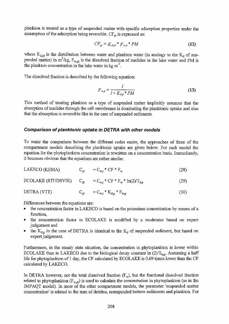
plankton is treated as a type of suspended matter with specific adsorption properties under the assumption of the adsorption being reversible. CF pl is expressed as:

CFP, = Kd,pl * Fw.p *PM (12)

where Kct,pt is the distribution between water and plankton water (in analogy to the Kct of suspended matter) in m

3/kg, F w,pt is the dissolved fraction of nuclides in the lake water and PM is

the plankton concentration in the lake water in kg m·3.

The dissolved fraction is described by the following equation:

1 F =----

w.p 1+ K *PM d,p (13)

This method of treating plankton as a type of suspended matter implicitly assumes that the absorption of nuclides through the cell membranes is dominating the planktonic uptake and also that the absorption is reversible like in the case of suspended sediments.

Camparisan af planktanic uptake in DETRA with ather madels

To make the comparison between the different codes easier, the approaches of three of the compartment models describing the planktonic uptake are given below. For each model the equation for the phytoplankton concentration is rewritten on a concentration basis. Immediately, it becomes obvious that the equations are rather similar.

LAKECO (KEMA) = C *CF* F w,t w (28)

ECOLAKE (STUDSVIK) = Cw,t * CF* Fw * ln(2)/Tb,p (29)

DETRA(VTT) (30)

Differences between the equations are: • the concentration factor in LAKECO is based on the potassium concentration by means of a

function, • the concentration factor in ECOLAKE is modified by a moderater based on expert

judgement and • the Kct,p in the case of DETRA is identical to the Kct of suspended sediment, but based on

expert judgement.

Furthermore, in the steady state situation, the concentration in phytoplankton is lower within ECOLAKE than in LAKECO due to the biological decay constant In (2)/T b,p· Assuming a half life for phytoplankton of 1 day, the CF calculated by ECOLAKE is 0.69 times lower than the CF calculated by LAKECO.

In DETRA however, not the total dissolved fraction (Fw), but the fractional dissolved fraction related to phytoplankton (F w,pD is used to calculate the concentration in phytoplankton ( as in the IMP AQT model). In most of the other compartrnent models, the parameter 'suspended matter concentration' is related to the sum of detritus, resuspended bottom sediments and plankton. F or

208

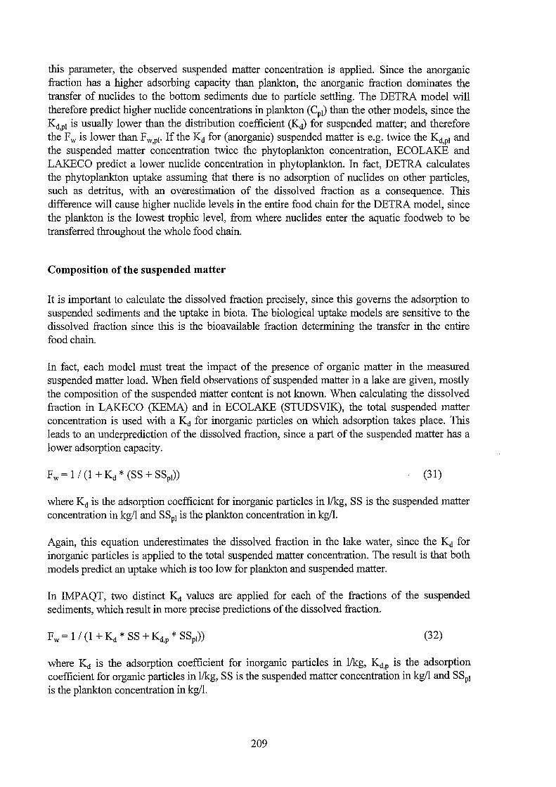
this parameter, the observed suspended matter concentration is applied. Since the anorganic fraction has a higher adsorbing capacity than plankton, the anorganic fraction dominates the transfer of nuclides to the bottom sediments due to particle settling. The DETRA model will therefore predict higher nuclide concentrations in plankton (CpJ) than the other models, since the Kd,pl is usually lower than the distribution coefficient (Kd) for suspended matter; and therefore the Fw is lower than Fw,pl· Ifthe Kd for (anorganic) suspended matter is e.g. twice the Kd,pl and the suspended matter concentration twice the phytoplankton concentration, ECOLAKE and LAKECO predict a lower nuclide concentration in phytoplankton. In fact, DETRA calculates the phytoplankton uptake assuming that there is no adsorption of nuclides on other particles, such as detritus, with an overestimation of the dissolved fraction as a consequence. This difference will cause higher nuclide Ievels in the entire food chain for the DETRA model, since the plankton is the lowest trophic Ievel, from where nuclides enter the aquatic foodweb to be transferred throughout the whole food chain.

Composition of the suspended matter

It is important to calculate the dissolved fraction precisely, since this governs the adsorption to suspended sediments and the uptake in biota. The biological uptake models are sensitive to the dissolved fraction since this is the bioavailable fraction determining the transfer in the entire food chain.

In fact, each model must treat the impact of the presence of organic matter in the measured suspended matter load. When field observations of suspended matter in a lake are given, mostly the composition of the suspended matter content is not known. When calculating the dissolved fraction in LAK.ECO (KEMA) and in ECOLAKE (STUDSVIK), the total suspended matter concentration is used with a Kd for inorganic particles on which adsorption takes place. This Ieads to an underprediction of the dissolved fraction, since a part of the suspended matter has a lower adsorption capacity.

(31)

where Kd is the adsorption coefficient for inorganic particles in 1/kg, SS is the suspended matter concentration in kg/1 and SSP1 is the plankton concentration in kg/1.

Again, this equation underestimates the dissolved fraction in the lake water, since the Kd for inorganic particles is applied to the total suspended matter concentration. The result is that both models predict an uptake which is too low for plankton and suspended matter.

In IMP AQT, two distinct Kd values are applied for each of the fractions of the suspended sediments, which result in more precise predictions of the dissolved fraction.

(32)

where Kd is the adsorption coefficient for inorganic particles in 1/kg, Kd,p is the adsorption coefficient for organic particles in 1/kg, SS is the suspended matter concentration in kg/1 and SSpi is the plankton concentration in kg/1.

209

In DETRA, some intermediate approach seems to be applied by lowering the Kd value when calculating the dissolved fraction, but using the total suspended matter concentration.

(33)

where Kd' is the corrected value (in situ Kd) to take into account the presence of organic matter in the lake water.

In the BIOMOVS I comparison study, DETRA's approachwas applied to the Swedish lake Hillesjön. Its Kd' value was significantly lower than that used by other modelers in the study and even equal to the concentration factor for phytoplankton Ks,pl· It was not clear from the documentation whether this Kd' value was based on expert knowledge or not. The correct way to calculate Kd' is expressed in the following equation:

(34)

The selection of a value for the Kd' equal to the value for Kd,pi in the case of lake Hillesjön (suspended sediment with an organic fraction of 50%), implies, that Kd is equal to Kd,pl· For radiocaesium this is unlikely. But even when this value is basedonexpert knowledge, equation (32) should be used in the calculation ofthe plankton concentration, taking into account the total suspended matter concentration instead of the organic fraction of the suspended matter as in equation (27).

In the IMP AQT model, the different fractions of suspended matter ( organic and inorganic) are treated separately, with different distribution coefficients Kd, suspended matter concentrations and settling rates for each fraction. This is the most correct approach, but requires more input parameters than those of the other compartment models.

It may be concluded, that the nuclide concentration in plankton is in fact overpredicted in DETRA and is slightly underpredicted in ECOLAKE and LAKECO. The correct method is the approach used in the IMP AQT model.

Uptake in organisms

In DETRA, benthos is not modelled, since it is not apart of the foodweb. As in ECOLAKE, the uptake ofnuclides in fish is assumed tobe via food ingestion only (Hewett and Jef:fries, 1976); the direct uptake via the gills is neglected.

The uptake rate Aupt,prey from plankton to prey fish is described and expressed in equation 3 5.

_ * Kprey Aupt.prey - C pl MP REY (35)

where CP1 is the nuclide concentration in phytoplankton, MPREY is the total biernass of the prey in the entire lake in kg and KP1 is the rate at which plankton is eaten by the entire prey fish population in kg/year.

For the transfer Aupt,pred from prey to predator fish, a similar equation is applied:

210

_ * Kpred Aupt.pred - C pr MP RED (36)

where Cpr is the calculated nuclide concentration in prey fish, MPRED is the total biernass of the predator in the entire lake in kg and Kpred is the rate at which the prey fish plankton is eaten by the entire predator fish population in kg/year.

As input, the total biernass of the prey fish consuming plankton and predator fish consuming prey fish is required as well as an assessment of the loss of plankton due to consumption of fish and the loss of prey fish due to the consumption of predatory fish. Although the equation is written on a concentration basis, the model works on a compartment basis. This seems to be the most appropriate description, but requires a lot of knowledge on the lake ecosystem. In LAKECO the equations are derived on a mass basis, but physiological parameters are required, assuming an optimum food uptake for each organism. This may lead to an overestimation of the uptake, but in LAKECO it is assumed that the fish population in a lake is in equilibrium with its prey organism and no shortage of food occurs. However, it is not completely clear from the descriptions whether DETRA follows the general approach of assuming optimum feeding pattems or the approach of the total biernass requiring a lot of input data. When it uses the first method, standard values for the respiration and growth rate can be assumed to calculate the food consumption rate. Otherwise, the model is less applicable due to the necessity of biomass estimations.

The biological half-lives ofthe organisms in the feodweb are based on expertjudgements for the various organisms related to the conditions in the ecosystem; no submodel to assess this important parameter for fish is introduced. The concentration factors for plankton are based on Iiterature values and on backfitting to measurements.

Mode/ling more nuc/ides

DETRA is designed in a generic way and can be regarded as a descriptive model tool. Most of the parameters are model-specific, which has the disadvantage that expert judgement is required. However, there also is the advantage that the adaptation to other nuclides is possible, since only nuclide-specific parameters have to be changed. The model has been applied to the transfer of radiocaesium and radiostrontium in Finnish watercourses, but the biological component was only tested on radiocaesium.

Possibility to app/y the model in Centra/ Europe


The model is a compartment model and suitable to be applied for lakes in which fully mixed conditions exist. For considerations ofthe general applicability of compartment models in terms of temporal and spatial resolution, we refer to the section in which the compartment model VAMP is evaluated in terms of applicability in Central Europe (see chapter VAMP in this Appendix).

211

DETRA is not developed to be applied to deep lakes with stratification periods. \Vhen DETRA is applied to deep lakes, as was done within the framework of the VAMP project, the rapid decrease of the nuclide concentration during the mixing period could not be reproduced by the code.


The DETRA model is, as mentioned earlier in this section, a generic model. There are no submodels implemented to allow an automatic adaptation to specific lake ecosystems. DETRA is a descriptive model to be used by experts and should be regarded as an investigation tool to test various scenarios. As a result, DETRA could be applied to a wide range of ecosystems, but expert knowledge is necessary to obtain reliable predictions. DETRA therefore has its limitations with respect to the application as a predictive tool in a decision support system. It must be noted that VTT, in collaboration with the Finnish institute STUK and as part of the RODOS project, is developing a classification scheme for lakes on the basis of various environmental parameters. This classification scheme allows to sort all lakes of a certain territory into a limited number of standard lakes only which makes it easier to apply a lake model to a large area with many lakes as only the standard lakes are considered. This classification procedure will be completed in 1998. A recommendation is to apply this classification method as aseparate tool for any decision support system. However, as this tool is still under development, it cannot be evaluated in this report.


The required input ofDETRA is listed below.

Environmental, geographical and hydrological information • Density of the soil in the catchment (kg/m3

)

• Size ofthe catchment area (d) • Depth of infiltrated soillayer in the catchment (m) • Porosity of the soil in the catchment (-) • Erosion rate soil to lake surface (kg m"2 y"1

)

• Water residence time ( d) • Mean depth ofthe lake (m) • Discharge rate (lake outflow) in m3 /d

Sedimentological information • Sedimentation rate of suspended matter (g m-2 year-1

)

Biological information • Aquatic food chain information • Predator and prey fish • Predator prey relations • Totalbiomass ofplankton, prey and predator fishin the lake. • Concentration Factor for plankton

212

Radiological information • Atmospheric load (both lake and catchment) in KBq m2


DETRA was tested on a cascade of Finnish lakes, -the Kymijoki watercourse-, (Korhonen, 1990) and on seven lakes in Europe within the framework ofthe VAMP project. The results are published in the IAEA Techdoc ofthe VAMP project (IAEA, in press). Within the framework ofBIOMOVS I, DETRA was tested successfully on lake Hillesjön (one ofthe three lakes in the lake scenario) with independent data sets (BIOMOVS, 1991). Generally, these tests showed a relatively good agreement between predictions and measurements. It must be noted that DETRA was continuously under development. In the VAMP study the original catchment model with a large number of vertical layers was substituted by an simplified model as described in this chapter, but still the samenamewas used.


DETRA is implemented in a particular software environment, which has been developed at VTT to solve differential equations. This package is comparable with commercial packages such as Timezero (Kirchner, 1990), or with the BIOPATH package owned by STUDSVIK. DETRA is applied as a scientific tool to perform radiological impact studies and therefore it is assumed that the code and the documentation are institute property and not freely available. Besides that, DETRA has never been developed as a commercial package with manuals, but as a scientific tool to support risk assessment studies.

Criteria for imp/ementation into a decision support system


As output the model provides the time dependent radionuclide concentration in lake water, in sediments, in prey and in predator fish.

In the present version of DETRA, the model output is listed in tables and stored in files. There is no link to other aquatic or radiological models and there exists no graphical presentation of the results.

Data assimilation

At present, DETRA is not designed to read incoming hydrological or radiological data and to adjust the model results on the basis of such data.

213


In DETRA, there is no countermeasure modeHing considered. The coupling to hydrological countermeasure models would be problematic since there are no features in DETRA which depend environmental parameters such as potassium or calcium concentration in lake water.

Conc/usion

DETRA is able to describe the behaviour of radiocaesium and radiostrontium in a lake system, when sufficient measurements on nuclide concentrations are present to calibrate the model before. The model can be regarded as a descriptive computer code or as a scientific tool for risk assessment.

As a predictive tool, the model is less applicable, in particular when no radiological or hydrological data are available, which is often the case in emergency situations. DETRA is applicable when calculations are supported by field measurements. The predictions become more reliable when important parameters are collected in the initial phase.

At present, the model is not implemented into a user-friendly environment nor does it contain countermeasure modules or data assimilation methods. However, there might be the possibility to integrate DETRA into a decision support system with other aquatic modules.

The flexibility of the model is not sufficient to deal with a wide range of lake ecosystems in Central Europe: The need of expert knowledge to operate the model is an important drawback of DETRA.

Finally it may be concluded that the present release ofthe DETRA compartment model does not meet the criteria since it contains a large number of model specific parameters. The model is not flexible in terms of design and lacks processes driven by environmental parameters. Modifications are necessary to apply the model to large regions such as the German territory. DETRA belongs to the type of traditional radiological models with default parameter sets to be applied for conservative assessments. The model should be improved and modified with powerful submodels before it can be built into a decision support system. Another drawback of the model is its limitation to describe the behaviour of radiocaesium and radiostrontium only, however, adjusting to other nuclides should be possible when appropriate data are available.

214

MARTE

In 1991, a model for the behaviour of dissolved nuclides in deep lakes was developed at ENEA, Italy and tested on two deep Italian lakes (Monte et al., 1991). To model the behaviour of nuclides properly, a description for stratification (monomictic) was implemented into the code. Since one of the main lakes, Bracciano, contains a very low suspended matter concentration, the contribution of the particulate fraction was assumed to be negligible. The model gave satisfying results for lake Bracciano, but was less reliable in the case of the second lake in the study, lake Vico, since the particulate matter in this lakewas not negligible. Therefore, the model MARTE (Model for Assessing the migration of Radionuclides Transport in the aquatic Environment) was developed which also takes into account the adsorption to suspended particles. MARTE was been tested within the framework of the VAMP project (IAEA, in press) and the model results for seven European lakes were published (Monte, 1993). To assess the initial concentration on the basis of deposition data, a submodel was developed and added to the computer code (Monte, 1995). In this section, MARTE is described briefly with the model release developed for deep lakes being emphasized.


In MARTE, as in most of the other hydrological compartment models such as LAKECO (KEMA) and ECOLAKE (STUDSVIK), the outflow rate is calculated on the basis of the hydrological residence time in the standard way: Rate = 1/Tresidence- The residence time is calculated using the generic expression:

V T= Q(t) (37)


•

When no information on the seasonal fluctuation in the discharge is available, the mean annual discharge rate Q is used. F or deep lakes with depths of more than 1 0 m, the volume of the epilimnion is used instead of the entire lake volume. In this case three vertical layers are considered, the epilimnion receiving water from the catchment and with an outflow via the Iake outlet, the thermocline and the hypolimnion. For instance, in Bracciano, the importance of modelling stratified layers was obvious since, after Chemobyl, the radionuclides in the deep Italian mountainous Iake entered the epilimnion (with a depth of approximately 10 m) during the summer stratification. Subsequent mixing in autumn diluted the nuclides within the entire Iake volume (total depth 89 m).

In MARTE, an approach has been developed for use on monomictic lakes (weil mixed, except in the summer period) typical for areas at high altitudes in the subalpine regions. In the model an active layer is defined which is in contact with the environment. During the winter period or mixing period, the active layer has its maximum depth and the transfer by diffusion between the

215

active layer and deeper layers is relatively high due to the absence of a vertical temperature gradient ( or due to the absence of a thermocline ). This causes a mixing effect between the active and deeper layers. In the spring, solar insolation causes a vertical temperature gradient which starts the summer stratification and the active layer then becomes the depth of the epilimnion. This depth remains stable till the end of the summer period, when the temperature difference and, hence, the epilimnion, starts to disappear, followed by the mixed period in winter. The interaction between the epilimnion and the hypolimnion is relatively low in this period.

This method is applied for monomictic lakes, but could be modified for dimictic lakes - lakes with stratification during the whole year with spring and autumn mixing - by changing the diffusion rates to a high value in the mixing periods and to a low value in the remairring stratified periods. The model needs the epilimnion or active depth as input. For the deep Italian lakes of the VAMP study, these were derived on the basis of temperature proflies measured in the summer. There is no thermic submodel included to predict the change of the epilimnion depth; this has to be estimated by the user.

The model applied in MAR TE to consider the secondary load, the catchment runoff, is defined by equation 38. A short- and a long-term transfer is described by means ofthis transfer function:

(38)

where Q(t) is discharge from the lake to the catchment in m3/s, D is the initial deposition on the catchment area in Bq/m2, 8 is an empirical coefficient describing the ratio between initial water concentration and initial deposition, a is a dimensionless coefficient and ß(t) is a time function to take into account the non-linear behaviour ofthe transfer.

The empirical coefficients and the exponents have to be derived from measurements on the drainage area. This was completed successfully for the transfer from various catchments to lakes in Europe, Ukraine and Russia (Monte, 1994).


In MARTE, the dissolved fraction is modelled by the following generic equation such as e.g. also in LAK.ECO:

(39)

where Kd is the distribution coefficient defined as the ratio of the nuclide concentration in the particulate phase (Bq/kg) and the concentration in the dissolved phase, in 1 kg"1

, and SS is the suspended matter concentration in kg r1

•

Basically, the sedimentation rate is modelled identically to other compartments models considered in this study (VAMP, DETRA, ECOLAKE and LAKECO).

216

The sediment model of MARTE is kept as simple as possible. The sediment is subdivided into two layers, the top layer, called the sediment "interface" or "active" layer and the bottom sediments. The layer beneath the bottom sediments is not modelled explicitly, thus all fluxes out of the deepest layer are regarded as a sink.

The interface layer is in fact treated as a part of the suspended sediments, in which a fraction of the deposited nuclides is stored immediately after deposition. Although most of the other compartment models consider a top sediment layer, this layer in MARTE is a very thin slice between the bottom sediments and the water column, comparable with the approach of the IMP AQT code, but modelled as an additional suspended sediment compartment belanging to the water phase.

Downward transport occurs due to sedimentation - :from the water column to the sediment layer -, due to burial :from the interface layer to the bottom sediment layer and also :from the bottom sediment to deeper layers. To take into account other unknown processes, mathematical rates without any physical meaning are used to describe the vertical transport of nuclides between the interface layer and the bottom sediments as well as the downward transport :from the bottom sediments. Therefore, resuspension, diffusion, bioturbation and porewater exchange are not taken into account explicitly, but summarised by a single parameter.

The fact that parameters governing the transfer in the bottom sediments are without physical meaning makes the comparison with Iiterature values difficult. Therefore, these parameters should be regarded as fitting objects. It might be possible that, following a lot of validation tests, generic values with certain ranges could be derived, but the problern of how to modify these values for different lake types remains.

The construction of a sediment interface layer as part of the suspended matter causes better predictions of the initial deposition in the lake (Monte, 1993; Monte, 1995). The introduction of this sediment interface layer where deposited nuclides are stored immediately after a fallout clearly shows the restriction of a compartment model. It is difficult to model the initial concentration and the concentration in the first weeks since no lake is totally mixed in this stage. Therefore, mispredictions are unavoidable for the first weeks after deposition, often resulting in wrong answers in the subsequent time period. Physically based approaches are introduced into the models to lower the initial concentration. It is difficult to judge which processes are really necessary to be considered or physically correct. Possible solutions to gain better results of the initial concentration in the lake are the introduction of a diffusion layer above the sediments, or the description of the rapid removal of nuclides :from the water column to the sediments due to the presence of insoluble particles in the fallout. This was modelled in the VAMP code by assuming a lower dissolved fraction in the initial phase causing a higher transfer to sediments, in ECOLAKE by assuming higher sedimentation rates in the initial phase andin LAKECO by assuming the presence of insoluble particles. Since compartment models are not meant to give predictions for the first days, it is hard to identify the best solution.

Biological uptake mode/ling

MAR TE contains a very simple biological model based on the uptake of nuclides :from the water phase by fish. There is no dynamic foodweb modeHing including predator prey relations. The

217

applied method is a combination between the elimination of nuclides by biological processes, expressed by the biological half life and the concentration factor method. This method is mostly applied when no detailed information on the foodweb is available. This approach is slightly modified in MARTE to take into account the potassium Ievel in the Iake water. The concentration factor is expressed in equation (40) as:

CF= Kfish [K]

(40)

where CF is the concentration factor fish in 1/kg, [K] is the potassium concentration in kg/1 and Kfish a constant depending on the fish type (predatory or non-predatory fish).

To demonstrate the effect on the transfer rates, the basicdifferential equation for describing the nuclide accumulation in fish is shown in equation ( 41) and the modified version, with substituting equation ( 40), is expressed in the equation ( 42). The final solution, as applied in MARTE, is given in equation (43).

(41)

where Cfish is the nuclide concentration in fish, Cw is the water concentration in Bq/1, Kupt is the uptake rate in d-1 and A.h is the biological retentionrate or eliminationrate in d-1

.

dCfish = A. *(Kfls")*C -/... *C dt h {K} w b fish

where Kfish is a fish dependent constant in 1/kg.

The solution ofthe differential equation simply is:

C - C * K fish * (J ( '\ f ll fish- w [K} - exp - 1\,h f;;

(42)

(43)

The advantage of this simple approach is the low amount of input parameters required. Important input parameters are the concentration factor CF and the biological half life of the fish species. The concentration factor CF water to fish is defined as the ratio between water and fish under equilibrium conditions. However, in most lakes it is not likely that equilibrium between water and fish is reached shortly after an accidental release. Consequently, these CF values cannot be measured in the lake, but must be derived from generic Iiterature values for the specific fish species. This must benotedas the major disadvantage ofthis method.

The uptake for caesium is govemed by the potassium concentration in the Iake water. To apply this, the variable Kfish (see equation (42)) must be derived on the basis of data sets and calibration efforts. Thus, this part of the model contains a moderater, however, it is only increasing the predictive power when tested on a large number of data sets. This action was performed by ENEA under the VAMP project and satisfying model results where obtained. Under the assumption that generic values for the CF submodel were derived successfully to be used in lakes where no radiological data are present, the character of the model would shift from descriptive to predictive.

218


The advantage of ENEA's lake model MARTE is its nuclide-independent character which allows the application for other nuclides as weiL One ofthe model's disadvantages isthat many processes are govemed by mathematical expressions only. The model has been intensively applied to describe the behaviour of radiocaesium, but further tests will be required to calibrate the model on a wide range of lake ecosystems and for nuclides other than radiocaesium.

Possibility to apply the model in Central Europe


As for other compartment models, MARTE can be applied to lakes in which fully mixed conditions occur. For considerations ofthe general applicability of compartment models in terms of temporal and spatial resolution, we refer to the section in which the compartment model VAMP is evaluated in terms of applicability in Central Europe (see chapter VAMP in this Appendix).

One advantage of MARTE is its submodel to describe the behaviour of nuclides in deep lakes with stratification periods. This submodel was tested on deep Italian lakes with surnmer stratification (monomictic lakes), but could be adapted easily to dimictic lakes, however, additional validation tests would be required. The disadvantage of this submodel is related to the fact that the behaviour of the epilimnion has to be provided by the user prior to the model application as there is no feature included to estimate the epilimnion depth on the basis of geographical data as included in the VAMP model. The user has to collect thermodynamic data sets to assess the stratification as a function of time. In the case of lacking data, an average epilimnion behaviour could be used based on bathymetry and climatological conditions of the lake. In comparison with the VAMP model, the present approach is more complicated to be applied by non-experts. The VAMP model, however, is only calibrated on dimictic lakes, which is often the case for the German territory, where deep lakes have two mixing periods. For a monomictic lake, the present release of the VAMP model should be modified and extensively tested. Therefore, a modified stratification submodel might be suitable for the application in the IMIS/P ARK system, but the stratification submodel of the VAMP code is still more flexible due to its moderators assessing the dynamic behaviour of the various layers in the lake on the basis of its geographicallocation.


The MARTE model is, as mentioned earlier in this section, a generic modeland can therefore be adapted easily to other nuclides, however, extensive validation and calibration tests seem to be necessary.

There are no submodels implemented to allow easy adaptations to various lake ecosystems. MARTE is a descriptive modeltobe used by experts and should be regarded as an investigation tool.

219

MARTE can be applied to a wide range of ecosystems, but reliable predictions are only possible if expert knowledge is available. MARTE therefore has its limitations with respect to the application as a predictive tool in a decision support system.


The required input of MARTE is listed below. The model specific parameters are not listed since the model uses standard non-site specific values.

Environmental, geographical and hydrological information • Water residence time ( d) • Mean depth ofthe Iake (m) • Discharge rate; Iake outflow (m3 /d) • Discharge rate; Iake inflow (m3 /d) • Lake surface (km2

)

Input of the Iake stratification model • Depth ofthe epilimnion as a function oftime (m) • Eddy diffusion between the verticallayers, during stratification and mixing (m2 d-1

)

• Velocity of the interface during and after the formation of the epilimnion in spring

Sedimentological information • Sedimentation rate ofthe suspended matter (g m-2 year-1

)

• Suspended matter concentration in the Iake water (mg/1)

Biological information • None (model uses standard values)

Radiological information • Atmospheric Ioad (both Iake and catchment) in KBq m2


MARTE was tested successfully within the framework of the VAMP project; the results are published in the IAEA Techdoc (IAEA, in press) and by Monte (1993). The stratified Iake model was tested on the behaviour of radiocaesium in two Italian mountainous lakes, Lago Bracciano and Lago Vico. Generally, these tests showed a relatively good agreement between predictions and measurements.


MARTE was developed by ENEA by means ofthe commercial packages Stellatm and Ithinktm. These are graphical packages to support the development of compartment models. It is mainly applied as a scientific tool to perform radiological impact studies by an expert and not meant to

220

be supplied as a commercial package tagether with a manual. However, it is assumed that the model could be delivered in any computer language by the institute, ifnecessary.

Criteria for imp/ementation into a decision support system


As output the model provides the time dependent concentration of radiocaesium in lake water, in sediments, in prey and predator fish.

In the present version ofMARTE the output is listed within a graphical tool. There is no link to other aquatic or radiological models and there also exists no graphical presentation ofthe results.

Data assimilation

At present the MARTE model is not designed to read incoming hydrological or radiological data and to adjust the model results on the basis of such data.


There are no countermeasures considered in MARTE. The coupling to hydrological countermeasure models would be problematic since there are no features in MARTE which depend on environmental parameters such as potassium or calcium concentration in Iake water.

Conclusion

MAR TE is able to describe the behaviour of radiocaesium in a Iake system, when appropriate measurements are present to calibrate the model before. MARTE can be regarded as a descriptive model and not necessarily as a predictive tool due to the high number of fitting parameters. However, many of these - not so sensitive - parameters are set to default values which were derived from various validation tests. The few remairring site specific parameters allow to apply the code relatively easily. Even if it Iooks as if the code is close to an optimum model size, it is doubtful whether these fixed parameters, such as the biological half-life, the concentration factor of fish and the distribution coefficient, are independent of the Iake type and whether reliable results can be obtained for the sediment concentration and fish under different climatological and environmental conditions. Many of these fixed parameter values are nuclidedependent and therefore have to be changed for nuclides other than radiocaesium. This requires additional extensive calibration studies.

At present, the model is not implemented into a user friendly environment nor does it contain countermeasure modules or data assimilation methods. However, it might be possible to integrate MARTE into a decision support system with other aquatic modules.

221

The model flexibility might be sufficient to deal with a wide range of lake ecosystems in Central Europe including deep stratified lakes, since the model proved its applicability for European lakes. An important drawback of MAR TE is the necessity of expert knowledge due to the lack of submodels to assess important parameters and also due to the presence of fixed model parameters which are partly nuclide specific.

It may be concluded that the present release ofthe MARTE compartment model does not meet all the criteria for the implementation into the IMIS/P ARK. system. The model is not inflexible in terms of design, lacks process driven environmental parameters and contains a lot of parameters which are only based on calibration studies. Modifications are necessary to apply the model to large areas such astheGerman territory. Therefore, it is obvious that MARTE, such as DETRA and ECOLAKE, belongs to the type of traditional radiological models with default parameter sets to be applied for conservative assessments. The model should be modified and improved with powerful submodels, before it can be implemented into a decision support system such as IMIS/P ARK..

222

References on Iake modelling

Abrahamson, 0., Häkanson, L. (in press). Presentation and analysis of a model simulating the response of potash treatment in lakes.

Al Rayyes, A.H., Ronneau, C., Stone, W.E.E., Genet, M.J., Ladrü~re, Cara, J. (1993) Radiocaesium in Hot Particles; Solubility vs Chemical Speciation. J. Envimom. Radioactivity 21 pp 143-151

Bergström, U and Nordlinder, S (1989) Comparison of predicted and measured Cs-137 concentrations in a Lake Ecosystem. In: Feldt W, Radioecology of Natural and Artificial Radionuclides - Proceedings of XV Regional Conf of IRP A.

Biomovs (1991) Dynamics within Iake ecosystems. Technical report 12, scenario A5. Biomovs II (1996) Technical Report II No. 10. Assessment of the Consequences of the

Radioactive Cantamination of Aquatic Media and Biota. Blaylock, B.G. (1982) Radionuclide Data Bases Available of Bioaccumulation Factors for

Freshwater Biota. Nuclear Safety, vol. 23, no 4. Carlsson, S. (1978) A model for the movement and loss of 137 Cs in a small watershed. Health

Physics 34, 33-37. Cazemier, W.G. (1986). Description ofthe population ofpikeperch, bream, roach and smelt in

IJsselmeer. (In Dutch). RIVO report (Research Institute for Fishery). Codell, R. B. (1985) Potential contamination of surface water supplies by atmospheric releases

from nuclear plants. Health Physics 49(5), 713-730. Comans, R.N.J., Hockley, D.E. (1992). Kinetics of caesium sorption on illite. Geochem.

Cosmochim. Acta. 56. 1157-64. Comans, R.H.J., Haller, M., V an der Weijden, C.H., (1989) Reversibility of caesium interaction

with clay minerals, suspended matter and sediments of Dutch watercourses. Department of Geochemistry, Institute ofEarth Sciences, University ofUtrecht. (In Dutch)

Comans. (1994). Personal Communications. Cremers, A., Elsen, A., de Prater, P.M., Maes, A. (1988). Quantitativeanalysis ofradioceasium

in soils. Nature, 335, 247-9. De Vries, D.J., De Vries, M.B., (1988). Modelling the fate of HCB and PCB153 in the lakes

Ketelmeer and IJsselmeer. Report T250 Delft Hydraulics. De Vries, M.B., Pieters, H., (1989) Accumulation ofheavy metals in organisms. Bioaccumulati

on of mercury in pikeperch. Data analysis on IJsselmeer, Ketelmeer and Markermeer. Delft Hydraulics. Report T 250

De Vries, D.J., Kroot, M.P. (1989) Modelling the behaviour and fate ofheavy metals in aquatic systems with IMP AQT. Process descriptions and application to Ketelmeer and IJsselmeer. (In Dutch). Delft Hydraulics, report number T0250.

Delft Hydraulics. (1985). Discharges ofnuclear power plants located at the IJsselmeer and at the Hollandsch Diep. Dispersion and accumulation of radioactivity in the aquatic environment. (In Dutch). Report R2112/R2152

Delft Hydraulics (1992). Ecotoxicological study on the construction of a sludge repository in Hollandsch Diep (in Dutch).

Häkanson, L., Jansson, M. (1983) Principles ofLake Sedimentology. Springer Verlag. Häkanson, L., Peters, H. (1996) Methods for predictive modelling. SPB Academic Publishing. Häkanson, L., Brittain, J.E., Monte, L., Reling, R., Bergström, U. (1996). Modelling of

Radiocaesium in Lakes- the VAMP model. J. Environ. Radioactivity. Vol. 33 No. 3 pp 255-308.

223

Häkanson, L. (1991) Ecometric and dynamic modelling exemplified by caesium in lakes after Chemobyl. Springer Verlag, ISBN 0 387 53997 2.

Heling, R. (1994). LAKECO, the ecological consequences of an accidental release of radionuclides on a lake ecosystem and its integration into the real-time-on-line decision support system for the off-site Emergency Management following a Nuclear Accident (RODOS). KEMA report. Nr. 40352-NUC 93-5852.

Heling, R.(1996). Off Site Emergency Planning Support. The validation of the Lake Ecosystem Model LAKECO. KEMAreportNr. 40901-NUC 95-9113.

Heling, R. (in press). LAKECO: Modelling the Transfer ofRadionuclides in a Lake Ecosystem. In Proceedings ofthe Fourth International Workshop on real-time computing ofthe environmental consequences of an accidental release for a nuclear installation. Aronborg, Sweden, 6-11 October 1996). Journal ofRadiation Protection Dosimetry.

Heling, R. (1990). Modelling the ecological consequences of an accidental relapse on the lake IJsselmeer. KEMA Report 931 05-MOS 90-3468 (In Dutch).

Hewett, C.J., Jefferies, D.F. (1976) The accumulation ofradioactieve caesium from water by the brown trout (Salmo trutta) and its comparison with plaice and rays. J. Fish Biology, 9, 479-489.

Hilton, J., Davison W., Livens, F., Kelly, M. Hamilton-Taylor J (1988) Transport mechanisms and rates for the long-lived Chemobyl deposits. DoE Report DoE/rw/88/104.

Hinten, T.G., Scott, D.E. (1990) Radiological Techniques fro Herpetology, with an Emphasis on Freshwater Turtles. From: Life History and Ecology of the Slider Turtle. Eds: J. Whitfield Gibbons, Smithsonian Institution press, Washington DC.

IAEA, (in press). VAMP Aquatic Work Group I. ModeHing of Radionuclide Transfer into Lakes.

J0rgenson, S.E., Nielsen, S.N., J0rgenson, L.E. (1991). Handbock ofEcological Parametersand Ecotoxicology. Elsevier Science Publishers B.V.

Kirchner (1990). Time-zero. The Integrated Modeling Environment. Reference Manual. Kolehmainen, S. 1972. The balances of 137Cs, stable caesium and potassium of bluegill

(Lepomis Macrochirus RAF.) and other fishin White Oak Lake. Korhonen, R. (1990). ModeHing the Transfer of 137Cs Fallout in a large Finnish Watercourse.

Health Physics 59, 4, 1990 pp 443-454. Kroot, M.P.J.M. (1992); Behaviour of radionuclides. Part of the issue "Description of the

modifications of the model IMP AQT". T7 40.0 1. Delft Hydraulics Delft (In Dutch). Kryshev, LI., Sazykina, T.G., Hoffman, F.O., Thiessen, K.M., Blaylock, B.G., Feng, Y.,

Galeriu, Heling, R., Kryshev, A.I., Kononovich, A.L., Watkins, B. (in press). Assessment of the consequences of the radioactive contamination of aquatic media and biota for the Chemobyl NPP Cooling Pond: Model Testing Using Chemobyl Data.

Laheij, G.M.H., Blaauboer, R.O. and Lembrechts, J. F. M. M. (1994) Risc calculations for discharges ofradionuclides into the environment. RIVM report 610053001 (in Dutch).

MacKenzie, J., Nicholson, S. (1987) COLDOS, a computer code for the estimation of collective doses from radioactive wastes to the sea. Implications for the collective dose assessment. Safety and ReHability Directorate. UKAEA, W arrington.

McDougall, S., Hilton, J. and Jenkins, A. (1991) A dynamic model of caesium transport in lakes and their catchments. Water Research 25 (4), 437-445.

Monte, L., Fratarcangeli, F., Pompei, S., Quaggia, S. Andras, G. (1991). A predictive model for the behaviour of dissolved radioactive substances in stratified lakes. J. Environmental Radioactivity 13 pp 297-308

224

Monte, L. (1995). A simple fonnula to predict approximate initial contamination of lake water following a pulse deposition of radionuclides. Health Physics, Volume 68.

Monte, L. (1993). A predictive model for the behaviour ofradionuclides in lake systems. Health Physics 65 (3) 1993 pp 288-294

Monte, L. (1994). Evaluation of Radionuclide Transfer Functions from Drainage Basins of Fresh Water Systems. Journal ofEnvirenmental Radioactivity 24.

Monte, L. Frararcangeli, S., Quaggia, S., Pompei, F. and Andrasi, G. (1991) A predictive model for the behaviour of dissolved radioactive substances in stratified lakes. Journal of Environmental radioactivity 13, 297-308.

Morgan, I.J., Tyler, P., Bell, M.V. (1994) The use of a perfused, whole body preparation to measure the branchial and intestinal influx of 13 7 -Caesium in the rainbow trout (Oncorhynchus mykiss). Journal ofFish Biology 45 pp247-256

Nordlinder, S., Bergstrom, U., Hammar, J., Notter, M. (1993) Modelling turnover of Cs-137 in two subarctic Salmonid Ecosystems. J. Nordic Freshw. Res.

NUREG (1981) Onishi, Y., Seme, R.J., Arnold, E.M., Cowan, C. E. and Thompson, F. L. Critical Review: Radionuclide transport, sediment transport and water quality mathematical modelling; and radionuclide adsorption/desorption mechanisms. NUREG/CR-1322 PNL-2901.

Ottoson, F ., Häkanson, L. (in press) Presentation and analysis of a model simulating the pH response of Iake liming.

Popov, AG., Reling, R. (1996) Aquatic Transfer Models to predict Wash-Off from Watersheds and the Migration ofRadionuclides in Lakes for Implementation in RODOS. In: Proceedings ofthe firstInternational Conference Minsk, Belarus. 18 to 22 March 1996.

Reichle, D. Dunaway, P.B., Nelson, D.J. (1970) Turnover of Radionuclides on Food Chains. Nuclear Safety, vol. 11, no.l.

Salbu, B. (1988) Radionuclides associated with colloids and particles in the Chernobyl fallout. In: Proceedings of an OECD(NEA)/CEC Workshop on recent advances in reactor accident consequence assessment, 25-29 January 1988. Rome. Paris: OECD Nuclear Energy Agency; 1988: pp. 53-57

Smits, J.G.C., Kroot, M.P.J.M., (1990). Application of IMPAQT on Cadmium in the lakes system Ketelmeer-IJsselmeer. Report T632. Delft Hydraulics (In Dutch).

Tcherkezian, V., Shkinev, Khitrov, L., Kolesov, G. (1994) Experimental Approach to Chernobyl Hot Particles. J. Environmental Radioactivity 22 pp.127-139

Ugedal, 0., Jonsson, 0., Njästad, Nreumann, R. (1992). Effects oftemperature and body size on radiocaesium retention in brown trout, Salmo trutta. Freshwater Biology 28: 165-171

Vanderploeg, H.A., Booth, R.S. and Clark, F.H. (1976) A specific activity and concentration model applied to caesium-137 movement in a eutrophic lake. In: Radioecology and Energy Resources, C E Cushing Jr (Ed), pp.164-177. Halsted Press, New Y ork.

Zheleznyak, M., Reling, R., Raskob, W., Popov, A., Borodin, R., Gofman, D., Lyashenko, G., Marinets, A., Pokhil, A., Shepeleva, T., Tkalich, P. (1996). Modelling of Hydrological Pathways in RODOS. In: In: Proceedings of the Conference on Radiological Consequences ofthe Chernobyl Accident held at Minsk. March 1996.

225

Radioecological Models for Inland Water Systems - CORE

Documents

Transcript of Radioecological Models for Inland Water Systems - CORE