Environ Monit Assess (2010) 170:231–244DOI 10.1007/s10661-009-1228-7

Comparison of different semi-empirical algorithmsto estimate chlorophyll-a concentration in inlandlake water

Hongtao Duan · Ronghua Ma · Jingping Xu ·Yuanzhi Zhang · Bai Zhang

Received: 4 January 2009 / Accepted: 29 October 2009 / Published online: 12 November 2009© Springer Science + Business Media B.V. 2009

Abstract Based on in situ water sampling and fieldspectral measurement from June to September2004 in Lake Chagan, a comparison of severalexisting semi-empirical algorithms to determinechlorophyll-a (Chl-a) content was made by apply-ing them to the field spectra and in situ chloro-phyll measurements. Results indicated that thefirst derivative of reflectance was well correlatedwith Chl-a. The highest correlation between thefirst derivative and Chl-a was at 680 nm. The two-

H. Duan (B) · R. MaState Key Laboratory of Lake Scienceand Environment, Nanjing Institute of Geographyand Limnology, Chinese Academy of Sciences,Nanjing 210008, Chinae-mail: htduan@niglas.ac.cn, htduan@gmail.com

J. XuState Key Laboratory of Remote Sensing Science,Jointly Sponsored by the Institute of Remote SensingApplications of Chinese Academy of Sciencesand Beijing Normal University,Beijing 100101, China

Y. ZhangInstitute of Space and Earth Information Science,The Chinese University of Hong Kong,Shatin, NT, Hong Kong

B. ZhangNortheast Institute of Geography and AgriculturalEcology, Chinese Academy of Sciences,Changchun 130012, China

band model, NIR/red ratio of R710/670, was also aneffective predictor of Chl-a concentration. Sincethe two-band ratios model is a special case ofthe three-band model developed recently, three-band model in Lake Chagan showed a higherresolution. The new algorithm named reverse con-tinuum removal relies on the reflectance peak at700 nm whose shape and position depend stronglyupon chlorophyll concentration: The depth andarea of the peak above a baseline showed a linearrelationship to Chl-a concentration. All of thealgorithms mentioned proved to be of value andcan be used to predict Chl-a concentration. Bestresults were obtained by using the algorithmsof the first derivative, which yielded R2 around0.74 and RMSE around 6.39 μg/l. The two-bandand three-band algorithms were further appliedto MERIS when filed spectral were resampledwith regard to their center wavelengths. Bothalgorithms showed an adequate precision, andthe differences on the outcome were small withR2 = 0.70 and 0.71.

Keywords Field spectral · Lake Chagan ·Continuum removal · Three-band model

Introduction

Lakes are valuable water resources and can beused for fishing, transport, agriculture, industry,

232 Environ Monit Assess (2010) 170:231–244

recreation, and tourism. To date, water qualityconditions for numerous lakes around the worldhave deteriorated so substantially that they arehardly recoverable by natural means of purifica-tion. The most common ecological problem of in-land water bodies is anthropogenic eutrophication(Ritchie et al. 1990). Chlorophyll-a (Chl-a) is amain parameter for determining the trophic state,which is one of the major factors affecting waterenvironment and produces visible changes on thewater surface (Zhang et al. 2002; Giardino et al.2001). Since Chl-a exists in all algae groups in ma-rine and freshwater systems, Chl-a concentrationis an important indicator for the bio-productionof inland water bodies. However, traditional fieldsampling methods used to estimate Chl-a concen-tration are time consuming and difficult to makefor large regional and global studies.

Remote sensing can provide a suitable meansto integrate limnological data collected from tra-ditional in situ measurements (Ritchie et al. 1990),and has the advantages of good spatial and tem-poral coverage and the possibility of measuringmany lakes simultaneously (Koponen et al. 2002).Hyperspectral sensing, expected by many to be-come a standard technology for measuring chloro-phyll concentration in water (Richardson 1996),offers the potential to detect water quality vari-ables such as Chl-a by using narrow spectral chan-nels of less than 10 nm, which could otherwise bemasked by broadband satellites such as LandsatTM (Schmidt and Skidmore 2001). As a funda-mental research tool for the application of currentand future hyperspectral sensing systems, fieldspectroradiometer is presently commonly used tocollect reflectance data (Han 2005).

Several methods for estimating Ch-a concentra-tion with remote sensing are being investigated.These methods, including empirical equationsand reflectance model, relate spectral reflectancemeasurements to the concentrations of Chl-a.Many studies have suggested that estimates ofChl-a concentration based on remote spectro-scopic measurements may be possible with spec-tral band ratios and their combinations (Kokaly2001). These studies used linear regression topredict Chl-a concentration of lakes water from

reflectance spectra. In each study, different wave-lengths were found to produce high correlations.However, these algorithms, which were developedfor particular water bodies and for particular sea-sons, cannot be used everywhere and at all timesof the year (Kutser et al. 2001). The suggestedreasons for this are many such as inaccurate atmo-spheric correction, variability in the concentra-tions of constituents in the water, and variations inthe materials themselves, sensor limitations, andbackground information influences (Feng et al.2005). Thus, many issues remain to be examinedin establishing the influence of variable Chl-a con-centration on the reflectance spectra and extend-ing Chl-a prediction to independent data sets.

The study reported in this paper is to investi-gate the potential of semi-empirical algorithms formonitoring Chl-a concentration in Lake Chagan.The algorithms chosen from the literature had toperform well in other studies. A new approachnamed reverse continuum removal was also de-veloped to isolate the peak around 700 nm, andthe peak depth and area were used to link thereflectance changes with Chl-a concentration andevaluate the potential of remote-sensing data forinversion.

Study area description

Lake Chagan, located in the northwest of Jilinprovince, Northeast China (see Fig. 1), is one ofthe ten largest fresh-water lakes in China. It hasa mean surface area of 372 km2, a mean depthof 2.52 m, and a peak storage capacity of 5.98 ×108 m3. The lake’s primary economic value is asa fishery, but it is also important for agriculturaland recreational uses. Like many other lakes inChina, Lake Chagan is eutrophic, with high Chl-acontent, and low Secchi disk transparency (SDT)(Duan et al. 2008): Chl-a is between 6.40 and58.21 μg/L and SDT rarely exceeds 0.50 m (seeTable 1). Since the Songhua River flows into LakeChagan through a canal, it is the main watersource for Lake Chagan. Water is also supplied tothe lake by the Holin, Tao’er River, and NenjiangRivers, natural precipitation, and ground water.

Environ Monit Assess (2010) 170:231–244 233

Fig. 1 Location of LakeChagan in China

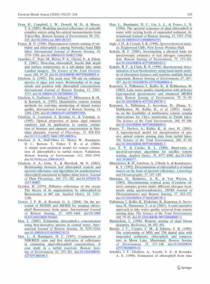
Table 1 Sample number and Chl-a concentration andsecchi disk transparency in different months

Number June July August September Summer6 8 9 20 43

Chl-a (μg·L−1)Min 6.40 28.14 15.15 11.24 6.40Max 14.68 58.21 37.15 47.23 58.21Mean 10.22 40.57 28.81 24.38 26.34

SDT (m)Min 0.10 0.22 0.22 0.18 0.10Max 0.46 0.24 0.30 0.32 0.46Mean 0.25 0.23 0.25 0.25 0.25

Methodology

Water sampling and field spectral measurements

Water sampling and field spectral measurementswere performed during the summer season fromJune to September in 2004. Due to the availabil-ity of water sample analysis in the laboratory,the number of water samples in different monthsvaried from 6 to 20 for Lake Chagan (Table 1).In each fieldwork trip, the position of the sam-pling boat was geo-located by a portable AshtechProMark2 global position system receiver with

234 Environ Monit Assess (2010) 170:231–244

0.3–3 m accuracy specification. SDT and fieldspectral data were simultaneously measured at se-lected points in the lake. At each sampling site, thelake water was also collected with a clean bottlefor further laboratory analysis within 4 h. A watersample was filtered using a glass micro-fiber filter(0.45 μm) to measure Chl-a with the standardspectro-photometric method. Acetone was usedto extract Chl-a from the water sample for over24 h. The sample was then read before and afterits acidification using a spectro-photofluorometer.Finally, Chl-a was calculated by comparison withthe known standards.

Field spectra were measured with a portableFieldspec FSR VNIR® spectrometer (ASD Inc.).The ASD radiometer has a spectral range be-tween 350 and 1,100 nm and a radiometric reso-lution of about 3 nm. Prior to the field campaign,the absolute radiance calibrations to the detectorwere performed. The measurements were takenfrom a boat platform above the lake surface, andthe spectra were measured at least ten times ateach sample station. A mean was taken as the finalresult. Each measured position was oriented to theboat side within the light propagation to minimizesun-glint from waves, but far away from the effectof the boat shadow.

Regression analysis

An alternative approach to the development ofsemi-empirical water color algorithms is by lin-ear regression analysis. Linear regression fits anobserved dependent data set (e.g., Chl-a concen-

tration) using a linear combination of indepen-dent variables (e.g., reflectance values at discretewavelengths). This leads to an algorithm based onregression analysis results, with the form as shownin Eq. 1:

Cchl-a = a + bx (1)

where Cchl-a is Chl-a concentration (μg/L), a andb are the regression coefficients, and x is the re-flectance ratio or derivative reflectance at a spe-cific wavelength (Wernand et al. 1998).

Results

Spectral characteristics of Chl-a

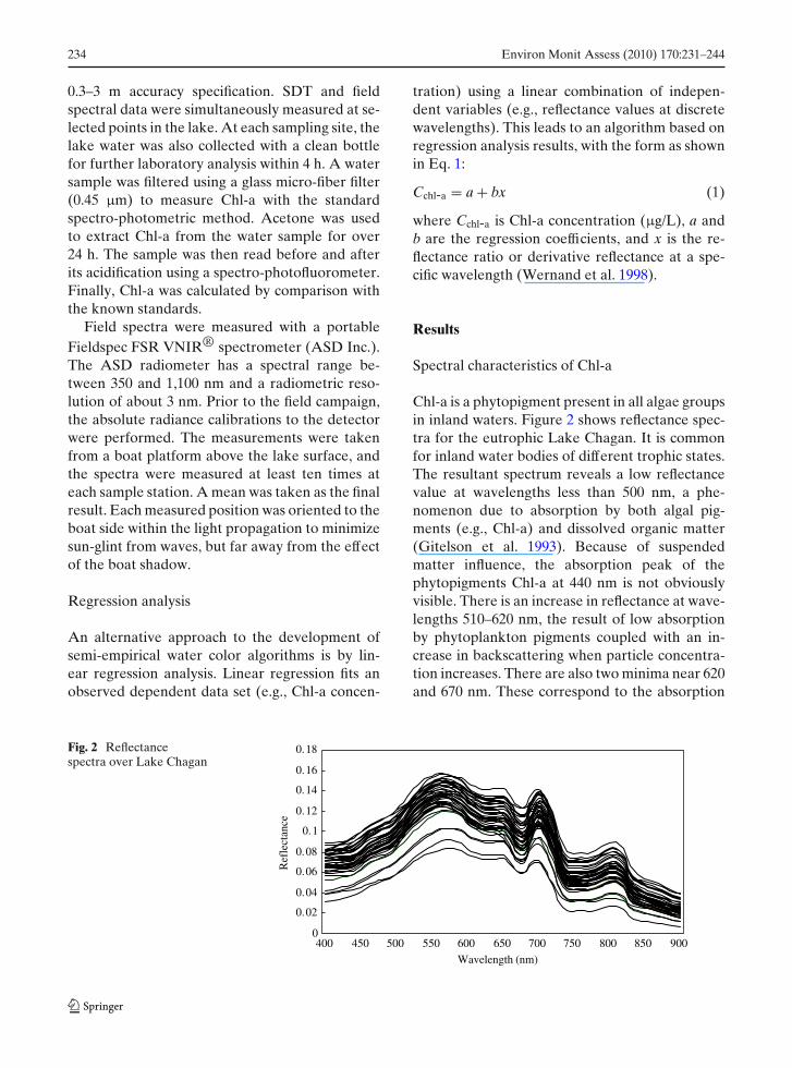
Chl-a is a phytopigment present in all algae groupsin inland waters. Figure 2 shows reflectance spec-tra for the eutrophic Lake Chagan. It is commonfor inland water bodies of different trophic states.The resultant spectrum reveals a low reflectancevalue at wavelengths less than 500 nm, a phe-nomenon due to absorption by both algal pig-ments (e.g., Chl-a) and dissolved organic matter(Gitelson et al. 1993). Because of suspendedmatter influence, the absorption peak of thephytopigments Chl-a at 440 nm is not obviouslyvisible. There is an increase in reflectance at wave-lengths 510–620 nm, the result of low absorptionby phytoplankton pigments coupled with an in-crease in backscattering when particle concentra-tion increases. There are also two minima near 620and 670 nm. These correspond to the absorption

Fig. 2 Reflectancespectra over Lake Chagan

0

0.02

0.04

0.06

0.08

0.1

0.12

0.14

0.16

0.18

400 450 500 550 600 650 700 750 800 850 900

Wavelength (nm)

Ref

lect

ance

Environ Monit Assess (2010) 170:231–244 235

maxima of phytoplankton pigments (Gitelson1992). Low reflectance at 620 nm is expected, dueto absorption by cyanobacteria (e.g. phycocyanin;Schalles et al. 1998). At 670 nm, a reflectance mini-mum corresponds to the Chl-a absorption band. Apeak of reflectance is also notable at 685–715 nm,due to fluorescence by Chl-a pigments (Gordon1979). It reaches 700 nm for the increase of Chl-acontents in Lake Chagan.

First derivative

Derivative spectra indicate the rate of changeof reflectance with wavelength (dR(λ)/dλ), whichis the slope of the reflectance curve at wave-length λ (Han 2005). Derivative analysis enablesthe shape of the reflectance pattern to be cor-related to chlorophyll concentrations. Figure 3ashows the first derivative reflectance curves forLake Chagan. Note that the much greater vari-ations among the spectral curves that appearedin Fig. 2 did not appear this time for their deriv-ative spectra. This phenomenon indicated that

derivative spectra were less affected by the waveeffects and able to remove pure water effects.To test if the first derivative reflectance valueat a specific wavelength can be used to estimatechlorophyll concentration, correlation coefficientswere calculated for all bands. Figure 3b shows theresults of correlation analysis performed on thefirst derivative and chlorophyll-a concentration;the first derivative had a much higher correlationwith chlorophyll-a concentration. The higher cor-relation coefficients (|R| > 0.8) were found pri-marily in the spectral regions between 660 and700 nm. These can be potential wavelength re-gions where the first derivative may be used toestimate chlorophyll-a concentration. It was foundthat with two-thirds of the samples (n = 28), thefirst derivative at 680 nm produced the highestpositive correlation with chlorophyll-a concentra-tion (R2 = 0.74; Fig. 3c). In addition, one-third ofthe samples (n = 15) were chosen as test data topredict Chl-a concentration for their ability. Asexpected, the results were promising with a lowerRMSE of 5.51 μg/L (Fig. 3d).

Fig. 3 First derivative:a first derivative spectra,b correlation coefficients(R), c regression model,d validation

-0.003

-0.002

-0.001

0

0.001

0.002

0.003

410 470 530 590 650 710 770 830 890

Wavelength (nm)

Firs

t der

ivat

e

-1

-0.8

-0.6

-0.4

-0.2

0

0.2

0.4

0.6

0.8

1

410450490530570610650690730770810850890

Wavelength (nm)

Cor

rela

tion

coef

fici

ent

y = 52538x - 4.7304 R2 = 0.74 N = 28 RMSE = 6.39

0

10

20

30

40

50

60

0 0.0005 0.001 0.0015

R680

Chl

-a c

once

ntra

tion

(µg/

L)

0

10

20

30

40

50

60

70

0 10 20 30 40 50 60 70Chl-a from in situ sampling (µg/L)

Chl

-a f

rom

fie

ld s

pect

ral (

µg/L

)

N = 15RMSE = 5.51

a b

c d

236 Environ Monit Assess (2010) 170:231–244

Two-band model

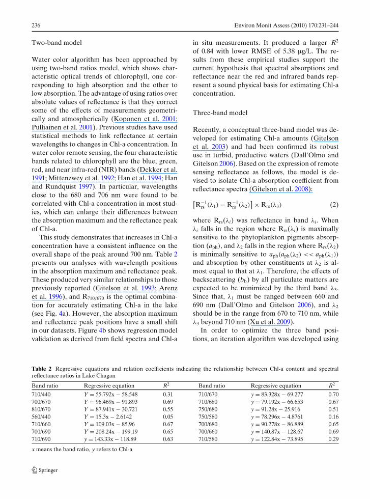
Water color algorithm has been approached byusing two-band ratios model, which shows char-acteristic optical trends of chlorophyll, one cor-responding to high absorption and the other tolow absorption. The advantage of using ratios overabsolute values of reflectance is that they correctsome of the effects of measurements geometri-cally and atmospherically (Koponen et al. 2001;Pulliainen et al. 2001). Previous studies have usedstatistical methods to link reflectance at certainwavelengths to changes in Chl-a concentration. Inwater color remote sensing, the four characteristicbands related to chlorophyll are the blue, green,red, and near infra-red (NIR) bands (Dekker et al.1991; Mittenzwey et al. 1992; Han et al. 1994; Hanand Rundquist 1997). In particular, wavelengthsclose to the 680 and 706 nm were found to becorrelated with Chl-a concentration in most stud-ies, which can enlarge their differences betweenthe absorption maximum and the reflectance peakof Chl-a.

This study demonstrates that increases in Chl-aconcentration have a consistent influence on theoverall shape of the peak around 700 nm. Table 2presents our analyses with wavelength positionsin the absorption maximum and reflectance peak.These produced very similar relationships to thosepreviously reported (Gitelson et al. 1993; Arenzet al. 1996), and R710/670 is the optimal combina-tion for accurately estimating Chl-a in the lake(see Fig. 4a). However, the absorption maximumand reflectance peak positions have a small shiftin our datasets. Figure 4b shows regression modelvalidation as derived from field spectra and Chl-a

in situ measurements. It produced a larger R2

of 0.84 with lower RMSE of 5.38 μg/L. The re-sults from these empirical studies support thecurrent hypothesis that spectral absorptions andreflectance near the red and infrared bands rep-resent a sound physical basis for estimating Chl-aconcentration.

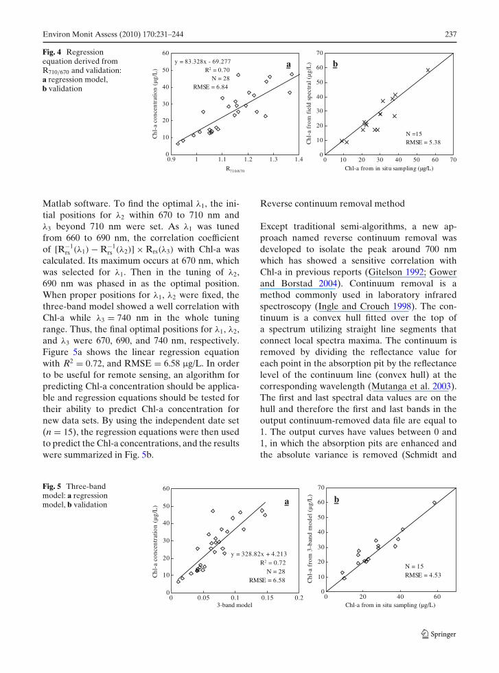
Three-band model

Recently, a conceptual three-band model was de-veloped for estimating Chl-a amounts (Gitelsonet al. 2003) and had been confirmed its robustuse in turbid, productive waters (Dall’Olmo andGitelson 2006). Based on the expression of remotesensing reflectance as follows, the model is de-vised to isolate Chl-a absorption coefficient fromreflectance spectra (Gitelson et al. 2008):

[R−1

rs (λ1) − R−1rs (λ2)

] × Rrs(λ3) (2)

where Rrs(λi) was reflectance in band λi. Whenλi falls in the region where Rrs(λi) is maximallysensitive to the phytoplankton pigments absorp-tion (aph), and λ2 falls in the region where Rrs(λ2)is minimally sensitive to aph(aph(λ2) << aph(λ1))

and absorption by other constituents at λ2 is al-most equal to that at λ1. Therefore, the effects ofbackscattering (bb) by all particulate matters areexpected to be minimized by the third band λ3.Since that, λ1 must be ranged between 660 and690 nm (Dall’Olmo and Gitelson 2006), and λ2

should be in the range from 670 to 710 nm, whileλ3 beyond 710 nm (Xu et al. 2009).

In order to optimize the three band posi-tions, an iteration algorithm was developed using

Table 2 Regressive equations and relation coefficients indicating the relationship between Chl-a content and spectralreflectance ratios in Lake Chagan

Band ratio Regressive equation R2 Band ratio Regressive equation R2

710/440 Y = 55.792x − 58.548 0.31 710/670 y = 83.328x − 69.277 0.70700/670 Y = 96.469x − 91.893 0.69 710/680 y = 79.192x − 66.653 0.67810/670 Y = 87.941x − 30.721 0.55 750/680 y = 91.28x − 25.916 0.51560/440 Y = 15.3x − 2.6142 0.05 750/580 y = 78.296x − 4.8761 0.16710/660 Y = 109.03x − 85.96 0.67 700/680 y = 90.278x − 86.889 0.65700/690 Y = 208.24x − 199.19 0.65 700/660 y = 140.87x − 128.67 0.69710/690 y = 143.33x − 118.89 0.63 710/580 y = 122.84x − 73.895 0.29

x means the band ratio, y refers to Chl-a

Environ Monit Assess (2010) 170:231–244 237

Fig. 4 Regressionequation derived fromR710/670 and validation:a regression model,b validation

y = 83.328x - 69.277 R2 = 0.70 N = 28 RMSE = 6.84

0

10

20

30

40

50

60

0.9 1 1.1 1.2 1.3 1.4

R710/670

Chl

-a c

once

ntra

tion

(µg/

L)

0

10

20

30

40

50

60

70

0 10 20 30 40 50 60 70Chl-a from in situ sampling (µg/L)

Chl

-a f

rom

fie

ld s

pect

ral (

µg/L

)

N =15RMSE = 5.38

a b

Matlab software. To find the optimal λ1, the ini-tial positions for λ2 within 670 to 710 nm andλ3 beyond 710 nm were set. As λ1 was tunedfrom 660 to 690 nm, the correlation coefficientof [R−1

rs (λ1) − R−1rs (λ2)] × Rrs(λ3) with Chl-a was

calculated. Its maximum occurs at 670 nm, whichwas selected for λ1. Then in the tuning of λ2,690 nm was phased in as the optimal position.When proper positions for λ1, λ2 were fixed, thethree-band model showed a well correlation withChl-a while λ3 = 740 nm in the whole tuningrange. Thus, the final optimal positions for λ1, λ2,and λ3 were 670, 690, and 740 nm, respectively.Figure 5a shows the linear regression equationwith R2 = 0.72, and RMSE = 6.58 μg/L. In orderto be useful for remote sensing, an algorithm forpredicting Chl-a concentration should be applica-ble and regression equations should be tested fortheir ability to predict Chl-a concentration fornew data sets. By using the independent date set(n = 15), the regression equations were then usedto predict the Chl-a concentrations, and the resultswere summarized in Fig. 5b.

Reverse continuum removal method

Except traditional semi-algorithms, a new ap-proach named reverse continuum removal wasdeveloped to isolate the peak around 700 nmwhich has showed a sensitive correlation withChl-a in previous reports (Gitelson 1992; Gowerand Borstad 2004). Continuum removal is amethod commonly used in laboratory infraredspectroscopy (Ingle and Crouch 1998). The con-tinuum is a convex hull fitted over the top ofa spectrum utilizing straight line segments thatconnect local spectra maxima. The continuum isremoved by dividing the reflectance value foreach point in the absorption pit by the reflectancelevel of the continuum line (convex hull) at thecorresponding wavelength (Mutanga et al. 2003).The first and last spectral data values are on thehull and therefore the first and last bands in theoutput continuum-removed data file are equal to1. The output curves have values between 0 and1, in which the absorption pits are enhanced andthe absolute variance is removed (Schmidt and

Fig. 5 Three-bandmodel: a regressionmodel, b validation a

N = 15 RMSE = 4.53

0

10

20

30

40

50

60

70

0 20 40 60Chl-a from in situ sampling (µg/L)

Chl

-a f

rom

3-b

and

mod

el (

µg/L

)

y = 328.82x + 4.213 R2 = 0.72 N = 28 RMSE = 6.58

0

10

20

30

40

50

60

0 0.05 0.1 0.15 0.23-band model

Chl

-a c

once

ntra

tion

(µg/

L)

b

238 Environ Monit Assess (2010) 170:231–244

Skidmore 2001). Continuum-removed absorptionfeatures can be compared by being scaled to thesame depth at the band center, thus allowing acomparison of the shapes of absorption features.

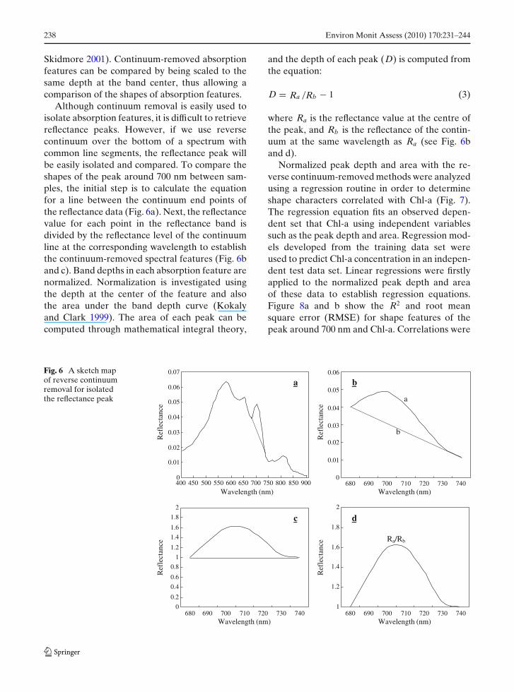
Although continuum removal is easily used toisolate absorption features, it is difficult to retrievereflectance peaks. However, if we use reversecontinuum over the bottom of a spectrum withcommon line segments, the reflectance peak willbe easily isolated and compared. To compare theshapes of the peak around 700 nm between sam-ples, the initial step is to calculate the equationfor a line between the continuum end points ofthe reflectance data (Fig. 6a). Next, the reflectancevalue for each point in the reflectance band isdivided by the reflectance level of the continuumline at the corresponding wavelength to establishthe continuum-removed spectral features (Fig. 6band c). Band depths in each absorption feature arenormalized. Normalization is investigated usingthe depth at the center of the feature and alsothe area under the band depth curve (Kokalyand Clark 1999). The area of each peak can becomputed through mathematical integral theory,

and the depth of each peak (D) is computed fromthe equation:

D = Ra /Rb − 1 (3)

where Ra is the reflectance value at the centre ofthe peak, and Rb is the reflectance of the contin-uum at the same wavelength as Ra (see Fig. 6band d).

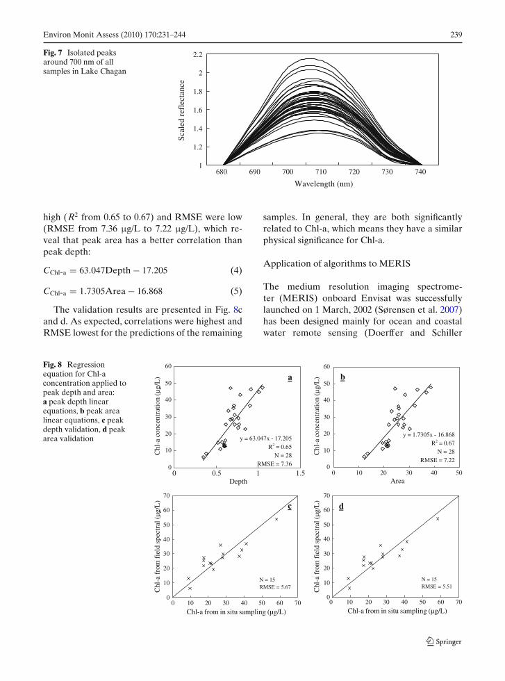
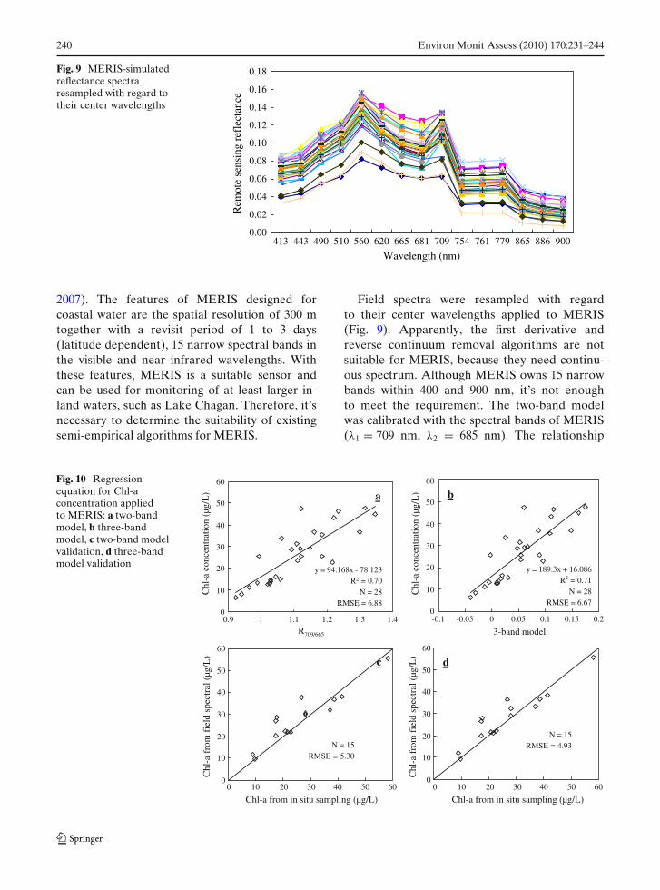
Normalized peak depth and area with the re-verse continuum-removed methods were analyzedusing a regression routine in order to determineshape characters correlated with Chl-a (Fig. 7).The regression equation fits an observed depen-dent set that Chl-a using independent variablessuch as the peak depth and area. Regression mod-els developed from the training data set wereused to predict Chl-a concentration in an indepen-dent test data set. Linear regressions were firstlyapplied to the normalized peak depth and areaof these data to establish regression equations.Figure 8a and b show the R2 and root meansquare error (RMSE) for shape features of thepeak around 700 nm and Chl-a. Correlations were

Fig. 6 A sketch mapof reverse continuumremoval for isolatedthe reflectance peak

0

0.01

0.02

0.03

0.04

0.05

0.06

0.07

0

0.01

0.02

0.03

0.04

0.05

0.06

400 450 500 550 600 650 700 750 800 850 900Wavelength (nm) Wavelength (nm)

680 690 700 710 720 730 740

Wavelength (nm)680 690 700 710 720 730 740

Wavelength (nm)680 690 700 710 720 730 740

Ref

lect

ance

Ref

lect

ance

Ref

lect

ance

Ref

lect

ance

0

0.2

0.4

0.6

0.8

1

1.2

1.4

1.6

1.8

2

1

1.2

1.4

1.6

1.8

2

a

b

a b

c d

Ra/Rb

Environ Monit Assess (2010) 170:231–244 239

Fig. 7 Isolated peaksaround 700 nm of allsamples in Lake Chagan

1

1.2

1.4

1.6

1.8

2

2.2

680 690 700 710 720 730 740

Wavelength (nm)Sc

aled

ref

lect

ance

high (R2 from 0.65 to 0.67) and RMSE were low(RMSE from 7.36 μg/L to 7.22 μg/L), which re-veal that peak area has a better correlation thanpeak depth:

CChl-a = 63.047Depth − 17.205 (4)

CChl-a = 1.7305Area − 16.868 (5)

The validation results are presented in Fig. 8cand d. As expected, correlations were highest andRMSE lowest for the predictions of the remaining

samples. In general, they are both significantlyrelated to Chl-a, which means they have a similarphysical significance for Chl-a.

Application of algorithms to MERIS

The medium resolution imaging spectrome-ter (MERIS) onboard Envisat was successfullylaunched on 1 March, 2002 (Sørensen et al. 2007)has been designed mainly for ocean and coastalwater remote sensing (Doerffer and Schiller

Fig. 8 Regressionequation for Chl-aconcentration applied topeak depth and area:a peak depth linearequations, b peak arealinear equations, c peakdepth validation, d peakarea validation y = 63.047x - 17.205

R2 = 0.65 N = 28 RMSE = 7.360

10

20

30

40

50

60

0 0.5 1 1.5Depth

Chl

-a c

once

ntra

tion

(µg/

L)

Chl

-a c

once

ntra

tion

(µg/

L)

Chl

-a f

rom

fie

ld s

pect

ral (

µg/L

)

Chl

-a f

rom

fie

ld s

pect

ral (

µg/L

)

y = 1.7305x - 16.868 R2 = 0.67

N = 28 RMSE = 7.22

0

10

20

30

40

50

60

0 10 20 30 40 50Area

a b

0

10

20

30

40

50

60

70

0 10 20 30 40 50 60 70

Chl-a from in situ sampling (µg/L)0 10 20 30 40 50 60 70

Chl-a from in situ sampling (µg/L)

N = 15RMSE = 5.51

0

10

20

30

40

50

60

70

N = 15 RMSE = 5.67

c d

240 Environ Monit Assess (2010) 170:231–244

Fig. 9 MERIS-simulatedreflectance spectraresampled with regard totheir center wavelengths

0.00

0.02

0.04

0.06

0.08

0.10

0.12

0.14

0.16

0.18

413 443 490 510 560 620 665 681 709 754 761 779 865 886 900

Wavelength (nm)

Rem

ote

sens

ing

refl

ecta

nce

2007). The features of MERIS designed forcoastal water are the spatial resolution of 300 mtogether with a revisit period of 1 to 3 days(latitude dependent), 15 narrow spectral bands inthe visible and near infrared wavelengths. Withthese features, MERIS is a suitable sensor andcan be used for monitoring of at least larger in-land waters, such as Lake Chagan. Therefore, it’snecessary to determine the suitability of existingsemi-empirical algorithms for MERIS.

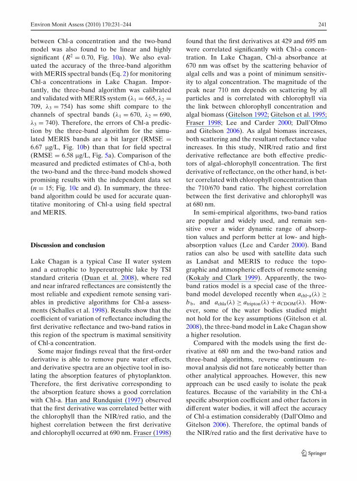
Field spectra were resampled with regardto their center wavelengths applied to MERIS(Fig. 9). Apparently, the first derivative andreverse continuum removal algorithms are notsuitable for MERIS, because they need continu-ous spectrum. Although MERIS owns 15 narrowbands within 400 and 900 nm, it’s not enoughto meet the requirement. The two-band modelwas calibrated with the spectral bands of MERIS(λ1 = 709 nm, λ2 = 685 nm). The relationship

Fig. 10 Regressionequation for Chl-aconcentration appliedto MERIS: a two-bandmodel, b three-bandmodel, c two-band modelvalidation, d three-bandmodel validation

y = 94.168x - 78.123 R2 = 0.70 N = 28 RMSE = 6.88

0

10

20

30

40

50

60

0.9 1 1.1 1.2 1.3 1.4

R709/665

Chl

-a c

once

ntra

tion

(µg/

L)

0

10

20

30

40

50

60

Chl

-a c

once

ntra

tion

(µg/

L)

y = 189.3x + 16.086 R2 = 0.71

N = 28 RMSE = 6.67

-0.1 -0.05 0 0.05 0.1 0.15 0.2

3-band model

a

N = 15RMSE = 5.30

0

10

20

30

40

50

60

0 10 20 30 40 50 60

Chl-a from in situ sampling (µg/L)0 10 20 30 40 50 60

Chl-a from in situ sampling (µg/L)

Chl

-a f

rom

fie

ld s

pect

ral (

µg/L

)

0

10

20

30

40

50

60

Chl

-a f

rom

fie

ld s

pect

ral (

µg/L

)

N = 15RMSE = 4.93

b

c d

Environ Monit Assess (2010) 170:231–244 241

between Chl-a concentration and the two-bandmodel was also found to be linear and highlysignificant (R2 = 0.70, Fig. 10a). We also eval-uated the accuracy of the three-band algorithmwith MERIS spectral bands (Eq. 2) for monitoringChl-a concentrations in Lake Chagan. Impor-tantly, the three-band algorithm was calibratedand validated with MERIS system (λ1 = 665, λ2 =709, λ3 = 754) has some shift compare to thechannels of spectral bands (λ1 = 670, λ2 = 690,λ3 = 740). Therefore, the errors of Chl-a predic-tion by the three-band algorithm for the simu-lated MERIS bands are a bit larger (RMSE =6.67 μg/L, Fig. 10b) than that for field spectral(RMSE = 6.58 μg/L, Fig. 5a). Comparison of themeasured and predicted estimates of Chl-a, boththe two-band and the three-band models showedpromising results with the independent data set(n = 15; Fig. 10c and d). In summary, the three-band algorithm could be used for accurate quan-titative monitoring of Chl-a using field spectraland MERIS.

Discussion and conclusion

Lake Chagan is a typical Case II water systemand a eutrophic to hypereutrophic lake by TSIstandard criteria (Duan et al. 2008), where redand near infrared reflectances are consistently themost reliable and expedient remote sensing vari-ables in predictive algorithms for Chl-a assess-ments (Schalles et al. 1998). Results show that thecoefficient of variation of reflectance including thefirst derivative reflectance and two-band ratios inthis region of the spectrum is maximal sensitivityof Chl-a concentration.

Some major findings reveal that the first-orderderivative is able to remove pure water effects,and derivative spectra are an objective tool in iso-lating the absorption features of phytoplankton.Therefore, the first derivative corresponding tothe absorption feature shows a good correlationwith Chl-a. Han and Rundquist (1997) observedthat the first derivative was correlated better withthe chlorophyll than the NIR/red ratio, and thehighest correlation between the first derivativeand chlorophyll occurred at 690 nm. Fraser (1998)

found that the first derivatives at 429 and 695 nmwere correlated significantly with Chl-a concen-tration. In Lake Chagan, Chl-a absorbance at670 nm was offset by the scattering behavior ofalgal cells and was a point of minimum sensitiv-ity to algal concentration. The magnitude of thepeak near 710 nm depends on scattering by allparticles and is correlated with chlorophyll viathe link between chlorophyll concentration andalgal biomass (Gitelson 1992; Gitelson et al. 1995;Fraser 1998; Lee and Carder 2000; Dall’Olmoand Gitelson 2006). As algal biomass increases,both scattering and the resultant reflectance valueincreases. In this study, NIR/red ratio and firstderivative reflectance are both effective predic-tors of algal–chlorophyll concentration. The firstderivative of reflectance, on the other hand, is bet-ter correlated with chlorophyll concentration thanthe 710/670 band ratio. The highest correlationbetween the first derivative and chlorophyll wasat 680 nm.

In semi-empirical algorithms, two-band ratiosare popular and widely used, and remain sen-sitive over a wider dynamic range of absorp-tion values and perform better at low- and high-absorption values (Lee and Carder 2000). Bandratios can also be used with satellite data suchas Landsat and MERIS to reduce the topo-graphic and atmospheric effects of remote sensing(Kokaly and Clark 1999). Apparently, the two-band ratios model is a special case of the three-band model developed recently when achl-a(λ) ≥b b, and achla(λ) ≥ atripton(λ) + aCDOM(λ). How-ever, some of the water bodies studied mightnot hold for the key assumptions (Gitelson et al.2008), the three-band model in Lake Chagan showa higher resolution.

Compared with the models using the first de-rivative at 680 nm and the two-band ratios andthree-band algorithms, reverse continuum re-moval analysis did not fare noticeably better thanother analytical approaches. However, this newapproach can be used easily to isolate the peakfeatures. Because of the variability in the Chl-aspecific absorption coefficient and other factors indifferent water bodies, it will affect the accuracyof Chl-a estimation considerably (Dall’Olmo andGitelson 2006). Therefore, the optimal bands ofthe NIR/red ratio and the first derivative have to

242 Environ Monit Assess (2010) 170:231–244

be adjusted and selected again. This avoids theneed to set fresh parameters for the models forwater bodies with specific optical properties, asthe peak around 700 nm is apparent and can easilybe picked out in order to minimize these effects.Once the spectral configuration is determined andunderstood, it is possible to specify a simple modelwith sufficient sensitivity to measure accuratelythe Chl-a concentration.

Previous studies have showed that the peakheight, which was quantified by measuring thedifference between reflectance at the wavelength,where the maximum reflectance is observed andthe baseline interpolated from measurements inthe peak around 700 nm, correlated well with theChl-a concentration (Gitelson 1992). Comparedwith peak height, peak depth used in reversecontinuum removal is not the difference butthe ratio between different reflectances. Peakheight is always calculated from the original data(Gitelson 1992), but peak depth is calculated fromthe data after normalization using reverse contin-uum removal analysis (Figs. 2 and 3). In general,results indicate that they are both significantlyrelated to Chl-a, which means they have a similarphysical significance for Chl-a.

The peak around 700 nm is important for theremote sensing of inland and coastal waters withregard to measuring chlorophyll. Therefore, thecorresponding region seems more appropriate forretrieval information on phytoplankton concen-tration from reflectance spectra. The magnitudeof the peak near 700 nm depends on scatteringby all particles and is correlated with chloro-phyll via the link between Chl-a concentrationand the reflectance changes including peak depthand area. The normalization approach in the pre-dictive models is effective because the slope ofthe reference baseline fitted between 680 and740 nm and its magnitude above zero reflectancedepend primarily on scattering by nonalgal seston(Schalles et al. 1998). With variation of organicand nonpigmented inorganic suspended matter,the baseline changes but has minimal influence onthe depth and area of the peak above this baseline.Thus, reflectance depth and area above the base-line depends almost entirely on phytoplanktondensity and is a useful measure of Chl-a (Gitelson1992; Gitelson et al. 1995; Fraser 1998).

All of the algorithms mentioned show a bettercorrelation and can be used to predict Chl-aconcentration. Because the number of samplingpoints is different in each month, it may pro-duce some errors to the algorithms. Water qual-ity variables are continually changing over time.Therefore, a different number of sampling pointsmay not lead to a comprehensive representa-tive of water quality during each month. Whenthe sampling points are limited, the algorithmsmay be affected and their precision will be re-duced. Fortunately, the 4 months from June toSeptember all fall within the summer season, withthe result that water quality variables such asChl-a and SDT (See Table 1) in Lake Chagan donot differ significantly. This helps limit and controlthe possible errors in the algorithms.

Acknowledgements We would like to acknowledge thefinancial supports provided by the National Natural Sci-ence Foundation of China (No.40801137, No.40871168,and No.40671138), the Special Prize of President Scholar-ship for Postgraduate Students of the Chinese Academyof Sciences (No.07YJ011001), and the Knowledge Inno-vation Program of the Chinese Academy of Sciences(No.CXNIGLAS200807). Thanks also for two anonymousreviewers for their critical comments.

References

Arenz, R. F., Lewis, W. M., & Saunders, J. F. (1996). Deter-mination of chlorophyll and dissolved organic carbonfrom reflectance data for Colorado reservoirs. Inter-national Journal of Remote Sensing, 17, 1547–1566.doi:10.1080/01431169608948723.

Dall’Olmo, G., & Gitelson, A. A. (2006). Effect of bio-optical parameter variability and uncertainties in re-flectance measurements on the remote estimation ofchlorophyll-a concentration in turbid productive wa-ters: Modeling results. Apply Optics, 45, 3577–3592.doi:10.1364/AO.45.003577.

Dekker, A. G., Malthus, T. J., & Seyhan, E. (1991). Quan-titative modeling of inland water quality for high reso-lution MSS systems. IEEE Transaction on Geoscienceand Remote Sensing, 29, 89–95. doi:10.1109/36.103296.

Doerffer, R., & Schiller, H. (2007). The MERIS Case 2water algorithm. International Journal of Remote Sens-ing, 28, 517–535. doi:10.1080/01431160600821127.

Duan, H., Zhang, Y., Zhang, B., Song, K., Wang, Z., Liu,D., et al. (2008). Estimation of chlorophyll-a concen-tration and trophic states for inland lakes in NortheastChina from Landsat TM data and field spectral mea-surements. International Journal of Remote Sensing,29, 767–786. doi:10.1080/01431160701355249.

Environ Monit Assess (2010) 170:231–244 243

Feng, H., Campbell, J. W., Dowell, M. D., & Moore,T. S. (2005). Modeling spectral reflectance of opticallycomplex waters using bio-optical measurements fromTokyo Bay. Remote Sensing of Environment, 99, 232–243. doi:10.1016/j.rse.2005.08.015.

Fraser, R. N. (1998). Hyperspectral remote sensing of tur-bidity and chlorophyll a among Nebraska Sand Hillslakes. International Journal of Remote Sensing, 19,1579–1589. doi:10.1080/014311698215360.

Giardino, C., Pepe, M., Brivio, P. A., Ghezzi, P., & Zilioli,E. (2001). Detecting chlorophyll, Secchi disk depthand surface temperature in a sub-alpine lake usingLandsat imagery. The Science of the Total Environ-ment, 268, 19–29. doi:10.1016/S0048-9697(00)00692-6.

Gitelson, A. (1992). The peak near 700 nm on radiancespectra of algae and water: Relationship of its mag-nitude and position with chlorophyll concentration.International Journal of Remote Sensing, 13, 3367–3373. doi:10.1080/01431169208904125.

Gitelson, A., Garbuzov, G., Szilagyi, F., Mittenzwey, K.-H.,& Karnieli, A. (1993). Quantitative remote sensingmethods for real-time monitoring of inland watersquality. International Journal of Remote Sensing, 14,1269–1295. doi:10.1080/01431169308953956.

Gitelson, A., Laorawat, S., Keydan, G., & Vonshak, A.(1995). Optical properties of dense algal culturesoutdoors and its application to remote estima-tion of biomass and pigment concentration in Spir-ulina platensis. Journal of Phycology, 31, 828–834.doi:10.1111/j.0022-3646.1995.00828.x.

Gitelson, A. A., Dall’Olmo, G., Moses, W., Rundquist,D. C., Barrow, T., Fisher, T. R., et al. (2008).A simple semi-analytical model for remote estima-tion of chlorophyll-a in turbid waters: Validation.Remote Sensing of Environment, 112, 3582–3593.doi:10.1016/j.rse.2008.04.015.

Gitelson, A. A., Gritz, Y., & Merzlyak, M. N. (2003).Relationship between leaf chlorophyll content andspectral reflectance and algorithms for nondestructivechlorophyll assessment in higher plant leaves. Journalof Plant Physiology, 160, 271–282. doi:10.1078/0176-1617-00887.

Gordon, H. (1979). Diffusive reflectance of the ocean:The theory of its augmentation by chlorophyll-2afluorescence at 685 nm. Applied Optics, 18, 1161–1166.

Gower, J. F. R., & Borstad, G. A. (2004). On the po-tential of MODIS and MERIS for imaging chloro-phyll fluorescence from space. International Journalof Remote Sensing, 25, 1459–1464. doi:10.1080/01431160310001592445.

Han, L. (2005). Estimating chlorophyll-a concentrationusing first-derivative spectra in coastal water. Inter-national Journal of Remote Sensing, 26, 5235–5244.doi:10.1080/01431160500219133.

Han, L., & Rundquist, D. C. (1997). Comparison ofNIR/RED ratio and first derivative of reflectancein estimating algal-chlorophyll concentration: Acase study in a turbid reservoir. Remote Sens-ing of Environment, 62, 253–261. doi:10.1016/S0034-4257(97)00106-5.

Han, L., Rundquist, D. C., Liu, L. L., & Fraser, L. N.(1994). The spectral responses of algal chlorophyll inwater with varying levels of suspended sediment. In-ternational Journal of Remote Sensing, 15, 3707–3718.doi:10.1080/01431169408954353.

Ingle, J. D., & Crouch, S. R. (1998). Spectrochemical analy-sis. Englewood Cliffs, New Jersey: Prentice Hall.

Kokaly, R. F. (2001). Investigating a physical basis forspectroscopic estimates of leaf nitrogen concentra-tion. Remote Sensing of Environment, 75, 153–161.doi:10.1016/S0034-4257(00)00163-2.

Kokaly, R. F., & Clark, R. N. (1999). Spectroscopic deter-mination of leaf biochemistry using band-depth analy-sis of absorption features and stepwise multiple linearregression. Remote Sensing of Environment, 67, 267–287. doi:10.1016/S0034-4257(98)00084-4.

Koponen, S., Pulliainen, J., Kallio, K., & Hallikainen, M.(2002). Lake water quality classification with airbornehyperspectral spectrometer and simulated MERISdata. Remote Sensing of Environment, 79, 51–59.doi:10.1016/S0034-4257(01)00238-3.

Koponen, S., Pulliainen, J., Servomaa, H., Zhang, Y.,Hallikainen, M., Kallio, K., et al. (2001). Analy-sis on the feasibility of multisource remote sensingobservations for Chl-a monitoring in Finish lakes.The Science of the Total Environment, 268, 95–106.doi:10.1016/S0048-9697(00)00689-6.

Kutser, T., Herlevi, A., Kallio, K., & Arst, H. (2001).A hyperspectral model for interpretation of pas-sive optical remote sensing data from turbid lakes.The Science of the Total Environment, 268, 47–58.doi:10.1016/S0048-9697(00)00682-3.

Lee, Z. P., & Carder, K. L. (2000). Band-ratio orspectral-curvature algorithms for satellite remotesensing. Applied Optics, 39, 4377–4380. doi:10.1364/AO.39.004377.

Mittenzwey, K. H., Gitelson, A., Ullrich, S., & Kondratyev,K. Y. (1992). Determination of chlorophyll a of inlandwaters on the basis of spectral reflectance. Limnologyand Oceanography, 37, 147–149.

Mutanga, O., Skidmore, A. K., & Van Wieren, S.(2003). Discriminating tropical grass (Cenchrus cil-iaris) canopies grown under different nitrogen treat-ments using spectroradiometry. ISPRS Journal ofPhotogrammetry and Remote Sensing, 57, 263–272.doi:10.1016/S0924-2716(02)00158-2.

Pulliainen, J., Kallio, K., Eloheimo, K., Koponen, S., Servo-maa, H., Hannonen, T., et al. (2001). A semi-operativeapproach to lake water quality retrieval from remotesensing data. The Science of the Total Environment,268, 79–93. doi:10.1016/S0048-9697(00)00687-2.

Richardson, L. (1996). Remote sensing of algal bloomdynamics. BioScience, 46, 492–501.

Ritchie, J. C., Cooper, C. M., & Schiebe, F. R. (1990).The relationship of MSS and TM digital data withsuspended sediments, chlorophyll, and tempera-ture in Moon Lake, Mississippi. Remote Sensingof Environment, 33, 137–148. doi:10.1016/0034-4257(90)90039-O.

Schalles, J. F., Gitelson, A., Yacobi, Y. Z., & Kroenke,A. E. (1998). Estimation of chlorophyll from time

244 Environ Monit Assess (2010) 170:231–244

series measurements of high spectral resolution re-flectance in an eutrophic lake. Journal of Phycology,34, 383–390. doi:10.1046/j.1529-8817.1998.340383.x.

Schmidt, K. S., & Skidmore, A. K. (2001). Exploring spec-tral discrimination of grass species in African range-lands. International Journal of Remote Sensing, 22,3421–3434. doi:10.1080/01431160152609245.

Sørensen, K., Aas, E., & Høkedal, J. (2007). Validation ofMERIS water products and bio-optical relationshipsin the Skagerrak. International Journal of RemoteSensing, 28, 555–568. doi:10.1080/01431160600815566.

Wernand, M. R., Shimwell, S. J., Boxall, S., & VanAken, H. M. (1998). Evaluation of specific semi-empirical coastal colour algorithms using historic

data sets. Aquatic Ecology, 32, 73–91. doi:10.1023/A:1009946501534.

Xu, J. P., Li, F., Zhang, B., Song, K. S., Wang, Z. M.,Liu, D. W., et al. (2009). Estimation of chlorophyll-aconcentration using field spectral data: A case studyin inland Case-II waters, North China. EnvironmentalMonitoring and Assessment. doi:10.1007/s10661-008-0568-z.

Zhang, Y., Koponen, S., Pulliainen, J., & Hallikainen, M.(2002). Application of an empirical neural networkto surface water quality estimation in the Gulf ofFinland using combined optical data and microwavedata. Remote Sensing of Environment, 81, 327–336.doi:10.1016/S0034-4257(02)00009-3.