Radio Resource Allocation in Fixed Broadband Wireless Networks*

Thomas K. Fong, Paul S. Henry, Kin K. Leung,†Xiaoxin Qiu and N.K. Shankaranarayanan

AT&T Laboratories - Research100 Schulz Drive

Red Bank, NJ 07701

April 8, 1997December 31, 1997 (Revised)

Abstract

We consider use of fixed broadband wireless networks to provide packet services for

telecommuting and Internet access. Each cell in such networks is divided into multiple sectors, each of

them served by a sector antenna co-located with the base station (BS), and user terminals also use

directional antennas mounted on the roof top of homes or small offices and pointed to their respective

BS antennas. To support a target data rate of 10 Mb/s, a bandwidth of several MHz is required. Since

radio spectrum is expensive, the bandwidth need to be reused very aggressively. Thus, efficient

strategies for frequency reuse and managing co-channel interference are critically important. We

propose here several algorithms for dynamic radio-resource allocation in the fixed wireless networks.

In particular, a method to be referred to as staggered resource allocation (SRA) method uses a

distributed scheduling algorithm to avoid major sources of interference, while allowing concurrent

packet transmission and meeting signal-to-interference objective. The performance of the method is

studied by analytic approximations and detailed simulation.

Our results show that the combination of directional antennas plus the SRA method is highly

effective in controlling co-channel interference. For reasonable system parameters, the SRA method

delivers a throughput in excess of 30% per sector while permitting a given frequency band to be re-used

in every sector of every cell. It also provides satisfactory probability of successful packet transmission.

In addition, a simple control mechanism can be applied in the method to improve performance for

harsh radio environments.

________________

* This paper was presented at the 6th WINLAB Workshop on Third Generation Wireless Networks, NewBrunswick, NJ, March 20-21, 1997.

† Please address correspondence to Kin K. Leung at AT&T Labs, Room 4-120, 100 Schulz Drive, Red Bank,NJ 07701 or kkleung@research.att.com.

- 2 -

1. INTRODUCTION

As work-at-home, telecommuting and Internet access become very popular, the demand for

broadband packet services will grow tremendously. Customers are expecting high quality, reliability

and easy access to high-speed communications from homes and small businesses. High-speed services

are needed in the very near future for: a) accessing World Wide Web for information and entertainment,

b) providing data rates comparable to local-area networks (LAN) for telecommuters to access their

computer equipment and data at the office, and c) multimedia services such as voice, image and video.

In this paper, we consider a wireless approach to this problem: fixed (i.e., non-mobile) broadband

packet-switched TDMA networks with user data rates of 10 Mb/s, link lengths typically less than 10

kilometers and operating frequency in the range of 1 to 5 GHz. We specifically focus on networks

using sector antennas at base stations and narrow-beam antennas at roof tops of homes and small

offices. Physical and link-layer issues arising in the design of such networks include modulation,

equalization, access techniques, co-channel interference, bandwidth usage, error control and multi-

access schemes [AEK96]. Our focus here is to address just one of these issues, namely, the co-channel

interference.

Microwave spectrum is expensive, so efficient strategies for re-using frequencies and managing

co-channel interference are critically important. To support a user data rate of 10 Mb/s in an

interference-limited wireless environment, a bandwidth of several MHz is needed for TDMA. In

contrast to narrowband cellular networks where radio spectrum is divided into multiple channel sets,

which are re-used only in relatively distant cells [L89], broadband wireless networks must re-use

bandwidth very aggressively, ideally reusing the same frequency band in every cell. The need for reuse

of a common radio bandwidth in all cells has also been noted by [BZFTB96] and [BFZA96] for mobile

broadband wireless networks. Using the whole frequency band to support a high data rate enables more

efficient sharing of bandwidth among users than the frequency partitioning method can. We also note

that although CDMA uses the same frequency band in all cells, the radio bandwidth required for

supporting the target data rate of 10 Mb/s will be excessive and the associated high processing speed

has not yet shown to be technologically feasible.

Many algorithms for channel allocation have been proposed to ensure satisfactory reception

quality in cellular networks; see references cited by [NK96]. Most of the existing work considers

circuit-switching networks and frequencies (or channels) are the resources to be allocated. In the

context of our packet-switched networks, time slots naturally become the bandwidth resources, which

are shared by all users in a sector or cell. We need to dynamically allocate time slots to various

- 3 -

transmitters to send data packets such that a given signal-to-interference ratio (SIR) can be guaranteed

at the intended receiver for successful packet reception. This results in the concept of dynamic

resource allocation. By using a central controller, [W96] and [KW97] propose approaches to assigning

time slots. In our fixed wireless networks, cell sectorization and directional antennas at fixed locations

are key components in reducing the amount of interference from neighboring sectors and cells. In this

paper, we propose strategies for managing co-channel interference that do not require a central

controller. They permit reuse of the same bandwidth in every cell, resulting in a high degree of spectral

efficiency.

The rest of this paper is organized as follows. By proving that the optimal time-slot assignment

to guarantee SIR requirements is NP-complete, Section 2 proposes two heuristic methods for

bandwidth allocation with reuse factor of 2 and 6. Section 3 introduces a more flexible approach, the

staggered resource allocation (SRA) method, and discusses its properties. We analyze the throughput

performance of the SRA method in Section 4. Using typical parameters, Section 5 presents several

numerical examples, and discusses the performance characteristics of the proposed methods. Finally,

Section 6 is our conclusion.

2. BANDWIDTH ALLOCATION IN FIXED BROADBAND WIRELESS NETWORKS

Consider a broadband wireless network where each cell is divided into multiple sectors, each of

which is covered by a sector antenna co-located with a base station (BS) at the center of the cell.

Because of the co-location, sector antennas are also referred to as BS antennas. Terminals (users) use

directional antennas mounted on the roof top and pointed to their respective BS antennas. The

beamwidth (angle) of each BS antenna should be just wide enough to cover the whole sector, while a

terminal antenna pointing to a designated BS antenna can have a smaller beamwidth to avoid

interference. The ratios of front-to-back-lobe gain (abbreviated by FTB ratio below) for BS and

terminal antennas may be different, and are assumed to be finite. Time is slotted such that a packet can

be transmitted in each slot. In addition, the downlink and uplink between terminals and BS are

provided by time-division duplex (TDD), using the same radio spectrum.

Even with some simplifications in this setting, the scheduling of packet transmissions for the

downlink to guarantee a given SIR at the receivers can be shown to be an NP-complete problem as

follows. Without loss of generality, consider that consecutive time slots for the downlink are grouped

into frames, each of which has L slots. Prior to the beginning of each frame, packets are scheduled to

transmit in slots of the frame. Let D be the set of all BS antennas. We further assume that regardless

of its location, each terminal pointing directly to BS antenna i receives a signal from each antenna j in

- 4 -

D with path gain G j i (which includes the propagation loss, and transmitter and receiver antenna gain).

Then the optimal scheduling is to minimize the total interference among concurrent packet

transmissions while guaranteeing a given SIR γ at the receivers. That is,

δi (t) Min

t =1ΣL

i∈ DΣ

j∈ D −iΣ δi (t) δj (t) G j i (1)

such that for all i ∈ D and t ∈ 1 , 2 , ... ,L,

δi (t) =î 0

1

otherwise

if antenna i transmits a packet in slot t

and

j∈ D −iΣ δi (t) δj (t) G j i

G ii_ ___________________ ≥ γ.

Theorem 1. The optimal scheduling problem in (1) is NP-complete.

Proof. We first apply the technique in [C69] to linearize the zero-one integer programming in (1) by

introducing a new set of variables ∆ i j (t) to replace all products of δi (t) δj (t)’s. Then, the proof is

completed by using the fact that the resultant, linear integer programming is NP-complete [GJ79,

p.245].

We remark that one can modify the optimization in (1) to consider path-gain factors G j i’s

dependent on the actual locations of receiving terminals. In that case, a link i is defined for each pair of

BS antenna and terminal, and D becomes the set of all links. Then, the problem is to minimize the total

amount of interference for all links in D subject to the SIR requirement. Clearly, such treatment causes

the computation complexity to grow rapidly beyond the capability of any centralized controller for

reasonable numbers of cells and terminals. For this reason, we choose to take a heuristic, distributed

approach in the following, aimed at identifying and controlling the major sources of interference.

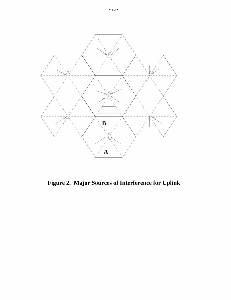
To make our ideas concrete, let us consider a hexagonal cell layout. Each cell is divided into six

sectors, each of which is served by a BS antenna with 60o beamwidth. Terminal antennas can have an

angle smaller than 60o . For the hexagonal layout, Figures 1 and 2 show the interference sources for

both downlink and uplink for a tagged sector under consideration (shaded in the figures). Using a

- 5 -

simple path-loss model [R96, p.102], we find that the major interference for the downlink in the tagged

sector comes from other intra-cell sectors, the alignment sector (A) and the opposite sector (B). (Sector

A is called the alignment sector because a terminal antenna in the shaded sector while pointing to its

BS antenna also sees the front lobe of the BS antenna for Sector A.) Similar observation can be made

in Figure 2 for the uplink. Interference received from other neighboring cells is significantly attenuated

because of the FTB ratio of directional antennas and distance. With this understanding, our challenge

is to develop resource allocation methods that avoid most of the major interferers.

2.1 Time-Slot Assignment With Reuse Factor of 2

In this assignment method, as shown in Figure 3, a fixed number of time slots for a downlink (or

uplink) are grouped into subframes and consecutive subframes are labeled alternately by 1 and 2. (Note

that the figure just shows the frame structure for a downlink or an uplink, excluding the TDD between

the two.) Sectors are also labeled by 1 and 2 such that no adjacent sectors share the same label. Sectors

with label i can schedule packet transmission in time slots of subframe i. As a result, each sector can

transmit on a 50% duty cycle, consuming at most half of the total bandwidth. Clearly, this assignment

is a time-domain analog to a frequency reuse factor of two in existing cellular networks, although the

reuse factor for our system and the cellular networks are expressed in terms of the number of sectors

and cells, respectively. In the present case, collisions with interfering packets are expected to occur,

and, depending on their severity, may necessitate retransmission.

There are two ways to improve system performance of this assignment method. First, a sector

can borrow (use) time slots that its neighboring sectors do not need. Note that this approach does not

increase the overall system capacity for uniform traffic load among sectors, but it does enable efficient

bandwidth sharing, especially for transient surges of traffic load. However, slot borrowing requires

information exchange and coordination among BS’s and that may not be desirable. A second way is to

simply allow use of slots in a subframe not originally assigned to a given sector. A simple protocol can

be applied to minimize concurrent transmissions (thus reducing interference); specifically, label-1

sectors schedule their packet transmission in time slots, starting from the left-hand side of subframe 1

and continuing on to subframe 2 if needed, while label-2 sectors transmit in slots starting from the

right-hand side of subframe 2 and continuing on to subframe 1. This allocation algorithm is thus called

the left-right protocol. Depending on the traffic load, this protocol yields as many as 3 to 6 concurrent

packet transmissions in each time slot in each cell. In the extreme, all sectors in a cell can transmit

simultaneously, yielding a reuse factor of 1. Thus, this left-right protocol can be viewed as a very

aggressive approach.

- 6 -

2.2 Time-Slot Assignment With Reuse Factor of 6

The assignment method with reuse factor of 6 is similar to that described above. As depicted in

Figure 4, time slots are now grouped into 6 subframes and sectors are labeled by 1 to 6 anti-clock-wise.

The labeling patterns for adjacent cells differ by a 120o rotation, thus creating a cluster of 3 cells whose

patterns can be repeated across the entire system. As described previously, sector i can schedule packet

transmission in subframe i for i = 1 to 6. Without slot borrowing and over-use, this method, which has

a reuse factor of 6, represents a conservative approach because each sector can use only one-sixth of the

total bandwidth. However, this may be appropriate for a radio environment where concurrent packet

transmissions within the same cell can cause severe interference, and thus should be prohibited.

In fact, there exists a flexible approach based on the above ideas that can perform aggressively or

conservatively, depending on traffic load and a control parameter, with reuse factor ranging from 1 to 6;

it is the subject of the next section.

3. The Staggered Resource Allocation (SRA) Method

In the staggered resource allocation (SRA) method, the frame structure and the sector labeling

are identical to those of the above method with reuse factor of 6 in Figure 4. However, a special slot

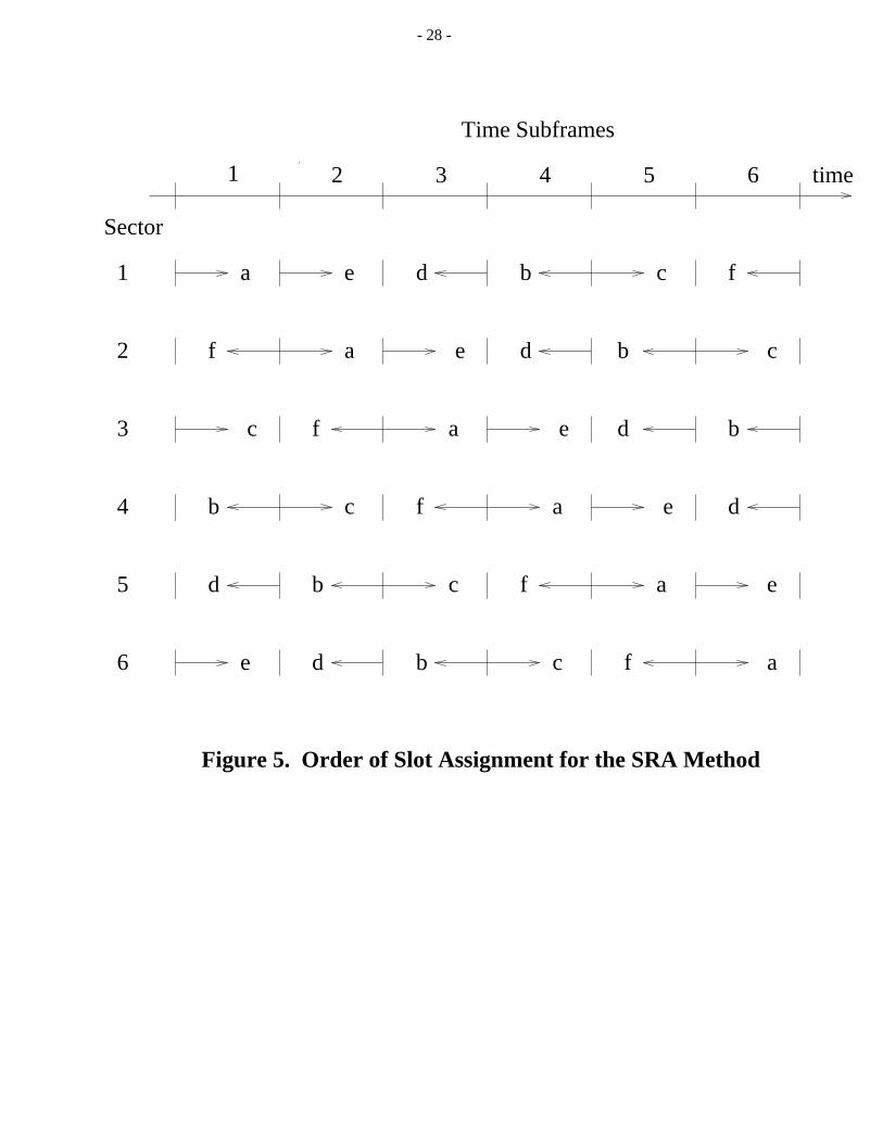
assignment order is established and followed by each sector. As shown in Figure 5, for example, a

sector with label 1 first schedules packets for transmission in time slots of subframe 1 (denoted by a).

If it has more traffic to send, it then uses subframe 4 (b), subframe 5 (c), etc. until subframe 6 (f). The

idea here is that, if interference due to concurrent packet transmission in the same cell can be tolerated,

then after using all slots in the first subframe a, a sector should use the first subframe of the opposite

sector in the same cell, in order to make the best use of the BS directional antennas. Following that,

time slots in the first subframes for the sectors next to the opposite sector are used. To avoid

interference due to imperfect antenna patterns of neighboring sectors, their first subframes are used as

the last resort. As the figure shows, the assignment order for the next sector is "staggered" by a right

rotation by one subframe based on the order for the previous sector. For this reason, this method is

called the staggered resource allocation (SRA) method. In addition, as an option to further avoid

concurrent packet transmission according to the principle of the left-right protocol, slots in each

subframe are assigned from the left or right-hand sides as indicated by the arrows in the figure. The

benefits of the SRA method in terms of interference avoidance and control of concurrent packet

transmissions are explained in the following.

- 7 -

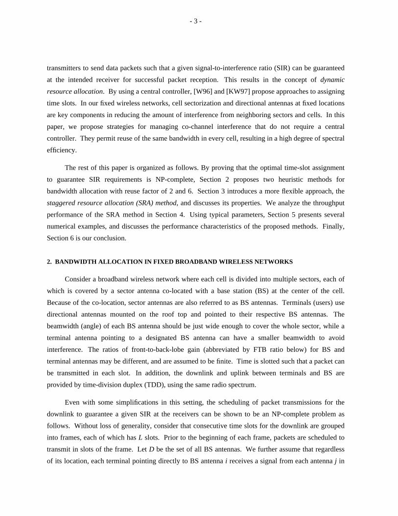
3.1 Avoidance of Major Interference

First, let us consider the intra-cell interference. It is easy to see from Figure 5 that if all sectors

have traffic load of less than one-sixth of total channel capacity, all packets are transmitted in different

time subframes, thus causing no interference within the same cell. This is identical to the conservative

assignment method with reuse factor of 6. Of course, as the traffic load increases, packets are

transmitted simultaneously, thus increasing the level of interference. Nevertheless, the special

assignment order exploits the characteristics of directional antennas to allow multiple concurrent packet

transmissions while maximizing the SIR.

Besides managing intra-cell interference, the SRA protocol also helps avoid interference from

major sources in the neighboring cells. This is particularly so when traffic load is low to moderate. To

see this, let us consider the downlink for Sector 1 in the middle cell of Figure 4. Sector 2 in the bottom

cell and Sector 3 in the upper cell are the major sources of interference. By examining the assignment

order for Sectors 1, 2 and 3, one finds that they will not transmit simultaneously, so they will not

interfere with each other provided that all of them have a traffic load of less than one-third of total

channel capacity (i.e., using only subframes a and b for transmission). The same comment also applies

to the uplink where Sectors 2 and 5 of the bottom cell in the figure now become the major sources of

interference. Due to the symmetry of the assignment order and cell layout, this same comment applies

to each sector in every cell.

To further reduce interference, the SRA method as shown in Figure 5 schedules packet

transmission for each sector starting from left to right and vice versa alternately in various time

subframes. To see the benefits of this alternate directions especially in case of uniform traffic load

among sectors, let us consider the time subframe 1 in the figure. According to the SRA method, Sector

4 uses the time subframe as the second subframe b for transmission. To avoid concurrent transmission

with Sector 1, which starts from the left-hand side of the time subframe 1, Sector 4 schedules packet

transmission from the right-hand side. If Sector 4 does not have enough packets to send in all slots of

the subframe 1, concurrent transmission with Sector 1 can be avoided.

As for Sector 3, under the uniform traffic condition, the fact that Sector 3 needs to transmit in its

third subframe c in the SRA order implies that Sector 1 probably has a similar traffic load. Thus, it is

likely that Sector 1 will transmit in all slots in the time subframe 1. So, the scheduling direction for

Sector 3 (from the left or the right-hand side) is unlikely to help avoid interference from transmission of

Sector 1. In contrast, it is probable that Sector 4 may not need to transmit in all slots in the time

subframe 1 (which is the second subframe b for Sector 4). By the same reason for the opposite

- 8 -

directions for Sectors 1 and 4, since Sector 4 schedules from the right-hand side, Sector 3 should begin

transmission from the left-hand side of the time subframe 1 to possibly avoid interference between

Sectors 3 and 4. The same reason applies to the scheduling directions for the rest of sectors.

3.2 A Control of Concurrent Transmissions for Enhanced Quality of Service

According to a given radio environment and antenna characteristics, the SRA method can be used

in conjunction with a control mechanism to improve the reception quality in terms of SIR at the

receiving ends. Specifically, the control limits packet transmissions only in the first few subframes for

each sector. For example, for the given radio environment, if at most three packets can be sent

simultaneously by various BS or terminal antennas in the same cell to ensure the required reception

quality, only time slots in subframes a, b and c as indicated in Figure 5 can be used for transmission by

each sector. In general, we show in the following that if each sector schedules packet transmission in

the first k subframes in the SRA method, there are at most k packets transmitted simultaneously by

various antennas in each cell at any time. The control limits the degree of concurrent transmissions,

thus the amount of interference, to achieve the desirable SIR. When different grades of quality of

services (QoS) such as for voice, secure data, non-realtime data calls are defined in terms of the SIR

threshold, the control can be used as a mechanism for providing the required QoS. The ability of the

mechanism to control the exact number of major interfers is also useful for systems using adaptive

antennas [WSG94] for suppression of interference where a specific number of interfers can be tolerated

depending on the antenna design.

To show the property of at most k concurrent transmissions, let Smi be the order of time subframe

m in the assignment sequence for sector i. That is, subframe m is the Smi -th subframe to be used by

sector i in the schedule. In general, consider that each cell consists of N sectors (thus each time frame

is divided into N subframes). For example, when N = 6, S11 = 1, S2

1 = 5, S31 = 4, S4

1 = 2, S51 = 3 and S6

1 = 6

for Sector 1, and S13 = 3, S2

3 = 6, S33 = 1, S4

3 = 5, S53 = 4 and S6

3 = 2 for Sector 3 according to Figure 5.

Basically, we list the assignment order for sector i, Smi , by 1 to 6 here, instead of by a, b, ..., f in the

figure. Define Ω ≡ 1 , 2 , ... ,N. Clearly, Smi ∈ Ω for all m , i ∈ Ω . Since each sector i uses the time

subframes sequentially in the SRA method, we have

Smi ≠ Sn

i for m≠n . (2)

As pointed out above, the assignment order of subframes for sector i + 1 in the SRA method is simply

that for sector i with a right rotation by one subframe. Thus,

- 9 -

Sm +ki +k = Sm

i for all i ,m ,k∈ Ω (3)

where the addition is taken to be modulo N.

Lemma 1. For the SRA method in a cellular environment with each cell divided into N sectors,

Smi ≠ Sm

j for all i≠ j and m ∈ Ω . Furthermore, Sm1 ,Sm

2 , ... ,SmN = Ω for each m ∈ Ω .

Proof. We assume that for some m , i , j ∈ Ω and i≠ j,

Smi = Sm

j . (4)

Since i , j ∈ Ω and i≠ j, there must exist k∈ Ω −N such that j = i + k in modulo N addition. Thus, (4)

becomes Smi = Sm

i +k , which is a contradiction to the combined fact of Smi = Sm +k

i +k and Sm +ki +k ≠Sm

i +k

obtained from (3) and (2), respectively. Since for all m, i ∈ Ω , Smi ∈ Ω and Sm

i ≠Smj for all i≠ j, it is

obvious that Sm1 ,Sm

2 , ... ,SmN = Ω. This completes the proof.

Theorem 2. If each sector can transmit packets only in the first k (≤ N) subframes according to the

assignment order of the SRA method, at most k packets are transmitted simultaneously in each cell in

any time slot.

Proof. When each sector i sends packets only in the first k subframes, only those subframes n with

1 ≤ Sni ≤ k are used. By Lemma 1, for each subframe m ∈ Ω ,

Sm1 ,Sm

2 , ... ,SmN = 1 , 2 , ... ,k,k + 1 , ... ,N. Thus only those sectors i with 1 ≤ Sm

i ≤ k are transmitting

in subframe m. That is, at most k packets are transmitted simultaneously in each cell at any time.

3.3 Optimality of the SRA Method in a Single-Cell Setting

Consider the downlink performance of the SRA method in a simple, single cell setting. Assume

that the cell is divided into N equal sectors and each sector BS antenna has a perfect antenna pattern

(i.e., it has a front lobe and a back lobe with a sharp distinction between them) with beamwidth of

360o / N, but with a finite FTB ratio. All antennas transmit at a fixed power level, and always have

packets ready for transmission. A power-law path-loss model and lognormal shadowing are also

assumed. Then, we define the success probability of a packet transmission targeted at a tagged terminal

located in one of the sectors as

- 10 -

P s = Pr I(c)

P w_ ___ ≥ γ

(5)

where P w is the power of the received signal, I(c) is the amount of interference provided that c

antennas (including the one sending a packet to the tagged terminal) are transmitting simultaneously

and γ is the required SIR detection threshold. Assume that the required "outage" probability is 1 − α.

That is, we need P s ≥ α. Then, we claim the following.

Lemma 2. The maximum (downlink) throughput of any scheduling policy for the single-cell setting

with N sectors is equal to the smaller value of c m and N packets/slot where c m ∈ 1 , 2 , 3 , . . . and

P s = Pr I(c m )

P w_ _____ ≥ γ

≥ α (6)

and

P s = Pr I(c m + 1 )

P w_ ________ ≥ γ

< α. (7)

Proof. Since there is only one radio path from all the BS antennas (which are co-located at the base

station) to the tagged terminal, the intended signal and interference experience the same lognormal

fading. Thus, for the fixed terminal location, the fading factor cancels out in the ratio of P w to I(c),

thus vanishing from (5). Based on this observation, the above system assumptions and the fact that

interference power is additive, P s in (5) becomes deterministic and decreases as c increases. Therefore,

there must exist c m ∈ 1 , 2 , 3 ,.. such that (6) and (7) hold. That is, c m packets can be transmitted

concurrently while meeting the SIR requirement. Since at most all N BS antennas can transmit

simultaneously, so the maximum throughput is bounded by N packets/slot. Given the assumption of

packets always ready for transmission, the maximum achievable throughput is thus the smaller value of

c m and N for the whole cell.

Now we claim the SRA method can achieve this maximum throughput in Lemma 2.

Theorem 3. The SRA method can yield the maximum achievable throughput of c m or N packets/slot

in the single-cell setting where c m is defined by (6) and (7).

- 11 -

Proof. Without loss of generality, let the maximum achievable throughput for the single-cell setting be

c m < N as defined by (6) and (7). Let the SRA method be used in conjunction with the transmission

control as discussed in Section 3.2 such that each BS antenna schedules packet transmissions in the first

c m subframes in the SRA assignment order. By Theorem 2, there are c m packets transmitted by c m

different antennas in each time slot of each subframe. Thus, since the SIR requirement is met for the

c m concurrent packet transmissions as indicated by (6) and (7), the SRA method with such a control

thus achieves the maximum throughput of c m packets/slot.

4. THROUGHPUT MODELS FOR THE SRA METHOD

An analytic approximate model and a detailed simulation model have been developed to study

the downlink throughput of the SRA method. Both models consider a fixed number of terminals

(users) in each sector, finite FTB ratios for BS and terminal antennas, radio path loss and lognormal

shadowing effects. They treat a packet transmission as successful if the SIR at the intended receivers

exceeds a given threshold and the SRA throughput defined as the number of packets successfully

transmitted per time slot in each sector.

While both models follow the SRA order of slot assignment in Figure 5, they ignore the left and

right directions of slot assignment. Rather, they assume that packets are scheduled for transmission

starting from the left-most time slot in each subframe. Although we believe the alternate assignment

directions can slightly improve the throughput, the assumption is made mainly for simplicity. Of

course, it can be relaxed with additional model complexity.

4.1 Analytic Approximate Model

Success of a packet transmission depends on the traffic load of various sectors, and the radio

environment and antenna characteristics. So, the exact throughput analysis requires consideration of

the interdependency among all BS antennas, thus becoming intractable. To develop an approximate

model, we assume that traffic process for each BS antenna is statistically independent, but yet packet

transmissions by all BS antennas are considered in estimating the probability of successful reception at

a receiver. Our simulation results in Section 5 reveal that such an approach yields excellent throughput

approximations for a wide range of parameters of interest.

Our approximate model consists of two submodels: a) a Markovian traffic submodel to capture

the traffic characteristics for each sector in the SRA method, and b) an interference submodel to

consider the radio environment and antenna characteristics. For simplicity, we assume here all sectors

have identical offered traffic load. Thus, the same traffic submodel is applicable to all sectors. This

- 12 -

assumption can be relaxed by applying different traffic parameters to the submodel for various sectors.

4.1.1 A Markovian Traffic Submodel We begin with our notation. Let M be the number of users

(terminals) in a sector. Let there be L time slots, indexed by 1 to L, in each frame. Given that we

consider a hexagonal-cell layout with six sectors per cell, L should be a multiple of 6. This submodel

assumes that all L slots can be used for transmission by each BS antenna. (This assumption can be

relaxed with some complexity to consider the control of concurrent transmission in Section 3.2.) We

also assume that packets are generated for each user according to a renewal process with a i being the

probability of having i ≥ 0 new packet arrivals in each time frame. The base station has a single buffer

that holds only one packet for each user. After a packet is successfully transmitted, it is removed from

the buffer at the end of the frame. When newly generated packets for a user find the buffer occupied,

they are lost and cleared.

Using the SRA method, let N m be the number of packets waiting for transmission by a BS

antenna at the beginning of frame m. Note that these packets represent an aggregated traffic load as

they include new arrivals or previous unsuccessful transmissions. We define G to be the normalized

aggregated offered load in terms of packets per slot for each sector; that is,

G = EN m / L . (8)

Observe that the sequence N m ;m = 1 , 2 , 3 , . . . can be modeled as a one-dimensional Markov

chain. This Markov chain is ergodic since it is irreducible, aperiodic, and has finite states. Thus, the

stationary distribution exists and let it be Π = π0 , ... ,πi , ... ,πM where πi is the probability that there

are i packets waiting for transmission by the BS antenna at the beginning of an arbitrary time frame at

steady state. Let P = p i j be the one step transition matrix for the Markov chain. Once P is

obtained as follows, Π can be computed from

Π = ΠP andi =1ΣM

πi = 1 . (9)

To find P, we start with the definition that p i j = PrN m +1 = j N m = i. By conditioning on

having k≥max ( 0 ,i − j) successful packet transmissions in frame m, p i j for 0≤ i , j≤M is given by

- 13 -

p i j =k =max( 0 ,i − j)

Σmin (i,L)

P k (L i , 1 ) A(M − i , j − (i − k) ,p) (10)

where A(M − i , j − (i − k) ,p) is the probability that M − i users (i.e., those with their single buffer

empty) generate j − (i − k) new packets in frame m with each user capable of generating at least one

packet in a frame with probability p. Since a i denotes the probability of generating i ≥ 0 new packets

by each user in a frame, p simply equals 1 − a 0 . For example, if packets for each user arrive according

to a Binomial distribution with parameter p and an exponential distribution with rate λ, then

A(M − i , j − i + k,p) =î j − i + k

M − i

p j − i +k ( 1 − p) M − j −k

and

A(M − i , j − i + k,p) =î j − i + k

M − i

( 1 − e− λL ) j − i +k e− λL(M − j −k) ,

respectively. In addition, P k (L i , 1 ) in (10) is the probability of having k successful packet

transmissions given that L i packets are scheduled for transmission starting from slot 1 of frame m.

Given N m = i and that all L slots in the frame are available for transmission, L i = min (i ,L). We use the

following recursion to compute the P k (L i , 1 )’s:

P k (L i , 1 ) = q 1 P k −1 (L i − 1 , 2 ) + ( 1 − q 1 ) P k (L i , 2 ) (11)

where q 1 is the probability of successful transmission in slot 1. The first term on the right-hand side of

(11) is obtained by observing that if slot 1 has a successful transmission, there should be another k − 1

successes in the remaining L i − 1 packets scheduled for transmission starting from slot 2. On the other

hand, the second term represents that the condition such that the transmission in slot 1 fails and the k

successful transmissions must take place in slot 2 or remaining slots in the frame. The ending

conditions of this recursion are, for any integer s≥1,

P m (n ,s) = 0 if m > n (12)

and

- 14 -

P 0 (n ,s) =l = sΠ

min (n + s,L)( 1 − q l ) . (13)

Eq.(12) reflects the fact that it is impossible to have more successful transmissions than the number of

waiting packets, while (13) shows that the probability of no success with n packet transmissions

starting from slot s is simply the product of probabilities of no success in all remaining slots in the

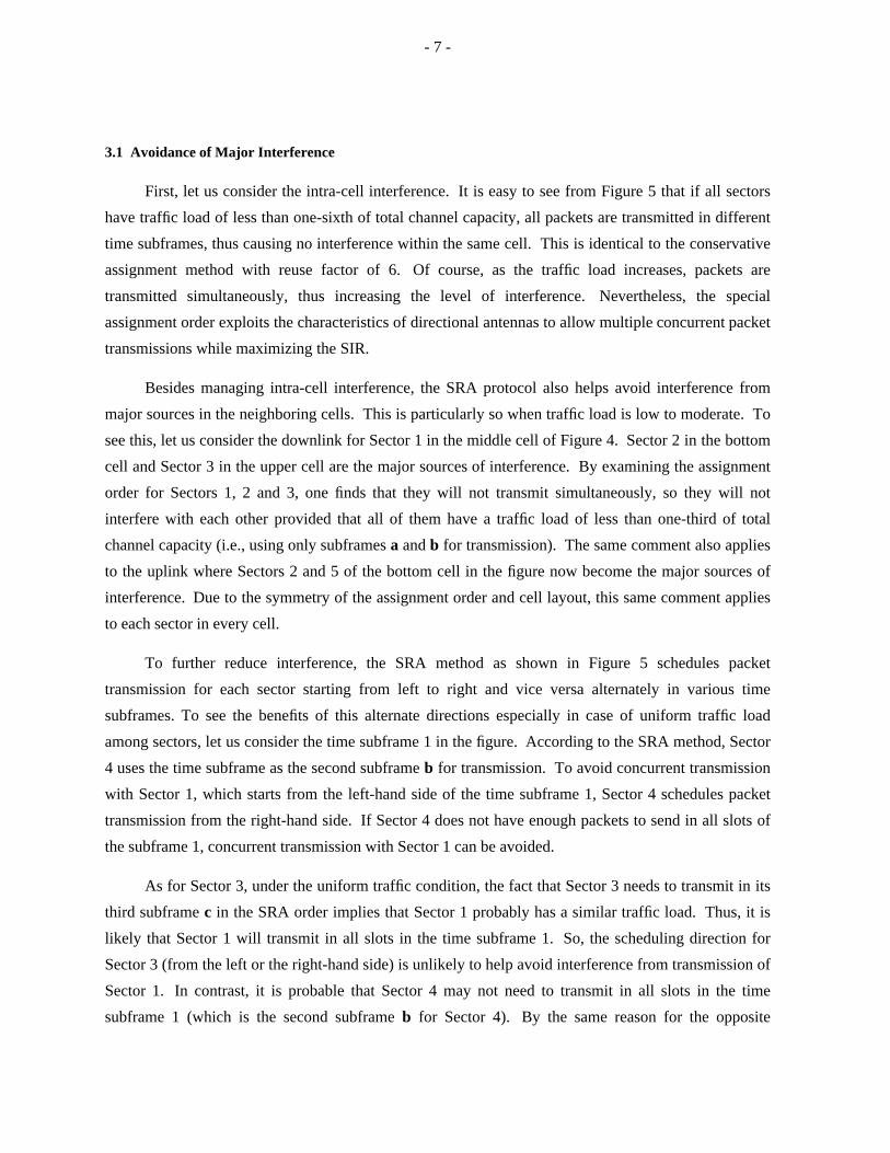
frame. Once q l’s are known from the interference submodel discussed below, the probabilities

P k (L i , 1 ) for all k and i can be obtained from the recursion in (11) to (13). Based on the P k (L i , 1 )’s,

transition probabilities in (10) can be computed, thus π; i = 1 , 2 , ... ,M is solved from (9). Finally, the

throughput of the SRA method in terms of packets per slot for each sector is

S =i =0ΣM

k =0ΣL i

kP k (L i , 1 ) πi . (14)

We can also approximate the success probability of an arbitrary packet transmission as follows. Since

each frame has L slots, the average number of packets scheduled for transmission in each frame is

given byi =1ΣM

min (i ,L) πi . Given the throughput S, the average number of successful packet

transmissions in each frame is LS. The success probability is approximated by

P s ∼∼

i =1ΣM

min (i ,L) πi

LS_____________ . (15)

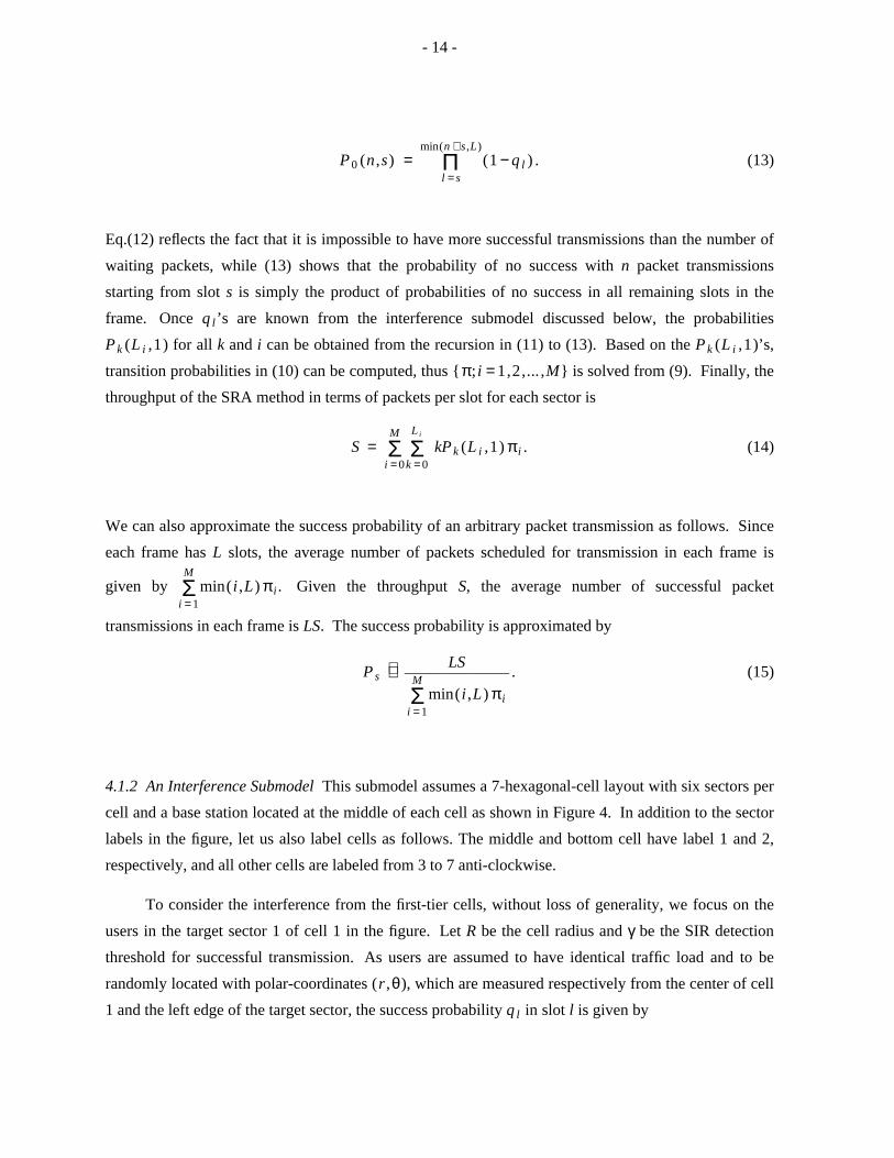
4.1.2 An Interference Submodel This submodel assumes a 7-hexagonal-cell layout with six sectors per

cell and a base station located at the middle of each cell as shown in Figure 4. In addition to the sector

labels in the figure, let us also label cells as follows. The middle and bottom cell have label 1 and 2,

respectively, and all other cells are labeled from 3 to 7 anti-clockwise.

To consider the interference from the first-tier cells, without loss of generality, we focus on the

users in the target sector 1 of cell 1 in the figure. Let R be the cell radius and γ be the SIR detection

threshold for successful transmission. As users are assumed to have identical traffic load and to be

randomly located with polar-coordinates (r ,θ), which are measured respectively from the center of cell

1 and the left edge of the target sector, the success probability q l in slot l is given by

- 15 -

q l =0∫R

0∫π/3

Pr Σ i =1

6 Ili (r ,θ)

β1 (r ,θ) S T r −n_ ____________ ≥ γ

rdθdr (16)

where S T is the fixed transmission power, β1 (r ,θ) is the lognormal shadow fading between the BS

antenna in cell 1 and the location at (r ,θ), n is the exponent of the propagation path loss and Ili (r ,θ) is

the aggregated interference from all sectors with label i received at location (r ,θ) in slot l. (It is

understood that the interference in the denominator of (16) excludes the desired signal from the BS

antenna of the target sector 1.) The amount of interference depends on the slot index l, the scheduling

order, traffic load in all other sectors, the distances between the target location and interfering BS, and

the FTB ratios of both BS and terminal antennas.

For example, for 1 ≤ l ≤ L /6, the amount of interference from sector 1 of all other cells received

at the location (r ,θ) in the target sector 1 is

Il1 (r ,θ) = S T F 1

i = lΣM

πi (17)

where

F 1 =d 2 (r ,θ) n

τ B τ T β2 (r ,θ)_ ___________ +d 3 (r ,θ) n

τ T β3 (r ,θ)_ _________ +d 4 (r ,θ) n

τ B β4 (r ,θ)_ _________ +d 5 (r ,θ) n

τ B β5 (r ,θ)_ _________ +d 6 (r ,θ) n

τ B β6 (r ,θ)_ _________

+d 7 (r ,θ) n

τ B τ T β7 (r ,θ)_ ___________ , (18)

d i (r ,θ) is the distance between the BS in cell i to location (r ,θ) in the target sector 1, β i (r ,θ)

represents the lognormal shadow fading between the BS antenna in cell i and location (r ,θ), and τ B

and τ T denote the FTB ratios in linear scale for the BS and terminal antenna, respectively. The

summation index in (17) has a lower bound of l because given 1 ≤ l ≤ L /6, a sector 1 does not

transmit in slot l if it has less than l packets pending for transmission, thus causing no interference.

Furthermore, the factor F 1 in (18) is obtained by observing that, for example, the interference from

sector 1 of cell 2 (i.e., the bottom one in Figure 4) propagates from the back lobe of the BS antenna to

the back lobe of terminal antenna at the target sector 1, thus being attenuated by both FTB ratios, τ B

and τ T . As indicated in the corresponding terms in (18), the magnitude of interference from sector 1 of

other cells is attenuated according to the FTB ratios of the (transmitting) BS and (receiving) terminal

- 16 -

antenna, depending on the directions of the antennas. Note that this way of finding F 1 represents an

approximate approach for some locations because it does not precisely consider the exact location and

the beamwidth of terminal antennas, but they are included in the simulation model below.

Using the same arguments, we have

Il1 (r ,θ) = S T F 1

i =3L /6 + lΣM

πi for L /6 + 1 ≤ l ≤ 2L /6 . (19)

This is because slots l with L /6 + 1 < l ≤ 2L /6 are in subframe 2 and sector 1 schedules packet

transmission in subframe 2 as the fifth subframe (denoted by e) according to the SRA order in Figure 5.

This implies that the sector 1 must have at least 4L /6 + 1 packets waiting for transmission, as reflected

by the lower bound for the summation index in (19). Similarly, the interference from sector 1 of all

other cells in other slots of the frame is given by

Il1 (r ,θ) = S T F 1

i =L /6 + lΣM

πi for 2L /6 + 1 ≤ l ≤ 3L /6 , (20)

Il1 (r ,θ) = S T F 1

i = l −2L /6ΣM

πi for 3L /6 + 1 < l ≤ 4L /6 , (21)

Il1 (r ,θ) = S T F 1

i = l −2L /6ΣM

πi for 4L /6 + 1 < l ≤ 5L /6 , (22)

and

Il1 (r ,θ) = S T F 1

i = lΣM

πi for 5L /6 + 1 < l ≤ L . (23)

Similarly, formulas for Ili (r ,θ) for i = 2 to 6 have been derived, but they are omitted here for brevity.

To obtain the throughput in (14), we first assume an initial distribution for πi ; i = 1 to M.

For example, we let πi = 1/ M for all i. Then, all q l for l = 1 to L can be computed from (16) by Monte-

Carlo simulation techniques [LK82]. These new q l’s in turn are used to generate the new P k (L i , 1 )’s,

p i j’s and finally new πi’s according to (11), (10) and (9), respectively. The iterations stop when the old

- 17 -

and new πi’s converge; that is,i

max π iold − πi

new < ε (e.g., 10 −3). Hence, the approximate throughput

for the SRA method at steady state is obtained in (14).

4.2 Simulation Model

The simulation model also considers the 7-hexagonal-cell layout in Figure 4. Each cell is

divided into 6 sectors, each of which is served by a BS antenna co-located at the center of the cell. The

beamwidth of each BS and terminal antenna is 60o and 30o , respectively, while each terminal antenna

points directly to its BS antenna. The FTB ratios for the BS and terminal antenna are finite and

adjustable as input parameters for the simulation. The model uses ideal antenna patterns in a way that

if a receiver antenna sees the front lobe of a transmitting antenna, the radio signal is not attenuated.

Otherwise, the signal is attenuated according to the FTB ratio. Each radio path between a pair of BS

and terminal antennas is characterized by a path-loss model [R96, p.102] and lognormal shadow fading.

For the downlink, since there is only one radio path between all BS antennas in the same cell (which

are co-located) and an arbitrary terminal, the intended signal and interference experience the same

lognormal fading and path loss. However, the fading from BS antennas in different cells are different

and independent. For each packet transmission, if the SIR at the intended receiver exceeds a threshold,

the packet is considered to be successfully received. Otherwise, the packet is retransmitted later. Since

our focus is on the throughput, the simulation model assumes no retransmission delay and that new and

transmitted packets in each sector are scheduled for transmission effectively in a random order.

There are 20 terminals (or users) randomly placed in each sector. For downlink traffic, as in the

approximate model, each BS antenna is assumed to have a buffer to hold one packet for each user.

When the buffer is occupied, subsequent packet arrivals for the user are blocked and cleared. Packets

are scheduled to transmit by each BS antenna according to the SRA method as discussed above.

To avoid non-uniform performance in the outer layer of cells, only the statistics in the middle cell

in Figure 4 are collected and reported below.

5. THROUHGPUT PERFORMANCE AND DISCUSSION

In this numerical study, each subframe has 12 time slots, each sector has 20 terminals, the

standard deviation of lognormal shadowing is 4 dB and the path loss exponent is 4.

Figure 6 presents the downlink throughput of the SRA method as a function of normalized

aggregated load from the analytic approximate model and the simulation model (represented by curves

and symbols, respectively). A set of typical FTB ratios for BS and terminal antennas, denoted by B

- 18 -

and T respectively, are considered in the examples. Clearly, the throughput depends on the SIR

detection threshold. With straightforward modulation and equalization schemes (e.g., QPSK and DFE),

the threshold probably lies between 10 to 15 dB. As shown in the figure, the maximum throughput in

each sector for the SRA protocol with these parameters ranges from 30% to 80%. That is, while re-

using the same frequency to support high user data rates in every sector of every cell, we can still

achieve a throughput in excess of 30%, which translates into a very large network capacity! For the

30% to 80% throughput per sector, each cell effectively has a data capacity of 1.8 to 4.8 times of the

channel data rate. Evidently, this happens because, as intuitively expected, the SRA protocol is capable

of selectively allowing concurrent packet transmission to increase throughput while avoiding major

interference to yield satisfactory reception. It is possible that the SRA throughput can be improved

further if the FEC code and power control are adopted in a way similar to that in [BFZA96] and

[BZFTB96].

In terms of the quality of the analytic model, as shown in Figure 6, the approximations closely

match the simulation results, except for the case with 15 dB detection threshold, and the FTB(B,T)

ratios of 20 and 10 dB at high traffic conditions. Given the stringent detection threshold and antenna

characteristics, packet transmission is likely to fail and subject to retransmissions in this case, thus

yielding high aggregated traffic load and strengthening the interdependence among all BS’s. When this

happens, the approximate model, which only captures part of the correlation among BS’s by use of

success probability, becomes inadequate for predicting accurate throughput. For other less stringent

parameter settings, the approximations are excellent.

Another way to quantify the merits of the SRA method is the success probability of an arbitrary

packet transmission. Using the approximation in (15), Figure 7 shows that the probability obtained

decreases as the traffic load grows. To avoid excessive retransmission delay, it is expected that the

success probability should be higher than 90%. In light of this, we observe from the figure that except

at high load for the most stringent case, the probability is above 90% for all other three settings.

Combining this with the throughput results discussed above, the SRA method is capable of sustaining a

throughput of 70% to 80% per sector, while yielding the satisfactory success probability. Even for the

most stringent case, the target success probability can be maintained by keeping the throughput below

30%, which still represents a large network capacity.

By focusing on the co-channel interference, two analytic models similar to that for the SRA

method, were developed to evaluate the throughput for the left-right protocol and the method with reuse

factor of 6 discussed in Section 2. For brevity, they are omitted here. Our analytic results in Figure 8

show that the SRA method provides much higher throughput than the left-right protocol and the

- 19 -

method with reuse factor of 6. As shown in the figure, the throughput of the method with reuse factor

of 6 is limited to about 1/6 simply because the method requires each time subframe be used by only one

sector in each cell. In addition, the left-right protocol effectively has a frequency reuse factor of one at

high-load situations. However, since it does not avoid major interference as well as the SRA method

does, the latter yields a higher throughput. Although the figure shows the comparison for a given

parameter setting, our numerical results reveal that the SRA method generally performs better than the

left-right protocol.

As discussed in Section 3.2, the SRA method can be used in conjunction with a control

mechanism to limit the degree of concurrent packet transmission for enhancing the reception quality.

Although our analytic model can be extended to evaluate the control mechanism, the model becomes

too complicated for practical use because it has to keep track of additional information related to the

frame indices. For this reason, we used the simulation model to study the performance impacts of such

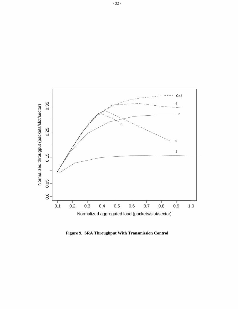
a control mechanism. In particular, simulation results in Figure 9 portray how the SRA throughput can

be improved for the most stringent case, namely, FTB(B,T)=(20dB,10dB) and the SIR threshold of

15dB. Let the degree of concurrent transmission be limited by the control to C packets per cell. Note

that when the control is not applied, C = 6 as time slots in all six subframes can be used for

transmission by each sector. As C decreases from 6, the maximum throughput first increases and

reaches the peak when C = 3. This is so because with a smaller C value, the control effectively limits

the degree of concurrent packet transmission, thus enabling more packets to exceed the SIR threshold

and improving the throughput. However, as C decreases further, the throughput starts to decrease

because only a small fraction of time slots are available for transmission by each sector when C is too

small. Note that when C = 1, the SRA method becomes identical to the method with reuse factor of 6,

having a maximum throughput of about 1/6.

We also observe from Figure 9 that for C = 4 to 6, the throughput first increases, reaches a peak

at a certain aggregated load, and then starts to decrease if the load increases further. In contrast, the

throughput for cases with C = 1 to 3 always increases, perhaps marginally with the traffic load. This is

because for the given parameter setting, if the degree of concurrent transmissions is higher than 3,

packet transmissions become more likely to fail as more packets are transmitted at high loads. On the

other hand, for C = 1 to 3, the throughput is limited mainly by the control even when the aggregated

load approaches 1. Thus, the throughput still increases slightly as the traffic load increases.

In a separate study, we find that for the most stringent parameter setting, even when C = 1, only a

few percent of randomly chosen locations such as those at the boundary of adjacent cells may have

difficulty in achieving the SIR threshold of 15dB. The percentage is reduced for a lower threshold

- 20 -

and/or higher antenna FTB ratios, and may increase for antenna patterns that are more practical than the

ideal one assumed here. To provide close to 100% coverage in harsh environment, it may be desirable

to enhance the SRA method to serve those "bad" locations. Other strategies to allocate radio resources

to "bad" and "good" locations can also been found in [QC97].

In addition to improving the throughput, the control mechanism also enhances the packet success

probability in the SRA method. This can be seen from the simulation results in Figure 10 for the most

stringent case. As one would expect, at a fixed traffic load, the probability increases as C decreases

simply because less concurrent transmission implies less interference. It is interesting to observe that

the probability is only marginally improved when C changes from 2 to 1, while the corresponding

throughput improvement is much larger in Figure 9. This characteristic of the SRA method can be

explored by network designers to obtain a balanced tradeoff between the throughput and success

probability for a given radio environment and the desired QoS.

Our further results (which are omitted for brevity) show that the SRA method is also very

effective in avoiding co-channel interference for uplink. This is particularly so when the control

mechanism is applied such that terminals in each sector are scheduled to transmit only in time slots of

the first subframe according to the SRA order. In this case of C = 1, even for the most stringent

parameters of FTB(B,T)=(20dB,10dB) and the SIR threshold of 15dB, the SRA method yields a stable

uplink throughput of 16.7% for each sector and very high packet success probability at high traffic

loads. In light of asymmetrical bandwidth consumption between uplink and downlink such as for

Internet applications [M97], this uplink throughput adequately matches that of the downlink.

6. CONCLUSION

We have shown that the combination of directional antennas plus dynamic resource allocation in

the time domain is highly effective in controlling co-channel interference in fixed wireless systems.

With our focus on the co-channel interference and for reasonable choices of system parameters, the

staggered resource allocation (SRA) technique delivers high throughput while permitting a given band

of frequencies to be re-used in every sector of every cell. The SRA method also provides satisfactory

probability of successful packet transmission. In addition, a simple control mechanism can be applied

in the SRA method to improve the throughput and success probability for harsh radio environments and

poor antenna characteristics. We believe the proposed approach is a significant step forward in

establishing the viability of fixed broadband wireless access networks.

- 21 -

ACKNOWLEDGEMENTS

Thanks are due to Lek Ariyavisitakul, Kapil Chawla, Len Cimini, Vinko Erceg, Tony Rustako

and Arty Srivastava for their helpful discussions.

- 22 -

REFERENCES

[AEK96] E. Ayanoglu, K.Y. Eng and M.J. Karol, "Wireless ATM: Limits, Challenges, and Proposals,"

IEEE Personal Communications, pp.18-34, August 1996.

[BFZA96] F. Borgonovo, L. Fratta, M. Zorzi and A. Acampora, "Capture Division Packet Access: A

New Cellular Access Architecture for Future PCNs," IEEE Communications Magazine,

pp.154-162, Sept. 1996,

[BZFTB96] F. Borgonovo, M. Zorzi, L. Fratta, V. Trecordi and G. Bianchi, "Capture-Division Packet

Access for Wireless Personal Communications," IEEE J. Select. Areas in Commun., pp.609-

622, Vol.14, No.4, May 1996.

[C69] W.W. Chu, "Optimal File Allocation in a Multiple Computer System," IEEE Trans. on

Computers, C-18, No.10, pp.885-889, Oct. 1969,

[GJ79] M.R. Garey and D.S. Johnson, Computers and Intractability: A Guide to the Theory of NP-

Completeness, W.H. Freeman and Company, San Francisco, 1979.

[KN96] I. Katzela and M. Naghshineh, "Channel Assignment Schemes for Cellular Mobile

Telecommunication Systems: A Comprehensive Survey," IEEE Personal Communications,

pp.10-31, June 1996.

[KW97] N. Kahale and P.E. Wright, "Dynamic Global Packet Routing in Wireless Networks," Proc. of

IEEE INFOCOM’97, Kobe, Japan, April 1997, pp.1416-1423.

[L89] W.C.Y. Lee, Mobile Cellular Telecommunications Systems, McGraw-Hill, New York, 1989.

[LK82] A.M. Law and W.D. Kelton, Simulation Modeling and Analysis, McGraw-Hill, New York

(1982).

[M97] B.A. Mah, "An Empirical Model of HTTP Network Traffic," Proc. of IEEE INFOCOM’97,

Kobe, Japan, April 1997, pp.593-602.

[QC97] X. Qiu and K. Chawla, "Resource Assignment in a Fixed Wireless System," IEEE Commun.

Letters, Vol.1, No.4, pp.108-110, July 1997.

[R96] T.S. Rappaport, Wireless Communications: Principles and Practice, IEEE Press and Prentice

Hall PTR, New York, 1996.

- 23 -

[W96] J.F. Whitehead, private communications, 1996.

[WSG94] J.H. Winter, J. Salz and R.D. Gitlin, "The Impact of Antenna Diversity on the Capacity of

Wireless Communication Systems," IEEE Trans. on Commun., pp.1740-1751, Vol.42, No.2-4,

Feb.-April 1994.

- 24 -

A

B

Figure 1. Major Sources of Interference for Downlink

- 25 -

A

B

Figure 2. Major Sources of Interference for Uplink

- 26 -

21

1

1

1

2

2

1 1

2

22

2

2

2

2

2

2

2

2

2

2 2

2

2

2 2

1 1

1

1

1 1

1 1

1 1 1

1

1 1

1

... ... time1 2

Figure 3. Time-Slot Assignment with Reuse Factor of 2

Subframe

- 27 -

21

34

5

6

21

65

4

3 3

5

2

1

4

56 4

32

1

4

1

65

4

32

1

5

2

1

43

6 6

23

56

1 2 3 4 5 6 1time

Figure 4. Time-Slot Assignment with Reuse Factor of 6

- 28 -

1 4 6 2 3 5

Time Subframes

a

a

a

a

a

a

b

b

b

b

b

b

c

c

d

d

d f e

c f

c d e

e

e

f

d f

c e f

c d f e

2

1

3

4

5

6

Figure 5. Order of Slot Assignment for the SRA Method

time

Sector

- 29 -

0.1 0.2 0.3 0.4 0.5 0.6 0.7 0.8 0.90

0.1

0.2

0.3

0.4

0.5

0.6

0.7

0.8

0.9

1

Normalized aggregated load (packets/slot/sector)

Nor

mal

ized

thro

ughp

ut (

pack

ets/

slot

/sec

tor)

___, xxx: FTB(B, T)=(25dB, 15dB), Threshold=10dB−.−, ooo: FTB(B, T)=(20dB, 10dB), Threshold=10dB......, ***: FTB(B, T)=(25dB, 15dB), Threshold=15dB−−−, +++: FTB(B, T)=(20dB, 10dB), Threshold=15dB

Figure 6. Throughput of the SRA Method

- 30 -

0.1 0.2 0.3 0.4 0.5 0.6 0.7 0.8 0.90

0.1

0.2

0.3

0.4

0.5

0.6

0.7

0.8

0.9

1

Normalized aggregated load (packets/slot/sector)

Pac

ket s

ucce

ss p

roba

bilit

y

___: FTB(B, T)=(25dB, 15dB), Threshold=10dB−.−: FTB(B, T)=(20dB, 10dB), Threshold=10dB......: FTB(B, T)=(25dB, 15dB), Threshold=15dB−−−: FTB(B, T)=(20dB, 10dB), Threshold=15dB

Figure 7. Packet Success Probability for the SRA Method

- 31 -

0 0.1 0.2 0.3 0.4 0.5 0.6 0.7 0.8 0.9 10

0.1

0.2

0.3

0.4

0.5

0.6

0.7

0.8

Normalized aggregated load (packets/slot/sector)

Nor

mal

ized

thro

ughp

ut (

pack

ets/

slot

/sec

tor)

Detection threshold=15dB

FTB (B, T)=(25dB, 15dB)

___: SRA method

−.−: Left−Right protocol

−−−: Method with reuse factor six

Figure 8. Comparison of the SRA Method, Left-Right Protocol and Method with Reuse Factor of 6

- 32 -

Normalized aggregated load (packets/slot/sector)

Nor

mal

ized

thro

ugpu

t (pa

cket

s/sl

ot/s

ecto

r)

0.1 0.2 0.3 0.4 0.5 0.6 0.7 0.8 0.9 1.0

0.0

0.05

0.15

0.25

0.35

C=3

2

4

5

6

1

Figure 9. SRA Throughput With Transmission Control

- 33 -

Normalized aggregated load (packets/slot/sector)

Pac

ket s

ucce

ss p

roba

bilit

y

0.1 0.2 0.3 0.4 0.5 0.6 0.7 0.8 0.9 1.0

0.0

0.2

0.4

0.6

0.8

1.0

C=1

2

3

4

5

6

Figure 10. Packet Success Probability for the SRA Method With Transmission Control