R7936 - Technical Manual HyPAR4 - GOV.UK

D. C. Mobbs 1, G. J. Lawson 1, A. D. Friend 1, N. M. J. Crout 2, J. R. M. Arah 1, M. G. Hodnett 3

1 Institute of Terrestrial EcologyBush Estate, Penicuik

Midlothian EH26 0QB

Phone: (+44) 131-445-4343 Fax: (+44) 131-445-3943

Web: www.nbu.ac.uk/ite/edin/agro

2 Physiology and Environmental Science University of Nottingham

Sutton Bonnington LE12 5RD

3Institute of HydrologyWallingford

Oxon OX10 8BB

© 1999 DFID Forestry Research Programme (R5652) Any conclusions derived from the HyPAR model are the responsibility of the user and not that of

The Institute of Terrestrial Ecology or the Department for International Development.

HyPAR Model for Agroforestry Systems

Technical Manual

Model Description for Version 3.0

July 1999

http://www.nbu.ac.uk/ite/edin/agro

Table of contents

i

1. HyPAR Model Overview...............................................................................1

1.1 Technical manual structure............................................................................................................ 2

2. The Weather Options ......................................................................................3 2.1 Predicted Daily Weather................................................................................................................ 3

2.2 Daily Weather Provided by the User ............................................................................................. 3

3. The Crop Model...............................................................................................5 3.1 Daily Assimilation......................................................................................................................... 6

3.2 Calculation of 'stress' ..................................................................................................................... 8

3.3 Interception of Light...................................................................................................................... 9

3.4 Water Uptake............................................................................................................................... 11

3.5 Nutrient Uptake ........................................................................................................................... 12

3.6 Phenological Development.......................................................................................................... 14

3.7 Partitioning of Resources............................................................................................................. 15

3.8 Leaf Growth................................................................................................................................. 16

3.9 Root Growth ................................................................................................................................ 18

3.10 Reproductive Growth ................................................................................................................ 22

3.11 Parameter Summary .................................................................................................................. 24

4. The Tree Model..............................................................................................27 4.1 Model structure for tree growth................................................................................................... 27

4.2 Irradiance calculations................................................................................................................. 28

4.3 Net photosynthesis....................................................................................................................... 29

4.4 Maintenance respiration .............................................................................................................. 31

4.5 Total daily tree carbon balance.................................................................................................... 32

4.6 Stomatal conductance .................................................................................................................. 33

4.7 Foliage energy balance and transpiration .................................................................................... 34

4.8 Nitrogen uptake ........................................................................................................................... 34

4.9 Tree litter production................................................................................................................... 35

4.10 Allocation in trees...................................................................................................................... 37

4.11 Root distribution........................................................................................................................ 44

4.12 Phenology .................................................................................................................................. 45

Table of Contents

ii

4.13 Tree Management ...................................................................................................................... 46

4.14 Parameter Summary .................................................................................................................. 47

5. Canopy Disaggregation.................................................................................48 5.1 Tree Representation..................................................................................................................... 48

5.2 Light Incident under the Canopy ................................................................................................. 49

5.3 Shadow output ............................................................................................................................. 53

6. Water Cycle....................................................................................................56 6.1 Soil Profile Specification............................................................................................................. 56

6.2 Aboveground Water .................................................................................................................... 56

6.3 Water Movement ......................................................................................................................... 57

6.4 PARCH soil water model option ................................................................................................. 58

6.5 SWM option ................................................................................................................................ 67

6.6 Water Uptake............................................................................................................................... 69

6.7 Annex 1 Derivation of Pedo Transfer Functions (PTFs) for the prediction of the water release curve of tropical soils. ....................................................................................................................... 71

7. Soil Nitrogen Model.......................................................................................79 7.1 Vertical Distribution of Nitrogen and Organic Matter ................................................................ 79

7.2 Soil Organic Matter ..................................................................................................................... 80

7.3 Temperature Limitation............................................................................................................... 81

7.4 Moisture Limitation..................................................................................................................... 81

7.5 C:N Limitation............................................................................................................................. 82

7.6 Nitrogen uptake by trees and crops ............................................................................................. 82

8. Model Output.................................................................................................84 8.1 Output file format ........................................................................................................................ 84

8.2 Graphical Output ......................................................................................................................... 84

8.3 Environment ................................................................................................................................ 85

8.4 Crop ............................................................................................................................................. 86

8.5 Tree.............................................................................................................................................. 89

8.6 Soil............................................................................................................................................... 92

8.7 Water ........................................................................................................................................... 95

Table of contents

iii

8.8 Field............................................................................................................................................. 95

9. References.......................................................................................................97

HyPAR v3.0

1

1. HyPAR Model Overview

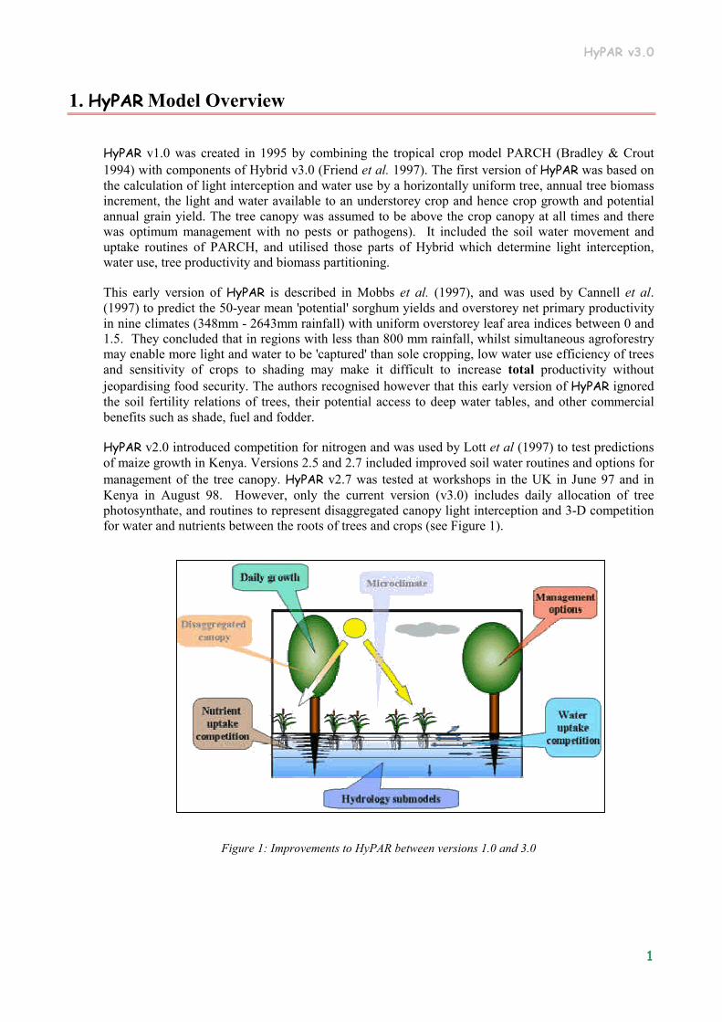
HyPAR v1.0 was created in 1995 by combining the tropical crop model PARCH (Bradley & Crout 1994) with components of Hybrid v3.0 (Friend et al. 1997). The first version of HyPAR was based on the calculation of light interception and water use by a horizontally uniform tree, annual tree biomass increment, the light and water available to an understorey crop and hence crop growth and potential annual grain yield. The tree canopy was assumed to be above the crop canopy at all times and there was optimum management with no pests or pathogens). It included the soil water movement and uptake routines of PARCH, and utilised those parts of Hybrid which determine light interception, water use, tree productivity and biomass partitioning.

This early version of HyPAR is described in Mobbs et al. (1997), and was used by Cannell et al. (1997) to predict the 50-year mean 'potential' sorghum yields and overstorey net primary productivity in nine climates (348mm - 2643mm rainfall) with uniform overstorey leaf area indices between 0 and 1.5. They concluded that in regions with less than 800 mm rainfall, whilst simultaneous agroforestry may enable more light and water to be 'captured' than sole cropping, low water use efficiency of trees and sensitivity of crops to shading may make it difficult to increase total productivity without jeopardising food security. The authors recognised however that this early version of HyPAR ignored the soil fertility relations of trees, their potential access to deep water tables, and other commercial benefits such as shade, fuel and fodder.

HyPAR v2.0 introduced competition for nitrogen and was used by Lott et al (1997) to test predictions of maize growth in Kenya. Versions 2.5 and 2.7 included improved soil water routines and options for management of the tree canopy. HyPAR v2.7 was tested at workshops in the UK in June 97 and in Kenya in August 98. However, only the current version (v3.0) includes daily allocation of tree photosynthate, and routines to represent disaggregated canopy light interception and 3-D competition for water and nutrients between the roots of trees and crops (see Figure 1).

Figure 1: Improvements to HyPAR between versions 1.0 and 3.0

HyPAR v3.0

2

1.1 Technical manual structure

This Technical Manual supplements the HyPAR User Guide and details the processes and algorithms contained in version 3.0 of the model. Updated versions of the manual can be found as an Adobe Acrobat PDF file located on the Agroforestry Modelling Web site (www.nbu.ac.uk/hypar).

Chapter 2 considers the options provided to run HyPAR with recorded daily weather, or to predict weather from a database of monthly data for worldwide sites on half-degree grid-squares. The PARCH crop model routines, parameterisation and the modifications made in the HyPAR implementation for multiple plots within a field are outlined in Chapter 3 (largely based on Crout et al. 1997). Chapter 4 introduces the tree model, the required parameters, and the changes introduced to account for a disaggregated canopy and tree-root system (based on Friend, 1997). Chapter 5 describes the options for light interception in an agroforestry system, for a uniform or disaggregated tree canopy. The range of soil hydrology and pedotransfer functions available is outlined in Chapter 6, together with the techniques used to account for tree and crop water competition in HyPAR v3.0. Chapter 7 explains HyPAR’s approach to modelling soil nitrogen flux competition for nitrogen between tree and crop roots. Chapter 8 provides fuller details than contained in the User Guide on the output files which can be selected by the user, and the available Excel spreadsheet macros for use in graphing model outputs.

http://www.nbu.ac.uk/hypar

HyPAR v3.0

3

2. The Weather Options

The tree and crop routines are driven by climate, so appropriate data must be supplied.

2.1 Predicted Daily Weather

Many global ecological models require globally gridded daily weather data, but such data are not directly available from the current global network of weather stations. HyPAR v3.0 uses a method described by Friend (1998) whereby a stochastic daily weather generator is parameterised to operate at half-degree scale for the Earth's terrestrial surface. The weather generator simulates 24-hour shortwave irradiance, precipitation, maximum and minimum temperatures, and mean water vapour pressure (Figure 2). Parameterisation and use of this weather generator obviates the need for real daily weather data for many applications. The HyPAR Control Centre enables files of monthly data to be inserted, copied and edited or created. In addition, for a specific simulation run, any of the above variables can be temporarily increased or decreased by a percentage chosen by the user.

5.000 6.0000.09 12.16 31.10 22.49 198.87 82.73 2.00 2915.030.14 14.68 32.17 23.22 216.26 83.24 2.00 3091.510.30 14.20 31.83 23.76 206.70 84.67 2.00 3163.290.46 14.99 31.65 23.14 215.28 86.13 2.00 3143.420.56 14.61 30.94 22.65 203.93 87.06 2.00 3067.620.76 15.22 29.09 22.10 173.22 88.87 2.00 2917.150.89 14.78 28.01 21.78 159.61 89.98 2.00 2833.130.62 14.65 28.28 21.51 175.34 87.59 2.00 2757.880.92 15.29 28.41 22.18 166.41 90.29 2.00 2911.380.66 14.68 29.56 22.03 188.10 87.96 2.00 2921.630.27 14.55 31.11 22.28 203.77 84.34 2.00 2954.400.13 13.02 31.23 21.96 206.13 83.08 2.00 2893.10

Figure 2: Typical input file required by the stochastic daily weather generator used within HyPAR. The first line shows the latitude and longitude of the site (degrees) followed by one row of figures for each month (January to December). The variables are: fraction of wet days per month, rain per wet day (mm), maximum and minimum daily temperature (oC), solar radiation (W/m2), relative humidity (only used if vapour pressure missing), wind speed (not used) and vapour pressure (Pa)

2.2 Daily Weather Provided by the User

If daily meteorological data are available, either recorded or generated from another source, they can be used directly if all the necessary variables are provided for a full 365 days per simulation year. Two input weather file formats are currently recognised by HyPAR:

2.2.1 ICRI Format

This is a format used in the original PARCH model. Each input file of data is called <name>W<nn>.wea where <name> is a mnemonic for the site and nn is a 2-digit representation of the year. Thus, if in the Control Centre the user selects edinW98.wea and wants a 4-year run then HyPAR expects to find edinW98.wea, edinW99.wea, edinW00.wea and edinW01.wea. Note that the 2-digit format means the run is limited to 100 years of daily climate before repeating. However, if a longer run is needed, use of the internal weather generator is recommended.

Inside each ICRI-type file HyPAR expects to find 365 rows each with complete daily data in the order:

AA, AA, Precipn(K1), PANE(K1), MAXTEMP(K1), MINTEMP(K1), RH14, RH07, AA, SDTEMP, SZ(K1)

HyPAR v3.0

4

i.e., two null columns (any number value), rainfall (mm), pan evaporation (mm), maximum daily temperature oC, minimum daily temperature oC, relative humidity at 2 p.m. or 0, relative humidity at 7 a.m. or 0, null, saturation deficit (only used if the relative humidity figures are both 0) and solar radiation (MJ/m2/day).

For example (in file n123w96.wea):

0 0 0.2 6.1476 29.5 17.18 51.7 100 0 0 29.1536 0 0 13 6.1873 29.01 17.11 50.8 100 0 0 28.378 0 0 6 5.146 29.44 16.21 51.2 100 0 0 25.8175 0 0 2 5.0315 28.04 17.11 56.4 100 0 0 25.2483

2.2.2 Embu Format

This format was added for ICRAF Embu data. Here the files are called clim<nnnn>.emb where nnnn is the 4-digit.year. The format inside the file is 4 comment lines followed by 365 rows

AA, i, Precipn(K1), MAXTEMP(K1), MINTEMP(K1), SZ(K1), PANE(K1), RH07, RH14, WINDS

i.e. AA is text, i is an integer for the day followed by rainfall, maximum temperature, minimum temperature, solar radiation, pan evaporation, relative humidity at 7am, relative humidity at 2pm, and wind speed.

For example:

Climatic Summary of KARI Embuyear 1993

Rainfall Air Tem Radiatn P.Evapo. RH (%) WindspeedMONTH DATE (mm) Max Min (mj) (mm) Max Min (Km/d)

JAN 1 4.4 22.4 13.2 10.48 1.9 87 76 87.3

JAN 2 0 22.7 15.1 13.05 2.5 95 70 103.4

JAN 3 0 23.4 12.7 20.92 4.5 74 62 156.3

JAN 4 0 23.4 11.1 22.72 5.5 74 62 162.2

JAN 5 1.8 23.6 11.1 18.76 4.3 62 60 168

2.2.3 Other daily weather file formats

Formats potentially usable with HyPAR include SBON and DSSAT. Please contact the first author if you require an additional input format to be provided.

HyPAR v3.0

5

3. The Crop Model

The crop components within HyPAR v3.0 are based on the tropical crop model PARCH (Bradley & Crout 1994), including the methods used to set a sowing date as well as the daily growth of the crop during the season. The model runs continuously from year to year allowing several annual crop seasons to be studied, though the current version permits only one crop per 365-day period. After each harvest, the roots are assumed to remain in the soil while aboveground residues may be left on the soil surface or removed. Residues include crop stalk and leaves, but exclude haulm. Fertiliser additions are described in Chapter 7.

HyPAR can be set to simulate different planting densities (in plants per ha). The timing of planting can be set in two ways: by specifying the minimum water content which must be present in the top 40cm of soil and by giving the earliest day on which planting can take place. Setting the former to a very low figure can force planting to take place on the date provided.

Figure 3: Annual and daily calculations in the PARCH model

In HyPAR, the crop is grown in 'plots' within a field of known dimensions. If the simulation is set to have a uniform tree canopy, only one crop plot is simulated and this is assumed to be representative of the growth across the whole field. If the tree canopy is disaggregated then the field must be divided

Resetvariables

Getweather

Set cultivarparameters

Incrementthermal time

Resource captureand limits

Partitionphotosynthate

Grow plantparts

Soil water

Outputinterpretation

Front endmenu

TimeLoop

YearLoop

Set soilparameters

Sow?

Yes

No

HyPAR v3.0

6

into a number of square plots for crop growth (see Chapter 5). Crop is planted and harvested simultaneously in every plot, these events being triggered when conditions in at least half of the plots meet the planting or harvesting criteria specified. Crop plants are restricted to one plot, i.e. roots cannot extend into neighbouring plots nor do leaves shade their neighbours (trees are not restricted either above or below ground and can extend throughout the field into all plots).

In the following model description, the main reference to the HyPAR cultivar-specific input parameters are identified with a symbol, , in the margin and listed in a table in Section 3.11.

3.1 Daily Assimilation

The method used to calculate daily assimilation follows that used by PARCH's pre-cursor model RESCAP (Monteith et al., 1989), and is based upon conversion coefficients for crop light and water use, modified when nutrients are limiting.

Experimentally, the relationship between dry matter accumulation and intercepted radiation has been shown to be approximately linear for many crops during optimal vegetative growth (Monteith, 1981; Gallagher & Biscoe, 1978). Thus, the rate of dry matter production per day, GL (g m-2 d-1) can be expressed as

tempSiL FfG ε= 3:1.

where: fi is the fractional light interception of the canopy (see below), εs is the conversion coefficient for intercepted light (g MJ-1), S is daily solar radiation (MJ m-2 d-1) and Ftemp is a zero to unity temperature-based factor which simulates the effect of temperature on photosynthesis on the basis of mean daily air temperature (T ) using the relationship shown in Figure 4.

Figure 4: Function used to describe the effect of temperature on photosynthetic rate in the PARCH model. Tb, Tm, T2 and T1 represent the base, maximum and upper and lower optimum temperatures of the crop respectively.

The conversion efficiency used here is equivalent to net photosynthesis, in that it is derived from the measured net dry matter production. Many workers (e.g. van Laar, 1992; Jansen & Gosseye, 1986) model carbon dioxide assimilation and gross photosynthesis at a more complex level, calculating net photosynthesis by subtracting maintenance, growth and photorespiration. This approach has more biological significance and is especially useful when the various respiration elements are large or variable. The main disadvantages are the added complexity and the assumption that our limited

HyPAR v3.0

7

knowledge of these processes is correct across a range of conditions. As the photo-respiration element of C4 crops is small and maintenance and growth respiration are assumed in many models to be a reasonably constant proportion of gross photosynthesis, an average value of net photosynthesis can be derived by analysis of seasonal growth data, as described above. This has been found to be a relatively conservative and robust approach for simple modelling purposes (Charles-Edwards, 1982; Monteith, 1977), and therefore has been adopted here.

Ong & Monteith (1984) summarised light conversion efficiencies for pearl millet across different sites and seasons. Whole season efficiency varied between 1.14 and 1.49 g MJ

-1, whereas pre-anthesis

efficiency ranged from 1.5 to 2.37 g MJ-1

. The same authors discussed the effects of light saturation on individual leaves, reducing from 2.5 to 1.1 g MJ

-1 as radiation was increased from 20 to 100% of full

sunlight. Under most field situations, the 'average' leaf within a canopy should be exposed to relatively low irradiance due to shading and light scattering. This means that on average, a non-stressed C4 crop is rarely light saturated, although this may not be true for more stressed canopies.

The simple light conversion efficiency approach described above is used in this model, with two values of εs. The first (2.5 g MJ-1) is for growth stages 1 (emergence to anthesis) and 2 (post anthesis). The second (2.3 g MJ-1) is for growth stage 3. Several reasons are proposed for this lowered value, mostly relating to the fact that growth stage 3 is when grain filling takes place. Firstly, the plant cells must manufacture RNA, ribosomes and other organelles in order to produce the proteins and oils of the seed (Muchow & Coates, 1986). Secondly, proteins and fats both need more energy per unit mass to produce than carbohydrate, and seed yield is measured in terms of mass rather than carbon equivalents. Thirdly, leaves may photosynthesise at a reduced rate as nitrogen is re-mobilised from them and they begin to senesce (Jansen & Gosseye., 1986). Birch et al. (1990) and Monteith et al. (1989) both use similar values of light conversion efficiency to those used here also split between pre- and post-anthesis.

Water limited growth, GW (g m-2 d-1), is given by

G XDW max= Ω

3:2.

where: Xmax is the maximum amount of water that the root system can supply (mm d-1). The calculation of this is described below. Ω is the crop transpiration equivalent (g (DW) mm-1(water) kPa-1), as described below and D is the daily average saturation vapour pressure deficit (kPa)

Nutrient limited growth, GN (g m-2 d-1), is given by

G F F GN N P L= min( , ) 3:3.

where: FN and FP are the nitrogen and phosphorus factors whose calculation is defined below.

The daily growth, G (g m-2 d-1), is then taken as

G G G GL W N= min( , , ) 3:4.

Daily transpiration, Q (mm-1 d-1), is related to daily growth, G, via the transpiration equivalent,

Q G D=Ω

3:5.

In HyPAR v3.0, the daily transpiration rate is also modified due to competition with the tree (described below). This total amount of water required is debited from the multi-layer soil water sub-model.

HyPAR v3.0

8

The links between light conversion and water use are well known, although the theory behind these links is of complex. During water stress in most crops the reduction in photosynthesis, like that of transpiration, is initially due to stomatal closure (Boyer, 1976). This is not always the case however (Krieg & Hutmacher, 1986), and an important factor limiting photosynthesis may be of photochemical origin, related to the slow regeneration of ribulose 1-5 diphosphate, caused by dysfunction of the thylakoids at low water potential (Farquhar & Sharkey 1982). However PARCH uses the dry matter/water use ratio (e.g. Azam-Ali et al., 1994; Muchow & Bellamy, 1991; Squire, 1990; Monteith, 1986), or ‘transpiration equivalent’ (qD or Ω), whereby the amount of dry matter produced per unit water transpired is assumed constant for a given crop at unit saturation deficit.

The model parameter input allows for the effect of roots on the estimates of εs and qD. A third parameter 'FractRoot' enables the user to specify the estimated proportion of the plant that was root when qD and εs were calculated. FractRoot should be zero if the estimates included roots, otherwise around 0.2. After input, the parameters are amended such that εs = εs (1+FractRoot) and qD = qD(1+FractRoot).

3.2 Calculation of 'stress'

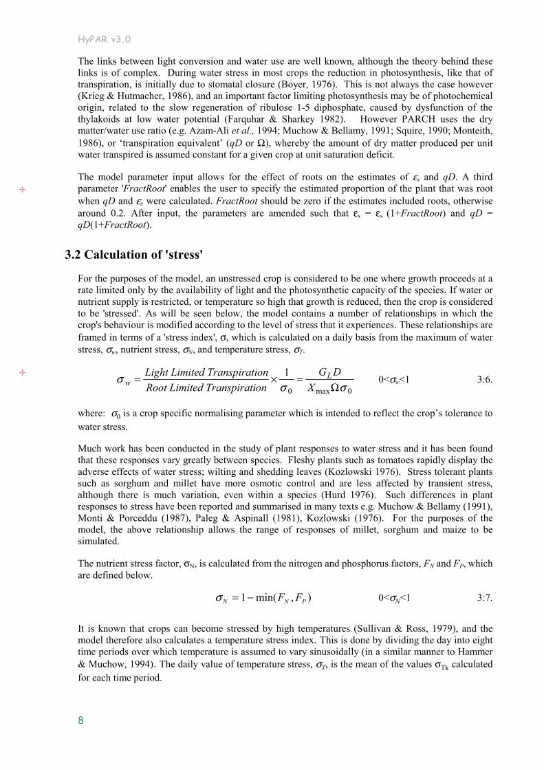
For the purposes of the model, an unstressed crop is considered to be one where growth proceeds at a rate limited only by the availability of light and the photosynthetic capacity of the species. If water or nutrient supply is restricted, or temperature so high that growth is reduced, then the crop is considered to be 'stressed'. As will be seen below, the model contains a number of relationships in which the crop's behaviour is modified according to the level of stress that it experiences. These relationships are framed in terms of a 'stress index', σ, which is calculated on a daily basis from the maximum of water stress, σw, nutrient stress, σN, and temperature stress, σT.

σσ σw

LLight Limited TranspirationRoot Limited Transpiration

G DX

= × =

1

0 0maxΩ 0<σw<1 3:6.

where: σ0 is a crop specific normalising parameter which is intended to reflect the crop’s tolerance to water stress.

Much work has been conducted in the study of plant responses to water stress and it has been found that these responses vary greatly between species. Fleshy plants such as tomatoes rapidly display the adverse effects of water stress; wilting and shedding leaves (Kozlowski 1976). Stress tolerant plants such as sorghum and millet have more osmotic control and are less affected by transient stress, although there is much variation, even within a species (Hurd 1976). Such differences in plant responses to stress have been reported and summarised in many texts e.g. Muchow & Bellamy (1991), Monti & Porceddu (1987), Paleg & Aspinall (1981), Kozlowski (1976). For the purposes of the model, the above relationship allows the range of responses of millet, sorghum and maize to be simulated.

The nutrient stress factor, σN, is calculated from the nitrogen and phosphorus factors, FN and FP, which are defined below.

σ N N PF F= −1 min( , ) 0<σN<1 3:7.

It is known that crops can become stressed by high temperatures (Sullivan & Ross, 1979), and the model therefore also calculates a temperature stress index. This is done by dividing the day into eight time periods over which temperature is assumed to vary sinusoidally (in a similar manner to Hammer & Muchow, 1994). The daily value of temperature stress, σT, is the mean of the values σTk calculated for each time period.

HyPAR v3.0

9

σ

σ

Tkk

mk

Tk k

T TT T

T > T

T T

= −−

= <

2

22

20

0<σT<1 3:8.

where: T2 is the upper limit of the crop's optimum temperature range for growth (see Figure 4), Tk is the temperature for period k, and Tm is the maximum temperature at which crop growth can occur.

Whisler et al. (1986) describe stress as “any condition that reduces the rate of a physiological process”. They go on to summarise the various models for combining stresses, namely: additive, multiplicative and limiting models. Quoting Blackman's law of limiting factors (Blackman, 1905), they state that the limiting model has the most biological significance. This 'limiting model' is used in PARCH, with the stress index σ being set to the larger of σW, σN and σT. This is then used for the calculation of the crop stress responses for that simulated day

σ σ σ σ= max( , , )W N T . 3:9.

It is unlikely that this simple stress index can be used to fully represent the complex processes which occur within different cultivars and crops under varying types of stress, yet data on such reactions is too limited to justify a higher level of detail. There is continuing debate as to whether the visible signs of stress are directly attributable to lowered water status, or to the effects of a mediator or plant hormone.

After the alleviation of stress, plant recovery is rarely instantaneous and the rate of stress recovery differs greatly, depending on the plant under study. Beardsell & Cohen (1975) reported that in water-stressed sorghum, control levels of both abscissic acid and stomatal conductance were regained within 24 hours of rewatering. In maize however, the recovery time was extended to 72 hours. To simulate this 'recovery lag', a factor is included in PARCH and HyPAR which limits the rate of recovery upon alleviation of stress. The factor takes a value between zero and one, zero giving the potential for instant recovery and e.g. 0.5 giving a maximum stress drop of 50% per day.

( )σ σ σt t t Recovery= −max , x 1 3:10.

where: σt is the calculated stress on the current day, and σt-1 is the stress from the previous day.

So, for example, with the recovery factor (Recovery) set to 0.5, re-watering after maximum water stress would leave the plant with 25% stress after two days, this reducing towards zero if no further stress was imposed.

3.3 Interception of Light

To account for the effects of leaf rolling (i.e. the physiological response by which some sorghum varieties respond to stress) and sparse canopies on light interception, a modified form of the established Beer's law approach (Hammer & Muchow, 1994; Gallagher & Biscoe, 1978) has been used, as described below.

3.3.1 Leaf rolling

In keeping with other stress adapted cereals and grasses, some sorghum cultivars have the ability to roll their leaves when under stress (Blum, 1979). This means that less light will be intercepted, reducing the radiation and evaporation load on the plant temporarily, without the need to reduce overall leaf area irreversibly (). Evidence of this was given by Hurd (1976), who reported that the leaf-rolling trait could be linked to drought resistance in durum wheat and also by Wright et al. (1983b) for sorghum. Blum (1979) though, argues that leaf rolling is a phenomenon of turgor loss and

HyPAR v3.0

10

is thus symptomatic of a plant with poor osmoregulation. If no long-term damage is caused to the photosynthetic apparatus of the leaf during rolling, we consider any temporary reduction in light interception as an advantage in transient stress situations.

In PARCH and HyPAR, leaf rolling is represented by a zero to unity factor, rollF , which represents the fraction of the leaf area which is available for light interception.

)(1 σγ rollrollF −= 3:11.

where: rollγ is the maximum reduction in leaf area the crop can achieve by leaf rolling.

Shirwa (1991) recorded values of leaf rolling of around 0.4 or 40% of available leaf area for two sorghum cultivars. Oppenheimer (1960) reported that the extent of the reduction in transpiring leaf area caused by rolling could amount to between 46 and 83%.

3.3.2 Sparse canopies

Gallagher & Biscoe (1978) describe a standard Beer's law equation to calculate fractional interception of light in terms of leaf area index and an extinction coefficient. It is accepted that Beer's law will only produce a reasonable representation of light attenuation for a uniformly closed canopy. Many canopies in the tropics, especially at low populations or with poor establishment will be slow to, or may never, reach complete canopy closure.

Several authors have used numerical integration to calculate crop light interception (e.g. Allen, 1974; Charles-Edwards & Thornley, 1973) but Whisler et al (1986) argue that this is computationally intensive and possibly unnecessary. They point out that the approximate, analytical solutions for the same conceptual model (e.g. Acock et al., 1985; Mann et al., 1980) provide similar accuracy but are appreciably faster. In the light of this information, it was decided to adopt a compromise between accuracy and speed within PARCH.

To represent the effect of sparse canopies, several simplifying assumptions have been made.

1. Crop plants exist as single entities, shading individual areas of ground; the canopy is only considered as closed when these entities overlap.

2. Until canopy closure occurs, competition for light (based on the standard Beer's law approach) takes place within each individual crop entity.

3. Light falling in the gaps between these shaded areas is lost to the crop.

To implement this, a logistic relationship between individual plant shade area, Ap (m2) and plant leaf area, Lp (m2), shown in Figure 5 is used. Canopy shade area per unit ground area, C, is given by the product of Ap and plant density after establishment P (plants m-2). This cover factor is constrained to a maximum value of 1.0.

The maximum leaf area for an individual plant is constrained by a parameter, maxPlantArea.

HyPAR v3.0

11

Leaf Area (m )

Gro

und

Are

a (m

)

0

0.25

0.5

0 0.25 0.5 0.75 1

Figure 5. Logistic function used to describe the relationship between ground area covers and individual plant leaf area

3.3.3 Leaf area index and fractional interception

The method for calculating leaf area index, L, is dependent on the value of C.

L L P C

LLA

C

p

p

p

= =

= <

10

10

.

. 3:12.

The standard Beer's law equation, incorporating the leaf rolling factor is then applied to calculate fractional interception, fi

( )f C kF Li roll= − −1 exp( ) 3:13.

where k is the extinction coefficient for sorghum, typically 0.4 to 0.5 (Muchow & Davies, 1988; Monteith et al., 1989).

3.4 Water Uptake

The implementation of competition for water between the tree and crop roots depends on the comparative densities of each root type, and their 'optimal' demands, and is described in Section 6.6. Soil water pools and flows are presented in Chapter 6.

Water demand is calculated each day by summing the potential extraction for each layer of the water balance sub-model. This assumes a maximum uptake rate of water per unit depth of soil, Umax. This is given a value of 0.1mm (water extracted) mm-1 (of soil depth) d-1, from work by Robertson et al. (1993b) and Jansen & Gosseye (1986).

The value of Umax is assumed to apply to water extraction from a layer if it contains free water (i.e. at or above field capacity) and is 'saturated' with roots such that the addition of more roots will not increase water extraction significantly. This is expected to be conservative across soil types, as it relates to water at a potential of less than -0.005 MPa (field capacity), which is by definition free to drain. If the water content of a layer, or the root density are below these values then potential

HyPAR v3.0

12

extraction is reduced. Extraction is assumed to be proportional to (aw/awfc)2, where aw is the available water content of the soil and awfc is the water content at field capacity. This approximates to the effect of a soil moisture release characteristic and allows simulated plants to quickly respond to the onset of water stress (as described by Gregory & Brown, 1987 and Passioura, 1983) within the simple framework of a model. In the case of root density, ρi (m root m-3 soil), extraction is assumed to be proportional to ρ ρi max where ρmax is the maximum effective root length density. This presumes a 'law of diminishing returns'; adding one root where previously there were none has a great effect on water uptake, whereas adding one root where there are many has little effect. The approach is a simplification of a full consideration of root radius, diffusion shells etc. (Grant, 1991; Hansen et al. 1991) and will be satisfactory whilst water diffusion rate and not root resistance is the most limiting element for uptake (Wright and Smith, 1983).

Combining these ideas and multiplying by the maximum uptake rate gives the potential extraction for crop for each layer X pot

i (mm (water) mm-1 soil d-1)

X awaw

Upoti i

fc

i

maxmax =

2ρρ

3:14.

This is multiplied by the layer thickness and summed for all layers to give the total potential extraction of water by the roots, Xmax (mm (water) d-1)

X X zpi i

imax = ∆ 3:15.

where: ∆zi is the thickness of layer i (mm).

This is the maximum potential extraction rate from the soil profile, assuming only crop roots are present. The daily demand for water by the crop is the crop transpiration Q, and if the crop's growth is water limited this will be equal to Xmax. The demand for water by the tree roots is found in a similar way. The amount of water actually extracted from the soil is found by comparing the sum of the crop and tree demands with the water content of each soil layer. If water is in limited supply, then competition takes place as described in Section ??.

3.5 Nutrient Uptake

3.5.1 Uptake of Nitrogen

The implementation of competition for nitrogen between the tree and crop roots depends on the comparative densities of each root type and their 'optimal' demands, and is described in Section 7.6 Soil nitrogen pools and flows are presented in Chapter7.

Nitrogen uptake by crop roots is calculated for each soil layer, and is dependent upon the concentration of nitrate within the layer, the root density, the water content and the nutrient stress of the crop.

For each layer the nitrogen uptake for a crop at optimal nitrogen status, U Ni , is given by,

( ) ( )U Naw

awNi i

i i

fcN= − − +0 07 1 0 09

0 25 051

2. ( exp( . [ ]

. .max

ρρ

σ 3:16.

HyPAR v3.0

13

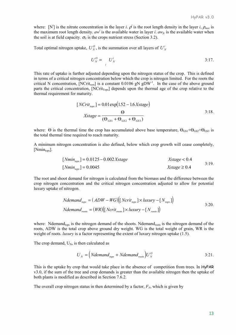
where: [Ni] is the nitrate concentration in the layer i. ρi is the root length density in the layer i, ρmax is the maximum root length density. awi is the available water in layer i. awfc is the available water when the soil is at field capacity. σN is the crops nutrient stress (Section 3.2).

Total optimal nitrogen uptake, U NO , is the summation over all layers of U N

i

U UNO

Ni

i= 3:17.

This rate of uptake is further adjusted depending upon the nitrogen status of the crop. This is defined in terms of a critical nitrogen concentration below which the crop is nitrogen limited. For the roots the critical N concentration, [NCritroot] is a constant 0.0106 gN gDW-1. In the case of the above ground parts the critical concentration, [NCritTops] depends upon the thermal age of the crop relative to the thermal requirement for maturity.

( )[ ] . exp . .

( )

NCrit Xstage

Xstage

tops

GS GS GS

= −

=+ +

0 01 152 16

1 2 3

ΘΘ Θ Θ

3:18.

where: Θ is the thermal time the crop has accumulated above base temperature, ΘGS1+ΘGS2+ΘGS3 is the total thermal time required to reach maturity.

A minimum nitrogen concentration is also defined, below which crop growth will cease completely, [Nmintops].

4.0 0045.0][4.0 002.00125.0][

≥=

<−=

XstageNminXstageXstageNmin

tops

tops 3:19.

The root and shoot demand for nitrogen is calculated from the biomass and the difference between the crop nitrogen concentration and the critical nitrogen concentration adjusted to allow for potential luxury uptake of nitrogen.

( )( )( )( )

Ndemand ADW WG Ncrit luxury N

Ndemand WR Ncrit luxury N

tops tops tops

roots roots roots

= − × −

= × −

[ ] [ ]

[ ] [ ] 3:20.

where: Ndemandtops is the nitrogen demand of the shoots. Ndemandroots is the nitrogen demand of the roots, ADW is the total crop above ground dry weight. WG is the total weight of grain, WR is the weight of roots. luxury is a factor representing the extent of luxury nitrogen uptake (1.5).

The crop demand, UN, is then calculated as

( )U Ndemand Ndemand UN tops roots NO= + 3:21.

This is the uptake by crop that would take place in the absence of competition from trees. In HyPAR v3.0, if the sum of the tree and crop demands is greater than the available nitrogen then the uptake of both plants is modified as described in Section 7.6.2.

The overall crop nitrogen status in then determined by a factor, FN, which is given by

HyPAR v3.0

14

FNcrit N

Ncrit NminNtops tops

tops tops= −

−−

1[ ] [ ]

[ ] [ ] 3:22.

where: [Ntops] is the actual concentration on nitrogen in the above ground parts of the crop (excluding grain).

When FN<1 the crop is below its optimum nitrogen concentration and photosynthesis will be nitrogen limited. However this does not necessarily imply that nitrogen is the most limiting resource, either water, temperature, or phosphorus could be more limiting. Nutrient stress, σN, is calculated directly from FN as described in Section 3.2

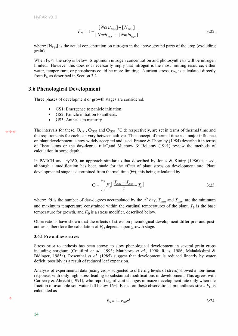
3.6 Phenological Development

Three phases of development or growth stages are considered.

•= GS1: Emergence to panicle initiation. •= GS2: Panicle initiation to anthesis. •= GS3: Anthesis to maturity.

The intervals for these, ΘGS1, ΘGS2 and ΘGS3 (oC d) respectively, are set in terms of thermal time and the requirements for each can vary between cultivar. The concept of thermal time as a major influence on plant development is now widely accepted and used. France & Thornley (1984) describe it in terms of “heat sums or the day-degree rule”,and Muchow & Bellamy (1991) review the methods of calculation in some depth.

In PARCH and HyPAR, an approach similar to that described by Jones & Kiniry (1986) is used, although a modification has been made for the effect of plant stress on development rate. Plant developmental stage is determined from thermal time (Θ), this being calculated by

Θ Θ= + − =

=

F T T Tbi

i nmax min

21

3:23.

where: Θ is the number of day-degrees accumulated by the nth day, Tmin and Tmax are the minimum and maximum temperature constrained within the cardinal temperatures of the plant, Tb is the base temperature for growth, and FΘ is a stress modifier, described below.

Observations have shown that the effects of stress on phenological development differ pre- and post-anthesis, therefore the calculation of FΘ depends upon growth stage.

3.6.1 Pre-anthesis stress

Stress prior to anthesis has been shown to slow phenological development in several grain crops including sorghum (Craufurd et al., 1993; Matthews et al., 1990; Rees, 1986; Mahalakshmi & Bidinger, 1985a). Rosenthal et al. (1985) suggest that development is reduced linearly by water deficit, possibly as a result of reduced leaf expansion.

Analysis of experimental data (using crops subjected to differing levels of stress) showed a non-linear response, with only high stress leading to substantial modifications in development. This agrees with Carberry & Abrecht (1991), who report significant changes in maize development rate only when the fraction of available soil water fell below 16%. Based on these observations, pre-anthesis stress FΘ is calculated as

FΘ Θ= −1 13γ σ 3:24.

HyPAR v3.0

15

where γΘ1 is a crop-specific parameter for pre-anthesis growth. In the case of sorghum, γΘ1 has been set to 0.5. Hence maximum stress (σ=1) will halve the increase in thermal time.

3.6.2 Post-anthesis stress

Water shortage after anthesis can lead to crop temperatures up to 10°C above air temperatures (Gates, 1980), thus speeding up crop development by over 33% relative to that expected from air temperature calculations (Eastin, 1976). Similar hastening of flowering through heat or drought stress has been described for sorghum (Stout et al., 1978) and wheat (Angus & Moncur, 1977). Planchon (1987) explains these changes in terms of chemical rather than physical factors; “Water deficit leads to hormonal disturbances resulting in early flowering and premature ageing of leaves”. This may be a more satisfactory explanation, as the direct modification of thermal time would also be effective prior to anthesis if water shortage occurred, thus reducing rather than extending GS1 and GS2. Many conflicting reports on the effects of stress on cereal development still exist and Craufurd et al. (1993) speculate that both timing and severity of stress may be important factors.

The situation becomes more complicated when the ambient temperature is close to, but below, the optimum temperature. Elevation of crop temperatures can then result in supraoptimal crop temperatures and a reduction in development rate. The proportion of the day over which this happens and the 'hangover' effects on other parts of the day are poorly defined at present.

To represent the effects of post-anthesis stress within the model, FΘ is calculated as

FΘ Θ= −1 3γ σ 3:25.

where: γΘ3 is a crop-specific parameter for post-anthesis growth (i.e. GS3), given a value of 0.33 for sorghum based on the observations by Eastin (1976).

3.7 Partitioning of Resources

For a crop to grow successfully, it must extract water and nutrients from the ground and also intercept light for photosynthesis. Therefore, there must be a compromise between root and shoot growth. There appears to be no specific optimum for the distribution of growth; this being dependent on growing conditions.

Changes in root:shoot ratio with stress have been described by many researchers e.g. Turner & Begg (1981), Pearson (1974), Brouwer (1966) and Harris (1914). A hypothesis was put forward by Davidson (1969) that “photosynthate is partitioned in inverse proportion to the functional efficiency of roots and foliage”.

The partitioning of assimilates within the crop model is controlled by an empirical fractional distribution, this being derived from literature and observed (unpublished) values. Partitioning to different organs changes with development stage, again in accordance with the literature. Many models adopt this as a sole strategy and it has been shown to give a reasonable representation if optimised for a certain situation (Hammer & Muchow, 1994; Maas, 1993a). However for the simulation to respond to differing conditions, an environmental response must be superimposed over this empirical framework.

Following Davidson (1969), a fraction of assimilate is first partitioned to the roots (fBG). For an

unstressed crop, the fraction of carbon partitioned below ground before anthesis ( f BG0 ) is set to 0.25.

This is increased linearly by stress

f fBG BG BG= +0 γ σ 3:26.

HyPAR v3.0

16

where: γBG is a stress response parameter for partitioning (0.4).

Van Laar et al. (1992) used a similar approach to that described above under modelled stress conditions, giving an increase in assimilates to roots of up to 50%. Ritchie (1991) described an even larger spread of dry matter partitioning for cereals, giving values of root partitioning from 10 to 70%. Kenyi (1991) and Ahmed (1988) found that at maturity, 8% and 15% respectively of sorghum dry weight was live root in unstressed treatments at the Tropical Crops Research Unit (TCRU), Nottingham. This is likely to be an underestimate of the total assimilate partitioned to roots, as there is continued senescence and destruction of root matter throughout the growth of the crop, as well as exudation and respiration (Ritchie, 1991). This was reflected in work by Blum & Arkin (1984), who showed a loss of two thirds of the total root length up to heading in a droughted sorghum crop. The values proposed above lie within this reported range.

Once the daily root fraction has been calculated, the remaining fraction (fAG) of carbohydrate is used for above ground growth. At the start of GS1, the proportion of the above ground assimilate partitioned to leaves (fL) is 0.9 (fLmax.). At anthesis, fL is taken as 0.1 (fLmin.) There is a linear change between these two values as the crop develops. Carbon partitioned to stem (fS) is calculated as 1 - fL. Van Laar et al. (1992) used a comparable, although more complex, function for wheat dry matter distribution. Similarly, van Heemst (1988) suggests functions for dry matter distribution in maize, millet and sorghum that follow this general form.

At anthesis, the remaining fractions partitioned to leaves and stem are reduced to zero over a seven day period defined as the grain setting period (GrainSetTime). Rosenthal et al. (1989) define this period as that between the end of leaf growth and anthesis, and also use the value of seven days for sorghum, rather than thermal time units.

The fraction partitioned to the haulm after anthesis (fH) is given as

fH = 1 - (fS + fL) 3:27.

during the grain setting period and 0.1 (fHmax) thereafter. Subsequently, the fraction partitioned to grain, fG, is calculated as that which is not partitioned to haulm.

3.8 Leaf Growth

Phenology and leaf area development establish the total amount of radiation intercepted by field crops and thus are important determinants in assimilate production and soil water balance (Muchow & Carberry, 1990). Crop simulation models used for research or management frequently require the development of leaf area to be mathematically described (Keating & Wafula, 1992) and thus a set of assumptions or functions representing our understanding of leaf growth, morphology and senescence are needed.

Leaf growth and tillering habits can be modelled with different levels of complexity, depending upon the situations in which the model will be used. In moist, temperate environments with adequate nutrients, light interception is the major factor affecting plant growth. In these situations, canopy development and architecture must be modelled to a high degree of accuracy in order to predict carbon assimilation (Ritchie, 1991)

In the Semi-Arid Tropics, water and nutrients are the most common factors which limit growth (Austin, 1989; Peacock & Heinrich, 1984), and in such situations, less complex assumptions can be made about canopy architecture (Whisler et al., 1986). Keating & Wafula (1992) review several complex approaches to leaf area development in cereals and describe a function designed to model the fully expanded area of maize leaves. The use of this function, although robust, necessitates the determination of four plant specific parameters. Even then, no account is taken of the effects of plant

HyPAR v3.0

17

stress on the growth of the leaves, and only optimal conditions are considered. A similar criticism can be levelled at the leaf area function derived by Muchow & Carberry (1990) for tropical grain sorghum.

Cereal leaf growth has been related to temperature by many workers (e.g. Whisler et al., 1986; Gallagher, 1979a) and sorghum leaf area to thermal time (Muchow & Carberry 1990; Hammer et al., 1987; Arkin et al., 1983). As a sole approach to modelling leaf expansion, Ritchie (1991) suggests that this will only be appropriate in conditions where temperature is the limiting factor. A more realistic approach for tropical conditions, according to Whisler et al (1986) is to include limitations for carbon, nitrogen and water availability, as these will frequently determine expansion rate.

For the purposes of this model, the driving force for leaf growth has been taken to be assimilate from photosynthesis partitioned to leaf growth, as described above. This increase in leaf mass is converted to an increase in leaf area via a specific leaf area term, ζ (m2 leaf kg-1 assimilate).

From observations, it is well known that leaves produced at different times (i.e. at different stages of development) on an individual crop are likely to have a different morphology and specific leaf area (e.g. Erenstein, 1990). To simplify this to a canopy level, two different values of specific leaf area are used for the unstressed crop (ζ0), one for early establishment (GS1; 35 m2 kg-1) and the other for mature leaf growth (30 m2 kg-1).

During the juvenile period of growth, which is taken as the first 15 days (Juvenile) (Jones & Kiniry, 1986), ζ0 is multiplied by a factor, ζ, reducing linearly from ζ0 to 1. This represents the rapid changes in specific leaf area after the first leaves emerge. These values are expected to be cultivar specific (Hammer et al., 1987).

Tissue growth is known to be affected by water stress (Whisler et al, 1986) and in particular the expansion of leaves can be greatly reduced (Spitters & Schapendonk, 1990; Green et al., 1971), resulting in a significantly lower specific leaf area. Within the model, the effects of crop stress (lowered water status) are represented by a leaf stress parameter, γζ, which reflects the reduction of specific leaf area at maximum stress. These ideas are combined to calculate specific leaf area on a daily basis using

)1( = 0 σγζζ ζ− 3:28.

Following work by Keating & Wafule (1991), a maximum daily thermal leaf expansion rate is defined during GS1. This operates in parallel with the carbohydrate-driven expansion described above, the most limiting determining leaf expansion on that day.

At present, the assumption is made (as with Monteith et al., 1989; Jones & Kiniry, 1986) that no leaf growth occurs after the crop enters reproductive development (GS3) and only senescence occurs during this period.

3.8.1 Leaf senescence

The simulation of leaf senescence is generally weak within crop models and contributes to the lower accuracy of growth prediction in the late reproductive stage (Hammer & Muchow, 1991, Penning de Vries & Spitters, 1991). Leaf senescence is a complex process and has several causes. Each leaf in the canopy has a maximum life-span, after which it begins to senesce (Penning de Vries & Spitters, 1991). This may have arisen from the fact that most non-crop plants are constantly exposed to damage from pests and diseases and leaves will eventually become ineffective. Thus, translocatable nutrients are removed from the leaf and it is usually shed. This phenological senescence occurs irrespective of the condition of the crop. However, soil and climatic conditions can also affect the rate of canopy senescence (Sionit & Kramer, 1977) and leaf shedding as a means of saving water is observed in many crops subjected to water stress (Finch-Savage & Elston, 1982).

HyPAR v3.0

18

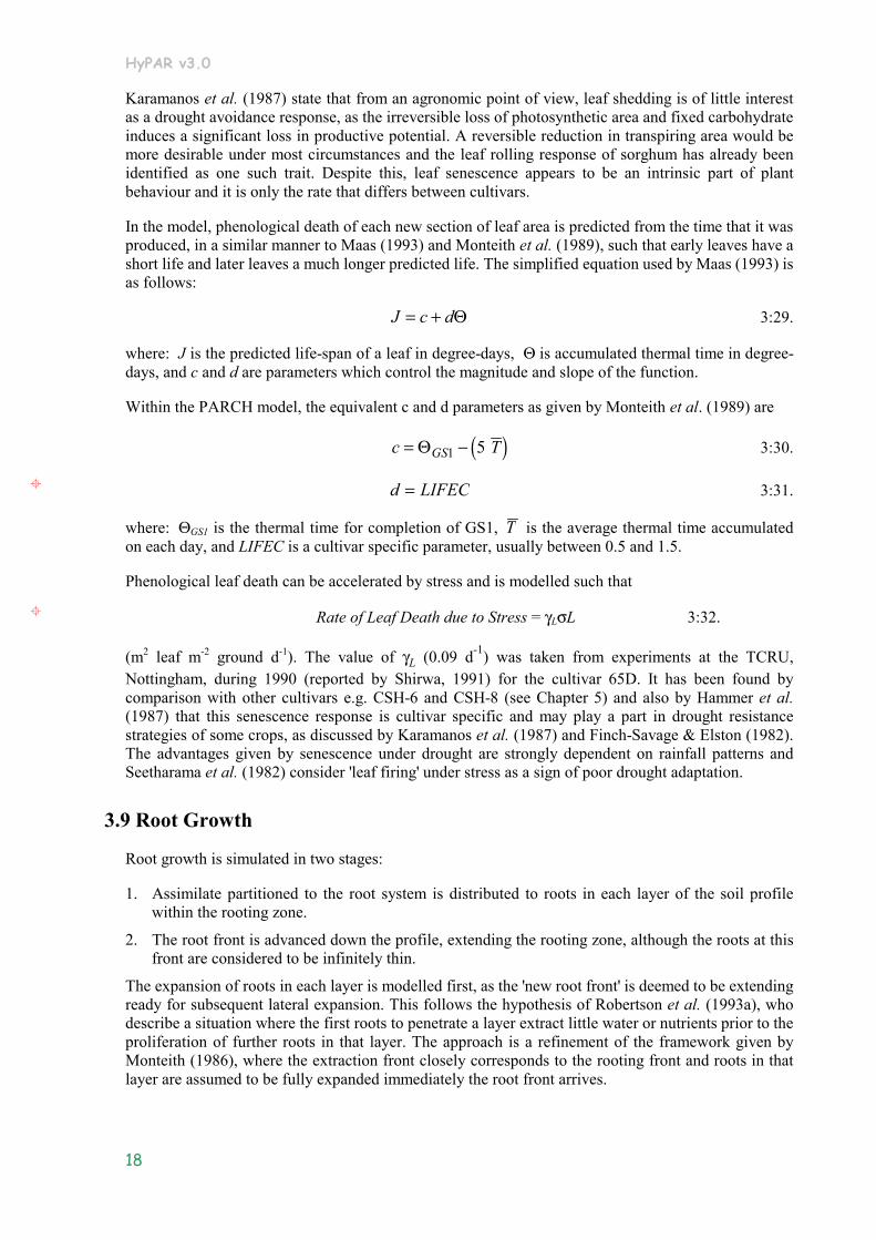
Karamanos et al. (1987) state that from an agronomic point of view, leaf shedding is of little interest as a drought avoidance response, as the irreversible loss of photosynthetic area and fixed carbohydrate induces a significant loss in productive potential. A reversible reduction in transpiring area would be more desirable under most circumstances and the leaf rolling response of sorghum has already been identified as one such trait. Despite this, leaf senescence appears to be an intrinsic part of plant behaviour and it is only the rate that differs between cultivars.

In the model, phenological death of each new section of leaf area is predicted from the time that it was produced, in a similar manner to Maas (1993) and Monteith et al. (1989), such that early leaves have a short life and later leaves a much longer predicted life. The simplified equation used by Maas (1993) is as follows:

J c d= + Θ 3:29.

where: J is the predicted life-span of a leaf in degree-days, Θ is accumulated thermal time in degree-days, and c and d are parameters which control the magnitude and slope of the function.

Within the PARCH model, the equivalent c and d parameters as given by Monteith et al. (1989) are

( )c TGS= −Θ 1 5 3:30.

d LIFEC= 3:31.

where: ΘGS1 is the thermal time for completion of GS1, T is the average thermal time accumulated on each day, and LIFEC is a cultivar specific parameter, usually between 0.5 and 1.5.

Phenological leaf death can be accelerated by stress and is modelled such that

Rate of Leaf Death due to Stress = γLσL 3:32.

(m2 leaf m-2 ground d-1). The value of γL (0.09 d-1) was taken from experiments at the TCRU, Nottingham, during 1990 (reported by Shirwa, 1991) for the cultivar 65D. It has been found by comparison with other cultivars e.g. CSH-6 and CSH-8 (see Chapter 5) and also by Hammer et al. (1987) that this senescence response is cultivar specific and may play a part in drought resistance strategies of some crops, as discussed by Karamanos et al. (1987) and Finch-Savage & Elston (1982). The advantages given by senescence under drought are strongly dependent on rainfall patterns and Seetharama et al. (1982) consider 'leaf firing' under stress as a sign of poor drought adaptation.

3.9 Root Growth

Root growth is simulated in two stages:

1. Assimilate partitioned to the root system is distributed to roots in each layer of the soil profile within the rooting zone.

2. The root front is advanced down the profile, extending the rooting zone, although the roots at this front are considered to be infinitely thin.

The expansion of roots in each layer is modelled first, as the 'new root front' is deemed to be extending ready for subsequent lateral expansion. This follows the hypothesis of Robertson et al. (1993a), who describe a situation where the first roots to penetrate a layer extract little water or nutrients prior to the proliferation of further roots in that layer. The approach is a refinement of the framework given by Monteith (1986), where the extraction front closely corresponds to the rooting front and roots in that layer are assumed to be fully expanded immediately the root front arrives.

HyPAR v3.0

19

3.9.1 Calculation of root growth

The rate of new root length production, R (cm root cm-2 ground d-1), is calculated from the assimilate available for growth (fBGG), using:

Rf GFBG= η

η 3:33.

where: η is the linear density of root material, 10-4 g cm-1, and Fη is an adjustment used during the juvenile stage when roots produced by the germinating seed, especially the seminal root(s), are very long and thin. As the root system becomes more mature the average thickness of new root production becomes much greater. Such changes in root growth are described for sorghum by Zartman & Woyewodzic (1979). The value of Fη varies linearly from Fη0 (6) to 1.0 over the juvenile period of 15 days.

3.9.2 Vertical distribution of root growth

New root production is distributed between the soil profile layers using an approach similar to that described by Jones & Kiniry (1986), although it has been extended to account for the effect of changing soil conditions (e.g. drying fronts) on root growth. Maximum depth is constrained by a parameter, maxRdepth, or the physical soil depth.

Under optimal soil conditions, it has been suggested that the root system will tend to adopt an exponentially reducing distribution with depth (Gerwitz & Page, 1974; Bloodworth et al., 1958). In practice, this is similar to the inverse square root distribution used by Monteith et al. (1989). Furthermore, root growth is known to be greatly affected by soil moisture, the roots expanding preferentially into moist soil (Blum & Arkin, 1984; Zartman & Woyewodzic, 1979).

To model these effects, a root weighting factor (ri) is calculated for each layer based upon the optimal exponential distribution modified by a soil free water factor, Ffree

i , and a nutrient factor, Fsoilni ,

calculated for each layer

( )r = F F0.693R

zR

zi freei

soilni

i+−

1 2

0 693

1 2

exp.

∆ 3:34.

where: R12

is the 'half depth' (mm). zi is the depth of a given layer (mm). ∆zi is the layer thickness

(mm).

F = 1 - Ffreei i

freeiψ

φ 00 1 < < 3:35.

where: ψi is the matric potential of the soil in layer i (m), φ0 is the permanent wilt point of the crop (m)

( ) ( )( )( )( )F F N Psoilni

Ni i= + − − − +1 50 1 0 1 1 117 015( ) max , min , . exp( . [ ] [ ] 3:36.

where: [Ni] is the nitrate concentration of layer i, [Pi] is the phosphate concentration of layer i

Values for R½ of around 0.25m match the sorghum rooting data collected at Nottingham (Kenyi, 1991; Ahmed, 1988) but it can be expected that crops grown on stored water profiles will be sensitive to this parameter, as it affects the timing and quantity of water use. The permanent wilt point is crop specific;

HyPAR v3.0

20

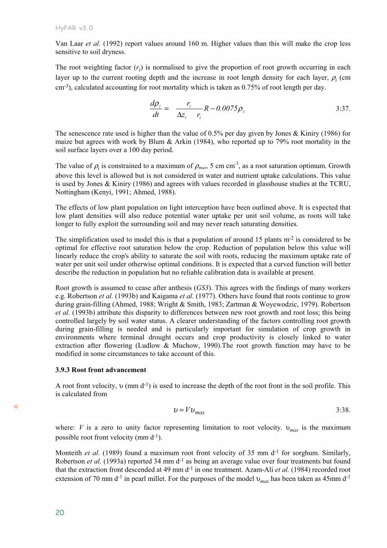
Van Laar et al. (1992) report values around 160 m. Higher values than this will make the crop less sensitive to soil dryness.

The root weighting factor (ri) is normalised to give the proportion of root growth occurring in each layer up to the current rooting depth and the increase in root length density for each layer, ρi (cm cm-3), calculated accounting for root mortality which is taken as 0.75% of root length per day.

ddt

rz r

R 0.0075i i

i ii

ρ ρ= −∆

3:37.

The senescence rate used is higher than the value of 0.5% per day given by Jones & Kiniry (1986) for maize but agrees with work by Blum & Arkin (1984), who reported up to 79% root mortality in the soil surface layers over a 100 day period.

The value of ρi is constrained to a maximum of ρmax, 5 cm cm-3, as a root saturation optimum. Growth above this level is allowed but is not considered in water and nutrient uptake calculations. This value is used by Jones & Kiniry (1986) and agrees with values recorded in glasshouse studies at the TCRU, Nottingham (Kenyi, 1991; Ahmed, 1988).

The effects of low plant population on light interception have been outlined above. It is expected that low plant densities will also reduce potential water uptake per unit soil volume, as roots will take longer to fully exploit the surrounding soil and may never reach saturating densities.

The simplification used to model this is that a population of around 15 plants m-2 is considered to be optimal for effective root saturation below the crop. Reduction of population below this value will linearly reduce the crop's ability to saturate the soil with roots, reducing the maximum uptake rate of water per unit soil under otherwise optimal conditions. It is expected that a curved function will better describe the reduction in population but no reliable calibration data is available at present.

Root growth is assumed to cease after anthesis (GS3). This agrees with the findings of many workers e.g. Robertson et al. (1993b) and Kaigama et al. (1977). Others have found that roots continue to grow during grain-filling (Ahmed, 1988; Wright & Smith, 1983; Zartman & Woyewodzic, 1979). Robertson et al. (1993b) attribute this disparity to differences between new root growth and root loss; this being controlled largely by soil water status. A clearer understanding of the factors controlling root growth during grain-filling is needed and is particularly important for simulation of crop growth in environments where terminal drought occurs and crop productivity is closely linked to water extraction after flowering (Ludlow & Muchow, 1990).The root growth function may have to be modified in some circumstances to take account of this.

3.9.3 Root front advancement

A root front velocity, υ (mm d-1) is used to increase the depth of the root front in the soil profile. This is calculated from

υ υ=V max 3:38.

where: V is a zero to unity factor representing limitation to root velocity. υmax is the maximum possible root front velocity (mm d-1).

Monteith et al. (1989) found a maximum root front velocity of 35 mm d-1 for sorghum. Similarly, Robertson et al. (1993a) reported 34 mm d-1 as being an average value over four treatments but found that the extraction front descended at 49 mm d-1 in one treatment. Azam-Ali et al. (1984) recorded root extension of 70 mm d-1 in pearl millet. For the purposes of the model υmax has been taken as 45mm d-1

HyPAR v3.0

21

to limit root extension. However, a maximum theoretical rate,Υmax of 70mm d-1 (υmax×1.5) is used in some root front calculations to allow low levels of stress to be non-limiting.

Four mechanisms are assumed to affect root front advancement, each represented by a zero to unity factor. On any day the root front advances at a rate determined by the most limiting of these four factors. The factors are:

3. Assimilate limitation (resulting from either low light or water capture), VA

4. Low temperature limitation, VT

5. Low crop water or nutrient status (overall stress), Vσ and

6. Root front soil conditions (low moisture / high strength) VS

Each of the velocity limitation factors is described below.

3.9.3.1 Assimilate Limitation Factor This is calculated using

V = F

r rd RA

downγ υ

( ) 0<VA<1 3:39.

where: γdown is a factor which represents the ratio of downward to horizontal growth; a value of 12 m (root depth) m-1 (root growth) has been used here.

Fν is a factor used to simulate the effect of increased root front velocity during the juvenile stage of the crop. This represents the change in root morphology from seminal roots to a more branching adventitious root system (as described by Zartman & Woyewodzic, 1979). The value of Fν varies linearly from Fν0 (4.0) to 1.0 over the juvenile period. r(rd) is the root weighting function described above, evaluated at the rooting depth.

The approach is empirical and based on unpublished relationships derived from controlled environment studies at Nottingham.

3.9.3.2 Temperature Limitation Factor The root front velocity of many crops has been linked with temperature or thermal time (Rosenthal et al., 1989, Jones & Kiniry, 1986) and this is modelled using a simple temperature relationship

V = T - TT - T

VTb

bT

1

0 1 < < 3:40.

where: T is the average daily temperature (°C), T1 is the lower point of the optimal temperature plateau, and Tb is the base temperature for growth.

3.9.3.3 Water Stress Limitation Overall stress is linked to root growth in that it represents plant turgor and reduced plant turgor equates to slower cell expansion, especially when mechanical resistance is encountered (Merrill & Rawlins, 1979). Root front velocity limitation due to stress is given by

V YV

max

maxσ γ σ

υ= −( )1 0<Vσ<1 3:41.

HyPAR v3.0

22

This is calculated in terms of the theoretical maximum root growth rate, although growth above υmax is not allowed. Coupled with a γV value of 0.8 this means that when σ=1, root growth rate will not drop below 20% of its maximum value, as the roots are the last part of the plant to become flaccid, being in contact with moisture bearing soil (Zahner, 1968).

3.9.3.4 Root Front Soil Moisture Limitation Apart from the moisture status of the crop as a whole, the moisture status of the expanding root tips also has an effect on the root front velocity. If root tips are exposed to totally dry soil, moisture is effectively removed from them, the cells becoming flaccid.

The soil free water factor, Ffree, is used to reduce root front velocity due to soil dryness, V FS free= . This is a similar approach to that used by Jones & Kiniry (1986).

During germination, the minimum rate of root front extension is constrained by either temperature or a rate of RDmin, 20mm d-1. This is to allow for the fact that a full energy balance is not calculated for the soil surface and thus cannot make accurate estimates of crop establishment. Removing this constraint leaves the model very sensitive to seedbed conditions, which are rarely well documented. The time specified for the seed reserved to be used is an input parameter to the model (Germination).

3.10 Reproductive Growth

Although resource capture during the vegetative phase is important to crop structural growth, the final determinant of yield is grain production within the reproductive phase. This is affected by many factors including assimilate storage, grain site survival and continued light interception and photosynthesis. Penning de Vries et al. (1983) report that in most graminae under stressed conditions, a considerable portion of the final yield can come from reserves stored in the stem and leaves. For rice, reserves start to build up some weeks before heading and can amount to about 25-30% of standing dry weight at heading (Yoshida, 1981). In wheat, around 20% of the grain weight may come from carbohydrate reserves, this being 30-50% of the total reserves formed during the growing season (Spiertz, 1982).Ritchie (1991) reports a typical range of reserve assimilates as being from 20 to 35% of stem weight at anthesis.

To calculate grain yield in the model, the number of grain sites set is first determined. This is assumed to take place during a grain setting period immediately following anthesis (i.e. at the beginning of GS3). Typically this grain setting period is seven days (Rosenthal et al., 1989). After the grain setting period, grain filling commences. This continues until either the grains reach a maximum size or GS3 ends and the crop achieves physiological maturity. The maximum grain weight, GWmax, is a cultivar specific parameter with an observed range of 0.025 and 0.065 g grain-1 for sorghum (Craufurd & Peacock, 1993).

3.10.1 Number of grain sites

To calculate the number of grain sites set, N (sites plant-1), the weight increase during GS2 (panicle initiation to anthesis) is multiplied by a grain number conversion factor, N0, (typically between 0.015 and 0.065 sites plant-1 g-1 (increase)).

N N W WP

GS GS = ( - ) 0 3 2 , 3:42.

where: P is the plant population per m2.

Jones & Kiniry (1986) and Rosenthal et al. (1989) describe similar approaches. The factor N0 must be determined experimentally for situations where grain number may be limiting to final yield. Craufurd

HyPAR v3.0

23

& Peacock (1993) described such a situation, where grain yield was found to be strongly correlated with number of grains. In that analysis, a 'thermal crop growth rate' was regressed against final grain number to give a predictive index. Many other researchers have also correlated seed number to daily dry matter accumulation (Vanderlip et al., 1984; Charles-Edwards, 1982; Edmeades & Danyard, 1979).

3.10.2 Grain filling

During GS3, assimilate from photosynthesis is partitioned to the grain and haulm. This is subject to a maximum rate of grain filling, ∆WG

max (g m-2 d-1) and if assimilation is not sufficient to maintain the maximum rate, grain filling can be supplemented by translocation from stem reserves and senescing leaves, τ (g m-2 d-1).

dWdt

F G dWdt

W

dWdt

F G

GG

GGmax

HH

= + <

=

τ ∆ 3:43.

The minimum time for grain filling under optimal conditions is taken as 23 days (PartitionTime) (Monteith et al., 1989). The maximum rate of filling per grain is therefore given by 1/23 GWmax, or for the whole of the canopy

∆W GW NPGmax max=

23 3:44.

If assimilation is such that it exceeds the maximum rate of grain filling the 'surplus' assimilate is added to stem reserves.

The rate of translocation is calculated as the difference between the maximum grain-filling rate and the assimilate available from photosynthesis, subject to a maximum rate of translocation, τmax which is calculated at the start of grain filling (i.e. after the grain set period). It is assumed that a maximum of 20% (Wres

0 (g m-2)) of stem weight, WS (g m-2), is available for translocation and that a minimum period of 20 days is required to translocate this material (i.e. τmax = Wres

0 /20, or τmax = DayTransPot ×Wres

0 ).

These figures are based on field observations but give values similar to those used by other workers. Jansen & Gosseye (1986) allow 10% of reserves to move to grain per day in their millet growth simulation. Similarly, Rosenthal et al. (1989) use a maximum translocation rate of 2.5% of the total culm weight per day under stressed conditions in the SORKAM model. Jansen & Gosseye (1986) also proposed that dying vegetative material, especially leaves, would provide added carbohydrate for the translocation pool. This has been simulated by allowing 10% of carbon from senesced leaves to become available for translocation to grain.

The reserves available, Wres, are reduced by translocation but are supplemented by leaf senescence. Once reserves are exhausted, translocation ceases. The rate of translocation can also slowed by a stress factor, (1 - γTσ).

The growth of grain can also be limited by nitrogen supply. The nitrogen uptake rate of the grain is calculated each day as the product of grain growth rate and a nitrogen requirement factor (which is adjusted depending upon the overall nutrient status of the crop).

HyPAR v3.0

24

( )dNdt

FdW

dtG

NG= 0 011 0 006. * . 3:45.

where: NG is the nitrogen content of the grain, FN is the nutrient status factor

Mobilisation of nitrogen from the shoots and roots of the crop meet this requirement for nitrogen. The amount of nitrogen available for mobilisation from shoots, Npool1, and roots, Npool2, is given by

N ADW W N N FN W N N F

pool G shoot shoot pool

pool R root roothoot pool

1

2

= − −= −

( )([ ] [ ])([ ] [ ])

min 3:46.

where: ADW is total above ground dry weight of the crop, WG is the total grain weight, [Nshoot] is the above ground nitrogen concentration, [Nminshoot] is the minimum possible above ground nitrogen concentration, [Nroot] is the root nitrogen concentration, [Nminroot] is the minimum possible root nitrogen concentration (taken to be 75% of the critical root nitrogen concentration), Fpool is a factor determining the proportion of the shoot and root nitrogen which can be mobilised, given below.

Fpool N= −0 4 0 25. . σ 3:47.

So at maximum nutrient stress only 15% of the shoot and root nitrogen can be mobilised, but at zero nutrient stress this fraction rises to 40%.

If the nitrogen demand exceeds the nitrogen available within the crop then the grain growth is restricted. In this case the assimilated dry matter that cannot be partitioned to the grain is instead allocated to the stem dry weight. If the nitrogen supply subsequently improves this stem dry matter has the possibility to be translocated to the grain at a later stage.

3.11 Parameter Summary

The cultivar editor in the HyPAR Control Centre allows the user to change crop parameters (see User Guide, Section 7.1). The table below lists the parameter names, the code names used by HyPAR and a reference to the full description in this chapter

Parameter Code name Short description See section

DayTransPot DayTransPot Factor for maximum fraction of stem available for translocation that can move each day.

3.10.2

Fν0 emRDfactor Roots this factor more likely to grow downwards at germination.

3.9.3.1

Fη0 emRWLfactor Roots this factor thinner at germination. 3.9.1

γdown FineRoot factor which represents the ratio of downward to horizontal root growth

3.9.3.1

FractRoot FractRoot Estimated proportion of the plant that was root when qD and εs were calculated, if not included.

3.1

Germination Germination Time for seed to use carbon supplies. 3.9.3.4

N0 GNC Conversion factor for grain number. 3.10.1

GrainSetTime GrainSetTime Time from anthesis to grain setting. 3.7

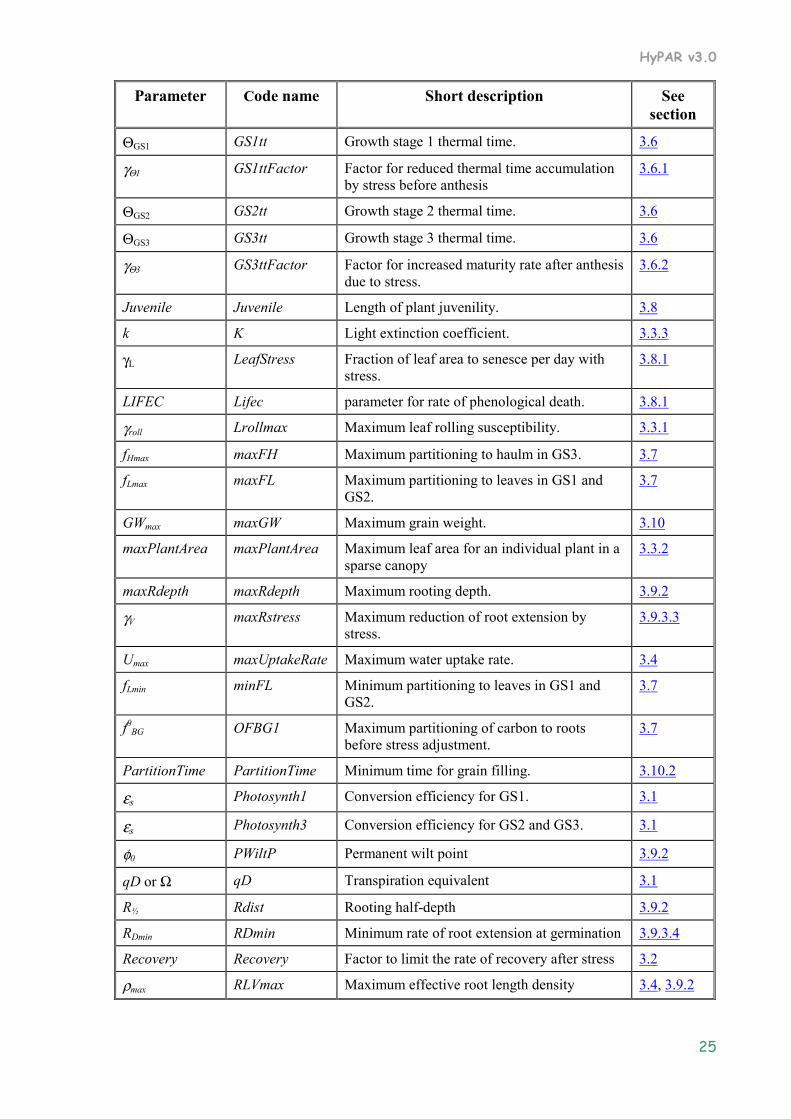
HyPAR v3.0

25


ΘGS1 GS1tt Growth stage 1 thermal time. 3.6

γΘ1 GS1ttFactor Factor for reduced thermal time accumulation by stress before anthesis

3.6.1



γΘ3 GS3ttFactor Factor for increased maturity rate after anthesis due to stress.

3.6.2

Juvenile Juvenile Length of plant juvenility. 3.8

k K Light extinction coefficient. 3.3.3

γL LeafStress Fraction of leaf area to senesce per day with stress.

3.8.1

LIFEC Lifec parameter for rate of phenological death. 3.8.1

γroll Lrollmax Maximum leaf rolling susceptibility. 3.3.1

fHmax maxFH Maximum partitioning to haulm in GS3. 3.7

fLmax maxFL Maximum partitioning to leaves in GS1 and GS2.

3.7

GWmax maxGW Maximum grain weight. 3.10

maxPlantArea maxPlantArea Maximum leaf area for an individual plant in a sparse canopy

3.3.2

maxRdepth maxRdepth Maximum rooting depth. 3.9.2

γV maxRstress Maximum reduction of root extension by stress.

3.9.3.3

Umax maxUptakeRate Maximum water uptake rate. 3.4

fLmin minFL Minimum partitioning to leaves in GS1 and GS2.

3.7

f0BG OFBG1 Maximum partitioning of carbon to roots

before stress adjustment. 3.7

PartitionTime PartitionTime Minimum time for grain filling. 3.10.2

εs Photosynth1 Conversion efficiency for GS1. 3.1

εs Photosynth3 Conversion efficiency for GS2 and GS3. 3.1

φ0 PWiltP Permanent wilt point 3.9.2

qD or Ω qD Transpiration equivalent 3.1

R½ Rdist Rooting half-depth 3.9.2

RDmin RDmin Minimum rate of root extension at germination 3.9.3.4

Recovery Recovery Factor to limit the rate of recovery after stress 3.2

ρmax RLVmax Maximum effective root length density 3.4, 3.9.2

HyPAR v3.0

26


υmax RRmax Maximum root front velocity 3.9.3

γBG RstressFBG stress response for partitioning 3.7

η RWLfactor root weight per unit length 3.9.1

ζ0 SLA1 specific leaf area for early establishment 3.8

ζ0 SLA2 specific leaf area for mature leaf growth 3.8

γζ SLAstress Modifier for specific leaf area 3.8

σ0 STindex Normalising parameter for stress 3.2

γT STransReduct Factor to limit translocation rate 3.10.2

Tb Tb Base temperature for growth 3.1

T1 Tbplateau Lower optimum temperature for growth 3.1, 3.2

Tm Tm Maximum temperature for growth 3.1, 3.2

T2 Tmplateau Upper optimum temperature for growth 3.1, 3.2

W0res TransPot Maximum fraction of stem available for

translocation 3.10.2

Note that the parameters WLsat, WLdamage, WLrecover, WLsuscept and WLdeath are included in the cultivar editor but not listed in this chapter. These parameters, relating to weeds, are retained in the input file for consistency with PARCH but are not used in HyPAR.

HyPAR v3.0

27

4. The Tree Model

The tree growth components within HyPAR are based on those in the Hybrid model (v3.0) (Friend et al, 1997). Hybrid is an individual-based plot model, driven by daily weather, which combines a mass-balance approach with the capacity to predict the relative dominance of different species or plant types and how they interact with atmospheric and soil processes. Further information on the Hybrid model and the processes represented can be found in Friend et al (1995, 1997) and Friend (1995).

Figure 6. The Hybrid Ecosystem model showing schematically the photosynthesis, allocation and decomposition processes represented in Hybrid

In the following model description, the main reference to the HyPAR species-specific input parameters are identified with a symbol, , in the margin and listed in a table in Section 4.14.

4.1 Model structure for tree growth

Hybrid and HyPAR v3.0 operate on a daily timestep. Photosynthesis, maintenance respiration, nitrogen uptake and transpiration are calculated daily for each individual tree. It is assumed that total daily net photosynthesis, transpiration and night-time respiration of each tree all scale linearly with their mean rates - that is, there is no need to calculate these rates on a shorter timestep than either the day or the night. The net daily individual tree increments in carbon and nitrogen, together with any stored carbon, are allocated at the end of each day to the different tree compartments (Section 4.10). Daily root litter

HyPAR v3.0

28

is added to the soil layers that they occupy. Leaf (and branch) daily litter is either added to the soil or removed from the site (Section 4.9). Trees are assumed to die when there is insufficient carbon to produce any foliage and the carbon and nitrogen contained in dead tree roots is added to the appropriate soil layers as fresh organic matter. Leaf and branch material is left or removed from the site as described for daily litter.

4.2 Irradiance calculations

Accurately determining the amount of radiation absorbed by each individual is essential for determining individual growth rates, and hence competitive success or failure, as well as productivity (Monteith, 1981).

To characterise a forest canopy for light interception by the trees, HyPAR follows the method used in Hybrid that was originally used by the gap model FORSKA (Prentice & Leemans, 1990). The foliage area of each individual tree crown is divided equally across the 1m deep layers in the area that it occupies. The term "crown" is used here for the foliage of an individual; "canopy" is used for the sum of the crowns within an area. Each layer could therefore contain foliage from many different individuals. The foliage distribution and the distribution of radiation down through the entire canopy, relative to that received at the top of the canopy, are calculated each time the foliage area of any individual tree changes. The relative amount of radiation absorbed by individuals in the lowest layer is re-calculated daily (and used to update the total relative individual absorption). The pattern of light passing through the tree canopy to the understorey crop is described in Chapter 5.

Beer's law is used to calculate the attenuation of photosynthetically active radiation (PAR: 400J700 nm) and shortwave radiation (SW: 400J3000 nm) down through the plot canopy. The attenuation of PAR and SW wavebands is calculated separately because they interact with the foliage in different ways.

The fractions of PAR and SW incident on the top of a 1m deep layer that are absorbed in that layer are assumed to be:

⋅−−=

=

n

jjifjI

pjI ZK

Zf

1,,,,

1exp1 , 4:1.

where fI,i is the fraction of radiation incident on layer i that is absorbed in layer i (the subscript I denotes either PAR or SW), KI,j is the radiation extinction coefficient of individual j, Zf,i,j is the foliage area of individual j in layer i, Zp is the area of the field, and n is the number of individuals in the field.

The fraction of radiation incident on each layer that is absorbed by each individual in that layer is calculated from the relative contribution of each individual to the total absorption in the layer:

=

⋅

⋅⋅= n

jjifjI

jifjIiIjiI

ZK

ZKff

1,,,

,,,,,, , 4:2.

where fI,i,j is the fraction of radiation incident on layer i that is absorbed by individual j in that layer. The fraction of radiation incident on the top layer of each individual that is absorbed by that individual in each layer that it occupies is calculated by multiplying the total transmissions (1 > fI,i), and individual absorptions (fI,i,j), down through each crown. Summing down through the layers in each crown then gives the total fraction of radiation incident on the top layer of each individual that is absorbed by the individual (fI,j). The parameter fPAR,j is equivalent to the FPAR parameter of Sellers et al. (1992), but applied to individual crowns rather than the whole canopy. This equivalence is used in the calculation of crown photosynthesis (see below).

HyPAR v3.0

29

The quantities of PAR and SW absorbed by the top leaf of each crown are used as inputs to the net photosynthesis and stomatal conductance routines. These quantities are calculated from the daily mean irradiances at the top of the plot:

IjItjIjI IKfI ⋅⋅= ,0,,0,, , 4:3.

where II,j,o is mean radiation absorbed by the top leaf of the crown of individual j, fI,j,o/t is the fraction of radiation incident at the top of the plot that is incident on the top layer of individual j, and II is the irradiance at the top of the plot. The fraction of plot radiation incident on the top layer of each individual is assumed to be:

tjwHIItJI ff,,0,, ) (1 = ⋅−α , 4:4.

where αI is the species reflection coefficient and fI,Hw,j/t is the fraction of radiation that penetrates the canopy that is incident on the top layer of individual j (calculated by multiplying fI,i down through the canopy); the subscript t denotes the top of the canopy and Hw,j is the height to the top of the crown of individual j. Heights are rounded to the nearest 1m for use in the radiation calculations.

Mean values for the species-specific parameters (KI and αI) are required. Jarvis and Leverenz (1983) reported that values of KPAR vary from 0.5 to 0.8 for broadleaved forests, and from 0.4 to 0.6 for coniferous forests. The means of these ranges (0.65 and 0.50 for cold deciduous broadleaved and evergreen needleleaved tree types, respectively) are recommended here. Foliage absorbs a higher proportion of PAR than SW; thus KPAR tends to be higher than KSW. Measured values for the ratio KPAR/KSW are relatively conservative and lie between 1.3 and 1.4 (Green, 1984, quoted by Russell et al., 1989, p. 24) hence 1.35 is used here. Using the estimates of KPAR given here, this results in values for KSW of 0.48 and 0.37 for cold deciduous broadleaved and evergreen needleleaved tree types, respectively.

Spitters (1986) presented an equation to calculate the reflection coefficient of a green, closed, canopy (αI ) from solar elevation and the single-leaf scattering coefficient. Using a scattering coefficient of 0.2 for PAR (Spitters, 1986), and assuming a mean solar elevation of 45b, αPAR is then 0.05 according to this equation. This is the same value as that given by Jones (1992) as typical for all vegetation types. Jones gave a corresponding value of 0.2 for αSW (Table 2.4 of Jones), and these two values for the two wavebands are used for the cold deciduous broadleaved tree types. Moore (1976) measured a value for αSW of 0.11 in a needleleaved forest. Applying the ratio of PAR to SW reflectance given by Jones results in a value of 0.03 for αPAR for the needleleaf tree type.

4.3 Net photosynthesis

The amount of radiation absorbed by each individual is critical to determining its productivity because of the central role of PAR in photosynthesis. In Hybrid and HyPAR, each day the mean rate of total crown net photosynthesis and the mean rate of net photosynthesis in the lowest crown layer are calculated for each tree. A significant assumption employed is that foliage physiological properties (such as nitrogen and Rubisco content) decrease down through each tree crown at the same rate as time-averaged PAR. This hypothesis is based on the assumption that photosynthetic capacity is distributed optimally, with respect to radiation, within the canopy and/or each individual's crown. A detailed discussion of this viewpoint, and its implications, was presented by Sellers et al. (1992).

Significant savings in execution time are obtained by adopting this hypothesis because the alternative would be to calculate photosynthesis and transpiration separately for each foliage layer of each crown. However, application of this optimisation hypothesis has the consequence that, for a given set of environmental conditions and a given total crown foliage nitrogen content, only one calculation of photosynthesis is necessary to obtain the rate of the entire crown. This is because total canopy, or

HyPAR v3.0

30

crown, net photosynthesis emerges as being linearly related to the rate of photosynthesis of the uppermost leaf at all values of IPAR (Sellers et al.1992):

PAR

PARpdfC K

fZAF ⋅⋅= 0,, , 4:5.

where FC,f,d is the mean daytime rate of crown net photosynthesis (subscript C denotes carbon, f foliage, and d daytime), Ao is the mean daytime rate of net photosynthesis of the uppermost leaf, Zp is the field area, and fPAR is the fraction of PAR incident on the uppermost foliage layer that is absorbed by the entire crown (see above; note that the subscript for individuals is omitted from now on). Furthermore, as a result of the optimisation hypothesis, the mean daytime rate of net photosynthesis in the lowest layer of each crown is a linear function of FC,f,d (see below). From Eqn. 5 it might appear that reducing KPAR will increase crown photosynthesis. However, the amount of PAR absorbed by the top leaf will be reduced (Eqn. 3), providing a limit to the influence of KPAR on productivity. KPAR also affects the amount of nitrogen in the top leaf (see Eqn. 7 below).

Net photosynthesis is calculated using the PGEN v2.0 model of Friend (1995). This model uses the well characterised biochemical formulations of Farquhar and co-workers (Farquhar and von Caemmerer, 1982; Farquhar et al., 1980). All equations (for photosynthesis, transpiration, and energy relations) in Friend (1995) are used in Hybrid and HyPAR except for those used to calculate leaf water potential (Eqns. 5, 20, 21, 33, 34, and 37 of Friend), absorbed radiation (Eqns. 38, 40, and 47 of Friend), optimal stomatal conductance (Eqns. 1 and 2 of Friend) and the co-limited rate of net photosynthesis (Eqn. 18 of Friend). Leaf water potential and optimal stomatal conductance are not required because stomatal conductance is calculated using an empirical (as opposed to optimisation) function, in which soil water potential is assumed to influence stomatal conductance directly (see below). Cuticular conductance to CO2 is constrained by a parameter, gmin, while the maximum leaf conductance to CO2 is limited by ηgmax. The radiation absorption equations of PGEN are replaced in Hybrid and HyPAR by the canopy radiation scheme described above (the value of absorbed PAR used to calculate Ao is given by Eqn. 3). The concept of co-limitation of net photosynthesis by the carboxylation-limited or ribulose-bisphosphate (RuBP) regeneration-limited rate (Eqns. 3 and 4 of Friend, 1995, respectively) is replaced by one of taking the minimum of these two rates, resulting in savings in execution time. Atmospheric pressure is assumed to be 101325 Pa throughout (it is an input to PGEN v2.0).

Four further minor simplifications have been made in adapting PGEN v2.0 for use in Hybrid. (i) Rather than calculate the rate of daytime dark respiration (of the top leaf) from foliage temperature and a foliage nitrogen factor (Eqn. 26 of Friend, 1995), the simpler approach of relating respiration directly to the maximum rate of carboxylation, as suggested by Collatz et al. (1991), is used:

, 0.015 = max,Cd VR ⋅ 4:6.

where Rd is the mean rate of dark respiration and Vc,max is the maximum rate of carboxylation by Rubisco (Eqn. 22 of Friend, 1995), of the uppermost leaf. Because Vc,max is dependent on temperature and Rubisco content (which in turn is dependent on foliage nitrogen, see below), this approach maintains the temperature and foliage nitrogen dependencies of the original PGEN v2.0 formulation. (ii) The radiative "resistance" to heat loss is assumed to be fixed at 213.21sm-1 in Eqn. 50 of Friend (1995). (iii) Leaf thickness is assumed to be 300e10-6 m in the calculation of the resistance to CO2 transfer from the leaf surface to outside the mesophyll liquid phase (Eqn. 31 of Friend 1995). (iv) the slope of the saturation vapour concentration versus temperature is calculated between air temperature and air temperature plus 0.1 K, rather than between air and foliage temperature (Eqn. 53 of Friend). This last approximation is necessary because no iteration to solve the energy balance is used, yet this slope needs to be known to calculate foliage temperature.

In the model, the rate of carboxylation-limited net photosynthesis is a linear function of foliage nitrogen. Thus, this rate per unit of foliage nitrogen need be calculated only once, on each day, for

HyPAR v3.0

31

each tree type. This value can then be scaled with the foliage nitrogen content of the top leaf to get the rates for each individual, resulting in substantial savings in execution time. However, RuBP-regeneration limited net photosynthesis is a saturating function of both foliage nitrogen and PAR, and must therefore be calculated for each individual each day, although the shared parameters between all individuals of the same species need be calculated only once.

As a consequence of the assumptions that foliage nitrogen is allocated optimally within each crown (see above), and photosynthetic capacity is a linear function of foliage nitrogen (Friend, 1995), it follows that the nitrogen content of each leaf must be directly proportional to the time-averaged PAR absorbed by that leaf relative to the whole crown. Therefore, the nitrogen content of the uppermost leaf of each individual tree is:

pf ZNfK = N

PAR

PAR ⋅ , 4:7.

where N is the nitrogen content of the uppermost leaf and Nf is the total foliage nitrogen of the individual crowns. Calculation of Nf is described below. During initial application of Eqn. 8 within Hybrid it was found that, under high leaf area conditions, unrealistically high top-leaf nitrogen contents were obtained. To overcome this, the observed approximate maximum limit of 4×10-3 kg m-2 (see Evans, 1989, Fig. 1) has been imposed on N. It is undesirable to require such a limit, but previous model simulations demonstrated its necessity. The need for this limit suggests that the optimisation theory is either incorrect, or that the relationship between nitrogen, photosynthesis, and respiration is not fixed down through the canopy. There is clearly a need for experimental work to help understand the relationships between radiation, foliage nitrogen, photosynthesis, and respiration in canopies. Nevertheless, without overwhelming information to the contrary, it is sensible (and often computationally efficient) to assume that plants make optimal use of their resources.

4.4 Maintenance respiration

The daily maintenance respiration fluxes from each living tissue compartment are important components of a plant's daily carbon balance. The term "maintenance respiration" refers to the CO2 evolution from a plant that is principally the result of protein repair and replacement and the respiratory processes that provide energy for the maintenance of ion gradients across cell membranes (Penning De Vries, 1975).

The mean nighttime foliage maintenance respiration rate of each tree is assumed to be a linear function of the total foliage nitrogen contents and exponential functions of air temperature (after Ryan, 1991):

e N = 6595fnf,C,nf,C,

nTF −⋅⋅η , 4:8.

where FC,f,n is night-time foliage maintenance respiration (subscript n denotes night-time), ηC,f,n is a constant, and Tn is mean night-time air temperature. The value of the constant ηC,f,n was estimated from Ryan (1991) to be 42.6×103 kg C kg N-1 s-1, and this value is used for all tree types. Total nitrogen, rather than Vc,max (Eqn 6), is used in Eqn. 8 because night-time respiration is related to the total metabolic activity of the foliage rather than to potential photosynthetic pathway activity. The temperature term in Eqn. 8 is the same as that used by Friend (1995), the constant 6595 K being the activation energy (J mol-1) divided by the gas constant, and is equivalent to a Q10 of 2.1. This temperature dependence is used in both Hybrid and HyPAR for all non-growth respiration rates.

Mean fine root maintenance respiration over each 24-hour period (FC,r) is calculated from fine root nitrogen content (Nr), and mean 24-hour soil temperature (Ts), using the same formulation as for FC,f,n (Eqn. 8). Separate values of FC,r for the daytime and night-time are not calculated because soil temperature is not expected to change greatly over any given 24-hour period.

HyPAR v3.0

32

In nature, tree sapwood respiration is required to maintain the living sapwood parenchyma cells, which are present in the sapwood. Tree sapwood respiration is clearly a carbon cost, but is balanced by certain advantages resulting from possessing living sapwood in the model as in nature (see below). Sapwood maintenance respiration rates are assumed to be linear functions of living carbon mass, and exponential functions of air temperature (after Ryan, 1990):

e C = 6595vwC,wC,

TF −⋅η , 4:9.

where FC,w is wood maintenance respiration, ηC,w is a constant, Cv is the mass of living carbon, and T is air temperature. The constant in Eqn. 9 is calculated from the measurements of Ryan (1990) to be 83.14 kg C kg C-1 s-1, and this value is used for all tree types. Two mean daily fluxes of sapwood respiration are calculated, one for the daytime and one for the night-time (FC,w,d and FC,w,n using Td (daytime air temperature) and Tn respectively in Eqn. 9).

4.5 Total daily tree carbon balance

Each day, the individual tree carbon stores are incremented by their daily net carbon balances. The daily change in the carbon store of all tree types (∆Ca) is given by:

,8640086400 F)F+F()t()FF(t = C C,rC,w,nC,f,ndC,w,dC,f,dda ⋅−⋅−−−⋅∆ 4:10.

where Ca is the carbon store, FC,f,d (Eqn 5) and FC,f,n (Eqn. 8) are the respective mean daytime and night-time fluxes of carbon between the foliage and the atmosphere, FC,w,d and FC,w,n are the respective mean daytime and night-time fluxes of carbon from the living wood, or structure (Eqn. 9), FC,r is the mean daily flux of carbon from the fine roots, td is the daylength, and the constant 86400 is the number of seconds in 24 hours.

For trees in Hybrid, if the carbon store is positive at the end of the year (after allowing for any additional carbon required to support foliage or fine root turnover that occurred during the year), this carbon is allocated to new growth and growth respiration (see below). Ca may become negative, and this is allowed for at the end of the year in the allocation routine. In HyPAR v3.0, available carbon is allocated to new growth and growth respiration daily rather than annually.

4.5.1 Carbon balance of the lowest foliage layer

The carbon balance of the lowest foliage layer of each tree is calculated daily. If, at the end of the year (Hybrid) or month (HyPAR) the accumulated carbon balance of an individual is negative, its foliage area is reduced by the amount present in the layer. This results in the foliage area being optimised on a daily timestep. It is assumed that foliage physiological properties fall down through each crown at the same rate as time-averaged PAR (see above), thus it follows that the rates of photosynthesis and respiration of any layer in the crown are linear functions of the rate of the top leaf, and indeed of the whole crown (assuming that the relative proportion of radiation reaching each leaf is the same as the time-mean relative proportion, as is the case in this model). Consequently, the carbon balance of the lowest foliage layer is a linear function of the whole crown rates of daytime photosynthesis and nighttime respiration:

( )F)t Ftf

fC,f,ndC,f,dd

PAR

HPAR, b+ ⋅−−⋅⋅ 86400( = dtCd 1b , 4:11.

where Cb is the carbon balance of the lowest 1m foliage layer in the tree crown, and fPAR,Hb+1 is the fraction of radiation incident on the uppermost layer of the individual that is absorbed by its lowest crown layer (indexed by the height to the base of the crown, Hb, plus 1 m).

HyPAR v3.0

33

4.6 Stomatal conductance

Stomatal conductance controls the flux of CO2 into, and water out of, the leaves of higher plants. CO2 is required for photosynthesis and as transpiration depletes soil water; transpiration is also an important determinant of leaf temperature. These effects are all treated in Hybrid v3.0 and HyPAR. The mean daytime stomatal conductance of the uppermost leaf of each individual tree is calculated for each day. This is achieved using empirical relationships between stomatal conductance and irradiance (IPAR,o), soil water potential, above-canopy air temperature, above-canopy water vapour pressure deficit (vpd), and above-canopy CO2 concentration. Stewart (1988) found that a multiplicative model based on the model of Jarvis (1976) using non-linear functions of solar radiation, specific humidity deficit, air temperature, and soil moisture deficit, could explain 73.3 % of the variance in surface conductance (calculated from water flux measurements) over 90 days in a pine forest near Thetford, England. The Stewart/Jarvis model is used here, and with the same parameterisation for the functions (though not the maximum stomatal conductance, see below) as used by Stewart (1988) in his non-linear version, except for the soil water response function. This function is replaced by a function which effects a linear closing response between soil water potentials of -0.2 MPa and -1.5 MPa, as is typically observed (e.g. Turner et al., 1985). A linear closing response to increasing atmospheric CO2 concentration, in which the stomata close by 40 % for a doubling of atmospheric CO2, with no further closure above an atmospheric CO2 partial pressure of 80 Pa, has been added. This degree of closure is, again, typically observed (e.g. Friend and Leith, In press). The use of empirically derived relationships with air parameters, rather than foliage parameters (such as leaf temperature), results in large savings in execution time by avoiding the need for iteration. Nevertheless, it should be noted that the Stewart/Jarvis model has six free parameters, and thus might be expected to fit any single dataset with a high degree of success.

The maximum stomatal conductance to water (gmax) is required by the stomatal conductance sub-model. In order to make the stomatal conductance function more realistic and dynamic than in its original conception, gmax is assumed to vary with foliage photosynthetic capacity. It is widely observed that stomatal conductance and photosynthesis are correlated with one another (Farquhar and Wong, 1984), presumably because of their functional relationship. Körner (1994) collated 73 field observations of maximum stomatal conductance and net photosynthesis (Amax) pairs in 11 major vegetation types, and found that the slope of the relationship differs between types. His values of maximum stomatal conductance are not the same as gmax used here. gmax is a hypothetical parameter that is unlikely ever to be reached, whereas the parameter quoted by Körner is measured in the field at the leaf level.

The values of gmax used in Hybrid v3.0 (and recommended for HyPAR) for different tree types and photosynthetic capacities were calculated from the maximum stomatal conductance values of Körner by assuming that these were measured under the following favourable, environmental conditions: an air temperature of 25 °C, a PAR flux of 1500 µmol m-2 s-1, a relative humidity of 70 %, an atmospheric CO2 concentration of 350 µmol mol-1, and no soil water limitation. Putting these values into the appropriate functions (Stewart, 1988; plus the CO2 response given here) yields a total factor of 0.37. Dividing the values given by Körner by this factor gives the ratios between gmax and Amax required for each tree type. Because Amax is not used directly in the model, gmax is actually calculated from the amount of foliage nitrogen bound in Rubisco; a reasonable surrogate for Amax within vegetation types (Field and Mooney, 1986). Consequently, gmax is re-calculated each time foliage nitrogen changes (i.e. daily).

A relationship between gmax and Rubisco is required. Evans (1989) presented the results of photosynthetic measurements across a range of species and foliage nitrogen contents. He found that at a foliage nitrogen content of 1.4e10-3 kg m-2, the greatest value of Amax was about 28 µmol CO2 m-2s-1. Using the mean gmax/Amax ratio of Körner (1994) for herbaceous graminoid species (the maximum photosynthetic rates of Evans were measured in wheat) gives gmax equal to 0.375 mol m-2 s-1 for this nitrogen content. Then, assuming that the fraction of foliage nitrogen bound in Rubisco is 0.23 (a typical value: Evans, 1989), the ratio between gmax and the amount of foliage nitrogen bound in

HyPAR v3.0

34

Rubisco (ηgmax) is 1359 mol m-2 s-1 / (kg (Rubisco N) m-2). This ratio is scaled using the data of Körner to give ratios of 1672 mol m-2 s-1 / (kg (Rubisco N) m-2) for cold deciduous broadleaved trees and 2223 mol m-2 s-1 / (kg (Rubisco N) m-2) for evergreen needleleaved trees.

Bulk soil water potential is used to calculate stomatal conductance. An additional effect of water potential on stomatal conductance is assumed to occur due to tree height (Friend, 1993). This effect is represented as a reduction in the effective soil water potential for stomatal conductance by 0.015 MPa for each 1 m of mean canopy height (Friend, 1993), on an individual tree basis. If the mean 24-hour air temperature is below zero, soil water potential is set to -1.5 MPa because the soil is assumed to be frozen.

4.7 Foliage energy balance and transpiration

The daytime canopy energy balance must be solved each day in order to calculate the foliage temperature and rate of transpiration of each plot. Transpiration influences soil water content and foliage temperature influences net photosynthesis and dark respiration. The mean daytime canopy temperature of the entire field (Tf) is calculated following the methods described by Friend (1995, Eqns. 41-53, but with changes as detailed above) prior to the physiological calculations. Total canopy conductance is calculated as the sum of all the individual-based conductances. These are each calculated on a ground area basis by scaling the predicted stomatal conductance of the uppermost leaf of each crown (see above), vertically to the whole crown, using fPAR and KPAR as for net photosynthesis (Eqn. 5). Boundary layer conductance is calculated following Friend (Eqn. 41 of Friend, with the leaf characteristic dimension, dleaf, set to 0.04 m), and added to the individual stomatal conductances. The isothermal net radiation of the entire canopy is calculated on a ground area basis by summing the absorbed shortwave radiation across individuals (reflection is subtracted from each individual as in Eqn. 4). This value is then used to replace the first term of the calculation of isothermal net radiation in Friend (Eqn. 45 of Friend; the remaining terms allow for longwave radiation absorptance and emmittance). Incident shortwave radiation on each individual is calculated from total plot radiation by multiplying mean daytime shortwave plot irradiance by the fraction of plot irradiance incident on the top of the individual (fSW,o/t; Eqn. 4) and fSW. Total transpiration is calculated from the canopy-to-air vapour density deficit and total resistance (the inverse of conductance) to water flux as in Friend (Eqn. 19 of Friend), but with the saturation density of water at leaf temperature calculated using the slightly different treatment given by Jones (1992, Appendix 4, p. 359).

The transpiration value calculated using the method in Hybrid as described above is used as the demand for water by the trees in HyPAR. This value is compared with the crop demand for water and with the available soil water. Actual uptake may be modified by competition if water is limited (see Section 6.6). The effect of competition for water is through changes to soil water potential experienced on the subsequent timestep.

4.8 Nitrogen uptake

Uptake of mineral nitrogen by each tree occurs each day. This uptake is accumulated in a store (Na) for allocation at the end of each day.

4.8.1 Hybrid method

In Hybrid v3.0, the daily uptake of nitrogen is positively related to fine root mass, soil mineral N content, and the C:N ratio of the entire plant (excluding the C and N bound in the heartwood):

HyPAR v3.0

35

v

vrTuN,u N

CNCf=F ⋅⋅⋅⋅ minη , 4:12.

where FN,u is the daily uptake of nitrogen from the soil by the, ηu is a constant, fT is a factor to allow for the effect of soil temperature (given by Eqn. 1a of Thornley, 1991, with his constants), Cr is the fine root carbon mass, Nmin is the soil mineral nitrogen content, CV is the non-heartwood plant carbon mass, and NV is the non-heartwood plant nitrogen mass. Eqn. 12 includes control of nitrogen uptake by soil nitrogen supply (Nmin), demand by the plant (CV/NV), and the ability of the plant to access nitrogen in the soil (Cr). It is assumed that the tree does not take up any nitrogen if CV/NV is lower than 10 kg C kg N-1 and/or N (the nitrogen content of the top leaf, Eqn. 7) is greater than (or equal to) 4×10-3 kg m-2. ηu is set at 0.036 m2 kg C-1 d-1 (ignoring C:N units) for all trees (calculated from Thornley, 1991).

4.8.2 HyPAR v3.0 method

The method described above was used in early versions of HyPAR but has been replaced in v3.0. The daily uptake of nitrogen is related to fine root mass, soil mineral N content, and the C:N ratio of the entire plant (excluding the C and N bound in the heartwood) but modified by competition with the crop and taking into account the root distribution of the trees across many plots (see Section 4.11).

The maximum nitrogen uptake is set by the sum of the demands of the individual trees. An estimate of demand of each tree is the nitrogen uptake required to maintain the tree at optimum C:N ratios. This is calculated by comparing the current C:N ratio in the foliage, wood (except heartwood) and fine roots with a theoretical optimum, as given by the input parameter, nfp, for the foliage, while maintaining the relative ratios set by χC:N(f/r) and χC:N(f/p) (see Section 4.10.2). Nitrogen in excess of 1.25 times the optimum in any compartment is moved to the N store, Na, and this store is used up before any extra N is taken from the soil. Thus the total N demand for each tree is the N deficit for the whole tree assuming optimum allocation between compartments. The demand is apportioned to each soil layer, or soil cell, proportional to the root density distribution (Section 4.11) and summed over all trees to give a total per cell.

Within each soil cell, the nitrogen demand by the trees is added to the demand by the crop, if present, and the total compared with the available soil mineral nitrogen in that cell. If N is limited, uptake competition occurs as described in Section 7.6.

It is assumed that there is no leaching of nitrogen from the plant, nor any direct input of nitrogen into the leaves from the atmosphere.

4.9 Tree litter production

Tree carbon and nitrogen litter production is also calculated daily using a largely empirical approach.

4.9.1 Carbon litter and related equations

The annual flux of carbon from trees to the soil, through non-individual mortality (i.e. normal litter production), is calculated as follows. The annual total wood plus bark litter carbon is assumed to be linearly proportional to wood carbon mass:

Cf = L wL,wC,w ⋅ , 4:13.

where LC,w is annual wood plus bark litter carbon (including heartwood), fL,w is the fraction of wood that goes to litter each year, and Cw is the total wood plus bark carbon mass. It is assumed that an equal proportion of the stored carbon also goes to litter (LC,a; the production of wood plus bark litter is assumed to be largely the result of damage, and so will include the storage compartment). fL,w is given

HyPAR v3.0

36

the nominal value of 0.01. The daily loss is estimated from this assuming a constant daily rate (1/365 of the annual figure).

Daily fine root litter carbon is calculated from the annual fine root turnover rate (fL,r). If this rate is greater than 1, then the additional carbon required is subtracted from the carbon store, Ca, after allowing for growth respiration (the assumption is made that the carbon store was used during the year to support fine root turnover). If Ca is then negative, then in order to conserve carbon the fine root litter carbon amount must be re-calculated based on the carbon available, hence:

( ))f(C+C);(Cf(=L Rg)arrL,rC,r ⋅⋅⋅ 1min , 4:14.

where Lc,r is annual fine root litter carbon and fRg is the fraction of carbon used for growth which is lost as growth respiration; this fraction is set to 0.25 (Ryan, 1991). In HyPAR v3.0 each tree has a known distribution of fine and coarse roots. The litter loss is found for each soil layer and added to the appropriate organic matter pools (see Section 7.2).

Fine root turnover is potentially a very important component of a tree's carbon budget, and indeed can represent the largest flux of carbon to the soil (Cannell, 1989). Observations and estimates indicate that fine roots turnover 2 to 5 times per year and it is known that fine root turnover is affected by the availability of water and nutrients (Cannell, 1989), though these effects are not included in this version of the model.

Following the production of wood plus bark and fine root litter, the storage carbon pool is updated by ∆Ca:

( ) ( )( )RgrC,rC,aa fCL;L=C −−−−∆ 10max . 4:15.

This expression allows for storage litter carbon (LC,a) and the depletion of carbon from the store for fine root turnover up to, but not exceeding, that which can be supported by the carbon available (Ca) at the end of the day. It also allows for any growth respiration resulting from this additional fine root turnover. No feedback to plant performance is allowed if lack of stored carbon results in fine root production being below that required.

If, at the end of a 30-day period (annually in Hybrid), the carbon balance of the lowest foliage layer of an individual tree (Cb; Eqn. 11) is below zero, then the foliage carbon in that layer enters the foliage litter pool, and the sapwood that was supplying the foliage in this layer with water (and nutrients) is transformed into heartwood. Thus, the heartwood area is increased by the amount required to maintain a fixed foliage area to sapwood area (at breast height) ratio:

cswhh iZ+Z:=Z , 4:16.

where Zh is heartwood area, Zsw is sapwood area at breast height, and ic is the number of layers in the crown (Hw - Hb). The height to the base of the crown (Hb) is increased by 1m after this increase in heartwood area. Annual foliage litter carbon is then calculated using the following expression, where the first part gives the carbon mass of the foliage in the lowest layer, and the second part gives the annual turnover of the remaining foliage:

−⋅i

CCf+i

C=Lc

ffL,f

c

fC,f , 4:17.

where LC,f is annual foliage litter carbon and fL,f is the foliage turnover rate.

If the carbon balance of the lowest foliage layer was positive, foliage litter carbon is calculated as a linear function of foliage carbon:

HyPAR v3.0

37

Cf=L fL,fC,f ⋅ , 4:18.

where fL,f is assumed to be 1 (hence deciduous) for broadleaved and 0.33 (hence evergreen) for needleleaved tree types .

4.9.2 Nitrogen litter

Daily tree wood plus bark litter nitrogen (LN,w) is calculated in the same way as wood plus bark litter carbon (Eqn 15) based on the annual expected rate:

Nf=L wL,wN,w ⋅ , 4:19.

where Nw is the nitrogen mass in the wood plus bark (including heartwood). Daily and annual storage litter nitrogen (LN,a) is calculated in the same manner as storage litter carbon (see above).

It is thought that no fine root nitrogen is re-translocated into the tree prior to litter production (as is consistent with some observations, e.g. Nambiar and Fife, 1991). However, some of the nitrogen may become available to the tree through the action of mycorrhiza. This can be investigated in the model by adjusting fL,r, the fraction of fine root nitrogen not returned to the plant from litter loss. Annual fine root litter nitrogen (LN,r) is calculated as a linear function of fine root litter carbon after allowing a fraction for re-use, fL,r. Fine root litter carbon can be greater than the total amount of fine root at any one time (see above), fine root litter nitrogen might also be greater than fine root nitrogen. Consequently, a check is made that sufficient nitrogen in the fine roots and store is available to support the required annual fine root litter nitrogen (LN,r):

( ) ( )( )N+N;CNL=L arrrC,rN,r ⋅min , 4:20.

Annual foliage litter nitrogen (LN,f) is assumed to follow foliage litter carbon, after allowing for any re-translocation:

CN

Lf=Lf

fC,ft,fN,f ⋅⋅ , 4:21.

where ft,f is the fraction of foliage nitrogen not re-translocated into the plant prior to litter loss. Measurements (Boerner, 1984; Chapin III and Van Cleve, 1989; Nambiar and Fife, 1991) suggest a mean value of about 0.5 for this fraction.

4.10 Allocation in trees

A number of different modelling approaches have been used to calculate the allocation of carbon and nitrogen within trees. In Hybrid and HyPAR v3.0 the approach to carbon allocation is to use methods that encapsulate the basic functional constraints between the different tree parts, with nitrogen allocation following carbon allocation using mostly empirical principles.

In HyPAR tree carbon and nitrogen allocation is calculated within each individual, following litter production, at the end of each day (see Figure 7). Allocation is carried out annually in Hybrid but otherwise the method is the same. Three constraints are used to calculate carbon allocation. First, it is assumed that there is a fixed allometric relationship between diameter at breast height and woody carbon mass (Eqns. 27 and 28 below). Secondly, it is assumed that foliage area is linearly proportional to the sapwood area at breast height (Eqn. 31) and that there is a fixed fraction of sapwood that is alive (fv; see Eqn. 36 below). Thirdly, it is assumed that there is a fixed ratio between the foliage and fine root carbon masses (Eqn. 32). These constraints can be parameterised differently for each tree type. Following carbon allocation, nitrogen is partitioned so as to maintain constant relative C:N ratios

HyPAR v3.0

38

between the sapwood plus bark, foliage, and fine root compartments. As heartwood grows, sapwood carbon and nitrogen become locked up until released by soil decomposition.

Assuming a fixed relationship between sapwood area and foliage area enables stem respiration to be predicted from foliage mass if the fraction of sapwood that is alive is known. The assumption that this live fraction is fixed is at least as important as the assumption that the foliage area/sapwood area is fixed. The latter hypothesis is taken from the "pipe model" theory of Huber (1928) and Shinozaki et al. (1964).

There are a far greater number of published measurements of foliage area/sapwood area ratios than of living sapwood fractions and it has emerged that observed within-species variation in the former could be accounted for by climatic differences (Whitehead et al., 1984; Mencuccini and Grace, 1995). Unfortunately, there are insufficient (published) measurements of the latter to enable a similar assessment to be made. Whitehead et al. (1984) suggested a method for predicting the foliage area/sapwood area ratio from tree permeability and hydrological variables. Hari et al. (1985) found a very strong linear relationship between the number of non-water conducting tree rings and the number of whorls of dead branches in Scots pine (Pinus sylvestris), showing that heartwood formation is linked to the death of foliage as assumed in Hybrid v3.0 (Eqn. 18). In addition to the functions of foliage water supply and support, sapwood also performs the important function of carbohydrate and nutrient storage, and this function is incorporated into Hybrid (see below).

4.10.1 Carbon allocation

HyPAR, like Hybrid, assumes that daily cambial expansion is limited by the residual supply of carbon, after accounting for litterfall, respiration, a minimum diameter increment, and replenishment of sapwood storage. This residual carbon is allocated dynamically using a pipe-model solution between new leaf, fine-root and wood increment.

At the end of each day the net, positive, carbon balance of each tree (Ca; including any stored carbon from previous years) is available for growth. If Ca is negative (which can occur due to unfavourable climatic conditions), then to conserve carbon the required amount is subtracted from the wood and bark (Cw). It is assumed that a minimum fraction (fw,m) of any available carbon is always used for new wood plus bark growth. Consequently, Cw is incremented by this minimum amount (∆Cw) prior to any further allocation (an allowance is made for growth respiration):

( )fCf=C Rgaw,mw −⋅⋅∆ 1 , 4:22.

The carbon available is reduced by this minimum allocation to the wood plus bark, and then partitioned between the foliage, wood plus bark, storage, and fine root carbon compartments. The total changes in these compartments, at the end of each day, are given by the differences between their daily increments (after allowing for growth respiration; Cj,inc) and their daily litter losses:

LC

jC,incj,j C =

t−

∂∂

, 4:23.

where the subscript j refers to f (foliage), w (wood plus bark), a (store), or r (fine roots). Because storage carbon is used for the foliage, wood plus bark, and fine roots increments, including their growth respiration, it must be true that:

( ) ( ) 0 = C 1 C + C + inca,incr,incw,incf, +− RgfC . 4:24.

HyPAR v3.0

39

These four values of Cj,inc are calculated by searching for a new stem diameter at breast height (Dw) within the three constraints given above by simultaneously solving Eqns. 25 through 34 below.

As mentioned, an allometric relationship is used to calculate woody mass from diameter.Total tree wood plus bark carbon mass (subscript w), non-storage inside-bark woody carbon mass (subscript i), and heartwood carbon mass (subscript h), are all calculated using the following expression (after Cannell, 1984):

( ) wjjFstj ZHf+= C ρη ⋅⋅⋅⋅1 , 4:25.

where fst is the below-ground fraction (see below), ηF is the tree form factor, Hj is height to the apex of the relevant compartment, Zj is the cross-sectional area at breast height of the relevant compartment, ρw is the mean wood plus bark density, and the subscript j refers to w, i, or h. Thus it is assumed that this relationship, which was derived for total tree mass, also holds for inside-bark mass and heartwood mass separately.

The global dataset collated by Cannell (1984) was used to estimate mean form factors for cold deciduous broadleaved and evergreen needleleaved trees of 0.60 and 0.56, respectively. Also, using

PGENnet photosynthesisC added to C-Pool

Calculate matching foliage &root increments

RecalculateDBH & wood

areasIncrementwood by

minimum %

Determineamount

‘available’

Subtract dark respiration

Replenish fromWood

Lose leaves Negative C balance in

lowest canopylayer?

Yes

Convert somesapwood toheartwood

C-Poolpositive?

No

Yes

No

Tree dies

Woodgone?

Yes

SufficientC in

Pool?

Yes

NoUse all C-

Pool for newfoliage/roots

Incrementfoliage &roots

Any moreC in

Pool?

Yes NoRun Pipe Modelincrement wood,foliage & roots

Subtract growth respiration

Recalculate height, DBH, areas

No

Figure 7 Flow chart showing the daily calculations for carbon allocation and tree growth

HyPAR v3.0

40

this source (and assuming that carbon is 50 % of oven dry weight), mean wood densities were estimated to be 305 and 205 kg C m-3, respectively.

The height to the apex of each compartment from the ground is calculated as an exponential function of the compartment's diameter at breast height:

bjj D=aH ⋅ , 4:26.

where a and b are tree species-specific constants. These height allometry constants, and the below-ground fractions (fst), were calculated from regressions developed by Young et al. (1980) for tree species in Maine, USA. Regressions for six broadleaved and 7 needleleaved species, 30 to 120 cm in height, were used. The mean below-ground fraction was calculated to be 0.220 for cold deciduous broadleaved trees and 0.222 for evergreen needleleaved trees. Mean values of a and b for cold deciduous broadleaved trees were calculated to be 28.51 and 0.4667, respectively, and the mean values for evergreen needleleaved trees were 32.95 and 0.5882, respectively.

The cross-sectional areas at breast height of each component are calculated from their respective diameters:

2

4 jj D=Z ⋅π. 4:27.

The inside-bark diameter at breast height is calculated by assuming that bark thickness is a constant fraction (fb) of total diameter:

( )fD=D bwi ⋅−⋅ 21 . 4:28.

This fraction was estimated from Elias (1980) to be 0.033 of for cold deciduous broadleaved trees and 0.01 for evergreen needleleaved trees. Heartwood diameter is derived from heartwood area (Eqn. 18) by solving Eqn. 29 for Dh.

Foliage carbon is assumed to be linearly proportional to sapwood area at breast height, thus:

slaZ=C sw

ff ⋅η , 4:29.

where ηf is the foliage to sapwood area ratio, Zsw is the sapwood area at breast height, and sla is the specific leaf area. Mean values of ηf for cold deciduous broadleaved and evergreen needleleaved types were calculated from Young et al. (1980) to be 4167 and 3333 m2 m-2, respectively. Mean specific leaf areas for cold deciduous broadleaved and evergreen needleleaved types were calculated to be 36.0 and 12.0 m2 kg C-1, respectively, from data for 6 species of each type (Knox and Friend, in prep).

Fine root carbon is assumed to be linearly proportional to foliage carbon, thus:

C=C ffrr ⋅η , 4:30.

where ηr/f is the ratio between fine root carbon and foliage carbon, and is assumed to be 1 for all types (calculated for lodgepole pine from Pearson et al., 1984; Table 4).

Sapwood area is the difference between the inside-bark and heartwood areas:

ZZ= hisw −Z . 4:31.

HyPAR v3.0

41

The storage of carbohydrate and nutrients is an important function of sapwood (Ryan, 1990). These reserves are used to build new leaves and roots as required (McLaughlin et al., 1980), and if low make trees more susceptible to death in a fluctuating environment. Storage also helps trees survive the effects of herbivory (Waring and Pitman, 1985). If sufficient carbon is available following allocation to foliage and fine roots, the sapwood storage compartment of each tree is completely filled. This takes priority over any stem growth above the minimum (Eqn. 24). The maximum potential size of the storage compartment is assumed to be:

Cff=C swvv,sta ⋅⋅ , 4:32.

where fv,st is the fraction of live sapwood that can be used as storage, fv is the fraction of sapwood that is alive (see below), and Csw is sapwood carbon . fv,st is estimated to be 0.67 for all tree types. Sapwood carbon is given by:

CC=C hisw − . 4:33.

Any carbon remaining following increments to the foliage, store, and fine roots (if the storage compartment can be filled completely) is added to the wood plus bark (and consequently inside-bark) compartment. This results in an increase in the sapwood area, making iteration necessary to find the new value of Dw.

The priority for carbon allocation, once a minimum has been added to the wood plus bark, is first foliage and fine roots, second storage, and third sapwood plus bark. The wood increment (Cw,inc) is found to an accuracy of 0.001% by iteration of Eqns. 25 through 34.

Because the heartwood area remains constant during the search for the new value of Dw, the sapwood area can only remain the same or increase. Consequently, it may become apparent (following calculation of the minimum wood increment) that there is not enough carbon available to produce the minimum foliage and fine root requirements based on the current sapwood area. In this case, the heartwood area is increased to keep the foliage area/sapwood area ratio constant, with no allocation to the carbon store or to the sapwood plus bark (above that given in Eqn. 24).

Once the new diameter at breast height (Dw), heartwood area (Zh), and stored carbon (Ca) values have been found, the tree state variables are all re-calculated. The amount of living sapwood is a crucial factor in determining stem respiration (Eqn. 9). It is assumed to be:

Cf=C swvv ⋅ . 4:34.

Deciduous trees tend to have higher fractions of living sapwood (parenchyma) than evergreen trees (Panshin et al., 1964), presumably because of the larger requirements in the spring for new foliage and fine root growth (McLaughlin et al., 1980). Values of fv for each tree type were calculated from the data for a wide range of North American species presented by Panshin et al. (1964). The mean value for cold deciduous broadleaved trees is 0.170, and that for evergreen needleleaved trees is 0.0708.

Foliage area (Zf) is also calculated following carbon allocation:

C=slaZ ff ⋅ . 4:35.

Total individual growth respiration (FC,Rg) is given by:

( ) ( )RgRgr,incw,incf,incC,Rg ffC+C+C=F −⋅ 1 . 4:36.

From the foregoing, it can be seen that the model explicitly represents the trade-offs associated with sapwood: its role as a water transport medium (Eqn. 31), its role as a storage compartment (Eqn. 34) and its contribution to maintenance respiration (Eqn. 9). The different values of fv and ηf between

HyPAR v3.0

42

different tree types determine their relative strategic balances between stress tolerance and growth rate (c.f. Grime, 1979).

4.10.2 Nitrogen allocation

If the carbon balance of the lowest foliage layer of the individual, Cb (Eqn. 11), is below zero, a proportion of the sapwood is turned into heartwood (Eqn. 18). Heartwood is also formed if insufficient carbon is available to produce the foliage and fine roots that could have been supported by the sapwood. If there is an increase in heartwood area, the corresponding increase in heartwood carbon mass is calculated using Eqns. 27-29. It is assumed that, in the process of heartwood formation, an equal proportion of sapwood nitrogen is turned into heartwood nitrogen (Nh), and thus made unavailable for any subsequent re-translocation during the life of the tree:

CNC=

dtNd

p

ph,inc

h ⋅ , 4:37.

where Ch,inc is the increase in heartwood carbon mass and Np and Cp are the respective amounts of nitrogen and carbon in the sapwood plus bark.

It is possible to calculate the amount of labile nitrogen within each tree available for allocation at the end of the day. It is assumed that, after litter production and any heartwood formation, all of the nitrogen in the plant, excluding that bound into heartwood, is available for allocation to the foliage, sapwood plus bark, and fine root compartments. The total amount of labile nitrogen available for allocation (Nav) is therefore given by:

LN+N+N+N=N Nrpfaav − , 4:38.

where LN is the total amount of litter nitrogen (LN,w + LN,r + LN,a + LN,f; ( Eqns. 21-23)).

Nitrogen allocation is calculated empirically to maintain fixed relative C:N ratios between the three compartments. Thus the C:N ratio of any one tissue will vary as a function of nitrogen uptake and loss, but the relative ratios between tissues will not change. If the partitioning coefficients (i.e. fractions of total nitrogen allocated) to the foliage, sapwood plus bark, and fine roots are c, d, and e respectively, then it can be shown that:

( ) ( )( )( )rrfNCppfNCf

CCC

c⋅+⋅+

=::11

1

χχ, 4:39.

and:

fC = d C c pN(f/p):C ⋅⋅χ , 4:40.

and:

fC = e C c rN(f/r):C ⋅⋅χ , 4:41.

where χC:N(f/p) and χC:N(f/r) are the relative C:N ratios between the foliage and sapwood plus bark, and foliage and fine roots, respectively. The first ratio, χC:N(f/p), was calculated to have a mean of 0.145 across 9 species, in data reported by Turner (1980) and Turner and Lambert (1981). This mean was calculated by including a 13% weighting for bark (sapwood and bark nitrogen contents were given

HyPAR v3.0

43

separately from sapwood nitrogen). The second ratio, χC:N(f/r), was calculated from the data of Nambiar and Fife (1991) for Pinus radiata seedlings to be 0.86.

The new tree nitrogen compartment sizes are then given by:

N=eNN=dNN=cN avravpavf ⋅⋅⋅ ,, , 4:42.

and Na is set to zero.

For HyPAR, these nitrogen compartments are constrained to a maximum proportional to (2.5 times) the individual tree input value for foliage nitrogen content, fnp. Excess nitrogen is stored (Na) and re-allocated on future days.

Foliage nitrogen (Nf) is further divided into three compartments: Rubisco-bound, chlorophyll-bound, and "other" (Evans, 1989). This partitioning is important for calculating photosynthesis rates. For each mole of nitrogen bound in chlorophyll, 12.5 moles are bound in the thylakoid complex (Evans, 1989), thus:

1512 = f+f.+f N,oN,chlN,Rub , 4:43.

where fN,Rub, fN,chl, and fN,o are the fractions of foliage nitrogen bound in Rubisco, chlorophyll, and "other" compartments, respectively. This other fraction is required by foliage for structural, nuclear, and cytoplasmic material; the rest being available for the thylakoids and Calvin cycle enzymes. It is logical that these last two compartments should be given priority if foliage nitrogen increases; consequently, the amount of nitrogen in the other fraction will remain constant if leaf structure does not change (Evans, 1989). Therefore, in this model, it is assumed that fN,o falls as foliage nitrogen increases. Indeed, Evans (1989) reported that when foliage nitrogen in spinach increased from 1.05 g m-2 to 2.80 g m-2 (on a leaf area basis), fN,o fell from 0.595 to 0.470.

It is observed that, on a projected foliage area basis, evergreen species often have higher foliage nitrogen contents, but lower maximum rates of photosynthesis, than deciduous species (Field and Mooney, 1986). A possible explanation for this is that, because the foliage of evergreen species must be displayed for more than one year, it makes evolutionary sense to invest relatively more resources, including nitrogen, in antiherbivory compounds (Gulmon and Mooney, 1986) and so less nitrogen is available for photosynthetic compounds such as Rubisco (Field and Mooney, 1986). This relationship between foliage longevity and fN,o is included in the model.

A guide to the relative investment of foliage nitrogen in photosynthesis between cold deciduous broadleaved and evergreen needleleaved tree types can be obtained from a comparison of their relative maximum rates of photosynthesis and specific leaf areas. Körner (1994) reported that the maximum rate of photosynthesis in boreal conifer trees is about 29 % greater than that in temperate deciduous trees (N.B. when expressed on a projected foliage area basis). If it is assumed: (i) that the foliage used for these measurements had the sla values given above; (ii) that these maximum rates of photosynthetic are determined by Rubisco and chlorophyll contents; and (iii) that both types have the same foliage C:N ratios, then, to account for the difference in the observed maximum rates of photosynthesis between the two types, it is necessary for the deciduous trees to have allocated 50% more foliage nitrogen to Rubisco and chlorophyll than the evergreen trees. This difference is included in Hybrid and HyPAR by making the intercept (ao) in the relation between fN,o and N (foliage nitrogen content expressed on a leaf area basis: Eqn. 7), a species-specific parameter:

10,471 .fN.a=f N,ooN,o ≥− . 4:44.

The slope of this relationship was derived from Evans (1989) as explained above. With ao set to 0.67 for cold deciduous broadleaved trees and 0.83 for evergreen needleleaved trees, the difference in fN,o between the types is consistent with the observed maximum rates of photosynthesis. Comparison of

HyPAR v3.0

44

the relative foliage nitrogen and photosynthesis measurements between non-evergreen and evergreen species, reported by Field and Mooney (1986), yields similar values to those derived here.

The ratio of fN,Rub to fN,chl (χRub/chl) represents the relative investment in light harvesting and dark reaction machinery, and so can be considered as an adaptation to different levels of irradiance. Evans (1989) gives values of fN,Rub for a range of crop species, with a mean of approximately 0.21, and values of fN,chl for a wider range of species, under conditions of both high and low irradiance, with a mean of 0.023. Thus, a reasonable value for χRub/chl is 0.21/0.023 (= 9.13).

4.11 Root distribution

In Hybrid v3.0, each tree individual has a known mass of fine roots and belowground woody material but their spatial distribution is not required for the model. A three-dimensional soil submodel has been added to HyPAR v3.0 to account for tree/crop interaction in an agroforestry system, so it is necessary to distribute the tree coarse and fine roots between horizontal plots and vertical soil layers.

The distribution of roots used in a given model run depends on the method of light interception. If the aboveground canopy is assumed to be uniformly distributed then the belowground roots are similarly assumed to be horizontally homogenous. If the canopy is disaggregated then the root distribution is also spatially explicit and three-dimensional. In both cases, there is an exponential decline of root length per unit soil with depth and a similar decline away from the tree in the disaggregated case.

4.11.1 Vertical distribution

The maximum depth, RTD (mm), reached by the roots is estimated from tree height (m),

HfR rdTD 1000= 4:45.

where frd is a species-specific parameter. RTD is constrained by the maximum soil depth. For each tree, the fraction of the total biomass of fine roots, F fi , found in each vertical layer of soil is

−

−−

−−

−=

hdTD

hdihdif

i RR

RdRdF

21

22 1

4:46.

where di is the depth to the bottom of layer i, and Rhd is the depth at which the fine root length per unit volume (RLV) has declined to half that at the surface. Rhd is a function of the potential maximum depth (unconstrained by the physical limit of the soil),

TDhdhd RfR = 4:47.

The fraction of total coarse roots in each layer, Fic, is found similarly, but Rhd is replaced by the 'half-

depth' for coarse roots (= 0.5Rhd).

The length of fine (cm) in each layer i is thus

ηr

fi CFRLV = 4:48.

where Cr is the total carbon in fine roots for the tree and η is the linear density of root material.

4.11.2 Spatially explicit distribution

The maximum distance (m) that roots reach away from the tree, RTW, is estimated from tree height

HyPAR v3.0

45

HfR rwTW = 4:49.

and the diameter of the rooting zone is therefore 2RTW. The fraction of root located below each plot square (i.e. soil column) is found by calculating a weighting factor, RWF, for each plot, p, and dividing by a normalising factor which is the sum of the RWF over all plots within the potential rooting zone (ignoring the field boundaries),

( ) ( ),22

+−−

−−= hwphwpf

p

RgwRgwRWF 4:50.

=

p

fp

fpf

p RWFRWF

F 4:51.

where f denotes fine roots, wp is the distance from the tree base to the mid-point of plot p, g is 0.5×plot size and Rhw is the distance at which the RLV has declined to half the value directly under the tree,

TWhwhw RfR = 4:52.

The sum of the fractions across the field may therefore be less than one, accounting for roots that extend out of the field area (a plot is considered to contain roots if the mid-point is within RTW m from the tree). The distribution of coarse roots, Fp

c, is calculated the same way but replacing Rhw with the value for coarse roots (0.5×Rhw).

The length of fine root in each soil cell (plot p and layer i) is thus

ηr

fp

fi CFF

RLV = 4:53.

4.12 Phenology

The ability to sense when foliage display will yield carbon gains without undue risk of frost damage is an important feature of all cold deciduous plant species. Cold temperate trees usually burst bud after a threshold accumulated number of day-degrees, but there is also a progressive loss in the day-degree requirement with more intense chilling (Cannell & Smith 1983).

Tree species in wettest tropical areas may have some leaf flushing in every month of the year, but there are normally seasonal peaks (Longman & Jenik 1987). Peak bud-break often occurs just before the onset of rains, though it may sometimes occur after the main rains (Whitmore 1975). The trigger for flushing is therefore not solely soil water content, and many species appear to demonstrate a period of dormancy when even heavy rains cannot stimulate bud-break. Additional factors like temperature and photoperiod are likely to be involved (Longman 1969). Buds tend to be maintained in a ‘pre-dormant’ state by inhibition from mature leaves (Wareing 1969), and out-of-season flushing can be stimulated by defoliation caused by caterpillars (Germain & Evrard 1956). Bud dormancy and growth-flushes are normal growth patterns for tropical tress, even in fairly constant climates, and many species have dormant buds for 9-10 months in a year. Very fast growing species show little dormancy (Coombe & Hadfield 1962), whereas other pioneers show marked dormancy, especially as they age (Njoku 1963, Addicott 1982).

The physiological factors that induce a change from active shoot growth to terminal bud dormancy appear to include both external and internal factors. Shortening day-length and cooler nights induce dormancy in some species (Longman 1969, Singh and Nanda 1981), but other factors like the red/far-red ratio of light, water stress and nutrient shortage will also be important. Internal conditions within

HyPAR v3.0

46

the tree also control the onset of dormancy, with each shoot flush confined to those leaf and stem units that are pre-formed in the bud. With rapidly growing young stems leaf production may deprive the growing tip of sufficient photosynthate and, in many cases, stems can be induced to continue extension growth if young expanding leaves are removed (Hallé & Martin 1968).

This model incorporates the interaction of chilling and bud dormancy in calculating the day-degrees required for budburst in cold-deciduous species. In dry deciduous species, it assumes that buds are burst as soon as soil water potentials rise above a given threshold (-1.5MPa). It may be necessary to introduce a photoperiod parameter to simulate dormancy and bud-burst in tropical deciduous trees.

A parameter, ptype, defines the phenology type of each tree species in the model. The selected type can be; evergreen (leaves present all year), cold deciduous (leaves only in summer, summer defined by degree-day requirement) or dry deciduous (leaves lost if soil below a critical water potential). HyPAR allows for two additional options. The first is similar to dry deciduous but rather than lose the leaves as soon as the soil water potential reaches the threshold, the leaves slowly decline over a period of 10 days (and take 10 days to be re-established after rain). The second option simulates the action of a species grown in some agroforestry systems where the tree loses its leaves at the start of the cropping season.

4.13 Tree Management

4.13.1 Pruning

Lower-branch pruning is always assumed, at a user-supplied percentage of canopy height. Regeneration takes place from stored carbon in sapwood, with the pipe-model attempting to restore the optimum live sapwood area/ foliage area at a speed controlled by the reserve mobilisation factor (frm) which is the maximum proportion of total tree carbon which can be extracted each day from reserves.

4.13.2 Coppicing

Coppicing is specified via the tree management dialogue and entails the removal of all aboveground wood and foliage. This is either removed from the site or applied to the surface. Regeneration takes place from stored carbon in sapwood, controlled by the reserve mobilisation factor (frm), which is the maximum proportion of total tree carbon that can be extracted each day from reserves.

4.13.3 Thinning

The above ground parts of named trees are removed at a time specified by the user. Wood and foliage can optionally, and separately, be applied to the soil or removed from the site.

HyPAR v3.0

47

4.14 Parameter Summary


KPAR kpar PAR extinction coefficient 4.2 KSW ksw SW extinction coefficient 4.2 αPAR rhop PAR reflection coefficient 4.2 αSW rhos SW reflection coefficient 4.2 fL,f fturn turnover rate of foliage 4.9.1 fL,w wturn turnover rate of wood 4.9.1 fL,r rturn turnover rate of fine roots 4.9.1 sla sla specific leaf area 4.10.1 fb bark ratio of dbh to bark thickness 4.10.1 ηf lasa ratio between leaf area and sapwood area (m2 m-2) 4.10.1 a ah allometry parameter for dbh (m) to height (m) 4.10.1 b bh allometry parameter for dbh (m) to height (m) 4.10.1 ch ch allometry parameter for crown diameter (m) Chapter 5 fst stf proportion of woody biomass below ground 4.10.1 ηr/f rlratio biomass ratio between fine roots and foliage 4.10.1 ft,f frcoeff foliage nitrogen retranslocation coefficient 4.9.2 ft,r rrcoeff fine root nitrogen retranslocation coefficient 4.9.2 frm rmf reserve mobilisation factor 4.13.1, 4.13.2ρw woodd mean wood and bark specific gravity 4.10.1 ηF formf tree form factor 4.10.1 χC:N(f/p) fsr ratio between C:N ratios of foliage and sapwood + bark 4.10.2 χC:N(f/r) frr ratio between C:N ratios of foliage and fine roots 4.10.2 fv live proportion of sapwood alive 4.10.1 fv,st storef maximum proportion of live sapwood used as C storage 4.10.1 ηu nupc N uptake parameter (not used in v3.0) 4.8 ηgmax ngr factor for maximum leaf conductance to CO2 4.6 gmin gmin minimum cuticular conductance to CO2 4.3 fN,Rub pruba proportion of foliage nitrogen bound in Rubisco 4.10.2 χRub/chl nrc ratio of fN,Rub to fN,chl 4.10.2 dleaf d_leaf leaf characteristic dimension 4.7 ptype ptype potential species vegetation type 4.12 fRg rgf factor to allow for growth respiration 4.9.1 fw,m wmf factor for calculating minimum wood mass increment 4.10.1 η TreeRWL root weight per unit length 4.11.1 fhd roothd factor for root distribution half depth 4.11.1 frd rootdf factor for rooting depth from height 4.11.1 fhw roothw factor for root distribution half width 4.11.2 frw rootwf factor for rooting width 4.11.2

HyPAR v3.0

48

5. Canopy Disaggregation

A numerical model of light interception in an agroforestry setting has been developed for HyPAR v3.0 and is provided as an option in the model. Light models frequently fall into two categories: either (a) assuming continuous canopy cover, or (b) modelling each individual tree in detail. The former causes problems because there is no part of the undergrowth that receives unobscured irradiation, and the latter is too computationally expensive for most situations.

This new model borrows techniques from signal processing to reduce the computation, yet retains the idea of individual trees. A two dimensional digital filter is calculated for each individual, and is applied to a plan of Kronecker delta functions, representing the tree locations. The computation time scales very favourably as the number of individuals is increased.

A standard overcast sky model determines the incident light. The algorithm is not limited to this sky model, but any direct light component would require the filters to be recalculated for different sun positions.

5.1 Tree Representation

5.1.1 Geometry

A tree crown is represented by a three-dimensional ellipsoid (or optionally an upper hemi-ellipsoid, but this option is not enabled in HyPAR v3.0). The three semi-axes, rx, ry and rz, define the size of the tree crown, and three spatial co-ordinates, ,,, 000 ZYX fix the location of the centre of the ellipsoid. Figure 8 illustrates a typical example. The advantage of a three dimensional ellipsoid is that it can approximate to a variety of shapes, from a tall narrow crown, as for many species of conifer, through to horizontally elongated "cigar'' shaped hedges.

R x R y

R z

Z 0

Z 0

R z

R x R y

Figure 8 Typical dimensions of trees in HyPAR v3.0

5.1.2 Tree Locations

The size of the field used for simulations in HyPAR v3.0 is given by two dimensions (x and y) in metres. The origin is assumed to be the lower left corner.

HyPAR v3.0

49

The field is subdivided into plots by specifying the required dimension of the plots. The plots are assumed to be square, and the number of plots in each direction is determined internally by HyPAR using the input field size and plot size. If necessary, the right and top edges of the field are ignored. A maximum of 20 divisions is allowed per side (i.e. 400 plots maximum). If there are many plots, the shade pattern will be more accurate but the simulation will take much longer to run. Within HyPAR, and in the output files, the plots are numbered one to n as shown in Figure 9.

1 2 3 4 56 7 8 9 10

11 12 13 14 1516 17 18 19 2021 22 23 2524

xm

ym

Figure 9 Numbering system for representing trees in field (maximum of one tree per plot)

The position of the trees is given in metres away from the reference point. In HyPAR v3.0, the positions are adjusted automatically so that each tree is placed on the nearest plot centre. This may mean that two trees are placed on the same point particularly if the gridsquares are large - if this happens the program will stop and the input tree positions must be adjusted or the gridsquare size reduced. The three radii, extinction coefficient and leaf volume index are then known for that grid square.

Light interception by a particular crown volume is treated as though it were the only individual in the plot, so careful consideration must be made when specifying densely spaced canopies. Rows of trees could be approximated by specifying a single individual with a particularly elongated crown radius in one dimension rather than many individual trees.

Each tree is assumed to grow across the whole field; each tree may shade the whole field and the roots from any tree can reach into any gridsquare (crop is grown independently in each gridsquare).

5.2 Light Incident under the Canopy

5.2.1 Canopy Light Interception Properties

As a ray of light passes through the ellipsoid, its intensity is reduced according to Beer's law,

−e I = I L k incidentabsorbed , 5:1

where k is the species dependent extinction coefficient (i.e. how opaque the leaves are), and L is the leaf area index traversed by the ray.

Ignoring reflections, as we do in this model, the transmitted intensity is given by the incident minus the absorbed, or

)e (1 I = I kL incidentdtransmitte − . 5:2

In order to calculate the transmitted intensity therefore, two unknowns must first be found; Iincident is the brightness of the sky in that direction, and L, which is directly proportional on the path length

HyPAR v3.0

50

through the crown. Each individual tree has a fixed total leaf area, and a "Leaf Volume Index'', D is defined as the leaf area density, or

VolumeLeafAreaD = . 5:3

The volume of the crown is given by

abcnV ×= π3

2 5:4

where n=1 for a hemi-ellipsoid and n=2 for a full ellipsoid.

The leaf volume index, D, will only lead to an accurate leaf area index, L, if we assume that the crown is not composed of leaves, but is a homogeneous, isotropic absorbing medium.

5.2.2 The Unobscured Sky

In the first instance, a general method for calculating the incident energy on the ground surface is developed. This is then extended, to calculate the energy absorbed by the crown, which would have otherwise fallen upon the same ground position.

It is well known that the light intensity falling on horizontal plane is given by integrating the brightness over the whole hemisphere of the sky, thus:

φθθθφθππ

d d ) , ( B = I 0

/2

0

2

0n sincos 5:5

where B0 (θ,φ) is the brightness function for the sky model.

HyPAR assumes a Standard Overcast Sky model, as described by Steven & Unsworth (1980), normalised to the overhead brightness,

b+1) b + (1 = ) , ( B0

θφθ cos 5:6

where b is set to 1.23, as found by Steven & Unsworth in the above paper. Equation 6 is independent of azimuth, φ, assumes a diffuse source with no direct component and the brightest direction being directly overhead. This precludes the consideration of the Sun's position in the sky, and is therefore independent of the time of day, or season.

5.2.3 Locating the Obscured Sky

The solid angle of sky that the tree crown obscures varies, depending on the relative displacement of the viewer from the tree. If the tree is seen to be at a great distance, then only a minute proportion of the sky will be obscured and thus will be detracting very little from the incident radiation at the point. However, as one approaches the tree, the proportion of obscured sky increases, until a maximum is reached directly under the tree. If the crown is defined to be an upper hemi-ellipsoid with its centre on the ground, then the entire sky is hidden. This fact is exploited in order to calculate numerically the unshaded incident light intensity.

Figure 10 shows how the cuboid enclosing the crown imposes an upper bound on the obscured solid angle. The projection of Figure 10 onto the XY horizontal plane allows the maximum ∆φ to be calculated by elementary trigonometry. The same Figure, projected onto a vertical plane with azimuth

HyPAR v3.0

51

normal to the line of sight to the centre of the crown, results in the maximum ∆φ. We now have the limits of our integral defined, which can be written as:

φθθθφθθφ d d ),(B = I aa sincos∆∆ 5:7

Note that Ia and Ba are now used, instead of In and Bn in Equation 5, because the problem is to find the amount of light absorbed by the crown within these limits of azimuth and zenith, hence the subscript a.

∆φ∆φ∆φ∆φ∆θ∆θ∆θ∆θ

(x,y,0)

Figure 10 Cuboid representing the solid angles of space obscured by a tree for a point (x.y) on the ground

5.2.4 Path Length Through the Canopy

The brightness of the ray falling on the ground is modulated by its path length through the crown, as well as its original brightness on the hemisphere of the sky. The attenuation in the crown is given by Beer's Law (Equation 1) which requires the path length through the absorbing medium. This section develops the algorithm for calculating this path length. An ellipsoid in three dimensions with its centre at (x0, y0, z0) is to be defined by the equation:

1)()()(2

20

2

20

2

20 =−+−+−

zyx rzz

ryy

rxx

5:8

If we let 00 ',' yyyxxx −=−= x' and 0' zzz −= , then we can rewrite Equation 8 as

12

2

2

2

2

2

=++zyx rz

ry

rx

5:9

The general line segment BA has a direction vector (xb-xa, yb-ya, zb-za) and parametric equations:

)z z( t + z =z )y y( t + y =y )x x( t + x = x

aba

aba

aba

−−−

5:10

HyPAR v3.0

52

Substituting Equation 10 into Equation 9, letting X=xb-xa, Y=yb-ya and Z=zb-za leads to:

1 = + r

x + x + t r

xX2 + t rX

2x

20

2a

2x

22x

2

′ 5:11

and similarly for y and z.

Since Equation 11 is a quadratic of the form at2 + 2bt + c = 0, it can be solved analytically, thus:

2a4ac b b = t

2

|0,1

± 5:12

The two solutions, 0t and 1t , represent the ray's entry and exit points on the surface of the ellipsoid

respectively. The line segment, S , between these two points is the path through the ellipsoid and has length

z + y + x = |S| 2s

2s

2s 5:13

where xs = X( 0t 1t− ), etc.

If the crown is an upper hemi-ellipsoid, then the intersection of S and the horizontal plane 0zz = gives a third point along the line. The distance between this point and the entry point on the surface of the ellipsoid is then used as the path length.

Beer's Law can now be applied to the incident ray to calculate the energy absorbed by the crown from that part of the sky, completing the integrand. The integral can now be performed numerically, using a two-dimensional Gaussian quadrature algorithm.

5.2.5 Two Dimensional Convolution

Following the procedure outlined in the preceding Sections generates a map of incident light intensity on the ground surrounding the tree. Shadow is obviously most intense directly under the tree and decreases away from the trunk.

"Filter"Single tree

Two trees

Figure 11 One-dimensional convolution of shadow around adjacent trees

HyPAR v3.0

53

Shadow over the whole plot is tackled by applying two-dimensional convolution. Figure 11 shows a simple one-dimensional filter, input series and output series.

The filter's job is to make a copy of itself, scaled by the input as the input series is fed through it. This process can be represented as

f x = z jj+ij

i 5:14

where z is the output series, x is the input series and f is the filter. The input series in Figure 11 is simply the sum of three Kronecker delta functions, f = δd( 1i ) + δd( 3i ) + δd( 3i ), such that it is zero everywhere except 1i , 2i and 3i , where it has the value of one.

The particular algorithm developed was based on one dimensional code Claerbout (1985), but extended to two dimensions, and given the ability to Apick out@ non-zero integers, and set them to one. This latter ability is important to allow more than one shape of crown to be present in the plot, in that the same input can be convolved with different filters, without having to have separate inputs for each shape of crown. However, within HyPAR v3.0, the trees grow and change crown size on a daily basis. This means that a separate filter is required for each tree, not tree class as originally designed.

Each time a convolution takes place, the resulting map of absorption by that particular shape of crown is subtracted from the unobscured incident light map. It is important to bear in mind, however, that each filter is calculated based on an otherwise unobscured sky. There is no interaction between crowns of differing shape.

5.3 Shadow output

5.3.1 Shadows Between Trees

In an attempt to verify the validity of the filter and convolution method, two distinct models were run. Both had hemi-ellipsoidal trees (Table 1) arranged on a ten metre regularly spaced grid.

zo rx ry rz d LA

1.0 1.976 1.976 4.0 0.5 50.0

Table 1: Standard Tree showing dimensions (Figure 8 & leaf area LA)

The first consisted of four standard trees forming a square, and the second had the surrounding twelve trees included in the plan (Figure 12).

The actual area of interest is limited to the ten metre square bounded by the four innermost trees, as this is the basic building block for a regular square pattern of planting. Any differences in the light intensity pattern in this square must be due to inaccuracies in the model, caused by insufficient interaction between trees.

Figure 13 show the distribution of light around sixteen trees. This is very similar to that around four trees. The differences between the two models are very low indeed, remaining below 2% virtually everywhere.

Figure 14 shows that around 80% of the surface area of a field with 5m tall Eucalyptus receives between 90 and 100% of full diffuse light, and pruning makes little difference.

HyPAR v3.0

54

Figure 12: Relative light distribution around sixteen trees.

Figure 13: Percentage difference between sixteen and four trees.

Figure 14: Distribution of shadow cast by different pruned trees. Basic trees are 8m high, hemi-ellipsoidal, K = 0.5, LAI - 25, and 5m apart. Pruning has removed the crown below four metres (tree

one), three metres (tree two), two metres (tree three) and one metre (tree four).

HyPAR v3.0

55

Figure 15 shows the importance of tree spacing, with 60% of the area receiving 40% or less of incident radiation at a 2m tree spacing.

Figure 15: Distribution of shadow cast by same basic trees as in Figure 14, but planted at 4 different spacings.

With identical trees planted at regular spacings, the filter convolution method described here can provide a rapid estimate of shadow pattern and intensity across a field. However, HyPAR v3.0 allows the user complete flexibility to specify the starting location, dbh, height, crown shape, leaf area density, light absorbivity, pruning method etc, and each tree grows independently thereafter. This means that filters must be calculated for each individual tree rather than a 'class' of tree, and potentially involves a significant computing overhead were such calculations to be made daily for each tree. Thus, the model currently only recalculates shadow filters when an individual tree has increased or decreased its Leaf Volume Index by 3% or more. Photosynthesis, respiration and carbon partitioning calculations continue to be conducted daily as described in Chapter 4.

The shadow convolution technique is acceptably accurate given the standard overcast sky assumption. Overlapping crowns, or sky-brightness models assuming anisotropic radiation and low-sun angles, would greatly increase computation time and possible errors.

Techniques described in this Chapter predict daily light penetration to crops growing below trees. Light interception and photosynthesis of trees is as described in Chapter 4.

HyPAR v3.0

56

6. Water Cycle

‘In many temperate Northern Hemisphere environments, the crop water supply can often be assumed to commence with a full soil water profile in spring, thus escaping any early water entry constraint. At this time evaporation is also low, and rainfall generally reliable. By contrast, in semi-arid tropical and subtropical regions, water related physical conditions early in the crop's history are particularly precarious, with a high probability that one or more of the processes of water entry, redistribution, extraction, evaporation and drainage will constrain the performance of the crop. It follows that realistic simulation of crop performance in these regions requires a model for water supply that treats, in a rigorous way, all components of the water balance’ (Williams et al, 1991).

A multi-layer water balance simulation is a key component of the HyPAR model. This simulates rainfall interception, evaporation from foliage, soil evaporation, infiltration, vertical redistribution of soil water and drainage.

6.1 Soil Profile Specification

The soil profile is divided into a number of discrete layers (maximum 15) in conventional fashion (e.g. Jones & Kiniry 1986), with narrower layers near the surface where changes that are more dynamic occur, and wider layers at depth. A reasonable approach has been found to be to use nine theoretical soil layers for a 1.5m profile, with widths increasing from 10mm at the surface to 500mm at depth. Evett & Lascano (1993) suggest that a surface layer as narrow as 2mm may be needed for accurate simulation of evaporation using an energy balance approach. This would be impractical in the simulation, as narrow surface layers require significantly more computation during rainfall events.

Each soil layer may have different soil type as defined by the sand, silt and clay content and the bulk density.

6.2 Aboveground Water

The Hybrid model was designed for global application and HyPAR retains some features not usually found in tropical agroforestry models! For example, there can be a snow pack and, if the minimum night-time temperature is below 0oC, the precipitation is assumed to fall as snow and is added to the snow pack. The snow melts gradually and is added to the surface soil water pool when the temperature rises.

Precipitation is intercepted first by the tree canopy then by the crop canopy, when both are present. Rain intercepted by the tree canopy is calculated as a linear function of leaf area index as in the FOREST-BGC model (i.e. 0.0005 m LAI-1 day-1: Running and Coughlan, 1988). Potential evaporation is calculated using the Penman-Monteith equation (Monteith and Unsworth, 1990, Eqn. 11.26a, p.187- separately for day and night) and any excess tree-canopy interception compared to potential evaporation is assumed to pass through the canopy (throughfall) to the crop or soil. The same interception and evaporation method is applied to the crop canopy (allowing for patches of bare soil if crop cover is less than one). Throughfall is added temporarily to a soil surface pool (the ‘puddle’).

Each day, some water in the ‘puddle’ is lost by evaporation and some infiltrates into the surface layer of the soil. Excess water is lost as runoff. Water in the soil moves between vertical layers where it may be taken up by plants or may eventually be lost to the system as drainage.

HyPAR v3.0

57

6.3 Water Movement

In the case of soil water movement and storage there are at least three approaches to modelling the basic processes and a range of formulae for generating the necessary parameters from more basic and readily available data. Adopting one set of equations rather than another may significantly affect the performance of the model, or it may not. However, it cannot be assumed in advance that the choice is irrelevant. Bypass flow in cracks may also be important, and information on cracking patterns is scarce.

HyPAR v3.0 offers alternative submodels for the soil water processes. In addition to the water submodel from PARCH (Crout et al. 1997), the user may also select a soil water movement model (SWM) that offers a menu with a range of 13 different combinations of water transport and pedotransfer functions (q.v.). These are listed in Table 2 and fully described in the following Sections.

Transport model

‘SWM’

‘PARCH’Tipping bucket Brooks-Corey van Genuchten

Campbell ( ) Rawls

Mishra

Pedo

tran

sfer

fu

nctio

n (P

TF)

Tomasella & Hodnett

Table 2: The thirteen combinations for soil hydrology within HyPAR v3.0

Where no information is available to narrow that range, the HyPAR menu should be explored. For any given site, local knowledge is invaluable in evaluating which choices should be made. Details of the simulated soil hydrology are sensitive to that choice; system-level properties may be less so. Nevertheless, caution is advised when applying ecosystem models to environments for which they have not been calibrated and for which parameters have to be obtained indirectly.

Although no measured data are available for comparison, it is safe to conclude that the tipping bucket model underestimates transport to depth. This is because simulated flow occurs only when the upper layers are nearly saturated, which is clearly unlikely. One of the other two transport models should be used instead. Most ecosystem models employ some version of the Brooks-Corey model because it is superficially simpler than van Genuchten and because the majority of published pedotransfer functions (PTFs) provide Brooks-Corey rather than van Genuchten parameters. Neither of these factors provides conclusive grounds for the choice of model; both may be implemented in a few lines of code, and Brooks-Corey and van Genuchten parameters are interconvertible. That being the case, the greater internal consistency of the van Genuchten model (which cannot produce k values in excess of ks: Arah, 1996) suggests that van Genuchten should be the default option.

Whatever the choice of transport model, its implementation depends on a number of parameters that must be derived from more readily available soil physical data. The formulae employed are the pedotransfer functions. SWM currently offers four options, one (Campbell 1974) purporting to be based on theoretical considerations, one (Rawls et al 1991) the result of direct regression of fitted parameters on physical data and two (Mishra et al 1989, Tomasella & Hodnett 1996) obtained

HyPAR v3.0

58

indirectly by regressing points on θ-ψ-k curves against physical data and subsequent fitting of these regressed points to the equations of the Brooks-Corey model.

Although they cover a wide range of soil textural classes, none of the PTFs offered by SWM is universally applicable: they have usually been developed from limited datasets, and generally only from temperate regions. The Tomasella-Hodnett scheme is unique in this respect, having been derived using data from tropical Brazilian soils. More work is required to develop reliable, and, if possible, generally applicable PTFs. At present, the user of SWM (and by extension, of HyPAR) must select the most appropriate PTF for him/herself.

It should also be noted that even the rudimentary soil physical data required by these PTFs is rarely available for depths greater than 1-2 m. Water retention in such layers may play an important role in semi-arid regions, where trees may obtain a large proportion of their water from deep roots.

6.4 PARCH soil water model option

The hydrology approach in the PARCH model has been retained as an alternative to calculate: evaporation, infiltration, redistribution by Darcy’s law, drainage and macropore (crack or preferential) flow.

Solving Darcy's equation, particularly in dry soils, can be a numerical problem of some size (ten Berge, 1992) and thus some compromises are necessary if the simulation is to run within a reasonable time. One approach that was examined was that used by Campbell (1985), involving a separation of variables and Matric Flux Potential (MFP). This was found to give reasonable results, but had the disadvantages of low speed and difficulty in identifying elements that could be modified to simulate management interventions, and was unable to simulate adjacent layers of different soil types. It was decided that the simpler and faster finite difference form of Darcy’s equation would be used, as outlined by Hillel (1977).

A number of empirical relationships have been taken from Campbell (1985), which describes soil characteristics in terms of fractions of clay, sand, silt and bulk density. In the simplest case, the user can enter values for these and the program will calculate the various parameters used by the water balance sub-models.

The minimum soil-specific inputs are: fraction clay, fraction silt, fraction sand and bulk density. From these the model can estimate: permanent wilting point, field capacity, saturated water content and saturated conductivity. This allows the model to be run with data found in most rudimentary soil surveys, but also allows for greater accuracy if more detailed experimental data are available, as all values can also be input manually.

6.4.1 Parameters

The relationships used for estimation of the above parameters are as follows.

6.4.1.1 Saturated water content The total saturated capacity qSAT (cm3 cm-3) for a given soil (total porosity) is calculated as

θ SATBD = 1 - 2.6

6:1.

where: BD is the bulk density in g cm-3.

Inclusion of the bulk density parameter is useful, as it enables the effects of tillage and compaction on hydraulic properties and moisture retention to be calculated (Campbell, 1985), and thus allows for the simulation of management interventions.

HyPAR v3.0

59

The approach described below makes calculations based on 'field saturation' (FCsat - cm3 cm-3) rather than total pore saturation (calculated above), which is given as

.8FCsat SATθ0= 6:2.

6.4.1.2 Field capacity 'Field capacity' (FC - cm3 cm-3), for the purposes of the simulation is defined as the water content of soil which has been wetted and left for 1 to 3 days initial redistribution (van Laar et al., 1992), and is calculated as

SATFC θ×= 5.0 6:3.

6.4.1.3 Permanent wilt point The permanent wilt point is the minimum plant available water where plants do not recover turgor overnight (MinAW - cm3 cm-3) as defined by van Laar et al. (1992). It is usually around a soil matric potential of 160 m, but can be approximated as

MinAW FC=3

6:4.

6.4.1.4 Hydraulic conductivity KSAT the saturated conductivity (kg s m-3) is calculated from soil texture using the method outlined by Campbell (1985)

( )KBDSAT

bf fc s=

− − −4 10 13313

6 9 3 7x . exp.

. . 6:5.

where: fc and fs are the mass fractions of clay and silt entered by the user.

Unsaturated conductivity is then

K KSATFCsat

m

= θθ 6:6.

where: m = 2b+3 (as derived by Campbell, 1974), q is percentage water content, qFCsat is percentage water content at field saturation, and b is a parameter whose derivation is outlined below.

6.4.1.5 Matric potential The matric potential (ym) is defined as the amount of work, per unit mass of water, required to transport an infinitesimal quantity of soil solution from the soil matrix to a reference pool of the same soil solution at the same elevation, pressure and temperature (Campbell, 1985). Many methods of estimating this potential from soil moisture content exist, but most are data intensive, requiring several paired measurements of water content and potential. Although providing a more accurate solution, these methods are not acceptable for the model described in this thesis, as the data requirements are prohibitively complex for most users.

Two methods of estimating ym from water content that have a less stringent data requirement have been examined for use with this model.

The first, which is fully described by Campbell (1985), is as follows. The soil matric potential, ym is calculated from

HyPAR v3.0

60

ψ ψ θθm e

b =

SAT

− 6:7.

where: b is a constant derived below, and ψe is the air entry potential.

These terms are obtained by first calculating the air entry potential at a standard bulk density of 1.3 g cm-3, yes

= - 0.5

ψ esgd

6:8.

b es g = - 2 + 0.2ψ σ 6:9.

where: dg is the geometric mean particle diameter (mm), and,σg is the geometric standard deviation.

These are calculated from the soil mass fractions of clay and silt, using standard diameter values (Shirazi & Boersma, 1984). Finally ye is given by

ψ ψe es

bBD = 1.3

0.67

. 6:10.

The second method is taken from the approach of Gregson et al. (1987). Here, a B parameter is first calculated from the water content and potential at field capacity.

( )( )B

pq

FC

FC=

lnlnψθ

−+

6:11.

where: p and q are parameters given by Gregson et al. (1987) as -7.89 and -4.02 respectively, ψFC is the negative of matric potential at field capacity, given as 0.005MPa, and θFC is percentage water content at field capacity.

This can then be used to estimate the potential (y - MPa) at any given water content, using

( )ψ θ= - ep eq B 6:12.

where: q is percentage water content, and B is defined above.

Both of the methods outlined above have minimal data requirements. The Campbell method has the advantage of relating particle size distribution to matric potential, which is likely to give results that are more realistic over a range of soils. The Gregson approach has one obvious shortfall when used as outlined above i.e. potential at any water content is linked to a reference potential at field capacity, and this is in turn derived from bulk density. Therefore, the entire moisture release curve is modified only by bulk density, if the user has not supplied an actual measurement of field capacity.

HyPAR v3.0

61

0.0001

0.01

1

100

10000

0 5 10 15 20 25 30 35 40 45 50

Water content (%)

Pote

ntia

l (M

Pa)

Gregson Campbell Sand Campbell Silt Campbell Clay

Figure 16: Comparison of moisture release curves derived from the method of Gregson et al. (1987) and that of Campbell (1985)

Figure 16 shows the moisture release curves produced by both methods, using parameters derived from a clay, a silt, and a sandy soil, all with constant bulk density. It can be seen that the curve derived by the Gregson method is calculated as being the same for each soil type. This is because bulk density is assumed constant and field capacity is estimated from this. If field capacity was specifically measured for each soil and the p and q parameters correctly derived, the results may have been more realistic. However, the object of this exercise is to find a simple yet robust method of estimating potential that does not require further input by the user.

Due to the above considerations, it was decided to adopt the Campbell method for calculation of potential in this model option.

6.4.1.6 Finite Difference Approach to Darcy's Equation Darcy's law describes the flux of a Newtonian fluid through a porous material and shows this flux to be directly proportional to, and in the direction of the potential gradient or driving force (Baveye & Sposito, 1984)

Flux = -k ddzψ

6:13.

Hillel (1977) states that the rate of water movement between theoretical soil compartments obeys Darcy’s law in finite difference form, and that the wetness of one compartment at any moment in time determines the compartment’s matric potential and hydraulic conductivity.

For this simulation, the flow between layers, F, is calculated using a modification of the model outlined by Hillel (1977).

F = k -z - z

ti+1 i

i+1 i

ψ ψ ∆ 6:14.

where: ∆t is a timestep, y and z are the potentials and depths for the two layers, and k is the hydraulic conductivity appropriately averaged.

HyPAR v3.0

62

The keyword here is ‘appropriate’, because the choice of layer widths is arbitrary and leads to arbitrary averaging of the hydraulic conductivity. A standard formula for k given by Hillel (1977) is

k = K + K2

i i+1 6:15.

where: Ki and Ki+1 are the hydraulic conductivities for layers i and i+1 respectively.

This is simple to implement but leads to major problems in circumstances where one layer is much wetter than the other. For instance, consider infiltration into a dry soil. The surface layer is saturated, the layer below it air-dry. The averaging of hydraulic conductivity in such a case is almost completely arbitrary unless the layer thickness and timestep are very small. This is prohibitively expensive in terms of computer time, unless some redistribution occurs by other methods. Nevertheless, the approach appears quite satisfactory when Ki and Ki+1 are of a similar magnitude, or when significant primary redistribution occurs by macropore flow as outlined below. Ten Berge et al. (1992) discuss this problem, and suggest that a matric flux potential approach is likely to provide a more accurate weighting for k.

Simplified permutations of the above approach are utilised by many crop models, for example the following which were discussed in chapter two; SUCROS (van Laar et al., 1992), SORKAM (Rosenthal et al., 1989) and CERES (Jones et al., 1986) to provide a rapid estimate of soil water balance processes. In the light of uncertainties from meteorological and soil data supplied to a model, this type of approach will usually provide a simulation of reasonable accuracy, without the need for excessive complexity (Whisler et al., 1986).

In addition to Darcian flow and redistribution between layers, several other processes are also considered.

6.4.2 Infiltration

Infiltration is the process by which liquid water enters the soil. This water then redistributes itself during and for a period after infiltration has stopped. Both infiltration and redistribution profoundly affect soil water balance (Campbell, 1985).

The rate of infiltration into a soil is a function of soil porosity and structure (which relate to saturated and unsaturated conductivity), as well as antecedent moisture conditions. When the soil is dry, although the potential gradient at the wet:dry interface is large, the conductivity is very small. This results in slow initial infiltration. As the soil is wetted, the gradient is reduced but conductivity is greatly increased, this results in infiltration rates approximating to saturated conductivity. This rate can only continue until subsequent layers are saturated. At that point, infiltration rate will be limited by redistribution from the saturated zone, and ponding may occur.

There are many numerical methods of simulating infiltration, and Williams et al. (1991) summarise the general methodology. The most notable of these are the Green & Ampt (1911) equation and numerical solutions of the Richards’ (1931) equation. Each method requires considerable paramaterisation and makes assumptions about the intensity and duration of rainfall events (which are rarely available in historical meteorological records). Unless further simplifying assumptions are employed, they are also computationally intensive.

The numerical solution of infiltration processes necessitates small timesteps. This is due to steep gradients in potential and conductivity, in addition to the intrinsic link between infiltration, evaporation and runoff. If a finite difference approach is used with a narrow surface layer, this will become saturated within a small timestep, and a redistribution, runoff and evaporation step will be necessary to 'realistically' represent these events. Within HyPAR the timestep, dt, is varied automatically to maximise program efficiency without significantly sacrificing accuracy.

HyPAR v3.0

63

Rainfall events are considered to form an initial puddle from which infiltration occurs. The rate is controlled by the potential and conductivity of the surface layer, in addition to the depth of the 'puddle', the water holding capacity of the surface layer and an infiltration rate parameter. This parameter is controlled by the user and linearly reduces the infiltration rate of the surface, and can be used to represent compaction and panning. Water from the 'puddle' can be lost through runoff and this is described below (in 6.4.5).

The width of surface layers during infiltration events has a major bearing on the number of timesteps needed, but also on accuracy when high evaporation or runoff rates are to be considered. Thus, a compromise must be made and a surface layer width of around 10mm has been found to be reasonable.

6.4.3 Macropore flow

It is widely recognised that macropores (e.g. cracks, fissures, channels formed by soil fauna or plant roots) allow a rapid non-equilibrium flow of water through the profile, this being termed by-passing, short-circuiting or channeling (Jarvis, 1991a). Radulovich et al. (1992) propose that bypass flow can occur in many soils, even under unsaturated conditions. They cite results that suggest that bypass flow will occur in non-capillary interpedal pore space whenever the application rate exceeds the infiltration rate of individual microaggregates.

The pores through which bypass flow occurs are defined as non-capillary pores, which drain at tensions ranging from nominal to that corresponding to field capacity. These large pores account for the difference between water content of a soil at saturation and water content at field capacity (Radulovich et al., 1989).

Macropore flow is rarely considered within simple crop growth simulations, being mainly restricted to solute leaching models, as described by Addiscott & Wagenet (1985). Campbell (1985) though, warns that models of simple Darcian flow are unlikely to give accurate predictions of saturated hydraulic conductivity in any soil where macropores occur. To date, only a few models have been developed that can account for macropore flow processes. Most of these rely on the two-domain assumption: that is, the total soil porosity is divided into two regions containing mobile and immobile (or slowly moving) water (Jarvis et al., 1991).

Although often neglected within crop models, evidence from pesticide leaching experiments points to the fact that bypass flow will be of considerable importance to dryland farming systems, particularly during infiltration. Using a chloride tracer, Jarvis et al. (1991b) found that 80% of water outflow from a field soil was via macropores, and reference was made to the rapid breakthrough of surface-applied solutes to the unsaturated zone.

This has great significance when considering the infiltration of large rainfall events on a dry profile. Such a situation will frequently arise at the start of the 'rainy season' in arid areas, and may be repeated during the season. If Darcian flow alone is considered, infiltration rates at the wet:dry boundary will be infinitely slow, as the hydraulic conductivity of a linear boundary with dry soil is minimal. In reality, the boundary is not linear, but has a greatly extended surface area due to liquid water flowing beyond the Darcian 'wetting front'. This has the effect of pre-wetting the microaggregates, allowing the actual wetting front to extend far more quickly than would be predicted.

Macropores of larger diameter and depth may also play a major role in water conservation. In the semi-arid tropics, potential evaporation is usually far higher than the corresponding rainfall, even during the rainy season (Sivakumar et al., 1984). It follows then, that any water that lies close to the soil surface has a high probability of being lost as evaporation during the season. Rapid flow of rainfall to deeper layers is likely to render it less susceptible to such direct loss through evaporation. Assuming that it has not passed beyond the root zone, it will then be more available for plant growth.

HyPAR v3.0

64

•= As stated above, no standard methods exist for modelling macropore flow, although the most common is reported to be the two-domain assumption (Jarvis et al., 1991a). A simplified version of this has been incorporated in PARCH, and as little knowledge of soils is expected of the user, the aim has been to involve a minimum number of parameters. Thus, only two parameters must be specified: The first is a crack depth parameter. This defines an exponential function which is used to redistribute water flowing via macropores. The value entered by the user can be thought of as a 'half depth' for the cracks (i.e. the number of cracks has fallen by 50% at this depth) and is usually between 100 and 500mm. This is shown schematically in Figure 17.

•= The second parameter is a zero to unity crack fraction which defines the proportion of rainfall which flows via cracks, and is thereby initially redistributed according to the exponential function, rather than by Darcian flow. As noted below, even with the crack fraction set to 1.0 there will still be significant Darcian flow in most soils, as all soil processes occur simultaneously within a small timestep.

Figure 17: Calculation of water distribution by macropores. The user-defined depth parameter determines the 'half-depth' for water distribution through the pores.

Macropore flow is assumed to occur only during the short period after rainfall or irrigation, when the top layer of the soil is at or near saturation. These are the conditions under which preferential flow is most likely to occur. The meteorological input for this model includes only the size of rainfall events, so the assumption is made that these occur as large single events. The rate at which these drain away from the surface ‘puddle’ will then depend on soil type and antecedent moisture. Therefore, a damp sand will drain away ponded water almost as fast as it arrives, whereas a heavy clay may pond this water for tens of minutes after rainfall has ceased, increasing the proportion of macropore relative to Darcian flow into the soil.

6.4.4 Evaporation

As water is being redistributed in the soil, it is also evaporating from the soil surface. The amount of water that evaporates depends on soil properties and environmental conditions. Under some circumstances, most of the precipitation received at the soil surface may be lost by evaporation (Campbell, 1985). Under annual field crops, the soil surface normally remains bare through the periods of tillage, planting, germination and early seedling growth. During this time, evaporation can deplete the moisture of the surface soil and thus affect the growth of young plants during their most vulnerable stage (Hillel, 1977). To avoid the complexities of data input necessary for Penman-type evaporation calculations, Class A Pan evaporation has been chosen as the standard for this model, as it is available at most sites in Africa where rainfall is measured. Ritchie (1991) discusses the relative merits and drawbacks of estimating evaporative demand, and states that ‘pan evaporation, with all its

HyPAR v3.0

65

problems appears to be no less reliable than some of the meteorological equations which have, in common with pan estimates, a requirement for local calibration’.

At the soil surface, a driving force for evaporation can be estimated from pan evaporation, vegetation cover and a surface dryness reduction factor. This is a refinement of the method used by Jones et al. (1986), allowing for crop fractional light interception (fi) rather than leaf area index. As PARCH can simulate areas of bare ground between expanding circles of crop, total soil potential evaporation is found by dividing the soil area into shaded and unshaded zones, then summing these. Class A pan evaporation is multiplied by 0.9 as it is assumed that even fully wetted soil will have a lower evaporation rate than an open water surface. This approach is similar to that used by Monteith et al. (1989).

( )ShadedEvaporation PanE f coveri = 0.9 1 - 6:16.

( )cover - 1 PanE 0.9 = aporationBareSoilEv 6:17.

( )DailyPE = Reduction ShadedEvaporation BareSoilEvaporation+ 6:18.

where:

Reduction = airdry

airdry

θ θθ θ

−−FC

(0 < Reduction < 1) 6:19.

and: PanE is Class A Pan evaporation (mm per day), cover is fractional ground shading by the crop, θ is fractional soil water content, θFC is the water content at field capacity, and θairdry is the air dry water content.

The assumption made above is that shaded and unshaded soil will have the same moisture content (and therefore the same Reduction factor). This assumption should be reasonably accurate as long as the root systems of the surrounding plants have exploited all of the surface soil. It is known (e.g. Doggett, 1988) that sorghum roots quickly extend up to 1.5m laterally from the stem, and are therefore likely to exploit any moisture-rich surface soil in all but the lowest populations.

Two factors affect the above assumption. If potential evaporation is low and the plant is well established, its uptake rate may be greater than the rate of evaporation, leading to drier soils below the plant. Conversely, if a plant is stressed and has closed its stomata it will provide shading for the ground below it and thus the soil at a distance from the plant may be drier. Simmonds & Williams (1989) examined the water use of groundnut plants in relation to population and studied the soil evaporation rate with distance from the plant. They found that only in the lowest population of 0.5 m plant spacing did the soil evaporation rate equal the amount of water extracted by the plant from the surface layers. They also reported that groundnut exhibited significant root axial resistance, preferentially extracting water closest to the plant despite the extensive lateral root system.

Although this is a simplistic approach, accuracy is improved by the fact that supply of water via matric and vapour flow is usually the rate-limiting factor, rather than demand. Only when the soil is wet directly following rainfall or irrigation will evaporation proceed at its potential rate (i.e. nearing that of a class A pan).

Evaporative demand is first satisfied by any ponded water that may be on the surface. Following this, the surface layer becomes progressively drier and 'capillary rise' determines supply rate. This semi-mechanistic approach is similar to that developed by Rowse (1975), and allows for more flexibility than the two stage model of Ritchie (1972). As discussed earlier, the assumption is made that rainfall

HyPAR v3.0

66

occurs in large ‘events’ that consequently result in a transient ‘puddle’ within the model. Depending on the actual intensity of the rainfall, this puddle may be a reality or an artefact. When studying a small area e.g. a tied furrow the puddle will cover the whole surface and may persist for a period of hours. The usual situation, though, is that parts of a field may pond water while the higher regions are relatively dry, the majority of the ponded water being within the surface roughness of the soil. As evaporative demand and infiltration rate are usually high, the duration of these puddles as simulated are usually of the order of minutes, leading to relatively small errors when assuming an evaporative demand of 0.9 x Class A pan.

At very low water potentials, liquid-phase transport becomes negligible, and most water movement is via isothermal and non-isothermal vapour flow. The non-isothermal component will become increasingly more important as soil irradiation increases (Cass et al., 1984). Isothermal vapour flow has been incorporated into the model (derived from Campbell, 1985) to enable realistic simulation of the evaporation drying front in the surface layers. This is of particular interest as seedling establishment is an area of great importance in arid agriculture and is sensitive to such drying fronts. Preliminary attempts have been made to simulate population reduction following early droughts, but no suitable validation data is available to continue this work at present. The importance of vapour flow is illustrated in Figure 18 (reproduced from p. 104: Campbell, 1985).

Figure 18: Simulated water content profiles during evaporation, with and without vapour transport in the soil

To simulate non-isothermal vapour flow (or thermally-induced vapour transport) in a satisfactory manner, a full energy balance approach is necessary (Hillel, 1977). This adds significantly to the processing time, and models of surface evaporation that use this approach e.g. ENWATBAL (Evett & Lascano, 1993) report run-times of up to 5 h for a 100 day simulation. This is obviously unacceptable for a model such as PARCH, where all other components have a run-time of around 10 s for a similar 100 day simulation. The SWEAT model of Daamen and Simmonds (1995) uses the Newton-Raphson method for calculating soil water balance, which is reportedly less restrictive on length of calculation timesteps than the finite difference method used in ENWATBAL, and may provide a faster simulation.

6.4.5 Surface flow (runoff)

The soil surface is assumed to have a limited storage capacity for ponding water. Depending on conditions of slope and vegetation cover, as well as considerations of scale, any water exceeding this storage capacity can be expected to runoff and be lost to the system.

An empirical relationship is used to correlate the size of daily rainfall events to the amount of runoff. The user defines a surface water holding capacity for the soil, which represents the largest rainfall event that will not generate runoff. This is likely to be a function of slope, surface roughness and saturated conductivity. The assumption is made that all rainfall events occur over a short time period

HyPAR v3.0

67

as rain ‘storms’, rather than being spread over a longer period as light rain or ‘drizzle’. Any rainfall above this waterholding capacity can then potentially move as runoff.

6.4.6 Drainage

Drainage is a complex process to simulate. The definition of drainage used in this model is that of water which descends below the fully expanded root zone and is effectively lost to the system (i.e. does not become part of a rising water table).

Because of the difficulties of describing and parameterising drainage in any given system, arbitrary assumptions must invariably be made. These will relate to the wetness at which the lowest layer will begin to drain and to the rate at which this drainage will occur. These in turn will be controlled by the composition and structure of the soil, and the permeability of the sub-strata.

Simplistic approaches to drainage have been described by many workers, including van Laar et al. (1992) and Whisler et al. (1986). In most cases, water in the lowest layer is considered to be available for drainage if above field capacity. A maximum daily drainage rate is given and excess water causes progressive waterlogging.

A similar, although slightly more complex approach has been adopted for PARCH. Drainage rate is related to the saturated conductivity of the lowest layer, this being modified by soil wetness and an arbitrary factor, DrainRate, which has a value between zero and one. A value of zero assumes an impervious sub-stratum; whereas a value of one will represent freely draining sand, i.e. the soil when saturated will lose water across its lower boundary at a rate equal to its saturated conductivity. Due to the difficulties highlighted above, this factor must be either estimated from experimental data or knowledge of the soil characteristics.

6.5 SWM option

The SWM submodel operates on a variable timestep, depending on the quantity of water in the surface puddle (the maximum timestep is one hour). On each timestep, the processes of infiltration, redistribution, drainage and evaporation are modelled. The water in each soil layer may be in the matrix or in pore space.

6.5.1 Transport model

Three basic flow equation options are offered. The simplest is the tipping-bucket model (TB), in which water in excess of a volumetric fraction, θf (the field capacity) simply moves down to the next layer provided there is room for it. The TB model requires two parameters, θs and θf. The other two models, BC (Brooks and Corey, 1964) and vG (van Genuchten, 1980), both assume that water movement is governed by Darcy's Law:

ddt

k ddz

θ ψ= 6:20.

but utilise different schemes for relating the soil moisture content θ, the moisture potential ψ and the hydraulic conductivity k (t is time, z depth).

The BC model assumes:

λ

ψψ

θθθθ

=

−−≡ s

rs

rS 6:21.

HyPAR v3.0

68

kk

Ss

=+

23

λ 6:22.

where θr is a residual moisture content, θs, ψs and ks the saturated moisture content, moisture potential and hydraulic conductivity, and λ is an exponent to be optimised by curve-fitting. The vG model has:

( ) ( )[ ]S r

s r

m m≡ −

− = + − −θ θθ θ

αψ1 1 1 6:23.

k k S Ssl m

m

= − −

1 1

12

6:24.

where θr, θs and ks have the same meanings as above, α is functionally equivalent to 1/ψs, and m is another optimisable exponent.

Lenhard et al (1989) showed how to convert the vG parameters α and m to their BC equivalents ψs and λ by equating the formulae for the midpoints of the two θ-ψ curves. Arah (1996) presented formulae for performing, somewhat indirectly, the reverse operation.

6.5.2 Pedotransfer functions

Ideally, the hydrology parameters should be obtained by curve-fitting the relevant equations to extensive ψ-θ and k-θ datasets. However, in practice, such information is rarely available and the parameters have to be derived by indirect means from more basic data (e.g. soil texture) using PTFs. Most PTFs calculate the BC parameters θr, θs, ψs, ks and λ. As explained above, these and their vG equivalents are interconvertible. SWM currently offers four options taken from the literature.

The first option 'C' (Campbell, 1985) is loosely based on physical theory. It seeks to express θr, θs, ψs, ks and λ as functions of the soil physical parameters fc (clay fraction), fs (sand fraction) and ρb (bulk density). The C formulae are reprised in Arah (1996).

The second scheme, R (Rawls et al, 1991), represents a class of pedotransfer function in which raw θ-ψ-k data are fitted to Eqs [2]-[3] to derive the parameters θr, θs, ψs, ks and λ and these fitted parameters are then regressed against soil physical data. The R formulae are detailed in Rawls et al (1991).

Mishra et al (1989) and Tomasella and Hodnett (1997a, b) adopt an alternative approach: individual points on the θ-ψ and θ-k curves are regressed against soil physical properties; the regressed points are then fitted to Eqs [2]-[3] to arrive at formulae for θr, θs, ψs, ks and λ. The M scheme (Mishra et al, 1989) calculates three θ-ψ and θ-k points, the T scheme (Tomasella and Hodnett, 1997a, b) seven. Relevant formulae may be found in the original references.

Further information on PTFs are contained in Annex 1, at the end of this chapter.

6.5.3 Infiltration

The rate of infiltration into a soil is a function of soil porosity and structure. Water enters the soil from the surface ‘puddle’ if there is space in the top layer of soil. If the surface matrix is saturated then water also fills up the soil cracks from the lower layers upwards. Water from the puddle can be lost through runoff or by evaporation.

HyPAR v3.0

69

6.5.4 Crack flow routine

All three transport models (TB, BC, vG) assume an horizontally homogeneous medium with no large macropores or cracks. This may grossly oversimplify the situation in some soils, particularly those with shrink/swell properties that may have cracks extending to a depth of 1 m or more. Such cracks may profoundly affect short-term water movement, especially during heavy rain. Any soil water movement model must take account of this possibility by providing a routine to represent crack flow.

SWM deals with crack flow simply and coherently as follows: (i) when rainfall is too intense to be accommodated within the matrix, cracks fill from the bottom up; (ii) any excess runs off; (iii) water in cracks moves preferentially during the next time step. Cracks are assumed to be included in field-measured bulk density data; their volume is subtracted from total porosity before matrix properties are calculated. They are assumed to decline exponentially with depth, with surface fraction and half-depth specifiable at each time step (to allow for shrinking and swelling, and infill where relevant). The user must specify initial value.

6.5.5 Evaporation

The total daily potential evaporation is estimated as described in Section 6.4.4, Equation 18, using pan evaporation. This total is divided into equal parts (usually 24, depending on the timestep) and extracted from the surface (puddle or soil) on each timestep if there is available water.

6.5.6 Surface flow

At the end of each simulated day, water may remain in the surface puddle if there was too much rainfall to be infiltrated or lost by evaporation. If the soil is sloping, then the excess water is lost as runoff otherwise it will remain on the surface.

6.5.7 Drainage

When the lowest soil layer is above field capacity, the excess water is lost from the system.

6.6 Water Uptake

The soil is divided into vertical layers and may be further divided into horizontal plots, depending on the chosen light interception submodel (See Chapter 5). Initial demand for water is distributed between the soil cells according to relative root densities for tree and crop separately.

6.6.1 Uptake

The original tree and crop models incorporated into HyPAR both calculate water uptake as if the roots of the other plant are not present. HyPAR treats these figures as a maximum transpiration demand (see Figure 19). The total demand is then compared with the available water in the soil. If there is sufficient, then the full amount is removed from the soil and there is no competition.

If the sum of the demands for uptake in any soil cell is greater than the available water, or the combined extraction exceeds a maximum rate, then competition must take place (see Figure 19).

6.6.2 Competition

Starting at the soil surface layer (in each plot independently), the combined demand is compared with the available water. If the supply is limited then all of the available water is removed from the soil. In HyPAR v3.0, any unfulfilled demand is passed down to the next soil layer enabling the tree to extract more water from depth. If competition for water occurs, then the crop suffers stress (although this is not the only source of stress). The tree responds the following day through the change in soil water potential.

HyPAR v3.0

70

Competitionfor below-ground

water

TREEWaterdemand

CROPWaterdemand

VPD

Stom.Cond.

Lightlimitedgrowth

Nlimitedgrowth

WUE

TREEOptimum

Uptake/layer

CROPOptimum

Uptake/layer

Max.Upt.Rate

SoilWater

Max.Upt.Rate

RLVRLV

TREEActual

Uptake/layer

CROPActual

Uptake/layer

TotalExtractionfrom soil

Figure 19 Water Competition between trees and crops where supply from each cell (plot x layer) is allocated to trees or crops depending on their comparative 'optimum demand' and root length ratio.

HyPAR v3.0

71

6.7 Annex 1 Derivation of Pedo Transfer Functions (PTFs) for the prediction of the water release curve of tropical soils.

Introduction

Parameters to represent the hydraulic properties of different soils are essential for a wide range of modelling studies, such as those to predict crop growth and yield and evaluate agroforestry systems, and those which represent the link between the soil, the vegetation and the atmosphere (SVAT models). On a plot scale, soil hydraulic properties can be measured, but it is a time consuming process and not possible for larger areas. For the latter case, the most widely used method (and indeed the only method) to obtain these properties is the application of Pedo Transfer Functions (Bouma and van Lanen, 1987). These are generally empirical relationships which allow the hydraulic properties of a given soil to be predicted from more widely available data, usually texture (% sand, silt and clay), bulk density and organic carbon (OC), or from textural class alone.

Some PTFs have been developed to predict single values of a hydraulic property, for example, the saturated hydraulic conductivity, the water content at particular matric potentials, or available water capacity (AWC). Others have been developed to predict the parameters of an equation which describes the whole of the water release and/or conductivity characteristic. The equations of Brooks and Corey (1964), and van Genuchten (1980) are examples.

Many PTFs have been developed using extensive databases of soils data from temperate regions. However, as they are empirical, these PTFs may give erroneous, or even completely absurd predictions when used outside the range of soils from whose data they were derived. As an example, the PTF of Rawls and Brakensiek (1989) is limited in its use to clay contents between 5% and 60% and sand contents between 5% and 70%. In the database of tropical soils used in this study, 19% of the horizons had clay contents above 60% and 16% had sand contents above 70%, so that more than 35% of the soils were “out of range”. The data in the database do not indicate the area under the various soil types world-wide, so these figures only serve as a rough guide to the proportion of tropical soils which may be outside the range of this PTF.

If PTFs are used outside their range of validity (which is not always clearly stated), they may, for example, predict that the water content at “field capacity” is higher than the water content at saturation. This has been shown to be the case for many tropical soils, particularly oxisols, which have a high clay content. They may contain 70% - 90% clay, implying, from a temperate soils viewpoint, that they are “heavy” clays, with a low permeability and a moderate to high available water capacity (AWC). In actual fact, many have a very low bulk density (0.9 - 1.1 gm cm-3), are highly permeable because of their micro-aggregated structure, and have a low, or very low, AWC.

For predicting the success or failure of agroforestry systems using models, the hydraulic properties, or the parameters used to derive them, must be sound. As an example, a 100% overestimation of AWC (predicted for some tropical soils using some temperate soil derived PTFs), might lead to an indication that a particular agroforestry system would be very successful, when in fact it might fail disastrously.

Types of PTF

There are 2 main types of PTF, “class” and “continuous”. A class PTF is used to predict the hydraulic properties of a textural class, for example silty clay loam, or sandy clay. Wosten et al. (1995) describe them as “cheap and easy to use” because only the textural class has to be determined. However they have limitations “because the approach only provides one, average hydraulic characteristic for each texture class”, even though there may be a considerable range of characteristics within a single textural class.

A continuous PTF (possibly better described as a “universal” PTF) is one which is used to predict the soil hydraulic characteristics using the measured textural data, soil OC etc. As these, and class PTFs

HyPAR v3.0

72

are derived empirically, it is unwise to apply them outside the range of data from which they have been derived. An example of the results of doing this have been illustrated above, where continuous PTFs derived using the data for temperate soils do not work for some tropical soils whose properties are very different. Wosten et al. (1995) have noted that the indirect methods (ie PTFs) cannot exist without the direct methods (ie field sampling/lab measurements), “because only direct measurements create the database from which indirect methods are derived”. This is a strong argument for the development of more physically based, rather than empirical, methods to derive soil hydraulic properties on a large scale. However, these are, as yet, at an early stage of development.

As the overall range of soil properties world-wide is so great, it is possible that a reliable “universal” PTF cannot be developed. An additional challenge is that both structure and soil mineralogy can have a significant effect on soil water retention and neither of these factors are taken into account in most PTFs. Structure is particularly important: oxisols and vertisols, for example, often show little textural variation with depth, but show major differences in soil hydraulic properties as a result of variation of structure with depth. As a totally “universal” PTF may prove to be difficult to develop, a third possible type of PTF is suggested; a “soil type” PTF, derived for major soil types. These may prove more successful as, within a major soil type, or group, the range of structure, mineralogy and texture should be much narrower than for soils as a whole. However, there is still the problem that some soils, particularly cambisols, may have marked changes of texture with depth.

Aims

The aim of this study is to attempt, within a limited time frame, to develop an improved means of predicting the water release curves specifically for the soils of the tropics. Textural and soil water release data for tropical soils is to be extracted from two major databases. Neither of these databases contain hydraulic conductivity data and it should be noted that the study has therefore had to been limited to the prediction of the water release curve alone. The lack of hydraulic conductivity data is a very serious limitation for modelling which must be addressed.

Here, “class” and “soil type” PTFs will be derived to determine the parameters of the van Genuchten (1980) formula for describing the water release characteristics of tropical soils. A further aim is to begin to develop a continuous (universal) PTF and a further refinement may be to develop a hybrid “soil type specific, continuous” PTF. The value of these approaches needs to be evaluated. A “look-up table” of van Genuchten parameters is to be produced, so that if the soil type and the textural data for a soil in a given area are known, the parameters for the most similar soil profile in the database can be identified and selected. For smaller areas, this may have significant advantages over the PTF approach.

Methods

Two databases, WISE and IGBP-DIS, were obtained from ISRIC in Wageningen. WISE contains fairly comprehensive data from 6837 soil horizons from 69 countries. For this study, the data for non-tropical regions was excluded, although the definition of the tropics was relaxed slightly, with data taken from between approximately 25°N and 25°S. The question of soils within the tropics but in temperate climates due to altitude was ignored as there were few examples in the database.

Table 1. “Tropical” soils data from the IGBP-DIS database, by country.

COUNTRY CODE SOILS HORIZONS BRAZIL BR 29 90 IVORY COAST CI 7 15 CHINA CN 24 74 COLOMBIA CO 9 35 COSTA RICA CR 8 24 CUBA CU 15 44

HyPAR v3.0

73

ECUADOR EC 18 50 GABON GA 4 14 INDONESIA ID 34 105 JAMAICA JM 1 2 KENYA KE 26 75 SRI LANKA LK 4 17 MALI ML 8 18 MALAYSIA MY 8 18 MOZAMBIQUE MZ 7 19 NIGERIA NG 6 18 NICARAGUA NI 11 30 PERU PE 16 90 PHILLIPINES PH 6 20 RWANDA RW 1 5 ZAMBIA ZA 5 15 ZAIRE ZR 2 7

The IGBP-DIS database is much larger, containing data from 131472 horizons, but most are in the continental US. There are data from 4156 horizons outside the US, but the majority are from non-tropical areas (relaxed definition). During the sorting and collation of the data it was noted that there was a significant overlap between the two databases. The identification of the overlap was complicated by the fact that they do not share a common coding, although WISE fortunately has a cross-reference file which also contains the co-ordinates of the sampling locations. The IGBP-DIS database has more detailed textural data, 5 sand fractions, 2 silt and one clay, compared to WISE which has only % sand, silt and clay. For this reason, and because of the overlap between the two databases (risk of including the same soils twice), effort was concentrated on the IGBP-DIS data.

After the initial selection of “tropical” soils, the data for those soil horizons with sufficient water release data were extracted. In most cases, 8 points, including saturation and “wilting point”, were available to describe the water release curve (0, -1, -3, -10, -20, -50, -250 and -1500 kPa). In some cases there were only 3 points, but these data could not be used as they are insufficient to define adequately the shape of the water release curve. After this sorting, the data available were reduced to just 785 horizons from 249 soil profiles in 22 countries. Details of the data extracted are shown in Table 1 by country and in Table 2 by soil type.

Table 2. “Tropical” soil types represented in the IGBP-DIS database.

Soil type (FAO 1992) Code Soil Horizons Sub-types

(& numbers of each) Acrisols Alisols Andosols Chernozems Cambisols Fluvisols Ferralsols Gleysols Kastanozems Luvisols Lixisols Nitosols Phaeozems Planosols

AC AL AN CH CM FL FR GL KS LV LX NT PH PL

34 6 27 2 36 6 44 8 1 11 6 6 13 4

106 19 83 13 121 23 136 27 3 30 18 18 49 7

ACf(12), ACg(6), ACh (11), ACp(3), ACu(2) ALf(3), ALh(3) ANh(7), ANm(4), ANu(10), ANz(6) CHk(2) CM-(2), CMc(4), CMd(3), CMe(5), CMo(17) FLc(2), FLe(3), FLt(1) FRg(8), FRh(8), FRr(9), FRu(7), FRx(12) GLd(4), GLe(3), GLt(1) KSk(1) LVa(1), LVf(3), LVh(1), LVj(1), LVv(2), LVx(3) LXf (1), LXh(5) NTh(4), NTr(1), NTu(1) PHc(3), PHh(5), PHl(5) PL-(3), PLe(1)

HyPAR v3.0

74

Plinthosols Podzols Regosols Solonchaks Solonetz Vertisols Xerosols Unclassified

PT PZ RG SC SN VR X --

1 3 4 2 2 9 3 11

3 9 13 6 5 25 9 30

PTu(1) PZg(1), PZh(2) RGd(3), RGe(1) SC-(1), SCk(1) SNh(2) VR-(3),VRe(4), VRh(1),VRk(1) NB 1974 classification - since reclassified

The van Genuchten (1980) model is one of the most widely used to describe the water release curve of soils:

θθ θα

( )( | | ) /h

hs r

n n=−

+ −1 1 1 [1]

where θs is the saturated water content, θr is the residual water content, h is the matric potential, and α and n are parameters describing the shape of the curve.

The residual water content, θr, is the water content at which the gradient of the water release curve (dθ/dh) is zero and is effectively the water content at a very large negative value of h. The amount of water retained by soils at negative heads greater than -1500 kPa (as determined by drying at 105°C) increases with clay content because of the increase in the amount of “bound” water. Residual water content has clearly some physical basis. However, as its value is obtained by curve fitting, certain curve shapes can result in very low values of θr which are not physically realistic for clay soils in particular. This may lead to problems in predicting the value of=θr using PTFs.

The parameter α is approximately equal to the inverse of the value of h at the point where the curve is steepest, and defines the extent of the first, almost flat, part of the curve from saturation. Small α values indicate a large plateau in the curve with no change of water content as h becomes more negative: this is generally more likely in fine grained, and unstructured soils. Large values of=α indicate a very short plateau, with some pores emptying under very small negative heads: this is generally more typical of sands or well-structured soils. In structureless soils, α is determined by texture, but where there is structure that is not texturally related, it may be, to some extent, independent of texture.

The parameter n is dimensionless and determines the steepness of the water release curve. If the value of n is large (eg 3), the curve is steep, with a rapid decrease in water content as h becomes more negative. If the value of n is low (eg 1.1), the change in water content is more gradual.

The parameters θs, θr, α and n were obtained by fitting the equation to the observed water release data using a non-linear least squares fitting routine developed by Javier Tomasella, and reported in Tomasella and Hodnett (1997). In general, the fits were very good, and poor fits were often an effective means of identifying errors in the database. Where these were encountered, the water release data were checked, edited as necessary and the fitting procedure re-run. In many cases, typing errors (eg 5.11 instead of 0.511) were the source of the problem. This process removed some “noise” from the results but was very time consuming. Some of the poorer fits resulted because the form of the curve defined by some sets of measurements was not altogether sigmoidal. These either had “steps” in the curve (which may be real, and not caused by measurement errors), or a slow change in water content until -250kPa and then an abrupt decrease. Van Genuchten (1980) noted that “it seems that much of the poor predictions can be traced to the inability of Eq (1) to match the experimental soil water retention data”.

Comparisons of saturated water content and porosity (calculated from bulk density and particle density) also revealed some errors in the database which were subsequently corrected.

HyPAR v3.0

75

The soils were then classified into textural classes, based on the USDA textural triangle. The most well represented classes were clay (36.2%), sandy clay loam (12.2%), sandy loam (13.2%), and clay loam (8.5%). There were no silts and very few sands or silt loams. The distribution of soil textures are shown by country in the textural triangle in Figure 1. The database was divided into subsets based on these classes and class PTFs were determined for each class. The database was also divided on the basis of major soil groupings (FAO) 1992). Five soil groups, Acrisols (AC), Andosols (AN), Cambisols (CM), Ferralsols (FR) and Phaeozems had an adequate number of data points to derive “type” PTFs. These 5 soil types accounted for 65% of the data in the database.

A “cut down” form of the IGBP database, stored as an MS “Access” (.mdb) file was produced. This includes the soil types (FAO and US), depth, horizon, textural data, OC, CEC, bulk density, the fitted parameters, and the observed values for saturation, “field capacity” (taken as -10 kPa) and wilting point (-1500kPa). This is intended to be used as a “look up” table: If the soil type and texture for an example profile at a site of interest are known, the parameters for the most closely matching soil can be selected. If carried out with care, this procedure may well yield more reliable estimates of van Genuchten parameters for plot and field scale studies than the application of either class, or continuous PTFs. However, this will depend on whether the particular soil type is represented in the database. At the larger (eg regional) scale, working from soil mapping units, either class or continuous PTFs will be the means of choice.

Results and Discussion

Class PTFs

The results of the class PTFs are presented in Table 3. In the case of α, the mean was also calculated using natural log (ln) transformed data. The arithmetic mean value of the untransformed α values ranged from 0.215 for silty loam to 0.897 for sandy clay loam. The ln transformed data are more representative of the mean where there were many very low values of α. These soils show a very slow change of water content from saturation, implying that there are few large (usually structural) pores. Soils with high α values have a very rapid decrease in water content from saturation. It is of note that in the whole database, 125 soils (15.9%) had α values of less than 0.1. These tended to be in the siltier classes, particularly silty clay loams and silty clays, although these classes also had many horizons with very high α values. The clay class spans a very wide range of texture, but it was of note that the clays with a silt content >30% also showed a marked peak of low α values, in common with the silty clay textural class. However, the clays with <10% silt did not show this peak. Typically these are micro-aggregated kaolinitic clays whose structure drains rapidly. Although the mean values for the textural classes do show notable differences, there can be very large variations within classes. This “within class” variation cannot be predicted using class PTFs.

On examination of the data in terms of clay mineralogy, it was noted that 55% and 73% of the montmorillonitic soils in the database had α values of less than 0.05 and 0.1 respectively, compared to only 5% of kaolinitic soils with an=α=value of less than 0.1. Kaolinitic clays are non-swelling, in contrast to montmorillonitic clays. It was also notable that only 35% the clays defined as montmorillonitic (calc.) had α values of less than 0.1. A knowledge of the clay mineral type is clearly very important; if the textural class and the clay type are known (in the case of the more clayey classes), a more appropriate value of α can be selected than if only the textural class is known.

Table 3. van Genuchten parameters for USDA textural classes

vG Parameter αααα n θθθθs θθθθr Mean se ln* Mean se Mean se Mean se

Textural Class SAND 0.371 0.042 0.306 2.303 0.197 0.431 0.020 0.032 0.005LOAMY SAND 0.777 0.267 0.387 1.870 0.119 0.449 0.015 0.052 0.010SANDY LOAM 0.596 0.053 0.418 1.473 0.035 0.471 0.011 0.072 0.007

HyPAR v3.0

76

LOAM 0.486 0.083 0.292* 1.302 0.025 0.533 0.014 0.115 0.014SILTY LOAM 0.215 0.037 0.162* 1.445 0.050 0.599 0.023 0.151 0.031SANDY CLAY LOAM 0.897 0.132 0.551 1.400 0.047 0.421 0.007 0.118 0.006CLAY LOAM 0.894 0.127 0.431 1.292 0.032 0.503 0.016 0.180 0.010SILTY CLAY LOAM 0.429 0.086 0.206* 1.301 0.043 0.577 0.019 0.186 0.017SANDY CLAY 0.821 0.121 0.607 1.289 0.037 0.450 0.015 0.173 0.011SILTY CLAY 0.489 0.092 0.276* 1.293 0.039 0.582 0.018 0.226 0.019CLAY 0.722 0.050 0.363 1.303 0.012 0.552 0.005 0.229 0.006*mean of natural log transformed values. Those marked * are recommended as the distributions of α tend to be lognormal.

Note: there were no silt soils represented in the database.

Except for the sandier textural classes and silt loams, the mean value of n is close to 1.3 and varies little. All textural classes apart from sand have a peak at about 1.3 in the distribution of n. Sand has the highest mean n value of 2.3, with a wide spread of values from 1.3 to 4.65 with no peaks. Loamy sand and sandy loam both have a scatter of higher (sand-like) n values. Silty loam has a peak at 1.3 and a secondary peak around 1.7. As n varies so little between textural classes, the assumption of a value of n of 1.35 for any soil would only lead to significant errors for sands and loamy sands.

θs is strongly related to dry bulk density. For all of the data, the relationship between θs and porosity (calculated from the bulk density, using a particle density of 2.48 and passing through the origin) had an R2 of 0.81. The soils which generally have very high values of θs are the Andosols whose bulk density is generally very low (mean 0.75 gm cm-3). These tend to be loamy in texture, with 62% being sandy loams, loams or silt loams. θs is highest for the silty classes and clays, and lowest for the soils with a high sand content. The latter tend to have a narrower spread of values compared to the silty soils.

In general, θr increases with clay content. Sandy soils have the lowest values, close to zero, with little scatter. The distributions of θr tend to spread with increasing silt and clay content. As discussed earlier, the best fit curves for some clayey soils result in very low or zero values for θr which appear not to be physically realistic. This is because the form of the curve defined by a particular set of measurements is not altogether sigmoidal and requires a very low value of θr to obtain the best fit.

The water release curves resulting from the mean van Genuchten parameters for each textural class are shown in Figure 2. Although there are marked differences between the curves, there can be a very large range of curves within each textural class. The influence of the parameter α is particularly strong. This is illustrated in Figure 3 where the mean curve for clay is shown, with some examples of the range of clay curves.

These results show that the use of the class PTFs may lead to significant errors because of the variation within a given textural class. Clearly, if only the textural class is known for a given site, there is no other option but to use these data. However, it can be seen that the selection of appropriate Van Genuchten parameters from the look-up table/database could give considerably better results.

Type PTFs

The mean van Genuchten parameter values for the major soil groupings (type PTFs) are shown in Table 4.

Table 4.

vG Parameter αααα n θθθθs θθθθr Mean se ln* Mean se Mean se Mean se

Major Soil Group

HyPAR v3.0

77

(FAO) ACRISOLS 0.869 0.124 0.509 1.300 0.019 0.456 0.008 0.159 0.010ANDOSOLS 0.687 0.160 0.303* 1.360 0.026 0.639 0.014 0.209 0.016CAMBISOLS 0.790 0.089 0.414* 1.344 0.033 0.511 0.010 0.141 0.009FERRALSOLS 0.783 0.059 0.558 1.430 0.029 0.537 0.007 0.181 0.008PHAEOZEMS 0.640 0.105 0.297* 1.275 0.016 0.529 0.015 0.164 0.016*mean of natural log transformed values. Those marked * are recommended as the distributions of α tend to be lognormal.

Overall, the differences between the mean van Genuchten parameters for the main soil types were very small, although the range within the types was often large. The most marked differences in mean values were in θs, which ranged from 0.639 for Andosols (mean bulk density = 0.75 gm cm-3) to 0.456 for Acrisols. θr showed a narrower range, but in all cases had a more dispersed distribution, often with a double peak. In these cases there were often a large number of cases where θr was close to zero.

The arithmetic mean values of α are very similar, with a range from 0.64 for Phaeozems to 0.87 for Acrisols. However, the ln transformed values are lower in all cases, and show a wider range, from 0.297 to 0.558, mainly because in many cases there are some very low values (less than 0.05). However, these are often balanced by a few high values, eg above 3.

The arithmetic mean values of n showed a narrow range, from 1.275 for Phaeozems, to 1.43 for Ferralsols. All showed a very marked peak in the frequency distribution between 1.2 and 1.4, with very few values below 1.1. There tended to be a skewed distribution with a tail of higher values which caused most of the difference between the means. The median values were lower than the means and very similar, ranging from 1.23 to 1.27.

It appears that the use of “type” PTFs has few advantages over the use of textural class PTFs

Discussion and Conclusions

It is anticipated that HYPAR users will have access to soil descriptions and analyses for the areas for which model simulations are to be carried out. In this instance, the approach of choice will be to select the most similar soil profile from the database and enter the parameters into HYPAR manually. The profiles can be matched on the basis of soil type names (FAO and US), and on texture (% sand silt and clay); other data, such as OC content, bulk density and CEC can also be taken into account in the matching process. It is advisable to attempt to match whole profiles, rather than individual horizons. If it is clear that the soil type/profile at the site cannot be adequately matched in the database, it will be necessary to utilise the class PTFs. Depending on the model selected, either van Genuchten parameters, or the water contents at saturation field capacity (FC) and permanent wilting point can be extracted.

A further important function of the database will be to assist in determining how the soil layers and soil types should be defined in the soils pull-down menu in the GUE of HYPAR. The main soil horizons (as sampled) are shown in the database, with their properties.

In the absence of detailed soils data for a site, the class PTFs should be utilised, although these still require textural data to identify the textural class. If just the main soil group name is known, the “type” PTFs can be applied (only for 5 of the most well represented soil types), but this approach is very much a “last resort”

In the dataset used to derive the class PTFs, the distribution of the data with respect to depth is strongly biased towards near surface samples: 54%, 83.5% and 98.5% of the samples were from above 0.5 m, 1.0 m and 1.5 m depth respectively. It can be seen that the proportion of samples from below 1.5 m is very small and hence the ability to predict the properties of soils below this depth is severely limited. In semi-arid areas, or humid areas with a strong dry season, water use from below 1.5

HyPAR v3.0

78

m depth may be a significant proportion of the annual total and it is important to be able to obtain sound estimates of hydraulic properties (particularly AWC) for this zone.

As mentioned earlier, the complete lack of hydraulic conductivity data in the database is a very serious limitation for modelling which must be addressed.

References

Bouma, J. and van Lanen, J.A.J., 1987. Transfer functions and threshold values; From soil characteristics to land qualities. In K.J.Beek et al. (Eds), Quantified land evaluation. International Institute Aerospace Surv. Earth Sci. ITC publ. 6. pp106-110.

Brooks, R.H. and Corey, A.T., 1964. Hydraulic properties of porous media. Hydrology Paper No. 3. Civil Engineering Dept. Colorado State Univ., Fort Collins, Colorado.

Rawls, W.J., and Brakensiek, D.L., 1985. Prediction of soil water properties for hydrologic modeling. In Jones, E.J. and Ward, T.J. (Eds) Watershed management in the Eighties. Proc. Symp. ASCE, Denver, Colorado. 30 April - 2 May 1985, ASCE, New York. pp293-299.

Tomasella, J., and M.G. Hodnett. 1998. Estimating soil water retention characteristics from limited data in Brazilian Amazonia. Soil Sci., in press.

van Genuchten, M. Th., 1980. A closed form equation for predicting hydraulic conductivity in unsaturated soils, Soil Sci. Soc. Am. J., 44, 892-898.

Wosten, J.H.M., Finke, P.A. and Jansen, M.J.W., 1995. Comparison of class and continuous pedotransfer functions to generate soil hydraulic characteristics. Geoderma 66, 227-237.

HyPAR v3.0

79

7. Soil Nitrogen Model

The soil nitrogen submodel is based largely upon that used within PARCH. The influence of soil nitrogen supply on plant growth can be simulated. Nitrate is distributed vertically between the soil profile layers from where it is available for both leaching and plant uptake. The mineralisation and immobilisation of nitrogen by soil organic matter is modelled using approaches derived from the CERES models (Jones & Kiniry, 1986). These account for the influence of soil moisture, temperature, and C:N ratio. Uptake is controlled by nitrogen availability within the soil, root distribution and plant nitrogen content.

The model allows for the addition of nitrogen, either in the form of mineral fertiliser, or as organic manure.

7.1 Vertical Distribution of Nitrogen and Organic Matter

The model assumes that any mineral fertiliser applied before the crop is planted (or on the day the crop is planted) is uniformly distributed within the plough layer. Fertiliser applied during the growing season is initially distributed into the upper soil layer. Any additions of organic fertilisers (i.e. manure) must take place before the crop is planted. This material is assumed to be distributed uniformly within the plough layer.

The initial soil humus, mineral nitrogen and soil organic matter (e.g. crop residues) are assumed to be uniformly distributed within the plough layer, and exponentially below this, as shown in Figure 20. The exponential distribution parameter is set such that 1% of the nitrogen is below a depth of ploughlayer+50cm.

N dz N k z z dztop

Z

top pz

zp

p

p

0

50

0 99+ − − =+

exp( ( ) . 7:1.

Where Ntop is the concentration of soil mineral nitrogen in the plough layer (defined by the user), Zp is the plough layer depth (defined by the user). In HyPAR v3.0, the soil profile can be very deep so it was necessary to add a further modification; the initial soil mineral nitrogen has a minimum of 1 mg/kg in all layers. In future versions of the model, the initial soil nitrogen will be an input in the same way as initial water content.

Ntop

Zp

Zp+5

N

depth

Figure 20: Uniform then exponential distribution with depth of mineral and organic nitrogen

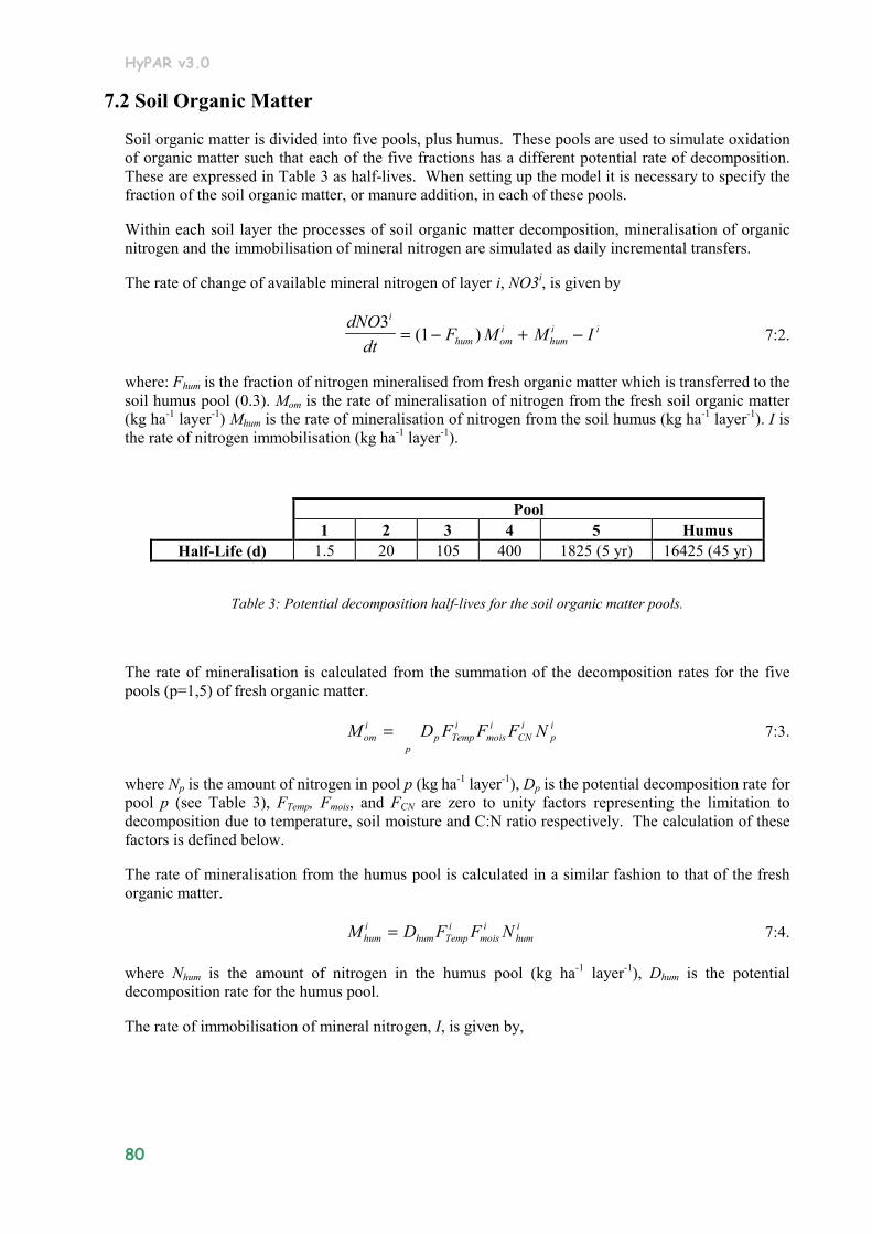
HyPAR v3.0

80

7.2 Soil Organic Matter

Soil organic matter is divided into five pools, plus humus. These pools are used to simulate oxidation of organic matter such that each of the five fractions has a different potential rate of decomposition. These are expressed in Table 3 as half-lives. When setting up the model it is necessary to specify the fraction of the soil organic matter, or manure addition, in each of these pools.

Within each soil layer the processes of soil organic matter decomposition, mineralisation of organic nitrogen and the immobilisation of mineral nitrogen are simulated as daily incremental transfers.

The rate of change of available mineral nitrogen of layer i, NO3i, is given by

dNOdt

F M M Ii

hum omi

humi i3

1= − + −( ) 7:2.

where: Fhum is the fraction of nitrogen mineralised from fresh organic matter which is transferred to the soil humus pool (0.3). Mom is the rate of mineralisation of nitrogen from the fresh soil organic matter (kg ha-1 layer-1) Mhum is the rate of mineralisation of nitrogen from the soil humus (kg ha-1 layer-1). I is the rate of nitrogen immobilisation (kg ha-1 layer-1).

Pool 1 2 3 4 5 Humus

Half-Life (d) 1.5 20 105 400 1825 (5 yr) 16425 (45 yr)

Table 3: Potential decomposition half-lives for the soil organic matter pools.

The rate of mineralisation is calculated from the summation of the decomposition rates for the five pools (p=1,5) of fresh organic matter.

M D F F F Nomi

p Tempi

moisi

CNi

pi

p= 7:3.

where Np is the amount of nitrogen in pool p (kg ha-1 layer-1), Dp is the potential decomposition rate for pool p (see Table 3), FTemp, Fmois, and FCN are zero to unity factors representing the limitation to decomposition due to temperature, soil moisture and C:N ratio respectively. The calculation of these factors is defined below.

The rate of mineralisation from the humus pool is calculated in a similar fashion to that of the fresh organic matter.

M D F F Nhumi

hum Tempi

moisi

humi= 7:4.

where Nhum is the amount of nitrogen in the humus pool (kg ha-1 layer-1), Dhum is the potential decomposition rate for the humus pool.

The rate of immobilisation of mineral nitrogen, I, is given by,

HyPAR v3.0

81

=

×=

02.0,min020

02.0,min020ionDecompositMatter Organic of Rate

i

i

p

iiCN

imois

iTempp

i

ii

OMON-.OMFFFD

OMON-. I

7:5.

where ONi is the amount of fresh organic nitrogen in layer i (kg ha-1 layer-1) and OMi is the amount of fresh organic matter (kg ha-1 layer-1).

This relationship implies that immobilisation will occur if the C:N ratio of the fresh organic matter is greater than 20 (taking the proportion of carbon in organic matter as 40%).

7.3 Temperature Limitation

Soil temperature affects the rate of decomposition through the relationship FTemp shown in Figure 21.

0.00

0.20

0.40

0.60

0.80

1.00

1.20

0 5 10 15 20 25 30 35 40Temperature (C)

Ftem

p

Figure 21: Relationship between the soil temperature decomposition limitation factor, FTEMP, and soil temperature

7.4 Moisture Limitation

The rate of decomposition is limited when the soil is both very dry and very wet. The relationship used in the model for Fmois is shown in Figure 22.

0.25FC Fsat FC

Fmois

1.0

Figure 22 Relationship between the soil moisture decomposition limitation factor, Fmois, and soil water content.

HyPAR v3.0

82

7.5 C:N Limitation

The rate of decomposition is affected by the C:N ratio of the substrate which is calculated for each layer as

CNOM

ON NO

i

i i=×+

0 43

. 7:6.

where ONi is the amount of fresh organic nitrogen in layer i (kg ha-1 layer-1), OMi is the amount of fresh organic matter (kg ha-1 layer-1) and NO3i is the amount of mineral nitrogen (kg ha-1 layer-1).

The model assumes that above a C:N ratio of 25 the rate of decomposition is reduced exponentially with increasing C:N ratio as shown in Figure 23.The relationship is

−−=25

)25(693.0exp CNFCN 7:7.

0.00

0.20

0.40

0.60

0.80

1.00

1.20

0 20 40 60 80 100 120C:N Ratio of System

Fcn

Figure 23 : The relationship between the CN decomposition limitation factor and the C:N ratio of the system.

7.6 Nitrogen uptake by trees and crops

7.6.1 Uptake

The soil is divided into vertical layers and may be further divided into horizontal plots, depending on the chosen light interception submodel (See Chapter 5). Initial demand for nitrogen is distributed between the soil cells according to relative root densities for tree and crop separately.

The maximum daily uptake of nitrogen by trees is related to fine root mass, soil mineral N content, and the C:N ratio of the entire plant (excluding the C and N bound in the heartwood), taking into account the root distribution of the trees across many plots (Section 4.8.2). Maximum nitrogen uptake by crop roots is calculated for each soil layer within each plot and is dependent upon the concentration of nitrate within the layer, the root density, the water content and the nutrient stress of the crop (Section 3.5.1).

HyPAR v3.0

83

If the sum of the demands for uptake in any soil cell is greater than the available soil nitrogen, or the combined extraction exceeds a maximum rate, then competition must take place.

7.6.2 Competition

The combined demand is first modified depending on the concentration of nitrate within the layer, the root density and the water content. For each soil cell the nitrogen demand, DN, is given by,

( )2

max 5.025.0][09.0exp(1(07.0

fc

iiCTi

Naw

awNDρ

ρ +−−= 7:8.

where: [Ni] is the nitrate concentration in the cell i, iCT+ρ is the total root length density, ρmax is the

maximum root length density, awi is the available water and awfc is the available water when the soil is at field capacity. The tree and crop demands are reduced in proportion to the initial demand if necessary.

Starting at the soil surface layer (in each plot independently), the combined demand is compared with the available N. If there is sufficient, then the full amount is removed from the soil and added to the tree and crop pools. If the supply is limited then all of the available N is removed from the soil and apportioned to tree and crop in proportion to their relative root densities. In HyPAR v3.0, any unfulfilled demand is added to that of the next soil layer down. The total tree uptake is re-allocated to individual trees according to their initial demand (Figure 24).

TREENutrientdemand

Competitionfor soil nutrients

TREENutrientdemand CROP

Nutrientdemand

Ncontent

Opt.N

Lightlim itedgrowth

Plant Ncontent

TREEOptimum

Uptake/layer

CROPOptimum

Uptake/layer

Max.Upt.Rate

SoilWater

Max.Upt.Rate

RLVRLV

TREEActual

Uptake/layer

CROPActual

Uptake/layer

TotalExtractionfrom soil

SoilN

TREEtotal

demand

TREENutrientdemand

TREENutrientdemand

TREENutrientdemand

TREEuptake

Figure 24: Nitrogen Competition between trees and crops where supply from each cell (plot x layer) is allocated to individual trees or crops depending on their comparative 'optimum N-demand' and root length ratios

HyPAR v3.0

84

8. Model Output

8.1 Output file format

The results from HyPAR are presented as a series of comma separated variable (csv) files. These files are designed to be read into a spreadsheet package, such as Microsoft Excel, or graphing package such as SigmaPlot.

Writing output files during a simulation run slows down the program, and printing all possible output variables uses up disk space. The HyPAR user interface therefore has a section to allow the user to select and limit the type of output created. There are six output file categories - Environment, Crop, Tree, Soil, Water and Field. Each of these has up to three options specifying the time step - Daily, Annual and Summary. Daily outputs are stored as one row per day; annual as one row per year, and summary as the average over the whole run. The latter file is particularly useful because climate variation makes it often preferable to present 20 or 30-year averages of crop yields etc. A global interval can be set for all daily files which prints out data every ‘n’ days, saving disk space.

•= Environment files: three file types are produced -- daily (envm0000.csv, where 0000 represents the year), annual (envmann.csv), and summary (envmsum.csv).

•= Crop files: daily (crop0000.csv), annual (cropann1.csv) and summary (cropsum.csv) files are produced for the field. In addition, if the ‘disaggregated’ tree canopy is selected then individual daily and annual crop output files can be produced for each plot within the field.

•= Tree files: some of the tree output files are for individual trees (tree*.csv), and others for the field as a whole (site*.csv). Again, daily, annual and summary files are produced.

•= Soil files: field scale soil files are the average of all plots on a daily (soil*0000.csv), annual (soilann.csv) and summary (soilsum.csv) basis. Variables are repeated for each layer in the profile. Individual files can also be requested for individual soil columns under each plot daily (but take care as this can generate a massive amount of output).

•= Water files: the daily water balance is recorded (watr0000.csv) at plot or field scale, for each soil layer.

•= Field files: there are two extra files created if the tree canopy is disaggregated (field0000a.csv and field0000b.csv).

All files have a comment in the first column after the data, giving a brief summary of the file including a note of the climate file used, and the hydrology model if appropriate

8.2 Graphical Output

A set of Microsoft Excel macros is provided (with the standard HyPAR installation) to create some graphs from the csv output files. These macros within the file HyPAR.xls are not exhaustive - once the HyPAR output files have been read into Excel (or other package) the user is free to generate any plot or modify the standard graphs as required.

When HyPAR.xls is opened (with macros enabled), a large button is visible on the first worksheet labelled “Click here for HyPAR output control”. This button launches the control dialogue. After the directory containing the required HyPAR output has been selected (usually C:\HyPAR\output), the tabs and the left-hand column of the control window become active. On each

HyPAR v3.0

85

tab, a list of files is given in the left-hand column - clicking on a button opens all files in the chosen directory that match the name on the button.

Once a file is open, the Plot button to the right becomes active. The Plot button runs the macros to create the standard plots. Each chart is created on a separate sheet within the output file (note: some macros are slow, please be patient!). Macros are not available for all files and the standard plots display only a sample of the total output.

A description of the output variables and the currently available standard graphs is given below.

8.3 Environment

There are three output files available containing data relating to the climate and site-specific data (related to latitude).

8.3.1 Daily

Daily data are displayed in a file with the selected year in the file name (e.g. envm1999.csv). Daily output can be further refined by setting the interval of days to output (e.g. an interval of 3 would output days 3, 6, 9, etc). The data in this file is the same for all plots.

File name: envm0000.csv (where 0000 is the year). Standard plots: none.

Column heading Units Notes

Date - Jul - Julian day number DAS - Days after sowing of crop Sunrise hour Time of sunrise Sunset hour Time of sunset Daylength seconds Day length Declination radians Solar declination T_max oC maximum 24-hour air temperature T_min oC minimum 24-hour air temperature Therm_t days accumulated thermal time (for crop) cd , dd days chilling days (for tree) Precip mm Incoming rainfall (above the tree canopy) S_rad MJ/m2 Solar radiation VapourP k Pa vapour pressure VPD k Pa vapour pressure deficit

8.3.2 Annual

File name: envmann.csv Standard plots: none.

HyPAR v3.0

86


Year - CO2 Pa Atmospheric carbon dioxide concentration Rain-tot mm Total annual rainfall Rain-pre mm Rainfall between January 1st and start of crop season Rain-dur mm Rainfall during the crop season Rain-post mm Rainfall between end of crop season and December 31st Tempmean oC Mean daily temperature Temprange oC Mean daily temperature range (maximum - minimum daily) VPD kPa Mean daily vapour pressure deficit Windsp m/s Mean daily wind speed (not used in HyPAR v3.0) Radiatn W/m2 Mean daily solar radiation Radiatn MJ/m2/day Mean daily solar radiation Radiatn MJ/m2/year Annual solar radiation

8.3.3 Summary

This file has the monthly and daily weather variables, averaged over the whole simulation run, for example if the run was over five years then this files shows the average weather for January, February, etc at this location.

File name: envmsum.csv Standard plots: (1) Daily - Precip, meanT, SolRad1 and VP. (2) Precip, meanT, SolRad1 and VP.


Month Precip mm Monthly total rainfall MeanT oC Mean daily temperature for month TRange oC Mean daily temperature range for month SolRad1 MJ/m2/day Mean daily solar radiation for month SolRad2 W/m2 Mean daily solar radiation for month VP kPa Mean daily vapour pressure for month Day Julian day Precip mm Daily total rainfall MeanT oC Mean daily temperature for this day TRange oC Mean daily temperature range for this day SolRad1 MJ/m2/day Mean daily solar radiation for this day SolRad2 W/m2 Mean daily solar radiation for this day VP kPa Mean daily vapour pressure for this day

8.4 Crop

If the tree canopy is disaggregated then there can be a number of independent 'plots' across the field within which the crop can grow. The crop output files are divided into those for separate plots or for

HyPAR v3.0

87

whole-field totals. With a uniform tree canopy there is only one plot, so only the field-scale files are produced. The digits in the file name represent the year and the plot number.

Plot scale Field scale Daily crop00_p000.csv crop0000.csv Annual cropann2.csv cropann1.csv Summary - cropsum.csv

8.4.1 Daily

File name: Crop00_p000.csv (e.g. crop98_p002). Standard plots: (1) WtRoot, WtLeaves, WtStem, WtHaulm, WtGrain, LAI for each plot.


Day Plot Stg Growth stage Lim Limiting factor for growth (W= water, L=light, N=nutrient) PlantLA m2 Leaf area Leafnum number of leaves per plant Cover cover, 0-1 LAI Leaf Area Index Intercept MJ/m2 Intercepted radiation DM_inc g/m2 Dry matter increment FBG Fraction of carbon allocated below ground WtRoot g/m2 Weight of root WtLeaves g/m2 Weight of leaves WtStem g/m2 Weight of stem WtHaulm g/m2 Weight of haulm WtGrain g/m2 Weight of grain TotDWt g/m2 Total dry weight RD m Rooting depth N_uptake kg/m2 Uptake of nitrogen W_uptake mm Uptake of water N_stress (0-1) Index of nitrogen stress W_stress (0-1) Index of water stress T_stress (0-1) Index of temperature stress Stress (0-1) Overall index for stress

File name: crop0000.csv Standard plots: (1) Chart0000 - WtRoot, WtLeaves, WtStem, WtHaulm, WtGrain, LAI


Day PlantLA m2 Leaf area

HyPAR v3.0

88

Leafnum number of leaves per plant Cover cover, 0-1 LAI Leaf Area Index Intercept MJ/m2 Intercepted radiation DM_inc g/m2 Dry matter increment FBG Fraction of carbon allocated below ground WtRoot g/m2 Weight of root WtLeaves g/m2 Weight of leaves WtStem g/m2 Weight of stem WtHaulm g/m2 Weight of haulm WtGrain g/m2 Weight of grain TotDWt g/m2 Total dry weight RD m Rooting depth N_uptake kg/m2 Uptake of nitrogen W_uptake mm Uptake of water Stress (0-1) Stress index Nstress (0-1) Index of nitrogen stress

8.4.2 Annual

File name: cropann2.csv Standard plots: none.


Year Plot# Plot number - every plot in the field is represented by a row X m The x co-ordinate of the plot centre (from field edge) Y m The y co-ordinate of the plot centre (from field edge) Sown day Julian day the crop was sown GS1end day end of growth stage 1 GS2end day end of growth stage 2 Harvest day day of harvest (end of crop season) Grain number/m2 number of grains produced in each plot Yield t/ha Grain yield for plot ADW t/ha Above ground dry weight at harvest Max_LAI m2/m2 Maximum Leaf Area Index reached during season Max_LAI day the day of the maximum LAI Water mm Total water uptake by the crop Light MJ/m2 Total light interception over the season Nutrients kg/ha Total nutrient uptake over the season ResDW t/ha Residue dry weight removed - (will be zero if residue left on soil) ResN t/ha N cont. of residue removed - (will be zero if residue left on soil)

File name: cropann1.csv Standard plots: none.

HyPAR v3.0

89


Year Sown day Julian day of year when crop was sown Harvest day Date of harvest Pop plants/m2 Number of crop established plants (an input variable) Grain num/m2 number of grains produced Yield t/ha Crop grain yield ADW t/ha Above ground dry weight H Index Harvest Index Max_LAI m2/m2 Maximum LAI reached for the field Water mm Total water uptake by the crop Light MJ/m2 Total light interception over the season Nutrients kg/ha Total nutrient uptake over the season ResDW t/ha Residue dry weight removed - (will be zero if residue left on soil) ResN t/ha Nitrogen content of residue removed - (will be zero if residue left on soil)

8.4.3 Summary

File name: cropsum.csv Standard plots: All variables as bar chart summary.


Grain yield t/ha Total grain yield, average over all years of the run ADW t/ha Above ground dry weight Grain_# num/m2 Number of grains produced Sown day Planting date (Julian day) Harvest day Harvest date Transp mm Total water uptake over the season Light MJ/m2 Total light intercepted over season Nutrients kg/ha Total nutrients taken up during the season

8.5 Tree

HyPAR can have a number of individual trees growing in a single field. Some output files are for separate trees (tree*.csv) and some are for the whole canopy across the field (site*.csv).

Individual scale Field scale Daily tree0000.csv site0000.csv Annual treeann.csv siteann.csv Summary sitesum.csv

HyPAR v3.0

90

8.5.1 Daily

File name: tree0000.csv Standard plots: none. This file has output for each tree, identified by the tree reference name in row three (a user-defined name entered in the tree individual editor). The current version of Microsoft Excel has a limit of 255 columns so as there are 19 variables per tree, the output is restricted to 13 trees.


Day Julian day of year (given in file name)Precip mm Rainfall (useful for graphs!) Sp. Species mnemonic ht m Height of tree hbc m Height to base of crown Crndiam m Crown diameter (assumed to be an ellipse) Rootdiam m Maximum diameter of rooting zone around tree DBH cm Diameter of stem at breast height Leaf area m2 Total leaf area Chwood kg Carbon in heart wood (total for tree) Cswood kg Carbon in sapwood (includes coarse roots) Cbark kg Carbon in bark Cfroots kg Carbon in fine roots (1mm diameter or less) Cfoliage kg Carbon in foliage Cstore kg Carbon in storage H_area cm2 Heartwood area Sap_area cm2 Sapwood area Nfol kg Nitrogen in foliage Nwood kg Nitrogen in wood (includes coarse roots) Nfroots kg Nitrogen in fine roots Nfolp %DW Proportion of nitrogen in foliage

File name: site0000.csv Standard plots: (1) C1 0000 - NetPhs, M_resp, G_resp, Litter. (2) C2 0000 - Biomass, Store. This file contains the daily carbon balance for all the trees in the field.


kday Julian day of year (given in file name.Biomass kg C Carbon biomass Store kg C Carbon in storage NetPhs kg C Net photosynthesis M_resp kg C maintenance respiration G_resp kg C Growth respiration Litter kg C litter (foliage and wood)

HyPAR v3.0

91

8.5.2 Annual

File name: treeann.csv Standard plots: none. This file shows the data for each tree as it stands on December 31st of each year of the run.


Year name Tree individual code name (e.g. t001) Sp. Species mnemonic (e.g. EGLO) ht m Height of tree hbc m Height to base of crown Crndiam m Crown diameter (assumed to be an ellipse) Rootdiam m Maximum diameter of rooting zone around tree DBH cm Diameter of stem at breast height Leaf_area m2 Total leaf area Chwood kg Carbon in heart wood (total for tree) Cswood kg Carbon in sapwood (includes coarse roots) Cbark kg Carbon in bark Cfroots kg Carbon in fine roots (1mm diameter or less) Cfoliage kg Carbon in foliage Cstore kg Carbon in storage Nfol kg Nitrogen in foliage Nwood kg Nitrogen in wood (includes coarse roots) Nfroots kg Nitrogen in fine roots Nfolp %DW Proportion of nitrogen in foliage

File name: siteann.csv Standard plots: none.


Year Trees /field number of trees modelled Trees /ha equivalent number of trees per hectare Total_LA m2 total leaf area LAI Leaf area index Biomass kg biomass mean_DBH cm mean diameter at breast height Foliage_C kg Foliage carbon Foliage_N kg Foliage nitrogen N %DW N concentration in foliage GPP kgC/m2/yr Gross primary productivity NPP kgC/m2/yr Net primary productivity Total_abs MJ/m2 Total intercepted radiation by tree canopy Litter-folC kg/m2 Carbon in removed foliage litter 1 Litter-wdC kg/m2 Carbon in removed wood litter 1

HyPAR v3.0

92

Litter-folN kg/m2 Nitrogen in removed foliage litter 1 Litter-wdN kg/m2 Nitrogen in removed wood litter 1 dd_flag flag to indicate conditions were suitable for dry deciduous trees

1 - this figure will be zero if the litter was left on the soil (a user-defined input option)

8.5.3 Summary

File name: sitesum.csv Standard plots: (1) PP_1 - mGPP, mNPP, mLAI. (2) PP_2 - dGPP, dNPP, dLAI


Month mGPP kgC/ha Gross primary productivity total for mNPP kgC/ha - as above for NPP mLAI - mean LAI for this month Day dGPP kgC/ha as above for year day dNPP kgC/ha dLAI

8.6 Soil

The soil files are complicated by the fact there can be output at field scale or plot scale as well as layer by layer. The 'profile' means all layers combined. The region of soil in one plot in one layer is referred to as a cell.

Plot scale Field scale Layer Profile Layer Profile

Daily soiln00_p000.csv soilr00_p000.csv

(watr00_p000.csv)1

soiln0000.csv soilr0000.csv

(watr0000.csv)1 soilt0000.csv

Annual soilann.csv Summary soilsum.csv

1see next section for water files

8.6.1 Daily

For the following three files, the field-scale output files have the same content, but averaged over all plots. Plot scale files are only created if the 'field only' box is not checked on the output tab.

File name: soiln0000.csv or soiln00_p000.csv (new file created for each selected plot) Standard plots: none. These variables are repeated for every soil layer -

HyPAR v3.0

93


Day Plot Wat-Cont mm Water content of layer FreshOM kg/ha fresh organic matter FreshON kg/ha fresh organic nitrogen Humus kg/ha humus content of layer HumusN kg/ha nitrogen in humus NO3 mg/kg soil mineral nitrogen in layer NO3 kg/ha soil mineral nitrogen in layer NO3net kg/ha Net mineralisation and immobilisation NO3flux kg/ha Net amount of nitrogen leached (last column) kg/ha Nitrogen lost with drainage water

File name: soilr0000.csv or soilr00_p000.csv (new file created for each selected plot) Standard plots: (1) C1 - Wupt-tree. (2) C2 - Wupt-crop. (3) C3 - Roots-tree. (4) C4 - Roots-crop. (5) C5 - NO3upt-tree. (6) C6 - NO3upt-crop.


Day Plot Wat-Cont mm Water content of layer Wat-flux mm net movement of water into/out of layer Roots-tree cm/cm3 Tree root density (all trees in field) Wupt-tree mm Water uptake by tree roots (all trees in field) NO3upt-tree kg/ha Nutrient uptake by tree roots Roots-crop cm/cm3 Crop root density Wupt-crop mm Water uptake by crop roots NO3upt-crop kg/ha Nutrient uptake by crop roots

File name: soilt0000.csv Standard plots: none. This file gives a field-scale summary of the water and nitrogen balance in the soil.

HyPAR v3.0

94


Day Julian dayTemp oC temperature WatCont mm water content of the profile AW mm water available for uptake by plants Top40 mm water content of top 40cm Swpot MPa soil water potential Wat-in mm Water entering the soil (rainfall minus interception by leaves) Wat-out mm Water leaving the soil (uptake, drainage, soil evaporation) Nut-conc kg/ha NO3 total content Nut-in kg/ha Mineral N entering soil (mineralisation) Nut-out kg/ha Mineral N leaving soil (immobilisation, uptake) Nut-loss kg/ha Mineral N lost with drainage water

8.6.2 Annual

File name: soilann.csv Standard plots: none.


Year Rainfall mm Rainfall TreeTrn mm Tree water uptake CropTrn mm Crop water uptake TreeEvap mm Evaporation losses following interception by tree leaves CropEvap mm Evaporation losses following interception by crop leaves SoilEvap mm Evaporation losses from soil surface Runoff mm Water lost as run off Drainage mm Water lost from the system as drainage Water_change mm Difference between water content on December 31st and the

tnetNO3 Net change in mineral N due to mineralisation and immobilisation NO3leach kg/ha Mineral N lost with drainage water TreeNup kg/ha N uptake by the tree CropNup kg/ha N uptake by the crop Nutrient_change kg/ha Difference between mineral N content on December 31st and the

previous January 1st.

8.6.3 Summary

There are 13 possible combinations of hydrology model and pedotransfer functions. Each of these options may result in a different set of conditions defining wilt point, field capacity and saturated capacity for the given soil types. These will not change during the run.

File name: soilsum.csv Standard plots: (1) SW_1 - Sat., F.Cap., PWP . (2) SW_2 - Sat_mm., F.Cap_mm, PWP_mm (3) SW_3 - Initial_mm, Final_mm

HyPAR v3.0

95


Layer Layer in soil profile (1 = surface)Depth mm Depth of layer mid-point below soil surface Width mm thickness of layer Type soil type in layer (user-defined) PWP mm Permanent wilt point F.Cap. mm Field capacity Sat. mm Saturated capacity MaxAW mm maximum available water for plants Initial mm initial water content (user defined) Final mm water content at end of simulation PWP_mm mm/mm As above, but expressed per mm rather than layer total F.Cap_mm mm/mm " Sat_mm mm/mm " MaxAW_mm mm/mm " Initial_mm mm/mm " Final_mm mm/mm "

8.7 Water

8.7.1 Daily

File name: watr0000.csv or watr00_p000.csv Standard plots: (1) C1 - Tree_evap, Crop_evap, Soil_evap (2) C2 - Precipn, WatCont... (3) C3 - TreeTrn, CropTrn, Precipn. This file shows the daily water balance.


Day (Plot) (plot number, only in watr00_p000) Precipn mm Rainfall Tree_evap mm Evaporation from tree canopy Crop_evap mm Evaporation from crop canopy Soil_evap mm Soil evaporation TreeTrn mm Tree transpiration CropTrn mm Crop transpiration Drainage mm Water lost as drainage RunOff mm Run off total for the day Puddle mm Surface water remaining at end of day WatCont... mm Water content of all layers, one per column

8.8 Field

There are two additional output files created when the tree canopy is disaggregated.

HyPAR v3.0

96

File name: field0000a.csv Standard plots: none This file gives the layout of the field. It shows the plot numbers, the tree positions and the fraction of light reaching each plot on the (Julian) day that the crop is sown. File name: field0000b.csv Standard plots: none. This file gives the layout of the field. It shows the plot numbers, the tree positions, the fraction of light reaching each plot on the (Julian) day that the crop is harvested and the crop yield per plot.

HyPAR v3.0

97

9. References

Acock, B., Reddy, V R., Whistler, F D., Baker, D N., McKnion, J M., Hodges, H F & Boote, K J (1985). The Soybean Crop Simulator GLYCIM: Model Documentation 1982, PB85171163/AS. US Dept Agric. Washington, DC (available from NTIS Springfield, Virginia).

Addicott, F.T. (1982). Abscission. Berkeley: University Press.

Addiscott, T M. & Wagenet, R J (1985). Concepts of Solute Leaching in Soils: A review of modelling approaches. Journal of Soil Science: 36: 411-424.

Ahmed, M O M (1988). Root growth and water use in two sorghum genotypes subjected to different irrigation regimes. Master of Science Thesis, University of Nottingham, Sutton Bonington Campus, UK.

Allen, L H., Jnr (1974). Model of light penetration into a wide-row crop. Agron. J. 66: 41-47.

Angus, J F & Moncur, M W (1977). Water stress and phenology in wheat. Australian Journal of Agricultural Research, 28: 171-181.

Arah, J.R.M. (1996) Approaches to modelling soil hydrology. Ch. 9. In: Agroforestry Modelling and Research Co-ordination Annual Report, 1995-96. ODA Forestry Research Programme R5652. ITE-NERC.

Arkin, G F., Ritchie, J T., Maas, S J (1978). A model for calculating light interception by grain sorghum canopy. Transactions of the ASAE. 21:303-308.

Arkin, G F., Rosenthal, W D & Jordan, W R (1983). A sorghum leaf area model. Am. Soc. Agrig. Eng. Tech. Pap. No. 83-2098.

Art, H.W. and Marks, P.L., (1978). A summary table of biomass and net annual primary production in forest ecosystems of the world. In: H.F.H. Leith. (H.F.H. Leith), Patterns of primary production in the biosphere. Dowden, Hutchinson and Ross, Inc, 177-192. 8. Stroudsburg, Pennsylvania: Dowden, Hutchinson and Ross, Inc, 1978.

Austin, M.P (1992). Modelling the environmental niche of plants: implications for plant community response to elevated CO2 levels. Australian Journal of Botany 40: 615-630.

Austin, R B (1989). Maximising crop production in water limiting environments. In Drought Resistance in Cereals (Ed. F. Baker). CAB International. (ICSU Press).

Azam-Ali, S N., Gregory, P J & Monteith, J L (1984). Effects of Planting Density on Water Use and Productivity of Pearl Millet (pennisetum typhoides) Grown on Stored Water. I. Growth of Roots and Shoots. Expl Agri, 20: 203-214.

Azam-Ali, S N., Crout, N M J & Bradley, R G (1994). Some Perspectives in Modelling Resource Capture by Crops. Proceedings of 52nd Easter School in Agricultural Science, Sutton Bonington, UK.

Baveye, P & Sposito, G (1984). The operational significance of the continuum hypothesis in the theory of water movement through soils and aquifers. Water Resour. Research, 20: 521-530.

Beardsell, M F & Cohen, D (1975). Relationships between leaf water status, Abscisic Acid levels and Stomatal resistance in maize and sorghum. Plant Physiol. 56: 207-212.

HyPAR v3.0

98

Berge, H F M Ten., Jansen, D M., Rappoldt, K & Stol, W (1992). The soil water balance module SAWAH: description and users guide. Simulation Reports CABO-TT, no.22. DLO-Centre for Agrobi. Research & Dept of Theor. Prod. Ecology, Wageningen Agriicultural Uni, 78p.

Birch, C J., Carberry, P S., Muchow, R C., Mccown, R L & Hargreaves J N G (1990). Development and Evaluation of a Sorghum Model Based on CERES-Maize in a Semi-Arid Tropical Environment. Field Crops Research, 24: 87-104. Elsevier Science Publishers BV, Amsterdam.

Blackman, F F (1905). Ann. Bot. (London) 19: 281-295.

Bloodworth, M E., Burleson, C A & Cawley, W R (1958). Root distribution of some irrigated crops using undisrupted soil cores. Agron. J, 50: 317-320.

Blum, A (1979). Genetic improvement of drought resistance in crop plants: A case for sorghum. In Stress Physiology in Crop Plants (Eds. H Mussell & R C Staples). J Wiley & Sons, N. York. pp. 429-445. *

Blum, A & Arkin, G F (1984). Sorghum Root Growth and Water-Use as Affected by Water Supply and Growth Duration. Field Crop Research, 9: 131-142. Elsevier Science Publishers BV, Amsterdam.

Boerner, R.E.J., (1984). Foliar nutrient dynamics and nutrient use efficiency of four deciduous tree species in relation to site fertility. Journal of Applied Ecology 21: 1029-1040.

Boyer, J S (1976). Water deficits and photosynthesis. In Water Deficits and Plant Growth. v. IV (Ed. T T Kozlowski). Academic Press, N. York. pp. 153-190.

Brooks, R.H. and Corey, A.T. (1964) Hydraulic properties of porous media. Colorado State University Hydrology Paper No 3, pp. 27

Brouwer, R (1966). Root growth of grasses and cereals. In The Growth of Cereals and Grasses. (Eds. F L Milthorpe and J D Ivins, 153-66. Butterworths, London.

Campbell, G S (1974). A simple method for determining unsaturated conductivity from moisture retention data. Soil Sci. 117: 311-314.

Campbell, G.S. (1985) Soil Physics with BASIC: Transport Models for Soil-Plant Systems. Elsevier, New York, pp. 150

Cannell, M.G.R., (1988). Chilling, thermal time and the date of flowering of trees. In: C.J. Wright. (C.J. Wright), Manipulation of fruiting. Butterworths, 99-113. London: Butterworths, 1988.

Cannell, M.G.R., (1984). Woody biomass of forest stands. Forest Ecology and Management 8: 299-312.

Cannell, M.G.R., (1989). Physiological basis of wood production: a review. Scandinavian Journal of Forest Research 4: 459-490.

Cannell, M.G.R. and Dewar, R.C., (1994). Carbon allocation in trees: a review of concepts for modelling. Advances in Ecological Research 25: 59-104.

Cannell, M.G.R. and Smith, R.I., (1983). Thermal time, chill days and prediction of budburst in Picea sitchensis. Journal of Applied Ecology 20: 951-963.

Carberry, P S & Abrecht, D G (1991). Tailoring crop models to the Semiarid Tropics. In Climatic risk in crop production: Models and management for the Semiarid Tropics and Subtropics. (Eds. R C Muchow & J A Bellamy). C.A.B. International, Wallingford, Oxon, UK. pp. 157-182.

HyPAR v3.0

99

Cass, A, Campbell, G S & Jones, T L (1984). Enhancement of thermal water vapor diffusion in soil. Soil Sci. Soc. Am. J. 48: 25-32

Chapin III, F.S. and Van Cleve, K., (1989). Approaches to studying nutrient uptake, use and loss in plants. In: R.W. Pearcy, J. Ehleringer, H.A. Mooney, and P.W. Rundel. (R.W. Pearcy, J. Ehleringer, H.A. Mooney, and P.W. Rundel), Plant physiological ecology: field methods and instrumentation. Chapman and Hall, 185-207. London: Chapman and Hall, 1989.

Charles-Edwards, D A & Thornley, J H M (1973). Light interception by an isolated plant: a simple model. Annals of Botany. 37: 919-928.

Charles-Edwards, D A (1982). Physiological determinants of crop growth. Academic Press, Sydney. 161 pp.

Claerboot, J.F. (1985). Fundamentals of geophysical data processing. Blackwell 247p.

Collatz, G.J., Ball, J.T., Grivet, C., and Berry, J.A., (1991). Physiological and environmental regulation of stomatal conductance, photosynthesis and transpiration: a model that includes a laminar bounday layer. Agricultural and Forest Meteorlogy 54: 107-136.

Comins, H.N. and McMurtrie, R.E., (1993). Long-term response of nutrient-limited forests to CO2 enrichment. Ecological Applications 3: 666-681.

Coombe, D.E. & Hadfield, W. (1962). An analysis of the growth of Musanga cecropioides. J.Ecol., 50, 221-34.

Cramer, W.P. and Leemans, R., (1993). Assessing impacts of climate change on vegetation using climate classification systems. In: A.M. Solomon and H.H. Shugart. (A.M. Solomon and H.H. Shugart), Vegetation dynamics and global change. Chapman and Hall, 190-217. Chapman and Hall, 1993.

Craufurd, P Q., Flower, D J & Peacock J M (1993). Effect of Heat and Drought Stress on Sorghum (sorghum bicolor). I. Panicle Development and Leaf Appearance. Expl Agric, 29: 61-76, Cambridge University Press.

Craufurd, P Q & Peacock J M (1993). Effect of Heat and Drought Stress on Sorghum (sorghum bicolor). II. Grain Yield. Expl Agric, 29: 77-86, Cambridge University Press.

Crout NME, Young SD & Bradley RG (1997). PARCH - Technical Manual. v3.00. Report to the UK Overseas Development Administration, University of Nottingham. 70p

Daamen, C C & Simmonds, L P (1995). Soil Water, Energy And Transpiration (SWEAT). A numerical model of water and energy fluxes in soil profiles and sparse canopies. Department of Soil Science, University of Reading, UK.

Davidson, R L (1969). Effects of soil nutrients and moisture on root/shoot ratios in Lolium perenne L. and Trifolium repens L. Annals of Botany. Vol 33 No.131.

De Wit, C.T., (1970). Dynamic concepts in biology. In: I. Setlik Pudoc. (I. Setlik Pudoc), Prediction and measurement of photosynthetic productivity. Wageningen, Netherlands: 1970.

Dewar, R.C., In press. Interpretation of an empirical model for stomatal conductance in terms of guard cell function. Plant, Cell and Environment

Dickinson, R.E., Henderson-Sellers, A., Rosenzweig, C., and Sellers, P.J., (1991). Evapotranspiration models with canopy resistance for use in climate models, a review. Agricultural and Forest Meteorology 54: 373-388.

HyPAR v3.0

100

Doggett, H (1988) Sorghum (Second edition). Longman, Harlow.

Eastin, J D (1976). Temperature influence on sorghum yield. In Proceedings of the 31st Annual Corn and Sorghum Research Conference. (Eds. H P Loden & D Wilkinson). American Seed Trade Association. pp. 19-23.

Edmeades, G O & Daynard, T B (1979). The relationship between final yield and photosynthesis at flowering in individual maize plants. Canadian J. Plant Sci., 59: 585-601.

Elias, T.S., (1980). The Complete Trees of North America. New York: Van Nostrand Reinhold.

Emanuel, W.R., Shugart, H.H., and Stevenson, M.P., (1985). Climatic change and the broad-scale distribution of terrestrial ecosystem complexes. Climatic Change 7: 29-43.

Erenstein, O (1990). Simulation of water-limited yields of sorghum, millet and cowpea for the 5th region of Mali in the framework of quantitative land evaluation. Department of Theoretical Production Ecology, Ag. Uni. Wageningen.

Evans, J.R., (1988). Acclimation by the thylakoid membranes to growth irradiance and the partitioning of nitrogen between soluble and thylakoid proteins. Australian Journal of Plant Physiology 15: 93-106.

Evans, J.R., (1989). Photosynthesis and nitrogen relationships in leaves of C3 plants. Oecologia 78: 9-19.

Evett, S R & Lascano R J (1993). ENWATBAL.BAS: A Mechanistic Evapotranspiration Model Written in Compiled Basic. Agron. J., 85: 763-772.

Farquhar, G.D. and von Caemmerer, S., (1982). Modelling of photosynthetic response to environmental conditions. In: O. Lange, P. Nobel, C. Osmond, and H. Zieger. (O. Lange, P. Nobel, C. Osmond, and H. Zieger), Physiological plant ecology II: water relations and carbon assimilation. Springer-Verlag, 549-587. 12B. Berlin: Springer-Verlag, 1982.

Farquhar, G.D., von Caemmerer, S., and Berry, J.A., (1980). A biochemical model of photosynthetic CO2 assimilation in leaves of C3 species. Planta 149: 78-90.

Farquhar, G D & Sharkey, T D (1982). Stomatal conductance and photosynthesis. Ann. Rev. Plant Physiol., 33: 317-345.

Farquhar, G.D. and Wong, S.C., (1984). An empirical model of stomatal conductance. Australian Journal of Plant Physiology 11: 191-210.

Field, C. and Mooney, H.A., (1986) The photosynthesis-nitrogen relationship in wild plants. In: T.J. Givnish. (T.J. Givnish), On the economy of plant form and function. Cambridge University Press, 25-55. Cambridge: Cambridge University Press, 1986.

Finch-Savage, W E & Elston, J (1982). The effect of temperature and water stress on the timing of leaf death in Vicia faba. Ann. Appl. Biol. 100: 567-579. *

Fischlin, A., Bugmann, H., and Gyalistras, D., (1995). Sensitivity of a forest ecosystem model to climate parameterization schemes. Environmental Pollution 87: 267-282.

France, J & Thornley, J H M (1984). Mathematical Models in Agriculture. A quantitative approach to problems in agriculture and related sources. Butterworths, London.

Friend, A.D., (1993). The prediction and physiological significance of tree height. In: A.M. Solomon and H.H. Shugart. (A.M. Solomon and H.H. Shugart), Vegetation Dynamics and Global Change. Chapman and Hall, 101-115. New York: Chapman and Hall, 1993.

HyPAR v3.0

101

Friend, A.D., (1998) Parameterisation of a global daily weather generator for terrestrial ecosystem and biogeochemical modelling. Ecological 109: 121-40).

Friend, A.D. and Leith, I.D., In press. Gas exchange measurements on European beech (Fagus sylvatica L.) grown for 2 years at different levels of atmospheric CO2 and nutrients. Global Change Biology

Friend, A.D., (1991). Use of a model of photosynthesis and leaf microenvironment to predict optimal stomatal conductance and leaf nitrogen partitioning. Plant, Cell and Environment 14: 895-905.

Friend, A.D., (1995). PGEN: an integrated model of leaf photosynthesis, transpiration, and conductance. Ecological Modelling 77: 233-255.

Friend, A.D. and Cox, P.M., (1995). Modelling the effects of atmospheric CO2 on vegetation-atmosphere interactions. Agricultural and Forest Meteorology 73: 285-295.

Friend, A.D., Shugart, H.H., and Running, S.W., (1993). A physiology-based gap model of forest dynamics. Ecology 74: 792-797.

Friend, A.D. Stevens, A.K., Knox, R.G. & Cannell, M.G.R. (1997) A process based terrestrial biosphere model of ecosystem dynamics. Ecological Modelling 95: 249-287.

Gallagher, J N & Biscoe, P V (1978). Radiation absorption, growth and yield of cereals. Journal of Agricultural Science, 91: 47-60.

Gallagher, J N (1979). Field studies of cereal leaf growth. I. Initiation and expansion in relation to temperature and ontogeny. J. Exp. Bot., 30: 625-636.

Gates, D M (1980). Biophysical Ecology. Springer-Verlag. New York. 611 pp.

Germain, R. & Evrard, C. (1956). Etude ecologique et phytosociologique de la foret a Brachystegia laurentii. INEAC Brussels No 67: 10105

Gerwitz, A & Page E R (1974). An empirical mathematical model to describe plant root systems. J Appl. Ecol, 11: 773-782.

Gifford, R.M. Germain, R. & Evrard, C. (1956). Etude ecologique et phytosociologique de la foret a Brachystegia laurentii. INEAC Brussels No 67: 10105

Grant, R. F. (1991). The distribution of water and nitrogen in the soil-crop system: a simulation study with validation from a winter wheat field trial. Fertilizer Research, 27: 199-213.

Green, C.F. Analysis of wheat growth in relation to husbandry and environment. PhD, Nottingham, 1984.

Green, P B., Erickson, R O & Buggy, J (1971). Metabolic and physical control of cell elongation rate. Plant Physiol. 47: 423-430.

Green, R E & Ampt, G (1911). Studies in soil physics. Part 1 - The flow of air and water through soils. J. Ag. Sci. 4: 1-24.

Gregory, P J & Brown, S C (1987). Roots and their role in water uptake and drought resistance. In Drought Resistance in Plants: Physiological and Genetic Aspects (Eds. L Monti & E Porceddu). CEC, Brussels. pp. 165-178.

Gregson, K., Hector, D J & Mcgowan, M (1987). A one-parameter model for the soil water characteristic. University of Nottingham, Sutton Bonington Campus, Leicester, LE12 5RD. Journal of Soil Science, 38: 483-486.

HyPAR v3.0

102

Grime, J.P., (1979). Plant Strategies and Vegetation Processes. Chichester: Wiley.

Gulmon, S.L. and Mooney, H.A., (1986). Costs of defense and their effects on plant productivity. In: T.J. Givnish. (T.J. Givnish), On the economy of plant form and function. Cambridge University Press, 681-698. Cambridge: Cambridge University Press, 1986.

Halle, F. & Martin, R. (1968). Etude de la croissance rythmique chez l'Hevea. Adansonia, 8, 475-503.

Hammer, G L., Hill, K & Schrodter, G N (1987). Leaf Area Production and Senescence of Diverse Grain Sorghum Hybrids. Field Crops Research, 17: 305-317. Elsevier Science Publishers BV, Amsterdam.

Hammer, G L & Muchow, R C (1991). Quantifying climatic risk to sorghum in Australia's semiarid tropics and subtropics: model development and simulation. In Climatic risk in crop production: Models and management for the Semiarid Tropics and Subtropics. (Eds. R C Muchow & J A Bellamy). C.A.B. International, Wallingford, Oxon, UK. pp. 329-358.

Hammer, G L & Muchow, R C (1994). Assessing climatic risk to sorghum production in water-limited subtropical environments. I. Development and testing of a simulation model. Field Crops Research 23: 221-237.

Hänninen, H., (1991). Does climatic warming increase the risk of frost damage in northern trees? Plant, Cell and Environment 14: 449-454.

Hansen, S., Jensen, N E., Nielsen, N E & Svendsen, H (1991). Simulation of nitrogen dynamics and biomass production in winter wheat using the Danish simulation model DAISY. Fertilizer Research, 27: 245-259.

Hari, P., Kaipiainen, L., Korpilahti, E., Ma:kela:, A., Nilson, T., Oker-Blom, P., Ross, J., and Salminen, R., (1985). Structure, radiation and photosynthetic production in coniferous stands. University of Helsinki, Department of Silviculture. Research Notes 54.

Harris, F S (1914). The effect of soil moisture, plant food and age on the ratio of top to roots in plants. J. Am Soc. Agron. 6: 65-75.

Heemst, H D J van (1988). Plant data values required for simple crop growth simulation models: review and bibliography. Simulation Report CABO-TT no.17. CABO/TPE, P.O. Box 14, Wageningen, The Netherlands. 100 pp.

Hillel, D (1977). Computer Simulation of Soil-Water Dynamics. Inter. Dev. Research Centre, Ottawa.

Huber, B., (1928). Weitere quantitative Untersuchungen u:ber das Wasserleitungssystem der Pflanzen. Jb. Wiss. Bot. 67: 877-959.

Hurd, E A (1976). Plant breeding for drought resistance. In Water Deficits and Plant Growth. v. IV (Ed. T T Kozlowski). Academic Press, N. York. pp. 317-353. *

Jansen, D M & Gosseye, P (1986). Simulation of growth of millet (Pennisetum americanum) as influenced by water stress. Simulation Reports CABO-TT no.10, Centre for Agrobiological Research and Department of Theoretical Production Ecology, Wageningen Agricultural University, 108 pp.

Jarvis, N J., Jansson, P-E., Dik, P E & Messing, I (1991a). Modelling Water and Solute Transport in Macroporous Soil. I. Model Description and Sensitivity Analysis. Journal of Soil Science, 42: 59-70.

HyPAR v3.0

103

Jarvis, N J., Bergström, L & Dik, P E (1991b). Modelling Water and Solute Transport in Macroporous Soil. II. Chloride Breakthrough under Non-Steady Flow. Journal of Soil Science, 42: 71-81.

Jarvis, P.G., (1976). The interpretation of the variations in leaf water potential and stomatal conductance found in canopies in the field. Philosophical Transactions of the Royal Society of London, Series B 273: 593-610.

Jarvis, P.G. and Leverenz, J.W., (1983). Productivity of deciduous and evergreen forests. In: O.L. Lange, P.S. Nobel, C.B. Osmond, and H. Ziegler. (O.L. Lange, P.S. Nobel, C.B. Osmond, and H. Ziegler), Encyclopedia of Plant Physiology, New Series. Springer-Verlag, 233-280. 12D. Berlin: Springer-Verlag, 1983.

Jenkinson, D.S. and Rayner, J.H., (1977). The turnover of soil organic matter in some of the Rothamstead classical experiments. Soil Science 123: 298-305.

Jenny, H., Gessel, S.P., and Bingham, F.T., (1949). Comparative study of decomposition rates of organic matter in temperate and tropical regions. Soil Science 68: 419-432.

Jones, C A & Kiniry, J R (1986). CERES-Maize: A simulation model of maize growth and development. Texas A&M University press, College Station, Texas, 194 pp.

Jones, C A, Cole, C V, Sharpley, A N, & Williams, J R. (1984). A simplified soil and plant phosphorus model: I. Documentation. Soil. Science Soc. Am. J., 48:800-805

Jones, C A, Sharpley, A N, & Williams, J R. (1984). A simplified soil and plant phosphorus model: III. Testing. Soil. Science Soc. Am. J., 48:810-813

Jones, H., (1992). Plants and microclimate: a quantitative approach to environmental plant physiology. 2nd ed., Cambridge: Cambridge University Press.

Kaigama, B K., Teare, I D., Stone, L R & Power, W L (1977). Root and top growth of irrigated and non-irrigated grain sorghum. Crop Sci, 17: 555-559.

Karamanos, A J & Papatheohari, C Y (1987). Understanding the mechanisms of drought resistance of some crop plants. In Drought Resistance in Plants: Physiological and Genetic Aspects. (Eds. L Monti & E Porceddu). CEC, Brussels. pp. 95-109.

Karl, T.R., Williams, C.N.J., and Quinlan, F.T., (1990). United States Historical Climatology Network (HCN) serial temperature and precipitation data. Carbon Dioxide Information Analysis Center, Oak Ridge National Laboratory, Oak Ridge, Tennessee. ORNL/CDIAC-30, NDP-019/R1.

Kaszkurewicz, A. and Fogg, P.J., (1967). Growing seasons of cottonwood and sycamore as related to geographic and environmental factors. Ecology 48: 785-793.

Keating, B A & Wafula B M (1992). Modelling the fully Expanded Area of Maize Leaves. Field Crops Research, 29: 163-176.

Kenyi, M S B (1991). Crop water use and the root systems of Bambara Groundnut (vigna subterranea (L.)) and sorghum (sorghum bicolor (L.) Moench). Master of Science Thesis. University of Nottingham, Sutton Bonington Campus, Leicester LE12 5RD.

Korner, C., (1994). Leaf diffusive conductances in the major vegetation types of the globe. In: E.-D. Schulze and M.M. Caldwell. (E.-D. Schulze and M.M. Caldwell), Ecophysiology of Photosynthesis. Springer-Verlag, 463-489. 100. Berlin: Springer-Verlag, 1994.

HyPAR v3.0

104

Kozlowski, T T (1976). Water Deficits and Plant Growth. Vol IV. Soil Water Measurement, Plant Responses and Breeding for Drought Resistance. Academic Press, N. York.

Kricher, J.C. and Morrison, G., (1988). A field guide to eastern forests. The Peterson field guide series, Boston: Houghton Mifflin.

Krieg, D R & Hutmacher, R B (1986). Photosynthetic rate control in sorghum: stomatal and nonstomatal factors. Crop Science, 26: 112-117.

Laar, H H Van, Goudriaan, J & Keulen, H van (1992) (Eds.). Simulation of crop growth for potential and water-limited production situations (as applied to spring wheat). Simulation Report CABO-TT no.23. Centre for Agrobi. Research (CABO) & Dept of Theor. Prod. Ecology. Wageningen Uni.

Leemans, R., (1991). Sensitivity analysis of a forest succession model. Ecological Modelling 53: 247-262.

Leith, H., (1978). Modelling the primary productivity of the world. In: H.F.H. Leith. (H.F.H. Leith), Patterns of primary production in the biosphere. Dowden, Hutchinson and Ross, Inc, 277-282. 8. Stroudsburg, Pennsylvania: Dowden, Hutchinson and Ross, Inc, 1978.

Lenhard, R.J., Parker, J.C. and Mishra, S. (1989) On the correspondence between van Genuchten and Brooks-Corey models. Journal of Irrigation and Drainage Engineering 115:744-751

Leuning, R., In press. A critical appraisal of a combined stomatal-photosynthesis model for C3 plants. Plant, Cell and Environment

Leuning, R., (1990). Modelling stomatal behaviour and photosynthesis of Eucalyptus grandis. Australian Journal of Plant Physiology 17: 159-175.

Levine, E.R., Ranson, K.J., Smith, J.A., Williams, D.L., Knox, R.G., Shugart, H.H., Urban, D.L., and Lawrence, W.T., (1993). Forest ecosystem dynamics: linking forest succession, soil process and radiation models. Ecological Modelling 65: 199-219.

Little, E.L.J., (1971). Atlas of United States Trees. Vol. 1. Washington, D.C.: US Department of Agriculture Forest Service.

Lloyd, J. and Farquhar, G.D., (1994). 13CO2 discrimination by the terrestrial biosphere. Oecologia In press:

Lloyd, J., Grace, J., Miranda, A.C., Meir, P., Wong, S.C., Miranda, H.S., Wright, I.R., Gash, J.H.C., and McIntyre, J., In press. A Simple Calibrated (SiC) model of Amazon rainforest productivity based on leaf biochemical properties. Plant, Cell and Environment

Longman, K.A. (1969). The dormancy and survival of plants in the humid tropics. Symp Soc Exp Biol, 23, 471-88.

Longman, K.A. & Jenik, J. (1987). Tropical forest and its environment. Harlow,Essex: Longman.

Ludlow, M M & Muchow, R C (1990). A critical evaluation of the traits for improving crop yields in water limited environments. Adv. Agron. 43: 107-153.

Maas, S J (1993a). Agroclimatology and Modelling. Parameterized Model of Gramineous Crop Growth: I. Leaf Area and Dry Mass Simulation. Agron. J, 85: 348-353.

Mahalakshmi, V & Bidinger, F R (1985). Water stress and time of floral initiation in pearl millet. Journal of Agricultural Science, 105: 437-445.

HyPAR v3.0

105

Mann, J E., Curry, G L., Demichele, D W & Baker, D N (1980). Light penetration in a row crop with random plant spacing. Agron. J., 72: 131-142.

Matthews, R B., Reddy, D M., Rani, A U., Azam-Ali, S N & Peacock, J M (1990). Response of Four Sorghum Lines to Mid-Season Drought. I. Growth, Water Use and Yield. Field Crops Research, 25: 279-296.

McGuire, A.D., Melillo, J.M., Joyce, L.A., Kicklighter, D.W., Grace, A.L., Moore III, B., and Vorosmarty, C.J., (1992). Interactions between carbon and nitrogen dynamics in estimating net primary productivity for potential vegetation in North America. Global Biogeochemical Cycles 6: 101-124.

McLaughlin, S.B., McConathy, R.K., Barnes, R.L., and Edwards, N.T., (1980). Seasonal changes in energy allocation by white oak (Quercus alba). Canadian Journal of Forest Research 10: 379-388.

Melillo, J., McGuire, A., Kicklighter, D., Moore III, B., Vorosmarty, C., and Schloss, A., (1993). Global climate change and terrestrial net primary productivity. Nature 363: 234-240.

Merrill, S D & Rawlins, S L (1979). Distribution and Growth of Sorghum Roots in Response to Irrigation Frequency. Agron. J., 71: 735-745.

Mencuccini, M. and Grace, J., 1995. Climate influences the leaf area/sapwood area ratio in Scots pine. Tree Physiology 15: 1-10.

Mishra, S., Parker, J.C. and Singhal, N. (1989) Estimation of soil hydraulic properties and their uncertainty from particle size distribution data. Journal of Hydrology 108:1-18

Mobbs, D.C., Cannell, M.G.R., Crout, N.M.J., Lawson, G.J. and Friend, A.D. (1996) A Process Based Tropical Agroforestry Model (HyPAR v1). I. Model description and capability. Chapter 2, in: Agroforestry Modelling and Research Co-ordination Annual Report, 1995-96. ODA Forestry Research Programme R5652. ITE-NERC.

Monserud, R.A. and Leemans, R., (1992). Comparing global vegetation maps with the Kappa statistic. Ecological Modelling 62:

Monteith, J L (1977). Climate and the efficiency of crop production in Britain. Philos. Trans. R. Soc. London, B. 281: 277-294.

Monteith, J.L., 1981. Climatic variation and the growth of crops. Quarterly Journal of the Royal Meteorological Society 107: 749-774.

Monteith, J L (1986). How do crops manipulate water supply and demand. Phil. Trans. R. Soc. London, A. 316: 245-259.

Monteith, J L., Huda, A K S & Midya, D (1989). RESCAP: A resource capture model for sorghum and pearl millet. In Modelling the growth and development of sorghum and pearl millet. (Eds. Virmani, S.M., Tandon, H.L.S. & Alagarswamy, G.). ICRISAT Research Bulletin 12, Patancheru, India. pp. 30-34.

Monteith, J.L. and Unsworth, M.H., (1990). Principles of Environmental Physics. 2nd ed., London: Edward Arnold.

Monteith, J L (1994)[(1992)]. Principles of Resource Capture by Crop Stands. Proceedings of 52nd Easter School in Agricultural Science, Sutton Bonington, UK. (Ed. J L Monteith, R K Scott & M H Unsworth). Nottingham University Press. pp. 1-16.

HyPAR v3.0

106

Monteith, J.L., In press. A reinterpretation of stomatal responses to humidity. Plant, Cell and Environment

Monti, L & Porceddu, E (1987). Drought Resistance in Plants: Physiological and Genetic Aspects. CEC, Brussels.

Moore, C.J., (1976). A comparative study of radiation balance above forest and grassland. Quarterly Journal of the Royal Meteorological Society 102: 889-899.

Muchow, R C & Coates D B (1986). An Analysis of the Environmental Limitation to Yield of Irrigated Grain Sorghum During the Dry Season in Tropical Australia Using a Radiation Interception Model. Aust. J. Agric. Res., 37: 135-148.

Muchow, R C & Davis, R (1988). Effect of Nitrogen Supply on the Comparative Productivity of Maize and Sorghum in a Semi-Arid Tropical Environment. II. Radiation Interception and Biomass Accumulation. Field Crops Research, 18: 17-30. Elsevier Science Publishers BV, Amsterdam.

Muchow, R C & Carberry, P S (1990). Phenology and Leaf-Area Development in a Tropical Grain Sorghum. Field Crops Research, 23: 221-237. Elsevier Science Publishers BV, Amsterdam

Muchow, R C & Bellamy, J A (1991) (eds.). Climatic risk in crop production: Models and management for the Semiarid Tropics and Subtropics. C.A.B. International, Wallingford, Oxon, UK

Murray, M.B., Cannell, M.G.R., and Smith, R.I., (1989) Date of budburst of fifteen tree species in Britain following climatic warming. Journal of Applied Ecology 26: 693-700.

Nambiar, E.K.S. and Fife, D.N., (1991). Nutrient retranslocation in temperate conifers. Tree Physiology 9: 185-207.

Njoku, E. (1963). Seasonal periodicity in the growth and development of some forest trees in Nigeria. J.Ecol., 51, 617-24.

Ong, C K & Monteith, J L (1984). Response of pearl millet to light and temperature. In Agrometeorology of Sorghum and Millet in the Semi-Arid Tropics. Proceedings of the International Symposium. (Eds. S. Virmani & M. Sivakumar). Inter. Crops Res. Inst. pp. 129-142.

Oppenheimer, H R (1960). Adaptation to drought: xerophytism. In Plant-Water Relationships in Arid and Semi-arid Conditions. v. 15. (UNESCO, Paris). pp. 105-138. *

Paleg, L G & Aspinall, D (1981). (Eds.) The physiology and biochemistry of drought resistance in plants. - Publisher.

Panshin, A.J., de Zeeuw, C., and Brown, H.P., (1964). Textbook of Wood Technology. Volume 1-Structure, identification, uses, and properties of the commercial woods of the United States. 2nd ed., Vol. 1. New York: McGraw-Hill Book Company.

Parton, W.J., Schimel, D.S., Cole, C.V., and Ojima, D.S., (1987). Analysis of factors controlling soil organic matter levels in Great Plains grasslands. Soil Science Society of America Journal 51: 1173-1179.

Parton, W.J., Scurlock, J.M.O., Ojima, D.S., Gilmanov, T.G., Scholes, R.J., Schimel, D.S., Kirchner, T., Menaut, J.-C., Seastedt, T., Garcia Moya, E., Apinan Kamnalrut, and Kinyamario, J.I., (1993). Observations and modeling of biomass and soil organic matter dynamics for the grassland biome worldwide. Global Biogeochemical Cycles 7: 785-809.

HyPAR v3.0

107

Passioura, J B (1983). Roots and Drought Resistance. Agricultural Water Management, 7: 265-280. Elsevier Science Publishers BV, Amsterdam.

Peacock, J M & Heinrich, G M (1984). Light and temperature responses of sorghum. In Agrometeorology of Sorghum and Millet in the Semi-Arid Tropics. Proceedings of the International Symposium. (Eds. S. Virmani &M. Sivakumar). Inter. Crops Res. Inst.

Pearson, J.A., Fahey, T.J., and Knight, D.H., (1984). Biomass and leaf area in contrasting lodgepole pine forests. Canadian Journal of Forest Research 14: 259-265.

Pearson, R W (1974). Significance of rooting pattern to crop production and some problems of root research. In The Plant Root and its Environment, (Ed. E W Carson), pp 247-270. University Press of Virginia, Charlottsville.

Penning De Vries, F.W.T., (1975). The cost of maintenance processes in plant cells. Annals of Botany 39: 77-92.

Penning De Vries, F W T, Laar, H van & Chardon, M C M (1983). Bioenergetics of growth of seeds, fruits and storage organs. In Potential productivity of field crops under different environments. IRRI pp. 37-60.

Penning De Vries, F W T & Spitters, C J T (1991). The potential for improvement in crop yield simulation. In Climatic risk in crop production: Models and management for the Semiarid Tropics and Subtropics. (Eds. R C Muchow & J A Bellamy). C.A.B. International, Wallingford, Oxon, UK. pp. 123-140.

Planchon, C (1987) Drought avoidance and drought tolerance in crop plants: inter and intraspecific variability. In Drought Resistance in Plants: Physiological and Genetic Aspects (Eds. L Monti & E Porceddu). CEC, Brussels. pp. 79-94.

Prentice, I.C., Sykes, M.T., and Cramer, W., (1993). A simulation model for the transient effects of climate change on forest landscapes. Ecological Modelling 65: 51-70.

Prentice, I.C., Cramer, W., Harrison, S.P., Leemans, R., Monserud, R.A., and Solomon, A.M., (1992). A global biome model based on plant physiology and dominance, soil properties and climate. Journal of Biogeography 19: 117-134.

Prentice, I.C. and Leemans, R., (1990). Pattern and process and the dynamics of forest structure: a simulation approach. Journal of Ecology 78: 340-355.

Press, WH et al. (1992). The are of scientific computing. Cambridge University Press.

Radulovich, R., Solórzano & Sollins, P (1989). Soil Macro-pore size distribution from water breakthrough curves. Soil Science Soc. Am. J., 53: 556-559.

Radulovich, R., Sollins, P., Baveye, P & Solórzano (1992). Bypass Water Flow through Unsaturated Microaggregated Tropical Soils. Soil Sci Soc. Am. J., 56: 721-726.

Raich, J.W., Rastetter, E.B., Melillo, J.M., Kicklighter, D.W., Steudler, P.A., Peterson, B.J., Grace, A.L., Moore III, B., and Vorosmarty, C.J., (1991). Potential net primary productivity in South America: application of a global model. Ecological Applications 1: 399-429.

Rawls, W.J., Gish, T.J. and Brakensiek, D.L. (1991) Estimating soil water retention from soil physical properties and characteristics. Advances in Soil Science 16:213-234

HyPAR v3.0

108

Rees, D G (1986). Crop growth and development and yield in semi-arid conditions in Botswana. I. The effects of population density and row spacing on Sorghum bicolor. Experimental Agriculture, 22: 153-167.

Rennolls, K., (1994). Pipe-model theory of stem-profile development. Forest Ecology and Management 69: 41-55.

Richardson, C., (1981). Stochastic simulation of daily precipitation, temperature, and solar radiation. Water Resources Research 17: 182-190.

Ritchards, L A (1931). Capillary conductuction of liquids through porous media. Physics, 1: 318-333.

Ritchie, J T (1972). A model for predicting evaporation from a row crop with incomplete cover. Water Resources Research, 8: 1204-1215.

Ritchie, J T (1991). Specifications of the ideal model for predicting crop yields. In Climatic risk in crop production: Models and management for the Semiarid Tropics and Subtropics. (Eds. R C Muchow & J A Bellamy). C.A.B. International, Wallingford, Oxon, UK. pp. 97-122.

Robertson, M J., Fukai, S., Ludlow, M M & Hammer, G L (1993a). Water Extraction by Grain Sorghum in a Sub-Humid Environment. I. Analysis of the Water Extraction Pattern. Field Crops Research, 33: 81-97. Elsevier Science Publishers BV, Amsterdam.

Robertson, M J., Fukai, S., Ludlow, M M & Hammer, G L (1993b). Water Extraction by Grain Sorghum in a Sub-Humid Environment. II. Extraction in relation to root growth. Field Crops Research, 33: 99-112. Elsevier Science Publishers BV, Amsterdam.

Rosenthal, W D., Vanderlip, R L., Jackson, B S & Arkin, G F (1989). SORKHAM: A Grain Sorghum Crop Growth Model. Texas Agricultural Experiment Station Computer Software Documentation Series MP 1669, College Station.

Rowse, H R (1975). Simulation of the water balance of soil columns and fallow soils. J Soil Sci. 26: 337-349.

Running, S.W. and Coughlan, J.C., (1988). A general model of forest ecosystem processes for regional applications. I. Hydrological balance, canopy gas exchange and primary production processes. Ecological Modelling 42: 125-154.

Running, S.W., Nemani, R.R., and Hungerford, R.D., (1987). Extrapolation of synoptic meteorological data in mountainous terrain and its use for simulating forest evapotranspiration and photosynthesis. Canadian Journal of Forest Research 17: 472-483.

Russell, G., Jarvis, P.G., and Monteith, J.L., (1989). Absorption of radiation by canopies and stand growth. In: G. Russell, B. Marshall, and P.G. Jarvis. (G. Russell, B. Marshall, and P.G. Jarvis), Plant canopies: their growth, form and function. Cambridge University Press, 21-39. 31. Cambridge: Cambridge University Press, 1989.

Ryan, J G & von Oppen, M (1984). Global production and demand for sorghum and millet to the year 2000. In Agrometeorology of Sorghum and Millet in the Semi-Arid Tropics. Proceedings of the International Symposium. (Eds. S. Virmani &M. Sivakumar). Inter. Crops Res. Inst. pp. 41-61.

Ryan, M.G., (1990.) Growth and maintenance respiration in stems of Pinus contorta and Picea engelmannii. Canadian Journal of Forest Research 20:

HyPAR v3.0

109

Ryan, M.G., (1991). Effects of climate change on plant respiration. Ecological Applications 1: 157-167.

Ryan, M.G., (1991). A simple method for estimating gross carbon budgets for vegetation in forest ecosystems. Tree Physiology 9: 255-266.

Sellers, P.J., Los, S.O., Tucker, C.J., Justice, C.O., Dazlich, D.A., Collatz, G.J., and Randall, A., In press. A revised land surface parameterization (SIB-2) for atmospheric general circulation models. Part 2, The generation of global climate fields of terrestrial biophysical parameters from satellite data. Journal of Climate

Sellers, P.J., Berry, J.A., Collatz, G.J., Field, C.B., and Hall, F.G., (1992). Canopy reflectance, photosynthesis, and transpiration. III. A reanalysis using improved leaf models and a new canopy integration scheme. Remote Sens. Environ. 42: 187-216.

Sharpley, A N, Jones, C A, Gray, C & Cole, C V. (1984). A simplified soil and plant phosphorus model: II. Prediction of Labile, Organic, and Sorbed Phosphorus. Soil. Science Soc. Am. J., 48:805-809

Shinozaki, K., Yoda, K., Hozumi, K., and Kira, T., (1964). A quantitative analysis of plant form - the pipe model theory. I. Basic analysis. Japanese Journal of Ecology 14: 97-105.

Shirazi, M A & Boersma, L (1984). A unifying quantitative analysis of soil texture. Soil Sci. Soc. Am. J., 48: 142-147.

Shirwa, A H (1991). Growth, development and yield of sorghum in response to soil moisture. Master of Science Thesis, University of Nottingham, Sutton Bonington Campus, UK.

Shugart, H.H. and West, D.C., (1979). Size and pattern of simulated forest stands. Forest Science 25: 120-122.

Sionit, N & Kramer, P J (1977). Effect of water stress during different stages of growth of soybean. Agron. J. 69: 274-278.

Simmonds, L P & Williams, J H (1989). population, water use and growth of groundnut maintained on stored water . II. Transpiration and evaporation from soil. Expl. Agric. 25: 63-75.

Singh, K. & Nanda, K.K. (1981). Effect of photoperiod on extension growth, rest period and flowering of Bauhinea acuminata seedlings. I. Analysis of the first year growth. Indian J Exp Biol, 19, 337-40.

Sivakumar, M V K, Huda, A K S & Virmani, S M (1984). Physical environment of sorghum- and millet-growing areas in South Asia. In Agrometeorology of Sorghum and Millet in the Semi-Arid Tropics. Proceedings of the International Symposium. (Eds. S. Virmani &M. Sivakumar). Inter. Crops Res. Inst. pp. 63-83

Smith, J.W., (1915). Phenological dates and meteorological data recorded by Thomas Mikesell between 1873 and 1912 at Wauseon, Ohio. Monthly Weather Review Supplement 2: 23-93.

Spiertz, J H J (1982). Grain formation and assimilate partitioning in wheat. Part 1: Ear development, assimilate supply and grain growth of wheat. In Simulation of plant growth and crop production. (Eds. F Penning de Vries & H van Laar). Simulation Monographs, Pudoc. Wageningen.

Spitters, C.J.T., (1986). Separating the diffuse and direct component of global radiation and its implications for modeling canopy photosynthesis. Part II. Calculation of canopy photosynthesis. Agricultural and Forest Meteorology 38: 231-242.

HyPAR v3.0

110

Spitters, C J T & Schapendonk, A H C M (1990). Evaluation of breeding strategies for drought tolerance in potato by means of crop growth simulation. Centre for Agrobiological Research. Wageningen. Plant and Soil, 123: 193-203.

Spitters, C.J.T., Toussaint, H.A.J.M., and Goudriaan, J., (1986). Separating the diffuse and direct component of global radiation and its implications for modeling canopy photosynthsis. Part I. Components of incoming radiation. Agricultural and Forest Meteorology 38: 217-229.

Squire, G R (1990). The physiology of tropical crop production. CAB International, Wallingford, Oxon, UK. 236 pp.

Stevens, A.K., Friend, A.D., and Mobbs, D.C., In press. Ecosystem responses to climate and atmospheric CO2 change: a physiological approach. Climatic Change

Stewart, J.B., (1988). Modelling surface conductance of pine forest. Agricultural and Forest Meteorology 43: 19-35.

Stout, D G., Kannangara, T & Simpson, G M (1978). Drought resistance of Sorghum bicolor. II. Water stress effects on growth. Canadian Journal of Planet Science 58: 225-233.

Sullivan, Cy & Ross, W M (1979). Selecting for Drought and Heat Resistance in Grain Sorghum. In Stress physiology in crop plants (Eds. H Mussell & R C Staples). John Wiley & Sons, New York. pp. 263-281.

Thornley, J.H.M., (1991). A transport-resistance model of forest growth and partitioning. Annals of Botany 68: 211-226.

Thornley, J.H.M. and Verberne, E.L.J., (1989). A model of nitrogen flows in grassland. Plant, Cell and Environment 12: 863-886.

Tomasella and Hodnett (1997) Estimating unsaturated hydraulic conductivity of Brazilian soils using soil-water retention data. Soil Science. In press.

Tomasella J. and Hodnett M.G. (1996). Soil hydraulic properties and van Genuchten parameters from an oxisol under pasture in Central Amazonia. In: Gash,J.H.C., Nobre,C.A., Roberts,J.M. & Victoria,R.L. (eds) Amazonian Deforestation and Climate. John Wiley & Sons, Chichester. 101-124.

Turner, J., (1980). Nitrogen and phosphorus distributions in naturally regenerated Eucalyptus spp. and planted Douglas-fir. Australian Forest Research 10: 289-294.

Turner, J. and Lambert, M.J., (1981). Nitrogen cycling within a 27-year-old Eucalyptus grandis stand. In: F.J. Hingston. (F.J. Hingston), Managing Nitrogen Economics of Natural and Man-made Ecosystems. CSIRO Division of Land Resources Management, Mandura, Western Australia: CSIRO Division of Land Resources Management, 1981.

Turner, N C & Begg, J E (1981). Plant water relations and adaption to stress. Plant and Soil, 58: 97-131.

Turner, N.C., Schulze, E.D., and Gollan, T., (1985). The responses of stomata and leaf gas exchange to vapour pressure deficits and soil water content. II. In the mesophytic herbaceous species Helianthus annuus. Oecologia 65: 348-355.

Urban, D.L., (1990). A versatile model to simulate forest pattern: a user's guide to ZELIG version 1.0. University of Virginia.

HyPAR v3.0

111

van Genuchten, M.T. (1980) A closed-form equation for predicting the hydraulic conductivity of unsaturated soils. Soil Science Society of America Journal 44:892-898

Vanderlip, R L, Charles-Edwards, D A, Foale, M A & Ferraris, R (1984). Predicting tiller number and seed number in grain sorghum. Agron. Abs. Am. Soc. of Agron., Madison, WI. p. 138.

Waring, R.H. and Pitman, G.B., (1985). Modifying lodgepole pine stands to change susceptibility to mountain pine beetle attack. Ecology 66: 889-897.

Webb, R.S., Rosenzweig, C.E., and Levine, E.R., (1991). A global data set of soil particle size properties. Digital raster data on a 1-degree geographic (lat/long) 180x360 grid. New York: NASA Goddard Institute of Space Studies,

Wesfall, J. and Stumm, W., (1980). The hydrosphere. In: O. Hutzinger. (O. Hutzinger), The handbook of environmental chemistry. Springer-Verlag, 1. New York: Springer-Verlag, 1980

Whisler, F D., Acock, B., Baker, D N., Fye, R E., Hodges, H F., Lambert, J R., Lemmon, H E., Mckinion, J M & Reddy V R (1986). Crop Simulation Models in Agronomic Systems. I. Need for Crop Simulation Models and Types of Models. Advances in Agronomy, 40: 141-208.

Whitehead, D., Edwards, W.R.N., and Jarvis, P.G., 1984. Conducting sapwood area, foliage area, and permeability in mature trees of Picea sitchensis and Pinus contorta. Canadian Journal of Forest Research 14: 940-947.

Wickham, J.D. and Box, E.O. Assessing the geographic variation of foliation patterns among deciduous tree species of the eastern United States. In 11th ISB-Congress in West Lafayette, USA, edited by D. Driscoll and E.O. Box, SPB Academic Publishing bv, The Hague, The Netherlands, 67-78, Year.

Williams, E.J., Hutchinson, G.L., and Fehsenfeld, F.C., (1992). NOx and N2O emissions from soil. Global Biogeochemical Cycles 6: 351-388.

Williams, J R, Dyke, P T & Jones, C A (1983). EPIC - a model for assessing the effects of erosion on soil productivity. p553-573. In: LAUENRITH, W K, SKOGERBOE, G V, & FLUG, M(eds). Analysis of ecological systems: State-of-the-art in ecological modelling. Elsevier Scientific Publ. Co., Amsterdam.

Williams, J R, Jones, C A, & Dyke, P T (1984). A modeling approach to determining the relationship between erosion and soil productivity. Trans ASAE 27:129-144.

Williams, J., Ross, P J & Bristow, K L (1991). Perspicacity, precision and pragmatism in modelling crop water supply. In Climatic risk in crop production: Models and management for the Semiarid Tropics and Subtropics. (Eds. R C Muchow & J A Bellamy). C.A.B. International, Wallingford, Oxon, UK. pp. 73-96.

Woodward, F.I. and Smith, T.M., (1994). Global photosynthesis and stomatal conductance: modelling the controls by soils and climate. Advances in Botanical Research 20: 1-41.

Woodward, F.I., Smith, T.M., and Emanual, W.R., In press. A global land primary productivity and phytogeography model. Global Biogeochemical Cycles

Woodward, F.I. and Friend, A.D., (1988). Controlled environment studies on the temperature responses of leaf extension in species of Poa with diverse altitudinal ranges. Journal of Experimental Botany 39: 411-420.

HyPAR v3.0

112

Wright, G C & Smith, R C (1983). Differences between Two Grain Sorghum Genotypes in Adaption to Drought Stress. II. Root Water Uptake and Water Use. Aust. J. Agric. Res, 34: 627-636.

Wright, G C., Smith, R C G & Morgan, J M (1983). Differences between Two Grain Sorghum Genotypes in Adaption to Drought Stress. III. Physiological Responses. Aust. J. Agric. Res, 34: 637-651.

Yoshida, S (1981). Fundamentals of rice crop science. IRRI.

Young, H.E., Ribe, J.H., and Wainwright, K., (1980). Weight tables for tree and shrub species in Maine. Life Sciences and Agricultural Experiment Station, University of Maine at Orono. Miscellaneous Report 230.

Zahner, R (1968). Water deficits and growth of trees. In Water Deficits and Plant Growth. v. II (Ed. T T Kozlowski). Academic Press, N. York. pp. 191-244.

Zartman, R E & Woyewodzic, R T (1979). Distribution Patterns of Two Hybrid Grain Sorghums Under Field Conditions. Agron. J., 71: 325-328.

HyPAR v3.0

113

R7936 - Technical Manual HyPAR4 - GOV.UK

Documents

Transcript of R7936 - Technical Manual HyPAR4 - GOV.UK