Autor: Paulo Sérgio da Silva Borges

A Model of Strategy Games Based on the Paradigm of the Iterated Prisoner's Dilemma

Employing Fuzzy Sets

Esta tese foi julgada adequada para a obtenção título de “Doutor em Engenharia", especialidade Engenharia de Produção e aprovada em sua forma fin pelo Programa de Pós-graduação.

Ricardo Ricardo M. B PhD

Coordenador do Programa de Pós-Graduação em Engenharia ~ - Produção

Banca Examinadora:

Ricardo M. Bírci , Ph.D, advisor

Qwag Jó, ólwz-W Suresh K. Khator, Ph.D

/A¿›ÀÍraha4í~ cz<fv@¬ E ar Lanze ,

Ph.D.

A^ÀYõ-À‹> ~ ~ 0-\J\¢>‹_§Ú

/ A ” io _ Novaes, Ph.D.

I °`“7 Luis Fernando Jacinto Maia, Dr. Eng.

11

Universidade Federal de Santa Catarina Programa de Pós-Graduação em Engenharia de Produção

A model 'of strategy games based on the paradigm of the Iterated Prisoner's Dilemma employing Fuzzy Sets

ih t f the conditions required for Doctoral Dissertation submitted as a partia! fulii nen o

the obtainance of the degree of Doctor in Production and Systems Engineering

_-_i ii.1 aa às II I IIIHI

-*_ as .Zi

I

I

P

*2

O

247.395

UFSC-BU

Paulo Sergio da Silva Borges

March 1996

Universidade Federal de Santa Catarina Programa de Pós Graduaçao em Engenharia de Produçao

Um modelo de jogos de estratégia com base no paradigma do Dilema do Prisioneiro Iterado, com emprego de Fuzzy Sets

Tese submetida como requisito parcial para obtenção do título de Doutor em Engenharia de Produçao

Orientador

Prof. Titular Ricardo Miranda Barcia, Ph.D.

I

Coordenador do Programa

Prof. Titular Ricardo Miranda Barcia, Ph. D.

Florianópolis, Março de 1996

iv

Agradecimentos e dedicatória

Agradeço ao Professor Abraham Kandel, da University of South Florida, que de forma sempre gentil incentivou a elaboração da presente Tese, provendo valiosos

comentados e sugestões para melhorá-la, e dispondo-se a participar' de minha banca

de examinadores.

Agradeço também a Joseph Benios, estudante graduado da University of South Florida, que incansavelmente auxiliou-me na preparação do programa

computacional para as simulações do modelo aplicativo usado nesta Tese.

Dedico este trabalho a meus pais, a minha esposa Hélia e aos meus filhos Márcia Beatrice e Paulo Vinicius.

\Í

Resumo

A Teoria de Jogos pode ser definida como a análise matemática formal de situações onde se observa algum tipo de conflito de interesses. Os jogadores são assumidos, pela teoria clássica, como racionais, o que significa que buscam sempre no jogo a maximização de suas utilidades esperadas. O jogo de 2 participantes conhecido por "Dilema do Prisioneiro" (PD) é considerado como o que melhor representa a contradição entre o emprego da racionalidade individual e da coletiva. Na versão tradicional do PD, as estrategias são sempre compostas pelas ações elementares “Cooperate" (C) ou “Defect” (D). O jogo iterado (IPD) constitui-seem um modelo que traduz com bastante fidelidade, e de forma simples, inúmeras questões freqüentemente encontradas na realidade, quando pessoas, grupos ou empresas disputam parcelas de recursos escassos ou limitados. A literatura disponivel sobre o tema e muito vasta, e muitas analises do lPD, incluindo simulações atraves de torneios computacionais e uso de tecnicas de inteligência artificial já foram efetuadas. Contudo, as estrategias consideradas no jogo estão restritas, na grande maioria dos estudos, a combinações deterministicas, condicionais ou probabilislicas das ações pontuais citadas, ou seja C e D. Nesta tese, uma nova versão do IPD e desenvolvida, chamada de Fuzzy Iterated Pn`soner”s Dílemma -- FIPD. Este metodo, ao permitir que os jogadores possam implementar ações graduais, objetiva uma modelagem mais realista do conflito de interesses representado pelo jogo, Adicionalmente, no FlPD os agentes decidem com base em um raciocinio qualitativo, traduzido neste trabalho pelo uso de sistemas especialistas difusos. A tese inclui dois enfoques do FIPD. O primeiro, de carater exploratório, consiste em um torneio computacional confrontando os estrategistas assistidos pelo sistema de decisão difuso entre si e com outros tipos de jogadores tradicionalmente bem sucedidos em trabalhos anteriores (TFT e Pavlov). O segundo enfoque, bem mais elaborado e detalhado, trata de uma aplicação pratica a um problema de divisão de mercado, onde varias firmas atuam vendendo produtos ou serviços a uma população diversificada de compradores, que possuem diferentes poder de compra e preferências relativas à qualidade dos itens. Esta abordagem imprimiu uma caracteristica altamente dinâmica às interações, simuladas com auxilio de um programa computacional orientado a objetos especialmente desenvolvido. As estrategias empregadas pelos participantes e seus desempenhos são analisados e discutidos, especialmente na segunda abordagem do FIPD, obtendo-se importantes conclusões a respeito do problema.

Vl

Abstract

Game Theory can be defined as the formal mathematical analysis of situations where some kind of conflict ofinterest exists. The classical theory assumes that the players are rafional, in the sense that they always seek the maximization ot their expected utilities. The 2-person game known by the name of “Prisoner's Dilemma” (PD) is considered as the situation which best depicts the contradiction between the individual and the collective rationality. ln its traditional version, the strategies in the PD are always composed by the elementary and dichotomic actions "Cooperate“ (C) ou “Defect" (D). The iterated game (IPD) constitutes a model that mirrors, in a simple and direct manner, several problems often found in the real world, when people, groups or companies are involved in a dispute over some limited or scarce resource. The available literature regarding that theme is vast, and many comprehensive analysis of the IPD have been already performed, including computational tournaments and the employment of artificial intelligence techniques. However, the strategies considered in the game are usually confined to deterministic or probabilistic combinations of the mentioned punctual actions C and D. ln this dissertation, an innovative version of the IPD is presented and developed, called Fuzzy lterated Pn`soner's Dilemma - FlPD. That method, by allowing the players to implement gradual actions, aims al attaining a more realistic model of the conflict of interested represented by the game. Additionally, in the FlPD the agents decide based on a qualitative system of reasoning, which in this work regards the utilization of mzzy expert systems (FES). The dissertation includes two approaches of the FlPD. The first has an exploratory character, and consists of a computational contest where the FES-assisted strategists confront each other and also other well known successful rules (TFT and Pavlov). The second approach, much more elaborate and perfected, is directed at a practical

application concerning a market share problem. There, several firms are present offering their products or services to a diversified population of buyers, the Consumers, which on their turn possess different buying powers and preferences relative to the quality of itens desired. That method has the advantage of imprinting a highly dynamic feature to the environment, which has been simulated by means of an object-oriented C++ program especially written. The strategies employed by the participants and their respective performances are extensively analyzed and discussed, mainly in the second approach, from which many important conclusions have been drawn.

vii

Contents

Page

Resumo v

Abstract v1

Chapter 1

Introduction

1.1 Preambie ........................................................................... ._ 1.1

1.2 The Prisoner's Dilemma ..................................................... .. 1.2

1.3 Description of the Problem and Objective of the Dissertation 1.3

1.4 Methodoiogy ...................................................................... .. 1.6

1.5 Structure and Outiine of the Dissertation .......................... .. 1.8

1.6 Main Contributions of the Dissertation ................................ .. 1.10

Chapter 2 A Review of Fundamental Topics of Game Theory

2.1 introduction ....................................................................... ._ 21 2.2 Representation of Strategic Games ................................... .. 24

2.2.1 Decision Trees ...................................................................... .. 24 2.2.2 Rule Sets .............................................................................. .. 25

2.3 Usual Methods for the Evaluation of the Sub-optima! Function ............................................................................ .. 25

2.3.1 The Minimax Method ............................................................ .. 26 2.3.2 Alpha-Beta Cuts ................................................................... .. 27 2.3.3 Other Methods ...................................................................... .. 2.8

V111

2.4 information Sets ................................................................ .. 28 2.5 Strategies .......................................................................... .. 29

2.5.1 Saddle Points ....................................................................... ._ 2.10 25.2 Pure and Mixed Strategies ................................................... _. 211 2.5.3 The Minimax Theorem .......................................................... _. 2.14

2.6 Preferences, Utility and Rationality ..................................... .. 216 2.6.1 Fundamental Axioms of Utility Theory .................................. _. 2_17 2.6.2 Prospect Theory ................................................................... .. 2319 2.6.3 Rationality and the Maximization of Expected Utility ............ .. 2_ 22 2.6.4 Other Criticisms to the Maximum Expected Utility Method 225

2.7 Extensive and Normal Forms of a Game ............................ .. 2.26 2.7.1 Extensive Form ..................................................................... _. 2_26 2.7.2 Normal Form ........................................................................ _. 2,27

2.8 Competitive Non-Zero-Sum Games ................................... _. 2.27

2.9 Dominant and Nash Equilibria ........................................... .. 2.28 2.9.1 Dominant Strategy Equilibrium ............................................. .. 229 2.9.2 Nash Equilibrium .................................................................. _. 2_30

2.10 Cooperative Games ......................................................... .. 2.32 210.1 Two-Person Cooperative Games ....................................... ._ 233 2.10.2 Von Neumann and Morgenstern Solution .......................... _. 234 2.10.3 Arbitration Schema ............................................................. ._ 2.39 210.4 Nash's Arbitration Scheme ................................................. _. 240 210.5 Criticisms to Nash's Scheme .............................................. _. 2_42 2.10_6 Other Arbitration Models ..................................................... ._ 2,42

2.11 Cournot and Bertrand Games .......................................... _. 2.44 2.11.1 Cournofs Theory ................................................................ .. 2,44 211.2 Bertrand's Model ................................................................ ._ 246 2.11 .3 Some Variations on the Bertrand Game ............................ .. 248 211.4 Concluding Remarks .......................................................... _. 2_51

LX

Chapter 3 The Prisoner's Dilemma Game: A Survey

3.1 introduction .................................................................... ._ 3.1

3.2 The Prisoner's Dilemma in the Context of 2><2 Games ....... _. 3.5

3.2.1 Some Peculiar Social Dilemmas ......................................... _. 3_5

3.2.2 The Effect of Preferences in 2..»:2 Games ............................. _. 3_7

3.2.3 Other Related 2:-›~;2 Games .................................................... _. 3_11

3.3 Computational Tournaments of the Prisoner's Dilemma .... _. 3.11

3.3.1 Overview ............................................................................... ._ 3_11

3.3.2 Aspects of the Tournaments' Dynamics .............................. ._ 3.12

3.4 Evolutionary Games, Spatial and Al Techniques Approaches ofthe PD ........................................................................... _. 3.19

3.4.1 An Evolutionary Biological Application: The Hawk-Dove Game 3_19 3.4.2 Spatial Models of the IPD ..................................................... ._ 3_24 3.4.3 Singular Reactive Strategies ................................................ ._ 325 3.4.4 The lF>D with Al-aided Players .............................................. ._ 3_27

3.5 The One-sided Prisoner's Dilemma ................................... ._ 3.39

3.6 Applications of PD-related Games to Economic Problems 3_41

3.6.1 international Trade Tariff Policy ............................................ ._ 3.41

3.6.2 Share Takeover .................................................................... ._ 3,42 3.6.3 An Oligopoly Game .............................................................. _. 3,43

3.7. _Concluding Remarks ......................................................... __ 3.45

Chapter 4 A Review of Fuzzy Set Theory and Expert Systems

4.1 Introduction _______________________________________________________________________ ._ 4.1

4.2 Fuzzy Measures and Fuzzy Set Theory ............................. ._ 4.2

4.2.1 General Discussion .............................................................. _. 4,2

4.2.2 Fuzzy Measures ................................................................... _. 4_4

4.2.3 Belief and Plausibility Measures ........................ ..

4.2.4 Fuzzy Set Theory ................................................. ..

4.3 Operations with Fuzzy Sets ............................................... ..

4.3.1 Basic Concepts ................................................... ._

4.3.2 The Extension Principle ........................................................ ..

4.3.3 Triangular Norms and Co-norms ........................ ._

4.3.4 The Fuzzy Integral .............................................. ._

4.3.5 Modification of the Fuzzy integral .......................................... _.

4.3.6 Linguistic Hedges ................................................................. _.

4.4 Fuzzy Expert Systems ....................................... _.

4.4.1 General Discussion ............................................ ._

4.4.2 Fuzzy Logic and Fuzzy Inference ....................... _.

4.4.3 Defuzzification Methods ..................................... ..

Chapter 5 A Fuzzy Approach to the Prisoner's Dilemma

5.1 introduction ....................................................................... ._

5.2 A Payofl Function .............................................................. ._

5.3 Fuzzy Decision Rules ........................................................ ._

5.3.1 Relation Between Accumulated Wealths ............................. ..

5.3.2 Last Iterations between the Parties ...................................... ..

5.3.3 Relation between overall Trends of Wealth .......................... ._

5.4 Determination of a PIayer's Action in a Move ...................... ..

5.5 Example of an lteration of the FlPD ................................... ._

5.5.1 Identification of the Players ................................ _.

5.5.2 The lteration Process ............................................................ ..

5.5.3 The Decision Process for a Player ..................... ._

5.5.4 Computation of the Payoffs .................................................. ..

5.5.5 Update of the Population and Players' Parameters

5.6 Simulations ...................................................................... ._

X

4.5

4.10

4.13

4.13

4.16

4.17

4.18

4.21

4.24

4.27

4.27

4.29

4.32

5.1

5.3

5.6

5.6

5.9

5.11

5.12

5.13

5.13

5.13

5.14

5.16

5.16

5.17

X1

5.7 Discussion of the Results ................................................. .. 5.19

5.8 Conclusions ...................................................................... ._ 5.20

Chapter 6 An Application of the Fuzzy lterated Prisoner”s Dilemma

6.1 Introduction ....................................................................... .. 6.1

6.2 Description of the Problem ................................................. .. 6.2

6.3 Methodology Overview ....................................................... _. 6.4 6.3.1 The Basic Game ................................................................... .. 6_4 6.3.2 Basic lteration Process ......................................................... .. 6_8

6.4 Detailed Formulation of the One-sided Fuzzy IPD Market Share Game ..................................................................... ._ 6.10

6.4.1 The Sellers ........................................................................... ._ 6_1O 6.4.2 The.Advertising Budget ........................................................ .. 6,11 6.4.3 The Size of the Potential Market .......................................... .. 6,12 6.4.4 The Firms' Revenues, Costs and Profit ................................ .. 6313 6.4.5 The Consumers .................................................................... _. 6,19 6.4.6 The Evaluation of a Product or Service by the Consumer .... ._ 6,37 6.4.7 The Consumers' Payoffs ...................................................... .. 6,45 6.4.8 The Consumefs Decision .................................................... _. 655

6.5 Summary of the Market Share Game ................................ .. 6.67

Chapter 7 Simulation of the One-sided Fuzzy IPD Market Share Game

7.1 The Simulation Program .................................................... .. 7.1

7.2 Methodology of the Experiments ........................................ .. 7.3

7.2.1 Bookkeeping of the Results .................................................. .. 7.3

7.2.2 Scope of the Simulations ...................................................... .. 7 4 7.3 Analysis and Discussion of the Results ............................... .. 7.8

7.3.1 General Remarks ................................................................. .. 7.8

X11

7.3.2 The Simulations of Phase I ................................................... .. 7.10

7.3.3 The Simulations of Phase Il .................................................. .. 7.22

7.3.4 The Simulations of Phase III .................................................. .. 7.35

7.3.5 The Simulations of Phase lV .................................................. .. 7.40 7.4 Final Remarks ................................................................... .. 7.49

Chapter 8 Conclusions

8.1 Summary of the Dissertation .............................................. ._ 8_1

8.2 Synopsis of the Results ..................................................... .. 82 8.2.1 The FIPD Tournaments ....................................................... .. 82 8.2.2 The 1S-FlPD and the Market Share Game ...................... ._ 84

8.3 Main Contributions of the Work .......................................... ._ 88 8.4 Limitations of the Work and Suggestions for Future

Developments ................................................................... .. 8. 7 8.4 Final Remarks .................................................................... .. 89

Appendix App. A Listing of the Consumers' Frequency and lncomes App 63 App. B Graphs of the Attractiveness to Price and Quality

Funotions .................................................................. .. App. 6.b

References and Bibliography ........................................................ _. Rem

Figures

2.1 Fragment of a Decision Tree with the Node's Gains attributed by the Minimax Method ....................................................................... ._ 2.6

2.2 Payoff Matrix of a Non-strictly Competitive Game I ........................ .. 2,28 2.3 Payoff Matrix of a Non-strictly Competitive Game ll ....................... .. 231 2.4 Payoff Matrix of a Strictly Solvable Competitive Game .................. .. 2_32 2.5 Payoff Matrix of a Cooperative Game ............................................ .. 2,34

.`\`.Hl

2.6 Negotiation Set R for the Von Neumann and Morgenstern SolutionV

of a Cooperative Game with Two Independent Mixed Strategies 2.35 2.7 Cooperative Solution Set R' and Pareto's Optimal Set ................. .. 2,37 2.8 Pareto's Optimal Set and the Negotiation Set ............................... .. 2,33 2.9 Space of Feasible Agreements with the status quo point ............. .. 2,41

2.10 Reaction Functions in the Cournot Duopoly Game ..................... .. 2,46 2.11 Bertrand Reaction Functions and Equilibrium Price with

Differentiated Products ................................................................. .. 2.50

3.1 Generic Payoff Matrix of the Prisoner's Dilemma .......................... .. 3_3

3.2 A FSM that plays TFT in the IPD .................................................... .. 329 3.3 Schematic Diagram of a Best Evolved FSM with Seven States .... .. 336 3.4 A Multi-layer Perceptron for the IPD with continuous Actions and

Payoffs ............................................................................................ _. 3-37

3.5 Normal Form of the Product Quality Game - An One-sided PD .... .. 3,40 3.6 Payoff Matrix of a Cournot Duopolistic Game ................................ .. 3_44

4.1 Relationship among the Main Classes of Fuzzy Measures ........... _. 4_4 4.2 Carnival Wheel with a Hidden Sector ............................................ .. 4_7

4.3 Some Shapes Commonly employed for the Membership Function uz_z(x) representing a Fuzzy Set S .................................................... .. 4_11

4.4 Comparison of Min, Max and Bounded Sum Operators ................ .. 414 4.5 Example of Fuzzy Sets that result from the Application of Linguistic

Hedges ........................................................................................... .. 4.25 4.6 Example of Three Criteria for determining the Centroid using the

Center of Gravity Method ................................................................ .. 4.34

5.1 Fuzzy Sets describing Possible Actions in the FlPD ..................... .. 5,4

5.2 The F|PD's Payoff Function ........................................................... ._ 55 5.3 Fuzzy Sets for the Qualitative Description of fi ............................. ._ 57 5.4 Fuzzy Sets for the Qualitative Description of fz .............................. .. 5,10

6.1 Normal Form of the Simplified PD With Qualitative Payoffs 6,6

6.2 Relation between the Cost qig and the cost c.g .............................. .. 6,18 6.3 Consumers' income Frequency Histogram ................................... .. 6,22

XIV

6.4 Fuzzy Sets describing the Consumers' Normalized Income ......... .. . 624 6.5 Fuzzy Sets describing the Consumers' Sensitivity to Price and

Quality ................................................................ ......................... .. 5.27 6.6 Basic Fuzzy Sets describing the price p¡g and the quality qrg ......... _. 631 6.7 Example of the Defuzzification of The Sensitivity to Price Parameter 635 6.8 Modified Fuzzy Sets according to a Consumers Sensitivity to Price 636 6.9 Modified Fuzzy Sets according to a Consumers Sensitivity to

Quality ............................................................................................ .. 6.37 6.10 Fuzzy Sets depicting the Attractiveness of the price prg ............... .. 6_39 6.11 Fuzzy Sets depicting the Attractiveness of the quality qrg ............. .. 640 6.12 The importance Factors of the Attributes Price, Quality .............. .. 6_43 6.13 Attractiveness lndexes cnpj and um ............................................... ._ 6_47 6.14 Range of the Synthetic Evaluation as a Function of the

Consumers' Sensitivities to Price ................................................... .. 6.43 6.15 Some Estimated Payoffs Functions ............................................. .. 659

7.1 Basic Diagram of the Simulation Process ...................................... .. 72 7.2 Syenthetic Evaluation Ranges & Optimum Prices .......................... .. 710 7.3(a-e) Ratio of Success - Game 1, Cycle 1 ..................................... .. 711 7.4 Cycle 1: % of Total Successful Iterations with All Firms ................. .. 713 7.5 Cycle 1- Market Share ................................................................... ._ 713 7.6 Cycle 1- Profit ................................................................................ .. 7.13 7.7 Cycle 1- Comparison between Profit and Market Share .............. ._ 7_14 7.8 Evolution of the Success Ratio for Consumers of Class 2 .............. .. 7_15 7.9 Evolution of the Success Ratio for Consumers of Class 3 .............. .. 715 7.10 Evolution of the Success Ratio for Consumers of Class 4 ............ .. 716 7.11 Evolution of the Success Ratio for Consumers of Class 5 ............ .. 716 7.12 Evolution of the Success Ratio for Consumers of Class 6 ............ .. 717 7.13 Evolution of the Success Ratio for Consumers of Class 7 ............ .. 717 7.14 Evolution of the Success Ratio for the Population of Consumers 718 7.15 Comparison of Global Profit and Market Share for Firms O and 1 719 7.16 Comparison of Global Profit and Market Share for Firms 2 and 3 7_19 7.17 Comparison of Global Profit and Market Share for Firms 4 and 5 720

XV

7.18 Firm 0: Success Ratio & Profit as a Function of Cost .................. _. 7. 23 7.19 Firm 1: Success Ratio & Profit as a Function of Cost .................. _. 724 7.20 Firm 2: Success Ratio & Profit as a Function of Cost .................. ._ 7_25 7.21 (a) Firm 0: Success Ratio .............................................................. ._ 730 7.21 (b) Firm 0: Profit ............................................................................. ._ 730 7.22(a) Firm 1: Success Ratio .............................................................. ._ 730 7.22(b) Firm 1: Profit ............................................................................. ._ 730 7.23(a) Firm 2: Success Ratio .............................................................. _. 730 7.23(b) Firm 2: Profit ............................................................................. ._ 7.30 7.24(a) Firm 3: Success Ratio .............................................................. ._ 731 7.24(b) Firm 3: Profit ............................................................................. ._ 731 7.25(a) Firm 4: Success Ratio .............................................................. ._ 731 7.25(b) Firm 4: Profit ............................................................................. ._ 731 7.26(a) Firm 5: Success Ratio .............................................................. __ 731 7_26(b) Firm 5: Profit ............................................................................. _. 731 7.27 Evolution of Success for Games 1-4 ............................................ _. 732 7.28 Evolution of Profit for Games 1-4 .................................................. _. 732 7.29 Units sold per Game ..................................................................... ._ 733 7.30 Firms' Profits per Game ................................................................ _. 733 7.31 Distribution of Buyers-Game 1 ................................................... __ 7.35 7.32 Contribution to Firms' Profits from fhe Consumers' Classes ........ ._ 735 7.33 Distribution of Successful Iterations ............................................. ._ 736 7.34 Distribution of Profits ..................................................................... _. 736 7.35 Game 1- Successes and Profit as functions- of the Markup ....... __ 7.37 7.36 Game 2- Successes and Profit as functions of the Markup ........ _. 7.37 7.37 Game 3- Successes and Profit as functions of the Markup ....... ._ 7.37 7.38 Game 4- Successes and Profit as functions of the Markup ....... _. 7.37

7.39 Game 5- Successes and Profit as functions of the Markup ....... _. 7.38 7.40 Game 6- Successes and Profit as functions of the Markup ....... _. 7.38 7.41 Conjoint Success Ratio for Classes 1 & 2 -_ Game 1 _________________ ._ 7.45 7.42 Firms' Accumulated Payoffs with Class 1 .................................... ._ 7,46

7.43 Total Profit in Game 1 (Without Advertising Expenses) ................. _. 747

7.44 Total Profit in Game 2 (Without Advertising Expenses) ................. ..

7.45 Number of lterations and Successes- Equivalent Advertising ..... ..

7.46 Number of lterations and Successes- Differentiated Advertising

Tables

2.1 information Categories of a Game ................................................. ..

2.2 Allais` Situation 1 ....................................................................... _.

2.3 Allais' Situation 2 ....................................................................... ..

3.1 Four Distinctive 2><2 Dilemmas .................................................. _.

3.2 Types of Players and their Ranking of Preferences ....................... ..

3.3 Possible Pairings of Players and the Resulting Joint Elective Strategies ................................................................................... ._

3.4 Payoff Matrix of A×elrod's Computational Tournaments of the IPD

3.5 The Hawk-Dove Games Payoff Matrix ...................................... ._

4.1 Mass Function and Belief lnteivals for the Carnival Wheel ........ _.

4.2 A Sample of Linguistic Hedges .................................................. _.

4.3 A Boolean Truth Table for the Statements P, Q ......................... ._

5.1 Usual Payoff Matrix of the PD Game ......................................... _.

5.2 Fuzzy Production Rules involving the Wealth Relation fz and an Action ai ..................................................................................... ._

5.3 Strategies used by the 512 Different Fuzzy Players of the FIPD

5.4(a) First Phase: Groups 1 to 16 ....................................................... ..

5.4(b) First Phase: Groups 17 to 32 ..................................................... ..

5.5 Second Phase ........................................................................... ..

5.6 Third Phase ................................................................................. ..

5.7 Fourth Phase (Final) .................................................................. ..

6.1 Actions and Payoffs in a Simplified One-Sided Market Share PD 6.2 Main Components of the Market Share Game .......................... ..

xvi

7.47

7.48

7.48

2.8

2.24

2.24

3.6

3.9

3.10

3.13

3.20

4.8

4.26

4.30

5.3

5.8

5.13

5.18

5.18

5.18

5.18

5.19

6.8

6.9

xvii

6.3 The Firms' Payoffs ......................................................................... .. 6.14 6.4 Relative Frequency Distribution of The Consumers' Income ......... .. 621 6.5 Specification of the Consumers' Income Fuzzy Sets .................... .. 6_ 23 6.6 Rules used by the Fuzzy Expert System associating income and

Sensitivities to Price and Quality ..................................................... .. 6.29 6.7 Operations for modifying the Fuzzy Sets depicting the Consumers'

Perceptions of Price and Quality .................................................... .. 6-31

6.8 Rules used by the Fuzzy Expert System associating the price perceived p..;, and its correspondent attractiveness ........................ _. 5.39

6.9 Rules used by the Fuzzy Expert System associating the quality perceived qm and its correspondent attractiveness ........................ .. 6.49

6.10 Possible Values of the Synthetic Evaluation o.-Q .......................... ._ 6.46 6.11 Maximum and Minimum Values for the Synthetic Evaluation ..... .. 6_48 6.12 Regression Equations for the Extreme Values that can be

assumed by ‹s¡g¡ as a Function of sm ............................................ .. 6_49 6.13 Consumers' Payoffs as a Function of c¡g¡ and sm» ......................... .. 6.50 6.14 Summary of the Games Payoffs ................................................. .. 6_51

7.1 Costs and Prices for Phase I .......................................................... .. 7_5

7.2 Phase ll, Group A: Constant Prices and Varying Costs .................. .. 7.6 7.3 Costs, Prices and Markups for Games of Phase ll, Group B .......... .. _7_6

7.4(a) Costs, Prices and Markups for Games of Phase ill .................... .. 7_7

7.4(b) Costs, Prices and Markups for Games of Phase Ill .................... .. 7.8 7.5 Results of Firm O ............................................................................. .. 7,22 7.6 Results of Firm 1 ............................................................................. .. 723 7.7 Results of Firm 2 ............................................................................. .. 725 7.8 Results of Firm 3 ............................................................................. .. 726 7.9 Results of Firm 4 ............................................................................. .. 7_27 7.10 Results of Firm 5 .......................................................................... .. 7,27 7.11 Total Payoffs received by All Firms and the Population (A) ......... .. 728 7.12 Total Payoffs received by All Firms and the Population (B) ......... .. 735 7.13 Phase lV: Prices and Costs for Games 1 and 2 ........................... .. 740 7.14 Determination of the Differentiated Advertising Budget ................. .. 7.41

7.15 (a-b) Game 1 - Equivalent Adverising Budgets .............................. .. 742

XV111

7.15 (c-e) Game 1 - Equivalent Adverising Budgets .............................. .. 7_43 7.16 (a) Game 2 - Differentiated Adverising Budgets ............................ _. 7_43 7.16 (b-e) Game 2 - Differentiated Adverising Budgets ......................... ._ 744

Chapter 1

Introduction

Discovering the Przsoner 's Dilemma is something like díscoveriíng air. It has always been with us, and people have

always' noticed it-more or' less.

-William Poundstone, in PriSoner's Dilemma (1992)

1.1 - Preamble

Understanding the pattem of behavior of rational agents when they are confionted by a mutual coøzƒlict of interest has been deserving a. continuous and increasing attention by researchers from various scientific areas. In classical Decision Theory the actors try to find the best solutions to their problems When dealing With possible states Qfthe world, that can be detemiinistic, probabilistie, fuzzy, or even chaotic. That approach usually does not

consider specific or particulaiized reactions from one agent to the deeds of another. On the other hand there is Game Theory, which has been developed aiming at. explaining how rational people oughzf to make decisions in antagonic situations, if they want to achieve a

paiticular goal. Game Theoiy is normativa and not descriptive, in the sense that it does not attempt to make predictions about how the agents Will actually behave.

The observed fact that decision makeis often fail to follow the theoretical

prescriptions regarding their resolutions towards the maximization of the expected utilities

raises some concems about the real meaning ot rationalizy and the adequate definition ot

urzílzíy, mainly when the dispute cannot be modeled by a .stricthz conzpetzfivel game. In a

non-zero-sum game, the players (decision makers) may not have a strictly opposed

1 Also called zero-sum or constam-sum games. See Chapter 2 ofthis Work.

1.2

preference of one outcome over another ( as in zero-sum games). If both players prefer the

same outcome over any other, the former is called Pareto-optima! [RAPO92].

In this work, the paradigm of a 2x2 game called the Iterated Prisoner 's Dilemma (IPD) is explored. Taking into account the vast diversity of individual comportment, that

are guided by many factors (psychological, environmental, utilitaúan, etc.), a mathematical analytical model of a complex system composed of many PD players turns out to be impracticable. Therefore, this dissertation approaches the problem using simulation

techniques, allied to a new fuzzy version of the PD. _

1.2 - The Prisoner's Dilemma

The Prz`soner's Dilemma game (PD), invented in 1950 by Melvin and Dresher from Rand Corporation, is considered by many the quintessence of a conflict of interest, a

social :rap that exposes in an elementary and clear fonn the discrepancy between

íncliviclual and collective rationality.

In the PD, all three principles of individual rational decision, that is, dominzmíng,

maxmin and equ.1Ílibr1`1un, point to the choice “Defection”. The players' maxmin strategies intersect in the same outcome, but that is not Pareto-optimal. Nevertheless, the collective

rational decision must be Pareto-optimal.

Herodotusl describes an early example of reasoning in the Prisoneris Dilenuna in

the conspiracy of Darius against the Persian emperor. A group of nobles met and decided to overthrow the emperor, it was proposed to adjourn till another meeting. Darius then

spoke up and said that if they adjourned, he knew that one of them Would go straight to the emperor and fink on them because if nobody else did, he would himself. Darius also suggested a solution - that they immediately go to the palace and kill the emperor3.

1 Cited in [RASM89], p. 38, Note 1.2 3 Danus meant that defiêction (delation) is the move that yields the best payotf-the emperofs gratitude and expected privileges- When adopted isolated in the presence of collective cooperation (silence about the plot). But if everyone goes to the emperor to delate the conspiracy-mutnal defection, all will be obviously worse off.

1.3

1.3 - Description of the Problem and Objective of the Dissertation

The Prisoner”s Dilemma is not about prisoners. Its use as an adequate paradigm to model conflicts of interest. is mirrored by a crescent number of applications in operations research, economics, biology, sociology, political science, etc. Thus, the achievement of a

better insight of the dynamics of the PD game are of great value in predicting how competitive systems might evolve.

The situation described in Herodotus fable above well illustrates the basic nature of the PD. However, those circumstances reflect the dichotomic character of the classical

game, in which there are no intermediate actions: A player can only either cooperate (C) or dqďct (D). But in real-life, practical problems, that is seldom the case, and the tra.ditional

binary PD is not able to capture the nuances of the real processes being modeled. A decision maker can almost ever employ gradual strategies, chosen from a continuous

palette of options between two limiting points. And even if the question alone does not a.dmit gradation concerning the final decision, the reasoning process that lea.ds to the

concluding move certainly passes through a non-discrete process. Likewise, the world is generally sufliciently diverse to allow a. player to compensa.te for an extreme settlement

With another related one.

A question that comes to mind is, What would happen in the IPD if one departs from the traditional dichotomic actions C and D and the participants in the game may select actions in a continuous range? Moreover, What if the players make their decisions based on a qualitative method?

The attempt to offer a contribution to the comprehension of those questions

constitutes the main subject of this dissertation, Which is the development of a model of the

IPD where the foregoing general assumptions are considered. In order to achieve that goal, a version of the PD has been developed and implemented. It has been denominated the

Fuzzzv Iterated Pr'isoner"s Dilerrm-za (FIPD), and relies basically on fuzzy set theory and

expert systems.

W hy use fuzzy sets associated With the Pn`soner”s Dilemma. paradigm?

l.4

Before oífering a straightforward answer, let us consider the way a person drives a

car. Depending on the vehicle trajectory, the driver assesses the situation and reacts

steering to the right or left, with different emphasis. In this manner, though the driver

succeeds in maíntaining the car under control, it does not know either the exact angle and other quantitative chamcteristics of its action conveyed to the wheels by the mechanical

system of the car, or the external physical numexical attributes of its path.

In the example above, the driver is using a qualitative method to make its decisions. In the PD, on the other hand, the counterpart of a. rationa.l player is another rational player, and they have conflicting (albeit non-strictly) interests. That situation is, in a sense, much more complex, because some variables of very difficult and questionable quantification are present in the decision process (e.g. rationality, preferences, utility, not mentioning moral

related attributes). Thus, the process is blurrzv because the variables that take part in it are

also bluiry.

Nevertheless, to handle this kind of situation, fi1zzy set. theory (FST) can provide a

adequate method to mirror the rules by which people manage and negotiate the perceptions

and actions involved in the game. Additionally, it has already been demonstrated by

numerous successful applications in many areas that the F ST can augment, and eventually exceed other more conventional mathematical techniques regarding the performance of an

obtained solution or control procedure directed at nonlinear or other complex phenomena.

Such is the problem of the IPD, and it isa assumed, With confidence, that the IPD is the case for an application of filzzy set theory and fuzzy expert systems, which resulted in

the F IPD models.

Two approaches regarding the FIPD are investigated: The first regards a

computational toumament of the FIPD where 512 different filzzy strategists confront

themselves and three other peculiar players, namely, Titgbr-Taí (TFT), Pmflov, and also a.

fuzzy version of TFT. The second consists of a practical application of the one-sided

version of the F IPD.

1.3

Apart from other specific questions addressed, especially in the latter and more elaborate model, the following topics motivated the research:

0 How do the players perceive a opponent*s strategy and What are their responses?

0 What is the dynamic behavior of the Whole environment, concerning the conflict of interest embedded in the process ?

0 Can an equilibrium be established? If it can, which are the charactenistics of the strategies that compound it?

0 Which are the dominant strategies in tenns of attaining the best results? Are they Stable?

A practical application of the IPD is developed along Chapter 6, Where the problem of modeling a competitive market is studied under the one-sided IPD approach. There, an environment With a variable number of Firms (sellers) and Consumers (buyeis) has been designed and initialized. Each Firm arbitrates the a.dvertising budget, the price and the cost

(associated to the quality) of its product or service, and offers it for sale in the market. The population is composed of one thousand buyers, differentiated by their incomes and

preferences relative to the price and quality of an item.

While the Finns can fix their variables freely, which is done arbitrarily in order to investigate the most successful policies, the consumers operate in a. dynamic mode,

Where the population`s consolidated decisions constantly influence each individual. It also

is affected by the tradeoff between its own expectations and concrete results achieved.

The final objective of the model contained in Chapter 6 is finding out how prices, costs and advertising budgets are related conceming the achievement of the best economic

results, not only in terms of the market share but also of the net profit. It is important to

note that. the consumers are not static in their decisions, because they are also rational in

the sense of seeking the greater benefits when dealing with the sellers. The subsequent

1.6

chapter implements the One-síded Fuzzçv PD(lSFIPD) through a simulation program with several examples.

1.4 - Methodology

The perfonnance of strategies in the dichotomic [PD has already' been exhaustively studied. The computational toumaments of the IPD accomplished by Axelrod [AXEL84] greatly increased the knowledge about how cooperation evolves, and which are the

characteristics of the most effective strategies to be employed. But all those conclusions are

entirely context dependent, and further research demonstrated that some very successful strategies, like TFT, would not do so well if some other newly fonnulated rules (like

Pavlov, or Generous TFT)4 were included among the opponents. Even so, the alluded

tournaments relied entirely on previously formulat.ed plans by human strategists.

The current direction of the research in the area is to employ soft computing and artificial intelligence techniques allied to intensive simulation methods in order to automate

the process of discovering new tactics to successfully playing the game.

In Chapter 5, the FIPD is outlined. Each player is represented by a collection of three fuzzy expert systems (FES). The FES have as inputs, or antecedents, three distinct factors, which regard the relation between a player and its opponent”s wealth (fi), the

a.dve1sa1y”s last three moves (fi) and the relation between the trends of its accumulated

payoff and that conceming the entire population. The outputs are given in terms of the

gradual action to be implemented in the current move, which varies between zero (total

defection) and one (total cooperation). The players using that decision process add up to

512, as ar result of the combination of the different tactics employed for each factor.

Included in the participants are three other Well known strategists, previously mentioned. A computational toumament using a. program in C++ language especially developed for the 'simulations was accomplished, and several conclusions were drawn from the results

[BORG95].

4 See Chapter 3.

1.7

The primary purpose of that pan of the dissertation is to investigate the

performance of the fuzzy players regarding their particular strategies. Because of the great

number of possible painvise combinations ( 132355), the contestants Were randomly

divided in groups, each confronting a. specific opponent about 150 times, on the average.

The essence of the model included in Chapter 5 is ftmdamentally investigative, and was developed as an inquiry about the effects of qualitative reasoning in the IPD.

The method utilized in Chapter 6 this Work is rather distinct. Departing from the usual recent approach of automating discovery of new effective strategies by means of AI techniques [AXEL87], [FOGE93a], [FOGE94c], the procedure had a. converse goal: How can a player effectively choose its strateg when randomly confronted to adaptive, AI guided players? Observe that the latter do not confront each other, so the iterations take

place only between the two types of players present in the planned market share game,

namely Firms and consumers. The paradigm employed Was' the one-sided IPD [RASM89], in which only one type of player-the Firms- is involved in a. PD-like

situation. The iterations consist of randomly assigned encounters between buyers and se1lers5. Of course, the seller Would prefer to sell a low cost item for a high price, and many of them. On its turn, the buyer genetically favors the value of its acquisition, choosing to buy the best quality product or service for the least amount of money. A conflict of interest is therefore formed.

The Firms may select their actions (price, cost and advertising budget) in a

continuous intelval, which Was manually done, aiming at finding the relations between the

selected policies and their performance. On the other hand, the Consumers, like in the classical PD, have only two choices: buy or not from a given supplier. But in the model, the Consumers are not at all equal in their resources and tastes, and they perform constant

updates in their decision processes, Which are again based in fuzzy expert systems and

Belief theory.

5 The mechanisms used to pick a pair of players to interact are not random in the sense of “any pair is equally al.il<e“, but instead, depend on the advertising budget specifiecl by each Finn.

1.8

The game is divided into qvcles where a fixed number of iterations is completed. During each cycle the Firms” variables remain constant, but they may be adjusted for the next round.

A simulation C++ program has been developed to implement the iterations, and the results are presented, discussed and analyzed.

1.5 - Structure and outline of the Dissertation

The dissertation has been divided in eight chapters. Chapters 2 through 4 contain a

bibliographic review of the topics of the theory related to the development of the research.

Chapters 5 through 7 approach the Fuzzy Iterated Prisonefs Dilemma, new with this Work and constituting the core of the project. Chapter 8 presents the conclusions.

ht the sequence, a brief description of each chapter”s content is given.

0 Chapter 1: This introduction, where the outline of the work is disclosed, including

the motivation, essence of the problem approached, and the methodologf

employed.

0 Chapter 2: C-ontains a review of the fundamental aspects of Game Theory. The text includes the characterization of a conflict of interest as a strategic game,

competitive (stiictly and non-strictly) and cooperative games. Also discussed are the

concepts of rationality, dominance, equilibrium and arbitration schema.

0 Chapter 3: Embodies the analysis of the P1isoner`s Dilemma game, Which

desetved a particular attention considering the fact that it constitutes the comeistone

of the research. The history, applications and most important theoretical

developments of the PD paradigm are examined and detailed. Special mention is made to the computational toumaments of the iterated PD, as Well as quite recent Works using artificial intelligence (AI) techniques for the modeling of the problem.

To complement the review, the chapter includes topics of other significant PD-like

games, as the biological-oriented H awk-Dove.

1.9

Chapter 4: The model developed in the Dissertation compounds the PD with Fuzzy Set Theory and respective tools. Therefore, a review of the related

techniques has been judged necessary. The chapter provides a description of the methods relying on fuzzy logic, fuzzy measures and belief theory, Which have been taken advantage of in the formulation of the FIPD. Moreover, the Working of the

fizzzzv integral is presented, and a modification in that method is introduced.

Chapter 5: An investigative version of the Fuzzy Iterated Prisoner”s Dilemma is detailed and simulated with a computer program. The strategies employed by the players depart from the traditional binary restriction, and the process of picking a

move relies on fuzzy expert. systems that take in consideration inputs other than the usually adopted sequence ofthe opponentís last moves.

Chapter 6: Consists of a. practical application of the one-sided version of the FIPD. In order to supply a realistic environment for the analysis of a conflict of interest modeled by the FIPD, a market share game including buyers and sellers has been designed, where the contestants exercise their strategies. The decision process of the buyers has been intended to mirror, as far as possible, the behavior of rational agents adopting qualitative reasoning. The experiments are accomplished by means of a object.-oiiented C++ program, implemented by intensive simulation of the interactions that take place between pairs of the agents, the Firms and the

C-onsumers.

Chapter 7: lncludes a. description of the program utilized to peifonn the

experiments, as well as the results attained by the computational simulation of the market share game detailed in the previous chapter. The outputs derived from the various situations assessed in the simulations are extensively examined, along with a

graphical presentation of the most outstanding results.

Chapter 8: Conclusions. An outlook of the research is depicted, including

limitations of the Work and suggestions of topics for further development.

1.10

1.6 - Main Contributions of the Dissertation

The most important advancements contained in this work regard the following topics:

0 Use of fuzzy reasoning in the Prisoner”s Dilemma Game;

0 Introduction of an adjustment process in the traditional fuzzy integral;

0 Development of a method of aggregating multiple decision criteria using the

modified fuzzy integral and elements of belief theory;

0 Implementation of an application of the ISFIPD to a practical problem;

0 Demonstration of the feasibility of using the IPD as a basis of building tools for decision-making through simulation techniques.

Chapter 2

A Review of Fundamental Topics of Game Theory

2.1 - Introduction

The purpose of this chapter is to proyide a. background of the most yital and basic

aspects of Game Theory. It is usually accepted that the mathematically formal study in this area began With Von Neumann”s papeis published in 1928 and 1937 [NEUM28]_, [NEUM37]. Another author, Maurice Frechet [FREC53], considers that this initiative

should be credited to Emile Borel [BORE38], although With some exemptionsl. The book “Theory of Games and Economic Behavior” is habitually referred as the first complete and systematic approach to the subject [NEUM44]. Game theory deals with situations where two or more agents have some conflict of interest, about some limited or scarce resource. It is not. a. prescn`ptive theory, because it does not intend to tell how people behave or make decisions, neither make predictions about their acts. If it Were so, such a theory would be also descriptive. The accuracy of a. descriptive theory could be measured by the rate of success With which it foresees What will be done in some particular circumstances by rational agents. So, rather than desciiptive or prcscriptive, game theory aims to be

normative.

4

The goal of a normativa theory is to infonn rational people what they ought to do to achieve the desired ends. Here a problem arises: What is it to be rational or not? The concept of rationality is commonly associated to maximízation of gains, which, by its tum seems to imply an egoistic and selfish conduct. Anatol Rapoport, from University of

1 The exeinptions regard the non-achievement of a proof for the Minimax Theorem, which is viewed M a conierstone of Game Theory. Botel supposed that the l\-"Iinimax Theorem was not generically valid, being only applicable in special circ-utnstances. The nierit of proving it for general conditions is owed to Von Neumann.

2.2

Toronto, presented a very good discussion of this theme [RAPO90], [RAPO92]. It is

argued that there is nothing Wrong with a gains-maximizing strategy. There are a. whole lot of things, concrete and abstract, that can be categorized as gains.. It can be money, power, self-esteem, knowledge, recognition, etc. On the other hand, one less disputed definition, is that of what consists a rational agem: It is someone who acts bearing in mind what the consequences of its decision should be. However, to accomplish this objective, the agent must be ableto effectively choose among the altematives, be aware of which consequences each one of them Will entail, and, ultimately, have the aptitude to establish its preferences over the available choices.

Before the development of Game Theory, the theory of decisions under risk was already established. Differently from the former, which is characterized, among other important things, by the existence of multiple (_two or more) intelligent agents, Decision

Theory involved only one actor and an uncertain situation, or probabilistic environment. This situation is sometimes mirrored as “games against Nature”.

In that setting, the notion of risk arises from the fact that the decision maker cannot, alone, or exclusively by means of its own acts, determine an. The result will be a

consequence of its acts and of the “state of the world” that comes forth, and can be classified, according to the agent”s preferences, in an ordinal scale, from better to worse.

Ifdecisions are to be made under certainty, all that has to be done by the agent. is a. specification of the qualitative order of its preferences, With no quantitative measures

attached to them. But, given the stochastic feature of the environment, With probabilities

associated to the occurrence of events, a numerical scale must be introduced regarding the

possible outcomes. The combination of these pairs of quantities is defined as the expected gain, Which, in short, is a Weighted sum of all possible gains that correspond to a particular decision, where the weights are the probabilities of each occurrence. This concept has been

established in the rnid-seventeenth century, by Blaise Pascal and Pierre de F ermatz . Here, the same nonnative feature present in Game Theory is also extant, because the method of

The ngorous definition ot`n1athe1nat1`cal expectation, that underlies the idea of Expected Gain, was first given by Christian Huygens, in “The Rationalis in Ludo Alea” . This work, published in 1657, contains the conespondence exchanged between Pascal and Fermat. about. this matter' ( Op. cit. [R.APO90]).

2.3

the expected gain did not intend to predict behaviots of the agents, as a descriptive theory should. Empirical evidence showed that human agents hardly ever made decisions that confomied to What should be called ratvfonal, that gains The discrepancies observed between the presciiptions of rational and actual choices were also extended to what should be understood as “commonscnse behavior”.

A very well known and dramatic instance of the foregoing situation is reflected by the St. Petersburg Paradof. The game contained in the St. Petersburg Paradox shows the inadequacy of the method of maximum expected value as an cxplanation for rational behavior. Hence, instead of value, what should be maximized is the zztility, which is

defmed as a function that assigns a cardinal measure to an individual”s preferences.

Although the theory regarding individual games can be defined as the analysis of situations where a conflict of interest. between players is present, the conflict in itself does not have a significant role in the modeling of the players* comportment, but actually in the

individual results that are consequences of those comportment. ln that case, the classical

theory presumes that:

i. The possible outcomes are perfectly characterized and known by all players; The available information is common knowledge among the players;

Additionally, it is assumed that every individual has ordered preferences for the

feasible outcomes, and that each also recognizes the other players' rankings. The

preferences are represented numeiically by an zztiliíyzƒiznction for each player, Which has as

arguments the variables that compound the possible results of the game. The utílizy concept will be discussed in a subsequent section of this chapter, which

also examines other relevant themes of Game Theory, with the following structure:

- Representa.tion of Strategic Games; - Information Sets;

3 The St. Petersburg Paradox is a. game proposed by Daniel Bemoulli in the mid~eighteenth century, where the maximization of the expected value criteria. seems to lead to an irrational decision. He also proposed an explanation for the paradox, suggesting that the utility of money is not a linear function of the amount obtained. For further information about the paradox, see [SAX/A7'2].

2.4

~ Strategies;

- The Minimax Theorem; - Preferences, Utility and Rationality; - Extensive and Normal Forms; ~ Non-zero Sum Games; - Nash and other Equilibriag - Cooperative Games and Arbitration Schemes.

2.2 - Representation of Strategic Games

Strategic games are distinct from parlor games because their outcomes are not entirely dependent on random occurrences. ln the former, the players* decisions influence or may even determine gains or losses to be a.chieved at the end of the game.

A strategic game can be represented in two Ways: a. As a connected graph, or decision tree, with nodes that. symbolize decision points

along the game, and branches, Which indicate the possible decisions that can be adopted from each node.

b. By a complete collection of rules, that establish Which player moves next, and the feasible altematives, for every situation that might take place.

2.2.1 - Decision Trees

The decision trees that represent games have a fmite number of nodes and branchesá. The nodes of a graph may admit amecedents and successors and are organized in various levels. A node Without successors is called terminal, and the starting node is named root. A move is the decision made by a player, depicted by a branch. A match is the players` sequence of moves. A particular stage of the match is denoted by a level. Level O

is the root node.

The moves that have been reached by different paths along the- graph are

disctiminated. When a player finds itself in a node, it should implement its move. For that

4 A distinction should be made between this condition and the number of repetitions of a game, that can be infinite.

2.5

purpose it relies on an information set, which stands for the maximum available knowledge to the participant at that stage according to the rules of the game. The extension of the information set is a valuable advantage, for it includes the data that is legally allowed by the

rules that, which Will aid the player” choices.

The players might be interested in exploiíng the game”s graph, so that they may get aware of the most advantageous moves. The most common investigation techniques are the width and depth explorations. The first hypothesis consists of an identification of all nodes of a given level 1", before examining level i+1. In the depth exploration, the survey proceeds

from a node] belonging to level i to another node k pertaining to level i+l, until a terminal node is reached. When this task is finished, the search goes back to the previous level, and the process is repeated until all tenninal nodes are found.

It is convenient for a player to have a method to quickly compare possible

sequences of moves, indicating those most promising in terms of future acquisition of

favorable positions. The expression favorable positions is related to a multicriteria decision problem, since it may regard potential gains, relative advantage, reduced exposition to

losses, more diversified oncoming choices, etc. The aggregation of all those principles can be likened to a player”s utility function, but its assessment would require an extensive

search of the decision tree, and this is just what is opportune to avoid.

One viable way to establish the prioiities for exploring the game”s graph is to

employ a sub-optzmal fim.ct1`on [SAMP76], which allows the player to predict, with some statistical confidence, the consequences of an action, spanned to the future levels of the

game.

2.2.3 - Rule Sets

Depending on the number of nodes, levels and branches, it may be the case that the representation of a game by means of a. graph becomes impracticable. The decision tree for

Chess, for instance, is estimated to have 10120 nodes. So, a game can also be described by a

set of rules, which must completely and unambiguously speciiy the development of the

5 One way to cheat in the game is to take possession of illegitimate infonnation.

2.0

game departing from every node. The antecedents, successors and the termination criteriaõ must also be defined. The methods of exploration mentioned for the graphical

representation are also applicable in the current case.

2.3 - Usual Methods for the Evaluation of the Sub-optimal Function

2.3.1 - T he Minimax Method (or Principle) This is one of the most often used methods to measure the advantage of a set of

an evaluation method is as good as far it can “look ahead”, decisions in a game. Note that

levels that it. considers. which corresponds to the number of future

Minimax method assumes that one of the In a game with two players, the

atest benefit for itself, Whereas the first), Will attempt to achieve the gre participants (say,

t benefit to the smallest possible amount. the other will try to confine tha

Consider, for examplei, the graph depicted in Figure 2.1. Levels {0; 2} and {1: 3} t

`

the nodes where the first and second can be, respectively, in any instant of the con am match. The branches indicate their' possible moves. In the decision tree, the nodes of Level 3 show the payofis, that Were estimated by an arbitrary evaluation function.

Âlfl Ú] l.&'u'El Ú

_-ff" ___` / W -»f“"`ƒ \

_. f_z

|_.

saí. eng; Lz111z11

. \ / ,./ \ ' ' em g¡1'Í4'¡ |=¡_¢1 H¡_¿rJ¡

'I

' Trim 11111351 Lew 2

.`\¬____ñ-_ z--"'_{d¡J;`.

`\,___L

.‹‹°"'/

'-.¬_¬______

š //-_)

"

--1

"¬¬-¬__,____¬P

/f

..-'”/,J/.

1-F”

""-"'-

.

FJÁ/*

. 1.,

,.‹-"/

'\ Levelít RU] U[-E] ll['lU] >ãIb] `1{3:] .;[20]

`

Glfil '[6] JÍÊÚI Klfil Ni:-31 0!-2] Í-ll] 'D T. â 1?

Figure 2.1 - Fragment of a Decision Tree with the Nodes' Gains attributed by the Minimax Method

6 A particular temrination condition maybe the number of levels. 7 The example was adapted trorn op. cít. [SAM'f'6].

2.7

The current level is zero, where player 1”s decision shall be made. The gains associated to the nodes of Levels 2, 1 and O were obtained using the l\~1inimax procedure.

The method attaches to the first player°s nodes the highest possible payoffs, and to the second player"s nodes, the lowest gains. In Level 1, for instance, the first player”s gain can

be limited by the second to 8, or -2 or 10, in case the fiist plays B, L or S, respectively. But if it takes into account that the other employed that reasoning, then the first should opt

for S, that will assure it a gain of at least 10. A variant of the same method is the M'z`m`mz.mz Regret Prínciple [BLAC54].

2.3.2 - Alpha-Beta Cuts

The Minimax procedure can be improved by reducing the extension of the

exploratoiy search in future levels. One common way of accomplishing this objective is

using a process called alpha-beta cuts.

Assurning that the first player opted for move S, from Figure 2.1, it can be deduced that the second player will favor T, discarding W, because this latter option implies in a.

greater gain for the first player (35) than the choice T, which yields only 10. When the available situations are investigated from W, one finds the value 35 in Y, higher than in any other node, and of course the first player, if allowed to decide from W, would not rationally select either X or Z. With this reasoning, the need to examine X, Z, and their successors is elimina.tcd. The value 10 in node W is denominated beta, which coiresponds to the mim`mum Qfthe maxzfma found among the successors ofa node.

The value of alpha is similarly determined, but then examining the decision levels concerning the second player and picking the maximum qf the mínima. The reason behind this procedure is that the second player is assured that the first would not select an option

that might result in a lower outcome. Referring to the graph of Figure 2.1, the exploration

of branches L and B from S turns out. needless. The combination of those two mentioned processes is designated an ézlpløa-betzz cut.

It can be further enhanced by ordering the gains associated to the nodes, so that those with

better chance are investigated in fiist place.

2.8

2.3.3 - Other methods

Using heuristics, it is possible to reduce still more the number of nodes to be Weighed, by the introduction of an estimate of the probability that the optimal move is discarded from the analysis when some nodes are not considered. With the same goal, that. is the decrease of the size of the region in the graph to be contemplated, the methods called

taperedforwardpruníng and convergence forward pruning can be citeds.

2.4 - Information sets

An infonnation set is the amount of knowledge allowed to a player in a generic moment ofa game, according to the game's rules. It is depicted by ar set of different nodes in the decision tree. Basically, in a game of strategf, Without any random factors, a player is able to know only the level where it is, but not the specific node. The smallest. the collection of nodes of an infonnation set, the greater is the amount of information available to a. player. An important restriction regarding the information sets is that for the nodes in the same set, the number of altematives depaxting from it must be the same, for if it Were not so, the player could disciiminate the particular region where it currently is by simply

counting the number of existent altematives, therefore reekoning the sub-region occupied. Regarding the information structure, a game can be characterized in four different

Ways [RASM89]:

M Perfectness ia) Perfect

¬"">-1ziz1z1z»z:iz1z1:1-éš'§:1š:E<z:1:§1z'IÉ1Ef*E1E1Ezí1§fÍ:f:-E1Í1iZi{:ifz1{;í1§~'É.§1E'§:íšE1'1iE1í1Í1šfE11:šífšišfiÍ1~:-E'z:-z1§i"”"'^V“ 11)) Ímpeffefif

. - 2.a) Certain

2. Certamty 1 .

;=::z-:za:.›.:»zz;»z.=-:i›:5:-:í›=-1-.zé-_.›:.11-zé-.-zt:.1;â;»zL:-~1:f~:»zv-i=;-;›§-1~z'‹:-z>¬-~1»:‹1:.zziz 2.b) UIlCeI1C31n

3' Symmetry 3.afl Symmetnc :í;1Í:í:“.`:1-É'í:Í:"í:í;IÍ:í.5'“Ií›:Í:»,z:`‹íií.íi1í:ft1;'¡»;'-.í:í:*IÍ:';iií:í'3'íÍ`:i§,í'1í:IÍ.í§.i'?Í'i:IÍ.í.1'í.l:í:I¡ 3.b,_l ASyI`[1l'l'l€ÍI`lC

4. Completeness 4'a'?_ Complete 4‹b__) IIlCOmplel€

Table 2.1 - Information Categories of a Game

S A more elaborate discussion about those methods is beyond the scope of the present Chapter. See [JAC.k74]. '

2.9

ó Perfect information games are those where each information set has only one node, that is, it is a singleton. In these games a player knows its exact position in the decision tree. The moves are sequential, not simultaneous, and any eventual random moves played by Nature are correctly observed by the players.

‹ In certain information games, Nature does not interfere (make any movesg) after

any player has moved. On the other hand, in a game of uncertaintyw, Nature”s moves may or may not be revealed to the players immediately.

ó In a game of symmetric information, every playeris information set has the same elements at any decision node or at the end nodeg. Under this category, Nature can make its moves and concurrent progress is also allowed, although no player can have privileged information. In the asymmetric type, a player might detain some private information, in the sense that its partition data is different and not worse

than another player”s.

‹ Complete information games are those where Nature does not move first, or, if

she does, the event is observed by the players. If a game is of incomplete

infonnation, it must be also of imperfect information, because in the former case

some player`s information set is not a singleton anymore.

An important concept regarding information sets is that of common knowledge. When this property is present in a game, any participam, besides being acquainted with the decision tree, also knows that the others have the same learning".

2.5 - Strategies

Along a game”s match, the contenders make decisions that determine an unique path in the graph, which goes from the initial to an end node. The collection of decisions that each player z' makes is called at strategy s,-. In other words, a strategy s,- is a contingency

9 A Na.ture”s move c-onfigures What is denominated a. state ofthe world. 1° The definitions “game of uncertainty” and “games of asymmetiic information” have been introduced by Rasmusen in op. cit. [RASM89]. H The term common knowledge is employed to avoid an infinite recursion of the type “each player knows that the others know that the others know...”.

2.10

plan that describes which action to take in every circumstance, from the beginning to the end of the game.

A game can be played of several manners, depending on the strategy sf selected by every participant. Each player possesses a. strategy' set S, that includes all possible

strategies that can be implemented. Then, a match will consist of a selection of adopted

strategies, or a strategy combination s={s1, sz,...,s,,,Í) that implies in the outcome of the

game. This definition refers to strategic games, those where there is no chance involved. `

2.5.1 - Saddle Points

Consider a strategy game with two players, P1 and Pz, which have strategf sets with m and n. elements, respectively. The outcome of such game is described by one of the (m :›<

n`) cells from the matrix A = (aü ), Where each cell corresponds to the payoffs to be

obtained by P1 and P2 When they employ the strategies 1' (i = 1, 2, ...,m`) and j (j = l, 2, ..._,n)_, in that order. Suppose that the payoffs represent payments that P2 must make to P1. Negative values mean 'that P1 should pay an amount to P2. Each paiticipant is seeking the highest feasible gain, what means the maxirnization of ai, for P1 and the minimízation of the

same quantity for P2. Given a strategy 1' chosen by P1, that. player knows that its payoff is at

least min a,-fi j=1, 2, ...,n. The criterion for the singling out 1' is the obtainance of max min a,-¡, í m, j n. Analogously, P2 can anticipate at least max a,-¡,

z' m, and therefore

impose a limit of av, z` m to player P1, for any strateg j. Because Pz's goal is symmetric in relation to P1, it Will choosej so that it can obtain min max ag, i m, j n.

The gains expressed by max min a¿,- and min max a¿¡ are connected to the strategies picked by P1 and P-2. It can be proved that those quantities obey the following

relation[DRES81]:

max min a,¿,- s min max a¿,- Eq_ 2_¡

It may also happen that the inequality in 2.1 is transformed in an equation, that is:

max min a¿¡ = min max aä= d Eq_ 2_.¿

2.11

In those circumstances, P1 can always select an strategy z`* such that guarantees for

itself a gain of at least d. C-onversely, P2 is capable of picking another strategyf that averts

P¡ from receiving more than d. If Equation 2,2 verifies, rf* and are optimal strategies for

P1 and P2, which correspond in matrix Ato the cell awe..-_ That element is denominated the saddle point of the game and assumes the value d.

The optimal strategies i* and J* have the follom properties: 0 P1 will always be able to obtain at least the payoff d if it chooses i*, independently

of Pƒs choice. 0 Playing j*, P2 is in a position to confine Pfs gain to at most d, no matter which

strategy P1 implements.

0 If either player previously announces that it will play its optimal strategy i* or ft, this fact does not bring any relevant information to the other, in the sense of supplying it With additional advantages (raising or decreasing d, respectively for player P, and P2).

The existence of saddle points is a characteristic of games with perfect infonnation, Which may or may not be strictly strategicn.

In the hypothesis that chance moves occur, each player, when deciding about its move, should take into account the possible outcomes from the random process, as well as the consequences of the chance moves regarding the game”s development”.

2.4.2 - Pure and Mixed Strategies

An strategy is called pure when the players” actions are deterministic and perfectly specified for every possible conjuncture to appear during the game. Before its move is implemented, any player oecupies a position in a particular level of the decision tree, within

a certain information set. To play, the participant has to opt for one of the branches that depart from the node where it currently is. Given that. each generic player 1' may be in one of lc information sets and discriminating by q (q = 1, 2, r) the branch it chooses, a pure

11' Another form of cha1'acte1ízing games With perfect information refer to the knowledge that the players detain, in ea.ch of their moves, ofthe game”shisto1y: The available data must be complete, retrievable and With no arnbiguities.

_ U Depending on the complexity of the game, regarding the quantity of nodes, levels and branches, the optimal strategies, though theoretically existent, many times cannot be found, because of the combinatoiial expansion of the altematives When an in-depth search is performed. Chess is a. cornmon example oftha.tsit11ation.

2.17

strategy is a another set with lc elements, each defining the action q' to be accomplished

by the player for eveiy one of the k information sets. Generically, for n players, the collection of pure strategies that can be employed in

a match is S,,={s1, sz, ..., s,,}.

Nevertheless, when it adopts a pure strategy, a player is granting additional

information to the others, since each will be able to spot, by the analysis of the foregoing moves, in which node of the current level that pure strategist is located. That implies in a

deliberately conceded advantage to the opponents, which is a circumstance to be avoided in

competitive games. To face that problem a player can execute a procedure designated by mixed strategy. This method consists in selecting moves dictated by a random process. In this manner a player Will elude its adversaries by barring them from recogarizing its strategy pattem“. Note that not. even the own player Will be able to know by anticipation which its next move will be.

Therefore, the collection of k actions with respect to the formulation of a pure

strategy needs to be modified, because it is not feasible to have a previous comprehensive

description of every player”s rea.ctions to the different situations that may take place in the game.

A mixed strategf for a generic player can be expressed by a matrix X = [x,], With

one column and as many rows as the number of altematives for the moves. The elements xi of the matiix X are the probabilities that the i-th strategy is employed, i=1, 2, ..., m. Thus,

X stands for the probability distribution of the m strategies of a. player. Each player Will have its own particular matrix, inasmuch as both the strategies and the probability

disttibutions are speciiied by the player itself.

14 For the adequate implementation of the method, it. is necessary that the moves be decided by means of a randomizer. lt is a. well known fact that mental altemation of decisions is pseudo-random, always containing some kind of regularity that may be detected by various mathematical techniques.

2.13

- à=1

X1

X2.

. Ill

X = = [x¡], i=1, 2, ...,m; X; íl; Zx¡ =1

x ml

The mixed strategf represented by X turns into a pure strategy when any of its elements is the unity, hence implying that all other are zero. So, only one strategy subsists.

How should a player elect the probabilities xƒ? A possible answer is to maximize its seczzrny level. For clarity, let us consider an example.

A game with two players has the following payotfmatiix:

Bi B-z

al 2

This game does not have a saddle point, because no single element of the matrix is the minimum of a row and the maximum of a column at the same time. If the row player (Pa) picks otz, its security level is maximum, equal to a loss of -3, as opposed to oq, that

makes it vulnerable to the greater loss of -6. With an equivalent purpose, P5 should play B1. However, when Pa performs this analysis, it is tempted into playing oq, Which brings it

better benefits when combined with B1. On its tum, P5 also reasons in the same direction, thereby prefening B2. This tends to bring up a never-ending chain of meta-reasonings with

no fmal objective conclusion other than the existence of an ind¿'Ú?:ren‹:e of Pa between the

two possible moves ou and ctz. To choose, P., may employ a random device with two equally probable outcomes”. P5 might also do the same.

15 An interesting question is: If a player' is indifterent to either strategy, then why use a randomizer, instead of simply arbitrating it? The reason may lie in the fact that a random device supplies the opponent with no specific clues, that could be built on discovering an opponenfs eventual personality bias. Finthennore, a player might also want to allow different probabilities of occurrence to the outcomes, Which is obviously itnpracticable to be mentally iinplemented.

2.14

A mzxed strategy is therefore defined as a method of selecting moves by associating pre-defined probabilities of occurrence to each of the available pure strategies. With this definition as a basis, the Minimafx' Theorem is established.

2.5 - The Minimax Theorem

As mentioned in the preceding section, in zero-sum games Where a saddle point exists, it corresponds to a pair of pure strategies i* and J* such that max min a,-¡ = min max a,-¡= d, for i =1, 2,...,m and j = 1, 2,..., n. If that condition verifies, then the strategies i* and j* are said to be an equilibriumlõ. Conversely, if two strategies 1"* and J* are in

equilibrium, it means that there is no other group of actions 1° that is a better response than i* to _¡*. The same is valid conceming _;*.

Now let us contemplate a game without a saddle point, or equilibtium pair. In this case both Pa and P5 Will employ each a particular mixed strategy, that is a probability

distribution over the pure strategies oq and Bj respectively. The column matrices l\fI=[xm-] and N =[x¡;,~] stand for the probabilities that the pure stra.tegies oq and Bj are adopted.

Assuming that Pq has selected a particular strategy 1` and that A=[a¡¿] represents the

payoffmatiix of the game, the expected gain gui of player Pa is given by Equation 2.3. zz

gm Zzfliyxm Eq. f=1

Thus, for Pa, the expected gain depends on which strategf i it decides to employ,

being depicted by the i-th row of the column matrix Ga.

of [ga] = ta,-1 [xa-1 = A N E‹1~2~4

Analogously for P5, its expected gain when practicing a strategy j against Pcjs niixed st1'a.tegy is

H!

i=l

15 See section 2.9. ›

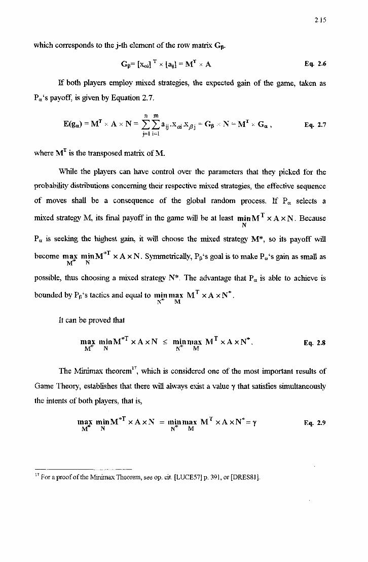
2.15

which corresponds to the j-th element of the row matrix Gn.

Gz.= [xa-1 T ›‹ la,-1 = MT ›< A Ei 2-6

Ifboth players employ mixed strategies, the expected gain of the game, taken as

Pgs payom is given by Equation 2.7.

'I' n m

T E(_g.z) =M >< A N = Z2a¡¿.x,,,,.x¡3j = G5 zzz N =M Ga, Eq. 2.7

j=1i=1

where MT is the transposed matrix of NI. While the players can have control over the parameters that they picked for the

probability distributions concerning their respective mixed strategies, the etfective sequence

of moves shall be a consequence of the global random process. If P., selects a.

mixed strategy M, its final payoff in the game Will be at least min MT × A × N. BecauseN

Pa, is seeking the highest gain, it will choose the mixed strategy M*, so its payoíf Will

become mag: min M” × A × N. Symmetrically, P¡ƒs goal is to make Pafs gain as small as M' N

possible, thus choosing a mixed strategy N *_ The advantage that Pa is able to achieve is bounded by P,›,“s tactics and equal to ntinmax MT × A × N *_

N M It can be proved that

minM*T × A×N É minmax MT ×A ×N"'. Eq. 2.8 N N* M

The Minimax theorem", Which is considered one of the most important results of

Game Theory, establishes that there will always exist a value 'y that satisfies simultaneously the intents of both players, that. is,

max minM*T × A×N = minmax MT × A ×N"= y Eq. 2.9 M*N N”"M

W For a proof of the Minimax Theorem, see op. cit. [LUCE57] p. 391, or [DRES81].

2.16

2.6 - Preferences, Utility and Rationality

Although Utility Theory does not refer exclusively to the Theory of Games, it is

known that its modem version was developed by Neumann and Morgensten [NEUM44] as a background to the latter.

,

The concept of utility and its respective maximization represented a progress

towards the characterization of what consist a rational conduct. Even so, the controveisy- has not dissipated. As the meaning of rationality interests such diversified areas as

Philosophy, Psychology, Economy, Sociology, the underlying concept of utility has

become a topic of ardent discussions among prominent scientists of these areas. Several questions arose from the discussions, but above all, remained these two issues: First, how does a. rational agent builds its utility function, thereby being able to assign a numetical

value to the set of events gains or losses under consideration? Second, provided that a

person possesses, in a way or another, a successfully constructed utility function regarding its predileetions, is it always rational to make decisions using the criteria of expected utility maximization?

Before addressing the second point, it is necessary to approach the methods of

determining the cardinal utility scale for an agent. This topic was first examined by Neumann and Morgenstem [NEUM44]. Basically, their method relied on the preferences manifested over risky choices, or more specifically, lotteries. To illustrate their technique,

consider an individual Who has ordinal preferences denoted by R2 >- R1 >- R3 is confronted

with three mutually exclusive choices: A or B. A designates the sure-thing non-monetaty prize, R1; B is a lottery ticket which enables the player to receive either R2 or R3 , both also non-monetaiy ptizes. Whether the lotteiy yields R; or R3 depends on a probability

distribution over these two altematives. The agent, before determining its pick, will be

interested in knowing what are the odds of getting R2 or R3. Assume the probabilities are p and (1-p), respectively. Furthennore, let 0 be the utility that coiresponds to R3, the least

desired outcome, and cl, to R1.

2.17

Starting from the principle that the agent is acting rationally in the sense that it will choose the option that maximizes its expected utility in situations involving risk, Equation

2.10 followsz

H(R1) =P1l(Rz) + (1-P)H(Râ`)- EW 11°

The tenn u(R1) stands for the utility assigned- to R1, and because R2 was set to l

and R3 to 0, it can be said that p turns out to be the utility associated with R1. The utilization of that method presupposes p being varied until Equation 2.10 verifies. At. that.

point, it is said that the agent is indifferent between the exclusive choices A and B. The success in using the described process is subject to some restrictions. Mainly,

there must be a consistency among any pairing of choices. For example, if a fouxth

alternative is introduced, say, R., the same procedure can be used to determine its utility, substituting R. for R1 in Equation 2.10. If doing this results in p' = u(R.4), the same

conclusion must also obtain from Eq. 2.11, where u(R¿) is now derived by means of a

lottery including R1 and R3.

M(.R«') = (1'<I)H(R5) + <1H(R1) Eq- 211

Since it is known from the previous computation and assumption that u(R¡) = p and u(R3) = 0, it. follows that. p' = pq must be satisfied in order to provide the desired

consistency to the method just described. Unfortunately, it is not always the case.

2.6.1 - Fundamental Axioms of Utility Theory

O» Axiom 1: Ordering of Alternatives Between any two prize values Ai and A,~ it is always possible to establish a

preference order, indicated by either A; se >- AJ- or Ai z >- A¡. Both preference and

indifference are considered as transitive relations so that if Ai m >- A5 and AJ» z >» Ak, then A¡ w >- Ak. ‹í> Axiom 2: Reducibility of composed Iotteries

It is always possible to establish a relation of indifi`erence between any composed

lottery and a simple lotteiy which prizes are A¡, With the respective probability of

2.18

occurrence equal to pi, i=1, 2, ...,r. The relation is expressed by Equation 2.12, where Lj are simple lotteiies of the type p¡,A,., and q¿ are the probabilities of their occurrence.

{qlL1: q2L2: ---a qSL's}§ {PlA1› PZA2: "'› pfAf} Eq_ 2_12

O Axiom 3: Continuity

In a lottery With prizes A1, Az, ..., Arm, a number k; G [0, 1] exists such that for any A¡ the indifference relation of Equation 2.13 verifies.

A, zz [1<.A,, ‹j1- 1<i)A,1 = Ã, En. 2.13

.\_.

It should be obseived that the indifference denoted by A, z Ai does not mean that those

two quantities are equal. Quite on the contrary, they are two rather distinct values.

(,› Axiom 4: Substitution .\z z‹.z

Given that A, z Aí, Aí can be substituted for A¡ in any lottery L, yielding:

(p1A,_,..., p¡A¿, p,Af) z (p1A1,..., p¡Ã¡, ..., p,.A,). Eq_ M4

Axiom 3 and 4 taken conjointly form another axiom, denominated independence of .\_.

zfrrelevant alterzmfives. It implies that the indifierence between A; and Ai is valid not only

When they are secluded, but also When the former is replaced by the latter in any

eompounded lottery. Stated in another Way, any other altematives p¡A,- present in a lottery altogether With A¡ are immaterial in relation to the mentioned substitutionlg.

13 It is assumed that the preferences are ranked A1 s‹ › A2 as › st › AI.

15' Regarding social choices, the independence of irrelevant altematives is the Condition #3 of Arrow”s Impossibility T heorem. lt is referred as the only one, among the five conditions of that theorem, that can be questioned Without provoking an evident modification of the subject*s essence. The rejection of Condition #3 would allow the inclusion, in the set of possible decisions, of hypothetical altematives specifically selected With the objective of evaluating the preference intensity over the truly' viable options. However, if the decision makers become aware that the hypothetical altematives are irnpracticable, they may deliberate on their authentic propensities and whence make their “moves” as if they were part of a strategic game. Then, the outcomes may be distoited in relation to the original goal, Which is the search for an aggregated expression of the collective preference, or social satisfa.cIion fimction (We1fa1'e

2.19

O Axiom 5: Transitivity of Preference and Indifference Relations

This axiom is an extension of Axiorn 1, generalizing the transitivity concept to any number of piizes A¡. Several studies, as those performed by Allais [ALLA53] and Tversky [TVER69], [TVER74] have shown that the condition of preferences transitivity carmot be always taken for granted when ma@ decisions under risk. Furthermore, there are some situations Where an individual simply will not be able to rank the altematives presented to it”.

<.> Axiom 6: Monotonicity

A lotteiy L1:[pA1, (1-p`)A,] is preferred or indifferent to another lottery Lz:[p`A1,

(1-p°`)A,] if and only if p fz p”, given that A1 z: >-A2 z >-A,.

Although Utility Theory is a successful model to explain decision making under

risk, there are controversies about generalizing it to all circumstances of this kind. An important research on this matt.er is the Prospect Theorjy, that is discussed in the sequence.

to 9* to - Prospect Theory

One of the postulates to the application of the expected utility method is the risk aversíonzl, Which asserts the concavity of the utility fiinction, that is, u”< O. Risk aversion can be characterized by the preference to a certain positive gain A in opposition to a lottery with an expected gain E(pA). In the expected utility approach the utilities are weighted by

their respective probabilities of occurrence. Kahncmann and Tversky [KAHN 79] have made a ciiticism of that. method by showing several empirical results which demonstrate its

Function). The obtainance of that fimction Was proved impossible under the five conditions of A1roW”s Theorem [ARRO5l].

Ê” A startling example of that situation is in a game discovered by the mathematician Walter Penney, presented by Martin Gardner [GARD'.74].

21 The other two are (1) Expectancy: U(À¡p1; Afpf) = p1u(A1)+...+p,u(_A¿), and (2) Aggregation of utilities: a lottery (A1p1; A,p;) is said to be accepzable from a previous ownership of an asset w if

U( w + Alpi; j, A,p,Í) > u(_w). The debate about risk aversion presented in ProspectThec1y has been cited in many other more recent Works, like for example [LINV9l] and [J OSE92].

É-J PJG

transgression in various instances. They have proposed, as a substitute to the former, What they called prøspect theory.

Prospect Theory focuses on some behavioral features called effects, which are

associated to the transgression of the expected utility principle. Those are:

- Certainzjv efièct: When a. positive gain tends to 100% of certainty, it. is generally

preferred over other rislty options, even if they can yield a higher prize, Within some variable limit. An experiment composed of two problems, each with two lotteries. Problem 1 had lottery A:(_4000, 0.80; 0, 0.20)22 and lottery B:(3000, 1). In problem 2 consisted of the lotteiy C:(4000, 0.20; 0, 0.80), and D:(3000, 0.75; 0, 0.25). Over 80% of the 95 individuals consulted in the poll preferred B in problem 1, but in problem 2, 65% selected C. Those results contradict the criteiion of selecting the altemative that yields max E(U). An explanation provided by Kahnemann and Tveisky for this behavior lies in the attra.ctiveness that the

certainly of the prize $3000 exerts on the decision.

~ Reflection effect: If instead of gains the choice regards losses, there is an inversion of the certainty effect, and the majority of individuals usually opt for “gambling”, in despite of a likely greater loss, also Within some variable limit.

- Isolation effect: Consists in a tendency to make decisions based only in parts of a compounded lotteiy. For example, consider a lottery with two stages: LI, with 75% of chance of ending the game with zero gains, and 25% of proceeding to the second stage, Where two sub-lotteries are available, Lz,1:(4000, 0.80; 0, 0.20) and L¿_‹¿:(3000, 1). The behavior of 141 individuals was investigated, and 78% of the sample opted for LH. This result is opposed to the conclusion obtained in the choice problem regarding the certainty effect, Which nevertheless is the same as the present after the combining the probabilities of the two stages.

Kahnemann and Tversky suggest that the variable that mostly affects the valuation of the Utility Function is the change that a risky prospect may impose to a pre-existent amount of Wealth. They conjecture that this factor surpasses the impoitance of the final position to be achieved through the game.

The notation (4000, 0,80; 0, 0.20) means a. lotteiy that yields 84000 with a. probability of 80% and zero with a 20% chance.

2.21

Prospect Theory has been developed with the objective of explaining the observed

violations of Utility Theory. The model distinguishes two basic sequential phases in the decision making process. The first is called the Edition Phase, Which aims at organizing the

available options and compiises the operations codíng, combination, segregation,

canceling, simplzfication and dominance detection. Those procedures attempt to make more explicit to a. player the options represented by the lotteries, without. alteiing their

respective relations between gains and losses. For instance, the combination operation

Would transfoim a. lottery L-:(10, 0.3; 10, 0.4) in L°:(10, 0.7).

The second phase is the evaluatzíon, whose purpose is to establish an attractiveness measure for each previously “edited” lottery”. The measure employed in the Prospect

Theory is two-dimensional and utilizes the scales (n)2“ and v(_a¡)15, that are subjective

evaluations of the probabilities and prizes.

A lottery is denominated regular if (P+q`)< 1, or a¡202a‹¿, or if alii az. If it is

regular, the basic equation of Prospect Theory follows, Which establishes the final value V of the lotteiy as a function of n(.) and v(.).

V(a1,P; az, qf) = 1r(p) ›~›< v(_á1f)+fl(<l) >~< V(11z) Eq. 2.15

The appearance of function v(_a¡f) is a concave line for positive values of a¡ (gainsf) and a. convex line for negative values (losses). lts gradient also decreases as the absolut.e

value of ai increases.

The function 1t(p) is not a. probability measure, but instead a. measure of how the decision maker perceives the probabilities, being called “decision Weight”. To illustrate the difference between a probability value and 1t(p), consider the game of tossing a. fair coin,

depicted by ($1000, 0.50; $0, 0.50). Empitical evidence hint that in this case 1r(0.50)<

0.50. If a gambler is offered an option of picking a sure prize instead of tossing the coin, it

Would eventually settle around $350, which means that n(0.50) 2 0.35. 1t(p) is

23 The formulation presented by Kahnemann and Tversky refers to simple lottenes of the type (al, pj. ag, q;

` 0, (1-p-qÍ)f), Where p+q l.

24 ntfp) does not obey the axioms of Probability Theory. In general, n(p`)+ 1t(_l -p`)< l.

25 ln that model, the prizes ai are the deviations of the absolute prizes A¡ in relation to an arbitrated reference point A*.

2.22

monotonically increasing in its domain [O, 1] as well as its gradient, indicating that small

probabilities (near zero) tend to be overvaluecL the inverse occurring with high

probabilities, that are usually undervaluedgõ. However, it has been observed that 1t(pf)

presents an erratic behavior for very small or very high values of p, contradicting the

pointed property in the sense of either a neglecting small probabilities or attributing

certainty to very low or very high values of p, respectively.

2.6.3 - Rationality and the Maximization of Expected Utility

As seen, the determination of a quantitative measure of utility is accomplished

through the observation of choices by a given agent in risky situations. This agent is

expected to be acting in accordance to the principle of rationality that dictates the

maximization of expected utilities in every circumstance. This assumption entails the rise of

a tautology, because expected utility is defined as that Which is maximized [RAPO90]. The requirement concerning the consistency of choices among lotteiies for the

determination of an agent°s utility fimction is also another problematic factor, because it is

not always endorsed by observed evidence. Therefore, the association between irrationality and inconsistency is intimately related to the method employed just described for the detemúnation of the cardinal scale of utility.

Maurice Allais posed important questionings to the expected utility hypothesis.

According to view, the historical development of the theoretical concept of the pure

psychologf of risk has passed through four successive stages [ALLA79]. Given a random

prospect, composed of various amounts of gains, its value V is represented by the

following equations in each of the considered stages:

0 Stage one: Mathematical expectation of gains expressed in monetary units Il

V = zpigi, Eq. 2.16 1=l

Where g¡ are monetary gains and p¡ are objective probabilities of occturence

associated to each g¡.

26 That phenomenon may panially explain why people bet in lotteries or make insurance.

2.23

0 Stage two: Substitution of psychological values (utilities) for the monetary units in

Equation 2.16.

Il

u(V_› = Ziwgl) Eq. 2-.lv i=1

where u(g¡) and u(\f') are the utilities, or psychological values, of the

altematives and of the combined prospect, respectively. This approach Was

originally developed by Bemoulli, in order to expose his St. Petersburg paradox.

0 Stage three: Substitution of szzlzjectíve for olzjective probabilities in Equation 2.17.

Il

ü‹V) = Z í›iu(gí)_, Eq. 2.18 i=1

Where piare the subjective probabilities of occurrence of each of the outcomes

gi and ü(V) is called the neo-Bemoullian formulation of the expected utility and

was also employed by Neumann and Morgenstem in their work on the Theory of Games.

0 Stage four: Inclusion of the dispersion of the utilities, taking into account the

probability distribution of their psychological values around the mean.

ü(_\f) = f(\If(y)) Eq. 2.19

where ̂ y=u(g'), \p(p^¡/) is the probability distribution function of ̂/_, f is a functional of 1;¡(_¬/) and ü(_`V) is the revised expected utility.

Allais supported the view contained in stage four because he sustained that the neo-

Bemoullian method (stage three) could give margin to inconsistencies. The demonstration of this fact is illustrated by Allais° classic example of choice involving risk, as follows.

Consider the two independent situations 1 and 2, each with two choices A and B:

2.24

$1o ooo with 100% zenzúnty

$50 000 With probability 10%, or f-`h°'¢° B $1o ooo with pmbzbflity 89%, of

$0 with probability 1%.

Table 2.2 ~ Allais' Situation 1

=-§':`;_5§;;§22;5%íëãš;5§52;5;55;if5;5;;z%15E:5š;5}55§z5í;í%; $10 000 withprobabi1i1y11%, or 51;-&;z.;;Ez¿QhQi¿ee5;(§zí¿;5;§5;52¿

ââ;;giââââfâ;â;;;;â~ââ~â $0 with probabflilõf 8% ;5}=5;í§;5;zi%z5í1;%155;5§zi§:5z;¿í§5§;5f;;§<z§;¿*l%;5§;5i;§§;:§;;i; S50 000 with probability 10% , or

Íf:ÊÍš'âšÊ}šÊZÊÊÊLšílšfëííišiš%ʧ?Ê11ÊÉÊíëi $0 With Prflbflbílity 90%

Table 2.3 - Allais' Situation 2

When confronted to the choices depicted in tables 2.2 and 2.3, many persons prefer A to B in situation 1 and D to C in situation 2. But, if the agents are rational, that should not happen, because this pattern of preferences is inconsistent With the piinciple of

choice in accordance to the maximum expected utility. The inconsistency is independent of the utility attiibuted by the agents to the monetary amounts”. Nevertheless, it cannot be

said that people who choose in this Way are irrational. They are only not using the criteria of maximizing the expected utility in their decisions, what is quite different. Thus, this

principle is not appropriated to define rationality.

One of the basic premises of the traditional approach is that each player will always be able to select the altemative that maximizes the expected value of its respective utility

function, among the options involwing iisk or unceitainty. This condition refers to the concept of ratz`omzlzÍt_1,› of the players, Which is at veiy strong assumption with broad

implications. Nevertheless, if this condition is satisfied, how should each participant decide, taking into account that the others” actions Will also be rational?

.., *7 For an explanatzion of the details of the inconsistency, usually known as the Paradox”, see [R_APo9o]_, p.9ó.

775

For example, suppose a game played by two contestants, P1 and P2. The sets

X={x1, xz,...,xm} and Y ={y¡, y2,...,y,,} represent their available actions. The convenience of P1 to adopt a particular x¡ depends on Which yj P2 will choose, and conversely. I-Iowever,

being P1 and P2 both rational, the situation is symmetric. This reasoning leads to the

conclusion that a rational choice depends on itself, thereby constituting a looping that does

not explain the process [BACH87]. On the other hand, some situations may arise where there are mutually preferred altematives, expressed by the utilities U1(xk yl)-:max and

Uz(y, Í xk)=max. The pair of actions (sk, y,) are said to be a Nash eqzzilibríunzfs.

2.6.4 - Other Criticisms to the Maximum Expected Utility Method

An interesting aspect of decision making regards the role that an individual assumes during that task. In an experiment performed by Bimbaum et al. [BIRN92], some volunteers Were separated in three distinct groups with the role models of buyers, sellers

and umpires. Depending on its respective characterization, each group showed diverse

preference profles even when the same individual was confronted With the same decision problem. Bimbaum*s experiment consisted in asking each individual to attach a “just” price to lotteries, respectively assuming one of the role models at a time. The assignment of values, Which indicated the preferences, varied according to the assumed role. For

example, the lotteiy (8, 0.5; 80, 0.5) ha.d a higher value than the lottery (32, 0.5; 40. 0.5)

under the seller's point-of-view. However, that appraisal was inverted when the decision regarded buyers.

Exploring another angle of the non-general applicability of Utility, Gul [GUL91] introduced a. model that he called T lzeorjv QfDisappoz`ntmemf Averszfon. The theory has equally the same objective as the previous methods, that is to supply a better explanation of

how rational agents make decisions under risk, and it has three basic features:

a. It Includes the traditional Expected Utility method as a particular case; b. It is consistent with Allais Paradoxeswg c. It is the most restrictive model that satisfies (af) and (b) conjointly.

For the definition ofNash and other equilibnurn concepts, see section 2.9. ln his paper Gul presents an example of preference ineonsistency owed named .filiais Ratio Paradox ‹

op. cit [ALLA7'9].

2.26

In Gul”s approach, the individual preferences are represented by a. parameter u

(utility function) and a real number b, b>1, Which is associated to attitudes toward risl-3°.

2.7 - Extensive and Normal Forms of a Game 2.7.1 - Extensive Form A game in its extensiva form is characterized by the following set of rules:

i. Representation by means of a finite graph tree, With nodes standing for decision points and branches indicating the available alternatives departing from each node; Partition of the set of all nodes in n+l subsets, n of them coiresponding to the players nodes, plus another set referring to moves made by any random process; Existence of a probability distribution associa.t.ed to every node where the move is performed by the random process, thereby establishing the chance of each

particular branch being selected;

iv. Grouping of the decision points of each player in iøzformation sets,

indistinguishable one from another in terms of the number of branches that diverge

from each of the their nodes, due to incomplete infonnation;

v. Equivalent identification of the branches that depart from the same node, so to

avoid the categorizing of the alternativos;

vi. For every player there exists a linear utility function defined over the terminal nodes

of the graph tree.

Conditions i-vi aim not only at defining the rules of the game, but also have the

objective of designating the preference patterns of the players through the mentioned utility

function. In this manner, distinct preferences manifested by any player over the outcomes

of a game imply in a. different game regarding its extensive form. The main motivation for defining a game in its extensive form is checking the existence of an equilibrium point for pure strategies.

3° 'lhe variable b in Gul`s model is similar to the function ntp) in Kahnemann and Tversky`s Prospect Theoiy, though the foiiner is presented in amore mathematically formal and elaborated context. '

")")"'

2.7.2 - Normal Form

A game in its normal form consists of the reduction of the extensive form into only one move, expressed by the selection, by every one of the n participants, of an availa.ble pure

strategy. The utility Ui for a player i that yields from a. set. of pure strategies s¡ employed by the n players can be defined by

Ui (S17 S2: "'7 sn) : Ui 7 Eq.

where oc is the collection of moves represented by the pure strategies picked by the

participants. If the choice of strategies is not deterministic, then it can be assumed that a

specific match ot of the game will happen With probability p. In that case the utility U, is described by Equation 2.21.

U1(S1z S2, Sn) : Zl3(0¿)-Uí(0f)- Eq' 211 Cl

In that way, the function U¡(.) altogether With the set of stra.tegies {s¡}, í =1, 2, ...,

n_, detemtine for each player i its gain in the match of a. game. This simplification, that can

be applied to any game, is called the normal form. That concept can be extended to the

hypothesis of mixed strategies. The gain of a player is then defined by the value of its

Expect Utility _ albeit the controversy” _ and for the probability distributions of each player`s pure strategies.

Besides the extensive and normal forms, a game can still be modeled according to its characteiistic function, not reviewed in this disseitation”.

2.8 - Competitive Non-zero-sum Games When two players P1 and P2 participate of a strictlv competitive game, given its

zero-sum attribute, the benefit that each one obtains is always accomplished by imposing a

loss to the other. In other words, any preference about the outcomes will be the inverse for

each other. When this condition does not verify, a game is no more strictly competitive, and the utility functions of the players do not add up to zero.

Ê* See section 2.6. *Ê For an explanation of the Characteristic Function, see op. cit {LUC-E57] and [BLAC»5‹4].

2.28

Several differences exist between the analysis of zero-surn and non-zero-sum

games. A first aspect to be mentioned regards the significance of the information derived from divulging or knowing previously which strateg a player will adopt. In strictly

competitive games, it has been seen that the participants, when acting rationally, should not announce which particular strategy they would implement, because that contained valuable

information, which could be used by an opponent to secure more advantageous positions and greater gains in the match. As a consequenee of the zero-sum feature, the player`s benefit Would decrease. However, this restriction is not applicable in non-zero-sum games. It is even feasible that the anticipated disclosure of a player°s intended may imply in mutual gains, if the revelation is perceived by the other as authentic, inducing it to take a

compatible action, and if the strategy is actually fulfilled. It must be noted that revealing the

strategy should not equal a negotiation process, which only takes place in cooperative

games”. The best known non-zero-sum competitive game is the Prísoner "s Dilernma, that is reviewed in greater detail in Chapter 3 of this disseitation.

Another significant contrast between zero-sum and non-zero-sum games regards alterations in the concept of strategy equilibrium, that is reviewed subsequently.

2.9 - Dominant and Nash Equitibria

C-onsider a game with the following payoff matrix:

Player B B1 Bz

011 (10.¬ 4) 1

(0.¬0) Player A Oflz (0, 0)

i

(5, 3)

Figure 2.2 - Payoff Matrix of aNon-Stricfly Competitive Game

The strategf pair (oq, B1) and (otz, B2) are in equilibrium, because ot; and ot; are the

best moves against B1 and B2, respectively. On the other hand, neither (oq, B2) nor (ctz, B1)

53 See section 2. IO.

2.29

are in equilibrium, and those pairs do not yield equivalent payoffs to the players. In zero-

sum games, if two pairs of strategies (oq, B1) and (otz, B2) are in equilibrium, so are (otl,

52) a1'ld(0¢2› Í5r)34-

Ifthe players decide to employ mixed strategies, in order to obtain their respective

security levels, those Would be the maxmin strategies, namely the combinations (*15‹x1, ggotz)

for player A and (ÊB1, ÊB2) for player B. In that case, the security levels are 10/3 and 8/3. It must be noted that the maxmin strategies do not constitute an equilibrium, so those

decisions are not the best reply against each other°s feasible actions. For example, assuming

that the player A deduces that B will use its maxmin strategy, A should play_ B2, whence attaining an expected gain of 16./3. If A understands that reasoning, it should opt for otz.

But A can also guess that B is going to use minimax, and in this case A must play oil,

Which yields an expected gain of 20/3. lt can be seen that a. reasoning loop arises, and this is an inherent difficulty of non-cooperative, non-zero-sum games. If the game were iterated and cooperative, in the sense that a pre-play negotiation is allowed, then the players could

reach an agreement Where the paits (oil, B1), (ooz, B2) would be used a certain proportion of

matches each.”

2.9.1 - Dominant Strategy Equilibrium

A strategy si* is a dorrzinmzt srrategv if it is a. player”s strictly best. response to any strategies the other players might adopt. This means that si* yields it the greatest payoff in any circumstances of the game [RASM89]. Othenvise, a strategy is called clominateci.

ut(fSâ*, St) Hist”, S,-_), V j ¬¬-* i, V St* =¢ sz” Eq, 2,22

When all players employ their respective dominant strategies, the resulting

combination is denoted a. donzinamf eqzøilibrizzrrz.

If is no smaller than any sj, 'V'

j 1 i, and greater for some j 's, then it is

denominated a weakly dominant strategf. An íterated do1›11'nant strate¿{_v equ1'l1`brium is

34 Furthennore, in zero-sum games the utilities associated to any pair of pure strategies are the 35 The proportion could be arbitrated based on the criteríon of equalizing the accumulated utilities. In the

example, that proportion is for (on, B1). This is a very naive solution, Which presupposes linear properties for the utilities and neglec-ts the eventual distinct bargaining power of the players.

2.30

found by excluding a weakly dominated strategf from one of the players, recalculating to

check the remaining weakly dominated strategies of all players and repeating the process

until only one strateg is left for every participam.

2.9.2 - Nash Equilibrium

In 1951, the game theorist John Nash proved that any 2-person non-cooperative game with a finite number of strategies has at least one pair of mixed strategies in

equilibriumsõ. The majority of games do not have even an iterated dominant equilibrium, but they may possess a Nash equilibiium, which is the “... most important and widespread equilibrium concept” [RASM89].

A strategf combination s* is a Nash equilibrium if no player has incentive to deviate from its choice provided that the opponent maintains its position. Every dominant.

strategy is a Nash equilibrium, but the inverse is not necessarily true.

Given two equilibrium pairs, this does not necessarily mean that the expected gains of each player are equal. I-Iowever, if it is the case, that is, E(_u,1(ot1_, B,')`) = E(u¡;(otz, B-2))

and E(ua(_ot1, [5-2)) = E(u¡;(ot2, (51)), the pairs (oil, B1), (ctz, B1) are said to be equfvalemf, and

also called interchézngeable if (oil, B2) and (otz, 61) are in equilibn`um3?.

The proof of the existence of at least one equilibrium pair of mixed strategies in non-cooperative games is associated to the concept of solution of a game. In Nash”s sense, a solution exists if any equilibrium pair is interchangeable. Thus, a game°s solution is the

set of all strategies that obey the latter condition, Which must not be equivalent.

For clarity, consider the game” represented by the payoff matrix of Figure 2.3.

56 Partly due to this work, Nash received the 1994 Nobel prize in Economics, altogether With J. Harsanyi and R. Selten. From that. property, in a stiictly competitive game, each pair of equilibrium strategies is both equivalent and interchangeable.

33 The example was obtained from [LUCE57]. That game has an interesting (and fi11st|'a.tir1g) feature. Each playe1'”s gain is completely determined by the other*s choice, therefore implying in a total indifference regarding a participant.`s own move. Observe that the pure strategy pair (ag, bg) would be the obvious pick if a. previous contract between the players could be sealed.

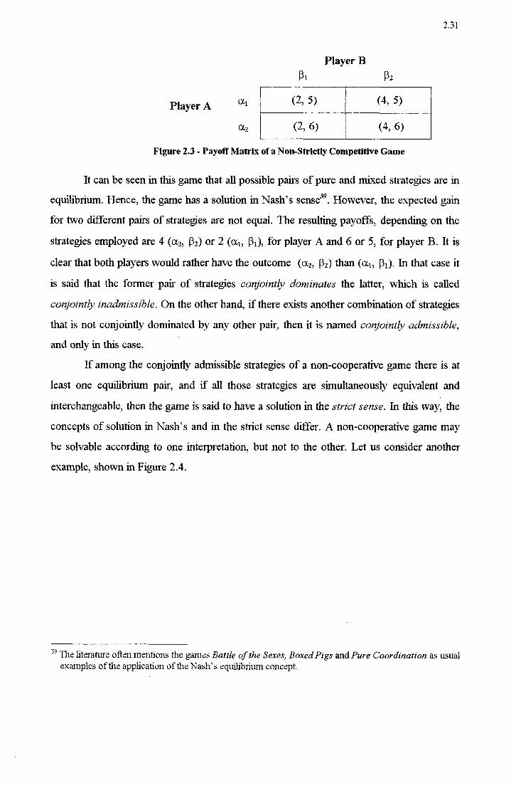
2.31

Player B B1 B2

Player A

Figure 2.3 - Payoff Matrix of a Non-Strictly Competitive Game

It can be seen in this game that all possible pairs of pure and mixed strategies are in equilibrium. Hence, the game has a solution in Nash°s sense”. However, the expected gain for two ditferent pairs of strategies are not equal. The resulting payoffs, depending on the

strategies employed are 4 (ocz, B2) or 2 (oq, B1), for player A and 6 or 5, for player B. It is clear that both players Would rather have the outcome (ocz, B2) than (oq, B1). In that case it

is said that the former pair of strategies conjointly dominates the latter, Which is called

conjomtly madrnissible. On the other hand, if there exists another combination of strategies that is not conjointly dominated by any other pair, then it is named conjoizrfly adnzissible, and only in this case.

O

Ifamong the conjointly admissible strategies of a non-cooperative game there is at least one equilibiium pair, and if all those strategies are simultaneously equivalent and

interchangeable, then the game is said to have a solution in the strict sense. In this way, the concepts of solution in Nash”s and in the strict sense differ. A non-cooperative game may be solvable according to one interpretation, but not to the other. Let us consider another

example, shown in Figure 2.4.

The literamre often mentíons the games Batzle ofzhe Sexes, Boxed Pigs and Pure Coordination as usual examples of the application of the Naslfs equilibrium concept.

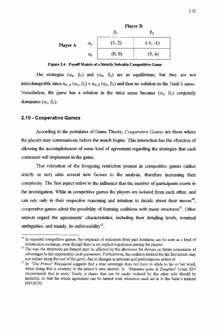
232

Player B B1 Bz

PIayerA al I

('1›

Oflz (0, 0) I

(3, 4)

Figure 2.4 - Payoff Matrix of a Strictly Solvable Competitive Game

The strategies (oil, B1) and (ctz, B2) are in equilibfium, but they are not

interchangeable since uA, B (oil, B2) :ê uA, B (ctz, Bl) and thus no solution in the Nash*s sense.

Nonetheless, the game has a solution in the strict sense because (ctz, B2) conjointly

dominates(ot1, B1).

2.10 - Cooperative Games

According to the postulates of Game Theory, Cooperativa Games are those where the players may communicate before the match begins. This interaction has the objective of allowing the accompiishment of some kind of agreement regarding the strategies that each contestant will implement in the game.

That relaxation of the foregoing restriction present in competitive games (either strictly or not) adds several new factors to the analysis, therefore increasing their

complexity. The first aspect refers to the influence that the number of participants exerts in the investigation. While in competitive games the players are isolated from each other, and can rely only in their respective reasoning and intuition to decide about their moves”,

cooperative games admit. the possibility of forming coalitions with many stnlcturesfl. Other aspects regard the agreements* characteristics, including their detailing levels, eventual

ambiguities, and its enforceability”.

4° In repeated competitive games, the sequence of outcomes from past iterations can be seen as a kind of infomtation exchange, even though there is no explicit negot1`at:ion among the players.

41 The Way the structures are formed may be affected by the allowance for threats or future concession of advantages to the opponent(s) (side paynzerztsí). Furthermore, the coalition formed for the first match may not endure along the rest ofthe game, due to changes in interests and performances achieved.

“Ê In "The Prince" l\~'Ia.quiave1 suggests that a Wise sovereign does not have to abide to his or her Word, when doing that is contrary to the pn'nce”s own interest. In "Ma.ximes pour le Dauphifi' Louis XIV recommends that in every Treaty, a clause that can be easily violated by the other side should be included, so that the whole agreement can be turned void, whenever such act is in the State`s interest [s1=oR53].

J J) ¿J

Bargaining power can be derived from diiterent u`ti1ity'1unctioñš, fF)'n'1"tIt"e_:1ccess to relevant infomiation, from the capacity to absorb temporary losses and from the capacity of formulating credible threats, among other factors. Bargaining power has a great

influence in the development. and conclusion of a cooperative game, especially when the game is repeated and has no detenninistic defined end known by the panies involved. That point-of-view is strengthened if one understands that in social relations, be they between

individuals, between companies or even nations, the consequences of the repeated

chara.cter of the transactions Will play their roles in the participants decisions.

This repetition, even if occurs in non-identical circumstances, has the dynamics of a.

very complex supergame, where the agents, interests, conjuncture, coalitions and even

rules are ever-changing. Under this view, it may be assumed that some type of cooperation will always be present in the game.

It is of fundamental importance to stress that the meaning of cooperation, in that

approach, totally departs from the usual definition, and on that account it must not be interpreted as a synonym of altruism, justice, good will or other qualities induced by the players” wish to self-renounce to prospective advantages that may be obtained by independent actions”.

In accordance to the model developed in this dissextation, the focus of the research

is centered in games involving pairs of players, although the population that takes part in the interactions is composed of multiple players”.

2.10.1 - Two-Person Cooperative Games

In this section, the following conditions are assumed:

i. Communication between players is total and unambiguous, and each participant leams what is stated from the other without any distortions or misunderstandings;

43 As a. matter of fact, it seems too rigid to classify the games in cooperativa or not. In most practical situations, the cornmunication between the players can assume various degrees, ranging fiom nonexzistent to total.

44 Chapter 5 consists of a investigative model of the Fuzzy lterated Prisonefs Dilemma with a population of 515 distinct types of players, and in Chapter 6 presents an application of an one-sided Fuzzy PD to a.

market share simulation, involtmg 1000 buyers and variable number of sellers (_.Fimts).

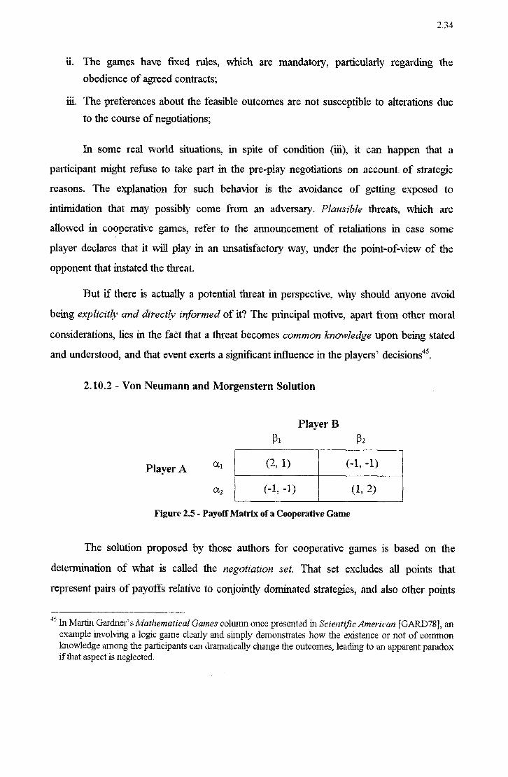
2.34

The games have fixed rules, Which are mandatory, particularly regarding the

obedience of agreed contracts;

The preferences about the feasible outcomes are not susceptible to alterations due to the course of negotiations;

In some real world situations, in spite of condition (iii), it can happen that a

participant might refuse to take part in the pre-play negotiations on account of strategic

reasons. The explanation for such behavior is the avoidance of getting exposed to

intimidation that may possibly come from an adversary. Plausíble threats, Which are

allowed in cooperative games, refer to the announcement of retaliations in case some player declares that it will play in an unsatisfactory way, under the point-of-view of the

opponent that instated the threat.

But if there is actually a potential threat in perspective, Why should anyone avoid being explicitly and directly ínformed of it? The principal motive, apart from other moral considerations, lies in the fact that a threat becomes common knowledge upon being stated and understood, and that event exefls a significant influence in the players” decisions”.

2.10.2 - Von Neumann and Morgenstern Solution

Player B Í51 Í52

P|a`,e¡.A al (2: 1) I

('11 '1,.)

Oo (-1, -1) ,

(1, 2)

Figure 2.5 - Payofl Matrix of a Cooperativa Game

The solution proposed by those authors for cooperative games is based on the

detennination of What is called the negotiation set. That set excludes all points that

represent pairs of payofls relative to conjointly dominated strategies, and also other points

45 ln l\-'la11in Gardnefs Mathematical Games column once presented in Scientific American [GARD78], an example involving a logic game clearly and simply demonstrates how the existence or not of common knowledge among the panicipants can drainatically change the outcomes, leading to an apparent paradox if that aspect is neglected.

2.35

which imply in the achievement, by any player, in gains that are inferior to those that could be obtained without any agreement. For clarity, let us reflect on the payoff matrix depicted in Figure 2.5.

The cells in the secondary diagonal are obviously undesired by both players. In a

repeated game, a plausible sequence of moves would be altemating, in phase, of the

strategies (oil, B1) and (otz, B2), what Would yield for each participant an average gain of But if the game is played only once, this value is not supposed to be achieved without a

previous stage Where an arrangement between the players is agreed. In the hypothesis a

negotiation betides, (oil, B1) and (az, B2) could obtain from a random device yielding a

50%-50% probability for each pair.

The negotiation set for this game is illustrated if Figure 2.6

Player B's ¡:›avc=ff` '

13 . ' " BÀ (1 › 3)

/'ff .f'

(2..1';11

¿_¿§¿¿;' i.1z'4,1z'-4) J

šíff /' »

ftziííšííšíšš ¡ ,

z»

-1 1 2

Ã? P1-ayer.~'Á's p.~1yofi"

vfiärzöyf1

1) ›::;-1 ,-

Figure 2.6 - Negofiation Set R for the Von Neumann and Morgenstern Solution of a Cooperative Game with Two Independent Mixed Strategies.

The shaded area R contains all the points which embody the pairs of payoffs (a.AB, bm) defined by the adoption of a pair of mixed strategies (_ QLA, BB), where:

2.36

UA: {[(P.‹\0fi1z (1'PA)0¿z]1 PA E [0¬ 1] gq, z_z.3(pa)

BB : [PBB1› (1`PB) Bzli, PB 'Ê io» 11- Eq' 2'23(b-)

The correspondence between any pair (OLA, BB) and (_aAB, bw), and vice-versa, is unique.

The point that represents the payofis (Ê, Ê) does not. belong to R. That average gain cannot be reached When the players decide on the values of pA and pg to be used in their respective mixed strategies (OLA, BB) independently, as in a competitive game. Conversely, ii

the game is cooperative, then it is possible to the players to assent. on a. pact Which product is a conjoínt mixed strategy. That scheme incorporates a specífic probability distribution over all the possible pairs of pure corgjoiní strategies (oq, Bj), i=1, 2; j=1, 2.

Regarding the example, a common payoff ofš is brought a.bout by the conjoint med strategy desigmred by [% ‹.‹×1, tm, 0‹.‹×1, Bza›, (az, Ba, %‹‹×z, Bz›1‹:›‹%, â).

Designating a generic conjoint mixed strategy by co,,,B=(`oLA, BB), and by Q the set that contains all feasible (om, the expected gains (_ utilities) associated to Q are

UAÍQ) Z 2343 Z EUA (PAB-was): Ú3AB'5 Q» PAB '5 [Oz 11- Eq. 2.2.-t(a) A_.B AB

: : uB (.pAB'wAB)› Ú~)A.BE Q: É [Os IL EQ. 2.24(Í)) «ZEN

0' â ã:M

Where aAB, bm; are the utilities that derive from a particular conjoint mixed strategy com and

PAB is the probability of electing a particular com.

2 37

Noting that com is an argument of the utility functions uA and 115, the pairs

(am, bm) that derive from each com can be mapped in a convex region R' configured by the points p, q and r shown in Figure 2.7.

Player B's pa;-'off Abàfi 1 p

1 7` .-.- ( ›-.J

'¿(§;,1z¿¿, A ¡/- Parettfs Dpumzl ser

\~%É“\ 1- ef (2_.11;. /' 1: :›: 1-: :z;- -'

.‹.--.-.¬.|1v'.|3|3|L|2|2 '

.`

I 4-; -:-;_¡:¡; -:Q :F :‹: :-; :‹; I I 1*

l _ <~',~*. '<~.< 1 L ‹: 2-; qr “ AB - ›;_~_z. _|,\_: , 1, à _-'

1 1.

Player Hs payuff I '¡';1'('Í" 'l'§';:,zY

\«›^~/*^

~\.

ašggm

‹-: ‹-. 44 <-:

rv,¿*"› 1”-1 -1) ~, ›

--l

Figure 2.7 - Cooperativo Solution Set R' and P:u'eto's Opfimal Set

A point (a. Àmb AB) E R' is said to be corzjomtly dommatea' by another point

(a;;B,bj¿B`) e R' if a;B za;,_B and b§B zbÀB simultaneously. Having in mind that R'

stands for the players” utility values or expected gains, the participants, being rational, Will

seek the maximization of their respective payoffs. Hence, all pairs (aim, bAB) that are

conjointly dominated shall be in due course discarded by them. The pre-play negotiations Will then close in upon the selection of conjoint mixed strategies which outcomes only include the points that belong to R' that do not have the former characteristic. Those points coirespond to the line segment depicted by pq in Figure 2.7, which is called Pareto's Optimal Set. When the players agree in restricting their strategies to those associated to pq, the possibility of acquiting higher payofis by means of further negotiations is exhausted, because beyond that settlement the preferences become strictly opposed. In the example,

2.38

player A prefers q and B prefers p, that correspond to the conjoint mixed strategies

‹.ú;,_B =[l(_a1,fi¡), 0(o:2,¿32)] and wj§B =[0(‹x¡,61), l(a¿_,|62)], respectively.

However, not. all points from the Pareto”s optimal set are achievable, in terms of

realistic plausible expectations. For instance, consider a game whose region R' is bounded

by the polygon abcd in Figure 2.8.

P1 'BH Ff . .

him ̂ We! qpayü Negot1at1onSet vcw b I __/ , .

fišíššííšíšíííšlšíšíiíší "”"

.

.Í-

'l

P1ayerA's payofi ‹ AB

Figure 2.8 - Pareto's Optimal Set and the Negoliation Set

In Figure 2.8, Pareto*s optimal set is defined by the line bcd. Supposing that the point (s, t`) stands for the payoifs when the players implement their maxmín strategies, in the non-cooperative version of a. game, it is out of question that none of them would accept a deal that Would yield an inferior benefit. Accordingly, Von Neumann and Morgensterrfs solution space for the cooperative game of Figure 2.8 is the subset vcw from Pareto°s set, denominated Negotiation Set (N).

The subset N is often viewed as the limit, in terms of mathematical treatment, for the imposition of restraints that could shrink the solution space for a cooperative game. The selection of a. particular point in N would then depend in other extrinsic att1ibut.es4°.

46' Some extraneous factors regard the players” psychological aspects, their bargaining power and conjlnlctllre variables.

2.39

In the example, the symmetty of the payoff matrix hints that the proposed

cooperative solution (Ê, Ê) is quite reasonable. Nevertheless, it seems that idealizing a

perfecn equitable settlement is seldom within reach in realistic situations. This is so because

each playerls role” greatly affects a solution that might be collectively accepted as just.

Therefore, the asymmetry in games may be present not only in the payoíf matrix, but also in the players' capacity to achieve successful compromises, in the resources to make credible threats, etc.

What can be deduced from those arguments is that the concept of solution to be found by the participants of the game themselves is not satisfactoiy, even When the solution is restricted to N. Therefore, a need to the introduction of a third party°s arbitrafion

scheme arises, whose goal is to establish an impaitial arrangement.

2.10.3 - Arbitration Schema”

An arbitration scheme” is a criteria for settling a conflict of interest, Where a third party, not directly involved in the dispute, stipulates the strategies that must be obeyed by the players in a non-strictly competitive game, so that a special point in the negotiation set

N can be reached. The characteiistic of that point is that it might be considered impaitial or just, and therefore produces a values of payoffs which are accepted in advance by the

47 For example, one party could be an union an the other a Cfompanyj, The negotiator could be representing its own interests or be a. deputy.

48 The arbitration schema delineated is this section refer to 2-person games. The solution of a n-person game involves the concepts of irnputation (jaxioms of individual and group ratiotlality), clzaraczer-isiic fimctions and core of a game, Which are also associated to methods of coalítion fbnning. Another method for solving n-person cooperative games is the Shapley Value, which in general gives more equitable solutions than the core does. The analysis of those topics are beyond the scope of this work,

,

and a good introduction to the subject can be found in [W INS95]. 4”

It should be emphasized that an arbitration scheme, in the present sense, regards a collection of rules that are expected to be followed by the players, aiming at the achievement of a solution for the conflict of interest, and it does not refer to exacting compliance from the contenders, Which are supposed to abide to the norms prescribed by the umpire.

2.40

players. The special point is not always unique. But any alternative must obey certain conditions, in order to be considered equitable and free of ambiguitiesso.

i. The arbitrated solution of the game must be depicted by a point in N, which means that each player”s gain has to be at least the value that it. would obtain When acting non-cooperatively;

ii. The unit of measure used to build the players” utilities must have no influence whatsoever in the selection of the arbitrated solution;

ni. The identity of the paiticipants shall not act upon the contention, this property representing a symmetrys 1;

iv. The variations in the solutions pointed out by an arbitration schema should be small When the difierences among the games to Which they refer are also small. In other words, the arbitrated solution points should not be subject to notable changes caused by negligible transformations A of the payoffmatricessz;

v. The potential capacity of the players to implement strategies that result extremely unfavorable to their' opponents must be taken into account by the arbitration

schema.

2.10.4 - Nash's Arbitration Scheme

In a bargaining problem, possible solution space may be represented by a convex closed region R in the plane defmed by the axes U and V, Which denote the scales of the players” utilities. Every point. (_u, v) in that region com-:sponds to a pair of utilities

associated to a specific agreement C.. Given two fcasible contracts C” and C”, a lotteiy involy-ing them is pictured by a line segment joining the points (u', v') and (_u”, v”). There exists in R a point. (u°, v°) that. symbolizes the status quo, that is, the achievement. of no compromise, denominated A0.

5° l\~flathe1na.tically, a generic and plausible arbitratlen scheme ƒ N:-=: s -› N, Where- s stands for the status quo preceding the realization ofthe game.

5Íf‹..T‹..Ní›. T<s>'> = T‹f<N. si.›f›, where Ttx. y;› =‹1›-zm f‹§A (N), A‹j S 3;» = A‹ƒ(N, 5)).

2.41

V /T* Player B's utflity

`ÍEEEEEÉEESEEEEEÊÉÉÊEÉÉÊÊEÉÊÊBÍ ',v' ÉÉEÊÉ ÍÍÍIIIIIIIIIÍIIIIIIIIIIIIIIIIIIIIIIIÍIÍIIIÍ!\

têâzâsszâzââzâsâââséée'

3

Player A's uiility u

Figure 2.9 - Space of Feasible Agreements With the status quo point (u°, v°)

Nash”s scheme objectives the determination of a function f that operates on (R, (u°, v°')') to reach another point (_'u*, v*) such that in a transformed region Ri, obtained by the

change of the axes'.o1igin to (u°, v°)_, the following relations verify:

(u*, v*_) é R”, u* 0, v* 0; En- 2<2›5

(u* >f. v*`) Tz (_u ›< v`), V (u, V) fé R”, u fz 0, v fz O 53. Efl' 2-25

The point (_'u* >-: v*) is called Nash *s Solution to the bargaining problem

(R', (0, 0)), Which can be easily eonverted to (R, (u°, v°)). Nash”s Solution is the only

arbitration scheme that has the properties:

i. Immunity to linear transformations of the utility seales; It. is optimal, in Pareto”s sense (equal or greater payofis than the status quo); Independence of irrelevant alternatives54;

53 u*v* is the maximum of all products uv. 5* Consider two games with regions R1 and R2. If R1 Q R¿, , and __f (R3 ,

(u`°, v°)`) E R1, then f (R1 _,

tfu”, v°f)f) = f (R2 , (_Íu°, v°)). Put in Words, if new contract possibilities are appended to a former bargaining problem in such way that. it. brings no change to the preexistent status quo, then, regarding the new setting, either the solution remains unaltered, or the new solution will belong to the added collection

2.42

iv. Symmetry (Equal gains for symmetric players” roles.

2. 10.5 - Criticisms to Nash's Scheme

Nash”s model still is the standard approach to the treatment of contlict of interest between two players, especially when conceming economic problems ([ANDE89], [DOWR89], [HOEL90], [LESL90]). ln spite of its prestige, Nash”s scheme has been often criticized, predominantly because of (a) the change of scales origin feature ([MYER77], [KALA77])_, (b) the observation of some divergence between theoretically obtained results and real life data ([NYDE`74], [ROTH79]) and (c) the irrelevant alternazives

Independence axiom (ALEX92]).

Myerson [MYER77] also showed that. in practical circumstances, evidence can be found that the players do accomplish inteipeisonal comparison of utilities, and this

condition is excluded from Nash`s solution by its compliance to the axiom of irrelevant independent alternatives.

2.10.6 - Other arbitration Models

Nash”s asiomatic treatment has been widely employed by several other authors to modeling strategic negotiation processes, though With some alterations. Harsanyi,

[I-IARS56], [`HARS77], starting from a vintage Zeuthenls work [ZEUT30]55, modified it in order that the bargaining procedure is accomplished through only two phases. In the last stage, the player Which attains the littlest disadvantage in conceding the other”s demand grants its request.

Rubinstein [RUBI82] devised another model where the negotiators propose a

sequence of offers and counter ofiers, whose values are systematically reduced by a

of possible contracts. An arbitration scheme that abides to that presciiption is defined as possessing _ independence to iirelevant altematives.

5° Zeuthen modeled the bargaining process as a sequence of small concessions from the player which incurs in the least significant loss when doing so. That method results mathematieally equivalent to the inaximization ot` the product uv in Nash”s procedure, but with the advantage of a.ttacln'ng a plausible psychological component to the negotiation.

2.43

discount factor, What induces to obtaining a settlement. Although this process may be potentially infmite, Rubinstein proved that it has an unique perfect equilibriumsó, Which is readily recognized by the players after the first bargaining phase.

Kalai and Smorodinski presented a strategic model of negotiation that implements a

solution through a proportionality method. In that method, the axiom of irrelevant independent altematives is replaced by another principle, called monotonicity axiom. It

establishes that, if the negotiation set is enlarged in such Way that When the gain of a player i increases, also does player*s j, then the latter player°s gain in the expanded game must not be inferior to the payotf it would achieve in the original configuration. The authors clairn that this axiom, contrarily to Nash*s, allows the participants to perform interpersonal

comparison ofutilities, what is more in accordance to the empiiical evidences mentioned in [MYER77].

In a more recent Work, Lootsma [LOOT89] proposed a methodologf for the resolution of two-party conflicts using at procedure with two stages. In the first, each player e.\-'amines its attitudes regarding possible concessions that could lead to a mutual agreement,

and subsequently, the information obtained relative to the preferences and to the

correlation between latent strategies is utilized to reach a reciprocal attractive contract. A criticism of Lootsmafs approach was prepared by Bogetoff [BOGE92], where he argues that Lootsma only detailed the second phase of his model, and unduly assumed that the players always tend to express their true preferences in the tirst phase. This last

supposition, although feasible When the contenders are looking forward to setting up a deal, is not realistic when the adversaries do not value sincerity or when the nature of the conflict overcomes that nonn”.

56 A perfect (Bayesian) equilibrium is a strategy combination S and a set of beliefs u such that at each node ofthe game: (1) The strategies for the rernainder of the game are Nash (equilibria) given the beliefs and strategies of the other players; and (2) The beliefs at each information set are rational given the evidence appeaiing that far in the game. Using this idea, Kreps and Wilson introduced the concept of sequential equilibrimn, applied only to games With discrete strategies, Where a. third condition irnposes further restrictioris on the players beliefs. From op. cit. [R_ASl\~'l89], p. 109-110.

57 In bargaining processes, the submission of false indications regarding preferences is a. sort ot` strategic behavior. In the majority of real cases, this conduct can be expected fiorn the negotiators, except When the mediation plan accounts for incentives designed to curb such comportrnent. Bogetoff (op. cit.

[BOGE-921) concludes that the cited rmfaithƒirlness is likely to take place more fiequently When the

2.44

2.11 - Cournot and Bertrand Games

2. 11.1 - Coumot Theory

In 1838 Coumot proposed a. new theory to explain the economic behavior of an oligopoly. The original problem considered the sale of water by two well owners in a small town. The product of each seller (water) is indistinguishable from one another, and hence both should be offered to the consomem for the same pn`ce. However, the price would fluctuate depending on the total quantity of water available daily. It consisted of the sum of the amounts q1 and qz amount pumped out from the ground by the suppliers 1 and 2 in a

given day [C-ASE79]. In this manner, the average price p should be a decreasing functionf of (q, + qz), shown in Equation 2.27.

P =ƒ(q1 + qz) = a - b(q1 + qz) Ea- 2-27

Supplier z`“s revenues r,- are

1; = aq .-

- bq z- (Q1 + qz). 1'= 1. 2. Ef» 228

Making ql = al: and substituting in Equation 2.28, comes:

32 V

_

al Eq. 2.29(a) fl = 5- × (X - ‹×~‹›‹ + .v›,› = í × 1f.‹-»~._›››

al I al Eq. Z.29(b)

fz Z g × (N - .v(x +.v)l = g × '1fz(.~\'z.v) .

where x, y are the players” actions and the function 1:, and nz correspond to the way the payoffs of the game G58 are related to the players” actions x, y, Which must be non-negative numbers.

G can be concisely represented by the players” following objectívej1`mctz'on.s59:

participants are pessimistic in relation to the achievement ofa safisfac-toiy arrangement prior to the outset _ of the process.

°"“ G is a. Coumot game played by the well owners 1 and 2.

2.45

0 Player 12 nzaxilnize 1T¡(x,y) , s.t. x -E 0, y 2 0;

O Player 2: maximize 1E¡(x,yf) _, S1. x 2 0, __v 3: 0;

Differentiating 1t¡(_x,y) and K2 (x,y) using Equations 2.29 (a) and (b), comes

ô , . ô - . T _n

, ‹__.\-.,y_) = _(x - + _t›á)) = 1- 2x - y EQ- 2-30(f*)

âx ôa `

'É , _ y _ in

2 Cx, : _êã_(.}; _. )_,v(x + yl)/) : 1 __ x ._ 2); , Eq. Õy Ôx

_ . . . _ 1- › which by making í1zl(j_~,-Mv) z 0 and i7¡2('x¬ V3 z 0 yields x*(\zí) = and

ôdx: i

i I ll 'I

1-'

1- ' _ . . . . .

y*(x) = -ii _ The optimal action tor player 1 is depicted by Equation 2.31. 4.

nf (XJ) : (1-4,v)2 Eq. 2.31

Figure 2.10 illustrates the recrcñon fimcnfons x*(y) and __v*(_x). The term reaction” comes from the fact that the convergence path is delimited by those functions, tending to the point (x*, y*). That point, located where the lines cross, is denominate the Cournot-

Nash equlllbrium. A property detained by the (_x*, y*) equilibrium is stability, because a

player's best response to another opponent°s move always closes in upon itó 1.

59 Strict maximization of the players' objective functions in G is impossible without a. coalition or cooperation between the participants; Nevertheless, each player can try to make its revenues as large as possible. The name reaction must not be understood literally, since the paflicipants of the game do not act in a sequential way, but simultaneously instead. Thus, a player has no opportunity to mull over the opponenfs move in order implement its own. As a matter of fact, the reaction functions depict the manner how Would the process evolve, in case the moves were successive.

61 The stability feature present in the Cournot-Nash equilibiium does not necessaiily always occur in Nash equilibiia found in other games.

6Ú

2.46

,-K.

r

1 _ \`\

`\

'\X =2‹ *(,1¿' '\,_

_ .y

\ ( K “Ê sf* J ., ,___

'\,____ \'.

\_` /" convergence process _. ........... .Í.`Ê'.2___`

1 1:'Ê .

â\ Ã 1 ,f `\

( .~' `.~' J z

u '

;

\'-z :›

Ú 1.-"3 U5 1 À'

D.5

Figure 2.10 - Reaction Functions in the Cournot Duopoly Game

A variationõz of the 'Cournot game occurs when the rule regarding simultaneous (and therefore previously unknown) moves is relaxed, allowing that one of the players be able to know in advance which was the adversa1y*s action. This conjuncture leads to

another sort of counterpoise, called the Stackelberg equilibrium [STAC52].i

2.ll.2 - Bertrand's Model

The theory developed by Cournot remained virmally unnoticed for about. half- century, and in 1883 it was reviewed by another French mathematician, J. Bextranda. An objection raised against Coumot°s model was that the sellers might actually control both qu.antíIies (by aceumulating inventories of the product) and prices. In this way, Bertrand

proposed an alike model, whose solution (as currently known) was based on a Nash equilibrium in prices, rather than in quantities. In spite their similaiity, the conclusions

derived from each version resulted entirely different.

Coumot*s model can be extended to n-players (op. cit. [CASE 79] Í).

°5 Almost at the same time, Coumotfs work was discovered by other economists (Walras, Edgeworth et al), who divulged the tl1eo1y to the economic community.

2.47

In Bertrand"s game, the strategy space are the prices that each seller decides to

charge for its merchandise, that are still indistinguishable. Once they fix their prices, the players Will try to sell as much as possible, with no production capacity constraintsfl. Furthermore, it is assumed that the buyers are completely aware of the prices olfered by the competitors, and, in the duopoly situation, they Will buy all the quantity they need only from the supplier which has the smaller price. The Equations that represent Be11ran‹l”s game follow -from the foregoing Coumot*s theory.

«à If (_'p1 < pz) :> qz = 0, q1 = D (total markets demand); , D

0 ÍÍ(_P1=P2)"-f>q1=CI2=:,~;

O Iftm > pz) =› Ch = 0, qz = D-

Using Equations 2.27 and 2.28, the quantities sold by player l are:

a _

q1 =% = D, when p1 < pz Eq. 2.32(zz)

: -' a _ p1 : D 'h : Q1 G2 T É z W 611 P1 P2 EQ- 2-32(b)

q1 = 0, when p1 > pz Em 2-32(c)

Accordingly, player 1's revenues (payoffs) are given by Equations 2.33(a)-(c).

Eq. 2.33(a) f1= pl (8 ̀ bp'*) , when P1 < nz

fi : fz = p1 X = When p1: p2 Eq'2.33(b)

rl = 0, When p1 ':› pz EQ- 2-33(€)

64 This cliaractelisüc of Be11Ia11d”s ofiginal model is quite unrealistic, and output ralíoning can be assumed. See section 2.113.

‹ 2.48

ln the Bertrand game, taking into account that a seller captures the total market

demand if is its price is only slightly inferior to the competit.or°s, this situation originates a

unique Nash equilibrium of both prices equal to zero. Why? The answer is based on the previous assumptionsõs and on the very essence of Nash equilibrium, Which is a position from Where no player has any incentive to deviate, provided the other(s) remain fixed.

One strange characteristic of Bertrand”s model is that a seller profit can abruptly change from a market share of 0% to 100% afier even a small price cut, provided that it becomes lesser than the other player”s. To downgrade this lesser-than-realistic feature,

some modifications have been proposed for Bertrand”s model, that have some impact in Cournot*s method as well. They are briefly mentioned in the next section of this work.

2.11.3 - Some V ariations on the Bertrand Game

I. Capacity Constraints

ln Bertrand*s approach, if the production capacity of the players is limited to L, it

could be the case that the seller with the low price entices more customers than it can

supply, because all Will try to buy fiom it. Under that hypothesis, there will be a fraction of the market that shall be forced to deal with the high-price competitoróõ. While the specific

rationing rule employed to divide the consumers into two groups is unimportant regarding

the low-price seller”s profits, it has a great influence on the other”s revenues.

Three of the most common rules are [RASM89]:

65 No production costs, no product differentiation, consumers” total knowledge of the market prices and _ willingness to buy only from the seller that charges less.

“Õ Provided that no consumer may abdicate ofbeing served.

2.49

- Intensig. = Razioníngz The buyers with more intense demand (values the product most) make the greater efforts to buy from the low-price seller. The competitor stays with the residual demand, that is, (D-L).

- Inverse Interasizy Rationing: The opposite of the former situation occurs. Those consumers which are mostly Willing to purchase the item but not to wait to be

served, buy the expensive product, and the rest of the demand ends up the low- price firm.

- Proportional Rationmg: Every consumer has the same chance of buying from Iow-

price supplier. That means that if M buyers Want to pay the low price

- L (M L), then ÊÁNÍ- of each type of customers (M; (D-M)f) Will be compelled to

pay the high price.

One consequence of the capacity constraint is that the former Nash equilibrium for the price (0, 0) does not. hold any longer. Indeed, there is no pure strategy Nash equilibiiumm in that variation, but a mixed strategy Nash equilibrium can be detemiined [LEv172], [DAsGsó].

II. Product Differentiation

The reason Why the classical Bertrand°s model leads to a (0, 0) price Nash equilibtium is the complete buyers” indifference to the quality of the products offered by either supplier. Thus, if one of the prices is only slightly inferior to the other, it is a

sufiicient. motive for that seller to absorb the Whole demand, if the production capacity is

not constrained. However, if product differentiation is considered, or if the consumer*s do not detain complete and perfect information on the prices being charged, the equilibiium becomes different. The quantities to be sold by each finn now Will depend from both prices that are present in the market, p1 and pz, and can be depicted by the linear functions of Equations 2.34(a) and (b).

That circumstance is known as the E dgewortlz Paradox [EDGE97].

2.50

q, =a' - b'p, +c'p2 Eq. 2..34(_z)

qz =a' - b'p2 +c'p1 Eq.2.34(b)

The diflerence between the price coefficients b' and 0' represent the degree of the product brands” substitutability. In those circumstances, the resulting payoffs are

rl = p1(a' - b'p, +c'p2) EQ- 2~35(fl)

rz = pz(_'a' - b'p2 +c'p1). E<I~ 2~35(b)

_ . _ . _ ôr . _ . l . Maxnmzmg player l”s payoft by makmg F1- = 0 , one amves at ns reactzon_ƒz.m‹:tzon. P1

_ a' +°'p2 Eq. 2.36 pl 2bz

Player 2 has a parallel condition, so the equilibrium price shall be pequfl = p1 = pz.

,‹.. Reacticun Flmcfions l F3 2

`-4» .r"'_\

'{¬. M-

\.__,-° Pia;-'ez' 1. U1-= fi.

¡' Player 2: D2-1 fgf D1) _ _,-›

zzzzzzzzzzzzzzzzzzzzz zh 'C _.--'*"`/F,

peuull 3' _'__.--""'fl-Hi- IJ'

E-E' *_

fx

.fi .F

5

Il; :

.f E

,x

III '

Ú Í i I:z

U À' a` V [31

2h' Zb'-zz'

Figure 2.11 - Bertrand Reaction Functions and Equilibrium Price With Differentiated Products

2.51

2. 11.4 - Concluding Remarks The applications of game theory to eeonomíes are numerous and regard many

diversified problems. For example, one could mention location models [GREE'75]_,

switehing eonsumers [KLEM87], predatoxy prieing [KREP82] and others. The review of all those models involves extensive details and is beyond the scope of this dissertation.

Chapter 3

The P1isoner"s Dilemma Game: A Survey

3.1 - Introduction

In 1950, scientists Melvin Dresher and Merrill Flood, from Rand Corporation, thought up a little odd game, that later became known by the name of “Pn`soner°s Dilermna”. This game, according to some authors, has become the most. famous of all nonzero-surn games [BACH77].

The denomination “Prisoner°s Dilemma” (PD) was first given by Albert Tuckerl, another Rand Consultant. In May 1950, attending an invitation from the Department. ot Psychology of Stanford University to give a lecture on Game Theory, Tucker decided to discuss the game that Dresher had recently shown him. C-onsidering the little background that the audience of psychologists had in Game Theory, he invented the anecdote of the prisoners. Flood, when confronted with the question of Whether he realized the importance of the PD at the time it was introduced, he responded that “I never foresaw the tremendous impact that this idea would have on science and society...”[POUN92].

Many PD-like situations have been mentioned in the literature since ancient timesz. Nevertheless, none of the referenced archaic instanees can be considered a valid precursor

to the modern PD as defmed by Dresher and Flood. Since its inception, a lot of research on the PD has been done, because it is a mathematical construct and mirrors many real

1 Albert Tucker Was a Princeton mathematician and knew both von Neumann, who pioneered in the formal and systematic mathematical approach of Game Theory, and John Nash, who was Tucker`s former student and became one of the Winners of the 1994 Nobel Prize in Economic Science.

É Early versions of the “Golden Ru.le”- “In eveiytluiig, do to others what you would have them do to you”, attributed to Jesus in the Gospel of Mattliew, appear in the wnfings of Seneca (_ 4 B.C..-65 A.D.), Aiistotle (384-322 B.C._Í), Plate (427'?-347 BC.) and Confucius (Í

551- 479 B.C.). Also in Hobbes* “Leviathan” (1651), the Prisonefs Dilemma tums up [POUN92].

32

world situations where a conflict of interest exists. Price Wars between competing

companies, the Cuban missile crisis in 1962, the arms race, and overpopulation problems are examples of PD-like circurnstances [KAND96]. Also, biology[Sl\/lIT82], ecology

[CAST95]_, evolutionary studies [SIGM93], sociology [GLAN94] and behavioral sciences [RAPO65], [NOWA95] have also benefited from the PD paradigm. Therefore, the

methodology dealing with the PD has received a great deal of research attention. As a

matter of fact, as early as 1971, close to 800 papers have already been published about the P133 [RAPo'/41.

The story of the prisoneis, as originally conceived by Tucker, involved monetary prizes and punishments rather than prison terms, and goes like this:

Two men, charged with a joint violation of law, were arrested and held by the police in two dgflerent cells, from where they cannot cornmttnicate with each

other. T hey are told, one by one, that: 1) If one confesses and the other does not, the former will be given a reward,

and the latter will befined;

2) lf both confess, then both will befined;

3) If neither confesses, no evidence ts gathered, so both go clear.

Over the years, the Pn`soner”s Dilemma. has been described With other “dressings”,

but its essence remains unaltered. One of the most absorbing versions was contributed by Douglas Hofstadter [HOFS85]. In that story, instead of prisoners, there are two dealers

who agree to trade some merchandise for money, and each agent is expected to leave its part of the deal in different places, known to both. The dilemma is: Should one cooperate and abide to the agreement, Whence making a reasonable profit from the transaction? Or should one detect, failíng to fulfrll its admitted responsibility in the deal and greatly

increasing its gains by collecting the other”s share without reciprocating?

3 In a posterior' survey, the number of articles on the PD rose to approximately 2000 in 197 7, and since the now famous experiments on this subject conducted by Axelrod [AXEL80] Were divulged in 1980, there has been a. surge in the quantity of scientific publications on the theme.

UJ JJ

A single iteration of the traditional PD involves two players, and is characterized, in its normal form, by the general payoffmatiix depicted in Figure 3.1.

Player B Cooperate (C) Defect. (D) (Do not Confess) (C»o11t`essf)

Cooperate (C) (R R) (S T.)

Player A (Do not Confess)

Defect (D) (Confess)

(Tz S) (P, P)

Figure 3.1 - Generic Payoff Matrix of the Prisoner's Dilemma

To constitute a Pnisoner”s Dilemma, the values represented by T, R, P and S in the cells of the matrix must obey the following relations:

1. T > R P s; Eq- 1-1‹a›

.. T + S 11- R > T Eq. 3.1(|›)

T + S 111- _,,- > P- Eq. 3.1(c)

The values often adopted for the payofis are T=5, R=3, P=l and S=0. If the game is to be played a single time, only the relation (if), ranking the payofl°s in order of preference

is needed to characterize the PD. However, if the game is going to be played repeatedly

-thus eonstituting an I terated Prísonefs Dílemma - IPD ~, then the cardinal valuation of the gains must be designated. Condition (ii) is necessary to avert the prospect that the

players” eventual strategy of mutually altemating between C and D may result more advantageous than playing reciproeal C"s in a row“. Condition (iii) is less frequently

4 A1tema.fing C-*s and D”s advantageously in terms of the resulting sum of payotfs would transfonn the dispute in at Coordination Game. There, the players may use colrelated strategies, (that might be reached

3.4

mentioned in the literature, but it aims at characterizing the move DD as the Worst possible in terms of the sum of the payoífs.

In its classical form, the PD is seen as a difiicult. choice problem because it gives rise t0 a Stliking contradiction between ratíonalzfv and commonsense reasoning. The attempts to solve it involve mainly alterations of the rules, allowing pre-contracting

schemes, threats and side benefits, bounded rationality of the players and reputation effects in the iterated version [BICC93].

The PD is also a true parados, because the MINIMAX strategies of both players intersect in the lower left cell, that is, mutual defection (DD), which corresponds to the unique Nash equilibiium in the game. Neither player has any grounds to regret the

MINIMAX choice, because it is also the dominant. strategy for both, therefore appearing that this option (DEFE.CT_`) is in the eontenders” best interest, independently of which decision the

opponent might make. What really happens, however, is that each player, by selecting this individually “rational” move (D), ends up With the payoff 1, henee worse than it would,

should both depart «from rationality and cooperate (C), in which case the gain for the two

would be 3, according to the usual numeric values of the payoffmatiix.

The gist of the parados in the PD is just the strife between individual and

collective rationality. And what is more impressive is that When the pair of players together forsake their greed and choose cooperate, the outcome will be better for both individually,

not only in the aggregated sense of the collective.

The quantity of available scientific material related to the Prisoner”s Dilemma is very large, ranging from purely theoretical developments [I-IUBE93], [GRIM94], to

operations research [FOGE93a] and political science [HARD82]. The subsequent sections of this chapter provide a review of some of the most salient and up-to-date aspects of the research that has been developed on the P1isoner”s Dilemma, which will include the

following general topics:

by means of a. randomizing device), which bring about a c-oirelated equilibria. See Chapter 2 of this work and op. eit.. [RASM89], p. 32-37'.

35

- The Prisoneris Dilemma in the context of 2 2 games; - Axelrod°s computational toumaments;

- Evolutionary, Spatial and AI techniques approaches of the PD; - The One-sided PD; - Applications of PD-related games to economic problems;

3.2 - The Prisoner's Dilemma in the context of 2 × 2 games

The traditional PD, as formulated by Flood and Dresher and obeying the conditions stated by Equations 3.l(_a)-(c`) is only one of a large family of games. As a matter of fact,

R) qg each possible type of 2 'tmes is straight connected to the valuation of the payotfs T,

R, P and S. If only the ordinal ranking of the payoffs is acknowledged, 78 distinct. games can be formed, Which are differentiated from each other by the players” strict preference ordering over the four outcomess T, R, P and S [RAPO66].

In order to provide amore convenient. and formal representation of general 2 :< 2

games, let us designate the actions COOPERATE and DEFECT as ag and a,z, respectively, for the row player (A), and bg and b ,‹, for the column player (B).

3.2.1 - Some Peculiar Social Dilemmas

If a 2 >»:: 2 game is symmetric, which is equivalent to saying that both players agree in the order of preference of the payotfs, there are 24 possible rankingsó of the payoffs

Which are determined by the feasible pairs of actions aøbo, aob 1, fz 150, a 1 b 1, not considering

the existence of “ties”. Not all of these games are dilemmas, since in many of them a

simultaneously advantageous strategy can be easily found by both players. To pose a true dilemma, the following resttictions apply:

Í. aübrf) >' agbú ajbg >'C1¡'b_¡;

5 A “tie” is a situation where the players may manifest some type of indifference between two or more possible outcomes. Iftíes are allowed in the payoffs, like, for instance, the ordering T›lL=P>-S, 726 games are possible [GUYE68].

4

5 quantity corresponds to 4!, the number of permutations of (4,950, aob 1, a¡b0, a _zb1.

4,. 3.0

Cljbgs >'‹.2(,›bO;

£l_¡b_¡ >'t7¿7b_¡

From the original list of 24 combinations, only four games remain, which have special denominations and are shown in Table 3.1.

Ranking of preferences Name of the Game

a¿z,,_., >. ¿z_,b_, >. ¿z0},,_., >. aúbl Prisoner”s Dilemma

Clzbg >' 07050 >' (1151 >' (T1061 Deadlock

a_,b0 >- aobo >- uol), >- a_,b_z Chicken

LÍl¿7b¡_'¡ >' 67150 >' (1151 >' (Íi¡_';b1 Stag

Table 3.1 - Fo Disfincfive 2 x 2 Dilemmas IlI`

The four games of Table 3.1 represent quite prevalent real-life intera.ctions among rational agents, and are much alike each other, although the Prisoner”s Dilemma may be seen as a. kind of “core”, With the others occupying the outer layers [POUN92]. The Prisoner*s Dilemma Will be the object of an extended discussion along this chapter, so

some comments are provided about the other related games.

0 The deadlock game cannot be considered properly a true dilemma, and mutual defection (a_,b¡) is a Nash equilibrium. Both players do not really want to

cooperate, each just wishes that the other does. The often observed failures in arms control treaties, for example, may be contemplated as a. deadlock game.

0 In clzickefz, the two players drive fast cars along a. straight road, headed to each other in a route of collision. If both sustain the course (DEFECTÍ), a mutual destruction ha.ppens for sure, which is obviously the least desired outcome for either player. Each one prefers that the other swerves (COOPERATE), which means assuming the chicken role ( but still preferable to dying). Mutual cooperation (both swenfe), though not bad if the two players adopt it concurrently, has a payoff that is inferior to the defector”s gain in the DEFECT- COOPERATE conclusion. There are

1

¬¬ 3./

two Nash equilibria in this type of game, namely a,,b@ and aobj, which, curiously, mean that each player' would rather do the opposíte of what the other doesy.

0 The stag hum” refers to a situation where two hunters, searching for food in a

forest, can coordinate (COOPERATE) and succeed in captuting a. stag, which, even

being equally shared, provides the best gain for both. But each can also forsake an ag-reed compromise in the conjoint chase and act isolated (_DE1='ECT), thereby being

able to catch a hare, which represents a quicker and safer of obtaining food, but in

a much smaller amount. In case the second player, who cannot determine what the other is doing, insists in the stag hunt, Which he cannot accomplish alone, he gets

nothing. Here, mutual cooperation (aübgf) is clearly the Nash equilibrium. The temptation to defect atises when the rationality of` the other player is put in doubt, bringing the belief that he will abandon the compromise. This dilemma may be more relevant and intense when the stag hum is played by large groupsg.

9° to l~J - The Effect of Preferences in 2 >< 2 Games

The classical PD assumes that both players are rational, in the sense their

preference functions are identical, and that they decide their moves always seeking the

maximum gain. These gains are represented by the payoíf values that appear in the payoff matrix, which stand for the utilities that the contenders may obtain in a given iteration. These numeric values of the utilities are fixed, and the players” preferences are ranked

from the greatest. to the smaller number.

An altemative and instructive approach, usually not taken into account in the

analysis of the conflict of interest. modeled by the PD among individuals belonging to a.

diversified population refers to the choice princzíple of the players. If the utility functions

vary, it may well be the case that the dilernma dissolves. The dissolution is caused by the

3 A Inulti-person version of the chickerz game is called the vc›hm1ee›~'s dilemma, in the sense that some tough job must be done, and it will benefit all. But everybody' would be equally in trouble if nobody enrolls.

3.8

variations in the players* predilections over the payofis. The new resulting games, though maintaining the numelic values of payoffs, depart from the original PD.

Note that the changes in preferences do not occur in the absolute sense. Rather,

they are related to the existence of an opponent and regard the conjoint outcome of the

game. Frohock [FROI-187] recalls that.

“... Prisoner"s Dilemma is a game played in conditions of z¿ncer'tain1._v, and this uncertainty can extend to knowledge of what principles the

opposíng player is using. lf compatible principles are found in the

Prisonerís Dilemma, then fz Pareto outcome is the saddle pointw. But like principles rrzay not be compatible, and different principles (compatible and opposed) are possible conditions of Prisoner's Dilemma games. Even in the original game the importance ofpairings is clear: egoists play to a suboptimal outcome, altruists play to an optimal equity outcome. If structures are formed jrom compatible pairings, no conflict between individual and collective rationality occurs. ”

Frohock describes seven types of “persona1ities”_, that are listed With their ordering

of preferences in Table 3.2.

3 The denominafion “stag hum” is owed to the philosopher Jean-Jacques Rousseau, who cited it as a metaph01'iJ1.-~'í Discourse or: Irzeqzmlity (1755).

9 If some benefit can be achieved only by the acnlation of the majority involved (but excludíng the non- paificipants), then the etforts consumed by the m1'nonty are Wasted. If the 11011-participants may also enjoy the benefit, then afi~ee-r'i‹1er~sit11a.tion occurs [1-1ARD82].

1° See C.ha.pter 2 of this Dissertation -A Review of Fundamental Topics of Game T lzeory.

The traditional PD player: seeks exclusively the satisfaction of its self interest

a_,b@ › albl >- aøbo >- a0b_z

Acts to maximize the opponent` s gain.

agbj >' a¿)Z7¿;› >' ajbxe >' alfbgj

Prefers the least possible retum for itself

‹.'2'¡_'›b_¡ >' £Z_zb_¡ >- >' L7_1b¿7

W Wants the highest and equal gains for both. If equality is not feasíble, favors the adversaiy.

agbg >' a¡b¡' >' agbg >' a¡b¿;|

fiffisíš Fancies the highest total gain. ¿1_¡bg >' (1_¿b_1 W L271_7b1_'J P' L'1¡_7b_¡

Chooses to minimize the other*s gain.

a¡b¿;\ >' (2161 (1069 >' (1951

Gives priority to the greatest difference between its payoff and the opponent`s.

Giba > 17.151 W 61050 >' ‹2‹pb_f

Table 3.1 - Types of Players and their Ranking of Preferences

30

Depending on the choice of the pairing of players, 28 distinct situations can betide.

In several of them, no conflict of interest arises at all, because the prionities each player

regarding the desired outcomes convey to mutual contentment.

The elective strategies for every possible combination of players' types are depicted in Table 3.3. The strategies marked with (ff) consign those outcomes which result from a

flawless rapport between the players” proneness.

3.10

i;555;;;§E5§;;§â5§;;11_;¿§f5§;ffz;§;5§;f§šÊ§ÉÊ§Ê r.'1_¡b_¡ %;B;5§_=àf틧;;5§Mo3§;f§;i§Êš§§Ê§Êf;ÊÊ;

"

flpbü

-:;zââzt§;f1_?.í§; 0050 z§¿13.j;z_i;›f:<fi}5;i;U§fz§;;§;¿§§5§f5§í§§§Êi§Ê§Ê§f 41.1.1170

Êí1**íÊ5šÊÊÊÊͧÊͧ¿ÊÊÊíʧÍÊÊÊ{ a¿7bÚ §:;Bz5;;â¿;§5;;Sàà;;;;5_;;;1§Í;¿§:5§;z§; 0051 (*)

E155 252 §;1\ífI¡jE¿§ 55€ 255 551- Ezš Z; :;§ 552 E; 470170 470171

§55Ê5§5í

`

z'1,_7b,_z (¬À-) ' ' ' ' '

§;§§í:í;§¿§§š_=§§ fzúbO

Êií5Ê5ÍÊͧÊ5ÊÉ5;£5¿5?;25¿5 015: a¡)bO

í`~Í¿~`=“-f'f~`

L'1_¡b¿ Úlobz (Í)

Í-f5íí55ÉÊ5ͧÊ'§>Í%ÊíÉÊíÊÉ5ÊÊ1ÊÊíÉɧɚÊ` ajbo (*) ;}e5§;5§zf`z;5§;5;;í;;5;; 430171

iíšíši{:z5š;5š;f5z5ši5fz;E 61.150 (*) .V ..u_u....§zMÓ55fã§êz5;5H55íí5{5§§j¶§§f§j fl,_'¡b¿¡ (*)

5-;-;;íEz§;f§;5;;¿f5¿§ií§¿§;5§z1§ 01150 52511z15;íâ5:5Mö1§;íj⧧;;§Sá§;:;§::ií;;;1:1:;1 00171

Í Ê. .T Êf-_E:§z É¡i<ÊíÉ Ê.

fi; Êf; É; É

5 É Í (1160 .._..y...t.;í¡51Yí?ÊiÊÊí?¿}í§Ê5IfÊÃíÍíÍÍÍ'Í~ÍÍÍ'ÍÍÍÍÍ tlgb _1

z; 551 š;§E15Ei52§ E;-Sá' EVE Ef É; 552 §'§É1jI a¡l›¿ :E_;¿_zV:1:í:': 00171

:;1 zf E;1E, í;5¿§£ âzzlãjfiifi šzi EI; 155 :Í ígzš 0151 ÊÉÊÉÉÉÊEWÉÍÊFÍ ¿1(›b1

ú'¿7›Z70 51151

Table 3.3 - Possible Pairíngs of Players and the Resulting Joint Elective Strategies

It is important to note that perhaps the greatest. difference between a. static PD (which is defined by a game played either only once or repeatedly, but with no memory of former iterations) and an iterated PD is that, in the latter, the structural change brings in an increasing insight about the other player's attitudes and pattem of behavior. This means

that the prior uncertainty (about the opponent's preferences) that influences the decisions is

progressively lessened by the knowledge that is acquired through the repetition of the

process [FROH87].

3.11

3.2.3 - Other Related 2 × 2 Games

Even though the Prisoner”s Dilemrna is considered the best-known 2 >< 2 game,

several others Within this category are regularly cit.ed and discussed in the Game Theory literature as important models of conflicts of interest. In those versions, the players” actions

are not. necessarily described as a. COOPERATE versus DEFEC1" choice, though they are still binary. Moreover, their payoff matrix do not comply to the requirements established for the PD. For this reason, those games diverge from the main subject of this chapter and do not pertain here. Yet, aiming the expansion of the bibliographic review on this important category of games, mentions to some outstanding instances of these representations were made in Chapter 2 of this Dissertation, as a framework for the presentation of essential

equílílwiurrz concepts of Game Theory.

3.3 - Computational Tournaments of the Prisoner's Dilemma

3.3.1 - Overview

The scientific curiosity about the frame of decisions, choices and strategies in the circumstances denoted by the P1isoner°s Dilemma in its iterated version (IPD) has been increasing since 1979. In that year, Robert Aselrod, a political scientist working in the

Universit_v of Michigan , conducted a computer tournament”, where 14 entries submitted

by game theorists from diversified areas (economics, biology, political science,

mathematics, ps_vcholog3~' and sociologv), and an additional random rule” were ran against each other in a round robin contest. All the strategies Were composed solely by combinations of the' elementary actions COOPERÀTE (C) and DEFECT (D). Subsequently, a

second toumament Was designed and implemented and this time 62 players competed, some of them the same as before. All the contestants received a report with the previous

results attained and the respective analysis .

H This tou1nament's results Were published in [AXEL80a] and [AXEL80b]. The implications of the results obtained gave origin in 1981 to another paper [AXEL81] with the title "The Evolution of Cooperation"_. to Which was awarded the Newcornb-Cleveland Prize by the American Association for the Advancement of Science in 1981.

12 The random strategy consisted of equal chances of choosing COOPERATE or DEFECT in each move .

3.12

A basic notion that should be well understood by all participants Was the irrelevance of the number of indiyidually favora.ble iterations that each player would get. It was stressed that what really mattered irr that contest Was the overall fitness of each strategy in

the described context, and so the strategies should be selected with this fact in mind .

Axelrod's studies of the IPD, his toumaments and further extensions of the subject, including later contributions, have had a great impact in the development of game theory altogether With its applications in a variety of scientific fields. They have been the origin of the present research work and were the starting point of this doctoral dissertation.

3.3.2 - Aspects of the Tournaments” Dynamics

Axelrod's project began With the desire to investigate When or in which

circumstances a. decision maker in a. situation of conflict of interests should COOPERATE” aiming mutual benefit or DEFECT, trying to get an edge over the others.

In his book "The Evolution of Cooperation" [AXEL84] Axelrod describes the rules and results of the computer' tournaments of the IPD and analyzes the ecological evolution of strategies by means of a simple criterion“ of reproduction and extinction. The proportion of individuals using each kind of strategy is a. measure of its success.

In that class of sirnulations the possibility of occurring mutations affecting the

original rules was not allowed. This is the same as saying that, given an initial collection ot

mles, their specifications remain fixed, Without -any alterations during the simulation, and

only the relative participation in the total population changes along the iterative process.

The payoif matrix employed by Axelrod is represented in Table 3.4.

13 lt must be noted that. COOPERATE, in the IPD's context, rneans almiism, and should not be confused With the term "cooperative" used in garne theory to adrnit the possibility of negotiations among players before the moves in a game.

14 The score attained by each strategy in accordance to the payoff rnatrix in the first round divided by the total score of all players is the measure of "success" of a. rule and corresponds to the expected number ot copies (using the same strategy) in the next generation.

3. l 3

Column Player

t ~ t t

~‹z~ até

Lim Plawf = = Í

5:0; 2 = = = =

Table 3.4 - Payoff Matrix of Axelrod's Computational Tournaments of the IPD

*-171 LAUJ WW O'-JJ

*U 1-I

*Ut-l P'-'Ut

The pairs of numbers in the cells of the matrix are the Line and Column Players” gains, respectively. The letters R, S, T and P correspond to the payofls regarding the individual roles assumed in a single iteration, namely "Reward" (mutual cooperation), "Sucker" (deceived), "Temptation" (Profiteer) and "Punishment" (mutual punishment).

The tournaments' rules Were the following:

i. The players may not make enforceable threats or comrnitments. Therefore, each must consider that úrrry strategy is available to the other, and there is no way to be sure of What will be done by the opponent until the game takes place.

11. The only information that the players can have are the previous results of the iterations performed.

Rqfitsal is not pemtitted, so no player may get away from an iteration or force the other to do so.

iv. The payofts relative to a particular' pair of elementary actions are constant. v. The only communication permitted to the players is that achieved by the

sequence of moves in the games.

The frst tournament consisted of 24 000 iterations, With each of the 15 strategists running 200 times against each other and itself. The Winner Was the strategy "TIT -FOR- TAT" (TFT)*5, with the average score of 504 points. This strategy starts cooperating, and thereafter simply repeats the opponent`s last move. The 8 best classified rules were all

"m'ce", that is, never defected first. A curious fact observed from the final outcomes was the influence that two particular strategies, Which ended in the bottom half, had on the

relative ordering of the top half. Axelrod called them lcmgnzakers, because they didn't

perform very well for themselves, but made it possible to others to gather a higher number

15 Submitted by Anatol Rapopoit, professor of the Department ofPsychology, University of Toronto.

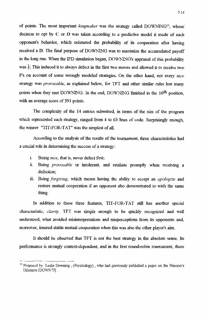
3.14

of points. The most important kíngnzaker was the strategy called DOWNING”, whose' decision to opt by C or D was taken according to a predictive model it made of` each opponent's behavior, Which estimated the probability of its cooperation after having

received a D. The final purpose of DOWNING Was to maximize the accumulated payofi in the long run. When the IPD simulation began, DOWNING's appraisal of this probability was 51; This induced it to always defect in the first two moves and allowed it to receive two P's on account of some wrongly modeled strategies. On the other hand, not every nice strategy was provocable, as explained below, for TFT and other similar rules lost many points When they met DOWNING. In the end, DOWNTNG finished in the 10th position, With an average score of 391 points.

The complexity of the 14 entries submitted, in terms of the size of the program Which represented each strategy, ranged from 4 to 63 lines of code. Surprisingly enough, the winner "TIT-FOR-TAT" was the simplest of all.

According to the analysis of the results of the toumament, three characteristics had a crucial role in detemrining the success of a strategy:

i. Being nice, that is, never defect first; Being provocable or intolerant, and retaliate promptly when receiving a

defection; .

ur. Being j‹`)rgiv1`ng, which means having the ability to accept. an apologzfze and restore mutual cooperation if an opponent also demonstrated to wish the same thing.

In addition to these three features, TIT -F OR-TAT still has another special

characteristic, clarity. TFT was simple enough to be quickly recognized and Well

understood, what avoided misinterpretations and misperceptions from its opponents and, moreover, insured stable mutual cooperation when this was also the other p1ayer's aim.

It should be observed that TFT is not the best strategy in the absolute sense. Its

performance is strongly context-dependent, and in the first round-robin tournament, there

lê Proposed by Leslie Downing , (Psychology) , Who had previously published a. paper on the Prisoners Di1e1nma[DOWN75] .

3.15

Would be three other rules Which could do better than TFT, should they have been included in that group”.

The second tournament was performed Within a completely different environment, not only because the diversity of participants, but also because the results of the first

contest had been ma.de public by means of the report sent to all new contestants. This account was used by the applicants to subside the formulation of their second toumamenfs strategies. Furthermore, the length of the game Was not any more fixed, as prevailing

originally. Instead, the number of iterations became probabilistic, governed by a parameter w = 0.99654, that stood for the chance that there Would be still another round (involving all pla_yers)'8. Five repetitions of the simulations Were performed, and the average number of iterations per simulation cycle was 151. Quite unexpectedly, "TIT -F OR-TAT", Which had been re-submitted by the same person, was again the winner”.

Although a detailed analysis of each strategy-"s success or failure Was made, those

results referred to a particular environment Where the simulations occurred. So, in order to

verify the general performance of ea.ch rule, new toumaments have been simulated.

The representativeness of every strategy in the next rounds was now function of the previous relative success, that is, how Well it performed before. The players that Were present in a. group from Which all pairvvise iterations were accomplished formed a

generafion. By this method, the number of individuals using the same rule in the next generation Was proportional to the product of the previous number of representatives and

their score, which, by its turn, Was the frequency Weighted average amount of points in the

iterations With the other rules”.

W Those Were: "TIT-FOR-TWO-'l`ATS" (answer With a D only after receiving two D's in a row from an adversaiy); "LOOK AHEAD" (analogous to search algoritlmts in graph trees, resembling some techniques used in chess playitlg programs); "DO\N'l\1ING*" (fa revised version of the original

DOWNING, Where the tactics of playing D in the two initial iterations was inverted to C). 18 The parameter w mirrors the importance given to future games' payoffis, and it can also be seen as a discount factor, because the strategies Were fixed.

H' Although TFT could have been suipassed by another niles in the first tournament, these same rules didn't succeeded in doing so in the second, on account ofthe changes in the environment that took place due to the presence ofa new breed of contestants.

2” The siniulation had 1000 generations , and TFT finished with the greater relative frequency, around 14%. lt should be noted that a. good performance in the initial generations does not mean that a final success is

3.16

The described process simulates the ecological perfomiance of the rules. In this approach, the best adapted strategies tend to proliferate, and those less fitted Will become extinct. The ecological simulation deals only with changes in the frequency distribution ot types, since the specification of every strategy remains fixed. On the other hand, in a

adaprive process, the rules can be modified, by means of the introduction of new proceedings or through murarion of already existent rules. The dynamics of Axelrod's mentioned toumaments” regard the former category of simulations, but he also investigated

the latter in a subsequent work, which is explicated in section 3.4.4-ll.

With the results of his toumaments as basis, Axelrod proved the following

propositions and theorem [AXEL8l], [A5(EL84], Which tum out to be a essential aspect of his research:

0 Proposítion I

If the discount parameter w is sufficiently large, there is no independent strategy that. can be better than the others.

0 Propositíon 2 V

If w 2 max [(T-R)/(R-S), (T-R)/(T-P)], and if all players adopt the TFT strategy, the Iterated Prisoner's Dilemma. has a. Nash equilibiium, and in this case TFT is called a collectively stable strategy, Which means that it cannot be irzvaded”°'“' by any other rule if member of the population uses it.

F4 ra 0 Chézracterizézííoii Theorem The interpretation of this theorem is that the move C or D iinplemented by a mle X in any point. n of the sequence of iterations is completely defined by the game's previous history, in order to be collectively stable. While the inequality above is not satisfied, X may choose C or D freely Without. loosing its collective stability. When a nile interacts With itself (XIX), the circumstances where the largest quantity

expected. This is so because When a rule runs against every other in the beginning and gets many points, it must keep the same competence with the surviving strategies, as those less apt get excluded of the game. The concept of invasiorz in a ecological IPD expresses the proliferation, by copy, of more successful strategies, regarding the accumulation of points. The "invasion“ takes place when the ability of a native strategy to gather points is surpassed by another.

23 A strategy X is collectively stable if and only if X plays D in the n-th iteration every time the number of points accuinulated (\1'11Í) by an opponent Y until that moment is such that V, (Yll .>V(X|X`)-vv“'*:z-<[T+

WP/(1 ~W )]. For a proof, see op. cit. [AXEL81].

21

\__`$

3.17

of points is amassed are when both are. Therefore, nice rules detain the greatest potential of keep on playing C, even When they are threatened by non-nice invaders. The important advice embedded in this theorem is that anyone Willing to adopt a collective stable strategy should only cooperate when its possible to absorb an exploitation and still maintain its mightiness.

Propositíolfz 3 A strategy X that has at non-zero probability of cooperating in the fiist itera.tion can be collectively stable only When w 2 (T -R)/(T -P). Propositíon 4 A nice strategy is collectively stable only if it is also provocézble, that is, retaliates immediately after receiving a defection.

Pr'oposítz'0n 5 The rule "ALL D" is collectively stable.

This means that as population W made up exclusively of "ALL D's" cannot be invaded by any other strategf Z that is implemented by a newcomer. However, if the invaders using Z come in clusters and disciiminate their opponents by means of establishing a certain proportion p of all iterations that are implemented with members of their own species, invasion becomes possible. Hence, a. p-cluster

invades a population W if pV(ZlZ) + (1-p)V(W|W) >V(\V|W)Ê'5. Proposition 6

The smallest value of p necessary for a specific strategf to be able to invade an "ALL D's" population in a cluster is accomplished by the strategies called

rna.rin-zaIl_1.= díscrímínatíng. These rules eventually play C for the first time even with those opponents which have never cooperated before. From this point on, the mutual cooperation is established (a sequence of ('C,C_) takes place) only With a

sti'ategv that is behaving in the same Way. Therefore, the nzaxinzallv discrímínatíng strategies never play C again With an "ALL D".

'J ¬ _¬ Axelrod observes that the pairings are not supposed to be random, because if this were so, a small group ofZ's would have little chance ofinteract with each other in an environment With a. great ntajonty of W's. Ctonsídenng the values from the standard payoff n1at1ix(Íl`=5, R=3, P=l and S=0f) and w=0.9, a group of Z's succeeds in invading the original population W if as few as 5% of all its iterations are within the group. If, however, the pairings are random, a. strategy Z thnves whenever its overall proportion q is above 1/17', With the other parameters as before. See op. cit. [AXEL84]_, pages 211-213.

3.18

0 Proposítíon 7

If a nice strategy cannot be invaded by a lone newcomer which acts ditferently, it

Will be also immune to clusters of the same kind of individuals. 0 Proposition 8

If a strategy is collectively stable, it is also terrítortallv stable.

This proposition refers to the spatialized IPD24, Which regards the dynamics of systems that are modeled by regions made up of cells, whose occupants interact With their "neighbors" and imitate them, on condition that their performance is

better. The territorial stability is associated With the immunity that a location has against modifications of its original strategy provoked by imitation of an invader. The specifications of What consists a neighborhood and the criteria. that make imitation possible can vary, and have a great influence on the way a territory is occupied. In these kind of systems, the "nice" character of a. rule does not assure that it will be not invaded, specially if the parameter w (the shadow of the future) is small”.

Axeh'od re-examined the problem of cooperation in the context. of the IPD in a

later paper [AXEL88]. That article reviewed the previous Work and presented short

commentaiies on several topics, suggested as lines of further investigations, including:

ó Itermions: Multiple players - " n-person PD" - NPD; â ilíoves: Possibility of inclusion of one more elementary act: get away, meaning

refitsal to play, that can be spontaneous or forced (o.str‹1cism.`); à Payojfs: How the solutions can be affected by changes in the values of the matrix; ó Noise: Accidental faulty implementation of strategies (tremblíng hand) or

misperception (blurred míndsf)26; ó Shadow of the future: Its implications in the strategies adopted and their equilibiia.

When the length of the IPD is finite or the discount factor w varies With time; ‹ Population ‹lymum`cs: Diiferences between Nash equilibria and ES S'sU;

24 An extended discussion of this approach is given in section 3.4.2. Axelrod illustrates the invasion ofa tenitory solely composed of Tl¡'I“s "inha.bitants" by ALL D's ; the IPD parameters used in this example were T=56, R=2, P=6 and S=0_, with w small, equal to 1/3. ln a. homogeneous population ofTFT's, the noise affects considerably the results. Regarding the factor noise, Nowak [NOWA92] mentions that, for an error rate less than 1%, the accumulated gains by each individual (fitness) is reduced by about 25%. W Evo1utiorzar_vSiabIe Strategies - See section 3.4.1.

3.19

ó Population structure: How the “clustering effect" can influence the possibility of a homogeneous population to be invaded by some other strategy.

Axelrod”s computational toumaments of the IPD and the insights that they brought can be considered indced a landmark in the study and comprehension of the mechanisms that govern conflicts of interest and the benefits of mutual cooperation. In its foreword to the 1990 edition of A.~;elrod°s book The Evolution of Cooperation, Richard Dawkins” states that “The world's leaders should all be looked up with this book and not released until they have read it. This would be a pleasure to them and might save the rest of us.”

3.4 - Evolutionary Games, Spatial and AI Techniques Approaches of the PD

3.4.1 - An Evolutionary Biological Application: The "Hawk-Dove" game

The first explicit application of Game Theory to evolutionary biology was given by R. Lewontin [LEWO6l]. His work, followed by numerous other related papers, examined how a species played against nature to minimize its probability of extinction. l-lowever, a

much more interesting an important contribution on that area was provided by the biologist John Maynard Smith [Sl\/lIT82], Who explored the way members of animal species play

games against each other. In this case, both the population dynamics and equilibria are

considered and analyzed, mainly by means of a special kind of game devised by Maynard Smith: The Hawk-Dove (HD) Game. Though not retaining the same structure of the PD"s payoff matrix, HD has various similar features regarding the choice of strategies, and was used to introduce the important concept of the Evoluiive Stable Smztegv - ESS, that

consists in a new class of equilibrium in games. Also, in Maynard Smith's model, the criteria of r-ationalitgz and pi-eferences stated in classic Game Theory are replaced by those of dynamic stability of populations and Darwinian adaptation

(_ “The survival of the

frt1.est").

ln the Hawk-Dove game the players are considered to be individuals from animal species which, like the participants of a PD, have basically two elementary actions

23 Author of The Selfish Gene (1976) and The Blind Waichmaker (1986), among other works.

3.20

available, namely Hawk (H) = Escalate or Dove (D) = Display, to be adopted one at a

time. The dynamic evolution of the strategies employed is analyzed in the course of several generations, from the assumption that each species aims at maximizing its expected

a.ccumulated adaptive gain, which depends on the behavior of its adversaiies. This

adaptive gain refers basically to the possibility of free (Without competition) exploitation of the resources offered by the environment where the species alrea.<t_v lives or intends t.o

establish itself.

The HD payoff matrix is represented in the Table 3.5.

Column Player

Linz Player 1/2 (V - C ) |

V ÊfÉÊ5ÊÊí§Éi§Êi5ʧ§išiälàšifiššÊi§Í;§§šÊíÊÍíš 0

Í

V/2 Table 3.5 - The Hawk-Dove Game's Payoff Matrix

The values in the cells cotrespond to Line Player's adaptive gain. V is the payoff of H mvk (H), when the other plays Dove (D) and C consists of a. loss, associated to a. 50% probability that a H strategist suffeis injuries When meeting another H. When a. dispute

takes place, the net expected adaptive gain is equally shared.

Assuming that when both players start a game they have an equal adaptive gain Wo, the accumulated payoff by each species after the game (fitness) will be noted by W (D) and W(H), provided that the relative frequency of H's in the Whole population of the species involved is p.

W‹_H) = Wo + p E(H,H) + (1-p) E(H,D) Eu. 3.2(a›

W(.D) = Wo + P E(DzH) + (1-P) E(D.zD) EH- 3-20')

E(.) is the Line Player's payoff in an iteration between any two type of strategists.

Along the iterations, the players reproduce (create "oÍTsprings"), which quantities are

propoltional to their respective achieved fitness.

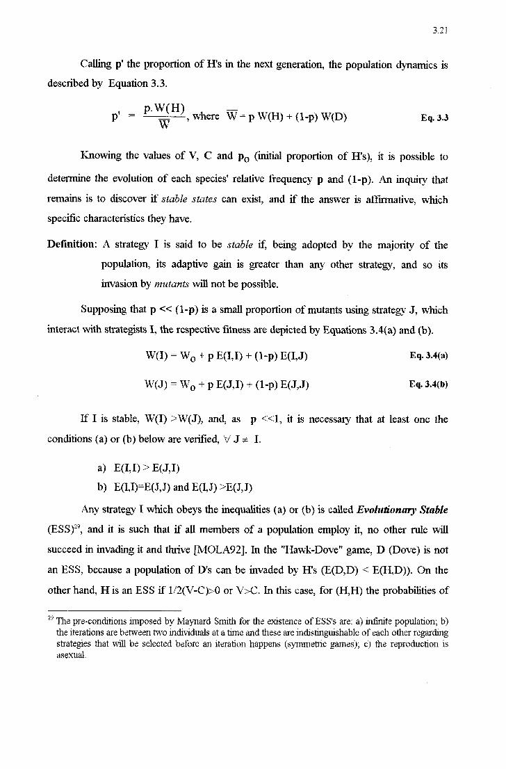
3.21

Calling p' the propoition of H's in the next generation, the population dynamics is described by Equation 3.3.

.W H _ P' = Wheffi W =PW(H) + (1-PÍ)W(DÍ) E‹i›3-3

Knowing the values of V, C and po (initial proportion of H's), it is possible to

determine the evolution of each species' relative frequency p and (1-p). An inquiry that remains is to discover if stézble states can exist, and if the answer is afiirmative, which specific characteristics they have.

Definition: A strateg I is said to be stable if, being adopted by the majority of the

population, its adaptive gain is greater than any other strategy, and so its

invasion by mutants Will not be possible.

Supposing that p << (_l-p) is a small proportion of mutants using strategy J, which interact with strategists I, the respective fitness are depicted by Equations 3.4( a) and (Ab).

W(1) = WO + p E(1,I) + (1-p) E(I,J'› Ea- 3.4‹a'›

W(J) = ivo + p E(_J,1) + (1-p) E(_J,J) Eq- 3.4‹b›

IfI is stable, W(I) .>W(J), and, as p <í<Il, it is necessary that at least one the

conditions (a) or (bf) below are verified, V J :ê I.

a) E(I,I) Ííf' E(J,I)

b) E(1_,I)=E(J,J) and E(I,J) .I>E(J,J)

Any strategf I Which obeys the inequalities (al) or (bf) is called Evolutionmzv Stable (ESS)”, and it is such that if all members of a. population employ it, no other rule will

succeed in invading it and thrive [MOLA92]. In the "Hawk-Dove" game, D (_Dove) is not an because a population of D's can be invaded by H's (E(D_,D) < E(H,D)). On the other hand, H is an ESS if l/2(V-C`)>z0 or V ;>C. In this case, for (H,Hf) the probabilities of The pre-conditions imposed by Maynard Smith for the existence of ESS's are: af) infinite populaüonj, b) the iterations are between two individuals at a time and these are indistinguishable of each other regarding strategies that will be selected before an iteration happens (syninienic games); c) the reproductíon is

asexual.

322

getting V or C are 50% for both players, and if V >C, it is worth running the risk of

receiving an injury (_ C.) to achieve the gain V”.

Besides mixed strategies involying H and D, several conditional behaviors are also considered in sequential HD games, such as:

o Retaliatez Start with D, but change to H if opponent escalates (adopts H); o “Bully": Start With H and retreat to D if opponent escalates; 0 "Bourgeois": Play H if owner (of the territory) and D if intruder;

Asymmetric games are also analyzed, thus relaxing one of the previous conditions assumed for the existence of ESS's. In this mode, the players are separated in categories

according to some attribute which indicates strength, such as bigger, better, etc., While the other has opposing characteristics. Also, every player is perfectly aware of its own characteristics. However, the strategies that are employed are supposed not to be

correlated either with this information or with the results of the previous iterations.

Reinhard Selten'[SELT80] proved that if a game has at least one asymmetry which is common knowledge to the contestants, then it cannot have a mixed ESS”. Assuming that one or more asymmetiies exists, another type of behavior is considered, called

Assessor. An assessor (A) chooses H if it finds itselfin a better position than its adversaiy, and selects D conversely. The acquisition of the infoimationií' concerning the other's

characteristics can be supposed to have a. cost c” for the assessor strategists. In a iterated

game involving the strategies H, D and A, A is an ESS if (_a)c -<í§1V and

(b)Cx `>V(,1-x); H is an ESS if (a)c -=1I§l(V-C.) and (b) Cx <V(1-x), where x is the

probability that the piivileged player wins a (I-LH) dispute. Alternate behaviors H and A cannot take place in an iterated game With the same values of the parameters V, C, c and x,

3"' ln the human case, this decision rule generally does not apply. Kahneman e Tversky, in their "Prospect Theory" [KAHN79] show empirical evidences that players' concerns for losses are greater than those for gains.

31 Taken in the traditional sense, as, for example, select an action A with probability p or another action B with probability (fl-p). In the case mentioned, however, pure E.SS's can exist. Presumed with no anibiguities. If there is a chance of errors in the assessor's process, Selten's theorem [SELT80] is no longer valid.

33 c =< C, that is, the cost c of acquiring the information about the adversary's strength is smaller than the loss C related to an eventual injury.

I

¿› \.) JJ

for if an assessor discovers that it is in inferiorityy, it gives up this strategy and chooses H or D depending on the mentioned parameters.

Maynard Smith notes that A has advantages that help it to be an ESS, because if c is small relative to C-_, the eventual privilege of a better relative position is a. reliable indicator

of success (x 21') if a (_H,H) dispute takes place. It should be observed that x does not need

to approach 1 in order to A be an ESS. Even if x < 0.5, A is an ESS When C 2=»';>\/'. This

fact gives rise to a kind of paradox, because it means that a player uses H if inferior and D ifin advantage. `

Several other contingencies can have a role in the evolution of asymmetric games.

One factor worth citing is the Resource Holding Power (RHP), which should be

interpreted as the demonstration, by a player, of the amount of resources available to it that can influence the outcome of a dispute. The RHP is a kind of a measure of power and has a relevant effect on the behavior of an opponent that uses the assessor rule. Specifically, in

the same Way a cost c was assigned to information gathering, it can also be assumed that a

similar expense will be associated to power exliibizion” with the purpose of intimidating an opponent. How accurately (level of perception) a threat is representecl by a displayed RHP is a factor equally important in the strategies' formulation and in their evolution”.

_ Although the Hawk-Dove game had its original aim as a paradigm for the

treatment of biologic problems, it has been quite influential in the general development of

Game Theory. In fact, the work of Maynard Smith [SMIT 82] marks the advent of Evolutíonargf Game Tlieory [WARN95]. Its significancc in the area can be measured by the great number of citations in the specialized litera.ture_, e.g. [COL-L9l], [GODF92], [NOWA92], [NOWA93], [BEND93], [FOGE93], [SIGM93], [ATMA94], [FOGE95].

54 Regarding the strength attiibute, not the rule H or D. The "Power display" must not be backed by the existence of the advantages; it may be a "blut`Í". ln human relations, a typieal example of how misperception of RHP's can be hazardous to all refers to the intemational political situation known as "cold war”. Each side involved in this kind of dispute attempted to show the maximum RHP possible (at high costs), so that no doubts might exist about its militaiy retaliation power (MAD: Mumal Assmerl Destruction policy). This was so because an underestimate fiom the other side could take it into believing that "playing tough" would be advantageous, and this would almost certainly bring an escalation obviously feared by anyone.

3.24

3.4.2 - Spatial Models of the IPD

An spatialized model of the it.era.ted P1isoner”s dilemma. has all the characteristics ot the classical version, plus a new feature, that is the embodiment of the dimension space in the game [NOWA92(a,b)], [l\/lAR93], [HUBE93], [NOWA94]. According to some rule, that can be random or not, the players are scattered in a field, usually a two-dimensional grid. There can be more than one manner by which the participants may interact. In the most cornrnon mode, the contestants compete With their “neighbors”37, that is, those

players which occupy adjacent cells in the grid in a. round-robin tournament, where each

plays once with one another. A completed round is called a generation, and at this point each cell copies the most successful strategy of its neighborhood. The evolution of such a

spatial grid is dependent on the values of payolf matrix. Even if the binary IPD is played, with only pure coopemtors and defectors, C and D actions allowed, quite complex

dynamics may result. It is possible that cooperators are extinguished, but often shifting

mosaics occur, With mixtures of pure cooperators and defectors coexisting indefmitely in

unsteady proportions. Nevcrtheless, recent studies performed mainly by Nowak found that the average composition of the population is predictable [NOW A95].

Besides the method described above, other approaches using the basic spatial

paradigm of the IPD appear in the literature. It Was employed, for instance, in the

philosophical issue of demonstrating the pervasiveness ot the Gödelian notion ot

frzarlzerrzatíczzl zmdecidabilíty in more practical, less abstracts problems [GRIM94]3s.

Another example is provided by Weeks et al. [WEEK96], who simulate a spatial IPD in a

playing field with “Walls” and random matchings. In this Work, variable payoffs are

considered and the players are represented by cellular automata machines, which evolvc

their strategies With the aid of a genetic algorithm.

37 Those players which occupy adjacent cells, usually eight in a. chessboard-like grid, or four, if diagonals are not included. An hexagonal-pattemed lield may also be considered.

32 Grim [GRIM9-4] argues that some formerly pure mathe1na.tic-al philosophical concepts, like Gódefs zzrzdecidabilirv, Rice`s theorem in recursion theory, and recent Cliaitiifs theorern in information theory, which are coming closer to more practical applications in physics, engineering, economics and theoretical biology.

3.25

The spatial models of the IPD are proving extremely useful as a new method of simulating and analyzing how cooperative behavior and mumal help can influence species evolution and the coexistence of diversity when territorial location is significant. It has been aiding studies in environments that range from the molecular and genetic level to

phenotypic and social structures [CAMP85], [NOWA95], [LLOY95].

3.4.3 - Singular Reactive Strategies

The strategies that decide their moves taking into account the opponent”s previous actions (C or D) are denominated reactive. In their simplest form, those rules only consider the last iteration. The best known of those kind of strategies is the famous Tit-for-Tat

(TFT), Which proved quite effective and robust in Axelrod”s computational toumaments of the IPD, and since then, also in many other subsequent inquiries on the subject. For this reason, TFT is regularly included in experiments regarding simulations of the lPD39. It has been serving as a kind of a reference parameter in the investigation of other strateges”

proficiencies. TFT has been used also as a basis for some related variations, as for

example, the Suspiciozrs TFT, whose only difference is that it starts defecting instead of

cooperating.

Employing another type of reactive strategies, Nowak and Sigmund [NOWA92] analyzed the infinite IPD” under the aspect of ecological development performed by heterogeneous populations. In that. model the players employ reactive strategies represented

by Ei = (y, pi, qi), where y is the probability that. a. player cooperates in the fn'st move and

pi e qi are the conditional probabilities of cooperating (C) after having received aC or D in the previous iteration, respectively.

Several simulations of this model of the IPD were accomplished, where 99 distinct reactive strategies (whose parameters pi and qi have been randomly chosen from unifonnly

distributed values in the inteival [0, 1]) participated together with TFT* _ almost TFT_ 39 ln the Fuz:_y I zerated Prz'soner “s Dile››z››za, whose model is presented and detailed in Chapter 5 of this

Dissertation, the traditional (dichotomic) TFT has been included in the population of strategies, along with a. gradual version (Fuzzy-TF'l') and also another celebrated reactive strategy, PAVLOV.

4° The probability of occuning a. next iteration, in that case, is taken to be equal to 1.

3.26

(parameters pi =0.99 and qi' =0.01 and ETp¡¬*= (0.99, 0.01)')“. The payofl` matrix Was the

same of Axelrod”s tournaments. The determination of the relative frequency xi' obtained by

particular strategy was given by

xi = x1f1(x) Eq. 3.5 ftavg) '

where xi is the frequency of i in the present generation, _7¶(x) the average gain of Ei in the

existing population and fiwg =Ê. x¡7§(x) is the average gain of the whole population.

The ecological evolution obseived during 1000 generations was rather interesting. Starting the process with a diversified composition of strategies, around the 100”

generation the rules that hardly ever played C (EALLD E (0, 0)) added up to practically 100% of the population. By the 150* generation, the so-called Generous TFT” - GTFT reappear. In the end, the winner Was Eüm =(_0.99, 0.33). The authors comment that the final success of GTFT was only possible because a small group of TFT* sunived near the 100” generation, When E_,._L¡¿, had almost taken over. Hence, in this case TF T* performed as a kind of cazfazfvzer, making the victory of GTF T possible. In the generations above the 300Íh, the average payoif of an iteration Was about 3 (the reward R for mutual cooperation), because at this time almost the entire population had already turned to

E-GTFT's, implying in ar high probability (0.99) of moves (C,Cf).

An equally remarkable contribution on the field Was also given by Nowak and Sigmund, regarding the robustness of TFT in rzoíq1.>43 environments [NOWA92], [NOW A93b]. Those researehers found that TFT does not endure in simulations which, mirroring real-life conditions, some mistakes are made [BEAR93]. Instead, another

strategy, employing the criteria Win-Star, Lose-Slzift, succeeded in dominating the modeled

41 Because an infinite duration (w =l`) is assumed, the memory of the first move will vanish, and so the parameter y can stay out of the notation of Ei.

42 Gene;-cms is the generic denomination of the strategies whose p¡ and q¡ values are near 1 and 0, respectively.

45 The tenn noise refers to enoneous implementation or perception of strategies, eg. tr-embling hrmcl and blurred minds. See Section 3.3.2.

3.27'

populations in the long mn. This reactive rule, dubbed PAVLOV, has a modus open-zndzf as straightforward as TFT, and it can be translated in the following: If in the previous

iteration both players made the same move (either CC or DD), PAVLOV cooperates. Otherwise (CD or DC), defect.

For its performance, PAVL-OV counted on four main advantageous attributes: i. It is able to maintain cooperation (CC) and continuously receive the reward payoíf; ii. It is provocable, defecting after receiving the suckefs payoff (CD);

It tries to restore mutual cooperation, playing C after a DD, but it is non- exploitable, because it turns to defection after an eventual failure in its objective.

iv. It takes advantage of the exploitable partners, stockpiling points from all-out

cooperatois (DC).

PAVLOV has the ability of quickly correcting errors. One drawback is that it fails against an All-D”, because in this case an alternation of DC”s and DD”s Would occur.

Still more recently, in simulations of the IPD with variable degrees of noise, Wu and Axelrod [WU95] showed that the reactive strategy Contrire TFT" (CTFT) performed better than both PAVLOV and GTFT When the noise level exceeded about 1%. Those authors also argue against the robustness of PAVLOV in the investigated environments.

3.4.4 - The. IPD with Finite. Automata and AI-aided players

Lately, some lines of research regarding the performance and evolution of adaptive

strategies in the IPD have been increasingly mal~;ing use of automata. and several AI related tools. The efforts in that direction include the use of Finite State Machines, Genetic

Algoiithms, Evolutionary Computing and Neural Networks. This section reviews a

representative sample of these techniques applied to IPD simulations.

I - The IPD played by a pair of Finite State Machines (FSM`s)

44 Neveitheless, a population composed of PAVLOV strategists cannot be invaded by All-D”s if PAVLOV is slightly less cooperative after a P than after a R. This behavior is mirrored by the conditional probabilities of cooperating alter each of the four possible previous outcomes, like, for instance p(C1|C.C{)=0.999, p(C1|CD)=0.001, p(ClDC{f›=0.00l, p(C.|DD)=0.995 [MILI93].

45 CTFT cooperates after the other player had defec-ted in response to a previous CT PT defection.

3.28

One of the first attempts to embed automatic decisions in IPD players mentioned in the literature was contributed by Rubinstein [RUBI86], who simulated an IPD supergameáó with two F SM”s. In each iteration the players selected moves that depended on the previous sequence of outcomes. A player's global strategy contemplated all possible

histories of results, implementing decisions that have been formulated exclusively by its respective FSM.

An FSM can represent a higher-order Markovian Process, and the finite machines that took part in the cited supergame had the following characteristics:

i. A fmite number of states, with an initial one; ii. An output function, Which defmes the move (C or D) to be accomplished in the km

iteration;

A transition filnction that deteimines the (k+l)“' state depending on the km state and opponent`s move. .

In this model, the players” problem is reduced to the choice of their FSM”s, since the moves are completely determined by the selected machines. Under those conditions it is also possible to find a pair of gains that is a Nash equilibrium'".

Besides the attainable results, another concem is the degree of the complexityis of the chosen F SM*s. A simple measure of this attribute is proposed, calculated only as a

function Which associates operational costs proportionally to the number of intemal states of each FSM. The costs are independent from the utilization of the states during the game.

The type of FSM employed is a Moore Machine”, denoted M, for player i and

represented by a four-tuple {Qâ, Cl? , 7»¡, u,}, Where

46 A "supergame" is a game that is repeated an infinite number of times. Each iteration is also denominated a period.

47 The PD does not have ajointly zzzírníssible pair of strategies; Therefore, the game is not soluble in the strict sense, though it is soluble in Nash°s sense. This result extends to the iterated PD. See Chapter 2. of this Dísseitation A Review ofF1.nzd(.‹menml Topics of Game Theory. lt is possible to specity more elaborated FSM`s complexity measures, as those dependent on the automaton`s type of the transition function. ›

Moore Machirzes are automata whose output, at any time, is a direct fimction of the state to which the machine transited. A more general class of automata are the Mealy Machines, in which the outputs derive fiom the transitions that occur fiom state to state. The path followed (the sequence of states) until a particular state may be different, therefor influencing the output. A Mealy machine can be always logically replaced by a Moore automata, though requiting a. greater number of states.

43

49

3.29

. Q¡ is the finite set of intemal states of Mi;

. qf E Qi is the initial state;

. M: Q,-› S¡, with S¡ being the set of available strategies for player i;

. 7»¡(q¡) is player i's strategy whenever M¡ is in state qi;

. tl,-: Q¡>¬<S¡ -› Qi (iâj), meaning that ui represents a transition function Which defines the next. intemal state with basis on the previous state and opponent`s move.

The choice of two particular F SM°s M1 and M2 completely define the sequence of outcomes, as long as the introcluctory move is settled by a zero-length string (no results yet) and the initial intemal state qf of the machines. For example, player i's first move may be s¡1=7t¡(`q¡l) E S¡. After j plays, M1 changes its intemal state to q¡2=u,-(_` q¡1, sf).

A diagram is a convenient way of depicting a. Finite State Machine. Figure 3.

portrays a FSM that uses the TFT strategy, With the characteristics Q={qC, qD}; q°= qc; 7.(qC)=s and u(_qC)=q,_, for s(state)={C_, D}.

CI D .-'IPF-.-_ F

/` \ /' ¬\~ ., ,._¬x \

N) \i`/ff `\-/I sucata qc 'lo1 H D *-«é“

f .¬ ,ff 1

tÍoutput)$`\"*\__ Í» _»--°"`) toutput)

Figure 3.2 - A FSM that plays TFT in the IPD

Afier a certain number of iterations, being finite, the FSM's will necessarily repeat a pair of previously assumed states. Calling q'=(_q1", qz"), t=1, 2, the sequence of states of

M1 and M3, there Will come an occasion tz, tz:-tl such that q'1 = q'1"1. The period tz is the

last of the qvcle, because in t2+1 the machines go back to the state they had in tl. The

length or duration of the cycle is T= tz-t1+1.

3.30

Two types of equilibrium are considered: Nash's and the semi-perfect, the latter concept introduced by Rubinstein in the paper. Both equilibria regard the players* ranking of preferences in the choice of the FSM's.

Defming the sequence of moves as s'=(s,', szt), t=1, 2, the average payofi m ot player i per cycle is given by Equation 3.6.

Í 1 z

1t¡(M¡, M2) = É 2 ;.i1(s') Eq_3_5 Í Í

1

For a generic FSM, M= (Q, qo, Ã, tt), |M| denotes the number of states that exist in the set Q, and M(_`q) is the machine whose initial state is q. Calling >¡_ the lexicographic order in 1F“..2, the definition in Equation 3.7 means that a player`s ranking of preferences

regarding a feasible pair of machines is established first, by the greatest average payoff it

can achieve, and second, by the lessei' number of states of its machine, provided the payofi is not inferior.

(Miz1\/Iz) >-â (1\/Ii”, Mi) if {Tfiâ(1\/Ii_.1\×íz)z -I MCI >L 1Iú(Mi”_¬1VIz'), -I Mâ”|} Eq. 3.7

Two F SM *s l\-41" and N12* are a Nash equilibrium if there is no other machine l\/I1 or 1\/I; that verifies either one of the relations depicted by Equations 3.8(a.) and (b).

(M1, 1v1“¿)z., (M",, 1v1"¿) Eq_ 3_s(,,)

(.ÍVÍ*i› Mz)«?>2 (M*i› Í\'Í*2_) Eq' 3°8(b)

The main definition of the paper regards the semi-perfect equilibrium (SPE), Which

asseits that a SPE holds if there is no iteration t, no M1 and no M2 that confirm the inequalities of Equations 3.9(_a) or (_b).

um M*z‹.‹fzc››>i ‹MH‹‹fi›, M*z‹q'z›› Eq. z.»‹zz›

‹M3‹¢i'szb›, Mzí›>z ‹M'1‹q'ic›, M*z‹.q'z*›c› Ei. wir»

_L¿)

UJ ›--

When a SPE occurs, there is no phase of the game in Which one of the players might want to alter its preference concerning the pair of FSM°s in order to accomplish its nem move. The distinction between the Nash and semi-perfect equilibria is that in the

former, the concept of optimality is linked to the selection of the ma.chines at the beginning of the game, While in the latter the preference about the FSM`s endures throughout the game, before every iteration.

The solution of the game consists in finding a pair of machines for which the SPE holds. For all stages of the process, each FSM must satisfy the conditions:

i. Neither player is able to increase its expected gain by unilaterally replacing its

machine;

No player can reduce the number of int.ema1 states of its machine; The approach of the IPD replacing conventional rational players by Íinite state

machines is quite interesting, and has been giving margin to several further' developments. In a subsequent paper, Abreu and Rubinstein [ABRE88] extended the analysis of the IPD played by FSM”s, exploring aspects of Nash equilibiium and refining the notion of n-zaclzíne corrzplexíty, With its respective implications in the costs, gains and optimal machine selection.

II - Genetic Algorithms

Using the AI technique Genetic Algoritlzms (GA) developed by John Holland [HOLLi75], Axehod examined the IPD where the population of players was submitted to an evolutionary adaptive process. The GA method performs variation and selection of individuals, taken as possible candidates for an optimal solution of ac problem. Under the

GA approach the level of abstraction considered is the Genotype, usually represented by a

binary coding. i

In contrast to his previous toumaments, the restiiction of fixed strategies Was

relaxed [AX'EL87]. Each entry Was denoted by a string with 70 positions (bits, or genes), that could be zero (DEFECT) or one (COOPERATE). The criterion for designating a generic strategy took into account all the possible combinations of the three previous moves, Which

_L¡)

U) I ~.)

were employed to defme the current action”. The resulting total number of strategies is 27°.

This number is so huge, that it is intractable even to brute strength computing. Axehod commented that, “ff a computer had examined those strategies az* the rate of 100 per

second since the beginning Qf the universe, less than one percent would have been checked by nm:-f.” So, the idea was to initialize a set of entries that would evolve by means of selection by relative fitness and generation of offspring by crossover and mutation. One of the main objectives of the experiment was to find out whether the GA could discover the TIT-FOR-TAT strategy [LEVY92].

Again, a computational simulation was programmed and implemented. The population of players to take part in the simulations comprised 20 random strategies, plus 8

other selected representatives, which were picked from the best performing strategies from A:‹elrod"s second computational tournamentj 1. A round of simulations involved 50

generations with 40 trials, each comprising 24000 iterations. Each game consisted of 151 moves per player, the same average from the original toumaments. The most successful

strategies Were coupled after all iterations in a given generation had been accomplished.

The ciiteiion employed by Axelrod was to allow one coupling for the average rules

(those inside the inteival il standard deviation), two couplings to rules With upper

punctuation (above l s.d.`) and no couplings to the inferior strategies. Each couple

generated two offspring, by means of the crossover GA operation. The other GA operator used Was mutation (changing a C for a D and vice-versaf)52.

Two different series of simulations were run. In the first, the 20 randomly selected strategies confronted only the eight mentioned representatives, which remained static. For

this series, the flowchart of operations subsumes the following steps:

The 70-position chromosome resulted from a string of 64 bits, which responded for the 43=64 possible combinations derived iiom the four attainable outcomes (CIC, CID, DC. and DD) in the preceding three interactions, plus six additional bits regarding the playefs move for the initial combinations of under three interactions. Thus there Were 27° possible strategies.

51 The second toumanient (see section 3.3.2) had 62 entries, and the eight chosen rules have been considered as a reasonable account for how well a given strategy did With the entire set [FOGE94]. Their special feature Was the "representativeness"

_, under the view that the score that a particular mle would get

when ran against all others was highly coirelated With the gain that could be obtained with the eight representatives.

52 Crossover and mutation probabilities averaged one and one-half per generation, respectively.

333

1. Initialize a population of 20 randomly selected strategies;

2. Perform a round-robin tournament of each random strategy against the 8 special representatives and record the weighted average payoffi

3. Determine the number of offspring from each parent policy proportionally to their performance;

4. Create offspring by crossover and mutation; 5. Return to step 2.

By the end of the experiment, Axelrod noted that the GA method evolved populations whose median perfomance, in terms of accumulated gains”, Was about the same as TFT, with behaviors also resembling it.

The second sequence of experiments consisted of ten trials and required that the evolving policies played facing each other, now excluding the eight fixed rules. The complexity of this new environment greatly increased, because now the players confronted opponents that were also concurrently evolving. The highly competitive process meant that a rule might either match its adversaries” ever increasing efiicacy or become extinct by the selection mechanism.

As a general outline, the population departed from initial cooperation, but inclined towards equal replication whenever a cooperative partner was recognized. The population's average score raised along the process, what meant that. the maturated participants in the

game developed the skill of diiferentiating cooperators from defectors.

II - Evolutionary Programming

Another important contribution to the IPD as played by logical stimulus-response devices was provided by Fogel [FOGE93a]“, [FOGE94a], [FOGE94b], [FOGE94c], [FOGE95], who studied the evolution of strategies in a population of FSM”s. Fogel employed the AI technique known as evolutionary programming (EP) [F OGE66] to

evolve the finite machines” behaviors along the iterations.

53 The payoffinaüix was the same employed in the original contests. 54 An update of this paper is provided by l-Iairald and Fogel [HARR95].

pá Q) £>

Like Genetic Algorithms (GA) and Evolution Strategies (ES)5°`, Evolutionary

Programming is one of the lines of investigation in the broader field of Evolutionaiy

Computation. Given its characteristics, EP has been successfully applied to simulated

evolution in games, operating directly on finite populations with varying mutation ra.tes. On the other hand, ESS analysis requires infinite populations and no mutation, just ecological selection [SMIT 821.

Regarding the Piisoner”s Dilemma, EP, in contrast to the GA approach, does not use a mapping of the previous moves as a background for formulating the players”

strategies. Instead, EP depicts the behavior of evolving individuals employing Finite State Machines (F SM*s) [FOGE94c]. As a sequence to an earlier investigation [F OGE9l], Fogel performed simulations of the IPD with FSM”s according to the following procedure [FOGE93a]:

l. Initialize a. population of 100 FSM”s at random starting With 1 to 5 states, but being allowed to possess a maximum of 8 statessõ in the course of the process;

2. Perfoim a. round-robin tournament with 151 iterations per player, what constitutes a generation (the maximum number of generations allowed per trial was 200);

3. Assign the respective payoffs to the competitors;

4. Evaluate fitness, in tenns of the accumulated payoffs;

5. Select the 50 best ranked machines to become parents of an equal number ot ofipring, which replace the 50 machines With the lowest punctuation in the next generation;

Developed by Schwefel [SCHW65] and Rechenberg [REC1H'."3]. The essential differences between ES and EP are: (DES rely on strict deteiministic selection EP typically emphasizes the probabilístic nature ot selection by conducting a stochastic tournament for survival a.t each generation. The probability that a.

particular trial solution will be maintained is made a function of its rank in the population. (2) ES typically abstracts coding structures as analogues of individuals. EP typically abstracts coding structures as analogues of distinct species (reproductive populations). Therefore, ES may use recombination opera.tions to generate new trials [BACK93], but EP does not, as there is no sexual comniunication between species [FOGE93b].

56 Fogel argues that “Eight-state FSM`s do not subsume all the behaviors that could be generated under the coding of Axelrod [AXEL8'7], but do allow for a dependence on sequences of greater than third order. Furthermore, “this limit ( of eight states) was chosen to provide a. reasonable chance for explaining the behavior of any machine through examination of its stincture.” Op. cit [FOGE.95]_, p. 209.

vv

3.35

6. Apply mutatíon to the parents in order to originate the offspring _ one oífspring per parem. Mutation could be one of the six modes [FOGE66]:

- Change an output symbol (C or D_`)57;

. Change a. state transition;

. Change start state; - Add a. state; - Delete a state;

- Change start symbol for the first move. 7. Goto step 2.

In that experiment, in despite of an initial tendency to mutual defection, after 5 to

10 generations, the evolution of the machines brought about the traditional reciprocating

behavior, in Which the players cooperate with equivalent policy holders and defect

otherwise. Such an evolved environment turned out to be quite inhospit to defectors, which

were not able to persist. Those conclusions follow the same pattem found by Axelrod

[zmELs71.'

To find out whether' the population size affected the rate at which cooperative

behavior evolved, F ogel accomplished another set of experiments, With variable population sizes: 50, 100, 250, 500 and 1000 parents.

Figure 3.3 shows a diagram of the best evolved FSM for a. population of 50

parents.

57 The input symbols are (CÍCI), (CD), (DC) and (DD).

P) DJ Ox

(1, qc F states inputs outputs D.ClC " C nom i C-UC D

c,o.fo if*;t\D.c:C DJWC f/ tac CÊDD

fã_¿^~f,\‹¿ De tz ® t

1 “ V,-,,

lr/ *><' .f>>< \ ~/ ./ 1 C.D D [WD ̀\~/' D.D:D 1,

âizãfz :v c,mc /,z D me R D.D/rc -

\_

`"¬~g,

*fz c mo ' n.cfc / '

./

'_/ _,./Jr/D'CƒÇAL fp» DlD ' / it, 4

"

DEÍIC C.C¡|C

.t

P `

n

:J

91)*

t

-/(YRB

*vz

n-›\lI

9..U

PPP? UOUÕ

Figure 3.3 - Schematic Diagram of a Best Evolved FSM with Seven States

The IPD with FSM players utilized the traditional dichotomic fonn of the game, with only the discrete inputs and outputs composed exclusively of C”s and D“s. However, in a subsequent. Work, Fogel investigated at modified IPD With continuous actions between those two extremes, that is discussed next.

HI - Evolutionary Simulation of the IPD with Neural Networks

In the IPD, a. strategy' can be considered a. transfer ƒimctzíon, Which transforms a

given sequence of inputs into an output. In the preceding case, the F SM-` s Were an adequate rep1'esentation for evolving strategies because of the discrete characteiistic of both

input and output. But if those variables are allowed to vaty continuous Within an interval,

the problem of representing players by means of logical stimulus-response devices cannot. be handled by automata with a fnite number of states. To overcome that restiiction, Multi- Layer Perce tronsss (MLP's can provide an effective form of replicating the contestants.P

53 A Perceptr-orz is a. teedtbrward network with one output node (or rzeuronf) that leams a separaüng hyperplane in a pattern space. The simplest model of the perceptron has two layers, one for the inputs (íactimtionsfi) and another for the outputs (signals). When hidden (intermediaiy) layers are added, the term Jllulti-Layer'Perceptron is used [ROSE62], [ANDE88]_, [KOSK92].

JJ JJJ

Using this method, Fogel [FOGE94e] and Harrald [HARR95] performed simulations of the IPD. Each player”s strategy was depicted by an MLP With 6 input nodes, a presciibed number of hidden nodes and a single output node. The output

(t. = cuirent move) was determined having as basis the three preceding interactions

S9 (t-1, t-2, t-3). Figure 3.4 illustrates the Multi-Layer Perceptron employed 3

(E)

./,z

I/

(f-11-Êfíz ~

.¬_/ -.

>§<. _. Plflifer

ff /,z uutpntnozle

Í/ If/f hidden nodes

if*

Q 'z

input nodes

Figure 3.4 - A Multi-Layer Perceptron for the IPD With continuous actions and Payoffs

A planar approximation fiinction supplied the payoffs, which varied in the inteival [-0.25, 4.75]. The payoffs were calculated as a function of the players” pair of actions ot

(player A) and B (player B). oc and [3 assumed values between -1 and l, which coirespond

to full defection and full cooperation, respectivelyóü. The payoff to player A is supplied by Equation 3.10.

“Í From [FooE94¢]. 6” The nodes (or neuronsf) actas fimctions, transducing an input. activation into an output signal, bounded to

a specified inteival. An example of a sigmoidal function is the differentiable logistic function . 1 . .

S( x) = -em , which approaches the z/meshoIzi_,fz'mcnIo›z (non-differentiable) When the constant c `

1 + e '

increases. S(x) tmnsduces negative activations to zero signals, and positive activations to the zmity signal. Zero activation corresponde to the threshold value, that. can be arbitraiily transduced to l, 0 or the previous signal value. ln Foge1`s model, all nodes of the MLP used sigmoidal filters scaled to [-1, l]. Op. cit. [KOSK92], p. 39-40.

3.38

jm, fa) = -0.'/sol + 1.753 + 2.25. En. 3-10

The routine for the evolutionary simulation involved five main steps [FOGE94c]:

1. A population of a chosen number of networks (MLP”s) Was initialized at random, With all Weights and biases starting uniformly distributed over [-0.5, 0.5]_;

2. Each parent network generated an oífspring, Which Was done by adding a standard gaussian random variable to every Weight and bias tenn;

3. All networks played against each other in a round-robin tournament with 151 iterations per competitor, constituting a generation. The fitness of ea.ch MLP Was taken as its average payoff per iteration;

4. Afler ranked according to their respective fitness, the top half was selected as new parents;

5. The procedure returned to step 2 until 500 generations had been executed.

Two sets of experiments were accomplished employing this method. The first used networks With 6 input neurons, 2 neurons in the hidden layer and one output node (6-2-1).

The second framework had an increased complexity, with 20 nodes in the hidden layer, and the same input/output configuration (6-20-1). For each setting ten trials were

conducted, With populations sizes of 10, 20, 30, and S0 parents. e

At the end of the series of experiments, the following general results Were achieved:

0 The 6-2-1 MLP”s did not show a tendency for cooperative behavior for any population size;

0 When the population size Was above a minimum value, a mutual cooperation trend Was likely to develop in the 6-20-1 networks. In one of the trials (#4), the average score reached about 2.9 points for the (6-20-1) MLP with 50 parents.

0 Even when a cooperative tendency arose, it. did not incline towards complete cooperation.

0 Although total and irreversible defection was generally associated With the

simulations using the (6-2-1) networks, it Was also likely to be acquired by the networks of the (6-20-1) setting.

3.39

The simulations provided several significant findings regarding the tradeoff between methodological features of the process employed and other broader aspects of the IPD.

Some of the conclusions are listed below.

o Mutual cooperation required a minimum complexity for the players (_MLP”s), Which is equivalent to the availability of flexible behaviors;

o The (6-20-1) networks were capable of reasonably sustainable cooperation, but not the (6-2-1) MLP”s.

o The level of cooperation lacked both completeness and stability, with the parents” mean payoff peaking at about 3.0 and declining thereafter, as the number of generations grew. Total and unrestricted cooperation Would have yielded 3.25.

o No level of cooperation seemed to show stability. The more steady evolved policy was mutual defection, with a very scarce tendency towards the restoration of cooperation.

- The population size appeared to affect the chance of the development of cooperative behavior in (6-20-1) networks, though quick instability in the mean payoff could be observed even in populations of 30 or 50 MLP”s.

F ogel suggests further research on the subject. One point that remained unsettled, for example, Was that the average payoff fluctuated between nearly complete cooperation,

neutralítjv and nearly complete clefection Within one or only a few generations. He speculates about the reason why that. happened, that could be the result of parents

interacting with diverse offspring or simply caused by the replacement of the parents by their offspring.

3.5 - The One-sided Prisoner's Dilemma

The traditional PD is a symmetric game, in the sense that the players have the same available set of strategies and also the payoffs are equivalent, if the actions are reversed.

However, there are other games with resembling properties in which an identical dzflemma

persists for only one of the players, which have been termed one-síded Ptisoner”s

Dilemmas (OSPD) [RASM89]. The OSPD does not obey the specifications of the

original PD, because neither the strategies nor the payoffs are symmetric. In the OSPD the

3.40

pair of actions (C, C) is stríctly preferred by at least one of the participants, what depaits

from the usual favored (D, C). The product qualiíy gameól is an example of an one-sided PD. Its simplest version is presented in Figure 3.5 in its normal form with arbitrarily

selected numeric payoffs.

Consumer

ii í%~%ífi~fiflf2›isâ â,âz;a;í;¿~;âçúââígâ; â~â¿é~;~;âsâ;pf

(5, 5) (-5, 1) seuzr

Figure 3.5 - Normal Form of the Product Quality Game - An one-sided PD

For the game depieted above, if it is played only once, it is easy to see that the

Consumer would like that both parties coopera.te (C, C), while the Seller values (D, C) most. The Seller has two options (strategies): Be honest (COOPERATE), offering a product of adequate quality, or decezft (DEFECT) by supplying an inferior article. The Consumer cannot discem the quality before the purchase is efleetuated. If the information is

symmetric, that is, if the Seller also does not know the Consumer”s decision, an one-sided PD is present. It Would be better for both if the Seller eooperated, but its W eakly Dominant strategy is deceít, hence the Consumer l›oycoUs. Therefore, the OSPD possess (D, D) as both Nash and Iterated Dominant strategy equilibiia, though not a Dominant equilibiiumõz.

In case the OSPD is iterated With a finite number of repetitions, the equilibtia found in the one-shot version remains valid, as demonstrated by Selten in his paper “The

Chainstore Paradox” [SELT78]. On the other hand, if either infnite repetitions are

6* From op. ai. [RAs1\‹1s9]_, p. 95. 62 See Chapter 2 -A Review ofFurzc1amental Topics of Game Theory 63 In that paper, Selten discusses the occurrence of inconsistencies between logica] reasoning (bacl<Ward and

forward ixidiictíon), as prescribed by Game theory, and plausible human behavior. Selten states that “...in this game, Well informed players are expected to disobey the theoretic normative recotnmendations”.

3.41

allowed or a reputation efiectói is to be considered, the Chainstore Paradox does not apply. In the former case, diverse equilibria can hold, as a consequence of the Folk Theoremõs.

The one-sided PD is specially important for this dissertation, because it is the basic paradigm adopted in the model developed in Chapter for the practical application of the Fuzzy IPD.

3.6 - Applications of PD-related Games to economic problems

Aside from other scientific areas of study already broached, the Prisoner's

Dilemma is likewise quite pervasive in economic models. It is often considered the

arclzenpal choice problem, because it contraries some basic tenets of liberal economicsóó, and “...is arguably the most influential discovery in game theory since its inception.”

[POUN92]. In this section, although a comprehensive review is impracticable, given its extent, a

few salient. applications of the PD to economic problems are considered.

3.6.1 - International Trade Tariff Policy

If a country that has an important share in intemational commerce, it can

manipulate prices in its own advantage by the adequate setting of imports and exports taiiffs. But if two countries simultaneously decide to impose protective taiiffs, the outcome

may be unfavorable for both. For any participant in this dispute, the most preferred result is that it can establish high restrictions while the other keeps its tariffs low. This situation

corresponds to a DE.FE.C.T-COOPERATE outcome in a traditional Prisoner*s Dilemma. The next. best desired outcomes are (C, C), (D, D) and (C, D), in that order. In this PD-like conflict of interest the equilibrium requirement Would make the nations ending up with a

mutual defection that us disadvantageous for both [MCl\/1192]. It should be observed that

6* see op. za. [RAsMs9], p. 94-98. see op. za. [RAsMs9], p. 91-93.

66 Liberal doctiines claim that the group welfare is furthered by the independent pursuit of individual interests op. cit. [BACI-1771, p. 63.

3.42

even if agreements are reached, they are unable to be enforced by any authority, and, hence, self-enforcement must be present.

The self-enforcing mechanism, in that case, is provided by the rules of GATT67 organization. They speciiy that whenever a participam departs from the contra.ct and raises its rates, an immediate and proportional retaliation from the affected countries should be

accomplished, which is done by also raising their own tariffs on the defectofs exports. Although the mentioned sanction procedure is sometimes seen as negative, it is in

fact the only basis for supporting the cooperative agreements” abiding, therefore being in

the collective interest of the treaty”s signatoiies. One of GATT's goals is to make its

regulations easily observed and understandable by its members, thereby assuiing the

tr'anspar'er1qi‹= of the process. Accordingly, the retaliatory strategies in the iterated game are efiective only if eventual deviations can be detected, which is ensured by clear -notmsós.

3.6.2 - Share Takeoverög

Assume that a. company is being mismanaged, and in those circumstances, a. share

is worth v. Ifthe management team is dismisscd, the share°s value would raise to (tetx), but no shareholder has enough shares to take that action alone. Suppose an outside bidder

makes a tender offer, valid for any number of shares offered, but conditional upon obtaining a majority, that is, more than 50% of the shares. Any bid p per share between v

and (,v+x) is attractive to both bidder and shareholders.

What might happen is that the shareholders will not accept the offer. This is so because the bidder would not make any profit if it bids more than (v+x), therefore those are dominated strat.egies. On the other hand, an individual shareholder would be Willing to hold out for the new (_v+x`) value, hence refusing p ('p-:_ (_`v+xf)`). This constitutes a typical

fi~ee-rider situation, where eveiy participant is refitsing to take part. in the airangement, but

expects to enjoy the resulting advantages When the deal is accomplished, thanks to the etfoits of others who accepted less.

67 General Agreement on Tariffs and Trade. 63 If some non-cooperative conducts can be concealed and put in pra.ct:ice_, the equilibiium point of the game would tend towards the tiaditional detective solution

69 This example Was provided by Rasmusen, in op. cit. [R_ASM89]_, p. 301-302.

3.43

A Prisonefis Dilemma plight tums out in takeovers if the bidder employs a two-lie tender offer. For instance, suppose the firm*s value is 30, and a monopolist bidder

proposes 10 for 51% of the stock and 5 for the other 49%, conditional upon succeeding in obtaining the control of the company. If a shareholder does not tender, it may lose the opportunitv of being included in the 51% who received 10, and will get only 5 afterwards. Sell, which stands for DEFECT, is a weakly dominant strategy, and all would profit refusing in block to accept the offer.

3.6.3 - An Oligopoly Game

For this instance, let us consider the simplest fonn of oligopoly, the duopoly, in which the number of participating selleis is two. In this environment, a similar product is offered in the market by both firms A and B. The Cozcrnot model is assumed, in the sense that the competitors choose their quantities and the price is a function of the total number of units produced. The selling price of a. fnm affects the other regarding its market share.

A numerical example” is provided in order to illustrate the game, With the cost and market demand (market cleaiing price) filnctions given by Equations 3.1l(a)_, (b) and 3.12.

CA : 4 “ 9-A + 9-A2 (NS °°SÍÍ) Eq. 3.11(a)

CB = 5 - qfi + ql; (Bis zoa) Ea- 1-11‹.1››

p = 10- 2(_qA + qB`) (market demand) EG- 3-12

The strategies of the duopolist firms is independently select a quantity output". The available outputs Were arbitrarily chosen as 0.92, 0.94 and 1.17 for qA and 0.41, 0.74 and

0.94 for qg. .

70 _ .

¬ ' ›¬ The example was bonowecl troin op. cit. [BACH7 /], p. 66. 71 A continuous output Would yield an infinite collection of strategiesj, To avoid this, the strategy set is

discretised, wliicli consists in an approximation that gets better as the number of possible strategies increase. Also, the utiliiy of each player is taken as the monetary profit attained.

L

3.44

Using those values and Equations 3.11(a), (_b) and 3.12, the payoff matrix of Figure 3.6 results. .

QB

z1zâz;š§iš;횧㚧i§;zâzzz;â_ _ _ §i;ii§ãí;ii;iš;§š;ãi;iš;§ã§§ã§§ä §i:íz-íf§€i;594t§íííÊ',ífššãziziitš

(3.14, 1.oó)“M (253, 1.33) (2.1õ, 1.26)

(14 (3,1õ, 1.04) (254, 1.35)E° (2.17, 1.23)

(321, 0.35) (244, 1.01) (1.s4, o.7s)EP

Figure 3.6 - Payotf Matrix of a Cournot Duopolistic Game

The cell marked EQ is the only Nash equilibrium pair, because neither player would want. to unilaterally deviate from it, provided the other remains fixed. On the other hand, the pair JM stands for the joint maximzmz profit. Should a collusion be made possible, meaning an arrangement between the players that would split the total gain, both could be better ofifl. ln this way, the top lefi. sub-matrix (marked in bold contour) likens a. PD”, because the dominance piinciple impels the players to EQ.

The cell With the EP superscript coiresponds to the efiicient point, in the sense that it represents the combination of productions such that marginal cost equals price, and it. is

only possible by outside mling.

The current example has assumed no reciprocal effects in -the total production costs of each firm. Nonetheless, even if the quantities produced by one firm influences the costs of the other, a quaszf-PD again may result, though with non-symmetiical payoffsm.

72 The total profit in EQ 3.89, whereas in JM it is 4.20; The additional total gain of 0.31 could be shared in some way that would be certainly advantageous for both duopolists.

73 'lhere is just a resemblance With a. PD, not an identity, because B has only the prospect of reaching an effective agreement With A regarding the extra profits, and not a. possible gain as those derived solely from the garne"s rules. In a PD, besides the dominance force, the cooperative outcome (mirrored by JM in this exainple), is actually Pareto-better (see chapter 2 of this dissertation).

74 see op. air. [BAc.H77], p. 74.

3.45

3.7 - Concluding Remarks

The existing and potential applications of the PD paradigm to scientific and

practical problems are numerous. In many situations, the model may not be a real PD in the traditional sense, with its respective rules. But in most instances the essence of the same dilemma persists, With intuition detying rationality, as in the 2 2 games Chicken or Stzzg

Hunt, brieflyp discussed in section 3.2.1. This is also the case of the one-sided PD (section 3.5) and of the economic applications featured in section 3.6. The potential is vast. For instance, Hardin [I-IARD82] provides a comprehensive account of the free rider and the

provision of public goods, under a multi-person PD approach, and Rasmusen [RASM89] illustrates several problems regarding Industrial Organization using PD-like paradigms.

Under a more theoretical point-of-view, but still with a orientation towards the

understanding of practical questions, Brams recently developed what he named “Theory of Moves” (TOM) [BRAM93], Where the PD is employed as one point-of-reference and the addition of a dynamic dimension to classical game theory is proposed. TOM also focuses on interdependent strategic situations in which the outcome is conditional to the choices

that all players make. Furthermore, it radically alters the rules of playing, enabling the

participants in the game to look ahead -sometimes several steps- before making a move. Using TOM, in the PD there are two nonmyopicü equilibria (NME's) which are (D, D) and (C, C). This angle of the PD was well explored in a paper co-authored by the author of this dissertation [KAND95].

One of the most important restrictions for the use of the original PD in modeling real-life problems is its dichotomic feature, With only two actions permitted. To overcome this difiiculty, this author proposed a Fztzwyi IPD, in which the game could be played with moves varying continuously in an interval whose extremes coincide with total cooperation and defection. In addition, the players would make their decisions based on qualitative reasoning, using fuzzy expert systems as a decision support system. Employing this

method, some investigations regarding the robustness and effectiveness of acclaimed

E A nonmyopic equilibriuni is associated with the players” regard at the future consequences of their actions, including the impact that they might have on the opponents” reactions [BR.AM94].

3.46

strategies such as TFT and PAVLOV against other general rules were performed using a

computational simulation program. The description and detailing of the Whole procedure was made in a paper co-written by this author [BORG95] and is also presented as the Chapter 5 of the present Dissertation.

Chapter 4

A Review of Fuzzy Set Theory and Expert Systems

4.1 - Introduction

The introduction of the notions pertaining fuzzy sets was first made by Lotfi Zadeh [ZADE65], and consisted in a extension of the previously existent concepts regarding the

theory of crisp sets. As a comerstone of fuzzy set theory is fuzzy logic. In the classical

approach, a statement can only be either true or false, therefore assuming truth values of

zero and one, respectively. Notwithstanding, in the realm of fuzzy logic the truth value

attributed to any assertion may range continuously between these two extrcmes, thus

having as its underlying foundation a multivalued logic [YAGE94]. For example, given a

declaration P, it. can be said that it has a truth value of p, Which can be modified, in the

same way as in the traditional theory, by the usual operators such as NOT, AND, OR, IMPLIES and IF AND ONLY IF [STEW93].

Fuzzy logic can represent a form of uncertainty and deals with qualitative

characteristics of an object, which may be vague or lacking precision, such as high, low, expensive, etc. Some of its most common and successful applications regard decision or control problems where perceptions, intuitions, subjective judgments and adjustments are

involved. Also, it is often the case that a system under analysis can only be described by nonlinear relations and very difficult to be mathernatically modeled. In this area, too, fuzzy

logic may prove to be a powerful tool, yielding quite satisfactory results.

In this chapter a review of the fundamental concepts of fuzzy logic, filzzy measures

and fuzzy expert systems are presented. The objective is to provide a background of the theory which is employed in other subsequent parts of the Dissertation, particularly in a.

4.2

fuzzy approach of the Prisoner°s Dilemma (Chapter 5) and in a model of this game directed to an application to a practical problem (Chapter 6).

The structure of the survey included in this chapter includes the following main topics:

a) Fuzzy Measures, Belief and Fuzzy Set Theory;

b) Operations on Fuzzy sets;

ci) Fuzzy Expert Systems.

The development of the theory regarding each of the mentioned topics has already rea.ched a very advanced and specialized level, and the quantity of rela.ted technical material is vast. So, for the sake of objectiveness, only the paramount and specific aspects of the mentioned subjects are addressed. A list of bibliographic references is provided, where in- deep knowledge of the themes can be found.

4.2 - Fuzzy Measures and Fuzzy Set Theory

4.2.1 - General discussion

Since its introduction, along its development, and even presently, the fuzzy set

theory has been ciiticized by many scientists and researchers. A large portion of the resistance against this field seems to derive from the idea that the results that can be

achieved by means of modeling problems with the tools provided by fuzzy set theory may also be reached employing statistics and classical probability theory, and therefore there is

no case for fuzzinessl. Nevertheless, lots of successful and eflicient practical applications in

a Wide range of products and problems have demonstrated that the use of fuzzy sets can

yield better results in many circumstances. Most certainly, there should be no reasons for such (sometimes) fierce dispute. Both fields of study have their merits and there are

numerous specific areas of scientific interest where one approach is able to perform better

than the other. The key proposition for the resolution of the controversy may lie in the fact

1 l\‹'lar1y ciitics claim that fuzzjness can be replaced by subjective probability, Which is usually defined by the degree of belief a person has that an event will occur [SMITST/]. This thought is a basis for Bayesian reasoning, whose adepts are some of the most critical of fuzzy set theory [STALT/'], [LlND82].

4.3

that the concept of fuzzy sets represent a distinctive class of uncertainty that is nor

probabilistic in its essence. F utthennore, one has also to consider the notions of ambiguity, generalityz and vagueness. Then, how should fuzziness be distinguished from those

concepts? Zadeh [ZADE76], [ZADE79] claims that. fuzáness is one component. of

vagueness. He gives an example using two statements3:

1. “Ruth has dark skin and owns a red Porsche.”

2. “Ruth lives somewhere near Berkeley.”

In statement 1. the adjectives “dark” and “red” are fuzzy because they have gradations, but

they are not ambiguous. On the other hand, “somewhere near” in phrase 2. contains an ambiguity, since in this case, rather than gradation, the imprecision refers to Ruth*s

location. Following Zadeh's definition, vagueness is a combination of both filzziness and

ambiguity.

For clarity, consider a universe of discourse X and a subset S C The

characteristic function uS(xf) is a mapping us: -› [0, l]. If S is a ciisp subset of X, uS(xf) can only assume the values O or l, meaning that x either is or is not a member of If S is

a fuzzy subset of X, than us(x) is usually called the membership fimcríon of S, and the

values it. assumes are grades ofmenzbershzp of an element x in

It is important to make a distinction between the grade of membership in a fuzzy set, that has unsharp boundaiies, and the degree. of certaz'm3.= With which a given element

belongs to a crisp set. The latter is termed a fuzzy measure, and its concept was first

presented by Sugeno[SUGE7“7]. There are several classes of fuzzy measures, but they are

always defined by a function which assigns to each subset of the universe of discourse X a

number between zero and one.

Í Also called nonspecificity.

° op. cat. [sM1Ts7],p.11.

4.4

4.2.2 --Fuzzy Measures

A fuzzy measure is defined by _a function g: P(X) -› [0, 1]_, where P(X) is the

power set of crisp subsets of the universe of discourse Xi. The function g then maps every subset A e P(X) in the interval [0,1], and must obey the following three axioms of measures” [WANG92]:

0 Afliom gl (bozmdmzv condition): g(0`)=0 and g(X')=1; O AXi0m g2 (mon0t0nicit_1.i): V A, B G P(X), if A ‹; B, then g (A) g(B); ø Axiom g3 ( continuízy): For every sequence (A,-, i eltl) of subsets of X, if either

A1 ‹;_ A-2 g or A1 Q Az :;› (that is, the sequence is monotonic), then _1i1l g(A¿ It = s .1im(A¿)

The diagram shown in Figure 4.1, extracted from op. cit. [WANG92], illustrates the relationship among the main classes of Fuzzy Measures.

ísãfisiëíiiilííifiiis

P b h'I > -

Bellef Illeasures y ¡:m:u::' ¡;:|:':âf::;Y

í§šiÍâÉfíÊͧ '\

ÍÊÉÍÍÉÍ `¬¬__ \ É ÊÊ Êf; É f'¿§ `¡f¿ }'¿

`-:í:`=`=-izÍ¿í:?§=í*1Íí:í;if'E-:flízif:Éí_`:ͧ.Í{.í:í;í:í:í. «.l¡-É-1'-ÊÍ1Ê`{ \\__ q::i~;-:1§:rf:›::z2:;q:;5:;1:1§:1==§:.2:-512.15;I:;;~;5@á:=;:'5:55:â§:-zfzáf;;§â:5zz;;~:5:§5.

"* Mfllhflmflffi-' j

Theozy of Cvidetxce

Figure 4.1 - Relationship among the Main Classes of Fuzzy Measures

Fuzzy Mcasurcs

4 The power set P(X) is the collection of all subsets of and can usually be replaced by a Borel field B or sigma-field defined on X [KOSK92].

5 Axciom gl means that independently of the amount of evidence, any element does not belong to the empty set and belongs to the universal set. Axiom g2 states that the evidence of the menibership of an element in a subset should be less or equal than the evidence of the membership of that element in a set Which contains that subset. Axiom g3 requires that gti.) be a continuous t`unc.t:ion.

4

45

In this part of the dissertation, the presentation Will be restrained to some of the fundamental topics regarding Belief and Plausibility Measures, since those are the

techniques that were adopted for the formulation of the model of application included in Chapter 6.

4.2.3 - Belief and Plausibility Measures

The application of Belief and Plausibility Measures has its origin in the Theory of Evidence, also called Dempster-Shafer Theory, after its founders [DEMP67], [SHAF76].

Both belief and plausibility measures consist of a mapping of the power set of X in the inten/al [0, l], that is:

Be1:P('X`)-› [0,l], and

4 Pl: P(X) -› [0,1].

Additionally to Axioms gl, g2 and g3_, the following axioms for Bel and Pl must be satisfied, respectively, where A1, Az, ...,A,, are subsets of A.

Bel(A1 U Az U... ‹¬~.A,,) 2 ZBeZ(A¡) - 2Bel(A¡ ‹'¬z A,-) + ...+ (-1')"H BeI(A1 ‹¬. A2 rw... f¬zA,,) i ¡‹:j

Eq4J

Pl(A, z¬-. Azf¬....›¬.A,,) 2 Pz(A.) - E P1(A¡ «_.› Aj) + ...+ (M-1)““P1(A, «._› A,‹...,› ~.zA,,) à ¡-:J

Eq42

Making n=2, A¡ = A and Az = Ã(the complement of A), Equations 4.1 and 4.2 yield the basic inequalities of belief and plausibility measures, respectively.

Bem) + B@z(_ Ã) 1; eq. 4.3

Pl(A) + Pl(A ) 2 1. Eq. 4.4

Belief and plausibility measures are associated in the manner depicted by Equations

4.5 and 4.6.

Pz(A) - 1 - Bem) Eq. 4.5

Bem) = 1 - P1(_Ã ) Eq. 4.6

4.6

A function m(_.`), such that mz P(X`) -› [0,l], m(,Q5)=0 and Z m(A) = 1 can be .-4 E PCC)

used to express Bel(.) and Pl(.). Considering the existence of uncertainty in the proposition

that a. particular element of X belongs to A, m(A) stands for the degree of evidence that. supports that claim, ofien called a mass _fimct1`on or a basic probzzbilily ézssignment. There is an important distinction between the meaning of m(A), which is defined on subsets A E

P(X), and that of probability distribution functions, defined on elements x E X6.

It can be seen (see footnote 6) that m(.) does not satisfy the axioms of fuzzy measures, but it is used to determine Bel(.) and Pl(_.).

Bel(_A) = 2 m(B) Eq. 4.7 BÇA

Pl(A) = E m(B) Eq.4.s Br`1A?¿ø

The connection between m(A) and Bel(A) is that the former denotes the degree of evidence that a particular element .r G belongs precisely to a set A, while the latter

designates the total belief that x belongs to A together with other specific subsets of A. Pl(A)_, on its tum, includes the amount of evidence assigned to Bel(A) plus the

belief that x belongs to other subsets whose intersections with A are not empty sets, that is, overlap With A. From these definitions it can be verified that the measure Pl(_.`) is less

restrictive than BeZ(A), consequently entailing the relation Pl( A) 12 Bel(A`).

A set A is denominated a focal element of m if m(A) > O. This definition means that the evidence denoted by m refers to A, its focus. A boafv of evidence is a. list of the

focal elements of m with their associated values m(A). The values Bel(A`) and Pl(A') can be viewed as the lower and upper bounds of a.

probability interval assigned to a focal element A C A notable feature of the Theory of

6 The function m(.) has the following characteristics: 0 lt is possible that m(X)¢ 1, 0 lt is not necessary that rn(A) 1' m(_B'_Í) if A C B; 0 m(A) and m( A fi may be unrelated.

.. 47

Evidence is that it can denote degrees of ignorance about a proposition. From Equation 4.3, one can see that a certain amount of belief regarding a. set A does not imply that the remaining belief should be assigned to the complement of A, A [YEN90].

A very illustrative example of the use of Belief Functions' is supplied by Thomas Strat [STRAT90]. This author uses the term support instead of belief to designate the lower bound of the probability interval7. The denomination support (Spt) is also adopted in the present work, notably regarding the elaboration of the decision process of the

Consumers participating in the game described in Chapter 6.

Consider a Carnival Wheel with ten equivalent. sectors, yielding the gain printed in each sector. Assume that there is as hidden sector, marked with a “'?”, that can carry any ot

the other visible values. The problem is to compute an estimation of the prize that should be expected from such gambling device, and compare it with a. fixed cost associated to the privilege of spinning the carnival Wheel.

/' !;_}~-I 1

\i\ 5

/f

\. ll ,__/Ie

. 10 'tl'

,zâzef-¡',=ezg_

ui

`

¬~Í,

=

J/

\

p/

*

\,

/'

li'

rf

-Í

/'fi

"\

J'

IIÚ :"`:"¬~"=:.:--

/'rx _, , .

\:~.../-f â21%ëízfliëiííâii. \

Figure 4.2 - Carnival Wheel with a hidden sector

The space of possible outcomes is {l, 5, 10, 20}. The mass function, support

and plausibilzty for the Carnival Wheels of Figure 4.2 are listed in Table 4.1.

7 The upper bound remains with the usual denomination, i. e., plausibiliry (PI). 8 Note that the {l}, {5}, {l0}, {20} and {1, 5, 10, 20} are treated asfocal elements.

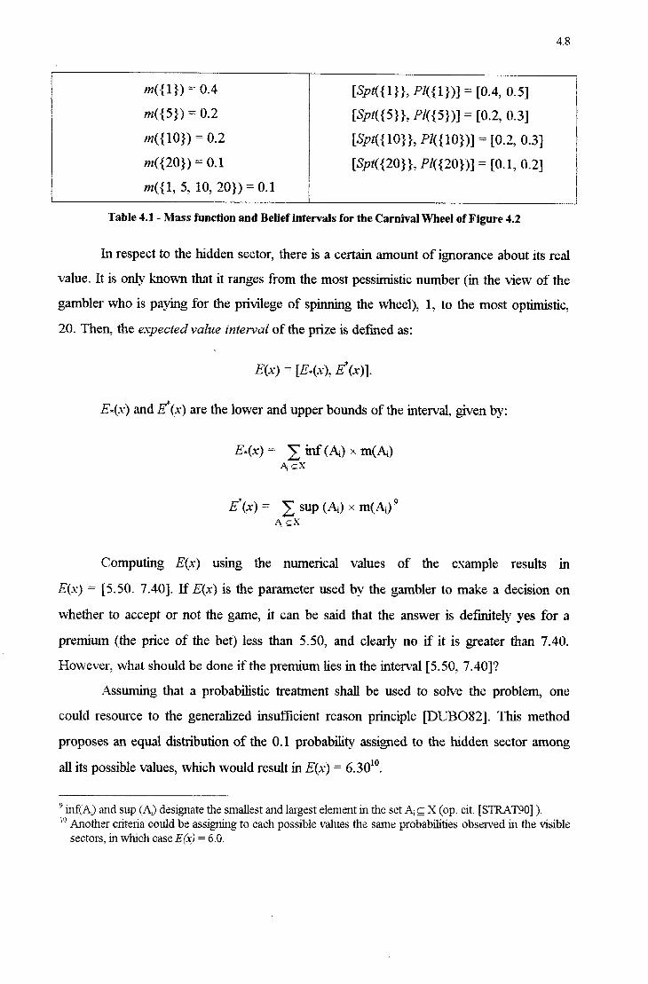
4.8

m({1}› = 0-4 [S'pr({1}}, Pl({1})] = [0-4., 0-51 zzz‹_{5}f› = 0.2 [spz({5}}, P1({5})] = [0.2, 0.3] ››z({10}) = 0.2 [spz({10}}, Pz({10})] = [0.2, 0.3] m‹§{20;›) = 0.1 [sp¢({20};», Pz<_'{20;»'›] = [0.1, 0.2] »z({1, 5, 10, 20;) = 0.1

Table 4.1 - Mass function and Belief intervals for the Carnival VVheel of Figure 4.2

In respect to the hidden sector, there is a certain amount of ignorance about its real value. It is only known that it ranges from the most pessimistic number (in the view of the gambler who is paying for the privilege of spinning the wheel), 1, to the most optimistic, 20. Then, the expected value interval of the prize is defined as:

E‹.»=› = [Ez‹‹.›zí›, E*‹.-0›1.

E *(x) and E*(x) are the lower and upper bounds of the interval, given by:

Ez~‹.×~› = 2 inf‹fv› mm A¡‹;X

E*(.×-) = 2 sup (Ag m‹_A,)” Ps :X

Computing E(_x) using the numeiical values of the example results in

E(_x_`) = [5.50. 7.40]. If E(x`) is the parameter used by the gambler to make a decision on Whether to accept or not the game, it can be said that the answer is defmitely yes for a

premium (the price of the bet) less than 5.50, and clearly no if it is greater than 7.40. However, What should be done if the premium lies in the interval [5.50_, 7.40]?

Assuming that a probabilistic treatment shall be used to solve the problem, one could resource to the generalized insufficient reason piinciple [DUBO82]. This method proposes an equal distribution of the 0.1 probability assigned to the hidden sector among all its possible values, which would result in E(x) = 6.3010.

9 inf‹_fA¡:j› and sup (A-,`) designate the smallest and largest element in the set A, Q X (op. cit. [STRAT90] ). m Another ciitena. could be assigning to each possible values the same probabilities observed in the visible sectors, in Which case E {Í›.j) = 6.0.

4.9

Altematively, Strat suggests an approach where the belief regarding either the

pessimistic (1) or the optimistic outcome (20) are parametrized by an unknown probability p, ensuing:

probability (hidden sector contains 20) =p probability (hidden sector contains 1) = 1- p

Taking into account the known frequencies and the parameter p and perfomiing a

simple calculation, the expected value of the prize is E(x) = 5.50 + l.90p. Using E(x) as the decision criteria, the gambler Would have to compare the premium with the prize that results from an estimated p. In the example, the feasible interval of the prize to be yielded from the camival wheel corresponds to p=0 and p=l, that is [5.50, 7.401. The two extreme values correspond to the most pessinzístic and most optízrzistic assessment, respectively.

In the referred work (op. cit. [STRAT90]), the author proves that the expected

utility E(x) attained from a prospective interval is given by

Ea-_) = 13..‹_.z~) + p[E*(.›z) - E-..(.›z)] Ea. 4.9

Where E».(x) and E*.(xf)] are the most pessz'rní.s'tic and most optimistíc appraisals, in that

order, and p is the probability of the occurrence of the most favorable outcome.

According to this procedure, E(x) has the role of a. distinguished point within the

feasible inteival, bounded by E}«(x) and E*(x)“. _

The question now tums to the adequate selection of p. In the original approach, the probability p is supposed be obtained from previous data. In the model that is

developed in Chapter 6 of the present work, the assessment. of pu, though still based on the available evidential information, has a different connotation. It is interpreted as a

pararneter that the decision maker employs to predict the degree of inte›:.s'ít1.= with which a

future event will be in its favor. It is important to stress this distinction, since the method

“ E -.(›{) and E Tx) are taken as the Support and Plazzsibility of x, respectively. 12 In Chapter 6, the corresponding variable is termed Âfgi .

4.10

that. is adopted to forecast p in the cited model does not rely on statistically significant data, but on incidental figures dynamically conveyed from the simulation process.

4.2.4 - Fuzzy Set Theory

The underlying concept of a fuzzy set is quite simple, yet intuitively appealing for the modeling of real World situations and problems. The advantages of the use of fuzzy sets are greatly amplified when one is trying to mirror the way an human decision maker reasons. For example, if a person is confifonted with a purchase decision, it Will most likely translate the present numeric variables to a qualitative scale, like eapensive, qfiordable,

dependable, etc, operate them in this environment and fmally make the decision. If the item under consideration is indiyisible, the solution will be dichotomous, whereas otherwise an

arbitrated amount is the output of the process.

Given an universe of d_iscourse X and a subset S Q X, an element xe X may belong paitially to S. This is equivalent to saying that the boundary of S is not sharp, therefore

ensuing diiferent possible degrees of membership of x in S. More specifically, S can be associated to a characteristíc function which maps any element xe in an interval [0, 1],

that is, ›

1.15: X-› [0, 1]

So, a fuzzy set S is described by a. set. of ordered pairs {x, uS(x)}, where ¡ÇtS(x`) is

called the membership function of the element x in the fuzzy set S. When the universe of discourse X is the real line, uS(x) can be represented by a. functional form. is a set of n

discrete points x¡, i =l, 2, n, p.S(x¡) must be expressed by the set of pairs

{ u5(_x1`)/Írl, u,S(_x-¿`)/.5:¿, ..., ;,\z5(x,,`),/Ívcn }, Which is also a form of representation of the fuzzy set

S. Figure 4.3 illustrates some common classes of membership functions.

The triangular and the trapezoidal shapes are by far the most customarily utilized

foims of depicting a fixzzy set . One reason for that preference is the convenience of

4.11

designating p.S(x,,) by linear fimctions, that, neveitheless can be modified by the

introduction of linguistic hedges”. F urthennore, the form of the fuzzy set representing a

certain domain should not be a. crucial aspect of the technique, hence the widespread use of simple linear shapesm.

_t1S'í.-K)

.z. _. .za j. .:, -, .;,.:..1_ .:, .j. .:..¿ .z..:_.;_.- `.,-_›_.:z;¿'§_z";._~»_1 .z.¿. {.-j. .:_ .:_._ _

__

Figure 4.3 - Some shapes oommonly employed for the membership function ps (x) representing a Fuzzy Set S.

Definitions

0 If there exists at least one element x belonging to the universe of discourse X such that its membership grade in a fuzzy subset B ‹; X is equal to 1, then B is denominated normal; otherwise, B is called subnormal”.

<,> The largest membership grade of any element of a fuzzy set B is the height of B; Therefore, if B is normal, its height is 1.

{.> Given ao fuzzy subset B, all elements x whose grade of membership p.B(x) i O

constitute a crisp set called the support of B, being denoted by

13 Linguistic hedges, or modifiers, operates on an original fuzzy qualification, expressed by an elementfs membership grade in a fuzzy set, and yields a. new characterization foi the element. See section 4.4. M Going still further if a svstem is too sensitive to the form of the membership fiinction at some point, maybe it should be the case to consider using an alteinative process for the solution of the problem being modeled ( Classroom notes from lectures on Fuzzy Sets given by Dr. A. Kandel, University of South Florida, Tampa, FL, Sept. 1994).

15 ~

After op. cit. {YAGE94].

4.12

Su1›1›‹Bl›=tx\»z‹x›>0, xêxi EM-1°

O The core of a fuzzy subset B ‹;X is the crisp set of X whose elements obey the condition:

Core (B) = [xi ¡.tB(x) > 1, xe .X1 EQ- 4-11

<`;~ Assuming B and C are two fuzzy subsets of X, if uB(x) 2 uC(x) V xe X, than C is a subset of (or contained in) B, C C B. On the other hand, if ttB(x) = tt¢(x) `r/

xe X, B and C are said to be equal. Consider, for example, B={0.3/r, 0.2/s,

0.6/t} and C={0.2/r, 0.2/s, 0.5/t}. In this case, C C B, or C is a subset of B, but B is nor a subset of C. The implication of this definition is that neither fuzzy subsethood nor supersethood admits gradations, hence insinuating an

accruement of the old black and white paradigm. This interesting question was

addressed by Kosko [KOSK9'2], Where he proposes an altemate approach,

making use of the concept of a. filzzy set as a point in a hypercube.

O The power M(A) of a fuzzy subset A is equivalent to its cardinality, sometimes called E-count (sigma.-count), denoted bylóz

M‹A›=2zzA‹x,›. E"-“Z i=1

Although the successful and efiicient application of fuzzy set theory in several

fields is an already established fact, as certain dispute between the latter and the classical

probabilistic approach to uncertainty is expected to endure. Yet, some effons have been

aimed at reconciling these two concepts, in the sense of correctly identifying the situations

16 The cardinality, or power, of a fuzzy subset A must be distinguished from the power set ofA, denoted by 21* and defined as the set which contains all subsets ofA.

4.13

where it is the case for using one or the other, as, for instance, the notions of fuzzy

probability and fuzzy random variable, introduced by Kwakemaak [KWAK'78]”.

4.3 - Operations with Fuzzy Sets

4.3.1 - Basic Concepts

<> Union of A and B: A ~._› B = C.

HCÍÍ) Z HA(~\`) V HBÍX) Z max [P-A(xi)› I~íB(x)].» VX '5 X EW “U3

O Intersection of A and B: A fz B = D. The union operator corresponds to the logical and, denoted by, such that

!›LD(x) = Ha(~`¿) ^ P‹B(.~\') = mm [HA(~\')z IJ»B(_x)l_¬ VX E Eq' 4-"

The union and intersection operations, performed by the max-min operators are of great importance in the fuzzy set theory, and have several distinguished properties.

Some of them are listed below, where a, b and c are membership grades of an arbitraiy element e X in the fuzzy sets A, B and C, respectively.

- min (0, a) = 0 for any a ¬¬¢ 0; - max(_1,a`)=1foranya:-#1;

- min (_a, a) = max (Ia, a`) for any a :: 1;”

- min (a, bf) = min(b, a); max (a, b)= max (_b, af); :> Commutativity

- min (min (a, b), c) = min(a, min (vb, c)) = min(_a, b, c), and - max (_max(a, b), c) = max(a, max (b, 0)): max(a, b, c); :> Associativitylg

17 These notions are based on what is called degree oƒrealization of a certain condition. For example, if

18

19

tever is associated With influenza, then each condition (fever and influenza) can be described by an obsewer or expert as “moderately fulfilled”, “hardly fulfilled”, etc. So, one can calculate a fuzzy probabihty that a patient has ar high fever given that the influenza is hardly realízed [BEC1K95]. A\.z'A=A .‹'\A=A Arw(Br-zC)=(Ar¬»B)f\C.=Ar¬Br\C;A\.:(VB\JC)=(AuB)\_›C.=AwB\-1C.

4.14

z min (a, max ( b, c) = max (min (a, b), min (a, c)), and ‹ max (a, min( b, c) = min (max (a, b_), max (11, 0)); => Distributivitym

';'.'> Bounded sum: D = A Q9 B, Which means that the bounded sum of the fuzzy sets A and B is the fuzzy set D. The grade of membership in D is the sum of memberships in each fuzzy set A and B, with an upper limit of 121:

H1›(1") = min (.HA(-Y) + Hsí.-YÍ), 1) EW 415

If A and B are crisp sets, than A G3 B would be reduced to A u B.

Figure 4.4 illustrates the behavior of the min, max and bounded sum operators.

bounded sum ( a, |,tB(,\{`_§|) um) 1. ,z- / ' _.~

,' / I' .-'J - ./

J

I.. `/ *_“ '\ m=»z‹ 3, zz»z<.=‹;››

a ' - - - - - - - - _ - '\

._~_ / ._,

, \-.._\ min( a , LL¡z,(x_ÍJ)

/ hi.-~

U” a 1H1afÃX.Í'

Figure 4.4 - Comparison of min, max and bounded sum operators

Negation (or complement): not-A = A = X - A;

/~¿_¡(_«\') : 1 ' lJ»A(.~\") 1;q_ 4_16

2 ° A rw ( B L.) CI) = (A rw B) LJ (A rw C1_`)j, A U (B rw C ) = (A u B) rw (Au C- ). 2* Smith (op.cít. [SMIT87] ,ÍJ desígnates the bounded sum, as defmed, as an union operator, but he also

considers the zíntersectzion or and-bounded sum, which is defined as untjx) = max (0, u,,_(,\~) + uB(_x`)-1"). In the latter case, ifA and B are crisp sets, D= A rw B. '

4.15

<> De Morgan's Law:

max ‹›zA‹x›, ›zzz‹›-›› = 1 - min ‹‹1- ›z,\‹«-››_, (1-›»B‹x››” E.,W *O Product operatoisz analog to those defined for joint probabilities of two

independent events. For two fuzzy subsets A and B, comes:

Intersection: AF-.B = ¡.LA(x¡) * pB(x¡) EQ- 4-l3(fl)

UÚÍOHÍ AUB Z P‹».(~`f¡) * l›1~B(~`‹`{) " I›LA(-Vi) * l›*B(~\"â) Eq' 4'13(›b)

O Ot-level set: Given a. filzzy subset A ‹: X, the oc-level set of A (also called oi- cut), denoted by Aa, is a crisp set containing all elements x whose membership

grade in A are equal or greater than og, ot e[0, 1]23. Therefore,

Au = txt ‹tzA‹x› oz V z- Jo. EQ- +19

With the concept of an ot-level set, it is possible to represent any fuzzy set by

means of crisp sets corresponding to its oa-cuts [WANG92], [YAGE94].

Defining a fuzzy subset F = o¿A such that

V A oc ifx‹;F

r p_F(_x) : HOLA (x) = .{O if x É F foran§oc[0,l].

then

A = U‹~zAa «qnd

Example:

22 The following propenies a1soholdu11de1'De 1\~'Io1'gan`s Law: not-(Ai-/B)=(i1ot-A) r¬. (not-B); not(AnB`)= (not-A) t_.› (not-B).

23 A ot-strong cut is described by Am» = {xi (}tA(_,rf) > ot, V .r E X}.

4.16

ot = 0.4 X={p, q, r, s, t}; A: { 0.1/p, 0.3/q, 1/r, 0.6/s, 0.9/t}; oLA = F = {O/p, Ofq, 1/r, 0.6/s_, 0.9/`t} (Fuzzy subset); A., = {r, s, t } (Crisp subset).

If ot varies, assuming its possible values in [0,1]_, the union of all erisp sets OLAQ

will then result in the fuzzy set A.

4.3.2 - The Extension Principle

The extension prineiple is an important notion of the Fuzzy Set Theory. It provides a rule for associating the elements of two or more fuzzy subsets.

Suppose X and Y are crisp sets, A and B two fuzzy sets andf is a function such that f: X-› Y, and ƒ(`x`) = y, x E X , y E Y. If A ‹: X, _ƒ(A_) is a fuzzy subset of F with the provem'

_

JÍA) = Uz {(uA(‹\*)/ƒ(X)}- Eq. 4.20

The basic concept that underlies the extension prineiple is a supremum of pairwkise minz'ma [KOSK92]24. In a more general and formal definition, the extension principle

performs a mapping: jí F(2X) -› F(*W), where F(2Y), F(2Y) are the fuzzy power sets” ofX and Y, respectively.

Example:

Assume X={$1, $4, $9} (prices of an item), and Í' ={VERY LOW, LOW, MEDIUM, HIGH, VERY HIGH} (perceived characteristics of the price of an item). Suppose that the functionfis defined as:

ƒ( If) = Low

24 ln this work, Kosko critieizes the extension principle, arguing it is complicated, With the tendency to push fuzzy theory into largely inaccessible regions of abstract mathematics...”, and “...achieves generality at the price of txiviality.” ( op. cit., p. 300).

25 The sets of all fuzzy subsets ofX and)',1'espective1y.

4.1"

j(4) = MEDIUM

ƒ( 9) = VERY HIGH

subset A = { 0.6./1, 0.8/4, 0.1/9}. Then,

ƒ(jA_`)={0.6/ LoW}\_› {0.8/' ME.D1UM}«__› {0.1/ vERY1¬11GH}

ƒ(A)=* {O.6/ Low, 0.8/ MEDIUM , 0.1/` VERY H1GH}

Denominating B =ƒ(A), then B is a fuzzy subset of Y, such that V y e Y,

»B‹››í› =

an xz¿¿z¿§:y t‹i»A‹x›1.

4.3.3 - 'Triangular Norms and Co-Norms

Triangular norrns (t-norms) and eo-norms (t-conorms) are operators T and S that perform an aggregation of fuzzy subsets, so that. they induce a. mapping from a pair of membership grades into another, at this time regarding the fuzzy set that was originated from the respective aggregation operation.

T: [0, 1] .=< [0, 1] -› [0,1] (t.-noim)

S: [O, 1] >< [0, 1] -› [0,1] (t-eonorm)

The min and the intersection product operators are examples t-norms, while the max, union product and bounded sum are instances of t-eo-norms.

Given a and b, two arbitrary membership grades in two different filzzy sets,

a t-noim T(a_, b) operator must have the properties:

. T(a, b) = T(b, a) (Commutativity);

. T(a, T(_b, c)) = T(T(a, b), c) (_Associativity);

. T(a, b) T(a, c) when b í c (Monotonicity);

. T(a, 1) = 1 (One Identity).

4.18

A t-cononn (also called s-norm), denoted by S(_a, 5), shares identical properties

with the t-norm, With the exception of the One-Idenrzízy, that is replaced by the Zero-

Identily, so that S(a, 1) = 0.

The conditions of distributivity and idempotency are not. present. in t-norms and s-

norms. Other pairs of T(.) and S( _) operators are cited in the literature, such as the Log operatorszó, the Lorentzian operators” and the Yager operators” [SMIT87].

4.3.4 - The Fuzzy Integral

The fuzzy integral is intimately related to the concept of fuzzy measures, presented in section 4.2.2. It was introduced by Sugeno [SUGE77] is a convenient way of aggregating multiple quality factors of an object, with the objective of yielding a single

synthetic evaluation index [TAHA90], [WANG92] [YAGE93]. Suppose V= {v,, vz, ..., v,,} is a. finite set. of factors regarding all the aspects, or

qualities, of an object under appraisal. V is the jàzctor space of the object. Now, the global evaluation is supposed to be reached taking into consideration the assessment of each

aspect of the factor space V, which are not equally important. One of the most common solutions for this kind of problems is the weighted mean, which is based on the assumption

that the factors are independent and therefore additive.

If a real number g(E) in the interval [0, 1] is associated to each subset E Q V, indicating its importance in the global evaluation, this number should reflect the best judgment that could be made of the item considering only the factors that are present. in the subset E. The function g(.) obeys the conditions g(QÍ5)=0, g(V)=1 and if E C F C V, then g(_`E_`) g(Ff)29, and is a fuzzy measure on (V, ZV).

25 Tila, bÂÍ>=10gz[1+(<ÂS°-1)tI.S”-1))/(S-1)] _; Sta.. bl): 1-1°g.[1+ ((S"° -l)(S1"” -1)Í>f'<ÍS-1)]-

2? T‹jzz, 1›)= zzz›.z'(2-fz-z›+zz1›) , s‹;'zz, b)= (zz+1›j›,f(1+zzz›j›.

23 T(a, b)= 1-minll, [(1-a`)' + (_ I-b`)'11'“' , S(a, b`)= min[l, (at + b')"'1, for t lz 1. In the Yager operator, when t=l, it becomes the bounded sum pair (see footnote 21) and When t-›<›0, it transtbnns into the min-max pair.

29 Qi is the empty set; In Chapter 6 the fimctions g(,)and h(.) are designated ¢(.) and 0t(Í."), respectively.

4.19

In the object”s judgment process, for each of the factors v¡ e V, a score h(v¡`) -5

[0,1] is settled by the examiner. Then, g(v¡) and h(_v¡) are compounded by means of a fuzzy

integral, denoted by Liz ôg 3°, corresponding to a syntízetú: evaluation of the item.

Li? Ôg = max [min (;min(h(v`)), g(Ef))] Eq. 4.21 E C V v e E

A good explanation for the workings of the fuzzy integral is given by Yager

[YAGE94]. The function g(E) is a measure of how the subset of factors E fulfills the importance concept, characterized by g. Note that g(_E) should be estimated independently

and ahead of the examination of the specific object under appraisal, therefore consisting in

a widely accredited postulation. On the other hand, h(v_`) regards the degree of satisfaction

of a particular subset of qualities pertaining the object. Thus, h(v) coiresponds to the score

to be attributed to that subset.. The operation min h(v) over all the elements V E E supplies

the extent. to which these elements satisfy h. The portion [min (min(_h(v)), of the

fuzzy integral matches the degree to which all v e E carry out the demands brought. into the process by the functions g and h simultaneously. Finally, the max of all minima conceming the subsets E is taken, yielding What is called the ob_iect”s symfhetic evaluation.

The fuzzy integral plays an important role in this dissertation, since it was the

method of aggregation chosen to compound the factors concerning the judgment. of an item by a Consumer, according to the model described in Chapter 6. For this reason, an

illustrative exainplem depicting the modus operandi of the fuzzy integral is presented.

Example

Suppose a potential buyer is evaluating a. certain model of a. car, and the features

that are being taken into consideration in the analysis are pefƒormzmce (P), congfort (C) and

3° In Chapter 6, the fuzzy integral is depic-ted by Lo: Ôø .

31 The example Was inspired and is an adaptation of the problem of “evaluating a Chinese dish”, in op. cit [WANG92], p.l85.

4.20

price (M). Hence, these are the qualilies orĈctors vi, i=1, 2, 3, of the object, the car, and V= {P, C, M}. The set function g(_{.}) appoints an importance measure to the subsets that result from the possible combinations that can be formed employing the individual factors P, C and M. The arbitrated values of g(.) for the example are:

g({P}) = 0.2 g({P, Cš) = 0-3

g({c}_) = 0.0 g({P, M}) = 0.9

s({M}) = 0-6 g({C, M}) = 0z7

and g({V}) = 1

The values of g({.}) do not have the additive property, that is present in the

traditional Weighted mean method. The explanation for the assignment of zero to g({C}`) is that the factor comfort, taken isolated, does not have any importance in the item"s

appraisal. Conversely, another peculiar aspect is that the factors can exhibit a. murual

reinforcement effect when taken together, as shown by the pairs {P, C}, {P, M}, { C, l\/I}. Then, to each factor, a score h(_v¡_) is adjudicated, assumed as

h(P) = 0.4 h(_C) = 0.6 h(_l\/I) = 0.7.

min h(_v¡) = h(P`) = 0.4; min h(v¡) Works as the parameter ot of an oc-level subset Eu of V, such that Ea = {v

í h(v¡) L: ot }. In other words, EC, is the collection of importance factors

whose scores are greater than or equal to min h(v¡), Which obviously correspond to the

Whole set of importance factors, V. Therefore, g(E.,_=0_4) = g(V)== 1.

The other values of g(Ea`) for ot min h(v¡) are determined in a similar Way, so

Eazofi = V - P = {C, M}; g(E,,=0_6`) = g(C, l\/I) = 0.7 and g(l\/I) = 0.6.

Éh ag = max [m¡n[0.4, 11, m¡n[0.ó, 0.71, mm[0.7, 0.61]

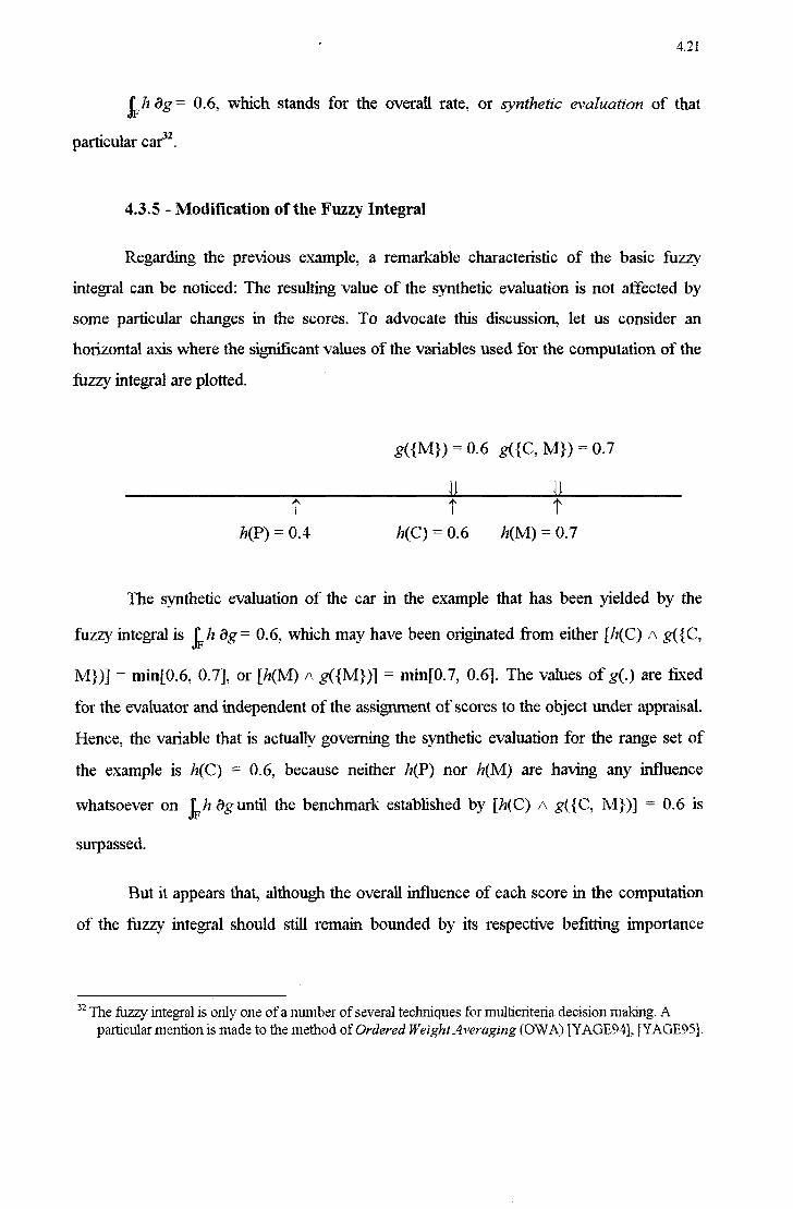
4.21

kh ôg= 0.6, which stands for the overall rate, or sjynthetíc evaluation of that particular car”.

4.3.5 - Modification of the Fuzzy Integral

Regarding the previous example, a remarkable characteristic of the basic fuzzy

integral can be noticed: The resulting value of the synthetic evaluation is not affected by some particular changes in the scores. To advocate this discussion, let us consider an

horizontal axis where the significant. values of the variables used for the computation of the

fuzzy integal are plotted.

8({M}) = 0-6 £({C.z M}) = 0-7

ll ll

T T T h(_P) = 0.4 1›z(c) = 0.6 1z(M)= 0.7

The synthetic evaluation of the car in the example that has been yielded by the

fuzzy integral is kl: ôg= 0.6, Which may have been originated from either [h(_C.) ,f\ g(_i{C,

M})] = min[0.6, 0.7], or [h(M) A g({M})] = n1in[0.7, 0.6]. The values of g(.) are fixed for the evaluator and independent of the assigmnent of scores to the object under appraisal.

Hence, the variable that is actually governing the synthetic evaluation for the range set of

the example is h(C) = 0.6, because neither h(_'P) nor h(M) are having any infiuence

whatsoever on kh âg until the benchmark established by [h(_C) A g(_{C, M}`)] = 0.6 is

suipassed.

But it appears that, although the overall influence of each score in the computation

of the filzzy integral should still remain bounded by its respective befitting importance

'32 The fuzzy integral is only one of a number of several techniques for multiciiteria. decision making. A particular mention is made to the method of Ordereâ Weiglzrfiver-aging (OWA) [YAGE94], [YAGE95].

4.22

factor, an adjustment inkh ôg should be promoted to contemplate some variations in the

attributes h(C`). For instance, suppose that in the example presented, the value of h(P) has assumed a different value. In this case, h(P) could lie anywhere between zero and h(C) =

0.6, Without having any impact on LI: ôg = 0.6. Therefore, if an evaluator relies solely on

the value yielded by the original fuzzy integral, it would be completely indifferent, in the situation depicted, to two items with scores regarding those extreme points [0_, O.6]. In

order to overpass this intuitively undue feature of the original fuzzy integral, a correction

composed of an increment (A+) and a decrement (AÍ) is proposed. The reasoning

concerning this correction is as follows:

1. As the fuzzy integral is defmed as a maximum operation over two or more minima, which on their tum are always represented by intersections of two fuzzy measures

(score and importance), the final value yielded by LI: ôg must be necessarily equal to

one of those minima, which is heneeforth designated as the gmerning value ot

LI: ôg 33.

2. The variations of the scores conceming the non-goveming measures, which originally

do not affect Lh õg if their associated minima are less than the goveming value, will

be now accounted for. The ranges of relevant variations are always restrained by (a) o f>

the governing value (li (.) or g"'(.`)), (b) the other scores (_`h(_`.f)`) and (cf) the importance

factor g(_.) that is associated with the score under consideration.

3. Each relevant variation may consist of either an increment or decrement over Lh ôg ,

depending on whether it is greater or lesser than the governing value, and taken as the

difference between it and the nearest of ( a), (b) or (c) described above”.

33 If there are two or more equal minima, each ofthern is separately picked as the goveming value. 34 In other words, the absolute value of the relevant. variation to be accounted for is the minimum of the

absolute values of the differences between the attribute under consideration and each one of (a), (bi) or (fc).

4.23

4. The inerement (A+) and the decrement (zí\`) to be added to Liz âg results from

weighting each relevant variation to a function of the importance factor isolatedly

associated to it”.

5. The final synthetic evaluation of the item shall then be given by 11:11 ôg + A+ + A".

Example:

Taking the governing value of Liz ôg as [h(C) /\. g({C, M})] = min[0.6, 0.7] = 0.6,

(aí) = h(C) = 0.6;

(b) = { h(P) = 0.4; Í*1(1\/l)= 0.7 };

(c') = g(_C, M) = 0.7 and g(P) = g(V`) = 1 (because h(P) = min(h(P), h(_C.), h(M)f) and the weights as g(.) themselves, comes:

A+ (M) = g(M) >< max[0, (h(M) - max(h(C), g(M))] = 0.6 (0.7 ~ 0.6) = 0.06;

A- (C) = g(C) r›< min[0, ('h(C) - min(h(C), g(_Cf))] = 0.7 >‹ (0.6 - 0.6) = 0.0;

A" (P) = g(_P) >< min[0, (h(C') - min(h(C), g(P))] = 0.2 1‹: (0.6 - 0.6) = 0.0;

Then, the fmal synthetic evaluation of the car of the example would be

[Fiz ôg+ A*(1\z1)= 0.6 + 0.06 = 0.66.

Discussion:

+ _ The increment A (M) - 0.06 resulting from the method proposed above tries to mirror an extra advantage that the evaluator is assigning to the car due to its score of Price

h(M). That gain represents the difference 0.1 relative the actual score and an inferior one,

(which for the present purpose is limited to the goveming value of 0.6), that could have

35 The function can be the importance factor itsielf. In the Chapter 6, this method has been applied using the weights g(.`) for the increments (gains) and g(_,)* for the decrements (losses).

4.24

been assigned to h(M) without interfering with the basic Lh ôg = 0.6. It has weighted by g(M) = 0.6, thus yielding 0.06.

Consideiing that the original fuzzy integral consists only of minima. and a. maximum operations, its possible values must necessarily be one of the intervening variables l1(.) g(.). With the proposed method, an hybrid approach is performed, With the convenience of making intennediary results possible. This system of performing a synthetic evaluation of an item with fuzzy measures will be employed in the application of a one-sided fuzzy iterated P1isoner”s Dilemma. presented in the Chapter 6 of this Dissertation.

4.3.6 - Linguistic Hedges

The imprecise terms usually employed to denominate fuzzy sets, such as HIGH,

LOW, ATTRACTIVE, etc., can also undergo alterations by linguistic modifiers or hedges.

F ormally, a linguistic' hedge 6 operates on an original fuzzy qualification Q¡,

accomplishing a new characterization R¡= e(Q¡`). For example, the label “expensive”

describing the price of an item can be reinforced by the hedge “very”36. The resulting concept “very expensive” is still fuzzy, but with a. different mapping rule from the

numerical value of the price to the interval [0, 1]. Conversely, one can anive at the notion

**moderately expensive” using a symmetiic line of reasoning. In this latter case, the hedge “moderately”37 functions as a weakening modifier [ZADE72]. The new membership grade of an element of the universe of discourse in an fuzzy set altered by a. linguistic hedge is

generally expressed by a. 'power of the original grade. The exponents 2 and É are usually

employed to represent “very” and “moderately”, respectively. In this way, uR¡(x) = [uQ¡(x)]3 for 6 = “very” and ¡.LR¡(x`) = [uQ¡(x`)]š for 6' = “moderately”. The graphical representation of a

standard fuzzy set and those resulting from the applications of those linguistic hedges is

shown in figure 4.5.

'36 In the application model detailed in the Chapter 6 of this work, the tenn “very”, rather than a linguistic modifier, is utilized to design an autonomous fuzzy set, when attached to other adjectival denominations, such as high or sensitive, for instance.

37 Also equivalent to “more or less” or “sort of”.

4.25

^ Mx] 1 uonfnmfn' caem» /,T

[.uÍX1ii1£2/ \\/ usar Ex|›Eus|irE _/ ¡'/

1

z׋›z«swz »‹×z›,>~\ /'

i

\ \ /Í df'

2 pg

..

PO

__ ./ *“

camp _/ 1

\ J/ ~

/ ___, \ / . / A

\`l/ z/ _.,/'fd̓¡›(K_'¿-]]¿

| § K i

1 ___.-f""'-F,t

X _

Figure 4.5 Example of Fuzzy Sets that result from the Application of Linguistic Hedges

Linguistic hedges can have basically two kinds of effect on the original concept:

Concentration, like the modifier “very”_, which brings about an intensification. or

reinforcement of the 'foregoing trait, and dilation, that consigns an expansion or

wezzkening of the object°s primary feature. The generalization of the concentration and dilation operators admits any exponents other than the original 2 and 1/2. When the exponent is greater than 1, a concentration effect betides, and smaller membership degrees

result. On the other hand, an exponent smaller than 1 implies in a dilation of the basal qualification, which produces greater membership values. The points xz and xl in Figure 4.5 illustrate the former and latter operators, in that order.

An elaboration of the idea of expanding and contracting basic fuzzy sets has been adopted in Chapter 6. There, a. Consumer°s perceptions regarding the price and the quality

of an item are affected by linguistic-like operators that act on the fuzzy sets employed to

qualify these attributes, in the form of exponents taken as ñmctions of the specific

characteristics of an individual.

In addition to the better known concentration and dilation hedges, Zadeh

[ZADE72] also explored contrast intensification and contrast diffusion modifiers. In the former, a fuzzy set is made less fuzzy by increasing membership values above 0.5 and

4.26

decreasing those below 0.5, thereby moving all membership degrees closer to either zero or one. In the latter, the membership values are hea.ded for 0.5, and in this case boosting the fuzziness of the set [SMÍlT87].

In theory, there are no formal rules defining the exact quantitative influence of linguistic modifiers over fiizzy sets, and it can be said that the assignment of a numeric value to an exponent associated to a hedge is a quite subjective matter. Table 4 [COX95] lists a. sample of feasible hedges.

1%:íšfff5fíí5ííâí;z§â§;¿» ' "'

"f;5§:5_í:~:§z;§;z§;Iízgâzizsiââãâisí fffiífzfšffzfí:5§š;EÍ5§;5í;;%:f

E¿}šÍ®[-f,íz§š«_1í;íÍ~_šÍ-Vflip; _ 4

{š.`íšI_;§;E5;šÉ;1ɧš§§š¿š5; š1jz§1š;§š§íE§§;âNQ§EE¿i;,i¿5;㧧išz§š¿i.1§š:

Ê%Í5íÊÊ?ÊÊ5Ê555Ê5§ÍFÊÊí ÊÉÊÍÉÊZÉÊÊ5ÊÊ5ÊÊ5§ÊÊÊí§Êí5Í%§í ÊfÊ5í§Ê5§Ê35i5§Ê*?ÊÊ55§¢ÊÍí¿iÊÊ:5ÊÍÊz

'fi -5zéij5:;51.5~55::NQM1INAm;Méí§:zf:f1:~=:f1 fz55§zfí5'55:ííFfEAlR~l¿M5š552:;5F;§i§5ë5~5zI1?›5I5 .-

'-Ê¡íÍz .íšÍ¿ÊiÍ¡.% .zz.- zzz; .z::z-...z 5ííÍ1?'zlíÊ-ÍiÍÊfÍ;- *Í:íÊíÍiÉ&z .z.:.-:.z:zzzz~:zz:z::›z zzzz â zzzzz-.F-E Í z1'*§iÉã1Í%i§ííÊí&iiÊiÍÊ

Table 4.2 - A Sample of Linguisfic Hedges

An outstanding feature of linguistic modifiers is their ability in providing means of approximating a fact intended as a. premise of a. rule. In this way, in the realm of fuzzy

logic, a conclusion can be deducted even if the premise is only roughly or incompletely

satisfied [BOUC-921. The topics of implication rules and fuzzy expert systems are

approached in the next section.

4.27

4.4- Fuzzy Expert Systems

4.4.1 - General Discussion

The initial project for developing artificial intelligence systems was quite ambitious, and the objective in the early sixties was to build general problem-solving programs, like the system proposed by Newell and Simon [FEIG63]38. Due to preliminary unsuccessful attempts in this direction, the focus turned to the discovery efficient algorithms capable of

dealing With large and complex data. structures, but limited to specific subject domains

[F OGE95]. So, the term expert .szvstezn was coined, and its functioning relied on information that had been previously retrieved from human experts and stored in the form of a program in a computer, usually employing the language LISP (1962) and later PROLOG (1972).

An expert system consists piimaiily of a knowledge base and an inference engine, which searches the former in order to check if there are any facts that match the queries posed to the system.

Example of representation of facts and a rule in pseudo-Prolog code:

. high(Price, Price 5); ::> fact

. very_sensitive( S, S 2 2.5); :> fact

. gif {(P11`ce 5) and (S 2.5)} :> rule

then attractiveness(_Price, unattractive);

When a uerv such as ?- - attractiveness rice, X)39, the inference en `

e ex lores Q . 8111 P the structure of facts and rules to determine the category of

If the elements in the knowledge are co1y`ectures, rather than facts, and diverse

truth values (or degrees of confidence) are ascribed to those elements by specialists, than a

collection of production rules of the type { IF premise THEN conclusion > can be created and assessed in order to answer' a variety of queries posed to the system, even though the

conjectures are matched only partially.

39' “GPS: A Program that Simulates Human Thought” 39 X is a. linguistic variable that qualifies the numenc variable “Pnc-e” in terms of “attractiveness

4.28

40 The first program to use this schema was DENDRAL , started in the mid-sixties

and improved along the subsequent years. The Well-known medical program MY C1N“ used several ideas successfiilly introduced by the DENDRAL project. Another outstanding expert system was PROSPECT, which was employed as a geological exploration aid and had more than one thousand rules [FOGE95].

Despite their relative success and accomplishments, expert systems have been

sometimes criticized in their ability to represent human intelligence. One point often mentioned regards the difliculty of capturing the behavior of complex cognitive systems with an assortment of facts and rules. As a reply to those critics, it should be said that

perhaps too much is being expected from expert systems in terms “intelligence” as only mirroring What is generally accepted and understood as the human course of action. Unquestionably, a human decision maker, While much more versatile in the mental

manipulation and association of facts, hypothesis and conclusions, usually falls behind the

performance of an expert. system when the decision tree has too many branches and levels. In those circumstances, the computer on which the expert system is running is then playing

the role of a facts-and-rules-cruncher, in substitution of the customary denomination of

nzunber-cmncher, and this task is significant in the treatment and solution of an a great

number of problems in assorted areas of interest.u

A question that has been recently occupying the thoughts of researchers in the field of artificial intelligence is the counterpoise of expert knowledge and general intelligence.

Hofstadter [HOF S95] comments about What he calls the expert .gvsterns trap, “... the idea

that the key to all intelligence is just. knowledge, knowledge, and ever more knowledge.”

He admits that “some domain knowledge is necessary to get off the ground” but

understands intelligence as having “a powerful, general and abstract knowledge-

independent core”.42

4° DENDRAL is a chernistry program that provided infonnation about the molecular st1uct1u'e of unknown compounds, based on their mass spectral and nuclear magnetic response data.

41 MYCIN diagnosed bacterial infection in hospital patients. 42 Hofstadter testifies that he has known “many people who were fountains of knowledge yet seemed to

lack all insight”.

4.29

The capacity to adapt itself to dynamic environments and leam from experience are also important attributes in proficient expert. systems”. Furthemiore, in most instances, the

achievements of expert systems can be greatly enhanced by associating them with other up-to-date soft computíng techniques, such as neural networks, genetic algorithrns and

fuzzy logica] inference, yielding What is commonly called a hybrid system [HALL94]. Some fundamental topics regarding fuzzy logic and inference are presented in the next section. ~

4.4.2 - Fuzzy Logic and Fuzzy Inference

In the same manner that fuzzy sets are an extension of ordinary sets, Fuzzy Logic

is, in most aspects, a generalization of classical logic, and many of the basic concepts of the latter are also valid for the former.

Consider that and Y represent, respectively, the universes of discourse of the two vaiiables price (x) and qztaliiy (ii) of a product being sold in the market by a Firm. Suppose

thatx is qualified by the predicates {A¿}, j=1, 2, ..., m andy by {B¡}, j=1, 2,..., n. A statement involying x and aj for example, could be: x is al. ln traditional binary

or Boolean logic, a statement can only be either true or false. Under this assumption, the

truth-value tS(x`) of any statement S regarding x equals 1 if S is true, or 0, if S is false.

A composite assertion I, comprising at the same time the variables x and y of the Type

L: IF x is A, THEN y is Bj, §í.v-;/ \-__@v-.__../

statement P statement Q

43 An example ofa dim-Witted biological expert system is given by the French naturalist J. H.Fabré, cited in Gould and Gould [GOUL85] and [FOGE95]. When the female wasp Sphexƒlavipermis must lay its eggs, it builds a. burrow and paralyzes a limited ciicket with venorn. The cricket is intended to serve as food for the grubs alter the eggs hatch. It is then taken to the entrance of the bunow and before dragging it inside, the wasp enters the lair for inspection. If the ciicket is moved from the place where the wasp put it while it was inside the buirow, the wasp repeats the same procedure of placing the eiicket in a. particular position and entering the hole for a new inspection, no matter how many times this is done. The wasp uses a rule based system that is incapable of leaming With the erqieiience, “astounding us with its extraordinary intelligence, and, in the next moment, surprises us with its stupidity, when confronted with a simple fact that depaits from its ordinaiy practice.”

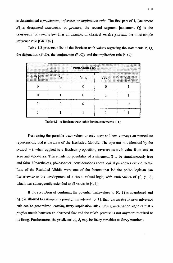
4.30

is denominated a.pr0duc11Íon, zflzference or irnplícation rule. The first part of I, [statement

P] is designated antecedem or premise; the second segment [statement Q] is the

conseguem or conclzzsion. I, is an example of classical modus ponens, the most simple inference rule [GRlF87].

Table 4.3 presents a list of the Boolean tiuth-values regarding the statements P, Q, the disjunction (P./\Q`), the conjunction (PVQ), and the implication mle P-›Q.

0 O O O 1

O 1 O 1 1

1 0 0 l O

1 1 1 1 1

Table 4.3 - A Boolean truth-table for the statements P, Q.

Restraining the possible truth-values to only zero and one conveys an immediate

repercussion, that is the Law of the Excluded Middle. The operator not (denoted by the symbol ¬), When applied to a. Boolean proposition, reveises its truth-value from one to

zero and vice-versa. This entails no possibility of a statement S to be simultaneously true and false. Nevertheless, philosophieal considerations about logical paradoxes caused by the

Law of the Excluded Middle were one of the fa.ctors that led the polish logician Jan Lukasiewicz to the development of a three- valued logic, with tmth values of {O, l},

which Was subsequently extended to all values in [O,l].

If the restriction of confining the potential truth-values to {O, l} is abandoned and

tS(x`) is allowed to assume any point in the inten/al [0, 1], then the modus ponens inference mle can be generalized, ensuing fuzzy implication rules. This generalization signifies that a.

perjfect match between an observed fact and the n1le”s premise is not anymore required to

its fiiing. Fuithermore, the predicates A,-, Bj may be fuzzy variables or fuzzy numbers.

4.31

In this Way, an approximate likeness between a fact and a n1le”s antecedent is av sufficient

condition for the rule”s activation. But this activation is not restricted to all or nothing either, and the conclusion°s truth-value will depend on the antecedent°s degree of confidence. That schema elicits a number of fuzzy implication mles. Zadeh's original

proposal for implication defines [SMIT 87]

IF P meu Q else ot*

as either (P and Q) or (¬P and 0)”.

The grade of membership of an element in a fuzzy set may cotrespond to the truth value (t;›_.,Q) ofa proposition P-›Q. tP_¡.Q, besides depending on tp and IQ, is also a. function of the particular implication rule taken into account. A implication can be interpreted

as describing a relation between two fuzzy sets [MUNA94]. Some important fuzzy implication rules and their correspondent. truth-values are displayed below.

. 1* i›~›zQ = max( min( tp, IQ), 1- tp) (Max-min implication _)

. t P_.,Q = max( 1- tp, IQ) (Arithmetic implication )

z É ifz,,':zrQ :P

. z¡,¬,Q = .. (Gogueifs implication )

*I otherwise

° ÍP-›Q : min (.1' ÍP + ÍQ› 1) ( Lukasiewicz' implication)

° Í P-1›Q : min UP» ÍQ) (_ Mamdaní's implication )

l if IQ IP Í :" í ou

1

ot o n 0 ~ 1› .Q ÍQ othemm (Godelnn imphcation )

M A synthetic expression for “If P is true, then Q is tnie, otherwise R is true”. 45 lf O is not specífied, it is inteipreted as the universe, and (¬P and 0) becomes simply ¬P.

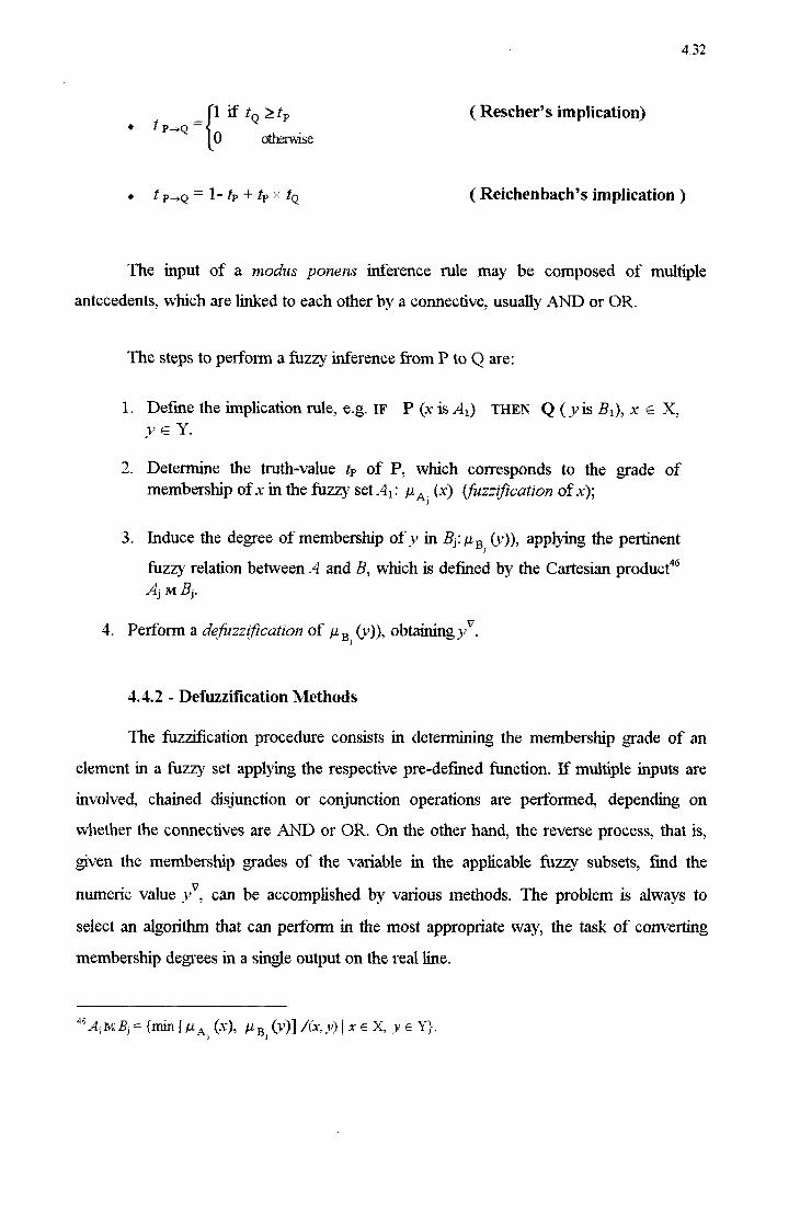
4.32

. z,,_,Q _ 1 if tQ zip ( Rescher”s implication)

0 otherwise

. tp_,Q = 1- tp + tp >< :Q (Reichenbach's implication )

The input of a. modus ponens inference rule may be composed of multiple antecedents, which are linked to each other by a connective, usually AND or OR.

The steps to perform a fuzzy inference from P to Q are:

1. Define the implication rule, e.g. IF P (x is A1) THEN Q ( yis B1), x E X, y E Y.

2. Determine the truth-value tp of P, Which corresponds to the grade of membership of x in the fuzzy set_.~'1¡: ¡uA,_ (lx) (fuzzification of x);

3. Induce the degree of membership of y in B,-: ¡.zBJ_ (5.-')), applying the pertinent fuzzy relation between and B, which is defined by the Cartesian product46 Âj M

4. Perfonn a defirzztficatvíon of ,uB¡ (y)), obtairiingyv.

4.4.2 - Defuzzification Methods

The fuzzification procedure consists in determining the membership grade of an element in a fuzzy set applying the respective pre-defmed function. If multiple inputs are

involved, chained disjunction or conjunction operations are performed, depending on

whether the connectives are AND or OR. On the other hand, the reverse process, that is, given the membership grades of the variable in the applicable subsets, fmd the numeric value yv, can be accomplished by various methods. The problem is always to

select an algorithm that can perform in the most appropriate Way, the task of converting

membership degrees in a single output. on the real line.

““'.4¡1vrB¿= {min [ ,u Ai (x), p¿B¡ (v)] /(Íx,y,`) I x e y e Y}.

4.33

There is not such a thing as the best method. He~e§efix:~e over another regarding the quality of the results depend heavily on the characteristics of the system that is being modeled.

Among the methods that are mostly often found in the literature and employed in the actual ñlzzy systems [YAGE93b] are":

0 The Center Qf/lrea A/Iethod - COA (also called center of gravity or centroid): -1-0°

“ye (_v)âv YV = -L;-_,-Ê-_-- Eq.-1.22 jiu, eB(_.v)ö.v

0 The fvíean 0fM'axz`ma Jiziíetlzod - MOIVI:

v 17 Y = -2fl1fl>\/~*B¿(..V)› Eq, 4,23 m BI

where m is the cardinality of Bjlšl p.Bj (V) #0.

When the COA defuzzification method is implemented, it is quite often the case

that multiple rules are fired, so that the conclusion is described by two or more fuzzy subsets that overlap. ln these circumstances the centroíd may be calculated either

considering the area regarding each subset as independently contributing to the

computation, or avoiding double-counting the intersection, thus eliminating the overlapped

portion of the area. In the program built to simulate the model of the market share game in Chapter 6, the former alternative was selected [KOSK93].

The defuzzification process can be significantly simplified if the singleton method is adopted. Instead of the center of gravity of an area, like in the COA method, the

centroid is determined taking into account the rules” strengths and the corresponding points

on the horizontal axis. Hence, a singleton is a single vertical line that stands for the

membership function [VIOT93]. Generally, the point on the horizontal axis that

47 As a matter of fact, defuzzification methods are constantly being refined and emiched by new techniques. For a recent and illustrative survey, see op. cit. [YAGE9-4], p. 313-355.

4.34

corresponds to the membership grade is not unique, so the middle points of each segment

are chosen as the x value of the particular activated fuzzy set to which the segment belongs.

fuzzy set A _./I

A mz) /' 10 \` \[,.‹^'/ Zz/ /,.f\ tzumul tumrsmq- Weimar;

_` .

\\ ,z/ff `\\1\\ `

I sàulmn

/ *\`

Z C?

¬

¬;:é.°>.¬:»xsó-.~

,1

\

_-À:

.

"X'¢1".'-SQÕIÍÍV,

Vl

n-4

0-4

y-w

ba

'-..\

Q

os

4-

f-

»

" tn zúzzzúàzzús

i

¿ singietqyfíš

..-12-1;-1I-ii~;IiI-;1~:I-;í-.I;í . j_¡_¡g1@f°¡¡'Bp .

;++ô+++â+fà+:~ ++â+éê+;â=â». ;

z5f:fš:-:5:¿f:;i:5šzz:::~:fz:ff:zšefâê.:êz5::=I:fízzz -

t

-'_--+\, < tzentrctds _1›

2 5 5.0 x

Figure 4.6 - Example of Three Criteria for determining the Centroid using the Center of Gravity Method (COA)

Figure 4.6 illustrates the defuzzification procedure using the center of gravity

method, with three altematives regarding the computation of the centroid. There is not a

big dilference between criteria II and III. The singleton yields quite distinct results if

compared to the former values of x, which, nonetheless, might also be appropriate

depending on the system being modeled. For the sake of objectiveness and minimization of

computational burden, the defilzzification method employing singletons was selected to

promote the simulations of the Fuzzy' Iterated Prisone1"s Dilemma game_FlPD-, to be presented next, in Chapter 5.

Chapter 5

A Fuzzy Approach to the Pn'soner's Dilemma

5.1 - Introduction

In this part of the dissertation, a model of the Fuzzy Iteratea'Pr1'soner 's Dilemma is presented and developed. The objective that is aimed With this treatment, allowing the

players to depart from the traditional dichotomic moves is the achievement of a deeper understanding of more realistic PD-like situations. The possibility of acting within a

continuous range of choices is much more similar to those cornmonly found whenever a

conflict of interest arise than the usual restriction to only two mutually exclusive selections..

The traditional IPD assumes a binary choice for the players, either cooperatz'on(C) or degfection(D). The implementation of the strategies generates sequences of these two kinds of moves. The resulting payofl`s are numerical values spccified in the cells of a payoff matrix according to a particular pair of decisions made by the participants. Some researchers have considered the deparmre from the binary choice. For example, Hardin

(1982) takes gradual cooperation into account mainly in the pursuit of divisible public

goods, and Harrald and Fogel [HARR95] employ a. planar approximation of Axelrod”s

payoff matrix as a basis for an evolutionary simulation of the IPD, but use neural networks

to represent the players' strategies.

Much of the present interest in the IPD derives from A\relrod`s computer

toumarnents [AXEL84], Where diversified strategies were confronted with each other and

the winner, TIT-FOR-TAT (TFT), proved robust in several other simulations of the IPD. Axelrod, in a subsequent Work [AXEL87], used a genetic algorithm to deterrnine if TFT could evolve from a random set of strategies.

5.2

The Fuzzy Iterated Prisonefs Dilemma - F IPD diverges from the usual classic C or D binary form, and thereby the moves selected by the players are mapped in a. scale

ranging from Oto 1, these extreme points corresponding, respectively, to full defection and full cooperation. Since the inputs of the game are no longer discrete, a payoff function consisting of two intersecting planes is used as a substitute of the payoff matrix.

Allowing the moves to vary continuously in an interval brings a wider range of possibilities to the IPD. But the main subject to be explored in this Chapter is the

representation of every player by a. specificfuziqv expert óystenz (FES). The participants will perceive and implement the actions pertaining to the game only qualitatively, according to individual rules. Then, the expert systems transform the qualitative strategies into numerical

values, Which will be the inputs of the payoif function.

The underlying idea resembles the Way a person drives a car. Depending on the vehicle trajectory, the driver assesses the situation and reacts steering to the right or left, With different emphasis. In this Way, though the driver succeeds in maintaining the car

under control, it does not know the exact angle and other numeiical characteristics of its action conveyed to the Wheels by the mechanical system of the car. Here, likewise, the

players are represented by their respective FES, which will sense, measure and implement

the actions that belong to the game, Where the moves, though gradual, are still labeled as

cooperation (C) or defection (D).

However, considering the subjective inteipretation of these two concepts (C and

D), they have been replaced by the game payofls, taken under three different fashions, as the players' sole inputs to generate their decisions. Three FES's are assigned to every

participant, each one having as input a distinct detemtinistic factor based on the payoffs

that take place during the game, and as the output. either COOPERATE or DEFECT, but with variable strength.

The universe of discourse of each input factor is divided into three fuzzy sets, and this schema yields 23 = 8 different strategies for any particular The total number of strategies for all three FES is then 83 = 512, which corresponds to the population of _fitzz§y stmtegz`.st.s or fizzzy players. In addition, both the “Pavlov” [BEAR93] and the TFT

5.3

strategists are present in the tournament. The purpose was checking how well these Well- known successful strategies fare when confronted to the standard players considered in this paper, that is, those whose actions are guided by the respective FES.

5.2 - A Payoff Function

The payoíf matrix of the classical IPD game is shown in Table 5.1 [AXEL84].

E

Column Playefs Decisions (Player 2)

Row Player”s Decisíons (Player 1) Cooperate I

Defect

Cooperate R ¿ R S | T Dem' iris Pzp

,

.

Table 5.1 - Usual Payoff Matrix of the PD game

The pair of values in the cells represents the payofis of the row and the column players, respectively. The meaning of the letters standing for the payoffs are:

R: Reward for mutual cooperation S: The “sucker*s” payoff T: Temptation to defect

P: Punishment for mutual defection

To represent a IPD, the values T, R, P, and S in Table 5.1 must obey the Equations 5.1 and 5.2. In the classic IPD game, a commonly adopted set of payoffs is

T=5,R=3,P=l,andS=O. T;-zR>p::z›3 Eq. 5.1

T S E.5.2-

5 <R q

But in the FIPD, insteacl of punctual choices, COOPER/moN and DEFECTION are considered as two non-overlapping fuzzy sets, and a particular' move, or action (a) is

defined by the degree Qfmernbershzp tl¢(a) Or }.tD('a) in one of these sets.

5.4

IU

r- Q 11 1 1 1 1 1 11 _V

1 1.z.¡ I I I 1 I I I 1 1

_

J , ¿ .K

› .›_' 3;

\ .` 5. 1'

\ z ¿ _ ._ À,

'› J'

'\. ~ ‹

I' _ 'L Í _

, ._ .

L.

_. `

\ 'L_ , K _ _ .

P un _ 1nn¡i=FEREucE

-1. 1*

" DEFECTIONÊ COOPERATIONI `111-"-1et"1`111i1'z1 Ílfl 0.5 1.0

Figure 5.1 - Fuzzy sets describing possible actions in the FIPD

The universe of discourse of the actions has been divided into only two mumally exclusive triangular' fuzzy sets C and D, but other shapes could be adopted. For instance, a

fuzzy set expressing INDIFFERENCE, centered on ‹z=0.5 could have been added, as shown in Figure 5.11. The degree of membership of an action in either fuzzy set COOPERATE or DEFECt. is given by Equations 5.3(a) and 5.3(b), respectively.

2a - 1 ; whena 2 0.5 ¡.zz:(a) =

_ Eq. 5.3(a)

O otherwzse

_

-2a + 1 ; whena 5 0.5 p.1z-.(a) =

_ Eq. 5.3(b)

O otherwise

Now, once the players can make moves anywhere in the inteival [0,1] (DEFECT, COOPERATE), the' typical payoff matrix shall be replaced by a linear function of two independent vanables that stand for each playefs action. The output, as shown in Figure 5.2, consists of the resulting payoff for player 1, depicted by two intercepting planes.

1 Using two fuzzy sets to chara.cte1ize the actions generate 8 rules for each decision factor (See section III). Since there are three decision factors, the total number of strategies will be 512 (23.>-f:2.3;z-423). If a third fuzzy set were added, this number Would increase to 19683 (`33`:=‹z;3?`:<:3i5Í,›, each one coiresponding to a different player in the game.

player 1 3 Pal/°fi'(P0

(0,111)b

f ¬~ _. '\

; .-› 1

_» z~'

Í-f1t*Í,c,3;z

~. \

-.z

~. ....._...--I-_--'-'¿

_U

_("J U '\_/

‹- ~

I.-' Ao

/'_ Iíclovo)

prayer 1 's /1'/va

action (A1)

¡......

-.\ ^\.

\\1 ...1

_;

\

Figure 5.2 - The FIPD's payoff function

,_

p¡ayer2!s action (A J

5.5

The payoflš eorresponding to the combínations of the extreme actions C- and D (p¢(af)=1 and pq; (a_`)=1, respeetively) were arbitrarily chosen as T = 5, R = 3, P = 1, and

S = O, which correspond to commonly employed values. The players” gains are given by Equations 5.4(a) and 5.4(b).

a`) Player 1*s payoff(p1 `):

1- 2a1 + 4212; when af -=l' a2 1 = Eq. 5.4(a) P {1-a1+3az; when az' 2 az

b) Player 2°s payofi`(pz):

1 - 2a: + 4:11; when az <íf af pf = Eq. 5.4(|))

' ' af 1~ az + 3:11, when az 2

5.6

5.3 - Fuzzy Decision Rules

A quite common criteria to model the players” strategies, also used here, is to base them on the sequence of the opponent“s last moves. Nevertheless, two other variables that

seem to be related to the player”s choices are added to the present model. The variables are represented by fl and fg, henceforth called decision factors, and defined as:

fz: Relation between the accumulated wealth of the player' and his opponenfs;

JE: Last iterations between the parties;

f3: Relation between the overall trends regarding the acquisition of wealth,

expressed by the player”s average gain per iteration divided by the global payoíf mean of the whole group.

In the sequence, each factor is detailed, including how they were modeled into fuzzy sets and fuzzy decision rules.

5.3.1 - Relation between accumulated wealths:fi One of the criteria that might affect a player”s decision is the relation between* his

own Wealth and that possessed by the opponent. The idea that underlies the adoption of the factor fl comes from Maynard Smith”s Hawk-Dove Game [SMIT82]. There, an element called Resource Holding Power - RHP, which stands for a contender”s measure of size, strength, Weapons, or other kinds of power symbols, plays a significant. part on the

resolution of a dispute.

The RHP component influences the formulation and efficacy of strategies. If a

player knows, for instance, that. its opponent has at much higher wealth, it is intuitively

aware that this fact can act upon its partner*s decisions, perhaps making it more daring

because it is confident of its relative ascendance. On the other hand, a favorable relation can also be used by the player as a hint that it is performing fairly well With its strategy if

compared to a current competitor. Also, a player with a high fi can implement strategies

5.7

With less eoneems about temporary losses. Equation 5.5 considers the relation between a

player whose wealth is wo and an opponent with wy.

_ W _ fg _ ~> .Ã t1:Is V WO: *ul Eq_ 5.5

To qualitatively charactelize ji, three fuzzy sets have been designed: MUCH LOWER (LW), SIMILAR (SL), and MUCH GREATER (GT), Which are the same for all players (Figure 5.3).

.ll

...1 ........ _- ._~`\v

Z

'-'-*Í-"*"']

I I I I I I I 1

_

_

'_`;='

1

\

§_,;;.f..:.:.f4 M _. 1

s1r11111f×R 1 :

1 .

\ L

"\ * 1v1ucH \__p u_,›~1\/1ucH

_ 1_.c11f1fE1=ê ff-""cê1=1EATEF2

N ..f'o.5? 11111111¡1"f1 u.u OMTU-5\×_ 055 1.11

."

ñz.

Figure 5.3 - Fuzzy Sets for the qualitative description of fl

In the fuzzy set SIMILAR, ,uEQ(f1=0.5f)=l, and the left and rightmost points

(¡1EQ(f¡”)=¡1EQ(7¶”p)=0) Were arbitrarily chosen as _7¶”=0.44 and f¡”=0.57, trying to mirror an

asymmetry usually found in human reasoning. This means that a player would restrain its concept of equivalence within an inten/al where its wealth is 20% lower and 30% greater than the opponent”s (i. e. points w0=0.8w, and wo=1.3w1j). For a similar reason the third

fuzzy set greater starts atj¶=0.55, Which results from w,,=l.2w1, approximately. The degree

of membership of fi in each of those fuzzy sets is given by Equations 5.6(_a) - 5.6(c).

-'>f +1 for 0 S fl S 0.50 ,tz ,(f'= "l `

Eq.s.ó(z) W 1) IO otherwise

5.8

2,211 - for 0.44 5 fl 5 0.50 ;zSL(_f,) = - % f, - ä for 0.50 5 fl 5 0.57 E4» 5~6<b>

O otherwise

%f¡ - là f07' 0.55 S f¡ S 1 Eq_ 5_5(c) 0 otherwise

I~¿or(fi') ={

The factor ji is used as an antecedent in a. set of fuzzy production rules, whose consequents are either gradual COOPERATION or DEFECTION. The same mechanism is

employed for the other two decision factors fz and]-_§,. The conclusions yielded separately by each expert system relative to _7¶ ,f¿ and fz are panial, and the Íinal decision shall be made conjointly, as Will be explained in the sequence. Regarding fl alone, the possible

combinations of rules are listed in Table 5.2. For each strategy Sifi the possible

consequents (C or D) are shown in the shaded cells.

\

Strategies 2

Wealth Relflfiflfl sl, SÉ- sí sí.. sã. SÉ”

`

s7,. SÉ. fx

l '

1 1 l l -Í l l 1 '

1

MUCH LOW íÊ5íÊ5ÊÊÊÊÍÍÍíÊÊ5ÊͧÉÊ1zší5Ê=EÉÊÊÍÊͧšÊ5ÊÍ5Êí5Í1ÊÍÊÉÊEÊÊEÊÊÉÉÊ 1-'*Í55šíÍ~?1QíÊÊí-Ê1§*~:*`*5I§§:§1~ʧí;ÍiÊÍ5ÊÊ5ÊÍí i51'5iÊÊíÊÊ:ÊÊEÊÊYÉÉÉÍÊÊÊÉÊÊÊÉÍÍÉEÊ 5iÉ?ÂÍíÍÊÍÊíÊ3š5ÊiÊÊi

SWR MIJCH GREATER

.Ê ÍÊ if .Í if :¡;if'.f:1Í: f' fi .fi ii EL); .¶; .f;IÉ;1Í: ::f1 :¡; If: If; :Ç If: if: .¡. If: 1 1;: if; :fz § .fi É: if: ;f; :Ç ;§; if, _;

Ef; É É .fi fg if; É E ff; 5;; É 5-É ZÉ §¿§¿ if: É :Ê

If;

¡¿. Ê; 5; .Ê ._:¿'

5: E `¡_ I E .LL

ti'

515 413' :E

Table 5.2 - Fuzzy Production Rules involving the Wealth relalionfi and an action a¡

É Si,-1: Strategy iin relation to the factorfi

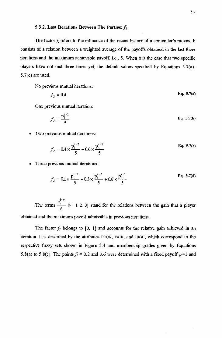
5.9

5.3.2. Last Iterations Between The Parties: jã

The factor já refers to the influence of the recent history of a contender's moves. .It consists of a relation between a weighted average of the payoffs obtained in the last three

iterations and the maximum achievable payoff, i.e., 5. When it is the case that two specific players have not met three times yet, the default values specified by Equations 5.7(a`)-

5.`7(_c) are used.

No previous mutual iterations: f? _: 04 Eq. 5.7(a)

One previous mutual iteration: PÉ*

f¬_ = ›_ Eq. s.7(_b)5

- Two previous mutual iterations: z-z t~1 _ . E . Í.7

fl =o.4×-pg +o.ó×p*T q ` (Q

0 Three previous mutual iterations:

f =o1×-Li 3

+o~2×_pi 2 +o6×_-pi

1 E°'5`7(d) `

5 "

5 `

5

t-v

The terms is- (v=1, 2, 3) stand for the relations between the gain that a player

obtained and the maximum payoff admissible in previous iterations.

The factor f¿ belongs to [0, 1] and accounts for the relative gain achieved in an

iteration. It is described by the attributes POOR, FAIR, and HIGH, which correspond to the

respective fuzzy sets shown in Figure 5.4 and membership grades given by Equations

5.8(a_`) to 5.8(_`c`). The pointsf¿ = 0.2 and 0.6 Were determined With a fixed payo1fp¡=1 and

5.10

p¡=3, respectively, which confoim to the pairs of dichotomic moves CC and DD. As to jà = 0.4, it Was calculated with p¡=2, originated from p<;(a)=tLD(a)=0 for both playersš.

P ,.,_t ................... --

- FAR ,

z

._

_

.‹__:.

_

ǧ'_._1¬¡

,..

_

y

.\¬;_;_`

. 1

0.5 \,

f

_.›

› 1"

_Pc‹c1R * Hic-›~H

.›

.~"`

.._.._.

._

_..

| í i 1 1 1 > fã 0.0 0.2 0.4 0.5 1.0

Figure 5.4 - Fuzzy Sets for the qualitative description of fz

The fuzzy expert. systems which employfi follow the same pattern adopted for fi, only substimting POOR, FAIR and HIGH for LOWER, SIMILAR and GREATER in Table 5.2.

-2.5f¿ +1 for 0 S fz s 0.40 H POOR (fz V) : {O otherwise

Eq' San)

sf, -1 for 0.20 5 fz é 0.40 ,zmR(__fí,) = -sf, + 3 fm 0.40 < f, < 0.60 E0- 5-80»

_

O otherwise

5 \ I/ ` _

¬

. . ef -=¬ tor 0.403]-z sl I1H1GH(fz ) = ° Z J

.

' EQ- 5~3(¢) 0 otherwise

From this point on, with any combination of actions a player will receive a greater payoff than its opponent. For this reason, fz = 0.4 Was chosen as the limit between the POOR and the HIGH fuzzy sets. As to fiizzy set. FAIR its limiting points have been determined under two assumptions: First, a fz below 0.2 means that the player is being exploited by the other pany and, thus, cannot see the outcome as “fair”. Second, in an opposite sense, if it obtains more than 3 points (B .>- 0.6), this reveals an advantageous situation over the opponent, implying in gains that might not be considered “fair”.

5.ll

5.3.3. Relation Between The Overall Trends Of Wealth: jÉ~,

The third factor j3 is a linear relation between a player”s (wf) and the population”s (_ Wn)

average payoffs per it.eration. This relation intends t.o portray the current. trend in the

accumulation of gains.

_.. -A

M* 2 ¬ K...

_. _

M= _=:í -k _ 2 _ = w

W? =; W" = -_- fz = _k Y-n k 2n W, +W

Eq. s.9(z) Eq. s.9(b) Eq. 5.9(¢)

Where:

. wfl is the Wealth of the player r at. the ƒh iteration,

. wi; is the average wealth per iteration that the player has received until iteration

k

. k is the number of iterations already performed by the player r,

. #7" is the average wealth per iteration that the Whole population has received

after n iterations, . n is the total number of iterations until the present instant,

. i E P, P:{players who have already played}

The fuzzy sets designed to represent the qualitative concepts associated to já are

similar to those shown in Figure 5.3, and eight fuzzy production can be generated in the

same manner as depicted in Table 5.2.

-2f +1 foz o<f goso p.LW (_f3) =

3 3 '

Eq. 5.10(a) O otherwzse

5.12

šf, - for 0.44 5 f3 S 0.50 ,uSL(_f,) = -äfs + for 0.50 S f, S 0.57 EQ- 5-1001)

O otherwise

_

Ef -lí for 0.55Sf 51 aGT(_Q)= 9 3 9

_

3 Eq.5.10(c) 0 otherwzse

5.4 - Determination of a PIayer's Action in a Move

The evaluation of fl, ƒ¿__ and já yields three separate partial conclusions about the intensity of cooperation/defection to be adopted. To accomplish the aggregation of the three limited results, the present. model employs a procedure that takes the maximum of the outcomes derived from the rules related to each factor. The general steps to be followed by a player r (r = 1 to rn) are valid for every factor fé, (q corrcsponds to the type of the

factor (q= J, 2 or 3 ) andj to the iteration (j = 1 to n)_).

i. Determination of fàr;

ii. Fzøzztjfication o_ƒ`_fá¡,'

iii. .filctívatíorz Qf the fitz2'_,v rule(Ls) matched by the fact (according to the player”s strategy Sq,,`);

_

iv. C0ns*olz'datz'0n qfthe partiaí c0n‹:lusz`0ns yz'eld1`ng the_final conclusíons (oz _, pg ); Every player is characterized by a set of 9 fuzzy rules (three for each SW, q=1, 2, 3). The inference process will fire the rules matched by the fuzzified decision factors. Each factor can originate either one or any pair of the possible pattial conclusions C- or D, with its associated strength (membership grade lt). The integration of the paitial conclusions is made through the fuzzy union, using the join operator \/ (fuzzy maximum), for the same class of conclusion. Hence, the fmal result to be derived in terms of cooperation and defection Will be a sole pair

of conclusions, taken as max( f) and max ( pg* ), q = 1, 2 and 3.

5.13

v. Deƒàzzíficafion of the final conclusíons to determine the final player "s action The final conclusion will consist of a pair of membership grades in either one or both fuzzy sets COOPERATE and DEFECT. I-Iowever, in order to find the payoffs in an iteration, the players' actions cannot be fuzzy. A defiazñiication procedure using the síngleton nzethodi translates the qualitative conclusions into a crisp value for

each player.

5.5 - Example of an Iteration of the FIPD

5.5.1 - Identification of the Players

The diagrarn depicted in Table 5.3 shows how a player is distinguished by the set of strategies it uses. Each player has 9 mles defining what it will do according to the value of each decision factor. Let us assume that. one of the players randomly chosen is P754. The subscript 764 means that it uses the strategy SÇÍ with respect to j¶, Sã for f¿ and SÊ3 for ]Ê,, as indicated by the shaded cells.

i

sl S2 S3 S: S5 só ͧ;'ÍÂ'}3t‹

S1 S2 33 S4 S5 S7 Se. fz S1 S: S3"¡$iií135 só S7 Sa =

.í;:3;:;í;:I: - J

Lw D Poon D D LWT T T O T C1 T T T ÕÉ Õ T Õ Í? TT T

U

O

Í? z'_U.__c:_. Ê-*Í

-_-tÍ_

o

o -5-_Ê.

Ti? _5_Í1_

Tí?

o __`? 53

Í*

o ÊTÍÍ :

U

#5*

ea

O

U _cÍ_~‹T

-TT

_

crr c io c HIGH D c c I

sL : FAIR n sL

Table 5.3 - Strategies used by the 512 different players of the FIPD5

5.5.2 - The Iteration Process

Assume that the other player, also randomly selected, was Pm. The iteration

process is as follows: First, each player deteimines its decision factors. Every f is qualitatively described by its corresponding fuzzy sets, and the rules that have been

4 A singleton is a membership grade value represented by a single vertical line that intercepts the horizontal axis in only one point [VlOT93]. ln our case, there will be two singletons, one for each fuzzy conclusion, COOPERATE and DEFECT. The final action is detemiined by the point where the resultam of the two singletons crosses the horizontal axis. This

_ point is calculated balancing the moments of the two singletons and of the resultant. See Chapter 4, section 4.4.2. ° A player is a strategist with three rules for each of the three decision factors. Thus, the total of players is 8 x 8 x 8 = 512.

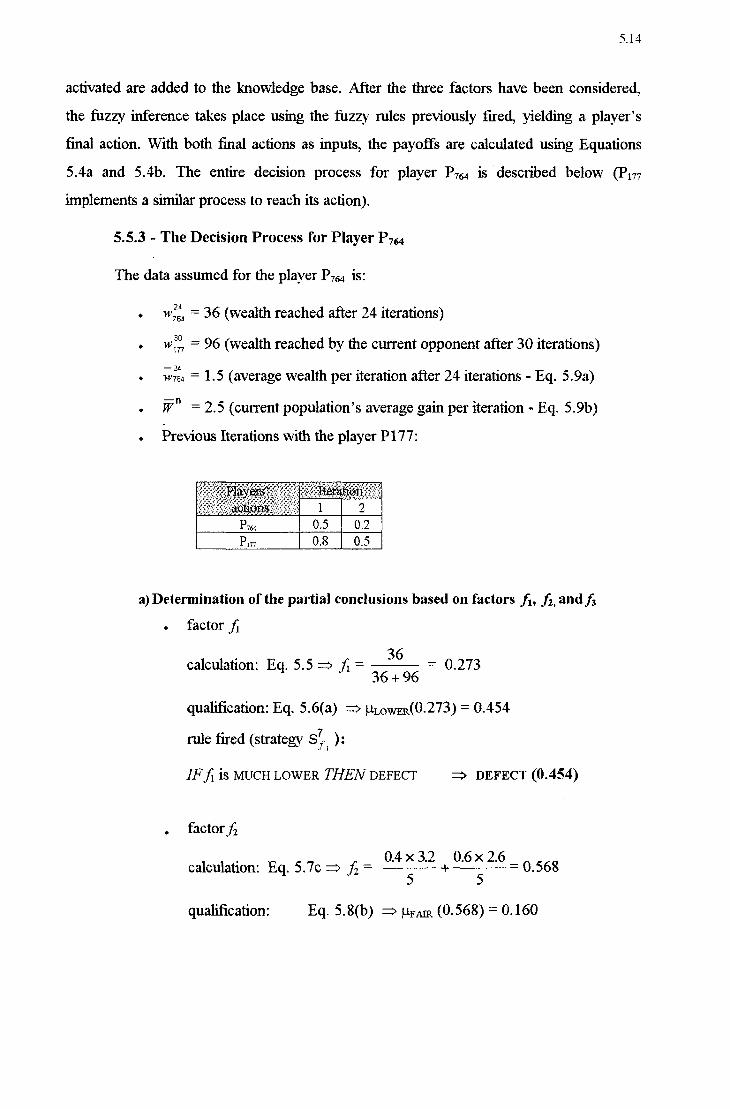
5.14

activated are added to the knowledge base. After the three factors have been considered,

the fuzzy inference takes place using the fuzzy rules previously fired, yielding as player's

final action. With both final actions as inputs, the payoffs are calculated using Equations

5.4a and 5.4b. The entire decision process for player P764 is described below (Pm implements a similar process to reach its action).

5.5.3 - The Decision Process for Player P764

The data assumed for the player P764 is:

. wi; = 36 (wealth reached after 24 iterationsf)

. vvfÍf7 = 96 (Wealth reached by the current opponent after 30 iterations)

. Í-ÍÉ4 = 1.5 (average wealth per iteration after 24 iterations - Eq. 5.9a)

. F7' = 2.5 (current population's average gain per iteration - Eq. 5.9b)

. Previous Iterations with the player P177:

,~.,~ ,,,-.,›.,.,-,,z_..~À..,__-À.. .-._-_,'.,.,.,-_,-,f,..,,-. _.z..-.t-,.z,-4.' ._.~ ‹.- .-_.- ,_.- .- .›_.-,.- ,,z,-

1 2 Pzz-4

I 0.5

1 0.2

Pm 1 os

1 0.5

a) Determination of the partia] conciusions based on factors fl, j}, andfz . factor fi

3 calculation: Eq. 5.5 :> ji = Á- = 0.273 36 + 96

qualification: Eq. 5.6(a) :> uLQWER(0.273_`) = 0.454

rule fired (strategy Sšzi ):

IFJÊ is MUCH LOWER THEN DEFECT :> DEFECT (0454)

. factorfi calculation: Eq. 5.7c :› fz =

04 É 32 06

É 26 = 0.568

qualification: Eq. 5.8(b) :> rtpm (0.568) = 0.160

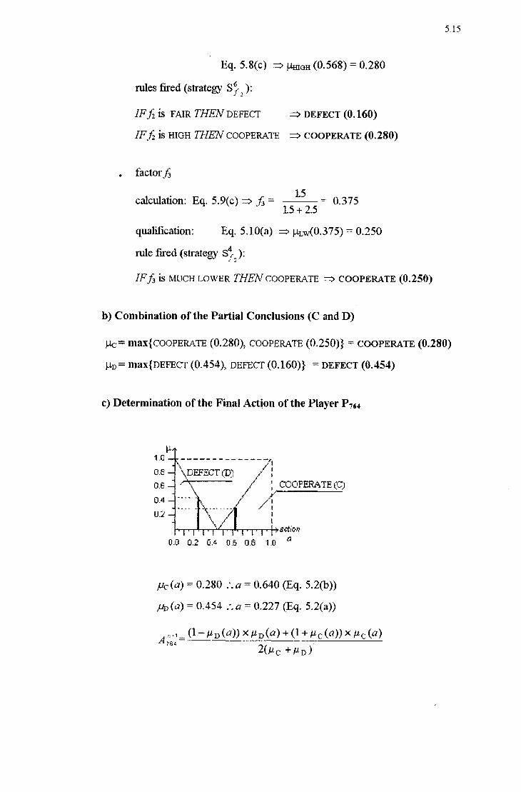
5.15

Eq. s.s(¢) z> pm, (0568) = 0.280 rules fired (strategy SÉ,-2 ):

- IFJQ is FAIR THEN DEFECT :> DEFECT (_0.160) IF_ƒ¿ is HIGH THEN COOPERATE :> cooPEmm‹: (0.280)

. factorjá

. - . _ 1.5 _ - ealeulatlon. Eq. >.9(_‹._) :> fg - L5+2.5

- 0.373

qualification: Eq. 5.10(a) := pLW(0.3'75) = 0.250

rule fired (strategy SÉ-3 ):

IFJÉ, is Much LQWER THEN COOPEMTE :> cooPE1uuE (0.250)

b) Combination of the Partial Conclusions (C and D)

¡.l,;¬=111ax{cooPE1m'rE (0280), COOPERATE (0.250)} = CQOPERATE (0.280) 0,,= nm{nE1‹¬EcT (0.454)_, Dm-EcT (0.1õ0)} = mmcr (0454)

c) Determination of the Final Action of the Player P764

H 1 .0 ............ _ _, 0.0 '\nEFEcT fm na

A' /xl oc‹PERmE(GJ

5:

C*

RJ

JB

f2

~`\f

\. \_

"'§_,

O

" 1-sctfon

0.0 0.2 0.4 0.6 0.0 1.0 Ú

,UC (_a) = 0.280 .ia = 0.640 (Eq. 5.2(b))

pp (a) = 0.454 .Za = 0.227 (Eq. 5.2(a))

A W: (1-flz>(¢1)') ×flD(<1) + (1 +00-(.‹1))× #¢(.‹1) 764 2(/ic +l¿D')'

5.16

.4;¿; = 0.413

5.5.4 - Computation of the payoffs

a) Player P764

A vnaâ; < A 1n7.7` Ê using Eq- 5-3(a.) :> P764 : 1 ' ZX-4 vhs.: + 4) Z: A -1n7.71

P754 :1 ' +

P754 =

P177

A1“7~.11 > A Inst; Â using :> PI77 : 1 " Arm?? + K A fue.:

P177 : 1 '

p¡77 =

5.5.5 - Update of the Population's and Players” Parameters

accumulated Wealth (PW): _.: (36 + 2182) = 38_182

accumulated Wealth (P171): ›‹.›Í,`; : (96 + 1387): 97387 25 average Pfl>'0fi° Pfif iffifflfíflfl (`P1‹›Á>= Em = 32.182 + 25= 1.527 (E‹1.s.9(a))

average payoff per iteration (P117): É; = 97.887 + 31 =3.157 (Eq.5.9(a)_) populatioxfs average payoff per iteration: W" z 2_5 (Eq_ 5_9(b~))

5.17

5.6 - Simulations

The computational tournaments Were implemented using a custom C++ program, specifically written for the implementation of this model of the FIPD. To run the

simulations, the 512fi1zzy players Were divided in groups of 16 participants each. Along the four different phases of the tournament, every goup included also the three non-fuzzy strategists, that is, the traditional TFT, the generalized TFT6 (TFT-g) and Pavlov.

In the first phase there Were 32 groups, each with 19 contenders. After running 30000 iterations per group, the competitors Were ranked by their average payoff. For the second round, the eight best fuzzy players from each group Were then selected, and eleven new groups Were formed from the original 32, by the participants by chance.

The third phase involved five groups, again picked from the foregoing best

perfoimers. The 16 final best fuzzy strategists, along with TFT, TFT-g and Pavlov played the last dispute. The total number of iterations per group was kept constant in 30000 in every phase, and there no player performed less than 3000 iterations. This means that, on the average, everyone encountered the same adversary in about 166 occasions.

Tables 5.4 to 5.7 display the results obtained in the four phases of the simulations,

always referring to groups of 19 players each (16 fuzzy and the three non-fuzzy).

'° The Generalized TFT strategist starts cooperatjng and, in the next iterations, repeats the previous punctual action of the opponent. Another possibility could be to consider the opponenfs action as an oe-cut in the fuzzy action (C or D) and use a defilzzificafion procedure to find its decision.

5.18

Winnefs Number

Group Avg. Payoff

Group*s Avg, Payoff

Smaflest Group payoif

Winner' s

Number Avg. Group's Payoff Avg,

Payofl`

Smallest payoff

1 455 2.54 2.17 1.93 17 PAVL-OV 2.48 2.11 1.75

2 PAVLOV 2.54 2.16 1.94 18 546 2.66 2.18 1.90

3 453 2.54 2.14 1.88 19 454 2.59 2.18 1.95

4 456 2.61 2.18 1.94 20 515 !`) U.) 'ui 2.14 1.96

5 PAVLOV 2.61 2.12 1.83 21 PAVLOV 2.51 2.10 1.65

6 566 2.60 T9 IJG 1.73 22 745 2.61 2.16 1.69

7 PAVLOV 2.43 2.12 1.87 23 PAVLOV 2.51 2.14 1.90

8 664 sv) lil U.) 2.17 1.85 24 476 2.58 2.16 1.54

9 353 2.58 2.16 1.95 25 356 2.56 2.15 1.89

10 PAVLOV 2.53 2.11 1.85 26 PAVLOV 2.50 2.10 1.84

11 355 2.55 2.19 1.90 27 354 2.54 2.17 1.94

12 436 2.42 2.13 1.93 28 446 2.69 2,17 1.98

13 554 2.53 2.14 1.81 29 PAVLOV 2.63 2.08 1.79

14 PAVLOV 2.69 2.16 1.77 30 556 2.60 2,15 1.71

1 5 PAVLOV 2.49 2.10 1.75 31 553 2.54 2.15 1.84

16 555 2. 71 2.16 1.91 32 PAVLOV 2.83 2.14 1.92

Table 5.4a - First Phase: Groups 1 to 16 Table 5.4b - First Phase: Groups 17 to 32

Group Winner Winner' s Group *s

Avg. Payoff Payoff

Avg, Smallest Group Winner Winnefs Group”s Smallest payofí Avg. payoff Avg,

Payofi Payoñ" 1 IFI 2.24 1,76

1

1.42 E1 2.09 1.68 1.35

2 556 2.21 1.92 1.31 ã F0 IQ U.) 1.66 1.17

3 TFT 2.10 1.83 1.19 Ei 2.18 1.63 1.28

4 7554 FJ IQ IQ 1.86 1.29 E1 2.08 1.62 1.17

5 TFT 2.18 1.80 1.47 3 1.76 1.56 1.05

6 TFT 2.16 1.86 1.35

7 :Ti 1.94 1.70 1.14

8 Ei 2.10 1.75 1.25 '

9 Ei 2.15 1.82 1.26

10 E 2.01 1,72 1.34

11 4-45 2.39 2. 05 1.41

Table 5.5 - Second Phase

Table 5.6 - Third Phase

5.19

áIfi1:i1IÍ:‹É1i:išiš:1-1É:1:2IiÂiílêíl-ÉIfÉIEIIÉIEIÊii?1%IEÉ11rãií215É151€IÉÊIEÊ11ÉIE?15-Ê1zilši?IiIÊI:ii?íííiíiíiííšišíííiíišIíííiííífšííFÉ1ÉIÉfãI?IfIEIE1É15fííi`1§1Éi§IÍIÊIE1%IE«Ê'fí<ÍIfIíI¡¡I'iÊ1§E11êifiE5??íífiš-51%-Í-EEIl1EÉz1F1?1:~z«11íiirfiíYÍ:ãi-:í1Í:1¡Ií:{í:1§1fr1fiã11:§1í:í"""*""*'*“*"->:1f§:§E§:1íí:;Çr1:IE1:}§í:{Ei.jiziE'§.§¡i:§¡¿š§fÍ¡f;Ej-zi*=""'f~*"“fff

Table 5.7 - Fourth Phase (Final)

5.7 - Discussion of the Results

Except in the fmal phase, all groups played two sirnulation rounds. As expected, the ranking order for each group showed variations, because the payoffs accumulated during the iterations are dependent of the sequential random selection of pairs. The tables

depicting the results refer to the round in which the greatest average payoffwas obtained.

An extra. round involving all the 512 fuzzy and the 3 non-fuzzy players in a sole group Was also performed. However, though the group played one million iterations, the results obtained were not conclusivo, because the participants played only about 7.5 times

With each particular opponent, on the average. This small number of iterations between the same pair is not enough for a. player to reach a. stabilized pattern of behavior Withphis

opponents7. The Winner of this round Was the fuzzy player 555 (the fuzzy “all-D”). TFT ranked 237m; TFT-g and PA\f'LOV finished in 317m and 374m places respectively. An interesting feature observed was that the 9 first contestants had “S” (which means defeetion in every circumstance) as the middle digit. This position corresponds to the factor fiz and

refers to the decision rule regarding the payoffs previously obtained. In the lirnited

experiments performed, the “all D” characteristic had an edge over the other players,

possibly because it exploits their “nicer" decision rules.

The first phase

In the 64 (2 ><32) runs, the digit 5 appeared at least once in 36 of the 64 Winners. In

28 cases it was the middle digit. Also, in 15 groups, the same fuzzy player won both runs,

7 A 486SX 331\‹lHz computer was employed, and the program run in a. virtual disk during about 100 hours unintenuptedly, or more than four days.

5.20

and 13 of them contained the digit “S” at least once in some position. Excluding the fuzzy players, PAVLOV performed quite well in this phase, winning 14 times. TFT arrived first 3 times.

The second phase From the 32 groups, 176 ñizzy players have been picked, forming 11 newly

arranged sets. The criteria was to select the individuals which appeared simultaneously among the eight best ranked fuzzy players in both rounds, along with some other players that, although not having this feature, also performed well. This time, TFT won 17 of the 22 rounds. Surprisingly, the PAVLOV strategist abandoned the success it had in the Íirst phase and scored poorly. Its best positions Were a second and fourth place, ranking in the lower half of the groups most of the times. The explanation for this fact seems to lie in the cognitive rule adopted by PAVLOV, which interprets an opponent”s action as only totally cooperative or detective, though the fuzzy players seldom, if ever, come out with the extreme actions O or l. Those circumstances entailed many C”s from PAVLOV, against less cooperative decisions from its adversaries, and consequent lower payoffs. Why, then, was PAVLOV so successful in the first phase? The answer may be the fact that the “DEFECTION biased” strategists were scattered among all the groups, and in the end they became present in a larger concentration, since they emerged as Winners fiom the

preceding level of the toumament.. On the other hand, TFT retains a tradition of being good in handling defectors, defmitely reciprocating with zero whenever it meets another player With a tendency of deciding towards defection, even if it is only a mild disposition.

As in the second phase the players with a defective mood outnumbered those more cooperative, TFT thiived, because in a. pair of actions, the one nearest to zero receives the greatest payoff.

The third an dƒinal phases As can be seen from the respective tables, the third and final phases turned out to

be only a confinnation of the tendency that had already been initiated by the increasing

exclusion of the “nicer” rules. Nevertheless, a fiercer dispute really has taken place in the

last phases. This observation can be confirmed by the average payoffs achieved by the

5.21

players, Which steadily drop as the tournament evolved. This assertion is valid for both

Winners and losers. Again, TFT ended in the first position, though closely followed by the 553 fuzzy strategist.

5.8 - Conclusions

The purpose of the model of the IPD presented in this Chapter of the dissertation was essentially the introduction of ai fuzzy model of the IPD. Departing from the classical

approach where only all or nothing decisions could be implemented, the conflict of interest

embedded in the game is treated as a problem allowing a continuous interval of strategies, represented by membership grades in the filzzy sets COOPERATION and DEFECTION which

now characterize the players” actions. Additionally, the participants” decisions were guided by fuzzy expert that took into consideration other variables besides those related to

the history of previous iterations, which are usually employed to assist the strategists. In this

framework, a. computer tournament. was performed, and some results achieved were

shortly discussed. Given the importance of the concepts introduced, the interest in further

extending the investigation of the FIPD is explored in Chapter 6 of this dissertation, where a subsequent theoretical development as Well as a practical application of the paradigm are

implemented.

Chapter 6

' An Application of the Fuzzy Iterated Prisoner”s Dilemma

6.1 - Introduction

In chapter 5, a theoretical model incorporating fuzzy expert systems as a basis for players making decisions in the Iterated Prisoner*s Dilemma (IPD) games Was presented, simulated and analyzed. As could be seen, allowing the contenders' actions to depart from the traditional Boolean resolutions COOPERATE and DEFECT brings new and important modifications in the game. Moreover, the fuzzy logic approach employed to describe the

way the players reason and perceive the stimuli from other players and also from the environment is much nearer real life situations than the former schema.. Another significant feature included in the model Was to take into account a diversity of variables, other than the usually employed history of previous it.erations. The computational toumaments

performed using these paradigms brought new light on the manner rational agents might behave when submitted to situations that. have a. resemblance with the conflict of interests

mirrored by the Iterated Prisoner's Dilemma Game. In this part of the dissertation, many of the ideas extracted from the theoretical

developments presented in chapters 4 and 5 Will be exploited. The aim is to demonstrate how the structure of a P1isoner°s Dilemma game can be applied to a practical problem in the domain of Industrial Engineering, where an evident conflict of interest is present and

where the decisions are made by rational agents. Uncertainty, incomplete and/or

ambiguous information, risk and subjective perceptions Will be still extant in the material

that follows. But in the realm of game theory, differently from standard optimization and decision problems, it is possible to combine random events, or states of the world, with actions that are entirely govemed by the participants. This characteristic usually brings new difficulties for the decision makers in achieving their desired goals, mainly because a

6.2

player”s action can always be opposed by a counteraction from the other part, and

everyone is simultaneously trying to achieve their own specific goals, which can be

opposing (but not always strictly contradictory, though this is not seldom the case).

The P1isoner's Dilemma (PD) is an adequate paradigm to model and understand what happens when rational agents are exposed to those kind of circumstances. It

reproduces the contradictions that arise from instances taken from everyday life where the simultaneous search of the individual optimum frequently leads to both individual and collective poor outcomesl. I-Iowever, given the qualiiications of the problem to be

approached, an altemative structure, which partially deviates from the traditional definition

of the Prisoner”s Dilemma Game, will be employed here. Instead of considering a two- sided PD, an one-sided 2 version [RASM89], allied to a fuzzy decision process by one of type of players shall be used to model the problem, which consists of a .Market Share Game. A detailed method is thoroughly developed, preceded by a description and

discussion of the approached problem. A methodology overview, including a simplified

outline of the proposed system, is also included. Along with the detailing, an example is

supplied, applying the concepts just introduced. The cun'ent Chapter ends with a summary of the algorithm.

The information about the computational simulation process and the results

obtained is deferred to Chapter 7.

6.2 - Description of the Problem

Among the most important questions that must be tackled by a. profit-

seeking company (the F inn) operating in a competitive environment, is the estimation of its revenues.

u

More often than not, the emphasis of the decision process is concentrated in

internal aspects of the Firm. These aspects, in general, deal With topics which regard

mainly production planning and control, financial management, quality control of products,

1 This paradox is the essence of the Prisone1'”s Dilemma. Game. For an enlightefning discussion of the theme, see [HOFS85].

2 See Chapter' 3 of the dissertation for an explanattion of that class of PD”s.

6.3

technology employed, investments, relationship with suppliers, sales policy, advertising

budget, etc. But a crucial factor influencing a. company”s performance with respect to its

ability to generate profits is the market 'share it detains. The market share is intimately

related to the internally managea.ble variables mentioned above. Nevertheless, an accurate

measure of the impact or effects that projected or just implemented alterations in the

attributes of a. product, such as quality, price and advertising, will have on the market share is still hard to detemiine.

The analytical models, generally based on empirical data, constitute an attempt to solve the problem. Unfortunately, the static models -suifer from the same plague that beset

other economic-related questions: the highly dynamic character of the process and the

capacity of evolutionaiy self-adjustment. of the agents involved. This ofien causes an unsatisfactoiy perfomance of traditional static or analytical models, which may tum out to be become either mathematically intractable or unattra.ctive under the point-of-view of the intended precision. In other words, because of its implicit nature, market share problems

belong to a class of issues that do not yield easily, in terms of the reliability of results, to

standard treatments, such as analytical or even econometric models of prediction.

Computational simulation methods provide an excellent alternative to approach the

problem of market share determination. Because of their iterative capabilities, they are able

to capture the dynamic and interrelated processes that permeate these kind of questions.

The problem considered in this dissettation is an application of the Fuzzy Iterated Prisoner”s Dilemma (_FlPD) to a. practical situation. It allows the acquisition of new insights of the processes that take place in a competitive market formed by suppliers of products or

services and Consumeis. The main general questions to be addressed by the model are:

0 What are the relationships between the market share of a. Fi1m”s product or service and the price, quality and advertising budget the company assigns to it?

0 How do the Consumers perceive changes in the attributes of a product or service, and update their decision functions?

6.4

0 Given the Consumers are diverse regarding their buying power, feature orientation and sensitivity to price and quality, how can the competitors identify market

opportunities (nichesf) and conveniently explore them?

0 What is the dynamic behavior of the whole environment, conceming the conflict of interest embedded in the process, both among competitors (sellers) and among Consumers and Firms?

0 Can an equilibrium be established? lf it can, Which are the characteiistics of the strategies that compound it?

0 Which are the dominant strategies in terms of attaining the best results (profits) for the Firms? Are they stable?

Those questions, along with other additional related analysis, Will be the object of a

simulated repeatednon-cooperative game between Firms and Consumers, both taken as individuals. The iterations will always be pairwise, but. the results achieved by both sides

will also influence their decisions regarding different contenders. The main goal of this application is the determination of a Fi1m”s market share When operating in a competitive environment, and having rational agents as customers.

6.3 - Methodology Overview

6.3.1 - The Basic Game

The Fuzzy Iterated Prisoner”s Dilemma paradigm, in its one-sided version, will

serve as the basis for modeling the game. It is considered suitable for the investigation and

resolution of the problems posed by the previous questions in the sense that in the relations

between a. Firm and a Consumer, both sides can COOPERATE or DEFECT.

ln the case of a.Fi1m, the degrees of cooperation or defection are expressed by the

compromise between the price and the quality of the item offered in the market for sale.

Under a Consumer°s point-of-view, a Firms' decisions may range from one extreme, denoted by price = Lowasr and quality = BEST (COOPERATE), to the other,

price = HIGHEST and quality = WORST (DEFECT). On the Consumer”s turn, it will go

6.5

through a fuzzy-based decision process, but the possible moves Will be still dichotomic and expressed by the decision to buy or not the product. or service3 when the opportunity to do so appears. While the COOPERATE move irnplemented by the Consumer means that the transaction has been effectuated, DEFECT implies that it will have to search for another

supplier.

Differently from the classic two-sided PD game, in which both players possess the same strategy set and symmetric payoffs, the one sided PD to be employed here does not. fit the usual defirrition of a PD, because the strategy sets for each participant are different

and because neither the payoffs nor information sets available to the players are symrnetric.

In order to better' clarify' the mechanisms that will be used to model the proposed

application with the one-sided Fuzzy Iterated Prisoner"s Dilemma, let us consider for a

while, as a sirnplification, that. only the dichotornic punctual choices COOPERATE and DEFECT are allowed for both players, as in the standard game. In this hypotheses, given a

typical iteration between any pair of players involved in an iteration, only the four usual

feasible outcomes CC, CD, DC and DD may result, regarding the combination of the decisions from the Consumer (potential buyer) and the Firm (potential seller).

The simplified qualitative one-sided PD used in this example is an adapted version of the one introduced by Rasmuseni. It can be represented, in its normal form, by the

payoff matrix shown in Figure 6.1. The payoffs for the Firm are expressed qualitatively by the terms high (HIG), medium (MED), LOW and lowest (LWT), in decreasing ordinal ranking order. On the other hand, the Consumers' gains are reduced to only three possibilities: high (HIG), neutral ( NTL) and LOW. This occurs because When the Consumer does not buy the

3 It could be the case that the consumer, too, might be able to decide in a continuous interval, instead of only the two punctual choices buy or not buy. This would happen if the product oñered by the supplier is divisible and the consumer Were to select a certain quantity in a given iteration. Although of interest, this relaxation will not be approached in the present work, and is left as a suggestion of future developrnents. See Chapter 8 - Conclusions.

4 Op. Cit. [RASM89]. The difference between the version employed lrere and Rasnrusen”s is the existence, in the former, of a IOW playe1"S weakly (Iolninant slmiegv and the consequent iterated dominam szraregv equilibrium, not present in the current game.

product or service, the quality of the item is unobserved, and its payoff will always be

neutral (_ NTL) in this case. Also, the payoífs are not interpersonal comparables.

Consumer

C D

C MED,H1o LWT,Nri. Firm

D H1G,Lc›w Low, NTL

Figure 6.1 - Normal Form of the Simplified One-sided PD With Qualitative Payoffs

ln the matrix cells, the first term refers to the row player. The criteria for assigninc, the qualitative payoffs shown in fig. 6.1 is explained below. They are always taken as a

function of the pair of moves selected by the contestants. The first letter, C or D, refers to the row player, the Firm, and the second stands for the column player.

CC: The Firm cooperated in the sense that is offering a product or service of suitable quality at a fair price. The Consumer also cooperated by means of

canying out its decision to purchase from the Firm involved in the iteration.

In this situation, the Firm receives a reasonable, or nzedzum (MED) payoff,

because it accomplished the sale, but the profit margin embedded in the transaction is not too high. This result derives from the assumption that

production costs of good quality products are higher. On the other hand, the Consumer gets a high (HIG) payoffl for having succeeded in achieving a

product. or service of suitable quality, at a convenient price.

5 Interpersonal comparison of utilities is one of the crucial problems of Game Theory. Some theoiists, e g [BACH77] admit that it is not possible at all. Foitunately, in the present model, this feature is not required.

0 CD: The Firm”s behavior is the same as in the previous case, but now the Consumer opts for not taking the offer. The Firm”s payofi° is the lowest (LWT), as long as it is not being compensated (consummate the sale) by the

Consumer for its efforts in offering it a good deal, in the Firm”s point-of- view. The buyer, having refltsed to purchase from this Firm and possibly having lost an opportunity to achieve a good valued item, will receive a

neutral (NTL) payoff.

0 DC: The F inn's article is of inferior quality and expensively tagged, yet the Consumer buys it. As a consequence, the Finn gets a high (HIG) payofl°, while the other player ends up with LOW, for evident reasons.

0 DD: The a11:icle`s attributes are as above, unfavorable to the prospective buyer, and it. decides to refuse the deal. Regarding the seller, its gain will be

almost as low as in a CD outcome, but because the effoits involved in

offering a poor quality and high priced item are much lesser than in the latter case, the lossiwill be somewhat smaller. For this reason, a low payolf will be

assigned to it. The Consumer is also in a position similar to the one that happens in CD, however itmust be satisfied for having avoided the Worst, with its refusal to accomplish an adverse acquisition. Recalling the features

possessed by the one-sided PD°, it is important to mention that only the row player is confronted With a dilemma equivalent to that which takes place in

the standard two-sided PD. This is so because in the one-sided PD at least one of the players prefers CC mostly.

Though in the qualitative payoff matrix both the Firm and the Consumer have identically labeled gains with ordinal equivalence, they do not stand for equal cardinal

values. In the one-sided PD, this asymmetry is the main relaxation of the rules that defme

the usual two-sided PD. Neither player has a dominant strategy, and so there is no

6 See Chapter 3.

0.7

dominant strateg equilibiium. Nevertheless, a unique DD Nash equilibiium peisists A summary of the players” actions and associated gains are presented in Table 6.1.

_. _. _. _. _. _. _. _

._ _

_.

íÊÍÊÍÍš}i§;}§ÊÊfš

Afiei' meeting a Firm, according to

a. specific selection mechanism, the

Consumer decides to purchase the

product or service being offered also

confomiing to a paxticulm' criteria.

The payoff it. receives is high or

ÍOW, depending on whether the

purveyor cooperated or defected.

Independently of being, chosen or

not, the policy adopted by the Firm is to offer products or services With

good quality at fair prices. Its payoff

in iteration is medium or lowest. if the Consumer cooperated or defected, respectively.

After choosing a Finn, according

to a specific selection mechanism, the

Consumer opts for NOT to buy from this snpplier, and will have to look

for another one. The payoff is

neutral (zero).

Independently of being chosen or

not, the policy adopted by the Firm is

to offer poor quality and expensively

priced products or services aiming a

high unitary profit. The payoff it

receives is high or ÍOW, if the

Consumer cooperated or defected,

tespectively.

Table 6.1 - Actions and Payoffs in a Simplified Ono-sided Market Share PD

6.3.2 - Basic Iteration Process

In order to implement the model, a hypothetieal setting is initialized, and a

are summarized in Table 6.2.

Simulation program will be run to generate the iterations. The components of the process

.9

;:=;z:5:;5:;f:;5â5*5f:z5:;5::5:;5:;í:;§:;5:;J:15:;5:;í:;5:;í:z5:â5:;5:;5:;§.;f:;5:;z:;5::5.;5:;5:;5:;5:¡5:;5:;f:;5:;5â5:j5:;í:;5:;5:;5::fézzá5:;5z;5:;5z5£i5§.55:55:f5:5fêízfiâišâfíiiíííizfšffíffäëšíííâfíâ52;55;fifiífííiíiâišífízëzfiíã5i;5Í1fi55E;¿555Í;Iílííífá55;í?zãíiíázšiíiiií-55;'?;

ÊÊÊÊÊÊÊÊÊÍ V .'zíÊ2?ÊzíëíšášEíiëëšíšëíífiší

_ _ zzÊ1i§?Í1. V. _ .ízáííšíšiíiíi-:Ê

ffÉÍÊÊÊzzzzzzzzzgzzzz;;z;zz;_:;;z;zz4zgzzgzz;zgzzzzzçzzzzzg-gzzgzz¿zz;zz;zz;zz;zz;;.;5zzízgzzgzzf.gzgfzgfzgfz;5z;¿z;5z;;z;;z;zz¿z;;z;5zzfz;5z;;z;z;;z;¿z;;z;5z;;z;5fg;zgfz;;;;z-;1z:;z;;z¿z;ízf5z;zz;

ÊíÊʧÉʧÊͧÉÍ;§Ê§ÉÉʧ§ÊíÉɧ}ʧÊɧ§Ê§ÊÊÍÊÊf;ͧ§§§Ê§ÊɧšÊ}§5*Ê151Ê5ÊÊÍÊ**íÊÊÊÉÉÉÊÊÊÊ1í51ÍÊÊÊ*Ê¿5«33:ÊÊ15

Table 6.2 Main Components of the Market Share Game

6.10

6.4 - Detailed Formulation of the One-sided PD Market Share Game

6.4. 1- The Sellers (Firms)

In a competitive market, a small number of sellers offer a similar product or service for sale to a population of Consumers. The number m of Firms present in the game is arbitrary. In this application, the simulations will be run With m í 6, but this number can be altered. The products or services offered by the Firms are differentiated from the

Consumers' point. of view, by their respective prices pg, and qualities q¡g, i = 1, 2,...,m,

g = 1, 2, ...,k7. The quality and cost of an item are closely interrelated, so that each of these variables can be expressed as an increasing filnction of the others. These variables are

entirely govemed by a seller"s decisions, and are perceived in distinct ways by the

Consumers. When a pairing between a Firm i and a Consumerj takes place, the latter distinguishes the price p,g before it makes its decision of buying or not the item. The quality

qig, though, is unobserved by the customer unless it purchases the product or service in

perspective.

A third factor, also controlled by the companies, is the advertising budget aig. While playing an important. role in attracting potential customers, the amount spent. in publicity does not influence the product quality, but Will effectivcly contribute to the Firm”s overall

costs. When the game starts, each competitor defines the variables p¡, ci, and ai, Which

can be modified in the course of the simulations depending on the results attained. The sellers* global goal is the maximization of their profits. The profit of a Firm during a given period is a function of those three variables, and also of the quantity of items sold. On its

turn, the volume of sales is determined by successful iterations with the customers,

symbolized by their Cooperation in the one¬sided PD, as previously explained. In this

version of the model, no restrictions are beirrg irnposed on the production capacity of the competitors, taken as unlimited. All these variables will be explained in the sequence.

J The index g refers to the cycle of the game. See Sections 6.4.2 and 6.4.3. See Section 6.4.4 - T he Firm 's Revenues, Costs and Profit.

6.11

6.4.2 - The Advertising Budget

Before the iterations start, along with the price pm and the quality qig, each Firm i

also defines an advertising budget a¡g that remains constant during a fixed period, called

cycle g, denoted by a specified total number of iterations scheduled to take place in this period of the game. It is assumed that the Finns know the size of the potential market, I,

and aig is a number between zero and one, taken as a percentage of the maximum theoretical possible revenues that would be conjointly achieved by all Firms in the limiting hypothesis as explained in section 6.4.4. Regarding only the random selection process of the Firms, the total a.bsolute value allocated to the publicity of the items being sold by ea.ch

Company is not relevant in this aspect of the simulations performedg. Instead, the relation between the amounts are considered.

The publicity expenses have an impact on the sellers” overall costs, and the

parameter that be used to account for this fraction of the costs will be the maximum price of an item considered in the game, max pig, arbitrarily fixed in 10 monetaiy units, as will be further made clear.

The selective process of a particular Firm to take part in an iteration is random, according to a probability distribution derived from the vaiious advertising budgets aig. The probability sig of a supplier i to be selected during a cycle g Will be given by:

3. sis =Ê`+mi×(1`Si), Eq.6.1 2 aig

i=1

The idea that underlies the formulation of s¡g by Equation 6.1 is that any Firm can

s be picked by the random selection process with a. probability E even though it refrained from spending in advertising. In other words, in the hypothetical market there will always

be a probability s, arbitranly fixed at the beginning of a cycle g, independent of the Firms'

advertising budgets a¡g. That. probability Will be shared by all the m competitors, that a Firm interacts With a consumer.rObviously, the more a seller spends in publicity, mixrored by the

9 However, the absolute value of the adveitising budget chosen by the supplíers is consequential in the task of establishing the net profit ofa Firm during a cycle of the game. See section 6.4.4.

6.12

value attributed to aig, the greater are its chances of being chosen more times as a potential

supplier, but that advertising effort will actuate only on the remaining probability (1- s).

As mentioned before, the cost incurred in advertising does not have any efficacy in improving the quality of the product or service and consequently a Consumer's

predisposition in purchasing it, but this decision Will affect the seller°s total profit achieved

at the end of each cycle”. The profit can be positively or negatively influenced, as long as there is a trade off between the capacity of pulling in a la.rger number of potential customers, mirrored by an enhanced chance of a Firm being selected when s¡ grows, and the increased costs When a¡g is raised. Also note that the efficacy of ag is relative, not absolute. In this manner, if every Firm elect. exactly the same value for its advertising

expenses in a given cycle, its expected number of iterations will be the same as if none had spent anything”.

6.4.3 - The Size of the Potential Market

The global game will be partitioned in k qvcles of identical length. The length of a

cycle is defined by an elective expected number of iterations per Consumer present in the game. When a cycle is completed, the Firms Will be allowed to modify their previous

decisions regarding the price, quality and the advertising budget. The criteria used to alter those variables is the pursue of optimum economic results, namely, the profit.

The size I of the potential market of the product or service is constant during each

cycle of the game. It is given by the totality of Consumers (n) times the expected quantity

of purchase opportunities per Consumer E(b) per cycle. This means that I random pairings will occur between sellers and buyers. It is important to recall that a pairing does not

necessarily mean that a transaction was completed, what only occurs if the Consumer coopemtes, or decides to accomplish the purchase. ln every cycle g, the number of times a

W See next section for the definition of this parameter. “ To avoid a divisiozz by zero error in the simulation program, that hypothesis will be Withdraw from the options to be nm.

6.13

particular Consumer j, j =1, 2, ...,n interacts with a Firm i, i =1, 2, ...,m, will be defined as

bm, and the absolute frequency of cooperations per Consumer shall be called bg.

II ITI

I= Zzbigj = nx E(b) , Vg EQ-6-2 _¡=n=1

The quantity of items sold by the Firm i during as cycle is v,g, and the aggregated

effective demand for all sellers is Vg.

ni vis = bíäí 1:q.õ.3

J=1

FIO :M= :Ma U'

fíãfi V :_ Eq.6.4

6.4.4 - The Firms” Revenues, Costs and Profit

I. Revenues

Each time a Firm meets a Consumer, basically only two things can happen: either

the customer purchases the item offered (cooperatesf) or declines (defectsf). On the other hand, at the beginning of every cycle the seller has a continuum of options” regarding its

policies towards the combination of price and cost of its product or service.

The revenues that a Finn receives in the course of every cycle of the game are originated from its payoff function. The inputs of that function are the moves performed

by the Finn and the other player. If the Consumer cooperates, the payoff ng to the Firm

shall be defmed as the unitary profit (p¡g - c¡g). Otherwise, the Firm is penalized by

receiving a. negative payofi. Here, the penalty payoff was discretionary fixed, consisting of

12 The choice of prices, costs and advertising budgets for each Firm is made by the researchetr.

6.14

two fixed parts tl, tz and a. portion proportional to the ratio fji , which can be interpreted Pig

as a Firm”s degree of cooperation.

Cooperates (buys) I

Deďcts (does not buy)

Ê5§ÊíÊIÍ§Ê ng = mg - Czg fr; = _ (W lr + tz × Ãíê) '*

ʧÊÊíÊ.ͧ§ ÊÊ Êif Ê? É ÊÊÊ ÍÊÊÊEÍ Êízš ÍEÊ ÍÊÊÊÉ ÊÍÊ É ÊÊÊ É ÊÊÉ ÊÉ5 EÉÊ Í§íÊ5Ê ÊÊÍ

` P fz

Table 6.3 - The Firms' Payoffs

This scheme is consistent with the assumption that. the loss associated with an

eventual non-consummated sale is greater when the Firm cooperated in a larger degree, Which means producing and selling an item With a lower unitary profit margin. Defection, though capable of bringing better' short-term benefits to the Firm, also has its risks, since in

the long run it will generally drive away would-be buyers, as will be explained in section 6.4.6.

The introduction of the subscript. g to represent. a particular cycle of the game is necessary because the Firms can alter the variables pig, c¡g and a¡g when a new cycle g begins. This possible modification in the sales policy can bring different results in tenns of

the revenues achieved, and shall constitute a subject. of interest for the analysis of the

simulations.

Conceming the variables p¡g, c¡g, and qig it is necessary to establish some important rules that. must be obeyed by during the game: drive away

0 pig and cig are expressed in monetary units;

0 The quality attribute q¡g is directly related to the cost of the item;

0 No Firm is allowed to decide on a price that is inferior to the cost of item

(Dig 2 ctg);

6.15

0 All prices are subject to a maximum and a minimum, that have been selected as 10 and (0+s) monetaiy units, respectively, for the purposes of this model

((0+S) íilhg í10);

0 During a cycle of the game, píg, qig and aig remain constant.

The total gross revenues obtained by a Firm i after the end of a cycle g, g=l, 2, ...,k is:

c_ ll

Rig : (Pig _ Gig) X Vig '(-ti +t'2 X äâ) X Híibiig] _ Vai

Eq' 6.5

ig j=1

ll. Costs and Quality

Two kinds of costs arepresent in each cycle g of the game:

a) Unitary production cost cg, and

bi) Advertising cost aig.

The total operational cost of a Firm i in a cycle Will be a function of its current

item`s price, cost, the fixed parameter t, the number of iterations in which the Firm took part (that could be called “customers” visits”)_, the number of consummated and non- consummated sales and the amount spent in publicity.

a.) Unitary Costs and Quality

Because of the structure adopted for the Simulation model, the operational costs

will be considered as embedded in the payoff function of each Firm, and to avoid

redundancy, they will not be treated separately. Thus, when selecting pig and cig, the Firm is deciding on its own payoff function, and, in a way, also partially on the Consumer's. This occurs because the quality q-Lg that the buyer assigns to the item is taken into account

6.16

in the model as a crescent function of the cost cig, settled by the seller to the item in a cycle gm, that is, q¡g=ƒ(c¡g).

Note that, as the quality qlg is not. observed by the Consumer unless it purchases the item, the information in the game becomes asymmetric. This is so because while the seller knows With anticipation its gains for any move that the other player eventually chooses, the same privilege is not granted to the buyer, whose access to this knowledge is denied beforehand. In this manner, only the advertising costs are considered apart. from the

payoff function.

According to the basic regulations established for the ranges of cig and pg (section 6.4.4 - I f), cig must be less or at most equal to pig. As will be seen in the sequence, each Consumer, depending on its own sensitivity parameters regarding price and quality, Will assess these two variables with the aid of two specific groups of fuzzy sets.

The sensitivity' parameters have opposite signals but the same absolute value, and as quality and price have reverse aflinities, a mutual cancellation of effects takes place, so the

fuzzy linguistic classifications of these attributes are equivalent. Thus, if q¡g is taken simply

as equal to cig, the Consumer*s perception of the quality of any item would be at most as

favorable as the price, in the extreme hypotheses when c¡g=p¡g. This situation, though

allowed by the game”s rules, is unrealistic, since the Firms must have some unitary margin of profit in their products or services, and they must be seen by the Consumer as

appropriate if a deal is to be accomplished. With those considerations in mind, a crescent

relation between cost and quality is proposed.

The grounds for the formulation of q¡g=f (cig) come from the presupposition that

every Consumer will assign a quantitative measure of quality q¡g to an item greater than its

cost cig. In this manner, the quality qig of an item is expressed as a nonlinear function of its

ra ¬ This assumption is, of course, a great simplificatzion. The list of factors that have influence in the quality ot a given item is very extensive and diverse. Operational and admínistrative efficiency, technology, availability ofmaterials and of a. trained labor team, experience, can be cited as sorne of the less apparent components of quality. Furtliermore, there is still the subjective perception of the user. ln the more recent specialized literatrlre on marketing, (eg. [MCl'vll92] I) a holistic view of the process is usually employed, where cost and quality' are dissociated and sometimes even inversely correlated. Nevertheless, regarding unitary variable production costs, it is generally considered that a strong correlation between cost and quality can be assumed for most kinds of products and services. So, for the sake of tractability, making the variables cost and quality directly interrelated in the model has been heeded as a reasonable approach.

6.17

production cost cu, plus an increment, as shown in Equation 6.6. The increment is a

fraction of the cost c¡g, depicted in Equation 6.7.

C¡ 2

Ci3

10x 3x i -2x __g.. +c¡o 10 10 '=

E 66 mz' ' q' ' .T c 1-|._.l£

10

2 3 Cig Gig

{,(,+×[í] -z×[_1,] Incrementz c_

- c¡g Eq' 6'7

1-gi 10

The increment of quality over cost. was foimulated having as basis an arbitrary polynomial function with a S-shaped curve. The criterion for choosing the parameters of Equation 6.6 was to pick the simplest form that fitted the desired effect (obtaining a S-

shaped curvef). It Was accomplished by using the polynomial y=3x2 + 2x3 (y, x e [0, 1] ) as the starting point. Then, the parameters were mathematically adjusted, so that when the increment is added to the second member of the linear equation qualizzv = cost, the range of the final function qig would be inside the same interval of the cost c¡g, that is, [0,l0].

The introduction of an increment With that specific mathematical behavior is based on the assumption that the gradient of quality, though always positive in the interval, is crescent

until a certain limit, thereafter decreasing“.

The hypothesis sketched above miirors the presumption that the products or

services which are of superior quality (and consequently most of the times higher pricedf)

generally require a disproportional larger effort to produce in terms of cost. In other words,

a2 . . . . , 14 = o occurs at c¡g = 2.5992, and the n1zn‹:|n1um value ot the mcreinent ls 1.8034 at c¡¿ = 0.18034. Gig'

6.18

the model is assuming that the quality of an item, as judged by the Consumers, increases With the associated cost of production initially at a crescent pace and then at. decreasing

rates. This conjecture is in accordance with the seemingly willingness of wealthy buyers to

pay imbalanced more expensive prices for items with high-end features.

The relation between the cost qg and the quality qig (function q¡g=f(c¡g) - Equation 6.6), and the absolute value of the increment (Equation 6.7) are illustrated in Figure 6.2.

_q¡° lncre mem of Quality over Cost 'IB

/

5

a ¬ .

z

t Quality 7 _ _ ._ _. _ __ Í\ í

E Í:ÍÍzÍÍ:§ÍjIÃzÍ_

fz' Íj Íi Íj Íj ÍjÍ Ízf Íj Íjf Íjf Ífj Íj Íj Íj Íj lj Íj Íjl lj Í_í Ízf Íj

__ . .›~ ;-;=;-:;-;-;= ;-':~;;‹;;-:-;;‹';=;=;-':~:;-;-‹;â;~:;â;-~;-: :=:-':-~;= =;-“ 6 Q _. :Í1`IÍ; fz :Z

:`-:

fz Ê: 1-; 5; :Í:%'?;‹:Í; :`:

fz IÍ; :íz 11; :Í :íz Ê; Ê-1 21' :`: 1'-1

IÍ; :fz 5-; :Í: :Í: .- __ z Ê: :`-:

_ i-¬-@@Sf, ~

_

l

É 6 â 6

-@›~af‹rz~e

zw

' ` ` “

§Í¿{;

~~--- Quality lncremeret 4 -L .»« z

“ 01

3 _.. __. ...__ ‹;,g_,v:j'{jͧ`jfÁf_ͧ`Q§Lj`Âz`i_..__¿_._ , _.

_ šífilizzziâ5§;2;z§i1!ñfite=ffilè?fit1f_z§z§fz1§;§§¿5§;____.,_

2 ¬ ~ 6 '

_

9 Il.

I I 7 |

i

I I 1

I

Í › o12345s?ss1o<=¡g Cost

Figure 6.2 - Relation between the Quality qig and the Cost c¡g

b) Advertising Costs

In order to determine the absolute value, in monetary units, of the advertising

budget, the following method will be adopted:

6.19

i) The total number of potential sales per cycle is I. In the limiting case, the

maximum unitary profit (pis-cig) a Firm i can achieve per item sold in every cycle g is 10 MU. This could happen in the extreme (and highly improbable) hypothesis when p¡g = 10 and cig = 0. If p¡g - qg = 10 for all i, then the maximum theoretically attainable total operational profit is 10 >< I for every cycle g.

ii) Using the limit amount 10 :.~‹: I as a reference, the absolute value Am allocated to the advertising expenses by a. Firm i in a cycle g shall be represented by

A¡g= a¡g × 10 × I . Eq. 6.8

III. Profit

Each Firm°s profit Pig Will be computed at the end of each cycle g. It is expressed

simply by the difference between the algebraic sum Rig of the payoffs received, or the revenues, and the advertising expenses.

Pig = R|g - .¡g Eq. 6.9

The profit. achieved by a. competitor in each cycle shall be the most important. factor that a Firm can use to revise its decisions regarding the policy to be adopted in later cycles.

It must. be recalled that the sellers are considered rational agents, and will act accordingly in

the pursuit of the best possible results.

6.4.5 - The Consumers

The population of buyers interacts With the Firms With the objective of purchasing the product. or service that they ofi`er in the market. As it Was already disclosed, the

Consumers are not all alike. They differ regarding their preference functions regarding the price and the quality of the item in perspective. This is equivalent to saying that they have

distinct utility functions regarding these attributes, and they will act to maximize it. The individualization of each Consumer taking into account all the plausible factors that.

contribute to each own utility function is a very hard task. Nevertheless, regarding the

6.20

buying decision of similar purpose items, it can be said that the vast majority of individuals would give preference to a.chieve the best possible value for the money spent. It is also

reasonable to assume that the income (or wealth, buying power) has a decisive role in the profile of preferences of a Consumer.

With those considerations in mind, it is proposed here that the Consumers be characterized by their income or buying power, which by its tum will affect their respective sensitivities to price and quality of a product or service, and generate the rules that they will

apply to make their acquisitions.

I. The Frequency Distribution of the Consumers' income

The population of Consumers will consist of 1000 individuals. They are classified, according to their income, in ten classes, approximately following a Beta probability density function, arbitrarily selected to represent the dispersion of the incomes. The absolute value of this variable does not have influence in the game°s process and results. So, all

individuals have incomes which are nolmalized in the interval (0, 1). Note that a buying power nearby zero does not contain any indications about an individual”s absolute wealth, or income. All potential customers present in the population are supposed to detain a

minima! wealth, which is immaterial to the purpose of the simulations to be run. What really matters, then, is the Normalized Income, which represents the differences among Constuners under the aspect of sensitivity to an item°s price and associated quality.

When the game is being played, the selection process of a Consumer from the population is made randomly, according to distribution of Incomes. No two players are exactly alike, since the criteria for generating the Wealth of every player was to fmd one Normalized income for each of the 1000 levels of the accumulated probability, calculated for equal steps of 0.l%. The reason for grouping the players in ten classes is linked to the adequate formatting of data. airning the convenience required for the posterior analysis of

the results conceming the Consumers` behavior.

The relative frequency, as well as the limits considered for the classes of the

population*s Normalized Incomes are shown in Table 6.4.

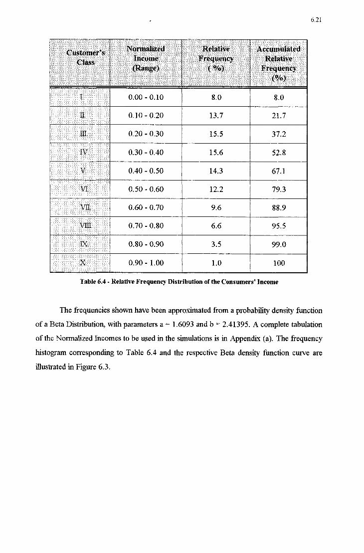
C -__l-_- '‹

-`.-_=.:_§.~.-z.:.;{.f_.‹.;.:ͶÍ:Íf_Í:Íɧ{Í:Í:Ííff

CMS ríršë1315:35fã?2555525íšãí5552;š;%;š;1;¿fí1§5¿ÊÊi%Ê:5ÊFÊ'Ê1Ê'ÊÊf5Êi

' 0 V '

0.00 - 0.10 8.0 8.0

0.10 - 0.20 13.7 21.7

0.20 - 0.30 15.5 37.2

0.30 - 0.40 15.6 52.8

0.40 - 0.50 14.3 67.1

0.50 - 0.60 12.2 79.3

6.2

~;:~_5:;-.âfzzzzzízzáz;z:¿5:;M1š£;5:¿¿:;iâ¿.;á:¿5:;¿r;¿:¿5:' 0.60 - 0.70 9.6 88.9

0.70 - 0.80 6.6 95.5

É

0-30 ' 0-90 3-5 99-0

:§;:f:`¡::¶::í-:É::§;:§;:} 0_9() _ L00 1_() 100

Table 6.4 - Relative Frequency Distribution of the Consumers' lncome

The frequencies shown have been approximated from a probability density function of a Beta Distribution, With parameteis a = 1.6093 and b = 2.41395. A complete tabulation of the Normalized Incomes to be used in the simulations is in Appendix (af). The frequency histogram coiresponding to Table 6.4 and the respective Beta. density filnction cuwe are illustrated in Figure 6.3.

6.22

A FYBQUBHCY

[112 ._.;... ._

_¿.... 111 Iv `

._ una H V t VI ¡ ¬

Customers' Classes : vn :

U_U4 __. I

. . ...- _ Vm

;

'

_ IX I _X UIUU O 1 I I I' I I I É I Y l f I V ›

0 0.2 0.4 0.5 0.8 1 (rhlzfigqfgfized)

Figure 6.3 -Consumers' Income Frequency Histogram With the Respective Beta Distribution Fitting

II. Characterization of the Consumers' Income by Fuzzy Sets

The universe of discourse of the Consumers' Normalized Income, defined by the interval (0, 1) Will be divided into fuzzy sets, which in this case are all either of trapezoidal

or triangular sha.pes. The main motives for this simplification are two: First, the volatility and subjectivity of the criteria for the classification of this kind of data, even when real figures are available, which is not the case in this research model. Second, it is at well

acknowledged fact the one of the advantages of the fuzzy logic tools is its remarkable

ability to yield very satisfactory results even when the characterization of the data. is not precise. In other words, -the fine tuning of the shapes of the fuzzy sets responsible for

modeling the information should not be a critical point for achieving success in the proper

6.23

working of the system built. If the outputs are too sensible to this approach, then maybe another more suitable tool should be found to deal With the problem. The same can be said about the points Which define the fuzzy sets. Here, the criteria employed to detemiine the

limiting and central points of the linguistic variables qualitying the Consumeis' Income was based on its accumulated frequency distribution jzc.

ffzpzzofidzl 0.00 0.10 0.25

0.00000 0.1 1609 0.22145

Triangular 0.10 0.30 0.50

0.11609 0.25369 0.38140

ÍÍÍÍ

Triangular 0.30 0.50 0.70

0.25369 0.38140 0.52183

Triangular 0.50 0.70 0.90

0.38140 0.52183 0.71354

ÊÍ~Í2i;ÉÊí

f5?5Ê555í55í15§Êí§ÍɧÍʧ55§55§55§Ê§§§Ê;§

Trapezoidal 0.75 0.90 1.00

0.56203 0.71354 1.00000

Table 6.5 Specification of the Consumers' Income Fuzzy Sets

The variable w=f(fa¢_) is the Nonnalized Income, and the argument, fac, is the

aecumulated relative frequency. Figure 6.4 depicts the Fuzzy Sets selected to qualify w¡ ,

with the degrees of membership u(w¿) shown in the vertical axis. Five levels of Income have been designed to accommodate the Consumers' wealth.

Why five fuzzy subsets? As will be seen subsequently, the domain of the several variables used in the current model is always partitioned in five linguistic qualifications. The reason for doing so is not grounded on theoretical or empirical evidences, but emulates a

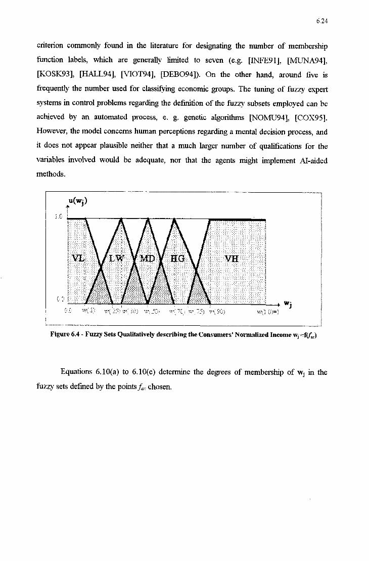
6.24

criterion commonly found in the literature for designating the number of membership function labels, which are generally limited to seven (e.g. [INFE9l], [MUNA94]_, [KOSK93], [HALL94], [VIOT94], [DEBO94]f). On the other hand, around five is

frequently the number used for classitying economic groups. The tuning of fuzzy expert systems in control problems regarding the definition of the fuzzy subsets employed can be achieved by an automated process, e. g. genetic algorithms [NOMU94], [COX95]. However, the model concems human perceptions regarding a mental decision process, and it does not appear plausible neither that a much larger number of qualifications for the variables involved would be adequate, nor that the agents might implement AI-aided

methods.

u(w¡)+ _ _ l :L f

¡_ __ .__ :_. .__ .j.

z: = :z :›; 1-: :‹: :-: .-:‹

'~ ' 1 1-' 3-' :-: 1'

:-: 1-zl

›: .-; .‹: .- -1 .~: .-1 .-; .-1 .-_‹

tiifiišiI§IIÊfiZfíÉI1ɧÊí1 _. Ifr iii Ii Iii'-ÉS Ii ~:1-ÉIíÊ1Éí1ÊIíÉ1-. É1

'fi ff 1.5 É IEI 1;. Íi É. 1fI‹ÉJí§i1Éi1fi YÉI If TÉÍ IÊÍ IÊIÉÍ ÉÊÍ

É-1;:_;:_;:_.¿_::_:§V;§_:§_:__::_:__ ._.§_:§_:§_;:::_:š¡;:;;_¡:§;: ¿¿::¡:§¡:_;;;§-::¡::¡::¡:§¡ ¿::;::;::¡::¡:¿:§¡::¿::¡;§¡:¿_ ___;¿,§¡;§¡;§¡:§¿:§¡::_;§¿;:¿;:;:;§¡:§¡:§§§{:§§.¿_.¿_.¿§._§;:¡:.§z_¡;;§;_§.

_

S

l

lg :_ .__ :..-___; :c_..z.:.:__ : '

__ .__ .__ :__ .__ :_ _; :. :_ ,z_ :__ .j. {. ._ .;_:__ .'_..z..z.¿..__ :__ :_:_ _

-

:_ .__ .__ .__ ._\ .__ :_ :__ ._ ___ .__ .__

: - - ‹

._ .__ .__¿_ __ ¿_ :_ .__ ¿_ :_ .__._ * '

'_ ._,._,.__ ._ :_.__

gif :'Í:":': :'.':':-.'Í¡:'::" :'f:`::'::'Í:`::': :Í:'fÍf 'Ê -'Â-ff-Í fÍÍ'Í:Í.'Í‹ `""' 1 'i

'Í.'Â.Í.'Í.'Í.'Â.Í.Í.'f 'À 'I 'l " "

.Í 'ÍIÍ S: .ff .Í

' À

ÍÍÍÍÂ Í"fÍ :'_'.'f

¡_. ._ :_ :__ ._ j, :__ .§_~'.. .j. :__ .§. '_

:__ .__.j.,¬__ .__ '_

.__ .__ .j.¿.:__.- .__ ___; .§._.:_ .__ ¿.¿. :__ .__¿_ '__ ._ __ _; _-__ _-_ _-__ -__,_

› ' .' I If " " .Í Í. .if 1:

~.‹

-'Í'

‹ wi

__

\É

x E \`

â -' W' * J

› - _. .. _' _ . <' ¬' _ rt, ., __ x,__.¿:¿ ;:;¡=¡|

Figure 6.4 - Fuzzy Sets Qualitafively describing the Consumers' Normalized Income w¡ =i`(ƒÇ,,)

Equations 6.10(a.) to 6.l0(e) determine the degrees of membership of wj in the

fuzzy sets defined by the points j,}C chosen.

1 if oâwj 50.116 uv,_(w¡)= -9.492w¡ + 2.102 if o.11ó<w¡ z<o.2~21

o if wj > 0.221

0 if oéwj 110.116 7.268 wj - 0.84-4 if 0.116<w¡ 50.254 -7.830w¡ + 2.986 if 0.254 50.3813

0 if wj : 3

u1,w(.Wj):

V. Ç z..

U) OO ›-4

0 ä wj 0.254 0.254 < wj 0.381

-7.121wj + 3.716 0.381<w¡ 110.522 0 wj .> 0.522

7.830 W- - 1.986 UMD (Wj 7 :

0 if 0 ii W 5' 0.381 -7.121w - 2.716 if 0.38l<Wí'0.522 -5.216 W + 3.722 if 0.522 ‹< W 0.714

0 if W > 0.714 uno (W) :

[Â 0 if w < 0.562 uVH (W) = ~t6.6OO W - 3.709 if 0.562 <¡ W S 0.714

1 if W ;> 0.714

III. The Consumers' Sensitivities to Price and Quality

6.25

Eq. 6.10 (a)

Eq. 6.10(b)

Eq.6.l0 (c)

Eq. ó.10(d)

Eq. 6.10 (e)

Every Consumer is índividualized by its Normalized Income, and that. attribute will be used to establish serzs1`tr`ví1_.y parameters to the pn`ce p¡g and the quality q¡g of a product

6.26

or service in prospect. To accomplish this objective, an universe of discourse for those two parameters is established, and qualitatively described by fuzzy sets.

The sensitivity parameters will serve as references to modify the way each buyer perceives the price and the quality of the item being sold. Whereas the price p¡g can be

appraised by the customer, and solely by it, before the decision to buy or not the product or

service is made, the complete appreciation of the quality q¡g only can be properly

consurmnated rf and afier the Consumer bought the item.

Nevettheless, regarding the quality, the players will be able to have access to some partial information transmitted from the other customers Who previously had a concrete experience with products or services purchased from Firm i, with which the present player is considering to deal. This topic of the model Will be explored in detail ahead.

The price of a product or service itern being sold in the market, When evaluated by any two Consumers with different Nonnalized Incomes is classified in distinct manners.

This seems to be a. natural approach, since in realistic situations people With a greater

wealth may find some price “reasonable”, while a less affluent individual is likely to assess it as more costly. Thus, the sensitivity parameters that are being introduced in the model

have as objective the accounting for those individual differences in perception.

Each sensitivity parameters s,¡, s,¡¡ represented in the horizontal axis of Figure 6.5

will be detennine‹L__ for every Consumer, by means of a set of fuzzy production rules,

Which have as antecedents and consequents the fuzzy sets illustrated by Figures 6.4 and

6.5, respectively.

6.27'

degree ofmembârsàrp . "(55), “Weil

10 ` .JL

_

_-

Í.IIÍÍ.- .'.Í`.ÍI.IÍÍÍIÍI. .ÍÍIIIÍÍ-, ÍÍÇ. .Í..ÍÍÍÍ'.ÍÍ.ÍlÂ.

I ' ` T ` ` ' ' ' '

- › ~ - - - - - - ~ - - -- - - -

,¡.fi-zé-2=;-:é2;2=:.-té-:â›:‹'.-;fI~:-›í-1='I-:=:I-:‹@2=.‹ » - › -

-.z;-;ë-:›:-1-=I-1::-;=.-:=I-:=:-i-ii-I=:-1-ii-:fi-2;-;f..- - - -

I

'

I

'

É I I

' Z i 'fi«I-;›I¬:2-I-í=I-zz-.iiI-;I~I2-.'I-I-ifí-t-I§~I-;-I‹í=-í›;-1i1~I‹;z

`

Í Í~Í Í

'

I

'Ç"'..l. .ÍÍ1Í'I' 'ÍÍÍÍÍÍÍI 'ÍIÇÍ'.`.`I`.:`....`.`.`.`.. 'Ç`.`.Ç`._Í`.\I`.`.I`ÍII ,.f[Í`.`.".I`

X _\/¿ , \,\¡_,/ a\ sm

-5.11 -2.5 DJ] 2.5 5.U ›$‹1i :re.12s:'¿:'r›:'t`y pzzameter to pnce, qu.zI:f)~'

Figure 6.5 - Fuzzy Sets describing the Consumers' Sensllivity to Price and Quality

The values of sm, sm are obtained through the defuzzification of the linguistic attributes u(Sp¡), u(s.¿¡ ) of the Consumer”s sensitivities to price, quality. The general expression for the defuzzification of sm is depicted in Equation 6.11.

sp __ AVS ×d1+AST ×0.25-PAMS ×0.5+A¡S ×0.75+Av¡ ×d¿ Eq 611 ¡_ p 4

. .

Avs +As'r +AMs *Ars +Avr

In Equation 6.11 above, the variables AVS, AST, ..., AV; conform to the areas of the

triangles representing the various filzzy subsets, truncated at the height of the

eoxresponding degrees of membership yielded by the production rules from Table 6.6. The variables (11, dz, and the numeric values are the distances of the centers of gravity of the

several areas to the point. sm = -5. The defuzzification method chosen was the center Qf grmnfly of area (COA), as was explained in Chapter 4.

The other parameter regarding quality, sq¡, will be taken as the opposite of Spj, that

is, s.¡¡ = -s¡,¡. The rules listed in Table 6.6 are similar for these both parameters, only the

consequents are reversed. This means that a wealthy individual, besides being more tolerant

6.28

in relation to price, is also more demanding When it focuses on quality, and conversely. Due to the fact that the la.bels of the fuzzy sets that designate the sensitivities to both price and quality are the same, the reversal of the fuzzy conclusions became necessary, and the defuzzification will simply yield parameters with identical modules and opposite signals.

The reason for this differentiation between q¡g and p¡g is the criteiion chosen to modify each buyer`s perceptions of price and quality.

The essential idea. that underlies the implementation of the proposed method is to promote modifications in a basic pattem of fuzzy sets that designate the non-fuzzy data

pertaining price and quality. The alterations Will consist in shifting consistently the

reference points that define the fuzzy sets in the hoiizontal and promoting specific dilation and concentration operations, in a similar manner to adjectival hedges

[ZADE72]. As a result, every Consumer Will be particularly characterized, and its decisions regarding the same circumstances may be different from other individuals.

The determination of the sensitivity parameters is done With the support of two

similar and simple filzzy expert systems. The only differences in the production rules are in the consequents, which are symmetrically opposed. Table 6.5 displays the rules for both

price and quality sensitivity parameteis.

6.29

Rule 1: If Income (w¡') is Veizv High. (VH) then the sensitivity to price (quality)

parameter s,,¡ (s.¡¡') is Very Insensitive (VI) (Very Sensiltve (VS)).

Rule 2: I ƒ Income (w¡) is High (HG) then the sensitivity to price (quality) parameter s¡,¡

(s,¡¡) is Insensitive (IS) (Sensitive (ST)).

Rule 3: If Income (w¡) is Medium (M])) then the sensitivity to price (quality) parameter s,,¡ is i\›Iedi11mSensitive (MS).

Rule 4: I f Income (w¡) is Low (LW) then the sensitivity to price (quality) parameter s¡,¡

(s.¡¡`) is Senszfive (Insensifive (IS_`)_).

Rule 5: If Income (w¡) is Very Low (VL) then the sensitivity to price (quality)

parameter s¡,¡ (s,¡_¡) is Very Sensitive (Vergt Insensitive (VS)).

Table 6.6 Rules used by the Fuzzy Expert System that associates a Consumers' Income W, and the Sensítivity to Price and Quality Parameters sw and sq¡ respectively.

The application of the rules from Table 6.6 Will deteimine the output (consequent) Sen.sítii=i1y to price ('qz¢ality) parameter sm (,sq¡) from the input (qantecedent) Income (wj) for

every Consumer j. Then, the basic configuration of the fuzzy sets that describe both the

price p¡g and the quality qig of a product. or service, illustrated in Figure 6.6, Will be

updated. This procedure generates a new specific partem of fuzzy sets for each Consumer

j, with which it will perceive the price being charged for the item by any Firm i during a

particular cycle g of the game, and the respective quality, if and after the product or service

is purchased.

The alterations promoted by sm and s.¡¡ in the basic pattems are of two kinds. First, all the reference points in the horizontal axis (u(p¡g)=0) will be consistently displaced to the

right or left”, of a distance s,,¡ from their original standard location. With this manipulation,

15 The displacement of the reference points is made to the right or left, depending on whether the signal of s is positive or negative, respectively.

6.30

the resulting group of fuzzy sets are vertically sectioned at either one of the right or left

extreme points (0 or 10) of the universe of discourse, losing the outer portion.

Second, the membership fimctions are adjusted by either a dilalion or

concenmaion operator, which by their tum are also filnctions of sm and s.¡¡. The criteria proposed in the process is to dilate or eoncentrate the membership functions Which refer to

points in the domain of p¡g or q¡g lesser than 5 + sm (or 5 + sm), With the operators:

_ ,, 1 Dilatlonz OJ = Eq_ 5_1z_(a)

1 + ...EL5

¬ - . 152 -i Çoncentratlon. X). = 1 + Eq. 6.12(b)

The direction of the shifting (left or right) and the application of the hedges 5, and

Xj will depend on the sensitivity parameters deteimined for every player (bu)/er), according

to the criteria listed in Table 6.7.

The choice of the denominator of lspjl Was arbitrary, but taking into account the range of values that the resulting expression would yield, and the possible shapes of the

ensuing curves.

N .al

_ u_z_‹p__› = [u‹;p__›1õj

fz. 1sp¡| : 2 1fs¡,¡ > 0 :1-1.~:1-':-_:-:i›;:¡:tÍ:ií:' pig< + Spj) ÍfPig>(.5-0+Sm`)

N ucon(Pig) : [u(_Pig)]¡j

¡Sm! = ‹= If Spà 0 u_zz‹p__› = [u‹p__›1f”

1151251;i:55:¿5:;¿:;i:¿5;i-"~' if Pag (5-0 + Sm)

ucon(_pig) :I [u(pig):IXj

ifp¡g<(_5.0+Spj)

.í O if spj : O none none

_

|Sq¡¡ I <= lfsqâ 0

zfiââíâfííiízE355;zizâ;i5=š;5fâzE;šzíi;;i;f%z 0 `

if Sqj = 0 110116 110116

-_

IS I

- 3 if s O udü(qig) : [u(qig)]õj

'

qi - qi ->

_¡__,._,_;___ if qàg > (5-0 - Sqí)

1›___..‹p__› = [u‹_qz_›1”`

if q¡g< (_ 5.0 - sq¡`)

10-.‹‹1__;› = [u‹q__›1“ ucon(_qig.) :

1.;a:zf:;§:é zâif' 'z;:;;:;::;.:;í:;;:f ¡f“11:<'<(Í5-O ' S01) Ífqiâ Í-" (5-O ' swf)

Table 6.7 - Operations for modifying the Fuzzy Sets that depict the Consumers' Perceptions of Price and Quality

u(p¡g),I1(q¿g) degree ofmemberaàrp

1. D \\

.___ ____H____,__ .___.__ __,

1zl;11"-z /zf;f;;~í55;1_»;"â~ __../z'§Í_fz§5ÉÊÊ{ÍÊÊ?'_ _/ÍÊÊÊÊÊ

Í , ,/ /' \ _ . _ _ _ _ _ _ _ _ . _ _ _ _ _ _ _ _,{_;.z_-,.›j_,_{_-,.‹ _ _ _ _ _ _ _ _ _ _ _ _ _ _ '__-_‹,- _ _ . _ _ _ _ n _ _ _ _ _ _

›z

_ , _ _ _ _ _-.›_›_f_›.‹.-_--.I-,f-_ _ _ , -‹

Ú Ú / \¡_.f RJ/ ~ _.__1-âzzzzzzâ:-z:z:z:1z=z:z:zz:â:z:z:zz:z:âz-ê-¢âz:zzà¢;z1:_:~zz1zz:íâzf:âz:â«1_

,_ Pâgfiig

0.00 2.50 5. 00 150 10.00 ,‹›zƒ.‹_zz _¢zzzm,z›

Figure 6.6 Basic Fuzzy Sets describing the Price pia and the Quality qigz

6.32

The equations for the Basic Fuzzy Sets in Figure 6.6 are not of interest because the standard configuration is only a starting point for designing the conclusive modified fuzzy sets that Will represent the sensitivity parameters. Instead, the equations that determine the

degree of membership of pis in the adjusted group of sets are given. Two cases must be considered: sm O or sq¡:< O and sp_¡< O or sq¡>0. The equations for each situation regarding the price are 6.1'3(a`) to 6.l3(e) and 6.14(a) to 6.14(e), respectively. The same formulas apply to the quality, substituting

I sq¡ I for spj and qig for pig.

Spjzü orsqjsü

í

1

Uv"L(Diâ)_ ,¿[Ov_..1_(Spj __pig) +110 j Spj < pig < spj Eq. 6.13(íI)

if -pia gsm

l` O otlzen-vise

r

'“ Spjflôj E Sm <pig SSH +2.5 uLW(p¡g)= ‹ [OMSH _ Pig .)

+ 215, if sw. + 2.5 < pig < sm + 5.0 Eq. 6.13(b) 0 otherwise

Í [04 (P is ` SP1) _ IFA if sm + 25 < pra SP1 + 50 uMI¿,('p¡g): [0 _4 (Sm, _ p ig + 3111 »S'm› 'Jr'

pra '~'Í.

SP1 + EQ. 6.l3(C)0

\

otherwise

p 4- [OA (Pig _ sm ) g ¡_,_]“x_f if sm + 5.0 ‹:_pig 5 sm +_7.5 uH`3('pig)_

[*>~4‹spi ~ p ..› . 41% if Sm + 7-> ~< Pzz 1° Eq- 6z13‹'‹1›

O `

otherwise

'

V

‹. ¬ xt .` uW¿p¡g‹)= j{[o.4(p¡g ~Ospj ,_ J]

1 11 sm + 7.5 < pig É 10 Em óme) otherwise

.<>›

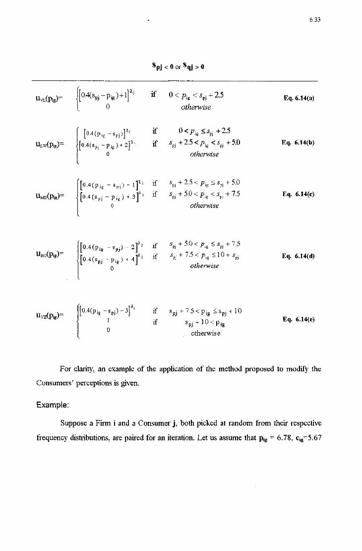
U) 1)

spj<0orsqj>0

U\,1(p¡g`)= ‹ iO'4{~SPJ' -pis ) +1] 1 If O <" pis <` Svi + 25 Eq. 6.14(a)

\ Ú otherwise

I

_spj:)].-xl' if 0<píg sspj uLW(p¡g)= ‹[0_4¿Sm_ _pig ) + .2]1,õ if sm. +25 < pis <sP¡ +5.0 Eq. 6.14(b)

o otherwisen

r

[0.4(pig _ sm_)_1]1_¡ if sw- +2.5<plg ásm +50É

uizm(l3ig): ‹ [0-4(Sp¡ * Pi» ) + 31" if Sm + 50 < pis < Sri + 75 Eq' 6'l4(c)

0 otherwise~

io-4(P¡g - Spi) _ 21% if Sm + 5-O '<¡ Piz; 5 SP1 ¬` 75 llH.;(1>âg)-

[OMS _ _ pi .) + 416,- if sm. + 7.5< pia í;10+ sm. Em 5_14(d) i PJ

O g otherwise

ó,- _ 0.4.-zr-3 '

- 10 11~m(1›¡g)= i (pla IPJ) i

If Sm” *Pig 5m* '

.. ,. E . 6.14 .

if sm- +10 se p¡g q (9)

0 .

otherwis e

For clarity, an example of the application of the method proposed to modify the Consumers' perceptions is given.

Example:

Suppose as Firm i and ao Consumer j, both picked at. random from their respective

frequency distributions, are paired for an iteration. Let us assume that pig = 6.78, c¡g=5.67

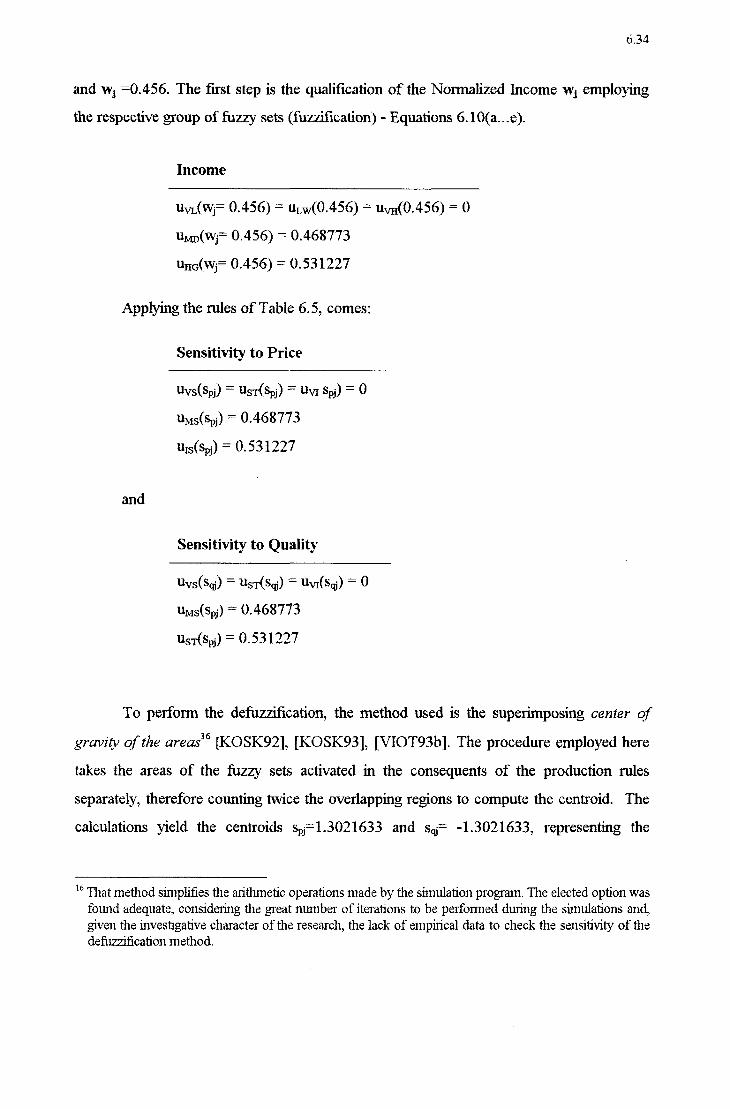
6.34

and wj =0.456. The first step is the qualification of the Nomxalized Income wj employíng the respective group of fuzzy sets (fuzzífication) - Equations 6. l0(a...e`).

Income

u\.zL(_W¡= 0.456) = uLW( 0.456) = u\›H(0.456f) = 0

uMD(vv¡= 0.456) = 0.46S773

uHG(_W¡= 0.456) = 0531227

Applying the rules of Table 6.5, comes:

Sensitivity to Price

Uvs(SPJ') = UST(Sp_i) 2 “VI SP1) Z 0

uMS(_s¡,¡`) = 0468773

U15(Sp¡') :

and

Sensitivity to Quality

uvS(sq¡) = uST(sq¡) = uv¡(sq¡) = O

uMS(_›Sp_¡`) :

uST(s,,¿) = 0531227

To perform the defuzzjfication, the method used is the superimposing center Qf gz~e¬›zzy efzzze areas” [1<osK92], [I<os1<93], [v1oT93b1. The pfeeedufe employed here takes the areas of the fuzzy sets activated in the consequents of the production mles

separately, therefore eounting twice the overlapping regions to compute the centroid. The calculations yield the centroids sm-=1.302l633 and sq¡= -13021633, representing the

15 That method símplifies the aríthmetic operations made by the símulaüon program. The elected option was found adequate, considerirlg the great number of iteratíons to be perfomred during the simulations and, given the investigative character of the research, the lack of empírica] data to check the sensitivity of the defuzzificatíon method.

6.35

Consumer”s sensitivity parameters for price and quality, respectively. Figure 6.7 illustrates

the defuzzification process regarding As to sq¡, the method is analogous.

u(p¡g) degree of membership

1.Ú 1

\1¡g[S¡›j]=D.531227` _ `\\ \1M$ISpj1=o.4fza173 \

DO / me / ea \ ls

...1..............11....1.;.;;.1z,:;1;z1z.1;,:z.1z‹1;,;›z11.....'1::.1:111111111

. 1 2 2 1 1 1 1 1 1 1 1

1

1 1 1 1 1 1 1 1 '_‹9:-'21-il:-gl-1-gi-1-5;-iv:=í-1-11:-fi'›;í-1¿Í:›fí›1=í›1 1~1-'-›1--.‹' 1 1 1 1 1 2 1 1 1 1 1 1 1 1

1

1 1 1 1 1

~ _, _

'

1 1 1 1 t 1 1 1 1 1 1 1 1 1 1 1 1

'

1 1 1 1 1.

'

1 1 1 1 1 1

1

1

1

1 : 1 1 1

' ' '

I 7 Í › SP-i _ . _

-5.0 -2.5 »l].U 2.5 5.0 sensitivity SPj='|.3Ú21533

centroid

Figure 6.7 - Example of the Deffuzziñcation of the Sensitivity to Price Parameter

Next, it is necessary to determine qig from cig using Equation 6.6, Which yields q¡g=7.447.

The parameters s,,¡ and s.¡¡ will alter the basic fuzzy sets which describe the

perceptions of the price p,g and the quality qig, according to the guidelines of Table 6.6.

The universe of discourse for those variables remain unchanged in [0_, lO]. The modified group of fuzzy sets for the price are illustrated in Figure 6.8, with a similar procedure is

performed for the quality.

sm = 13021633; sq¡ = -13021633

1 Dilation operator (Eq. 6.12(_a)): õj : = 0.7934

1+ -;-Â5

13021633 Concentration operator (Eq. 6.12(b_`)): xi = 1+ -š--= 1.2604

6.36

Then, to the Consumer chosen for the example, whose income is W,-=O.456, the price and the quality of the product or service in perspective offered by Firm i shall be

qualified by the respective modified fuzzy sets, using equations 6.13(a...e`) and 6.14(a...e).

Price

uw_(p¡g=6.78)=u¡_w(p¿g=6.78)=u\,-H(p¡g=6.78)=0; (Eqs. 13(a,b_,e))

uMD(p¡g=6.7 8) = 0.7654 ; (Eq. 6.13(c)f)

uHG(p¡g=6.78) = 0.1242 _; (Eq. 6.13(d))

UÍD- ] degree ofmemhershíp , (1+Ú_2604Í 1? [u¡_p1g)] q1+o_2õoz1) íuíplgfl

*

__. z _

IIÍÍÍ ÍÍÍ.'IÍͧͧ_. .ÍI`ÍÍÍ_`II_ÍÍÍ__. _ÍIÍ III .Í \

1`Úi":':í1'I'_::`Ê\_~. /iÕ\\n"/ .-f"'f'} .fli

:'::::_ ;:'_':1¿;:.\` /¡_;'/_;;:”::`:`_~\E // ëfix 7' 'ii11¿1¡7\._'ÊÊÍÍf1ÊÊÍÊÊÊÊÊiÊÊ7Ê: ::_'5:"1"':_"ÊÍ: -"`

I

:ÊÊ:R

f'ÍÍÊÍÍÍ“_fÍÍ_‹;,}:,:1:_':1:it:':::::`:"::š§\;,:Í':::;::"::Hâ¿"~ Í, 5*

ff ~ ~ 1

\ /Ó`\' '\ \ -"

Í 1 1 1 1 i

2-í E 1 5 5 5 -_

5

5 5 51 1

f_1_5,f5 z

f'51 5 5 5

5 5

_

55 5 5 _ 5 5 5

5--__

¿ ¡

_-

¿ f

_Í

f f f § A-¡ ¡ ¡ ¡ ¡

_ _ _ _

*_ _ _ _ . _ . _ _ _ ,_ _ _ /VH

` I.

.f

\:\1 Í*

Í A I/e \ \ Í D Ú QI 1

W'

, _ _ _ _ _ _ _ _.

. _ _ _ _ Í

` `

_ I I

'

I I Ç I.__-jk-jz_ '

I _ I I I

i

I I Í I Í

_'

I _ Í Í Í I .

i . . › . . . . . z . . . r`_':'.'.-'z:Ç'_,{':'_'.Ç!,'S12':Ç':§'›^Ç'¡1'_:Í',1'_fi',-" f'.'_~ . . . . . . '.-'_%¬'_'¡'_'4."_',:'_ _ . . . . , . . . . . . . . ¿^

_ _ . _ . _ _ . . _ 7 . _ _ _

›- - -. f-z ,- A Pig =5.7a pm” s h ifl *pj = 13021633

Figure 6.8 Modified Fuzzy Sets according to a Consumer's Sensifivíty to Price

Quality

uvL(q¡g=7.447Í)=um‹§q¡g=7.447`)=uvH(q¡g=7.447`)=0; (Eqs. 6.13(_`a,b,e`)`)

uMD(q¡g=7.447) = 0.4622 ; (Eq. 6.13(c))

uH¢(q¡g=7.447f) = 0.3737 ; (Eq. 6.13(d))

6.37

u[q¡g) degree ofmembership [umign [um

)](1-I-02604) ¿ "' Ig

,dk ¡//' .

'Í'

šš'5_15_íÍÍ~Ê51*z~. aí.5í?fiiiizií§?§ÊiiÍ*s,šff§ii1iiz E/ `*

\`\ \` 1) í; r\ \ \¡

,,..:'.I.:'.:i'.:i -i?i›:Ií~ííf»:›¬::::1::1:'1:':::: :1::;:.:::t. ~;;::;;;

U U Í

à

\\i ` fi/J ` 3 / /

ê ` ' ` 'K '

t t V « 1=;;;1;;11;ê ,. 0.00 2.50 5.00 `£`:›_s;1\\$ 10.06

"Q A quality iftigl M4? shift

IS.¡¡l=1.3n21s33

Figure 6.9 - Modified Fuzzy Sets according to a Consumer's Sensitivity to Quality

The Consumer*s perceptions determined regarding the price and the quality of the

item being sold by Firm i found in this example will be saved for further illustration of the

market share game, Which is going to be presented along the detailing of the proposed

model.

The next steps to be approached are the item's evaluation by the Consumer (presupposing it purchased the merchandise), the assigmnent of payoffs and the final

C-onsumer's decision (to buy or not the item).

6.4.6 - The evaluation of a product or service by the Consumer

The payoff a Consumer will receive in an iteration With as particular Finn depends,

in a first basis, on its decision about buying or not the product or service offered. Ifit does

not buy, its payoff is zero, independently of the price pi; and quality qíg assigned by Firm i

to the item in perspective. On the other hand, if the Consumer purchases the item, it will

have the opportunity to observe its quality, and Will receive a payoff that Will be a function

6.38

of its subjective evaluation of the deal. The criteria and mechanism employed to perform that evaluation are explained in the following section.

Let us suppose that a Consumer has decided to buy an item from a. particular

supplíer (Firmf)". After the purchase has been consummated, the buyer observes the

quality of the merchandise, and with its own perceptions achieved for the factors price and qzralíty, it will then perform an evaluation of the deal. This appraisal Will serve as the basis for the assignment ofpayoffs to this category of players.

In order to carry out this objective, each of the perceptions of the two mentioned factors will again constitute the inputs of a. fuzzy expert system, each of which yields as the

output a new variable, to be called the attractiveness cnpj of the price pig, and of the quality oc.¡¡ as perceived by the Consumer j.

The variables am- and ot,¿¡, likewise other forrner parameters present in the game”s model, shall be described qualitatively by fuzzy sets. The universe of discourse is the

interval [0, 1], which is divided into similar fuzzy sets for both attributes 011,3 and oi.¡¡. The

mapping of pig into ‹1.,,_¡ and q¡g into oiq¡ Will be made with the aid of the fuzzy production rules listed in Table 6.8 and 6.9, respectively.

Figures 6.10 and 6.11 depict the fuzzy sets qualifying the attractiveness of the price

pm and of the quality qig, both modulated according to every Consumer”s sensitivity

parameters sm and s,¡¡.

W The explanation of how the Consumer has anived at that decision is deferred to a. subsequent section of this work. See 6.4.7.

6.39

Rule 1

Rule 2

Rule 3

Rule 4:

Rule 5

If the price p¡_.5 is Very High (VH) then the attractiveness of the price or.¡.¡ is Veizv

Unattractive (VU).

If the price pi; is High (HG) then the attractiveness of the price o:¡,_¡ is Unalíractive

(NA).

If the price pm is Medirim (MD) then the attractiveness of the price o‹.¡,¡ is Neutral

(NT )~

If the price pk is Low (LWÍ) then the attractiveness of the price oL,,¡ is

A2Ítractive(_ATf).

If the price pu is Very Low (VL) then the attractiveness of the price or.,,¡ is Veijv

Attractive (V A).

Table 6.8 - Rules used by the Fuzzy Expert System that associates the Price ph., as perceived by a Consumer to its correspondeut Attractiveness

tiewe ofmembezsírrp A u`

1 . ú .,

¡_ L

.\ X /t.\ ,zf .xx ,ff .

íi`z\ /,-Íziéfliz*-f\ _/íáíã-la.~\_ /ii \

I

\* /Í \ /* \* / _,/.Í:f¡ÍÍ':.'::'::.' ..1::::.t;'.::;'1..' z:;:::1:C::1:.::. _..::;:::;

L.U 0.25 13.5 BITS 1.0 Ufpj aIt.mcz:¿\.=ês:‹êss ofrl.-*xe price p¡g

Figure 6.10 - Fuzzy Sets depicting the Attractiveness of the Price pig

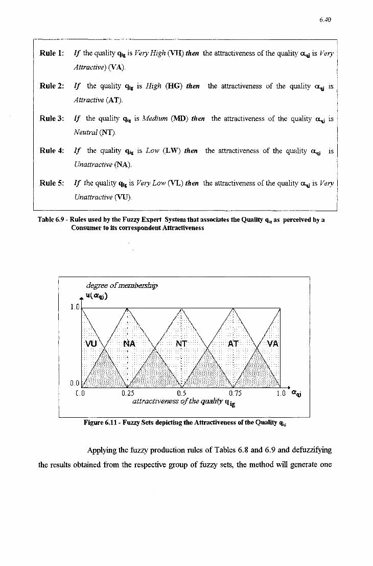
6.40

Rule 1:

Rule 2

Rule 3

Rule 4

Rule 5 ‹z

If the quality qk is Ve;yH1`gh. (VH) then the attractiveness of the quality md is Ve;§v Attractiw) (VA).

If the quality q¡g is High (HG) then the attractiveness of the quality o‹.,¡¡ is

A ttracfive (AT).

If the quality q¡g is Medium (MD) then the attractiveness of the quality or.q¡ is

Neutral (NT).

If the quality qig is Low (LW) then the attractiveness of the quality oL,¡¡ is

Unattractive (NA).

I f the quality q¡g is Ve13›L0w (VL) then the attractiveness of the quality o‹.q¡ is Very

Unattractive (VU).

Table 6.9 - Rules used by the Fuzzy Expert System that associates the Quality me as perceived by a Consumer to its correspondeut Attractiveness

1.D.` :\` ‹`/1,"`í\` -

‹

DD ':I51š1šffi-55151?'š?1š1%:fi%i-z==.“

›

degree oƒ`membeJabzp . fltfluâ)

z .',

_., ...I H

íevuilêf'w.~N;aí«f3~¬yf'â;íísâzr~iTââs;¿\

:\ ' /K 1 3/

00 0.¿5 0.5 ,

0.75 1.0 eq; afifactiversess a5f'£.¿se guâ1rfy'q¡g

Figure 6.11 - Fuzzy Sets depicting the Attractiveness of the Quality qíg

Applying the fuzzy production rules of Tables 6.8 and 6.9 and defuzzifying

the results obtained from the respective group of filzzy sets, the method will generate one

6.41

specific value for each of the variables ‹x,¿ and u..¿¡. It is rather intuitive that the payofi to be assigned to a player should reflect, as well as possible, the utility, or level of satisfaction that is obtained from the product or service purchased. It can also be claimed that the

evaluation of the item by means of the attractiveness factors may be considered a

reasonable approach to that problem. So, the payofi Which results fiom an accomplished transaction depends on a trade-ofi` between the attributes price and quality. The problem consists in the assessment, by an individual referee (the Consumer), of the gain obtained with the purchase of the item (object). In the present case, the object has an attribute space

X={price, qual1Í1y}.

One traditional approach to that evaluation problem is the method of the weighted mean. Although still largely employed, this technique relies on the presupposition that the attributes of the object (_ attractiveness of price, quality) are independent of one another, and

that their individually assigned scores may be added to provide a final conclusion.

Nevertheless, as pointed out by Wang and Klir [WANG92], “(_ )... in most real problems, these effects are interactive...; Ifwe adopt a nona.ddititive set function (a fuzzy' measure) to characteiize the importance of the two factors and, relevantly, use Fuzzy Integrals as a

synthetic evaluator of the quality a satisfactory result may be obtained.” Following the procedure proposed by Wang and Klir, each subset price, quality of

the attribute space X is connected with a real number ‹l›(prícei), ‹l›(qualz`z).=), ¢›(.) e [0,l],

that will stand for the importance” of each respective attribute.

Given any generic subsets of the att.ribut.e space X, e.g E and F, the function ¢(.) must obey the conditions:

° ¢(@) = 0 and <l›(X) = 1; 0 IfE ‹: F CX, then ‹l›(E) ¢(F)

The sole attributes of the product or service being judged are price and quality, and

they do not have sub attributes. So, only one space exists in this model.

'S The set function corresponds to the weights in the weighted mean method. However, ¢(.) does not have the additive property, so, for instance, ‹1›(x,Í,) + ¢›(x2`) af ¢(x¡ + rg). See Op. Cit. [WANG92].

6.42

An important characteristic of Wang and Klir'”s method is that the sum of the relevance measures of any attributes taken alone is not equal to that of the combination. In

other Words, the object”s properties reinforce each other.

The fuzzy integral L CY Ô¢ , where oc is the attractiveness of the object (product or service) being evaluated, may be employed for the aggregation of the attributes price pig

and quality q¡g regarding their respective importance mirrored by the set. function ¢(_.).

To compute ¢(price) and ¢(quaIity) once again the Consumers” respective Incomes will be used. This criterion has been preferred rather than an arbitrary setting of constant

numeric values because it allows the individualization of every evaluator (Consumer).

Therefore, each Consumer is made unique by its sensitivities to price and quality (spj, sq¡f)

and also by its importance factors ¢(prz'ce) and ‹t›(qualz`ty), which are expressed as ‹1›(_sp¡)

and ‹t›(sq¡). The importance factors have been designed to lie in the inteival [0.l, 0.4], and

their sum is not constant, since the idea derived from the proposed use of fuzzy integrals is that the importance of the attributes are mutually strengthened if they are contemplated

conjointly.

In order to implement the assignment of values to ¢(s¡,¡) and ‹l›(Sq¡), they shall be

defmed as an increasing functions of (Wma - W) and (W - Wmm) respectively, as shown in

Equations 6.15 and 6.16.

¢(5pí) z + 01 Eq. 6.15(zz_) VVv

' mfllfí

'H

- z

'

'›<( ._ and ¢(s _): ~+0_1 Eq.ó.1z(b) V

(U \Vffl3I/Í

Figure 6.12 shows the cutves illustrating the behavior of the functions.

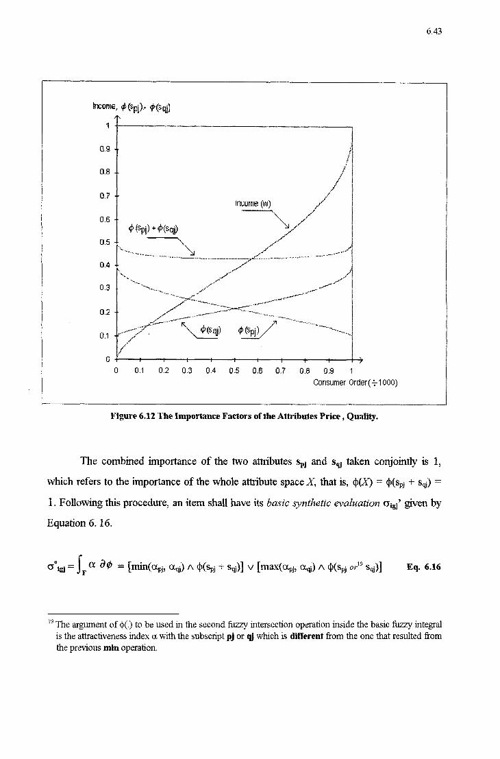
6.43

income, ‹;l›{sp¡), ¢{âq¡)

1 ' "'1

0.9 ~ É .Í

L

na - _f ;§

/' “‹

Ú-7 " .

f'/_

income (uu) ff H

__ \`›`N /z.,‹

'95 lspj) * '35 lsql) _./6

(15 ., *_í\` ..‹/X

¡z

"¬~... `\ f" fã zi ~ _ _ ‹»~

`""""""*-"'^'-~--------e..............,-..._ _.............- ..........¢›---~'^"'~'^*'*"""

0.6

\. ml*\

,f ,tz W. ¡:

.___u` “_/" 9/If ;

¬___ vw” _« t

H' _,.«-I t "~ . -- -¬____`^_ 'MJ' /__,_,.› ii Á

_..-‹-""'r-r - -` W t e_»__›~_ ___”,

0 1 _ ,/f ..,..r»- ._ mf' ...~--~"",d-V: w`__"""

---\._ II/.-:'v""'V'J'”W,Á

.fa ¬_4.'¬_"'*'=«

.

,«~»~"Ã^”', RH. 5 "J / 'if /.II

' \í ___.-f" KT;

.Í

_!

‹e~ ze fã Q Q r 11

rf 1

D 1 ¡ ¡ x â 1 z t F s ¡ ) 0 0.1 0.2 0.:= 0.4 0.5 0,5 0.? 0.8 0.9 1

Consurner 0rder(+1fJ00)

Figure 6.12 The lmportance Factors of the Attributes Price , Quality.

The combined importance of the two attiibutes sm and sq¡ taken conjointly is 1,

Which refers to the importance of the Whole attribute space X, that is, (t›(X) = ¢(_`sp,- + sq¡) =

1. Following this procedureâ an item shall have its basic symfhelic evaluation ow” given by Equation 6. 16.

= L “ 3°* = [mm‹‹×p_@, ‹›«z.z'› A ¢<s,›z + sol V [max‹‹×pz, ‹×z.ze› A ‹1›‹;spj se] Ei «-16

W The argument of ¢(.) to be used in the second fuzzy intersection operation inside the basic fuzzy integral is the attractiveness index ou with the subscript pj ot qi which is different from the one that resulted from the previous min operation.

6.44

Taking into account the discussion contained in Chapter 4 of this Dissertation, the

firzal qvnthetic evaluation mg, of the object with the basic fuzzy integral o°¡g¡ = L CY Õ¢ of the attractiveness indexes ocpj and otqj with respect to their importance measures ¢(sp¡) and

¢(sq¡`) will be modified from its original formulation. According to the alteration proposed,

the final synthetic evaluation Gig Will then consist of a sum of three values: (1) the original fuzzy integral (Eq. 6.16); ( 2) an increment (A+), which corresponds to the gain obtained by an eventual better score of an attribute (price or quality) that is not aifecting the original

fuzzy integral, and (3) a decrement (N), relative to a loss derived from an prospective worse feature that is not critical on the value yielded by the original fuzzy integral. The increment has been taken proportional to ¢(.) and decrement proportional to [¢(_.`)]%. The reason for this approach regards a presupposed greater concem to losses than to gains. As both ‹l›(Spj) and ¢(sq¿) mirror the importance a particular Consumer assigns to the price and

quality of an item, the influence exerted on (A+) and (A`) will be compatible.

Condition Increment (A+) & Decrement (A`)

0% “qt A+ = ¢(Sq;) 1× {mfl«\' [0, (Ow - m1fl(0¢p;,111fiX(0fl°z,¡, ¢(Sq¡))Í))]} Eq. ó.17(zz)

°H›1 > 0% A+ = <l›(.Sp_¡) >< {mfiX [Oz (<×1›¡ - HIHX (.<X*p;_¬ m‹1X(.(<׋¶~z <l>(.Sz›j)))'))]} Eq. 6.1'/(_1›)

°H›1'í% A- = ‹t›‹s,,,-f âmm t‹›,‹‹×,,j - mm ‹‹t›<sz,i›. wi-››1} Eq. õ.17(¢)

0% “qi

1\

A” = ¢›‹sqí›% âmin t0.‹‹×.t - min ‹¢‹s»j›, ‹×z›,›››1} Eq. 6.1'/(tú)

6.45

Then, the final synthetic evaluation is depicted by Equation 6.18.

em = ølg, + A* + A' Eq. 6.18

The values of um will be mapped into the final payoffs, after a scale transformation that equals the minimum and maximum attainable values of um to -1 and 1, respectively. The determination of the Consumer°s payoff iigff' in a given iteration y,

= 1, 2, ...,b¡¡g With Firm i in the cycle g zf (and only ii) it purchased the product. or

service is provided is explained in the next section.

6.4.7 - The Consumer's Payoffs

Once the item has been evaluated by means of the transformed fuzzy integral, being asciibed a. value of om, a payofl` must be assigned to the buyer, reflecting its personal gain (or loss) With the effectuated transaction. I-Iowever, the link between the product. or

service”s synthetic evaluation sig and the correspondent Consumer”s payoff zig is not

straightfoivvard, so a discussion of this matter is needed in order to anive at an adequate

scale for z¡g¡. For this purpose, some considerations about the range of om are necessary.

First, it is important to recall that the attractiveness indexes otpj and ocq¡ are obtained

through the application of a group of fuzzy production rules regarding an itemls price and

quality. Since the characterizations of price and quality depend on the Consumer°s

sensitivities spj and sq¡, the mappings pg -› o‹.p_¡ and q¡g -› orq¡ Will be different for each

particular buyer j. The importance measures cb(_s,,¡) and ¢(sq¡`) are also individualized per

Consumer.

W' The assigmnent. of the three subscrípts ig] to the synthetic evaluation ci and the payoff z was necessary in order identify the particular pair of players (i, j) as well as the cycle g to Which 0' and z refer. Still, to preserve the history of the iterations” results to be generated in the simulations, a fourth superscript y regarding the iterations” sequence order will be added to the payoff z. On the other hand, the attractiveriess indexes ow am- do not need those expedients, since they are used only momentarily, and can be dynamically erased and updated by the program during runtime,

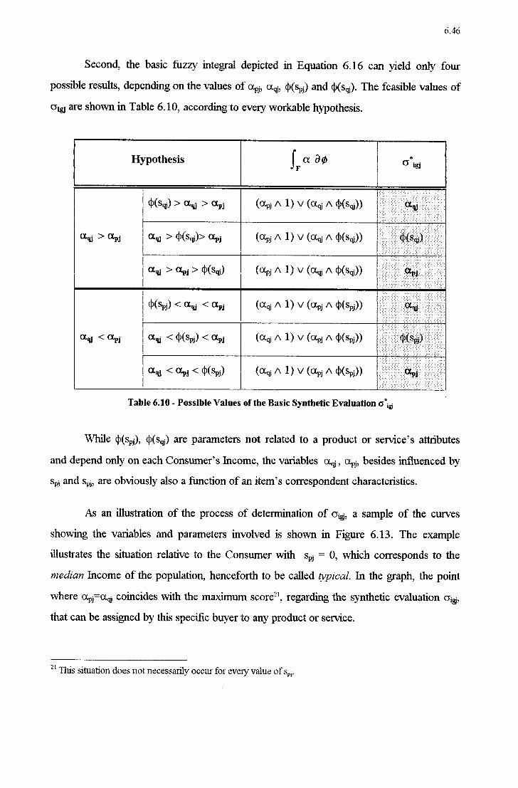
6.46

Second, the basic fuzzy integral depicted in Equation 6.16 can yield only four

possible results, depending on the values of 09,5, Ofiqiz ¢(_Spj) and ¢(s.¡¡). The feasible values of

em are shown in Table 6.10, according to every workable hypothesis.

Hypothesis La âø Ig] Go

¢(sq¡) > ot.¡¡ > cnpj (ofipj ^ 1) V (aqi ^ ¢(Sq¡))

“qi > um “qi > ¢('S‹1i)> um (api ̂ 1) V (Ow ̂ ¢(SzJÍ))

oL,¡¡ > oz.¡,¡ > ‹t›(sq,-) (Ohm ^ 1) V (Ow ̂ ¢(S‹ú))

¢(SpjÍ> < <׋ú < um (Ota ̂ 1) V (fllpj ^ ¢(Sp,~))

om..

‹išfiÍ'11`Í*ÍÍ`¡Í`ÍÍ`ÍÍÍÍ`ÍÍ*Í

°*‹u < am <1‹u < fl>(Spâ) < um (Ole ^ 1) V (U1›z'^ ¢(Sr›â))

OL-ú < um < ¢(Sz›âÍ) (aqi ̂ 1) V (Ow: ̂ <l>(Sz›.âÍ)`) @j`›'jͧÊ'EÊÊ*ÉÉf{'ÉÊ'Ê

Table 6.10 - Possible Values of the Basic Synthetic Evaluation o'°¡

While ¢(s,,¡f), ¢(Sq¡f) are parameters not related to a product or service”s attributes

and depend only on each Consumer°s Income, the variables ocq¡ , ocpj, besides infiuenced by

sm and sp,-, are obviously also a function of an item”s correspondent characteristics.

As an illustration of the process of determination of og, a sample of the curves showing the variables and parameters involved is shown in Figure 6.13. The example illustrates the situation relative to the Consumer with sm- = 0, which corresponds to the median Income of the population, henceforth to be called typical. In the graph, the point

where oL¡,j=oLq¡ coincides With the maximum score”, regarding the synthetic evaluation ‹3¡g-_,

that can be assigned by this specific buyer to any product or service.

21 This situation does not necessarily occur for every value of sp,-.

' 6.47

Note that, according to the rules of the game, a supplier can set any cost to the item it is cunently selling, only provided that it is less 01° at most equal to its piice.

The curves showing the behavior of otpj and onq¡ for other sensitiwities values are

included in the A1›pe11db<'”.

Àüraetiveziew of Price, Quality tor a twice! _. cz -

,¬ .. . “PI WA 'customer (sf-sqffl ; fflspj )= ‹}5tS‹,¡¡)= 0.215 ,i

in z zz

Q .›__. . . _ . _ . _ . _ . _ . , . . . . . , , . , , . . . . . . _ _ . . . , . . , _ _ . . , . . . . . . , . . . ._ , .._._. . ,.~,__,.__.,z›¢.-'_'.','.;

-.` __,

Quality

f_x 111)

8 _.z~"“i

.,__› l..~ 1

z 1

,__ _.. _ .__.i..__._ .max U_ ,

, IQI

_ zi .... ...°?'p¡.._/' ...... .. z __________ ...z~ev‹= '1 .' .¡ z«.¬.z,._...¬»...,........,,-,v.›,- ,....`lè__ ._

1

›

953

üf

PI'

06

× n . . . _ . _ . _ . _ . . . . . . . _ . _ . . . _ . _ . . _ . _ . _ _ . , . . . . . . . _ _ _ . _ . _ . . . _ . _ _ . _. *r

z

1- _.

- . ,

flÍÍI`ü0Í'UBfl

fi \-~_ ...

'~ “ mm oz- 1

onsszig -

i

Ú 1 . 1 1

l

1 ú › ú Y . . )

ci 1 2 3 ill 5 e v e 9 10 .-433 cig , [Im

Figure 6.13 - Attractiveness Indexes ‹x.,,¡, or.,¡¡, and the Range of the Synthetic Evaluation G¡g¡

As can be seen from Figure 6.13, the behavior of otpj, otqj is far from a smooth

cuwe, even in the simplest. case as displayed, of the zzvpical Consumer. The same can be

said of c5¡g¡.

The maximum and minimum values of o¡g¡ that. can be assigned to any item for eveiy combination of price and quality are listed in Table 6.11. They were determined

22 The cuives Were obtained employing the fuzzy e.\pe1t. system (ÍTa.b1es 6.8, 6.9)1'ega1'ding the qualification of piice and quality and defilzzifiyiixg the corresponding attractziveness (Figures 6.10 and 6.11). The calculations were perfonned using a. spreadsheet.

applying Equation 6.18 for eleven points regarding sm. Figure 6.14 illustrates

corresponding graph

6.48

the

.os9 .mó .115 .132 .137 .oss .137 .132 .1o9 [106 .os9

.sou .S09 {.5o9 .54s .572 .ssa ,597 .õos .S98 .5ó1 .soo

Table 6.11 - Maximum and Minimum Values for the Syntheüc Evaluation of an Item

3D|'| ._

r;

E'-ra

u

.

n Synt

et

:_

z

hfiíkä

-Ei

'11

tem

r"

1

!3!3Í:',C'.Ú-7!-'Í'

1:-‹_1¬r3¬.\1cof..D

0.3

.UF-Í' -1.1

Ú v | 1 r ‹ 1 1 u 1 "‹,

(1. .

/~. Ê]

Synthetic Evaluation Ranges

~*~f*›'1Â\'I

_F<ange of 'variation of the S',fr1ihetic= Evaluation

.ç,¬..-z.-z-_-r É 1 ; 1".. _ :*É'Í'Í_.

._ 2 'J'

“*l'fÍ if:

Mliü U~

__ ._ ›=‹=... .....â1*. ___.- -rá ̂'*' ` " ` “›~ez.__ à. __ `,.._._(.. “K ev ¬*

,.V. .`...`.‹. ..._._...._‹....‹...-vzr¬_.\..v.v. v._._.....v_.., `.\._........ .....›.m..-.N-\¬.›\‹..`¬......_.q

as a function of the C;0nsumers'sensili\'it\f to price

-5 -4 -3 ‹1 U 1 3 4 5s,,¡=- Seneitivity Tu Price

Süj

Figure 6.14 - Ranges of the Synthefic Evaluation as a Function of the Consumers' Sensitivities to Price

6.49

A convenient range for the payoffs is the interval [-l,l]. In order to associate the values of the synthetic evaluation to that scale, the mmirnum and maxirnurn values that may be assumed by um for each sm- shall conespond the extreme points -1 and 1, respectively. In this manner, each Consumer will have an individual scale, and consequently, a specific linear transformation to perform the mapping om -› zm. The quantities NIAX om and MIN o¡g¡ are non-linear functions of (sp,-, swf), but to avoid unessential computational

burden, these values Will be inferred from linear regressions for ten intervals of variation of the sensitivity parameters sm- = -sq¡. Table 6.12 lists the respective regression equations,

calculated from the data contained in Table 6.11 and Figure 6.14.

[-5, -4) 0171379 + 0.016304 sm 0.547475 + 0.09495 sm

[-4, -3) 0142639 + 0.009199 sm 0.507731 - 0000441s,,,~

[-33 -2) 0165335 + 0.016931 sm 0.625640 + 0.038862 spj

[-21 -1) 0141339 + 0004683 spj 0.595290 + 0023687 Sm

['12 0083333 - 0053323 sm 0581965 + 0.10362 spj

10, 1) 0083333 + 0053248 sm- 0.5s1965 +0.015030 Sm

ll, 2) 0.141320 - 0.004739 s,,,~ 0591281 + 0005714 sw-

Í2.z 3) 0177014 - 0022586 sm» 0611647 - 0004469 sm

j3. 4) 0120173 - 0003639 sm» 0708553 - 0036771 sm

Í4, 5) 0170257 - 0016160 Sm 0307345 - 0061469 Sm-

Table 6.12. - Regression Equafions for the Extreme Values that may be assumed by ‹s¡ as a Function of sm

With the MIN and MAX values of Gig available, the mapping Gig ~› zm, with z.¡g¡

6.50

e [-1, 1] is forthright, using the general linear transformation of Equation 6.19.

. . -MING' Z =.2× °-gm iai _1 Eq.6.19 'gi MAxo¡g¡ - 1vuNo¡g¡

Table 6.13 presents the specifie equations for each range of sp_¡.

_.

,Í _-

_.`_ Ç.-__.: ¿j _{ í ;,{ ›j

_{ -z _-j _-z ,-:_-z ›z _j _-'›_-1 ¿ .Z _.: _{_-:_-1 _{ _{ _{ _{ 1 H: _:-Nf ___ ___.:

1: Z-_ ví ___ : _: __: _ _ ,__ __

_ _ V _ _ __ __: Vi __

cru, - 0171379 - 0016384 s» 1-5, -4› = " ” ~1

0188048 - 0.00344 sw- 10, 1) _ em _ 0.03333 _ o.‹)53zz4s_‹m W-

0.249:¬16_0.019115sp,*

[-47 1' Íãí

_ aim. _ 0142639 _ 0.009199sp¿1 _

0182546- o.0o4s25Spj 11, 2) Gigi

_ 0.14132 + 0_04739s,,¡ ~”1¿,~="'T"*¬"_"í'-"Í c›._-24961 + 0.005 227%

1-3: '2) Ziai _ 6-ig, _‹:›.165s35_0.o16931SPj

1 ` _0.229903_0.010966;p¿ 12, 3)

1

_ _ _o'¿_¡ _ 0177014 + O.O2586spJ1 “ff

0_217311+0.c›9059.;m_

_ oza - O.141339 - O‹04683s .

-2 -1 . ________H_1 1 ” 1 **' 0.:z26976+0.09502Sm [-3. 4)

6,9 _ 0120173 + ‹).‹:›‹;›3639sp¿ *É ̀

0.29419 _ 0016573 .

PJ

o'. . - 0.0S333+ O.C›S33'-els

[-1_, Q) zig z~_1 .;2-19316 + c›1c›31›143.>~m. [43 5]

_ _ «ig _ 0170257 + 0.1616.‹m 1 o.31s544z1_ o.o2:z65.zm

"

i_ ~¡ Table 6.13 - Consumers' Payoffs as Linear Functions of cw and sw

As the Consumers” payoffs zig belong to the ínterval [-1, 1], the midpoínt zero

means indifference, neither a gain nor a loss.

6.51

It should be observed that the Firms” payoffs, aheady established in Section 6.4.4-I,

belong to a quite different interval, namely [-(_t1+ tz), 10)”. As a matter of fact, the distinct intervals chosen to contain the feasible payoffs for each category of players (buyers or sellers) do not have to be alike. In this model, the problem of compaiison of utilities between the two categories of players is not relevant, so the scales with which the payoffs are measured can be independent for Firms and C-onsumers. I-Iowever, the cardinal

valuation of the gains have a significant role in the decision making of each class of contenders. The Consumers will take their payotfs into account to anive at the decision of Whether to purchase or not an item, and for the Firms, the gains accumulated in the course of the iterations are the measure of the degree of success they are reaching With their policies of cost, price and advertising. The game”s payofis are summaiized in Table 6.14.

Pig _ “fg

Í

0,»

} Pc "=í.i{zzâf§z.}1.í§;zi11;«â}.{;§¿izi1.zgízf-zgêíífizíâi'

- 1°, +1., × .

=1 1, '¡:1¡;1-; 1 '¿; :=

í

'

'¡; r= ‹ ¬

Table 6.14- Summary of the Game's Payoffs

In order to consolidate the concepts just presented, the example developed in

section 6.4.5 will be extended incorporating the item”s evaluation and the determination of the Consumer°s payofi`.

23 The parameters tl and t2 are intended to have the defmflt values tl = O and t2 = 0.1, but they can be difterently a1'bitra.ted before the game commences, and remain constant throughout the simulations in a cycle; They represent a calibration of the penalty that is imposed to a. Firm when its product or service is refiised by a. customer.

Example (continued from page 6.33)

Recalling the perceived characteristics of the item purchased:

Price

uz»L(pig=6.78)=uLw(pig=6.78)=Hw‹‹p¡g=6.78)=0;

uM,,(p.g=õ.7s) = 0.7654;

u,,G(p.g=õ.7s'› = 0.1242.

Quality

lIvL(;q¡g=7.447')=uLW(q¡g=7.447')=uvH(;q¡g=7.44"/')=0;

llMD(q¡g=7.447) = 0.4622;

uHG(q¡g=7.447f) = 0.3737.

6.52

The next phase is the calculation of the attractiveness indexes for the item.

Applying the rules from Table 6.8 and 6.9 in the fuzzy sets shown in Figures 6.10 and

6.11 respectivel_\,~' for otpj and otq¡_, comes:

Attractiveness of Price

UvA(.0°pj):\1A1¬(0<1›j):llw(U1›j):Ú5

u,¢r(iocp_¡i) = 0.7654;

uNA(0t1,¿) =.0. 1242.

Attractiveness of Quality

uw(00.¡)=u~.i(0¢p;_)=uvA(10Lp;')=0;

llNT(O(.q¡) :

u_u(_‹›z.,¡j) = 0.3737.

6.53

Defuzzifiving otpj and otq¡ using the method of the center of gravity of area yields:

cnpj = 0.4506 and

mu = 0.6152.

As mentioned before, um and aq are the scores the Consumer assigns to the product. regarding price and quality separately. To reach the final, or aggregated evaluation of the item, these two scores must be integrated ( in a fuzzy manner) With respect to the

importance factors ‹1›(s,,¡) and ¢(sq¡).

The Consumer's sensitivity parameters are: s¡,¿=1.302163; sq¡=-L302163; Refening to

Equation 6.15, comes:

¢(s¡,,~) = 0192437,

¢(_'sq¡) = 0239039 and

¢(Spj+ Sqí) :

Aggregating the scores and importance factors using the fuzzy integral of Equation 6.18,

the basic integral yields:

°°fi:J = if a aø = [1T1í11(.°°pâ› 0%) /\ ¢(.Sp1-+ S‹ú)] V [m1“(°°p›'› 0%) ̂ 4>(Sp¡ °"S‹úÍ)]

= max{ [min(_min(0.4506, 0.6152), 1], min[0.6l5'2 , 0.2390'39]}

= 0.4506 0

The increment A+ and decrement A' are, for (_`ot¡,_¡ otq¡`):

N = ¢(Sq¡) {mflX[0z (Ota - mflX(<×a~.¬ mflX(0¢°q¡, ‹t›(S‹zâ))))]}

= 0239039 .»< {mzzX[0, (0.6152 - mzzx(0.450ó, mz›x(o.08333_, o.239039))]}

= 0113934582

6.54

Ao = ¢›‹s.›;f imintø, um - m1n<¢‹;sqz›, ‹›‹‹,z››1}

= o.192437i {min[o, (o.45oõ - mm(o.23o939, o.ó152))]}

= 0

The final value for the synthetic evaluation Will be:

Gm = U°¡g¡ + A+ + A` = 0.4506 + 003934582 + O = 0.489946

According to Table 6.13, the payoff z¡g¡ Will be obtained through the equation

eg, _ 0.14132 + o.oo4739sF_,1 _

o.2249s1+c›.oc›5227.â,¡°

which corresponds to the range of s¡,,~= 1.3022.

Then, substituting for sp¡= 1.3022.and og = 0489946,

Z¡g¡= 0368904

One important point to mention is that the Consumer`s payofi" Which derives from a

completed transa.ction is not directly relat.ed to the amount paid for the product or service

purchased. This fact is quite comprehensible under the assumptions used in the model,

which ascribe different utilities for the monetaiy unit, depending on the individual”s

sensitivity to price. In the current example, a payoff zero, besides being obtainable when the deal is not accomplished, could also be attainable by a product with a synthetic

evaluation o¡g¡ E 0.37249”. Considexing that the price p¡g=6.7 8 did not change, the decrease

in the synthetic evaluation is necessarily implied from a reduction in the quality of the item.

Using the curves for ‹1.¡¡ from the Appendix and linearly interpolating, a. cost. c-,g E 3.2 Would result for the item as the one that coiresponds to z¿g¡=0. In other words, this

24 Using the coirespondent equalion foi' sp,-=l .302 from Table 6.13.

6.55

particular Consumer is indifierent in buying for 6.78 MU an item which cost 3.2 MU to the supplier to produce, or not acquiring it at all.

6.4.8 - The Consumer's Decision

A crucial phase of the game is the Consumer*s decision Whether it will or Will not consummate the transaction Which is being offered to it by Firm i. To arrive at this

important conclusion, when confronted with the mentioned dichotomic choice, a potential buyer j will basically take into account two inputs:

a) An estimate of the payoff that it Would obtain zf it buys the product or

service. Note that this appeasement is perfonned under íncomplete, or

partíal information, because the buyer can have direct access to only one of

the item”s attributes, that is, the price pigzs.

b) A reference value, valid for this specific occasion, to which the Consumer will match its estimate. This reference has the role of a tkreshold for the

Consumer”s decision making.

The result that outcomes from the cited comparison will indicate Whether the

transaction is accomplished. The two mentioned inputs Will be separately discussed in the sequence.

I. The payoff estimate

As demonstrated in section 6.4.7 , the payoff z¡g¡ is a linear and increasing function

of Gig, This transfonnation of scale became necessary in order to establish a common reference measure of the gains /losses achieved in the iterations for the Whole population of

Consumers. Recalling that the synthetic evaluation o¡g¡ is determined by the modified fuzzy

integral, o,g¡ = L CY ÔÍÕ + A+ + AÍ, it should be noted that, since ¢(sp¡), ¢(sq¡) are fixed for

25 Recall tha.t the product or service” s quality q¡g is not accessible to the potential Cionstuner in this stage.

6.56

each Consumer j, ‹b(s,,¡ + sq¡`) =1 and otpj =ƒ(_p¡g,, spj), all variables involved are known by the time the Consumer is estimating o¡g¡, with the exception of otqj.

From Table 6.10, it can be seen that, Whichever situation occurs, the basic synthetic evaluation o°¡g¡ from a consummated purchase can only be one of the four values ¢(s,,_¡)_,

cb(sq¡), otpj or otqfõ. But otq¡ is inaccessible to the Consumer at this point, and even the space of possible alternatives cannot be completely described.

To suipass this restiiction, a resort to an Expected Vt-zlz.te Inrerval (EVI) of the

payoffzig using belieffimctíons [SI-IAF 76] is proposed. The EVI method to be employed here is based in a paper by Thomas Strat [STRA90], and it was found to be appropriate to the present case, where fuzzy reasoning is being employed. This is so because ar frequency or probabilistic original approach to the problem Would require a greater number of data points in order to assess the chance of occurrence of each element from the frame of discernment (outcome space), which is not feasible to the Consumer as demonstrated above.

According to the theory [SHAF67], given a. subset S contained in the space ot

outcomes Q (S t; Q), the belief in S is bounded by two limiting points: a lower limit, called support, denoted by Spt(pS'), and an upper limit, the plziztsíbility, represented by P|(s)=1-spt(s)”.

Following the above definition, the payoff that Would be ascribed to the buyer from

a consummated transaction will be between the support and plausible values, that is,

between Spt(z¡g`) and Pl(z¡g`). The method presented by Strat considers only these two extreme points, that are inteipreted as the least and most favorable possible outcomes,

^'° lt should be observed that it is not possible that a basic synthetie evaluation can be one of the importance factors ¢(s,,_l) or ‹1›(sq¡`) When the one associated to the greatest attractivity (ow or em-) is either greater than it or smaller than the smallest attractivity. In those circumstances, there will be only one type of adjustment in the basic fuzzy integral, either an increment, A+, 01' decrement, A- , but not both at the same time.

27 É is the cornplemenr of S. Also, in most texts, the term Belief is used instead of Support denoting the lower extreme of the Belief inteiyal. See Chapter 4 of this work - A Review of Fuzzy Sex Theory and Expert Systems - and op. oit [STRA90].

,- ¬ 0.5.'

respectively. In the sequence, a probability 7» is assigned to the occurrence of the altemative

Which is most desirable to the decision maker”.

In the present model, the meaning of 7» shall be adjusted to the circumstances.

Here, it Will be assumed that Ã, rather than a probability, is a prediction of the degree of cooperation of the supplier i in a. particular iteration y of a cycle g of the game, mirrored

by the item”s quality q¡g = jíqg) (the method for the assessment of 2» is explained ahead). Fuitheimore, the payoffs may lie anywhere in the interval bounded by Pl(z¡g¡) and

Spt(z¡g¡'). The analogy with the probabilistic approach is straightfoiward, since a. greater

value of 7» implies in a bigger benefit, or payoff, to the Consumer”.

To figure the predicted payoif, the consumer must fmd a point Within [P|(z¡g¡),

Spt(z¡g¡)], With the aid of 7a. Instead of mapping directly in that interval, a function

associating 7» -› E*(z¡g) has been designed. For that operation, both pessimistic (Spt(z¡g¡'))

and optimistic (Pl(z¡g¡')`) assessments act like attractors for the desired point Et, which is

miirored by the role that the ratio plays in spotting E* (_z¡g¡) inside the P1(2ígi) - SPÍ(2igi)

inteiyal delimited by Spt (z¡g¡) and P|(z¡g¡).

The ratio is taken relatively to 0.5, which stands for 2. located at P1(21a1) - SPf(.21g1)

the middle point of the inten/al [(_`Pl('z¡g¡), Spt(_`z¡g¡)]. The resulting expression, that yields

_ . - Pl""-St . , values m the range [-1, 1]_, centered m zero for à = , is a measure of the

predicted fulfillment of expectations for the current iteration.

In this manner, the estimated payoff for the current iteration, denoted by E*(_z¡g`), is given by Equations 6.20 (ia, b).

Although here it is not the case, because À is settled by a rational agent, that is, the Firm, 7. could also be interpreted as the Nature š move, in a situation of random occurrences not govemed by preferences.

29 Note that, even in the One-sided P1isoner`s Dilemma, as the dichotomic choice C or D by the seller has been relaxed, its total cooperation, while extremely favorable to the buyer, implies in a zero unitaiy profit to the Firm. On the other hand, a continued and significant grade of dégfeczion. implemented by the Firm Will keep its potential customers refraining from consummating their purchases.

6.58

IF ‹›× -Sp¢‹tzigâ›› 05 P1‹z1gà› - Spr‹tzâgâ›

E”‹;z¡g› = -1 ׋P1‹zâgâc›-×› +›×, tP1‹zâgú›-S1›f‹z1gà›1 >‹› E* 6-2°<=*> P1(_2ígl) ' SPÍ(.2íãl)

[F ~_ 05 P1(2íãÍ) ' SPÍ(2iâl)

E"‹lzié›= f¿×(>»-spt(zíg¡››_1 ׋>×-Spf(zigât›'›+À, [P1(zit›-Spr‹zâg1t›1 ››‹› E*I~6~2°<'*> t ”

P1(z1â1j›-Spf(zâg1› ' l t l

Vflten a new cycle begins, and the Consumer has not yet iterated With a particular Firm though, the fulfillment. of expectations shall assume the value l, meaning that. the

Consumer starts the cycle being thoroughly cooperative. This does not mean that it will buy the item, only that it is assigning to E*(z¡g) the maximum value, that is, PI(_z¡g¡).

In the hypothesis that Pl(zig) = Spt(zig`)_, E*(z¡g) Will be arbitmted as l of -1,

depending on Whether Pl(_zig`) > 0 or Pl(_`zig`) ‹<:; O, respectively.

The outlook of the fimetion E*(_z¡g) = ƒ( Spt(zig'), Pl(zig), 7z. ) is i1lustra.t.ed by the

sample of cuwes of Figure 6.15.

6.59

Sample of Estimated Payoff Functions Based on the Belief Interval

1 ,.., mf' _

_/ //J 0.8 - ,-

.›'

-

‹‹

046 _ /,f / z l,

.fr ff o 4

//I

«'¡;_z _/

Est

mated

Payoff .O M

.xx 1.» Ig' _:

0 _./" .-' f' 1 1 1 1 1 1 1 ‹ 11 1 1 1 1 1 '1 1 1

À, 1 ,_

-1 -0.7 -0.4 , 0.2 0.5 os '_

'°'2* ,.-zr;Í?”/

J .Q .-.

_¡' J. .

-0.4 . ,ff _ /,

,Í /' `,¢

4/ -0.6 - ff ix .l`¡'›Iv“ .¡{›

. z -0.8 - ~- W"

J, fr. ./`

z‹

-1 _ ......... ff

Lambda, Support & Plausibility Payoffs

Figure 6.15 -Some Estimated Payoff Functions

Now, Ãfgj is a measure of Firm i's degree of cooperation as predicted by the

Consumer j, in the iteration of order y of cycle g.

Analyzing Equations 6.16, 6.17, 6.18 and Table 6.10, it can be inferred that.

Spt(z¡g¡) should be determined ernploying the most pessirmfstic synthetic evaluation taken

for the utmost Worst case, that is, when q¡g = 0. Under this assumption, Lof' ⢠stands

for the smallest possible value of 0°¡g¡ When ocpj is known, Where ocv corresponds to the attractivities for {p¡g, q¡g = 0}

6.60

Then, most pessimistic synthetie evaluation oV¡g¡ is given by:

Conversely, to find P|(z¡g¡), ocq¡ is evaluated using the best possible prospect for the

item”s hypothetical quality q¡g3°. P|(,z¡g¡) Will be calculated using o*¡g¡_, Which is the most

optinzístíc synthetic evaluation. Equations 6.22(a.) and (b) are used to compute ‹5.¡g¡,

Where oc*q¡ is the hypothetical most optz'mz'stic attractiveness of quality, which on its tum is calculated making c¡g = pg in Equation 6.6.

If Ofqi °°››â Í* “hm : 1111“{°°p›› m¡fl(°°*‹ú› ¢(S‹úÍ))} + A+ + A' Eq. õ.22(z)

If ou =› = marta, mmw, ‹t~‹s.z,~›e›; + A* + A” 1:q.õ.zz‹t››

Hence, both Spt(z¡g¡) and PI(z¡g¡) can be determined using the appropriate equation

from Table 6.13 replacing the argument mg by ‹SV¡g¡ and o*¡g¡, respeetively, and also

employing the specific Consumer”s sensitivity sm.

However, the parameter Ãifgj is still unknown, and therefore it will be predicted

with basis on the available previous data, both from the Consumer”s own experiences and from the population likewise. Here, the population Will be represented as a typical

Consumer in two distinct Ways:

a) By the nzedian of the sensitivities parameters of all the C-onsumers, which coiresponds to s,,¡=0, sq¡=0, as established by the model. This form is used to determine the

importance to be allocated to the second type of representation.

3° The “most optiniistic” presuppositíon can also be dubbed unrealistic under a. Firnfs p1'aetic-al point-of- view, as long as it corresponds to c¡g=p,g. But here this conjecture is adniitted, since the plausible, not the woricable, payoff is being investigated.

6.61

b) By the average payolf obtained during the iterations of all members of the population with a specific Firm i in a cycle of the game.

The forecast of %Ê'¡'g¡ shall be aceomplished using for each source of information

(Consumer and population), a relationship between earlier payoffs.

The Weight or importance that a Consumer assigns to its own experience- in terms of payoffs received -and that derived from the population are assumed as different: The relevance of the latter will be taken as proportional to the sírrzilózrity between itself and the

typical Consumer described in the representation (a) above.

The similarity Will be measured in a scale 0 to 1 and postulated as the proximity of

.. ._ isfri 01-Sai . .. sensrtrvrtres, expressed by 1- . In this manner, the nearer sm (or Sqr) rs from 0,

the more a particular Consumer and the typical one are considered alike, and the

signiircance assigned to the popula.tion”s data- the average payoff z¡ - will tend to l. On the other hand, the Weight regarding a Consumer"s own experience shall be alwa_iz=s taken

equal to 1. Then, the Firm”s degree Qfcooperatíon Ày¡'g¡ is plugged in Equation 6.20.

The resulting expression for 7@¡'g¡ is depicted in Equation 6.2331.

. .,

l

sn. 7 _ »›'~1 avg tis il š

+ .W 7-Jg, =

`

_

'

¬ Eq. 6.23 ¬ Ifiz›| .r

_,

.L í.J

where:

0 22;: payoff obtained by the Consumer j With Firm i, in the correspondent

iteration of order y-1 of cycle gy;

31 Note that only the payoffs received by the Consumer as a result fiom accomplished purchases are considered, thus excluding the zeros that derived from eventual non-corisurnrnated purchases. “ The current iteration being processed is the ym.

6.62

0 avg zig: average popu]ation”s payoff in the transactions involving Firm i until the

current moment, thus considering all accumulated results of the cycle, in tenns of the Consumers' payoffs. It is calculated by Equation 6.25.

J J W' 2 = ___ E . 6.2.4 O lg

Zibia q

J

The default. values are 1;; 1 =1.0 and avg z¡ = 0.0.

Now the payoif estimate E*(_z¡g) from Equation 6.20 can be thoroughly determined, and the threshold for the Consumer's decision Will be established in the sequence.

Il. The decis¡on's threshold

The choice of a threshold for the Consumefls decision of buying or not the product or service in perspective was arbitrarily formulated in this model. Nonetheless, a fixed and

constant value for this parameter, e. g. .-.¬ero33, has been avoided, because the idea is to

allow a dynamic behavior for the buyers and consequently for the sellers. In this way, every Consumer Will have a distinct and ever changing threshold value, influenced by how the game develops. Its determination will take into account each buyer”s own knowledge base, along With some information gathered from the population”s perfonnance. Using this

.v

conception, the threshold Tšj Will be given by:

Case 1: IF a Consumer has not iterated yet (default value)

Y _ Tgj : O_O Eq. 6.25(a)

35 Implying that the Consumer would accept all deals With a. predio-ted positive value.

6.63

Case 2: IF max{ avg zg ,(ma\;(z`§3,z§1,zÉ;JT*)} O

Tê = 0_0 Eq. 6.25(b)J

a. -í _ --3 -2 .1~_` Case 3. IFmm¡_ avg ag ,(max(_z§¡ ,zš ,ZÉ )} z0

5.- - , --3 «-2 -1} E .' Tgj- n11n{avg2g,n1a>›(Zš¡ ,zšj ,zši ƒ+AT fl-5-2°(°)

Case 4: IF ' Í __ _-3 j›2 _-'-1

`

_, mm¡avg.~g ,(max(zš _,z;¡ ,zšj )} 0.0

and maxfav " (1na*§(`z*"`3 zY`2 z*"1)" `>00 ^Í g¿'g> '.gj›gj7gj_Í-'

,V . >__ 7 7 ,,, .,z ,_ _ Tgl- n1a>,{› avg fg, n1ax(z;¿ ,zšj z*g¡1}-A* ,

Eq-6-1-=(d)

where avg zg is the average payoff in the transactions involving all the and the

N Qø . _1

_

-_” t Consume1'”s Class, reflarcl 0 all cyeles, and ZY- zY" '- ° are the last three ayofis _

. O . _ gl > gl .

received by the Consumerj from any Firm i, i = 1, 2, ..., m, in the current cycle,

excluding eventual zeroes due to non-consummated purchases.

In Equation 6.25(fdf), the amount A* = [(_ n1ax(_'zš¡'3 , zšfl, 2;* ) - pt `)2 + (avg zg -ttt)2]% ,

max(z*'.'3 z*'.`2,zY.`1)+av‹fz, rrm;(z`f-`3,zyz'i1,zyz'1) _ _ Where to = g' 3 g'

O g' O

'” or -i7›-g-'%g'- mntates the sample

standard deviation of the pair of values n1ax'(zšÍ3,z;Í2, zšilf) and avg ag when both are

greater than zero, or only one is greater or equal to zero. At represents an adjustment in the

6.64

required reference threshold. This operation has the objective of providing some flexibility for the Consumer”s decision.

É Z É 1' Cl8SSDj _i' avg = ei Eq. 6.26 Z Z bzgf

1 J

In aceordance to this mechanism, the point of decision will be eonstantly updated in

the course of the game, with the buyer trying to keep up With its best achievements, but.

also monitoring the general trend from the rest of the population. The default value for any missing value, a situation that Will certainly occur in the beginning of the game, is zero.

The Consumer”s final decision in the iteration will be the outcome from the

comparison:

â Y If E (Zig) 2 Tgj 9 Buys

z ‹‹ 3

If E (Zig) < Tgj -) Does not Buy

At this point, an ensample With the application of the proposed method is

oppoitune, so an example is provided.

Example

Suppose the Consumer from the previous example (p. 6.53) has not yet decided

a.bout the purchase of the item offered to it, so the quality is unobserved. Assume that all other variables and parameters remain the same. Additionally, consider that the following

information from previous simulation rounds is available:

0 otpj = 0.4506 (from page 6.54)

0 avg z¡g = 0.345 (_assumed);

o zfšl = 0.234 (assumed`);

OO*

0 avg zg = 0.342 (Vassumed`);

0 Zšfl = 0.213 (_assumed);

0 zãlfz = 0.354 (assumed);

0 3 = NA (use default zero);

° Gviâi : Oiofii V [api ^ ¢(Sp_i`)1 + 1111595.) X im” 10» (U-pj ' max (Ú**t>.i›

mflX(.(_'0flq¡, ¢(S1›.1Í)')`)i)')]} + ¢(Sp_¡)% >*< ímífl [0,(0¢p_â' min (¢(_Sq¡), 0¢q¡))1}

= 0.192.437 + 004495328 ~ 0.02603

= 0.2113 (the most pessírrzislfic synthetic evaluation of the item in perspective);

Spt(_z¡g¡) is calculated using the adequate Equation from Table 6.13, in this case the one that corresponds to the range of s - = 1.307, that is [1 7) pj ~ 1 ›^- a

replaeing og by o°¡g¡.

02113 - 014132 + 0004739 ×130'7 : - . I I H -1: _ 0224981 + 0005227 X 1.302

As stated in the definition, Spt(z¡g¡) is the lower bound of the inteival where the Consumer believes its payoff Will lie; in other words, Spt(z¡g¡) is the buyer's most pessimistic estimate of the payoff for the current iteration.

Now, the upper limit PI(z¡g¡) needs to be determined.

Making cig = pig = 6.78 yields (Eq. 6.6) qig = 8.54;

From Equations 6.l3(_c`) and (fd), using sq¡ = -1.302, the most optimistic quality

q¡g = 8.54 is qualified as:

uMD(`q¡g = 8.54): 0.058;

uHG(_q¡g :

To obtain otflú, rules 2 and 3 from Table 6.9 are fired, resulting in:

uNT‹,0z*.,¡ ) = 0.058 and

u,,G(‹×*q¡ ) = 0.87.

After the defiizzification procedure (Figure 6.11), comes:

oL*qj = 0.724 (the most optímistíc attraetiveness of quality).

Since o¢*q¡ ;~› ocpj, Equation 6.22(a) is applied, yielding:

õigi = ma.\{0.4s0õ, mín(0.724, 0239039); + 0239039 (0124 _ 0.4506)

=O.51595

Again, resourcing to Ta.ble 6.13, P|(z¡g¡) is computed using 6*¡g¡ as the substimte

for the argument 0¡g¡.

PI .

_. : 0.51595 - 0.14132 + 0.00-4739 × 1.302 _ 64289 (4Z¡&) Y I

_ 1 _” 0. 0224981 + 0005227 X 1.302

6.66

The prediction of the 'supp1ier*s degree of cooperation ?Ê¡'g¡ is defined by Equation

6.23.

.f

avg z,g :-z; 1-\ v_ `

i' _~-1

54 '

_‹3.345z›.z0739ó+0.234 kw

¡ _,¿”|

` 1.7396

., _ _

;0;g¡ = 0.2812

5

Resourcing to Equation 6.20 (a), comes:

. .

2×(›×-1;¿?._Spr‹,"`›`› . V. -,,

.. 2×(02812 +0ó~71) E '(›Z¡g) = -1] x [(1643 - 0.2812) + 0,2812 0.643 +0.671

E"'(z.g) = 0.4438

6.67

The value E*(z¡g) = 0.4438 matches the Consumer's expectations about the payofl`

it might receive if it buys the item. Now, this decision Will be made comparing

0.1706 With the current threshold 1; , determined employing Equation 6.25(c).

1;; 0.342 + 0.00849

1; = 0.3505

The presumed reason for that conclusion is that the Consumer gives credence to the possibility of accomplishing a good deal, based on its particular preferences and on the evidence it gathered from the foregoing process. Though, it should be remembered that the game has a dynamic characteristic: Recall that. the payoff that are assigned to other

Consumers in the event of succeeded purchases Will obviously affect the variables that

compound both Ãfg and 'tä¡, crucial in its decision process. It may Well be the case that its

punctual verdict about buying (or not) from this very same Firm gets reversed in a future

iteration.

6.5 - Summary of the Market Share Game

In this section, a. synopsis of the developed model will be presented. The main concepts and variables used are highlighted in order to allow a clearer comprehensive

insight. of the process. In this manner, a review of the salient aspects contained in the model Will be supplied.

a) Pre-play settings:

0 Number of Fiims (m);

0 Fixed pan. of the probability of any Firm being selected in an it.e1'a.tion (s);

6.68

0 Fixed parts of the F inns` negative payoffs-Penalty parameters t, and tz;

o Number I of iterations per cycle (min I= 3000)

b) Initialization of Firms:

For each Firm i, i= 1, 2, ..._,m, the ensuing variables shall be defined for every

cycle:

0 Price pigg

0 Cost cig;

0 Advertising budget aig;

0 Penalty parameters tl and tz;

The values assigned to those variables are valid only during a cycle of the game. After the completion of the first cycle, the simulation program Will halt, and a. opportunity

to continue the game is offered to the user. If another cycle is to be run, p¡g_, c¡g and a¡g

may be modified.

c) The Consumers° Data A set of information for each Consumer j is required, containing the elements listed

in the sequence.

Identiflcation of the Player and fixed Parameters:

0 Serial Number j, j=1..l000 (Section 6.4.5- I ');

0 Sensitivity Parameters (Table 6.6)

SP1:

Sqi:

0 Importance Factors (Eq. 6.16(a.) and (b);

¿i)(.Spj_):

<l7(Sq¡') =

6.69

lterations” Data:

0 Payoff achieved in the last iteration with each of the m firms (Section

6.4.8- I);1 Zigy =

0 Last three payofis obtained in a cycle g of the game, With any Firm i (Section

6.4.8- II);

2;' " =

zgyq = Zgy'1 z

0 Current decision threshold (Section 6.4.8- ll);

Y z *gi

Besides the information base mentioned above, which concerns every particular

Consumer j, additional figures With respect to the population as a Whole are necessary for the buyers° decision process. Likewise the Iteratíons' Data, the following variables are

constant.ly being updated along the simulation process, and shared by all players.

0 Average population”s payoif in all the transactions involving each of the Firms i

separately and accumulated through a cycle of the game (Eq.6.24`);

avg zig =

0 Average populatiorfs payoff in all the transactions involving all m Firms, accumulated through all qvcles of the game (Eq.6.26');

ZlVg Zg:

d) The Simulation Process

Before the simulation starts, the pre-play settings are defmed and the Finns are

initialized. The following steps describe the most. impoitant. procedures and events that occur in the simulation process.

Step 1: Determine for each Consumer, its fixed parameters sm-, sq¡, ‹1>(sp,~), ¢(sq¡);

6.70

Step 2: Select a Consumer j at random from its population;

Step 3: Select a Film i according to the probability distribution defmed by Equation 6.1;

Step 4: Charaeterize the price p¡g for the item being sold by the Firm i chosen

according to the particular Customer”s perception;

Step S: Determine the Consumer's attractiveness of price otpj ( Table 6.8);

Step 6: Compute the Consumer”s most optirrzistic attractiveness of quality ot*q¡

(Equation 6.6, With c¡g= p¡g and Table 6.9);

Step 7: Calculate the Consumer”s most pessinzístic and most opt1`místz`c synthetic

evaluations csV,g¡ and ‹5*igj, respectively (Equations 6.21 and 6.22);

Step 8: Determine the support and plausible values Spt(Çz¡g¡`) and PI(z¡g¡;) for the

payoff (Table 6.13);

Step 9: Estimate the Firm`s degree of cooperation lfgi (Equation 6.23);

Step 10: Compute the C.onsumer's estimated payoff E*(z¡g`) (Equation 6.20);

Step 11: Determine the Consumer”s threshold rã (Equation 6.25);

Step 12: The Consumer decides to buy or not the item by comparing E*(z¡g`) and rf . 1 g¡ ,

Step 13: A payoff is assigned to the Consumer: either zero or the value zš'g¡

defmed by Equation 6.18 and Table 6.13;

Step 14: A payoff is assigned to the Firm (Table 6.14); Step 15: The bookkeeping of the results obtained in the iteration is made;

Step 16:. Check if the number of iterations I established for the cycle has been reached; if not, retum to Step 2; ifyes, the simulation process halts and

6,71

may either be continued, starting a new cycle of the game with new values for pig, cig, a¡g and tl, tz, or terminated.

e) Bookkeeping and analysis of the results

The records of the results obtained in the simulation process Will be the source of the analysis of the market share game. The criteria adopted for this important feature of the model, as Well as the investigations to be performed on the output data and the respective

conclusions reached consist. the body of Chapter 7 of this work.

Chapter 7

Simulations of the One-sided Fuzzy IPD Market Share Game

7.1 - The Simulation Program

A special program was Written to perform a. sample of simulations of the model developed as a practical application of the FIPD, detailed in the Chapter 6. The need for developing a specific code derived from the fact. that, in spite of the existence of a

sigiificant diversity of software platfonns commercially available, none had the committing

flexibility to allow its employment in the current case, given the specific conditions

required._

The programming language elected was C++1, mainly because of its low-level capabilities, widespread use and object-oriented features. Also, the code has been prepared

to run under DOS, because no improved interface (e.g. Windows) was considered

necessary, only the achieved results. ln this manner, after running a. game, that could

consist. of one or more qvcles, the output, composed of snapshots of the partial results achieved during runtime, is saved in a tab-'delimited text file, ready to be imported and

manipulated in a higher level platform. This has been done With a sprea.dsheet (Excel),

Where the data Was analyzed.A

While the population of Consumers remained constant (1000 elements), the

number of Firms could vary from 1 to 6, each with its own particular values for their variablesz.

The basic steps performed by the simulation program are depicted by the diagram

shown in Figure 7.1.

* Borland C++, version 4.52, 1995. * Recalling the Firms variables: Cost, Price, Advertising Budget and penalty parameters tf, and t,.

-_'.-.f.-I¿.-I1.-§§Í-Íj.-ͧ.-I-'.-I;-`§.-I‹:,‹I{i-I¿ ,,‹-,x

~.{.: : .' _: .;.',‹,“.'. :`.".;1 .'_â`ê-'=

1 r_-‹.-1:-Ç.-ç.ç,z:,gt›g›z¿;«_,2¿_.'ç, ,:..1-,1t›.;¡‹'›r_‹,.z_,z_‹.z¿,‹_-:.z

'**š'‹Ê›*Z~=<§*§*§'ë'§*§1à=×313‹§×à"š*à7e§×;§=×s'¿1

/z

..z;.z=;

Jr- ›

Compute Consumer'

Attractivities Price (app) a

Quality (uq) u

Rules

Evaluate th

,RJ

'ô

of

e Belle lnterval of the payoffs with

the adjusted FUZZY INTEGRAL

/"

/-"¶_" / ,

Consumer Buys

- .‹<=z=.~.z!:z'-mz*

<`.r;.t_›.. V . ;‹‹'.`:1›“.'‹"`-1°. '-`:'-` -êà.~_'.~<

\ /1 ~-\ ( T )

× \\ No g

Consumer does not

\ Buy\ ,~.§›'-Íšr-.l›z:×,'›' \ .-vim-:›z-i-z'f=f

¬i.. .¬:‹*-f:í1>›v,›*.›“ ‹¬,> _ . ..¿.¬ z.,._. -_ ~.. .~‹ __,

.-‹, «__ . ..‹ z-..

‹

I.” 2 ./'

1

¡n¡t¡a¡¡ze Define number of

. iteranons ofthe S¡m“'5"°“ Firms begins Cycle

\`

v ,_,--f-'* Random

'1. Nurnber of Firms choose 2, Cost C -3_ Firme Oflsulmef

4 .Amfezfiâing euóger Firm 5. Penalty Parameters

smg Compute Consumer's "

Fuzy producfion Sensitlvitles to Price (sp) Check

` and Quality (sq) using Fuzzy Production Rules \ mcøme

Detennine the predicted degree of "Fulfillment of Expectations based on

Compute Consumer

the Firm chosen ( Et)

"×. /'

l ~ _/ `\..

(success) \/eg Determine .\ É =:__` Eúz ;,\= 1; '? j:›‹ _| Consumer's

\___ Decision Thresh

~~. //

~` / 1.55'-;:‹›¿têf.=_z.z^.‹‹ mz '›-â--.âê':szé-fz; zh

Program retums

I 1/r z i ,

_\ 1,.-i 2 Averages

Consumer s

\

É

's

previous experience with Expected Pa

_____í___l

Assign Payoffs Consumer & Firm Update lteration › Success and

sêzoéââ: Í0 SÍEP 1 Yes '« / \ .

×.` À . . -"

«..ü,.¡«¿ z sfilzfi fi .~ z - 4 < ~ ¬ U .~ ,» ;.'¿.«;-¿';~*s~`-‹,=›=‹;?" .› ,/' `-~ ›‹z,. _» _-. 4-1-_~ _›

-- _

'ql-z _,‹~_.~ vx°:.z .1¿..--fz=v.:z-:~r-›‹-;‹i - x-'z-_-z_.1-.'›f.-I-1-.v ' ¬

*»~›-.*.».z“i.=-.'‹7*..›.z=›.'-.*.‹-.*›.--fšzâz*zz _-fú:.àú:ú'zzzà'~ú¬‹àú~úfimfiízšúúàfi,=~-~ / "×

No ._j" Last Ita-rat»-:›n of the /" Run another `¬~ ~ _

× `\ Liycle T'

Cycle? / " \\

-. /z ___. I .

,, Í \_ _,~ *~ «‹

` z "~"' Yes

Figure 7.1 - Basic Diagram of the Simulation Process

~-¬J

The tuning of the model Was accomplished by experimentally running preliminary simulations, which added up to about 1.200.000 iterations. The purpose of this Phase was observing the results and checking if they Were reasonably compatible with a rational

behavior, under the light of the personal differences in preferences on the part of the Consumers. The elements involved in the tuning stage were:

0 The importance factors (¢s¡,¡, ¢_;q¡); 0 Functions for the assignment of the 'Consumers' payoifs; 0 Decision thresholds of the Consumers;

0 The Firms' degree ofcooperation (Z), and ƒitljillfrzefzt ofexpectations. One aspect of the game to be recalled is that the buyers do not compete among

themselves, and, as the model incorporated a one-sided Prisoner*s Dilemma, it is the duty of the Firms to adjust their behavior to the circumstances.

7.2 - Methodology of the Experiments

7.2.1 - Bookkeeping of the results

A mostly significant aspect that had to be taken care of, was the bookkeeping of the results generated by the simulation program. As previously mentioned, the bookkeeping was implemented by means of petiodic sna.pshots of the current status of the players. The snapshots are taken by the program at different intervals along the iterations, depending on

the Class to which the chosen Consumer belongs. They record the following data, which is done independently for every cycle of the game:

1. The Consumers* Classes (1 to 10, With the general Class 11 representing the whole population);

2. The Firms that took part in the iterations with each Class (_ O to 5), with the general Finn 7 representing the collection of all Firms;

3. The number of encounters for each pair randomly selected (Class-Firm); 4. The number of successful iterations per pair; 5. The Consumers” accumulated payoíf per pair; 6. The Firms* accumulated payoff per pair; 7. The serial number of the iteration referred to the cycle

7.11

7.2.2 - Scope of the Simulatious

The possible combinations of (Number of Firms), 1; Cost }, < Price Íâ, (Advertising

Budget>, { Penalty Parameters ) and /Ç Number of Cycles > to be simulated are vast, in fact irgfiirite. Furthermore, due to the model structure, it makes a. big difference if a specific set

of values for the Firms” parameters is offered to the Consumers in the first cycle or in a

subsequent one. In the latter case, the historic from previous cycles is likewise important.

For those reasons, and also taking into account that the primary goal of the present

research is the proposal of a new methodological approach to the modeling of conflict of interest using the Prisoner*s Dilemrna Paradigm, a limited number of experiments have been performed.

It is important to emphasize that the parameters employed in the model do not

originate from any set of collected or empirical data, neither from other theoretical studies

extracted from knowledge of Consumers” demeanor. Nevertheless, the parameters have

been carefully selected (and tuned), always having in mind a plausible conduct of

Consumers under the circumstances considered.

The cases studied with the simulation program consisted of four approaches

(Pha.ses). In Phases I, II and III, the probability of an encounter Consumer-Firm was

made the same for every Company (equivalent advertising budgets). In Phase IV the Firms with the smallest ratio of success/iterations obtained in Phase III promot.ed a boost in their

advertising budgets, and the tradeoff between benefits and additional advertising costs is

analyzed. The four Phases are described next..

Phase I. A general competition including six Firms, composed of one game With tive cycles with 18000 iterations each. In the average, every member of the population had three encounters With every Firrn. The costs were set at three

levels-one equal pair for each level-, remaining constant throughout the

cycles. The prices were initially arbitrated at two levels for each cost. After the first cycle, they decreased for three of the Firms, while the other three

Companies kept their prices without alterations. The criteria for varying prices

Was to decrease them by 20% of the initial (Cycle 1) absolute markup in each cycle. The inputs are shown in Table 7.1. The penalty parameters for the Firms were t,=0.0 and t¿=0.l.

7§ 1.-.

Cost Price Cost Price Cost Price 1 Cost Price Cost Price

aiíšiííš?;i:&§§iÍzf§;1:;z;:;§;s;⧠1.00 Í1“;'50 1.00 i.1.i..1z5:;0:2;;;z 1.00

A

1.00 1.00

1.00 .1£1í~;00; 1.00 ~~=f:1-3.ë»850ÍšfÊš 1.00 1.00 1.00 f 5íf1í:;;ä2£›~

ÇÍÍÊ-EÉʧ^Ê'ÉÊIÉíšÊIÊ:'Ét11í.

¡.-§zI¡Í;I¡IÍzI¡Í` 4.00 51005 4.00 =*l515;;;I.f:1QIÊÊ'5 -4.00 E5 '00 4.00 4.00 1ÍÊ5Á0_QÍ

4. 00 -4. 00 4.00 ._ 5§4...90‹-~ 4.00 .ÕÂ3 4.00 ífz34..-5313.'

L7í:*Í:1:í:í~í;`Ê'1:`I3'Í:í:í_'íÊf:íÍíl

7 . 00 7.00 1z§;'_¿;¿§§_~51:'(¿_;{;5f§-' 7.00 558 _ 50. . 7.00 235. 5.0 7.00 fí'3f%í5Q<í

7. 00 í5›S.>.:;0.a 7.00 .ízëšifõšílfi 1 7.00 558.

j

7.00 -5-7;-80. 7. 00 §i7i;~14`0.f

The results obtained in this part of the simulations were the object of a

more complete analysis and discussed under several aspects, as will be

presented further in this Chapter.

Phase II. A tournament with nine games, each with one cycle running 30000

iterations, so that a buyer Would meet a Firm five times, in the average. For

the first group of games (Group A - games 1-5), the prices were kept

fixed, and the costs varied. The criteria for altering costs Was starting oft with a specific profit rnargin for each Firm, shown in Table 7.2, and

decrease it by É of the initial markup in every new cycle, With the costs getting nearer the prices. For the other group (Group B _ games 1- 4), the

Table 7.1 - Costs and Prices for tire General Competition (Phase I)

initial profit margins varied between 700% (Firm 0) and 42.86% (Finn being reduced thereañer in each subsequent game.

¬ /.(7

5),

The costs and prices employed in this approach of the expeiiments are presented in Tables 7.2 and 7.3.

í'1'.;1_1: 1-1- ›:~'_-:í-:if`:í:-:"í-=:íí-'Tííí:Í'I:Í:ítÍ-'fífi 1 _

.~1ÃÍíí¡í"Í_Í¡.Í1 Í**`Íí`¡:`:T'Í1~iÍÍ`tíÉf=-ÉÍí¡1í;í<';Ííí1ÍÍ¿tíÍI‹. _ . 51Í;`*Í'Íí-¿íÉ`_í¡1‹ii›Í.-1-'ff'Ê-Í~:=í“íÍi'-'Í'ÉÍ'í¿¡1ÉfzíiízífiÊí1ÉÉ11šÍ;íÊ¡Êí-_Í¿-1?í~:¡'--;*-:Í“li,-1í"*:-Ê..Ê'¡Í¡.;f` *

_ - -J.-

z›í1:;5zí§z- .5šz:5:15íííífz@*-“.4?.1_..€5í_2~`._l_ '-1

. -.z;:~

Í: 51 *Ê

2:; fz 1%:

íší Ê&1Ê'1/'Í°Ê1Í¡1 *Ê ÊEÊ

-1'-15-51-ââzãsmz_-55-55 5-53. 1;:'_¿1:;' ';_ '31 ¿_11_:._,;_:›:_::_;_ 1¡:1¿(9¿5§~¡_1¿:1-: 1_;1f ¿_

13;

:§_ _¡ ._ .¿_.z _¿, ._ _ p

ÍÊ ÍÍ}5_'í§:1-

É Máflmv -1;'-í1_z:1=_'1‹í}z«1;_,3;

Ê5:;1:;5_0_ 111' 11513

;Í;Ií;:3;1:í;.0Q 0.50 ÉÉ;Éí;f'Z;íf1f00íÍÍíffíÉ 0.56 5:15:;5â5í<`_c›1:¿5=z 515555

....i

0.71 ::;5í;f:àzf;_41øl;f~¢- -5

; 0.83 _;f;r_z;;2_o;'.1zz_

_'¡_t¡";:1:_:1:'::_ 1.50 113551;5f;í:š'9;5:;&í5:; 1.63 ;:zz<;1::š§_¢í›Í:§¿f51%;&šâ5;z 1.80 iiiíãííiizii zzzdšw 1-; 2;: i¡: .1 2.28 .¡ 1~.1_-;:

É. 2.2.4 Íziš

f`_z Í-

>;í_1:^Ê gi 2.50 :1ÉÍíÊÊ1;ÍíffíÉ'Íí::í¿ 2.68 ÉIÉ É-É :Ê 114012 íí: É-É ÊíÊÍÉ_ 2.88 :Í;í¡:tí;:;::

âšãzzz

1.99

1.1) ›- .¡J

_¡ :›:

:¡_ 1-:QQ '- ;_ .¡_ 11. 3.41 _Í; -_ 2.11 Í. Í.

: ÍÍ 1-É :E3 Ê? ÊÍÊ ÊÍ;

4.00 ÉÉÊ1¡:1EÊí;Ê3§ÉÉíÉ:íÉÊíf 4.2.2 222;2;5E2$;5Eg5z;_Í;5E:E 4.46 Éí§{¡fÍí_É}Íl 4.74 iiÊ5§ÊfÊ555Í:11§?1Ê:Ê5%Ê;Ê: }

5.05 í~z5r:z;_›

1

iííiíí :zzzíâzzzvzso 6.00 1;íí;zí;1%2z~ã~;-iíâifâfia 6.25 z1i5z;§í;5_2Q5ziífãâiíâií. 6.52 111-15:;

1 6.82

1f_ ÍEÍ 1;:

ÍLÍ 1-Í Í-

Í 7.14

Êš351~i`5 É'

Í*-É ÊIÊ ÊíÊ9Í;00ÍÍ ._ Í. 7.50 z

1- :fz Éífi Êš 32.01 É'z É'-É

:Ê Í-1 Ux

âgzz;1z;1z6;í};Í&;Ešj§§;~~ 8.04 'z:;1%¿z*-ãíiiz 1¿2ÊÉÉ 8.33 :Ê'EEí`zÊiÉÊí;Ê1ÉÊ8*_É-ÉÊIÉ-í_Ê-EÉ 8.65

._-:.;: .;;1-:1;:1›: .;:.¡::;: 1¡::¿::¡; 1;:1¡ 1; 1;:

1-'

1;; 1;: 1;: 1-: :-1

1;: :-1

1¡: :¡;; 1;:1;:1;;:§:¿::§:¡::;:-;í-::;:§:¿:1 \1¡`1:¡`;:-":-É:-`_:¡`;:-`::¡`~:`:'f

Table 7.2 - Phase II, Group A: Constant Prices & Varying Costs

15151ifi{f§ši!ë!iš_5í;5§f&§§š5§1 5§;1§f§;5;_=§í-E

ff

ii 1% šif É

iiiÍ

¡ :__ 1;: (ÍYÃ/¿1)`:›: ij 1' '-

É Í; fg ZÉ: I; ZÉ:

E1 ÊEÉ 5 ÊšÊ5fÊ:Ê

1:'

íšaiízíijízii 1515?; ':¬:_¿íz fz: 2.”. .1z.í..í_ 1...; z

_;pfi¢;¿Í;5Ê;5'f'15~5Màf1×31i2

1:1f:;;._(¿f!z<1Í›¢Ê›Í 5%; iz

'ii'

:Í :P1

_111'_1 ÍOÍ}{ ¿_1Í¡Q É-__ Ê§Ê 0.80 1551-15¿_:«“.fí0£›°Êš§?§âÊ?: 0.60 'i

É ij 1;: í if '¡: I_í

I

0.40 .ri

2' 1:-300i:á¿z1rí 111 _.. 0.20 100

:j 1 1;: .1:¡:

1;: 2;:

';: 1;: 1;

¡ p

1;; 3.30 1" í:11_2[) I_:1;:_' 2.85 :Ez 1;, .E1 'E1151 :Zz 2.40 1;; fi :§: 16 0:. '¡:

ff: 1] 1? :I 1.95 '11 if 3130 1:1 Ei

-_«2f~-í~>-1 5 3

2:1; 5-íc›:;~ 51% 5.50 1

'z1i:zíz¿ƒ_11§_12_z__0I_¿i;í§;1§1;§ 4.75 1: 1:

1:; 1:: 1‹; §)_():‹: :í :P 11

3 4.00 IÍ; 'Íj

fz Ilz. __»

lu) JI

1;; _; .3 0; 1-1 25'

3;

..Í1 .'13'f' Í: Í I_1';'¡ ¡ Ê4Ê()IÕÊ?` 8.0

z _

z.z1<_oo:1::;z~1~f~1

7.2.0 2 6.40 if -_

f¡ 1601: É 'É'

1`¡_ 131 1 5.60 _ É

--í 1.40 Í? Í

'I 1111-

1» zíz ;Í; 1; IÍ; 15: 13' 1ífi§()Q;§; ii;

:' 9.6 š`;fš;ši§6Q;;zz§zz;vz;5

9.00 :fz Jf: :fz :íz

12 _; . 8.40 13' lí'

13: .“.¿10= 1-É 13: 1í_ 1: : 7.80 :_i;:¡- := 13. _-30; 51'. Í'

1-sw-z fz -:ff-â-oozz z:_~ 10.0 9.60 9.20 8.80 f::`25Í.'7Í1:-Í

Table 7.3 - Costs, Prices and Markups for Simulations of Games of Phase II, Group B

1-:

'11 121” 117

Phase III.

,-›¬I

The same costs assigned for Firms 1, 2, 3 and 4 in the initial game of Group A shall be used in the simulations of Group B. An exception is made With those regarding Firms O and 5. For these two cases, the costs have been

reduced, With two separate objectives: For the former Firm, to allow the

participation, in the market, of buyers belonging to Class 1 (what did not

happen With the values employed in the games of Group A, as will be shortly seen); For the latter, to make possible a larger profit margin.

This approach consists of a toumament With six unrelated games, each With six fiims competing in a. particular segment. of the market. All the games are composed of a single cycle. The objective of this Phase was to investigate how the ratio Price /Cost (which can be likened to the inverse of the degree Qfcooperation) of the Firms, might affect the Firms” success ratio, as well

as their net profits. The inputs for this Phase are depicted in Tables 7.4(a) and (b`). The .prices and costs in every game have been scattered Within several ranges, in order to discover which are the Consumers' preferred

choices.

. .

-í.=.z;¿:à Cost Pnce 1:55;3zz¿z.¿¿2¿;.¿§zí.:¿:fi¿:: Cost Pfloe 15112111;:;¿g;:;;z::5=¿¿.f Cost PU”

1šfšfzš51552šílšflšzišzšíãišfššišâí' 025 0.40 Zi Í:

ft 5: Í: :Ê 11 2.00 2.80 3.50 4.20 2.0

ÍfÊIÍfíÉI§ÊÍfi§¡ÊI;`ÊÊIÍ1íÊíÊ1ÍíʧíÍí§ÊiÉ¡ÊÍÉ 0.2.5 0.55 55;?-:z5;â1;2~.0Í;›;5:§`1 2.00 3.20 3.50 4.90 4.0

¡.É;É'‹:I{:f:'f'§:If:§íz~I§ifíf:}:f:f§Í'fí§: 0.25 0.70 151z:;1i1128@t 15251: 2.00 3.60 3.50 5.60 60

Ef;-`E§§§jEI;Í;1;3;§š;;z;z»zi;zizr 0.25 0.85 Í: 1:. 2240:; .fz fi 2.00 4.00 100 Í . 3.50 6.30 80

“ígigšiígšggí..gif;ãtgšzígšgšgízfgšgígí 0.25 1.00 13; :~; É: 13; ii; 1: 2.00 4.40 3.50 7.00 10.0.

. 0.25 1.15 ;;_¿z:};36§)§}jE1¡}§§ 2.00 4.80 3.50 7.70 120..

Table 7.4(_a) - Phase III: Games 1 - 3

z¬y

, ,_.

.

=i-:-:iÍ:í:=i?:š:~;í:Í:3íi:í:›:§:§§:f;§:{;§:§:§ Cost Price `:1`;Ê1:'Í%)';'-':`;1';Él:

:

Cost Price Í?/o )

Cost Price :1(:'*/fêi

5.40 :Íí f1ffíf'.'2-.íifíffíffifílff

`

5.50 6.60 6.50 7.15 . . _. 1-Í ÊÍÊQ 4. 50

ti:5:5:§;i:;§z{z:;3j;{;iE;É¿i;E;2;i¿§;. 450 6.075 ÊIÊ ÊIÉ ÊIÉ 3Í5.Ê1} ÊIÉ Êíí Éíf É 5.50 7.15 lÉ3.9.ÍfÍÍÍ-ÍÍ-.É 6.50 7.80

1;:¡:_.¿:¿z¡.;;:¡í;:z-;¡;¿:;¡:¡:;:¡;;:¿; 4,50 6.75 ;-z ÊÍ ÊÉ Ê§.9Êí§ ii: É Éíif 5.50 7.70 Efëritâ 6.50 8.45 1130

É1¿:'Í1ÊÊíÉ11Ê1Ê%1Êi§5.Ê1ÉÉíÊ1Ê'ÉÉÊíÉiÊ` 4.50 7.425 1;' izi ii 615-:1 1:1

'-5.' 5.50 8.25 *;:'ÍÍ-Í\0Í:'t: 6.50 9.10 ...40

'¡;;¿;;:¿;'¡;¿;:_;;¡;|;_:¡;;;¿;I¡:¡:;:¡:;:¿; 4.50 8.10 5f;;›Eâ5í§85_fz?zÍ;1f¿;í;¿í;1 5.50 8.80 ÊÍÍ 6.50 9.75 1.;1.:¡;:50

zí-555ëíiiâëläëíflšãízšíiziàëíázëšzí 4.50 8.775 1-;

1-' 95: 1-: ici 5.50 9.35 1zââzzfta:*=: 6.50 10.0 ._ 5353

Phase IV.

Table 7.4(b) _ Phase 3: Games 4 ~ 6

Here, the simulations have been specifically conducted to observing the

influence of different advertising budgets in the Firms” profits and the

relation between purchases and iterations_success ratio. The Phase was divided into two games, with four Fiims each. In Game 1, all Firms had the same expected frequency of encounters with Consumers, because of

equivalent advertising expenses. In Game 2, the Companies modified this situation by altering their publicity costs. Because the criteria of chosen the participants and their variables is based on the results yielded by Phase 111, it was found preferable to present the data used in this stage directly in

Section 7.3.5, after the mentioned outcomes have been displayed and

commented.

7 3 - Analysis and Discussion of the Results

7.3. 1 - General Remarks

As Will be shortly seen from the simulations” outputs, the lower end of the

population is not vety sensible to improvements in quality, and the Firms aiming at that

Classes would not do much better if they boosted the quality of their items While

7.9

maintaining the same prices. When the prices get higher, the sellers start to lose customers from the lower Classes but gain buyers from the more afiluent levels.

One important rule of the game states that no Firm can sell for a price that is

inferior to the respective item°s cost, and the Consumers are aware of this nonn. Thus, While smaller prices are always attractive ( in different intensitiesf) to every member of the population, they also carry a message about the maximum quality that might be embedded in the product or service on sale, Which turns out to be the plazwrfble payoff, derived from the most optimistic evaluation of the item (_`cost=price_).

As a matter of fact, lowering prices is not necessarily always a good policy,

depending on the Class to which the item is aimed. The attainment of the maximum gain varies With every Class of Consumers, and also of the current competition. The Consumers” preferences are basically subordinate to the sensitivity to price, quality, and

also on the nonlinear relations that result from the employment of the adjusted fuzzy integral.

One relevant aspect to be recalled is that the price of the product is completely

visible from the very start of the evaluation process, and the quality, before a transaction is

consummated, can be only predicted.

Figure 7.2 illustrates the prices (+10) that correspond to the plausible payoffs, as

Well as the ranges of the synthetic evaluation Gig for the values of sm. The term “optimum price” should be understood as the price that yields the greatest possible payoff to a.

particular Consumer, in the occurrence of the plaus1'bz'li1,v hypothesis3.

3 Although the actual payoff increases with a greater quality and a smaller price, during the synthetic evaluation process, the true quality ofan item is transparent (cannot be seen beforehand). Hence, if a price deviates significantly from the optimunr in that stage, the upper bound of the evaluation interval will become consequently lower, thus limiting the range of the predicted payoff to be achieved in the transaction.

7.10

i

_-f'

0.9 ܤ f"

;

É

É

os -, ,, 1;

-7

0 7 -F -f' «i A - i

ââ ° 1 f 2; '- 1- z

`

I1

Uai

O

_ o.e¡ r°m__,,,°...fl.-‹›;;z~‹› ~~~~ --‹›-~-~‹›,`r\

Synthet

c &

Opt

mum

Price Eva 05 -¬">--- Support

__ 0.4 ¡

1..-«'“"' Flausibifity

O 3 ;

Í

-‹-<;-~-› Optimum Price

0' 2 -"7"Nv¡‹

i

_..~-"' __,_,,«.2.›¬›~---£.* _›_.{fx~»-- *›_¡

0.1 à.~~›-~¬£2f'"""""Í' J\"\:-f"'W f "`¬°-¬-‹:›‹~.~_ «i

¬ ¡-

z _. 1

_‹^`

0 . . . . z. . . . .

-5 -4 -3 -2 -1 O 1 2 3 4 uz

~«--‹£

Sensitivity to Price (Sp)

Figure 7.2 - Synthetic Evaluation Ranges and Optimum Prices as Functions of sw

7.3.2 - The Simulations of Phase I

In this Phase, no Consumers belonging to Class 1 (Which has the lowest income)

ever accomplished a purchase, with the minimum price set at MU$l.50. This fact indicates an unattended and unexplored market niche concerning that category of buyers, that is

rather numerous, but has great. limitations regarding the purchasing power, together with a.

significant slack in the demand for quality. On the other hand, Classes 8, 9 and 10 had a

rate of 100% of success in the iterations with Firms 4 and 5. Considering the relative

insensitivity to price of the Consumers pertaining to this spectmm, that finding can be

inteipreted as a hint that the Fnms selling to those members might obtain a higher profit if they increase their prices, What could be done associated to some expenses in advertising.

The graphs depicted in Figures 7.2(_a`)-(f) summarize the evolution of the

Consumers” conduct along the iterations of Cycle 1. ln this stage, the prices from Firms 1, 3 and 5 Were the highest of the game. Because of the algorithm employed for the

Consumers' decision, which always employed the maximum fulfilhnent of expectations in

7.11

the first iteration With any Firm in a given cycle, the rate of success for those Firms steadily decreased along the course of encounters. This situation is due to the presence, of another Firm ofiering a more advantageous deal, in the same range of cost/price.

The average slope is different for each Class, as should be expected. For the Firms with the lower prices, ao equilibrium seems to have been reached, in tenn of the percentage of successful iterations.

of

success

.2äK

l

0.9

(LB

11.7

PJ ea

‹:\ Lu

11.4

0.3

0.2

D 1

0

CIass2 :Cycle 1 Classã :Cycle 1

1 __... _. l

\

`

F

t

W DB '

-.z.

›.:› <:- f.› _ [LEI \;›g›

~- 0U

**‹>~›.¡> .;_~,.‹ ‹ <__.~ , z

.. l`¡ ` ‹›-‹:,,-<«\ zf_+‹,› ‹^ .~ A H' Of

..â\~ Firmü “ ›

I ` “QO W

Í Firmü _ 1:' 1:; ; *‹` o Ftrmt C* «-4 G 2

‹:\ Fnrmt F1 ‹ . ._ O ››

fg DA -. 0 (___

. C' f O '

X E u

1

0.7 _ . . . . . .D ..

Q.

1-c›-+

.

o of

success

!3 cn

5:' u¬

O .

P U3.. . . . . . . . . . . . . . . . . . , . . . . . . _ . _ . , _ .QC›‹;, ~'o.

5 0 ,_‹, _ 0.2

›

.`. ¡`›-ry

‹_›.;, _ _ _ . . . . . . . . . , . . . . . . _ . . . . , . . .u'.›..` o ‹›,, ‹- 0.1 --

20 E0 1001-113180220 250300 3-'10 380 20 BD 1413 2|3ü 260 3320 380 4413

Iterations Iterations

Figure 7.3(a) Figure 7.3(b`)

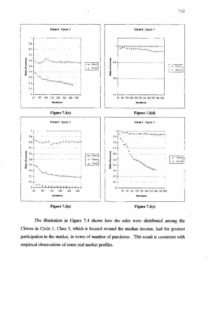
7.12

1

_

Class!! : Cycle 1

0.9 --I

U5 _... ._

QÀ7 __

of

success

.D

.D

.Q

la

U1

G)

ci

_

0 _

C

I R

ess í ‹ )

..¢ f, ° ‹' f V ‹:›-~r›‹› <›~‹›~:t› '¢~<›'<›<>-‹;›.;z..z› “`

'¿ «‹,››- Firmí ofsucc

G ez

É ci V Firms

Rafa 3!O

Ú_3.L. _ _._

uozarmür 0.5 ' -'c››:›o,~, _ › › ~ Ooo.

_ U0 0.2

0.1 --

Ú ' . V V | - | z . V r¬ V - › . z . . . V ‹ - › š ÚÂ ÊÚ BD WD ÊÚÚ ÊEÚ 321] ÊÊÚ ›'1~'-IU

Iteratinns

Class 5 :Cycle 1

Cl O-O-Q 0 oo 0-0-00 O-O-O O-O-O O-O › - - -

'¬':›'°`“".»-':>. |×.,. A _ c 9» v \ »O.`-‹,.Q.{,À__›A *' ¬'~'~¢.<¬-‹'›-<› ‹>-=>

~‹:› Furo? -\:~ Firm?

20 B0 100 140 1802211260 300340 380420 Rerations

Figure 7.3(c) Figure 7.301)

Class 6 :Cycle 1

1 a

0.9 _ . . . . . . . . _ . . . . . . . . . . _ . . . . . . . . . . _ ¬ (lg›

_, _ á _ i "»‹~. ,, o--M . 0..«.› wo- 0‹-o..z:›zf` ng 0.8 -- -

,_ _ 0.0 1:-

93... _ _ _ 0.7

of

success

695€ 1 .B 55 01 .T . . . . . . . , . . . _ . . . _ _ . . . . . . _ _ ._

›

_

; -r›- F|rm3

~ - - ›- Firm4

A Fimiõ Ratio

of

su:

.D

um 3:' .-11

Ratio I: Jz

.Q

4:

\ "'v

_. *'\ __

\>z¬"‹.` -_

‹I>-<3`‹. ., :

._ _ _. _ ‹'.*.<.~+‹¿...~,.-.l;.__¿,__(.. ,¿_,_<_:'___:(› U2

DJE) 0.3

ÚÍ2

n.. ._ _ . . . . . , . _ _ (U

0. ¿."¿.\'.*'4'Ê*Ê `

U :fu au mu Qou zen 3:›ú

0.1

lte ratíons

Class 7 :Cycle 1

`. '¢“~**"` . , ¬ ._ 1 u > *-'<«~‹.'› ~~›'~f'¬- «>~.-'\'*--:-<>‹3v~c›c»<;~¢,<;.¢z;;׋>‹L›

C\

IJ

00O J

_

_.. _. O ._ _

l' *F _' ~c› z Fírm4 _. ..1C,n__'

í '- 0, 5

~ ‹:›. F|rm5 agz

.. OI; ‹

O Í

00°C. n_

30 G0 90 120 150 100 210 240 270 300

Iterations

Figure 7.3(e)

The illustration in Figure 7.4 shows how the sales Were distributed among the Classes in Cycle 1. Class 5, which is located around

Figure 7.3(c)

the median income, had the greatest paiticipation in the market, in terms of number of purchases _ This result is consistent With

empiiical obseivations of some real market profiles.

Class 8 12%

-z:'z‹“.*,..\z^».›~.;;z*f¬§s ›\-1* “:\:~;1:;fz›i×'é›f;›r~¬à;.=Í'I?1>

" f¿%`=¬`›'俧.“še`Í»›z*

11%

,_;¡¿ fit'

g._‹

(1 .f

Cycle1: Total Market Dlstribution of Customers

oass 9 Gass 10 oass 2 6% 2°/° 11 °/›

1 À

.1 zz

Gass 3 _

`

:.I¡- , 12% /S

w _; '

,

o › ' 1

Class 5 25%

, . ,. .

03557 ÍÊ'Ê` :'::1:t":s .‹~;3*› ' " ': 11% ÍÊÍ. í:::zÊfÉ-Í-~Ê'^

_; tt.. ' GESS 4 10°,°

El Class 2

B Class 3

El Class 4

D Class 5 Class 6

U Gass 7

U Gass 8

El Class 9

Class 6 E 0355 10

Figure 7.4 - Cycle 1: % of Total Successful lterafions With All Firms

".l3

Cycle 1: Market Share

F|rm5 12% Flrm0

18%

\. .'\.~ xa - - ~

37: ‹ -

`

._¿2›'¬›:zÊ;§¿. '.~z*»"Í‹\;›:‹z'›-f.z_ : ti :

~‹ .zz firm 1 -- -

' :;f ::' _,, _¿.._.z¿`¿_.\_`v,_¿.|.‹._`,¿.Ç_,`v

. : :_ `_ _ _ __..:.*_,:_,:_:¿.

‹

6%

3.”‹*<-ä»"".3':ÊVÍ;{'-:ÉS

~\,=»*›.N:'\r`*-É *'-“~

\.‹»-Êä;ê=-

Hrm 2 .

21% Hrm 3

Profit

MU$

Cycle 1: Proflt (No Adve rtlsi ng Ex pe nse s)

1490 _.-....___-_....._-...._.‹..._. ..._.H_.___

1200 -. '¬

1000

800

600

400~

200 -

0 16% Flrm O Flrm 2 Firm 4

gure 7.5 - Cycle 1: % of Successful lterafions Figure 7.6 - Cycle 1: Absolute Values of Profit per achieved by the Firms with the Population Firm

7.14

As can be seen from Figures 7.5, 7.6 and 7.7, Firm 4 had the best performance in Cycle 1, either in the rate of successful it.e1'a.tions or profit. The reason for this realization seems to lie on Firm 4°s relative profit margin (_`21.43%_), which Was the smallest of all competitors. In subsequent cycles, Finn 4 lost the initial advantage it had during the

iterations of Cycle 1, even though its cost and price had remained constant, which shows the effect. of a. fiercer competition, because its closest. adveisary, Firm 5, had lowered its price. -

Cycle 1

Profit and Market Shares 0.4

0.35 f-1

0.3 "‹

_ 0.25

O 2 Cl Ftoftt Share '

El Market Share

0.05 ,i¬

O , .Li í;f';.

'

Firm 0 Firm 1 Hrm 2 Firm 3 Hrm 4 Firm 5

% of

Tota

O ..-I U1

Figure 7.7 - Cycle 1: Comparison between Profit and Market Shares, as % of the Total

Figures 7.8 through 7.13 depict how the market evolved along the cycles of the game, separately for each Class of Consumeis. The graplts show the information regarding the Finns from Which the Consumers bought. As mentioned earlier, Class 1 did not buy from anyone, implying in the existence of an unattended niche. As to Classes 8, 9 and 10, Which only bought from Firms 4 and 5, the rate of successful iterations Was 100% for both Companies in every cycle except cycle 5, when the rate of success for Finn 5 fell to 0.622, 0.531 and 0.429, concerning Classes 8, 9 and 10, respectively. This result demonstrates the inadequacy of decreasing prices too much, mainly on the higher segment of the market. Figure 7.14 illustrates the information for the population as a Whole.

Class 2: Ratio of Success

___ Fxrm U: 0-8 § com-1.0

:› F' r¡ce= 1.5 [conslanl furallflvclusl Fim-, 1;

FH 1

.- E 1

1 :'-:` E Q 5 ~,.1.n °

0.6 GSS

1

c Price-1.4

0.5 -l'

rn 1,

sl.-=1.ü

w -Í~ F'ric.e='l_

Rat

0 of

Succ `

1 ij ¡j;¡¡ Firm 1- 1;; '_:

IIS I `

_. i{.;É;;É:§š~¿1

s

Í;§5;§;;§z;§§; z z W ¿§z;[z;§;;jE;z

¡

;:.;'._i;í_i;1§;5_ ¡.§¡;};};:};1 F um xz :;;.§¡i:.4;i¡:§¡ P m__e,__‹ ,_¿ ¡;¿¡1:.;1i;;:i¡'

“Ç-f:ff:§Í:fÉ:f;" Fim 11 ¡ÍfÍt{Ê:{Ê:§Í c z z»-1.o §::§Í:{Í:§Êrf §Í:§Êtfi`›ftf

525-í;ë¿52;'z CD w ;;;z¿§;5;;§;;|p..z.-¬.zz |;;;¿;;;;¿;;;;-;55;;z;f;;§;_ í :1~_z:¿^:›_:t¡z' P úzz- 2 lu ¿::¡;:¡:i-_z:¿; ¿z:¿::-_z:¡;:¿ -z:~'¿::¡;:‹j

.gi :â_Í::¡`:'_í:.¿`;:}::}:3:Iff:f; ._í:._-::¡:§ -:_í .j::¿:f::f:Ê:

0.4

._ 0.-3

0.2

0.1

í

Qlcle 1 Cycle 2 Ojcle 3 Cycle 4 O¡cle 5

ElF1rmCl

¡3Hrm1

Figure 7.8 - Evolution of the Rafio of Success along the Cycles among Menlbers of Class 2

Class 3: Ratio of Success U arm 0 Firm G:

0.7 1- P '¡H=1-5 P ‹¡¢›zz1.G 1 leo na-lanl io r all E uclesl 55:5555555555:Ê1¡ÍÊÍÊ%Ê5f5Ê5¡555íÊ: "ÍÍ5ÊÊ"í'5:5Ê3

- -

5Í.ÊE›

0,6%, ..,iš.¿¿¿¿;¿:¿¿¿¿¿¿¿¿'¿¿_¿:¬

šzzzzzâzâzš

.;Z¡ZÍ;3;ÍIÍI¡1¡.1IÍI¡1¡1 IP rica: 'Á _I`

_›

In 712 .›S_1¡1

. . . _ 51531252 ¡.`u¡IÍI'-I-1

36%

of

Success

0.5 -};Ê';íf.Ê 1=_;;ifí1íií:íif=i:ií.í. ..í

Rato

0.2 âíífífí . ¡;¿,:¡¡¿.¿.¡.;

l

'-:.-'z:š'E2z1: _ V; z-z-z- \

U1

,:r..:.:r.'.:.i;

0.4 *-

CM'-*-'° zzzzzm 'šiášãšffifãíãâ ff* P‹f=-==1~2 wâââââ «=.;z..z.ú . â vz _ 03 `::‹::› : \:› Pnm:-1,8 - ¬:':-1: 1- ›:'-.›

1

O ¬:-;~-- *W :¡. ',:¿z_ :-:~-¡'›:-- .-;¿z¿:|¡¡:_'-

Qfcle1 Ojcle 2 Qrcle 3 Cycle 4 (yo

zâziã

\e5

Fsrm l: . l=|rm1 °“*~'=*-° HW-10

Figure 7.9 - Evolution of the Ratio of Success along the Cycles among Members of Class 3

7.15

0.6

0.5

inn n-:uml fo r all E vale 5) z¡':;:5zz,f..›f›;'r:,¬*~.:: H -

: 1-:-:“.›,=\'-un.-'»*: ;›-.;›;›_- _

":='V*t§z=:.'*:~.“l-fi?-`z-z«"' "1=:*=:'111%-"":-2-:=t=f:-*ri-" ' **I=ffF"”' 31

Class 4. Ratio of Success Firm 2: Cust=4_(I '¡°°'5‹U ;:z=z:2íz.*z"=s.âzz:Êza

" z5»§=ÊT.z;~5.=.š

SS 0.4

Succe

0.3

Ratio

of

ãiäâêâëâáâãfigšfgziãâëiâ ;_*_~:_zz_>-z _ éâzâêâââêgzz _

:›-¿¡:.;~;_~¿zj,{-;›_-;- :¡:¡;¡:¡:¡:¡z¡z¿z¡:¿:¡:¡:z¿<\;¡§f¬~ ;¿;¿;¿.}._. .¡:;:;:¡: Pnce‹4_9 l;:z:¡:¡:¿:;; P nc:-š. E :2E*Í_"~.,'“-1=-:I-=?.2'E1ErE1E;2:ErE=š=i1EfE=Í.:.1==:,§-íEzz;~¿ã:2:E €:=_rf_=ÊãE E¬=_2Er=¢ã2š:E

zí. 5'f?.:š.§I:'‹1{šzšífšzfšíííšíšffšíšíáfífÊ,Í';ÊÊ; *ííšíí-§”=ffs =*ffz“:.z=' =.=é:z'= =`íf=`šfí¢í=`

41:; _ 'F1

'

f F- z.

" _'_:_t; ;.;: z*';:-

`=:=:rz1~"_~'?~'›z~'*I‹f: 'fm -" '.~'›"-.›×'*É~' "m "› :=

515555;-i;_~I_-:,¬-z‹l 1 »I;-¿~~1 _ 1i.^.,,¬~ â1:=z=â:z›;^z›:-Í~,;--; E 0 SI-4.0 1-HH*-0 í= -'*››= Ô

__=z;z3..;-1;›z.-:.-‹_‹:- =_¬;2*._:z. zä _:xf.›

O 2 5'15f£5E:-\'-Â?-".-=.Ízz[_«z¿1 F' :ic e = 5.5 P ri; e = 5.2 ' I_~z» 1 ›

' 5 _ _ _ _ .

' ..:^: :5:¡:¡1.'-`‹'^Í;'-'Í A `

:~Ê¡:¡:-:í.¡:í:'l=šz>Í11'* ‹ às ‹'*‹Í~ .¡_;.;.-__-_-_‹.fl.'.,'_, .;.¡.;.;.;,¡.¡.-.Í-z~.“.z'z -r 1 ~‹‹‹n> âzz=âzê:'›i\~:*:›I-:=;-~; 5-.zz=.=::¿=z:s:z _› z

z=::;=2=zr=<5z:--4í`.~."1~'€~§ 'z‹_“«"~ .\'~f f

01 ‹›;:‹.¡..¡.<¿«-«›,<_ :¡.;:¡:¡: :¡;¡.¡`\¬›'z;.z -‹¬ ‹ ‹ ›.

_ . .V -i-'-ía;<.;*_-¬ » ^

\_c

'

¡'='z=:=.'zi'z=i=.:-Ez~f§õ:â:a« '=.z~¡â=.'z'z'zfz=zz:z=:=.'=:_zâ

`ƒÉ'›E;E1'‹§z¡‹‹-§\§T=Ê;55šz=§55E'Z=E5132333552321 2=_'-1_'-E=`z'- V

' _'

' ' '-~I'9.'-E'‹E= - ¬. - -_~.-:~z- .

1-f:â;z';.:_z'~_=:.;Í:›_:;;‹__‹:s:¿;f;f;fl;:%::;:;zs;¿¿;:s;:§z;z;.;z; ;;5;§f:f; F"'“ 3-

;z;.§;§â§s§z§ F""' ° ;z,_z;z;z=z;éF-‹.t~.z›_=4.z1

š

š,

!I=Iz-e--¿vâ1ñ~'=:jrz::=¿:zzz=êi;=âizz;=:=§z==z=í=f1=zzz›- =âz=='1%; l: ú =z.â.n =5`-íë'í=i=`51 1: z, z_-».=4.D

._ Í

E

âzíêiëâiz-íiêâê êêâë ;ââzâêiãf%f%=âfê%š§=fff§1_íšâššš§šš°°="“°

" ;§=:i1~§í

-_'-'f_1.i

‹z~-_-z-z~.,.~._z¬.__z~,,z~.,\ z.z.z-: _ \ ¬ \-~›z-z~~z‹.¬_\z« ,-,,.^_z ¡,_› _... “M z ~ ‹ f ~.

__z

2

í

U §:§:iÍ; l ...,

mvíãf *I-'E= ,.z.\›»« ¿;_zz-

_~j:«;^i~Ç'.~z --z .›\.~.,~__-.- ;z¡z_zz,

:‹ê:â::;_z §=z:~;.=!

z

Cycle 1 Cycle 2 Q/ele 3 Cycle 4

l

1

Cycle 5

|:1Hm12 lJF|rm3

Figure 7.10 - Evolution of the Ratio of Success along the Cycles among Members of Class 4

Prme

Firm 2:

120:.-l-4.0 '

=5.Ú Class 5. Ratio of Success

lconxlanl io ral! Cuclesl

Ratio

of

Success

QU

0.6

...._.. 0.2

0.1

¡\-.--:-;-..;z=:‹.¿ââ- ` ' `

f.'íÍ°1Í~Í'-Iv

U7 _:-;~:-:__-_'-¬_'_:›».-_* _` › I

z_.,z .~=.z

153-':'5%.“.'z*.'z¬::rz `~:›--:- ^.L'z';'::.'. H'-11 1.'-J:J::~.*1_:.`

' ' '

*'.~.^.~:݃-';. '

- -

1. r_f__: ;.¡¿g;fi;=¬

,¬,.¬.,,

1 5 E 5.- fz, §;2=rz§~¿z-=-z <^f_'-E'-1-:.='¿'=.'êâ5E'

“_=É=_E;‹,_¡;¡Ç¿z_~;¡äz:;¡'J

O -.‹_~,-.‹,‹_-1,:

1

'.;¡:¿`:¡.. .. « z

zzzzfizfzz _ ,._.-_ _; ) ,

yrrz : ëz

J_."›.. ' '-Éli *Í

-'- '

::;1:.=:.=:.‹ -_'-_'-11-.mz-2:z¬c'

-~=--'z=_.f-.-'›.°Í\'.‹‹f ›¡: ..@..>._›;::'

~ ›'.'.-_:'_'*'.£ :_-,rw-. . ››..¬¿. z› U ,_ 1

_, . ,fl . U., z

:‹:\ _

zrz` ;=.-fz-_: z -I! zi-1 rz=:.*2=.‹.-;

-' >-=‹:r-.¬;¬.:^;~_:

zg _;zj-z; -.._.4‹.._-mz...

_

`I£`5'E;E=5.zjz;;j--;šÊE§ F, 3` FW" '11 'm

E 0 5 1= :Á ,D ':"¬.'_z'›'z °°='=^-U P _ 5¬

r=‹f¡‹.z=5.s "°°' '*

`w=""»›'zT

=z1z=-rz'-z=:'›z=*z‹:<¬.=f.'‹~:z* :-:-:':-: :-1 _›_~_~_›,›;,=;,‹_

-_=z=_z;:1z'_z',_=: -,-,-,-.=.-.~,,-;J¬

=Í'E¢¡=`:'›E;'_:}z'-§¿?#-'z1z'§_ .¡:¡:;:¡;¡.¿:¡..,n¡¿.*¡_.' E152;-'E=z=z:5I'~ÍEe.'.=_f.f.-.\

_-;~^_:‹;‹;:z ;_-,.-_.,_._._¬,..,.,.›.,

33551555555-55zšzíšfézzêz ÊJÃ.-l}:;::

. 'f;“&=.=;“›'-f-:f=z~_ -E=5=*'5=--:=E= :';›E*;I^.:.t

'UL-`;T :::-'-:-:›:-: ~~*'›'-'-.== -zv:

1z:;;gz».;f.5_z.›z;‹.f=›z z;-zz z; z z;-.‹.::;':;â

.. :-.:-_--..~z:zêz›,;-1.¬'-_ “ ~:~.›:.=?=: ¡.".'¡Z¡í¡.'›:Í'v ä.':l'.'¡Ãi'i` .W

f .z........«z.«...-.~-.¬.....-..~....~.....».».«¬.z~.~,_¬..,..,.w.........t.,..-~¿..›..-.«....,...,..,..¬..,,:»..,_.. -z:z:z=_ :‹z›z'--z^z=~-:~¬¡¬¬-¬~f¡¿.¿¡¿¿:z¿

1-E--Iii'-E=":1-1:1›:f1§=;

.»-~-.-z-z¿.¡.;.;.-z ;¡.'.-_.;.V _ .-.¿1, 1zu:z1-.z=z1z='zz1z:z:z›z¡_; ~ 1-:‹=~-za=zzz===;z;z.=.-zz~->z.szzz§

1. "" "ÍÍ“Íz»Í`l:‹. › ='.'-'›'z-›'~í›: '‹

Fsrm 3. ;~:-: :¡:1 =Í'ͬ'E':"'°_;Éí=Í :1.-. 1-_-:-:í .,_,¬-... -~ .-,¿_.‹.-. _- - _-.Í

l=4 U i

'

..\

l -v~'- ~~¬›

. ~z~-.‹-F» . Prír.-e==1.9 i`_Êí'Í5.5;Ê*.Í~Í _ zšfƒgšf

;¬'~<.';'.: ;-:_:;1¡:;.-:‹-¡:-:- ."›':';:,Ys : .--:-.¿,

"5íÍL551Ê `"`"Ã5Ê=ÊíÍ5í

.‹.;;;¬~: zizzz 5

:,;.--.-~¿.\ :=_ _1: :;' EM ¬ '

.f_:;=;:f

= _wEz_ ._ _ -_f_;¿¡,f_§~_-_: -~ V:

- ...fã_

« 'z---:'z=z;_;z¡ - wi- ...,....

~:‹;:»:=: 'i~2:Iâ2:2=2~2 :-.'-:~:-:~:<~f‹:~ â§1jzê§:izj=z;:§zj=-

.=.-.=z1z.=z.›=zz.=; E ° “'

;.^;z*~'.' - .V . ...':',r›:- :¡:¡:¡:¡z:¡:¡:¡:

- '-Í'V="Í'-'1`-':'-Í"-`:'›í'› C' °*"^'°

~. :-:-: =¿'.'.=:.=1= . _ *.'*:~".:i -_1:'-.1-'‹'~Iz1~I: .;_;`_+f.'.;.=.z_{'.~z Pruzzzâuà z.f‹›_.¿i'§;.~ _

_-;E;.l.='§'f.~v.~.:z' 1 E

.~=`-.‹5z›I~.§ `r-1I'¡'3=:jE-1:51 -¡:;l*,'z'.z=z-V'›_".ƒ.' :;;;:-';¡:;'-:¡ .?;›¡';:-:\ 1'› -'-'-';:¡':¡;¡

_ _.-1_;_-'¿_~_z¿_z._êj~_ ›: ;¿¡¿›'r¿;.2 ::»-:z ¡ .-\_.¿.-.N _ .›\,':~.:›'.* -íf

ãëšz F ‹‹ ffl 11~

i

É `»`!x`-'‹"?-'‹ -Ê:¡1ÊIÍ.ÍZÍI¡_ ~'f`i\"r'¡`-'~"‹`›

- '.':l1;'.'-Té Y -' '- '›'.f.'z'.'¿. 4_(¡

z¿_._-¡.» .¡.'.-z à_‹_›__z_z¡= :;:¡-_; ,¿..._s... .¿' .;:

|

H Í” Ojcle 1 Qlcle 2 Cycle 3 Cycle 4 cycle 5

EJF1rm2 UHrm3

Figure 7.11 - Evolution of the Ratio of Success along the Cycles among Members of Class 5

1

QQ z:í";:*“;:¢t¡:;:;§

Price-9.5 .

'_ , Fim15 [|:nn'~lar‹I_fnrel|Eyr.-les-l C°',' 7'0

« Fm zzz Class 6: Ratio of Success czzz=7,0 _

_ EIFÍITI14 Firm 5-.

'rf

¿z¿z_-;¿f°f..~_.-.zm Â/

__ t`

F1rm3

§i§z Fim 5-

0.0 .fãfíí

0.7

0.6 tiííí

of

Success

0.5 ~;͚ͧ

.z l

>"' ' "----'- '

z=z=z1z;-_=z;5;¡.;E E›'z1'z;E =.;'z5E_"' '

':5_E;I; íziãggz 3 __ 1 Fim Firm H= ;í;I;f;:giz:_:;:;f;í;§,;í;;j;;_Fifm 5~ 'í;1I.;:í;í;1;z tz

zzszzlzz ¢..z..zz;z zzmm - -5%

f‹:¿._› F*ri‹~e=55 Pnr››-52 ,,

F'r|r:e=S_2 ;,›;¡_'_;; z.1._:_-;¿;_:_- ;_;

;§â;_=;íIfê;%â%f2;f;§§s§sfs§ A "¬. P~=f=2-f~ sz5zsz5z5z5;2;s:a;=;szz;§;â

z.E'ost-F. El rice-7.4 Ê?

z

, Ó ÊÍÊÍÊííÊ.›glÊ'‹ãfíÊfÊ“Ê:

~‹¿‹Í*~`í:,~

ââõzzà

u . 'ÉL1

;=_=_§f§

_-_-_-_-_~_-_-_~ _-_-_-_-:_-:›;¿›§š\_:›__2_~:f_-:I _

l'

ëëfíšz 0.4 lifíf' zig

Rat

o

ter* '

°»' A

_

0 ¬=~ *www

*sk

äí =_:z :=ífí=_-í=_í=f=_š'z

.,__.._ 1›. ;-1-1' 3:5'-z

ash É

_

" -_ -“__ "\i‹°“

._ Fzzmâ-_ '

_ ';z2;';â`;f;§fíê`â:z

_; :z___;z_:j›_;' :jz_:j-;z_. -_ v'..':'_.j:_z_;j¡z_z5~

0_3 _;=j-_;;_-;;:_ cz-zzzm :;1;¡;1 - @*€§_'z__'_:z1~'_-j_';'_;: ‹z=z=z=z.z' 5=;.5z;zf - a‹“i_2;=5:5=.=.z=;=_:.:= _ ._

0.2 _. __ *ãÊ`fi§í;:itf;i;i;:

1==z\I›:=:5-2›:z-E-1:5: A. '¿§.‹ ;›iz==:~;=:-5:' '12

.z- fz__

. _,

‹¡.'-.f-zw

Fšfâëë

àâš . -

ii .z

__¿\$×'Í

K. z=;'›:=z= ':=zrz-,.‹*\×** ,___ _

_

;ã:;§;í;ã =§;_1i§;=

=%'z';1-

z§šâ=';⧠iâãfêlíâ

->¿àz _1z_=_z

‹~_§f5` --.‹;-*:.zz

__ _. ___, v¡¡¿¿.›_ .:¡:›:

4 äii

_;«%§¿ :.=:fs

E

1

fã -0

.'.›$.#./-‹

C>,1cIe1 Cycle 2 Ojcle 3 Cycle 4 Cycle 5

Figure 7.12 - Evolution of the Ratio of Success along the Cycles among Members of Class 6

l

I'.`f›.s|=

1

7.0

FW f*¢ Class 7: Ratio of Success

Pricu=Bj2 :` `¡Prir:›:-7.8 Pvir:

p¡,c¿=8_5 ' Firm 5. Firm 5. Fífm 5

(constant forallfiyclesj C°5"7'Ú C°`¿"'7'fl cas" :-

7.0

711

0.9

CGSS

0.6 Í

Í "` Firm 5' :"'

‹: fz zzzv 0 55;-

F

-z--zi

_; :~5 zu;

l

-' _ rf

2: “ricei=Ei_E- ' 7'

Rat

o of

Suc

0

“

0.2

0.1

O _¿,_,___

mm. sz s

Co:'.7lÚI F' fiz-z-.=e.@ *

í_z .ã

.. _ âíz=zf==-1_¢_=zf

5

.-;§?.=5š%

fzfâzšãí

__ __š

.iÍ=,Êf¿

5=:z:~§ :;:f:›;

ElF|rm4 DF1rm5

1 ó 1 ›

cycle 1 que 2 cycle 3 cycle 4 cycle 5

Figure 7.13 - Evolution of the Ratio of Success along the Cycles among Members of Class 7

7 L- ~`1

7.18

Population: Ratio of Success

U4 15z;z;.;zgz1z;z;z;.;zzz55;z;z;z5'z;?Ê;z;zzz;z;z;zz.;z ;;zrz;z;z_z;z;z;zrz=z=z§z= ;z;~53;i=z=.:z;.;z;zzz;zVzf.=<z-z=z=z=-=zrzrz=z:z=z=.=z=z:z--=z'z:›.. =.=z:›=zz

035 rzzzzâêzêzzzzzzzzzzzââézâiâfzíâiiíêíãfiíiâiâëífâëâ@z=zêâëâíââ§%âfâ*§ëiã;íâ맧êfââ=ãé fé:ífziâãâíëíšêffiâàí¢âí=šë~š:;í»'li-äišãí 551551;-¿5-E5235zE;E;.;15:;E;I55¿E;¿5z1E¿-;:;=;šjš*55E551;=§;z;=5E55=š;š;:531;,-E;*=:;I;š=š5š':;ÊIE;55š5E;z¢5'Ir5=°=E5E¡í-E1~'§=E'š=:I.1=zr5=E251:=.-:'.=:rE \' 3115

O 3 ,=_f=_a›¿f=_§=zf=_f›-:1_§-¿ zzl-;==.=z:="z=a s~=& 5-'z=:-s=.1=ézâz'z=-1 5=z;5:5=1;sz;zazzzê:tz=z:z=5z:;:§=e=fzé-%;==;¢=5é:5%âë;zz=§2zi if;-;í.'f-5â%5lâ5â:z=›l5=2f:*5 zizz; ífššiëš E Flrm Ú

<= ê>z~~~z-.~:-z-ze: ;'z-zw;-=-5* - as-às z-1 .-z -.~i-*~:::::z.::-.~. -. r =.: z z . z'":':'

1

¿¿¿,¿¿.¡¿¿¿;¿¿¿¿¿¿ g;z§;§§¿ .5;;;¿v¿;¿Ê¿z¿f¿Í-šzffšffzif1;;§§Êëz2;:;ê§I;5f5§5§1Êe§:z;§ 1.&âf;f§â5;5;§-555;§zf;zz§z;§; zlâfíg;¿;§§;§;§:;5§;;;:I;;- .ff U Hrm1 0,25 eg“gâ§,§â§â§âg2gâ;:;z;âgâgffgêf2¿=¿âçgfz⧧ê%fiš1%1%.í1§;ã:â;*fff êšiãzëfiââáêãëêê:f%iê%§f§fê%5% :¿z‹;-f-šiíâë

.fê â=fzi;ââ2~zf~;;z;z.zâzâêiââ-izâ 2.-Jâzëêiâézâzâêâââzzmézzézzâê :à.*~àzâ@=zâ U 5"" 2 izzzzfúgzrz :zz ›¡zj:1:;:§:;-5:5:f:5.¡.-›5:=: ,:;'5:2:;z;z;z¡:;:'z;.;z;gg '"-

5;1:{:5:=_:jz;š›:;›;:_:;›5z;5z -‹;;"I55.1151;:;E;-5E=:¡z-.;:;z'E ':' E_-11;? ;›;-:.--;-: :: 3' -:-:v:-:-:---;;z-:-. -: zg -:‹1›:-:.,---:vz-:,r -1 :›:›--;›:‹:z ¬-:-: .-:‹:- -›;~ ~:-:;:- -;-:-:-: :-:z:- ,- - z-me

f_.z¿z. ,z,._z¿z,z;,,z, :.,_ z.z,».z;z,z;z_.z,z;z,z,z, ~ ,›: .,._...,,.,z,z,z,z_z-z;~.z ~::-.;-.z-z-z.z....;›z.z... «_ ;. :;z' .zz Firm 3

_ 0.15 1?? IÍÍÍÍ 'Z É

, z z zzâz; ;~: _zéz;.z z-~z; 2.1

= = zzsë

E Hrm 4

u

~

_ _ ›

\ tz» Q E] All Hrms

0.05 ~

. E âz

Rat`o

of

Success

.Q

S3

C)

-4

IQ

:...::::

:::.:;:7'“t::__.:'::

,_

..f:

mí

.-1-1

i-t=-

_ É

E131-:¿

'

É

~111*11;f;f;íí51.

m""2zí~z55:

äfíi

flÍ']Í:¡:_-;_Í.Í:_~:Í

'.;,¡-_.¡:.z

í-1

z

*" -.-tzíšiëííšišiä

~Ê

h¡`:íÍÍ1Í:`1Í;¡1Í

ministram

-:~:~:‹:z‹:z:- í:‹:.~..

Cycle 1 Cycle 2 Cycle 3 Qƒcle 4 Q/ele 5

Figure 7.14 - Evolution of the Ratio of Success along the Cycles among Members of the Population

The graphs of Figures 7.15, 7.16 and 7.17 show the variation of the market share and profit of the pair of Firms that competed in the same range, as functions of the price.

Note that only the 1, 3 and 5 varied their prices, While the other even-numbered

Companies maintained theirs charges constam.

In the lower end (Figure 7.15), the results clearly demonstrate that Finn 1 did not

get any benefit by reducing its prices beyond about 1.6. lts local maximum profit. occurs nearby this point. Even though there is some room for a market share gain (Firm 1),

pushing prices further down only causes monetary losses to both competitois.

For the mid-range Companies, the same comments apply, With the difference that no local maximum occurred for Firm 3. A strategy that. seems appropriate for the present and previous case is to experiment a slight increase in price, since the cun/es indicate that

the profit could be larger in that direction.

Mkt.

Shr.[X1000)

E Profil

zoo 1 ~~~~~~~~ ~--M ~~~~~ ~» ~~~~~~~~~~~~~~ «z-~« -- F» -~~~-»~~» z -‹-~-»- ~~~~~~W 2 1.e 1.6 1.4 1.2

Comparison of Performance "'<*'“'F""¬ 1fMkl-5"'-(U/°°) , _ . -'<~'-~Firm 1- Profil Firm 0. Constant Cost & Price ,.....z_~,.....|=¡fm 0;M|<1_shr,(o/00)

Firm 1: Constant Cost & Variable Price "'“"f"""F¡fm 0 - Pwffl 200 f FM ~..............¬...........___ ._

“_3

¡\ «›_....._"________ ~ _ _ í E

-» .._.~..».~.¡:;_____________________,___ _ __‹_H__ _

1 _' v___`_,_,..,.---~---- -----~'.Í---~-~..,›; ` '“ - _ É ___z-›' * ~~.` ̀ ̀ rj ,

.›--¬~›.~»z»›››-zz.zz,,. Ã ,.~"" ` ~ 5

W- -«=...‹....-=zzM¬.z-..,_\_,,_,,_, /.‹'

100 + '**'*¬*=f-z»›.z.‹z;.

- 'ø *"“'r§¡,¡¡°..\y.,`›_y .w.¬.›.«.¬»\w. __ _ 'W

.»..%.;...,...,- .w.».W_ ¬

`___ ._-* a._f› fa; ~a^.¬,“

É i

,

Ã-ao...~.`.~×:'»-.~....¬._»«.~.¬«`«.....".\~....á;~.\~»¬..~...»....‹

_

.` ...-__.. . _.._' 2 .l ' *vn `°-'-=z-

. n ¬.,..._¬o._..-,_, .... _., 34... ._,,ë_¬ ¬¬¿,`_"›V 50

\;>{`“=zz¢~. ú#"'F wkffzü M

“'“"-~ F tt* ao 1 °*=~.-.z ..-"'" wie; r *'11-›-__ .sr wz. U - '-~›.....z‹sz " ¬

‹ R. Y

.§__ 'zu Fe

¬ *tz

~50 ¬: ""'»\e, vo “à

:_

100 š`“\_ 1 'QQ 1 \-.

1so ~É "*=›

Price ot' Firm 1

Figure 7.15 - Comparison of Global Profit and Market Share for Firms 0 and 1

1x1

000)

& Proft

Mkt.

Shr.

Comparison of Performance -...z-~f=¡rm 3:Mm.sm.(o/0031 Firm 2: Constant Cost Prl ce

. â:'N';f«§fšhr.(. O/00.) Firm 3: Constant Cost & Vanable Price »««z~««¡:¡fm z _ prum

70° T-.__-.._...- .... ...... .._.._,..._.. rrrr -._.-.,..... ..................... -.....~.,..- ......... .W ................. _._.......,-..«...¬¿

sou

500 ‹f*~«-~z-.«W,.'.`: -¬

›‹-»‹i\,¿¡“`“ r \

. ,Í“-‹».~.... . ,_ -...â\ -w _ lia» ' 400 -5

fi- 1

"- '~ ~

1

. "à "I 1:;-'Í *ax ‹zw-‹›=.‹›=«-=»-.‹¬~\V

..~z¿¿__q`_`_)VW“L.` r "“¬"=-..

ri

5. “ \ '‹"""**'¬-«.‹.. 5;

1‹--¬........ _ . wwí 200 _ _ ` F -

_ 1;

1 \ ~ ~ - ~ .‹-........,_ il

1oo‹1 "

.‹

'l0

-100

-zgg _.....____...¬_.e-..«...«.. .... _......-..._._..._.._. ,,,, -._.... ...... -................_.__._..._.._._.. 5.5 5.2 4.9 4.6 4.3

Price of Firm 3

Figure 7.16 - Comparison of Global Profit and Market Share for Firms 2 and 3

O

7.20

In the higher end, the shape of the profit curve for Firm 5 attest that decreasing the

price below around 8.6 is to no avail. Again, its market share raises, but the monetaty result diminishes.

Comparison of Performance Fm 5: Mm. STM 0,00) Firm 4: Constant Cost & Pnce ~›---«-›~~Firm 5 - Profa - . - ~-:W Firm 4: Mm. snr.( o/oo) Firm 5. Constant Cost & Vanable Price _m_,__\F¡rm4 _ pmfü

1400 .,...-~..-V _ --_. _-- ... M.-1 _ W. mz

Mkt.

:(1000

Prof!

Jëék'

154 É ..-'

1200 afzz-W 1

`iê'°-1:1.,

i *Ê %“m,

â _. 1000 ¬ `=«-¡.,,ú`_m wW,.¿“z..z»..~»‹\K,_._,ÀW â

` '¡""*'%1-ui “,¿,»›‹›'1"""' "'¡'>'.v-,

i

\'\«:x:l:\‹`^ '

`^“V¡,í' `

-.s “Ã t . .Q ‹ ._››....... ._, _.,

g` ¬ .-1

U V À n

`-›‹.,¬` \."¡}¡, á.

~' 600 Shi”.

1 *\t;›_\ -_

1 =~›.¬ ¿. _- É

"""“~`^~'~"-wz_»~ zw .t,..,,,, 4 O O =.',Í\‹~.` . _ _ .

`

t ““-'--~«-~.-~`_\¡_.,___ ..... _s-.....;.-.:__~ ¬<zz.¬_g__`) ,

I zon 1 - ‹ -~»«-~.._`_ «f

. .

'° '~~‹_'›~~~_._.........__._____`..__WJ«.

-¬......«...«1

Ú-1 9 8.6 8.2 7.8 7.4

Price of Firm 3

Figure 7.17 - Comparison of Global Proft and Market Share for Firms 4 and 5

Conclusions for Phase I of the Simulations

Recall that the even-numbered Finns remained static, serving as a kind of

benchmark for the formulation of its closest eompetitor”s policies.

0 For the market aimed at the less affluent Consumers, competing by increasing

quality and consequently cost, is not quite important- the specific buyers are

somewhat insensible to that attribute. Moreover, here ai small difl`e1'ence in price

can be fundamental.

0 As a general remark, reducing prices too much is not a good policy- this appears to bring about two different effects: For the initial Classes, some gain in the market

7.21

share occur, until a certain limit, but the profit normally plunges more abmptly. For

the other extreme, since the potential buyers do not have knowledge about the real

profit margin of the Firms, it looks like a suspicion about the quality embedded in the product afises, which causes a narrower intelval for the it.em”s anticipated

evaluation.

A greater emphasis in the quality should be a priority if a Firm plans to acquire a

larger slice of the upper spectmm of Consumers. In this case, price should not be the object of competition.

The results achieved by the Firms are completely interrelated, so it is Wise not to “rock the boat”, in terms of starting a. price war with the objective of gaining a.

larger number of buyers; In the case of sellers and buyers, if a Firm is too

cooperative regarding the Consumers, it will appear defective in the eyes of the f Ms. , -' vz- «a _...

other Companies, which may cause 1'etahato1'y";pofic1es and collective losses.

Although in this model there is no diíferentiation in quality due to technological attributes of the items being sold, this could be done by assigning diverse filnctions

to the perception of quality based in the cost”.

As mentioned earlier, the possibilities to combine costs, prices and adveltising costs are endless. The purpose of the present group of experiments is to demonstrate the anatytical capabilities of the model. _

4 See Cl1a.pte1'ó, Section 6.4.4.

722

7.3.3 - The Simulations of Phase II

The analysis of the results of this Phase will be done independently for each Firm because they do not compete (mainly) for the same niches of the markets. Furthermore,

only those Classes which played a significant role on the Firms” results shall be examined.

a) Group A, Games 1 - 5: Variable (increasing) costs, constant prices

Firm 0: Price = 1.0

5555 3 *°'°f*t

35.65 96.75 1 .o5 -33.60 as

1

_,

_í.._í._í.J__í‹

._,-_._....J

5463 146-38 4-18 -26-121

62.96 143.16 6.07 -29.62

59.61 104.91 3.92 -43.48

65.45 56.66 0.75 -64.55

_ Table 7.5 - Results of Firm 0

‹

For Firm O, whose price Was the lowest available to customers, the results indicate that an optimum point could be found Within the interval covered by the simulations. The point Where the cost was z 0.58 yielded the best profit. The ratio of success continued to increase after that point, but it. brought. no additional monetary benefit. for that Fiim, since its absolute profit margin also got lower.

An interesting finding was that the Consumers from Class 1 could not find an

appropriate deal from any seller, not even with the relatively low price 1.00 charged by Firm 1. Once again., it hints to the existence of an untended market. niche in the lower

spectrum of incomes.

Figure 7.18 shows the curves for the iterations performed between Firm 0 and Class 2

of Consumers. Class 3, Which also initially accomplished a small percentage of purchases (Table 7.5), did not sustain its willingness to buy from Firm 0, prefening the

Neveltheless, the interdependency still prevails, thereby it may happen that some of the Consumers ofa Class migrate to another, if the relation cost/(price of the nearest competitor becomes more attractive.

deals offered by Companies 1 and 2, as illustrated next in Table 7.6, 7.7 and Figure 7.19.

Hr):

Rato%

4` wø

S 8.

Succ.

,__ ~_«

Prof

t

F¡¡›m O & c|asS 2 ~~-‹.';-«~«~C|aS 22 Succ. Ratiø (%) Pride = 1.0 (Conâfant) Gass 2: Hofit

160 ¬ ----- W-~ f

›_“W¡...z‹..,¬f-...‹.».........,,,_,¿" . uv NW '

f “,¿‹›"N› "`°V\»

,V M-7"

^='“›.~.-_»

Q ›.\.,\_

“Hz

1 ` .-=Y"' &*"ffz-\

¬ f ¬ ,gy

.,~v

100

eo

60-j

«If

20f

‹ F›

\.zf

O ¬ . Q

4›'5"`F “qr

* 4 <'›.‹

Ke. *z

ct. «_ .

¢ 1

"`°~...š

_. _ _ __ ___ `_

._---~`-7'\›¿.^'*í

0.5 0.56 0.63 0.11 nas Cost

\

Figure 7.18 - Firm 0: Success Ratio and Profit as a Function of Cost

Finn 1: Price = 2.55

íiiíâíííÍ%¢.šištÍí5ii:;z-i'*%Êšífí

'l . ¡1Cià$S -{'2ÉÍÍÊÍ-1

1; ¿s'ú;zj¢Çöz.z%;1:g';à;¿ti¿>Í;5;; ;§i:ez¿{;z;1;â5;;9ê¢f¡r¿;âA. iii.. - 'Y¡fSll¢¢EÊ1ÊRátiÓçÊjÊɧÍ.¡ ͧ~ÍÊ§Ê ÉiíÊF?|Êöfí'fiÊ::1§ÉI;Ê`É:1:Í 1-Í

:lz~›1:@|àssflz4:.âzizâzfãí í1%%iziiic¡1à1áší?4f;

V 6 , _ _¿¡¿ ¿¿:_¿.¡.¿(%).:_.,_.

r

lifííífšífíí

4.77 -4.11 70 566. 64 0.08 23.91

5.56 -6.17 73 544.98 0.10 21 .89

1.-zé.;Il1»í'-:fli*;á1-¢;%%0 3.72 '

-27.94 89 521.86 0.14 36.33

4.53 -36.84 94 401.77 0.14 8.78

3.47 -51.15 B7 7

192.05 0.13 -28.34

Table 7.6 - Results of Firm 1

7.24

Firm 1`& Class 3 (xwoó) Gas 3' Succ. Ratio

Price = 2.55 (Constant) ~«~-~=«~(>|ass 3: Frofit

1000.00 ‹- z - ~ -0

900.00 - WN. ~ * " ̀ "W

._ 300.00-õ

Proft

$) & Succ.

Rato

(X1000)

sz*

*

N

_,.‹;

i

M

_-W-W«z.._..m..M.,....__.,.-M.._-.l..-

\,..N.M

«b

700.00 cz- ~ * ' "

M , ^' ='*'-›w=-I.-.~.z‹..z-..««‹~«.z.».~.zzz›\.z«\.\«».-..z.,.,, _ - - -

._-a«..1...‹,, 500.00 í "~“-›*››z~.-..,..._r,.

°~*\=.\:..,

400.00 M. ... W.. -f

1

.. - 300.00 i"°“`~¬=-«,.,_

200.00 i 100.00 Â

0.00 ¬` t

.~-

1.5 1.63 1.8 1.99 Cost

Figure 7.19 - Firm 1: Success Ratio and Profit as a Function of Cost

The Consumers that. belong to Class 3 shared their preference almost equally between Firms 2 and 3. It can be seen that, in an apparent contradictory manner, that category of

buyers decreased the rate of acquisitions from both Firms, When the cost embedded in the product raised.

To explain this presumable glitch, it. must be recalled that the neither the evaluation

function nor the decision threshold for the Consumers pertain exclusively to any

particular pair Firm Class. Instea.d the functions incoiporate constantly updated figures,

in runtime, that come from the iterations with the rest of the population With the same Firm-À and the fillfillment of expectations- for the estimated payoií and from other Finns With the same Class-t (decision”s threshold). Hence, better or worse deals that

are taking place elsewhere are playiiig a role in the outcomes from the simulation

program.

Table 7.7 shows the results achieved by Firm 2 with Classes 2 and 3. Considering that

those two category of Consumers performed a signifieant number of successful

7.25

iterations with Company 2, the graph of Figure 7.20 illustrates the cun/es With the added outcomes.

Finn 2: Price = 3.75

Cost C1ass2 Suco Ratio (%) Class 2 Profit Class 3 Suco Ratio (%fi~)j-'Cltassj-3ši1§'E?-nofitifi 20.25 158 98 76.96 763.85

.

-.-

._

__.-;¬

15.39 83 30 82.60 650.90

9.88 -12 os 88.82 416.28

2881 2147 96 60 84.39 578.52

I

Í

8.52 -51 os 75.58 176.73¡

Table 7.7 - Results of Firm 2

Firm 2 8. c|asse,s 3, 4 (a99re9a1ed) ÉÍÍÊÊÊÍ 3 & 4: S“°°' Ram”

Price = 3.75 (Cønstant) - =~=-====-==C1asses 3 & 4: Profit

1gg0 T__._-_......._. ............... ._.._.._.. ........................................................... __.. .................................. ..

900 sf*-z«._.,% . "'‹!'._-qa

._ 800 `*"¬~*z›,;;mg

1

`=,`v;"'*-¬~#-‹¬-.~»»~»“ _ 700 ` `M.»“"`“*“-¬.‹\. `

"~>à~.~ «vz

600 1 `°'~'._\‹

1 .›. "W

* »-›~~-».»- z_¿;.. âà ser ~~~---

Prof!

S & Succ.

Rato

X1000)

" 400 Â °`*=».,_*

i 300 -“ '“*«..k_

¿ 1 “sé lí

A `ø

. _,Ê 200 - `“ . .E

100 0 ¬*

. . .

2.5 2.68 2.88 3.13 3.41 Cost

Figure 7.20 - Firm 2: Success Ratio and Profit as a Function of Cost

A point of maximum ratio of success can be identified around the cost = 2.88. But it is not associated to the maximum profit, given the payoff functions selected for the Firms. On the other hand, it appears that Firm 2 is not acting wel1- in the sense of optimizing

7.26

its profit- by improving the quality of the item. The shape of the profit curve hints that, on the contrary, a reduction of cost, With the price fixed, Would be a better strategy to be a.dopt.ed in this case.

The foregoing comment applies almost integrally for Firms 3 and 4, since the

figures depicted in Table 7.8 and 7.9 are coherent With the stated presumption.

However, va relevant difference between those two suppliers can be seen: While Firm 3

had its customers picked from Classes 4, 5 ( the majority) and 6, Firm 4 had the bulk of its market niche distributed among the Consurners from Classes 6 and 7.

Finn 3: Pn`ce = 5.40

-z.z.¢z¢zzzz»--,;¿--.‹---z-z-z--;}z§zz}.§;jzz}.z;_z,z}z5äz%;;Ç1&ášsišÁ&íi:%Í'?ízíšeiizíšfzíš

2:1 515:; 1;:

5;; ;(%;a:: fé 515:; 1-: §:=;;l;&; ía;

laiäšš Í Í ÊÍÊ ÊÍE ÊÊÊ Ê15 ÊÊ

'55 ÊÉÍ ÊÊ Êíf 155 ÊÉÍ Ê ÍÍÉ

ÍÍÍÍ Í 'fi

:..:.:.(%)Í...:_._ _.

í;.C:;1;i1ssí5¿ã15z5z

:E7-ÉÊÊEÊP.Í'ršÉ¿:›1f«zii'irÍšÊE¡

f .faut ii 33.81 327. 55 100.00 905. 81 16.3 98.91

36.12 279.20 100.00 807.12 18 87.33

27.90 159.11 100.00 637. 32 14.5 39.05

25.57 76.86 100.00 440.88 19.49 33.90 Í'-ͻʧ 13.88 -22. 35 95.48 226.35 18.47 -6.67

Table 7.8 - Results of Firm 3

As can be clearly inferred from the tabulated results for Firm 4, the improvement in

quality derived from the assignment of a higher cost to the item had very little impact in

the market share concerning Classes 6 and 7, Which appear to be already satisfied with

the initial value. The same situation did not occur With Classes 8, 9 and 10, which show a trend of a. larger ratio of success associated with increasing quality. Conversely, due to

the reduction on the profit margin, Company 4 suffered untoward consequences in its profits. For the data employed in the runs of simulations, the best position was attained

with the initial values (cost = 6.00, price = 7.50).

Firm 42 Price = 7.50

f7¬

._ :›.__¿¡_¿.V_:.¿._.;¿_;.:.¡

_.

=“=* ~

1¬.i;C›;|ià`s*š: 161€: 151.

F”¡ff.¿Í?ÍÍÍ5§'íÍÊ§Í Ê? ši5¿Ê%šÊIiÀ3äÍí§í5'§%%l¿Ê 1ÍfÊÊ-55: 55

:I15fEš¡ášsšfíã1ffSü'è.iš1Ê횧ii251 â5;íCí\àzs1's;5557; 21 f;1.¿5iCz!'àés' 15851 Su cd. 5'

zi. li 5lCVlášší1'8'~* *

fz =z :z'›=z'.›1z‹àfit1~ f

;_ , _j zí.5;?Ram;1(%ÍÍ;.51'if-1ÍÍ¿í -í

1*

fz? Fífófíí' .j Í; Ê5

82.87 1262.59 96.71 1101.44 28.90 237. 28 83.73 1184.93 96.92 1132.82 23.12 160.44 83.25 966.56 89.37 812.00 29.97 171.07

82.73 1013.11 80.08 840.63 32.66 213.53 80.51 680.54 75.63 483.85 32.71 146.03

ãfããf

ííí fáššš í9š Êší É

5§£55ÍF?{rlõfíztf5Í1š5í.fI

' ..

;;f5:;;:fã-rí<';>'.fât§:*z;§

30.22 128.54 19.61 22.11

27.51 106.93 14.49 18.16

28.64 101.97 28.21 19.63

IÍÊÊIÍ›.fʧÊÔʧj8'2Ã}ͧfÍš§;§ÉÉÉ 21.34 61.23 27.66 23.80

34.38 -65.86 30.61 17.54

Table 7.9 - Results of Firm 4

Firm 5: Price = 9.00

ffzzjz gigf;5§;;R;à11ö;5§(%).§;1§5f駧;§§5‹;§§;5% íiáriäfiítâfzffiâ :ig

Íãfff-4 A A

z§zEi§:;zi5.°.íz|f£¿:1:`_1'zi£¡'55§5E§‹-; Êiš Êâzíí 5.Í-.¡'É1Í.Í.ÍÍš§Â°:1-Í5-Í ÊÊÊ ii 5.; ÍÊÍ

z; Í. ÍÊÊ ííí ÊIÍÊÊÍÍÊ .if

Í: Ê

Í55 l'äÍ.šSÊ ãí$í¢ ii 55 5¿C1läSÍ$Í5Êf§; Í Í

2.74 -23.42 65.77 461.75 100.00 451.50

4.79 -14.19 69.63 405.21 100.00 395.56

3.28 -33.42 50.35 186.59 100.00 312.00 ííšíi'-í5i.:%E:&Íâf.í.>'.5;3.Íi5fI.;ii 4.09 -38.95 39.15 96.81 100.00 203.01

0.84 -54.96 24.15 5.49 97.95 99.52

Iááš; z9ffÊ 5?

.O :ía 3?

5;; ziz1í5t;;1.f:5

Í 2 F-äfofit' 3:' É É Ê' Ê' :Ez

:_Í

Í'

.fi

fiz?51í¿fIèf¿:1fit';v:;:fí'-1

100.00 244.50 100.00 87.00

;~¢š;5:â;i;§fZš;ãí£6;.;§1§:§15:§¢1 100.00 210.80 100.00 60.76

100.00 161.28 100.00 54.72

100.00 102.51 100.00 33.50 fzjãšâíífíâzâBãšiiñãiízëíífšiífišf' 100.00 -72.56 100.00 19.60

Table 7.10 - Resuits of Firm 5

Conclusions for the Simulations of Phase II, Group A

7.28

0 The best overall success ratio and profit perfonnance Were grabbed by Firms 3 and

4, obtained from the iterations accomplished With the Consumers situated around and above the median income.

0 Firm 5, Which offered the highest price, 9.00, achieved vinually 100% of successfill iterations With Constuners from Classes 8, 9 and 10, even With the lowest cost, 7.50.

This finding demonstrates that, in the absence of competition in that range of cost,

there is no point in reducing the profit margin for the mentioned categories of

Consumeis, if the Firm's objective is improving its participation in the market .

0 The model of the market share game imposes limitations to prices and costs to the range [0_, 10], mainly because of the design of the fuzzy sets that characteiize those

variables and the Consumers” reasoning and preferences. Should it be not the case,

the results point out to feasibility of greater profits With higher prices, for the upper

income Classes of buyers.

0 For all the games of the present Group, each with 30000 pairwise encounters, the

number of successful iterations varied between 4999 (Games 3 and 4) and 4387

(Game 5). The behavior of the global payoffs for Consumers and Firms evolved in opposite directions, steadily rising and decreasing, for buyers and sellers,

respectively. The results are in Table 7.11.

5585.63 Í |

4373.28 I

3429.69 \

2369.10 J

219.19

|

2782.86 I

2936.27 |

3117.59

Table 7.11 - Total Payoffs received by All Firms and the Population

0 The Consumers that belong to Classes 5, 6 and 7 add up to 36.1% of the entire

population, and their individual normalized incomes are situated bet.ween 0.40 and

7.29

0.70, What gives them a good flexibility When considering purchases. This

characteristic of the experimental data. used in the simulations partially explains why Firm 4 performed well: The combination price/'cost offered by this Company reached the Consumers that detaín about. 512% of the total income. In a. real

market, a fierce competition should be expected in this slice.

o On the other hand, Class l has 8% of all members of the population, though possesses only 0.63% of the total Wealth. In other Words, that Class is a special

fra.ction of the market, which is intensely price oriented and with few demands regarding quality. That is why it Was not able to find any satisfactory deal among the presented offers.

0 For the set of values experimented and the parameters of the model, the

improvement of quality by way of increasing costs was not, in general, productive. In almost all instances the increment. in the number' of successes was not worth the loss of the absolute amount of profit.

b) Group B, Games 1 - 4: Variable (decreasing) prices, constant costs

In the four games of this round of simulations, the costs for the participating Firms

(Firm 0 - Firm 5) have been kept constant, and the prices varied. The ciiterion for varying prices Was not the same for every Firm, and depended on their costs. shows The inputs used in this series of games are depicted in Table 7.3

The graphs presented next in Figures 7.2l(a, b) through 7.26(a_, b) show selected success ratios and profits attained by each Firm, as functions of the prices. Except for

Firms 0 and 5, which implement cost f price policies aimed at the extreme ranges of

incomes, in all other cases the points of maximum success ratio and profit can be clearly identified. Also, as expected, the Classes of Consumers had difierent behaviors. Recall that

sometimes, the penalty imposed to the Firms When a Consumer declines, arbitrarily fixed in 10% of the ratio costfprice, affect. their overall outcomes.

17'» . _.)

Succ.

Rat

o

F-irm 0: Succ. Ratio 0.35

uz ×\ M ~¬~¬.____-.z»~' M. / 55

0.25

02 ---¬~~ ---- -»~_-...:_Ê~.z 0.15

ass 0. 1 , Q 4

0.05 í"“`“`"""""r--~>~-“--~~~~~-~---~«....,___›

0

Q -l i W...

www/.íf_,..

pulation

0.8 0.6 0.4 0.2 Price

Profrt

'mo _1

1233 -5

-250

Firm 0: Profit 200 150

_ ,, Gass 2Q 100 \ _` \\_ . __* ¡š 50 ._ ........ ___;`v`:›.`_:“w;"""~`__` 2

O *ÍIÍ""`--~..::~¬

-50 *~~\.

Ó!

f'

,J

I

~ ...,.`..W.....-

MJ.

.

0.8 0.6 0.4 0.2 . Price

Figure 7.2-1(_a') Figure 7.2.1(b)

Succ.

Rat

o

Firm 1: Succ. Ratio 0.0 ---«------~‹--~¬ 9.7 r/-....¬,`_W__›_w_ø_..-

S3 0) ""¬,.

«_

\`\

`l

Ã

~ ..

Wwi..

`..._`.`W....WN.....wJ.. 0.5/I (14

.‹' Ciass 0.3 .f

4 __.. .` 5

%%%% -- 0.1 ..~-~-"""_'*«~

P0 '

Fx" - ~~ puiaiion xx , 0,

3.3 2.85 Pr¡ce2.4 1.95

Prof

t

Firm 1: Prcfit 1000 ---¿--------‹-›--¬ SOU

ã

"'\_Y Pop/uiation /.

1z 600 /.X

H

.f '\;

f Gass 3` 400 1

.....,---i"` '

"`""'~›¬` ""-\ z 200 _,.1

-ass 4 "*~».._L O `" «fi

s» (9 N 9% N ‹k T*

LW.

..›

8 -zgg ....._....._..W-

Price

Figure 7.22 (a) Figure 7.22(b)

Succ.

Rato

Firm 2: Succ. Ratio 0.9 -.-_~.-_z.-..._....z¬ 0.a

SÉ \`‹ /", É

“"`*"*

š 0.5 -

3-; / ‹""/r'/

Prof

t

Firm 2: Proflt 1000 -‹-»--~»-~-~-- ~~~~~~ ---»~---~¬

Y 000

HÇ

600 ›

Í

Noo.

_]

ti'

¡_!

' .f`¿\

./I

""*'§-›^~~~.»..._,___ _ ___... O

`

0.1 ki .

I

Q --W Ê _2QQ .,..._._.._._..__.__.._____.__......í

5.5 4.75 4 3.25 5.5 4.75 4 3.25 pfice Price

Figure 7.23(a) Figure 7.23(b)

7-» ..J

Succ.

Rat

o

Firm 3: Succ. Ratio Firm 3: Profit

`\

1 //. 2500 -_-¬ 0.8

g

fi M, \ _f“' ,f" ¡"

0.6 Í _ 1500 4 É

rof

t 00., fz mo

J ..... . . “rd _,__,_,....-.. .._.._.-_.._.-.., __ g _ ______` z ,__:.~»¢..=._._,.._ __ -.._ ....«._ _ .M .__ 0.2 _

¿y__N_~_g__ 500 __`__`_\ ›.z

O 1

.

O

v-.

_P

.«ri»~-«,¿;. - ›-- _» ›

5.5 4.75 4 3.25 5_5 4_75 4 325 -Price Price

Figure 7.24(a) Figure 7.24(_b)

Succ.

Rat

o

Firm 4: Succ. Ratio

\ .‹~-¬-._\_ 1 \'\ ./'J N-"""""`“"¬,.v--::.'f`

\ f ‹‹ ..-»

/ ,zf ...... .~-

Firm 4: Profit 1 2 Population 4ÚÚO

3ÕÚÚ 3OÚÚ 250Ú 20 U0 1500 ,f

-.....š._.:ff.

500 H 0 "

.×'

t K

~

'‹.1K 2.r Vl

›1¡ ‹' z

'Í r .;....,..._.._.

Gass 7 0.8

0.6

.(0 OÉ

‹

"“'‹‹.›

.WN

(O

..._

9° -ã

V\_\

_×I

-

N._....0...5.....

OD

Prof

t

I U1O OO

@

\ '

'

.H

zu po

_

.

-F .H

M.«...i..-

W

CD

0.4

0-2

01 1...... f

._

Price Price

Figure 7.25(a) Figure 7.25(b)

Succ.

Rat

o

Firm 5: Succ. Ratio Firm 5: Proflt 0-5 -~--~-~~ ~~~~~~~~~~~~~~~~~~~~~ ~~-~ ~~~~~~~~~~ -~ 1400 ~-~»~~--~--~------~-- pulation

-""" ----- ._ ___..

i`\ 1000 Ciass 8 800 * 0.3

ã

Population i

›.__.....¬.~.`_`

600 400 200

Í 0.2 ~~~ _¬..._

Ciass 7 0.1 *__ ______________ ,._

K Profit

o

I

--1

.

Ff/

0.

.Í

Í;

_

1;

ø-I -`._,

O BJ OO

|...__..

10 9.6 9.2 8.8 ` '''' W” "" """""""'

p¡¡¢3 10 9.6 pflce 9.2 8 8

Figure 7.26(a) Figure 7.26(b)

7.32

The prices for every Firm steadily decreased from Game l to 4. From the graphs in the Figures 7.27 and 7.28 it can be seen that a greater degree of cooperation on the part of the sellers also entails augmented success ratios, revealing an increased willingness of the Consumers to cooperate, too. Nevertheless, regarding the global monetary results for all the Companies as a Whole, it appears that the best overall results are achieved When the prices are leveled somewhere around the values employed in Games 2 and 3. This

neighborhood, given the current environment, can be interpreted as an equilibrizmz

between buyers and sellers, although the benefits bestowed to the fonner category of players always raise when the relationship price/cost is reduced.

Evolution of % of Success Firms' Total Profits

'â;š'§'.;'z§ãgiziëãfšiãëãfšfäfâfëiãiíëãišƒzë'šfiffffšfšëifšëãë 'zífzi 7000 ` 15 3000 '

iêâzâêâgígâégâgzéâgzgégâ zgâgzgzgzg ;z§z;â§z§é â;1ã§3 5000 ~"~-"¿:I~;:¡ ;:;;:¡;›;:;:-;: -zz

10 - 4ooo - sooo 5 fzífif ããfãfãfëá' fiiifíxiãíãf 1f%:'âi%=ãf

iífi, ¿.;z;í1;;'5:;š:5:1»1~1.f~>f1= =z:z. :s=:=:=;=; zzzzzzzz.. ;=¿:âz¿=§:z zzz=

2000

Game Game Game Game Game Game Game Game 1 2 3 4 1 2 3 4

% of

terafons

Prof

ts

Figure 7.27 Figure 7.28

Regarding both the volume of sales and the profit, Firm 4 once again revealed itself as the leader of the market. With a fixed cost of MU$6.00 and prices varying in the range MU$9.60 - 7.80, it reached all the Classes of Consumers with incomes above the upper- middle level. The satisfaction of the buyers, measured by their totaled payoffs, also had its maximum With Firrn 4.

¬-¡

1800

1600

1400

Number

of

Units 1 200

1000

800

600

400

200

0

Units Sold per Game

sÊÊ';¡`â`*eÉ

4 IÊÍÍÉÍÍÍ

(

iâzãâíít

§'z:E;'zz;';`

z. z, zš

ãšsšifš

'Ya zä'

5;

:I

§§.§ÂÍͧ

;Ê`

L;

.. ._,.. ;;;, fwgv-

...W ?.

_. fãéãâšâãëããáêãâäâëâWšzãâíâëâãifiëií

éââszíff iffâãíízëfë z'â:%âfâë:ëâ**

5-1; ãfíëiizzãa; â§â§â;â;zfâ,,

\5š?;=§ózs;5-zëíz ÊÊÊÍÍÊÊÉÊÊÍ ÍÊÊÍÊÊÊÊÊÊÊÊÉÊÊ §ÊšÊšfšÊšÊ

if ziãiãšíšëí äzifi 5:51

.ía fifz -=z›;¬ 'z:iâià':›.‹z›ê :z.â‹: âš ãšf ‹§s§í§ z1:_f-â; zz;ê; if- ââígã À; ëzg' :si ;s=âz :-fr. zeze; 2: êzzzâ

Hrm O Farm 1 Farm 2 F1rm 3

zlz'-zizgz 9; \

-

Firm 4

--«z‹ 25"

§§¡§

,Qi

~..;1 5:1;

Êi: išâ

~ -z-A

F|rm

vz

5

EGame1 Game 2

EIGame3 UGame 4

Figure 7.29

4000

3500 ' 3000

2500

2000 Profits

1500

1000

500

Firms' Profitsm per Game

z-.z

z-

IÍ-¡í':íÊíÊÍ4;‹

Ífífíf

i

‹:§;f:z:¿

§:f Í _:f;§:Í:

-

:f;f;zf.31¶1

Í;¶.¡;f:5:f

'«"*

1:2fz=z=:=zzzë=1=z=5‹í'f:5=ë=§:51:2.íãfšézfzâë;z5iííãífšéšzíziš5z5E;5;5=í==:5=i=2=ë=ã1 5: ;=s=:15=.=i~í-&5z55¢i=

ÂÍÂÊÍEÍÍÊÍÊÊÊÊÉfÊ¿ÊÊÊÍÊ{ÊÊ5ÊÊÍÍÊíÊÍÍÍÊÍÍÍÍÊÍÍÊÍÉÍÍÍÊÍ*fiÊÊ5íÍ?'É:ÍÊãÍÊÊÍÉ5*Ê5Ê5Ê:ÍíÊ5Í5 Ê? ÍÍÍfÍfÍf“Í'ÊÊ5Êf*¿?

5% ;§ê;â;;§ê{âl⧧§â§§§§

1šâšišâíâãgã5252;âiâëâzâãâ;¿ã;i;z;§gââiâââ;êzziêzzíêi:i:§;§5;;äíãfiíízëçizâigëgz ãgf ;ã .ifš ä=š§*ií§š;§^ë3š§š;%¿¡â

.§LÍíí11:ííiiíií1:;I1í;*í';.i';Ií.1ííI'.;zi ;z;z1z;í;f;š;íiš;11§;ší1;1;š;§'f' f;í:if=;iíí f;í;í;f:;f

íššãÍfiäšiíšíššzíšÊšÊ1ʚʚʚÍíÊ:ʧɚʚ':ÊEÊFIʚ횚횧1§ëjí§í¿ëíÊfʚʚ?šÊÍjšfšgígä -' *À `§`:¿išÊ%¡ílf

22.

šfífãfšfizifãfšëíëšfíêâsãêfëíëšiëêfišëšëšëšgãíšëâí š=`;â§:%s§;í¿;í.¿ -~:-;'í;`:'_ z;;z;z;_¿'= fggíz

=áâ==5*=ãíifãâãeëëíiifiizãêã ziãfifãi šã szz§'z`::~I-'; â§z§â;;='~:`:- fâzââ;-ii? -âiâí

0 4,

sm

E1 Game 1

Game 2 El Game 3

El Game 4

Figure 7.30

Conclusions for the Simulations of Phase II, Group B

_~¬J

U) J)

7.34

In spite of the reduced costs and prices offered by Firm 0, the Consumers of Class 1

did not. accomplish a. significant number of buys. The same phenomenon, in a lesser degree, happened with Class 10. This finding suggests a confirmation that the

strongest slice of the market pertains to the Consumers situated around the median income, with a bias to the upper end.

The Consumers of Classes 8, 9 and 10 have been good buyers, With a high ratio of success, close to 100% for Firms 4 and 5. However, given the relatively small

number of individuals belonging to those categories, they did not contribute very much to the global results. Those circumstances hint that additional efforts should be made to a.ttract those Classes. This could be made by means of some specifically focused advertising policy, not implemented in the current model.

In general, the Firms” best. results were achieved during Game 3, when the markups had a mode of 60%.

The items With the lowest cost, olfered by Firm O and aimed at the less aflluent Consumers, supported a large markup (700% in Game 1), and subsequently

reducing it (100% in Game 4) did not bring any increased benefits to that supplier. As a matter of fact, the opposite happened, with both the success ratio and profit being reduced with that strategy.

Class 5 steadily reduced its purchases from Firm 2 (cost = 2.50) When that Firm lowered its prices, but conversely raised the proportion of acquisitions from Firm 3

(cost = 4.0). Classes 6 and 7, though, did not respond favorably to prices below 7.20. This indicates that a higher price can represent a. better deal to certain

Consumers, even When the quality associated With the item remains untouched.

For Group B, the number of successful iterations varied between 2342 (Game 1) and 5388 (Game 4). The evolution of the Firms' payoffs behaved differently from the Games of Group A- the slope of the profit curve changed its signal Within the

7.35

considered interval--, but the Consurners* gains increased consistently With the

reduction of markups. respectively. The results are in Table 7.12.

_

Firms, 5395 I

7955 I

7807 I

5342

I l 443

i

1025 1855 2708

'Table 7.12- Total Payoffs received by All Firms and the Population

7.3.4 - The Simulations of Phase III

In each of the six games played in this Phase, six Firms competed in the same market segment, with an equivalent cost and differentiated prices. In the analysis that.

follows, the results obtained from Game 1 contain some additional detail, since the

panicipating Companies aimed their items at the Consumeis of lower income, specially

Class 1, which has demonstrated strong limitations in its purchase power in the previous experiments.

Distfibufivfl Of Buyefs comraburiøn to Total Pmfir Class 3 9%

` Class 1

_50 i...r.._,................_â Class 2 Class Class Ctass 57% 1 2 3

350 -¬ B\

Profit

MU$

.-à

-Ã

|\_)

R)

Qeesâaä

Figure 7.31 - Customers of Game 1 Figure 7.32 - Firms' Profits from Customers

In Game 1, where the cost Was constant and equal to 2.50, only Classes 1, 2 and 3

turned out. as actual customers. All other Classes did not. accomplish any purchase. Class 1,

7.36

though contributing with 34% of all successful iterations_Figure 7.31, did not supply the greatest profit to the Firms, not even to Firm 1, which had the lowest markup (60%). Class

3, which initially bought from the Firms, on account of the introductoty optimistic decision

ctitetion of the model, quickly withdraw from the market, as negative payoífs accumulated.

The data. shown in Figures 7.32 regard only the outcomes that derived from the iterations with those three Classes, hence excluding the negative payoffs yielded by non-successful iterations With the other Consumers.

Firm 0 contrasted the larger slice of the market (35%) with the lowest profit, 3% of the total. Firms 4 and 5, with markups of 300% and 360%, respectively, attained the best. monetaty results with only a modest market share, as illustrated by Figures 7.33 and 7.34. Firm 3 performed worse than Firm 2 and 4, in spite of the fact that its markup (240%) lies between those of the former Companies. An explanation for this occurrence concerns the preference functions of the consumets, since the combination of Firm 3”s cost and price

was possibly disadvantageous in presence of the competition from both sides.

H 5 Ftrmü

rm 11% 3% Hrm1

-.~::?:"', 1°/ Fim' 4 :lí--:V-; :- Í;/O ::i`;-z:~ ÊÍÉ-¡ÉI¿:í¡Êíí:'-:-1

O

1rÍz1zÍÍ.1.§;ÍÉ',Í.›'.Íf 0 .-

` I`;'iÍ`:~¡;í`;'

§¡:z¡:f1{-;_¡:z›i¿~:{¡:--. `°°”° fifmfi fífââ-âfâië

fz. 40% ff;-1: ››:ff.:.:.=›1:;:'.-z‹: .z-=z:..: F ,,.:ê.í. um 2 Hrm3 ` '.‹,_z1 t~-:z;_:_:_:¡_:_i¡::z¿;_àz.;›_1.~z

6°/ f

,_ ; :-:-:-\;¿:›:~_-;_;›-i:'; 19%°

.¡1;;5;;5.;§;;f.;1.;5z§Ç:zz:g{z;E:;z¿5z; --

I, HW 2 âz¡z:;§Lz1I;1Í;.;EE¡I`;Íz;§E;;f»":*"`

F' " 'fm 3 . Hrrn 1 Flrrn 1

(.»._¿._ \_¬¿_,_ »~ 40%

21°Á› 230/O

Figure 7.33 - Distribution of Successful igure 7.34 - Distribution of Proflts Iterations

The graphs that follow illustrate, for each Game, comparisons between the total number of successful iterations and the monetaiy results achieved, as functions of the

current markup. Now the profit has been computed taking into account the gains and losses obtained with the iterations with all Classes, whether successful or not.

-.l JJ ._ z'

--- Successes Game 2 ---~ Suççesses Game 1 _ H"-mm

¢¢§=g_z5 Cost - 2.00 700 1200 TM »»»»»»»»»» -.~.»...« ...... _.M~--«~.... 600 " 1000 \

V". _ 500 \\ _ Ã 400 -« 800 aoo "~-~~~s¬_`

V

\

200 ' E M 500 `-__ \\

fr

.`_ ____,,....‹. -`_ __,..«

100 ~¬~~¬*¿

Prof

t ($) & Succ.

ter.

ÉiI

Prof

t ($) & Succ.

ter.

š _ O _

_..-›-"""›' _- `\\.._ | 1 1 ,_.›‹ 1 _. *›-` _.,- N -s. .z

_ J__`

¬

, zoo .`_

v ¬-_~-¬__4__×_“1,_..,-_;~.-»~--» 100 _, - ze

-zoo Ji”--~-~---«~»~-~--z zzzzzzzzz M»-»« ......... O 4 ,, , ` _ ` í

60 120 180 240 300 360 40 59 39 100 120 149 F|rm0 Hrm1 F|rm2 firm3 F‹rm4 F|rm5 firmg ¡:¡,.m1 H,-mz F,,m3 ¡:,¡m4 ¡:,m.,5

ÍVWKUP (°/›) Markup (%)

Figure 7.35 Figure 7.36

In terms of the population as a Whole, the deals offered by the Firms in Game 1

proved to yield very low profits. In fact, only With very large markups (360%) a positive gain appeared. This rather negative result is due, mostly, to the refusal of the wealthier

C-onsumers. Even with the lowest markup, the percentage of success a.chieved in Game 1

Was low, around 5%. As to Game 2, the best overall results also took place When the markup was the lowest, in this case 40%. Here, the proportion of success almost doubled, and positive gains were always present for any markup considered.

cos: = 3.50 nom cost = 4.50 Pf°fi*

1400 Í WW Í _ *___ 3000 ......... ...-_...- .......................................... N...

Profit

($)

8.

Succ.

ter.

'aê

'5

O

O

O P”

_

Ô

`\I

Proft

($)

& succ.

ter.

88

O

O

O

_.

gl'

V

ld

_,‹/'NN

,.›='

,f

M.l.We¿iW.M.a..~ieWM.z

1200 , 2500 1000

I I 2000

aoo ~›~--›-\á

1500 i GÚO ¡›~" “iq 1

.~' em J

____.._~.. x __`

20 40 60 80 100 120 20 35 50 65 80 95 F|rm0 F1rm1 F|m12 Hrm3 ñrm4 F|rm5 Hrm0 F|rm1 Hrm2 F|rm3 Hrm4 Fim15

Markup (%) Markup (%)

Figure 7.37 Figure 7.38

~›-J JJ DO

In Game 3 the Consumers, taken collectively, appear to show little variation in the rates of buys for the markups 20% - 40% and 80% - 120%. Regarding the markups, the total profit had a local maximum at 40%, but the global optimum is around 100%, which also coincides With a local maximum in the number of successes. Conve1"sel}›~'_, Game 4

presents a clear point of maximum profit, approximately associated With the greatest

number of success, with a margin of about 45%.

The best policies for unitary profit margins with respect to costs vaiying from 5.50 to 6.50 seems to lie in the vicinity of markups between 40% - 50%, as demonstrated by the graphs in Figures 7.39 and 7.40. Although the Wealthier Consumers, to whom the simulations of Game 6 Were directed, have a low sensibility to price, the absence of

competitors operating in a difi`erent cost/quality range caused them to reduce their buying rate when the markup Was higher. Neveitheless, the profit increased, showing that for that category of Consumers the attainment of a. maximum success rate is not strongly correlated With monetaiy results.

Game 5 Successes Game 6 -~-~~-successes cos = 5.50 F"°f'“

i cus: = s.5o *°'°"*i

..................................................... .._...._.,_.,__....... .......... ..._ ¬...._.........-W.. ........... ...........,......._........._....,..............«......«......a.....z.-.........›.‹..............;

3500 1400 " """“"`

-_ ooo Í E

- \,`

1ooo

1

\ Succ

ter.

N

U)š 'â

š

W..iM....W.«

8.

Succ.

ter. ãO 9,/

f H.

I J I

. “_ ooo ._, ooo `\ ^ soo “'¬~-`___,.,»-~¬--›‹~~...`__ eoo \_`.'

~v ›` _ _,...-a.. -× ' ooo '~~¬~_,\__

' 400 500 "

200 O z

. , . . 0 20 30 40 50 60 70 10 20 30 40 50 53.85

F|rm0 F|rm1 Hrm2 F|rm3 F|rm4 Hrm5 Hrm0 Hrm1 Ftrm2 Hrm3 F‹rm4 F1m15

Markup (%) Markup (%)

Prof

t (3&

Proft

$) /_z

_

Figure 7.39 Figure 7.40

7.39

Conclusions for the Simulations of Phase III

The best result in tenns of net profits were achieved in Game 5 (cost = 5.50) by Firm 3 With the price $8.25, which received a total of more than MU $3500. The corresponding success ratio Was about 4%. All other sellers in that game also

performed Well, with a. minimum profit of l\/IU$2000.

The highest. success ratio in this group of games also occurred in Game 5, and it has been detained by Firm 0 (_`== 7%), but it did not coincide with the greatest profit.

The Consumers of Class 1 contributed with very little to the Firms” gains, When exposed to the same probability of iterating as the other Classes. One line of action foreseen to handle this slice of the market is (i): Work with low costs (below $0.50) and relatively large markups (300% and beyond); (ii) Increase the volume of sales

by raising advertising expenses speczfically aimed to that category, thus avoiding unproductive attempts of conquering other Classes of Consumers.

Though informative, the results obtained from this Phase of experiments cannot be straightfoiwardly transferred to other situations of competition because only one

alternative of cost/quality Was present in each game. It must be recalled that both the Consumers” evaluation functions and decision thresholds are quite context-

dependem.

In general terms, the best buyeis Were the Consumers from the middle and upper-

middle Classes, which are much more flexible conceming their spectra of favorable deals.

The relation that yielded the most attraetive results for the Firms is located around

the cost fz- 315.00 and markup of 40 - 50%.

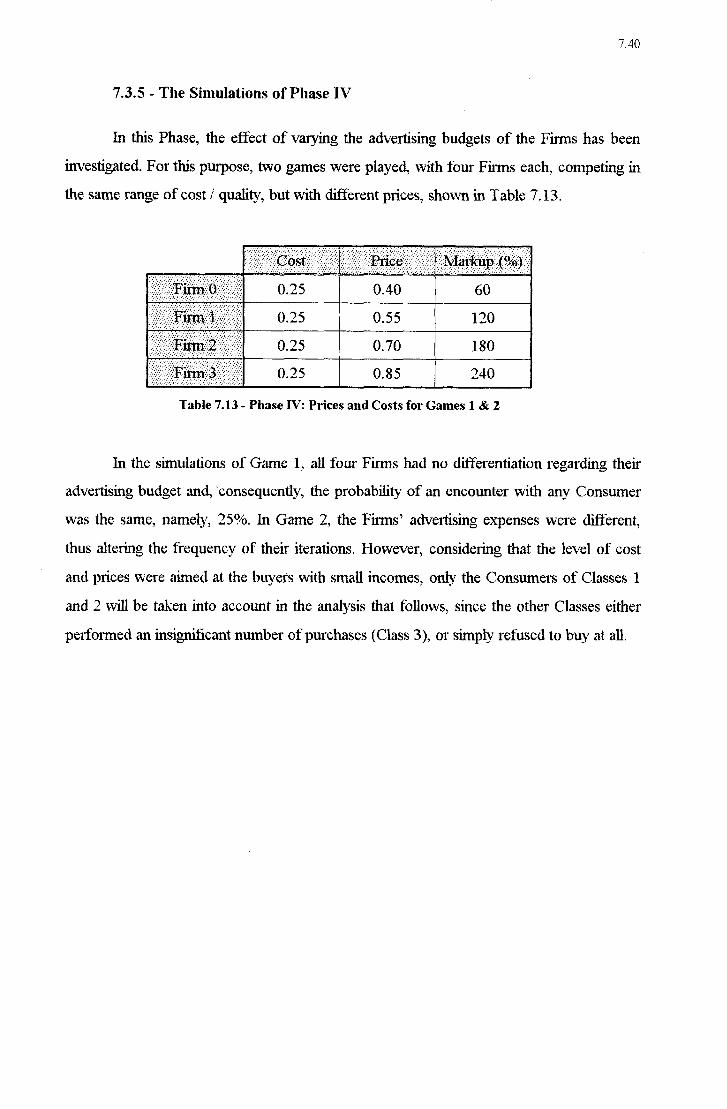
7.40

7.3.5 - The Simulations of Phase IV

In this Phase, the effect of varying the advertising budgets of the Firms has been

investigated. For this purpose, two games Were played, with four Firms each, competing in the same range of cost ./A quality, but With different prices, shown in Table 7.13.

60

0.25 0.55 1 ') A-

0.25 0.70 180

0.25 0.85 240

*Fama ‹›-25 0.40

Table 7.13 - Phase IV: Prices and Costs for Games 1 & 2

In the simulations of Game 1, all four Firms had no differentiation regarding their advertising budget and, consequently, the probability of an encounter with any Consumer was the same, namely, 25%. In Game 2, the Firms' advertising expenses were different, thus altering the frequency of their iterations. I-Iowever, considering that the level of cost

and prices were aimed at the buyers with small incomes, only the Consumers of Classes l

and 2 will be taken into account in the analysis that follows, since the other Classes either

performed an insignificant. number of purchases (Class 3), or simply refused to buy at all.

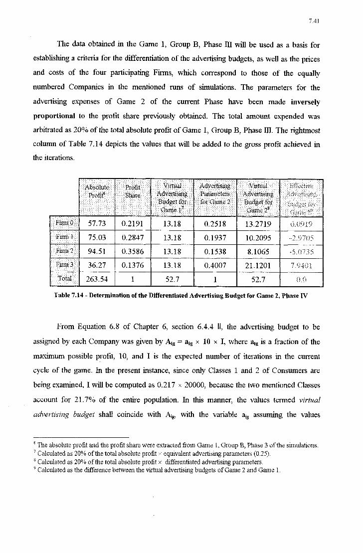
7.41

The data obtained in the Game 1, Group B, Phase DI will be used as a basis for establishing a criteria for the differentiation of the advertising budgets, as Well as the prices

and costs of the four participating Firms, which correspond to those of the equally

numbered Companies in the mentioned runs of simulations. The parameters for the

adveitising expenses of Game 2 of the current Phase have been made inversely

proportional to the profit share previously obtained. The total amount expended was arbitrated as 20% of the total absolute profit of Game 1, Group B, Phase 111. The rightmost column of Table 7.14 depicts the values that Will be added to the gross profit achieved in the iterations

'ãiíata-efit€*22¿.á@z¿§1§a.zz;;“zz§2Sfia:e5í1?{;1@;%ë 5.l}Ê¿fÍ¿i~.1P.*.\L'..<°>§1.Í.=.Í+°‹L1.-*1âã"':

"'

' '

.fÊ'§5Eš`\íÍ.1`f:t;e`1-'-f't§ãzÍff.ë1.'iš šíšiiš

*E152

:if-¿:›Ê::::-:I-; If :--

5fÓi'5í;GäinÍe51=§f'Ê;' 55;5§;í~

Ílfííií:-:Í . 2 2 .%Á¿z1f\'%`t%`11i`SÇi.iz1»8¿f ÍfÍiÍ"Í:¿ÍfÍíl

1ÊÊíÉ2ÊÊ'1'*

-~. ø.. _. . ._

š.::ti¿Ê.;o›:â:w¢

df\5'š:Êí":if§šs.i.t"

' 1 '

l=**2-`tê.«??‹1ê.Íf-é¬íí=í ztiÍ«f.v‹

.~,-\ 1. . . .-..›`..{›

'‹:.f‹c:›ttz-z;-:

Jr É Ê§; 57.73 0.2191 13.18 0.2518 13.2719 (3. 09 1. 9 75.03 0.2847 13.18 0.1937 10.2095

; z.p¿¡z¿;¡¡¿ 5:; af 94.51 0.3586 13.18 0.1538 8.1065 _ tl 3 fi

¶fazrzí.%.;=é 36.27 0.1376 13.18 0.4007 21.1201 7,011-il Ê.

263.54 1 52.7 1 52.7 'vz' J.,

.

.

Table 7.14 - Determination of the Differentiated Advertising Budget for Game 2, Phase IV

From Equation 6.8 of Chapter 6, section 6.4.4 II, the advertising budget to be

assigned by each Company was given by A¡g = aig × 10 >< I, Where a¡g is a fraction of the

maximum possible profit, 10, and I is the expected number of iterations in the current. cycle of the game. In the present instance, since only Classes 1 and 2 of Consumers are

being examined, I Will be computed as 0.217 :›< 20000, because the two mentioned Classes

account for 217% of the entire population. In this manner, the values termed virtual

aclvertísing budget shall coincide With A¡g, With the variable a¡g assuming the values

b The absolute profit. and the profit share were extraeted from Game 1, Group B, Phase 3 of the simulations. 7 Calculated as 20% of the total absolute profit :>‹< equivalent advertising parameters (_ 0.25). C.alct1la.ted as 20% of the total absolute profit >< differentiated advertising parameters.

9 Caleulated as the difference between the virtual adveitising budgets of Game 2 and Game 1.

7.42

0003058, 0002352, 0.00l868 and 0004866, respectively for Firms 0, 1, 2 and 31°. It

must be noted that. the objective of the simulations of this Phase has been to evaluate the

influence of contrasted advertising budgets, while all other variables present in the two

games under consideration are kept unchanged. Thus, only the marginal advertising

expenses_ the diflerence between both virtual budgets, shall be taken into account to

compute the fnal results, videlieet., the last column of Table 7.14.

The results yielded by the simulation program for Game 1 are surnmarized in the sequence.

I. Tables 7.15(a) - (e): Game 1 - Equivalent Advertising Budgets

-5

`

-À __» lã À ._\ ...s .O0 66.150 1.135

ii \1 |\) ¿ ._\. \l U1 0.24 -7.875 -0.135

Ízlass

1162 0.53 58.275 O7 .À 0) ...t O

Table 7.15(a) - Phase IV, Game 1: Simulation Partial Results for Firm 0

O) C) ¡:¡' ¿¡-.¡z¿-:¡¡. ¡; :‹¡1~;-:-¡.¡›1¡~:¡-:¡› 424 O_19 I

83635 0,1 66 l\) ...x ._\

'¡1.j¿:§zj1z1j:'_z:§}-;j:', z-1-"_2¡-'¡›-*_1;-j}:1}:}1;1z11;; 681 0.31 l

41.9361 0.834

\Class No Abs Suco Suco Ratto Abs Proftt Prof|tRat1o

Í\J (0 _À _\ O :ietz.zé'z;í;f=:z;.1:fz&-;:2%z'zífz:.í;zf=f;.r 1105 0.26 l

50.2996

Table 7.15(b) - Phase IV, Game 1: Simulation Partial Results for Firm 1

1° Although the values of as appear to be quite small, it should be remembered that they regard a fractíon of the utmost plausíble profit to be attained in a cycle, unrealistíc in piactice, and sewing exclusively as a reference.

7.43

Ç 2-_; ti;

:f

'11 'íz ;Í 1-1 :P if: 111 :fz :f: 1;: i§1::.'¿N 78

I

0.1 Q I

23.5647

-À C) ._\ 0.440

É if: if; :_';

:_Í: if: If; ,Í if: if; :ff :_Í; :_Í; I; 1:: 682 ...x _.\ |\) 0.16 30.043 0.560 ›z.-.. z: 121;;-í =;s¿;í 221:: iii ii: iii

52 aí íšf 1 083

,E1102 ~;â;e.í f~ _

._s (OO 0.18 53.607 _s Q

Table 7.15(c) - Phase IV , Game 1: Simulation Partial Results for Firm 2.

5:; zg ¡._ j_._ gzz. '.ƒ1'-_.;;z¿ I1¿;z¿z;._;'1:: U) (O .B Í\) 01 0.074

5:;.‹;zê§1z.;.:'í~. :¿=J;;2f;;5¿;z:z;1 O) U)O _; ._L fx) 0.18 Í

51.965 0.926 555; z- zg

'z

-. z;

1.1 z¿z§1¿¿â¿¿2_'. ;jEš;Eš

0.06 |

4.147

íi;»f{5§IʧE§ 1 024 137 0.13 I

56.112 ...\ Õ

Table 7.15(‹l) - Phase IV, Game 1: Simulation Partial Results for Firm 3

;í=;;5;=í;z';;2;áz:;* ¿:~ ::_;z1fl.5z:í;&ë;s5;' ';§?51.f1-ii; 1 660 O) f\)

-lb 0.38 102.226 0.468 ":

.fií z -1 1

.Ç :_.

'

:¡: Q 2: É :`_; :¡

¡ ¡ Ó) __: Õ 0.22

I 116.070 0.532

'_' -_

1- í_. Í

2714 -zzzzf:5›=.f¡ÊÍfš 4374 1234 0.26

I

218.295 ...s (D

Table 7.15(_e) - Phase IV, Game 1: Simulation Partial Results for All Firms

H. Tables 7.16(a) - (e): Game 2 - Difierentiated Advertising Budgets

Succ Ratio Abs Profit Prof1tRat|o

Jä l\) (O 1.000 64.350 1.069

if.. ZHÍÍÁH fi.” M

:_ ff 'Í

'í;:; ;. 733 0.267 -4.163 -0.069 _x (O Ó)

E511: E

.:vVI:"':-2.5 1162

.;1: ;...'|:í':'

I 0 538 60 188 0) I\) UI _-L O

Table 7.16(a) - Phase IV , Game 2: Simulation Partial Results for Firm 0

7.44

4.

EÍíäššÉif'í:'šÊšÉÍí:IÍÍ}ÍEfEÊ5Ê J“ÊÊNóffííltëfáfiónšíffí IÍNÕÊLÍE: i;S'úõc.*Eífší lÊ*fí5Í{S:U?¿Cz;1íÊ1Rati'ÓÊ Êfíílí E ÁÉÍ?ÁE5SͧÊrF?1'öfiÍ`ÊÉ..Ê5?1 Í

'Í .Âi5P.fof.itÊíRáti0. 1: 3

I\) (0 CD *`I (Q 0.265 13.746 0.237

203 |

0.356 44.173 0.763

112;§s;¿§¿2â§zIiââiíáiíëçââiâái- 262 1

0.325 57.913 @

U1

Ú)

\l

(Q

_;

:L Ô

Table 7.l6(b) - Phase IV, Game 2: Simulation Partial Results for Firm 1

0 235 25 378 0.440 00 lx) 0) \J O)

0 215 32 307 0.560 -5 Ô) (O -A Õ ¢\

1 & 2 O 223 57 686 *J (O l\) _\ '\l \l .A O

Table 7.16(c) - Phase IV, Game 2: Simulation Partial Results for Firm 2

Í 01 r×› ×| ro ro 0.042

I

-1.653 -0.036

(O (JO 0) -Â ...L U1 0.123

Í

44.653 1.033

521)3115.2:f;§;§§§§;;í;5§.z§;; 1463 0.094 1

43.200 __.: O) \I _.: (D

àfffma Table 7.16(d) - Phase IV, Game 2: Simulation Parfial Results for Firm 3

1QiëišÉÊšíšííšãfâÊ%5%ÍEÊiš5šÊí 51?iN.¢ší51l'€š?á§í.Q0ëíiíí~Ní¢¿›šÊšíAb$;Í' ii É 5% I$ÍU..<>.¢1=iÍš-ííz Räiíšíš šfílffšíií I5:É\Í béãšiš E?f.0Íf.-¡z.f.Íš 5-ff Ifílííííf í{šF*FÍ°'f.¡Í*.íR.€=iÍzí1:<5Íi 11 iíf

`1'{ÍíƒÊ{2{Í'_{f{~Ê{Ê{{1f¡§ííÊ1¡i{Ê¡_{Ê‹_ 2709 0.227 1 1 7.1 71 0.535

.Í-:}§;1Í-z¡;zf.z§.fÊ;z;;zÊ-;Ê-i§z;Ê1§ 1577 606 0.364 ]

101.622 0.465

615 Ç 1

'~:;1zz&z&ziz2..ez@::.zzz:.1z:¿z; 4286 |

1221 I

0.285 I

216.993 _.› É

Table 7.l6(e) - Phase IV, Game 2: Simulation Partial Results for All Firms

7.45

Observing the results from Game 2, it can be seen that the number of iterations in which Firms 1 and 2 took part in fact decreased in comparison to Game 1, a nalllral

consequence of the bias imposed by random selection process. However, the accumulated profit accumulated along the iterations had an opposite behavior, slightly increasing, even

Without the reduction due to smaller advertising expenses. Why this? The main reason for that occurrence is the presence of Firm 0, which offered a better deal to the Consumers ot Classes 1 and 2 by means of a significant smaller markup over the commonly established cost.. Because of the competition presented by Firm 0, Which always maintained 100% ot buyers, the success ratio of the other Firms steadily decreased as the game proceeded, as illustrated by Figure 7.41.

Firms' Success Ratios _

Classes 1 & 2 - Game 1

0.9 ¬

Rato .O

_

~:

Success

O O Q

.0

_

ro

‹››

sz

u¬

,, , «ll

\. '<›..

\_

`

Í Hrm 3 _" 0.1 - ._ ,......___

O ¬ Í' › › . 1 1 | | 1 1 | 1 |

10 4-0 70 100 130 150 190 220 250 280

Number of Iterations

Figure 7.41 - Conjoint Success Ratio for Classes 1 & 2., Phase IV, Game 1

A comparable event took place With Firm 1, 2 and 3's accumulated payoffs, whose results regarding Class 1 are depicted in Figure 7.42. For Class 2 the circumstances were

similar.

7.46

Firms' Accumulated Payoffs Iterations with Class 1

45 »«~-W »-,

40 _

/' ff/ 35 Jø/,I i

Accum.

Payoff

./'1 30 Mv,/'f ............. Fufrn O

25 A V*//t

""'“~~~~-"t ` ”“"r-#1 . ;.-,rm

20 , /-f' ››››››››››› »« Firmz

_z' 5:

15 J, ..;;¢f/ _-.. ..... _.-. Fuzm 3

1° « ~ - â;

/z ;`

04 . . . . . . . .

10 40 70 100 130 160 190 220 250 280

Number of Iterations

Figure 7.42 - Firms' Accumulated Payofis with Class 1, Phase IV, Game 1.

According to the rules of the game, non-accomplished purchases mean sure

losses-the penalty for the Consumer°s dejèczion. In this manner, there is no point in trying to increase the number of iterations if they necessarily translate into negative gains. This is

Why Firms 1 and 2 ended up better off in Game 2, in spite the fact that their frequency of iterations had been reduced, comparatively to Game 1.

On the other hand, an opposite phenomenon happened to Firm 3, Which boosted its number of encounters in Game 2 for no avail. Recall that Finn 3 had the highest

markup.

The total gains obtained by the Firm O and 3 in Game 1 With Classes 1 and 2 taken aggregated do not difier very much-Figure 7.43-, basically because of the varied

decision rules of the Consumers are compensated by larger unitary profits. Class 1 was the

greatest contiibutor to the revenues obtained by the Firm with the lower price, and the

opposite occurred With Class 2.

Accum.

Prof

t

Accum ulated Profit Equivaie nt Advertising

7o - zz ez

Í. eo

i

1

'›§¶.'-

~ 50 1 :z<»fz< 1

<:z:*.;;

5

1=;`í::». :äTf,íÊí:-:

4°

so; of

20 -“

-

1 -'.“:: '}a='._1. `›,-'.=.":.

1 .-*.¡\_¡;š;z 1,-¿_1.;-.= z¿.".¡.Ç›.

1o -1 .2:;â, ze

O , ›. `...; _« ›.‹.

f

í -1g ..... .,... ...... .~.._-.......-........,...._....._.___.._z

Hrm O Hrm 1 Firm 2 Firm 3

.El Ciass 1

Class 2 U Classes 1 & 2

Figure 7.43 - Total Profit in Game 1 (Without advertising, expensas)

_-J ‹£'à \~.I

When the Firms act on their probability of being chosen for an iteration by employing diverse advertising budgets_,_it can be seen that, while Firm 0 praetically had no alterations in its profit, Firms 1 and 2 jumped to more favorable results, and Finn 3, to a

VVOÍSÔ 011€.

Accum.

Prof

t

70~

60-í

504

40~

304

20‹

1U¬ 0.1

_1Q _...,.s,....eWe..-.,......-...-.-_ --..-....-.-....... ......... .-t_...._._..._~_......_..»

Accum ulated Profit Differe ntiated Advertising

.`_._,_~

1 \. \

E 'I' /-TI

1

.:.; ¡Ç¬;

Í,"l*`zr ' Í?-

. ~ '. 4., u' / "`,'."/Í. ~fl;..¬ ‹.\Ç'.~,z'.'‹ ¬z.»-.

V. -'.'¬'.\‹;` «V _~ ,. ,¡‹_,¿_¿, I 2-Í* Í:-é:-'FI-Z _ *

-,

..2›f;. -4.¢I.‹;.fVz;I"I;I ¡,.,¿_:' ¿.¿\¿V.»¿¡;.-¡.¡V .-;z;z._‹,‹_¿í

,,.¿.`«,, ' '

Firm D F|rm 1 Firm 2 ñrm 3

,

É

Í

É

Z

f

2;

J

U Class 1

Ciass 2

EI Ciasses 1 & 2

Figure 7.44 - Total Profit in Game 2 (without advertising expensas)

NOW, When the Values of the effective advertísilzg bua'get-- Table 7.14, rightmost eo11m1n- are added to the outcomes shown in Figure 7 .44, there will be an íntensification of the foregoing comments.

Figures 7.45 and 7.46 summalize the general results concemjng the profit and the total number of iterations and suceesses obtained in Phase IV.

Accum.

Prof't

Num be r of Ite rations & Successes Equivale nt Advertising

1200 ¢--»--_»«»-~-

1000

000

000 - >~

~

ill Iii1

O 'ÍL 1? '- I -ZÊ I 15'

Firm Firm Firm Firm 0 1 2 3

2

ê

E

1

É

E Class 1 lterations

ElClass 1 Success Class 2 lterations

EI Class 2 Success El Classes 1 & 2 lterations D Classes 1 8‹ 2 Success

Figure 7.45 - Game 1, Phase IV

Accum.

Profl

Number oflterations & Successes Differentiated Advertising

1eoo¡ «C --- z - 1400

Í

1200 ¬

1000 ¬

zzzzà

Firm Firm Firm Firm 0 1 2 3

eoo -g

¿¿z

400 200

O â

ãízl

C..

....__...\

`.`.."`~

"w`.u‹

1 z‹

í1

El Class 1 terations

El Class 1 Success Class 2 lerations

EI Class 2 Success El Classes 1 & 2 lterations U Classes 1 8. 2 Success

Figure 7.46 - Game 2, Phase IV

f¬iz

7.49

Conclusions for the Simulations of Phase IV

0 In this Phase, two Games were played: Game 1, with no ditferentiation in the F irms* advertising budgets, hence with the same expected number of iterations for each Firm, and Game 2, Where the Companies had distinct probabilities of performing iterations, due to particular publicity costs.

0 When the sellers compete for the same spectrum of buyers, the results indicated that the Firms which offer the items of same cost/ quality at higher prices soon lose their

ability to accomplish sales, because the Consumers rapidly prefer the deals Where

they can fmd better advantage. This outcome, though intuitively obvious, indicates that the model is adequate in terms of mirroring practical situations.

0 Increasing advertising expenses in the presence of more efiicient competition has

demonstrated to be useless; Quite on the contrary, because, since there is a penalty imposed to the Firms when the Consumers are called to iterate and refuse to buy, the accumulation of negative payoffs due to sequential refizsals pulls the final profit

to a worse position.

0 Fitm 0, Which had the best overall performance in Game 1, maintained its rank in Game 2. On the other hand, Firms 1 and 2, Which had a smaller number of iterations, had greater prohts, on account of the foregoing cited reasons.

7.4 - Final Remarks

In this Chapter, the problem of analyzing several instances of a market competition

has been simulated With the One-sided Fzzzzjy Iterated Prís0ner's Dílemma-IS-FIPD. Regarding the playeis embodied by the Firms, the flzwor of the classic P1isoner”s Dilemma is actually present. Although the motivation of using this paradigm in this kind of problem

has already been discussed in Chapter 6, it is opponune to mention that the basic dilemma

of the traditional IPD is also extant in the Workings of the IS-FIPD model of a market share game. Some significant similatities regarding those two approaches are:

7.50

The Firms_ in the IS-FIPD, the category of players that is actually involved in a

PD- can either cooperate or defect, in a gradual manner, by establishing diverse levels of markups;

Defection pays, until a certain extent, since the decision functions used by the

Consumeis tend t.o initiate the game in a cooperative mood, Which is quickly and constantly updated.

However, the Consumers are reactive decision makers, and dqďction is soon answered

With defection, Which implies in losses to the sellers. The Consumers° dqƒèction is

symbolized by the act of not buying from the non-cooperative Firms;

In the long nm, if well adjusted, cooperation is worth, yielding positive though smaller

payoffs to both sides involved.

8.1

Chapter 8

“...the individual pursuit Qf a large share of the pie often sabotages ejffícíeriqv.

""

-¬J. McMiIlan, in Games, Strategies and Managers, 1992.

Conclusions

8.1 - Summary of the Dissertation The vast majority of studies and applications of the IPD regard a 2:›<2 game, with

two players and two mutually exclusive strategies, COOPERATE and DEFECT, With the

participants usually formulating their decisions by means of some app1'aisa.l of the foregoing sequence of moves.

In this Dissertation, the IPD Was explored With some alternative and new approaches, basically:

0 Admittance of gmdalions in the st1'a.t.egies, between the extreme points C and D;

0 Formulation of decision systems for the players that incorporate other

variables besides the history of previous encounteis;

0 Introduction of fuzzy logic and fuzzy expert systems to asciibe a qualitative

reasoning method for the players-eveizvtlzirig is a matter of degreel;

1 This quotation is borrowed from Dr. A. Kandel, who used it in a. course on fuzzy systems attended by the author of this dissertation in the second semester of 1994 at the University of South Floiida.

8.2

0 Employment of a one-sided Prisoner”s Dilemma to model a market share game;

The Dissertation is informally divided in 2 parts. Chapters 1 through 4 contain the

introduction and a review of the fundamental theoretical aspects of Game Theory, the

Prisoner's Dilemma Game and Fuzzy Sets. In Chapter' 4, a. contribution Was also made regarding the aggregation of decision criteria. using thefuzzy integral. A modification to the original approach of this method Was studied and implemented, which comprises the

inclusion of an ƒncrement A+ and a. decrement ÁY in the fonnulation of L (Y 3¢ . Chapters

5 through 8 comprise exploratory models of the Fuzzy Iterated Prisoner's Dilemma -FIPD, and a practical application of the FIPD using the one-sided version of the game With its simulations results, and the conclusions.

One significant portion of the work regarded the creation of two specially written object-oriented C++ codes to run the simulations concerning the models presented in Chapters 5 and 6, since no commercially available package firlfilled the specifrcations to

perfonn the required tasks.

The achievement of a greatcer' insight of the Workings of the PD paradigm has been the major goal of the present research, and the most important acquired outcomes are

summarized in the sequence

8.2 - Synopsis of the Results

8.2.1 - The FIPD Tournaments (Chapter 5)

The toumaments consisted in confronting the fuzzy players, differentiated by their respective rules, against themselves and simultaneously against other traditionally successfirl

strategists in earlier' contests, TFT and PAVLOV. Those established rules maintained their usual dichotomic character regarding the criteria of assessment of previous moves and

implementation of decisions. The results that have been obtained from the limited set. of

8.3

simulations performed showed a quite erratic pattern conceming efficiency in accumulating

payoffs. In the first phase of the iterations, PAVLOV, Which uses the simple rule win-stay, lose-change, Was the overall Winner in most instances. In this stage, TFT did not thrive. As to the fuzzy players, a noticeable feature was the prevalence of déjfection-biased strategfsts

among the best performers, indicated by the presence of the digits 4, 5, 6, 7 in their fuzzy

classification numbersz. In short, the predominantly nice and forgrívzfng fuzzy strategists did

not succeed in the competitive environment.

Nevertheless, the realization of the subsequent phases of the toumament, from

which the poorest perfonners have been excluded, revealed a change in the results. From the second phase on, PAVLOV abandoned its success and TFT began to shine, only eventually defeated by the defection-biased fuzzy rules. On the other hand, fuzzy-TFT did not. leave the ground, and the binary TFT ended up as the final Winner of the toumaments.

Three relevant. aspects concerning the simulations are worth merrtioning, though:

- The frrst is the fact. that PAVL-OV and TFT (binary and fuzzy versions) were always picked to participate in every phase of the simulations, in contrast with the exclusion

criterion applied to the other players. This criterion provided an advantage to those

participants, which had renewed opportunities to recover from precedent comedowns.

- The second topic refers to the influence of the probabilistic characteristic of sequential

assignment of pairs of players to being confronted. Because the expert systems

- take into consideration a set of data which is derived from the history of the game, the

resulting decisions that Were adopted along the tournament phases Were strongly

influenced by the particular succession of pairwise encounters. Although the cited

,¬

overall recipe for good performance appears to have been confirmed in hundreds ot

thousands of iterations, there still remains a speculation Whether a defmite and unique

stable configuration might. really arise from the equally many possible starting

arrangements. This question induces a conjecture about the an inherent unpredictable

The digit 5 stands for Widespread defection in every circunrstance, and 4, 6, 7 correspond to defection in two out of three resolution clarrses.

8.4

trait of complex and dynamic social (and other) systems, Where some small fortuitous changes can make a big difference.

- The third point. consigns the frequency distribution of the types of playets. ln the model there Were 512 distinct filzzy categories, and three other special participants. However, each type counted With only one representative in all matches. An ecologically designed tournament comes immediately to mind, Where the most apt strategies proliferate and the Worst become extinct. Nonetheless, even in this circumstance, it appears that the

considerations about the intrinsic unpredictability of the resulting equilibiium still

endure.

9° to to - The One-Sided FIPD-1S-FIPD- and its application to a Market Share Game (Chapters 6 and 7)

Chapters 6 can be considered the nucleus of the Dissertation. A model based on the lS-FIPD has been implemented and extensively detailed. Along the text, several problems conceming the relationship between the conflict of interest posed by a market With Firms and Consumers, the IPD and the use of methods based in filzzy set theory Were approached and successfully formulated.

ln Chapter 7, With the aid of an object-oriented C++ program, the IS-FIPD has been simulated under a number of different aspects, Which were divided in four phases, summaiized below. .

- Phase I: A general toumament with six Firms operating at diverse market segments regarding the quality and cost of items. The game was divided in five qvcles. From a

cycle to the next, half of the Companies made alterations in their prices, while the costs were kept constant for all Firms. Among the diverse conclusions achieved, it

was found that the most successful Company Was number 4, which operated with fixed cost and prices throughout the cycles, and aimed them at the upper-middle Classes of Consumers.

- Phase II: Here, two groups of Games Were simulated. In Group A, the objective was observing the effect of conioint of diminishing costs and fixed prices on the

8.5

performance of the Firms. In Group B, the opposite policy Was adopted, With

constant costs and decreasing prices. Following a characteristic already' found in

Phase 1, the Consumers from Class 1- With the smallest incomes- Were quite reticent in accomplishirrg purchases. In fact, there were no buyers from that category in Group A, at a price of MU$l.00. ln Group B, their general contribution to the Firms” profits Was insignificant. The best contributors to the Companies profits were the Classes 5, 6 and 7, Which, aside being more numerous, also had more flexibility in their decision criteria, being less specific in their preferences and buying from more sellers.

Another' interesting finding Was that the more eflicient markup in terms of obtaining a maximum profit Was between 40% and 60%.

Phase Ill: This stage consisted of six games, each With six Firms competing together

in the same slice of the global market. The costs Were fixed in each game, and the sellers offered their items With different markups.

The best result in terms of net profits Were achieved in Game 5, When the cost Was 5.50 and the price, $8.25, which corresponds to ar markup of 50%, thus confirming the same optimum range found in Phase II. The respective success ratio Was about 4%. The highest success ratio in Phase III occurred also in Game 5, and it has been detained by Firm O (À: 7%), but it did not coincide With the greatest profit. This

result evinces that the IS-FIPD model is appropriate in terms of coiroborating that the pursue of the greatest market share by means of decreasing markups can be disadvantageous

Phase IV: While in all other experiments no differentiation Was imposed to the Firms” probabilities of iterating with the Consumers, now the Companies were able to make adjustments in their advertising budgets With the objective of altering that feature. Two rounds of sirnulations Were run, with four Firms playing. For the sake of comparison, in the first game the Companies had equivalent advertising expenses, contrasting With different ones in the second. The main finding in this phase was that increasing advertising expenses in the presence of more efficient competition

8.6

has demonstrated to be useless, because the Consumers rapidly tum their attention to the deals Where they can find better advantage, measured by the obtained payoffs.

In fact, due to the penalty payoff imposed to the sellers When a Consumer refuses to buy in an iteration, increasing the frequency of it.erations can even be worse

regarding the capacity of accumulating profits.

As could be perceived from the analysis of the simulations performed in Chapter 7, the model of the lS-FIPD is practically unending in terms of possible experimentation.

Many combinations of costs, prices, costs, number of Firms, range of the competition and advertising budgets can be implemented, apart from other lower-level adjustments in the parameters employed for the Consumers” decision For this reason, the examples presented

and discussed have been limited, and experiments focused on a selected number of situations, with. the objective of demonstrating the potential of the process.

Finally, it is very important to emphasize here that the proposed method is intended

as an analysis tool. Therefore, the parameters of the models, as well as the data employed

in the simulations did not come from empirical observations, and have been arbitrarily but judiciously selected to mimic real data. As a consequence, the calibration of the model and

its application to true sets of information remains as a suggestion for further improvement.

8.3 - Main Contributions of the Work

The scientific contributions presented by the present dissertation can be

summaiized by the following topics:

1. The admittance of gradual decisions in the Pn`soner”s Dilemma using elements of Fuzzy Set Theory;

2. The use of Belief Theory associated with Fuzzy Logic to implement

decisions in a conflict of interest;

3. Introduction of adjustment factors in the method of the Fuzzy Integral; 4. Association of simulation methods With fuzzy decision criteria for the IPD;

8.7

5. Development of an analysis tool with an actual and practical application to the paradigm of the IPD;

8.4 - Limitations of the Work and Suggestions for Future Developments

a.

b.

C.

Establishment of the general structures of the models of the FIPD

Besides fuzzy expert systems, other architectures could have been employed instead. For example, the techniques of genetic algorithms, multi-layered

perceptrons (Neural Networks) and evolutionaiy programming (with Finite State Machines- FSMs_`) have already been investigated, as discussed in Chapter 3. But, by the time that this text is presented, the mentioned AI methods lack the use of fuzziness in their' approach of the IPD. Therefore, those seem to be a promising line of research for building other realistic models of the IPD.

Choice of the variables

Selecting valiables that can realistically mimic rational human behavior, represented by the agents” actions and perceptions in an IPD, is a challenging task. That

problem is intimately correlated to finding an efficient frame to poitray preferences,

rationality and utility. In both models presented, a departure from the usually adopted information sets depicted by the “sequence of the opponent's last moves” has been sought and implemented. However, the current choice of variables on which the actors count to make their decisions provide just a. possible configuration, and many other influencing factors could have been ascribed to the method. In this manner, other opportunities of research are open in that field, by altematively picking diverse variables to mirror a rational decision process. Those may include psychological factors regarding the agents, enviromnental dynamic changes and

influence of extraneous contingencies, among several others.

Detailing of the models

The encounters between the players in the two models of the FIPD have been guided by previously arbitrated particular probabilistic methods, Which parameters

8.8

remain static along the simulation course. This fact entails the speculation for a

quest of an adaptive random rule to govem the pairings, that might be continuously induced by the outputs of the game, thereby embodying a recurrent system. The inclusion of this and other alike features in the design of a. simulated IPD must be carefully done, though. This suggestion regards the risk of ending up With a system which has some sort of chaotic dynamics embedded in it, which Would be of rather complex analysis and could also lead to no further understanding of the nature of

the conflict of interest depicted by the IPD.

An important aspect worth mentioning refers to the tuning of the fuzzy expert systems. The choice of the numeric parameters that particularize the fuzzy sets employed were discretionaiy, and some singling out had to be done in order to attain the computational simulation programs and ums. Nevertheless, it might be

desirable to adjust. the parameters of the fuzzy system to a. set of empiiical data,

What could be done in accordance to some specific query. The production rules utilized had single antecedents. This particular

countenance has been deliberately picked in order to shun the trap of a

combinatorial explosion of feasible individual strategies for playing the game. Recall

that in the model of Chapter 5, a choice of three decision factors, each also with three qualitative assessments and only two strategies, namely, COOPERATE and DEFECT, led to 512 distinct fuzzy players. As a further development, it is proposed

that. the players may count on two-antecedem; decision rules, Which Would be aggregated and mapped into the consequent through T-norrns or S-nomis fuzzy operatois or still any other operator from a palette of options, including weighted

and nomnonotonic fuzzy operators4.

Although multi-antecedent rules (With more than two) could be used, ditferently from control problems, it appears that it is not the case that the decisions adopted by human agents in a PD-like conflict of interest would take that course. Regarding nonrnonotonic aggregation operations, Yager and Filev (op. cit. [YAGE«94], p. 40) state that, in ordei to do default or connnonsense reasoning, nonmonotoiiic- logic is more appropriate, which entails the utilization of that class of operators.

8.9

Relaxation of pairvvise iteration - n-person IPD

Despite the diversity of individual types of players considered, the iterations were

always paiivvise. Other forms of pd-like simations involving three or more players

(e. g. the stag hzmt, the fiwze-rider problem) might take advantage of a firzzy

approach to the decision method.

Allowance ot features belonging to cooperative games

The PD is an essentially competitive game, though obviously non-strictly so. This is a necessary condition for it to possess the strikingly contradiction between the

individual and the collective rationality. But it must be conceded that the restriction

regarding the nonexistence of bargaining or negotiation between the parties

participating in the disput.e- exercised throughout. the formulation of the presented

method remarkably strong. On the other hand, total communication and

enforcement of agreed contracts would completely dissolve the dilemma posed by the PD paradigm. Thus, under the same mtíonale that inspired the depaiture from the dichotomic game, a gradual compromise amid the contenders looks as though

viable to be modeled and simulated in an eventual upcoming exploration of the

theme.

Further Simulations

For both models of the FIPD, the sirnulations mn with the respective programs cover only a part of the possibilities, that can be taken as illimitable. Hence,

additional probing can always be realized, perhaps with a particular emphasis to

some specific concems whose claiification is sought.

8 4 Final Remarks

Philosophers are intrigued by the Prisoner°s Dilemma. The incongruity embedded in it rs appalling because a widespread individual rationality leads not only to collective

Jrrationality, but also to individual losses and, therefore, irrationality. The PD paradigm,

8.10

particularly its repeated version-IPD-, has been extensively employed to model conflicts of interest that tum up in a diversity of scientific areas, fiom operations research to social sciences and biology. The importance of the PD within the realm of Game Theory is

unquestionable, since it reflects With both simplicity and clarity What this branch of knowledge is all about. On its turn, Game Theory is captivating an increasing interest. as a

powerful tool for developing application models aimed at real life situations and problems where rational and reactive actions are extant.. A confirmation of the recognition of this trend Was the granting of the 1994 Nobel Prize in Economics to three Game Theorists.

Chapter 6 - Appendix a 6a.ii

0.053 0.0757 0.253 0.2234 0.453 0.3510: 0.653 0.4865 0.853 0.6585 0.054 0.0767 0.254 0.2241 0.454 0.3516 0.654 0.4872 0.855 0.6595 0.055 0.0776 0.255 0.2247 0.455 0.3523 0.655 0.4879 0.855 0.6606 0.056 0.0785 0.256 0.2254 0.456 0.3529 0.656 0.4887 0.856 0.6617 0.057 0.0795 0.257 0.2260 0.457 0.3535 0.657 0.4894 0.857 0.6628 0.058 0.0804 0.258 0.2267 0.458

! 0.3542 0.658 0.4901 0.8581 0.6638

0.059 0.0813 0.259 0.2273 0.459 0.3548 0.659 0.4909 0.859 0.6649 0.06 0.0822 0.26 0.2280 0.46 0.3555 0.66 0.4916 0.86 0.6660

0.061 0.0832 0.261 0.2286 0.461 0.3561 0.661 0.4923 0.861'

0.6671 0.062 0.0841 0.262 0.2292 0.462 0.3568 0.662 0.4931 0.862 0.6682 0.063 0.0850 0.263 0.2299 0.463 0.3574 0.663 0.4938 0.863 0.6693 0.064 0.0859 0.264 0.2305 0.464 0.3581 0.664 0.4946 0.8641 0.6704* 0.065 0.0868 0.265 0.2312 0.465 0.3587 0.665 0.4953 0.865 0.6716 0.066 0.0877 0.266 0.2318 0.466 0.3593 0.666 0.4960 0.866 0.6727 0.067 0.0886 0.267 0.2325 0.467 0.3600 0.667 0.4968 0.867 0.6738 0.068 0.0894 0.268 0.2331. 0.468 0.3606 0.668 0.4975 0.868 0.6749 0.069 0.0903 0.269 0.23315 0.469 0.3613 0.669 0.4983 0.869 0.6761 0.07 0.0912 0.27 0.2344 0.47 0.3619 0.67 0.4990 0.87' 0.6772

0.071 0.0921 0.271 0.2351 0.471 0.3626 0.671 0.4998 0.871 0.6783 0.072 0.0929 0.272 0.2357 0.472 0.3632 0.672 0.5005 0.872 0.6795 0.073 0.0938 0.273 0.2364 0.473 0.3639 0.673 0.5013 0.873 0.6806 0.074 0.0947 0.274 0.2370 0.474 0.3645 0.674 0.5020 0.874 0.6818 0.075 0.0955 0.275 0.2376 0.475 0.3652 0.675 0.5028 0.875 0.6829 0.076 0.0964 0.276 0.2383 0.476 0.3658 0.676 0.5035 0.876 0.6841 0.077 0.0972 0.277 0.2300 0.477 0.3664 0.677 0.5043 0.877 0.6853 0.078 0.0981 0.278 0.2396 0.478 0.3671 0.678 0.5050 0.878 0.6864 0.079 0.0989 0.279 o.24o2_ 0.479 0.3677 0.679 0.5058 0.879 0.6876 0.08 0.0998 0.28 0.2409 0.48 0.3684 0.68 0.5065 0.88 0.6888

0.081 0.1006 0.281 0.2415 0.481 0.3690 0.681 0.5073 0.881 0.6900 0.082 0.1015 0.282 0.2422 0.482 0.3697 0.682 0.5080 0.882 0.6912 0.083 0.1023 0.283 0.2428 0.483 0.3703 0.683 0.5088 0.883 0.6924 0.084 0.1031 0.284 0.2435 0.484 0.3710 0.684 0.5096 0.884 0.6936 0.085 0.1040 0.285 0.2441 0.485 0.3716 0.685 0.5103 0.885 0.6948 0.086 0.1048 0.286 0.2447 0.486 0.3723 0.686 0.5111 0.886 0.6960 0.087 0.1056 0.287 0.2454 0.487 0.3729 0.687 0.5118 0.887 0.6972 0.088 0.1064 0.288 0.2460 0.488 0.3736 0.688 0.5126 0.888 0.6984 0.089 0.1072 0.289 0.2465 0.489 0. 3742 0.689 0.5134 0.889 0.6996 0.09 0.1081 0.29 0.2473 0.49 0.3749 0.69 0.5141 0.89 0.7009

0.091 0.1089 0.291 0.2479 0.491 0.3755 0.691 0.5149 0.891 0.7021 0.092 0.1097 0.292 0.2486 0.492 0.3762 0.692 0.5157 0.892 0.7034 0.093 0.1105 0.293 0.2492 0.493 0.3768 0.693 0.51õZ 0.893 0.7046 0.094 0.1113 0.294 0.2498 0.494 0.3775 0.694 0.5172 0.894 0.7059 0.095 0.1121 0.295 0.2505 0.495 0.3781 0.695 0.5180 0.895 0.7071 0.096 0.1129 0.296 0.2511 0.496 0.3788 0.696 0.5187 0.896 0.7084 0.097 0.1137 0.297 0.2518 0.497 0.37941 0.697 0.5195 0.897 0.7097 0.098 0.1145 0.298 0.2524 0.498 0.3801 0.698 0.5203 0.898 0.71101 0.099 0.1153 0.299 0.2530 0.499 0.3808 0.699 0.5211 0.899 0.7122

0.1 0.1161 0.3 0.2537 0.5 0.3814 0.7 0.5218 0.9 0.7135 0.101 0.1169 0.301 0.2543 0.501 0.3821 0.701 0.5226 0.901 0.7148 0.102 0.1177 0.302 0.2550 0.502 0.3827 0.702 0.5234 0.902 0.7161 0.103 0.1185 0.303 0.2556 0.503 0.3834 0.703 0.5242 0.903 0.7175 0.104 0.1192 0.304 0.2562 0.504 0.3840 0.704 0.5249 0.904 0.7188 0.105 0.1200 0.305 0.2569 0.505 0.3847 0.705 0.5257 0.905 0.7201

Chapter 6 - Appendix a 6a.¡¡i

0.106 0.1208 0.306 0.2575 0.506 0.3853 0.706 0.5265 0.906 0.7214 0.107 0.1216 0.307 0.2582 0.507 0.3860 0.707 0.5273 0.907 0.7228 0.108 0.1224 0.308 0.2588 0.508 0.3866 0.708 0.5281 0.908 0.7241 0.109 0.1231 0.309 0.2594 0.509 0.3873 0.709 0.5288 0.909 0.7255 0.11 0.1239 0.31 0.2601 0.51 0.3880 0.71 0.5296 0.91 0.7269

0.111 0.1247 0.311 0.2607 0.511 0.3886 0.711 0.5304 0.911 0.7282 0.112 0.1255 0.312 0.2613 0.512 0.3893 0.712 0.5312 0.912 0.7296 0.113 0.1262 0.313 0.2620 0.513 0.3899 0.713 0.5320 0.913 0.7310' 0.114 0.1270 0.314 0.2626 0.514 0.3906 0.714 0.5328 0.914 0.7324 0.115 0.1278 0.315 0.2633 0.515 0.3912 0.715 0.5336 0.915 0.7338 0.116 0.1285 0.310 0.2639 0.516 0.3919 0.716 0.5344 0.916 0.7352 0.117 0.1293 0.317 0.2645 0.517 0.3926 0.717 0.5352 0.917 0.7366 0.118 0.1300 0.318 0.2652 0.518 0.3932 0.718 0.5359 0.918 0.7381 0.119 0.1308 0.319 0.2658 0.519 0.3939 0.719 0.5367 0.919 0.7395 0.12 0.1316 0.32 0.2664 0.52 0.3945 0.72 0.5375 0.92 0.7410

0.121 0.1323 0.321 0.2671 0.521 0.3952 0.721 0.5383 0.921 0.7424 0.122 0.1331 0.322 0.2677 0.522 0.3959 0.722 0.5391 0.922 0.7439 0.123 0.1338 0.323 0.2683 0.523 0.3965 0.723 0.5399 0.923 0.7454 0.124 0.1346 0.324 0.2690 0.524 0.3972 0.724 0.5407 0.924 0.7469 0.125 0.1353 0.325 0.2696 0.525 0.3978 0.725 0.5415 0.925 0.7484 0.126 0.1361 0.326 0.2703 0.526 0.3985 0.726 0.5423 0.926 0.7499 0.127 0.1368 0.327 0.2709 0.527 0.3992 0.727 0.5432 0.927 0.7514 0.128 0.1376 0.328 0.2715 0.528 0.3998 0.728 0.5440 0.928 0.7529 0.129 0.1383 0.329 0.2722 0.529 0.4005 0.729 0.5448 0.929 0.7545 0.13 0.1390 0.33 0.2728 0.53 0.4012 0.73 0.5456 0.93 0.7560

0.131 0.1398 0.331 0.2734 0.531 0.4018 0.731 0.5464 0.931 0.7576 0.132 0.1405 0.332 0.2741 0.532 0.4025 0.732 0.5472 0.932 0.7592 0.133 0.1413 0.333 0.2747 0.533 0.4031 0.733 0.5480 0.933 0.7608 0.134 0.1420 0.334 0.2753 0.534 0.4038 0.734 0.5488 0.934 0.7624 0.135 0.1427 0.335 0.2760 0.535 0.4045 0.735 0.5496 0.935 0.7640 0.136 0.1435 0.336 0.2766 0.536 0.4051 0.736 0.5505 0.936 0.7656 0.137 0.1442 0.337 0.2772 0.537 0.4058 0.737 0.5513 0.937 0.7672 0.138 0.1449 0.338 0.2779 0.538 0.4065 0.738 0.5521 0.938 0.7689 0.139 0.1457 0.339 0.2785 0.539 0.4071 0.739 0.5529 0.939 0.7706 0.14 0.1464 0.34 0.2791 0.54 0.4070. 0.74 0.5537 0.94 0.7723

0.141 0.1471 0.341 0.2798 0.541 0.4005' 0.741 0.5546 0.941 0.7740 0.142 0.1478 0.342 0.2804 0.542 0.4091 0.742 0.5554 0.942 0.7757 0.143 0.1486 0.343 0.2810 0.543 0.4098 0.743 0.5562 0.943 0.7774 0.144 0.1493 0.344 0.2817 0.544 0.4105 0.744 0.5570 0.944 0.7791 0.145 0.1500 0.345 0.2823 0.545 0.4111 0.745 0.5579 0.945 0.7809 0.146 0.1507 0.346 0.2829 0.546 0.4118 0.746 0.5587 0.946 0.7827 0.147 0.1515 0.347 0.2836 0.547 0.41251* 0.747 0.5595 0.947 0.7845 0.148 0.1522 0.348 0.2842 0.548 0.4132 0.748 0.5604 0.948 0.7863 0.149 0.1529 0.349 0.2848 0.549 0.4138 0.749 0.5612 0.949 0.7881 0.15 0.1536 0.35 0.2855 0.55 0.4145 0.75 0.5620 0.95 0.7900

0.151 0.1543 0.351 0.2861 0.551 0.4152 0.751 0.5629 0.951 0.7919 0.152 0.1550 0.352 0.2867 0.552 0.4158 0.752 0.5637 0.952 0.7938 0.153 0.1558 0.353 0.2874 0.553 0.4165 0.753 0.5645 0.953 0.7957 0.154 0.1565 0.354 0.2880 0.554 0.41 72 0.754 0.5654 0.954 0.7976 0.155 0.1572 0.355 0.2886 0.555 0.4179 0.755 0.5662 0.955 0.7996 0.156 0.1579 0.356 0.2893 0.556 0.4185 0.756 0.5671 0.956 0.8016 0.157 0.1586 0.357 0.2899 0.557 0.4192 0.757 0.5679 0.957 0.8036 0.158 0.1593 0.358 0.2905 0.558 0.4199 0.758 0.5688 0.958 0.8056

Chapter 6 _ Appendix a 6a.iv

0.159 0.1600 0.359 0.2912 0.559 0.4206 0.759 0.5696 0.959 0.8077 0.16 0.1607 0.36 0.2918 0.56 0.4212 0.76 0.5705 0.96 0.8097

0.161 0.1614 0.361 0.2925 0.561 0.4219 0.761 0.5713 0.961 0.8119 0.162 0.1621 0.362 0.2931 0.562 0.4226 0.762 0.5722 0.962 0.8140 0.163 0. 1628 0.363 0.2937 0.5631 0.4233 0. 5730 0.963 0.8162 0.164 0.1635 0.3645 0.2944 0.564 0.4239

0.763 É

I 0.764 0.5739 0.964 0.8184 0.165 0.1642 0.365" 0.2950 0.565 0.4246 0.765 0.5747 0.965 0.8206 0.166 0.1649 0.366 0.2956 0.566 0.4253 0.766 0.5756 0.966 0.8229 0.167 0.1656 0.36? 0.2963 0.567 0.4260 0.767 0.5765 0.967 03252 0.168 0.1663 0.368 0.2969 0.568 0.4267 0.768 0.5773 0.968 0.8276 0.169 0.1670 0.369 0.2975 0.569 0.4273 0.769 0.5782 0.969 0. 8299 0.17 0.1677 0.37 0.2982 0.57 0.4280 0.77 0.5791 0.97 0.8324

0.171 0.1684 0.371 0.2988 0.571 0.4287 0.771 0.5799 0.971 0.8349 0.172 0.1691 0.372 0.2994 0.572 0.4294 0.772 0.5808 0.972 0.8374 0.173 0.1698 0.373 0.3001 0.573 0.4301 0.773 0.5817 0.973 0.8400 0.174 0.1705 0.374 0.3007 0.574 0.4307 0.774 0.5825 0.974 0.8426 0.175 0.1712 0.375 0.3013 0.575 0.4314 0.775 0.5834 0.975 0.8453 0.176 0.1719 0.376 0.3020 0.576 0.4321 0.776 0.5843 0.976 0.8480 0.177 0.1726 0.377 0.3026 0.577 0.4328 0.777 0.5852 0.977 0.8508 0.178 0.1733 0.378* 0.3032 0.578 0.4335 0.778 -0.5861 0.978 0.8537 0.179 0.1740 0.379 0.3039 0.579 0.4342 0.779 0.5869 0.979 0.8566 0.18 0.1747 0.38 0.3045 0.58 0.4348 0.78 0.5878 0.98 0.8596

0.181 0.1754 0.381 0.3051 0.581 0.4355 0.781 0.5887 0.981 0.8628 0.182 0.1761 0.382 0.3058 0.582 0.4362 0.782 0.5896 0.982 0.8660 0.183 0.1767 0.383" 0.3064 0.583 0.4369 0.783 0.5905 0.983 0.8693 0.184 0.1774 0.334 0.3070 0.584 0.4376 0.784 0.5914 0.984 0.8727 0.185 0.1781 0.385 0.3077 0.585 0.4383 0.785 0.5923 0.985 0.8762 0.186 0.1788 0.386 0.3083 0.586 0.4390 0.786 0.5932 0.986 0.8798 0.187 0.1795 0.387* 0.3089 0.587 0.4397 0.787 0.5941 0.987 0.8837 0.188 0.1802 0.383* 0.3096 0.588 0.4403 0.788 0.5950 0.988 0.8876 0.189 0.1808 0.389 0.3102 0.589 0.4410 0.789 0.5959 0.989 0.8918 0.19 0.1815 0.39 0.3108 0.59 0.4417 0.79 0.5968 0.99 0.8962

0.191 0.1822 0.391 0.3115 0.591 0.4424 0.791 0.5977 0.991 0.9008 0.192 0. 1829 0.3926 0.3121 0.592 0.4431 0.792 0.5986 0.992 0.9057 0.193 0.1836 0.393 0.3127 0.593 0.4438 0.793 0.5995 0.993 0.9110 0.194 0.1843 0.394 0.3134 0.594 0.4445 0.794 0.6004 0.994 0.9167 0.195 0.1849 0.395 0.3140 0.595 0.4452 0.795 0.6013 0.995 0.9230 0.196 0.1856 0.396 0.3146 0.596 0.4459 0.796 0.6022 0.996 0.9301 0.197 0.1863 0.397 0.3153 0.597 0.4466 0.797 0.6031 0.997 0.9382 0.198 0.1870 0.393 0.3159 0.598 0.4473 0.798 0.6041 0.998 0.9481 0.199 0.1876 0.399 0.3165 0.599 0.4480 0.7991 0.6050 0.999 0.9614

0.2 0.1883 0.4 0.3172 0.6 0.4487 0.8 0.6059 0.9999 0.9856

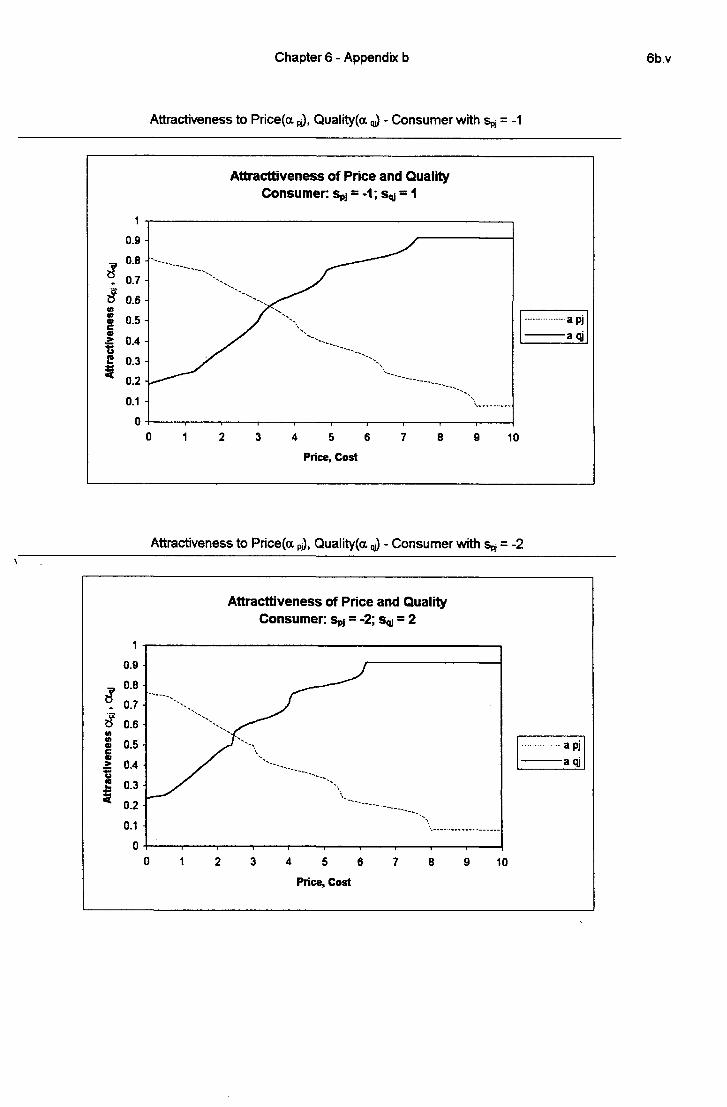
Chapter 6 - Appendix b 6b.v

Attractiveness to Price(o. ,,¡), QuaI¡ty(a .¡¡) - Consumer with s,,¡ = -1

z?

É VGIIES8

Attract

0.9 z

o.s

o.7 -

0.6 -

0.4 - ` ía “Í

0.3

0.2

O ¬" 1 Á 1 I I I I I 1 I

Attracttiveness of Price and Quality Consumer: s,¡ = -1; sq = 1

\¬

O 1 2 3 4 5 6 7 8 9 10

Price, Cost

Attractiveness to Price(a p¡), QuaIity(a ,,¡) - Consumer with sp; = -2

3ã

Attract

veness

Attracttiveness of Price and Quality Consumer: s,,¡ = -2; sql = 2

X"

_ .... ̀_ im v `

`

\

1" 1 1 1 1 *I 1 1 I 1 I

O 1 2 3 4 5 6 7 8 9 10

Price, Cost

Chapter 6 - Appendix b

Attractiveness to Price(a Pi). QuaIity(a qj) - Consumer with spj = -3

=Í'

â

Attractiveness

Attracttiveness of Price and Quality Consumer: s,,¡ = -3; sq, = 3

1

0.9 -

0.8 -

0.7 ~*~...

0.6 -

999 uam

0.2 ~ ~~~~~~~ _.

0.1 -

O 'I 1 1 1 1 Á

1' 1 › 1 J

O 1 2 3 4 '5 6 7 8 9 10

Price, Cost

.._...__..._..._ a

...___a

Attractiveness to Prioe(a PJ), QuaIity(a qi) - Consumer with spj = -4

3'

Ê

Attractiveness

1

0.9

0.8

0.7

0.6

9 ui .° a

.°

w

0.2

0.1

0

Attracttiveness of Price and Quality Consumer: s,,¡ = -4; sq¡ = 4

-`._~_$\

Price, Cost

1 1 Á 1 '1 1 Á 1 1 1 K

O 1 2 3 4 5 6 7 8 9 10

8 ea qi

Chapter 6 - Appendix b

Attractiveness to Price(8 Pi), QuaIity(a qj) - Consumer with spj = -5

=Ê`

É

Attractivenes

Attracttiveness of Price and Quality Consumer: sp, = -5; sq¡ = 5

1

0.9 -

0.8 -

0.7

0.6

.°.°.°

u-um

0.2

0.1 -

0¬ 0 1 2

```` `Ҧ`_..__

_..._.-..._..... 8 11 a qi

1 1'

1 1 Á 1 1 1 1 I

3 4 5 6 7 8 9 10

Price, Cõši

Attractiveness to Price(a pj), QuaIity(a q¡) - Consumer with spj = 5

3â

Attract

veness

Attracttiveness of Price and Quality Consumer: |s,¡| = |s.,¡| =5

1

0.9

0.8 ~

0.7 -

0.6 -

.°.°

Aun

9u

0.2

0.1

0

2 _-a qi 1 1 1 1 1 1 Í 1 1 I

O 1 2 3 4 5 6 7 8 9 10

Price, Cost

Chapter 6 - Appendix b 6b.viii

Attractiveness to Price(a Pi). QuaIity(a qi) - Consumer with spj = 4

Attmctiveness

3â

1

0.9

0.8

0.7

0.6

.°P.°

Gãšñ

0.2

0.1

0

Attracttiveness of Price and Quality Consumer: |s,,¡| = |s.¡¡| =4

.______.__.__í..í_í___.___.-\ \.

"_ _ C `_` "`

.

......._......._.. a ` iam

1 | 1 \ v › 1 1 1 | I

0 1 2 3 4 5 6 7 8 9 10

Price, Cost

Attractiveness to Pr¡ce(a pj), QuaIity(a qj) - Consumer with spj = 3

3â

Attractlveness

1

0.9

0.8

0.7

0.6

.°.°.° uam

0.2

0.1

0

Attracttiveness of Price and Quality Consumer: sp, = 3; sq¡ = - 3

J"

¬1

"'*-\,.__

` __...._._...___. .__ a

.... ._

a

¬ ¡ Á . . . v 1 › 1 I

0 1 2 3 4 5 6 7 8 9 10

Price, Cost

Chapter 6 - Appendix b 6b ix

Attractiveness to Price(a pj), 'QuaIity(a qi) - Consumer with spj = 2

3É

Attractivenes

1

Attracttiveness of Price and Quality Consumer: s,,¡ = 2; sm = - 2

0.9 -'_

0.8 -

0.7 ›

0.6 -

.°.°.° uam

0.2

0.1

O

`~`›`_v`

'1 Á 1 1 Á 4 Á 1 À 1 I

0 1 2 3 4 5 6 7 8 9 10

Price, Cost

Attractiveness to Prioe(a pj), QuaIity(a qj) ~ Consumer with sp] = 1

3Ê

Attractiveness

1

0.9

0.8

0.7

0.6

PPP uam

02 0.1

O

Attracttiveness of Price and Quality Consumer: |s,,¡| = |sq¡| =1

J---«›«z‹1,\ 1.*

' """'-..._\

› «

-_._` -1 Q

'-. .....,,~

1 1 1 I 1

0 1 2 3 4 5 6 7 8 9 10

Price, Cost

. ...». 8

an .íí_.aql '~.

` ‹ `_~.

1

R.l

References and Bibliography

[ABRE88] Abreu, D., Rubinstein, A. `( 1988): “The Stmcture of Nash Equilibrium in Repeated Games with Finite Automata” - Econometrica, 56, 6, p. 1259-1281.

[ALEX92] Alexander, C-. (1992): “The Kalai-Smorodinski Solution in Wage Negotiations”- Joumal Qfthe Operational Research Socieízv, 43, 8, p. 779-786.

[ALLA53] Allais, M. (1953): “Le Comportement de l”Homme Rationell devant le Risque” - Econometrica, 21, p.503-546.

[ALLA79] Allais, M.(1979): “Criticism of the Posmlates and Axioms of the American School” - found in Rafionzzlizgzf in Action, p. 113-139 ed. by Paul K. Moser -

Cambridge University Press,

Research” -z'vIIT Press, Cambridge, MA, USA. :ANDE89] Anderson, S., Devereux, M. (1989): “Profit Shaiing and Optimal Labour

Contracts” - Canadian Journal QfEconornetrics, 22, p. 425-433. :ANDR93] Andreoni, J., Varian, H. (1993): “Pre-Play Contracting in the Prisoner”s

Dilemma” - Research Report, University of Vlfisconsin, USA. :ARRO51] Arrow, K. (1951): “Social Choice and Individual Values”i- Cowles Comíssíon

Ílfƒonograph #12, John Wiley and Sons, Inc. NY, USA. :ATMA94] Atmar, Wirt (1994): “Notes on the Simulation of Evolution” - IEEE

T rcznsactíons on Neural Networks, 5, 1, p. 130-147. :AXEL80a] A:§eh'od,' R. (1980): “Effective Choice in the Prisoner”s Dilemma” - Journal

QfConflz`ct Resolzmon, 24, p. 3-25. i.-'U{EL80b] Axelrod, R. (1980): “More Effective Choice in the Prisoner*s Dilemma” -

Journal of Co¡zƒlictRes0lutí0n, 24, p. 379-403. :AXEL8l] Axelrod, R., Hamilton, W. (1981): “The Evolution of Cooperation” - Science,

211, p. 1390-1396. ÍAXEL84] Axeh'od, R. (1984): “The Evolution of Cooperation”- Basz`c Books, NY, USA. :A\IEL87] Axelrod, R. (1987):”The Evolution of Strategies in the Iterated Prisoner”s

Dilemma” - In L. Davis (Edj), Genetic Algorithms and Simulated Annealíng. London: Pitman.

[AXEL87] Axelrod, R. (1987): “The Evolution of Strategies in the Iterated P1isoner`s Dilemma” - found in Genetic .fillgorithrns and Simulatea' .z-lnnealíng, by L. Davis (ed.), Pittman, London, UK.

[ALXEL88] Axelrod, R., Dion, D. (1988): “The Further Evolution of Cooperation” -

Science, 242, p.l`385-1390. [BACH77] Bacharach, M. (1977): “Economics and the Theoiy of Games” - Wesíview

Press, p. 61, 63, 90-93, 95-96, 102-103, 120, Boulder, CO, USA.

LANDESS] Anderson, J., Rosenfeld, E. (cds) ( 1988): “Neurocomputingr Piinciples of

R2

[BÃCK93] Back, T., Rudolph, G., Schwefel, H.-P. (1993): “Evolutionary Programming and Evolution Strategies: Similarities and Differences” - Proceedings of the Second Annual Conference on Evolutíonarzv Prograf:-mzíng - D. B. Fogel and W . Atmar (eds.) Evolutionary Programming Society, La Jolla, CA, USA, p. 11-22.

:BALD79] Baldwin, B., Meese, G. (1979): “Social Behavior in Pigs Studied by Means of Operant Conditioning” - Animal Behavior, 27, p. 947-957.

:BEAR93] Beardsley, T. (1993): "Never Give a Sucker an Even Break”, Sci. American, Oct. 1993, p. 12.

:BECK95] Becker, Helmut (1995): “The Regulaiization of the Ill posed Notion “Fuzzy Probability” IEEE Transactions on Fuzzy Systems, to appear.

:BEND93] Bendor, J. (1993): “Uncertainty and the Evolution of Cooperation” - Journal of Conflict Resolution, 37, 4, p. 709-734.

ÍBICC93] Bicchieri, C. ( 1993): “Rationality and Coordination” - Cambridge University Press, USA, p.177.

:BL»AC54] Blackwell, D., Girschick (1954): “Theory of Games and Statistical Decisions” -

John Wilev and Sons, Inc., NY, USA. fBOGE92] Bogetoff, P. (1992): “A Note on Conflict Resolution and Tiuthtelling" -

European Journal of Operatíonal Research, 60, p. 109-116. ÍBORE38] Borel, E. (1938): “Applications aux jeux de hasard” - T raite' du Calcul des

Probabilités e de ses applications, Gauthier Villars, Paris,.France. Í_BORG95] Borges, P., Pacheco, R., Khator, S., Barcia, R. (1995): “A Fuzzy Approach to

the Prisoner”s Dilemma” - Submitted for consideration in BioSystems, July, 1995.

:BOUC92] Bouchon-Meunier, B. ( 1992): “Linguistic Hedges and Fuzzy Logic” -

Proceedings of the IEEE Internatƒofial Conference on Fita.-ay Sfvstenis, p. 247- 254, S. Diego, CA, March 1992.

ÍBRAM93] Brams, Steven J. ( 1993): “Theory of Moves” - _.-*lrnerican Scientist, Vol. 81, Nov-Dec 1993, p. 562- 570.

:BRAM94] Brams, Steven J. (1994): “Theory of Moves” - Cambridge Uiiíversizfin Press, Cambridge,

[BUSC93] Busch, M., Reinhardt, E. (1993): “Nice Strategies in a. World of Relative Gains” - Journal QfConfl1`ct Resolution, 37, 3, p. 427-445.

:CAl\›-íP85] Campbell, R., Sowden, L.(eds.)(_ 1985): “Paradoxes of Rationality and Cooperation” - The University of British Columbia Press, Vancouver, Canada.

:CASE79] Case, J. (1979): “Economics and the Competitive Process” - New York Universit}z* Press, p. 39-78, NY, USA

:CAST95] Casti, J. (1995): “Cooperationz The Ghost in the Machinery of Evolution”, found in Cooperation & Conflict in General Evolutz`ona1fy Process - Casti, J.

and Karlqvist, A. (eds.), Wiley & Sons, Inc. NY, p. 63-87. [CAUD93] Caudill, M (1993): “The Possibilties of Probabilities” - AI Expert, 8, 3, p. 28-

31. [CHVVE94] Chwe, l\z¶. (1994): “Farsighted Coalitional Stability” - Journal of Economic

T lieorjv, 63, 2, p. 299-325.

R3

[COLL-91] Coll, J., Hirshleifer, J. (1991): “The Limits of Reciprocity” - Ral1`onalz`zjv and soezfzzy, 3, 1, p. 35-64.

5

[COX95] Cox, E. (1995): “Analyzing Financial Data with Fuzzy Sets” - AI in Finance, 1,

4, p.19-22. [COX95] Cox, Earl (1995): “Relational Database Queries Using Fuzzy Logic” - ._-11 Expert,

10, 1, p. 23-29. [DASG86] Dasgupta, P., Maskin, E. (1986): “The Existence of Equilibrium in

Descontinuous Economic Games, II: Applications”- Review of Economic Studies, 53( 1), 172: p. 1-26.

[DEBO94] Deboeck, G. (1994): “Why use Fuzzy Modelling?” - AI in Finance, 1, 2, p. 17-24.

[DEl\/1P67] Dempster, A. P. (1967): “Upper and Lower Probabilities lnduced by Multivalued Mappings” -.--'lnnals ofjwotløematical Statistics, V. 38, p.325-329.

[DOWR90] Dowtick, S. (1989): “Union-Oligopoly Bargaining”- Economic Journal, 99, p. 1123-1142.

[DOWR90] Dowrick, S. (1990): “The Relative Profitability of Nash Bargaining on the Labour Demand Curve or the Contract Curve”"- Economic Letters, 33, p. 121- 125.

ÍDRESSI] Dresher, M. (1981): “The Mathematics of Games of St.rat.egy” - Dover Publiccztíons, Inc., NY, USA.

ÍDUBO80] Dubois, D., Prade, I-I. (1980): “Fuzzy Sets and Systems: Theory and Applications” -Academic Pr-ess,

:DUBO82] Dubois, D., Prade, H. (1982): “On Several Representations of an Uncertain Body of Evidence” - found in Fzzzzy Information and Deczfslfon Processes, ed. by M. l\/I. Gupta and E. Sanchez, North Holland, p. 167-181.

:EDGE97]Edgewo1th, F. (1897): “La Teoria Pura del Monopolio”- Gíornale degli Econormlsfti, (1925), 40, p. 13-31.

_ELLI94] Ellison, Glenn (1994): “Cooperation in the PD with Anonymous Random 1\/Iatch” - Review ofEconomz`c Studies, 61, 3, p. 567-588.

:FEIG63] F eigenbaum, E., and Feldman, J. (eds.)(1963): “Computers and Thought”, p. 279-293 -.fl‹1'cGraw-Hill, NY, USA.

:FOGE66] Fogel, L., Owens, A., Walsh, M. (1966): “Artificial Intelligence through Simulated Evolution” - John Wiley, NY, USA.

:FOGE93a] Fogel, D. (1993): “Evolving Behaviors in the Iterated Prisoner"s Dilemma” -

Evolutionary Computation, 1, 1, The rlƒassaclzusetts Institute of T eohnologv Press, p. 77-97

[FOGE93b] Fogel, D. (1993): “On the Philosophical Differences between Genetic Algorithms and Evolutionary Algorithms” - Proceedings Qftlze Second Annual Conference on Evolzmfonmjv Progmmmíng - D. B. Fogel and W. Atmar (eds.) Evolutionaty Programming Society, La Jolla, CA, USA, p. 23-29.

[FOGE94a] Fogel, D., Stayton, L. (1994): “Simulated Evolution” - BioSi.›stenzs, 33, 3, p.233.

[F OGE94b] Fogel, D. ( 1994): “An Introduction to Simulated Evolutionary Optimization” -

IEEE Transactions on Neural Networ'ks, 5, 1, p. 3-14.

R.4

[FOGE94c] Fogel, D. (1994): “An Introduction to Evolutionary Computation” - Tutorial presented at the IEEE World Congress on Computational Intelligence, Orlando, Florida, June 1994.

IFOGE95] Fogel, D. (1995): “Evolutionary Computation” - IEEE Press, NY. TREC53] Fréchet, M. (1953): “Émile Borel, Initiator of the Theory of Psychological

Games and its applications” - Dover Publications, Inc., NY, USA. fFUDE90] F udenberg, D., Maskin, E. ( 1990): “Evolution and Cooperation in Noisy

Repeated Games” -ƒlrrierican Economic Review, 80, p. 274-279. _T"UDE90] Fudenberg, D., Tirole, J. (1992): “Game Theory” - 11-II T Press, Cambridge,

Massachusetts, USA. '

ÍGARD74] Gardner, M. (1974): “On the Paradoxical Situations that arise from Nontransitive Relations” - Scient¿`fic.«-lmerican, Oct. 74, p. 120-125.

:GLAN94] Glance, N., Huberman, B. (1994): “The Dynamics of Social Dilemmas” -

Scient.1ficAnzericai1, 270, 3, p. 76-81. :GODF92] Godfray, H. (1992): “The Evolution of Forgiveness” - Nature, 355, p. 206-

207. :GOUL85] Gould, J. and Gould, C. ( 1985): “An Animalls Education: How comes the

mind to be fumished?“ - The Sciences, 24, 4, p. 24-31. :GREE75] Greenhut, M., Ohta, H. (1975): “Theory of Spatial Pricing and Market Areas”

- Duke Universií_v Press, NC, USA.u

ÍGRIF87] Griffiths, M. and Palissier, C. (1987): “Algorithmíc Methods for Artificial Intelligence”, p. 67-68 - Chapman and Hall, NY, USA.

iGRIl\/194] Grim, P. (1994): “Computation and Undecidability in the Spatialized Prisoner*s Dilemma” - Research Report #94-02, Group for' Logic and Formal Semantics, State University of New York, USA.

[GUYE68] Guyer, M., Hamburger, M. (1968): “A Note on “A Taxonomy of 2;«.;2

Games” - General S}>s'tems, 13, p. 205-208. [HALL94] Hall, L. and Kandel, A. (1994): “The Evolution of Expert Systems” - found in

Sojif Computing - Fuzzy Logic, Neural Networks and Distribz.a“ed Intelligence, ed. by Aminzadeh, F. and Jamshidi, M., p. 1-28 - Prentice Hall, l\lY, USA.

[HARD82] Hardin, Russell (1982): “Collective Action” - John Hopkins Um'versity Press, Baltimore, USA.

[HARR95] Harrald, P., F ogel, D. (1995): “Evolving Continuous Behaviors in the Iterated Prisoner”s Dilemma” - BioS_vsz'ems, Special Issue on the Prisoner”s Dilemma, to be published.

[HARS56] Harsanyi, J. (1956): “Approaches to the Bargaining Problem before and after the Theory of Games: A Critical Discussion of Zeuthen°s, Hiclds and Nash”s Theories” - Econonzerrica, 24, p. 144-157.

[HARS77] Harsanyi, J. (1977): “Rational Behavior and Bargaining Equilibrium in Games and Social Situations” - Caiiibriclge K./'ni\z>er's'i13> Press,

[HOEL90] Hoel, M. (1990): “Local versus Central Wage Bargaining with Endogenous Investments” - Scandinavian Journal QfEconomz`cs, 92, p. 453-469.

[HOF S85] Hofstadter, D. (1985): “Metamagical Themas: Questing for the Essence of Mind and Pattern” - Basic Books, NY, USA.

R5

[HOFS85] Hofstadter, D. (1985): “Methamagical Themas” - Basic Books, NY, USA. [HOF S95] Hofstadter, D.,and Fluid Analogies Research Group (1995_): “Fluid Concepts

and Creative Analogies: Computer Models of Fundamental Mechanisms of Thought”, p. 35-36 - Basic Books, NY, USA.

[HOLL75] Holland, J. (1975): “Adaptation in Natural and Artificial Systems”- MIT Press (Ed. 1993), USA.

[HUBE93] Huberman, B., Glance, N. (1993): “Evolutionary Games and Computer Simulations” - Proceedings of the National Academy qfS'c1`ences, USA, Vol. 90, p. 7716-7718.

,

[INFE9l] lnfelise, N. (1991): “A Clear Vision of Fuzzy Logic” - Control Engineering, July, p. 28-30.

[JACK74] Jackson, P. (1974): “Introduction to Artificial Intelligence” - Petrocelli Books, NY, USA.

[JOSE92] Josephs, R., Lanick, R., Steele, C., Nisbett, R. ( 1992): “Protecting the Self from Negative Consequences of Risl<y Decisions” - Journal Q/`Per.sonali13» and Social Psychology, 62, 1, 1). 26-37.

:KAHN79] Kahneman, D., Tversky, A. (1979): “Prospect Theory: An Analysis of Decisions under Risk” - Econometrica, 47, 2, p. 263-291.

:KAHN79] Kahnemann, D., Tversky, A. (1979): “Prospect Theory: An Analysis of Decision under Risk” - Econometríca, 47, 2, p. 263-291.

:KALA75] Kalai, E., Smorodinslày, M. (1975): “Other Solutions to Nash*s Bargaining Problem” - Econometríca, 45, p. 513-518.

ÍKAL-A77] Kalai, E. (1977): “Proportional Solutions to Bargaining Situations:

_

Inteipersonal Utility Compaiisons” - Econometríca, 45, p. 1623-1630. ÍKAND96] Kandel, A., Zhang, Y. and Borges, P. (1996): “Fuzzy Moves in the Prisoner*s

Dilemma” - IEEE' T ransactíons onilzƒan, Systerrzs and Qvbe1'netics, to appear. ÍKLEM87] Klemperer, P. (1987): “The Competitiveness of Markets with Switching

Costs” - Rand Journal oƒ`Economz'cs, 18, 1, p. 138-150. ÍKOLL93] Kollock, P. (1993): “An Eye for an Eye leaves Everyone Blind” - Amerzfcan

Socíologícal Review, 58, 6, 1). 768-787. :KOSK92] Kosko, B. (1992): “Neural Networks and Fuzzy Systems” - Prentice Hall, NJ,

USA, p. 120, 149-150, 182, 315-316. KOSK93] Kosko, B. and Isaka, S. (1993): “Fuzzy Logic” - Scierznƒic _-"lmer~ican, July

1993, p.'76-81. ÍKREP82] Kreps, D., Wilson, R. (1982): “Reputation and Imperfeet Information” -

Journal of Economic T heor_1,=, 27, 2, p. 253-279. :KWAK78] Kwakemaak, H. (1978): “Fuzzy Random Vaiiables I - Definitions and

Theorems” - Information Science, 15, p.1-29. ÍLESL90] Leslie, D. (1990): “A Disequilibrium Model under Bilateral Monopoly” -

Bulletin of Economic Research, 42, 3, p.l55-174. ;LEVl72] Levitan, R., Shubik, M. (1972): “Price Duopoly and Capacity Constraints” -

International Economic Review, 13, 1, p. 111-122. ÍLEVY92] LEVY, S. ( 1992): “Artificial Life - The Quest for a New C»rea.tion” - Pantheon

Books, NY, USA, p. 181-184.

R6

:LEWO61] Lewontin, R. (_1961): “Evolution and the Theoiy of Games” - J. T lzeor. Biology, 69, 543-560.

[LIND82] Lindley, D. V. (1982): “Scoring Rules and the Inevitability of Probability” -

International Statística1Revíew, 50, p. 1-26. ÍLINS94] Linster, B. (1994): “Stochastic Evolutionary Dynamics in the Repeated PD” -

Economic Inquzry, 32, 2, p. 342-357. fL1N`V91] Linville, P., Fischer, G. (1991): “Preferences for Separating or Combining

Events” - Journal QfPersonalí1y and Social P.sz1.›chologv, 60, 1, p. 5-23. _`LLOY95] Lloyd, A. (1995): “Computing Bouts of the Prisoner`s Dilemma” - Scterztzfic

American, 272, 6, p. 110-115. :LOOT89] Lootsma, F. (1989): “Conflict Resolution via Paiiwise Comparison of

C0ncessionS”- European Journal of Operanfonal Research, 40, p. 109-116. IUCES7] Luce, R., Raiffa, H. (1957): “Games and Decisions” - 7m ed., John Wiley and

S'ons,_ Inc., NY, USA. :MAR93] Mar, G., St. Denis, P. (1993): “The Spatial Dimensions of Evolution” -

International Journal of B{furcatz'on and Chaos, 3, p. 35-78. :MAY87] Mar, R. (1987): “More Evolution of Cooperation” - Nature, 327, p. 15-17. ÍMCMI92] Mcl\/Iillan, J. (1992): “Games Strategies and Managers” - Oâtforcl C,f'ni\.›er's'i1§›.=

Press, p. '73-74, 78-79, 168-169, NY, USA,. ÍMILI93] Milinski, M. (1993): “Cooperation wins ans stays” - Nature, 364, 1, p.12-13. ÍMOLA92] Molander, Per (1992): “The Prevalence of Free Riding” - Journal of Conflict

Resolution, 36, 4, p. 756-771. ÍMUNA94] l\/lunakata, T., Jani, Y. (1994): “Fuzzy Systems: “Fuzzy Systems: An

Overview” - Conzmzmícations oflfhe./lC1l.‹;Í, 37, 3, p. 69-75. ÍMURN92] Mumighan, J. (1992): “Bargaining Games” - Will1ÍamM'orrow and Co, Inc.,

NY, USA. :l\×íYER7“7] Myerson, R. (1977): “Two Person Bargaining Problem and Comparable

Utility” - Econometríca, 45, 11.1631-1639. :NACH92] Nachbar, J. (1992): “Evolution in the Finitely Repeated Prisoner”s Dilemma” -

Journal of Economic Behavior and Organization, 19, p. 307-326. ÍNASH50] Nash, J. (1950): “The Bargaining Problem” - Economeírica, 18, p. 155-162. :NEUl\/128] Neumann, J. Von (1928): “Zur Theoiie der Gesellschaftsspiele” -

M'atlzemat1ÍschenAnnalen, 100, p. 295-330. :NEUM37] Neumann, J. Von (1937): “Úber ein ökonomischen Gleichungssystem und

eine Verallgemeinerung des Brouwerschen Fixpunktsatzes" - Ergebenísse eines .Matlzerzzatik Kolloquíurns, 8, p. 73-83.

[NEUM44] Neumann, J. Von, Morgenstern, O. (1944): “Theory of Games and Economic Behavior” - Princeton University Press, Princeton, USA.

[NlCO95] Nieolis, J. Katsikas, A. (1995): “Chaotic Dynamics of Linguistic-like Processes at the Synthatic and Semantic Levels: ln Pursuit. of a. Multifractal Attractor” -

found in Cooperatzfon & Conflict in General Evolutiofuzrjszf Process - Casti, J.

and Karlqvist, A. (_eds.`), Wiley & Sons, Inc. NY, p. 227-342. `

[NOMU94] Nomura, H., Hayashi, I., Wakami, N. (1994): “A Self-tuning Method of Fuzzy Reasoning by Genetic Algoiithm” - found in Fuzzy Control Svstenzs, p. 339-353,. ed. by A. Kandel and G. Langholz, CRC Press, USA.

RI'

[NOW A92a] “Tit for tat in Heterogeneous Populations” - Nature, 355, p. 250-253. [NOWA92b] Nowak, M., May, R. (1992): “Evolutionaiy Games and Spatial Chaos” -

Nature, 359, p. 826-829. [NOWA93a.] Nowak, M., Sigmund, K (1993): “A Strategy of Win-Stay, Lose-Shift that

outperfonns Tit-for-Tat in the Piisonefs Dilemma Game” - Namre, 364, p. 56-58. -

[NOW A93b] Nowak, M., Sigmund, K (1993): “Chaos and the Evolution of C.oopei'ation”- Proceedings of the l7\Ízztio11alAcade1ny QfScz`ences ofthe United States, 90, p. 5091-5094.

[NOWA94] Nowak, M., Bonhoffefer, S. (1994): “Spatial Games and the Maintenance of Cooperation” - Proceedings ofthe National Academv ofSc1`ences ofthe United States, 91, p. 4877-4881.

[NOW A95] Nowak, M., May, R., Sigmund, K. (1995): “The Arithmetics of Mutual Help” - Scíenttfic.-›<lnzerícan, 272, 6, p. 76-81.

[NYDE74] Nydegger, R., Owen, G. (1974): “Two Person Bargaining: An Experimental Test of Nash`s Axioms” - Internzflvtiotial Journal of Game Theozjv, 3, p. 239- 249.

:PEAR88] Pearl, J. (1988): “Probabilistic Reasoning in Intelligent Systems” - Alargam- Kazzfmamz Publishers, Palo Alto, CA, USA.

:POUN92] Poundstone, W. (1992): “Piisonerís Dilemma - John von Neumann, Game Theory and the Puzzle of the Bomb”- Doubledagv, p. 8, 117.

:RAPO65] Rapoport, A., Chammah, A. (1965): “Prisoner*s Dilemma: A Study in Conflict and Cooperation” - Univer'sity ofjwichígan Press, Ann Arhor, MI, USA.

:RAPO66] Rapoport, A., Guyer, M. (1966): “A Taxonomy of 2:-›‹;2 Games“ - General Sfvsterns, 11, p. 203-214.

A

:RAPO7-1] Rapopoit, A. (1974): “Prisoner'”s Dilemma: Recollections and Observations”, found in Game Theory as a T heory of Conflict Resolution - Rapoport, A. (ed. ), D. Reidel Publishing Company, Boston, USA, p. 20-21.

[RAPO90] Rapoport, A (1990): “The problem With Gains-Maximizing Strategies” - found in Psychological Dimensions of War, p.91-115, ed. by Betty Glad - Sage Publications, Newbury Park, CA, USA.

IRAPO92] ] Rapopon, A (1992): “Game Theoiy Defmed “ - found in Ratíomzlity and Society, 4, 1, p. 74-82.

ÍRASM89] Rasmusen, E. ( 1989): “Games and Infonnation” - Baszfl and Blaclnvell Ltd., p. 94-96, Oxford, UK.

:RECH73] Rechenberg, I. (1973): “Optimierung Technischer Systeme nach Piinzipen der Biologischen Evolution” - Frommann-Holzboog Verlag, Stuttgart, Germany.

1RIOL92] Riolo, R. (1992): “Suivival of the Fittest Bits” - Scientific American, 267, 1, p. 114-1 16.

ÍROSE62] Rosenblatt, F. (1962): “Principles of Neurodynamics” - Spartan Books, NY, USA.

ÍROTH79] Roth, A., Malouf, M. (1979): “Game Theoretic Models and the Role of Information in Bargaining”- Póycliological Review, 86, p. 574-594.

:RUBI82] Rubinstein, A. (1982): “A Perfect. Equilibrium in a Bargaining Model” -

Economelfrzfca, 50, p. 97-109.

R8

ÍRUBI86] Rubinstein, A. (1986): “Finite Automata Play the Repeated Prisoner`s Dilemma”- Journal of Economic T heorzv, 39, p. 83-96.

:SAl\/lP76] Sampson, J. (1976): “Adaptive Information Processing: An Introductoiy Survey” - Springer Verlag, NY, USA.

:SAND95] Sandholm, T, Crites, R. (1995): “Multiagent Reinforcing Learning in the IPD” - BioSystems, Special Issue on the Prisoner"s Dilemma, to be published.

ÍSAVA72] Savage, L. (1972): “The Foundation of Statistics” - p. 91-104, Dover Publications, Inc., NY, USA.

:SCHW65] Schwefel, H.-P. (1965): “Kybemetische Evolution als Strategic der Experimentelle forschung in der Stirmnungstechnik” - Diploma T hesis, Technical University of Berlin.

:SELT78] Selten, R. (1978): “The Chainstore Paradox” - T heoizv and Decision, 9, p. 127- 159.

:SELT80] Selten, R. (1980): “A Note on Evolutionaiy Stable Strategies in Asymmetric Animal C-onflicts” -J. Tlieor. Biology, 84, p. 83-96.

:SFOR53: Sforza, C. (1953): “l\/Iaquiavel”, Bibl. Pensamento Vivo, Livraria 1\~;Íartins Editora, SP, Brasil.

:SHAF76: Shafer, G. ( 1976): “A Mathematical Theory of Evidence” - Princeton University Press, NJ, USA.

:SIGM93: Sigmund, K. (1993): “Games of Life: Explorations in Ecology, Evolution and Behaviour” - Oxford University Press, NY, USA.

:Sl\/IIT82: Smith, J. Maynard (1982): “Evolution and the Theory of Games” - Carnbrige University Press,

:SMIT87: Smithson, Michael (1987): “Fuzzy Set Analysis for Behavioral and Social Sciences” - Springer Verlag, NY, USA.

ÍSTACSZ] Stackelberg, H. (1952): “The Theory of the Market Economy” - transl. english by A. Peacock, William H odge, London,

ÍSTAL77] Stallings, W. (1977): “Fuzzy Set Theory versus Bayesian Statistics”- IEEE Transactions on St›s'ier:zs_, .Man and Cyberrieiics, 7, p. 216-219

:STEI93] Stein, R. (1993): “The Dempster-Shafer Theory of Evidential Reasoning” - AI Esgrert, 8, 8, p.26-31.

ÍSTEW93] Stewart, Ian (1993): “A partly tme story”- Scientific.4rizer'icaiz, Feb 93, p. 86. :STRAT90] Strat, T.M. (1990): “Decision Analysis using Belief Functions” -

International Journal ofApproximate Reasoning, 4, p.39l, Elsevier Science Publishing Co., Inc, NY, USA.

[SUGE77] Sugeno, M. (1977): “Fuzzy Measures and Fuzzy Integrals: A Suivey”- in M. M. Gupta, G. N. Saridis and B. R. Gaines (eds.) - Fuzzy Automata and Decision Processes - Amsterdam, North Holland.

[TAHA90] Tahani, K., Keller, J. (1990): “Information Fusion in Computer Vision using the Fuzzy Integral” - IEEE Transactions on Stisteiiis, Alan and CÍfi.›Z›eriietics', 20, p.733-741.

[TUKE49] Tukey, J. (1949): “A Problem in Strategy” - Econometrica, 17, p.73. [TVER69] Tverslày, A. (1969): “Intransitivity of Preferences” - Psvclzologiczzl Review, 76,

p. 31-48.

R9

:TVER74] Tversl<y, A., Kahnemarm, D. (1974): “Juggement under Uncertainty: Heuristics and Biases” - Science, 185, p. 1124-1131.

IVIOT93] Viot, G.(_1993`): “Fuz.zy Logic: Concepts to Constructs” - _.-'11 Expert, 8, 13, p.26-33.

Ã/“'1OT93b] Viot, G. (1993): “Fuzzy Logic in C” - Dr. Dobbs Journal, 18, 2, p. 40-49. :WANG92] Wang, Z. and Klir, G. J. (1992): “Fuzzy Measure Theory”, p. 107-134, 175-

193.- Plenzm-1 Press - USA. :WARN95] Wärneiyd, Karl ( 1995): “Language, Eyolution, and the Theory of Games” -

found in Cooperanfon and C' onflict in General Evolutionaizv Process - Casti, J.

and Karlqvist, A. (eds.), Wiley & Sons, Inc. NY, p. 405-421. ÍWATS94] Watson, J. (1994): “Cooperation in the Infinitely Repeated Pn`soner's Dilemma

with Perturbations” - Games and Economic Behavior, 7, p. 260-285. :WEEK96] Weeks, M., Ragade, R. (1996): “Different Payoff Values and Wandering

Players in the Prisoner`s Dilemma” - Submitted for publication in Biobft-isierris; refereed in 07./'95 by the author of this Dissertation.

:W1NS95] Winston, W. (1995): “Introduction to Mathematical Programming -

Applications and Algorithms” - Dztxbzzry Press, Belmont, CA, USA. :W'U95] Wu, Jianzhong, Axelrod, R. (1995): “How to cope with Noise in the Iterated

Prisoner”s dilemma” - Journal qfConflict Resolution, 39, 1, p. 183-189. :YAGE93a] Yager, R. (1993): “A general Approach to Criteria Aggregation using Fuzzy

Measures” - International Journal ofliúfan-.Machine Stuclies, 38, p.187-213. :YAGE93b] Yager, R., Filev, D. (1993): “SLIDE: A Simple adaptive Defuzzification

Method” - IEEE Transactions on Fuzzzv Sflvsiems, 1, 1, p. 69-78. :YAGE94] Yager, R. R. and Filev, Dimitar (1994): “Essentials of Fuzzy Modeling and

C0ntr0l”- John Wiley and Sons, Inc, NY, USA. ÍYAGE95] Yager, R. R. (1995): “lvlulticiiteria Decision Making Using Fuzzy Q_uantii`1e1's”-

Proceedings of the IEEE/[AFE Conference on Conzputational Intelligence for Financial Engineering, NY, April 1995.

[YEN90] Yen, J. (1990): “Generalizing the Dempster-Shafer Theory to Fuzzy Sets”, IEEE Transactions on M'an, Systeins and Cfvbernetics, 20, p. 559.

[ZADE65] Zadeh, Lotfi (1965): “Fuzzy Sets”- Information and Control, 8, p. 338-353. [ZADE7 2] Zadeh, L. A. (1972): “A Fuzzy-set Theoretic lnterpretation of Linguistic

Hedges”, Journal ofC'yZ›ernetics 2, p.4-34. [ZADEH72] Zadeh, Lotfi (1972): “A Fuzzy Set Theoretical 1nterp1'et.a.tion of Hedges”-

Journal offivbernetics, 2, p.4-34. [ZEUT30] Zeuthen, F. (1930): “Problems of Monopoly and Economic Welfare” -

Routhledge, London,