
Assessing monetary policy in the euro area: a factor-augmented VAR approach
Upload
khangminh22Category
view
3download
0
Volume 10 N° 3 (2011)
Highlights in this issue:
– Focus: Debt dynamics and sustainability in the euro area
– Internal devaluation and external imbalances: a model-based analysis
– Sectoral implications of external rebalancing
– Sectoral resilience to shocks
– House price imbalances and structural features of housing markets
ISSN 1830-6403

Legal notice Neither the European Commission nor any person acting on its behalf may be held responsible for the use which may be made of the information contained in this publication, or for any errors which, despite careful preparation and checking, may appear. This paper exists in English only and can be downloaded from the website (ec.europa.eu/economy_finance/publications) A great deal of additional information is available on the Internet. It can be accessed through the Europa server (http://europa.eu) KC-AK-11-003-EN-N ISSN 1830-6403 © European Union, 2011

Table of contents
Editorial 5
I. Debt dynamics and sustainability in the euro area 7
I.1. Recent debt developments in the euro area 7
I.2. Debt developments and sustainability 9
I.3. Assessing the risk of fiscal crises 15
I.4. Conclusions 18
II. Special topics on the euro-area economy 21
II.1. Internal devaluation and external imbalances: a model-based analysis 22
II.2. Sectoral implications of external rebalancing 28
II.3. Sectoral resilience to shocks 35
II.4. House price imbalances and structural features of housing markets 41
III. Recent DG ECFIN publications 47
Boxes
I.1. The intertemporal budget constraint 11
2.1. Adjustment via migration 32
3.1. An econometric framework to estimate industrial sectors' resilience to common shocks 36
4.1. Housing markets and the real economy 42


EDITORIAL
- 5 -
Over the summer months, the crisis has reached new levels of seriousness and urgency as dangerous feedback loops between sovereign risks, banking sector health and the wider economy have re-emerged. The weakening of business and consumer confidence in recent months across the euro area should be seen as a cautionary development. Not only does it suggest a weakening of the current business cycle position, but it also places the sovereign debt crisis in a more challenging environment marked by greater risk aversion and uncertainty. Projections from the Commission's latest interim forecasts, published on September 15, show slower growth in the second half of this year than expected at the time of the spring forecasts. Downside risks to growth prospects have increased, primarily due to concerns about the unresolved euro-area crisis and its repercussions on financial markets' health as well as the global economic slowdown.
These developments underscore the need for determined policy action. The implementation of the comprehensive crisis resolution agreements reached at the Euro Area Summit on 21 July 2011 is key in this respect. The EFSF will play a central role here, and its resources will need to be optimised and greater flexibility ensured. Once the new EFSF is ratified, efficient use of its financial envelope must be made, and the Commission is working on options to this end.
Europe can act in a resolute and timely manner to adopt bold measures. The agreement reached between the European Parliament and the Council on 4 October on the six legislative proposals on strengthening economic governance in the EU, also known as the 'six-pack', bears witness to this. Nevertheless, the scale and nature of the crisis demands that we go further in our response. The Commission will therefore build on the six-pack and soon present a proposal for a single, coherent framework to deepen economic governance, particularly in the euro area. Continued cooperation between Member States and European institutions is of utmost importance so as to bolster confidence in the euro-area's ability to weather the crisis.
With sovereign debt being one of the main issues at the heart of the crisis, the current edition has made public debt dynamics its main theme. In a focus section an overview of the debt situation is given in both short and medium-term
perspectives. Not only do the higher debt levels following the crisis require higher primary surpluses to cover the additional interest payments, but debt can also act as a brake on growth. Given the additional difficulties presented by an ageing population, the outlook for the medium term is challenging. The focus shows that setting public finances on a sustainable path will require significant consolidation measures – over and above those already introduced – in a number of euro-area Member States. Nevertheless, the responses required are not unprecedented, and responding in a timely manner can both reduce the total effort required and ensure that the euro-area economies benefit as soon as possible from the positive impact of debt reduction on growth. The section also presents instruments to assess the risk of fiscal crises that should help policymakers to act timely in the face of future adverse shocks.
While fiscal imbalances are clearly at the forefront of the current policy debate, they are by no means the only instance of relevant economic imbalances. Macroeconomic adjustment will also be necessary in areas that evade direct policy control and where rebalancing will be market-based, for instance in the case of large external deficits. But, as a number of contributions in this edition show, structural policies can play an important enabling role also in market-based adjustment processes. Hence, a number of measures can used to make the rebalancing of a large external deficits more growth friendly. Theses include policies that emulate the effects of a nominal exchange rate depreciation such as a shift in the burden of taxation away from labour. Measures facilitating the required adaptation on the supply side – e.g. in terms of resource reallocation to the export sector – also have a role to play. Structural policies can also help reducing the occurrence of costly imbalances. Appropriate housing taxation and regulation can contribute to curb excessive house price volatility while moving to lower levels of product market regulation (PMR) can improve the economy's resilience to shocks.
Looking into more details into these findings, our first special topic on internal devaluation shows how specific policy measures can support external rebalancing through relative competitiveness changes. Various kinds of

Quarterly Report on the Euro Area III/2011
- 6 -
'internal devaluation' can mimic the effects of nominal devaluations by reducing domestic prices and encouraging expenditure-switching. The section looks at two potential measures of internal devaluation and assesses their effectiveness using the Commission's macro-economic model QUEST. The simulations show that tax reforms aiming at a shift of the burden of taxation from labour to consumption can raise employment, boost GDP and improve the net foreign asset position. Alternatively, and bearing in mind that public-sector wages grew faster than in the private sector in many Member States in pre-crisis years, public sector wage discipline can spill over to private sector wages. This should reduce production costs and improve competiveness in addition to the policy's direct budgetary impact. However, similarly to nominal exchange rate adjustments, internal devaluations are unlikely to have permanent trade balance effects if real labour costs are not permanently affected or if increasing domestic demand leads to a rise in imports.
Secondly, a special topic is dedicated to the mechanics of external rebalancing from a supply-side perspective. As the pre-crisis decade witnessed a growing sectoral skew towards non-tradable production (primarily housing and services) in a number of Member States running high external deficits, the associated changes in prices and shifts in resources will have to be eventually unwound. If prices adjust insufficiently or if resources are not reallocated properly, the rebalancing of the current account will be associated with a persistent rise in unemployment. The section concludes that the more integrated the tradable and non-tradable sectors are and the more easily resources move across sectors, the smaller the required price adjustment for the current account to close without leaving excess supply.
A further special topic investigates the euro-area Member States' resilience to shocks by analysing differences in the adjustment capacity of industrial sectors to common output shocks. Some structural characteristics of the economy are found to play an important role. In particular, high levels of product market regulation (PMR) have a negative impact on resilience. These results suggest that reducing PMR would help improve Member States' overall cyclical resilience and thereby improve the cross-country synchronisation of the business cycle.
A final section is dedicated to the analysis of key structural features of housing markets, which in themselves have potentially important impact on economic and financial stability. The analysis suggests that policies aimed at encouraging housing ownership, especially for the low income population, may also have a negative impact on house price stability. In addition, variable mortgage interest rates, high loan-to-value ratios as well as tax incentives for house purchase appear to increase the risk of housing market imbalances. Both for social policy and macroeconomic stability, close monitoring of housing markets is therefore warranted.
The crisis is forcing considerable macroeconomic adjustment on many economies in the world. Swift and direct action is required in the area of public debt reduction, as well as in promoting external rebalancing so as to avoid large external debt build-ups. In the longer term, economies will need to be made more economically resilient, including through changes in product, capital and labour markets. Neither the challenges nor the tools of economic policy are genuinely new, but their importance has rarely been greater.
MARCO BUTI
DIRECTOR-GENERAL
Focus I. Debt dynamics and sustainability in the euro area
- 7 -
The economic and financial crisis has led to a marked increase in government debt in the euro area countries. While the magnitude of the increase is in line with that resulting from other financial crises, its cumulative effect is greater and brings the question of the medium-term sustainability of public finances to the fore. Not only does higher debt require higher primary surpluses to cover the additional interest payments but it can act as a brake on growth. Given the additional difficulties presented by an ageing population, the outlook for the medium term is challenging. This focus section presents an overview of the debt situation both currently and through medium-term projections. It shows that setting public finances on a sustainable path will require significant consolidation measures — over and above those already introduced — in a number of euro area Member States. In some of them, the primary balance required to bring debt back to a sustainable level is particularly high by historical standards. Nevertheless, the responses required are not unprecedented, and responding in a timely manner can both reduce the total effort required and ensure that the European economies benefit as soon as possible from the positive impact that debt reduction has on growth. The section also presents instruments for assessing the risk of fiscal crises that should help policymakers to take early action in the event of additional shocks emerging with adverse effects on sustainability.
I.1. Recent debt developments in the euro area
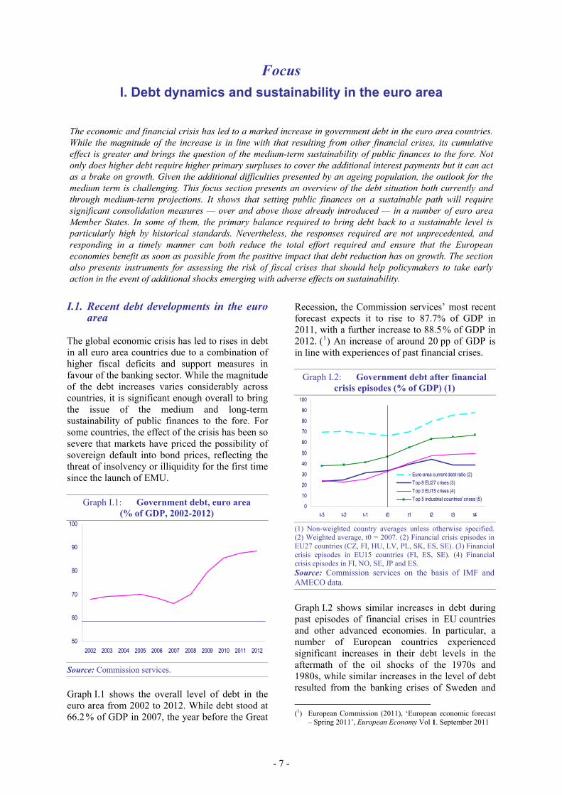
The global economic crisis has led to rises in debt in all euro area countries due to a combination of higher fiscal deficits and support measures in favour of the banking sector. While the magnitude of the debt increases varies considerably across countries, it is significant enough overall to bring the issue of the medium and long-term sustainability of public finances to the fore. For some countries, the effect of the crisis has been so severe that markets have priced the possibility of sovereign default into bond prices, reflecting the threat of insolvency or illiquidity for the first time since the launch of EMU.
Graph I.1: Government debt, euro area (% of GDP, 2002-2012)
50
60
70
80
90
100
2002 2003 2004 2005 2006 2007 2008 2009 2010 2011 2012
Source: Commission services.
Graph I.1 shows the overall level of debt in the euro area from 2002 to 2012. While debt stood at 66.2 % of GDP in 2007, the year before the Great
Recession, the Commission services’ most recent forecast expects it to rise to 87.7% of GDP in 2011, with a further increase to 88.5 % of GDP in 2012. (1) An increase of around 20 pp of GDP is in line with experiences of past financial crises.
Graph I.2: Government debt after financial crisis episodes (% of GDP) (1)
0
10
20
30
40
50
60
70
80
90
100
t-3 t-2 t-1 t0 t1 t2 t3 t4
Euro-area current debt ratio (2)Top 8 EU27 crises (3)Top 3 EU15 crises (4)Top 5 industrial countries' crises (5)
(1) Non-weighted country averages unless otherwise specified. (2) Weighted average, t0 = 2007. (2) Financial crisis episodes in EU27 countries (CZ, FI, HU, LV, PL, SK, ES, SE). (3) Financial crisis episodes in EU15 countries (FI, ES, SE). (4) Financial crisis episodes in FI, NO, SE, JP and ES. Source: Commission services on the basis of IMF and AMECO data.
Graph I.2 shows similar increases in debt during past episodes of financial crises in EU countries and other advanced economies. In particular, a number of European countries experienced significant increases in their debt levels in the aftermath of the oil shocks of the 1970s and 1980s, while similar increases in the level of debt resulted from the banking crises of Sweden and (1) European Commission (2011), ‘European economic forecast
– Spring 2011’, European Economy Vol 1. September 2011

Quarterly Report on the Euro Area III/2011
Finland in the 1990s. While today’s situation is broadly in line with the experience of past crises, the one significant difference is that the current starting level of debt is higher.
Within the overall total, moreover, there is large variation across countries. Graph I.3 shows the debt level in all euro area countries in both 2007 and 2012, the latter as predicted by the Commission services in the spring 2011 forecasts. It shows that while some countries such as Estonia, Cyprus and Malta are likely to see very modest rises in their debt, Spain and Portugal are expected to experience increases of above 30 pp of GDP and Greece and Ireland of over 60 and 90 pp respectively.
The euro area is not alone in experiencing large increases in debt as a result of the current crisis. Indeed, the debt increases seen so far and forecast for the next year in both the USA and Japan are larger. From a starting level of 62.3 % of GDP in 2007, debt in the USA is forecast, by the Commission, to reach 102.4 % of GDP by 2012, with the respective figures for Japan being 167.0 % in 2007 to 215.9 % by 2012. The rise in debt in these leading economies measured in percentage points of GDP is higher than for any euro area country except Greece and shows that this is a problem not restricted to the euro area.
Graph I.3: Debt in 2007 and 2012, euro area Member States (% of GDP)
0
20
40
60
80
100
120
140
160
180
EE LU SI SK FI NL CY MT ES AT DE FR EA* BE PT IE IT EL
20122007
Source: Commission services.
The increases in debt are a serious concern for policymakers. High debt brings into question the sustainability of an economy, where sustainability relates to the ability of a government to service its debt over the long term. Not only is high debt more costly to service as it requires higher interest payments to be made, but its secondary effects also create difficulties. Once it passes a certain threshold, there is evidence that debt has a negative effect on economic growth, while the
perceived risk associated with high debt levels can lead to increases in the interest rate payable on new debt. (2) Thus interest payments rise not just because of the volume of the debt, but also because the cost of borrowing has risen. Moreover, the higher taxes required to service the debt will act as a brake on growth. It is clear that there is considerable variation within the euro area as to the extent that these issues affect different countries. Not only are the levels of debt quite different, but the other factors affecting sustainability are also far from identical. Growth rates vary and will continue to vary across countries, with some of them being in a better position to meet their obligations due to expected increases in their productivity. Different ageing profiles also mean that some countries are facing significant slowdowns in potential growth as their economies age, as well as significant increases in age-related public spending.
This focus section will look at why debt has increased to the current levels by considering the debt dynamics at play. It will then consider what this means in terms of the longer-term debt sustainability of the euro area countries by looking at projections for debt and will discuss how these fit into an overall assessment of risk facing these countries, before looking at alternative measures of risk associated with debt.
Why debt has increased
The economic and financial crisis has led to increases in debt due to higher deficits and to the support measures introduced by many Member States in favour of the banking sector. Relative to 2007, deficits have risen in all euro area countries for reasons both within and outside governments’ control. (3) The structure of the tax and spending
(2) Reinhard and Rogoff (2010) find that debt over 90 % of GDP is associated with lower GDP growth, (Reinhard, C.M. and K.S. Rogoff (2010), ‘Growth in a time of debt’, American Economic Review, Vol. 100, No 2, May). Cecchetti et al. (2010) find that high levels of government debt negatively affects future growth and that there is a threshold effect for debt at a level of 80 %-100 % of GDP, over which additional debt has an additional significant adverse effect on future growth (Cecchetti S.G, M.S. Mohanty and F. Zampolli (2011), ‘The real effects of debt’, paper prepared for the ‘Achieving maximum long-run growth’ symposium sponsored by the Federal Reserve Bank of Kansas City, Jackson Hole, Wyoming, 25-27 August). For a more in-depth discussion of the effect of debt on growth, see Part III of European Commission (2010), ‘Public finances in EMU 2010,’ European Economy 4|2010 (available online at http://ec.europa.eu/economy_finance/publications/european_economy/2010/pdf/ee-2010-4_en.pdf ).
(3) Over the longer term, many of the aspects of the tax and spending system that are outside governments’ control over the shorter term can be changed. This statement therefore
- 8 -

I. Debt dynamics and sustainability in the euro area
system means that as economic activity slows, lower tax receipts coupled with higher spending (primarily due to increased support for the unemployed and to the maintenance of spending plans set in advance under the expectation of stronger growth) cause deficits to grow automatically. Typically, a slowdown in economic activity will tend to be part of an economic cycle, and the upswing part of the cycle will lead to a return of revenues and a reduction in deficits, as the automatic stabilisers act in the opposite direction. However, some of the non-discretionary increase in deficits seen in the current crisis is due to factors that are not part of the classic economic cycle and that are not necessarily expected to have a counteracting upswing. Receipts linked to asset markets such as the housing and stock markets have fallen, following sharp downward corrections, leading to increased deficits. (4) Insofar as these receipts were previously used to fund expenditure programmes which remain in place as the revenues disappear, this fall in receipts creates a permanent increase in the deficit that needs to be addressed through consolidation measures.
Aside from these non-discretionary effects, many governments also introduced measures to support demand in their economies, which also increased deficits. These measures were generally intended to be temporary and many have already been withdrawn as part of the current consolidation process. Nevertheless, even where they have been reversed, they still have an effect on the debt. Reversing the measures eliminates their direct effect on the deficit, but the additional borrowing that they generate has been added to the stock of debt – which adds to debt interest payments to be
refers to the short term and reflects the fiscal position that results from the interaction of the system in place at the time of the crisis and the changing macroeconomic situation.
(4) For a more in-depth discussion see Section IV.2 European Commission (2009) ‘Public finances in EMU 2009,’ European Economy 5|2009 (available online at http://ec.europa.eu/economy_finance/publications/publication15390_en.pdf ) and European Commission (2010) op.cit.
met until the stock is reduced. If the additional support they provided is strong enough to have a beneficial medium-term effect on economic output, the additional growth may eventually negate the effect of the higher debt. But if the measures were not optimally planned or if there are serious concerns about short-term sustainability or liquidity, these measures could ultimately add to the difficulties of some governments.
Discretionary policy measures were also used to support the financial sector. These measures, which include bank recapitalisations, are off-balance-sheet in the sense that they do not form part of the deficit although they do add to (gross) debt. As such measures often include the transfer of assets to the government, the total net increase in debt once the immediate years of the crisis are over is likely to be lower than the initial increase insofar as the government is able to sell its assets and recoup some of its investment.
I.2. Debt developments and sustainability
Debt dynamics – how debt increases
The increase in debt depends on the size of the primary deficit, the debt level combined with the level of interest rates, and economic growth and stock-flow adjustment. (5) The following equation gives the year-on-year debt dynamics:
t
t
t
tt
t
t
t
t
t
t
t
t
YSF
yyi
YD
YPD
YD
YD
+⎟⎟⎠
⎞⎜⎜⎝
⎛+−
+=−−
−
−
−
1*
1
1
1
1 ,
where t is a time subscript; D, PD, Y and SF are the stock of government debt, the primary deficit, nominal GDP and the stock-flow adjustment respectively, and i and y represent the average nominal cost of debt and nominal GDP growth. (5) The stock-flow adjustment consists of government
transactions that affect the debt level but not the primary balances, such as the purchasing of shares in financial companies.
Table I.1: Debt dynamics in the euro area since the onset of the crisis (% of GDP)
Total Interest rate Growth rate2008 66.2 69.9 3.6 -1.0 3.2 1.4 3.0 -1.62009 69.9 79.3 9.5 3.5 0.9 5.1 2.8 2.32010 79.3 85.4 6.0 3.2 2.1 0.8 2.8 -2.02011 85.4 87.7 2.4 1.3 0.6 0.4 3.0 -2.52012 87.7 88.5 0.8 0.4 0.2 0.2 3.2 -2.9
Total increase 2007-11 21.5 7.0 6.8 7.7 11.6 -3.9
Interest-growth rate differential
Increase in debt due toPrevious
year's outturn Current year Increase
Debt Primary deficit
Stock flow adjusment
Source: Commission spring 2011 forecasts.
- 9 -

Quarterly Report on the Euro Area III/2011
The primary deficit equals the deficit net of interest costs. Rises in the overall deficit due to automatic stabilisers, non-cyclical non-discretionary changes such as the effect on revenues of asset markets or structural changes to the economy, or discretionary changes to tax and spending will have a one to one equivalent effect on the primary deficit. The term in parentheses represents the ‘snowball’ effect of public debt. It measures the combined effect of interest expenditure and economic growth on the debt ratio. A higher starting level of debt increases the value of this term directly through the value of the first component, and possibly indirectly through a reduced level of economic growth and a higher interest rate. Whether the snowball effect is positive or negative depends on the interest-growth-rate differential ( ). When the differential is positive (i.e. the interest rate is higher than the rate of economic growth), the snowball effect is positive leading to an increase in debt. If it is negative – usually in countries that have exceptionally high growth rates – economic growth is high enough to make up for the interest payments, pushing the ratio of debt to GDP down.
tt yi −
The final term in the equation is the stock-flow adjustment. Usually, it is assumed that this will average zero over a long enough time period, although the experience of the first decade or so of EMU has shown that it has tended to be positive, adding to the upward dynamics of debt.
Table I.1 shows the increases in debt over the crisis years, and their components, for the euro area. Using 2007 as the base year (the first line shows the increase from 2007 to 2008), the table provides the outcomes until 2010 and the Commission’s spring 2011 forecasts for 2011 and 2012. Overall, by the end of 2011, debt is expected to rise by 21.5 pp of GDP, with around a third of the increase due to the primary deficits, another third due to stock-flow adjustments and a final third due to the snowball effect. In the later years, the consolidation efforts and return of growth are such as to leave interest payments as the primary upward driver of debt.
Until the actual debt level falls, there is little reason to suppose that interest payments will fall. In practice, however, the relationship between interest payments and the debt level is not simple. Interest payments are a function of existing obligations by governments and of the new borrowing that they undertake. This new borrowing is composed of both the new additions to the stock of debt and the rolling over of
existing debt reaching maturity. The amount of new borrowing and the relative terms of the rolled over debt compared with the terms at which it was being financed make the year-on-year difference in the interest rate effect shown in Table I.1.
The level at which governments are able to undertake new borrowing and roll over debt which has reached maturity will depend on the market’s demand for this debt and the price it is prepared to pay for it. Countries where a large pool of saving exists and the population has typically used government bonds as a preferred form of saving (maybe as hedge against future tax increases) should be able to borrow at lower rates than countries with no such tradition, other things being equal. But a key feature of the price and therefore the interest rate will depend on the perceived riskiness of the debt in terms of the risk of default and this in turn will be linked to the sustainability of the debt level.
The sustainability of debt
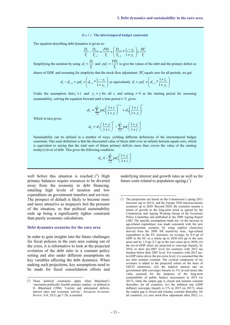
The sustainability of public finances relates to continued ability of a government to finance its debt. Although there are a number of definitions of sustainability that could be given, the intertemporal budget constraint can serve as a starting point for defining what a sustainable debt level entails. The intertemporal budget constraint (IBC) is given by:
tT
tt i
ypdd ⎟⎠⎞
⎜⎝⎛
++−≤ ∑
= 11
10
A derivation of this equation is given in Box II.1. Intuitively, the IBC is met if the stream of future primary surpluses is large enough to enable a government to meet its financing obligations. Doing so is dependent on the starting level of debt, the primary balances that are possible and any future differential between interest rates and growth rates. Where debt levels are high, not only is the stream of future surpluses that are needed high, but the impact of high debt on the differential between interest rate and growth rate is likely to require even higher primary balances to make up for the lower growth and/or higher interest. The feasibility of running high enough primary balances is essentially political. While there is necessarily a point at which the required primary balances are so high as to either take up all of GDP or require tax to be so high that growth grinds to a halt, political constraints will apply
- 10 -
I. Debt dynamics and sustainability in the euro area
well before this situation is reached. (6) High primary balances require resources to be diverted away from the economy to debt financing, entailing high levels of taxation and low expenditure on government transfers and services. The prospect of default is likely to become more and more attractive as taxpayers feel the pressure of the situation, so that political sustainability ends up being a significantly tighter constraint than purely economic calculations.
Debt dynamics scenarios for the euro area
In order to gain insights into the future challenges for fiscal policies in the euro area coming out of the crisis, it is informative to look at the projected evolution of the debt ratio in a constant policy setting and also under different assumptions on key variables affecting the debt dynamics. When making such projections, key assumptions need to be made for fiscal consolidation efforts and
(6) These political constraints apply when Blanchard’s ‘maximum politically feasible primary surplus’, as defined in O. Blanchard (1984) ‘Current and anticipated deficits, interest rates and economic activity’, European Economic Review, Vol. 25(1), pp 7–28, is reached.
underlying interest and growth rates as well as for future costs related to population ageing.(7)
(7) The projections are based on the Commission’s spring 2011 forecasts (up to 2012), and the Europe 2020 macroeconomic scenarios up to 2020. Beyond 2020, the scenarios assume a return of growth to the long-term trend as agreed by the Commission and Ageing Working Group of the Economic Policy Committee and published in the 2009 Ageing Report (AR). The specific assumptions made are: (i) the increase in age-related expenditure was made consistent with the new macroeconomic scenario, by using implicit elasticities derived from the 2009 AR sensitivity tests. Age-related expenditure in the EU increases, on average, by 0.4 pp of GDP in the EU as a whole up to 2020 (0.6 pp in the euro area) and by 1.9 pp (2.2 pp in the euro area) up to 2030; (ii) the tax-to-GDP ratios are projected to converge linearly, by 2018, to their pre-2007 level for countries with 2012 tax burdens below their 2007 level. For countries with 2012 tax-to-GDP ratios above the pre-crisis level, it is assumed that the tax ratio remains constant. The cyclical component of tax revenues is added to the projected values on the basis of OECD elasticities; (iii) the implicit interest rate on government debt converges linearly to 3 % in real terms (the value assumed for the purposes of the long-term sustainability of public finance assessment) in 2015 (or 2017), when the output gap is closed and remains constant thereafter, for all countries; (iv) the inflation rate (GDP deflator) converges linearly to 2 % in 2015 (or 2017), when the output gap is closed and remains constant thereafter, for all countries; (v) zero stock-flow adjustment after 2012, i.e.
Box I.1: The intertemporal budget constraint
The equation describing debt dynamics is given as:
t
t
t
tt
t
t
t
t
t
t
t
t
YSF
yyi
YD
YPD
YD
YD +⎟⎟
⎠
⎞⎜⎜⎝
⎛+−+=−
−
−
−
−
1*
1
1
1
1
Simplifying the notation by using t
tt Y
Dd = and t
tt Y
PDpd = to give the values of the debt and the primary deficit as
shares of GDP, and assuming for simplicity that the stock-flow adjustment tSF equals zero for all periods, we get:
⎟⎟⎠
⎞⎜⎜⎝
⎛+−+=− −−
t
tttttt y
yidpddd1
*11 or equivalently ⎟⎟⎠
⎞⎜⎜⎝
⎛+++= −
t
tttt y
idpdd11*1
Under the assumption that iit = and yyt = for all t, and setting t=0 as the starting period for assessing sustainability, solving the equation forward until a time period t=T, gives:
TtTT
ttT y
idyipdd ⎟⎟
⎠
⎞⎜⎜⎝
⎛+++⎟⎟
⎠
⎞⎜⎜⎝
⎛++=
−
=∑ 1
111
01
Which in turn gives: tT
tt
T
T iypd
iydd ⎟
⎠⎞
⎜⎝⎛
++−⎟
⎠⎞
⎜⎝⎛
++= ∑
= 11
11
10
Sustainability can be defined in a number of ways, yielding different definitions of the intertemporal budget constraint. One such definition is that the discounted value of future debt over an infinite horizon equals zero, which is equivalent to saying that the total sum of future primary deficits more than covers the value of the starting (today's) level of debt. This gives the following condition:
tT
tt i
ypdd ⎟⎠⎞
⎜⎝⎛
++−≤ ∑
= 11
10
- 11 -

Quarterly Report on the Euro Area III/2011
Graph I.4 depicts the projected evolution for the government gross debt ratio, for the euro area. The solid thick line shows the outcome for a baseline scenario under the assumption of no fiscal consolidation measures beyond those contained in the Commission’s spring 2011 forecasts (i.e. structural primary balance/GDP ratio kept constant at the 2012 estimated level(8)) and incorporating the expected future age-related spending. (9) Primary balances fall short of what is needed to stabilise the ratio of public debt to GDP, which rises steadily over the projection period. By 2015, the debt is projected to be at around 90 % of GDP in the euro area (more than 20 pp of GDP higher than before the crisis). It would continue increasing to about 93 % of GDP by 2020 and further to 113 % of GDP by 2030, albeit with large differences across countries.
Graph I.4: Medium-term debt projections under alternative assumptions – euro area
(% of GDP)
40
50
60
70
80
90
100
110
120
130
140
2000 2005 2010 2015 2020 2025 2030
PastBaselineBaseline + 1 pp rise in interest-growth differ.Baseline + 1 pp fall in intest-growth differ.Consolidation scenario (0.5%)Consolidation scenario (1.0%)
Source: Commission services.
Table I.2 presents a breakdown of the medium-term debt-to-GDP projections for the euro area that allows the contributions of the main drivers in the baseline scenario to be considered: 1) the primary balance; 2) age-related expenditure; 3) the snowball effect. The fiscal consolidation over the years to 2012 results in a reduction in the structural primary balance, which helps to limit the increase in the debt ratio in the period to 2020. However, ageing costs weigh on the primary balance over time and, on current policies, would
no further purchases of financial assets or recapitalisations of financial institutions, nor disposal of such assets.
(8) For Greece, Ireland and Portugal, the structural primary balances in their economic adjustment programmes (2014 for Greece and 2015 for Ireland and Portugal) are kept constant in the baseline scenario.
(9) For details on future age-related spending, see European Commission and Economic Policy Committee (2009), ‘2009 Ageing Report: Economic and budgetary projections for the EU-27 Member States (2008-2060)’, European Economy, No 2.
send the primary balance into the red again in the mid 2020s. Moreover, with rising debt, the snowball effect would prove significant over time; interest expenditure would rise continuously and increasingly outweigh the growth effect.
Sustained fiscal consolidation would curb the euro area’s debt dynamics
Graph I.4 also shows the results of additional scenarios built up to examine the long-run implications of a gradual fiscal adjustment and also of alternative assumptions on the differential between interest rate and growth rate. A first fiscal consolidation scenario is based on the assumption of all euro-area countries implementing fiscal consolidation efforts from 2012, measured in terms of an improvement of the structural balance by 0.5 % of GDP per year until the medium-term objective (MTO) reported by the country is reached. (10) (11) The graph illustrates that, for the euro area, this consolidation pace – the benchmark consolidation effort in the Stability and Growth Pact – would be enough to halt the growth in debt by 2013, after which the ratio of debt to GDP would decrease, but only slowly, from 89 % in 2013 to 78 % in 2020. It would fall below 60 % only in 2029.
A stronger consolidation effort of 1 % of GDP per year until the MTO of each euro area Member State is reached would also halt the increase in the government debt ratio from 2013. Nevertheless, in 2020, the debt ratio would still be larger than before the crisis (by about 6 pp of GDP), and it would fall below the 60 % threshold only in 2026.
Stress tests based on different assumptions on the interest/growth rate differential
In addition to the aforementioned scenarios, stress tests reveal the sensitivity of debt developments to different assumptions on the interest rate and economic growth by modelling an increase and decrease of 1 pp in the differential between these two variables. The interest/growth rate differential is a critical input parameter in determining the future evolution of public debt. Countries with high levels of debt face the possibility of an ever
(10) For Greece, Ireland and Portugal all extrapolations are done
taking into account their economic adjustment programmes (till 2014 and 2015 respectively) i.e. using the debt levels and primary balances at the end of the programmes.
(11) The MTO effectively corresponds to a close to balance or surplus budgetary position. See section I.3 of European Commission (2011) ‘Public finances in EMU 2011,’ European Economy, No. 3|2011 available online at: http://ec.europa.eu/economy_finance/publications/european_economy/2011/pdf/ee-2011-3_en.pdf.
- 12 -

I. Debt dynamics and sustainability in the euro area
increasing debt burden in the event of either higher interest rates or lower GDP growth rates or both. Empirical evidence also confirms that when debt becomes very large, it may be difficult to generate the primary balance that is necessary to ensure sustainability. (12) In turn, a deteriorating domestic outlook for fiscal deficits and debt is likely to be associated with higher interest rates. As the increase in interest rates only affects new debt issuance and refinancing needs, countries with short average debt maturity rates are more exposed to interest rate shocks than those that have longer debt maturity rates.
The stress tests on the interest/growth rate differential clearly show that a higher interest rate and/or a lower GDP growth rate will have a strong adverse impact on debt going forward (see Graph I.4), pointing to a markedly more demanding consolidation effort than under a baseline scenario if markets impose on them a risk premium that translates into a lasting increase in the average cost of debt. By contrast, a lower differential would broadly lead to stabilisation of the debt ratio at the current elevated level until the early 2020s, which would however start increasing thereafter due to the effect of ageing on public finances and on growth.
Though these scenarios are based on a number of simplifying assumptions, they suggest that fast debt reduction requires determined and sustained consolidation efforts. Nonetheless, even in the scenario in which a structural fiscal adjustment of 1 pp per year is assumed until the MTOs are reached, it would take 15 years for the debt ratio in the euro area to fall below the 60 % of GDP threshold. The simulations also reveal that if
(12) See IMF (2010), ‘Fiscal Space’, IMF Staff Position Note,
September 1.
measures are put in place to reduce the interest rate and/or increase the GDP growth rate, the effect on the debt ratio could be significant. Still, this would only stabilise the debt ratio over the coming decade, and from the 2020s onwards it would start to rise again. If, by contrast, growth prospects and/or financing conditions were worse than in the baseline scenario, curbing the debt dynamics would be even more challenging.
It is clear that reversing the effect of the crisis and dealing with the effects of an ageing population will require a strong and sustained policy response. Nevertheless, the benefits of rising to the challenge in timely manner are clear. Not only do strong policy measures change the perception of the sustainability risk faced by Member States, but the sooner that countries can benefit from the reduced interest payments and higher growth that lower debt entails, the better the outlook.
While this analysis highlights the magnitude of the challenge ahead, expanding it to take other factors into account can help better understand the related policy implications. The remainder of this text presents additional methodologies that complement the assessment presented so far and provide a broader picture of the current debt situation. These include the analysis of fiscal reaction functions (in the remainder of this section) and of the risk of fiscal crises (next section).
Using fiscal reaction functions as part of sustainability analysis
In order to assess whether it is feasible to put in place the policy responses required to address the sustainability challenge facing the euro area economies, fiscal reaction functions (FRF) can be
Table I.2: General government gross debt for the euro area – baseline projections (in %) 2009 2010 2011 2012 2013 2014 2015 2016 2017 2018 2019 2020 2025 2030
Gross debt ratio 79.3 85.4 87.9 88.7 89.1 89.4 89.7 90.5 91.2 91.8 92.5 93.2 100.2 113.2changes in the debt ratio (1+2+3) 9.4 6.1 2.4 0.9 0.4 0.3 0.3 0.8 0.7 0.7 0.7 0.7 1.9 3.0
of which (1) Overall primary balance (+ = deficit) 3.5 3.2 1.3 0.4 -0.1 -0.5 -0.7 -0.6 -0.6 -0.5 -0.3 -0.2 0.7 1.7Structural primary balance (kept constant at 2012 lvl) 1.4 1.2 0.0 -0.6 -0.7 -0.8 -0.8 -0.8 -0.8 -0.8 -0.8 -0.8 -0.8 -0.8Cyclical component 2.1 2.0 1.3 1.0 0.7 0.3 0.0 0.0 0.0 0.0 0.0 0.0 0.0 0.0Ageing cost (incl. revenues pensions tax) 0.2 0.3 0.5 0.7 0.9 1.0 1.2 1.3 2.0 3.0Property incomes -0.1 -0.1 -0.1 -0.1 -0.1 -0.1 -0.1 0.0 0.0 0.0Revenues -0.1 -0.2 -0.3 -0.4 -0.5 -0.6 -0.6 -0.6 -0.6 -0.5
(2) Snowball effect (interest rate/growth differential) 5.2 0.8 0.5 0.3 0.4 0.7 0.9 1.4 1.3 1.2 1.0 0.9 1.3 1.6Interest expenditure 2.9 2.8 3.0 3.2 3.6 4.0 4.4 4.4 4.5 4.5 4.5 4.5 4.8 5.4Growth effect (real) 3.0 -1.4 -1.4 -1.5 -1.6 -1.7 -1.7 -1.3 -1.4 -1.5 -1.7 -1.8 -1.6 -1.7Inflation effect -0.7 -0.6 -1.2 -1.4 -1.5 -1.6 -1.8 -1.8 -1.8 -1.8 -1.8 -1.8 -1.9 -2.2
(3) Stock flow adjustment 0.7 2.1 0.7 0.2 0.1 0.1 0.1 0.0 0.0 0.0 0.0 0.0 0.0 0.0PM : Structural balance (+ = deficit) 2.7 2.9 3.4 3.6 3.6 3.6 3.6 3.7 5.4 7.0
Key macroeconomic assumptionsGDP growth (real) -4.1 1.8 1.6 1.8 1.9 1.9 2.0 1.4 1.6 1.7 1.9 2.0 1.6 1.6Interest rate (real) 2.9 2.7 2.1 2.0 2.3 2.7 3.0 3.0 3.0 3.0 3.0 3.0 3.0 3.0Inflation (GDP deflator) 1.0 0.8 1.4 1.7 1.8 1.9 2.0 2.0 2.0 2.0 2.0 2.0 2.0 2.0
Source: Commission services.
- 13 -
Quarterly Report on the Euro Area III/2011
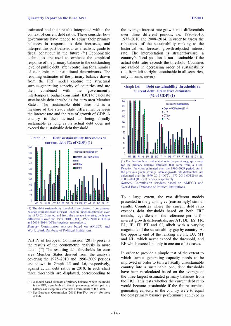
estimated and their results interpreted within the context of current debt ratios. These consider how governments have tended to adjust their primary balances in response to debt increases, and interpret this past behaviour as a realistic guide to fiscal behaviour in the future. (13) Econometric techniques are used to evaluate the empirical response of the primary balance to the outstanding level of public debt, after controlling for a number of economic and institutional determinants. The resulting estimates of the primary balance drawn from the FRF model capture the structural surplus-generating capacity of countries and are then combined with the government’s intertemporal budget constraint (IBC) to calculate sustainable debt thresholds for euro area Member States. The sustainable debt threshold is a measure of the steady state differential between the interest rate and the rate of growth of GDP. A country is then defined as being fiscally sustainable as long as its actual debt does not exceed the sustainable debt threshold.
Graph I.5: Debt sustainability thresholds vs current debt (% of GDP) (1)
0
20
40
60
80
100
120
140
160
180
200
MT FI LU NL CY BE EE SK SI ES FR PT AT IE DE EL IT
Debt to GDP ratio (2010)DT1DT1bisDT1ter
decreasing sustainability
(1) The debt sustainability thresholds are derived from primary balance estimates from a Fiscal Reaction Function estimated over the 1975–2010 period and from the average interest-growth rate differentials over the 1990–2010 (DT1), 1975–2010 (DT1bis) and 2008–2014 (DT1ter) periods, respectively. Source: Commission services based on AMECO and World Bank Database of Political Institutions.
Part IV of European Commission (2011) presents the results of the econometric analysis in more detail. (14) The resulting debt thresholds for euro area Member States derived from the analysis covering the 1975–2010 and 1990–2009 periods are shown in Graphs I.5 and I.6, respectively, against actual debt ratios in 2010. In each chart three thresholds are displayed, corresponding to (13) A model-based estimate of primary balance, where the model
is the FRF, is preferable to the simple average of past primary balances as it captures structural determinants of the latter.
(14) See European Commission (2011) Part IV.4, op cit for more details.
the average interest rate-growth rate differentials over three different periods, i.e. 1990–2010, 1975–2010 and 2008–2014, in order to assess the robustness of the sustainability ranking to the historical vs. forecast growth-adjusted interest rate. The interpretation is straightforward: a country’s fiscal position is not sustainable if the actual debt ratio exceeds the threshold. Countries are ranked in decreasing order of sustainability (i.e. from left to right: sustainable in all scenarios, only in some, never).
Graph I.6: Debt sustainability thresholds vs current debt, alternative estimates
(% of GDP) (1)
0
20
40
60
80
100
120
140
160
180
200
MT BE FI NL LU EE SK IT SI DE AT FR PT ES IE CY EL
Dept to GDP ration (2010)DT2DT2bisDT2ter
decreasing sustainability
(1) The thresholds are calculated as in the previous graph except for the primary balance estimates that come from a Fiscal Reaction Function estimated over the 1990–2009 period. As in the previous graph, average interest-growth rate differentials are calculated over the 1990–2010 (DT2), 1975–2010 (DT2bis) and 2008–2014 (DT2ter) periods, respectively. Source: Commission services based on AMECO and World Bank Database of Political Institutions
To a large extent, the two different models presented in the graphs give (reassuringly) similar results. Countries where the current debt ratio exceeds debt thresholds based on both FRF models, regardless of the reference period for interest growth differentials, are AT, DE, ES, FR, EL, IE, IT, PT and SI, albeit with a varying magnitude of the sustainability gap by country. At the opposite end of the ranking are FI, LU, MT and NL, which never exceed the threshold, and BE which exceeds it only in one out of six cases.
In order to provide a simple test of the extent to which surplus-generating capacity needs to be improved in order to turn a fiscally unsustainable country into a sustainable one, debt thresholds have been recalculated based on the average of the three largest estimated primary balances from the FRF. This tests whether the current debt ratio would become sustainable if the future surplus-generating capacity of the country were to equal the best primary balance performance achieved in
- 14 -

I. Debt dynamics and sustainability in the euro area
the past according to the FRF model. (15) Graphs I.7 and I.8 show the debt thresholds based on the best estimated primary balance (‘DT1best’ and ‘DT2best’) together with the general thresholds (‘DT1’ and ‘DT2’), both derived from the first and second FRF model, respectively, against the actual debt ratio. (16)
Graph I.7: Debt sustainability thresholds for the best 3 years of estimated primary balance (1975–2010) vs. current debt (% of GDP) (1)
0
20
40
60
80
100
120
140
160
180
200
NL MT FI LU CY BE AT DE EE ES PT IT SI FR IE EL
DT1DT1bestDebt to GDP ratio (2010)
(1) DT1 = Debt Threshold 1 as in Graph II.5; DT1best = Debt Threshold derived from the (average of the) three largest estimated primary balances from the FRF estimated over the 1975-2010 period and from the average interest rate-GDP growth rate differential over the 1990-2010 period. Figures for thresholds in a few countries exceed the maximum value of the axis (200 %). Source: Commission services, AMECO and World Bank Database of Political Institutions
This approach obviously increases the estimated level of sustainable debt. According to ‘DTbest’, the sustainability assessment moves from negative to positive for AT, DE, ES, IT, PT and SI according to the first FRF model, and for AT, CY, DE, ES and IT according to the second FRF model. For most countries, the response required by the sustainability challenge is therefore challenging, but not unprecedented. However, a few Member States remain fiscally unsustainable even under this more ‘optimistic’ scenario, i.e. FR, EL and IE according to both models, and PT and SI according to the second FRF model.
(15) A current debt ratio becomes sustainable if it is lower than
the recalculated debt threshold. (16) As explained in section IV.4 of European Commission
(2011), whenever the overall average of estimated primary balances was negative, it has been restricted to positive primary balance values in order to increase the number of countries included in threshold calculation. This implies that for those countries with only one or two positive values for the estimated primary balance, the main debt threshold already implies a significant over-estimation of surplus-generating capacity and would decrease if based on the best three-year primary balance values. These countries were then excluded from calculation of DTbest, i.e. SK in Graph II.7 and MT and SK in Graph II.8.
Of course, achieving in the future the best outcomes seen so far for several years may raise serious political difficulties, as the primary balances on which this exercise was based are unlikely to be maintained indefinitely. Moreover, although past fiscal behaviour can serve as a guide to the future, providing information about the feasible magnitude of future primary balance, it can only serve as an imperfect guide, particularly given the unique circumstances in which the European economies find themselves. Nevertheless, there are countries, such as Belgium, that have maintained sizeable primary surpluses for long periods of time, indicating that it is possible if the political willingness is there.
Graph I.8: Debt sustainability thresholds for the best three years of estimated primary balance
(1990–2009) vs current debt (% of GDP) (1)
0
20
40
60
80
100
120
140
160
180
200
NL BE FI LU AT DE CY IT ES EE SI FR IE PT EL
DT2DT2bestDebt to GDP ratio (2010)
(1) DT2 = Debt Threshold 2 as in Graph II.6; DT2best = Debt Threshold derived from the (average of the) three largest estimated primary balances from the FRF estimated over the 1990-2009 period and from the average interest rate-GDP growth rate differential over the 1990-2010 period. Figures for thresholds in a few countries exceed the maximum value of the axis (200 %).. Source: Commission services, AMECO and World Bank Database of Political Institutions
I.3. Assessing the risk of fiscal crises
Expanding on the existing methodologies to gauge fiscal risks
The analysis and discussion so far has focused on looking at debt projections and gaining an idea of future sustainability based on debt dynamics and the intertemporal budget constraint set out in the first part of this section. But aside from assumptions and projections about the primary balances and their components, interest and growth rates, it is evident that levels of debt and concepts of sustainability depend on a broad range of other factors. The Great Recession has illustrated how problems emanating from the financial sector can have devastating effects on public finances and on governments’ perceived
- 15 -

Quarterly Report on the Euro Area III/2011
ability to control them. In turn, the growth rate of the economy is related to a host of other variables, with competitiveness problems often being symptoms of deep-seated productivity challenges.
The framework for assessing fiscal sustainability can be usefully complemented by fiscal crisis risk models that aim at timely detection of risks of debt distress. These models help to gauge fiscal crisis risks by allowing for the determination of critical thresholds for a set of variables and for composite indicators combining them. By identifying increased risk of debt distress, policymakers can respond in a timely manner.
Models of this kind are taken into consideration by the IMF to supplement the framework used for assessing external and fiscal sustainability in the context of Fund-supported programmes and Article IV surveillance. Recently, fiscal crisis risk models have also become a building block of the joint IMF-FSB Early Warning Exercise ,(17) created in 2008 at the request of the G20, in response to the need to improve policymakers’ ability to spot risks and vulnerabilities quickly in order to be able to coordinate early policy responses.
Results from a fiscal crisis risk model based on the ‘signals approach’(18) are presented here. The model provides thresholds based on past behaviour, beyond which fiscal crisis signals are detected for: 1) each individual variable included in the analysis, 2) a composite indicator incorporating all variables, 3) thematic composite indicators referring to different subsets of variables (e.g. fiscal, financial, competitiveness).
The signals approach allows consideration (and aggregation into an overall index) of a large set of variables, thus permitting quite a comprehensive analysis of underlying vulnerabilities. For the analysis presented here, both fiscal and macro-financial variables are selected and their correlation with past fiscal crises is first analysed. An optimal threshold (for each variable included in the analysis) is found, which maximises the ability of the variable to predict a fiscal crisis
(17) See IMF (2011), ‘The IMF-FSB early warning exercise.
Design and methodological toolkit’, September 2010, (available online at: http://www.imf.org/external/np/pp/eng/2010/090110.pdf).
(18) Seminal papers on this approach are: Kaminsky, G., S. Lizondo, and C.M. Reinhart (1998), ‘Leading indicators of currency crises’, IMF Staff Papers, Vol. 45, No. 1. and Kaminsky, G.L. and C.M. Reinhart (1999), ‘The twin crises: the Causes of banking and balance-of-payments problems’, American Economic Review, Vol. 89(3), pp. 473-500.
based on the value taken by the variable one year ahead of the crisis. A variable will be sending a ‘crisis signal’ when it takes a value above or below such optimal threshold, depending on the variable in question. (19) (20) Once these triggering thresholds are calculated, the variables can be aggregated into composite indicators of fiscal crisis vulnerability.
Giving concrete guidance in a sustainability assessment framework based on the overall fiscal crisis vulnerability index requires careful consideration of which variables drive the outcome of the exercise on a country by country basis. This makes the signals approach an instrument that is best used at the beginning of the assessment procedure.
In the context of a regular fiscal crisis early warning exercise, the overall indicator of fiscal crisis vulnerability can be computed for a selected sample of countries in each year and compared against the critical threshold identified. Indicator values beyond the threshold for a country in a given year provide warnings of fiscal crisis risks for the following year. The values of thematic indicators (grouping different subsets of variables – fiscal, financial and competitiveness variables) and of the individual variables themselves relative to their respective thresholds can also be used to complete the picture of the sources of vulnerabilities and to highlight areas where early policy intervention might be required. Finally, alongside the analysis of values taken against critical thresholds at a certain point in time, the monitoring at country level should also pay attention to the evolution of the fiscal crisis vulnerability indicator over time, with increases in the value of the indicator highlighting increased vulnerability. This is of course also relevant in cases where countries remain below the critical threshold of fiscal crisis risk.
(19) For the change in public debt over GDP, for instance, a value
above the optimal threshold would signal a fiscal crisis, while for the general government balance over GDP a value below the optimal threshold is taken as a crisis signal.
(20) In brief, the methodology for determining the optimal thresholds works as follows. Using historical data, signals sent by the variable for the different countries and years are compared to the crisis definition. A signal is correct when for the country in question the variable indicates a crisis (non-crisis) year and indeed the year following that in which the signal is recorded turns out to be a crisis (non-crisis) year. On the contrary, a signal is wrong when the variable has signalled no crisis ahead of a crisis year (type II error) and when it has signalled a crisis ahead of a non-crisis year (type I error). The optimal threshold is chosen in such a way as to minimise the share of not signalled crises plus the share of non-crises signalled as crises (see Part IV, Chapter 3 in European Commission (2011) for more details).
- 16 -
I. Debt dynamics and sustainability in the euro area
Preliminary results
The calculation of the optimal thresholds is based on a panel of 33 countries (all EU countries except CY, LU and MT, and nine other advanced economies).(21) Data come from AMECO, the IMF’s World Economic Outlook (WEO) and the Bank for International Settlements. Time series covering the period 1970-2010 are used whenever possible but for a number of variables data are only available starting from 1995. The identification of fiscal crisis events over the time interval 1970–2010 is borrowed from Baldacci et al. (22) A fiscal crisis episode is identified if any of four different criteria is satisfied: high inflation rates, large sovereign bond yield spreads, public debt default or restructuring/rescheduling based on Standard & Poor’s definition, large-scale IMF-supported programme in place.
The fiscal variables entering the calculations include the general government’s gross debt (and its first difference), the short-term debt, the total, primary and cyclically-adjusted balances, the change in government expenditure and in government final consumption expenditure, and the change in projected age-related public expenditure. Among the macro-financial variables, the following are considered: net financial assets of the total economy, net savings of households and non-financial corporations, private sector debt, net acquisition of financial assets for the private sector, leverage of financial corporations, short-term debt of non-financial corporations, and competitiveness variables like the change in the real effective exchange rate, the change in nominal unit labour costs and the current account.
European Commission (2011) Part IV presents the results of the analysis and the derived thresholds for both the individual variables and the composite indicators. It shows that the overall composite indicator derived would have correctly identified 73 % of past crisis events and 83 % of past non-crisis events (i.e. correctly signalled that no crisis was imminent), highlighting quite a good overall performance for this type of
(21) CY, LU and MT are excluded from the sample as the
necessary information on recorded fiscal crisis events over the past four decades is currently missing. The other nine advanced economies included in the analysis are: Australia, Canada, Iceland, Israel, Japan, New Zealand, Norway, Switzerland, US.
(22) Baldacci, E., Petrova, I., Belhocine, N., Dobrescu, G., and S. Mazraani, (2011) ‘Assessing Fiscal Stress’, IMF Working Paper 11/100.
methodology. (23) The fact that the indicator displays a relatively good performance at not missing crises is a particularly encouraging feature.
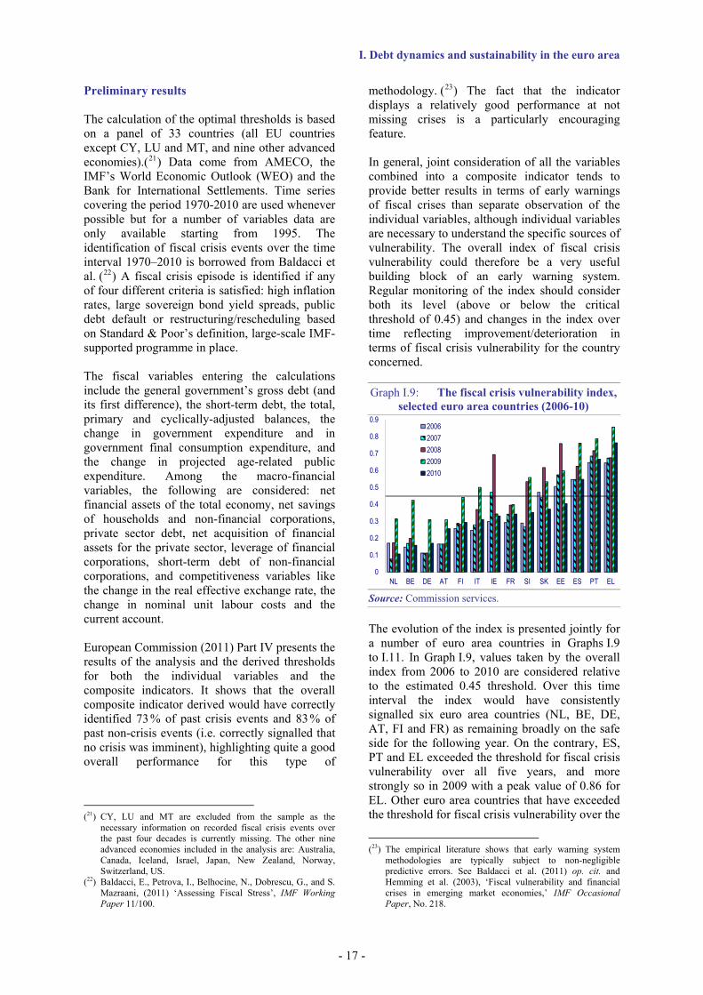
In general, joint consideration of all the variables combined into a composite indicator tends to provide better results in terms of early warnings of fiscal crises than separate observation of the individual variables, although individual variables are necessary to understand the specific sources of vulnerability. The overall index of fiscal crisis vulnerability could therefore be a very useful building block of an early warning system. Regular monitoring of the index should consider both its level (above or below the critical threshold of 0.45) and changes in the index over time reflecting improvement/deterioration in terms of fiscal crisis vulnerability for the country concerned.
Graph I.9: The fiscal crisis vulnerability index, selected euro area countries (2006-10)
0
0.1
0.2
0.3
0.4
0.5
0.6
0.7
0.8
0.9
NL BE DE AT FI IT IE FR SI SK EE ES PT EL
20062007200820092010
Source: Commission services.
The evolution of the index is presented jointly for a number of euro area countries in Graphs I.9 to I.11. In Graph I.9, values taken by the overall index from 2006 to 2010 are considered relative to the estimated 0.45 threshold. Over this time interval the index would have consistently signalled six euro area countries (NL, BE, DE, AT, FI and FR) as remaining broadly on the safe side for the following year. On the contrary, ES, PT and EL exceeded the threshold for fiscal crisis vulnerability over all five years, and more strongly so in 2009 with a peak value of 0.86 for EL. Other euro area countries that have exceeded the threshold for fiscal crisis vulnerability over the
(23) The empirical literature shows that early warning system
methodologies are typically subject to non-negligible predictive errors. See Baldacci et al. (2011) op. cit. and Hemming et al. (2003), ‘Fiscal vulnerability and financial crises in emerging market economies,’ IMF Occasional Paper, No. 218.
- 17 -

Quarterly Report on the Euro Area III/2011
last three years are EE, IE, SI and SK in 2008 and EE, IT, SI and SK in 2009.(24) Graph I.9, also shows that the crisis vulnerability index is lower in 2010 than in 2009 for all countries, signalling a reduced risk. As economic and fiscal fundamental continue to strengthen, it is expected that the index will continue to fall in 2011.
Graph I.10: Evolution of the fiscal crisis vulnerability index for DE, FR, IT 1999-2010
0.0
0.1
0.2
0.3
0.4
0.5
0.6
0.7
0.8
0.9
1999 2000 2001 2002 2003 2004 2005 2006 2007 2008 2009 2010
ESELPTIE
Source: Commission services.
Graphs I.10 and I.11 provide information on the evolution of the fiscal crisis vulnerability index between 1999 and 2010 for selected countries. Spikes in the index are particularly evident for IE, ES, EL and PT in 2008 and 2009.
Graph I.11: Evolution of the fiscal crisis vulnerability index for ES, EL, PT, IE 1999-2010
0.0
0.1
0.2
0.3
0.4
0.5
0.6
0.7
0.8
0.9
1999 2000 2001 2002 2003 2004 2005 2006 2007 2008 2009 2010
ESELPTIE
Source: Commission services.
The analysis of the overall index should be complemented by analysis of the thematic composite indicators. These two indicators provide information on the respective contributions of different groups of variables to
(24) The low values for IE are explained by the fact that IE does not provide series for the financial variables which are consolidated by national account subsector (non-consolidated data could be used in a regular assessment).
fiscal crisis vulnerability. The analysis should then be further deepened at individual variable level to have the full picture of where vulnerabilities stem from.
By looking retrospectively at the results obtained for countries that were particularly strongly hit by the crisis, it is possible to gauge the usefulness of the more detailed indicators. As an example, on an ex post basis, it is now clear that Greece was building up imbalances in the run-up to the crisis that have since proved very costly. (25) Our results for Greece show that many fiscal variables were consistently signalling crisis risks from 2002 onwards. For the years since 2006 almost all fiscal variables with relatively high signalling power (the primary balance, cyclically adjusted balance, gross and net debt, and change in projected age-related public expenditure) identified a risk of crisis, while the change in gross debt over GDP started flashing red in 2009. Fiscal crisis signals have also been sent by macro-financial variables with some of the highest signalling powers, including net financial assets of the total economy, net savings of households and private sector debt since 2007, and the leverage of financial corporations since 2008. (26) On the competitiveness side, the current account over GDP and the growth rate of nominal unit labour costs have been flashing red since 2006. Thus, not only did the overall indicator correctly point to weaknesses in Greece, but also the analysis of the sub-indices and of the single variables showed that both the government (the fiscal side) and the private sector (the macro-financial side) had put in place a dangerous excess of consumption accompanied by a process of debt accumulation.
I.4. Conclusions
The deterioration in the public finances of the euro area since the onset of the economic and financial crisis comes on top of already high starting levels of debt and at a time when the European economies are facing the prospect of the sustainability challenge of an ageing population. In the absence of additional consolidation measures, taking the Commission’s spring 2011 forecasts and projecting the debt ratio forward while incorporating additional age-related
(25) It should be noted that any such a conclusion is based on an
ex-post analysis relying on currently available data and not on data that were available in real time. Furthermore, the risk assessment instruments presented here have been developed in response to the crisis and were not available before the crisis.
(26) Some of these variables are also part of the Scoreboard on which the recently adopted Excessive Imbalance Procedure will be based.
- 18 -
I. Debt dynamics and sustainability in the euro area
- 19 -
spending shows debt passing the 100 % of GDP mark over the next 15 years and continuing to increase thereafter.
It is clear that in order to reverse the increases in growth and ensure the sustainability of public finances, significant permanent consolidation measures – over and above those already introduced – will be necessary in a number of euro area countries. The analysis based on the fiscal reaction functions shows that in some cases the required primary balance to bring debt back to a sustainable level is particularly high, albeit not unprecendented, by historical standards.
Moreover, although the aftermath of the current crisis is central to budgetary policy, it is important not just to focus on the present, but to put into place measures to reduce the likelihood and/or severity of future crises. The ability to predict the risk of future crises is a valuable one, to allow policy measures to be taken in due time, where a risk of a crisis is identified. In this context, the indicators of fiscal crisis risk presented in this section are an important part of the toolbox required to analyse debt sustainability.


II. Special topics on the euro-area economy
- 21 -
While fiscal imbalances are at the forefront of the current policy debate, they are by no means the only area where policy action is needed. The contributions in this chapter take a closer look at external imbalances, housing imbalances and industries' resilience to shocks in the euro area. The analyses show that while macroeconomic adjustment in these areas is essentially market based, structural policies can play an important role in either facilitating market-based adjustment or reducing the risk of emergence of imbalances.
Internal devaluation and external imbalances: a model-based analysis
While nominal exchange rate devaluations are not an available policy tool for the correction of external imbalances in EMU, various ‘internal devaluation’ measures can mimic the effects of nominal devaluations by reducing domestic prices and encouraging similar expenditure-switching effects. This section looks at two potential internal devaluation measures: (i) a tax shift from employers’ social security contributions towards consumption taxes; (ii) public-sector wage moderation. The effectiveness of these measures is assessed using QUEST, the Commission’s structural macro-economic model. The simulations show that the tax reform can raise employment, boost GDP and improve the net foreign asset position. Public-sector wage moderation is also shown to spill over to private-sector wages, thereby reducing production costs and improving competitiveness. However, like ‘external’ exchange rate adjustments, internal devaluations are unlikely to have permanent trade balance effects. Over time, their positive effect on GDP translates into higher domestic and import demand and this income effect largely offsets the original improvement in the trade balance.
Sectoral implications of external rebalancing
External imbalances have accumulated in several euro-area Member States over the pre-crisis period. Though the largest current account deficits have been receding since 2008, the external rebalancing process still has some way to go. Successful external adjustment relies on changes in both the demand side and – an often-neglected point – the supply side. Evidence shows that large and persistent current account imbalances in the euro area are associated with supply distortions in the form of skews in the industrial composition of the economy. Successful rebalancing requires a reversal of the excessive pre-crisis growth in non-tradable output and a reallocation of capital and labour to the tradable sector. The reallocation process may be hampered by sectoral mismatches between supply and demand for labour, in which case, external rebalancing could come at the cost of persistently higher unemployment. To counter these risks policies should aim at facilitating labour mobility across sectors and at supporting investment in the tradable sector.
Sectoral resilience to shocks
This section analyses business cycles at the level of disaggregated industrial sectors in euro-area Member States and looks at differences in the adjustment capacity of sectors and of Member States to common euro-area output shocks. In particular, it focuses on the role played by country-specific characteristics such as product market reforms and openness (to goods and services as well as capital) in improving this adjustment capacity. The findings show that, given sectors’ different resilience to shocks, the sectoral composition of the economy is an important factor explaining countries’ overall level of cyclical resilience. However, structural characteristics of the economy such as product market regulation (PMR) are found to play an even more important role. A high level of PMR has a negative impact on resilience. This result helps to better understand the reasons behind country differences in the response to shocks and suggest that reducing PMR would help improve Member States’ overall cyclical resilience and the cross-country synchronisation of the business cycle.
House price imbalances and structural features of the housing markets
Historical experience, especially from the latest recession, shows that house price imbalances may have a deep impact on the economy as a whole and require close monitoring. The recently adopted Excessive Imbalance Procedure (EIP) will involve regular reviews of housing markets in Member States. Against this background this section discusses a few structural features of the housing market that may have important implications for the sector’s stability. It shows that policies aimed at encouraging housing ownership, especially for the low-income population, may have a negative impact on house price stability. Establishing a stable and functional rental market, particularly for lower-income households, may therefore be seen as beneficial alternative for macroeconomic stability. In addition, variable mortgage interest rates, high loan-to-value ratios as well as tax incentives for house purchase appear to increase the risk of housing market imbalances.

Quarterly Report on the Euro Area III/2011
II.1. Internal devaluation and external imbalances: a model-based analysis
Recent developments have highlighted the urgent need for some euro-area Member States to restore their external balances and to improve their competitiveness. While nominal exchange rate adjustment is not an available tool for the correction of external imbalances in a currency union, alternative policies of ‘internal devaluation’ can mimic the expenditure-switching effects of ‘external’ exchange rate devaluation. (27) Internal devaluation policies aim to reduce domestic prices either by affecting relative export-import prices or by lowering domestic production costs and thereby yielding a real exchange rate depreciation. An example of such internal devaluation is a revenue-neutral shift from taxes on labour to taxes on consumption. By reducing the tax burden on exports and raising that on imports this policy can help to restore competitiveness. Likewise, public-sector wage moderation may achieve overall wage moderation by exerting downward pressure on wages in the private sector and thereby reduce firms’ production costs and lead to a real exchange rate depreciation restoring competitiveness.
This section analyses the potential effects of these policies based on simulations using a three-region version of the European Commission’s QUEST model: (28) a small euro-area member country, the rest of the euro area, and the rest of the world. The model includes tradable and non-tradable sectors and trade in final goods and intermediate inputs. It also distinguishes between private-sector and public-sector employment.
The policy measures analysed are: (i) a tax reform shifting government revenue from social security contributions towards consumption taxes and (ii) a public-sector wage reduction aiming at achieving overall labour cost moderation. The rest of the section discusses each scenario in more details.
Switching the tax burden from labour to consumption
The first set of scenarios assumes a revenue-neutral shift from social security contributions (SSCs) of firms towards destination-based taxes
(27) Calmfors, L. (1998), ‘Macroeconomic policy, wage setting,
and employment — what difference does the EMU make?’, Oxford Review of Economic Policy, Vol. 14, No 3.
(28) For references, see: http://ec.europa.eu/economy_finance/research/macroeconomic_models_en.htm.
such as VAT. The reduction in SSCs lowers unit labour costs and leads to a reduction in producer prices, including for exported goods. This boosts foreign demand for exports. At home, higher consumption taxes offset the fall in producer prices but raise prices on imported goods. Hence, the effects are similar to those of an exchange rate depreciation and yield an improvement in the trade balance. However, in the long run, increased consumption taxes are shifted into higher nominal wages and real wage costs will return to pre-reform levels. Therefore, like external exchange rate devaluations, the effects on the trade balance are not likely to be permanent.
The scenarios shown in Graph II.1.1 consist of reductions in employers’ social security contributions of 1 % of (baseline) GDP that are compensated by an increase in consumption taxes of equal size, such that the reform is ex ante budget-neutral. The endogenous improvement in fiscal positions from this tax reform due to economic expansion can be used for two purposes. In the first scenario, the revenues are, in the medium term, recycled back into the economy through cuts in labour income taxes. These further tax reductions give rise to an additional expansionary effect while keeping the reform also ex post budget-neutral in the very long run. (29) In a second scenario there is no further tax reduction in the medium term but instead the higher tax revenue is used to reduce government debt. (30) Without these further reductions in labour taxes, the GDP and employment gains are somewhat smaller in this second scenario. However, with less of a demand stimulus, imports are also more negatively affected and the overall improvement in the trade balance is therefore more persistent.
The reduction in wage costs boosts employment and GDP increases by 0.35 % after 10 years, but by only half that amount when the revenue is used to reduce government debt. The tax reform shifts taxation from labour to other sources of income such as profits/rents, income from financial wealth and transfers. Consumption of liquidity-constrained households declines on impact as consumer prices rise, also because transfer and unemployment benefit recipients are not compensated for the increase in consumption taxes in this scenario and face a reduction in their disposable income of more than 1 %. Consumption of unconstrained households (29) Technically this is done through a labour tax rule ensuring a
stable debt-to-GDP ratio at some target in the long run, while allowing some deviation in the short and medium run.
(30) The labour tax rule is turned off for 30 years and then a new 10 pp lower debt target is imposed in the long run.
- 22 -

II. Special topics on the euro-area economy
increases as permanent incomes rise, but in the first couple of years the former outweighs the latter and aggregate consumption is lower. In the medium term, disposable income of wage earners increases gradually as wages rise due to higher labour demand, and consumption rises.
As the tax shift leads to lower domestic prices, the real interest rate increases and this leads to lower
investment in the short run. In the medium to long run, investment rises above baseline as activity expands. However, investment rises by less than GDP, due to an increase in relative prices of (partially imported) investment goods to the GDP deflator, while labour costs fall, leading to substitution to more labour-intensive production.
Graph II.1.1: Switching the tax burden from labour to consumption (deviation from baseline)
0
0.1
0.2
0.3
0.4
0 1 2 3 4 5 6 7 8 9 10
GDP (%)
Main scenario (1)
With debt reduction (2)
With compensation (3)
0
0.1
0.2
0.3
0 1 2 3 4 5 6 7 8 9 10
Employment rate (pp)
Main scenario (1)
With debt reduction (2)
With compensation (3)
0
0.1
0.2
0.3
0.4
0 1 2 3 4 5 6 7 8 9 10
Real Effective Exchange Rate (%)
Main scenario (1)
With debt reduction (2)
With compensation (3)
-0.1
0
0.1
0.2
0 1 2 3 4 5 6 7 8 9 10
Trade Balance (pp of GDP)
Main scenario (1)
With debt reduction (2)
With compensation (3)
-4.0
-3.0
-2.0
-1.0
00 1 2 3 4 5 6 7 8 9 10
Government Debt (pp of GDP)
Main scenario (1)
With debt reduction (2)
With compensation (3)
0
0.1
0.2
0.3
0.4
0.5
0.6
0 1 2 3 4 5 6 7 8 9 10
Net Foreign Assets (pp of GDP)
Main scenario (1)
With debt reduction (2)
With compensation (3)
(1) Main scenario: labour supply elasticity 0.2, no compensation of transfer/benefit recipients; (2) Debt reduction scenario: as baseline scenario, but additional revenue used to reduce debt (reduction in long-run debt target); (3) Compensation scenario: labour supply elasticity 0.2, with compensation of transfer/benefit recipients. Source: European Commission, QUEST simulations.
- 23 -

Quarterly Report on the Euro Area III/2011
Lower export prices raise exports and lower domestic prices shift demand towards domestic products and away from imported goods (real effective depreciation). The competitiveness effect is supplemented by the short-run negative income effect of the policy, which temporarily reduces total and import demand. Imports fall both because of increasing relative import prices and because of the negative income effect. Competitiveness gains and the income effect provide a boost to the trade balance of slightly over 0.1 % of GDP. In the medium run, the improvement in the trade balance gradually evaporates as the positive income effect of the reform raises imports over time and the deterioration of the terms of trade counterbalances the impact of the increased net export volume on the trade balance. In the second scenario the additional tax revenue is used to reduce government debt, leading to a smaller positive income effect and a more persistent improvement in the trade balance, with a consequently larger improvement in the net foreign asset position.
Sensitivity analyses. These scenarios imply sharp reductions in real transfers and benefits as recipients of these are not compensated for the increase in VAT. If they are compensated for the increase in consumer prices, as in the third scenario in Graph II.1.1, the real benefits of the reform are significantly smaller as the costs of compensation add a significant burden on fiscal positions. Consumption declines by less on impact as real disposable incomes fall by less, but the increase in transfer and benefit expenditure reduces fiscal space and the resulting labour tax reduction is smaller. The compensation for unemployment benefits also puts upward pressure on workers’ wage demands and the reduction in wage costs for firms is consequently smaller. The first-year GDP impact is slightly larger but medium-term output gains are lower than those in the first scenario. The trade balance and net foreign indebtedness also improve by less as consumption is higher in this scenario.
The macroeconomic impact of the type of tax reforms presented in Graph II.1.1 depends on the labour market structure. Sensitivity analysis indicates that with a more elastic labour supply a similar tax reform leads to a smaller increase in real (gross) wages and to a larger rise in employment. Thus, with a labour supply elasticity of 0.5 instead of the baseline 0.2, real wage costs for firms decline by more, long-run employment and output effects can double and the gain in the NFA-to-GDP ratio would be about 50 % larger.
Public-sector wage reduction
A number of euro-area Member States have adopted measures to reduce their public wage bill in recent years. Wage reductions, wage or hiring freezes, and outsourcing of public services have been undertaken, e.g. in Spain, Portugal and Italy. In other countries, measures to curb public expenditure have been taken on an ongoing basis, such as in Ireland and Greece, where reductions or freezes of public employees’ salaries were implemented already in 2009 and followed by further consolidation measures in 2010.
Besides their direct budgetary impact, public-sector wage reductions can contribute to internal devaluations by putting downward pressure on private-sector wages and thereby allowing domestic price moderation. The resulting gains in competitiveness allow the economy’s external balance and net foreign asset position to improve.
The model extension used for these simulations disaggregates final government consumption into compensation of employees and government purchases of goods and services. (31) It is assumed that the government chooses the level of public employment. Public wages are fixed in a wage bargaining process, where a wage mark-up captures the bargaining power of public-sector employees. Consequently, a public-sector wage reduction is captured by a fall in the wage mark-up in the public sector. The reduction is transmitted to the private sector via an increase of the labour supply to this sector as households try to offset the fall in income from the public sector. (32)
Graph II.1.2 displays the impulse responses of selected variables to a permanent 8 % reduction in the public-sector mark-up, which implies a permanent public-sector wage reduction of around 9-10 % below the initial baseline in real terms in the long run. This amounts to an ex-ante fiscal consolidation of around 0.9-1 % of baseline GDP, in contrast to the tax shift scenario discussed above, which was ex-ante budgetary neutral. However, over time, the debt rule with an unchanged long-run debt target enforces long-run budgetary neutrality. This is achieved by a progressive decrease in the labour income tax.
(31) Total government consumption amounted to around 22 % of
GDP in the euro area in 2010, out of which the compensation of public employees accounted for around 10.5 % of GDP.
(32) The transmission mechanism in the model is fully endogenous. It does not rely on a more direct signalling role of the government on private wage setting.
- 24 -
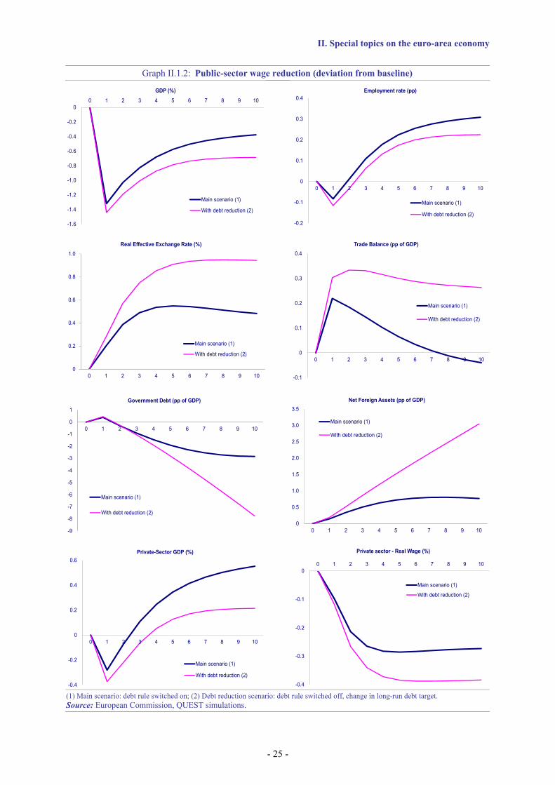
II. Special topics on the euro-area economy
Graph II.1.2: Public-sector wage reduction (deviation from baseline)
-1.6
-1.4
-1.2
-1.0
-0.8
-0.6
-0.4
-0.2
00 1 2 3 4 5 6 7 8 9 10
GDP (%)
Main scenario (1)
With debt reduction (2)
-0.2
-0.1
0
0.1
0.2
0.3
0.4
0 1 2 3 4 5 6 7 8 9 10
Employment rate (pp)
Main scenario (1)
With debt reduction (2)
0
0.2
0.4
0.6
0.8
1.0
0 1 2 3 4 5 6 7 8 9 10
Real Effective Exchange Rate (%)
Main scenario (1)
With debt reduction (2)
-0.1
0
0.1
0.2
0.3
0.4
0 1 2 3 4 5 6 7 8 9 10
Trade Balance (pp of GDP)
Main scenario (1)
With debt reduction (2)
-9
-8
-7
-6
-5
-4
-3
-2
-1
0
1
0 1 2 3 4 5 6 7 8 9 10
Government Debt (pp of GDP)
Main scenario (1)
With debt reduction (2)
0
0.5
1.0
1.5
2.0
2.5
3.0
3.5
0 1 2 3 4 5 6 7 8 9 10
Net Foreign Assets (pp of GDP)
Main scenario (1)
With debt reduction (2)
-0.4
-0.2
0
0.2
0.4
0.6
0 1 2 3 4 5 6 7 8 9 10
Private-Sector GDP (%)
Main scenario (1)
With debt reduction (2)-0.4
-0.3
-0.2
-0.1
00 1 2 3 4 5 6 7 8 9 10
Private sector - Real Wage (%)
Main scenario (1)
With debt reduction (2)
(1) Main scenario: debt rule switched on; (2) Debt reduction scenario: debt rule switched off, change in long-run debt target. Source: European Commission, QUEST simulations.
- 25 -

Quarterly Report on the Euro Area III/2011
The simulations confirm the spillover of the public wage reduction to the private sector. In contrast to the impact of the tax reform, this policy measure leads to a long-lasting (although relatively small) private wage moderation of around 0.3 %.
The public wage reduction affects the economy directly through the fall in employees’ labour income (contractionary effect) and indirectly through the downward pressure on private-sector production costs (expansionary effect). The simulations suggest that the expansionary effect dominates over the medium term: private and total employment, private-sector output, investment and household consumption all increase in response to the policy under the baseline scenario. In the short run, however, domestic demand as well as private output fall below their baseline levels.
The public wage reduction affects relative trade prices and trade volumes via declining domestic production costs. The simulations show that the real effective exchange rate depreciates by around 0.5 % after 3 years.
The real depreciation leads to an expansion in export volumes. At the same time, the falling export prices dampen the resulting improvement in external balances in value terms. Imports decline in the short run but then tend to increase over time along with increasing domestic demand.
In spite of the permanent wage reduction, the overall impact of the public wage reduction on the external balances is fairly modest: the 10 % wage reduction in the public sector is found to lead to a transitory improvement in the trade balance, with a peak of around 0.2 % of GDP translating into an improvement in the NFA-to-GDP ratio by around 0.8 % after ten years.
Sensitivity analyses. The baseline wage reduction scenario assumes no change in the long-run government debt target and allows the labour income tax to be progressively reduced. This allows an additional reduction in firms’ labour cost which per se contributes to the gain in competitiveness and the improvement in the external position.
If the public wage reduction is not recycled through a labour tax cut but is used instead to reduce the public debt, the gains in the external balances achieved by the wage reduction turn out to be markedly larger. This is because the
domestic expansion is, in that case, curtailed by the uncompensated fall in wages. Lower domestic demand leads to a steeper fall in prices (real depreciation) and a more persistent fall in imports and hence to a much more persistent improvement in the trade balance than otherwise (see dashed line in Graph II.1.2). (33) This, however, comes at the cost of persistently lower household consumption and investment.
As in the case of the tax-shift scenarios, the results of the public-sector wage reduction scenarios depend on the structure of the labour market. The propagation of the public-sector wage moderation is also contingent on the labour market structure. When labour supply reacts more sensitively to changes in wages, the same 10 % public wage moderation is more strongly transmitted to private wages and thereby amplifies the gain in competitiveness. In particular, with higher labour supply elasticity, the transmission of the public wage moderation to private wages could even double. External balances would also improve more, though their improvement is somewhat dampened by increasingly deteriorating terms of trade. The NFA-to-GDP ratio is found to improve by around 1.2 % of GDP after ten years. (34)
Relationship with the economic literature. The results of the model simulations presented in this section are broadly in line with recent findings in the macroeconomic literature. Evidence presented in a number of empirical studies supports the interaction between private and public wages. Positive co-movement between private and public wages, as established in the QUEST model, is reported e.g. by Afonso and Gomes (2008), Lamo, Pérez and Schuknecht (2008) for OECD countries and Holm-Hadulla et al. (2010) for the euro area. (35) The above-cited papers as well as Pérez and Sanchez (2010) also agree on the bidirectional causal relationship between wages in both sectors. Most evidence suggests causality runs from the
(33) Technically this is done by switching off the debt rule for the
first 20 years of the simulation and by reducing the debt target by 20 pp in the long run.
(34) The baseline scenario assumes a labour supply elasticity of 0.2. This alternative scenario is based on an elasticity of 0.5 instead.
(35) Afonso, A. and P. Gomes (2008), ‘Interactions between private and public sector wages’, ECB Working Paper Series, No 971; Lamo, A., J. Pérez and L. Schuknecht (2008), ‘Public and private sector wages: Co-movement and causality’, ECB Working Paper Series, No 963; Holm-Hadulla, F., K. Kamath, A. Lamo, J. Pérez and L Schuknecht (2010), ‘Public wages in the euro area: Towards securing stability and competitiveness’, ECB Occasional Paper Series, No 112.
- 26 -

II. Special topics on the euro-area economy
- 27 -
private to the public sector; nevertheless, public wages may take the lead in many instances.
In addition, there is also broad agreement among these studies that public wage moderation is transmitted to private wages and also has a stimulating impact on private employment by orders of magnitude similar to those found in our simulations. The implications for total employment and further propagation to the economy depend, however, on the specific policy measure as well as on the modelling assumptions; see Finn (1998), Pappa (2003), Ardagna (2007), Quadrini and Trigari (2008) and Gomes (2010). (36)
To the best of our knowledge, there are no empirical studies on the effect of public employment policies on external (im)balances. However, the relationship between a broader set of fiscal policies and external balances is also supported by empirical evidence. Using a broad database, Abbas et al. (2010) estimate that a fiscal expansion of 1 % of GDP worsens the current account by 0.2-0.3 % of GDP. (37) The impulse responses generated by the QUEST model predict very similar magnitudes. In another study, Nickel and Vansteenkiste (2008) also establish a positive relationship between fiscal deficits and current account deficits. According to their estimations, however, the strength (and the presence) of this relationship depends on the public debt level. (38)
Concluding remarks
The results presented in this section show that the effects of nominal exchange rate devaluations can be mimicked by internal devaluations, which can lead to similar expenditure switching from foreign to domestic output.
(36) Finn, M. (1998), ‘Cyclical effects of government’s
employment and goods purchases’, International Economic Review, Vol. 39, No 3; Pappa, E. (2004), ‘New Keynesian or RBC transmission? The effects of fiscal policy in labour markets’, IGIER Working Paper, No 293; Ardagna, S. (2007), ‘Fiscal policy in unionised labour markets’, Journal of Economic Dynamics and Control, Vol. 31, No 5, pp. 1498-1534; Quadrini, V. and A. Trigari (2008),‘Public employment and the business cycle’, Scandinavian Journal of Economics, Vol. 109, No 4, pp. 723-742; Gomes, P. (2010), ‘Fiscal policy and the labour market: The effects of public sector employment and wages’, mimeo, London School of Economics.
(37) Abbas, A., J. Bouhga-Hagbe, A. Fatás, P. Mauro, and R. Velloso (2010),‘Fiscal policy and the current account’, IMF Working Paper, No 10/121.
(38) Nickel, C. and I. Vansteenkiste (2008),‘Fiscal policies, the current account and Ricardian equivalence’, ECB Working Paper Series, No 935.
Internal devaluation measures, such as a tax shift from labour to consumption or public-sector wage moderation, increase trade competitiveness by reducing domestic production costs and hence improve external balances over the short term.
The decline in relative domestic tradable prices is similar to the competitiveness effect of nominal exchange rate devaluations. Moreover, permanent internal devaluation measures have a long-lasting impact on competitiveness (real effective depreciation), contrary to permanent nominal exchange rate devaluation, where the effect is only transitory (nominal depreciation passes through into higher prices of intermediate imports and raises production costs and prices at horizons over which these are flexible).
However, the long-lasting competitiveness gain from a permanent internal devaluation measure does not result in a permanent improvement in the trade balance. The tax shift from labour to consumption and public-sector wage moderation boost GDP and employment over time, translating into higher domestic and (with unchanged preferences) import demand. The positive income effect of internal devaluation largely offsets the improvement in the trade balance over the longer horizon.
Supplementing internal devaluations with fiscal consolidation reinforces the positive trade-balance effect over the short and medium term. Internal devaluation acts mainly through the supply-side channel, i.e. lower production costs and tradable prices. Fiscal consolidation adds negative demand effects (lower public-sector demand, higher taxes), which reduce domestic and import demand and weaken and/or delay the positive income effect of the supply-side measures. The result illustrates that a long-lasting rebalancing of external accounts crucially depends on the rebalancing of domestic demand.
Overall, the effects of internal devaluations on external balances are similar to those of external exchange rate devaluations, which also have positive effects on trade in the short run, but do not lead to permanent trade-balance improvements in the long run.
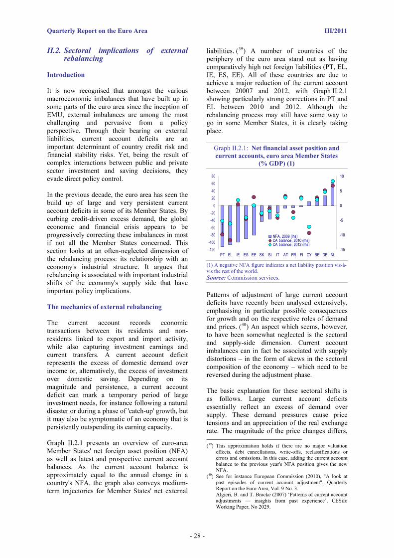
Quarterly Report on the Euro Area III/2011
II.2. Sectoral implications of external rebalancing
Introduction
It is now recognised that amongst the various macroeconomic imbalances that have built up in some parts of the euro area since the inception of EMU, external imbalances are among the most challenging and pervasive from a policy perspective. Through their bearing on external liabilities, current account deficits are an important determinant of country credit risk and financial stability risks. Yet, being the result of complex interactions between public and private sector investment and saving decisions, they evade direct policy control.
In the previous decade, the euro area has seen the build up of large and very persistent current account deficits in some of its Member States. By curbing credit-driven excess demand, the global economic and financial crisis appears to be progressively correcting these imbalances in most if not all the Member States concerned. This section looks at an often-neglected dimension of the rebalancing process: its relationship with an economy's industrial structure. It argues that rebalancing is associated with important industrial shifts of the economy's supply side that have important policy implications.
The mechanics of external rebalancing
The current account records economic transactions between its residents and non-residents linked to export and import activity, while also capturing investment earnings and current transfers. A current account deficit represents the excess of domestic demand over income or, alternatively, the excess of investment over domestic saving. Depending on its magnitude and persistence, a current account deficit can mark a temporary period of large investment needs, for instance following a natural disaster or during a phase of 'catch-up' growth, but it may also be symptomatic of an economy that is persistently outspending its earning capacity.
Graph II.2.1 presents an overview of euro-area Member States' net foreign asset position (NFA) as well as latest and prospective current account balances. As the current account balance is approximately equal to the annual change in a country's NFA, the graph also conveys medium-term trajectories for Member States' net external
liabilities. (39) A number of countries of the periphery of the euro area stand out as having comparatively high net foreign liabilities (PT, EL, IE, ES, EE). All of these countries are due to achieve a major reduction of the current account between 20007 and 2012, with Graph II.2.1 showing particularly strong corrections in PT and EL between 2010 and 2012. Although the rebalancing process may still have some way to go in some Member States, it is clearly taking place.
Graph II.2.1: Net financial asset position and current accounts, euro area Member States
(% GDP) (1)
-120-100-80-60-40-20
020406080
PT EL IE ES EE SK SI IT AT FR FI CY BE DE NL-15
-10
-5
0
5
10
NFA, 2009 (lhs)CA balance, 2010 (rhs)CA balance, 2012 (rhs)
(1) A negative NFA figure indicates a net liability position vis-à-vis the rest of the world. Source: Commission services.
Patterns of adjustment of large current account deficits have recently been analysed extensively, emphasising in particular possible consequences for growth and on the respective roles of demand and prices. (40) An aspect which seems, however, to have been somewhat neglected is the sectoral and supply-side dimension. Current account imbalances can in fact be associated with supply distortions – in the form of skews in the sectoral composition of the economy – which need to be reversed during the adjustment phase.
The basic explanation for these sectoral shifts is as follows. Large current account deficits essentially reflect an excess of demand over supply. These demand pressures cause price tensions and an appreciation of the real exchange rate. The magnitude of the price changes differs, (39) This approximation holds if there are no major valuation
effects, debt cancellations, write-offs, reclassifications or errors and omissions. In this case, adding the current account balance to the previous year's NFA position gives the new NFA.
(40) See for instance European Commission (2010), "A look at past episodes of current account adjustment", Quarterly Report on the Euro Area, Vol. 9 No. 3. Algieri, B. and T. Bracke (2007) ‘Patterns of current account adjustments — insights from past experience’, CESifo Working Paper, No 2029.
- 28 -

II. Special topics on the euro-area economy
however, across sectors leading to changes in relative prices. In particular, price increases are likely to be higher in the non-tradable sector than in the tradable sector where competition from imports tends to constrain producers' pricing behaviour. The ensuing rise in the relative price of non-tradables induces investors to move to that sector, entailing a reallocation of the economy's capital and labour resources. The skew in the economy's production structure towards non-tradables is all the more likely if the current account deficit persists over several years and therefore leaves enough time for supply forces to respond to the changes in price signals.
Two arguments suggest that sectoral skew resulting from the mechanics described above is likely to be stronger for a country in a monetary union. First, evidence from the first decade of the euro indicates that large current account deficits are easier to sustain over long periods of time in a monetary union, leading to long cycles of excess demand and giving more time for presumably slow sectoral shifts to take place.
Second, a country-specific cyclical boom is likely to be associated with comparatively stronger demand pressures in the non-tradable sector in a member of a monetary union due to an asymmetry in the adjustment process. In a country running its own monetary policy, the typical response to a cyclical upswing involves a policy tightening that affects both tradable and non-tradable activities. By contrast, in a monetary union, a bigger part of the adjustment to a country-specific cyclical upswing is market-based. This is the so-called competitiveness channel: excessive demand pressures push up inflation above the monetary union's average, leading to a steady appreciation of the real exchange rate which progressively cools off the economy by curbing exports and fuelling imports. Hence, the adjustment tends to weigh more on the tradable than on the non-tradable sector, an asymmetry that is likely to reinforce shifts in capital and labour from the tradable to the non-tradable sector.
Overall, current account rebalancing processes require improvements in competitiveness but also a reversal of the sectoral skew on the supply side accumulated during the boom phase. As demand pressures fade, demand for domestic goods weakens and domestic prices need to adjust downwards to curb excess supply. Excess supply will be particularly large for non-tradables, calling either for larger price falls in that sector and/or a reallocation of supply from non-tradable to
tradable. In the absence of appropriate price adjustment and/or sectoral shifts in labour and capital, the current account rebalancing will give rise to a lasting increase in unemployment.
An interesting implication of this analysis is that price and sectoral adjustment can be seen as complementary forces in current account rebalancing processes. The size of the price adjustment needed to bring current account back to equilibrium without excess supply depends on the magnitude of the resource reallocation process. The more easily resources are moved from the non-tradable to the tradable sector, the smaller the required competitiveness gains. Some model simulations indicate that this complementarity may be significant. (41)
Sectoral skews were clearly visible in some Member States in pre-crisis years
In the pre-crisis decade a confluence of economic tailwinds spurred domestic demand growth and expanded private sector balance sheets across the euro area, particularly in the periphery. The most prominent manifestation of this was the rapid house price appreciation and strong rise in construction and residential investment in ES and IE, which distorted these economies' industrial structure. The following two graphs show output developments for the five euro-area Member States exhibiting the largest net external liabilities ("EXT-5" – IE, EL, ES, EE, PT) with a view to detecting wider sectoral imbalances in economic activity over the past decade. (42)
A marked divergence in output growth is evident both between countries and within countries' tradable and non-tradable sectors. The euro area (EA17) depicted in Graph II.2.3 serves as an overall benchmark and shows even but slow output growth across the non-tradable and tradable sectors, with the crisis impact visible in a much sharper decline in tradable than non-tradable output in 2009. By contrast, most of the Member States of the periphery depicted in graphs II.2.2 and II.2.3 experienced rather different
(41) See e.g. Engler, P., M. Fidora and C. Thimann (2009),
‘External imbalances and the US current account: How supply-side changes affect an exchange rate adjustment’, Review of International Economics 17(5), 2009, p. 927-941.
(42) The industrial division follows the conventional grouping of ISIC codes A-E as tradable, and codes F-P as non-tradable. Due to the resulting treatment of comparatively tradable services such as wholesale and transport as non-tradable this will tend to underestimate tradable output, although the findings of this section are generally robust to the choice of tradability definition.
- 29 -

Quarterly Report on the Euro Area III/2011
developments in the run-up to the crisis and thereafter.
Graph II.2.2: Real gross value added, selected countries (2000=100, 1996-2010)
60
80
100
120
140
160
180
1996 1998 2000 2002 2004 2006 2008 2010
IE tradable IE non-tradablePT tradable PT non-tradableEL tradable EL non-tradable
Source: Commission services.
Graph II.2.3: Real gross value added, selected countries (2000=100, 1996-2010) (cont'd)
60
80
100
120
140
160
180
1996 1998 2000 2002 2004 2006 2008 2010
EE tradable EE non-tradableES tradable ES non-tradableEA17 tradable EA17 non-tradable
Source: Commission services.
Firstly, output growth was significantly faster in Ireland, Greece, Portugal, Estonia and Spain than in the euro area prior to the crisis, though with a sharper fall thereafter. Secondly, a number of countries (IE, ES, EL) experienced considerably faster growth in their non-tradables sector than for tradables.(43) Thirdly, a number of the selected Member States (IE, EL, EE) recorded a comparatively stronger fall in nontradable output in the crisis period of 2009-2010 than for tradables, unlike the euro area aggregate, which only saw falls in tradable output. These falls in non-tradable output in the EXT-5 are indicative of sectoral rebalancing processes already at work. Based on this prima facie evidence, it does appear
(43) For Greece the attribution of wholesale & retail trade (G51-
G52) and shipping & telecoms (I61& I64) is pivotal, as these jointly doubled in size between 2000 and 2007. For all the other above countries the tradability definition does not affect the picture.
that at least in Spain, Greece and Ireland a pronounced boom in non-tradable output occurred in the pre-crisis years.
The role of construction activity in explaining the nontradable boom in the periphery is considerable, but by no means accounts for all of it: construction and other non-tradable output in the EXT-5 rose in lockstep up to the crisis, at rates well above tradable output. It is however true that the crisis-induced contraction in the EXT-5 group has been particularly sharp in the construction sector.
Overall, these findings suggests that a stronger concentration of productive resources took place in nontradables in the EXT-5, thus invariably constraining tradable growth and limiting potential exports. To the extent that non-tradable output has fallen permanently since the crisis in countries such as Ireland, the ensuing relative price falls in the nontradable sector should boost tradable production.
Implications for employment
The analysis has important implications for the labour markets of Member States undergoing a major current account rebalancing. The EXT-5 countries experienced markedly faster growth in non-tradable employment than the EA17 in the pre-crisis years (see Graph II.2.4), also saw a faster rise in the share of non-tradable in total employment than the rest of the euro area. Current account adjustment economies will thus need to reallocate a significant share of employment from the non-tradable to the tradable sector in the years to come. Graph II.2.4 shows marked falls in hours worked in the nontradable sector of the EXT-5 in 2009 and 2010, suggesting that this labour reallocation process has started already.
The required labour reallocation process will not necessarily be smooth and easy. Companies' labour demand may differ significantly between the tradable and non-tradable sectors, notably in terms of required skills and qualifications and in terms of job location. This implies a risk of lasting mismatches between supply and demand. The emergence of such mismatches could be one of the explanations of the apparent disconnection between inflation and unemployment observed in some peripheral Member States. (44) In these Member States surges in unemployment rates
(44) Other possible key explanations include downward rigidities
in prices and wages and a sharp cyclical drop in labour productivity during the recession.
- 30 -

II. Special topics on the euro-area economy
have so far led to only modest deceleration in inflation. (45) This disconnect is also reflected in the European Commission estimates of the NAIRU which point to significant rises in labour market frictions in some Member States over 2010-12 (see Graph II.2.5). A small impact of unemployment on inflation implies that competitiveness rebalancing in current account deficit countries is slow.
Graph II.2.4: Total hours worked in non-tradable sector (2000=100, 2000-2010)
95
100
105
110
115
120
125
2000 2001 2002 2003 2004 2005 2006 2007 2008 2009 2010
EXT-5
Euro area
Source: Commission services.
If not properly addressed, mismatches between labour supply and demand also raise the risk of a permanent rise in unemployment thereby transforming the original external imbalance into an internal imbalance. Obviously, the risk of mismatches turning into permanent unemployment depends on the quality of labour market institutions and can be reduced by policies facilitating labour mobility, skills improvement or vocational training. As discussed in detail in Box II.2.1, an additional factor is migration. This may come as a surprise insofar as the euro area is usually seen as a region where, contrary to the US, migration plays virtually no role in adjustment to asymmetric country shocks. But, while this may have been true in the distant past, migration has clearly played a role in reducing unemployment differences in Europe in recent years. This is exemplified by the case of Ireland and Spain, where migration inflows reduced labour market tensions during the boom years and outflows are now cushioning the rise in unemployment. Besides these two countries, the box presents econometric analysis pointing to a negative relationship between net migration and unemployment in the EU and the euro area.
(45) The rise in taxes and other administrated prices in the context
of fiscal consolidation strategies are another push factor for inflation.
Graph II.2.5: NAIRU, euro-area Member States (in% of labour force)
0
2
4
6
8
10
12
14
16
18
BE DE EE IE EL ES FR IT CY LU MT NL AT PT SI SK FI EA
20072011
Source: Commission services.
Implications for investment
Successful external rebalancing will not only depend on labour reallocation but also on capital redeployment. Capital reallocation across sectors can take two main forms. Firstly, gross capital investment can flow into different industries over time, thus affecting the capital stock via incremental flow changes. Secondly, existing physical capital may in principle be sold or leased between industries, although the extent to which a significant second-hand market for productive capital exists is likely to vary greatly between industries and countries. (46) Overall, this implies that major sectoral reallocations of productive capital will occur in an incremental way, and in periods of tight credit conditions this potentially slow process may take even longer.
Abstracting from differences in depreciation rates, changes in an industry's capital stock can only take place incrementally through these two channels, so that gross fixed capital formation (GFCF) becomes a key variable of interest when identifying sectoral reallocation. Total GFCF flows have shown a clear cyclical element over the past decade and a half for the euro area as a whole, but for the EXT-5 this has been far more pronounced, where GFCF more than doubled in volume terms between the mid-nineties and 2007. The subsequent strong decline was also far more marked for the EXT-5, sending average annual investment back to its 2000 level.
While a housing boom certainly represents a non-tradable boom from a supply-side perspective, it (46) Anecdotal evidence suggests that the market for second hand
productive assets may be large in the case of vehicles, but less so in the case of machinery or even entire plants. Second-hand capital trade further appears to display a strong cross-border pattern, being typically sold from advanced industrialised countries to lesser-developed industrial nations.
- 31 -
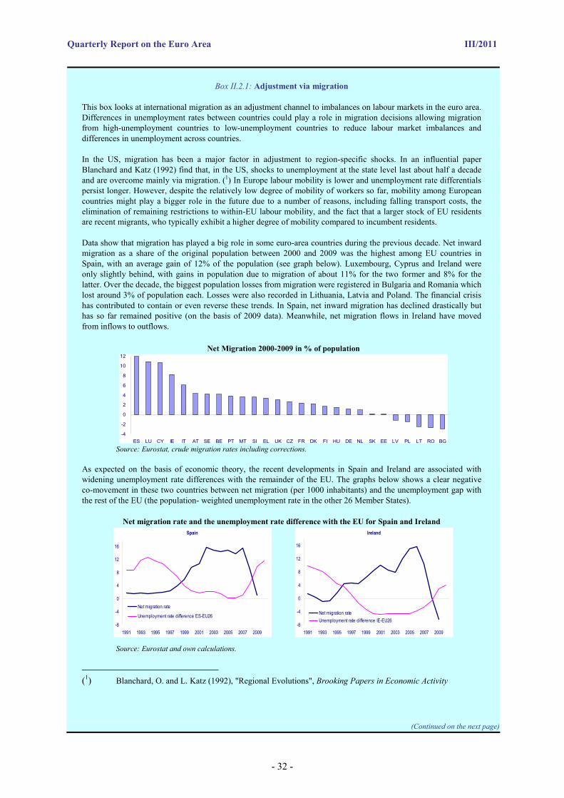
Quarterly Report on the Euro Area III/2011
Box II.2.1: Adjustment via migration
This box looks at international migration as an adjustment channel to imbalances on labour markets in the euro area. Differences in unemployment rates between countries could play a role in migration decisions allowing migration from high-unemployment countries to low-unemployment countries to reduce labour market imbalances and differences in unemployment across countries.
In the US, migration has been a major factor in adjustment to region-specific shocks. In an influential paper Blanchard and Katz (1992) find that, in the US, shocks to unemployment at the state level last about half a decade and are overcome mainly via migration. (1) In Europe labour mobility is lower and unemployment rate differentials persist longer. However, despite the relatively low degree of mobility of workers so far, mobility among European countries might play a bigger role in the future due to a number of reasons, including falling transport costs, the elimination of remaining restrictions to within-EU labour mobility, and the fact that a larger stock of EU residents are recent migrants, who typically exhibit a higher degree of mobility compared to incumbent residents.
Data show that migration has played a big role in some euro-area countries during the previous decade. Net inward migration as a share of the original population between 2000 and 2009 was the highest among EU countries in Spain, with an average gain of 12% of the population (see graph below). Luxembourg, Cyprus and Ireland were only slightly behind, with gains in population due to migration of about 11% for the two former and 8% for the latter. Over the decade, the biggest population losses from migration were registered in Bulgaria and Romania which lost around 3% of population each. Losses were also recorded in Lithuania, Latvia and Poland. The financial crisis has contributed to contain or even reverse these trends. In Spain, net inward migration has declined drastically but has so far remained positive (on the basis of 2009 data). Meanwhile, net migration flows in Ireland have moved from inflows to outflows.
Net Migration 2000-2009 in % of population
-4
-2
0
2
4
6
8
10
12
ES LU CY IE IT AT SE BE PT MT SI EL UK CZ FR DK FI HU DE NL SK EE LV PL LT RO BG Source: Eurostat, crude migration rates including corrections.
As expected on the basis of economic theory, the recent developments in Spain and Ireland are associated with widening unemployment rate differences with the remainder of the EU. The graphs below shows a clear negative co-movement in these two countries between net migration (per 1000 inhabitants) and the unemployment gap with the rest of the EU (the population- weighted unemployment rate in the other 26 Member States).
Net migration rate and the unemployment rate difference with the EU for Spain and Ireland Spain
-8
-4
0
4
8
12
16
1991 1993 1995 1997 1999 2001 2003 2005 2007 2009
Net migration rate
Unemployment rate difference ES-EU26
Ireland
-8
-4
0
4
8
12
16
1991 1993 1995 1997 1999 2001 2003 2005 2007 2009
Net migration rateUnemployment rate difference IE-EU26
Source: Eurostat and own calculations.
(1) Blanchard, O. and L. Katz (1992), "Regional Evolutions", Brooking Papers in Economic Activity
(Continued on the next page)
- 32 -
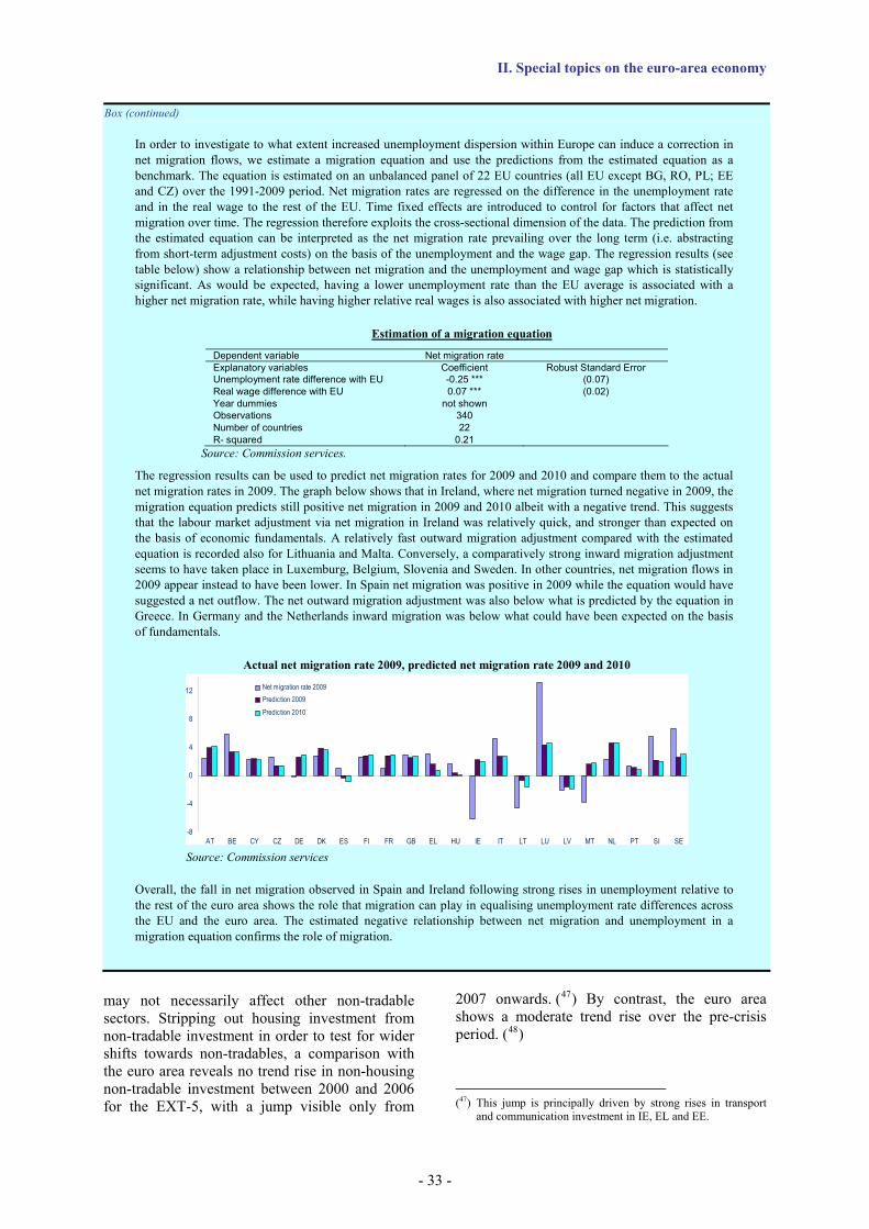
II. Special topics on the euro-area economy
may not necessarily affect other non-tradable sectors. Stripping out housing investment from non-tradable investment in order to test for wider shifts towards non-tradables, a comparison with the euro area reveals no trend rise in non-housing non-tradable investment between 2000 and 2006 for the EXT-5, with a jump visible only from
2007 onwards. (47) By contrast, the euro area shows a moderate trend rise over the pre-crisis period. (48)
(47) This jump is principally driven by strong rises in transport
and communication investment in IE, EL and EE.
Box (continued)
In order to investigate to what extent increased unemployment dispersion within Europe can induce a correction in net migration flows, we estimate a migration equation and use the predictions from the estimated equation as a benchmark. The equation is estimated on an unbalanced panel of 22 EU countries (all EU except BG, RO, PL; EE and CZ) over the 1991-2009 period. Net migration rates are regressed on the difference in the unemployment rate and in the real wage to the rest of the EU. Time fixed effects are introduced to control for factors that affect net migration over time. The regression therefore exploits the cross-sectional dimension of the data. The prediction from the estimated equation can be interpreted as the net migration rate prevailing over the long term (i.e. abstracting from short-term adjustment costs) on the basis of the unemployment and the wage gap. The regression results (see table below) show a relationship between net migration and the unemployment and wage gap which is statistically significant. As would be expected, having a lower unemployment rate than the EU average is associated with a higher net migration rate, while having higher relative real wages is also associated with higher net migration.
Estimation of a migration equation
Dependent variable Net migration rate Explanatory variables Coefficient Robust Standard Error Unemployment rate difference with EU -0.25 *** (0.07) Real wage difference with EU 0.07 *** (0.02) Year dummies not shown Observations 340 Number of countries 22 R- squared 0.21
Source: Commission services.
The regression results can be used to predict net migration rates for 2009 and 2010 and compare them to the actual net migration rates in 2009. The graph below shows that in Ireland, where net migration turned negative in 2009, the migration equation predicts still positive net migration in 2009 and 2010 albeit with a negative trend. This suggests that the labour market adjustment via net migration in Ireland was relatively quick, and stronger than expected on the basis of economic fundamentals. A relatively fast outward migration adjustment compared with the estimated equation is recorded also for Lithuania and Malta. Conversely, a comparatively strong inward migration adjustment seems to have taken place in Luxemburg, Belgium, Slovenia and Sweden. In other countries, net migration flows in 2009 appear instead to have been lower. In Spain net migration was positive in 2009 while the equation would have suggested a net outflow. The net outward migration adjustment was also below what is predicted by the equation in Greece. In Germany and the Netherlands inward migration was below what could have been expected on the basis of fundamentals.
Actual net migration rate 2009, predicted net migration rate 2009 and 2010
-8
-4
0
4
8
12
AT BE CY CZ DE DK ES FI FR GB EL HU IE IT LT LU LV MT NL PT SI SE
Net migration rate 2009Prediction 2009Prediction 2010
Source: Commission services
Overall, the fall in net migration observed in Spain and Ireland following strong rises in unemployment relative to the rest of the euro area shows the role that migration can play in equalising unemployment rate differences across the EU and the euro area. The estimated negative relationship between net migration and unemployment in a migration equation confirms the role of migration.
- 33 -
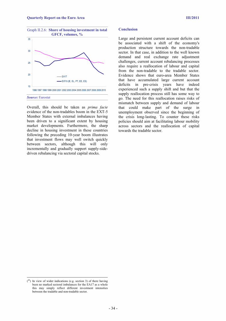
Quarterly Report on the Euro Area III/2011
- 34 -
Conclusion Graph II.2.6: Share of housing investment in total GFCF, volumes, %
Large and persistent current account deficits can be associated with a shift of the economy's production structure towards the non-tradable sector. In that case, in addition to the well known demand and real exchange rate adjustment challenges, current account rebalancing processes also require a reallocation of labour and capital from the non-tradable to the tradable sector. Evidence shows that euro-area Member States that have accumulated large current account deficits in pre-crisis years have indeed experienced such a supply shift and but that the supply reallocation process still has some way to go. The need for this reallocation raises risks of mismatch between supply and demand of labour that could make part of the surge in unemployment observed since the beginning of the crisis long-lasting. To counter these risks policies should aim at facilitating labour mobility across sectors and the reallocation of capital towards the tradable sector.
15
20
25
30
35
1996 1997 1998 1999 2000 2001 2002 2003 2004 2005 2006 2007 2008 2009 2010
EA17
EXT-5 (IE, EL, PT, EE, ES)
Source: Eurostat
Overall, this should be taken as prima facie evidence of the non-tradables boom in the EXT-5 Member States with external imbalances having been driven to a significant extent by housing market developments. Furthermore, the sharp decline in housing investment in these countries following the preceding 10-year boom illustrates that investment flows may well switch quickly between sectors, although this will only incrementally and gradually support supply-side-driven rebalancing via sectoral capital stocks.
(48) In view of wider indications (e.g. section 3) of there having
been no marked sectoral imbalances for the EA17 as a whole this may simply reflect different investment intensities between the tradable and non-tradable sector.

II. Special topics on the euro-area economy
II.3. Sectoral resilience to shocks
Introduction
Economic policy has two general goals: growth and stability. Growth aims to maximise living standards (income net of social and environmental costs) and stability aims to minimise fluctuations (booms and busts) in income, employment and prices in the short and medium term. The two goals are not independent since long-term growth is likely to be higher in a stable environment.
Resilience to shocks – i.e. the capacity of the economy to weather shocks with limited output losses - is crucial for macroeconomic stability. At firm level, resilience means the ability of enterprises to avoid bankruptcy or significant losses during economic downturns, thanks to prompt adjustment of their production technology, product characteristics, trade linkages, employment regimes, etc. At sectoral level, resilience means low responsiveness of sectoral output to shocks. It is supported by low entry and exit barriers that facilitate a more efficient reallocation of resources. The flexibility of firms and openness of sectors translates into low co-movements between sectoral output changes and aggregate common shocks. The current crisis shows that in a monetary union, the inability of countries to smoothly adjust to asymmetric shocks or to common shocks with asymmetric effects can be very costly.
The latest recession has demonstrated how important the policies supporting resilience are and, in particular, has brought to the forefront of public discussion the role that structural reforms can play. Adjustment channels other than the exchange rate are particularly important for euro-area countries, which, without national monetary and thus exchange rate policy, need to rely on the smooth and proper functioning of other adjustment mechanisms. Regulations that facilitate adjustment in firms have an important role to play in this respect. Understanding the reasons behind euro-area countries’ different resilience to shocks is a first step in identifying how to improve it, and taking into account countries’ sectoral composition and the various sectors’ different adjustment capacity to shocks could shed some light on the matter. This section examines the adjustment capacity, or resilience, of industrial sectors in the euro area to common shocks and describes the role that institutional
factors and, in particular, product market regulations, play in this adjustment process. (49)
Methodology
The starting point of the analysis is the identification of sector-level business cycles in the EU countries that are then confronted with common euro-area GDP shocks. The focus is on ‘classical’ cycles, i.e. fluctuations of output levels (rather than variations in ‘output gaps’). Resilience is defined as a low impact of common shocks on sectoral output cycles, and it is measured as the conditional correlation between sectoral output changes (over sectoral business cycle phases) and common disturbances (see Box 1 for more details). Common disturbances are defined as euro-area shocks that are derived from a small euro-area VAR model. Regression analysis is used to estimate resilience and how it is affected by product market regulations (measured by the OECD product market regulation composite indicator, PMR) and other structural variables such as the level of financial development (measured by the equity market capitalisation to GDP ratio), trade openness and participation in EMU. The industry sector is the focus of the econometric work and the analysis is carried out for 21 industry sub-sectors (2-digit NACE). The analysis of quarterly data is undertaken for the period 1980-2008, and separately for the period 2008-2010Q2.
In theory, countries’ product market regulation could be expected to have a negative effect on resilience as stricter regulations reduce the ability to adapt to shocks; however, strict regulations could also be working as a form of protectionism insulating inefficient sectors from shocks. Likewise, the level of financial development and trade openness could have a positive, but also a negative, effect on resilience. Highly integrated economies, from a financial and a trade point of view, could be more exposed to external shocks and therefore show less resilience. On the other hand, a high level of financial development and trade openness may positively affect resilience because the indicators could also capture easy access to financial markets (resulting e.g. in consumption smoothing and smaller fluctuations of investment), and the fact that more open economies tend to be more efficient, competitive and can recover quicker thanks to foreign demand
(49) The section relies heavily on a recent study commissioned by
the European Commission on the subject: Canova, F., L. Coutinho and Z. Kontolemis (2011), ‘Product market reforms and adjustment in the European economy’.
- 35 -
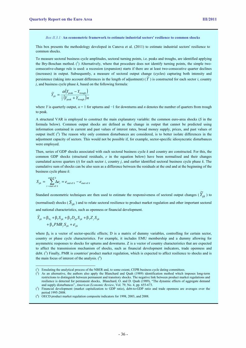
Quarterly Report on the Euro Area III/2011
Box II.3.1: An econometric framework to estimate industrial sectors' resilience to common shocks
This box presents the methodology developed in Canova et al. (2011) to estimate industrial sectors' resilience to common shocks.
To measure sectoral business cycle amplitudes, sectoral turning points, i.e. peaks and troughs, are identified applyingthe Bry-Boschan method. (1) Alternatively, where that procedure does not identify turning points, the simple two-consecutive-change rule is used: a recession (expansion) starts if there are at least two-consecutive quarter declines (increases) in output. Subsequently, a measure of sectoral output change (cycles) capturing both intensity andpersistence (taking into account differences in the length of adjustment) (Y~ ) is constructed for each sector i, country j, and business cycle phase k, based on the following formula:
( )( )nYY
YYYijk ~
troughpeak21
troughpeak
+−
=α
where Y is quarterly output, α = 1 for upturns and −1 for downturns and n denotes the number of quarters from trough to peak.
A structural VAR is employed to construct the main explanatory variable: the common euro-area shocks (S in the formula below). Common output shocks are defined as the change in output that cannot be predicted using information contained in current and past values of interest rates, broad money supply, prices, and past values ofoutput itself. (2) The reason why only common disturbances are considered, is to better isolate differences in the adjustment capacity of sectors. This would not be possible if, for example, sector-specific idiosyncratic disturbances were employed.
Then, series of GDP shocks associated with each sectoral business cycle k and country are constructed. For this, the common GDP shocks (structural residuals, e in the equation below) have been normalised and their changescumulated across quarters (t) for each sector i, country j, and earlier identified sectoral business cycle phase k. The cumulative sum of shocks can be also seen as a difference between the residuals at the end and at the beginning of thebusiness cycle phase k:
kk
k
kttijk eeeS ofstart of end
of end
ofstart
−=Δ= ∑=
Standard econometric techniques are then used to estimate the responsiveness of sectoral output changes ( ijkY~ ) to
(normalised) shocks ( ijkS ) and to relate sectoral resilience to product market regulation and other important sectoral
and national characteristics, such as openness or financial development.
ijkijkj
ijkjijkijkijkiijk
SPMR
SZSDSY
ε β
ββββ~
4
3210
++
+++=
where β0 is a vector of sector-specific effects; D is a matrix of dummy variables, controlling for certain sector,country or phase cycle characteristics. For example, it includes EMU membership and a dummy allowing forasymmetric responses to shocks for upturns and downturns. Z is a vector of country characteristics that are expectedto affect the transmission mechanism of shocks, such as financial development indicators, trade openness anddebt. (3) Finally, PMR is countries' product market regulation, which is expected to affect resilience to shocks and is the main focus of interest of the analysis. (4)
(1) Emulating the analytical process of the NBER and, to some extent, CEPR business cycle dating committees. (2) As an alternative, the authors also apply the Blanchard and Quah (1989) identification method which imposes long-term
restrictions to distinguish between permanent and transitory shocks. The negative link between product market regulations and resilience is detected for permanent shocks, Blanchard, O. and D. Quah (1989), “The dynamic effects of aggregate demand and supply disturbances”, American Economic Review, Vol. 79, No. 4, pp. 655-673.
(3) Financial development (market capitalization to GDP ratio), debt-to-GDP ratio and trade openness are averages over the period 1995-2008.
(4) OECD product market regulation composite indicators for 1998, 2003, and 2008.
- 36 -
II. Special topics on the euro-area economy
in the economies not suffering from the recession (e.g. emerging countries).
Main results
The regression results show that product market regulations negatively impact the resilience of industrial sectors. (50) This finding is in line with the effects generally predicted in the literature. Ahn (2002) argued that all components of firms’ efficiency (allocative, productive, and dynamic) are likely to be adversely affected if product markets are highly regulated. The liberalisation of product markets usually improves allocative efficiency (quicker reallocation of resources to more productive firms and sectors) by facilitating entry and exit and increasing the contestability of markets (Melitz, 2003). In addition, product market reforms aimed at increasing competition can lead to an increase in price and wage flexibility that also facilitates reallocation of resources (see for example Rotemberg and Woodford, 2001; Bulhol et al., 2006). Product market reforms are also said to increase productive efficiency through the impact on incentives for workers and managers to increase productivity (Nickell et al., 1997; Griffith and Harrison, 2004). (51)
The regression results also indicate that trade openness is not significantly correlated with resilience, contrary to the level of financial development, which has a negative and significant impact. As mentioned before this could be related to the fact that countries with more developed financial systems are more open and, hence, more exposed to external financial shocks (e.g. through portfolio and investment flows, and through the activities of multinational companies). The fact that a high level of financial development may facilitate the transmission of common shocks
(50) The results reported refer to the period 1980-2008 unless otherwise indicated.
(51) Ahn, S. (2002), ‘Competition, innovation and productivity growth: A review of theory and evidence’, OECD Economics Department Working Papers, No 317. Melitz, M. (2003), ‘The impact of trade on intra-industry reallocations and aggregate industry productivity’, Econometrica, Vol. 71, No 6, pp. 1695-1725. Rotemberg, J. and M. Woodford (1991), ‘Markups and the business cycle’, in Blanchard, O. and S. Fischer (eds.), NBER Macroeconomics Annual, Vol. 6. Boulhol, H., S. Dobbelaere, and S. Maioli (2006), ‘Imports as product and labour market discipline’, IZA Discussion Paper Series, No 2178, June. Nickell, S., D. Nicolitsas and N. Dryden (1997), ‘What makes firms perform well’, European Economic Review, Vol. 41, pp. 783-796. Griffith, R. and R. Harrison (2004), ‘The link between product market reform and macro-economic performance’, European Commission Economic Paper, No 209.
should, however, be put in perspective and weighed against the well-documented positive effect of financial deepening on growth. Finally, regression results also show that industrial sectoral output responds more to euro-area GDP shocks in countries that belong to EMU, independently of size. (52) Although this result seems obvious, it does not have to be. When the accounting bias is controlled for, the EMU dummy remains significant, most likely showing that euro-area countries are more sensitive also to shocks originating outside the euro area.
Main results for countries
Countries’ sensitivity to shocks induced by product market regulations (PMR), financial development and EMU membership is depicted in Graph II.3.1. It is evident that product market regulations play an important role in determining the resilience of countries. The countries that display a lower correlation with the euro-area shocks (e.g. Norway, Denmark, Hungary, the UK) are the ones for which the average levels of PMR over the sample are relatively low, meaning that regulatory constraints are light. In contrast, others that are at the bottom of the ranking (e.g. Spain, Greece and France) had on average relatively high PMR levels over the sample. These countries, with the exception of Greece, have nevertheless progressed significantly in lowering their levels of regulation, and this moves them up in the resilience scale if we consider only the most recent PMR levels.
The level of financial development also emerges as playing a role in determining resilience. Countries with more developed financial markets such as the UK and the Netherlands, which are relatively well positioned in terms of product market regulations, move down the resilience scale (i.e. the marginal effect of the shock, independently of sectoral composition, increases) due, presumably, to their greater exposure to shocks through financial market linkages. This finding is consistent with related business cycle literature, which tends to find that financial integration increases business cycle synchronisation across countries. (53) EMU
(52) To control for a possible accounting bias, due to the fact that large sectors in euro-area countries could be more correlated with euro-area output shocks simply because they contribute more to euro-area GDP, the analysis also controls for the size of sector and country in total euro-area production. The effect is, however, non-significant, indicating that such an accounting bias is not of much importance in the analysis.
(53) Kose, M. A., E. S. Prasad and M. E. Terrones (2004), ‘Volatility and Co-movement in an Integrated World Economy: An Exploration.’ In Macroeconomic Policies in
- 37 -

Quarterly Report on the Euro Area III/2011
membership also seems to increase susceptibility to common shocks, although, on the other hand, it presumably reduces the occurrence of country-specific shocks (a hypothesis not tested here, though). Therefore the offsetting role of vigorous reforms is even more important for countries in the euro area and for those with a high degree of financial development, as these two latter determinants increase vulnerability to common shocks.
Graph II.3.1: Sensitivity to euro-area shocks — Contribution of key country-specific
characteristics (1980-2008)
0.0 0.2 0.4 0.6 0.8 1.0 1.2 1.4
HUDKNOCZUKSEPLCHATPTDEIE
BENLIT
FRFI
ESEL
EMUFin.Dev
PMR
Each component’s contribution is the product of the estimated coefficient times the country-specific data variable (for PMR, financial development and EMU: ßPMRPMRj + ßFDFDj + ßEMUEMUj). The actual period for some countries is shorter due to data availability. See also Box 2.1.
Source: Commission services, based on Canova et al. (2011).
The ranking in Graph II.3.1 does not control for sectoral composition effects. When sectoral differences in sensitivity to shocks are accounted for, countries’ resilience is altered. (54) For some countries the effects of sectoral composition are substantial and lead to significant movements in the ranking: Germany moves down due to the relatively large weight of less resilient industries (such as manufacturing of motor vehicles). Conversely, in countries such as Greece and Italy, sectoral composition has a positive effect on resilience due to the predominance of relatively more resilient mature industries in these countries, particularly producing basic goods such as ‘food and beverages’ and ‘wearing apparel’. The sector-specific resilience is further described in the subsequent section. In general, however, the effect of country characteristics (such as PMR) dominates and sectoral composition effects do not radically change the ranking of countries.
the World Economy, ed. H. Siebert. Artis, M. J. and T. Okubo (2009), ‘Globalisation and business cycle transmission’, North American Journal of Economics and Finance, Vol. 20.
(54) Estimated using the sectoral dummy interactions, see Box 1.
Main results for sectors
Turning to the sectoral dimension, the number of cyclical fluctuations varies significantly across industry sectors. This heterogeneity could be attributed to asymmetric shocks (e.g. change in tastes), common shocks with idiosyncratic impact across sectors and countries (e.g. oil price shocks, the impact of which depends on the energy intensity of production) or policies at national or EU-wide level that are sector-specific (e.g. specific national industrial policies).
Graph II.3.2: Estimated resilience of industry subsectors to euro-area shocks (1980-2008)(1)
3.59 (trunc.)
0.0 0.4 0.8 1.2 1.6 2.
EU Average
Mining
Textlies
Leather
Wearing Apparel
Food and Beverages
Coke and Petrol
Chemicals & Pharma
Computers & Electronics
Motor Vehicles
0(1) Differences in sectoral resilience identified from significant sectoral dummy variables. The average resilience for the EU is calculated using EU sector weights; sectors for which dummy variables were not significant have resilience equal to the baseline sector (chemicals and pharmaceuticals). The three largest subsectors are marked with the dark red bars. Source: Commission services, based on Canova et al. (2011).
Concerning sectoral resilience to shocks, the commonly perceived sensitivity of the car industry to shocks is confirmed by the analysis (Graph II.3.2). This relatively low resilience is present also in another major euro-area manufacturing industry: the production of chemicals and pharmaceuticals. At the other extreme, and somehow surprisingly, mining, as well as wearing apparel, textile and leather production, which are often perceived as declining industries, appear to perform relatively well in the ranking of resilience. Clustering industrial sectors into intermediate goods, investment and consumption goods confirms that consumer goods sectors are more resilient, while those producing investment goods are less so due to more elastic demand.
The focus of the analysis in this section is on industrial sectors. To get a sense of how industry compares with other economic sectors (services, construction, etc.), the analysis was extended to a
- 38 -
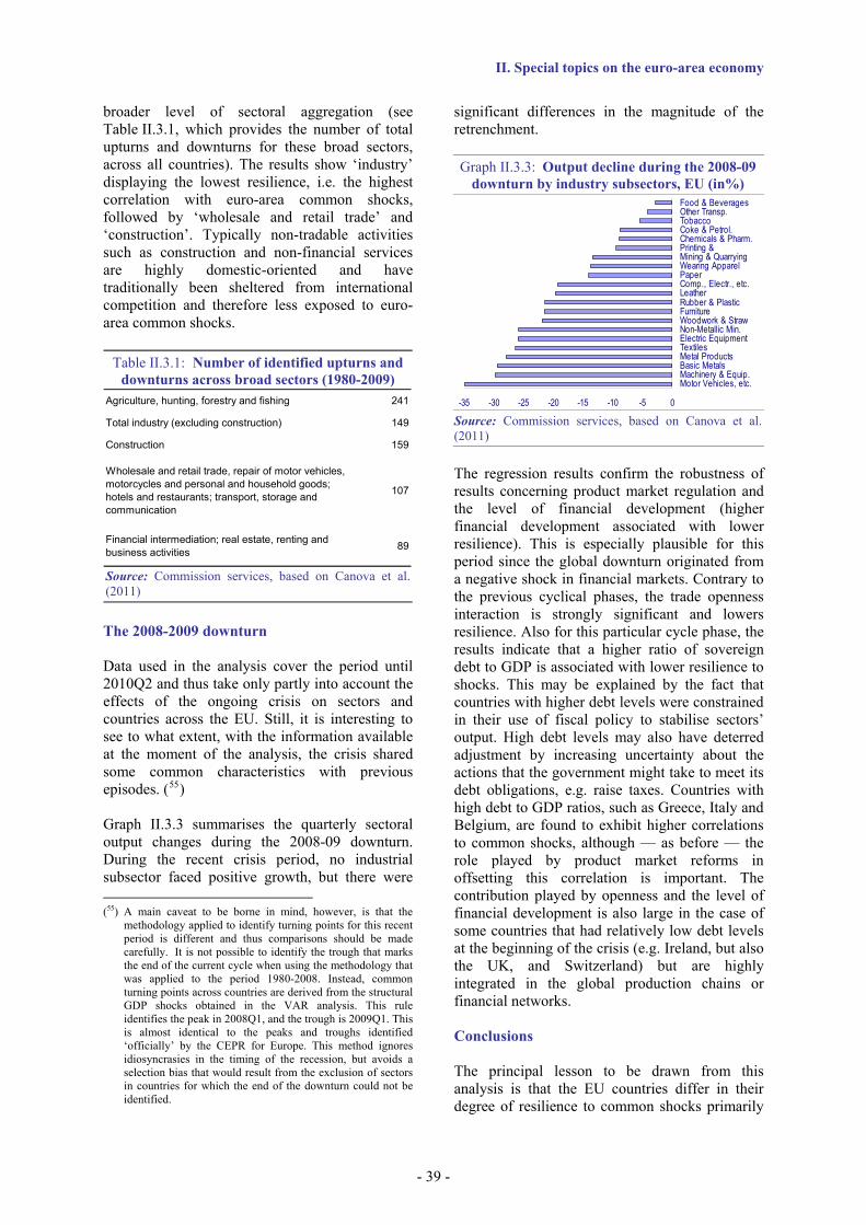
II. Special topics on the euro-area economy
broader level of sectoral aggregation (see Table II.3.1, which provides the number of total upturns and downturns for these broad sectors, across all countries). The results show ‘industry’ displaying the lowest resilience, i.e. the highest correlation with euro-area common shocks, followed by ‘wholesale and retail trade’ and ‘construction’. Typically non-tradable activities such as construction and non-financial services are highly domestic-oriented and have traditionally been sheltered from international competition and therefore less exposed to euro-area common shocks.
Table II.3.1: Number of identified upturns and downturns across broad sectors (1980-2009)
Agriculture, hunting, forestry and fishing 241
Total industry (excluding construction) 149
Construction 159
Wholesale and retail trade, repair of motor vehicles, motorcycles and personal and household goods; hotels and restaurants; transport, storage and communication
107
Financial intermediation; real estate, renting and business activities 89
Source: Commission services, based on Canova et al. (2011)
The 2008-2009 downturn
Data used in the analysis cover the period until 2010Q2 and thus take only partly into account the effects of the ongoing crisis on sectors and countries across the EU. Still, it is interesting to see to what extent, with the information available at the moment of the analysis, the crisis shared some common characteristics with previous episodes. (55)
Graph II.3.3 summarises the quarterly sectoral output changes during the 2008-09 downturn. During the recent crisis period, no industrial subsector faced positive growth, but there were (55) A main caveat to be borne in mind, however, is that the
methodology applied to identify turning points for this recent period is different and thus comparisons should be made carefully. It is not possible to identify the trough that marks the end of the current cycle when using the methodology that was applied to the period 1980-2008. Instead, common turning points across countries are derived from the structural GDP shocks obtained in the VAR analysis. This rule identifies the peak in 2008Q1, and the trough is 2009Q1. This is almost identical to the peaks and troughs identified ‘officially’ by the CEPR for Europe. This method ignores idiosyncrasies in the timing of the recession, but avoids a selection bias that would result from the exclusion of sectors in countries for which the end of the downturn could not be identified.
significant differences in the magnitude of the retrenchment.
Graph II.3.3: Output decline during the 2008-09 downturn by industry subsectors, EU (in%)
-35 -30 -25 -20 -15 -10 -5 0
Motor Vehicles, etc.Machinery & Equip.Basic MetalsMetal ProductsTextilesElectric EquipmentNon-Metallic Min.Woodwork & StrawFurnitureRubber & PlasticLeatherComp., Electr., etc.PaperWearing ApparelMining & QuarryingPrinting &Chemicals & Pharm.Coke & Petrol.TobaccoOther Transp.Food & Beverages
Source: Commission services, based on Canova et al. (2011)
The regression results confirm the robustness of results concerning product market regulation and the level of financial development (higher financial development associated with lower resilience). This is especially plausible for this period since the global downturn originated from a negative shock in financial markets. Contrary to the previous cyclical phases, the trade openness interaction is strongly significant and lowers resilience. Also for this particular cycle phase, the results indicate that a higher ratio of sovereign debt to GDP is associated with lower resilience to shocks. This may be explained by the fact that countries with higher debt levels were constrained in their use of fiscal policy to stabilise sectors’ output. High debt levels may also have deterred adjustment by increasing uncertainty about the actions that the government might take to meet its debt obligations, e.g. raise taxes. Countries with high debt to GDP ratios, such as Greece, Italy and Belgium, are found to exhibit higher correlations to common shocks, although — as before — the role played by product market reforms in offsetting this correlation is important. The contribution played by openness and the level of financial development is also large in the case of some countries that had relatively low debt levels at the beginning of the crisis (e.g. Ireland, but also the UK, and Switzerland) but are highly integrated in the global production chains or financial networks.
Conclusions
The principal lesson to be drawn from this analysis is that the EU countries differ in their degree of resilience to common shocks primarily
- 39 -

Quarterly Report on the Euro Area III/2011
- 40 -
as a result of country-specific characteristics, among which product market regulation stands out as a major factor. Within the euro area in particular, the unequal ability of countries to adjust to shocks raises policy concerns as channels of adjustment other than the monetary and exchange rate channels need to work as smoothly as possible.
The analysis also indicates that international integration — of goods and services as well as capital — may amplify the transmission of shocks. Since further advancement in integration seems inevitable in view of technological development and the irrefutable overall benefits of integration, it should go hand-in-hand with flexible functioning of product markets to reinforce the adjustment capacity. Thus vigorous reforms in product markets are particularly important for countries in the euro area and for those that are highly integrated.
Turning to the sectoral findings, the results corroborate the fragility of some sectors (e.g. car manufacturing) as well as the higher resilience of consumer goods compared with investment goods. Given cross-country differences in the
sectoral composition of output, this differentiated sectoral resilience to common shocks has an effect on the countries’ estimated resilience. However, the findings show that country-specific structural characteristics such as the level of product market regulations have a stronger impact on resilience than sectoral composition effects.
The latest deep recession is a strong common shock that can also provide insights into which factors determine the differing resilience of countries and sectors. In particular, analysis of the years 2008-09 confirms that flexible and well-functioning product markets facilitate a country’s adjustment capacity. However, the particular circumstances that triggered this recession, namely a banking crisis and ensuing financial turmoil, make it unique and drawing generalised conclusions becomes more difficult.
Future studies in this area could explore the possibilities of extending the detailed resilience analysis to other sectors, such as services. For that, though, data at sectoral level is required, in particular covering characteristics such as sector-specific product market regulations as well as sectoral effects of labour market policies.

II. Special topics on the euro-area economy
II.4. House price imbalances and structural features of housing markets
House prices and housing markets feature prominently in the monitoring of macroeconomic imbalances in the euro area. The recently adopted Excessive Imbalance Procedure (EIP) will involve regular reviews of housing markets in Member States. (56) The EIP will be based on a scoreboard comprising a concise set of key macroeconomic variables, aimed at capturing external imbalances, differences in competitiveness, and internal imbalances. These variables will also include real house prices. (57)
This section reviews the linkages between house prices and the rest of the economy and discusses a number of structural features of the housing and mortgage markets which are important for the stability of housing markets and of the broader macroeconomy.
Why should macroeconomists care about housing markets?
House prices are of interest for macroeconomic policy makers essentially for three reasons. First, fluctuations in house prices may have broader macroeconomic consequences, as house prices impact on the rest of the economy via wealth effects, fluctuations in residential construction, and the effects of those fluctuations on bank balance sheets and credit supply (see Box 1 for more details). Second, housing markets are essentially asset markets and can therefore be susceptible to speculation, periods of "irrational exuberance" and patterns of "boom and bust". Third, the structural features of housing markets (e.g. in terms of home ownership, mortgage market regulation and taxation) remain quite
(56) On 15 March 2011, the (ECOFIN) Council reached a "general approach" on the Commission's proposal for a Regulation on the prevention and correction of macroeconomic imbalances : this paved the way for the trialogue discussions with the European Parliament under the co-decision procedure.
(57) The indicator included in the scoreboard is the year-on-year change in real house prices. Although data on house price indices are provided by various institutions, the real estate market lacks a harmonized indicator fit for cross-country comparison. The only harmonised index is the Eurostat experimental house price index (HPI) which measures price developments of all residential properties purchased by households, both new and existing, independently of their final use and their previous owners. Only market prices are considered and the land component is included. The HPI currently covers the period 2005Q1-2010Q3 and 17 EU Member States. A recent Regulation on House Price Indices requires EU Member States to provide HPI data starting from 2012Q2.
heterogeneous across euro-area Member States. This could be an important cause of differences in business cycle fluctuations across countries.
There is ample evidence of the strong cyclicality of house prices. In the OECD countries, during the period 1970-1995, the typical housing cycle featured 6 years of booming prices (with a cumulated growth of 40%) and around 5 years of correction (with a cumulated adjustment of 25%).
The most recent house price cycle has been particularly pronounced, with an average length of 9 years of price increases in the period preceding the global economic and financial recession. All euro-area countries except Germany, Austria, Portugal and Cyprus (due to the short period available) witnessed a cumulated growth in prices of over 40% during the expansion phase (see Table 1). However, the length and the speed of this expansion has shown significantly variations across countries, reflecting large differences in the structure of housing and mortgage markets, as well in macroeconomic conditions.
Since the second half of 2007, euro-area housing markets have clearly entered a phase of retrenchment, with an adjustment taking place in most Member States and cumulated falls in house prices in double-digit territory in some of them (IE, ES, CY, SK, EE). Again, big differences between Member State in the speed and strength of the downturn were a noticeable feature.
The large swings in house prices observed during the past years point to the existence of significant imbalances in the housing markets of some Member States in the years preceding the crisis. Measuring the magnitude of such imbalances is technically challenging. Housing imbalances can be defined in several ways, including in terms of (i) pronounced deviations of house prices from their fundamental values, or (ii) excessive house price volatility. While the latter can be observed directly, estimating the equilibrium house price is a more challenging task, because distinguishing between fundamental and non-fundamental sources of house price movements in real time is not straightforward. House price changes are driven by current, and expected future, "fundamentals" (e.g. demographic factors, improved productivity) or by deviations from the fundamentals (e.g. due to excessive credit provision). (58)
(58) Fundamentals can also deviate from their long-term or
equilibrium values.
- 41 -
Quarterly Report on the Euro Area III/2011
Estimates of equilibrium house prices are usually accompanied by a high degree of uncertainty, mainly due to major endogeneity problems linked to identifying the contributions of supply and demand to the equilibrium prices. However, when they are interpreted with caution, estimates of equilibrium house prices can provide an indication of the magnitude of over/under-shooting, and thereby of the magnitude of the potential adjustment ahead. Bearing this in mind, previous analytical work undertaken by the Commission has found that a number of euro-area Member States entered the global economic crisis with overvalued house prices, but that much of the misalignment now seems to have been corrected
in the euro area. (59) However, other variables such as the price-to-income (affordability) ratio and price-to-rent ratio may point to a higher misalignment when current levels are compared to the long-term averages.
Over the past decade, EMU and financial integration have resulted in greater synchronisation of euro-area national real estate markets. Nevertheless, there are still large cross-country differences with regard to the structure of housing and mortgage markets, reflecting the diversity of regulatory, institutional, fiscal and financial frameworks.
(59) See for instance: European Commission (2010), ‘House price
imbalances in the euro area’, Quarterly Report on the Euro Area, Vol. 9 (3).
Box II.4.1: Housing markets and the real economy
This box reviews the three main channels through which house prices can affect the macroeconomy and economicgrowth.
1) Rising real estate prices can affect household consumption spending through a wealth effect, in the form of real estate valuations. Some empirical analyses suggest the impact of a significant fall in real estate prices may even be more important than an equivalent decline in stock prices, 1 though this finding is not unchallenged. 2
2) Rising real estate prices relative to construction costs can stimulate housing construction through higherprofitability. The reverse is true for falling house prices. A sudden decline in property prices renders investment lessattractive and reduces the profitability of the construction sector. As a result, investment may dry up and contribute toan economic slowdown. This process is also often associated with an intersectoral substitution effect that leads to a re-allocation of resources between the tradable and the non-tradable construction sector. In a boom period, higher returns in the housing sector relative to the tradable sector attract production factors from the tradable sector andthereby limit the supply of tradable products. In a bust period, economic adjustment towards higher production in the tradable sector is required, and this is often associated with low growth and high unemployment during the transitionperiod. Recent analysis by the European Commission supports this view of the importance of intersectoral substitution effects.3
3) Booms and busts in real estate markets are often correlated with large movements in monetary and creditaggregates with possible implications for macroeconomic imbalances and financial stability. Higher house prices(and therefore higher valued household collateral) reduce the influence of asymmetric information between borrowerand lender and improve lending conditions. As lenders’ willingness to supply credit increases, investment andconsumer durable expenditure increases, often reinforcing the cycle through further rises in house prices and stronger growth in credit. Over the past decade in the euro area, this process was facilitated by international capital flowswhereby corporations as well as the household sector in several deficit countries were financing themselves abroad by attracting financial resources from Member States with lower investment returns. Conversely, in the bust period,the drop in house prices reduces household collateral, contributing to write-downs and/or write-offs by banks, and leading to a sharp deceleration of credit flows in the economy.
1 Case, K., R. J. Shiller and J. M. Quigley (2001), "Comparing wealth effects: The stock market versus the housing market", NBER Working Papers 8606, National Bureau of Economic Research. 2 Buiter, W. H. (2010), "Housing wealth isn't wealth", Economics — The Open-Access, Open-Assessment E-Journal, Kiel Institute for the World Economy, vol. 4(22), pp. 1-29. 3 European Commission (2009), "Competitiveness developments in the euro area", in: Quarterly Report on the Euro Area, European Commission, DG ECFIN, Brussels, Vol. 8, No 1.
- 42 -

II. Special topics on the euro-area economy
Work on the impact of these structural differences on housing cycles and housing imbalances remains limited. The rest of this section looks at three structural features of housing and mortgage markets that have been identified in a recent study by the Centre for European Economic Research (ZEW) funded by the European Commission, as being critical for the stability of housing markets. (60) These are: the structure of home ownership, the structure of taxation, and mortgage market and housing supply responses. This analysis is a continuation of the work being done by the Commission on regulatory and supervisory tools to limit financial instability risks associated with housing bubbles. (61)
(60) ZEW Study on "Housing markets and intra-euro area
macroeconomic imbalances: Identifying policy instruments", mimeo.
(61) See for instance: European Commission (2010), "Regulatory changes in the financial sector and the prevention of housing bubbles", Quarterly Report on the Euro Area, Vol. 9 No. 4.
Home ownership and rental markets
Ownership structures differ widely between euro-area countries. Home ownership rates are particularly high in Spain, Ireland, Greece, and Italy and comparatively low in Germany. An increase in home ownership rates can be observed in most euro-area countries, and this increase is particularly pronounced in Spain. Andrews et al. (2011) find that the increase in the share of owner occupied housing during the past few decades in most OECD countries is only partially explained by changes in household characteristics, such as population ageing. (62) They further find that policy factors such as taxation incentives and rental regulation have played a role in influencing households' choice of tenure.
The empirical analysis in the aforementioned ZEW study finds that the change in the
(62) Andrews, D., A. Caldera Sanchez and A. Johansson (2011),
"Housing markets and structural policies in OECD countries", OECD Economics Department Working papers, No. 836, OECD Publishing.
Table II.4.1: Real House Price growth (in %) (1) Year-on-year Cumulative Growth Average
growth rate Cumulative Adjustment Data source
2007 2008 2009 2010
BE 4.5 0.5 -1.0 0.6 [95Q2-07Q3] 84 5.0 [07Q3-10Q4] -1 ESTAT/ECB
DE -0.4 -1.0 0.0 0.7 [08Q4-97Q1] 3 2.7 [08Q4-10Q4] -15 OECD
IE 4.1 -10.1 -16.0 -9.9 [97Q2-07Q1] 172 10.1 [07Q1-11Q1] -38 ESTAT/OECD
EL 1.7 0.6 0.3 -5.9 [00Q1-07Q3] 61 6.4 [07Q3-11Q1] -14 ESTAT/OECD
ES 6.4 -4.9 -7.2 -4.2 [95Q4-07Q3] 155 8.0 [07Q3-11Q1] -22 ESTAT/OECD
FR 4.5 -1.3 -7.2 5.0 [96Q2-07Q4] 110 6.5 [07Q4-11Q1] -1 OECD
IT 3.1 -0.6 -1.0 -1.3 [99Q4-07Q3] 43 4.7 [99Q4-07Q3] -10 ECB
CY 9.4 1.1 -7.3 -7.5 [05Q2-08Q1] 27 8.9 [08Q1-10Q4] -21 ESTAT/ECB
LU 6.9 0.2 -3.6 2.7 [95Q2-08Q2] 129 6.4 [08Q2-10Q4] -2 ESTAT/ECB
MT 19.3 7.0 -6.4 -1.5 [01Q2-08Q3] 157 13.2 [08Q3-10Q3] -11 ESTAT/ECB
NL 2.7 0.2 -4.9 -2.9 [90Q4-08Q3] 152 5.3 [08Q3-11Q1] -11 ESTAT/OECD
AT 1.5 -1.3 3.4 0.7 [04Q3-07Q2] 11 3.9 [07Q2-11Q1] 1 ESTAT/ECB
PT -1.6 1.3 1.7 0.7 [07Q4-10Q1] 7 3.1 [10Q1-11Q1] -2 ECB
SI 18.5 -2.3 -8.7 0.7 [03Q2-08Q1] 76 12.0 [08Q1-11Q1] -10 ECB
SK 14.1 5.6 -16.0 -4.5 [05Q1-08Q1] 43 12.1 [08Q1-11Q1] -29 ESTAT/ECB
FI 1.8 -1.8 -2.1 7.0 [01Q3-08Q2] 34 4.4 [08Q2-11Q1] 2 ESTAT/OECD
BG 18.6 15.2 -23.1 -10.8 [02Q2-08Q3] 225 17.3 [08Q3-11Q1] -39 ESTAT/BIS
CZ 6.6 -4.8 1.3 -8.5 [05Q4-09Q1] 13 3.7 [09Q1-10Q3] -17 ESTAT/BIS
DK 0.8 -8.2 -13.9 0.4 [93Q2-06Q3] 176 7.7 [06Q3-10Q4] -22 ESTAT/OECD
EE 5.3 -21.6 -34.8 -1.1 [03Q3-07Q2] 153 25.5 [07Q2-11Q1] -54 ECB
LV 34.0 -30.6 -30.3 -4.8 [06Q1-07Q4] 81 35.4 [07Q4-11Q1] -53 BIS
LT 28.0 0.2 -32.9 -13.0 [00Q3-08Q1] 417 22.5 [08Q1-11Q1] -46 BIS
HU -8.8 -3.2 10.7 -7.8 [02Q4-09Q1] 19 2.8 [09Q1-11Q1] -15 ESTAT/BIS
PL 126.3 -44.2 114.2 [08Q3-09Q4] 174 89.4 [09Q4-09Q4] BIS
SE 7.8 3.9 10.9 -4.7 [96Q3-09Q4] 172 7.6 [09Q4-11Q1] -12 ESTAT/OECD
UK 8.3 11 2 -0.1 [98Q1-09Q4] 162 8.3 [09Q4-11Q1] -9 ESTAT/OECD
Trough to peak (2) Peak to latest data
(1) For 2010, the latest available quarterly data point provided by Eurostat is Q3. First data point: 2001 (MT, AT), 2004 (SI), 2005 (EE), 2006 (CY). The deflator used is the consumer deflator: Household and NPISH final consumption expenditure (P31_S14_S15). (2) The peaks and troughs identification is done following a [-6, +6] quarters window, following Rousová and Van den Noord (2011), "Predicting Peaks and Troughs in Real House Prices", OECD Economics Department Working Papers, No. 882. Source: Commission services.
- 43 -

Quarterly Report on the Euro Area III/2011
homeownership rate is a key variable in explaining the volatility of house prices. Increases in the homeownership rate have a strong positive effect on the volatility of house prices. Given this result, the often-expressed political goal of increasing home ownership rates might conflict with the goal of stable housing markets characterised by low price volatility. Reasoning along these lines, subsidies or tax incentives for home owners may come at the cost of lower market stability.
Graph II.4.1: Residential mobility vs. owner occupation rates (in %, 2007) (1)
DE
DK
ES
FR
ELIEIT
NL
PT
SE
UK US
30
40
50
60
70
80
90
4 9 14 19 24
Aver
age o
wner
occu
patio
n rate
s
Average residential mobility
(1) Residential mobility is measured by the share of households that moved within the year. Source: ZEW.
Price volatility may not be the only negative consequence of high ownership rates. Given that home owners are less mobile than renters, high rates of ownership can also have major implications for residential and labour mobility. A home owner is estimated to be 11% less likely to move than a home renter. (63) Low residential mobility is typically found in countries where owner occupation rates are high, as owners typically face higher transactions costs for moving than households that live in rented houses. This can be clearly seen in Graph II.4.1, which shows a negative relationship between owner occupation rates and residential mobility, measured as the percentage of households that changed residence within the last two years.
Another finding of the ZEW study is that ownership structures and the supply of social housing are important for macroeconomic stability. A higher share of low income homeowners is positively related to house price growth and the occurrence of house price imbalances, whereas the share of social housing has a negative relationship with imbalances. The (63) Andrews et al. (2011), op. cit.
possible policy implications of this finding depend on the drivers of homeownership among low income households. If low income households are more or less forced to become homeowners because of the lack of alternatives (i.e. the rental market is not well established and there are no adequate social housing opportunities), reducing the occurrence of housing imbalances involves fostering a stable and properly functioning rental market. However, if tax incentives and subsidies, as well as the availability of mortgages with variable interest rates, are the main driving forces for low income households to become homeowners, the policy response should involve changes in the taxation system as well as mortgage market conditions.
Graph II.4.2: Low income owners and real house price growth
AU
CA
DE
DK
ES
FR
EL
IE
IT
JP
NL
PT
SE
UK
US
-1
0
1
2
3
4
0 10 20 30 40 50 60 70 80 9
Avg share of low income homeowners in low income households (1980-2005,%)
Real
hous
e pric
e grow
th (A
AG in
%, 1
970-2
010)
0
Source: ZEW.
Graph II.4.3: Rent control and real house price growth (1)
AUCA
DE
DK
ES
FR
EL
IE
IT
JP
NL
PT
SE
UK
US
-1
0
1
2
3
4
0.0 0.5 1.0 1.5 2.0 2.5 3.0 3.5 4.0 4.5 5.0
Rent control in the private rental market (2009)
Real
hous
e pric
e grow
th (A
AG in
%, 1
970-2
010)
(1) Rent control is measured with an OECD composite indicator combining data on the extent of rent controls, on how increases in rents are determined and on the permitted cost pass-through onto rents. Source: ZEW.
- 44 -

II. Special topics on the euro-area economy
Mortgage market structures and tax incentives
ZEW's analysis also shows that both house prices and credit volumes are higher in countries where variable interest rates are common (e.g. ES, UK) compared to countries where mortgage contracts with fixed interest rates prevail (e.g. DE). Moreover, the impact of credit growth on house price growth seems to be amplified in countries with variable interest rate settings and/or where mortgage interest is tax deductible. Also, housing markets are more volatile if mortgages with variable interest rates are dominant. This could provide an additional argument for housing policy to support long-term finance with fixed rates, particularly so as to avoid myopic behaviour of households which might lead to repayment difficulties further down the line.
These results are in keeping with those of a number of previous studies which have identified some key structural sources of housing instability. Almeida et al. (2006) find that the sensitivity of house prices and mortgage demand to income shocks is higher in countries where loan-to-value ratios are higher, i.e. in countries where households are on average less credit-constrained. (64) Similarly, Calza et al. (2009) conclude that more developed mortgage markets tend to magnify the impact of monetary policy shocks on house prices, residential investment and consumption. (65)
Personal income and property taxation systems may also provide incentives or deterrents to potential homebuyers. The difference between the market interest rate and the financing cost of housing, also known as the tax wedge, has a strong positive correlation with house price volatility (Van Den Noord, 2005). (66) A high inflation environment also tends to reduce real after-tax mortgage interest rates.
Taxes and subsidies consist of a wide range of different types of taxes and subsidies, the main ones being: mortgage rate deductibility, tax on imputed rents, capital gains tax, recurrent taxes on land and buildings, wealth taxes, inheritance tax, value added tax (VAT), and stamp duties.
(64) Almeida, H., M. Campello and C. Liu (2006), "The financial accelerator: Evidence from the international housing markets" Review of Finance 10 (3), pp 321–352.
(65) Calza, A., Monacelli, T. and L. Stracca (2009): "Housing finance and monetary policy", ECB Working Paper No. 1069.
(66) Van Den Noord, P. (2005), “Tax Incentives and house price volatility in the euro area: Theory and evidence”, Économie Internationale, Vol. 101 (2005), pp. 29-45.
Subsidies are often limited to first-time buyers and depend on income or the value of the house.
Supply responses
A third important structural feature that affects housing market imbalances is the flexibility/price elasticity of housing supply. The responsiveness of supply to changes in prices plays an important role in shaping house price developments. A responsive housing supply reduces house price volatility, but potentially at the expense of greater fluctuations in residential investment, with the net impact on overall economic activity being unclear. (67) Thus, it seems that during boom periods, inelastic housing supply reinforces house price overvaluation, while high supply elasticity coupled with expectations of future housing price rises may lead to overshooting in construction activity.
Both cases raise specific policy problems in both the upswing phase and the adjustment phase. Under inelastic supply, house prices may increase more in the boom period, involving a drop in affordability with negative distributional effects. During the downturn, less adjustment is needed on the supply side as shifts in labour resources from the rest of the economy to the construction sector were limited during the boom period. At the same time, in a rigid supply environment, price decreases may be more dramatic, with potential strong spillover effects on private consumption (via wealth effects) as well as on bank balance sheets (via reduced collateral values and higher rates of delinquency).
Under elastic supply, demand pressures on prices tend to be more cushioned in the upswing. (68) However, a strong response by supply during boom years may raise serious issues both in terms of diverting productive resources from the tradable sector and by leaving a large excess housing stock in the early stage of the downturn.
Even though supply is rather inelastic in the short term, it is fairly elastic in the longer term, but with big differences across EU Member States related
(67) Andrews, D., A. Caldera Sanchez and A. Johansson (2011),
"Housing markets and structural policies in OECD countries", OECD Economics Department Working papers, No. 836.
(68) While new housing units may well be built in order to take advantage of profit opportunities during a demand boom, it would seem entirely irrational for housing units to be destroyed due to price falls. Non-residential land use is the main alternative use, but land prices tend to follow house prices. Furthermore, there is no market for second-hand building materials.
- 45 -

Quarterly Report on the Euro Area III/2011
- 46 -
in part to planning restrictions. (69) Therefore, the adjustment needs that follow protracted boom phases tend to be greater, as the adjustment to a large oversupply in the housing stock is likely to be painful both for real estate companies and for construction workers who need to find a job in another sector.
Conclusion
The financial crisis has revealed the need to reconsider policy objectives for housing markets. Guaranteeing a socially acceptable minimum standard of housing for all, addressing market failures and ensuring that housing markets do not lead to a build-up of imbalances with detrimental consequences for macroeconomic stability might prove to be challenging and sometimes contradictory objectives.
(69) The main issues surrounding housing supply dynamics are
explored using the example of the UK in Kuenzel, R. and B. Bjørnbak (2008), "The UK Housing market: Anatomy of a house price boom", ECFIN Country Focus Vol. 5 Issue 11: http://ec.europa.eu/economy_finance/publications/publication13282_en.pdf
Several considerations are to be assessed against the specificity of national housing market systems. First, because of their potentially negative impact on house price stability, it is important to weigh carefully incentives for increased housing ownership, especially for low-income households. Establishing well-functioning rental markets as well as other housing opportunities (e.g. shared ownership) for lower income households may prove to be a viable alternative. Secondly, variable mortgage interest rates, high loan-to-value ratios and tax incentives for house purchase seem to increase the risk of imbalances in housing markets. Finally, more analysis is needed on the supply side of housing in order to better understand the overall impact of supply flexibility on macroeconomic stability.

III. Recent DG ECFIN publications
- 47 -
III. 1. Occasional Papers
EUROPEAN ECONOMY. OCCASIONAL PAPERS. 84. September 2011. Economic Adjustment Programme for Ireland - Summer 2011 Review http://ec.europa.eu/economy_finance/publications/occasional_paper/2011/pdf/ocp84_en.pdf EUROPEAN ECONOMY. OCCASIONAL PAPERS. 83. September 2011. The Economic Adjustment Programme for Portugal - First review - Summer 2011 http://ec.europa.eu/economy_finance/publications/occasional_paper/2011/pdf/ocp83_en.pdf EUROPEAN ECONOMY. OCCASIONAL PAPERS. 82. July 2011. The Economic Adjustment Programme for Greece - Fourth Review - Spring 2011 http://ec.europa.eu/economy_finance/publications/occasional_paper/2011/pdf/ocp82_en.pdf EUROPEAN ECONOMY. OCCASIONAL PAPERS. 81. July 2011. 2011 Economic and Fiscal Programmes of potential candidate countries: EU Commission's assessment http://ec.europa.eu/economy_finance/publications/occasional_paper/2011/pdf/ocp81_en.pdf EUROPEAN ECONOMY. OCCASIONAL PAPERS. 80. July 2011. 2011 Pre-accession Economic Programmes of candidate countries: EU Commission assessment http://ec.europa.eu/economy_finance/publications/occasional_paper/2011/pdf/ocp80_en.pdf EUROPEAN ECONOMY. OCCASIONAL PAPERS. 79. June 2011. The Economic Adjustment Programme for Portugal http://ec.europa.eu/economy_finance/publications/occasional_paper/2011/pdf/ocp79_en.pdf EUROPEAN ECONOMY. OCCASIONAL PAPERS. 78. May 2011. The Economic Adjustment Programme for Ireland - Spring 2011 Review http://ec.europa.eu/economy_finance/publications/occasional_paper/2011/pdf/ocp78_en.pdf EUROPEAN ECONOMY. OCCASIONAL PAPERS. 77. February 2011. The Economic Adjustment Programme for Greece - Third Review http://ec.europa.eu/economy_finance/publications/occasional_paper/2011/pdf/ocp77_en.pdf EUROPEAN ECONOMY. OCCASIONAL PAPERS. 76. February 2011. The Economic Adjustment Programme for Ireland http://ec.europa.eu/economy_finance/publications/occasional_paper/2011/pdf/ocp76_en.pdf EUROPEAN ECONOMY. OCCASIONAL PAPERS. 75. February 2011. Capital flows to converging European economies – from boom to drought and beyond http://ec.europa.eu/economy_finance/publications/occasional_paper/2011/pdf/ocp75_en.pdf EUROPEAN ECONOMY. OCCASIONAL PAPERS. 74. December 2010. Joint Report on Health Systems http://ec.europa.eu/economy_finance/publications/occasional_paper/2010/pdf/ocp74_en.pdf EUROPEAN ECONOMY. OCCASIONAL PAPERS. 73. December 2010. Progress towards meeting the economic criteria for accession: the assessments of the 2010 Progress Reports and the Opinions http://ec.europa.eu/economy_finance/publications/occasional_paper/2010/pdf/ocp73_en.pdf

Quarterly Report on the Euro Area III/2011
III.2. Economic Papers
EUROPEAN ECONOMY. ECONOMIC PAPERS. 445. September 2011 Narcissa Balta and Eric Ruscher Household savings and mortgage decisions: the role of the "down-payment channel" in the euro area http://ec.europa.eu/economy_finance/publications/economic_paper/2011/ecp445_en.htm EUROPEAN ECONOMY. ECONOMIC PAPERS. 444. July 2011 Ignazio Angeloni, Agnès Bénassy-Quéré, Benjamin Carton, Zsolt Darvas, Christophe Destais, Jean Pisani-Ferry, André Sapir, and Shahin Vallée. Global currencies for tomorrow: A European perspective http://ec.europa.eu/economy_finance/publications/economic_paper/2011/pdf/ecp444_en.pdf EUROPEAN ECONOMY. ECONOMIC PAPERS. 443. July 2011 Lukas Vogel. Structural reforms and external rebalancing in the euro area: A model-based analysis http://ec.europa.eu/economy_finance/publications/economic_paper/2011/pdf/ecp443_en.pdf EUROPEAN ECONOMY. ECONOMIC PAPERS. 442. March 2011 Julia Lendvai, Laurent Moulin and Alessandro Turrini. From CAB to CAAB? Correcting Indicators of Structural Fiscal Positions for Current Account Imbalances http://ec.europa.eu/economy_finance/publications/economic_paper/2011/pdf/ecp442_en.pdf EUROPEAN ECONOMY. ECONOMIC PAPERS. 441. March 2011 Matteo Barigozzi, Antonio M. Conti and Matteo Luciani. Measuring Euro Area Monetary Policy Transmission in a Structural Dynamic Factor Model http://ec.europa.eu/economy_finance/publications/economic_paper/2011/pdf/ecp441_en.pdf EUROPEAN ECONOMY. ECONOMIC PAPERS. 440. March 2011 Paolo A. Pesenti and Jan J.J. Groen. Commodity prices, commodity currencies, and global economic developments http://ec.europa.eu/economy_finance/publications/economic_paper/2011/pdf/ecp440_en.pdf EUROPEAN ECONOMY. ECONOMIC PAPERS. 439. February 2011 Pedro Gomes Fiscal policy and the labour market: the effects of public sector employment and wages http://ec.europa.eu/economy_finance/publications/economic_paper/2011/pdf/ecp439_en.pdf EUROPEAN ECONOMY. ECONOMIC PAPERS. 438. February 2011 Jordi Suriñach, Fabio Manca and Rosina Moreno. Extension of the Study on the Diffusion of Innovation in the Internal Market http://ec.europa.eu/economy_finance/publications/economic_paper/2011/pdf/ecp438_en.pdf EUROPEAN ECONOMY. ECONOMIC PAPERS. 437. February 2011 Ronald Albers and Marga Peeters. Food and Energy Prices, Government Subsidies and Fiscal Balances in South Mediterranean Countries http://ec.europa.eu/economy_finance/publications/economic_paper/2011/pdf/ecp437_en.pdf EUROPEAN ECONOMY. ECONOMIC PAPERS. 436. February 2011 Michael G. Arghyrou and Alexandros Kontonikas. The EMU sovereign-debt crisis: Fundamentals, expectations and contagion http://ec.europa.eu/economy_finance/publications/economic_paper/2011/pdf/ecp436_en.pdf EUROPEAN ECONOMY. ECONOMIC PAPERS. 435. December 2010 Lars Jonung, and Staffan Lindén. The forecasting horizon of inflationary expectations and perceptions in the EU – Is it really 12 months? http://ec.europa.eu/economy_finance/publications/economic_paper/2010/pdf/ecp435_en.pdf
- 48 -
III. Recent DG ECFIN publications
- 49 -
III.3. Other publications
Tax reforms in EU Member States 2011– October 2011 http://ec.europa.eu/economy_finance/publications/european_economy/2011/pdf/ee-2011-5_en.pdf The 2012 Ageing Report: Underlying Assumptions and Projection Methodologies – September 2011 http://ec.europa.eu/economy_finance/publications/european_economy/2011/pdf/ee-2011-4_en.pdf Interim forecast – September 2011 http://ec.europa.eu/economy_finance/articles/eu_economic_situation/pdf/2011/2011-09-interim-forecast-final_en.pdf European Economic forecast – Spring 2011 http://ec.europa.eu/economy_finance/publications/european_economy/2011/pdf/ec-forecast-spring2011.pdf Labour market developments in Europe, 2011 – Spring 2011 http://ec.europa.eu/economy_finance/publications/european_economy/2011/pdf/ee-2011-2_en.pdf Public finances in EMU – 2011 http://ec.europa.eu/economy_finance/publications/european_economy/2011/pdf/ee-2011-3_en.pdf Convergence report 2010 http://ec.europa.eu/economy_finance/publications/european_economy/2010/pdf/ee-2010-3_en.pdf
III.4. Regular publications
Business and Consumer Surveys (harmonised surveys for different sectors of the economies in the European Union (EU) and the applicant countries) http://ec.europa.eu/economy_finance/db_indicators/surveys/index_en.htm Business Climate Indicator for the euro area (monthly indicator designed to deliver a clear and early assessment of the cyclical situation) http://ec.europa.eu/economy_finance/publications/cycle_indicators/2011/pdf/2_en.pdf Key indicators for the euro area (presents the most relevant economic statistics concerning the euro area) http://ec.europa.eu/economy_finance/db_indicators/key_indicators/documents/key_indicators_en.pdf Monthly and quarterly notes on the euro-denominated bond markets (looks at the volumes of debt issued, the maturity structures, and the conditions in the market) http://ec.europa.eu/economy_finance/publications/bond_market/index_en.htm Price and Cost Competitiveness http://ec.europa.eu/economy_finance/db_indicators/competitiveness/index_en.htm

Quarterly Report on the Euro Area III/2011
Contributors to this issue are:
Focus: Debt dynamics and sustainability in the euro area
K. Berti, P. Eckefeldt, C. Frayne and M. Governatori
Internal devaluation and external imbalances: a model-based analysis
J. Lendvai, J. in't Veld and L. Vogel
Sectoral resilience to shocks J. Monteagudo and A. Rutkowski
Sectoral implications of external rebalancing F. D'Auria, R. Kuenzel and R. Voelter
House price imbalances and structural features of the housing markets
C. Cuerpo Caballero and A. Mordonu
Overall coordination and editing R. Felke and E. Ruscher
Comments on the report would be gratefully received and should be sent to the Editor-in-Chief:
Elena Flores Director – Policy strategy and coordination Economic and Financial Affairs Directorate-General European Commission Rue de la loi 200 BU1 0/209B-1049 Brussels
or by e-mail to [email protected], [email protected], [email protected]
- 50 -
Copyright © 2022 FDOKUMEN