Quantum mechanical origin of QSAR: theory and applications

R. Carbo-Dorca* , L. Amat, E. Besalu´, X. Girones, D. Robert

Institut de Quı´mica Computacional, Universitat de Girona, Girona 17071, Catalonia, Spain

Abstract

In this paper, search is carried out on how to develop the formalism where quantum similarity measures (QSM) become anatural product of the theoretical framework. This fact is later used to establish a fundamental connection between quantumtheory and QSAR, which is analysed in turn within the realm of discrete quantum chemistry. In order to perform such a task,several theoretical tools are revised in a previous step. The first section is devoted to construct the concept oftagged set. Next,the definition of quantum object (QO) is clarified by means of ideas from a quantum theory background and the previous taggedset formalism. In the definition of QO, density functions (DF) play a fundamental role and a possible simplified mathematicalpicture is presented. On the road to prepare the problem solving tools,convex setsresult to be prominent, and the notion ofvector semispaceappears as a consequence. Thetransformation rule, a device to connect wavefunctions with DF, is defined in anew step. Various products of this preliminary discussion are described, among others the concept of kinetic energy and otherobservable distributions. QSM as a source of discrete representation of molecular structures is made evident in this context.Further theoretical development intends to study discretisation, the transformation of infinite dimensionalfunctional spacesinton-dimensional ones. This result adds new perspectives to the discrete representation of QO, because it (a) provides a source ofnew QO descriptors, like a generalisation of scalar product and new similarity indices, (b) describes the QSPR theoreticalbackground enabling the construction of the adequate mathematical tools in order to discuss connected problems (limitations oflinear models, tuned-QSAR,p-valued classification of QO, among others), (c) allows the construction of sound and generalalternatives of Hammet’ss or log P parameters. All the steps above summarised are completed and illustrated, when possible,with practical application examples and visualisation pictures.q 2000 Elsevier Science B.V. All rights reserved.

Keywords: Tagged sets; Tagged ensembles; Convex sets; Vector semispaces; Definite positive operators; Discrete molecular representations;Density functions; Kinetic energy and angular momentum density functions; Electrostatic molecular potentials; Quantum objects; Similaritymatrices; QSAR; QSPR;p-Valued problems; Generalised scalar products; Generalised Carbo´ index

1. Introduction

The present contribution starts with the mathe-matical interpretation and further development ofthe ideas associated with quantum similarity measures(QSM) [1–40], which, among other possibilities, canbe used to construct discreten-dimensional mathema-tical representations of molecular structures. Thequantum object (QO) definition given in preceding

studies [41–44], and frequently used afterwards[46–81], will constitute the axis of the present form-alism. This definition previously requires a fundamen-tal one, which may be related tofuzzy settheory[82,83], but it can be independently redefined as anew collection of mathematical devices:tagged sets[84]. In this way, the theoretical discussion leads QOto become a concept inseparably coupled to densityfunctions (DF). From the point of view of QSM, forpractical purposes, first-order DF are good candidatesto be used in this kind of molecular comparisons [1]

Journal of Molecular Structure (Theochem) 504 (2000) 181–228

0166-1280/00/$ - see front matterq 2000 Elsevier Science B.V. All rights reserved.PII: S0166-1280(00)00363-8

www.elsevier.nl/locate/theochem

* Corresponding author.

although higher order DF can be employed as well[49,51,53] and other quantum systems can bestudied in the same way as molecular structures[54,55]. Several new possibilities become apparentalong the path of this theoretical development,among others, kinetic energy and electrostaticpotential density distributions as well as DF trans-formations. Thus, tagged sets, DF and QO open theway to an easy definition of QSM structure and theirgeneralisation.

Once an appropriate theoretical framework is estab-lished, the possibility of using QSM appears as anatural tool to construct somen-dimensional QOdescription. This circumstance produces, in turn, theway to study several aspects related to QSPR, such asthe theoretical foundations, new descriptors, intrinsicQSAR problems associated to linear andp-valuedmodels, among others. The QO discretisation formal-ism could be further employed to obtain a new alter-native point of view in the way quantum chemistrycan be written. It can be based on diagonal matrixspaces, already discussed in a preliminary fashionelsewhere [41–44].

In order to understand the evolution, relative to theconnection between quantum chemistry and QSAR,the originating ideas can be now discussed. Severalyears ago, Bell [45] presented various proposalsrelated to the attempt to polish some ambiguous theo-retical aspects of quantum mechanics. One of Bell’ssuggestions was to produce a set of clear backgrounddefinitions, where the theory could be easily devel-oped. Following this spirit, in the field of QSM, thepresent work is structured along a set of definitions,intended to propose a sound formal basis encompass-ing the whole area, starting from the basic aspects andending at the final applications.

Thus, this paper will be organised in the followingway: in Section 2, tagged sets and vector semispaceswill be defined. Density functions, quantum objectsand convex sets will be discussed in Section 3. Quan-tum similarity measures will follow in Section 4 andthe related subjects of discretisation and similaritymatrices will be analysed in Section 5. This previousdescription provides a study of the theoretical back-ground of QSPR and illuminates several variedaspects of the problem. When possible, numerical orgraphical application examples, related to the theore-tical development, will be given.

2. Tagged sets

Consider a collection of objects of arbitrary natureforming a set, and a collection of mathematicalelements: Boolean strings, column or row vectors,matrices, functions, etc., forming another set, whichcan be generally taken completely independent innature from the initial one. Both sets can be relatedby means of a new composite set construction,according to the following definition.

Definition 1 (Tagged sets). Let us suppose thatknown a given set, the object set,S and anotherset, made of some chosen mathematical elements,which will be hereafter called tags, form a tag set,T. A tagged set,Z, can be constructed by the orderedproduct:Z �S × T :

Z � { ;u [ Z j 's [ S ∧ 't [ T! u � �s; t�}Tagged sets constitute a mathematical structure,

present in a frequent manner within the chemicalinformation universe. Atomic or molecular parametricdescription may be made and studied inside thisgeneral but simple tagged set construction. It canbe admitted that a primitive unnoticed tagged setstructure started when chemistry was born. Indeed, amolecular structure as a chemical object of study hasattached a large cohort of attributes, accumulatingwith time. Such a situation may be generalised bysetting a tagged set formal building up rule, wheremolecules become elements of the object set andtheir ordered attributes can be attached to the tag set.

2.1. Boolean tagged sets

Tagged sets may be considered as sets such thattheir elements and any kind of coherent informationto describe them aresimultaneously taken intoaccount. The simplest among tagged sets can bedefined whenever the tag set part elements can betransformed into or expressed byn-dimensionalBoolean or bit strings. Everyn-bit string could beeasily associated with any of the 2n vertices of ann-dimensional unit length hypercube,Hn. Thus, anyset of objects, possessing some kind of informationattached to them, can be structured as a tagged set,using the appropriaten-dimensional cube vertices asthe tag set elements [41,84].

R. Carbo-Dorca et al. / Journal of Molecular Structure (Theochem) 504 (2000) 181–228182

Moreover, there appears to be present a character-istic feature, which will reappear throughout thispaper, associated to the definition of any hypercubevertex tag set. Boolean tags are formed by unit lengthn-dimensional cube vertices, which due to the bit-likenature of their components can be considered directedand included into a positive definite hyper-quadrantsection belonging to somen-dimensional space. It isalso obvious that other tagged sets can be transformedinto a Boolean form: consider a tag set made byn-tuples of rational numbers as a quite common andgeneral example. The nature of the molecular infor-mation precludes the possibility of easily transform-ing chemical tagged sets into Boolean moleculartagged sets. In general, the effortless transformationof a tagged set into a Boolean one is propitiated bytwo circumstances. First, the natural intrinsicpositivedefinite(PD) character of the experimental or theore-tical information is gathered into the tag set. Second,by the peculiar structure of modern electronic com-putational tools.

From the above point of view, Boolean tagged setscan be considered as a sort of canonical form, whichcan describe, in some ultimate way, any kind ofdiscrete rational information orderly attached to achosen object set.

Due to the nature of Boolean tags, any Booleantagged set may presentdegeneracy. By this term itis understood that two different objects share thesame Boolean tag, i.e. ifZ �S × T is a Booleantagged set, a Boolean degeneracy is defined wheneverthe following expression holds:

a;b [ Z ∧ t [ T) a � �s1; t� ∧ b � �s2; t�:

2.2. Functional tagged sets

Until now, tagged sets in this discussion have beensupposed to be implicitly constructed employingn-dimensional vector-like tag sets. However, there isno need to circumscribe tag set parts to finite-dimen-sional space subsets.

Another crucial point has to be considered beforegoing ahead in the description of tagged sets. It isrelated to Boolean tagged sets, and appears when ainfinite-dimensional hypercube vertex subset is takenas the tag set part. Then, a parallelism between theinfinite-dimensional vertices and the elements of the

[0,1] segment acting as tags naturally appears. Finally,the possible use of Boolean matrices of arbitrarydimension�m× n�; must be considered or still moregenerally: Boolean hyper-matrices, as sound candi-dates to belong to the tag set part. All these multiplepossibilities, associated to Boolean tagged sets, openthe way to consider the possible definition of stillmore general tagged sets.

As mentioned above, tag sets can also be made ofelements coming from infinite-dimensional spaces.Any function space can be considered belonging tothe infinite-dimensional class of spaces. Moreover,among all the possible function families, possessinghomogeneous properties, the most appealing candi-date, from the molecular point of view, correspondsto a subset of some probability density functionalspace.

Two reasons point towards this kind of choice.Firstly, probability DF (PDF) are normalizable, theyare PD functions too, yielding values within the [0,1]segment, and they may, thus, behave as someisomorphic infinite-dimensional limit form of aBoolean tag set. Second, according to the interpreta-tion given by von Neumann [85] or Bohm [86], PDFformed by the squared module of state wavefunctions,constitute mathematical elements attached to thedescriptive behaviour of quantum systems. Recent[87], and not so recent [45], discussions signaltowards this descriptive role of the quantum DF too.It seems that, in this case from a quantum mechanicalperspective, a PDF must be necessarily used, if one iswilling to take into account the whole informationattached to a given molecular structure.

From the preceding ideas, PDF tagged sets appearto be the natural infinite-dimensional extensionconnected to the discreten-dimensional Booleantagged sets to be used in quantum chemical applica-tions. Actually, there is no need to search for any newmathematical structure: Definition 1 as it is, stillholds, even when any infinite-dimensional spacesubset is employed as the tag set part.

The tagged set structure is so general that, withinthe functional tags one can even consider using time-dependent functions. Then, the individual behaviourof a given object set in front of time can also be takeneasily into account, both as separate time-dependentfunction or considering time forming the nature ofanother variable embedded in the functional tags.

R. Carbo-Dorca et al. / Journal of Molecular Structure (Theochem) 504 (2000) 181–228 183

An obvious example may be found in chemicalreactions. The reactants and products forming theobjects, while the reaction dynamical transformationprocess could be described by some time-dependentfunctional tags.

2.3. Vector semispaces

This broad catalogue of tag set candidates; Booleanstrings, PD n-dimensional vectors and functions,permit a great flexibility when a particularmoleculartagged setneeds to be defined. At the same time, itwill be very convenient to discuss which kind of tagsets can be chosen as candidates to fill the gapbetween a Boolean hypercube and a PDF space. Anatural choice may be constituted byn-dimensionalvector spaces with some appropriate restrictions. Thenext auxiliary definition could be used accordingly.

Definition 2 (Vector semispaces). Avector semi-space(VSS) over the PD real fieldR1, is a vectorspace (VS) with a structure of abeliansemigroupasso-ciated to the vector addition

By an additive semigroup [112], it is understoodhere, is an additive group without the presence ofreciprocal elements. So, within the VSS structure,no negative vectors are present and no vector differ-ences are defined. All VSS elements can be consid-ered, in the same way as Boolean hypercube verticesare, directed towards the region of the positive axishyperquadrant. Throughout this contribution, it willalso be accepted thatnull elementsare both includedin the scalar field as well as in the VSS structure. VSSlinear combinations are to be considered made withpositive coefficients, and so, vector co-ordinates arealways positive or in some special cases null. MetricVSS may be constructed in the same manner as theusual metric VS, taking into account that scalarproducts will also become PD, and consequently nonegative cosines of vector angles could be obtained.However, no classically defined distances areallowed, being the result of vector difference norms.Cosine-like inverses can be used instead.

In fact, any VSS could be taken as attached to someVS, if some rule is defined, describing the transforma-tion of the VS elements into a VSS. The relevant VSSgenerating rules will be discussed below.

Nothing opposes to the fact that any VSS tag setpart can be constituted by normalised vectors, whoseelements will then be numbers belonging to the unitsegment [0,1]. Thus, in this way VSS tag sets could beassociated to Boolean tag sets as described in Section2.1.

3. Density functions as object tags

In the following section, the background ideas forfundamental relationship between quantum systemsand tagged sets will be discussed. It can be admittedthat DF are, since the early times of quantummechanics, an indispensable tool to precisely definemechanical systems at the adequate microscopicscale. Therefore, tag set parts made of quantum DFare ought to be associated to quantum system’s infor-mation. The quantum theoretical structure fitsperfectly into the tagged set formalism and permitsthe definition of valuable new elements.

3.1. Quantum objects

The idea ofquantum object(QO) without a well-designed definition has been used frequently in theliterature [46–50,53]. Moreover, the backgroundmathematical structure leading towards the recentlypublished [41,42] definition of QO is to be found inthe previous section. In order to obtain a sound QOdefinition, some preliminary considerations areneeded.

3.1.1. Expectation values in classical quantummechanics

Starting from the fact that classical quantum studyof microscopic systems is essentially associated withthe following algorithm:

Algorithm 1: Classical quantum mechanics(1) Construction of the Hamilton operator,H.(2) Computation of the state energy–wavefunctionpairs, {E,C}, by solving Schrodinger equation:HC � EC:

(3) Evaluation of the state DF,r � uCu 2:

Once the state DF is known, all observable propertyvalues of the system,v , can be formally extractedfrom it, as expectation values,kvl; of the associatedhermitian operator,V , acting over the corresponding

R. Carbo-Dorca et al. / Journal of Molecular Structure (Theochem) 504 (2000) 181–228184

function,r . In the same way as in theoretical statisticsit can be written:

kvl �ZV�r �r�r � dr �1�

wherer shall be considered ap-dimensional particleco-ordinate matrix. It must be also noted that Eq. (1)can be interpreted as some scalar product or linearfunctional: kvl � kV j rl; defined within the spacewhere both the involvedV�r � and r�r � p-particleoperators belong.

A typical example of the scheme described abovemay be constituted by the electronic part ofelectro-static molecular potentials(eEMP), first employed byBonaccorsi et al. [91]. eEMP evaluated at the positionR in three-dimensional space,V(R), computed overfirst-order DF,r (r ), is defined using Eq. (1) as:

V�r � � ur 2 Ru 21 ∧ V�R� �Z

ur 2 Ru21r�r � dr : �2�

Not taking into account the electron charge sign,eEMP acts as a PD distribution, with maxima locatedat molecular nuclei. A similar form of the eEMP whencompared with the DF must be expected. This parti-cular aspect will be discussed later, and several visualexamples given.

3.1.2. Quantum object definition and generating rulesThus, after these preliminary considerations, the

next definition can be ready made.

Definition 3 (Quantum object). A quantum objectcan be defined as an element of a tagged set, madeby quantum systems in well-defined states taken asthe object set part and the corresponding densityfunctions constitute the tag set part.

The interesting fact, which must be stressed here, isthe leading role of DF played in quantum mechanicalsystems description and, as a consequence, in the QOdefinition. The DF generation in varied wavefunctionenvironments has been studied since the early times ofquantum chemistry [113]. The most appealing aspectof this situation corresponds to the way DF,r , areconstructed, starting from the original system’s wave-functions,C This formation process has been called agenerating rule[42], which can be shortened by usingthe symbol:R�C! r�: A generating rule can easily

be written, summarising the three steps of quantummechanical Algorithm 1:

R�C! r�

� { ;C [ H�C� ! 'r � C pC � uCu 2 [ H�R1�} :�3�

In Eq. (3) the wavefunction Hilbert VS [118],H(C),and the DF VSS,H(R1), are given explicitly definedover the complex and the real fields, respectively.

3.2. Density functions

It is well known [113,114] how DF can be variablereduced. Integrating the raw DF definition, whichappears in the generating rule of Eq. (3) or as thethird step of Algorithm 1, over the entire system particleco-ordinates, exceptr of them, produces arth orderDF. This kind of reduction has been studied in manyways [88,89,90,94] and will not be repeated here.

When practical implementation of QSM has beenconsidered in this laboratory, a simplified manner toconstruct the first-order DF form [95] has also beenproposed and namedatomic shell approximation(ASA) DF. A procedure has been recently described[100], bearing the correct necessary conditions toobtain PD ASA DF, possessing appropriate probabil-ity distribution properties. The ASA DF developmentcould be trivially related with the first-order DF formas expressed within MO theory, because the first-order MO DF structure can be defined as:

r�r � �X

i

wi uwi�r �u2; �4�

although this MO DF can be written in a general way,as a double sum of products of function pairs, coupledwith a set of matrix coefficients [124]. However, asimple matrix diagonalisation, followed by a unitaryMO basis set transformation, can revert DF to theformal expression in Eq. (4) (see for instance [113]or [133] for more details). The coefficient set:W �{ wi} , R1

; usually interpreted as MO occupationindices, corresponds in any case to a collection ofpositive real numbers. The original MO function set:f � {wi�r �} , H�C� belongs to a Hilbert VS, butappears when used within DF in a squared modularform, that is: F � { uwi�r �u2} , H�R1�: Thisnew basis is a set of PD functions belonging to a

R. Carbo-Dorca et al. / Journal of Molecular Structure (Theochem) 504 (2000) 181–228 185

infinite-dimensional VSS. The result of the PD linearcombination of PD functions is a PD first-order DF,r�r �. Here, a unit norm convention has been adopted.

IfZuwi u

2dr � 1;

;i )Zr�r � dr �

Xi

wi

Zuwi u

2dr �X

i

wi � 1;

�5�and this result can be interpreted considering thecoefficient setW � { wi} ; as a discrete probabilitydistribution.

W, being a PD real numerical set, can be organisedas an-dimensional vector,w � �w1;w2;…wn�: More-over, eitherW or w can be generated using a complexcoefficient set:X � { xi} , C: A new set of coeffi-cients can be obtained using the modules of theXset elements, as:wi � uxi u

2; ;i: Supposing defined a

column vector with these elements ofX : x � { xi} ;then the norm of such a vector is forced tobe:kx j xl � x1x � 1; and corresponds to the lastcondition in Eq. (5). All of this defines a device inclose parallelism and similar to the previous quantummechanical infinite-dimensional generating rule,presented in Eq. (3). For this purpose, thediscretegenerating rulecan be described as follows:

R�x! w� �

×;x [ Vn�C� ! 'w � { wi � xp

i xi � uxi u2} [ Vn�R1�

∧x1x �X

i

xpi xi �

Xi

uxi u2 � 1! kwl �

Xi

wi � 1

8><>:9>=>;:�6�

If an equivalent set of conditions as those shown inEq. (5) hold for somerth order DF basis functions, adiscrete generating rule, such as the one describedabove, can be extended to DF of arbitraryrth ordertoo.

3.3. Convex conditions and ASA fitting

3.3.1. General discussionOptimisation of the coefficient vector,w, in order to

obtain an approximate function completely adapted toab initio DF, must be restricted within the boundariesof some VSS:Vn(R

1) and the element sum,kwl, shall

be unity. This feature can be cast into a uniquesymbol, which can be referred to asconvex con-ditions, Kn(w), applying over then-dimensionalvectorw and written as:

Kn�w� ; { w [ Vn�R1� ∧ kwl �X

i

wi � 1} �7�

In a similar notation, the elements of the setW, orthese of the vector,w � { wi} ; can be used instead inthe symbol defining the convex conditions, i.e.:

Kn�{ wi} � ; { ;i:wi [ R1 ∧X

i

wi � 1} �8�

Together, Eqs. (7) and (8) can be considered thediscrete counterparts of the continuous convex con-ditions, defining a convex DF:

K∞�r� ; {r [ H�R1� ∧Zr�r � dr � 1} : �9�

Convex sets [119,120] play a leading role in optimi-sation problems. Recently, they have been introducedas an important mathematical structure to deal withchemical problems [24]. Thus, it is not strange thatconvexity may be attached to the definition of QO.Moreover, vector coefficients may be easily trans-formed by means of norm conserving orthogonaltransformations, like elementary Jacobi rotations(EJR) [121]. EJR can be applied over a generatingvector to obtain the desired optimal coefficients,while preserving convex conditions [42,81,100].

As mentioned at the end of Section 3.2, the DF formshown in Eq. (4) can be used to build up new DFelements, preservingK∞(r). If w is taken as a vector,assuming the convex conditionsKn(w), while P �{ ri�r �} # H�R1�; is used as a given set of homo-geneous order DF, then the linear combination:

r�r � �X

i

wiri�r � [ H�R1� �10�

produces a new DF with the same order and charac-teristic properties like the elements in the setP, asmentioned previously. It can be said that convexconditions over vector coefficients, affecting DFsuperpositions, are the way to allow the constructionof new DF of the same nature, bearing the same prop-erties. Quite a considerable proportion of chemicalcomputations, performed over numerous molecularsystems, is based on such principle.

R. Carbo-Dorca et al. / Journal of Molecular Structure (Theochem) 504 (2000) 181–228186

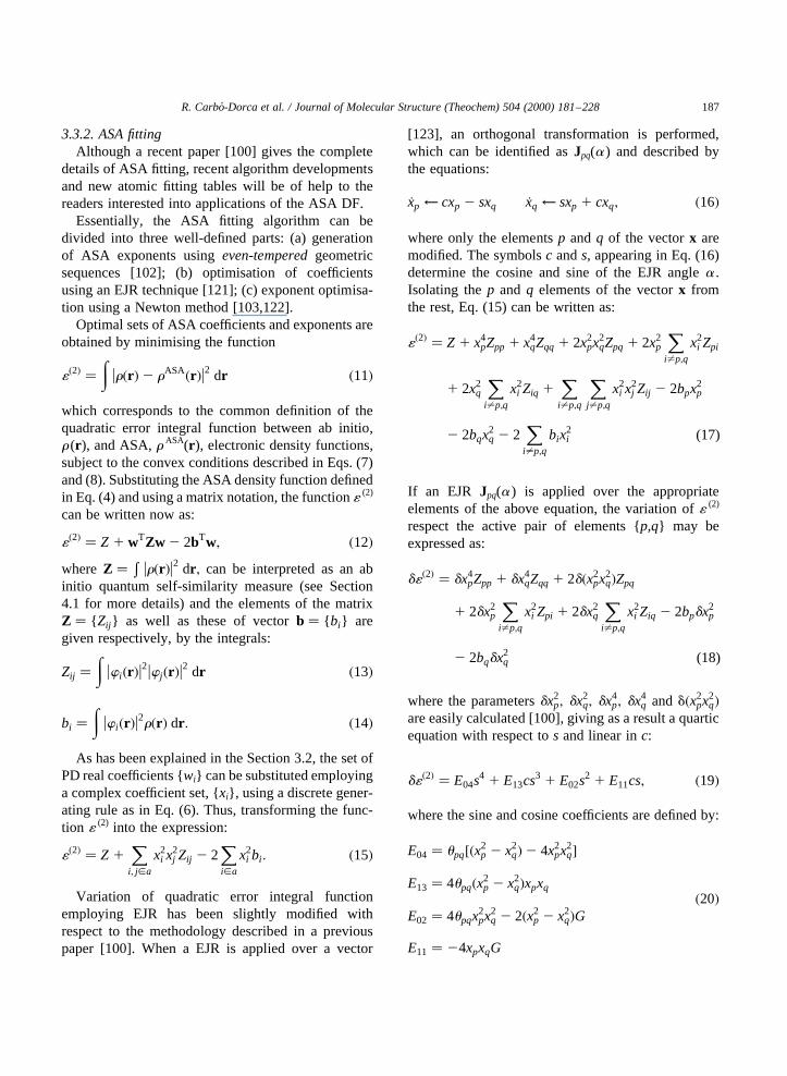
3.3.2. ASA fittingAlthough a recent paper [100] gives the complete

details of ASA fitting, recent algorithm developmentsand new atomic fitting tables will be of help to thereaders interested into applications of the ASA DF.

Essentially, the ASA fitting algorithm can bedivided into three well-defined parts: (a) generationof ASA exponents usingeven-temperedgeometricsequences [102]; (b) optimisation of coefficientsusing an EJR technique [121]; (c) exponent optimisa-tion using a Newton method [103,122].

Optimal sets of ASA coefficients and exponents areobtained by minimising the function

1�2� �Z

ur�r �2 rASA�r �u2 dr �11�

which corresponds to the common definition of thequadratic error integral function between ab initio,r (r ), and ASA,r ASA(r ), electronic density functions,subject to the convex conditions described in Eqs. (7)and (8). Substituting the ASA density function definedin Eq. (4) and using a matrix notation, the function1 (2)

can be written now as:

1�2� � Z 1 wTZw 2 2bTw; �12�where Z � R

ur�r �u2 dr ; can be interpreted as an abinitio quantum self-similarity measure (see Section4.1 for more details) and the elements of the matrixZ � { Zij } as well as these of vectorb � { bi} aregiven respectively, by the integrals:

Zij �Z

uwi�r �u2uwj�r �u2 dr �13�

bi �Z

uwi�r �u2r�r � dr : �14�

As has been explained in the Section 3.2, the set ofPD real coefficients {wi} can be substituted employinga complex coefficient set, {xi}, using a discrete gener-ating rule as in Eq. (6). Thus, transforming the func-tion 1 (2) into the expression:

1�2� � Z 1X

i; j[a

x2i x2

j Zij 2 2Xi[a

x2i bi : �15�

Variation of quadratic error integral functionemploying EJR has been slightly modified withrespect to the methodology described in a previouspaper [100]. When a EJR is applied over a vector

[123], an orthogonal transformation is performed,which can be identified asJpq(a ) and described bythe equations:

_xp ← cxp 2 sxq _xq ← sxp 1 cxq; �16�

where only the elementsp andq of the vectorx aremodified. The symbolsc ands, appearing in Eq. (16)determine the cosine and sine of the EJR anglea .Isolating thep and q elements of the vectorx fromthe rest, Eq. (15) can be written as:

1�2� � Z 1 x4pZpp 1 x4

qZqq 1 2x2px2

qZpq 1 2x2p

Xi±p;q

x2i Zpi

1 2x2q

Xi±p;q

x2i Ziq 1

Xi±p;q

Xj±p;q

x2i x2

j Zij 2 2bpx2p

2 2bqx2q 2 2

Xi±p;q

bix2i (17)

If an EJR Jpq(a ) is applied over the appropriateelements of the above equation, the variation of1 (2)

respect the active pair of elements {p,q} may beexpressed as:

d1�2� � dx4pZpp 1 dx4

qZqq 1 2d�x2px2

q�Zpq

1 2dx2p

Xi±p;q

x2i Zpi 1 2dx2

q

Xi±p;q

x2i Ziq 2 2bpdx2

p

2 2bqdx2q (18)

where the parametersdx2p; dx2

q; dx4p; dx4

q andd�x2px2

q�are easily calculated [100], giving as a result a quarticequation with respect tos and linear inc:

d1�2� � E04s4 1 E13cs3 1 E02s

2 1 E11cs; �19�

where the sine and cosine coefficients are defined by:

E04 � upq��x2p 2 x2

q�2 4x2px2

q�

E13 � 4upq�x2p 2 x2

q�xpxq

E02 � 4upqx2px2

q 2 2�x2p 2 x2

q�GE11 � 24xpxqG

�20�

R. Carbo-Dorca et al. / Journal of Molecular Structure (Theochem) 504 (2000) 181–228 187

and

G�X

i±p;q

x2i �Zpi 2 Zqi�1 x2

pZpp 2 x2qZqq 2 �x2

p 2 x2q�Zpq

2bp 1 bq

upq � Zpp 1 Zqq 2 2Zpq

The optimal sine,sp, related to the EJR procedureis obtained imposing the gradient condition�dd1�2�=ds� � 0: Then

dd1�2�

ds� 2c�T1t2 2 2T2t 2 T3� � 0 �21�

wheret � �s=c� and�dc=ds� � 2t; and a set of auxili-ary parameters:T1 � E13s

2 1 E11; T2 � 2E04s2 1

E02 andT3 � 3E13s2 1 E11 can be easily introduced.

The optimal angle,a p, to be used into the EJRJpq(a ),is computed by solving the quadratic Eq. (21) int,employing an iterative algorithm.

However, the procedure to obtaina p can be greatlyimproved using straightforward Taylor expansions[104] in order to replace thes and c expressions,present in Eq. (16). For small values of the EJRanglea , up to third order, there can be written:

c� cos�a� < 1 2a2

21 u�a3�

s� sin�a� < a 1 2a2

3!

!1 u�a3�

�22�

As a consequence, it is possible to obtain a newd1 (2)

expression, where the formerc and s values can besubstituted bya . Taking into account that the follow-ing approximate relationships hold:

s2 < a2 ∧ s3 � ss2 < a 1 2a2

3!

!a2 < a3 ∧ s4 < 0

cs< 1 2a2

2

!a 1 2

a2

3!

!< a 1 2

2a2

3

!∧ cs3

< 1 2a2

2

!a3 < a3 (23)

Then, Eq. (19) may be rewritten as:

d1�2� � a3a 1 a2b 1 ac; �24�

where a� E13 2 �2=3�E11; b� E02 and c� E11: Ifthe stationary point null gradient condition is takeninto account on Eq. (24), the following second-orderequation ina is obtained:

dd1�2�

da� 3a2a 1 2ab 1 c� 0; �25�

and the hessian:

d2d1�2�

da2 � 6aa 1 2b� ^�����������b2 2 3ac

p�26�

provides the minimum condition, which is fulfilled forthe root:

a1 � 2b 1�����������b2 2 3acp

3a; �27�

so, the optimal cosine and sine are given by:

cp < 1 2a2

1

2sp < a1 1 2

a21

6

!�28�

Using this solution into the EJR transformation, asdefined in Eq. (16), a simple expression is obtainedfor the coefficient set variation:

_xp ← coptxp 2 soptxq � 1 2a2

1

2

!xp 2 a1 1 2

a21

6

!xq

_xq ← soptxp 1 coptxq � a1 1 2a2

1

6

!xp 1 1 2

a21

2

!xq

�29�In this manner, Taylor expansions for the definition

of the sine and cosine of the EJR transformation, elim-inate the need to follow the iterative procedureemployed until now to obtaina p. As a consequence,a very small amount of computational time is requiredfor ASA fitting procedures.

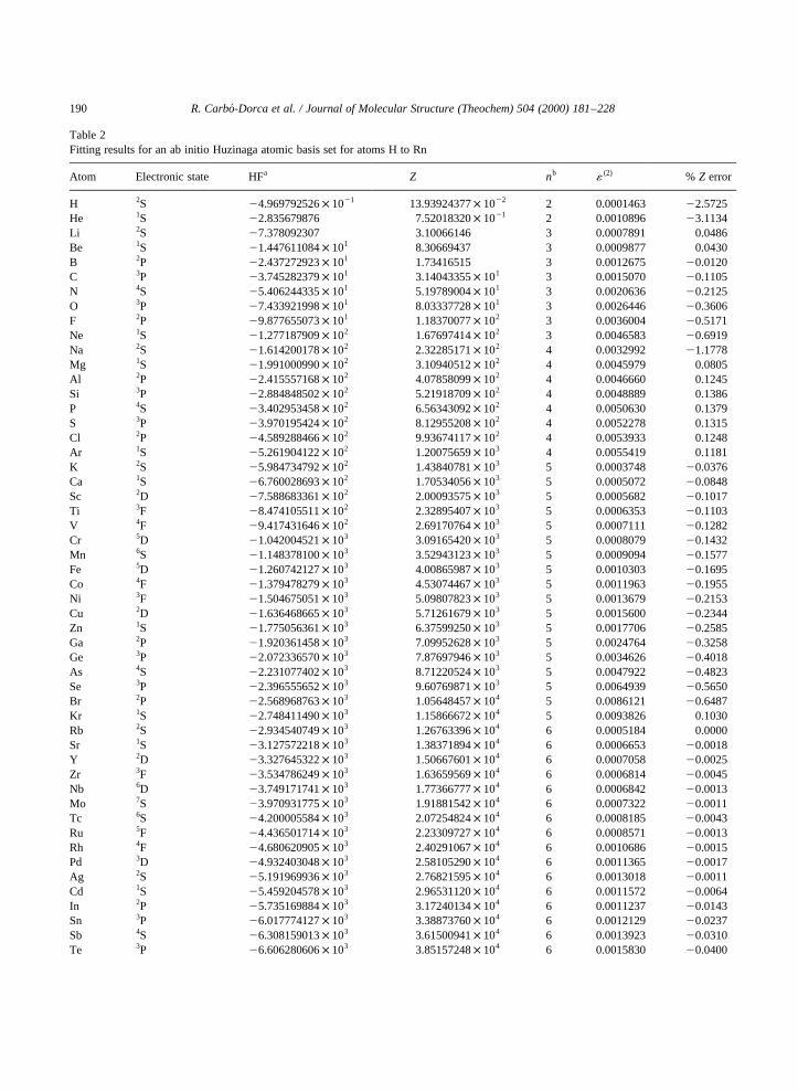
As an application example of this new algorithmdevelopment, an atomic basis set has been fitted in asimilar way as in previous work [100]. In this firststudy, an atomic density fitting of a 3-21G basis setfor atoms H to Ar was examined in great detail. Here,a new 1S-TypeGaussian basis set for atoms H to Rnhas been studied, fitting the ASA density functionsfrom an ab initio Huzinaga basis set [105,106]. Ithas been chosen, among the multiple basis setschemes provided by the reference [105], the set ofprimitive functions for ab initior (r ) calculations

R. Carbo-Dorca et al. / Journal of Molecular Structure (Theochem) 504 (2000) 181–228188

given in Table 1, which are described using the origi-nal Huzinaga’s contraction scheme notation.

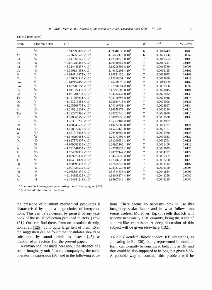
The leading results for such an ASA fitting arepresented in Table 2, where the values for theHartree–Fock energy, ab initio quantum self-similar-ity measure, number of fitted functions, the quadraticintegral function and absolute relative error for theatoms H to Rn are described. The number of atomicshells per atom varies with respect to the row of theperiodic table, and in this way, similar values of thefunction1 (2) for all the atoms are obtained.

The coefficients and exponents for this basis set ofASA functions are available for downloading at aWWW site [107].

3.4. Positive definite operators

The relationship between DF and PD operators willbe studied next.

3.4.1. General considerations on PD operatorsThe DF themselves may be considered as elements

of a VSS or also, alternatively, as members of a PDoperator set, which can be collected in turn intoanother isomorphic VSS, whose elements may beconsidered PD operators.

The most relevant thing to be noted in the contextof PD operator VSS, as well as in the isomorphic VSScompanions structure, is theclosed natureof suchVSS, when appropriate PD coefficient sets areknown, i.e. PD linear combinations of PD operatorsremain PD operators. Discrete matrix representationsof such PD operators are PD too, and PD linear combi-nations of PD matrices will remain PD in the sameway. These properties can be expressed in a compactand elegant way, using convex conditions symbols, aspreviously discussed in Section 3.3.1: if {K∞(r i), ;i}andKn(w) hold, then Eq. (10) is a convex functionfulfilling K∞(r).

3.4.2. Differential operators and kinetic energyThere is another interesting question, which has not

been deservingly discussed in the literature yet. Itcould be attached to the interpretation of the role ofdifferential operators, as momentum representativeswithin the framework of classical quantum mechanicswhen the position space point of view is chosen,which constitutes the usual, most frequent, computa-tional chemistry option.

3.4.2.1. Statement of the problem.There appears to bepresent a formal puzzle, when one tries to connect asecond-order differential operator, representing theQO kinetic energy (KE), using the expression of anexpectation value. KE expectation values do not fulfilthe usual statistical formalism represented by Eq. (1),but they possess a kind of expression, whichadequately transformed and, avoiding scalar factors,looks like a norm, when writing the equalities:

2kKl � 2ZC p7 2C dV �

Z�7C� p�7C� dV; �30�

where the change of sign can be attributed to Green’sfirst identity [93].

The available textbooks do not explain this situa-tion (see for a recent example Ref. [92]). However, thecurrent literature presents it as a de facto characteristicand the usual trend is to classify this oddity withinthe fuzziness of quantum mechanical postulates.Discussed since the formulation of quantum theory,

R. Carbo-Dorca et al. / Journal of Molecular Structure (Theochem) 504 (2000) 181–228 189

Table 1Notation for the contracted Gaussian primitive basis set

Atomic symbol Huzinaga notationa

H, He 3Li, Be 33B, C, N, O, F, Ne 33/3Na, Mg 432/3Al, Si, P, S, Cl, Ar 432/42K, Ca 4322/42Sc, Ti, V, Cr, Mn, Fe,Co, Ni, Cu, Zn

4322/42/3

Ga, Ge, As, Se, Br, Kr 4322/422/3Rb, Sr 43222/422/3Y, Zr, Nb, Mo, Tc, Ru,Rh, Pd, Ag, Cd

43222/422/33

In, Sn, Sb, Te, I, Xe 43222/4222/42Cs, Ba 432222/4222/42La 432222/4222/42/3Ce, Pr, Nd, Pm, Sm,Eu, Gd, Tb, Dy, Ho, Er,Tm, Yb

432222/4222/42/4

Lu, Hf, Ta, W, Re, Os,Ir, Pt, Au, Hg

432222/4222/423/3

Tl, Pb, Bi, Po, At, Rn 432222/42222/422/3

a The expansion pattern: (Ks1, Ks2,…/Kp1, Kp2,…/Kd1, Kd2,…/Kf1,…) is used as the notation to specify the number of terms inthe expansion of the atomic basis set [104].

R. Carbo-Dorca et al. / Journal of Molecular Structure (Theochem) 504 (2000) 181–228190

Table 2Fitting results for an ab initio Huzinaga atomic basis set for atoms H to Rn

Atom Electronic state HFa Z nb 1 (2) % Z error

H 2S 24.969792526× 1021 13.93924377× 1022 2 0.0001463 22.5725He 1S 22.835679876 7.52018320× 1021 2 0.0010896 23.1134Li 2S 27.378092307 3.10066146 3 0.0007891 0.0486Be 1S 21.447611084× 101 8.30669437 3 0.0009877 0.0430B 2P 22.437272923× 101 1.73416515 3 0.0012675 20.0120C 3P 23.745282379× 101 3.14043355× 101 3 0.0015070 20.1105N 4S 25.406244335× 101 5.19789004× 101 3 0.0020636 20.2125O 3P 27.433921998× 101 8.03337728× 101 3 0.0026446 20.3606F 2P 29.877655073× 101 1.18370077× 102 3 0.0036004 20.5171Ne 1S 21.277187909× 102 1.67697414× 102 3 0.0046583 20.6919Na 2S 21.614200178× 102 2.32285171× 102 4 0.0032992 21.1778Mg 1S 21.991000990× 102 3.10940512× 102 4 0.0045979 0.0805Al 2P 22.415557168× 102 4.07858099× 102 4 0.0046660 0.1245Si 3P 22.884848502× 102 5.21918709× 102 4 0.0048889 0.1386P 4S 23.402953458× 102 6.56343092× 102 4 0.0050630 0.1379S 3P 23.970195424× 102 8.12955208× 102 4 0.0052278 0.1315Cl 2P 24.589288466× 102 9.93674117× 102 4 0.0053933 0.1248Ar 1S 25.261904122× 102 1.20075659× 103 4 0.0055419 0.1181K 2S 25.984734792× 102 1.43840781× 103 5 0.0003748 20.0376Ca 1S 26.760028693× 102 1.70534056× 103 5 0.0005072 20.0848Sc 2D 27.588683361× 102 2.00093575× 103 5 0.0005682 20.1017Ti 3F 28.474105511× 102 2.32895407× 103 5 0.0006353 20.1103V 4F 29.417431646× 102 2.69170764× 103 5 0.0007111 20.1282Cr 5D 21.042004521× 103 3.09165420× 103 5 0.0008079 20.1432Mn 6S 21.148378100× 103 3.52943123× 103 5 0.0009094 20.1577Fe 5D 21.260742127× 103 4.00865987× 103 5 0.0010303 20.1695Co 4F 21.379478279× 103 4.53074467× 103 5 0.0011963 20.1955Ni 3F 21.504675051× 103 5.09807823× 103 5 0.0013679 20.2153Cu 2D 21.636468665× 103 5.71261679× 103 5 0.0015600 20.2344Zn 1S 21.775056361× 103 6.37599250× 103 5 0.0017706 20.2585Ga 2P 21.920361458× 103 7.09952628× 103 5 0.0024764 20.3258Ge 3P 22.072336570× 103 7.87697946× 103 5 0.0034626 20.4018As 4S 22.231077402× 103 8.71220524× 103 5 0.0047922 20.4823Se 3P 22.396555652× 103 9.60769871× 103 5 0.0064939 20.5650Br 2P 22.568968763× 103 1.05648457× 104 5 0.0086121 20.6487Kr 1S 22.748411490× 103 1.15866672× 104 5 0.0093826 0.1030Rb 2S 22.934540749× 103 1.26763396× 104 6 0.0005184 0.0000Sr 1S 23.127572218× 103 1.38371894× 104 6 0.0006653 20.0018Y 2D 23.327645322× 103 1.50667601× 104 6 0.0007058 20.0025Zr 3F 23.534786249× 103 1.63659569× 104 6 0.0006814 20.0045Nb 6D 23.749171741× 103 1.77366777× 104 6 0.0006842 20.0013Mo 7S 23.970931775× 103 1.91881542× 104 6 0.0007322 20.0011Tc 6S 24.200005584× 103 2.07254824× 104 6 0.0008185 20.0043Ru 5F 24.436501714× 103 2.23309727× 104 6 0.0008571 20.0013Rh 4F 24.680620905× 103 2.40291067× 104 6 0.0010686 20.0015Pd 3D 24.932403048× 103 2.58105290× 104 6 0.0011365 20.0017Ag 2S 25.191969936× 103 2.76821595× 104 6 0.0013018 20.0011Cd 1S 25.459204578× 103 2.96531120× 104 6 0.0011572 20.0064In 2P 25.735169884× 103 3.17240134× 104 6 0.0011237 20.0143Sn 3P 26.017774127× 103 3.38873760× 104 6 0.0012129 20.0237Sb 4S 26.308159013× 103 3.61500941× 104 6 0.0013923 20.0310Te 3P 26.606280606× 103 3.85157248× 104 6 0.0015830 20.0400

the presence of quantum mechanical postulates ischaracterised by quite a large choice of interpreta-tions. This can be evidenced by perusal of any text-book of the usual collection provided in Refs. [125–131]. One can find there, from no postulate descrip-tion at all [125], up to quite large lists of them. Eventhe suggestion can be found that postulates should besubstituted by sound definitions instead [45], asmentioned in Section 1 of the present paper.

A remark shall be made here about the absence of ascalar imaginary unit factor accompanying the nablaoperator in expression (30) and in the following equa-

tions. There seems no necessity now to use thisimaginary scalar factor and in what follows tooseems useless. Moreover, Eq. (30) tells that KE willbecome necessarily a DP quantity, being the result ofa norm-like expression. A deep discussion of thissubject will be given elsewhere [132].

3.4.2.2. Extended Hilbert spaces.KE integrands, asappearing in Eq. (30), being represented in modularform, can formally be considered behaving as DF, andthus could be also supposed to belong to a given VSS.A possible way to consider this problem will be

R. Carbo-Dorca et al. / Journal of Molecular Structure (Theochem) 504 (2000) 181–228 191

Table 2 (continued)

Atom Electronic state HFa Z nb 1 (2) % Z error

I 2P 26.912293010× 103 4.09840835× 104 6 0.0018443 20.0480Xe 1S 27.226259525× 103 4.35652173× 104 6 0.0021366 20.0562Cs 2S 27.547866175× 103 4.62560670× 104 7 0.0016553 0.0108Ba 1S 27.877289281× 103 4.90580352× 104 7 0.0017217 0.0103La 2F 28.214448257× 103 5.19296892× 104 7 0.0016739 0.0095Ce 3H 28.560134394× 103 5.49392201× 104 7 0.0018155 0.0102Pr 4I 28.914118872× 103 5.80521430× 104 7 0.0018673 0.0103Nd 5I 29.276534340× 103 6.12856051× 104 7 0.0019810 0.0111Pm 6H 29.647454065× 103 6.46418670× 104 7 0.0019589 0.0102Sm 7F 21.002700168× 104 6.81196354× 104 7 0.0037966 20.0997Eu 8S 21.041527457× 104 7.17297705× 104 7 0.0020845 0.0104Gd 7F 21.081201752× 104 7.54534432× 104 7 0.0027032 0.0136Tb 6H 21.121763004× 104 7.93110897× 104 7 0.0023948 0.0118Dy 5I 21.163216483× 104 8.32934713× 104 7 0.0024998 0.0121Ho 4I 21.205563774× 104 8.74110751× 104 7 0.0028697 0.0134Er 3H 21.248813204× 104 9.16858375× 104 7 0.0024286 0.0110Tm 2F 21.292976991× 104 9.60751440× 104 7 0.0025990 0.0115Yb 1S 21.338065566× 104 1.00623338× 105 7 0.0030558 0.0139Lu 2D 21.383819206× 104 1.05352182× 105 7 0.0058882 20.1618Hf 3F 21.430740505× 104 1.10222989× 105 7 0.0029727 0.0121Ta 4F 21.478572471× 104 1.15253120× 105 7 0.0027151 0.0104W 5D 21.527318958× 104 1.20430854× 105 7 0.0031980 0.0128Re 6S 21.576990684× 104 1.25773802× 105 7 0.0030633 0.0120Os 5D 21.627572807× 104 1.31290650× 105 7 0.0032791 0.0128Ir 4F 21.679088555× 104 1.36962105× 105 7 0.0031468 0.0113Pt 3F 21.731541053× 104 1.42790927× 105 7 0.0033635 0.0125Au 2D 21.784934901× 104 1.48797142× 105 7 0.0034272 0.0122Hg 1S 21.839279390× 104 1.54963238× 105 7 0.0035502 0.0125Tl 2P 21.894511809× 104 1.61306625× 105 7 0.0037250 0.0120Pb 3P 21.950699432× 104 1.67855642× 105 7 0.0038512 0.0107Bi 4S 22.007825555× 104 1.74587237× 105 7 0.0039560 0.0094Po 3P 22.065884451× 104 1.81514538× 105 7 0.0041634 0.0091At 2P 22.124889325× 104 1.88606874× 105 7 0.0043268 0.0082Rn 1S 22.184844245× 104 1.95907846× 105 7 0.0045285 0.0080

a Hartree–Fock energy computed using theatomic program [108].b Number of fitted atomic functions.

shortly described in terms of all things said up to now.Supposing that the original Hilbert space,H(C),where wavefunctions belong, is modified intoanother extended one,H �7��C�; which also containsthe wavefunction first derivatives, the quantummechanical momentum representation, that is:

;C [ H�C� ) C [ H �7��C� ∧ '7�C� [ H �7��C�

Then, considering the attached VSS,H(R1), wherethe DF belong, one can also accept that:

;r � uCu 2 [ H�R1� ) 'k � u7Cu 2 [ H�R1�to every DF,r , there exists in this way a momentumDF or perhaps, one can call, in a better way, this kindof distribution: KE DF,k , belonging to a Hilbert VSS.The KE DF when integrated provides the expectationvalue of the QO KE. The following sequence,developing details appearing in Eq. (30), will shedlight over the proposed question:

2kKl �Zk dV �

Zu7Cu 2 dV �

Z�7C� p�7C� dV

� 2ZC pu7u 2C dV � 2ku7u 2l ; 2

ZC pDC dV

� 2kDl;

where the minus sign appears as a consequence ofGreen’s first identity [93], as has been observedwhen Eq. (30) was discussed.

It can be concluded that KE can be consideredrelated to the norm of momentum, the QO wave-functions gradient. As a consequence, it could beinteresting, to obtain KE DF,k , maps or images inthe same way as they are customarily obtained for theDF, r [24,25]. A complementary information to elec-tronic DF will surely be obtained from these represen-tations. Similar behaviour of both functions at largedistances from the molecular nuclei shall be expected,but with very different behaviour near the nuclei.

3.4.2.3. Generating rules.It seems plausible tosummarise the features of this discussion. To obtaina coherent picture, with KE occupying a sound place,among other quantum mechanical structures, then theHilbert VS, H �7��C�; could be defined not onlycontaining wavefunctions but their first derivatives

too. This allows to construct the associated DF VSS,H �7��R 1�; as containing not only DF but also KEDF. The elements of this peculiar Hilbert VS, whereboth wavefunctions and their gradients are contained,can be ordered in the form of column vectors, like:

uFl � uC;7Cl [ H �7��C�;this form can be attached to a scalar to vectortransformation using a vectorial operator, involvingthe gradient, such as:

u1;7l�C� � uC;7Cl � uFl:

or by a diagonal transformation, employing the sameelements:

Diag�1;7�uCl � Diag�uCl;7uCl� � uFl: �31�In the case of one particle QO, the necessaryquadrivector structure, adopted by the extendedwavefunctions, acquire a qualitative similarity torelativistic spinors [134,135]. In order to obtainmathematical coherence, even non-relativistic quantummechanics, it seems, could be easily attached to avector-like wavefunction representation, originatingdue to the presence of momentum and thus of KEdifferential operators.

The generating rule within the extended wave-function domain, can be written now as:

R�uFl! ur;kl�

�;uFl � uC;7Cl [ H �7��C� !

'r � C pC � uCu 2 ∧ 'k � �7C� p�7C�� u7Cu 2 ) ur;kl [ H�7��R 1�

8>><>>:9>>=>>;:�32�

The DFr can be considered normalised, accordingto Eq. (5). The KE DFk , can be normalised too, thegradient density norms being in absolute value twicethe kinetic energykKl: This amounts the same as toconsider the extended wavefunction,uFl : kFuFl ��1 1 2kKl�; normalised. This is a consequence of thecharacteristics of the spaces containing both, thewavefunction and their gradient, whose elements,then, should be considered square summable func-tions. The normalisation of the extended wave-function uFl; may produce, perhaps, an energyscaling as interesting as the squared particle number

R. Carbo-Dorca et al. / Journal of Molecular Structure (Theochem) 504 (2000) 181–228192

scale factors, as discussed before [42]. However, theproperty that really matters is the generating wave-function normalisability.

The projectors associated to the extended quantummechanical wavefunctions will possess a matrixstructure like:

uFlkFu � uCu 2 C p�7C��7C� pC u7Cu 2

0@ 1A � P

then, using the symmetrisation:Q� �1=2��P1 1 P�;the new projector could be written as the matrix:

Q� r u jl

k ju k

!so: Tr�Q� � Tr�P� � r 1 k; and the off-diagonalelements can be related to the current density:

u jl � 12 �C p�7C�1 �7C� pC�:

3.4.2.4. Diagonal Hamiltonian operators.There isonly a final point to underline: the calculation ofenergy expectation values, within the extendedHilbert space framework. This can be done, forexample, using the Born–Oppenheimer approach,defining an electronic Hamilton operator with adiagonal matrix structure and, in addition, supposinguCl normalised:

H � diag�V; 12 I � ∧ kC j Cl � 1) E � kFuHuFl

� kCuVuCl 1 12 k7C j 7Cl ; kVl 1 kKl: (33)

In the diagonal Hamilton operator definition,V is thepotential part andI , a unit matrix with the appropriatedimension. In any case, the KE inverse mass factors ifneeded, could be supposed implicitly inserted into thegradient symbols, if necessary. This result allows thepossible use of standard variational procedures, evenin the extended spaceH �7��C�:

It can be seen that, not only the Hamiltonian opera-tor could be written as a diagonal matrix, but theelements of the extended Hilbert space too, as hasbeen shown in Eq. (31). So, the system energy inEq. (33) can be also written from this alternativepoint of view as a trace of a diagonal matrix:

E � kFuHuFl � kDiag�kCuVuCl; 12 k7C j 7Cl�l;

where the symbolkAl is constructed according to thedefinition:

Definition 4 (Elements sum of a (m× n) matrixA). Known a (m× n) matrix A � { aij } by thesymbolkAl it is meant:

kAl �Xmi�1

Xnj�1

aij :

It must be noted here that whenA � Diag�ai�; thenkAl � TruAu: Also, the matrix operationkAl can beconsidered a linear transformation from the�m× n�matrix vector space to the background definition field.

3.4.2.5. ASA kinetic energy DF.ASA DF formalismcould be easily extended to KE DF formalism. In thiscase, as ASA DF can be considered constructed by thegeneral MO DF form, as in Eq. (4), then the MO KEDF may be written accordingly as:

k�r � �X

i

vi u7w i�r �u 2: �34�

Because in ASA the basis functions {wi�r �} areassumed to be normalised 1s GTO functions, withcentre at the positionRI , one can write the gradientvector as:

7w i�r � � 7�N�a i� exp�2ai ur 2 RI u2��

� 22ai�r 2 RI �wi�r �;and after this, one can obtain straightforwardly theASA KE DF expression:

k�r � � 4X

i

gi ur 2 RI u2uwi�r �u2;

usinggi � via2i : This result, in the above framework,

tells that ASA KE DF basis functions acquire afunctional structure as a 2s GTO.

3.4.2.6. Quadrupole DF.These previous findingsallow us to think of the possible use of another setof elements in EHS, made with the extended partmultiplied by the position vector, as:uxl � uC; rCl:The new extended functions are the quantummechanical position companions of the formermomentum functions:uFl � uC;7Cl: In the samemanner as before for the extended functionsuFl; a

R. Carbo-Dorca et al. / Journal of Molecular Structure (Theochem) 504 (2000) 181–228 193

density and a projector can be also described foruxl: Aquadrupole DF (QDF) can be thus defined as:

q�r � � ur u 2r�r �;forming part of the density function attached to thisnew breed of extended functions:

uxu2 � r 1 ur u2r � �1 1 ur u2�r � r�r �1 q�r �:Also, this new extended DF can be obtained as thetrace of the projector:

uxlkxu � 1 ur l

kr u ur lkr u

!r � r uml

kmu Q

!;

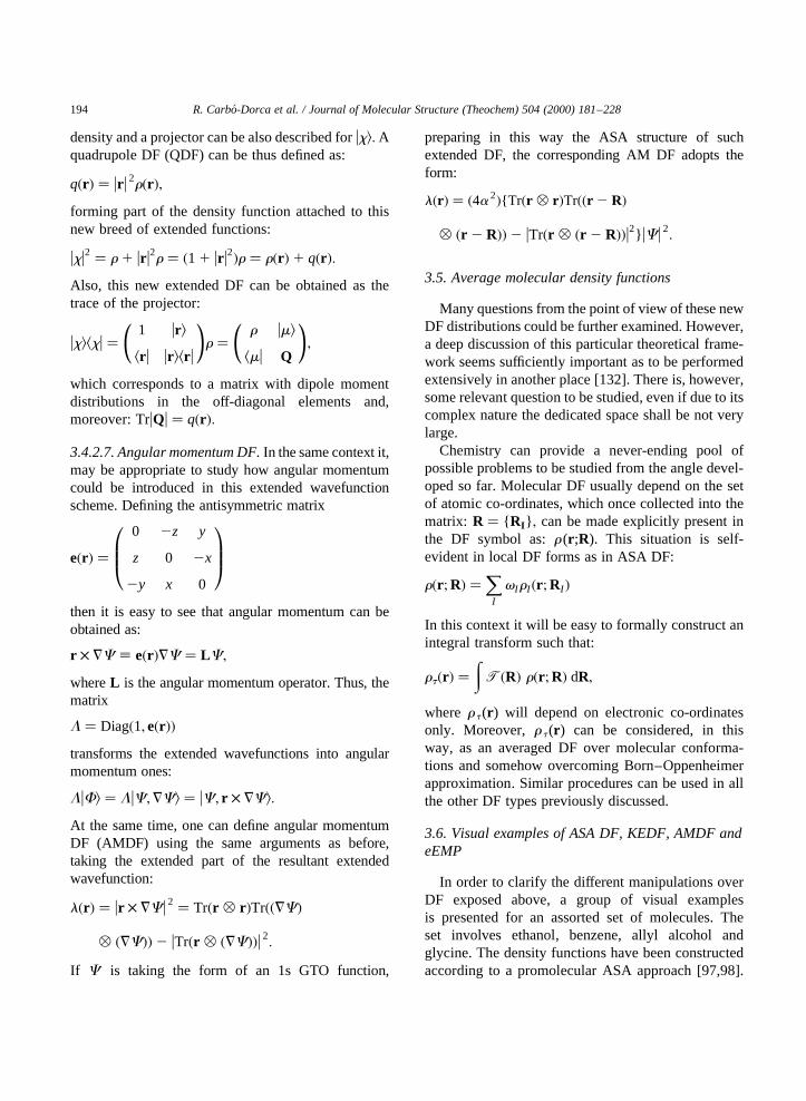
which corresponds to a matrix with dipole momentdistributions in the off-diagonal elements and,moreover: TruQu � q�r �:3.4.2.7. Angular momentum DF.In the same context it,may be appropriate to study how angular momentumcould be introduced in this extended wavefunctionscheme. Defining the antisymmetric matrix

e�r � �0 2z y

z 0 2x

2y x 0

0BB@1CCA

then it is easy to see that angular momentum can beobtained as:

r × 7C ; e�r �7C � LC;

whereL is the angular momentum operator. Thus, thematrix

L � Diag�1;e�r ��transforms the extended wavefunctions into angularmomentum ones:

LuFl � LuC;7Cl � uC; r × 7Cl:

At the same time, one can define angular momentumDF (AMDF) using the same arguments as before,taking the extended part of the resultant extendedwavefunction:

l�r � � ur × 7Cu 2 � Tr�r ^ r �Tr��7C�

^ �7C��2 uTr�r ^ �7C��u 2:

If C is taking the form of an 1s GTO function,

preparing in this way the ASA structure of suchextended DF, the corresponding AM DF adopts theform:

l�r � � �4a 2�{Tr �r ^ r �Tr��r 2 R�

^ �r 2 R��2 uTr�r ^ �r 2 R��u2} uCu 2:

3.5. Average molecular density functions

Many questions from the point of view of these newDF distributions could be further examined. However,a deep discussion of this particular theoretical frame-work seems sufficiently important as to be performedextensively in another place [132]. There is, however,some relevant question to be studied, even if due to itscomplex nature the dedicated space shall be not verylarge.

Chemistry can provide a never-ending pool ofpossible problems to be studied from the angle devel-oped so far. Molecular DF usually depend on the setof atomic co-ordinates, which once collected into thematrix: R � { RI } ; can be made explicitly present inthe DF symbol as:r (r ;R). This situation is self-evident in local DF forms as in ASA DF:

r�r ;R� �X

I

vIrI �r ;RI �

In this context it will be easy to formally construct anintegral transform such that:

rt�r � �ZT�R� r�r ;R� dR;

where rt (r ) will depend on electronic co-ordinatesonly. Moreover, rt (r ) can be considered, in thisway, as an averaged DF over molecular conforma-tions and somehow overcoming Born–Oppenheimerapproximation. Similar procedures can be used in allthe other DF types previously discussed.

3.6. Visual examples of ASA DF, KEDF, AMDF andeEMP

In order to clarify the different manipulations overDF exposed above, a group of visual examplesis presented for an assorted set of molecules. Theset involves ethanol, benzene, allyl alcohol andglycine. The density functions have been constructedaccording to a promolecular ASA approach [97,98].

R. Carbo-Dorca et al. / Journal of Molecular Structure (Theochem) 504 (2000) 181–228194

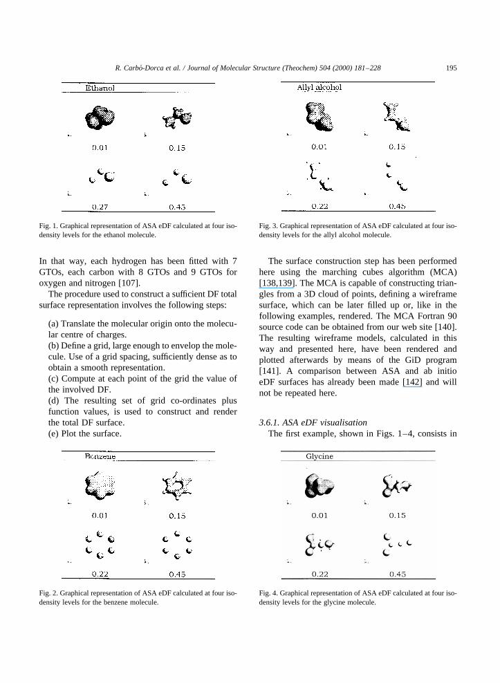
In that way, each hydrogen has been fitted with 7GTOs, each carbon with 8 GTOs and 9 GTOs foroxygen and nitrogen [107].

The procedure used to construct a sufficient DF totalsurface representation involves the following steps:

(a) Translate the molecular origin onto the molecu-lar centre of charges.(b) Define a grid, large enough to envelop the mole-cule. Use of a grid spacing, sufficiently dense as toobtain a smooth representation.(c) Compute at each point of the grid the value ofthe involved DF.(d) The resulting set of grid co-ordinates plusfunction values, is used to construct and renderthe total DF surface.(e) Plot the surface.

The surface construction step has been performedhere using the marching cubes algorithm (MCA)[138,139]. The MCA is capable of constructing trian-gles from a 3D cloud of points, defining a wireframesurface, which can be later filled up or, like in thefollowing examples, rendered. The MCA Fortran 90source code can be obtained from our web site [140].The resulting wireframe models, calculated in thisway and presented here, have been rendered andplotted afterwards by means of the GiD program[141]. A comparison between ASA and ab initioeDF surfaces has already been made [142] and willnot be repeated here.

3.6.1. ASA eDF visualisationThe first example, shown in Figs. 1–4, consists in

R. Carbo-Dorca et al. / Journal of Molecular Structure (Theochem) 504 (2000) 181–228 195

Fig. 1. Graphical representation of ASA eDF calculated at four iso-density levels for the ethanol molecule.

Fig. 2. Graphical representation of ASA eDF calculated at four iso-density levels for the benzene molecule.

Fig. 3. Graphical representation of ASA eDF calculated at four iso-density levels for the allyl alcohol molecule.

Fig. 4. Graphical representation of ASA eDF calculated at four iso-density levels for the glycine molecule.

the representation of ASA eDF for the set of mole-cules mentioned above. The representation shows thesurface plotted at four iso-density levels.

As it can be seen from the above examples, ASAeDF describes accurately the systems for low and highiso-density levels. The approximation reaches abinitio like quality for these extreme values, howeverASA it is not so precise at intermediate values, whenbonds are formed, due to the nature of the pro-molecular approach, which emphasises the densityaround nuclei. However, the differences in the isoden-sity shapes [24], are not really significant and they canbe ignored when computing QSM.

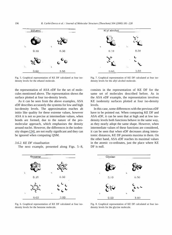
3.6.2. KE DF visualisationThe next example, presented along Figs. 5–8,

consists in the representation of KE DF for thesame set of molecules described before. As inthe ASA eDF example, the representation involvesKE isodensity surfaces plotted at four iso-densitylevels.

In this case, some differences with the previous eDFhave to be pointed out. When comparing KE DF andASA eDF, it can be seen that at high and at low iso-density levels both functions behave in the same way,as they nearly adopt the same shape. However, whenintermediate values of these functions are considered,it can be seen that when eDF decreases along intera-tomic distances, KE DF presents maxima in them. Onthe other hand, ASA eDF reaches its maximal valuesin the atomic co-ordinates, just the place where KEDF is null.

R. Carbo-Dorca et al. / Journal of Molecular Structure (Theochem) 504 (2000) 181–228196

Fig. 5. Graphical representation of KE DF calculated at four iso-density levels for the ethanol molecule.

Fig. 6. Graphical representation of KE DF calculated at four iso-density levels for the benzene molecule.

Fig. 7. Graphical representation of KE DF calculated at four iso-density levels for the allyl alcohol molecule.

Fig. 8. Graphical representation of KE DF calculated at four iso-density levels for the glycine molecule.

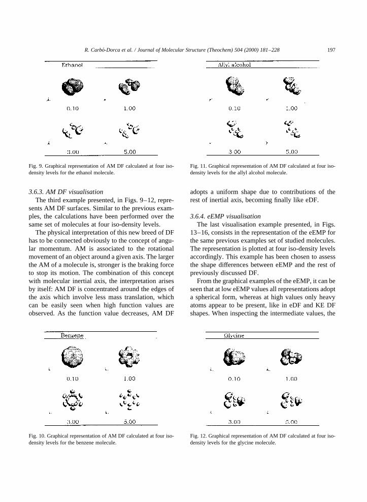
3.6.3. AM DF visualisationThe third example presented, in Figs. 9–12, repre-

sents AM DF surfaces. Similar to the previous exam-ples, the calculations have been performed over thesame set of molecules at four iso-density levels.

The physical interpretation of this new breed of DFhas to be connected obviously to the concept of angu-lar momentum. AM is associated to the rotationalmovement of an object around a given axis. The largerthe AM of a molecule is, stronger is the braking forceto stop its motion. The combination of this conceptwith molecular inertial axis, the interpretation arisesby itself: AM DF is concentrated around the edges ofthe axis which involve less mass translation, whichcan be easily seen when high function values areobserved. As the function value decreases, AM DF

adopts a uniform shape due to contributions of therest of inertial axis, becoming finally like eDF.

3.6.4. eEMP visualisationThe last visualisation example presented, in Figs.

13–16, consists in the representation of the eEMP forthe same previous examples set of studied molecules.The representation is plotted at four iso-density levelsaccordingly. This example has been chosen to assessthe shape differences between eEMP and the rest ofpreviously discussed DF.

From the graphical examples of the eEMP, it can beseen that at low eEMP values all representations adopta spherical form, whereas at high values only heavyatoms appear to be present, like in eDF and KE DFshapes. When inspecting the intermediate values, the

R. Carbo-Dorca et al. / Journal of Molecular Structure (Theochem) 504 (2000) 181–228 197

Fig. 10. Graphical representation of AM DF calculated at four iso-density levels for the benzene molecule.

Fig. 9. Graphical representation of AM DF calculated at four iso-density levels for the ethanol molecule.

Fig. 11. Graphical representation of AM DF calculated at four iso-density levels for the allyl alcohol molecule.

Fig. 12. Graphical representation of AM DF calculated at four iso-density levels for the glycine molecule.

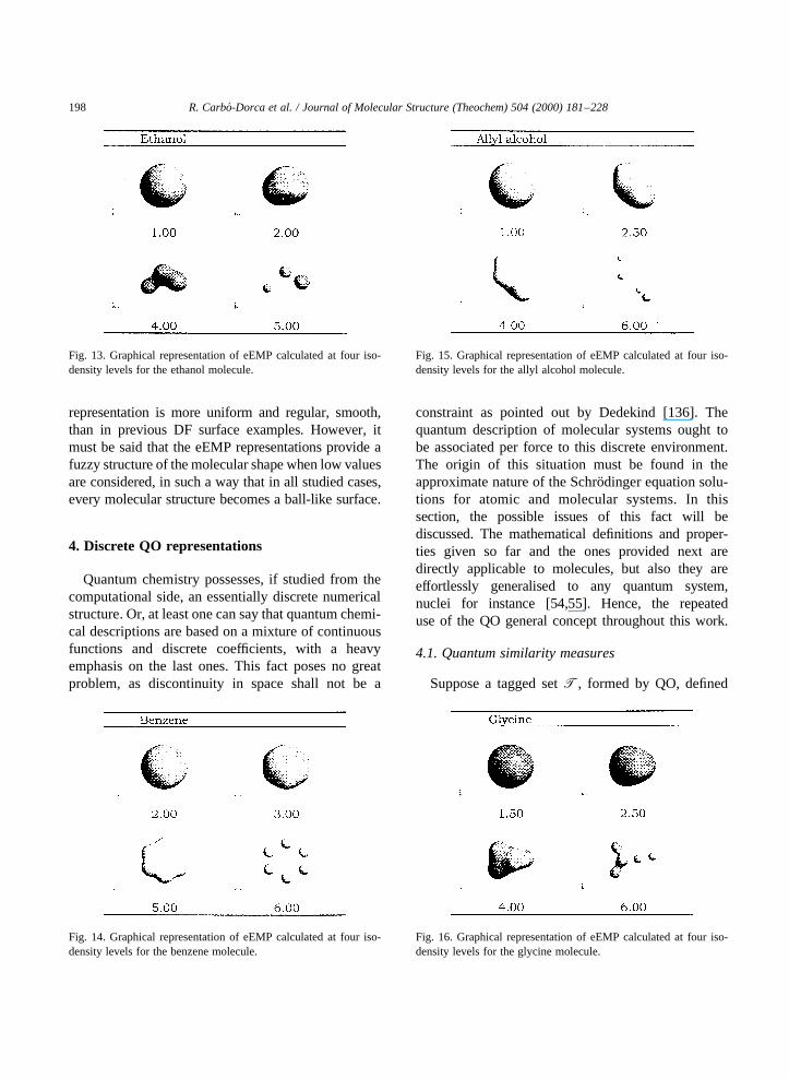
representation is more uniform and regular, smooth,than in previous DF surface examples. However, itmust be said that the eEMP representations provide afuzzy structure of the molecular shape when low valuesare considered, in such a way that in all studied cases,every molecular structure becomes a ball-like surface.

4. Discrete QO representations

Quantum chemistry possesses, if studied from thecomputational side, an essentially discrete numericalstructure. Or, at least one can say that quantum chemi-cal descriptions are based on a mixture of continuousfunctions and discrete coefficients, with a heavyemphasis on the last ones. This fact poses no greatproblem, as discontinuity in space shall not be a

constraint as pointed out by Dedekind [136]. Thequantum description of molecular systems ought tobe associated per force to this discrete environment.The origin of this situation must be found in theapproximate nature of the Schro¨dinger equation solu-tions for atomic and molecular systems. In thissection, the possible issues of this fact will bediscussed. The mathematical definitions and proper-ties given so far and the ones provided next aredirectly applicable to molecules, but also they areeffortlessly generalised to any quantum system,nuclei for instance [54,55]. Hence, the repeateduse of the QO general concept throughout this work.

4.1. Quantum similarity measures

Suppose a tagged setT, formed by QO, defined

R. Carbo-Dorca et al. / Journal of Molecular Structure (Theochem) 504 (2000) 181–228198

Fig. 13. Graphical representation of eEMP calculated at four iso-density levels for the ethanol molecule.

Fig. 14. Graphical representation of eEMP calculated at four iso-density levels for the benzene molecule.

Fig. 15. Graphical representation of eEMP calculated at four iso-density levels for the allyl alcohol molecule.

Fig. 16. Graphical representation of eEMP calculated at four iso-density levels for the glycine molecule.

from an object set,M, made by microscopic systemsand taking the tag set,P, as the collection of thesystems DF in a given state and computed within auniform order for every system, i.e.:T �M × P:

Then, choose a PD operator,V , provided with theappropriate homogeneous dependence on the tag setDF co-ordinates. The following definition can be usedto describe QSM [41].

Definition 5 (Quantum similarity measures). Sup-pose a quantum system setM, and a chosen DFtag setP are known. A QSM,Z(V ), weighted by aPD operatorV , is an application of a quantumobject tagged set,T �M × P; direct product:T ^

T; into the PD real field,R1, such asZ�V� : T ^

T! R 1:

4.1.1. Some QSM formsIn practice, this can be translated into anintegral

measurecomputation involving two QO {A;B} [ T:

zAB�V� �ZZ

rA�r1�V�r 1; r2�rB�r2� dr1 dr2 [ R 1

�35�

where {rA; rB} [ P; are the respective tag set DF ofthe involved QO pair. The tag set DF can be takenhere in a very broad sense, following the previousdiscussion on the possible extension of the DFconcept. This form as presented in Eq. (35) is theone currently quoted in the literature [46–65]. Thevalues of the integralzAB are always PD and real,being all the integrand elements PD functions oroperators. In Eq. (35), the QSM can be interpretedas a weighted scalar product between the DF asso-ciated with the involved QO. When both QO,{ A,B}, in Eq. (35) are the same, the QSM will becalled a quantum self-similarity measure (QS-SM).This last form is nothing else but a norm of theinvolved DF, as well as Eq. (35) can be considereda scalar product. Finally, theDP nature of all theinvolved integrands, providing the structure of ameasure to this kind of integrals, can be also margin-ally interpreted as some kind of generalised molecularvolume.

The usual choice for the PD weight operator in Eq.(35) has been Dirac delta functiond�r1 2 r2�: This

transforms the general QSM definition into the so-called overlap-like QSM:

zAB �ZZ

rA�r1�d�r1 2 r2�rB�r2� dr1 dr2

�ZrA�r �rB�r � dr : �36�

A choice of a third DF tag as the PD weight opera-tor: V�r 1; r2� ; rC�r �; transforms the general defini-tion (35) into a triple QSM [109]:

zAB;C �ZrA�r �rC�r �rB�r � dr �37�

and in the same way multiple QSM can be defined[93,95,102,123].

4.1.2. Coulomb energy as a QS-SMHowever, other possibilities are open to the QSM

definition, reverting at the end to a formal structure asthe one appearing in Definition 5. This may be illu-strated by the expectation value of the Coulombenergy for ap-particle system, which may be writtenemploying Eq. (1), as:

R � �r1; r2;…rp� ∧ V�R� �Xi,j

r 21ij :kCl

�ZV�R�r�R� dR . 0 �38�

where the density matrix is evaluated using the gener-ating rule (3) over the total particle co-ordinates. It iswell known that this produces, for example, in theframework of MO theory closed shell mono-config-urational case an expression, where Coulomb {kii jjj l} and exchange {kij j ij l} two-electron integralsplay a leading role [110]:

kCl �X

i

Xj

�2kii j jj l 2 kij j ij l� . 0 �39�

Although both parts of the expression can be usedby themselves as self-similarity measures [40] overMOs, the positive definite nature of the molecularquantum Coulomb energy, as a whole, can be consid-ered such a similarity measure too. The same can besaid when observing the multi-configurational equiva-lent of Eq. (39) (see for example Ref. [111]). Thisopens the way to the potential use as a moleculardescriptor of this self-similarity measure, which

R. Carbo-Dorca et al. / Journal of Molecular Structure (Theochem) 504 (2000) 181–228 199

appears computed customarily in the availablequantum chemical programs. In Eq. (39) a negativesign is present, which can be associated to the deter-minantal structure of electronic wavefunctions, aconsequence of Pauli exclusion principle.

Coulomb operators can be used to compare a givenfirst-order DFr(r ) with the eEMPV(R) used here as aPD distribution, defined as in Eq. (2). The appropriateQSM, can be easily associated to a QS-SM, weightedwith a Coulomb operator. However, this QS-SM isalso nothing but a classical Coulomb energy. Theproof is self-evident if the following QS-SM isdefined and studied their equivalent suite of integralforms:

Z�ur 2 Ru 21� �Zr�R�V�R� dR

�Zr�R��

Zur 2 Ru21r�r � dr � dR

�ZZ

r�R�ur 2 Ru21r�r � dr dR

�Zr�r ��

Zur 2 Ru21r�R� dR� dr �

Zr�r �V�r � dr

�Z

V�r �r�r � dr : (40)

The final integral also connects Coulomb energywith Eq. (1). From this point of view, Coulomb energycan be interpreted as the expectation value of eEMP.

A comparison of two eEMP produces a new breedof QSM: the so-called gravitational-like form of QSM[49,71], which has been used several times [54–65] asa basis for QSAR studies.

Moreover, as it was pointed out above, Coulombenergy may also be seen as a QSM, adopting anotherpoint of view. To start, one can take Eq. (38). Afterthis, using Eq. (35) and consideringA� B; a QS-SMinvolving a square DF, may be rewritten as:

z�2�AA�V� �ZV�R�r 2

A�R� dR: �41�

Thus, nothing opposes that this last second-order DFintegral can be generalised to anth order DF form:

z�n�AA�V� �ZV�R�r n

A�R� dR �42�

in this manner, a first order QS-SM form could beeasily written as a particular case:

z�1�AA�V� �ZV�R�rA�R� dR: �43�

Then, if theV operator structure as given in Eq. (38),is used in Eq. (43), it is easy to see thatZ �1�AA�V� � kCl.

Continuing the above discussion and definitions, inSection 4.1.4, a generalised QSM structure will bepresented.

4.1.3. Other possible similarity measuresThe definition in Section 3.4.2 of the KE DF, leads

to the possible comparison between this new collec-tion of DF and electronic DF, eEMP and KE DFthemselves. The following QSM can be taken asexamples of the application of Definition 4. Thenew possible measures, among others, are describedin the following integrals, featuring three correspond-ing QSM within the overlap-like formalism:

�a� krAudukBl �ZZ

rA�r1�d�r1 2 r2�kB�r2� dr1 dr2

�ZrA�r �kB�r � dr ;

ZrA�r �u7CB�r �u 2dr

�b� kVAudukBl �ZZ

rA�R�uR 2 r u21kB�r � dr dR

�c� kkAudukBl �ZkA�r �kB�r � dr (44)

Other operator forms can be employed in the sameway as it is shown in Eq. (34), but the resulting defini-tions are trivial and will not be written here. No calcu-lations based on the above integrals have been madeso far. It is indubitable that it will be worth tryingthem as a new and varied source of QO descriptors.Also they can be taken as the basis of new molecularsuperposition devices, in the same way that QSMbased on electronic DF have been used [80].

Some questions remain, thus, unanswered for themoment. Among others, it can be asked how will a KEeEMP look like or a Coulomb expression substitutingDF by KE DF. Coulomb QSM based on KE DF willlook as Eq. (44), for instance, but with the left-handside DF substituted by the proper KE DF:kA�r �. Theuse of KE DF, will permit to order the elements of a

R. Carbo-Dorca et al. / Journal of Molecular Structure (Theochem) 504 (2000) 181–228200

QOS according their momentum distributions actingas tag set parts and, consequently, a possible differentordering pattern could emerge.

Here is, perhaps, the adequate place to speak aboutother probability density distributions such as Boltz-mann functions, as candidates to support molecularcomparisons. This kind of similarity measures havealready been proposed and studied elsewhere [72].However, it must be said that probability distribu-tions, whose origin can be the statistical mechanics,constitute adequate tags for assorted molecules, and ifknown and well defined, they can be as a good choiceas quantum mechanical DF tags are. When a molecu-lar tagged set has the attached tag set made of Boltz-mann distributions, one can spoke about Boltzmannobject sets (BOS). The aforementioned discussionabout quantum mechanical DF, including similaritymeasures, can apply in this case.

4.1.4. A general definition of QSMThe characteristic properties of Coulomb energy, as

discussed in Section 4.1.2, connect Eq. (1) with Defi-nition 5 too. Considering the fact that a QSM can bealso computed, looking at Eq. (1) as a scalar product,constructed within the VSS, containing the PD opera-tors and density functions, as pointed out before. Fromthis point of view, Eq. (36) appears as a particular caseof Eq. (1), where the operator on the left has beensubstituted by another DF. This precludes the possiblegeneralisation of Definition 5 in a very easy manner,as the next definition shows:

Definition 6 (General QSM). A general QSM,G(V ), can be considered a PD multiple scalar productdefined by a contractedn-direct product of a QOS,T:

G�V� : ^n

K�1T! R 1

:

This allows to mixn DF: {r I �r �; I � 1; n} of the QOSwith v PD operators, collected into a set:V �{VK�r �; K � 1;v} ; belonging to the same VSS, forexample:

G�V� �Z"Yv

K�1

VK�r �#"Yn

I�1

rI �r �#

dr ; �45�

where the co-ordinate vector,r , shall be taken here in

a broad general sense, in order to make possible thecalculation of the integral. Thus, Eqs.(1), (2), (36),(38) and (40) can be all of them considered as diverseforms of QSM.

Finally, one can note that from inspecting Eq. (45),takingv � n � 1; Eq. (1) can be deduced and, thus,any quantum expectation value becomes a particularform of QSM. A general picture of QSM was alreadygiven and studied in Ref. [49], but the present formalstructure has a better adaptation to the tagged setstheoretical background.

4.2. Discrete representation of quantum objects:similarity matrices

4.2.1. Theoretical considerationsThe possibility of obtaining multiple relationships

between the appropriate number of QOS elements, viatheir DF tags, in terms of QSM, as discussed in theprevious section, has other interesting consequences,besides the calculation of the possible relationshipbetween QO. The most relevant one constitutes thepotential representation of a QO as a discrete vectoror matrix.

Definition 7 (Similarity matrices). Suppose a QOS:T �M × P of cardinality n is known. Thesymmetric�n × n� matrix: Z � { zIJ} ; whose elementsare made using QSM between pairs of QO inT, willbe called a similarity matrix (SM).

By construction, provided that all the involved QOare different, any SM could be considered a PD metricmatrix, belonging to some matrix VSS:Z [M�n×n��R 1� [53]. Such a matrix can also be inter-preted as the representation of the PD operator,V ,in the basis set defined by the QO DF. Consideringthe SM column vectors: Z � { zI } ; this setalso belongs to some n-dimensional VSS:;I : zI [ Vn�R 1�. Moreover, every column,zI , ofthe SM can be considered as an-dimensional discreterepresentation of theIth QO in the tagged QOS. Theset of columns of the SM was also referred withinearlier papers [46–50], in an obvious descriptivemanner, as a molecular point cloud.

Discrete mathematics can be of much help in thedescription of tagged sets and the relationships of their

R. Carbo-Dorca et al. / Journal of Molecular Structure (Theochem) 504 (2000) 181–228 201

elements, several aspects of the basic information onthis subject can be found in Refs. [116,117].

4.2.2. Examples of similarity matricesThe overall relationships between the elements of a

molecular data set can be expressed in matrix form,yielding the SM. As an illustrative example, Table 3shows the Coulomb QS matrix for 15 indole deriva-tives [56,66]. An extension of this data set will be usedlater as a validation set in a QSAR study based uponMQSM. The geometry of these compounds has beencomputed at a semiempirical AM1 level [154], andthe density functions have been calculated using theASA approximation. As it has been discussed, any SMis symmetric, indicating that the QSM between twomolecules is identical independently of the order ofthe comparison of the QO. This fact is used tocompress the information only in the upper triangleof the matrix. In Table 3, the upper triangle, includingthe diagonal elements, contains the Coulomb MQSM.In this particular case, the Coulomb measures rangeapproximately from 3800 to 6100. The order ofmagnitude of the different types of MQSM is highlyconnected to the structural form of the molecule, andto the presence of heavy atoms. Due to the particularconstruction of the SM, the diagonal elements of SMbring out information on the size of the compound.

Several transformations of these SM can beperformed, yielding the so-called molecular QSindices (MQSI), which scale or normalise the SM.In particular, a normalisation of the MQSM, knownin the literature as Carbo´ index, [1] can be defined as:

CIJ � ZIJ�ZII ZJJ�1=2:

The overall set of Carbo´ indices can also be expressedin a matrix form. Carbo´ index can be interpreted as thecosine of the angle subtended by both involved DF ininfinite-dimensional space, and so it ranges from zeroto one. If the value is closer to one, both QOs areconsidered to be similar. Therefore, for two identicalQOs, that is, the main diagonal Carbo´ index elementsthe value of one is found, irrespective of the analysedQO. This redundant information is neglected in theexample given below. In this way, the lower triangleof the Table 3 matrix shows the Carbo´ indices for theselected 15 indole derivatives [56,66].

5. Discrete representations and QSAR limits

Discrete QO tagged sets may be defined at the sametime as the original infinite-dimensional ones.Suppose a QO tagged set,T �M × P is known,and a similarity matrix,Z � { zI } ; considered as ahypermatrix, formed by column vectors as elements,can be evaluated using the Definition 7 procedure.

Definition 8 (Discrete quantum object sets). Adiscrete quantum object set can be constructed as anew tagged set:Z �M × Z ∧ Z � { zI } ; with thesame object part as the original QOS tagged set,T,but with the tag part formed by the columns of thesimilarity matrix,Z.

5.1. Discrete expectation values

The point of view appearing in Definition 8 is thesame as finding out the way to project a set of points,defined in some infinite-dimensional VSS, into an-dimensional vector structure. It can be also consid-ered that any similarity matrix, collecting a similarityrelationship between any studied QO and a set ofparent QO structures, is a source of anunbiasedQOrepresentation in the form ofn-dimensional discreteinformation. SM columns are to be considered mole-cular descriptors chosen in such a way, that theremaining arbitrariness of choice corresponds to thenature of the weight operator appearing in the MQSMcalculation.

Obviously, from this point of view, discrete QOrepresentations will depend on the PD weight operator,V . Suppose that a collection of discrete QO tagged setsis formed using various PD operators, {V i}, producinga collection of PD SM: {Z(V i)}. A new PD SM, can beobtained, choosing a set of PD scalars, {a i} [ R 1

; byforming the linear combination:

Z �X

i

aiZ�V i�:

The columns of the combined SMZ can beconsidered linear combinations with the samecoefficients, as those employed to construct thenew PD SM. That is:

;zI [ Z : zI �X

i

aizI �V i�:

R. Carbo-Dorca et al. / Journal of Molecular Structure (Theochem) 504 (2000) 181–228202

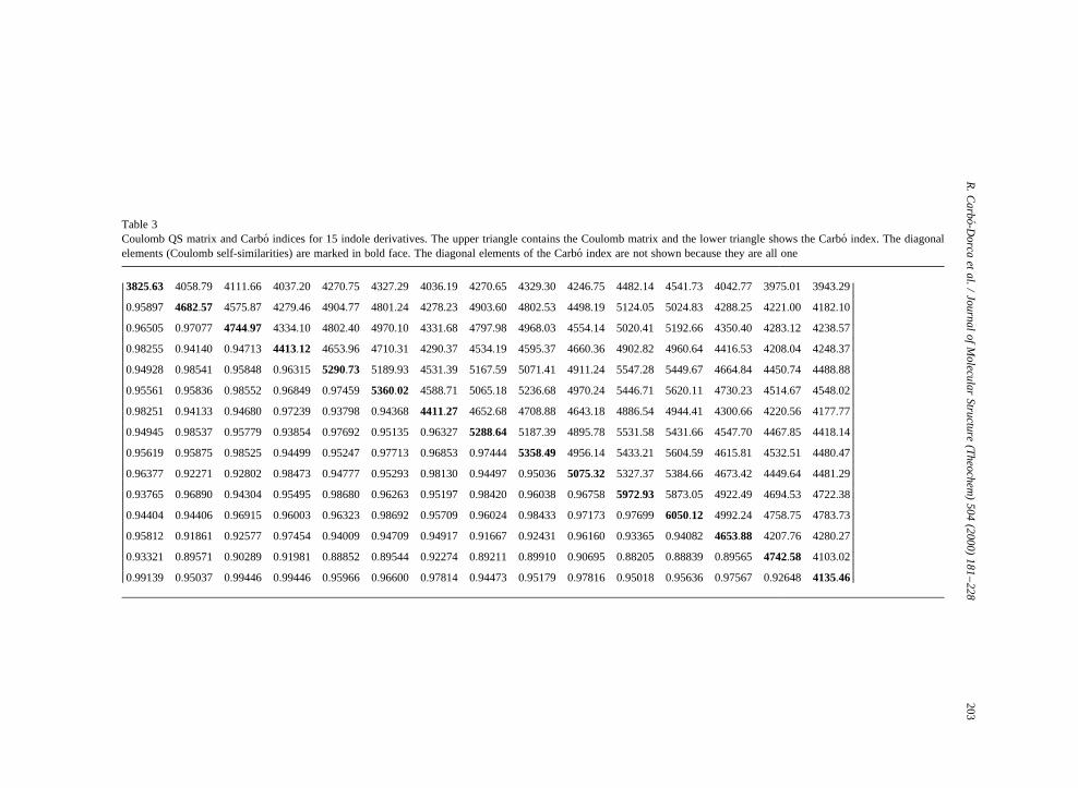
R.

Ca

rbo-D

orca

et

al.

/Jo

urn

alo

fM

ole

cula

rS

tructu

re(T

he

och

em

)5

04

(20

00

)1

81

–2

28

203

Table 3Coulomb QS matrix and Carbo´ indices for 15 indole derivatives. The upper triangle contains the Coulomb matrix and the lower triangle shows the Carbo´ index. The diagonalelements (Coulomb self-similarities) are marked in bold face. The diagonal elements of the Carbo´ index are not shown because they are all one

3825:63 4058:79 4111:66 4037:20 4270:75 4327:29 4036:19 4270:65 4329:30 4246:75 4482:14 4541:73 4042:77 3975:01 3943:29

0:95897 4682:57 4575:87 4279:46 4904:77 4801:24 4278:23 4903:60 4802:53 4498:19 5124:05 5024:83 4288:25 4221:00 4182:10

0:96505 0:97077 4744:97 4334:10 4802:40 4970:10 4331:68 4797:98 4968:03 4554:14 5020:41 5192:66 4350:40 4283:12 4238:57

0:98255 0:94140 0:94713 4413:12 4653:96 4710:31 4290:37 4534:19 4595:37 4660:36 4902:82 4960:64 4416:53 4208:04 4248:37

0:94928 0:98541 0:95848 0:96315 5290:73 5189:93 4531:39 5167:59 5071:41 4911:24 5547:28 5449:67 4664:84 4450:74 4488:88

0:95561 0:95836 0:98552 0:96849 0:97459 5360:02 4588:71 5065:18 5236:68 4970:24 5446:71 5620:11 4730:23 4514:67 4548:02

0:98251 0:94133 0:94680 0:97239 0:93798 0:94368 4411:27 4652:68 4708:88 4643:18 4886:54 4944:41 4300:66 4220:56 4177:77

0:94945 0:98537 0:95779 0:93854 0:97692 0:95135 0:96327 5288:64 5187:39 4895:78 5531:58 5431:66 4547:70 4467:85 4418:14

0:95619 0:95875 0:98525 0:94499 0:95247 0:97713 0:96853 0:97444 5358:49 4956:14 5433:21 5604:59 4615:81 4532:51 4480:47

0:96377 0:92271 0:92802 0:98473 0:94777 0:95293 0:98130 0:94497 0:95036 5075:32 5327:37 5384:66 4673:42 4449:64 4481:29

0:93765 0:96890 0:94304 0:95495 0:98680 0:96263 0:95197 0:98420 0:96038 0:96758 5972:93 5873:05 4922:49 4694:53 4722:38

0:94404 0:94406 0:96915 0:96003 0:96323 0:98692 0:95709 0:96024 0:98433 0:97173 0:97699 6050:12 4992:24 4758:75 4783:73

0:95812 0:91861 0:92577 0:97454 0:94009 0:94709 0:94917 0:91667 0:92431 0:96160 0:93365 0:94082 4653:88 4207:76 4280:27

0:93321 0:89571 0:90289 0:91981 0:88852 0:89544 0:92274 0:89211 0:89910 0:90695 0:88205 0:88839 0:89565 4742:58 4103:02

0:99139 0:95037 0:99446 0:99446 0:95966 0:96600 0:97814 0:94473 0:95179 0:97816 0:95018 0:95636 0:97567 0:92648 4135:46

�������������������������������������������������

�������������������������������������������������

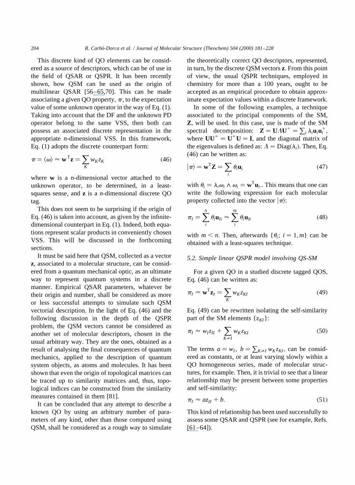
This discrete kind of QO elements can be consid-ered as a source of descriptors, which can be of use inthe field of QSAR or QSPR. It has been recentlyshown, how QSM can be used as the origin ofmultilinear QSAR [56–65,70]. This can be madeassociating a given QO property,p , to the expectationvalue of some unknown operator in the way of Eq. (1).Taking into account that the DF and the unknown PDoperator belong to the same VSS, then both canpossess an associated discrete representation in theappropriaten-dimensional VSS. In this framework,Eq. (1) adopts the discrete counterpart form:

p � kvl < w Tz�XK

wKzK �46�

where w is a n-dimensional vector attached to theunknown operator, to be determined, in a least-squares sense, andz is a n-dimensional discrete QOtag.

This does not seem to be surprising if the origin ofEq. (46) is taken into account, as given by the infinite-dimensional counterpart in Eq. (1). Indeed, both equa-tions represent scalar products in conveniently chosenVSS. This will be discussed in the forthcomingsections.

It must be said here that QSM, collected as a vectorz, associated to a molecular structure, can be consid-ered from a quantum mechanical optic, as an ultimateway to represent quantum systems in a discretemanner. Empirical QSAR parameters, whatever betheir origin and number, shall be considered as moreor less successful attempts to simulate such QSMvectorial description. In the light of Eq. (46) and thefollowing discussion in the depth of the QSPRproblem, the QSM vectors cannot be considered asanother set of molecular descriptors, chosen in theusual arbitrary way. They are the ones, obtained as aresult of analysing the final consequences of quantummechanics, applied to the description of quantumsystem objects, as atoms and molecules. It has beenshown that even the origin of topological matrices canbe traced up to similarity matrices and, thus, topo-logical indices can be constructed from the similaritymeasures contained in them [81].

It can be concluded that any attempt to describe aknown QO by using an arbitrary number of para-meters of any kind, other than those computed usingQSM, shall be considered as a rough way to simulate

the theoretically correct QO descriptors, represented,in turn, by the discrete QSM vectorsz. From this pointof view, the usual QSPR techniques, employed inchemistry for more than a 100 years, ought to beaccepted as an empirical procedure to obtain approx-imate expectation values within a discrete framework.

In some of the following examples, a techniqueassociated to the principal components of the SM,Z, will be used. In this case, use is made of the SMspectral decomposition:Z � ULU1 � P

i liuiu1i ;

whereUU1 � U1U � I , and the diagonal matrix ofthe eigenvalues is defined as:L � Diag�li�: Then, Eq.(46) can be written as:

upl � wTZ �X

i

uiui �47�

with ui � livi ∧ vi � wTui :. This means that one canwrite the following expression for each molecularproperty collected into the vectorupl:

pI �Xn

i

uiuIi <Xm

i

uiuIi �48�

with m , n: Then, afterwards {ui ; i � 1;m} can beobtained with a least-squares technique.

5.2. Simple linear QSPR model involving QS-SM

For a given QO in a studied discrete tagged QOS,Eq. (46) can be written as:

pI < wTzI �XK

wKzKI �49�

Eq. (49) can be rewritten isolating the self-similaritypart of the SM elements {zKI }:

pI < wI zII 1XK±I

wKzKI �50�

The termsa� wI ; b� PK±I wKzKI ; can be consid-

ered as constants, or at least varying slowly within aQO homogeneous series, made of molecular struc-tures, for example. Then, it is trivial to see that a linearrelationship may be present between some propertiesand self-similarity:

pI < azII 1 b: �51�This kind of relationship has been used successfully toassess some QSAR and QSPR (see for example, Refs.[61–64]).

R. Carbo-Dorca et al. / Journal of Molecular Structure (Theochem) 504 (2000) 181–228204

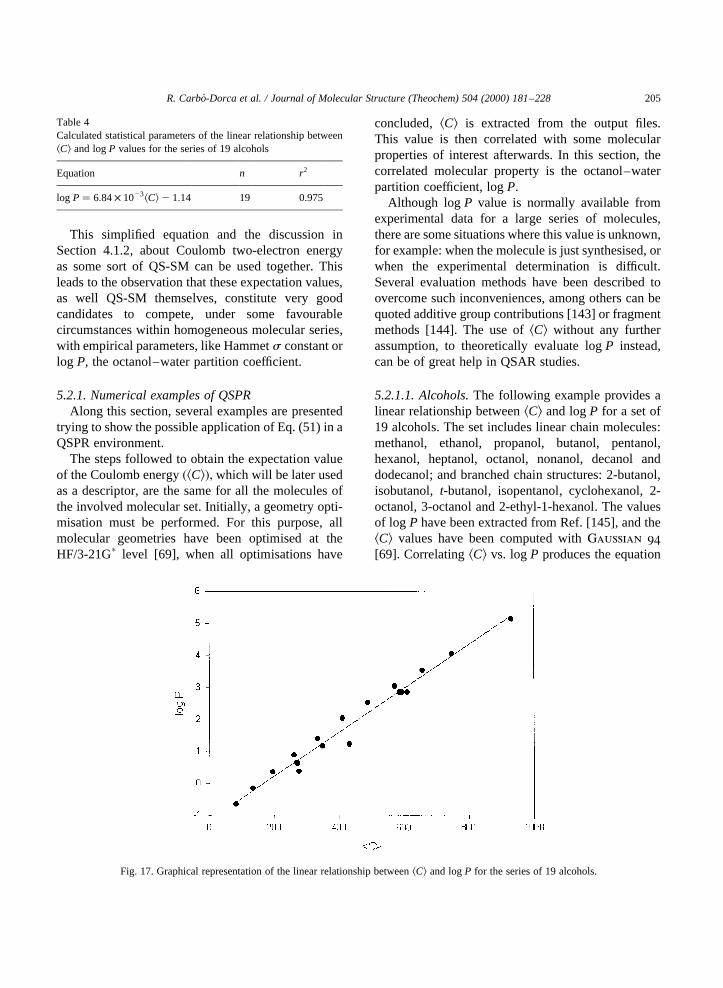
This simplified equation and the discussion inSection 4.1.2, about Coulomb two-electron energyas some sort of QS-SM can be used together. Thisleads to the observation that these expectation values,as well QS-SM themselves, constitute very goodcandidates to compete, under some favourablecircumstances within homogeneous molecular series,with empirical parameters, like Hammets constant orlog P, the octanol–water partition coefficient.

5.2.1. Numerical examples of QSPRAlong this section, several examples are presented

trying to show the possible application of Eq. (51) in aQSPR environment.

The steps followed to obtain the expectation valueof the Coulomb energy�kCl�; which will be later usedas a descriptor, are the same for all the molecules ofthe involved molecular set. Initially, a geometry opti-misation must be performed. For this purpose, allmolecular geometries have been optimised at theHF/3-21Gp level [69], when all optimisations have

concluded,kCl is extracted from the output files.This value is then correlated with some molecularproperties of interest afterwards. In this section, thecorrelated molecular property is the octanol–waterpartition coefficient, logP.

Although logP value is normally available fromexperimental data for a large series of molecules,there are some situations where this value is unknown,for example: when the molecule is just synthesised, orwhen the experimental determination is difficult.Several evaluation methods have been described toovercome such inconveniences, among others can bequoted additive group contributions [143] or fragmentmethods [144]. The use ofkCl without any furtherassumption, to theoretically evaluate logP instead,can be of great help in QSAR studies.

5.2.1.1. Alcohols.The following example provides alinear relationship betweenkCl and logP for a set of19 alcohols. The set includes linear chain molecules:methanol, ethanol, propanol, butanol, pentanol,hexanol, heptanol, octanol, nonanol, decanol anddodecanol; and branched chain structures: 2-butanol,isobutanol, t-butanol, isopentanol, cyclohexanol, 2-octanol, 3-octanol and 2-ethyl-1-hexanol. The valuesof log P have been extracted from Ref. [145], and thekCl values have been computed withGaussian 94[69]. CorrelatingkCl vs. logP produces the equation

R. Carbo-Dorca et al. / Journal of Molecular Structure (Theochem) 504 (2000) 181–228 205

Table 4Calculated statistical parameters of the linear relationship betweenkCl and logP values for the series of 19 alcohols

Equation n r2

log P� 6:84× 1023kCl 2 1:14 19 0.975

Fig. 17. Graphical representation of the linear relationship betweenkCl and logP for the series of 19 alcohols.

presented in Table 4, and the plotted regression line isshown in Fig. 17, all data concerning the set is listed inTable 5.

As can be seen from Fig. 17,kCl and logP are ingood relationship, being possible the use of one oranother as a molecular descriptor in homologousseries.

It must be pointed out that all software packagescompute first-order density functions normalised tothe number of electrons�ne�, but densities normalisedto unity can be also considered. This simple step onlyimplies scaling the value ofkCl obtained by regularcomputations by an22

e factor, that is:kCNl � n22e kCl:

The application of a second-order polynomialfitting to the previous set of alcohols produces anew relationship betweenkCNl and logP. kCNl valuescan be deduced from Table 5. The resulting equationis presented in Table 6 and the corresponding regres-sion line is plotted in Fig. 18.

As can be seen from the results, the use of scaledkCNl produces a second-order fitting, which slightlyimproves the structure–property relationship.

5.2.1.2. Mixed molecules: acetates, carboxylic acidsand amides.In this new example, the set of moleculesused is a mixture of three kinds of compounds:acetates, carboxylic acids and amides. The setconsists in 14 molecules and it is constituted by

R. Carbo-Dorca et al. / Journal of Molecular Structure (Theochem) 504 (2000) 181–228206

Table 5kCl and logP values for a set of 19 alcohols

Molecule kCl log P

Methanol 81.07 20.66Ethanol 134.84 20.16Propanol 196.33 0.34Butanol 263.38 0.88Pentanol 335.28 1.4Hexanol 411.32 2.03Heptanol 490.92 2.53Octanol 573.7 3.03Nonol 659.3 3.53Decanol 747.47 4.03Dodecanol 930.62 5.132-Butanol 272.5 0.61Isobutanol 271.06 0.65t-Butanol 277.88 0.37Isopentanol 348.98 1.16Cyclohexanol 433.79 1.232-Octanol 589.36 2.833-Octanol 595.93 2.832-Ethyl-1-hexanol 611.28 2.83

Table 6Calculated statistical parameters of the relationship betweenkCNland logP values for the series of 19 alcohols

Equation N r2

log P� 274:25kCNl2 2

122:34kCNl 1 12:9719 0.988

Fig. 18. Graphical representation of the relationship betweenkCNl and logP for the series of 19 alcohols.

methyl-, ethyl-, propyl- and butylacetate, acetic,propionic, butyric, valeric and hexanoic acids, aswell as formamide,N-methyl,N-ethyl, N-propyl andN-butylformamide. The values of logP have beenextracted from Ref. [145], and thekCl values havebeen computed by means ofGaussian 94 [69].

Correlating kCl vs. logP produces the equationpresented in Table 7 and the plotted regression lineis shown in Fig. 19. All data concerning this set islisted in Table 8.

Even if the relationship betweenkCl and logP isnot as good as in the previous case, it must be pointedout that the set consists in three different kinds ofcompounds. This result proves that when the studiedstructures are similar enough, even in cases wherethey do not constitute a homogeneous series, asound relationship can be established between logPandkCl:

However, there is the possibility of using, asdiscussed in the previous example,kCNl as a molecu-lar descriptor in a polynomial expression, which canbe easily deduced from Table 8. The results of this

relationship are presented in Table 9 and graphicallyplotted in Fig. 20.

As can be seen from this last example, the use ofkCNl provides an almost perfect relationship withlog P for the studied series of molecular structures.Taking into account that a selection made by threedifferent kinds of molecules has been correlatedwith a single descriptor, the use ofkCNl and a poly-nomial regression is justified. This opens the door tothe possibility of usingkCNl; instead of logP, as analternative molecular descriptor for QSAR purposes.

In the examples given before, it seems that logP

R. Carbo-Dorca et al. / Journal of Molecular Structure (Theochem) 504 (2000) 181–228 207

Table 7Calculated statistical parameters of the linear relationship betweenkCl and logP values for the series of 14 compounds

Equation n r2

log P� 7:95× 1023k Cl 2 2:14 14 0.892

Fig. 19. Graphical representation of the linear relationship betweenkCl and logP for the series of 14 compounds.

Table 8kCl and logP values for a set of 14 compounds

Molecule kCl log P

Methylacetate 274.67 0.18Ethylacetate 349.27 0.73Propylacetate 426.6 1.24Butylacetate 506.92 1.78Acetic acid 202.27 20.17Propionic acid 272.28 0.33Butyric acid 344.87 0.79Valeric acid 421.59 1.39Hexanoic acid 501.31 1.92Formamide 131.33 21.51N-Methylformamide 194.51 20.97N-Ethylformamide 264.44 20.43N-Propylformamide 337.14 0.11N-Butylformamide 413.94 0.65

andkCl correlate usually very well in a linear manner,while log P and kCNl adopt a second-order poly-nomial form. This characteristic opens the way tosearch forkCNl values attached to optimal properties.

5.2.1.3. Full SM as QSPR descriptor generator5.2.1.3.1. Preliminary details.When one deals with

practical QSPR problems, the discrete expectationvalue law must be slightly modified. Thus, thatalgebraic relation is transformed into a reducedexpression where the number of parameters is lessthan the number of equations, yielding a truestructure–activity relationship. In this case, theequality turns out into an approximation:

pI < wTf �zI �:Now w is an m-dimensional vector, beingm , n;and f �zI � is a transformation of the similarityvectors that reduces their dimensionality. The

solution to this problem is found out by a leastsquares technique.

There exist several possible transformations ofthe similarity matricesZ in order to reduce theirdimensionality [137]. Principal component analysis(PCA) [146], partial least squares (PLS) [147],classical scaling or the more general multidimen-sional scaling [148] are examples of this kind oftransformations.

Once the SMZ is transformed, some type of vari-able selection must be also performed. The most usualchoice is made by selecting the variables arrangedfollowing the order given by the explained variance,but this is not the only possible way. In particular, theso-calledmost predictive variables method[149] hasbeen employed successfully to select the optimal vari-ables. This method arranges the variables in relationto the correlation with the external data, allowing aspecific order for each property studied. To avoidundesirable noise parameterisation, a variance thresh-old is imposed, which rejects all those variables thatexplain less than the filter value.

In order to quantify the quality of the modelproposed, several statistical parameters can be used,the most frequently employed are: (a) Pearsonr2

coefficient, a goodness-of-fit measure; (b)q2 pre-dictive coefficient, found by the leave-one-out proce-dure, which indicates how good can be the model

R. Carbo-Dorca et al. / Journal of Molecular Structure (Theochem) 504 (2000) 181–228208

Table 9Calculated statistical parameters of the relationship betweenkCNland logP values for the series of 14 compounds

Equation n r2

log P� 440:67kCNl2 2

162:72kCNl 1 13:4514 0.993

Fig. 20. Graphical representation of the relationship betweenkCNl and logP for the series of 14 molecules.

predictions [150]; (c) standard deviation of fitting andprediction errors.

For computational reasons, the molecular densityfunctions used in practical QSAR calculations arenot the ab initio ones, but the accurate fitting basedon ASA [96–101], as explained in Section 3.3.2. Opti-mised molecular geometries, found at a semiempiricalAM1 level, with the ampac 5.0 program were used[154]. The similarity measures are built employingeither overlap or Coulomb operators, and the matricesare normalised by means of the Carbo´ index transfor-mation. All the MQSM computations have beencarried out withmolsimil 97 software [151], andthe statistical calculations using thetqsar-simprogram [152].

5.2.1.3.2. Practical example: flavylium salts asinhibitors of the xanthine oxydase enzyme.Anapplication example of QSM to QSAR is used tostudy a set of 16 flavylium salts and their ability toinhibit the Xanthine Oxidase enzyme, measured bypKEI, KEI being the dissociation constant of theenzyme–inhibitor complex. A previous QSAR studyon this same data set was reported by D. Amic, D.Davidovic-Amic and D. Beslo, using classical (not3D) descriptors [153].

The general structure of these flavyliumcompounds is shown in Fig. 21. For the QSM calcula-tions, semiempirical AM1 geometries have been used.The molecular density functions have been calculatedusing the ASA approximation. Overlap operator andCarboindexes have been used. The dimensionality ofthe SM have been reduced by means of the classicalscaling technique [148], and the principal axes havebeen selected using the most predictive variablesmethod [149]. The results obtained are given inTable 10, where the optimal model has been markedin bold face. As can be seen, the best model isobtained when using 5 PCs, yielding satisfactorypredictions.

The cross-validated activities are given in Table 11,and Fig. 22 shows a plot of the cross-validated versusthe experimental activities. To assess that the modelobtained is a true QSAR, and to detect possible chancecorrelations, a randomisation test has been performed.No case with shuffled activities yields a good QSARmodel, and the best value for a random activity vectorwas 0.510, considerably lower than the value attainedwith the correct activity vector, 0.833.

The relationship obtained improves the resultsfound in the original study [153], where several equa-tions are described involving Hansch’s hidrophobicityparameterp , Hammett’ss , a descriptor related to thecharge densities, and a discrete valued indicator vari-able. The best result was found when using all these ar 2 � 0:996 value, but it must be noted that neithercross-validation nor a randomisation test werereported.

5.3. Convex superposition of SM

Suppose, now, in another possible QSAR situation,that a discrete QOS is known. The associated discrete

R. Carbo-Dorca et al. / Journal of Molecular Structure (Theochem) 504 (2000) 181–228 209

Fig. 21. General form of the studied flavylium salts. Substituentpositions are marked.

Table 10QSAR results for the flavylium salts set

Number of PCs Selected PCs Explained variance (%) r2 q2 sn

1 1 39.98 0.483 0.355 0.6712 1, 2 56.45 0.742 0.597 0.4733 1, 2, 10 58.37 0.857 0.705 0.3524 1, 2, 10, 8 61.22 0.904 0.786 0.2905 1, 2, 10, 8, 5 67.42 0.924 0.833 0.2576 1, 2, 10, 8, 5, 4 74.33 0.935 0.720 0.238

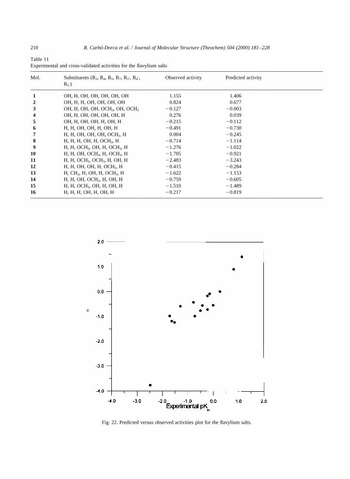
R. Carbo-Dorca et al. / Journal of Molecular Structure (Theochem) 504 (2000) 181–228210

Table 11Experimental and cross-validated activities for the flavylium salts

Mol. Substituents (R3, R4, R5, R7, R30, R40,R50)

Observed activity Predicted activity

1 OH, H, OH, OH, OH, OH, OH 1.155 1.4062 OH, H, H, OH, OH, OH, OH 0.824 0.6773 OH, H, OH, OH, OCH3, OH, OCH3 20.127 20.0034 OH, H, OH, OH, OH, OH, H 0.276 0.0395 OH, H, OH, OH, H, OH, H 20.215 20.1126 H, H, OH, OH, H, OH, H 20.491 20.7307 H, H, OH, OH, OH, OCH3, H 0.004 20.2458 H, H, H, OH, H, OCH3, H 20.714 21.1149 H, H, OCH3, OH, H, OCH3, H 21.276 21.022

10 H, H, OH, OCH3, H, OCH3, H 21.705 20.92111 H, H, OCH3, OCH3, H, OH, H 22.483 23.24312 H, H, OH, OH, H, OCH3, H 20.415 20.28413 H, CH3, H, OH, H, OCH3, H 21.622 21.15314 H, H, OH, OCH3, H, OH, H 20.759 20.60515 H, H, OCH3, OH, H, OH, H 21.510 21.48916 H, H, H, OH, H, OH, H 20.217 20.819

Fig. 22. Predicted versus observed activities plot for the flavylium salts.

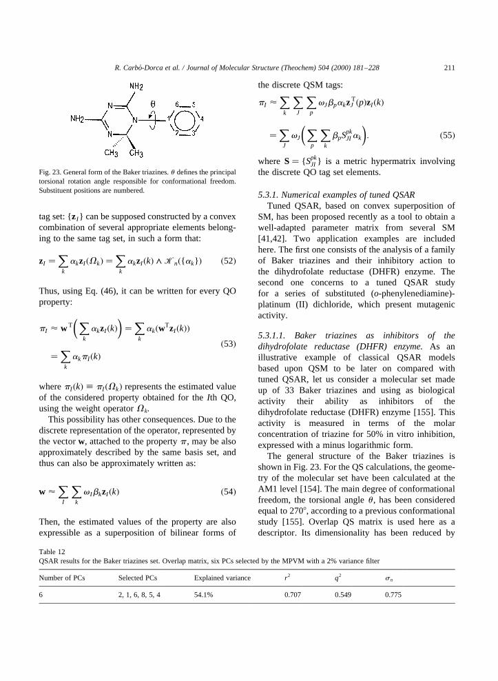
tag set: {zI } can be supposed constructed by a convexcombination of several appropriate elements belong-ing to the same tag set, in such a form that:

zI �X

k

akzI �Vk� �X

k

akzI �k� ∧ Kn�{ak} � �52�

Thus, using Eq. (46), it can be written for every QOproperty:

pI < w T�X

k

akzI �k���X

k

ak�wTzI �k��

�X

k

akpI �k��53�

wherepI �k� ; pI �Vk� represents the estimated valueof the considered property obtained for theIth QO,using the weight operatorV k.

This possibility has other consequences. Due to thediscrete representation of the operator, represented bythe vectorw, attached to the propertyp , may be alsoapproximately described by the same basis set, andthus can also be approximately written as:

w <X

I

Xk

v IbkzI �k� �54�

Then, the estimated values of the property are alsoexpressible as a superposition of bilinear forms of

the discrete QSM tags:

pI <X

k

XJ

Xp

vJbpakzTJ �p�zI �k�

�XJ

vJ

�Xp

Xk

bpSpkJI ak

�: �55�

where S� { SpkJI } is a metric hypermatrix involving

the discrete QO tag set elements.

5.3.1. Numerical examples of tuned QSARTuned QSAR, based on convex superposition of

SM, has been proposed recently as a tool to obtain awell-adapted parameter matrix from several SM[41,42]. Two application examples are includedhere. The first one consists of the analysis of a familyof Baker triazines and their inhibitory action tothe dihydrofolate reductase (DHFR) enzyme. Thesecond one concerns to a tuned QSAR studyfor a series of substituted (o-phenylenediamine)-platinum (II) dichloride, which present mutagenicactivity.

5.3.1.1. Baker triazines as inhibitors of thedihydrofolate reductase (DHFR) enzyme.As anillustrative example of classical QSAR modelsbased upon QSM to be later on compared withtuned QSAR, let us consider a molecular set madeup of 33 Baker triazines and using as biologicalactivity their ability as inhibitors of thedihydrofolate reductase (DHFR) enzyme [155]. Thisactivity is measured in terms of the molarconcentration of triazine for 50% in vitro inhibition,expressed with a minus logarithmic form.

The general structure of the Baker triazines isshown in Fig. 23. For the QS calculations, the geome-try of the molecular set have been calculated at theAM1 level [154]. The main degree of conformationalfreedom, the torsional angleu , has been consideredequal to 2708, according to a previous conformationalstudy [155]. Overlap QS matrix is used here as adescriptor. Its dimensionality has been reduced by

R. Carbo-Dorca et al. / Journal of Molecular Structure (Theochem) 504 (2000) 181–228 211

Fig. 23. General form of the Baker triazines.u defines the principaltorsional rotation angle responsible for conformational freedom.Substituent positions are numbered.

Table 12QSAR results for the Baker triazines set. Overlap matrix, six PCs selected by the MPVM with a 2% variance filter

Number of PCs Selected PCs Explained variance r2 q2 sn

6 2, 1, 6, 8, 5, 4 54.1% 0.707 0.549 0.775

means of the classical scaling technique [148], and theprincipal axes (PC) have been selected using the mostpredictive variables method (MPVM) [149] with afilter of 2% of variance. This means that the PCpossessing weighted eigenvalues lower than 2.0 willbe rejected. The optimal results obtained are given inTable 12. The best model is obtained when using 6PCs, yielding quite poor predictions, quantified by theq2 coefficient. The presence of principal axes of lowvariance (such as the 8th PC) does not suppose arelevant decrease of the explained variance (54.1%vs. 60.4% if the first 6 PCs was used), and it doesnot improve the possibility of chance correlations.This is due to the fact that the variance explained bythe different axes is uniformly distributed, and there

are several components with about 1–3% ofvariance. The selection of the first axes comparedto the MPVM choice is not justified by a greatdifference of variance, and the results are substan-tially improved.

Fig. 24 shows a plot of the cross-validated versusthe experimental activities. These QSAR results areslightly lower than those reported by the originalstudy [155], where no cross-validation wasperformed. Alternatively, the current model improvesanother study carried out in our laboratory, whereother statistical techniques were employed. Inthat study, the optimal result was found whenusing 3 PLS factors, yielding:q2 � 0:486 andr2 �0:602 [56]. As can be observed, the general activity

R. Carbo-Dorca et al. / Journal of Molecular Structure (Theochem) 504 (2000) 181–228212

Fig. 24. Predicted versus observed activities plot for the Baker triazines. Overlap QS matrix and 6 PCs have been used.

Table 13Optimal TQSAR results for the Baker triazines set. Overlap and Coulomb QS matrices have been employed, 5 PCs selected with the MPVMwith a 2% variance filter

TQSAR model No. of PCs Selected PCs Explained variance r2 q2 sn

0:44× Z OVE 1 0:56× ZCOU 5 2, 1, 6, 10, 14 48.3% 0.761 0.663 0.699

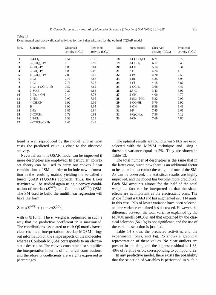
trend is well reproduced by the model, and in mostcases the predicted value is close to the observedactivity.

Nevertheless, this QSAR model can be improved ifmore descriptors are employed. In particular, convexset theory can be used to carry out convex linearcombinations of SM in order to include new informa-tion in the resulting matrix, yielding the so-called atuned QSAR (TQSAR) approach. Thus, the Bakertriazines will be studied again using a convex combi-nation of overlap (ZOVE) and Coulomb (ZCOU) QSM.The SM used to build the multilinear regression willhave the form:

Z � aZOVE 1 �1 2 a�ZCOU;

with a [ �0;1�: Thea weight is optimised in such away that the predictive coefficientq2 is maximised.The contributions associated to each QS matrix have aclear chemical interpretation: overlap MQSM bringsout information on the shape aspects of the molecules,whereas Coulomb MQSM corresponds to an electro-static descriptor. The convex constraint also simplifiesthe interpretation in terms of numerical contributions,and thereforea coefficients are weights expressed aspercentages.

The optimal results are found when 5 PCs are used,selected with the MPVM technique and using athreshold variance equal to 2%. They are shown inTable 13.

The total number of descriptors is the same that inthe latter case, since now there is an additional factorto be taken into account: the weight of one of the SM.As can be observed, the statistical results are highlyimproved, and the model has become more predictive.Each SM accounts almost for the half of the totalweight, a fact can be interpreted as that the shapeeffects are as important as the electrostatic ones. Theq2 coefficient is 0.663 and has augmented in 0.114 units.In this case, PCs of lower variance have been selected,and the variance explained has decreased. However, thedifference between the total variance explained by theMPVM model (48.3%) and that explained by the clas-sical selection (56.1%) is not significant, and the use ofthe variable selection is justified.

Table 14 shows the predicted activities and theexperimental ones, and Fig. 25 shows a graphicalrepresentation of these values. No clear outliers arepresent in the data, and the highest residual is 1.88,40% of relative error, corresponding to compound 22.

In any predictive model, there exists the possibilitythat the selection of variables is performed in such a

R. Carbo-Dorca et al. / Journal of Molecular Structure (Theochem) 504 (2000) 181–228 213

Table 14Experimental and cross-validated activities for the Baker triazines for the optimal TQSAR model

Mol. Substituents Observedactivity (LC50)

Predictedactivity (LC50)

Mol. Substituents Observedactivity (LC50)

Predictedactivity (LC50)

1 3,4-Cl2 8.54 8.36 18 3-COCH2Cl 6.21 6.722 3-(CH2)2–Ph 8.19 7.93 19 3-OCH3 6.17 6.463 4-CH2–Ph 8.05 6.84 20 4-CN 5.14 6.344 3-CH2–Ph 8.00 9.02 21 2-F 4.74 4.135 4-(CH2)2–Ph 7.89 6.18 22 4-Ph 4.70 6.586 3-CF3 7.76 7.88 23 2-Br 4.25 4.957 3-Cl 7.76 6.76 24 2-Cl 4.15 3.878 3-Cl, 4-OCH2–Ph 7.52 7.62 25 2-OCH3 3.68 4.479 3-SO2F 7.27 6.88 26 2,5-Cl2 3.43 3.06

10 3-Ph, 4-OH 7.14 6.73 27 2-CH3 4.00 4.7911 3-NO2 7.07 7.05 28 3-SO2–NH2 5.32 7.0912 4-CH2CN 6.92 6.05 29 3-CONH2 5.70 6.9013 H 6.92 6.05 30 3-OH 6.38 6.4614 3-Ph 6.85 6.84 31 3-F 7.45 6.6515 3-COCH3 6.79 6.81 32 3-C(CH3)3 7.50 7.1216 2,3-Cl2 6.52 5.29 33 3-CN 7.69 7.8017 4-COCH2Cl-Ph 6.45 6.49

R. Carbo-Dorca et al. / Journal of Molecular Structure (Theochem) 504 (2000) 181–228214

Fig. 25. Baker triazines predicted versus observed activities. Overlap and Coulomb QS matrices. 5 PCs plot.

Fig. 26. Plot ofq2 againstr2 for the real (1 ) and randomised (X) triazine activities.

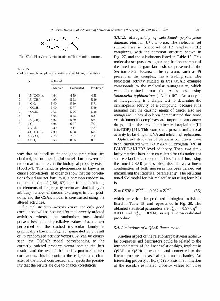
way that an excellent fit and good predictions areobtained, but no meaningful correlation between themolecular structure and the biological property exists[156,157]. This random phenomenon is known aschance correlations. In order to show that the correla-tions found are not fortuitous, a common randomisa-tion test is adopted [156,157] here. In this technique,the elements of the property vector are shuffled by anarbitrary number of random exchanges in their posi-tions, and the QSAR model is constructed using thealtered activities.

If a real structure–activity exists, the only goodcorrelations will be obtained for the correctly orderedactivities, whereas the randomised ones shouldpresent low fit and predictive values. Such a testperformed on the studied molecular family isgraphically shown in Fig. 26, generated as a resultof 75 randomised activity vectors. As can be clearlyseen, the TQSAR model corresponding to thecorrectly ordered property vector obtains the bestresults, and the rest of the models produce poorestcorrelations. This fact confirms the real predictive char-acter of the model constructed, and rejects the possibi-lity that the results are due to chance correlations.

5.3.1.2. Mutagenicity of substituted (o-phenylenediamine) platinum(II) dichloride.The molecular setstudied here is composed of 12cis-platinum(II)complexes, with the common structure shown inFig. 27, and the substituents listed in Table 15. Thismolecular set provides a good application example ofthe fitted atomic gaussian basis set presented in theSection 3.3.2, because a heavy atom, such as Ptpresent in the complex, has a leading role. Thebiological activity studied in this QSAR examplecorresponds to the molecular mutagenicity, whichwas determined from the Ames test usingSalmonella typhimurium(TA-92) [67]. An analysisof mutagenicity is a simple test to determine thecarcinogenic activity of a compound, because it isassumed that the causing agents of cancer also aremutagenic. It has also been demonstrated that somecis-platinum(II) complexes are important anticancerdrugs, like the cis-diamminedichloroplatinum(II)(cis-DDP) [31]. This compound present antitumoralactivity by binding to DNA and inhibiting replication.

Optimised structures of platinum complexes havebeen calculated withGaussian 94 program [69] atB3LYP/LANL2DZ level of theory. Then, two simi-larity matrices have been calculated for this molecularset: overlap-like and coulomb-like. In addition, usingthe tuned QSAR process described above, a linearcombination of both measures has been carried outmaximising the statistical parameterq2. The resultingtuned SM model for this molecular set using four PCsis:

Z � 0:938× ZCOU 1 0:062× ZOVE �56�which provides the predicted biological activitieslisted in Table 15, and represented in Fig. 28. Theobtained statistical parameters are:r2

calc� 0:977; q2 �0:933 and r2

pred� 0:934; using a cross-validatedprocedure.

5.4. Limitations of a QSAR linear model

Another aspect of the relationship between molecu-lar properties and descriptors could be related to theintrinsic nature of the linear relationships, implicit inQSAR or QSPR procedures and connected to thelinear structure of classical quantum mechanics. Aninteresting property of Eq. (46) consists in a limitationof the possible estimated property values for those

R. Carbo-Dorca et al. / Journal of Molecular Structure (Theochem) 504 (2000) 181–228 215

Fig. 27. (o-Phenylenediamine)platinum(II) dichloride structure.

Table 15cis-Platinum(II) complexes: substituents and biological activity

X log(1/C)

Observed Calculated Predicted

1 4,5-(OCH3)2 4.64 4.59 4.552 4,5-(CH3)2 4.99 5.28 5.403 4-CH3 5.60 5.69 5.714 4-OC2H5 5.60 5.77 5.895 4-OCH3 5.65 5.56 5.486 H 5.63 5.43 5.377 4,5-(CH)4 5.92 5.70 5.618 4-Cl 6.94 6.97 7.019 4,5-Cl2 6.89 7.17 7.31

10 4-COOCH3 7.00 6.88 6.8211 4,5,6-Cl3 7.73 7.54 7.1412 4-NO2 8.65 8.66 8.71

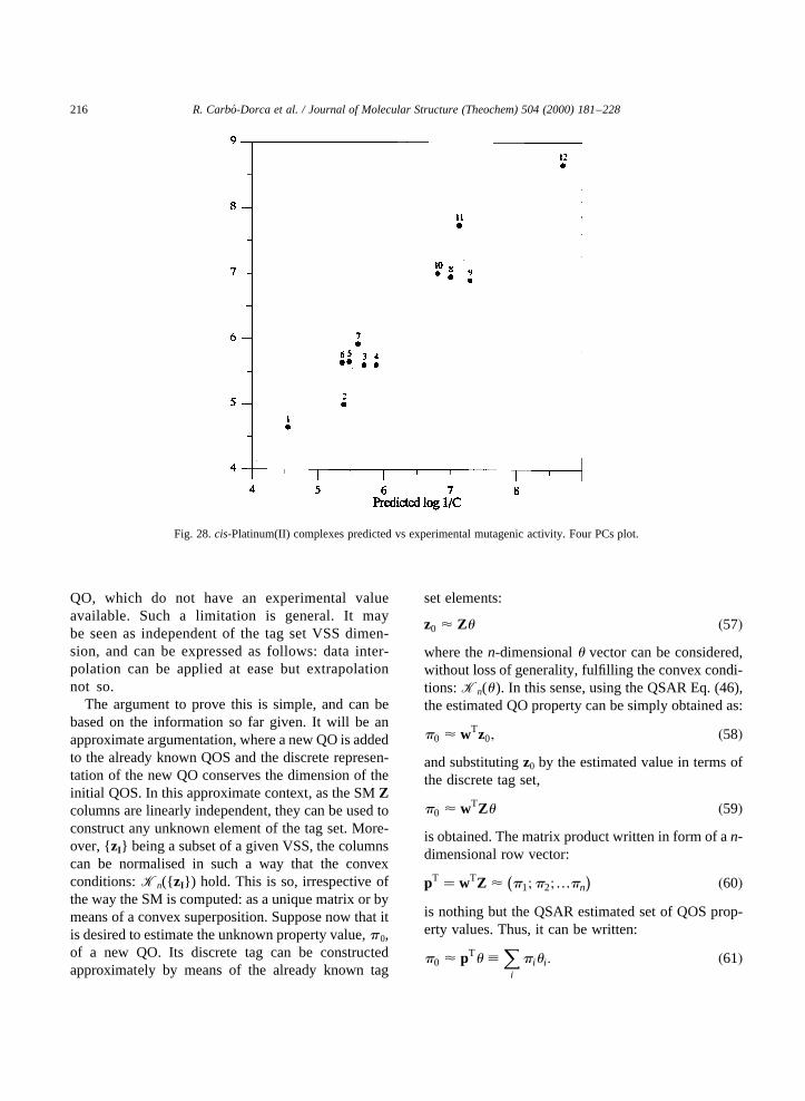
QO, which do not have an experimental valueavailable. Such a limitation is general. It maybe seen as independent of the tag set VSS dimen-sion, and can be expressed as follows: data inter-polation can be applied at ease but extrapolationnot so.

The argument to prove this is simple, and can bebased on the information so far given. It will be anapproximate argumentation, where a new QO is addedto the already known QOS and the discrete represen-tation of the new QO conserves the dimension of theinitial QOS. In this approximate context, as the SMZcolumns are linearly independent, they can be used toconstruct any unknown element of the tag set. More-over, {zI} being a subset of a given VSS, the columnscan be normalised in such a way that the convexconditions:Kn({ zI}) hold. This is so, irrespective ofthe way the SM is computed: as a unique matrix or bymeans of a convex superposition. Suppose now that itis desired to estimate the unknown property value,p0,of a new QO. Its discrete tag can be constructedapproximately by means of the already known tag

set elements:

z0 < Zu �57�where then-dimensionalu vector can be considered,without loss of generality, fulfilling the convex condi-tions:Kn(u). In this sense, using the QSAR Eq. (46),the estimated QO property can be simply obtained as:

p0 < wTz0; �58�and substitutingz0 by the estimated value in terms ofthe discrete tag set,

p0 < wTZu �59�is obtained. The matrix product written in form of an-dimensional row vector:

pT � wTZ < p1;p2;…pn

ÿ � �60�is nothing but the QSAR estimated set of QOS prop-erty values. Thus, it can be written:

p0 < pTu ;X

i

piui : �61�

R. Carbo-Dorca et al. / Journal of Molecular Structure (Theochem) 504 (2000) 181–228216

Fig. 28.cis-Platinum(II) complexes predicted vs experimental mutagenic activity. Four PCs plot.

This result proves, within the limits of the approx-imations used, that the convex nature, attachable toVSS elements, forces the value of the QSAR esti-mated property to be interpolated. In this manner, itmust be said that these inferred values of the propertywill forcibly lie in the interval bounded by the mini-mal and the maximal values of the property.

The above result corresponds to a rough estimation,as was observed at the beginning of this discussion.This is so, because the inclusion of a new QO in theQOS tagged set augments in one the dimension of thetag VSS was not taken into account. Despite this, itseems reasonable to seriously consider this result asan argument, making QSAR extrapolations unfavour-able within a VSS description.

It must be noted, finally, that this limitation of thelinear QSAR models may be originate from a moregeneral property. A situation, which can be connectedto the mathematical nature of the problem, and that,probably, can be attached to the extent of what can bededuced from the known experimental data. Perhaps itmay be almost impossible to obtain reliable informa-tion on unknown QO from current data knowledgeusing empirical linear models. The problem consistsinto the fact that discretisation of quantum expectationvalues can be considered the basis of QSPR. Then,only trying a whole VS parameter description as inprincipal component analysis or borrowing argumentsof non-linear quantum mechanics can solve, perhaps,this impasse.

5.5. p-valued QSPR

In some cases, the outcome of experiments cannotbe presented in the form of rational numbers, asoccurs in the previously discussed QSPR problems.The experimental situation is better expressed, forinstance, as ap-valued set of symbols, which at theend can be transformed into Boolean strings. Herewill be discussed the structure of this kind of scenario,when the problem consists into that a theoreticalframe has to be found for estimation purposes inthis p-valued context.

5.5.1. General descriptionIn such a situation, the QSPR equation treatment

cannot be written in the same way as before. Whentrying to evaluate the discrete operator representation,

the limited pool of values of the property must betaken into account. The statistical framework tostudy this kind of problems can be found in manyplaces, but a convenient treatment is presented in arecent reference [115].

Eq. (49) is still valid but the left hand side values ofthe property can only be associated to any onecontained into thep-valued set:

pI [ { p1; p2;…pp} ; ;I : �62�Also, the estimated values obtained by means of theright hand side of Eq. (49) can be bounded andordered inp classes, according to appropriate rules.Then, the equations giving rise to the discrete QSPRprocedure may be written:

;I : wTzI # uJ ∧ wTzI $ uJ21; �63�where the symbols at the right hand side of theinequalities correspond to some appropriate bound-aries defining the problem classes. For example,when a dichotomous set of property values arepresent, then the equations may be classified through-out an arithmetic mean, defined by:

�u � n21X

I

wTzI �64�

and the QSPR problem could be written according thefollowing rule:

If pI � 0 : wTzI # �u ∧ pJ � 1 : wTzj . �u : �65�Formally, this result appears as having a linearprogramming structure. A straightforward manipula-tion of Eq. (65) shows that this way is too simple toproduce in difficult cases significant results.

5.5.2. Optimal classificationHowever, there are other possible ways to solve this

discrete experimental outcome, attached to a discreteQOS description. A discussion will be carried out forthe particular case of a dichotomic classification.

Supposing if a discrete QOS formed byn QO isknown,. Also known shall be the�n × n� SM, Z �{ z1; z2;…; zn} ; whose columns constitute the QOdiscrete tag set. It must be also supposed that adichotomic valued property set for each QO is avail-able. The dichotomic values can be associated, with-out loss of generality, to a bit valued set: {0,1}.

In this manner, the whole set of the dichotomic

R. Carbo-Dorca et al. / Journal of Molecular Structure (Theochem) 504 (2000) 181–228 217

experimental outcome can be collected into a Booleanvector:v � �v1; v2;…; vn� ∧ vI [ {0 ;1} : Furthermore,this experimental vectorv, may be considered as avertex belonging to some appropriately definedn-dimensional unit Boolean hypercube,Hn. This isthe same as the geometrical structure used in the defi-nition of Boolean tagged sets in Section 2.1 (see Ref.[84] for more details).

In the Boolean vectorv, there will be alwayspresentn0 null as well asn1 unit scrambled bits, insuch a way thatn� n0 1 n1: Thus,v belongs to somevertex subset ofHn, forming a vertex class having incommonn0 null and n1 unit bits: Hc , Hn: Thereexists one vertex,vc [ Hc; which is canonicallyordered in the following sense: the firstn0 positionsare null bits, the lastn1 ones are made of unitelements. Appropriate ordering of the experimentaloutcome events can be seen as a projection of theelements ofHc into the vectorvc:

P�v� � vc:

This situation inHn can be considered as a cano-nical ordering algorithm to be used in such experi-mental output structure, attached to QOS or totagged sets in general. It will cause a simple reorder-ing of the SM columns in the discrete QOS case, or areordering of the tagged set elements in manyproblems of this kind. It will transform arbitraryordering into this canonical ordering, thus bringingany experimental output into close connection withdescriptor matrices. In any case, the same data isobtained at the end, with the same pattern, avoidinginformation loss.

Then, any investigation having such form could beconsidered connected to an experimental vectoroutcome, canonically ordered according to the vertexvc. The SM can be partitioned into two submatrices:Z � { Z0;Z1} ; whose columns are the QO discretetags associated to the null or unit bit experimentaloutcome, respectively:

Z0 � �z01; z02;…; z0n0� ∧ Z1 � �z11; z12;…; z1n1

�:At this stage, one can easily see that the problem hassufficient information to allow more than the evalua-tion of a mean vector, as in the previous discussion(see Eq. (64)). The dichotomic class partition will alsopermit to evaluate two class centroid vectors:�z�0�; z�1��, representing the two classes considered.

Class centroids can be obtained by just averagingthe vectors apparently belonging to the two classes.However, they can be also optimised, once alterna-tively constructed using appropriate procedures [161].

5.5.3. Degenerate aspects of p-valued QSPRAs in classical QSPR problems with a rational

experimental outcome, as discussed in Section 5.4,there can be some similar harsh limitations when thep-valued experimental case is studied. In the presentframework, a curious situation appears, and as itseems important to remark, some discussion will begiven here.

In p-valued experiments, the outcome is easilyattached to a classZc , Hn; belonging to an-dimen-sional hypercube. Ordering will transform bothexperimental data and QOS tags into a system withknown SM Z and an attached canonical vertex bitvector vc [ Zc: The number of vertices inHn islimited to 2n, and the number of vertex classes becomelimited to v� n 1 1 : { Zc; c� 1; v} : Then, suchexperimental structure can only provide a resulthaving any of then available canonically orderedclass vectors. One can resume the situation by sayingthe problem becomesdegenerate, in a similar way asthe one discussed in Section 2.1. By this, according tothe early definition, it is meant that a set of severalSM: {Zk} may have attached the same canonicaloutcomevc.

Leaving apart the statistical point of view, which itis not so clear to apply in the case of QOS, attached top-valued experimental outcome, one can try to discussthe problem further on. Such drawback can be moredramatically seen when severalp-valued experimentsare performed using various QOS of the same cardin-ality, involving perhaps quite diverse objects and tags.The experimental outcome conveniently coded andcanonically ordered may be attached to the samevertex, however the QOS may greatly differ. Althoughthe QO within a QOS can be ordered following theprevious procedure, one can ask which analyticalsense could be attached to the results.

5.5.4. Final remarksIn any case, one must take into account that,p-

valued outcome degeneracy seems to preclude thefact that very inhomogeneous OS can possess thesame experimental outcome vector. In this manner,

R. Carbo-Dorca et al. / Journal of Molecular Structure (Theochem) 504 (2000) 181–228218

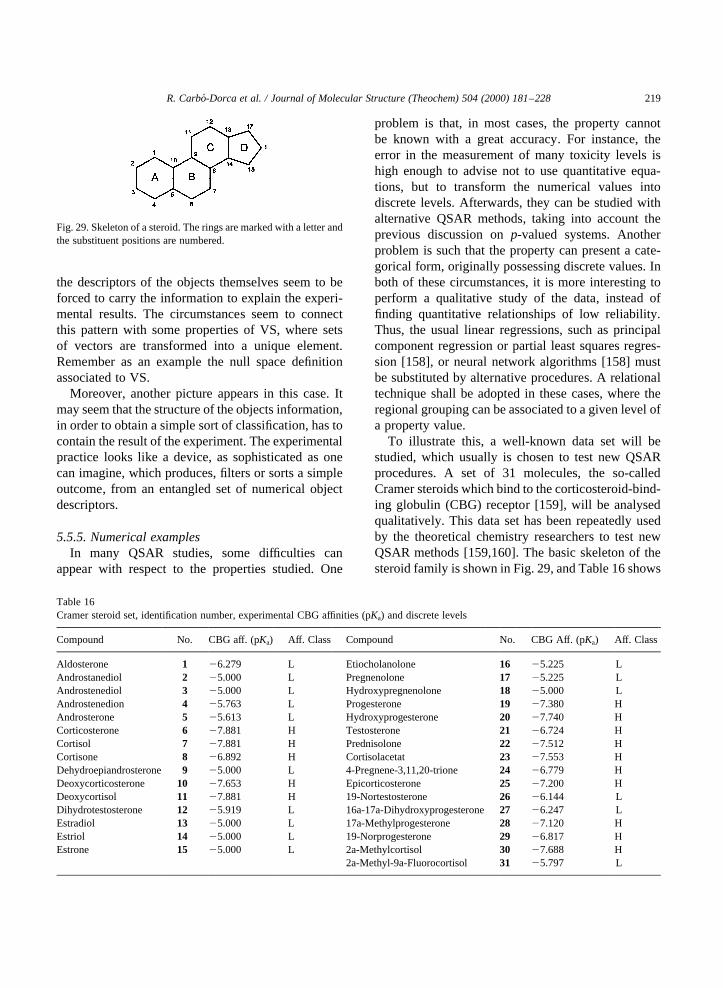
the descriptors of the objects themselves seem to beforced to carry the information to explain the experi-mental results. The circumstances seem to connectthis pattern with some properties of VS, where setsof vectors are transformed into a unique element.Remember as an example the null space definitionassociated to VS.

Moreover, another picture appears in this case. Itmay seem that the structure of the objects information,in order to obtain a simple sort of classification, has tocontain the result of the experiment. The experimentalpractice looks like a device, as sophisticated as onecan imagine, which produces, filters or sorts a simpleoutcome, from an entangled set of numerical objectdescriptors.

5.5.5. Numerical examplesIn many QSAR studies, some difficulties can

appear with respect to the properties studied. One

problem is that, in most cases, the property cannotbe known with a great accuracy. For instance, theerror in the measurement of many toxicity levels ishigh enough to advise not to use quantitative equa-tions, but to transform the numerical values intodiscrete levels. Afterwards, they can be studied withalternative QSAR methods, taking into account theprevious discussion onp-valued systems. Anotherproblem is such that the property can present a cate-gorical form, originally possessing discrete values. Inboth of these circumstances, it is more interesting toperform a qualitative study of the data, instead offinding quantitative relationships of low reliability.Thus, the usual linear regressions, such as principalcomponent regression or partial least squares regres-sion [158], or neural network algorithms [158] mustbe substituted by alternative procedures. A relationaltechnique shall be adopted in these cases, where theregional grouping can be associated to a given level ofa property value.

To illustrate this, a well-known data set will bestudied, which usually is chosen to test new QSARprocedures. A set of 31 molecules, the so-calledCramer steroids which bind to the corticosteroid-bind-ing globulin (CBG) receptor [159], will be analysedqualitatively. This data set has been repeatedly usedby the theoretical chemistry researchers to test newQSAR methods [159,160]. The basic skeleton of thesteroid family is shown in Fig. 29, and Table 16 shows

R. Carbo-Dorca et al. / Journal of Molecular Structure (Theochem) 504 (2000) 181–228 219

Fig. 29. Skeleton of a steroid. The rings are marked with a letter andthe substituent positions are numbered.

Table 16Cramer steroid set, identification number, experimental CBG affinities (pKa) and discrete levels

Compound No. CBG aff. (pKa) Aff. Class Compound No. CBG Aff. (pKa) Aff. Class

Aldosterone 1 26.279 L Etiocholanolone 16 25.225 LAndrostanediol 2 25.000 L Pregnenolone 17 25.225 LAndrostenediol 3 25.000 L Hydroxypregnenolone 18 25.000 LAndrostenedion 4 25.763 L Progesterone 19 27.380 HAndrosterone 5 25.613 L Hydroxyprogesterone 20 27.740 HCorticosterone 6 27.881 H Testosterone 21 26.724 HCortisol 7 27.881 H Prednisolone 22 27.512 HCortisone 8 26.892 H Cortisolacetat 23 27.553 HDehydroepiandrosterone 9 25.000 L 4-Pregnene-3,11,20-trione 24 26.779 HDeoxycorticosterone 10 27.653 H Epicorticosterone 25 27.200 HDeoxycortisol 11 27.881 H 19-Nortestosterone 26 26.144 LDihydrotestosterone 12 25.919 L 16a-17a-Dihydroxyprogesterone27 26.247 LEstradiol 13 25.000 L 17a-Methylprogesterone 28 27.120 HEstriol 14 25.000 L 19-Norprogesterone 29 26.817 HEstrone 15 25.000 L 2a-Methylcortisol 30 27.688 H

2a-Methyl-9a-Fluorocortisol 31 25.797 L

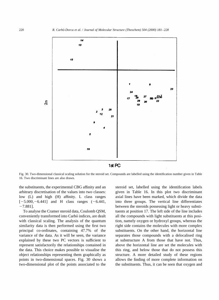
the substituents, the experimental CBG affinity and anarbitrary discretisation of the values into two classes:low (L) and high (H) affinity. L class ranges[25.000,26.441] and H class ranges (26.441,27.881].

To analyse the Cramer steroid data, Coulomb QSM,conveniently transformed into Carbo´ indices, are dealtwith classical scaling. The analysis of the quantumsimilarity data is then performed using the first twoprincipal co-ordinates, containing 47.7% of thevariance of the data. As it will be seen, the varianceexplained by these two PC vectors is sufficient torepresent satisfactorily the relationships contained inthe data. This choice makes possible to visualise theobject relationships representing them graphically aspoints in two-dimensional spaces. Fig. 30 shows atwo-dimensional plot of the points associated to the

steroid set, labelled using the identification labelsgiven in Table 16. In this plot two discriminantaxial lines have been marked, which divide the datainto three groups. The vertical line differentiatesbetween the steroids possessing light or heavy substi-tuents at position 17. The left side of the line includesall the compounds with light substituents at this posi-tion, namely oxygen or hydroxyl groups, whereas theright side contains the molecules with more complexsubstituents. On the other hand, the horizontal lineseparates those compounds with a delocalised ringat substructure A from those that have not. Thus,above the horizontal line are set the molecules withthis ring, and below those that do not possess thisstructure. A more detailed study of these regionsallows the finding of more complete information onthe substituents. Thus, it can be seen that oxygen and

R. Carbo-Dorca et al. / Journal of Molecular Structure (Theochem) 504 (2000) 181–228220

Fig. 30. Two-dimensional classical scaling solution for the steroid set. Compounds are labelled using the identification number given in Table16. Two discriminant lines are also drawn.

hydroxyl-substituted compounds can also be sepa-rated, and, in relation to the steroids with bulky substi-tuents, the COCH2OH chain can be differentiatedfrom COCH3 substituent and from COCH2OOCCH3

chain of compound23. Compound1 is the onlyexception in this structural classification, and can beconsidered a misclassification of the model [161].

Much more interesting than to identify commonstructural features of the compounds, is to relatethese groups to discrete levels of a given property.In the present case, the above representation is plottedagain labelling each molecule with the correspondingdiscrete affinity class. This is shown in Fig. 31.

As can be seen, the steroids are rather well classi-fied in terms of their CBG affinity, in spite of only halfof the information is explained by the first two PCs.The only misclassifications, 6 of a total of 31, aremainly made up of compounds of intermediateactivity (1, 21, 27). Also, there appear misclassifiedsome molecules, located at the central region of theplot (17, 18), where the classification is less clear.

Finally, steroid31 appears also out of classification,but this molecule is an outlier in most of the QSARstudies of the Cramer family, due to the fluorine atposition 9.

Other projections can be performed in order toobtain better visual discrimination. Thus, the projec-tion on the first and third principal axes leads to Fig.32. As can be seen, now there are only two misclassi-fied compounds, and one of them is the outlier mole-cule 31. This fact indicates, together with theevidences shown in the previous examples, thatthe first PCs are not always the best descriptors ofthe system, and one can make use of lower varianceaxes to improve the discrimination. The explainedvariance is even poorer, but the most essential infor-mation can be extracted. The visualisation of all thepossible two- or three-dimensional subspaces can be ahard task, and for this reason, some practical compu-tational algorithms have been developed in ourlaboratory. In particular, an algorithm has beenused, which searches the two-dimensional subspace,

R. Carbo-Dorca et al. / Journal of Molecular Structure (Theochem) 504 (2000) 181–228 221

Fig. 31. Two-dimensional classical scaling solution for the steroid set. Compounds are labelled using the following notation.X: Low activitycompounds;W: High activity compounds;B: Low activity compounds misclassified: {1, 17, 18, 27}; A: High activity compound misclassified:{ 21}; w: Low activity compound31 misclassified.

minimising the number of crossings between linksof molecular pairs belonging to different classes[162].

These results indicate that the steroid set is a dataset where the activity can be clearly associated to thetype and position of the substituents. Thus, moleculeswith light substituents (oxygen or hydroxyl groups) atposition 17 lead to low activity values, whereas thepresence of the chain COCH2OH usually augmentsthe CBG affinity of the molecule. Further, theexistence of the ring A in a delocalised form doesnot improve the activity of the compounds. Thisinformation can be employed to improve thecomputer-aided molecular design models and tounderstand better the steroid–protein interactions.

5.6. Boolean tagged ensembles

From all things said in the above sections, deal-ing with p-valued experimental outcome, asummary can be structured in terms of a new defi-

nition of tagged sets associated to such experimen-tal Boolean form. The next definition will try todeal with them.

Definition 9 (Boolean tagged ensembles). Supposea collection,C � {TI } ; of tagged sets bearing thesame cardinality is known. That is:;TI [ C!#�TI � � n:

Suppose a unitn-dimensional hypercube,Hn �{ vp} is known.

A Boolean tagged ensemble,E, is a tagged setwhose object set isC, and whose tag set isHn:

E � C × Hn � { ;ZI ;p [ Eu'TI [ C ∧ 'vp [ H

) ZI ;p � �TI ; vp�} :

In the light of this definition, a Boolean tagged ensem-ble isdegenerateif: ;ZI ;p [ E! vp � vc; vc being

R. Carbo-Dorca et al. / Journal of Molecular Structure (Theochem) 504 (2000) 181–228222

Fig. 32. Two-dimensional classical scaling solution for the steroid set using the 1st and 3rd PCs. Compounds are labelled using the followingnotation:X: Low activity compounds;W: High activity compounds;B: Low activity compounds misclassified: {27, 31}.

a vertex common to all the tagged sets in the Booleantagged ensemble.

The definition of Boolean tagged ensembles can beviewed as some kind of recursive property attached tothe tagged set definition. The notion of Booleantagged ensemble can be easily generalised to variouskinds of tagged ensembles:

Definition 10 (Tagged ensembles). A taggedensemble is a tagged set whose object set elementsare tagged sets.

For example, suppose a QOS, discrete or not, ofcardinality n is known. Suppose an-dimensionalvector, made of experimental results is also known,so to say. Suppose that both mathematical structuresare constructed in such a manner that every QO is in aone-to-one correspondence with the experimentalvector elements. This construct can be considered anelement of a tagged ensemble.

Then, QSPR studies will deal in this manner withelements of tagged ensembles, and their aim could bedescribed as the way in which a relationship is to befound between objects and tags defining the taggedensemble.

6. Generalised scalar products inn-dimensionalVSS

Other interesting questions appear when thinkingon the peculiar structure of QOS and their descriptorspaces forming the tag set elements. Several of themwill be discussed here.

6.1. Permanent of a matrix

If the structure of SM and of discrete QOS isobserved, as well as the presence of VSS, containingthe discrete representation of DF, then, there appearsthe possibility to obtain single parameters reducing,somehow, the SM in part or as a whole into a uniquescalar. In order to accomplish such task, a general-isation of the scalar product may be proposed inan n-dimensional VSS. This needs of a previousdefinition:

Definition 11 (Permanent of a (n× n) matrix). -Known a �n × n� matrix: Z � { zI } � { zJI} ∧ { zI

[ Cn�R1�}, the permanent ofZ: PeruZu; can becomputed as:

PeruZu �Xn

�i�P�i�q�i�;

where i � { ip} ; is the index vector of the nestedsummation symbol:

Pn�i� , [88]; P�i� � 0 if 'ip � iq

in the index vector, and is 1 otherwise; finally:q�i� �Qnk�1 z

kik :

Thus, the permanent is like a determinant but withoutconsidering index permutation parity. For moredetails see Ref. [95].

6.2. Generalised scalar product of n vectors

Defined as above, PeruZu permits to be considered ascalar product involvingn vectors, the columns ofZ,in n-dimensional VSS. The operation is distributivewith respect to the sum of a vector on any column ofthe matrix, and multiplying a column by a scalar, thepermanent is scaled by the same amount. The columnorder is immaterial. The same properties apply to thematrix rows.

6.3. Generalised norm of a vector

A norm, associated to the kind of generalised scalarproduct, inn-dimensional VSS can be easily definedas the permanent of a matrix with the same columnrepeatedn times:

NPer�z� � Peru�z; z;…z�u � �n!�Yn

k�1

zk

!:

This makes clear that only in VSS, where vectorelements are completely PD, this kind of norm canbe defined as a PD computational device.

6.4. Generalised carbo´ similarity index

The construction of generalised scalar products andnorms, involving several discrete DF representations,may be used to define the associated similarityindices. In the way so many times discussed in theliterature, even when the initial definition of QSM[1] was given. See Refs. (51,53,73–79) for a generalreview on the subject.

The so called Carbo´ index involving two QO,

R. Carbo-Dorca et al. / Journal of Molecular Structure (Theochem) 504 (2000) 181–228 223

defined by means of a cosine-like formulation:

rAB � zAB�zAAzBB�2�1=2� �66�where the SM elements of dimension�2 × 2� are used.The elements of this matrix can be also ordered as:

Z2 �zAA zAB

zAB zBB

!� zA zB

ÿ �: �67�

Then, using the generalised scalar product and norm,defined in Section 4.2.2, a Carbo´ index may bedefined. It can be based in this two QO matrix repre-sentations, according to Eq. (66) and taking intoaccount the origin of the SM elements, as:

RAB � PeruZ2u�NPeruzAuNPeruzBu�2�1=2�

� Peru zA zB

ÿ �u �Peru zA zA

ÿ �uPeru zB zB

ÿ �u�2�1=2�

� 12 �zAAzBB 1 z2

AB���zAAzAB��zABzBB��2�1=2�

� 12 �r21

AB 1 rAB� (68)

The interesting result consists in that for two QOthis generalised Carbo´ index, RAB, becomes anarithmetic average of the classical Carbo´ indexand its inverse. As inverse cosine-like similarityindices behave as distance indices, one canconclude that generalised two QO similarityCarbo indices behave as averaged cosine-like anddistance-like indices. Three or more QO similarityindices computed in the same way, may behave ina more complex fashion, but it is evident that theyconstitute a new bred of molecular descriptors tobe taken into account.

7. Conclusions

A general discussion on the formal structure ofQSM and the surrounding problems has been carriedout. Several definitions design in an accurate mannerthe notion of QO and, in this way, the tagged setstructure of QOS naturally appears. The attachedformalism becomes a rich source of new concepts,such as the KE DF and other DF forms, which arebased on extended Hilbert spaces. This formalism

leads towards a matrix formulation of energy expecta-tion values. The new density functions forms can bedescribed and visualised too, producing usefulsuggestive pictures of the molecular structureenvironment.

Discretisation of QO descriptions, via general defi-nitions of QSM, also conduces to the definition of SMand discrete QOS. The ascription of all the involvedtag sets to some VSS, allows the analysis of severalaspects of QSM as well as of the QSPR. In this way, itcan be said that QSMn-dimensional vectors, asso-ciated to a given molecular structure, can be consid-ered, from a quantum mechanical optic, as anunbiased way to represent microscopic systems in adiscrete manner. In this QSM context, the user has noway to choose arbitrarily the parameters and, doingso, possibly interact with the resulting model. Empiri-cal QSAR parameters, whatever be their origin,shall be considered as examples of more or lesssuccessful attempts to simulate such QSM vector-ial description.

New mathematical devices like the permanent ofthe SM, which can be considered as generalised scalarproducts, can be used as a possible source of QOdescriptors. Therefore, these new descriptors can beviewed as another of the consequences of the presentframework. They can be employed as a new source ofquantum similarity indices computation, which areeasily defined and possessing an interesting potentialbehaviour.

Acknowledgements

One of us (R.C.-D.) wishes to express his debt toProf. K. Hirao, who has made possible a researchstage at the Department of Industrial Chemistry,Faculty of Engineering, University of Tokyo, duringNovember 1997. This platform allowed enlighteningdiscussions with him and permitted the making of afirst draft, involving the theoretical side of the presentpaper.

Lively discussions on the many facets of theproblems contained in this work were also carriedout with Prof. P.G. Mezey, during his 1998 stay atthe IQC in Girona. The authors thank his remarksand comments, which helped to improve severalaspects of the initial manuscript.

R. Carbo-Dorca et al. / Journal of Molecular Structure (Theochem) 504 (2000) 181–228224

Finally, thanks are also due to Mr A. Bach, for hisdevoted way to test numerically some of the newestaspects of this work, in especial the KE DF develop-ment part.

This work has been partially financed by a CICYTResearch Project: #SAF 96-0158 and sponsored by aCOMET contract: #ENV4-CT97-0508.

References

[1] R. Carbo, M. Arnau, L. Leyda, Int. J. Quant. Chem. 17(1980) 1185–1189.

[2] E.E. Hodgkin, W.G. Richards, Int. J. Quant. Chem. 14 (1987)105–110.

[3] C. Burt, W.G. Richards, Ph. Huxley, J. Comput. Chem. 11(1990) 1139–1146.

[4] A.C. Good, E.E. Hodgkin, W.G. Richards, J. Chem. Inf.Comp. Sci. 32 (1992) 188–191.

[5] A.C. Good, Sung-Sau So, W.G. Richards, J. Math. Chem. 36(1993) 433–438.

[6] A.C. Good, W.G. Richards, J. Chem. Inf. Comp. Sci. 33(1993) 112–116.

[7] D.L. Cooper, N.L. Allan, J. Comp. Aid. Mol. Des. 3 (1989)253–259.

[8] D.L. Cooper, N.L. Allan, J. Am. Chem. Soc. 114 (1992)4773–4776.

[9] D.L. Cooper, K.A. Mort, N.L. Allan, D. Kinchington, Ch.McGuidan, J. Am. Chem. Soc. 115 (1993) 12615–12616.

[10] N.L. Allan, D.L. Cooper, Top. Curr. Chem. 173 (1995) 85–111.

[11] J. Cioslowski, E.D. Fleishmann, J. Am. Chem. Soc. 113(1991) 64–67.

[12] J.B. Ortiz, J. Cioslowski, Chem. Phys. Lett. 185 (1991) 270–275.

[13] J. Cioslowski, M. Challacombe, Int. J. Quant. Chem. S25(1991) 81–93.

[14] J. Cioslowski, S.T. Mixon, Can. J. Chem. 70 (1992) 443–449.[15] J. Cioslowski, A. Nanayakkara, J. Am. Chem. Soc. 115

(1993) 11213–11215.[16] J. Cioslowski, B.B. Stefanov, P. Constans, J. Comput. Chem.

17 (1996) 1352–1358.[17] R. Ponec, M. Strnad, Collect. Czech. Chem. Commun. 55

(1990) 896–902.[18] R. Ponec, M. Strnad, Collect. Czech. Chem. Commun. 55

(1990) 2583–2589.[19] R. Ponec, M. Strnad, J. Phys. Org. Chem. 4 (1991) 701–705.[20] R. Ponec, M. Strnad, J. Math. Chem. 8 (1991) 103–112.[21] R. Ponec, M. Strnad, Int. J. Quant. Chem. 42 (1992) 501–

508.[22] R. Ponec, J. Chem. Inf. Comp. Sci. 33 (1993) 805–811.[23] R. Ponec, Overlap Determinant Method in the Theory of

Pericyclic Reactions, Lecture Notes in Chemistry 65,Springer, Berlin, 1995.

[24] P.G. Mezey, Shape in Chemistry: an Introduction to Mole-cular Shape and Topology, VCH, New York, 1993.

[25] P.G. Mezey, Molecular similarity I, in: K. Sen (Ed.), Topicsin Current Chemistry, vol. 173, Springer, Berlin, 1995, pp.63–83.

[26] Ch. Lee, Sh. Smithline, J. Phys. Chem. 98 (1994) 1135–1138.

[27] C. Amovilli, R. McWeeny, J. Mol. Struct. (Theochem) 227(1991) 1–9.

[28] A.C. Good, J. Mol. Graph. 10 (1992) 144–151.[29] R. Benigni, M. Cotta-Ramusino, F. Giorgi, G. Gallo, J. Med.

Chem. 38 (1995) 629–635.[30] J.D. Petke, J. Comput. Chem. 14 (1993) 928–933.[31] A. Riera, J. Mol. Struct. (Theochem) 259 (1992) 83–98.[32] F. Fratev, O.E. Polansky, A. Mehlhorn, V. Monev, J. Mol.

Struct. 56 (1979) 245–253.[33] F. Fratev, V. Monev, A. Mehlhorn, O.E. Polansky, J. Mol.

Struct. 56 (1979) 255–266.[34] M.A. Johnson, G. Maggiora (Eds.), Concepts and Applica-

tions of Molecular Similarity Wiley, New York, 1990.[35] R. Carbo(Ed.), Molecular similarity and reactivity: from

quantum chemical to phenomenological approaches Under-standing Chemical Reactivity, vol. 14, Kluwer Academic,Dordrecht, 1995.

[36] K. Sen (Ed.), Molecular Similarity Topics in CurrentChemistry, vols. 173 and 174, Springer, Berlin, 1995.

[37] P.M. Dean (Ed.), Molecular Similarity in Drug DesignBlackie Academic & Professional, London, 1995.

[38] R. Carbo-Dorca, P.G. Mezey (Eds.), Advances in MolecularSimilarity, vol. 1, JAI Press, Greenwich, CT, 1996.

[39] R. Carbo-Dorca, P.G. Mezey (Eds.), Advances in MolecularSimilarity, vol. 2, JAI Press, Greenwich, CT, 1998.

[40] R. Carbo, Ll. Domingo, Int. J. Quant. Chem. 23 (1987) 517–545.

[41] R. Carbo-Dorca, J. Math. Chem. 23 (1998) 353–364.[42] R. Carbo-Dorca, J. Math. Chem. 23 (1998) 365–375.[43] R. Carbo-Dorca, in: R. Carbo´-Dorca, P.G. Mezey (Eds.),

Advances in Molecular Similarity, vol. 2, JAI Press, Green-wich, CT, 1998, pp. 43–72.

[44] R. Carbo-Dorca, E. Besalu´, J. Mol. Struct. (Theochem) 451(1998) 11–23.

[45] J.S. Bell, Speakable and Unspeakable in QuantumMechanics, Cambridge University Press, Cambridge, 1993.

[46] R. Carbo, B. Calabuig, Comp. Phys. Commun. 55 (1989)117–126.

[47] R. Carbo, B. Calabuig, J. Mol. Struct. (Theochem) 254(1992) 517–531.

[48] R. Carbo, B. Calabuig, in: A.S. Fraga (Ed.), ComputationalChemistry: Structure, Interactions and Reactivity, Elsevier,Amsterdam, 1992, p. 300–324.

[49] R. Carbo, B. Calabuig, L. Vera, E. Besalu´, Adv. QuantumChem. 25 (1994) 253–313.

[50] R. Carbo, B. Calabuig, Int. J. Quant. Chem. 42 (1992) 1681–1709.

[51] R. Carbo, E. Besalu´, in: R. Carbo(Ed.), Molecular Similarityand Reactivity: from Quantum Chemistry to Phenomenologi-cal Approaches, Kluwer Academic, Dordrecht, 1995, p. 3–30.

[52] R. Carbo, B. Calabuig, J. Chem. Inf. Comp. Sci. 32 (1992)600–606.

R. Carbo-Dorca et al. / Journal of Molecular Structure (Theochem) 504 (2000) 181–228 225

[53] R. Carbo-Dorca, E. Besalu´, L. Amat, X. Fradera, in: R.Carbo-Dorca, P.G. Mezey (Eds.), Advances in MolecularSimilarity, vol. 1, JAI Press, Greenwich, CT, 1996. p. 1–42.

[54] D. Robert, R. Carbo´-Dorca, J. Math. Chem. 23 (1998) 327–351.

[55] D. Robert, R. Carbo´-Dorca, Structure–property relationshipsin nuclei. Prediction of the binding energy per nucleon usinga quantum similarity approach, Technical Report IT-IQC-98-15. See also Nuovo Cimento, 111A (1998) 1311–1322.

[56] X. Fradera, L. Amat, E. Besalu´, R. Carbo´-Dorca, Quant.Struct.–Act. Relat. 16 (1997) 25–32.

[57] M. Lobato, L. Amat, E. Besalu´, R. Carbo´-Dorca, ScientiaGerundensis 23 (1998) 17–28.

[58] M. Lobato, L. Amat, E. Besalu´, R. Carbo´-Dorca, Quant.Struct.–Act. Relat. 16 (1997) 465–472.

[59] D. Robert, R. Carbo´-Dorca, J. Chem. Inf. Comp. Sci. 38(1998) 620–623.

[60] L. Amat, D. Robert, E. Besalu´, R. Carbo´-Dorca, J. Chem. Inf.Comp. Sci. 38 (1998) 624–631.

[61] R. Ponec, L. Amat, R. Carbo´-Dorca, Molecular basis ofquantitative structure–property relationships (QSPR): aquantum similarity approach, Technical Report: IT-IQC-98-07. See also: J. Comput-Aided Mol Des., 13 (1999)259–270.

[62] L. Amat, R. Carbo´-Dorca, R. Ponec, J. Comp. Chem. 19(1998) 1575–1583.

[63] R. Ponec, L. Amat, R. Carbo´-Dorca, Similarity approach toLFER: substituent and solvent effects on the acidities ofcarboxylic acids, Technical Report: IT-IQC-98-14. Seealso: J. Phys. Org. Chem. 12 (1999) 447–454.

[64] P.G. Mezey, R. Ponec, L. Amat, R. Carbo´-Dorca,Enantiomer 4 (1999) 371–378.

[65] X. Girones, L. Amat, R. Carbo´-Dorca, Electron–electronrepulsion energy as a molecular descriptor in QSAR andQSPR studies, J. Comput.-Aided Mol. Des., in press. Seealso Technical Report: IT-IQC-98-36.

[66] D. Hadjipavlou-Litina, C. Hansch, Chem. Rev. 94 (1994)1483–1505.

[67] C. Hansch, B.H. Venger, A. Panthananickal, J. Med. Chem.23 (1980) 459–461.

[68] S.E. Sherman, S.J. Lippard, Chem. Rev. 87 (1987) 1153–1181.[69] M.J. Frisch, G.W. Trucks, H.B. Schlegel, P.M.W. Gill, B.G.

Johnson, M.A. Robb, J.R. Cheeseman, T. Keith, G.A. Peters-son, J.A. Montgomery, K. Raghavachari, M.A. Al-Laham,V.G. Zakrzewski, J.V. Ortiz, J.B. Foresman, J. Cioslowski,B.B. Stefanov, A. Nanayakkara, M. Challacombe, C.Y.Peng, P.Y. Ayala, W. Chen, M.W. Wong, J.L. Andres, E.S.Replogle, R. Gomperts, R.L. Martin, D.J. Fox, J.S. Binkley,D.J. Defrees, J. Baker, J.P. Stewart, M. Head-Gordon, C.Gonzalez, J.A. Pople,Gaussian 94 (Revision E.2), Gaus-sian, Inc., Pittsburgh, PA, 1995.

[70] R. Carbo, E. Besalu´, L. Amat, X. Fradera, J. Math. Chem. 18(1995) 237–246.

[71] E. Besalu´, R. Carbo´, J. Mestres, M. Sola`, in: I.K. Sen (Ed.),Molecular Similarity, Topics in Current Chemistry, vol. 173,Springer, Berlin, 1995, pp. 31–62.

[72] R. Carbo, E. Besalu´, J. Math. Chem. 20 (1996) 247–261.

[73] R. Carbo, E. Besalu´, L. Amat, X. Fradera, J. Math. Chem. 19(1996) 47–56.

[74] D. Robert, R. Carbo´-Dorca, J. Chem. Inf. Comput. Sci. 38(1998) 469–475.

[75] L. Amat, D. Robert, E. Besalu´, R. Carbo´-Dorca, J. Chem. InfComput. Sci. 38 (1998) 624–631.

[76] D. Robert, R. Carbo´-Dorca, J. Chem. Inf. Comput. Sci. 38(1998) 620–623.

[77] D. Robert, L. Amat, R. Carbo´-Dorca, J. Chem. Inf. Comput.Sci. 39 (1999) 333–344.

[78] D. Robert, L. Amat, R. Carbo´-Dorca, Three-dimensionalquantitative structure–activity relationships from tunedmolecular qunatum similarity measures. Prediction of thecorticosteroid-binding globulin binding affinity for a steroidfamily, Technical Report: IT-IQC-98-17. See also J. Chem.Inf. Comput. Sci. 38 (1998) 624–631.

[79] X. Girones, L. Amat, R. Carbo´-Dorca, SAR1 QSAR Envir.Research 10 (1999) 545–556.

[80] P. Constans, L. Amat, R. Carbo´-Dorca, J. Comp. Chem. 18(1997) 826–846.

[81] R. Carbo-Dorca, L. Amat, E. Besalu´, M. Lobato, in: R.Carbo-Dorca, P.G. Mezey (Eds.), Advances in MolecularSimilarity, vol. 2, JAI Press, Greenwich, CT, 1998. p. 1–42.

[82] L.A. Zadeh, Inform. Control 8 (1965) 338.[83] E. Trillas, C. Alsina, J.M. Terricabras, Introduccio´n a la

Logica Difusa, Ariel Matema´tica, Barcelona, 1995.[84] R. Carbo-Dorca, J. Math. Chem 22 (1997) 143–147.[85] J. Von Neumann, Mathematical Foundations of

Quantum Mechanics, Princeton University Press, Princeton,NJ, 1955.

[86] D. Bohm, Quantum Theory, Dover Publications, New York, 1989.[87] See, for a recent review: S. Goldstein, Physics Today, March

1988, p. 42 and April 1988, p. 38.[88] R. Carbo, E. Besalu´, J. Math. Chem. 18 (1995) 37–72.[89] R. McWeeny, Proc. R. Soc. A 253 (1959) 242–259.[90] P.O. Lowdin, Linear Algebra for Quantum Theory, Wiley-

Interscience, New York, 1998.[91] R. Bonaccorsi, E. Scrocco, J. Tomasi, J. Chem. Phys. 52

(1970) 5270–5284.[92] P.W. Atkins, R.S. Friedman, Molecular Quantum

Mechanics, Oxford University Press, Oxford, 1997.[93] A. Jeffrey, Handbook of Mathematical Formulas and Inte-

grals, Academic Press, New York, 1995.[94] E.R. Davidson, Reduced Density Matrices in Quantum

Chemistry, Academic Press, New York, 1976.[95] I.M. Vinigradov (Ed.), Encyclopaedia of Mathematics, vol.

7, Reidel–Kluwer Academic, Dordrecht, 1987, p. 126.[96] J. Mestres, M. Sola`, M. Duran, R. Carbo´, J. Comput. Chem.

15 (1994) 1113–1120.[97] P. Constans, R. Carbo´, J. Chem. Inf. Comput. Sci. 35 (1995)

1046–1053.[98] P. Constans, L. Amat, X. Fradera, R. Carbo´-Dorca, in: R.

Carbo-Dorca, P.G. Mezey (Eds.), Advances in MolecularSimilarity, vol. 1, JAI Press, Greenwich, CT, 1996, pp.187–211.

[99] L. Amat, R. Carbo´, P. Constans, Scientia Gerundensis 22(1996) 109–121.

R. Carbo-Dorca et al. / Journal of Molecular Structure (Theochem) 504 (2000) 181–228226

[100] L. Amat, R. Carbo´-Dorca, J. Comput. Chem. 18 (1997)2023–2039.

[101] L. Amat, R. Carbo´-Dorca, Fitted electronic density functionsfrom H to Rn for use in quantum similarity measures:cis-diamminechloroplatinium(II) complex as an applicationexample, Technical Report: IT-IQC-98-34. See also J.Comput. Chem. 20 (1999) 911–920.

[102] S. Huzinaga, M. Klobukowski, J. Mol. Struct. (Theochem)167 (1998) 1–209.

[103] G.S.G. Beveridge, R.S. Schechter, “Optimization: Theoryand Practice”, McGraw Hill, Kogakushz, Tokyo (1970).

[104] M.R. Spiegel, Mathematical Handbook, McGraw-Hill, NewYork, 1968.

[105] S. Huzinaga (Ed.), Gaussian Basis Sets for Molecular Calcula-tions Physical Sciences Data, vol. 16, Elsevier, Amsterdam, 1984.

[106] S. Huzinaga, J. Chem. Phys. 42 (1965) 1293–1302.[107] ASA coefficients and exponents can be seen and downloaded

from the WWW site: http://iqc.udg.es/cat/similarity/ASA/func432.html.

[108] Atomic Program 1995, by R. Carbo´-Dorca, based on: ageneral program for calculation of SCF orbitals by the expan-sion method, B. Roos, C. Salez, A. Veillard, E. Clementi,IBM Research/RJ518(#10901), 1968.

[109] R. Carbo´, B. Calabuig, E. Besalu´, A. Martınez, Mol. Engng 2(1992) 43–64.

[110] R.G. Parr, The Quantum theory of Molecular ElectronicStructure, W.A. Benjamin, New York, 1963.

[111] R. Carbo´, J.M. Riera, A General SCF Theory, Lecture Notesin Chemistry, vol. 5, Springer, Berlin, 1978.

[112] I.M. Vinigradov (Ed.), Encyclopaedia of Mathematics, vol.8, Reidel–Kluwer Academic, Dordrecht, 1987, p. 249.

[113] P.O. Lowdin, Phys. Rev. 97 (1955) 1474–1489.[114] R. McWeeny, Revs. Mod. Phys. 32 (1960) 335–369.[115] J.C. Grove, D.J. Hand, Biplots, Chapman & Hall, London, 1996.[116] M. Marcus, A Survey of Finite Mathematics, Dover, New

York, 1969.[117] H.-H. Nageli, Mathematiques Discre`tes, Presses Polytechni-

ques et Universitaires Romandes, Lausanne, 1998.[118] S.K. Berberian, Introduccio´n al Espacio de Hilbert, Editorial

Teide, Barcelona, 1970.[119] J. Stoer, Ch. Witzgall, (Die Grundlehren der matematischen

Wissenchaften in Einzeldarstellungen), Convexity and Optimi-zation in Finite Dimensions, vol. 163, Springer, Berlin, 1970.

[120] P.M. Gruber, J.M. Wills (Eds.), Handbook of ConvexGeometry North-Holland, Amsterdam, 1993.

[121] C.G.J. Jacobi, J. Reine, Angew. Math. 30 (1846) 51–94.[122] D.A. Pierre, Optimization Theory with Applications, Wiley,

New York, 1969.[123] R. Carbo´, L. Molino, B. Calabuig, J. Comp. Chem. 13 (1992)

155–159.[124] E.V. Ludena, in: S. Fraga (Coordinador), Quı´mica Teorica,

Nuevas Tendencias Consejo Superior de InvestigacionesCientıficas, Madrid, 4 (1987) 117–160.

[125] P.A.M. Dirac, The Principles of Quantum Mechanics, Clar-endon Press, Oxford, 1958.

[126] H. Eyring, J. Walter, G.E. Kimball, Quantum Chemistry,Wiley, New York, 1944.

[127] F.L. Pilar, Elementary Quantum Chemistry, McGraw-Hill,Princeton, 1990.

[128] L. Pauling, E.B. Wilson Jr., Introduction to QuantumMechanics, Dover, New York, 1985.

[129] A. Messiah, Me´canique Quantique, Dunod, Paris, 1959.[130] A.S. Davydov, Quantum Mechanics, Pergamon, New York,

1965.[131] H.A. Bethe, R. Jackiw, Intermediate Quantum Mechanics,

Benjamin, Menlo Park, 1986.[132] R. Carbo´-Dorca, E. Besalu´, X. Girones, Extended

density functions and quantum chemistry, Adv.Quantum Chem., in press. See also Technical Report: IT-IQC-99-02.

[133] I. Shavitt, in: H.F. Schaefer III (Ed.), Methods of ElectronicStructure Theory, Modern Theoretical Chemistry, vol. 3,Plenum, New York, 1977, p. 189–275.

[134] R.E. Moss, Advanced Molecular Quantum Mechanics,Chapman & Hall, London, 1973.

[135] W. Greiner, Relativistic Quantum Mechanics, Springer,Berlin, 1997.

[136] R. Dedekind, Essays on the Theory of Numbers, Dover, NewYork, 1963.

[137] J.T. Tou, R.C. Gonza´lez, Pattern Recognition Principles,Addison-Wesley, Reading, MA, 1977.

[138] A. Watt, M. Watt, Advanced Animation and RenderingTechniques, Addison-Wesley, Reading, MA, 1992.

[139] W.E. Lorensen, H.E. Cline, Marching cubes: a high-resolu-tion 3D surface reconstruction algorithm, ComputerGraphics 21 (4) (1987) 163–169.

[140] Fortran procedure for Marching Cubes Algorithm can beobtained from: http://iqc.udg.es/cat/similarity/ASA/mca.html.

[141] GiD, Geometry and Data, a pre/postprocessor graphicalinterface. It can be downloaded at http://gatxan.upc.es.

[142] X. Girones, L. Amat, R. Carbo´-Dorca, Comparative study ofisodensity surfaces using “ab initio” and ASA density func-tions, Technical Report: IT-IQC-98-30. See also: J. Molec.Graph. Model. 16 (1998) 190–196.

[143] T. Fujita, J. Iwasa, C. Hansch, J. Am. Chem. Soc. 86 (1964)5175.

[144] R.F. Rekker, The Hydrophobic Fragmental Constants. It’sDerivation and Applications. A means of CharacterisingMembrane Systems. Elsevier, New York, 1977.

[145] C. Hansch, A. Leo, D. Hoekman, ACS Professional Refer-ence Book 1995.

[146] I.T. Jolliffe, Principal Component Analysis, Springer, NewYork, 1986.

[147] S. Wold, E. Johansson, M. Cocchi, PLS—partial least-squares projections to latent structures, in: H. Kubinyi(Ed.), 3D QSAR in Drug Design, ESCOM, Leiden, 1993,p. 1185–1189.

[148] Borg, P. Groenen, Modern Multidimensional Scaling,Springer, New York, 1997.

[149] C.M. Cuadras, C. Arenas, Commun. Stat. Theor. Meth. 19(1990) 2261–2279.

[150] D.M. Allen, Technometrics 16 (1974) 125–127.[151] L. Amat, E. Besalu´, R. Carbo´, molsimil 97, Institute of

Computational Chemistry, University of Girona, 1997.

R. Carbo-Dorca et al. / Journal of Molecular Structure (Theochem) 504 (2000) 181–228 227

[152] L. Amat, D. Robert, E. Besalu´, tqsar-sim, Institute ofComputational Chemistry, University of Girona, 1997.

[153] D. Amic, D. Davidovic-Amic, D. Beslo, J. Chem. Inf.Comput. Sci. 38 (1998) 815–818.

[154] ampac 5.0., 1994 Semichem, 7128 Summit, Shawnee, KS66216 D.A.

[155] A.J. Hopfinger, J. Am. Chem. Soc. 102 (1980) 7196–7206.[156] S. Wold, L. Ericksson, in: H. Van der Waterbeemd (Ed.),

Chemometric Methods in Molecular Design, VCH, NewYork, 1995, p. 309–318.

[157] H. Van de Waterbeemd (Ed.), Structure–Property Correla-tions in Drug Design Academic Press, San Diego, 1996.

[158] A. Ajay, J. Med. Chem. 36 (1993) 3565–3571.[159] R.D. Cramer, D.E. Patterson, J.D. Bunce, J. Am. Chem. Soc.

110 (1988) 5959–5967.[160] For a brief review of the QSAR studies on this data set, see: D.

Robert, L. Amat, R. Carbo´-Dorca, 3D QSAR from tunedmolecular quantum similarity measures: Prediction of theCBG binding affinity for a steroids family, Technical Report:IT-IQC-98-17, see also: ref. [77].

[161] D. Robert, R. Carbo´-Dorca, Facet diagrams for quantumsimilarity data, Technical Report: IT-IQC-98-32.

[162] E. Besalu´, Scientia Gerundensis 20 (1994) 87–93.

R. Carbo-Dorca et al. / Journal of Molecular Structure (Theochem) 504 (2000) 181–228228