Q

IU

a

ARA

KFCCI

1

ssooBfactid

cmsindarmr

0d

International Journal of Applied Earth Observation and Geoinformation 15 (2012) 16–27

Contents lists available at ScienceDirect

International Journal of Applied Earth Observation andGeoinformation

jo u rn al hom epage: www.elsev ier .com/ locate / jag

uantitative land cover change analysis using fuzzy segmentation

van Lizarazo ∗

niversidad Distrital Francisco Jose de Caldas, Carrera 7 No. 40-53, Bogota, Colombia

r t i c l e i n f o

rticle history:eceived 5 October 2010ccepted 18 May 2011

eywords:uzzy image segmentation

a b s t r a c t

Fuzzy image segmentation was proposed recently as an alternative GEOBIA method for conducting dis-crete land cover classification. In this paper, a variant of fuzzy segmentation is applied for continuousland cover change analysis. The method comprises two main stages: (i) estimation of compositionalland cover for each data by fuzzy segmentation; and (ii) change analysis using a fuzzy change matrix.The fuzzy segmentation stage outputs fuzzy-crisp and crisp-fuzzy image regions whose spectral and

ontinuous land coverhange analysis

mpervious surface mapping

geometric properties are measured to populate the set of predictors used to estimate land cover at sin-gle dates. The variant of fuzzy image segmentation is implemented using advanced machine learningtechniques and tested in a rapidly urbanizing area using Landsat multi-spectral imagery. Experimentalresults suggest that the method produces accurate characterization of continuous land cover classes.Thus, the proposed method is potentially useful for enhancing the current GEOBIA perspective whichfocuses mainly on discrete land cover classifications.

. Introduction

Significant research in geographic object-based image analy-is (GEOBIA) aims to improve categorical classification of remotelyensed imagery. This trend has been highlighted in recent reviewf GEOBIA literature (Hay and Blaschke, 2010). A large percentagef most recent articles focus on evaluating advantages of GEO-IA classifications over traditional pixel-based classifications, see,

or example, Johansen et al. (2010), Kim et al. (2010), Lizarazond Barros (2010). GEOBIA classifications are esentially discrete orrisp classifications of land cover, which allocate categorical labelso pixels. This classification type has demonstrated to be usefuln different applications including thematic mapping and changeetection in rural and urban environments (Jensen, 2005).

In contrast to discrete or crisp land cover classification, aontinuous or fuzzy land cover classification allows degrees ofembership of pixels to different thematic categories. A fuzzy clas-

ification is based on the idea that remotely sensed imagery ismprecise, meaning that the boundaries between different phe-omena are fuzzy, or there is heterogeneity within a class perhapsue to physical differences. This ambiguity intensifies in urbanreas where mixed pixels occurs in images with different spatialesolution. Urban land cover classes, both natural and human-

ade, usually appear as intermixed gradations of grey levels in

emote sensing images (Herold et al., 2003; Mesev, 2003).

∗ Tel.: +57 1 2350529.E-mail address: ilizarazo@udistrital.edu.co

303-2434/$ – see front matter © 2011 Elsevier B.V. All rights reserved.oi:10.1016/j.jag.2011.05.012

© 2011 Elsevier B.V. All rights reserved.

A continuous classification can also be defined as a methodto assign quantitative values expressing class composition per-centages (Clapham, 2005). As continuous classifications estimatesub-pixel land cover classes, they may be, in many cases, muchmore useful than discrete classifications. In addition, a continuousclassification seems to be an appealing way to represent the spec-tral hetereogeneity within land cover classes present in imageryat several spatial resolutions (Fisher and Arnot, 2007). Examplesof successful application of continuous classification of land coverinclude urbanization monitoring in urban and suburban water-sheds (Clapham, 2005; Goetz and Jantz, 2006).

The percentage impervious surface is an indicator of the degreeof urbanization as well as a major indicator of environmen-tal quality (Arnold and Gibbons, 1996). Impervious surfaces areanthropogenic features through which water cannot infiltrateinto the soil, such as roads, driveways, sidewalks, parking lots,and rooftops (Weng and Lu, 2007). Digital extraction of imper-vious surfaces from medium spatial resolution images has beendemonstrated difficult due to the mixed pixel problem (Clapham,2005). Current approaches for impervious surfaces mapping makeuse of automated masking, visual interpretation and pixel-basedregression algorithms (Clapham, 2005; Jantz et al., 2005). Suchapproaches produce very accurate results but they are labour inten-sive and time consuming (Lizarazo, 2010).

This paper explores the potential of the Fuzzy Image RegionsMethod (FIRME) for continuous classification of land cover. FIRME

was recently proposed as a new GEOBIA method for discrete clas-sification of urban land cover (Lizarazo and Barros, 2010). Fuzzyimage regions are image objects with indeterminate boundariesand uncertain thematic content which are produced by a fuzzy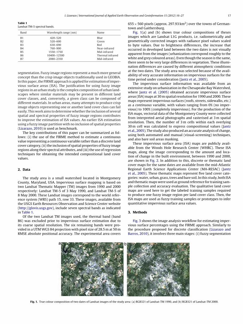

I. Lizarazo / International Journal of Applied Earth Obs

Table 1Landsat TM-5 spectral bands.

Band Wavelength range (nm) Name

B1 420–520 BlueB2 520–600 GreenB3 630–690 RedB4 760–900 Near-infraredB5 1550–1750 Mid-infrared

scIvrscdiestu(

lvcrtv

2

Ctr8et(i

BivR

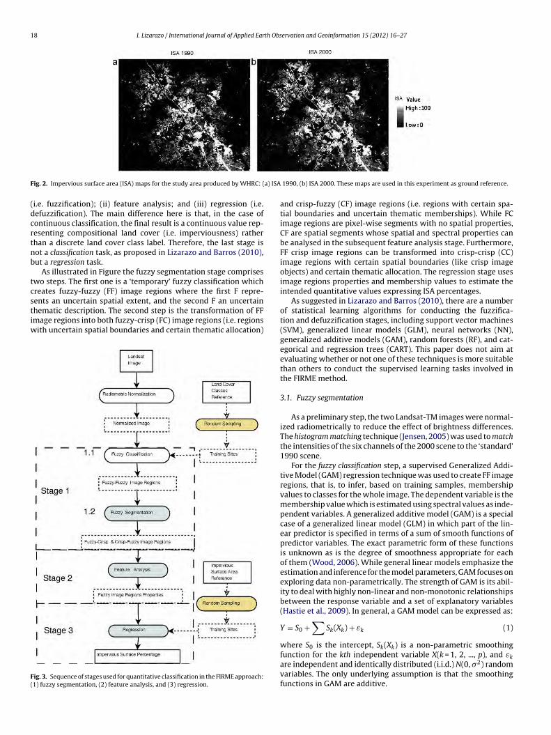
Fig. 3 shows the image analysis workflow for estimating imper-

B6 10400–12500 Thermal infraredB7 2080–2350 Mid-infrared

egmentation. Fuzzy image regions represent a much more generaloncept than the crisp image objects traditionally used in GEOBIA.n this paper, the FIRME approach is applied for estimation of imper-ious surface areas (ISA). The justification for using fuzzy imageegions in an urban study is the complex composition of urban land-capes where similar materials may be present in different landover classes, and, conversely, a given class can be composed ofifferent materials. In urban areas, many attempts to produce crisp

mage objects representing one or another land cover class can failasily. This work aims to determine whether the inclusion of severalpatial and spectral properties of fuzzy image regions contributeso improve the estimation of ISA values. An earlier ISA estimationsing a fuzzy image partition with no inclusion of spatial propertiesLizarazo, 2010) is used as benchmark.

The key contributions of this paper can be summarized as fol-ows: (i) the use of the FIRME method to estimate a continuousalue representing a continuous variable rather than a discrete landover category, (ii) the inclusion of spatial properties of fuzzy imageegions along their spectral attributes, and (iii) the use of regressionechniques for obtaining the intended compositional land coveralues.

. Data

The study area is a small watershed located in Montgomeryounty, Maryland, USA. Impervious surface mapping is based onwo Landsat Thematic Mapper (TM) images from 1990 and 2000espectively: Landsat TM-5 of 3 May 1990, and Landsat TM-5 of

May 2000. These Landsat images correspond to the world refer-nce system (WRS) path 15, row 33. These images, available fromhe USGS Earth Resources Observation and Science Center websitehttp://glovis.usgs.gov), include seven spectral bands as indicatedn Table 1.

Of the two Landsat TM images used, the thermal band (band6) was excluded prior to impervious surface estimation due to

ts coarse spatial resolution. The six remaining bands were pro-ided in a UTM WGS 84 projection with pixel size of 28.5 m at 50 mMSE absolute positional accuracy. The experimental area covers

Fig. 1. True colour composition of two dates of Landsat images of the study are

ervation and Geoinformation 15 (2012) 16–27 17

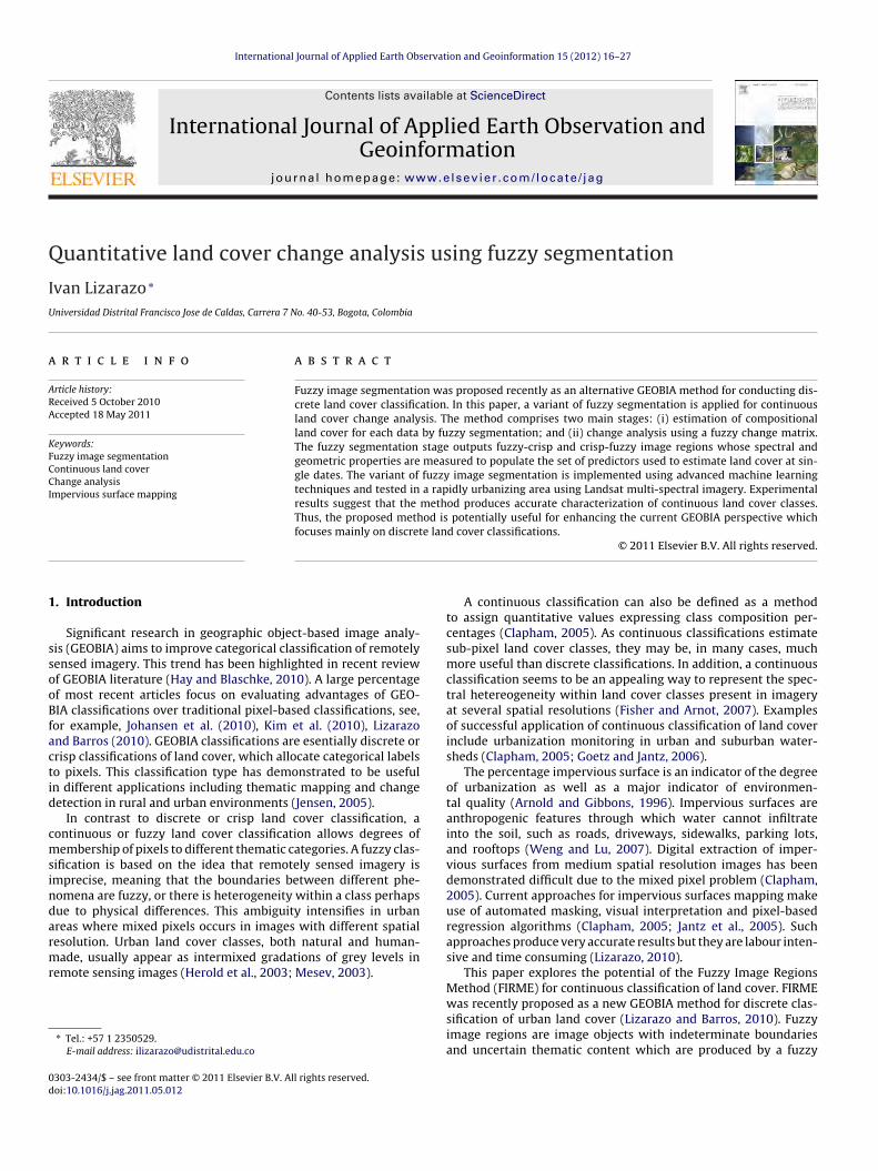
655 × 560 pixels (approx. 297.93 km2) over the towns of German-town and Gaithersburg.

Fig. 1(a) and (b) shows true colour compositions of thesesimages which are Landsat L1G products, i.e. radiometrically andgeometrically corrected images with radiance pixel values scaledto byte values. Due to brightness differences, the increase thatoccurred in developed land between the two dates is not visuallyapparent from the images (urbanization correspond roughly to thewhite and grey coloured areas). Even though the season is the same,there seem to be very large differences in vegetation. These illumi-nation differences are caused by different atmospheric conditionsat the two dates. The study area was selected because of the avail-ability of very accurate information on impervious surfaces for thetime period under consideration (Jantz et al., 2005).

The impervious surface information was available from anextensive study on urbanization in the Chesapeake Bay Watershed,where Jantz et al. (2005) obtained accurate impervious surfaceareas (ISA) maps at 30 m spatial resolution for 1990 and 2000. Thesemaps represent impervious surfaces (roofs, streets, sidewalks, etc.)as a continuous variable, with values ranging from 0% (no imper-vious) to 100% (completely impervious). For the production of theISA maps, vectorial data of the Montgomery County were collectedfrom interpreted aerial photographs and rasterised at 3 m spatialresolution. Then, the number of 3 m cells within each overlying30 m cell was calculated to express compositional values (Jantzet al., 2005). The study also produced an accurate analysis of change,using both automated and manual (visual-screening) techniques,and also bare soil areas masking.

These impervious surface area (ISA) maps are publicly avail-able from the Woods Hole Research Center (WHRC). These ISAmaps, along the image corresponding to the amount and loca-tion of change in the built environment, between 1990 and 2000,are shown in Fig. 2. In addition to this, discrete or thematic landcover maps for the same dates are available from the mid-AtlanticRegional Earth Science Applications Center (MA-RESAC) (Jantzet al., 2005). These thematic maps represent five land cover cate-gories: water, urban, grass, trees and bare soil. In this study, both ISAand thematic maps were used as ground reference for training sam-ple collection and accuracy evaluation. The qualitative land covermaps are used here to get the labeled training samples requiredto produce one fuzzy image region per land cover class. Then, theISA maps are used as fuzzy training samples or prototypes to inferquantitative impervious surface area values.

3. Methods

vious surface percentages using the FIRME approach. Similarly tothe procedure proposed for discrete classification (Lizarazo andBarros, 2010), it involves three main stages: (i) fuzzy segmentation

a: (a) RGB321 of Landsat-TM 1990, and (b) RGB321 of Landsat-TM 2000.

18 I. Lizarazo / International Journal of Applied Earth Observation and Geoinformation 15 (2012) 16–27

F a) ISA

(dcrtnb

tcstiw

F(

ig. 2. Impervious surface area (ISA) maps for the study area produced by WHRC: (

i.e. fuzzification); (ii) feature analysis; and (iii) regression (i.e.efuzzification). The main difference here is that, in the case ofontinuous classification, the final result is a continuous value rep-esenting compositional land cover (i.e. imperviousness) ratherhan a discrete land cover class label. Therefore, the last stage isot a classification task, as proposed in Lizarazo and Barros (2010),ut a regression task.

As illustrated in Figure the fuzzy segmentation stage compriseswo steps. The first one is a ‘temporary’ fuzzy classification whichreates fuzzy-fuzzy (FF) image regions where the first F repre-

ents an uncertain spatial extent, and the second F an uncertainhematic description. The second step is the transformation of FFmage regions into both fuzzy-crisp (FC) image regions (i.e. regions

ith uncertain spatial boundaries and certain thematic allocation)

ig. 3. Sequence of stages used for quantitative classification in the FIRME approach:1) fuzzy segmentation, (2) feature analysis, and (3) regression.

1990, (b) ISA 2000. These maps are used in this experiment as ground reference.

and crisp-fuzzy (CF) image regions (i.e. regions with certain spa-tial boundaries and uncertain thematic memberships). While FCimage regions are pixel-wise segments with no spatial properties,CF are spatial segments whose spatial and spectral properties canbe analysed in the subsequent feature analysis stage. Furthermore,FF crisp image regions can be transformed into crisp-crisp (CC)image regions with certain spatial boundaries (like crisp imageobjects) and certain thematic allocation. The regression stage usesimage regions properties and membership values to estimate theintended quantitative values expressing ISA percentages.

As suggested in Lizarazo and Barros (2010), there are a numberof statistical learning algorithms for conducting the fuzzifica-tion and defuzzification stages, including support vector machines(SVM), generalized linear models (GLM), neural networks (NN),generalized additive models (GAM), random forests (RF), and cat-egorical and regression trees (CART). This paper does not aim atevaluating whether or not one of these techniques is more suitablethan others to conduct the supervised learning tasks involved inthe FIRME method.

3.1. Fuzzy segmentation

As a preliminary step, the two Landsat-TM images were normal-ized radiometrically to reduce the effect of brightness differences.The histogram matching technique (Jensen, 2005) was used to matchthe intensities of the six channels of the 2000 scene to the ‘standard’1990 scene.

For the fuzzy classification step, a supervised Generalized Addi-tive Model (GAM) regression technique was used to create FF imageregions, that is, to infer, based on training samples, membershipvalues to classes for the whole image. The dependent variable is themembership value which is estimated using spectral values as inde-pendent variables. A generalized additive model (GAM) is a specialcase of a generalized linear model (GLM) in which part of the lin-ear predictor is specified in terms of a sum of smooth functions ofpredictor variables. The exact parametric form of these functionsis unknown as is the degree of smoothness appropriate for eachof them (Wood, 2006). While general linear models emphasize theestimation and inference for the model parameters, GAM focuses onexploring data non-parametrically. The strength of GAM is its abil-ity to deal with highly non-linear and non-monotonic relationshipsbetween the response variable and a set of explanatory variables(Hastie et al., 2009). In general, a GAM model can be expressed as:

Y = S0 +∑

Sk(Xk) + εk (1)

where S0 is the intercept, Sk(Xk) is a non-parametric smoothing

function for the kth independent variable X(k = 1, 2, ..., p), and εkare independent and identically distributed (i.i.d.) N(0, �2) randomvariables. The only underlying assumption is that the smoothingfunctions in GAM are additive.

th Obs

r2e

cmatmaAe(itf

uw((

rd

C

woc

atuw0riT

siotmca

3

tbuts

u

C

wlliou

I. Lizarazo / International Journal of Applied Ear

GAM models have been applied in remote sensing studieselated to stochastic simulation of land cover change (Brown et al.,002) and model-assisted estimation of forest resources (Opsomert al., 2007).

The supervised GAM regression model was fitted using landover memberships as dependent (response) variable and six nor-alized bands as predictor variables. The GAM technique was

pplied to create individual regression models from categoricalraining samples randomly sampled from the available land cover

aps. For creating each regression model, the GAM technique waspplied using the one-against-all technique (Hastie et al., 2009).

random sample of 2000 pixels was used to obtain training pix-ls for each land cover. Training samples were assigned either 100full membership) or 0 (null membership) to each land cover. Oncendividual predictions were undertaken for every land cover, a sum-o-one constraint was applied to membership values to interpretuzzy image regions as compositional classes.

This stage produced five fuzzy-fuzzy image regions: water,rban, grass, trees and soil. Then, these fuzzy-fuzzy image regionsere transformed into three new images: (i) crisp image regions,

ii) crisp-fuzzy image regions, and (iii) fuzzy-crisp image regionsusing membership values of 0.60 as threshold).

The crisp image C was obtained using a logical union operatoreferred to as the fuzzy t-conorm MAX operator (Ross, 2004), andefined as follows:

= �i1U�i2 . . . U�ic = max(�i1, �i2, . . . , �i3) (2)

here max( ) indicates the largest membership value of the ith pixelr neighborhood. Then, contiguous pixels belonging to the samelass were clumped and sieved.

The crisp-fuzzy (CF) image was obtained by keeping the bound-ry of crisp image regions and replacing their interior values (i.e.he largest membership value) with the original membership val-es at each fuzzy image region. Finally, the fuzzy-crisp (FC) imageas created by the union of a crisp interior (defined by using the

.60 membership value as threshold) and the conditional boundaryepresented by the confusion index (referred to as CI, and explainedn the next section) using the following statement: IF MAX > = 0.60,HEN FC = MAX, OTHERWISE FC = CI.

By creating both CF and FC image regions the set of spatial andpectral features to be used in the continuous classification processs enhanced. CF image regions resembles the crisp image objectsutput by a hard segmentation process but, besides their crisp spa-ial boundaries, provide additional thematic information (i.e. their

embership values). FC crisp image regions express both thematicertainty at their cores (i.e. membership values higher than 0.60)nd spatial uncertainty at their boundaries.

.2. Feature analysis

The feature analysis stage aims to identify spatial and spec-ral properties of fuzzy image regions. Contextual relationshipsetween fuzzy image regions can be measured to uncover potentialnderlying structural information. In addition, geometric and spec-ral properties of fuzzy image regions can provide clues to resolvepectral confusion between land cover classes.

Thematic uncertainty between FF image regions were evaluatedsing the confusion index (CI) (Burrough et al., 1997):

I = 1 −[�max i − �(max −1)i

]. (3)

here �maxi and �(max−1)i are, respectively, the first and secondargest membership value of the ith pixel. The CI measures the over-

ap of fuzzy classes at any point and provides insight for furthernvestigating the sites with high membership values to more thanne class Bragato (2004). CI values are in the range [0,1], CI val-es closer to 1 describe zones where overlap is critical. CI values

ervation and Geoinformation 15 (2012) 16–27 19

can provide a useful indication of the locations of transition zonesbetween classes.

In addition, the information entropy (H) was evaluated at eachpixel of the FF image regions as follows (Gonzalez, 2008):

H = −n∑

i=1

p(xi) log p(xi) (4)

where p(xi) is the probability for each digital number (or intensitylevel) in the image under consideration (obtained from a histogramof the image intensities), and log is the natural logarithm with basee = 2.718282. While, in information theory, generally the log witha base of 2 is used, the calculation may be conducted in any base.Then, the entropy of the full set of FF image regions was summa-rized using the entropy index (ENTRO) (Gonzalez, 2008):

ENTRO =m∑

c=1

Hi

log(128)(5)

where m is the number of fuzzy image regions (or land cover classesof interest).

Mean values of spectral bands TM-1, TM-3 and TM-4 within CCimage regions were evaluated as spectral indices. Finally the shapeindex, a geometry attribute, representing the perimeter area ratiowas calculated at every CC image region. The feature analysis stagetherefore outputs three contextual indices per date, the confusionindex (CI), the entropy index (ENTRO), and the shape index (SHAPE),and three spectral indices, MEAN B1, MEAN B3 and MEAN B4.

3.3. Regression

For the final regression stage, the estimation of impervious sur-face percentages within individual pixels was conducted usingthirteen predictors as follows:

1. fuzzy image region water,2. fuzzy image region urban,3. fuzzy image region grass,4. fuzzy image region trees,5. crisp-crisp (CC) image regions,6. crisp-fuzzy (CF) image,7. confusion index,8. entropy index,9. fuzzy-crisp (FC) image at 60% threshold,

10. mean of band TM-4 within crisp image regions,11. mean of band TM-3 within crisp image regions,12. mean of band TM-1 within crisp image regions, and13. shape index of CC image regions.

A random forest (RF) technique was applied to create the imper-vious regression model from training samples, this time usingtraining samples extracted from the ISA maps. A RF is a regressorthat builds not one but hundreds of decision trees and combinesits decisions using simple voting or advanced techniques based onconsensus theory (Hastie et al., 2009). The premise is that com-bining many trees is often more accurate than relying on only onetree. A random forest is a collection of classification and regres-sionn trees (CART) following specific rules for: (i) tree growing, (ii)tree combination, (iii) self-testing, and (iv) post-processing. Eachtree is grown at least partially at random: randomness is injectedby growing each tree on a different random subsample of the train-ing data. This technique is referred to as the bagging technique (or

bootstrap aggregating). Each tree is grown on about 63% of the orig-inal training data (due to the bootstrap sampling process). Thus, theremaining is available to test any single tree. This left out data isthe ‘out of bag’ (OOB) which allows calibration of the performance

20 I. Lizarazo / International Journal of Applied Earth Observation and Geoinformation 15 (2012) 16–27

Fig. 4. Fuzzy-fuzzy image regions obtained in the fuzzification stage for the 1990 and 2000 dates. From top to botton: water, urban, grass, trees and bare soil.

th Obs

osmfi2

rtd

••

fFtrdrco

Fr

I. Lizarazo / International Journal of Applied Ear

f each tree. RF have been explored for per-pixel land cover clas-ification and experimental results suggest it is computationallyore eficient and more accurate than other methods such as arti-

cial neural networks (ANN) (Gislason et al., 2006; Pal and Mather,003).

The RF technique was selected due to its good performance foregression tasks in remote sensing (Walton, 2008). For creatinghe regression model, the RF model was setup using the followingefault parameters:

number of trees = 500,number of variables to try at every split = 3.

As a final step, an evaluation of the accuracy of impervious sur-ace mapping was conducted using the ground reference images.or such a purpose the original ISA 1990 and 2000 maps (andhe urban development map), produced by WHRC at 30 m spatialesolution, were subset and resampled to 28.5 m to match the win-

ow and pixel size of the Landsat-TM images of 28.5 m. While thisesampling degrades the quality of ground reference data, it wasonsidered a more preferable choice than coarsening the pixel sizef the Landsat images.

ig. 5. Image regions derived in the fuzzification stage for the 1990 and 2000 dates. From tegions with threshold at 0.60 membership.

ervation and Geoinformation 15 (2012) 16–27 21

Direct comparison between the predicted and the ground refer-ence ISA was conducted using the Pearson’s correlation coefficient(Hall, 1979). Area estimation of impervious surfaces in a givenimage was calculated by taking the sum of all pixel membershipvalues for the image under consideration Fisher et al. (2006).

Once the impervious surface areas were estimated, the sub-sequent task to be conducted was change analysis. Loss and Gainestimation was conducted based on the predicted impervious sur-faces, using a change matrix (as suggested by Fisher et al. (2006)for per-pixel fuzzy change analysis) to accommodate zones of NoChange and Change. The diagonal cells of the change matrix indi-cating no change has occurred in a cover class Cj between time t1and time t2 were obtained following Fisher et al. (2006):

�(Cj[no change]) = min(�(Cj[t1]), �(Cj[t2])) (6)

where min indicates the minimum operator (intersection) between

fuzzy sets, i.e. the minimum value of the membership values�(Cj[ti]) to class Cj for a given time t1 or t2.

Gain, the total area of class j which is gained, is given by the areaswhich are not members of class (Cj) at time t1, denoted as �(¬Cj[t1])

op to botton: crisp-fuzzy image regions, crisp image regions, and fuzzy-crisp image

2 th Obs

aw

�

wsc

waw

�

wle

�

mGfs

2 I. Lizarazo / International Journal of Applied Ear

nd are members of class (Cj) at time t2, denoted as �(Cj[t2]). Gainas calculated following Fisher et al. (2006):

(Cj[gain]) = max(0, �(¬Cj[t1]) + �(Cj[t2]) − 1) (7)

here max indicates the maximum operator (union) between fuzzyets, i.e. the maximum value of each membership value to a givenlass �(Cj).

Loss, the total area of class j which is lost, is given by the areashich are members of class (Cj) at time t1, denoted as �(Cj[t1]), and

re not members of class (Cj) at time t2, denoted as �(¬Cj[t2]). Lossas calculated using the equation Fisher et al. (2006):

(Cj[loss]) = max(0, �(Cj[t1]) + �(¬Cj[t2]) − 1) (8)

The off-diagonal cells representing change in the change matrixere calculated as the intersection of the gain in class Cj and the

oss in class Ck over the interval t1 to t2 using the equation Fishert al. (2006):

(Cj[change]) = min(�(Cj[gain]), �(Ck[loss])) (9)

All the processes for quantitative classification were imple-

ented by using R (R Development Core Team, 2010) and SAGA

IS (Cimmery, 2007-2010). In addition to the R base package, theollowing libraries were used to develop the method: rgdal, sp, spat-tats, maptools, RSAGA, gam and randomForest.

Fig. 6. Contextual and spatial indices obtained from fuzzy image regions for the 199

ervation and Geoinformation 15 (2012) 16–27

4. Results

The FF image regions created in the first step of the fuzzy seg-mentation stage are shown in Fig. 4

The CC image regions, CF image regions, and FC image regionscreated in the second step of the fuzzy segmentation stage aredepicted in Fig. 5

The complete set of spectral and spatial indices calculated inthe feature analysis stage is shown in Figs. 6 and 7. Fig. 6 depictsthe confusion index (CI), the entropy index (ENTRO), and theshape index (ENTRO). Fig. 7 depicts MEAN B1, MEAN B3, andMEAN B4.

Spectral indices obtained from crisp image regions for the 1990and 2000 dates: (a) mean of TM-1, (b) mean of TM-3, and (c) meanof TM-4.

Figs. 7 and 8 show the impervious surface areas (ISA) maps in1990 and 2000 as predicted using the FIRME approach with a ran-dom sample of 2000 pixels which represents 0.54% of the studyarea.

The Pearson’s correlation coefficient (Hall, 1979) between the

predicted ISA images and the ground reference images, shown inFigs. 8 and 9, are 0.793 and 0.821 respectively. It is a good approx-imation to the ground reference data obtained by (Jantz et al.,2005), and minor misprediction problems are detected only after a

0 and 2000 dates: (a) confusion index, (b) entropy index, and (c) shape index.

I. Lizarazo / International Journal of Applied Earth Observation and Geoinformation 15 (2012) 16–27 23

and 2

csrbam

a

TCia

Fig. 7. Spectral indices obtained from crisp image regions for the 1990

areful visual assessment. As Table 2 shows, GAM-RF based fuzzyegmentation overestimates impervious surface by 7.3% and 6.1%espectively. Table 2 also shows that the correlation coefficientetween the ISA change predicted by the FIRME method and the

ctual change is 0.569. The fuzzy segmentation method overesti-ates ISA change by 10.13%.As this study aimed at analyzing the contribution of fuzzy-crisp

nd crisp-fuzzy image regions to increasing the accuracy of the

able 2omparison between the FIRME method and the SIMPLE method for obtaining

mpervious surface areas. Training sample is 2000 pixels. Area error was calculateds the ratio between predicted area and reference area.

Test correlationcoefficient

95% confidenceinterval

Areaerror (%)

ISA 1990FIRME 0.793 [0.776, 0.809] +7.3SIMPLE 0.754 [0.734, 0.772] +10.1ISA 2000FIRME 0.821 [0.806, 0.835] +6.1SIMPLE 0.790 [0.773, 0.806] +8.5CHANGEFIRME 0.569 [0.539, 0.598] +10.1SIMPLE 0.512 [0.479, 0.544] +12.3

000 dates: (a) mean of TM-1, (b) mean of TM-3, and (c) mean of TM-4.

ISA estimation, an earlier land cover change analysis using a sim-pler fuzzy segmentation approach (Lizarazo, 2010) was used asbenchmark. In that method, fuzzy segmentation, the first stage,outputs fuzzy-fuzzy image regions. Then, in the feature analysisstage, contextual properties of fuzzy-fuzzy image regions are eval-uated. Table 2 also presents the results obtained using this simplesegmentation option. It is apparent that the FIRME method outper-forms the SIMPLE method for one date ISA estimates. In such a case,the area error using the FIRME method is about 28% lower than thearea error using the SIMPLE method. With regard to change in ISAvalues, the FIRME method is approximately 18% more accurate thanthe SIMPLE method.

In order to establish whether the impervious surface percent-ages correspond with the ones found at a specific place in thereference data, an additional test was conducted. A random selec-tion of 10,000 pixels was taken from the ground reference imageand used to assess the location error by comparing predicted andactual values of impervious surface percentages. Table 3 shows theroot mean square error (RMSE) for predicted 1990 and 2000 imper-

vious surface percentages, and for predicted impervious surfaceschange. It can be seen that, in the FIRME case, approximately 68%of the samples fall within 15% of absolute error bound. In the SIMPLEcase, the maximum absolute error bound is 20%.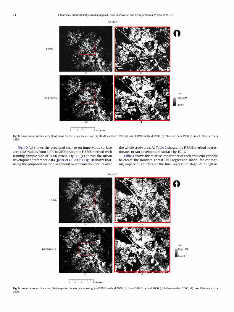

24 I. Lizarazo / International Journal of Applied Earth Observation and Geoinformation 15 (2012) 16–27

F hod 191

atdu

F2

ig. 8. Impervious surface area (ISA) maps for the study area using: (a) FIRME met990.

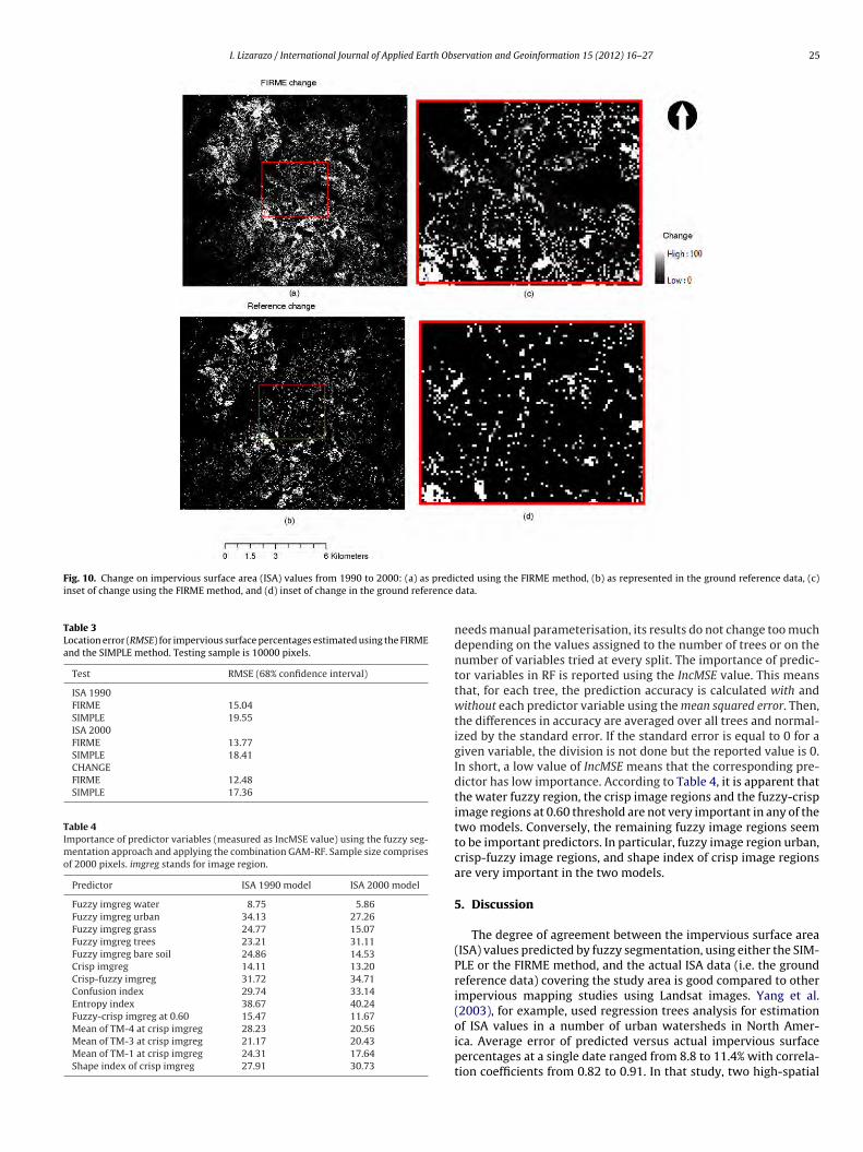
Fig. 10 (a) shows the predicted change on impervious surface

rea (ISA) values from 1990 to 2000 using the FIRME method withraining sample size of 2000 pixels. Fig. 10 (c) shows the urbanevelopment reference data (Jantz et al., 2005). Fig. 10 shows that,sing the proposed method, a general overestimation occurs over

ig. 9. impervious surface area (ISA) maps for the study area using: (a) FIRME method 20000.

90, (b) inset FIRME method 1990, (c) reference data 1990, (d) inset reference data

the whole study area. As Table 2 shows, the FIRME method overes-

timates urban development surface by 10.1%.

Table 4 shows the relative importance of each predictor variableto create the Random Forest (RF) regression model for estimat-ing impervious surface at the final regression stage. Although RF

00, (b) Inset FIRME method 2000, (c) Reference data 2000, (d) Inset Reference data

I. Lizarazo / International Journal of Applied Earth Observation and Geoinformation 15 (2012) 16–27 25

Fig. 10. Change on impervious surface area (ISA) values from 1990 to 2000: (a) as prediinset of change using the FIRME method, and (d) inset of change in the ground reference

Table 3Location error (RMSE) for impervious surface percentages estimated using the FIRMEand the SIMPLE method. Testing sample is 10000 pixels.

Test RMSE (68% confidence interval)

ISA 1990FIRME 15.04SIMPLE 19.55ISA 2000FIRME 13.77SIMPLE 18.41CHANGEFIRME 12.48SIMPLE 17.36

Table 4Importance of predictor variables (measured as IncMSE value) using the fuzzy seg-mentation approach and applying the combination GAM-RF. Sample size comprisesof 2000 pixels. imgreg stands for image region.

Predictor ISA 1990 model ISA 2000 model

Fuzzy imgreg water 8.75 5.86Fuzzy imgreg urban 34.13 27.26Fuzzy imgreg grass 24.77 15.07Fuzzy imgreg trees 23.21 31.11Fuzzy imgreg bare soil 24.86 14.53Crisp imgreg 14.11 13.20Crisp-fuzzy imgreg 31.72 34.71Confusion index 29.74 33.14Entropy index 38.67 40.24Fuzzy-crisp imgreg at 0.60 15.47 11.67Mean of TM-4 at crisp imgreg 28.23 20.56Mean of TM-3 at crisp imgreg 21.17 20.43Mean of TM-1 at crisp imgreg 24.31 17.64Shape index of crisp imgreg 27.91 30.73

cted using the FIRME method, (b) as represented in the ground reference data, (c)data.

needs manual parameterisation, its results do not change too muchdepending on the values assigned to the number of trees or on thenumber of variables tried at every split. The importance of predic-tor variables in RF is reported using the IncMSE value. This meansthat, for each tree, the prediction accuracy is calculated with andwithout each predictor variable using the mean squared error. Then,the differences in accuracy are averaged over all trees and normal-ized by the standard error. If the standard error is equal to 0 for agiven variable, the division is not done but the reported value is 0.In short, a low value of IncMSE means that the corresponding pre-dictor has low importance. According to Table 4, it is apparent thatthe water fuzzy region, the crisp image regions and the fuzzy-crispimage regions at 0.60 threshold are not very important in any of thetwo models. Conversely, the remaining fuzzy image regions seemto be important predictors. In particular, fuzzy image region urban,crisp-fuzzy image regions, and shape index of crisp image regionsare very important in the two models.

5. Discussion

The degree of agreement between the impervious surface area(ISA) values predicted by fuzzy segmentation, using either the SIM-PLE or the FIRME method, and the actual ISA data (i.e. the groundreference data) covering the study area is good compared to otherimpervious mapping studies using Landsat images. Yang et al.(2003), for example, used regression trees analysis for estimation

of ISA values in a number of urban watersheds in North Amer-ica. Average error of predicted versus actual impervious surfacepercentages at a single date ranged from 8.8 to 11.4% with correla-tion coefficients from 0.82 to 0.91. In that study, two high-spatial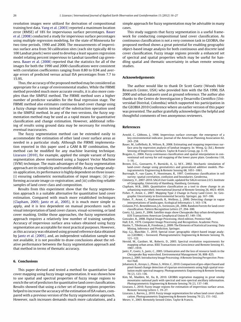

2 th Obs

rteeuto1mniwa1

ampnFaimcie

antmLs(as(fs

te(avcaAsabnat

6

cteRhpH

6 I. Lizarazo / International Journal of Applied Ear

esolution images were utilized for derivation of compositionalraining/test data. Yang et al. (2003) reported a maximum locationrror (RMSE) of 18% for imperviuous surface percentages. Bauert al. (2008) conducted a study for impervious surface percentagessing multiple regression modeling, for the state of Minnesota forwo time periods, 1990 and 2000. The measurements of impervi-us surface area from 50 calibration sites (each site typically 40 to00 Landsat pixels) were used to develop a least squares regressionodel relating percent impervious to Landsat tasselled cap green-

ess. Bauer et al. (2008) reported that the statistics for all of themages for both the 1990 and 2000 classifications were consistent

ith correlation coefficientes ranging from 0.80 to 0.94 and aver-ge errors of predicted versus actual ISA percentages from 7.7 to5.9%.

Thus, the accuracy of the proposed method may be considered asppropriate for a range of environmental studies. While the FIRMEethod provided much more accurate results, it is also more com-

lex than the SIMPLE method. The FIRME method uses a higherumber of predictor variables for the final regression stage. TheIRME method also estimates continuous land cover change using

fuzzy change matrix instead of the substraction operation usedn the SIMPLE method. In any of the two versions, the fuzzy seg-

entation method may be used as a rapid means for quantitativelassification and change estimation. However, additional refin-ng of results using ground data may be necessary for resolvingventual inaccuracies.

The fuzzy segmentation method can be extended easily toccommodate the estimation of other land cover surface areas aseeded in a particular study. Although the FIRME implementa-ion reported in this paper used a GAM & RF combination, the

ethod can be modified for any machine learning technique.izarazo (2010), for example, applied the simple variant of fuzzyegmentation above mentioned using a Support Vector MachineSVM) technique. The main advantages of the fuzzy segmentationpproach are its simplicity and transferability. As any change analy-is application, its performance is highly dependent on three issues:i) ensuring radiometric normalization of input images; (ii) per-orming accurate image co-registration; and (iii) collecting reliableamples of land cover class and composition.

Results from this experiment show that the fuzzy segmenta-ion approach is a suitable alternative for quantitative land coverstimation. Compared with much more established techniquesClapham, 2005; Jantz et al., 2005), it is much more simple topply, and it is less dependent on manual procedures such asisual interpretation of land cover classes, visual-screening, or landover masking. Unlike those approaches, the fuzzy segmentationpproach requires a relatively low number of training samples.ccuracy of impervious surface area values obtained using fuzzyegmentation are acceptable for most practical purposes. However,s this accuracy was obtained using ground reference data obtainedy Jantz et al. (2005), and, an independent validation sample wasot available, it is not possible to draw conclusions about the rel-tive performance between the fuzzy segmentation approach andhat method in terms of thematic accuracy.

. Conclusions

This paper devised and tested a method for quantitative landover mapping using fuzzy image segmentation. It was shown howo use spatial and spectral properties of fuzzy image regions tonrich the set of predictors for quantitative land cover classification.

esults showed that using a richer set of image regions propertieselped to increase the accuracy of the estimation of ISA values, com-ared with a previous version of the fuzzy segmentation approach.owever, such increases demands much more calculations, and a

ervation and Geoinformation 15 (2012) 16–27

simple approach for fuzzy segmentation may be advisable in manycases.

This study suggests that fuzzy segmentation is a useful frame-work for conducting compositional land cover classification. Ascontinuous classification is not a very common task in GEOBIA, theproposed method shows a great potential for enabling geographicobject-based image analysis for both continuous and discrete landcover classification. Fuzzy image regions provide a enhanced setof spectral and spatial properties which may be useful for han-dling spatial and thematic uncertainty in urban remote sensingstudies.

Acknowledgements

The author would like to thank Dr Scott Goetz (Woods HoleResearch Center, USA) who provided him with the ISA 1990, ISA2000 and urban datasets used as ground reference. The author alsothanks to the Centro de Investigacion y Desarrollo Cientifico (Uni-versidad Distrital, Colombia) which supported his participation inthe GEOBIA 2010 Conference where an earlier version of this paperwas presented. The author gratefully acknowledges the helpful andthoughtful comments of two anonymous reviewers.

References

Arnold, C., Gibbons, J., 1996. Impervious surface coverage: the emergence of akey environmental indicator. Journal of the American Planning Association 62,243–258.

Bauer, M., Loffelholz, B., Wilson, B., 2008. Estimating and mapping impervious sur-face area by regression analysis of landsat imagery. In: Weng, Q. (Ed.), RemoteSensing of Impervious Surfaces. Taylor & Francis Group, pp. 3–19.

Bragato, G., 2004. Fuzzy continuous classification and spatial interpolation in con-ventional soil survey for soil mapping of the lower piave plain. Geoderma 118,1–16.

Brown, D.G., Goovaerts, P., Burnicki, A., Li, M.Y., 2002. Stochastic simulation ofland-cover change using geostatistics and generalized additive models. Pho-togrammetric Engineering & Remote Sensing 68, 1051–1061.

Burrough, P., van Gaans, P., Hoostmans, R., 1997. Continuous classification in soilsurvey: spatial correlation, confusion and boundaries. Geoderma.

Cimmery, V., 2007-2010. SAGA User Guide, updated for SAGA version 2.0.5. Instituteof Geography, University of Hamburg. Hamburg, Germany.

Clapham, W.B., 2005. Quantitative classification as a tool to show change in anurbanizing watershed. International Journal of Remote Sensing 26, 4923–4939.

Fisher, P., Arnot, C., 2007. Mapping Type 2 Change in Fuzzy Land Cover. In: Geo-graphic Uncertainty in Environmental Security. Springer, pp. 167–186.

Fisher, P., Arnot, C., Wadsworth, R., Wellens, J., 2006. Detecting change in vagueinterpretations of landscapes. Ecological Informatics 1, 163–178.

Gislason, P.O., Benediktsson, J.A., Sveinsson, J.R., 2006. Random Forests for land coverclassification. Pattern Recognition Letters 27, 294–300.

Goetz, S.J., Jantz, P., 2006. Satellite maps show Chesapeake Bay urban development.EOS Transactions American Geophysical Union 87, 149–156.

Gonzalez, R., 2008. Digital Image Processing, third edition. Prentice Hall.Hall, E.H., 1979. Computer Image Processing and Recognition. Academic Press.Hastie, T., Tibshirani, R., Friedman, J., 2009. The Elements of Statistical Learning: Data

Mining, Inference and Prediction. Springer.Hay, G.J., Blaschke, T., 2010. Special issue: geographic object-based image analy-

sis (GEOBIA) – foreword. Photogrammetric Engineering & Remote Sensing 76,121–122.

Herold, M., Gardner, M., Roberts, D., 2003. Spectral resolution requirements formapping urban areas. IEEE Transactions on Geoscience and Remote Sensing 41,1907–1919.

Jantz, P., Goetz, S., Jantz, C., 2005. Urbanization and the loss of resource lands in theChesapeake Bay watershed. Environmental Management 36, 808–825.

Jensen, J., 2005. Introductory Image Processing: A Remote Sensing Perspective. Pren-tice Hall.

Johansen, K., Arroyo, L., Phinn, S., Witte, C., 2010. Comparison of geo-object based andpixel-based change detection of riparian environments using high spatial reso-lution multi-spectral imagery. Photogrammetric Engineering & Remote Sensing76 (2), 123–136.

Kim, M., Madden, M., Xu, B., 2010. GEOBIA vegetation mapping in great smokymountains national park with spectral and non-spectral ancillary information.Photogrammetric Engineering & Remote Sensing 76 (2), 137–149.

Lizarazo, I., 2010. Fuzzy image regions for estimation of impervious surface areas.Remote Sensing Letters 1, 19–27.

Lizarazo, I., Barros, J., 2010. Fuzzy image segmentation for urban land cover classifi-cation. Photogrammetric Engineering & Remote Sensing 76 (2), 151–162.

Mesev, V., 2003. Remotely Sensed Cities. Taylor & Francis.

th Obs

O

P

R

R

I. Lizarazo / International Journal of Applied Ear

psomer, J.D., Jay, B.F., Moisen, G.G., Kauermann, G., 2007. Model-assisted esti-mation of forest resources with generalized additive models. Journal of theAmerican Statistical Association 100, 400–416.

al, M., Mather, P.M., 2003. An assessment of the effectiveness of decision treemethods for land cover classification. Remote Sensing of the Environment 86,

554–565.

Development Core Team, 2010. R: A Language and Environment for StatisticalComputing. R Foundation for Statistical Computing. Vienna, Austria, ISBN 3-900051r-r07-0.

oss, T., 2004. Fuzzy Logic with Engineering Applications. Wiley.

ervation and Geoinformation 15 (2012) 16–27 27

Walton, J.T., 2008. Subpixel urban land cover estimation: comparing Cubist, Ran-dom Forests, and Support Vector Regression. Photogrammetric Engineering &Remote Sensing 74, 1213–1222.

Weng, Q., Lu, D., 2007. Subpixel analysis of urban landscapes. In: Weng, Q., Quat-trochi, D.A. (Eds.), Urban Remote Sensing. CRC Press, pp. 109–135 (chapter 6).

Wood, S., 2006. Generalized Additive Models: An Introduction with R. Chapman andHall.

Yang, L., Huang, C., Homer, C., Wylie, B., Coan, M., 2003. An approach for mappinglarge-area impervious surfaces: synergistic use of Landsat 7 ETM+ and highspatial resolution imagery. Technical Report. USGS/EROS Data Center.