Article

Evaluation and Prediction of the Impacts of Land CoverChanges on Hydrological Processes in Data ConstrainedSouthern Slopes of Kilimanjaro, Tanzania

Mateso Said 1,2,* , Canute Hyandye 3, Ibrahimu Chikira Mjemah 4, Hans Charles Komakech 1

and Linus Kasian Munishi 5

�����������������

Citation: Said, M.; Hyandye, C.;

Mjemah, I.C.; Komakech, H.C.;

Munishi, L.K. Evaluation and

Prediction of the Impacts of Land

Cover Changes on Hydrological

Processes in Data Constrained

Southern Slopes of Kilimanjaro,

Tanzania. Earth 2021, 2, 225–247.

https://doi.org/10.3390/earth2020014

Academic Editor: Tommaso Caloiero

Received: 5 May 2021

Accepted: 27 May 2021

Published: 30 May 2021

Publisher’s Note: MDPI stays neutral

with regard to jurisdictional claims in

published maps and institutional affil-

iations.

Copyright: © 2021 by the authors.

Licensee MDPI, Basel, Switzerland.

This article is an open access article

distributed under the terms and

conditions of the Creative Commons

Attribution (CC BY) license (https://

creativecommons.org/licenses/by/

4.0/).

1 Department of Water and Environmental Science and Engineering, School of Materials, Energy,Water and Environmental Sciences and Engineering,The Nelson Mandela African Institution of Science and Technology, Arusha P.O. Box 447, Tanzania;hans.komakech@nm-aist.ac.tz

2 Department of Environmental Engineering and Management, College of Earth Sciences and Engineering,The University of Dodoma, Dodoma P.O. Box 11090, Tanzania

3 Department of Environmental Planning, Institute of Rural Development Planning (IRDP),Dodoma P.O. Box 138, Tanzania; chyandye@irdp.ac.tz

4 Department of Geography and Environmental Studies, Solomon Mahlangu College of Science and Education,Sokoine University of Agriculture, Morogoro P.O. Box 3001, Tanzania; chikira@sua.ac.tz

5 Department of Sustainable Agriculture, Biodiversity and Ecosystem Management,School of Life Sciences and Bioengineering, The Nelson Mandela African Institution of Science andTechnology, Arusha P.O. Box 447, Tanzania; linus.munishi@nm-aist.ac.tz

* Correspondence: matesos@nm-aist.ac.tz

Abstract: This study provides a detailed assessment of land cover (LC) changes on the water balancecomponents on data constrained Kikafu-Weruweru-Karanga (KWK) watershed, using the integratedapproaches of hydrologic modeling and partial least squares regression (PLSR). The soil and waterassessment tool (SWAT) model was validated and used to simulate hydrologic responses of waterbalance components response to changes in LC in spatial and temporal scale. PLSR was further usedto assess the influence of individual LC classes on hydrologic components. PLSR results revealedthat expansion in cultivation land and built-up area are the main attributes in the changes in wateryield, surface runoff, evapotranspiration (ET), and groundwater flow. The study findings suggestthat improving the vegetation cover on the hillside and abandoned land area could help to reduce thedirect surface runoff in the KWK watershed, thus, reducing flooding recurring in the area, and thatwith the ongoing expansion in agricultural land and built-up areas, there will be profound negativeimpacts in the water balance of the watershed in the near future (2030). This study provides a forecastof the future hydrological parameters in the study area based on changes in land cover if the currentland cover changes go unattended. This study provides useful information for the advancement ofour policies and practices essential for sustainable water management planning.

Keywords: land use change; SWAT model; water balance; PLSR; Mount Kilimanjaro

1. Introduction

Anthropic activities such as those leading to extensive land cover changes and climatechanges are among the main drivers for changes in hydrological processes of the water-shed [1–3]. Anthropogenic modification of land use/cover is a topmost determinant ofenvironmental changes at spatial and temporal scales [4,5]. It is a principal determiningfactor of global environmental changes with severe impacts on human livelihoods [6]. Thecurrent rates are higher than ever recorded [7]. Many studies have also shown that landuse/cover changes influence the hydrology of watersheds [8–11]. Thus, evaluating the im-pact of land cover (LC) and climate changes on water resource availability is an important

Earth 2021, 2, 225–247. https://doi.org/10.3390/earth2020014 https://www.mdpi.com/journal/earth

Earth 2021, 2 226

challenge for the current hydrological science [12,13]. Further, there is a growing need for ascientific community to balance human needs and environmental sustainability [14]. Thus,understanding the environmental impacts of land use/cover changes is a fundamentalpart of sustainable land planning and development [15].

In practice, land cover changes affect the surface water balance of an area, thusimpacting evapotranspiration, initial surface runoff, and groundwater flow [14,16]. Apartfrom impacting water resources and hydrologic water balance, LC changes can directlyaffect local communities, the biota, and possible water management plans [17,18]. Thespatial distribution patterns of land use/cover can substantially impact runoff and sedimenttransport processes at different dimensions [19,20]. It has both local, regional and globaloccurrence and is reported to continue in the future [14]. It potentially has large impactson water resources; thus, it is important to understand the possible effects of LC changeson the runoff variability and possible measures [21].

Most places in East Africa have experienced a conversion of natural forests to settle-ments, urban centers, farmlands, and grazing lands at varying dimensions [22,23]. Thisconversion creates a need for a balance between the needs for a sprouting population, suchas food production, and the minimization of the negative environmental impacts on otherecosystem services such as quality and quantity of water [24]. Although food productionrequires a sustainable water supply, land use/cover changes resulting from agriculturalexpansion affect water resources. These changes afflict food production in the long run [25].Thus, it is essential to manage land use/cover changes at a catchment scale [26]. However,quantifying its impacts is one of the challenging activities [27].

Mt. Kilimanjaro slopes are typical landscapes with the highest recorded land cover dy-namics, and their consequences on water resources, food and energy production have beenreported in previous studies [28]. Changes in land cover in most of the areas surroundingMt. Kilimanjaro slopes have the potential to impact water resources [29–34]. These changestrigger the need to understand land cover change trajectories and surface–groundwaterinteraction among the critical requirements in water management practices in the area.Surface–groundwater interaction affects water management and water rights changes,nutrients loading from aquifers to streams, and in-stream flow requirements for aquaticspecies at a watershed scale [35,36]. The knowledge regarding land use/cover changesin relation to water balance components on the slopes of Mt. Kilimanjaro is of utmostimportance due to limited information with regard to groundwater flow [37].

Land degradation and land cover changes have contributed to the decline in surfacewater resources around Mt. Kilimanjaro [34]. Human activities are reported as the maincontributor to the rapid land cover changes around the same area. The activities includeencroachment due to logging, agricultural expansion and settlements, which in turn havecreated significant changes in the land cover [38]. Indeed, the increased anthropogenicactivities are mainly driven by the fast-growing population, which also strengthen thepressure on the available water resources on a day to day basis [39]. Other drivers includesocioeconomic development and pressure on land for expansion in agriculture [40].

Some of the proposed strategies to curb the expansion of agriculture due to the demandfor food to suffice the expanding population on the slopes of Mt. Kilimanjaro include theimprovement of the land tenure security and the introduction of modern land and waterconservation measures [41]. These strategies are aimed at increasing per capital productionand discourage the opening up of more land for agriculture [34]. Shrinking in the forest areaalong the mountain landscapes has also been reported in several studies [42,43]. However,the quantitative estimates of water losses due to deforestation in the Pangani basin arescanty or missing [44]. Hence, it is essential to understand the effect of land managementpractices at the basin and sub-basins scale; these practices increase the impact of hydrologicvariability on the society and ecosystem [21].

Mount Kilimanjaro is hydrologically important [42,45], as a water tower for the EastAfrican region [46]. Local populace on the mountain slopes of North-eastern Tanzaniaand South-eastern Kenya predominately depends on freshwater supplies for domestic, hy-

Earth 2021, 2 227

dropower production, industrial, and irrigation [42,47]. Further, the mountain harbors themost effective water source in the fog interception zone along the thick forest reserve [45].Therefore, impacting the water balance of Mt. Kilimanjaro will affect the attainment of thelocal, regional and global sustainable development milestones.

KWK watershed is one of the mountainous watersheds along the southern slopes ofMt. Kilimanjaro and the northern part of the Pangani river basin. Being located on themountain slopes with greater human activities, KWK experiences tremendous changes inits land cover, thus necessitating quantifying the impacts of land cover changes on the waterbalance of the watershed for sustainable water resources management. However, despitethe growing need, simulation of hydrological processes using water balance components,such as surface runoff in mountainous areas with irregular terrain and complex hydrologicprocesses, is challenging [48]. Estimating the parameters for the hydrological simulationmodel (SWAT) is hampered by the variation of temperature and precipitation with elevationand spatial variability due to complex terrain [49].

A modeling approach is typically the best method to assess the impacts of landuse/cover change on the water balance. Models can be used to evaluate the historical andfuture implications of land use/cover changes on the hydrology of a catchment [50]. Thisstudy used a soil and water assessment tool (SWAT) for assessing the impacts of land coverchanges on the water balance components of the KWK watershed on the southern slopes ofMt. Kilimanjaro. SWAT has been tested and used to solve complex watershed managementproblems in many regions all over the world [21,47,51–53]. Therefore, the objectives of thispaper are three-fold viz: to set up, parameterize and calibrate the SWAT model in terms ofstreamflow. Further, to investigate the impact of land cover changes on the water balancein historical (1993–2018) and the near future (2018–2030), and to establish the impact ofthe individual land cover type on the water balance using PLSR modeling. This studyprovides a comprehensive analysis of the historical and future land cover dynamics andtheir impacts on the hydrological processes. Hence, the findings of this study are usefulfor the advancement of our policies, practices and management practices aimed to attainenvironmental and water resources sustainability. Apart from analyzing the historicalimpacts of land cover changes on hydrological processes, this study also forecasts thefuture hydrological parameters in the study area based on changes in land cover if thecurrent land cover changes go unattended. In a broader perspective, the results from thisstudy may help realization of the United Nations sustainable development goals, such asending poverty (Goal 1), food security (Goal 2), availability and sustainable managementof water and sanitation for all (Goal 6), biodiversity conservation (Goal 15) and energy forall (Goal 7) [54].

2. Materials and Methods2.1. The Study Area

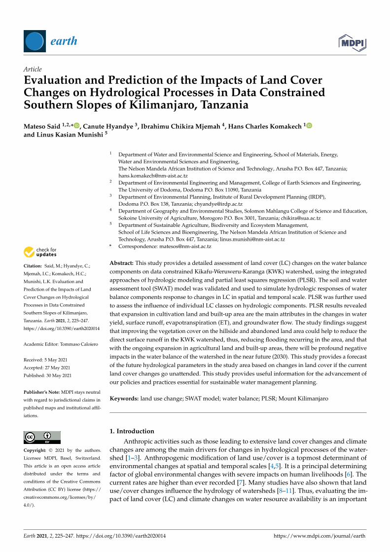
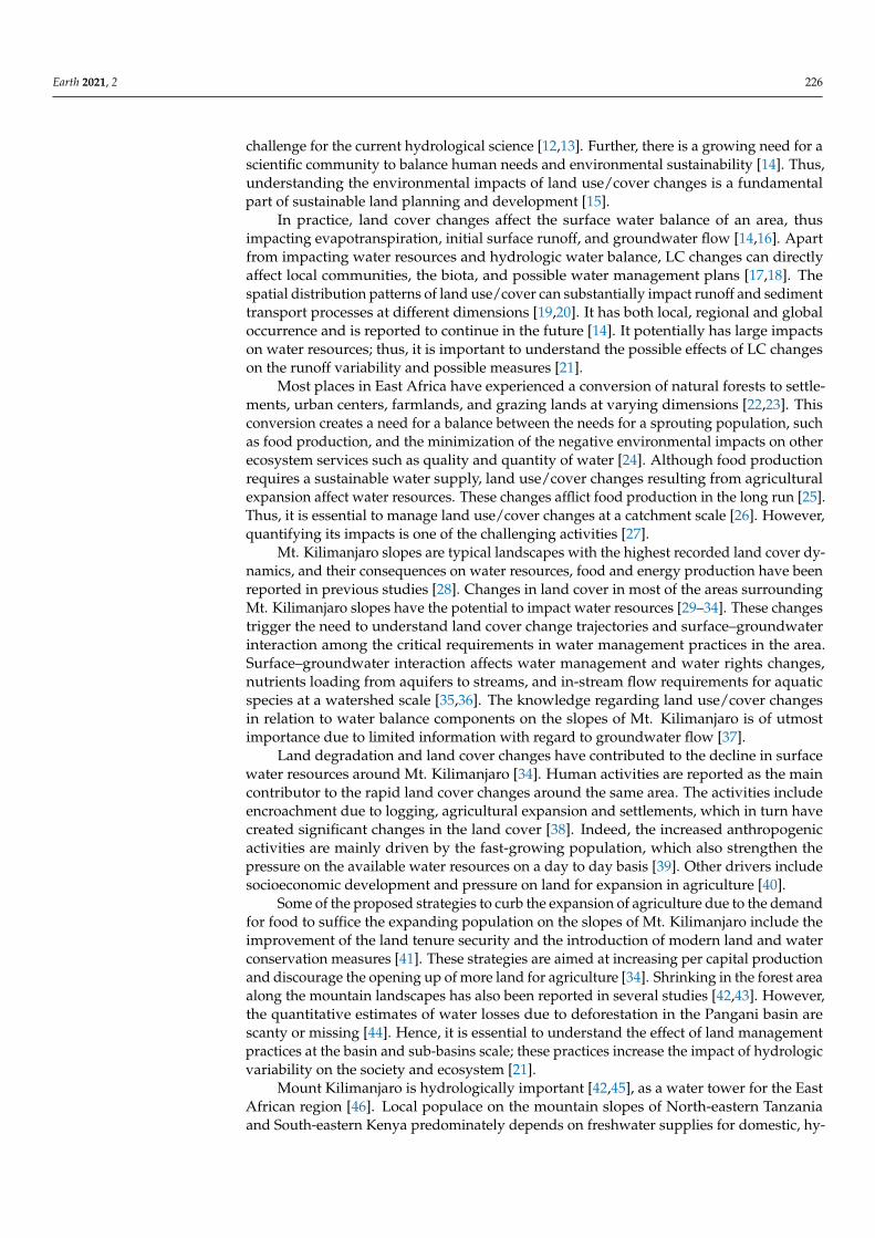
This study was done at the Kikafu, Weruweru, and Karanga (KWK) watershed,which spans from the thick mountain forest on the southern slopes of Mount Kilimanjaro(Figure 1a). The study area, rainfall pattern (Figure 1b), population and anthropic activitieswere detailed in Said, Komakech [28] and Said, Hyandye [41]. It is worth mentioning thatthe largest water extractor is agriculture, being dominated by small to large scale irrigationalong the mountain slopes. The primary soil types in the agricultural area are chromicluvisols, Eutic cambisols, haplic nitisols, and humic nitisols (Figure 2b). More than 70%of the watershed falls under 0–8% slope class (Figure 2a) dominated by maize and beanfarms; runoff velocity is high in the lowlands due to a comparatively high annual rainfallin the highlands. Therefore, runoff is the most crucial management factor in the watershed.

Earth 2021, 2 228Earth 2021, 2, FOR PEER REVIEW 4

Figure 1. Location of KWK watershed (a) and mean annual rainfall (b).

Figure 2. Slope (a) and soil maps (b).

2.2. The General Approach of the Study This study employed both the historical and the near future (2030) land cover change

analysis approach to analyze and simulate water balance changes in the KWK watershed. Several studies suggest that there might be potential impacts of land cover changes on the hydrology of Mt. Kilimanjaro; nevertheless, there is limited knowledge on this. Thus, with

Figure 1. Location of KWK watershed (a) and mean annual rainfall (b).

Earth 2021, 2, FOR PEER REVIEW 4

Figure 1. Location of KWK watershed (a) and mean annual rainfall (b).

Figure 2. Slope (a) and soil maps (b).

2.2. The General Approach of the Study This study employed both the historical and the near future (2030) land cover change

analysis approach to analyze and simulate water balance changes in the KWK watershed. Several studies suggest that there might be potential impacts of land cover changes on the hydrology of Mt. Kilimanjaro; nevertheless, there is limited knowledge on this. Thus, with

Figure 2. Slope (a) and soil maps (b).

2.2. The General Approach of the Study

This study employed both the historical and the near future (2030) land cover changeanalysis approach to analyze and simulate water balance changes in the KWK watershed.Several studies suggest that there might be potential impacts of land cover changes on

Earth 2021, 2 229

the hydrology of Mt. Kilimanjaro; nevertheless, there is limited knowledge on this. Thus,with a high population rate in the watershed, it was worth analyzing these impacts ofland cover changes on hydrological processes. This study is an integrative work done in ageographic information system (GIS) environment and statistical analysis at a watershedscale. Field surveys and interviews were also done to gain community insight on waterdemand, withdrawal and crop management. Where necessary, precise locations of someof the land features such as forests, water bodies, forests and agriculture fields weredetermined using a hand-held Garmin Global Positioning System (GPS) for further analysis.ArcSWAT embedded in ArcGIS version 10.5 was used to set up and parameterize the KWKSWAT model. The calibration of the KWK SWAT model was done in SWAT Calibrationand Uncertainty Procedures (SWAT CUP) using the river flow gauged data. The landcovers were varied in SWAT to establish the relationship between land cover changes andhydrological response in the studied watershed. Thereafter, PLSR was done to determinethe relationship between individual land use/cover changes and hydrological responseusing the XLSTAT add-in tool in Microsoft Excel.

2.3. Soil and Water Assessment Tool (SWAT)

Soil and water assessment tool (SWAT) is a popular physical-based hydrological modelused to simulate hydrologic processes within the watershed [55]. Since its development bythe United States Department of Agriculture (USDA), SWAT has been used to predict theimpact of management practices on water, sediments, and agricultural chemical yields inlarge data-scarce basins [56]. SWAT has been used to assess the impacts of anthropogenicactivities that degenerate the natural river basin systems and thus impacting the waterbalance of a watershed [57,58]. In recent years, SWAT has been widely used to simulatewatershed hydrological processes in many countries [21,52,53,59,60].

SWAT operates on a daily time step with optional monthly or annual output. Themodel divides a watershed into a unique combination of soil and vegetation types whichprovides the basic unit for computation of flow accumulation. SWAT simulates the hydro-logical cycle using the water balance equation (Equation (1))

SWt = SW0 +t

∑i=1

(Ri − Qi − ETi − Gi − Bi) (1)

where SWt (mm) is the final soil water content, SW0 is the initial soil water content on dayi, t is the time, Ri is the precipitation amount on day i. Qi (mm) is the amount of surfacerunoff on day i, ETi (mm) is the evapotranspiration (ET) amount on day i. Gi (mm) isthe amount of water entering the vadose zone from the soil profile on day i, and Bi is theamount of return flow on day i.

To be able to tell whether the changes were attributed to climate or land use/coverchanges, only land use/cover was varied. The land phase of the hydrological cycle issimulated in the soil and water assessment tool (SWAT) based on the water balanceequation [61]. SWAT model simulates the surface runoff volumes and peak runoff ratesusing the Soil Conservation Service (SCS) curve number (CN) [62] for each of the hydrologicresponse unit (HRU) using daily rainfall data. The HRU analysis in SWAT includes thedelineation of HRUs by overlaying the spatial map of slope classes, land use, and soildata. Thus, changes in land use will likely generate HRUs of different pattern; as a result,different hydrological parameters will be simulated.

2.4. ArcSWAT Model Input Data

Watershed data, namely soil, land use, slope, and weather data, are required to runthe SWAT model. These data are used to define the hydrologic response units (HRU) of thewatershed. The detailed information for all data used to prepare the SWAT model for theKWK watershed is summarized in Table 1.

Earth 2021, 2 230

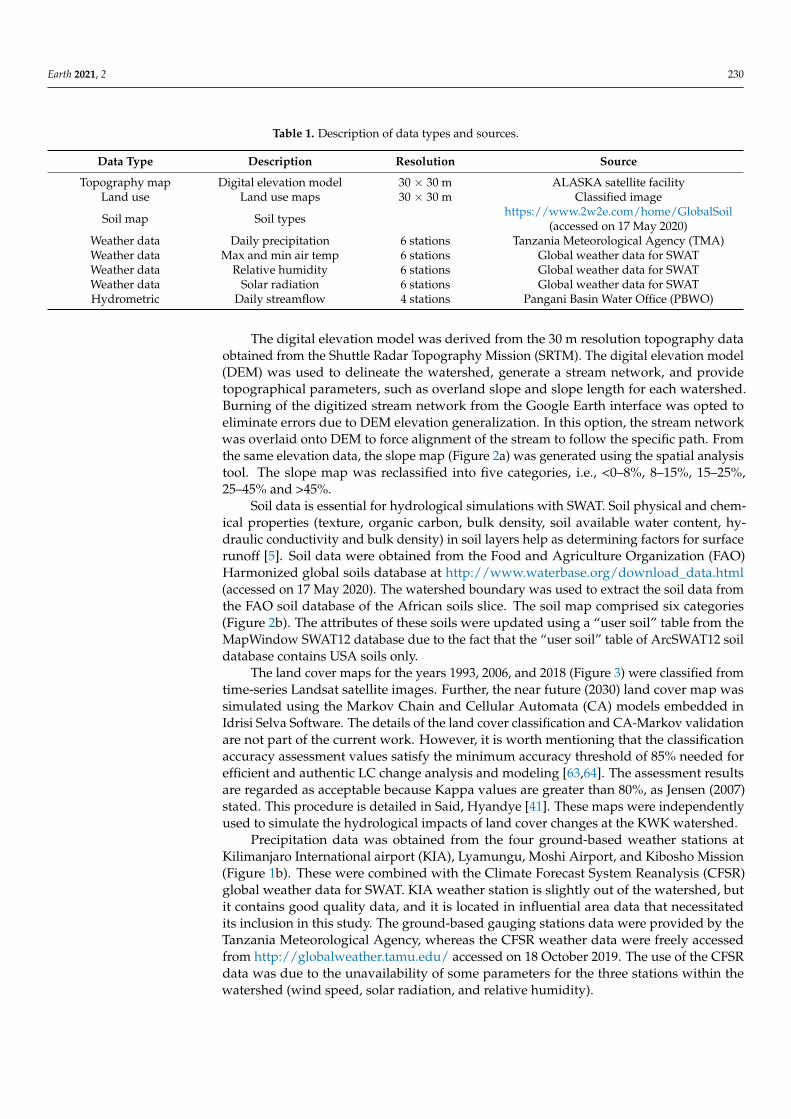
Table 1. Description of data types and sources.

Data Type Description Resolution Source

Topography map Digital elevation model 30 × 30 m ALASKA satellite facilityLand use Land use maps 30 × 30 m Classified image

Soil map Soil types https://www.2w2e.com/home/GlobalSoil(accessed on 17 May 2020)

Weather data Daily precipitation 6 stations Tanzania Meteorological Agency (TMA)Weather data Max and min air temp 6 stations Global weather data for SWATWeather data Relative humidity 6 stations Global weather data for SWATWeather data Solar radiation 6 stations Global weather data for SWATHydrometric Daily streamflow 4 stations Pangani Basin Water Office (PBWO)

The digital elevation model was derived from the 30 m resolution topography dataobtained from the Shuttle Radar Topography Mission (SRTM). The digital elevation model(DEM) was used to delineate the watershed, generate a stream network, and providetopographical parameters, such as overland slope and slope length for each watershed.Burning of the digitized stream network from the Google Earth interface was opted toeliminate errors due to DEM elevation generalization. In this option, the stream networkwas overlaid onto DEM to force alignment of the stream to follow the specific path. Fromthe same elevation data, the slope map (Figure 2a) was generated using the spatial analysistool. The slope map was reclassified into five categories, i.e., <0–8%, 8–15%, 15–25%,25–45% and >45%.

Soil data is essential for hydrological simulations with SWAT. Soil physical and chem-ical properties (texture, organic carbon, bulk density, soil available water content, hy-draulic conductivity and bulk density) in soil layers help as determining factors for surfacerunoff [5]. Soil data were obtained from the Food and Agriculture Organization (FAO)Harmonized global soils database at http://www.waterbase.org/download_data.html(accessed on 17 May 2020). The watershed boundary was used to extract the soil data fromthe FAO soil database of the African soils slice. The soil map comprised six categories(Figure 2b). The attributes of these soils were updated using a “user soil” table from theMapWindow SWAT12 database due to the fact that the “user soil” table of ArcSWAT12 soildatabase contains USA soils only.

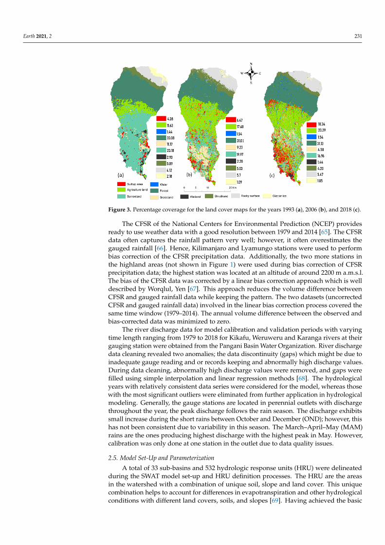
The land cover maps for the years 1993, 2006, and 2018 (Figure 3) were classified fromtime-series Landsat satellite images. Further, the near future (2030) land cover map wassimulated using the Markov Chain and Cellular Automata (CA) models embedded inIdrisi Selva Software. The details of the land cover classification and CA-Markov validationare not part of the current work. However, it is worth mentioning that the classificationaccuracy assessment values satisfy the minimum accuracy threshold of 85% needed forefficient and authentic LC change analysis and modeling [63,64]. The assessment resultsare regarded as acceptable because Kappa values are greater than 80%, as Jensen (2007)stated. This procedure is detailed in Said, Hyandye [41]. These maps were independentlyused to simulate the hydrological impacts of land cover changes at the KWK watershed.

Precipitation data was obtained from the four ground-based weather stations atKilimanjaro International airport (KIA), Lyamungu, Moshi Airport, and Kibosho Mission(Figure 1b). These were combined with the Climate Forecast System Reanalysis (CFSR)global weather data for SWAT. KIA weather station is slightly out of the watershed, butit contains good quality data, and it is located in influential area data that necessitatedits inclusion in this study. The ground-based gauging stations data were provided by theTanzania Meteorological Agency, whereas the CFSR weather data were freely accessedfrom http://globalweather.tamu.edu/ accessed on 18 October 2019. The use of the CFSRdata was due to the unavailability of some parameters for the three stations within thewatershed (wind speed, solar radiation, and relative humidity).

Earth 2021, 2 231Earth 2021, 2, FOR PEER REVIEW 7

Figure 3. Percentage coverage for the land cover maps for the years 1993 (a), 2006 (b), and 2018 (c).

Precipitation data was obtained from the four ground-based weather stations at Kil-imanjaro International airport (KIA), Lyamungu, Moshi Airport, and Kibosho Mission (Figure 1b). These were combined with the Climate Forecast System Reanalysis (CFSR) global weather data for SWAT. KIA weather station is slightly out of the watershed, but it contains good quality data, and it is located in influential area data that necessitated its inclusion in this study. The ground-based gauging stations data were provided by the Tanzania Meteorological Agency, whereas the CFSR weather data were freely accessed from http://globalweather.tamu.edu/ accessed on 18th October 2019. The use of the CFSR data was due to the unavailability of some parameters for the three stations within the watershed (wind speed, solar radiation, and relative humidity).

The CFSR of the National Centers for Environmental Prediction (NCEP) provides ready to use weather data with a good resolution between 1979 and 2014 [65]. The CFSR data often captures the rainfall pattern very well; however, it often overestimates the gauged rainfall [66]. Hence, Kilimanjaro and Lyamungo stations were used to perform bias correction of the CFSR precipitation data. Additionally, the two more stations in the highland areas (not shown in Figure 1) were used during bias correction of CFSR precip-itation data; the highest station was located at an altitude of around 2200 m a.m.s.l. The bias of the CFSR data was corrected by a linear bias correction approach which is well described by Worqlul, Yen [67]. This approach reduces the volume difference between CFSR and gauged rainfall data while keeping the pattern. The two datasets (uncorrected CFSR and gauged rainfall data) involved in the linear bias correction process covered the same time window (1979–2014). The annual volume difference between the observed and bias-corrected data was minimized to zero.

The river discharge data for model calibration and validation periods with varying time length ranging from 1979 to 2018 for Kikafu, Weruweru and Karanga rivers at their gauging station were obtained from the Pangani Basin Water Organization. River dis-charge data cleaning revealed two anomalies; the data discontinuity (gaps) which might be due to inadequate gauge reading and or records keeping and abnormally high dis-charge values. During data cleaning, abnormally high discharge values were removed, and gaps were filled using simple interpolation and linear regression methods [68]. The hydrological years with relatively consistent data series were considered for the model, whereas those with the most significant outliers were eliminated from further application in hydrological modeling. Generally, the gauge stations are located in perennial outlets

Figure 3. Percentage coverage for the land cover maps for the years 1993 (a), 2006 (b), and 2018 (c).

The CFSR of the National Centers for Environmental Prediction (NCEP) providesready to use weather data with a good resolution between 1979 and 2014 [65]. The CFSRdata often captures the rainfall pattern very well; however, it often overestimates thegauged rainfall [66]. Hence, Kilimanjaro and Lyamungo stations were used to performbias correction of the CFSR precipitation data. Additionally, the two more stations inthe highland areas (not shown in Figure 1) were used during bias correction of CFSRprecipitation data; the highest station was located at an altitude of around 2200 m a.m.s.l.The bias of the CFSR data was corrected by a linear bias correction approach which is welldescribed by Worqlul, Yen [67]. This approach reduces the volume difference betweenCFSR and gauged rainfall data while keeping the pattern. The two datasets (uncorrectedCFSR and gauged rainfall data) involved in the linear bias correction process covered thesame time window (1979–2014). The annual volume difference between the observed andbias-corrected data was minimized to zero.

The river discharge data for model calibration and validation periods with varyingtime length ranging from 1979 to 2018 for Kikafu, Weruweru and Karanga rivers at theirgauging station were obtained from the Pangani Basin Water Organization. River dischargedata cleaning revealed two anomalies; the data discontinuity (gaps) which might be due toinadequate gauge reading and or records keeping and abnormally high discharge values.During data cleaning, abnormally high discharge values were removed, and gaps werefilled using simple interpolation and linear regression methods [68]. The hydrologicalyears with relatively consistent data series were considered for the model, whereas thosewith the most significant outliers were eliminated from further application in hydrologicalmodeling. Generally, the gauge stations are located in perennial outlets with dischargethroughout the year, the peak discharge follows the rain season. The discharge exhibitssmall increase during the short rains between October and December (OND); however, thishas not been consistent due to variability in this season. The March–April–May (MAM)rains are the ones producing highest discharge with the highest peak in May. However,calibration was only done at one station in the outlet due to data quality issues.

2.5. Model Set-Up and Parameterization

A total of 33 sub-basins and 532 hydrologic response units (HRU) were delineatedduring the SWAT model set-up and HRU definition processes. The HRU are the areasin the watershed with a combination of unique soil, slope and land cover. This uniquecombination helps to account for differences in evapotranspiration and other hydrologicalconditions with different land covers, soils, and slopes [69]. Having achieved the basic

Earth 2021, 2 232

operational KWK SWAT model, the model was further edited to include managementactivities such as crops management schedule season in the watershed. Since it was notpossible to estimate the rate of fertilizer applications for various crops as well as quantifyingthe amount of water used for irrigation, the KWK SWAT model adopted auto fertilizationand auto irrigation for the crops.

The KWK SWAT model parameters, such as the potential evapotranspiration, wereestimated using the Hargreaves method, while the curve number method was used for therunoff estimation. Other parameters were manually edited before carrying out automaticparameters estimation using the SWAT model calibration and uncertainty procedure (SWAT-CUP) [70]. The manual parameter adjustments were based on the expert knowledge of thewatershed physical and hydrogeological characteristics such as river channel width, leafarea index, and soil types.

2.6. Automatic Calibration and Validation of the SWAT Model

The SWAT model calibration and uncertainty procedure (SWAT-CUP) was used to cal-ibrate and validate the KWK SWAT model automatically. Model calibration and sensitivityanalysis were done at the watershed outlet due to data discontinuity and abnormally highdischarge values as compared to precipitation. Simulations that were set up using the 1993LULC map were used to calibrate monthly streamflow from 1987 to 1993. After calibration,the simulations that were set up using the same LULC map was used to validate themonthly streamflow from 1994 to 2000. Selection of the calibration and validation timei.e., between 1987 and 2000 was based on the quality of the available discharge data, andgood data continuity. Sensitivity analysis was carried out in SWAT-CUP, whereby 22 flowparameters were used, and the model was run for 1000 iterations. The significance of thesensitivity of each parameter was determined using t-stat and p-value [71]. The higherthe absolute t-stat values among the parameters and the smaller p-values, the higher thesensitivity. Usually, p-values close to 0 and 0.05 are acceptable [72]. The t-stat is used toidentify the relative significance of the parameter, whereas the p-value is used to ascertainthe sensitivity significance [71].

Generally, the calibration process was based on varying the hydrological parametersiteratively. The agreement between the simulated and observed streamflow was used asa decision tool for the final parameter variation. The model performance was evaluatedcomparatively using the streamflow hydrograph for simulated and observed streamflowfor both calibration and validation periods. Statistical evaluation of the model was doneusing per cent bias (PBIAS), coefficient of determination (R2), the Nash and Sutcliffesimulation efficiency (NS). R2 is a measure of the extent of uniformity between observedand simulated data; R2 ranges from 0 to 1, with higher values indicating high suitability.However, values higher than 0.5 are considered acceptable for simulation [73]. NS showthe extent that observed and simulated data fit each other (Nash and Sutcliffe, 1970), whereNSE = 1 is the best value. Per cent bias (PBIAS) measures the average tendency of thesimulated data to be larger or smaller than their observed values for a given quantityover the calibration or validation period; the value becomes the best as it comes to zero.The RMSE-observations standard deviation ratio (RSR) standardizes RMSE using theobservations standard deviation; generally, the best simulation performance is consideredto have relatively lower RSR and hence lower RMSE. The details of model evaluation canbe found in Moriasi, G. Arnold [74].

The calibrated flow parameters were used to check the model capacity to simulatemeasured streamflow results. The streamflow validation of the model was done usinga new streamflow dataset without any adjustment in the calibrated flow parameters.Evaluation of the model performance was done using PBIAS, R2, and ENS, respectively.

The calibrated and validated parameters from SWAT-CUP were returned into theKWK SWAT model. The new parameters from SWAT-CUP were used to either replaceor modify the existing values in the SWAT model. This process was accomplished usingthe Manual Calibration Helper function in the ArcSWAT environment. Updating the

Earth 2021, 2 233

SWAT model using the calibrated and validated parameters from SWAT-CUP meant thatthe KWK SWAT model was ready for use in hydrological processes simulation in theKWK watershed.

2.7. Partial Least Squares Regression Analysis

Partial least squares regression (PLSR) is a robust multivariate regression method,especially when there are collinear predictors, high correlated predictors, numerous predic-tors equal to or higher than observations and many independent variables [75]. Analysisof land cover change impacts on water balance components is widely performed usingmultivariate regression analyses [5,21,74,75]. PLSR is an extension of a multiple linearregression model. In the simplest form, a linear model specifies the relationship betweena dependent variable y, and a set of predictor variables x, as shown in Equation (2). Themodel parameter is estimated as a slope of a simple bivariate regression between a matrixcolumn or row as the Y-variable and another parameter vector as the X-variable; this isdone for each variable [76].

y = k0 + k1x1 + k2x2 + . . . + knxn (2)

where k0 is the regression coefficient for the intercept and ki values are the regressioncoefficients (for variables 1 to n) computed from the land cover change data.

The predictive quality of the model in this study was improved by running seriesof PLSR models, in each run; the Q2 cumulated (Q2

cum) was used to eliminate variableswith the least influence until the largest Q2

cum was attained. Generally, Q2cum above 0.5 is

considered to be of good predictive power [74]. The cross-validated root mean squarederror (RMSECV) was used to avoid skewness by the data points, especially when there areoutliers. The model’s predictive power was measured by using the global goodness of fit(R2) and the cross-validated model quality index (R2

cross). R2 is a fraction of variance inthe dependent variable, which can be predicted by the model; whereas, R2

cross measuresprediction goodness. Generally, the importance of predictors (for all variables) is measuredby the variable importance for the projection (VIP), where the larger the values, the higherthe predictor relevance.

In determining the land use types that interact with hydrological components morethan the other, the regression coefficients (RCs) and the variable importance of the pro-jection (VIP) were used. VIP values can be used to show a broader expression of therelative importance of predictors [77]. Based on the world’s criteria, VIPs are categorizedto indicate the importance of a particular predictor in influencing the dependent variables;VIP values > 1 and/or VIP > 0.8 show that the predictor variable is significantly important,i.e., those predictors with large VIP values can best explain the dependent variable [78,79],the values >0.8 are most pertinent, whereas the values <0.5 show insignificance in ex-plaining the variable [74,78,80]. The RCs show the direction and strength of the impact ofeach independent variable. Generally, a small RC and large VIP shoes the importance ofthe variable in prediction in that direction, whereas the small RC and small VIP indicateinsignificance of the particular variable; thus, it can be omitted from the model. Moreover,PLSR weight (w) provides more precise and reasonable insight into the sign (+ or −) ofthe weight of the corresponding coefficients in the model. Usually, the squares of w valuesgreater than 0.2 show that the PLSR component is mainly weighted on the correspondingvariables. In addition, the w value shows the direction of influence that the LC class hason the corresponding water balance components. i.e., the negative sign means inverselyrelated, whereas a positive sign means it is directly proportional to most of the selectedhydrologic components.

PLSR method associates principal component analysis (PCA) and multiple linearregression features [81]. The method is suitable when the predictors show multicollinear-ity [82,83]. Generally, land use data exhibit collinearity because an increase in the percent-age/area of one type will automatically decrease the percentage/area of one or more ofthe other land use type [84]. Thus, it is appropriate in this study because it eliminates

Earth 2021, 2 234

co-dependence among the variables and provides a more unbiased view of the contributionof the changes in water balance components at the watershed scale.

In this study, PLSR modeling was used to determine the association between thesimulated hydrological components and land use/cover classes. The land use types arethe predictors, and the annual hydrological components are the response feature. Theseanalyses were done using the statistical package for social science (SPSS) version 21 andthe XLSTAT add-in tool [50].

2.8. Simulation of Impacts of LU Change Scenarios on Hydrological Processes

The calibrated and validated SWAT model was used to simulate the impacts of LUchanges on the hydrological processes of the watershed based on historical LU data for theyears 1993, 2006 and 2018. The future impacts of the LC change scenario were assessedusing the LU map for the year 2030. Both temporal and spatial variation of land coverchange scenarios on various watershed water balance components were considered. In thisstudy, the annual average values of the selected hydrological components were used toassess the impact of land cover changes on the hydrology of KWK watershed. The selectedhydrologic components were surface runoff (SurfQ), lateral flow (LatQ), groundwater flow(GWQ), actual evapotranspiration (ET), and water yield (WatQ).

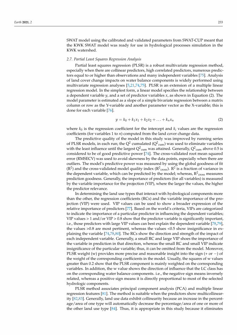
The methods and steps applied in this study to assess LUC change impacts on hy-drological processes in KWK watershed are summarized in Figure 4. The figure can besplit into three major blogs: the SWAT model set up and parameterization (left-hand side),SWAT model calibration and validation, and fine-tuning of the model (middle blog). Thelast blog (right-hand side) presents the PLSR modeling and assessment of impacts of landuse and cover changes on hydrological processes.

Earth 2021, 2, FOR PEER REVIEW 11

Figure 4. Workflow applied in this work.

3. Results 3.1. Sensitivity Analysis

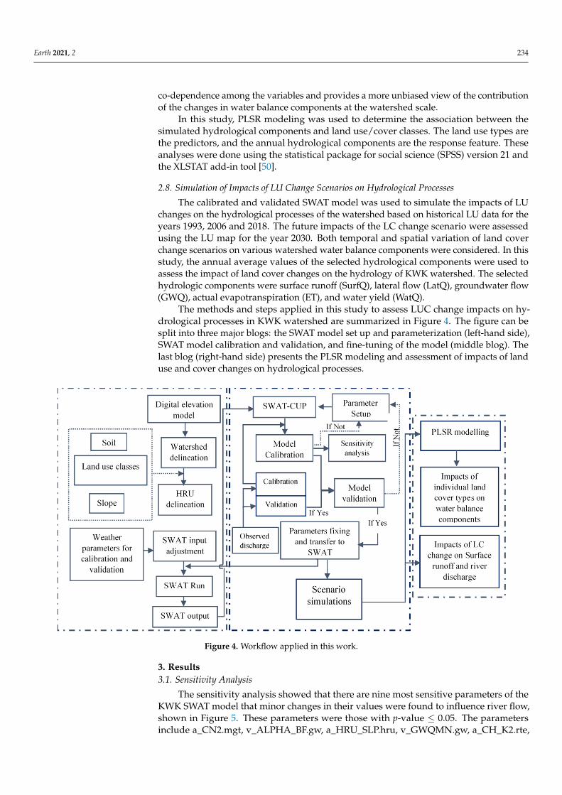
The sensitivity analysis showed that there are nine most sensitive parameters of the KWK SWAT model that minor changes in their values were found to influence river flow, shown in Figure 5. These parameters were those with p-value ≤ 0.05. The parameters in-clude a_CN2.mgt, v_ALPHA_BF.gw, a_HRU_SLP.hru, v_GWQMN.gw, a_CH_K2.rte, a_SOL_AWC().sol, a_SLSUBBSN.hru, v_GW_REVAP.gw, a_CANMX.hru and SOL_K().sol. The t-statistical values of the parameters are used to rank the parameters in the order of magnitude of their influence on the streamflow. According to Abbaspour [72], the higher the absolute t-test values, and low p-values, the more sensitive the parameter. The information regarding parameters sensitivity analysis is always helpful in making modelers’ work easy as it highlights which parameters to fine-tune during calibration of a hydrological model.

Figure 4. Workflow applied in this work.

3. Results3.1. Sensitivity Analysis

The sensitivity analysis showed that there are nine most sensitive parameters of theKWK SWAT model that minor changes in their values were found to influence river flow,shown in Figure 5. These parameters were those with p-value ≤ 0.05. The parametersinclude a_CN2.mgt, v_ALPHA_BF.gw, a_HRU_SLP.hru, v_GWQMN.gw, a_CH_K2.rte,

Earth 2021, 2 235

a_SOL_AWC().sol, a_SLSUBBSN.hru, v_GW_REVAP.gw, a_CANMX.hru and SOL_K().sol.The t-statistical values of the parameters are used to rank the parameters in the orderof magnitude of their influence on the streamflow. According to Abbaspour [72], thehigher the absolute t-test values, and low p-values, the more sensitive the parameter.The information regarding parameters sensitivity analysis is always helpful in makingmodelers’ work easy as it highlights which parameters to fine-tune during calibration of ahydrological model.

Earth 2021, 2, FOR PEER REVIEW 12

Figure 5. Results of parameter sensitivity analysis (p-value and t-stat).

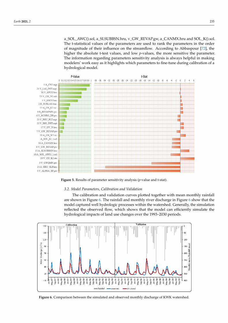
3.2. Model Parameters, Calibration and Validation The calibration and validation curves plotted together with mean monthly rainfall

are shown in Figure 6. The rainfall and monthly river discharge in Figure 6 show that the model captured well hydrologic processes within the watershed. Generally, the simula-tion reflected the observed flow, which shows that the model can efficiently simulate the hydrological impacts of land use changes over the 1993–2030 periods.

Figure 6. Comparison between the simulated and observed monthly discharge of KWK watershed.

Figure 5. Results of parameter sensitivity analysis (p-value and t-stat).

3.2. Model Parameters, Calibration and Validation

The calibration and validation curves plotted together with mean monthly rainfallare shown in Figure 6. The rainfall and monthly river discharge in Figure 6 show that themodel captured well hydrologic processes within the watershed. Generally, the simulationreflected the observed flow, which shows that the model can efficiently simulate thehydrological impacts of land use changes over the 1993–2030 periods.

Earth 2021, 2, FOR PEER REVIEW 12

Figure 5. Results of parameter sensitivity analysis (p-value and t-stat).

3.2. Model Parameters, Calibration and Validation The calibration and validation curves plotted together with mean monthly rainfall

are shown in Figure 6. The rainfall and monthly river discharge in Figure 6 show that the model captured well hydrologic processes within the watershed. Generally, the simula-tion reflected the observed flow, which shows that the model can efficiently simulate the hydrological impacts of land use changes over the 1993–2030 periods.

Figure 6. Comparison between the simulated and observed monthly discharge of KWK watershed.

Figure 6 shows that the simulated flow reflected the observed flow. However, it is worth stating that the model did not mimic very well both low and high flows as indicated

Figure 6. Comparison between the simulated and observed monthly discharge of KWK watershed.

Earth 2021, 2 236

Figure 6 shows that the simulated flow reflected the observed flow. However, it isworth stating that the model did not mimic very well both low and high flows as indicatedin Figure 6. There is a high level of baseflow throughout the year due to springs alongthe watershed.

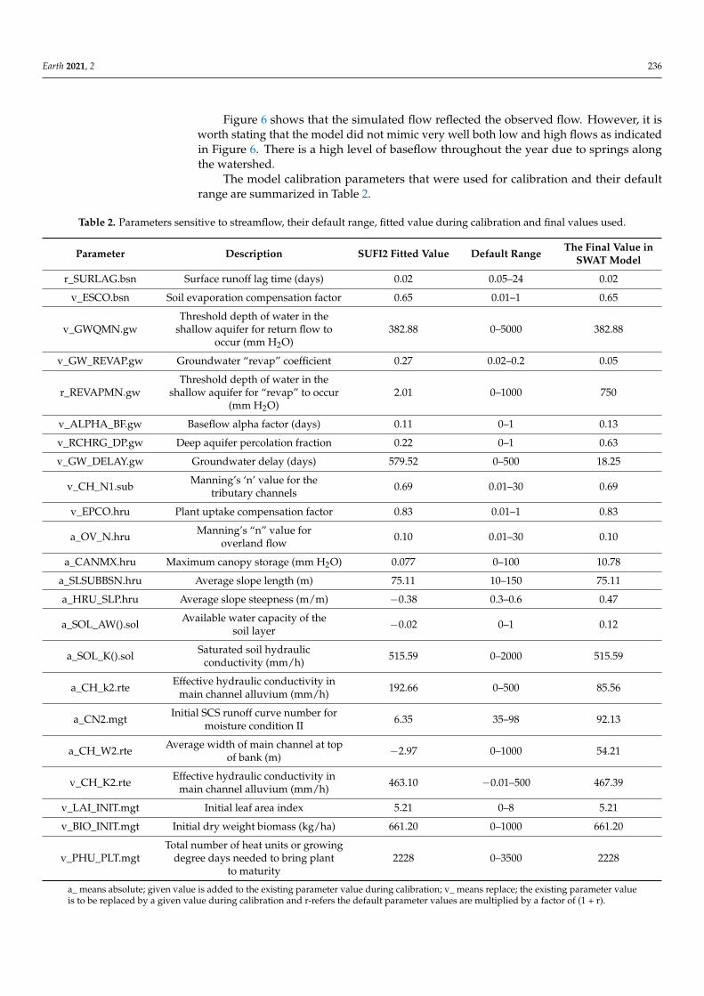
The model calibration parameters that were used for calibration and their defaultrange are summarized in Table 2.

Table 2. Parameters sensitive to streamflow, their default range, fitted value during calibration and final values used.

Parameter Description SUFI2 Fitted Value Default Range The Final Value inSWAT Model

r_SURLAG.bsn Surface runoff lag time (days) 0.02 0.05–24 0.02

v_ESCO.bsn Soil evaporation compensation factor 0.65 0.01–1 0.65

v_GWQMN.gwThreshold depth of water in the

shallow aquifer for return flow tooccur (mm H2O)

382.88 0–5000 382.88

v_GW_REVAP.gw Groundwater “revap” coefficient 0.27 0.02–0.2 0.05

r_REVAPMN.gwThreshold depth of water in the

shallow aquifer for “revap” to occur(mm H2O)

2.01 0–1000 750

v_ALPHA_BF.gw Baseflow alpha factor (days) 0.11 0–1 0.13

v_RCHRG_DP.gw Deep aquifer percolation fraction 0.22 0–1 0.63

v_GW_DELAY.gw Groundwater delay (days) 579.52 0–500 18.25

v_CH_N1.sub Manning’s ‘n’ value for thetributary channels 0.69 0.01–30 0.69

v_EPCO.hru Plant uptake compensation factor 0.83 0.01–1 0.83

a_OV_N.hru Manning’s “n” value foroverland flow 0.10 0.01–30 0.10

a_CANMX.hru Maximum canopy storage (mm H2O) 0.077 0–100 10.78

a_SLSUBBSN.hru Average slope length (m) 75.11 10–150 75.11

a_HRU_SLP.hru Average slope steepness (m/m) −0.38 0.3–0.6 0.47

a_SOL_AW().sol Available water capacity of thesoil layer −0.02 0–1 0.12

a_SOL_K().sol Saturated soil hydraulicconductivity (mm/h) 515.59 0–2000 515.59

a_CH_k2.rte Effective hydraulic conductivity inmain channel alluvium (mm/h) 192.66 0–500 85.56

a_CN2.mgt Initial SCS runoff curve number formoisture condition II 6.35 35–98 92.13

a_CH_W2.rte Average width of main channel at topof bank (m) −2.97 0–1000 54.21

v_CH_K2.rte Effective hydraulic conductivity inmain channel alluvium (mm/h) 463.10 −0.01–500 467.39

v_LAI_INIT.mgt Initial leaf area index 5.21 0–8 5.21

v_BIO_INIT.mgt Initial dry weight biomass (kg/ha) 661.20 0–1000 661.20

v_PHU_PLT.mgtTotal number of heat units or growing

degree days needed to bring plantto maturity

2228 0–3500 2228

a_ means absolute; given value is added to the existing parameter value during calibration; v_ means replace; the existing parameter valueis to be replaced by a given value during calibration and r-refers the default parameter values are multiplied by a factor of (1 + r).

Earth 2021, 2 237

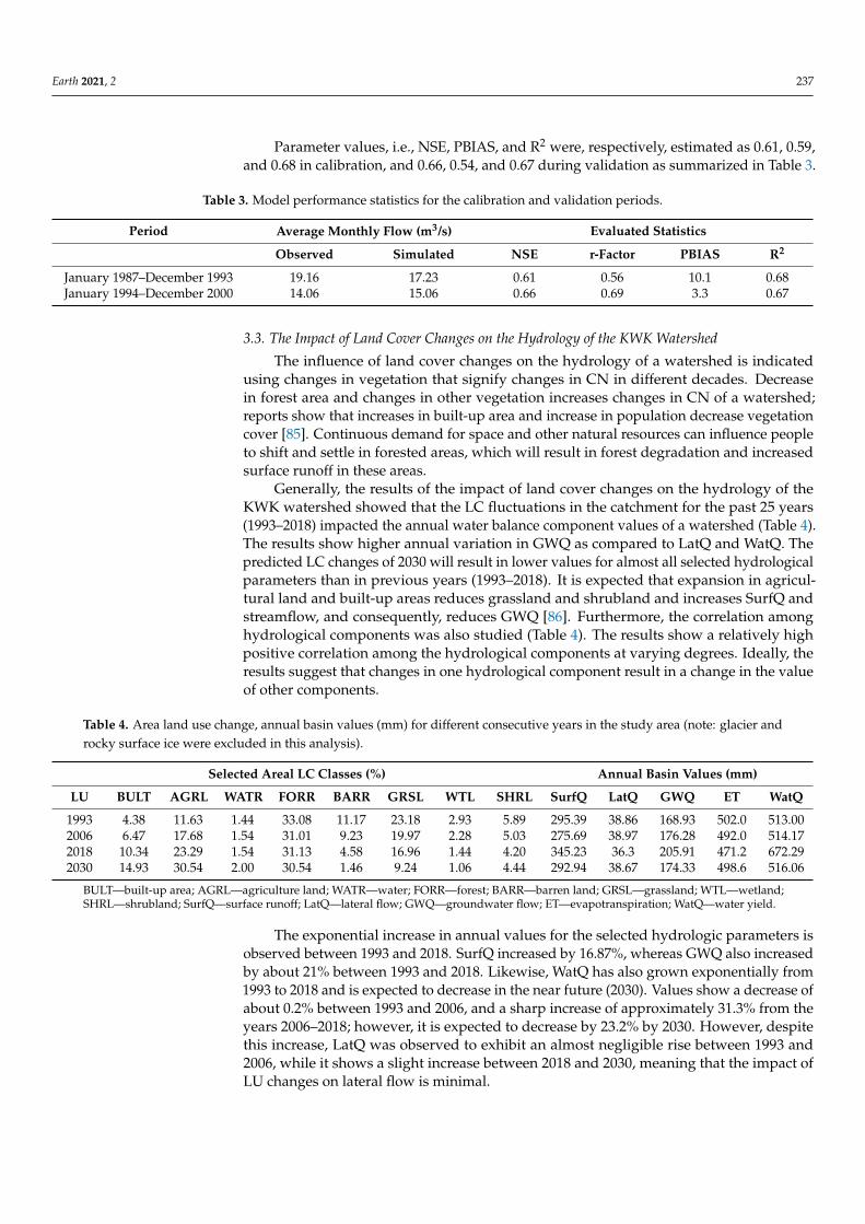
Parameter values, i.e., NSE, PBIAS, and R2 were, respectively, estimated as 0.61, 0.59,and 0.68 in calibration, and 0.66, 0.54, and 0.67 during validation as summarized in Table 3.

Table 3. Model performance statistics for the calibration and validation periods.

Period Average Monthly Flow (m3/s) Evaluated Statistics

Observed Simulated NSE r-Factor PBIAS R2

January 1987–December 1993 19.16 17.23 0.61 0.56 10.1 0.68January 1994–December 2000 14.06 15.06 0.66 0.69 3.3 0.67

3.3. The Impact of Land Cover Changes on the Hydrology of the KWK Watershed

The influence of land cover changes on the hydrology of a watershed is indicatedusing changes in vegetation that signify changes in CN in different decades. Decreasein forest area and changes in other vegetation increases changes in CN of a watershed;reports show that increases in built-up area and increase in population decrease vegetationcover [85]. Continuous demand for space and other natural resources can influence peopleto shift and settle in forested areas, which will result in forest degradation and increasedsurface runoff in these areas.

Generally, the results of the impact of land cover changes on the hydrology of theKWK watershed showed that the LC fluctuations in the catchment for the past 25 years(1993–2018) impacted the annual water balance component values of a watershed (Table 4).The results show higher annual variation in GWQ as compared to LatQ and WatQ. Thepredicted LC changes of 2030 will result in lower values for almost all selected hydrologicalparameters than in previous years (1993–2018). It is expected that expansion in agricul-tural land and built-up areas reduces grassland and shrubland and increases SurfQ andstreamflow, and consequently, reduces GWQ [86]. Furthermore, the correlation amonghydrological components was also studied (Table 4). The results show a relatively highpositive correlation among the hydrological components at varying degrees. Ideally, theresults suggest that changes in one hydrological component result in a change in the valueof other components.

Table 4. Area land use change, annual basin values (mm) for different consecutive years in the study area (note: glacier androcky surface ice were excluded in this analysis).

Selected Areal LC Classes (%) Annual Basin Values (mm)

LU BULT AGRL WATR FORR BARR GRSL WTL SHRL SurfQ LatQ GWQ ET WatQ

1993 4.38 11.63 1.44 33.08 11.17 23.18 2.93 5.89 295.39 38.86 168.93 502.0 513.002006 6.47 17.68 1.54 31.01 9.23 19.97 2.28 5.03 275.69 38.97 176.28 492.0 514.172018 10.34 23.29 1.54 31.13 4.58 16.96 1.44 4.20 345.23 36.3 205.91 471.2 672.292030 14.93 30.54 2.00 30.54 1.46 9.24 1.06 4.44 292.94 38.67 174.33 498.6 516.06

BULT—built-up area; AGRL—agriculture land; WATR—water; FORR—forest; BARR—barren land; GRSL—grassland; WTL—wetland;SHRL—shrubland; SurfQ—surface runoff; LatQ—lateral flow; GWQ—groundwater flow; ET—evapotranspiration; WatQ—water yield.

The exponential increase in annual values for the selected hydrologic parameters isobserved between 1993 and 2018. SurfQ increased by 16.87%, whereas GWQ also increasedby about 21% between 1993 and 2018. Likewise, WatQ has also grown exponentially from1993 to 2018 and is expected to decrease in the near future (2030). Values show a decrease ofabout 0.2% between 1993 and 2006, and a sharp increase of approximately 31.3% from theyears 2006–2018; however, it is expected to decrease by 23.2% by 2030. However, despitethis increase, LatQ was observed to exhibit an almost negligible rise between 1993 and2006, while it shows a slight increase between 2018 and 2030, meaning that the impact ofLU changes on lateral flow is minimal.

Earth 2021, 2 238

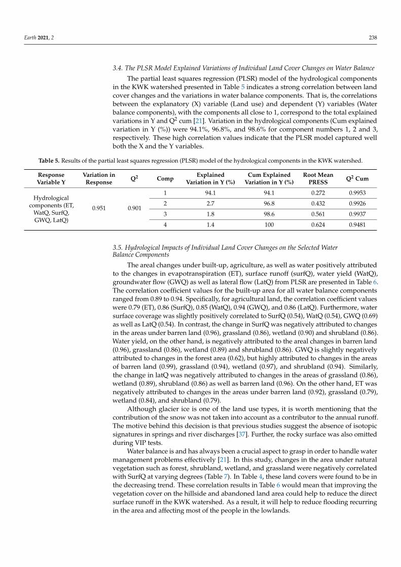
3.4. The PLSR Model Explained Variations of Individual Land Cover Changes on Water Balance

The partial least squares regression (PLSR) model of the hydrological componentsin the KWK watershed presented in Table 5 indicates a strong correlation between landcover changes and the variations in water balance components. That is, the correlationsbetween the explanatory (X) variable (Land use) and dependent (Y) variables (Waterbalance components), with the components all close to 1, correspond to the total explainedvariations in Y and Q2 cum [21]. Variation in the hydrological components (Cum explainedvariation in Y (%)) were 94.1%, 96.8%, and 98.6% for component numbers 1, 2 and 3,respectively. These high correlation values indicate that the PLSR model captured wellboth the X and the Y variables.

Table 5. Results of the partial least squares regression (PLSR) model of the hydrological components in the KWK watershed.

ResponseVariable Y

Variation inResponse Q2 Comp Explained

Variation in Y (%)Cum Explained

Variation in Y (%)Root Mean

PRESS Q2 Cum

Hydrologicalcomponents (ET,

WatQ, SurfQ,GWQ, LatQ)

0.951 0.901

1 94.1 94.1 0.272 0.9953

2 2.7 96.8 0.432 0.9926

3 1.8 98.6 0.561 0.9937

4 1.4 100 0.624 0.9481

3.5. Hydrological Impacts of Individual Land Cover Changes on the Selected WaterBalance Components

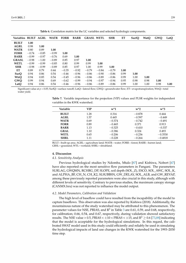
The areal changes under built-up, agriculture, as well as water positively attributedto the changes in evapotranspiration (ET), surface runoff (surfQ), water yield (WatQ),groundwater flow (GWQ) as well as lateral flow (LatQ) from PLSR are presented in Table 6.The correlation coefficient values for the built-up area for all water balance componentsranged from 0.89 to 0.94. Specifically, for agricultural land, the correlation coefficient valueswere 0.79 (ET), 0.86 (SurfQ), 0.85 (WatQ), 0.94 (GWQ), and 0.86 (LatQ). Furthermore, watersurface coverage was slightly positively correlated to SurfQ (0.54), WatQ (0.54), GWQ (0.69)as well as LatQ (0.54). In contrast, the change in SurfQ was negatively attributed to changesin the areas under barren land (0.96), grassland (0.86), wetland (0.90) and shrubland (0.86).Water yield, on the other hand, is negatively attributed to the areal changes in barren land(0.96), grassland (0.86), wetland (0.89) and shrubland (0.86). GWQ is slightly negativelyattributed to changes in the forest area (0.62), but highly attributed to changes in the areasof barren land (0.99), grassland (0.94), wetland (0.97), and shrubland (0.94). Similarly,the change in latQ was negatively attributed to changes in the areas of grassland (0.86),wetland (0.89), shrubland (0.86) as well as barren land (0.96). On the other hand, ET wasnegatively attributed to changes in the areas under barren land (0.92), grassland (0.79),wetland (0.84), and shrubland (0.79).

Although glacier ice is one of the land use types, it is worth mentioning that thecontribution of the snow was not taken into account as a contributor to the annual runoff.The motive behind this decision is that previous studies suggest the absence of isotopicsignatures in springs and river discharges [37]. Further, the rocky surface was also omittedduring VIP tests.

Water balance is and has always been a crucial aspect to grasp in order to handle watermanagement problems effectively [21]. In this study, changes in the area under naturalvegetation such as forest, shrubland, wetland, and grassland were negatively correlatedwith SurfQ at varying degrees (Table 7). In Table 4, these land covers were found to be inthe decreasing trend. These correlation results in Table 6 would mean that improving thevegetation cover on the hillside and abandoned land area could help to reduce the directsurface runoff in the KWK watershed. As a result, it will help to reduce flooding recurringin the area and affecting most of the people in the lowlands.

Earth 2021, 2 239

Table 6. Correlation matrix for the LC variables and selected hydrologic components.

Variables BUILT AGRL WATR FORR BARR GRASL WETL SHR ET SurfQ WatQ GWQ LatQ

BUILT 1.00AGRL 0.98 1.00WATR 0.80 0.89 1.00FORR −0.74 −0.85 −0.99 1.00BARR −0.99 −0.97 −0.76 0.69 1.00

GRASL −0.98 −1.00 −0.89 0.85 0.97 1.00WETL −0.99 −0.99 −0.85 0.80 0.99 0.99 1.00SHR −0.98 −0.99 −0.89 0.85 0.97 1.00 0.99 1.00ET 0.89 0.79 0.44 −0.35 −0.92 −0.79 −0.84 −0.79 1.00

SurQ 0.94 0.86 0.54 −0.46 −0.96 −0.86 −0.90 −0.86 0.99 1.00WtrQ 0.94 0.85 0.54 −0.45 −0.96 −0.86 −0.89 −0.86 0.99 1.00 1.00GWQ 0.99 0.94 0.69 −0.62 −0.99 −0.94 −0.97 −0.94 0.95 0.98 0.98 1.00LatQ 0.94 0.86 0.54 −0.46 −0.96 −0.86 −0.89 −0.86 0.99 1.00 1.00 0.98 1.00

Significant value at p = 0.05; SurfQ—surface runoff; LatQ—lateral flow; GWQ—groundwater flow; ET—evapotranspiration; WtrQ—totalwater yield.

Table 7. Variable importance for the projection (VIP) values and PLSR weights for independentvariables in the KWK watershed.

Variable VIP w*1 w*2 w*3

BUILT 1.28 0.316 −0.878 0.444AGRL 1.57 0.445 −0.597 −0.449WATR 0.69 −0.374 −0.742 −0.491FORR 0.89 −0.465 0.371 0.913BARR 1.13 −0.325 −0.410 −0.337GRAL 1.10 −0.386 0.324 0.493WETL 0.65 −0.206 −0.236 −0.3530SHRL 1.11 −0.228 −0.264 −0.4818

BULT—built-up area; AGRL—agriculture land; WATR—water; FORR—forest; BARR—barren land;GRSL—grassland; WTL—wetland; SHRL—shrubland.

4. Discussion4.1. Sensitivity Analysis

Previous hydrological studies by Ndomba, Mtalo [87] and Kishiwa, Nobert [47]have also reported on the most sensitive flow parameters in Pangani. The parametersSURLAG, GWQMN, RCHRG_DP, SLOPE, soil depth (SOL_Z), ESCO, SOL_AWC, SOL_K,and ALPHA_BF, CH_N, CH_K2, SLSUBBSN, GW_DELAY, SOL_ALB, and GW_REVAP,among these previously reported parameters were also crucial in this study, although withdifferent levels of sensitivity. Contrary to previous studies, the maximum canopy storage(CANMX.hru) was not reported to influence the model output.

4.2. Model Parameters, Calibration and Validation

The high level of baseflow could have resulted from the incapability of the model tocapture baseflows. This observation was also reported by Kishiwa (2018). Additionally, themountainous nature of the study watershed may be attributed to this phenomenon. Theparameter values for NSE, PBIAS, and R2 in Table 3 are 0.61, 0.59, and 0.68, respectively,for calibration; 0.66, 0.54, and 0.67, respectively, during validation showed satisfactoryresults. The NSE value > 0.5, PBIAS < ±10 < PBIAS < ±15, and R2 ≥ 0.6 [73,88] indicatingthat the model is acceptable for the hydrological simulations. In this regard, the cali-brated SWAT model used in this study could efficiently and reliably be used in simulatingthe hydrological impacts of land use changes in the KWK watershed for the 1993–2030time step.

Earth 2021, 2 240

4.3. The Impact of Land Cover Changes on the Hydrology of the KWK Watershed

The results show that land cover has changed throughout the study period within thecatchment; previous studies also show that land use has changed on the entire slopes of Mt.Kilimanjaro [29,32,33,89,90]. The possible reasons for the escalation of agricultural landand the built-up area may be due to higher population growth rate and socioeconomicdevelopment such as the fair prices for horticultural crops in the lowlands. Thus, morepeople are engaging in growing crops in the catchment. Further, the influx of people fromoutside and highland areas has resulted in an increase of cropland and extension of thebuilt-up areas to the lowland areas that were previously considered comparatively dryand less productive. Perhaps we could experience more decrease in the area under forest;however, most of the forest area falls in the upper area of the Kilimanjaro National Park,which is protected by the law. Although, reports still show anthropogenic activities suchas logging, forest burning, charcoal making, the establishment of new villages, livestockkeeping and cultivation, landslides, and quarrying across the protected forest reserve [91].Additionally, the conversion of the lower montane forest into coffee plantation are amongthe factors contributing to forest loss [92].

Despite the conservation activities, it is worth stating that there is still a flimsy decreasein the forest area, especially close to the forest borders and in the lowlands [29]. Thus,observation shows that the magnitude of variation in ET values is small despite the changein LC with time. However, monthly fluctuations in ET support that the model perfectlycaptures cropping season that is expected to have relatively higher ET values during vege-tative stages; although in general agreement with the fact that seasonal crops (agriculturalland) have less ET than perennial trees [5,80]. Studies show that evapotranspiration takes acountable amount of water infiltrating the soil in semiarid regions, and effective rechargedepends solely on extreme rainfall events [93].

The expansion of agricultural land, built-up areas, and shrinking of grassland [41]may have resulted in increased surface runoff in the KWK watershed, especially in thelowlands. The changes in WatQ as a result of changes in vegetation is due to changes inCN values. CN values increased with an increase in built-up areas, bare agricultural landsand decreased forest areas [85]. Although, the variation in land use results in changesin hydrological processes, the soil types, geological conditions, and slope are among thefactors governing the impacts of land use changes on the water balance components [94].Thus, KWK being located on the mountain slopes is expected to be affected by these factors.Other studies reported a similar trend in the basin. For example, Kishiwa, Nobert [47]predicted an increase in the annual streamflow by 10% in the year 2060 and steady growthin the streamflow annually, taking 2001 as a baseline year.

Generally, in a situation where most vegetation is converted to built-up areas and theexpansion in agricultural land, compaction causes lower permeability and storage capacityresulting in a lower infiltration capacity. Thus, transforming a substantial fraction of rainfallinto surface runoff. SurfQ and GWQ increases as the areas with cleared vegetation foragriculture and built-up areas increases. A similar observation was reported in SouthAfrica, where SurfQ is higher and GWQ is lower in bare lands [95]; GWQ is higher in theforest and other vegetative places due to increased infiltration into the shallow and deepaquifers. This may be a reason for flood reoccurrence being common in lowland areas,especially at the beginning of the season, where there are no plants in the farms.

4.4. The PLSR Model Explained Variations of Individual Land Cover Changes on Water Balance

The PLSR variable importance of the projected values (VIP) and weights of the inde-pendent variables are given in Table 7. The highest VIP value was obtained in agriculturalland (VIP = 1.57), built-up area (VIP = 1.28), barren land (VIP = 1.13), shrubland andgrassland (VIP = 1.10). It can be noted from Table 7 that forest has comparatively lowerinfluence in impacting the selected water balance components (VIP 0.89). Nevertheless, theforest is still important in influencing water balance components, whereas wetland andwater were of minor importance. The relative importance of predictors (VIP) shows that

Earth 2021, 2 241

water and wetland exert comparatively less significance (VIP less than 0.8). Component1 was dominated by agricultural land and built-up areas on the positive side, whereaswater, forest, barren land, grassland, wetland and shrubland were on the negative side. Incomponent 2, all land use/cover classes were negative sided except forest, which was onthe positive side. Component 3 was also dominated by the negative sided classes exceptfor forest and grassland, while the positive side included water, barren land, wetland andshrubland, agricultural land and built-up areas.

4.5. Hydrological Impacts of Individual Land Cover Changes on the Selected WaterBalance Components

Most of the previous studies have shown that an increase in vegetation cover, partic-ularly forests, leads to decreasing SurfQ and flood occurrence [5,21]. According to [96],clearing of forest by 45% increased the SurfQ by around 40%. Additionally, an increasein runoff due to replacing rangeland through expansion in agricultural land and built-upareas was reported from 2000 to 2013 in the Olifants basin, South Africa [95].

Increased ET and increased runoff may be a result of the conversion of vegetatedareas to agriculture and built-up areas. However, the increased agricultural lands lead tohigher water abstraction [97]; this might be the reason for the slight decrease in ET in thenear future (Table 4). Increased SurfQ due to increased built-up area was reported in someprevious reports [98,99]. Therefore, it is envisaged that the observed reduction in ET reflectsthe conversion to agricultural lands, which increases water use. Additionally, conversionto agricultural land increases the CN value, thus reducing ET. Memarian, Balasundram [15]also observed that an increase in a built-up area and agricultural land increases CN, thusreducing ET.

Further, increase in cultivated lands is at the expense of other vegetation covers; thus,increased runoff was also reported by Gashaw, Tulu [5] in the Andassa watershed, Blue NileBasin, Ethiopia, Woldesenbet, Elagib [80], and [100] in Rwanda. Contrary to these results,the study by Twisa, Kazumba [53] in the Wami Ruvu basin revealed a negative influence onsurface runoff and water yield by natural forest, woodland, bushland, grassland, water, andwetland. Further, the study reported a negative influence of the built-up area on GWQ andET. At the same time, natural forest, bushland, woodland, grassland, water, and wetlandhad a positive influence on ET and GWQ. However, KWK being located on a mountainousplace with complex terrain is expected to behave differently from other catchments.

Agricultural land and built-up areas are the main attributes in the changes in WatQ,SurfQ, ET, and GWQ; this means that with the ongoing expansion in agricultural land andbuilt-up areas, the water balance of a watershed will be affected negatively. However, it isworth mentioning that groundwater was not used in the study for validation; thus, caremust be taken during GWQ results interpretation. The observation supports the reportby Anand, Gosain [51], stating that the intensification of urban and cultivated lands is anessential environmental stressor that significantly affects water balance components of acatchment. For instance, an increase in the built-up area contributes to a higher proportionof surface runoff and streamflow and lowers the quantity of groundwater flow [86].

The increase in WatQ observed in 2018 (Table 4) may chiefly be a result of a decreasein ET resulting from changed forest covers [101]. The small increase in water yield as aresult of land cover effects has been reported in an East African watershed [102]. Previousstudies also reported an increase in the WatQ and decreased ET [103,104]. Additionlly, anincrease in SurfQ due to deforestation and vice versa has been reported in a watershed inSouth China [105].

Increased SurfQ and decreased ET rate observed in Table 4 may equally be attributedto increased built-up areas, and reduction in forest cover. Previous reports that usedthe SWAT model also reported a similar trend in the Jinjiang catchment, China, due todeforestation and increased built-up areas [106]. Forest degradation and increased built-upareas decrease ET and increase SurfQ in SWAT simulations [107]. Additionally, Sajikumarand Remya [108] used SWAT to assess the impacts of the land cover on runoff; their reportshows increased runoff due to changed land cover in Kerala.

Earth 2021, 2 242

Generally, the increase in runoff may imply increasing soil erosion and sedimentationif left unattended. Twisting land use trends to allow more vegetation cover will reducewet season flow, increase dry season flow, SurfQ, LatQ and GWQ [75]. Techniques suchas replacing cereals with fruit trees and intensifying agronomic practices will advocateincreasing productivity of small farms and discourage opening up more land for agriculture.Further, using soil and water management practices may be useful to increase vegetationcover at the KWK watershed.

The PLSR results in Table 7 show that all land use/cover classes are important ininfluencing changes in water balance components, except for shrubland and wetland.Thus, regulation of other LC classes should be implemented to regulate the impacts in thehydrology of the KWK watershed. The current reported rapid population growth, climatechange and expansion in agricultural land, built-up areas, and other economic activitiescan significantly impact the future if the situation goes unattended [109,110]. The PLSRresults from this study are suitable for designing and carrying out sustainable naturalresources management practices at the basin scale and other similar environments [111].Moreover, the results from this study show the potential of using a combined PLSR andhydrologic modeling framework for impact studies in data-constrained environments.

5. Conclusions

In this study, the implication of the hydrology of the KWK watershed due to changesin land cover over the past few decades and in the near future were evaluated using thecalibrated SWAT model and PLSR. The KWK watershed has mostly featured transformationin agriculture and built-up area; thus, a forecast for the future hydrological processes basedon changes in land cover in the study area was presented in this study. The effect ofland cover change resulting from various land use activities such as urbanization andexpansion in agricultural activities is evident. Explicitly, the findings of this work showthat changes in the water balance components are the function of the land use changesand vegetation distribution within the watershed. The major LULC changes that affectedsurface runoff and groundwater components in the watershed during the study periodwere the expansion of agricultural land, built-up area, and shrinking of the grassland.

The cultivation land area is directly proportional to the surface runoff but inverselyproportional to the groundwater flow. However, the decline in woody shrub area hasthe same effect as the expansion of cultivation land on surface runoff and groundwaterflows. Farmland expansion has increased surface runoff and water yield while decreasingthe groundwater component and actual evapotranspiration in the KWK watershed. Simi-larly, the decline in woodland coverage resulted in higher surface runoff and water-yieldcomponents but decreased groundwater components and actual evapotranspiration.

The surface runoff of the area during the wet season due to land use and land coverchanges shows the implications in the water resources, environmental wellbeing andeconomic activities in downstream users, especially fishing and irrigation activities alongthe Nyumba ya Mungu Dam. The results suggest the threatening of the supply of ecosystemservices, threatening the people living within and surrounding the watershed. Further,the increased surface runoff would trigger flood recurrence, and possibly sedimentationon the lower slopes poses a threat to fishing and agriculture production and hydropowerproduction. The results of this study have contributed to understanding the attributionof land use changes on the hydrologic components. The information generated from thiswork will help stakeholders and managers to make rational choices regarding land andwater resources management. The approach utilized in this work can be applied to thewhole basin and other basins to predict the land use changes and associated impacts onwater resources.

Limitations of the Study

The analytical power of PLSR is outstanding and useful for data analysis in manydimensions. However, PLSR is not with limitations; one limitation is that it only provides

Earth 2021, 2 243

a general insight into the relationships between different predictors (land use types) andwater balance components. However, it cannot provide detailed information on the spatialland use patterns [19,77]. The spatial distribution patterns of land use can significantlyinfluence hydrologic processes at different scales. Thus, future research could focus on therelationship between spatial land use patterns and changes in the water balance compo-nents. Furthermore, the availability of good quality meteorological and river dischargedatasets, and spatial distribution network might have affected the results to some extent.Thus, future studies should focus on generating good quality datasets and improve spatialdistribution of ground based meteorological stations.

Author Contributions: Conceptualization, M.S., H.C.K., I.C.M. and L.K.M.; methodology, M.S. andC.H.; software, M.S. and C.H.; validation, M.S., C.H. and I.C.M.; formal analysis, M.S.; investigation,M.S.; resources, I.C.M.; data curation, M.S.; writing—original draft preparation, M.S.; writing—review and editing, M.S. and L.K.M.; visualization, L.K.M.; supervision, H.C.K. and I.C.M.; projectadministration, H.C.K. and I.C.M.; funding acquisition, M.S. All authors have read and agreed to thepublished version of the manuscript.

Funding: This research was supported by African Development Bank (AfDB) through grant num-ber 2100155032816, hosted at The Nelson Mandela African Institution of Science and Technology,Arusha Tanzania.

Data Availability Statement: The Tanzania Meteorological Agency (TMA) and the Pangani basinwater board (PBWB) are the custodians of the raw weather and river flow data, respectively. Landsatimages were sourced from the US Geological Survey (USGS) at https://glovis.usgs.gov (accessedon 17 May 2020). Soil data was downloaded from the FAO Harmonized global soils database athttp://www.waterbase.org/download_data.html (accessed on 17 May 2020). The Climate ForecastSystem Reanalysis (CFSR) global weather data for SWAT were sourced at https://globalweather.tamu.edu (accessed on 17 May 2020).

Acknowledgments: The authors would like to acknowledge the Center of Excellence in WaterInfrastructure and Sustainable Energy Futures (WISE FUTURES) of NM-AIST for financing theexchange program at the Indian Institute of Technology Delhi, where mentorship and guidance inSWAT model were obtained.

Conflicts of Interest: The authors declare that they have no conflict of interest.

References1. Zhou, Y.; Xu, Y.J.; Xiao, W.; Wang, J.; Huang, Y.; Yang, H. Climate Change Impacts on Flow and Suspended Sediment Yield in

Headwaters of High-Latitude Regions—A Case Study in China’s Far Northeast. Water 2017, 9, 966. [CrossRef]2. Briones, R.; Ella, V.; Bantayan, N. Hydrologic impact evaluation of land use and land cover change in Palico Watershed, Batangas,

Philippines Using the SWAT model. J. Environ. Sci. Manag. 2016, 19, 96–107.3. Neupane, R.P.; Kumar, S. Estimating the effects of potential climate and land use changes on hydrologic processes of a large

agriculture dominated watershed. J. Hydrol. 2015, 529, 418–429. [CrossRef]4. Karimi, H.; Jafarnezhad, J.; Khaledi, J.; Ahmadi, P. Monitoring and prediction of land use/land cover changes using CA-Markov

model: A case study of Ravansar County in Iran. Arab. J. Geosci. 2018, 11, 592. [CrossRef]5. Gashaw, T.; Tulu, T.; Argaw, M.; Worqlul, A.W. Modeling the hydrological impacts of land use/land cover changes in the Andassa

watershed, Blue Nile Basin, Ethiopia. Sci. Total Environ. 2018, 619–620, 1394–1408. [CrossRef] [PubMed]6. Olson, J.M.; Alagarswamy, G.; Andresen, J.A.; Campbell, D.J.; Davis, A.Y.; Ge, J.; Huebner, M.; Lofgren, B.M.; Lusch, D.P.; Moore,

N.J.; et al. Integrating diverse methods to understand climate–land interactions in East Africa. Geoforum 2008, 39, 898–911.[CrossRef]

7. Baldus, R.D.; Hahn, R.; Mpanduji, D.G.; Siege, L. The selous-niassa wildlife corridor. Tanzania Wildlife Discussion Series 2003.Available online: http://www.suaire.sua.ac.tz/handle/123456789/2072 (accessed on 17 May 2021).

8. Kitalika, A.J.; Machunda, R.L.; Komakech, H.C.; Njau, K.N. Land-Use and Land Cover Changes on the Slopes of MountMeru-Tanzania. Curr. World Environ. 2018, 13, 331–352. [CrossRef]

9. Kashaigili, J.; Majaliwa, A. Implications of land use and land cover changes on hydrological regimes of the Malagarasi River,Tanzania. J. Agric. Sci. Appl. 2013, 2, 45–50. [CrossRef]

10. Marhaento, H.; Booij, M.J.; Hoekstra, A. Hydrological response to future land-use change and climate change in a tropicalcatchment. Hydrol. Sci. J. 2018, 63, 1368–1385. [CrossRef]

11. Yadav, S.; Babel, M.S.; Shrestha, S.; Deb, P. Land use impact on the water quality of large tropical river: Mun River Basin, Thailand.Environ. Monit. Assess. 2019, 191, 614. [CrossRef]

Earth 2021, 2 244

12. Yin, Z.; Feng, Q.; Yang, L.; Wen, X.; Si, J.; Zou, S. Long Term Quantification of Climate and Land Cover Change Impacts onStreamflow in an Alpine River Catchment, Northwestern China. Sustainability 2017, 9, 1278. [CrossRef]

13. Zhang, L.; Karthikeyan, R.; Bai, Z.; Srinivasan, R. Analysis of streamflow responses to climate variability and land use change inthe Loess Plateau region of China. Catena 2017, 154, 1–11. [CrossRef]

14. Foley, J.A.; DeFries, R.; Asner, G.P.; Barford, C.; Bonan, G.; Carpenter, S.R.; Chapin, F.S.; Coe, M.T.; Daily, G.C.; Gibbs, H.K.; et al.Global Consequences of Land Use. Science 2005, 309, 570–574. [CrossRef] [PubMed]

15. Memarian, H.; Balasundram, S.K.; Abbaspour, K.C.; Talib, J.B.; Sung, C.T.B.; Sood, A.M. SWAT-based hydrological modelling oftropical land-use scenarios. Hydrol. Sci. J. 2014, 59, 1808–1829. [CrossRef]

16. Fohrer, N.; Haverkamp, S.; Eckhardt, K.; Frede, H.-G. Hydrologic Response to land use changes on the catchment scale. Phys.Chem. Earth Part B Hydrol. Oceans Atmosphere 2001, 26, 577–582. [CrossRef]

17. Abe, C.A.; Lobo, F.D.L.; Dibike, Y.B.; Costa, M.P.D.F.; Dos Santos, V.; Novo, E.M.L.M. Modelling the Effects of Historical andFuture Land Cover Changes on the Hydrology of an Amazonian Basin. Water 2018, 10, 932. [CrossRef]

18. Dos Santos, V.; Laurent, F.; Abe, C.; Messner, F. Hydrologic Response to Land Use Change in a Large Basin in Eastern Amazon.Water 2018, 10, 429. [CrossRef]

19. Fu, B.-J.; Wang, Y.-F.; Lu, Y.-H.; He, C.-S.; Chen, L.-D.; Song, C.-J. The effects of land-use combinations on soil erosion: A casestudy in the Loess Plateau of China. Prog. Phys. Geogr. Earth Environ. 2009, 33, 793–804. [CrossRef]

20. Defersha, M.B.; Melesse, A.M. Field-scale investigation of the effect of land use on sediment yield and runoff using runoff plotdata and models in the Mara River basin, Kenya. Catena 2012, 89, 54–64. [CrossRef]

21. Shawul, A.A.; Chakma, S.; Melesse, A.M. The response of water balance components to land cover change based on hydrologicmodeling and partial least squares regression (PLSR) analysis in the Upper Awash Basin. J. Hydrol. Reg. Stud. 2019, 26, 100640.[CrossRef]

22. Maitima, J.M.; Mugatha, S.M.; Reid, R.S.; Gachimbi, L.N.; Majule, A.; Lyaruu, H.; Pomery, D.; Mathai, S.; Mugisha, S. The linkagesbetween land use change, land degradation and biodiversity across East Africa. Afr. J. Environ. Sci. Technol. 2009, 3, 310–325.

23. Smith, P.; House, J.I.; Bustamante, M.; Sobocká, J.; Harper, R.; Pan, G.; West, P.C.; Clark, J.M.; Adhya, T.; Rumpel, C.; et al. Globalchange pressures on soils from land use and management. Glob. Chang. Biol. 2016, 22, 1008–1028. [CrossRef] [PubMed]

24. Mustard, J.F.; DeFries, R.S.; Fisher, T.; Moran, E.F. Land-Use and Land-Cover Change Pathways and Impacts; Springer Science andBusiness Media LLC: Berlin/Heidelberg, Germany, 2012; Volume 6, pp. 411–429.

25. Guzha, A.; Rufino, M.; Okoth, S.; Jacobs, S.; Nobrega, R. Impacts of land use and land cover change on surface runoff, dischargeand low flows: Evidence from East Africa. J. Hydrol. Reg. Stud. 2018, 15, 49–67. [CrossRef]

26. Bradford, A.; Zhang, L.; Hairsine, P. Implementation of a Mean Annual Water Balance Model Within a Gis Framework and Application tothe Murray-Darling Basin; CRC for Catchment Hydrology: Boca Raton, FL, USA, 2001.

27. Stonestrom, D.A.; Scanlon, B.R.; Zhang, L. Introduction to special section on Impacts of Land Use Change on Water Resources.Water Resour. Res. 2009, 45. [CrossRef]

28. Said, M.; Komakech, H.C.; Munishi, L.K.; Muzuka, A.N.N. Evidence of climate change impacts on water, food and energyresources around Kilimanjaro, Tanzania. Reg. Environ. Chang. 2019, 19, 2521–2534. [CrossRef]

29. Mbonile, M.J.; Misana, S.; Sokoni, C. Land use change patterns and root causes of land use change on the southern slopes ofMount Kilimanjaro, Tanzania. In Land Use Change Impacts and Dynamics (LUCID) Project Working Paper Number 25; InternationallLivestock Research Institute: Nairobi, Kenya, 2003.

30. Mmbaga, N.E.; Munishi, L.K.; Treydte, A.C. How dynamics and drivers of land use/land cover change impact elephantconservation and agricultural livelihood development in Rombo, Tanzania. J. Land Use Sci. 2017, 12, 168–181. [CrossRef]

31. Chiwa, R. Effects of Land Use and Land Cover Changes on The Hydrology of Weruweru-Kiladeda Sub-Catchment in Pangani River Basin,Tanzania; Kenyatta University: Nairobi, Kenya, 2012.

32. Soini, E. Changing livelihoods on the slopes of Mt. Kilimanjaro, Tanzania: Challenges and opportunities in the Chaggahomegarden system. Agrofor. Syst. 2005, 64, 157–167. [CrossRef]

33. Misana, S.B. Land-use/cover changes and their drivers on the slopes of Mount Kilimanjaro, Tanzania. J. Geogr. Reg. Plan. 2012, 5,151–164. [CrossRef]

34. Ngugi, K.; Ogindo, H.; Ertsen, M. Impact of land use changes on hydrology of Mt. Kilimanjaro. The case of Lake Jipe catchment.In Proceedings of the EGU General Assembly Conference Abstracts, Vienna, Austria, 12–17 April 2015.

35. Bailey, R.T.; Wible, T.C.; Arabi, M.; Records, R.M.; Ditty, J. Assessing regional-scale spatio-temporal patterns of groundwater-surface water interactions using a coupled SWAT-MODFLOW model. Hydrol. Process. 2016, 30, 4420–4433. [CrossRef]

36. Deb, P.; Kiem, A.S.; Willgoose, G. A linked surface water-groundwater modelling approach to more realistically simulaterainfall-runoff non-stationarity in semi-arid regions. J. Hydrol. 2019, 575, 273–291. [CrossRef]

37. McKenzie, J.M.; Mark, B.G.; Thompson, L.G.; Schotterer, U.; Lin, P.-N. A hydrogeochemical survey of Kilimanjaro (Tanzania):Implications for water sources and ages. Hydrogeol. J. 2010, 18, 985–995. [CrossRef]

38. Shishira, E.; Yanda, P.Z. Forestry Conservation and Resource Utilisation on the Southern Slopes of Mount Kilimanjaro: Trends, Conflictsand Resolutions; Dar es Salaam University Press (DUP): Dar es Salaam, Tanzania, 2018.

39. Gao, J.; Li, F.; Gao, H.; Zhou, C.; Zhang, X. The impact of land-use change on water-related ecosystem services: A study of theGuishui River Basin, Beijing, China. J. Clean. Prod. 2017, 163, S148–S155. [CrossRef]

Earth 2021, 2 245

40. Lambin, E.F.; Geist, H.J.; Lepers, E. Dynamics Ofland-Use Andland-Coverchange Intropicalregions. Annu. Rev. Environ. Resour.2003, 28, 205–241. [CrossRef]

41. Said, M.; Hyandye, C.; Komakech, H.C.; Mjemah, I.C.; Munishi, L.K. Predicting land use/cover changes and its association toagricultural production on the slopes of Mount Kilimanjaro, Tanzania. Ann. GIS 2021, 1–21. [CrossRef]

42. Agrawala, S.; Moehner, A.; Hemp, A.; Aalst, M.V.; Hitz, S.; Smith, J.; Meena, H.; Mwakifwamba, S.M.; Hyera, T.; Mwaipopo,O.U. Development and Climate Change in Tanzania: Focus on Mount Kilimanjaro; Organisation for Economic Cooperation andDevelopment: Paris, France, 2003; p. 72.

43. Mbonile, M.J. Migration and intensification of water conflicts in the Pangani Basin, Tanzania. Habitat Int. 2005, 29, 41–67.[CrossRef]

44. Shaghude, Y.W. Review of Water Resource Exploitation and Landuse Pressure in the Pangani River Basin. West. Indian Ocean J.Mar. Sci. 2007, 5, 195–208. [CrossRef]

45. Hemp, A. Climate change-driven forest fires marginalize the impact of ice cap wasting on Kilimanjaro. Glob. Chang. Biol. 2005, 11,1013–1023. [CrossRef]

46. Viviroli, D.; Dürr, H.H.; Messerli, B.; Meybeck, M.; Weingartner, R. Mountains of the world, water towers for humanity: Typology,mapping, and global significance. Water Resour. Res. 2007, 43. [CrossRef]

47. Kishiwa, P.; Nobert, J.; Kongo, V.; Ndomba, P. Assessment of impacts of climate change on surface water availability usingcoupled SWAT and WEAP models: Case of upper Pangani River Basin, Tanzania. In Proceedings of the International Associationof Hydrological Sciences, Beijing, China, 6–9 November 2018; Volume 378, pp. 23–27.

48. Abudu, S.; Cui, C.L.; Saydi, M.; King, J.P. Application of snowmelt runoff model (SRM) in mountainous watersheds: A review.Water Sci. Eng. 2012, 5, 123–136. [CrossRef]

49. Anand, J.; Gosain, A.; Khosa, R.; Srinivasan, R. Regional scale hydrologic modeling for prediction of water balance, analysis oftrends in streamflow and variations in streamflow: The case study of the Ganga River basin. J. Hydrol. Reg. Stud. 2018, 16, 32–53.[CrossRef]

50. Huisman, J.; Breuer, L.; Bormann, H.; Bronstert, A.; Croke, B.; Frede, H.-G.; Gräff, T.; Hubrechts, L.; Jakeman, A.; Kite, G.; et al.Assessing the impact of land use change on hydrology by ensemble modeling (LUCHEM) III: Scenario analysis. Adv. WaterResour. 2009, 32, 159–170. [CrossRef]

51. Anand, J.; Gosain, A.; Khosa, R. Prediction of land use changes based on Land Change Modeler and attribution of changes in thewater balance of Ganga basin to land use change using the SWAT model. Sci. Total Environ. 2018, 644, 503–519. [CrossRef]

52. Hyandye, C.B.; Worqul, A.; Martz, L.W.; Muzuka, A.N.N. The impact of future climate and land use/cover change on waterresources in the Ndembera watershed and their mitigation and adaptation strategies. Environ. Syst. Res. 2018, 7, 7. [CrossRef]

53. Twisa, S.; Kazumba, S.; Kurian, M.; Buchroithner, M.F. Evaluating and Predicting the Effects of Land Use Changes on Hydrologyin Wami River Basin, Tanzania. Hydrology 2020, 7, 17. [CrossRef]

54. UN. The Sustainable Development Goals Report 2019; UN: New York, NY, USA, 2019.55. Gassman, P.W.; Reyes, M.R.; Green, C.H.; Arnold, J.G. The Soil and Water Assessment Tool: Historical Development, Applications,

and Future Research Directions. Trans. ASABE 2007, 50, 1211–1250. [CrossRef]56. Arnold, J.G.; Moriasi, D.N.; Gassman, P.W.; Abbaspour, K.C.; White, M.J.; Srinivasan, R.; Santhi, C.; Harmel, R.D.; van Griensven,

A.; Van Liew, M.W.; et al. SWAT: Model Use, Calibration, and Validation. Trans. ASABE 2012, 55, 1491–1508. [CrossRef]57. Yevenes, M.A.; Mannaerts, C.M. Seasonal and land use impacts on the nitrate budget and export of a mesoscale catchment in

Southern Portugal. Agric. Water Manag. 2011, 102, 54–65. [CrossRef]58. Lam, Q.D.; Schmalz, B.; Fohrer, N. The impact of agricultural Best Management Practices on water quality in a North German

lowland catchment. Environ. Monit. Assess. 2011, 183, 351–379. [CrossRef]59. Meaurio, M.; Zabaleta, A.; Uriarte, J.A.; Srinivasan, R.; Antigüedad, I. Evaluation of SWAT models performance to simulate

streamflow spatial origin. The case of a small forested watershed. J. Hydrol. 2015, 525, 326–334. [CrossRef]60. Wang, G.; Yang, H.; Wang, L.; Xu, Z.; Xue, B. Using the SWAT model to assess impacts of land use changes on runoff generation

in headwaters. Hydrol. Process. 2012, 28, 1032–1042. [CrossRef]61. Neitsch, S.L.; Arnold, J.G.; Kiniry, J.R.; Williams, J.R. Soil and Water Assessment Tool Theoretical Documentation: Version 2009;

Grassland Soil and Water Research Laboratory, Agricultural Research Service, Blackland Research Center, Texas AgriculturalExperiment Station: Temple, TX, USA, 2011; p. 618.

62. USDA, S. National Engineering Handbook, Section 4: Hydrology; USDA, S.: Washington, DC, USA, 1972.63. Ahmed, B.; Ahmed, R.; Zhu, X. Evaluation of Model Validation Techniques in Land Cover Dynamics. ISPRS Int. J. Geo-Information

2013, 2, 577–597. [CrossRef]64. Araya, Y.H.; Cabral, P. Analysis and Modeling of Urban Land Cover Change in Setúbal and Sesimbra, Portugal. Remote. Sens.

2010, 2, 1549–1563. [CrossRef]65. Roth, V.; Lemann, T. Comparing CFSR and conventional weather data for discharge and soil loss modelling with SWAT in small

catchments in the Ethiopian Highlands. Hydrol. Earth Syst. Sci. 2016, 20, 921–934. [CrossRef]66. Worqlul, A.W.; Yen, H.; Collick, A.S.; Tilahun, S.A.; Langan, S.; Steenhuis, T.S. Evaluation of CFSR, TMPA 3B42 and ground-based

rainfall data as input for hydrological models, in data-scarce regions: The upper Blue Nile Basin, Ethiopia. Catena 2017, 152,242–251. [CrossRef]

Earth 2021, 2 246

67. Koch, M.; Cherie, N. SWAT-modeling of the impact of future climate change on the hydrology and the water resources in theupper blue Nile river basin, Ethiopia. In Proceedings of the 6th International Conference on Water Resources and EnvironmentResearch, ICWRER, Koblenz, Germany, 3–7 June 2013.

68. Setegn, S.G.; Srinivasan, R.; Dargahi, B. Hydrological Modelling in the Lake Tana Basin, Ethiopia Using SWAT Model. OpenHydrol. J. 2008, 2, 49–62. [CrossRef]

69. Abbaspour, K.C. Swat-Cup2: SWAT Calibration and Uncertainty Programs Manual Version 2; Swiss Federal Institute of AquaticScience and Technology Department of Systems Analysis, Eawag, Swiss Federal Institute of Aquatic Science and Technology,Eds.; Swiss Federal Institute of Aquatic Science and Technology: Duebendorf, Switzerland, 2011.

70. Chanapathi, T.; Thatikonda, S.; Raghavan, S. Analysis of rainfall extremes and water yield of Krishna river basin under futureclimate scenarios. J. Hydrol. Reg. Stud. 2018, 19, 287–306. [CrossRef]

71. Abbaspour, K. SWAT Calibration and Uncertainty Programs—A User Manual, in Swiss Federal Institute of Aquatic Science and Technology;Swiss Federal Institute of Aquatic Science and Technology: Eawag, Switzerland, 2015.

72. Van Liew, M.W.; Arnold, J.G.; Garbrecht, J.D. Hydrologic Simulation on Agricultural Watersheds: Choosing Between Two Models.Trans. ASAE 2003, 46, 1539–1551. [CrossRef]

73. Moriasi, D.N.; Arnold, J.G.; Van Liew, M.W.; Bingner, R.L.; Harmel, R.D.; Veith, T.L. Model Evaluation Guidelines for SystematicQuantification of Accuracy in Watershed Simulations. Trans. ASABE 2007, 50, 885–900. [CrossRef]

74. Shi, Z.; Ai, L.; Li, X.; Huang, X.; Wu, G.; Liao, W. Partial least-squares regression for linking land-cover patterns to soil erosionand sediment yield in watersheds. J. Hydrol. 2013, 498, 165–176. [CrossRef]

75. Gashaw, T.; Tulu, T.; Argaw, M.; Worqlul, A.W. Evaluation and prediction of land use/land cover changes in the Andassawatershed, Blue Nile Basin, Ethiopia. Environ. Syst. Res. 2017, 6, 17. [CrossRef]

76. Wold, S.; Sjöström, M.; Eriksson, L. PLS-regression: A basic tool of chemometrics. Chemom. Intell. Lab. Syst. 2001, 58, 109–130.[CrossRef]

77. Yan, B.; Fang, N.; Zhang, P.; Shi, Z. Impacts of land use change on watershed streamflow and sediment yield: An assessmentusing hydrologic modelling and partial least squares regression. J. Hydrol. 2013, 484, 26–37. [CrossRef]

78. Wold, S.; Eriksson, L. Chemometric Methods in Molecular Design: Methods and Principles in Medicinal Chemistry. In PLS forMultivariate Linear Modeling; Van der Waterbeemd, H., Ed.; Verlag-Chemie: Weinheim, Germany, 1995; pp. 195–218.

79. Ai, L.; Shi, Z.; Yin, W.; Huang, X. Spatial and seasonal patterns in stream water contamination across mountainous watersheds:Linkage with landscape characteristics. J. Hydrol. 2015, 523, 398–408. [CrossRef]

80. Woldesenbet, T.A.; Elagib, N.A.; Ribbe, L.; Heinrich, J. Hydrological responses to land use/cover changes in the source region ofthe Upper Blue Nile Basin, Ethiopia. Sci. Total Environ. 2017, 575, 724–741. [CrossRef] [PubMed]

81. Abdi, H. Partial least square regression (PLS regression) in Encyclopedia of Measurement and Statistics; Salkind, N.J., Ed.; SagePublications: Thousand Oaks, CA, USA, 2007; p. 13.

82. Fang, N.; Shi, Z.; Chen, F.; Wang, Y. Partial Least Squares Regression for Determining the Control Factors for Runoff andSuspended Sediment Yield during Rainfall Events. Water 2015, 7, 3925–3942. [CrossRef]

83. Onderka, M.; Wrede, S.; Rodný, M.; Pfister, L.; Hoffmann, L.; Krein, A. Hydrogeologic and landscape controls of dissolvedinorganic nitrogen (DIN) and dissolved silica (DSi) fluxes in heterogeneous catchments. J. Hydrol. 2012, 450–451, 36–47. [CrossRef]

84. King, R.S.; Baker, M.; Whigham, D.; Weller, D.E.; Jordan, T.E.; Kazyak, P.F.; Hurd, M.K. Spatial Considerations for LinkingWatershed Land Cover to Ecological Indicators in Streams. Ecol. Appl. 2005, 15, 137–153. [CrossRef]

85. Kundu, S.; Khare, D.; Mondal, A. Past, present and future land use changes and their impact on water balance. J. Environ. Manag.2017, 197, 582–596. [CrossRef] [PubMed]

86. Marhaento, H.; Booij, M.; Rientjes, T.; Hoekstra, A. Attribution of changes in the water balance of a tropical catchment to land usechange using the SWAT model. Hydrol. Process. 2017, 31, 2029–2040. [CrossRef]

87. Ndomba, P.M.; Mtalo, F.W.; Killingtveit, Å. A guided swat model application on sediment yield modeling in Pangani river basin:Lessons learnt. J. Urban Environ. Eng. 2008, 2, 53–62. [CrossRef]

88. Santhi, C.; Arnold, J.G.; Williams, J.R.; Dugas, W.A.; Srinivasan, R.; Hauck, L.M. Validation of the Swat Model on a Large RiverBasin with Point and Nonpoint Sources. JAWRA J. Am. Water Resour. Assoc. 2001, 37, 1169–1188. [CrossRef]

89. Stump, D.; Tagseth, M. The history of precolonial and early colonial agriculture on Kilimanjaro: A review. In Culture, History andIdentity: Landscapes of Inhabitation in the Mount Kilimanjaro Area; Clack, T., Ed.; Archaeopress: Oxford, UK, 2009; pp. 107–124.

90. Tagseth, M. The expansion of traditional irrigation in Kilimanjaro, Tanzania. Int. J. Afr. Hist. Stud. 2008, 41, 461–490.91. Lambrechts, C.; Hemp, C.; Nnyiti, P.; Woodley, B.; Hemp, A. Aerial Survey of the Threats to Mt. Kilimanjaro Forests; UNDP: New

York, NY, USA, 2002.92. Gütlein, A.; Gerschlauer, F.; Kikoti, I.; Kiese, R. Impacts of climate and land use on N2O and CH 4 fluxes from tropical ecosystems

in the Mt. Kilimanjaro region, Tanzania. Glob. Chang. Biol. 2017, 24, 1239–1255. [CrossRef]93. Andersen, F.H. Hydrological Modeling in a Semi-Arid Area Using Remote Sensing Data. Ph.D. Thesis, Department of Geography

and Geology, University of Copenhagen, Copenhagen, Denmark, 2008.94. Bruijnzeel, L. Hydrological functions of tropical forests: Not seeing the soil for the trees? Agric. Ecosyst. Environ. 2004, 104,

185–228. [CrossRef]95. Gyamfi, C.; Ndambuki, J.M.; Salim, R.W. Hydrological Responses to Land Use/Cover Changes in the Olifants Basin, South Africa.

Water 2016, 8, 588. [CrossRef]

Earth 2021, 2 247

96. Siriwardena, L.; Finlayson, B.; McMahon, T. The impact of land use change on catchment hydrology in large catchments: TheComet River, Central Queensland, Australia. J. Hydrol. 2006, 326, 199–214. [CrossRef]

97. Wagner, P.D.; Kumar, S.; Schneider, K. An assessment of land use change impacts on the water resources of the Mula and MuthaRivers catchment upstream of Pune, India. Hydrol. Earth Syst. Sci. 2013, 17, 2233–2246. [CrossRef]

98. Tavakoli, M.; De Smedt, F.; Vansteenkiste, T.; Willems, P. Impact of climate change and urban development on extreme flows inthe Grote Nete watershed, Belgium. Nat. Hazards 2014, 71, 2127–2142. [CrossRef]

99. Du, J.; Qian, L.; Rui, H.; Zuo, T.; Zheng, D.; Xu, Y.; Xu, C.-Y. Assessing the effects of urbanization on annual runoff and floodevents using an integrated hydrological modeling system for Qinhuai River basin, China. J. Hydrol. 2012, 464–465, 127–139.[CrossRef]

100. Karamage, F.; Zhang, C.; Fang, X.; Liu, T.; Ndayisaba, F.; Nahayo, L.; Kayiranga, A.; Nsengiyumva, J.B. Modeling Rainfall-RunoffResponse to Land Use and Land Cover Change in Rwanda (1990–2016). Water 2017, 9, 147. [CrossRef]

101. Baldyga, T.J.; Miller, S.N.; Driese, K.L.; Gichaba, C.M. Assessing land cover change in Kenya’s Mau Forest region using remotelysensed data. Afr. J. Ecol. 2008, 46, 46–54. [CrossRef]

102. Baker, T.J.; Miller, S.N. Using the Soil and Water Assessment Tool (SWAT) to assess land use impact on water resources in an EastAfrican watershed. J. Hydrol. 2013, 486, 100–111. [CrossRef]

103. Wagner, P.D.; Bhallamudi, S.M.; Narasimhan, B.; Kantakumar, L.N.; Sudheer, K.; Kumar, S.; Schneider, K.; Fiener, P. Dynamicintegration of land use changes in a hydrologic assessment of a rapidly developing Indian catchment. Sci. Total Environ. 2016, 539,153–164. [CrossRef] [PubMed]

104. Wijesekara, G.; Gupta, A.; Valeo, C.; Hasbani, J.-G.; Qiao, Y.; Delaney, P.; Marceau, D. Assessing the impact of future land-usechanges on hydrological processes in the Elbow River watershed in southern Alberta, Canada. J. Hydrol. 2012, 412–413, 220–232.[CrossRef]

105. Niu, J.; Sivakumar, B. Study of runoff response to land use change in the East River basin in South China. Stoch. Environ. Res. RiskAssess. 2013, 28, 857–865. [CrossRef]

106. Lin, B.; Chen, X.; Yao, H.; Chen, Y.; Liu, M.; Gao, L.; James, A. Analyses of landuse change impacts on catchment runoff usingdifferent time indicators based on SWAT model. Ecol. Indic. 2015, 58, 55–63. [CrossRef]

107. Zhang, M.; Wei, X.; Sun, P.; Liu, S. The effect of forest harvesting and climatic variability on runoff in a large watershed: The casestudy in the Upper Minjiang River of Yangtze River basin. J. Hydrol. 2012, 464–465, 1–11. [CrossRef]

108. Sajikumar, N.; Remya, R. Impact of land cover and land use change on runoff characteristics. J. Environ. Manag. 2015, 161,460–468. [CrossRef]

109. Garcia, M.C.; Alvarez, R. TM digital processing of a tropical forest region in southeastern Mexico. Int. J. Remote. Sens. 1994, 15,1611–1632. [CrossRef]

110. Mondal, M.S.H. The implications of population growth and climate change on sustainable development in Bangladesh. Jàmbá J.Disaster Risk Stud. 2019, 11, 1–10. [CrossRef]

111. FAO. Sustainable Land Management (SLM) in Practice in the Kagera Basin: Lessons Learned for Scaling Up at Landscape Level: Results ofthe Kagera Transboundary Agro-ecosystem Management Project (Kagera TAMP); Food and Agriculture Organization of the UnitedNations: Rome, Italy, 2017.