SPATIO-TEMPORAL CHANGES IN LAND COVER IN RESPONSE

TO ANTHROPOGENIC AND HYDRODYNAMIC FACTORS IN

NYANDO WETLAND, KENYA

OKOTTO-OKOTTO JOSEPH

A thesis submitted to the Graduate School in partial fulfilment for the requirements

of the award of a Degree of Master of Science in Natural Resources Management of

Egerton University

EGERTON UNIVERSITY

AUGUST, 2016

ii

DECLARATION AND RECOMMENDATION

Declaration by the Candidate:

This thesis is my original work and has not, wholly or partially, been presented for an award

of a degree in any other University.

Signature: ………………………………… Date: ………………………………

Joseph Okotto-Okotto (NM11/1999/07)

Recommendation by the Supervisors:

This thesis is the candidate’s work and has been prepared with our guidance and assistance.

It is submitted with our approval as University supervisors.

Signature: ………………………………… Date: ………………………………

Dr. Gilbert Obati Obwoyere

Faculty of Environment and Resources Development

Department of Natural Resources Management

Egerton University

Signature: ………………………………… Date: ………………………………

Dr. John Momanyi Mironga

Faculty of Environment and Resources Development

Department of Geography

Egerton University

Signature: ………………………………… Date: ………………………………

Prof. Phillip Okoth Raburu

University of Eldoret

School of Natural Resources Management

Department of Fisheries and Aquatic Sciences

iii

COPYRIGHT

© Joseph Okotto-Okotto, 2016

All rights reserved. No part of this thesis may be reproduced, stored in a retrieval system or

transmitted, in any form or by any means, electronic, mechanical, photocopying, or

otherwise, without permission from the author.

iv

ACKNOWLEDGEMENT

First and foremost, glory, honour and praise are due to my heavenly Father Jehovah God and

to Jesus Christ my Lord and Saviour for His ever-abounding grace, undeserved blessings,

steadfast love and providence given to me throughout the period of my study. Secondly, I

am most indebted to Egerton University, especialy the Faculty of Environment and

Resources Development (FERD) for the opportunity they gave me and the continual

encouragement even when things seemed difficult.

Thirdly, there are many people and organizations that deserve heartfelt and sincere thanks

for their precious and invaluable contributions to this study. My deepest gratitude go to Dr.

Gilbert Obwoyere and Dr. John Mironga of the Departments of Natural Resources

Management and Geography, respectively, at Egerton University and Prof. Phillip Raburu

of the Department of Fisheries and Aquatic Sciences, University of Eldoret, who supervised

me through this work. The tremendous professional, technical, moral support, guidance and

patience they unreservedly gave me during this study made it what it has come to be!

Furthermore, I extend heartfelt thanks to Prof. Okeyo-Owuor, the Director-General of

Victoria Institute of Research on Environment and Development (VIRED) International and

Dr. Lorna Okotto who agreed to go through this work. My association with all the people I

have mentioned in this paragraph has been a journey of learning and hope in socio-ecological

research.

Finally, my sincere and heartfelt gratitude are due to Dr. Eng. Peter Kabok, the Managing

Director of the Lake Basin Development Authority (LBDA), for the overwhelming support

which included partial funding and encouragement. I must also thank the Ecology of

Livelihoods (ECOLIVE) project team, colleagues and friends at Victoria Instituted for

Research on Environment and Development (VIRED) International for partly sponsoring

and facilitating my fieldwork. Many thanks also go to Mr. Everton Namasake, Prof. Julius

Otieno Manyala and my colleagues Moses Omondi and Dennis Werunga, for the invaluable

consultative and brainstorming sessions that renewed and strengthened my skills and

competence in Geo-information Systems, remote sensing and statistical packages. Heartfelt

thanks also go to Fredrick Koba, Joseph Angugo and Oyando Bonnie for the dexterity and

assistance with proof reading and formatting of this work. My heartfelt thanks also go out to

my great friend Fredrick B. Ojuang’ and all others that I might not have mentioned herein

but who directly or indirectly contributed to my success in this study. They must have learnt

something of me too;

“I am a slow walker, but I never walk back”.

Abraham Lincoln (1809-1865)

v

DEDICATION

I dedicate this work to my loving wife Dr. Lorna Grace Okotto and adoring children; Lizzah

and Jack, who have been the fulcrum of my academic and spiritual life; for the love,

encouragement, understanding, all round support and prayers they have accorded me on this

journey; their selfless sacrifices that have encouraged me to labour in hard work that is

bearing fruits now and in the generations to come.

Finally, to my mother Teresa Adhiambo Okotto - who has remained a pillar in my life and

my late father, Joseph Walter Okotto Odillah, who never was for me to see, but remains a

scar of joy in my heart forever.

"At times, our own light goes out and is rekindled by a spark from another

person. Each of us has a cause to think with deep gratitude of those who

have lighted the flame within us."

“Albert Schweitzer”

vi

ABSTRACT

In the last three decades, wetlands have received much attention worldwide due to their

declining coverage and spatial distribution with more than 50% lost since the 1950s. Like

other wetlands worldwide, Nyando Wetland, the second largest lacustrine wetland ecosystem

on the Kenyan shores of Lake Victoria, is facing a major threat of degradation from both the

fluctuations of Lake Victoria water levels and anthropogenic factors operating in its

neighbourhoods. This study was conducted to determine how the spatial and temporal

changes in land use/cover in response to anthropogenic and hydrodynamic factors such as

land use, human population growth and lake level changes affected the area covered by the

wetland between 1984 and 2010. Remote sensing, ground-truthing, socio-ecological tools

such as questionnaires, focus group discussion protocols and data analysis tools such as

Geographical Information System, logistic, simple and multiple regression models were used

to achieve the objectives of the study. The Driver-Pressure-State-Impact-Response model

was used as a framework for analysis. Results showed that there is an increasing trend for

small-scale agriculture (+58 ha/yr) against a decreasing trend for water area (-29 ha/yr) and

a reduction by 31% of the area of Nyando Wetland over the study period. Population growth

was found to indirectly but significantly (SSAg p = 0.01, R2 = 0.89; RFTw p = 0.01, R2 =

0.80) influence the decline in wetland area through agricultural activities. The receding

shoreline had a significant (p = 0.02, R2 = 0.89) influence on the spatial decline of the

wetland. The study concludes that anthropogenic and hydrodynamic factors are significantly

affecting the wetland and could compromise its ecological integrity. It is recommended that

long-term health of the wetland should be contingent upon sound and effective ecotone zone

planning and management. Thus integrated participatory and adaptive research should be

conducted to stimulate quick responses and regenerative actions that could be used to restore

and conserve the wetland ecosystem.

vii

TABLE OF CONTENTS

DECLARATION AND RECOMMENDATION ........................................................................... ii

COPYRIGHT .................................................................................................................................... iii

ACKNOWLEDGEMENT ................................................................................................................. iv

DEDICATION ..................................................................................................................................... v

ABSTRACT ...................................................................................................................................... vi

TABLE OF CONTENTS.................................................................................................................. vii

LIST OF FIGURES ........................................................................................................................... xi

LIST OF PLATES ........................................................................................................................... xiii

LIST OF APPENDICES .................................................................................................................. xiv

LIST OF ACRONYMS AND ABBREVIATIONS .......................................................................... xv

CHAPTER ONE ................................................................................................................................ 1

1.0 INTRODUCTION ................................................................................................................ 1

1.1 Background ............................................................................................................................. 1

1.1.1 Statement of the Problem ........................................................................................... 4

1.2 Broad Objective ...................................................................................................................... 4

1.2.1 Specific Objectives .................................................................................................... 5

1.2.2 Hypotheses ................................................................................................................. 5

1.3 Justification ............................................................................................................................. 5

1.4 Scope and Limitations of the Study ........................................................................................ 6

1.5 Definition of Key Terms ......................................................................................................... 8

CHAPTER TWO ............................................................................................................................. 10

2.0 LITERATURE REVIEW .................................................................................................. 10

2.1 Definition of Wetlands ......................................................................................................... 10

2.2 Threats Facing Wetlands ...................................................................................................... 11

2.2.1 Land Use/Cover Changes ..................................................................................................... 13

2.2.2 Human Population Growth ................................................................................................... 16

2.2.3 Lake-water Level Changes ................................................................................................... 19

2.3 Application of Remote Sensing and GIS Tools in Wetland Research ..................... 20

2.5 The Research Gaps ............................................................................................................... 24

2.6 Conceptual Framework ......................................................................................................... 26

2.6.1 Driver-Pressure-State-Impact-Response Framework of Analysis (D-P-S-I-R) ....... 27

CHAPTER THREE ......................................................................................................................... 29

3.0 MATERIALS AND METHODS ....................................................................................... 29

3.1 Description of the Study Area .............................................................................................. 29

3.1.1 Topography and Drainage .................................................................................................... 29

3.1.2 Soils ...................................................................................................................................... 29

viii

3.1.3 Human Population and Agriculture ...................................................................................... 31

3.1.4 Biodiversity........................................................................................................................... 31

3.3. Research Design, Variables, Data Requirements, Sources and Types ................................. 32

3.3.1. Research Design ...................................................................................................... 32

3.3.2. Research Variables .................................................................................................. 33

3.4 Application of GIS and Remote Sensing Tools .................................................................... 34

3.4.1 Procedures for Measuring Land Use Changes ......................................................... 35

3.4.2 Field Surveys for Collection of Reference Data ...................................................... 35

3.4.3 Satellite Image Processing ....................................................................................... 36

3.4.4 Data Merging and Layer Stacking ........................................................................... 38

3.4.5 Geo-referencing and Re-sampling of the Images .................................................... 38

3.4.6 Image Sub-setting .................................................................................................... 40

3.4.7 Spectral Enhancements ............................................................................................ 42

3.4.8 Image Classification ................................................................................................ 43

3.4.9 Post Classification ................................................................................................... 45

3.4.10 Accuracy Assessment .............................................................................................. 45

3.5. Measurement of Changes in Population Growth in the Study Area ..................................... 46

3.5.1. Human Population Data ........................................................................................... 46

3.6. Measurement of Socio-ecological Data ................................................................................ 48

3.6.1. Socio-ecological Data .............................................................................................. 48

3.6.2. The Study Population .............................................................................................. 49

3.6.3 Sampling Design, Frame, and Size .......................................................................... 49

3.6.4 Questionnaire Administration .................................................................................. 52

3.6.5 Key Informant Interviews ........................................................................................ 53

3.6.7 Focus Group Discussions ........................................................................................ 53

3.6.8 Ethical Considerations ............................................................................................. 55

3.7. Data for Lake Levels ............................................................................................................ 55

3.8 Field Observations and Documentation ................................................................................ 56

3.8.1 Visual Observations ................................................................................................. 56

3.8.2 Photographic Documentation .................................................................................. 57

3.9 Analysis of Land Cover, Population, Lake Level and Socio-ecological Data ...................... 57

3.9.1. Data Processing and Analysis for Land Cover/Use Change .................................... 57

3.9.2. Population Data Processing and Analysis ............................................................... 57

3.9.3. Socio-economic Data Processing and Analysis ....................................................... 60

3.9.4. Lake Level Data Processing and Analysis ............................................................... 62

3.9.5. Analysis of Relationships between Predictor Variables and Wetland Area ............ 63

CHAPTER FOUR ........................................................................................................................... 65

4.0 RESULTS ............................................................................................................................ 65

4.1. Image Classification and Land Use/Land Cover Mapping ................................................... 65

4.2. Changes in Land Cover/Use in Nyando Wetland ................................................................. 68

ix

4.2.1 Changes in Small-scale Agriculture (SSAg) ........................................................... 71

4.2.2 Changes in Mixed Bushes Open Grassland, with Exposed Bare Ground (OPGb) .. 74

4.2.3 Rice Farms and Turbid Paddy Water Surfaces (RFTw) .......................................... 76

4.2.3 Implications and Impacts of Land Use/Cover Changes in Nyando Wetland .......... 80

4.2.4 Hypothesis testing for Objective one ....................................................................... 84

4.3 Population Size, Growth and Land Use Conversions in the Wetland .................................. 85

4.3.1 Characteristics of Human Population ...................................................................... 85

4.3.2 Human Population Growth Patterns ........................................................................ 87

4.3.3 Household Spatiotemporal Interactions with Nyando Wetland............................... 90

4.3.4 Hypothesis Testing for Objective Two .................................................................... 96

4.4 Lake Level Changes ............................................................................................................. 97

4.4.1 Lake Victoria Shoreline Recession (WATr) .......................................................... 102

4.4.2 Spatial and Temporal Changes in the Area of Nyando Wetland (WTLa) ............. 104

4.4.3 Hypothesis Testing for Objective Three ................................................................ 108

4.5 Analysis of Results ............................................................................................................. 109

CHAPTER FIVE ........................................................................................................................... 112

5.0 DISCUSSION .................................................................................................................... 112

CHAPTER SIX .............................................................................................................................. 124

6.0 CONCLUSIONS AND RECOMMENDATIONS .......................................................... 124

6.1 Conclusions......................................................................................................................... 124

6.2 Recommendations ............................................................................................................... 125

6.3 Areas for Further Research ................................................................................................. 127

REFERENCES .............................................................................................................................. 128

APPENDICES ................................................................................................................................ 154

x

LIST OF TABLES

Table 3.1: Description of Characteristics of Image Scenes of 1984, 1995, 1999 and 2010 from which

the Study Area was Clipped Out ........................................................................................ 36

Table 3.2: Population Data for the Administrative Units Covering the Study Area ........................... 47

Table 3.3: Sample Sizes for Each Sample Unit Based on Distance from the Wetland Measured from

the Centre of the Wetland Polygon .................................................................................... 51

Table 4.1 The Spatial Change Detection Statistics (No. of Pixels) after Classification of the Images of

1984, 1995, 1999 and 2010 ................................................................................................ 68

Table 4.2 Measures of Land Use Change in Nyando Wetland between 1984 and 2010 in Hectares . 69

Table 4.3 Image Classification Accuracy Assessment for Nyando Wetland during the Study

Period ................................................................................................................................. 71

Table 4. 4: Changes in the Land Used for Crops in Nyando Wetland for the Period Starting 1980 - 2010

............................................................................................................................................ 78

Table 4. 5 The Period Respondents have Been Carrying out Farming Activities in Nyando Wetland 83

Table 4. 6 Regression Analysis Output of the Model Showing the Effects of Land Cover/Use Variables

on WTLa in Nyando Wetland during the Study Period ..................................................... 85

Table 4.7 Regression Analysis Output of Model Showing the Effects of OPGb Variable as Excluded

from the Model ................................................................................................................... 85

Table 4. 8 Age Categories of the Household Heads in Nyando Wetland Area during the Study

Period ................................................................................................................................. 86

Table 4. 9 Measures of Association between the Response Variable and Predicted Probabilities in

Nyando Wetland during the Study Period .......................................................................... 94

Table 4. 10 Logistic Regression of Wetland Farming and Potential Decision Risk Factors in Nyando

Wetland during the Study Period ....................................................................................... 94

Table 4. 11 Simple Correlations between the Dependent and the Independent Variables in the Nyando

Wetland study..................................................................................................................... 96

Table 4. 12 Effect of Population on the Regression Model for All Study Variables on WTLa in Nyando

Wetlands during the Study Period ...................................................................................... 97

Table 4. 13 Changes in the Acreage of the Wetland as Perceived by Respondents ............................ 107

Table 4. 14 Multiple Regressions of Water Area (WATr) and Mean Lake Level on (WTLa) in Nyando

Wetlands during the Study Period .................................................................................... 108

Table 4. 15 Data Values for the Dependent and Explanatory Variables in Nyando Wetland during the

Study Period ..................................................................................................................... 109

xi

LIST OF FIGURES

Figure 2.1: The DPSIR Conceptual Framework for the Nyando Wetland Study ............................... 27

Figure 3.1: Location of the Study Area (Nyando Wetland) within the Nyando Basin ....................... 30

Figure 3.2: Characteristics of the 1984, 1995, 1999 and 2010 before Sub-setting to Clip out the Study

Area during the Study Period ........................................................................................... 37

Figure 3.3: A Screen Shot of Two Separate Images, Displayed in Two Viewers in ERDAS IMAGINE

9.2 During the Rectification Process. ............................................................................... 40

Figure 3.4: A Screen Shot of the Shape File for Sub-Setting the Area of Interest (AOI) in ERDAS

IMAGINE 9.2 during the Study Period ............................................................................ 41

Figure 3.5: Band Combination to a False (Bands 4, 3, 2) and True (Bands 3, 2, 1) Colour Images of

the Subset Images during the Study Period ...................................................................... 42

Figure 3.7: Summary of the Entire Study Process during the Study Period in the Nyando Wetland

Study. ............................................................................................................................... 64

Figure 4.1: (a, b) Spatial Rendition of Land Use/Cover as at (a) 1984, (b) 1995 in Nyando Wetland 66

Figure 4.2: (a, b) Spatial Rendition of Land Use/Cover as at (c) 1999 and (d) 2010 in Nyando Wetland

.......................................................................................................................................... 67

Figure 4.3: Quantitative Illustration of Changes in Area of Land Use Classes Measured Over Time

from Satellite Images ....................................................................................................... 70

Figure 4.4: (a, b) Changes in Small-Scale Agricultural Land Use in Nyando Wetland 1984-2010 ... 72

Figure 4.5: (a, b) Changes in OPGb in Nyando Wetland for the Period between 1984 and 2010 ...... 75

Figure 4.6: Spatial Rendition of Area of RFTw in 1984 in Nyando Wetland .................................... 76

Figure 4.7: Spatial Rendition of Changes in Area of RFTw between 1984 and 2010 in Nyando Wetland

.......................................................................................................................................... 77

Figure 4.8: The Methods Used to Clear the Wetland Area for SSAg in Nyando Wetland during the

Study Period ..................................................................................................................... 79

Figure 4.9: Respondents Ranking of Reasons for Expansion of Smallscale Agricultural Activities into

Wetland Areas during the Study Period ........................................................................... 80

Figure 4.10: Agricultural Activities, Economic Returns from Farming Inside and Outside Nyando

Wetland during the Study Period ..................................................................................... 81

Figure 4.11: Perceived Impact of Wetland Cultivation using Granivores (Quelea quelea) as an Indicator

of Biodiversity Changes in Nyando Wetland during the Study Period ............................ 83

Figure 4.12: Education Attainment Levels of the Household Head in Nyando Wetland ..................... 86

Figure 4.13: Human Population of the Study Area between 1989 and 2009 ........................................ 88

Figure 4.14: Population Growth Rates of the Study Area as Compared to Mean National Growth

Rates ................................................................................................................................. 89

Figure 4.15: Population Growth Curve of the Study Area as Represented by the Two Locations of

Kochogo and Kakola during the Study Period ................................................................. 89

xii

Figure 4.16: Spatial Representation of Population Changes in the Study Area between 1979 and

2010 .................................................................................................................................. 90

Figure 4.17: Spatial Distribution of Sampled Households in the Study Area ....................................... 91

Figure 4.18: The Distribution of the Household Survey Data and Model Fit for Nyando Wetland during

the Study Period ............................................................................................................... 92

Figure 4.19: Spatial Renditions between Distance and Land Owned Inside Nyando Wetland ............ 95

Figure 4.20: A Scatter Plot of Land Owned Inside Nyando Wetland against Distance of Respondents

from Wetland.................................................................................................................... 95

Figure 4.21: A Three Dimensional Plot Showing the Annual versus Monthly Variation in the Lake

Victoria Levels at Kisumu Gauging Station from 1970 to 2010 ...................................... 98

Figure 4.22 a: A 39-Year Time Series Decomposition Plot for Mean Lake Level in the Multiplicative

Model ............................................................................................................................... 99

Figure 4.22 b: A Linear Trend Model of Actual Versus Fitted Trend of Lake Victoria Levels at Kisumu

Gauging Station from 1970 to 2009 ............................................................................... 100

Figure 4.23: Component Analysis of the Lake Victoria Levels (m.a.s.l.) in Terms of (“a” and “b”)

Trends and (“c” and “d”) Seasonality at Kisumu Gauging Station from 1970 to 2009. 100

Figure 4.24: Residual Plots of the Mean Lake Victoria levels (m.a.s.l.) at Kisumu Gauging Station

Showing a) the Normal Probability Plot, b) Histogram of Residuals, c) Residuals versus

Fitted Values and d) Residuals Versus Order of the Data .............................................. 101

Figure 4.25: Respondents’ Perception of Lake Level Recession in Nyando Wetland ........................ 102

Figure 4.26: Water Area and Shoreline Recession between 1984 and 2010 along Nyando Wetland Area

Fringing Lake Victoria ................................................................................................... 103

Figure 4.27: Attitudes of Respondent towards Land Exposed by Receding Lake Victoria Waters in the

Wetland Area during the Study Period ........................................................................... 103

Figure 4.28: Spatial Rendition of Changes in Area Covered by Nyando Wetland 1984-1995 ........... 105

Figure 4.29: Spatial Rendition of Changes in Area Covered by Nyando Wetland1984 - 1999 .......... 106

Figure 4.30: Spatial Rendition of Changes in Area Covered by Nyando Wetland (1984 - 2010) ...... 107

Figure 4.31: Relationships between Nyando Wetland Area (WTLa) and the Predictor Variables -

Smallscale Agriculture (SSAg), Rice Farms and Turbid Paddy Water Surfaces (RFTw),

Open Grassland, Mixed Bushes with Exposed Bare Ground (OPGb), Water Area (WATr)

Proxy For Lake Water Level and Human Population Growth (Pop) ............................. 111

xiii

LIST OF PLATES

Plate 4.1 Livestock Foraging in a Burned Area of the Wetland Being Prepared for Agriculture at

the Edges of the Remaining Wetland during the Study Period .................................... 73

Plate 4.2 Rice Farming and Flooded Paddy Water Surfaces in the Wetland .............................. 77

Plate 4.3: Patches of Mixed Agricultural Activities Noted Right in the Middle of Nyando Wetland

(shown by the arrow) on the North Eastern Part of the Photograph ............................ 79

Plate 4.4 Area Exposed by Receding Lake Victoria Water Level Currently Under Cultivation on

the Lake-Ward Side of Nyando Wetland ................................................................... 104

xiv

LIST OF APPENDICES

Appendix 1: Land Use Decisions and Hydrodynamics Questionnaire .............................................. 154

Appendix 2: Tablesa for Finding a Base Sample Sizeb According to Watson, (2001) ...................... 163

Appendix 3: List of Key Informants .................................................................................................. 165

Appendix 4: Key Informants Interview Protocol for the Nyando Wetlands Study (2010) ............... 166

Appendix 5: List of FGD Participants ............................................................................................... 167

Appendix 6: Letter for the Recruitment of Focus Group Discussion Participants for the Nyando

Wetlands Study in 2010 ................................................................................................ 168

Appendix 7: Focus Group Discussion Questions for the Nyando Wetlands Study in 2010 .............. 169

Appendix 8: Average of Lake Levels in Metres ................................................................................ 170

Appendix 9: Population Projections .................................................................................................. 172

Appendix 10: Variance of Lake Levels in metres (m)......................................................................... 176

Appendix 11: Sample t-test for Returns on Crops Cultivated Inside or Outside the Wetland ............ 178

xv

LIST OF ACRONYMS AND ABBREVIATIONS

1HB04 Lake Level Gauging Station Code

AOI Area of Interest

CVA Change Vector Analysis

DPSIR Driver-Pressure-State-Impact-Response

ECOLIVE Ecology of Livelihoods

ENVI Environment for Visualization of Images

ERDAS Earth Resources Data Analysis System

ETM+ Enhanced Thematic Mapper

FAO Food and Agricultural Organization

FCC False Colour Composite

GCPs Ground Control Points

GIS Geographical Information Systems

IBA Important Bird Areas

ICRAF International Centre for Research in Agro Forestry

(Currently- World Agro Forestry Centre)

JICA Japan International Coorperation Agency

KNBS Kenya National Bureau of Statistics

Landsat TM Landsat Thematic Mapper

LBDA Lake Basin Development Authority

LVBC Lake Victoria Basin Commission.

MEMR Ministry of Environment and Mineral Resources

NWWG National Wetlands Working Group

OECD Organization for Economic Co-operation and

Development

OPGb Open Grassland, Mixed Bushes with Exposed Bare

Ground in Hectares.

RFTw Rice Farms and Turbid Paddy Water Surfaces in

Hectares

RMSE Root Mean Square Error

SM Soil Moisture Content

xvi

SPOT French Satellite Pour l’Observation de la Terre’

(English; Satellite for Observation of Earth")

SPOT HRV Satellite Probatoired’Observation de la Terre (SPOT)

High Resolution Visible

SPSS Statistical Package for Social Sciences

SSAg Small-Scale Agriculture

TOPEX/Poseidon A joint satellite mission between the U.S. space agency

(NASA) and the French space agency, CNES, to map

ocean surface topography: TOPEX means the NASA-

built Nadir pointing Radar Altimeter using C band (5.3

GHz) and Ku band (13.6 GHz) for measuring height

above sea surface while Poseidon means the French

CNES-built solid state Nadir pointing Radar Altimeter

using Ku band (13.65 GHz)

NASA National Aeronautics and Space Administration

CNES Centre National D'études Spatiales (National Centre

for Space Studies)

MGDR-B The (Merged Geophysical Data Record-B) dataset

containing altimeter and microwave radiometer data

U0 Unclassified

UNDP United Nations Development Programme

UNEP United Nations Environmental Programme

USDA United States Department of Agriculture

UTM Universal Transverse Mercator

VIRED Victoria Institute for Research on Environment and

Development

WATr Water (Area Covered by Lake Victoria within the

Study Area Used in the Study as a Proxy for Shoreline

Recession)

WGS World Geodetic System

WTLa Wetland Area

1

CHAPTER ONE

1.0 INTRODUCTION

1.1 Background

Wetlands are ecotone systems between terrestrial and aquatic landscapes. They are among the

most productive ecosystems of the earth (Dugan, 1993; Maltby, Hogan, Immiri, Tellam and

van der Peijl, 1994; Mitsch and Gossellink, 2000). They have high potential for all season

agricultural activity and provide both food and income as well as a wide range of ecosystem

services for riparian communities (Millennium Ecosystem Assessment, 2005; Dobiesz, et al.,

2010; Kihwele, Mnaya, Meng’ataki, Birkett and Wolanski, 2012). Wetlands have been

described as “the kidneys of the landscape” because of the functions they perform in the

hydrological and chemical cycles (Barbier, Acreman and Knowler, 1997 and Dobiesz, et al.,

2010). They have also been called “biological supermarkets” because of the extensive food

webs and rich biodiversity they support (Barbier, et al., 1997). Wetlands are therefore some

of the most important ecosystems of the earth, but which are significantly endangered in the

world today (Millennium Ecosystem Assessment, 2005).

In the last three decades, wetlands have received much attention worldwide due to the threats

they are facing that are causing their rapid decline in coverage and spatial distribution. Threats

posed by human activities have been blamed as a major cause of wetland decline and the

resultant land degradation and loss of biodiversity. Since the 1950s, over 50% of worlds’

wetlands have been lost and the trend of this decline must be curtailed if their role in the

provision of ecosystem goods and services has to be maintained (Spiers, 1999; Dobiesz, et

al., 2010). Even as the number and spatial spread of wetlands continue to dwindle, it is feared,

especially in the developing world, that some of these important ecosystems are fast

disappearing or are already extinct without any documentation. Research activities that could

generate the desired information and undertake documentation of these important

ecosystemsare scarce (Hues and Hues, 1992; Spiers, 1999; Millennium Ecosystem

Assessment, 2005). Accordingly, there is little knowledge on the linkages between human

activities and the dynamics of wetland ecosystems.

2

In Africa for instance, the percentage of wetland area is uncertain but estimated to be between

1% and 16% of the total land area (Bullock, et al., 1998). Although the exact extent of

wetlands area in Kenya is unknown owing to lack of a detailed wetlands inventory at a

localized scale and resolution, they are estimated to occupy about 3% to 4% of the land surface

which is approximately 14,000 km2. This figure fluctuates up to 6% during the rainy seasons

(Kenya Wetlands Forum 2012; Republic of Kenya, 2013, Republic of Kenya, 2014). In the

Lake Victoria basin where the study area is located, however, the wetlands that surround the

lake are estimated to occupy about 535,453 hectares (LVBC, 2011). They thus cover an

extensive area and support a wide range of economic activities that sustain a significant

proportion of the population in the basin (Kairu, 2001).

Many plant and animal species found in the wetlands of the Lake Victoria basin are important

sources of food, income and recreation for the local communities. The wetlands are

biologically diverse and provide essential habitats for many species such as water birds,

amphibians and wetland-dependent mammals such as hippopotamus and sitatunga. They are

also important fish spawning grounds and major sources of livelihoods, many of which are

important for the economic progress of the local communities. The wetlands also provide

physical stability, critical water filtration functions and pollution abatement for Lake Victoria

(LVBC, 2011). With a catchment population density of 170 persons per km2 (Twesigye,

Onywere, Getenga, Mwakalila and Nakiranda, 2011), approximately 30% (about 30-39

million people) of the Lake Victoria basin population largely draw their livelihoods from the

wetlands or wetland related resources (Kairu, 2001; Dobiesz, et al., 2010; Adero and Kiema,

2011; LVBC, 2011). However, like many other wetlands elsewhere, most of these wetlands

are undergoing severe stress even as they stand out as very important ecosystems to the

riparian communities (Kassenga, 1997; Kairu, 2001; Syphard and Garcia, 2001; Kipkemboi,

2006).

The Nyando Wetland, located at the mouth of River Nyando on the shores of Lake Victoria

in Kisumu County, within the basin, which is the subject of this study is one of such wetlands.

It is the second largest wetland in the Lake Victoria basin after Yala swamp (175 km2) and by

1970, the wetland had an area of more than 90 km2 (Hues and Hues, 1992; Khisa, et al., 2013).

During the last half of the century or so, this wetland and the livelihoods it supports, like many

others in the basin, has become more and more threatened. The wetland’s ecological integrity

3

is jeopardized by the interactions between the ecosystem and increasing anthropogenic

activities and Lake water level fluctuations (Ryan, 2007; Maitima, Olson, Mugatha, Mugisha

and Mutie, 2010). These situations create multiple stresses leading to degradation and loss of

the wetland (Davis, et al., 2010).

In order to address this rapidly evolving scenario, a better understanding of interactions

between the activities of riparian community and dynamics of wetland ecosystems at both

spatial and temporal scales is needed (Kareri, 1992; Bronsveld, Chutrittanapan, Pattanakanok,

Suwanwerakamtorn and Trakooldit, 1994; Odada, Ochola and Olago, 2009; Davis, et al.,

2010). Such an understanding will enable proper and better scientific planning, design and

implementation of appropriate and sustained mitigation and management measures which are

still scarce in the Nyando Wetland area (Kipkemboi, 2006; Owino and Ryan, 2007; Maitima,

et al., 2010; Khisa, et al., 2013).

The major constraints in studying pristine wetland habitats are their inaccessibility and

difficulty in navigating during physical examination. The use of remote sensing and

Geographic Information Systems (GIS) when integrated with social-economic tools can

provide better opportunities for data generation and prediction of future trends in interactions

between wetland dynamics and human activities. Information generated from these

techniques are valuable for monitoring, modeling, predicting, and determining land cover and

land use changes as well as pressures on the wetland ecosystems and resources through human

use (Kareri, 1992; Ozesmi and Bauer, 2002; Mironga, 2004; Liverman and Cuesta, 2008).

According to Ghirlanda, Enquist and Perc (2010), further research work should focus more

on both the dynamics of resource consumption and the cultural evolution of beliefs that

influence population growth and patterns of resource use. To determine such, large amounts

of information are often required and it is necessary to integrate application of spatial

renditions (mapping) and social research procedures. But the necessary research tools and

procedures that integrate wetland dynamics and socio-economic situations for spatio-temporal

description are still less well developed and applied. This study integrated some these tools

such as Geographical Information Systems (GIS), Remote Sensing (RS) and socio-economic

tools to address spatio-temporal links and factors driving ecological and human actions that

are threatening the ecological integrity of Nyando Wetland. The aim is to generate data and

4

information that can be used to design sustainable conservation and policy measures that

could be used to restore and conserve Nyando wetland.

1.1.1 Statement of the Problem

Nyando Wetland is facing a major threat of degradation due to anthropogenic and

hydrodynamic drivers, which could irreparably destroy the wetland, disrupt the ecological

balance and negatively impact on the livelihood of the riparian communities. The natural

landscape of this wetland is rapidly being converted to human uses; but the temporal and

spatial dimensions of the conversions are still unclear (Ong and Orengo, 2002). Such

uncertainty could lead to a total decimation and collapse of the entire Nyando Wetland

ecosystem in the near future. Furthermore, human population change in the locations

surrounding the wetland seem to be a critical driver to the observed wetland use and

conversions. This trend is expected to continue. Notably, the characteristics of the population

that drive these changes, even as the population itself increases, are yet to be clearly

understood making it difficult to plan, design and implement sustainable management

measures for the wetland. In addition, the Lake Victoria water level has also been fluctuating

and receding over the last three decades. This has exposed large areas of wetland predisposing

it to the danger of deleterious conversions by local communities. The extent and nature of

wetland exposure by the fluctuation of the lake’s water level, which may lead to rapid changes

and destruction in the wetland, is also still a matter of conjecture. Studies that could generate

scientific data and give insight into the linkages between community actions as the human

population grows around the wetland, their decision making mechanisms in livelihood

systems and other drivers of the wetland change such as the lake level fluctuation, are scarce.

These studies are essential for designing sustainable management measures and such a

scarcity could lead to irreversible destruction of Nyando Wetland.

1.2 Broad Objective

The broad objective of the study was to investigate spatio-temporal changes of land use/cover

types caused by anthropogenic and hydrodynamic factors in Nyando Wetland so as to

generate data and information that could be used to design conservation and policy measures

to conserve the wetland.

5

1.2.1 Specific Objectives

The specific objectives were as follows:

1) To examine spatio-temporal land cover/use changes in Nyando Wetland between 1984

and 2010.

2) To examine the influence of human population growth on land cover /use in Nyando

Wetland between 1984 and 2010.

3) To evaluate how the lake/water level variations influence land use decisions in the

wetland between 1984 and 2010.

1.2.2 Hypotheses

H01: There are no significant spatio-temporal changes in land use/cover types that can be

attributed to changes in the size of Nyando Wetland.

H02: There are no significant changes in human population growth that can be attributed

to the changes in the size of Nyando Wetland.

H03: Fluctuation in lake levels do not significantly contribute to changes in the size of

Nyando Wetland leading to human encroachment.

1.3 Justification

For decades, the land cover/use in Nyando Wetland has continued to change but studies on

the spatial magnitude and what influences the changes over time are scarce or lacking. This

has resulted in limited knowledge on spatial and temporal changes taking place in and around

the wetland. This situation also makes it difficult to understand the drivers and their

characteristics necessary for the design of measures for the sustainable management of the

wetland. The allegations that both human activities and Lake level changes are drivers of

change in Nyando Wetland are yet to be fully investigated, analyzed and documented.

Consequently, these changes continue unabated. This is likely to result in the degradation and

destruction of the integrity of the wetland and could adversely reduce its ability to effectively

perform ecological and livelihood functions.

Nyando Wetland is an important ecological filter for Lake Victoria besides being an important

habitat of immense biodiversity. Its degradation could have far reaching impacts not only on

the local communities but also other riparian communities sharing Lake Victoria as a resource

in the East African Region. There is need for data and information that could help in the

6

prioritization and design of intervention strategies to save, restore and manage the wetland for

the present generation and posterity. For any restoration measures to be effective, it must be

founded on sound knowledge of the past and present state of the wetland, the complex and

dynamic interactions between its various biotic and abiotic components, and the key factors

driving its decline (Azza, 2006). Many knowledge gaps still exist in these areas in Nyando

Wetland making it difficult to arrive at the most critical interventions required for the various

stages of restoration.

Previous studies have concentrated more on the impact of Lake level changes on fish catches,

aquatic plants and organisms (Kairu, 2001; LVBC, 2006; Obiero, Raburu, Okeyo-Owuor and

Raburu, 2012) with minimal attention to the interrelationships between Lake level changes,

human population growth and the wetland ecosystem dynamics. In the past few decades

however, sharp oscillatory changes in water levels have been occurring in Lake Victoria due

to factors that are yet to be fully understood, a phenomenon that if combined with the

increasing population pressure, could negatively affect lacustrine ecosystems such as Nyando

Wetland. This study was therefore, aimed at generating scientific information that will

contribute to better understanding of the current changes and the socio-ecological and hydro-

dynamic drivers as embodied in Lake level changes to better inform the development of policy

instruments and management plans for the wetland.

1.4 Scope and Limitations of the Study

The study covered a temporal extent of 26-years starting from March, 1984 to January, 2010

and a spatial extent of 9 administrative locations riparian to the wetland. The base year for the

study was fixed at 1984 because the study utilized remote sensing approaches, which began

delivering relatively good quality satellite images suitable for the purposes of the study at that

time. In this regard, one of the most important limitations of the study was the availability of

the required high resolution imagery. Although satellite images were available since the mid-

1970s, the high resolution imageries that were most suitable for this kind of study such as

SPOT-6 or SPOT-7 images (1.5 m Pan/Pan sharpened, 6.0 m resolution), recent coverage

turned out to be quite expensive beyond the financial resources that were available for the

study. Some good resolution imagery identified as the alternative data sources such as those

of Landsat-5 TM and Landsat-6 Enhanced Thematic Mapper Plus ETM +, with image

7

resolutions of 30 m in Multi-Spectral Scanner-MSS mode and 20 m - panchromatic mode

were however, freely available from the United States Geological Society (USGS) website.

The acquisition and availability of these images started in 1984. Consequently, the limitations

were circumvented by accessing these images free from www.http/landsat.usgs.gov/ and

complementing them with aerial photographs covering parts of the study area. This was

further supported by a slightly higher level of inputs from ancillary data sources implying

more fieldwork and increased resource requirements for the study.

The other limitation was that the ideal result of image pre-processing is that all images after

image pre-processing should appear as if they were acquired from the same sensor (Hall,

Strebel and Nickeson, 1991) to increase interpretability and comparability of image data in a

time series study such as the present one. The possibility of minor variations that may have

existed between images acquired by different sensors at different dates of the year could be a

concern for comparability and accuracy in the study. This limitation was overcome by

securing images of the same season (dry) rather than the same dates since it was not possible

to secure same date images across the study period. Same season spectral signatures were

comparable and ideal for the purposes of the study, which aimed at patterns rather than

specifics of species level mapping. Consequently, due to the limitation of spatial resolution

of the Landsat products secured for the study and the heterogeneous nature of the environment

of the study area, the mapping of cover types, especially vegetation related ones could

therefore be carried out only at community level rather than at species level. While species

level mapping could have provided much higher accuracies, it was possible to map at

community level with reasonably comparable accuracies by integrating the results of image

interpretation with ancillary data.

The highly dynamic nature of the basic population enumeration units such as sub-locations in

the study area also limited the comparability of population data in the time series analysis to

administrative locational units rather than at the basic enumeration units which could have

resulted in higher accuracies. Finally, there might be some other relevant factors, which

significantly influence the interactions between human populations, land use, lake levels and

the Nyando Wetland. However, the discussion of other relevant factors was considered as

being beyond the scope of this work. The study has limited its discussions to human

population growth, land use through its proxies comprising various cover types and lake level

8

fluctuations. The study has also covered the influence of these factors on the area covered by

Nyando Wetland over the study period.

1.5 Definition of Key Terms

Anthropogenic; A variant whose character relates to or results from the influence of human

beings on the environment

Classification; an abstract of representing the situation in the field using well-defined

diagnostic criteria to order or arrange objects into groups or sets on the basis of their

relationships.

Digital signature; a unique spectral response of each object on the earth’s surface to the

electromagnetic energy

Driver; any natural or human-induced factor that causes a change in a system

Ecosystem; a community of living organisms in conjunction with the nonliving components

of their environment (things like air, water and mineral soil), interacting as a system

Hydrodynamic; the motions and actions of water bodies as influenced by forces from within

and without it

Image classification; the process of extracting information classes from a multiband raster

image by grouping all pixels in the image into one of the several land cover classes,

or "themes" on the basis of their digital signature similarities.

Image resolution: description of the level of detail an image holds.

Kappa coefficient; an index of the agreement between two images ranging from 0 to +/-1

where 1 = full agreement (images are identical, no change), -1 = full disagreement (the

images are opposite, complete transformation in a consistent manner), 0 - no

correlation (change is random).

Land cover; the observed physical or biological material cover on the earth's surface

including vegetation of various types such as papyrus or grassland, water or bare soil.

Land use; the expression of man's management of various ecosystems for the welfare of

human populations or the human activity that occurs on land such as agriculture or

grazing.

9

Mixel; expresses the mixed nature of the contents of the smallest unit area or cell on an image

whose size is determined by the aperture of the source or the receiving optics of the

sensing system.

Overall accuracy; percentage of correctly classified points from the field visited set.

Photomorphic regions; image segments or areas with similar properties of size, shape,

tone/colour, texture and pattern or areas of relatively uniform tone and texture on an

image

Pixel; smallest unit area or cell on the image whose size is determined by the aperture of the

source or the receiving optics of the sensing system

Pressure; ways in which drivers are expressed physically, reflecting the inter-linkages

between a human activity and the surrounding natural environment i.e. the actual

consequences of a driver on a system to which the system reacts.

Producer’s accuracy; measure of the error that a ground truth point is correctly mapped, and

reflects the error of omission

Resampling; digital process of changing the sample rate or dimensions of digital imagery by

temporally or aerially analyzing and sampling the original data

Resolution; minimum distance between two adjacent features or the minimum size of a

feature, which can be detected by a remote sensing system

Spatio-temporal; a variant that operates on the earth’s surface and is a function of time

Spatial resolution; a measure of the smallest area identifiable on an image as a discrete

separate unit. In raster data, it is often expressed as the size of the raster cell.

User’s accuracy; a measure of the error of commission for a category, and reflects the

probability that a polygon or point on the map is correctly identified.

Wetland; areas of marsh, fen, peat land or water, whether natural or artificial, permanent or

temporary, with water that is static or flowing, fresh, brackish or salty, including areas

of marine water, the depth of which at low tide does not exceed six metres.

10

CHAPTER TWO

2.0 LITERATURE REVIEW

2.1 Definition of Wetlands

Wetland ecosystems exist in landscapes where the water balance ensures an adequate water

supply at or near the surface. They are restricted to locations where, on average, precipitation

exceeds evaporation loss, or where sustained inflows from surface or subsurface sources

alleviate the water deficit (Price, Branfireun, Waddington and Devito, 2005). These

ecosystems include lakes, rivers, rice fields, marshes, fens, peatland, riparian and coastal

zones adjacent to the wetlands, or islands or bodies of marine water, the depth of which does

not exceed six (6) metres at low tide, lying within such environments (Crafter et al., 1992;

Dugan, 1993; Mitsch and Gosselink, 2000; Hollis, Holland, Maltby, and Larson, 2000;

Millennium Ecosystem Assessment, 2005; Mitsch, Gosselink, Anderson and Zhang, 2009).

As defined by the Ramsar convention on Wetlands of 1971, wetlands are “areas of marsh,

fen, peat land or water, whether natural or artificial, permanent or temporary, with water

that is static or flowing, fresh, brackish or salty, including areas of marine water, the depth

of which at low tide does not exceed six metres” (Ramsar Convention Secretariat, 2010). This

definition has been adapted in Kenya to include swamps, marshes, bogs, shallow lakes, ox‐

bow lakes, dams, riverbanks, floodplains, rice paddies, water catchment areas, fishponds,

lakeshores and seashores. Also included are deltas, estuaries, mud flats, mangroves, salt

marshes, sea grass beds and shallow reefs (Republic of Kenya, 2014).

Wetlands are dynamic systems; not only connected physically and socially with processes

occurring over a much wider territory, but also provide many services that contribute to

human well-being and poverty alleviation (Hollis, et al., 2000; Amezaga, Santamaria and

Green, 2002; Janssen, et al., 2005; Kipkemboi, 2006; Mitsch, et al., 2009). Cowardin, et al.

(1979) and Maltby (1986) referred to wetlands as “a water logged wealth” whose

functionality attains a unique and peculiar position in the ecosystems of the world due to their

hydrologic conditions and their ecotonal characteristics.

Ecotonalism in wetlands implies that they share features of both terrestrial and aquatic

systems and are remarkably productive ecosystems (Maltby, 1986; Maltby, et al., 1994;

11

Mitsch, and Gossellink, 2000). This gives them, high agricultural potential and provides

opportunities for an all season agricultural activity (Gibbs, and Partners, 1956). These

ecotonal characteristics have attracted human activities to these fragile ecosystems. The

wetlands are the new frontiers of development and thus threatening their very existence as

natural ecosystems of value to humans and the environment at large. Even though the Ramsar

Convention has been in force in Kenya since 1990, an environment-friendly Constitution was

promulgated in 2010 and contains provisions on proper environmental stewardship as a basic

human right. This includes sustainable management of ecosystems such as wetlands. The

Environmental Management and Coordination Act (1999) and its by-laws contain a number

of innovative wetland provisions. The prolonged absence of a national wetlands policy and a

sector-specific wetlands law has impeded to the sustainable management of these vital but

fragile ecosystems (MEMR, 2012) and contributed immensely to their degradation.

2.2 Threats Facing Wetlands

During the last three decades, human societies have been faced with land scarcity,

demographic growth, rising poverty, severe economic stresses (Dugan, 1992) and precarious

weather patterns in a drying up climate (Urama and Ozor, 2010; FAO, 2011). Consequently,

communities and their various development institutions have continued to view wetland

ecosystems as a panacea for addressing these challenges. Wherever wetlands are seen in the

landscape, they are largely valued in terms of their potential to provide farmland for food.

This normally results in the alteration of the natural physical and biochemical processes of

these ecosystems. Such practices often leads to an unprecedented change of use, degradation

and loss of wetlands in space, their quality and ability to perform their functions over time

(Dugan, 1992; Barbier, et al., 1997; Kairu, 2001; Kipkemboi, 2006).

The primary drivers of this loss include the pressure arising from population growth;

increasing economic development for wealth creation and poverty alleviation; infrastructure

development; effects of invasive species; conversion to and reclamation for agriculture;

increased pollution including silt loading; over-exploitation; unclear government policies and

even more recently; the advent of global climate change (Geist and Lambin, 2002; Dixon,

2005; Millennium Ecosystem Assessment, 2005; Grünbühel, 2005; Mironga, 2005a; Hecky,

Bootsma and Odada, 2006; Hierl, Loftin, Longcore, McAuley and Urban, 2007; Wood and

van Halsema, 2008; Odada, et al., 2009; Tomer, et al., 2009). These works have sketched a

12

compelling evidential framework that depicts a gloomy future for wetlands worldwide. They

indicate that as much as 50% of the globally known wetland areas have been lost since AD,

1900.

Within Africa, especially in the upper Nile and the Congo basins, time series data show that

more than 70% of swamps have been lost within a period of less than 20 years (MacLean,

2004). A case study on four African wetlands has gone further to identify agriculture, which

is an element of land use, as the main human activity that changes, modifies and creates

immense pressure on wetland ecosystems across the continent. This leads to major losses of

pristine characteristics of the ecosystems (Schuyt, 2005). Kenya’s case is however more grim

with about 10% of the original national wetland area estimated to be surviving and still

pristine (Mironga, 2005a). Owino and Ryan (2007) have shown that about 50% of the papyrus

wetland in the Kenyan part of Lake Victoria and in particular, the Kusa wetland area, was lost

over the period between the years of 1969 and 2000, largely, to anthropogenic uses. Their

work has attributed phenomenal losses of wetland habitats, to human activities. However,

nothing much exists in terms of accurate spatial and temporal estimates. Where they exist,

they are inconsistent and incomparable. As a result, an exact estimate of the total extent of

wetlands as well as the magnitudes of changes taking place in space and time and factors

driving the changes within them are grey areas for research.

The implications of wetlands’ cumulative spatial and biophysical losses at the local, national,

regional, continental and global scales are still the subject of critical research interests

(Mironga, 2005b). The interest are generated by the fact that the information is essential for

effective management of wetlands, which, however, requires accurate and comprehensive

spatial data on location, size, classification, and connectivity in the landscape (Mironga,

2005b; Murphy, Ogilvie, Connor and Arp, 2007). Pereira (1991) and Sandstrom (1995) placed

emphasis on the need for precise predictions of the nature of stresses and impacts that could

be triggered by land use conversions, which lead to reductions in the area covered by such

ecosystems. They averred that the nature of stresses and impacts have over the years remained

precarious and location specific. It has been noted that ecosystems undergoing such stresses

are likely to be less stable and could fail to provide the necessary ecosystem services and

resources in the long run (Dobiesz, et al., 2010; Davis, et al., 2010).

13

According to Whitlow (1983), there is evidence that anthropogenic activities epitomized in

changes in land uses on the landscape can disrupt environmental balances, especially in

wetland ecosystems. Such ecosystems could be irreparably destroyed within a matter of few

years. This could affect, both directly and indirectly, the livelihoods of the riparian

communities who benefit from the resources that these important ecosystems provide (Hollis,

et al., 2000; Silvius, et al., 2000; Amezaga, et al., 2002). While, the values of wetlands are

well-documented (Maltby, 1986, Mitsch and Gosselink, 2000), the extents of spatial damage

to the wetlands still remain as relative estimates, especially in developing countries. Unlike

in the other parts of the globe, there is a dearth of scientific investigation and inconsistent

mapping policies and practices in Africa, to determine where and when these losses occur and

design intervention measures (Murphy, et al., 2007).

A compelling scientific evidence of the changes that have been taking place in wetlands in

Kenya (as in the study area) over the last thirty years or so have been graphically presented in

the Kenya Wetlands Atlas (MEMR, 2012). Using satellite imagery, various kinds of changes

in wetland ecosystems including agricultural encroachment, urban growth into wetland areas,

altered hydrology, modified and degraded coastal areas and the impacts of climate change all

over the country have been described. Unfortunately, limited efforts were made to quantify

losses specific to individual wetland such as the Nyando Wetland. This makes the information

in the atlas largely useful for spurring initiation of management and conservation issues at the

national level rather than at the unique ecosystem level. Degradation and loss is still a

widespread problem that needs to be urgently addressed with a focus on individual wetland

ecosystems level.

2.2.1 Land Use/Cover Changes

Land is a fundamental factor of production, and through much of the course of human history,

it has been tightly coupled to economic growth (Richards, 1990). It is therefore important as

a key and finite resource for most human activities including agriculture, industry, forestry,

energy production, settlement, recreation, and water catchment and storage for human

progress. Land is thus a finite resource and its use and management is normally constrained

by environmental factors such as soil characteristics, climate, topography, and vegetation and

socio-political and economic considerations (Schimel, et al., 1991). As a result, control over

14

land and its use is often an object of intense human interactions with ecosystems in the

environment. Human activities that make use of, and hence change or maintain, attributes of

land cover are considered to be the proximate sources of change. They range from the initial

conversion of natural forest into cropland to on-going grassland management (Turner, 1989;

Hobbs, et al., 1991; Schimel, et al., 1991).

Gils, Huizing, Kannegieter and Zee (1991) terms the expression of man's management of

various ecosystems for the welfare of human populations as land use. Land use is further more

elaborately defined by Liverman and Cuesta (2008) as the human activity that occurs on land

such as agriculture or grazing. This may include additional social characterizations such as

subsistence or commercial agriculture. Land cover on the other hand is defined as the physical

and biological cover on land including vegetation of various types such as papyrus or

grassland, water or bare soil. Land cover normally indicates the kind of activity to which the

specific location on the ecosystem is assigned by human reasoning. Such human reasoning

leads to various land use decisions, which therefore modify the land characteristics in ways

that often introduce new uses, (Bronsveld, et al., 1994). The conversions from one cover type

to another are referred to as land use changes. The changed uses cannot be measured directly

but are often estimated through the observation and measurement of indicators of use such as

the predominant land cover types on the affected land areas (Bronsveld, et al., 1994 and

Duram, Bathgate and Ray, 2004). Land use and land cover changes are therefore important

phenomena that define the relationship between humans, the economic system and the

environment such as a wetland ecosystem. It needs to be measured, monitored and wisely

managed for the sustainability of such ecosystems. This is to ensure that current and future

human actions take into account effects on the environment, economy and society; and that

what is done today should not compromise the well-being of future generations (Strange and

Bayley, 2008; UNEP, 2011).

Several studies such as those of Dixon and Wood (2003), Walters and Shrubsole (2003) and

Houlahan, Keddy, Makkay and Findlay (2006), examined the issue of wetland connectivity

to adjacent land uses in connection with the changes as cover type conversions expand. They

concluded that differences in the land-use-diversity relationships among different plant

functional groups suggest that adjacent land uses affects wetland plant communities. These

studies focused on relative relationships without spatial and temporal considerations. The

15

cultural inclinations and practices that are often a function of the human populations that live

around these wetland ecosystems have also received limited attention. Mironga (2005 a and

b) and Makalle, Obando and Bamutaze (2008) found out that some of the cultural inclinations

and practices lead to unsustainable land use practices that drive the processes of loss and

degradation not only of other ecosystems but also of wetlands. Consequently, changes in land

use in a wetland ecosystem cannot be examined in isolation of the riparian human institutions,

perceptions and attitudes as they exploit the wetlands (Mironga, 2005 “a” and “b”). Those

who live in areas where wetlands play an important role in the sustenance of livelihood

support systems are highly dependent on the services that wetlands render to humanity. They

are directly harmed by changes to uses that degrade wetlands and are therefore part of these

ecosystems and its sustainable management (Hollis, et al., 2000; Amezaga, et al., 2002;

Schuyt, 2005).

Unfortunately, wetland benefits that accrue from these relationships such as the fertile land

with water all-year-round that attract agricultural land uses, are regarded as a type of public

good since they display characteristics of non-excludability and non-rivalry in consumption

(Hodge and McNally, 2000; Wood and Halsema, 2008). The tragedy is therefore that

communities have for centuries generally treated wetlands such as the Nyando Wetland

ecosystem as common property resources. Each community has had its own traditions and

practices in their utilization and management based on their indigenous knowledge. However,

as noted by Gordon (1954) and Hardin (1968), an asset that is everyone's property, as is the

case in most wetland ecosystems such as the Nyando is in essence no one's property and they

are often mismanaged or overused to the detriment of the very users. This results in both a

decline in quantities and deterioration in the quality of these ecosystems (Gustard and

Wesselink, 1993; Fruhling, 1996; Sahin, 1996; Schuyt, 2005). Orwa, Raburu, Njiru and

Okeyo-Owuor (2012), has shown that human disturbances of this nature have reductive

consequences on habitat quality and compromises species richness in the Nyando ecosystem

over time and space. They however did not quantify the spatial and temporal extents of these

disturbances, largely agricultural land uses, in the wetland. Past research on the relationships

between these riparian land users and wetlands (Wilson, 1996), is also rather limited in Kenya

and internationally (Mironga, 2005 b; Khisa, et al., 2013, Rongei, et al., 2013).

16

2.2.2 Human Population Growth

A close association has been inferred between population growth and land use changes in

terrestrial and ecotonal landscapes such as wetlands. Ben-Edigbe (2009) did some work on

population growth and land use change and found that they are interdependent, with

population growth being a function of land use change. This is because population is sustained

by food, shelter and clothing, all of which are derivatives of the manner in which land is used

and a source of pressure on the ecosystem. Hence the expanding world population is seriously

increasing demands on the earth’s resources (Benedick, 2000; Liverman and Cuesta, 2008),

which includes wetlands. In addition, human societies are becoming more organized. This is

not only in ensuring that people have sufficient land and natural resources for basic needs, but

also to support the multifarious activities of the increasingly complex social and economic

behaviour patterns emerging in the world (Burrow and MacDonnell, 1998; Walingo, et al.,

2009; Maitima, et al., 2010). Consequently, the primary cause of land use conversions in most

locations on the earth’s surface remains the need to meet the demands of the ever-increasing

human population. Similar observations have been made within the Lake Victoria basin,

where the study area is found, by Pereira (1991) and ICRAF (1986).

Benedick (2000) indicated that many of the trends of global environmental problems affecting

wetlands are influenced directly or indirectly by demographic dynamics such as population

size, population growth rates, population densities, and migration of people. Changes in the

size, composition and distribution of human populations affect these areas by changing land

use and land cover (Creel, 2003; AFIDEP and PAI, 2012). However, there exist mediating

factors such as income levels, consumption patterns, technological structure, and economic

and political institutions (Cohen, 1999; Ben-Edigbe, 2009; AFIDEP and PAI, 2012). These

intervening factors often make it difficult to establish, with scientific precision, clear

correlations between population pressures and environmental degradation and therefore, a

grey area for further research (Holdren, et al.,1993) which this study sort to explore.

Hopfenberg and Pimentel (2001) showed that human population growth, like those of other

animal species in an ecosystem, is subject to the same dynamic processes. They vary

according to food availability, which influences the extent of use of their environmental

resources. A concomitant increase in the population causes a decline in those of other species

17

whose habitats are interfered with in favour of food production. Furthermore, studies have

indicated that this is aggravated by the current perspective in both the scientific and lay

communities that food production must be increased in order to support a growing human

population (Anifowoshe, 1990; Brundtland, 1993; Waggoner, 1994; Postel, 2001). The

increases are often horizontal rather than vertical. This leads to spatial and temporal

conversions of ecosystems with most studies focusing on mono-disciplinary investigations

that do not capture the whole story of the changes (Holdren, et al., 1993). The position has

been supported by Dobiesz, et al., (2010) in a study to determine metrics for use in measuring

ecosystem status. They found that transitioning systems (such as wetlands which have

ecotonal characteristics) vary widely. They vary in spatial and temporal trends and face a

variety of increasing anthropogenic pressures. There are however, minimal efforts to integrate

metrics that assess the pressures they face in a precise way.

According to Pereira (1991), human populations have doubled in the last three or so decades

in most developing countries; but with a continued heavy dependence on subsistence

agriculture over the same period as the source of food. The UN population projections predicts

that the populations of developing countries will rise to about eight billion by 2025 and nine

billion by 2050 (Young, 1999). This growth is expected to be much faster in Africa whose

population has been increasing rapidly and will add 1.0 billion to rise from 13 to 20 per cent

of the world’s population during the period (The United Nations, 2004). This is due to the fact

that several countries in Sub-Saharan Africa are experiencing high rates of population growth,

at varied population sizes (UNFPA, 2012; Zuberi and Thomas, 2012). For instance, while the

population increases for Tanzania mainland and Zanzibar are 10,163,585 (30.4%) and

321,814 (32.8%) respectively since 2002, Nigeria's population size increased by 57 million

from 1990 to 2008, a 60% growth rate in less than two decades (Agwanda and Amani, 2014;

United Nations, 2015).

Kenya is no exception from these population growth trends. High fertility, combined with

declining child mortality, gave Kenya one of the world's fastest population growth rates in the

1970s and 1980s (Thuku, Gachanja and Obere, 2013). The total population rose from about

10 million at independence in 1963 to 15 million by 1978 and to about 40 million in 2009

(Republic of Kenya, 1989; Republic of Kenya, 2010). Within the study area, the population

of Nyanza Province alone, for instance, rose from 1 million in 1962 to 2.1 million in 1969

18

and from 4.5 million in 1993 to an estimated 5.4 million in 2009 (Republic of Kenya, 1989;

Republic of Kenya, 2010). While various government interventions such as family planning

and education and awareness campaigns have ameliorated the growth levels, there is still

concern that the expansion, which is rapid will exert undue pressure on land and water

resources (Thuku, et al., 2013). It has been suggested that population related pressures on

ecosystems will continue to intensify in the future in direct proportion with the rapidly

expanding population in the study area (ICRAF, 1986; Oucho, 1993). The increasing

population needs clothing, food and shelter that have to be met from the natural resource base

including the wetlands. The responses to these pressures have traditionally been to increase

land area under agriculture (Hopfenberg and Pimentel, 2001). Future major problems are

therefore predicted for vulnerable habitats such as wetlands. Already, horizontal agricultural

expansion activities have spread to these marginal areas which are too fragile to support

sustainable crop production (Schuyt, 2005). The extent of the incursions is, however, in

argument.

Wetland riparian communities have livelihood strategies that combine subsistence agriculture

with utilization of wetland resources for a wide range of purposes (Silvius, et al., 2000). Such

communities operate within the framework of the distance decay principle as explained by

Waldo Tobler’s First Law of Geography (Sui, 2004). This Law asserts “Everything is related

to everything else, but near things are more related than distant things”. This means that the

closer the populations settle in proximities of wetland ecosystems, the more intense the

interactions and pressure on the wetland and its resources. This is influenced by a host of

factors including kinships, travel time and costs (Verma, Ramyaa and Marru, 2013). Thus the

consequences of the rapid increases in human populations is expected to bear serious effects

(Madulu, 2004; McWhinney and Angela, 2007) on catchment hydrology and natural

resources including wetland resources of the study area.

The combined effects of population growth and environmental changes precipitated by the

accompanying land-use changes are increasing environmental degradation, including wetland

depletion and poverty. Unfortunately, they are not usually prioritized, analyzed and addressed

together in Kenya’s strategies for development (AFIDEP and PAI, 2012). The role of

population growth and attendant effects on climate change has been recognized in Kenya’s

Vision 2030, which is the long-range development blue print covering the government’s

19

development intentions over the coming years. The document, nevertheless, fails to link

population growth to the decline of areas of wetlands at the local and regional levels in the

country. The issues have only been marginally included in the Vision’s Second Medium Term

Plan for 2013-2017. Although, major efforts have been made towards the formulation of a

policy on wetland conservation to address the wetland issues, this has remained in a draft form

since the 1998 (Republic of Kenya, 2013). It is only recently that the policy was passed

through the National Environment Council, the cabinet and received parliamentary approval

in 2014 as sessional paper number 12 of 2014. However, strategies for its operationalization

are yet to be developed which may require substantial amount of information as inputs from

studies such as the present one.

2.2.3 Lake-water Level Changes

The main characteristic of wetland areas is that they are areas with the water table at or near

or above the land surface for long enough to promote hydric soils, hydrophytic vegetation,

and biological activities adapted to wet environments (Warner & Rubec, 1997). Most

wetlands are therefore easily impacted upon by hydrological changes, both natural and human

induced. Assel, Quinn and Sellinger (2004), for instance, associated high air temperatures

with unusually high evaporation rates and decreased basin runoff, producing the largest

single-year drop in the levels of Lakes Michigan, Huron and Erie in over 150 years of record.

They observe that periodic lower water levels will normally allow wetland plants to germinate

while periodic high water levels are often needed to maintain wetlands. Their study reports

that lake or water level fluctuations may lead to a myriad of unforeseen ecological impacts.

This may include decreased water quality, floods and progressive drying up of parts of the

wetland landscapes. This is likely to lead to the cascading of impacts through both vegetative

and physical changes that make them predisposed to invasion by humans (Khisa, et al., 2013).

If not addressed, these impacts could potentially affect the human populations in regard to

health, long-term economic uncertainties and survival.

According to Gikuma-Njuru (2010), many shoreline wetlands, which are infested by the water

hyacinth, suffer from recession of lake level not only due to accumulation of dead biomass

and invasion by the elephant grass but also due to climatic variability and sedimentation. This

has impacted on the shallower wetland areas during the past decade or so, for example those

of Lake Victoria basin where the study area is located. Awange, Aluoch, Ogallo, Omulo and

20

Omondi (2008) and Adero and Kiema (2011) variously support this position. Such

modifications not only change habitats and affect biodiversity but also make shallow areas of

wetlands vulnerable to invasion by communities (Jensen, 2009; Rongei, et al., 2013).

Evidence for their rapid loss due to these natural fluctuations and how these influence

consequent land use decisions is beginning pilling up (Hues and Hues, 1992; Williams and

Lyon, 1997; Spiers, 1999); but with minimal spatial and temporal characterization.

Sokol, et al. (2001) reiterated that the level of moisture saturation, chemistry, topography and

climate influence both the human decisions to invade the wetlands and the development of

wetland ecosystems. The ability to accurately measure water level changes in wetlands is

critical for ecology and natural hazards mitigation. This includes improved storm surge

modelling and for the design of management measures. However, for many reasons, the water

level and gauging stations are often scarce or even absent in the floodplain/wetlands. This is

apparently due to the difficulty in physical access to the sites and logistics in data gathering

(Lee, et al., 2009). Satellite remote sensing can provide useful measurements to monitor the

water level variation over such regions (Sokol, et al., 2001; Lee, et al., 2009).

A study carried out by Lee, et al. (2009) on Lousiana wetlands concluded that TOPEX

altimetry data is capable of measuring accurate water level changes beneath heavy vegetation

canopy in swampy areas. It also showed that satellite remote sensing could reliably reveal

wetland dynamic flow characteristics along tracks with a spatial scale of 660m or longer. Al-

Khudhairy (2002) also used multi-temporal Landsat TM imagery and simultaneous ground-

based measurements of water levels to infer statistical relationships. The study showed that

satellite imagery has much to offer in providing a historical perspective of wetland hydrology

that otherwise would not be available. Most of these are helpful in monitoring changes in the

hydrological regime of wetlands.

2.3 Application of Remote Sensing and GIS Tools in Wetland Research

Research in wetland ecosystems using remote sensing techniques has been less

comprehensive when compared to terrestrial ecosystems (Penuelas, et al., 1993; Marshall and

Lee, 1994; Ozesmi and Bauer, 2002; Nelson, Cheruvelil and Soranno, 2006; Underwood, et

al., 2006; Dahl, 2006). This is probably due to the difficulties often experienced in mapping

cover types that signify land use changes in semi-aquatic ecosystems such as wetlands using

21

remote sensing data sources. Their problematic nature was reported by Wolter, et al., (2005)

who averred that because water absorbs much of the electromagnetic spectrum used in

remotely sensing these cover types, clear distinction and detection depends on the stage of

growth and canopy size. For instance, the depth of the macrophyte canopy and rice stalks in

the water column is, especially, critical for their detection and accurate delineation as

distinctive land use categories (Han and Rundquist, 2003; Peñuelas, Gamon, Griffin and

Field, 1993; Wolter, et al., 2005). Studies of Valta-Hulkkonen, Kanninen, Ilvonen, and Leka,

(2005) and Wolter, et al. (2005) have shown that non-canopy forming submerged vegetative

species in wetland ecosystems are often misclassified leading to inaccuracies in mapping

outputs. The situation is even more complicated with increased turbidity (Underwood, et al.,

2006). Consequently, researchers have primarily used remote sensing to detect dense

homogenous clusters of cover types in these ecosystems (Nelson, et al., 2006).

However, Pinnel, Heege and Zimmermann (2004) were able to successfully distinguish

between two submerged macrophyte groups of the Chara and Potomageton using hyper-

spectral sensors. The effect of canopy coverage on the spectral signature of the emergent

macrophyte known as the yellow pond lily (Nuphar polysepalum) which is a wetland cover

type was also examined by Jakubauskas, Kindscher, Fraser, Debinski and Price (2000) using

hand held hyper spectral sensors. They found that the amount of reflectance decreased in the

green and infrared parts of the spectrum as the coverage of emergent macrophyte decreased.

This gives hope that such applications are plausible in other remote sensing platforms and

applications. Airborne hyper-spectral images, aerial photographs and satellite images are all

products of remote sensing platforms. They have been used to remotely acquire spatial and

temporal information from wetland cover types (Madden, 2004; Gidley, 2009).

Cost consideration makes aerial photography more accessible to researchers and a large

amount of archival data derived from these sources exists (Underwood, et al., 2003). Many

disadvantages of use of aerial photography, however, limit their utilization for wetland

studies. These include poor spectral resolution of aerial photographs and the labour intensive

nature of their visual interpretation. Consequently, the ability of satellite images to contain

variations in brightness caused by “light fall off” and bidirectional effects in these platforms,

their panoramic nature and time series availability has made multispectral satellite imagery

the preferred choice over aerial photography for mapping tasks in intermixed wetland cover

22

types (Jensen, et al., 1986; Moore, et al., 2000; Nelson, et al., 2006). Madden (2004) however,

notes that developments in aerial photography have improved both the spatial and spectral

resolution making aerial photographs just as good as high resolution satellite imagery. Their

limitation is that they require multiple passes to cover the same area otherwise acquired at one

point in time by satellite imagery. This could introduce changes in light and atmospheric

conditions, which in turn can affect classification attempts (Congalton, and Green, 1999;

Jensen, 2007). Consequently, high spectral and spatial resolution satellite imagery are

preferred for the acquisition of more detailed temporal and spatial spectral information that

can be used to classify and map aquatic macrophyte species relative to traditional photography

(Jensen, Hodgeson and Christensen, 1986).

Classification attempts by most researchers have varied in approaches and the number of

distinguishable classes mapped depending on the task and the resolution of the imagery used

(Anderson, Hardy, Roach and Witmer, 1976). In broad terms, the number of classes, used by

most investigations vary from 5-10 categories (Jensen, et al., 1986; Mackey, et al., 1992;

Olmanson, Bauer and Brezonik, 2002; Sawaya, Olmanson, Heinert, Brezonik and Bauer,

2003; Valta-Hulkkonen, et al., 2005; Wolter, et al., 2005; Everitt, Yang and Deloach, 2008).

In their classification approaches, cover types especially, vegetation types are aggregated

broadly by plant structure (Vis, et al., 2003; Nelson, et al., 2006) into broad ecological

categories (Everitt et al., 2005) without delving into the species levels. Laba, et al. (2008) for

instance mapped twenty classes, some at the species level; but most of his classes were based

on ecological categories (such as wooded swamp, scrub/shrub and salt meadow). The focus

of a study influences the choice of resolution of imagery and hence number of classes (Everitt,

et al., 2008; Underwood, et al., 2006).

The lower spatial and spectral resolutions of earlier satellites such as the early Landsat series

were unable to identify mixed cover types. Unless in places they dominated the beds and

normally lead to lower accuracies in classifications (Underwood, et al., 2006; Laba, et al.,

2008; Everitt, et al., 2008). More recent satellite platforms, such as Landsat TM, Quickbird

and IKONOS, have provided more detailed results when it comes to spatial and spectral

resolution (Jakubauskas, et al., 2000; Sawaya, et al., 2003; Everitt, et al., 2005; Laba, et al.,

2008; Everitt, et al., 2008). The use of remote sensing approaches presupposes large data

volumes. This makes it challenging for use by resource managers without sufficient expertise

23

and data processing capabilities (Madden, 2004). Timoney (2002) found out that lack of

socio-ecological understanding to generate the desired information to design response

measures by resource managers is confounded by problems of data quality, quantity, scale,

ecological complexity and failure to consult or analyze historical datasets. This is mainly the

case with the spatial aspects, as a basis for planning the future of important ecosystems such

as wetlands. This could, however, be resolved by the integration of high resolution data from

remote sensing platforms and ground based socio-ecological surveys (Fuller, Wyatt and Barr,

1998).

The present extent and quality of wetland information is insufficient to support effective

management of the dwindling wetland resources. Particular attention needed to be paid to the

potential of linking upcoming tools in this area such as GIS and remote sensing with socio-

economic data to determine their impacts on wetland resource health. These tools are capable

of not only predictive analysis but also accessing required data and information in the difficult

terrains that are in wetland environments, (Ringrose, Matheson and Boyle, 1988; Williams,

1990; Mackey 1993; Markham, Dudley and Stolton, 1993; Jensen, Rutchey, Koch, and

Narumalani, 1995; Haack, 1996; Burrow and MacDonnell, 1998; Mironga, 2004).

Consequently, adequate progress in understanding the human causes of land-cover change is

frustrated by temporal, spatial and conceptual inconsistencies between social, satellite and

physical science data sets. These are adequately addressed in geospatial analytical

environments.

Investigations done by Liverman and Cuesta (2008) presented a similar argument and averred

that most studies have failed to link the social and natural sciences through the study of land-

use and land-cover changes. Local case studies have also failed to link these tools with larger

scale modelling efforts and scientific research with the needs of local stakeholders. This has

led to lack of understanding on the processes of land use change as driven by human needs.

These gaps provide grounds for most drivers of change in wetland environments to operate

stealthily to catastrophic levels and impede their sustainable management.

GIS and the human context analysis tools to understand the human population dynamics such

as growth, density and migration in and around protected areas or areas such as wetlands and

24

how they affect resources in such areas has been recommended by McWhinney and Angela

(2007). These methods rely heavily on rasterized cartographic products for overlay analysis.

Capturing the right data in space and time could improve understanding of the current state

of threatened wetland ecosystems. This could allow for comparisons of their responses to

stressors thereby providing more reliable insights into future changes in the health of these

ecosystems locally and globally (Dobiesz, et al., 2010). Turchin (2009) contends that in order

to capture such data and make them amenable to studies of this nature, there are challenges.

These include the need to focus on smaller areas because population change, which is one of

the stressors, may be asynchronous in different regions of focus. Besides selecting the

appropriate spatial scale, there is also need to decide on the temporal scale at which dynamics

of the human populations can be conveniently studied and linked to changes occurring on the

landscape. In Kenya, the temporal scale of the national census time-steps is truncated into

decade time scales. These needs to be captured in a GIS for efficient spatial and temporal time

scales for modelling of changes and the relationships between such changes and the resources

such as those of the wetlands upon which many communities depend for livelihoods.

2.5 The Research Gaps

Few studies have been carried out in the Nyando Wetland that address spatial and temporal

dynamics of vegetation cover types of the ecosystem and how they respond to pressures of

surrounding population growth. Some of the studies that have attempted to address the subject

(Ong and Orengo, 2002; Obiero, et al., 2012; Rongei, Kipkemboi, Okeyo-Owuor and van

Dam, 2013), have expressed concern at the rate at which the wetland is being converted into

agriculture with cautions on the perceived consequences but without clear determination of

the rates of decline or increase. They have not estimated or examined the spatial and temporal

extents of these conversions, which are essential in establishing the rapidity and direction of

the changes important in the design of intervention measures. Owino and Ryan (2007) used

aerial photographs at three small but Important Bird Areas (IBAs) at Dunga, Koguta and Kusa

wetlands which are 15 km to the north west, 13 km to the south west and 500 m to the south

of the study area respectively to asses papyrus area and habitat losses as a result of human

activities. While the temporal resolution of 31 years covered by the work is good enough for

ecosystem change evaluation; the spatial scale of the study sites do not cover the Nyando

Wetland area and is focused on peripheral wetland areas of IBAs, which may not adequately

25

cover what is going on in the main Nyando Wetland. The study does also not consider the

influence of the other factors such as the receding lake levels which are predisposing these

habitats to accelerated losses.

Consequently, literature survey revealed that agencies and scientists working in wetlands,

such as Nyando approach wetland problems from their own sectoral (e.g. fisheries,

agriculture, water) backgrounds. This lacks an integrated vision on problems facing the

wetlands. Most of the scientific research tend to be mono-disciplinary. The literature is replete

with empirical observations of ecosystem dynamics such as hydrodynamics interpreted in

mathematical models and developed into the adaptive management approaches for responding

to ecosystem change (Reid, et al., 2006). Serious attempts to integrate the social dimension

are scarce in resilience work. This is reflected in the numbers of sciences involved in

explorative studies and new discoveries of linked social-ecological systems (Folke, 2006;

Berkes, Kofinas and Chapin, 2009).

In recognition of the fact that humans cannot stand outside the nature-society system, there is

urgent need to link and integrate the empirical observations with the social systems to

moderate and mitigate decisions that the society makes to exploit the ecosystem resources

(Berkes and Folke, 2002; Mamun, 2010). The study is therefore concerned with those human

and hydrologic factors that alter the land surface and its vegetation cover types. These aspects

effectively make land-use/land-cover changes, which affect the wetland a hybrid category

system that involves technology in the social-ecological modifications of the landscape. The

research gaps identified above are important issues that need to be understood and addressed

if sustainable management plans are to be drawn for wetland ecosystems such as that of

Nyando Wetland.

The main gap addressed by this study, therefore, is the spatial and temporal dynamics of land

use in and around the Nyando Wetland ecosystem and how the wetland cover type responds

to pressures of surrounding population growth and the declining Lake Victoria water levels.

In the present study, these are essentially the linkages between observed pixel characteristics

and the socio-ecological factors that drive the processes of change.

26

2.6 Conceptual Framework

This study is based on the premise that, the activities performed by mankind in an effort to

use the land and it resources reflect human goals that are shaped by underlying social driving

forces. These forces could be moderated by proximity to the resource in question. Proximate

source variables change the land cover, with further environmental consequences that may

ultimately feedback to affect the use of land itself (Meyer and Turner, 1992; Berkes and Folke,

2002). According to Waldo Tobler’s first law of Geography, “everything is related to

everything else, but near things are more related to each other than distant things (Tobler,

1970; Miller, 2004). In which case, there is a principle of distance decay that influences

relationships within a socio-ecological context in all natural environments. This controls the

interaction between humans and the natural resources of the earth’s surface in spatial and

temporal dimensions. Thus elements of the natural environment that are closer to each other

are expected to interact more intensely than those far away from each other. Land use for

instance is a human activity that directly alters the physical environment in direct proportion

with increasing human numbers. Higher and greater magnitudes of impacts of these

alterations are therefore expected on resources that are closer and accessible to human

residential locations than those that are further away from where they live.

In order to address these basic principles of environmental interaction, this study required a

robust analytical framework capable of integrating both realms of the natural and social

science research that involve both social and ecological elements of the ecosystem. A useful

starting point was to seek to better describe and understand the nature of driving forces and

how they function and interface with the ecosystem. In particular, the effects they exert on the

ecosystem in response to environmental pressures, both anthropogenic and non-

anthropogenic was critical. This was found in the overall philosophy of the Pressure-State-

Impact-Response (P.S.I.R.) concept as proposed by Timmerman and Ottens (1998) and

Segnestam (2002). The P.S.I.R concept evolved over time to include the element of the drivers

of such relationships and was subsequently referred to as the Drivers-Pressure-Impact-

Response (DPSIR). This is one of the most widely used frameworks for analysis in these sorts

of studies (OECD, 1994; Van der Grift, and Van Dael, 1999; Sear, et al., 2001; Millennium

Ecosystem Assessment, 2005; Grünbühel, 2005; Zhang and Fujiwara, 2007; Arthurton, et al.,

2008; Valkering,, Tabara, Wallman and Offermans, 2009). The framework owes its origins

to Rapport and Friend, (1979) and was modified to improve its applicability and use this study.

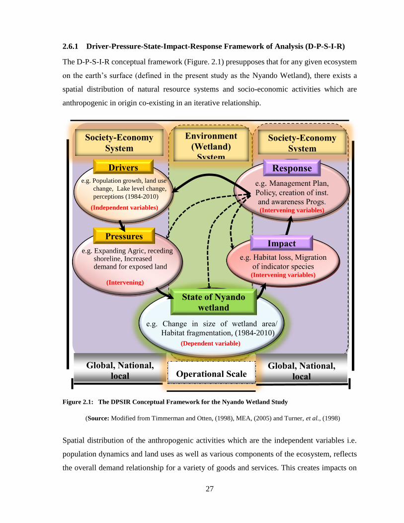
27

2.6.1 Driver-Pressure-State-Impact-Response Framework of Analysis (D-P-S-I-R)

The D-P-S-I-R conceptual framework (Figure. 2.1) presupposes that for any given ecosystem

on the earth’s surface (defined in the present study as the Nyando Wetland), there exists a

spatial distribution of natural resource systems and socio-economic activities which are

anthropogenic in origin co-existing in an iterative relationship.

Figure 2.1: The DPSIR Conceptual Framework for the Nyando Wetland Study

(Source: Modified from Timmerman and Otten, (1998), MEA, (2005) and Turner, et al., (1998)

Spatial distribution of the anthropogenic activities which are the independent variables i.e.

population dynamics and land uses as well as various components of the ecosystem, reflects

the overall demand relationship for a variety of goods and services. This creates impacts on

Society-Economy

System

Environment

(Wetland)

System

Society-Economy

System

Global, National,

local

Drivers Response

e.g. Population growth, land use

change, Lake level change,

perceptions (1984-2010)

Pressures

e.g. Management Plan,

Policy, creation of inst.

and awareness Progs. (Intervening variables)

Impact e.g. Expanding Agric, receding

shoreline, Increased demand for exposed land

e.g. Habitat loss, Migration

of indicator species (Intervening variables)

State of Nyando

wetland

e.g. Change in size of wetland area/

Habitat fragmentation, (1984-2010)

Global, National,

local Operational Scale

(Independent variables)

(Intervening)

variables)

(Dependent variable)

28

the ecosystem which the society responds to in various ways to either correct or enhance the

systems. For instance, changes in land use for food production from within and/or without the

area will respond to endogenous or exogenous influences of human population increases. The

consequence of these populations or other factor based demands is a build-up of

environmental pressure e.g. increased conversion of wetland biotic cover types into

agricultural cover types, over-harvesting of papyrus or other wetland products.

This is generated through the driving forces such as population increases, landlessness, food

production and market values of wetland products. The driving forces and pressure causes a

change in the ecosystem which is the dependent variable’s state (e.g. reduced spatial extent

of the wetland and reduced macrophyte quantities or quality).

Thus, the production activities will result in various types and quantities of residuals, as well

as goods and services also measured variously. Such changes in the state of the ecosystem

have impacts on the human and non-human receptors resulting in a number of perceived social

welfare changes. The welfare changes result in a stimulus for management actions which will

depend on the institutional structure, culture/value system and competing demands for the

scarce resources and for other goods and services in the wetland. The concept has been

recommended as simple and flexible enough to be conceptually valid over a range of spatial

scales (Von Bodungen and Turner, 2001). The present study therefore, applied this modified

framework of analysis.

29

CHAPTER THREE

3.0 MATERIALS AND METHODS

3.1 Description of the Study Area

The Nyando Wetland is located between latitudes 00º 09' S and 00º 20' S and longitudes 34º

45' E and 35º 00' E. In 1948, the wetland was estimated to cover some 90 km2. It lies astride

the Nyakach and Kano Plains at the Mouth of River Nyando on the edge of Winam Gulf in

Nyakach Bay on the shores of Lake Victoria (Osumba, Okeyo-Owuor and Raburu, 2010)

(Figure 3.1).

3.1.1 Topography and Drainage

The altitude of the study area ranges between 1,100 m (at the lakeshore) and 1,110 m.a.s.l.

(on the Plains). The main river that drains the wetland is River Nyando which has an

approximate catchment area of 3,450 km2 (JICA, 1992) and about 115 km long. The

catchment extends from the shores of Lake Victoria at an altitude of 1,100 metres above sea

level (m.a.s.l.) (where the study area is located), to over 3,112 m.a.s.l. at Mt. Londiani on the

western fringes of the East African Rift Valley. Besides numerous surface drains and minor

streams, three (3) other ephemeral streams (Nyaidho, Awach Kano, and Asawo) also feed into

the wetland. According to Ongwenyi (1983), climate of the study area can be classified as

semi-humid with an annual mean rainfall ranging from about 1,000 mm to about 1,600 mm

which is bimodal.

3.1.2 Soils

The soils are mainly alluvium formed by large quantities of silt and sand carried by the

Nyando River and several streams including the massive sheet washes that flow into the area

from the neighbouring Nyakach uplands and from the highlands in the upper and mid

catchment areas of the river Nyando basin. Black cotton soils, sandy red soils, and lateritic

soils are common in the Nyakach and Kano Plains area. Sediments of lacustrine and

fluviatiles, which are believed to have originated from Lake Victoria (DHV Consulting

Engineers, 1987), are also common in the area, mainly at the edges. Commonly, patches of

unformed reddish volcanic soils occur, especially on the flood plains around Gem Rae,

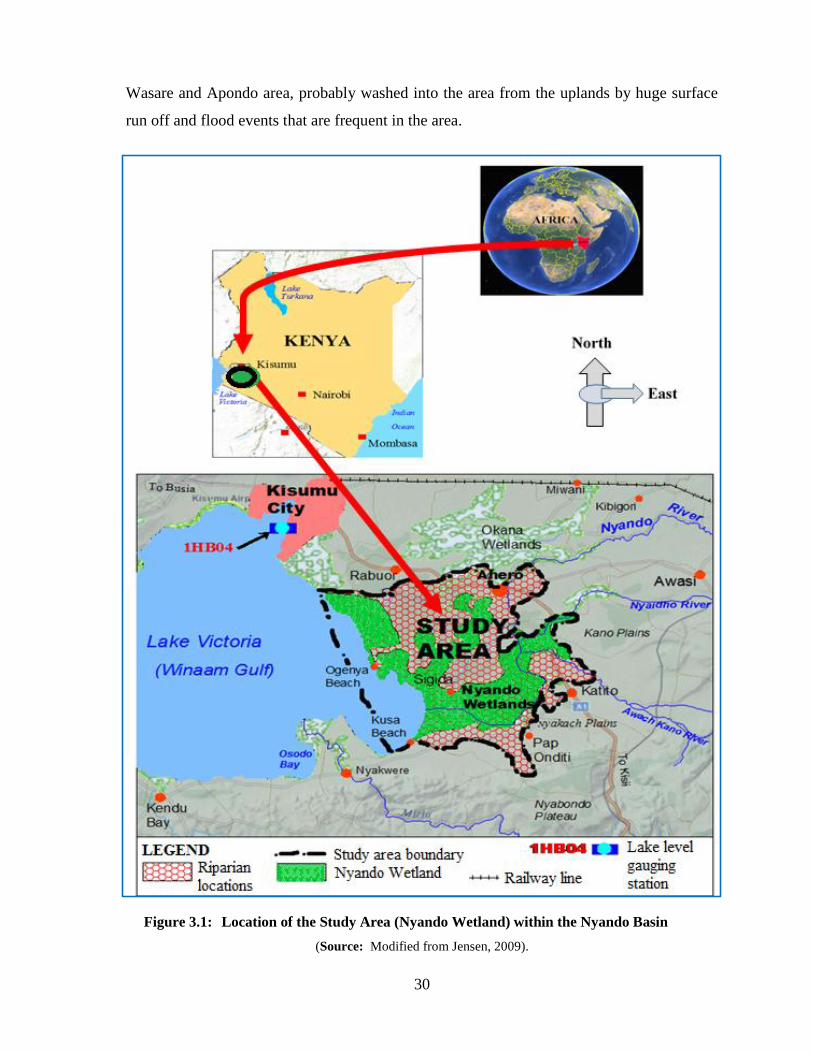
30

Wasare and Apondo area, probably washed into the area from the uplands by huge surface

run off and flood events that are frequent in the area.

Figure 3.1: Location of the Study Area (Nyando Wetland) within the Nyando Basin

(Source: Modified from Jensen, 2009).

31

3.1.3 Human Population and Agriculture

Administratively, the area falls within the two sub-counties of Kisumu County. These are

Nyando and Nyakach, and covers 8 locations and 23 sub-locations. Due to the desire to

investigate the effect of distance on the drivers and resource constraints, the study was limited

to the riparian locations and sub-locations adjoined to the wetland with a total population of

73,285 people and 13,817 households. Compared to the national figure of 66.4 persons per

km2 (Population Reference Bureau, 2011), the entire county including the study area had an

estimated population density of 465 persons per km2 with an annual growth rate of 2.5% per

annum between 1999 and 2009 (Republic of Kenya, 2010).

The population in the study area that was engaged in agricultural activities has been estimated

variously to range between 55% and 65% (ECOSYSTEMS, 1983; JICA, 1992). The major

crops grown in the area consist of cereals, such as maize, rice and sorghum, followed by pulses

such as beans, green-grams, cowpeas and groundnuts, and cotton, and tuber crops such as

cassavas and sweet potatoes. There is also some sugarcane grown, though not in large

quantities around the wetland, mainly on the Kano side of the wetland. Cultivation pattern

and growth period of crops are largely affected by seasonal distribution of rainfall and

flooding over the land.

3.1.4 Biodiversity

The study area is rich in endemic wetland plants characteristic of ecosystems along the shores

of Lake Victoria (Gichuki, et al., 2001; Raburu, Khisa and Masese, 2012). Besides Cyperus

papyrus, the other dominant wetland plants in the area include Phragmites australis and

Vossia cuspidata (Bennun and Njoroge, 1999). Nyando Wetland is one of the few remaining

habitats for some of the endangered species such as the Sitatunga antelope (Tragelaphus

spekii) and papyrus-endemic wildlife species such as pythons, Hippopotamus amphibius,

crocodiles, wetland monkeys, wetland mongooses, papyrus-endemic wetland birds, and a host

of fish species (Osumba, 2009; Raburu, et al., 2012).

32

3.3. Research Design, Variables, Data Requirements, Sources and Types

3.3.1. Research Design

The multidisciplinary nature of the present research and the ECOLIVE project which partly

sponsored the study, made it necessary for this research to adopt a mixed method design

approach to address its objectives. The term mixed methods research was used in this research

to refer to all procedures for collecting and analyzing both quantitative and qualitative data in

the context of the present study (Driscoll, Appiah-Yeboah, Salib and Rupert, 2007). In this

approach, qualitative observations and interviews were first made to offer the opportunity to

provide subtle details that outline the problem during field reconnaissance visits. This was

followed by the use of more detailed qualitative and quantitative tools, like a remote sensing,

surveys and GIS to validate or invalidate observations made during the qualitative phase.

Concurrent mixed method data collection strategies were employed to validate one form of

data with the other, to transform the data for comparison, or to address different types of

research questions and objectives.

Both the primary and secondary data were collected and applied to the conceptual framework

and model. Secondary data were obtained by carrying out literature review on studies so far

done on the subject matter in the study area or elsewhere. These included journal articles,

reports, and published books in the subject matter of the research. Primary data were obtained

through formal and informal interviews of randomly selected riparian households, key

informants’ interviews (KII) and focus group discussions (FGDs). In the application of socio-

ecological tools, same individuals provided both qualitative and quantitative data in structured

questionnaires with both closed and open ended questions so that the data could be more easily

compared during the analysis stage (Driscoll, et al., 2007). Furthermore, satellite images and

ground truthing were used to carry out field measurements of spatial and temporal changes

on cover types to estimate changes in land uses in and around the wetland. Data from remote

sensing, lake level and population growth measurements were then integrated with the socio-

ecological data in models and in a GIS environment to address the research questions and

objectives.

While this approach relegates qualitative analysis to an exploratory tool and doesn’t maximize

quantitative analysis as a tool to both explore, define and investigate the problem and suggest

33

potential solutions, some of the data generated were also vulnerable to the problem of

collinearity. Thus some of the response categories were themselves linked as a consequence

of the coding strategy and ended up limiting the extent to which various kinds of statistical

procedures could be reasonably used, particularly the more rigorous parametric measures of

association, such as t-tests and analyses of variance. The design however had several merits

that made it suitable for the present research. It had the ability to complement one method

with another to facilitate communication, promote collaboration, and provide good quality

and dependable research outputs (Johnson and Onwuegbuzie, 2004), which were highly

desirable in the study. The design also made it plausible to examine the research questions

from different perspectives and combine different methods with different biases involving

quantitative and qualitative techniques (Leech and Onwuegbuzie, 2009). Furthermore, this

research design enabled quantitative data to generalize the assessment and shed new light on

qualitative findings during the analysis stage in a triangulatory process (Morse, 1991;

Johnson, Onwuegbuzie and Turner, 2007; Venkatesh, Brown and Bala, 2013). It thus used

the strengths of both methodologies to provide a broader perspective on the overall subject of

the research.

3.3.2. Research Variables

During this study, a range of variables were selected and measured to provide spatio-temporal

data. These include time series land use/cover types and quantities, demographic

characteristics (population size), lake water levels, and area left behind by receding shoreline

changes. The dependent variable was held as the spatial extent of wetland (WTLa) cover type

measured in hectares as an indicator of the extent of wetland replacement with other land uses.

The independent variables were those whose changes led to changes in wetland cover type

and size through a conversion or a replacement process i.e. area under subsistence small-scale

agriculture (SSSAg), area under rice crop and turbid paddy water surfaces areas (RFTw), open

grassland area, mixed bushes areas and bare ground area (OPGb) as well as areas left behind

by receding shorelines (used as a proxy for the declining lake Victoria levels - WATr). All

these measurements were converted from pixel quantities to ha for further analysis. Data for

analyzing change in human population size were obtained from the national census figures

for Kisumu, Nyando and Lower Nyakach divisions. Other sub-drivers on wetland change

were measured through household questionnaire survey administered to respondents. These

34

included the distance of respondents’ homes to wetland (DR); water availability to respondent

for agriculture (soil moisture content - SM), perceptions of soil fertility; flood frequency;

yields of maize crops inside and outside the wetland (Maize returns) and grazing

intensity/damage on wetland.

3.4 Application of GIS and Remote Sensing Tools

Full Scene digital and hard copy Landsat TM and Landsat ETM satellite images processed to

level 1G were secured and used. Hardcopy images for use in reconnaissance and ground-

truthing activities were processed, clipped to study area, enlarged and printed at the scale of

1:50,000 at the Department of Resource Surveys and Remote Sensing (DRSRS). In order to

perform a multi-stage analysis to improve the accuracy, aerial photographs at the scale of

1:50,000 were obtained for specific sample sites from the Surveys of Kenya's photo-library

in Nairobi. There was 15% cloud cover in both the photographs and the satellite images which

was acceptable. To the advantage of the study, the image areas covering the study area in all

the images were 100% cloud free. The season of photography or imagery was also taken into

account to ensure that images used are those acquired during the period when maximum

contrast among different land uses can be assured (Wilde, Jessen and Stevens, 1996). Due to

the fact that wetland ecosystems are always wet, such a period only occurs during the dry

season.

In the study area, the dry season was the period between December and March, which is

normally a period of land preparation and distinctions between wetland and non-wetland areas

is maximum. During this period the soil moisture content in wetland soils are higher than

those of soils in non-wetland area and the differences between wetland and non-wetland cover

types are maximum thus allowing for maximum contrast (Islam, et al., 2008). They were also

suitable months when land preparation is at its peak in the study area providing high contrast

among cover types. This made it possible to isolate the intruding land uses in the wetland

area. These seasonal considerations were designed to minimize false change results from

differences between the dates due to soil moisture, temporary surface water from recent

rainfall events, or leaf water content if wet season imagery were used.

35

Landasat-TM images in the time series analysis were for 1984, 1995, 1999 and 2010 (Figure

3.2) with 1984 chosen as a base year. The year 1984 was chosen as the base year because

most dates before then had very coarse resolution imagery (56m by 79m = 1.1 acres) which

could not adequately meet the needs of the study. The Landsat satellite started delivering good

quality images in 1984. The base year for the time series was therefore pegged on this fact.

Thus the TM imagery was considered appropriate for the study due to its relatively good

resolution of 30 metres capable of providing sufficient information on patterns of land cover

that were targeted in the study. Consequently, a 1984 (March, dry season) TM image was

used to represent the decade of the 1980s. The decade of the 1990s was, however, represented

by two images; one of 1995 TM image (March, dry season), and a similar 1999 TM

(December, dry season) images. The 1999 image was meant to neutralize the within decadal

variability and anchor the change vector analysis process. Finally a 2010 Landsat ETM image

(January, dry season) was used to represent the decade of 2000s which was the study’s decadal

end time step. These data sources were considered adequate to cover the needs of the study

since the objective was to measure broad categories of land cover/uses that influence the area

covered by thev wetland. Since time series analysis requires a number of time steps to stabilize

the change analysis process, more than two time steps was required. A decadal time step

covering three decades between 1984 and 2010 was used. This was because patterns of change

in land and land use phenomena, though dynamic depending on the driving forces, often have

slow progress and require such periods to detect major spatial and temporal changes.

3.4.1 Procedures for Measuring Land Use Changes

3.4.2 Field Surveys for Collection of Reference Data

Field reconnaissance was carried out to familiarize and understand the images to be able to

correlate the image features with ground features. Using image interpretation elements such

as tone, texture, and association (Lillesand, et al., 2007), coloured hardcopy images were used

in the field to locate sites that typify various observable patterns of cover types occurring in

the study area. Such sites were geo-referenced, ground features described (both

instantaneously and retrospectively) and used as training sample sites.

The sample sites were selected using a systematic random approach. Reference data collected

in the field were geo-referenced using a Garmin 12 Global Positioning System (GPS) with ±3

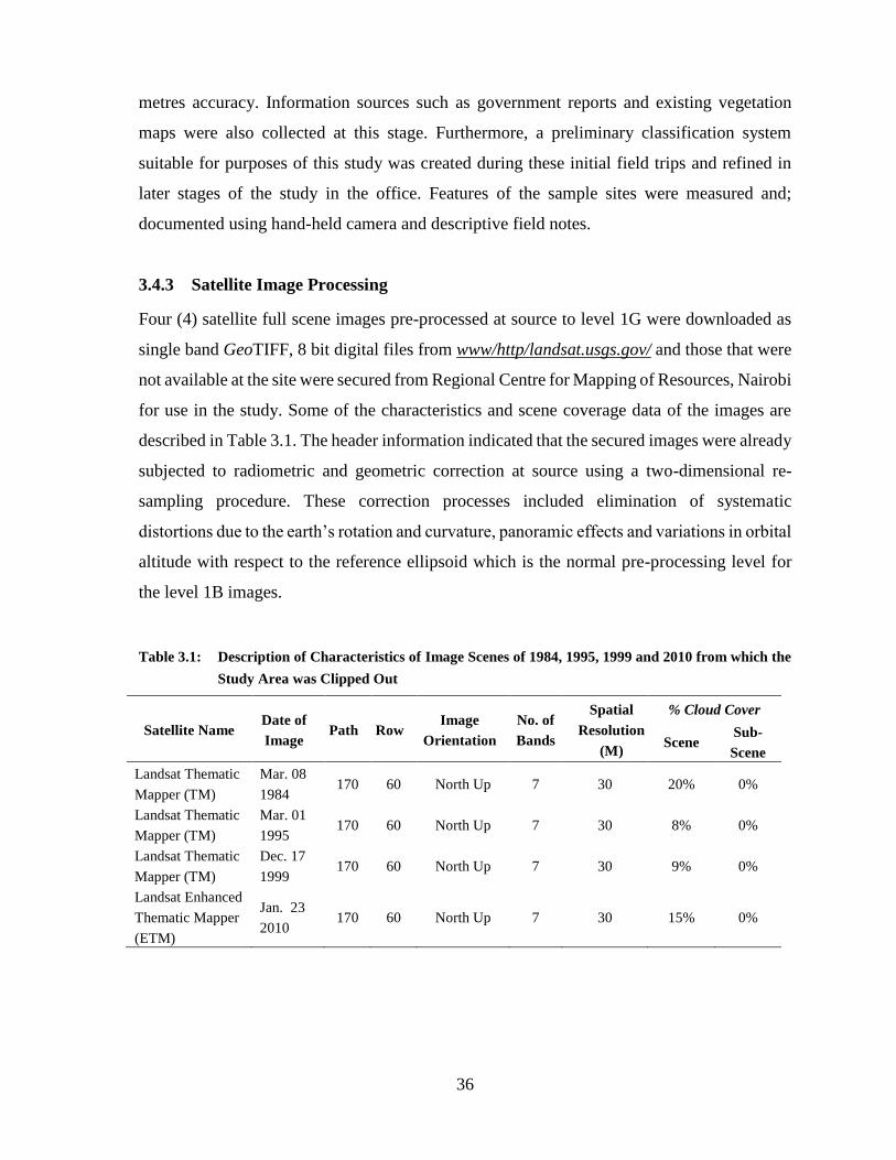
36

metres accuracy. Information sources such as government reports and existing vegetation

maps were also collected at this stage. Furthermore, a preliminary classification system

suitable for purposes of this study was created during these initial field trips and refined in

later stages of the study in the office. Features of the sample sites were measured and;

documented using hand-held camera and descriptive field notes.

3.4.3 Satellite Image Processing

Four (4) satellite full scene images pre-processed at source to level 1G were downloaded as

single band GeoTIFF, 8 bit digital files from www/http/landsat.usgs.gov/ and those that were

not available at the site were secured from Regional Centre for Mapping of Resources, Nairobi

for use in the study. Some of the characteristics and scene coverage data of the images are

described in Table 3.1. The header information indicated that the secured images were already

subjected to radiometric and geometric correction at source using a two-dimensional re-

sampling procedure. These correction processes included elimination of systematic

distortions due to the earth’s rotation and curvature, panoramic effects and variations in orbital

altitude with respect to the reference ellipsoid which is the normal pre-processing level for

the level 1B images.

Table 3.1: Description of Characteristics of Image Scenes of 1984, 1995, 1999 and 2010 from which the

Study Area was Clipped Out

Satellite Name Date of

Image Path Row

Image

Orientation

No. of

Bands

Spatial

Resolution

(M)

% Cloud Cover

Scene Sub-

Scene

Landsat Thematic

Mapper (TM)

Mar. 08

1984 170 60 North Up 7 30 20% 0%

Landsat Thematic

Mapper (TM)

Mar. 01

1995 170 60 North Up 7 30 8% 0%

Landsat Thematic

Mapper (TM)

Dec. 17

1999 170 60 North Up 7 30 9% 0%

Landsat Enhanced

Thematic Mapper

(ETM)

Jan. 23

2010 170 60 North Up 7 30 15% 0%

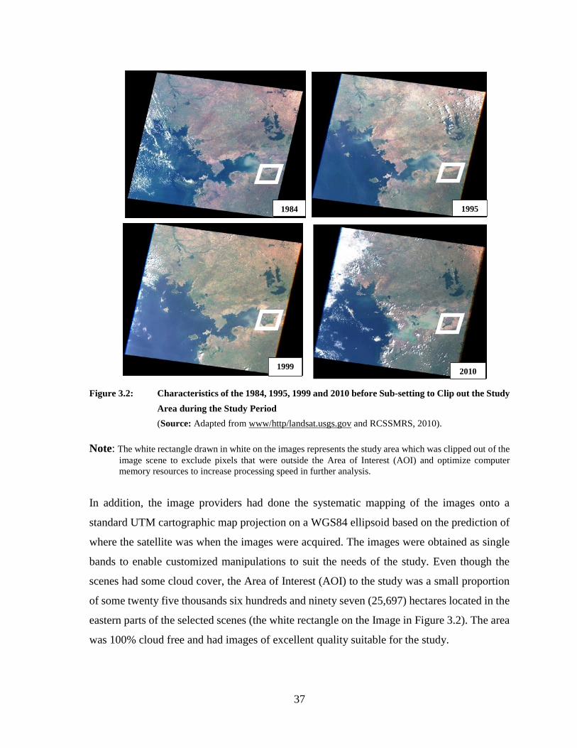
37

Figure 3.2: Characteristics of the 1984, 1995, 1999 and 2010 before Sub-setting to Clip out the Study

Area during the Study Period

(Source: Adapted from www/http/landsat.usgs.gov and RCSSMRS, 2010).

Note: The white rectangle drawn in white on the images represents the study area which was clipped out of the

image scene to exclude pixels that were outside the Area of Interest (AOI) and optimize computer

memory resources to increase processing speed in further analysis.

In addition, the image providers had done the systematic mapping of the images onto a

standard UTM cartographic map projection on a WGS84 ellipsoid based on the prediction of

where the satellite was when the images were acquired. The images were obtained as single

bands to enable customized manipulations to suit the needs of the study. Even though the

scenes had some cloud cover, the Area of Interest (AOI) to the study was a small proportion

of some twenty five thousands six hundreds and ninety seven (25,697) hectares located in the

eastern parts of the selected scenes (the white rectangle on the Image in Figure 3.2). The area

was 100% cloud free and had images of excellent quality suitable for the study.

1984 1995

1999 2010

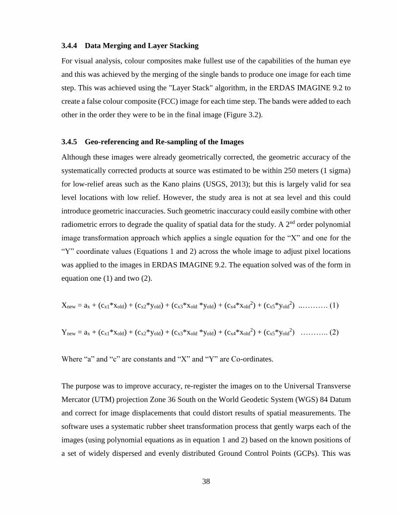
38

3.4.4 Data Merging and Layer Stacking

For visual analysis, colour composites make fullest use of the capabilities of the human eye

and this was achieved by the merging of the single bands to produce one image for each time

step. This was achieved using the "Layer Stack" algorithm, in the ERDAS IMAGINE 9.2 to

create a false colour composite (FCC) image for each time step. The bands were added to each

other in the order they were to be in the final image (Figure 3.2).

3.4.5 Geo-referencing and Re-sampling of the Images

Although these images were already geometrically corrected, the geometric accuracy of the

systematically corrected products at source was estimated to be within 250 meters (1 sigma)

for low-relief areas such as the Kano plains (USGS, 2013); but this is largely valid for sea

level locations with low relief. However, the study area is not at sea level and this could

introduce geometric inaccuracies. Such geometric inaccuracy could easily combine with other

radiometric errors to degrade the quality of spatial data for the study. A 2nd order polynomial

image transformation approach which applies a single equation for the “X” and one for the

“Y” coordinate values (Equations 1 and 2) across the whole image to adjust pixel locations

was applied to the images in ERDAS IMAGINE 9.2. The equation solved was of the form in

equation one (1) and two (2).

Xnew = ax + (cx1*xold) + (cx2*yold) + (cx3*xold *yold) + (cx4*xold2) + (cx5*yold

2) ..………. (1)

Ynew = ax + (cx1*xold) + (cx2*yold) + (cx3*xold *yold) + (cx4*xold2) + (cx5*yold

2) ……….. (2)

Where “a” and “c” are constants and “X” and “Y” are Co-ordinates.

The purpose was to improve accuracy, re-register the images on to the Universal Transverse

Mercator (UTM) projection Zone 36 South on the World Geodetic System (WGS) 84 Datum

and correct for image displacements that could distort results of spatial measurements. The

software uses a systematic rubber sheet transformation process that gently warps each of the

images (using polynomial equations as in equation 1 and 2) based on the known positions of

a set of widely dispersed and evenly distributed Ground Control Points (GCPs). This was

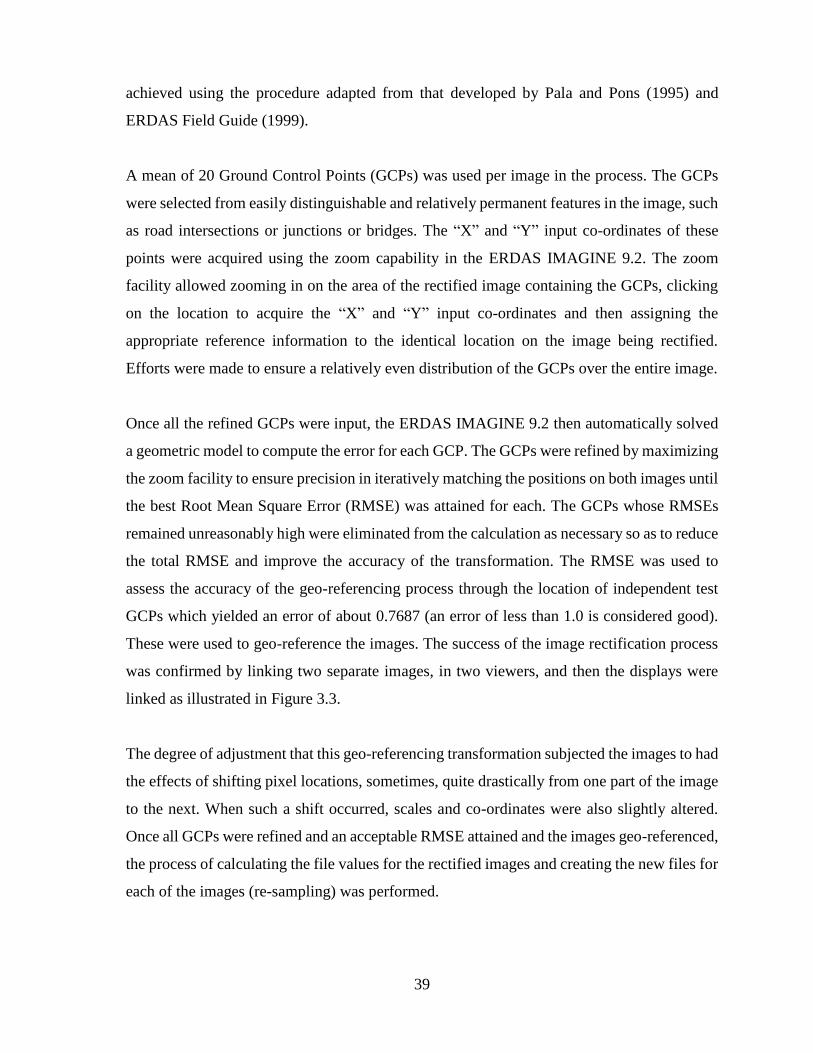
39

achieved using the procedure adapted from that developed by Pala and Pons (1995) and

ERDAS Field Guide (1999).

A mean of 20 Ground Control Points (GCPs) was used per image in the process. The GCPs

were selected from easily distinguishable and relatively permanent features in the image, such

as road intersections or junctions or bridges. The “X” and “Y” input co-ordinates of these

points were acquired using the zoom capability in the ERDAS IMAGINE 9.2. The zoom

facility allowed zooming in on the area of the rectified image containing the GCPs, clicking

on the location to acquire the “X” and “Y” input co-ordinates and then assigning the

appropriate reference information to the identical location on the image being rectified.

Efforts were made to ensure a relatively even distribution of the GCPs over the entire image.

Once all the refined GCPs were input, the ERDAS IMAGINE 9.2 then automatically solved

a geometric model to compute the error for each GCP. The GCPs were refined by maximizing

the zoom facility to ensure precision in iteratively matching the positions on both images until

the best Root Mean Square Error (RMSE) was attained for each. The GCPs whose RMSEs

remained unreasonably high were eliminated from the calculation as necessary so as to reduce

the total RMSE and improve the accuracy of the transformation. The RMSE was used to

assess the accuracy of the geo-referencing process through the location of independent test

GCPs which yielded an error of about 0.7687 (an error of less than 1.0 is considered good).

These were used to geo-reference the images. The success of the image rectification process

was confirmed by linking two separate images, in two viewers, and then the displays were

linked as illustrated in Figure 3.3.

The degree of adjustment that this geo-referencing transformation subjected the images to had

the effects of shifting pixel locations, sometimes, quite drastically from one part of the image

to the next. When such a shift occurred, scales and co-ordinates were also slightly altered.

Once all GCPs were refined and an acceptable RMSE attained and the images geo-referenced,

the process of calculating the file values for the rectified images and creating the new files for

each of the images (re-sampling) was performed.

40

Figure 3.3: A Screen Shot of Two Separate Images, Displayed in Two Viewers in ERDAS

IMAGINE 9.2 During the Rectification Process.

(Source: Modified from www/http/landsat.usgs.gov and RCSSMRS, 2010).

Each image was re-sampled using bilinear interpolation algorithm to 30m × 30m, which is the

nominal resolution for TM images. Bilinear-interpolation re-sampling operated by finding the

4 pixels in the original image closest to each of the object pixel in the new image, and

assigning that pixel in the new image with the average value of the 4 pixels in the original

image. The method was chosen to ensure that the original image radiometry was as much as

possible preserved.

3.4.6 Image Sub-setting

The new layer-stacked and rectified images were huge files and varied in sizes. For instance,

the 1999 image was 6,932 by 6,316 pixels per line per file while the 1984 and 1995 ones were

6,979 by 6,299 and 6,973 by 6,299 pixels per line per file, respectively. In order to have

images that covered only the study area and same in size, a shape file (map coordinate-based

vectors-Figure 3.4) was generated from ArcGIS 10.1 covering the Area of interest (AOI)

(Nyando Wetland shape file). The reason for using a shape file was based on its portability

between images and between image processing packages.

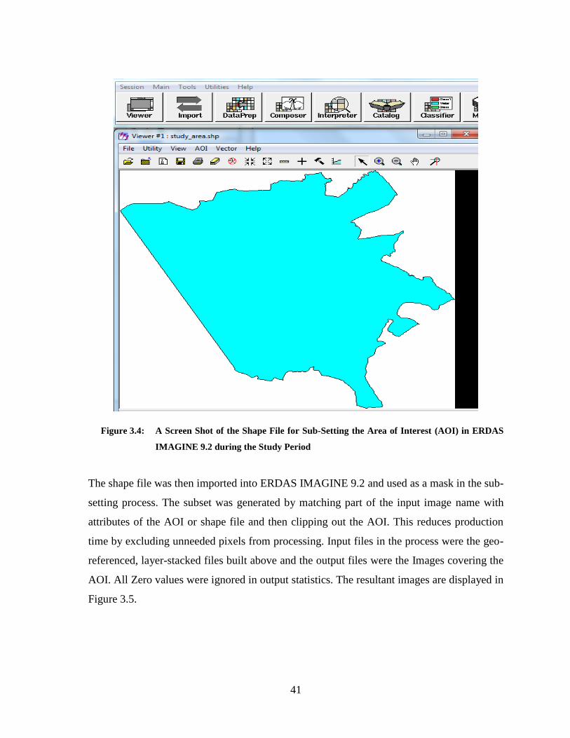
41

Figure 3.4: A Screen Shot of the Shape File for Sub-Setting the Area of Interest (AOI) in ERDAS

IMAGINE 9.2 during the Study Period

The shape file was then imported into ERDAS IMAGINE 9.2 and used as a mask in the sub-

setting process. The subset was generated by matching part of the input image name with

attributes of the AOI or shape file and then clipping out the AOI. This reduces production

time by excluding unneeded pixels from processing. Input files in the process were the geo-

referenced, layer-stacked files built above and the output files were the Images covering the

AOI. All Zero values were ignored in output statistics. The resultant images are displayed in

Figure 3.5.

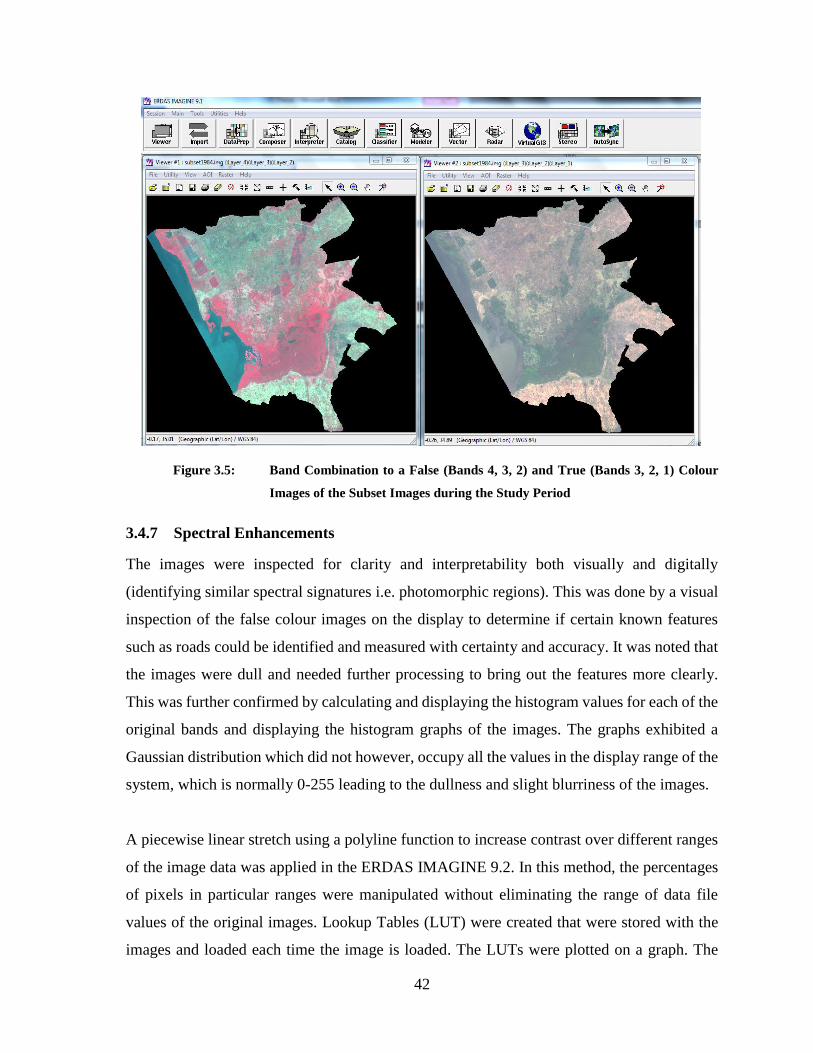
42

Figure 3.5: Band Combination to a False (Bands 4, 3, 2) and True (Bands 3, 2, 1) Colour

Images of the Subset Images during the Study Period

3.4.7 Spectral Enhancements

The images were inspected for clarity and interpretability both visually and digitally

(identifying similar spectral signatures i.e. photomorphic regions). This was done by a visual

inspection of the false colour images on the display to determine if certain known features

such as roads could be identified and measured with certainty and accuracy. It was noted that

the images were dull and needed further processing to bring out the features more clearly.

This was further confirmed by calculating and displaying the histogram values for each of the

original bands and displaying the histogram graphs of the images. The graphs exhibited a

Gaussian distribution which did not however, occupy all the values in the display range of the

system, which is normally 0-255 leading to the dullness and slight blurriness of the images.

A piecewise linear stretch using a polyline function to increase contrast over different ranges

of the image data was applied in the ERDAS IMAGINE 9.2. In this method, the percentages

of pixels in particular ranges were manipulated without eliminating the range of data file

values of the original images. Lookup Tables (LUT) were created that were stored with the

images and loaded each time the image is loaded. The LUTs were plotted on a graph. The

43

graph shored a linear rise with break points dividing the ranges of data into three sections:

low, medium and high. The break points created segments on the graph that were interactively

manipulated to increase or reduce contrast of particular ranges of data. The LUT graph line

with the steepest (highest) slope brings out the most contrast by stretching output values

farther apart in the display range. The basic strategy used was that if the grey values of the

images were logically spread to utilize the full range possible on the display device (0-255

brightness values), then the quality of imagery and interpretation would be enhanced. Finally,

a crisp filter was applied to the images to sharpen the overall scene luminance and feature

edges without distorting the inter-band content variance of the images.

3.4.8 Image Classification

The next step was to convert spectral raster data of the imagery into a finite set of classes that

represent the surface cover types in the area of study. There are traditionally two broad

categories of image classification: unsupervised and supervised. The study first employed an

unsupervised classification algorithm on the images. This was in an attempt to identify

spectrally homogenous (photomorphic) groups within the image that were later assigned to

informational categories as suggested by Richards (1993). The product of this process yielded

nine categories. Due to the small farm sizes leading to a “mixel” concept situation and

resolution constraints (Foody and Mathur, 2006a); the nine categories could not be

consistently applied throughout the time steps of the study period without signature confusion.

The product was, therefore, manually refined in a supervised classification process into five

broad classes by merging classes, which had strong signature similarities with potential for

confusion. Such strong signature similarities generally define patterns of land uses/cover

types that could be grouped together into various category with minimum effects on the

classification accuracy.

During this process, known surface features within the imagery were manually identified and

a statistical module in the ERDAS IMAGINE 9.2 used to determine the spectral signatures of

the identified features or group of features. The spectral signature files were then used as a

basis for the definition of representative training areas for each of the classes on the images.

The rules of correspondence between the spectral and the land use-land cover categories were

44

then established. These were generated from fieldwork or ancillary information (ground data).

Four main operational strategies for the rules were as follows:

1. Spatial correspondence between the spectral class and the training areas.

2. The spectral class is mainly inside a particular class.

3. The spectral class is not an insignificant part of the class.

4. Pixel remained unclassified if it belonged to a class that is split too much between two

or more classes.

Using a maximum likelihood classifier, the "spectral signatures" of the identified features or

groups of features were then used to classify the rest of the image with an underlying

assumption of a normal (Gaussian) distribution within each class. The probability of a pixel

value occurring in each class was computed and pixels were assigned to the class with the

highest probability or likelihood of it being a member. The outputs were classified images

with numbered labels that were then assigned to the various land use/cover categories for each

of the time steps (1984, 1995, 1999 and 2010).

This combination of methods was important because the multi-modal nature of the features

in the study area made a single method approach relatively inadequate (Anderson, et al., 1976;

Richards, 1993). The statistic of crops such as cereals or groups of cereals obtained in the area

rarely followed normal distributions due to the different stages of growth and “mixel”

characteristics of the pixels in the different fields covered by the training areas. Rice farms

were, for instance, difficult to distinguish from turbid water surfaces on the satellite imagery

as the farming practices observed in and outside the wetland were based on flooded basins or

paddocks. Consequently, only open turbid water surfaces contained in rectangular, regularly

shaped features were grouped together with the rice farms even if they were not planted with

rice as one category known as Rice Farms and Turbid paddy Water Surfaces (RFTw). This

was based on basic principles of image interpretation and ground-truthing outcomes to assure

consistency in measurement. Small plot sizes of individual cover types relative to pixels size

also further complicated the situation making it necessary to seek photomorphism as a basis

for grouping of the categories. This hybrid approach was adapted from Estes, et al., (1983)

and Fung (1992).

45

3.4.9 Post Classification

The classified images were imported into ENVI 5.0 for post-classification comparative

analysis. This involved the determination of the level of disagreements (land cover wise)

between images taken on varying dates i.e. 1984, 1995, 1999 and 2010. These independently

classified images were compared and their accuracy assessed. The classified images were

exported to ArcGIS 10.1 after accuracy assessment.

3.4.10 Accuracy Assessment

The error matrix calculation that is a commonly used method of assessing accuracy of a

classification was applied in the study. The method compared the agreement between classes

predicted through image processing procedures to those observed independently of the

classification on the ground (Gidley, 2009). 256 random points were generated using a

random generator. The pixels falling on the points, which were randomly distributed

throughout the image, were selected for the exercise. Each of the pixel sites formed the basis

of sample site definition and each of the sample sites was redefined and identified as a field

plot of approximately 2 x 2 pixels in size as modified from the recommendations of Biging,

et al., (1999) and Foody, Mathur, Sanchez-Hernandez and Boyd (2006b). These

considerations were also informed by the number of points and area sizes normally chosen to

assess accuracy in literature which range from 50 to 200 points per study site (Foody, 2002;

Sawaya, et al., 2003; Everitt, et al., 2005; Wolter, et al., 2005; Baker, Lawrence, Montagne

and Patten, 2007; Everitt, et al., 2008; Laba, et al., 2008). Sample sites which fell on

inaccessible locations, especially in the boggy wetland locations were systematically dropped

and replaced by points of similar classes that fall in accessible locations within the wetland.

The coordinates of these sample sites were fed into a Garmin 12 GPS as waypoints and the

GPS was used to navigate to ground locations of the sites. Recordings of observations at these

ground locations were made independently (Congalton and Green 1999). The original images

along with direct field observations were then used to determine the true land cover

represented by each random pixel site. These groundtruth data were compared with the

classification maps. If the ground truth data and classification data matched, then the

classification of that pixel was considered as accurate. The desired measures of association

among the map overlays and accuracy elements such as the Kappa Index of Agreement,

overall accuracy, producer’s accuracy and user’s accuracy (Lu, Mausel, Brondizio and Moran,

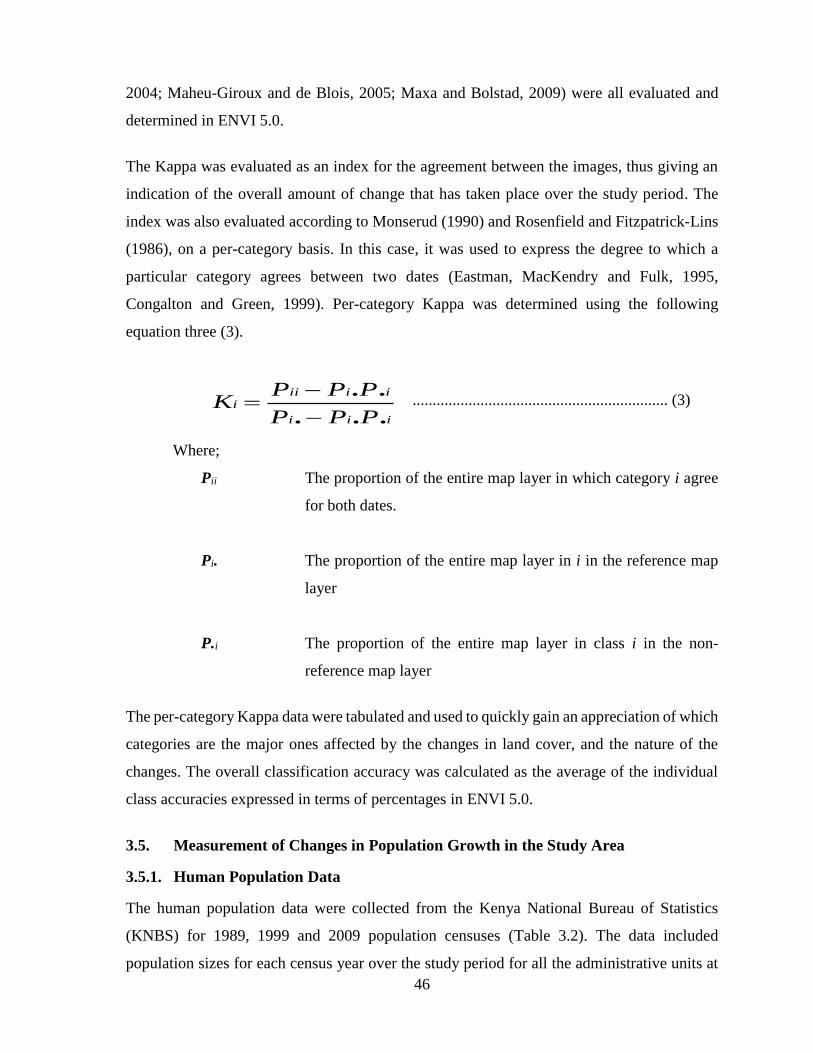
46

2004; Maheu-Giroux and de Blois, 2005; Maxa and Bolstad, 2009) were all evaluated and

determined in ENVI 5.0.

The Kappa was evaluated as an index for the agreement between the images, thus giving an

indication of the overall amount of change that has taken place over the study period. The

index was also evaluated according to Monserud (1990) and Rosenfield and Fitzpatrick-Lins

(1986), on a per-category basis. In this case, it was used to express the degree to which a

particular category agrees between two dates (Eastman, MacKendry and Fulk, 1995,

Congalton and Green, 1999). Per-category Kappa was determined using the following

equation three (3).

................................................................ (3)

Where;

Pii The proportion of the entire map layer in which category i agree

for both dates.

Pi. The proportion of the entire map layer in i in the reference map

layer

P.i The proportion of the entire map layer in class i in the non-

reference map layer

The per-category Kappa data were tabulated and used to quickly gain an appreciation of which

categories are the major ones affected by the changes in land cover, and the nature of the

changes. The overall classification accuracy was calculated as the average of the individual

class accuracies expressed in terms of percentages in ENVI 5.0.

3.5. Measurement of Changes in Population Growth in the Study Area

3.5.1. Human Population Data

The human population data were collected from the Kenya National Bureau of Statistics

(KNBS) for 1989, 1999 and 2009 population censuses (Table 3.2). The data included

population sizes for each census year over the study period for all the administrative units at

iii

iiiii

PPP

PPPK

...

..

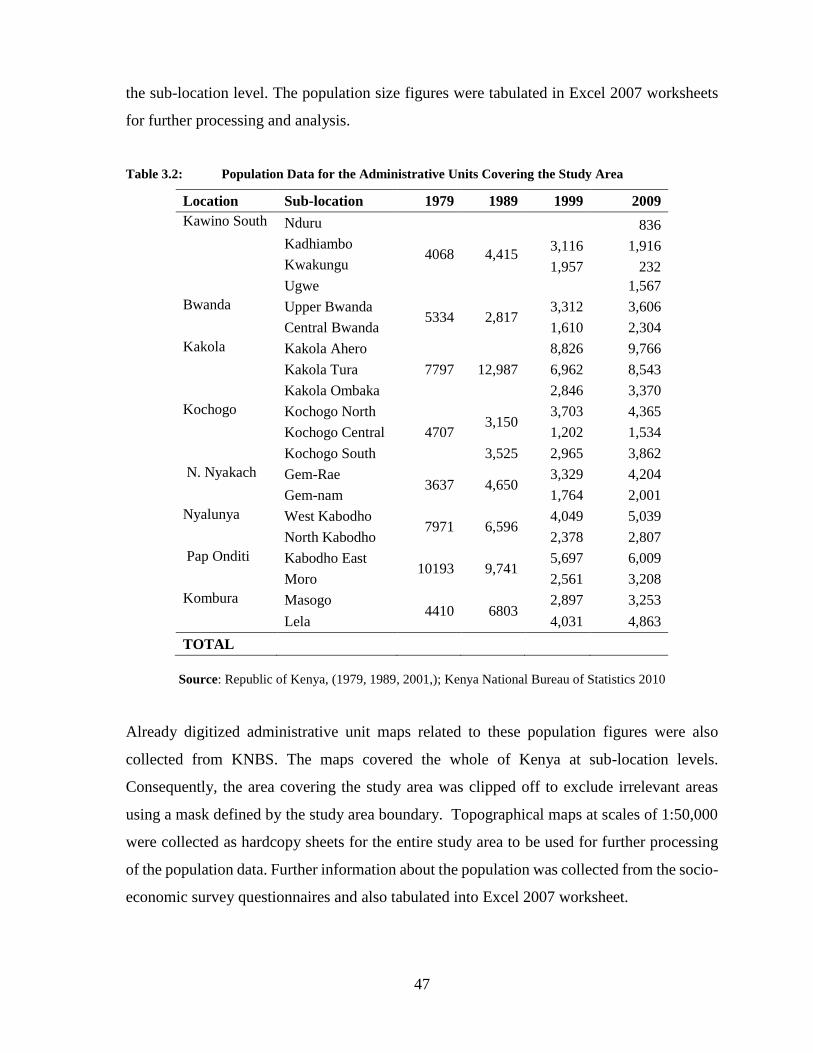
47

the sub-location level. The population size figures were tabulated in Excel 2007 worksheets

for further processing and analysis.

Table 3.2: Population Data for the Administrative Units Covering the Study Area

Location Sub-location 1979 1989 1999 2009

Kawino South Nduru

4068 4,415

836

Kadhiambo 3,116 1,916

Kwakungu 1,957 232

Ugwe 1,567

Bwanda Upper Bwanda 5334 2,817

3,312 3,606

Central Bwanda 1,610 2,304

Kakola Kakola Ahero

7797 12,987

8,826 9,766

Kakola Tura 6,962 8,543

Kakola Ombaka 2,846 3,370

Kochogo Kochogo North

4707 3,150

3,703 4,365

Kochogo Central 1,202 1,534

Kochogo South 3,525 2,965 3,862

N. Nyakach Gem-Rae 3637 4,650

3,329 4,204

Gem-nam 1,764 2,001

Nyalunya West Kabodho 7971 6,596

4,049 5,039

North Kabodho 2,378 2,807

Pap Onditi Kabodho East 10193 9,741

5,697 6,009

Moro 2,561 3,208

Kombura Masogo 4410 6803

2,897 3,253

Lela 4,031 4,863

TOTAL

Source: Republic of Kenya, (1979, 1989, 2001,); Kenya National Bureau of Statistics 2010

Already digitized administrative unit maps related to these population figures were also

collected from KNBS. The maps covered the whole of Kenya at sub-location levels.

Consequently, the area covering the study area was clipped off to exclude irrelevant areas

using a mask defined by the study area boundary. Topographical maps at scales of 1:50,000

were collected as hardcopy sheets for the entire study area to be used for further processing

of the population data. Further information about the population was collected from the socio-

economic survey questionnaires and also tabulated into Excel 2007 worksheet.

48

3.6. Measurement of Socio-ecological Data

3.6.1. Socio-ecological Data

As an initial step, an exploratory survey of the study area was done to familiarize with the

local representatives of the county administration, village elders and various geographic

features of interest. These included visual distribution of homesteads, cover types such as

macrophytes or plant community associations and human activities in the wetland. A canoe

was used to access various points and areas of interest in the swampy and flooded or water

filled parts of the wetland. Subsequently, a questionnaire was designed and pretested on a

small sample population of 40 people drawn from Masogo, Lela and Katho Sub-locations in

Kombura Location and Irrigation sub-location in Kawino location. The pre-test population

sample size was dictated by the minimum number of data points which is 30 (Fabrigar,

Wegener, MacCallum and Strahan, 1999) required by SPSS package to perform a valid

analysis. They were randomly selected from among respondents within the study area with

characteristics similar to those that were targeted for the actual detailed survey. Those who

participated in the pre-test were excluded from the detailed actual survey.

The data resulting from the pre-test were analyzed and results used to refine the questionnaires

by incorporating additional information, removing irrelevant questions and restructuring

questions that were deemed ambiguous to the respondents. Actual field work was carried out

in the later parts of the month of January and in February and March, 2010 to collect the

primary data. Data collection involved questionnaire administration and observations. The

household surveys using questionnaires covered 200 households. (A sample questionnaire is

included in Appendix 1). Focus group discussions and key informants interviews were also

carried out to obtain views from stakeholders such as farmers and fishermen. These were used

to triangulate information, for instance, exploring the reasoning behind some observed

unusual phenomena such as a negative population growth during particular periods.

Secondary data from both published and unpublished sources were collected to provide

background information about the study area including physical and socio-economic aspects.

The questionnaires were also used to collect factual and perception data on the ecological

aspects of the study according to Piran, Vaughan, Renwick and Barker (2005). Independent

verifications of the ecological facts were carried out using participant observation.

49

3.6.2. The Study Population

The population of households that surround the Nyando Wetland, was estimated at 13,817

households distributed in 23 sub-locations within 9 locations (Republic of Kenya, 1979).

3.6.3 Sampling Design, Frame and Size

The sampling frame was considered as a list of all the households in the study area. It was

assumed that most of the households were engaged in one form of land use or the other

affecting the wetland presupposing a relatively homogeneous normally distributed population

in terms of the purpose of the study. Purposive sampling was used to select the locations and

sub-locations for the study to include those that are riparian to the wetland. The distance decay

principle underpinning the study was used to select the 9 administrative locations and the 23

sub-locations that are adjunct to the wetland and whose residents were likely to interact with

and influence the state of wetland. The sampling units were defined as the 23 Sub locations.

The sample size was determined according to the method proposed by Watson (2001). The

method used a formula based on the relationship between the required sample sizes, number

of people in the study population, estimated variance in the population, level of precision,

desired confidence level and estimated response rate to generate a standard table (Appendix

2). The table could be used to easily determined sample sizes for populations of between 100

and 100,000. Since the study population of 13,817 lies between 10,000 and 15,000, the sample

size was selected from the predetermined values in the table generated for a desired

confidence interval of 95%. From the table, for a variability of 30% which tends towards

homogeneity, the ideal sample size would be 170 respondents for a population of 15,000

against 390 respondents for an assumed variability of 50%. Since the study population fell

between 10,000 and 15,000, it was assumed that any number between 170 and 390 could

suffice. Numbers between 170 and 390 were therefore generated and randomly selected. The

number 200 was selected as the overall sample size for the study.

Since the enumeration unit for human populations is the sub-location, the study sample unit

was adopted as the 23 sub-locations units in the study area. The estimated sample size of 200

was then distributed for each sub-location according to its population and proximity to the

wetland. Using equation 7 as shown in Table 3.3.

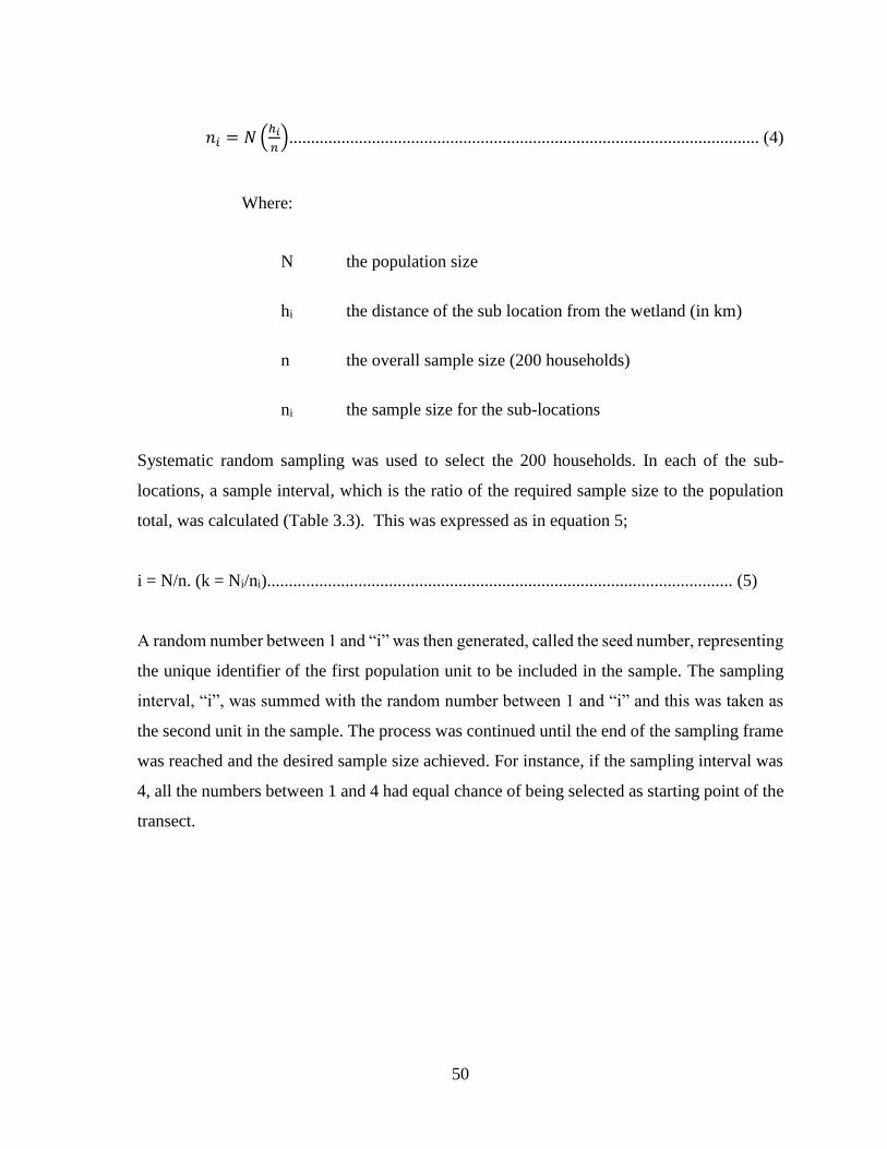
50

𝑛𝑖 = 𝑁 (ℎ𝑖

𝑛)............................................................................................................ (4)

Where:

N the population size

hi the distance of the sub location from the wetland (in km)

n the overall sample size (200 households)

ni the sample size for the sub-locations

Systematic random sampling was used to select the 200 households. In each of the sub-

locations, a sample interval, which is the ratio of the required sample size to the population

total, was calculated (Table 3.3). This was expressed as in equation 5;

i = N/n. (k = Ni/ni)........................................................................................................... (5)

A random number between 1 and “i” was then generated, called the seed number, representing

the unique identifier of the first population unit to be included in the sample. The sampling

interval, “i”, was summed with the random number between 1 and “i” and this was taken as

the second unit in the sample. The process was continued until the end of the sampling frame

was reached and the desired sample size achieved. For instance, if the sampling interval was

4, all the numbers between 1 and 4 had equal chance of being selected as starting point of the

transect.

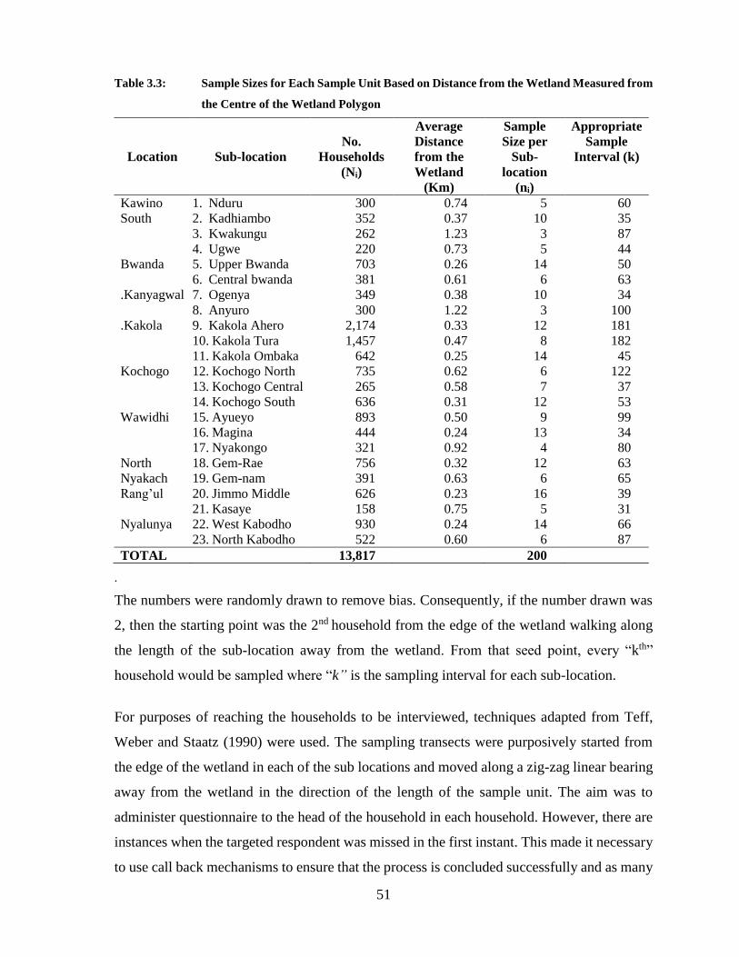
51

Table 3.3: Sample Sizes for Each Sample Unit Based on Distance from the Wetland Measured from

the Centre of the Wetland Polygon

Location Sub-location

No.

Households

(Ni)

Average

Distance

from the

Wetland

(Km)

Sample

Size per

Sub-

location

(ni)

Appropriate

Sample

Interval (k)

Kawino

South

1. Nduru 300 0.74 5 60

2. Kadhiambo 352 0.37 10 35

3. Kwakungu 262 1.23 3 87

4. Ugwe 220 0.73 5 44

Bwanda 5. Upper Bwanda 703 0.26 14 50

6. Central bwanda 381 0.61 6 63

.Kanyagwal 7. Ogenya 349 0.38 10 34

8. Anyuro 300 1.22 3 100

.Kakola 9. Kakola Ahero 2,174 0.33 12 181

10. Kakola Tura 1,457 0.47 8 182

11. Kakola Ombaka 642 0.25 14 45

Kochogo 12. Kochogo North 735 0.62 6 122

13. Kochogo Central 265 0.58 7 37

14. Kochogo South 636 0.31 12 53

Wawidhi 15. Ayueyo 893 0.50 9 99

16. Magina 444 0.24 13 34

17. Nyakongo 321 0.92 4 80

North

Nyakach

18. Gem-Rae 756 0.32 12 63

19. Gem-nam 391 0.63 6 65

Rang’ul 20. Jimmo Middle 626 0.23 16 39

21. Kasaye 158 0.75 5 31

Nyalunya 22. West Kabodho 930 0.24 14 66

23. North Kabodho 522 0.60 6 87

TOTAL 13,817 200

.

The numbers were randomly drawn to remove bias. Consequently, if the number drawn was

2, then the starting point was the 2nd household from the edge of the wetland walking along

the length of the sub-location away from the wetland. From that seed point, every “kth”

household would be sampled where “k” is the sampling interval for each sub-location.

For purposes of reaching the households to be interviewed, techniques adapted from Teff,

Weber and Staatz (1990) were used. The sampling transects were purposively started from

the edge of the wetland in each of the sub locations and moved along a zig-zag linear bearing

away from the wetland in the direction of the length of the sample unit. The aim was to

administer questionnaire to the head of the household in each household. However, there are

instances when the targeted respondent was missed in the first instant. This made it necessary

to use call back mechanisms to ensure that the process is concluded successfully and as many

52

as possible targeted respondents were reached and interviewed. However, where such

callbacks were unsuccessful, use was made of a simple “YES” and “NO” randomization

technique to select a neighbouring household.

3.6.4 Questionnaire Administration

A questionnaire (Appendix 1) was administered to the selected respondents to elicit the

desired information. Each of the respondents’ household location was also geo-referenced

using a Garmin12 Global Positioning System (GPS) with a ±3 metres accuracy level. The

purpose of geo-referencing was to make the data spatially analyzable and linked to data from

other spatial data sources. This was in view of the fact that distances to a resource such as the

wetland was assumed to play a signification role in human population interaction as explained

in the distance decay concept (Tobler, 1970; Miller, 2004).

Once a target respondent was identified and secured, an amicable environment for a

comfortable engagement with the respondent was set. This was done by making the

appropriate introductions including the purpose of the visit, the study and a request for the

respondent’s permission to engage in the study. The researcher then administered the

questionnaire personally during the survey in a language in which the respondent was

comfortable and concurrently recorded the answers. The use of this approach ensured direct

contact between the researcher and the respondent, a factor which facilitated elaboration of

aspects that may not have been easily understood by the respondent. The contact was

therefore, important for probity and personality assurance to enhance credibility of responses.

The procedure also enabled the researcher to ensure that the questionnaire was completed

before leaving the respondent to minimize distortion of questions and cases of incomplete

questionnaires.

If the household head was literate and desired to fill the questionnaires him/herself, it was

allowed. However, availability of the researcher to explain or clarify any question that is not

clear to the respondent was always ensured. On completion of such a questionnaire, it was

collected and rechecked. Further clarification in places not properly filled was secured and

recorded by the researcher on the relevant sections in the questionnaire. All the completed

questionnaires were serialized, stacked together and stored to await processing and analysis.

53

3.6.5 Key Informant Interviews

Structured interviews were held with people defined as having specialized knowledge about

the issues being investigated on the wetland. The respondents for this process were identified

and selected in the field in consultation with the local administration (Appendix 3). They were

interviewed intensively over an extensive period for the purpose of providing a relatively

complete historical and ethnographical description of the social, and cultural patterns and the

technical issues facing the Nyando Wetland. The interrogation process was subjected to open-

ended questions probing the various objectives of the study. This was guided by a protocol

designed for this purpose (Appendix 4). The information generated from this process was

used to triangulate primary data obtained through the other sources stated above. They also

proved corroboratory in nature to authenticate the quality of information generated from other

sources. These were useful for understanding the dynamics of the issues being studied. The

approach provided respondents with an opportunity to go beyond simple responses.

3.6.7 Focus Group Discussions

The purpose of the Focus Group Discussions for this research was set and designed to further

probe, discuss and help explain the preliminary findings from remote sensing based land-

use/cover mapping, socio-ecological survey, population and lake level data analyses. Ten sets

of questions were developed to address the key issues, which emerged from the above

research stages. The questions covered the uses of the land in the wetland, the history of the

uses, the changes that had taken place over time, effects on the riparian communities, the

dangers of continued degradation of the wetland and other key research themes such as

population growth and lake level recession (Appendix 7).

Ethnographically, the study area is occupied by two broad sub-groupings of the human

populations belonging to the Luo community known as the Kano people (“Jokano”) and the

Nyakach people (“Jonyakach). Each sub-group is composed of various clans and sub-clans

linked together by a common ancestral history and they are known to interact with the wetland

as a source of livelihood. The River Nyando traverses the wetland and forms a common border

which has been a frequent source of conflict between the two sub-groups, often over the rights

of access to the resources of the wetland. Consequently, in order to hold successful Focus

Group Discussions (FGDs) in a free, accessible and non-threatening environment, a total of 2

54

FGDs were held in the study area; one for the Kano people at Ahero Multipurpose Centre on

5th May, 2010 and the other for the Nyakach people at Pap Onditi Market Centre in Nyakach

on the 12th May, 2010 (Appendix 5).

For each of the two groups, 9 participants were identified and selected based on age, gender,

knowledge based on their previous experiences with the subject matter, willingness to

participate, practicability and feasibility. The group's composition was carefully planned to

create a non-threatening environment that promotes freedom of expression of opinions and to

assure gender, youth and vulnerable groups’ inclusivity in the exercises. The date and venue

of the FGDs were then identified. Invitations were sent out to participants two weeks in

advance (Appendix 6) and a personal contact was made with each one of the identified

participants to fully brief them on the purpose and expectations of FGDs and to confirm their

participation.

In order to stimulate enthusiastic participation, the location of the venue was carefully selected

and set. Selection of the venue was based on accessibility, non-interruptiveness, non-

disruptiveness, comfortability and pleasantness for the two groups. Once the group reported

at each of the venues, the researcher conducted an introductory session, explained the purpose

of the FGD again and the expected operational steps during the meeting. Participants were

assured that individual responses would be anonymized before being reported. Ground rules

for the FGDs were developed in a participatory and all inclusive way and set in place to guide

the process. The rules were designed to ensure that people of all genders and age groups

represented in each of the groups were free to actively talk, express their opinions and also

respond to other members’ opinions, as well as questions posed by the researcher. During the

four-hour activity, discussions were most often started by questions put from an open

perspective for each key issue area, and then narrowed to specific probing questions, finishing

up with suggestions for actions and any questions that needed further clarification.

The spoken, open-ended, relatively broad, and qualitative information upwelling from the

discussions were recorded both manually on flip charts and note books as well as digitally

using voice recorders. Perception ranking exercises were carried out to validate responses of

questionnaires to triangulate and establish the reasons for the observed trend of the expansion

55

of agricultural activities towards the edges of the wetland. Immediately after the FGDs were

completed, summaries were made of the notes and the recordings transcribed for analysis.

3.6.8 Ethical Considerations

As an integral part of everyday life, ethics, which is basically an informed consent of the

participants in the research, assured the rights, privacy and welfare of the people and

communities (Fontana and Frey, 2000; Berg, 2001). In order to ensure that the study,

especially the socio-economic surveys, was conducted in the most ethical manner, no

respondents were interviewed before their consent to participate was secured. The consents

were always secured after the seeking of mandates to carry out the study, clarification

regarding the nature of the research, clarification on how confidentiality/anonymity would be

assured/protected and provision of the copy of the interview questions. Respect for indigenous

intellectual property rights, culture and local community decisions were as much as possible

observed so that the study would be seen as adding value to their activities in and around

Nyando Wetland. All respondents were offered the right of veto and censure for any material

they were associated with, for example, knowledge about those carrying out illegal activities

in the wetland. An additional safeguard was that no material in any way could be attributed

to the individual participant. Compliance with the set of ethical standards by the National

Council for Science and Technology for all research conducted in Kenya was also ensured

during the study.

3.7. Data for Lake Levels

Changes in Lake levels were estimated from data generated by the existing lake level gauging

station (1HBO4) installed at the shores of Lake Victoria by the Ministry of Water,

Environment and Natural Resources. The Water Resources Management Authority

(WARMA), which is a parastatal under the Ministry, through the regional office of the Lake

Victoria South Catchment Area (LVSCA) – Kisumu, rehabilitated the gauging station

recently in 2006. This station provided a good database with the historical sequence of data

for the study (Appendix 8). WARMA maintains the database in their regional offices in

Kisumu. The Lake levels have been measured by the then Ministry of Water (MOW) and

WARMA since the 1950s. The institutions have been using a manual gauge (1HB04) situated

at the shores of Lake Victoria in Kisumu, which is about 30 km from the study area; but which

56

is also within the same gulf shoreline as the study area. The data were collected to cover the

period slightly beyond that of interest to the study covering from 1970 to 2010. This was

approximately more than a decade before the base year for the land use/cover change

measurements. The aim was to cater for an anticipated time lag before a response is

experienced in the wetland, if lake level decline persisted.

The data were collected from source in Excel 2007 spread sheet formats as pre-processed data

in a two columned table of a continuous thread of daily gauge height records spanning some

14,517 records of data over the 39 year period. The Lake level data was based on a local

datum at the Kisumu pier constrained to the zero gauge at Jinja in Uganda and reduced to

1122.8 m metres above sea level (m.a.s.l), which is an orthometric height referred to an

equipotential gravity plane. These were converted to metres above sea level to reflect the lake

levels and re-tabulated in a matrix of years and months (Appendix 8). Data for a period of

some 2 years (1st of January, 2005 and 3rd of February 2007) were however missing due to a

collapse of the pier pillar on which the gauge was installed. The data gap was however

continuous and with the length of the data period spanning more than three decades, the gap

was considered inconsequential for long-term trend analysis since the study was interested in

the trends and broad relationships. Monthly mean water levels were calculated and tabulated

and missing data values were treated according to Garsison (2015). To check the effects of

the changes in Lake level on the shoreline, spatial shoreline changes were estimated from

overlays generated from interpretation of satellite images. Perception responses on shoreline

recession by communities were measured using questionnaires in the household survey.

3.8 Field Observations and Documentation

3.8.1 Visual Observations

Visual observation was used as an important method for gathering data. Hardcopy satellite

images were carried along to the field and used to compare and associate observed ground

land use patterns with spectral formations visually observable on the images. The purpose of

this was to gather data and ancillary information for the development of a classification

system, image interpretation, classification and post-classification procedures. Observations

were also carried out at sampling sites to collect data that helped in the verification of whether

the information given by the respondents are in any way related to the observable features in

57

the sample unit. This method was also applied during FGDs to gauge behavioural dispositions

that could be useful in interpreting certain pertinent opinions. Non-verbal communications

and group interactions were observed to give insights into feelings on particular issues.

3.8.2 Photographic Documentation

Horizontal photography was used to record observable features that helped in explaining

various issues addressed by the objectives of the study. Data collected using this method

accurately and reliably reflected the actual situation on the ground and helped in the

description of class characteristics. Photographs were also used to validate results from other

data collection procedures, for instance, showing the vegetation destruction going on in the

wetland, the form and type of land use activities and the extent of recession of the shoreline.

3.9 Analysis of Land Cover, Population, Lake Level and Socio-ecological Data

3.9.1. Data Processing and Analysis for Land Cover/Use Change

Simple differencing change detection procedures were run on the classified images to quantify

and produce maps for each land use/cover category in each time-step. A table of extracted

classified pixel data was created in ENVI 5.0. The classified pixel data table was imported

into ArcGIS 10.1. Feature classes for all the classified areas represented by the pixel groups

were created in a geo-database to enable spatial and temporal visualization as well as for

further analysis. The geo-database created incorporated land-use categories from the

classified images and the quantifiable socio-economic data sets. The attribute table associated

with these pixel categories was extracted and imported into an Excel 2007 worksheet and

converted to hactarage. Various measures of land use change were then calculated for each

time step using descriptive statistics such as percentages and graphs.

3.9.2. Population Data Processing and Analysis

Population data were imported both into ArcGIS 10.1 and Excel 2007 worksheets.

Calculations were then carried out in Excel 2007 to project the population data at location

levels to the land use/cover change detection time steps and seek for relationships. Taking

into account the inconsistencies in change patterns of some of the administrative units, two

locations of Kakola and Kochogo which exhibited a near normal change pattern were used to

typify population growth in the study area. The compounded rate of growth method was used

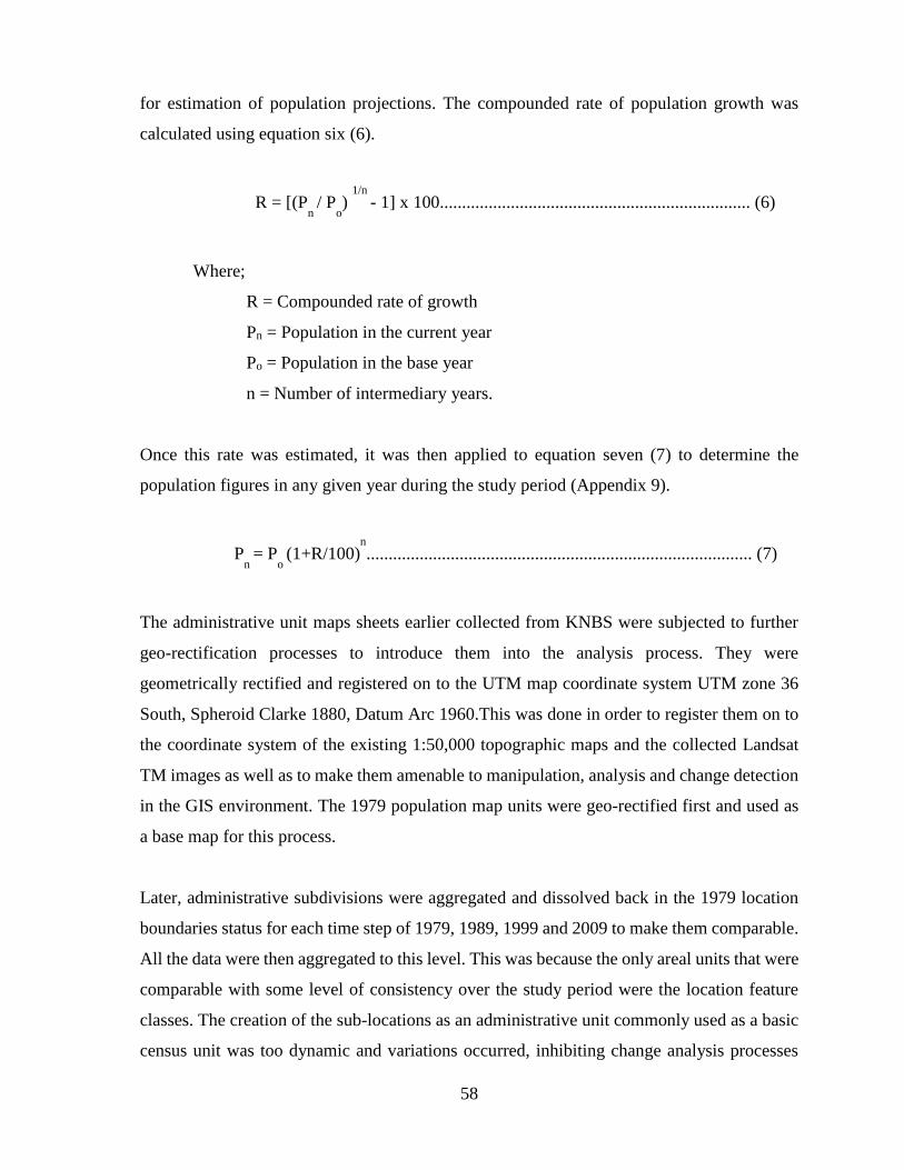
58

for estimation of population projections. The compounded rate of population growth was

calculated using equation six (6).

R = [(Pn / P

o)

1/n

- 1] x 100...................................................................... (6)

Where;

R = Compounded rate of growth

Pn = Population in the current year

Po = Population in the base year

n = Number of intermediary years.

Once this rate was estimated, it was then applied to equation seven (7) to determine the

population figures in any given year during the study period (Appendix 9).

Pn

= Po (1+R/100)

n

....................................................................................... (7)

The administrative unit maps sheets earlier collected from KNBS were subjected to further

geo-rectification processes to introduce them into the analysis process. They were

geometrically rectified and registered on to the UTM map coordinate system UTM zone 36

South, Spheroid Clarke 1880, Datum Arc 1960.This was done in order to register them on to

the coordinate system of the existing 1:50,000 topographic maps and the collected Landsat

TM images as well as to make them amenable to manipulation, analysis and change detection

in the GIS environment. The 1979 population map units were geo-rectified first and used as

a base map for this process.

Later, administrative subdivisions were aggregated and dissolved back in the 1979 location

boundaries status for each time step of 1979, 1989, 1999 and 2009 to make them comparable.

All the data were then aggregated to this level. This was because the only areal units that were

comparable with some level of consistency over the study period were the location feature

classes. The creation of the sub-locations as an administrative unit commonly used as a basic

census unit was too dynamic and variations occurred, inhibiting change analysis processes

59

and the units were avoided as much as possible. The population statistics were then associated

with their respective location units in an ArcGIS 10.1 database to prepare and visualize the

spatial dimensions of each time-step. The population size was then used to represent the labels

in the various spatial units for each time step so that they could be used to generate maps and

also generate the graphs for the time step years. This enabled determination of areas of

population concentrations and whether the population size was increasing or decreasing

within the study period.

In keeping with the “ecumene” principle, the wetland feature class was erased from the spatial

data set using the erase tool to mask out the wetland areas and only deal with spatial

administrative units’ areas that were outside the wetland. The erase tool created a feature class

by overlaying the input features with the polygons of the erase features. Only those portions

of the locations falling outside the wetland feature class boundaries were copied to the output

feature class that represented the new feature class. The population data representing the

locations were then changed to point data by the use of a feature to point data tool in ArcGIS

10.1. A feature class containing points generated from the representative locations of input

features was created.

After the point data was created where the population in any given location or sub-location

was represented by a point in the middle of the feature class polygon acting as a height, the

point data was interpolated using the Spline with Barriers tool in the Spatial Analyst module

in ArcGIS 10.1. This is a tool that interpolates a raster surface, using barriers from points

using a minimum curvature spline technique. The barriers were entered as the polygon

representing the area of study to limit the generated raster to that area.

The population surface maps were generated to indicate areas of population pressure for the

wetland. Due to the coarseness of the spatial units of data that could be comparable

(administrative locations) over the time series, the population surface maps were only used as

a background to population graphs. This was to give a visual comparison between the surface

map and the bar graphs showing the time series change in the size and distribution of

population of the study area. The 2009 situation was refined using the sub-location data to

improve the resolution of the surface map which was finally used in this process.

60

3.9.3. Socio-economic Data Processing and Analysis

The questionnaires were rechecked for completeness, serialized for identification and linkage.

During this process, 4 questionnaires were dropped from the pack due to inadequacy of the

responses leaving 196 questionnaires for further analysis. The linkages were achieved through

a coding procedure in which each of the questionnaires was given a serial code from the first

to the last and all the questions and responses were given numerical value codes to enable

linkages from the data to the idea and from the idea to all the data pertaining to that idea in

the database. Values of either 1 or 0 were given to the dichotomous (yes or no) responses and

values of 1, 2, three onwards were given to ordinal (low, medium, high) and explanatory

response data. The data were then entered into an Excel 2007 worksheet.

Data cleaning was carried out to improve the quality of data and make them “fit for use” in

the research by identifying and reducing errors in the data and improving their documentation

and presentation. The strategy used was to check each of the data values in the database to

ensure that they were correct and at the very least, conformed to known set of rules, applicable

standards and conventions. The process involved format checks, completeness checks,

reasonableness checks, limit checks, review of the data to identify outliers or other errors,

duplicate records, spelling errors and assessment of data to ensure validity. Within Excel

2007, several worksheets were created one for each logical step. The first worksheet contained

the original data as they were entered. Several subsequent sheets were dedicated to the interim

data processing phases each sheet representing a particular check step. The final worksheet

was dedicated to the final cleaned data ready for further analysis. In each of the check steps,

suspect records and data values were flagged up and rechecked by making comparisons with

the original data in the questionnaires and making appropriate corrections.

To refine the data for eventual statistical analysis, the cleaned data was further processed by

parsing the data using Excel 2007 built-in parsing wizard. The wizard splits cell data at

specified delimiters, such as commas, tabs, or spaces, and puts the output into separate cells.

The data were re-coded and a “comma-separated values” (.csv) data file was prepared. The

.csv data file was imported into the SPSS version 11.5 and preliminary data analysis carried

out using descriptive statistics in both Excel 2007 and the SPSS to exploit analytical and

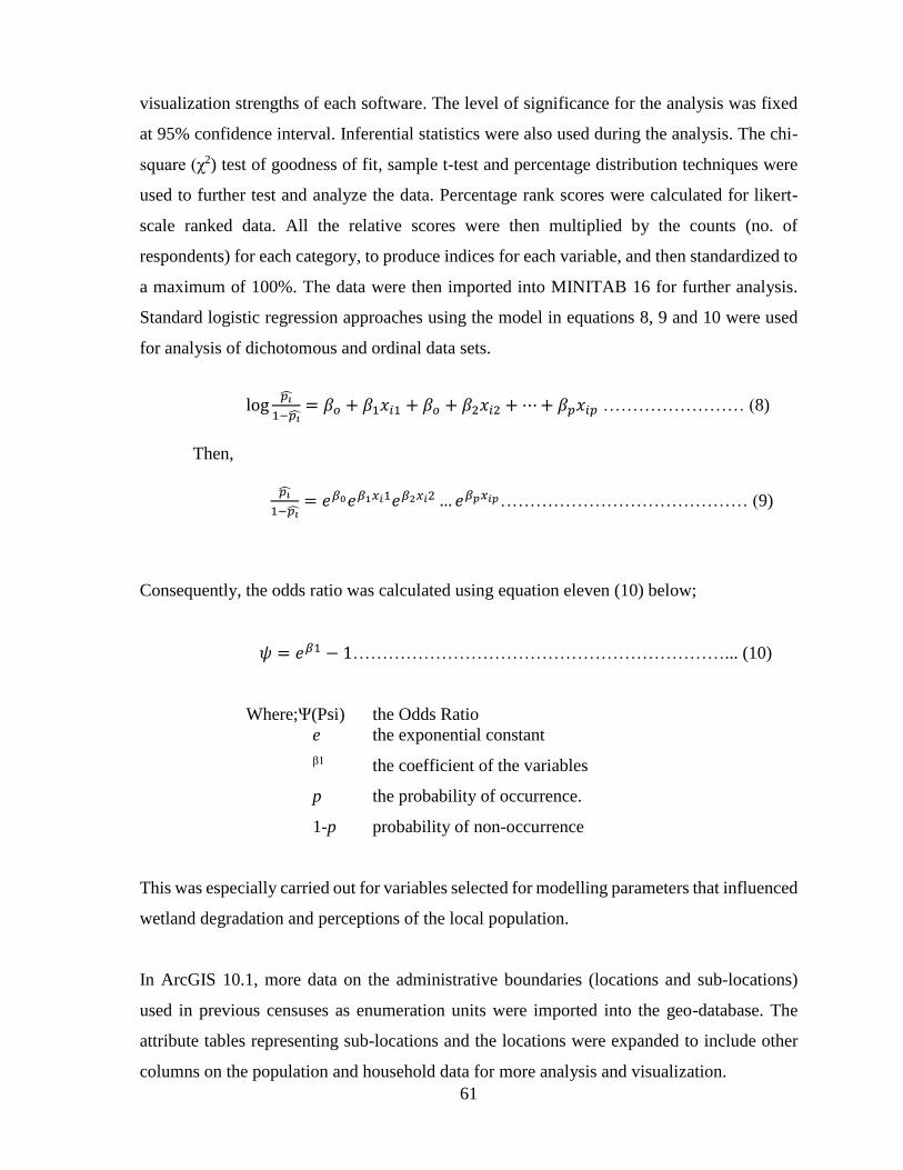
61

visualization strengths of each software. The level of significance for the analysis was fixed

at 95% confidence interval. Inferential statistics were also used during the analysis. The chi-

square (χ2) test of goodness of fit, sample t-test and percentage distribution techniques were

used to further test and analyze the data. Percentage rank scores were calculated for likert-

scale ranked data. All the relative scores were then multiplied by the counts (no. of

respondents) for each category, to produce indices for each variable, and then standardized to

a maximum of 100%. The data were then imported into MINITAB 16 for further analysis.

Standard logistic regression approaches using the model in equations 8, 9 and 10 were used

for analysis of dichotomous and ordinal data sets.

log𝑝�̂�

1−𝑝�̂�= 𝛽𝑜 + 𝛽1𝑥𝑖1 + 𝛽𝑜 + 𝛽2𝑥𝑖2 + ⋯ + 𝛽𝑝𝑥𝑖𝑝 …………………… (8)

Then,

𝑝�̂�

1−𝑝�̂�= 𝑒𝛽0𝑒𝛽1𝑥𝑖1𝑒𝛽2𝑥𝑖2 … 𝑒𝛽𝑝𝑥𝑖𝑝…………………………………… (9)

Consequently, the odds ratio was calculated using equation eleven (10) below;

𝜓 = 𝑒𝛽1 − 1………………………………………………………... (10)

Where;Ψ(Psi) the Odds Ratio

e the exponential constant

β1 the coefficient of the variables

p the probability of occurrence.

1-p probability of non-occurrence

This was especially carried out for variables selected for modelling parameters that influenced

wetland degradation and perceptions of the local population.

In ArcGIS 10.1, more data on the administrative boundaries (locations and sub-locations)

used in previous censuses as enumeration units were imported into the geo-database. The

attribute tables representing sub-locations and the locations were expanded to include other

columns on the population and household data for more analysis and visualization.

62

Information from FGDs summaries were reviewed and analyzed in one sitting for each of the

FGD sessions. Comments that appeared repeatedly as well as those which appeared

unexpectedly eliciting emotional responses were checked out and noted. This was to identify

trends that could be useful in explaining certain observed trends and issues in the previous

stages of the research.

3.9.4. Lake Level Data Processing and Analysis

Since the Lake level data were only associable with the polygon named “Lake” and not the

administrative unit polygons, analysis in GIS was found to be impractical and of little use.

Analysis and manipulation for results was therefore carried out in the Excel 2007 and

MINITAB 16. Monthly means of the daily lake level data were calculated and tabulated.

Extreme environmental pulses such as “Lamina” or “El nino” that could influence the

distribution were identified and either excluded from the analysis or normalized. The data was

transposed and then classified by year and by month to enable frequency analysis. This

exercise was carried out in Excel 2007 using a filter function to arrange the data into a format

that was used to interrogate for homogeneity (Appendix 10). The data were then imported

into MINITAB 16 for further analysis, which included statistical comparisons and trend

analysis.

A sequence plot, which is a graph of the data series values on the vertical axis against time on

the horizontal axis, was made. The purpose of the sequence plot was to give a visual

impression of the nature of the time series and suggest if there are any behavioural patterns in

the time series to inform model selection. A general linear trend model was then selected and

fitted to the time series data to estimate trends. However, due to the potentially additive or

multiplicative seasonality that were noted to be present in the trends, the data were further

subjected to exponential smoothing using Holt-Winters method (Goodwin, 2010). The

method calculated the dynamic estimates for three components which included the levels,

trends, and seasonality. Shoreline shifts signifying lake level changes were measured from

satellite images using overlay procedures in ArcGIS 10.1.

63

3.9.5. Analysis of Relationships between Predictor Variables and Wetland Area

A wetland polygon was generated with a centroid. Respondents’ spatial locations were then

plotted on the map from the X and Y co-ordinates files that were generated from the GPS

waypoint data and incorporated in the database. Distances of respondents from the nearest

wetland boundary point and centroid were generated and added into the database. Six most

frequent perception responses were then selected as parameters for further analysis. These

included distances of respondents from the wetland, fertility of the soil in the wetland as an

incentive to work in the wetland, good soil moisture content in the wetland soils as an

incentive to circumvent frequent droughts in the area, animal destruction of crops in the

wetland as a disincentive to cultivate the wetland and flood frequency also as a disincentive

to work in the wetland due to its attendant destructive events.

The proportional odds and logistic regression models were applied and fitted to the data for

the selected parameters to investigate the relationships between the categorical outcomes and

the explanatory variables according to Brant (1990), Agresti (2002) and Thompson (2009). In

order to understand how the variables have related to each other over time, a correlation

analysis was carried out to determine the nature of the relationship between the dependent

variable (wetland) and the explanatory variables (land use, population and lake levels). Land

use was measured through its elemental indicators such as areas covered by small-scale

agriculture, rice farms and turbid water surfaces; open grasslands, bushes and water area.

Figure 3.7 presents a generalized summary of the study process.

.

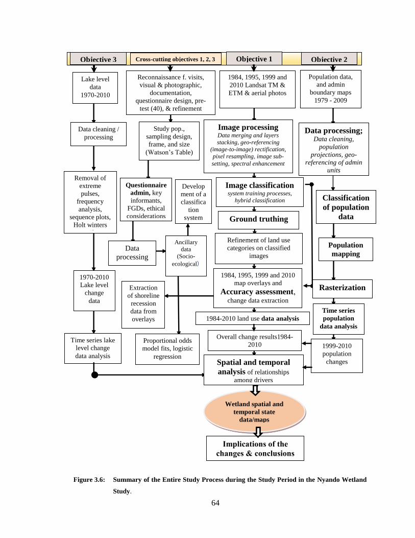
64

Figure 3.6: Summary of the Entire Study Process during the Study Period in the Nyando Wetland

Study.

Rasterization

Data processing; Data cleaning,

population

projections, geo-

referencing of admin

units

Classification

of population

data

Population data,

and admin

boundary maps

1979 - 2009

Ancillary

data

(Socio-

ecological)

Image classification system training processes,

hybrid classification

Refinement of land use

categories on classified

images

Overall change results1984-

2010

Implications of the

changes & conclusions

Wetland spatial and

temporal state

data/maps

1999-2010

population

changes Spatial and temporal

analysis of relationships

among drivers

1984-2010 land use data analysis

Reconnaissance f. visits,

visual & photographic,

documentation,

questionnaire design, pre-

test (40), & refinement

Ground truthing

,

Data cleaning /

processing

Lake level

data

1970-2010

Develop

ment of a

classifica

tion

system

Image processing Data merging and layers

stacking, geo-referencing

(image-to-image) rectification,

pixel resampling, image sub-

setting, spectral enhancement

1984, 1995, 1999 and 2010

map overlays and

Accuracy assessment, change data extraction

Population

mapping

Time series

population

data analysis

Extraction

of shoreline

recession

data from

overlays

1970-2010

Lake level

change

data

1984, 1995, 1999 and

2010 Landsat TM &

ETM & aerial photos

Study pop.,

sampling design,

frame, and size

(Watson’s Table)

Removal of

extreme

pulses,

frequency

analysis,

sequence plots,

Holt winters

smoothing

Time series lake

level change

data analysis

Proportional odds

model fits, logistic

regression

Questionnaire

admin, key

informants,

FGDs, ethical

considerations

Data

processing

Objective 3 Objective 1 Objective 2 Cross-cutting objectives 1, 2, 3

65

CHAPTER FOUR

4.0 RESULTS

4.1. Image Classification and Land Use/Land Cover Mapping

Five land use categories were identified and used as a basis for class definitions and

assignment for the land cover and use mapping exercise. These categories were:

1. Water area (WATr)

2. Wetland area (WTLa)

3. Rice farms and turbid paddy water surfaces (RFTw)

4. Small-scale agriculture (SSAg), (predominantly subsistence)

5. Open grassland, mixed bushes with exposed bare ground (OPGb)

6. Unclassified (U0)

These five land use/cover categories were used to run a change detection procedure on the

various satellite images to produce 4 map overlays presented in Figure 4.1“a” and “b” and

Figure 4.2 “a” and “b”. Each land use/cover category was quantified in each time-step. These

were first quantified as the number of pixels belonging to each category presented in Table

4.1 and then expressed as ground surface areas depicting spatial extents in hectares (ha) as

presented in Table 4.2 and Figure 4.3.

66

Figure 4.1: (a, b) Spatial Rendition of Land Use/Cover as at (a) 1984, (b) 1995 in Nyando Wetland

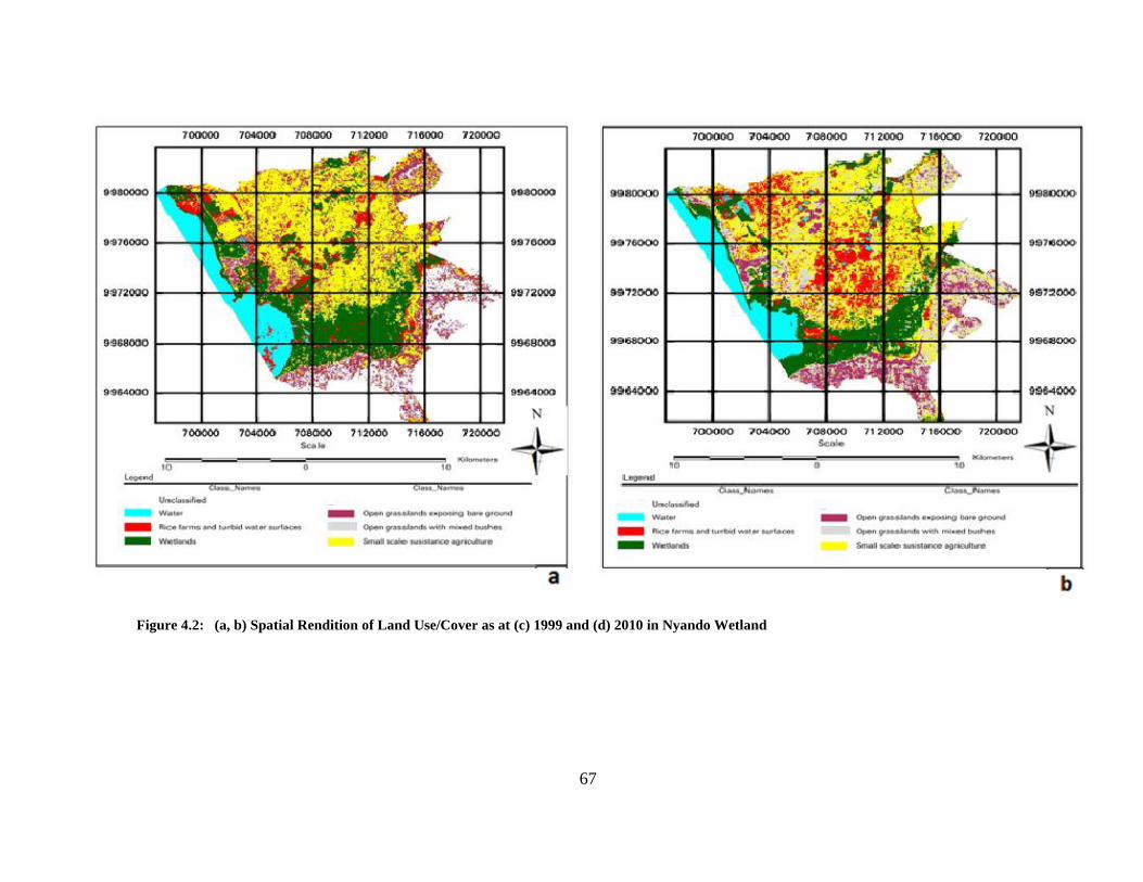
67

Figure 4.2: (a, b) Spatial Rendition of Land Use/Cover as at (c) 1999 and (d) 2010 in Nyando Wetland

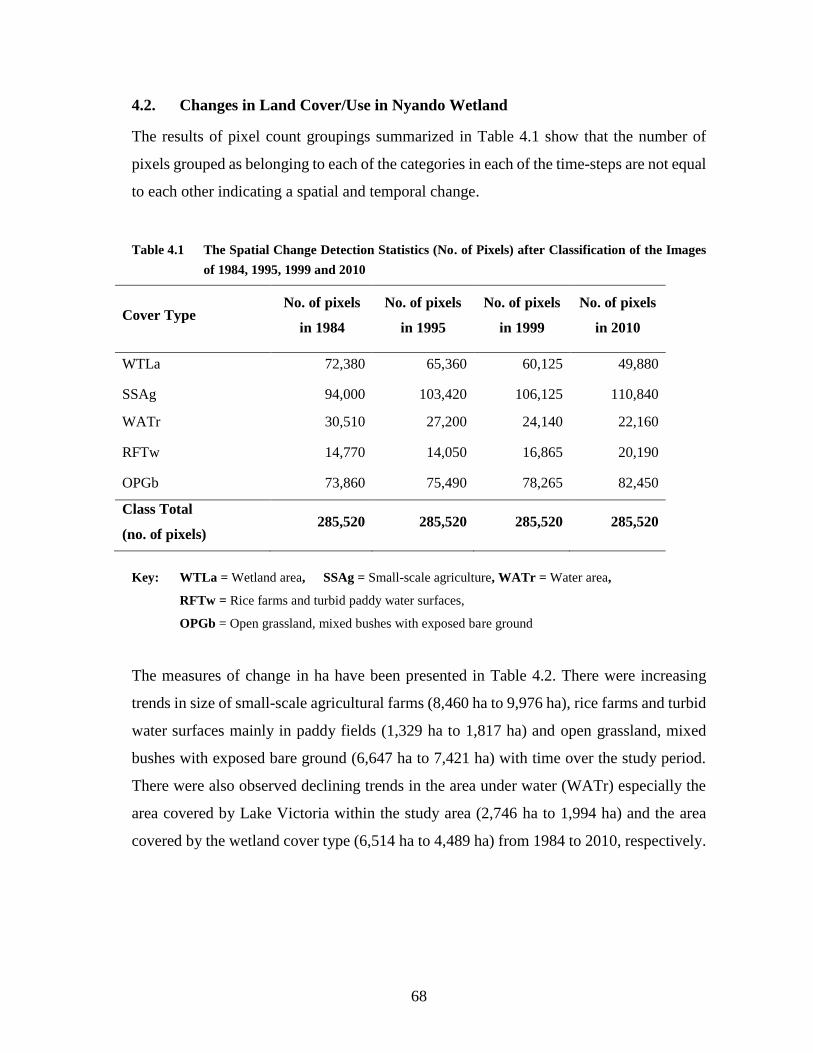
68

4.2. Changes in Land Cover/Use in Nyando Wetland

The results of pixel count groupings summarized in Table 4.1 show that the number of

pixels grouped as belonging to each of the categories in each of the time-steps are not equal

to each other indicating a spatial and temporal change.

Table 4.1 The Spatial Change Detection Statistics (No. of Pixels) after Classification of the Images

of 1984, 1995, 1999 and 2010

Cover Type No. of pixels

in 1984

No. of pixels

in 1995

No. of pixels

in 1999

No. of pixels

in 2010

WTLa 72,380 65,360 60,125 49,880

SSAg 94,000 103,420 106,125 110,840

WATr 30,510 27,200 24,140 22,160

RFTw 14,770 14,050 16,865 20,190

OPGb 73,860 75,490 78,265 82,450

Class Total

(no. of pixels) 285,520 285,520 285,520 285,520

Key: WTLa = Wetland area, SSAg = Small-scale agriculture, WATr = Water area,

RFTw = Rice farms and turbid paddy water surfaces,

OPGb = Open grassland, mixed bushes with exposed bare ground

The measures of change in ha have been presented in Table 4.2. There were increasing

trends in size of small-scale agricultural farms (8,460 ha to 9,976 ha), rice farms and turbid

water surfaces mainly in paddy fields (1,329 ha to 1,817 ha) and open grassland, mixed

bushes with exposed bare ground (6,647 ha to 7,421 ha) with time over the study period.

There were also observed declining trends in the area under water (WATr) especially the

area covered by Lake Victoria within the study area (2,746 ha to 1,994 ha) and the area

covered by the wetland cover type (6,514 ha to 4,489 ha) from 1984 to 2010, respectively.

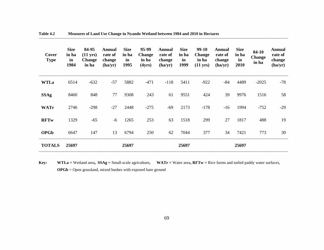
69

Table 4.2 Measures of Land Use Change in Nyando Wetland between 1984 and 2010 in Hectares

Cover

Type

Size

in ha

in

1984

84-95

(11 yrs)

Change

in ha

Annual

rate of

change

(ha/yr)

Size

in ha

in

1995

95-99

Change

in ha

(4yrs)

Annual

rate of

change

(ha/yr)

Size

in ha

in

1999

99-10

Change

in ha

(11 yrs)

Annual

rate of

change

(ha/yr)

Size

in ha

in

2010

84-10

Change

in ha

Annual

rate of

change

(ha/yr)

WTLa 6514 -632 -57 5882 -471 -118 5411 -922 -84 4489 -2025 -78

SSAg 8460 848 77 9308 243 61 9551 424 39 9976 1516 58

WATr 2746 -298 -27 2448 -275 -69 2173 -178 -16 1994 -752 -29

RFTw 1329 -65 -6 1265 253 63 1518 299 27 1817 488 19

OPGb 6647 147 13 6794 250 62 7044 377 34 7421 773 30

TOTALS 25697 25697 25697 25697

Key: WTLa = Wetland area, SSAg = Small-scale agriculture, WATr = Water area, RFTw = Rice farms and turbid paddy water surfaces,

OPGb = Open grassland, mixed bushes with exposed bare ground

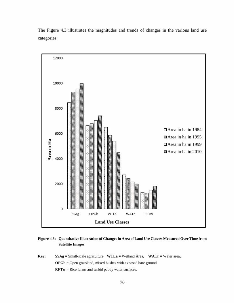
70

The Figure 4.3 illustrates the magnitudes and trends of changes in the various land use

categories.

Figure 4.3: Quantitative Illustration of Changes in Area of Land Use Classes Measured Over Time from

Satellite Images

Key: SSAg = Small-scale agriculture WTLa = Wetland Area, WATr = Water area,

OPGb = Open grassland, mixed bushes with exposed bare ground

RFTw = Rice farms and turbid paddy water surfaces,

0

2000

4000

6000

8000

10000

12000

SSAg OPGb WTLa WATr RFTw

Are

a i

n H

a

Land Use Classes

Area in ha in 1984

Area in ha in 1995

Area in ha in 1999

Area in ha in 2010

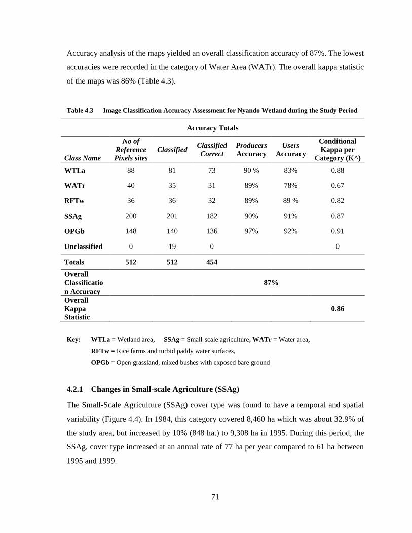
71

Accuracy analysis of the maps yielded an overall classification accuracy of 87%. The lowest

accuracies were recorded in the category of Water Area (WATr). The overall kappa statistic

of the maps was 86% (Table 4.3).

Table 4.3 Image Classification Accuracy Assessment for Nyando Wetland during the Study Period

Accuracy Totals

Class Name

No of

Reference

Pixels sites

Classified Classified

Correct

Producers

Accuracy

Users

Accuracy

Conditional

Kappa per

Category (K^)

WTLa 88 81 73 90 % 83% 0.88

WATr 40 35 31 89% 78% 0.67

RFTw 36 36 32 89% 89 % 0.82

SSAg 200 201 182 90% 91% 0.87

OPGb 148 140 136 97% 92% 0.91

Unclassified 0 19 0 0

Totals 512 512 454

Overall

Classificatio

n Accuracy

87%

Overall

Kappa

Statistic

0.86

Key: WTLa = Wetland area, SSAg = Small-scale agriculture, WATr = Water area,

RFTw = Rice farms and turbid paddy water surfaces,

OPGb = Open grassland, mixed bushes with exposed bare ground

4.2.1 Changes in Small-scale Agriculture (SSAg)

The Small-Scale Agriculture (SSAg) cover type was found to have a temporal and spatial

variability (Figure 4.4). In 1984, this category covered 8,460 ha which was about 32.9% of

the study area, but increased by 10% (848 ha.) to 9,308 ha in 1995. During this period, the

SSAg, cover type increased at an annual rate of 77 ha per year compared to 61 ha between

1995 and 1999.

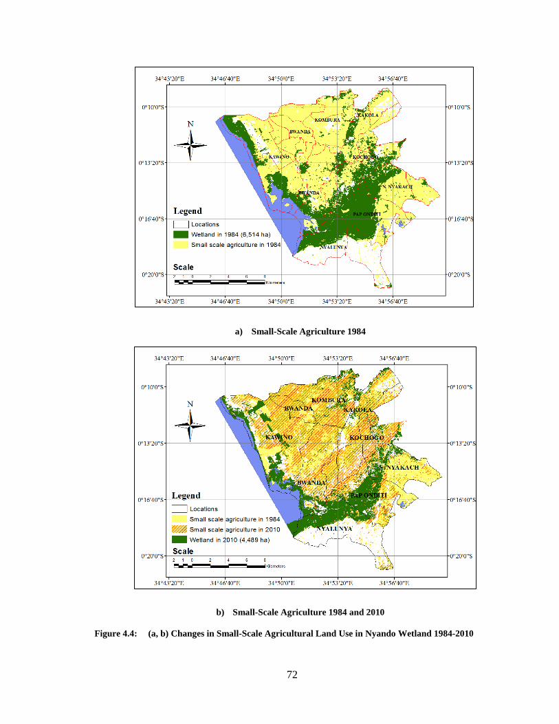
72

a) Small-Scale Agriculture 1984

b) Small-Scale Agriculture 1984 and 2010

Figure 4.4: (a, b) Changes in Small-Scale Agricultural Land Use in Nyando Wetland 1984-2010

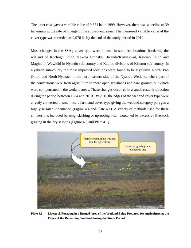
73

The latter case gave a variable value of 9,551 ha in 1999. However, there was a decline to 39

ha/annum in the rate of change in the subsequent years. The measured variable value of the

cover type was recorded as 9,976 ha by the end of the study period in 2010.

Most changes in the SSAg cover type were intense in southern locations bordering the

wetland of Kochogo South, Kakola Ombaka, Bwanda/Kanyagwal, Kawino South and

Magina in Wawidhi in Nyando sub-county and Kadibo divisions of Kisumu sub-county. In

Nyakach sub-county the most impacted locations were found to be Nyalunya North, Pap

Onditi and North Nyakach in the north-eastern side of the Nyando Wetland, where part of

the conversions were from agriculture to more open grasslands and bare ground; but which

were compensated in the wetland areas. These changes occurred in a south-easterly direction

during the period between 1984 and 2010. By 2010 the edges of the wetland cover type were

already converted to small-scale farmland cover type giving the wetland category polygon a

highly serrated indentation (Figure 4.4 and Plate 4.1). A variety of methods used for these

conversions included burning, slashing or uprooting often worsened by excessive livestock

grazing in the dry seasons (Figure 4.9 and Plate 4.1).

Plate 4.1 Livestock Foraging in a Burned Area of the Wetland Being Prepared for Agriculture at the

Edges of the Remaining Wetland during the Study Period

Framers opening up wetland

area for agriculture

Livestock grazing in an

opened up area

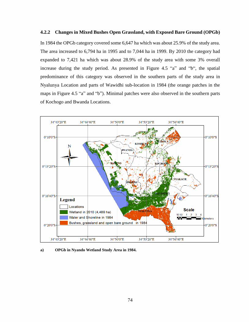
74

4.2.2 Changes in Mixed Bushes Open Grassland, with Exposed Bare Ground (OPGb)

In 1984 the OPGb category covered some 6,647 ha which was about 25.9% of the study area.

The area increased to 6,794 ha in 1995 and to 7,044 ha in 1999. By 2010 the category had

expanded to 7,421 ha which was about 28.9% of the study area with some 3% overall

increase during the study period. As presented in Figure 4.5 “a” and “b“, the spatial

predominance of this category was observed in the southern parts of the study area in

Nyalunya Location and parts of Wawidhi sub-location in 1984 (the orange patches in the

maps in Figure 4.5 “a” and “b”). Minimal patches were also observed in the southern parts

of Kochogo and Bwanda Locations.

a) OPGb in Nyando Wetland Study Area in 1984.

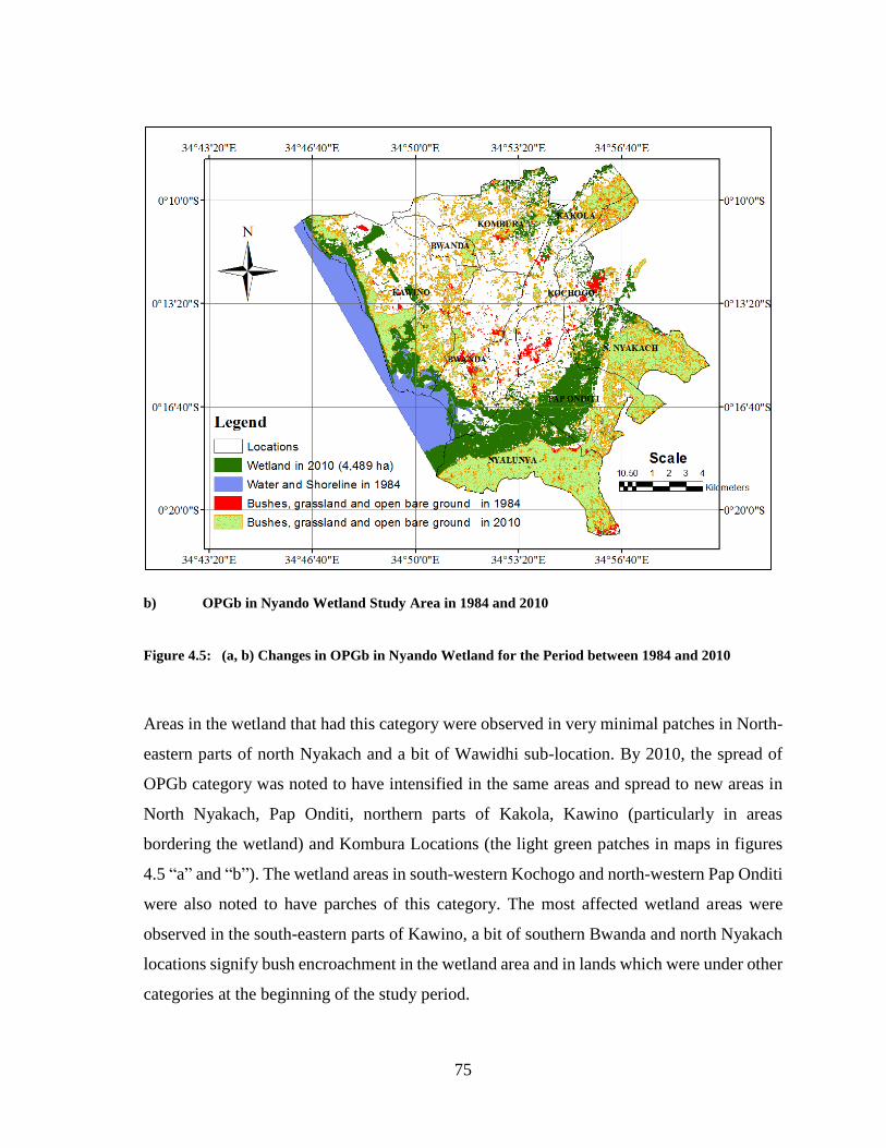
75

b) OPGb in Nyando Wetland Study Area in 1984 and 2010

Figure 4.5: (a, b) Changes in OPGb in Nyando Wetland for the Period between 1984 and 2010

Areas in the wetland that had this category were observed in very minimal patches in North-

eastern parts of north Nyakach and a bit of Wawidhi sub-location. By 2010, the spread of

OPGb category was noted to have intensified in the same areas and spread to new areas in

North Nyakach, Pap Onditi, northern parts of Kakola, Kawino (particularly in areas

bordering the wetland) and Kombura Locations (the light green patches in maps in figures

4.5 “a” and “b”). The wetland areas in south-western Kochogo and north-western Pap Onditi

were also noted to have parches of this category. The most affected wetland areas were

observed in the south-eastern parts of Kawino, a bit of southern Bwanda and north Nyakach

locations signify bush encroachment in the wetland area and in lands which were under other

categories at the beginning of the study period.

76

4.2.3 Rice Farms and Turbid Paddy Water Surfaces (RFTw)

The spatial extent of RFTw is presented in Figure 4.6 and Figure 4.7. Regular flooded

rectangular paddy fields are used as rice farms in the study area (Plate 4.2).

Figure 4.6: Spatial Rendition of Area of RFTw in 1984 in Nyando Wetland

The RFTw cover type declined in area by 5%, from 1,329 ha in 1984 to 1,265 ha in 1995.

Estimates show that between the years 1995 and 2010, the area under this category

progressively reclaimed at least 19 ha. (2%) annually. In 1995, the area under the category

began to expand such that by 1999 it was 1,518 ha and then increased to 1,817 ha in 2010.

Many more patches of this category occurred within the wetland in 2010 compared to 1984.

77

Figure 4.7: Spatial Rendition of Changes in Area of RFTw between 1984 and 2010 in Nyando Wetland

Plate 4.2 Rice Farming and Flooded Paddy Water Surfaces in the Wetland

(Evidence of multiple agricultural activities and grain eating (Granovores) bird

nuisance (the scarecrows) are clearly seen in the fore and mid grounds)

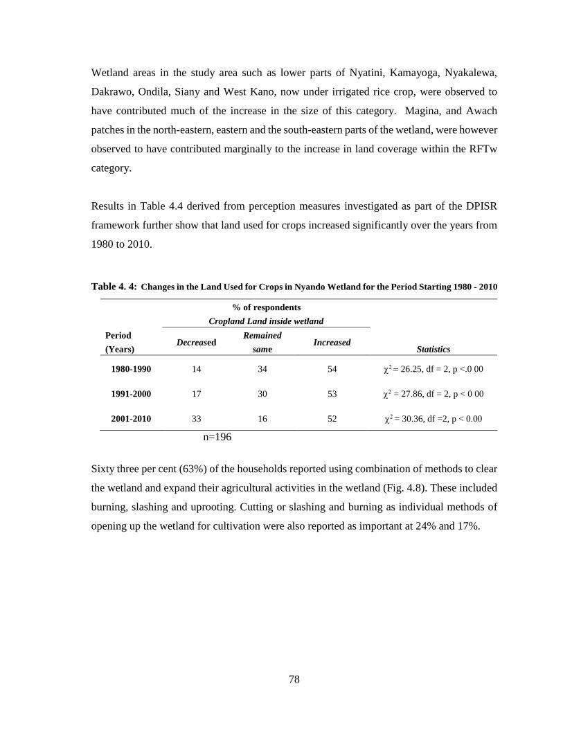
78

Wetland areas in the study area such as lower parts of Nyatini, Kamayoga, Nyakalewa,

Dakrawo, Ondila, Siany and West Kano, now under irrigated rice crop, were observed to

have contributed much of the increase in the size of this category. Magina, and Awach

patches in the north-eastern, eastern and the south-eastern parts of the wetland, were however

observed to have contributed marginally to the increase in land coverage within the RFTw

category.

Results in Table 4.4 derived from perception measures investigated as part of the DPISR

framework further show that land used for crops increased significantly over the years from

1980 to 2010.

Table 4. 4: Changes in the Land Used for Crops in Nyando Wetland for the Period Starting 1980 - 2010

Period

(Years)

% of respondents

Statistics

Cropland Land inside wetland

Decreased Remained

same Increased

1980-1990 14 34 54 26.25, df = 2, p <.0 00

1991-2000 17 30 53 = 27.86, df = 2, p < 0 00

2001-2010 33 16 52 = 30.36, df =2, p < 0.00

n=196

Sixty three per cent (63%) of the households reported using combination of methods to clear

the wetland and expand their agricultural activities in the wetland (Fig. 4.8). These included

burning, slashing and uprooting. Cutting or slashing and burning as individual methods of

opening up the wetland for cultivation were also reported as important at 24% and 17%.

79

Figure 4.8: The Methods Used to Clear the Wetland Area for SSAg in Nyando Wetland during the

Study Period

There were several patches of the small scale agriculture (SSAg) cover type right inside the

Nyando Wetland (Plate 4.3) especially on the northern, north western, north eastern and

eastern frontiers of the wetland. This phenomenon is reflected by the intensity of the reddish

colour renditions for the 2010 SSAg cover type on the maps in Figure 4.4.

Plate 4.3: Patches of Mixed Agricultural Activities Noted Right in the Middle of Nyando Wetland

(shown by the arrow) on the North Eastern Part of the Photograph

(Photo courtesy; MEMR, 2012)

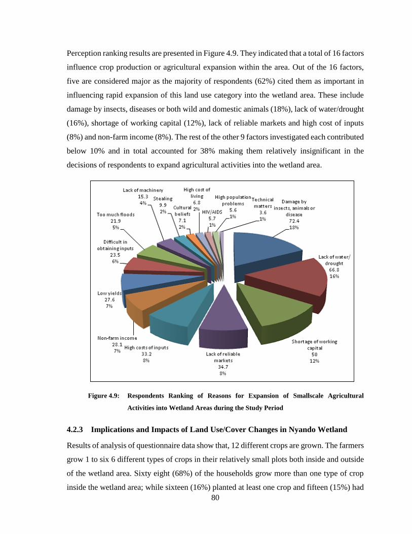
80

Perception ranking results are presented in Figure 4.9. They indicated that a total of 16 factors

influence crop production or agricultural expansion within the area. Out of the 16 factors,

five are considered major as the majority of respondents (62%) cited them as important in

influencing rapid expansion of this land use category into the wetland area. These include

damage by insects, diseases or both wild and domestic animals (18%), lack of water/drought

(16%), shortage of working capital (12%), lack of reliable markets and high cost of inputs

(8%) and non-farm income (8%). The rest of the other 9 factors investigated each contributed

below 10% and in total accounted for 38% making them relatively insignificant in the

decisions of respondents to expand agricultural activities into the wetland area.

Figure 4.9: Respondents Ranking of Reasons for Expansion of Smallscale Agricultural

Activities into Wetland Areas during the Study Period

4.2.3 Implications and Impacts of Land Use/Cover Changes in Nyando Wetland

Results of analysis of questionnaire data show that, 12 different crops are grown. The farmers

grow 1 to six 6 different types of crops in their relatively small plots both inside and outside

of the wetland area. Sixty eight (68%) of the households grow more than one type of crop

inside the wetland area; while sixteen (16%) planted at least one crop and fifteen (15%) had

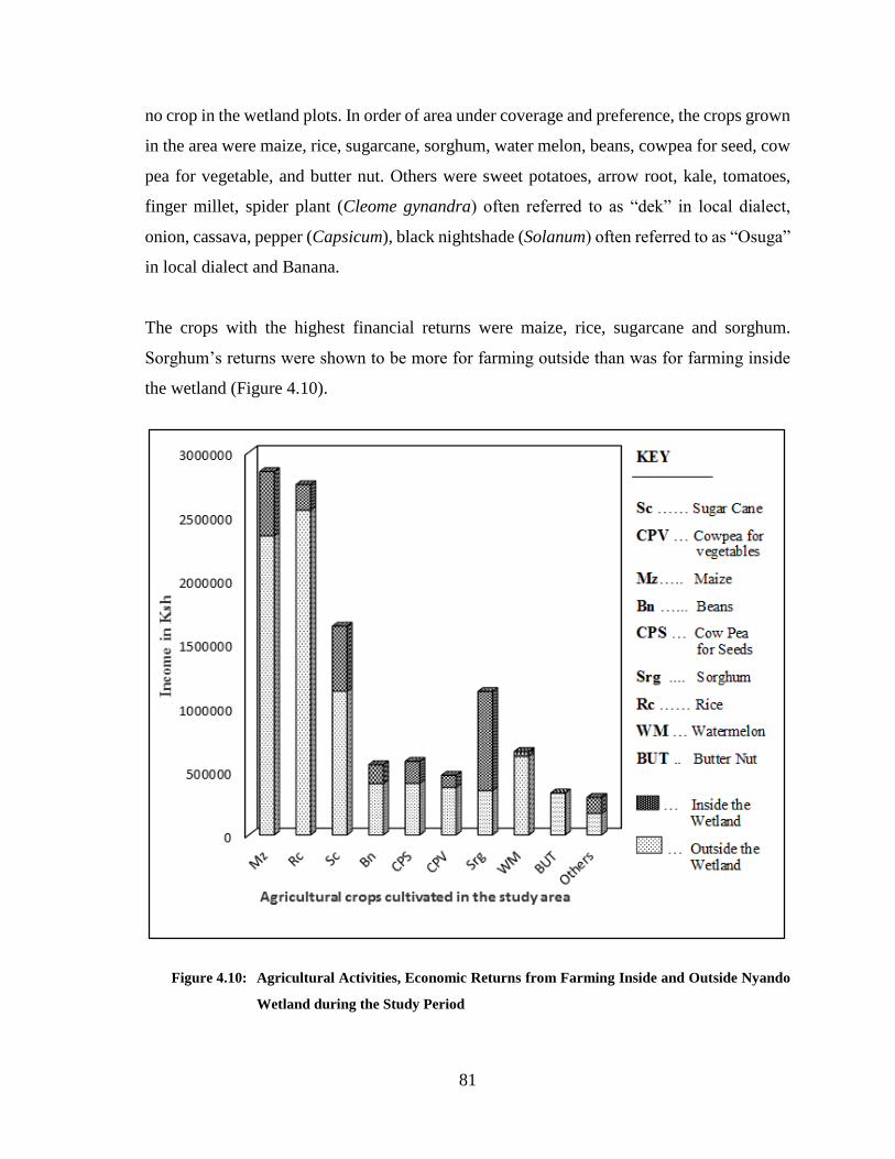
81

no crop in the wetland plots. In order of area under coverage and preference, the crops grown

in the area were maize, rice, sugarcane, sorghum, water melon, beans, cowpea for seed, cow

pea for vegetable, and butter nut. Others were sweet potatoes, arrow root, kale, tomatoes,

finger millet, spider plant (Cleome gynandra) often referred to as “dek” in local dialect,

onion, cassava, pepper (Capsicum), black nightshade (Solanum) often referred to as “Osuga”

in local dialect and Banana.

The crops with the highest financial returns were maize, rice, sugarcane and sorghum.

Sorghum’s returns were shown to be more for farming outside than was for farming inside

the wetland (Figure 4.10).

Figure 4.10: Agricultural Activities, Economic Returns from Farming Inside and Outside Nyando

Wetland during the Study Period

82

Of the annual income of more than Kshs. 11,226,560 obtained by the respondents in Nyando

Wetland area, 77% originated from farming activities inside the wetland while only 23% are

proceeds from farming activities outside the wetland. It may then be that this difference arose

from the fact that there are normally higher yields in terms of quantity per unit area than can

be obtained from farming outside the wetland.

However, sample t-test values (Appendix 11) associated with corresponding p-values for the

same crops indicated that crops such as maize (t-stat = 0.59, p = 0.56), rice (t-stat = 0.45, p

= 0.65), sugar cane (t-stat = 0.06, p = 0.95), sorghum (t-stat = -1.23, p = 0.23), cow peas for

seeds (t-stat = 0.47, p = 0.63) and beans (t-stat = 0.81, p = 0.42) have p-values greater than

the common alpha level of 0.05 at 95% confidence level. This suggests that there is no

evidence for a significant difference in financial returns for these crops whether cultivated

inside or outside the wetland. This means that perhaps there are other factors other than

financial profitability driving the communities to open up wetland areas for farming of these

crops in the wetland. The only crops that showed evidence of a difference in economic

returns, with p- values less than or equal to 0.05 were cow peas for vegetables (t-stat = 2.23,

p = 0.02) and water melon (t-stat = 2.47, p = 0.03) meaning that they are actually profitable.

The number of years the households have been farming in the wetland is given in Table 4.5.

The various respondents claim that they have practiced agriculture in the Nyando Wetlands

for periods ranging from 2-58 years. This time variation between categories was found to be

statistically significant at 95% confidence level ( = 90.78, df = 5, p < 0.00). The modal

categories of 1-10 yrs and 11-20 yrs which constitute more than 62.2% of the land users have

actually been practicing agriculture in the wetland for the last 20 years.

83

Table 4. 5 The Period Respondents have Been Carrying out Farming Activities in Nyando

Wetland

Years (categories) Frequency Per cent

1-10 61 31.1

11-20 61 31.1

21-30 36 18.4

31-40 22 11.2

41-50 11 5.6

above 51 5 2.6

Total 196 100.0

(X̅=18.52, median = 15, mode = 7, σ - 12.67, minimum = 2, maximum = 58, ( = 90.78, df

= 5, p < 0.00)

Perception of habitat/biodiversity change due to the observed conversions, using granoivores

such as the Ploceidae family of birds e.g. Ploceus spekei and Quilea quilea, as indicators of

change and as part of the DPSIR framework are presented in Figure 4.11.

Figure 4.11: Perceived Impact of Wetland Cultivation using Granivores (Quelea quelea) as an

Indicator of Biodiversity Changes in Nyando Wetland during the Study Period

84

The results show that between 1980 and 1990, 47% of the respondents indicated that grain

eating birds had increased in the wetland as compared to 28% and 25% who thought, the

birds had decreased and remained the same respectively. This is significant (9.01, df 2,

p<0.05). Similarly, between 1991-2000 and 2001-2010, more people, 61% and 67%

respectively reported increases in grain eating birds than in previous periods in which 14%

and 10% were reported respectively. The analysis shows that the difference is significant

( 44.68, df = 2, p < 0.00) and (= 71.15, df = 2, p < 0.00).

4.2.4 Hypothesis testing for Objective one

Stating the first hypothesis to address objective one of the study;

H01: There are no significant spatio-temporal changes in land use/cover types that can be

attributed to changes in the size of Nyando Wetland

Or the Alternative;

The regression analysis output in Table 4.6 shows that out of the four land use variables

considered in the study (WATr (x1), SSAg (x2), OPGb (x3) and RFTw (x4)), only three have

significant effects on the changes in wetland area. The open grasslands and mixed bushes

(OPGb) (x3) was excluded from the model because the regression output showed that it was

not a significant addition to the model possibly due to collinearity at a tolerance level of

7.03*10-7 (Table 4.7). This can be attributed to the fact that when the wetland area is

negatively affected by the anthropogenic land use variables (SSAg (x2), RFTw (x4)), the open

grasslands and mixed bushes (OPGb) tends to increase possibly due to other non-agricultural

areas such as fallow areas in the wetland. It therefore changes with respect to impacts of the

anthropogenic factors on the wetland. As for the other land use variables, the adjusted R2 is

positive (0.998) therefore suggesting that the model is significant since all the three

explanatory variables in the model have significant effect on the dependent variable (wetland

area - WTLa).

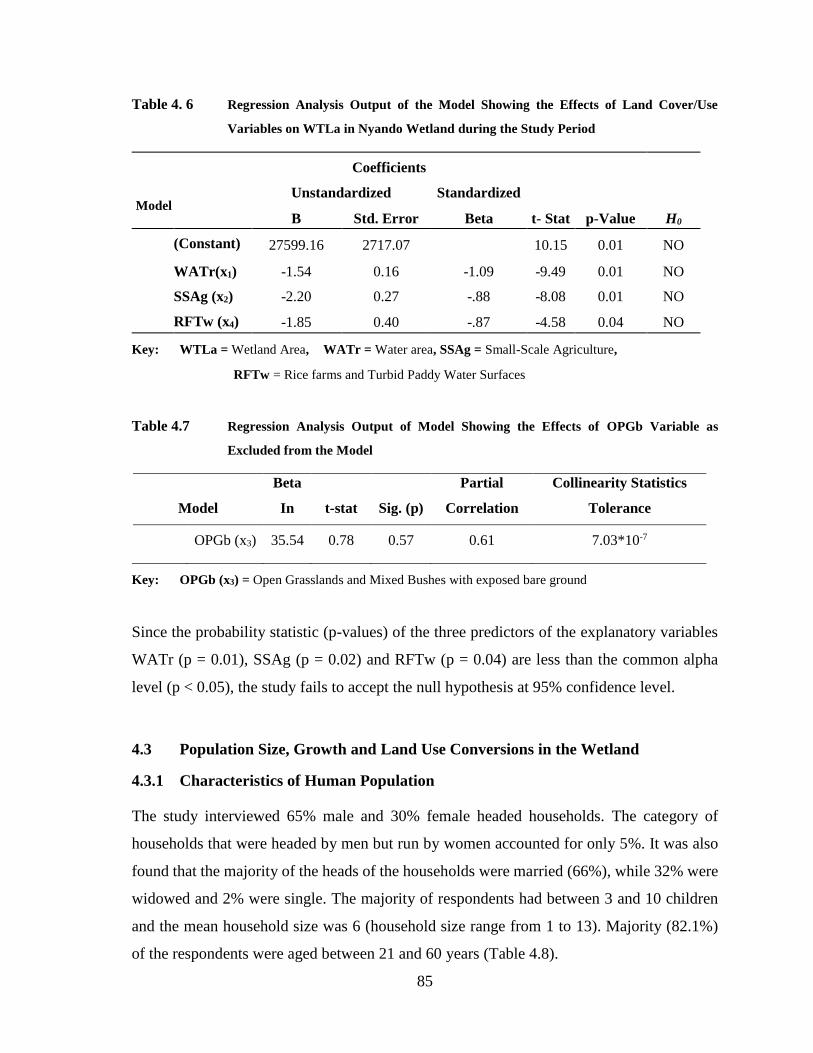
85

Table 4. 6 Regression Analysis Output of the Model Showing the Effects of Land Cover/Use

Variables on WTLa in Nyando Wetland during the Study Period

Coefficients

Model Unstandardized Standardized

t- Stat p-Value

B Std. Error Beta H0

(Constant) 27599.16 2717.07 10.15 0.01 NO

WATr(x1) -1.54 0.16 -1.09 -9.49 0.01 NO

SSAg (x2) -2.20 0.27 -.88 -8.08 0.01 NO

RFTw (x4) -1.85 0.40 -.87 -4.58 0.04 NO

Key: WTLa = Wetland Area, WATr = Water area, SSAg = Small-Scale Agriculture,

RFTw = Rice farms and Turbid Paddy Water Surfaces

Table 4.7 Regression Analysis Output of Model Showing the Effects of OPGb Variable as

Excluded from the Model

Model

Beta

In t-stat Sig. (p)

Partial

Correlation

Collinearity Statistics

Tolerance

OPGb (x3) 35.54 0.78 0.57 0.61 7.03*10-7

Key: OPGb (x3) = Open Grasslands and Mixed Bushes with exposed bare ground

Since the probability statistic (p-values) of the three predictors of the explanatory variables

WATr (p = 0.01), SSAg (p = 0.02) and RFTw (p = 0.04) are less than the common alpha

level (p < 0.05), the study fails to accept the null hypothesis at 95% confidence level.

4.3 Population Size, Growth and Land Use Conversions in the Wetland

4.3.1 Characteristics of Human Population

The study interviewed 65% male and 30% female headed households. The category of

households that were headed by men but run by women accounted for only 5%. It was also

found that the majority of the heads of the households were married (66%), while 32% were

widowed and 2% were single. The majority of respondents had between 3 and 10 children

and the mean household size was 6 (household size range from 1 to 13). Majority (82.1%)

of the respondents were aged between 21 and 60 years (Table 4.8).

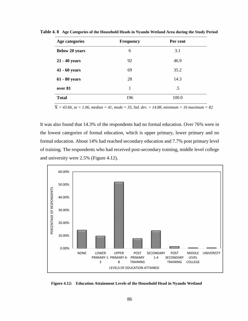
86

Table 4. 8 Age Categories of the Household Heads in Nyando Wetland Area during the Study Period

Age categories Frequency Per cent

Below 20 years 6 3.1

21 - 40 years 92 46.9

41 - 60 years 69 35.2

61 - 80 years 28 14.3

over 81 1 .5

Total 196 100.0

x̅ = 43.66, se = 1.06, median = 41, mode = 35, Std. dev. = 14.88, minimum = 16 maximum = 82

It was also found that 14.3% of the respondents had no formal education. Over 76% were in

the lowest categories of formal education, which is upper primary, lower primary and no

formal education. About 14% had reached secondary education and 7.7% post primary level

of training. The respondents who had received post-secondary training, middle level college

and university were 2.5% (Figure 4.12).

Figure 4.12: Education Attainment Levels of the Household Head in Nyando Wetland

0.00%

10.00%

20.00%

30.00%

40.00%

50.00%

60.00%

NONE LOWERPRIMARY 1-

3

UPPERPRIMARY 4-

8

POSTPRIMARYTRAINING

SECONDARY1-4

POSTSECONDARY

TRAINING

MIDDLELEVEL

COLLEGE

UNIVERISTY

PER

CEN

TAG

E O

F R

ESP

ON

DEN

TS

LEVELS OF EDUCATION ATTAINED

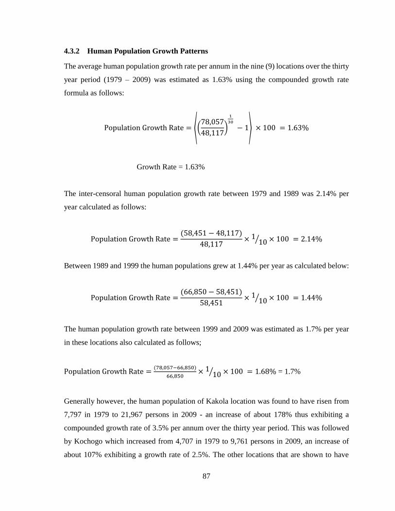
87

4.3.2 Human Population Growth Patterns

The average human population growth rate per annum in the nine (9) locations over the thirty

year period (1979 – 2009) was estimated as 1.63% using the compounded growth rate

formula as follows:

Population Growth Rate = ⟨(78,057

48,117)

1

30

− 1⟩ × 100 = 1.63%

Growth Rate = 1.63%

The inter-censoral human population growth rate between 1979 and 1989 was 2.14% per

year calculated as follows:

Population Growth Rate =(58,451 − 48,117)

48,117× 1

10⁄ × 100 = 2.14%

Between 1989 and 1999 the human populations grew at 1.44% per year as calculated below:

Population Growth Rate =(66,850 − 58,451)

58,451× 1

10⁄ × 100 = 1.44%

The human population growth rate between 1999 and 2009 was estimated as 1.7% per year

in these locations also calculated as follows;

Population Growth Rate =(78,057−66,850)

66,850× 1

10⁄ × 100 = 1.68% = 1.7%

Generally however, the human population of Kakola location was found to have risen from

7,797 in 1979 to 21,967 persons in 2009 - an increase of about 178% thus exhibiting a

compounded growth rate of 3.5% per annum over the thirty year period. This was followed

by Kochogo which increased from 4,707 in 1979 to 9,761 persons in 2009, an increase of

about 107% exhibiting a growth rate of 2.5%. The other locations that are shown to have

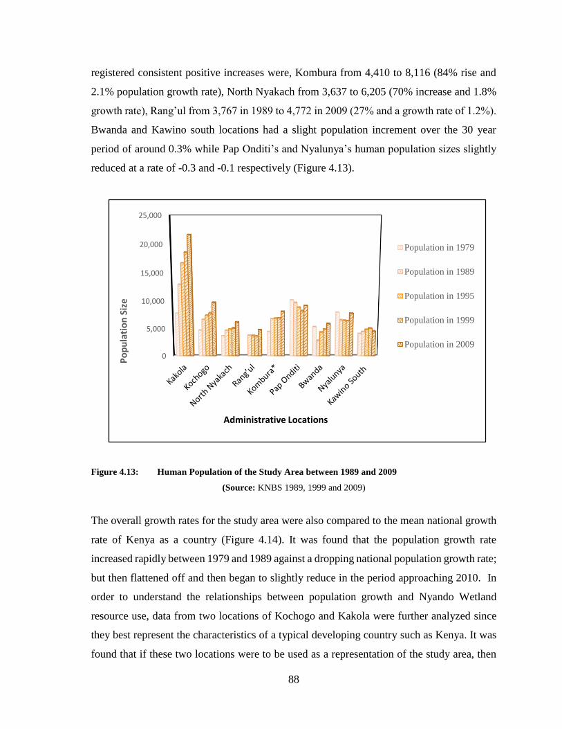
88

0

5,000

10,000

15,000

20,000

25,000

Po

pu

lati

on

Siz

e

Administrative Locations

Population in 1979

Population in 1989

Population in 1995

Population in 1999

Population in 2009

registered consistent positive increases were, Kombura from 4,410 to 8,116 (84% rise and

2.1% population growth rate), North Nyakach from 3,637 to 6,205 (70% increase and 1.8%

growth rate), Rang’ul from 3,767 in 1989 to 4,772 in 2009 (27% and a growth rate of 1.2%).

Bwanda and Kawino south locations had a slight population increment over the 30 year

period of around 0.3% while Pap Onditi’s and Nyalunya’s human population sizes slightly

reduced at a rate of -0.3 and -0.1 respectively (Figure 4.13).

Figure 4.13: Human Population of the Study Area between 1989 and 2009

(Source: KNBS 1989, 1999 and 2009)

The overall growth rates for the study area were also compared to the mean national growth

rate of Kenya as a country (Figure 4.14). It was found that the population growth rate

increased rapidly between 1979 and 1989 against a dropping national population growth rate;

but then flattened off and then began to slightly reduce in the period approaching 2010. In

order to understand the relationships between population growth and Nyando Wetland

resource use, data from two locations of Kochogo and Kakola were further analyzed since

they best represent the characteristics of a typical developing country such as Kenya. It was

found that if these two locations were to be used as a representation of the study area, then

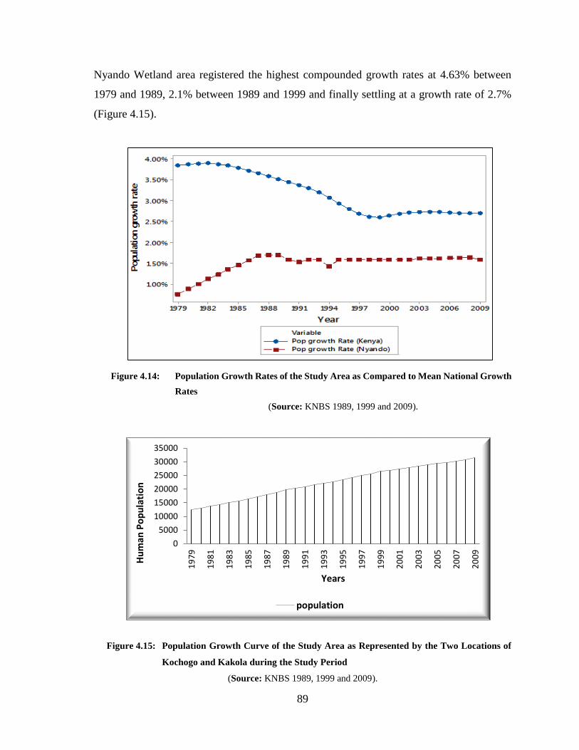
89

0

5000

10000

15000

20000

25000

30000

35000

19

79

19

81

19

83

19

85

19

87

19

89

19

91

19

93

19

95

19

97

19

99

20

01

20

03

20

05

20

07

20

09

Hu

man

Po

pu

lati

on

Years

population

Nyando Wetland area registered the highest compounded growth rates at 4.63% between

1979 and 1989, 2.1% between 1989 and 1999 and finally settling at a growth rate of 2.7%

(Figure 4.15).

Figure 4.14: Population Growth Rates of the Study Area as Compared to Mean National Growth

Rates

(Source: KNBS 1989, 1999 and 2009).

Figure 4.15: Population Growth Curve of the Study Area as Represented by the Two Locations of

Kochogo and Kakola during the Study Period

(Source: KNBS 1989, 1999 and 2009).

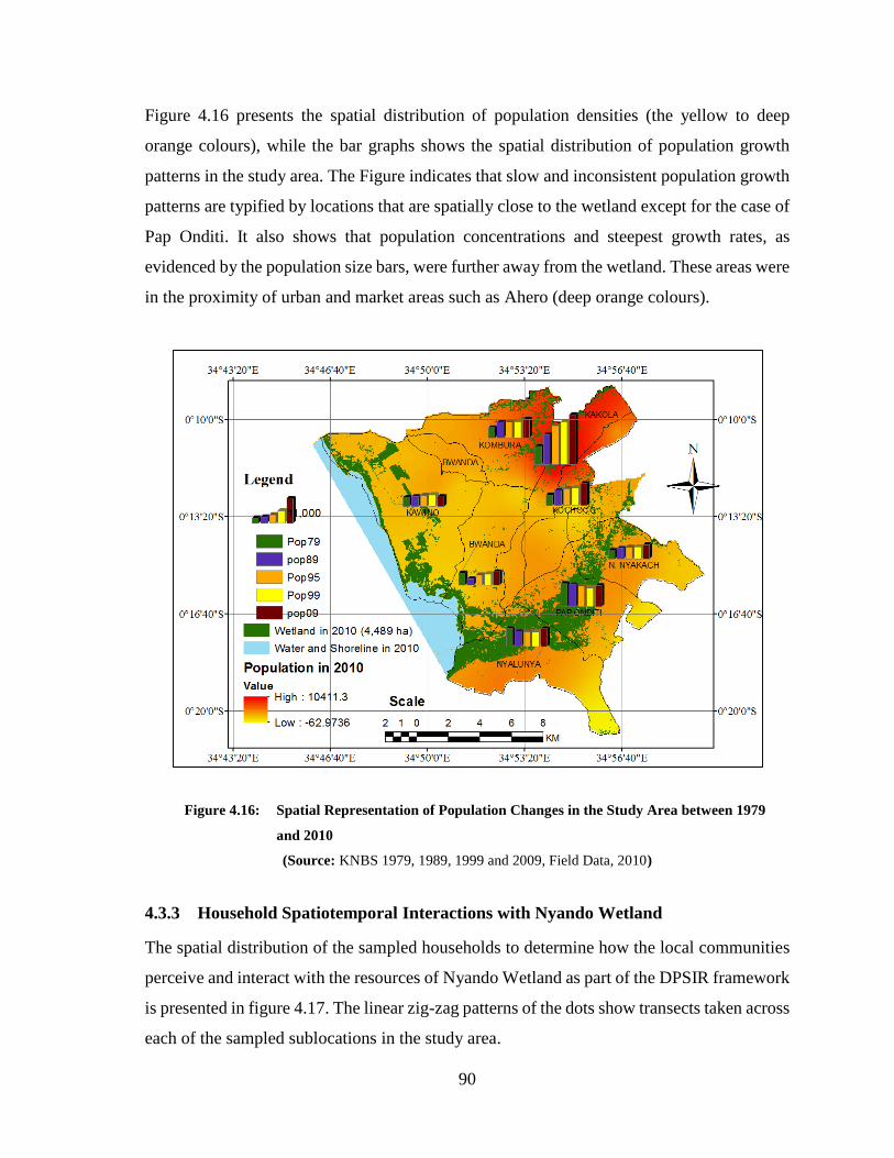
90

Figure 4.16 presents the spatial distribution of population densities (the yellow to deep

orange colours), while the bar graphs shows the spatial distribution of population growth

patterns in the study area. The Figure indicates that slow and inconsistent population growth

patterns are typified by locations that are spatially close to the wetland except for the case of

Pap Onditi. It also shows that population concentrations and steepest growth rates, as

evidenced by the population size bars, were further away from the wetland. These areas were

in the proximity of urban and market areas such as Ahero (deep orange colours).

Figure 4.16: Spatial Representation of Population Changes in the Study Area between 1979

and 2010

(Source: KNBS 1979, 1989, 1999 and 2009, Field Data, 2010)

4.3.3 Household Spatiotemporal Interactions with Nyando Wetland

The spatial distribution of the sampled households to determine how the local communities

perceive and interact with the resources of Nyando Wetland as part of the DPSIR framework

is presented in figure 4.17. The linear zig-zag patterns of the dots show transects taken across

each of the sampled sublocations in the study area.

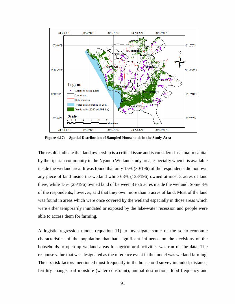
91

Figure 4.17: Spatial Distribution of Sampled Households in the Study Area

The results indicate that land ownership is a critical issue and is considered as a major capital

by the riparian community in the Nyando Wetland study area, especially when it is available

inside the wetland area. It was found that only 15% (30/196) of the respondents did not own

any piece of land inside the wetland while 68% (133/196) owned at most 3 acres of land

there, while 13% (25/196) owned land of between 3 to 5 acres inside the wetland. Some 8%

of the respondents, however, said that they own more than 5 acres of land. Most of the land

was found in areas which were once covered by the wetland especially in those areas which

were either temporarily inundated or exposed by the lake-water recession and people were

able to access them for farming.

A logistic regression model (equation 11) to investigate some of the socio-economic

characteristics of the population that had significant influence on the decisions of the

households to open up wetland areas for agricultural activities was run on the data. The

response value that was designated as the reference event in the model was wetland farming.

The six risk factors mentioned most frequently in the household survey included; distance,

fertility change, soil moisture (water constraint), animal destruction, flood frequency and

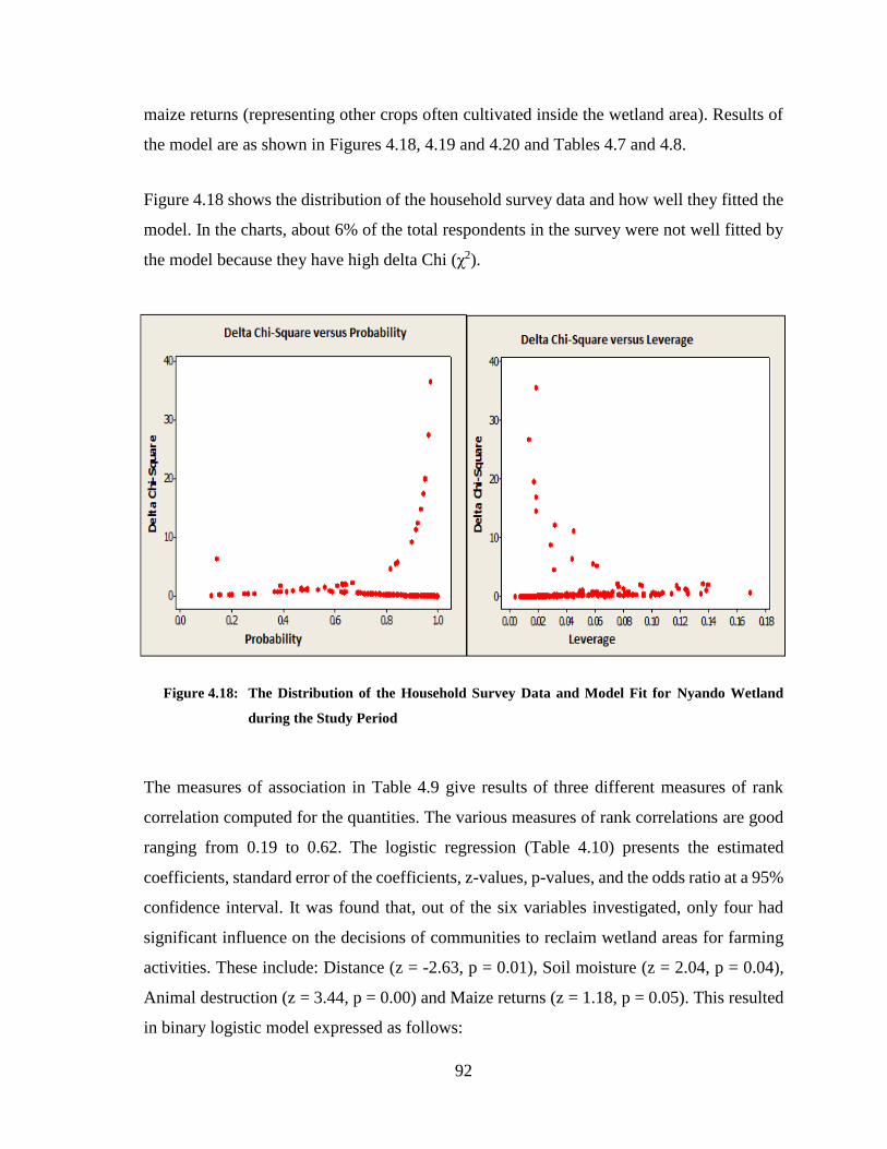
92

maize returns (representing other crops often cultivated inside the wetland area). Results of

the model are as shown in Figures 4.18, 4.19 and 4.20 and Tables 4.7 and 4.8.

Figure 4.18 shows the distribution of the household survey data and how well they fitted the

model. In the charts, about 6% of the total respondents in the survey were not well fitted by

the model because they have high delta Chi (χ2).

Figure 4.18: The Distribution of the Household Survey Data and Model Fit for Nyando Wetland

during the Study Period

The measures of association in Table 4.9 give results of three different measures of rank

correlation computed for the quantities. The various measures of rank correlations are good

ranging from 0.19 to 0.62. The logistic regression (Table 4.10) presents the estimated

coefficients, standard error of the coefficients, z-values, p-values, and the odds ratio at a 95%

confidence interval. It was found that, out of the six variables investigated, only four had

significant influence on the decisions of communities to reclaim wetland areas for farming

activities. These include: Distance (z = -2.63, p = 0.01), Soil moisture (z = 2.04, p = 0.04),

Animal destruction (z = 3.44, p = 0.00) and Maize returns (z = 1.18, p = 0.05). This resulted

in binary logistic model expressed as follows:

93

Logit, 𝐖𝐜 = −0.10975 − 0.32802𝐱𝟏 + 1.03128𝐱𝟐 + 1.58611𝐱𝟑 + 0.00014𝐱𝟒 ................ (11)

Where:

Wc= Decisions of respondents to farm inside (yes) or outside (no) the wetland

x1=Distance

x2=Soil moisture

x3=Animal destruction

x4=Maize returns

It was also found that soil moisture was the single most important factor providing incentives

for conversion of wetland areas into agricultural activities since; for every unit increase in

soil moisture whose odds ratio was 2.80, the odds of wetland farming increased by 180% all

other factors held constant. This was as compared to the odds ratio for maize returns, which

was signifying fertility or productivity of wetland soils that was found to be 1.0. Thus for

each unit increase in maize returns, while the other variables were held constant, the odds of

wetland farming did not change at all. On the other hand, animal destruction was found to be

significant in this particular model and is reported by 88% of the respondents but the other

benefits of wetland farming alleviate the effects of this variable in the model. Other variables

such as fertility change (z = -0.14, p = 0.89) (z = 0.23, p = 0.82) and flood frequency (z =

0.14, p = 0.89), (z = 0.10, p = 0.27) have p-values greater than 0.05 and therefore not

statistically significant. The odds ratio for distance was estimated as e-0.328019 (0.72); and eB1–

1(-0.28). For each additional unit increase in distance from the wetland, the odds of wetland

farming decreased by 28%, all other factors held constant.

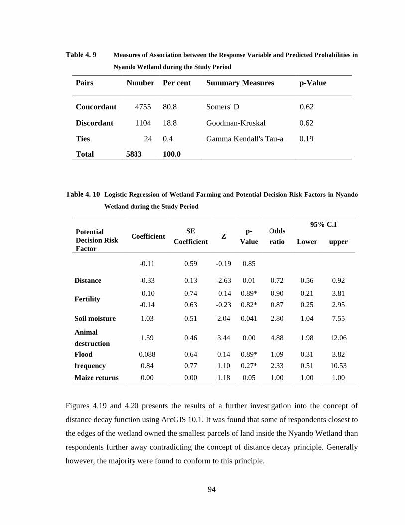
94

Table 4. 9 Measures of Association between the Response Variable and Predicted Probabilities in

Nyando Wetland during the Study Period

Pairs Number Per cent Summary Measures p-Value

Concordant 4755 80.8 Somers' D 0.62

Discordant 1104 18.8 Goodman-Kruskal 0.62

Ties 24 0.4 Gamma Kendall's Tau-a 0.19

Total 5883 100.0

Table 4. 10 Logistic Regression of Wetland Farming and Potential Decision Risk Factors in Nyando

Wetland during the Study Period

Potential

Decision Risk

Factor

Coefficient SE

Coefficient Z

p-

Value

Odds

ratio

95% C.I

Lower upper

-0.11 0.59 -0.19 0.85

Distance -0.33 0.13 -2.63 0.01 0.72 0.56 0.92

Fertility -0.10 0.74 -0.14 0.89* 0.90 0.21 3.81

-0.14 0.63 -0.23 0.82* 0.87 0.25 2.95

Soil moisture 1.03 0.51 2.04 0.041 2.80 1.04 7.55

Animal

destruction 1.59 0.46 3.44 0.00 4.88 1.98 12.06

Flood

frequency

0.088 0.64 0.14 0.89* 1.09 0.31 3.82

0.84 0.77 1.10 0.27* 2.33 0.51 10.53

Maize returns 0.00 0.00 1.18 0.05 1.00 1.00 1.00

Figures 4.19 and 4.20 presents the results of a further investigation into the concept of

distance decay function using ArcGIS 10.1. It was found that some of respondents closest to

the edges of the wetland owned the smallest parcels of land inside the Nyando Wetland than

respondents further away contradicting the concept of distance decay principle. Generally

however, the majority were found to conform to this principle.

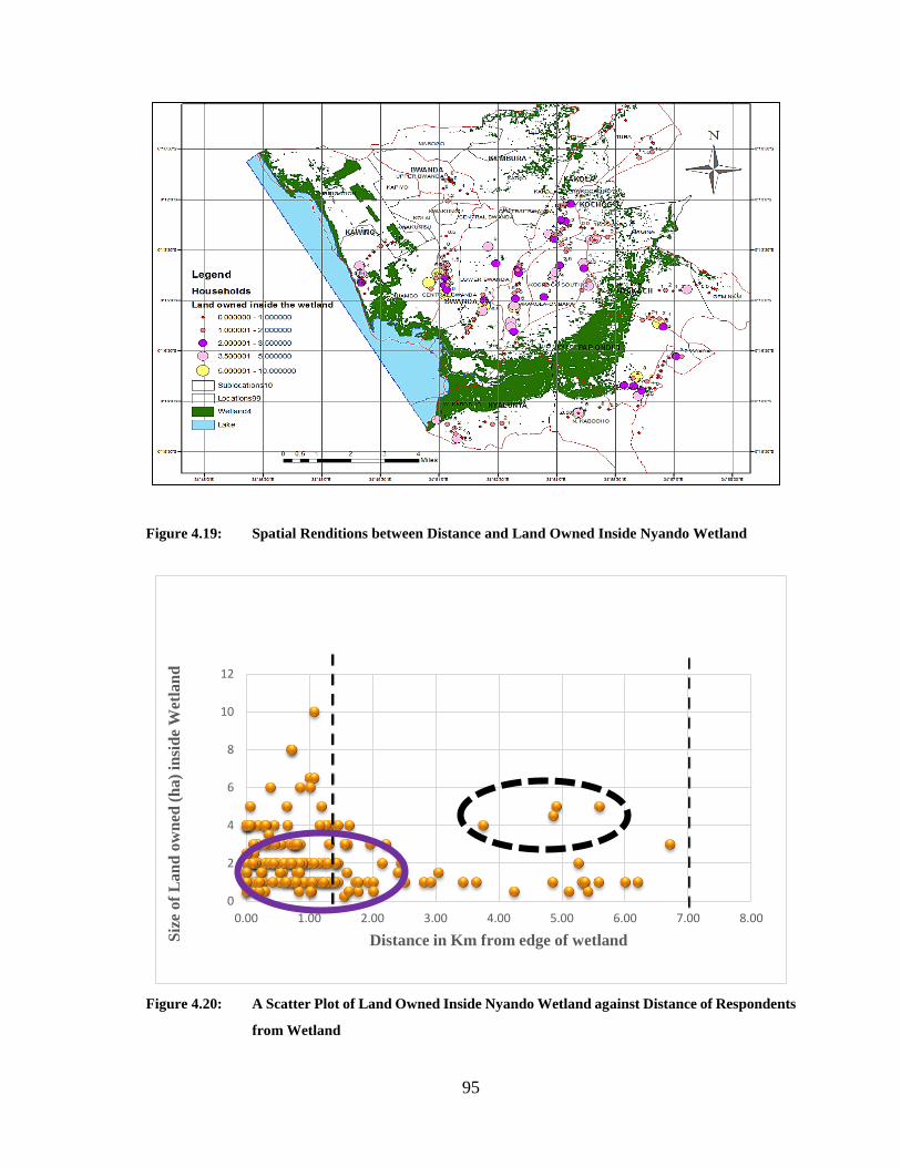
95

0

2

4

6

8

10

12

0.00 1.00 2.00 3.00 4.00 5.00 6.00 7.00 8.00

Siz

e o

f L

an

d o

wn

ed (

ha)

insi

de

Wet

lan

d

Distance in Km from edge of wetland

Figure 4.19: Spatial Renditions between Distance and Land Owned Inside Nyando Wetland

Figure 4.20: A Scatter Plot of Land Owned Inside Nyando Wetland against Distance of Respondents

from Wetland

96

4.3.4 Hypothesis Testing for Objective Two

Stating the second hypothesis to address objective two of the study;

H02: There are no significant changes in human population growth that can be

attributed to the changes in the size of Nyando Wetland.

Or the Alternative;

In a simple linear correlation matrix (Table 4.11), there is a high negative correlation (-0.97)

between the WLTa (wetland area) and population increase as a parameter. Population

increase also has a strong positive relationship with SSAg (0.97) and the RFTw (0.85).

Table 4. 11 Simple Correlations between the Dependent and the Independent Variables in the

Nyando Wetland study

WTLa

(y)

SSAg

(x1)

RFT

w (x2)

OPGb

(x3)

WATr

(x4)

Populatio

n (x5)

MLl

(x6)

WTLa (y) 1.00

SSAg (x1) -0.94 1.00

RFTw (x2) -0.89 0.73 1.00

OPGb (x3) -0.98 0.88 0.97 1.00

WATr (x4) 0.94 -0.92 -0.91 -0.97 1.00

Population (x5) -0.97 0.97 0.85 0.95 -0.94 1.00

MLl (x6) 0.45 -0.31 -0.61 -0.55 0.46 -0.53 1.00

Key: WTLa = Wetland area, SSAg = Small-scale agriculture, WATr = Water area,

RFTw = Rice farms and turbid paddy water surfaces, MLl = Mean Lake Level,

OPGb = Open grassland, mixed bushes with exposed bare ground

Note: The numeric values denote the extent to which any of the variables are correlated to the wetland area

(WTLa) which is the dependent variable.

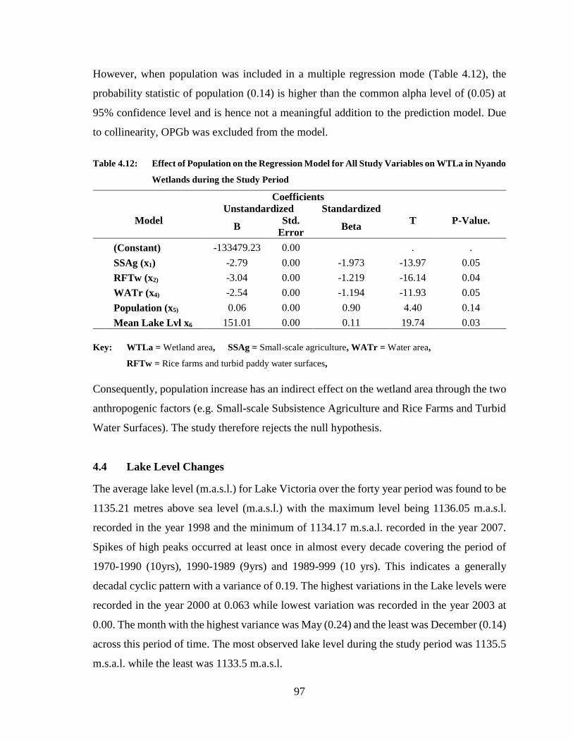
97

However, when population was included in a multiple regression mode (Table 4.12), the

probability statistic of population (0.14) is higher than the common alpha level of (0.05) at

95% confidence level and is hence not a meaningful addition to the prediction model. Due

to collinearity, OPGb was excluded from the model.

Table 4.12: Effect of Population on the Regression Model for All Study Variables on WTLa in Nyando

Wetlands during the Study Period

Coefficients

Model

Unstandardized Standardized

T P-Value. B

Std.

Error Beta

(Constant) -133479.23 0.00 . .

SSAg (x1) -2.79 0.00 -1.973 -13.97 0.05

RFTw (x2) -3.04 0.00 -1.219 -16.14 0.04

WATr (x4) -2.54 0.00 -1.194 -11.93 0.05

Population (x5) 0.06 0.00 0.90 4.40 0.14

Mean Lake Lvl x6 151.01 0.00 0.11 19.74 0.03

Key: WTLa = Wetland area, SSAg = Small-scale agriculture, WATr = Water area,

RFTw = Rice farms and turbid paddy water surfaces,

Consequently, population increase has an indirect effect on the wetland area through the two

anthropogenic factors (e.g. Small-scale Subsistence Agriculture and Rice Farms and Turbid

Water Surfaces). The study therefore rejects the null hypothesis.

4.4 Lake Level Changes

The average lake level (m.a.s.l.) for Lake Victoria over the forty year period was found to be

1135.21 metres above sea level (m.a.s.l.) with the maximum level being 1136.05 m.a.s.l.

recorded in the year 1998 and the minimum of 1134.17 m.s.a.l. recorded in the year 2007.

Spikes of high peaks occurred at least once in almost every decade covering the period of

1970-1990 (10yrs), 1990-1989 (9yrs) and 1989-999 (10 yrs). This indicates a generally

decadal cyclic pattern with a variance of 0.19. The highest variations in the Lake levels were

recorded in the year 2000 at 0.063 while lowest variation was recorded in the year 2003 at

0.00. The month with the highest variance was May (0.24) and the least was December (0.14)

across this period of time. The most observed lake level during the study period was 1135.5

m.s.a.l. while the least was 1133.5 m.a.s.l.

98

The highest fluctuation peaks were experienced in the months of May, June and July 1990

and 1998 when the levels rose to 1136.4 m.a.s.l. Such high levels were also observed in the

same months in 1999. The lowest levels were recorded in the months of March and October

over the 40-year period. It was also observed that the first decade between 1970 and 1979

recorded the highest average Lake level of 1135.48 m.a.s.l. while the least average level was

experienced in the final decade of 2000 and 2009 (1134.82 m.a.s.l.). In regard to the daily

levels observed, the highest level was 1136.4 metres from 30th May to 1st June, 1998 and the

lowest level observed was 1133.78 m.a.s.l. on 29th March, 2007. Consequently, the

fluctuations of Lake Victoria levels were observed to have attained negative maximum

amplitude of 2.62 m.a.s.l. during the period between 1970 and 2010.

Heterogeneity tests were performed on 7 classes of Lake level data taken on a daily basis

over a 40-year period overlapping the study period. It was found that the frequency

distribution of the Lake level is heterogeneous. A generally declining trend of the lake levels

was observed over the study period with peak levels in June/July of each year. This was

found to be significant (=19734.12, df =234, p < 0.00). The 3D plot showing the general

declining trends of the fluctuation over time is presented in Figure 4.21.

Figure 4.21: A Three Dimensional Plot Showing the Annual versus Monthly Variation in the Lake

Victoria Levels at Kisumu Gauging Station from 1970 to 2010

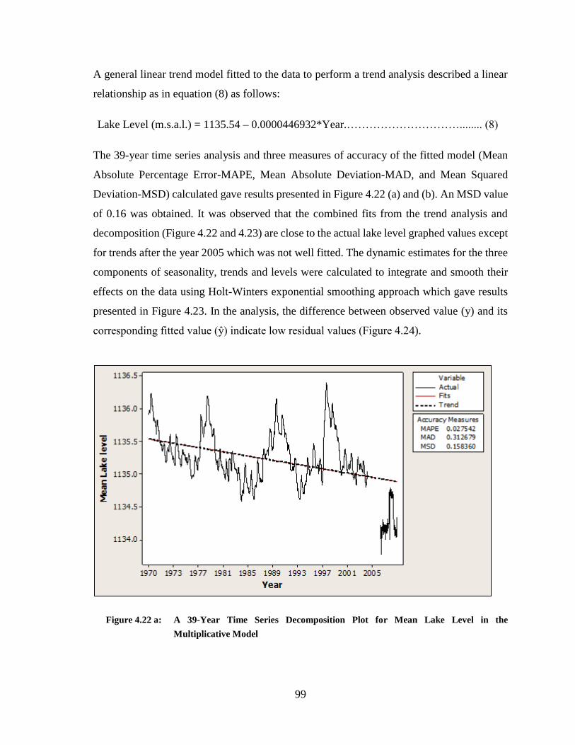
99

A general linear trend model fitted to the data to perform a trend analysis described a linear

relationship as in equation (8) as follows:

Lake Level (m.s.a.l.) = 1135.54 – 0.0000446932*Year.…………………………........ (8)

The 39-year time series analysis and three measures of accuracy of the fitted model (Mean

Absolute Percentage Error-MAPE, Mean Absolute Deviation-MAD, and Mean Squared

Deviation-MSD) calculated gave results presented in Figure 4.22 (a) and (b). An MSD value

of 0.16 was obtained. It was observed that the combined fits from the trend analysis and

decomposition (Figure 4.22 and 4.23) are close to the actual lake level graphed values except

for trends after the year 2005 which was not well fitted. The dynamic estimates for the three

components of seasonality, trends and levels were calculated to integrate and smooth their

effects on the data using Holt-Winters exponential smoothing approach which gave results

presented in Figure 4.23. In the analysis, the difference between observed value (y) and its

corresponding fitted value (ŷ) indicate low residual values (Figure 4.24).

Figure 4.22 a: A 39-Year Time Series Decomposition Plot for Mean Lake Level in the

Multiplicative Model

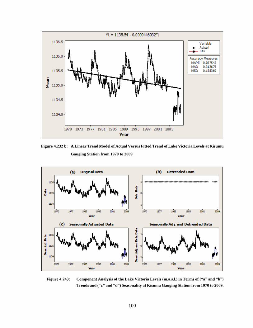
100

Figure 4.232 b: A Linear Trend Model of Actual Versus Fitted Trend of Lake Victoria Levels at Kisumu

Gauging Station from 1970 to 2009

Figure 4.243: Component Analysis of the Lake Victoria Levels (m.a.s.l.) in Terms of (“a” and “b”)

Trends and (“c” and “d”) Seasonality at Kisumu Gauging Station from 1970 to 2009.

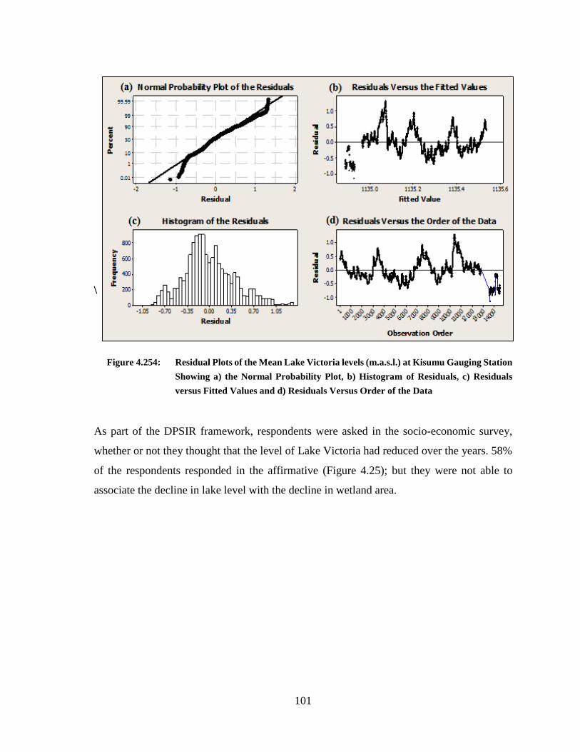
101

\

Figure 4.254: Residual Plots of the Mean Lake Victoria levels (m.a.s.l.) at Kisumu Gauging Station

Showing a) the Normal Probability Plot, b) Histogram of Residuals, c) Residuals

versus Fitted Values and d) Residuals Versus Order of the Data

As part of the DPSIR framework, respondents were asked in the socio-economic survey,

whether or not they thought that the level of Lake Victoria had reduced over the years. 58%

of the respondents responded in the affirmative (Figure 4.25); but they were not able to

associate the decline in lake level with the decline in wetland area.

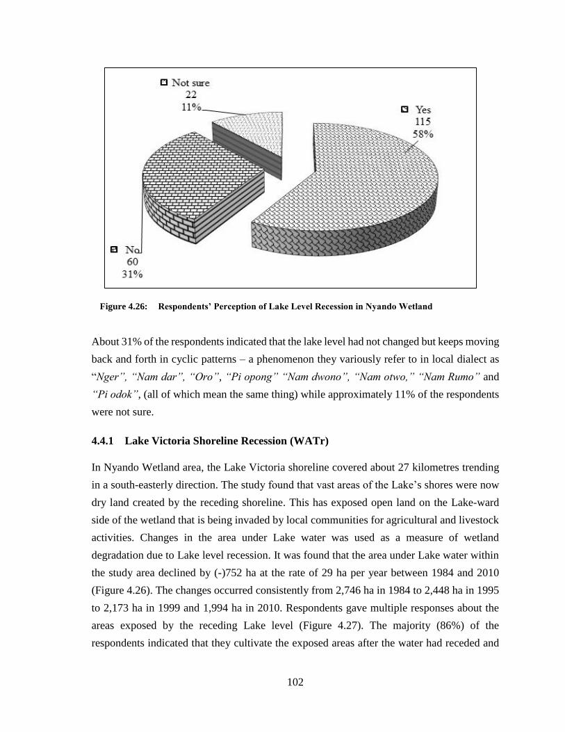
102

Figure 4.26: Respondents’ Perception of Lake Level Recession in Nyando Wetland

About 31% of the respondents indicated that the lake level had not changed but keeps moving

back and forth in cyclic patterns – a phenomenon they variously refer to in local dialect as

“Nger”, “Nam dar”, “Oro”, “Pi opong” “Nam dwono”, “Nam otwo,” “Nam Rumo” and

“Pi odok”, (all of which mean the same thing) while approximately 11% of the respondents

were not sure.

4.4.1 Lake Victoria Shoreline Recession (WATr)

In Nyando Wetland area, the Lake Victoria shoreline covered about 27 kilometres trending

in a south-easterly direction. The study found that vast areas of the Lake’s shores were now

dry land created by the receding shoreline. This has exposed open land on the Lake-ward

side of the wetland that is being invaded by local communities for agricultural and livestock

activities. Changes in the area under Lake water was used as a measure of wetland

degradation due to Lake level recession. It was found that the area under Lake water within

the study area declined by (-)752 ha at the rate of 29 ha per year between 1984 and 2010

(Figure 4.26). The changes occurred consistently from 2,746 ha in 1984 to 2,448 ha in 1995

to 2,173 ha in 1999 and 1,994 ha in 2010. Respondents gave multiple responses about the

areas exposed by the receding Lake level (Figure 4.27). The majority (86%) of the

respondents indicated that they cultivate the exposed areas after the water had receded and

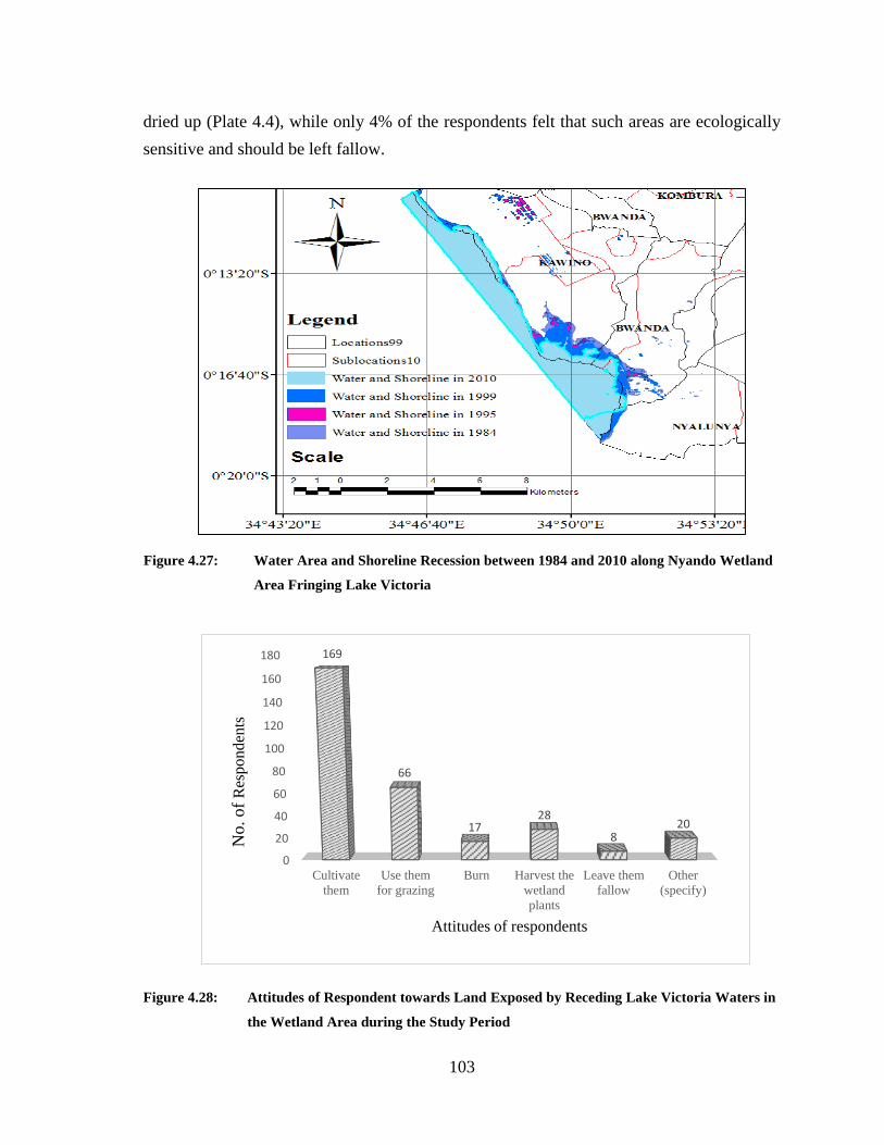
103

dried up (Plate 4.4), while only 4% of the respondents felt that such areas are ecologically

sensitive and should be left fallow.

Figure 4.27: Water Area and Shoreline Recession between 1984 and 2010 along Nyando Wetland

Area Fringing Lake Victoria

Figure 4.28: Attitudes of Respondent towards Land Exposed by Receding Lake Victoria Waters in

the Wetland Area during the Study Period

0

20

40

60

80

100

120

140

160

180

Cultivate

them

Use them

for grazing

Burn Harvest the

wetland

plants

Leave them

fallow

Other

(specify)

169

66

1728

820

No. of

Res

ponden

ts

Attitudes of respondents

104

Plate 4.4 Area Exposed by Receding Lake Victoria Water Level Currently Under Cultivation

on the Lake-Ward Side of Nyando Wetland

4.4.2 Spatial and Temporal Changes in the Area of Nyando Wetland (WTLa)

The area covered by WTLa category decreased from 6,514 ha in 1984 to 5,582 ha in 1995

especially in areas such as West Kano Irrigation Scheme, Ogenya and Ugwe and minimally

at Siginda in Kakola-Ombaka sub-location forming a thin band of WTLa, about 0.2-1.0 km,

along the edges of the wetland. In 1995, some incursions were also noted in Wasare and

Magina sub-location areas ranging from 0.2 km to 3.3 km into the wetland. The Lake-ward

edges of the wetland in nearly all other riparian sublocations were least affected during this

period as shown by the bright green renditions on the map in Figure 4.28.

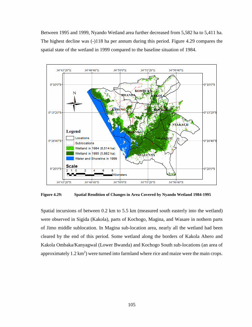
105

Between 1995 and 1999, Nyando Wetland area further decreased from 5,582 ha to 5,411 ha.

The highest decline was (-)118 ha per annum during this period. Figure 4.29 compares the

spatial state of the wetland in 1999 compared to the baseline situation of 1984.

Figure 4.29: Spatial Rendition of Changes in Area Covered by Nyando Wetland 1984-1995

Spatial incursions of between 0.2 km to 5.5 km (measured south easterly into the wetland)

were observed in Sigida (Kakola), parts of Kochogo, Magina, and Wasare in nothern parts

of Jimo middle sublocation. In Magina sub-location area, nearly all the wetland had been

cleared by the end of this period. Some wetland along the borders of Kakola Ahero and

Kakola Ombaka/Kanyagwal (Lower Bwanda) and Kochogo South sub-locations (an area of

approximately 1.2 km2) were turned into farmland where rice and maize were the main crops.

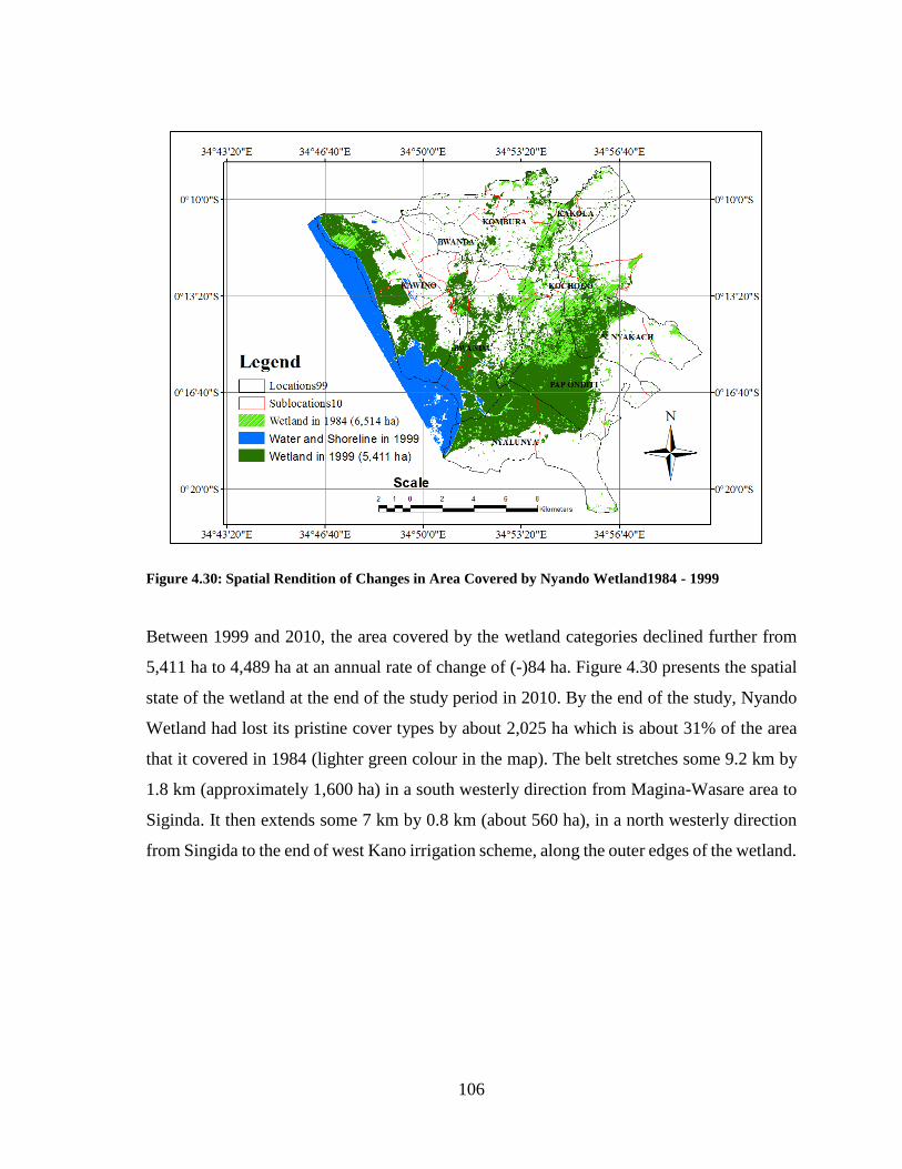
106

Figure 4.30: Spatial Rendition of Changes in Area Covered by Nyando Wetland1984 - 1999

Between 1999 and 2010, the area covered by the wetland categories declined further from

5,411 ha to 4,489 ha at an annual rate of change of (-)84 ha. Figure 4.30 presents the spatial

state of the wetland at the end of the study period in 2010. By the end of the study, Nyando

Wetland had lost its pristine cover types by about 2,025 ha which is about 31% of the area

that it covered in 1984 (lighter green colour in the map). The belt stretches some 9.2 km by

1.8 km (approximately 1,600 ha) in a south westerly direction from Magina-Wasare area to

Siginda. It then extends some 7 km by 0.8 km (about 560 ha), in a north westerly direction

from Singida to the end of west Kano irrigation scheme, along the outer edges of the wetland.

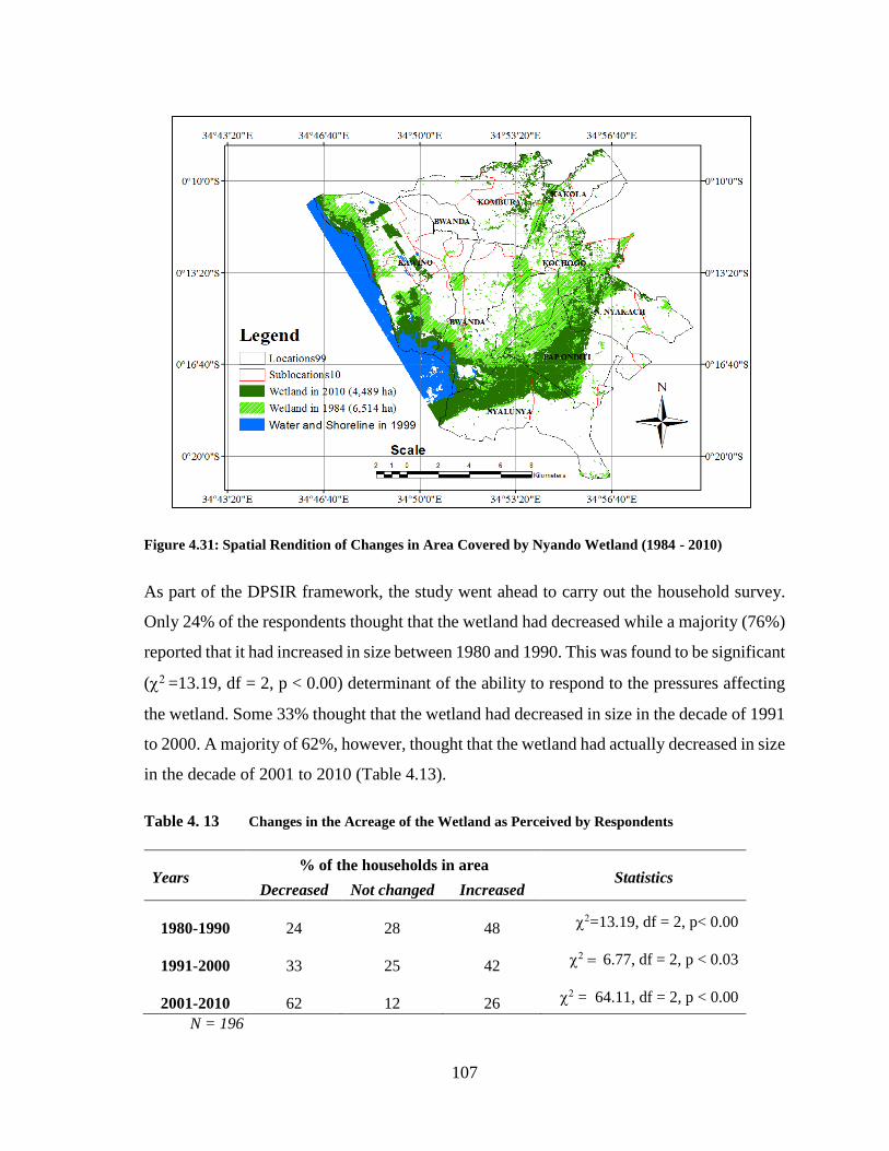
107

Figure 4.31: Spatial Rendition of Changes in Area Covered by Nyando Wetland (1984 - 2010)

As part of the DPSIR framework, the study went ahead to carry out the household survey.

Only 24% of the respondents thought that the wetland had decreased while a majority (76%)

reported that it had increased in size between 1980 and 1990. This was found to be significant

(=13.19, df = 2, p < 0.00) determinant of the ability to respond to the pressures affecting

the wetland. Some 33% thought that the wetland had decreased in size in the decade of 1991

to 2000. A majority of 62%, however, thought that the wetland had actually decreased in size

in the decade of 2001 to 2010 (Table 4.13).

Table 4. 13 Changes in the Acreage of the Wetland as Perceived by Respondents

Years % of the households in area

Statistics Decreased Not changed Increased

1980-1990 24 28 48 =13.19, df = 2, p< 0.00

1991-2000 33 25 42 6.77, df = 2, p < 0.03

2001-2010 62 12 26 = 64.11, df = 2, p < 0.00

N = 196

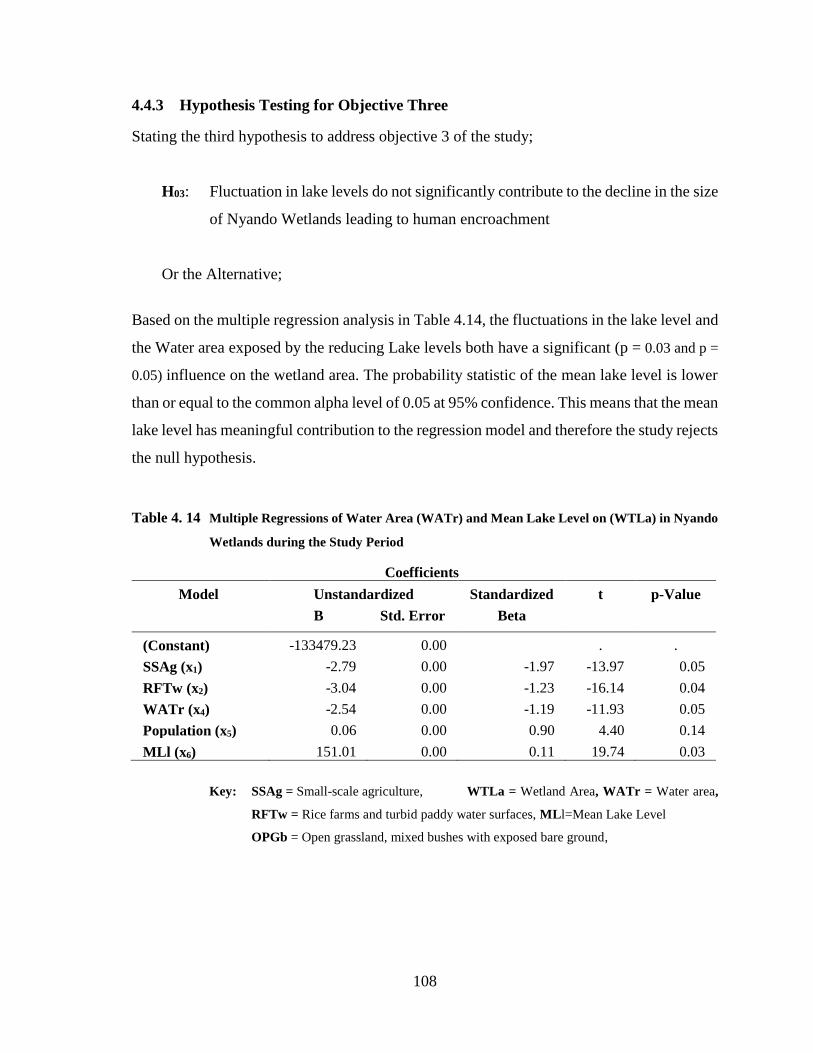
108

4.4.3 Hypothesis Testing for Objective Three

Stating the third hypothesis to address objective 3 of the study;

H03: Fluctuation in lake levels do not significantly contribute to the decline in the size

of Nyando Wetlands leading to human encroachment

Or the Alternative;

Based on the multiple regression analysis in Table 4.14, the fluctuations in the lake level and

the Water area exposed by the reducing Lake levels both have a significant (p = 0.03 and p =

0.05) influence on the wetland area. The probability statistic of the mean lake level is lower

than or equal to the common alpha level of 0.05 at 95% confidence. This means that the mean

lake level has meaningful contribution to the regression model and therefore the study rejects

the null hypothesis.

Table 4. 14 Multiple Regressions of Water Area (WATr) and Mean Lake Level on (WTLa) in Nyando

Wetlands during the Study Period

Coefficients

Model Unstandardized Standardized t p-Value

B Std. Error Beta

(Constant) -133479.23 0.00 . .

SSAg (x1) -2.79 0.00 -1.97 -13.97 0.05

RFTw (x2) -3.04 0.00 -1.23 -16.14 0.04

WATr (x4) -2.54 0.00 -1.19 -11.93 0.05

Population (x5) 0.06 0.00 0.90 4.40 0.14

MLl (x6) 151.01 0.00 0.11 19.74 0.03

Key: SSAg = Small-scale agriculture, WTLa = Wetland Area, WATr = Water area,

RFTw = Rice farms and turbid paddy water surfaces, MLl=Mean Lake Level

OPGb = Open grassland, mixed bushes with exposed bare ground,

109

4.5 Analysis of Results

The values of anthropogenic and hydrodynamic drivers (variables) that were measured in the

study indicate spatial and temporal change between 1984 and 2010 with regard to the

observed degradation and loss of wetland area. While the wetland area reduced by 31% and

the area covered by the waters of Lake Victoria in the wetland decreased by 27%, the

combined increase of small-scale subsistence agriculture and area under rice cultivation was

21% as open grasslands increased by 18% and the human population increased by 57%

(Table 4.15). The interpretation of this scenario is that agriculture based variables including

rice cultivation driven by the needs of the increasing population and water area could be

driving wetland loss in the study area as further analyzed in the following paragraphs.

Table 4. 15 Data Values for the Dependent and Explanatory Variables in Nyando Wetland during

the Study Period

Year Wetland

Area (y)

Land Use Elements/Parameters

Population(x5)

Mean

Lake

Level

(x6) SSAg

(x1) RFTw

(x2)

OPGb

(x3) WATr

(x4)

1984 6514.20 8460.00 1329.30 6647.40 2745.90 53521.50 1134.89

1989 6353.55 9064.35 1011.15 6544.35 2723.40 60440.00 1135.47

1995 5882.40 9307.80 1264.50 6794.10 2448.00 66225.00 1135.03

1999 5411.25 9551.25 1517.85 7043.85 2172.60 68849.00 1135.84

2009 5095.35 9794.70 1771.20 7293.60 1897.20 80066.00 1134.28

2010 4489.20 9975.60 1817.10 7420.50 1994.40 84266.50 1134.50

Key: SSAg = Small-scale agriculture RFTw = Rice farms and turbid paddy water surfaces WTLa =

Wetland area, OPGb = Open grassland, mixed bushes with exposed bare ground, WATr =

Water area,

The simple linear correlation matrix (in Table 4.11) presents how the variables relate with

each other. In the table, a negative correlation was found between wetland area (dependent

variable) and SSAg, RFTw, OPGb, and population (independent variables). The OPGb had

the highest negative correlation coefficient (-0.98) followed by population (-0.97), SSAg (-

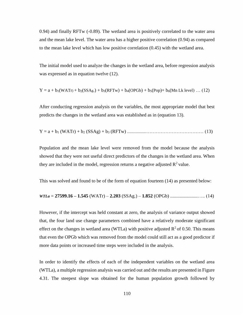
110

0.94) and finally RFTw (-0.89). The wetland area is positively correlated to the water area

and the mean lake level. The water area has a higher positive correlation (0.94) as compared

to the mean lake level which has low positive correlation (0.45) with the wetland area.

The initial model used to analyze the changes in the wetland area, before regression analysis

was expressed as in equation twelve (12).

Y = a + b1(WATr) + b2(SSAg.) + b3(RFTw) + b4(OPGb) + b5(Pop)+ b6(Mn Lk level) … (12)

After conducting regression analysis on the variables, the most appropriate model that best

predicts the changes in the wetland area was established as in (equation 13).

Y = a + b1 (WATr) + b2 (SSAg) + b3 (RFTw) ................……………………………… (13)

Population and the mean lake level were removed from the model because the analysis

showed that they were not useful direct predictors of the changes in the wetland area. When

they are included in the model, regression returns a negative adjusted R2 value.

This was solved and found to be of the form of equation fourteen (14) as presented below:

WTLa = 27599.16 – 1.545 (WATr) – 2.203 (SSAg.) – 1.852 (OPGb) .......................….. (14)

However, if the intercept was held constant at zero, the analysis of variance output showed

that, the four land use change parameters combined have a relatively moderate significant

effect on the changes in wetland area (WTLa) with positive adjusted R2 of 0.50. This means

that even the OPGb which was removed from the model could still act as a good predictor if

more data points or increased time steps were included in the analysis.

In order to identify the effects of each of the independent variables on the wetland area

(WTLa), a multiple regression analysis was carried out and the results are presented in Figure

4.31. The steepest slope was obtained for the human population growth followed by

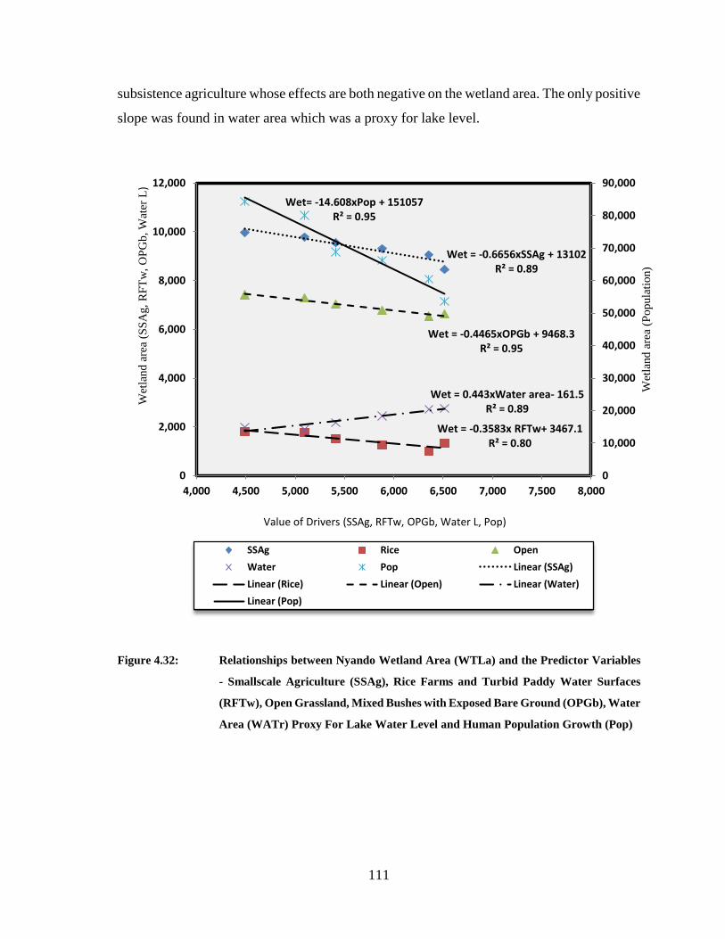
111

subsistence agriculture whose effects are both negative on the wetland area. The only positive

slope was found in water area which was a proxy for lake level.

Figure 4.32: Relationships between Nyando Wetland Area (WTLa) and the Predictor Variables

- Smallscale Agriculture (SSAg), Rice Farms and Turbid Paddy Water Surfaces

(RFTw), Open Grassland, Mixed Bushes with Exposed Bare Ground (OPGb), Water

Area (WATr) Proxy For Lake Water Level and Human Population Growth (Pop)

Wet = -0.6656xSSAg + 13102R² = 0.89

Wet = -0.3583x RFTw+ 3467.1R² = 0.80

Wet = -0.4465xOPGb + 9468.3R² = 0.95

Wet = 0.443xWater area- 161.5R² = 0.89

Wet= -14.608xPop + 151057R² = 0.95

0

10,000

20,000

30,000

40,000

50,000

60,000

70,000

80,000

90,000

0

2,000

4,000

6,000

8,000

10,000

12,000

4,000 4,500 5,000 5,500 6,000 6,500 7,000 7,500 8,000

Wet

land

are

a (P

op

ula

tio

n)

Wet

land

are

a (S

SA

g,

RF

Tw

, O

PG

b, W

ater

L)

Value of Drivers (SSAg, RFTw, OPGb, Water L, Pop)

SSAg Rice Open

Water Pop Linear (SSAg)

Linear (Rice) Linear (Open) Linear (Water)

Linear (Pop)

112

CHAPTER FIVE

5.0 DISCUSSION

The findings of the present study are discussed in relation to how the decline in the area

covered by the wetland has been influenced by anthropogenic and hydrodynamic drivers

operating in the study area during the study period. The drivers include various types of land

cover/uses found in the study area such as the small-scale subsistence agriculture; rice farms

and turbid paddy water surfaces; open grassland, mixed bushes with exposed bare ground

and; area covered by Lake Victoria waters. These were mapped with an overall classification

accuracy of 87% and overall kappa statistic of 0.86. The accuracies achieved were typical of

those achievable when satellite imagery of the level of resolutions used in this study are used

as data sources and therefore acceptable and comparable to those of other studies such as

Congalton and Green (1999), Lu, et al. (2004), Maheu-Giroux and de Blois (2005), Ozdogan,

et al. (2006), Maxa and Bolstad (2009) and Beekhuizen and Keith (2010). With these

accuracy levels in mind, it is clear that the rapid human population growth and the declining

Lake Victoria water level, when combined with the demands for human use, constitute

unrelenting negative driving forces of environmental change in Nyando Wetland. The

interactions among these factors are leading to an unprecedented decline in the wetland size

and degradation of its natural resources (Ogello, Obiero and Munguti, 2013).

The results show that the area under small-scale subsistence agriculture, which is one of the

drivers, has expanded from 8,460 ha to 9,976 ha (an increase of 17.95%) while rice farms

and turbid paddy water surfaces increased from 1,329 ha to 1,817 ha (an increase of 36.7%)

during the period under study. The land cover changes caused by these two agricultural

categories recorded an increase of 8% to stand at 46% of the study area by 2010. This

observation is comparable to Olang, Kundu, Bauer and Fürst (2011) who recorded a 44.1%

agricultural cover for 1986 in the entire Nyando river basin meaning that the general trend

of increase in this land use category is similar in most parts of the basin. Between 1984 and

2010, the study found that the small-scale subsistence agriculture category recorded the

highest rate of increase of 10% (77 ha per year) in the Nyando Wetland study area. This

increase could be attributed to the initiatives of sugar cane out-grower companies to expand

cane growing in the Nyando basin. Several out growers companies and societies such as

113

Onyisa, Janam, Disi Muti-Purpose Out-growers Associations and New Odiembo Farmers’

Cooperative Society were formed and these groups operated in the lower Nyando basin (i.e.

Ahero, Kimira, Kochogo and Kakola-Ombaka) to promote sugarcane farming for Miwani

Sugar Factory. However, between 1995 and 1997 after the factory collapsed there was a

corresponding decline in the annual rate of land cover change for this particular category

because many farmers abandoned growing sugar cane leaving some farms fallow. Many of

these fallows converted to open grassland, mixed bushes with exposed bare ground.

All other factors held constant, it may however, be concluded that about 58 ha of new

agricultural areas were on average created each year in the study area over the 26 year period

(1984 to 2010). Even though there may be minor differences of findings, especially in

magnitude of change reported by this study as compared to other findings such as those of

Olang’, et al., (2011) and Muiruri, Wenninger, van Griensven, Uhlenbrook and Khisa,

(2012), the trends in the results are all consistent that there is an unprecedented increase the

Small-scale Agriculture category. Observed variations in magnitude could be attributed to

methodological approaches, data sources, resolutions and non-uniformity in class definitions

common in most land use studies worldwide (Gils, et al., 1991; Bronsveld, et al., 1994,

Liverman and Cuesta, 2008,). However, from a physical scientific view, the import of this

observation is that as this category of land use continues to increase, there will be a

corresponding decrease in the area covered by Nyando Wetland.

This is even clearer when it is considered that 54%, 53% and 52% of the households

significantly increased their cropland between the periods of 1980 to 1990, 1991 to 2000 and

2001 to 2010 respectively. Most of these expansions were reported to occur in and around

the wetland with a strong statistically significant level (r2 = -0.94; R2 = 0.89) and were also

observed in satellite image derived map layers prepared during the study. The observed moon

shaped south-easterly rippled progression of conversions from wetland cover type to

agricultural categories indicates the expansion of this category in the study area is creating

great agricultural pressure that will significantly reduce the size and cause fragmentation of

the wetland (Wood and Halsema, 2008; Orwa, et al., 2012). Much as pressure on the wetland

driven by the need for more agricultural land was reported in this study, the respondent’s

also highly ranked damage by animals, insects and disease and human-wildlife (especially

114

the human-hippoptamus) conflict as constraints to cropland expansion into the wetland.

Studies carried out by Gerakisa, et al. (1998), Svotwa, Ngwenya, Manyanhaire and Jiyane,

(2007), Lamarque, et al., (2009) and Pachaur, (2014) elsewhere also attributed this sort of

conflict to human population growth creating the need for more agricultural land, which

drives expansion of crop farming and industrial activities such as disposal of wastes into

fragile ecosystems like Nyando Wetland.

On the other hand, the rice farms and turbid paddy water surfaces, which is an agricultural

land use category, experienced a 5% drop in area between 1984 and 1995, followed by a

steady increase up to the end of 2010 at an average increase of 19 ha per annum. The drop in

area under this category could be attributed to shortage of water in most rice growing areas

(Otieno, 1996), especially in the northern parts of the study area. During this period, the study

found that there was a shortage of irrigation water, which was partly attributed to interference

with farmers’ water drawing systems at the time of construction of the irrigation canals and

associated infrastructure such as outlet gates for Nyatini and West Kano schemes. This was

started in 1991 and ended in 1993. The farmers had difficulty accessing the water from a

deepened river Nyatini thus; reducing their area of command. The irrigation infrastructure

was commissioned in late 1993 (Leereveld and Otieno, 1995). This combined with drought

frequency (Ambeje, Gitonga and Kerkmann, 2009; Omondi, 2010; Muvundja, et al., 2014)

that occurred during this period explains the drop in area under this category in the 1980s

and part of the 1990s.

Effective utilization of the irrigation infrastructure began in 1994 with farmers progressively

expanding the areas under the category at the rate of 19 ha per annum. A proliferation of

private millers providing some sort of ready market for the farmers and promotional activities

by these millers buttressed the expansion efforts for this category (Otieno, 1996), leading to

the observed increases of this cover type in the subsequent periods. This category was

observed even in the middle of the wetland and with a strong positive correlation (r2 = -0.89;

R2 = 0.80) with the declining wetland area. Its continued expansion could lead to habitat

modifications not compatible with normal wetland functions and result in an irreversible

change in the ecological character of the wetland (Ramsar Convention Secretariat, 2010).

115

This notwithstanding, the moderate to severe drought conditions reported in the study area

for the period between 1995 and 2000 by Awange, et al. (2007) and Huho, Ngaira and

Ogindo (2010) is believed to have not only influenced the rice farms and turbid paddy water

surfaces category thereby affecting the wetland; but also the dynamics of open grassland,

mixed bushes with exposed bare ground in the study area. In these studies, rainfall during

the years from 1961 to 1999 was abnormally lower than 25% of the normal average amounts

in the study area. They also observed that the number of drought events and severity which

are predisposing conditions for the development and expansion of this land cover category

were also increasing in the last 3 decades. This could explain the expansion of open

grassland, mixed bushes with exposed bare ground. In 1994, this land use category covered

26% of the study area but later increased to about 29% at an annual rate of 30 ha per year

especially in the southern parts of the study area. About 10% of the changes were found in

areas previously occupied by small-scale agriculture, especially sugarcane, at the edges of

the wetland. Consequently, this study attributes the increases in this category to both climate

change related changes such as increased drought events (Ambeje, et al., 2009; Omondi,

2010; Obiero, et al., 2012; Muvundja, et al., 2014) and the abandonment of sugarcane fields

due to the collapse of Miwani sugar factory during the same period. Many of these sugarcane

fields that could not support other agricultural activities such as horticulture and maize or

rice farming converted to fallow areas and developed into open grassland, mixed bushes with

exposed bare ground.

This is especially clearer when it is noted that the highest increase in open grassland, mixed

bushes with exposed bare ground category occurred between 1995 and 1999 and coincided

with the period of abandoning of the sugarcane fields. A strong negative correlation (r2 = -

0.98; R2= -0.95) was found between open grassland, mixed bushes with exposed bare ground

and the declining wetland area. This means that as its dominance increases with all other

factors held constant, the wetland area will continue to decline especially in areas where

grazing and related destructive human activities are dominant. In many instances, even

elsewhere, the magnitude of change in response to grazing for most wetland attributes is

variable; but responses are often negative, with very occasional exceptions Morris and Reich,

(2013). Extensive grazing in Nyando Wetland (Obiero, et al., 2012) has therefore the

potential of changing the biophysical characteristics of the wetland ecosystem in ways that

116

could make it suitable for colonization and dominance by open grassland, mixed bushes with

exposed bare ground (Reeves and Champion, 2004).

Human population growth is closely (r2 = -0.97; R2 = -0.95) associated with the decline of the

area of Nyando Wetland. This is especially important when it is considered that more than

eighty two per cent (82.1%) of the human population in the study area were in the age group

between twenty one (21) and sixty (60) years, which is agriculturally active and rapidly

growing. For instance, the populations of Kakola, Kochogo and North Nyakach locations

increased by 178%, 107% and 70% respectively as the entire study area’s population grew

at the highest compounded growth rates of 4.63% between 1979 and 1989. This was above

(1.7% more than) the national growth rates of 2.9 % during the same period (KNBS, 1990).

The growth rate however dropped to 2.1% between 1989 and 1999 and finally settling at

2.7% in 2009, which was slightly below the national average growth rate of 3% (KNBS,

2010). Results however, showed that this population has a doubling time of fifteen (15) years

and if the rates were held constant from 1979, it was expected to hit the doubling mark in

1994; but it doubled in 1997. It was three (3) years lower than the Malthusian generalized

proposition of about 25 years doubling times for populations of developing countries such

as that of the study area (Haupt and Kane, 2004). This implies that a slowing down but still

rapid population growth is experienced in the study area which has implications in the use

of the resources of Nyando Wetland. A slowing down rate of growth in human population

has also been reported by KNBS (2010) and attributed to population control and management

activities in the area and the county at large. The designs and implementation of these

population control and management activities such as family planning education and

awareness campaigns needs to be enhanced by the county government to integrate

population, environment/climate change and development initiative to interest target

communities.

The results presented in this study show that the demographic momentum, which has resulted

in high human population growth and densities (356.5 persons per km2), has an indirect

influence on the riparian households’ drive to extend their croplands into the wetland areas

where there is enough soil moisture for all-year-round agricultural activities. The momentum

117

has ensured that each individual’s share of arable land outside the wetland has concomitantly

continued to decrease with the increasing human population resulting in smaller and

overused plots. Consequently, the local people have been compelled to look for alternative

land to their formal land holdings elsewhere. In the households’ perceptions as measured in

the study, such land is available in the wetland because their ancestors once lived there and

were displaced by an expanding wetland since the 1950s. This wetland, in their view, is now

moving back to where it used to be before the 1950’s hence the urge to reclaim their right.

In the wetland, their land shortage problems, land quality issues including soil fertility

affecting yields and the droughts affecting crops appear to be solved. Increasing human

populations living in a limited area often add agricultural and resource use demands leading

to the degradation of an ecosysten (Cohen, 1999; Benedick, 2000; Liverman and Cuesta,

2008; Ben-Edigbe, 2009; AFIDEP and PAI, 2012). Similar studies elsewhere, also concur

that such degradation worldwide are caused by the mounting utility pressure of a rapidly

growing human populations (Benedick, 2000; Owino and Ryan 2007; MEMR, 2012).

In Nyando wetland, there has been widespread resource degradation during the past 26 years.

The degradation has taken the form of wetland fragmentation and a reducing wetland area

which could compromise its biophysical and socio-ecological functions.

As it emerged from this study, the number of years of human activities in the wetland among

the households ranged between 2 and 58 years with a mean of 18.52. This means that some

of the local people have been utilizing the wetland for close to 6 decades. It is however,

noteworthy that about 31% of the respondents in the study area had owned these parcels

inside the wetland area for a period of between 1 and 10 years, 31% between 11 to 20 years,

18% between 21, to 30 years, 6% between 41 to 50 years and only 3% had been utilizing the

wetland area for more than 51 years. The differences in the number of years of ownership

(activities) between the various categories of land users were found to be statistically

significant. This could imply that since wetland ecosystems often attract human populations

from far-flung areas with the motivation of farming and grazing, the study area population could

be having a segment that is immigrant in nature (Liz, 2003; Kadigi and Mdoe, 2004). Thus

besides the normal growth that comes with the natural population increases through the

balance of births and deaths, there is an immigrant population among this agriculturally

118

active population who began to acquire land in the wetland only recently. Such a trend could

cause a conflict between wetland conservation and the human uses which would most likely

worsen with increasing human population size around the wetland (Mvula and Haller, 2009;

Kioko and Okello, 2010).

The proposition is further strengthened by about 6% of the total respondents in the survey

that were not well fitted by the model because of a high delta Chi (χ2) that caused a high

Pearson Residual. This could indicate that these respondents were not from the riparian

communities or were recent immigrants who had poor knowledge of the issues that were

being investigated or that their responses were simply unreliable. About 62% of the study

population seems to have acquired ownership in the last two (2) or so decades and rental/lease

tenured segment (4%) within the last decade. This implies that even though activity has been

going on in the wetland for close to several decades, there is a segment of new entrants into

the wetland farming activity. However, this could also be associated with the spatial

variations in distance-decay parameter estimates, which are ascribed to variations in user-

resource interaction decision-making processes as influenced by distance from the wetland

as a resource (Fotheringham, 1981; Verma, et al., 2013). In the study, the odds ratio for

distance was estimated at 0.28. It means that for each additional unit increase in distance

from the wetland, the odds of wetland farming decreased by 28% all other factors held

constant. This shows a relatively weak influence of a distance as deterrent on farming inside

the wetland (Brant, 1990; Verma, et al., 2013).

As presented in the scatter plot, distance from where a household lives to the location of the

wetland does not have a strong influence on the farmers’ decisions to move into the wetland,

open it up and set up farmlands in it. This does not conform to known principles of distance-

decay as espoused by Fotheringham (1981) and can be attributed to other factors much

stronger than distance operating in the study area. The odds ratio for maize returns, which

was signifying fertility or productivity of wetland soils, was further examined and found to

be 1.0. This however meant that for each unit increase in maize returns, while the other

variables were held constant, the odds of wetland farming do not change at all. This could be

explained by the fact that the values of maize returns is given in thousands of Shillings.

Therefore, a 1 shilling increase would bear a negligible effect on the decision of a farmer to

119

farm inside the wetland instead of utilizing his land outside the wetland. Furthermore, animal

destruction was significant in this particular model and is reported by many respondents but

the other benefits of wetland farming alleviate the effects of this variable in the model. Other

variables such as fertility change (z = -0.14, p = 0.89) (z = -0.23, p = 0.82) and flood

frequency (z = 0.14, p = 0.89), (z = 0.10, p = 0.27) have p-values greater than 0.05 hence

they do not have statistically significant effects on wetland farming. This may be so because

of the way the questions were put to respondents or because returns from wetland activities

smother the effects of these variables in the model. On the other hand, it was established that

for every unit increase in soil moisture whose odds ratio is 2.80. The odds of wetland farming

increased by 180% all other factors held constant. This typifies a very strong influence and

appears to be the strongest attraction to the wetland which is overriding the element of

distance-decay among other factors.

In this regard, the respondents ranked as second priority the lack of “water/drought at 16%.

This shows that the competition for natural resources in the wetland is driven by the search

for areas where water is constantly available for crops and livestock. Consequently, besides,

fertility influenced by flooding events and decayed wetland organic matter; the main “pull”

factor to these areas is availability of all-year-round adequate soil moisture. This assures

higher crop production and economic returns for the farmers activities in such areas and is

comparable to findings of Kairu (2001), Dobiesz, et al. (2010), Adero and Kiema 2011) and

LVBC 2011. According to the local people, this factor causes them to encroach the wetland

area for agricultural crop farming. This has led to the intensification of agricultural activities

on the banks of river Nyando mainly on the flood plains in the lower reaches, at the edges of

the wetland and inside the wetland as observed from the satellite image data. Consequently,

at least 85% of the households, sampled in this study, relied on the wetland area for

subsistence agricultural activities.

With all the above factors at play in the study area, increasing human population implies

increased resource use now and in the future (KNBS, 2010; NCPD, 2013; National Academy

of Sciences, 2015). The human population growth has a strong relationship with small-scale

subsistence agriculture and Rice farms and turbid paddy water surfaces. There is however a

negative adjusted R2 value when it is included in a multiple regression model indicating that

120

regressing it along with these other variables is not meaningful. This is because population

increase per-se does not necessarily have a direct influence on the area of the wetland. Its

influence depends on the socio-economic characteristics of the population in question and is

location and technology specific (Ningala, et al., 2008). Tiffen, et al., (1994) suggests a

similar explanation in their findings. In this study, the regression model suggests that

population growth affects the wetland area, indirectly through the anthropogenic activities,

that is small-scale subsistence agriculture and Rice farms and turbid paddy water surfaces.

This fact coupled with the fact that sixty three (63%) of households use a combination of

methods to clear the wetland habitat for agricultural purposes could imply a gloomy future

for Nyando Wetland. It could mean that, for the last 3 or so decades, respondents have been

using all manner of tools and methods at their disposal to reclaim the wetland for agricultural

expansion and encroachment (Chikomo, 2014). This is regardless of whether the tools and

methods are environmentally friendly or not. The result echoes the principles of the “tragedy

of the commons” in the use of common property resources as expounded by Hardin (1968)

and Mvula and Haller (2009). The apparently “free” access to the resources of the wetland

and the pressures generated by the drivers of change (UNDP, 2009) in space and time

presents the motive of uncontrolled utility approaches laced with high potential for

degradation and detriment for the wetland.

This fact coupled with the fact that sixty three (63%) of households use a combination of

methods to clear the wetland habitat for agricultural purposes could imply a gloomy future

for Nyando Wetland. It could mean that, for the last 3 or so decades, respondents have been

using all manner of tools and methods at their disposal to reclaim the wetland agricultural

expansion and encroachment (Chikomo, 2014). This is regardless of whether the tools and

methods are environmentally friendly or not. The result echoes the principles of the “tragedy

of the commons” in common property resources use as expounded by Hardin (1968) and

Mvula and Haller (2009). The apparently “free” access to the resources of the wetland and

the pressures generated by the drivers of change (UNDP, 2009) in space and time presents

the motive of uncontrolled utility approaches laced with high potential for degradation and

detriment for the wetland.

121

The Driver-Pressure-State-Impact-Response framework of analysis (OECD, 1994;

Millennium Ecosystem Assessment, 2005; Zhang and Fujiwara, 2007; Arthurton, et al.,

2008; Valkering, et al., 2009) used in this study has provided useful insights into the

underlying causal relationships between human activities, resultant impacts on the Nyando

Wetland and concomitant responses. Analysis within the framework has shown that there is

evidence of fragmentation and habitat change caused by the impacts of anthropogenic and

hydrodynamic drivers on the Nyando Wetland. For instance, between 1980 and 1990, a

significant proportion (47%) of the respondents (χ2 = 9.02, df = 2, p < 0 05) reported that

there is a progressive decline of indigenous birds in the wetland. They have been replaced

by shoals of grain eating birds exotic to the area which are pests to their crops. Between the

periods of 1991-2000 and 2001-2010, there were massive increases in these birds

(44.68, df = 2, p < 0.00 and 71.16, df = 2, p < 0 05), respectively. This signifies an

impact of habitat change occasioned by conversion of more land in the wetland into

agricultural fields (Mensing, Galatowitsch and Tester, 1998; Chikomo, 2014), largely of

grains attracting the granivourous birds and is comparable to what Syphard and Garcia

(2001) found in their studies elsewhere. The changes in the habitat could trigger grave

consequences not only for the physico-chemical functions of the wetland but also its

biodiversity and other ecosystem services it offers to the environment.

The situation is further complicated by the receding lake level exposing an area prone to

agricultural invasion (Obiero, et al., 2012; Rongei, et al., 2013). The area exposed by the

receding shoreline observed by the present study, which signifies Lake level changes was (-

) 752 ha at an annual rate of change of 29 ha over the 26-year period. This observation

compares with Obiero, et al. (2012) which found that as much as 1,336.3 ha of new land had

been left behind by the receding lake. Even though the two studies give different results, the

concurrence that there is an exposed area is significant. The quantitative differences could

be as a result of time-frames, methods applied and the area covered by both studies. The

results of regression analysis showed that if all other factors were held constant in an analysis

of all other variables against the wetland area, 94.5% of the reductions in Nyando Wetland

area could be accounted for by the decrease in the water area due to the shifting shorelines.

Further, analysis of Lake level data showed that the average Lake level reduced by 1.88

metres. With the highest levels (1136.05 m.s.a.l.) recorded in year 1998 to its lowest (1134.17

122

m.s.a.l.) recorded in 2007. If however, the period between 1970 and 2010 was considered,

the decline reached a maximum amplitude of 2.62 m over a 40-year-period. There were clear

decadal cyclic patterns (every 9 to 10 years) of high and low peaks and an overall variance

of 0.19. A best-fit trend line drawn through the peaks exhibited a generally declining gradient

during the study period. Similar results were obtained by the Republic of Kenya, (2004);

Kull (2006), Kiwango and Wolanski (2008), Ambeje, et al. (2009), Vuglinskiy, et al. (2009),

Omondi (2010), Adero and Kiema, (2011) and Muvundja, et al. (2014).

The declining gradient further indicates a reducing lake level, which has the effect of moving

the water of Lake Victoria away from the wetland. This progressively opening up areas of

new rich and moist lacustrine land on the shoreline areas as the Lake recedes. This creates

conditions that promote fragmentation of the wetland as observed in earlier studies (Rongei,

et al., 2013). Given the obvious link between a low Lake level and a declining wetland area,

a strong correlation was anticipated. However, while there is a strong correlation between

the area exposed by the shifting shoreline and the declining wetland area (r2 =0.94, R2 = 0.89),

there was a low linear correlation between the declining wetland area and the declining mean

lake levels (r2 = 0.45). The probability statistic of the mean Lake level was higher than the

common alpha level of 0.05 at 95% confidence. This could mean that the correlation of Lake

level with wetland area is affected by other factors such as sedimentation at the mouth of

River Nyando.

The effects of this could be seen in north-westerly extents of the shoreline located in the

irrigation scheme and parts of southern and south western Kadhiambo sub-locations. An area

that did not experience much shift compared to other shoreline areas located near the delta

of the river Nyando. Differences in the magnitude of shifts in these areas could be attributed

to the high levels of sediment loads deposited (Gikuma-Njuru, 2010) at the mouth of River

Nyando. This load significantly modifies the depth of Lake levels and subjects this area to

accelerated desiccation and conversion into drier land areas, thereby distorting the

relationships. The findings of this study compares well with those by Mungai, Swallow,

Mburu, Onyango and Njui (2004), and Tobella (2009) who cited sedimentation visible as a

plume on satellite imagery at the mouth of river Nyando, as a cause for concern in the wetland

and the gulf area. This is especially important because accelerated sedimentation could

123

enhance drying up processes of large areas of lake-wetland littoral zones as the shoreline

retreats with declining Lake level (Azza, 2006).

The Lake level data measured at station 1HB04 and analyzed by this study over a 40-year

period indicates that while the Lake’s level has been declining over the years, Lake Victoria

has held it most observed mean at 1135.5 m.s.a.l. which was above the long-term mean for

the Lake of 1135.0 m.s.a.l. However, abnormally low decadal peaks observed, after the year

2005 distorts this relatively stable cyclic pattern and suggests a sudden and significant

accelerated decline. The drop was also found by Kite (1982), Awange, et al. (2008), Adero

and Kiema (2011) and Khisa, et al. (2013). This could be explained by a combination of

factors ranging from the variability in rainfall trends, prolonged long-term and short-term

droughts, decrease in river flows to crustal movements. However, the most likely explanation

so far is the ambitious expansion programme of the Owen Falls Dam (Nalubaale) in Uganda.

After 1977, a hydropower bypass was set up at the Ruzizi. In addition to this the Ruzizi

channel was dredged and widened, these activities seems to have disturbed the Lake level

regime considerably (Muvundja, et al., 2014).

Since, 1993 the Ugandan government has been expanding the hydro-power generation

capacity by constructing a second dam about 1 Kilometre downstream of the Nalubaale dam

across the White Nile, which has greatly modified the Lake’s outlet. It is possible that after

commissioning in 2003, the power company operating the dams may have drawn too much

water through to meet rising demands for electricity both nationally and regionally. It is

reported (Muvundja, et al., 2014) that they have been using water at a rate of 20% to 50%

above the allowable discharge agreed on between Uganda and Egypt in 1957 (USDA, 2005;

Kull, 2006; Kiwango and Wolanski, 2008). Consequently, the areas occupied by Lake

Victoria are expected to continue to shrink away from shoreline wetlands as long as the

situation is not addressed. Shrinking Lake level conditions could create dry conditions

denying the wetland, which has a lateral hydrological connectivity to the Lake such as

Nyando its hydro-graphic requirements for proper functioning (Khisa, et al., 2013). Such a

condition could promote increased agricultural activities in the wetland and worsen its future.

Further research is however required to determine the relativeness between the water use at

Ruzizi and the decline in the Lake levels.

124

CHAPTER SIX

6.0 CONCLUSIONS AND RECOMMENDATIONS

6.1 Conclusions

Nyando Wetland is an ecosystem besieged by unrelenting negative forces of environmental

change which are anthropogenic and hydro-dynamic in nature. These forces have led to an

unprecedented decline in the area of the wetland and degradation of its natural resources. In

addressing the first objective of the study, it was concluded that there are significant changes

in area covered by various land uses between 1984 and 2010. The areas exposed by the

declining area of the wetland have been occupied largely by small-scale subsistence

agriculture. The areas under the greatest pressure of agricultural encroachment are in the

north-western, northern and north-eastern parts of the wetland and are largely characterized

by fertile flood plain deposit from frequent fluvial and flood events.

Based on the second objective of the study, it is concluded that during the 1979 to the 1989

period, significant differences in population increases occurred in a generally rapid

exponential growth. Although the population growth rate has levelled off, its relative

constancy is a major cause for concern for the resources of Nyando Wetland. It is further

concluded that the population growth, per see, does not seem to have a direct influence on

the changes in the wetland area but causes indirect changes through the anthropogenic

activities whose magnitude expands in space and time in response to the growing population

size.

Data derived from studying the third objective led to the conclusion that fluctuations of Lake

Victoria water level is a cyclic event which occurs almost every decade with the lowest level

and steepest declining trends recorded after 2005. Subsequent decline thereafter, were mainly

due to adverse human activities and to a limited extent climatic variations (frequent

droughts). Therefore both the fluctuations in Lake level and the decrease in the water area

occasioned by the shifting shoreline as a result of the declining Lake level had a strongly

significant relationship to the declining wetland area, all other factors held constant.

125

6.2 Recommendations

The study therefore recommends as follows;

1. The County Government of Kisumu and non-governmental organizations operating

in the study are such as VIRED international, VI-Agro and care-Kenya should as

matter of priority, promote programs that encourage local communities to embrace

innovation and agricultural systems that increase production through vertical

expansion such as aquaponics, use of improved drought and disease resistant high

yielding crop varieties and organic farming with proper control and management of

their ecological effects in the neighbourhoods of the wetland.

2. The organizations should also encourage income diversification as a strategy for

reducing exploitation pressure on the resources of Nyando wetland.

3. A joint effort among the County Government of Kisumu, NEMA, various

development partners and the local communities should urgently be initiated to

develop and implement a participatory Wetlands’ Management Plan (WMP) that

focusses on the conservation and effective management of Nyando Wetland for its

long-term health.

4. The County Government of Kisumu, National Environment Management Authority

(NEMA) and the development partners in the study area should promote participatory

wetland rehabilitation of degraded areas. Such a promotions should embrace wise use

principles that integrate non-destructive uses of the wetland’s resources to reduce

livelihood pressures on the wetland.

5. While reproductive health is a human right, the National Council for population

Development, the County Government of Kisumu and local non-governmental

organizations should empower local community institutions such village community

workers, with sufficient knowledge and resources to encourage the local

communities to balance such rights with development. This should be aimed at

creating an environment suitable for a successful transition from current family sizes

126

to smaller and ecologically sensitive families to reduce population growth rates in

the study area.

6. The County and National Government, especially the National Environment

Management Authority (NEMA), should ensure that Nyando Wetland is treated as

fragile common property resource on the edge of degradation and should be

conserved through clear policy frameworks based on public trust doctrines reinforced

with sound traditional practices. The conservation should thus embrace wise use

principles postulating that the wetland is vital for the survival of people, plants and

animals living on or near it and therefore must be protected by the local communities

from further degradation for the common good.

7. The organizations, such as VIRED International, presently carrying out education

and awareness activities on the importance of ecologically friendly wetland

management practices in the study area, should intensify their efforts to stem the rapid

loss of the area covered by the wetland.

8. There should be close and effective joint monitoring and control of non-returnable

abstraction of waters for socio-economic development from Lake Victoria by a joint

body with jurisdiction in the countries riparian to Lake Victoria such as the East

African Community to ensure compliance with the “agreed curve” agreements.

9. The stakeholder institutions such as NEMA, LBDA, Ministry of Water and LVBC

should take the lead in ensuring checks against over-release of Lake water for

hydropower production and measures for sustainable land and water management not

only in the Nyando Wetland study area but also in the entire basin.

10. Finally, the combination of remote sensing, GIS and socio-ecological tools in a mixed

methods research is recommended as an effective approach for wetland ecosystem

studies which can offer timely conservation data, even for physically inaccessible

areas of the wetland. However, there is need for higher resolution imagery to improve

accuracy of results for well-targeted interventions.

127

6.3 Areas for Further Research

1. Integrated and participatory adaptive research to stimulate quick responses

and regenerative actions that could restore and conserve the wetland

ecosystem should be carried out in the study area.

2. Further research on the extent to which the human induced area reduction in

the size of Nyando Wetland would compromise the biochemical functions of

the ecosystem especially with a focus on the nutrient budgets of the wetland

should be conducted

3. The effects of sedimentation on the future of biodiversity in Nyando Wetland

should be studied.

4. A quantification of the hydrological drawdown effects of the declining water

levels of Lake Victoria on Nyando Wetland should be carried out.

5. The links between sedimentation and wetland desiccation in Nyando Wetland

ecosystem should be investigated.

6. The links between the water use at Ruzizi in Uganda and the declining Lake

levels should be studied in more detail.

7. Indigenous knowledge and sustainable wetland management practices for the

Nyando Wetland ecosystem should be studied.

8. The potential of Nyando Wetland for alternative uses such tourism as a

pressure release mechanism for sustainable management of the wetland

should be investigated.

128

REFERENCES

Adero, N. J. & Kiema, J. B. K. (2011). Flow based structural modelling and dynamic

simulation of Lake water levels. In: T. M. Gasmelseid, (Ed.), Handbook of research

on hydroinformatics: technologies, theories and applications (pp. 316-331). Hershey

Pennsylvania: IGI Global.

AFIDEP & PAI, (2012). “Population, climate change, and sustainable development in

Kenya”. Nairobi and Washington, DC: African Institute for Development Policy

(AFIDEP) and Population Action International (PAI). Retrieved from:

http://pai.org/wp-content/uploads/2013/01/Kenya_PIB_Final.pdf.

Agresti, A. (2002). Categorical data analysis, (2nd Edition). New York: John Wiley & Sons,

Agwanda A. & Amani H., (2014). Population growth, structure and momentum in Tanzania.

Dar es Salaam: THDR 2014: Background paper No. 7, ESRF Discussion paper 61.

Economic and Social Research Foundation.

Al-Khudhairy, D. H. A., Leemhuis, C., Hofhnann V., Shepherd, I. M., Calaon. R.,

Thompson, J. R., Gavin, H., Gasca-Tucker, D. L, Zalldls, Q., Bilas G. & Papadlmos,

D. (2002). Monitoring wetland ditch water levels using Landsat TM and ground-

based measurements. Photogrammetric Engineering & Remote Sensing, 68 (8), 809-

818.

Ambeje, P., Gitonga, I. & Kerkmann, J. (2009). Prolonged drought in Kenya (2003-2009).

Kenya Meteorological Department and, EUMETSAT-Monitoring Weather and

Climate from Space. Retrieved from:

http://oiswww.eumetsat.org/WEBOPS/iotm/iotm/20091001_drought/20091001_dro

ught.html.

Amezaga, J. M., Santamaría, L. & Green, A. J. (2002). Biotic wetland connectivity;

supporting new approach for wetland policy. Acta Oecologica, International Journal

of Ecology, 23, 213–222.

Anderson, J. R., Hardy, E. E., Roach, J. T. & Witmer, R. E. (1976). A land use and land

cover classification system for use with remote sensor data. Washington DC: U. S.

Geological Survey, Professional Paper 964. Retrieved from:

http://www.pbcgis.com/data_basics/anderson.pdf.

129

Anifowoshe, T. O. (1990). ‘Food production; problems and prospects. GeoJournal, 20 (3),

243–247.

Arthurton, R., Le Tissier, M., Snoussi, M., Kitheka, J., Shaghude, Y., Kane, A., Flöser, G. &

Kremer, H. (2008). Global change assessment and synthesis of river catchment -

coastal sea interactions and human dimensions in Africa. AfriCat: LOICZ - LOICZ

Reports and Studies No. 30, pp. LOICZ IPO, Geesthacht, Germany. Retrieved from:

http://www.ihdp.unu.edu/docs/Publications/LOICZ/Reports/loicz-Report-30.pdf.

Assel, R. A., Quinn, F. H. and Sellinger C. E. (2004). Hydroclimatic factors of the recent

record drop in Laurentian Great Lakes water levels. American Meteorological

Society. (pp 1143-1153). DOI: 10.1175/BAMS-85-8-1143.

Awange, J. L., Aluoch, J., Ogallo, L.A., Omulo, M. & Omondi, P. (2007). Frequency and

severity of drought in the Lake Victoria region (Kenya) and its effects on food

security. Climate Research, 33, 135–142.

Awange, J. L., Ogalo, L., Bae, K. H., Were, P., Omondi, P., Omute, P. & Omullo, M. (2008).

Falling Lake Victoria water levels: is climate a contributing factor? Climate Change.

89, 281-297.

Azza, N. (2006). The dynamics of shoreline wetlands and sediments of northern Lake

Victoria (Doctoral Dissertation, UNESCO-IHE Institute for Water Education,

Wageningen University, Delft, The Netherlands). Retrieved from:

https://www.google.com/?client=firefox-

b#q=Azza%2C+N.+(2006).+The+dynamics+of+shoreline+wetlands+and+sediment

s+of+northern+Lake+Victoria+(Doctoral+Dissertation%2C+UNESCO-

IHE+Institute+for+Water+Education%2C+Wageningen+University%2C+Delft%2

C+.

Baker, C., Lawrence, R. L., Montagne, C. & Patten, D. (2007). Change detection of wetland

ecosystems using Landsat imagery and change vector analysis. Wetlands, 27(3), 610–

619.

Barbier, E. B., Acreman, M. C. & Knowler, D. (1997). Economic valuation of wetlands: A

guide for policy makers and planners. Gland, Switzerland: Ramsar Convention

Bureau,

http://www.ramsar.org/sites/default/files/documents/pdf/lib/lib_valuation_e.pdf.

130

Beekhuizen, J. & Keith, C. C. (2010). Toward accountable land use mapping: using geo-

computation to improve classification accuracy and reveal uncertainty. International

Journal of Applied Earth Observation and Geo-information, 12, 127–137.

Benedick, R. E. (2000). Human population and environmental stresses in the twenty-first

century. Features. Environmental Change & Security Project Report, Issue 6. In

Kreibich R. and Simonis, U, E. (Eds). Globaler wandel-global change: Berlin:

Ursachenkomplexe und Lösungsansätze. [Global Transformation-Global Change:

Causal Structures, Indicative Solutions]. Retrieved from:

https://www.ciaonet.org/attachments/12465/uploads.

Ben-Edigbe, J. (2009). Constrained multivariate land use model for population growth.

European Journal of Scientific Research, 38 (3), 411-424.

Bennun, L. A. & Njoroge P. (1999). Important bird areas in Kenya. Nairobi, Kenya: The

East Africa Natural History Society.

Berg, K. A. (2001, July-August). Historical attitudes and images and the implications on

carnivore survival. Endangered Species Update, 18, pp.185–189.

Berkes, F. & Folke, C. (2002). Back to the future: ecosystem dynamics and local knowledge.

In L. Gunderson and C. S. Holling, (Eds) (2002). Panarchy: understanding

transformations in human and natural systems (pp. 121–144). Washington, DC.

USA: Island Press.

Berkes, F., Kofinas, G. P. & Chapin F. S. (2009). Conservation, community and livelihoods.

In: F. .S. Chapin, III, G. P. Kofinas and C. Folke. (Eds) (2009). Principles of

ecosystem stewardship: resilience-based resource management in a changing world

(pp. 129-147). New York: Springer-Verlag.

Biging, G. S., Chrisman, N. R., Colby, D. R., Congalton, R. G., Dobson, J. E., Ferguson, R.

L., Goodchild, M. F., Jensen, J. R. & Mace, T. H. (1999). Accuracy assessment of

remote sensing-detected change detection. Monograph Series. MD, USA: American

Society for Photogrammetry and Remote Sensing (ASPRS).

Brant, R. (1990). Assessing proportionality in the proportional odds model for ordinal

logistic regression. Biometrics, 46, 1171-1178.

Bronsveld, K., Chutrittanapan, S., Pattanakanok, B., Suwanwerakamtorn, R. & Trakooldit,

P.S. (1994). The use of local knowledge in land use/land cover mapping from satellite

images. ITC Journal, 4; 349-358.

131

Brundtland, G. H. (1993). Population, environment and development. Rafael M. Salas

Memorial Lecture, 28 September 1993 (pp. 1-16). New York: United Nations

Population Fund (UNFPA).

Bullock, A., Gilman K., McCartney M., Waughray D., Blyth K. & Andrews A. (1998).

Hydrological strategy to develop and manage African wetland resources for

sustainable agricultural use. Wetland characterization and classification for

sustainable agricultural development, Part III. Rome: FAO/SAFR. Retrived from

www.fao.org.

Burrow, P. A. & MacDonnell, R. A. (1998). Principles of geographic information system.

Spatial information systems and geostatistics (pp 1-292). New York: Oxford

University Press.

Chikomo, T. (2014). Community perceptions of environmental indicators for management

of wetland important bird areas in Kenya. Doctoral Dissertation. Kenya: University

of Nairobi. Retrieved from:

https://www.google.com/search?q=Community+perceptions+of+environmental+in

dicators+for+management+of+wetland+important+bird+areas+in+Kenya&ie=utf-

8&oe=utf-8&client=firefox-b.

Cohen, J. (1999). Human population growth and tradeoffs in land-use. In S. C. Szaro, (Ed.)

(1999); Ecological stewardship: A common reference for ecosystem management

(pp. 677-702). New York: Elsevier Science. Retrieved from:

http://lab.rockefeller.edu/cohenje/PDFs/277CohenHumanPpnGrowthEcologicalSte

wardship1999.pdf.

Cohen, J. E. (2008). Make secondary education universal, Nature, 456, 572–573.

Congalton, R. G. & Green K. (1999). Assessing the accuracy of remotely sensed data:

principles and practices (pp. 10-180). London/New York: Lewis Publishers.

Convention on Wetlands of International Importance especially as Waterfowl Habitat,

Ramsar (Iran), (1971). UN Treaty Series No. 14583. As amended by the Paris

Protocol, 3 December 1982, and Regina Amendments, 28 May 1987. Retrieved from:

http://portal.unesco.org/en/ev.php-

URL_ID=15398&URL_DO=DO_TOPIC&URL_SECTION=201.html.

Cowardin, L. M., Carter, V., Golet, F. C. & LaRoe, E. T. (1979). Classification of wetlands

and deep-water habitats of the United States. U. S. Department of the Interior, Fish

132

and Wildlife Service, Washington, D.C. Jamestown, ND: Northern Prairie Wildlife

Research Center. Retrieved from:

http://www.npwrc.usgs.gov/resource/wetlands/classwet/index.htm.

Crafter, S. G., Njuguna, S. G. & Howard, G. W. (Eds) (1992, July). Wetlands of Kenya.

Proceedings of the KWWG seminars on wetlands of Kenya. 3rd- 5th July, 1991.

Nairobi, Kenya: National Museums of Kenya.

Dahl, T. E. (2006, September). Remote sensing as a tool for monitoring wetland habitat

change. In Aguirre- C., Bravo, P. J., Pellicane, D., Burns P. & Draggan, S. (Eds)

(2006). Monitoring science and technology symposium: unifying knowledge for

sustainability in the western hemisphere: Proceedings, 2004 September 20-24, (pp.

1-8); Denver, Co. RMRS-P-42CD. Fort Col/ins, CO: U.S: Department of Agriculture,

Forest Service, Rocky Mountain Research Station.

https://www.fws.gov/wetlands/Documents%5CRemote-Sensing-as-a-Tool-for-

Monitoring-Wetland-Habitat-Change.pdf

Davis, J., Sim, L. & Chambers, J. (2010). Multiple stressors and regime shifts in shallow

aquatic ecosystems in antipodean landscapes. Freshwater Biology, 55 (1), 5–18.

DHV Consulting Engineers, (1987). Rural domestic water supply and sanitation programme.

Water resources survey and training programme. Report on Nyakach Division.

Ammersfoort, The Netherlands; DHV Consulting Engineers.

Dixon, B. A. (2005). The sustainable management of headwater wetlands: the role of

indigenous knowledge in South-West Ethiopia. In Libor, J., (Ed) (2005). Sustainable

Management of headwater resources: Research from Africa and India (pp. 60-69).

Tokyo, Japan: United Nations University Press.

Dixon, B. A. & Wood, P. A. (2003). Wetland cultivation and hydrological management in

Eastern Africa; matching community and hydrological needs through sustainable

wetland use. Natural Resources Forum, 27, 117-129.

Dobiesz, N. E., Hecky, R. E., Johnson, T. B., Sarvala, J., Dettmers, J. M., Lehtiniemi, M.,

Rudstam, L. G., Madenjian, C. P. & Witte, F. (2010). Metrics of ecosystem status for

large aquatic systems – a global comparison. Journal of Great Lakes Research, 36,

123–138.

133

Driscoll, D. L., Appiah-Yeboah, A., Salib, P. & Rupert, D. J. (2007). Merging qualitative and

quantitative data in mixed methods research: how to and why Not. Ecological and

Environmental Anthropology. Paper 18: University of Georgia. Retrieved from:

http://digitalcommons.unl.edu/icwdmeea/18.

Dugan, P. J. (1992). Wetland management: A critical issue for conservation in Africa. In:

Matiza T. & Chabwela H. N. (Eds). Wetlands management: A critical issue for

conservation in Africa, wetlands conservation conference for Southern Africa (pp. 1–

8). Gland: IUCN.

Dugan, P. J. (Ed.) (1993). Wetlands in danger – A world conservation atlas. New York:

Oxford University Press.

Duram, L. A., Bathgate J. & Ray, C. (2004). A local example of land-use change: Southern

Illinois-1807, 1938, and 1993. The Professional Geographer, 56 (1): 127–140.

Eastman, R. J., MacKendry, E. J., & Fulk, A. M. (1995). Change and time series analysis.

(2nd edition) Explorations in geographic information systems technology. Vol.1.

Palais des Nations, Geneva 10, Switzerland: United Nations Institute for Training

and Research.

ECOSYSTEMS, (1983). Integrated land use survey. Kisumu Kenya: Lake Basin

Development Authority.

ERDAS Field Guide, (1999). Earth resources data analysis system. (pp 1-628). Atlanta, GA:

ERDAS Inc.

Estes, J. E., Hajic E. J., & Tinney I. (1983). Fundamentals of image analysis: analysis of

visible and thermal infra-red data. In Colwell R. N., (Ed). Manual of Remote Sensing.

Fall Curch V. A: American Society of Photogrametry.

Everitt, J. H., Yang, C. & Deloach, C. J. (2005). Remote sensing of giant reed with quickbird

satellite imagery. Journal of Aquatic Plant Management, 43, 81-85.

Everitt, J. H., Yang, C. & Deloach, C. J. (2008). Comparison of quickbird and SPOT 5

satellite imagery for mapping giant reed. Journal of Aquatic Plant Management, 46,

77-82.

F.A.O., (2011). The state of the world’s land and water resources for food and Agriculture:

Managing systems at risk. Rome, Italy: Food and Agriculture Organization of the

United Nations.

134

Fabrigar, L. R., Wegener, D. T., MacCallum, R. C., & Strahan, E. J. (1999). Evaluating the

use of exploratory factor analysis in psychological research. Psychological Methods,

4, 272-299.

Folke, C. (2006). Resilience: The emergence of a perspective for social–ecological systems

analyses. Global environmental change, 16, 253–267.

Fontana, A. & Frey, J. H. (2000). The interview: from structured questions to negotiated text.

In K. Enzin & Y. S. Lincoln, (Eds). Handbook of qualitative research. 2nd Edition

(pp. 645-672). Thousand Oaks, CA: Sage Publications, Inc.

Foody, G. M. (2002). Status of land cover classification accuracy assessment. Remote

Sensing of Environment, 80, 185–201.

Foody, G. M. & Mathur, A. (2006a). The use of small training sets containing mixed pixels

for accurate hard image classification: Training on mixed spectral responses for

classification by a SVM. Remote Sensing of Environment, 103; 179 -189.

Foody, G. M., Mathur, A., Sanchez-Hernandez, C., & Boyd, D. S. (2006b). Training set size

requirements for the classification of a specific class. Remote Sensing of

Environment, 104; 1–14.

Fotheringham, S. A. (1981). Spatial structure and distance-decay parameters. Annals of the

Association of American Geographers, 71 (3), 425-436.

Fruhling, P. (1996). A liquid more valuable than gold. On the water crisis in Southern Africa,

future risks and solutions. S-105 25, Stockholm, Sweden: Swedish International

Development Cooperation (SIDA).

Fuller, R. M., Wyatt, B. K. & Barr, C. J. (1998). Countryside survey from ground and space:

different perspectives, complementatary results. Journal of Environmental

Management, 54:101-126.

Fung, T. (1992). Land use land cover change detection with Landsat MSS and SPOT HRV

data in Hong Kong. Geocarto International, 3, 33-40.

Garsison, D. G. (2015). Missing values analysis and data imputation. 2015 Edition.

Statistical Associates Blue Book Series (pp 1-26). Statistical Associates Publishing

Geist, H. J. & Lambin, E. F. (2002). Proximate causes and underlying driving forces of

tropical deforestation. BioScience, 52 (2), 143-150.

135

Gerakisa, A. & Kalburtji K. (1998). Agricultural activities affecting the functions and values

of Ramsar wetland sites of Greece. Agriculture, Ecosystems and Environment, 70,

119-128.

Ghirlanda, S., Enquist, M. & Perc, M. (2010). Sustainability of culture-driven population

dynamics. Theoretical Population Biology, 77, 181-188.

Gibbs, A. & Partners (1956). Kenya Nile Basin water resources survey. Nairobi Kenya: Sir

Alexander Gibb Consulting Engineers.

Gichuki, J., Guebas, F. D., Mugo, J., Rabuor, C. O., Triest, L. & Dehairs, F. (2001). Species

inventory and the local uses of the plants and fishes of the lower Sondu Miriu wetland

of Lake Victoria, Kenya. Hydrobiologia, 458, 99-106.

Gidley, S. L. (2009). Using high resolution satellite imagery to map aquatic macrophytes on

multiple lakes in northern Indiana. Master thesis, USA: Indiana University.

Gikuma-Njuru, P. (2010, February). Hydrology of Nyanza gulf and its influence on nutrient

dynamics and functional capacity of Nyando wetlands system. A presentation at the

international symposium on wetlands in a flood pulsing environment, from 1st - 5th.

Global and local - mires and peat lands in the African landscape (2). Maun, Botswana:

University of Waterloo.

Gils, H., Huizing, H., Kannegieter, A. & Zee, D. (1991). The evolution of the ITC system of

land use and land cover classification (LUCC). ITC Journal, 3: 163-167.

Goodwin, P. (2010). The Holt-winters approach to exponential smoothing: 50 years old and

going strong. Hot New Research: FORESIGHT. Retrieved from:

www.forecasters.org/foresight.

Gordon, H. S. (1954). The economic theory of common-property resources. Journal of

political economy, 62(2), 124 - 42.

Grünbühel, C. M. (2005). Identification of gaps and issues in the research on socio-economic

drivers of biodiversity; A long-term biodiversity, ecosystem and awareness research

network. Project no. GOCE-CT-2003-505298.IFF -.ALTER-Net: Institute of Social

Ecology. Retrieved from: www.alter-net.info

Gustard, A. & Wesselink, A. J. (1993). Impact of landuse change on water resources;

Balqluhidder catchments. Journal of hydrology, 145, 389-401.

Haack, B. (1996). Monitoring wetland changes with remote sensing: An East African

example. Environmental Management, 20, 411–419.

136

Hall, F. G., Strebel, D. E. & Nickeson, J. E. (1991). Radiometric rectification: toward a

common radiometric response among multidate, multisensor images. Remote Sensing

of Environment; 35, 11-27.

Hardin, G. (1968). The Tragedy of the Commons. Science, 162, 1243-8.

Haupt, A. and Kane, T. T. (2004). Population handbook, 5th edition, (pp 1-70). Washington,

DC 20009-5728 USA: Population Reference Bureau.

Hecky, R. E., Bootsma, H. A. & Odada, E. O. (2006). African lake management initiatives:

The global connection. Lakes & reservoirs. Research and management, 11, 203-213.

Hierl, L. A., Loftin, C. S., Longcore, J., R., McAuley, D. G. & Urban, D. L. (2007). A

multivariate assessment of changes in wetland habitat for water birds at Moosehorn

National Wildlife Refuge, marine, USA. Wetlands, 27(1), 141–152.

Hobbs, R. J. and Hopkins, A. J. M., (1991). The role of conservation corridors in a changing

climate. In D. A. Saunders & R. J. Hobbs (Eds). Nature conservation 2; the role of

corridors (pp. 281-290). Chipping Norton: Surrey Beatty and Sons.

Hodge, I. & McNally, S. (2000). The values of wetlands: landscape and institutional

perspectives wetland restoration, collective action and the role of water management

institutions. Ecological Economics, 35, 107-118.

Holdren, J. P. & Ehrlich, P. R. (1993). Human population and the human environment.

American Scientist, 62, 282-292.

Hollis, G. E., Holland, M. M., Maltby, E. & Larson J. S. (2000). Wise use of wetlands. Nature

and Resources (UNESCO), 14(1), 2-12.

Hopfenberg, R. & Pimentel, D. (2001). Human population numbers as a function of food

supply. Environment, Development and Sustainability, 3, 1-15.

Houlahan, J. E., Keddy, P. A., Makkay, K. & Findlay, C. S. (2006). The effects of adjacent

land use on wetland species richness and community composition. Wetlands, 26(1),

79-96.

Hues, R. H. & Hues, J. S. (1992). A Directory of African Wetlands (pp 820). IUCN, Gland,

Swizerland, Cambrigde and Nairobi, Kenya / WCM: UK/UNEP,

Huho, J. M., Ngaira, J. K. W. & Ogindo H. O. (2010). Drought severity and their effects on

rural livelihoods in Laikipia District, Kenya. Journal of Geography and Regional

Planning, 3(3), 35-043.

137

ICRAF, (1986). Lake Basin river catchment development; Catchment conservation and

rehabilitation. Kisumu – Kenya: Lake Basin Development Authority.

Islam, Md. A., Thenkabail, P. S., Kulawardhana R. W, Alankara R., Gunasinghe S, Edussriya

C. & Gunawardana A. (2008). Semi-automated methods for mapping wetlands using

Landsat ETM+ and SRTM data. International Journal of Remote Sensing, 29(24),

7077-7106.

Jakubauskas, M., Kindscher K., Fraser A., Debinski D. & Price K. P. Z. (2000). Close range

remote sensing of aquatic macrophyte vegetation cover. International Journal of

Remote Sensing, 21(18), 3533-3538.

Janssen, R., Goosen, H., Verhoeven, M. L., Verhoeven, J. T. A., Omtzigt, A. Q. A., &

Maltby, E. (2005). Decision support for integrated wetland management.

Environmental modelling & software; 20, 215-229.

Jensen, J. (2009). Understanding the links between water, livelihoods and poverty in the

Nyando river basin, Kenya. Master thesis. USA: University of Florida.

Jensen, J. R. (2007). Remote Sensing of the Environment. 2nd edition. Upper Saddle River:

Pearson Prentice Hall.

Jensen, J. R., Hodgeson, M. & Christensen, E. (1986). Remote sensing inland wetlands: a

multispectral approach. Photogrammetric Engineering and Remote Sensing, 52(1),

87-100.

Jensen, J. R., Rutchey, K., Koch, M. S. & Narumalani, S. (1995). Inland wetland change

detection in the everglades water conservation area 2A using a time series of

normalized remotely sensed data. Photogrammetric engineering and remote sensing,

61, 199-209.

JICA-Japan International Co-operation Agency, (1992). Feasibility study on Kano Plain.

Vol: I. Kisumu, Kenya: Lake Basin Development Authority - LBDA.

Johnson, B. R. & Onwuegbuzie, A. J. (2004). Mixed methods research: a research paradigm

whose time has come. American Educational Research Association. Educational

Researcher, 33(7), 14-26.

Johnson, B. R., Onwuegbuzie, A. J. & Turner, L. A. (2007). Toward a definition of mixed

methods research. Journal of Mixed Methods Research, 1(2), 112-133.

138

Kadigi, R. M. J. & Mdoe, N. S. (2004). Should irrigated agriculture in Usangu Basin be

abandoned for Sustainable wildlife management in the Ruaha National Park in

Tanzania? Research Journal of Chemistry and Environment, 8(2), 69-76.

Kairu, J. K. (2001). Wetland use and impact on Lake Victoria, Kenya region. Lakes &

Reservoirs: Research and Management, 6, 117-125.

Kareri, R. W. (1992, July). The ecological and economic values of Kenya’s wetlands. In S.

A. Crafter, S. G. Njuguna, and G. W. Howard (Eds). Wetland of Kenya. Proceedings

of a Seminar on Wetlands of Kenya, 3-5th July 1991 (pp. 99-107). Gland Switzerland:

IUCN

Kassenga, G. R. (1997). A descriptive assessment of the wetlands of the Lake Victoria Basin

in Tanzania. Resources Conservation and Recycling, 20, 127-141.

Kenya National Bureau of Statistics (KNBS), (2010). Population orojections by province.

Retrieved from: http://www.knbs.or.ke/

Kenya Wetlands Forum, (2012). Why conserve wetlands? Retrieved from:

http://kenyawetlandsforum.org/index

Khisa, P. S., Uhlenbrook, S., van Dam, A. A., Wenninger, J., van Griensven, A. & Abira M.

(2013). Ecohydrological characterization of the Nyando wetlands, Lake Victoria,

Kenya: a state of system (SoS) analysis. African Journal of Environmental Science

and Technology, 7(6), 417-434.

Kihwele, E., Mnaya, B., Meng’ataki, G., Birkett, C. & Wolanski E. (2012). The Role of

vegetation in the water budget of the Usangu Wetlands, Tanzania. Wetlands

Ecological Management, 20(5), 389-398. DOI 10.1007/s11273-012-9260-8.

Kioko, J. & Okello M. M. (2010). Landuse cover and environmental changes in a semiarid

rangeland, Southern Kenya. Journal of Geography and Regional Planning, 3(11),

322-326.

Kipkemboi, J. (2006). Fingerponds. Seasonal integrated aquaculture in East African

freshwater wetlands - exploring their potential for wise use strategies. Doctor

dissertation, The Netherlands: Wageningen Delft,. Retrieved from: www.balkema.nl,

www.taylorandfrancis.

Kite, G. W. (1982). Analysis of Lake Victoria levels. Hydrological Sciences Journal, 27(2),

99-110, DOI: 10.1080/02626668209491093.

139

Kiwango, Y. A. & Wolanski, E. (2008). Papyrus wetlands, nutrients balance, fisheries

collapse, food security, and Lake Victoria level decline in 2000-2006. Wetlands Ecol.

Manage., 16(2), 89-96.

Kull, D. (2006). Connections between recent water level drops in Lake Victoria, dam

operations and drought. Retrieved from:

http://www.internationalrivers.org/files/attached-files/full_report_pdf.pdf.

Laba, M. R., Downs, S., Smith, S., Welsh, C., Neider, S., White, M., Richmond, W., Philpot

& Baveye, P. (2008). Mapping invasive wetland plants in the Hudson River National

Estuarine Research Reserve using Quickbird satellite imagery. Remote Sensing of

Environment. 112: 286-300.

Lake Victoria Basin Commission - LVBC, (2006). Special report on the declining of water

levels of Lake Victoria, Arusha, Tanzania: East African community secretariat.

Retrieved from: http://www.eac.int/lvdp/lake_victoria_waterlevels_apr_06.pdf.

Lake Victoria Basin Commission - LVBC, (2011). A study on aquatic biodiversity in the

Lake Victoria basin, Kenya. African Centre for Technology Studies. ACTS Press.

Lamarque, F., Anderson, J., Fergusson, R., Lagrange, M., Osei-Owusu, Y. & Bakker, L.

(2009). Human-wildlife conflict in Africa; causes, consequences and management

strategies. Rome, Italy: FAO Forestry, (pp 157): Food and Agriculture Organization

of the United Nations.

Lee, H., Shum, C. K., Yi, Y., Ibaraki, M., Kim, J., Braun, A., Kuo, C. & Lu, Z. (2009).

Louisiana wetland water level monitoring using retracked TOPEX/poseidon

altimetry. Marine Geodesy, 32, 284-302.

Leech, N. L. & Onwuegbuzie, A. J, (2009). A Typology of mixed methods research designs.

Qual Quant, 43, 265–275.

Leereveld, G. & Otieno, B. O. (1995). Manual for the operation and maintenance of the

major works of South West Kano Irrigation Project. 2nd Edition, Ahero: Kenya

Smallholder Irrigation Support Organization (SISO).

Lillesand, T. M., Kiefer, R. W. & Chipman, J. W. (2007). Remote sensing and image

interpretation, 6th Edition (pp 756). John Wiley & Sons.

Liverman, D. M. & Cuesta, R. M. R. (2008). Human interactions with the earth system:

people and pixels revisited. Earth Surface Processes and Landforms, 33, 1458-1471.

140

Liz; C., (2003). Ripple effects: population and coastal regions. Report. Population Reference

Bureau. MEASURE Communication 1875 Connecticut Ave., NW, Suite 520,

Washington, USA. Retrieved from: www.measurecommunication.org or

www.prb.org

Lu, D., Mausel, P., Brondizio, E. & Moran, E. (2004). Change detection techniques.

International. Journal of Remote sensing, 25(12), 2365-2407.

Mackey H. E., (1993, February). Six years of monitoring annual changes in a fresh water

marsh with SPOT HRV data. A paper presented at the annual meeting of the society

of Photogrammetry and Remote Sensing. Iken South Carolina. Retrieved from:

http://www.osti.gov/scitech/servlets/purl/6752610

Mackey H. E., Jensen J. R., Narumarani, S. & Weatherbeem, O. (1992). Measurement of

seasonal and yearly aquatic macrophyte changes in a reservoir using multidate

aerial photography and spot digital remote sensor data. Proceedings of the Annual

Meeting of Photogrammetry and Remote Sensing.

MacLean, IMD. (2004). An ecological and socio-economics of biodiversity Conservation of

East African Wetlands. Doctorate Thesis, University of East Anglia, Norwich, 210.

Madden, M. (2004). Remote sensing and Geographic Information System operations for

vegetation mapping of invasive exotics. Weed Technology, 18, 1457-1463.

Madulu, N. F. (2004). Assessment of linkages between population dynamics and

environmental change in Tanzania. AJEAM-RAGEE, 9, 88-102.

Maheu-Giroux, M. & de Blois, S. (2005). Mapping the invasive species Phragmites australis

in linear wetland corridors. Aquatic Botany, 83, 310-320.

Maitima, J. M., Olson, J. M., Mugatha, S. M., Mugisha, S. & Mutie, I. T. (2010). Land use

changes, impacts and options for sustaining productivity and livelihoods in the basin

of Lake Victoria. Journal of Sustainable Development in Africa, 12(3), 189-190.

Makalle, A. M. P., Obando, J. & Bamutaze, Y. (2008). Effects of land use practices on

livelihoods in the trans-boundary sub-catchments of the Lake Victoria Basin. African

Journal of Environmental Science and Technology, 2(10), 309-317.

Maltby, E. (1986). Waterlogged wealth: Why waste the world's wet places. London:

Earthscan.

Maltby. E., Hogan D. V., Immiri C. P., Tellam, J. H. & van der Peijl, M, .J. (1994). Building

a new approach to the investigation and assessment of wetland ecosystems

141

functioning. In: W. J. Mitsch (Ed.), Global Wetlands: Old World and New (pp. 637-

658). Amsterdam, Elsevier.

Mamun, A., A. (2010). Understanding the value of local ecological knowledge and practices

for habitat conservation in human-altered floodplain systems: A case from

Bangladesh. Environmental Management, 45, 922-938.

Markham, A., Dudley, N. & Stolton, S. (1993). Some like it hot: climate change, biodiversity

and the survival of species. Gland, Switzerland: WWF –International.

Marshall, T. & Lee P. F. (1994). Mapping aquatic macrophytes through digital image

analysis of aerial photographs: An assessment. Journal of Aquatic Plant

Management, 32, 61-66.

Maxa, M. & Bolstad, P. (2009). Mapping northern wetlands with high resolution satellite

images and lidar. Wetlands, 29(1), 248-260.

McWhinney, E. & Angela S. M. (2007). Human population dynamics in protected areas.

Innovations in conservation series. Parks in Peril Program. Arlington, VA, USA: The

Nature Conservancy.

MEMR, (2012). Kenya wetlands atlas. Nairobi, Kenya: Ministry of Environment and

Mineral Resources.

Mensing, D. M., Galatowitsch S. M. & Tester J. R. (1998). Anthropogenic effects on the

biodiversity of riparian wetlands of a northern temperate landscape. Journal of

environmental Management, 53; 349–377.

Meyer, W. B & Turner B. L, (1992). Human population growth and global land-use/cover

change II. Annual Review of Ecology and Systematics, 23, 39 -61.

Millennium Ecosystem Assessment (2005). Ecosystems and human well-being: synthesis.

Washington, DC: Island Press

Miller, H. J. (2004). Tobler’s first law and spatial analysis. Annals of the Association of

American Geographers, 94(2), 284–289.

Mironga, J. M. (2004). Geographic Information Systems (GIS) and remote sensing in the

management of shallow tropical lakes. Applied Ecology and Environmental

Research, 2(1), 82-103.

Mironga, J. M. (2005a). Conservation related attitudes of wetland users in Kisii District,

Kenya: AJEAM-RAGEE, 10:14-25.

142

Mironga, J. M. (2005b). Effect of farming practices on wetlands of Kisii District, Kenya.

Applied Ecology and Environmental Research, 3(2), 81-91.

Mitsch, W. J. & Gosseink, J. G. (2000). Wetlands. 3rd Edition: International Thomson

Publishing

Mitsch, W. J., Gosselink, J. G., Anderson C. J. & Zhang, L., (2009). Wetland ecosystems,

New York: John Wiley & Sons, Inc.

Monserud, R. A. (1990). Methods for comparing global vegetation maps, Laxenburg,

Austria. IIASA Working Paper, WP-90-40: IIASA.

Moore, K. A., Wilcox D. J. & Orth, R. J. (2000). Analysis of the abundance of submersed

aquatic vegetation communities in Chesapeake Bay. Estuaries, 23(1), 115-127.

Morris, K., & Reich, P. (2013). Understanding the relationship between livestock grazing

and wetland condition. Arthur Rylah institute for environmental research technical

report series No. 252. Department of Environment and Primary Industry, Heidelberg,

Victoria

Morse, J. (1991). Approaches to qualitative-quantitative methodological triangulation.

Nursing Research, 40, 120-123.

Muiruri, J. T., Wenninger, J. W., van Griensven, A., Uhlenbrook, S. & Khisa, P. (2012).

Hydrological modelling of the Nyando catchment in Kenya and the impacts of climate

change and land use change on the water balance. Republic of Macedonia:

BALWOIS - Ohrid

Mungai, D., Swallow, B., Mburu, J., Onyango, L. & Njui, A. (Eds) (2004, December).

Reversing environmental and agricultural decline in the Nyando River basin.

Proceedings of a Workshop. Imperial Hotel, Kenya, Kisumu: ICRAF.

Mungai, D., Swallow, B., Mburu, J., Onyango, L. & Njui, A., (Eds) (2004, December).

Reversing environmental and agricultural decline in the Nyando river basin (pp. 27-

30). Proceedings of a Workshop. World Agroforestry Centre (ICRAF), Nairobi the

National Environment Management Authority of Kenya (NEMA): the water quality

component of the Lake Victoria Environment Management Programme (LVEMP)

and the Ministry of Agriculture and Rural Development.

Murphy, P. N. C., Ogilvie, J., Connor, K. & Arp, P. A. (2007). Mapping wetlands: a

comparison of two different approaches for New Brunswick, Canada. Wetlands,

27(4). 846-854.

143

Muvundja, F. A., Wüest, A., Isumbisho, M., Kaninginia, M. B., Paschee, N., Rinta, P., &

Schmid, M. (2014). Modelling Lake Kivu water level variations over the last seven

decades. Limnologica, 47, 21-33.

Mvula, P. M. & Haller, T. (2009). Common pool resource management in Lake Chibva,

Malawi: a wetland under pressure. Development Southern Africa, 26, (4).

National Academy of Sciences, (2015). Population growth, resource consumption, and the

environment: Population Summit of the World's Scientific Academies (1993).

NCPD, (2013). Kenya population situation analysis. Republic of Kenya. Nairobi, Kenya:

National Council for Population Development (NCPD), Supported by United Nations

Population Fund (UNFPA).

Nelson, S. A. C., Cheruvelil, K. S. & Soranno, P. (2006). Satellite remote sensing of

freshwater macrophytes and the influence of water clarity. Aquatic Botany, 85, 289-

298.

Ningala, T., Harteminka, A. E. & Bregt, A. K. (2008). Land use change and population

growth in the Morobe province of Papua New Guinea between 1975 and 2000.

Journal of Environmental Management, 87, 117–124. Elsevier.

Obiero, K. O., Raburu, P. O., Okeyo-Owuor, J. B &. Raburu, E. A. (2012). Community

perceptions on the impact of the recession of Lake Victoria waters on Nyando

wetlands. Scientific Research and Essays, 7(16) 1647-1661.

Odada, E. O., Ochola, W. O. &. Olago, D. O. (2009). Understanding future ecosystem

changes in Lake Victoria Basin using participatory local scenarios. African Journal

of Ecology, 47, (Suppl. 1), 147–153.

OECD, (1994). Environmental indicators. OECD Core Set. OECD: Paris, France.

Ogello, E. O., Obiero, K. & Munguti, J. M. (2013). Lake Victoria and the common property

debate: is the tragedy of the commons a threat to its future? Lakes, reservoirs and

ponds, 7(2), 101-126.

Olang, L. O., Kundu, P., Bauer, T. & Fürst, J. (2011). Analysis of spatio-temporal land cover

changes for hydrological impact assessment within the Nyando River Basin of

Kenya. Environment monitoring and assessment, 179, 389-401. DOI

10.1007/s10661-010-1743-6.

Olmanson, L. G., Bauer, M. E. & Brezonik, P. L. (2002). Aquatic vegetation surveys using

high-resolution IKONOS imagery. FIEOS 2002 Conference proceedings. Pecora

144

15/Land satellite information iv/ISPRS Commission I/FIEOS. Minnesota, USA.

Retrieved from; http://www.isprs.org/proceedings/xxxiv/part1/paper/00006.pdf.

Omondi, O. P. (2010). The impact of flooding characteristics on cotton cultivation in Lower

Kano Plain in Nyando District, Western Kenya. Master’s Dissertation: The

University of Zululand. Uri: Http://Hdl.Handle.Net/10530/547

Ong, C. & Orego, F. (2002). Links between land management, sedimentation, nutrient flows

and smallholder irrigation in the Lake Victoria Basin. In: H. G. Blank, C. M. Mutero

and H. Murray-ust, (Eds). The changing face of irrigation in Kenya: opportunities

for anticipating change in eastern and southern Africa, (pp. 135–154). Colombo, Sri

Lanka: International Water Management Institute.

Ongwenyi, G. S. (1983). A preliminary account of the hydrology of Lake Victoria drainage

Basin in Kenya. Kisumu: Lake Basin Development Authority.

Orwa, P. O., Raburu, P., Njiru J. & Okeyo-Owuor, J. B. (2012). Human influence on macro-

invertebrate community structure within Nyando Wetlands, Kenya. International

Journal of Aquatic Science, 3(2).

Osumba, J. J. L. (2009). Comparative analysis of papyrus (Cyperus papyrus) biomass

regeneration potential in Winam Gulf Wetlands of Lake Victoria Basin, Kenya.

Master thesis: Moi University.

Osumba, J. J. L., Okeyo-Owuor, J. B. & Raburu, P. O. (2010). Effect of harvesting on

temporal papyrus (Cyperus papyrus) biomass regeneration potential among swamps

in Winam Gulf wetlands of Lake Victoria Basin, Kenya. Wetlands Ecological

Management, 18, 333-341.

Otieno, B. O. (1996, October). Food security and water management; development of

smallholder rice irrigation schemes with emphasis on farmers’ participation in Kano

plains in Kisumu District, Nyanja Province Kenya. Proceedings of the Conference on

Global Coalition for Africa; Democracy and Democratization- the Challenge of Food

Security. The Netherlands: Wageningen Agricultural University.

Oucho, J. (1993, December). Demographic profile and human resources in Nyanza. In F. M.

Rugenyi & J. A. Odondi (Eds). Nyanza 30 years after independence: Where it was,

where it is, and where it is going, (pp. 9-22). Workshop Proceedings. Provincial

Monitoring and Evaluation Committee (PMEC). Tom Mboya Labour College,

Kisumu, Kenya.

145

Owino, A. O. & Ryan, P. G. (2007). Recent papyrus swamp habitat loss and conservation

implications in Western Kenya. Wetlands Ecology and Management, 15(1), 1-12.

Ozdogan, M. & Woodcock, C. E. (2006). Resolution dependent errors in remote sensing of

cultivated areas. Remote Sensing of Environment, 103, 203-217.

Ozesmi, S. L., & Bauer, M. E. (2002). Satellite remote sensing of wetlands. Wetlands

Ecology and Management, 10, 381-402.

Pachaur, R K. (Ed.) (2014, December). Participatory approaches mitigating human-animal

conflict in India. Terra Green Earth Matters, 7(9), 22-30.

Pala, V., & Pons X. (1995). Incorporation of relief in polynomial-based geometric

corrections. Photogrammetric Engineering and Remote Sensing, 61, 935-944.

Peñuelas, J., Gamon, J. A., Griffin, K. L. & Field, C. B. (1993). Assessing community type,

plant biomass, pigment composition and photosynthetic efficiency of aquatic

vegetation from spectral reflectance. Remote Sensing of the Environment.46: 110-

118.

Pereira, C. (1991). The role of forestry in the management of tropical watersheds (pp. 139-

150). Keynote paper, Nestor Couret, Tetston, Maidestone, U.K: World Forestry

Congress.

Pinnel, N., Heege, T. & Zimmermann, S. (2004). Spectral discrimination of submerged

macrophytes in lakes using hyperspectral remote sensing data. SPIE proceedings

Ocean Optics XVII. (1-15.). 3, 82393 Iffeldorf, Germany: Limnological Institut of

Technical University of Munich Hofmark. Etrieved from:

http://www.ib.usp.br/limnologia/textos/Spectral%20discrimination%20of%20subm

erged%20macrophytes%20in%20lakes%20using%20hyperspectral%20remote%20s

ensing%20data.pdf.

Piran C. L. W., Vaughan N. J., Renwick A. R. & Barker N. H. L., (2005). Questionnaires in

ecology: a review of past use and recommendations for best practice. British

Ecological Society, Journal of Applied Ecology, 42, 421-430.

Population Reference Bureau, (2011). The Kenya population data sheet. Washington, DC,

1875 Connecticut Avenue, NW Suite 520: Population Reference Bureau.

Postel, S. (2001). Growing more food with less water. Scientific American, 284(2), 46-50.

Price J. S., Branfireun, B. A., Waddington, J. M. & Devito, K. J. (2005). Advances in

Canadian wetland hydrology, 1999 - 2003. Hydrological. Processes, 19, 201-214.

146

Raburu, P. O., Khisa, P. & Masese, F. O. (2012). Background Information on Nyando

Wetland. In P. O. Raburu, J. B. Okeyo-Owuor, and F. Kwena, (Eds) (2012).

Community based approach to the management of Nyando Wetland, Lake Victoria

Basin, Kenya. Kisumu. Kenya: KDC - VIRED - UNDP.

Ramsar Convention Secretariat, (2010). Wise use of wetlands: concepts and approaches for

the wise use of wetlands. Ramsar handbooks for the wise use of wetlands, 4th ediyion,

Vol. 1. Gland, Switzerland: Ramsar Convention Secretariat.

Rapport, D. & Friend, A. (1979). Towards a comprehensive framework for environmental

statistics; a stress – response approach. Statistics Canada Catalogue (pp 11-510).

Ottawa, Canada: Minister of Supply and Services.

Reeves, P. N. & Champion, P. D. (2004). Effects of livestock grazing on wetlands: literature.

Review Environment. Waikato Technical Report no. 16 of 2004. HAMILTON

EAST: Environment Waikato.

Reid, W. V., Berkes, F., Wilbanks, T. & Capistrano, D. (Eds). (2006). Bridging scales and

knowledge systems: linking global science and local knowledge in assessments.

Washington DC: Millennium Ecosystem Assessment and Island Press.

Republic of Kenya, (1979). Population census. Vol. I & II. Central Bureau of Statistics,

Ministry of Finance and Planning, Nairobi: Government Printer.

Republic of Kenya, (1989). Population census. Central Bureau of Statistics, Ministry of

Finance and Planning, Nairobi: Government Printer.

Republic of Kenya, (1999). Population and housing census. Counting our people for

development. Vol. I & II. Nairobi, Kenya: Central Beurea of Statistics.

Republic of Kenya, (2004). National policy on disaster management (Revised Draft) (p 4)

Nairobi: Ministry of Environment, Water and Natural Resources.

Republic of Kenya, (2010). 2009 Kenya population and housing sensus. Counting for

implementation of Vision 2030; Population distribution by political units. Vol. Ib.

Nairobi: KNBS.

Republic of Kenya, (2013). Draft national wetlands conservation and management policy.

Nairobi: Ministry of Environment, Water and Natural Resources.

147

Republic of Kenya, (2014). National wetlands conservation and management policy.

Sessional Paper No.12 of 2014. Nairobi, Kenya: Ministry of Environment Water and

Natural Resources.

Richards, J. A. (1993). Remote sensing digital image analysis. Berlin: Springer-Verlag

Richards, J. F. (1990). Land transformation in the earth as transformed by human action.

(pp. 163-178). New York: Cambridge University Press.

Ringrose, S., Matheson, W. & Boyle, T. (1988). Differentiation of ecological zones in the

Okavango Delta, Botswana, by classification and contextual analyses of Landsat

MSS data. Photogrammetric Engineering and Remote Sensing, 54, 601-608.

Rongei, P. J. K., Kipkemboi, J., Okeyo-Owuor, J. B. & van Dam, A. A. (2013). Ecosystem

services and drivers of change in Nyando floodplain wetland, Kenya. African Journal

of Environmental Science and Technology, 7(5), 274-291.

Rosenfield, G. H. & Fitzpatrick-Lins, K. (1986). A coefficient of agreement as a measure of

thematic classification accuracy. Photo-grammetric Engineering and Remote

Sensing, 52(2), 223-227.

Sahin, V. & Hall, M. J. (1996). The effects of afforestation and deforestation on water yields.

Journal of Hydrology, 178, 293-309.

Sandstrom, K. (1995). Forests and water-friends or foes? Hydrological implications of

deforestation and land degradation. s-581 83,.Linkoping: Linkoping University.

Sawaya, K. E., Olmanson, L. G., Heinert, N. J., Brezonik, P. L. & Bauer, M. E. (2003).

Extending satellite remote sensing to local scales: Land and water resource

monitoring using high-resolution imagery. Remote Sensing of Environment, 88, 144-

156.

Schimel, D. S., Kittel, T. G. F, and. Parton W. J. (1991). Terrestrial biogeochemical cycles:

global interactions with atmosphere and hydrology. Tellus, 43AB, 188-203.

Schuyt, K. D. (2005). Economic consequences of wetland degradation for local populations

in Africa. Ecological Economics, 53, 177-190.

Sear, C., Hulme, M., Adger, N. & Brown, K. (2001). The impacts of global climate change

on the UK overseas territories; technical report and stakeholder survey. Natural

Resources Institute, University of Greenwich and Tyndall Centre for Climate Change

Research, Norwich: University of East Anglia.

148

Segnestam, L. (2002). Indicators of environment and sustainable development; theories and

practical experience. Environmental Economics Series Paper No. 89. U.S.A: The

World Bank, Environment Department.

Silvius, M. J., Oneka, I. M. & Verhagen, A. (2000). Wetlands: lifeline for people at the edge.

Wetlands International, Phys. Chem. Earth (B), 25(7-8), 645-652.

Sokol, J., Pultz, T. J. & Bulzgis, V. (2001, April). Monitoring wetland hydrology in Atlantic

Canada using multi-temporal and multi-beam radarsat data. Remote Sensing and

Hydrology 2000. The International Association of Hydrological Sciences-IAHS

Publ. No. 267): (Proceedings of a symposium held at Santa Fe, New Mexico, USA,

April, 2000: The International Association of Hydrological Sciences.

Spiers, A. G. (1999). Review of international/continental wetland resources. In C. M.

Finlayson & A. G. Spiers (Eds). Global review of wetland resources and priorities

for wetland inventory, supervising scientist (pp. 63-104). Report 144, Canberra,

Australia: Supervising scientist.

Strange, T. & Bayley, A. (2008). Sustainable development-linking, economy society and

environment (pp 56 - 58): OED publiblishing. Rtrieved ftom:

http://www.keepeek.com/Digital-Asset-

Management/oecd/environment/sustainable-development_9789264055742-

en#page2

Sui, D. Z. (2004). Tobler’s first law of geography: a big idea for a small world? Annals of

the Association of American Geographers, 94(2), 269-277.

Svotwa, E., Ngwenya, J., Manyanhaire, O. T. & Jiyane, J. (2007). Residents’ perception of

the human/wildlife conflict in Kariba Urban. Journal of Sustainable Development in

Africa, 9, 2.

Syphard, A. D. &. Garcia, M. W. (2001). Human- and beaver-induced wetland changes in

the Chickahominy River watershed from 1953 to 1994. Wetlands, 21(3), 342-353l.

Teff, J. F., Weber, M. T. & Staatz, J. M. (1990). An analytical review and synthesis of

preferred research methods in the MSU food security project. International

development working paper No. 38. Washington, DC: The Department of

Agricultural Economics, Michigan State University and U.S. Agency for

International Development.

149

Thompson, L. A. (2009). R (and S-PLUS) manual to accompany Agresti’s categorical data

Analysis (2002). 2nd edition. Retrieved from:

https://home.comcast.net/~lthompson221/Splusdiscrete

Thuku G. K., Gachanja P. and Obere A., (2013). The impact of population change on

economic growth in Kenya. International Journal of Economics and Management

Sciences, 2(6), 2013, 43-60

Tiffen, M., Mortimore, M., & Gachuki, F. (1994). More people, less erosion. Environmental

recovery in Kenya. Chichester. John Wiley and Sons.

Timmerman, J. G. & Ottens, J. J. (1998, August). The information cycle: a framework for

the management of our water resources. In Stockholm International Water

Institute/EMECS (1998). With rivers to the sea; interaction of land activities, fresh

water and enclosed coastal seas. (pp. 407-415). Proceedings of the 7th Stockholm

Water Symposium and 3rd International Conference on Environmental Management

of Enclosed Coastal Seas (EMECS), August, 1997. Stockholm. Sweden: Stockholm

International Water Institute (SIWI) and Environmental Management of Enclosed

Coastal Seas (EMECS).

Timoney, K. (2002). A dying delta? A case study of a wetland paradigm. Wetlands, 22(2),

282-300.

Tobella, A. B. (2009). Water infiltration in Nyando River basin. Master Dissertation.

Sweden: Swedish Uniniversity of Agricultural Sciences (SLU). Retrived from:

http://urn.kb.se/resolve?urn=urn:nbn:se:slu:epsilon-2-300

Tobler, W. R. (1970). A computer movie simulating urban growth in the Detroit region.

Economic Geography, 46, 234-40.

Tomer, M., Tanner, C. & Howard-Williams, C. (2009). Discussing wetlands, agriculture,

and ecosystem services: Perspectives from two countries. WSP SECTION 3, SWS-

FYI. Retrieved from: http://sws.org/2009_meeting/docs/SWS0021.pdf.

Turchin, P. (2009). Long-term population cycles in human societies. In The year in ecology

and conservation biology (1162, 1-17), Annals of New York Academy of Sciences.

DOI;10.1111/i.1749-6632.2009.04447.x.

Turner, M. G. (1989). Landscape ecology: The effect of pattern on process. Annual Review

Ecological Systems, 20, 171-197. Retrieved from: www.annualreviews.org/aronline.

150

Twesigye, C. K., Onywere, S. M., Getenga, Z. M., Mwakalila, S. S. & Nakiranda, J. K.

(2011). The impact of land use activities on vegetation cover and water quality in the

Lake Victoria watershed. The Open Environmental Engineering Journal, 4, 66-77.

Underwood, E., Mulitsch, M. J., Greenberg, J. A., Whiting, M. L., Ustin, S. L. & Kefauver,

S. C. (2006). Mapping invasive aquatic vegetation in the Sacramento-San Joaquin

Delta using hyperspectral imagery. Environmental Monitoring and Assessment, 121,

47-64.

Underwood, E., Ustin, S. & DiPietro, D. (2003). Mapping nonnative plants using

hyperspectral imagery. Remote Sensing of Environment, 86, 150-161.

UNEP, (2006). Lake Victoria: falling water levels concern for growing population,

Washington, D.C, UNEP. Retrieved from:

http://na.unep.net/OnePlanetManyPeople/AtlasDownload/Urban_Posters/Lake_Vict

oria.pdf.

UNEP, (2011). Decoupling natural resource use and environmental impacts from economic

growth: A report of the working group on decoupling to the international resource

panel. (Fischer-Kowalski M., Swilling M., von Weizsäcker E. U., Ren Y., Moriguchi

Y., Crane W., Krausmann F., Eisenmenger N., Giljum S., Hennicke P., Romero

Lankao P., Siriban Manalang A., Sewerin S). UNEP.

UNFPA (2012). Impacts of population dynamics, reproductive health and gender on poverty

UNFPA-United Nations Fund for Population Activities. (2010). Population situation

analysis: A conceptual and methodological guide. New York: United Nations

Population Fund.

United Nations, (2004). World population to 2300. ST/ESA/SER. A/236, New York:

Department of Economic and Social Affairs, Population Division.

United Nations, (2015). World population prospects: The 2015 revision, key findings and

advance tables. Working Paper No. ESA/P/WP.241: Department of Economic and

Social Affairs, Population Division.

Urama, K. C. & Ozor, N. (2010). Impacts of climate change on water resources in Africa:

The role of adaptation: African Technology Policy Studies Network (ATPS).

Retrieved from: http://www.ourplanet.com/climate-adaptation/Urama_Ozorv.pdf.

USDA, (2005). Low water levels observed on Lake Victoria. Production Estimates and Crop

Assessment Division, Foreign Agricultural Service: United States Department of

151

Agriculture, (USDA). Retrieved from: http://reliefweb.int/report/kenya/usda-low-

water-levels-observed-lake-victoria.

USGS, (2013). Landsat processing details. Retrieved from:

http://landsat.usgs.gov/landsat_processingdetails.php.

Valkering, P., Tabara, J. D., Wallman, P. & Offermans, A. (2009). Modelling cultural and

behavioural change in water management: An integrated, agent based, gaming

approach. Bridging Sciences & Policy. The Integrated Assessment Journal, 9(1), 19-

46.

Valta-Hulkkonen, K., Kanninen, A., Ilvonen, R. & Leka, J. (2005). Assessment of aerial

photography as a method for monitoring aquatic vegetation in lakes of varying tropic

status. Boreal Environment Research, 10, 57-66.

van der Grift, B. & van Dael, J. G. F. (1999). Problem-oriented approach and the use of

indicators. Working Programme 1996/1999. Volume 2:.UN/ECE Task Force on

Monitoring & Assessment under the Convention on the Protection and Use of

Transboundary Watercourses and International Lakes-Helsinki, 1992. Nieuwegein,

The Netherlands: KIWA NV, Research & Consultancy, Department of water

Resources and Water Management.

Venkatesh, V., Brown, S. A. & Bala, H. (2013). Bridging the qualitative - quantitative

divide; - guidelines for conducting mixed methods research in information systems.

Research Article. MIS Quarterly. 37(1), 21-54.

Verma, A., Ramyaa, R, & Marru, S. (2013). Validating distance decay through agent based

modeling. Security-informatics 2:3: Springer. Retrieved from: http://www.security-

informatics.com/content/2/1/3. Open access

Vis, C., Hudon, C. & Carignan, R. (2003). An evaluation of approaches used to determine

the distribution and biomass of emergent and submerged aquatic macrophytes over

large spatial scales. Aquatic Botany, 77, 187-201.

von Bodungen, B. & Turner, R.K. (2001). Science and integrated coastal management: An

introduction (pp 378). Berlin: Dalhen University Press.

Vuglinskiy, V., Monteduro, M., Sessa, R., Gronskaya, T. & Crétaux, J. F. (2009). Water level

in lakes and reservoirs, water storage: Assessment of the status of the development

of standards for the terrestrial essential climate variables. Global Terrestrial

Observing System. Rome : FAO.

152

Waggoner, P. E. (1994). How much land can ten billion people spare for nature? Report

121. Ames Iowa: Council for Agricultural Science and Technology (CAST).

Walingo, M. K., Liwenga, E. T., Kangalawe, R. Y. M., Madulu, N. F. & Kabumbuli, R.

(2009). Perceived impact of land use changes and livelihood diversification strategies

of communities in the Lake Victoria Basin of Kenya. Journal of Agricultural

Biotechnology and Sustainable Development, 1(3), 069-078.

Walters, D. & Shrubsole, D. (2003). Agricultural drainage and wetland management in

Ontario. Journal of Environmental Management, 69, 369–379.

Warner B. G. & Rubec C.D.A. (Eds) (1997). The Canadian wetland classification system.

(pp. 1-68). National Wetland Working Group: University of Waterloo, Wetlands

Research Centre.

Watson, J. (2001). How to Determine a Sample Size: Tipsheet #60, University Park, PA:

Penn State Cooperative Extension. Retrieved from:

http://www.extension.psu.edu/evaluation/pdf/TS60.pdf

Whitlow, J. R. (1983). Hydrological implications of land use in Africa, with particular

reference to Zimbabwe. Zimbabwe Agricultural Journal, 890(5), 193-212.

Wilde, H., Jessen, M. & Stevens, P. (1996). Land use mapping using satellite data of

Manawata New Zealand. ITC Journal, 2, 149-156.

Williams, D. C. & Lyon, J. G. (1997). Historical aerial photographs and a Geographic

Information System (GIS) to determine effects of long-term water level fluctuations

on wetlands along the St. Marys River, Michigan, USA. Aquatic Botany, 58, 363-

378.

Williams, M. (1990). Protection and retrospection in wetlands: In M. Williams (Ed.). A

threatened landscape. (pp. 325-353). Oxford: Blackwell.

Wilson, G. A. (1996). Farm environmental attitudes and ESA Participation. Geoform, 27,

115-131.

Wolter, P. T., Johnston, C. A. & Niemi, G. J. (2005). Mapping submerged aquatic vegetation

in the US Great Lakes using Quickbird satellite data. International Journal of Remote

Sensing, 26(23), 5255-5274.

Wood, A., & van Halsema, G. E. (Eds) (2008). Scoping Agriculture-wetland Interactions;

Towards a sustainable multiple-response strategy. FAO Water Reports 33. Rome,

FAO.

153

Young, A. (1999). Is there really spare land? A critique of estimates of available cultivable

land in developing countries. Environment, Development and Sustainability 1(1); 3 –

18.

Zhang, J. and Fujiwara, A., (2007). Development of the DPSIR+C framework for measuring

social capacity of environmental management. Discussion Paper Series, Vol. 2007-

4. Japan: Graduate School for International Development and Cooperation,

Hiroshima University.

154

APPENDICES

Appendix 1: Land Use Decisions and Hydrodynamics Questionnaire

Part I: Background Information

1. Interview date

2. Name of Enumerator

3. Name of Respondent

4. Place of Birth

4. District

5. Division

6. Location

7. Sub-location

8. Village

9. Clan

10. GPS location of Homestead/Respondent

11. What is the type of household?

a. Male- headed [ ]

b. Female headed [ ]

c. Male –headed, female run [ ]

d. Child –headed (Headed by someone less than 18years old) [ ]

e. Elderly supporting orphans [ ]

12. What is the role of the respondent in the household?

a. Household head [ ]

b. Husband [ ]

c. Wife [ ]

d. Child [ ]

e. Worker [ ]

f. Other (specify)…………………………………………………

155

Household information

13. 14. 15. 16. 17. Age (yrs)

Sex/ gender Marital Status Type of

marriage Level of education

1=Male 2=Female

1=Married 2=Single 3= Widowed 4= Divorced 5=Other (specify)

1=Monogamous 2=Polygamous 3=Inheritance 4= Others

1= None 2=Lower Primary (Std1-3) 3= Upper primary (Std4-8) 4= Post primary training 5=Secondary (Form 1-4) 6=Post-secondary training 7=Middle level colleges 8= University

Part II: Household characteristics

18. Describe the Households characteristics?

Others (specify).........................................................................................................

19. Indicate if you cultivate or farm the following inside or outside the wetland and how many seasons you do so per year;

a B c d e f g H

Crop In the

wetl

Out the

wetl

Returns

(Ksh)

No. of

Seasons

(in)

Reason

No. of

Seasons

(out)

Reason

i Maize

ii Rice

iii Sugar Cane

iv Green Grams

v Beans

vi Cow peace for

seed

vii Cow peace for

veg.

viii Sorghum

ix Millet

x Water melon

xi Butter nut

xii Sweet Potatoes

xiii Arrow roots

xiv Dek

No. in

household

No of

females

No. of

males Children

Grand-

children Relatives Workers

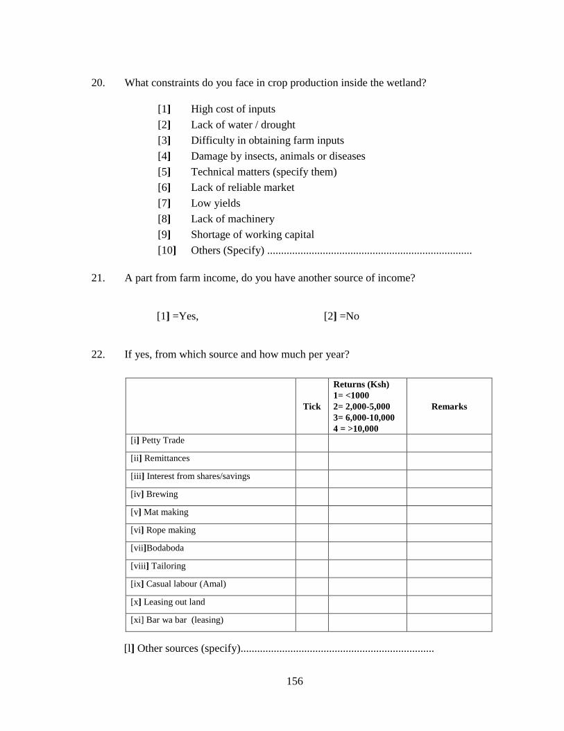
156

20. What constraints do you face in crop production inside the wetland?

[1] High cost of inputs

[2] Lack of water / drought

[3] Difficulty in obtaining farm inputs

[4] Damage by insects, animals or diseases

[5] Technical matters (specify them)

[6] Lack of reliable market

[7] Low yields

[8] Lack of machinery

[9] Shortage of working capital

[10] Others (Specify) ..........................................................................

21. A part from farm income, do you have another source of income?

[1] =Yes, [2] =No

22. If yes, from which source and how much per year?

Tick

Returns (Ksh)

1= <1000

2= 2,000-5,000

3= 6,000-10,000

4 = >10,000

Remarks

[i] Petty Trade

[ii] Remittances

[iii] Interest from shares/savings

[iv] Brewing

[v] Mat making

[vi] Rope making

[vii]Bodaboda

[viii] Tailoring

[ix] Casual labour (Amal)

[x] Leasing out land

[xi] Bar wa bar (leasing)

[l] Other sources (specify)......................................................................

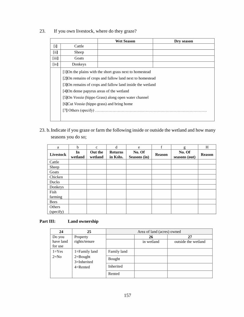
157

23. If you own livestock, where do they graze?

Wet Season Dry season

[i] Cattle

[ii] Sheep

[iii] Goats

[iv] Donkeys

[1]On the plains with the short grass next to homestead

[2]On remains of crops and fallow land next to homestead

[3]On remains of crops and fallow land inside the wetland

[4]On dense papyrus areas of the wetland

[5]On Vossia (hippo Grass) along open water channel

[6]Cut Vossia (hippo grass) and bring home

[7] Others (specify) …………………………………………………………………………

23. b. Indicate if you graze or farm the following inside or outside the wetland and how many

seasons you do so;

a b c d e f g H

Livestock In

wetland

Out the

wetland

Returns

in Kshs.

No. Of

Seasons (in) Reason

No. Of

seasons (out) Reason

Cattle

Sheep

Goats

Chicken

Ducks

Donkeys

Fish

farming

Bees

Others

(specify)

Part III: Land ownership

24 25 Area of land (acres) owned

Do you

have land

for use

Property

rights/tenure 26 27

in wetland outside the wetland

1=Yes

2=No

1=Family land

2=Bought

3=Inherited

4=Rented

Family land

Bought

Inherited

Rented

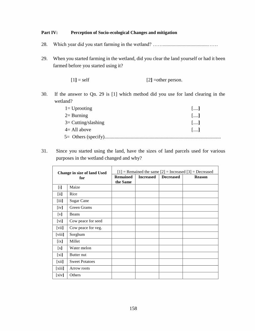
158

Part IV: Perception of Socio-ecological Changes and mitigation

28. Which year did you start farming in the wetland? ……....................................……

29. When you started farming in the wetland, did you clear the land yourself or had it been

farmed before you started using it?

[1] = self [2] =other person.

30. If the answer to Qn. 29 is [1] which method did you use for land clearing in the

wetland?

1= Uprooting [....]

2= Burning [....]

3= Cutting/slashing [....]

4= All above [....]

5= Others (specify).............................................................................................

31. Since you started using the land, have the sizes of land parcels used for various

purposes in the wetland changed and why?

Change in size of land Used

for

[1] = Remained the same [2] = Increased [3] = Decreased

Remained

the Same

Increased Decreased Reason

[i] Maize

[ii] Rice

[iii] Sugar Cane

[iv] Green Grams

[v] Beans

[vi] Cow peace for seed

[vii] Cow peace for veg.

[viii] Sorghum

[ix] Millet

[x] Water melon

[xi] Butter nut

[xii] Sweet Potatoes

[xiii] Arrow roots

[xiv] Others

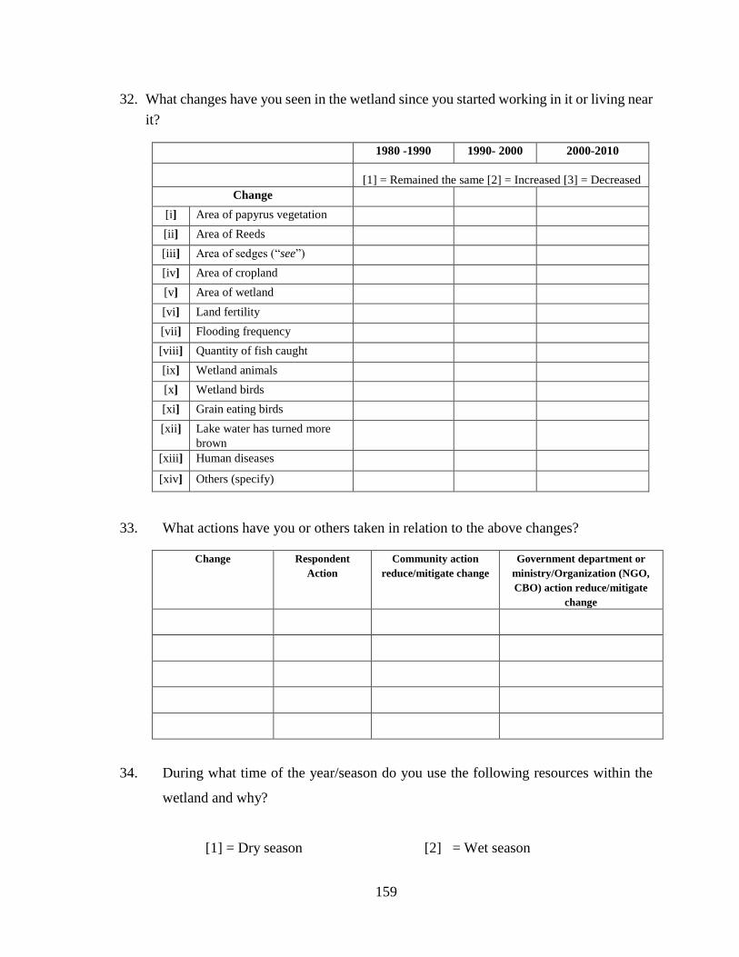
159

32. What changes have you seen in the wetland since you started working in it or living near

it?

1980 -1990 1990- 2000 2000-2010

[1] = Remained the same [2] = Increased [3] = Decreased

Change

[i] Area of papyrus vegetation

[ii] Area of Reeds

[iii] Area of sedges (“see”)

[iv] Area of cropland

[v] Area of wetland

[vi] Land fertility

[vii] Flooding frequency

[viii] Quantity of fish caught

[ix] Wetland animals

[x] Wetland birds

[xi] Grain eating birds

[xii] Lake water has turned more

brown

[xiii] Human diseases

[xiv] Others (specify)

33. What actions have you or others taken in relation to the above changes?

Change Respondent

Action

Community action

reduce/mitigate change

Government department or

ministry/Organization (NGO,

CBO) action reduce/mitigate

change

34. During what time of the year/season do you use the following resources within the

wetland and why?

[1] = Dry season [2] = Wet season

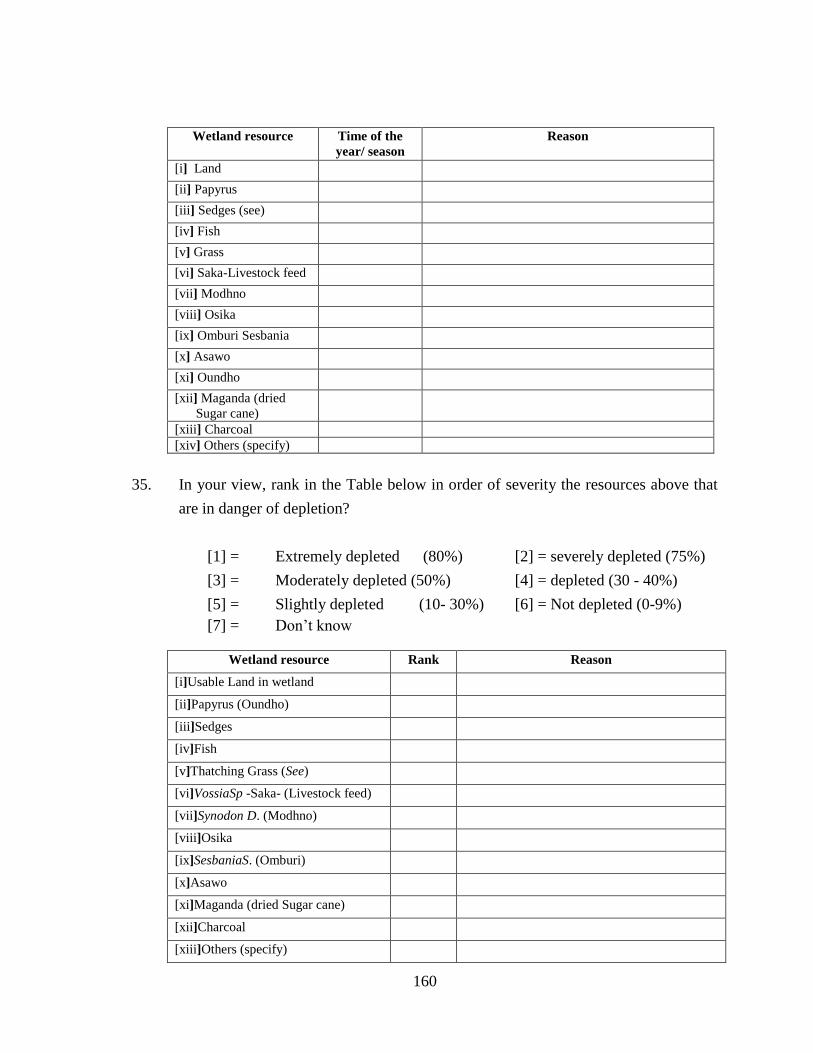
160

Wetland resource Time of the

year/ season

Reason

[i] Land

[ii] Papyrus

[iii] Sedges (see)

[iv] Fish

[v] Grass

[vi] Saka-Livestock feed

[vii] Modhno

[viii] Osika

[ix] Omburi Sesbania

[x] Asawo

[xi] Oundho

[xii] Maganda (dried

Sugar cane)

[xiii] Charcoal

[xiv] Others (specify)

35. In your view, rank in the Table below in order of severity the resources above that

are in danger of depletion?

[1] = Extremely depleted (80%) [2] = severely depleted (75%)

[3] = Moderately depleted (50%) [4] = depleted (30 - 40%)

[5] = Slightly depleted (10- 30%) [6] = Not depleted (0-9%)

[7] = Don’t know

Wetland resource Rank Reason

[i]Usable Land in wetland

[ii]Papyrus (Oundho)

[iii]Sedges

[iv]Fish

[v]Thatching Grass (See)

[vi]VossiaSp -Saka- (Livestock feed)

[vii]Synodon D. (Modhno)

[viii]Osika

[ix]SesbaniaS. (Omburi)

[x]Asawo

[xi]Maganda (dried Sugar cane)

[xii]Charcoal

[xiii]Others (specify)

161

Part V: Lake /water level Changes

36. Are there times when the shoreline moves inwards or outwards?

i) Yes [ ]

ii) No [ ]

37. What term is used to refer to this phenomenon in local language?

...........................................................................................................................

38. When does this movement usually occur in this area?

i) January [ ]

ii) February [ ]

iii) March [ ]

iv) April [ ]

v) May [ ]

vi) June [ ]

vii) July [ ]

viii) August [ ]

ix) September [ ]

x) October [ ]

xi) November [ ]

xii) December [ ]

39. How often does it occur?

i) Once a year [ ]

ii) Twice a year [ ]

iii) Thrice a year [ ]

iv) Four times a year [ ]

v) Continuous, slow and permanent [ ]

vi) Continuous, slow and temporary [ ]

v) Other (Specify)……………………………………………………………

40. a) What do you do with the areas that are exposed when the shoreline retreats?

i) Cultivate them [ ]

ii) Use them for grazing [ ]

iii) Burn [ ]

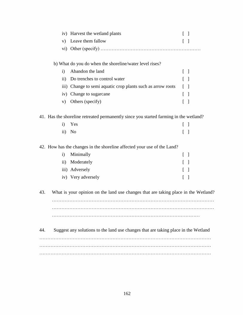
162

iv) Harvest the wetland plants [ ]

v) Leave them fallow [ ]

vi) Other (specify) ………………………………………………………

b) What do you do when the shoreline/water level rises?

i) Abandon the land [ ]

ii) Do trenches to control water [ ]

iii) Change to semi aquatic crop plants such as arrow roots [ ]

iv) Change to sugarcane [ ]

v) Others (specify) [ ]

41. Has the shoreline retreated permanently since you started farming in the wetland?

i) Yes [ ]

ii) No [ ]

42. How has the changes in the shoreline affected your use of the Land?

i) Minimally [ ]

ii) Moderately [ ]

iii) Adversely [ ]

iv) Very adversely [ ]

43. What is your opinion on the land use changes that are taking place in the Wetland?

…………………………………………………………………………………………

…………………………………………………………………………………………

…………………………………………………………………………………

44. Suggest any solutions to the land use changes that are taking place in the Wetland

………………………………………………………………………………………………

………………………………………………………………………………………………

………………………………………………………………………………………………

163

Appendix 2: Tablesa for Finding a Base Sample Sizeb According to Watson, (2001)

+/- 5% Margin of Errorc

Sample Size

Variability

Population 50% 40% 30% 20% 10% d

100 e 81 79 63 50 37

125 96 93 72 56 40

150 110 107 80 60 42

175 122 119 87 64 44

200 134 130 93 67 45

225 144 140 98 70 46

250 154 149 102 72 47

275 163 158 106 74 48

300 172 165 109 76 49

325 180 173 113 77 50

350 187 180 115 79 50

375 194 186 118 80 51

400 201 192 120 81 51

425 207 197 122 82 51

450 212 203 124 83 52

500 222 212 128 84 52

600 240 228 134 87 53

700 255 242 138 88 54

800 267 252 142 90 54

900 277 262 144 91 55

1,000 286 269 147 92 55

2,000 333 311 158 96 57

3,000 353 328 163 98 57

4,000 364 338 165 99 58

5,000 370 343 166 99 58

6,000 375 347 167 100 58

7,000 378 350 168 100 58

8,000 381 353 168 100 58

9,000 383 354 169 100 58

10,000 385 356 169 100 58

15,000 390 360 170 101 58

20,000 392 362 171 101 58

25,000 394 363 171 101 58

50,000 397 366 172 101 58

100,000 398 367 or172 101 58

Qualifications for a, b, c, d and e are presented in items a, b, c, d, and e below;

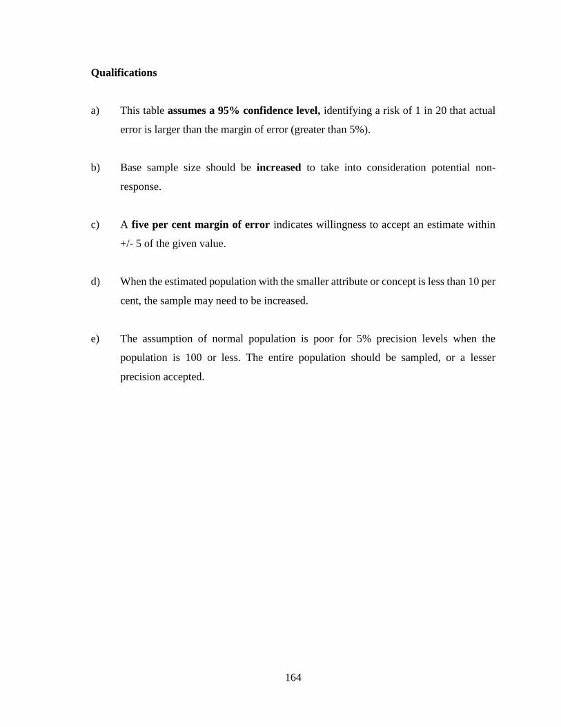
164

Qualifications

a) This table assumes a 95% confidence level, identifying a risk of 1 in 20 that actual

error is larger than the margin of error (greater than 5%).

b) Base sample size should be increased to take into consideration potential non-

response.

c) A five per cent margin of error indicates willingness to accept an estimate within

+/- 5 of the given value.

d) When the estimated population with the smaller attribute or concept is less than 10 per

cent, the sample may need to be increased.

e) The assumption of normal population is poor for 5% precision levels when the

population is 100 or less. The entire population should be sampled, or a lesser

precision accepted.

165

Appendix 3: List of Key Informants

NO. NAME MIN/ORG CONTACT

1 Rhoda Apunda Agriculture 0735244984

2 Betty Okello Scc-Vi Agroforestry 0720400109

3 Samson A. Gillo Ag. Chief 0721817413

4 Mark D Nyadiang’a Chief West Kochieng’ 0727162464

5 Raymond Oluoch Chief Kakola 0721845140

6 John Omiti Asst. Chief Wasare 0716052957

7 Susan Odhiambo Fisharies – Nyando 0723435428

8 Walter Oyosi Chief Nyalunya 0716849779

9 Paul Abura Chairman Flood Control – Ogenya 0728986970

10 Walter Ogada Opinion Leader – Bwanda 0720897882

11 Benard Opaa D.E.O. - Nema 0720563430

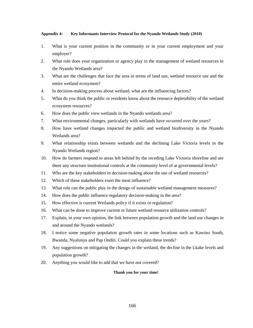
166

Appendix 4: Key Informants Interview Protocol for the Nyando Wetlands Study (2010)

1. What is your current position in the community or in your current employment and your

employer?

2. What role does your organization or agency play in the management of wetland resources in

the Nyando Wetlands area?

3. What are the challenges that face the area in terms of land use, wetland resource use and the

entire wetland ecosystem?

4. In decision-making process about wetland, what are the influencing factors?

5. What do you think the public or residents know about the resource depletability of the wetland

ecosystem resources?

6. How does the public view wetlands in the Nyando wetlands area?

7. What environmental changes, particularly with wetlands have occurred over the years?

8. How have wetland changes impacted the public and wetland biodiversity in the Nyando

Wetlands area?

9. What relationship exists between wetlands and the declining Lake Victoria levels in the

Nyando Wetlands region?

10. How do farmers respond to areas left behind by the receding Lake Victoria shoreline and are

there any structure institutional controls at the community level of at governmental levels?

11. Who are the key stakeholders in decision-making about the use of wetland resources?

12. Which of these stakeholders exert the most influence?

13. What role can the public play in the design of sustainable wetland management measures?

14. How does the public influence regulatory decision-making in the area?

15. How effective is current Wetlands policy if it exists or regulation?

16. What can be done to improve current or future wetland resource utilization controls?

17. Explain, in your own opinion, the link between population growth and the land use changes in

and around the Nyando wetlands?

18. I notice some negative population growth rates in some locations such as Kawino South,

Bwanda, Nyalunya and Pap Onditi. Could you explain these trends?

19. Any suggestions on mitigating the changes in the wetland, the decline in the Lkake levels and

population growth?

20. Anything you would like to add that we have not covered?

Thank you for your time!

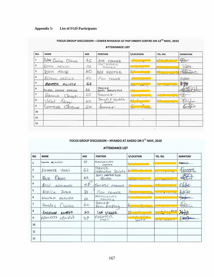
167

Appendix 5: List of FGD Participants

168

Appendix 6: Letter for the Recruitment of Focus Group Discussion Participants

for the Nyando Wetlands Study in 2010

Has Nyando Wetlands responded to anthropogenic and hydrodynamic drivers of land

use/cover changes in space and time over the last three decades?

Dear Sir/Madam,

My name is Joseph Okotto-Okotto. I am a graduate student at Egerton University taking a course in

Natural Resources management. I am currently in the research phase of my course of study and I am

studying the human and hydro dynamic drivers of change in Nyando Wetlands over the past 26 years.

My aim is to integrate what I can see and gather from technical scientific views with what people can

tell me as they see or experience or know on the ground to corroborate and understand the dynamics

of these drivers. This will help in the planning and design of measures that could influence policy

and not only be of benefit to the communities but also to the Nyando wetlands ecosystem for

posterity. The Wetlands happen to be in an area where you live/under your jurisdictions. I am

interested in contacting residents to have a small group discussion about the issues affecting the

Wetlands and how citizens’ actions could influence the course of these challenges.

I have contacted you because you have been identified as knowledgeable, keen, nurturing a great

interest in wetland resources and their utilization. The one to two hour discussion will comprise

approximately 9 individuals and will be recorded if all participants agree to it. All given responses

will not be identified and will be kept secure and confidential. Any contact information will not be

shared under any circumstances. If you would be willing to participate in the discussion, kindly fill

out the contact information below, cut it off and send it back to me. You will be contacted further via

email or phone.

If you have any additional questions at any time or would like more information, please feel free to

contact; Dr. Obati G. Obwoyere - +254 725 214 510 or onacha2002@yahoo.com in the Department

of Natural Resources management, or Dr. Mironga J. Momanyi – mmironga@yahoo.com in the

Department of Geography, Egerton University or Prof. Phillip O. Raburu – +254 717 631 789 or

praburu2002@yahoo.com in the Department of Fisheries and Aquatic Sciences, School of Natural

Resources Management University of Eldoret or myself , telephone; +254 713 925 989 or

jokotto@hotmail.com.

Yours faithfully

J. Okotto-Okotto

------------------------------------------------------------------------------------------------------------

I wish to participate in the Focus Group Discussion.

Name: ________________________________ Email: ___________________________

Phone: ________________________________ Address: _________________________

169

Appendix 7: Focus Group Discussion Questions for the Nyando Wetlands Study in 2010

Part A: Introductory Remarks

My name is Joseph Okotto-Okotto from the Lake Basin Development Authority. I am a graduate student at Egerton University taking a course in Natural Resources management. I am currently in the research phase of my course of study and I am studying the human and hydro dynamic drivers of change in Nyando Wetlands in space and time. My aim is to integrate what I can see and gather from technical scientific views with what people can tell me as they see or experience or know on the ground to corroborate and understand the dynamics of these drivers. This will help in the planning and design measures that could not only be of benefit to the communities but also to the ecosystem for posterity. The Wetland happens to be in an area where you live/under your jurisdictions. I am here before you hoping you would be willing to answer for me a few questions. I wish to assure you that anything you tell me is confidential. Nothing you say will be personally attributed to you in any reports that result from this interview. My thesis report will be written in a manner that no individual comment can be attributed to a particular person. Are you willing to answer my questions for me today? Do you have any questions before we begin?

Part B: Guide Questions

1. What are the wetland resources in the Nyando wetlands area?

2. What are the challenges facing Nyando Wetlands and when did they start affecting the

wetlands. (Probe: every challenge mentioned; what needs to happen to help in addressing

these challenges? Think back to the challenges we talked about in No. 1….., What could be

done about those?)

3. What is the link between population growth and the Challenges that Nyando wetlands is

currently phasing (Probe: Negative population growth in some locations, immigrant impacts,

why people close to the wetlands have smaller plots that than those further away etc.)

4. Briefly describe local institutional/Agency/organization/community’s interest in promoting

sustainable wetland management with specific reference to Nyando wetland management

(Probe: every challenge mentioned).

5. Briefly tell me what you know about the levels of Lake Victoria and how you think it is

affecting the Nyando wetlands (Probe: the challenges posed by the declining lake level and

what should be done to address the changes).

6. Discuss the issue of water scarcity (Probe: Is this is a problem we face in the Nyando wetlands

area? Why or why not? In which ways? How is it affecting the uses of land for agriculture,

how are people adapting to this? Any relationships to wetland farming)?

7. Who or what group has the most say in how wetland resources are used or managed in the

Nyando Wetlands area?

8. What changes have you observed in wetland environments near you?

9. What values do you place on wetlands? (attitudes towards the wetlands, a ranking Exercise)

10. What would you like to share or discuss about the wetlands that we have not touched in our

discussion?

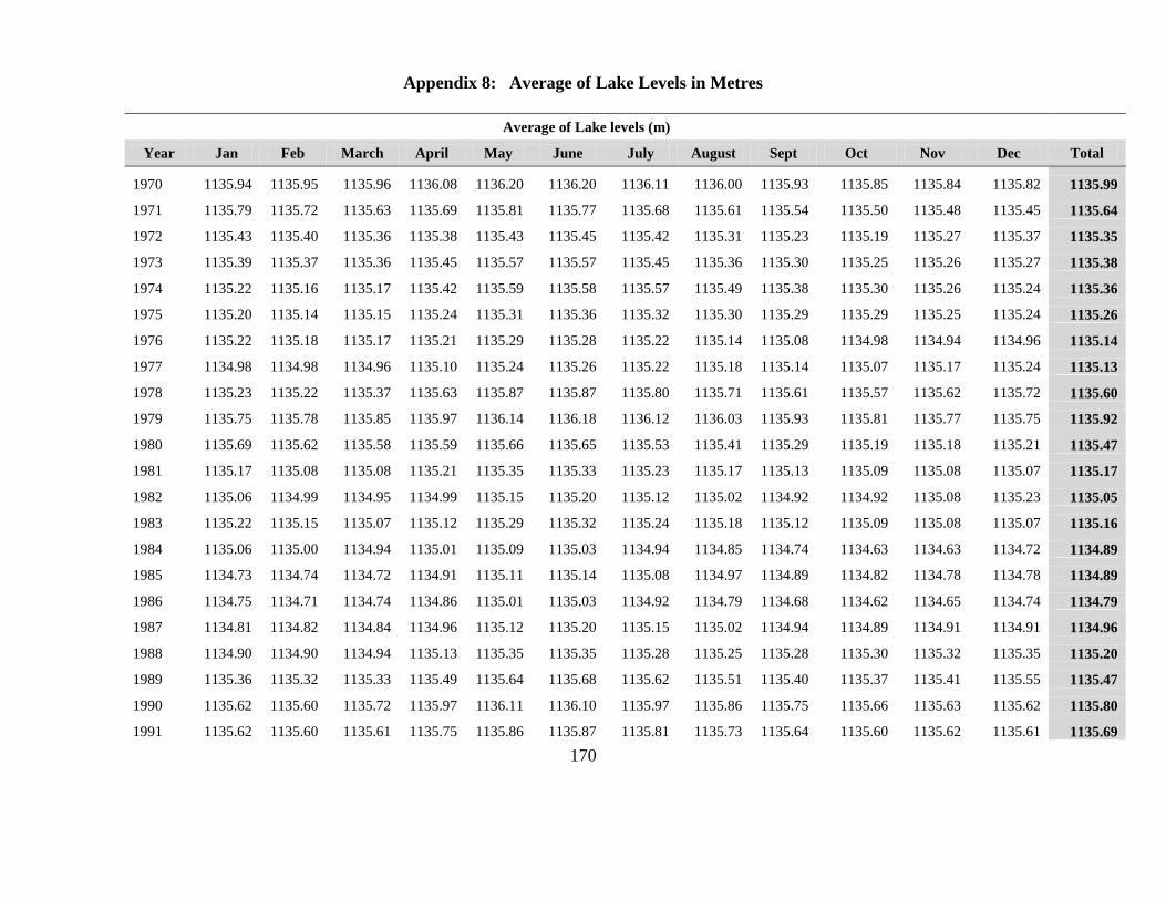
170

Appendix 8: Average of Lake Levels in Metres

Average of Lake levels (m)

Year Jan Feb March April May June July August Sept Oct Nov Dec Total

1970 1135.94 1135.95 1135.96 1136.08 1136.20 1136.20 1136.11 1136.00 1135.93 1135.85 1135.84 1135.82 1135.99

1971 1135.79 1135.72 1135.63 1135.69 1135.81 1135.77 1135.68 1135.61 1135.54 1135.50 1135.48 1135.45 1135.64

1972 1135.43 1135.40 1135.36 1135.38 1135.43 1135.45 1135.42 1135.31 1135.23 1135.19 1135.27 1135.37 1135.35

1973 1135.39 1135.37 1135.36 1135.45 1135.57 1135.57 1135.45 1135.36 1135.30 1135.25 1135.26 1135.27 1135.38

1974 1135.22 1135.16 1135.17 1135.42 1135.59 1135.58 1135.57 1135.49 1135.38 1135.30 1135.26 1135.24 1135.36

1975 1135.20 1135.14 1135.15 1135.24 1135.31 1135.36 1135.32 1135.30 1135.29 1135.29 1135.25 1135.24 1135.26

1976 1135.22 1135.18 1135.17 1135.21 1135.29 1135.28 1135.22 1135.14 1135.08 1134.98 1134.94 1134.96 1135.14

1977 1134.98 1134.98 1134.96 1135.10 1135.24 1135.26 1135.22 1135.18 1135.14 1135.07 1135.17 1135.24 1135.13

1978 1135.23 1135.22 1135.37 1135.63 1135.87 1135.87 1135.80 1135.71 1135.61 1135.57 1135.62 1135.72 1135.60

1979 1135.75 1135.78 1135.85 1135.97 1136.14 1136.18 1136.12 1136.03 1135.93 1135.81 1135.77 1135.75 1135.92

1980 1135.69 1135.62 1135.58 1135.59 1135.66 1135.65 1135.53 1135.41 1135.29 1135.19 1135.18 1135.21 1135.47

1981 1135.17 1135.08 1135.08 1135.21 1135.35 1135.33 1135.23 1135.17 1135.13 1135.09 1135.08 1135.07 1135.17

1982 1135.06 1134.99 1134.95 1134.99 1135.15 1135.20 1135.12 1135.02 1134.92 1134.92 1135.08 1135.23 1135.05

1983 1135.22 1135.15 1135.07 1135.12 1135.29 1135.32 1135.24 1135.18 1135.12 1135.09 1135.08 1135.07 1135.16

1984 1135.06 1135.00 1134.94 1135.01 1135.09 1135.03 1134.94 1134.85 1134.74 1134.63 1134.63 1134.72 1134.89

1985 1134.73 1134.74 1134.72 1134.91 1135.11 1135.14 1135.08 1134.97 1134.89 1134.82 1134.78 1134.78 1134.89

1986 1134.75 1134.71 1134.74 1134.86 1135.01 1135.03 1134.92 1134.79 1134.68 1134.62 1134.65 1134.74 1134.79

1987 1134.81 1134.82 1134.84 1134.96 1135.12 1135.20 1135.15 1135.02 1134.94 1134.89 1134.91 1134.91 1134.96

1988 1134.90 1134.90 1134.94 1135.13 1135.35 1135.35 1135.28 1135.25 1135.28 1135.30 1135.32 1135.35 1135.20

1989 1135.36 1135.32 1135.33 1135.49 1135.64 1135.68 1135.62 1135.51 1135.40 1135.37 1135.41 1135.55 1135.47

1990 1135.62 1135.60 1135.72 1135.97 1136.11 1136.10 1135.97 1135.86 1135.75 1135.66 1135.63 1135.62 1135.80

1991 1135.62 1135.60 1135.61 1135.75 1135.86 1135.87 1135.81 1135.73 1135.64 1135.60 1135.62 1135.61 1135.69

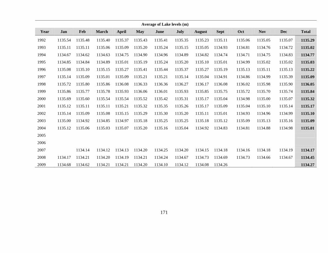
171

Average of Lake levels (m)

Year Jan Feb March April May June July August Sept Oct Nov Dec Total

1992 1135.54 1135.48 1135.40 1135.37 1135.43 1135.41 1135.35 1135.23 1135.11 1135.06 1135.05 1135.07 1135.29

1993 1135.11 1135.11 1135.06 1135.09 1135.20 1135.24 1135.15 1135.05 1134.93 1134.81 1134.76 1134.72 1135.02

1994 1134.67 1134.62 1134.63 1134.75 1134.90 1134.96 1134.89 1134.82 1134.74 1134.71 1134.75 1134.83 1134.77

1995 1134.85 1134.84 1134.89 1135.01 1135.19 1135.24 1135.20 1135.10 1135.01 1134.99 1135.02 1135.02 1135.03

1996 1135.08 1135.10 1135.15 1135.27 1135.41 1135.44 1135.37 1135.27 1135.19 1135.13 1135.11 1135.13 1135.22

1997 1135.14 1135.09 1135.01 1135.09 1135.21 1135.21 1135.14 1135.04 1134.91 1134.86 1134.99 1135.39 1135.09

1998 1135.72 1135.80 1135.86 1136.08 1136.33 1136.36 1136.27 1136.17 1136.08 1136.02 1135.98 1135.90 1136.05

1999 1135.86 1135.77 1135.78 1135.93 1136.06 1136.01 1135.93 1135.85 1135.75 1135.72 1135.70 1135.74 1135.84

2000 1135.69 1135.60 1135.54 1135.54 1135.52 1135.42 1135.31 1135.17 1135.04 1134.98 1135.00 1135.07 1135.32

2001 1135.12 1135.11 1135.11 1135.21 1135.32 1135.35 1135.26 1135.17 1135.09 1135.04 1135.10 1135.14 1135.17

2002 1135.14 1135.09 1135.08 1135.15 1135.29 1135.30 1135.20 1135.11 1135.01 1134.93 1134.96 1134.99 1135.10

2003 1135.00 1134.92 1134.85 1134.97 1135.18 1135.25 1135.25 1135.18 1135.12 1135.09 1135.13 1135.16 1135.09

2004 1135.12 1135.06 1135.03 1135.07 1135.20 1135.16 1135.04 1134.92 1134.83 1134.81 1134.88 1134.98 1135.01

2005

2006

2007 1134.14 1134.12 1134.13 1134.20 1134.25 1134.20 1134.15 1134.18 1134.16 1134.18 1134.19 1134.17

2008 1134.17 1134.21 1134.20 1134.19 1134.21 1134.24 1134.67 1134.73 1134.69 1134.73 1134.66 1134.67 1134.45

2009 1134.68 1134.62 1134.21 1134.21 1134.20 1134.10 1134.12 1134.08 1134.26 1134.27

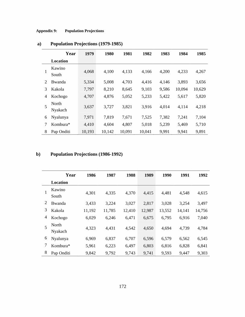
172

Appendix 9: Population Projections

a) Population Projections (1979-1985)

Year 1979 1980 1981 1982 1983 1984 1985

Location

1 Kawino

South 4,068 4,100 4,133 4,166 4,200 4,233 4,267

2 Bwanda 5,334 5,008 4,703 4,416 4,146 3,893 3,656

3 Kakola 7,797 8,210 8,645 9,103 9,586 10,094 10,629

4 Kochogo 4,707 4,876 5,052 5,233 5,422 5,617 5,820

5 North

Nyakach 3,637 3,727 3,821 3,916 4,014 4,114 4,218

6 Nyalunya 7,971 7,819 7,671 7,525 7,382 7,241 7,104

7 Kombura* 4,410 4,604 4,807 5,018 5,239 5,469 5,710

8 Pap Onditi 10,193 10,142 10,091 10,041 9,991 9,941 9,891

b) Population Projections (1986-1992)

Year 1986 1987 1988 1989 1990 1991 1992

Location

1 Kawino

South 4,301 4,335 4,370 4,415 4,481 4,548 4,615

2 Bwanda 3,433 3,224 3,027 2,817 3,028 3,254 3,497

3 Kakola 11,192 11,785 12,410 12,987 13,552 14,141 14,756

4 Kochogo 6,029 6,246 6,471 6,675 6,795 6,916 7,040

5 North

Nyakach 4,323 4,431 4,542 4,650 4,694 4,739 4,784

6 Nyalunya 6,969 6,837 6,707 6,596 6,579 6,562 6,545

7 Kombura* 5,961 6,223 6,497 6,803 6,816 6,828 6,841

8 Pap Onditi 9,842 9,792 9,743 9,741 9,593 9,447 9,303

173

c) Population Projections (1993-1999)

Year 1993 1994 1995 1996 1997 1998 1999

Location

1 Kawino

South 4,684 4,754 4,825 4,897 4,970 5,044 5,073

2 Bwanda 3,758 4,039 4,341 4,665 5,014 5,388 4,922

3 Kakola 15,397 16,067 16,766 17,495 18,255 19,049 18,634

4 Kochogo 7,166 7,294 7,425 7,558 7,693 7,831 7,870

5 North

Nyakach 4,830 4,876 4,922 4,969 5,016 5,064 5,093

6 Nyalunya 6,529 6,512 6,495 6,479 6,462 6,445 6,427

7 Kombura* 6,853 6,866 6,878 6,891 6,904 6,916 6,928

8 PapOnditi 9,161 9,022 8,884 8,749 8,616 8,485 8,258

d) Population Projections (2000-2006)

Year 2000 2001 2002 2003 2004 2005 2006

Location

1

Kawino

South 5,021 4,969 4,918 4,867 4,817 4,768 4,719

2 Bwanda 5,021 5,122 5,224 5,329 5,436 5,545 5,657

3 Kakola 18,939 19,248 19,563 19,882 20,207 20,537 20,873

4 Kochogo 8,059 8,253 8,451 8,654 8,862 9,075 9,293

5

North

Nyakach 5,204 5,318 5,434 5,553 5,674 5,798 5,924

6 Nyalunya 6,569 6,714 6,862 7,014 7,169 7,327 7,489

7 Kombura* 7,047 7,168 7,291 7,416 7,543 7,672 7,804

8 Pap Onditi 8,354 8,451 8,549 8,648 8,749 8,850 8,953

174

e) Population Projections (2007-2005)

Year 2007 2008 2009 2002 2003 2004 2005

Location

1

Kawino

South 4,670 4,622 4,551 4,918 4,867 4,817 4,768

2 Bwanda 5,770 5,886 5,910 5,224 5,329 5,436 5,545

3 Kakola 21,214 21,561 21,679 19,563 19,882 20,207 20,537

4 Kochogo 9,516 9,745 9,761 8,451 8,654 8,862 9,075

5

North

Nyakach 6,054 6,186 6,205 5,434 5,553 5,674 5,798

6 Nyalunya 7,654 7,823 7,846 6,862 7,014 7,169 7,327

7 Kombura* 7,937 8,074 8,116 7,291 7,416 7,543 7,672

8 Pap Onditi 9,057 9,162 9,217 8,549 8,648 8,749 8,850

f) Population Projections (2006-2009)

Year 2006 2007 2008 2009

Location

1 Kawino South 4,719 4,670 4,622 4,551

2 Bwanda 5,657 5,770 5,886 5,910

3 Kakola 20,873 21,214 21,561 21,679

4 Kochogo 9,293 9,516 9,745 9,761

5 North Nyakach 5,924 6,054 6,186 6,205

6 Nyalunya 7,489 7,654 7,823 7,846

7 Kombura* 7,804 7,937 8,074 8,116

8 Pap Onditi 8,953 9,057 9,162 9,217

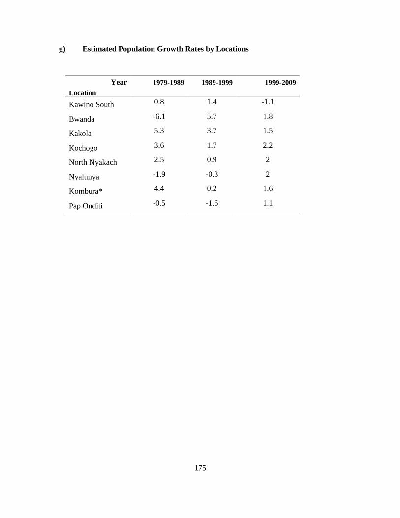
175

g) Estimated Population Growth Rates by Locations

Year 1979-1989 1989-1999 1999-2009

Location

Kawino South 0.8 1.4 -1.1

Bwanda -6.1 5.7 1.8

Kakola 5.3 3.7 1.5

Kochogo 3.6 1.7 2.2

North Nyakach 2.5 0.9 2

Nyalunya -1.9 -0.3 2

Kombura* 4.4 0.2 1.6

Pap Onditi -0.5 -1.6 1.1

176

Appendix 100: Variance of Lake Levels in metres (m)

Variance of Lake levels (m)

Year Jan Feb March April May June July Aug Sept Oct Nov Dec Total

1970 0.0003 0.0001 0.0004 0.0021 0.0005 0.0005 0.0013 0.0007 0.0008 0.0002 0.0001 0.0000 0.0167

1971 0.0003 0.0003 0.0007 0.0035 0.0003 0.0008 0.0003 0.0005 0.0005 0.0002 0.0000 0.0001 0.0150

1972 0.0005 0.0000 0.0003 0.0002 0.0004 0.0000 0.0006 0.0008 0.0006 0.0000 0.0018 0.0003 0.0073

1973 0.0000 0.0000 0.0002 0.0029 0.0005 0.0009 0.0015 0.0005 0.0001 0.0004 0.0003 0.0001 0.0118

1974 0.0005 0.0001 0.0016 0.0069 0.0003 0.0001 0.0002 0.0013 0.0010 0.0003 0.0001 0.0000 0.0251

1975 0.0005 0.0002 0.0005 0.0013 0.0012 0.0001 0.0001 0.0001 0.0000 0.0000 0.0006 0.0002 0.0048

1976 0.0008 0.0001 0.0002 0.0011 0.0008 0.0004 0.0004 0.0004 0.0006 0.0008 0.0001 0.0000 0.0140

1977 0.0000 0.0000 0.0000 0.0037 0.0012 0.0001 0.0004 0.0000 0.0007 0.0000 0.0023 0.0001 0.0118

1978 0.0001 0.0004 0.0053 0.0065 0.0024 0.0001 0.0010 0.0008 0.0009 0.0000 0.0010 0.0008 0.0465

1979 0.0001 0.0002 0.0018 0.0025 0.0017 0.0001 0.0008 0.0006 0.0011 0.0011 0.0000 0.0000 0.0251

1980 0.0010 0.0006 0.0000 0.0001 0.0008 0.0011 0.0012 0.0016 0.0009 0.0006 0.0004 0.0001 0.0378

1981 0.0007 0.0005 0.0015 0.0014 0.0020 0.0013 0.0003 0.0003 0.0001 0.0001 0.0001 0.0001 0.0094

1982 0.0002 0.0007 0.0001 0.0009 0.0034 0.0002 0.0011 0.0009 0.0004 0.0008 0.0038 0.0002 0.0115

1983 0.0003 0.0007 0.0003 0.0027 0.0022 0.0004 0.0007 0.0001 0.0005 0.0000 0.0000 0.0001 0.0074

1984 0.0001 0.0004 0.0006 0.0027 0.0000 0.0008 0.0006 0.0010 0.0014 0.0006 0.0007 0.0005 0.0264

1985 0.0001 0.0002 0.0003 0.0070 0.0015 0.0003 0.0007 0.0015 0.0004 0.0004 0.0000 0.0001 0.0229

1986 0.0004 0.0000 0.0003 0.0032 0.0013 0.0005 0.0015 0.0018 0.0009 0.0000 0.0003 0.0013 0.0176

1987 0.0001 0.0000 0.0007 0.0037 0.0015 0.0001 0.0013 0.0014 0.0003 0.0003 0.0006 0.0004 0.0167

1988 0.0002 0.0001 0.0010 0.0070 0.0012 0.0004 0.0004 0.0002 0.0002 0.0000 0.0003 0.0001 0.0307

1989 0.0001 0.0002 0.0018 0.0017 0.0022 0.0001 0.0007 0.0012 0.0006 0.0001 0.0002 0.0027 0.0155

1990 0.0004 0.0001 0.0045 0.0048 0.0005 0.0012 0.0013 0.0008 0.0013 0.0002 0.0001 0.0001 0.0354

1991 0.0000 0.0000 0.0004 0.0013 0.0008 0.0001 0.0008 0.0002 0.0015 0.0007 0.0001 0.0001 0.0105

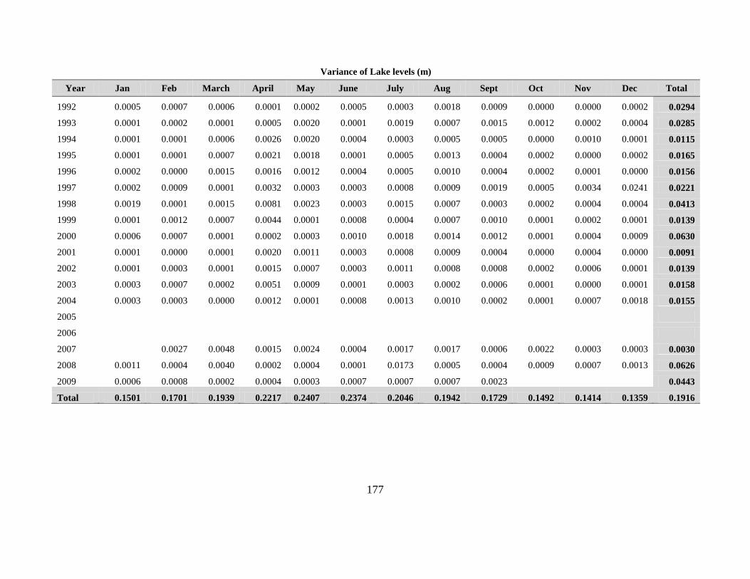
177

Variance of Lake levels (m)

Year Jan Feb March April May June July Aug Sept Oct Nov Dec Total

1992 0.0005 0.0007 0.0006 0.0001 0.0002 0.0005 0.0003 0.0018 0.0009 0.0000 0.0000 0.0002 0.0294

1993 0.0001 0.0002 0.0001 0.0005 0.0020 0.0001 0.0019 0.0007 0.0015 0.0012 0.0002 0.0004 0.0285

1994 0.0001 0.0001 0.0006 0.0026 0.0020 0.0004 0.0003 0.0005 0.0005 0.0000 0.0010 0.0001 0.0115

1995 0.0001 0.0001 0.0007 0.0021 0.0018 0.0001 0.0005 0.0013 0.0004 0.0002 0.0000 0.0002 0.0165

1996 0.0002 0.0000 0.0015 0.0016 0.0012 0.0004 0.0005 0.0010 0.0004 0.0002 0.0001 0.0000 0.0156

1997 0.0002 0.0009 0.0001 0.0032 0.0003 0.0003 0.0008 0.0009 0.0019 0.0005 0.0034 0.0241 0.0221

1998 0.0019 0.0001 0.0015 0.0081 0.0023 0.0003 0.0015 0.0007 0.0003 0.0002 0.0004 0.0004 0.0413

1999 0.0001 0.0012 0.0007 0.0044 0.0001 0.0008 0.0004 0.0007 0.0010 0.0001 0.0002 0.0001 0.0139

2000 0.0006 0.0007 0.0001 0.0002 0.0003 0.0010 0.0018 0.0014 0.0012 0.0001 0.0004 0.0009 0.0630

2001 0.0001 0.0000 0.0001 0.0020 0.0011 0.0003 0.0008 0.0009 0.0004 0.0000 0.0004 0.0000 0.0091

2002 0.0001 0.0003 0.0001 0.0015 0.0007 0.0003 0.0011 0.0008 0.0008 0.0002 0.0006 0.0001 0.0139

2003 0.0003 0.0007 0.0002 0.0051 0.0009 0.0001 0.0003 0.0002 0.0006 0.0001 0.0000 0.0001 0.0158

2004 0.0003 0.0003 0.0000 0.0012 0.0001 0.0008 0.0013 0.0010 0.0002 0.0001 0.0007 0.0018 0.0155

2005

2006

2007 0.0027 0.0048 0.0015 0.0024 0.0004 0.0017 0.0017 0.0006 0.0022 0.0003 0.0003 0.0030

2008 0.0011 0.0004 0.0040 0.0002 0.0004 0.0001 0.0173 0.0005 0.0004 0.0009 0.0007 0.0013 0.0626

2009 0.0006 0.0008 0.0002 0.0004 0.0003 0.0007 0.0007 0.0007 0.0023 0.0443

Total 0.1501 0.1701 0.1939 0.2217 0.2407 0.2374 0.2046 0.1942 0.1729 0.1492 0.1414 0.1359 0.1916

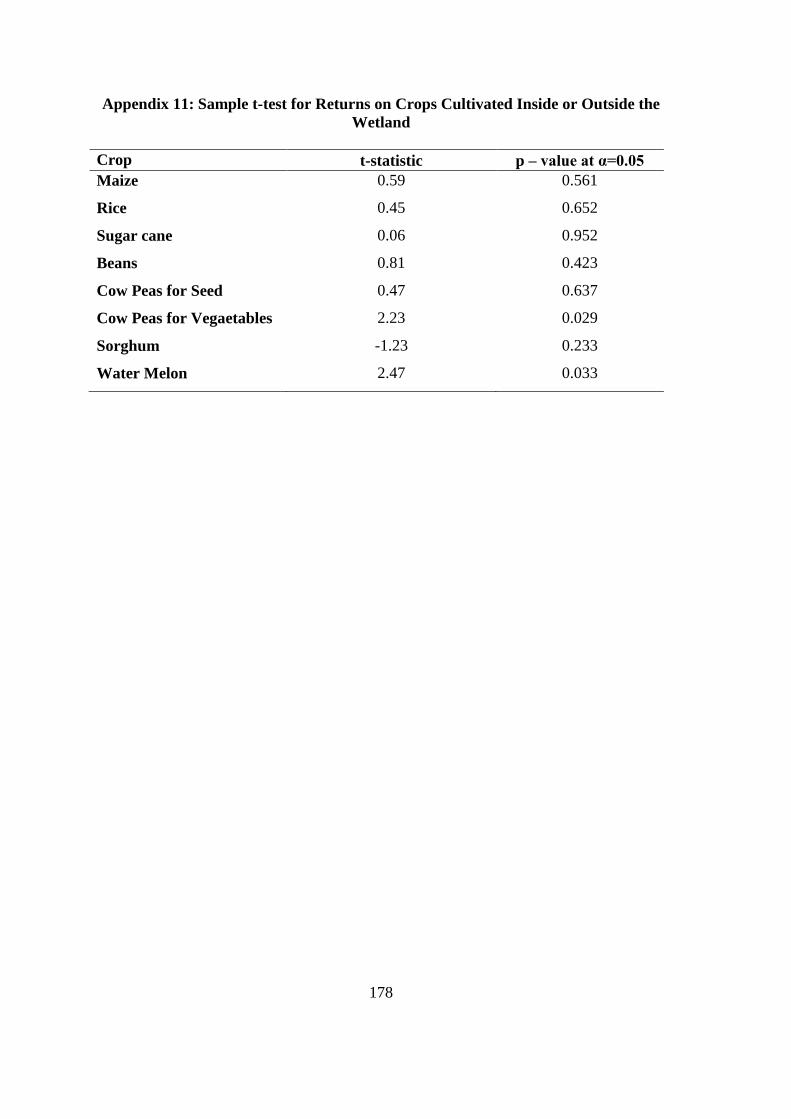
178

Appendix 11: Sample t-test for Returns on Crops Cultivated Inside or Outside the

Wetland

Crop t-statistic p – value at α=0.05

Maize 0.59 0.561

Rice 0.45 0.652

Sugar cane 0.06 0.952

Beans 0.81 0.423

Cow Peas for Seed 0.47 0.637

Cow Peas for Vegaetables 2.23 0.029

Sorghum -1.23 0.233

Water Melon 2.47 0.033