Quantitative imaging of collective cell migration during Drosophila gastrulation: multiphoton...

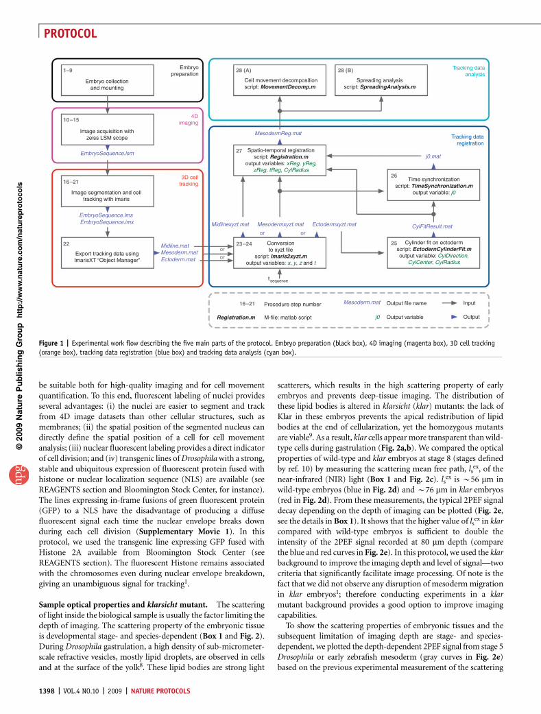
Quantitative imaging of collective cell migrationduring Drosophila gastrulation: multiphotonmicroscopy and computational analysisWilly Supatto1,2, Amy McMahon1, Scott E Fraser1 & Angelike Stathopoulos1

1Division of Biology and Beckman Institute, California Institute of Technology, Pasadena, California, USA. 2Present address: Institut Jacques Monod, CNRS UMR 7592,Universite Paris 7, Paris, France. Correspondence should be addressed to W.S. ([email protected]) or A.S. ([email protected]).

Published online 10 September 2009; doi:10.1038/nprot.2009.130

This protocol describes imaging and computational tools to collect and analyze live imaging data of embryonic cell migration. Our

five-step protocol requires a few weeks to move through embryo preparation and four-dimensional (4D) live imaging using multi-

photon microscopy, to 3D cell tracking using image processing, registration of tracking data and their quantitative analysis using

computational tools. It uses commercially available equipment and requires expertise in microscopy and programming that is

appropriate for a biology laboratory. Custom-made scripts are provided, as well as sample datasets to permit readers without

experimental data to carry out the analysis. The protocol has offered new insights into the genetic control of cell migration during

Drosophila gastrulation. With simple modifications, this systematic analysis could be applied to any developing system to define cell

positions in accordance with the body plan, to decompose complex 3D movements and to quantify the collective nature of cell

migration.

INTRODUCTIONQuantitative imaging of collective cell migration in a developingembryoThe combination of advanced imaging and image analysis techni-ques enables the investigation of large, dynamic cell populationswithin a developing embryo1,2. These imaging approaches providea unique opportunity to study embryonic morphogenesis from thelevel of cellular processes to the scale of an entire tissue or organism.Gastrulation in the Drosophila melanogaster embryo is an excellentmodel system for the study of embryonic morphogenesis3. In lessthan 2 h of development, B6,000 cells undergo stereotypicalmorphogenetic events, such as tissue invagination4, convergence-extension5,6, planar cell intercalation5,6, radial cell intercalation1,epithelial-to-mesenchymal transition7, synchronized waves of celldivision1 and collective cell migration1. Although the geometry ofthe Drosophila embryo is relatively simple at early stages ofdevelopment, the morphogenetic events involve highly dynamicprocesses and complex 3D movements of cells that prevent acomplete investigation of most wild-type or mutant phenotypesbased on the analysis of fixed embryos.

This protocol presents the quantitative imaging of complexcell migration in vivo, using mesoderm cell spreading duringDrosophila gastrulation as a model system. The experimentalstrategy combines 4D in vivo imaging using 2-photon excitedfluorescence (2PEF) microscopy, 3D cell tracking using imageprocessing and automated analysis of cell trajectories using com-putational tools. This quantitative approach decomposes 3D cellmovements, generating a precise description of morphogeneticevents. Furthermore, this protocol describes the quantitative inves-tigation of the collective nature of mesoderm cell migration. Thereproducibility of morphogenetic events among wild-type embryoscan be tested and mutant phenotypes can be dynamically analyzed.This approach provides a method to study complex or even subtlemutant phenotypes, such as the ability to distinguish cell popula-tions that exhibit different behaviors1. We recently applied this

approach to gain insights into the control of cell migration duringmesoderm formation in Drosophila embryos1.

Experimental designThe experimental workflow is divided into five main parts (Fig. 1):embryo preparation (Steps 1–9), 4D imaging (Steps 10–15), 3D celltracking (Steps 16–22), tracking data registration (Steps 23–27) andtracking data analysis (Step 28). Flies containing a fluorescentreporter are mated and embryos are collected. The chorion isremoved and the embryos are mounted for live imaging and 4Dimage dataset acquisition using a 2PEF microscope. TypicallyB2,000 mesoderm and ectoderm cells moving through the fieldof view are imaged during 2–3 h of development. Each imagingdataset contains B109 voxels and is processed using Imarissoftware to track the trajectories of the cell collection. Finally, aquantitative and automated analysis of the cell trajectories is carriedout using Matlab. Customized Matlab scripts required to performSteps 23–28 are provided in the supplemental section of thisprotocol (Supplementary Data 1). A sample dataset is alsoprovided to allow readers to start the procedure at Step 23 withouthaving to collect experimental data (Supplementary Data 2). Thisprotocol can be directly applied to study mesoderm spreading ingastrulating Drosophila embryos. However, the workflow is notspecific to this particular stage or model system. In addition, eachpart described in Figure 1 can be used independently and includedin a different working strategy. In order to facilitate the adaptationof this protocol to other stages or model organisms, we discussbelow each part of the workflow with general comments and advicethat are summarized in Table 1. The specific experimental choicesmade to study Drosophila gastrulation are clearly indicated.

Embryo preparationNuclear fluorescent labeling. A critical component of this pro-tocol is the choice of the fluorescent reporter, as this reporter must

p

uor

G g

n ih si l

bu

P eru ta

N 900 2©

nat

ure

pro

toco

ls/

moc.er

ut an.

ww

w//:ptt

h

NATURE PROTOCOLS | VOL.4 NO.10 | 2009 | 1397

PROTOCOL

be suitable both for high-quality imaging and for cell movementquantification. To this end, fluorescent labeling of nuclei providesseveral advantages: (i) the nuclei are easier to segment and trackfrom 4D image datasets than other cellular structures, such asmembranes; (ii) the spatial position of the segmented nucleus candirectly define the spatial position of a cell for cell movementanalysis; (iii) nuclear fluorescent labeling provides a direct indicatorof cell division; and (iv) transgenic lines of Drosophila with a strong,stable and ubiquitous expression of fluorescent protein fused withhistone or nuclear localization sequence (NLS) are available (seeREAGENTS section and Bloomington Stock Center, for instance).The lines expressing in-frame fusions of green fluorescent protein(GFP) to a NLS have the disadvantage of producing a diffusefluorescent signal each time the nuclear envelope breaks downduring each cell division (Supplementary Movie 1). In thisprotocol, we used the transgenic line expressing GFP fused withHistone 2A available from Bloomington Stock Center (seeREAGENTS section). The fluorescent Histone remains associatedwith the chromosomes even during nuclear envelope breakdown,giving an unambiguous signal for tracking1.

Sample optical properties and klarsicht mutant. The scatteringof light inside the biological sample is usually the factor limiting thedepth of imaging. The scattering property of the embryonic tissueis developmental stage- and species-dependent (Box 1 and Fig. 2).During Drosophila gastrulation, a high density of sub-micrometer-scale refractive vesicles, mostly lipid droplets, are observed in cellsand at the surface of the yolk8. These lipid bodies are strong light

scatterers, which results in the high scattering property of earlyembryos and prevents deep-tissue imaging. The distribution ofthese lipid bodies is altered in klarsicht (klar) mutants: the lack ofKlar in these embryos prevents the apical redistribution of lipidbodies at the end of cellularization, yet the homozygous mutantsare viable9. As a result, klar cells appear more transparent than wild-type cells during gastrulation (Fig. 2a,b). We compared the opticalproperties of wild-type and klar embryos at stage 8 (stages definedby ref. 10) by measuring the scattering mean free path, ls

ex, of thenear-infrared (NIR) light (Box 1 and Fig. 2c). ls

ex is B56 mm inwild-type embryos (blue in Fig. 2d) and B76 mm in klar embryos(red in Fig. 2d). From these measurements, the typical 2PEF signaldecay depending on the depth of imaging can be plotted (Fig. 2e,see the details in Box 1). It shows that the higher value of ls

ex in klarcompared with wild-type embryos is sufficient to double theintensity of the 2PEF signal recorded at 80 mm depth (comparethe blue and red curves in Fig. 2e). In this protocol, we used the klarbackground to improve the imaging depth and level of signal—twocriteria that significantly facilitate image processing. Of note is thefact that we did not observe any disruption of mesoderm migrationin klar embryos1; therefore conducting experiments in a klarmutant background provides a good option to improve imagingcapabilities.

To show the scattering properties of embryonic tissues and thesubsequent limitation of imaging depth are stage- and species-dependent, we plotted the depth-dependent 2PEF signal from stage 5Drosophila or early zebrafish mesoderm (gray curves in Fig. 2e)based on the previous experimental measurement of the scattering

p

uor

G g

n ih si l

bu

P eru ta

N 900 2©

nat

ure

pro

toco

ls/

moc.er

ut an.

ww

w//:ptt

h

1–9

Embryo collectionand mounting

Image acquisition withzeiss LSM scope

Image segmentation and celltracking with imaris

Export tracking data usingImarisXT “Object Manager”

EmbryoSequence.lsm

EmbryoSequence.lms

Midline.mat

Midlinexyzt.mat Mesodermxyzt.mat

MesodermReg.mat

Tracking dataanalysis

Tracking dataregistration

or

or

or

or

Ectodermxyzt.mat CylFitResult.mat

j0.mat

Mesoderm.mat

Mesoderm.matEctoderm.mat

EmbryoSequence.imx

Embryopreparation

28 (A)

27

26

25

28 (B)

Cell movement decompositionscript: MovementDecomp.m

Spatio-temporal registrationscript: Registration.m

output variables: xReg, yReg,zReg, tReg, CylRadius

Time synchronizationscript: TimeSynchronization.m

output variable: j0

Cylinder fit on ectodermscript: EctodernCylinderFit.moutput variable: CylDirection,

CylCenter, CylRadius

Spreading analysisscript: SpreadingAnalysis.m

4Dimaging

3D celltracking

10–15

16–21

23–24

16–21

j0

Procedure step number

M-file: matlab scriptRegistration.m

Output file name

Output variable

Input

Output

Conversionto xyzt file

script: Imaris2xyzt.moutput variables: x, y, z and t

t sequence

22

Figure 1 | Experimental work flow describing the five main parts of the protocol. Embryo preparation (black box), 4D imaging (magenta box), 3D cell tracking

(orange box), tracking data registration (blue box) and tracking data analysis (cyan box).

1398 | VOL.4 NO.10 | 2009 | NATURE PROTOCOLS

PROTOCOL

p

uor

G g

n ih si l

bu

P eru ta

N 900 2©

nat

ure

pro

toco

ls/

moc.er

ut an.

ww

w//:ptt

h

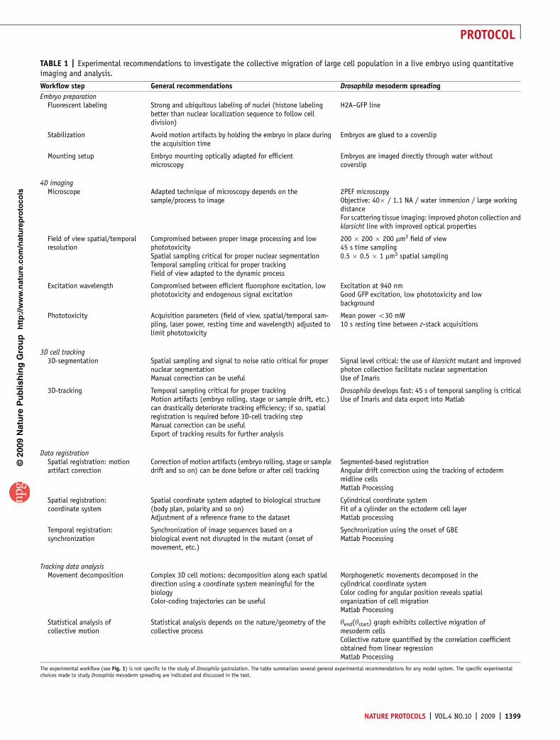
TABLE 1 | Experimental recommendations to investigate the collective migration of large cell population in a live embryo using quantitativeimaging and analysis.

Workflow step General recommendations Drosophila mesoderm spreading

Embryo preparationFluorescent labeling Strong and ubiquitous labeling of nuclei (histone labeling

better than nuclear localization sequence to follow celldivision)

H2A–GFP line

Stabilization Avoid motion artifacts by holding the embryo in place duringthe acquisition time

Embryos are glued to a coverslip

Mounting setup Embryo mounting optically adapted for efficientmicroscopy

Embryos are imaged directly through water withoutcoverslip

4D imagingMicroscope Adapted technique of microscopy depends on the

sample/process to image2PEF microscopyObjective: 40� / 1.1 NA / water immersion / large workingdistanceFor scattering tissue imaging: improved photon collection andklarsicht line with improved optical properties

Field of view spatial/temporalresolution

Compromised between proper image processing and lowphototoxicitySpatial sampling critical for proper nuclear segmentationTemporal sampling critical for proper trackingField of view adapted to the dynamic process

200 � 200 � 200 mm3 field of view45 s time sampling0.5 � 0.5 � 1 mm3 spatial sampling

Excitation wavelength Compromised between efficient fluorophore excitation, lowphototoxicity and endogenous signal excitation

Excitation at 940 nmGood GFP excitation, low phototoxicity and lowbackground

Phototoxicity Acquisition parameters (field of view, spatial/temporal sam-pling, laser power, resting time and wavelength) adjusted tolimit phototoxicity

Mean power o30 mW10 s resting time between z-stack acquisitions

3D cell tracking3D-segmentation Spatial sampling and signal to noise ratio critical for proper

nuclear segmentationManual correction can be useful

Signal level critical: the use of klarsicht mutant and improvedphoton collection facilitate nuclear segmentationUse of Imaris

3D-tracking Temporal sampling critical for proper trackingMotion artifacts (embryo rolling, stage or sample drift, etc.)can drastically deteriorate tracking efficiency; if so, spatialregistration is required before 3D-cell tracking stepManual correction can be usefulExport of tracking results for further analysis

Drosophila develops fast: 45 s of temporal sampling is criticalUse of Imaris and data export into Matlab

Data registrationSpatial registration: motionartifact correction

Correction of motion artifacts (embryo rolling, stage or sampledrift and so on) can be done before or after cell tracking

Segmented-based registrationAngular drift correction using the tracking of ectodermmidline cellsMatlab Processing

Spatial registration:coordinate system

Spatial coordinate system adapted to biological structure(body plan, polarity and so on)Adjustment of a reference frame to the dataset

Cylindrical coordinate systemFit of a cylinder on the ectoderm cell layerMatlab processing

Temporal registration:synchronization

Synchronization of image sequences based on abiological event not disrupted in the mutant (onset ofmovement, etc.)

Synchronization using the onset of GBEMatlab Processing

Tracking data analysisMovement decomposition Complex 3D cell motions: decomposition along each spatial

direction using a coordinate system meaningful for thebiologyColor-coding trajectories can be useful

Morphogenetic movements decomposed in thecylindrical coordinate systemColor coding for angular position reveals spatialorganization of cell migrationMatlab Processing

Statistical analysis ofcollective motion

Statistical analysis depends on the nature/geometry of thecollective process

yend(ystart) graph exhibits collective migration ofmesoderm cellsCollective nature quantified by the correlation coefficientobtained from linear regressionMatlab Processing

The experimental workflow (see Fig. 1) is not specific to the study of Drosophila gastrulation. The table summarizes several general experimental recommendations for any model system. The specific experimentalchoices made to study Drosophila mesoderm spreading are indicated and discussed in the text.


PROTOCOL

properties (gray in Fig. 2d). The signal decay shows that stage 5 andstage 8 Drosophila embryos (dark gray and blue curves in Fig. 2e,respectively) exhibit significantly different properties; however,these two stages are separated by only 1 h of development. Inaddition, the 2PEF signal at 80 mm is expected to be five timesweaker in Drosophila at gastrulation (blue curve in Fig. 2e)compared with early zebrafish embryos (light gray in Fig. 2e) forthe same labeling and imaging conditions. Hence, the maximumdepth of imaging and the choice of the microscopy techniquedepend on the stage and model system. For instance, as opposed to

Drosophila embryos, the imaging of mesoderm structures at 80 mmin early zebrafish embryos is achievable with confocal microscopyand does not require 2PEF microscopy11.

Embryo mounting procedure. The mounting procedure is acritical step of the embryo preparation for optimized imaging. Theuse of materials inducing optical aberrations on the optical path,such as agarose gel, should be avoided or limited. To enable aproper quantification of cell movements and avoid motion arti-facts, the embryos must be precisely oriented and maintained in

p

uor

G g

n ih si l

bu

P eru ta

N 900 2©

nat

ure

pro

toco

ls/

moc.er

ut an.

ww

w//:ptt

h

Figure 2 | Optical properties of the mesoderm in

early Drosophila and zebrafish embryos. On

brightfield microscopy, wild-type Drosophila

embryos (a) at stage 8 (s8) appear darker than

klarsicht mutants (b), which is due to the different

light-scattering properties of the cells. The

experimental quantification of these optical

properties is performed as explained in Box 1.

Each fluorescent imaging dataset is analyzed by

plotting G(z) (see Box 1 for its definition) and

fitting the experimental data using a linear

regression (c). This analysis allows estimation of

the scattering mean free path lsex of the excitation

light from embryonic tissues at different stages or

from different species (d). The graph (d) shows

that klarsicht Drosophila embryos (red) exhibit lsex

B76 mm, which is 20 mm larger than that of wild-

type embryos at the same stage (blue). The error

bars represent the standard deviation of the lsex

estimations for N ¼ 8 embryos. Previous studies

show that similar measurements performed in

Drosophila blastoderm cells at stage 5 (s5) and in

zebrafish mesoderm cells at bud stage (10 hpf, hours post fertilization) result in lsex two and three times larger, respectively11,17 (dark and light gray in d,

respectively). These measures are used to plot the typical 2PEF signal decay in depth (e) as explained in Box 1. This graph shows the loss of fluorescence signal

when imaging deeper inside an embryonic tissue and permits comparison of the expected signal loss observed in tissues with different optical properties. It

shows that the difference in optical properties between wild-type Drosophila (blue curve) and klarsicht (red curve) s8 embryos is significant and enables one to

obtain twice the fluorescent signal at 80 mm within klarsicht embryos. 80 mm is the position of the deepest mesoderm cells in this embryo. It also shows that

the signal is three times higher in wild-type Drosophila at s5, and five times higher in zebrafish embryos under similar imaging conditions (dark and light gray

curves at 80 mm, respectively). The scale bar in a indicates 50 mm. wt, wild type.

BOX 1 | HOW TO CHARACTERIZE THE OPTICAL PROPERTIES OF A BIOLOGICAL SAMPLE IN2PEF MICROSCOPY

In most biological tissues, light scattering is the main physical process limiting the depth of imaging. In 2PEF microscopy, it can becharacterized experimentally by measuring lS

ex, the scattering mean free path of the excitation light. This length provides an estimate of themaximum depth of imaging and allows for comparison of the imaging conditions between different biological samples. If light absorption andoptical aberrations can be neglected, and assuming the fluorescence collection efficiency is constant within the depths of imaging15, thedetected 2PEF signal F from a homogeneous fluorophore distribution is expected to scale as24:

FðzÞ / P0 � exp � z

lexs

� �� 2

ð1Þ

where z and P0 are the imaging depth and the average incident laser power at the tissue surface, respectively. Hence, lSex is experimentally

estimated by acquiring a z-stack of images through the sample with a given incident power, by measuring the average 2PEF signal /F(z)S in ahomogenous area at each z-position and the background signal Fbackground, and by plotting GðzÞ ¼ 1

2 ln FðzÞh i � FBackground

� �. A linear

regression on G(z) provides an estimate of the slope as�1/lSex (Fig. 2c). We measured lS

ex at 940 nm in the mesoderm and ectoderm tissues inwild-type and klar embryos at stage 8 as 56 and 76 mm, respectively (Fig. 2d). The estimation of lS

ex shows the typical 2PEF signal decay basedon equation (1) (Fig. 2e). This graph shows that at 80 mm in depth, the signal in wild-type embryos at stage 8 is low (blue line) and twice asmuch signal can be expected in a klar mutant at the same stage (red line). As a comparison, we provide ls

ex measurements and signal decay instage 5 Drosophila embryos and in zebrafish embryos from previous reports11,17 (Fig. 2d,e). It demonstrates that the optical properties ofembryonic tissues and the subsequent limitation of imaging depth is highly stage- and species-dependant.

Drosophilawt

Drosophilaklar

s8 s8

1.5140 1

0.8

0.6

0.4

0.2

0

klarN =8

Zebrafish:

Drosophila:

wt (10 hpf)

wt (s5)

wt (s8)klar (s8)

wtN =8

120

100

80

60

40

Drosophila(s8)

wt D

roso

phila

(s5

)

wt Z

ebra

fish

(10

hpf)

References11 and 17

0 20 40Imaging depth (μm)

60 80

20

0

G(z

)

Sca

tterin

g m

ean

free

pat

h (μ

m)

2PE

F s

igna

l dec

ay (

a.u.

)

1

0.5

00 20 40

Imaging depth (μm)

Experimental dataLinear regression

60 80

a

c d e

b


PROTOCOL

place during the image acquisition. Furthermore, the mounting ofthe embryos should not deform the embryo itself (for instance, bysqueezing the embryo between coverslips), as this might alter thecell behaviors. In the case of Drosophila embryos, we found thatmounting them in water and imaging without an additionalcoverslip between the specimen and the objective offered the bestcompromise between embryo health and image quality. Thisarrangement avoids the refractive index mismatch between theembryo and immersion solution that would be present when usingan oil-immersion objective, prevents embryo hypoxia and does notinduce deformation. The embryos are oriented and maintained inplace by gluing them on a coverslip. The orientation is first basedon the shape of the embryo: the dorsal side has less curvature thanthe ventral side (Supplementary Movie 2). The well-orientedembryos are then selected at early stage 6 under the 2PEF micro-scope10 with the ventral side facing the objective. The onset ofventral furrow formation at stage 6 makes it easy to identify well-oriented embryos: the furrow should face the objective, in themiddle of the field of view.

4D imagingMultiphoton microscopy for in vivo imaging of scatteringembryos. Choosing the appropriate microscopy technique toimage living embryos depends on several criteria: the requiredspatial and temporal resolution, the size or shape of the embryo andvolume to image, the sensitivity to phototoxicity, and the opticalproperties of the tissue. Imaging the early stages of Drosophilagastrulation is limited by two major factors: the light-scatteringproperties of the tissue and the phototoxicity. These limitations areespecially apparent when imaging mesoderm formation usingconfocal microscopy. When using confocal microscopy only halfof the required depth is visualized and the required spatio-temporalsampling quickly induces strong phototoxicity (see below). 2PEFmicroscopy12 and other multi-photon microscopy techniques8 arebetter choices to support the 4D (3D in space and 1D in time),long-term, deep-tissue imaging of Drosophila embryos in a mannerthat does not compromise their viability.

In multi-photon microscopy, the sample is illuminatedwith NIR radiation and the spatial resolution is intrinsically 3D,resulting in: (i) good penetration and low absorption of theexcitation light, and (ii) efficient collection of the emitted light,including scattered photons, owing to the absence of pinhole. Wereported the imaging of internalized mesoderm cells up to a depthof 80 mm within the embryo using 2PEF1. Another significantadvantage of using NIR radiation, compared with the linearexcitation at 488 nm used in standard fluorescence microscopy, isthat the nonlinear excitation of GFP can be obtained using awavelength (see below) that induces a lower background (i.e.,auto-fluorescence).

The main limitation of 2PEF microscopy, as with any laser-scanning microscopy, is the time taken for image acquisition.Although Drosophila embryonic development is fast, the morpho-genetic movements are slow enough to be captured with laserscanning microscopy. However, the acquisition speed becomes alimitation when imaging a large volume of cells while trying tomaintain good spatial and temporal sampling. As a consequenceand in order to avoid phototoxicity and obtain a signal level andspatio-temporal sampling suitable for proper image analysis, the2PEF imaging of Drosophila mesoderm cells requires careful

adjustment of the imaging parameters (i.e., objective, spatial andtemporal sampling, field of view, resting time, laser power andwavelength).

Phototoxicity. The depth of imaging, the level of fluorescentsignal and the speed of acquisition required for this procedure caneasily lead the investigator to use imaging conditions that inducephototoxic effects and prevent the normal development of theimaged embryo. For this reason, it is important to systematicallycheck for any sign of photo-induced effects on movement. Theimaging parameters must be carefully tuned in order to stay faraway from phototoxic conditions while maintaining sufficientimage quality to support the subsequent image-processing steps.Although the molecular mechanisms resulting in phototoxicity in2PEF microscopy are not fully understood, phototoxic processesusually seem to be highly nonlinear13,14, meaning that the thresholdis sharp and that small changes in imaging parameters are enoughto switch from toxic to non-toxic conditions.

Several criteria can be used to identify phototoxic effects inDrosophila during gastrulation. The level of endogenous fluorescentsignal (also called autofluorescence) is often a good indicator. If theendogenous signal from the yolk or the vitelline membrane beginsto approach the level of the GFP fluorescent signal, it indicates thatthe imaging conditions will most likely induce phototoxicity. Inthis case, a different GFP labeling and/or a different excitationwavelength should be used. The cell movements can indicatephototoxicity: if these movements slow down independently ofthe temperature and specifically within the field of view, it shows aclear effect of phototoxicity. Finally, it is possible to observe moresubtle effects at low laser power level, including changes affectingcell division rates. Cell divisions occurring a few minutes earlier orlater than normal induce a disruption of the cell division patternthat can be quantified1. We interpret this effect as a mild disruptionof cytoskeleton dynamics. Lastly, it is important to note thatphototoxic effects may result long before any photobleaching isinduced. Hence, the mere absence of photobleaching is not a goodindicator of non-invasiveness.

How to choose the appropriate objective. For the deep-tissueimaging of highly scattering tissue using 2PEF microscopy, the idealobjective must have a large working distance, a high numericalaperture (NA), a low magnification and good transmission of NIRlight. The large working distance prevents embryo hypoxia andallows deep-tissue imaging. The high NA improves the spatialresolution, the 2-photon excitation and the light collection effi-ciency. The low magnification allows image acquisition from a largearea, which significantly improves 2PEF signal collection effi-ciency15. For this procedure, we used a 40� water immersionobjective with 1.1 NA and a working distance of 600 mm.

How to choose the appropriate excitation wavelength. Thechoice of the excitation wavelength is critical to obtain an efficientfluorophore excitation, a low endogenous signal (background) andlow phototoxicity. Use of a tunable femtosecond laser allows theuser to test different wavelengths and choose the best compromise.When imaging GFP, the optimal 2-photon excitation wavelength is940–950 nm. We observed that in gastrulating Drosophila embryos,the use of lower wavelengths leads to higher phototoxicity, lowerGFP excitation efficiency, as well as higher levels of endogenous

p

uor

G g

n ih si l

bu

P eru ta

N 900 2©

nat

ure

pro

toco

ls/

moc.er

ut an.

ww

w//:ptt

h


PROTOCOL

fluorescent signal. Consequently, in this case, the absorptionof water in the 950-nm wavelength range does not have asignificant role in the phototoxicity.

Improved collection efficiency of scattered photons in 2PEFmicroscopy. In most techniques of fluorescence microscopy,such as confocal microscopy, only the ballistic photons that are notscattered from the emission spot en route to the detector contributeto the fluorescent signal. As the fluorescence excitation is restrictedto the focal volume in 2PEF microscopy, every emitted photon cancontribute to the signal, including scattered photons. In practice, itmeans that the signal collected from scattering tissue can beimproved by collecting light in every spatial direction. For instance,the 2PEF signal can be collected in both the trans- and epi-directionif the microscope setup permits it. In our case, we added a silvermirror in the trans-direction, which reflects forward-directedphotons and contributes to the collection of some of them by theobjective in the epi-direction. This straightforward procedureallowed us to collect up to 30% more 2PEF signals in the sameillumination conditions, thus significantly improving the imagequality and facilitating the image-processing steps.

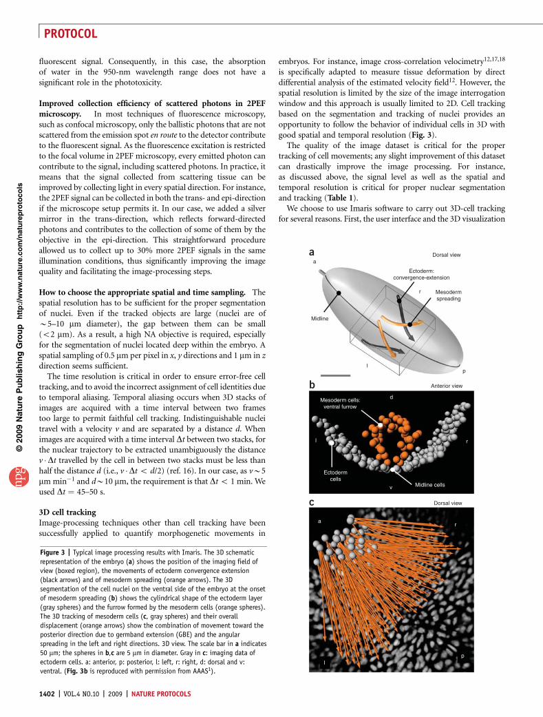
How to choose the appropriate spatial and time sampling. Thespatial resolution has to be sufficient for the proper segmentationof nuclei. Even if the tracked objects are large (nuclei are ofB5–10 mm diameter), the gap between them can be small(o2 mm). As a result, a high NA objective is required, especiallyfor the segmentation of nuclei located deep within the embryo. Aspatial sampling of 0.5 mm per pixel in x, y directions and 1 mm in zdirection seems sufficient.

The time resolution is critical in order to ensure error-free celltracking, and to avoid the incorrect assignment of cell identities dueto temporal aliasing. Temporal aliasing occurs when 3D stacks ofimages are acquired with a time interval between two framestoo large to permit faithful cell tracking. Indistinguishable nucleitravel with a velocity v and are separated by a distance d. Whenimages are acquired with a time interval Dt between two stacks, forthe nuclear trajectory to be extracted unambiguously the distancev �Dt travelled by the cell in between two stacks must be less thanhalf the distance d (i.e., v �Dt o d/2) (ref. 16). In our case, as vB5mm min�1 and dB10 mm, the requirement is that Dt o 1 min. Weused Dt ¼ 45–50 s.

3D cell trackingImage-processing techniques other than cell tracking have beensuccessfully applied to quantify morphogenetic movements in

embryos. For instance, image cross-correlation velocimetry12,17,18

is specifically adapted to measure tissue deformation by directdifferential analysis of the estimated velocity field12. However, thespatial resolution is limited by the size of the image interrogationwindow and this approach is usually limited to 2D. Cell trackingbased on the segmentation and tracking of nuclei provides anopportunity to follow the behavior of individual cells in 3D withgood spatial and temporal resolution (Fig. 3).

The quality of the image dataset is critical for the propertracking of cell movements; any slight improvement of this datasetcan drastically improve the image processing. For instance,as discussed above, the signal level as well as the spatial andtemporal resolution is critical for proper nuclear segmentationand tracking (Table 1).

We choose to use Imaris software to carry out 3D-cell trackingfor several reasons. First, the user interface and the 3D visualization

p

uor

G g

n ih si l

bu

P eru ta

N 900 2©

nat

ure

pro

toco

ls/

moc.er

ut an.

ww

w//:ptt

h

Dorsal view

Anterior view

Dorsal view

Mesoderm cells:ventral furrow

Ectodermcells

Midline cells

d

l

v

ar

pl

r

Ectoderm:convergence-extension

Midline

Mesodermspreading

r

lp

aa

b

c

Figure 3 | Typical image processing results with Imaris. The 3D schematic

representation of the embryo (a) shows the position of the imaging field of

view (boxed region), the movements of ectoderm convergence extension

(black arrows) and of mesoderm spreading (orange arrows). The 3D

segmentation of the cell nuclei on the ventral side of the embryo at the onset

of mesoderm spreading (b) shows the cylindrical shape of the ectoderm layer

(gray spheres) and the furrow formed by the mesoderm cells (orange spheres).

The 3D tracking of mesoderm cells (c, gray spheres) and their overall

displacement (orange arrows) show the combination of movement toward the

posterior direction due to germband extension (GBE) and the angular

spreading in the left and right directions. 3D view. The scale bar in a indicates

50 mm; the spheres in b,c are 5 mm in diameter. Gray in c: imaging data of

ectoderm cells. a: anterior, p: posterior, l: left, r: right, d: dorsal and v:

ventral. (Fig. 3b is reproduced with permission from AAAS1).


PROTOCOL

of the imaging dataset are extremely efficient. The cell tracks can bevisualized, checked and manually corrected using the trackingeditor (provided in version 5.7). The Imaris XT interface withMatlab improves the functionality of the software without extensiveknowledge of computer programming: for instance, the data can beexported into Matlab for further analysis. Together, it appears to bea good compromise option, as it combines the user-friendly inter-face and standard analysis of commercial software with sufficientflexibility that users can customize the tools for their applicationswithout the need to write a complete custom software package.Because an improved background knowledge of Imaris softwareand its functionalities can drastically reduce the time spent inperforming 3D cell tracking of a large dataset, users should considerobtaining experience with the software from Bitplane (Saint Paul,MN, USA) through user-training sessions (contact Bitplane custo-mer service for details).

This protocol describes the tracking of two cell populationsduring Drosophila gastrulation: mesoderm and ectoderm cells.These two groups are defined by sorting the cell trajectories usingImaris functions. The mesoderm cells are those that have invagi-nated and the ectoderm cells stay at the surface of the embryo. Afew midline cells (a sub-population of the ectoderm) are indepen-dently tracked and their trajectories are used for spatial registration(see below). The tracking of mesoderm and midline cells is donecarefully so that the trajectories span the entire time sequence.

Tracking data registrationRegistration is an important step including any spatial or temporaltransformation of the datasets that enables their comparisonbetween experiments. This protocol describes three types of dataregistration: correction of motion artifacts, transformation of theadapted spatial coordinate system, and synchronization of imagingsequences (Table 1 and Figs. 4 and 5).

In image analysis, different methods of registration exist. Forinstance, the distribution of specific markers in the sample can beused to correct its drift during acquisition (landmark-based spatialregistration), or the voxel values of an image sequence can be usedto synchronize several datasets (voxel-based temporal registra-tion19). In this procedure, we used the segmented objects them-selves to perform both spatial and temporal registration in a fullyquantitative and automated manner. For this reason, the registra-tion is performed after the 3D cell tracking. Under some experi-mental conditions, spatial registration has to be done before 3D celltracking; for instance, strong motion artifacts during the imageacquisition (embryo rolling, sample or stage drift and so on) candegrade the cell-tracking process.

In this protocol, the spatial registration includes the definition ofcell positions in accordance with the body plan. The choice of aspatial coordinate system adapted to the geometry of the tissue orembryo enables the user to investigate complex cell movements in3D by decomposing their trajectories into components that have abiological meaning. The appropriate coordinate system depends onthe biological model used: for instance, during the early stages ofdevelopment, a spherical coordinate system is adapted to the shapeof zebrafish2 or Xenopus laevis20, whereas a Cartesian coordinatesystem remains appropriate for avian embryos18. In the case ofDrosophila gastrulation, the embryo has a cylindrical shape in thearea where mesoderm spreading occurs (Supplementary Movie 2).The protocol shows first how a cylinder is fitted onto the spatialdistribution of ectoderm cells (EctodermCylinderFit.m Matlabscript, Supplementary Data 1 and Table 2) in order to identifythe anterior–posterior axis of the embryo and to switch fromCartesian (x, y and z) to cylindrical (r, y and z) coordinate system(Fig. 4). In this coordinate system, the movements in each direction(radial, angular or longitudinal) can be directly compared fromone embryo to the other and correspond to specific morpho-genetic events1.

The final step of spatial registration is the angular drift correction(Registration.m Matlab script, Supplementary Data 1 andTable 2). During acquisition, the embryo can exhibit some rollinginside its vitelline membrane, corresponding to a solid rotationaround the anterior–posterior axis (Supplementary Movies 2 and3). This angular drift is corrected by tracking a few cells from theectoderm midline and defining their angular position at each timepoint as y ¼ 0 radian (Fig. 5a–c).

The temporal registration corresponds to the synchronization ofimage sequences based on the occurrence of a specific morphoge-netic event (TimeSynchronization.m Matlab script, SupplementaryData 1 and Table 2). We choose the onset of germband extension(GBE)5,6 as the time reference to synchronize the sequences anddefine t ¼ 0 min (Fig. 5d). At this time, both ectoderm andmesoderm cells start moving toward the posterior direction1.

It is important to notice that the references used for spatial andtemporal registration are identical among embryos and are notdisrupted in mutants. Hence, they depend on the model systemstudied. In this protocol, the estimation of the anterior-posterioraxis using the shape of the ectoderm layer, the angular referencey ¼ 0 rad using the ectoderm midline cells and the time synchro-nization based on the onset of GBE are independent of themesoderm spreading process. In addition, we used these referencesfor registration because they are not disrupted in the mutant westudied1.

p

uor

G g

n ih si l

bu

P eru ta

N 900 2©

nat

ure

pro

toco

ls/

moc.er

ut an.

ww

w//:ptt

h

Figure 4 | Cylinder fit on the spatial distribution

of ectoderm cell positions obtained with

EctodermCylinderFit.m script (Step 25). The part of

the embryo imaged has a cylindrical shape (a)

with its main direction aligned with the anterior–

posterior direction. The cylindrical coordinate

system (b) is obtained after fitting a cylinder on

the distribution of ectoderm cells (a,c). After the

final registration (Step 27), the Cartesian

reference frame is rotated and the z axis is aligned

with the anterior–posterior axis of the embryo as

in c. The angular position of the midline (black line in a,b) defines the value y ¼ 0. a: anterior, p: posterior, d: dorsal, v: ventral.

p

d d

v va aa

p

p

z

r y

x�

150

–100

–100

–50–50

050

100

050

100

z (μm)

y (μm) x (μm

)

10050

0

a b c


PROTOCOL

Tracking data analysisOnce the tracking data are registered, the cell trajectories can beanalyzed directly and compared between embryos. We provide twoexamples of tracking data analysis useful for studying complex 3Dmovements of cell migration and quantifying the collective natureof this process: decomposition of cell trajectories along eachcylindrical direction (Fig. 6) using MovementDecomp.m Matlabscript (Supplementary Data 1 and Table 2) and mesodermspreading analysis (Fig. 7) using SpreadingAnalysis.m Matlab script(Supplementary Data 1 and Table 2).

Advantages and limitations of this protocol to investigate in vivocell migrationThere are a number of protocols available to investigate cellmigration in tissue culture or in model organisms (see ref. 21 forinstance). Here we discuss the advantages and specificity of thisprotocol for studying cell migration in vivo:(i) The cells are imaged in challenging conditions: they move fast

and deep inside a scattering and photo-sensitive embryo.Hence, we describe here an optimized imaging approach.

(ii) Most studies of cell migration are limited to 2D in space and tocells migrating on a fixed substrate; however, inside a livingorganism, it usually occurs in 3D, with the simultaneouscombination of different movements. This protocol showshow to investigate such complex movements in 3D by choos-ing the appropriate spatial coordinate system and decompos-ing the cell trajectories into meaningful components. In thisstudy, the mesoderm cells migrate on a moving celllayer (ectoderm): we recently demonstrated how the datagenerated by this protocol allowed us to investigate themechanical coupling between two cell layers and to decoupletheir movements1.

(iii) During embryonic development, cells rarely migrate alone butmore often as a collective. The method for tracking a large cellpopulation described in this protocol allows for simultaneousobservation of individual and collective behaviors, both ofmigrating and non-migrating cells. This approach allows the

investigator to evaluate migration using a statistical analysisand to identify variability within the cell population1. Byfollowing a limited number of cells using techniques such aslocal photo-activation, one can focus on specific behaviors,but they may not necessarily be representative of the collective.

(iv) Whereas many studies analyze the cell-tracking results using aqualitative or manual approach, we provide a quantitative andautomated analysis of cell trajectories. In this protocol, thespatial and temporal registration of the data enables theinvestigator to quantitatively compare the experiments, totest the reproducibility between embryos and to quantifymutant phenotypes1. In addition, the statistical analysis ofcell trajectories presented here illustrates how to quantify thecollective nature of a cell migration process.

(v) Sophisticated quantitative imaging of cell movements usuallyinvolves fully custom-designed approaches that are difficult toimplement or modify by other laboratories without strongexpertise2. This protocol uses commercially available equip-ment and software and provides customized Matlab scriptsthat are annotated and simple enough to be used and modifiedwith minimum expertise. Imaris, the commercial softwareused to perform 3D cell tracking, is extremely user-friendly;its interface, ImarisXT, can be used with classic programminglanguages and image-processing software, such as Matlab orImageJ, enabling a user with minimum skills in programmingto improve the functionality of this software for specificscientific applications. Together, these aspects enable the userto implement, modify or extend this protocol in a biologylaboratory without extensive expertise in microscopy or com-puter science.

This protocol has two main limitations. First, cell migration isinvestigated by only tracking the cell nuclei. Although this approachcan generate a lot of biological insights, the analysis of other cellfeatures, such as cell shape changes, can be required for specificstudies. In the case of mesoderm spreading in Drosophila, thechallenging scattering conditions (see above) strongly limit the

p

uor

G g

n ih si l

bu

P eru ta

N 900 2©

nat

ure

pro

toco

ls/

moc.er

ut an.

ww

w//:ptt

h

1.5

Midline cellsbefore spatial registration

Mesoderm cellsbefore spatial registration

Mesoderm cellsafter spatial registration

Mesoderm cellsafter temporal registration

1

0.5

0 50 100Timepoint

150 0 50 100Timepoint

150 0 50 100Timepoint

150

r

r

l

l

r

p

al

θ in

rad

0

–0.5

–1

1.5

1

0.5

θ in

rad

0

–0.5

–1

1.5 140

120

100

80

60

40

20

0 50 100Timepoint

t = 0 min

1500

1

0.5

0 in

rad

z in

μm

0

–0.5

–1

a b c d

Figure 5 | Spatial and temporal registration (Steps 26 and 27). The Registration.m script subtracts the average angular movement of midline cells (a) from the

angular movement of mesoderm cells (b) to obtain a correction of the angular drift (c). After correction, the average angular position of mesoderm cells (black

line in b,c) remains close to 0 during the entire spreading process, showing the symmetrical nature of the spreading. The TimeSynchronization.m script

identifies the onset of germband extension (GBE, at t ¼ 0 min) and displays the mesoderm cell movement toward the posterior direction (d). The gray lines

represent the trajectories of midline cells (a) or mesoderm cells (b–d). The black line is the average trajectory of the cell population. The dashed gray lines in

a–c show y ¼ 0 rad position. The dashed gray lines d show t ¼ 0 min position. The timepoints (horizontal axis of the graphs) represent the image number

within the sequence; after temporal synchronization these timepoints are converted into minutes. a: anterior, p: posterior, l: left, r: right, d: dorsal, v: ventral,

rad: radians.


PROTOCOL

imaging of structures other than nuclei, such as cell membranes.The second limitation concerns the 3D cell tracking: the fluorescentsignal from the deepest nuclei is weak and its segmentation andtracking requires manual correction. This step, which is not fullyautomated, limits the number of cells segmented per experiment.For this reason, we limited our application of this protocol to

B100,000 segmented cell positions per embryo (including ecto-derm and mesoderm cells)1. To increase this number, furtherimprovement of imaging quality and/or of image segmentation/tracking strategy would be required. The subsequent computeranalysis of cell trajectories provided here is automated and is notlimited by the cell number.

MATERIALSREAGENTS.Drosophila transgenic line with an ubiquitous expression of Histone 2A-GFP

fusion protein (Bloomington Drosophila Stock Center, stock number 5941)and klar mutant line Bloomington Drosophila Stock Center, stock number3256

.Halocarbon Oil 27 (Sigma, cat. no. H8773)

.Heptane (EMD, cat. no. HX0080)

.50% (vol/vol) Bleach (Clorox) or sodium hypochlorite (Reagent grade,Sigma, cat. no. 239305) ! CAUTION Bleach is poisonous. Wear personalprotection, such as gloves and goggles.

.Glacial acetic acid (VWR, cat. no. MK312146) ! CAUTION Acetic acid iscorrosive. Handle with gloves.

.Ethanol (Sigma-Aldrich, cat. no. 459836) ! CAUTION Ethanol is flammable.

.UltraPure agarose (Invitrogen, cat. no. 15510-019)

.Apple juice (generic brand)

.Sucrose (generic brand)EQUIPMENT.Paintbrush (small brush size: 3/0 White Sable Robert Simmons).Double-sided sticky tape (TESA) m CRITICAL If another brand is used,

ensure the glue is not toxic to the embryos..Coverslips (22 � 22 mm, No.1, VWR, cat. no. 48366 067).35 � 10 mm petri dishes (BD Falcon, cat. no. 353001).60 � 15 mm petri dishes (BD Falcon, cat. no. 353002).2PEF Microscope: Zeiss LSM 510 with Chameleon Ultra Laser (Coherent)

p

uor

G g

n ih si l

bu

P eru ta

N 900 2©

nat

ure

pro

toco

ls/

moc.er

ut an.

ww

w//:ptt

h

TABLE 2 | Description of the customized Matlab scripts contained in Supplementary Data 1.

Matlab script name Description

Imaris2xyzt.m Converts the tracking data exported by ImarisXT Object Manager into x, y, z and t matrices. x(i,j), y(i,j), z(i,j) and t(j)are the spatial cartesian coordinates in mm and the time in minute of each cell i at each time point j. i and j areintegers. In case the tracking data appear noisy (i.e., trajectories with small movements at high frequency), thisscript can smooth them in time by using a five point Loess quadratic fit applied to each spatial component. RequiresImaris tracking files (Mesoderm.mat, Ectoderm.mat or Midline.mat) and stores the results in Mesodermxyzt.mat andEctodermxyzt.mat or Midlinexyzt.mat files, respectively

EctodermCylinderFit.m Fits a cylinder on the distribution of ectoderm cell positions (Fig. 4c). Estimates the direction (CylDirection), thecenter (CylCenter) and the radius (CylRadius) of the cylinder. Requires Ectodermxyzt.mat and stores the result into thefile CylFitResult.mat

TimeSynchronization.m Estimates j0, the time point for which t¼ 0 min as the onset of germband extension (GBE) by checking the mesodermcell movements toward the posterior direction (Fig. 5d). Requires Mesodermxyzt.mat and CylFitResult.mat and storesj0 in the j0.mat file

Registration.m Spatial and temporal registration of the tracking data. Registers the time matrix t by using the j0 value. Rotates in 3Dthe Cartesian reference frame using the cylinder fit result so that the z axis is aligned with the embryo anteriorposterior direction (main axis of the cylinder). In this frame, the new Cartesian components x, y, and z can be directlyconverted into the cylindrical components r, y, and z using the cart2cyl.m function from geom3d toolbox. Anadditional rotation of the frame along the anterior-posterior axis creates the mesoderm cell angular positions y in the[�p/2 p/2] range using cart2cyl0.m function. Corrects the angular drift of mesoderm cells using the midline trackingdata (Fig. 5a–c). Requires Mesodermxyzt.mat, Midlinexyzt.mat, CylFitResult.mat and j0.mat. Stores the registeredmesoderm cell tracking data (xReg, yReg, zReg and tReg matrices) into the MesodermReg.mat file

MovementDecomp.m Loads the MesodermReg.mat file and converts the Cartesian coordinates into the Cylindrical coordinates. Plots thetime variation of each component (r(t), y(t), and z(t)) for each cell into three graphs as displayed in Figure 6.Requires MesodermReg.mat file

SpreadingAnalysis.m Loads the MesodermReg.mat file and converts the Cartesian coordinates into the Cylindrical coordinates. Displays y(t)for each cell with a color coding for the angular position at the onset of the furrow collapse, as in Figure 7c. Identifiesthis timepoint (jstart) as the time when the furrow has a cylindrical shape. Displays the angular position at the end ofthe spreading yend (defined as 120 min after jstart) depending on the angular position at the onset ystart (at jstart) foreach cell. Performs a linear regression on the distribution of the points in this graph and the result is displayed on it asin Fig. 7d). Requires MesodermReg.mat file

Browse.m Browse function

cart2cyl0.m Converts cartesian to cylindrical coordinates. This function is similar to cart2cyl.m from the geom3D toolbox butreturn y in [�p p], instead of in [0 2p]


PROTOCOL

.C-Aprochromat 40�/1.1 NA W Corr UV-VIS-IR (Carl Zeiss)objective.

.Software: Imaris 5.7 with ImarisTrack, Imaris MeasurementPro, andImarisXT modules (Bitplane) and Matlab 7.7 (The MathWorks).

.Computer: 3.0 GHz Dual-Core Processor, 16 Gb DDR RAM, Large SATAHard Drive (4 100 Gb, faster than 7000 rpm)

.1-liter glass bottles and 25-ml plastic pipettes.

.Optional: Thumbtack/Needle

.Small basket to handle the embryos. One can use 100-mm cell strainers(BD Falcon, cat. no. 352360)

.Standard dissecting microscope

REAGENT SETUPApple juice plate Dissolve 22 g of sucrose in 350 ml of H2O and pour it into a1-liter bottle. Add 7 g of agarose into this bottle, mix by vigorous shaking.Microwave first for 2 min, and then twice for 1 min, mix the solution inbetween. m CRITICAL The agarose solution must boil in the microwave.Put aside to cool to B60 1C. Add 10 ml of ethanol and 5 ml of glacial aceticacid to the solution. Add 50 ml of apple juice and mix well. Pipette into35 � 10 mm dishes (B60 plates per preparation) using a 25-ml plastic pip-ette or syringe. The plates can be stored in a container at 4 1C for weeks.! CAUTION Acetic acid is corrosive. Handle with gloves. ! CAUTION Ethanolis flammable.

p

uor

G g

n ih si l

bu

P eru ta

N 900 2©

nat

ure

pro

toco

ls/

moc.er

ut an.

ww

w//:ptt

h

Figure 7 | Analysis of mesoderm cell spreading

using SpreadingAnalysis.m (Step 28B). (a) Three

specific cell movements are identified. First, a cell

moving from ystart to yend (angular positions at

the onset and at the end of the process,

respectively) with yend / ystart 4 1 corresponds to

a normal spreading behavior (white area). In this

case, the cell (+ sign) is moving on top of the

ectoderm layer (gray ovals), further away from the

midline position (black ovals, y ¼ 0 position). A

disrupted spreading (light gray area) with cells

moving toward the midline (x sign) corresponds to

0 o yend / ystart o 1. Finally, the most disrupted

behavior (dark gray area) corresponds to a cell

crossing the midline (o sign) and moving on the

opposite side of the embryo with yend / ystart o 0.

These three behaviors correspond to three

different areas of the yend(ystart) graph (b): white,

light gray and dark gray, respectively. The

movement of each cell is represented by a point

on this graph and the slope of the gray lines is

the yend / ystart in each case (normal spreading,

+ sign and disrupted movements, x and o signs).

This representation is used by the script to

analyze the spatial organization of the cell

movements in the angular direction. It first

displays y(t) for each cell with a color coding for

the angular position at the onset of the furrow

collapse (c) and the yend(ystart) graph (d). The

experimental data obtained from a wild-type

embryo (+ signs in d) are mainly located in the

white area of the graph, corresponding to a normal spreading. This distribution is analyzed using a linear regression as described in Anticipated results. The

result of the regression is shown on the graph (gray line and values A, B and R, see Anticipated Results for details, B is the zero intercept of the regression

line). rad: radians. (Fig. 7d is modified with permission from AAAS1.)

Figure 6 | Decomposition of mesoderm cell

movements into their cylindrical components

using MovementDecomp.m (Step 28A). This script

decomposes the registered trajectories of

mesoderm cells into their cylindrical components

(r, y and z, for radial, angular and longitudinal

components, respectively) and plots the three

graphs r(t), y(t) and z(t) as shown in this figure

(a,b and c, respectively). The gray lines represent

the trajectories of mesoderm cells along each

cylindrical direction. The black line is the average

trajectory of the cell population. In the radial

direction (a), r ¼ 0 corresponds to the center of the embryo and mesoderm cells moving toward positive values of r are moving closer to the ectoderm layer, at

the periphery of the embryo. The graph r(t) shows the furrow collapse with the cells moving toward the ectoderm (a). In the angular direction (b), y ¼ 0

corresponds to the position of the ectoderm midline and the cells moving toward positive or negative values of y are moving toward the right or left side of the

embryo, respectively. The graph y(t) shows the angular spreading of the mesoderm cells with movements toward the left and right directions (b). In the

longitudinal direction (c), z ¼ 0 is arbitrarily chosen, and the cells moving toward positive or negative values of z are moving toward the posterior or anterior

end of the embryo, respectively. The graph z(t) shows the movement of germband extension (GBE) with a concerted movement of mesoderm cells toward the

posterior direction (c). rad: radians.

01

140

120

100

80

60

40

20

0

0.5

–0.5

–1

0

10

20

30

40

50r in

μm

z in

μm

θ in

rad

60

70

80

900 50

Time in min100 0 50

Time in min100 0 50

Time in min100

a b c

Normal spreading:�end / �start > 1

1

0.5 Disrupted

Disrupted

Start End

Normal

Linear regression

A = 2.04B = 0.04R = 0.94

–0.5

–1

–1 –0.5 0 0.5 1

0

1

0.5

–0.5

–1

0

1

0.5

–0.5

–1

0

Disrupted spreading:0 < �end / �start < 1

Disrupted spreading:�end / �start < 0

�start in rad

�end = A.�start + B

–1 –0.50 25 50Time in min

75 100 0 0.5 1

�start in rad

� end

in r

ad� e

nd in

rad

� in

rad

�end

�start

a b

c d

0


PROTOCOL

Agarose plate Dissolve 30 g of sucrose in 350 ml of H2O and pour it into a1-liter bottle. Add 10 g of agarose to the bottle, mix by vigorous shaking.Microwave first for 2 min, and then twice for 1 min, mixing the solution inbetween. m CRITICAL The agarose solution must boil in the microwave.Put aside to cool to B60 1C. Pipette into 60 � 15 mm dishes (B20 platesper preparation) using a 25-ml plastic pipette or syringe. The plates can bestored in a container at 4 1C for weeks.

EQUIPMENT SETUPPreparation of coverslips coated with glue for embryo imaging Add shortpieces (5–10 cm) of double-sided tape to a 200-ml glass bottle. Add heptane tocover the pieces of tape (typically 50 ml for 50 cm of tape). Gently shake thebottle at least overnight at room temperature (18–25 1C) to dissolve the glue.The heptane–glue bottle can be stored at room temperature for months. Preparecoverslips coated with glue at least 10 min before using them. Add a 60–100-mldroplet of heptane–glue to the middle of each coverslip and allow to dry for 10min. The coated coverslips can be stored for a few days at room temperaturein a box to protect them from dust.Microscope settings for live imaging (Zeiss LSM 510) Most of ourimaging datasets have been acquired using a Zeiss LSM 510 microscopeand a Chameleon Ultra femtosecond laser. However, the protocol can beaccomplished with any similar 2PEF microscope. The embryos were imagedusing C-Aprochromat 40�/1.1 NA W Corr UV-VIS-IR objective at 940 nm.The non-descanned pathway is used with a single short pass filter (KP680nm)to cut out the laser light. 3D stacks of dimensions 200 � 200 � 80 mm3 with0.5 � 0.5 � 1 mm3 voxel size and 1.9 ms pixel dwell time were acquiredevery 45–50 s for B3 h.

LSGE and geom3D toolboxes for Matlab processing The Matlabprocessing requires two freely available toolboxes: the Least Squares GeometricElements (LSGE) library and the geom3D toolbox. The LSGE library wasdeveloped by the Centre for Mathematics and Scientific Computing(National Physical Laboratory, Teddington, UK) and is available from theEUROMETROS website (http://www.eurometros.org/metros/packages/lsge).The geom3D toolbox was developed by David Legland and is availablefrom Matlab Central website (http://www.mathworks.com/matlabcentral/fileexchange/24484). Download the files, save the ‘lsge-matlab’ and ‘geom3D’folders and their content on your computer and add both of them inthe Matlab path (using ‘File/Set Path’ from the Matlab menu).Customized Matlab scripts Download the Matlab scripts from thesupplemental section of this protocol (Supplementary Data 1). Unzip thecorresponding file and place all contained files (Imaris2xyzt.m,EctodermCylinderFit.m, TimeSynchronization.m, Registration.m, Movement-Decomp.m, SpreadingAnalysis.m, Browse.m, and cart2cyl0.m) in the same folder.The customized Matlab scripts included here are designed and annotated in orderto allow the user to run and modify them with only basic knowledge of Matlabprogramming. However, to further manipulate the data, a working knowledge ofMatlab is required. Table 2 provides a list of the scripts and their description.Sample tracking data files In order to run the Matlab processing and start theprocedure at Step 23 without an imaging dataset, we provide sample trackingdata files. Download the files from the supplemental section of this protocol(Supplementary Data 2). Unzip the corresponding file and place all of thefiles (Mesoderm.mat, Ectoderm.mat and Midline.mat) in the same folder asthe Matlab scripts.

PROCEDUREEmbryo preparation � TIMING 4 h per set of embryos for imaging1| Grow flies in standard culture bottles (the generation time is B10 d at 25 1C; see http://flystocks.bio.indiana.edu/Fly_Work/culturing.htm for details).

2| Transfer the flies into a collection bottle and add an apple juice plate (see Reagent setup and standard procedurein reference 22).

3| Collect the embryos after 2–3 h of laying at 25 1C.

4| Add a few droplets of halocarbon oil on the embryos to make the chorion translucent, stage the embryos10, and selectB10–20 stage 5 embryos. Embryos reach stage 5 after 2–3 h of development. This stage is easily identified by looking at thetransparent layer of cellularizing cells at the embryo periphery (see http://flymove.uni-muenster.de/ for pictures of stages).

5| Dechorionate the embryos using either option A (dechorionation with bleach) or option B (dechorionation with a needle),depending on the user’s preference and ability.(A) Dechorionation with bleach

(i) Transfer the embryos into a basket using a paintbrush.(ii) Remove the oil from the bottom with a paper towel.(iii) Rinse the embryos with a few milliliters of water.(iv) Soak the basket in fresh 50% bleach (vol/vol) and control the dechorionation by looking at the embryos under a dissect-

ing microscope. When the first bubble appears between the chorion and the vitelline membrane of any embryo, immedi-ately proceed to step v (should take 10–40 s).

(v) Rinse the basket with copious amounts of water to remove the bleach.(vi) Remove the water from the bottom with a paper towel.m CRITICAL STEP Do not over-bleach the embryos, in order to ensure their viability and normal development.

(B) Dechorionation with a needle(i) Prepare a microscope slide with a double-sided tape on one side of it.(ii) Transfer the embryos into a basket using a paintbrush.(iii) Remove the oil from the bottom with a paper towel.(iv) Rinse the embryos with a few milliliters of water.(v) Transfer the embryos to the sticky tape on the slide prepared in Step 5 option B(i).(vi) Use a needle or thumbtack to gently tear the chorion open.(vii) Use a paintbrush to gently remove the embryo from the chorion. (See video step 7 in reference 23 for details.)

p

uor

G g

n ih si l

bu

P eru ta

N 900 2©

nat

ure

pro

toco

ls/

moc.er

ut an.

ww

w//:ptt

h


PROTOCOL

m CRITICAL STEP After dechorionation, the embryos are more fragile, and therefore they should only be gently manipulated.Minimize the time they spend in the air without water.

6| Gently transfer the embryos onto an agarose plate (see Reagent setup). Once placed on this plate, the water content of theagarose gel prevents them from drying.m CRITICAL STEP From Step 6 to Step 8, the embryos have to be kept as clean as possible: any piece of chorion, dust or agarosesticking to their surface can have a large negative impact on the imaging quality.

7| Align and orient the embryo dorsal side up at the center of the agarose plate.? TROUBLESHOOTING

8| Cut the central piece of agar and transfer it under a dissecting scope.

9| Gently stick the embryos to a coverslip coated with glue (see Equipment setup) by bringing the coverslip glue side downtowards the embryos until they just touch the coverslip. Turn over the coverslip and add a water droplet on top of the embryos.m CRITICAL STEP Be careful not to crush the embryos with the coverslip.

4D imaging � TIMING 3 h per imaging acquisition10| Using an inverted Zeiss LSM microscope, add a water droplet onto the long working distance water objective. Place thecoverslip (from Step 9) under the microscope with the embryos facing the objective. Bring the embryos into focus usingbrightfield transmitted illumination to avoid any bleaching of GFP.

11| Adjust the femtosecond laser to a wavelength of 940 nm. Adjust the mean power to a level no higher than B20 mW at theobjective focus (use a powermeter to check it).

12| Choose a well-oriented embryo early at stage 6 (ref. 10) with the ventral furrow facing the objective, in the middle of thefield of view. Adjust the position and field of the acquisition. Use a 200 � 200 mm2 field in the center of the embryo (Fig. 3aand Supplementary Movie 2). Select the appropriate spatial and temporal sampling as discussed in the Introduction: typically0.5 mm per pixel in x and y, and 1 mm in z; 45–50 s of time between each z-stack including 10 s of the resting time. Adjust thenumber of z-slices to the image, such that data are acquired from the most ventral ectoderm cells to the expected position ofthe most dorsal mesoderm cells when the ventral furrow is fully formed (typically 80 mm z-stack).

13| Adjust the photomultiplier tube gain to avoid any saturation of the fluorescent signal from the mesoderm cells at every z-position. Saturation occurs when the signal detected causes the pixel to reach its maximum value (255 for an 8-bit image).There will be some saturation in the fluorescent signal from the ectoderm.

14| Run the time-lapse acquisition for 3 h at 25 1C. Monitor the temperature during acquisition: it is critical as the speed ofdevelopment is highly sensitive to the temperature (development proceeds at a rate that is approximately twice as fast at 25 1Ccompared with 18 1C).’ PAUSE POINT Store the acquisition data until use. The rest of the protocol can be paused at any time.? TROUBLESHOOTING

15| Repeat Steps 1–15 several times in order to obtain a good imaging dataset (i.e., no phototoxicity, good orientation, goodsignal-to-noise ratio, correct time and spatial window, sufficient number of cells staying within the field of view).

3D cell tracking � TIMING weeks16| Load and visualize the imaging datasets in 3D using Imaris. Select a good dataset (see Step 15) and crop it in time andspace to focus on the useful time and spatial window. Ensure that the spatial calibration (size of voxels in mm per pixel)corresponds to your microscope calibration. Save the file as EmbryoSequence.imsm CRITICAL STEP In order to carry out the 3D cell tracking efficiently and reduce the time spent to do it; extensive knowledgeof Imaris software is recommended. The user is invited to follow Bitplane user-training sessions or to contact the Bitplanecustomer service for further information.? TROUBLESHOOTING

17| Segment the nuclear position using Imaris spot detection: adjust the size to 4–5 mm.? TROUBLESHOOTING

18| Track the cell movements using Imaris spot tracking. Use the ‘autoregressive motion’ option with gap size set to 2; thescripts provided to analyze the data are not designed for a larger gap.

p

uor

G g

n ih si l

bu

P eru ta

N 900 2©

nat

ure

pro

toco

ls/

moc.er

ut an.

ww

w//:ptt

h


PROTOCOL

19| Sort and manually correct the tracks using the Tracking Editor, so that each track is complete from the beginning to theend of the sequence. However, keep in mind that the scripts provided to analyze the data handle only one-branch track, mean-ing that each track has a maximum of one spot per time point (see the annotations in Matlab scripts for details, SupplementaryData 1). This is a concern, as after a cell division only one daughter will acquire the initial track sequence. Manual correction isrequired. First, detect the cell divisions manually. Subsequently, duplicate each track before a cell division so that each daughtercell has its own track from the beginning to the end.

20| Complete the tracking data using manual spot detection and tracking. Save the scene file as EmbryoSequence.imx

21| Perform Steps 17–20 successively for mesoderm cells, ectoderm cells and a few cells (typically 8) from the midline. UseImaris functions to select the tracks from the corresponding subpopulation of cells. The midline cells can be visually discernedand tracked manually (Supplementary Movie 3). Because the ectoderm is used only as a reference, the tracks from the ecto-derm do not need to be complete (i.e., not all tracks have to go from the beginning to the end and some cells can be missing)for the subsequent analysis: typically 50% of cells tracked representing the ectoderm movement is sufficient. There is no needto identify the daughter cells after division in this case.? TROUBLESHOOTING

22| Split and export the tracking data using ImarisXT Object Manager into three different files: Mesoderm.mat, Ectoderm.matand Midline.mat

Tracking data registration � TIMING 1 h23| Place the tracking data files (Mesoderm.mat, Ectoderm.mat and Midline.mat) in the same folder as the customized Matlabscripts (Supplementary Data 1 and Table 2). One can start the procedure at this step using the sample-tracking data filesprovided in the supplementary section of this protocol (Supplementary Data 2).

24| Convert Imaris tracking files into x, y, z and t matrices using the Imaris2xyzt.m Matlab script. This script outputs x(i,j),y(i,j), z(i,j) and t(j), with i and j representing the cell number and the time point, respectively. x and y are the image plane coor-dinates, z the axial direction of imaging and t the time. Enter the tsequence, the time calibration (time delay between z-stacks).This script checks errors in the tracking dataset: if required, correct the tracking in Imaris and recheck for errors (see scriptannotations for details). Run the script for each Imaris tracking file (Mesoderm.mat, Ectoderm.mat and Midline.mat). Output:Midlinexyzt.mat, Mesodermxyzt.mat and Ectodermxyzt.mat.

25| Fit a cylinder on the 3D distribution of ectoderm cell positions (Fig. 4) using the EctodermCylinderFit.m Matlab script.

26| Synchronize the sequences based on the onset of GBE (Fig. 5d) using the TimeSynchronization.m Matlab script.

27| Perform the final registration (Fig. 5a–c) of the tracking data using the Registration.m Matlab script. The registered meso-derm cell-tracking data (xReg, yReg, zReg and tReg matrices) are saved in the MesodermReg.mat file.

Tracking data analysis � TIMING 1 h28| A number of different analyses can be performed after tracking data registration1. For example, to decompose the celltrajectories into their cylindrical components, use option A below. To carry out a statistical analysis of the mesoderm cellmigration and quantify its collective nature, use option B.(A) Display the tracking data using MovementDecomp.m Matlab script (Fig. 6).

(i) Run MovementDecomp.m Matlab script and follow the instructions. The mesoderm cell 3D trajectories are decomposedalong each cylindrical coordinate (r(t), y(t) and z(t)) as shown in Fig. 6.

(B) Analyze the mesoderm cell spreading using SpreadingAnalysis.m (Fig. 7).(i) Run SpreadingAnalysis.m and follow the instructions. It displays the spreading analysis of mesoderm cells: spatial organi-

zation as in Fig. 7c and yend(ystart) graph with the statistical analysis results as in Fig. 7d.

� TIMINGSteps 1–9, Embryo preparation: 4 h per set of embryos for imaging.Steps 10–15, 4D imaging: 3 h per imaging acquisition. Repeat Steps 1–15 several times in order to obtain 3–4 correct imagingdatasets: B1 week.Steps 16–22, 3D cell tracking: several weeks per imaging dataset depending on the quality of the dataset and on the efficiencyof the user to perform the tracking correction with Imaris.Steps 23–27, Tracking data registration: 1 h maximum per dataset.Step 28, Tracking data analysis: 1 h maximum per dataset.

p

uor

G g

n ih si l

bu

P eru ta

N 900 2©

nat

ure

pro

toco

ls/

moc.er

ut an.

ww

w//:ptt

h


PROTOCOL

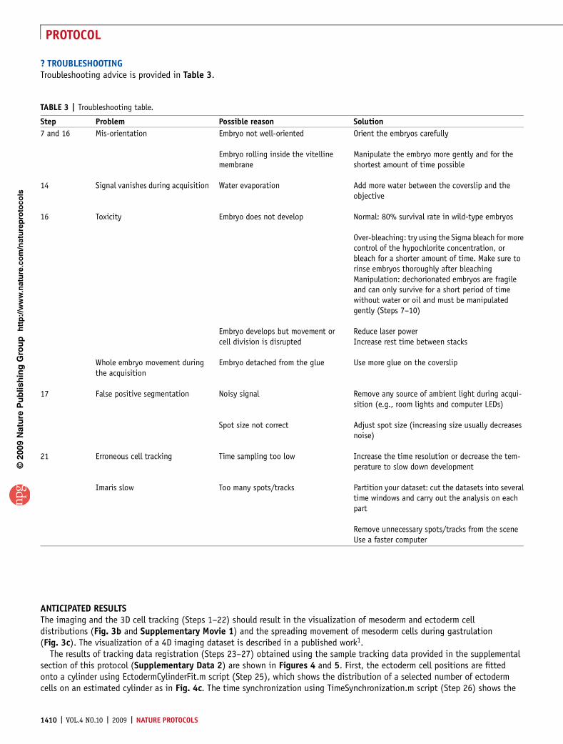
? TROUBLESHOOTINGTroubleshooting advice is provided in Table 3.

ANTICIPATED RESULTSThe imaging and the 3D cell tracking (Steps 1–22) should result in the visualization of mesoderm and ectoderm celldistributions (Fig. 3b and Supplementary Movie 1) and the spreading movement of mesoderm cells during gastrulation(Fig. 3c). The visualization of a 4D imaging dataset is described in a published work1.

The results of tracking data registration (Steps 23–27) obtained using the sample tracking data provided in the supplementalsection of this protocol (Supplementary Data 2) are shown in Figures 4 and 5. First, the ectoderm cell positions are fittedonto a cylinder using EctodermCylinderFit.m script (Step 25), which shows the distribution of a selected number of ectodermcells on an estimated cylinder as in Fig. 4c. The time synchronization using TimeSynchronization.m script (Step 26) shows the

p

uor

G g

n ih si l

bu

P eru ta

N 900 2©

nat

ure

pro

toco

ls/

moc.er

ut an.

ww

w//:ptt

h

TABLE 3 | Troubleshooting table.

Step Problem Possible reason Solution

7 and 16 Mis-orientation Embryo not well-oriented Orient the embryos carefully

Embryo rolling inside the vitellinemembrane

Manipulate the embryo more gently and for theshortest amount of time possible

14 Signal vanishes during acquisition Water evaporation Add more water between the coverslip and theobjective

16 Toxicity Embryo does not develop Normal: 80% survival rate in wild-type embryos

Over-bleaching: try using the Sigma bleach for morecontrol of the hypochlorite concentration, orbleach for a shorter amount of time. Make sure torinse embryos thoroughly after bleachingManipulation: dechorionated embryos are fragileand can only survive for a short period of timewithout water or oil and must be manipulatedgently (Steps 7–10)

Embryo develops but movement orcell division is disrupted

Reduce laser powerIncrease rest time between stacks

Whole embryo movement duringthe acquisition

Embryo detached from the glue Use more glue on the coverslip

17 False positive segmentation Noisy signal Remove any source of ambient light during acqui-sition (e.g., room lights and computer LEDs)

Spot size not correct Adjust spot size (increasing size usually decreasesnoise)

21 Erroneous cell tracking Time sampling too low Increase the time resolution or decrease the tem-perature to slow down development

Imaris slow Too many spots/tracks Partition your dataset: cut the datasets into severaltime windows and carry out the analysis on eachpart

Remove unnecessary spots/tracks from the sceneUse a faster computer


PROTOCOL

movement of the mesoderm cells toward the posterior direction and estimates the time point at which the onset of movementoccurs (Fig. 5d). The Registration.m script (Step 27) shows the angular movements of mesoderm cells before and after angulardrift correction, as in Figure 5a–c.

After the tracking data registration, the decomposition of mesoderm cell movements into their cylindrical components r(t),y(t) and z(t) using MovementDecomp.m script (Step 28A) yields the three graphs of Figure 6. Each of these graphs correspondsto a specific morphogenetic event: (i) r(t) shows the furrow collapse with the cells moving toward the periphery of the embryo(Fig. 6a); (ii) y(t) shows the angular spreading of the mesoderm cells with movements toward the left and right directions(Fig. 6b); (iii) z(t) shows the movement of GBE with a concerted movement toward the posterior direction (Fig. 6c).

The analysis of mesoderm spreading using SpreadingAnalysis.m (Step 28A) yields the two graphs of Figure 7c,d. The firstgraph shows y(t) for each cell with a color coding for the angular position at the onset of furrow collapse. It shows that theangular distribution of the mesoderm cells is maintained over the 2 h of mesoderm spreading (Fig. 7c). The yend (ystart) graph(Fig. 7d) is used to investigate the collective migration of mesoderm cells during their spreading. The position of each cell inthis graph corresponds to a specific movement behavior detailed in Figure 7a,b. When yend/ystart41 (white areas in thegraphs), the cells are spreading normally. If 0oyend/ystarto1 (light gray areas in the graphs), the cells are not spreading andmove in the opposite direction, toward the midline. If yend/ystarto0 (dark gray areas in the graphs), the cells are not spreading,cross the midline and move to the opposite side of the embryo. In wild-type embryos, the cells’ positions in the yend(ystart)graph are mainly distributed in the white area (Fig. 7d). In addition, they tend to be aligned along a specific line: a linearregression gives an estimation of the slope of this line (A) and of the correlation coefficient (R) (Fig. 7d). As reported pre-viously1, A and R values should be close to 2 and 1, respectively. This statistical analysis provides a quantitative tool for investi-gating the collective behavior exhibited by mesoderm cells during their spreading. The behavior is quantitatively defined as thespreading strength A, which corresponds to the typical value of yend/ystart. The collective nature of the process is quantified byR: a value close to 1 demonstrates the spreading behavior A ¼ yend/ystart is shared by the entire cell population, as in wild-typeembryos; a lower value means the cell spreading is disrupted, as in mutants. This quantitative analysis has been used to demon-strate (i) the reproducibility of the collective behavior in wild-type embryos and (ii) the disruption of the process and the iden-tification of different cell populations in a mutant embryo1.

The procedure described in this paper details every experimental step from the preparation of embryos for imagingto the quantitative analysis of mesoderm cell spreading. In addition to this analysis (Step 28), the cell movements can be ana-lyzed in any manner that users finds interesting by developing their own customized Matlab scripts to analyze the registereddata (Step 27).

Note: Supplementary information is available via the HTML version of this article.

ACKNOWLEDGMENTS We thank M. Liebling for advice on Imaris and Matlab, andthe Caltech Biological Imaging Center for sharing equipment. This work wassupported by grants to AS from National Institutes of Health (R01 GM078542), theSearle Scholars Program and the March of Dimes (Basil O’Conner Starter ScholarAward, 5-FY06-145), grants to SF from the Caltech Beckman Institute and NationalInstitutes of Health (Center for Excellence in Genomic Science grantP50HG004071), and fellowship to W.S. from the Caltech Biology Division.

AUTHOR CONTRIBUTIONS W.S. designed the experimental workflow and thecomputational analysis. W.S. and A.M. acquired and processed the data.W.S., A.M., S.E.F. and A.S. wrote the paper.

Published online at http://www.natureprotocols.com.Reprints and permissions information is available online at http://npg.nature.com/reprintsandpermissions.

1. McMahon, A., Supatto, W., Fraser, S.E. & Stathopoulos, A. Dynamic analyses ofDrosophila Gastrulation provide insights into collective cell migration. Science322, 1546–1550 (2008).

2. Keller, P.J., Schmidt, A.D., Wittbrodt, J. & Stelzer, E.H.K. Reconstruction ofZebrafish early embryonic development by scanned light sheet microscopy.Science 322, 1065–1069 (2008).

3. Leptin, M. & Grunewald, B. Cell shape changes during gastrulation in Drosophila.Development 110, 73–84 (1990).

4. Kam, Z., Minden, J.S., Agard, D.A., Sedat, J.W. & Leptin, M. Drosophilagastrulation: analysis of cell shape changes in living embryos bythree-dimensional fluorescence microscopy. Development 112, 365–370(1991).

5. Irvine, K.D. & Wieschaus, E. Cell intercalation during Drosophila germbandextension and its regulation by pair-rule segmentation genes. Development 120,827–841 (1994).

6. Bertet, C., Sulak, L. & Lecuit, T. Myosin-dependent junction remodelling controlsplanar cell intercalation and axis elongation. Nature 429, 667–671 (2004).

7. Smallhorn, M., Murray, M.J. & Saint, R. The epithelial-mesenchymal transitionof the Drosophila mesoderm requires the Rho GTP exchange factor Pebble.Development 131, 2641–2651 (2004).

8. Debarre, D. et al. Imaging lipid bodies in cells and tissues using third-harmonicgeneration microscopy. Nat. Methods 3, 47–53 (2006).

9. Welte, M.A., Gross, S.P., Postner, M., Block, S.M. & Wieschaus, E.F. Developmentalregulation of vesicle transport in Drosophila embryos: forces and kinetics. Cell 92,547–557 (1998).

10. Hartenstein, V. Atlas of Drosophila development. In The Development of Drosophilamelanogaster (eds. Bate, M. & Martinez Arias, A.) 36 and 52 (Cold Spring HarborLaboratory Press, Cold Spring Harbor, NY, USA, 1993).

11. Supatto, W., Fraser, S.E. & Vermot, J. An all-optical approach for probingmicroscopic flows in living embryos. Biophys. J. 95, L29–L31 (2008).

12. Supatto, W. et al. In vivo modulation of morphogenetic movements in Drosophilaembryos with femtosecond laser pulses. Proc. Natl. Acad. Sci. USA 102,1047–1052 (2005).

13. Hopt, A. & Neher, E. Highly nonlinear photodamage in two-photon fluorescencemicroscopy. Biophys. J. 80, 2029–2036 (2001).

14. Ji, N., Magee, J.C. & Betzig, E. High-speed, low-photodamage nonlinear imagingusing passive pulse splitters. Nat. Methods 5, 197–202 (2008).

15. Beaurepaire, E. & Mertz, J. Epifluorescence collection in two-photon microscopy.Appl. Optics 41, 5376–5382 (2002).

16. Vermot, J., Fraser, S.E. & Liebling, M. Fast fluorescence microscopy for imagingthe dynamics of embryonic development. HFSP J. 2, 143–155 (2008).

17. Debarre, D. et al. Velocimetric third-harmonic generation microscopy:micrometer-scale quantification of morphogenetic movements in unstainedembryos. Opt. Lett. 29, 2881–2883 (2004).

18. Zamir, E.A., Czirok, A., Cui, C., Little, C.D. & Rongish, B.J. Mesodermal celldisplacements during avian gastrulation are due to both individual cell-autonomous and convective tissue movements. Proc. Natl. Acad. Sci. USA 103,19806–19811 (2006).

p

uor

G g

n ih si l

bu

P eru ta

N 900 2©

nat

ure

pro

toco

ls/

moc.er

ut an.

ww

w//:ptt

h


PROTOCOL

19. Liebling, M., Forouhar, A.S., Gharib, M., Fraser, S.E. & Dickinson, M.E.Four-dimensional cardiac imaging in living embryos via postacquisitionsynchronization of nongated slice sequences. J. Biomed. Opt. 10, 054001 (2005).

20. Tyszka, J.M., Ewald, A.J., Wallingford, J.B. & Fraser, S.E. New tools forvisualization and analysis of morphogenesis in spherical embryos. Dev. Dyn. 234,974–983 (2005).

21. Guan, J.L. Cell Migration: Developmental Methods and Protocols (Humana Press,Totowa, NJ, USA, 2005).

22. Greenspan, R.J. Fly Pushing: The Theory and Practice of Drosophila Genetics.17–21 (Cold Spring Harbor Laboratory Press, Cold Spring Harbor, NY, USA,2004).

23. Reed, B., McMillan, S. & Chaudhary, R. The Preparation of Drosophila embryos forlive-imaging using the hanging drop protocol. J. Vis. Exp. 25 (2009).

24. Oheim, M., Beaurepaire, E., Chaigneau, E., Mertz, J. & Charpak, S. Two-photonmicroscopy in brain tissue: parameters influencing the imaging depth.J. Neurosci. Methods 111, 29–37 (2001).

p

uor

G g

n ih si l

bu

P eru ta

N 900 2©

nat

ure

pro

toco

ls/

moc.er

ut an.

ww

w//:ptt

h


PROTOCOL

Quantitative imaging of collective cell migration during Drosophila gastrulation: multiphoton...

Documents

Transcript of Quantitative imaging of collective cell migration during Drosophila gastrulation: multiphoton...