
QUALITATIVE PERFORMANCE ANALYSIS FOR LARGE ...
188
QUALITATIVE PERFORMANCE ANALYSIS FOR LARGE-SCALE SCIENTIFIC WORKFLOWS by Emilia S. Buneci Department of Computer Science Duke University Date: Approved: Daniel A. Reed, Supervisor Jeffrey S. Chase Carla S. Ellis Vincent W. Freeh Dissertation submitted in partial fulfillment of the requirements for the degree of Doctor of Philosophy in the Department of Computer Science in the Graduate School of Duke University 2008
-
Upload
khangminh22 -
Category
Documents
-
view
0 -
download
0
Transcript of QUALITATIVE PERFORMANCE ANALYSIS FOR LARGE ...
QUALITATIVE PERFORMANCE ANALYSIS FOR
LARGE-SCALE SCIENTIFIC WORKFLOWS
by
Emilia S. Buneci
Department of Computer ScienceDuke University
Date:Approved:
Daniel A. Reed, Supervisor
Jeffrey S. Chase
Carla S. Ellis
Vincent W. Freeh
Dissertation submitted in partial fulfillment of therequirements for the degree of Doctor of Philosophy
in the Department of Computer Sciencein the Graduate School of
Duke University
2008

ABSTRACT
QUALITATIVE PERFORMANCE ANALYSIS FOR
LARGE-SCALE SCIENTIFIC WORKFLOWS
by
Emilia S. Buneci
Department of Computer ScienceDuke University
Date:Approved:
Daniel A. Reed, Supervisor
Jeffrey S. Chase
Carla S. Ellis
Vincent W. Freeh
An abstract of a dissertation submitted in partial fulfillment of therequirements for the degree of Doctor of Philosophy
in the Department of Computer Sciencein the Graduate School of
Duke University
2008

Copyright c© 2008 by Emilia S. Buneci
All rights reserved
Abstract
Today, large-scale scientific applications are both data driven and distributed. To
support the scale and inherent distribution of these applications, significant heteroge-
neous and geographically distributed resources are required over long periods of time
to ensure adequate performance. Furthermore, the behavior of these applications
depends on a large number of factors related to the application, the system soft-
ware, the underlying hardware, and other running applications, as well as potential
interactions among these factors.
Most Grid application users are primarily concerned with obtaining the result
of the application as fast as possible, without worrying about the details involved
in monitoring and understanding factors affecting application performance. In this
work, we aim to provide the application users with a simple and intuitive perfor-
mance evaluation mechanism during the execution time of their long-running Grid
applications or workflows. Our performance evaluation mechanism provides a qual-
itative and periodic assessment of the application’s behavior by informing the user
whether the application’s performance is expected or unexpected. Furthermore, it
can help improve overall application performance by informing and guiding fault-
tolerance services when the application exhibits persistent unexpected performance
behaviors.
This thesis addresses the hypotheses that in order to qualitatively assess applica-
tion behavioral states in long-running scientific Grid applications: (1) it is necessary
to extract temporal information in performance time series data, and that (2) it is
sufficient to extract variance and pattern as specific examples of temporal informa-
tion. Evidence supporting these hypotheses can lead to the ability to qualitatively
assess the overall behavior of the application and, if needed, to offer a most likely
iv
diagnostic of the underlying problem.
To test the stated hypotheses, we develop and evaluate a general qualitative perfor-
mance analysis framework that incorporates (a) techniques from time series analysis
and machine learning to extract and learn from data, structural and temporal features
associated with application performance in order to reach a qualitative interpretation
of the application’s behavior, and (b) mechanisms and policies to reason over time
and across the distributed resource space about the behavior of the application.
Experiments with two scientific applications from meteorology and astronomy
comparing signatures generated from instantaneous values of performance data ver-
sus those generated from temporal characteristics support the former hypothesis that
temporal information is necessary to extract from performance time series data to be
able to accurately interpret the behavior of these applications. Furthermore, tempo-
ral signatures incorporating variance and pattern information generated for these ap-
plications reveal signatures that have distinct characteristics during well-performing
versus poor-performing executions. This leads to the framework’s accurate classifi-
cation of instances of similar behaviors, which represents supporting evidence for the
latter hypothesis. The proposed framework’s ability to generate a qualitative assess-
ment of performance behavior for scientific applications using temporal information
present in performance time series data represents a step towards simplifying and
improving the quality of service for Grid applications.
v

Acknowledgements
There are many people who have contributed to this work and have supported
me throughout this journey. First, I would like to thank my advisor, Dan Reed, for
his guidance and encouragement throughout my graduate career. He consistently
challenged me to see the “bigger picture” and helped me focus on the important
aspects of this work. I would like to thank my committee members –Jeff Chase,
Carla Ellis and Vince Freeh – for their time and patience in guiding me through the
process. I would particularly like to acknowledge and thank Jeff Chase for his time
towards the end of the journey, for his consistent questioning and guidance that have
helped improve this work significantly.
This work has benefited from the input of many people throughout various stages,
including Lavanya Ramakrishnan, Aydan Yumerefendi, Piyush Shivam, Anirban
Mandal, Gopi Kandaswamy, Sarat Kocherlakota, Shivnath Babu, Ilinca Stanciulescu,
Diane Pozefsky, Alan Porterfield, Rob Fowler, Xiaobai Sun, Rachael Brady, John
Good, Todd Gamblin, Tingting Jiang, and Seda Vural. Thank you all for your time.
On a more personal level, I am indebted to my family for their support through
the year: my mom, for her constant encouragement, my sister Dana, for making me
laugh and helping me see life from a different angle. And finally, I will be eternally
indebted to the one person who suffered most throughout this research: Saul, thank
you for your love, friendship and support.
vi
Contents
Abstract iv
Acknowledgements vi
List of Figures xii
List of Tables xvi
1 Introduction 1
1.1 Challenge: User-Centric, Qualitative Performance Analysis . . . . . . 4
1.2 Research Questions . . . . . . . . . . . . . . . . . . . . . . . . . . . . 6
1.3 Contributions . . . . . . . . . . . . . . . . . . . . . . . . . . . . . . . 7
2 Background 9
2.1 The Computational Grid Environment . . . . . . . . . . . . . . . . . 9
2.2 Large-Scale Scientific Applications . . . . . . . . . . . . . . . . . . . . 10
2.2.1 Distributed Scientific Workflows . . . . . . . . . . . . . . . . . 12
2.2.2 Workflow Performance Analysis On Grid Resources . . . . . . 17
2.3 Summary . . . . . . . . . . . . . . . . . . . . . . . . . . . . . . . . . 18
3 Methodologies for Data Analysis and Visualization 19
3.1 Time Series . . . . . . . . . . . . . . . . . . . . . . . . . . . . . . . . 19
3.1.1 Stationary Time Series . . . . . . . . . . . . . . . . . . . . . . 21
3.1.2 The Auto-correlation Function and Its Properties . . . . . . . 23
3.2 Temporal Signatures . . . . . . . . . . . . . . . . . . . . . . . . . . . 30
3.2.1 Feature Selection and Extraction . . . . . . . . . . . . . . . . 30
3.2.2 Building Temporal Signatures . . . . . . . . . . . . . . . . . . 42
vii
3.3 Supervised Learning . . . . . . . . . . . . . . . . . . . . . . . . . . . 43
3.3.1 Training . . . . . . . . . . . . . . . . . . . . . . . . . . . . . . 44
3.3.2 Classification . . . . . . . . . . . . . . . . . . . . . . . . . . . 44
3.3.3 General Issues Affecting Classifiers . . . . . . . . . . . . . . . 48
3.4 Methodologies for Data Visualization . . . . . . . . . . . . . . . . . . 50
3.4.1 Performance Time Series Data Visualizations . . . . . . . . . 50
3.4.2 Temporal Signatures Visualizations . . . . . . . . . . . . . . . 52
3.5 Summary . . . . . . . . . . . . . . . . . . . . . . . . . . . . . . . . . 60
4 Qualitative Performance Analysis Framework 61
4.1 Architecture . . . . . . . . . . . . . . . . . . . . . . . . . . . . . . . . 61
4.2 Characteristics . . . . . . . . . . . . . . . . . . . . . . . . . . . . . . 65
4.3 Temporal Signature Component . . . . . . . . . . . . . . . . . . . . . 67
4.3.1 Performance Time Series Selection . . . . . . . . . . . . . . . 68
4.3.2 Features Selection and Extraction . . . . . . . . . . . . . . . . 69
4.3.3 Temporal Signature Definition . . . . . . . . . . . . . . . . . . 69
4.3.4 Temporal Signature Generation . . . . . . . . . . . . . . . . . 70
4.4 Supervised Learning Component . . . . . . . . . . . . . . . . . . . . 71
4.4.1 Training: Learning Expected and Unexpected Signatures . . . 71
4.4.2 Classification: Performance Validation and Diagnosis . . . . . 73
4.5 Qualitative Reasoning Component . . . . . . . . . . . . . . . . . . . . 74
4.6 Summary . . . . . . . . . . . . . . . . . . . . . . . . . . . . . . . . . 76
5 Framework Evaluation 77
5.1 Execution Environment . . . . . . . . . . . . . . . . . . . . . . . . . . 78
5.1.1 Computational Resources . . . . . . . . . . . . . . . . . . . . 78
viii
5.1.2 Performance Time Series Data Collection . . . . . . . . . . . . 81
5.2 Scientific Workflows . . . . . . . . . . . . . . . . . . . . . . . . . . . . 81
5.2.1 Montage . . . . . . . . . . . . . . . . . . . . . . . . . . . . . . 82
5.2.2 LEAD . . . . . . . . . . . . . . . . . . . . . . . . . . . . . . . 83
5.3 Labeling Application Performance Expectation . . . . . . . . . . . . . 89
5.4 Temporal Signatures of Expected Application Executions . . . . . . . 92
5.4.1 Temporal Signature for a Task Within an Experiment . . . . . 92
5.4.2 Temporal Signatures for a Group of Tasks in an Experiment . 94
5.4.3 Temporal Signatures Across Experiments . . . . . . . . . . . . 94
5.4.4 Summary . . . . . . . . . . . . . . . . . . . . . . . . . . . . . 100
5.5 Temporal Signatures for Unexpected Application Executions . . . . . 100
5.5.1 Case 1: Diagnosed Data-Intensive Application Running on SlowNetwork . . . . . . . . . . . . . . . . . . . . . . . . . . . . . . 101
5.5.2 Case 2: Diagnosed Corrupted Monitoring Data File Binary . . 105
5.5.3 Case 3: Undiagnosed Consistently Different Resource Charac-teristics Across Experiments . . . . . . . . . . . . . . . . . . . 105
5.5.4 Summary . . . . . . . . . . . . . . . . . . . . . . . . . . . . . 107
5.6 Qualitative Performance Validation and Diagnosis . . . . . . . . . . . 108
5.6.1 Task-Level . . . . . . . . . . . . . . . . . . . . . . . . . . . . . 108
5.6.2 Workflow-Level . . . . . . . . . . . . . . . . . . . . . . . . . . 109
5.7 Framework Evaluation . . . . . . . . . . . . . . . . . . . . . . . . . . 113
5.7.1 Comparison of Classification Accuracy Between InstantaneousValues Signatures and Temporal Signatures . . . . . . . . . . 113
5.7.2 Classification Accuracy Using Temporal Signatures . . . . . . 117
5.8 Performance Impact of Framework . . . . . . . . . . . . . . . . . . . 121
ix
5.9 Limitations . . . . . . . . . . . . . . . . . . . . . . . . . . . . . . . . 123
5.9.1 Limitations of the Current Evaluation . . . . . . . . . . . . . 123
5.9.2 Limitations of the Approach . . . . . . . . . . . . . . . . . . . 126
5.10 Summary . . . . . . . . . . . . . . . . . . . . . . . . . . . . . . . . . 128
6 Related Work 130
6.1 Temporal Signatures . . . . . . . . . . . . . . . . . . . . . . . . . . . 130
6.1.1 Time Series Analysis . . . . . . . . . . . . . . . . . . . . . . . 131
6.1.2 Dimensionality Reduction for Time Series Data . . . . . . . . 133
6.1.3 Application and System Signatures . . . . . . . . . . . . . . . 138
6.2 Learning Techniques for Problem Diagnosis . . . . . . . . . . . . . . . 141
6.2.1 Classification Techniques . . . . . . . . . . . . . . . . . . . . . 141
6.2.2 Clustering Techniques . . . . . . . . . . . . . . . . . . . . . . 142
6.3 Context: Performance Analysis of Scientific Workflows . . . . . . . . 142
6.3.1 Performance Monitoring . . . . . . . . . . . . . . . . . . . . . 143
6.3.2 Workflow Optimizations . . . . . . . . . . . . . . . . . . . . . 144
6.3.3 Comprehensive Workflow Performance Analysis . . . . . . . . 147
6.3.4 Performance Analysis and Visualization . . . . . . . . . . . . 148
6.3.5 Discussion . . . . . . . . . . . . . . . . . . . . . . . . . . . . . 149
6.4 Summary . . . . . . . . . . . . . . . . . . . . . . . . . . . . . . . . . 152
7 Conclusion and Future Directions 154
7.1 Conclusions . . . . . . . . . . . . . . . . . . . . . . . . . . . . . . . . 154
7.2 Future Directions . . . . . . . . . . . . . . . . . . . . . . . . . . . . . 154
7.2.1 Variable and Feature Selection for Performance Data . . . . . 155
7.2.2 Learning Techniques . . . . . . . . . . . . . . . . . . . . . . . 156
x

7.2.3 Reasoning with Qualitative Information . . . . . . . . . . . . 157
7.2.4 Problem Diagnosis: Correlation and Causation . . . . . . . . 157
A Upper Bound Calculation for Sample Variance 159
Bibliography 161
Biography 171
xi

List of Figures
2.1 Example of static workflow in astronomy. . . . . . . . . . . . . . . . . 13
2.2 Simplified LEAD workflow. . . . . . . . . . . . . . . . . . . . . . . . . 15
2.3 Detailed LEAD workflow. . . . . . . . . . . . . . . . . . . . . . . . . 16
3.1 Performance time series data example. . . . . . . . . . . . . . . . . . 21
3.2 Random time series and its auto-correlation function. . . . . . . . . . 25
3.3 Flat time series and its auto-correlation function. . . . . . . . . . . . 27
3.4 Periodic time series and its auto-correlation function. . . . . . . . . . 28
3.5 Ramp time series and their auto-correlation function. . . . . . . . . . 29
3.6 Auto-correlation function for a random time series. . . . . . . . . . . 35
3.7 Computed confidence bands values for k ¥ 1 . . . . . . . . . . . . . . 35
3.8 Auto-correlation function for a periodic time series. . . . . . . . . . . 37
3.9 Auto-correlation function for a ramp time series. . . . . . . . . . . . . 38
3.10 Auto-correlation function for an almost periodic time series. . . . . . 40
3.11 Auto-correlation function of a ramp time series with added noise. . . 41
3.12 Auto-correlation function for time series with periodic and ramp be-haviors. . . . . . . . . . . . . . . . . . . . . . . . . . . . . . . . . . . 42
3.13 Example of k-nearest neighbor classifier for k � 1 and k � 5. From [32]. 46
3.14 Semi-log y-axis visualization of multiple mime series. . . . . . . . . . 51
3.15 Performance time series visualized as a set of stacked individual plots. 52
xii
3.16 Temporal signature visualization as a set of two bar charts. . . . . . . 53
3.17 Temporal signature visualization as color vector. . . . . . . . . . . . . 54
3.18 Example of the projection of a data point P in 8 dimensions. From [55]. 55
3.19 P1�P6 using two different software implementations of Star-Coordinates. 57
3.20 P1 � P6 visualized on a Kiviat diagram. . . . . . . . . . . . . . . . . . 58
3.21 Visualization of groups of temporal signatures using our novel colormatrix visualization. . . . . . . . . . . . . . . . . . . . . . . . . . . . 59
4.1 Teresa: high-level process overview. . . . . . . . . . . . . . . . . . . 62
4.2 Teresa: framework components. . . . . . . . . . . . . . . . . . . . . . 62
4.3 Teresa: detailed framework architecture. . . . . . . . . . . . . . . . . 64
4.4 Teresa as Grid service. . . . . . . . . . . . . . . . . . . . . . . . . . . 65
4.5 Teresa: Temporal signature design component. . . . . . . . . . . . . 67
4.6 Teresa: Supervised learning component. . . . . . . . . . . . . . . . . 72
4.7 Teresa: Qualitative reasoning component. . . . . . . . . . . . . . . . 74
4.8 Global workflow performance ratio, R for different values of N . . . . . 76
5.1 Architecture overview: Dante cluster. . . . . . . . . . . . . . . . . . . 79
5.2 Architecture overview: NCSA TeraGrid Mercury Cluster. . . . . . . . 80
5.3 Example Montage workflow. . . . . . . . . . . . . . . . . . . . . . . . 82
5.4 Example LEAD workflow. . . . . . . . . . . . . . . . . . . . . . . . . 86
5.5 Execution times for all experiments with mProjExec. . . . . . . . . . 91
5.6 Performance time series and temporal signature for one task frommProjExec Experiment #5. . . . . . . . . . . . . . . . . . . . . . . . 93
xiii
5.7 Temporal signatures for mProjExec Experiment # 5. . . . . . . . . . 95
5.8 Temporal signatures across experiments: mProjExec experiments # 5,6, 7. . . . . . . . . . . . . . . . . . . . . . . . . . . . . . . . . . . . . 96
5.9 Temporal signatures across experiments: mProjExec experiments #12, 13, 14. . . . . . . . . . . . . . . . . . . . . . . . . . . . . . . . . 97
5.10 Temporal signatures across experiments: mProjExec experiments #20, 21, 22. . . . . . . . . . . . . . . . . . . . . . . . . . . . . . . . . 98
5.11 Temporal signatures across experiments: WRF experiments # 35, 36,37. . . . . . . . . . . . . . . . . . . . . . . . . . . . . . . . . . . . . 99
5.12 Performance time series and temporal signature for one task from un-expected mProjExec experiment #23. . . . . . . . . . . . . . . . . . . 102
5.13 Unexpected temporal signatures for mProjExec Experiments # 23, 24,25. . . . . . . . . . . . . . . . . . . . . . . . . . . . . . . . . . . . . 103
5.14 Temporal signatures across slowio cluster for unexpected mProjExec
application executions. . . . . . . . . . . . . . . . . . . . . . . . . . . 104
5.15 Unexpected temporal signatures on specific nodes during WRF experi-ments # 51, 52, 53. . . . . . . . . . . . . . . . . . . . . . . . . . . . 106
5.16 Time series data from WRF Experiment #51 for the compute nodetg-c256 exhibiting the abnormal behavior. . . . . . . . . . . . . . . 107
5.17 Periodic evaluation of application behavior using temporal signatures. 109
5.18 Scenario 1: Workflow instance with expected qualitative behavior. . . 111
5.19 Scenario 2: Workflow instance with unexpected qualitative behavior. 112
5.20 Examples of instantaneous signatures extracted from both expectedand unexpected performance data. . . . . . . . . . . . . . . . . . . . 115
5.21 Balanced accuracy results for classification with instantaneous signa-tures and with temporal signatures. . . . . . . . . . . . . . . . . . . . 117
xiv
5.22 Impact of smoothing on the variance feature calculation and the directimpact on framework accuracy. . . . . . . . . . . . . . . . . . . . . . 121
6.1 Related areas and problem context . . . . . . . . . . . . . . . . . . . 131
6.2 Time series from the electrocardiogram diagnosis of a healthy andunhealthy patient. . . . . . . . . . . . . . . . . . . . . . . . . . . . . 136
6.3 Kiviat-graphs, visual system signatures. . . . . . . . . . . . . . . . . . 139
6.4 Application signature using poly-lines. . . . . . . . . . . . . . . . . . 139
6.5 Example of two time profiles of identical processes. . . . . . . . . . . 140
6.6 Example of two temporal signatures of system-calls used for intrusiondetection. . . . . . . . . . . . . . . . . . . . . . . . . . . . . . . . . . 140
7.1 Other contexts where Teresa can be applied. . . . . . . . . . . . . . 156
xv
List of Tables
3.1 Summarized properties of the ACF given specific patterns in time series. 24
3.2 Encoding the pattern into a discrete value within t1, 2, 3, 4, 5u. . . . . 32
3.3 Accuracy results for identifying random patterns in time series of dif-ferent lengths, N and with varying amplitudes. . . . . . . . . . . . . . 39
3.4 Numerical values for six vectors in 8D, comprising two different cate-gories. . . . . . . . . . . . . . . . . . . . . . . . . . . . . . . . . . . . 56
4.1 Example of input performance time series metrics. . . . . . . . . . . . 69
5.1 Architectural characteristics of computing resource sites. . . . . . . . 78
5.2 Set of system-level performance time series analyzed. . . . . . . . . . 81
5.3 mProjExec with data set M101 on all clusters. . . . . . . . . . . . . . 84
5.4 mProjExec with data set M57 on all four clusters. . . . . . . . . . . . 85
5.5 WRF2.2 and WRF2.0* with mesoscale data set on all four clusters. . . 88
5.6 WRF2.2 with non-mesoscale data set on all clusters except* slowio. 89
5.7 Framework efficacy evaluation. . . . . . . . . . . . . . . . . . . . . . . 119
5.8 Considerate use of smoothing: impact of unfit application of smoothingfor calculation of variance feature. . . . . . . . . . . . . . . . . . . . . 120
5.9 Performance impact of temporal signatures and their subsequent clas-sification. . . . . . . . . . . . . . . . . . . . . . . . . . . . . . . . . . 122
xvi

Chapter 1
Introduction
Grids are systems that coordinate distributed resources using standard, general-
purpose protocols and interfaces to deliver desired qualities of service [38]. They rep-
resent one of the solutions offering a computational infrastructure enabling progress
and new modes of research and collaboration in both science and industry. Grids en-
able organizations to tackle problems previously infeasible to solve due to computing
and data-integration constraints. They also reduce costs through automation and
improved IT resource utilization.
Scientists use Grids to solve grand challenge problems like weather modeling [29],
earthquake simulation [104, 113], high-energy physics simulations [58], or help un-
derstand the mechanisms behind protein folding [83]. For example, thousands of
physicists from universities and laboratories around the world have joined forces to
design, create, operate, and analyze the products of a major particle accelerator, and
are pooling their computing, storage, and networking resources to analyze petabytes
of data [39, 88, 45].
Companies use Grids and service oriented infrastructures to automate business
transactions and enable cross-industry collaborations to increase profit and compet-
itiveness [79]. Consider an industrial consortium commissioning the study of the
feasibility of a next-generation supersonic aircraft by multidisciplinary simulation of
the entire aircraft. Generating this type of simulation involves integrating propri-
etary software and coordinating resource sharing for a prearranged set of resources
(i.e., design databases, data, or computing resources) [39]. More recently, companies
have started to offer cloud or utility computing [65, 68], a web-scale virtual comput-
1
ing environment offering on-demand access to storage [6], computing [5], and other
services on a pay-per-use basis. Science or research “clouds” are under development;
they will function as huge virtual laboratories, where authorized users will be able to
analyze data, build new tools and share this data with other researchers [10].
These examples from both the academic and business world differ in many re-
spects: the number and type of participants, the resources being shared, the duration
of the interaction, and the type of activity. However, in each case, interested par-
ticipants want to share resources to perform some task that each could not perform
independently. Sharing implies providing access to a multitude of resources: software,
computers, data, sensors, and other resources. Grids and, more recently, computing
clouds, offer technologies to coordinate resource sharing and problem solving.
Grids are complex and highly dynamic systems and their ease of management and
utilization are key to their success. As part of the effort to make Grids easier to use
within the scientific application domain, it is important to understand the character-
istics of the factors affecting application performance, and to support scientific users
with intuitive tools to evaluate and interpret application behavior during execution.
Previous efforts in performance diagnosis and optimizations include quantitative
mechanisms that assess, based on performance metric thresholds, whether an applica-
tion’s performance expectations are being met at a given point [93, 96, 109, 106, 37].
Threshold-based techniques are a form of service level agreements (SLAs) for scien-
tific Grid applications. Such approaches are definitely useful to a user who knows (1)
the key metrics to monitor, and (2) the best value of the threshold that would capture
the most important performance problems without triggering too many false alarms.
The major weakness of threshold-based approaches that rely on static, non-adaptive
thresholds is the assumption that these meaningful threshold values are known in ad-
vance. This is seldom true in practice. In a complex and dynamic environment such
2
as a Grid, on which different applications with varied characteristics execute, finding
meaningful performance metric thresholds may be very difficult. Furthermore, from a
usability perspective, threshold-level approaches work well if there are relatively few
metrics specified and monitored, and if the impact of these metrics on the application
performance, both individually and as a set, is simple and easy to understand and
predict.
In this thesis, we propose an alternative and novel performance analysis methodol-
ogy which addresses the disadvantages of static threshold-based approaches by learn-
ing differences between characteristics of performance time series data during good
and degraded application performance states. Our approach redefines and expands
the concept of an SLA in terms of the qualitative notion of performance as perceived
by the scientific application user. Instead of depending on a user to specify a set
of numerical thresholds within an SLA (i.e., the application’s memory utilization
should be ¤ 1 GB, and the available network bandwidth should be in the range of
r100 Mb{s�300 Mb{ss), our framework relies on the user to express his or her level
of satisfaction with various executions of the application by labeling these executions
as having a desirable or undesirable performance1. From these sets of historical ex-
pected and unexpected behaviors, our framework provides the workflow user with
periodic qualitative assessments of application behavior during on-line execution.
Because our target applications are long-running scientific applications (i.e., ex-
ecution times can take days, weeks or even months), persistent changes in perfor-
mance behaviors are of interest and not transient or localized ones. Therefore, to
qualitatively assess application behavior in this class of applications, we investigate
the hypotheses that: (1) it is necessary to analyze and extract temporal/historical
information in performance time series data, and that (2) it is sufficient to use vari-
1Additionally, we may refer throughout the thesis to these binary states of performance as goodand poor or as expected and unexpected.
3
ance and pattern as representative features of temporal information for a reasonably
accurate characterization of behaviors.
1.1 Challenge: User-Centric, Qualitative Perfor-
mance Analysis
In a dynamic environment such as the Grid, extrinsic forces can affect application
performance, which leads to significant difficulties in obtaining accurate models of
application performance. We are interested in exploring a qualitative approach to
performance analysis, which draws on human experience [59] in creating and using
qualitative descriptions of mechanisms. We want to provide a qualitative evalua-
tion of application performance because simple to use and understand descriptions
of application behaviors are easier for workflow users to reason with than complex
performance models, and because they can reduce the complexity of the scheduling
policies by supporting categorical resource control in Grid environments.
In the context of scientific Grid applications, we seek to define and extract charac-
teristics of monitored performance data that correlate well with important high-level
application states (i.e., well-performing, poor-performing). For example, consider a
case where the user is unsatisfied with the recent executions of his or her applica-
tion, as the average run times may be twice as long as previous runs. There could
be different and multiple causes of degraded application performance such as more
competition for network bandwidth, changes of configuration in the computational
environment or application source code changes, to name a few of the possibilities.
Our framework’s goal is twofold: to automatically detect (1) the existence of a pos-
sible problem, and (2) the type of problem affecting application performance during
executions.
We define qualitative performance analysis as the qualitative performance val-
idation and diagnosis of applications. Qualitative performance validation assesses
4

whether an observed behavior is expected or unexpected. Qualitative performance
diagnosis searches and offers the application user possible causes of unexpected be-
havior (e.g., low network bandwidth). These simple, intuitive and qualitative an-
swers to the possible problems affecting large-scale scientific workflows can be used
to build and deploy rescheduling policies for a simplified resource control in complex
distributed environments, similarly to the qualitative preference specifications used to
exercise effective control over quantitative trust-based resource allocations proposed
in [27].
Below, we summarize the main challenge we address and the problem specifica-
tion, together with the assumptions and requirements.
Challenge
To bound the performance variability of scientific Grid applications.
Problem Specification
Input: Continuous performance time series collected from Grid computing re-
sources where applications execute.
Output: Qualitative performance analysis of the application.
Assumptions: The following assumptions apply: (1) workloads of interest are
long-running component workflow scientific applications, and (2) performance time
series metrics are selected by an expert2, and reflect the temporal performance of the
workloads over time.
Requirements: The following requirements apply:
1. On-line re-evaluation of behavior is necessary at larger time scales (i.e., tens
of minutes) rather than smaller time scales (i.e., minutes or seconds), because
target applications have significant resource requirements3, resulting in a high
2Either human or software-based.3See Section 2.2.1 for LEAD workflow resource requirements [29, 100].
5

cost for application migration, restart or over-provisioning.
2. Performance metrics of interest are easy to collect and are provided by existing
distributed monitoring software.
3. Answers to the output questions are accurate to a specified level and useful
most of the time.
4. Approach is scalable to thousands of Grid computing resources.
1.2 Research Questions
This thesis answers the following questions:
1. What does it mean to assess the performance of an application qual-
itatively? We investigate the user-centric definition of well-performing and
poor-performing application states in the context of large-scale scientific appli-
cations executing on distributed resources. Furthermore, we study how periodi-
cally sampled performance data can be correlated with the qualitative behavior
of the application.
2. What characteristics present in the performance time series data are
necessary and sufficient to correlate with the high-level behavior of
these long-running applications? We test the hypothesis that temporal
information present in performance data is necessary to analyze in order to
characterize more accurately the application’s behavior. Moreover, we inves-
tigate if specific examples of temporal features in performance data, such as
relative variance and pattern are sufficient to characterize expected and unex-
pected application behaviors.
3. How can we gather samples of application behavior effectively and
accurately? We investigate the cost of gathering samples of performance data
6
correlated with qualitative application behavior and propose methodologies for
gathering samples of behaviors as effectively and accurately as possible.
4. How can we use samples of application behavior for qualitative per-
formance analysis (i.e., validation and diagnosis)? We use the sample
knowledge base acquired to show how it can be utilized for on-line qualitative
performance validation and diagnosis for large-scale scientific workflows, within
a specified accuracy.
1.3 Contributions
This thesis proposes a novel, qualitative performance analysis framework that
supports workflow users in (a) understanding via intuitive behavioral characteriza-
tions the performance of their applications, and (b) supporting fault-tolerance and
rescheduling services by simplifying and categorizing the space of scheduling policies
options. Moreover, the framework investigates what performance data features are
necessary and sufficient to characterize the higher-level behavior of applications. To
support these goals, our framework:
1. Defines a general process to extract useful features from multi-variate perfor-
mance time series data, and to generate a compact signature of this data. We
present the mathematical details of generating a signature from performance
data in Chapter 3, and detail the high-level process of using signatures for
performance validation and diagnosis in Chapter 4.
2. Demonstrates how to use generated performance signatures to automatically
learn characteristics associated with both well-performing and poor-performing
application behavioral states. We describe the learning process in Chapter 4,
and we detail specific examples of learning in the evaluation chapter, Chapter
5.
7

3. Develops techniques and policies for reasoning about observed application be-
havior temporally and spatially. We evaluate the techniques proposed on two
large-scale scientific workflows and we present results in Chapter 5.
8

Chapter 2
Background
This chapter describes the context in which the proposed framework works, in-
cluding characteristics of the computational Grid environment, and those of the target
scientific Grid applications.
2.1 The Computational Grid Environment
The computing environments where distributed scientific applications execute are
often heterogeneous. They include a variety of computing resources such as super-
computers, homogeneous commodity clusters, servers or ensembles of workstations,
all with a variety of architectural characteristics (processor speeds, memory, network
interconnects). Similarly, there is heterogeneity in the software available on com-
puting resources, with different operating systems, scientific applications, libraries
or other software applications of interest. Grids often have a highly heterogeneous
and unbalanced communication network, comprising a mix of different inter-machine
networks and a variety of Internet connections whose bandwidth and latency vary
greatly in time and space.
The reason for the heterogeneity of Grids is at least three-fold: (1) organizations
participating with computing resources often have different hardware configurations,
network speeds, storage systems and software stacks on their computing resources,
(2) failed or misbehaving components or computational resources are usually replaced
with different (more powerful) ones, as cost per performance ratios keep falling, and
(3) any necessary increases in performance or capacity due to expected increases in
load are usually obtained with better performing components.
Another important characteristic of the computational Grid environment is the
9
availability of resources. Computational Grid resources can be dedicated, shared, or
on-demand. Their availability can vary significantly, not only because of unavoidable
system failures, but also because the owners of the resources can decide when and un-
der what circumstances their resources will be shared (i.e., dedicated supercomputer
becomes unavailable).
The dynamic resource fluctuation and the resource sharing can dramatically im-
pact the performance of the system or application of interest. Therefore, automatic
mechanisms, which monitor and detect persistent behavior anomalies of applications
are critical to the creation of a robust computational framework.
2.2 Large-Scale Scientific Applications
The computational Grid environment provides the necessary infrastructure for
scientists to solve problems that were previously infeasible due to computing and
data-integration constraints.
For example, the Linked Environments for Atmospheric Discovery (LEAD) multi-
disciplinary effort addresses the fundamental IT research challenges to accommodate
the real-time, on-demand, and dynamically-adaptive needs of mesoscale weather re-
search1 [29]. The LEAD project utilizes the Grid to achieve its scientific research
goals. This effort is a major shift away from a 50 year paradigm, in which weather
sensing and prediction, and computing infrastructures operated in fixed modes inde-
pendent of weather conditions [28].
Scientific fields have developed over long periods of time large-scale software codes
to assist them in their research. These large-scale scientific applications have tradi-
tionally been computationally focused. They have been mostly implemented as par-
allel codes designed to be executed on supercomputers, clusters and/or symmetric
1Mesoscale weather - floods, tornadoes, hail, strong wind, lightning and winter storms - causeshundreds of deaths, routinely disrupts transportation and commerce and results in significanteconomic losses.
10
multiprocessors (SMPs). Two emerging trends have been changing these scientific
applications.
First, many scientific fields such as biology, astronomy, physics, meteorology have
recently seen an exponential increase in scientific data following significant technolog-
ical breakthroughs in scientific instruments. The improved instruments can generate
large amounts of data, which typically require complex and computationally-intensive
analysis and multi-level modeling [11]. In astronomy, breakthroughs in telescope, de-
tector and computer technologies have resulted in astronomical sky surveys producing
petabytes (PB) of data in the form of sky images and sky object catalogs [114]. Sky
survey databases such as DPOSS (Palomar Digital Sky Survey) [26], and the 2MASS
(Two Micron All Sky Survey) [2] are three and ten TB respectively. In high-energy
physics, the prime experimental data from the CERN CMS detector will be over one
petabyte (PB) a year [78]. In the future, CMS and other experiments now being
built to run at CERN’s Large Hadron Collider will accumulate data on the order of
100 PB within the next decade.
Second, recent improvements in the computing infrastructure (e.g., computers,
networks, storage systems, sensors) have enabled collaboration, data sharing and
other new modes of interaction which involve distributed resources. The result is
an emphasis on coupling the existing distributed infrastructure via easy to use tools
with standard interfaces.
The unifying theme is that traditionally, computationally focused large-scale sci-
entific applications have been changing due to the exponential increase in scientific
data and due to the improved coupling infrastructure. The emerging large-scale sci-
entific applications are data driven and distributed: they analyze distributed data
sources, use distributed computing resources and software tools which enable scien-
tists in their pursuance of answering fundamental scientific questions.
11
2.2.1 Distributed Scientific Workflows
The new large-scale scientific Grid applications are no longer monolithic codes;
rather, they are represented by various components or tasks which perform data
collection, pre-processing, transformations, analysis and visualizations as part of a
workflow.
A workflow is a systematic way of specifying application logic and coordination.
Scientists can simply specify what tasks/components need to be accomplished and
in what order, and can specify the data inputs and flow among the components.
Once a workflow is specified, various mechanisms, such as those in Pegasus [25],
automatically map it on available computing resources meeting desired requirements.
Workflows can be static or dynamic. A static workflow executes all the compo-
nents in the order specified and outputs results of various stages. A dynamic workflow
can change the execution flow of one or more components adaptively, depending on
current system conditions or results of components of interest.
Two examples of scientific workflows are detailed in the following section. We
present a static workflow from astronomy and a dynamic workflow from meteorology.
Static Workflows
The National Virtual Observatory (NVO) [114] is contributing to a new mode of
performing astrophysics research. The NVO was designed to support the federation
of astronomical sky surveys because there are probably many undiscovered phenom-
ena in the data that have not yet been discovered due to the tremendous amount
of data requiring analysis. Therefore, it provides the tools to explore within and
extract relevant information from these massive, multi-frequency surveys. This type
of unprecedented access enabled astronomers to: (1) perform detailed correlation
within the data, (2) understand the basis of the physical processes that result in the
correlations, and (3) potentially identify new classes of astrophysical phenomena.
12
Selects a galaxy cluster
Look-up cluster in internally stored catalogUser
Retrieve X-ray and optical images
Launch distributed analysis
Generate initial galaxy catalog
Merge images cut-out pointers into catalog
Calculate morphological parameters on the grid for each galaxy
Download final table and images for analysis and visualization
Software tools handlethe user's request
transparently
User
Analyzes & interprets results
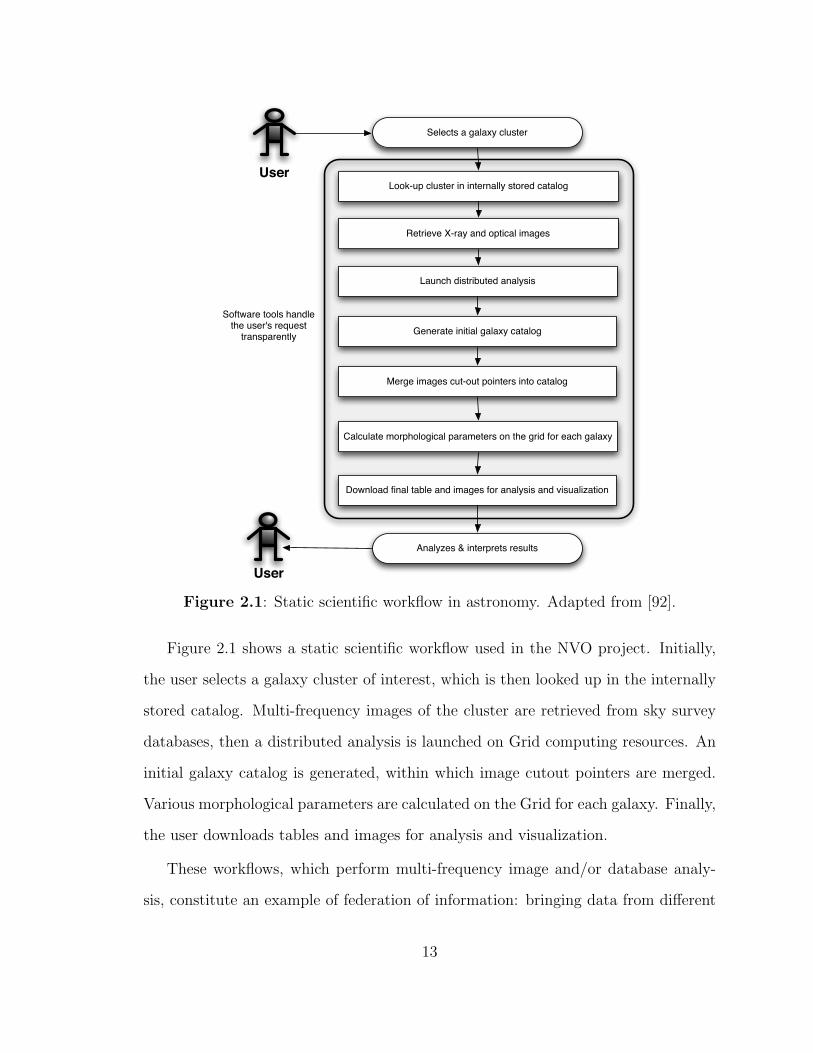
Figure 2.1: Static scientific workflow in astronomy. Adapted from [92].
Figure 2.1 shows a static scientific workflow used in the NVO project. Initially,
the user selects a galaxy cluster of interest, which is then looked up in the internally
stored catalog. Multi-frequency images of the cluster are retrieved from sky survey
databases, then a distributed analysis is launched on Grid computing resources. An
initial galaxy catalog is generated, within which image cutout pointers are merged.
Various morphological parameters are calculated on the Grid for each galaxy. Finally,
the user downloads tables and images for analysis and visualization.
These workflows, which perform multi-frequency image and/or database analy-
sis, constitute an example of federation of information: bringing data from different
13
sources into the same frame of reference. This type of data federation is very impor-
tant in astronomy because it enables discoveries of new sky objects and phenomena
(i.e., brown dwarf stars can be found by a search spanning infrared image catalogs)
[114].
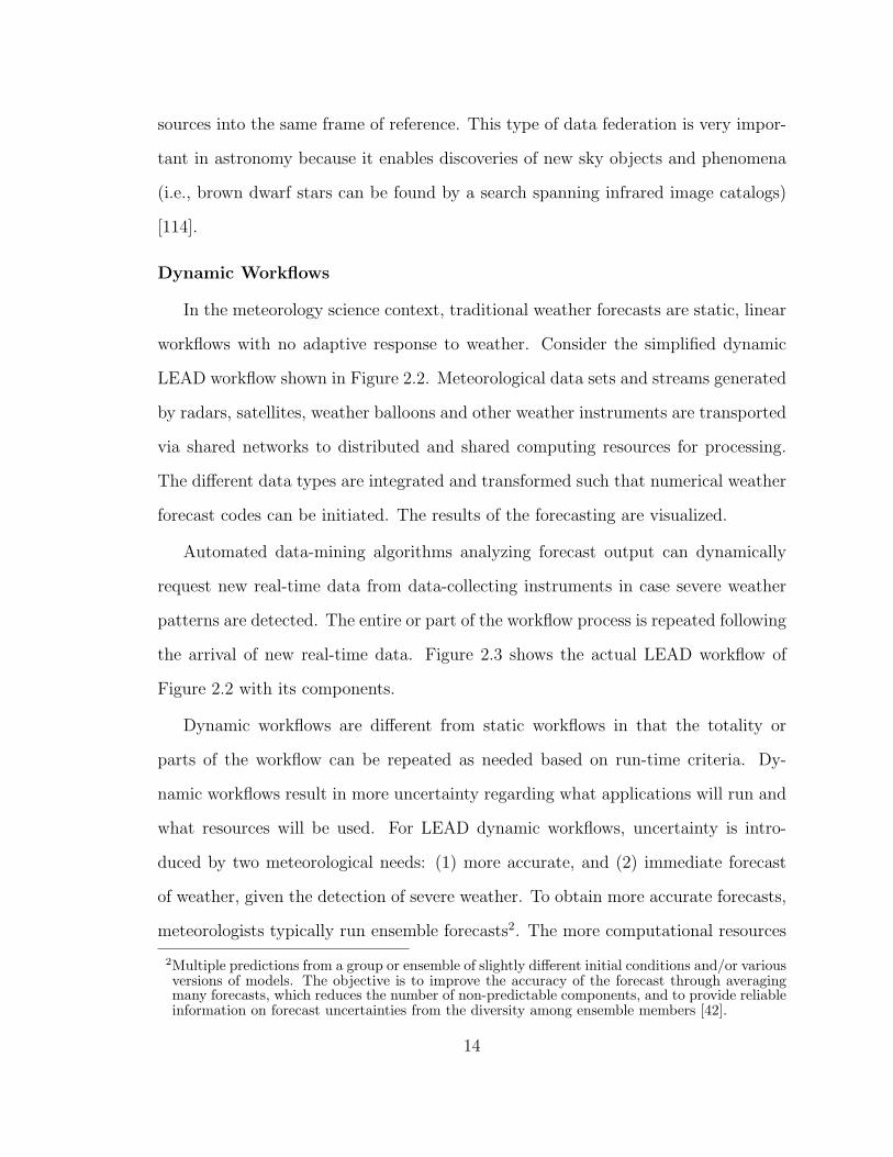
Dynamic Workflows
In the meteorology science context, traditional weather forecasts are static, linear
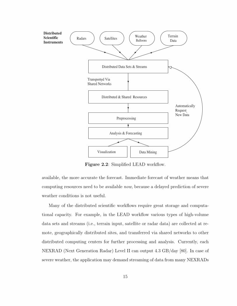
workflows with no adaptive response to weather. Consider the simplified dynamic
LEAD workflow shown in Figure 2.2. Meteorological data sets and streams generated
by radars, satellites, weather balloons and other weather instruments are transported
via shared networks to distributed and shared computing resources for processing.
The different data types are integrated and transformed such that numerical weather
forecast codes can be initiated. The results of the forecasting are visualized.
Automated data-mining algorithms analyzing forecast output can dynamically
request new real-time data from data-collecting instruments in case severe weather
patterns are detected. The entire or part of the workflow process is repeated following
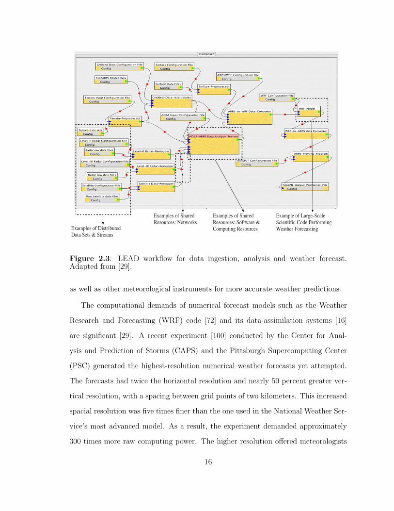
the arrival of new real-time data. Figure 2.3 shows the actual LEAD workflow of
Figure 2.2 with its components.
Dynamic workflows are different from static workflows in that the totality or
parts of the workflow can be repeated as needed based on run-time criteria. Dy-
namic workflows result in more uncertainty regarding what applications will run and
what resources will be used. For LEAD dynamic workflows, uncertainty is intro-
duced by two meteorological needs: (1) more accurate, and (2) immediate forecast
of weather, given the detection of severe weather. To obtain more accurate forecasts,
meteorologists typically run ensemble forecasts2. The more computational resources
2Multiple predictions from a group or ensemble of slightly different initial conditions and/or variousversions of models. The objective is to improve the accuracy of the forecast through averagingmany forecasts, which reduces the number of non-predictable components, and to provide reliableinformation on forecast uncertainties from the diversity among ensemble members [42].
14
Distributed Data Sets & Streams
Distributed & Shared Resources
Radars Satellites Weather Balloons
Terrain Data
Distributed Scientific Instruments
Transported Via Shared Networks
Preprocessing
Analysis & Forecasting
Data Mining Visualization
Automatically Request New Data
Figure 2.2: Simplified LEAD workflow.
available, the more accurate the forecast. Immediate forecast of weather means that
computing resources need to be available now, because a delayed prediction of severe
weather conditions is not useful.
Many of the distributed scientific workflows require great storage and computa-
tional capacity. For example, in the LEAD workflow various types of high-volume
data sets and streams (i.e., terrain input, satellite or radar data) are collected at re-
mote, geographically distributed sites, and transferred via shared networks to other
distributed computing centers for further processing and analysis. Currently, each
NEXRAD (Next Generation Radar) Level II can output 4.3 GB/day [80]. In case of
severe weather, the application may demand streaming of data from many NEXRADs
15
Examples of Distributed Data Sets & Streams
Examples of Shared Resources: Networks
Examples of Shared Resources: Software & Computing Resources
Example of Large-Scale Scientific Code Performing Weather Forecasting
Figure 2.3: LEAD workflow for data ingestion, analysis and weather forecast.Adapted from [29].
as well as other meteorological instruments for more accurate weather predictions.
The computational demands of numerical forecast models such as the Weather
Research and Forecasting (WRF) code [72] and its data-assimilation systems [16]
are significant [29]. A recent experiment [100] conducted by the Center for Anal-
ysis and Prediction of Storms (CAPS) and the Pittsburgh Supercomputing Center
(PSC) generated the highest-resolution numerical weather forecasts yet attempted.
The forecasts had twice the horizontal resolution and nearly 50 percent greater ver-
tical resolution, with a spacing between grid points of two kilometers. This increased
spacial resolution was five times finer than the one used in the National Weather Ser-
vice’s most advanced model. As a result, the experiment demanded approximately
300 times more raw computing power. The higher resolution offered meteorologists
16
improved storm forecast capability, such as the ability to capture individual thunder-
storms together with their rotation information.
CAPS used the numerical forecast model WRF executing on 307 Alphaserver
ES45 nodes (four 1 GHz processors with 4 GB RAM per node) to produce the daily
forecast from mid-April through early June during 2005 for over two-thirds of the
continental United States. The forecasts executed approximately two months on
these high-performing computational resources.
2.2.2 Workflow Performance Analysis On Grid Resources
For the astronomy application example, the Grid implications are that these mas-
sive astronomical data collections are made available without worries about differ-
ences in storage systems, security environment or access mechanisms. These static
workflows execute a series of workflow components, sequentially or in parallel, fol-
lowing a directed acyclic graph flow. The workflows may have real-time constraints
on the total execution time. Thus, workflow performance analysis tools must de-
tect timely if components are not performing as expected. Both quantitative and
qualitative performance analysis approaches offer methods to enforce soft or hard
performance guarantees.
For the meteorology application example, generating accurate and immediate se-
vere weather forecasts requires significant computational and data demands. The
data and computational resources utilized are distributed and are integrated via cou-
pling tools such as Grids and web services. However, in an integrated, distributed
computing environment there are a variety of challenges to overcome, such as re-
source contention, software and hardware failures, data dependencies and optimal
resource allocations. Resource contention and sharing in this environment cause the
performance of applications to vary widely and unexpectedly. Therefore, creating
mechanisms that enable soft real-time performance guarantees by characterizing re-
17

source behavior to ensure timely completion of tasks is especially critical in real-time
environments.
2.3 Summary
We presented the context in which we apply our qualitative performance analysis
framework: large-scale scientific Grid applications executing in a distributed comput-
ing environment. The complexity and dynamism of these new scientific applications
makes monitoring and understanding application resource behavior both critical and
challenging. This work complements existing quantitative Grid performance analysis
approaches with qualitative ones, which together will offer a more robust computa-
tional environment during the execution of scientific workflows.
18
Chapter 3
Methodologies for Data Analysis andVisualization
This chapter describes methodologies for performance data analysis and visual-
ization which we employ to extract temporal information from time series data and
to characterize qualitatively the behavior of long-running scientific applications. We
introduce concepts from time series analysis and pattern recognition in time series
and show how to build temporal signatures from time series data. We also introduce
fundamental concepts from supervised learning and show how we use it on temporal
signatures to differentiate between desired and undesired application performance
states. Lastly, we describe supporting techniques from multi-variate data visualiza-
tion which help with the analysis and interpretation of results from our performance
data.
3.1 Time Series
A time series T is a set of observations, denoted by z0, z1,� � � , zk,� � � ,zN generated
sequentially at time points τ0, τ1, � � � , τk,� � � , τN . Successive time points can be
collected at a fixed interval of time, h, or at different intervals of time. In this thesis,
we are concerned with equidistant series.
Time series analysis uses statistical methods to analyze dependencies in a chrono-
logical sequence of observations. When applied to performance metric time series,
the observations can be any quantitative data gathered from any metric of inter-
est (i.e., CPU utilization, amount of free memory, or number of I/O read requests).
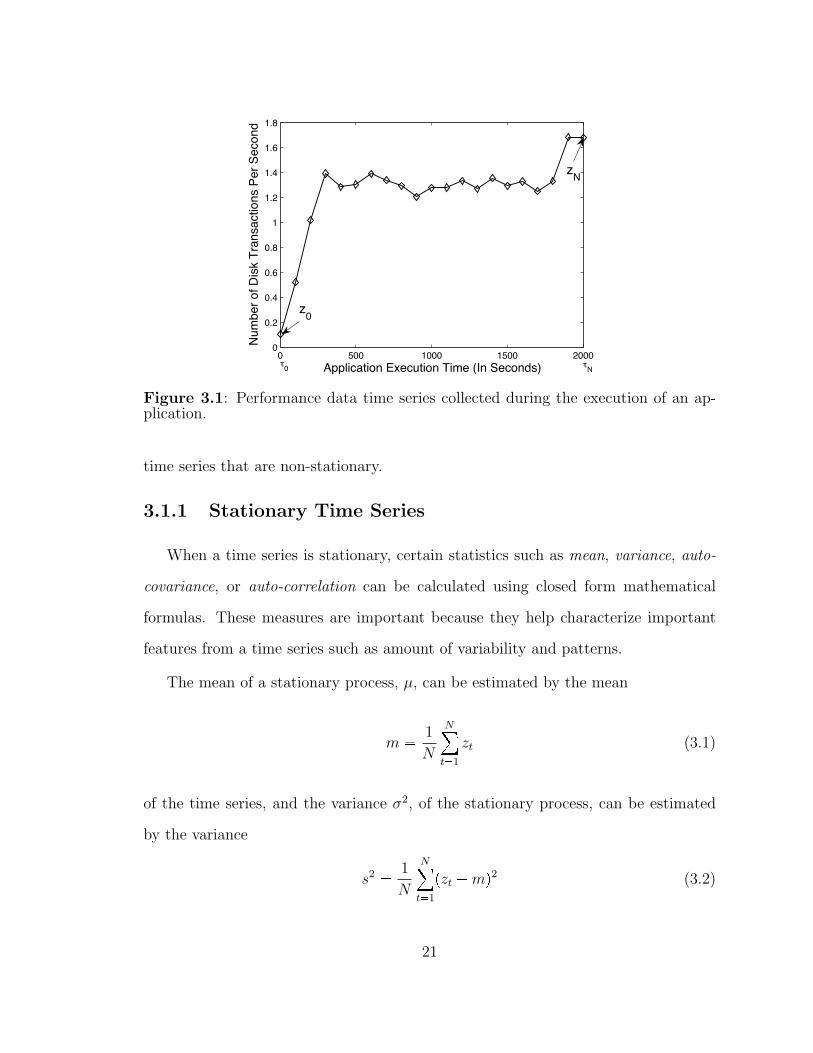
Figure 3.1 depicts a performance data time series, number of disk transactions per
second z0, � � � , zk, � � � , z2000, collected every τk � 100 seconds during the execution of
19
an application on a computing system.
Our objective is to characterize temporally the behavior of the underlying process
generating the series. This characterization is achieved by exploiting correlations
among observations to identify a qualitative temporal structure for the performance
data processes.
When collecting performance metrics, the value of τ0 corresponds to starting an
application’s execution on a computing system, and h corresponds to the frequency
of sampling of performance data. The value of N corresponds to the completion of
the execution of the application on the computing resource.
Two characteristics of time series are essential to the type of analysis that can be
applied: stationary and non-stationary. In a stationary series, the underlying process
remains in statistical equilibrium, with observations fluctuating around a constant
mean with constant variance. In contrast, a non-stationary series has unfixed mo-
ments (i.e., mean or variance) which tend to increase or decrease over time.
Although many empirical time series are non-stationary, we assume that most
snapshots of the time series analyzed will at least meet the weak stationarity condi-
tion, that is only the first two moments (i.e., mean and variance) do not vary with
respect to time. If most time series analyzed in the experimental setting will not meet
this condition, then estimation formulas for mean, variance and auto-correlation com-
monly utilized under the stationary and weakly-stationary conditions, will result in
biased estimates. The use of such formulas and therefore of our specific temporal
information extraction techniques under non-stationarity will result in a decreased
efficacy for our framework, as the extracted features will not be accurately describ-
ing temporal behaviors. However, other methodologies from pattern recognition and
analysis of time series such as those proposed in [64, 87, 95] can be employed to achieve
the same goal of compact temporal characterization of behavior from performance
20
0 500 1000 1500 20000
0.2
0.4
0.6
0.8
1
1.2
1.4
1.6
1.8
Application Execution Time (In Seconds)
Num
ber o
f Disk
Tra
nsac
tions
Per
Sec
ond
zN
z0
!0 !N
Figure 3.1: Performance data time series collected during the execution of an ap-plication.
time series that are non-stationary.
3.1.1 Stationary Time Series
When a time series is stationary, certain statistics such as mean, variance, auto-
covariance, or auto-correlation can be calculated using closed form mathematical
formulas. These measures are important because they help characterize important
features from a time series such as amount of variability and patterns.
The mean of a stationary process, µ, can be estimated by the mean
m � 1
N
N
t�1
zt (3.1)
of the time series, and the variance σ2, of the stationary process, can be estimated
by the variance
s2 � 1
N
N
t�1
pzt �mq2 (3.2)
21
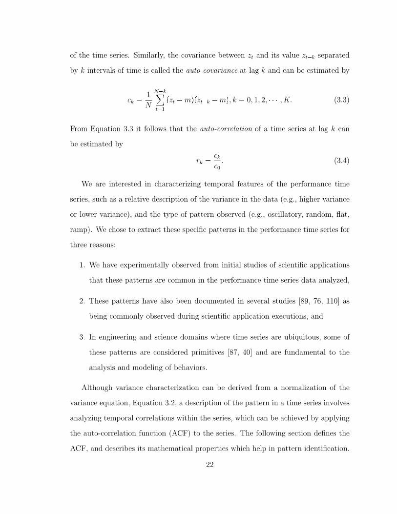
of the time series. Similarly, the covariance between zt and its value zt�k separated
by k intervals of time is called the auto-covariance at lag k and can be estimated by
ck � 1
N
N�k
t�1
pzt �mqpzt�k �mq, k � 0, 1, 2, � � � , K. (3.3)
From Equation 3.3 it follows that the auto-correlation of a time series at lag k can
be estimated by
rk � ckc0. (3.4)
We are interested in characterizing temporal features of the performance time
series, such as a relative description of the variance in the data (e.g., higher variance
or lower variance), and the type of pattern observed (e.g., oscillatory, random, flat,
ramp). We chose to extract these specific patterns in the performance time series for
three reasons:
1. We have experimentally observed from initial studies of scientific applications
that these patterns are common in the performance time series data analyzed,
2. These patterns have also been documented in several studies [89, 76, 110] as
being commonly observed during scientific application executions, and
3. In engineering and science domains where time series are ubiquitous, some of
these patterns are considered primitives [87, 40] and are fundamental to the
analysis and modeling of behaviors.
Although variance characterization can be derived from a normalization of the
variance equation, Equation 3.2, a description of the pattern in a time series involves
analyzing temporal correlations within the series, which can be achieved by applying
the auto-correlation function (ACF) to the series. The following section defines the
ACF, and describes its mathematical properties which help in pattern identification.
22
3.1.2 The Auto-correlation Function and Its Properties
As shown in Equation 3.4, the auto-correlation coefficient at lag k measures the
covariance between two values zt and zt�k, a distance k apart, normalized by the
value of the covariance at k � 0. The set of all the auto-correlation coefficients of a
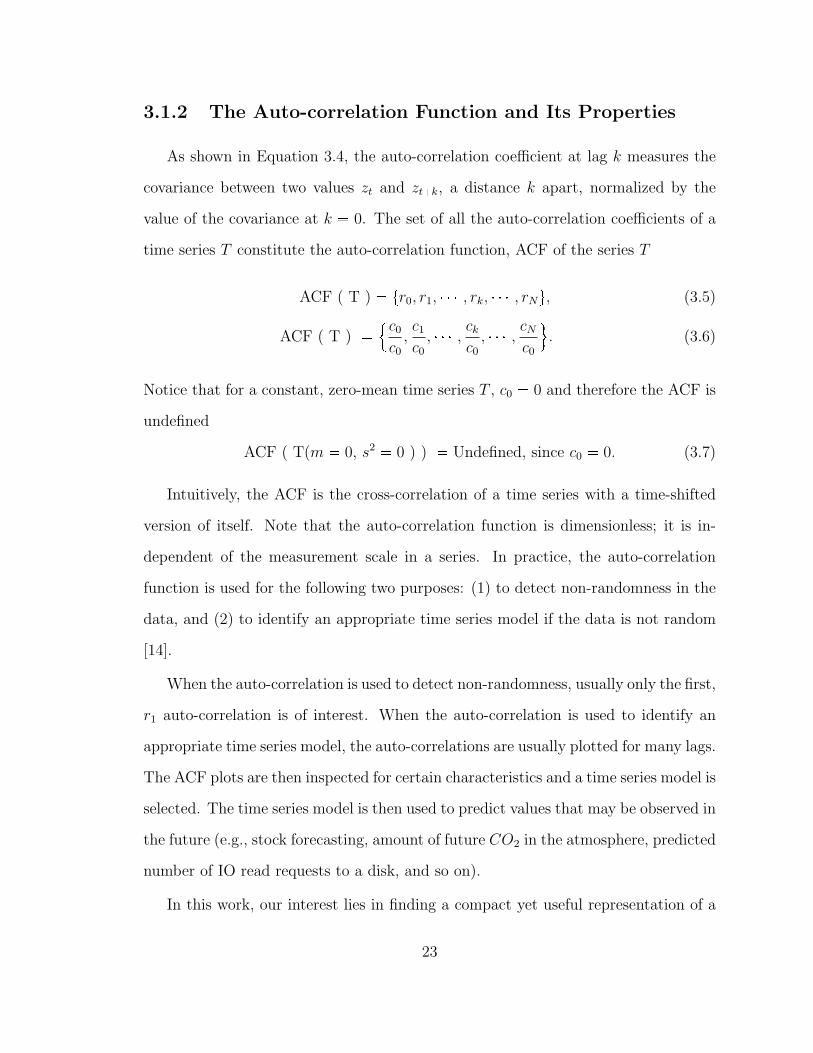
time series T constitute the auto-correlation function, ACF of the series T
ACF ( T ) � tr0, r1, � � � , rk, � � � , rNu, (3.5)
ACF ( T ) �!c0c0,c1c0, � � � , ck
c0, � � � , cN
c0
). (3.6)
Notice that for a constant, zero-mean time series T , c0 � 0 and therefore the ACF is
undefined
ACF ( T(m � 0, s2 � 0 ) ) � Undefined, since c0 � 0. (3.7)
Intuitively, the ACF is the cross-correlation of a time series with a time-shifted
version of itself. Note that the auto-correlation function is dimensionless; it is in-
dependent of the measurement scale in a series. In practice, the auto-correlation
function is used for the following two purposes: (1) to detect non-randomness in the
data, and (2) to identify an appropriate time series model if the data is not random
[14].
When the auto-correlation is used to detect non-randomness, usually only the first,
r1 auto-correlation is of interest. When the auto-correlation is used to identify an
appropriate time series model, the auto-correlations are usually plotted for many lags.
The ACF plots are then inspected for certain characteristics and a time series model is
selected. The time series model is then used to predict values that may be observed in
the future (e.g., stock forecasting, amount of future CO2 in the atmosphere, predicted
number of IO read requests to a disk, and so on).
In this work, our interest lies in finding a compact yet useful representation of a
23
time series and not in finding a time series model in order to forecast future values.
In essence, we want to extract –similarly with [3]– possible features of interest in
the time series that may help differentiate between good and degraded performance
application states.
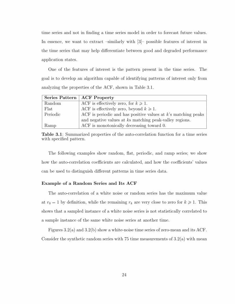
One of the features of interest is the pattern present in the time series. The
goal is to develop an algorithm capable of identifying patterns of interest only from
analyzing the properties of the ACF, shown in Table 3.1.
Series Pattern ACF PropertyRandom ACF is effectively zero, for k ¥ 1.Flat ACF is effectively zero, beyond k ¥ 1.Periodic ACF is periodic and has positive values at k’s matching peaks
and negative values at ks matching peak-valley regions.Ramp ACF is monotonically decreasing toward 0.
Table 3.1: Summarized properties of the auto-correlation function for a time serieswith specified pattern.
The following examples show random, flat, periodic, and ramp series; we show
how the auto-correlation coefficients are calculated, and how the coefficients’ values
can be used to distinguish different patterns in time series data.
Example of a Random Series and Its ACF
The auto-correlation of a white noise or random series has the maximum value
at r0 � 1 by definition, while the remaining rk are very close to zero for k ¥ 1. This
shows that a sampled instance of a white noise series is not statistically correlated to
a sample instance of the same white noise series at another time.
Figures 3.2(a) and 3.2(b) show a white-noise time series of zero-mean and its ACF.
Consider the synthetic random series with 75 time measurements of 3.2(a) with mean
24
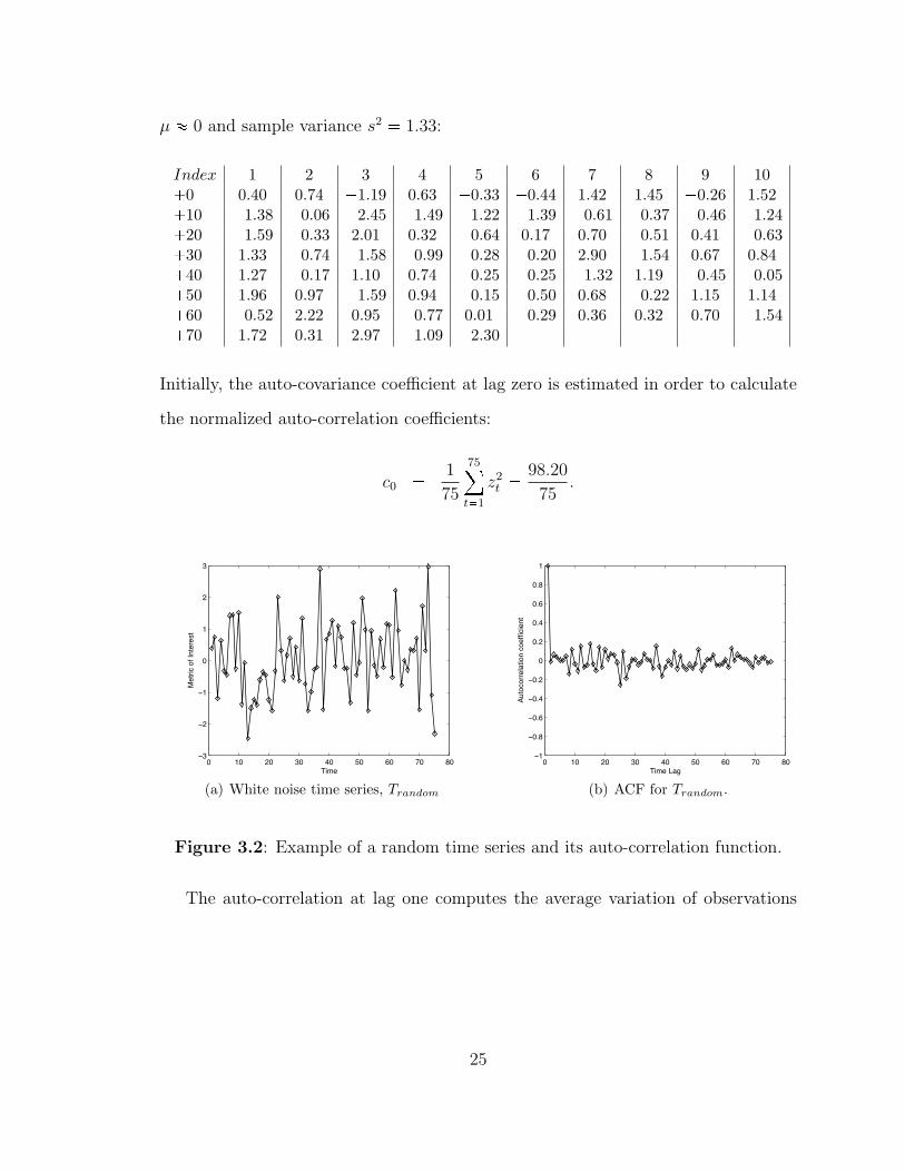
µ � 0 and sample variance s2 � 1.33:
Index 1 2 3 4 5 6 7 8 9 10�0 0.40 0.74 �1.19 0.63 �0.33 �0.44 1.42 1.45 �0.26 1.52�10 �1.38 �0.06 �2.45 �1.49 �1.22 �1.39 �0.61 �0.37 �0.46 �1.24�20 �1.59 �0.33 2.01 0.32 �0.64 0.17 0.70 �0.51 0.41 �0.63�30 1.33 �0.74 �1.58 �0.99 �0.28 �0.20 2.90 �1.54 0.67 0.84�40 1.27 �0.17 1.10 0.74 �0.25 �0.25 �1.32 1.19 �0.45 �0.05�50 1.96 0.97 �1.59 0.94 �0.15 �0.50 0.68 �0.22 1.15 1.14�60 �0.52 2.22 0.95 �0.77 0.01 �0.29 0.36 0.32 0.70 �1.54�70 1.72 0.31 2.97 �1.09 �2.30 � � � � �
Initially, the auto-covariance coefficient at lag zero is estimated in order to calculate
the normalized auto-correlation coefficients:
c0 � 1
75
75
t�1
z2t �
98.20
75.
0 10 20 30 40 50 60 70 80!3
!2
!1
0
1
2
3
Time
Met
ric o
f Int
eres
t
(a) White noise time series, Trandom
0 10 20 30 40 50 60 70 80!1
!0.8
!0.6
!0.4
!0.2
0
0.2
0.4
0.6
0.8
1
Time Lag
Auto
corre
latio
n co
effic
ient
(b) ACF for Trandom.
Figure 3.2: Example of a random time series and its auto-correlation function.
The auto-correlation at lag one computes the average variation of observations
25
that are one time step apart:
r1 � c1c0
r1 � 75
98.20�� 1
75
74
t�1
pzt � zt�1q�
r1 � 1
98.20� pz1 � z2 � z2 � z3 � � � � � z74 � z75q � �0.007.
Similarly, the auto-correlation at lag 37 computes the average variation of observa-
tions that are 37 time steps apart:
r37 � c37
c0
r37 � 75
98.20�� 1
75
38
t�1
pzt � zt�37q�
r37 � 1
98.20� pz1 � z38 � z2 � z39 � � � � � z38 � z75q � 0.15.
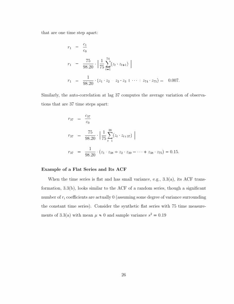
Example of a Flat Series and Its ACF
When the time series is flat and has small variance, e.g., 3.3(a), its ACF trans-
formation, 3.3(b), looks similar to the ACF of a random series, though a significant
number of ri coefficients are actually 0 (assuming some degree of variance surrounding
the constant time series). Consider the synthetic flat series with 75 time measure-
ments of 3.3(a) with mean µ � 0 and sample variance s2 � 0.19
26
0 10 20 30 40 50 60 70 80!2
!1.5
!1
!0.5
0
0.5
1
1.5
2
Time
Met
ric o
f Int
eres
t
(a) Flat time series, Tflat, with some variance.
0 10 20 30 40 50 60 70 80!1
!0.8
!0.6
!0.4
!0.2
0
0.2
0.4
0.6
0.8
1
Time Lag
Auto
corre
latio
n co
effic
ient
(b) ACF for Tflat.
Figure 3.3: Example of a flat time series and its auto-correlation function.
Index 1 2 3 4 5 6 7 8 9 10�0 0.00 2.00 0.00 0.00 0.00 0.00 0.00 0.00 0.00 �2.00�10 0.00 0.00 0.00 0.00 0.00 0.00 0.00 0.00 0.00 0.00�20 0.00 0.00 0.00 0.00 0.00 0.00 0.00 0.00 0.00 2.00�30 0.00 0.00 0.00 0.00 0.00 0.00 0.00 0.00 0.00 0.00�40 0.00 0.00 0.00 0.00 0.00 0.00 0.00 0.00 0.00 �1.00�50 0.00 0.00 0.00 0.00 0.00 0.00 0.00 0.00 0.00 0.00�60 0.00 0.00 0.00 0.00 0.00 0.00 0.00 0.00 0.00 0.00�70 0.00 0.00 0.00 0.00 �1.00 � � � � �
.
The auto-correlation at lag one is r1 � 0, while the coefficient at lag 20 is r20 ��0.4286, reflecting that when one of the series measurements increases the other one,
20 lags apart, decreases or vice versa.
Example of a Periodic Series and Its ACF
When a series is periodic, the ACF transformation is also periodic. The intuition
behind this property stems from the fact that as one compares two time-shifted
versions of a periodic series, when the series’ peaks overlap, the ACF coefficients are
positive while when the series’ peaks and valleys overlap, the ACF coefficients are
27
0 10 20 30 40 50 60 70 80!1
!0.8
!0.6
!0.4
!0.2
0
0.2
0.4
0.6
0.8
1
Time
Met
ric o
f Int
eres
t
(a) Periodic time series, Tperiodic, with somevariance.
0 10 20 30 40 50 60 70 80!1
!0.8
!0.6
!0.4
!0.2
0
0.2
0.4
0.6
0.8
1
Time Lag
Auto
corre
latio
n co
effic
ient
(b) ACF for Tperiodic.
Figure 3.4: Example of a periodic time series and its auto-correlation function.
negative1.
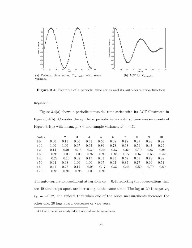
Figure 3.4(a) shows a periodic sinusoidal time series with its ACF illustrated in
Figure 3.4(b). Consider the synthetic periodic series with 75 time measurements of
Figure 3.4(a) with mean, µ � 0 and sample variance, s2 � 0.51
Index 1 2 3 4 5 6 7 8 9 10�0 0.00 0.15 0.30 0.43 0.56 0.68 0.78 0.87 0.93 0.98�10 1.00 1.00 0.97 0.93 0.86 0.78 0.68 0.56 0.43 0.29�20 0.14 �0.01 �0.16 �0.30 �0.44 �0.57 �0.69 �0.79 �0.87 �0.94�30 �0.98 �1.00 �1.00 �0.97 �0.93 �0.86 �0.77 �0.67 �0.55 �0.42�40 �0.28 �0.13 0.02 0.17 0.31 0.45 0.58 0.69 0.79 0.88�50 0.94 0.98 1.00 1.00 0.97 0.92 0.85 0.77 0.66 0.54�60 0.41 0.27 0.12 �0.03 �0.17 �0.32 �0.46 �0.59 �0.70 �0.80�70 �0.88 �0.94 �0.98 �1.00 �0.99 � � � � �
.
The auto-correlation coefficient at lag 40 is r40 � 0.44 reflecting that observations that
are 40 time steps apart are increasing at the same time. The lag at 20 is negative,
r20 � �0.72, and reflects that when one of the series measurements increases the
other one, 20 lags apart, decreases or vice versa.
1All the time series analyzed are normalized to zero-mean.
28
0 10 20 30 40 50 60 70 80!2
!1.5
!1
!0.5
0
0.5
1
1.5
2
Time
Met
ric o
f Int
eres
t
(a) Ramp-up time series, Tramp�up.
0 10 20 30 40 50 60 70 80!1
!0.8
!0.6
!0.4
!0.2
0
0.2
0.4
0.6
0.8
1
Time Lag
Auto
corre
latio
n co
effic
ient
(b) ACF for Tramp�up.
0 10 20 30 40 50 60 70 80!2
!1.5
!1
!0.5
0
0.5
1
1.5
2
Time
Met
ric o
f Int
eres
t
(c) Ramp-down time series, Tramp�down.
0 10 20 30 40 50 60 70 80!1
!0.8
!0.6
!0.4
!0.2
0
0.2
0.4
0.6
0.8
1
Time Lag
Auto
corre
latio
n co
effic
ient
(d) ACF for Tramp�down.
Figure 3.5: Example of ramp time series and their auto-correlation function.
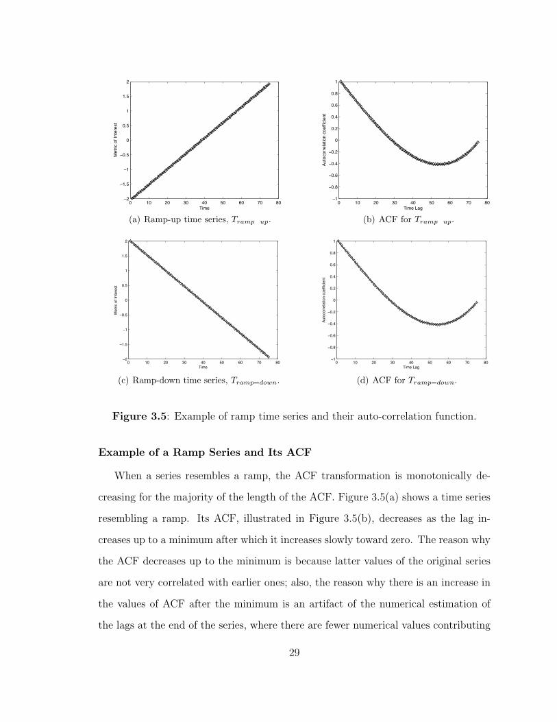
Example of a Ramp Series and Its ACF
When a series resembles a ramp, the ACF transformation is monotonically de-
creasing for the majority of the length of the ACF. Figure 3.5(a) shows a time series
resembling a ramp. Its ACF, illustrated in Figure 3.5(b), decreases as the lag in-
creases up to a minimum after which it increases slowly toward zero. The reason why
the ACF decreases up to the minimum is because latter values of the original series
are not very correlated with earlier ones; also, the reason why there is an increase in
the values of ACF after the minimum is an artifact of the numerical estimation of
the lags at the end of the series, where there are fewer numerical values contributing
29
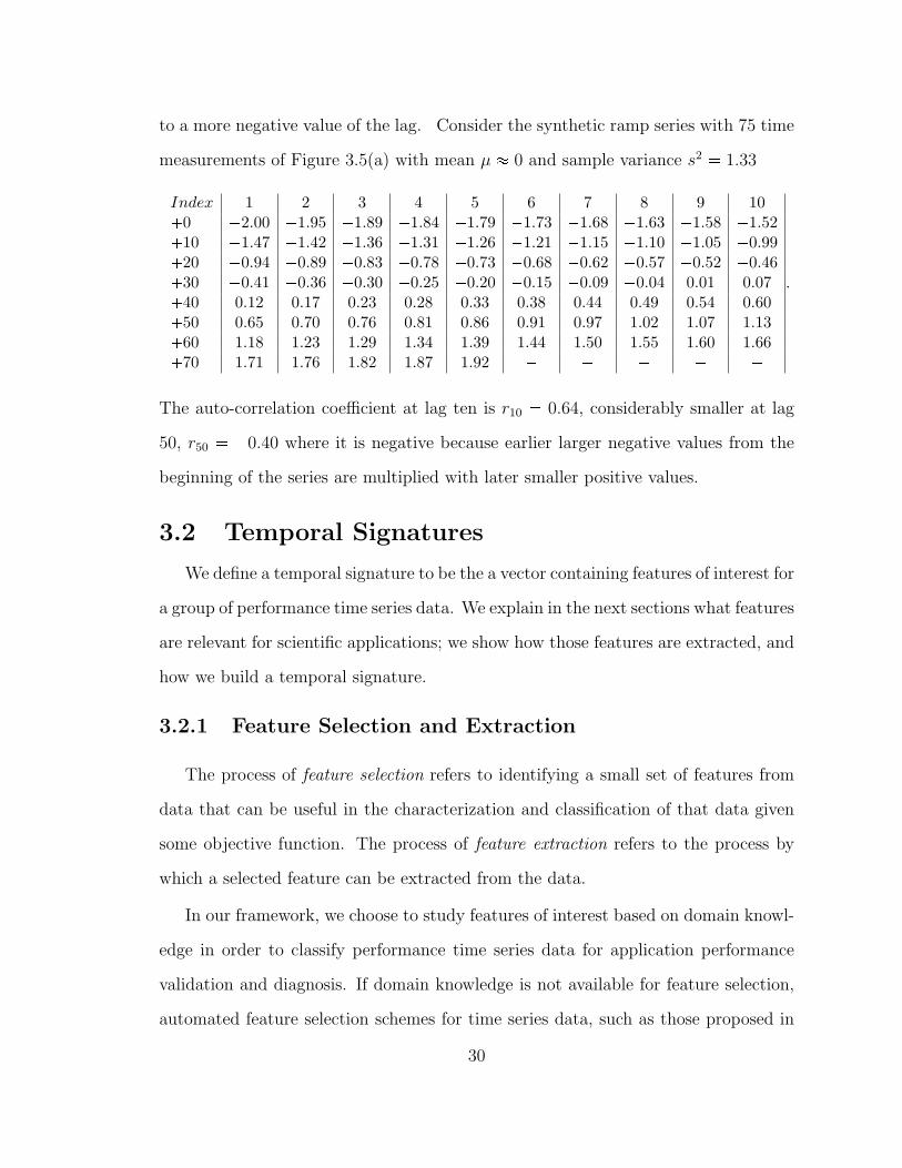
to a more negative value of the lag. Consider the synthetic ramp series with 75 time
measurements of Figure 3.5(a) with mean µ � 0 and sample variance s2 � 1.33
Index 1 2 3 4 5 6 7 8 9 10�0 �2.00 �1.95 �1.89 �1.84 �1.79 �1.73 �1.68 �1.63 �1.58 �1.52�10 �1.47 �1.42 �1.36 �1.31 �1.26 �1.21 �1.15 �1.10 �1.05 �0.99�20 �0.94 �0.89 �0.83 �0.78 �0.73 �0.68 �0.62 �0.57 �0.52 �0.46�30 �0.41 �0.36 �0.30 �0.25 �0.20 �0.15 �0.09 �0.04 0.01 0.07�40 0.12 0.17 0.23 0.28 0.33 0.38 0.44 0.49 0.54 0.60�50 0.65 0.70 0.76 0.81 0.86 0.91 0.97 1.02 1.07 1.13�60 1.18 1.23 1.29 1.34 1.39 1.44 1.50 1.55 1.60 1.66�70 1.71 1.76 1.82 1.87 1.92 � � � � �
.
The auto-correlation coefficient at lag ten is r10 � 0.64, considerably smaller at lag
50, r50 � �0.40 where it is negative because earlier larger negative values from the
beginning of the series are multiplied with later smaller positive values.
3.2 Temporal Signatures
We define a temporal signature to be the a vector containing features of interest for
a group of performance time series data. We explain in the next sections what features
are relevant for scientific applications; we show how those features are extracted, and
how we build a temporal signature.
3.2.1 Feature Selection and Extraction
The process of feature selection refers to identifying a small set of features from
data that can be useful in the characterization and classification of that data given
some objective function. The process of feature extraction refers to the process by
which a selected feature can be extracted from the data.
In our framework, we choose to study features of interest based on domain knowl-
edge in order to classify performance time series data for application performance
validation and diagnosis. If domain knowledge is not available for feature selection,
automated feature selection schemes for time series data, such as those proposed in
30
[87], can be employed. The following sections motivate the choice of our features,
and explain the process of extracting those features from the set of performance time
series data.
Relative Variance
We extract the amount of variability present in time series because it is an indica-
tor of fluctuation around the average resource utilization of applications. This data
can be extracted using the sample variance s2 defined in Equation 3.2. However, the
sample variance depends on the scale of the measurement of a particular performance
data time series. Therefore, we transform the s2 values to a normalized r0, 1s space,
with 0 signifying the lowest variance seen in the particular metric and �1 signifying
the highest variance observed. This data normalization must be performed because
(1) the value of the feature extracted must be independent of the scale of the time
series, and (2) future application of clustering and classification algorithms requires
bounded and normalized values in order to produce unbiased results. The normalized
variance is labeled as s2n. Furthermore, we discretize this normalized variance into
three different categorical levels: (1) low, (2) moderate, and (3) high, correspond-
ing to normalized variance ranges of [0-0.33], [0.34-0.66] and [0.67-1]. We call our
measure of variability the normalized, categorical variance s2n,c, and it takes the cat-
egorical values of t1, 2, 3u corresponding to the {low, moderate, high} variability in
the data.
Pattern Identification
Another important feature to extract from a time series is the type of pattern
present in the data. The pattern information supplements the information provided
by the variance in the time series, because it further characterizes how the metric
varies around an expected baseline. Consider there is a pattern identification mech-
anism that, given a time series of interest, can tell if the series is most likely from a
31
random distribution, whether it is oscillatory in nature, whether it is flat or whether
it is similar to a ramp. Other patterns may occur, such as a self-similar pattern; how-
ever, currently we are interested in detecting among four different patterns: random,
periodic, flat or ramp. Treating the pattern identification mechanism as a black box
taking as input time series T and outputting one of the four patterns or an unknown
pattern, we map the results into a numeric space in the discrete set t1, 2, 3, 4, 5u, such
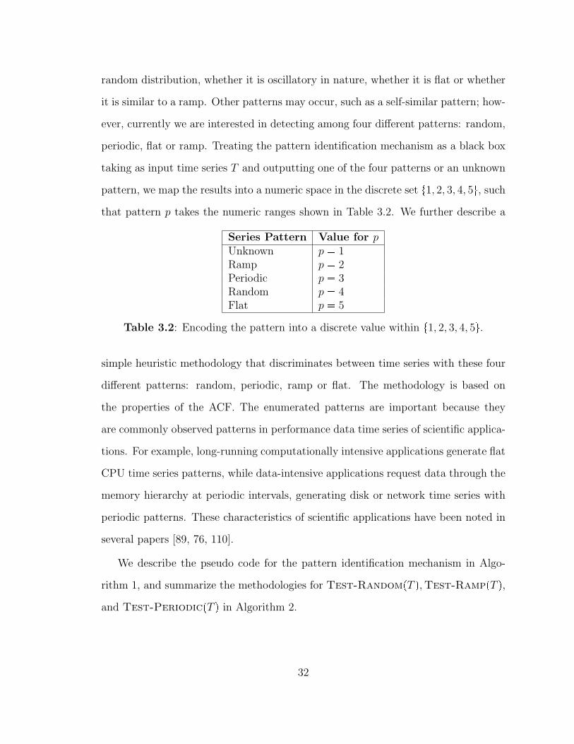
that pattern p takes the numeric ranges shown in Table 3.2. We further describe a
Series Pattern Value for pUnknown p � 1Ramp p � 2Periodic p � 3Random p � 4Flat p � 5
Table 3.2: Encoding the pattern into a discrete value within t1, 2, 3, 4, 5u.
simple heuristic methodology that discriminates between time series with these four
different patterns: random, periodic, ramp or flat. The methodology is based on
the properties of the ACF. The enumerated patterns are important because they
are commonly observed patterns in performance data time series of scientific applica-
tions. For example, long-running computationally intensive applications generate flat
CPU time series patterns, while data-intensive applications request data through the
memory hierarchy at periodic intervals, generating disk or network time series with
periodic patterns. These characteristics of scientific applications have been noted in
several papers [89, 76, 110].
We describe the pseudo code for the pattern identification mechanism in Algo-
rithm 1, and summarize the methodologies for Test-RandompT q,Test-RamppT q,and Test-PeriodicpT q in Algorithm 2.
32
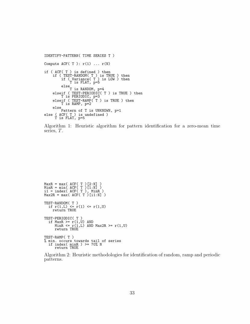
IDENTIFY-PATTERN( TIME SERIES T )
Compute ACF( T ): r(1) ... r(N)
if ( ACF( T ) is defined ) thenif ( TEST-RANDOM( T ) is TRUE ) then
if ( Variance( T ) is LOW ) thenT is FLAT, p=5
elseT is RANDOM, p=4
elseif ( TEST-PERIODIC( T ) is TRUE ) thenT is PERIODIC, p=3
elseif ( TEST-RAMP( T ) is TRUE ) thenT is RAMP, p=2
elsePattern of T is UNKNOWN, p=1
else ( ACF( T ) is undefined )T is FLAT, p=5
Algorithm 1: Heuristic algorithm for pattern identification for a zero-mean timeseries, T .
MaxR = max( ACF( T )[2:N] )MinR = min( ACF( T )[1:N] )i1 = index( ACF( T ), MinR )Max2R = max( ACF( T )[i1:N] )
TEST-RANDOM( T )if r(1,L) <= r(1) <= r(1,U)
return TRUE
TEST-PERIODIC( T )if MaxR >= r(1,U) AND
MinR <= r(1,L) AND Max2R >= r(1,U)return TRUE
TEST-RAMP( T )% min. occurs towards tail of seriesif index( minR ) >= 70% N
return TRUE
Algorithm 2: Heuristic methodologies for identification of random, ramp and periodicpatterns.
33
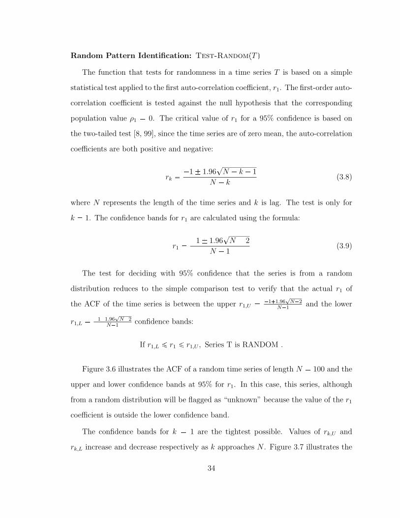
Random Pattern Identification: Test-RandompT qThe function that tests for randomness in a time series T is based on a simple
statistical test applied to the first auto-correlation coefficient, r1. The first-order auto-
correlation coefficient is tested against the null hypothesis that the corresponding
population value ρ1 � 0. The critical value of r1 for a 95% confidence is based on
the two-tailed test [8, 99], since the time series are of zero mean, the auto-correlation
coefficients are both positive and negative:
rk � �1 � 1.96?N � k � 1
N � k(3.8)
where N represents the length of the time series and k is lag. The test is only for
k � 1. The confidence bands for r1 are calculated using the formula:
r1 � �1 � 1.96?N � 2
N � 1(3.9)
The test for deciding with 95% confidence that the series is from a random
distribution reduces to the simple comparison test to verify that the actual r1 of
the ACF of the time series is between the upper r1,U � �1�1.96?
N�2N�1
and the lower
r1,L � �1�1.96?
N�2N�1
confidence bands:
If r1,L ¤ r1 ¤ r1,U , Series T is RANDOM .
Figure 3.6 illustrates the ACF of a random time series of length N � 100 and the
upper and lower confidence bands at 95% for r1. In this case, this series, although
from a random distribution will be flagged as “unknown” because the value of the r1
coefficient is outside the lower confidence band.
The confidence bands for k � 1 are the tightest possible. Values of rk,U and
rk,L increase and decrease respectively as k approaches N . Figure 3.7 illustrates the
34
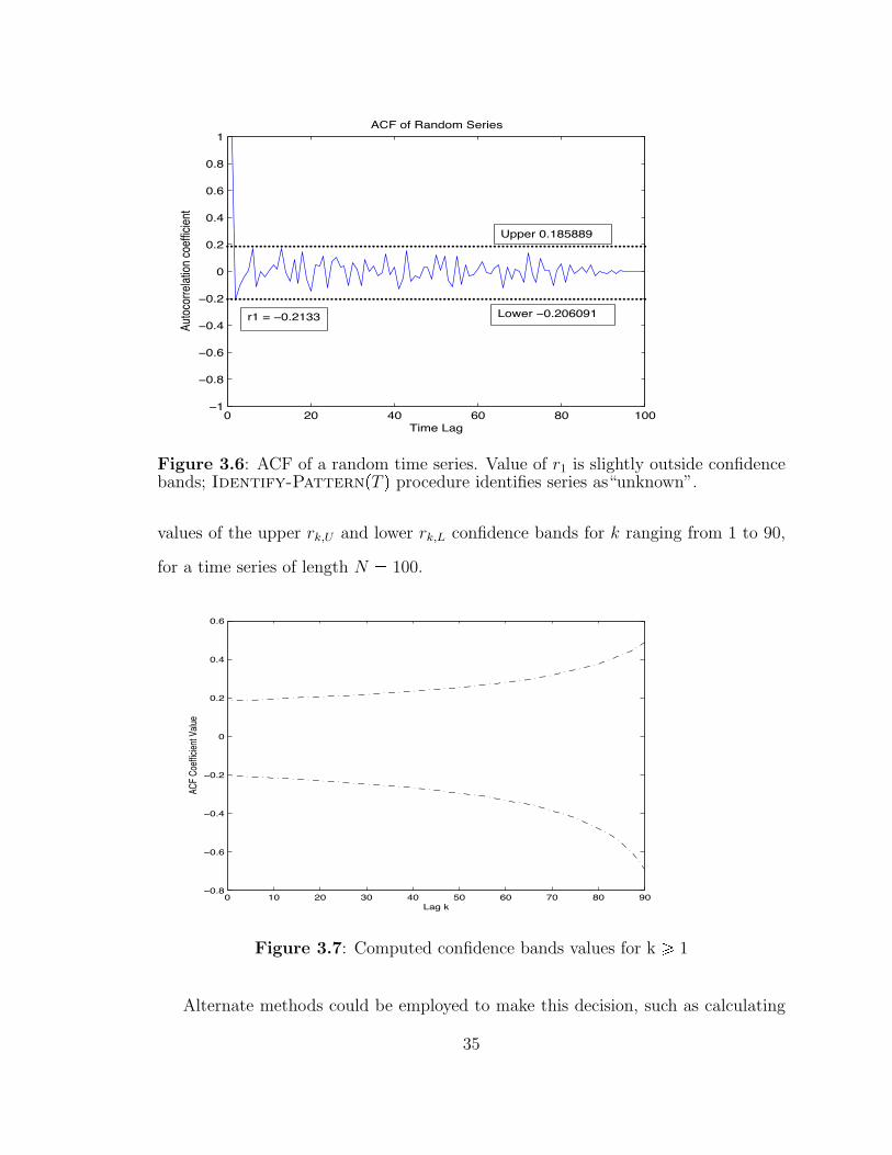
0 20 40 60 80 100!1
!0.8
!0.6
!0.4
!0.2
0
0.2
0.4
0.6
0.8
1
Time Lag
Autoc
orre
lation
coeff
icien
t
ACF of Random Series
r1 = !0.2133
Upper 0.185889
Lower !0.206091
Figure 3.6: ACF of a random time series. Value of r1 is slightly outside confidencebands; Identify-PatternpT q procedure identifies series as“unknown”.
values of the upper rk,U and lower rk,L confidence bands for k ranging from 1 to 90,
for a time series of length N � 100.
0 10 20 30 40 50 60 70 80 90!0.8
!0.6
!0.4
!0.2
0
0.2
0.4
0.6
Lag k
ACF C
oeffic
ient V
alue
Figure 3.7: Computed confidence bands values for k ¥ 1
Alternate methods could be employed to make this decision, such as calculating
35
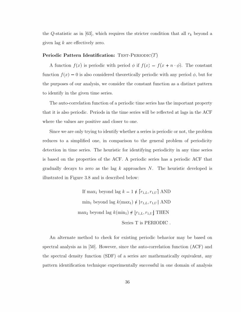
the Q-statistic as in [63], which requires the stricter condition that all rk beyond a
given lag k are effectively zero.
Periodic Pattern Identification: Test-PeriodicpT qA function fpxq is periodic with period φ if fpxq � fpx � n � φq. The constant
function fpxq � 0 is also considered theoretically periodic with any period φ, but for
the purposes of our analysis, we consider the constant function as a distinct pattern
to identify in the given time series.
The auto-correlation function of a periodic time series has the important property
that it is also periodic. Periods in the time series will be reflected at lags in the ACF
where the values are positive and closer to one.
Since we are only trying to identify whether a series is periodic or not, the problem
reduces to a simplified one, in comparison to the general problem of periodicity
detection in time series. The heuristic for identifying periodicity in any time series
is based on the properties of the ACF. A periodic series has a periodic ACF that
gradually decays to zero as the lag k approaches N . The heuristic developed is
illustrated in Figure 3.8 and is described below:
If max1 beyond lag k � 1 R rr1,L, r1,U s AND
min1 beyond lag k(max1) R rr1,L, r1,U s AND
max2 beyond lag k(min1) R rr1,L, r1,U s THEN
Series T is PERIODIC .
An alternate method to check for existing periodic behavior may be based on
spectral analysis as in [50]. However, since the auto-correlation function (ACF) and
the spectral density function (SDF) of a series are mathematically equivalent, any
pattern identification technique experimentally successful in one domain of analysis
36
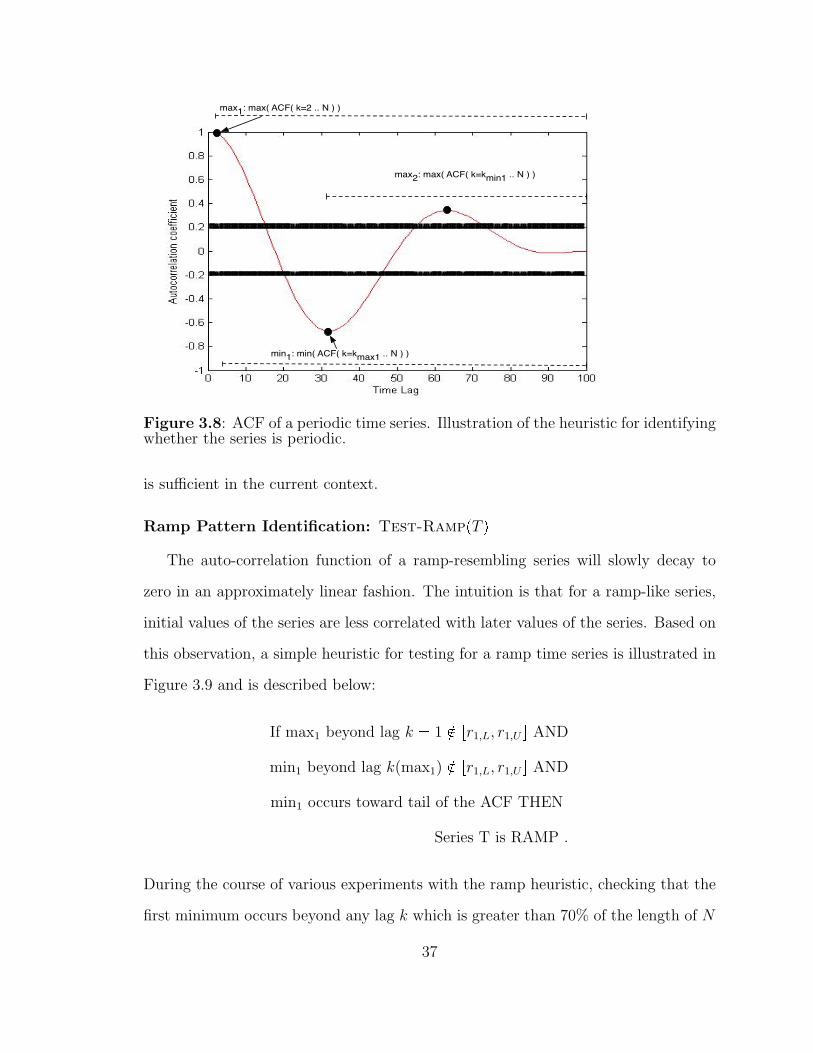
max1: max( ACF( k=2 .. N ) )
min1: min( ACF( k=kmax1 .. N ) )
max2: max( ACF( k=kmin1 .. N ) )
Figure 3.8: ACF of a periodic time series. Illustration of the heuristic for identifyingwhether the series is periodic.
is sufficient in the current context.
Ramp Pattern Identification: Test-RamppT qThe auto-correlation function of a ramp-resembling series will slowly decay to
zero in an approximately linear fashion. The intuition is that for a ramp-like series,
initial values of the series are less correlated with later values of the series. Based on
this observation, a simple heuristic for testing for a ramp time series is illustrated in
Figure 3.9 and is described below:
If max1 beyond lag k � 1 R rr1,L, r1,U s AND
min1 beyond lag k(max1) R rr1,L, r1,U s AND
min1 occurs toward tail of the ACF THEN
Series T is RAMP .
During the course of various experiments with the ramp heuristic, checking that the
first minimum occurs beyond any lag k which is greater than 70% of the length of N
37
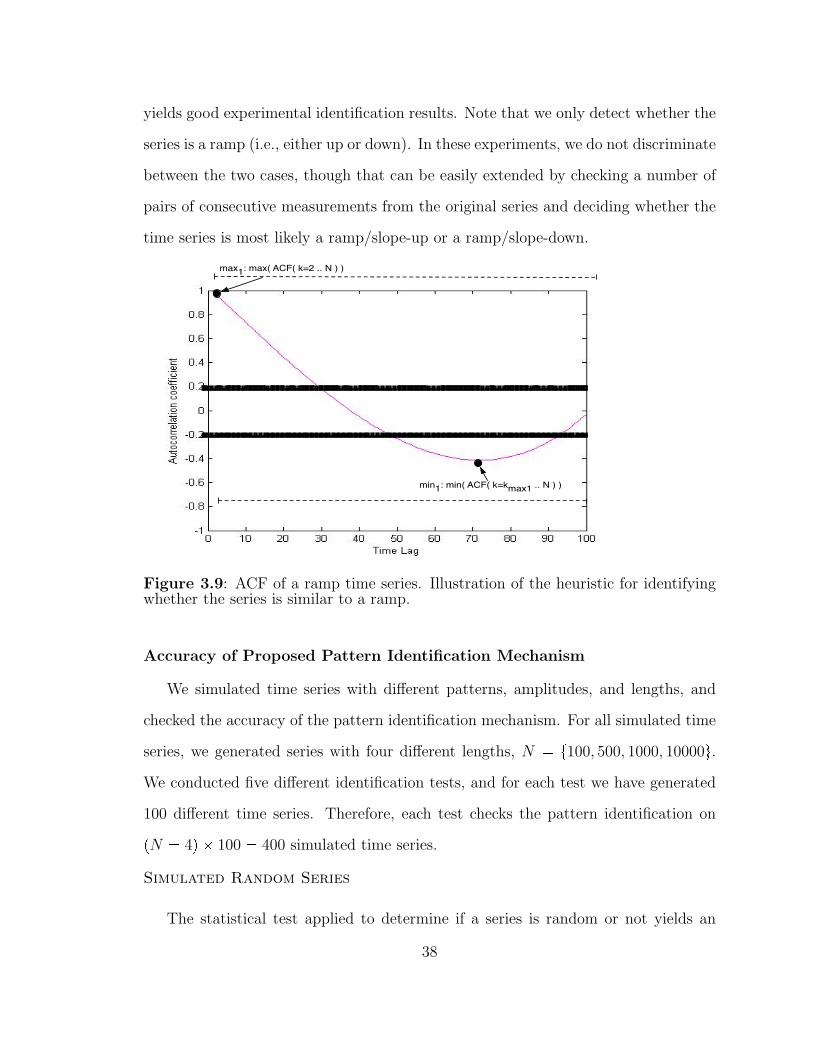
yields good experimental identification results. Note that we only detect whether the
series is a ramp (i.e., either up or down). In these experiments, we do not discriminate
between the two cases, though that can be easily extended by checking a number of
pairs of consecutive measurements from the original series and deciding whether the
time series is most likely a ramp/slope-up or a ramp/slope-down.
max1: max( ACF( k=2 .. N ) )
min1: min( ACF( k=kmax1 .. N ) )
Figure 3.9: ACF of a ramp time series. Illustration of the heuristic for identifyingwhether the series is similar to a ramp.
Accuracy of Proposed Pattern Identification Mechanism
We simulated time series with different patterns, amplitudes, and lengths, and
checked the accuracy of the pattern identification mechanism. For all simulated time
series, we generated series with four different lengths, N � t100, 500, 1000, 10000u.We conducted five different identification tests, and for each test we have generated
100 different time series. Therefore, each test checks the pattern identification on
pN � 4q � 100 � 400 simulated time series.
Simulated Random Series
The statistical test applied to determine if a series is random or not yields an
38
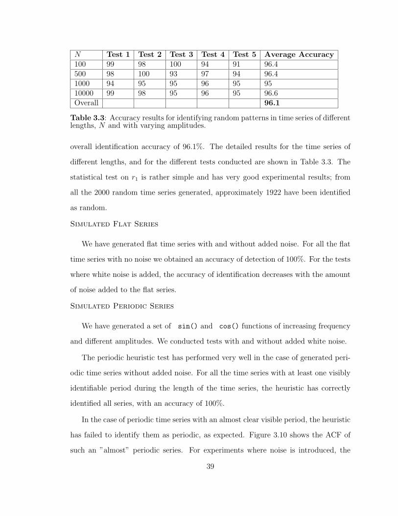
N Test 1 Test 2 Test 3 Test 4 Test 5 Average Accuracy100 99 98 100 94 91 96.4500 98 100 93 97 94 96.41000 94 95 95 96 95 9510000 99 98 95 96 95 96.6Overall 96.1
Table 3.3: Accuracy results for identifying random patterns in time series of differentlengths, N and with varying amplitudes.
overall identification accuracy of 96.1%. The detailed results for the time series of
different lengths, and for the different tests conducted are shown in Table 3.3. The
statistical test on r1 is rather simple and has very good experimental results; from
all the 2000 random time series generated, approximately 1922 have been identified
as random.
Simulated Flat Series
We have generated flat time series with and without added noise. For all the flat
time series with no noise we obtained an accuracy of detection of 100%. For the tests
where white noise is added, the accuracy of identification decreases with the amount
of noise added to the flat series.
Simulated Periodic Series
We have generated a set of sin() and cos() functions of increasing frequency
and different amplitudes. We conducted tests with and without added white noise.
The periodic heuristic test has performed very well in the case of generated peri-
odic time series without added noise. For all the time series with at least one visibly
identifiable period during the length of the time series, the heuristic has correctly
identified all series, with an accuracy of 100%.
In the case of periodic time series with an almost clear visible period, the heuristic
has failed to identify them as periodic, as expected. Figure 3.10 shows the ACF of
such an ”almost” periodic series. For experiments where noise is introduced, the
39
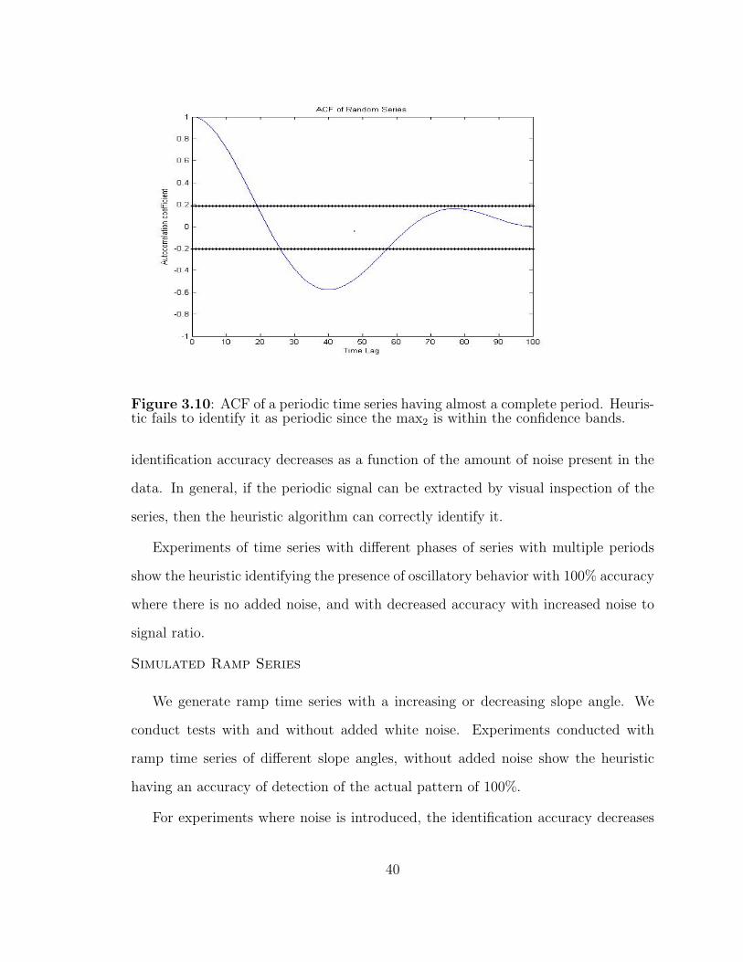
Figure 3.10: ACF of a periodic time series having almost a complete period. Heuris-tic fails to identify it as periodic since the max2 is within the confidence bands.
identification accuracy decreases as a function of the amount of noise present in the
data. In general, if the periodic signal can be extracted by visual inspection of the
series, then the heuristic algorithm can correctly identify it.
Experiments of time series with different phases of series with multiple periods
show the heuristic identifying the presence of oscillatory behavior with 100% accuracy
where there is no added noise, and with decreased accuracy with increased noise to
signal ratio.
Simulated Ramp Series
We generate ramp time series with a increasing or decreasing slope angle. We
conduct tests with and without added white noise. Experiments conducted with
ramp time series of different slope angles, without added noise show the heuristic
having an accuracy of detection of the actual pattern of 100%.
For experiments where noise is introduced, the identification accuracy decreases
40
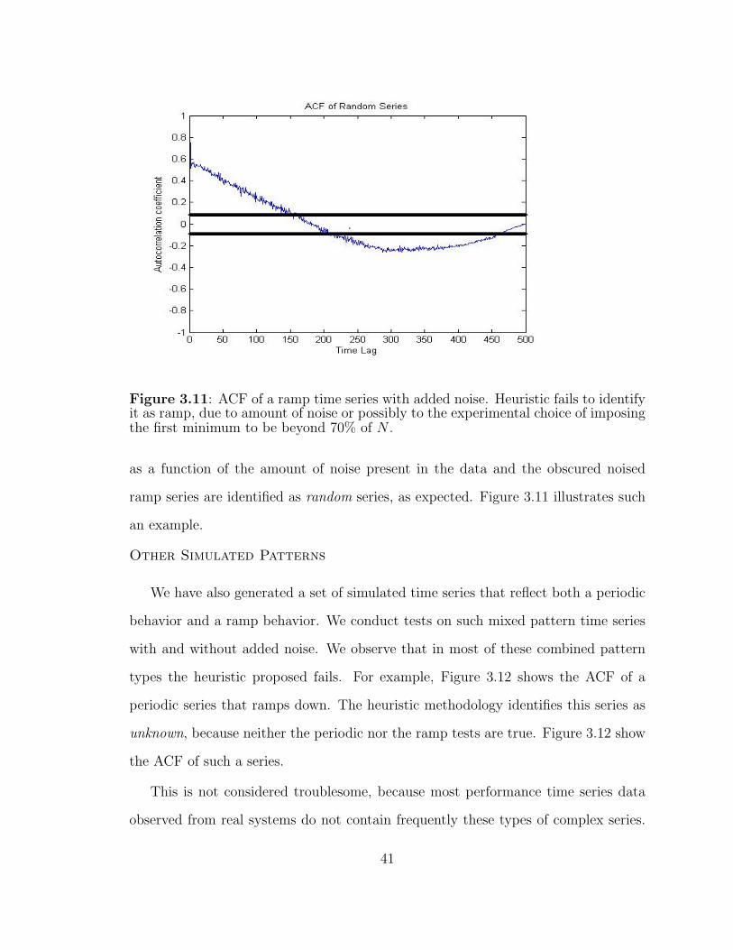
Figure 3.11: ACF of a ramp time series with added noise. Heuristic fails to identifyit as ramp, due to amount of noise or possibly to the experimental choice of imposingthe first minimum to be beyond 70% of N .
as a function of the amount of noise present in the data and the obscured noised
ramp series are identified as random series, as expected. Figure 3.11 illustrates such
an example.
Other Simulated Patterns
We have also generated a set of simulated time series that reflect both a periodic
behavior and a ramp behavior. We conduct tests on such mixed pattern time series
with and without added noise. We observe that in most of these combined pattern
types the heuristic proposed fails. For example, Figure 3.12 shows the ACF of a
periodic series that ramps down. The heuristic methodology identifies this series as
unknown, because neither the periodic nor the ramp tests are true. Figure 3.12 show
the ACF of such a series.
This is not considered troublesome, because most performance time series data
observed from real systems do not contain frequently these types of complex series.
41
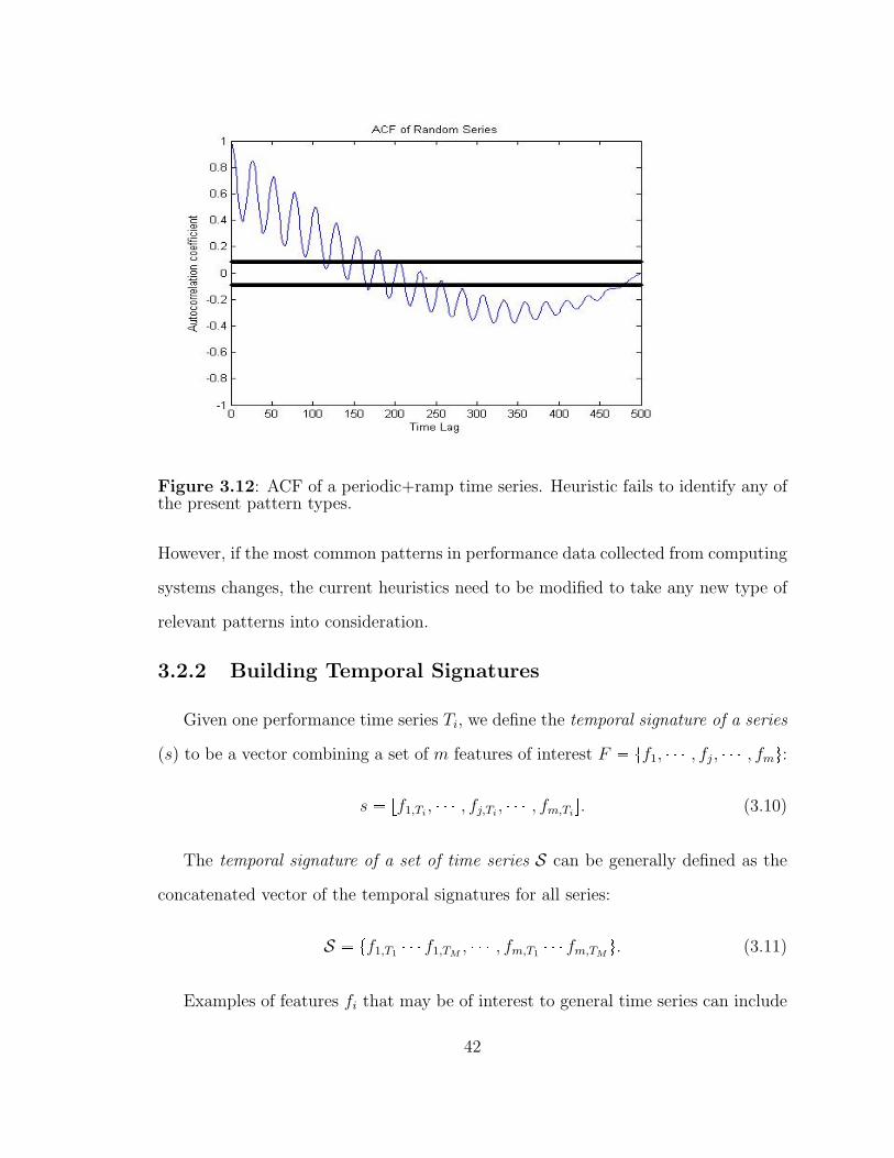
Figure 3.12: ACF of a periodic+ramp time series. Heuristic fails to identify any ofthe present pattern types.
However, if the most common patterns in performance data collected from computing
systems changes, the current heuristics need to be modified to take any new type of
relevant patterns into consideration.
3.2.2 Building Temporal Signatures
Given one performance time series Ti, we define the temporal signature of a series
(s) to be a vector combining a set of m features of interest F � tf1, � � � , fj, � � � , fmu:
s � rf1,Ti, � � � , fj,Ti
, � � � , fm,Tis. (3.10)
The temporal signature of a set of time series S can be generally defined as the
concatenated vector of the temporal signatures for all series:
S � tf1,T1 � � � f1,TM, � � � , fm,T1 � � � fm,TM
u. (3.11)
Examples of features fi that may be of interest to general time series can include
42
both quantitative or statistical features such as mean, variance, number of outliers,
as well as qualitative features such as pattern, relative variance, sudden changes in
trend, convexity, concavity and so on. We describe in Section 6.1.2 other examples
of feature that can be extracted from time series from other domains.
Temporal Signatures for Scientific Applications
We define the temporal signature of a time series (s) as:
s � rRelative VariancepTiq,PatternpTiqs � rs2n,cpTiq, ppTiqs.
Given a set of M performance time series, pT1 through TMq, having been selected
a priori to be as independent as possible, we further define the temporal signature
of set of time series, S as the concatenated vector of the temporal signatures of all
series:
S � ts2n,cpT1q � � � s2
n,cpTMq, ppT1q � � � ppTMqu. (3.12)
The temporal signature captures features of interest for a set of performance time
series; it represents a quantitative vector that carries compressed information about
characteristics of the set of time series. We hypothesize that we can use temporal sig-
natures to differentiate between well-performing and ill-performing application states
executing on distributed computing resources.
3.3 Supervised Learning
Supervised learning is a machine learning technique for creating a function or
mapping from a set of training data to a set of output values [32]. The training
data consist of pairs of input objects (typically vectors), and desired outputs. In our
framework’s case, the training data is the set of feature vectors (temporal signatures
- S) of applications, while the outputs represent a qualitative label of application
performance (e.g., expected, unexpected - slow disk performance, unexpected - memory
43
leak, and so on).
The object of the supervised learner is to predict the value of the function for any
valid input data after being trained on a number of training samples (e.g., pairs of
temporal signatures and target output - qualitative performance of application).
3.3.1 Training
When gathering a set of training data points, one must carefully design experi-
mental conditions in order for the training set to be characteristic of the “real-world”
use of the classifier function. In our framework, we gather a set of performance time
series metrics during application execution, which are transformed in temporal sig-
natures - that is, the input objects to the classification function. The corresponding
outputs are also gathered from either (a) an automatic system defining application
performance, or from (b) workflow application users.
The accuracy of the classifier will depend on how the input object is represented:
that is, it will depend on the temporal signature definition. The temporal signature
is a feature vector, which is descriptive of the original time series data. The number
of features should not be too large, but should be large enough to accurately predict
the output (see more about the issue of over-fitting in Section 3.3.3).
3.3.2 Classification
Classification is the act of distributing objects into classes or categories of the
same type. Classes or categories are defined a priori either by an expert, or found
with unsupervised learning techniques (i.e., clustering techniques). There exist a
wide range of classification techniques available for data analysis. The most widely
used classifiers include k-nearest neighbors, neural networks, fuzzy, Gaussian mixture
model, Bayesian, decision trees and support vector machines [32]. Each of the classi-
fiers have strengths and weaknesses. There is no single classifier that works best on
44
all given problems. Classifier performance depends greatly on the characteristics of
the data to be classified.
In our data analysis, we use a classifier based on the k-nearest-neighbor (knn) rule.
Given a set of n labeled feature vectors ~xj with label D, t ~x1, ~x2, . . . , ~xnu belonging
to label D, let ~xj P D be the training sample nearest to a new test point ~x. Then,
the nearest-neighbor rule (k � 1) for classifying ~x is to assign it the label associated
with ~xj [32]. Figure 3.13(a) illustrates the rule in a 2D space where two prototypes
are labeled as lighter points and darker points. The nearest point is one from the
dark-colored point class, and therefore the new point’s label or class will also be the
dark-colored class.
An extension to the nearest-neighbor rule is the k-nearest neighbor rule. This
rule classifies ~x by assigning it the label most frequently represented among the k
nearest samples. The process is illustrated in Figure 3.13(b). Out of the five nearest
points, three are in the dark-colored class while two are in the light-colored class.
Since the majority of the five points neighboring ~x are in the dark-colored class, the
new point’s class will also be the dark-colored class.
Depending on the data present in the feature vectors ~x, various measures of sim-
ilarity can be used, depending on context. Common choices of similarity definitions
include the squared Euclidean distance, Pearson’s correlation coefficient, the Maha-
lanobis (city-block) distance or the Hamming distance when the data is binary or
categorical. For the specific instance of our current temporal signature S, where the
features have categorical values, we use as a measure of similarity the normalized
Hamming distance. The Hamming distance is defined as the number n of features
(or columns) that must be changed in a feature vector in order to transform one
vector ~xA into another one ~xB. The normalized Hamming distance divides n by
the total number of features in the vector. To illustrate with an example, given
45
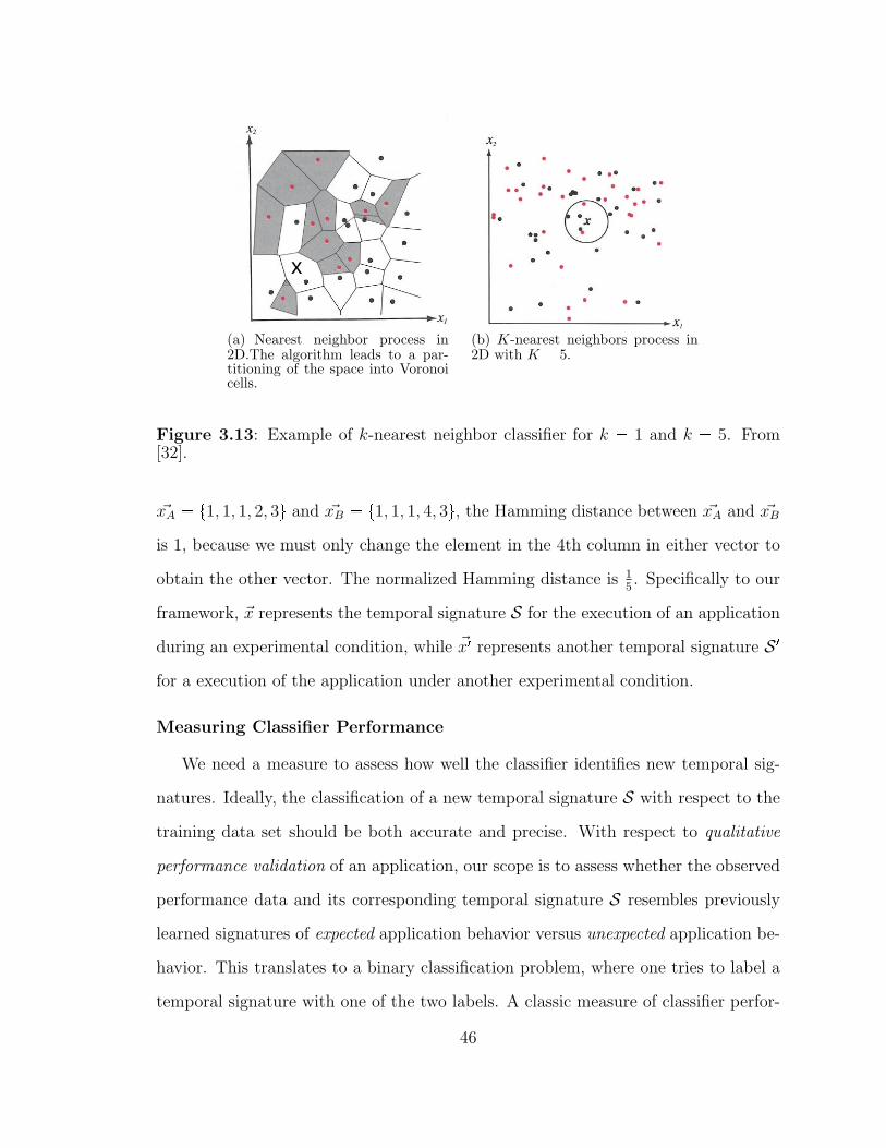
x
(a) Nearest neighbor process in2D.The algorithm leads to a par-titioning of the space into Voronoicells.
(b) K-nearest neighbors process in2D with K � 5.
Figure 3.13: Example of k-nearest neighbor classifier for k � 1 and k � 5. From[32].
~xA � t1, 1, 1, 2, 3u and ~xB � t1, 1, 1, 4, 3u, the Hamming distance between ~xA and ~xB
is 1, because we must only change the element in the 4th column in either vector to
obtain the other vector. The normalized Hamming distance is 15. Specifically to our
framework, ~x represents the temporal signature S for the execution of an application
during an experimental condition, while ~x1 represents another temporal signature S 1
for a execution of the application under another experimental condition.
Measuring Classifier Performance
We need a measure to assess how well the classifier identifies new temporal sig-
natures. Ideally, the classification of a new temporal signature S with respect to the
training data set should be both accurate and precise. With respect to qualitative
performance validation of an application, our scope is to assess whether the observed
performance data and its corresponding temporal signature S resembles previously
learned signatures of expected application behavior versus unexpected application be-
havior. This translates to a binary classification problem, where one tries to label a
temporal signature with one of the two labels. A classic measure of classifier perfor-
46
mance is the classification accuracy (A), which is a measure of how well the classifier
correctly identifies or excludes a condition:
A � NTP �NTN
NTP �NFP �NFN �NTN
, (3.13)
that is, the proportion of true results in the population (where NTP is the num-
ber of true positives, NTN is the number of true negatives, NFP is the number of
false positives, and NFN is the number of false negatives). However, in cases where
target classes are rare (e.g., such as performance problems), using the above classi-
fication accuracy as a measure of classifier performance may be misleading, as the
accuracy value (A) may be inflated due to a larger number of expected application
performance states that can typically be gathered. For example, consider that we
have collected n � 100 samples of application performance and have extracted cor-
responding temporal signatures. Consider we have n1 � 80 of the cases representing
expected application behavior and n2 � 20 representing unexpected application be-
havior. Assume that the knn classifier identifies correctly all of the expected cases,
resulting in NTP � 80, and that it miss-classifies all of the unexpected cases, resulting
in NTN � 0. The accuracy of the classifier will be misleadingly high:
A � 80 � 0
100� 0.8. (3.14)
Our goal is to classify signatures from both expected and unexpected categories. There-
fore, similarly to [21, 30], we additionally use as a measure of classifier performance
the balanced accuracy (BA):
BA � p1 �RFP q � p1 �RFNq2
, (3.15)
47
where RFP is the ratio of false positives (i.e., indicating there is a performance prob-
lem where there is none), and RFN is the ratio of false negatives (i.e., failing to
indicate there is an actual problem affecting application performance). In the exam-
ple given above, the value of the balanced accuracy will be only 0.5., more indicative
of a less accurate classification.
Furthermore, with respect to qualitative performance diagnosis of an application,
our scope is to identify the most likely performance problem affecting the applica-
tion. This translates to a multi-category classification problem, where the various
categories are the examples of performance problems available in our training data.
We assume in our experimental context that the number of samples of temporal sig-
natures of performance problems is about the same across the different unexpected
categories. Thus, within this context, using the classic measure of classifier perfor-
mance A seems appropriate. However, it is still possible that within the categories of
unexpected behaviors to have more samples for relatively frequently-occurring per-
formance problems, and to have fewer samples for rarer events. If that is indeed the
case, one can choose different metrics of accuracy that account for classes with fewer
samples, such as those proposed in [53].
3.3.3 General Issues Affecting Classifiers
We briefly discuss some important issues affecting any supervised learner tech-
nique. These issues are significant because the different numbers of metrics analyzed,
the different features, as well as the sample size of the training set will affect the
accuracy of our framework.
Problems of Dimensionality
When designing a classifier, one must pay attention to how the accuracy of the
classifier depends upon the dimensionality of the data (e.g., number of features in
48
the temporal signature), and on the amount of training data points (e.g., number
of application experiments which are used for learning a knowledge base). Another
issue of importance is how complex (in terms of time and space) the classifier chosen
should be.
Inductive Bias
The inductive bias of a learning algorithm is a set of assumptions that the classifier
function uses to predict outputs in case of novel input patterns. Below are two
questions we address with respect to this issue.
What happens if the experimental data from which training is per-
formed is actually incorrectly labeled (e.g., data is a false negative or false
positive)? These types of data instances are usually treated as noise as they would
typically be further away from the rest of the crowd from their actual class. It is
usually accepted that the training data sets will not be perfect and therefore the
focus is on making the classifier more robust.
What happens if a new signature to be tested is not like anything ever
seen before in the training data set? Most conventional supervised learning
techniques assume that the training and test data are drawn from the same distribu-
tion. Under this assumption, data from training and testing should be similar. The
opposite case is called ”sample selection bias,” which means the training set is biased
because of some experimental setup difference. When designing learning algorithms,
it is the convention to assume similar data from train and test.
However, we may run in this issue in the cases of performance problems never
encountered. In this case, the data will be incorrectly labeled and the accuracy of the
classifier will decrease over time, as the classifier will be unable to correctly predict
the new cases of performance problems. This issue can be addressed by extending
our framework to include an adaptive learning classifier, that will self-correct over
49
time, and gradually include new samples of performance problems in applications.
Over-fitting
Over-fitting is an important area of research in statistical pattern recognition, as
it is important to strike a balance between the complexity of the classifying function
and the efficacy of classification. A classifier function should be “sufficiently” complex
so that it can capture the differences between categories on training data, yet not too
complex so that it performs poorly on new patterns [32].
3.4 Methodologies for Data Visualization
Our framework analyzes multi-variate time series data and extracts features from
this data; therefore, we must employ the help of any available multi-variate visual-
ization techniques to better understand the data and the efficacy of the techniques
we propose. In the following sections, we describe a series of techniques to visualize
multi-variate performance time series data, temporal signatures, as well as meth-
ods to visualize groups of temporal signatures in the corresponding high-dimensional
variable and feature space.
3.4.1 Performance Time Series Data Visualizations
We consider the case of plotting a set of M time series, T1 � � �TM , where each series
Ti has a set of equidistant sampled values, z1, � � � zn, that have values at potentially
different scales (e.g., T1 has samples revolving around 10 while T5 has samples revolv-
ing around 10, 000). We have studied two different methods of visualizing these sets
of time series data: (1) a semi-log on the y-axis visualization, and (2) a stacked-plots
visualization. Each has advantages and disadvantages, which we further discuss.
50
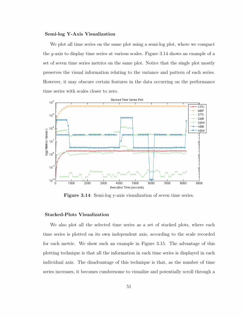
Semi-log Y-Axis Visualization
We plot all time series on the same plot using a semi-log plot, where we compact
the y-axis to display time series at various scales. Figure 3.14 shows an example of a
set of seven time series metrics on the same plot. Notice that the single plot mostly
preserves the visual information relating to the variance and pattern of each series.
However, it may obscure certain features in the data occurring on the performance
time series with scales closer to zero.
Figure 3.14: Semi-log y-axis visualization of seven time series.
Stacked-Plots Visualization
We also plot all the selected time series as a set of stacked plots, where each
time series is plotted on its own independent axis, according to the scale recorded
for each metric. We show such an example in Figure 3.15. The advantage of this
plotting technique is that all the information in each time series is displayed in each
individual axis. The disadvantage of this technique is that, as the number of time
series increases, it becomes cumbersome to visualize and potentially scroll through a
51
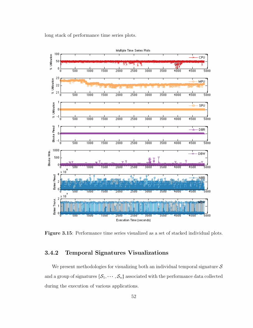
long stack of performance time series plots.
Figure 3.15: Performance time series visualized as a set of stacked individual plots.
3.4.2 Temporal Signatures Visualizations
We present methodologies for visualizing both an individual temporal signature S
and a group of signatures tS1, � � � ,Snu associated with the performance data collected
during the execution of various applications.
52
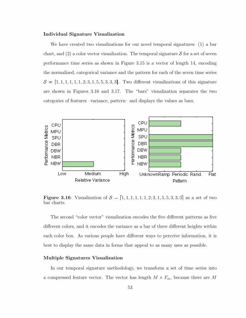
Individual Signature Visualization
We have created two visualizations for our novel temporal signatures: (1) a bar
chart, and (2) a color vector visualization. The temporal signature S for a set of seven
performance time series as shown in Figure 3.15 is a vector of length 14, encoding
the normalized, categorical variance and the pattern for each of the seven time series
S � r1, 1, 1, 1, 1, 1, 2; 3, 1, 5, 5, 3, 3, 3s. Two different visualizations of this signature
are shown in Figures 3.16 and 3.17. The “bars” visualization separates the two
categories of features –variance, pattern– and displays the values as bars.
Figure 3.16: Visualization of S � r1, 1, 1, 1, 1, 1, 2; 3, 1, 5, 5, 3, 3, 3s as a set of twobar charts.
The second “color vector” visualization encodes the five different patterns as five
different colors, and it encodes the variance as a bar of three different heights within
each color box. As various people have different ways to perceive information, it is
best to display the same data in forms that appeal to as many uses as possible.
Multiple Signatures Visualization
In our temporal signature methodology, we transform a set of time series into
a compressed feature vector. The vector has length M � Fm, because there are M
53
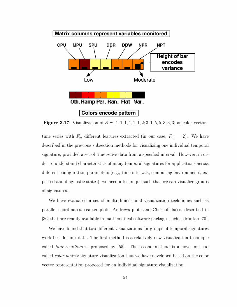
Height of barencodes variance
Moderate
Colors encode pattern
Low
CPU MPU SPU DBR DBW NPR NPT
Matrix columns represent variables monitored
Figure 3.17: Visualization of S � r1, 1, 1, 1, 1, 1, 2; 3, 1, 5, 5, 3, 3, 3s as color vector.
time series with Fm different features extracted (in our case, Fm � 2). We have
described in the previous subsection methods for visualizing one individual temporal
signature, provided a set of time series data from a specified interval. However, in or-
der to understand characteristics of many temporal signatures for applications across
different configuration parameters (e.g., time intervals, computing environments, ex-
pected and diagnostic states), we need a technique such that we can visualize groups
of signatures.
We have evaluated a set of multi-dimensional visualization techniques such as
parallel coordinates, scatter plots, Andrews plots and Chernoff faces, described in
[36] that are readily available in mathematical software packages such as Matlab [70].
We have found that two different visualizations for groups of temporal signatures
work best for our data. The first method is a relatively new visualization technique
called Star-coordinates, proposed by [55]. The second method is a novel method
called color matrix signature visualization that we have developed based on the color
vector representation proposed for an individual signature visualization.
54
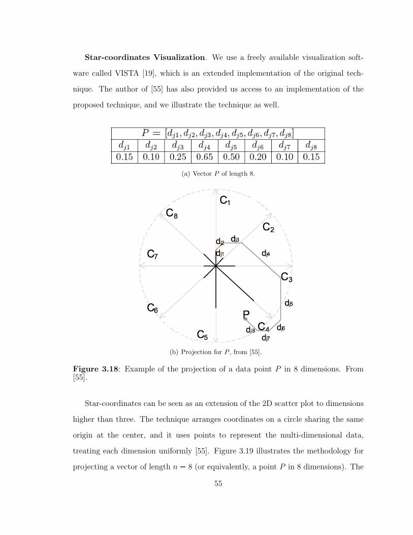
Star-coordinates Visualization. We use a freely available visualization soft-
ware called VISTA [19], which is an extended implementation of the original tech-
nique. The author of [55] has also provided us access to an implementation of the
proposed technique, and we illustrate the technique as well.
(a) Vector P of length 8.
(b) Projection for P , from [55].
Figure 3.18: Example of the projection of a data point P in 8 dimensions. From[55].
Star-coordinates can be seen as an extension of the 2D scatter plot to dimensions
higher than three. The technique arranges coordinates on a circle sharing the same
origin at the center, and it uses points to represent the multi-dimensional data,
treating each dimension uniformly [55]. Figure 3.19 illustrates the methodology for
projecting a vector of length n � 8 (or equivalently, a point P in 8 dimensions). The
55
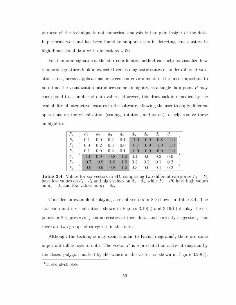
purpose of the technique is not numerical analysis but to gain insight of the data.
It performs well and has been found to support users in detecting true clusters in
high-dimensional data with dimensions ¤ 50.
For temporal signatures, the star-coordinates method can help us visualize how
temporal signatures look in expected versus diagnostic states or under different vari-
ations (i.e., across applications or execution environments). It is also important to
note that the visualization introduces some ambiguity, as a single data point P may
correspond to a number of data values. However, this drawback is remedied by the
availability of interactive features in the software, allowing the user to apply different
operations on the visualization (scaling, rotation, and so on) to help resolve these
ambiguities.
Pi [ d1 d2 d3 d4 d5 d6 d7 d8 ]P1 [ 0.1 0.0 0.2 0.1 1.0 0.9 0.8 1.0 ]P2 [ 0.0 0.2 0.3 0.0 0.7 0.9 1.0 1.0 ]P3 [ 0.1 0.0 0.2 0.1 0.9 0.9 0.9 1.0 ]P4 [ 1.0 0.9 0.8 1.0 0.1 0.0 0.2 0.0 ]P5 [ 0.7 0.9 1.0 1.0 0.2 0.2 0.1 0.2 ]P6 [ 0.9 0.9 0.8 1.0 0.3 0.0 0.1 0.2 ]
Table 3.4: Values for six vectors in 8D, comprising two different categories.P1 � P3have low values on d1�d4 and high values on d5�d8, while P4�P6 have high valueson d1 � d4 and low values on d5 � d8.
Consider an example displaying a set of vectors in 8D shown in Table 3.4. The
star-coordinates visualizations shown in Figures 3.19(a) and 3.19(b) display the six
points in 8D, preserving characteristics of their data, and correctly suggesting that
there are two groups of categories in this data.
Although the technique may seem similar to Kiviat diagrams1, there are some
important differences to note. The vector P is represented on a Kiviat diagram by
the closed polygon marked by the values in the vector, as shown in Figure 3.20(a).
1Or star glyph plots.
56
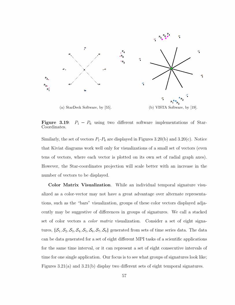
P1
P6
P5
P4
P3
P2
(a) StarDeck Software, by [55].
P1
P6P5P4
P3
P2
(b) VISTA Software, by [19].
Figure 3.19: P1 � P6 using two different software implementations of Star-Coordinates.
Similarly, the set of vectors P1-P6 are displayed in Figures 3.20(b) and 3.20(c). Notice
that Kiviat diagrams work well only for visualizations of a small set of vectors (even
tens of vectors, where each vector is plotted on its own set of radial graph axes).
However, the Star-coordinates projection will scale better with an increase in the
number of vectors to be displayed.
Color Matrix Visualization. While an individual temporal signature visu-
alized as a color-vector may not have a great advantage over alternate representa-
tions, such as the “bars” visualization, groups of these color vectors displayed adja-
cently may be suggestive of differences in groups of signatures. We call a stacked
set of color vectors a color matrix visualization. Consider a set of eight signa-
tures, tS1,S2,S3,S4,S5,S6,S7,S8u generated from sets of time series data. The data
can be data generated for a set of eight different MPI tasks of a scientific applications
for the same time interval, or it can represent a set of eight consecutive intervals of
time for one single application. Our focus is to see what groups of signatures look like;
Figures 3.21(a) and 3.21(b) display two different sets of eight temporal signatures.
57
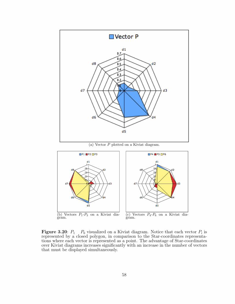
(a) Vector P plotted on a Kiviat diagram.
(b) Vectors P1-P3 on a Kiviat dia-gram.
(c) Vectors P4-P6 on a Kiviat dia-gram.
Figure 3.20: P1 � P6 visualized on a Kiviat diagram. Notice that each vector Pi isrepresented by a closed polygon, in comparison to the Star-coordinates representa-tions where each vector is represented as a point. The advantage of Star-coordinatesover Kiviat diagrams increases significantly with an increase in the number of vectorsthat must be displayed simultaneously.
58
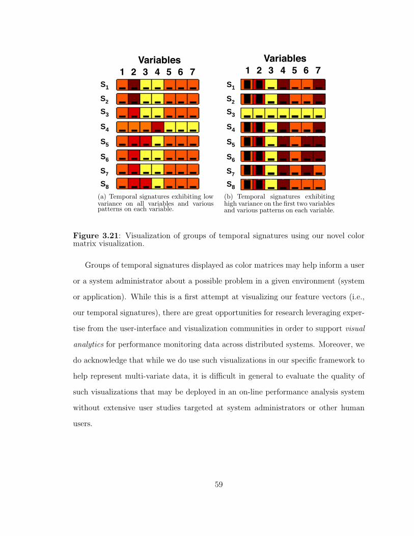
1 2 3 4 5 6 7Variables
S7
S8
S6
S5
S4
S2
S3
S1
(a) Temporal signatures exhibiting lowvariance on all variables and variouspatterns on each variable.
1 2 3 4 5 6 7Variables
S7
S8
S6
S5
S4
S2
S3
S1
(b) Temporal signatures exhibitinghigh variance on the first two variablesand various patterns on each variable.
Figure 3.21: Visualization of groups of temporal signatures using our novel colormatrix visualization.
Groups of temporal signatures displayed as color matrices may help inform a user
or a system administrator about a possible problem in a given environment (system
or application). While this is a first attempt at visualizing our feature vectors (i.e.,
our temporal signatures), there are great opportunities for research leveraging exper-
tise from the user-interface and visualization communities in order to support visual
analytics for performance monitoring data across distributed systems. Moreover, we
do acknowledge that while we do use such visualizations in our specific framework to
help represent multi-variate data, it is difficult in general to evaluate the quality of
such visualizations that may be deployed in an on-line performance analysis system
without extensive user studies targeted at system administrators or other human
users.
59
3.5 Summary
We described the core data analysis and visualization methodologies employed in
this framework. This chapter presented how we:
1. Select and extract relevant features from performance time series data in order
to generate a compact representation of the data,
2. Build temporal signatures for scientific applications,
3. Use concepts from supervised learning to gather a knowledge base of qualitative
performance states,
4. Evaluate the efficacy of our classifier for both qualitative performance validation
and diagnosis, and
5. Employ multi-variate visualization techniques to aid in representation and anal-
ysis of our results.
60
Chapter 4
Qualitative Performance AnalysisFramework
This chapter describes Teresa, (Temporal Reasoning for Scientific Applications),
a general qualitative performance analysis framework that monitors long-running
tasks of a scientific workflow to qualitatively validate and diagnose their performance
in distributed Grid environments. Teresa has four high-level processing steps:
1. Selection of long-running computational tasks in workflows,
2. Collection of available performance time series data from environments where
these tasks execute,
3. Analysis of data to extract characteristics correlated with well-performing and
ill-performing executions of these tasks, and
4. Reasoning about the qualitative performance state of the workflow over time.
Figure 4.1 presents a diagram of the above high-level process.
4.1 Architecture
While Figure 4.1 presented a high-level, “black-box” view of our framework, we
further elaborate on its composition. Teresa has three components: (1) a temporal
signature design component, (2) a supervised learning component, and (3) a qualita-
tive reasoning component. Figure 4.2 expands on the components within Teresa.
Teresa analyzes input data from a set of workflow monitoring tools, such as
Grid infrastructure monitoring or workflow monitoring (e.g., execution engine, task
61
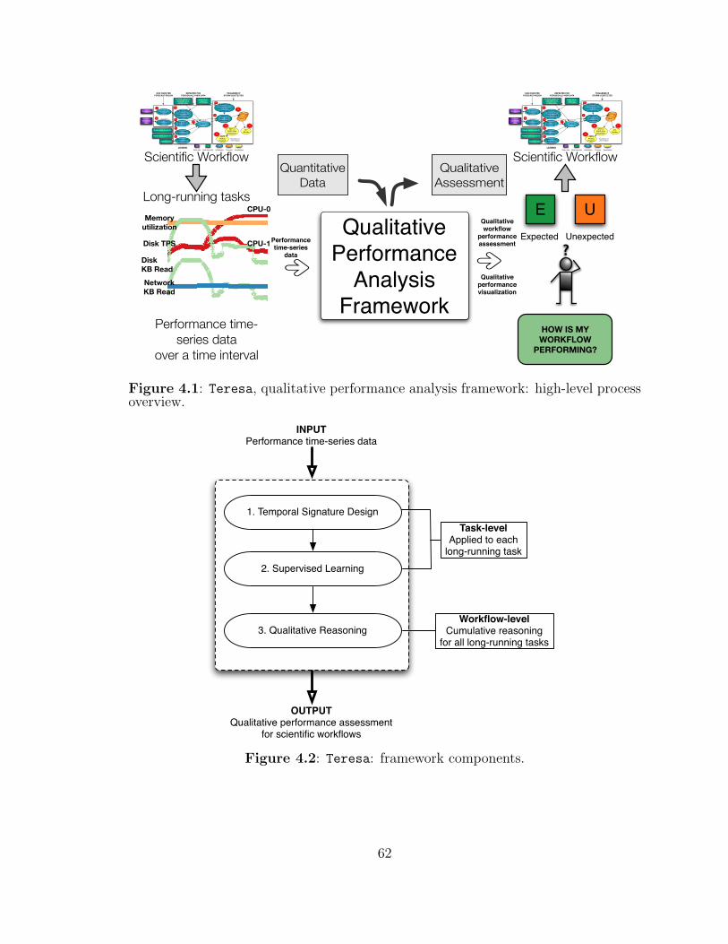
Qualitative Performance
Analysis Framework
Long-running tasks
Terrain data
Surface, terrestrial
data
Radar data (Level II)
Radar data (Level III)
Satellite data
NAM, RUC, GFS data
Surface, upper air mesonet, wind
profiler data
TerrainPreprocessor
1
WRF StaticPreprocessor
2
3D Model Data Interpolator
(Initial Boundary Conditions)
3
88D RadarRemapper
4
NIDS RadarRemapper
5
Satellite DataRemapper
6
ADAS7
3D Model Data Interpolator
(Lateral Boundary Conditions)
8
ARPS to WRF Data Interpolator
9
IDV Bundle
11
ARPSPlottingProgram
13
WRF to ARPS DataInterpolator
12
10
WRF
LEGENDReal-time dataStatic data Initialization Forecast Visualization
RUN ONCE PER
FORECAST REGION
TRIGGERED IF
STORM IS DETECTED
REPEATED FOR
PERIODICALLY NEW DATA
Visualization on
user's request
Scientific Workflow
Performancetime-series
data
Qualitativeworkflow
performanceassessment
Qualitativeperformancevisualization
Qualitative
Assessment
Quantitative
Data
Expected
E
Unexpected
U
Terrain data
Surface, terrestrial
data
Radar data (Level II)
Radar data (Level III)
Satellite data
NAM, RUC, GFS data
Surface, upper air mesonet, wind
profiler data
TerrainPreprocessor
1
WRF StaticPreprocessor
2
3D Model Data Interpolator
(Initial Boundary Conditions)
3
88D RadarRemapper
4
NIDS RadarRemapper
5
Satellite DataRemapper
6
ADAS7
3D Model Data Interpolator
(Lateral Boundary Conditions)
8
ARPS to WRF Data Interpolator
9
IDV Bundle
11
ARPSPlottingProgram
13
WRF to ARPS DataInterpolator
12
10
WRF
LEGENDReal-time dataStatic data Initialization Forecast Visualization
RUN ONCE PER
FORECAST REGION
TRIGGERED IF
STORM IS DETECTED
REPEATED FOR
PERIODICALLY NEW DATA
Visualization on
user's request
Scientific Workflow
?
HOW IS MY
WORKFLOW
PERFORMING?
Performance time-
series data
over a time interval
CPU-0
Memory
utilization
CPU-1 Disk TPS
Network
KB Read
Disk
KB Read
Figure 4.1: Teresa, qualitative performance analysis framework: high-level processoverview.
INPUTPerformance time-series data
1. Temporal Signature Design
2. Supervised Learning
3. Qualitative Reasoning
OUTPUTQualitative performance assessment
for scientific workflows
Task-levelApplied to each
long-running task
Workflow-levelCumulative reasoning
for all long-running tasks
Figure 4.2: Teresa: framework components.
62
monitoring, etc). The temporal signature design component takes quantitative perfor-
mance time series data over a specified time interval and transforms it into a temporal
signature, S, for each long-running task in a workflow. The supervised learning com-
ponent assesses whether an application’s temporal signature matches expected or
unexpected behaviors. Previous application behaviors are learned in a training phase
off-line. If the application behaves in an unexpected way, the qualitative reasoning
component, which operates at the global workflow level, considers the implication
to the global workflow performance of the unexpected behaviors of the flagged long-
running tasks. A multitude of policies can be specified and invoked, depending on
the characteristics of the scientific workflow (e.g., if 50% of the workflow tasks seem
to be affected by a congested network, then checkpoint the application and restart
in an hour).
We illustrate more detailed description of the framework, with the flow of infor-
mation between components and their sub-components in Figure 4.3. The framework
has on-line and off-line sub-components. On-line sub-components are utilized when
the framework analyzes performance time series as they are received from monitor-
ing software; the on-line sub-components are: (a) temporal signature generation, (b)
on-line classification (of temporal signatures), and (c) qualitative reasoning.
The framework utilizes off-line sub-components in the configuration and training
phases; the off-line sub-components are: (a) performance time series selection, (b)
features selection, (c) temporal signature definition, (d) expected & unexpected tem-
poral signatures training, and (e) policies for reasoning with qualitative diagnostic
information.
Within the service oriented environment of Grids, the framework is a performance
analysis service for scientific workflows, providing a periodic qualitative evaluation
of performance of long-running tasks in a workflow. Grid infrastructure or workflow
63

LEGENDINPUTPerformance time-series data
1. Temporal Signature Design
2. Supervised Learning
3. Qualitative Reasoning
OUTPUTQualitative performance assessment
for scientific workflows
Temporal SignatureGeneration
Time-seriesSelection
FeatureSelection &Extraction
SignatureDefinition
Online ClassificationPerformance
Validation & Diagnosis
Training PhaseExpected and
Unexpected Temporal Signatures
Qualitative Reasoning
Policies forreasoning with
qualitative task states
EXPECTEDSIGNATURES?
UNEXPECTEDSIGNATURES?
KEEPMONITORING
onlineoffline
Figure 4.3: Flow of information through Teresa, its three components and its on-line and off-line sub-components.
monitoring services provide the performance time series data as input to the Teresa
service, whose output can be utilized by a scheduling service and/or by a fault-
tolerance service such as [54] to improve the performance of the monitored workflow,
as shown in Figure 4.4.
64
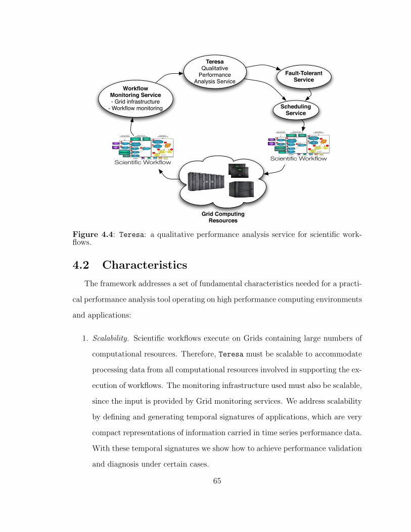
TeresaQualitative
Performance Analysis Service
Workflow Monitoring Service- Grid infrastructure
- Workflow monitoring
Grid Computing Resources
Terrain data
Surface, terrestrial
data
Radar data (Level II)
Radar data (Level III)
Satellite data
NAM, RUC, GFS data
Surface, upper air mesonet, wind
profiler data
TerrainPreprocessor
1
WRF StaticPreprocessor
2
3D Model Data Interpolator
(Initial Boundary Conditions)
3
88D RadarRemapper
4
NIDS RadarRemapper
5
Satellite DataRemapper
6
ADAS7
3D Model Data Interpolator
(Lateral Boundary Conditions)
8
ARPS to WRF Data Interpolator
9
IDV Bundle
11
ARPSPlottingProgram
13
WRF to ARPS DataInterpolator
12
10
WRF
LEGENDReal-time dataStatic data Initialization Forecast Visualization
RUN ONCE PER
FORECAST REGION
TRIGGERED IF
STORM IS DETECTED
REPEATED FOR
PERIODICALLY NEW DATA
Visualization on
user's request
Scientific Workflow
Scheduling Service
Fault-TolerantService
Terrain data
Surface, terrestrial
data
Radar data (Level II)
Radar data (Level III)
Satellite data
NAM, RUC, GFS data
Surface, upper air mesonet, wind
profiler data
TerrainPreprocessor
1
WRF StaticPreprocessor
2
3D Model Data Interpolator
(Initial Boundary Conditions)
3
88D RadarRemapper
4
NIDS RadarRemapper
5
Satellite DataRemapper
6
ADAS7
3D Model Data Interpolator
(Lateral Boundary Conditions)
8
ARPS to WRF Data Interpolator
9
IDV Bundle
11
ARPSPlottingProgram
13
WRF to ARPS DataInterpolator
12
10
WRF
LEGENDReal-time dataStatic data Initialization Forecast Visualization
RUN ONCE PER
FORECAST REGION
TRIGGERED IF
STORM IS DETECTED
REPEATED FOR
PERIODICALLY NEW DATA
Visualization on
user's request
Scientific Workflow
Figure 4.4: Teresa: a qualitative performance analysis service for scientific work-flows.
4.2 Characteristics
The framework addresses a set of fundamental characteristics needed for a practi-
cal performance analysis tool operating on high performance computing environments
and applications:
1. Scalability. Scientific workflows execute on Grids containing large numbers of
computational resources. Therefore, Teresa must be scalable to accommodate
processing data from all computational resources involved in supporting the ex-
ecution of workflows. The monitoring infrastructure used must also be scalable,
since the input is provided by Grid monitoring services. We address scalability
by defining and generating temporal signatures of applications, which are very
compact representations of information carried in time series performance data.
With these temporal signatures we show how to achieve performance validation
and diagnosis under certain cases.
65

2. Metric independence. The framework must be flexible; given a set of monitored
metrics that reflect the temporal performance of the application, it must be
possible to assess and diagnose the observed temporal behavior. However, if
another set of metrics is deemed more representative of application behavior,
the framework principles must still apply and behavioral reasoning must still be
possible. We address this by including in our framework design the ability for
the user to define different application signatures from different metrics. The
off-line sub-component time series Selection allows for this flexibility.
3. Accuracy of qualitative performance assessment. The framework must make de-
cisions based on qualitative data obtained by transforming/compressing large
amounts of quantitative information. This process results in loss of information
which may have implications on the accuracy of the qualitative transformations.
However, the framework should provide simple and intuitive performance as-
sessment answers, and should offer a statistical estimation of the correctness of
the qualitative assessment. We address the issue of the accuracy of validation
and diagnosis by associating with our framework an accuracy-of-assessment
metric within the on-line classification sub-component. If the framework con-
sistently falls below a specified accuracy threshold, Ta, then it will go into
a training mode, until a better accuracy of performance assessment can be
achieved.
4. Assessment over appropriate time scale. Due to the nature of the long duration
of resource consumption by the distributed scientific workflows, the reasoning
decisions made by the framework should similarly be made on a longer tempo-
ral scale, typically of the order of several tens of minutes. The framework’s goal
is to detect persistent behavioral violations and ignore small-scale variability,
because the cost of performing any type of performance recovery mechanisms
66
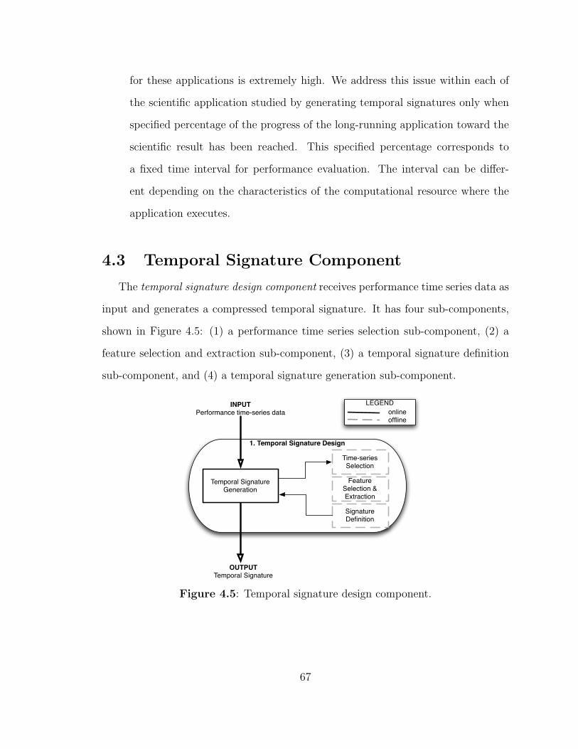
for these applications is extremely high. We address this issue within each of
the scientific application studied by generating temporal signatures only when
specified percentage of the progress of the long-running application toward the
scientific result has been reached. This specified percentage corresponds to
a fixed time interval for performance evaluation. The interval can be differ-
ent depending on the characteristics of the computational resource where the
application executes.
4.3 Temporal Signature Component
The temporal signature design component receives performance time series data as
input and generates a compressed temporal signature. It has four sub-components,
shown in Figure 4.5: (1) a performance time series selection sub-component, (2) a
feature selection and extraction sub-component, (3) a temporal signature definition
sub-component, and (4) a temporal signature generation sub-component.
INPUTPerformance time-series data
1. Temporal Signature Design
Temporal SignatureGeneration
Time-seriesSelection
FeatureSelection &Extraction
SignatureDefinition
LEGENDonlineoffline
OUTPUTTemporal Signature
Figure 4.5: Temporal signature design component.
67
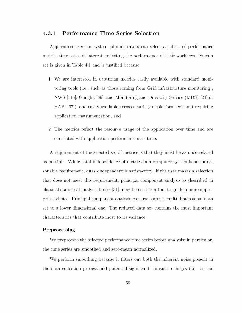
4.3.1 Performance Time Series Selection
Application users or system administrators can select a subset of performance
metrics time series of interest, reflecting the performance of their workflows. Such a
set is given in Table 4.1 and is justified because:
1. We are interested in capturing metrics easily available with standard moni-
toring tools (i.e., such as those coming from Grid infrastructure monitoring ,
NWS [115], Ganglia [69], and Monitoring and Directory Service (MDS) [24] or
HAPI [97]), and easily available across a variety of platforms without requiring
application instrumentation, and
2. The metrics reflect the resource usage of the application over time and are
correlated with application performance over time.
A requirement of the selected set of metrics is that they must be as uncorrelated
as possible. While total independence of metrics in a computer system is an unrea-
sonable requirement, quasi-independent is satisfactory. If the user makes a selection
that does not meet this requirement, principal component analysis as described in
classical statistical analysis books [31], may be used as a tool to guide a more appro-
priate choice. Principal component analysis can transform a multi-dimensional data
set to a lower dimensional one. The reduced data set contains the most important
characteristics that contribute most to its variance.
Preprocessing
We preprocess the selected performance time series before analysis; in particular,
the time series are smoothed and zero-mean normalized.
We perform smoothing because it filters out both the inherent noise present in
the data collection process and potential significant transient changes (i.e., on the
68
Workload MetricsPercentage CPU UtilizationAmount of Free MemoryNumber of Local Disk Transactions per SecondLocal Disk Number of Bytes Read per SecondLocal Disk Number of Bytes Written per SecondNetwork Number of Bytes Read per SecondNetwork Number of Bytes Written per Second
Table 4.1: An example set of easy-to-collect, non-invasive performance time seriesmetrics that can be used as input to the qualitative performance analysis framework.
scale of a couple of seconds or minutes), which are typically insignificant in the case
of long-running scientific workloads (i.e., longer than 30 minutes).
We also normalize the time series to a zero-mean, to ease pattern analysis due to
the metrics reflecting different measuring scales.
4.3.2 Features Selection and Extraction
We are interested in characterizing the selected performance time series such that
we extract the maximum amount of information in the least amount of space. Our
approach is to extract from the quantitative time series features that may correlate
with performance variability, such as amount of variability and the type of pattern
of the series. Both features are of interest because performance time series may
have a similar amount of variability but different temporal patterns. The specific
methodologies by which we perform the feature extraction are described in more
detail in Chapter 3.
4.3.3 Temporal Signature Definition
Once the performance time series have been selected, together with the features
of interest, we define the temporal signature of a series, s, to be a vector combining
69
the selected features:
s � rRelative Variance,Patterns.
Given M selected performance time series, pT1 through TMq, we further define the
temporal signature of set of time series S as the concatenated vector of the temporal
signatures of all series:
S � tRelative VariancepT1 � � �TMq,PatternpT1 � � �TMqu. (4.1)
The S vector captures the features of interest for all selected performance time series;
it represents a compressed quantitative vector that ideally should carry sufficient
information to enable discrimination between series with different characteristics. For
example, if a time series has a large amount of variance, that feature will be reflected
in a larger quantitative value of its normalized,categorical variance s2n,c. Similarly, if
another time series has a random pattern, that will be reflected in its corresponding
pattern feature value.
Applications executing on varied Grid resources may exhibit over time different
characteristics of these features. Some performance time series may be high varying
and periodic while others may be low varying and flat; we hypothesize that these
differences in temporal application behaviors can be captured via temporal signature
vectors, S.
4.3.4 Temporal Signature Generation
Given a definition for a temporal signature, the next step involves generating
such signatures from performance time series. The temporal signature generation
component generates S vectors from applications’s performance time series data.
It uses the configuration information set off-line in the previous three components
(i.e., time series selection, feature selection & extraction, and temporal signature
70
definition). The resulting temporal signatures are received as input by the supervised
learning component where they are further analyzed.
4.4 Supervised Learning Component
The supervised learning component receives temporal signatures as input. It has
two different sub-components, as shown in Figure 4.6: (1) an offline training compo-
nent, and (2) an on-line classification component.
4.4.1 Training: Learning Expected and Unexpected Signa-tures
The training sub-component of our framework must gather various instances of
temporal signatures that are indicative of both well-performing and ill-performing
application states. We conduct this necessary acquisition of training samples as
explained in the following subsections.
Signatures Associated with Expected Application Behaviors
In a controlled environment, we conduct performance studies of long-running
tasks within workflows to capture temporal signatures in instances where the tasks
complete successfully and in a well-performing manner (i.e., no resource contentions
or faults). The definition of a successful and well-performing experiment is further
discussed in more detail in Chapter 5, with specific examples as to how it can be
defined in the context of different scientific workflows.
We hypothesize that the temporal signatures of these tasks have similar character-
istics that can be compactly grouped in classes of behaviors. The intuition behind our
hypothesis stems from previous large-scale application performance studies showing a
small number of equivalent classes of behaviors characterizing collected performance
data [85, 23].
Therefore, via passively running experiments, we label a set of successful experi-
71
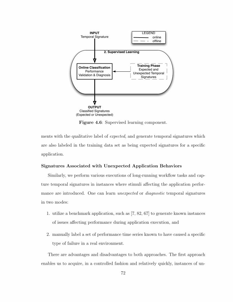
INPUTTemporal Signature
2. Supervised Learning
Online ClassificationPerformance
Validation & Diagnosis
Training PhaseExpected and
Unexpected Temporal Signatures
LEGENDonlineoffline
OUTPUTClassified Signatures
(Expected or Unexpected)
Figure 4.6: Supervised learning component.
ments with the qualitative label of expected, and generate temporal signatures which
are also labeled in the training data set as being expected signatures for a specific
application.
Signatures Associated with Unexpected Application Behaviors
Similarly, we perform various executions of long-running workflow tasks and cap-
ture temporal signatures in instances where stimuli affecting the application perfor-
mance are introduced. One can learn unexpected or diagnostic temporal signatures
in two modes:
1. utilize a benchmark application, such as [7, 82, 67] to generate known instances
of issues affecting performance during application execution, and
2. manually label a set of performance time series known to have caused a specific
type of failure in a real environment.
There are advantages and disadvantages to both approaches. The first approach
enables us to acquire, in a controlled fashion and relatively quickly, instances of un-
72
expected temporal signatures for an application, and to label them with a known
diagnostic state (e.g., signature was captured during known memory leak issue af-
fecting the application). The disadvantage lies in potentially capturing signatures
that will not have the same characteristics with signatures captured during a real
performance problem. For the second approach, we are presented with the opposite
situation: we capture within signatures real instance of performance problems, but
are not able to learn these instances fast, as severe problems affecting the application
may not occur frequently. Furthermore, we do rely on a third-party (e.g., such as
a system administrator or application user) to correctly label the performance time
series captured during such an event.
4.4.2 Classification: Performance Validation and Diagnosis
The on-line classification sub-component takes the temporal signature generated
by the first component and assesses whether the signature matches expectations.
Let us call this input temporal signature S. The classification component applies
the knn classifier method as described in Section 3.3.2 against the training data set,
and assess whether S is closest to signatures in expected behavioral classes, Ei or to
signatures in unexpected behavioral classes, Ui. The resulting classification label for
S represents the qualitative temporal behavioral state of the application for the time
interval of analysis. If S belongs to an unexpected behavioral class, the classification
label represents the possible diagnostic problem affecting the performance of the
application.
For example, consider that a set of long-running workflow tasks have three ex-
pected qualitative behaviors, E � tE1, E2, E3u, and two unexpected behaviors U �tU1, U2u, characterized by different examples of temporal signatures labeled in the
training phase with these class labels. The Ei classes represent expected labels while
the Ui classes represent unexpected labels as follows: U1 corresponds to temporal
73
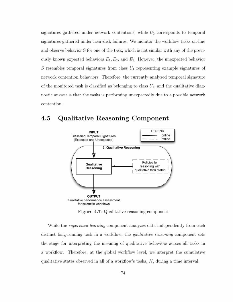
signatures gathered under network contentions, while U2 corresponds to temporal
signatures gathered under near-disk failures. We monitor the workflow tasks on-line
and observe behavior S for one of the task, which is not similar with any of the previ-
ously known expected behaviors E1, E2, and E3. However, the unexpected behavior
S resembles temporal signatures from class U1 representing example signatures of
network contention behaviors. Therefore, the currently analyzed temporal signature
of the monitored task is classified as belonging to class U1, and the qualitative diag-
nostic answer is that the tasks is performing unexpectedly due to a possible network
contention.
4.5 Qualitative Reasoning Component
INPUTClassified Temporal Signatures
(Expected and Unexpected)
3. Qualitative Reasoning
OUTPUTQualitative performance assessment
for scientific workflows
Qualitative Reasoning
Policies forreasoning with
qualitative task states
LEGENDonlineoffline
Figure 4.7: Qualitative reasoning component
While the supervised learning component analyzes data independently from each
distinct long-running task in a workflow, the qualitative reasoning component sets
the stage for interpreting the meaning of qualitative behaviors across all tasks in
a workflow. Therefore, at the global workflow level, we interpret the cumulative
qualitative states observed in all of a workflow’s tasks, N , during a time interval.
74
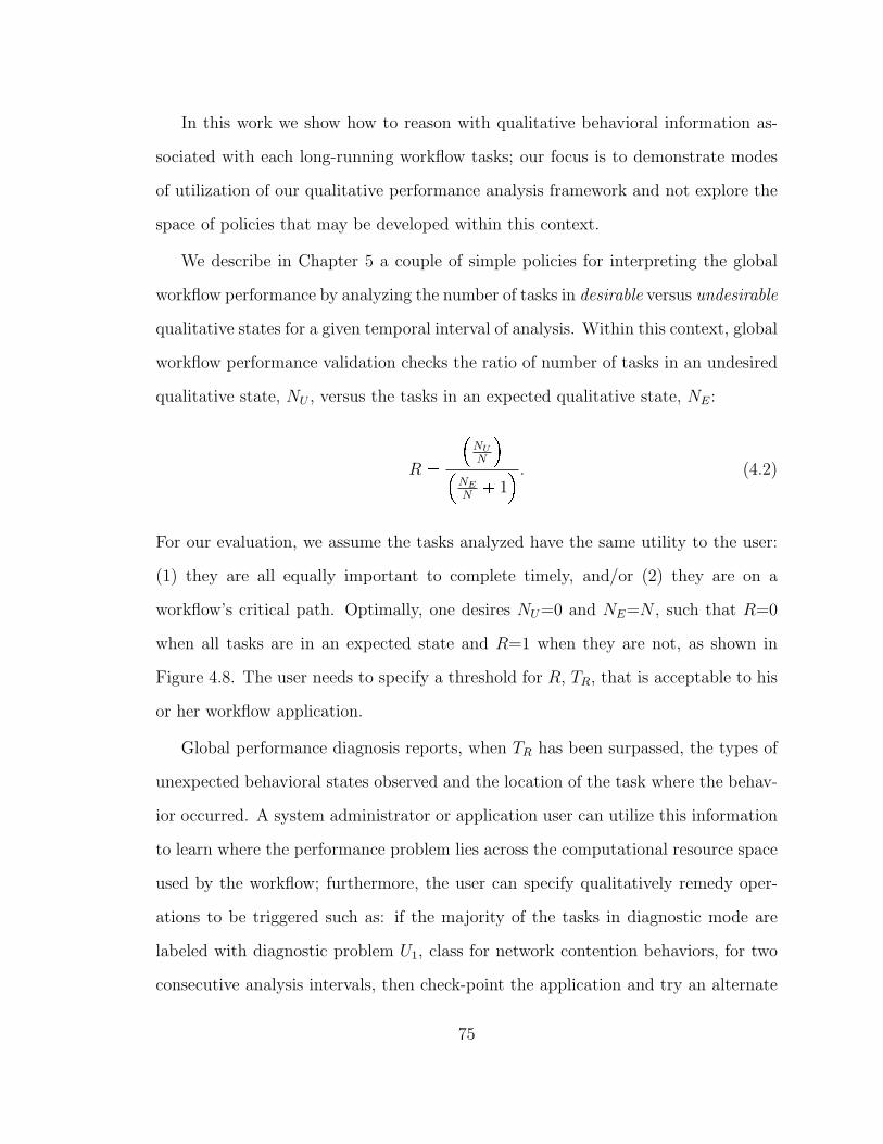
In this work we show how to reason with qualitative behavioral information as-
sociated with each long-running workflow tasks; our focus is to demonstrate modes
of utilization of our qualitative performance analysis framework and not explore the
space of policies that may be developed within this context.
We describe in Chapter 5 a couple of simple policies for interpreting the global
workflow performance by analyzing the number of tasks in desirable versus undesirable
qualitative states for a given temporal interval of analysis. Within this context, global
workflow performance validation checks the ratio of number of tasks in an undesired
qualitative state, NU , versus the tasks in an expected qualitative state, NE:
R �
�NU
N
�
NE
N� 1
. (4.2)
For our evaluation, we assume the tasks analyzed have the same utility to the user:
(1) they are all equally important to complete timely, and/or (2) they are on a
workflow’s critical path. Optimally, one desires NU=0 and NE=N , such that R=0
when all tasks are in an expected state and R=1 when they are not, as shown in
Figure 4.8. The user needs to specify a threshold for R, TR, that is acceptable to his
or her workflow application.
Global performance diagnosis reports, when TR has been surpassed, the types of
unexpected behavioral states observed and the location of the task where the behav-
ior occurred. A system administrator or application user can utilize this information
to learn where the performance problem lies across the computational resource space
used by the workflow; furthermore, the user can specify qualitatively remedy oper-
ations to be triggered such as: if the majority of the tasks in diagnostic mode are
labeled with diagnostic problem U1, class for network contention behaviors, for two
consecutive analysis intervals, then check-point the application and try an alternate
75
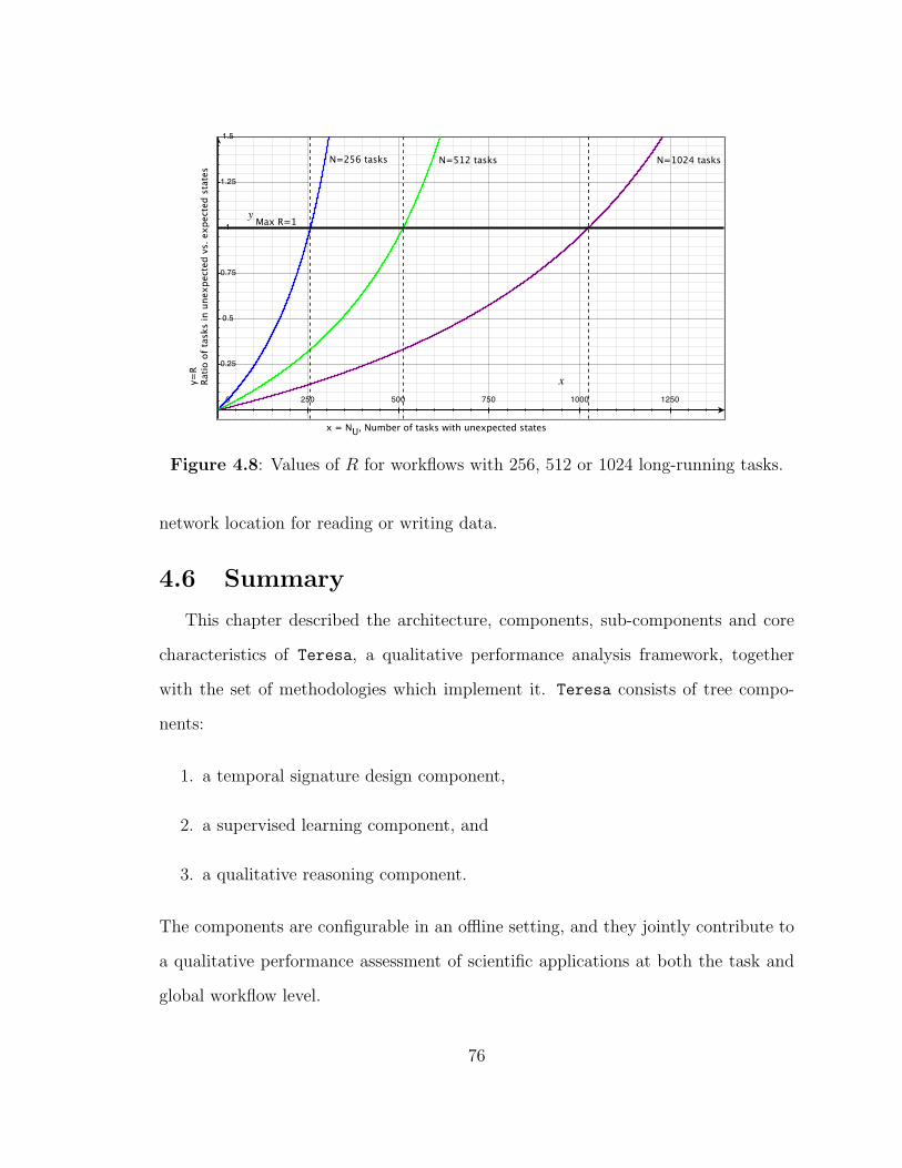
0 250 500 750 1000 1250
0.25
0.5
0.75
1
1.25
1.5
Max R=1
x = NU, Number of tasks with unexpected states
y=R
Ratio
of t
asks
in u
nexp
ecte
d vs
. exp
ecte
d st
ates
N=256 tasks N=512 tasks N=1024 tasks
Figure 4.8: Values of R for workflows with 256, 512 or 1024 long-running tasks.
network location for reading or writing data.
4.6 Summary
This chapter described the architecture, components, sub-components and core
characteristics of Teresa, a qualitative performance analysis framework, together
with the set of methodologies which implement it. Teresa consists of tree compo-
nents:
1. a temporal signature design component,
2. a supervised learning component, and
3. a qualitative reasoning component.
The components are configurable in an offline setting, and they jointly contribute to
a qualitative performance assessment of scientific applications at both the task and
global workflow level.
76
Chapter 5
Framework Evaluation
In this chapter we describe the data sets we use to evaluate our qualitative per-
formance analysis framework, Teresa, as well as the results of the evaluation. We
conduct benchmark experiments with long-running tasks from two different large-
scale scientific workflows executing on four different architectural configurations of
Grid resources.
We first describe characteristics of the computational environments from which
we gathered our data sets, the performance time series metrics collected from each
environment and characteristics of the scientific workflows studied. Next, we de-
scribe how to generate temporal signatures for our experimental data and study the
differences in temporal signatures for application executions in cases of good qualita-
tive performance versus cases of known degraded performance due to a performance
stress factor or bottleneck. We then evaluate the efficacy of our framework by of-
fering supporting evidence for our two hypotheses. For the first hypothesis we show
how signatures based on temporal information are superior to signatures based on in-
stantaneous values of the performance metrics. We show supporting evidence for the
second hypothesis by computing the balanced classification accuracy for never-seen
temporal signatures of different expectation labels (i.e., expected or unexpected),
which is an indicator of how well our framework will be able to distinguish accurately
and precisely both healthy and unhealthy application performance states. Finally, we
discuss the performance impact of our framework, limits of our current evaluation,
as well as limitations of our overall approach.
77
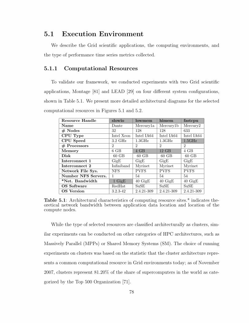
5.1 Execution Environment
We describe the Grid scientific applications, the computing environments, and
the type of performance time series metrics collected.
5.1.1 Computational Resources
To validate our framework, we conducted experiments with two Grid scientific
applications, Montage [81] and LEAD [29] on four different system configurations,
shown in Table 5.1. We present more detailed architectural diagrams for the selected
computational resources in Figures 5.1 and 5.2.
Resource Handle slowio lowmem himem fastcpuName Dante Mercury1a Mercury1b Mercury2# Nodes 32 128 128 633CPU Type Intel Xeon Intel IA64 Intel IA64 Intel IA64CPU Speed 3.2 GHz 1.3GHz 1.3GHz 1.5GHz# Processors 2 2 2 2Memory 6 GB 4 GB 12 GB 4 GBDisk 60 GB 60 GB 60 GB 60 GBInterconnect 1 GigE GigE GigE GigEInterconnect 2 Infiniband Myrinet Myrinet MyrinetNetwork File Sys. NFS PVFS PVFS PVFSNumber NFS Servers. 1 54 54 54*Net. Bandwidth 1 GigE 40 GigE 40 GigE 40 GigEOS Software RedHat SuSE SuSE SuSEOS Version 3.2.3-42 2.4.21-309 2.4.21-309 2.4.21-309
Table 5.1: Architectural characteristics of computing resource sites.* indicates the-oretical network bandwidth between application data location and location of thecompute nodes.
While the type of selected resources are classified architecturally as clusters, sim-
ilar experiments can be conducted on other categories of HPC architectures, such as
Massively Parallel (MPPs) or Shared Memory Systems (SM). The choice of running
experiments on clusters was based on the statistic that the cluster architecture repre-
sents a common computational resource in Grid environments today; as of November
2007, clusters represent 81.20% of the share of supercomputers in the world as cate-
gorized by the Top 500 Organization [71].
78
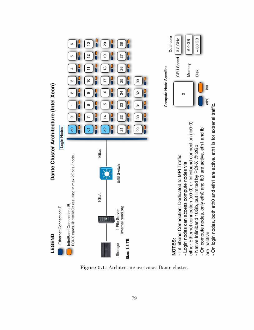
Dant
e Cl
uste
r Arc
hite
ctur
e (In
tel X
eon)
Stor
age
1 Fi
le S
erve
rin
tern
al.re
nci.o
rg
Logi
n No
des
1Gb/
s
Size
: 1.8
TB
d00
12
34
56
d17
89
1011
1213
d214
1516
1718
1920
2122
2324
2526
2728
2930
LEG
END
Ethe
rnet
Con
nect
ion:
E
Infin
iBan
d Co
nnec
tion:
IB,
PCI-X
car
ds @
133
MG
z re
sultin
g in
max
2G
bits
/ no
de.
NOTE
S:- I
nfini
band
Con
nect
ion:
Ded
icate
d to
MPI
Tra
ffic
- Log
in n
odes
can
acc
ess
com
pute
nod
es v
iaei
ther
Eth
erne
t con
nect
ion
(c0-
0) o
r Infi
niba
nd c
onne
ctio
n (ib
0-0)
- Nat
ive In
finib
and
10G
b, b
ut lim
ited
by P
CI-X
@ 2
Gb
- On
com
pute
nod
es, o
nly
eth0
and
ib0
are
activ
e. e
th1
and
ib1
are
inac
tive.
- On
logi
n no
des,
bot
h et
h0 a
nd e
th1
are
activ
e. e
th1
is fo
r ext
rena
l tra
ffic.
0
Com
pute
Nod
e Sp
ecific
s
3.2
GHz
CPU
Spee
d
Dual
-cor
e
Mem
ory
6.0
GB
Disk
~ 60
GB
E/IB
Swi
tch
3132
33
eth0
ib0
1Gb/
s
Figure 5.1: Architecture overview: Dante cluster.
79
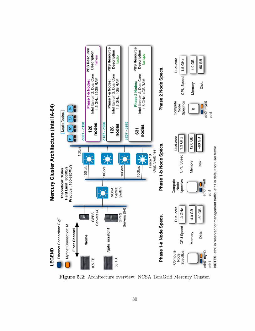
Mer
cury
Clu
ster
Arc
hite
ctur
e (In
tel I
A-64
)
8.5
TB
t1t2
t3
LEG
END
Ethe
rnet
Con
nect
ion:
Gig
E
Myr
inet
Con
nect
ion:
MLo
gin
Node
s
1Gb/
s
t4Fi
ber C
hann
el
Theo
retic
al: 1
Gb/
sHa
rd L
imit:
800
Mb/
sPr
actic
al: 1
60-3
20M
b/s
Com
pute
No
de
Spec
ifics
1.3
GHz
CPU
Spee
dDu
al-c
ore
Mem
ory
12.0
GB
Disk
: ~6
0 G
Bet
h0m
yri0
0
Com
pute
No
de
Spec
ifics
1.5
GHz
CPU
Spee
d
Mem
ory
4.0
GB
Disk
: ~6
0 G
Bet
h0m
yri0
Phas
e 1-
a No
des:
In
tel I
tani
um 2
, Dua
l Cor
e1.
3 G
Hz, 4
GB
RAM
Phas
e 1-
b No
des:
In
tel I
tani
um 2
, Dua
l Cor
e1.
3 G
Hz, 1
2GB
RAM
Phas
e 2
Node
s:
Inte
l Ita
nium
2, D
ual C
ore
1.5
GHz
, 4G
B RA
M
128
node
s
128
node
s
631
node
s
Com
pute
No
de
Spec
ifics
1.3
GHz
CPU
Spee
d
Mem
ory
4.0
GB
Disk
: ~6
0 G
Bet
h0m
yri0
Phas
e 1-
a No
de S
pecs
.
eth1
eth1Ph
ase
1-b
Node
Spe
cs.
Phas
e 2
Node
Spe
cs.
eth
1
PBS
Reso
urce
De
scrip
tion
fast
cpu
PBS
Reso
urce
De
scrip
tion
him
emG
PFS
Serv
ers
(4)
GPF
SSe
rver
s (5
4)
PBS
Reso
urce
De
scrip
tion
fast
io
c001
- c1
28
c187
- c2
56
c257
- c9
26
58 T
B
/hom
e
/gpf
s_sc
ratc
h1
NOTE
S: e
th0
is re
serv
ed fo
r man
agem
ent t
raffi
c, e
th1
is de
faul
t for
use
r tra
ffic.
Forc
e 10
G
igE
Switc
hes
NCSA
Ce
ntra
l Sw
itch
10G
b/s
10G
b/s
10G
b/s
10G
b/s
Dual
-cor
eDu
al-c
ore
Figure 5.2: Architecture overview: NCSA TeraGrid Mercury Cluster.
80
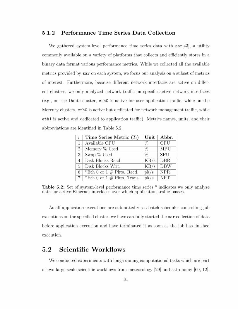
5.1.2 Performance Time Series Data Collection
We gathered system-level performance time series data with sar[43], a utility
commonly available on a variety of platforms that collects and efficiently stores in a
binary data format various performance metrics. While we collected all the available
metrics provided by sar on each system, we focus our analysis on a subset of metrics
of interest. Furthermore, because different network interfaces are active on differ-
ent clusters, we only analyzed network traffic on specific active network interfaces
(e.g., on the Dante cluster, eth0 is active for user application traffic, while on the
Mercury clusters, eth0 is active but dedicated for network management traffic, while
eth1 is active and dedicated to application traffic). Metrics names, units, and their
abbreviations are identified in Table 5.2.
i Time Series Metric (Ti) Unit Abbr.1 Available CPU % CPU2 Memory % Used % MPU3 Swap % Used % SPU4 Disk Blocks Read KB/s DBR5 Disk Blocks Writ. KB/s DBW6 *Eth 0 or 1 # Pkts. Recd. pk/s NPR7 *Eth 0 or 1 # Pkts. Trans. pk/s NPT
Table 5.2: Set of system-level performance time series.* indicates we only analyzedata for active Ethernet interfaces over which application traffic passes.
As all application executions are submitted via a batch scheduler controlling job
executions on the specified cluster, we have carefully started the sar collection of data
before application execution and have terminated it as soon as the job has finished
execution.
5.2 Scientific Workflows
We conducted experiments with long-running computational tasks which are part
of two large-scale scientific workflows from meteorology [29] and astronomy [60, 12].
81
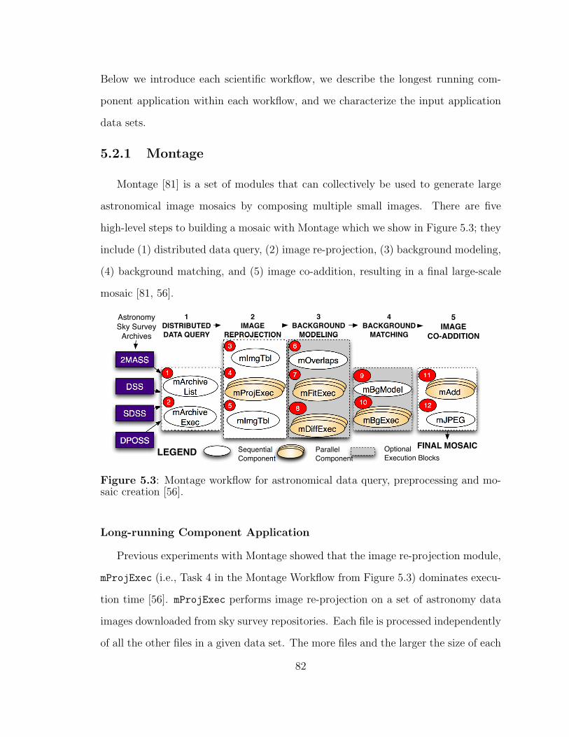
Below we introduce each scientific workflow, we describe the longest running com-
ponent application within each workflow, and we characterize the input application
data sets.
5.2.1 Montage
Montage [81] is a set of modules that can collectively be used to generate large
astronomical image mosaics by composing multiple small images. There are five
high-level steps to building a mosaic with Montage which we show in Figure 5.3; they
include (1) distributed data query, (2) image re-projection, (3) background modeling,
(4) background matching, and (5) image co-addition, resulting in a final large-scale
mosaic [81, 56].
DPOSS
SDSS
2MASS
DSS
AstronomySky Survey
Archives
mArchive List
mArchiveExec
1
2
1DISTRIBUTEDDATA QUERY
FINAL MOSAIC
5IMAGE
CO-ADDITION
11
mJPEG12
mAddmAddmAdd
4BACKGROUND
MATCHING
mBgModel9
10
mAddmAddmBgExec
3BACKGROUND
MODELING
mOverlaps6
7
8
mAddmAddmFitExec
mAddmAddmDiffExec
mImgTbl3
4
mImgTbl
5
2IMAGE
REPROJECTION
mAddmAddmProjExec
SequentialComponent
ParallelComponent
OptionalExecution BlocksLEGEND
Figure 5.3: Montage workflow for astronomical data query, preprocessing and mo-saic creation [56].
Long-running Component Application
Previous experiments with Montage showed that the image re-projection module,
mProjExec (i.e., Task 4 in the Montage Workflow from Figure 5.3) dominates execu-
tion time [56]. mProjExec performs image re-projection on a set of astronomy data
images downloaded from sky survey repositories. Each file is processed independently
of all the other files in a given data set. The more files and the larger the size of each
82
file in the data set, the longer the time it takes for mProjExec to finish the required
processing. We conduct experiments with this module on two different data sets,
described in the following section.
Astronomy Data Sets
One data set, which we label M101, represents 7902 image files from a 15 0 area
of the sky around the spiral galaxy, M101 in the U band obtained from the SDSS
data archive. Each file has an approximate size of 5.8 MB, resulting in a total size
of 45 GB for all the files in the data set. The application, mProjExec reads all these
files and generates re-projections of these images, generating as output a data set
of approximately 99 GB. The second data set, which we label M57, represents 7422
image files from a 15 0 area of the sky around the ring nebula, M57, in the J band
obtained from the 2MASS data archive. Each file in the second data set has an
approximate size of 2.0 MB, resulting in a total size of 15 GB for all the files in
the data set. Similarly, mProjExec reads all these files and generates re-projections
of these images, generating as output a data set of approximately 30 GB. All the
experiments with data set M101 are listed in Table 5.3, while all experiments with
data set M57 are listed in Table 5.4.
5.2.2 LEAD
Mesoscale weather causes hundreds of deaths, routinely disrupts transportation
and commerce and results in significant economic losses [91]. Mitigating the impact of
such events implies significantly changing the traditional weather sensing and predic-
tion paradigm, where forecasts are static, linear workflows with no adaptive response
to weather. The Linked Environments for Atmospheric Discovery (LEAD) project
[29] addresses the fundamental technological challenges of real-time, on-demand,
dynamically-adaptive needs of mesoscale weather research. Figure 5.4 shows an exam-
83
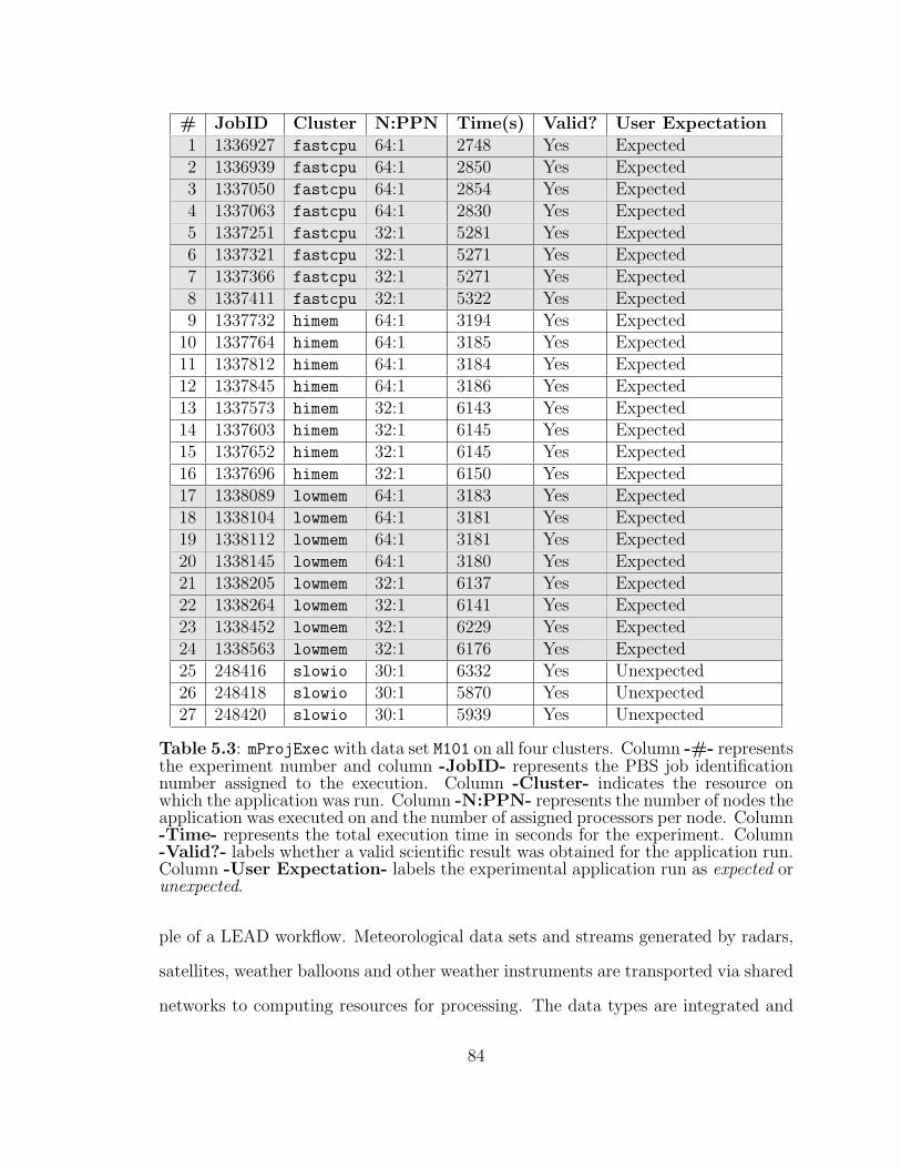
# JobID Cluster N:PPN Time(s) Valid? User Expectation1 1336927 fastcpu 64:1 2748 Yes Expected2 1336939 fastcpu 64:1 2850 Yes Expected3 1337050 fastcpu 64:1 2854 Yes Expected4 1337063 fastcpu 64:1 2830 Yes Expected5 1337251 fastcpu 32:1 5281 Yes Expected6 1337321 fastcpu 32:1 5271 Yes Expected7 1337366 fastcpu 32:1 5271 Yes Expected8 1337411 fastcpu 32:1 5322 Yes Expected9 1337732 himem 64:1 3194 Yes Expected
10 1337764 himem 64:1 3185 Yes Expected11 1337812 himem 64:1 3184 Yes Expected12 1337845 himem 64:1 3186 Yes Expected13 1337573 himem 32:1 6143 Yes Expected14 1337603 himem 32:1 6145 Yes Expected15 1337652 himem 32:1 6145 Yes Expected16 1337696 himem 32:1 6150 Yes Expected17 1338089 lowmem 64:1 3183 Yes Expected18 1338104 lowmem 64:1 3181 Yes Expected19 1338112 lowmem 64:1 3181 Yes Expected20 1338145 lowmem 64:1 3180 Yes Expected21 1338205 lowmem 32:1 6137 Yes Expected22 1338264 lowmem 32:1 6141 Yes Expected23 1338452 lowmem 32:1 6229 Yes Expected24 1338563 lowmem 32:1 6176 Yes Expected25 248416 slowio 30:1 6332 Yes Unexpected26 248418 slowio 30:1 5870 Yes Unexpected27 248420 slowio 30:1 5939 Yes Unexpected
Table 5.3: mProjExec with data set M101 on all four clusters. Column -#- representsthe experiment number and column -JobID- represents the PBS job identificationnumber assigned to the execution. Column -Cluster- indicates the resource onwhich the application was run. Column -N:PPN- represents the number of nodes theapplication was executed on and the number of assigned processors per node. Column-Time- represents the total execution time in seconds for the experiment. Column-Valid?- labels whether a valid scientific result was obtained for the application run.Column -User Expectation- labels the experimental application run as expected orunexpected.
ple of a LEAD workflow. Meteorological data sets and streams generated by radars,
satellites, weather balloons and other weather instruments are transported via shared
networks to computing resources for processing. The data types are integrated and
84
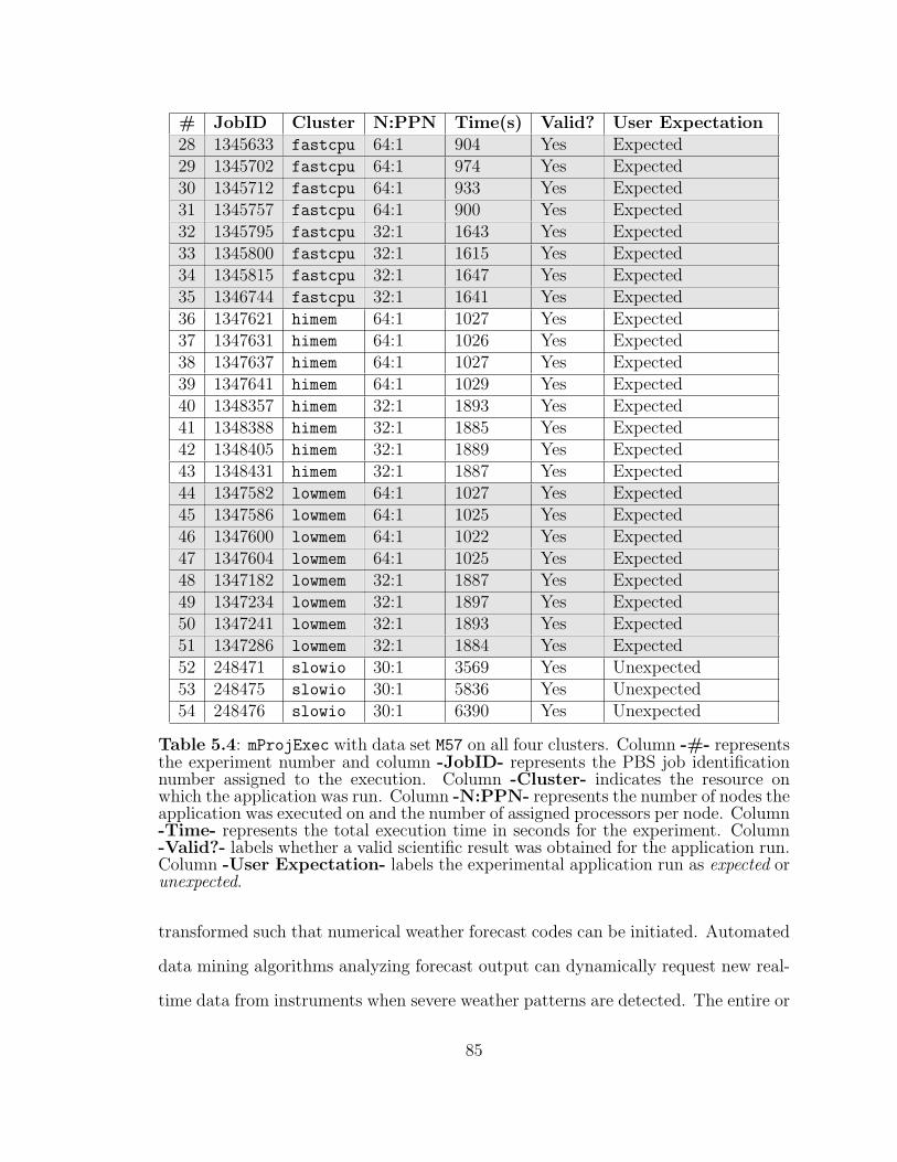
# JobID Cluster N:PPN Time(s) Valid? User Expectation28 1345633 fastcpu 64:1 904 Yes Expected29 1345702 fastcpu 64:1 974 Yes Expected30 1345712 fastcpu 64:1 933 Yes Expected31 1345757 fastcpu 64:1 900 Yes Expected32 1345795 fastcpu 32:1 1643 Yes Expected33 1345800 fastcpu 32:1 1615 Yes Expected34 1345815 fastcpu 32:1 1647 Yes Expected35 1346744 fastcpu 32:1 1641 Yes Expected36 1347621 himem 64:1 1027 Yes Expected37 1347631 himem 64:1 1026 Yes Expected38 1347637 himem 64:1 1027 Yes Expected39 1347641 himem 64:1 1029 Yes Expected40 1348357 himem 32:1 1893 Yes Expected41 1348388 himem 32:1 1885 Yes Expected42 1348405 himem 32:1 1889 Yes Expected43 1348431 himem 32:1 1887 Yes Expected44 1347582 lowmem 64:1 1027 Yes Expected45 1347586 lowmem 64:1 1025 Yes Expected46 1347600 lowmem 64:1 1022 Yes Expected47 1347604 lowmem 64:1 1025 Yes Expected48 1347182 lowmem 32:1 1887 Yes Expected49 1347234 lowmem 32:1 1897 Yes Expected50 1347241 lowmem 32:1 1893 Yes Expected51 1347286 lowmem 32:1 1884 Yes Expected52 248471 slowio 30:1 3569 Yes Unexpected53 248475 slowio 30:1 5836 Yes Unexpected54 248476 slowio 30:1 6390 Yes Unexpected
Table 5.4: mProjExec with data set M57 on all four clusters. Column -#- representsthe experiment number and column -JobID- represents the PBS job identificationnumber assigned to the execution. Column -Cluster- indicates the resource onwhich the application was run. Column -N:PPN- represents the number of nodes theapplication was executed on and the number of assigned processors per node. Column-Time- represents the total execution time in seconds for the experiment. Column-Valid?- labels whether a valid scientific result was obtained for the application run.Column -User Expectation- labels the experimental application run as expected orunexpected.
transformed such that numerical weather forecast codes can be initiated. Automated
data mining algorithms analyzing forecast output can dynamically request new real-
time data from instruments when severe weather patterns are detected. The entire or
85
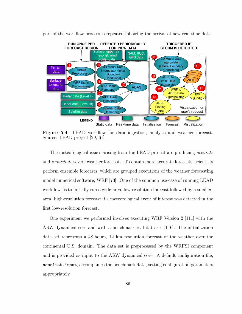
part of the workflow process is repeated following the arrival of new real-time data.
Terrain data
Surface, terrestrial
data
Radar data (Level II)
Radar data (Level III)
Satellite data
NAM, RUC, GFS data
Surface, upper air mesonet, wind
profiler data
TerrainPreprocessor
1
WRF StaticPreprocessor
2
3
88D RadarRemapper
4
NIDS RadarRemapper
5
Satellite DataRemapper
6
ADAS7
3D Model Data Interpolator
(Lateral Boundary Conditions)
8
ARPS to WRF Data Interpolator
9
IDV Bundle
11
ARPSPlottingProgram
13
WRF to ARPS DataInterpolator
12
10
WRF
LEGENDReal-time dataStatic data Initialization Forecast Visualization
RUN ONCE PERFORECAST REGION
TRIGGERED IFSTORM IS DETECTED
REPEATED PERIODICALLY FOR NEW DATA
Visualization on user's request
3D Model Data Interpolator (Initial
Boundary Conditions)
Figure 5.4: LEAD workflow for data ingestion, analysis and weather forecast.Source: LEAD project [29, 61].
The meteorological issues arising from the LEAD project are producing accurate
and immediate severe weather forecasts. To obtain more accurate forecasts, scientists
perform ensemble forecasts, which are grouped executions of the weather forecasting
model numerical software, WRF [73]. One of the common use-case of running LEAD
workflows is to initially run a wide-area, low-resolution forecast followed by a smaller-
area, high-resolution forecast if a meteorological event of interest was detected in the
first low-resolution forecast.
One experiment we performed involves executing WRF Version 2 [111] with the
ARW dynamical core and with a benchmark real data set [116]. The initialization
data set represents a 48-hours, 12 km resolution forecast of the weather over the
continental U.S. domain. The data set is preprocessed by the WRFSI component
and is provided as input to the ARW dynamical core. A default configuration file,
namelist.input, accompanies the benchmark data, setting configuration parameters
appropriately.
86
While this particular data set may run to completion on a couple of tens of com-
puting nodes within a reasonable amount of time (i.e., 5396 seconds on 32 machines
with an Intel Xeon 3.2 GHz, 6 GB RAM and Infiniband interconnect), hundreds of
these data sets forming large ensembles will require a significant amount of resources
to finish in time for the actual weather prediction to be useful. Larger Grids will
provide the necessary computing power to process computationally intensive forecast
ensembles processing streamed, distributed data sources.
Long-running Application Component
Within such LEAD workflows, the longest-running component is the numerical
code, Weather Research and Forecasting (WRF) [73] (i.e., Task 10 in the LEAD
Workflow from Figure 5.4). Therefore, we conduct experiments with WRF on two
different data sets representing weather with different characteristics.
Weather Data Sets
One data set, which we label mesoscale, represents a 48-hour forecast during
mesoscale weather from 24th October 2001, over a low-resolution of 12 km within the
entire continental United States. The input files have an approximate size of 0.34 GB
and the output data is 0.64 GB. The second data set, which we label non-mesoscale,
represents a 24-hours forecast during non-mesoscale (i.e., good) weather from Novem-
ber 6th, 2007 over a high-resolution of 4 km in a grid of 1000 km2 within the conti-
nental United States. The input files have an approximate size of 0.25 GB and the
output data is 2.9 GB. All experiments with the mesoscale data set are listed in
Table 5.5, and all experiments with the non-mesoscale data set are listed in Table
5.6.
87
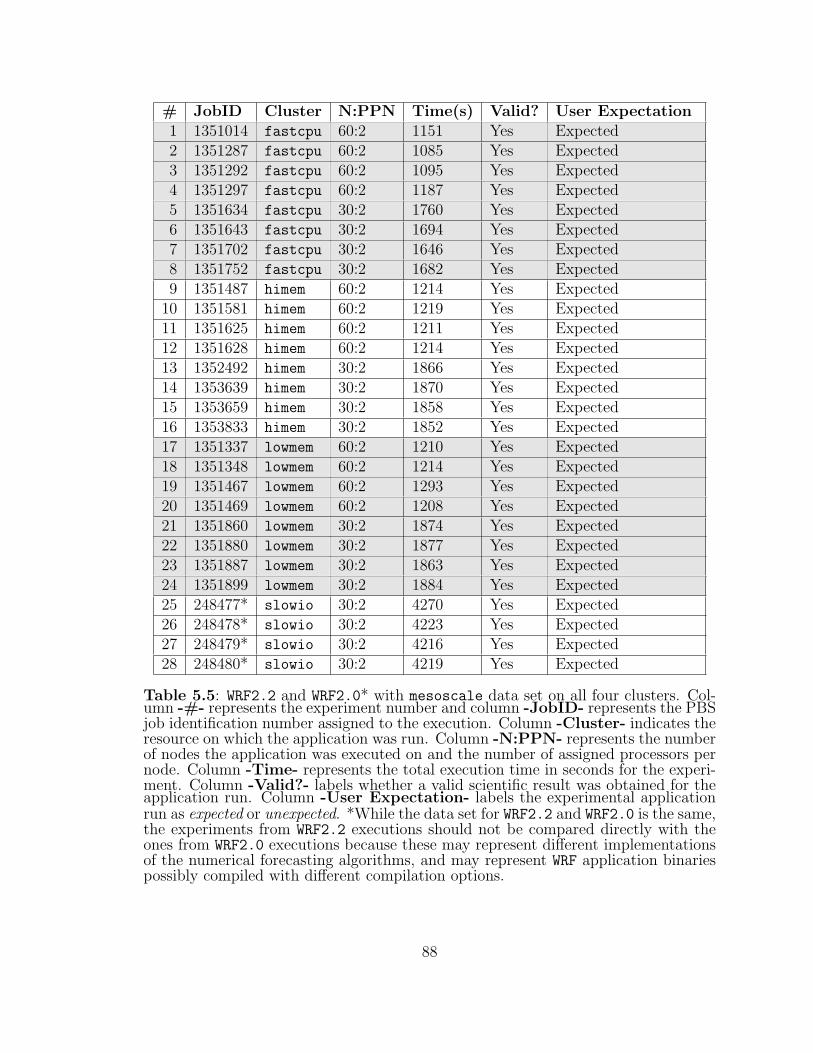
# JobID Cluster N:PPN Time(s) Valid? User Expectation1 1351014 fastcpu 60:2 1151 Yes Expected2 1351287 fastcpu 60:2 1085 Yes Expected3 1351292 fastcpu 60:2 1095 Yes Expected4 1351297 fastcpu 60:2 1187 Yes Expected5 1351634 fastcpu 30:2 1760 Yes Expected6 1351643 fastcpu 30:2 1694 Yes Expected7 1351702 fastcpu 30:2 1646 Yes Expected8 1351752 fastcpu 30:2 1682 Yes Expected9 1351487 himem 60:2 1214 Yes Expected
10 1351581 himem 60:2 1219 Yes Expected11 1351625 himem 60:2 1211 Yes Expected12 1351628 himem 60:2 1214 Yes Expected13 1352492 himem 30:2 1866 Yes Expected14 1353639 himem 30:2 1870 Yes Expected15 1353659 himem 30:2 1858 Yes Expected16 1353833 himem 30:2 1852 Yes Expected17 1351337 lowmem 60:2 1210 Yes Expected18 1351348 lowmem 60:2 1214 Yes Expected19 1351467 lowmem 60:2 1293 Yes Expected20 1351469 lowmem 60:2 1208 Yes Expected21 1351860 lowmem 30:2 1874 Yes Expected22 1351880 lowmem 30:2 1877 Yes Expected23 1351887 lowmem 30:2 1863 Yes Expected24 1351899 lowmem 30:2 1884 Yes Expected25 248477* slowio 30:2 4270 Yes Expected26 248478* slowio 30:2 4223 Yes Expected27 248479* slowio 30:2 4216 Yes Expected28 248480* slowio 30:2 4219 Yes Expected
Table 5.5: WRF2.2 and WRF2.0* with mesoscale data set on all four clusters. Col-umn -#- represents the experiment number and column -JobID- represents the PBSjob identification number assigned to the execution. Column -Cluster- indicates theresource on which the application was run. Column -N:PPN- represents the numberof nodes the application was executed on and the number of assigned processors pernode. Column -Time- represents the total execution time in seconds for the experi-ment. Column -Valid?- labels whether a valid scientific result was obtained for theapplication run. Column -User Expectation- labels the experimental applicationrun as expected or unexpected. *While the data set for WRF2.2 and WRF2.0 is the same,the experiments from WRF2.2 executions should not be compared directly with theones from WRF2.0 executions because these may represent different implementationsof the numerical forecasting algorithms, and may represent WRF application binariespossibly compiled with different compilation options.
88
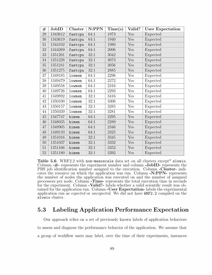
# JobID Cluster N:PPN Time(s) Valid? User Expectation29 1343612 fastcpu 64:1 1973 Yes Expected30 1343619 fastcpu 64:1 1940 Yes Expected31 1344102 fastcpu 64:1 1980 Yes Expected32 1344269 fastcpu 64:1 2006 Yes Expected33 1351201 fastcpu 32:1 3042 Yes Expected34 1351228 fastcpu 32:1 3073 Yes Expected35 1351241 fastcpu 32:1 3056 Yes Expected36 1351275 fastcpu 32:1 2885 Yes Expected37 1349185 lowmem 64:1 2296 Yes Expected38 1349479 lowmem 64:1 2272 Yes Expected39 1349558 lowmem 64:1 2316 Yes Expected40 1349726 lowmem 64:1 2293 Yes Expected41 1349892 lowmem 32:1 3416 Yes Expected42 1350100 lowmem 32:1 3306 Yes Expected43 1350157 lowmem 32:1 3285 Yes Expected44 1350339 lowmem 32:1 3281 Yes Expected45 1347747 himem 64:1 2295 Yes Expected46 1348035 himem 64:1 2289 Yes Expected47 1348905 himem 64:1 2346 Yes Expected48 1349133 himem 64:1 2325 Yes Expected49 1351016 himem 32:1 3345 Yes Expected50 1351037 himem 32:1 3332 Yes Expected51 1351166 himem 32:1 3352 Yes Expected52 1351180 himem 32:1 3392 Yes Expected
Table 5.6: WRF2.2 with non-mesoscale data set on all clusters except* slowio.Column -#- represents the experiment number and column -JobID- represents thePBS job identification number assigned to the execution. Column -Cluster- indi-cates the resource on which the application was run. Column -N:PPN- representsthe number of nodes the application was executed on and the number of assignedprocessors per node. Column -Time- represents the total execution time in secondsfor the experiment. Column -Valid?- labels whether a valid scientific result was ob-tained for the application run. Column -User Expectation- labels the experimentalapplication run as expected or unexpected. We did not have WRF2.2 compiled on theslowio cluster.
5.3 Labeling Application Performance Expectation
Our approach relies on a set of previously known labels of application behaviors
to assess and diagnose the performance behavior of the application. We assume that
a group of workflow users may label, over the time of their experiments, instances
89
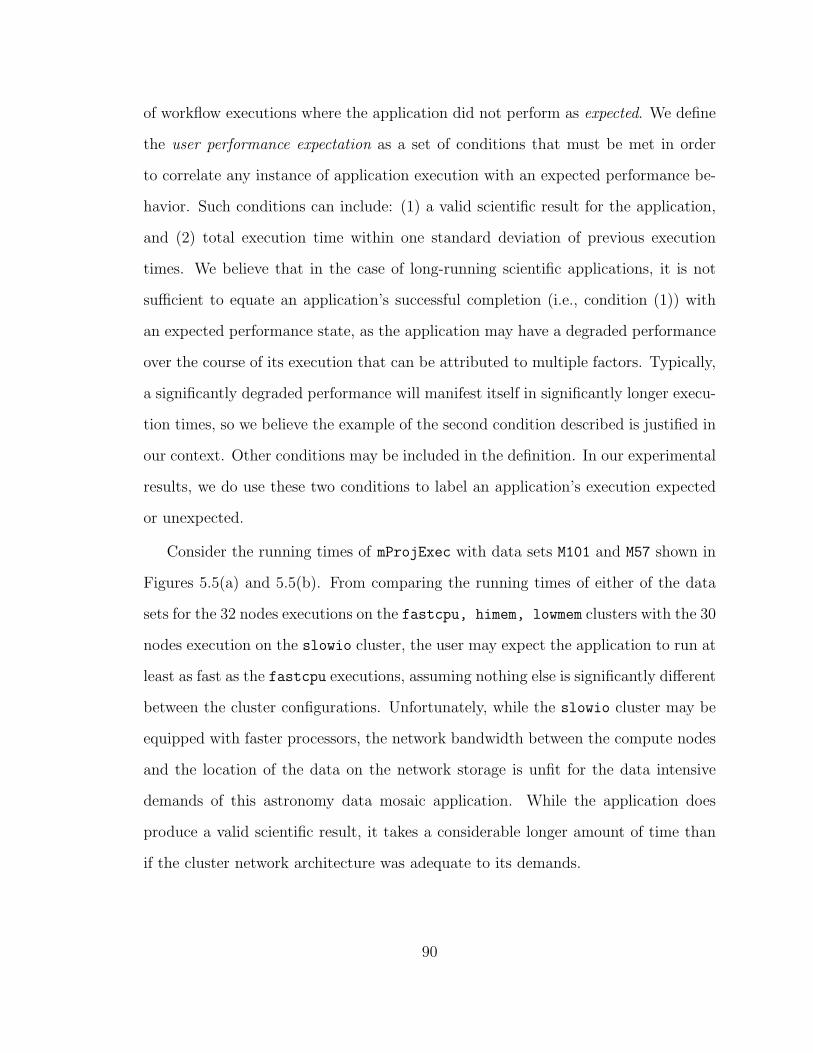
of workflow executions where the application did not perform as expected. We define
the user performance expectation as a set of conditions that must be met in order
to correlate any instance of application execution with an expected performance be-
havior. Such conditions can include: (1) a valid scientific result for the application,
and (2) total execution time within one standard deviation of previous execution
times. We believe that in the case of long-running scientific applications, it is not
sufficient to equate an application’s successful completion (i.e., condition (1)) with
an expected performance state, as the application may have a degraded performance
over the course of its execution that can be attributed to multiple factors. Typically,
a significantly degraded performance will manifest itself in significantly longer execu-
tion times, so we believe the example of the second condition described is justified in
our context. Other conditions may be included in the definition. In our experimental
results, we do use these two conditions to label an application’s execution expected
or unexpected.
Consider the running times of mProjExec with data sets M101 and M57 shown in
Figures 5.5(a) and 5.5(b). From comparing the running times of either of the data
sets for the 32 nodes executions on the fastcpu, himem, lowmem clusters with the 30
nodes execution on the slowio cluster, the user may expect the application to run at
least as fast as the fastcpu executions, assuming nothing else is significantly different
between the cluster configurations. Unfortunately, while the slowio cluster may be
equipped with faster processors, the network bandwidth between the compute nodes
and the location of the data on the network storage is unfit for the data intensive
demands of this astronomy data mosaic application. While the application does
produce a valid scientific result, it takes a considerable longer amount of time than
if the cluster network architecture was adequate to its demands.
90
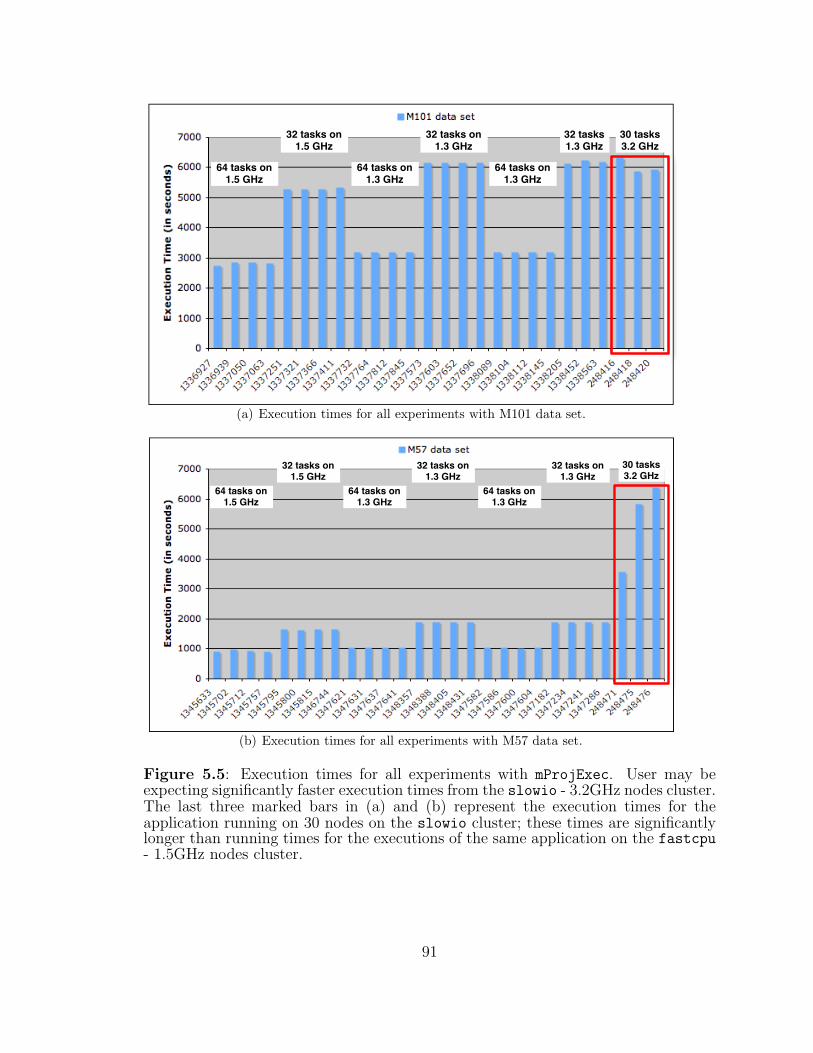
64 tasks on1.5 GHz
64 tasks on1.3 GHz
64 tasks on1.3 GHz
32 tasks on1.5 GHz
32 tasks on1.3 GHz
32 tasks1.3 GHz
30 tasks3.2 GHz
(a) Execution times for all experiments with M101 data set.
64 tasks on1.5 GHz
64 tasks on1.3 GHz
64 tasks on1.3 GHz
32 tasks on1.5 GHz
32 tasks on1.3 GHz
30 tasks3.2 GHz
32 tasks on1.3 GHz
(b) Execution times for all experiments with M57 data set.
Figure 5.5: Execution times for all experiments with mProjExec. User may beexpecting significantly faster execution times from the slowio - 3.2GHz nodes cluster.The last three marked bars in (a) and (b) represent the execution times for theapplication running on 30 nodes on the slowio cluster; these times are significantlylonger than running times for the executions of the same application on the fastcpu- 1.5GHz nodes cluster.
91
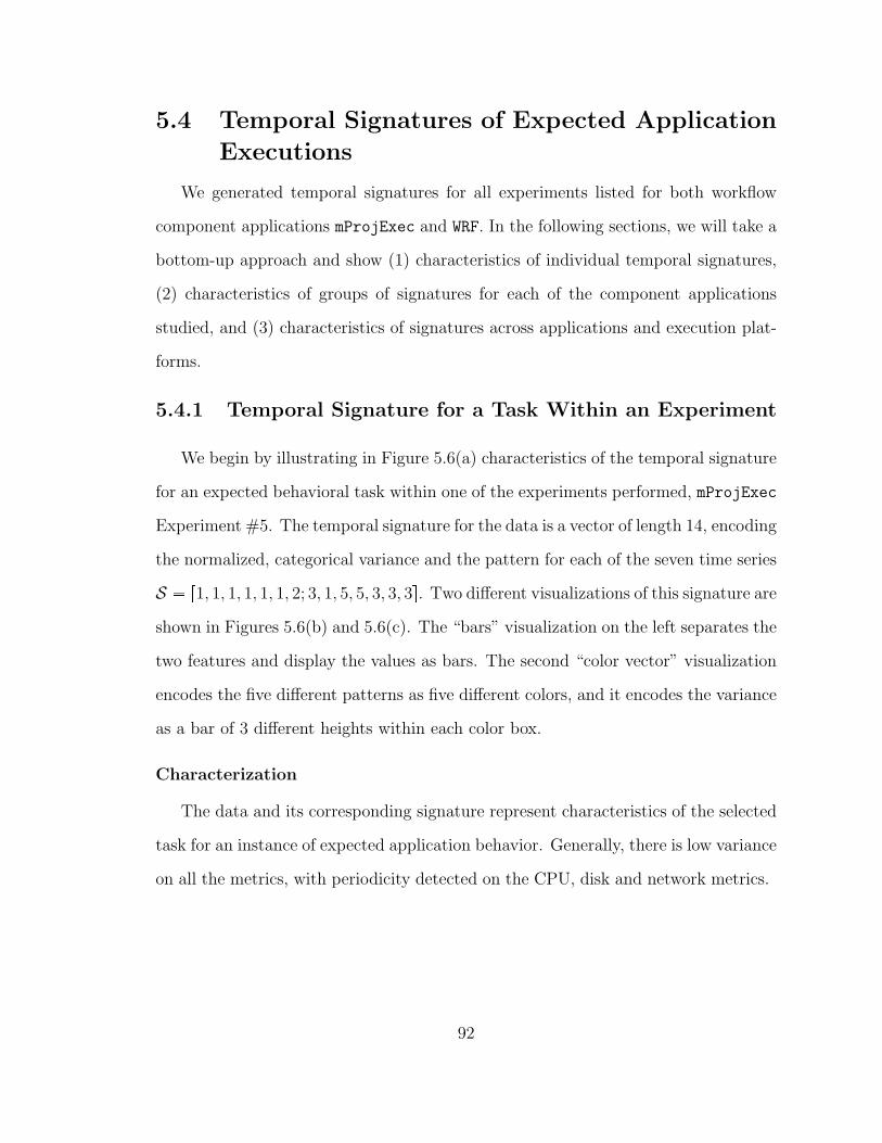
5.4 Temporal Signatures of Expected Application
Executions
We generated temporal signatures for all experiments listed for both workflow
component applications mProjExec and WRF. In the following sections, we will take a
bottom-up approach and show (1) characteristics of individual temporal signatures,
(2) characteristics of groups of signatures for each of the component applications
studied, and (3) characteristics of signatures across applications and execution plat-
forms.
5.4.1 Temporal Signature for a Task Within an Experiment
We begin by illustrating in Figure 5.6(a) characteristics of the temporal signature
for an expected behavioral task within one of the experiments performed, mProjExec
Experiment #5. The temporal signature for the data is a vector of length 14, encoding
the normalized, categorical variance and the pattern for each of the seven time series
S � r1, 1, 1, 1, 1, 1, 2; 3, 1, 5, 5, 3, 3, 3s. Two different visualizations of this signature are
shown in Figures 5.6(b) and 5.6(c). The “bars” visualization on the left separates the
two features and display the values as bars. The second “color vector” visualization
encodes the five different patterns as five different colors, and it encodes the variance
as a bar of 3 different heights within each color box.
Characterization
The data and its corresponding signature represent characteristics of the selected
task for an instance of expected application behavior. Generally, there is low variance
on all the metrics, with periodicity detected on the CPU, disk and network metrics.
92
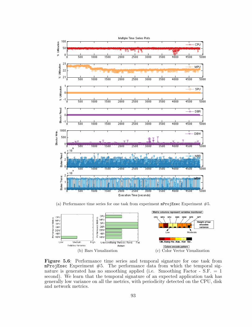
(a) Performance time series for one task from experiment mProjExec Experiment #5.
(b) Bars Visualization
Height of barencodes variance
Moderate
Colors encode pattern
Low
CPU MPU SPU DBR DBW NPR NPT
Matrix columns represent variables monitored
(c) Color Vector Visualization
Figure 5.6: Performance time series and temporal signature for one task frommProjExec Experiment #5. The performance data from which the temporal sig-nature is generated has no smoothing applied (i.e. Smoothing Factor - S.F. = 1second). We learn that the temporal signature of an expected application task hasgenerally low variance on all the metrics, with periodicity detected on the CPU, diskand network metrics.
93
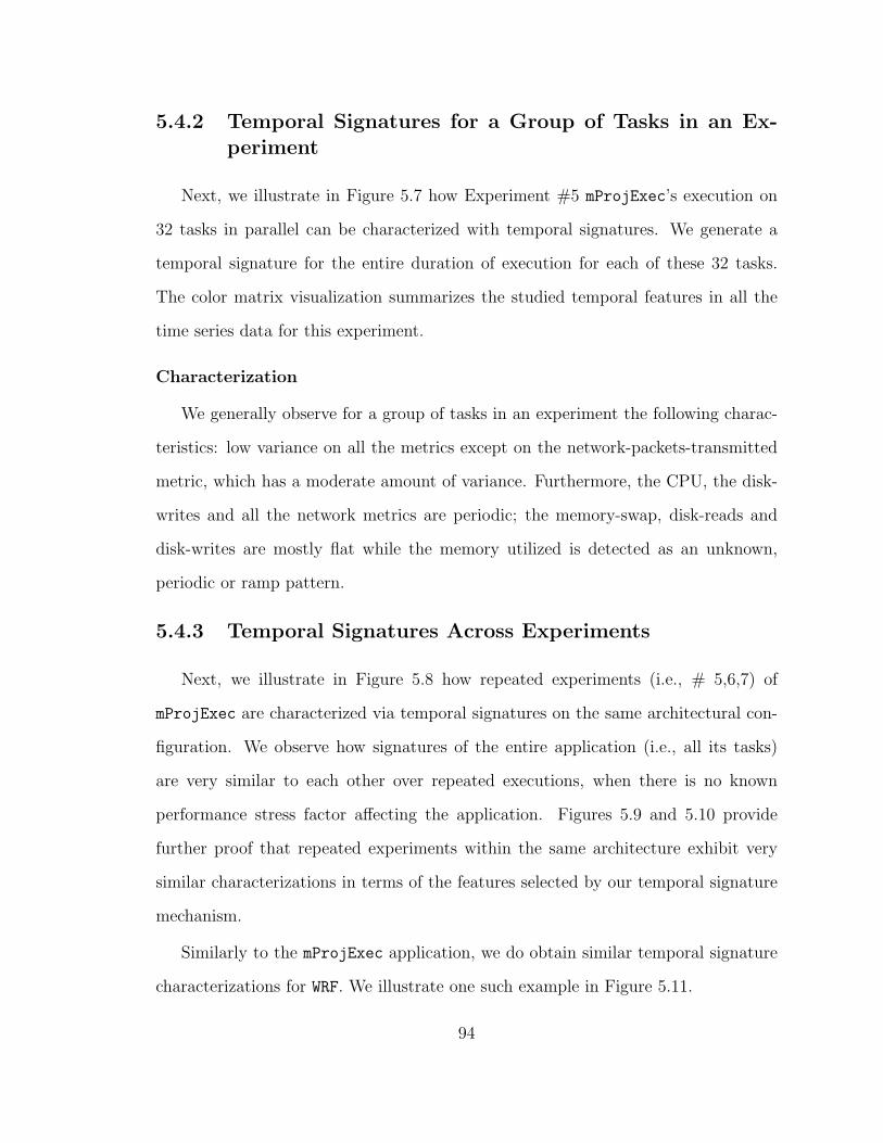
5.4.2 Temporal Signatures for a Group of Tasks in an Ex-periment
Next, we illustrate in Figure 5.7 how Experiment #5 mProjExec’s execution on
32 tasks in parallel can be characterized with temporal signatures. We generate a
temporal signature for the entire duration of execution for each of these 32 tasks.
The color matrix visualization summarizes the studied temporal features in all the
time series data for this experiment.
Characterization
We generally observe for a group of tasks in an experiment the following charac-
teristics: low variance on all the metrics except on the network-packets-transmitted
metric, which has a moderate amount of variance. Furthermore, the CPU, the disk-
writes and all the network metrics are periodic; the memory-swap, disk-reads and
disk-writes are mostly flat while the memory utilized is detected as an unknown,
periodic or ramp pattern.
5.4.3 Temporal Signatures Across Experiments
Next, we illustrate in Figure 5.8 how repeated experiments (i.e., # 5,6,7) of
mProjExec are characterized via temporal signatures on the same architectural con-
figuration. We observe how signatures of the entire application (i.e., all its tasks)
are very similar to each other over repeated executions, when there is no known
performance stress factor affecting the application. Figures 5.9 and 5.10 provide
further proof that repeated experiments within the same architecture exhibit very
similar characterizations in terms of the features selected by our temporal signature
mechanism.
Similarly to the mProjExec application, we do obtain similar temporal signature
characterizations for WRF. We illustrate one such example in Figure 5.11.
94
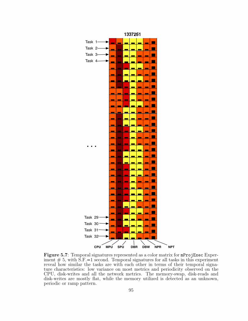
CPU MPU SPU DBR DBW NPR NPT
Task 1Task 2Task 3Task 4
Task 29Task 30Task 31Task 32
. . .
Figure 5.7: Temporal signatures represented as a color matrix for mProjExec Exper-iment # 5, with S.F.�1 second. Temporal signatures for all tasks in this experimentreveal how similar the tasks are with each other in terms of their temporal signa-ture characteristics: low variance on most metrics and periodicity observed on theCPU, disk-writes and all the network metrics. The memory-swap, disk-reads anddisk-writes are mostly flat, while the memory utilized is detected as an unknown,periodic or ramp pattern.
95
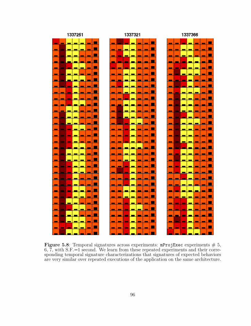
Figure 5.8: Temporal signatures across experiments: mProjExec experiments # 5,6, 7, with S.F.�1 second. We learn from these repeated experiments and their corre-sponding temporal signature characterizations that signatures of expected behaviorsare very similar over repeated executions of the application on the same architecture.
96
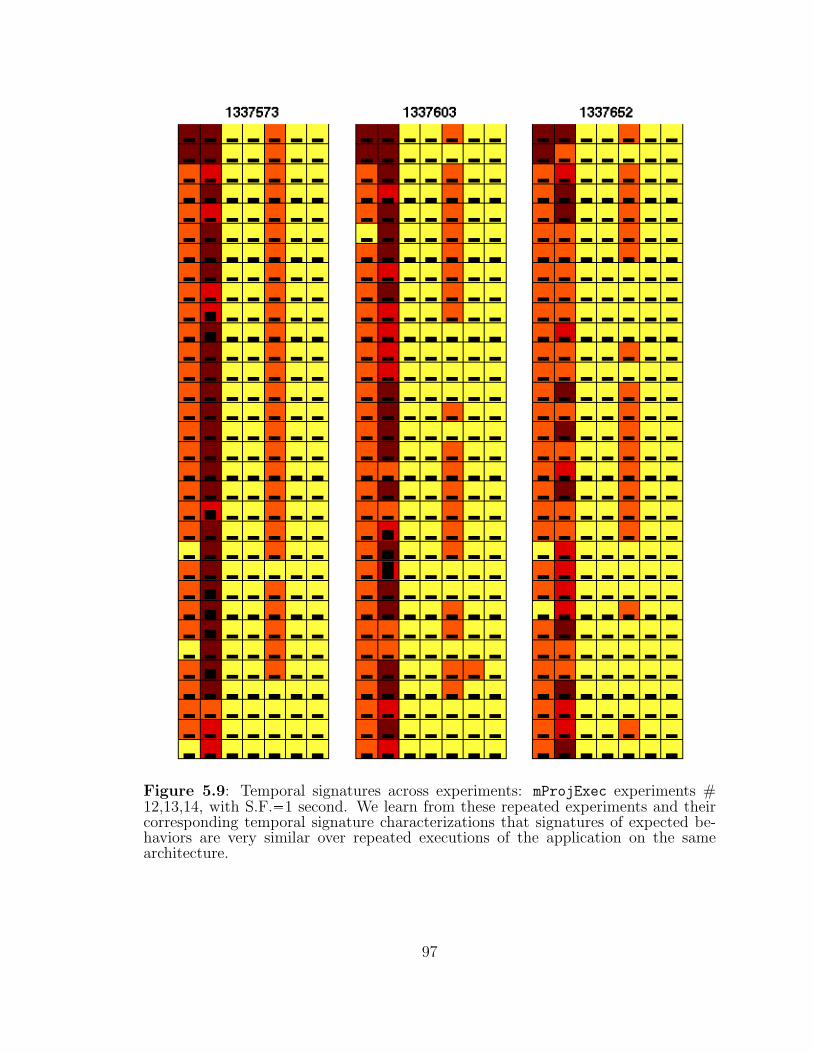
Figure 5.9: Temporal signatures across experiments: mProjExec experiments #12,13,14, with S.F.�1 second. We learn from these repeated experiments and theircorresponding temporal signature characterizations that signatures of expected be-haviors are very similar over repeated executions of the application on the samearchitecture.
97
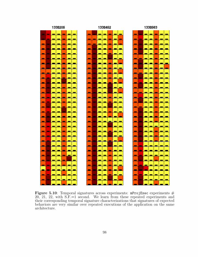
Figure 5.10: Temporal signatures across experiments: mProjExec experiments #20, 21, 22, with S.F.�1 second. We learn from these repeated experiments andtheir corresponding temporal signature characterizations that signatures of expectedbehaviors are very similar over repeated executions of the application on the samearchitecture.
98
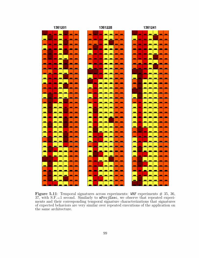
Figure 5.11: Temporal signatures across experiments: WRF experiments # 35, 36,37, with S.F.�1 second. Similarly to mProjExec, we observe that repeated experi-ments and their corresponding temporal signature characterizations that signaturesof expected behaviors are very similar over repeated executions of the application onthe same architecture.
99
5.4.4 Summary
We have described characteristics observed in performance time series data col-
lected from two different scientific applications during instances of expected perfor-
mance. Generally, the temporal signature characterization of the time series data
reveals low variance on the majority of metrics with some occasional moderate vari-
ance on the network metrics. In terms of patterns, we observe typically periodicity
on the CPU, disk-writes, network-reads and network-writes metrics; we observe flat
behaviors with low variance on the swap-memory, and on the local disk-reads metrics.
Finally, the memory-utilization metric seems to vary considerably more in terms of
the patterns we observe, as we observe ramp, periodic, flat and unknown patterns sys-
tematically across experiments and applications. This fact results from two sources:
1) the sensitivity of our pattern detection mechanism, and 2) other system processes
or daemons running at the same time with the application, causing some fluctuation
on the metric.
5.5 Temporal Signatures for Unexpected Applica-
tion Executions
We describe two instances where we label the performance of application exe-
cutions as unexpected or problematic, and describe the context. We also describe
an instance where the temporal signatures are indicating a known problem on some
resources (i.e., monitoring data corrupted on one specific node on the slowio clus-
ter), and another instance suggesting a possible problem with a specific node in the
Teragrid cluster. Both of these later instances do not seem to affect application per-
formance for our experiments, but can help system administrators easily investigate
reasons why certain resources do not behave similarly with other nodes in the cluster.
100
5.5.1 Case 1: Diagnosed Data-Intensive Application Run-ning on Slow Network
We illustrate in Figure 5.12(a) the performance time series data collected during
mProjExec Experiment # 23 executing on the slowio cluster. During this experi-
ment, 30 compute nodes attempt to continuously read and write from the network
7902 files totaling 45 GB. While the application does produce a valid scientific result,
as all images are processed correctly, the total execution time on these compute nodes
is significantly longer than what a user may expect had the network configuration
of cluster not be the bottleneck for processing. This mismatch case of running a
data intensive application over an low-bandwidth network (i.e., there is one shared
1 Gb Ethernet link between all the compute nodes and the network file server) has
the following effects on the application and environment: (1) the application’s run
time increases significantly because the CPU must wait for the data to arrive from
the network (and this behavior is seen in the high variance and high amplitude peri-
odicity of the CPU metric), and (2) the operating system keeps allocating memory
buffers to handle the file IO requests submitted by the application. We believe that
this allocation goes unbounded, as one observes the memory utilization on the sys-
tem to be slowly but consistently increasing until all the memory of the system is
fully utilized. While this behavior may be the result of a possible memory leak of
the application, we believe that this is not the case, as the swap memory metric
remains at zero even after all the memory on the system has been used. Figure 5.13
shows all signatures generated for each unexpected performance experimental run
from mProjExec Experiments # 23, 24 and 25.
101
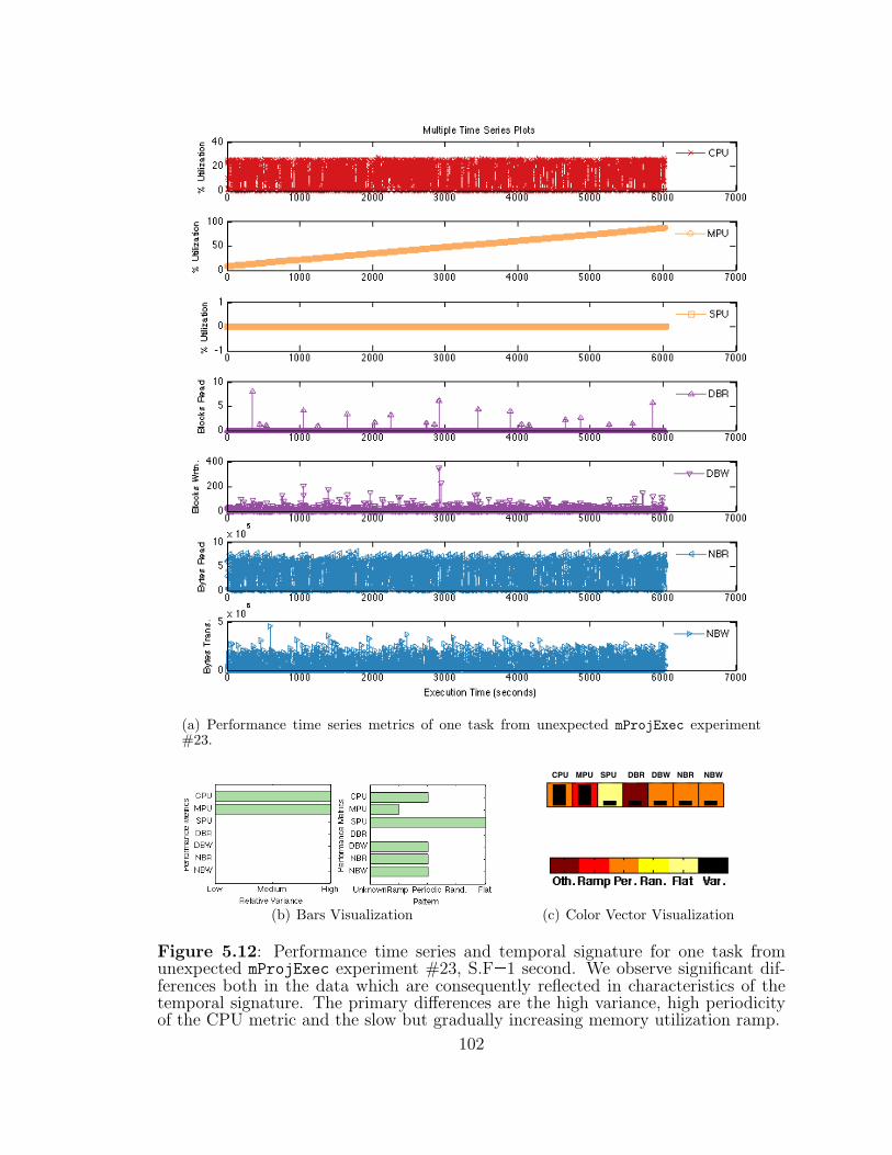
(a) Performance time series metrics of one task from unexpected mProjExec experiment#23.
(b) Bars Visualization
CPU MPU SPU DBR DBW NBR NBW
(c) Color Vector Visualization
Figure 5.12: Performance time series and temporal signature for one task fromunexpected mProjExec experiment #23, S.F�1 second. We observe significant dif-ferences both in the data which are consequently reflected in characteristics of thetemporal signature. The primary differences are the high variance, high periodicityof the CPU metric and the slow but gradually increasing memory utilization ramp.
102
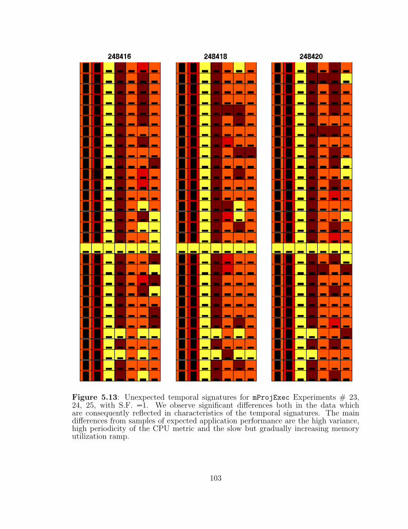
Figure 5.13: Unexpected temporal signatures for mProjExec Experiments # 23,24, 25, with S.F. �1. We observe significant differences both in the data whichare consequently reflected in characteristics of the temporal signatures. The maindifferences from samples of expected application performance are the high variance,high periodicity of the CPU metric and the slow but gradually increasing memoryutilization ramp.
103
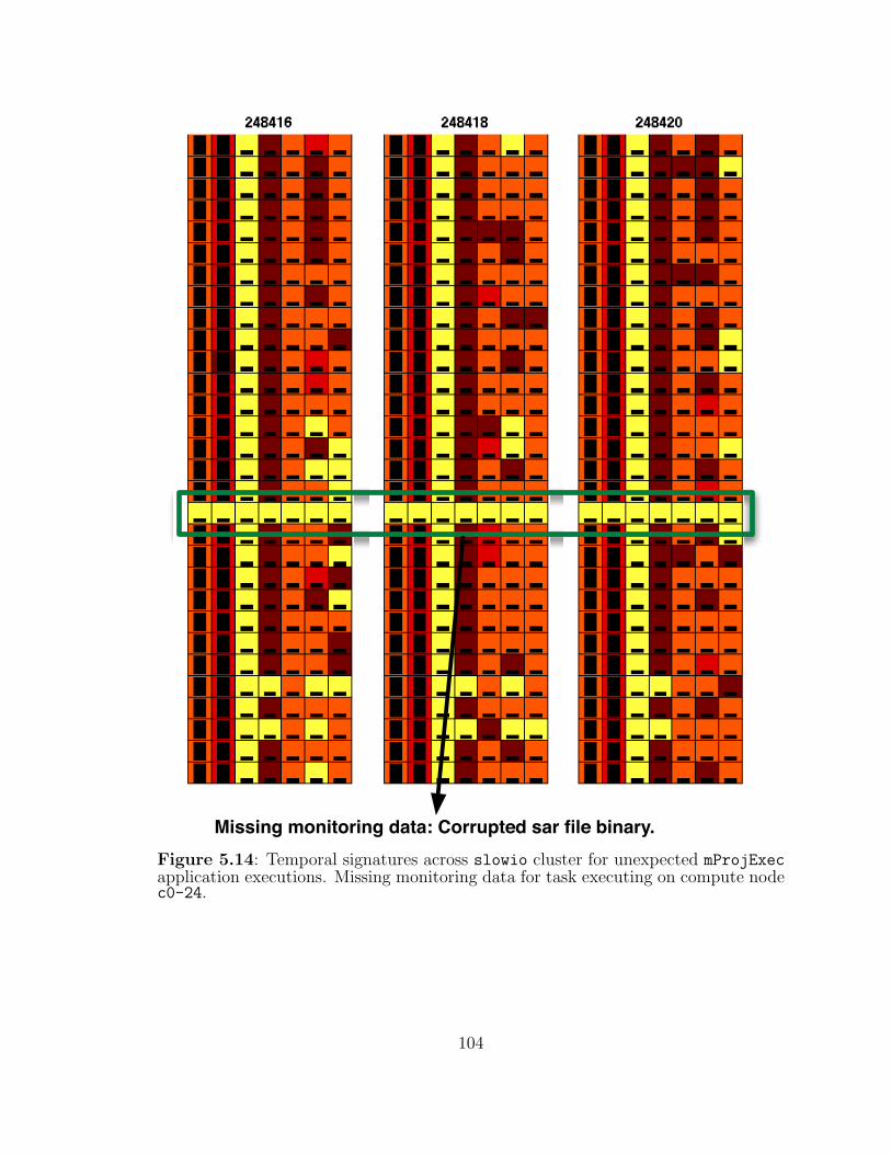
Missing monitoring data: Corrupted sar file binary.Figure 5.14: Temporal signatures across slowio cluster for unexpected mProjExecapplication executions. Missing monitoring data for task executing on compute nodec0-24.
104
5.5.2 Case 2: Diagnosed Corrupted Monitoring Data FileBinary
Compute node c0-24 on the slowio cluster has been generating corrupted sar
binary files (i.e., the performance monitoring data) for many of the experiments
we have ran on the cluster, which results in empty monitoring data files or zero-
time series for the performance metrics that we capture. The results of our scientific
application experiments were not affected, though the presence of such a problem can
be indicative to a system operator that configuration settings may not be properly set
on that host or that the monitoring application’s daemon may need to be restarted
to produce valid monitoring data. Figure 5.14 shows how all the temporal signatures
from the flat, zero-valued time series immediately indicate the lack of data.
5.5.3 Case 3: Undiagnosed Consistently Different ResourceCharacteristics Across Experiments
We have noticed during the execution of WRF on the himem cluster, Experiments
# 51, 52 and 53, that the temporal signature of one task running across executions
on the Teragrid node tg-c256 is significantly different than most of the signatures for
other tasks, as emphasized in Figure 5.15). When inspecting the performance time
series data which generated those abnormal temporal signatures, we also noticed an
abnormality on the memory metrics (MPU: percent-utilization and SPU: percent-
swap-utilization), as they vary highly between 0 and 100%. While this behavior does
not seem to affect our application and we do not know the source of this behavior,
it may be prudent for a system operator to investigate such behaviors on the node,
in order to prevent the node’s possible future failure during a user’s application
execution.
105
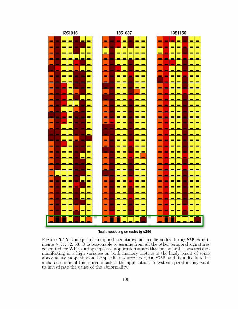
Tasks executing on node: tg-c256
Figure 5.15: Unexpected temporal signatures on specific nodes during WRF experi-ments # 51, 52, 53. It is reasonable to assume from all the other temporal signaturesgenerated for WRF during expected application states that behavioral characteristicsmanifesting in a high variance on both memory metrics is the likely result of someabnormality happening on the specific resource node, tg-c256, and its unlikely to bea characteristic of that specific task of the application. A system operator may wantto investigate the cause of the abnormality.
106
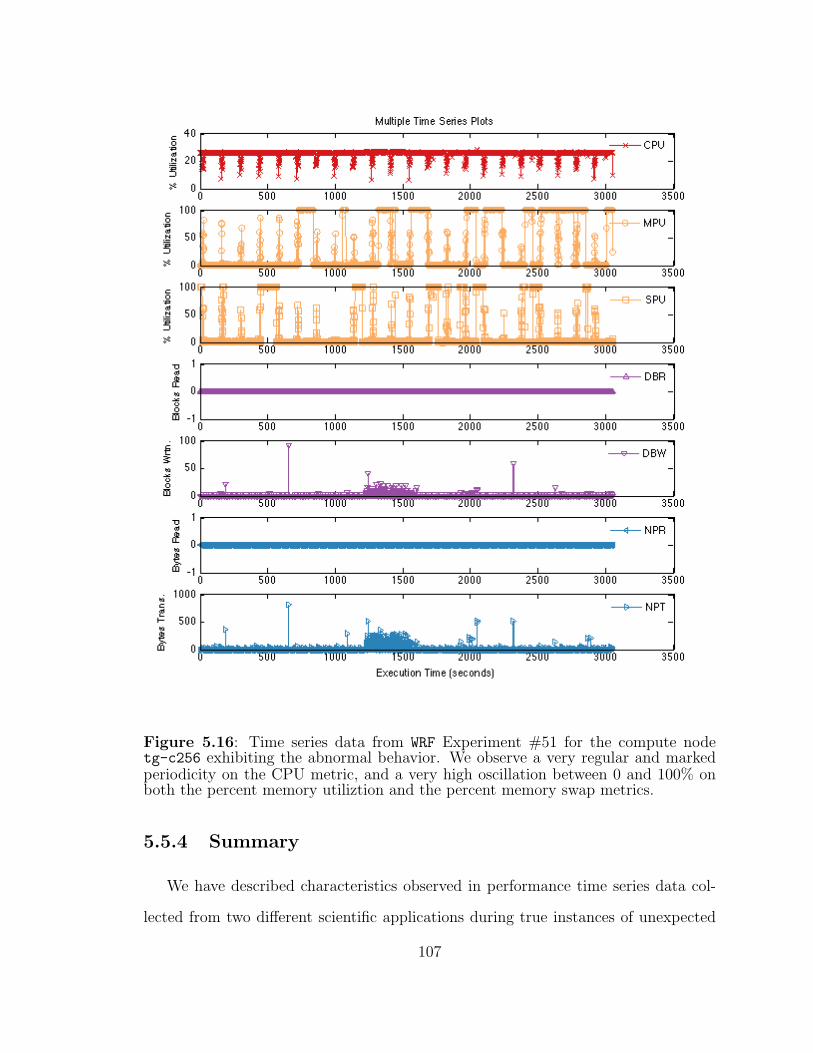
Figure 5.16: Time series data from WRF Experiment #51 for the compute nodetg-c256 exhibiting the abnormal behavior. We observe a very regular and markedperiodicity on the CPU metric, and a very high oscillation between 0 and 100% onboth the percent memory utiliztion and the percent memory swap metrics.
5.5.4 Summary
We have described characteristics observed in performance time series data col-
lected from two different scientific applications during true instances of unexpected
107
performance. Generally, the temporal signature characterization of the time series
data in degraded performance instances reveals higher variance on metrics on which
the expectation was lower variance; similarly, in terms of patterns, we observe sig-
nificant changes in patterns from cases of expected performance executions. The
ability to make an automatic distinction between performance data collected dur-
ing expected and unexpected behavior circumstances is fundamental to performance
problem identification for applications and systems.
5.6 Qualitative Performance Validation and Diag-
nosis
We describe in the following sections the process of qualitative performance vali-
dation and diagnosis in scientific workflows using temporal signatures. We associate
high-level, qualitative behaviors of applications with their corresponding temporal
signatures and show how this correlation can provide, in a simple and intuitive man-
ner, answers about the behavior of workflow components as well as interpret the
global behavior of the application.
5.6.1 Task-Level
For the duration of each task within a workflow we can generate temporal sig-
natures as illustrated in Figure 5.17. The evaluation epochs can be determined in
several ways. In the case of scientific applications that output progress logs (i.e., logs
recording the amount of work already performed -such as how many astronomy files
have been reprojected or how many forecast hours have been computed), it is rela-
tively simple to correlate the information in the logs with monitoring time-stamps in
order to get evaluation time points across all tasks within a workflow instance. If
the scientific application does not produce a progress output log that can be easily
used for time-stamp generation, or in the case of a scientific application that cannot
108
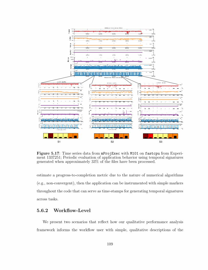
S1 S2 S3
Figure 5.17: Time series data from mProjExec with M101 on fastcpu from Experi-ment 1337251; Periodic evaluation of application behavior using temporal signaturesgenerated when approximately 33% of the files have been processed.
estimate a progress-to-completion metric due to the nature of numerical algorithms
(e.g., non-convergent), then the application can be instrumented with simple markers
throughout the code that can serve as time-stamps for generating temporal signatures
across tasks.
5.6.2 Workflow-Level
We present two scenarios that reflect how our qualitative performance analysis
framework informs the workflow user with simple, qualitative descriptions of the
109
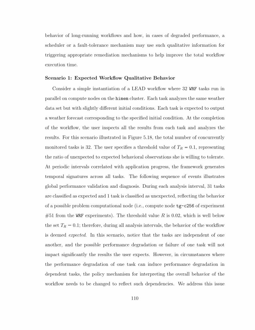
behavior of long-running workflows and how, in cases of degraded performance, a
scheduler or a fault-tolerance mechanism may use such qualitative information for
triggering appropriate remediation mechanisms to help improve the total workflow
execution time.
Scenario 1: Expected Workflow Qualitative Behavior
Consider a simple instantiation of a LEAD workflow where 32 WRF tasks run in
parallel on compute nodes on the himem cluster. Each task analyzes the same weather
data set but with slightly different initial conditions. Each task is expected to output
a weather forecast corresponding to the specified initial condition. At the completion
of the workflow, the user inspects all the results from each task and analyzes the
results. For this scenario illustrated in Figure 5.18, the total number of concurrently
monitored tasks is 32. The user specifies a threshold value of TR � 0.1, representing
the ratio of unexpected to expected behavioral observations she is willing to tolerate.
At periodic intervals correlated with application progress, the framework generates
temporal signatures across all tasks. The following sequence of events illustrates
global performance validation and diagnosis. During each analysis interval, 31 tasks
are classified as expected and 1 task is classified as unexpected, reflecting the behavior
of a possible problem computational node (i.e., compute node tg-c256 of experiment
#51 from the WRF experiments). The threshold value R is 0.02, which is well below
the set TR � 0.1; therefore, during all analysis intervals, the behavior of the workflow
is deemed expected. In this scenario, notice that the tasks are independent of one
another, and the possible performance degradation or failure of one task will not
impact significantly the results the user expects. However, in circumstances where
the performance degradation of one task can induce performance degradation in
dependent tasks, the policy mechanism for interpreting the overall behavior of the
workflow needs to be changed to reflect such dependencies. We address this issue
110
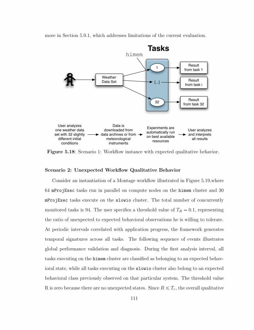
more in Section 5.9.1, which addresses limitations of the current evaluation.
WeatherData Set
1
32
[...]
himem Tasks
Resultfrom task 1
Resultfrom task i
Resultfrom task 32
User analyzesone weather dataset with 32 slightly
different initial conditions
Data isdownloaded from
data archives or frommeteorological
instruments
Experiments areautomatically runon best available
resources
User analyzesand interprets
all results
Figure 5.18: Scenario 1: Workflow instance with expected qualitative behavior.
Scenario 2: Unexpected Workflow Qualitative Behavior
Consider an instantiation of a Montage workflow illustrated in Figure 5.19,where
64 mProjExec tasks run in parallel on compute nodes on the himem cluster and 30
mProjExec tasks execute on the slowio cluster. The total number of concurrently
monitored tasks is 94. The user specifies a threshold value of TR � 0.1, representing
the ratio of unexpected to expected behavioral observations he is willing to tolerate.
At periodic intervals correlated with application progress, the framework generates
temporal signatures across all tasks. The following sequence of events illustrates
global performance validation and diagnosis. During the first analysis interval, all
tasks executing on the himem cluster are classified as belonging to an expected behav-
ioral state, while all tasks executing on the slowio cluster also belong to an expected
behavioral class previously observed on that particular system. The threshold value
R is zero because there are no unexpected states. Since R ¤ Tr, the overall qualitative
111
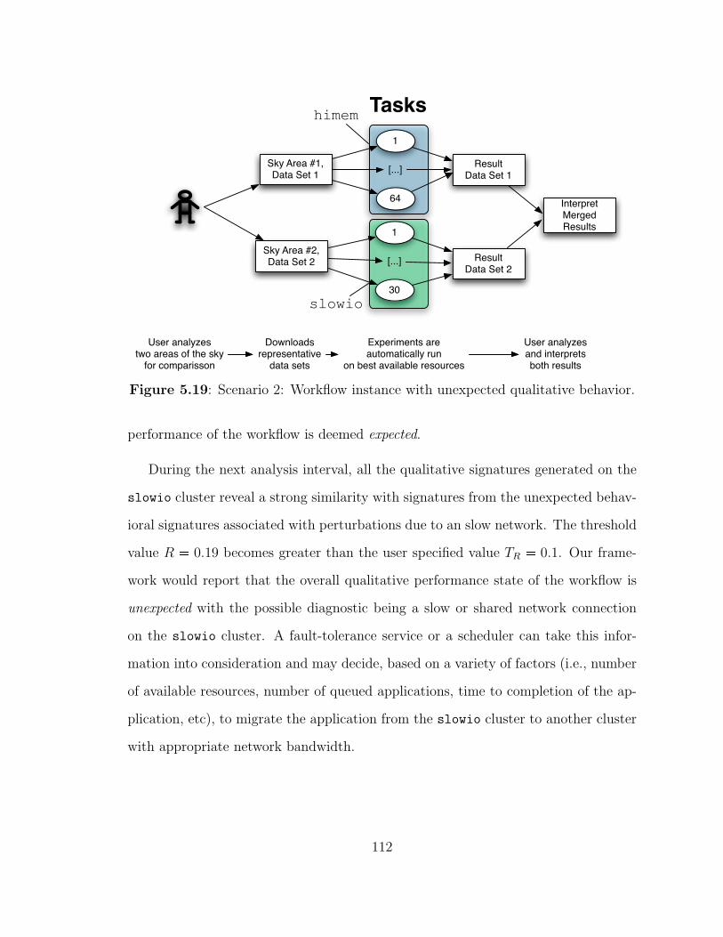
User analyzestwo areas of the sky
for comparisson
Downloadsrepresentative
data sets
Experiments areautomatically run
on best available resources
Sky Area #1,Data Set 1
Sky Area #2,Data Set 2
1
64
[...]
Tasks
1
30
[...]
himem
slowio
ResultData Set 1
ResultData Set 2
InterpretMerged Results
User analyzesand interpretsboth results
Figure 5.19: Scenario 2: Workflow instance with unexpected qualitative behavior.
performance of the workflow is deemed expected.
During the next analysis interval, all the qualitative signatures generated on the
slowio cluster reveal a strong similarity with signatures from the unexpected behav-
ioral signatures associated with perturbations due to an slow network. The threshold
value R � 0.19 becomes greater than the user specified value TR � 0.1. Our frame-
work would report that the overall qualitative performance state of the workflow is
unexpected with the possible diagnostic being a slow or shared network connection
on the slowio cluster. A fault-tolerance service or a scheduler can take this infor-
mation into consideration and may decide, based on a variety of factors (i.e., number
of available resources, number of queued applications, time to completion of the ap-
plication, etc), to migrate the application from the slowio cluster to another cluster
with appropriate network bandwidth.
112
5.7 Framework Evaluation
We infer the efficacy of our framework based on temporal signatures from the
main usage modality for signatures: classification. The evaluation criteria is based
on the ability of a classifier to correctly classify a new, “never-seen” signature as
belonging to the correct category of performance behaviors, expected and unexpected.
Similarly to [22], to say that temporal signatures are accurate, meaningful and of
high-quality is to imply that classification based on those signatures performs well.
Furthermore, in order to test the first hypothesis, we analyze a subset of the ex-
perimental data to show an example where performance data signatures based on
temporal information are superior –in terms of accuracy of classification– to signa-
tures based on instantaneous data values, which do not carry temporal information.
To test our second hypothesis, we analyze all the experimental data for which we
have examples of both expected and unexpected behaviors, and report the overall
balanced accuracy obtained. For both cases of our evaluation, we use K-fold cross-
validation1 as the technique to help test the accuracy of our classifier in the absence
of new experimental samples of behavior.
5.7.1 Comparison of Classification Accuracy Between Instan-taneous Values Signatures and Temporal Signatures
In this section, we test the validity of our first hypothesis which states that it is
necessary to extract temporal information in performance time series data for the case
of long-running scientific applications. We show need by providing an example where
instantaneous values of performance metrics are not able to accurately distinguish
cases of expected and unexpected performance behaviors.
1Cross-validation is a statistical method of partitioning existing sample data into subsets suchthat learning is performed on a subset of the data, while validation of the learning is performedon another subset of the data. In K-fold cross-validation, the data is partitioned randomly intoK subsets; training is performed on K-1 of the subsets, while the validation is done with theremaining subset. This process is repeated K times (or folds) such that each of the K subsets isused exactly once as a validation subset.
113
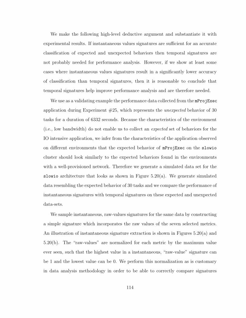
We make the following high-level deductive argument and substantiate it with
experimental results. If instantaneous values signatures are sufficient for an accurate
classification of expected and unexpected behaviors then temporal signatures are
not probably needed for performance analysis. However, if we show at least some
cases where instantaneous values signatures result in a significantly lower accuracy
of classification than temporal signatures, then it is reasonable to conclude that
temporal signatures help improve performance analysis and are therefore needed.
We use as a validating example the performance data collected from the mProjExec
application during Experiment #25, which represents the unexpected behavior of 30
tasks for a duration of 6332 seconds. Because the characteristics of the environment
(i.e., low bandwidth) do not enable us to collect an expected set of behaviors for the
IO intensive application, we infer from the characteristics of the application observed
on different environments that the expected behavior of mProjExec on the slowio
cluster should look similarly to the expected behaviors found in the environments
with a well-provisioned network. Therefore we generate a simulated data set for the
slowio architecture that looks as shown in Figure 5.20(a). We generate simulated
data resembling the expected behavior of 30 tasks and we compare the performance of
instantaneous signatures with temporal signatures on these expected and unexpected
data-sets.
We sample instantaneous, raw-values signatures for the same data by constructing
a simple signature which incorporates the raw values of the seven selected metrics.
An illustration of instantaneous signature extraction is shown in Figures 5.20(a) and
5.20(b). The “raw-values” are normalized for each metric by the maximum value
ever seen, such that the highest value in a instantaneous, “raw-value” signature can
be 1 and the lowest value can be 0. We perform this normalization as is customary
in data analysis methodology in order to be able to correctly compare signatures
114
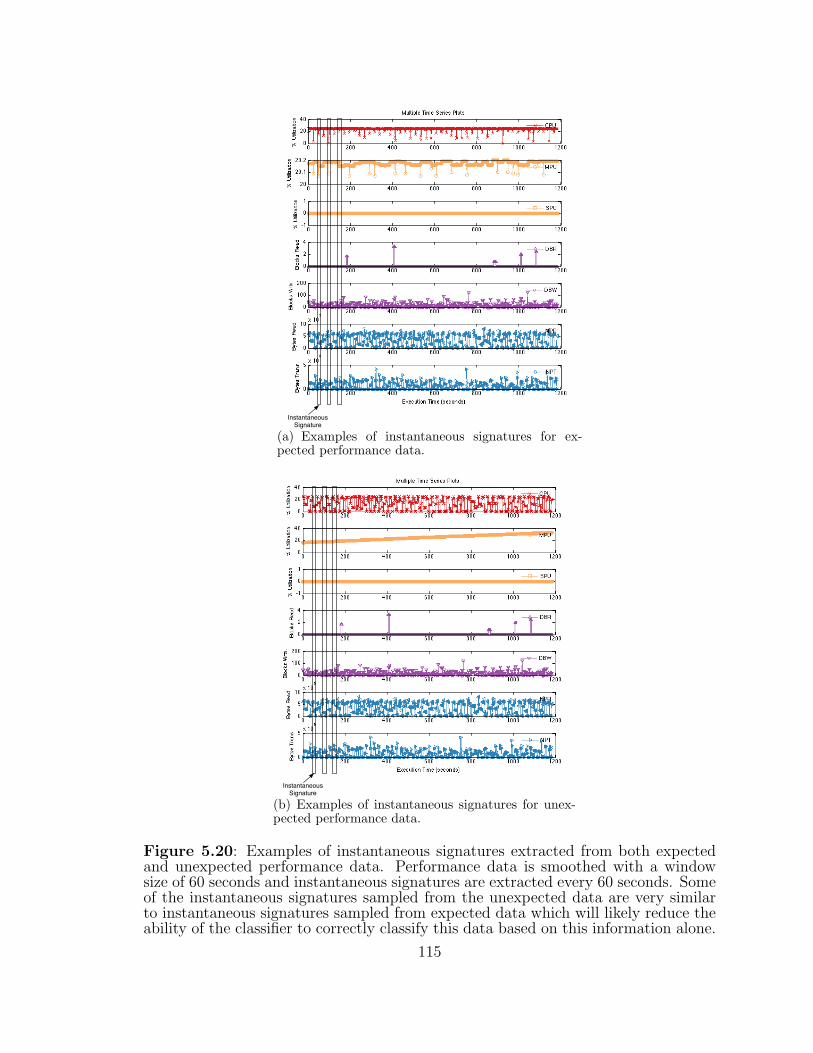
InstantaneousSignature
(a) Examples of instantaneous signatures for ex-pected performance data.
InstantaneousSignature
(b) Examples of instantaneous signatures for unex-pected performance data.
Figure 5.20: Examples of instantaneous signatures extracted from both expectedand unexpected performance data. Performance data is smoothed with a windowsize of 60 seconds and instantaneous signatures are extracted every 60 seconds. Someof the instantaneous signatures sampled from the unexpected data are very similarto instantaneous signatures sampled from expected data which will likely reduce theability of the classifier to correctly classify this data based on this information alone.
115
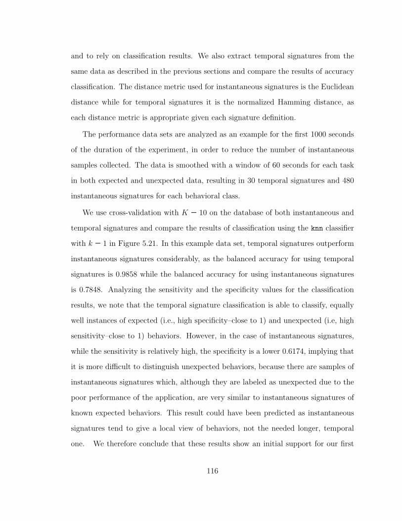
and to rely on classification results. We also extract temporal signatures from the
same data as described in the previous sections and compare the results of accuracy
classification. The distance metric used for instantaneous signatures is the Euclidean
distance while for temporal signatures it is the normalized Hamming distance, as
each distance metric is appropriate given each signature definition.
The performance data sets are analyzed as an example for the first 1000 seconds
of the duration of the experiment, in order to reduce the number of instantaneous
samples collected. The data is smoothed with a window of 60 seconds for each task
in both expected and unexpected data, resulting in 30 temporal signatures and 480
instantaneous signatures for each behavioral class.
We use cross-validation with K � 10 on the database of both instantaneous and
temporal signatures and compare the results of classification using the knn classifier
with k � 1 in Figure 5.21. In this example data set, temporal signatures outperform
instantaneous signatures considerably, as the balanced accuracy for using temporal
signatures is 0.9858 while the balanced accuracy for using instantaneous signatures
is 0.7848. Analyzing the sensitivity and the specificity values for the classification
results, we note that the temporal signature classification is able to classify, equally
well instances of expected (i.e., high specificity–close to 1) and unexpected (i.e, high
sensitivity–close to 1) behaviors. However, in the case of instantaneous signatures,
while the sensitivity is relatively high, the specificity is a lower 0.6174, implying that
it is more difficult to distinguish unexpected behaviors, because there are samples of
instantaneous signatures which, although they are labeled as unexpected due to the
poor performance of the application, are very similar to instantaneous signatures of
known expected behaviors. This result could have been predicted as instantaneous
signatures tend to give a local view of behaviors, not the needed longer, temporal
one. We therefore conclude that these results show an initial support for our first
116
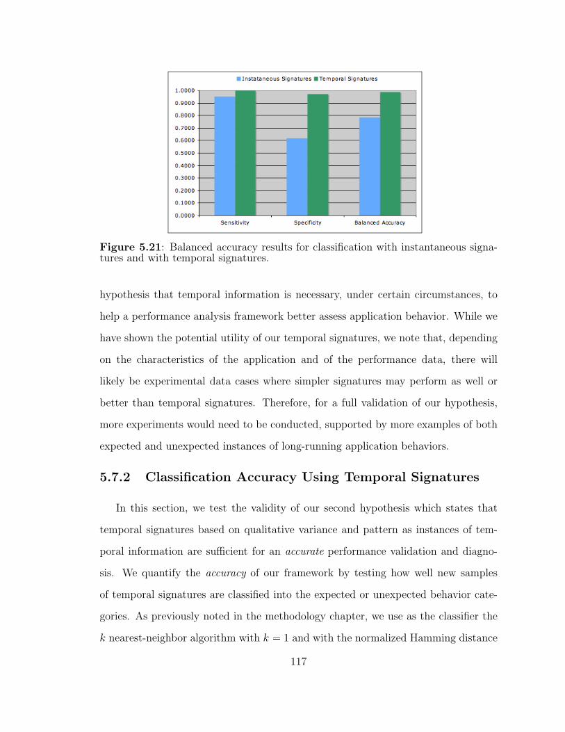
Figure 5.21: Balanced accuracy results for classification with instantaneous signa-tures and with temporal signatures.
hypothesis that temporal information is necessary, under certain circumstances, to
help a performance analysis framework better assess application behavior. While we
have shown the potential utility of our temporal signatures, we note that, depending
on the characteristics of the application and of the performance data, there will
likely be experimental data cases where simpler signatures may perform as well or
better than temporal signatures. Therefore, for a full validation of our hypothesis,
more experiments would need to be conducted, supported by more examples of both
expected and unexpected instances of long-running application behaviors.
5.7.2 Classification Accuracy Using Temporal Signatures
In this section, we test the validity of our second hypothesis which states that
temporal signatures based on qualitative variance and pattern as instances of tem-
poral information are sufficient for an accurate performance validation and diagno-
sis. We quantify the accuracy of our framework by testing how well new samples
of temporal signatures are classified into the expected or unexpected behavior cate-
gories. As previously noted in the methodology chapter, we use as the classifier the
k nearest-neighbor algorithm with k � 1 and with the normalized Hamming distance
117
as the similarity metric between temporal signatures. The classification of temporal
signatures corresponds to performance validation (i.e., deciding whether the label
is expected or unexpected), and diagnosis (i.e., deciding which type of unexpected
behavior is detected).
We generate a temporal signature for the entire duration of each task from each
experiment described in Tables 5.3 and 5.4, resulting in a total of 1242 signatures for
the first Montage data set, and 1242 signatures of the second Montage data set. Out
of these signatures, there are 90 instances of unexpected behaviors and 1152 instances
of expected or good-performance behaviors. We note that the ratio of samples of ex-
pected to unexpected behaviors is 1142:90 which represents approximately 13:1. This
ratio strongly supports our choice of balanced accuracy as a measure of evaluating
framework efficacy, because a simpler accuracy metric may inflate accuracy results
due to a larger sample of expected signatures.
Cross-validation with K � 20 partitions all 1242 signatures from each Montage
data sets into subsets, where training is performed on approximately 1085 signatures
and validation is performed on the remaining 157 signatures. Both the training and
validation data sets are randomly chosen each time from both sets of expected (1152)
and unexpected signatures (90).
Table 5.7 shows supportive evidence for our secondary hypothesis that qualita-
tive variance and pattern as instances of temporal information are sufficient for the
creation of performance signatures that can accurately –with accuracies higher than
98.66%– detect instances of expected and unexpected behaviors in long-running sci-
entific applications.
Although these results reflect a very good, high-accuracy of detection, we cau-
tiously note that the accuracy of our framework will most likely decrease as more
experimental data from more applications, configurations and different instances of
118
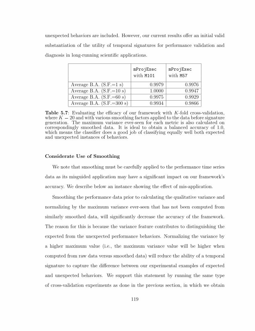
unexpected behaviors are included. However, our current results offer an initial valid
substantiation of the utility of temporal signatures for performance validation and
diagnosis in long-running scientific applications.
mProjExec
with M101
mProjExec
with M57
Average B.A. (S.F.=1 s) 0.9979 0.9976Average B.A. (S.F.=10 s) 1.0000 0.9947Average B.A. (S.F.=60 s) 0.9975 0.9929Average B.A. (S.F.=300 s) 0.9934 0.9866
Table 5.7: Evaluating the efficacy of our framework with K-fold cross-validation,whereK � 20 and with various smoothing factors applied to the data before signaturegeneration. The maximum variance ever-seen for each metric is also calculated oncorrespondingly smoothed data. It is ideal to obtain a balanced accuracy of 1.0,which means the classifier does a good job of classifying equally well both expectedand unexpected instances of behaviors.
Considerate Use of Smoothing
We note that smoothing must be carefully applied to the performance time series
data as its misguided application may have a significant impact on our framework’s
accuracy. We describe below an instance showing the effect of mis-application.
Smoothing the performance data prior to calculating the qualitative variance and
normalizing by the maximum variance ever-seen that has not been computed from
similarly smoothed data, will significantly decrease the accuracy of the framework.
The reason for this is because the variance feature contributes to distinguishing the
expected from the unexpected performance behaviors. Normalizing the variance by
a higher maximum value (i.e., the maximum variance value will be higher when
computed from raw data versus smoothed data) will reduce the ability of a temporal
signature to capture the difference between our experimental examples of expected
and unexpected behaviors. We support this statement by running the same type
of cross-validation experiments as done in the previous section, in which we obtain
119
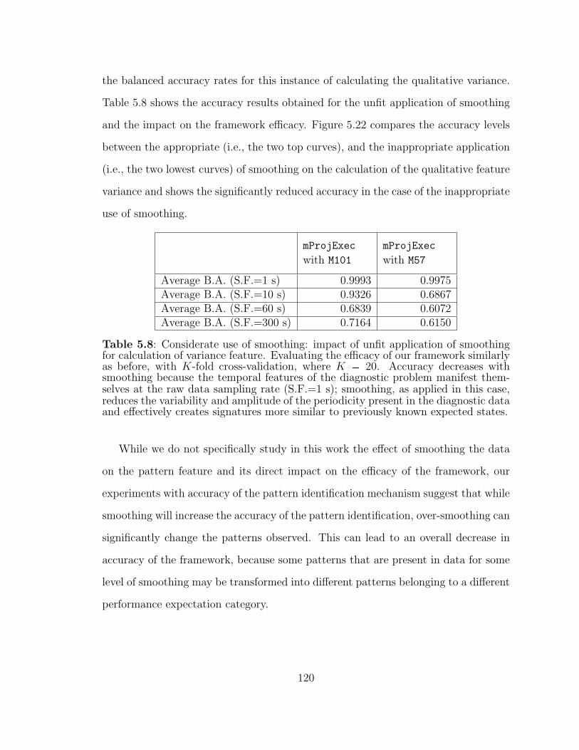
the balanced accuracy rates for this instance of calculating the qualitative variance.
Table 5.8 shows the accuracy results obtained for the unfit application of smoothing
and the impact on the framework efficacy. Figure 5.22 compares the accuracy levels
between the appropriate (i.e., the two top curves), and the inappropriate application
(i.e., the two lowest curves) of smoothing on the calculation of the qualitative feature
variance and shows the significantly reduced accuracy in the case of the inappropriate
use of smoothing.
mProjExec
with M101
mProjExec
with M57
Average B.A. (S.F.=1 s) 0.9993 0.9975Average B.A. (S.F.=10 s) 0.9326 0.6867Average B.A. (S.F.=60 s) 0.6839 0.6072Average B.A. (S.F.=300 s) 0.7164 0.6150
Table 5.8: Considerate use of smoothing: impact of unfit application of smoothingfor calculation of variance feature. Evaluating the efficacy of our framework similarlyas before, with K-fold cross-validation, where K � 20. Accuracy decreases withsmoothing because the temporal features of the diagnostic problem manifest them-selves at the raw data sampling rate (S.F.=1 s); smoothing, as applied in this case,reduces the variability and amplitude of the periodicity present in the diagnostic dataand effectively creates signatures more similar to previously known expected states.
While we do not specifically study in this work the effect of smoothing the data
on the pattern feature and its direct impact on the efficacy of the framework, our
experiments with accuracy of the pattern identification mechanism suggest that while
smoothing will increase the accuracy of the pattern identification, over-smoothing can
significantly change the patterns observed. This can lead to an overall decrease in
accuracy of the framework, because some patterns that are present in data for some
level of smoothing may be transformed into different patterns belonging to a different
performance expectation category.
120
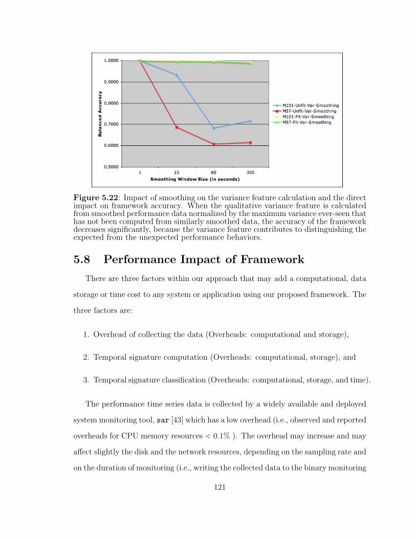
Figure 5.22: Impact of smoothing on the variance feature calculation and the directimpact on framework accuracy. When the qualitative variance feature is calculatedfrom smoothed performance data normalized by the maximum variance ever-seen thathas not been computed from similarly smoothed data, the accuracy of the frameworkdecreases significantly, because the variance feature contributes to distinguishing theexpected from the unexpected performance behaviors.
5.8 Performance Impact of Framework
There are three factors within our approach that may add a computational, data
storage or time cost to any system or application using our proposed framework. The
three factors are:
1. Overhead of collecting the data (Overheads: computational and storage),
2. Temporal signature computation (Overheads: computational, storage), and
3. Temporal signature classification (Overheads: computational, storage, and time).
The performance time series data is collected by a widely available and deployed
system monitoring tool, sar [43] which has a low overhead (i.e., observed and reported
overheads for CPU memory resources 0.1% ). The overhead may increase and may
affect slightly the disk and the network resources, depending on the sampling rate and
on the duration of monitoring (i.e., writing the collected data to the binary monitoring
121
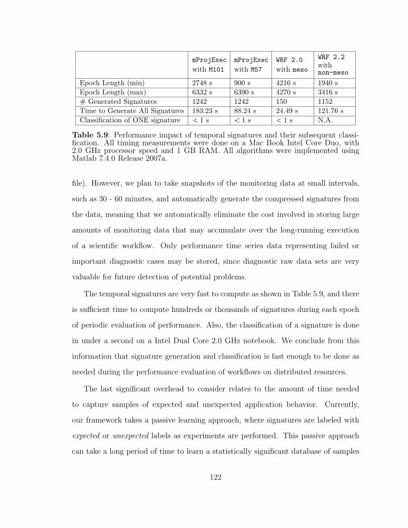
mProjExec
with M101
mProjExec
with M57
WRF 2.0
with meso
WRF 2.2withnon-meso
Epoch Length (min) 2748 s 900 s 4216 s 1940 sEpoch Length (max) 6332 s 6390 s 4270 s 3416 s# Generated Signatures 1242 1242 150 1152Time to Generate All Signatures 183.23 s 88.24 s 24.49 s 121.76 sClassification of ONE signature 1 s 1 s 1 s N.A.
Table 5.9: Performance impact of temporal signatures and their subsequent classi-fication. All timing measurements were done on a Mac Book Intel Core Duo, with2.0 GHz processor speed and 1 GB RAM. All algorithms were implemented usingMatlab 7.4.0 Release 2007a.
file). However, we plan to take snapshots of the monitoring data at small intervals,
such as 30 - 60 minutes, and automatically generate the compressed signatures from
the data, meaning that we automatically eliminate the cost involved in storing large
amounts of monitoring data that may accumulate over the long-running execution
of a scientific workflow. Only performance time series data representing failed or
important diagnostic cases may be stored, since diagnostic raw data sets are very
valuable for future detection of potential problems.
The temporal signatures are very fast to compute as shown in Table 5.9, and there
is sufficient time to compute hundreds or thousands of signatures during each epoch
of periodic evaluation of performance. Also, the classification of a signature is done
in under a second on a Intel Dual Core 2.0 GHz notebook. We conclude from this
information that signature generation and classification is fast enough to be done as
needed during the performance evaluation of workflows on distributed resources.
The last significant overhead to consider relates to the amount of time needed
to capture samples of expected and unexpected application behavior. Currently,
our framework takes a passive learning approach, where signatures are labeled with
expected or unexpected labels as experiments are performed. This passive approach
can take a long period of time to learn a statistically significant database of samples
122

of behavior. However, this can be remedied by using an active learning approach such
as proposed by [101], where known stress factor can be applied to the applications
of interest in a controlled fault-injection test-bed, and signatures of diagnostic states
can be generated at a much faster rate and with more accurate labels.
5.9 Limitations
We address limitations of our current framework evaluation as well as higher-
level limitations of the approach. First, we list and describe ways in which our
framework could be improved by further evaluation and expansion. Last, we de-
scribe circumstances that will likely cause our approach to perform poorly and may
require significant changes in operating assumptions, implementation techniques, and
evaluation.
5.9.1 Limitations of the Current Evaluation
We list and describe several avenues which we believe would significantly improve
the current framework and expand on its current evaluation.
Passive Learning of Behaviors
Currently, we have passively learned instances of expected and unexpected be-
haviors for our experimental data sets. The major disadvantage of a passive learning
approach is that gathering a representative sample of behaviors will be slow. An al-
ternative approach can leverage an active learning technique, such as that proposed
in [101]. We could construct a fault-tolerance test bed where we inject a variety
of common faults known to affect the performance of long-running applications in
production environments.
This approach would enable us to acquire, in a controlled fashion and relatively
quickly, instances of expected and more importantly –unexpected– temporal signa-
123
tures for an application, and to label them with a known diagnostic state (e.g.,
signature was captured during known memory leak issue affecting the application).
The disadvantage of using temporal signatures of applications under a controlled,
fault-tolerance test bed lies in the fact that such signatures may not have the same
characteristics with signatures captured during a performance problem occurring in
real production environments.
Adaptation to Change
The current framework assumes that once a set of behaviors has been learned, the
overall accuracy of validation and diagnosis will remain constant due to the assump-
tion that behaviors drawn from the same distribution with the training data set will
be analyzed. Because the space of parameters that can affect temporal signatures and
application behaviors is large and complex, it is likely that new application behaviors
will cause a reduction in framework’s accuracy because they are not captured in the
baseline learning set. Under this circumstance, Teresa would need to be enhanced
with a dynamic learning mechanism that would re-learn baseline behaviors once the
overall accuracy decreases below an accepted user value.
Workflow Tasks Independence
While the use of temporal signatures is independent on the dependence relation-
ship in a set of workflow tasks, we currently evaluate workflow-level behavior under
the assumption that behaviors of the tasks do not have a significant dependence on
the temporal observed behavior. The current time series collected and analyzed may
not specifically expose dependent behaviors in a group of tasks (e.g., MPI communica-
tion patterns), but such performance time series may be captured and characteristics
of the temporal signatures can be further studied, together with the implication on
variation of observed temporal signatures for a set of interdependent tasks.
124
Alternate Signature Definitions
In this work we have defined and presented results for a specific instance of a
temporal signature, containing structural and temporal features of performance time
series with two discrete features: relative variance and pattern. There are many other
possibilities of defining signatures for performance time series data. For example, a
continuous feature version of our current signature may capture as one feature, f1,
the continuous normalized variance r0, 1s as well as a feature for each of the pattern of
interest, f2 for the periodic pattern, f3 for the ramp pattern, f4 for the flat pattern,
and f5 for the random pattern, each varying from r0, 1s, where the values in the
interval may represent confidence levels for the detection of each pattern (i.e., 0: non-
confident, and 1: complete confidence). The signature would encode five features for
each of the selected time series.
Additionally, signatures could be also created by varying the number of time
series for which features are extracted. Coupled with the metric attribution work
by Cohen [21], we can use different subsets of times series for different signatures
targeted at identifying different performance problems. For example, time series M �t1, 2, 3, 4, 5u with the discrete features f1 and f2 may be used to identify problems
related to memory and disk, while time series M � t1, 2, 6, 7u with the same discrete
features, may be used to identify problems related to the network.
Impact of Smoothing the Data on Signatures
Smoothing must be carefully applied to the raw performance data, as it has a
direct impact on the two features we selected for our particular signature definition,
as discussed in Section 5.7.2. If the data is unprocessed, with no smoothing filter
applied, small amounts of variance may have an impact on the pattern identification
mechanism, as patterns may be incorrectly classified. At the other extreme, too
much smoothing can significantly reduce the amount of variance in the series, and
125
may change patterns.
As smoothing will often be used to pre-process monitored data in order to reduce
noise or local variations, care must be taken in applying it because smoothing over
large windows of time may hide some important variations in the data which are
correlated with a significant and persistent performance problem. To support identi-
fication of problems without worrying about finding an optimal smoothing window,
signatures can be generated for different windows, and performance validation and
diagnosis can be done on all these signatures, potentially triggering performance
problem identification for some smoothing levels and not for others.
Transferability of Temporal Signatures
One question that arises from the characteristics of temporal signatures for Mon-
tage and LEAD is whether temporal signatures are transferable – that is, if we learn
a set of expected and unexpected temporal signatures for an application, can we
use them to validate the performance for a new application that exhibits expected
signatures similar to a known application? A further study expanding on this issue
could be of great value in providing further evidence for the practicality and general
applicability of such a qualitative performance analysis approach.
5.9.2 Limitations of the Approach
There are two main circumstances of our approach under which if the operating
assumptions change, they will likely impact the accuracy of our framework. The
contexts refer to our approach’s (1) reliance on an expert for supporting the initial
learning of expected and unexpected behavioral instances, and (2) assumption that
the behaviors of the applications are not dependent on the scientific data analyzed
and on the application’s configuration. Furthermore, there is an inherent loss of
accuracy of validation and diagnosis because we correlate a limited set of performance
126
metrics with higher-level application states. We describe these issues in the following
subsections.
Reliance on Expert for Learning Behavior Instances
Our framework does rely on a human expert or a semi-automated expert to label
samples of performance data associated with both good and degraded performance
behaviors. This setting allows our framework to assess performance via classifiers
in an on-line setting. However, the disadvantage of relying on a human or semi-
automated experts for gathering of training data sets is that accurate labels of be-
haviors are very hard (in terms of time and expertise) to acquire.
In the absence of training data, the alternative is to use unsupervised learning
techniques (i.e., clustering) that may automatically discover groups of behaviors,
which over time, can be associated with various qualitative behavioral descriptions
for a given application. Neither technique (classification or clustering) lacks disad-
vantages. While the disadvantage of the supervised learning technique is that it
requires an expert’s pre-labeled instances of behaviors, the disadvantage of the unsu-
pervised learning technique is that deciding how many behavioral clusters truly exist
in a sampled training set and their practical meaning is typically hard to interpret.
These disadvantages suggest that maybe combining both techniques in an effort to
strengthen their individual advantages may be most practical under certain contexts.
Application Data and Configuration Dependence
Teresa currently assumes that the scientific applications executions do not exhibit
parameter or data dependent behavior. If this assumption is removed, our framework
needs to allow for two modifications: (a) a methodology for deciding the appropriate
time interval for generating signatures periodically, and (b) a characterization how
differences in application data characteristics impact the performance time series
collected and the generated temporal signatures.
127
Characteristics of temporal signatures under these changed assumptions can be
learned by analyzing the impact of various parameters and the contents of the input
data on the time series analyzed. Our work can be expanded by including methods
to map such dependencies described in work by [33, 103].
Non-uniqueness of Diagnostic Signatures
Our temporal signatures correlate symptoms of performance problems in scientific
applications and their execution environments. There could be many problem root
causes that manifest themselves in similar symptoms; therefore, temporal signatures
associated with one symptom may represent different causes or types of problems.
The goal of our framework is to offer guidance in identifying the most likely type
of problem affecting the application and not necessarily to find the root-cause of
the problem. Because it is likely that different behaviors will exhibit similar signa-
tures, this will reduce the ability with which our framework can pinpoint the most
likely problem affecting an application. We discuss more about the related issue of
correlation and causation in the concluding Section 7.2.4.
5.10 Summary
This chapter demonstrated how Teresa reasons qualitatively about temporal be-
haviors for long running components within two large-scale scientific workflows. We
described the scientific applications, their components, and characteristics of the com-
putational environment where we conducted data collection experiments. We further
showed instances of temporal signatures for applications during good performance
executions and during degraded performance executions, and described scenarios of
how the qualitative performance information can be used in practice to reason about
application behavior.
We have presented evidence supporting the hypothesis that temporal information
128

is necessary to extract and analyze in order to achieve performance validation and
diagnosis for the class of long-running scientific applications. Furthermore, temporal
signatures incorporating variance and pattern information generated for these ap-
plications reveal signatures that have distinct characteristics during well-performing
versus poor-performing executions. This leads to the framework’s accurate classifi-
cation of instances of similar behaviors, which represents supporting evidence for the
second hypothesis that it is sufficient to extract variance and pattern as instances of
temporal information available in performance data.
We described the performance impact of using our framework in practice and
addressed both limitations of our current evaluations and limitations of the overall
approach.
129
Chapter 6
Related Work
This thesis uses concepts and techniques spanning several areas, including time
series analysis, pattern recognition, dimensionality reduction and compression, learn-
ing algorithms for problem diagnosis, methodologies for multi-variate data analysis,
and visual analytics. We apply the framework in the context of performance analy-
sis of Grid scientific applications1. Figure 6.1 shows a visual map of the techniques
borrowed from related areas, and how we combine them to achieve a qualitative
performance assessment in scientific workflows.
The following sections describe some of the more relevant examples of approaches
similar to our own as they have been used in the analysis of distributed systems and
applications.
6.1 Temporal Signatures
Our framework generates a compressed representation of data in performance time
series during application execution. For this purpose, it uses some methodologies
employed in classical time series analysis as well as techniques for feature extraction
from time series data.
While there is a significant body of research in computer science, engineering and
other fields employing similar methodologies, we describe only the ones most similar
with our proposed work.
1Used interchangeably with scientific workflows or scientific Grid workflows.
130
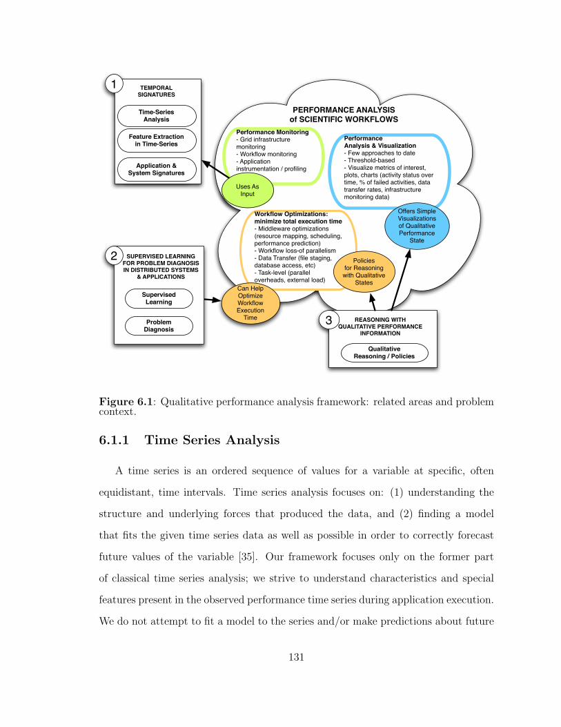
Application & System Signatures
PERFORMANCE ANALYSISof SCIENTIFIC WORKFLOWS
Performance Monitoring- Grid infrastructure monitoring- Workflow monitoring- Application instrumentation / profiling
Workflow Optimizations: minimize total execution time- Middleware optimizations (resource mapping, scheduling, performance prediction)- Workflow loss-of parallelism- Data Transfer (file staging, database access, etc)- Task-level (parallel overheads, external load)
PerformanceAnalysis & Visualization- Few approaches to date- Threshold-based- Visualize metrics of interest, plots, charts (activity status over time, % of failed activities, data transfer rates, infrastructure monitoring data)
Uses As Input
Can HelpOptimize Workflow Execution
Time
Offers SimpleVisualizationsof Qualitative Performance
State
Policiesfor Reasoningwith Qualitative
States
1
3
Supervised Learning
Problem Diagnosis
2 SUPERVISED LEARNINGFOR PROBLEM DIAGNOSISIN DISTRIBUTED SYSTEMS
& APPLICATIONS
Time-SeriesAnalysis
TEMPORALSIGNATURES
REASONING WITHQUALITATIVE PERFORMANCE
INFORMATION
QualitativeReasoning / Policies
Feature Extractionin Time-Series
Figure 6.1: Qualitative performance analysis framework: related areas and problemcontext.
6.1.1 Time Series Analysis
A time series is an ordered sequence of values for a variable at specific, often
equidistant, time intervals. Time series analysis focuses on: (1) understanding the
structure and underlying forces that produced the data, and (2) finding a model
that fits the given time series data as well as possible in order to correctly forecast
future values of the variable [35]. Our framework focuses only on the former part
of classical time series analysis; we strive to understand characteristics and special
features present in the observed performance time series during application execution.
We do not attempt to fit a model to the series and/or make predictions about future
131
performance metric values.
There are two common classes of techniques applied to time series analysis: fre-
quency domain techniques and time domain techniques. Frequency domain method-
ologies, such as spectral analysis or wavelet analysis, investigate a given time series
with respect to frequency, while time-domain ones, such as auto-correlation and cross-
correlation analysis, investigate the series with respect to time. In our work, we rely
primarily on using time domain methodologies, in particular we make use of auto-
correlation analysis for pattern detection.
Examples of Time Series Analysis for Performance Analysis
Various time series analysis methodologies have been widely employed in under-
standing and improving the performance of applications and systems. We present
a small subset of such examples and discuss similarities and differences with our
approach.
Tran addresses in [105] the Input/Output (I/O) performance in high-performance
computing (HPC) systems. An adaptive framework, called TsModeler, automati-
cally models I/O requests using auto-regressive integrated moving average (ARIMA)
time series models to predict temporal patterns of I/O requests. The resulting time
series models coupled with spatial Markov model predictions enable more efficient
prefetching of blocks in I/O systems. Our framework uses similar time series analysis
techniques, in particular aspects related to auto-correlation analysis for automatic
time series model identification. However, mathematical properties of the ACF are
only used for a heuristic pattern identification mechanism, instead of more complex
methods, such as periodicity detection mechanisms [4, 34]. We do not attempt to
find a best model for any of the performance time series; we are only interested in
extracting a small set of features from the series that we hypothesize can be used for
problem diagnosis in long-running scientific Grid applications.
132
Brutlag [18] proposes a mathematical model based on exponential smoothing and
Holt-Winters forecasting for the automatic aberrant behavior detection in network
time series. Aberrant network behavior in performance time series data is decom-
posed in three components: (1) an algorithm for predicting values of a time series
one time step into the future, (2) a measure of deviation between the predicted and
observed values, and (3) a mechanism to reason if one or more observed values are
“significantly deviant” from the prediction. A similar approach is also described in
[112], where the focus is to detect as soon as possible network performance failures
by studying deviations in the performance time series data of number of Internet ser-
vice requests processed over a specific time interval. While they do not use specific
time series model fitting for forecasting as in [18], they do use the expected mean
and variance of each process to identify whether the observation is within expected
norms. While we are also interested in detecting unexpected or aberrant behavior in
time series, we do not take the same approach with [18]. As previously stated, we do
not use techniques for time series forecasting. Furthermore, we analyze characteris-
tics of a set of time series, not only an individual time series, as we are interested
in an application’s behavior as it utilizes necessary resources within a system (e.g.,
CPUs, memory, disk, network).
6.1.2 Dimensionality Reduction for Time Series Data
Massive data sets have become common in many applications and pose new chal-
lenges for knowledge discovery. When dealing with massive multi-variate time series
data, we must employ specific techniques that analyze these data as automatically
as possible and provide us with the needed information to make a specific decision
within a specific context. This general problem is known as dimensionality reduc-
tion, and various techniques have been developed to address it. The techniques are
broadly classified in two categories: (1) variable selection, and (2) feature selection
133

& extraction. The process of variable selection refers to identifying a small set of
time series metrics variables that are most useful in identifying or detecting a specific
objective function. Feature selection refers to the automatic process of identifying a
small set of relevant features or characteristics within the selected variables that can
be of further use for the same objective function; feature extraction is the process
by which a selected feature can be extracted from the data. There are significant
benefits to using techniques for dimensionality reduction. Benefits include: (1) mak-
ing easier data understanding and visualization, (2) reducing the measurement and
storage requirements, (3) reducing the time needed to train a classifier for the data,
and (4) defying the curse of dimensionality to improve the classifier efficacy [46].
In this work we assume that variable selection has been already performed by
either a domain expert or by an automatic technique such as the metric attribution
described by Cohen [21]. Our focus is on deciding on a set of features in time series
that would be most useful and relevant to distinguish between possible persistent
problem states affecting application performance.
The types of features that one can select and extract form time series data can
be broadly classified in two categories: (1) statistical features, and (2) structural
features.
Statistical features are extracted using established concepts from statistical de-
cision theory to discriminate among data from different groups based on quantita-
tive features of the data [87]. Common techniques for statistical feature extraction
include various time series transformations, including the identity transformation,
Fourier transformations and wavelet transformations. Examples of statistical fea-
tures in time series data include mean, variance, frequency counts, auto-correlation
coefficients, wavelet transform coefficients and so on.
Structural features are extracted using methods relied on syntactic grammars to
134
discriminate among data from different groups based upon the morphological in-
terconnections present within data. Examples of structural features in time series
include the extraction of presence of straight lines, parabolas, peaks, sinusoidal, tri-
angular or rectangular patterns.
Limitations of using statistical features for classifications include the difficulty of
extracting structural patterns or sub-patterns from the data using only quantitative
features, while the limitation of using structural features for classification include the
difficulty of implementing the feature extraction in general, in the absence of specific
domain knowledge.
Below we give some selected examples from both approaches using both types of
features to achieve classification of time series data.
Use of Statistical Features for Time Series Classification
Nurmi and Floreen [86] propose a method to selecting features in time series
data that is generated in adaptive, context-aware systems. Data available in these
contexts include time series data from a user’s GPS, cellular phone, car accelerometer
reading. Other sensors may measure physical characteristics of the user context,
and the potential for data generation is enormous. Therefore, the authors devise a
scheme involving feature selection in time series in order to reduce communications
and computational costs. The features used are statistical measurements of the time
series and include the mean, variance, auto-correlation and absolute magnitude and
they various subsets of them are selected for transmission at different times, ti, based
on their relevance to the user activity.
Mierswa [74, 75] describes a methodology that extracts and uses a set of statistical
features from audio data. Statistical features extracted include the average loudness,
average distance and variance between extreme values, tempo and variance of the
auto-correlation, k highest peaks after a Fourier transfomration and so on. The
135
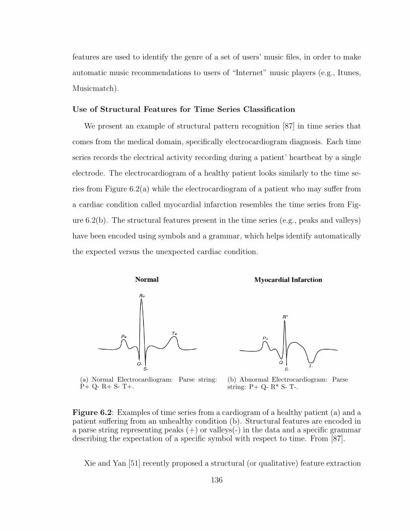
features are used to identify the genre of a set of users’ music files, in order to make
automatic music recommendations to users of “Internet” music players (e.g., Itunes,
Musicmatch).
Use of Structural Features for Time Series Classification
We present an example of structural pattern recognition [87] in time series that
comes from the medical domain, specifically electrocardiogram diagnosis. Each time
series records the electrical activity recording during a patient’ heartbeat by a single
electrode. The electrocardiogram of a healthy patient looks similarly to the time se-
ries from Figure 6.2(a) while the electrocardiogram of a patient who may suffer from
a cardiac condition called myocardial infarction resembles the time series from Fig-
ure 6.2(b). The structural features present in the time series (e.g., peaks and valleys)
have been encoded using symbols and a grammar, which helps identify automatically
the expected versus the unexpected cardiac condition.
(a) Normal Electrocardiogram: Parse string:P+ Q- R+ S- T+.
(b) Abnormal Electrocardiogram: Parsestring: P+ Q- R* S- T-.
Figure 6.2: Examples of time series from a cardiogram of a healthy patient (a) and apatient suffering from an unhealthy condition (b). Structural features are encoded ina parse string representing peaks (+) or valleys(-) in the data and a specific grammardescribing the expectation of a specific symbol with respect to time. From [87].
Xie and Yan [51] recently proposed a structural (or qualitative) feature extraction
136
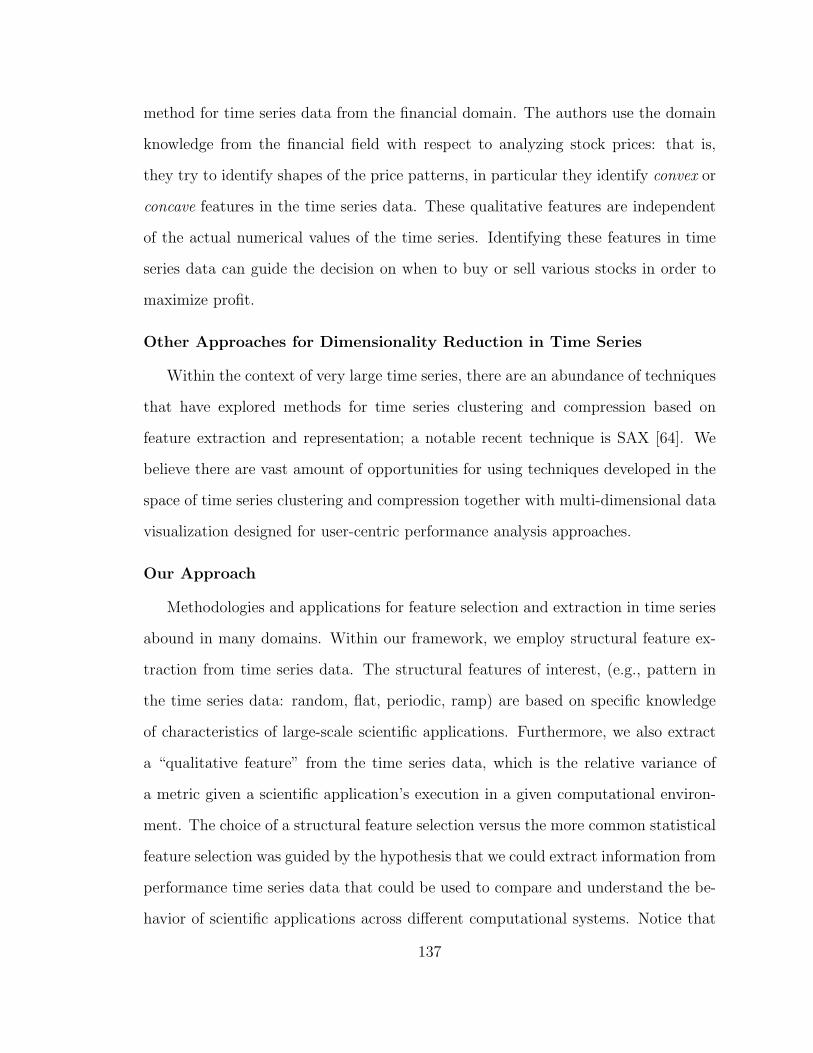
method for time series data from the financial domain. The authors use the domain
knowledge from the financial field with respect to analyzing stock prices: that is,
they try to identify shapes of the price patterns, in particular they identify convex or
concave features in the time series data. These qualitative features are independent
of the actual numerical values of the time series. Identifying these features in time
series data can guide the decision on when to buy or sell various stocks in order to
maximize profit.
Other Approaches for Dimensionality Reduction in Time Series
Within the context of very large time series, there are an abundance of techniques
that have explored methods for time series clustering and compression based on
feature extraction and representation; a notable recent technique is SAX [64]. We
believe there are vast amount of opportunities for using techniques developed in the
space of time series clustering and compression together with multi-dimensional data
visualization designed for user-centric performance analysis approaches.
Our Approach
Methodologies and applications for feature selection and extraction in time series
abound in many domains. Within our framework, we employ structural feature ex-
traction from time series data. The structural features of interest, (e.g., pattern in
the time series data: random, flat, periodic, ramp) are based on specific knowledge
of characteristics of large-scale scientific applications. Furthermore, we also extract
a “qualitative feature” from the time series data, which is the relative variance of
a metric given a scientific application’s execution in a given computational environ-
ment. The choice of a structural feature selection versus the more common statistical
feature selection was guided by the hypothesis that we could extract information from
performance time series data that could be used to compare and understand the be-
havior of scientific applications across different computational systems. Notice that
137
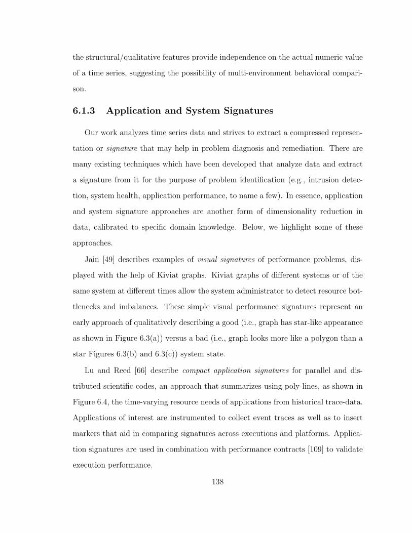
the structural/qualitative features provide independence on the actual numeric value
of a time series, suggesting the possibility of multi-environment behavioral compari-
son.
6.1.3 Application and System Signatures
Our work analyzes time series data and strives to extract a compressed represen-
tation or signature that may help in problem diagnosis and remediation. There are
many existing techniques which have been developed that analyze data and extract
a signature from it for the purpose of problem identification (e.g., intrusion detec-
tion, system health, application performance, to name a few). In essence, application
and system signature approaches are another form of dimensionality reduction in
data, calibrated to specific domain knowledge. Below, we highlight some of these
approaches.
Jain [49] describes examples of visual signatures of performance problems, dis-
played with the help of Kiviat graphs. Kiviat graphs of different systems or of the
same system at different times allow the system administrator to detect resource bot-
tlenecks and imbalances. These simple visual performance signatures represent an
early approach of qualitatively describing a good (i.e., graph has star-like appearance
as shown in Figure 6.3(a)) versus a bad (i.e., graph looks more like a polygon than a
star Figures 6.3(b) and 6.3(c)) system state.
Lu and Reed [66] describe compact application signatures for parallel and dis-
tributed scientific codes, an approach that summarizes using poly-lines, as shown in
Figure 6.4, the time-varying resource needs of applications from historical trace-data.
Applications of interest are instrumented to collect event traces as well as to insert
markers that aid in comparing signatures across executions and platforms. Applica-
tion signatures are used in combination with performance contracts [109] to validate
execution performance.
138
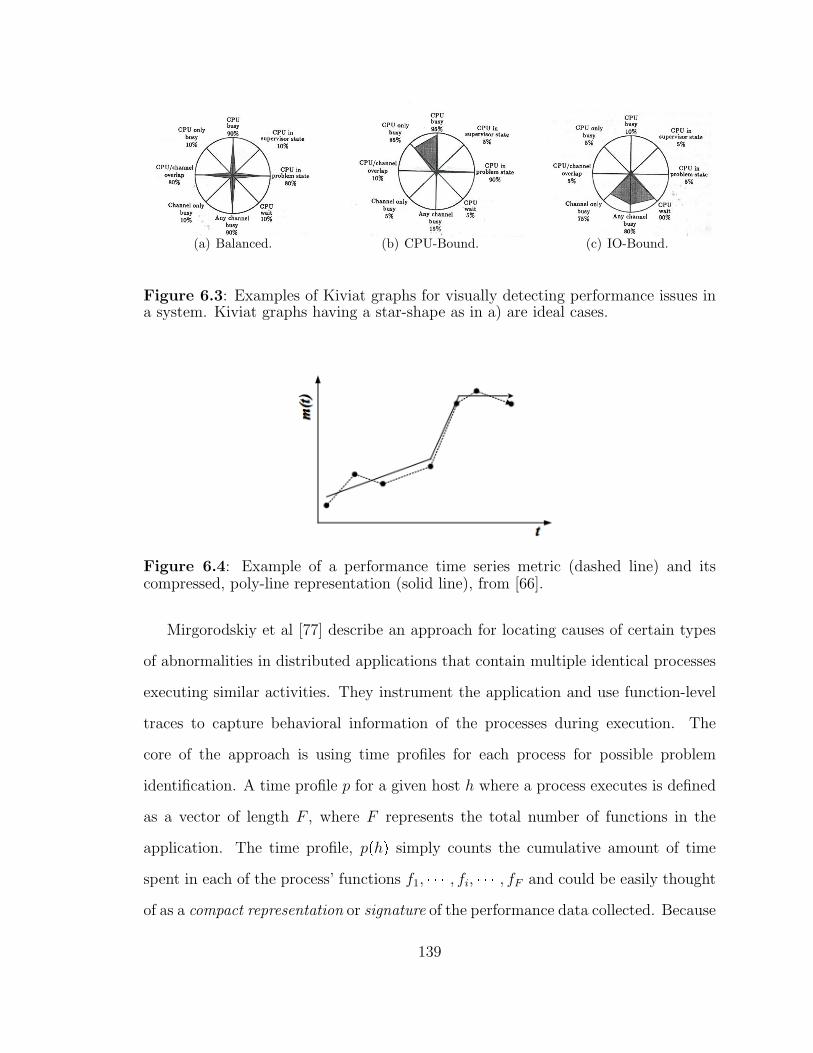
(a) Balanced. (b) CPU-Bound. (c) IO-Bound.
Figure 6.3: Examples of Kiviat graphs for visually detecting performance issues ina system. Kiviat graphs having a star-shape as in a) are ideal cases.
Figure 6.4: Example of a performance time series metric (dashed line) and itscompressed, poly-line representation (solid line), from [66].
Mirgorodskiy et al [77] describe an approach for locating causes of certain types
of abnormalities in distributed applications that contain multiple identical processes
executing similar activities. They instrument the application and use function-level
traces to capture behavioral information of the processes during execution. The
core of the approach is using time profiles for each process for possible problem
identification. A time profile p for a given host h where a process executes is defined
as a vector of length F , where F represents the total number of functions in the
application. The time profile, pphq simply counts the cumulative amount of time
spent in each of the process’ functions f1, � � � , fi, � � � , fF and could be easily thought
of as a compact representation or signature of the performance data collected. Because
139
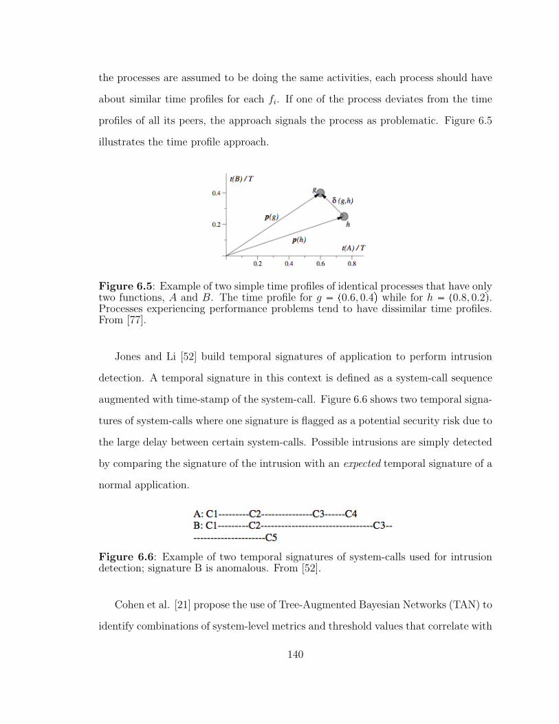
the processes are assumed to be doing the same activities, each process should have
about similar time profiles for each fi. If one of the process deviates from the time
profiles of all its peers, the approach signals the process as problematic. Figure 6.5
illustrates the time profile approach.
Figure 6.5: Example of two simple time profiles of identical processes that have onlytwo functions, A and B. The time profile for g � p0.6, 0.4q while for h � p0.8, 0.2q.Processes experiencing performance problems tend to have dissimilar time profiles.From [77].
Jones and Li [52] build temporal signatures of application to perform intrusion
detection. A temporal signature in this context is defined as a system-call sequence
augmented with time-stamp of the system-call. Figure 6.6 shows two temporal signa-
tures of system-calls where one signature is flagged as a potential security risk due to
the large delay between certain system-calls. Possible intrusions are simply detected
by comparing the signature of the intrusion with an expected temporal signature of a
normal application.
Figure 6.6: Example of two temporal signatures of system-calls used for intrusiondetection; signature B is anomalous. From [52].
Cohen et al. [21] propose the use of Tree-Augmented Bayesian Networks (TAN) to
identify combinations of system-level metrics and threshold values that correlate with
140
high-level performance states in a three-tier Web service. TAN models are further
used for offline forensic diagnosis and in limited settings for performance forecasting.
More recent work by Cohen et al. [22] presents a method for automatically extracting
an indexable signature that distills the essential characteristics from a system state.
The technique clusters system states corresponding to similar problems, allowing
diagnosticians to identify recurring problems and to characterize the core features of
a group of problems.
6.2 Learning Techniques for Problem Diagnosis
There exist two fundamental approaches by which one can learn from perfor-
mance data cases of expected or unexpected behavior. One approach, called super-
vised learning (or classification), relies on an expert to provide samples of behaviors
that correspond to healthy and unhealthy performance states. The other approach,
called unsupervised learning (or clustering), attempts to discover groups of data that
correlate with performance states. While there are a large number of works employ-
ing such techniques, we only present a few examples to illustrate the techniques as
applied to performance data.
6.2.1 Classification Techniques
A component of our framework includes a supervised-learner (or classifier) that
trains to distinguish good versus bad performance cases. In an on-line-setting, it
helps to distinguish possible problem states affecting application performance.
Classification techniques used for a wide range of data abound in literature [32,
47]. Methods include k-nearest-neighbor search, neural networks classifiers, fuzzy
classifiers, Bayesian classifiers, or support vector machines. The current work uses
a classifier based on the k-nearest-neighbor algorithm. In the next section, we will
describe some approaches that use classification to help with problem diagnosis in
141
distributed systems and applications.
Yuan et al [117] describe a technique based on supervised learning to identify
reproducible failures from system call traces of applications. Similarly to the approach
we take in our framework, the label of the trace determines the type of observed
problem and in the case described the root cause of the problem.
6.2.2 Clustering Techniques
In [77], the authors use dynamic instrumentation to collect control-flow traces of
each process in a distributed application that contains multiple identical processes
performing similar activities. Because the processes are assumed to behave similarly
by having the same control-flow, problems such as fail-stop2 are detected by identi-
fying processes that stopped earlier than the rest, while non-fail-stop problems are
detected using outlier detection techniques to identify processes that behave differ-
ently from the rest.
Roth and Miller [98] introduce a scalable performance diagnosis approach for
finding performance problems in applications with a large number of processes. The
approach employs two techniques: (1) a well-established technique for methodically
examining the solution space and (2) a Sub-Graph Folding Algorithm for bottleneck
search, that dynamically clusters application processes based on their qualitative
behavior.
6.3 Context: Performance Analysis of Scientific
Workflows
The fundamental metric that defines performance in the case of workflow appli-
cations is the total time to execute the entire instance of a workflow, Tworkflow. This
time depends on several factors, including (1) the amount of resources allocated to it,
2A problem in which some processes stop earlier than the rest.
142
(2) the type of computational resources assigned (e.g., CPU speed, memory size, disk
and network resources), and (3) characteristics of the workflow/application executing
on these resources.
Because of these factors, researchers have employed a variety of techniques to
improve the overall execution time, including mechanisms that optimize the amount
and types of resources available to the workflow before and during execution as well as
methodologies to understand characteristics of the specific application and optimize
for those specific characteristics (e.g., load imbalance, communication, external load,
etc). Moreover, very recent approaches have looked at building the infrastructure and
required tools to provide performance monitoring data, analysis and visualization for
scientific workflows at multiple levels of abstraction, ranging task-level monitoring to
global workflow level monitoring.
In the following section, we present an overview of some of these key approaches.
We then present our framework within this larger context and discuss similarities,
differences and interactions between our framework and these related approaches.
6.3.1 Performance Monitoring
There are many distributed performance monitoring tools available for Grids; a
detailed categorization and comparison of the tools is done in [41]. Our focus is to
be aware of performance monitoring tools that have been made available to support
performance monitoring of scientific workflows, as this data can be used as input by
our framework.
SCALEA-G [108] is one of the few unified monitoring and performance analysis
for Grid applications. The framework offers support for both source code and dy-
namic instrumentation for profiling and monitoring events of Grid applications. The
performance monitoring data is used by methodologies for performance analysis and
143
visualization for scientific workflows. Some of these approaches are detailed later, in
Section 6.3.4. Another performance monitoring framework is MonALISA [62], which
is a widely used distributed service for collecting and processing monitoring infor-
mation for Grids and distributed applications. The monitoring information gathered
can be used by higher-level services to provide decision support, in order to maintain
and optimize workflow through the Grid.
Another widely used performance data monitoring for clusters and Grids is Gan-
glia [69]. Ganglia utilizes a hierarchical design to gather data from federations of
clusters. It employs the use of commonly used technologies for data representation
(XML), data compaction and transport (XDR), and for storage and visualization
(RRDtool). It utilizes carefully designed data structures and algorithms to have a
low overhead at both the individual node resource level and for groups of resources.
Ganglia is currently used on thousands of clusters around the world [1].
Our methodology can easily integrate with any Grid application performance
monitoring system and provide a qualitative performance analysis service to the Grid
application users.
6.3.2 Workflow Optimizations
Because there are many different levels at which a scientific workflow’s execution
time can be improved, we present a brief overview of related work studying effi-
cient resource selection and mapping, scheduling strategies, methods to detect loss
of parallelism in workflows, optimizations for data transfers, as well as comprehen-
sive methods attempting to optimize workflow performance by optimizing at multiple
levels at once.
144
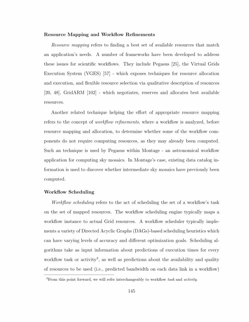
Resource Mapping and Workflow Refinements
Resource mapping refers to finding a best set of available resources that match
an application’s needs. A number of frameworks have been developed to address
these issues for scientific workflows. They include Pegasus [25], the Virtual Grids
Execution System (VGES) [57] - which exposes techniques for resource allocation
and execution, and flexible resource selection via qualitative description of resources
[20, 48], GridARM [102] - which negotiates, reserves and allocates best available
resources.
Another related technique helping the effort of appropriate resource mapping
refers to the concept of workflow refinements, where a workflow is analyzed, before
resource mapping and allocation, to determine whether some of the workflow com-
ponents do not require computing resources, as they may already been computed.
Such an technique is used by Pegasus within Montage - an astronomical workflow
application for computing sky mosaics. In Montage’s case, existing data catalog in-
formation is used to discover whether intermediate sky mosaics have previously been
computed.
Workflow Scheduling
Workflow scheduling refers to the act of scheduling the set of a workflow’s task
on the set of mapped resources. The workflow scheduling engine typically maps a
workflow instance to actual Grid resources. A workflow scheduler typically imple-
ments a variety of Directed Acyclic Graphs (DAGs)-based scheduling heuristics which
can have varying levels of accuracy and different optimization goals. Scheduling al-
gorithms take as input information about predictions of execution times for every
workflow task or activity3, as well as predictions about the availability and quality
of resources to be used (i.e., predicted bandwidth on each data link in a workflow)
3From this point forward, we will refer interchangeably to workflow task and activity.
145
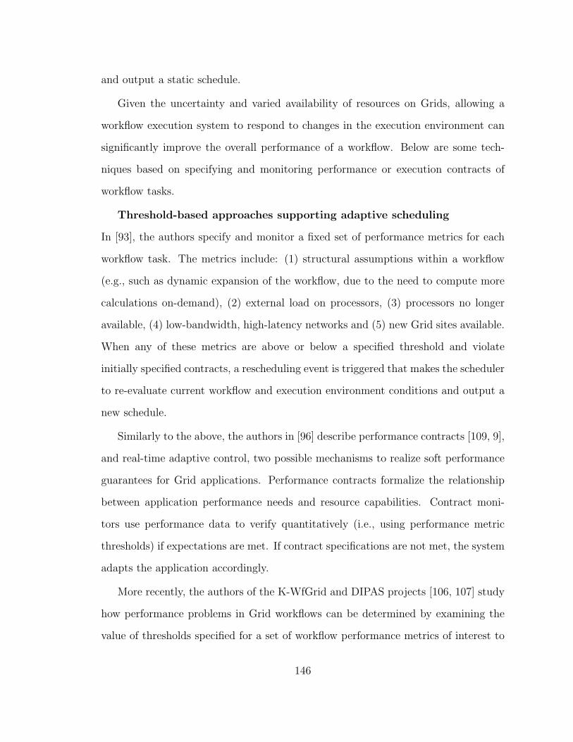
and output a static schedule.
Given the uncertainty and varied availability of resources on Grids, allowing a
workflow execution system to respond to changes in the execution environment can
significantly improve the overall performance of a workflow. Below are some tech-
niques based on specifying and monitoring performance or execution contracts of
workflow tasks.
Threshold-based approaches supporting adaptive scheduling
In [93], the authors specify and monitor a fixed set of performance metrics for each
workflow task. The metrics include: (1) structural assumptions within a workflow
(e.g., such as dynamic expansion of the workflow, due to the need to compute more
calculations on-demand), (2) external load on processors, (3) processors no longer
available, (4) low-bandwidth, high-latency networks and (5) new Grid sites available.
When any of these metrics are above or below a specified threshold and violate
initially specified contracts, a rescheduling event is triggered that makes the scheduler
to re-evaluate current workflow and execution environment conditions and output a
new schedule.
Similarly to the above, the authors in [96] describe performance contracts [109, 9],
and real-time adaptive control, two possible mechanisms to realize soft performance
guarantees for Grid applications. Performance contracts formalize the relationship
between application performance needs and resource capabilities. Contract moni-
tors use performance data to verify quantitatively (i.e., using performance metric
thresholds) if expectations are met. If contract specifications are not met, the system
adapts the application accordingly.
More recently, the authors of the K-WfGrid and DIPAS projects [106, 107] study
how performance problems in Grid workflows can be determined by examining the
value of thresholds specified for a set of workflow performance metrics of interest to
146
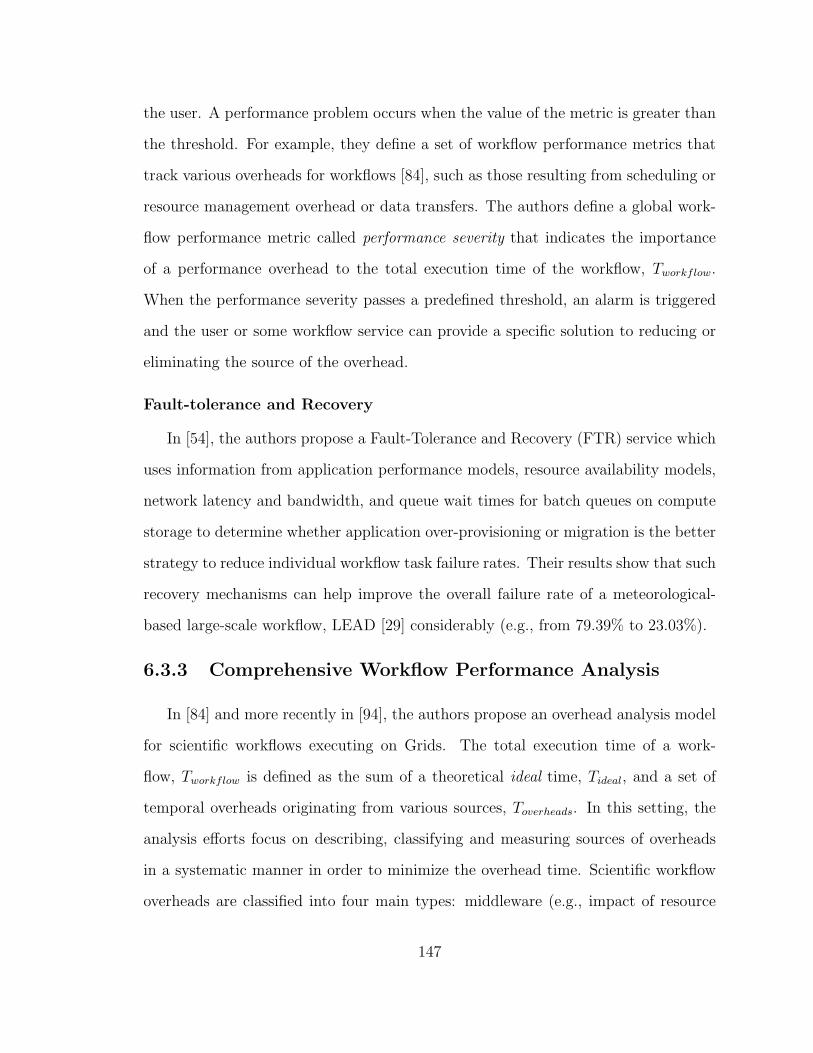
the user. A performance problem occurs when the value of the metric is greater than
the threshold. For example, they define a set of workflow performance metrics that
track various overheads for workflows [84], such as those resulting from scheduling or
resource management overhead or data transfers. The authors define a global work-
flow performance metric called performance severity that indicates the importance
of a performance overhead to the total execution time of the workflow, Tworkflow.
When the performance severity passes a predefined threshold, an alarm is triggered
and the user or some workflow service can provide a specific solution to reducing or
eliminating the source of the overhead.
Fault-tolerance and Recovery
In [54], the authors propose a Fault-Tolerance and Recovery (FTR) service which
uses information from application performance models, resource availability models,
network latency and bandwidth, and queue wait times for batch queues on compute
storage to determine whether application over-provisioning or migration is the better
strategy to reduce individual workflow task failure rates. Their results show that such
recovery mechanisms can help improve the overall failure rate of a meteorological-
based large-scale workflow, LEAD [29] considerably (e.g., from 79.39% to 23.03%).
6.3.3 Comprehensive Workflow Performance Analysis
In [84] and more recently in [94], the authors propose an overhead analysis model
for scientific workflows executing on Grids. The total execution time of a work-
flow, Tworkflow is defined as the sum of a theoretical ideal time, Tideal, and a set of
temporal overheads originating from various sources, Toverheads. In this setting, the
analysis efforts focus on describing, classifying and measuring sources of overheads
in a systematic manner in order to minimize the overhead time. Scientific workflow
overheads are classified into four main types: middleware (e.g., impact of resource
147
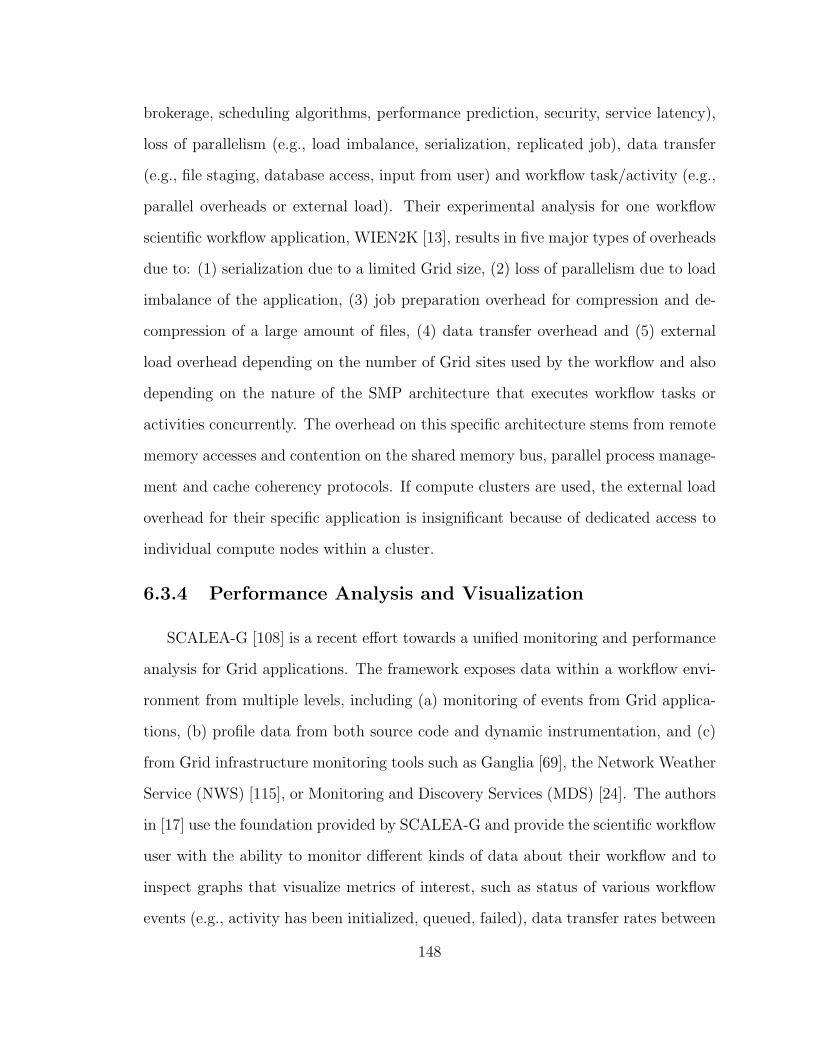
brokerage, scheduling algorithms, performance prediction, security, service latency),
loss of parallelism (e.g., load imbalance, serialization, replicated job), data transfer
(e.g., file staging, database access, input from user) and workflow task/activity (e.g.,
parallel overheads or external load). Their experimental analysis for one workflow
scientific workflow application, WIEN2K [13], results in five major types of overheads
due to: (1) serialization due to a limited Grid size, (2) loss of parallelism due to load
imbalance of the application, (3) job preparation overhead for compression and de-
compression of a large amount of files, (4) data transfer overhead and (5) external
load overhead depending on the number of Grid sites used by the workflow and also
depending on the nature of the SMP architecture that executes workflow tasks or
activities concurrently. The overhead on this specific architecture stems from remote
memory accesses and contention on the shared memory bus, parallel process manage-
ment and cache coherency protocols. If compute clusters are used, the external load
overhead for their specific application is insignificant because of dedicated access to
individual compute nodes within a cluster.
6.3.4 Performance Analysis and Visualization
SCALEA-G [108] is a recent effort towards a unified monitoring and performance
analysis for Grid applications. The framework exposes data within a workflow envi-
ronment from multiple levels, including (a) monitoring of events from Grid applica-
tions, (b) profile data from both source code and dynamic instrumentation, and (c)
from Grid infrastructure monitoring tools such as Ganglia [69], the Network Weather
Service (NWS) [115], or Monitoring and Discovery Services (MDS) [24]. The authors
in [17] use the foundation provided by SCALEA-G and provide the scientific workflow
user with the ability to monitor different kinds of data about their workflow and to
inspect graphs that visualize metrics of interest, such as status of various workflow
events (e.g., activity has been initialized, queued, failed), data transfer rates between
148
Grid sites, analysis and comparison of activity distribution for Grid sites as well as
querying of infrastructure monitoring information during execution (e.g., what is the
CPU load on host A at a specified Grid site).
Another similar project aimed at expanding the number of performance moni-
toring and analysis tools for scientific workflows is the K-WfGrid project, [106]. It
exposes the monitoring and analysis of workflows and the corresponding computa-
tional infrastructure through a Web portal. The difference from [17] appears to be
the introduction of XML-based representations for describing application structures
and specifying instrumentation requests, to ease the interaction between the many
services and clients involved in providing monitoring data and analysis services.
6.3.5 Discussion
In our research, we assume that the workflow application has already been mapped
and scheduled on the best computational resources available. Furthermore, we do
not address the issue of distributed performance monitoring for a scientific workflow,
as our framework strictly analyzes easily available time series data correlated with
workflow or task performance. For example, our approach can use data provided
at the workflow level by an integrated Grid performance monitoring tool such as
SCALEA-G [108] or that in the related K-WfGrid project [106], and transform it to
a compact representation so as to learn essential characteristics of data that correlate
well with workflow performance states. Performance monitoring and visualization
tools such as those in [17] are very valuable since they enhance the support provided
to a scientific user to understand the performance of a workflow. However, they do
rely on the user to “analyze” the data charts, plots and other visual information. This
analysis process may be reasonable for a user with prior experience to performance
analysis tools and for inspection of moderate amounts of data and plots. However,
when the workflow scales to thousands of nodes, and the amounts of data monitored is
149
very large, even experienced performance analysts will have difficulties understanding
the performance of the analyzed workflow. Our approach represents a small-step
towards a self-assessing and self-diagnosing performance framework, where we rely
a user’s notion of a successful and well-performing workflow or activity execution to
learn patterns in the performance data associated with these qualitative performance
states.
The qualitative performance analysis framework we propose in this thesis is in-
tended to help minimize the total workflow execution time, Tworkflow, by analyzing,
during execution, performance data characteristics of the longest-running workflow
tasks, and offering qualitative and intuitive interpretations of performance to both
the scientific application user and a fault-tolerance and recovery service, such as [54],
which can use the information to trigger recovery/scheduling events based on specific
policies.
Comprehensive Workflow Performance Analysis
Using the overhead terminology introduced by [84], this thesis concentrates on
understanding the overhead involved only in long-running activities (or tasks) within
a scientific workflow, the reasoning being that since long-running components con-
stitute a significant time of the total running time, optimizing this subset of tasks
will result in the optimization of the overall execution time of a workflow, Tworkflow.
Our framework can analyze activities that are either individual programs or parallel
programs; we only require a labeling of whether the long-running activity was suc-
cessful, as well as performance monitoring data of interest collected from where each
studied activity executes.
Threshold-based Approaches
Threshold-based approaches such as those in [93, 96, 106], are definitely useful to a
user who knows (1) the key metrics to monitor, and (2) the best value of the threshold
150
that would capture the most important performance problems without triggering false
alarms. The major weakness of threshold-based approaches that rely on static, non-
adaptive thresholds is the assumption that these meaningful threshold values are
known in advance. This is seldomly true in practice. Furthermore, in a complex
and dynamic environment such as a Grid on which different scientific workflows with
varied characteristics execute, finding meaningful performance metric thresholds for
a scientific workflow is extremely difficult.
While there are no formal service-level agreements (SLA) for scientific workflows
as in the commercial Grid domain (though specific threshold methods could be con-
sidered in essence, SLAs for workflows), we attempt to define the concept of an SLA
in terms of the qualitative notion of performance as understood by the scientific user.
Our approach will integrate well with self-healing, fault-tolerance and recovery ap-
proaches for scientific workflow tasks as described in [54], because in the cases of
long-running workflow tasks, the FTR framework does not need to wait for the task
to fail in order to initiate a remedy action. The qualitative performance output of our
framework can notify FTR of persistent performance problems/degradations affect-
ing long-running activities and various policies for triggering an FTR action can be
implemented, depending on each tasks’s effect on the global workflow performance.
Problem Diagnosis in Large-Scale Distributed Environments
Because of the assumption of process similarity, the methodology in [77] does not
require learning a database of reference data to distinguish good versus anomalous
behaviors. On the contrary, our approach relies on a supervised learning technique
to identify in a training phase well-performing versus poor-performing application
states. The performance data we collect is also different in two ways: (1) it does not
come from sources involving application instrumentation (static or dynamic), and (2)
it is collected at much coarser time scales then instrumentation traces. As a result,
151
the types of diagnostic problems we are able to detect are dependent on whether the
specific problem will manifest itself persistently over a longer period of time within
the data we analyze.
6.4 Summary
We described in this chapter selected works spanning three main domains: time
series analysis and dimensionality reduction, supervised learning for problem diag-
nosis and qualitative reasoning. We have discussed how our proposed framework
compares and contrasts with these selected works.
The performance analysis framework we propose in this thesis is different from
existing approaches supporting the performance scientific workflows in several ways:
1. We focus only on the performance of long-running tasks within a scientific
workflow,
2. We analyze and extract information only from performance time series data
and not qualitative variables such as those describing the execution status of a
task (e.g., running, started, failed),
3. We do not currently analyze data that require instrumentation of application
code,
4. We target the scientific workflow user who does not have the experience of using
traditional performance analysis tools for the science applications,
5. We show how to correlate qualitative behavioral task states to performance
time series metrics and how to use it for problem diagnosis and remediation.
While similar methodologies at the intersection of machine learning, statistical
induction, and systems [44] have been previously applied in different domains [21, 22,
152

15], we believe, to the best of our knowledge, this to be a first work looking at a user-
centric, qualitative performance evaluation and failure detection by automatically
deriving correlations from the data in the context of scientific workflows executing in
Grid environments.
153
Chapter 7
Conclusion and Future Directions
This thesis presented a general qualitative performance analysis framework that
incorporated (a) techniques from time series analysis and machine learning to extract
and learn from data, features of interest associated with application performance
in order to reach a qualitative interpretation of the application’s behavior, and (b)
mechanisms and policies to reason over time and across the distributed resource space
about the qualitative behavior of the application.
7.1 Conclusions
Our empirical evaluation with two real Grid applications from meteorology and
astronomy on diverse physical computing resources showed support for our two stated
hypotheses: (1) for the class of long-running scientific applications it is necessary to
analyze temporal information present in performance data, and (2) that variance
and pattern as specific instances of such information are sufficient for accurate per-
formance validation and diagnosis.
The proposed framework’s ability to generate a qualitative assessment of per-
formance behavior for scientific applications using temporal information present in
performance time series data represents a step towards simplifying and improving
the quality of service for Grid applications.
7.2 Future Directions
We look forward to future research that will strive to achieve a comprehensive
qualitative performance analysis of scientific workflows, by transforming information
found in performance metrics into meaningful, qualitative information useful to both
154
a workflow user and a performance analyst/or performance analysis service.
Additionally, it would be very interesting to test the efficacy of our approach given
variations on the techniques we proposed, as shown in the x-axis, and variations on
context, as described in the z-axis of Figure 7.1.
Below we discuss four potential directions for improvement specific to our context:
scientific workflow applications executing in distributed Grid environments.
7.2.1 Variable and Feature Selection for Performance Data
In this thesis we have chosen a set of variables (e.g., system-level time series
data), and a set of features of the variables (e.g., relative variance and pattern) to
build temporal signatures of applications for performance validation and diagnosis.
Our choices were guided by specific domain knowledge of scientific applications. How-
ever, many performance time series variables can be collected and used for analysis.
For this purpose, the analyst may want to consider existing techniques for automatic
variable and feature selection in order to build a good predictor of application per-
formance. Guyon et al [46] present a good overview of available techniques, which
include independent variable ranking based on correlation criteria or information the-
oretic criteria, variable subset selection based on wrappers and embedded methods
or filters, and feature selection methods employing clustering or matrix factorization
techniques. More specifically to feature extraction in time series data, the work of
Olszewski [87] presents a good overview of existing statistical and structural feature
extraction techniques for time series; the author also proposes a generalized approach
for automatic structural feature extraction, which would be especially useful in do-
mains where one may not know a priori features of interest to investigate.
155
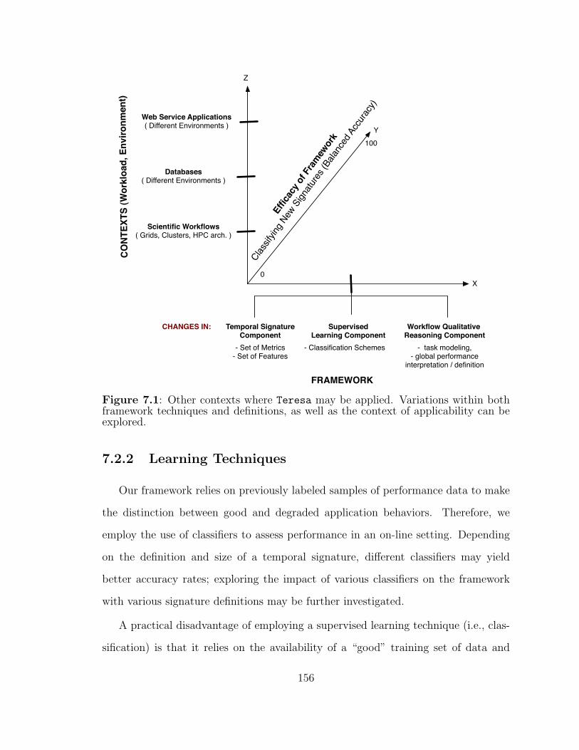
Effic
acy o
f Fra
mewor
k
Classif
ying N
ew S
ignatu
res (B
alanc
ed Ac
curac
y)
Y
X
Z
FRAMEWORK
CONT
EXTS
(Wor
kloa
d, E
nviro
nmen
t)
0
100
Temporal SignatureComponent
SupervisedLearning Component
Workflow Qualitative Reasoning Component
CHANGES IN:
- Set of Metrics- Set of Features
- Classification Schemes - task modeling,- global performance
interpretation / definition
Scientific Workflows( Grids, Clusters, HPC arch. )
Databases( Different Environments )
Web Service Applications( Different Environments )
Figure 7.1: Other contexts where Teresa may be applied. Variations within bothframework techniques and definitions, as well as the context of applicability can beexplored.
7.2.2 Learning Techniques
Our framework relies on previously labeled samples of performance data to make
the distinction between good and degraded application behaviors. Therefore, we
employ the use of classifiers to assess performance in an on-line setting. Depending
on the definition and size of a temporal signature, different classifiers may yield
better accuracy rates; exploring the impact of various classifiers on the framework
with various signature definitions may be further investigated.
A practical disadvantage of employing a supervised learning technique (i.e., clas-
sification) is that it relies on the availability of a “good” training set of data and
156

signatures for classification. In the absence of training data, the alternative is to use
unsupervised learning techniques (i.e., clustering) that may automatically discover
groups of behaviors, which over time, can be associated with various qualitative be-
havioral descriptions for a given application.
7.2.3 Reasoning with Qualitative Information
In this framework, we have only presented a couple of simple examples of how
one can implement global workflow policies based on the performance states of a
workflow’s long-running tasks to reason about workflow behavior over time, and to
trigger an adaptive re-scheduling if needed. We have assumed that each task within
a workflow has the same utility to the user; this however can be expanded in order
to reflect alternate scenarios.
Towards a Comprehensive Qualitative Performance Analysis for Work-flows
We presented a prototype framework that uses easy-to-collect, non-instrumented
performance time series, and makes a qualitative assertion about the performance of
the long-running tasks in a workflow. It would be ideal to extend our current frame-
work so that other qualitative information can be extracted from performance data
correlated with factors causing different types of workflow performance overheads as
described in [84], such as middle-ware, loss of parallelism, or data transfer.
7.2.4 Problem Diagnosis: Correlation and Causation
In diagnosis problems across science and engineering domains, it is important to
achieve two goals:
1. distinguish between normal and abnormal data within the target domain, and
2. identify the cause of the abnormal/ symptomatic data observation (and possibly
157
the chain of events from cause to symptom).
As applied to the domain of computing systems, the first goal is called problem
diagnosis or identification, while the second goal is called root cause analysis. The task
of root cause analysis is in general more difficult than problem identification because,
in essence, reverse-engineering the system that produced the diagnosis symptom data
is more challenging than observing expected and symptomatic states and building a
predictor. The crux of the problem lies in the distinction between correlation and
causation.
The performance time series data analyzed in this work allows our framework to
observe correlations between temporal features in time series data and symptoms of
performance for long-running scientific applications. Our work could be expanded
by addressing the challenging root-cause problem and incorporating techniques from
the causality inference literature [90].
158
Appendix A
Upper Bound Calculation for SampleVariance
Given a time series Z � z1, � � � , zt, � � � , zN sampled at a fixed interval of time, h,
we define the sample mean, m as:
m � 1
N
N
t�1
zt (A.1)
and the sample variance, s2 as:
s2 � 1
N
N
t�1
pzt �mq2. (A.2)
If the time series Z is bounded, that is zt P rzmin, zmaxs, so is its mean, m:
zmin ¤m ¤ zmax (A.3)
�zmin ¥ �m ¥ �zmax (A.4)
�zmax ¤ �m ¤ �zmin, (A.5)
but,
zmin ¤zt ¤ zmax. (A.6)
159
We add (A.5) and (A.6):
zmin � zmax ¤ pzt �mq ¤ zmax � zmin
�pzmax � zminq ¤ pzt �mq ¤ zmax � zmin
|zt �m| ¤ pzmax � zminq
pzt �mq2 ¤ pzmax � zminq2
s2 � 1
N
N
t�1
pzt �mq2 ¤ 1
N�Npzmax � zminq2.
Therefore, the sample variance will also be bounded:
s2 ¤ pzmax � zminq2. (A.7)
160
Bibliography
[1] Ganglia Web Site. http://www.ganglia.info, 2008.
[2] The Two Micron All Sky Survey. http://www.ipac.caltech.edu/2mass/,2006.
[3] M. Adya, F. Collopy, J. S. Armstrong, and M. Kennedy. Automatic Identifica-tion of Time Series Features for Rule-Based Forecasting. International Journalof Forecasting, 17:143–157, 2001.
[4] M. Ahdesmaki, H. Lahdesmaki, R. Pearson, H. Huttunen, and O. Yli-Harja.Robust Detection of Periodic Time Series Measured from Biological Systems.BMC Bioinformatics, 6(117), 2005.
[5] The Amazon Elastic Compute Cloud (EC2). http://www.amazon.com/b/
?node=201590011, 2008.
[6] Amazon Simple Storage Service (Amazon S3). http://www.amazon.com/gp/
browse.html?node=16427261, 2008.
[7] D. Anderson and J. Chase. Fstress User Manual. http://www.cs.duke.edu/
ari/fstress/, 2002.
[8] R. L. Anderson. Distribution of the Serial Correlation Coefficients. Annals ofMathematical Statistics, 8(1):1–13, 1941.
[9] R. Aydt, C. Mendes, D. A. Reed, and F. Vraalsen. Specifying and Moni-toring GRaDS Contracts. Technical report, University of Illinois at Urbana-Champaign, July 2001.
[10] S. Baker. Google and the Wisdom of Clouds: A Lofty New Strat-egy Aims to Put Incredible Computing Power in the Hands ofMany. http://www.businessweek.com/magazine/content/07_52/
b4064048925836.htm?chan=magazine+channel_top+stories, December13th 2007.
[11] F. Berman and T. Hey. The Scientific Imperative. In The Grid 2: Blueprintfor a New Computing Infrasctructure, pages 13–24. Morgan Kaufmann, 2004.
[12] B. G. Berriman, E. Deelman, J. C. Good, J. Jacob, D. Katz, C. Kesselman,A. C. Laity, T. Prince, G. Singh, and M.-H. Su. Montage: A Grid Enabled En-gine for Delivering Custom Science-Grade Mosaics on Demand. In Proceedingsof SPIE: Astronomical Telescopes and Instrumentation, volume 5487, Glasgow,Scotland, 2004.
161
[13] P. Blaha, K. Schwarz, G. Madsen, D. Kvasnicka, and J. Luitz. Wien2k: AnAugmented Plane Wave Plus Local Orbitals Program for Calculating CrystalProperties. Technical report, Institute of Physical and Theoretical Chemistry,Technische Universitat, 2001.
[14] G. Box and G. Jenkins. Time Series Analysis: Forecasting and Control.Holden-Day, 1970.
[15] D. Breitgand, E. Henis, and O. Shehory. Automated and Adaptive ThresholdSetting: Enabling Technology for Autonomy and Self-Management. In SecondInternational Conference on Autonomic Computing (ICAC’05), 2005.
[16] K. Brewster. Application of a Bratseth Analysis Scheme Including DopplerRadar Data. In Proceedings of the 15th Conference on Weather Analysis andForecasting, pages 92–95, 1996.
[17] P. Brunner, H.-L. Truong, and T. Fahringer. Performance Monitoring andVisualization of Grid Scientific Workflows in Askalon. In High PerformanceComputing and Communications, volume 4208, pages 170–179. Springer Berlin/ Heidelberg, 2006.
[18] J. Brutlag. Aberrant Behavior Detection in Time Series for Network Monitor-ing. In Lisa XIV, New Orleans, LA, USA, 2000.
[19] K. Chen and L. Liu. Vista: Validating and Refining Clusters Via Visualization.Information Visualization, 3(4):257–70, 2004.
[20] A. Chien, H. Casanova, Y.-S. Kee, and R. Huang. The Virtual Grid DescriptionLanguage: VgDL. Technical report, University of California San Diego, UCSD,2005.
[21] I. Cohen, M. Goldszmidt, T. Kelly, J. Symons, and J. Chase. CorrelatingInstrumentation Data to System States: A Building Block for Automated Di-agnosis and Control. In Proceedings of the OSDI, 2004.
[22] I. Cohen, S. Zhang, M. Goldszmidt, J. Symons, T. Kelly, and A. Fox. Captur-ing, Indexing, Clustering, and Retrieving System History. In In Proceedings ofSOSP, Brighton, United Kingdom, 2005.
[23] P. E. Crandall, R. A. Aydt, A. A. Chien, and D. A. Reed. Input/OutputCharacteristics of Scalable Parallel Applications. In Proceedings of the 1995ACM/IEEE Supercomputing Conference, volume 2, page 1643, San Diego, CA,USA, 1995. ACM.
162
[24] K. Czajkowski, S. Fitzgerald, I. Foster, and C. Kesselman. Grid InformationServices for Distributed Resource Sharing. In Proceedings of IEEE Interna-tional Symposium on High Performance Distributed Computing, page 181, SanFrancisco, CA, 2001. Institute of Electrical and Electronics Engineers Inc.
[25] E. Deelman, G. Singh, M.-H. Su, J. Blythe, Y. Gil, C. Kesselman, G. Mehta,and K. Vahi. Pegasus: A Framework for Mapping Complex Scientific Workflowsonto Distributed Systems. Scientific Programming, 2005.
[26] S. G. Djorgovsky, R. R. Gal, S. C. Odewahn, R. R. de Carvalho, R. Brun-ner, G. Longo, and R. Scaramella. The Palomar Digital Sky Survey(DPOSS). http://www.citebase.org/cgi-bin/citations?id=oai:arXiv.
org:astro-ph/9809187, 1998.
[27] J. Doyle and M. McGeachie. Exercising Qualitative Control in AutonomousAdaptive Survivable Systems. In Self-Adaptive Software: Applications, pages1–6. 2003.
[28] K. Droegemeier. Linked Environments for Atmospheric Discovery. Technicalreport, University of Oklahoma, 1st July 2005.
[29] K. Droegemeier, D. Gannon, D. Reed, B. Plale, J. Alameda, T. Blatzer,K. Brewster, R. Clark, B. Domenico, S. Graves, E. Joseph, D. Murray, R. Ra-machandran, M. Ramamurthy, L. Ramakrishnan, J. A. Rushing, D. Weber,R. Wilhelmson, A. Wilson, M. Xue, and S. Yalda. Service-Oriented Envi-ronments for Dynamically Interacting with Mesoscale Weather. Computing inScience and Engineering, 7(6):12–29, 2005.
[30] S. Duan and S. Babu. Processing Forecasting Queries. In Proceedings of the33rd international Conference on Very Large Data Bases (VLDB)., Vienna,Austria, 2007.
[31] R. O. Duda, P. E. Hart, and D. G. Stork. Chapter 10: Unsupervised Learningand Clustering. In Pattern Classification, pages 568–573. John Wiley & Sons,2001.
[32] R. O. Duda, P. E. Hart, and D. G. Stork. Pattern Classification. John Wiley& Sons, Inc, 2nd edition, 2001.
[33] L. Eeckhout, H. Vandierendonck, and K. De Bosschere. Quantifying the Impactof Input Data Sets on Program Behavior and Its Applications. Journal ofInstruction-Level Parallelism, 5:1–33, 2003.
[34] M. Elfeky, W. Aref, and A. Elmagarmid. Periodicity Detection in Time SeriesDatabases. IEEE Transactions on Knowledge and Data Engineering, 17(7),2005.
163
[35] NIST/SEMaTECH E-Handbook of Statistical Methods. http://www.itl.
nist.gov/div898/handbook/index.htm, 2003.
[36] B. S. Everitt and G. Dunn. Chapter 3: The Initial Examination of MultivariateData. In Applied Multivariate Data Analysis. Edward Arnold; A division ofHodder & Stoughton, London, 1991.
[37] T. Fahringer, R. Prodan, R. Duan, J. Hofer, F. Nadeem, F. Nerieri, S. Podlip-ing, J. Qin, M. Siddiqui, H.-L. Truong, A. Villazon, and M. Wieczorek.ASKaLON: A Development and Grid Computing Environment for ScientificWorkflows. In Ian J. Taylor, Ewa Deelman, Dennis B. Gannon, and MatthewShields, editors, Workflows for E-Science: Scientific Workflows for Grids,pages 450–471. Springer-Verlag, 1st edition, 2006.
[38] I. Foster. What Is the Grid: A Three Point Checklist. Grid Today, 2002.
[39] I. Foster, C. Kesselman, and S. Tuecke. The Anatomy of the Grid: EnablingScalable Virtual Organizations. International Journal of High PerformanceComputing Applications, 15(3):200, 2001.
[40] D. G. Galati and M. A. Simaan. Automatic Decomposition of Time Series intoStep, Ramp, and Impulse Primitives. Pattern Recognition, 39:2166–2174, 2006.
[41] M. Gerndt, R. Wismuller, Z. Balaton, G. Gombas, P. Kacsuk, Z. Nemeth,N. Podhorszki, H. L. Truong, T. Fahringer, M. Bubak, E. Laure, and T. Mar-galef. Performance Tools for the Grid: State of the Art and Future, ApartWhite Paper. Technical report, Technische Universitaet Muenchen, 2004.
[42] T. Gneiting and A. E. Raftery. Athmospheric Science: Weather Forecastingwith Ensemble Methods. Science, 310(5746):248–249, 2005.
[43] S. Godard. The Sysstat Utilities. http://perso.orange.fr/sebastien.
godard/.
[44] M. Goldszmidt, I. Cohen, A. Fox, and S. Zhang. Three Research Challengesat the Intersection of Machine Learning, Statistical Induction, and Systems.In 10th conference on Hot Topics in Operating Systems, volume 10, Santa Fe,NM, 2005.
[45] GridPP: UK Computing for Particle Physics. http://www.gridpp.ac.uk/,2008.
[46] I. Guyon and A. Elisseeff. An Introduction to Variable and Feature Selection.Journal of Machine Learning Research, 3:1157–1182, 2003.
[47] T. Hastie, R. Tibshirani, and J. Friedman. The Elements of Statistical Learn-ing: Data Mining, Inference, and Prediction. Springer, 2001.
164
[48] R. Huang, H. Casanova, and A. A. Chien. Using Virtual Grids to SimplifyApplication Scheduling. In Proceedings of the 20th International Parallel andDistributed Processing Symposium, Rhodes Island, Greece, 2006. IEEE.
[49] R. Jain. The Art of Computer Systems Performance Analysis. John Wiley andSons, Inc, 1991.
[50] G. M. Jenkins and D. G. Watts. Spectral Analysis and Its Applications. Holden-Day, 1968.
[51] X. Jinfei and Y. Wei-Yong. A Qualitative Feature Extraction Method for TimeSeries Analysis. In Yan Wei-Yong, editor, Control Conference, 2006. CCC2006. Chinese, pages 2220–2225, 2006.
[52] A. Jones and S. Li. Temporal Signatures for Intrusion Detection. In 17thAnnual Computer Security Applications Conference, New Orleans, Louisiana,2001.
[53] M. V. Joshi. On Evaluating Performance of Classifiers for Rare Classes. InIEEE International Conference on Data Mining, pages 641–644, 2002.
[54] G. Kandaswamy, A. Mandal, and D. A. Reed. Fault Tolerance and Recoveryof Scientific Workflows on Computational Grids. In Workshop on Resiliency inHigh-Performance Computing in conjunction with CCGrid08, 2008.
[55] E. Kandogan. Star Coordinates: A Multi-Dimensional Visualization Techniquewith Uniform Treatment of Dimensions. IEEE Symposium on InformationVisualization, 2000.
[56] D. S. Katz, G. B. Berriman, E. Deelman, J. Good, C. Kesselman, A. C. Laity,T. A. Prince, G. Singh, and M.-H. Su. A Comparison of Two Methods forBuilding Astronomical Image Mosaics on a Grid. In 7th Workshop on HighPerformance Scientific and Engineering Computing (HPSEC-05), 2005.
[57] Y.-S. Kee, D. Nurmi, G. Singh, A. Mutz, C. Kesselman, and R. Wolski.VGES: The Next Generation of Virtualized Grid Resource Provisioning. In1st IEEE/IFIP International Workshop on End-to-end Virtualization and GridManagement (EVGM 2007), 2007.
[58] A. Khan, T. Adye, C. A. J. Brew, F. Wilson, B. Bense, R. D. Cowles, D. A.Smith, D. Andreotti, C. Bozzi, E. Luppi, P. Veronesi, R. Barlow, M. P. Kelly,J. C. Werner, A. Forti, G. Grosdidier, E. Feltresi, A. Petzold, H. Lacker, andJ. E. Sundermann. Grid Applications for High Energy Physics Experiments.In The 6th IEEE/ACM International Workshop on Grid Computing, page 4,2005.
165

[59] B. Kuipers. Introduction to Qualitative Reasoning. In Qualitative Reasoning:Modeling and Simulation with Incomplete Knowledge, pages 1–16. The MITPress, Cambridge, 1994.
[60] A. C. Laity, N. Anagnostou, B. G. Berriman, J. C. Good, J. Jacob, D. Katz,and T. Prince. Montage: An Astronomical Image Mosaic Service for the NVO.In Astronomical Data Analysis Software and Systems XIV, ASP ConferenceSeries, volume XXX, 2005.
[61] The Lead Portal: Linked Environments for Atmospheric Discovery. https:
//portal.leadproject.org/gridsphere/gridsphere, 2007.
[62] I. C. Legrand, H. B. Newman, R. Voicu, C. Cirstoiu, C. Grigoras, M. Toarta,and C. Dobre. Monalisa: An Agent Based, Dynamic Service System to Monitor,Control and Optimize Grid Based Applications, September 2004.
[63] R. Levich and R. Rizzo. Alternative Tests for Time Series Dependence Basedon Autocorrelation Coefficients. Technical report, Stern School of Business,New York University, 1998.
[64] J. Lin, E. Keogh, P. Patel, and S. Lonardi. Finding Motifs in Time Series. In2nd Workshop on Temporal Data Mining, Edmonton, Alberta, Canada, 2002.
[65] S. Lohr. Google and I.B.M. Join in Cloud Computing Research. http://www.nytimes.com/2007/10/08/technology/08cloud.html, 8th October 2007.
[66] C.-d. Lu and D. A. Reed. Compact Application Signatures for Parallel andDistributed Scientific Codes. In Proceedings of Supercomputing, 2002.
[67] S. Lu, Z. Li, F. Qin, L. Tan, P. Zhou, and Y. Zhou. Bugbench: Benchmarksfor Evaluating Bug Detection Tools. In PLDI Workshop on the Evaluation ofSoftware Defect Detection Tools, 2005.
[68] J. Markoff. Software Via the Internet: Microsoft in ’Cloud’ Computing. http://www.nytimes.com/2007/09/03/technology/03cloud.html, 3rd September2007.
[69] M. L. Massie, B. Chun, and D. Culler. The Ganglia Distributed MonitoringSystem: Design, Implementation, and Experience. Parallel Computing, 30(7),2004.
[70] Matlab: Statistics Toolbox. http://www.mathworks.com/products/
statistics/demos.html?file=/products/demos/shipping/stats/
mvplotdemo.html, 2007.
[71] H. Meuer, E. Strohmaier, J. Dongara, and H. Simon. Top 500 SupercomputerSites. http://www.top500.org/stats/list/30/archtype, 2007.
166
[72] J. Michalakes. Development of a Next-Generation Regional Weather Researchand Forecast Model. In Proceedings of the 9th ECMWF Workshop on the Useof Parallel Processors in Meteorology, 2000.
[73] J. Michalakes, J. Dudhia, D. Gill, T. Henderson, J. Klemp, W. Skamarock, andW. Wang. The Weather Research and Forecast Model: Software Architectureand Performance. http://wrf-model.org/wrfadmin/docs/ecmwf_2004.pdf,2004.
[74] I. Mierswa. Automatic Feature Extraction from Large Time Series. http:
//citeseer.ist.psu.edu/736218.html, 2004.
[75] I. Mierswa and K. Morik. Automatic Feature Extraction for Classifying AudioData. Machine Learning, 58(2):127–149, 2005.
[76] E. L. Miller and R. H. Katz. Input/Output Behavior of Supercomputing Ap-plications. In Proceedings of the ACM/IEEE Conference on Supercomputing,pages 567–576, Albuquerque, New Mexico, 1991.
[77] A. Mirgorodskiy, N. Maruyama, and B. P. Miller. Problem Diagnosis in Large-Scale Computing Environments. In Proceedings of the 2006 ACM/IEEE con-ference on Supercomputing, Tampa, FL, USA, 2006.
[78] High Energy Particle Physics Experiments Description. http://www.griphyn.org/projinfo/physics/highenergy.php, 2006.
[79] IBM Grid Computing. http://www-1.ibm.com/grid/about_grid/index.
shtml, 2006.
[80] Integrated Data Radar Services. https://www.radarservices.org/
technical.php#Network, 2006.
[81] The Montage Project: An Astronomical Image Mosaic Engine. http://
montage.ipac.caltech.edu/, 2007.
[82] J. Moore. Gamut: Generic Application EMULaTOR. http://issg.cs.duke.edu/cod/, 2004.
[83] A. Natrajan, M. Crowley, N. Wilkins-Diehr, M. A. Humphrey, A. D. Fox,A. S. Grimshaw, and C. L. I. Brooks. Studying Protein Folding on the Grid:Experiences Using CHaRMM on NPaCI Resources under LEgion. In 10th IEEEInternational Symposium on High Performance Distributed Computing, pages14–21, 2001.
[84] F. Nerieri, R. Prodan, T. Fahringer, and H.-L. Truong. Overhead Analysis ofGrid Workflow Applications. In 7th IEEE/ACM International Conference onGrid Computing, pages 17–24, 2006.
167
[85] O. Nickolayev, P. C. Roth, and D. Reed. Real-Time Statistical Clustering forEvent Trace Reduction. In Proceedings of the Third Workshop on Environmentsand Tools for Parallel Scientific Computing, Lyon, France, 1997.
[86] P. Nurmi and P. Floreen. Online Feature Selection for Contextual Time SeriesData (Extended Abstract). In Subspace, Latent Structure and Feature Selectiontechniques: Statistical and Optimisation perspectives Workshop, 2005.
[87] R. T. Olszewski. Generalized Feature Extraction for Structural Pattern Recog-nition in Time-Series Data. PhD thesis, Carnegie Mellon Univeristy, 2001.
[88] Particle Physics Data Grid. http://www.ppdg.net/, 2008.
[89] B. K. Pasquale and G. C. Polyzos. A Static Analysis of I/O Characteristics ofScientific Applications in a Production Workload. In Proceedings of the 1993ACM/IEEE conference on Supercomputing, pages 388–397, Portland, Oregon,United States, 1993.
[90] J. Pearl. Causality: Models, Reasoning, and Inference . Cambridge UniversityPress, 2000.
[91] R. A. Pielke and R. Carbone. Weather Impacts, Forecasts, and Policy. Bulletinof the American Meteorological Society, 83:393–403, 2002.
[92] R. Plante and J. Annis. Relationship of Galaxy Morphology to the Intra-Cluster Medium: An NVO Demonsration. Technical report, US National Vir-tual Observatory, 2002.
[93] R. Prodan and T. Fahringer. Dynamic Scheduling of Scientific Workflow Appli-cations on the Grid: A Case Study. In 20th Symposium of Applied Computing,pages 687–694, Santa Fe, New Mexico, USA, 2005. ACM Press.
[94] R. Prodan and T. Fahringer. Overhead Analysis of Scientific Workflows inGrid Environments. IEEE Transactions on Parallel and Distributed Systems,19(3):378–393, 2008.
[95] C. A. Ratanamahatana, E. Keogh, A. Bagnall, and S. Lonardi. A Novel BitLevel Time Series Representation with Implications for Similarity Search andClustering. Data Mining and Knowledge Discovery, 2005.
[96] D. Reed and C. Mendes. Intelligent Monitoring for Adaptation in Grid Appli-cations. Proceedings of the IEEE, 93(2), 2005.
[97] M. Reed and C. Quammen. Health Application Programming Interface (HaPI).http://www.renci.org/software/hapi/, 2005.
168
[98] P. C. Roth and B. P. Miller. On-Line Automated Performance Diagnosis onThousands of Processes. In Proceedings of 2006 ACM SIGPLAN Symposiumon Principles and Practices of Parallel Programming, New York, 2006.
[99] J. D. Salas, J. W. Delleur, V. Yevjevich, and W. L. Lane. Applied Modeling ofHydrologic Time Series. Water Resources Publications, 1980.
[100] M. Schneider. Improved Storm Forecast Capability Demonstrated. http://
www.teragrid.org/news/news05/0705.html, July 2005.
[101] P. Shivam, S. Babu, and J. Chase. Active and Accelerated Learning of CostModels for Optimizing Scientific Applications. In Conference on Very LargeData Bases (VLDB), 2006.
[102] M. Siddiqui and T. Fahringer. GridaRM: Askalons Grid Resource ManagementSystem. In Advances in Grid Computing - Egc 2005, volume Volume 3470/2005of Lecture Notes in Computer Science. Springer Berlin / Heidelberg, 2005.
[103] V. Taylor, W. Xingfu, and R. Stevens. Prophesy: An Infrastructure for Perfor-mance Analysis and Modeling of Parallel and Grid Applications. PerformanceEvaluation Review, 30(4):13, 2003.
[104] Terashake: Simulating a Big Shake in Southern California Basins. http://
www.teragrid.org/news/news05/terashake.html, 2005.
[105] N. Tran and D. A. Reed. Automatic Arima Time Series Modeling for Adap-tive I/O Prefetching. IEEE Transactions on Parallel and Distributed Systems,15(4):362, 2004.
[106] H.-L. Truong, P. Brunner, T. Fahringer, F. Nerieri, R. Samborski, B. Balis,M. Bubak, and K. Rozkwitalski. K-Wfgrid Distributed Monitoring and Per-formance Analysis Services for Workflows in the Grid. In e-Science and GridComputing (e-Science ’06), Amsterdam, The Netherlands, 2006.
[107] H.-L. Truong, P. Brunner, V. Nae, and T. Fahringer. Dipas: A Distributed Per-formance Analysis Service for Grid-Based Workflows. Technical report, ViennaUniversity of Technology, June 2007.
[108] H. L. Truong and T. Fahringer. Scalea-G: A Unified Monitoring and Perfor-mance Analysis System for the Grid. In Second European AcrossGrids Confer-ence, AxGrids 2004, volume 3165 of Grid Computing. Second European Across-Grids Conference, AxGrids 2004. Revised Papers (Lecture Notes in ComputerScience), pages 202–211, Nicosia, Cyprus, 2004. Springer-Verlag.
169
[109] F. Vraalsen, R. A. Aydt, C. L. Mendes, and D. A. Reed. Performance Con-tracts: Predicting and Monitoring Grid Application Behavior. In Grid Com-puting - GRID 2001: Proceedings of the 2nd International Workshop on GridComputing, 2001.
[110] F. Wang, Q. Xin, B. Hong, S. Brandt, E. Miller, D. Long, and T. McLarty. FileSystem Workload Analysis for Large Scale Scientific Computing Applications.In In Proceedings of the 21st IEEE / 12th NASA Goddard, College Park, MD,2004.
[111] W. Wang, D. Barker, C. Bruyre, J. Dudhia, D. Gill, and J. Michalakes. User’sGuide for Weather Research and Forecast Modeling System Version 2.0. http://www.mmm.ucar.edu/wrf/users/docs/user_guide/, 2004.
[112] A. Ward, P. Glynn, and K. Richardson. Internet Service Performance FailureDetection. ACM SIGMETRICS Performance Evaluation Review, 26(3):38–43,1998.
[113] When the Earth Shakes. http://www.teragrid.org/news/sci-high07/
shakes.html, 2007.
[114] R. Williams. Grids and the Virtual Observatory. In Fran berman, GeoffreyFox, and Tony Hey, editors, Grid Computing: Making the Global Infrastructurea Reality, Wiley Series in Communications Networking & Distributed Systems,pages 837–858. John Wiley & Sons, Ltd, 2003.
[115] R. Wolski, N. T. Spring, and J. Hayes. Network Weather Service: A Dis-tributed Resource Performance Forecasting Service for Metacomputing. FutureGeneration Computer Systems, 15(5):757, 1999.
[116] WRF Benchmark Data. http://box.mmm.ucar.edu/wrf/bench/, 2004.
[117] C. Yuan, N. Lao, J.-R. Wen, J. Li, Z. Zhang, Y.-M. Wang, and W.-Y. Ma.Automated Known Problem Diagnosis with Event Traces. Technical report,Microsoft Research, June 2005.
170

Biography
Emilia Sorana Buneci was born in Bucharest, Romania on February 14th, 1979.
During 1997-2001, she attended Christian Brothers University in Memphis, TN, USA,
where she graduated as a valedictorian with B. S. degrees in Computer Science and
Mathematics. She was awarded the Alumni Academic Award, and the Dominic
Dunn Award - given to the most outstanding science graduate in 2001. In 2003,
she has earned a M. S. from Duke University, Durham, NC, USA, for which she has
received the Best Master Thesis Award from the Department of Computer Science.
She earned a Ph.D. degree in Computer Science from Duke University, Durham, NC,
USA in May 2008.
Her scientific publications are listed below:
1. Emma Buneci and Daniel Reed. Analysis of Application Heartbeats: Learning
Structural and Temporal Features in Time Series Data for Identification of
Performance Problems Submitted, 2008.
2. Emma Buneci, Kenneth Roberts, Rachael Brady, Allen Song, Xiaobai Sun,
and Marty Woldorff. Component-wise models of the BOLD response in the
human primary visual cortex. In Proceedings of the 10th Annual Meeting of the
Organization for Human Brain Mapping, Budapest, Hungary, June 2003.
3. Emma Buneci. Zope - Making Dynamic Web Applications with an Open-Source
Framework, chapter Using DTML Tags. Software & Support Verlag GmhH,
June 2001.
Academic honors received since obtaining her bachelor’s degrees are listed below:
• Doctoral Showcase Presentation at the Supercomputing ’07 Conference in Reno,
Nevada, USA. November, 2007.
171

• Best Poster Award at the Teragrid ’07 Conference, Student Research Compe-
tition, Madison, Wisconsin, USA. June, 2007.
• Best Master Thesis Award, Department of Computer Science, Duke University,
Durham, NC, USA. October, 2004.
• Graduate Teaching Assistant Award, Department of Computer Science, Duke
University, Durham, NC, USA. October, 2002.
• Graduate School Fellowship, Department of Computer Science, Duke Univer-
sity, Durham, NC, USA. 2001-2002.
She has been a member of professional organizations such as ACM, IEEE and
USENIX, and a member of the Women in Science and Engineering, and of the Grad-
uate and Professional Student Council at Duke University.
172