KUNGL TEKNISKA HÖGSKOLANInstitutionen förSignaler, Sensorer & SystemSignalbehandling100 44 STOCKHOLM

ROYAL INSTITUTEOF TECHNOLOGY

Department ofSignals, Sensors & Systems

Signal ProcessingS-100 44 STOCKHOLM

Performance Analysis of Direction Findingwith Large Arrays and Finite DataM. Viberg, B. Ottersten, A. NehoraiFebruary 23, 1993TRITA{SB{9303

Performance Analysis of Direction Findingwith Large Arrays and Finite Data1M. VibergDept. of Electrical EngineeringLink�oping UniversityS-581 83 Link�oping, Sweden B. OtterstenDept. of Telecommunication TheoryRoyal Institute of TechnologyS-100 44 Stockholm, SwedenA. NehoraiDept. of Electrical EngineeringYale UniversityNew Haven, CT 06520, USASubmitted to Trans. on Signal ProcessingAbstractThis paper considers analysis of methods for estimating the parameters of narrowbandsignals arriving at an array of sensors. This problem has important applications in, forinstance, radar direction �nding and underwater source localization. The so-called de-terministic and stochastic maximum likelihood (ML) methods are the main focus of thispaper. A performance analysis is carried out assuming a �nite number of samples andthat the array is composed of a su�ciently large number of sensors. Several hundreds ofantennas are not uncommon in, e.g., radar applications. Strong consistency of the param-eter estimates is proved and the asymptotic covariance matrix of the estimation error isderived. Unlike the previously studied large sample case, the present analysis shows thatthe accuracy is the same for the two ML methods. The covariance matrix of the estimationerror attains the Cram�er-Rao bound. Under a certain assumption, the ML methods can beimplemented by means of conventional beamforming for su�ciently large m. Surprisingly,this is shown to be possible also in the presence of perfectly correlated emitters.1M. Viberg and B. Ottersten were supported in part by the Swedish Research Council for EngineeringSciences. The work of A. Nehorai was supported by the Air Force O�ce of Scienti�c Research underGrant No. AFOSR-90-0146, by the O�ce of Naval Research under Grant No. N00014-91-J-1298 andby the National Science Foundation under Grant No. MIP-9122753.1

1 IntroductionSensor array signal processing has been an active research area for more than threedecades. The generic problem is to determine unknown signal parameters from simul-taneous measurements of spatially distributed sensors. Several important applicationshave been reported, for example, interference rejection in radar and radio communicationsystems and source localization using underwater sonar arrays.A vast number of methods have been proposed for solving the estimation problem,see e.g. [1, 2, 3]. Asymptotic results for several estimators have recently appearedin the literature, assuming the number of time samples (snapshots), N , to be large,[4, 5, 6, 7]. In particular, it has been shown that the maximum likelihood method basedon a stochastic, Gaussian model of the signal waveforms is asymptotically (for largeN) e�cient, i.e., the estimation error covariance attains the corresponding Cram�er-Raobound (CRB). On the other hand, the ML estimator based on a deterministic model ofthe signal waveforms is not e�cient. This is due to the fact that the number of estimatedparameters in the deterministic model increases with increasing sample size, whereas thenumber of parameters in the stochastic model remains �xed.In many real-time applications the large sample results are of little use, due to alimited data collection time. To obtain accurate parameter estimates in these cases, itis generally necessary to employ an array with a large number, m, of sensors. Arrays ofseveral hundred antennas are not uncommon in, for example, radar systems. An analysisof the various estimators in this case is di�erent from the previously studied \large N"case. It has been shown earlier that the ML methods are asymptotically equivalent whenboth N and m are large, see [6]. Herein, the equivalence is veri�ed for arbitrary N , andthe covariance matrix of the estimation error is shown to attain the (deterministic) CRB.Since the computational requirements of the ML techniques increase signi�cantly withincreasing m, computationally more e�cient alternatives are of great interest. Undercertain assumptions on the array geometry, the Fisher information matrix (FIM) isasymptotically diagonal and it is shown that the ML estimators can be implementedby means of the conventional beamforming method without impairing the asymptotice�ciency. Surprisingly, this is possible even in the presence of coherent signal waveforms.2

2 Estimation ProblemThis section formulates the DOA estimation problem and brie y describes the meth-ods under consideration.2.1 Problem FormulationConsider an array of m sensors, having arbitrary positions and response characteris-tics. Impinging on the array are the waveforms of d far-�eld point sources, where d < m.Under the narrowband assumption, the array output x(t) is modeled by the followingequation x(t) = A(�)s(t) + n(t) : (1)The columns of them�d matrixA are the array propagation vectors, a(�i); i = 1; : : : ; d.These vectors are functions of the DOAs and they model the array response to a unitwaveform from the direction �i. The signal parameters are collected in the parametervector �T = [�1; : : : ; �d]. The d-vector s(t) is composed of the complex emitter waveforms,received at time t, and the m-vector n(t) accounts for additive measurement noise aswell as modeling errors. The array output is sampled at N distinct time instants, andthe data matrix is formed XN = A(�)SN +NN ; (2)where XN = [x(1); : : : ;x(N)]; SN = [s(1); : : : ; s(N)], and NN = [n(1); : : : ;n(N)].Based on these measurements, the problem of interest is to determine the DOAs ofall emitters. The number of signals, d, is assumed to be known.The main interest herein is to ascertain the accuracy of the maximum likelihood(ML) estimates of �. Two ML approaches have been studied in the literature. In the so-called deterministic model, no restrictions are put on the signal waveforms, i.e., they aremodeled as arbitrary sequences, [3, 8]. An alternative is the stochastic model, where thesignals are assumed to be stationary Gaussian random processes. In both models, thenoise term, fn(t)g is assumed to be Gaussian. The noise has zero mean and is spatiallyand temporally white, i.e., E[n(t)n�(s)] = �2I�t�s; (3)3

where �(t) is the Kronecker delta and (�)� is complex conjugate transpose. Both methodsare of course applicable regardless of the actual distribution of the signal waveforms. Wewill study their performance under the deterministic model.A crucial assumption for most DOA estimation methods is that the functional formof a(�) is available to the user. For simplicity, it will be assumed that the sensors areomnidirectional and scaled so that ja(�)j = pm. If is further assumed that a(�) hasbounded derivatives up to third order.To enable unique identi�cation of the DOAs, it is usually assumed that the arraymanifold has no ambiguities [1], i.e., that for distinct parameters �1; : : : ; �m, the matrix[a(�1); : : : ;a(�m)] has full rank. Since the dimension of this matrix increases in thepresent case, a slightly di�erent condition is required.Assumption A.1. For all distinct �1; : : : ; �2d, there exists an � > 0 and an M such that1mha(�1); : : : ;a(�2d)i�ha(�1); : : : ;a(�2d)i � � I ; for all m > M : (4)The matrix inequality X � Y means that X �Y is positive semide�nite. 2For d = 1, the above has a simple interpretation. It means that the sidelobes of thearray must remain lower than the mainlobe by a �xed amount.The following assumption on the array response vectors will be used when analyzingthe beamforming method.Assumption A.2. Array response vectors corresponding to distinct DOA's are orthog-onal for large m, i.e. limm!1 1ma�(�)a(�) = 8><>: 1; � = �0; � 6= � (5)2As an example, this assumption is known to be satis�ed for uniform linear arrays.Note that Assumption A.2 implies Assumption A.1.4

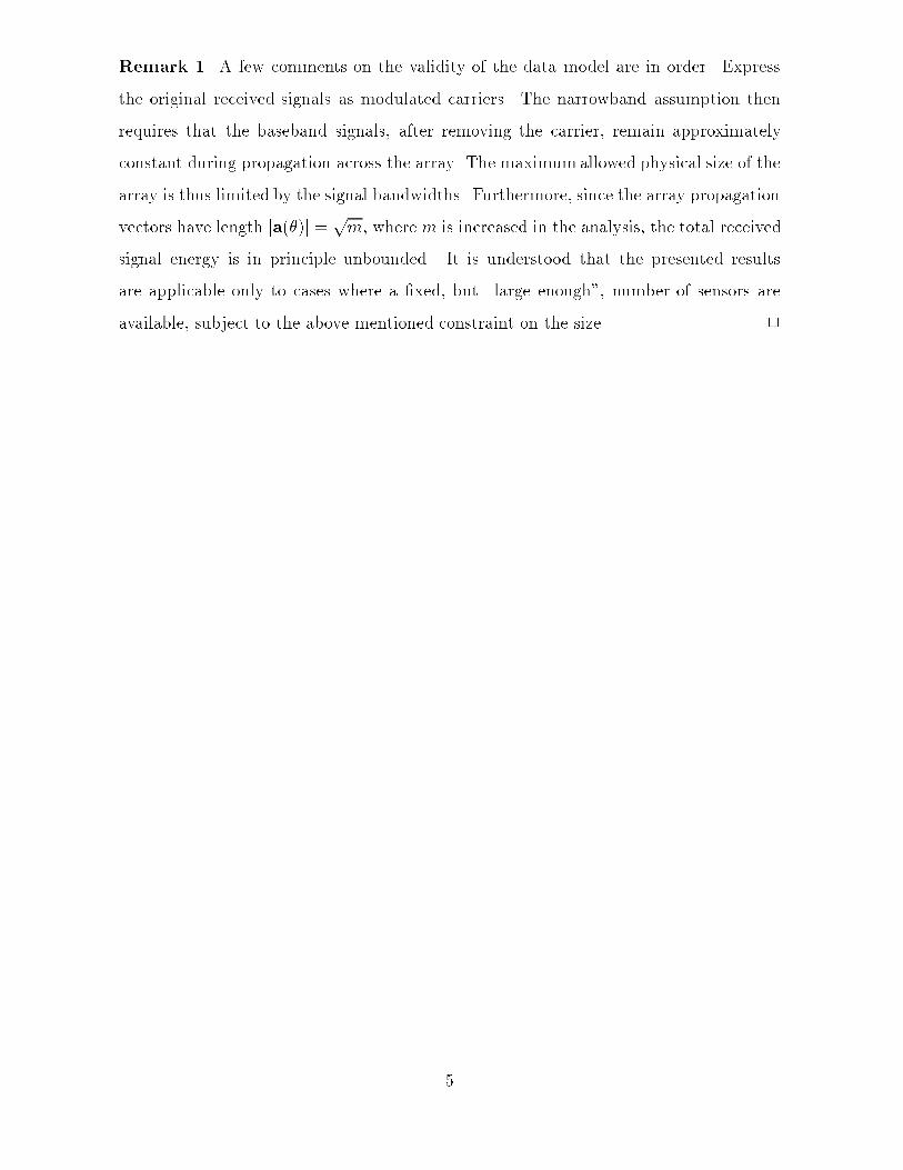
Remark 1 A few comments on the validity of the data model are in order. Expressthe original received signals as modulated carriers. The narrowband assumption thenrequires that the baseband signals, after removing the carrier, remain approximatelyconstant during propagation across the array. The maximum allowed physical size of thearray is thus limited by the signal bandwidths. Furthermore, since the array propagationvectors have length ja(�)j = pm, where m is increased in the analysis, the total receivedsignal energy is in principle unbounded. It is understood that the presented resultsare applicable only to cases where a �xed, but \large enough", number of sensors areavailable, subject to the above mentioned constraint on the size. 2

5

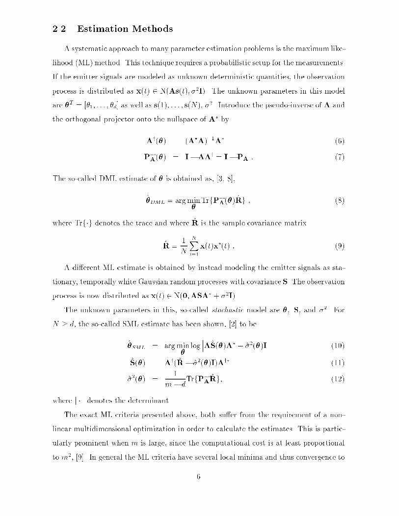
2.2 Estimation MethodsA systematic approach to many parameter estimation problems is the maximum like-lihood (ML) method. This technique requires a probabilistic setup for the measurements.If the emitter signals are modeled as unknown deterministic quantities, the observationprocess is distributed as x(t) 2 N(As(t); �2I). The unknown parameters in this modelare �T = [�1; : : : ; �d] as well as s(1); : : : ; s(N), �2. Introduce the pseudo-inverse of A andthe orthogonal projector onto the nullspace of A� byAy(�) = (A�A)�1A� (6)P?A(�) = I�AAy = I�PA : (7)The so-called DML estimate of � is obtained as, [3, 8],�DML = arg min� TrfP?A(�)Rg ; (8)where Trf�g denotes the trace and where R is the sample covariance matrixR = 1N NXt=1 x(t)x�(t) : (9)A di�erent ML estimate is obtained by instead modeling the emitter signals as sta-tionary, temporally white Gaussian random processes with covariance S. The observationprocess is now distributed as x(t) 2 N(0;ASA� + �2I) .The unknown parameters in this, so-called stochastic model are �; S, and �2. ForN � d, the so-called SML estimate has been shown, [2] to be�SML = arg min� log ���AS(�)A� + �2(�)I��� (10)S(�) = Ay(R� �2(�)I)Ay� (11)�2(�) = 1m� dTrfP?ARg; (12)where j � j denotes the determinant.The exact ML criteria presented above, both su�er from the requirement of a non-linear multidimensional optimization in order to calculate the estimates. This is partic-ularly prominent when m is large, since the computational cost is at least proportionalto m2, [9]. In general the ML criteria have several local minima and thus convergence to6

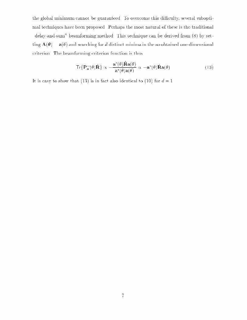
the global minimum cannot be guaranteed. To overcome this di�culty, several subopti-mal techniques have been proposed. Perhaps the most natural of these is the traditional\delay-and-sum" beamforming method. This technique can be derived from (8) by set-ting A(�) = a(�) and searching for d distinct minima in the so-obtained one-dimensionalcriterion. The beamforming criterion function is thusTrfP?a (�)Rg / �a�(�)Ra(�)a�(�)a(�) / �a�(�)Ra(�) (13)It is easy to show that (13) is in fact also identical to (10) for d = 1.

7

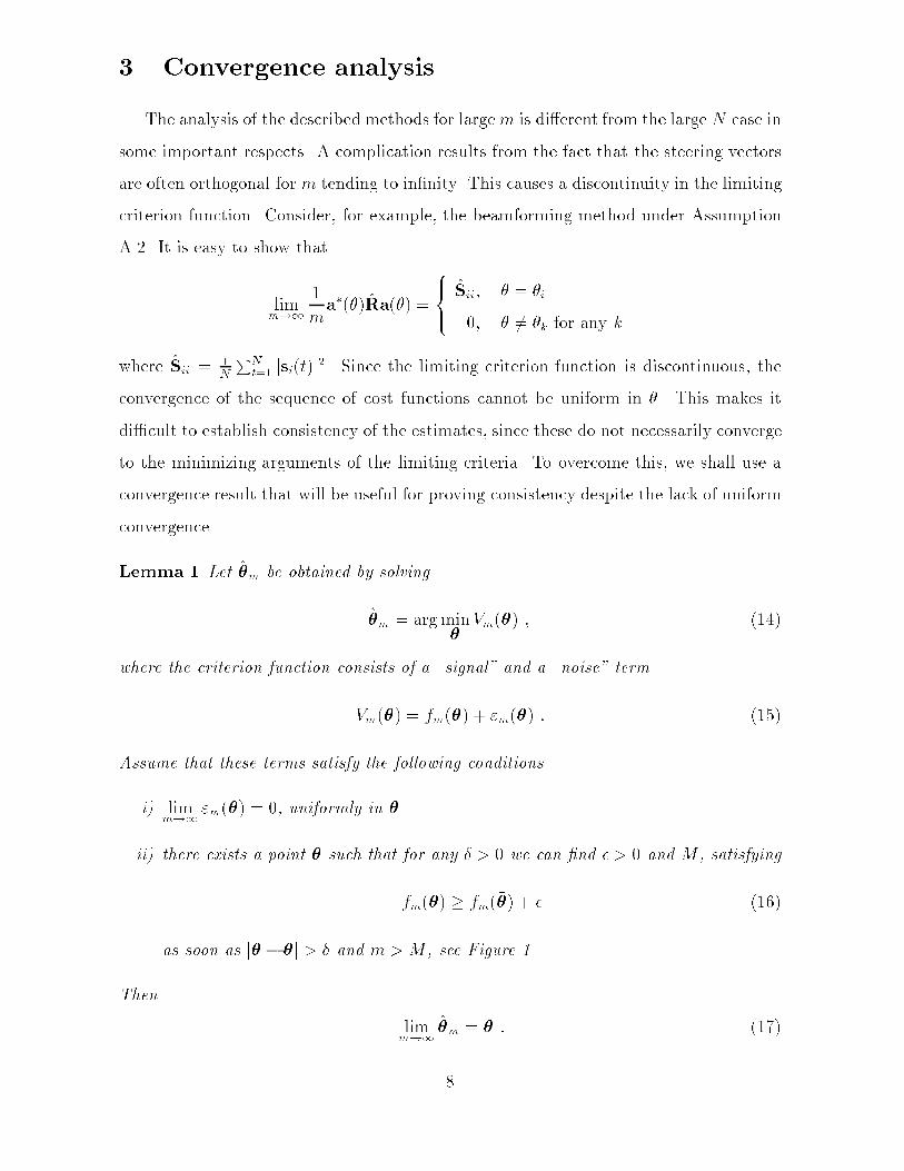
3 Convergence analysisThe analysis of the described methods for largem is di�erent from the large N case insome important respects. A complication results from the fact that the steering vectorsare often orthogonal for m tending to in�nity. This causes a discontinuity in the limitingcriterion function. Consider, for example, the beamforming method under AssumptionA.2. It is easy to show thatlimm!1 1ma�(�)Ra(�) = 8><>: Sii; � = �i0; � 6= �k for any kwhere Sii = 1N PNt=1 jsi(t)j2. Since the limiting criterion function is discontinuous, theconvergence of the sequence of cost functions cannot be uniform in �. This makes itdi�cult to establish consistency of the estimates, since these do not necessarily convergeto the minimizing arguments of the limiting criteria. To overcome this, we shall use aconvergence result that will be useful for proving consistency despite the lack of uniformconvergence.Lemma 1 Let �m be obtained by solving�m = arg min� Vm(�) ; (14)where the criterion function consists of a \signal" and a \noise" termVm(�) = fm(�) + "m(�) : (15)Assume that these terms satisfy the following conditionsi) limm!1 "m(�) = 0, uniformly in �.ii) there exists a point �� such that for any � > 0 we can �nd � > 0 and M , satisfyingfm(�) � fm(��) + � (16)as soon as j� � ��j > � and m > M , see Figure 1.Then limm!1 �m = �� : (17)8

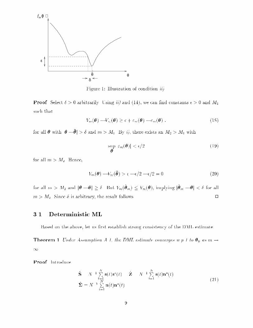
θ θ

ε

fm ( )θ

δFigure 1: Illustration of condition ii).Proof Select � > 0 arbitrarily. Using ii) and (14), we can �nd constants � > 0 and M1such that Vm(�)� Vm(��) � �+ "m(�)� "m(��) : (18)for all � with j� � ��j > � and m > M1. By i), there exists an M2 > M1 withsup� j"m(�)j < �=2 (19)for all m > M2. Hence, Vm(�)� Vm(��) > �� �=2 � �=2 = 0 (20)for all m > M2 and j� � ��j � �. But Vm(�m) � Vm(��), implying j�m � ��j < � for allm > M2. Since � is arbitrary, the result follows. 23.1 Deterministic MLBased on the above, let us �rst establish strong consistency of the DML estimate.Theorem 1 Under Assumption A.1, the DML estimate converges w.p.1 to �0 as m!1.Proof Introduce S = N�1 NPt=1 s(t)s�(t) Z = N�1 NPt=1 s(t)n�(t)� = N�1 NPt=1n(t)n�(t) (21)9

and subtract the parameter-independent term Trf�g=m from the DML criterion function(8), to yield Vm(�) = 1mTrfP?ARg � 1mTrf�g : (22)By (9) and (21) the sample covariance matrix can be writtenR = A(�0)SA�(�0) +A(�0)Z+ Z�A�(�0) + � : (23)Hence, we can write, Vm(�) = fm(�) + "m(�), wherefm(�) = 1mTrfP?AA(�0)SA�(�0)g (24)"m(�) = 2mRe �TrfP?AA(�0)Zg�+ 1mTrfPA�g : (25)Let us �rst verify the condition i) of Lemma 1. Consider the �rst term of (25). Usingthe short-hand notation A0 = A(�0) and A = A(�), we havesup� ���� 1mTrfP?AA0Zg���� � �����Tr(ZA0m )�����+ sup� �����Tr(ZAm �m(A�A)�1 � A�A0m )����� (26)� C � sup� ZAm F (27)for some constant C (independent of m). Note thatfZA(�)=mgij = 1N NXt=1 si(t)� 1m mXk=1nk(t)Akj(�) : (28)The last sum is readily seen to converge to zero w.p.1 as m tends to in�nity, for all valuesof �, see e.g. [10], Theorem 4.2.3. Thus, the �rst term of (25) converge almost surelyto zero, uniformly in �. By similar arguments it is straightforward to verify that this istrue also for the second term.To verify condition ii), rewrite the signal term (24) asfm(�) = 1mTrfP?AA0SA�0g = 1mkA0L+ATk2F ; (29)where L and T are de�ned by the relationsS = LL� (30)T = �AyA0L : (31)10

Let k denote the number of components of � that are not present in �0. If j���0j � � > 0,we have 1 � k � d. Assume, without loss of generality, that the unique DOAs in �0 and� are �01; : : : ; �0k and �1; : : : ; �k respectively. Let lTi and tTi denote the rows of L and T,and introduce the matricesQ = hl1; : : : ; lk; t1; : : : ; tk; lk+1 + tk+1; : : : ; ld + tdiT (32)B = [a(�01); : : : ;a(�0k);a(�k+1); : : : ;a(�d)] (33)We can then rewrite (29) asfm(�) = 1mkBQk2F= TrfQ� 1mB�BQg� �TrfQ�Qg � �S11 > 0 = fm(�0) : (34)In the last expression, S11 = l1l�1 denotes the upper left element of S which is nonzeroby assumption, and in the �rst inequality we have used Assumption A.1. Now, theinequality (34) holds for all m (su�ciently large), which shows that condition ii) ofLemma 1 is satis�ed with �� = �0. The assertion of the Theorem follows. 23.2 Stochastic MLIt is di�cult to analyze the stochastic ML method in the form (10), due to theincreasing dimension of the parametrized covariance matrix. We will make use of thedeterminant identity jI + ABj = jI + BAj to rewrite the criterion function in a formwhich is easier to analyze, and which in fact also simpli�es numerical evaluation of thecriterion: log ���AS(�)A� + �2(�)I��� = log �2m(�) �����2(�)AS(�)A� + I���= log �2m(�) �����2(�)S(�)A�A+ I���= log �2(m�d)(�) ���S(�)A�A + �2(�)I��� : (35)Inserting (11){(12) in the expression above leads after some manipulations to the nor-malized cost functionVm(�) = log 1m� dTrfP?ARg+ 1m� d log jA�RAj � 1m� d log jA�Aj : (36)11

It is clear that the determinant of A�RA is zero whenever N < d. This is why N � dmust be assumed for the concentrated form (10) of the SML criterion to be valid. Using(36), we can establish the strong consistency of the SML estimate.Theorem 2 Let Assumption A.1 hold, and assume in addition that N � d. The SMLestimate then converges w.p.1 to �0 as m tends to in�nity.Proof Write Vm(�) = fm(�) + "m(�), wherefm(�) = log 1m� dTrfP?ARg (37)"m(�) = 1m� d log jA�RAj � 1m� d log jA�Aj : (38)Obviously, fm(�) is minimized by the DML estimate. It follows from the proof of The-orem 1 and from (20) that fm(�) satis�es condition ii) of Lemma 1 with �� = �0. Fur-thermore, it is easy to see that for large msup� ���A�RA��� � C m2 w:p:1 (39)sup� jA�Aj � C m w:p:1 (40)implying that "m(�) converges to zero uniformly in �. Application of Lemma 1 nowestablishes Theorem 2. 23.3 BeamformingAs explained in Section 2.2, the Beamforming method decouples the d-dimensionalsearch required by theMLmethods into the search for d local minima in a one-dimensionalversion of the same criterion. This is reasonable only if steering vectors corresponding todistinct DOA's are approximately orthogonal. Thus, the consistency of the Beamformingmethod requires the condition provided by Assumption A.2.Theorem 3 If Assumption A.2 holds, the Beamforming estimates converge to the trueDOAs w.p.1 as m!1.Proof By (13), the Beamforming estimates are the local minima of the normalizedcriterion Vm(�) = �a�(�)Ra(�)ma�(�)a(�) = �a�(�)Ra(�)m2 : (41)12

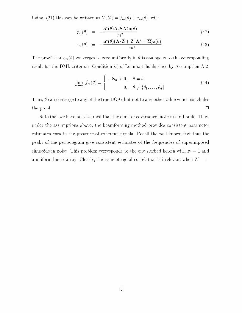
Using, (21) this can be written as Vm(�) = fm(�) + "m(�), withfm(�) = �a�(�)A0SA�0a(�)m2 (42)"m(�) = �a�(�)(A0Z+ Z�A�0 + �)a(�)m2 : (43)The proof that "m(�) converges to zero uniformly in � is analogous to the correspondingresult for the DML criterion. Condition ii) of Lemma 1 holds since by Assumption A.2.limm!1 fm(�) = 8><>: �Sii < 0; � = �i0; � 6= f�1; : : : ; �dg (44)Thus, � can converge to any of the true DOAs but not to any other value which concludesthe proof. 2Note that we have not assumed that the emitter covariance matrix is full rank. Thus,under the assumptions above, the beamforming method provides consistent parameterestimates even in the presence of coherent signals. Recall the well-known fact that thepeaks of the periodogram give consistent estimates of the frequencies of superimposedsinusoids in noise. This problem corresponds to the one studied herein with N = 1 anda uniform linear array. Clearly, the issue of signal correlation is irrelevant when N = 1.

13

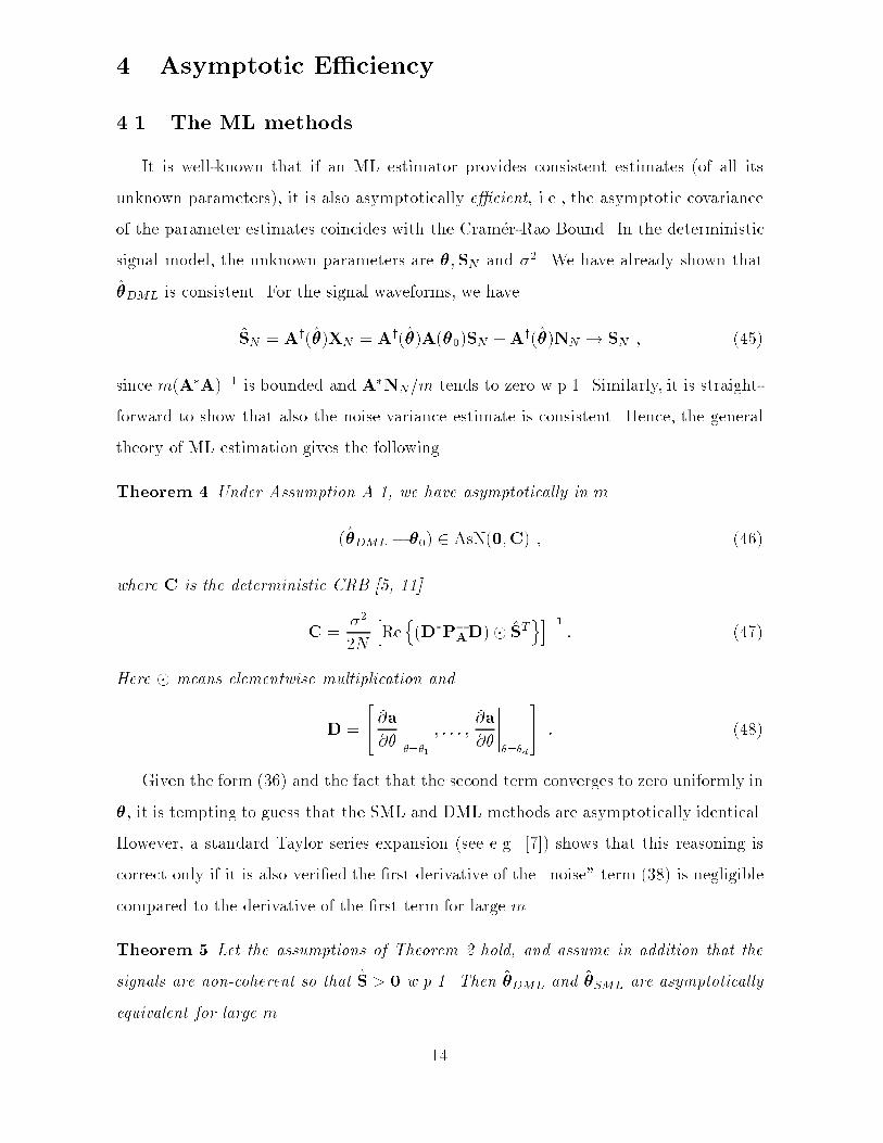
4 Asymptotic E�ciency4.1 The ML methodsIt is well-known that if an ML estimator provides consistent estimates (of all itsunknown parameters), it is also asymptotically e�cient, i.e., the asymptotic covarianceof the parameter estimates coincides with the Cram�er-Rao Bound. In the deterministicsignal model, the unknown parameters are �;SN and �2. We have already shown that�DML is consistent. For the signal waveforms, we haveSN = Ay(�)XN = Ay(�)A(�0)SN +Ay(�)NN ! SN ; (45)since m(A�A)�1 is bounded and A�NN=m tends to zero w.p.1. Similarly, it is straight-forward to show that also the noise variance estimate is consistent. Hence, the generaltheory of ML estimation gives the following.Theorem 4 Under Assumption A.1, we have asymptotically in m(�DML � �0) 2 AsN(0;C) ; (46)where C is the deterministic CRB [5, 11]C = �22N hRen(D�P?AD)� SToi�1 : (47)Here � means elementwise multiplication andD = 24 @a@� ������=�1 ; : : : ; @a@� ������=�d35 : (48)Given the form (36) and the fact that the second term converges to zero uniformly in�, it is tempting to guess that the SML and DML methods are asymptotically identical.However, a standard Taylor series expansion (see e.g. [7]) shows that this reasoning iscorrect only if it is also veri�ed the �rst derivative of the \noise" term (38) is negligiblecompared to the derivative of the �rst term for large m.Theorem 5 Let the assumptions of Theorem 2 hold, and assume in addition that thesignals are non-coherent so that S > 0 w.p.1. Then �DML and �SML are asymptoticallyequivalent for large m. 14

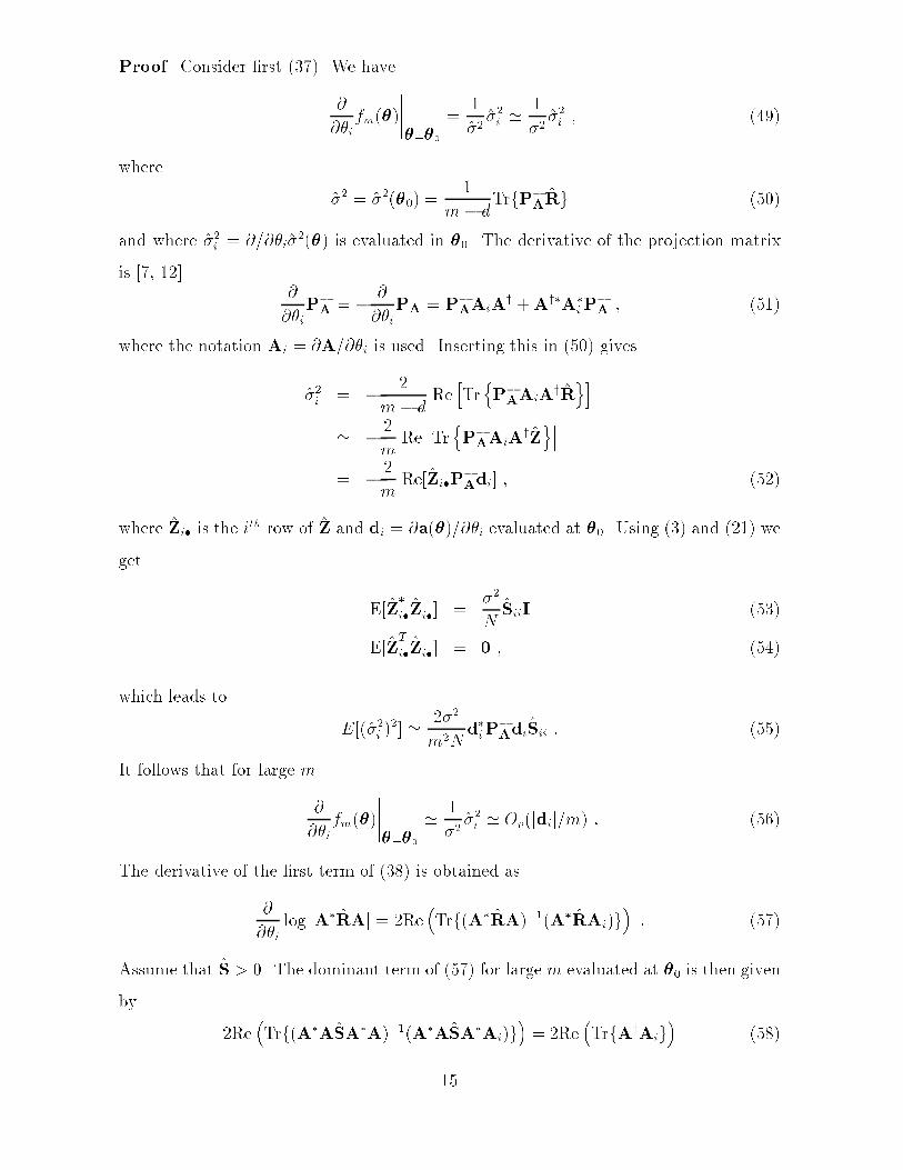
Proof Consider �rst (37). We have@@�ifm(�)������=�0 = 1�2 �2i ' 1�2 �2i ; (49)where �2 = �2(�0) = 1m� dTrfP?ARg (50)and where �2i = @=@�i�2(�) is evaluated in �0. The derivative of the projection matrixis [7, 12] @@�iP?A = � @@�iPA = P?AAiAy +Ay�A�iP?A ; (51)where the notation Ai = @A=@�i is used. Inserting this in (50) gives�2i = � 2m� d Re hTr nP?AAiAyRoi' � 2m Re hTrnP?AAiAyZoi= � 2m Re[Zi�P?Adi] ; (52)where Zi� is the ith row of Z and di = @a(�)=@�i evaluated at �0. Using (3) and (21) weget E[Z�i�Zi�] = �2N SiiI (53)E[ZTi�Zi�] = 0 ; (54)which leads to E[(�2i )2] ' 2�2m2N d�iP?AdiSii : (55)It follows that for large m@@�ifm(�)������=�0 ' 1�2 �2i ' Op(jdij=m) : (56)The derivative of the �rst term of (38) is obtained as@@�i log jA�RAj = 2Re �Trf(A�RA)�1(A�RAi)g� : (57)Assume that S > 0. The dominant term of (57) for large m evaluated at �0 is then givenby 2Re �Trf(A�ASA�A)�1(A�ASA�Ai)g� = 2Re �TrfAyAig� (58)15

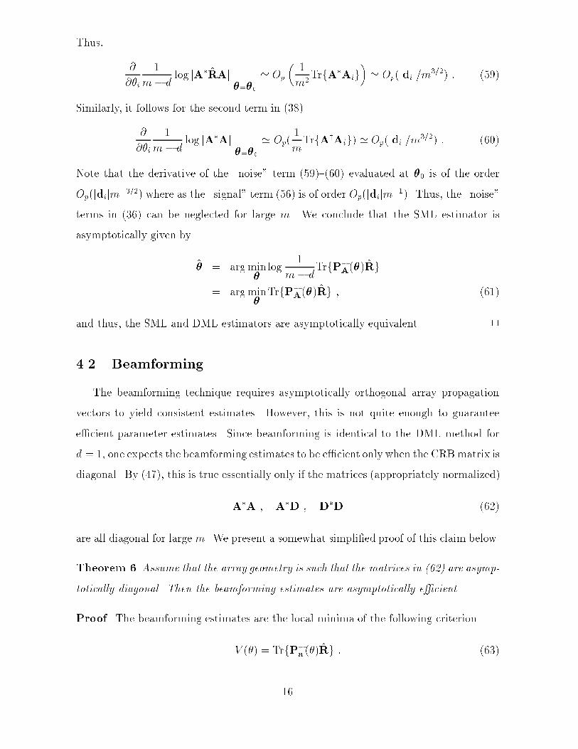
Thus, @@�i 1m� d log jA�RAj������=�0 ' Op � 1m2TrfA�Aig� ' Op(jdij=m3=2) : (59)Similarly, it follows for the second term in (38)@@�i 1m� d log jA�Aj������=�0 ' Op( 1mTrfAyAig) ' Op(jdij=m3=2) : (60)Note that the derivative of the \noise" term (59){(60) evaluated at �0 is of the orderOp(jdijm�3=2) where as the \signal" term (56) is of order Op(jdijm�1). Thus, the \noise"terms in (36) can be neglected for large m. We conclude that the SML estimator isasymptotically given by � = arg min� log 1m� dTrfP?A(�)Rg= arg min� TrfP?A(�)Rg ; (61)and thus, the SML and DML estimators are asymptotically equivalent. 24.2 BeamformingThe beamforming technique requires asymptotically orthogonal array propagationvectors to yield consistent estimates. However, this is not quite enough to guaranteee�cient parameter estimates. Since beamforming is identical to the DML method ford = 1, one expects the beamforming estimates to be e�cient only when the CRBmatrix isdiagonal. By (47), this is true essentially only if the matrices (appropriately normalized)A�A ; A�D ; D�D (62)are all diagonal for large m. We present a somewhat simpli�ed proof of this claim below.Theorem 6 Assume that the array geometry is such that the matrices in (62) are asymp-totically diagonal. Then the beamforming estimates are asymptotically e�cient.Proof The beamforming estimates are the local minima of the following criterionV (�) = TrfP?a (�)Rg : (63)16

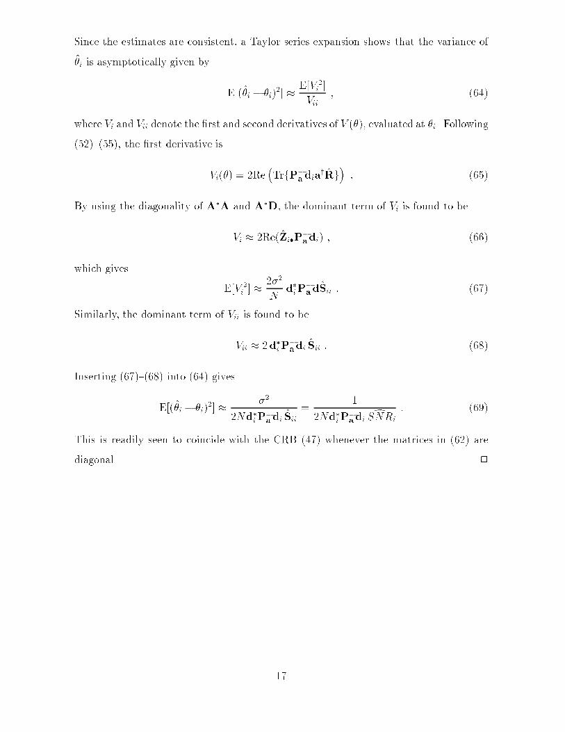
Since the estimates are consistent, a Taylor series expansion shows that the variance of�i is asymptotically given by E[(�i � �i)2] � E[V 2i ]Vii ; (64)where Vi and Vii denote the �rst and second derivatives of V (�), evaluated at �i. Following(52){(55), the �rst derivative isVi(�) = 2Re �TrfP?adiayRg� : (65)By using the diagonality of A�A and A�D, the dominant term of Vi is found to beVi � 2Re(Zi�P?adi) ; (66)which gives E[V 2i ] � 2�2N d�iP?adSii : (67)Similarly, the dominant term of Vii is found to beVii � 2d�iP?adi Sii : (68)Inserting (67){(68) into (64) givesE[(�i � �i)2] � �22Nd�iP?adi Sii = 12Nd�iP?adi dSNRi : (69)This is readily seen to coincide with the CRB (47) whenever the matrices in (62) arediagonal. 217

5 ConclusionsThe behavior of the deterministic and stochastic maximum likelihood methods asthe number of sensors tends to in�nity is studied. An \identi�ability" condition isintroduced, which essentially says that the sidelobes of the array must not approachthe level of the main lobe for increasing m. It is shown that both ML methods giveconsistent estimates of the DOAs under this condition. The asymptotic e�ciency of theDML method follows from the fact the all parameters are consistently estimated (unlikethe case for large N). The same is not true for the stochastic ML method, since thesignal covariance matrix cannot be consistently estimated. However, the DML and SMLestimates are found to be asymptotically equivalent thus implying asymptotic e�ciencyalso for the SML method.It is shown that the traditional beamforming method gives consistent estimates ifsteering vectors corresponding to di�erent DOAs are asymptotically orthogonal inde-pendent of signal correlation. Since this technique coincides with the DML method forone signal, the beamforming estimates are asymptotically e�cient if the CRB is asymp-totically diagonal.Interesting questions that deserve further study include a more precise classi�cationof the set of array con�gurations that satisfy Assumption A.1 and also those for whichthe matrices in (62) (appropriately normalized) are diagonal. A well-known case is theuniform linear array, see [5] Appendix G for details. It is also of interest to investigate towhat extent the assumptions on the noise made herein (complex Gaussian distribution,temporal and spatial whiteness) can be relaxed.18

References[1] R. O. Schmidt, A Signal Subspace Approach to Multiple Emitter Location andSpectral Estimation, PhD thesis, Stanford Univ., Stanford, CA, Nov. 1981.[2] J.F. B�ohme, \Estimation of Spectral Parameters of Correlated Signals in Wave-�elds", Signal Processing, 10:329{337, 1986.[3] M. Wax, Detection and Estimation of Superimposed Signals, PhD thesis, StanfordUniv., Stanford, CA, March 1985.[4] M. Kaveh and A. J. Barabell, \The Statistical Performance of the MUSIC andthe Minimum-Norm Algorithms in Resolving Plane Waves in Noise", IEEE Trans.ASSP, ASSP-34:331{341, April 1986.[5] P. Stoica and A. Nehorai, \MUSIC, MaximumLikelihood and Cram�er-Rao Bound",IEEE Trans. ASSP, ASSP-37:720{741, May 1989.[6] P. Stoica and A. Nehorai, \Performance Study of Conditional and UnconditionalDirection-of-Arrival Estimation", IEEE Trans. ASSP, ASSP-38:1783{1795, Octo-ber 1990.[7] M. Viberg and B. Ottersten, \Sensor Array Processing Based on Subspace Fitting",IEEE Trans. SP, SP-39(5):1110{1121, May 1991.[8] J.F. B�ohme, \Estimation of Source Parameters By Maximum Likelihood and Non-linear Regression", In Proc. ICASSP 84, pages 7.3.1{7.3.4, 1984.[9] B. Ottersten, M. Viberg, P. Stoica, and A. Nehorai, Exact and large sample MLtechniques for parameter estimation and detection in array processing, In S. Haykin,editor, Radar Array Signal Processing. Springer-Verlag, Wien - New York, 1992, ToAppear.[10] W.F. Stout, Almost Sure Convergence, Academic Press, New York, 1974.19

[11] H. Clergeot, S. Tressens, and A. Ouamri, \Performance of High Resolution Fre-quencies Estimation Methods Compared to the Cram�er-Rao Bounds", IEEE Trans.ASSP, 37(11):1703{1720, November 1989.[12] G. Golub and V. Pereyra, \The Di�erentiation of Pseudo-Inverses and NonlinearLeast Squares Problems Whose Variables Separate", SIAM J. Num. Anal., 10:413{432, 1973.

20