DIRECTION FINDING WITH A UNIFORM CIRCULAR ARRAY PLACED ON A MOVING PLATFORM

DIRECTION FINDING WITH A UNIFORM CIRCULAR ARRAY

PLACED ON A MOVING PLATFORM

A THESIS SUBMITTED TO

THE GRADUATE SCHOOL OF NATURAL AND APPLIED SCIENCES

OF

THE MIDDLE EAST TECHNICAL UNIVERSITY

BY

EVRİM ANIL EVİRGEN

IN PARTIAL FULFILLMENT OF THE REQUIREMENTS FOR DEGREE OF

MASTER OF SCIENCE

IN

THE DEPARTMENT OF ELECTRICAL AND ELECTRONICS ENGINEERING

SEPTEMBER 2001

Approval of the Graduate School of Natural and Applied Sciences

_______________________ Prof. Dr. Tayfur Öztürk Director

I certify that this thesis satisfies all the requirements as a thesis for the degree of Master of Science.

_______________________ Prof. Dr. Fatih CANATAN Head of Department

This is to certify that we have read this thesis and that in our opinion it is fully adequate, in scope and quality, as a thesis for the degree of Master of Science.

_______________________ Assist. Prof. Dr. Arzu Tuncay Koç Supervisor

Examining Committee Members

Prof. Dr. Yalçın TANIK _______________________

Assist. Prof. Dr. Arzu Tuncay Koç _______________________

Prof. Dr. Mete SEVERCAN _______________________

Assoc. Prof. Dr. Sencer KOÇ _______________________

Levent Alkışlar _______________________

iii

ABSTRACT

DIRECTION FINDING WITH A UNIFORM CIRCULAR ARRAY PLACED

ON A MOVING PLATFORM

EVİRGEN, Evrim Anıl

MSc. , Department of Electrical and Electronic Engineering

Supervisor: Assist. Prof. Dr. Arzu Tuncay Koç

September 2001, 99 pages

In this study direction finding (DF) with a uniform circular array (UCA), which is

placed on a moving platform, is studied. First, the problem is formulated in which

the effects of both antenna array and source movements are included as Doppler

phase shifts. Then, assuming that the array moves in one direction with a constant

speed, a new DF algorithm is proposed. The proposed algorithm uses different time

samples of the UCA’s spatial samples to construct two virtual subarrays, and

therefore there is an inherent displacement between subarrays. In the proposed

algorithm, the direction of arrivals (DOAs) of the incoming signals are estimated by

using the sample correlation matrices of the two virtual subarrays. Thus proposed

algorithm is based on the ESPRIT algorithm, and it is named as SAPESA (synthetic

aperture ESPRIT algorithm). An iterative procedure is proposed for the estimation

iv

of the DOAs in both azimuth and elevation. The performance of the proposed DF

algorithm is investigated through computer simulations. Its performance is

compared to that of the MUSIC algorithm. It is observed that each algorithm is

superior to the other in different occasions.

Keywords : direction finding, uniform circular array, moving platform, synthetic

aperture.

v

ÖZ

HAREKETLİ PLATFORMA YERLEŞTİRİLEN DÜZGÜN DAİRESEL

ANTEN DİZİSİ İLE YÖN BULUNMASI

EVİRGEN, Evrim Anıl

Yüksek Lisans, Elektrik ve Elektronik Mühendisliği Bölümü

Tez Yöneticisi: Yrd. Doç. Dr.Arzu Tuncay Koç

Eylül 2001, 99 sayfa

Bu araştırmada, hareketli bir platform üzerine yerleştirilmiş düzgün dairesel bir

anten dizisi ile yön bulunması konusu üzerinde çalışılmıştır. Öncelikle problem

anten dizisi ve kaynak hareketlerini, Doppler faz kaymaları olarak içerecek şekilde

formüle edilmiştir. Daha sonra, anten dizisinin sadece bir yönde ve sabit hızla

hareket ettiği varsayılarak yeni bir yön bulma algoritması önerilmiştir. Önerilen

algoritma düzgün dairesel anten dizisinin değişik zaman ve yerlerdeki örneklerini

iki sanal altdizi oluşturmakta kullanır, bu nedenle iki altdizi arasında doğal olarak

uzaysal farklılık oluşacaktır. Önerilen algoritmada edinilen sinyallerin geliş açıları

sanal altdizilerin örnek korelasyon matrisleri kullanılarak kestirilir. Dolayısıyla,

önerilen algoritma ESPRIT algoritmasına dayanır ve SAPESA olarak adlandırılır.

Geliş açılarının yanca açısı ve yükseliş açısı kısımlarının kestirimi için tekrarlı bir

vi

metod önerilmiştir. Önerilen yön bulma algoritmasının performansı bilgisayar

simülasyonları ile araştırılmıştır. Bu algoritmanın performansı MUSIC

algoritmasının performansı ile karşılaştırılmıştır. Herbir algoritmanın diğerine

değişik durumlarda üstünlük sağladığı simülasyonlarda gözlenmiştir.

Anahtar Kelimeler: yön bulma, düzgün dairesel anten dizisi, hareketli platform,

sentetik aralık.

vii

ACKNOWLEDGEMENTS

I appreciate to Assist. Prof. Dr. Arzu Tuncay Koç for her valuable supervision

during the development and the improvement stages of this thesis. This thesis

would not be completed without her guidance and support.

I also wish to thank to ASELSAN Inc. for the facilities provided for the completion

of this thesis.

Thanks a lot to my parents, Aydın and Sevinç Evirgen; my sister, Beril Evirgen; and

my friends, Tuçe Sarı, Özgür Gören, Ziya Ulusoy, Aslı Dinç, Ayşegül Dersan,

Taner Yaldız, Ceren Serim, Ebru Solak, Anıl Helvacı, Özgür Aslan for their trust,

great encouragement and continuous morale support.

viii

TABLE OF CONTENTS

ABSTRACT ............................................................................................................. iii

ÖZ .............................................................................................................................. v

ACKNOWLEDGEMENTS ................................................................................... vii

TABLE OF CONTENTS ...................................................................................... viii

LIST OF FIGURES ............................................................................................... xii

LIST OF ABBREVIATIONS ..................................................................... .........xvi

CHAPTER

1 INTRODUCTION ................................................................................................. 1

1.1. Direction Finding ....................................................................................... 1

1.2. The Motivation and Purpose of This Work................................................ 7

1.3. Outline of the Thesis .................................................................................. 9

2 THE DF ALGORITHM.. ................................................................................... 10

2.1. Signal Modeling ....................................................................................... 11

2.1.1. Uniform Circular Array (UCA) ....................................................... 15

2.1.2. Doppler Effect .................................................................................. 16

2.1.3. Description of Source and Array Motions ....................................... 17

2.1.4. Signal Model .................................................................................... 24

ix

2.2. Subspace Based Methods ......................................................................... 26

2.2.1. Basic Principles ................................................................................ 26

2.2.2. Summary of the MUSIC Algorithm ................................................ 29

2.2.3. Summary of the ESPRIT Algorithm ................................................ 29

2.3. SAPESA (Synthetic APerture ESPRIT Algorithm) ................................. 31

2.3.1. Resolving Left-Right Ambiguity ..................................................... 36

2.3.2. Elevation Estimation (2-D SAPESA) .............................................. 39

2.4. Estimation of Source Signals and Estimation of Source Speeds ............. 42

2.5. Discrimination of Source Signals and Reflections................................... 44

3 SIMULATIONS .................................................................................................. 46

3.1. Explanations about the Simulations ......................................................... 46

3.1.1. Iterative MUSIC Algorithm for 2-Dimensional DOA Estimation ... 48

3.2. Simulations about 2-D SAPESA & MUSIC for Single Source Case ...... 49

3.2.1. Effect of the Number of Iterations on Performance ......................... 49

3.2.2. Effect of the Change in the Statistical Properties of the Source

Signals During the Observation Duration on Performance ............................. 51

3.2.3. Effect of the Number of Antennas on Performance ......................... 53

3.2.4. Effect of the Number of Samples on Performance .......................... 55

3.2.5. Effect of the Signal-to-Noise Ratio on Performance ....................... 56

3.2.6. Effect of the Percent Overlapping between Virtual Subarrays on

Performance ..................................................................................................... 57

3.2.7. Effect of the Sampling Frequency on Performance ......................... 59

x

3.2.8. General Comments on the Results of Simulations about 2-D

SAPESA & MUSIC for Single Source Case ................................................... 61

3.3.Simulations about 1-D SAPESA & MUSIC for Two Source Case ............... 61





Performance ..................................................................................................... 64


3.4. Simulations about 2-D SAPESA & MUSIC for Two Source Case ......... 67

3.4.1. Effect of the Number of Iterations on Performance ......................... 67





Performance ..................................................................................................... 73


3.4.7. General Comments on Simulations about 2-D SAPESA & MUSIC

for Two Source Case ........................................................................................ 77

3.5. Effect of Array Speed on the Performance of MUSIC for Coherent

Sources Case ........................................................................................................ 77

4 CONCLUSIONS ................................................................................................. 80

REFERENCES ....................................................................................................... 85

xi

APPENDICES ........................................................................................................ 87

A - DERIVATION OF CRAMÉR-RAO BOUNDS ............................................ 87

B - RESULTS ......................................................................................................... 94

xii

LIST OF FIGURES

FIGURE

2.1. Graphical explanation of the problem ............................................................... 12

2.2. Antenna placement of a uniform circular array ................................................ 16

2.3. Straight motion of sensor array ......................................................................... 18

2.4. Rotational motion of sensor array ..................................................................... 18

2.5. Motion of emitting source ................................................................................. 19

2.6. Description of array motion and construction of virtual subarrays................... 31

2.7. Antennas that are used to resolve left-right ambiguity ..................................... 36

2.8. Estimation of the emitter location in the case of the array placed on an aircraft

.......................................................................................................................... 39

3.1. Effect of the number of iterations on performance (w=30, w=25) .............. 50

3.2. Effect of the number of iterations on performance (w=60, w=60) .............. 50

3.3. Effect of the change in the statistical properties of the signal during observation

duration on performance (w=30, w=25) ..................................................... 52

xiii

3.4. Effect of the change in the statistical properties of the signal during observation

duration on performance (w=60, w=60) ..................................................... 52

3.5. Effect of the number of antennas on performance (w=30, w=25) ............... 53

3.6. Effect of the number of antennas on performance (w=60, w=60) ............... 54

3.7. Effect of the number of samples on performance (w=30, w=25) ................ 55

3.8. Effect of the number of samples on performance (w=60, w=60) ................ 55

3.9. Effect of the SNR on performance (w=30, w=25) ...................................... 56

3.10. Effect of the SNR on performance (w=60, w=60) .................................... 57

3.11. Effect of the percent overlapping on performance (w=30, w=25) ............ 58

3.12. Effect of the percent overlapping on performance (w=60, w=60) ............ 59

3.13. Effect of the sampling frequency on performance (w=30, w=25) ............ 60

3.14. Effect of the sampling frequency on performance (w=60, w=60) ............ 60

3.15. Effect of the number of antennas on performance .......................................... 62

3.16. Effect of the number of samples on performance ........................................... 63

3.17. Effect of the SNR on performance .................................................................. 64

3.18. Effect of the percent overlapping on performance .......................................... 65

3.19. Effect of the sampling rate on performance .................................................... 66

3.20. Effect of the number of iterations on performance (Source 1) ....................... 68

3.21. Effect of the number of iterations on performance (Source 2) ....................... 68

xiv

3.22. Effect of the number of antennas on performance for source 1 (Modulation

=AM) ................................................................................................................ 69

3.23. Effect of the number of antennas on performance for source 2 (Modulation

=AM) ................................................................................................................ 70

3.24. Effect of the number of samples on performance for source 1 (Modulation

=AM) ................................................................................................................ 71

3.25. Effect of the number of samples on performance for source 2 (Modulation

=AM) ................................................................................................................ 71

3.26. Effect of the signal-to-noise ratio on performance for source 1 (Modulation

=AM) ................................................................................................................ 72

3.27. Effect of the signal-to-noise ratio on performance for source 2 (Modulation

=AM) ................................................................................................................ 73

3.28. Effect of the percent overlapping on performance for source 1 (Modulation

=AM) ................................................................................................................ 74

3.29. Effect of the percent overlapping on performance for source 2 (Modulation

=AM) ................................................................................................................ 75

3.30. Effect of the sampling rate on performance for source 1 (Modulation=AM) . 76

3.31. Effect of the sampling rate on performance for source 2 (Modulation=AM) . 76

3.32. Effect of the array speed on the performance of MUSIC algorithm (All results

of 100 trials are given in the graph) ................................................................. 78

xv

3.33. Effect of the array speed on the rms errors of the estimates of azimuth only

DOAs for the MUSIC algorithm ...................................................................... 78

xvi

LIST OF ABBREVEATIONS

CRB Cramér-Rao Bound

DOA Direction of Arrival

ESPRIT Estimation of Parameters via Rotational

Invariance Techniques

MUSIC Multiple Signal Classification

SAPESA Synthetic Aperture ESPRIT Algorithm

SNR Signal-to-Noise Ratio

UCA Uniform Circular Array

1

CHAPTER 1

INTRODUCTION

1.1. Direction Finding

Array signal processing deals with the processing of signals carried by propagating

waves. The signal is received by an array of sensors located at different points in

space in the field of interest. The aim of array processing is to extract useful

characteristics of the received signal (e.g., its signature, direction, speed of

propagation). [1]

The goals of array processing are to combine the sensors' outputs cleverly

to enhance the signal-to-noise ratio (SNR) beyond that of a single sensor's

output,

to characterize the field by determining the number of sources of propagating

energy, the locations of these sources, and the waveforms they are emitting,

to track the energy sources as they move in space. [2]

The sources under consideration, may be uncorrelated (i.e., independent

from each other), correlated (i.e., dependent by some amount designated by the

correlation coefficient), or coherently related (i.e., correlation coefficient is 1, these

sources are identical) to each other.

2

The array itself takes a variety of different geometries depending on the

application of interest. The most commonly used configuration is the linear array, in

which the sensors (all of a common type) are spaced along a straight line. If sensor

spacings are uniform, this is called a uniform linear array (ULA). Another common

configuration is a planar array, in which the sensors form a rectangular grid or lie on

concentric circles. If the sensors are placed on a single circle with uniform spacings,

this is called a uniform circular array (UCA).

Array signal processing has a variety of application areas. Some of them are

exploration seismology, sonar, radar, radio astronomy, and tomography.

In exploration seismology, array processing is used to bring out the physical

characteristics of a limited region of the interior of the earth, which may have

potential for trapping commercial quantities of hydrocarbons.

In passive, listening-only sonar, the received signal is externally generated,

and the primary requirement of array processing is to estimate both the temporal

and spatial structure of the received signal field. The array sensors consist of sound

pressure-sensing electromechanical transducers known as hydrophones, which are

immersed in the underwater medium.

In radar array processing, a transmitting antenna is used to floodlight the

environment surrounding the radar site, and a receiving array of antenna elements

are used to listen to the radar returns caused by reflections from targets located in

the path of the propagating wave.

3

In tomography, array processing is used to obtain cross-sectional images of

objects from either transmission or reflection data. In most cases the object

illuminated from many different directions either sequentially or simultaneously

and the image is reconstructed from data collected either in transmission or

reflection. [1]

Besides having these various areas of applications, array signal processing

has one important purpose: direction finding (DF). A direction finder is a passive

device that determines the direction/angle of arrival (DOA/AOA) of radio-

frequency energy [3]. Purpose of most direction finding operations is to detect the

position of the emitter, which can be calculated from the bearings of several

direction finders.

There are 3 types of information, which can be extracted from the received

signal:

Amplitude information

Phase information

Frequency information

One needs to make at least two observations in order to find the direction.

One of these observations is used as reference. From other observations, amplitude,

phase and/or time-difference are determined with respect to this reference.

There are basically five different DF methods [3]:

4

Amplitude Information Based Methods: Methods using either direct or

comparative amplitude response of the antenna subsystem for DOA

information.

Phase Differential-to-Amplitude Based Methods: Methods using the phase

differential between disposed antenna elements with the phase differential

converted to amplitude DOA information.

Phase Information Based Methods: Methods using the phase differential

between disposed antenna elements for DOA information.

Time Information Based Methods: Methods using the time-of-arrival

differential between disposed antenna elements for DOA information.

High Resolution Methods: These methods are more complex than the previous

ones. They are based on correlation matrix, eigenvalue and eigenspace

computations. Computational costs of these methods are higher than those of the

previous ones, which is an important drawback for many practical systems.

In general, the problems of determining the number of sources and

estimating the DOAs of the received signals have been treated separately. A good

summary of high resolution methods as well as the initial approaches for the DOA

estimation, and also some approaches the determination of the number of sources,

can be found in [4].

In DF antenna array design the closest array elements have to be at most /2

apart so as to overcome the ambiguity problem, where is the wavelength of the

received signal [3].

5

In practice, there are two widely used array configurations:

Linear Arrays: Antennas are placed on a straight line. Traditionally, sensors are

equally spaced (uniform linear array-ULA); but non-uniform spacing is also

used. They have the so-called left-right ambiguity. Covers only 180 ° of

horizontal surface. They do not provide uniform resolution over the entire

space.

Circular Arrays: Antennas are placed on a circle, mostly with uniform spacing

(uniform circular array-UCA). They provide 360° azimuthal coverage. They can

provide also information about the source elevation angle due to its planar

structure. They provide better resolution capabilities compared to linear arrays.

There are basically two different types of DF [3]:

Cooperative direction finding, is the one in which the emitter of information is

interested in being received, detected and located. They operate in narrow

frequency bands, typically between 118-400 MHz

Uncooperative direction finding, is the case where the monitoring or worse still

the location of emissions by a third party is not in the interest of the originator.

As the frequency bands to be monitored vary with the users, most monitoring

direction finders are of broadband design.

Application areas of DF systems can be listed as follows [3]:

Military:

6

Cooperative Emitters: Air and marine navigation, search and rescue, para-

rescue, landing-drop-zone location, drop-zone assembly, personnel and

vehicle locators, emission control, frequency management.

Uncooperative Emitters: Communication intelligence (COMINT), electronic

order of battle (EOB), electronic support measures (ESM), emitter homing

and targeting, friendly force location, force strength assessments,

interference source location.

Civilian:

Cooperative Emitters: Air and marine navigation, emergency beacon

location, search and rescue, para-rescue, wildlife tracking, personnel and

vehicle location, position radio markers.

Uncooperative Emitters: Spectrum monitoring, spectrum density

calibrations, amateur radio-frequency management.

Government:

Cooperative Emitters: Same as in the civilian area.

Uncooperative Emitters: Regulatory enforcement, spectrum density

calibrations, spectrum monitoring, para-military.

Research:

Cooperative Emitters: Advanced modulation DF vulnerability, propagation

studies, component and device evaluation, remote environmental sensing.

7

Uncooperative Emitters: Advanced COMINT investigations, DF network

architectures, radio noise definitions, and electromagnetic studies of severe

weather.

1.2. The Motivation and Purpose of This Work

The motivation of this work is to investigate some DF algorithms' performance, in

the case of a moving antenna array platform, and to propose an effective algorithm

if possible. This is a fairly important subject since some DF systems are intended to

operate on moving platforms. This can be a land vehicle, a naval or an airborne

platform. As these arrays can move freely, they can be used more effectively

compared to the stationary ones.

The particular problem considered in this work is the estimation of DOAs,

in both azimuth and elevation, of L incident plane waves, at a known wavelength

, by using N data samples taken from a UCA with M antennas. The sources can

be anywhere in the 3-dimensional space, and therefore, the DOAs of the incoming

signals are estimated in both azimuth and elevation. The problem is formulated in

which the effects of both antenna array and source movements are included as

Doppler frequency shifts. Then assuming that the array moves only in the +x

direction with a fixed speed, a new DF algorithm is proposed. The array in that type

of motion can be thought as creating a synthetic aperture, simulating a ULA. This

situation makes it possible to apply the traditional ESPRIT algorithm [5,6] to this

virtual ULA. The proposed algorithm is based on this idea. Although this property

is used to develop the DF algorithm, this part of the algorithm only makes a

direction estimation covering (0) – (180) in azimuth. The UCA geometry of the

8

real array is used to increase the azimuthal coverage to (0) – (360) and to estimate

elevation angle, which is assumed to be between (0) – (90).

In the proposed algorithm, the temporal samples of the spatial samples of

the array are grouped into two virtual subarrays such that there is a known

displacement between the 1st, 2

nd and n

th elements of each virtual subarray. So if the

speed of antenna array is known, this displacement can be calculated. Finally, the

key idea in the ESPRIT algorithm is applied using these two virtual subarrays to

estimate the DOAs with the assumption that the characteristics of the signal under

concern do not change much during observation duration. This is the basic idea that

lies behind the development of the algorithm. There are several parameters, that

affect the algorithm’s performance and these parameters are restricted by some

practical values (for instance, the sampling rate cannot exceed a certain limit value).

Therefore, a compromise should be made between the performance of the proposed

algorithm and the practical limitations on the parameters that can improve the

performance. The performance of the proposed algorithm is investigated through

computer simulations, for which the variable parameters are chosen carefully in

making the compromise indicated above. The behavior of the algorithm is examined

by also observing the behavior of the MUSIC algorithm [7] for comparison

purposes. It is observed that the proposed algorithm outperforms the MUSIC

algorithm in some scenarios.

9

1.3. Outline of the Thesis

This thesis is organized as follows: In Chap. 2, the problem is stated and

formulated; the proposed DF algorithm is developed and described in detail. Some

practical values, limitations, and practical advantages related to the implementation

of this algorithm, are also indicated. Being related to the DOA estimation problem,

some ideas about the estimation of the complex envelopes of emitter signals,

estimation of source speeds, and discrimination of original signal from reflected

signals are discussed.

In Chap. 3, typical results of the computer simulations are presented, along

with the discussions related to effects of different parameters. To investigate the

performance of the proposed algorithm, the root-mean-square (rms) errors and bias

of DOA estimates are plotted along with those of the MUSIC algorithm; the

Cramér-Rao bounds (CRBs) on the rms errors of DOA estimates are also indicated

to see the lower bounds on the performance measure.

Finally, some concluding remarks are given in Chap. 4.

10

CHAPTER 2

THE DF ALGORITHM

In this study, the problem of estimating the direction of arrivals (DOAs) of plane

waves by using a uniform circular antenna array, which is placed on a moving

platform, is investigated. Aim of this study is to find the DOA estimates of L

narrowband plane waves from the measurements taken by an array consisting of M

sensors ( )(1 iMx

ty for 1,...,0 Ni ).

The problem is formulated, in which the effects of both antenna array and

source movements are included as Doppler phase shifts. Array movement under

concern includes straight and circular motions whereas only radial motion of the

sources relative to the array is included in the formulation.

In this chapter, the proposed algorithm (Synthetic APerture ESprit

Algorithm - SAPESA), which is based on the well-known ESPRIT algorithm, is

developed. Some limitations about the implementations of SAPESA are discussed,

whereas certain advantages of the algorithm are also given.

Basic principles of subspace based methods are presented briefly. A

summary of the MUSIC algorithm [7] is presented, since it will be used throughout

the simulations for comparison with the proposed algorithm. A summary of the

ESPRIT algorithm [5,6] is also given for being a basis to the proposed algorithm.

11

After the discussion of DOA estimation, other problems related to this

subject are briefly introduced, such as estimation of the complex envelopes of

source signals, estimation of source speeds, and discrimination of original signal

and its reflections. Some ideas about the solution of these problems are suggested in

the last sections of this chapter.

2.1.Signal Modeling

In order to fit a proper mathematical model to a practical problem and to solve it,

obviously some reasonable assumptions should be put forward. Details of the

assumptions given in this section can be found in [4]. For the problem under

concern the followings will be assumed:

It will be assumed that the transmission medium is isotropic and homogenous so

that the radiation propagates in straight lines.

The sources are assumed to be in the far field of the array. With these

assumptions, the radiations impinging on the array can be written in the form of

a sum of plane waves.

It will also be assumed that the transmission medium is non-dispersive so that

the signal waveforms do not change as they propagate.

Another assumption is that, the incoming signals are narrowband; time delay

between any two elements of the array is small compared to the time variations

and phase modulations of the carrier frequency. Therefore, the propagation of a

wavefront between sensors is modeled as a simple phase delay of the carrier.

It is assumed that the antennas are polarization matched to the incident wave.

12

Each channel of the receiver is assumed to be ideal in the sense that its transfer

characteristics are independent of frequency. The bandwidth of the receiver

employed should be selected to be at least equal the bandwidth of source

signals. If the transfer characteristics of the channels are not identical this can be

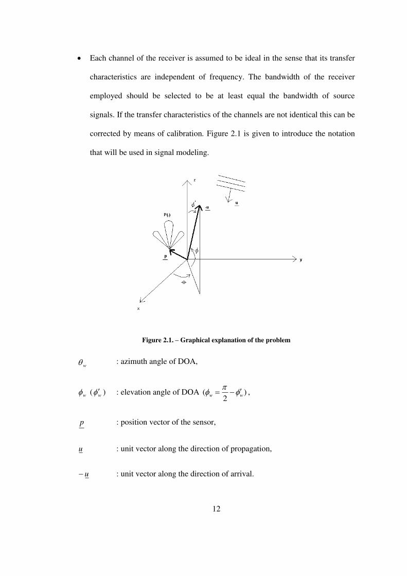
corrected by means of calibration. Figure 2.1 is given to introduce the notation

that will be used in signal modeling.

Figure 2.1. – Graphical explanation of the problem

w : azimuth angle of DOA,

w ( w ) : elevation angle of DOA )2

( ww ,

p : position vector of the sensor,

u : unit vector along the direction of propagation,

u : unit vector along the direction of arrival.

13

If the signal waveform is f(t) at the origin, then the sensor output is

)),(()()(~ww ptfPts , (2.1)

where

(.)P : the antenna pattern,

www : the DOA parameter vector,

: the time required for the wave to travel the distance between the origin and

sensor. It can be calculated as follows:

pu τ

c

, (2.2)

where

pu : the dot product of the vectors u and p ,

c : the speed of light ( 810.3c m/s).

The vector u can be decomposed as follows:

zwywwxww

zwywwxww

uuu

uuuu

.sin.cos.sin.cos.cos

.cos.sin.sin.sin.cos

(2.3)

(ux , uy , uz are the unit vectors in the directions +x, +y, and +z respectively).

Representing the amplitude and phase of the signal waveform at the origin

by )(t and )(t , respectively, and assuming that the receiver gain and phase are

known, the signal at the receiver output can be expressed as

))()(cos().().()(~0 tttPts w , (2.5)

14

where 0 is the center frequency of the narrowband receiver. Narrowband

assumption implies that, (t) and (t) remain unchanged in value during a time

interval of duration || ( tt and tt ). So (2.5) equation

becomes

))()(cos().().()(~0 tttPts w . (2.6)

Therefore, the complex envelope of the received signal is

0.).().()( )( jtj

w eetPts , (2.7)

and a sample at the receiver output at a time instant it can be written as

0).().()(j

iwi etaPts , (2.8)

where

)().()( itj

ii etta

. (2.9)

If the array consists of M sensors located at p1, p2, ..., pM , the receiver

consists of M identical channels, ignoring the interferences between channels

caused by the mutual couplings between array elements, outputs of each channel

can be written as

mj

iwmim etaPts0).().()(

. (2.10)

For L plane waves impinging on the array from L distinct directions,

denoted by vectors u1, u2, ..., uL, the output of the m'th channel is

L

l

τj

ilwlmimmloetaPts

1

).().()(

, (2.11)

15

where

c

puml

ml

.

The L plane wave signals considered may either be radiated from different

sources or may arise from multipath propagation.

In practice, measurements are often corrupted by a noise, which is additive,

stationary, zero-mean Gaussian, and the received signal at the output of the m'th

channel can be expressed as

)()()( imimim tntsty . (2.12)

2.1.1. Uniform Circular Array (UCA)

A uniform circular array with radius r is shown in Fig.2.2. Choosing the origin as

the reference point, and the x-axis as the reference line, the angular position of the

m'th sensor is

M

msm

2 for m = 0, ..., M-1 , (2.13)

and the position vector for the m'th sensor is

ysmxsmmururp .sin..cos. for m = 0, ..., M-1. (2.14)

16

Figure 2.2. – Antenna placement of a uniform circular array

Phase difference between the complex envelopes of the signals received at

the origin and at element m is obtained as (see equations (2.3), (2.11), and (2.14))

)cos(.cos.2

]sin.sincos..[coscos.2

.2. 00

smwlwl

smwlsmwlwl

ml

ml

r

r

c

puf

(2.15)

2.1.2. Doppler Effect

If there is a movement associated with the sensor array or the emitting sources,

there will be a Doppler effect in the measurements taken. [8]

Doppler frequency associated with a source and/or a sensor moving with

some speed and the source that emits a wave with wavelength is

r

d

vf . (2.16)

17

Here rv denotes the radial component of the source's velocity with respect

to the sensor. Then phase shift associated with the Doppler frequency shift

occurring at the m’th sensor due to the motion of the l’th source relative to this

sensor at time it is

i

rml

idml tv

t ..2.

. (2.17)

Here rmlv denotes the radial component of the l'th source's relative velocity with

respect to the m'th sensor of the array. The relative velocity can be investigated with

the help of three separate motions as will be explained in the next section.

2.1.3. Description of Source and Array Motions

The relative velocities associated with the source motion and associated with

the straight and rotational motions of the array will be combined in obtaining the

relative velocity of the l'th source with respect to the m'th sensor.

1) Relative velocity associated with the straight motion of sensor array

In this type of motion, each element and the center of the circle of array moves with

strv vector, which is a 3-dimensional vector with vstr and vstr representing the

corresponding azimuth and elevation angles of this vector, respectively, which is

defined using the similar notation given in Fig.2.1. Figure 2.3 shows a case for

which 0vstr and 0vstr .

18

Figure 2.3. - Straight motion of sensor array

The vector strv can be expressed in terms of vstr and vstr as

zvstryvstrvstrxvstrvstrstrvstrstrstr uuuvuvv .sin.cos.sin.cos.cos.. . (2.18)

2) Relative velocity associated with the rotational motion of sensor array

Figure 2.4. is given in order to introduce the notation for the rotational motion of

the array. This type of motion is 2-dimensional since the circle, where the sensors

located, stands in the xy-plane.

Figure 2.4. - Rotational motion of sensor array

In the rotational motion, the center of the circle of array is stationary while

each array element turns around the circle with the speed rotv , where

19

rotrotrot vrv . is the speed of each array element and rot is the angular speed

of the rotation of the array, and rotrot T2 is the rotation period of the array.

Therefore, the angular position of the m’th sensor at time it , due to the rotational

movement can be expressed as

)(.2

)( irotiism ttM

mt for m=0,…,M-1, (2.19)

The velocity vector for the m’th array element becomes

yismxismirotirotm ututtvtv ).

2)(sin().

2)(cos().()(

for m=0,…,M-1.

(2.20)

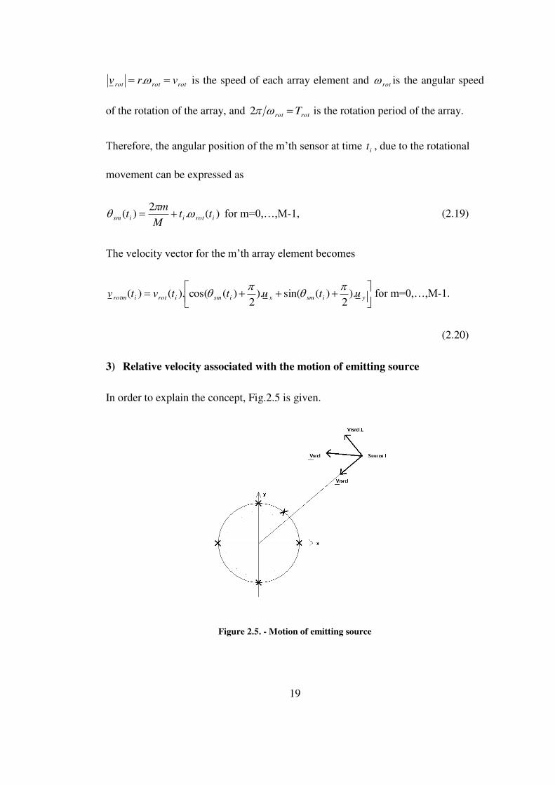
3) Relative velocity associated with the motion of emitting source

In order to explain the concept, Fig.2.5 is given.

Figure 2.5. - Motion of emitting source

20

The vector srclv represents the motion of the l’th source, and it can be

decomposed into two orthogonal parts as follows:

vrsrclrsrclvrsrclrsrclvsrclsrcl uvuvuv ... (2.21)

where

srclv : the speed of the l’th source

vsrclu : the unit vector along the direction of the l’th source’s motion

rsrclv : the radial component of the l’th source’s speed

lvrsrcl uu : the unit vector along the direction of the l’th source’s motion’s radial

component (see Fig.2.1)

rsrclv : the tangential component (perpendicular to the radial component) of the l’th

source’s speed

vrsrclu : the unit vector along the direction of the l’th source’s motion’s tangential

component

The interested part of the source's motion, which is interested, is the radial

motion of the source with respect to the sensor array (approaching or receding of

the source relative to the sensor array) since other part of source motion that is

perpendicular to the radial motion of the source with respect to the sensor array, has

no effect on the formulation, as long as it does not affect the DOA parameters.

Since Doppler frequency shift is related to the relative approaching/receding

motion of the interested emitter, the formulation includes only this type of motion,

21

whereas other motions, which are perpendicular to the straight line connecting the

sensor and the emitter, are out of concern in this formulation. It is known that the

relative approaching motion increases the Doppler frequency shift, whereas the

relative receding motion decreases it. [8]

To extract the necessary components that are parallel to the DOA vector, dot

product of sensor's velocity with lu (remembering that lu points the DOA of

the l’th source signal) and dot product of source's velocity with lu will be added.

(See Figs. 2.1, 2.3 - 2.5)

Therefore, the radial component of the relative velocity of the m’th sensor with

respect to the l’th source, at time it , is

lvsrcisrclvrotmirotvstristrrml uutvuutvutvv )).(()()).().(( . (2.22)

Using (2.3) and (2.18) - (2.21), (2.22) becomes

)()().()().(

).(sin).(cos).(sin).(cos).(cos

).2

2.).(sin(

).2

2.).(cos(

).(

).(sin

).(cos).(sin

).(cos).(cos

).(

ilivsrclirsrclivrscrlirsrcl

ziwlyiwliwlxiwliwl

yiirot

xiirot

irot

zivstr

yivstrivstr

xivstrivstr

istrrml

tututvtutv

ututtutt

uM

mtt

uM

mtt

tv

ut

utt

utt

tvv

(2.22)

(It should be noted that vsrcll uu )

Since the problem is too difficult to solve with this generality, some

reasonable assumptions should be put forward to continue further from this stage. A

simplifying assumption is that the speed of the straight and the rotational motions of

22

the array are constant; stristr vtv )( ; rotirot vtv )( . Furthermore, it can be assumed

that the sources' accelerations are not too much so the sources' velocities remain

constant during observation duration; ivtv rsrclirsrcl ,)( . (For the worst case in

which number of samples is large, e.g., 4000, and sampling rate is small, e.g., 50

kHz, observation duration becomes 4000*(1/50000) seconds = 0.08 seconds. For a

fast ground vehicle, acceleration is around 5.56 m/s2 . So the change in its speed is

0.44 m/s during observation interval, and it can be neglected.)

It can also be assumed that the sources' motions do not affect DOA

parameters (azimuth and elevation angles of the incoming wave) significantly. For

the worst case, in which the observation duration is long, e.g, 0.08 s and the average

speed of a fast ground vehicle is around 250 m/s, a displacement is of 20 meters but

since the sources are assumed to be in the far field of the array, a distance between

the sensor array and emitter is of at least 3-4 km. By some straightforward

calculations, the change in the direction of the emitter in azimuth is found to be

41016.1 x degree, and it can be assumed to be negligible. Therefore, the DOA

parameters can be considered to remain unchanged during observation duration.

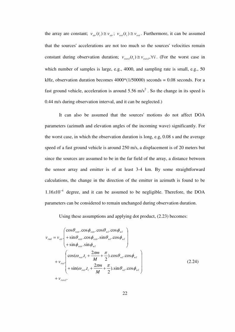
Using these assumptions and applying dot product, (2.23) becomes:

.

cos.sin).2

2.sin(

cos.cos).2

2.cos(

.

sin.sin

cos.sin.cos.sin

cos.cos.cos.cos

.

rsrcl

wlwlirot

wlwlirot

rot

wlvstr

wlwlvstrvstr

wlwlvstrvstr

strrml

v

M

mt

M

mt

v

vv

(2.24)

23

Using the well-known trigonometric identities, (2.24) can be simplified further,

.cos.2

2.cos.

sin.sincos.cos).cos(.

rsrclwlwlirotrot

wlvstrwlvstrwlvstrstrrml

vM

mtv

vv

(2.25)

Therefore, the Doppler phase shift caused by the relative motions of the

m’th sensor and the l’th source, can be expressed as (see (2.17))

i

rsrclirotwlwlrot

wlvstrwlvstrwlvstrvstr

idml tv

M

mtr

v

t .2.sin.cos..

sin.sincos.cos).cos(.

.2

.

(2.26)

Thus the signal received at the output of the m'th channel of the receiver,

including the Doppler effect caused by the motions of the array and/or the sources,

can be written as (see Eqns. (2.11), (2.12) and (2.15))

)(

..exp.

).(2

cos.cos..2

.exp).().()(

1

im

L

l

idml

wliirotwlwlmil

im

tn

tj

ttM

mrjPta

ty

,for

m=0,…,M-1.

(2.27)

Substituting (2.26) in (2.27) concludes the formulation of the problem.

24

2.1.4. Signal Model

If it is assumed that the array moves only in the +x direction, i.e, vrot = 0,

vstr = 0, vstr = 0, then (2.27) becomes

)(

].cos.cos..[2

.exp.

2cos.cos.

2.exp).().(

)(1

im

L

l

irsrclwlwlstr

wlwlwlmil

im tn

tvvj

M

mrjPta

ty

for m=0,…,M-1. (2.28)

Equation (2.28) can be written in a more compact form as:

)()().,().()( 111 iMxiLxiLxLMxLiMxtntxtFAty , (2.29)

where

LLll ,..,.., 11

TiLiiLx tatatx )(...)()( 11

: complex envelopes of the incoming signals at

time it ,

wlwlMxL

M

mrjlmA

2

cos.cos...2

.exp),1( m=0,…,M-1, l=1,…,L :

array manifold matrix (for omnidirectional antennas),

)(1 iMx tn : vector of spatial samples of additive white Gaussian noise,

25

irsrclwlwlstriLxL tvvjdiagtF .cos.cos...2

.exp),(

, l=1,…,L : phase

shift matrix caused by array and source movements. The matrix ),( iLxL tF can be

re-written in combination of two matrices as follows

)().,(),( iLxLvrsrcliLxLvstriLxL tFtFtF , (2.30)

where

iwlwlstrivstr tvjdiagtF .cos.cos...2

.exp),( , l=1,…,L : phase shift matrix

caused by array

movement only,

irsrclivrsrcl tvjdiagtF ...2

.exp)(

, l=1,…,L : phase shift matrix caused by

source movements only.

Since N

iiMxty

11)(

is available, in the case under study, a more compact form

of (2.29) can be formed as

MxNLxNiLxLvrsrcliLxLvstrMxLMxN NXtFtFAY ).().,().( (2.31)

where

)(...)(111 NMxMxMxN tytyY

: data matrix,

)(...)( 111 NLxLxLxN txtxX

,

26

)(...)( 111 NMxMxMxN tntnN

.

Now the problem is to estimate when MxNY is available. In order to solve

this problem, the use of a high resolution method is attractive.

2.2. Subspace Based Methods

Throughout the subsections, M, L, and N will represent the number of antennas, the

number of sources and the number of samples, respectively.

2.2.1. Basic Principles

The subspace based methods exploit the underlying structure of the array

correlation matrix:

IARAtytyERH

xi

H

i .)(.).()().( 2 , (2.32)

where

)(...)()( 1 LaaA : array manifold matrix,

)(a : array steering vector,

)().( i

H

ix txtxER : signal correlation matrix,

2 : power of the additive white Gaussian noise.

These methods are based on the fact that the signal part of the array output

vectors lies in the so-called signal subspace, which is a lower dimensional subspace

of the array manifold.

27

If the rank of the signal correlation matrix is L , then the rank of the matrix

H

x ARA .. is also L since A is assumed to be of full rank due to the unambigious

array assumption. Any vector in the null space of the matrix H

x ARA .. is an

eigenvector of R with the corresponding eigenvalue 2 . Since H

x ARA .. is positive

semi-definite, 2 is the smallest eigenvalue of R with multiplicity LM . The

array covariance matrix has the eigendecomposition,

H

NN

H

SS

M

i

H

iii EEEEeeR ...... 2

1

, (2.33)

where 2

11 ...... MLL are the eigenvalues of R , and Mee ,...,1

denote the corresponding orthonormal eigenvectors, S is a diagonal matrix with

diagonal entries being L ,...,1 which will be denoted by Ldiag ...1 ,

and LS eeE ...1 , MLN eeE ...1 . Since the range space of

H

x ARA .. and the range space of SE are the same, the L -dimensional range space

of SE is contained in the L -dimensional range space of A . Obviously, LL ,

equality being true only if all the signal waveforms are noncoherent, in which case

the range spaces of SE and A coincide. The range space of SE is referred to as the

signal subspace and its orthogonal complement, the range space of NE , is

commonly called the noise subspace although in fact the noise has values in the

whole M -dimensional space.

It must be noted that only when LL , any vector in the noise subspace is

also in the null space of H

A , i.e.,

28

0).( N

HEA . (2.34)

The subspace based methods use either the signal subspace or the noise subspace

for the estimation of the signal parameters. In practice a finite number of noisy

data vectors is available, i.e. 1

0)(

N

iity . Therefore, an estimate of the array

correlation matrix, which is called the sample correlation matrix, should be found.

The most popular estimate for R is

)(.)(.1ˆ

i

H

i

i tytyN

R . (2.35)

The issue is then the estimation of either signal or the noise subspace. The

estimates of these subspaces are commonly found either from the

eigendecomposition of the sample correlation matrix, or equivalently, from the

singular value decomposition of the data matrix itself, although there are other

approaches which do not use eigendecomposition techniques in an attempt to

reduce the computational complexity at the cost of performance.

The signal and noise subspaces can be estimated from a consistent estimate

R . Let M ...1 represent the eigenvalues of R , and Mee ,...,1 are the

corresponding eigenvectors. Assuming that L is known, the signal and noise

subspace estimates can be formed as MxLLS eeE ...ˆ

1 and

)(1 ...ˆ

LMMxMLN eeE , respectively.

A good summary of subspace based methods and other approaches for DF

can be found in [4].

29

2.2.2. Summary of the MUSIC (Multiple Signal Classification) Algorithm [7]

In the MUSIC algorithm, DOA estimates are obtained using the noise subspace.

The algorithm is based on the fact that the noise subspace is orthogonal to the signal

subspace, which implies that the noise subspace is orthogonal to the array steering

vectors corresponding to the DOAs if the rank of the signal covariance matrix is

equal to the number of signals, L (i.e., signals are noncoherent).

Outline of the MUSIC algorithm:

1. The MUSIC spectrum is calculated as

)(.ˆ.ˆ).(

)().()(

aEEa

aaP

H

NN

H

H

, (2.36)

where can be either one (azimuth only, ) or two (azimuth and

elevation, ) dimensional. The MUSIC spectrum corresponds to the

reciprocal of the distance between two subspaces for a given vector and it

has peaks around the locations of DOAs.

2. Assuming that L is known, the estimates of the DOAs are determined as the

locations where the MUSIC spectrum has its L peaks.

2.2.3. Summary of the ESPRIT (Estimation of Signal Parameters via

Rotational Invariance Techniques) Algorithm [5,6]

In the classical ESPRIT algorithm two identical subarrays, which are placed at two

different locations with a known displacement, are used to sample the same signals

at the same time. Since there is a displacement invariance between these subarrays,

30

the only difference between the samples of these subarrays is the phase difference

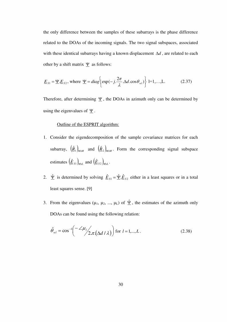
related to the DOAs of the incoming signals. The two signal subspaces, associated

with these identical subarrays having a known displacement d , are related to each

other by a shift matrix as follows:

21 . SS EE , where

)cos..

2.exp( wldjdiag

l=1,…,L. (2.37)

Therefore, after determining , the DOAs in azimuth only can be determined by

using the eigenvalues of .

Outline of the ESPRIT algorithm:

1. Consider the eigendecomposition of the sample covariance matrices for each

subarray, MxM

R1ˆ and

MxMR2ˆ . Form the corresponding signal subspace

estimates MxLSE 1

ˆ and MxLSE 2

ˆ .

2. is determined by solving 21ˆ.ˆˆ

SS EE either in a least squares or in a total

least squares sense. [9]

3. From the eigenvalues (μ1, μ2, ..., μL) of , the estimates of the azimuth only

DOAs can be found using the following relation:

/..2cosˆ 1

dl

wl for Ll ,...,1 . (2.38)

31

2.3. SAPESA (Synthetic APerture ESPRIT Algorithm)

When the array is moving in one direction with a constant speed, its trajectory is a

straight line. Proposed algorithm uses different time samples of the real array to

generate two virtual subarrays. Since different time instants of the same array are

used to form the two subarrays, there is a displacement between them inherently. To

introduce the idea Fig.2.6. is given.

Figure 2.6. – Description of array motion and construction of virtual subarrays

In this algorithm the first K snapshots are assumed to behave as the first

virtual subarray and the last K snapshots are assumed to behave as the second

virtual subarray ( NK ). If KN 2 , virtual subarrays are overlapping. If

KN 2 , virtual subarrays are non-overlapping. Since a displacement of

sstr TKNvd )..( is present between the n’th samples taken from each virtual

subarray, the classical ESPRIT algorithm can be applied for this case as if two

identical subarrays, which are placed d apart, are present.

32

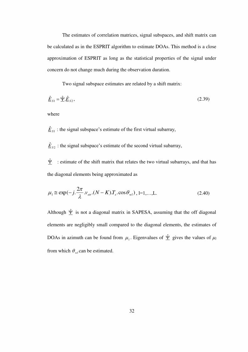
The estimates of correlation matrices, signal subspaces, and shift matrix can

be calculated as in the ESPRIT algorithm to estimate DOAs. This method is a close

approximation of ESPRIT as long as the statistical properties of the signal under

concern do not change much during the observation duration.

Two signal subspace estimates are related by a shift matrix:

21ˆ.ˆˆ

SS EE , (2.39)

where

1ˆ

SE : the signal subspace’s estimate of the first virtual subarray,

2ˆ

SE : the signal subspace’s estimate of the second virtual subarray,

: estimate of the shift matrix that relates the two virtual subarrays, and that has

the diagonal elements being approximated as

)cos.)..(.2

.exp( l wlsstr TKNvj , l=1,…,L. (2.40)

Although is not a diagonal matrix in SAPESA, assuming that the off diagonal

elements are negligibly small compared to the diagonal elements, the estimates of

DOAs in azimuth can be found from l . Eigenvalues of gives the values of l

from which wl can be estimated.

33

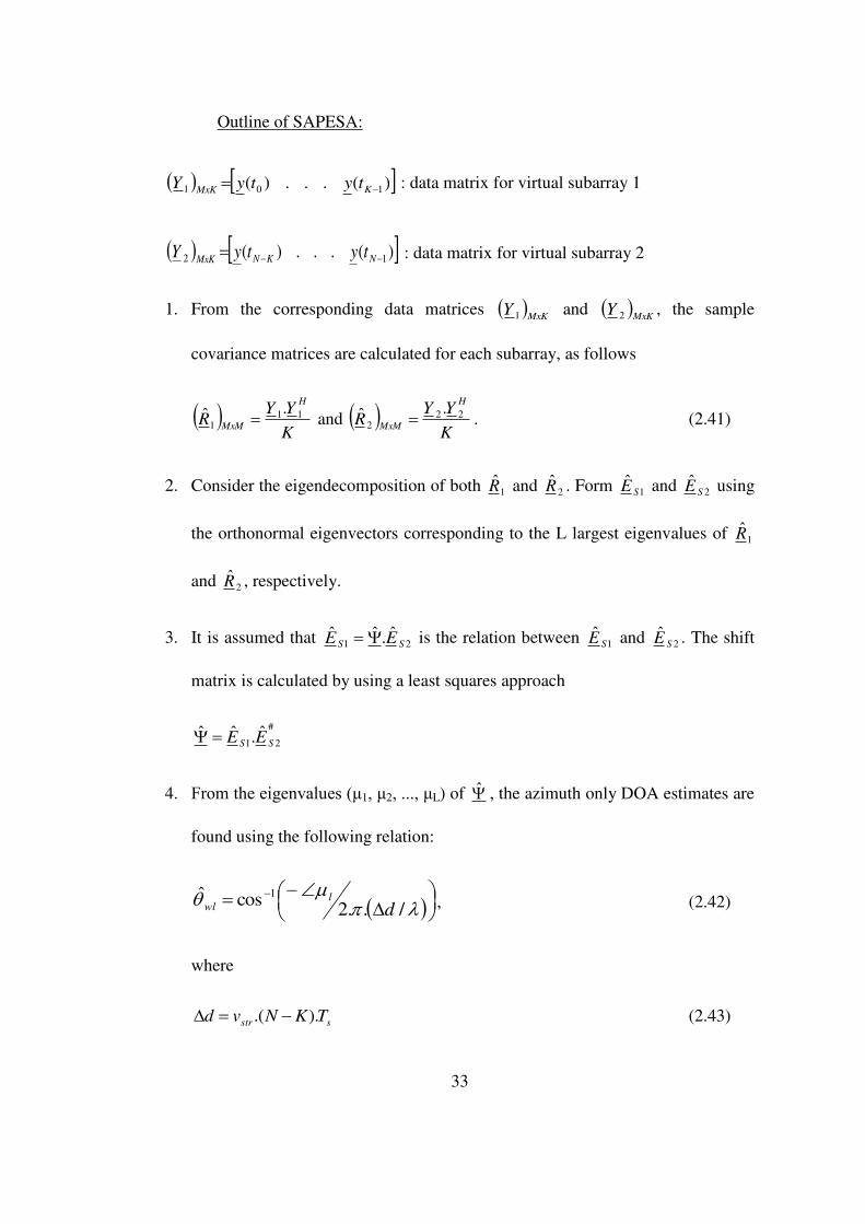
Outline of SAPESA:

)(...)( 101 KMxKtytyY : data matrix for virtual subarray 1

)(...)( 12 NKNMxKtytyY : data matrix for virtual subarray 2

1. From the corresponding data matrices MxK

Y 1 and MxK

Y 2 , the sample

covariance matrices are calculated for each subarray, as follows

K

YYR

H

MxM

111

.ˆ and K

YYR

H

MxM

222

.ˆ . (2.41)

2. Consider the eigendecomposition of both 1R and 2R . Form 1ˆ

SE and 2ˆ

SE using

the orthonormal eigenvectors corresponding to the L largest eigenvalues of 1R

and 2R , respectively.

3. It is assumed that 21ˆ.ˆˆ

SS EE is the relation between 1ˆ

SE and 2ˆ

SE . The shift

matrix is calculated by using a least squares approach

#

21ˆ.ˆˆ

SS EE

4. From the eigenvalues (μ1, μ2, ..., μL) of , the azimuth only DOA estimates are

found using the following relation:

/..2cosˆ 1

dl

wl , (2.42)

where

sstr TKNvd )..( (2.43)

34

is the displacement between the two virtual subarrays as defined before.

While performing this method, there are certain limitations as indicated

below:

1. It should be guaranteed that the source signals received in two virtual subarrays

are as close to each other as possible (i.e., statistical properties of the signals are

similar; they are the same in the ideal case). So that the shift information can be

extracted well enough to estimate the DOAs in azimuth accurately.

The observation duration should be chosen small enough so that the changes in

the source signals are small. On the other hand, choosing a short observation

duration results in less known signal characteristics and less information

gathered. So a compromise should be made between these two contradicting

situations.

2. Appropriate values of strv , ss fT 1 , K, and N should be chosen so that the

arguments of l satisfies the following inequality (see (2.40)):

wlsstr TKNv cos.)..(.

2 (2.44)

which implies

5.0)..(

sstr

d

TKNvR . (2.45)

Otherwise, phase jumps occur in phase of eigenvalues of vs. DOA graphs

and the mapping given in (2.42) becomes ambiguous, i.e., two different DOAs

35

produce the same phase shifts, and therefore, it is not possible to correctly

determine the DOA estimates.

On the other hand, choosing dR closer to zero makes the algorithm less

sensitive to DOA changes. The algorithm still works although its performance

degrades.

So the best choice of dR appears to be 0.5, for which the resolution is the best

and the performance is optimum (in terms of the rms errors of the DOA

estimates).

Besides the limitations, this algorithm has two important practical

advantages:

1. SAPESA needs only one array for DF instead of two identical subarrays, unlike

the classical ESPRIT algorithm. Some drawbacks of using two identical

subarrays are to manufacture two identical subarrays, and to match the channels

of these two subarrays by means of calibration, and therefore, a larger cost for

the system.

2. As in the classical ESPRIT algorithm, SAPESA does not need exact knowledge

of array manifold unlike MUSIC and some other subspace-based algorithms.

The measurement process to have a knowledge of array manifold, is difficult

and has a cost in practice, and this fact makes SAPESA an attractive alternative

to the algorithms, which use exact knowledge of array manifold for the

estimation process.

36

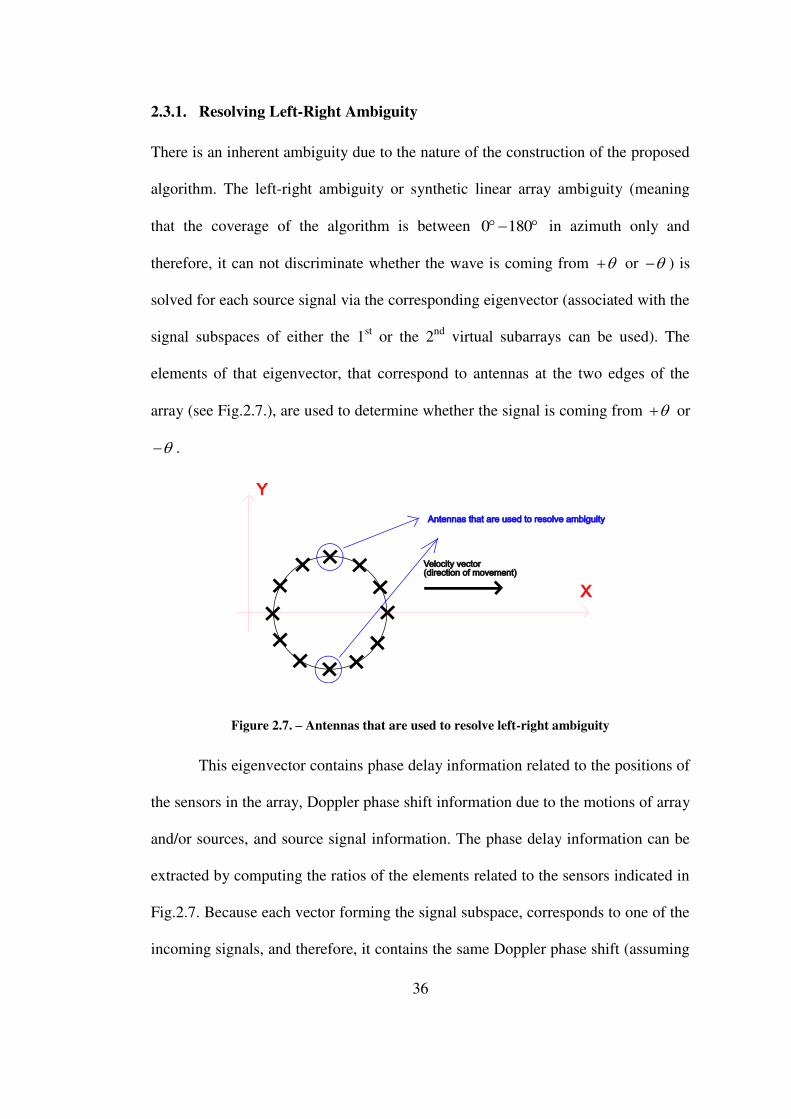
2.3.1. Resolving Left-Right Ambiguity

There is an inherent ambiguity due to the nature of the construction of the proposed

algorithm. The left-right ambiguity or synthetic linear array ambiguity (meaning

that the coverage of the algorithm is between 1800 in azimuth only and

therefore, it can not discriminate whether the wave is coming from or ) is

solved for each source signal via the corresponding eigenvector (associated with the

signal subspaces of either the 1st or the 2

nd virtual subarrays can be used). The

elements of that eigenvector, that correspond to antennas at the two edges of the

array (see Fig.2.7.), are used to determine whether the signal is coming from or

.

Figure 2.7. – Antennas that are used to resolve left-right ambiguity

This eigenvector contains phase delay information related to the positions of

the sensors in the array, Doppler phase shift information due to the motions of array

and/or sources, and source signal information. The phase delay information can be

extracted by computing the ratios of the elements related to the sensors indicated in

Fig.2.7. Because each vector forming the signal subspace, corresponds to one of the

incoming signals, and therefore, it contains the same Doppler phase shift (assuming

37

that the array motion is in one direction only) and the same source signal

information. This observation leads to the idea of resolving left-right ambiguity and

that of estimating the elevation angle as well, by using the phase delay information

extracted as explained above. Details of the estimation of elevation angle will be

given in the following section.

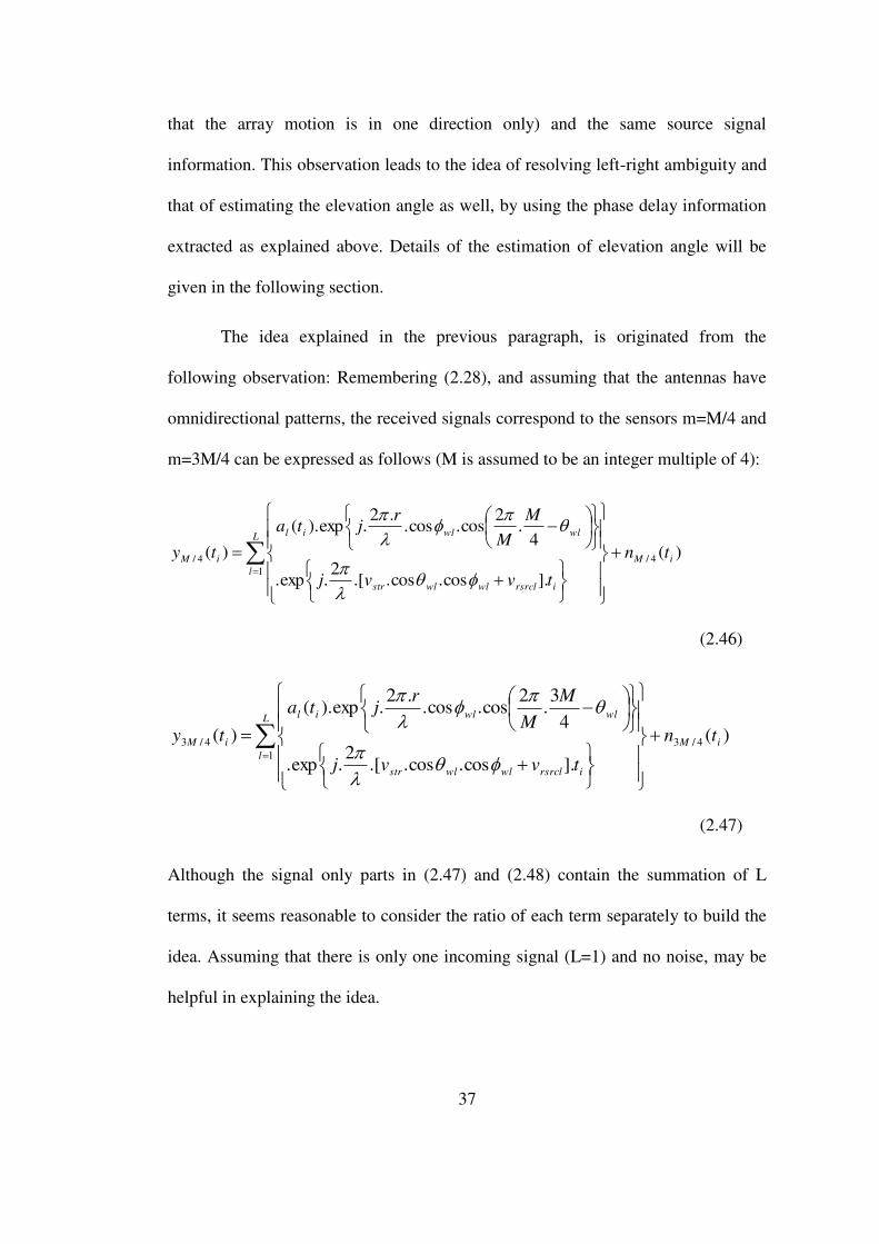
The idea explained in the previous paragraph, is originated from the

following observation: Remembering (2.28), and assuming that the antennas have

omnidirectional patterns, the received signals correspond to the sensors m=M/4 and

m=3M/4 can be expressed as follows (M is assumed to be an integer multiple of 4):

)(

].cos.cos..[2

.exp.

4.

2cos.cos.

.2.exp).(

)( 4/

1

4/ iM

L

l

irsrclwlwlstr

wlwlil

iM tn

tvvj

M

M

rjta

ty

(2.46)

)(

].cos.cos..[2

.exp.

4

3.

2cos.cos.

.2.exp).(

)( 4/3

1

4/3 iM

L

l

irsrclwlwlstr

wlwlil

iM tn

tvvj

M

M

rjta

ty

(2.47)

Although the signal only parts in (2.47) and (2.48) contain the summation of L

terms, it seems reasonable to consider the ratio of each term separately to build the

idea. Assuming that there is only one incoming signal (L=1) and no noise, may be

helpful in explaining the idea.

38

.sin.2.cos..2

.exp

2

3cos

2cos.cos.

.2.exp

2

3cos.cos.

.2.exp

2cos.cos.

.2.exp

4/3

4/

wlwl

wlwlwl

wlwl

wlwl

M

M

rj

rj

rj

rj

y

y

(2.48)

Since it is known that each eigenvector in the signal subspace gives

characteristics of the corresponding signal, the ratio of the corresponding elements

of that vector can be approximated as follows:

wlwl

l

l

l

rj

Me

Me

sin.2.cos.

.2.exp

)14/3(

)14/(, l=1,...,L, (2.49)

where le denotes the eigenvector (in the signal subspace’s estimate for the 1st

virtual subarray) corresponding to the l’th DOA estimate in azimuth.

Remark: It should be emphasized that the signal subspace’s estimate for the 2nd

virtual subarray can also be used for left-right ambiguity resolution.

From the sign of the argument of the ratio given in (2.49) )(l , it is

possible to determine that whether the signal is coming from or . ( wlsin is

positive for 0wl and wlsin is negative for 0wl )

The correction procedure can be summarized as follows (For 25.00 r ):

If 0 l , then ll ˆ360ˆ ,

else l is correct, do not make a correction.

39

2.3.2. Elevation Estimation (2-D SAPESA)

Although DF systems are generally intended to estimate DOA in only 1-dimension

(azimuth only), in some situations, 2-dimensional (azimuth and elevation) DOA

estimation is needed, especially if the receiving sensor array and/or the emitter

are/is placed on an airborne platform.

In case of the emitter located on the ground and the sensor array placed on

an aircraft, approximate position of the emitter can also be determined since the

distance between the emitter and the aircraft can be calculated using the altitude of

the aircraft and the estimated elevation angle as depicted in Fig.2.8.

Figure 2.8. – Estimation of the emitter location in the case of the array placed on an aircraft

(Distance between the aircraft and the emitter) = (Altitude of the aircraft) / sin

(2.50)

This scenario shows how important the elevation angle estimation can be in some

situations.

40

The proposed DF algorithm, SAPESA, can estimate DOA in 1-D, but it can

be further developed for estimating DOA in 2-D. DOA azimuth is estimated as

previously in SAPESA but a correction factor is included to compensate for the

effect of elevation. Thus 2-D SAPESA is an iterative algorithm. In the first step of

the iteration process elevation angle is chosen to be 0°. For elevation estimation, the

same idea as in the left-right ambiguity resolution is used. The phase delay

information is extracted by computing the ratios of certain elements of each vector

in the estimate of the signal subspace for either the 1st or the 2

nd virtual subarrays.

Remembering (2.49), and using the similar reasoning, the ratio of the elements of

the signal eigenvector related to m=0 and m=2M/4 can be approximated as follows

(M is assumed to be an integer multiple of 4):

wlwl

l

l

l

rj

Me

e

cos.2.cos.

.2.exp

)14/2(

)1(, l=1,...,L. (2.51)

After estimating the azimuth angle for the l’th source, the elevation angle

estimate can be found by combining the phase information obtained from l and

l ;

wl

l

wl

l

lr

wr

w

ˆcos...4

.cos.ˆsin...4

.cos.ˆ 11 (2.52)

where w and w are the weighting coefficients.

Outline of 2-D SAPESA:

1-3. Steps 1-3 are the same as in the 1-D SAPESA. From the eigenvalues (μ1, μ2,

..., μL) of , azimuth angle of the incident wave is estimated.

41

/..2cosˆ 10

dl

wl , (2.53)

where

sstr TKNvd )..(

It should be noted that elevation is assumed to be 0° in this step as a starting

point for the iteration process.

4. Using the estimated azimuth angle, elevation angle is estimated as follows

(remember (2.49), (2.51) and (2.52)) :

)14/3(

)14/(ˆ

Me

Me

l

ll ,

)14/2(

)1(ˆ

Me

e

l

ll ; (M is an integer multiple of 4)

i

wl

l

i

wl

li

wlr

wr

w

ˆcos...4

ˆ.cos.ˆsin...4

ˆ.cos.ˆ 11

,

where le denotes the signal subspace eigenvector corresponding to the l’th

azimuth angle estimate for the first virtual subarray

Remark: In this work, i

lw ˆsin 2 and i

lw ˆcos2 are chosen arbitrarily as

the weighting coefficients and used to average two different elevation estimates.

Different weighting coefficients can be used but this pair is used in the

simulations whose results are given in the following chapter. For 25.0r , the

elevation estimates are unambigious, i.e., the field of view is 900 w .

42

Remark: It should be noted that instead of the signal eigenvectors of the first

virtual subarray, signal eigenvectors of the second virtual subarray can also be

used for elevation angle estimation.

5. Using the estimated elevation angle, the estimate of azimuth angle is updated as

follows:

1

1

ˆcos)./.(.2cosˆ

i

ll

li

wld

e

(2.54)

Remark: Although the azimuth estimates are found by (2.54), the following

equation is used in this work to improve the convergence rate of the algorithm:

2

ˆˆcos)./.(.2

cos

ˆ

1

1

1

i

wli

ll

l

i

wl

d

e

. (2.55)

6. Steps 4 & 5 can be performed iteratively to get better estimates. But while

performing such an iterative estimation technique, the convergence of the

estimates should be checked (for instance; if 211 ˆˆˆˆ i

l

i

l

i

l

i

l , continue

the iteration loop, else stop), otherwise wrong estimates could be obtained.

2.4. Estimation of Source Signals and Estimation of Source Speeds

Once the DOAs of the incoming signals are estimated, the next step is to estimate

the complex envelopes of these signals. Equation (2.31) can be rewritten as:

MxN

FF

LxNMxLMxN NXAY ).( , (2.56)

where

43

LxNiLxLvrsrcliLxLvstr

FF

LxN XtFtFX ).().,( , (2.57)

and others are as defined in section 2.1.4.

After estimating the DOAs, FF

LxNX can be found by solving (2.56), for

instance as follows:

MxNLxM

FF

LxN YAX .)ˆ(ˆ # . (2.58)

Since the speed of the array is known, the Doppler effect due to the array

movement can be compensated by the following multiplication:

)(ˆ).,ˆ()(ˆ11 i

FF

Lxivstri

F

Lx txtFtx , i=0,...,N-1 (2.59)

where )(ˆ1 i

FF

Lx tx represents the ith

column of FF

LxNX . The signal, )(ˆ1 i

F

Lx tx , includes

only the source signal and the Doppler phase shift due to the source motion (see

(2.57)).

Since this method relies on the assumption that the DOA estimates are good

enough, the proper DF algorithm should be carefully chosen.

Phase changes of F

LxNX are due to only source motions and source signals.

So source motion can be estimated by differentiating phase of F

LxNX with respect to

time, averaging them and multiplying the result with sT.2

, a factor, which comes

from (2.28).

Averaging the derivatives related to the time instants, for which the

amplitudes of the signal are high, is more appropriate for the explained purposes

44

while their phases are less affected from noise than the others, which means that

more accurate estimates of the source speed can be obtained by this way.

Finally, complex envelopes of the source signals can be estimated by

compensating the effect of source movements as follows:

)(ˆ).(ˆ)(ˆ1

#

1 i

F

LxivrsrcliLx txtFtx , i=1,...,N (2.60)

2.5. Discrimination of Source Signals and Reflections

After estimating the source signals as discussed previously, the reflection signals

can be determined. The idea is as follows: a time delay in the reflected signals with

respect to the original signals can be observed if the sampling rate is high enough.

As a numerical example:

metersmTc

skHz

T

kHzf

smc

s

s

s

60010*6.

10*2500

1

500

10*3

2

6

8

For this case, a time delay of at least sT can be observed, if the reflected

signal travels 600 meters more than the original one if a sampling rate of 500kHz is

used.

So the cross-correlation function of two different estimated source signals

can be used as a measure for determining whether a signal is the reflection of

another, since the peak of this function is high if they are similar signals. Also by

examining the cross-correlation function it can be determined which signals are the

45

delayed version of another. Therefore, the delayed signals are determined as the

reflections.

Comparing the powers of similar estimated source signals may be another

criterion for determining the reflected signal. Obviously, the reflected one have less

energy than the original signals and this criterion may be used if the time delay

between signals are not enough for using the previous approach.

46

CHAPTER 3

SIMULATIONS

3.1.Explanations about the Simulations

Mainly two algorithms are considered for DF purposes: MUSIC and SAPESA

(Synthetic Aperture ESPRIT Algorithm). It is observed by the simulations that each

algorithm is superior to the other in different occasions.

Simulations are carried out with the MATLAB, in order to observe the

effects of several parameters for the SAPESA and MUSIC. Those parameters are

the change in the statistical properties of the signal during observation duration,

number of samples, number of antennas, percent of the overlapping between virtual

subarrays, sampling rate, and signal-to-noise ratio (SNR). In the following sections,

the SNR for each signal is defined as

2log.10

rSignalPoweSNR , (3.1)

where 2 is the power of the additive white Gaussian noise corrupting the

measurements.

Unless otherwise stated, the parameters chosen as follows: number of

antennas, M=4; total number of samples, N=900; number of samples for each

47

virtual subarray, K=675; speed of the array, strv =88.2m/s; center frequency of the

signal(s), cf =500MHz; sampling frequency, sf =66.150kHz; relative source

speed(s), rsrclv =0m/s; radius of the array, 25.0r .

In chosing the parameters, it is intended to select the parameters close to

practical values and to keep the parameter

sstr TKNvd )..(

, which is related to

SAPESA (see (2.43)), around 0.5 to observe the best performance of SAPESA. For

some simulations, two parameters are varied simultaneously in keeping that

parameter, around 0.5 and observe only the effect of the varied parameters.

For each data point, simulations are repeated 100 times. Root-mean-square

(rms) errors and bias errors of the DOA estimates, for these 100 trials are given in

the graphs. Bias errors for azimuth and elevation estimates are defined as follows:

100)(ˆ)ˆ(100

1

Trial

wlwlwl TrialBiasError ,

100)(ˆ)ˆ(100

1

Trial

wlwlwl TrialBiasError .

The Cramér-Rao bounds (CRBs) on the rms error of DOA estimates are also given

for each case for performance evaluation.

It is expected that the type of the modulation of source signal affects the

performance of SAPESA, since the changes in the phase of the received signal is

more in phase modulation and frequency modulation compared to the amplitude

modulated and continuous wave signals. So the simulations are performed for both

AM and FM type modulations but it is observed that the type of signal modulation

48

does not affect performance much, so only the results of simulations for AM type

modulated signals are given in this chapter.

3.1.1. Iterative MUSIC Algorithm for 2-Dimensional DOA Estimation

Since the DOAs are estimated in both azimuth and elevation (2-dimensional), the

MUSIC spectrum is 2-dimensional for this case. Therefore, a 2-dimensional search

has to be performed. The following peak search algorithm for the MUSIC spectrum

is used in the simulations:

1. First the elevation angle is assumed to be zero for each signal. The MUSIC

spectrum is calculated with 310 degree resolution for different azimuth angles

between 0 - 360 degrees. Then a peak search is performed over this 1-

dimensional spectrum to estimate the azimuth angles corresponding to L peaks

of this spectrum, where L is the number of signals.

2. The MUSIC spectrum is calculated with 310 degree resolution for different

elevation angles between 0 - 90 degrees, for each of the L azimuth angles

estimated in the previous step. Then a peak search is performed separately over

these 1-dimensional spectras for each signal to update the estimates of the

elevation angles.

3. The MUSIC spectrum is calculated with 310 degree resolution for different

azimuth angles between 0 - 360 degrees, for each of the L elevation angles

estimated in the previous step. Then a peak search is performed separately over

these 1-dimensional spectras for each signal to update the estimates of the

azimuth angles.

49

4. Steps 2 & 3 are performed iteratively until two successive azimuth (or

elevation) estimates have a difference smaller than a certain limit value.

During the simulations whose results are given in the following sections,

iteration loop is repeated until two successive azimuth estimates have a difference

smaller than 310 degree or iteration loop is repeated 10 times.

3.2.Simulations about 2-D SAPESA & MUSIC for Single Source Case

In the simulations whose results are given in the subsections of this section, sources

are located at either 25,30 or 60,60 . The SNR is 10dB for

single source case, unless otherwise stated.

For the simulations with single source, the reason for repeating every

simulation for different angle pairs ( 25,30 and 60,60 ) is that,

due to the synthetic linear array structure, the performance of SAPESA is different

for different azimuth angles, and it is thought that it would be better to observe this

behavior.

3.2.1. Effect of the Number of Iterations on Performance

In this section, it is intended to show the effect of the number of iterations on the

performances of SAPESA and MUSIC algorithms. The performance improvement

of SAPESA with iterations can be observed from Figs. 3.1 and 3.2.

It is observed that the iterative MUSIC algorithm converges after 2-3

iterations. Although it can not be seen by the graphs given, number of iterations of

the iterative SAPESA algorithm required for convergence varies between 6 steps to

50

50 steps depending on the trial but limiting the number of steps to 10 was observed

to be reasonable for a good performance, as it can be seen from the graphs.

Since it was observed that the first step of the iteration of SAPESA does not give

reasonable results, so the corresponding results will not be presented in the

following subsections.

0 2 4 6 8 10 120

2

4

6

8

10Effect of number of iterations on performance

Azim

uth

RM

S e

rror

Number of iterations

Iterative MUSIC

Iterative SAPESA

CRB

0 2 4 6 8 10 120

2

4

6

8


Azim

uth

Bia

s e

rror


Iterative MUSIC

Iterative SAPESA

0 2 4 6 8 10 120

2

4

6


Ele

vation R

MS

err

or


Iterative MUSIC

Iterative SAPESA

CRB

0 2 4 6 8 10 12-2

0

2

4

6


Ele

vation B

ias e

rror


Iterative MUSIC

Iterative SAPESA

Figure 3.1. - Effect of the number of iterations on performance (w=30, w=25)

0 2 4 6 8 10 120

5

10

15


Azim

uth

RM

S e

rror


Iterative MUSIC

Iterative SAPESA

CRB

0 2 4 6 8 10 120

5

10

15


Azim

uth

Bia

s e

rror


Iterative MUSIC

Iterative SAPESA

0 2 4 6 8 10 120

0.1

0.2

0.3

0.4

0.5Effect of number of iterations on performance

Ele

vation R

MS

err

or


Iterative MUSIC

Iterative SAPESA

CRB

0 2 4 6 8 10 120

0.1

0.2

0.3

0.4Effect of number of iterations on performance

Ele

vation B

ias e

rror


Iterative MUSIC

Iterative SAPESA

Figure 3.2. - Effect of the number of iterations on performance (w=60, w=60)

51

3.2.2. Effect of the Change in the Statistical Properties of the Source Signals

During the Observation Duration on Performance

In this section, it is intended to show the effect of the change in the statistical

properties of source signals during observation duration on performance of

SAPESA. The correlation coefficient between the first K samples and the last K

samples of the complex envelope of the emitted signal,

)(...)( 101 NxN tstss , is taken as a measure to observe this effect as

follows:

H

VAVA

H

VAVA

H

VAVA

ssss

ssntnCoefficieCorrelatio

2211

21

...

.

where

)(...)( 1011

KxKVA tstss

)(...)( 112

NKNxKVAtstss .

For the simulations presented in this chapter, the signal is created to observe this

specific behavior and it is not an AM signal.

It is observed by the simulations whose results are given in Figs 3.3 and 3.4

that the performance of the SAPESA increases, as the changes in the statistical

properties of the source signals get smaller, i.e., correlation coefficient gets larger.

For both 25,30 ww and 60,60 ww cases optimum performance is

achieved when correlation is between 0.8 and 1.0. Although this parameter has very

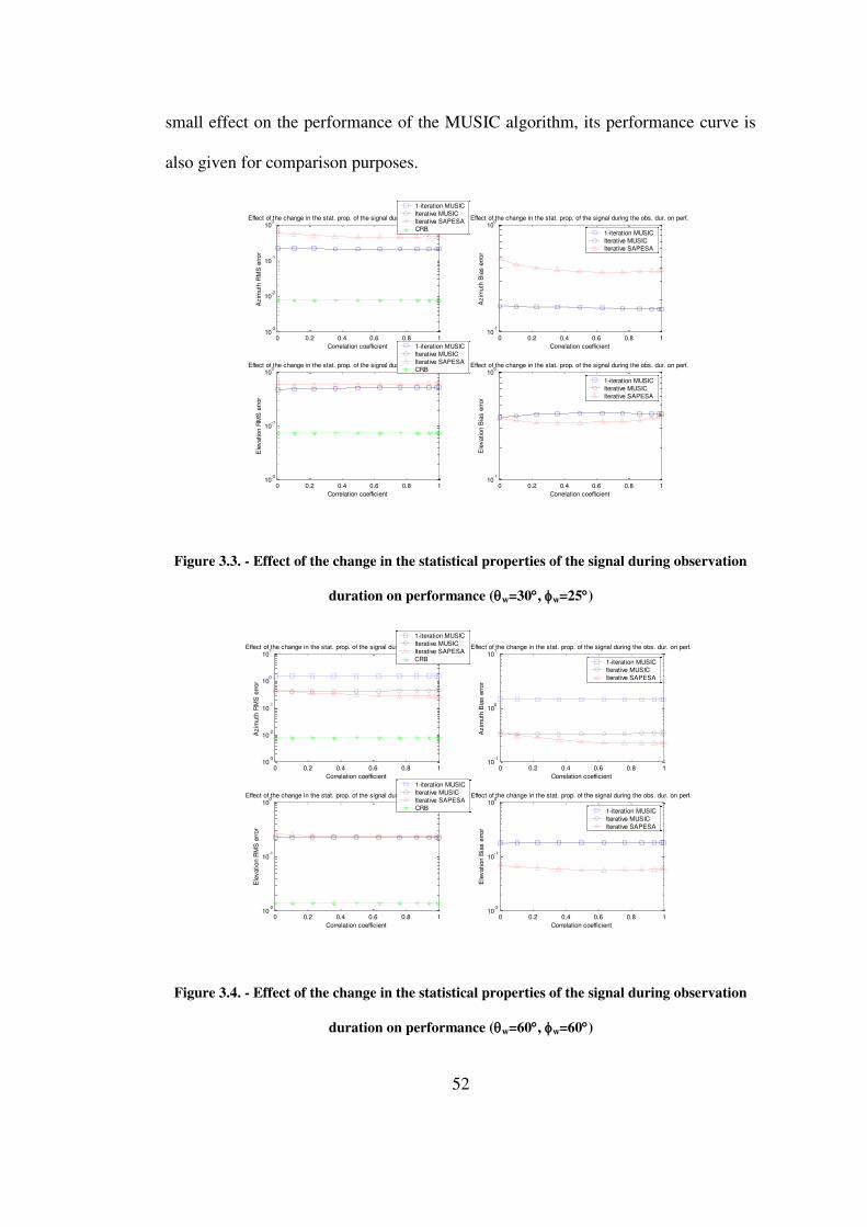
52

small effect on the performance of the MUSIC algorithm, its performance curve is

also given for comparison purposes.

0 0.2 0.4 0.6 0.8 110

-3

10-2

10-1

100

Effect of the change in the stat. prop. of the signal during the obs. dur. on perf.

Azim

uth

RM

S e

rror

Correlation coefficient

1-iteration MUSIC

Iterative MUSIC

Iterative SAPESA

CRB

0 0.2 0.4 0.6 0.8 110

-1

100


Azim

uth

Bia

s e

rror


1-iteration MUSIC

Iterative MUSIC

Iterative SAPESA

0 0.2 0.4 0.6 0.8 110

-2

10-1

100


Ele

vation R

MS

err

or


1-iteration MUSIC

Iterative MUSIC

Iterative SAPESA

CRB

0 0.2 0.4 0.6 0.8 110

-1

100


Ele

vation B

ias e

rror


1-iteration MUSIC

Iterative MUSIC

Iterative SAPESA

Figure 3.3. - Effect of the change in the statistical properties of the signal during observation

duration on performance (w=30, w=25)

0 0.2 0.4 0.6 0.8 110

-3

10-2

10-1

100

101


Azim

uth

RM

S e

rror


1-iteration MUSIC

Iterative MUSIC

Iterative SAPESA

CRB

0 0.2 0.4 0.6 0.8 110

-1

100

101


Azim

uth

Bia

s e

rror


1-iteration MUSIC

Iterative MUSIC

Iterative SAPESA

0 0.2 0.4 0.6 0.8 110

-2

10-1

100


Ele

vation R

MS

err

or


1-iteration MUSIC

Iterative MUSIC

Iterative SAPESA

CRB

0 0.2 0.4 0.6 0.8 110

-2

10-1

100


Ele

vation B

ias e

rror


1-iteration MUSIC

Iterative MUSIC

Iterative SAPESA

Figure 3.4. - Effect of the change in the statistical properties of the signal during observation

duration on performance (w=60, w=60)

53

3.2.3. Effect of the Number of Antennas on Performance

In this section, it is intended to show the effect of the number of antennas on the

performances of SAPESA and MUSIC algorithms.

As it can be observed from Figs 3.5 and 3.6, increasing the number of

antennas improves the performance of MUSIC greatly as expected, whereas it does

not seem to improve the performance of SAPESA much. Performance of SAPESA

is close to the performance of MUSIC when the number of antennas is small. This

behavior should be further examined in the future.

0 5 10 15 20 25 30 3510

-3

10-2

10-1

100

Effect of number of antennas on performance

Azim

uth

RM

S e

rror

Number of antennas

1-iteration MUSIC

Iterative MUSIC

Iterative SAPESA

CRB

0 5 10 15 20 25 30 3510

-2

10-1

100


Azim

uth

Bia

s e

rror

Number of antennas

1-iteration MUSIC

Iterative MUSIC

Iterative SAPESA

0 5 10 15 20 25 30 3510

-2

10-1

100


Ele

vation R

MS

err

or

Number of antennas

1-iteration MUSIC

Iterative MUSIC

Iterative SAPESA

CRB

0 5 10 15 20 25 30 3510

-2

10-1

100


Ele

vation B

ias e

rror

Number of antennas

1-iteration MUSIC

Iterative MUSIC

Iterative SAPESA

Figure 3.5. - Effect of the number of antennas on performance (w=30, w=25)

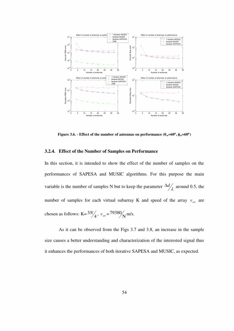
54

0 5 10 15 20 25 30 3510

-3

10-2

10-1

100

101


Azim

uth

RM

S e

rror

Number of antennas

1-iteration MUSIC

Iterative MUSIC

Iterative SAPESA

CRB

0 5 10 15 20 25 30 3510

-2

10-1

100

101


Azim

uth

Bia

s e

rror

Number of antennas

1-iteration MUSIC

Iterative MUSIC

Iterative SAPESA

0 5 10 15 20 25 30 3510

-3

10-2

10-1

100


Ele

vation R

MS

err

or

Number of antennas

1-iteration MUSIC

Iterative MUSIC

Iterative SAPESA

CRB

0 5 10 15 20 25 30 3510

-2

10-1

100


Ele

vation B

ias e

rror

Number of antennas

1-iteration MUSIC

Iterative MUSIC

Iterative SAPESA

Figure 3.6. - Effect of the number of antennas on performance (w=60, w=60)

3.2.4. Effect of the Number of Samples on Performance

In this section, it is intended to show the effect of the number of samples on the

performances of SAPESA and MUSIC algorithms. For this purpose the main

variable is the number of samples N but to keep the parameter d around 0.5, the

number of samples for each virtual subarray K and speed of the array strv are

chosen as follows: K=4

3N , strv =N

79380 m/s.

As it can be observed from the Figs 3.7 and 3.8, an increase in the sample

size causes a better understanding and characterization of the interested signal thus

it enhances the performances of both iterative SAPESA and MUSIC, as expected.

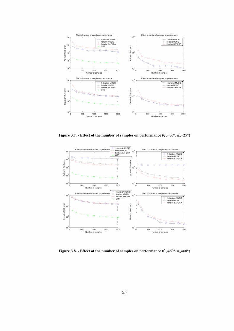
55

0 500 1000 1500 200010

-3

10-2

10-1

100

101

Effect of number of samples on performance

Azim

uth

RM

S e

rror

Number of samples

1-iteration MUSIC

Iterative MUSIC

Iterative SAPESA

CRB

0 500 1000 1500 200010

-1

100

101


Azim

uth

Bia

s e

rror

Number of samples

1-iteration MUSIC

Iterative MUSIC

Iterative SAPESA

0 500 1000 1500 200010

-2

10-1

100

101


Ele

vation R

MS

err

or

Number of samples

1-iteration MUSIC

Iterative MUSIC

Iterative SAPESA

CRB

0 500 1000 1500 200010

-1

100

101


Ele

vation B

ias e

rror

Number of samples

1-iteration MUSIC

Iterative MUSIC

Iterative SAPESA

Figure 3.7. - Effect of the number of samples on performance (w=30, w=25)

0 500 1000 1500 200010

-3

10-2

10-1

100

101


Azim

uth

RM

S e

rror

Number of samples

1-iteration MUSIC

Iterative MUSIC

Iterative SAPESA

CRB

0 500 1000 1500 200010

-1

100

101


Azim

uth

Bia

s e

rror

Number of samples

1-iteration MUSIC

Iterative MUSIC

Iterative SAPESA

0 500 1000 1500 200010

-3

10-2

10-1

100


Ele

vation R

MS

err

or

Number of samples

1-iteration MUSIC

Iterative MUSIC

Iterative SAPESA

CRB

0 500 1000 1500 200010

-1

100


Ele

vation B

ias e

rror

Number of samples

1-iteration MUSIC

Iterative MUSIC

Iterative SAPESA

Figure 3.8. - Effect of the number of samples on performance (w=60, w=60)

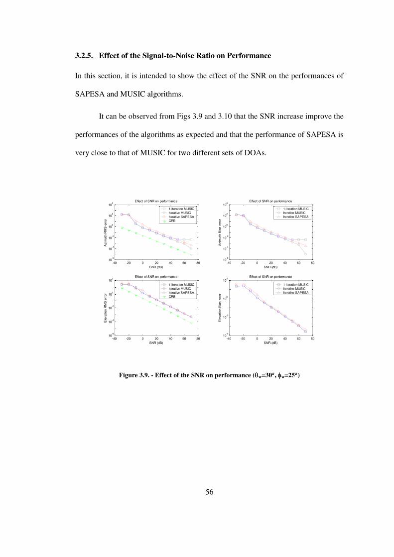
56

3.2.5. Effect of the Signal-to-Noise Ratio on Performance

In this section, it is intended to show the effect of the SNR on the performances of

SAPESA and MUSIC algorithms.

It can be observed from Figs 3.9 and 3.10 that the SNR increase improve the

performances of the algorithms as expected and that the performance of SAPESA is

very close to that of MUSIC for two different sets of DOAs.

-40 -20 0 20 40 60 8010

-6

10-4

10-2

100

102

104

Effect of SNR on performance

SNR (dB)

Azim

uth

RM

S e

rror

1-iteration MUSIC

Iterative MUSIC

Iterative SAPESA

CRB

-40 -20 0 20 40 60 8010

-6

10-4

10-2

100

102

104


SNR (dB)

Azim

uth

Bia

s e

rror

1-iteration MUSIC

Iterative MUSIC

Iterative SAPESA

-40 -20 0 20 40 60 8010

-6

10-4

10-2

100

102


SNR (dB)

Ele

vation R

MS

err

or

1-iteration MUSIC

Iterative MUSIC

Iterative SAPESA

CRB

-40 -20 0 20 40 60 8010

-4

10-2

100

102


SNR (dB)

Ele

vation B

ias e

rror

1-iteration MUSIC

Iterative MUSIC

Iterative SAPESA

Figure 3.9. - Effect of the SNR on performance (w=30, w=25)

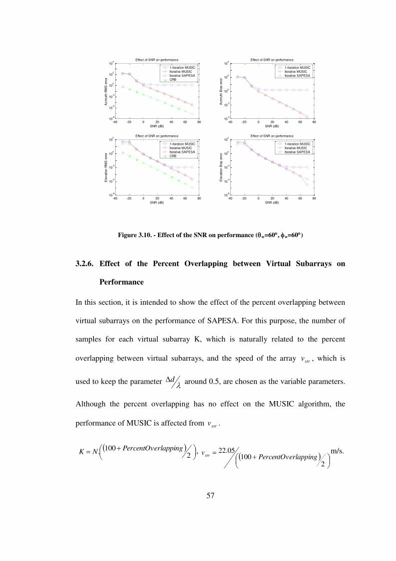
57

-40 -20 0 20 40 60 8010

-6

10-4

10-2

100

102

104


SNR (dB)

Azim

uth

RM

S e

rror

1-iteration MUSIC

Iterative MUSIC

Iterative SAPESA

CRB

-40 -20 0 20 40 60 8010

-4

10-2

100

102

104


SNR (dB)

Azim

uth

Bia

s e

rror

1-iteration MUSIC

Iterative MUSIC

Iterative SAPESA

-40 -20 0 20 40 60 8010

-6

10-4

10-2

100

102


SNR (dB)

Ele

vation R

MS

err

or

1-iteration MUSIC

Iterative MUSIC

Iterative SAPESA

CRB

-40 -20 0 20 40 60 8010

-6

10-4

10-2

100

102


SNR (dB)

Ele

vation B

ias e

rror

1-iteration MUSIC

Iterative MUSIC

Iterative SAPESA

Figure 3.10. - Effect of the SNR on performance (w=60, w=60)


Performance

In this section, it is intended to show the effect of the percent overlapping between

virtual subarrays on the performance of SAPESA. For this purpose, the number of

samples for each virtual subarray K, which is naturally related to the percent

overlapping between virtual subarrays, and the speed of the array strv , which is

used to keep the parameter d around 0.5, are chosen as the variable parameters.

Although the percent overlapping has no effect on the MUSIC algorithm, the

performance of MUSIC is affected from strv .

2100

.rlappingPercentOve

NK ,

2100

05.22rlappingPercentOve

vstrm/s.

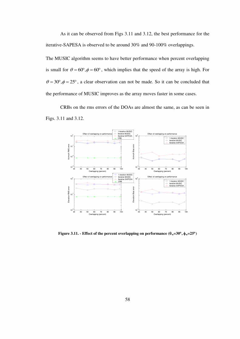
58

As it can be observed from Figs 3.11 and 3.12, the best performance for the

iterative-SAPESA is observed to be around 30% and 90-100% overlappings.

The MUSIC algorithm seems to have better performance when percent overlapping

is small for 60,60 , which implies that the speed of the array is high. For

25,30 , a clear observation can not be made. So it can be concluded that

the performance of MUSIC improves as the array moves faster in some cases.

CRBs on the rms errors of the DOAs are almost the same, as can be seen in

Figs. 3.11 and 3.12.

30 40 50 60 70 80 90 10010

-3

10-2

10-1

100

Effect of overlapping on performance

Azim

uth

RM

S e

rror

Overlapping (percent)

1-iteration MUSIC

Iterative MUSIC

Iterative SAPESA

CRB

30 40 50 60 70 80 90 10010

-1

100

Effect of overlapping on performanceA

zim

uth

Bia

s e

rror


1-iteration MUSIC

Iterative MUSIC

Iterative SAPESA

30 40 50 60 70 80 90 10010

-2

10-1

100


Ele

vation R

MS

err

or


1-iteration MUSIC

Iterative MUSIC

Iterative SAPESA

CRB

30 40 50 60 70 80 90 10010

-1

100


Ele

vation B

ias e

rror


1-iteration MUSIC

Iterative MUSIC

Iterative SAPESA

Figure 3.11. - Effect of the percent overlapping on performance (w=30, w=25)

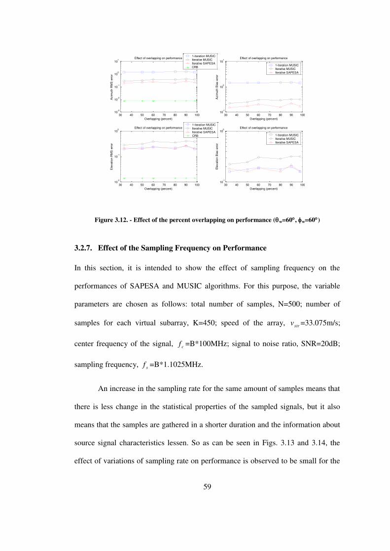
59

30 40 50 60 70 80 90 10010

-3

10-2

10-1

100

101


Azim

uth

RM

S e

rror


1-iteration MUSIC

Iterative MUSIC

Iterative SAPESA

CRB

30 40 50 60 70 80 90 10010

-1

100

101


Azim

uth

Bia

s e

rror


1-iteration MUSIC

Iterative MUSIC

Iterative SAPESA

30 40 50 60 70 80 90 10010

-2

10-1

100


Ele

vation R

MS

err

or


1-iteration MUSIC

Iterative MUSIC

Iterative SAPESA

CRB

30 40 50 60 70 80 90 10010

-1

100


Ele

vation B

ias e

rror


1-iteration MUSIC

Iterative MUSIC

Iterative SAPESA

Figure 3.12. - Effect of the percent overlapping on performance (w=60, w=60)

3.2.7. Effect of the Sampling Frequency on Performance

In this section, it is intended to show the effect of sampling frequency on the

performances of SAPESA and MUSIC algorithms. For this purpose, the variable

parameters are chosen as follows: total number of samples, N=500; number of

samples for each virtual subarray, K=450; speed of the array, strv =33.075m/s;

center frequency of the signal, cf =B*100MHz; signal to noise ratio, SNR=20dB;

sampling frequency, sf =B*1.1025MHz.

An increase in the sampling rate for the same amount of samples means that

there is less change in the statistical properties of the sampled signals, but it also

means that the samples are gathered in a shorter duration and the information about

source signal characteristics lessen. So as can be seen in Figs. 3.13 and 3.14, the

effect of variations of sampling rate on performance is observed to be small for the

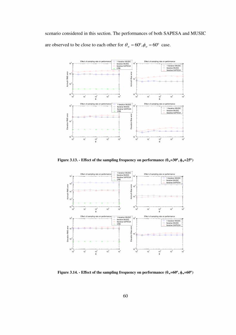
60

scenario considered in this section. The performances of both SAPESA and MUSIC

are observed to be close to each other for 60,60 ww case.

100

101

102

103

104

10-3

10-2

10-1

100

Effect of sampling rate on performance

B

Azim

uth

RM

S e

rror

1-iteration MUSIC

Iterative MUSIC

Iterative SAPESA

CRB

100

101

102

103

104

10-2

10-1

100


B

Azim

uth

Bia

s e

rror

1-iteration MUSIC

Iterative MUSIC

Iterative SAPESA

100

101

102

103

104

10-2

10-1

100


B

Ele

vation R

MS

err

or

1-iteration MUSIC

Iterative MUSIC

Iterative SAPESA

CRB

100

101

102

103

104

10-1

100


B

Ele

vation B

ias e

rror

1-iteration MUSIC

Iterative MUSIC

Iterative SAPESA

Figure 3.13. - Effect of the sampling frequency on performance (w=30, w=25)

100

101

102

103

104

10-3

10-2

10-1

100

101


B

Azim

uth

RM

S e

rror

1-iteration MUSIC

Iterative MUSIC

Iterative SAPESA

CRB

100

101

102

103

104

10-2

10-1

100

101


B

Azim

uth

Bia

s e

rror

1-iteration MUSIC

Iterative MUSIC

Iterative SAPESA

100

101

102

103

104

10-3

10-2

10-1

100


B

Ele

vation R

MS

err

or

1-iteration MUSIC

Iterative MUSIC

Iterative SAPESA

CRB

100

101

102

103

104

10-2

10-1

100


B

Ele

vation B

ias e

rror

1-iteration MUSIC

Iterative MUSIC

Iterative SAPESA

Figure 3.14. - Effect of the sampling frequency on performance (w=60, w=60)

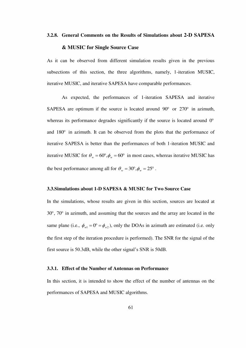
61

3.2.8. General Comments on the Results of Simulations about 2-D SAPESA

& MUSIC for Single Source Case

As it can be observed from different simulation results given in the previous

subsections of this section, the three algorithms, namely, 1-iteration MUSIC,

iterative MUSIC, and iterative SAPESA have comparable performances.

As expected, the performances of 1-iteration SAPESA and iterative

SAPESA are optimum if the source is located around 90 or 270 in azimuth,

whereas its performance degrades significantly if the source is located around 0

and 180 in azimuth. It can be observed from the plots that the performance of

iterative SAPESA is better than the performances of both 1-iteration MUSIC and

iterative MUSIC for 60,60 ww in most cases, whereas iterative MUSIC has

the best performance among all for 25,30 ww .

3.3.Simulations about 1-D SAPESA & MUSIC for Two Source Case

In the simulations, whose results are given in this section, sources are located at

30, 70 in azimuth, and assuming that the sources and the array are located in the

same plane (i.e., 21 0 ww ), only the DOAs in azimuth are estimated (i.e. only

the first step of the iteration procedure is performed). The SNR for the signal of the

first source is 50.3dB, while the other signal’s SNR is 50dB.




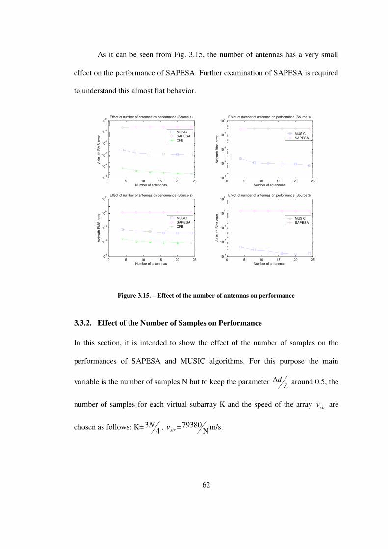
62

As it can be seen from Fig. 3.15, the number of antennas has a very small

effect on the performance of SAPESA. Further examination of SAPESA is required

to understand this almost flat behavior.

0 5 10 15 20 2510

-5

10-4

10-3

10-2

10-1

100

Effect of number of antennas on performance (Source 1)

Azim

uth

RM

S e

rror

Number of antennnas

MUSIC

SAPESA

CRB

0 5 10 15 20 2510

-4

10-3

10-2

10-1

100


Azim

uth

Bia

s e

rror

Number of antennnas

MUSIC

SAPESA

0 5 10 15 20 2510

-6

10-4

10-2

100

102


Azim

uth

RM

S e

rror

Number of antennnas

MUSIC

SAPESA

CRB

0 5 10 15 20 2510

-3

10-2

10-1

100

101


Azim

uth

Bia

s e

rror

Number of antennnas

MUSIC

SAPESA

Figure 3.15. – Effect of the number of antennas on performance





number of samples for each virtual subarray K and the speed of the array strv are


3N , strv =N

79380 m/s.

63

As it can be seen from the Fig. 3.16, the performance of SAPESA is

optimum when the number of samples is around 750. On the other hand, as it can be

observed clearly, increasing the number of samples improves the performance of

MUSIC as expected. The behavior of SAPESA should be further examined.

0 500 1000 150010

-4

10-3

10-2

10-1

100

101

Effect of number of samples on performance (Source 1)

Azim

uth

RM

S e

rror

Number of samples

MUSIC

SAPESA

CRB

0 500 1000 150010

-3

10-2

10-1

100

101


Azim

uth

Bia

s e

rror

Number of samples

MUSIC

SAPESA

0 500 1000 150010

-4

10-3

10-2

10-1

100


Azim

uth

RM

S e

rror

Number of samples

MUSIC

SAPESA

CRB

0 500 1000 150010

-3

10-2

10-1

100

Effect of number of samples on performance (Source 2)A

zim

uth

Bia

s e

rror

Number of samples

MUSIC

SAPESA

Figure 3.16. – Effect of the number of samples on performance




As it can be observed from Fig. 3.17, the performance of SAPESA is better

than that of MUSIC for low SNR values. For high SNR values, the performance of

SAPESA is limited by a threshold, which may be due to the assumption introduced

in the development of the algorithm in which it is assumed that the characteristics of

64

the signals do not change much during observation duration (see section 2.3).

Validity of this assumption lessens especially for scenarios where more than one

signal exists, since the signals can interfere each other.

On the other hand, as it can be observed clearly, increasing the SNR

improves the performance of MUSIC as expected. The behavior of SAPESA should

be examined further.

-20 0 20 40 60 8010

-6

10-4

10-2

100

102

Effect of SNR on performance (Source 1)

SNR (dB)

Azim

uth

RM

S e

rror

MUSIC

SAPESA

CRB

-20 0 20 40 60 8010

-6

10-4

10-2

100

102


SNR (dB)

Azim

uth

Bia

s e

rror

MUSIC

SAPESA

-20 0 20 40 60 8010

-6

10-4

10-2

100

102

104


SNR (dB)

Azim

uth

RM

S e

rror

MUSIC

SAPESA

CRB

-20 0 20 40 60 8010

-4

10-2

100

102

104


SNR (dB)

Azim

uth

Bia

s e

rror

MUSIC

SAPESA

Figure 3.17. – Effect of the SNR on performance


Performance



samples for each virtual subarray, K, which is naturally related to the percent

65

overlapping between virtual subarrays and the speed of the array, strv , which is

used to keep the parameter d around 0.5, are chosen as the variable parameters.

Although the percent overlapping has no effect on the MUSIC algorithm, the

performance of MUSIC is affected from strv .

2100

.rlappingPercentOve

NK ,

2100


vstrm/s.

As can be seen in Fig. 3.18, the best performance for the iterative-SAPESA

is observed to be around 30% and 80% overlappings. Although it can not be clearly

observed, the MUSIC algorithm seems to give its best performance when percent

overlapping is small, which implies that the speed of the array is high.

30 40 50 60 70 80 90 10010

-6

10-4

10-2

100

102

Effect of overlapping on performance (Source 1)

Azim

uth

RM

S e

rror


MUSIC

SAPESA

CRB

30 40 50 60 70 80 90 10010

-3

10-2

10-1

100

101


Azim

uth

Bia

s e

rror


MUSIC

SAPESA

30 40 50 60 70 80 90 10010

-4

10-3

10-2

10-1

100

101


Azim

uth

RM

S e

rror


MUSIC

SAPESA

CRB

30 40 50 60 70 80 90 10010

-3

10-2

10-1

100

101


Azim

uth

Bia

s e

rror


MUSIC

SAPESA

Figure 3.18. – Effect of the percent overlapping on performance

66


In this section, it is intended to show the effect of sampling frequency on the

performances of SAPESA and MUSIC algorithms. For this purpose, the variable

parameters are chosen as follows: total number of samples, N=500; number of

samples for each virtual subarray, K=450; speed of the array, strv =33.075m/s;

center frequency of the signal, cf =B*100MHz; sampling frequency,

sf =B*1.1025MHz.

As it can be seen from Fig. 3.19, the best performance of SAPESA is

acceptable for some B values and its best performance is achieved for 110B . It

seems that some modifications of SAPESA are necessary to improve its

performance.

100

101

102

103

104

10-6

10-4

10-2

100

102

Effect of sampling rate on performance (Source 1)

B

Azim

uth

RM

S e

rror

MUSIC

SAPESA

CRB

100

101

102

103

104

10-3

10-2

10-1

100

101

102


B

Azim

uth

Bia

s e

rror

MUSIC

SAPESA

100

101

102

103

104

10-4

10-2

100

102

104


B

Azim

uth

RM

S e

rror

MUSIC

SAPESA

CRB

100

101

102

103

104

10-4

10-2

100

102

104


B

Azim

uth

Bia

s e

rror

MUSIC

SAPESA

Figure 3.19. – Effect of the sampling rate on performance

67

3.4.Simulations about 2-D SAPESA & MUSIC for Two Source Case

Sources are located at 30, 70 in azimuth and 30, 10 in elevation, respectively.

The SNR for the signal of the first source is 50.3dB, while the other signal’s SNR is

50dB.

3.4.1. Effect of the Number of Iterations on Performance

In this section, it is intended to show the effect of the number of iterations on the

performances of SAPESA and MUSIC algorithms. For this purpose: total number

of samples, N=2000; number of samples for each virtual subarray, K=1775.

Figures 3.20 and 3.21 show that iterative SAPESA has a reasonable

performance except for the 2nd

signal’s elevation estimate. Iterative SAPESA

achieves a reasonable convergence in 10 steps; on the other hand, iterative MUSIC

has a very slow convergence rate, especially for the source having larger elevation

angle, which is a very important drawback for this algorithm. The plots show that

how SAPESA can give a reasonable performance even in some situations where

MUSIC fails. To increase the convergence rate of iterative MUSIC, some

modifications should be made in the iterative peak search procedure.

68

0 2 4 6 8 10 120

5

10

15

20Effect of number of iterations on performance (Source 1)

Azim

uth

RM

S e

rror


Iterative MUSIC

Iterative SAPESA

CRB

0 2 4 6 8 10 120

5

10

15


Azim

uth

Bia

s e

rror


Iterative MUSIC

Iterative SAPESA

0 2 4 6 8 10 120

5

10

15

20


Ele

vation R

MS

err

or


Iterative MUSIC

Iterative SAPESA

CRB

0 2 4 6 8 10 120

5

10

15

20


Ele

vation B

ias e

rror


Iterative MUSIC

Iterative SAPESA

Figure 3.20. - Effect of the number of iterations on performance (Source 1)

0 2 4 6 8 10 120

0.5

1

1.5


Azim

uth

RM

S e

rror


Iterative MUSIC

Iterative SAPESA

CRB

0 2 4 6 8 10 120.2

0.4

0.6

0.8

1

1.2

1.4

1.6Effect of number of iterations on performance (Source 2)

Azim

uth

Bia

s e

rror


Iterative MUSIC

Iterative SAPESA

0 2 4 6 8 10 120

2

4

6

8


Ele

vation R

MS

err

or


Iterative MUSIC

Iterative SAPESA

CRB

0 2 4 6 8 10 125

5.5

6

6.5

7

7.5

8

8.5Effect of number of iterations on performance (Source 2)

Ele

vation B

ias e

rror


Iterative MUSIC

Iterative SAPESA

Figure 3.21. - Effect of the number of iterations on performance (Source 2)

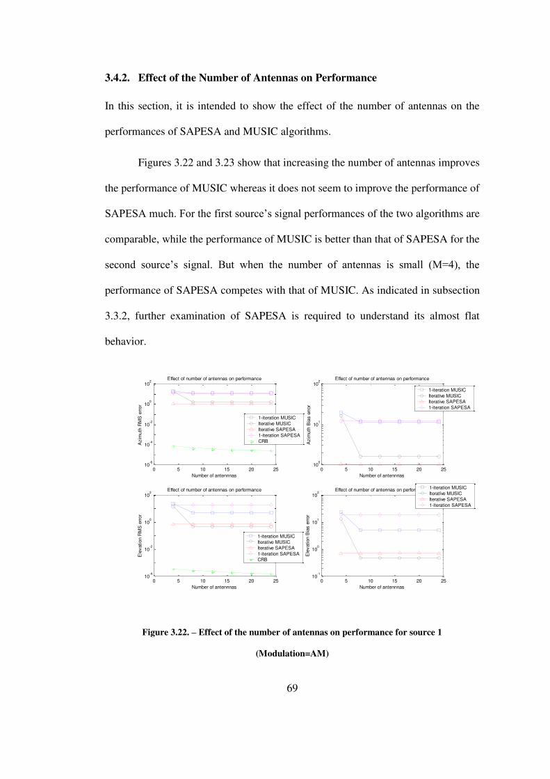
69




Figures 3.22 and 3.23 show that increasing the number of antennas improves

the performance of MUSIC whereas it does not seem to improve the performance of

SAPESA much. For the first source’s signal performances of the two algorithms are

comparable, while the performance of MUSIC is better than that of SAPESA for the

second source’s signal. But when the number of antennas is small (M=4), the

performance of SAPESA competes with that of MUSIC. As indicated in subsection

3.3.2, further examination of SAPESA is required to understand its almost flat

behavior.

0 5 10 15 20 2510

-6

10-4

10-2

100

102


Azim

uth

RM

S e

rror

Number of antennnas

1-iteration MUSIC

Iterative MUSIC

Iterative SAPESA

1-iteration SAPESA

CRB

0 5 10 15 20 2510

0

101

102


Azim

uth

Bia

s e

rror

Number of antennnas

1-iteration MUSIC

Iterative MUSIC

Iterative SAPESA

1-iteration SAPESA

0 5 10 15 20 2510

-4

10-2

100

102


Ele

vation R

MS

err

or

Number of antennnas

1-iteration MUSIC

Iterative MUSIC

Iterative SAPESA

1-iteration SAPESA

CRB

0 5 10 15 20 2510

-1

100

101

102


Ele

vation B

ias e

rror

Number of antennnas

1-iteration MUSIC

Iterative MUSIC

Iterative SAPESA

1-iteration SAPESA

Figure 3.22. – Effect of the number of antennas on performance for source 1

(Modulation=AM)

70

0 5 10 15 20 2510

-6

10-4

10-2

100

102


Azim

uth

RM

S e

rror

Number of antennnas

1-iteration MUSIC

Iterative MUSIC

Iterative SAPESA

1-iteration SAPESA

CRB

0 5 10 15 20 2510

-2

10-1

100

101


Azim

uth

Bia

s e

rror

Number of antennnas

1-iteration MUSIC

Iterative MUSIC

Iterative SAPESA

1-iteration SAPESA

0 5 10 15 20 2510

-3

10-2

10-1

100

101


Ele

vation R

MS

err

or

Number of antennnas

1-iteration MUSIC

Iterative MUSIC

Iterative SAPESA

1-iteration SAPESA

CRB

0 5 10 15 20 2510

-1

100

101


Ele

vation B

ias e

rror

Number of antennnas

1-iteration MUSIC

Iterative MUSIC

Iterative SAPESA

1-iteration SAPESA

Figure 3.23. – Effect of the number of antennas on performance for source 2

(Modulation=AM)





number of samples for each virtual subarray, K, and speed of the array, strv , are


3N , strv =N

79380 m/s.

Figures 3.24 and 3.25 show that increasing the number of samples does not

affect the performances much. Further examination of thsi case is required in the

future.

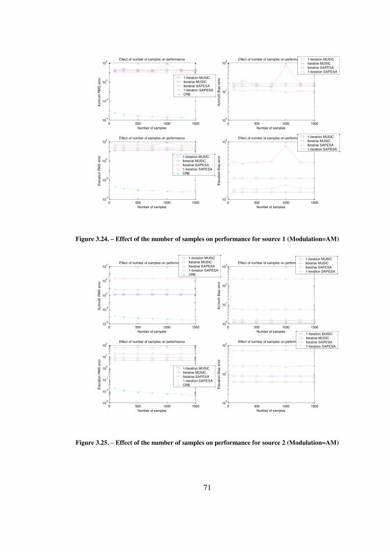
71

0 500 1000 150010

-4

10-2

100

102


Azim

uth

RM

S e

rror

Number of samples

1-iteration MUSIC

Iterative MUSIC

Iterative SAPESA

1-iteration SAPESA

CRB

0 500 1000 150010

0

101

102


Azim

uth

Bia

s e

rror

Number of samples

1-iteration MUSIC

Iterative MUSIC

Iterative SAPESA

1-iteration SAPESA

0 500 1000 150010

-4

10-2

100

102


Ele

vation R

MS

err

or

Number of samples

1-iteration MUSIC

Iterative MUSIC

Iterative SAPESA

1-iteration SAPESA

CRB

0 500 1000 150010

1

102


Ele

vation B

ias e

rror

Number of samples

1-iteration MUSIC

Iterative MUSIC

Iterative SAPESA

1-iteration SAPESA

Figure 3.24. – Effect of the number of samples on performance for source 1 (Modulation=AM)

0 500 1000 150010

-4

10-2

100

102

104


Azim

uth

RM

S e

rror

Number of samples

1-iteration MUSIC

Iterative MUSIC

Iterative SAPESA

1-iteration SAPESA

CRB

0 500 1000 150010

0

101

102

103


Azim

uth

Bia

s e

rror

Number of samples

1-iteration MUSIC

Iterative MUSIC

Iterative SAPESA

1-iteration SAPESA

0 500 1000 150010

-3

10-2

10-1

100

101

102


Ele

vation R

MS

err

or

Number of samples

1-iteration MUSIC

Iterative MUSIC

Iterative SAPESA

1-iteration SAPESA

CRB

0 500 1000 150010

0

101

102


Ele

vation B

ias e

rror

Number of samples

1-iteration MUSIC

Iterative MUSIC

Iterative SAPESA

1-iteration SAPESA

Figure 3.25. – Effect of the number of samples on performance for source 2 (Modulation=AM)

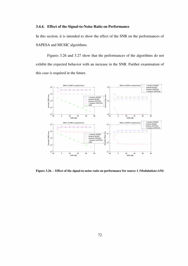
72




Figures 3.26 and 3.27 show that the performances of the algorithms do not

exhibit the expected behavior with an increase in the SNR. Further examination of

this case is required in the future.

-20 0 20 40 60 8010

-6

10-4

10-2

100

102


SNR (dB)

Azim

uth

RM

S e

rror

1-iteration MUSIC

Iterative MUSIC

Iterative SAPESA

1-iteration SAPESA

CRB

-20 0 20 40 60 8010

0

101

102


SNR (dB)

Azim

uth

Bia

s e

rror

1-iteration MUSIC

Iterative MUSIC

Iterative SAPESA

1-iteration SAPESA

-20 0 20 40 60 8010

-6

10-4

10-2

100

102


SNR (dB)

Ele

vation R

MS

err

or

1-iteration MUSIC

Iterative MUSIC

Iterative SAPESA

1-iteration SAPESA

CRB

-20 0 20 40 60 8010

-1

100

101

102


SNR (dB)

Ele

vation B

ias e

rror

1-iteration MUSIC

Iterative MUSIC

Iterative SAPESA

1-iteration SAPESA

Figure 3.26. – Effect of the signal-to-noise ratio on performance for source 1 (Modulation=AM)

73

-20 0 20 40 60 8010

-6

10-4

10-2

100

102

104


SNR (dB)

Azim

uth

RM

S e

rror

1-iteration MUSIC

Iterative MUSIC

Iterative SAPESA

1-iteration SAPESA

CRB

-20 0 20 40 60 8010

0

101

102

103


SNR (dB)

Azim

uth

Bia

s e

rror

1-iteration MUSIC

Iterative MUSIC

Iterative SAPESA

1-iteration SAPESA

-20 0 20 40 60 8010

-4

10-2

100

102


SNR (dB)

Ele

vation R

MS

err

or

1-iteration MUSIC

Iterative MUSIC

Iterative SAPESA

1-iteration SAPESA

CRB

-20 0 20 40 60 8010

0

101

102


SNR (dB)

Ele

vation B

ias e

rror

1-iteration MUSIC

Iterative MUSIC

Iterative SAPESA

1-iteration SAPESA

Figure 3.27. – Effect of the signal-to-noise ratio on performance for source 2 (Modulation=AM)


Performance



samples for each virtual subarray, K, which is naturally related to the percent

overlapping between virtual subarrays, and the speed of the array, strv , which is

used to keep the parameter d around 0.5, are chosen as follows:

2100

.rlappingPercentOve

NK ,

2100


vstrm/s.

Although the percent overlapping has no effect on the MUSIC algorithm, it is

thought that the performance of MUSIC may be affected from strv .

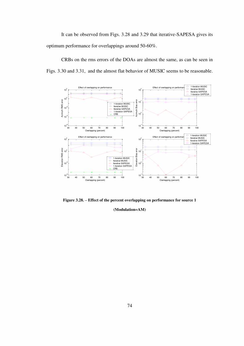
74

It can be observed from Figs. 3.28 and 3.29 that iterative-SAPESA gives its

optimum performance for overlappings around 50-60%.

CRBs on the rms errors of the DOAs are almost the same, as can be seen in

Figs. 3.30 and 3.31, and the almost flat behavior of MUSIC seems to be reasonable.

30 40 50 60 70 80 90 10010

-6

10-4

10-2

100

102


Azim

uth

RM

S e

rror


1-iteration MUSIC

Iterative MUSIC

Iterative SAPESA

1-iteration SAPESA

CRB

30 40 50 60 70 80 90 10010

-1

100

101

102


Azim

uth

Bia

s e

rror


1-iteration MUSIC

Iterative MUSIC

Iterative SAPESA

1-iteration SAPESA

30 40 50 60 70 80 90 10010

-4

10-2

100

102


Ele

vation R

MS

err

or


1-iteration MUSIC

Iterative MUSIC

Iterative SAPESA

1-iteration SAPESA

CRB

30 40 50 60 70 80 90 10010

-1

100

101

102

Effect of overlapping on performanceE

levation B

ias e

rror


1-iteration MUSIC

Iterative MUSIC

Iterative SAPESA

1-iteration SAPESA

Figure 3.28. – Effect of the percent overlapping on performance for source 1

(Modulation=AM)

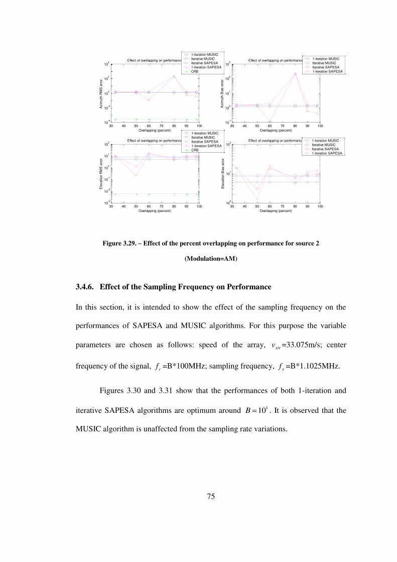
75

30 40 50 60 70 80 90 10010

-4

10-2

100

102

104


Azim

uth

RM

S e

rror


1-iteration MUSIC

Iterative MUSIC

Iterative SAPESA

1-iteration SAPESA

CRB

30 40 50 60 70 80 90 10010

-1

100

101

102

103


Azim

uth

Bia

s e

rror


1-iteration MUSIC

Iterative MUSIC

Iterative SAPESA

1-iteration SAPESA

30 40 50 60 70 80 90 10010

-3

10-2

10-1

100

101

102


Ele

vation R

MS

err

or


1-iteration MUSIC

Iterative MUSIC

Iterative SAPESA

1-iteration SAPESA

CRB

30 40 50 60 70 80 90 10010

0

101

102


Ele

vation B

ias e

rror


1-iteration MUSIC

Iterative MUSIC

Iterative SAPESA

1-iteration SAPESA

Figure 3.29. – Effect of the percent overlapping on performance for source 2

(Modulation=AM)


In this section, it is intended to show the effect of the sampling frequency on the

performances of SAPESA and MUSIC algorithms. For this purpose the variable

parameters are chosen as follows: speed of the array, strv =33.075m/s; center

frequency of the signal, cf =B*100MHz; sampling frequency, sf =B*1.1025MHz.

Figures 3.30 and 3.31 show that the performances of both 1-iteration and

iterative SAPESA algorithms are optimum around 110B . It is observed that the

MUSIC algorithm is unaffected from the sampling rate variations.

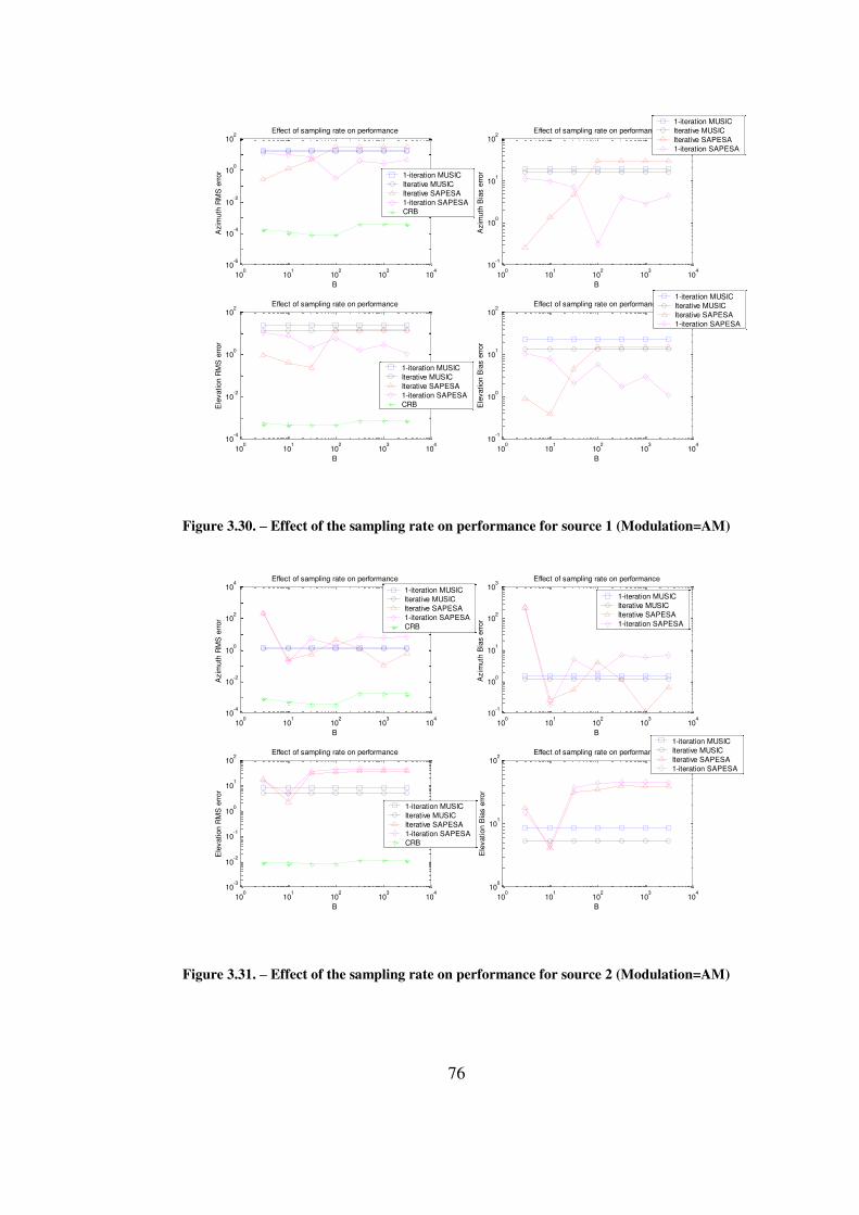
76

100

101

102

103

104

10-6

10-4

10-2

100

102


B

Azim

uth

RM

S e

rror

1-iteration MUSIC

Iterative MUSIC

Iterative SAPESA

1-iteration SAPESA

CRB

100

101

102

103

104

10-1

100

101

102


B

Azim

uth

Bia

s e

rror

1-iteration MUSIC

Iterative MUSIC

Iterative SAPESA

1-iteration SAPESA

100

101

102

103

104

10-4

10-2

100

102


B

Ele

vation R

MS

err

or

1-iteration MUSIC

Iterative MUSIC

Iterative SAPESA

1-iteration SAPESA

CRB

100

101

102

103

104

10-1

100

101

102


B

Ele

vation B

ias e

rror

1-iteration MUSIC

Iterative MUSIC

Iterative SAPESA

1-iteration SAPESA

Figure 3.30. – Effect of the sampling rate on performance for source 1 (Modulation=AM)

100

101

102

103

104

10-4

10-2

100

102

104


B

Azim

uth

RM

S e

rror

1-iteration MUSIC

Iterative MUSIC

Iterative SAPESA

1-iteration SAPESA

CRB

100

101

102

103

104

10-1

100

101

102

103


B

Azim

uth

Bia

s e

rror

1-iteration MUSIC

Iterative MUSIC

Iterative SAPESA

1-iteration SAPESA

100

101

102

103

104

10-3

10-2

10-1

100

101

102


B

Ele

vation R

MS

err

or

1-iteration MUSIC

Iterative MUSIC

Iterative SAPESA

1-iteration SAPESA

CRB

100

101

102

103

104

100

101

102


B

Ele

vation B

ias e

rror

1-iteration MUSIC

Iterative MUSIC

Iterative SAPESA

1-iteration SAPESA

Figure 3.31. – Effect of the sampling rate on performance for source 2 (Modulation=AM)

77

3.4.7. General Comments on Simulations about 2-D SAPESA & MUSIC for

Two Source Case

It is observed by the simulation results that the iterative-MUSIC algorithm has a

slow convergence rate, especially for sources with high elevation angles, which is

an important drawback for this algorithm. On the other hand, iterative-SAPESA has

a fast convergence but it has good performance only for certain situations.

Therefore, further examination of SAPESA is required to improve its performance

in terms of several variable parameters.

3.5.Effect of Array Speed on the Performance of MUSIC for Coherent Sources

Case

In this section, effect of the array speed on the MUSIC algorithm’s performance is

investigated. It was previously observed in [10] that array movement has a

decorrelating effect on source signals thus improves the performance. In this work,

it is observed that in correlated signals’ case increasing the speed reduces the rms

error and that especially the source signals, whose DOAs are close to each other,

can be distinguished easier.

To observe the effect of the speed of the array on the performance of

MUSIC algorithm, when the sources are coherent: number of antennas, M=4;

number of source signals, L=3; the sources are placed at 60, 65, 70 azimuth with

0 degree elevation angles; total number of samples, N=2000; the array moves in

the +x direction with a speed of strv =88.2m/s; relative source speeds, rsrclv =0m/s

for all three sources; center frequency of the signal, cf =500MHz; signal to noise

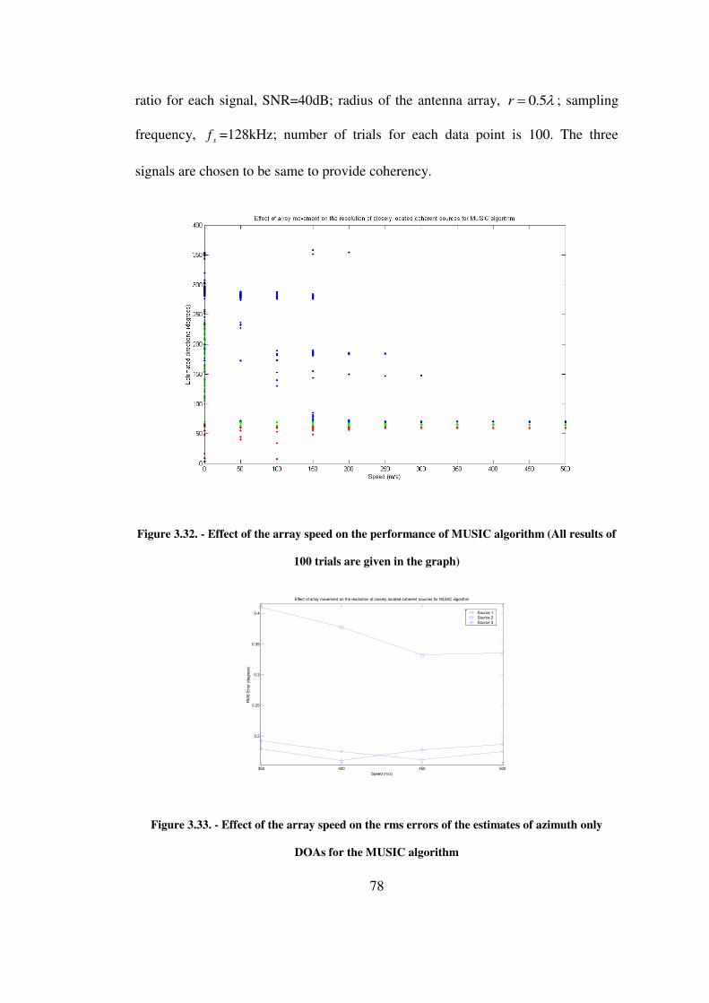
78

ratio for each signal, SNR=40dB; radius of the antenna array, 5.0r ; sampling

frequency, sf =128kHz; number of trials for each data point is 100. The three

signals are chosen to be same to provide coherency.

Figure 3.32. - Effect of the array speed on the performance of MUSIC algorithm (All results of

100 trials are given in the graph)

350 400 450 500

0.2

0.25

0.3

0.35

0.4

Speed (m/s)

RM

S E

rror

(degre

es)

Effect of array movement on the resolution of closely located coherent sources for MUSIC algorithm

Source 1

Source 2

Source 3

Figure 3.33. - Effect of the array speed on the rms errors of the estimates of azimuth only

DOAs for the MUSIC algorithm

79

It can be observed from Fig. 3.32 that the MUSIC algorithm can distinguish

three sources clearly for speeds greater than 300 m/s. As can be seen in Fig. 3.33 an

increase in the speed improves the performance of the MUSIC algorithm even in

such a difficult scenario. The results show that the motion of the array can be

utilized beneficially to improve the performance of the MUSIC algorithm, when the

incoming signals are coherent.

80

CHAPTER 4

CONCLUSIONS

In this work, multiple emitter DF by using a UCA which is placed on a moving

platform is considered. In the problem formulation, the Doppler frequency shift

caused by both the movements of the array and the emitters are taken into

consideration. Then, assuming that the array moves in the +x direction with a

constant speed, a new algorithm is developed and it is named as SAPESA (synthetic

aperture ESPRIT algorithm).

SAPESA creates two virtual subarrays by using different temporal samples

of the spatial samples of the array, thus there is a known displacement between

these virtual subarrays. Afterwards, SAPESA performs the ESPRIT algorithm using

these two virtual subarrays. For better resolution, it is desired that the distance

between two virtual subarrays ( sstr TKNvd )..( ) is maximum without causing

an ambiguity. The parameters that affect the performance are strv (speed of the

array), sT (sampling period), )( KN (N: total number of samples, K: number of

samples used to construct each subarray). strv , sT , N , K are the design parameters

that can be controlled and affect the performance of SAPESA.

It is observed by the simulations, given in Chapter 3, that the performance of

the SAPESA competes with that of the MUSIC algorithm for certain situations

81

(when number of antennas are small, SNR is low, variations in the signal

characteristics is small and overlapping between two virtual subarrays is large).

SAPESA has a faster convergence rate than the MUSIC algorithm if there are two

signals; a few steps of iterations is sufficient for SAPESA to converge. On the other

hand, both MUSIC and SAPESA does not exhibit expected behaviors especially

with respect to increases in number of antennas, number of samples and SNR for

two source, 2-D DOA estimation case. These behaviors should be examined more

detailly in future.

Since the performance of SAPESA is closely related to the changes in the

signal characteristics during observation duration, the simulations are carried out for

both AM and FM type modulated signals. Although the performance is expected to

be better for AM type modulated signals compared to the FM type modulated

signals, since the changes in the phase of the signal is less for AM type modulated

signals, the performances for both cases are observed to be similar. This can be

reasonable since the variations in the amplitude of the modulated signal is more in

the case of AM type modulated signals compared to the FM type modulated signals.

So it can be concluded that the type of the modulation of the received signal is not a

critical parameter for the performance of the algorithm.

Some advantages of SAPESA can be given as follows: SAPESA has no

resolution limit while MUSIC has the drawback of having a resolution limit,

meaning that, MUSIC spectrum is calculated only for a limited set of azimuth and

elevation values, which is a difficulty in estimating the actual peak of the MUSIC

spectrum. SAPESA has also lower computational cost and does not need storage for

82

antenna manifolds, like the ESPRIT algorithm, which is a very important advantage

especially in 2-dimensional DOA estimation problems. SAPESA, has a better

performance if the interested source is located around 90 and 270 azimuth angles.

While its performance decreases if the interested source is located around 0 and

180 azimuth angles. This is due to the synthetic linear array structure created by

the algorithm, which makes it an attractive alternative, especially for the situations

where the field of view is narrow.

The advantages, given in the previous paragraphs, make SAPESA a good

alternative for both 1 and 2-dimensional direction estimation problems.

In Chapter 3, simulations about the effect of array movement on the

performance of MUSIC algorithm is given, which shows that the motion of the

array can be utilized beneficially to improve DOA estimation performance of

MUSIC in the case of coherent signals.

Both the 2-dimensional iterative MUSIC and the 2-dimensional iterative

SAPESA algorithms have some convergence measures, so as to check the reliability

of the iteration process. In the simulations the following measures are used. For

MUSIC, if two successive azimuth estimates have a difference smaller than a

number, iteration stops, i.e, 1ˆˆ i

l

i

l . For SAPESA, if the difference between

two successive azimuth estimates gets larger than the previous difference, iteration

stops, i.e, 211 ˆˆˆˆ i

l

i

l

i

l

i

l , (see Section 2.3.2.). But instead of the

convergence of the azimuth estimates, the convergence of the elevation estimates

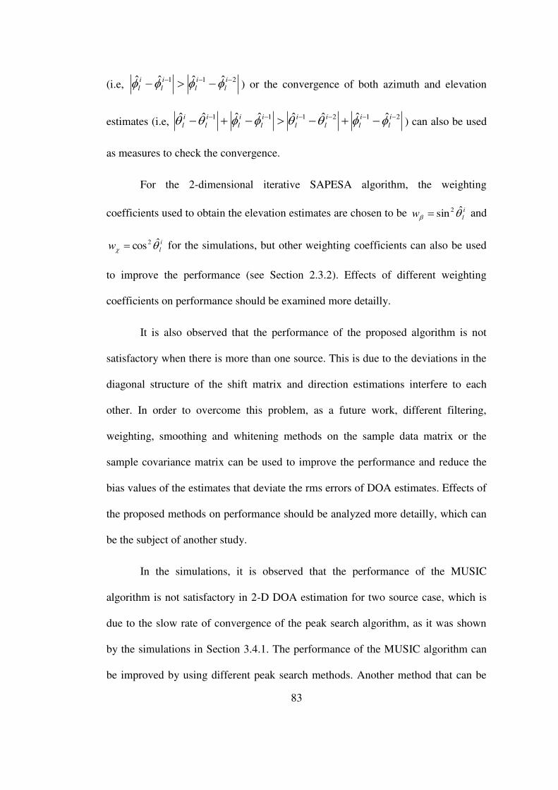
83

(i.e, 211 ˆˆˆˆ i

l

i

l

i

l

i

l ) or the convergence of both azimuth and elevation

estimates (i.e, 212111 ˆˆˆˆˆˆˆˆ i

l

i

l

i

l

i

l

i

l

i

l

i

l

i

l ) can also be used

as measures to check the convergence.

For the 2-dimensional iterative SAPESA algorithm, the weighting

coefficients used to obtain the elevation estimates are chosen to be i

lw ˆsin 2 and

i

lw ˆcos2 for the simulations, but other weighting coefficients can also be used

to improve the performance (see Section 2.3.2). Effects of different weighting

coefficients on performance should be examined more detailly.

It is also observed that the performance of the proposed algorithm is not

satisfactory when there is more than one source. This is due to the deviations in the

diagonal structure of the shift matrix and direction estimations interfere to each

other. In order to overcome this problem, as a future work, different filtering,

weighting, smoothing and whitening methods on the sample data matrix or the

sample covariance matrix can be used to improve the performance and reduce the

bias values of the estimates that deviate the rms errors of DOA estimates. Effects of

the proposed methods on performance should be analyzed more detailly, which can

be the subject of another study.

In the simulations, it is observed that the performance of the MUSIC

algorithm is not satisfactory in 2-D DOA estimation for two source case, which is

due to the slow rate of convergence of the peak search algorithm, as it was shown

by the simulations in Section 3.4.1. The performance of the MUSIC algorithm can

be improved by using different peak search methods. Another method that can be

84

used to improve the performance of the MUSIC algorithm is to use the estimates of

the SAPESA as the initial points to start the iteration process of the iterative

MUSIC algorithm.

In the formulations and the development of the algorithm, mutual coupling

effects of the antennas are ignored, which is a fairly important subject in practical

systems, since the array elements are close to each other especially for the signals

having high center frequencies, implying shorther wavelengths. As a future work

effects of the mutual coupling of array elements should be taken into account in

both formulation and simulations, and some modifications to the algorithms should

be proposed to lower these effects if possible.

In this work, the simulations are performed assuming that the array

manifolds are ideal. But in the practical systems, the array manifolds can be fairly

different from the ideal characteristics. As a future work, the algorithms’

performances should be investigated by the simulations using the measured array

manifolds.

In this work it is intended to develop an algorithm for estimating the

directions of telecommunication waves whose observation durations are relatively

short compared to radar systems. As a future work, assuming that the observation

duration is long, which may be the case for many radar systems, a formulation for

the purpose of localization may be more meaningful, since the DF estimates are

found at different points in the space and localization is possible.

85

REFERENCES

[1] S. Haykin (Editor), J. H. Justice, N. L. Owsley, J. L. Yen and A. C. Kak,

Array Signal Processing, Prentice Hall Inc., Englewood Cliffs, NJ, 1985.

[2] Don H. Johnson and Dan E. Dudgeon, Array Signal Processing, Prentice

Hall Inc., Englewood Cliffs, NJ, 1993.

[3] Herndon H. Jenkins, Small-Aperture Radio Direction-Finding, Artech

House, 1991.

[4] Arzu Tuncay Koç, “Direction Finding with a Uniform Circular Array via

Single Snapshot Processing”, Ph.D. thesis, Middle East Technical Univ.,

1996.

[5] Richard Roy, “ESPRIT – Estimation of Signal Parameters via Rotational

Invariance Techniques”, Ph. D. Dissertation, Stanford University, 1987.

[6] Richard Roy and Thomas Kailath, “ESPRIT – Estimation of Signal

Parameters via Rotational Invariance Techniques”, IEEE Transactions on

Acoustics, Speech, and Signal Processing, Vol. 37, No. 7, pp. 984-995, July

1989.

86

[7] Ralph Otto Schmidt, “Signal Subspace Approach to Multiple Emitter

Location and Spectral Estimation”, PhD. Dissertation, Stanford University,

1982.

[8] M. Skollnik, Introduction to Radar Systems, McGraw-Hill, Inc., NY, 1980.

[9] Gene H. Golub and Charles F. Van Loan, Matrix Computations, The Johns

Hopkins University Press, London, 1993.

[10] Fred Haber and Michael Zoltowski, “Spatial Spectrum Estimation in a

Coherent Signal Environment Using an Array in Motion”, IEEE

Transactions on Antennas and Propagation, Vol. AP-34. No. 3, pp. 301-310,

March 1986.

[11] H. L. Van Trees, Detection, Estimation, and Modulation Theory, Part I,

Wiley, NY, 1968.

87

APPENDIX A

DERIVATION OF CRAMÉR-RAO BOUNDS

The reason underlying the need for the Cramér-Rao bounds (CRBs) is to compare

the simulation results with a lower bound and to get an idea about the performance

of the experimented algorithms. The CRB is the ultimate limit an algorithm can

achieve. Thus the algorithm’s efficiency can be observed by comparing its

performance with this limit value.

In order to compute the Cramér-Rao bounds of the estimated parameters,

CRB covariance matrix must be calculated. [11]

1

.

TE : CRB covariance matrix (A.1)

where

TE . : Fischer Information Matrix (FIM)

)ln(LT

(A.2)

|)(...)( 1 NtytypL : Joint pdf of N

iity1

)(

given (A.3)

where

)()().(.)( 111tetxtFAty MxLxLxLMxLMx

(A.4)

88

)(1

tyMx

is the observation vector at time t.

TLLx txtxtx )(...)()( 11 is the vector of complex envelopes of source

signals at time t.

MxLA is the array manifold matrix. )(...)( 111 LMxMxMxL aaA

( )(1 lMxa is the array steering vector corresponding to the DOA vector l .)

)(tF LxL is the Doppler frequency shift matrix at time t. Assuming that the sources

are stationary, it is as follows:

tvjtvjdiagtF LLstrstrLxL .cos.cos..

2.exp....cos.cos..

2.exp)( 11

(A.5)

M is the number of antennas.

L is the number of sources.

)(1 teMx : vector representing the additive white Gaussian noise which corrupts the

measurements

2 : the noise variance, is the standard deviation of the additive white Gaussian

noise.

is the unknown parameters’ vector (for this problem

TTTTTNxNxxx )(~)(...)1(~)1( ) (A.6)

where v represents the real part of a vector/matrix v , v~ represents the imaginary

part of a vector/matrix v .

89

The CRB on the rms error of the thi parameter of the vector is the square

root of the thi diagonal entry of .

Remembering the formula derived at Section 2.1 of Chapter 2, the likelihood

function can be written as follows:

N

t

H

MNMN

txtFAtytxtFAty

NyyL

12

2

)()..(.)(.)()..(.)(.2

1exp.

.2

1))(),...,1((

(A.7)

where,

First the derivatives of the log-likelihood function with respect to ,

)}(Re{)( txtx , )}(Im{)(~ txtx and TLL ..11 have to be

calculated.

N

t

HHHHAtFtxtyAtFtxty

MNMNL

12

2

).().()(.).().()(..2

1

ln.2

2ln.2

)ln(

(A.8)

N

t

Htete

MNL

12222

)().(..2

1

2

)ln(

(A.9)

)(.).(Re.1

)(.).()(.).(..2

1

)(

)ln(

2

2

keAkF

keAkFkeAkFkx

L

HH

cHH

k=1,...,N (A.10)

90

)(.).(Im.1

)(.).(.)(.).(...2

1

)(~)ln(

2

2

keAkF

keAkFjkeAkFjkx

L

HH

cHH

k=1,...,N (A.11)

N

t

HH

N

t i

HHH

N

t

c

i

TTT

i

HHH

i

tetDtXL

ted

AtFdtx

ted

AtFdtxte

d

AtFdtx

L

12

12

12

)().().(Re.2

1)ln(

)(.).(

).(Re.2

1

)(.).(

).()(.).(

).(..2

1)ln(

(A.12)

where

i

i

i

LMxL

LLxL

L

d

add

ddtD

tx

tx

tx

tx

tX

)()(

)(...)()(

)(..00

.)(..0

.....

0..)(.

00..)(

)(

221

22

1

1

Then the entries of the FIM are computed as follows:

Using Result 1 given in Appendix 2:

91

22

2222

22

22

22

1 142

132

2

22

22

4

.

)1().1(.4

.

4

..2

4

.

)().().().(.4

1

)().(.4

..2

4

.)ln(

NM

MMNMNNMNM

seseteteE

teteENMNML

E

HHN

t

N

s

N

t

H

(A.13)

By Result 2 given in Appendix 2 ,

)ln(L is uncorrelated with any of the other

derivatives.

pk

HH

HHH

T

pFAAkF

pFApekeAkFE

px

L

kx

LE

,2

22

.)(..).(Re.2

1

)(.).().(.).(Re.2

1.

1

)(

)ln(.

)(

)ln(

(A.14)

where

elsewhere

pkpk

,0

,1, is the dirac delta function.

pk

HH

HHH

T

pFAAkF

pFApekeAkFE

px

L

kx

LE

,2

22

.)(..).(Im.2

1

)(.).().(.).(Im.2

1.

1

)(~)ln(

.)(

)ln(

(A.15)

92

)().(.).(Re.2

1

)().().().(.).(Re.2

1.

1

)ln(.

)(

)ln(

2

122

kXkDAkF

tXtDtekeAkFE

L

kx

LE

HH

N

t

HHH

T

(A.16)

pk

HH

HHH

T

pFAAkF

pFApekeAkFE

px

L

kx

LE

,2

22

.)(..).(Re.2

1

)(.).().(.).(Re.2

1.

1

)(~)ln(

.)(~)ln(

(A.17)

)().(.).(Im.

2

1

)(.).().(Im.2

1

)(.).().().().(Im.2

1.

1

)ln(.

)(~)ln(

2

2

122

kXkDAkF

kFAkDkX

kFAketetDtXE

L

kx

LE

HH

THH

N

t

HHH

T

(A.18)

N

t

HH

N

t

N

s

HHH

T

tXtDkDkX

sXsDsetetDtXE

LLE

12

1 122

)().().().(Re.2

1

)().().().().().(Re.2

1.

1

)ln(.

)ln(

(A.19)

Defining:

NM

CR.

4)(var

22

(A.20)

93

)(..)(.2

12

tFAAtFHHH

(A.21)

1

HG (A.22)

)().(.).(.2

12

kXkDAkFHH

k

(A.23)

Since H is Hermitian, HHT ~~

1

11

1

1

1

~..

~0

~~0.00.

~0....

.00....

....00.

~0..0

~0

0..0~

0

0....00)(var

NN

N

N

CR

HH

HH

HH

HH

(A.24)

Using Result 4 & Result 5 given in Appendix 2:

N

t

HHHHHH

N

tHHHHH

HH

N

t

tt

tXtDAtFtFAAtFtFAItDtX

tXtDtFAtFAAtFtFAtDtX

tXtDtDtX

GCRB

1

1

2

11*2

1

*1

)().(.).(.)(..).().(.).().(Re.2

1

)().().(..)(..).().(.).().(

)().().().(Re.

2

1

..Re)(

(A.25)

94

APPENDIX B

RESULTS

Result 1 :

stMM

stMseseteteE

HH

,).(

,.)().().().(

22

22

(A.26)

Proof : For st ,

(A.27)

For st ,

(A.28)

Since,

4).2.(

4.3

4.).1(

)()(.)()().()().(

222

1

42

1 1

2

1 1

222

MMMMM

teEteEteEteteEteteEM

i

ij

M

i

M

ijj

i

M

i

M

j

ji

T

22

2

2

.)(~).(~)().(

)().()().(.)().()().().().(

MteteEteteE

teteEseseEteteEseseteteE

TT

HHHHH

22

2

22

2

2

1)().(2

)(~).(~)().(.)(~).(~2)().(

)(~).(~)().()().(.)().()().().().(

MteteE

teteEteteEteteEteteE

teteEteteEseseEteteEseseteteE

T

TTTT

TTHHHH

95

(A.29)

Result 2 : 0)().().( seteteETH

for all t and s. (A.30)

Proof : For st , 0)().().( seteteETH

since e(t) and e(s) are independent . For

st , 0)().().( seteteETH

since third-order moments of Gaussian variables are

zero.

Result 3 : ).Re().Re(.2

1)Re().Re(

HTTyxyxyx (A.31)

).Re().Re(.2

1)Im().Im(

HTTyxyxyx

(A.32)

).Im().Im(.2

1)Im().Re(

HTTyxyxyx (A.33)

Result 4 : If H is a nonsingular complex matrix and if its inverse is G, then:

GG

GG

HH

HH~

~

~

~ 1

(A.34)

Proof :

GG

GG

HH

HHI ~

~

.~

~

(A.35)

IGHGH ~

.~

. (A.36)

0.~~

. GHGH (A.37)

222

22

2 ).(2

.2

).2()().().().( MMMMMseseteteE

HH

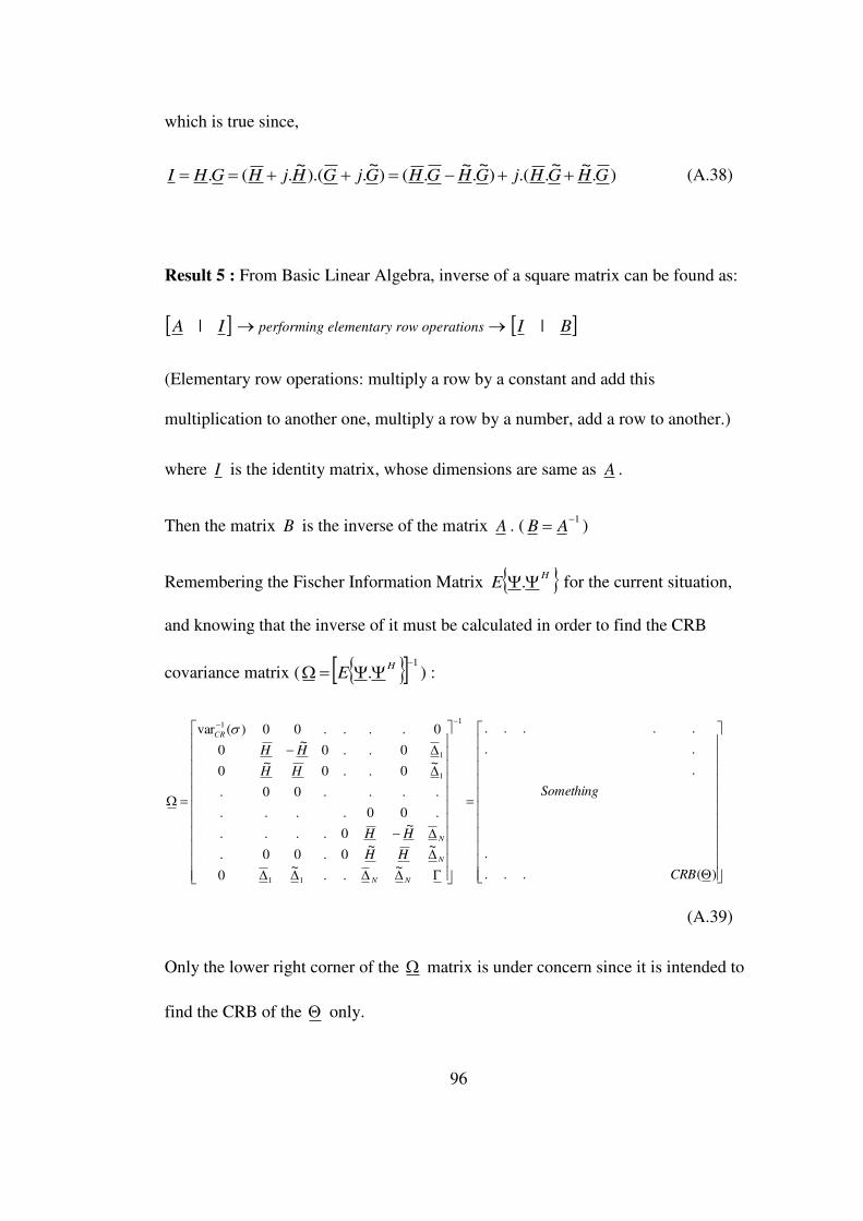
96

which is true since,

).~~

..()~

.~

.()~

.).(~

.(. GHGHjGHGHGjGHjHGHI (A.38)

Result 5 : From Basic Linear Algebra, inverse of a square matrix can be found as:

IA | performing elementary row operations BI |

(Elementary row operations: multiply a row by a constant and add this

multiplication to another one, multiply a row by a number, add a row to another.)

where I is the identity matrix, whose dimensions are same as A .

Then the matrix B is the inverse of the matrix A . (1 AB )

Remembering the Fischer Information Matrix HE . for the current situation,

and knowing that the inverse of it must be calculated in order to find the CRB

covariance matrix ( 1

.

HE ) :

)(...

.

.

..

.....

~..

~0

~~0.00.

~0....

.00....

....00.

~0..0

~0

0..0~

0

0....00)(var1

11

1

1

1

CRB

Something

HH

HH

HH

HH

NN

N

N

CR

(A.39)

Only the lower right corner of the matrix is under concern since it is intended to

find the CRB of the only.

97

I

I

I

I

I

I

I

I

HH

HH

HH

HH

NN

N

N

CR

..00

.0

..

.

.

..

0.

00..

|

|

|

|

|

|

|

|

~..

~0

~~0.00.

~0....

.00....

....00.

~0..0

~0

0..0~

0

0....00)(var

11

1

1

1

(A.40)

Define 1

HG

Perform the following elementary row operations:

Multiply n’th row by ( GT

n . ) and add to the last row. (n is even; n=2,4,…)


n

~. ) and add to the last row. (n is odd, n>2;

n=3,5,…)

I

Something

G

G

HH

HH

HH

HH

N

nn

T

n

n

T

n

N

N

N

CR

|

|

|

|

|

|

|

|

~.

~.

..~0..

~00

~~0.00.

~0....

.00....

....00.

~0..0

~0

0..0~

0

0....00)(var

1

1

1

1

1

(A.41)

Perform the following elementary row operations:


n .~ ) and add to the last row. (n is even; n=2,4,…)

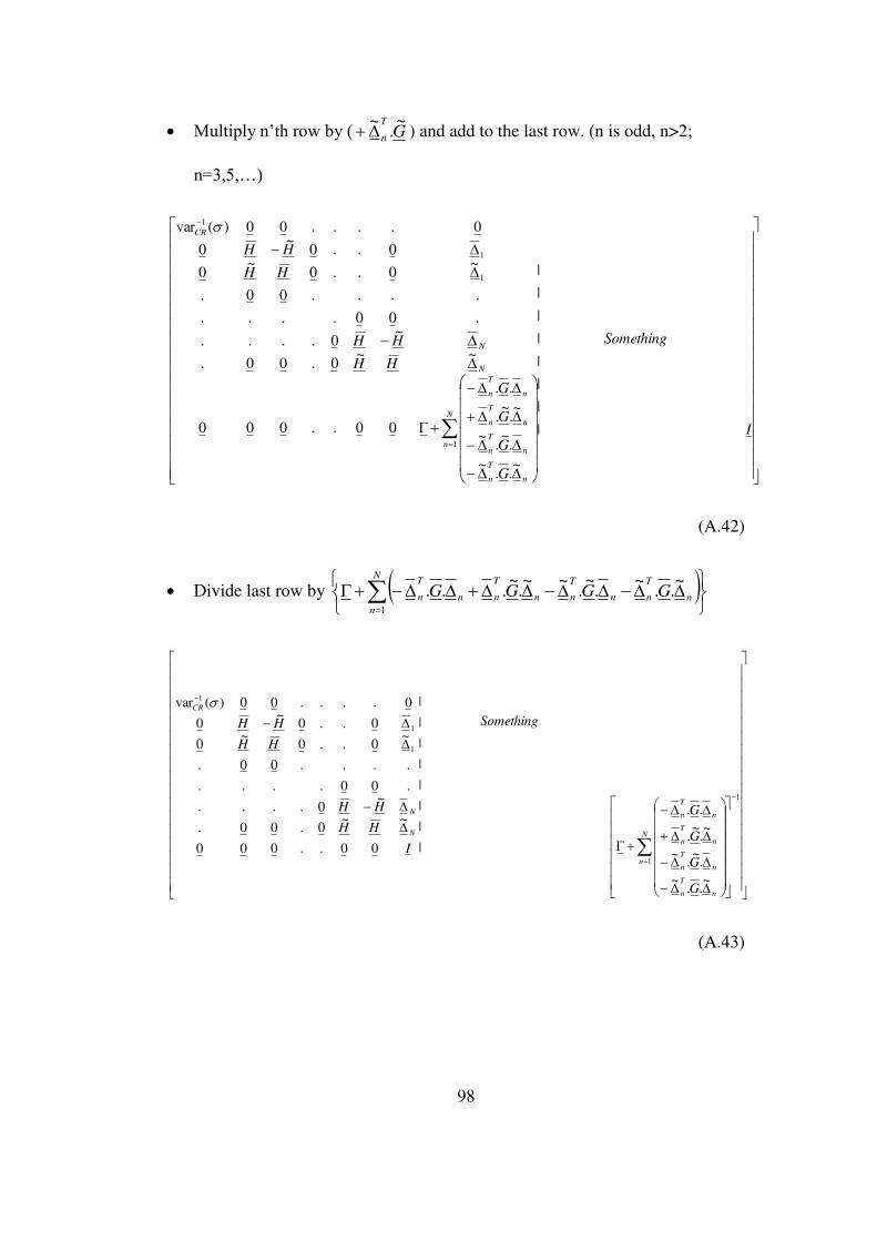
98


n

~.

~ ) and add to the last row. (n is odd, n>2;

n=3,5,…)

I

Something

G

G

G

G

HH

HH

HH

HH

N

n

n

T

n

n

T

n

n

T

n

n

T

n

N

N

CR

|

|

|

|

|

|

|

|

~..

~

.~

.~

~.

~.

..

00..000

~~0.00.

~0....

.00....

....00.

~0..0

~0

0..0~

0

0....00)(var

1

1

1

1

(A.42)

Divide last row by

N

n

n

T

nn

T

nn

T

nn

T

n GGGG1

~..

~.

~.

~~.

~...

1

1

1

1

1

~..

~

.~

.~

~.

~.

..

|

|

|

|

|

|

|

|

00..000

~~0.00.

~0....

.00....

....00.

~0..0

~0

0..0~

0

0....00)(var

N

n

n

T

n

n

T

n

n

T

n

n

T

n

N

N

CR

G

G

G

G

Something

I

HH

HH

HH

HH

(A.43)

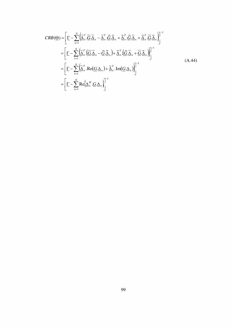
99

1

1

1

1

1

1

1

1

..Re

.Im.~

.Re.

~..

~.

~~.

~..

~..

~.

~.

~~.

~...)(

N

n

n

H

n

N

n

n

T

nn

T

n

N

n

nn

T

nnn

T

n

N

n

n

T

nn

T

nn

T

nn

T

n

G

GG

GGGG

GGGGCRB

(A.44)

DIRECTION FINDING WITH A UNIFORM CIRCULAR ARRAY PLACED ON A MOVING PLATFORM

Documents

Transcript of DIRECTION FINDING WITH A UNIFORM CIRCULAR ARRAY PLACED ON A MOVING PLATFORM