Direction finding in the presence of mutual coupling
161
-
Upload
independent -
Category
Documents
-
view
1 -
download
0
Transcript of Direction finding in the presence of mutual coupling

�
�
~r
~�
~�
x
y
z
l
d
Direction Finding in the Presence of
Mutual Coupling
Thomas Svantesson
Department of Signals and Systems
School of Electrical and Computer Engineering
chalmers university of technology
Sweden 1999


Thesis for the degree of Licentiate of Engineering
Technical Report No. 307L
Direction Finding in the Presence ofMutual Coupling
by
Thomas Svantesson
Department of Signals and Systems
School of Electrical and Computer Engineering
Chalmers University of Technology
S-412 96 G�oteborg, Sweden
G�oteborg 1999

Direction Finding in the Presence of Mutual Coupling
This thesis has been prepared using LATEX.
Copyright c 1999, Thomas Svantesson.
All rights reserved.
Thomas SvantessonDirection Finding in the Presence of Mutual Coupling.
Technical Report No. 307L.
Licenciate Thesis.
ISBN 91-7197-775-9
Printed in Sweden.
Chalmers Reproservice
G�oteborg 1999


Abstract
The area of sensor array processing has attracted considerable interest in
the signal processing community. The focus of this work has been on high
resolution Direction Of Arrival (DOA) estimation algorithms that detect and
locate aircrafts using radar systems. These algorithms exploit the fact that an
electromagnetic wave that is received by an array of antenna elements reaches
each element at di�erent time instants. In practical antennas the elements
of the array a�ect each other through mutual coupling and this reduces
the direction �nding ability. The e�ects of mutual coupling on direction
�nding are examined in this thesis. To be able to analyze the e�ects of
mutual coupling, the coupling needs to be calculated. Here, the coupling in
a Uniform Linear Array (ULA) of thin and �nite dipoles is calculated using
basic electromagnetic concepts.
The e�ects of coupling on the estimation of the DOA is studied by calcu-
lating a lower bound on the variance of the DOA estimates, the Cram�er-Rao
lower Bound (CRB). It is found that a known coupling does not a�ect the
CRB signi�cantly. Several methods of estimating the DOAs in the presence
of a known coupling are derived and analyzed in simulations.
However, in some cases the coupling might not be known, and one way
of mitigating the e�ects of an unknown coupling is to estimate the coupling
along with the DOAs. The CRB for this case is derived. Several methods
of estimating the directions and coupling parameters are also derived, and
it is found that estimating the coupling along with the DOAs mitigates the
e�ects of an unknown coupling.
Keywords: Estimation, detection, direction of arrival estimation, mutual
coupling, physical modeling, sensor array processing, subspace methods.
I

Contents
Abstract I
Contents iii
Acknowledgments vii
Abbreviations and Acronyms ix
Notation xi
1 Introduction 1
1.1 Background . . . . . . . . . . . . . . . . . . . . . . . . . . . . 1
1.2 Outline . . . . . . . . . . . . . . . . . . . . . . . . . . . . . . . 4
1.3 Contributions . . . . . . . . . . . . . . . . . . . . . . . . . . . 5
2 The Dipole Element 7
2.1 Geometry . . . . . . . . . . . . . . . . . . . . . . . . . . . . . 7
2.2 Radiation Intensity Pattern . . . . . . . . . . . . . . . . . . . 8
2.3 A Circuit Model . . . . . . . . . . . . . . . . . . . . . . . . . . 10
2.4 Receiving Plane Waves . . . . . . . . . . . . . . . . . . . . . . 14
2.5 Antenna Aperture . . . . . . . . . . . . . . . . . . . . . . . . . 15
3 A Linear Array of Dipoles 17
3.1 Geometry . . . . . . . . . . . . . . . . . . . . . . . . . . . . . 18
3.2 Mutual Coupling and Circuit Model . . . . . . . . . . . . . . . 18
3.3 Radiation Intensity . . . . . . . . . . . . . . . . . . . . . . . . 20
3.4 Receiving Plane Waves . . . . . . . . . . . . . . . . . . . . . . 25
3.5 Array Aperture . . . . . . . . . . . . . . . . . . . . . . . . . . 28
3.6 Conclusions . . . . . . . . . . . . . . . . . . . . . . . . . . . . 30
iii
4 Coupling E�ects on Direction Finding Accuracy 31
4.1 Data Model . . . . . . . . . . . . . . . . . . . . . . . . . . . . 32
4.2 Direction Finding Accuracy . . . . . . . . . . . . . . . . . . . 33
4.3 Computer Experiments . . . . . . . . . . . . . . . . . . . . . . 34
4.3.1 Angular Dependence . . . . . . . . . . . . . . . . . . . 35
4.3.2 Correlated Signals . . . . . . . . . . . . . . . . . . . . 36
4.3.3 Element Spacing . . . . . . . . . . . . . . . . . . . . . 38
4.4 Conclusions . . . . . . . . . . . . . . . . . . . . . . . . . . . . 39
5 Estimation With a Known Coupling 41
5.1 Data Model . . . . . . . . . . . . . . . . . . . . . . . . . . . . 41
5.2 Direction Finding Accuracy . . . . . . . . . . . . . . . . . . . 43
5.3 Estimation Methods . . . . . . . . . . . . . . . . . . . . . . . 45
5.3.1 The Structure of the Covariance Matrix . . . . . . . . 46
5.3.2 Estimation Methods: Beamforming and MUSIC . . . . 48
5.3.3 Other Methods . . . . . . . . . . . . . . . . . . . . . . 50
5.4 Signal Detection . . . . . . . . . . . . . . . . . . . . . . . . . . 55
5.5 Conclusions . . . . . . . . . . . . . . . . . . . . . . . . . . . . 58
6 Modeling of an Unknown Coupling 61
6.1 Reduced Coupling Model . . . . . . . . . . . . . . . . . . . . . 62
6.2 Uniqueness . . . . . . . . . . . . . . . . . . . . . . . . . . . . 64
6.3 Conclusions . . . . . . . . . . . . . . . . . . . . . . . . . . . . 72
7 Estimation With an Unknown Coupling 75
7.1 Data Model . . . . . . . . . . . . . . . . . . . . . . . . . . . . 76
7.2 Maximum Likelihood . . . . . . . . . . . . . . . . . . . . . . . 76
7.3 Direction Finding Accuracy . . . . . . . . . . . . . . . . . . . 79
7.4 Iterative MUSIC . . . . . . . . . . . . . . . . . . . . . . . . . 86
7.5 Other Iterative Methods . . . . . . . . . . . . . . . . . . . . . 88
7.6 Noise Subspace Fitting . . . . . . . . . . . . . . . . . . . . . . 91
7.7 Computer Experiments . . . . . . . . . . . . . . . . . . . . . . 92
7.8 Signal Detection . . . . . . . . . . . . . . . . . . . . . . . . . . 101
7.9 Conclusions . . . . . . . . . . . . . . . . . . . . . . . . . . . . 101
7A The Maximum Likelihood Method . . . . . . . . . . . . . . . . 102
7B The Asymptotic Covariance of SML . . . . . . . . . . . . . . . 108
7C The Noise Subspace Fitting Method . . . . . . . . . . . . . . . 112
8 E�ects of Model Errors 117
8.1 Impact of Model Errors . . . . . . . . . . . . . . . . . . . . . . 118
8.2 Average Error . . . . . . . . . . . . . . . . . . . . . . . . . . . 121
iv

8.3 Interference Rejection . . . . . . . . . . . . . . . . . . . . . . . 125
8.4 Conclusions . . . . . . . . . . . . . . . . . . . . . . . . . . . . 127
9 Conclusions and Future Work 129
9.1 Conclusions . . . . . . . . . . . . . . . . . . . . . . . . . . . . 129
9.2 Future Work . . . . . . . . . . . . . . . . . . . . . . . . . . . . 131
References 133
v


Acknowledgments
First, I would like to thank my advisor Mats Viberg for all his help, en-
couraging words, and for contributing to the open-minded atmosphere in the
department. Thanks also to all my colleagues and friends at the department
for making this a fun and interesting place to work at. Especially, I would
like to thank my senior colleague Tony Gustafsson for his outstanding exper-
tise.
I also would like to thank Anders Derneryd, Lars Josefsson, and Per-
Simon Kildal for fruitful discussions regarding mutual coupling modeling.
Finally, I am grateful to Fredrik Athley, Dr. Jonas Sj�oberg, and Prof. Mats
Viberg for their careful proof-reading of the manuscript.
This work was supported in part by the Swedish Foundation for Strategic
Research, under the Personal Computing and Communications Program.
vii

viii

Abbreviations and Acronyms
AIC An Information theoretic Criterion
AP Alternating Projection
CMA Constant Modulus Algorithm
CRB Cram�er-Rao lower Bound
DML Deterministic Maximum Likelihood
DOA Direction Of Arrival
EMF Electro-Motive Force
ESPRIT Estimation of Signal Parameters via Rotational Invariance
Techniques
FIM Fisher Information Matrix
GLRT Generalized Likelihood Ratio Test
MDL Minimum Description Length
MDLC Extended version of MDL that uses DML and AP
ML Maximum Likelihood
MODE Method Of Direction Estimation
MOM Method Of Moments
MSE Mean Square Error
MUSIC MUltiple SIgnal Classi�cation
MVU Minimum Variance Unbiased
NSF Noise Subspace Fitting
OTH Over The Horizon
RMSE Root Mean Square Error
SML Stochastic Maximum Likelihood
SNR Signal to Noise Ratio
ix

SSF Signal Subspace Fitting
ULA Uniform Linear Array
VHF Very High Frequency
VOR VHF Omni-directional Radio range
WSF Weighted Subspace Fitting
x
Notation
In this thesis the following conventions are used. Vectors are written as bold-
face lower-case letters. Matrices are written as boldface upper-case letters.
The meaning of the following symbols are, if nothing else is explicitly stated:
Rm ; C m The set of real and complex-valued m-vectors, respectively.
R(A) The column space of the matrix A.
rk (A) The rank of the matrix A.
Ay The Moore-Penrose pseudo-inverse of a m � n matrix A. If
m � n andA is of full rank it is de�ned asAy =�AHA
��1AH .
AH ; A�; AT Complex conjugate transpose, Complex conjugate and
Transpose operator, respectively.
Ai;j The (i; j)th element of A.
Aj;: The jth row of A. Other submatrices of A are denoted with
a similar MATLAB-like notation.
Tr(A) The trace operator.
kAkF The Frobenius matrix norm kAkF =
qTr(AAH).
Im The m�m identity matrix. Subscript m is often omitted.
xi
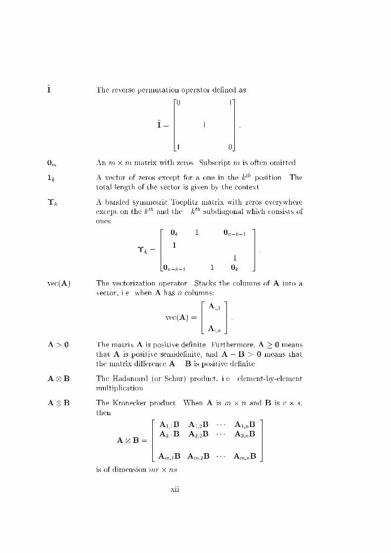
~I The reverse permutation operator de�ned as
~I =
26666640 1
. ..
1
. ..
1 0
3777775 :
0m An m�m matrix with zeros. Subscript m is often omitted.
1k A vector of zeros except for a one in the kth position. The
total length of the vector is given by the context.
�k A banded symmetric Toeplitz matrix with zeros everywhere
except on the kth and the �kth subdiagonal which consists of
ones
�k =
266640k 1 0n�k�1
1. . .
. . .. . .
. . . 1
0n�k�1 1 0k
37775 :vec(A) The vectorization operator. Stacks the columns of A into a
vector, i.e. when A has n columns:
vec(A) =
264 A:;1
...
A:;n
375 :A > 0 The matrix A is positive de�nite. Furthermore, A � 0 means
that A is positive semide�nite, and A � B > 0 means that
the matrix di�erence A�B is positive de�nite.
A�B The Hadamard (or Schur) product, i.e. element-by-element
multiplication.
AB The Kronecker product. When A is m � n and B is r � s,
then
AB =
26664A1;1B A1;2B � � � A1;nB
A2;1B A2;2B � � � A2;nB...
......
Am;1B Am;2B � � � Am;nB
37775is of dimension mr � ns.
xii
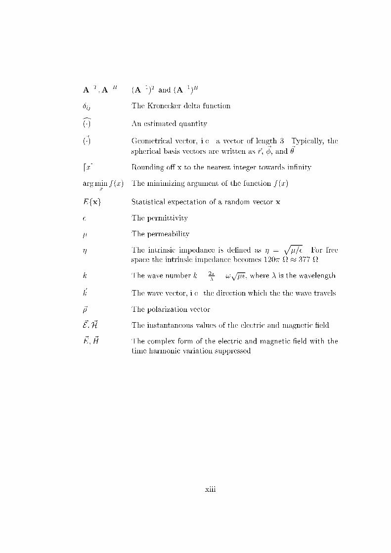
A�T ;A�H (A�1)T and (A�1)H .
�ij The Kronecker delta function.
c(�) An estimated quantity.
~(�) Geometrical vector, i.e. a vector of length 3. Typically, the
spherical basis vectors are written as ~r, ~�, and ~�.
dxe Rounding o� x to the nearest integer towards in�nity.
argminx
f(x) The minimizing argument of the function f(x).
Efxg Statistical expectation of a random vector x.
� The permittivity.
� The permeability.
� The intrinsic impedance is de�ned as � =p�=�. For free
space the intrinsic impedance becomes 120� � 377 .
k The wave number k = 2��= !
p��, where � is the wavelength.
~k The wave vector, i.e. the direction which the the wave travels.
~� The polarization vector.
~E; ~H The instantaneous values of the electric and magnetic �eld.
~E; ~H The complex form of the electric and magnetic �eld with the
time harmonic variation suppressed.
xiii

xiv
Chapter 1Introduction
This chapter gives a background to the problem of �nding the directions
of waves that are incident upon an array of elements. More precisely,
the direction �nding in the presence of mutual coupling between the
antenna elements is considered. An outline of the thesis and the published
work by the author are also presented.
1.1 Background
In the last decades, the area of sensor array processing has attracted consid-
erable interest in the signal processing community [21, 33]. The focus of this
work has been on high resolution DOA estimation algorithms for detection
and identi�cation of aircrafts using radar systems. These algorithms can also
be used in sonar applications where underwater arrays of acoustical sensors
are used to locate and identify other vessels. However, in recent years the
rapid development in the communication �eld has inspired some work on
using antenna arrays at base stations. The antenna array can be used to
receive and transmit energy only in the desired directions, and thus decrease
the interference from other users.
The key to obtaining high resolution in the DOA estimates is to use a
parameterized model of the array measurements. The quality of the esti-
mates then depends heavily on how well the model describes the data. In
the array case this implies that the response of the array needs to be known.
Also, the statistical assumptions regarding the signals and the noise must be
correct for the quality of the estimates to obey the theoretical predictions
derived using the assumed model. However, in practice, the array response is
never known exactly, and the statistical assumptions are only approximately
1

CHAPTER 1. INTRODUCTION
correct even for large data sets. Temperature, pressure, humidity and me-
chanical vibrations are only some factors which a�ect the properties of the
array resulting in a time-varying array response.
Much work has been made on di�erent calibration schemes that try to
overcome uncertainties in the array response. Those e�orts have mainly
been focused on obtaining estimation algorithms that are robust to modeling
errors [21]. Essentially, two di�erent approaches of minimizing the errors have
been studied. Firstly, the model errors are treated as random perturbations
from some nominal model, and robust estimation methods are derived based
on the statistical assumptions regarding the perturbations. Those analyses
typically lead to weighted estimation algorithms that minimize the variance
of the estimates [79, 80, 85]. Secondly, some part of the array response is
assumed unknown, but not random, and estimated together with the DOAs.
Typically, the locations of the sensors are assumed unknown but close to
some nominal array and estimated [36, 53, 91].
Independently of the approach used, one modeling error that frequently is
considered in the literature is unknown gain and phase of the sensors used in
the array. Many di�erent algorithms that estimate the gain and phase, either
together with the DOAs or using known calibration sources, have appeared
in the literature [17, 21, 42, 48, 79, 93].
Most of these methods do not use any detailed physical reasoning or
measurements. One source of modeling error in practical antennas is that the
di�erent elements of the antenna a�ect each other through mutual coupling,
and this e�ect can drastically reduce the performance of the direction �nding
algorithms. The subject of mutual coupling has not attracted much interest,
as compared to the case of independent sensors, in the signal processing
literature. Mutual coupling is on the other hand a well known problem for
antenna designers, and in the electromagnetical literature mutual coupling
is a well covered subject [5, 15, 31].
Although very little work on mutual coupling has been published in the
signal processing literature, some studies have been made. In [50], the ef-
fects of an uncompensated mutual coupling on the estimation performance
is studied using measurements. When using antenna arrays in digital com-
munication applications it might be argued that the information retrieval
is the main concern and not DOA estimation. But if the DOA estimation
is severely a�ected due to mutual coupling, it is reasonable to believe that
mutual coupling also a�ects the information retrieval problem when array
antennas are used [8, 34]. Since many communication systems now proposed
include antennas arrays, the problem of mitigating the e�ects of mutual cou-
pling is probably a neglected topic in present systems. Recently the e�ects
of mutual coupling on the Constant Modulus Algorithm (CMA) was investi-
2
1.1. BACKGROUND
gated in [95], and in [86] the e�ects on an aircraft navigation aid radio beacon
facility (VOR) was studied.
If mutual coupling can pose a problem when estimating DOAs or signals,
it is then of interest to reduce or otherwise mitigate the e�ects of mutual cou-
pling. The most natural way of doing this is to design the antenna from the
start in order to avoid high levels of mutual coupling and that is usually done.
Reducing the mutual coupling is in fact one of the most important design
problems in antenna design and much work has been published. The e�ects
of coupling on the radiation pattern for wire antennas has been thoroughly
studied, see for instance [24, 28, 70]. But it is not always best to design the
antenna with the lowest possible mutual coupling. Instead, it is important
to account for the coupling correctly. Actually, a known coupling can some-
times increase the estimation performance if compensated for correctly. This
will be shown in Chapter 4
Another way of reducing the e�ects of mutual coupling is to introduce
extra antenna elements that are not used, i.e. dummy elements. The mutual
coupling e�ects on DOA estimation by using dummy elements are investi-
gated in [37]. Furthermore, the coupling can also be compensated for by
using analog low-loss networks [4, 63].
Adding additional hardware to combat mutual coupling is expensive and
power consuming. An appealing alternative is to use signal processing meth-
ods instead, since the available processing power grows larger for every year
due to the rapid development of the silicon industry. Therefore, this thesis
will focus on the e�ects of mutual coupling and methods of compensating for
it using signal processing methods.
If the coupling is known, it is relatively straightforward to compensate
for the mutual coupling. One natural idea is to multiply the data with a
correction matrix and then apply a coupling free estimation method [27, 64].
Note that this method can be implemented either in hardware or using signal
processing. However, the multiplication a�ects not only the signal part,
but also the noise which changes color. Therefore, methods that rely on a
white noise covariance are not, at least not directly, applicable using this
method. Most DOA estimation schemes are possible to extend to include a
known mutual coupling by using an e�ective steering matrix. However, in
the literature, essentially only one method has been extended to include a
known coupling [47, 54, 92, 94]. Here, that method will be brie y discussed
and also several existing coupling free estimation methods will be extended
to include a known coupling.
The coupling might not be known in all scenarios, and if left uncompen-
sated it will reduce the possibilities of direction �nding. Di�erent compen-
sation algorithms or calibration methods can now be applied. For instance,
3
CHAPTER 1. INTRODUCTION
it can be assumed that the DOAs are known and only the coupling and per-
haps additional calibration parameters are estimated [42, 49, 50, 62]. On
the other hand, if the DOAs are also assumed to be unknown and estimated
along with the coupling, so-called auto-calibration methods result. Although
many auto-calibration schemes for unknown gain and phase have appeared,
the only e�ort to estimate both an unknown coupling and unknown DOAs
that have, to the author's knowledge, appeared in the literature is presented
in [18]. Here, that method will be reviewed and several other methods of
estimating unknown DOAs and coupling will be introduced.
Note that in this thesis, the coupling is assumed to be non-random and
is actually calculated using basic electromagnetics. No knowledge about the
coupling is assumed when the coupling is estimated. Of course, in a real-
istic scenario some knowledge about the coupling usually exists and should
be exploited. For instance, methods that use calibration data together with
some random perturbation, as well as unknown gain and phase of the sensor
responses, should of course be considered. However, to get some preliminary
results, the e�ects of mutual coupling on direction �nding and the improve-
ment by estimating the coupling are studied in a simple coupling scenario.
1.2 Outline
The outline of this thesis is as follows. To be able to examine the e�ects of mu-
tual coupling, a model for the coupling is needed. In the antenna literature,
almost all derivations are for the transmitting case since the transmitting
and receiving patterns are equal. Here, a model for the induced voltages on
the antenna elements is needed to �nd the e�ects of mutual coupling on the
estimation of the DOA for the incident wave. Therefore, an expression for
the induced voltages on a linear array of thin and �nite dipoles are derived.
In Chapter 2, the fundamental electromagnetic properties of the dipole ele-
ment are reviewed, which are then used to derive the expressions in the array
case. The induced voltages of a linear array of dipole elements are derived
in Chapter 3, where also some properties and e�ects of mutual coupling are
examined.
Once a model for the induced voltages is found, the e�ects of a known
coupling on the direction accuracy are examined in Chapter 4. The e�ects
are studied by calculating the Cram�er-Rao lower bound of the variance of
the DOA estimates for a few di�erent scenarios.
In Chapter 5, methods for estimating the DOAs in the presence of a
known coupling are discussed. Many DOA algorithms, derived for the hy-
pothetical coupling free case, can be extended to include a known mutual
4
1.3. CONTRIBUTIONS
coupling. By �rst reviewing the published methods that do include a known
coupling and then introducing several extensions of other DOA algorithms,
the �eld of sensor array processing is introduced. The problem of detecting
the number of incident waves is also brie y discussed in Chapter 5.
Usually the coupling is obtained using calibration measurements, but in
some cases, obtaining the coupling might not be possible. For instance, the
environment might be changing too quickly to allow for calibration measure-
ments. If the coupling is left uncompensated, it will drastically reduce the
possibilities of performing direction �nding. One way of mitigating these ef-
fects is to estimate the coupling along with the DOAs using signal processing
methods. However, the electromagnetical coupling model derived in Chapter
3 generally contains too many parameters to be estimated.
In Chapter 6, a parameterization of the coupling with a feasible number
of parameters, unlike a direct estimation of the electromagnetic model, is
derived. Furthermore, the question of uniqueness of the parameter estimates
is discussed. Also, a necessary condition for uniqueness is derived that gives a
limit on the number of coupling parameters that can be uniquely estimated.
Next, the parameterization of the coupling is used to estimate both an
unknown coupling and DOAs in Chapter 7. A Maximum Likelihood (ML)
method is derived. Based on the ML expressions, the Cram�er-Rao lower
bound is also derived. Then, several estimation methods are proposed along
with a review of the method introduced in [18]. The properties of the di�erent
estimation methods are examined in a few computer experiments.
The impact of the model errors, introduced by using the reduced model
to estimate the coupling, is examined in Chapter 8. The e�ects are studied
using data generated using the full electromagnetic model and estimated
with the reduced model derived in Chapter 6, using the estimation methods
derived in Chapter 7. The e�ects of an unknown coupling on the estimation
of the signal in the presence of a jammer is also examined.
Finally, the thesis is concluded in Chapter 9 by commenting on the results
derived and some proposals for future work are presented.
1.3 Contributions
Parts of this thesis have been or will be presented at the following conferences:
� T. Svantesson and M. Viberg. "On the Direction Finding Accuracy of
a Calibrated Array in the Presence of Mutual Coupling". In Nordiskt
antennsymposium, pages 385{392, G�oteborg, Sweden, May 1997.
� T. Svantesson. "The E�ects of Mutual Coupling Using a Linear Array
5
CHAPTER 1. INTRODUCTION
of Thin Dipoles of Finite Length". In Proc. 8th IEEE Signal Processing
Workshop On Statistical Signal and Array Processing, Portland, USA,
September 1998.
� T. Svantesson and M. Viberg. "Mutual Coupling in Antenna Arrays:
E�ects and Cures". In Proc. PCC Workshop, pages 99{103, Stock-
holm, November 1998.
� T. Svantesson. "Modeling and Estimation of Mutual Coupling in a
Uniform Linear Array of Dipoles". To be presented at IEEE ICASSP
99, Phoenix, USA, March 1999.
� T. Svantesson. "Methods of Mitigating the E�ects of Mutual Coupling
in Antenna Arrays: A Signal Processing Approach". To be presented
at RVK 99, Karlskrona, Sweden, June 1999
Parts of the thesis have also been published in technical reports [71, 74].
6
Chapter 2The Dipole Element
Wire antennas are some of the oldest, cheapest and most common
antennas. Among wire antennas, the dipole antenna is probably the
simplest. Many results are therefore derived for the dipole antenna.
The goal here is to obtain a simple model of the mutual coupling in an array.
Hence, the analysis should be simple, yet contain most of the interesting
parameters. Thus, the dipole antenna is suitable for a study of the properties
of mutual coupling.
First, the geometry of the dipole is de�ned, and the radiation intensity
is calculated. Then a simple circuit model of the dipole is introduced and
some parameters of this model are calculated. Finally, the dipole is used as
a receiving antenna and expressions for the induced voltage from an incident
plane wave as well as the antenna aperture are obtained.
2.1 Geometry
The simplest wire antenna is the in�nitesimal dipole for which the analysis
is especially simple. In this study of mutual coupling a thin dipole of �-
nite length will be considered instead. This is a more realistic antenna and
the resulting analysis does not get overly complicated. In order not to fur-
ther complicate the analysis, the antenna is assumed to be located in free
space which means that the in uence of the ground plane and objects in the
antenna environment are not considered.
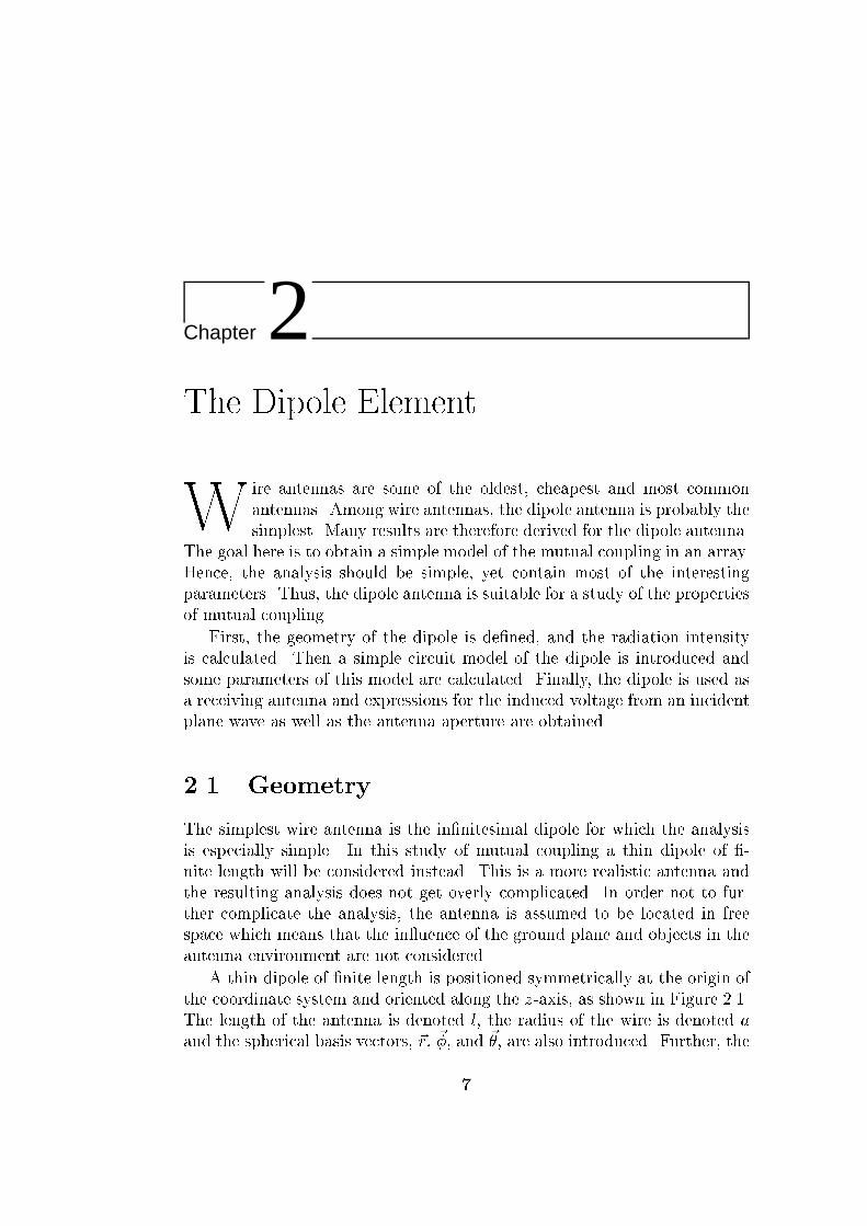
A thin dipole of �nite length is positioned symmetrically at the origin of
the coordinate system and oriented along the z-axis, as shown in Figure 2.1.
The length of the antenna is denoted l, the radius of the wire is denoted a
and the spherical basis vectors, ~r, ~�, and ~�, are also introduced. Further, the
7

CHAPTER 2. THE DIPOLE ELEMENT
�
�
Feed
~r~�
~�
2a
x
y
z
l
Figure 2.1: Relation of dipole to coordinates.
radius a of the dipole is assumed small compared to its length (a� l).
Note that the antenna is center-fed, i.e. the dipole may be energized
by a transmission line which is connected at the center of the dipole. The
radiation from this transmission line will be ignored and other e�ects from
it will be included in the terminating impedance.
2.2 Radiation Intensity Pattern
One of the most important characteristics of an antenna is the directional
properties of the radiated energy, i.e. the radiation intensity pattern which
is obtained from the radiated �eld of the antenna. In order to calculate
the radiated �eld, the current distribution must be known. For a very thin
dipole, the current distribution at z = z0 can be approximated by
~I(z0) = ~z I0 sin
�k(l
2� jz0j)
��l=2 � z0 � l=2 ; (2.1)
8
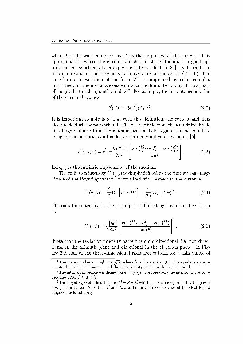
2.2. RADIATION INTENSITY PATTERN
where k is the wave number1 and I0 is the amplitude of the current. This
approximation where the current vanishes at the endpoints is a good ap-
proximation which has been experimentally veri�ed [5, 31]. Note that the
maximum value of the current is not necessarily at the center (z0 = 0). The
time harmonic variation of the form ej!t is suppressed by using complex
quantities and the instantaneous values can be found by taking the real part
of the product of the quantity and ej!t. For example, the instantaneous value
of the current becomes
~I(z0) = Re[~I(z0)ej!t]: (2.2)
It is important to note here that with this de�nition, the current and thus
also the �eld will be narrowband. The electric �eld from the thin �nite dipole
at a large distance from the antenna, the far-�eld region, can be found by
using vector potentials and is derived in many antenna textbooks [5]
~E(r; �; �) = ~� j�I0e
�jkr
2�r
"cos�kl2cos �
�� cos�kl2
�sin �
#: (2.3)
Here, � is the intrinsic impedance2 of the medium.
The radiation intensity U(�; �) is simply de�ned as the time average mag-
nitude of the Poynting vector 3 normalized with respect to the distance:
U(�; �) =r2
2Reh~E � ~H�
i=
r2
2�j ~E(r; �; �)j2: (2.4)
The radiation intensity for the thin dipole of �nite length can thus be written
as
U(�; �) = �jI0j28�2
"cos�kl2cos �
�� cos�kl2
�sin(�)
#2: (2.5)
Note that the radiation intensity pattern is omni-directional, i.e. non-direc-
tional in the azimuth plane and directional in the elevation plane. In Fig-
ure 2.2, half of the three-dimensional radiation pattern for a thin dipole of
1The wave number k = 2�
�= !
p��, where � is the wavelength. The symbols � and �
denote the dielectric constant and the permeability of the medium respectively.2The intrinsic impedance is de�ned as � =
p�=�. For free space the intrinsic impedance
becomes 120� � 377 .3The Poynting vector is de�ned as ~P = ~E � ~H which is a vector representing the power
ow per unit area. Note that ~E and ~H are the instantaneous values of the electric and
magnetic �eld intensity.
9
CHAPTER 2. THE DIPOLE ELEMENT
�
�
r
x
y
z
Figure 2.2: Three-dimensional radiation pattern of a thin dipole with sinu-
soidal current distribution (l = �=2).
�=2 length is shown. Maximum energy is thus radiated in the azimuth plane,
which perhaps is expected since the dipole is oriented along the ~z axis. The
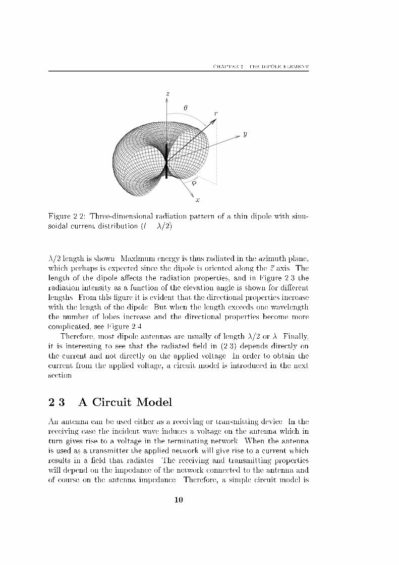
length of the dipole a�ects the radiation properties, and in Figure 2.3 the
radiation intensity as a function of the elevation angle is shown for di�erent
lengths. From this �gure it is evident that the directional properties increase
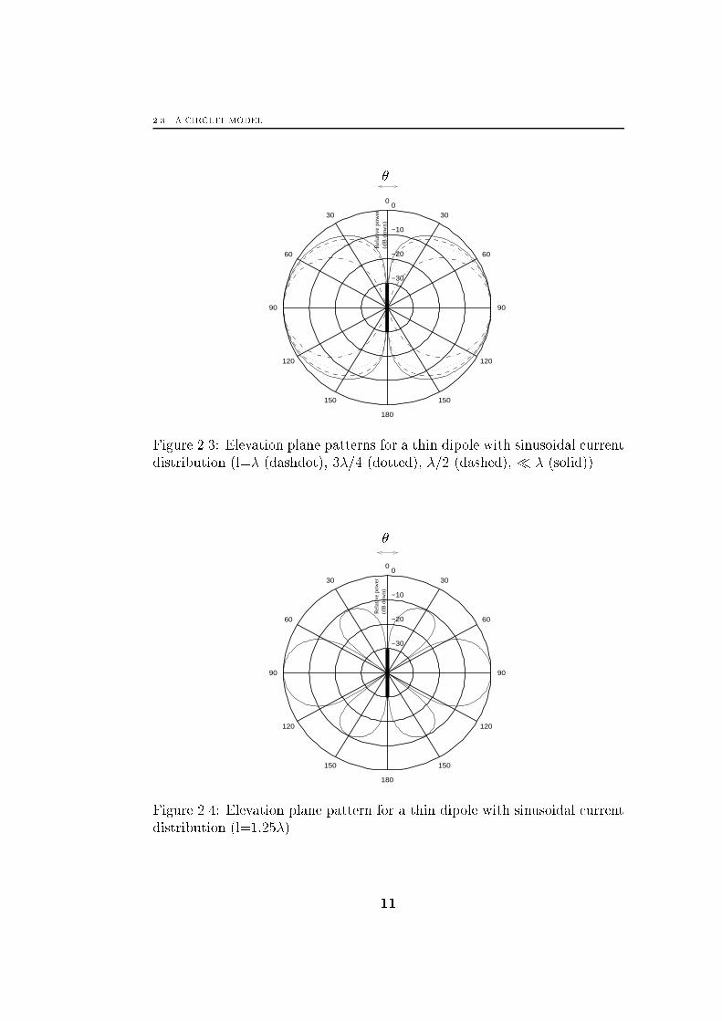
with the length of the dipole. But when the length exceeds one wavelength
the number of lobes increase and the directional properties become more
complicated, see Figure 2.4.
Therefore, most dipole antennas are usually of length �=2 or �. Finally,
it is interesting to see that the radiated �eld in (2.3) depends directly on
the current and not directly on the applied voltage. In order to obtain the
current from the applied voltage, a circuit model is introduced in the next
section.
2.3 A Circuit Model
An antenna can be used either as a receiving or transmitting device. In the
receiving case the incident wave induces a voltage on the antenna which in
turn gives rise to a voltage in the terminating network. When the antenna
is used as a transmitter the applied network will give rise to a current which
results in a �eld that radiates. The receiving and transmitting properties
will depend on the impedance of the network connected to the antenna and
of course on the antenna impedance. Therefore, a simple circuit model is
10
2.3. A CIRCUIT MODEL
−30
−20
−10
030
150
60
120
9090
120
60
150
30
180
0
(dB
dow
n)R
elat
ive
pow
er
�
Figure 2.3: Elevation plane patterns for a thin dipole with sinusoidal current
distribution (l=� (dashdot), 3�=4 (dotted), �=2 (dashed), � � (solid)).
−30
−20
−10
030
150
60
120
9090
120
60
150
30
180
0
(dB
dow
n)R
elat
ive
pow
er
�
Figure 2.4: Elevation plane pattern for a thin dipole with sinusoidal current
distribution (l=1:25�).
11
CHAPTER 2. THE DIPOLE ELEMENT
introduced before the actual calculations of the transmitted and received
radiation are begun.
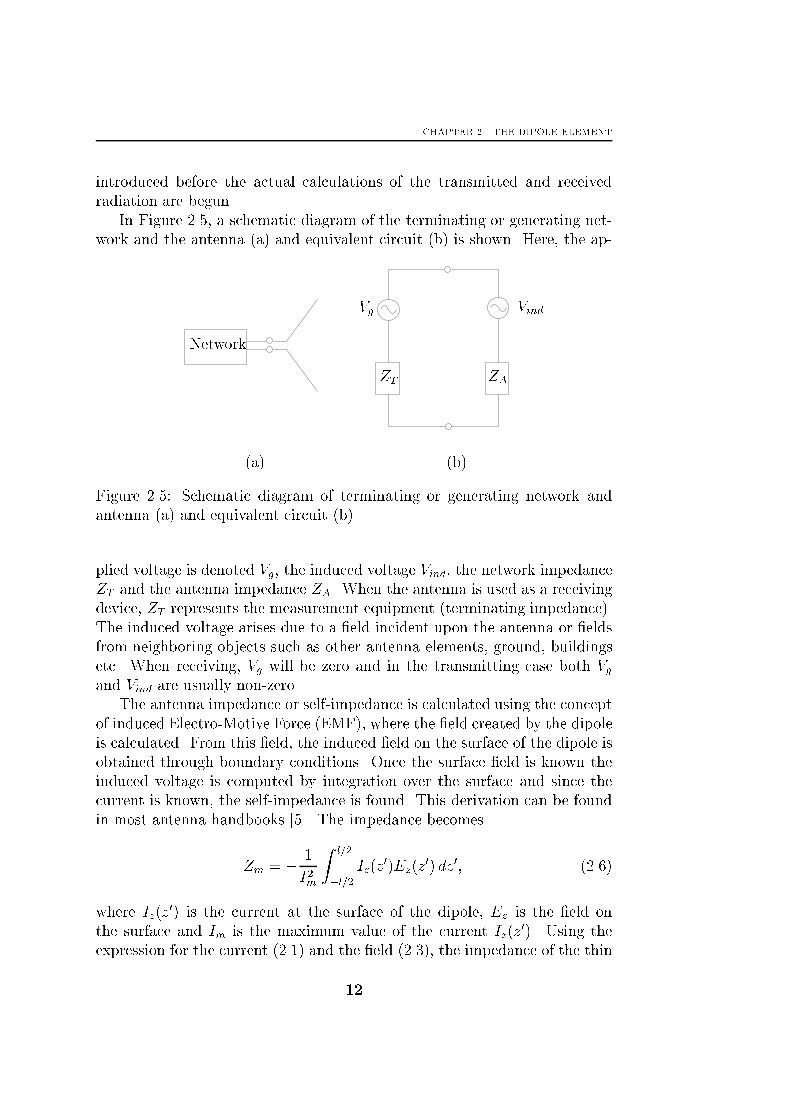
In Figure 2.5, a schematic diagram of the terminating or generating net-
work and the antenna (a) and equivalent circuit (b) is shown. Here, the ap-
Network
Vg Vind
ZT ZA
(a) (b)
Figure 2.5: Schematic diagram of terminating or generating network and
antenna (a) and equivalent circuit (b).
plied voltage is denoted Vg, the induced voltage Vind, the network impedance
ZT and the antenna impedance ZA. When the antenna is used as a receiving
device, ZT represents the measurement equipment (terminating impedance).
The induced voltage arises due to a �eld incident upon the antenna or �elds
from neighboring objects such as other antenna elements, ground, buildings
etc. When receiving, Vg will be zero and in the transmitting case both Vgand Vind are usually non-zero.
The antenna impedance or self-impedance is calculated using the concept
of induced Electro-Motive Force (EMF), where the �eld created by the dipole
is calculated. From this �eld, the induced �eld on the surface of the dipole is
obtained through boundary conditions. Once the surface �eld is known the
induced voltage is computed by integration over the surface and since the
current is known, the self-impedance is found. This derivation can be found
in most antenna handbooks [5]. The impedance becomes
Zm = � 1
I2m
Z l=2
�l=2
Iz(z0)Ez(z
0) dz0; (2.6)
where Iz(z0) is the current at the surface of the dipole, Ez is the �eld on
the surface and Im is the maximum value of the current Iz(z0). Using the
expression for the current (2.1) and the �eld (2.3), the impedance of the thin
12
2.3. A CIRCUIT MODEL
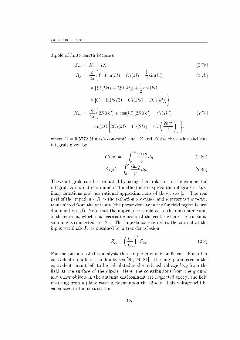
dipole of �nite length becomes
Zm = Rr + jXm (2.7a)
Rr =�
2�
�C + ln(kl)� Ci(kl) +
1
2sin(kl) (2.7b)
� [Si(2kl)� 2Si(kl)] +1
2cos(kl)
� [C + ln(kl=2) + Ci(2kl)� 2Ci(kl)]
�Xm =
�
4�
�2Si(kl) + cos(kl) [2Si(kl)� Si(2kl)] (2.7c)
� sin(kl)
�2Ci(kl)� Ci(2kl)� Ci
�2ka2
l
���;
where C = 0:5772 (Euler's constant) and Ci and Si are the cosine and sine
integrals given by
Ci(x) =�Z 1
x
cos y
ydy (2.8a)
Si(x) =
Z x
0
sin y
ydy: (2.8b)
These integrals can be evaluated by using their relation to the exponential
integral. A more direct numerical method is to express the integrals in aux-
iliary functions and use rational approximations of these, see [1]. The real
part of the impedance Rr is the radiation resistance and represents the power
transmitted from the antenna (the power density in the far-�eld region is pre-
dominantly real). Note that the impedance is related to the maximum value
of the current, which not necessarily occur at the center where the transmis-
sion line is connected, see 2.1. The impedance referred to the current at the
input terminals Iin is obtained by a transfer relation
ZA =
�Im
Iin
�2
Zm: (2.9)
For the purpose of this analysis this simple circuit is su�cient. For other
equivalent circuits of the dipole, see [20, 24, 81]. The only parameter in the
equivalent circuit left to be calculated is the induced voltage Vind from the
�eld at the surface of the dipole. Here, the contributions from the ground
and other objects in the antenna environment are neglected except the �eld
resulting from a plane wave incident upon the dipole. This voltage will be
calculated in the next section.
13
CHAPTER 2. THE DIPOLE ELEMENT
2.4 Receiving Plane Waves
When the antenna is used as a receiving device, the source of radiation is
usually located at such a large distance that the wave incident upon the
antenna can be considered to be a plane wave. Furthermore, the plane wave
is assumed to be uniform, i.e. the electric �eld in a plane perpendicular to
the propagation direction has the same amplitude, direction and phase. The
direction of the electric �eld (as well as the magnetic) is transverse to the
direction of propagation.
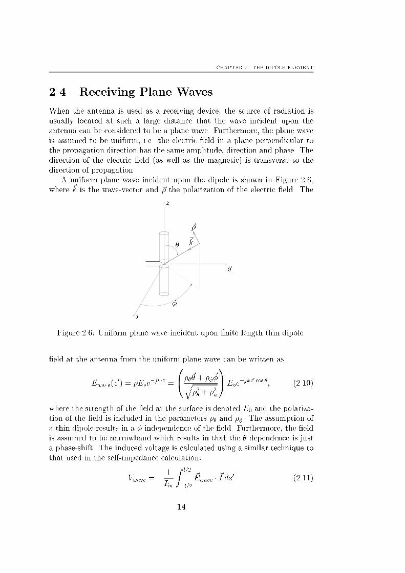
A uniform plane wave incident upon the dipole is shown in Figure 2.6,
where ~k is the wave-vector and ~� the polarization of the electric �eld. The
~k
~�
�
�
x
y
z
Figure 2.6: Uniform plane wave incident upon �nite length thin dipole.
�eld at the antenna from the uniform plane wave can be written as
~Ewave(z0) = ~�Eoe
�j~k�~z =
0@��~� + ��~�q�2� + �2�
1AEoe�jkz0 cos �; (2.10)
where the strength of the �eld at the surface is denoted E0 and the polariza-
tion of the �eld is included in the parameters �� and ��. The assumption of
a thin dipole results in a � independence of the �eld. Furthermore, the �eld
is assumed to be narrowband which results in that the � dependence is just
a phase-shift. The induced voltage is calculated using a similar technique to
that used in the self-impedance calculation:
Vwave = � 1
Iin
Z l=2
�l=2
~Ewave � ~I dz0 (2.11)
14
2.5. ANTENNA APERTURE
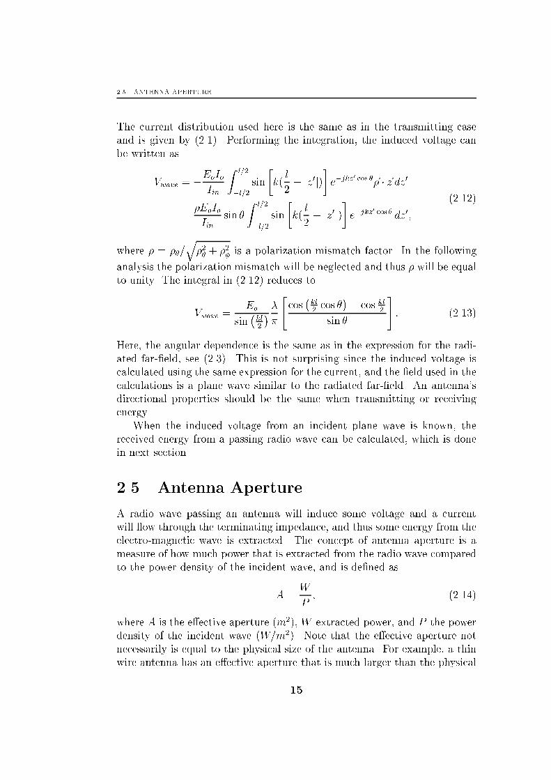
The current distribution used here is the same as in the transmitting case
and is given by (2.1). Performing the integration, the induced voltage can
be written as
Vwave = �EoIo
Iin
Z l=2
�l=2
sin
�k(l
2� jz0j)
�e�jkz
0 cos �~� � ~z dz0
=�EoIo
Iinsin �
Z l=2
�l=2
sin
�k(l
2� jz0j)
�e�jkz
0 cos � dz0;
(2.12)
where � = ��=q�2� + �2� is a polarization mismatch factor. In the following
analysis the polarization mismatch will be neglected and thus � will be equal
to unity. The integral in (2.12) reduces to
Vwave =Eo
sin�kl2
� ��
"cos�kl2cos �
�� cos kl2
sin �
#: (2.13)
Here, the angular dependence is the same as in the expression for the radi-
ated far-�eld, see (2.3). This is not surprising since the induced voltage is
calculated using the same expression for the current, and the �eld used in the
calculations is a plane wave similar to the radiated far-�eld. An antenna's
directional properties should be the same when transmitting or receiving
energy.
When the induced voltage from an incident plane wave is known, the
received energy from a passing radio wave can be calculated, which is done
in next section.
2.5 Antenna Aperture
A radio wave passing an antenna will induce some voltage and a current
will ow through the terminating impedance, and thus some energy from the
electro-magnetic wave is extracted. The concept of antenna aperture is a
measure of how much power that is extracted from the radio wave compared
to the power density of the incident wave, and is de�ned as
A =W
P; (2.14)
where A is the e�ective aperture (m2), W extracted power, and P the power
density of the incident wave (W=m2). Note that the e�ective aperture not
necessarily is equal to the physical size of the antenna. For example, a thin
wire antenna has an e�ective aperture that is much larger than the physical
15
CHAPTER 2. THE DIPOLE ELEMENT
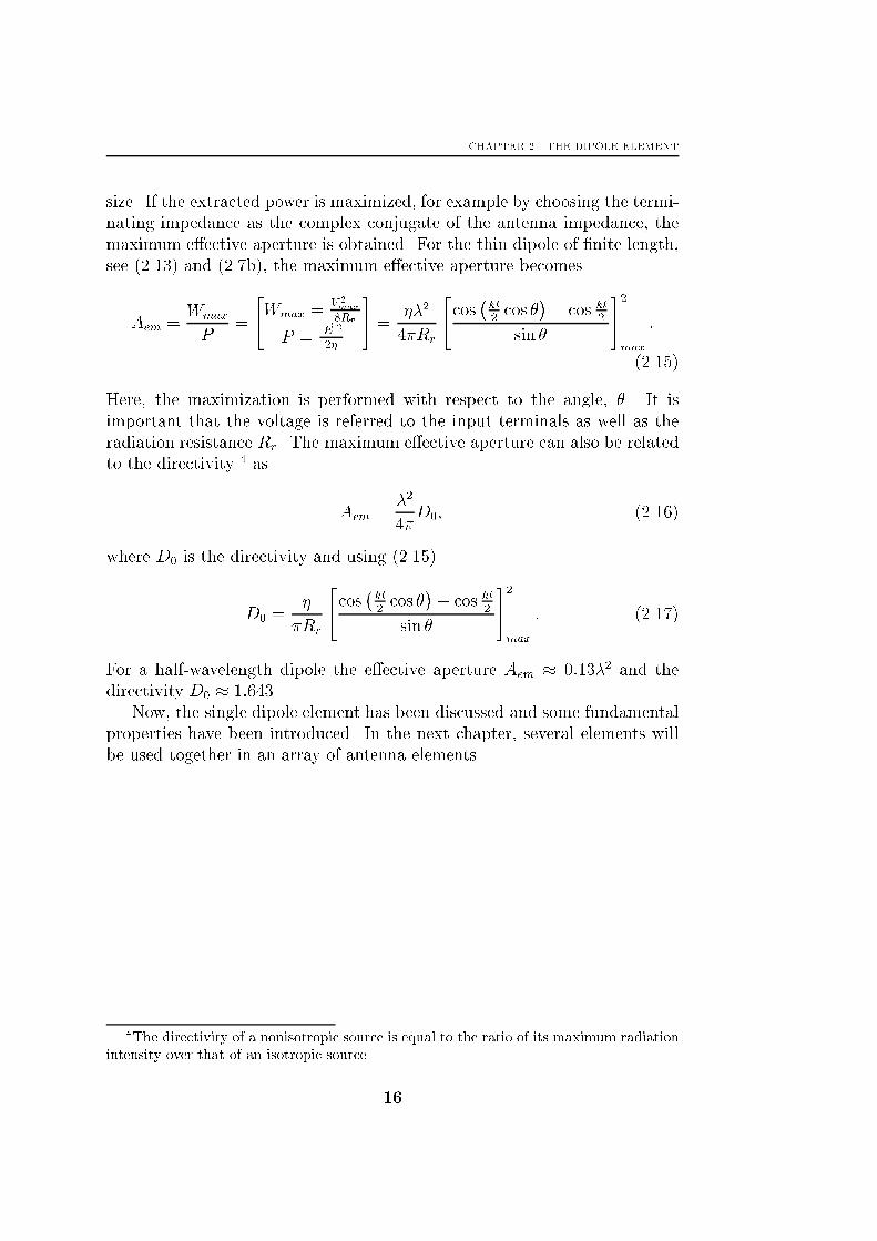
size. If the extracted power is maximized, for example by choosing the termi-
nating impedance as the complex conjugate of the antenna impedance, the
maximum e�ective aperture is obtained. For the thin dipole of �nite length,
see (2.13) and (2.7b), the maximum e�ective aperture becomes
Aem =Wmax
P=
"Wmax =
V 2max
8Rr
P =j ~Ej2
2�
#=
��2
4�Rr
"cos�kl2cos �
�� cos kl2
sin �
#2max
:
(2.15)
Here, the maximization is performed with respect to the angle, �. It is
important that the voltage is referred to the input terminals as well as the
radiation resistance Rr. The maximum e�ective aperture can also be related
to the directivity 4 as
Aem =�2
4�D0; (2.16)
where D0 is the directivity and using (2.15)
D0 =�
�Rr
"cos�kl2cos �
�� cos kl2
sin �
#2max
: (2.17)
For a half-wavelength dipole the e�ective aperture Aem � 0:13�2 and the
directivity D0 � 1:643.
Now, the single dipole element has been discussed and some fundamental
properties have been introduced. In the next chapter, several elements will
be used together in an array of antenna elements.
4The directivity of a nonisotropic source is equal to the ratio of its maximum radiation
intensity over that of an isotropic source.
16
Chapter 3A Linear Array of Dipoles
In many applications high demands regarding the directional properties
of the antenna are often posed. A single element usually has a relatively
wide radiation pattern which can be improved by increasing the electrical
size of the antenna. This can be accomplished by increasing the physical
size of the element (for the wire antenna, see Figure 2.3). Another way of
increasing the electrical size is to use several elements in some geometrical
con�guration, i.e. using an array of elements. There are several factors which
a�ect the directional properties:
� the geometrical con�guration of the array such as the relative displace-
ment of the elements
� the amplitude and phase of the excitation currents
� the radiation pattern of the individual elements
Here, only linear arrays will be considered where all the elements are thin
dipoles of �nite length. Furthermore, the elements are spaced equidistantly
and thus leading to an equispaced linear array which in signals processing
usually is referred to as a Uniform Linear Array (ULA). Due to the computing
complexity most results are for the half-wavelength dipole, but the analysis
is general and is valid for dipoles of any length. The parameters remaining
then are: the relative displacement of the elements and the amplitude and
phase of the excitation currents.
In this chapter, the geometry of the linear array of dipole elements is �rst
introduced and the circuit model is extended to include coupling between
elements in the array. Once the circuit model is found, the amplitudes and
phases of the currents are obtained and the radiation characteristics are ex-
17
CHAPTER 3. A LINEAR ARRAY OF DIPOLES
amined. Finally, the induced voltages when a plane wave is incident upon
the array are calculated and the aperture of the array is discussed.
3.1 Geometry
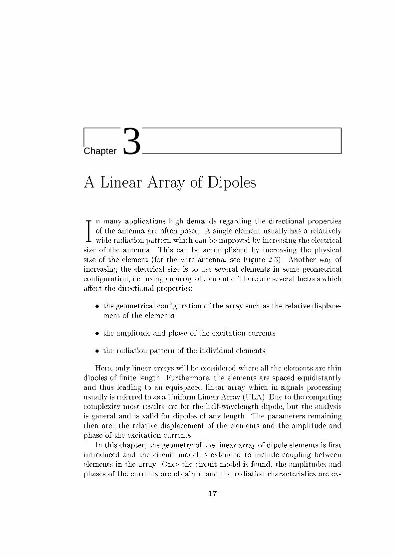
A linear array of n thin dipoles of �nite length is shown in Figure 3.1. The
dipoles are oriented along the z-axis and positioned along the x-axis with a
distance d between the elements. Note that the array of dipoles is located in
�
�
~r
~�
~�
x
y
z
l
d
Figure 3.1: The geometry of the array of dipoles and the relation to the
coordinates.
free space, and that the in uence of the ground plane and other objects in
the antenna environment is neglected. If the elements in the array are placed
closely, the elements will a�ect each other and in the next section mutual
coupling will be considered.
3.2 Mutual Coupling and Circuit Model
Each element in the array is connected to some network which applies a
voltage. This voltage will give rise to a current which in turn results in a
�eld that radiates, but �elds from other antennas will induce a voltage which
18

3.2. MUTUAL COUPLING AND CIRCUIT MODEL
also a�ects the current. The elements are thus mutually coupled and the
circuit model presented in Section 2.3 must be modi�ed. One way of treating
the coupling is to use the concept of mutual impedances, which relates the
induced voltage at one antenna, due to a current in another antenna, to that
current. The mutual impedance is de�ned as
Z21 =V21
I1; (3.1)
where V21 is the voltage appearing at the terminals of antenna 2 due to a
current I1 in antenna 1. This impedance can be calculated by using a similar
technique as used in the self impedance calculation [40]. In the general case,
the calculations are intractable, but for the �nite thin dipole some results
exist. Here, the elements are placed side-by-side, see Figure 3.1, and for this
particular con�guration results can be found in [32]. For two identical �nite
length dipoles placed side-by-side, the expressions for the mutual impedance
are simpli�ed if the length l is a multiple of half a wavelength. The mutual
impedance between element m and n in the array then become
Zmn = R + jX (3.2a)
R =�
4� sin2(kl=2)[2Ci(u0)� Ci(u1)� Ci(u2)] (3.2b)
X = � �
4� sin2(kl=2)[2Si(u0)� Si(u1)� Si(u2)] (3.2c)
u0 = kdjm� nj (3.2d)
u1 = k�p
d2jm� nj2 + l2 + l�
(3.2e)
u2 = k�p
d2jm� nj2 + l2 � l�; (3.2f)
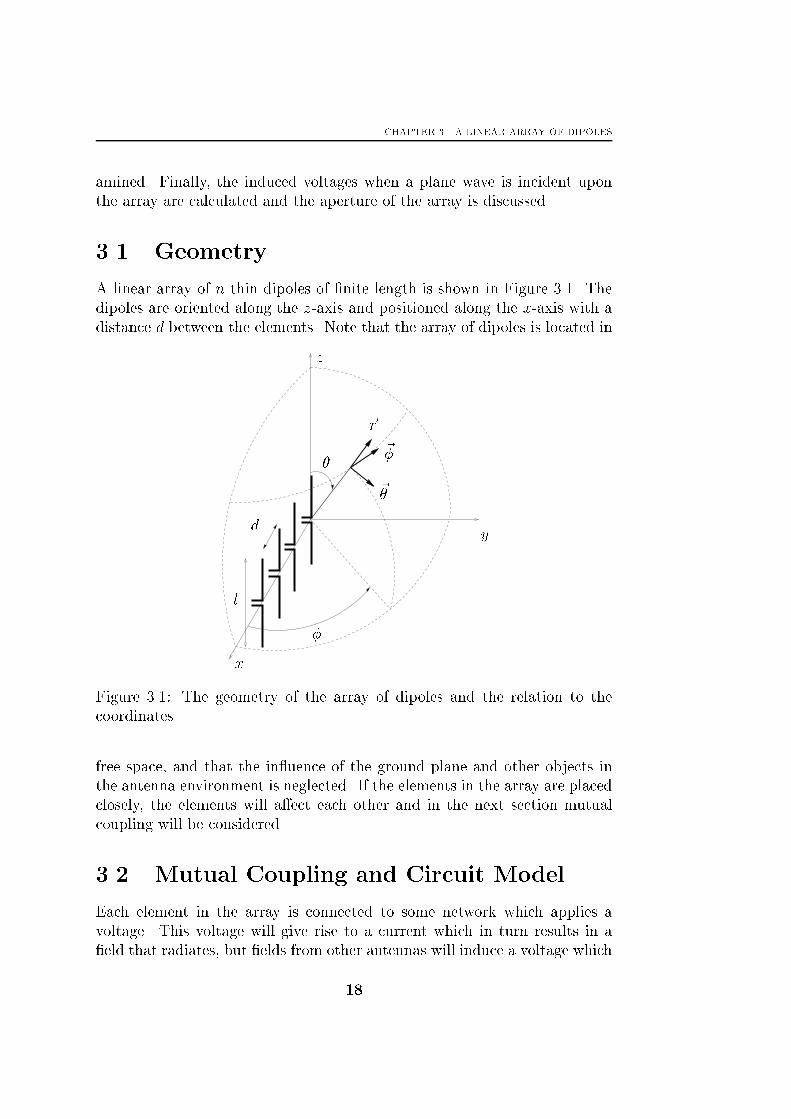
where Ci and Si are the cosine and sine integrals of (2.8a) and (2.8b). In Fig-
ure 3.2 the mutual impedance of two thin half-wavelength dipoles oriented
side-by-side is shown as a function of the element separation d. The mu-
tual impedance approaches the self-impedance when the element separation
diminishes. For larger element separations the mutual impedance quickly
vanishes. Hence, only elements that are close a�ect each other.
Using the mutual impedances, the dipole voltages can be calculated based
on a network model [19]. However, the simple circuit model derived in Section
2.3 can easily be modi�ed to include the e�ects of mutual coupling The
induced voltage on dipole i, see Figure 2.5, can be written as
Vindi =Xk 6=i
IkZik + Vwavei ; (3.3)
19
CHAPTER 3. A LINEAR ARRAY OF DIPOLES
0 0.4 0.8 1.2 1.6 2 2.4 2.8 3.2 3.6 4−40
−20
0
20
40
60
80
Separation d (in wavelengths)
Mut
ual i
mpe
danc
e in
ohm
s
Figure 3.2: Mutual impedance of thin half-wavelength dipole oriented side-
by-side (R solid, X dotted).
where Zik is the mutual impedance of element i and element k. Consequently,
the induced voltage is a sum of the contribution from neighboring elements
and, if present, an incident plane wave. Next, the circuit model will be used
to calculate the radiation intensity.
3.3 Radiation Intensity
The radiated �eld from the array will of course consist of the sum of the �elds
from the individual elements. Expressions for the radiated far-�eld from a
single element were calculated in Section 2.2, assuming that the element
was positioned at the origin. In the case of an array, the elements are not
located at the origin, but since the �eld is calculated in the far-�eld region
the expressions can still be used, and only a phase di�erence between the
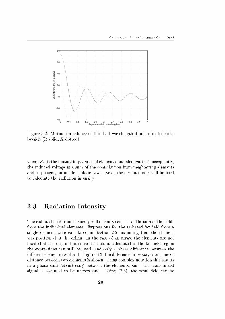
di�erent elements results. In Figure 3.3, the di�erence in propagation time or
distance between two elements is shown. Using complex notation this results
in a phase shift kd sin � cos� between the elements, since the transmitted
signal is assumed to be narrowband. Using (2.3), the total �eld can be
20
3.3. RADIATION INTENSITY
�
�
x
y
z
d
Figure 3.3: The geometry of the array and the distance the wave travels
between two elements.
written as
~Earray(r; �; �) = ~� j�e�jkr
2�r
"cos�kl2cos �
�� cos�kl2
�sin �
#nXi=1
Iie�jkd(i�1) sin � cos �;
(3.4)
where Ii is the current in element i. Here, it is noted that the total �eld
is obtained from the �eld of the single element by multiplication by some
geometrical factor due to the array con�guration. Thus, the total �eld can
be written in matrix form as
~Earray(r; �; �) = ~Eelement(r; �; �)��bT (�; �)Icurrent
�(3.5)
bT (�; �) =�1 e�jkd sin � cos� � � � e�jkd(n�1) sin � cos�
�(3.6)
ITcurrent =�I1 I2 � � � In
�: (3.7)
Applying the modi�ed circuit model, the currents can be related to the ap-
plied voltage at element i as
Vgi = Ii(ZA + ZT ) +Xk 6=i
IkZik; (3.8)
21

CHAPTER 3. A LINEAR ARRAY OF DIPOLES
which also can be written in matrix form as
Vg =
26664Vg1Vg2...
Vgn�1
37775 =
26664ZA + ZT Z12 � � � Z1n
Z21 ZA + ZT � � � Z2n...
......
...
Zn1 Zn2 � � � ZA + ZT
3777526664I1I2...
In
37775 =
= (Z+ ZT I)Icurrent;
(3.9)
where Z is the mutual impedance matrix. For dipoles located in free space
Zkl=Zlk (reciprocal), the mutual impedance matrix has a symmetric (not
Hermitian) Toeplitz structure. The total �eld can therefore be expressed
using the applied voltage, Vg as
~Earray(r; �; �) = ~Eelement(r; �; �)� bT (�; �)(Z+ ZT I)�1Vg: (3.10)
Figure 3.4: Three-dimensional radiation pattern of a �ve element half-
wavelength dipole array with an element separation of d = �=2 using voltages
Vg = (Z + ZT I)b�(90�; 50�).
Once the total radiated �eld is obtained, it is interesting to study the
radiation intensity. The radiation intensity will depend on the applied voltage
Vg, and by properly selecting this voltage most of the radiated energy can
be concentrated to a narrow direction, i.e. beam-forming. Many di�erent
22
3.3. RADIATION INTENSITY
techniques of forming these beams exist [60, 82], but here only the most
basic technique is discussed.
If the applied voltages are chosen as Vg = (Z + ZT I)b�(�0; �0) [24] ,
where * denotes complex conjugate, the phase shifts due to the geometrical
con�guration are compensated for and a beam in the (�0; �0) direction is
expected. However, the phase shift kd sin � cos� does not depend uniquely
on the angles. Instead of a single beam the radiation pattern becomes a
cone with elliptical cross-section, see Figure 3.4 where the array is excited
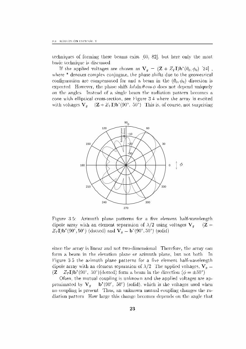
with voltages Vg = (Z+ZT I)b�(90�; 50�). This is, of course, not surprising
−30
−20
−10
0
30
210
60
240
90
270
120
300
150
330
180 0
Rel
ativ
e po
wer
(dB
dow
n)
�
Figure 3.5: Azimuth plane patterns for a �ve element half-wavelength
dipole array with an element separation of �=2 using voltages Vg = (Z +
ZT I)b�(90�; 50�) (dotted) and Vg = b�(90�; 50�) (solid).
since the array is linear and not two-dimensional. Therefore, the array can
form a beam in the elevation plane or azimuth plane, but not both. In
Figure 3.5 the azimuth plane patterns for a �ve element half-wavelength
dipole array with an element separation of �=2. The applied voltages, Vg =
(Z+ ZT I)b�(90�; 50�)(dotted) form a beam in the direction (� = �50�).
Often, the mutual coupling is unknown and the applied voltages are ap-
proximated by Vg = b�(90�; 50�) (solid), which is the voltages used when
no coupling is present. Thus, an unknown mutual coupling changes the ra-
diation pattern. How large this change becomes depends on the angle that
23
CHAPTER 3. A LINEAR ARRAY OF DIPOLES
the beam is directed at, the number of elements, and the element separation
distance. Although that the e�ects in Figure 3.5 might seem small, mutual
coupling will signi�cantly change the direction �nding properties.
One indication of this can be found in the element patterns, i.e. the
radiation pattern when only exciting one element. In antenna design, one
goal is to obtain similar radiation patterns for all element patterns. This in-
dicates low mutual coupling and good mechanical precision in the antenna.
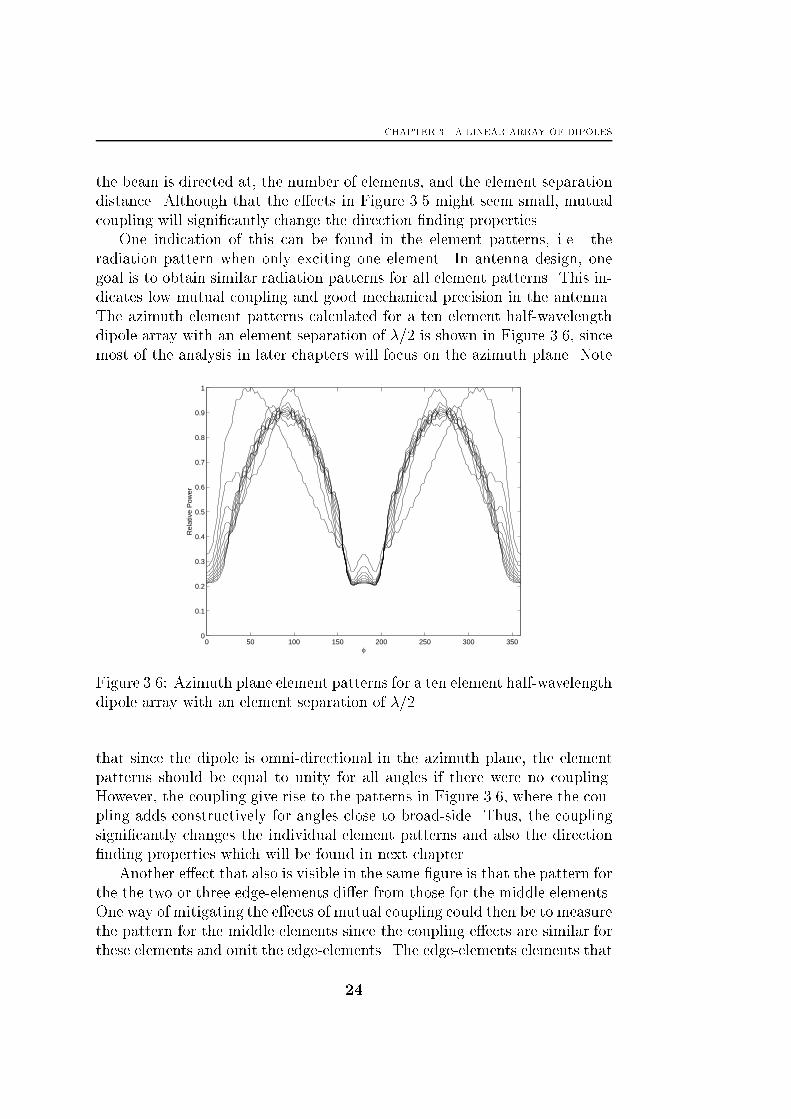
The azimuth element patterns calculated for a ten element half-wavelength
dipole array with an element separation of �=2 is shown in Figure 3.6, since
most of the analysis in later chapters will focus on the azimuth plane. Note
0 50 100 150 200 250 300 3500
0.1
0.2
0.3
0.4
0.5
0.6
0.7
0.8
0.9
1
φ
Rel
ativ
e P
ower
Figure 3.6: Azimuth plane element patterns for a ten element half-wavelength
dipole array with an element separation of �=2.
that since the dipole is omni-directional in the azimuth plane, the element
patterns should be equal to unity for all angles if there were no coupling.
However, the coupling give rise to the patterns in Figure 3.6, where the cou-
pling adds constructively for angles close to broad-side. Thus, the coupling
signi�cantly changes the individual element patterns and also the direction
�nding properties which will be found in next chapter.
Another e�ect that also is visible in the same �gure is that the pattern for
the the two or three edge-elements di�er from those for the middle elements.
One way of mitigating the e�ects of mutual coupling could then be to measure
the pattern for the middle elements since the coupling e�ects are similar for
these elements and omit the edge-elements. The edge-elements elements that
24
3.4. RECEIVING PLANE WAVES
not are used are then usually called dummy elements. This is a common
technique and in [37] it is used in a signal processing application.
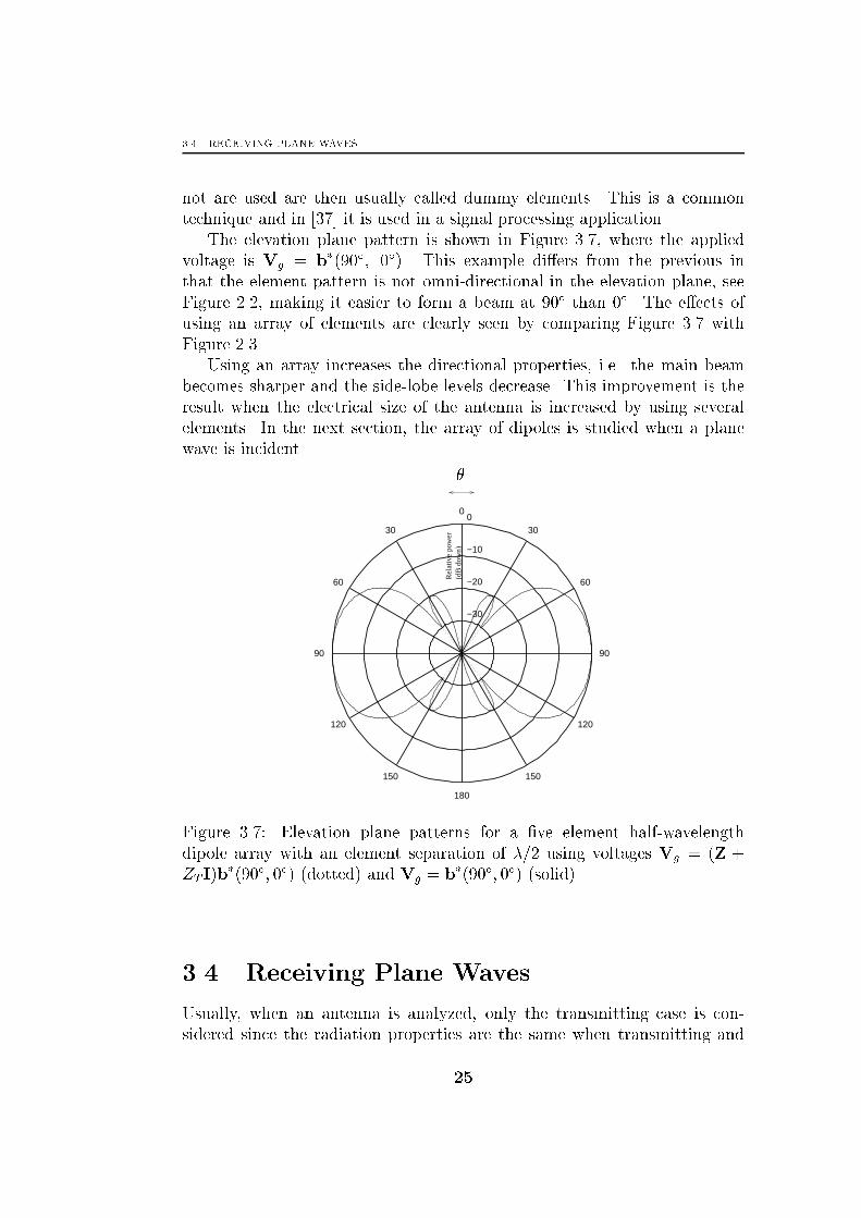
The elevation plane pattern is shown in Figure 3.7, where the applied
voltage is Vg = b�(90�; 0�). This example di�ers from the previous in
that the element pattern is not omni-directional in the elevation plane, see
Figure 2.2, making it easier to form a beam at 90� than 0�. The e�ects of
using an array of elements are clearly seen by comparing Figure 3.7 with
Figure 2.3.
Using an array increases the directional properties, i.e. the main beam
becomes sharper and the side-lobe levels decrease. This improvement is the
result when the electrical size of the antenna is increased by using several
elements. In the next section, the array of dipoles is studied when a plane
wave is incident.
−30
−20
−10
030
150
60
120
9090
120
60
150
30
180
0
Rel
ativ
e po
wer
(dB
dow
n)
�
Figure 3.7: Elevation plane patterns for a �ve element half-wavelength
dipole array with an element separation of �=2 using voltages Vg = (Z +
ZT I)b�(90�; 0�) (dotted) and Vg = b�(90�; 0�) (solid).
3.4 Receiving Plane Waves
Usually, when an antenna is analyzed, only the transmitting case is con-
sidered since the radiation properties are the same when transmitting and
25
CHAPTER 3. A LINEAR ARRAY OF DIPOLES
receiving. However, when using an antenna for direction �nding, an explicit
model for the received voltages is needed in order to formulate direction �nd-
ing algorithms. In [19], a network model was used to examine the received
voltages. Here, the mutual impedance and the circuit model discussed pre-
viously will be used to derive a model that give the induced voltages from a
plane wave.
When an array of dipoles is used as a receiving antenna, the incident
plane wave will induce a voltage on the dipoles just as in the case of a single
dipole. The neighboring dipoles of each dipole will, however, also radiate
and the �elds from these will induce additional voltages. This e�ect will
be included by using the mutual impedances calculated in Section 3.2. The
induced voltage, in element i, in this case becomes
Vindi = Vwavei �Xk 6=i
IkZik: (3.11)
Note that the sign of the induced voltage from the neighboring dipoles is
di�erent from the sign in (3.3), which was derived in the transmitting case.
This is due to the de�nition of the direction of the currents. In the transmit-
ting case it is the generator voltage Vg that is the driving force and in the
receiving case it is Vwave. Using the circuit model in Figure 2.5, the following
system of equations is obtained
Vwavei = Ii(ZA + ZT ) +Xk 6=i
IkZik; (3.12)
where Vwavei and Ii are the voltage and current at dipole i and i = 1; 2; : : : ; n
respectively. This can be written in matrix form as
Vwave = (Z + ZT I) Icurrent ; (3.13)
where Vwave and Icurrent are column vectors with the values at each element,
and Z is the mutual impedance matrix. The measurement equipment is rep-
resented by the terminating impedance ZT . Assuming that the terminating
impedance is the same for all dipoles, the measured voltage becomes
VT = ZT (Z + ZT I)�1Vwave : (3.14)
Since the �eld is assumed to be a uniform plane wave, the �eld at the di�erent
dipoles will only di�er by a phase shift, due to the di�erence in propagation
time and that the received signal is assumed to be narrowband, see Figure 3.3.
The �eld at dipole i is
E0i = E0e�jkd(i�1) sin � cos�; (3.15)
26
3.4. RECEIVING PLANE WAVES
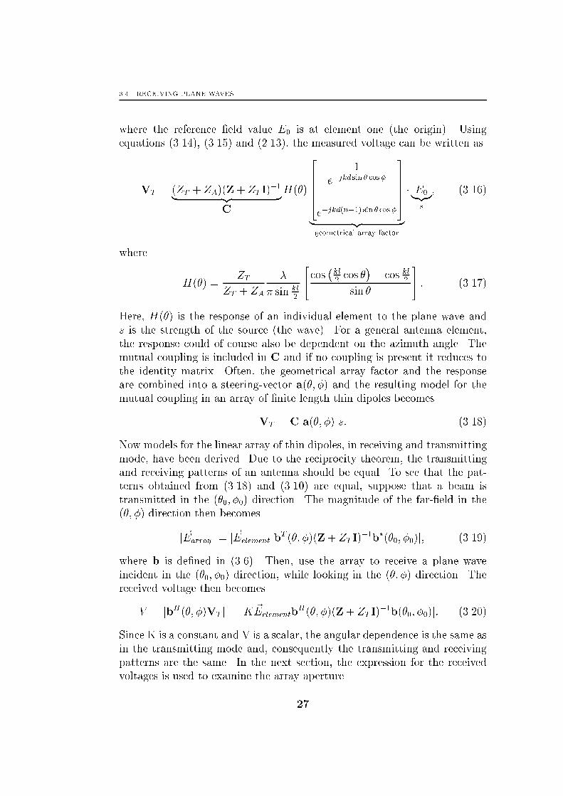
where the reference �eld value E0 is at element one (the origin). Using
equations (3.14), (3.15) and (2.13), the measured voltage can be written as
VT = (ZT + ZA)(Z+ ZT I)�1| {z }
C
H(�)
266641
e�jkd sin � cos�
...
e�jkd(n�1) sin � cos �
37775| {z }geometrical array factor
� E0|{z}s
; (3.16)
where
H(�) =ZT
ZT + ZA
�
� sin kl2
"cos�kl2cos �
�� cos kl2
sin �
#: (3.17)
Here, H(�) is the response of an individual element to the plane wave and
s is the strength of the source (the wave). For a general antenna element,
the response could of course also be dependent on the azimuth angle. The
mutual coupling is included in C and if no coupling is present it reduces to
the identity matrix. Often, the geometrical array factor and the response
are combined into a steering-vector a(�; �) and the resulting model for the
mutual coupling in an array of �nite length thin dipoles becomes
VT = C a(�; �) s: (3.18)
Now models for the linear array of thin dipoles, in receiving and transmitting
mode, have been derived. Due to the reciprocity theorem, the transmitting
and receiving patterns of an antenna should be equal. To see that the pat-
terns obtained from (3.18) and (3.10) are equal, suppose that a beam is
transmitted in the (�0; �0) direction. The magnitude of the far-�eld in the
(�; �) direction then becomes
j ~Earrayj = j ~Eelement bT (�; �)(Z+ ZT I)
�1b�(�0; �0)j; (3.19)
where b is de�ned in (3.6). Then, use the array to receive a plane wave
incident in the (�0; �0) direction, while looking in the (�; �) direction. The
received voltage then becomes
V = jbH(�; �)VT j = jK ~EelementbH(�; �)(Z+ ZT I)
�1b(�0; �0)j: (3.20)
Since K is a constant and V is a scalar, the angular dependence is the same as
in the transmitting mode and, consequently the transmitting and receiving
patterns are the same. In the next section, the expression for the received
voltages is used to examine the array aperture.
27

CHAPTER 3. A LINEAR ARRAY OF DIPOLES
3.5 Array Aperture
It is interesting to examine how coupling a�ects the received power and
thus also the aperture of the array. The received power will depend on
the direction of incidence and the terminating impedance, representing the
measurement equipment. Using (3.18), the received power (real) can be
written as
W =1
2Re
�sHaHCHCas
ZT
�=
E2RT�2
2�2 sin2 kl2
"cos�kl2cos �
�� cos kl2
sin �
#2� bH(Z + ZT I)
�H(Z + ZT I)�1b;
(3.21)
where bH =�1; ejkd sin � cos�; � � � ; ejkd(n�1) sin � cos ��. To obtain the maximum
30
60
90
120
150
180
30
60
90
1
2
3
4
5
6
7
8
��
Figure 3.8: Array factor of a �ve element half-wavelength dipole array with
element separation of �=2.
e�ective aperture this expression should be maximized over the angles and
the choice of terminating impedance. In the single element case the ter-
minating impedance was chosen as the complex conjugate of the antenna
impedance. In the array case, the coupling introduces a dependence between
the elements which results in di�erent impedances in di�erent elements. This
dependence also changes with the angles. Here, the terminating impedance
in all elements is chosen the same as in the single element case. Using (2.15),
28
3.5. ARRAY APERTURE
the e�ective aperture then becomes
Aearray = Aeelement� 4R2
TbH(Z + ZT I)
�H(Z + ZT I)�1b| {z }
array factor
(3.22)
In the case of no coupling the array factor reduces to the number of elements
of the array.
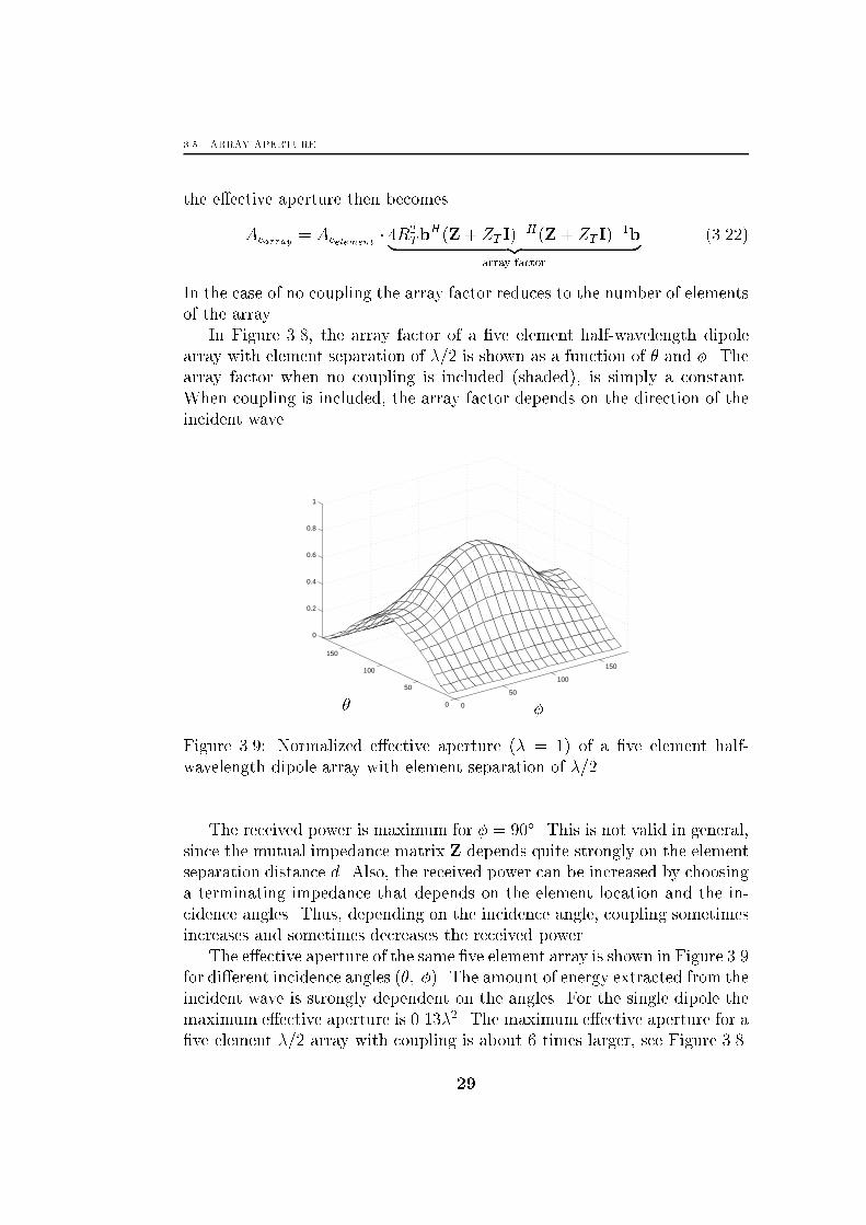
In Figure 3.8, the array factor of a �ve element half-wavelength dipole
array with element separation of �=2 is shown as a function of � and �. The
array factor when no coupling is included (shaded), is simply a constant.
When coupling is included, the array factor depends on the direction of the
incident wave.
0
50
100
150
0
50
100
150
0
0.2
0.4
0.6
0.8
1
� �
Figure 3.9: Normalized e�ective aperture (� = 1) of a �ve element half-
wavelength dipole array with element separation of �=2.
The received power is maximum for � = 90�. This is not valid in general,
since the mutual impedance matrix Z depends quite strongly on the element
separation distance d. Also, the received power can be increased by choosing
a terminating impedance that depends on the element location and the in-
cidence angles. Thus, depending on the incidence angle, coupling sometimes
increases and sometimes decreases the received power.
The e�ective aperture of the same �ve element array is shown in Figure 3.9
for di�erent incidence angles (�; �). The amount of energy extracted from the
incident wave is strongly dependent on the angles. For the single dipole the
maximum e�ective aperture is 0.13�2. The maximum e�ective aperture for a
�ve element �=2 array with coupling is about 6 times larger, see Figure 3.8.
29

CHAPTER 3. A LINEAR ARRAY OF DIPOLES
Without mutual coupling the maximum e�ective array aperture is 5 times
larger than that for the single dipole.
3.6 Conclusions
Using an array gives a clear improvement of the directional properties com-
pared to the single element case but e�ects like mutual coupling that dete-
riorates the directional properties also appear. Here, the radiation pattern
and also the receive properties of a uniform linear array was derived with the
e�ects of mutual coupling included.
First, an expression for the electric �eld in the far-�eld region was de-
rived. By calculating the radiation pattern for a few di�erent scenarios it
was found that mutual coupling changes the radiation pattern slightly. But
more importantly, the coupling a�ects the element patterns resulting in dif-
ferent patterns for di�erent elements. In particular, the edge-elements were
found to have element patterns that di�ered signi�cantly from the inner el-
ements. If not accounted for, these e�ects will severely reduce the direction
�nding performance since many methods assume independent and identical
sensors.
Furthermore, expressions for the induced voltages, when using the an-
tenna as a receiving device to extract energy from a passing plane wave,
were derived. Usually in the literature only the transmitting pattern is con-
sidered. When using the antenna for direction �nding, an explicit model for
the induced received voltages is needed. Therefore, a model for the induced
voltages from a plane wave that includes mutual coupling was derived.
The derivation of the induced voltages was carried out for an equidistantly
spaced linear array of thin dipoles of �nite length. However, the derivation is
easily modi�ed to other geometrys and other elements since essentially only
the induced voltage from the incident wave and the impedances were speci�c
for the dipoles. By using Booker's relation, which is an extension of Babinet's
principle [15], the results regarding the mutual- and self-impedances of the
center-fed dipoles could be extended to be valid for center-fed slots in a
large, thin ground plane. The derivation could also be extended to vertical
monopoles above a ground plane.
Finally, the array aperture and received energy was calculated and it was
found that mutual coupling changes the aperture size. Depending on the
incidence angle, mutual coupling sometimes actually increases the aperture
and sometimes reduces it.
In the next chapter, the model for the induced voltages will be used to
analyze the e�ects of mutual coupling on the direction �nding accuracy.
30

Chapter 4Coupling E�ects on Direction Finding
Accuracy
Probably the most addressed problem in sensor array processing is es-
timation of the direction of arrival (DOA) of a plane wave incident
upon the array. This problem has been analyzed extensively the last
decades, see [21, 33] and further references therein. However, almost all anal-
yses have assumed that the sensors are independent. In practice, the sensors
will be dependent due to mutual coupling. The e�ects of a known coupling
on the direction �nding accuracy will be investigated in this chapter using
the model for the induced voltages derived previously. That model needs
to be complemented with some noise and statistical assumptions and these
additions are presented �rst.
The mutual coupling e�ects on the DOA estimation accuracy will then
be investigated. Since it is the e�ect of the coupling in the DOA estimation
that is interesting and not a particular estimator, at least not in the �rst
case, a measure of how good DOA estimates the model can deliver is needed.
Therefore, a lower bound on the variance of the estimated angles for an
unbiased estimator is derived.
That lower bound is then used to address the e�ects of a known coupling
on DOA estimation performance. A natural extension is to examine the
possibilities of estimating both the coupling and the DOA parameters and
that is done in Chapter 7. Here, the coupling is assumed to be known and
based on the expressions for the induced voltages, a model for the measured
data will �rst be introduced.
31
CHAPTER 4. COUPLING EFFECTS ON DIRECTION FINDING ACCURACY
4.1 Data Model
The objective here is to obtain a model for the voltages that are induced
by a plane wave. These voltages are measured using some measurement
equipment that will a�ect the voltages obtained. All these e�ects are included
in the terminating impedance ZT that represents the measurement equipment
in the receiving mode. Although it is these voltages that are measured, some
noise will inevitably be included in the measurements also.
Noise e�ects are very di�cult to model, since there are many di�erent
types of noise [60]. There is noise that is due to errors in the signal model,
which is of a systematic nature. The received �eld can also be distorted
by environmental noise such as cosmic noise, atmospheric absorption noise,
solar noise etc. It can further be man-made noise, such as jammers and power
tools etc. The receiver will also generate some noise such as thermal noise,
shot noise and icker noise. Depending on the actual receiving environment,
receiver noise or environmental noise could dominate.
A natural way of introducing the noise would be to just include an addi-
tive term to the expression derived for the received voltage, see Section 3.4.
This is the case when the receiver noise dominates. The model that describes
the data would then be
V = C a(�; �) s+N: (4.1)
This model makes no speci�c assumptions about the origin of the noise. If
it is assumed that the main noise contribution is, for example, cosmic noise,
then the noise will induce a voltage on the dipole and this voltage will be
a�ected by the coupling in the same way as the signal. In that case the data
model becomes
V = C a(�; �) s+CN: (4.2)
Now it is clear that if the coupling is known it can easily be counteracted
by multiplying by C�1 (assuming C to be full rank), and the result is the
model used when no coupling is present. This possibility has been studied
in [27] and [64]. Probably the most realistic model would be a combination
of these models. However, since the model in (4.2) can be brought back to
the model without coupling and since receiver noise in many applications is
the dominant noise contribution, it is more interesting to study the model in
(4.1).
The model in (4.1) needs to be de�ned in more detail since only one
source is included and the statistical nature of the signals and noise needs
to be de�ned. Furthermore, the notation will be slightly changed in order to
follow the standard notation in sensor array signal processing literature.
32
4.2. DIRECTION FINDING ACCURACY
Consider p plane waves incident upon an n element linear dipole array
and the problem is to estimate the DOA:s of these waves. In order to simplify
the calculations, the waves are assumed to arrive in the x-y plane (� = 90�),
see Figure 3.1. The induced voltages are measured and sampled at time t,
and the data model becomes
x(t) = CA(�)s(t) + n(t): (4.3)
Here, the vector with measured voltages x(t) is n � 1, the steering matrix
A(�) = [a(�1); : : : ; a(�p)] is n�p, the signal vector s(t) is p�1, and the noisevector n(t) is n� 1. The DOA:s that are estimated are then contained in �.
The induced voltages are sampled N times, i.e. t = t1; : : : ; tN . When ana-
lyzing the direction �nding accuracy, the distributions of the signals and noise
are usually needed and some additional assumptions are therefore needed:
� n > p, and that the steering matrix A(�) is full rank for distinct
incidence angles
� the coupling matrix has full rank, i.e. rk(C) = n which implies that
rk(CA(�)) = rk (A(�)) = p
� n(t) is circularly Gaussian distributed Efn(t)g = 0, Efn(t)nH(s)g =�2I �ts and Efn(t)nT (s)g = 0 8 t; s
The last assumption could in principle be relaxed, but the investigation of the
direction �nding accuracy would become signi�cantly more complex. With
this assumption the noise is temporally as well as spatially white, since it
is assumed independent from element to element. The noise power, �2, is
assumed equal in all the receivers.
Two models for the signal have been studied in the literature: 1) the
deterministic (conditional) model which assumes the signal to be nonrandom,
and 2) the stochastic (unconditional) model which assumes the signal to be
random (Gaussian). Here, the deterministic model will be used, but in the
later chapters the stochastic model will be used.
A model for the measured data has been derived and it is interesting to
proceed to study how a known coupling a�ects the direction �nding accuracy.
This is carried out in the next section.
4.2 Direction Finding Accuracy
The model in the previous section will now be used to examine how mutual
coupling between the elements of the array a�ects the DOA estimation ac-
curacy. Since it is the e�ect of the coupling in the DOA estimation that is
33
CHAPTER 4. COUPLING EFFECTS ON DIRECTION FINDING ACCURACY
interesting and not a particular estimator, at least not in the �rst case, a mea-
sure of how good DOA estimates the model can deliver is needed. Here, the
Cram�er-Rao lower Bound is used which gives a lower bound on the variance
of the estimated angles for an unbiased estimator.
Now, it is interesting to examine what happens to this bound when cou-
pling is included. It is important to note that the coupling is assumed to
be known and the signals are assumed to be non-random in the following
calculation of the CRB for the DOA:s.
For su�ciently large number of samples N, the (asymptotic) Cram�er-Rao
lower Bound can be derived using direct di�erentiation [13, 22, 65]. The
introduction of a known coupling is accounted for by changing the steering
vector in the derivation to an e�ective steering vector CA(�). This does not
a�ect the derivation much, and the asymptotic CRB inequality becomes
Ef(�� �0)(�� �0)Tg � B
B =�2
2N
�Ref(DHCHP?
CACD)� STg��1 ; (4.4)
where
D =
�@a(�)
@�
???�=�1
; � � � ; @a(�)@�
???�=�p
�(4.5)
P?CA = I�CA(AHCHCA)�1AHCH (4.6)
S = limN!1
1
N
tNXt=t1
s(t)sH(t) : (4.7)
Here, � denotes the Hadamard (or Schur) product, i.e., element-wise multi-
plication and P?CA is the orthogonal projector on the null space of (CA)H .
The matrix S is the limiting signal sample covariance matrix.
The bound in (4.4) represents the lowest possible variance when using an
unbiased estimator �. It applies to a thought situation where the experiment
of obtaining N samples and estimating the angles is performed many times
with the same signal vector s(t), but di�erent noise realizations n(t).
Next, this bound is calculated for a few di�erent scenarios and examined
when coupling is included and not.
4.3 Computer Experiments
To examine the e�ect of mutual coupling, the CRB from the previous sec-
tion is calculated for a few di�erent scenarios. The CRB when coupling is
34
4.3. COMPUTER EXPERIMENTS
0
20
40
60
80
0
20
40
60
80
−50
−30
−10
10
30
50
�1 �2
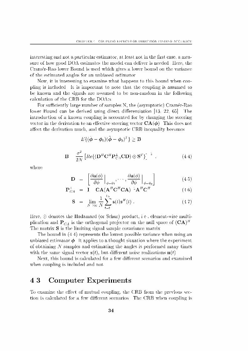
Figure 4.1: The logarithm of CRBcoupling for �2 versus the angles for an array
of 5 �=2 dipoles spaced �=2 apart.
included is compared with the CRB when coupling is excluded. This calcu-
lation is carried out for di�erent locations of the source signals, correlated
signals, and for di�erent element spacings. In all of these examples the ter-
minating impedance is chosen as the complex conjugate of the single antenna
impedance.
4.3.1 Angular Dependence
Consider a �ve element half-wavelength dipole array with element separation
of �=2. This array has been used for several of the �gures in Chapter 3. Two
plane waves are incident upon the array and the DOA:s (�1; �2) of these
are to be estimated. The signal waveforms are uncorrelated and the signal
power is equal to the noise power (SNR= 0 dB) and N = 200 snapshots are
collected.
The logarithm of the CRB for �2 with coupling is shown in Figure 4.1.
The fact that it is harder to estimate angles close together is obvious from
the �gure. Note that there is a corresponding �gure for the other angle �1.
For angles close to end-�re (� = 0�) the CRB is quite large, and this is due
to the fact that the CRB is inversely proportional to the derivative of the
steering vector, and for �2 = 0� the derivative is zero.
Now it is interesting to compare the CRB with and without coupling. In
35

CHAPTER 4. COUPLING EFFECTS ON DIRECTION FINDING ACCURACY
0
20
40
60
80
0
20
40
60
80
0
0.5
1
1.5
2
�1 �2
Figure 4.2: The ratio of the standard deviation for �2 with and without
coupling versus the angles for an array of 5 �=2 dipoles spaced �=2 apart.
Figure 4.2, the ratio of the standard deviation with and without coupling is
shown. Here, it is found that the coupling does not signi�cantly change the
CRB bound if the coupling is known. This result depends on the geomet-
rical con�guration of the array and the array elements, but also on several
parameters such as number of elements, correlation of the signals and ele-
ment spacing. These dependences are studied next and the in uence of the
number of elements is studied �rst.
In Figure 4.3, the CRB ratio for an array of 25 elements (otherwise the
same as previous array) is shown. A larger di�erence is found here. The CRB
with coupling gets lower as �2 gets larger. This can partly be explained by
considering the received power which is maximum for �2 = 90�, see Figure 3.8
on page 28. This e�ect gets larger for a larger array and that is why it did
not show in the �rst �gure for the array with few elements. If the change
in received power is compensated for, the ratio will mostly reside at unity
except for angles near end-�re (�2 = 0�), where it is hard to estimate the
DOA. This is shown in Figure 4.4.
4.3.2 Correlated Signals
Consider a 25 element half-wavelength dipole array with element separation
of �=2. Two plane waves are incident upon the array and the DOA:s (84�; 85�)
36
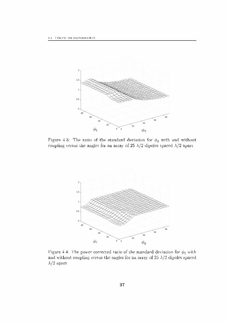
4.3. COMPUTER EXPERIMENTS
0
20
40
60
80
0
20
40
60
80
0
0.5
1
1.5
2
�1 �2
Figure 4.3: The ratio of the standard deviation for �2 with and without
coupling versus the angles for an array of 25 �=2 dipoles spaced �=2 apart.
0
20
40
60
80
0
20
40
60
80
0
0.5
1
1.5
2
�1 �2
Figure 4.4: The power corrected ratio of the standard deviation for �2 with
and without coupling versus the angles for an array of 25 �=2 dipoles spaced
�=2 apart.
37

CHAPTER 4. COUPLING EFFECTS ON DIRECTION FINDING ACCURACY
0 0.1 0.2 0.3 0.4 0.5 0.6 0.7 0.8 0.9 10.18
0.2
0.22
0.24
0.26
0.28
0.3
0.32
0.34st
anda
rd d
evia
tion
�
Figure 4.5: The standard deviation with coupling (solid) and without
(dashed) for the wave incident from 84� upon an array of 25 �=2 dipoles
spaced �=2 apart for di�erent correlations.
are to be estimated. The signal to noise ratio (SNR) is -10dB and N = 1000
snapshots are collected. In this simulation, the correlation dependence of the
CRB is examined. The signal covariance matrix is
S = 10(SNR=10) ��1 �
� 1
�: (4.8)
The CRB is now calculated for di�erent values of �. In Figure 4.5, the
standard deviation for the wave incident from 84� is calculated for di�erent
correlations. First of all it is noted that it becomes harder to estimate the
DOA when the signal correlation increases. But the e�ects of coupling do not
depend on the correlation. The ratio of the standard deviation with coupling
(solid) and without (dashed) is essentially unchanged by the change in cor-
relation. Here, coupling actually improved the estimation performance but
that depends on the incidence angles as discussed previously, see Figure 4.3.
The conclusion that the e�ects of coupling are almost independent of the
correlation remains.
4.3.3 Element Spacing
Consider a 25 element half-wavelength dipole array with element separation
of �=2. Two plane waves are incident upon the array and the DOA:s (84�; 85�)
38
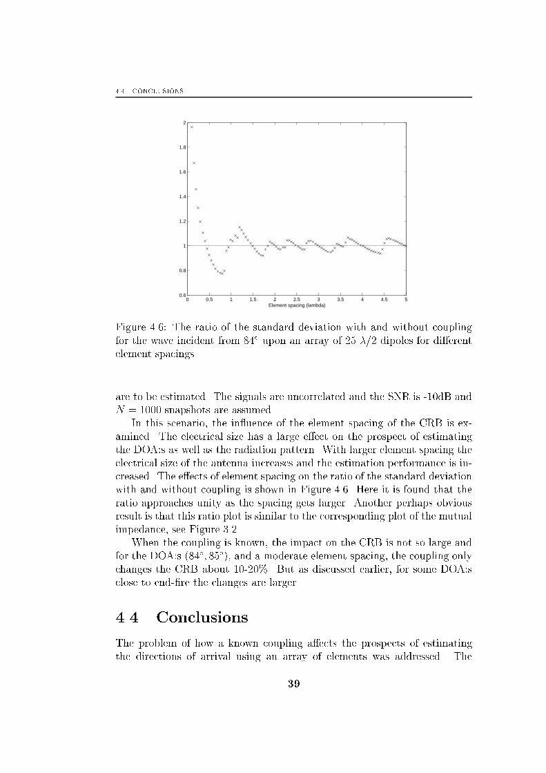
4.4. CONCLUSIONS
0 0.5 1 1.5 2 2.5 3 3.5 4 4.5 50.6
0.8
1
1.2
1.4
1.6
1.8
2
Element spacing (lambda)
Figure 4.6: The ratio of the standard deviation with and without coupling
for the wave incident from 84� upon an array of 25 �=2 dipoles for di�erent
element spacings.
are to be estimated. The signals are uncorrelated and the SNR is -10dB and
N = 1000 snapshots are assumed.
In this scenario, the in uence of the element spacing of the CRB is ex-
amined. The electrical size has a large e�ect on the prospect of estimating
the DOA:s as well as the radiation pattern. With larger element spacing the
electrical size of the antenna increases and the estimation performance is in-
creased. The e�ects of element spacing on the ratio of the standard deviation
with and without coupling is shown in Figure 4.6. Here it is found that the
ratio approaches unity as the spacing gets larger. Another perhaps obvious
result is that this ratio plot is similar to the corresponding plot of the mutual
impedance, see Figure 3.2.
When the coupling is known, the impact on the CRB is not so large and
for the DOA:s (84�; 85�), and a moderate element spacing, the coupling only
changes the CRB about 10-20%. But as discussed earlier, for some DOA:s
close to end-�re the changes are larger.
4.4 Conclusions
The problem of how a known coupling a�ects the prospects of estimating
the directions of arrival using an array of elements was addressed. The
39
CHAPTER 4. COUPLING EFFECTS ON DIRECTION FINDING ACCURACY
direction �nding accuracy, i.e. the Cram�er-Rao lower Bound on the estimated
DOA:s, was used as a measure of these e�ects. The derivation of the induced
voltages in a linear array of dipole elements from previous chapter was used
to obtain a model for the data that are measured when using an array to
estimate the direction of an incident wave. Some stochastical assumptions
were also introduced that were needed when calculating the lower bound on
the variance of the DOA estimates.
The CRB with a known mutual coupling was presented and analyzed for
a few di�erent estimation scenarios. It was found that the coupling e�ects on
the CRB were dependent on the DOA:s but the e�ects was relatively small.
Furthermore, the correlations of the signals did not change the coupling
e�ects, considering the CRB, appreciably. The element separation did a�ect
the CRB. But for moderate element spacings, the e�ects were not large.
To sum up the chapter, the e�ects of a known mutual coupling in the
scenarios studied here are not large (of course depending on the application).
Depending on the geometrical con�guration, the array elements, number of
elements, and element spacing, the coupling increases or decreases the CRB.
In the analysis of the CRB, the coupling was introduced through the
coupling matrix C. Other e�ects than coupling can also be included in the
C matrix. For example, e�ects such as the gain and phase of the individual
sensors could be included. In that case, the analysis of the CRB in this
chapter is still valid by simply changing the C matrix to include those e�ects.
In the next chapter, some methods of estimating the DOAs in the presence
of a known coupling will be introduced.
40
Chapter 5Estimation With a Known Coupling
The problem of estimating the DOA, when a known coupling is present,
will be considered in this chapter. The mutual coupling is calculated
using the model that was derived in Chapter 3 for the induced voltages
on a ULA of thin and �nite length dipoles. First, the model will be reviewed
and some statistical assumptions regarding the signals and the noise will be
introduced. In Chapter 4, the CRB was used to examine the estimation
performance. Here, the corresponding bound is derived, using the statistical
assumptions made in this chapter.
Several methods for estimating the DOA are then reviewed and thus also
a small part of the area of sensor array processing. However, the methods
are discussed in the context of mutual coupling and the algorithms that
have appeared in the literature that include a known coupling are reviewed
�rst. After that, some straightforward extensions of existing methods for
the coupling free case are introduced. Finally, the problem of estimating the
number of signals is brie y discussed.
5.1 Data Model
The direction of an incident wave can be estimated by measuring the received
voltages at the di�erent elements of the array and by assuming the wave
to be plane, simple geometry then gives the direction. However, due to
mutual coupling, the measured voltage at each element will depend not only
on the incident �eld but also on the voltages on the other elements. The
received voltage on each element will induce a current on the element which
in turn radiates a �eld which a�ects the surrounding elements, i.e. mutual
coupling. Here, mutual coupling in an array of n dipoles of �nite length,
41
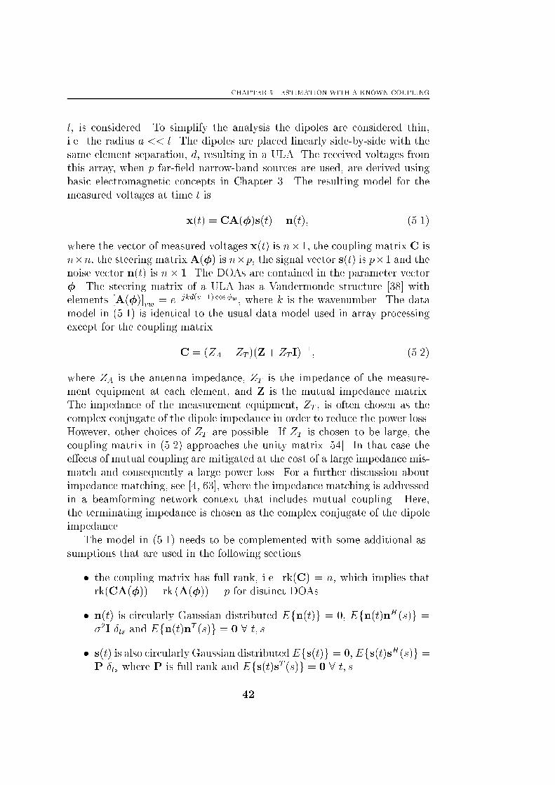
CHAPTER 5. ESTIMATION WITH A KNOWN COUPLING
l, is considered. To simplify the analysis the dipoles are considered thin,
i.e. the radius a << l. The dipoles are placed linearly side-by-side with the
same element separation, d, resulting in a ULA. The received voltages from
this array, when p far-�eld narrow-band sources are used, are derived using
basic electromagnetic concepts in Chapter 3. The resulting model for the
measured voltages at time t is
x(t) = CA(�)s(t) + n(t); (5.1)
where the vector of measured voltages x(t) is n�1, the coupling matrix C is
n�n, the steering matrixA(�) is n�p, the signal vector s(t) is p�1 and thenoise vector n(t) is n� 1. The DOAs are contained in the parameter vector
�. The steering matrix of a ULA has a Vandermonde structure [38] with
elements [A(�)]vw = e�jkd(v�1) cos�w , where k is the wavenumber. The data
model in (5.1) is identical to the usual data model used in array processing
except for the coupling matrix
C = (ZA + ZT )(Z + ZT I)�1; (5.2)
where ZA is the antenna impedance, ZT is the impedance of the measure-
ment equipment at each element, and Z is the mutual impedance matrix.
The impedance of the measurement equipment, ZT , is often chosen as the
complex conjugate of the dipole impedance in order to reduce the power loss.
However, other choices of ZT are possible. If ZT is chosen to be large, the
coupling matrix in (5.2) approaches the unity matrix [54]. In that case the
e�ects of mutual coupling are mitigated at the cost of a large impedance mis-
match and consequently a large power loss. For a further discussion about
impedance matching, see [4, 63], where the impedance matching is addressed
in a beamforming network context that includes mutual coupling. Here,
the terminating impedance is chosen as the complex conjugate of the dipole
impedance.
The model in (5.1) needs to be complemented with some additional as-
sumptions that are used in the following sections.
� the coupling matrix has full rank, i.e. rk(C) = n, which implies that
rk(CA(�)) = rk (A(�)) = p for distinct DOAs
� n(t) is circularly Gaussian distributed Efn(t)g = 0, Efn(t)nH(s)g =�2I �ts and Efn(t)nT (s)g = 0 8 t; s
� s(t) is also circularly Gaussian distributedEfs(t)g = 0, Efs(t)sH(s)g =P �ts where P is full rank and Efs(t)sT (s)g = 0 8 t; s
42
5.2. DIRECTION FINDING ACCURACY
� n > p, i.e. the number of dipoles are larger than the number of incident
signals
Note that �ts denotes the Kronecker delta and that both the signal and
the noise are random. Speci�cally, they are both assumed to be Gaussian
distributed and this model is sometimes called the stochastic or unconditional
signal model. In Chapter 4, the signal was assumed to be non-random and
that model is therefore sometimes called the deterministic or the conditional
signal model. However, since the signal in that case is considered unknown
and hence also estimated along with the DOAs, the number of unknowns
increases as the number of samples N increases. Actually, it is shown in
[43, 66] that the asymptotic (largeN) covariance of the DOAs estimates using
the deterministic signal model is larger than the asymptotic covariance for a
stochastic signal model when n < 1. Furthermore, and most importantly,
the Cram�er-Rao lower Bound derived using the deterministic signal model
cannot be reached and therefore is not asymptotically tight, in contrast to
the bound based on the stochastic signal model that is asymptotically tight.
Since both the signal and the noise are assumed to be Gaussian, all infor-
mation about the DOAs and the signals are contained in the �rst and second
order moments. Many estimation schemes have appeared in the literature
that exploit the properties of the second moment to estimate the DOAs.
Some of these schemes will be discussed in the following sections. But �rst,
in order to assess the quality of the di�erent estimation methods, a lower
bound for the variance of the DOA estimates will be derived.
5.2 Direction Finding Accuracy
Most proposed estimators are asymptotically unbiased and the variance of
the estimates is therefore a good �gure of merit for these estimators. A
lower bound on the variance of DOA estimates is therefore very useful when
addressing the quality of a estimation schemes. Probably the most widely
used bound is the Cram�er-Rao lower Bound, which is a lower bound on the
variance of DOA estimates, assuming that the estimator is unbiased. There
are unbiased estimators that, at least asymptotically, attains the bound and
hence the bound is called asymptotically tight and the estimators are called
e�cient. The CRB therefore serves as a benchmark when evaluating di�erent
estimation methods. In Chapter 4, the e�ects of mutual coupling on the DOA
estimation was examined by calculating the CRB using the model in (5.1) and
the deterministic signal model. Here, the CRB will be derived for a stochastic
signal model, since the bound in this case becomes asymptotically tight and
thus more appropriate when considering di�erent estimation schemes.
43
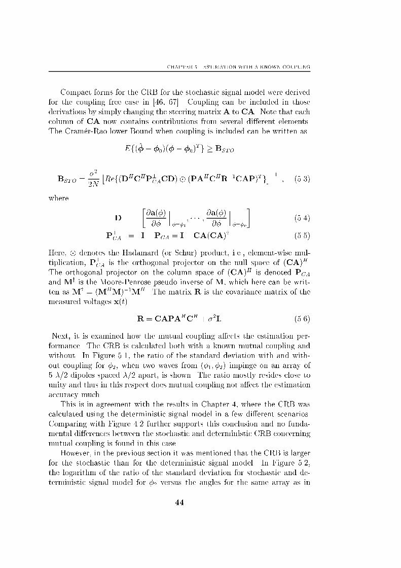
CHAPTER 5. ESTIMATION WITH A KNOWN COUPLING
Compact forms for the CRB for the stochastic signal model were derived
for the coupling free case in [46, 67]. Coupling can be included in those
derivations by simply changing the steering matrixA to CA. Note that each
column of CA now contains contributions from several di�erent elements.
The Cram�er-Rao lower Bound when coupling is included can be written as
Ef(�� �0)(�� �0)Tg � BSTO
BSTO =�2
2N
�Ref(DHCHP?
CACD)� (PAHCHR�1CAP)Tg��1 ; (5.3)
where
D =
�@a(�)
@�
???�=�1
; � � � ; @a(�)@�
???�=�p
�(5.4)
P?CA = I�PCA = I�CA(CA)y (5.5)
Here, � denotes the Hadamard (or Schur) product, i.e., element-wise mul-
tiplication, P?CA is the orthogonal projector on the null space of (CA)H .
The orthogonal projector on the column space of (CA)H is denoted PCA
and My is the Moore-Penrose pseudo inverse of M, which here can be writ-
ten as My = (MHM)�1MH . The matrix R is the covariance matrix of the
measured voltages x(t).
R = CAPAHCH + �2I: (5.6)
Next, it is examined how the mutual coupling a�ects the estimation per-
formance. The CRB is calculated both with a known mutual coupling and
without. In Figure 5.1, the ratio of the standard deviation with and with-
out coupling for �2, when two waves from (�1; �2) impinge on an array of
5 �=2 dipoles spaced �=2 apart, is shown. The ratio mostly resides close to
unity and thus in this respect does mutual coupling not a�ect the estimation
accuracy much.
This is in agreement with the results in Chapter 4, where the CRB was
calculated using the deterministic signal model in a few di�erent scenarios.
Comparing with Figure 4.2 further supports this conclusion and no funda-
mental di�erences between the stochastic and deterministic CRB concerning
mutual coupling is found in this case.
However, in the previous section it was mentioned that the CRB is larger
for the stochastic than for the deterministic signal model. In Figure 5.2,
the logarithm of the ratio of the standard deviation for stochastic and de-
terministic signal model for �2 versus the angles for the same array as in
44

5.3. ESTIMATION METHODS
0
20
40
60
80
0
20
40
60
80
0
0.5
1
1.5
2
�1 �2
Figure 5.1: The ratio of the standard deviation with and without coupling
for �2 versus the angles for an array of 5 �=2 dipoles spaced �=2 apart.
Figure 5.1 is shown. The logarithm is positive for all angles, i.e. the CRB
for the stochastic signal model is larger than for the deterministic model as
stated previously. The di�erence is not very large for angles with su�cient
angular separation. Also, the large ridge through the plot corresponds to es-
timating DOAs for two signals arriving from the same direction. In this case,
the estimation procedure breaks down and it is hard to draw any conclusions
regarding these angles.
The e�ects of mutual coupling on the CRB using the stochastic signal
model are thus more or less the same as on the CRB calculated for the
deterministic signal model. Now, a measure for the quality of the proposed
DOA estimation schemes is derived. In the next section, several methods for
estimating the DOAs in the presence of a known coupling will be studied
and compared to the CRB.
5.3 Estimation Methods
The problem of estimating the DOA in the presence of a known coupling is
not very di�erent from the usual DOA estimation problem. Most algorithms
which have appeared in the last decades can be modi�ed to include a known
mutual coupling. Essentially, it is just to change the steering matrix A to an
45
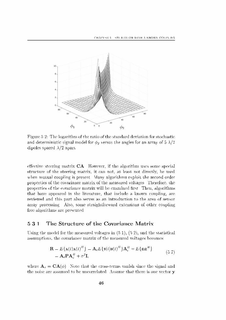
CHAPTER 5. ESTIMATION WITH A KNOWN COUPLING
0
20
40
60
80
0
20
40
60
80
0
2
4
6
8
10
�1 �2
Figure 5.2: The logarithm of the ratio of the standard deviation for stochastic
and deterministic signal model for �2 versus the angles for an array of 5 �=2
dipoles spaced �=2 apart.
e�ective steering matrix CA. However, if the algorithm uses some special
structure of the steering matrix, it can not, at least not directly, be used
when mutual coupling is present. Many algorithms exploit the second order
properties of the covariance matrix of the measured voltages. Therefore, the
properties of the covariance matrix will be examined �rst. Then, algorithms
that have appeared in the literature, that include a known coupling, are
reviewed and this part also serves as an introduction to the area of sensor
array processing. Also, some straightforward extensions of other coupling
free algorithms are presented.
5.3.1 The Structure of the Covariance Matrix
Using the model for the measured voltages in (5.1), (5.2), and the statistical
assumptions, the covariance matrix of the measured voltages becomes
R = Efx(t)x(t)Hg = AeEfs(t)s(t)HgAHe + EfnnHg
= AePAHe + �2I;
(5.7)
where Ae = CA(�). Note that the cross-terms vanish since the signal and
the noise are assumed to be uncorrelated. Assume that there is one vector y
46
5.3. ESTIMATION METHODS
that is perpendicular to the steering matrix Ae, or
Aey = 0: (5.8)
Then Ry = �2y, i.e. y is an eigenvector of R with corresponding eigenvalue
�2. Since the steering matrix Ae is full rank with dimensions n � p and P
also is full rank, there are n � p independent vectors y that are perpendic-
ular to Ae. Actually, it is possible to write the eigendecomposition of the
covariance matrix as a sum of two parts. One part consisting of eigenvectors
corresponding to eigenvalues equal to the noise variance, and a second part
that is related to the signal
R = E�EH = Es�sEHs + �2EnE
Hn : (5.9)
Furthermore, by exploiting the orthonormality of the eigenvectors
EsEHs +EnE
Hn = I; (5.10)
the covariance matrix can be written as
R = Es(�s � �2I)EHs + �2I = Ese�EHs + �2I: (5.11)
Comparing (5.11) with (5.7) reveals that the subspace spanned by the columns
of Es must be equal to the subspace spanned by the columns of AeP or
RfEsg = RfAePg � RfAeg (5.12)
with equality if the signal covariance matrix P is of full rank. The subspace
spanned by Ae (or Es) is usually called the signal subspace and the corre-
sponding space spanned by En is therefore called the noise subspace. Note
that due to the orthogonality of the eigenvectors, these spaces are orthogonal.
A related entity is the array manifold A, that is de�ned as the collection
of all steering vectors within the DOA range, or
A = fa(�i) j �i 2 �g: (5.13)
The array manifold is a p-dimensional subset of the n-dimensional space and
this observation is important in the derivation of the subspace based methods
presented later.
Almost all methods discussed in the following sections will exploit the
properties of the covariance matrix of the measured voltages R. However, it
is the induced voltages x(t) that are measured and not the covariance matrix.
Usually, R is estimated as
R =1
N
NXt=1
x(t)xH(t) (5.14)
47
CHAPTER 5. ESTIMATION WITH A KNOWN COUPLING
which is an unstructured maximum likelihood estimate of the covariance
matrix in (5.7).
The structure in (5.7) and (5.11) has been exploited in numerous DOA
estimation schemes, presented during the latest decades. For a review of
some of these methods, see [21, 33]. Many of those methods are possible
to use also in the presence of mutual coupling with slight changes, but in
the signal processing literature only a few methods, that include a known
coupling, have been presented. Those methods will be reviewed in the next
subsection, and then some additional methods that include a known coupling
are proposed.
5.3.2 Estimation Methods: Beamforming and MUSIC
Probably, the most used method of obtaining estimates of the DOAs is beam-
forming [60, 82]. As the name beamforming suggests, the received energy is
focused to one direction (or beam) at a time. This can be expressed as
y(�) = aH(�)x: (5.15)
A spatial spectrum is obtained by calculating jy(�)j2 for � 2 �. The presence
of mutual coupling can be taken care of by changing the multiplication in
(5.15) from aH(�) to a(�)HC�1, i.e. premultiply the measured voltages x(t)
with C�1 as suggested in [27, 64]. The noise covariance matrix then changes
from �2I to �2C�1C�H . If the method relies on that the noise covariance
is white (�2I), the premultiplication method does not work. Note, that the
beamforming method ignores the noise and premultiplication can thus be
applied. Similar methods, but more oriented towards pattern design, can be
found in [24, 28, 70].
The spatial spectrum in (5.15) is a spatial analogue of the classical pe-
riodogram in time series analysis. As with the periodogram, the spatial
spectrum has a resolution threshold. Waves arriving with electrical angle
separation 1 less than 2�=n can not be resolved with this method. That was
one of the motivations for the interest in the so-called subspace methods that
will be described next.
Subspace based methods rely on observations regarding the eigendecom-
position of the covariance matrix into a signal subspace and a noise subspace,
as discussed in previous subsection. One of the most popular subspace meth-
ods, MUltiple SIgnal Classi�cation (MUSIC), was introduced in [58]. The
method is based on the observation in (5.8), that the noise eigenvectors are
perpendicular to the steering matrix or the signal subspace. The algorithm
1The electrical angle is de�ned as kd cos�.
48

5.3. ESTIMATION METHODS
calculates the noise subspace using an eigendecomposition of the estimated
covariance matrix in (5.14). Then, the estimates of the DOAs are taken as
those � that gives in the smallest value of aH(�)En. Usually this is formu-
lated as �nding the p largest peaks in the "MUSIC spectrum"
PMU(�) =1
aH(�)EnEH
n a(�): (5.16)
This algorithm is straightforwardly adopted to the case of a mutual cou-
pling by simply exchanging the steering vector a(�) to Ca(�). Another way
of handling the coupling is to employ the method of premultiplication as
described above. But as mentioned previously, that changes the noise covari-
ance matrix and a generalized eigendecomposition has to be used in order to
obtain the correct noise eigenvectors. These two methods have been investi-
gated in [35, 47, 94]. Here, the steering vector is changed and in Figure 5.3,
10 20 30 40 50 60 70 80 9010
−2
10−1
100
101
102
103
104
105
DOA (deg)
SpatialMusic
Figure 5.3: The spatial and MUSIC spectrum when coupling is compensated
for (solid) and not (dotted). An array of 10 �=2 dipoles spaced �=2 apart
is used and two waves are incident from (60�; 63�), and 1000 snapshots with
SNR = 20dB.
the MUSIC spectrum of (5.16) is shown when two sources are present at
(60�; 63�), using an array with 10 �=2 elements spaced �=2 apart. The solid
line is when the coupling is compensated for, i.e. using the correct coupling
matrix, and the dotted line is when the coupling matrix is unknown and
replaced by the unity matrix. With a known coupling, the method works
49
CHAPTER 5. ESTIMATION WITH A KNOWN COUPLING
well and two peaks at the correct angles appear. However, if the coupling is
unknown the method does not work well. Also included in Figure 5.3 is the
corresponding spatial spectra for the beamforming method in (5.15). The
beamforming method fails to resolve the sources, since in this case the res-
olution limit is more than 10�. The resolution threshold of MUSIC is much
lower, and therefore does that method succeed in resolving the DOAs. This,
of course, is the main reason for using subspace based methods like MUSIC
instead of beamforming. However, the di�erence between when the coupling
is known or not is small for the beamforming method, i.e. the beamforming
method is robust. The MUSIC method, as all subspace based methods, is
more sensitive to errors in the steering vector as seen in the �gure.
An interesting application of the MUSIC method for Over The Horizon
(OTH) radar arrays is found in [62], where ionized meteor trails are used to
estimate the sensor positions and mutual coupling in a calibration scheme.
The MUSIC method along with the beamforming method are, to the
author's knowledge, the only DOA estimation algorithms presented that in-
clude the presence of a known coupling. As mentioned above, several other
algorithms are easily extended to include a known coupling. In the next
section some straightforward extensions will be proposed.
5.3.3 Other Methods
Most DOA estimation algorithms can be extended to include a known cou-
pling. In this subsection, some straightforward extensions of other DOA
algorithms will be proposed. Some of these algorithms will be used later
when the DOAs are estimated along with an unknown coupling. First two
computationally simple algorithms, that exploit a special structure of the
antenna array, will be considered.
The popular MUSIC method discussed in the previous subsection can be
applied to any type of antenna array. However, if the antenna is a ULA, the
estimation procedure can be simpli�ed. In this case, the steering vector has
elements [a(�)]v = e�jkd(v�1) cos� and the expression in (5.16) can be viewed
as a polynomial in z = e�jkd cos �. Therefore, the search for the DOAs in the
MUSIC method described above can be avoided. Instead, �nd the roots of
the polynomial
f(z) = aT (z�1)CHEnEH
nCa(z): (5.17)
Pick the p roots closest to the unit circle, zi and calculate the angle and solve
for �i in \zi = \e�jkd cos �i. This method is known in the literature as the
Root-MUSIC method and was presented in [7]. Not only does this method
50
5.3. ESTIMATION METHODS
avoid the numerical search, but also improves the resolution threshold of the
spectral MUSIC discussed in previous subsection. A performance analysis in
[52] shows that the improvement in resolution threshold is due to the fact
that a small error in the radius of the root does not e�ect the estimation
performance. Thus, only errors in the angle of the root e�ect the estimation
performance and this decreases the resolution threshold. The presence of
mutual coupling is taken care of by simply introducing the coupling matrix,
C, as in (5.17).
Another subspace-based method that also relies on a special structure
of the array is Estimation of Signal Parameters via Rotational Invariance
Techniques (ESPRIT) [55]. ESPRIT exploits a shift structure of a special
steering matrix constructed as
As =
�A1
A1�
�; (5.18)
where A1 is a l � p steering matrix and � is p � p diagonal matrix with
elements �ii = e�jk�cos�i . Of course, not all arrays have this shift structure,
but for example a ULA can be divided into two parts which have this struc-
ture. Several di�erent strategies for forming these two parts are discussed in
the literature [44], but here maximum overlapping structures will be used,
i.e. the �rst part consists of the �rst n�1 elements and the second part of thelast n� 1 elements, that is, l = n� 1 and � = d. ESPRIT exploits this shift
structure and the fact that for the coupling free case RfEsg = RfA(�)g(assuming P full rank). When coupling is present RfEsg = RfCA(�)g andthe shift structure has vanished. However, RfC�1Esg = RfA(�)g and the
shift structure is obtained. Another way of obtaining this result is to pre-
multiply the data with C�1 and the same result is obtained by calculating
the generalized eigenvalue factorization. Thus, there exists a nonsingular T
such that
JC�1Es = As(�)T; (5.19)
where J is a 2(n � 1) � n selection matrix. The basic idea is to �nd those
�:s that best �t this relation. This �t can be made in a least squares sense
or in a total least square sense [44, 55]. Here, the total least squares method
is used. In Figure 5.4, the Root Mean Square Error (RMSE) of the modi�ed
MUSIC and ESPRIT methods are shown. The Cram�er-Rao lower Bound is
also shown for the case with coupling and without. The MUSIC method is
close to the CRB, but ESPRIT performs worse, since it only exploits the
invariance structure and not the full steering matrix. The same relation is is
found also in the coupling free case [44]. However, it is interesting to observe
51
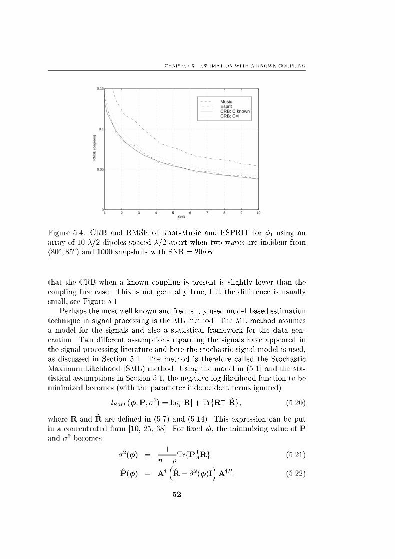
CHAPTER 5. ESTIMATION WITH A KNOWN COUPLING
1 2 3 4 5 6 7 8 9 100
0.05
0.1
0.15
SNR
RM
SE
(de
gree
s)
MusicEspritCRB: C knownCRB: C=I
Figure 5.4: CRB and RMSE of Root-Music and ESPRIT for �1 using an
array of 10 �=2 dipoles spaced �=2 apart when two waves are incident from
(80�; 85�) and 1000 snapshots with SNR = 20dB.
that the CRB when a known coupling is present is slightly lower than the
coupling free case. This is not generally true, but the di�erence is usually
small, see Figure 5.1.
Perhaps the most well known and frequently used model-based estimation
technique in signal processing is the ML method. The ML method assumes
a model for the signals and also a statistical framework for the data gen-
eration. Two di�erent assumptions regarding the signals have appeared in
the signal processing literature and here the stochastic signal model is used,
as discussed in Section 5.1. The method is therefore called the Stochastic
Maximum Likelihood (SML) method. Using the model in (5.1) and the sta-
tistical assumptions in Section 5.1, the negative log likelihood function to be
minimized becomes (with the parameter independent terms ignored)
lSML(�;P; �2) = log jRj+ TrfR�1Rg; (5.20)
where R and R are de�ned in (5.7) and (5.14). This expression can be put
in a concentrated form [10, 25, 68]. For �xed �, the minimizing value of P
and �2 becomes
�2(�) =1
n� pTrfP?
ARg (5.21)
P(�) = Ay�R� �2(�)I
�AyH; (5.22)
52
5.3. ESTIMATION METHODS
where Ay denotes the Moore-Penrose pseudo inverse of A. Inserting these
expressions in (5.20), the concentrated negative log likelihood function is
obtained
� = argmin�
nlog jAP(�)AH + �2(�)Ij
o(5.23)
and the DOA estimates are taken as the minimizing arguments of it. A
known coupling is easily taken care of by simply exchanging the steering
matrix A to the e�ective steering matrix Ae = CA. The SML method is
e�cient since the variance of the DOA estimates attains the Cram�er-Rao
lower Bound. The ESPRIT method discussed previously does not attain
the CRB, and the MUSIC method only attains the bound if the signals are
uncorrelated and both the number of snapshots and the source signal power
are large. The function in (5.21) is unfortunately a non-linear function of
the DOAs, and therefore a numerical search is necessary. This search can be
computationally heavy and that is why subspace-based methods like MUSIC
and ESPRIT, that are less computationally intensive but not e�cient, are
attractive. The advantage of a lower computational load is thus traded for a
higher variance of the estimates.
Another type of methods that have attracted considerable attention are
the "Subspace Fitting" methods [69, 83, 84]. With a speci�c weighting of the
criterion, those methods are e�cient and thus have properties similar to the
SML method. Also, connections to spectral-based methods such as MUSIC
and beamforming as well as connections to ESPRIT, can be established.
The Subspace Fitting methods are, as all subspace methods, based on the
properties of the covariance matrix in (5.9). Two versions of Subspace Fitting
have appeared; one based on the signal subspace (SSF) and one based on
noise signal subspace (NSF). The Signal Subspace Fitting (SSF) version is
based on the observation that the signal eigenvectors are equal to a linear
combination of steering vectors. This is essentially the same observation that
is made in the ESPRIT method, see (5.19). Here, the criterion is formulated
as
f�; Tg = arg min�;T
kEs �ATk2W ; (5.24)
where kAk2W denotes TrfAWAHg and W is a positive de�nite weighting
matrix. This function can be concentrated in the same manner as the SML
method and the concentrated criterion function becomes
�SSF = argmin�
TrnP?AEsWE
H
s
o: (5.25)
53

CHAPTER 5. ESTIMATION WITH A KNOWN COUPLING
The Noise Subspace Fitting (NSF) formulation of the Subspace Fitting crite-
rion is based on the same observation as in MUSIC, namely that the columns
of A are orthogonal to the noise subspace or EHnA = 0. In this case, an es-
timate of the DOA is obtained by minimizing the following criterion
�NSF = argmin�kEHnAk2U ; (5.26)
where U is a p� p positive de�nite weighting matrix. Note that the steering
matrix enters the criterion function quadratically and thus estimates of pa-
rameters that enter linearly in the steering matrix can be found analytically.
Di�erent weightings give di�erent asymptotic properties, and by choosing a
speci�c weighting it can be shown that the estimates calculated using (5.25)
and (5.26) are asymptotically equivalent to the SML method that is e�-
cient [45]. Furthermore, if the weighting matrix U = I, the NSF method
reduces to MUSIC. Both of the subspace �tting methods are readily adapted
to the presence of a known coupling by exchanging the steering matrix into
an e�ective steering matrix as before.
The weighted subspace methods in (5.25) and (5.26) require a numerical
search, and thus the computational load is higher than methods like MUSIC
and ESPRIT. One optimization method suitable for these problems is the
damped Newton method [14]. This method can also be used to compute the
estimate when the SML method is used.
If the array is a ULA, the numerical search can be avoided by exploiting
the additional structure provided by the ULA. The basic idea is to param-
eterize the nullspace of AH directly instead of parameterizing A, and then
use P?A. Several di�erent papers using this parameterization in di�erent con-
texts have appeared. In [11], the parameterization is applied in combination
with the Deterministic Maximum Likelihood (DML) method and in [69] the
parameterization is used in the Method Of Direction Estimation (MODE)
context (similar to a Root-SSF formulation). The computations involved are
then only eigendecompositions and polynomial rootings, in the same man-
ner as in Root-Music, instead of the search otherwise performed. How to
include the presence of a known mutual coupling in these methods is not
straightforward and is still an open question.
Now, several methods for estimating the DOAs when a known mutual
coupling is present have been presented. Two of these have appeared in
the literature and the rest were straightforward extensions of existing al-
gorithms. The exposition of algorithms also introduced the �eld of sensor
array processing as well as the e�ects of mutual coupling. However, the sur-
vey was of course far from complete and for further algorithms and methods
see [21, 23, 33].
54
5.4. SIGNAL DETECTION
All of the methods discussed in this chapter rely on a parameteriza-
tion (parametric methods) except for beamforming, that is a spectral based
method. All of the parametric methods discussed herein assume that the
number of sources or signals is known. If the number of sources is not known,
it must be estimated along with the DOAs. This will be brie y touched upon
in the next section.
5.4 Signal Detection
The parametric methods presented in the previous sections all require the
knowledge of the number of sources or number of incident waves. Estimating
the number of signals is usually called detection, and here that subject will
be brie y discussed. The division into a signal subspace and a noise sub-
space in Section 5.3.1 requires the knowledge of the dimension of the signal
subspace p0. When the signal covariance P is of full rank, the dimension of
the signal subspace is equal to the number of signals, p0 = p. In that case the
problem reduces to testing the multiplicity of the smallest eigenvalue (�2).
Two methods based on information theory have been proposed in [88]. The
�rst method is Akaike's An Information theoretic Criterion (AIC), which es-
sentially is the log-likelihood adjusted with a penalty term for choosing too
many signals or too large model order. The second method is Rissanen's and
Schwartz's Minimum Description Length (MDL) method, which basically is
the same as AIC but using a slightly di�erent penalty term.
However, if the signal covariance P is not of full rank, i.e. there are co-
herent signals, the dimension of the signal subspace p0 will di�er from the
number of signals p and the methods in [88] will not work. Methods that
simultaneously estimate both the number of signals and the DOAs have been
proposed instead. The MDL method was extended to simultaneously esti-
mate the number of signals and the DOAs in [90]. The estimation technique
used for the DOA estimation was the DML method and a suitable method
of initialization is the Alternating Projection (AP) method in [96]. That
method (MDLC) estimates the number of signals even when the signal co-
variance is rank de�cient.
Another way of handling rank de�cient signal covariances is the method of
Generalized Likelihood Ratio Test (GLRT) [45, 51, 59], where the hypothesis
that the data are described by the model in (5.7) with p signals is tested
against the hypothesis that the covariance matrix of the measurements has
55

CHAPTER 5. ESTIMATION WITH A KNOWN COUPLING
AIC
MDL
GLRT
1 2 3 4 5 6 7 8 9 100
0.1
0.2
0.3
0.4
0.5
0.6
0.7
0.8
0.9
1
Angle separation (degrees)
Figure 5.5: The probability of correct detection as a function of the angular
separation for the methods GLRT (95%), AIC, and MDL when the signals
are non-coherent and the �rst signal is incident from �1 = 90�.
an arbitrary structure
H0 : R = APAH + �2I
H1 : R is arbitrary:
The estimated number of signals is the smallest value, p, of which the hy-
pothesis H0 not is rejected.
A method that also simultaneously estimates the DOAs and the number
of signals is described in [84], where the Weighted Subspace Fitting (WSF)
method is used for estimating the DOAs. The detection scheme is based
on the observation that a large distance between the signal subspace and
the array manifold indicates that there might be coherent sources. This
observation is formalized and results in a chi-square test. Furthermore, that
method needs knowledge of the dimension of the signal subspace and the
methods described above could be used to estimate this. As in the case of the
GLRT, a multi-dimensional search results and a good method of obtaining
initialization values is the method of Alternating Projections [96]. Here, the
methods AIC, MDL, MDLC and GLRT are investigated in a few simulations.
In Figure 5.5, the probability of correct detection when an array of 6 �=2
dipoles spaced �=2 apart is used and two signals are incident upon the array
is shown. The �rst signal is incident from �1 = 90� and the other incidence
56
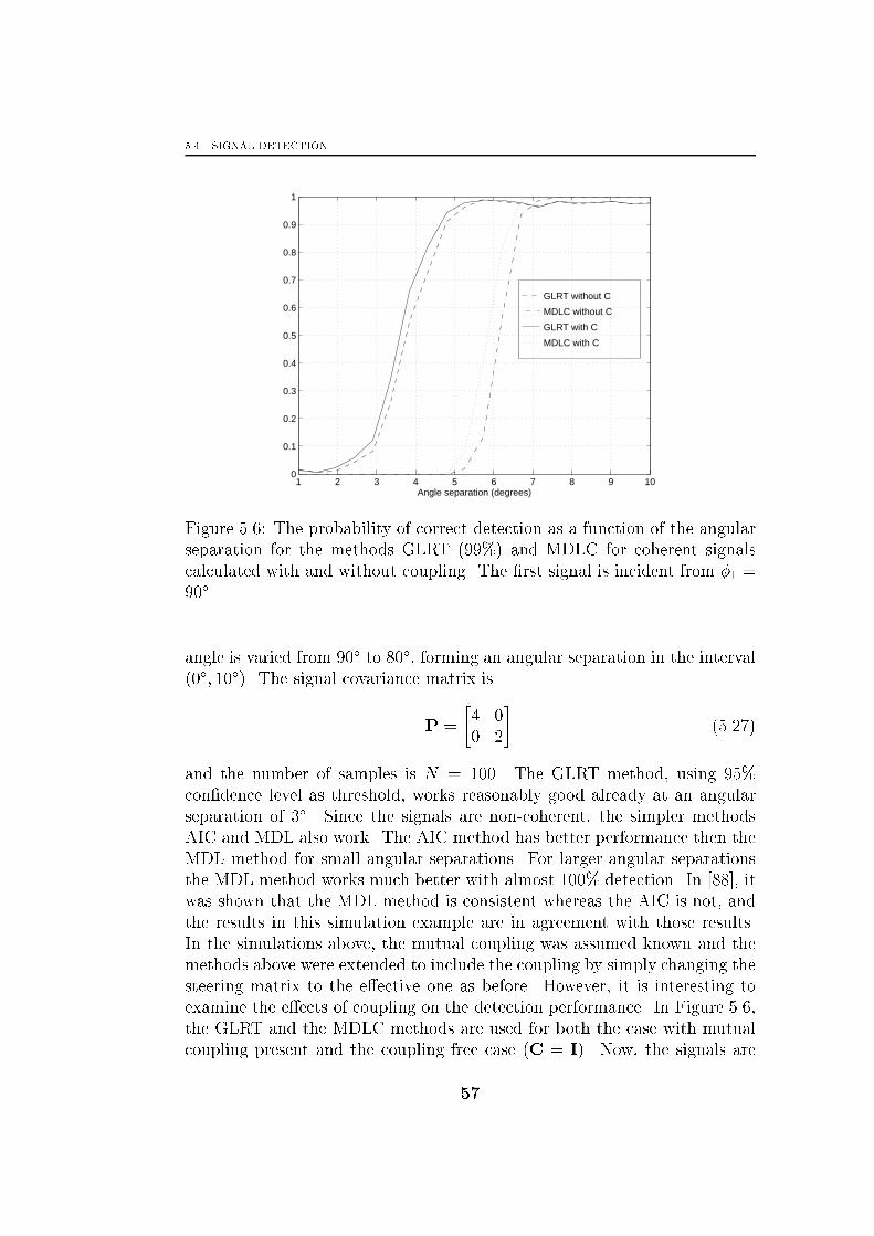
5.4. SIGNAL DETECTION
GLRT without C
MDLC without C
GLRT with C
MDLC with C
1 2 3 4 5 6 7 8 9 100
0.1
0.2
0.3
0.4
0.5
0.6
0.7
0.8
0.9
1
Angle separation (degrees)
Figure 5.6: The probability of correct detection as a function of the angular
separation for the methods GLRT (99%) and MDLC for coherent signals
calculated with and without coupling. The �rst signal is incident from �1 =
90�.
angle is varied from 90� to 80�, forming an angular separation in the interval
(0�; 10�). The signal covariance matrix is
P =
�4 0
0 2
�(5.27)
and the number of samples is N = 100. The GLRT method, using 95%
con�dence level as threshold, works reasonably good already at an angular
separation of 3�. Since the signals are non-coherent, the simpler methods
AIC and MDL also work. The AIC method has better performance then the
MDL method for small angular separations. For larger angular separations
the MDL method works much better with almost 100% detection. In [88], it
was shown that the MDL method is consistent whereas the AIC is not, and
the results in this simulation example are in agreement with those results.
In the simulations above, the mutual coupling was assumed known and the
methods above were extended to include the coupling by simply changing the
steering matrix to the e�ective one as before. However, it is interesting to
examine the e�ects of coupling on the detection performance. In Figure 5.6,
the GLRT and the MDLC methods are used for both the case with mutual
coupling present and the coupling free case (C = I). Now, the signals are
57

CHAPTER 5. ESTIMATION WITH A KNOWN COUPLING
correlated and the signal covariance is
P =
�4 2:8
2:8 2
�(5.28)
and the threshold for the GLRT method is calculated based on a con�dence
level of 99% The GLRT method works better than the Extended version of
MDL that uses DML and AP (MDLC) method that was based on the MDL
method and the deterministic signal model. Also, it is interesting that both
methods work better with mutual coupling present than in the coupling free
case. This is in agreement with the observations made when estimating only
the directions. However, as in the estimation case these e�ects are angle
dependent and not generally true. In Figure 5.7, the same simulations are
performed using �1 = 50� instead of �1 = 90�. Here, the e�ects of coupling
are negligible if the coupling is compensated for.
If the coupling is left uncompensated, the GLRT method collapse and
detection fails. The MDLC methods appears to be more robust, but that
method requires, as found in the examples, a larger angular separation of
the sources to work than the GLRT method. This is one important e�ect
of mutual coupling. Since in the case of DOA estimation, uncompensated
coupling only introduces some errors and reduces the resolution, but the
e�ects on the detection are more severe since signals are lost and false signals
appear. Of course, the simulations presented here are by no means exhaustive
and no general conclusions can be drawn. But, as in the case of estimation
of the DOAs alone, a compensated known coupling can actually increase the
performance in some cases.
5.5 Conclusions
The e�ects of a known coupling was examined. First, by studying the esti-
mation performance by calculating the CRB for the stochastic signal model.
Then the area of sensor array processing was presented by reviewing the
most popular methods of DOA estimation. In most cases, the methods were
extended to include the presence of a known coupling. Particularly, the MU-
SIC, Root-Music, SML, and the Subspace �tting methods were extended
to include a known coupling. These methods will be further extended in
Chapter 7 to estimate an unknown coupling along with the DOAs.
Furthermore, the problem of signal detection was discussed. If the covari-
ance matrix of the signals is nonsingular, the methods AIC and MDL can be
used. Those methods were found to work even in the presence of coupling,
known or unknown, without any modi�cations. However, if the covariance
58
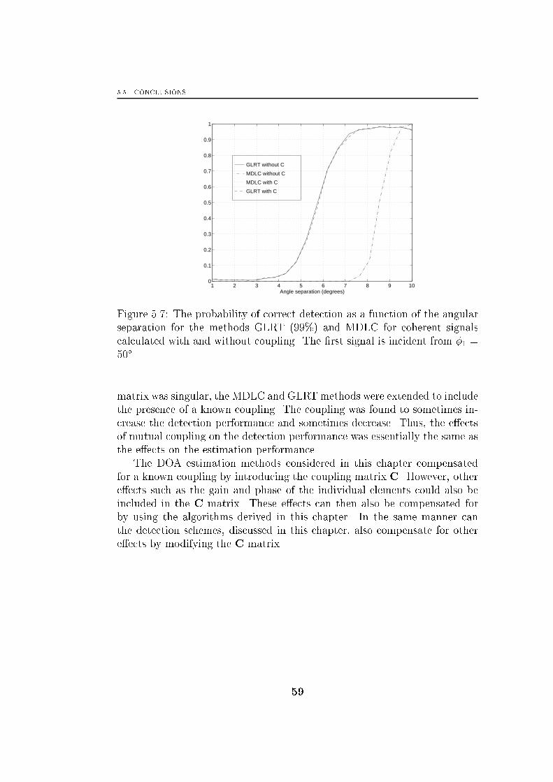
5.5. CONCLUSIONS
GLRT without C
MDLC without C
MDLC with C
GLRT with C
1 2 3 4 5 6 7 8 9 100
0.1
0.2
0.3
0.4
0.5
0.6
0.7
0.8
0.9
1
Angle separation (degrees)
Figure 5.7: The probability of correct detection as a function of the angular
separation for the methods GLRT (99%) and MDLC for coherent signals
calculated with and without coupling. The �rst signal is incident from �1 =
50�.
matrix was singular, the MDLC and GLRTmethods were extended to include
the presence of a known coupling. The coupling was found to sometimes in-
crease the detection performance and sometimes decrease. Thus, the e�ects
of mutual coupling on the detection performance was essentially the same as
the e�ects on the estimation performance.
The DOA estimation methods considered in this chapter compensated
for a known coupling by introducing the coupling matrix C. However, other
e�ects such as the gain and phase of the individual elements could also be
included in the C matrix. These e�ects can then also be compensated for
by using the algorithms derived in this chapter. In the same manner can
the detection schemes, discussed in this chapter, also compensate for other
e�ects by modifying the C matrix.
59

CHAPTER 5. ESTIMATION WITH A KNOWN COUPLING
60
Chapter 6Modeling of an Unknown Coupling
The methods discussed in the previous chapter compensate for the cou-
pling by adjusting the signal processing methods to account for the
coupling. However, to do that the coupling has to be known. In some
rare occasions the coupling might be analytically obtained, as in the case of
a ULA of dipoles in free space. But in most cases, calibration measurements
are necessary. In some cases, obtaining the coupling might not be possible
due to time aspects, the environment is changing to quickly, or that calibra-
tion measurements with known sources is simply not possible in the actual
environment. If the coupling is left uncompensated, it will drastically reduce
the possibilities of performing direction �nding.
One way of mitigating these e�ects is to estimate the coupling along with
the DOAs using signal processing methods. Since this is an introductory
study on the e�ects of mutual coupling and the improvements by estimat-
ing the coupling, a simple coupling scenario is considered. The coupling is
considered to be unknown and deterministic, and no assumptions regarding
the coupling are made. If some knowledge of the coupling exists, it should
of course be included in a more realistic scenario, as well as gain and phase
uncertainties in the array response. Furthermore, the nominal array response
could be known and some random deviation from this response considered.
But, as a �rst study, a simple case is considered in order to get some �rst
results regarding the possible improvements by estimating the coupling as
well as the DOAs.
Directly estimating the coupling using the full electromagnetic coupling
matrix, derived in Chapter 3, usually requires too many parameters, and
therefore a reduced model will be derived in this section. That model will
be used in the following sections to compensate for the coupling by estimat-
ing it along with the DOAs. Furthermore, the uniqueness of the estimates
61

CHAPTER 6. MODELING OF AN UNKNOWN COUPLING
obtained using that model is discussed. The section is concluded by deriving
a necessary condition for uniqueness, that gives a limit on the number of
coupling parameters that are possible to estimate.
6.1 Reduced Coupling Model
The model for the coupling derived in Chapter 3 needs to be simpli�ed in
order to be used to estimate the mutual coupling. A direct estimation of the
full coupling matrix is usually not feasible, since it involves the estimation
of a relatively large number of parameters. The coupling matrix contains n2
complex entries, and if no constraints on the matrix are imposed, n2 complex
parameters need to be estimated. However, by examining the structure of
the coupling matrix C, it is found that the number of parameters can be
signi�cantly reduced and a model with few parameters can be found.
First, it is illuminating to study the magnitude of the coupling matrix
elements. In Figure 6.1, the logarithm of the magnitude of the elements of
the coupling matrix are shown for the case of an array of 10 �=2 dipoles
spaced �=2 apart. From this �gure it is clear that the magnitude of the
coupling decreases quite rapidly with the distance. Thus, only the coupling
with the closest elements need to be considered. This corresponds to only
parameterizing the elements on the �rst subdiagonals1 of the coupling matrix,
since the elements far from the main diagonal are relatively small.
Furthermore, the matrix entries along each subdiagonal are almost the
same. To see this, the normalized magnitude of the elements on a few sub-
diagonals are shown in Figure 6.2 for the same array as in Figure 6.1. The
magnitude of the coupling is approximately the same along the subdiagonals,
and thus it can be modeled by using only one parameter for each subdiagonal
resulting in a coupling matrix of Toeplitz structure. A more complex model
that better approximates the coupling could be formed by adding additional
parameters that model the shape of the magnitude change along the subdi-
agonals. Here, the objective is to derive a simple model and thus only one
parameter for each subdiagonal is used, which also gives a linear model in
the coupling parameters.
Also, noting that the coupling from element i to k is the same as the
coupling from k to i results in a symmetric (not Hermitian!) Toeplitz matrix.
1The ith subdiagonal of a n�n matrix C is the n� i length vector with the kth element
Ck;k+i.
62
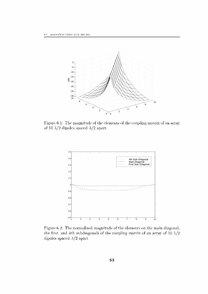
6.1. REDUCED COUPLING MODEL
02
46
810
0
2
4
6
8
10−35
−30
−25
−20
−15
−10
−5
0
[dB
]
Figure 6.1: The magnitude of the elements of the coupling matrix of an array
of 10 �=2 dipoles spaced �=2 apart.
1 2 3 4 5 6 7 8 9 100.5
0.6
0.7
0.8
0.9
1
1.1
1.2
1.3
1.4
1.5
4th Sub−DiagonalMain DiagonalFirst Sub−Diagonal
Figure 6.2: The normalized magnitude of the elements on the main diagonal,
the �rst, and 4th subdiagonals of the coupling matrix of an array of 10 �=2
dipoles spaced �=2 apart.
63
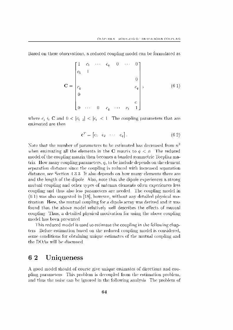
CHAPTER 6. MODELING OF AN UNKNOWN COUPLING
Based on these observations, a reduced coupling model can be formulated as
C =
2666666666664
1 c1 � � � cq 0 � � � 0
c1 1. . .
......
. . .. . . 0
cq. . . cq
0. . .
. . ....
.... . .
. . . c10 � � � 0 cq � � � c1 1
3777777777775; (6.1)
where ci 2 C and 0 < jci+1j < jcij < 1. The coupling parameters that are
estimated are then
cT =�c1 c2 � � � cq
�: (6.2)
Note that the number of parameters to be estimated has decreased from n2
when estimating all the elements in the C matrix to q < n. The reduced
model of the coupling matrix then becomes a banded symmetric Toeplitz ma-
trix. How many coupling parameters, q, to be include depends on the element
separation distance since the coupling is reduced with increased separation
distance, see Section 4.3.3. It also depends on how many elements there are
and the length of the dipole. Also, note that the dipole experiences a strong
mutual coupling and other types of antenna elements often experiences less
coupling and thus also less parameters are needed. The coupling model in
(6.1) was also suggested in [18], however, without any detailed physical mo-
tivation. Here, the mutual coupling for a dipole array was derived and it was
found that the above model relatively well describes the e�ects of mutual
coupling. Thus, a detailed physical motivation for using the above coupling
model has been presented.
This reduced model is used to estimate the coupling in the following chap-
ters. Before estimation based on the reduced coupling model is considered,
some conditions for obtaining unique estimates of the mutual coupling and
the DOAs will be discussed.
6.2 Uniqueness
A good model should of course give unique estimates of directions and cou-
pling parameters. This problem is decoupled from the estimation problem,
and thus the noise can be ignored in the following analysis. The problem of
64

6.2. UNIQUENESS
uniqueness has been analyzed for the coupling free case in [89], where two suf-
�cient conditions for uniqueness are derived. One condition for uniqueness
for every batch of signals is derived using subspace concepts, and another
condition for almost every batch of signals is derived based on results from
topology. The uniqueness problem has also been analyzed in [12, 41, 78, 87].
These results seem di�cult to extend to the case when an unknown coupling
is present, since in that case the e�ective steering matrix is C(c)A(�), and
thus the unknowns are multiplied with each other.
The problem of uniqueness is the question of under which conditions the
unknown parameters of the model can be determined uniquely. The obtained
data are the measured voltages, and the following model is used
x(t) = C(c)A(�)s(t) + n(t); (6.3)
where � = ejkd cos�. Now, the received vector x(t) is sampled at N time
instants and stacked in a matrix X and the following model results
X = C(c)A(�)S+N; (6.4)
where X and N are n�N matrices and S is a p� N matrix. The problem
of uniqueness is based on the following noiseless relation
X = C(c)A(�)S = C(c0)A(�0)S0 ) fc;�;Sg = fc0;�0;S0g: (6.5)
If equation (6.5) holds for every set of measured voltages X, only one set of
parameters gives X, thus the solution (c; �; S) is unique. This is a rather
di�cult problem already without coupling, and with an unknown coupling
it seems di�cult to obtain a general result. One step towards the general
result is to consider the parameterization of the array. If
C(c)A(�) = C(c0)A(�0) ) fc;�g = fc0;�0g (6.6)
holds, the array is said to be unambiguously parameterized. However, if
the signal is known and of full row rank, it can be removed from (6.5) by
multiplying with the pseudo-inverse of S. Therefore, an unambiguously pa-
rameterized array implies uniqueness if the signal is known and of full row
rank. A known signal could correspond to a training sequence in communi-
cation applications, and in that case the solution is unique if (6.6) holds. To
examine the uniqueness and ambiguity problem for the parameterization of
the reduced coupling model, the condition in (6.6) is rewritten as
f( ;y) = C(c)A(�)�C(c0)A(�0) = C(c)A(�)�Y = 0; (6.7)
65
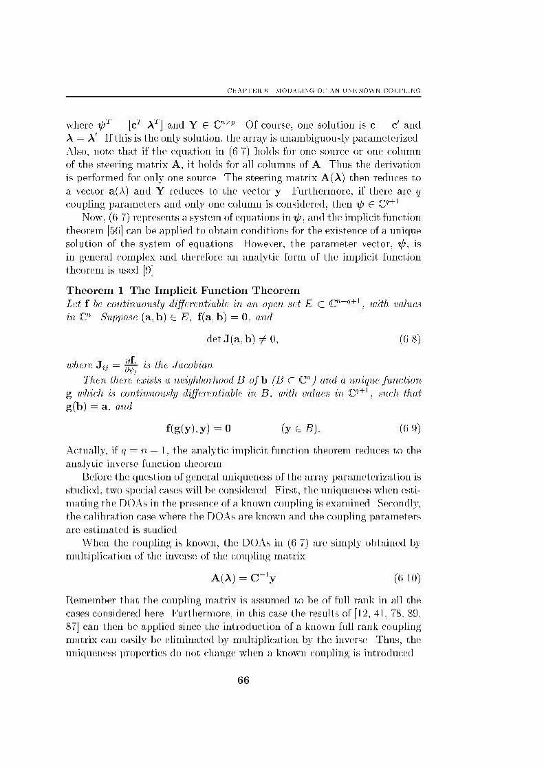
CHAPTER 6. MODELING OF AN UNKNOWN COUPLING
where T = [cT �T ] and Y 2 Cn�p . Of course, one solution is c = c0 and
� = �0. If this is the only solution, the array is unambiguously parameterized.
Also, note that if the equation in (6.7) holds for one source or one column
of the steering matrix A, it holds for all columns of A. Thus the derivation
is performed for only one source. The steering matrix A(�) then reduces to
a vector a(�) and Y reduces to the vector y. Furthermore, if there are q
coupling parameters and only one column is considered, then 2 Cq+1 .
Now, (6.7) represents a system of equations in , and the implicit function
theorem [56] can be applied to obtain conditions for the existence of a unique
solution of the system of equations. However, the parameter vector, , is
in general complex and therefore an analytic form of the implicit function
theorem is used [9].
Theorem 1 The Implicit Function Theorem
Let f be continuously di�erentiable in an open set E � Cn+q+1 , with values
in Cn. Suppose (a;b) 2 E; f(a;b) = 0, and
detJ(a;b) 6= 0; (6.8)
where Jij =@fi@ j
is the Jacobian.
Then there exists a neighborhood B of b (B � Cn) and a unique function
g which is continuously di�erentiable in B, with values in Cq+1 , such that
g(b) = a, and
f(g(y);y) = 0 (y 2 B): (6.9)
Actually, if q = n� 1, the analytic implicit function theorem reduces to the
analytic inverse function theorem.
Before the question of general uniqueness of the array parameterization is
studied, two special cases will be considered. First, the uniqueness when esti-
mating the DOAs in the presence of a known coupling is examined. Secondly,
the calibration case where the DOAs are known and the coupling parameters
are estimated is studied.
When the coupling is known, the DOAs in (6.7) are simply obtained by
multiplication of the inverse of the coupling matrix.
A(�) = C�1y (6.10)
Remember that the coupling matrix is assumed to be of full rank in all the
cases considered here. Furthermore, in this case the results of [12, 41, 78, 89,
87] can then be applied since the introduction of a known full rank coupling
matrix can easily be eliminated by multiplication by the inverse. Thus, the
uniqueness properties do not change when a known coupling is introduced.
66
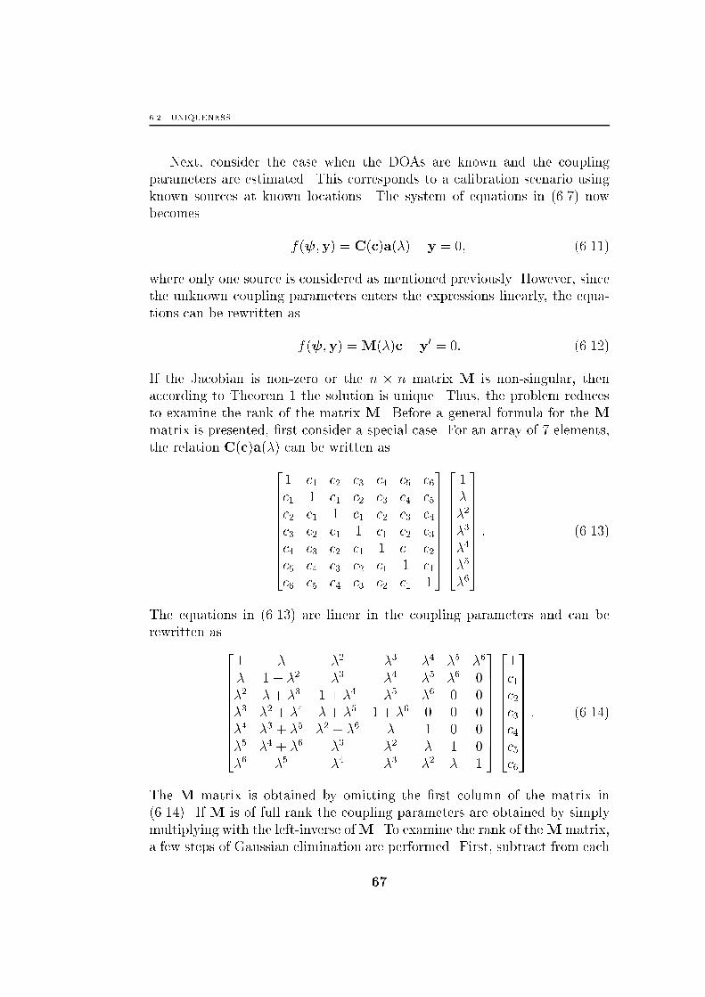
6.2. UNIQUENESS
Next, consider the case when the DOAs are known and the coupling
parameters are estimated. This corresponds to a calibration scenario using
known sources at known locations. The system of equations in (6.7) now
becomes
f( ;y) = C(c)a(�)� y = 0; (6.11)
where only one source is considered as mentioned previously. However, since
the unknown coupling parameters enters the expressions linearly, the equa-
tions can be rewritten as
f( ;y) =M(�)c� y0 = 0: (6.12)
If the Jacobian is non-zero or the n � n matrix M is non-singular, then
according to Theorem 1 the solution is unique. Thus, the problem reduces
to examine the rank of the matrix M. Before a general formula for the M
matrix is presented, �rst consider a special case. For an array of 7 elements,
the relation C(c)a(�) can be written as2666666664
1 c1 c2 c3 c4 c5 c6c1 1 c1 c2 c3 c4 c5c2 c1 1 c1 c2 c3 c4c3 c2 c1 1 c1 c2 c3c4 c3 c2 c1 1 c1 c2c5 c4 c3 c2 c1 1 c1c6 c5 c4 c3 c2 c1 1
3777777775
2666666664
1
�
�2
�3
�4
�5
�6
3777777775: (6.13)
The equations in (6.13) are linear in the coupling parameters and can be
rewritten as2666666664
1 � �2 �3 �4 �5 �6
� 1 + �2 �3 �4 �5 �6 0
�2 �+ �3 1 + �4 �5 �6 0 0
�3 �2 + �4 �+ �5 1 + �6 0 0 0
�4 �3 + �5 �2 + �6 � 1 0 0
�5 �4 + �6 �3 �2 � 1 0
�6 �5 �4 �3 �2 � 1
3777777775
2666666664
1
c1c2c3c4c5c6
3777777775: (6.14)
The M matrix is obtained by omitting the �rst column of the matrix in
(6.14). If M is of full rank the coupling parameters are obtained by simply
multiplying with the left-inverse ofM. To examine the rank of theMmatrix,
a few steps of Gaussian elimination are performed. First, subtract from each
67
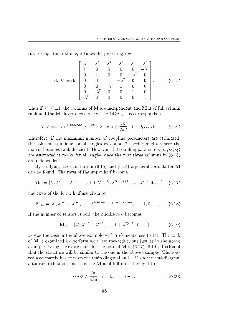
CHAPTER 6. MODELING OF AN UNKNOWN COUPLING
row, except the �rst one, � times the preceding row
rk M = rk
2666666664
� �2 �3 �4 �5 �6
1 0 0 0 0 ��70 1 0 0 ��7 0
0 0 1 ��7 0 0
0 0 ��7 1 0 0
0 ��7 0 0 1 0
��7 0 0 0 0 1
3777777775: (6.15)
Thus if �7 6= �1, the columns ofM are independent andM is of full column
rank and the left-inverse exists. For the DOAs, this corresponds to
�7 6= �1) ej14kd cos � 6= ej2� ) cos� 6= l�
7kdl = 0; : : : ; 6: (6.16)
Therefore, if the maximum number of coupling parameters are estimated,
the solution is unique for all angles except at 7 speci�c angles where the
matrix becomes rank de�cient. However, if 3 coupling parameters (c1; c2; c3)
are estimated it works for all angles since the �rst three columns in (6.15)
are independent.
By studying the structure in (6.15) and (6.14) a general formula for M
can be found. The rows of the upper half become
Mi;: = [�i; �i�1 + �i+1; : : : ; 1 + �2(i�1); �2(i�1)+1; : : : ; �n�1; 0; : : : ] (6.17)
and rows of the lower half are given by
Mi;: = [�i; �i�1 + �i+1; : : : ; �2i+1�n + �n�1; �2i�n; : : : ; 1; 0; : : : ]: (6.18)
If the number of sensors is odd, the middle row becomes
Mi;: = [�i; �i�1 + �i+1; : : : ; 1 + �2(i�1); 0; : : : ] (6.19)
as was the case in the above example with 7 elements, see (6.14). The rank
of M is examined by performing a few row-reductions just as in the above
example. Using the expressions for the rows ofM in (6.17)-(6.19), it is found
that the structure will be similar to the one in the above example. The row-
reduced matrix has ones on the main diagonal and ��n on the anti-diagonal
after row-reduction, and thus the M is of full rank if �n 6= �1 or
cos� 6= l�
nkdl = 0; : : : ; n� 1: (6.20)
68
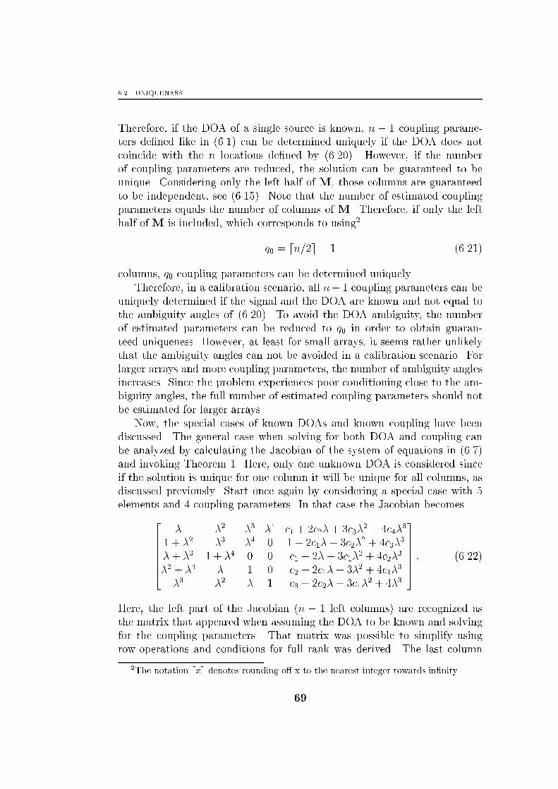
6.2. UNIQUENESS
Therefore, if the DOA of a single source is known, n � 1 coupling parame-
ters de�ned like in (6.1) can be determined uniquely if the DOA does not
coincide with the n locations de�ned by (6.20). However, if the number
of coupling parameters are reduced, the solution can be guaranteed to be
unique. Considering only the left half of M, those columns are guaranteed
to be independent, see (6.15). Note that the number of estimated coupling
parameters equals the number of columns of M. Therefore, if only the left
half of M is included, which corresponds to using2
q0 = dn=2e � 1 (6.21)
columns, q0 coupling parameters can be determined uniquely.
Therefore, in a calibration scenario, all n� 1 coupling parameters can be
uniquely determined if the signal and the DOA are known and not equal to
the ambiguity angles of (6.20). To avoid the DOA ambiguity, the number
of estimated parameters can be reduced to q0 in order to obtain guaran-
teed uniqueness. However, at least for small arrays, it seems rather unlikely
that the ambiguity angles can not be avoided in a calibration scenario. For
larger arrays and more coupling parameters, the number of ambiguity angles
increases. Since the problem experiences poor conditioning close to the am-
biguity angles, the full number of estimated coupling parameters should not
be estimated for larger arrays.
Now, the special cases of known DOAs and known coupling have been
discussed. The general case when solving for both DOA and coupling can
be analyzed by calculating the Jacobian of the system of equations in (6.7)
and invoking Theorem 1. Here, only one unknown DOA is considered since
if the solution is unique for one column it will be unique for all columns, as
discussed previously. Start once again by considering a special case with 5
elements and 4 coupling parameters. In that case the Jacobian becomes266664� �2 �3 �4 c1 + 2c2�+ 3c3�
2 + 4c4�3
1 + �2 �3 �4 0 1 + 2c1�+ 3c2�2 + 4c3�
3
�+ �3 1 + �4 0 0 c1 + 2�+ 3c1�2 + 4c2�
3
�2 + �4 � 1 0 c2 + 2c1�+ 3�2 + 4c1�3
�3 �2 � 1 c3 + 2c2�+ 3c1�2 + 4�3
377775 : (6.22)
Here, the left part of the Jacobian (n � 1 left columns) are recognized as
the matrix that appeared when assuming the DOA to be known and solving
for the coupling parameters. That matrix was possible to simplify using
row-operations and conditions for full rank was derived. The last column
2The notation dxe denotes rounding o� x to the nearest integer towards in�nity.
69
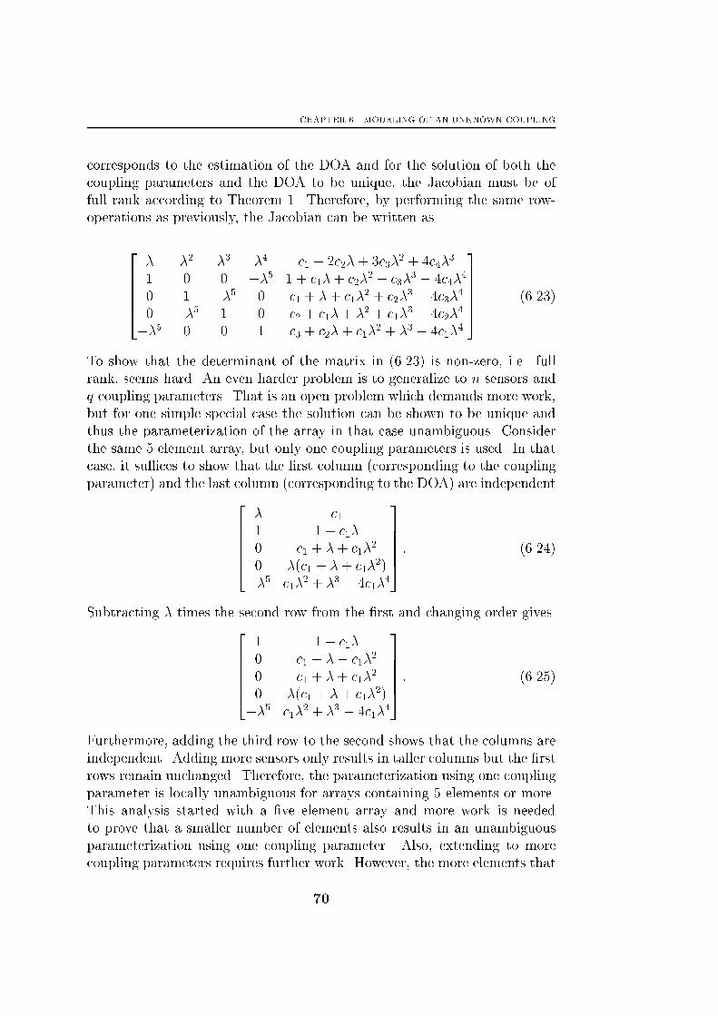
CHAPTER 6. MODELING OF AN UNKNOWN COUPLING
corresponds to the estimation of the DOA and for the solution of both the
coupling parameters and the DOA to be unique, the Jacobian must be of
full rank according to Theorem 1. Therefore, by performing the same row-
operations as previously, the Jacobian can be written as
266664� �2 �3 �4 c1 + 2c2�+ 3c3�
2 + 4c4�3
1 0 0 ��5 1 + c1�+ c2�2 + c3�
3 � 4c4�4
0 1 ��5 0 c1 + �+ c1�2 + c2�
3 � 4c3�4
0 ��5 1 0 c2 + c1�+ �2 + c1�3 � 4c2�
4
��5 0 0 1 c3 + c2�+ c1�2 + �3 � 4c1�
4
377775 (6.23)
To show that the determinant of the matrix in (6.23) is non-zero, i.e. full
rank, seems hard. An even harder problem is to generalize to n sensors and
q coupling parameters. That is an open problem which demands more work,
but for one simple special case the solution can be shown to be unique and
thus the parameterization of the array in that case unambiguous. Consider
the same 5 element array, but only one coupling parameters is used. In that
case, it su�ces to show that the �rst column (corresponding to the coupling
parameter) and the last column (corresponding to the DOA) are independent266664� c11 1 + c1�
0 c1 + �+ c1�2
0 �(c1 + �+ c1�2)
��5 c1�2 + �3 � 4c1�
4
377775 : (6.24)
Subtracting � times the second row from the �rst and changing order gives2666641 1 + c1�
0 c1 � �� c1�2
0 c1 + �+ c1�2
0 �(c1 + �+ c1�2)
��5 c1�2 + �3 � 4c1�
4
377775 : (6.25)
Furthermore, adding the third row to the second shows that the columns are
independent. Adding more sensors only results in taller columns but the �rst
rows remain unchanged. Therefore, the parameterization using one coupling
parameter is locally unambiguous for arrays containing 5 elements or more.
This analysis started with a �ve element array and more work is needed
to prove that a smaller number of elements also results in an unambiguous
parameterization using one coupling parameter. Also, extending to more
coupling parameters requires further work. However, the more elements that
70
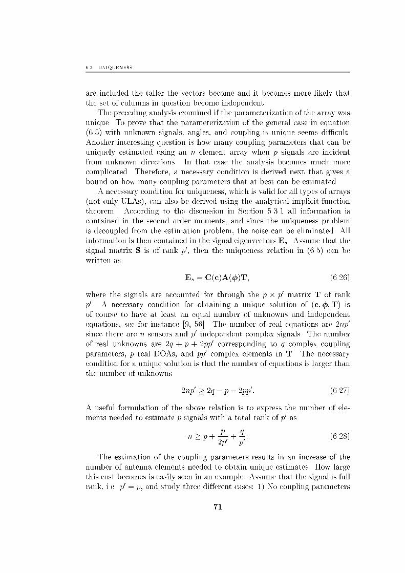
6.2. UNIQUENESS
are included the taller the vectors become and it becomes more likely that
the set of columns in question become independent.
The preceding analysis examined if the parameterization of the array was
unique. To prove that the parameterization of the general case in equation
(6.5) with unknown signals, angles, and coupling is unique seems di�cult.
Another interesting question is how many coupling parameters that can be
uniquely estimated using an n element array when p signals are incident
from unknown directions. In that case the analysis becomes much more
complicated. Therefore, a necessary condition is derived next that gives a
bound on how many coupling parameters that at best can be estimated.
A necessary condition for uniqueness, which is valid for all types of arrays
(not only ULAs), can also be derived using the analytical implicit function
theorem. According to the discussion in Section 5.3.1 all information is
contained in the second order moments, and since the uniqueness problem
is decoupled from the estimation problem, the noise can be eliminated. All
information is then contained in the signal eigenvectors Es. Assume that the
signal matrix S is of rank p0, then the uniqueness relation in (6.5) can be
written as
Es = C(c)A(�)T; (6.26)
where the signals are accounted for through the p � p0 matrix T of rank
p0. A necessary condition for obtaining a unique solution of (c;�;T) is
of course to have at least an equal number of unknowns and independent
equations, see for instance [9, 56]. The number of real equations are 2np0
since there are n sensors and p0 independent complex signals. The number
of real unknowns are 2q + p + 2pp0 corresponding to q complex coupling
parameters, p real DOAs, and pp0 complex elements in T. The necessary
condition for a unique solution is that the number of equations is larger than
the number of unknowns
2np0 � 2q + p+ 2pp0: (6.27)
A useful formulation of the above relation is to express the number of ele-
ments needed to estimate p signals with a total rank of p0 as
n � p+p
2p0+
q
p0: (6.28)
The estimation of the coupling parameters results in an increase of the
number of antenna elements needed to obtain unique estimates. How large
this cost becomes is easily seen in an example. Assume that the signal is full
rank, i.e. p0 = p, and study three di�erent cases: 1) No coupling parameters
71
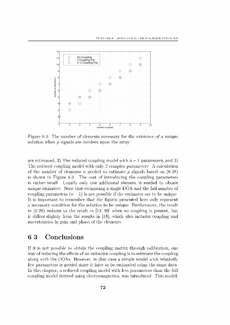
CHAPTER 6. MODELING OF AN UNKNOWN COUPLING
1 2 3 4 5 6 7 8 9 101
2
3
4
5
6
7
8
9
10
11
12
Number of signals
Num
ber
of e
lem
ents
nNo Coupling2 Coupling Par.n−1 Coupling Par.
Figure 6.3: The number of elements necessary for the existence of a unique
solution when p signals are incident upon the array.
are estimated, 2) The reduced coupling model with n� 1 parameters, and 3)
The reduced coupling model with only 2 complex parameters. A calculation
of the number of elements n needed to estimate p signals based on (6.28)
is shown in Figure 6.3. The cost of introducing the coupling parameters
is rather small. Usually only one additional element is needed to obtain
unique estimates. Note that estimating a single DOA and the full number of
coupling parameters (n� 1) is not possible if the estimates are to be unique.
It is important to remember that the �gures presented here only represent
a necessary condition for the solution to be unique. Furthermore, the result
in (6.28) reduces to the result in [12, 89] when no coupling is present, but
it di�ers slightly from the results in [18], which also includes coupling and
uncertainties in gain and phase of the elements.
6.3 Conclusions
If it is not possible to obtain the coupling matrix through calibration, one
way of reducing the e�ects of an unknown coupling is to estimate the coupling
along with the DOAs. However, in that case a simple model with relatively
few parameters is needed since it have to be estimated using the same data.
In this chapter, a reduced coupling model with less parameters than the full
coupling model derived using electromagnetics, was introduced. This model,
72
6.3. CONCLUSIONS
a banded symmetric Toeplitz matrix, coincided with the model conjectured
in [18], but here it was based on physical reasoning. Note that although the
reduced model captures the properties of the full electromagnetical model
of the coupling, it of course deteriorates the direction �nding. Therefore,
a calibration scheme where the full coupling matrix is estimated should be
applied if possible. But if not possible, estimating the coupling reduces the
e�ects of an unknown coupling.
When estimating the coupling along with the DOAs new problems arise.
One problem is the question of uniqueness of the estimates of the parame-
ters of the reduced coupling model. This was analyzed in this chapter and
although no general results regarding the uniqueness were obtained, it was
shown that the parameterization of the array, in a calibration scenario, is lo-
cally unambiguous. If the number of coupling parameters are equal to or less
than dn=2e � 1, the parameterization is locally unambiguous for all DOAs.
Otherwise the parameterization becomes ambiguous at n di�erent angles in
that calibration scenario. In general with both unknown DOA and coupling
no results were obtained, but it was found that arrays with more than four el-
ements are unambiguously parameterized (locally) if one coupling parameter
is used.
Furthermore, a necessary condition for uniqueness was presented. In the
next chapter, this reduced model is used to estimate both the coupling and
the DOAs using di�erent methods.
73

CHAPTER 6. MODELING OF AN UNKNOWN COUPLING
74
Chapter 7Estimation With an Unknown
Coupling
If it is not possible to obtain the coupling matrix through calibration or
some other means, the e�ects of an unknown coupling can be mitigated
by estimating both the coupling and the DOAs. However, the number of
unknown parameters generally becomes too large if a direct estimation of the
elements of the coupling matrix is performed together with a DOA estima-
tion. Using the reduced coupling model, derived in the previous section, the
number of parameters becomes feasible. Here, the reduced coupling model
will be used throughout this chapter in the simple scenario of a completely
unknown coupling. In practice, some knowledge of the coupling usually ex-
ists, which of course should be used.
First, the model and the stochastic assumptions will be reviewed. Then,
the Stochastic Maximum Likelihood estimator for the present data model,
is derived. The Cram�er-Rao lower Bound on the variance for the case of an
unknown coupling is derived based on the SML expressions.
After establishing the lower bound, several methods of estimation are dis-
cussed. Estimation of an unknown mutual coupling has received very little
interest in the signal processing literature. To the author's knowledge the
only e�ort of estimating the DOAs and the coupling have been presented
in [18]. Therefore, the iterative MUSIC algorithm in [18] is discussed �rst
and some related methods are proposed. Furthermore, the NSF method is
extended to estimate both an unknown coupling and the DOAs. The proper-
ties of the di�erent estimation methods are then examined and compared to
the CRB in a few computer experiments. The chapter is concluded by brie y
considering the problem of signal detection in the presence of an unknown
coupling.
75

CHAPTER 7. ESTIMATION WITH AN UNKNOWN COUPLING
7.1 Data Model
The input data to the estimation algorithms in the following sections are
the measured voltages of the antenna elements. As before, the antenna is a
uniform linear array of n dipoles and p waves are incident upon the array.
One important di�erence to the case of a known coupling is that the reduced
coupling model is used here. Sampling the voltages x(t) at N time instants
t = t1; : : : ; tN (taking N "snapshots") gives the following model
X = CA(�)S +N; (7.1)
where
X =�x(t1) � � � x(tN)
�(7.2)
S =�s(t1) � � � s(tN)
�(7.3)
N =�n(t1) � � � n(tN)
�: (7.4)
The matrix of measured voltagesX is n�N , the signal matrix S is p�N , the
noise matrix N is n�N , and the coupling matrix C is n� n with elements
Cij = cji�jj. Note that c0 = 1 and jcij < 1 8 1 � i � q. The steering matrix
A(�) is n� p, and for a ULA it has a Vandermonde structure with elements
[A(�)]vw = e�jkd(v�1) cos �w , where k is the wavenumber and d is the element
separation distance. The DOAs are contained in the parameter vector �.
Furthermore, the coupling matrix is assumed to be of full rank and both
the signal s(t) and the noise n(t) are circularly Gaussian distributed as in
Section 5.1. Also, the number of dipoles are chosen as to ful�ll the necessary
condition derived in previous section
n � p+p
2p0+
q
p0; (7.5)
where p0 is the rank of the signal matrix S and q � n � 1 is the number of
coupling parameters used.
Based on the data model in (7.1) and the statistical assumptions above,
the maximum likelihood estimator for an unknown coupling and unknown
DOAs will be derived in the next section.
7.2 Maximum Likelihood
The method of Maximum Likelihood estimation is one of the most popular
estimation method used in signal processing. One of the reasons is that for
large enough data records the ML estimator is approximately the Minimum
76

7.2. MAXIMUM LIKELIHOOD
Variance Unbiased (MVU) estimator, and thus it is asymptotically e�cient.
Here, the maximum likelihood estimator for the data model presented in the
previous section will be derived. Since not only the noise, but also the signals,
are assumed to be stochastic, the resulting maximum likelihood method is
usually called the Stochastic Maximum Likelihood method, see Section 5.3.3.
For the coupling-free case the SML has been derived in a concentrated form
[10, 25, 68]. The derivation of the SML, when an unknown coupling is present,
follows basically the same lines as the coupling-free case. However, some
properties do change and of course the number of unknowns increase, and
therefore the important steps of the derivation are included in some detail in
Appendix 7A.
The SML estimation method is based on maximizing the likelihood by
choosing the values of the unknown parameters that give the maximum. The
unknown parameters are the DOAs �, the coupling c, and the free parameters
of the signal and noise covariances. Note that both the coupling parameters ciand the signal covariance P are in general complex. When the objective is to
estimate the DOAs, the signal and noise covariances are nuisance parameters
and the expression that is to be maximized can be concentrated into the
following form
� = f�; cg = argmin�;c
VSML(�; c) = argmin�;c
log dethCAPAHCH + �2I
i;
(7.6)
where
P = (CA)yhR� �I
i(CA)yH (7.7)
�2 =1
n� pTrnP?CAR
o: (7.8)
Note that the dependence of C(c), A(�), P(�; c), and �2(�; c) on the pa-
rameters have been omitted in order to reduce the notation complexity. For
a more detailed discussion of deriving the likelihood function, see Appendix
7A. To obtain a closed form solution for the coupling or the DOAs is, in
general, not possible. Therefore, the parameter values are obtained through
a numerical search. Many di�erent optimization techniques have been pro-
posed in the signal processing literature. Here, a damped Newton method
[14] will be used. The estimate is calculated iteratively as
�k+1 = �k � �kH�1V0; (7.9)
where �k is the estimate at iteration k, �k is the step length, H denotes the
Hessian matrix of the criterion function, and V0 denotes the gradient. The
77

CHAPTER 7. ESTIMATION WITH AN UNKNOWN COUPLING
Hessian and the gradient are evaluated at �k. The step length is chosen
using a simple scheme, starting with a value � � 1 and then decreasing the
value until the value of the criterion function is less than in previous iteration.
If the criterion not decreases, the iteration is terminated. Of course there is
no guarantee that the search will end in the global minimum. However, if
the search is initiated "su�ciently close", the global minimum will be found.
When implementing the above search method, two problems appear.
First, for �H�1V0 to be a descent direction the Hessian must be positive
de�nite, which not necessarily have to be the case far from the true opti-
mum. Also, the evaluation of the Hessian is computationally cumbersome,
and therefore the Hessian is replaced by the Fisher Information Matrix (FIM)
which is more easily evaluated and also guaranteed to be positive de�nite if
the estimation problem is well posed. This leads to a method that in the
statistical literature is known as the scoring method [45]. Furthermore, it
will be derived in the next section that the asymptotic Hessian essentially
coincides with the asymptotic covariance matrix of the estimates. Since,
the ML method is statistically e�cient, an expression for the FIM and the
Cram�er-Rao lower bound are thus also found.
In order to implement the search, the gradient and the asymptotic Hessian
of the criterion function in (7.6) must be calculated. The steps involved in
this calculation is similar to those in [67], but the introduction of the coupling
matrix results in slight changes. The calculations are included in Appendix
7A, where it also is shown that the gradient becomes
V0(�) =
266642ReTr
hGAHCHRP?
CA@(CA)
@�1
i...
2ReTrhGAHCHRP?
CA@(CA)
@�p+2q
i37775 ; (7.10)
where
G = (AHCHRCA)�1 � 1
�2(AHCHCA)�1; (7.11)
and �2 is de�ned in (7.8). The estimated covariance matrix, R, is de�ned in
(5.14). The expression for the asymptotic Hessian is also derived in Appendix
7A
H = V00a(�) =
�H�� H�c
HT�c Hcc
�: (7.12)
The block matrices are as follows
H�� =2
�2Ren�PAHCHR�1CAP
�T � �DHCHP?CACD
�o; (7.13)
78

7.3. DIRECTION FINDING ACCURACY
where
D =
�@a(�)
@�
???�=�1
; � � � ; @a(�)@�
???�=�p
�: (7.14)
Also,
H�c =
�@2Va
@�@cr
@2Va
@�@ci
�= HT
�c; (7.15)
where �@2Va
@�@cr
�ij
= 2�2ReTr
hPAHCHR�1CAPAH�jP
?CAC
@A@�i
i(7.16)�
@2Va
@�@ci
�ij
= � 2�2ImTr
hPAHCHR�1CAPAH�jP
?CAC
@A@�i
i(7.17)
and �k is banded symmetric Toeplitz matrix with zeros everywhere except
on the kth and the �kth subdiagonal which consists of ones. Finally,
Hcc =
�Hcrcr Hcrci
HTcrci
Hcici
�; (7.18)
where
[Hcrcr ]ij =2�2ReTr
�PAHCHR�1CAPAH�jP
?CA�iA
�(7.19)
[Hcrci]ij = � 2�2ImTr
�PAHCHR�1CAPAH�jP
?CA�iA
�(7.20)
[Hcici]ij = � 2�2ReTr
�PAHCHR�1CAPAH�jP
?CA�iA
�: (7.21)
Now, using the scoring method, i.e. equation (7.9) with the gradient and
Hessian in (7.10) and (7.12), the implementation of the SML method is
straightforward.
The relation between the SML method and the Cram�er-Rao bound will
be used in the next section to derive a formula for the CRB.
7.3 Direction Finding Accuracy
When comparing di�erent estimation schemes, it is important to known the
fundamental performance limit of the estimation problem at hand. The
Cram�er-Rao lower bound gives the lowest possible variance of a unbiased
estimator and thus serves as a fundamental performance limit that is useful
when comparing di�erent estimation schemes. In Section 5.2, the CRB was
79
CHAPTER 7. ESTIMATION WITH AN UNKNOWN COUPLING
calculated for the case of a known mutual coupling. Here, the bound will be
calculated when an unknown mutual coupling is present.
The Cram�er-Rao lower bound for a parameter vector � is de�ned as
Ef(���0)(���0)Tg � I�1(�); (7.22)
where I(�) is the FIM with elements
I(�)ij = �E�@2 log p(x;�)
@�i@�j
�: (7.23)
Note that p(x;�) is the probability density function for the measurements
parameterized by the unknown parameters� that are to be estimated. When
viewed as a function of the unknown parameters �, p(x;�) is termed the
likelihood function.
The CRB is usually evaluated using (7.22)-(7.23) and for the coupling free
case, formulas have appeared in [6, 57]. However, when estimating the DOAs,
the signal and noise covariances can often be regarded as nuisance parameters
and thus the CRB for these parameters are not important. A more compact
expression for the CRB on the DOAs is possible to obtain by observing the
fact that the likelihood function can be concentrated regarding the signal and
the noise covariance as derived in the previous section. Compact expressions
for the CRB for the coupling free case have been derived in [46, 67].
The CRB for the case when an unknown mutual coupling is present has
been derived in the literature [18], where also the phase and gain of the an-
tenna elements are considered unknown. In that derivation the de�nition
in (7.22) was used, resulting in a large Fisher matrix to be inverted. Here,
compact expressions for the CRB on the DOAs in the presence of an un-
known mutual coupling will be derived based on the concentrated likelihood
function.
An expression for the CRB on the DOAs can be derived by exploiting
the relation between the ML method and the CRB. From general statistical
theory it follows that if there is a unique solution, the ML estimator converges
in probability to the true parameter vector under very general conditions [30].
Furthermore, the ML estimator is found to be asymptotically e�cient [30],
i.e. the covariance matrix for the ML estimates coincides with the CRB for
large number of samples (N � 1). Once the asymptotic expression for the
covariance matrix for the ML estimates is obtained, the general CRB formula
is also obtained. The number of samples enters only as a scaling, since the
likelihood expression is proportional to the number of samples, and therefore
is the CRB expression valid for all N [67].
80
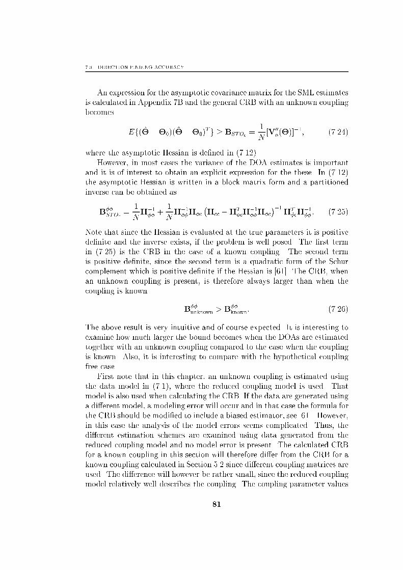
7.3. DIRECTION FINDING ACCURACY
An expression for the asymptotic covariance matrix for the SML estimates
is calculated in Appendix 7B and the general CRB with an unknown coupling
becomes
Ef(���0)(���0)Tg � BSTOc
=1
N[V00
a(�)]�1; (7.24)
where the asymptotic Hessian is de�ned in (7.12).
However, in most cases the variance of the DOA estimates is important
and it is of interest to obtain an explicit expression for the these. In (7.12)
the asymptotic Hessian is written in a block matrix form and a partitioned
inverse can be obtained as
B��STOc
=1
NH�1�� +
1
NH�1��H�c
�Hcc �HT
�cH�1��H�c
��1HT�cH
�1�� : (7.25)
Note that since the Hessian is evaluated at the true parameters it is positive
de�nite and the inverse exists, if the problem is well posed. The �rst term
in (7.25) is the CRB in the case of a known coupling. The second term
is positive de�nite, since the second term is a quadratic form of the Schur
complement which is positive de�nite if the Hessian is [61]. The CRB, when
an unknown coupling is present, is therefore always larger than when the
coupling is known
B��unknown > B
��known: (7.26)
The above result is very intuitive and of course expected. It is interesting to
examine how much larger the bound becomes when the DOAs are estimated
together with an unknown coupling compared to the case when the coupling
is known. Also, it is interesting to compare with the hypothetical coupling
free case.
First note that in this chapter, an unknown coupling is estimated using
the data model in (7.1), where the reduced coupling model is used. That
model is also used when calculating the CRB. If the data are generated using
a di�erent model, a modeling error will occur and in that case the formula for
the CRB should be modi�ed to include a biased estimator, see [61]. However,
in this case the analysis of the model errors seems complicated. Thus, the
di�erent estimation schemes are examined using data generated from the
reduced coupling model and no model error is present. The calculated CRB
for a known coupling in this section will therefore di�er from the CRB for a
known coupling calculated in Section 5.2 since di�erent coupling matrices are
used. The di�erence will however be rather small, since the reduced coupling
model relatively well describes the coupling. The coupling parameter values
81

CHAPTER 7. ESTIMATION WITH AN UNKNOWN COUPLING
0
20
40
60
80
0
20
40
60
80
0
0.5
1
1.5
2
2.5
3
3.5
4
�1 �2
Figure 7.1: The ratio of the standard deviation for unknown coupling and
known coupling for �2 versus the angles for an array of 5 �=2 dipoles spaced
�=2 apart and q = 1.
are here chosen from the �rst column of the coupling matrix calculated using
electromagnetics. Usually, only a few coupling parameters are included when
estimating and that also give rise to a small di�erence. In the following,
the increase in the square root of the CRB (the standard deviation) when
the coupling needs to be estimated (using the reduced model), is compared
to when the coupling is known. Although these comparisons of the CRB
for di�erent cases gives some insight on how well it is possible to estimate
the DOAs, it is only meaningful for reasonably large SNRs. For high SNR
scenarios the model error will dominate in a realistic scenario. Here, however,
the data are generated using the same model as the estimators are based on
and thus the estimators considered here will be asymptotically unbiased.
In Figure 7.1, the ratio of the standard deviation for an unknown coupling
and a known coupling for �2 versus the angles is shown. An array of 5 �=2
dipoles spaced �=2 apart is used and only one coupling parameter is estimated
(q = 1). The ratio is larger than unity, but the increase is not dramatic.
Also, the ratio is above unity everywhere due to the fact that the CRB for
an unknown coupling always is larger than the CRB for a known coupling
as found in (7.26). It is also important to note that the main diagonal
corresponds to two waves arriving from the same angle and thus impossible
to discriminate. The Hessian becomes rank de�cient and the CRB becomes
82
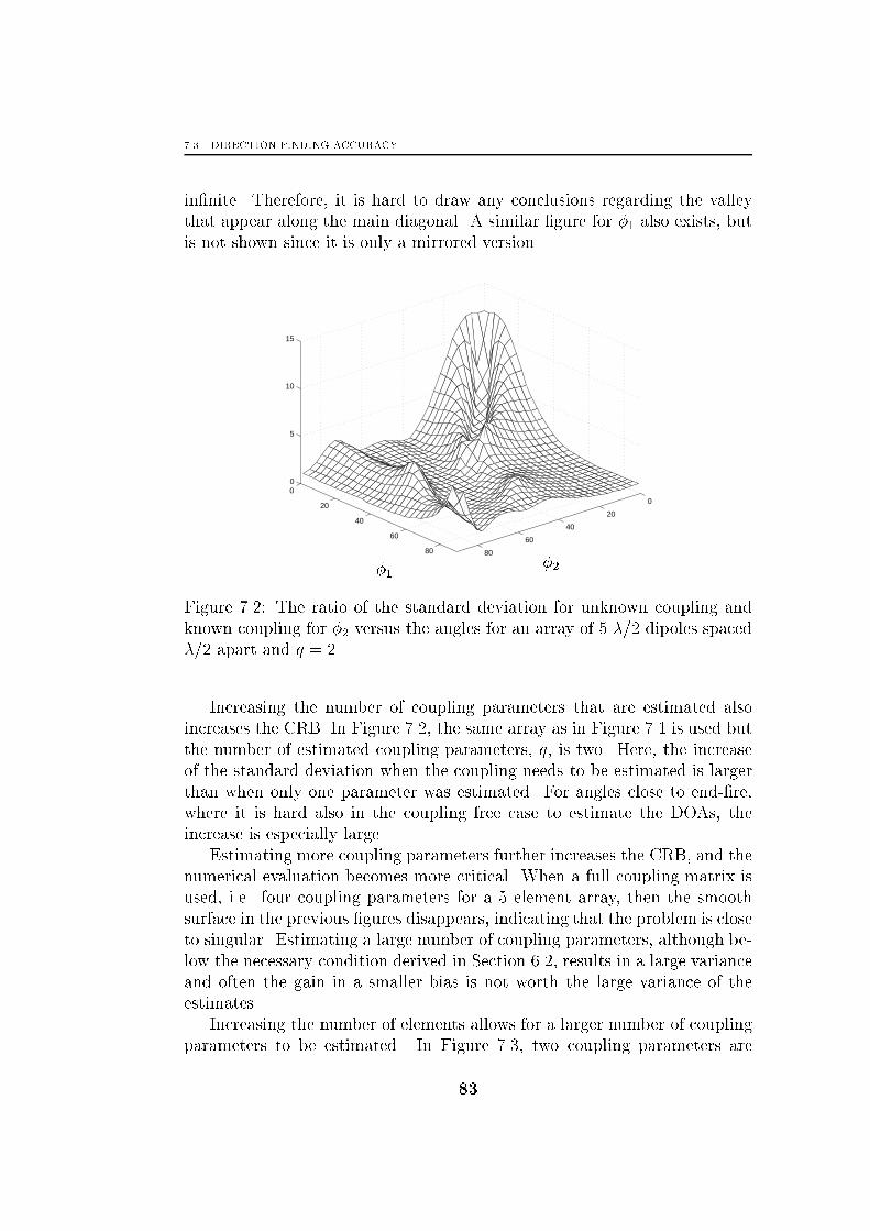
7.3. DIRECTION FINDING ACCURACY
in�nite. Therefore, it is hard to draw any conclusions regarding the valley
that appear along the main diagonal. A similar �gure for �1 also exists, but
is not shown since it is only a mirrored version.
0
20
40
60
80
0
20
40
60
80
0
5
10
15
�1�2
Figure 7.2: The ratio of the standard deviation for unknown coupling and
known coupling for �2 versus the angles for an array of 5 �=2 dipoles spaced
�=2 apart and q = 2.
Increasing the number of coupling parameters that are estimated also
increases the CRB. In Figure 7.2, the same array as in Figure 7.1 is used but
the number of estimated coupling parameters, q, is two. Here, the increase
of the standard deviation when the coupling needs to be estimated is larger
than when only one parameter was estimated. For angles close to end-�re,
where it is hard also in the coupling free case to estimate the DOAs, the
increase is especially large.
Estimating more coupling parameters further increases the CRB, and the
numerical evaluation becomes more critical. When a full coupling matrix is
used, i.e. four coupling parameters for a 5 element array, then the smooth
surface in the previous �gures disappears, indicating that the problem is close
to singular. Estimating a large number of coupling parameters, although be-
low the necessary condition derived in Section 6.2, results in a large variance
and often the gain in a smaller bias is not worth the large variance of the
estimates.
Increasing the number of elements allows for a larger number of coupling
parameters to be estimated. In Figure 7.3, two coupling parameters are
83
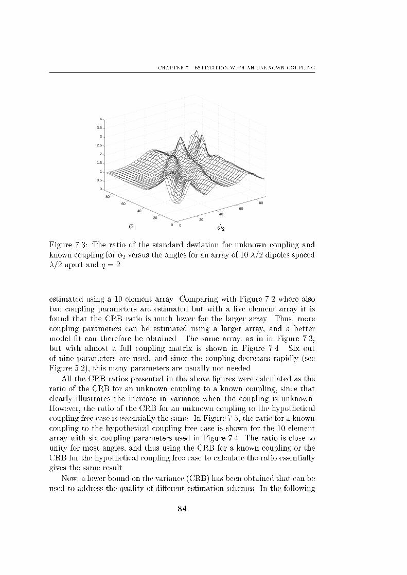
CHAPTER 7. ESTIMATION WITH AN UNKNOWN COUPLING
0
20
40
60
80
0
20
40
60
80
0
0.5
1
1.5
2
2.5
3
3.5
4
�1 �2
Figure 7.3: The ratio of the standard deviation for unknown coupling and
known coupling for �2 versus the angles for an array of 10 �=2 dipoles spaced
�=2 apart and q = 2.
estimated using a 10 element array. Comparing with Figure 7.2 where also
two coupling parameters are estimated but with a �ve element array it is
found that the CRB ratio is much lower for the larger array. Thus, more
coupling parameters can be estimated using a larger array, and a better
model �t can therefore be obtained. The same array, as in in Figure 7.3,
but with almost a full coupling matrix is shown in Figure 7.4. Six out
of nine parameters are used, and since the coupling decreases rapidly (see
Figure 5.2), this many parameters are usually not needed.
All the CRB ratios presented in the above �gures were calculated as the
ratio of the CRB for an unknown coupling to a known coupling, since that
clearly illustrates the increase in variance when the coupling is unknown.
However, the ratio of the CRB for an unknown coupling to the hypothetical
coupling free case is essentially the same. In Figure 7.5, the ratio for a known
coupling to the hypothetical coupling free case is shown for the 10 element
array with six coupling parameters used in Figure 7.4. The ratio is close to
unity for most angles, and thus using the CRB for a known coupling or the
CRB for the hypothetical coupling free case to calculate the ratio essentially
gives the same result.
Now, a lower bound on the variance (CRB) has been obtained that can be
used to address the quality of di�erent estimation schemes. In the following
84
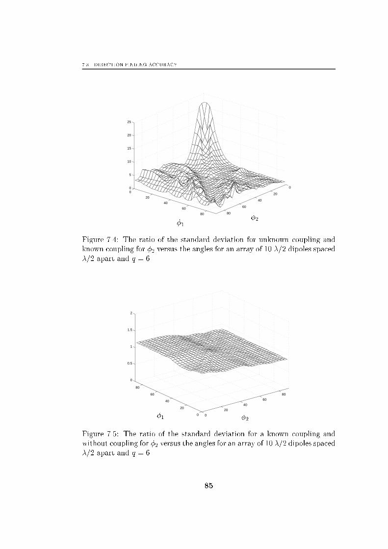
7.3. DIRECTION FINDING ACCURACY
0
20
40
60
80
0
20
40
60
80
0
5
10
15
20
25
�1�2
Figure 7.4: The ratio of the standard deviation for unknown coupling and
known coupling for �2 versus the angles for an array of 10 �=2 dipoles spaced
�=2 apart and q = 6.
0
20
40
60
80
0
20
40
60
80
0
0.5
1
1.5
2
�1 �2
Figure 7.5: The ratio of the standard deviation for a known coupling and
without coupling for �2 versus the angles for an array of 10 �=2 dipoles spaced
�=2 apart and q = 6.
85
CHAPTER 7. ESTIMATION WITH AN UNKNOWN COUPLING
sections a few methods of estimating both an unknown coupling and DOAs
are discussed. Then, some simulations are performed where these methods
are compared to each other and to the CRB that was derived in this section.
7.4 Iterative MUSIC
The SML method requires a multidimensional search, which is computation-
ally demanding already when only DOAs are estimated. The search becomes
even more demanding when q coupling parameters are added. Also, the ini-
tialization of the search becomes more important the more parameters that
are estimated, and the possibilities of ending up in a local minimum increases.
Therefore, it is of great interest to eliminate the full parameter search, or at
least reduce the number of parameters that are needed to search over. In
[18], an iterative version of the MUSIC algorithm that accounts for an un-
known coupling as well as gain and phase uncertainties is presented. The
only search performed is the DOA search, i.e. search for peaks in the MU-
SIC spectrum just as in the coupling free case. The price that has to be paid
for this reduction in computational complexity is that the estimation scheme
must be performed several times, i.e. iterated. Actually, [18] is to the au-
thor's knowledge the only e�ort of explicitly estimating the mutual coupling,
and therefore that estimation scheme will be described in some detail here.
Using the notation in the previous sections the criterion that is minimized
becomes [18]
Jc = kEHnC(c)�A(�)k2F =
pXk=1
kEHnC(c)�a(�k)k2F ; (7.27)
where F denotes the Frobenius norm, En the noise eigenvectors (see (5.9)),
and � contains the gain and phase. Here, only the mutual coupling will be
studied and thus � = I will be assumed in the following. Furthermore, in
[18] the coupling model is the same as the reduced coupling model derived
in previous sections. In [18], however, no detailed physical motivation was
presented. A similar model for a circular array was also conjectured in [18].
Now, when estimating the DOAs and the unknown mutual coupling the
estimation scheme becomes an iterative two step procedure.
Step 1: Estimating the DOAs
Search for the p highest peaks in the MUSIC spectrum
PMU(�) = kEHnC(c)a(�)k�2: (7.28)
86

7.4. ITERATIVE MUSIC
The DOAs estimates are then taken as the angles where these peaks appear.
Note that this is the same step as in the MUSIC algorithm for a known
coupling. In the �rst iteration, the identity matrix is used as coupling matrix.
Step 2: Estimating the Mutual Coupling
Insert the estimated DOAs from previous step in the criterion function Jc.
The following lemma [18] will then prove useful.
Lemma 1 For any M�1 complex vector x and any M�M banded complex
symmetric Toeplitz matrix B
Bx = Q(x) � b (7.29)
where the L� 1 vector b is given by
bi = B1i; i = 1; 2; � � � ; L (7.30)
and L is the highest subdiagonal that is di�erent from zero. The M � L
matrix Q(x) is given by the sum of the following matrices
[W1]kl =
(xk+l�1; k + l �M + 1
0; otherwise(7.31)
[W2]kl =
(xk�l�1; k � l � 2
0; otherwise(7.32)
Using Lemma 1 the criterion function can be written as
Jc = �cH
(pX
k=1
QH(k)EnEH
nQ(k)
)�c; (7.33)
where
Q(k) = Q(a(�k)) (7.34)
�c = [1 cT ]T (7.35)
ck = C1k; k = 1; 2; � � � ; L (7.36)
and the vector c contains the unknown coupling parameters. Now, (7.33)
represents a quadratic minimization problem under a linear constraint, since
the coupling matrix C is assumed to be unity on the main diagonal. Solving
the constrained minimization problem using Lagrangian multipliers
�c = G�111(1T1G
�111)�1; (7.37)
87

CHAPTER 7. ESTIMATION WITH AN UNKNOWN COUPLING
where
G =
pXk=1
QH(k)EnEH
nQ(k): (7.38)
Note that the vector 11 has a one in the �rst position and the rest is zero.
The iterative MUSIC algorithm thus estimates the DOAs in Step 1 and
estimates the coupling in Step 2, and the �nal estimates are obtained by
iterating between these two steps. At each iteration the value of the criterion
function decreases, and thus convergence is guaranteed [18] which is very
important. Another important property of an iterative algorithm is how
many iterations that usually are needed. The convergence rate of the iterative
MUSIC method and the iterative methods introduced in the next section will
be examined in some simulation examples in Section 7.7
7.5 Other Iterative Methods
The idea to iteratively estimate the DOAs and the coupling parameters is
very intuitive, and can of course be applied to other DOA estimation algo-
rithms. Many methods for estimating the DOAs when a known coupling is
present can be formulated iteratively when an unknown coupling is present.
The main reason for formulating an iterative procedure is to reduce the com-
putational cost by avoiding an extensive numerical search, and thus also
avoiding initialization and convergence problems. A closed form solution for
the coupling parameter should therefore exist in order to avoid a numerical
search for the coupling parameters. First, a straightforward extension of the
Root-Music to the case of unknown coupling will be discussed. The Root-
Music method can the formulated as two steps:
Step 1: Estimating the DOAs
When the array is a ULA, the search in the MUSIC method for the DOAs can
be avoided by viewing the MUSIC function as a polynomial in z = ejkd cos�,
exactly like the known coupling case, see Section 5.3.3. The DOA estimates
are then obtained by picking the p roots of the polynomial (5.17)
f(z) = aT (z�1)CHEnEH
nCa(z): (7.39)
closest to the unit circle, zi, and calculate the angle and solve for �i in
\zi = \e�jkd cos�i.
Step 2: Estimating the Mutual Coupling
Return to the MUSIC criterion and insert the DOA estimates into the crite-
rion
Jc = kEHnC(c)A(�)k2F ; (7.40)
88
7.5. OTHER ITERATIVE METHODS
where the estimates of the coupling parameters c are taken as the values of
c that minimize the criterion function. The same formulas result as in the
iterative MUSIC method in the previous section
�c = G�111(1T1G
�111)�1; (7.41)
where
G =
pXk=1
QH(k)EnEH
nQ(k): (7.42)
However, at the true parameters the noise eigenvectors are orthogonal to
the steering matrix or En ? Ae, and the criterion in (7.40) becomes zero.
Since the criterion also can be written as a quadratic form of G, this means
that G becomes singular. Close to the minimum, G therefore becomes ill
conditioned and the expression for coupling estimates that includes G�1
needs to be modi�ed. By applying the formula of a partitioned inverse, [38],
the coupling estimates can be written as
c = �G�122G
H12; (7.43)
where G is partitioned as
G =
�G11 G12
GH12 G22
�: (7.44)
Note that G11 is a scalar and that the matrix G is Hermitian, i.e. G =
GH . This expression for the coupling estimates is better conditioned and
can be used close to the minimum, i.e. close to the true parameters. This
modi�cation of the coupling estimate is of course suitable to make also in
the iterative MUSIC method described in the previous section.
The iterative Root-Music algorithm estimates the DOAs in Step 1 and
estimates the coupling in Step 2, and the �nal estimates are obtained by
iterating between these two steps just as in the iterative MUSIC method.
The drawback of this method is that convergence is not guaranteed, since
the roots of the polynomial (5.17) are not exactly the minima of the criterion
function in (7.40). The minima for the criterion function lie by de�nition on
the unit circle, but the roots of polynomial lie close to the unit circle, but not
exactly on the unit circle. Usually this di�erence is small and the method
works well, but due to this fact convergence can not be guaranteed.
Another method that would be interesting to obtain an iterative form of
is the ESPRIT method. However, it appears di�cult to obtain an iterative
method with guaranteed convergence without resorting to a numerical search.
89

CHAPTER 7. ESTIMATION WITH AN UNKNOWN COUPLING
Nevertheless, it is straightforward to extend the ESPRIT algorithm to a two
step iterative version for the case of an unknown coupling.
Step 1: Estimating the DOAs
The DOAs are obtained as those �:s that best �t the relation
JC�1Es = As(�)T: (7.45)
The total least squares solution to this �tting problem can be put in a general
subspace �tting context as [83]
min�;T
kJC�1Es �AsTk2F ; (7.46)
where As is the steering matrix with the shift structure de�ned in (5.18).
Solving this minimization problem gives an estimate of the DOAs.
Step 2: Estimating the Mutual Coupling
It seems di�cult to obtain an estimate of the coupling parameters from the
above criterion without resorting to a numerical search. In that case it is
probably better to use a multi-dimensional estimation scheme as SML from
the start. However, a closed form solution for the coupling parameters is
possible to obtain by changing of the criterion that is to be minimized to
minckJEs � JC(c)ATk2F ; (7.47)
where the values of A and T are calculated using the DOA estimates from
Step 1. That, of course, eliminates any possibilities of guaranteed conver-
gence, but gives a computationally cheap solution with reasonably good
properties if the criterias are su�ciently similar.
The iterative ESPRIT algorithm thus estimates the DOAs in Step 1 and
estimates the coupling in Step 2, and the �nal estimates are obtained by
iterating between these two steps.
In the iterative versions of Root-Music and ESPRIT, a large numerical
search was avoided by jumping between two di�erent criteria, that had an-
alytical solutions, at the expense of giving up any convergence guarantees.
The main motivation for this was that the computational demands of these
methods were kept small. Similar iterative formulations of multi-dimensional
search methods like WSF and MODE seem to be of little interest, since a
search for the DOAs still has to be performed. A better solution is probably
to include the coupling parameters in the search instead, even though this
increases the computational complexity. However, for one multi-dimensional
method it is possible to concentrate the criterion function regarding the cou-
pling parameters in the same manner as the SML method was concentrated
with respect to the noise and signal covariances. That method will be dis-
cussed in the next section.
90
7.6. NOISE SUBSPACE FITTING
7.6 Noise Subspace Fitting
Most DOA estimation algorithms are possible to adopt to an unknown cou-
pling, but solving for the unknown parameters usually requires a multi-
dimensional search. One method, the Noise Subspace Fitting method (see
Section 5.3.3), is however possible to concentrate in the same manner as the
SML method. Therefore, only a search for the DOAs are needed just as in the
coupling free case and the introduction of the unknown coupling parameters
only marginally increases the computational complexity. The NSF criterion
function can be formulated as
� =n�; c
o= argmin
�VNSF (�) = argmin
�kEHnC(c)A(�)k2U ; (7.48)
where U is a p� p positive de�nite weighting matrix. That function can be
concentrated regarding the coupling parameters, see Appendix 7C
VNSF (�) = G11 �G12G�122G
H12; (7.49)
where G is partitioned as in (7.44) and calculated as
G =MHhEnE
H
n A�U�ATiM; (7.50)
where M is a n2 � n selection matrix
M =
26664M1
M2
...
Mn
37775 where Mk =
8><>:I k = 1"
~I I2:k;:
I1:n�k+1;:
#i > 1
(7.51)
and Ik:m;: denotes the kth to mth rows of the unity matrix and ~I is the reverse
permutation operator de�ned as
~I =
26666640 1
. ..
1
. ..
1 0
3777775 : (7.52)
Alternatively, the matrix G can be written as
G =
pXk=1
QH(AUHk;:)EnE
H
nQ(A:;k); (7.53)
91
CHAPTER 7. ESTIMATION WITH AN UNKNOWN COUPLING
where the functionQ(x) is de�ned in Lemma 1. The criterion is concentrated
with respect to the q coupling parameters, and only a p dimensional search
for the DOAs are needed just as in the coupling free case. The DOA parame-
ters enter the expression non-linearly and a damped Newton method is used,
similar to the SML method in Section 7.2. In the SML method large simpli-
�cations were possible by using an asymptotic Hessian in the search process
leading to the scoring method. Here, the true Hessian is used in a damped
Newton method. The gradient and Hessian, needed in the implementation
of the search method, are derived in Appendix 7C.
The weighting U in (7.48) can be chosen as to minimize the variance of
the DOA estimates. The derivation in the coupling free case is valid also
in this case since Ae(�) = C(c)A(�) can be seen as an e�ective steering
matrix with parameters c and �. Choose the weighting as [45]
Uopt = Aye(�0)Ese�2
�s�1E
H
s AyHe (�0); (7.54)
where �0 are the true parameters, e� is de�ned in (5.11), and �s is de�ned in
(5.9). Also, note that the replacement of �0 by a consistent estimate � does
not a�ect the asymptotic properties if p0 = p [45], and with this weighting the
variances of the estimates are minimized and achieves the CRB. Furthermore,
it can be shown that the estimates (not only in the distribution) of the NSF
method are asymptotically equivalent with those of the SML method [46].
Thus, when an unknown mutual coupling is estimated, the SML method
that requires a search also for the coupling parameters is asymptotically
equivalent to the NSF method that only requires a search for the DOAs.
The NSF method is therefore a good candidate for DOA estimation if the
signal covariance is of full rank (p0 = p).
Now, several methods of estimating both DOAs and coupling have been
discussed and in the next section the properties of these algorithms will be
examined in some simulation scenarios.
7.7 Computer Experiments
Usually it is hard to analytically compare the performance of di�erent es-
timation schemes, and here the di�erent algorithms discussed in previous
sections will be evaluated by calculating the estimates in a few di�erent sce-
narios numerically. First, the convergence rate of the iterative formulations
of the algorithms will be studied, and then variance of the di�erent estimates
are compared to the CRB. Throughout this section the di�erent methods of
estimation are compared using data generated by the reduced model and
92
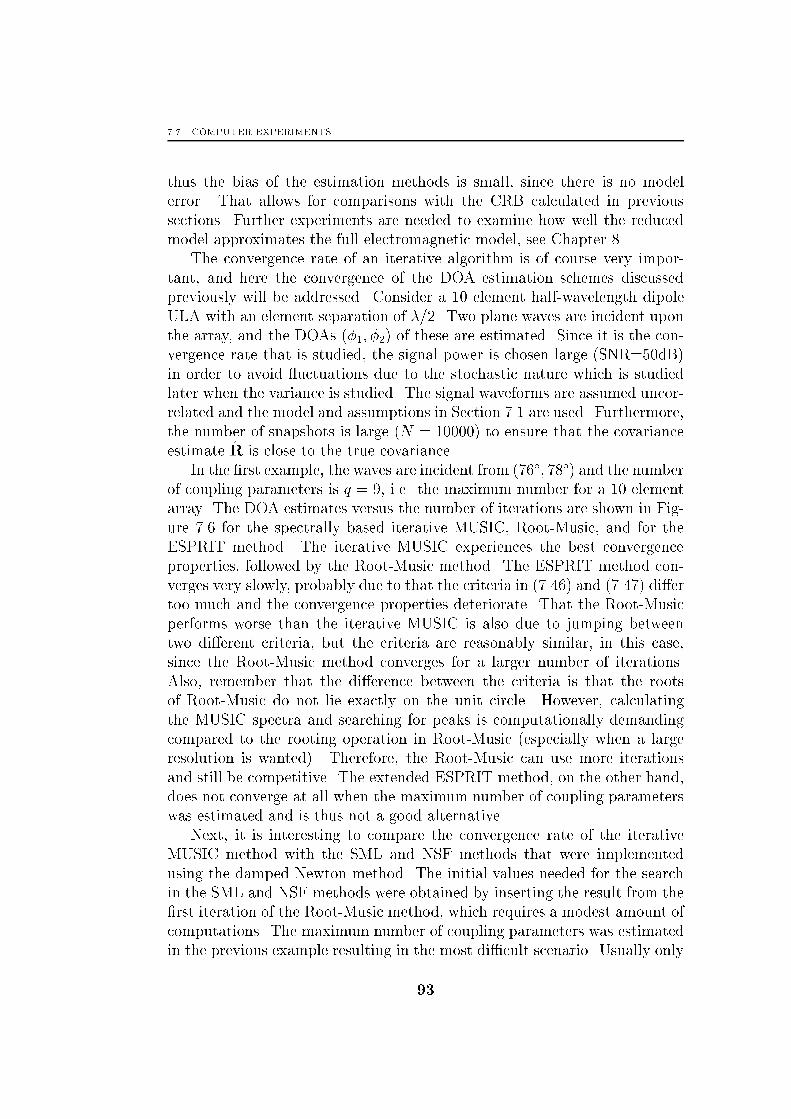
7.7. COMPUTER EXPERIMENTS
thus the bias of the estimation methods is small, since there is no model
error. That allows for comparisons with the CRB calculated in previous
sections. Further experiments are needed to examine how well the reduced
model approximates the full electromagnetic model, see Chapter 8.
The convergence rate of an iterative algorithm is of course very impor-
tant, and here the convergence of the DOA estimation schemes discussed
previously will be addressed. Consider a 10 element half-wavelength dipole
ULA with an element separation of �=2. Two plane waves are incident upon
the array, and the DOAs (�1; �2) of these are estimated. Since it is the con-
vergence rate that is studied, the signal power is chosen large (SNR=50dB)
in order to avoid uctuations due to the stochastic nature which is studied
later when the variance is studied. The signal waveforms are assumed uncor-
related and the model and assumptions in Section 7.1 are used. Furthermore,
the number of snapshots is large (N = 10000) to ensure that the covariance
estimate R is close to the true covariance.
In the �rst example, the waves are incident from (76�; 78�) and the number
of coupling parameters is q = 9, i.e. the maximum number for a 10 element
array. The DOA estimates versus the number of iterations are shown in Fig-
ure 7.6 for the spectrally based iterative MUSIC, Root-Music, and for the
ESPRIT method. The iterative MUSIC experiences the best convergence
properties, followed by the Root-Music method. The ESPRIT method con-
verges very slowly, probably due to that the criteria in (7.46) and (7.47) di�er
too much and the convergence properties deteriorate. That the Root-Music
performs worse than the iterative MUSIC is also due to jumping between
two di�erent criteria, but the criteria are reasonably similar, in this case,
since the Root-Music method converges for a larger number of iterations.
Also, remember that the di�erence between the criteria is that the roots
of Root-Music do not lie exactly on the unit circle. However, calculating
the MUSIC spectra and searching for peaks is computationally demanding
compared to the rooting operation in Root-Music (especially when a large
resolution is wanted). Therefore, the Root-Music can use more iterations
and still be competitive. The extended ESPRIT method, on the other hand,
does not converge at all when the maximum number of coupling parameters
was estimated and is thus not a good alternative.
Next, it is interesting to compare the convergence rate of the iterative
MUSIC method with the SML and NSF methods that were implemented
using the damped Newton method. The initial values needed for the search
in the SML and NSF methods were obtained by inserting the result from the
�rst iteration of the Root-Music method, which requires a modest amount of
computations. The maximum number of coupling parameters was estimated
in the previous example resulting in the most di�cult scenario. Usually only
93
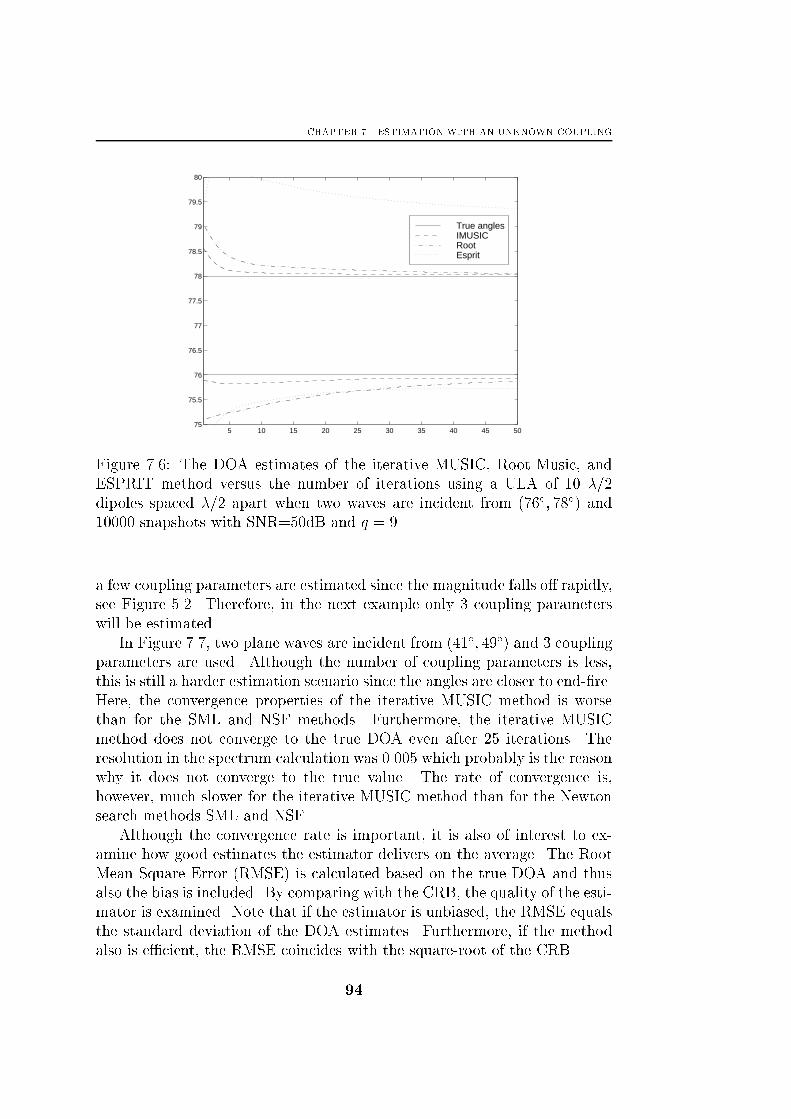
CHAPTER 7. ESTIMATION WITH AN UNKNOWN COUPLING
5 10 15 20 25 30 35 40 45 5075
75.5
76
76.5
77
77.5
78
78.5
79
79.5
80
True anglesIMUSICRootEsprit
Figure 7.6: The DOA estimates of the iterative MUSIC, Root-Music, and
ESPRIT method versus the number of iterations using a ULA of 10 �=2
dipoles spaced �=2 apart when two waves are incident from (76�; 78�) and
10000 snapshots with SNR=50dB and q = 9.
a few coupling parameters are estimated since the magnitude falls o� rapidly,
see Figure 5.2. Therefore, in the next example only 3 coupling parameters
will be estimated.
In Figure 7.7, two plane waves are incident from (41�; 49�) and 3 coupling
parameters are used. Although the number of coupling parameters is less,
this is still a harder estimation scenario since the angles are closer to end-�re.
Here, the convergence properties of the iterative MUSIC method is worse
than for the SML and NSF methods. Furthermore, the iterative MUSIC
method does not converge to the true DOA even after 25 iterations. The
resolution in the spectrum calculation was 0.005 which probably is the reason
why it does not converge to the true value. The rate of convergence is,
however, much slower for the iterative MUSIC method than for the Newton
search methods SML and NSF.
Although the convergence rate is important, it is also of interest to ex-
amine how good estimates the estimator delivers on the average. The Root
Mean Square Error (RMSE) is calculated based on the true DOA and thus
also the bias is included. By comparing with the CRB, the quality of the esti-
mator is examined. Note that if the estimator is unbiased, the RMSE equals
the standard deviation of the DOA estimates. Furthermore, if the method
also is e�cient, the RMSE coincides with the square-root of the CRB.
94
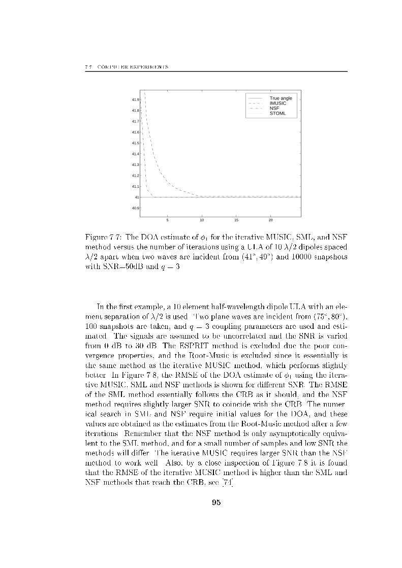
7.7. COMPUTER EXPERIMENTS
5 10 15 20
40.9
41
41.1
41.2
41.3
41.4
41.5
41.6
41.7
41.8
41.9 True angleIMUSICNSFSTOML
Figure 7.7: The DOA estimate of �1 for the iterative MUSIC, SML, and NSF
method versus the number of iterations using a ULA of 10 �=2 dipoles spaced
�=2 apart when two waves are incident from (41�; 49�) and 10000 snapshots
with SNR=50dB and q = 3.
In the �rst example, a 10 element half-wavelength dipole ULA with an ele-
ment separation of �=2 is used. Two plane waves are incident from (75�; 80�),
100 snapshots are taken, and q = 3 coupling parameters are used and esti-
mated. The signals are assumed to be uncorrelated and the SNR is varied
from 0 dB to 30 dB. The ESPRIT method is excluded due the poor con-
vergence properties, and the Root-Music is excluded since it essentially is
the same method as the iterative MUSIC method, which performs slightly
better. In Figure 7.8, the RMSE of the DOA estimate of �1 using the itera-
tive MUSIC, SML and NSF methods is shown for di�erent SNR. The RMSE
of the SML method essentially follows the CRB as it should, and the NSF
method requires slightly larger SNR to coincide with the CRB. The numer-
ical search in SML and NSF require initial values for the DOA, and these
values are obtained as the estimates from the Root-Music method after a few
iterations. Remember that the NSF method is only asymptotically equiva-
lent to the SML method, and for a small number of samples and low SNR the
methods will di�er. The iterative MUSIC requires larger SNR than the NSF
method to work well. Also, by a close inspection of Figure 7.8 it is found
that the RMSE of the iterative MUSIC method is higher than the SML and
NSF methods that reach the CRB, see [74].
95

CHAPTER 7. ESTIMATION WITH AN UNKNOWN COUPLING
0 5 10 15 20 25 300
0.2
0.4
0.6
0.8
1
1.2
1.4
1.6
1.8
SNR (dB)
RM
SE
(de
gree
s)SMLCRBNSFIMUSIC
Figure 7.8: The RMSE of the DOA estimate of �1 for the iterative MUSIC,
SML, and NSF method versus SNR using a ULA of 10 �=2 dipoles spaced
�=2 apart using 200 Monte-Carlo simulations. Two waves are incident from
(75�; 80�) and 100 snapshots are used with q = 3.
Next, a more di�cult scenario is considered where the DOAs are further
away from broad-side (41�; 49�) and two more coupling parameters (q = 5)
are estimated. In Figure 7.9 the RMSE for the iterative MUSIC, SML, and
NSF are shown together with the CRB. The SML and NSF methods follow
relatively closely the CRB, but the iterative MUSIC method has a larger
RMSE for high SNR. Note that the spectral resolution was 0:01� which should
be su�cient to give a lower RMSE than that obtained in Figure 7.9. The
high RMSE is due to slow convergence, and when the maximum number of
iterations is reduced to 10, the RMSE further increases [74]. But for the SML
and NSF methods the reduction in iterations does not a�ect the RMSE.
The strength of the iterative MUSIC method is that convergence is guar-
anteed, unlike the Newton search employed in the SML and NSF methods
that can end up in a local minimum. However, in the examples studied here
the Newton search �nds the true minimum. The initial values taken from the
�rst estimates from the Root-Music are close enough to the true minimum
for the search to converge at the global minimum. One important property
of an iterative method is the number of iterations needed to converge to the
minimum, and here the Newton methods require sometimes substantially
less computations than the iterative-MUSIC method. Also, the calculation
96

7.7. COMPUTER EXPERIMENTS
0 5 10 15 20 25 300
0.05
0.1
0.15
0.2
0.25
0.3
0.35
0.4
0.45
SNR (dB)
RM
SE
(de
gree
s)
SMLCRBNSFIMUSIC
Figure 7.9: The RMSE of the DOA estimate of �1 for the iterative MUSIC,
SML, and NSF method versus SNR using a ULA of 10 �=2 dipoles spaced
�=2 apart using 200 Monte-Carlo simulations. Two waves are incident from
(41�; 49�) and 1000 snapshots with q = 5 and an iteration limit of 20.
of the MUSIC spectrum and searching for peaks is computationally demand-
ing when many iterations are needed. The implementation is of course very
important, but the iterative MUSIC method is not less demanding than the
NSF and SML methods, and for the coupling free case the main motivation
for using MUSIC is that it is computationally cheap.
An important drawback of the iterative MUSIC method is that its thresh-
old for resolving closely spaced signal sources is substantially higher than for
the Root-Music, SML, and NSF methods. This is especially important when
estimating DOAs in the presence of an unknown coupling, since the e�ect of
the coupling is to mix di�erent steering vectors and thus blurring the MUSIC
spectrum. In Figure 7.10, the MUSIC spectrum for a known compensated
coupling and an uncompensated coupling when two waves are incident from
(30�; 33�) is shown. Two clearly discernible peaks appear when the coupling
is compensated for, but for the unknown coupling only one broad peak ap-
pears. This a�ects the iterative MUSIC method, since it estimates the angles
as a �rst step and then estimates the coupling. Obtaining two DOA estimates
appears di�cult, and the method is not really applicable in this case.
However, resolving closely spaced sources can be of great importance and
a lot of work have been done in this �eld. Here, the RMSE for closely spaced
97
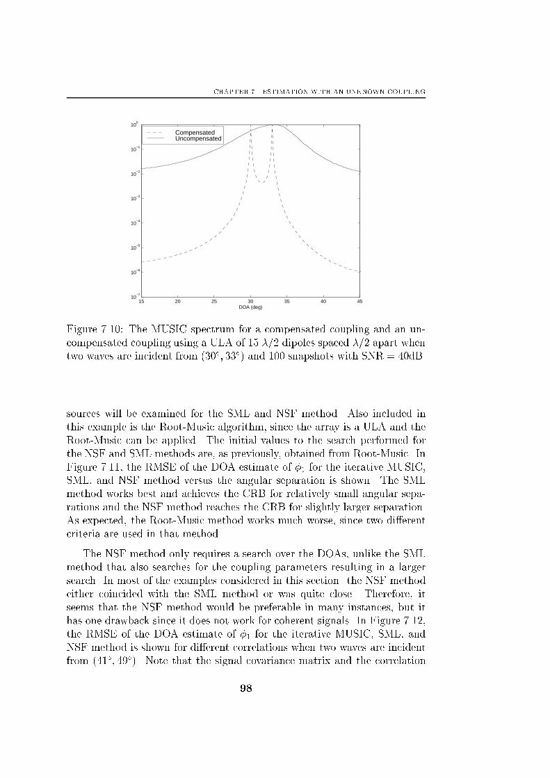
CHAPTER 7. ESTIMATION WITH AN UNKNOWN COUPLING
15 20 25 30 35 40 4510
−7
10−6
10−5
10−4
10−3
10−2
10−1
100
DOA (deg)
CompensatedUncompensated
Figure 7.10: The MUSIC spectrum for a compensated coupling and an un-
compensated coupling using a ULA of 15 �=2 dipoles spaced �=2 apart when
two waves are incident from (30�; 33�) and 100 snapshots with SNR = 40dB.
sources will be examined for the SML and NSF method. Also included in
this example is the Root-Music algorithm, since the array is a ULA and the
Root-Music can be applied. The initial values to the search performed for
the NSF and SML methods are, as previously, obtained from Root-Music. In
Figure 7.11, the RMSE of the DOA estimate of �1 for the iterative MUSIC,
SML, and NSF method versus the angular separation is shown. The SML
method works best and achieves the CRB for relatively small angular sepa-
rations and the NSF method reaches the CRB for slightly larger separation.
As expected, the Root-Music method works much worse, since two di�erent
criteria are used in that method.
The NSF method only requires a search over the DOAs, unlike the SML
method that also searches for the coupling parameters resulting in a larger
search. In most of the examples considered in this section. the NSF method
either coincided with the SML method or was quite close. Therefore, it
seems that the NSF method would be preferable in many instances, but it
has one drawback since it does not work for coherent signals. In Figure 7.12,
the RMSE of the DOA estimate of �1 for the iterative MUSIC, SML, and
NSF method is shown for di�erent correlations when two waves are incident
from (41�; 49�). Note that the signal covariance matrix and the correlation
98
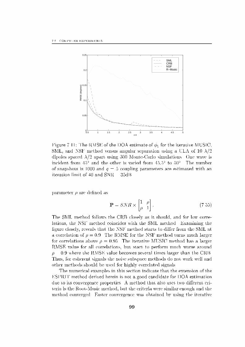
7.7. COMPUTER EXPERIMENTS
0.5 1 1.5 2 2.5 3 3.5 4 4.5 50
0.05
0.1
0.15
0.2
0.25
∆ θ
RM
SE
(de
gree
s)
SMLCRBNSFR−Music
Figure 7.11: The RMSE of the DOA estimate of �1 for the iterative MUSIC,
SML, and NSF method versus angular separation using a ULA of 10 �=2
dipoles spaced �=2 apart using 300 Monte-Carlo simulations. One wave is
incident from 45� and the other is varied from 45:5� to 50�. The number
of snapshots is 1000 and q = 5 coupling parameters are estimated with an
iteration limit of 40 and SNR = 35dB.
parameter � are de�ned as
P = SNR ��1 �
� 1
�: (7.55)
The SML method follows the CRB closely as it should, and for low corre-
lations, the NSF method coincides with the SML method. Examining the
�gure closely, reveals that the NSF method starts to di�er from the SML at
a correlation of � = 0:9. The RMSE for the NSF method turns much larger
for correlations above � = 0:95. The iterative MUSIC method has a larger
RMSE value for all correlations, but start to perform much worse around
� = 0:9 where the RMSE value becomes several times larger than the CRB.
Thus, for coherent signals the noise subspace methods do not work well and
other methods should be used for highly correlated signals.
The numerical examples in this section indicate that the extension of the
ESPRIT method derived herein is not a good candidate for DOA estimation
due to its convergence properties. A method that also uses two di�erent cri-
teria is the Root-Music method, but the criteria were similar enough and the
method converged. Faster convergence was obtained by using the iterative
99

CHAPTER 7. ESTIMATION WITH AN UNKNOWN COUPLING
MUSIC method that experienced rapid convergence in the easier scenarios.
However, for the more di�cult scenarios also the iterative MUSIC method
experienced slow convergence.
0 0.1 0.2 0.3 0.4 0.5 0.6 0.7 0.8 0.9 10
0.02
0.04
0.06
0.08
0.1
0.12
0.14
0.16
0.18
0.2
Correlation ρ
RM
SE
(de
gree
s)
SMLCRBNSFIMUSIC
Figure 7.12: The RMSE of the DOA estimate of �1 for the iterative MUSIC,
SML, and NSF method versus correlation using a ULA of 10 �=2 dipoles
spaced �=2 apart using 200 Monte-Carlo simulations. Two waves are incident
from (41�; 49�) and 500 snapshots with q = 5 and an iteration limit of 20 and
SNR = 20dB.
The fastest convergence was obtained for the SML and NSF methods that
usually only needed a few iterations. When comparing the average error of
the estimates similar results were obtained. The Root-Music method was
slightly worse than the iterative MUSIC method that worked well in the
easier scenarios, but for the more di�cult scenarios the convergence rate
became a problem. Also, the iterative MUSIC method experienced a higher
RMSE than the SML and NSF method that were asymptotically e�cient,
i.e. reached the CRB.
One major drawback for the iterative MUSIC method is that it has a
higher resolution threshold than SML and NSF. This was found to be espe-
cially important when the coupling is unknown and needs to be estimated.
If not compensated for, the coupling will blur the MUSIC spectrum and fur-
ther reduce the resolution threshold. Thus, the iterative MUSIC method is
not suited for resolving closely spaced sources where SML and NSF probably
should be used.
100
7.8. SIGNAL DETECTION
Finally, it was found that both the MUSIC method and the NSF method
do not work for highly correlated signals just as in the coupling free case.
Apart from the correlated case, the NSF method closely followed the SML
method. Therefore, the NSF method seems preferable since it only requires a
p dimensional search unlike the SML method that requires a p+q dimensional
search.
7.8 Signal Detection
All parametric methods in this section require that the number of incident
signals is known. If the number of incident waves is unknown it can be
estimated and that is usually called detection. However, when the coupling
also is unknown and estimated another problem appears. The number of
coupling parameters to use is also unknown, and two types of detection
results, signal detection and coupling detection.
The number of incident waves or signals is usually important since that
could correspond to the number of aircrafts or submarines. If the signal co-
variance matrix is of full rank, the signal detection part essentially reduces
to testing the rank of the steering matrix or the multiplicity of the smallest
eigenvalue. In that case, methods like AIC and MDL can be used and no
correction for the coupling is necessary. However, when the signal covari-
ance matrix is rank de�cient, i.e. there are coherent signals, other detection
schemes are needed.
When the coupling is known, methods that simultaneously estimate the
DOAs and the number of signals are used, see Section 5.4. If the coupling
is not known and the number of coupling parameters also is unknown, those
methods needs to be modi�ed. That will not be done here, and through out
this report the number of coupling parameters is assumed known. Also, in a
more realistic scenario the number of coupling parameters is simply chosen as
the minimum number parameters that reasonably well describe the coupling.
7.9 Conclusions
As a �rst approach of investigating the e�ects of mutual coupling, a simpli�ed
scenario of a completely unknown and deterministic mutual coupling was
considered. Of course, in a more realistic scenario also a random coupling
error and gain and phase uncertainties should be studied. Here, estimating
an unknown coupling in this simpli�ed scenario was investigated. First, the
SML estimator was derived and using those expressions, the CRB for the
101
CHAPTER 7. ESTIMATION WITH AN UNKNOWN COUPLING
unknown coupling case was also derived. If a feasible number of coupling
parameters was used, it was found that the increase in the CRB was not
large.
Furthermore, a number of methods for estimating the DOAs in the pres-
ence of an unknown coupling was discussed. First, the only method found
in the literature, the iterative spectral MUSIC, was reviewed and then sev-
eral extensions of coupling free methods were introduced. The Root-Music
method was extended to include the presence of an unknown coupling. Also,
the NSF method was extended to include an unknown coupling, and it was
shown that the criterion could be concentrated with respect to the coupling
and thus only a search for the DOAs was needed.
These methods were also analyzed in a few numerical examples where it
was found that the convergence rate of the iterative MUSIC and the Root-
Music was slower than for the NSF and SML methods. The main argument
of using MUSIC in the coupling free case is that it is computationally cheap.
But with coupling those methods require many iterations and therefore do
not require less computational power than multidimensional search methods
like SML and NSF. One problem with multidimensional search methods is
to �nd initial values for the search. Here it was found that the Root-Music
method gave initial values accurate enough. Therefore, the SML and NSF
methods were found to be good candidates for �nding the DOA. The NSF
method was found to have similar performance as the e�cient SML method
in most cases and therefore the NSF was usually to prefer since it only
requires a search over the DOAs. But for highly correlated signals the NSF
method does not work well (together with the MUSIC methods) and the
SML method should be used instead.
7A The Maximum Likelihood Method
The Likelihood Function
The measured voltages x(t) are, using the stochastic assumptions and the
data model in Section 7.1, Gaussian distributed. However, since the voltages
in general are complex, they belong to a multivariate complex Gaussian
distribution. Especially, since both the signal and the noise are circularly
Gaussian, the likelihood function can be written in a compact form [29] as
p(X;�) =1
�NnjRjN exp�"
NXk=1
xH(tk)R�1x(tk)
#; (7A.1)
102
7.9. CONCLUSIONS
where
R = CAPAHCH + �2I (7A.2)
is the covariance matrix of the voltages. Note that both the signal and the
noise are assumed to be zero mean processes. Taking the logarithm of the
likelihood function results in
log p(X;�) = �N n log(�) + log jRj+ 1
N
NXk=1
xH(tk)R�1x(tk)
!(7A.3)
Using that Tr(ABC) = Tr(BCA), the logarithm of the likelihood function
can be written as
log p(X;�) = �N�n log(�) + log jRj+ Tr(R�1R)
�; (7A.4)
where
R =1
N
NXk=1
x(tk)xH(tk): (7A.5)
Now it is possible to maximize this expression with respect to the signal and
noise covariances, see [68], and (7.6) results.
The Gradient and Hessian
In general, the coupling parameters are complex and instead of de�ning a
complex di�erentiation, here the complex parameters are divided into a com-
plex and real part. This results in a parameter vector � = f�; cr; cig and
the SML criterion function becomes
VSML(�) = log dethCAPAHCH + �2I
i; (7A.6)
and inserting the expression for P in (7.7) gives
VSML(�) = log dethCA(CA)y
hR� �I
i(CA)yHAHCH + �2I
i= log det
hPCARPCA + �2P?
CA
i:
(7A.7)
The gradient and the Hessian are de�ned as
V0 =@VSML
@�(7A.8)
Hij =@2VSML
@�i@�j
: (7A.9)
103
CHAPTER 7. ESTIMATION WITH AN UNKNOWN COUPLING
Using the di�erentiation result [29]
@ log detA(x)
@x= Tr
�A�1(x)
@AH(x)
@x
�; (7A.10)
and the simpler notation Ae = CA, the gradient can be written as
V0k = Tr
��PAe
RPAe+ �2P?
Ae
��1 @
@�k
�PAe
RPAe+ �2P?
Ae
��: (7A.11)
Also,
@PAe
@�k
=
�PAe
@PAe
@�k
�+
�PAe
@PAe
@�k
�H(7A.12)
and TrB(C+CH) = 2ReTr[BC] gives
V0k = 2ReTr
��PAe
RPAe+ �2P?
Ae
��1PAe
R@PAe
@�k
+ �2P?Ae
@P?Ae
@�k
�+ Tr
��PAe
RPAe+ �2P?
Ae
��1 @�2@�k
P?Ae
�:
(7A.13)
From (7.8) it follows that
@�2
@�k
= � 1
n� dTr
�@PAe
@�k
R
�: (7A.14)
Now, invoke the matrix inversion lemma�PAe
RPAe+ �2P?
Ae
��1=�CAPAHCH + �2I
��1=
1
�2
�I�Ae
�PAH
e Ae + �2I��1
PAHe
� (7A.15)
and insert in (7A.13)
V0k = 2ReTr
�1
�2
�I�Ae
�PAH
e Ae + �2I�PAH
e
��PAe
R@PAe
@�k
+ �2P?Ae
@P?Ae
@�k
��� Tr
�1
�2
�I�Ae
�PAH
e Ae + �2I�PAH
e
� P?Ae
n� pTr
�@PAe
@�k
R
��:
(7A.16)
104
7.9. CONCLUSIONS
However,
TrP?Ae
n� pTr
�@PAe
@�k
R
�= 2ReTr
�PAe
R@PAe
@�k
�(7A.17)
and AHe P
?Ae
= 0 gives
V0k = 2ReTr
�P?Ae
@P?Ae
@�k
� 1
�2Ae
�PAH
e Ae + �2I��1
PAHe PAe
R@PAe
@�k
�:
(7A.18)
Next, note that
Tr
�P?Ae
@P?Ae
@�k
�= 0 (7A.19)
and
@PAe
@�k
Ae = P?Ae
@Ae
@�k
(Ae)yAe + (Ae)
yH @AHCH
@�k
P?AeAe = P?
Ae
@Ae
@�k
:
(7A.20)
Furthermore,
P(Ae)HAe + �2 =(Ae)
yhR� �2I
i(Ae)
yHAHe Ae + �2
=(AHe Ae)
�1AHe RAe
(7A.21)
which reduces the gradient expression to
V0k =� 2ReTr
�1
�2(AH
e RAe)�1AH
e Ae
�PAH
e PAeRP?
Ae
@(Ae)
@�k
��= 2ReTr
��(AH
e RAe)�1 � 1
�2(AH
e Ae)�1
�AHe RP
?Ae
@(Ae)
@�k
�:
(7A.22)
Next, introduce the matrix
G = (AHe RAe)
�1 � 1
�2(AH
e Ae)�1: (7A.23)
Inserting Ae = CA, the gradient can be written
V0(�) =
266642ReTr
hGAHCHRP?
CA@(CA)
@�1
i...
2ReTrhGAHCHRP?
CA@(CA)
@�p+2q
i37775 : (7A.24)
105
CHAPTER 7. ESTIMATION WITH AN UNKNOWN COUPLING
Here, it is important to note that the expression for the di�erentiation with
respect to the DOA can be simpli�ed by noting that
@(CA)
@�k= C
@A
@�k; (7A.25)
where the derivative has only one non-zero column, ak, and thus can the
expressions for the p derivatives with respect to the DOAs be reduced to
@V
@�k= 2Re
hGk;:A
HCHRP?CACak
i; (7A.26)
where Gk;: denotes the kth row of the matrix G. For the derivatives with
respect to the coupling there are in general no non-zero columns and therefore
the expressions become
@V
@crk= 2ReTr
hGAHCHRP?
CA�kA
i(7A.27)
@V
@cik= �2ImTr
hGAHCHRP?
CA�kA
i; (7A.28)
where �k is a banded symmetric Toeplitz matrix with zeros everywhere
except on the kth and the �kth subdiagonal which consists of ones.
The Hessian, using the chain-rule, becomes
@2V
@�i@�j
= 2ReTr
�@
@�j
�@(CA)
@�i
G
�AHCHRP?
CA
�+ 2ReTr
�@(CA)
@�i
G@
@�j
�AHCHRP?
CA
��:
(7A.29)
Evaluating this expression exactly leads to rather cumbersome expressions,
but by considering the asymptotic Hessian, i.e. a large number of samples
N ! 1, the expression can be reduced considerably. Since the estimates
of � and P are known to be asymptotically statistically consistent and ef-
�cient [10] and both are functions of R which also is consistent and thus
the asymptotic Hessian is found by simply replacing R with R. Also, the
steering matrix A(�) is evaluated at the true DOAs �0. Using the reduced
notation Ae = CA once again and observing that
AHe RP
?Ae
= AHe
�AePA
He + �2I
� �I�Ae(A
He Ae)
�1AHe
�= 0; (7A.30)
the asymptotic Hessian expression becomes
@2Va
@�i@�j
= 2ReTr
�@Ae
@�i
G
�@Ae
@�j
RP?Ae
+AHe R
@P?Ae
@�j
��: (7A.31)
106
7.9. CONCLUSIONS
However,
AHe R
@P?Ae
@�j
= �AHe RAe(A
He Ae)
�1@AHe
@�j
P?Ae
(7A.32)
and
RP?Ae
= �2P?Ae: (7A.33)
Thus,
@2Va
@�i@�j
= 2ReTr
�G��2I�AH
e RAe(AHe Ae)
�1� @AH
e
@�j
P?Ae
@Ae
@�i
�(7A.34)
and by applying the matrix inversion lemma�AHe RAe
��1=(AH
e Ae)�1�AHe AeP+ �2I
��1=
1
�2(AH
e Ae)�1hI�PAeAe
�PAH
e Ae + �2I��1i (7A.35)
the asymptotic Hessian reduces to
@2Va
@�i@�j
=2
�2ReTr
�PAH
e R�1AeP
@AHe
@�j
P?Ae
@Ae
@�i
�: (7A.36)
Furthermore, the asymptotic Hessian can be written as a block matrix
H = V00a(�) =
@2Va
@�2 =
�H�� H�c
Hc� Hcc
�: (7A.37)
Since the derivative with respect to the DOA results in a matrix with only
one non-zero column, H�� can be written as
H�� =2
�2Ren�PAHCHR�1CAP
�T � �DHCHP?CACD
�o; (7A.38)
where
D =
�@a(�)
@�
???�=�1
; � � � ; @a(�)@�
???�=�p
�: (7A.39)
Also,
H�c =
�@2Va
@�@cr
@2Va
@�@ci
�= HT
�c; (7A.40)
107
CHAPTER 7. ESTIMATION WITH AN UNKNOWN COUPLING
where�@2Va
@�@cr
�ij
= 2�2ReTr
hPAHCHR�1CAPAH�jP
?CAC
@A@�i
i(7A.41)�
@2Va
@�@ci
�ij
= � 2�2ImTr
hPAHCHR�1CAPAH�jP
?CAC
@A@�i
i:(7A.42)
Finally,
Hcc =
�Hcrcr Hcrci
HTcrci
Hcici
�; (7A.43)
where
[Hcrcr ]ij =2�2ReTr
�PAHCHR�1CAPAH�jP
?CA�iA
�(7A.44)
[Hcrci]ij = � 2�2ImTr
�PAHCHR�1CAPAH�jP
?CA�iA
�(7A.45)
[Hcici]ij = � 2�2ReTr
�PAHCHR�1CAPAH�jP
?CA�iA
�: (7A.46)
7B The Asymptotic Covariance of SML
The SML estimates � are obtained as
� = f�; cg = argmin�
VSML(�); (7B.1)
where VSML(�) is de�ned in (7A.6). Introducing the simpli�ed notation
VSML(�) = V (�), the gradient of V with respect to � which is derived in
Appendix 7A becomes
V0(�) =@V(�)
@�
???�=
^�= 0: (7B.2)
A Taylor series expansion of (7B.2) around the true parameter vector �0
gives
0 = V0(�0) +V00(�0)(���0) + � � � ; (7B.3)
where V00(�0) denotes the Hessian matrix. The higher order terms can be
neglected since � converges to �0 as N !1 under very general conditions
[30]. Furthermore, the Hessian can be replaced by the asymptotic Hessian
V00a(�0) = lim
N!1V00(�0); (7B.4)
108
7.9. CONCLUSIONS
since all terms that tend to zero faster than (� ��0) can be neglected in
the asymptotic analysis. The asymptotic Hessian were derived in Appendix
7A. Thus,
���0 = � [V00a(�0)]
�1V0(�0) (7B.5)
assuming that the inverse exists which is true if the problem is well posed,
see Section 7.3. The covariance matrix for the asymptotic SML estimates
then becomes
BSML = [V00a(�0)]
�1B [V00
a(�0)]�1; (7B.6)
where
B = limN!1
E [V0(�0)] [V0(�0)]
T(7B.7)
Since the asymptotic Hessian already is derived in previous appendix, it is
left to evaluate B. The gradient has elements
V0(�i) = 2ReTr
�GAHCHRP?
CA
@(CA)
@�i
�; (7B.8)
where G is de�ned in (7A.23). Since AHCHRP?CA tends to zero as N !1,
G can be replaced with G, and R and � are replaced by R and � without
a�ecting the asymptotic covariance matrixB [67]. Using the simpler notation
Ae = CA, the elements become
Bij = 4 limN!1
E
�Re Tr
�GAH
e RP?Ae
@(Ae)
@�i
�� Re Tr
�GAH
e RP?Ae
@(Ae)
@�j
��= 2 lim
N!1E
�Re
�Tr
�GAH
e RP?Ae
@(Ae)
@�i
�� Tr
�GAH
e RP?Ae
@(Ae)
@�j
���+ 2 lim
N!1E
�Re
�Tr
�GAH
e RP?Ae
@(Ae)
@�i
�� Tr
�@(AH
e )
@�j
P?AeRAeG
���:
(7B.9)
Now, using TrA � TrB = TrAB [38] the �rst term in (7B.9) becomes
Re
�E
�Tr
��GAH
e RP?Ae
@(Ae)
@�i
��GAH
e RP?Ae
@(Ae)
@�j
����= Re
�E
�Tr
�1
N
NXm=1
�GAH
e x(tm)xH(tm)P
?Ae
@(Ae)
@�i
�
1
N
NXn=1
�GAH
e x(tn)xH(tn)P
?Ae
@(Ae)
@�j
����; (7B.10)
109
CHAPTER 7. ESTIMATION WITH AN UNKNOWN COUPLING
where the expression for R (7A.5) has been inserted. Furthermore, since
xH(tn)P?Ae
= nH(tn)P?Ae
(7B.11)
the �rst term can be written as
1
N2E
� pXl=1
pXk=1
NXm=1
NXn=1
Gk;:AHe x(tm)| {z }A
nH(tm)P?Ae
@(Aek)
@�i| {z }B
�Gl;:AHe x(tn)| {z }C
nH(tn)P?Ae
@(Ael)
@�j| {z }D
�: (7B.12)
Here, Gk;: denotes the kth row of G and@(Ae
l)
@�j
denotes the lth column.
The expectation of the product of four Gaussian random variables can be
expressed as [26]
E[ABCD] =E[AB] � E[CD]
+
b2Xk=1
E[(1TkC)A] � E[D (B1k)] (7B.13)
+ E[A(E[BC])D]� 2E[A]E[B]E[C]E[D];
where 1k denotes the vector having a "1" at the kth position and zero else-
where. Also, A;B;C;D are jointly Gaussian random variables of dimen-
sions (a1 � a2); (b1 � b2); (c1 � c2); (d1 � d2). In the present case, A;B;C;D
are scalars. Since the noise and the signal are assumed uncorrelated and
AHe P
?Ae
= 0
E[AB] = E[BC] = 0: (7B.14)
Next, note that E[n�(tm)nH(tn)] = 0 8 m;n giving
E[DB1k] = E[DB] = E[BTD] = 0: (7B.15)
Finally, since both the signal and the noise are assumed to be zero mean
E[B] = 0 and all the terms in (7B.12) become zero, and so also the �rst term
in (7B.9).
Proceeding with the second term in (7B.9), it can also be rewritten along
110
7.9. CONCLUSIONS
the same lines as
1
N2E
� pXl=1
pXk=1
NXm=1
NXn=1
Gk;:AHe x(tm)| {z }A
nH(tm)P?Ae
@(Aek)
@�i| {z }B
� @(AHel)
@�j
P?Aen(tn)| {z }
C
xH(tn)AeGHl;:| {z }
D
�: (7B.16)
The product formula in (7B.13) will be used also for the second term in
(7B.9), but �rst the di�erent expectations need to be evaluated. Since the
matrices A and B are the same as in previous case E[AB]=0. Next, note
that
E[DB] = E
�xH(tn)AeG
Hl;:n
H(tm)P?Ae
@(Aek)
@�i
�=@(AT
ek)
@�i
P?Ae
TE[n�(tm)n
H(tn)]AeGHl;: = 0 (7B.17)
and also that
E]BC] = E
"nH(tn)P
?Ae
@(Aek)
@�i
@(AHel)
@�j
P?Aen(tm)
#
=@(AH
el)
@�j
P?AeE[n(tm)n
H(tn)]P?Ae
@(Aek)
@�i
= �2@(AH
el)
@�j
P?Ae
@(Aek)
@�i
�mn;
(7B.18)
where �mn denotes the Kronecker delta. Furthermore,
E[A (E[BC])D] = E[BC]E[AD] = E[BC]Gk;:AHe E[x(tn)x
H(tm)]AeGHl;:
= �2@(AH
el)
@�j
P?Ae
@(Aek)
@�i
Gk;:AHe RAeG
Hl;:�mn (7B.19)
and since E[B] = 0 the second term in (7B.9) becomes
Re
"1
N2
pXl=1
pXk=1
NXm=1
NXn=1
�2@(AH
el)
@�j
P?Ae
@(Aek)
@�i
Gk;:AHe RAeG
Hl;:�mn
#(7B.20)
=�2
N2Re
"NXk=1
NXl=1
@(AHel)
@�j
P?Ae
@(Aek)
@�i
Gk;:AHe RAeG
Hl;:
#(7B.21)
=�2
NReTr
"@(AH
el)
@�j
P?Ae
@(Aek)
@�i
GAHe RAeG
H
#: (7B.22)
111
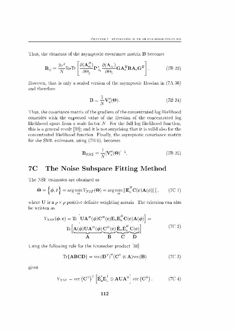
CHAPTER 7. ESTIMATION WITH AN UNKNOWN COUPLING
Thus, the elements of the asymptotic covariance matrix B becomes
Bij =2�2
NReTr
"@(AH
el)
@�j
P?Ae
@(Aek)
@�i
GAHe RAeG
H
#: (7B.23)
However, that is only a scaled version of the asymptotic Hessian in (7A.36)
and therefore
B =1
NV00a(�): (7B.24)
Thus, the covariance matrix of the gradient of the concentrated log likelihood
coincides with the expected value of the Hessian of the concentrated log
likelihood apart from a scale factor N . For the full log likelihood function,
this is a general result [39]; and it is not surprising that it is valid also for the
concentrated likelihood function. Finally, the asymptotic covariance matrix
for the SML estimates, using (7B.6), becomes
BSML =1
N[V00
a(�)]�1: (7B.25)
7C The Noise Subspace Fitting Method
The NSF estimates are obtained as
� =n�; c
o= argmin
�VNSF (�) = argmin
�kEHnC(c)A(�)k2U ; (7C.1)
where U is a p� p positive de�nite weighting matrix. The criterion can also
be written as
VNSF (�; c) = TrhUAH(�)CH(c)EnE
H
nC(c)A(�)i=
TrhA(�)UAH(�)| {z }
A
CH(c)| {z }B
EnEH
n| {z }C
C(c)| {z }D
i(7C.2)
Using the following rule for the Kronecker product [38]
TrfABCDg = vec(DT)T(CT A)vec(B) (7C.3)
gives
VNSF = vec�CT�T h
E�
nET
n AUAHivec�CH�: (7C.4)
112
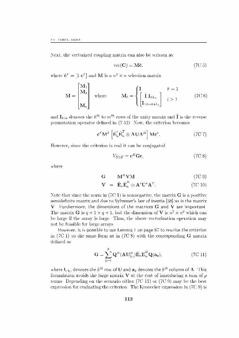
7.9. CONCLUSIONS
Next, the vectorized coupling matrix can also be written as
vec(C) =M�c; (7C.5)
where �cT = [1 cT ] and M is a n2 � n selection matrix
M =
26664M1
M2
...
Mn
37775 where Mk =
8><>:I k = 1"
~I I2:k;:
I1:n�k+1;:
#i > 1
(7C.6)
and Ik:m denotes the kth to mth rows of the unity matrix and ~I is the reverse
permutation operator de�ned in (7.52). Now, the criterion becomes
�cTMThE�
nET
n AUAHiM�c�: (7C.7)
However, since the criterion is real it can be conjugated
VNSF = �cHG�c; (7C.8)
where
G = MHVM (7C.9)
V = EnEH
n A�U�AT : (7C.10)
Note that since the norm in (7C.1) is nonnegative, the matrixG is a positive
semide�nite matrix and due to Sylvester's law of inertia [38] so is the matrix
V. Furthermore, the dimensions of the matrices G and V are important.
The matrix G is q + 1� q + 1, but the dimension of V is n2 � n2 which can
be large if the array is large. Thus, the above vectorization operation may
not be feasible for large arrays.
However, it is possible to use Lemma 1 on page 87 to rewrite the criterion
in (7C.1) to the same form as in (7C.8) with the corresponding G matrix
de�ned as
G =
pXk=1
QH(AUHk;:)EnE
H
nQ(ak); (7C.11)
whereUk;: denotes the kth row ofU and ak denotes the k
th column ofA. This
formulation avoids the large matrix V at the cost of introducing a sum of p
terms. Depending on the scenario either (7C.11) or (7C.9) may be the best
expression for evaluating the criterion. The Kronecker expression in (7C.9) is
113

CHAPTER 7. ESTIMATION WITH AN UNKNOWN COUPLING
valid also for other linear parameterizations of the coupling matrix that not
result in a banded complex symmetric Toeplitz matrix. However, Lemma 1
can also be generalized to other parameterizations, and which formulation to
choose depends on the explicit parameterization and the size of the array.
Now, in order to concentrate the criterion regarding the coupling param-
eters c use the partitioned form of the matrix G
G =
�G11 G12
GH12 G22
�(7C.12)
which follows since G is Hermitian and
VNSF =G11 +G12c+ cHGH12 + cHG22c =
G11 +�G�1
22GH12 + c
�HG22
�G�1
22GH12 + c
��G12G�122G
H12:
(7C.13)
The coupling parameters that minimize the criterion become
c = �G�122G
H12: (7C.14)
Inserting (7C.14) into (7C.13) gives the concentrated criterion function
VNSF (�) = G11 �G12G�122G
H12: (7C.15)
The criterion is concentrated with respect to the q coupling parameters and
only a p dimensional search for the DOAs are needed, just as in the coupling
free case. The DOA parameters enter the expression non-linearly, and a
damped Newton method is used, similar to the SML method in Section 7.2.
But in the SML method, large simpli�cations were possible by using an
asymptotic Hessian in the search process leading to the scoring method. In
the NSF method, the FIM could be used instead of the true Hessian if the
weighting matrix U is chosen as to minimize the variance of the estimates.
That is possible since the NSF method achieves the CRB. Here, however, the
true Hessian is used in a damped Newton method.
To implement the search, it is necessary to �nd expressions for the gra-
dient and Hessian of the NSF criterion and that is done next.
The kth element of the gradient becomes
V0k =
@VNSF
@�k=@G11
@�k� 2Re
�@G12
@�kG�1
22GH12
�+G12G
�122
@G22
@�kG�1
22GH12:
(7C.16)
114

7.9. CONCLUSIONS
The expression for the Hessian becomes
Hkm =@2VNSF
@�k@�m=
@2G11
@�k@�m+ 2Re
�@G12
@�kG�1
22
@G22
@�mG�1
22GH12 +
@G12
@�mG�1
22
@G22
@�kG�1
22GH12 �G12G
�122
@G22
@�kG�1
22
@G22
@�mG�1
22GH12 �
@2G12
@�k@�mG�1
22GH12 �
@G12
@�kG�1
22
@GH12
@�k
�+G12G
�122
@2G22
@�k@�mG�1
22GH12:
(7C.17)
The derivatives of G depends on which of the formulations (7C.9) or (7C.11)
is used. First, the expressions for the Kronecker formulation in (7C.9) will
be given and then the expressions for the summation form in (7C.11). Since
neither the selection matrix nor the noise eigenvalues depend on the DOAs,
the derivative becomes
@G
@�k=MH
��EnE
H
n
��@A�U�AT
@�k
��M; (7C.18)
where
@A�U�AT
@�k=
�@a�k@�k
U�k;:A
T
�+
�@a�k@�k
U�k;:A
T
�H: (7C.19)
Furthermore,
@2G
@�k@�m=MH
��EnE
H
n
��@2A�U�AT
@�k@�m
��M; (7C.20)
where
@2A�U�AT
@�k@�m=
�U�km
@a�k@�k
@aTm@�m
�+
�U�km
@a�k@�k
@aTm@�m
�H(7C.21)
if k 6= m and�@2a�k@�2k
U�k;:A
T +U�kk
@a�k@�k
@aTk@�k
�+
�@2a�k@�2k
U�k;:A
T +U�kk
@a�k@�k
@aTk@�k
�H(7C.22)
for k = m. For the summation form of G in (7C.11), the derivative becomes
@G
@�k=
pXl=1
U�lkQ
H(@ak
@�k)EnE
H
nQ(al) +QH(AUHk;:)EnE
H
nQ(@ak
@�k): (7C.23)
115

CHAPTER 7. ESTIMATION WITH AN UNKNOWN COUPLING
The second derivatives become
@2G
@�k@�m= U�
mkQH(
@ak
@�k)EnE
H
nQ(@am
@�m) +U�
kmQH(
@am
@�m)EnE
H
nQ(@ak
@�k)
(7C.24)
if k 6= m and
pXl=1
U�lkQ
H(@2ak
@�2k)EnE
H
nQ(al) + 2U�kkQ
H(@ak
@�k)EnE
H
nQ(@ak
@�k) +
QH(AUHk;:)EnE
H
nQ(@2ak
@�2k)
(7C.25)
if k = m. Finally, inserting the expressions for the derivatives of G into
(7C.16) and (7C.17) gives the gradient and the Hessian.
116

Chapter 8E�ects of Model Errors
In the preceding chapter, the e�ects of an unknown coupling were miti-
gated by estimating the coupling along with the DOAs. To reduce the
number of estimated coupling parameters, the reduced coupling model
derived in Chapter 6, was used. For this coupling model, the CRB was cal-
culated and several estimation methods were derived. The quality of these
estimation methods was then addressed by comparing the empirical variance
of the estimates in a few Monte-Carlo simulations with the CRB. However,
the data used in those comparisons were generated using the reduced cou-
pling model, in order for the comparison to the CRB to be valid. Usually
when examining di�erent estimation schemes the correct data model is used
(as in Chapter 7), since when designing estimation schemes the focus is on
�nding the best way of utilizing the model at hand. But for the methods
to work well in practice, it is of course important to examine how well the
model actually describes the measured data. This will be examined in this
chapter, but instead of measured data, the expressions for the induced volt-
ages, derived in Chapter 3 using fundamental electromagnetics, will be used.
The DOAs and the coupling parameters will then be estimated using the
reduced coupling model introduced in Chapter 6 and the estimation schemes
from Chapter 7.
How the estimation of both the coupling and the DOAs work is examined
in a few scenarios. Several methods are used to estimate the parameters and
the result is presented using the MUSIC spectra to gain some insight of
the problems. Then, the average RMSE error is calculated for a few cases
using the di�erent estimation methods. Finally, since the e�ect of coupling
essentially changes the response of the array and in some way blurs the
response, it is interesting to examine the e�ects on the signal estimates when
a jammer is present.
117
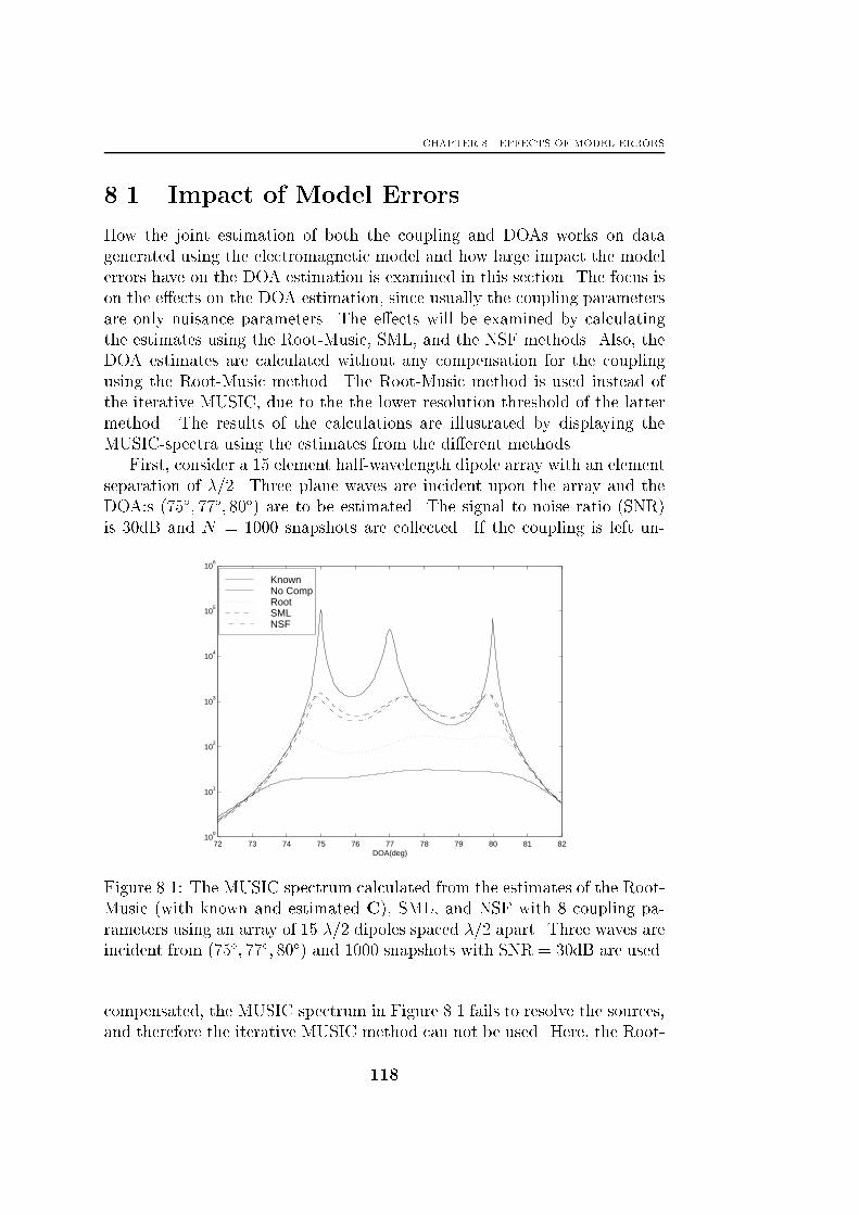
CHAPTER 8. EFFECTS OF MODEL ERRORS
8.1 Impact of Model Errors
How the joint estimation of both the coupling and DOAs works on data
generated using the electromagnetic model and how large impact the model
errors have on the DOA estimation is examined in this section. The focus is
on the e�ects on the DOA estimation, since usually the coupling parameters
are only nuisance parameters. The e�ects will be examined by calculating
the estimates using the Root-Music, SML, and the NSF methods. Also, the
DOA estimates are calculated without any compensation for the coupling
using the Root-Music method. The Root-Music method is used instead of
the iterative MUSIC, due to the the lower resolution threshold of the latter
method. The results of the calculations are illustrated by displaying the
MUSIC-spectra using the estimates from the di�erent methods.
First, consider a 15 element half-wavelength dipole array with an element
separation of �=2. Three plane waves are incident upon the array and the
DOA:s (75�; 77�; 80�) are to be estimated. The signal to noise ratio (SNR)
is 30dB and N = 1000 snapshots are collected. If the coupling is left un-
72 73 74 75 76 77 78 79 80 81 8210
0
101
102
103
104
105
106
DOA(deg)
KnownNo CompRootSMLNSF
Figure 8.1: The MUSIC spectrum calculated from the estimates of the Root-
Music (with known and estimated C), SML, and NSF with 8 coupling pa-
rameters using an array of 15 �=2 dipoles spaced �=2 apart. Three waves are
incident from (75�; 77�; 80�) and 1000 snapshots with SNR = 30dB are used.
compensated, the MUSIC spectrum in Figure 8.1 fails to resolve the sources,
and therefore the iterative MUSIC method can not be used. Here, the Root-
118
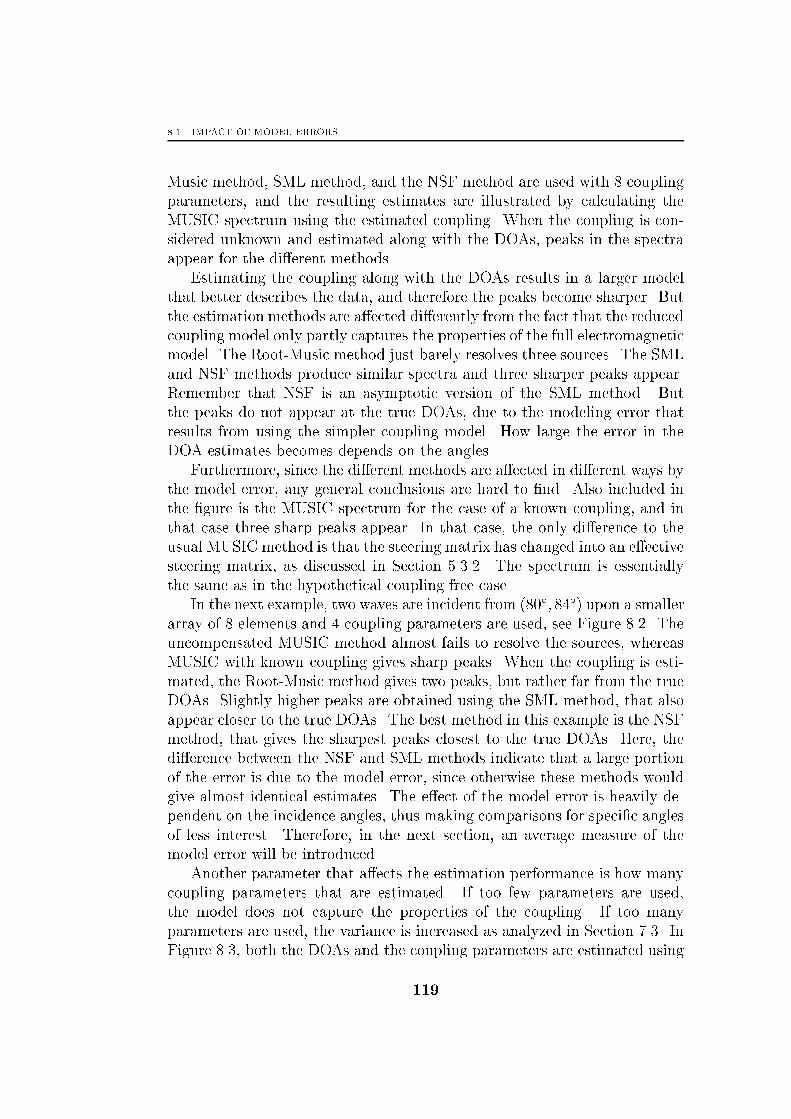
8.1. IMPACT OF MODEL ERRORS
Music method, SML method, and the NSF method are used with 8 coupling
parameters, and the resulting estimates are illustrated by calculating the
MUSIC spectrum using the estimated coupling. When the coupling is con-
sidered unknown and estimated along with the DOAs, peaks in the spectra
appear for the di�erent methods.
Estimating the coupling along with the DOAs results in a larger model
that better describes the data, and therefore the peaks become sharper. But
the estimation methods are a�ected di�erently from the fact that the reduced
coupling model only partly captures the properties of the full electromagnetic
model. The Root-Music method just barely resolves three sources. The SML
and NSF methods produce similar spectra and three sharper peaks appear.
Remember that NSF is an asymptotic version of the SML method. But
the peaks do not appear at the true DOAs, due to the modeling error that
results from using the simpler coupling model. How large the error in the
DOA estimates becomes depends on the angles.
Furthermore, since the di�erent methods are a�ected in di�erent ways by
the model error, any general conclusions are hard to �nd. Also included in
the �gure is the MUSIC spectrum for the case of a known coupling, and in
that case three sharp peaks appear. In that case, the only di�erence to the
usual MUSIC method is that the steering matrix has changed into an e�ective
steering matrix, as discussed in Section 5.3.2. The spectrum is essentially
the same as in the hypothetical coupling free case.
In the next example, two waves are incident from (80�; 84�) upon a smaller
array of 8 elements and 4 coupling parameters are used, see Figure 8.2. The
uncompensated MUSIC method almost fails to resolve the sources, whereas
MUSIC with known coupling gives sharp peaks. When the coupling is esti-
mated, the Root-Music method gives two peaks, but rather far from the true
DOAs. Slightly higher peaks are obtained using the SML method, that also
appear closer to the true DOAs. The best method in this example is the NSF
method, that gives the sharpest peaks closest to the true DOAs. Here, the
di�erence between the NSF and SML methods indicate that a large portion
of the error is due to the model error, since otherwise these methods would
give almost identical estimates. The e�ect of the model error is heavily de-
pendent on the incidence angles, thus making comparisons for speci�c angles
of less interest. Therefore, in the next section, an average measure of the
model error will be introduced.
Another parameter that a�ects the estimation performance is how many
coupling parameters that are estimated. If too few parameters are used,
the model does not capture the properties of the coupling. If too many
parameters are used, the variance is increased as analyzed in Section 7.3. In
Figure 8.3, both the DOAs and the coupling parameters are estimated using
119
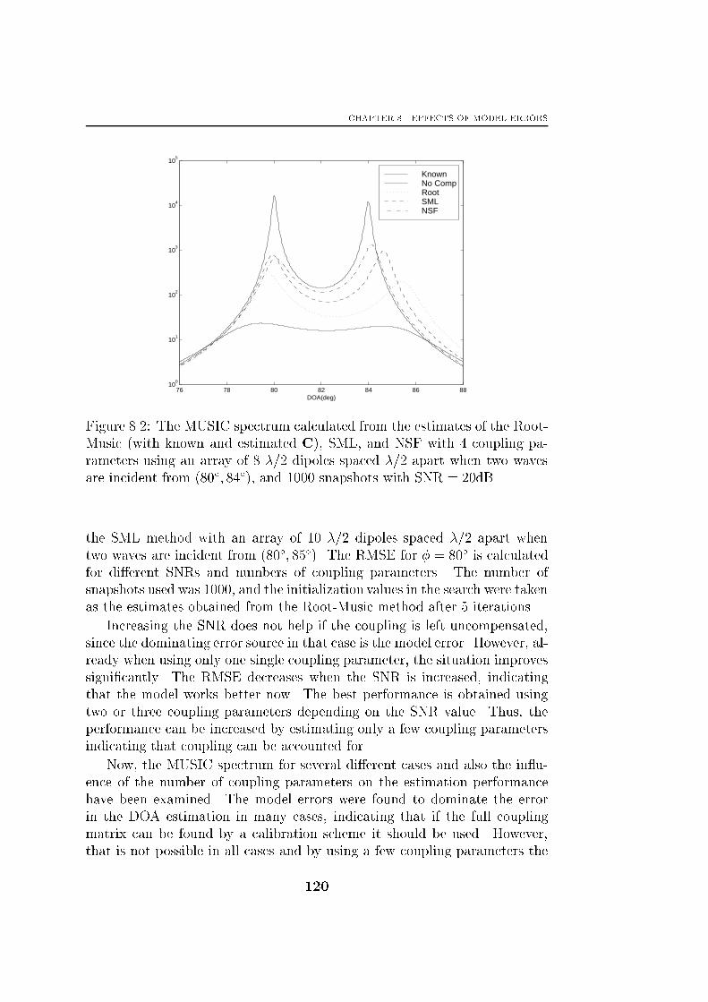
CHAPTER 8. EFFECTS OF MODEL ERRORS
76 78 80 82 84 86 8810
0
101
102
103
104
105
DOA(deg)
KnownNo CompRootSMLNSF
Figure 8.2: The MUSIC spectrum calculated from the estimates of the Root-
Music (with known and estimated C), SML, and NSF with 4 coupling pa-
rameters using an array of 8 �=2 dipoles spaced �=2 apart when two waves
are incident from (80�; 84�), and 1000 snapshots with SNR = 20dB.
the SML method with an array of 10 �=2 dipoles spaced �=2 apart when
two waves are incident from (80�; 85�). The RMSE for � = 80� is calculated
for di�erent SNRs and numbers of coupling parameters. The number of
snapshots used was 1000, and the initialization values in the search were taken
as the estimates obtained from the Root-Music method after 5 iterations.
Increasing the SNR does not help if the coupling is left uncompensated,
since the dominating error source in that case is the model error. However, al-
ready when using only one single coupling parameter, the situation improves
signi�cantly. The RMSE decreases when the SNR is increased, indicating
that the model works better now. The best performance is obtained using
two or three coupling parameters depending on the SNR value. Thus, the
performance can be increased by estimating only a few coupling parameters
indicating that coupling can be accounted for.
Now, the MUSIC spectrum for several di�erent cases and also the in u-
ence of the number of coupling parameters on the estimation performance
have been examined. The model errors were found to dominate the error
in the DOA estimation in many cases, indicating that if the full coupling
matrix can be found by a calibration scheme it should be used. However,
that is not possible in all cases and by using a few coupling parameters the
120
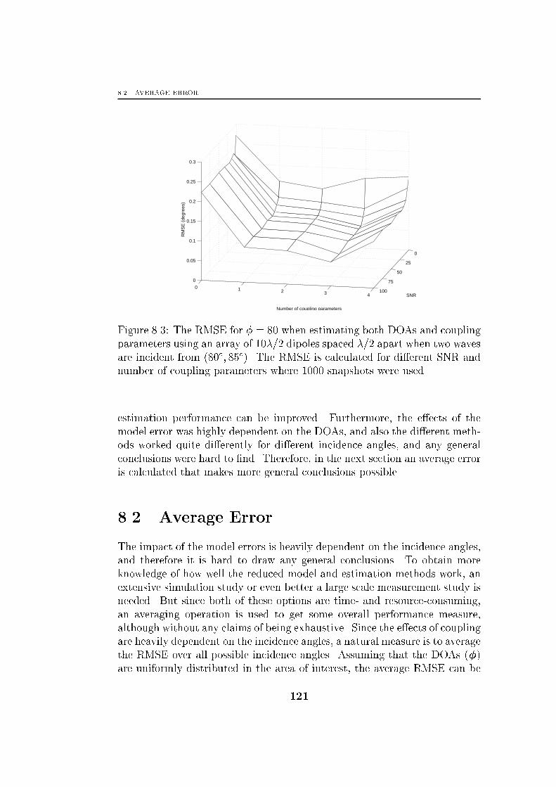
8.2. AVERAGE ERROR
0
25
50
75
1000 1 2 3 4
0
0.05
0.1
0.15
0.2
0.25
0.3
SNR
Number of coupling parameters
RM
SE
(de
gree
s)
Figure 8.3: The RMSE for � = 80 when estimating both DOAs and coupling
parameters using an array of 10�=2 dipoles spaced �=2 apart when two waves
are incident from (80�; 85�). The RMSE is calculated for di�erent SNR and
number of coupling parameters where 1000 snapshots were used.
estimation performance can be improved. Furthermore, the e�ects of the
model error was highly dependent on the DOAs, and also the di�erent meth-
ods worked quite di�erently for di�erent incidence angles, and any general
conclusions were hard to �nd. Therefore, in the next section an average error
is calculated that makes more general conclusions possible.
8.2 Average Error
The impact of the model errors is heavily dependent on the incidence angles,
and therefore it is hard to draw any general conclusions. To obtain more
knowledge of how well the reduced model and estimation methods work, an
extensive simulation study or even better a large scale measurement study is
needed. But since both of these options are time- and resource-consuming,
an averaging operation is used to get some overall performance measure,
although without any claims of being exhaustive. Since the e�ects of coupling
are heavily dependent on the incidence angles, a natural measure is to average
the RMSE over all possible incidence angles. Assuming that the DOAs (�)
are uniformly distributed in the area of interest, the average RMSE can be
121
CHAPTER 8. EFFECTS OF MODEL ERRORS
de�ned as
~R =
pXk=1
E [RMSE(�k)]: (8.1)
However, calculating the expectation is di�cult, and therefore an approxi-
mative measure can be de�ned as
�R =
pXk=1
1
Nav
NavXn=1
RMSEn(�k); (8.2)
where the RMSE value is averaged over Nav Monte-Carlo simulations using
DOAs that are uniformly distributed over the area of interest. Using this
average RMSE value, the e�ect of the modeling errors can be evaluated and
the di�erent algorithms compared. Such a comparison, of course, only tells
part of the story, but at least it is better than calculating the estimates for
speci�c scenarios.
First, a 5 element half-wavelength dipole array with element separation of
�=2 will be considered, since the coupling e�ects are larger for a small array.
Two plane waves are incident upon the array and the DOAs of these are
assumed to be uniformly distributed in the interval 20��90�. Waves incident
closer to end-�re are excluded, since the estimation performance there is
severely reduced. The signal to noise ratio (SNR) is chosen large (50dB), in
order to let the part of the RMSE due to the model errors dominate over
the variance part. Also, N = 1000 snapshots are collected and Nav = 5000
Monte-Carlo simulations are averaged to calculate the average RMSE value�R in Figure 8.4.
To avoid that a single realization dominates the RMSE value, i.e. so-
called outliers, estimates that are more than 10� o� are excluded from the
averaging operation. The uncompensated Root-Music method results in an
average RMSE value close to 4�. However, by modeling the coupling and es-
timating only one coupling parameter the average RMSE can be signi�cantly
reduced. The averaging operation gives only a very rough picture of the ef-
fects of model errors and the di�erent estimation methods behave similarly
in this case. To examine the quality of the di�erent estimation methods a
more detailed analysis is needed.
Adding more coupling parameters does not further reduce the average
RMSE error signi�cantly. The RMSE error is still quite large, thus the
reduced coupling model considered here only captures some of the coupling
properties. But that the RMSE decreases signi�cantly when only estimating
one coupling parameter, indicates that the model is reasonably good.
122

8.2. AVERAGE ERROR
1 2 3 40
0.5
1
1.5
2
2.5
3
3.5
4
4.5
5
Number of coupling parameters
Ave
rage
RM
SE
No CompRootSMLNSF
Figure 8.4: The average RMSE �R for the Root-Music (with uncompensated
and estimated C), SML, and NSF methods versus the number of coupling
parameters. An array of 5 �=2 dipoles spaced �=2 apart is used. Two waves
are incident from uniformly distributed angles in (20�; 90�). The number of
snapshots is N = 1000, SNR = 50dB, and Nav = 5000.
For larger arrays, more coupling parameters can be estimated and next, a
larger array of 15 elements is considered. The average RMSE is calculated by
averaging the results from 5000 simulations. Here, the average RMSE error
is smaller due to the larger array, and therefore estimates that deviates more
than 3� are considered to be outliers and are excluded from the averaging
operation. Another implication of a larger array is that it allows for more
parameters to be estimated with just a small increase in variance, as discussed
in Section 7.3. The RMSE value when estimating 5 coupling parameters is
decreased to less than half the value when no compensation is applied. The
di�erent estimation methods give similar results, also in this case.
The contribution to the average RMSE from model errors is quite large
and for larger SNR values, the model error part will dominate. In Figure 8.6,
the average RMSE is shown for an array of 8 elements for di�erent SNRs.
For small SNRs, the variance of the estimates dominate �R and estimating
coupling parameters further increases the RMSE. For larger SNRs, the model
error part dominate, and here the RMSE can be decreased by estimating a
few coupling parameters.
The RMSE values in these simulations are relatively large indicating that
123
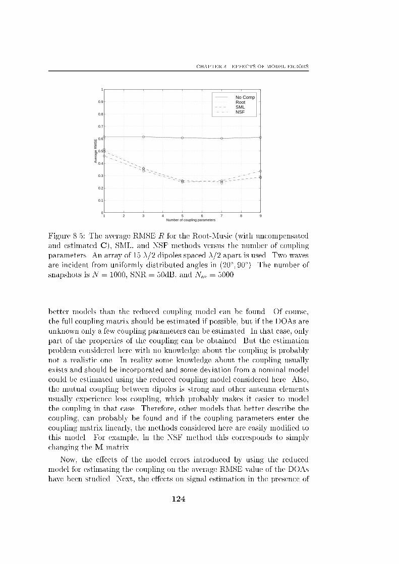
CHAPTER 8. EFFECTS OF MODEL ERRORS
1 2 3 4 5 6 7 8 90
0.1
0.2
0.3
0.4
0.5
0.6
0.7
0.8
0.9
1
Number of coupling parameters
Ave
rage
RM
SE
No CompRootSMLNSF
Figure 8.5: The average RMSE �R for the Root-Music (with uncompensated
and estimated C), SML, and NSF methods versus the number of coupling
parameters. An array of 15 �=2 dipoles spaced �=2 apart is used. Two waves
are incident from uniformly distributed angles in (20�; 90�). The number of
snapshots is N = 1000, SNR = 50dB, and Nav = 5000.
better models than the reduced coupling model can be found. Of course,
the full coupling matrix should be estimated if possible, but if the DOAs are
unknown only a few coupling parameters can be estimated. In that case, only
part of the properties of the coupling can be obtained. But the estimation
problem considered here with no knowledge about the coupling is probably
not a realistic one. In reality some knowledge about the coupling usually
exists and should be incorporated and some deviation from a nominal model
could be estimated using the reduced coupling model considered here. Also,
the mutual coupling between dipoles is strong and other antenna elements
usually experience less coupling, which probably makes it easier to model
the coupling in that case. Therefore, other models that better describe the
coupling, can probably be found and if the coupling parameters enter the
coupling matrix linearly, the methods considered here are easily modi�ed to
this model. For example, in the NSF method this corresponds to simply
changing the M matrix.
Now, the e�ects of the model errors introduced by using the reduced
model for estimating the coupling on the average RMSE value of the DOAs
have been studied. Next, the e�ects on signal estimation in the presence of
124
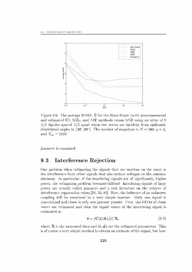
8.3. INTERFERENCE REJECTION
10−2
10−1
100
101
102
0
1
2
3
4
5
6
Ave
rage
RM
SE
SNR
No CompRootSMLNSFKnown C
Figure 8.6: The average RMSE �R for the Root-Music (with uncompensated
and estimated C), SML, and NSF methods versus SNR using an array of 8
�=2 dipoles spaced �=2 apart when two waves are incident from uniformly
distributed angles in (20�; 90�). The number of snapshots is N = 500, q = 3,
and Nav = 5000.
jammers is examined.
8.3 Interference Rejection
One problem when estimating the signals that are incident on the array is
the interference from other signals that also induce voltages on the antenna
elements. In particular, if the interfering signals are of signi�cantly higher
power, the estimation problem becomes di�cult. Interfering signals of large
power are usually called jammers and a rich literature on the subject of
interference suppression exists [16, 23, 82]. Here, the in uence of an unknown
coupling will be examined in a very simple manner. Only one signal is
transmitted and there is only one jammer present. First, the DOAs of these
waves are estimated and then the signal values of the interesting signal is
estimated as
s = (C(c)A(�))yX; (8.3)
where X is the measured data and (c; �) are the estimated parameters. This
is of course a very simple method to obtain an estimate of the signal, but here
125
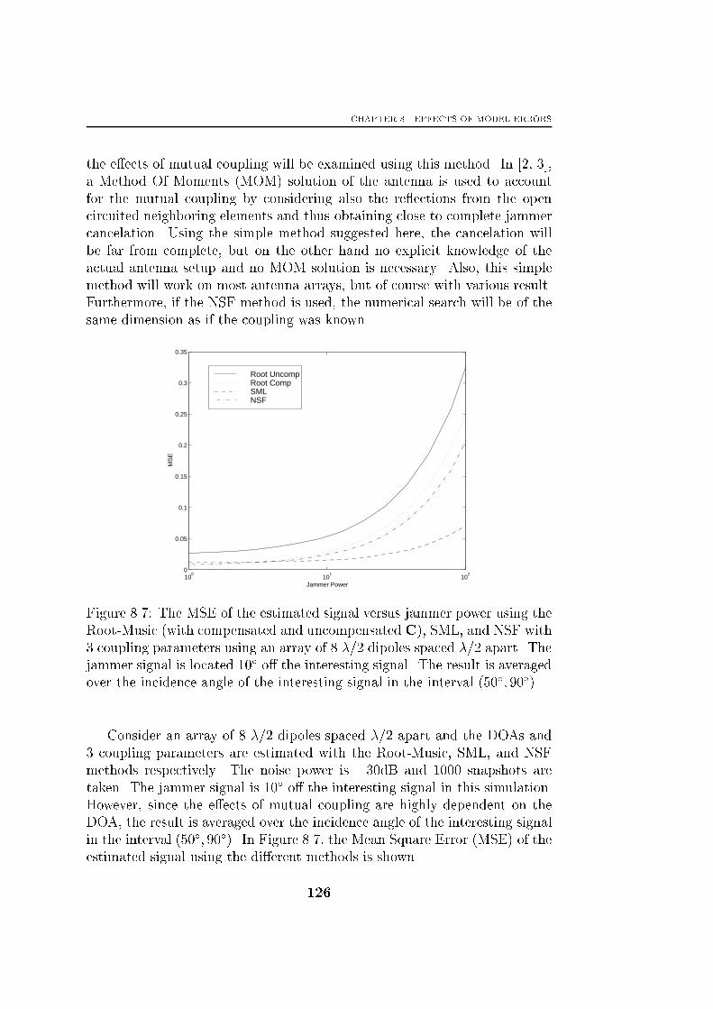
CHAPTER 8. EFFECTS OF MODEL ERRORS
the e�ects of mutual coupling will be examined using this method. In [2, 3],
a Method Of Moments (MOM) solution of the antenna is used to account
for the mutual coupling by considering also the re ections from the open
circuited neighboring elements and thus obtaining close to complete jammer
cancelation. Using the simple method suggested here, the cancelation will
be far from complete, but on the other hand no explicit knowledge of the
actual antenna setup and no MOM solution is necessary. Also, this simple
method will work on most antenna arrays, but of course with various result.
Furthermore, if the NSF method is used, the numerical search will be of the
same dimension as if the coupling was known.
100
101
102
0
0.05
0.1
0.15
0.2
0.25
0.3
0.35
Jammer Power
MS
E
Root UncompRoot CompSMLNSF
Figure 8.7: The MSE of the estimated signal versus jammer power using the
Root-Music (with compensated and uncompensated C), SML, and NSF with
3 coupling parameters using an array of 8 �=2 dipoles spaced �=2 apart. The
jammer signal is located 10� o� the interesting signal. The result is averaged
over the incidence angle of the interesting signal in the interval (50�; 90�).
Consider an array of 8 �=2 dipoles spaced �=2 apart and the DOAs and
3 coupling parameters are estimated with the Root-Music, SML, and NSF
methods respectively. The noise power is �30dB and 1000 snapshots are
taken. The jammer signal is 10� o� the interesting signal in this simulation.
However, since the e�ects of mutual coupling are highly dependent on the
DOA, the result is averaged over the incidence angle of the interesting signal
in the interval (50�; 90�). In Figure 8.7, the Mean Square Error (MSE) of the
estimated signal using the di�erent methods is shown.
126
8.4. CONCLUSIONS
If the coupling is left uncompensated, the signal estimate deviates signif-
icantly already for equal signal powers, and increases rapidly with increasing
jammer power. The Root-Music method reduces the error in signal power
for low jammer power, but for high jammer power the reduction is small.
The NSF method o�ers more error reduction or interference suppression for
higher jammer power. The best method is the SML method, that o�ers
the best interference rejection especially for high jammer power. Thus, the
interference rejection can be increased signi�cantly by estimating a few cou-
pling parameters along with the DOAs. For better performance, a more
complex model is needed. However, as discussed in previous section usually
some knowledge about the coupling exists and should be used to formulate
another coupling model.
8.4 Conclusions
If it is not possible to obtain the coupling matrix by calibration measure-
ments, an unknown uncompensated coupling will deteriorate the DOA esti-
mation performance. However, the e�ects of the unknown coupling can be
mitigated by estimating the unknown coupling and that was examined in
this chapter. Data was generated using the full electromagnetical coupling
model, and the coupling was estimated using the reduced coupling model.
That introduces model errors and the impact of these errors was examined.
First, the e�ects of an unknown coupling was investigated by estimat-
ing the DOAs, and the coupling parameters using the methods derived in
Chapter 7. It was found that the e�ects were angle dependent, but the es-
timation performance could be improved by estimating only a few coupling
parameters.
To get some general result of the improvement by estimating the coupling,
an average RMSE value was calculated and it was found that the model error
could be substantially reduced by estimating only a few coupling parameters.
But for high SNRs, the model error dominated the RMSE value. The value
was reduced compared to the uncompensated case, although much larger
than the RMSE value for the known coupling case. But, if it is not possible
to obtain the coupling matrix by some calibration scheme, the e�ects can
thus be reduced by estimating a few coupling parameters.
Finally, the e�ects of an unknown mutual coupling were examined in a
scenario where an interesting signal was received in the presence of a jammer
signal. If coupling was not compensated for, the estimated signal deviated
signi�cantly from the true signal. However, by estimating the coupling along
with the DOAs, the deviation was decreased substantially.
127

CHAPTER 8. EFFECTS OF MODEL ERRORS
128
Chapter 9Conclusions and Future Work
The main results from the di�erent chapters will be reviewed in this
chapter and some general conclusions regarding direction �nding and
mutual coupling will be presented. Finally, some interesting future
work is proposed in last section.
9.1 Conclusions
The e�ects of mutual coupling on direction �nding have not attracted much
interest in the signal processing literature. In the antenna design community
this is an important issue and is well covered in the literature. To be able to
analyze the e�ects of mutual coupling, the coupling needs to be calculated.
Here, a uniform linear array of thin and �nite dipoles is used since analytical
results are possible to �nd for dipoles.
In the antenna literature, the radiation pattern is probably the most
important characteristic of an antenna. Since the transmitting and receiv-
ing pattern can be shown to be equivalent, not much work has been done
on �nding explicit expressions for the induced voltages in receiving mode.
Therefore, expressions for the induced voltages are derived in this thesis. In
Chapter 2, the fundamental electromagnetic properties of the dipole element
are reviewed, which are then used to derive the expressions in Chapter 3.
The e�ects of a known coupling on the direction �nding accuracy are
then examined in Chapter 4. The accuracy is examined by calculating the
Cram�er-Rao lower bound on the variance of the DOA estimates. It is found
that the e�ects of a known coupling are dependent on the incidence angles,
but the e�ects are generally small. Somewhat surprisingly, it is also found
that in some cases, a known coupling can actually increase the estimation
129

CHAPTER 9. CONCLUSIONS AND FUTURE WORK
performance. This is not valid in general. The main conclusion is that if the
coupling is known, the e�ects are usually small. Hence, it is important to
know the coupling.
Next, several methods for estimating the DOAs, in the presence of a
known coupling, are discussed in Chapter 5. First, two methods that have
appeared in the literature; the classical beamforming method and the spec-
tral MUSIC, are reviewed. Then, several straightforward extensions of some
coupling free algorithms such as Root-MUSIC, SML, and WSF are proposed.
Most of the methods discussed in this report require the knowledge of the
number of incident waves in order to estimate the DOAs. If the number of
signals is unknown it can be estimated or detected. The problem of detection
in the presence of a known coupling is also discussed in Chapter 5. It is found
that if the signals are non-coherent, the same methods as in the hypothetical
coupling free case, can be used. If the signals are coherent, methods that
include a known coupling are needed. Two methods, MDLC and GLRT, are
extended to include a known coupling.
Usually the coupling is obtained using calibration measurements, but in
some cases, obtaining the coupling might not be possible. For instance, the
environment might be changing too quickly to allow for calibration measure-
ments. If the coupling is left uncompensated, it will drastically reduce the
possibilities of performing direction �nding. One way of mitigating these ef-
fects is to estimate the coupling along with the DOAs using signal processing
methods. However, the electromagnetical coupling model derived in Chapter
3 generally contains too many parameters to be estimated.
In Chapter 6, a parameterization of the coupling with a feasible number
of parameters, unlike a direct estimation of the electromagnetic model, is
derived. Furthermore, the question of uniqueness of the parameter estimates
are discussed and it is shown that for a ULA the coupling parameterization
is, in a calibration scenario at least locally, unambiguous. Also, a neces-
sary condition for uniqueness is derived that gives a limit on the number of
coupling parameter that are possible to estimate.
Next, the parameterization of the coupling is used to estimate both an
unknown coupling and DOAs in Chapter 7. A ML method is derived. Based
on the ML expressions, the corresponding Cram�er-Rao lower bound is also
derived. Then, the Root-Music is extended to estimate an unknown coupling.
Furthermore, it is shown that that the NSF method can be concentrated with
respect to the coupling parameters and thus only a search for the DOAs is
needed.
In Chapter 8, the performance of the estimation methods derived in Chap-
ter 7, with data generated using the full electromagnetic model, is examined.
It is found that the errors due to using the reduced coupling model are highly
130
9.2. FUTURE WORK
dependent on the incidence angle. Therefore, an average measure is calcu-
lated and it is found that the average error can be signi�cantly reduced by
estimating the coupling along with the DOAs. But, the remaining error is
still quite large, and therefore more complex models should be considered. If
possible, the full coupling matrix should be estimated through a calibration
measurement. But, if that is not possible, estimating the coupling along with
the DOAs mitigates the e�ects of an unknown coupling. Also, the estimation
methods derived in Chapter 7 can easily be modi�ed to use other coupling
models.
9.2 Future Work
In this thesis, the e�ects of mutual coupling are investigated for a uniform
linear array of dipoles. It would be interesting to extend the analysis to a
circular array of dipoles and examine the coupling e�ects in that case. Also,
examining the coupling e�ects using real measurements would of course be
of great interest. Measurements using a linear array of dipoles would be
interesting to examine, and see how well the analytical expression describe
the measurements. Even more interesting would be to study some other type
of antenna, and test the di�erent DOA estimation algorithms derived herein
for a known coupling.
Next, it would be interesting to investigate how the reduced coupling
model can be used to improve results in scenarios where no calibration mea-
surements are possible. In that case, the di�erent algorithms for estimating
both the unknown DOAs and the coupling could be tested on measured data.
Finally, the study of the e�ects of mutual coupling could be extended to
some digital communication scenario, where an array of antenna elements are
used. Probably, the information retrieval could be improved by considering
the coupling in that case as well.
131

CHAPTER 9. CONCLUSIONS AND FUTURE WORK
132
Bibliography
[1] M. Abramowitz and I. A. Stegun. Handbook of Mathematical Functions.
National Bureau of Standards:Applied Mathematics Series 55, Washing-
ton DC, 1970.
[2] R.S. Adve. "Accounting for the E�ects of Mutual Coupling in Adaptive
Antennas". In Proceedings of the 1997 IEEE National Radar Conference,
pages 361{366, Syracuse, New York, May 1997.
[3] R.S. Adve and T.K. Sarkar. "Elimination of the E�ects of Mutual Cou-
pling in an Adaptive Nulling System with a Look Direction Constraint".
In Proceedings of the IEEE Antennas and Propagation Society Interna-
tional Symposium, volume 2, pages 1164{1167, Baltimore, Maryland,
July 1996.
[4] J.B. Anderssen and H.H. Rasmussen. "Decoupling and Descattering
Networks for Antennas". IEEE Trans. on Antennas and Propagation,
AP-24:841{846, December 1976.
[5] C. Balanis. Antenna Theory: Analysis and Design. John Wiley and
sons, Inc., New York, 1982.
[6] W. J. Bangs. Array Processing with Generalized Beamformers. PhD
thesis, Yale University, New Haven, CT, 1971.
[7] A.J. Barabell. "Improving the Resolution Performance of Eigenstructure
Based Direction-Finding Algorithms". In Proc. IEEE ICASSP 83, pages
336{339, Boston, MA, 1983.
[8] C. Beckman and J. Eriksson. "Mutual Coupling E�ects on Direction
of Arrival Estimation". In Proc. RadioVetenskap och Kommunikation
(RVK 96), pages 410{414, Kiruna, Sweden, June 1996.
133
BIBLIOGRAPHY
[9] M.S. Berger. Nonlinearity and Functional Analysis. Academic Press,
New York, 1977.
[10] J.F B�ohme. "Estimation of Spectral Parameters of Correlated Signals
in Wave�elds". Signal Processing, 10:329{337, 1986.
[11] Y. Bresler and A. Macovski. \Exact Maximum Likelihood Parameter
Estimation of Superimposed Exponential Signals in Noise". IEEE Trans.
ASSP, ASSP-34:1081{1089, October 1986.
[12] Y. Bresler and A. Macovski. On the number of signals resolvable by
a uniform linear array. IEEE Trans. on Acoustics, Speech, and Signal
Processing, 34(6):1361{1375, December 1986.
[13] H. Clergeot, S. Tressens, and A. Ouamri. "Performance of High Reso-
lution Frequencies Estimation Methods Compared to the Cramer-Rao
Bounds". IEEE Trans. on Acoustics, Speech, and Signal Processing,
37(11):1703{1720, November 1989.
[14] J.E. Dennis and R.B. Schnabel. Numerical Methods for Unconstrained
Optimization and Nonlinear Equations. Prentice Hall, Englewood Cli�s,
NJ, 1983.
[15] R. S. Elliot. Antenna Theory and Design. Prentice-Hall, Englewood
Cli�s NJ, 1981.
[16] A. Farina. "Antenna-Based Signal Processing Techniques for Radar Sys-
tems". Artech House, Boston, 1992.
[17] B. Friedlander and A.J. Weiss. "Eigenstructure Methods for Direction
Finding with Sensor Gain and Phase Uncertainties". In Proc. IEEE
ICASSP 88, pages 2681{2684, New York City, April 1988.
[18] B. Friedlander and A.J. Weiss. "Direction Finding in the Presence
of Mutual Coupling". IEEE Trans. on Antennas and Propagation,
39(3):273{284, March 1991.
[19] I.J. Gupta and A.K. Ksienski. "E�ect of Mutual Coupling on the Perfor-
mance of Adaptive Arrays". IEEE Trans. on Antennas and Propagation,
31(5):785{791, September 1983.
[20] M. Hamid and R. Hamid. "Equivalent Circuit of Dipole Antenna of Arbi-
trary Length". IEEE Trans. on Antennas and Propagation, 45(11):1695{
1696, November 1997.
134
BIBLIOGRAPHY
[21] S. Haykin, editor. Advances in Spectrum Analysis and Array Processing,
volume I-III. Prentice-Hall, 1991-1995.
[22] S. Haykin, editor. Advances in Spectrum Analysis and Array Processing,
volume III. Prentice-Hall, 1995.
[23] S. Haykin and J. Litva T.J. Shepherd (eds). "Radar Array Processing".
Springer-Verlag, Berlin, 1993.
[24] N. Inagaki and K. Nagai. "Exact Design of an Array of Dipole Antennas
Giving the Prescribed Radiation Patterns". IEEE Trans. on Antennas
and Propagation, 18:128{129, January 1971.
[25] A.G. Ja�er. "Maximum Likelihood Direction Finding of Stochastic
Sources: A Separable Solution". In ICASSP 88, volume 5, pages 2893{
2896, New York, April 1988.
[26] P.H. Janssen and P. Stoica. "On the Expectation of the Product of
Four Matrix-Valued Gaussian Random Variables". IEEE Trans. on Au-
tomatic Control, 33(9):867{870, September 1988.
[27] L. Josefsson. "Mutual Coupling E�ects on the Performance of Finite
Radar Antenna Arrays". In Proc. Radar 94, pages 713{716, Paris, 3-6
May 1994.
[28] Y-W. Kang and D.M. Pozar. "Correction of Error in Reduced Sidelobe
Synthesis due to Mutual Coupling". IEEE Trans. on Antennas and
Propagation, AP-33:1025{1028, September 1985.
[29] S. M. Kay. Fundamentals of Statistical Signal Processing. Prentice-Hall,
Englewood Cli�s, NJ, 1993.
[30] M.G. Kendall and A. Stuart. The Advanced Theory of Statistics, vol-
ume 2. Charles Gri�n & Company Limited, London, 1961.
[31] P-S. Kildal. "Foundations of Antennas: A Uni�ed Approach". Com-
pendium, Gothenburg, 1998.
[32] J. D. Kraus. Antennas. McGraw-Hill, New York, 1950.
[33] H. Krim and M. Viberg. \Two Decades of Array Signal Processing Re-
search: The Parametric Approach". IEEE Signal Processing Magazine,
13(4):67{94, July 1996.
135

BIBLIOGRAPHY
[34] B. Lindmark, S. Lundgren, J.R. Sanford, and C. Beckman. "Dual-
Polarized Array for Signal-Processing Applications in Wireless Commu-
nications". IEEE Trans. on Antennas and Propagation, 46(6):758{763,
June 1998.
[35] J. Litva and M. Zeytinoglu. "Application of high-resolution direction
�nding algorithms to circular arrays with mutual coupling present".
Technical report, Part II prepared for the Defense Research Establish-
ment Ottawa, McMaster University, Ontario, Canada, July 1990.
[36] J.T. Lo and S.L. Marple. "Eigenstructure Methods for Array Sensor
Localization". In Proc. IEEE ICASSP 87, volume 4, pages 2260{2264,
Dallas, USA, 1987.
[37] S. Lundgren. "A Study of Mutual Coupling E�ects on the Direction
Finding Performance of ESPRIT With a Linear Microstrip Patch Array
Using the Method of Moments". In IEEE AP-S Symposium, pages 1372{
1375, Baltimore, July 1996.
[38] H. L�utkepohl. Handbook of Matrices. John Wiley & Sons, West Sussex,
England, 1996.
[39] K.V. Mardia, J.T. Kent, and J.M. Bibby. "Multivariate Analysis". Aca-
demic Press, London, 1979.
[40] B. K. J. C. Nauwelaers and A. R. Van de Capelle. "Integrals for the
Mutual Coupling Between Dipoles or Between Slots: With or With-
out Complex Conjugate". IEEE Trans. on Antennas and Propagation,
36(10):1375{1381, October 1988.
[41] A. Nehorai, D. Starer, and P. Stoica. "Direction of Arrival Estimation
in Applications with Multipath and Few Snapshots". Circuits, Systems,
and Signal Processing, 10(3):327{342, 1991.
[42] B.C. Ng and C.M.S. See. "Sensor-Array Calibration Using a Maximum-
Likelihood Approach". IEEE Trans. on Antennas and Propagation,
44(6):827{835, June 1996.
[43] B. Ottersten, M. Viberg, and T. Kailath. "Asymptotic Robustness of
Sensor Array Processing Methods". In Proc. ICASSP 90, pages 2635{
2638, Albuquerque, NM, April 1990.
[44] B. Ottersten, M. Viberg, and T. Kailath. "Performance Analysis of
the Total Least Squares ESPRIT Algorithm". IEEE Trans. on Signal
Processing, 39(5):1122{1135, May 1991.
136
BIBLIOGRAPHY
[45] B. Ottersten, M. Viberg, T. Kailath, and A. Nehorai. "Exact and large
sample ML techniques for parameter estimation and detection in ar-
ray processing". In Haykin, Litva, and Shepard, editors, "Radar Array
Processing", pages 99{151. Springer-Verlag, Berlin, 1993.
[46] B. Ottersten, B. Wahlberg, M. Viberg, and T. Kailath. "Stochastic
Maximum Likelihood Estimation in Sensor Arrays by Weighted Sub-
space Fitting". In Proc. 23rd Asilomar Conf. Sig., Syst.,Comput., pages
599{603, Monterey, CA, November 1989.
[47] K.M. Pasala and E.M. Friel. "Mutual Coupling E�ects and Their Re-
duction in Wideband Direction of Arrival Estimation". IEEE Trans. on
Aerospace and Electronic Systems, 30(4):1116{1122, October 1994.
[48] A. Paulraj and T. Kailath. "Direction of Arrival Estimation by Eigen-
structure Methods with Unknown Sensor Gain and Phase". In Proc.
IEEE ICASSP, pages 17.7.1{17.7.4, Tampa, FL, March 1985.
[49] L. Pettersson, M. Danestig, and U. Sj�ostr�om. "An Experimental S-
Band Digital Beamforming Antenna". IEEE Aerospace and Electronics
Systems Magazine, May 1997.
[50] J. Pierre and M. Kaveh. "Experimental Performance of Calibration
and Direction-Finding Algorithms". In Proc. IEEE ICASSP, volume 2,
pages 1365{1368, Toronto, Canada, May 1991.
[51] H.V. Poor. "An Introduction to Signal Detection and Estimation".
Springer-Verlag, Berlin, second edition, 1994.
[52] B.D. Rao and K.V.S. Hari. "Performance Analysis of Root-Music".
IEEE Trans. on Acoustics, Speech, and Signal Processing, 37(12):1939{
1949, December 1989.
[53] Y. Rockah and P.M. Schultheiss. "Array Shape Calibration Using
Sources in Unknown Locations-Part I: Far-Field Sources". IEEE Trans.
on Antennas and Propagation, 35(3):286{299, March 1987.
[54] C. Roller and W. Wasylkiwskyj. "E�ects of Mutual Coupling on Super-
Resolution DF in Linear Arrays". In Proc. IEEE ICASSP, pages V257{
V260, San Francisco, CA, 1992.
[55] R. H. Roy. "ESPRIT, Estimation of Signal Parameters via Rotational
Invariance Techniques". PhD thesis, Stanford University, CA, August
1987.
137
BIBLIOGRAPHY
[56] W. Rudin. "Principles of Mathematical Analysis". McGraw-Hill, New
York, 1976.
[57] R. O. Schmidt. A Signal Subspace Approach to Multiple Emitter Location
and Spectral Estimation. PhD thesis, Stanford Univ., Stanford, CA,
November 1981.
[58] R.O. Schmidt. \Multiple Emitter Location and Signal Parameter Esti-
mation". In Proc. RADC Spectrum Estimation Workshop, pages 243{
258, Rome, NY, 1979.
[59] S.D. Silvey. "Statistical Inference". Penguin, London, 1970.
[60] M. I. Skolnik. Introduction to Radar System. McGraw-Hill, New York,
1962.
[61] T. S�oderstr�om and P. Stoica. System Identi�cation. Prentice-Hall, Lon-
don, U.K., 1989.
[62] I.S.D. Solomon, Y.I. Abramovich, D.A. Gray, and S.J. Anderson. "Per-
formance of OTH Radar Array Calibration". In Proc. IEEE ICASSP
98, volume 4, pages 2025{2028, Seattle, Washington, USA, May 1998.
[63] R.A. Speciale. "Advanced Design of Phased-Array Beam-Forming Net-
works". IEEE Antennas and Propagation Magazine, 38(4):22{34, Au-
gust 1996.
[64] H. Steyskal and J. S. Herd. "Mutual Coupling Compensation in
Small Array Antennas". IEEE Trans. on Antennas and Propagation,
38(12):1971{1975, December 1990.
[65] P. Stoica and A. Nehorai. \MUSIC, Maximum Likelihood and Cram�er-
Rao Bound". IEEE Trans. ASSP, ASSP-37(5):720{741, May 1989.
[66] P. Stoica and A. Nehorai. \MODE, Maximum Likelihood and Cram�er-
Rao Bound: Conditional and Unconditional Results". In Proc. ICASSP
90 Conf, pages 2715{2718, Albuquerque, NM, April 1990.
[67] P. Stoica and A. Nehorai. "Performance Study of Conditional and Un-
conditional Direction-of-Arrival Estimation". IEEE Trans. on Acoustics,
Speech, and Signal Processing, 38(10):1783{1795, October 1990.
[68] P. Stoica and A. Nehorai. "On the Concentrated Stochastic Likelihood
Function in Array Signal Processing". IEEE Trans. on Circuits and
Systems, 14(5):669{674, 1995.
138
BIBLIOGRAPHY
[69] P. Stoica and K.C. Sharman. "Novel eigenanalysis method for direction
estimation". Proc. IEE, F:19{26, February 1990.
[70] B.J. Strait and K. Hirasawa. "Array Design for a Speci�ed Pattern
by Matrix Methods". IEEE Trans. on Antennas and Propagation, AP-
17:237{239, March 1969.
[71] T. Svantesson. "The E�ects of Mutual Coupling on the Direction Find-
ing Accuracy of a Linear Array of Thin Dipoles of Finite Length". Tech-
nical Report S2-SP-98-2, Department of Signal and Systems, Chalmers
University of Technology, G�oteborg, Sweden, 1998.
[72] T. Svantesson. "The E�ects of Mutual Coupling Using a Linear Array
of Thin Dipoles of Finite Length". In Proc. 8th IEEE Signal Processing
Workshop On Statistical Signal and Array Processing, Portland, USA,
September 1998.
[73] T. Svantesson. "Methods of Mitigating the E�ects of Mutual Coupling
in Antenna Arrays: A Signal Processing Approach". To be presented at
RVK 99, June 1999.
[74] T. Svantesson. "Modeling and Estimation of Mutual Coupling in a
Uniform Linear Array of Dipoles". Technical Report S2-SP-99-2, De-
partment of Signal and Systems, Chalmers University of Technology,
G�oteborg, Sweden, 1999.
[75] T. Svantesson. "Modeling and Estimation of Mutual Coupling in a
Uniform Linear Array of Dipoles". To be presented at IEEE ICASSP
99, March 1999.
[76] T. Svantesson and M. Viberg. "On the Direction Finding Accuracy of
a Calibrated Array in the Presence of Mutual Coupling". In Nordiskt
antennsymposium, pages 385{392, G�oteborg, Sweden, May 1997.
[77] T. Svantesson and M. Viberg. "Mutual Coupling in Antenna Arrays:
E�ects and Cures". In Proc. PCC Workshop, pages 99{103, Stockholm,
November 1998.
[78] A. Swindlehurst. "DOA Identi�ability for Rotationally Invariant Ar-
rays". IEEE Trans. on Signal Processing, 40(7):1825{1828, July 1992.
[79] A. Swindlehurst and T. Kailath. "A Performance Analysis of Subspace-
Based Methods in the Presence of Model Errors, Part I: The MUSIC
Algorithm". IEEE Trans. on Signal Processing, 40(7):1758{1774, July
1992.
139

BIBLIOGRAPHY
[80] A. Swindlehurst and T. Kailath. "A Performance Analysis of Subspace-
Based Methods in the Presence of Model Errors-Part II: Multidimen-
sional Algorithms". IEEE Trans. on Signal Processing, 41(9):1277{1308,
September 1993.
[81] T.G. Tang, Q.M. Tieng, and M.W. Gunn. "Equivalent Circuit of
a Dipole Antenna Using Frequency-Independent Lumped Elements".
IEEE Trans. on Antennas and Propagation, 41(1):100{103, January
1993.
[82] B.D. Van Veen and K.M. Buckley. "Beamforming: A Versatile Approach
to Spatial Filtering". Signal Proc. Magazine, pages 4{24, April 1988.
[83] M. Viberg and B. Ottersten. \Sensor Array Processing Based on Sub-
space Fitting". IEEE Trans. SP, SP-39(5):1110{1121, May 1991.
[84] M. Viberg, B. Ottersten, and T. Kailath. \Detection and Estimation
in Sensor Arrays Using Weighted Subspace Fitting". IEEE Trans. SP,
SP-39(11):2436{2449, November 1991.
[85] M. Viberg and A.L. Swindlehurst. "A Bayesian Approach to Auto-
Calibration for Parametric Array Signal Processing". IEEE Trans. on
Signal Processing, 42(12):3495{3506, December 1994.
[86] R. Wakabayashi, H. Kawakami, G. Sato, T. Amano, and Y. Suzuki.
"Analysis of Course Errors on CVOR Antennas (Including E�ects of
Mutual Coupling Between Elements". IEEE Trans. on Vehicular Tech-
nology, 47(2):392{405, May 1998.
[87] M. Wax. \On Unique Localization of Constrained-Signals Sources".
IEEE Trans. on ASSP, ASSP-40(6):1542{1587, June 1992.
[88] M. Wax and T. Kailath. \Detection of Signals by Information Theoretic
Criteria". IEEE Trans. on ASSP, ASSP-33(2):387{392, April 1985.
[89] M. Wax and I. Ziskin. On unique localization of multiple sources by
passive sensor arrays. IEEE Trans. on Acoustics, Speech, and Signal
Processing, 37(7):996{1000, July 1989.
[90] M. Wax and I. Ziskind. \Detection of the Number of Coherent Signals
by the MDL Principle". IEEE Trans. on ASSP, ASSP-37(8):1190{1196,
August 1989.
140
BIBLIOGRAPHY
[91] A.J. Weiss and B. Friedlander. "Array Shape Calibration Using Sources
in Uknown Locations- A Maximum Likelihood Approach". IEEE Trans.
on Acoustics, Speech, and Signal Processing, 37(12):1958{1966, Decem-
ber 1989.
[92] A.J. Weiss and B. Friedlander. "Mutual Coupling E�ects on Phase-
Only Direction Finding". IEEE Trans. on Antennas and Propagation,
40(5):535{541, May 1992.
[93] A.J. Weiss and B. Friedlander. "Comparison of Signal Estimation Using
Calibrated and Uncalibrated Arrays". IEEE Trans. on Aerospace and
Electronic Syst., 33(1):241{249, January 1997.
[94] C. Yeh, M. Leou, and D.R. Ucci. "Bearing Estimations with Mu-
tual Coupling Present". IEEE Trans. on Antennas and Propagation,
37(10):1332{1335, October 1989.
[95] H. Yuan, K. Hirasawa, and Y. Zhang. "The Mutual Coupling and
Di�raction E�ects on the Performance of a CMA Adaptive Array".
IEEE Trans. Vehicular Tech., 47(3):728{736, August 1998.
[96] I. Ziskind and M. Wax. \Maximum Likelihood Localization of Multiple
Sources by Alternating Projection". IEEE Trans. on ASSP, ASSP-
36:1553{1560, October 1988.
141