QT variability and HRV interactions in ECG: quantification and reliability

IEEE TRANSACTIONS ON BIOMEDICAL ENGINEERING, VOL. 53, NO. 7, JULY 2006 1317

QT Variability and HRV Interactions in ECG:Quantification and Reliability

Rute Almeida* , Sónia Gouveia, Ana Paula Rocha, Member, IEEE, Esther Pueyo, Juan Pablo Martínez, andPablo Laguna, Senior Member, IEEE

Abstract—In this paper, a dynamic linear approach was usedover QT and RR series measured by an automatic delineator, toexplore the interactions between QT interval variability (QTV)and heart rate variability (HRV). A low-order linear autoregres-sive model allowed to separate and quantify the QTV fractionscorrelated and not correlated with HRV, estimating their powerspectral density measures. Simulated series and artificial ECGsignals were used to assess the performance of the methods, con-sidering a respiratory-like electrical axis rotation effect and noisecontamination with a signal-to-noise ratio (SNR) from 30 to 10 dB.The errors found in the estimation of the QTV fraction related toHRV showed a nonrelevant performance decrease from automaticdelineation. The joint performance of delineation plus variabilityanalysis achieved less than 20% error in over 75% of cases forrecords presenting SNRs higher than 15 dB and QT standarddeviation higher than 10 ms. The methods were also applied to realECG records from healthy subjects where it was found a relevantQTV fraction not correlated with HRV (over 40% in 19 out of 23segments analyzed), indicating that an important part of QTVis not linearly driven by HRV and may contain complementaryinformation.

Index Terms—Heart rate variability, modelling, QT interval, QTVariability, QT-RR interactions, RR interval.

I. INTRODUCTION

THE electrocardiogram (ECG) analysis is extensively usedas a diagnostic tool to provide information on the heart

function. Each cardiac beat (Fig. 1) is typically associated witha sequence of six principal waves denoted by P, Q, R, S, T, andeventually U, whose characteristics are clinically relevant. Inparticular, the time interval between consecutive beats (RR in-terval) corresponds to the cardiac cycle duration and the time

Manuscript received June 15, 2005; revised December 18, 2005. This workwas supported in part by the Ministerio de Ciencia y Tecnologia, Spain, andFEDER Grupo Consolidado GTC from DGA under Project TEC2004-05263-c02-02, and in part by the Fundação para a Ciência e Tecnologia (FCT), Por-tugal, through the programmes POCTI and POSI, with national and EuropeanCommunity Structural Funds (ESF), though Centro de Matemática da Univer-sidade do Porto (CMUP). The work of R. Almeida and S. Gouveia was sup-ported in part by the by FCT and ESF (Community Support Framework III)under Grant SFRH/BD/5484/2001 and Grant SFRH/BD/18894/2004. Asteriskindicates corresponding author.

*R. Almeida is with the Departamento de Matemática Aplicada, Faculdadede Ciências da Universidade do Porto (UP) and Centro de Matemática daUP (CMUP), Rua Campo Alegre 687, 4169-007 Porto, Portugal (e-mail:[email protected]).

S. Gouveia and A. P. Rocha are with the Departamento de MatemáticaAplicada, Faculdade de Ciências da Universidade do Porto (UP) andCentro de Matemática da UP (CMUP), 4169-007 Porto, Portugal (e-mail:[email protected]; [email protected]).

E. Pueyo, J. P. Martínez, and P. Laguna are with the CommunicationsTechnology Group, Aragón Institute of Engineering Research (I3A), Uni-versity of Zaragoza, 50018 Zaragoza, Spain (e-mail: [email protected];[email protected]; [email protected]).

Digital Object Identifier 10.1109/TBME.2006.873682

Fig. 1. Schematic representation of the five most common ECG waves andother relevant information in a cardiac beat.

between the QRS complex onset and the T wave end (QT in-terval) represents the duration of the ventricular depolarizationand repolarization phenomena.

The QT interval is currently considered as an index of theventricular repolarization (VR) time, in spite of including thetotal (depolarization plus repolarization) ventricular electricalactivity. Abnormal QT values have been associated with ven-tricular pro-arrhythmicity [1]–[3]. Lass et al. [4] studied VRdispersion assessed by RTapex or RTend intervals (respectively,the time between the R peak and T peak or end), which arealternatives to dispersion across leads. They found a strongcorrelation between level of myocardial electrical instabilityand RTend and RTapex time domain parameters (and otherT wave based parameters). In a small group of patients withhypertrophic cardiomyopathy, Cuomo et al. [5] found abnormalQT beat-to-beat variations [QT interval variability (QTV)] bothin time and frequency domain parameters, with the SDANNparameter [standard deviation (SD) of averaged QT on normalbeats in 5-min segments] presenting a high predictive value foridentifying patients with history of syncope. These findingssupport the idea that syncope in those patients may be related torepolarization changes. A normalized QTV index (QTVI = logratio between the QT and HR variabilities, each normalized byits square mean) proposed in [6] and [7] allowed an improve-ment in the identification of cardiac arrest patients, comparedto electrophysiologic test and other risk stratifiers. IncreasedQTVI has also been associated to life-threatening arrhythmia,sudden death in heart disease patients, and congestive cardiacfailure in atrial fibrillation patients.

Despite the fact that VR length is extensively related withHR, several authors refer direct influences of autonomic nervous

0018-9294/$20.00 © 2006 IEEE

1318 IEEE TRANSACTIONS ON BIOMEDICAL ENGINEERING, VOL. 53, NO. 7, JULY 2006

system over VR [8]–[11] or report nonautonomic influences[12], [13]. In normal subjects, the direct effect of autonomic al-terations over ventricular myocardium cells has been shown tochange the QT in a way independent of heart rate (HR) [14].Therefore, the QTV fraction not driven by the RR beat-to-beatvariations [heart rate variability (HRV)] can itself have clin-ical meaning. Increased QTVI uncoupled with HRV was foundduring ischemic episodes [15] and dilated cardiomyopathy (is-chemic and nonischemic) [16]; variations in QT versus RR in-teractions, possibly related with the high incidence of suddendeath, were reported in heart failure patients [17].

The study of QTV requires the extraction of RR and QT in-tervals and, thus the ECG waves delineation. Besides the smalleramplitude of QTV compared to HRV, one of the main problems instudying this relation is the low amplitude and flat boundaries oftheTwaves,withconsequentuncertainty in its enddelineation. Inclinical practice, noise contamination increases delineation dif-ficulty and can result in spurious QTV. Some authors use alter-native VR measures which do not require T wave end location,such as the RTapex interval. The use of the RTapex to assess VRis based on the assumption that the RR dependence of VR is con-centrated on the early portion of the QT interval [18]. Porta et al.[19] studied the RR and RTapex intervals interactions, proposinga linear low-order dynamic parametric approach that allowed toquantify the fraction of the RTapex Variability (RTV) driven byHRV. The RTV was described as RR driven around the respi-ratory frequency and at low frequency (0.04–0.14 Hz), while arelevant RR-unrelated RTV fraction was found at lower frequen-cies. Using the same model, Lombardi et al. [20] reported a RTVfraction driven by HRV significantly greater in young subjectsthan in postmyocardial infaction patients and age matched con-trolsubjects.However, inspiteofbeingeasier tomeasure,RTapexpresents even shorter length than QT interval and more reducedvariability range. Moreover, the interval from T peak to T end(Tapex-end) was reported as RR independent in healthy subjects[21]. Variations of QT and QTapex were comparatively studied innormals, heart failure and ventricular hypertrophy situations: theterminal part of the T wave showed no HR dependence at rest andpresented, both in exercise and in disease, substantial variabilitynot related to QTapex variability. Furthermore, important abnor-malities in QT interval, including HR-dependent ones, would bemissed if the QTapex interval had been used to assess VR [21]. Infact, Yan et al. [22] stated that the interval Tapex-end representstransmural dispersion of VR and, thus may be considered as anarrhythmic risk index.

The QTV fraction effectively correlated with HRV has notbeen yet clearly quantified. In this paper, the QTV and HRVare assessed by the RR and QT intervals computed from au-tomatic ECG delineation, thus avoiding intraobserver/interob-server variability. A wavelet transform based methodology pre-viously validated [23] is used for that purpose. This system hasproven to be quite robust against noise and morphological vari-ations, even in the problematic T wave delineation. From themeasured series, the QT and RR short term interactions are ex-plored using a flexible orders version of the model proposed byPorta et al. [19], and the fraction of QTV driven by HRV is quan-tified. Preliminary versions of this methodology were partiallyvalidated in [24] and [25].

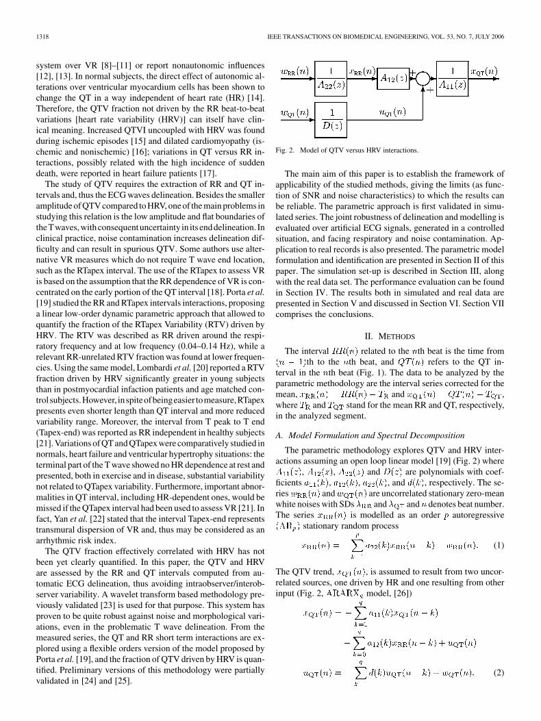
Fig. 2. Model of QTV versus HRV interactions.

The main aim of this paper is to establish the framework ofapplicability of the studied methods, giving the limits (as func-tion of SNR and noise characteristics) to which the results canbe reliable. The parametric approach is first validated in simu-lated series. The joint robustness of delineation and modelling isevaluated over artificial ECG signals, generated in a controlledsituation, and facing respiratory and noise contamination. Ap-plication to real records is also presented. The parametric modelformulation and identification are presented in Section II of thispaper. The simulation set-up is described in Section III, alongwith the real data set. The performance evaluation can be foundin Section IV. The results both in simulated and real data arepresented in Section V and discussed in Section VI. Section VIIcomprises the conclusions.

II. METHODS

The interval related to the th beat is the time fromth to the th beat, and refers to the QT in-

terval in the th beat (Fig. 1). The data to be analyzed by theparametric methodology are the interval series corrected for themean, and ,where and stand for the mean RR and QT, respectively,in the analyzed segment.

A. Model Formulation and Spectral Decomposition

The parametric methodology explores QTV and HRV inter-actions assuming an open loop linear model [19] (Fig. 2) where

, , and are polynomials with coef-ficients , , , and , respectively. The se-ries and are uncorrelated stationary zero-meanwhite noises with SDs and and denotes beat number.The series is modelled as an order autoregressive

stationary random process

(1)

The QTV trend, , is assumed to result from two uncor-related sources, one driven by HR and one resulting from otherinput (Fig. 2, model, [26])

(2)

ALMEIDA et al.: QT VARIABILITY AND HRV INTERACTIONS IN ECG 1319

Therefore, the model accounts for the possible QT dependenceon its past values and those of the RR interval. Recent studiesevidenced these QT dependencies [27]. For simplicity, the sameorder was assumed for all ARARX model polynomials, whilea possibly different order was allowed for the AR model. Thisis a generalization from previous approaches, where the sameorder was considered for all polynomials in the model[19]. The order in (1) represents the memory of of itsown past while order in (2) produces a cumulative memoryeffect between the polynomials and or , dependingon the dependence considered. Notice that cor-responds to assigning to series a double memory thanto series.

The assumption of uncorrelated sources allows to computethe power spectral density (PSD) of , , as thesum of the partial spectra, and , that ex-press the contributions related and unrelated to the RR interval,respectively

where is the frequency in Hz. As both andseries are evenly sampled in beats but not in time, the meanRR interval was used as sampling period for estimatingthe PSD functions, which has been shown acceptable for lowfrequencies far from the Nyquist frequency [28]. Each spectrum

, can be written as

(3)

Factorizing it is possible to decompose the complexspectral density in components, each one referred to one ofits poles , [29] and [30]. Inverting the -trans-form in the complex spectrum definition and computing theline integral using the Cauchy Residue Theorem, the autocor-relation function and the correspondent complex spectral den-sity can be decomposed as and

.According to [30], each term in can be written as

for , calculated at . Since theresidues for complex conjugate poles are complex conjugate,the total power in the spectrum can be written as the sum of

components: one for each pair of complex conjugatepoles and (located at frequencies and ) and one foreach real pole (at or ), if they exist.That is

(4)

Due to the symmetry of with respect to , fre-quencies associated to complex conjugate poles correspond tocomplex conjugate components that can be combined in a real

, related to a power component[29]. Each term in the last sum of (4) can be seen as the powerof a real component corresponding to or

(that is, for real). Therefore, in (3)

can be decomposed into components , contributingmainly at frequencies . The power within agiven frequency band, denoted by , can be obtained bysumming the contributions of the poles located in the band .That is

where for real poles and for complex conjugatepoles. The relative fraction of the QTV driven by RR in thefrequency band is given by

(5)

This algebraic decomposition of the spectrum does not guar-antee the achievement of admissible spectral components, oncenegative power components can occur, if poles are too close to-gether [31]. If this happens near the limit of a frequency band

, a negative value can be obtained and protection rulesneed to be considered in the estimation, as will be explained inthe next section.

B. Model Identification and Order Selection

From and interval series, the polynomialwas estimated using least squares, while the ARARX model

parameters were iteratively obtained using a generalized leastsquares methodology [26]. A large enough signal-to-noise ratio(SNR) guarantees that the minima of the square residue areglobal [26] and convergence to white noise residualsis expected in a reasonable small number of iterations for ade-quate model orders.

Orders , between 2 and 18 were considered to be adequatefor modelling a given data segment if the residualsand can be considered uncorrelated white noises (5%significance bilateral test on the normalized autocorrelationsand crosscorrelation, both for the first 40 lags and for alllags). Model orders producing a negative global contributionin a frequency band, as remarked in Section II-A, were alsoconsidered as inadequate. Optimal and were automaticallyselected from the adequate orders. First, order of in theAR model is chosen by minimizing the Akaike informationcriteria (AIC) [26]. The order is taken as the one minimizingthe multivariate AIC

(6)

where stands for the determinant of the covariance ma-trix of the residuals and , and is the numberof intervals (beats) in the segment. The order , and therefore the


variance, were already determined in the previous step,and thus this is not a multivariate minimization in strict sense,as only the order remains to be chosen. To reduce overfit prob-lems in AIC, the number of estimated parametersshould be small (less that 10%) with respect to the total numberof intervals in the series [32]. Regarding the extreme case

, segments with a minimum of about 350 beats shouldbe considered.

III. DATA SETS

Test data was simulated for validation of the previously de-scribed methodology. The and series were sim-ulated using the linear relations model (Fig. 2) and artificialECG signals matching those intervals were constructed to eval-uate the methodology in a more realistic context. Along withmorphologic beat-to-beat variability, real ECG signals are alsoaffected by extra cardiac factors, such as respiration or muscularactivity, which have also been considered in the simulation. RealECG records from a database were used to illustrate the methodin clinical practice.

A. Simulated Data

Assuming that the linear model in Fig. 2 holds, it is neces-sary to define reference parameters for series genera-tion in controlled simulation. Aiming to obtain realisticresulting from and an uncorrelated source , ina first step were constructed the series

(7)

from which the reference model parameters are going to beextracted. The series and are independent

realizations obtained using an integral pulse frequencymodulation model, following modulating signals [28],agreeing to the spectra typically found at supine rest andhead-up tilt situations, respectively (Fig. 3, upper left corner)[33]. The RR uncorrelated QTV part does not need to have aRR like spectral shape, as has been here considered. However,this choice assigns to the uncorrelated part a spectral behaviourwhich puts the method under evaluation in the more difficultsituation, that is with the same kind of frequency distributionas in the RR. So, the spectral overlap will force the methodto search for uncorrelations rather than just make frequencyfiltering. The parameters and in (7) allow to setmean and SD and adjusting is equivalent to considerdistinct QTV levels. Parametric model identification in (1) and(2), considering and given by(7) provides the reference coefficients values , ,

, and the residual noise SD for the simulation. TheQT reference models construction is summarized in the upperblock of the diagram in Fig. 3. In this study, two different QTVlevels and were mod-elled, which were chosen to express extreme situations foundin healthy subjects [34]. In order to allow a better spanning ofthe QTV level range, additional QT reference models were alsoconstructed for , 10, 8, and 3 ms. The orderwas chosen to include similar memory ( , ) on its

own past for both and , while dependson past samples.

Once the QT reference model parameters were obtained, thetest data was simulated as outlined in the central block of Fig. 3.The fraction driven by RR, , was obtainedby feeding the correspondent part of the model (Fig. 2) withindependent realizations of

(8)Analogously, and the fraction noncorrelated with RR

were obtained feeding with simulated white noise(SD ),

(9)

Fifty uncorrelated realizations (trials) of more than 1000 beatswere simulated regarding the following three cases of possibledependencies.

A) QT and RR fully correlated: .B) QT and RR uncorrelated: .C) Mixture of the two dependencies

Several simulation approaches were then considered and dif-ferent test data sets were obtained, as summarized in Table I. Theclean simulated test data sets (“ ”) were defined from the seriessimulated directly from each reference model, considering thethree dependence cases. Artificial ECG signals were constructedbased on those series and were used to obtain signal derived datasets. The interval measurements from the marks provided byautomatic delineation of those noncontaminated ECGs led, foreach dependence case, a new data set (“ ”). Different contam-ination types were considered by including a respiratory-likeelectrical axis rotation effect (“ ”) or adding real prerecordednoise (“ ”) to the ECG signals in the dependence case . Thesetest data sets are further described next.

1) Clean Series Simulation: A segment of 350 beats fromevery realization of the series simulated directly from each ref-erence model were considered in test data, defining the cleantest data sets (“ ”), respectively, , , and .

2) Signal Derived Series: Artificial ECG signals were con-structed fitting the previously generated and se-ries in each data set. A clean and well defined template beat waschosen from a 3-lead baseline corrected real file, sampled at 500Hz, the same resolution than the real data (see Section III-B).Each ECG was obtained by concatenation of the template beat,following the series, properly scaled from QRS end toT wave end to reflect the variability inherent to . Byapplying the same scaling to template beats from the orthog-onal leads , and , 3-lead artificial ECG signals with sameQTV and HRV in all leads can be ob-tained. Automatic delineation over these signals [23] provided


Fig. 3. Methods block diagram: QT reference models construction (upper block), test data sets simulation (central block), QTV versus HRV interactions modelestimation (lower block), performance evaluation (right side).

the fiducial marks and the corresponding series andsignal derived (“ ”) were checked for RR outliers [35]

and missing QT values. Segments of consecutive 350 valid beatsmeasures were considered and denoted as data sets , , and

.3) Noise Contamination: Different contamination types

were considered over the 50 trials in the situation of mixture

of dependencies (case ), as illustrated in Fig. 4. A respira-tory-like electrical axis rotation effect (“ ”) was simulated andthe data set was constructed from the series of automaticallydelineated intervals over the ECG signal affected by respiratorynoise. Other contamination types were considered by addingprerecorded noise to the artificial ECG and a new data set

was defined from the and series obtained


TABLE ISIMULATED DATA: MEAN AND SD OF �̂ IN VALID SEGMENTS (ms). (NC: NOT CONSIDERED)

Fig. 4. Example of (a) a simulated ECG signal, (b) the same ECG with noisecontamination (thicker line) with respiratory-like electrical axis rotation effect,and (c) muscular artifacts with SNR = 15 dB. Clean ECG superimposed(thinner line) in (b) and (c).

from the delineation over these noisy (“ ”) ECGs. Outliersand missing values can occur due to misdetection in automaticdelineation. After delineation, all potential RR outliers wereexcluded [35] and segments of consecutive 350 valid beatsmeasures considered in the test data sets.

Lungs expansion and contraction during the respiratory cyclechanges the heart electric axis within the chest, resulting inscaling and rotation on the ECG. It is assumed that the angularvariation around a lead axis is a function of the amount of air inthe lungs at each time, which was modelled as a sinusoid. Therotation angle around each orthogonal lead isgiven by

(10)

where is sample index, is the maximum value allowedfor , and and denote respiratory and sampling

frequency, respectively. The rotation matrix can be com-puted as the product of planar rotations with anglesand the effect of a three lead rotation should not be differentthan along one single lead [36]. For the sake of simplicity,only the rotation around the axis was considered with

. The respiratory frequency was set to, corresponding to the central frequency of the

highest variability peak on the model spectra (Fig. 3).The ECG signals affected by respirationwere constructed as the product of matrix by the 3-leadECG vector .

Prerecorded noise from the MIT-BIH Noise Stress Test Data-base [37] was used, corresponding to baseline wandering, elec-trode movement artifacts and muscular artifacts. The first leadof the noise records was resampled at 500 Hz and multiplied bya constant to get a predefined SNR (levels from 30 dB to 5 dB)when added to the artificial ECG. The data set comprehendsthe and series obtained from the contaminatedECGs considering all noise types and SNR levels.

B. Real Data Set

ECG recordings of young normal subjects from POLI/MEDLAV database [38] were used in this study (20 records24 min long sampled at 500 Hz with and leads). Eachlead was processed by the automatic delineation system [23].In addition to all potential RR outliers [35], QT intervals outof a 3-SD band were also rejected, as they are unlikely to bephysiologically meaningful and must have resulted from errorin delineation. In the subsequent analysis, segments of 350consecutive beats with valid RR and QT intervals measure-ments were considered. Longer segments were carved up. Eachqualified segment was evaluated for the QT variability level(estimated as the QT SD) and SNR level (estimated as the ratiobetween the power of a running averaged and amplitude fittedbeat and the power of a segment between QRS complexeshigh-pass filtered with a fifth-order Butterworth filter withcut-off frequency 10 Hz).


IV. PERFORMANCE EVALUATION

The actual spectra of the simulated series was obtaineddirectly from the reference parameters in each QT referencemodel given in Section III-A, used to generate the simulatedseries. The spectral decomposition was performed as describedin Section II-A and the reference variability measurescalculated. The errors in the estimated variability measures

are computed as

(11)

The QTV fraction driven by HRV was chosen as a performancemeasure since it is more likely to be correctly estimated, due tothe fact that any spurious QTV will be considered as part of theuncorrelated fraction. The percentage errors in the quantifi-cation of the QTV fraction correlated with HRV are defined asthe difference between the ratios calculated from (5) for esti-mated, , and reference measures,

(12)

The percentage errors depend on both QTV fractions andthus are more sensitive performance indicators than the errors

, since overestimated leads to an artificial decreaseon .

From the estimated coefficients and the residuesand , the signals and , corre-sponding to the fractions, were explicitly calculated.The similarity between and the corresponding sim-ulated series in (8) was evaluated by the magnitudeof the squared spectral coherence and the phase ofthe cross-spectra , obtained by bivariate modelling[31]. Analogously, and in (9) were alsocompared.

V. RESULTS

The measures were estimated considering frequency bandstypically used in HRV studies [33]: low-frequencyas 0.04–0.15 Hz and high-frequency as 0.15–0.4 Hz.Total power was taken from 0.04 Hz to the highestfrequency present in each spectrum .

A. Simulated Data

Both for the directly simulated data sets , and theones obtained by automatic delineation without noise contami-nation no potential RR outliers or missing QT in-tervals occurred. Adequate segments (350 consecutive beats andno potential RR outliers) were also found in all 50 trials of datasets and for for all QT reference models.The reduced number of qualified segments led us to exclude datawith from the analysis. The estimated QT SD,

, in the valid segments of each data set obtained from QTreference models and are reported in Table I ( meanand SD across trials).

Fig. 5. Histograms of orders p and q selected by AIC in model identificationfor (a) clean RR simulated series and (b) clean QT simulated series with QTreference models Hi and Lo, and (c) and (d) real data set segments. Darkerclasses in (a) and (b) corresponds to the reference order.

A minimum of 48 (out of 50) valid estimated models for eachQT reference model were found for every data set and noise typein data set for SNR level 15 dB.

1) Clean Simulated Series: The AIC selected orders for theAR model are presented in Fig. 5(a), with in 82% ofthe cases. For the ARARX model, AIC selected orders

in more than 80% of the series in data sets and for all QTreference models, while more spread orders were selected fordata set , as illustrated in Fig. 5(b) for QT reference models

and .For QT reference models and , the mean and SD of

are presented in Table II(a) for data sets and ;the mean and SD of are also presented in Table II(a)for data sets and and in Table II(b) for data set . Inall cases for QT reference models with ,

, and. The distributions of for QT reference

models and in datasets , and are presented inFig. 6(a). In this chart, and in all similar ones, the central boxgoes from 1st to 2nd quartiles, with a horizontal line marking themedian, and stands for values out of the quartiles box. Con-sidering QT reference models corresponding to ,

for more than 81% of the series with ,and 78% with . For QT reference model ,for 78% with (74% with , 71% with ).The comparison between estimated and reference fractions, re-garding both and were evaluated acrosstrials (Fig. 7). The magnitude of the squared coherencewas found to be higher in the QTV fraction driven by RR than inthe uncorrelated one. For QT reference models with lower ,


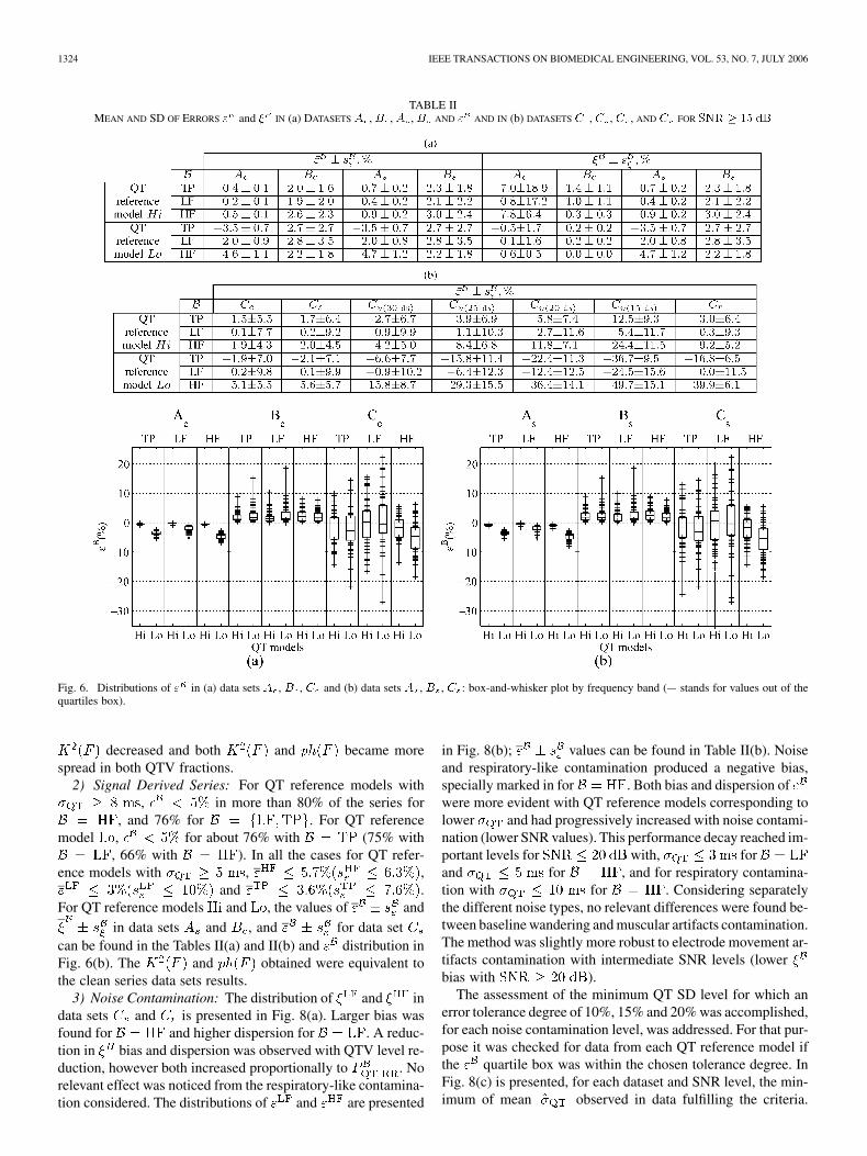
TABLE IIMEAN AND SD OF ERRORS " and � IN (a) DATASETS A , B , A , B AND " AND IN (b) DATASETS C , C , C , AND C FOR SNR � 15 dB

Fig. 6. Distributions of " in (a) data sets A , B , C and (b) data sets A , B , C : box-and-whisker plot by frequency band (+ stands for values out of thequartiles box).

decreased and both and became morespread in both QTV fractions.

2) Signal Derived Series: For QT reference models with, in more than 80% of the series for

, and 76% for . For QT referencemodel , for about 76% with (75% with

, 66% with ). In all the cases for QT refer-ence models with , ,

and .For QT reference models and , the values of and

in data sets and , and for data setcan be found in the Tables II(a) and II(b) and distribution inFig. 6(b). The and obtained were equivalent tothe clean series data sets results.

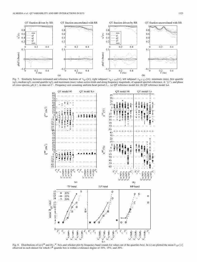
3) Noise Contamination: The distribution of and indata sets and is presented in Fig. 8(a). Larger bias wasfound for and higher dispersion for . A reduc-tion in bias and dispersion was observed with QTV level re-duction, however both increased proportionally to . Norelevant effect was noticed from the respiratory-like contamina-tion considered. The distributions of and are presented

in Fig. 8(b); values can be found in Table II(b). Noiseand respiratory-like contamination produced a negative bias,specially marked in for . Both bias and dispersion ofwere more evident with QT reference models corresponding tolower and had progressively increased with noise contami-nation (lower SNR values). This performance decay reached im-portant levels for with, forand for , and for respiratory contamina-tion with for . Considering separatelythe different noise types, no relevant differences were found be-tween baseline wandering and muscular artifacts contamination.The method was slightly more robust to electrode movement ar-tifacts contamination with intermediate SNR levels (lowerbias with ).

The assessment of the minimum QT SD level for which anerror tolerance degree of 10%, 15% and 20% was accomplished,for each noise contamination level, was addressed. For that pur-pose it was checked for data from each QT reference model ifthe quartile box was within the chosen tolerance degree. InFig. 8(c) is presented, for each dataset and SNR level, the min-imum of mean observed in data fulfilling the criteria.


Fig. 7. Similarity between estimated and reference fractions of x (n), right subpanel x (n), left subpanel x (n): minimum (min), first quartile(q1), median (q2), second quartile (q3), and maximum (max) values across trials and along frequency magnitude, of squared spectral coherence,K (F ), and phaseof cross-spectra, ph(F ), in data set C . Frequency axis assuming uniform heart period T . (a) QT reference model Hi; (b) QT reference model Lo.

Fig. 8. Distributions of (a) � and (b) " : box-and-whisker plot by frequency band (stands for values out of the quartiles box). In (c) are plotted the mean �̂ (n)observed in each dataset for which " quartile box is within a tolerance degree of 10%, 15%, and 20%.


TABLE IIIREAL DATA SET SEGMENTS DESCRIPTION. V = 100� =T

Notice that values for mean are presented for a dataset orSNR level only if data from at least one QT reference modelfulfilled the criteria.

B. Real Data

Segments with valid measured series were found for 7 recordsin lead X and 5 records in lead Z, out of the 20 records availablein the real database. There were not any segments qualified inlead Y. A total of 24 segments were analyzed, as summarized inTable III, with several segments in the same file. The SDof in those segments varied mostly from 2 to 12 ms,with a maximum variation coefficientof 3.1. The exception is the segment 24 which presents muchlarger values both for and (more than the double ofthe maximum for all the other segments). The minimum SNRmean value found was 15.9 dB again for segment 24; for allother segments SNR values found were higher than 18.5 dB. Novalid AR model was found for the in segment 5 of leadZ. The orders selected by AIC in AR indentification [Fig. 5(c)]were found to be for 19 segments and in ARARX[Fig. 5(d)] for 20 over the remaining 23 segments.Only in 3 out of the 24 segments was found .

The estimated QTV fractions are presented in Fig. 9:for 19 out of 23 segments, the maximum

of is 64.8%, and for 15 of thesegments.

VI. DISCUSSION

Restrictive criteria for considering valid interval measureswere used, aiming to guaranty that the parametric methods areonly applied to data that can be considered as close as possibleto stationarity, an essential restriction for this class of methods.In data facing higher noise levels this resulted in a low number

Fig. 9. QTV fractions estimated in real records segments: HRV driven fractionin darker grey, uncorrelated fraction in lighter.

of segments qualified for the analysis. For many records in realdata, it was not possible to find segments with valid intervalmeasures in any of the available leads and the lead Y (usuallynoisier and thus likely to present more outliers) had no qualifiedsegments at all.

Adequate model identification was possible for more than90% of the analyzed segments (both simulated and real). TheQT reference models used in the simulation allowed to produce

series resulting from and other uncorrelatedsource. In the simulated data sets outliers exclusion in the QTseries was not considered, as they can result from the simulationitself instead of delineation errors, since the models do not guar-antee fully realistic series in a physiological sense. The ordersselected for modelling the majority of the clean simulated series

and the ARARX models arein accordance with the reference orders ( , ) usedin simulation. In data set , the QTV fraction uncorrelated toHRV is null and, therefore, all the relevant memory effect is in-cluded in AR model part: the ARARX part tries to model whitenoise and selects more spread out orders. In the real data set seg-ments, AIC selected mainly reinforcing the adequacy ofallowing different orders for AR and ARARX models. In fact,there is no reason to constrain the QT and RR sequences to at-tached memories of its own past. Mean value of in dataset is near for all QT reference models. The lowervalues in data sets and were expected, as only one of theQT dependencies (one QTV fraction) was included.

The errors found in the quantification of the QTV fractiondriven by HRV over clean simulated series were low for all datasets, indicating that the parametric method is able to correctlyestimate both QTV fractions. Higher dispersion and bias ofwere found for QT reference models with lower . This effectwas expected as the QTV amounts to be estimated were smallerand thus the delineation errors proportionally assumed higherimportance. The high between estimated and referencefractions reflect the degree of similarity found both in power andin the peaks location. Erroneous QTV due to delineation errorsshould be considered as noncorrelated with HRV, explaining theslightly inferior in this fraction, namely in QT referencemodels with lower . The negligible values confirmthe absence of time delays in the dependence of on

.


The mean values of in data sets , and differless than one sample from the correspondent values in ,and and no relevant differences were noticed in performance,coherence or phase. The adequateness of the RR and QT inter-vals measured by the automatic delineator presented in [23] forstudying these relations was then confirmed. The slightly lowerperformance found for QT reference models with ,can be related not only with the lower QTV levels to be mea-sured, but also with insufficient ECG time resolution (2 ms) re-sulting from the sampling rate chosen . Still, neg-ligible effects of in the QT interval measurement were foundby Risk et al. [39], for values between 300 and 500 Hz. Bylooking the tendencies shown in that work, one can infer thansame negligible differences will be found for .

The negative bias found in for , with no relevant perfor-mance decrease in , represents an overestimation of the QTVfraction not correlated with RR. The waves slope is affectedby the beat rotation resulting in cyclic delineation errors, withimpact in the QTV series. These small delineation errors areconsistent with overestimation, specially for ,which assume relative higher importance for lower QTV levels.The parametric method was inapplicable with noise contami-nation corresponding to due to the number ofoutliers in and missing QT intervals resulting from de-lineation errors. The progressively increased mean withthe SNR reduction in the qualified segments strongly indicatedthat delineation errors have introduced spurious variability inthe measured series. A delineation improvement is needed toallow a faithful QTV estimation in noisier ECG records. Asexpected, the joint performance of delineation and parametricapproach depended not only on the noise level, but also onthe QTV level to be measured. In the presence of moderatenoise, the quality of the estimation decreased withSNR level, but not to unusable levels, as far as the levelof QTV to be measured is not too low .Spurious QTV resulting from noise was correctly quantifiedas not related with RR. Thus, the ratio underestimated theimportance of in total QTV and the quantificationof the relative fraction of variability driven by RRwas more affected than the absolute measures. The resultsoutlined in Fig. 8 provide, for the used delineation system[23], the limits for which the QTV fraction quantification isreliable, as a function of SNR and QTV range. Those limitswould surely be less restrictive if the RTapex [19] was used,since T peak estimation is less noise sensitive, but the eventualvariability of the T peak to T end interval (and its potentialclinical value) would be lost. The limits found could be evenpushed forward by exploring a more robust delineator [40].

Regarding the real data set, the fraction uncorrelated withHRV was found to be higher than 40% for most of the segmentsfor all frequency bands considered, suggesting that other factorsrather than RR could drive an important part of QTV. It is worth-while to remark that uncorrelation between that part of QTV andHRV does not imply the absence of physiological dependencebetween them, since nonlinear effects are not considered in thepresent modelling. As SNR level is around 20 dB and SDis 10 ms for many of the real files, it is likely that the errorsin the estimated fractions reach 15% or 20%. Even so, it is pos-

sible to state that the fraction uncorrelated with HRV still havea relevant importance in the QTV.

VII. CONCLUSION

Exploring short term RR and QT interactions in clinical rou-tine data, facing noise contamination, is a challenging and com-plex problem. In this paper, this relation was assessed by au-tomatic delineation and the characterization of the QT versusRR variabilities using parametric modelling was discussed. Therobustness was evaluated with simulated data. No relevant per-formance decrease resulted from delineation, and the decreasein estimation quality due to ECG noise does not degrade thevariability measures to nonuseful levels, with moderate contam-ination . Noisier ECG records will require animprovement of the delineation system. The level of QTV to bemeasured is also important in the relevance of the errors. Themethods are not adequate to study reduced QTV (QT SD 10ms). In real data, the different orders selected for the two modelparts can be associated to differences in the memory of the se-ries and need a deeper analysis.

In spite of the limitations in this methodology, the fractionuncorrelated with HRV was found to have an importance inQTV that cannot be ignored. Clinical interpretation studies onthe uncorrelated fraction and its possible relation with direct au-tonomic effects over the VR should be considered and can nowbe faced within the framework of this modelling.

REFERENCES

[1] F. Gaita, C. Giustetto, F. Bianchi, C. Wolpert, R. Schimpf, R. Ric-cardi, S. Grossi, E. Richiardi, and M. Borggrefe, “Short QT syndromea familial cause of sudden death,” Circulation, vol. 108, pp. 965–970,2003.

[2] Y. G. Yap and A. J. Camm, “Drug induced QT prolongation and tor-sades de pointes,” Heart, vol. 89, pp. 1363–1372, 2003.

[3] M. Rubart, “Congenital long QT syndrome: looking beyond the heart,”Heart Rhythm, vol. 1, no. 1, pp. 65–66, 2004.

[4] J. Lass, J. Kaik, D. Karai, and M. Vainu, “Ventricular repolarizationevaluation from surface ECG for identification of the patients withincreased myocardial electrical instability,” Proc. 23rd Annu. Int.Conf. IEEE Engineering in Medicine and Biology Society, 2001, pp.390–393.

[5] S. Cuomo, F. Marciano, M. L. Migaux, F. Finizio, E. Pezzella, M.A. Losi, and S. Betocchi, “Abnormal QT interval variability in pa-tients with hypertrophic cardiomyopathy. Can syncope be predicted?,”J. Electrocardiol., vol. 37, no. 2, pp. 113–119, 2004.

[6] R. D. Berger, “QT variability,” J. Electrocardiol., vol. 36 suppl., no. 5,pp. 83–87, 2003.

[7] V. K. Yeragani, S. Adiga, N. Desai, and R. D. Berger, “Beat-to-beatQT interval variability in atrial fibrillation with and without congestivecardiac failure,” Ann. Noninvasive Electrocardiol., vol. 9, pp. 304–305,2004.

[8] M. Merri, M. Alberti, and A. J. Moss, “Dynamic analysis of ventricularrepolarization duration from 24-hour Holter recordings,” IEEE Trans.Biomed. Eng., vol. 40, no. 12, pp. 1219–1225, Dec. 1993.

[9] F. Marciano, S. Cuomo, M. L. Migaux, and A. Vetrano, “Dynamic cor-relation between QT and RR intervals: how long is QT adaptation toheart rate?,” Comput. Cardiol., pp. 413–416, 1998.

[10] V. Shusterman, B. Aysin, S. I. Shah, S. Flanigan, and K. P. Anderson,“Autonomic nervous system effects on ventricular repolarization andRR interval variability during head-up tilt,” Comput. Cardiol., pp.717–720, 1998.

[11] V. Shusterman, A. Beigel, S. I. Shah, B. Aysin, R. Weiss, V. K. Gotti-paty, D. Schartzman, and K. P. Anderson, “Changes in autonomic ac-tivity and ventricular repolarization,” J. Electrocardiol., vol. 32 suppl,pp. 185–192, 1999.


[12] A. Gastaldelli, M. Emdin, F. Conforti, S. Camastra, and E. Ferrannini,“Insulin prolongs the QTc interval in humans,” Am. J. Physiol. Regul.Integr. Comp. Physiol., vol. 279, pp. R2022–R2025, 2000.

[13] R. M. Colzani, M. Emdin, F. Conforti, C. Passino, M. Scalattini, and G.Iervasi, “Hyperthyroidism is associated with lengthening of ventricularrepolarization,” Clin. Endocrinol., vol. 55, no. 1, pp. 27–32, 2001.

[14] A. R. Magnano, S. Holleran, R. Ramakrishnan, J. A. Reiffel, and D. M.Bloomfield, “Autonomic nervous system influences on QT interval innormal subjects,” J. Am. Coll. Cardiol., vol. 39, no. 11, pp. 1820–1826,2002.

[15] T. Murabayashi, B. Fetics, D. Kass, E. Nevo, B. Gramatikov,and R. D. Berger, “Beat-to-beat QT interval variability associatedwith acute myocardial isquemia,” J. Electrocardiol., vol. 35, no.1, pp. 19–25, 2002.

[16] R. D. Berger, E. K. Kasper, K. L. Baughman, E. Marban, H. Calkins,and G. F. Tomaselli, “Beat-to-beat QT interval variability novel evi-dence for repolarization lability in ischemic and nonischemic dilatedcardiomyopathy,” Circulation, vol. 96, no. 5, pp. 1557–1565, 1997.

[17] C. C. E. Lang, J. M. M. Neilson, and A. D. Flapan, “Abnormalities ofthe repolarization characteristics of patients with heart failure progresswith symptom severity,” Ann. Noninvasive Electrocardiol., vol. 9, no.3, pp. 257–264, 2004.

[18] M. Merri, J. Benhorin, M. Alberti, E. Locati, and A. J. Moss, “Electro-cardiographic quantitation of ventricular repolarization,” Circulation,vol. 80, pp. 1301–1308, 1989.

[19] A. Porta, G. Baselli, E. Caiani, A. Malliani, F. Lombardi, and S. Cerutti,“Quantifying electrocardiogram RT-RR variability interactions,” Med.Biol. Eng. Comput., vol. 36, no. 1, pp. 27–34, 1998.

[20] F. Lombardi, A. Colombo, A. Porta, G. Baselli, S. Cerutti, and C.Fiorentini, “Assessment of the coupling between RT and RR in-terval as an index of temporal dispersion of ventricular repolarization,”PACE, vol. 21, pp. 2396–2400, 1998.

[21] P. P. Davey, “QT interval measurement: Q to T or Q to T ,”J. Intern. Med., vol. 246, no. 2, pp. 145–149, 1999.

[22] G. X. Yan and C. Antzelevitch, “Cellular basis for the normal T waveand the electrocardiographic manifestations of the long-QT syndrome,”Circulation, vol. 98, pp. 1928–1936, 1998.

[23] J. P. Martínez, R. Almeida, S. Olmos, A. P. Rocha, and P. Laguna,“A wavelet-based ECG delineator: evaluation on standard databases,”IEEE Trans. Biomed. Eng., vol. 51, no. 4, pp. 570–581, Apr. 2004.

[24] R. Almeida, A. P. Rocha, E. Pueyo, J. P. Martínez, and P. Laguna,“Modelling short term variability interactions in ECG: QT versus RR,”in Computational Statistics 2004. Prague: Physica-Verlag, 2004, pp.597–604.

[25] R. Almeida, E. Pueyo, J. P. Martínez, A. P. Rocha, and P. Laguna,“Quantification of the QT variability related to HRV: robustness studyfacing automatic delineation and noise on the ECG,” Comput. Cardiol,pp. 769–772, 2004.

[26] L. Ljung, System Identification Theory for the User, 2nd ed. UpperSaddle River, NJ: Prentice-Hall PTR, 1999.

[27] E. Pueyo, P. Smetana, M. Malik, and P. Laguna, “Evaluation of QTinterval response to marked RR interval changes selected automaticallyin ambulatory recordings,” Comput. Cardiol., pp. 157–160, 2003.

[28] J. Mateo and P. Laguna, “Improved heart rate variability signal analysisfrom the beat occurrence times according to the IPFM model,” IEEETrans. Biomed. Eng., vol. 47, no. 8, pp. 985–996, Aug. 2000.

[29] S. Johnsen and N. Andersen, “On power estimation in maximum en-tropy spectral analysis,” Geophysics, vol. 43, no. 4, pp. 681–690, 1978.

[30] G. Baselli, A. Porta, O. Rimoldi, M. Pagani, and S. Cerutti, “Spectraldecomposition in multichannel recordings based on multivariate para-metric identification,” IEEE Trans. Biomed. Eng., vol. 44, no. 11, pp.1092–1101, Nov. 1997.

[31] S. L. Marple, Digital Spectral Analysis With Applications. : PrenticeHall, 1987.

[32] S. Waele and P. M. T. Broersen, “Order selection for vector autore-gressive models,” IEEE Trans. Acoust., Speech, Signal Process., vol.51, no. 2, pp. 427–433, Feb. 2003.

[33] T. F. of the ESC/ASPE, “Heart rate variability: standards of measure-ment, physiological interpretation, and clinical use,” Eur. Heart J., vol.17, pp. 354–381, 1996.

[34] B. T. Jensen, C. E. Larroude, L. P. Rasmussen, N. H. Holstein-Rathlou,M. V. Hojgaard, E. Agner, and J. K. Kanters, “Beat-to-beat QT dy-namics in healthy subjects,” Ann. Noninvasive Electrocard., vol. 9, no.1, pp. 3–11, 2004.

[35] J. Mateo and P. Laguna, “Analysis of heart rate variability in thepresence of ectopic beats using the heart timing signal,” IEEE Trans.Biomed. Eng., vol. 50, no. 3, pp. 334–343, Mar. 2003.

[36] M. Astrom, H. C. Santos, L. Sornmo, P. Laguna, and B. Wohlfart, “Vec-torcardiographic loop alignment and the measurement of morphologicbeat-to-beat variability in noisy signals,” IEEE Trans. Biomed. Eng.,vol. 47, no. 4, pp. 497–506, Apr. 2000.

[37] G. B. Moody and R. G. Mark, “The MIT-BIH arrhythmia database onCD-ROM and software for use with it,” Comput. Cardiol., pp. 185–188,1990.

[38] F. Pinciroli, G. Pozzi, P. Rossi, M. Piovosi, A. Capo, R. Olivieri, and M.Della Torre, “A respiration-related EKG database,” Comput. Cardiol.,pp. 477–480, 1998.

[39] M. R. Risk, J. S. Bruno, M. Llamedo Soria, P. D. Arini, and R. A. M.Taborda, “Measurement of QT interval and duration of the QRS com-plex at different ECG sampling rates,” Comput. Cardiol., pp. 495–498,2005, to be published.

[40] R. Almeida, J. P. Martínez, A. P. Rocha, S. Olmos, and P. Laguna,“Improved QT variability quantification by multilead automatic delin-eation,” Comput. Cardiol., pp. 503–506, 2005.

Rute Almeida was born in Porto, Portugal, in 1979.She received a 4-year degree in mathematics appliedto technology in 2000 from Faculty of Sciences,University of Porto (FCUP), Porto. Since October of2001, she is working towards the Ph.D. degree at theApplied Mathematics Department of FCUP.

She was with the Autonomic Function StudyCenter from Hospital S. João between March andOctober 2000, working in methods for automaticdelineation of the ECG. She is currently a memberof Centro de Matemática da Universidade do Porto

and an Invited Assistant in the Mathematics Department of Minho University(Portugal). Her main research interests are in time-scale methods and theautomatic analysis of the ECG, namely the study of ventricular repolarization.

Sónia Gouveia was born in Leiria, Portugal, in 1977.She received the 4-year degree in mathematics ap-plied to technology and the M.Sc. degree in computa-tional methods in sciences and engineering from theUniversity of Porto, Porto, Portugal. Since March of2005, she is working towards the Ph.D. degree in ap-plied mathematics, supported by an individual Ph.D.degree grant from Foundation for Science and Tech-nology (Portugal) and European Social Fund.

From 1999 to 2003, she was with the AutonomicFunction Study Center from Hospital S. João,

working in methods for automatic processing of biomedical signals and fordata analysis in autonomic dysfunction diseases. Currently, she is with theCentro de Matemática da Universidade do Porto as a Researcher. Her mainresearch interests are signal processing techniques for the characterization ofbiomedical signals.

Ana Paula Rocha (M’02) was born in Coimbra, Por-tugal, in 1957. She received the Applied Mathematicsdegree and the Doctor degree (Ph.D. degree in ap-plied mathematics, systems theory, and signal pro-cessing) from the Faculty of Sciences, University ofPorto (FCUP), Porto, in 1980 and 1993, respectively.

She is an Auxiliar Professor in the Department ofApplied Mathematics at FCUP, Portugal. She is cur-rently a member of Centro de Matemática da Univer-sidade do Porto. Her research interests are in biomed-ical signals and system analysis (EMG, cardiovas-

cular systems analysis and autonomic nervous system characterization), time-frequency/time-scale signal analysis, point processes spectral analysis, and datatreatment and interpretation.


Esther Pueyo received the M.S. degree in mathe-matics from the University of Zaragoza, Zaragoza,Spain, in 1999. During 2000, she was a research stu-dent at the Department of Mathematics, Universityof Zaragoza, where she developed a minor thesis inthe field of calculus.

In 2001, she began the Ph.D. degree studies at theDepartment of Electronic Engineering and Commu-nications, University of Zaragoza, with a grant sup-ported by the Spanish government.

Currently, she is an Assistant Professor with theDepartment of Electronic Engineering and Communications, University ofZaragoza. Her research activity lies in the field of biomedical signal processingand her primary interests include the study of heterogeneities in the repolariza-tion period of the electrocardiographic signal.

Juan Pablo Martínez was born in Zaragoza,Aragón, Spain, in 1976. He received the M.S. degreein telecommunication engineering and the Ph.D. de-gree in biomedical engineering from the Universityof Zaragoza (UZ), in 1999 and 2005, respectively.

From 1999 to 2000, he was with the Departmentof Electronic Engineering and Communications, UZ,as a Research Fellow. Since 2000, he is an AssistantProfessor in the same department. He is also a Re-searcher with the Aragon Institute of Engineering Re-search (I3A), UZ. His professional research activity

lies in the field of biomedical signal processing, with main interest in signals ofcardiovascular origin.

Pablo Laguna (M’92–SM’06) was born in Jaca(Huesca), Spain, in 1962. He received the M.S.degree in physics and the Ph.D. degree in physicscience from the Science Faculty at the Universityof Zaragoza, Zaragoza, Spain, in 1985 and 1990,respectively. The Ph.D. degree thesis was developedat the Biomedical Engineering Division of theInstitute of Cybernetics (U.P.C.-C.S.I.C.) under thedirection of P. Caminal.

He is Full Professor of Signal Processing andCommunications in the Department of Electrical

Engineering at the Engineering School, and a Researcher at the Aragn Institutefor Engineering Research (I3A), both at University of Zaragoza. From 1992 to2005, he was Associated Professor at same university and from 1987 to 1992 heworked as Assistant Professor of Automatic Control in the Department of Con-trol Engineering at the Politecnic University of Catalonia (U.P.C.), Catalonia,Spain, and as a Researcher at the Biomedical Engineering Division of theInstitute of Cybernetics (U.P.C.-C.S.I.C.). His professional research interestsare in signal processing, in particular applied to biomedical applications.

QT variability and HRV interactions in ECG: quantification and reliability

Documents

Transcript of QT variability and HRV interactions in ECG: quantification and reliability